Embed Size (px)
Citation preview
INVESTIGATION OF AMMONIA AND EQUIPMENT
CONFIGURATIONS FOR SUPERMARKET APPLICATIONS
by
TIMOTHY P. MCDOWELL
A thesis submitted in partial fulfillment of
the requirements for the degree of
MASTER OF SCIENCE
(MECHANICAL ENGINEERING)
at the
UNIVERSITY OF WISCONSIN-MADISON
1993
ABSTRACT
The need for replacement refrigerants has been of increasing concern with the
international agreements which legislated the phasing-out of many of the refrigerants
currently being used in the world. The refrigerants that are currently used to provide the
cooling for the refrigerated cases in supermarkets are being phased-out and the
refrigerants R22 and ammonia (R717) are two of the refrigerants that have been proposed
as replacements. The choice of refrigerants for supermarket applications is important
because approximately 4% of the national electrical power consumption is by
supermarkets. It is important to ensure that the new refrigerants do not have significantly
lower system performance. The use of R22 is a concern because it still has a potential for
contributing to global warming. Ammonia does not contribute to ozone depletion or
global warming but it is toxic at low concentrations. An ammonia system would have to
employ a secondary heat transfer fluid to provide the cooling to the refrigerated cases.
The work documented in this thesis studies the best design method for ammonia -
secondary fluid systems and compares their performance to the performance of R22
systems.
Both R22 and ammonia have high discharge temperatures leaving the compressor and
it is necessary to utilize staged compression. Three different methods of staging the
ii
compression were compared for both of the refrigerants: basic staged compression,
staged compression and evaporation, and staged compression with a flash tank. The best
method for R22 systems is staged compression and evaporation and the best method for
ammonia systems is staged compression with flash tank.
Six different secondary fluids were evaluated for use with ammonia in the
supermarket system. The fluids are a propylene glycol fluid called Dowfrost, an ethylene
glycol fluid called Dowtherm SR-1, a mineral oil called Multitherm 503, a silicon based
heat transfer fluid called Syltherm XLT, ethanol, and propane. When the system
performance was evaluated for the fluids, the system using propane yielded the highest
performance with Dowfrost and Dowtherm SR-1 yielding the second highest
performance. However, in a application, such as a supermarket, where the general
public could come into contact with the secondary fluid, the toxicity and flammability of
the secondary fluids need to be considered. Propane is highly flammable and explosive
and Dowtherm SR- 1 is toxic, so Dowfrost is the best choice of the six fluids evaluated.
The performance of the R22 system and the ammonia - Dowfrost system was
compared. The performance of the R22 system was about 4% higher than the ammonia -
Dowfrost system. With further improvements in the two heat exchangers used in the
ammonia - Dowfrost system the performance could be even closer.
The overall system performance of the ammonia - secondary fluid refrigeration
system is governed by a large set of design parameters. A parametric study was done of
the influence that these parameters have on the overall system performance. From this
parametric study, design rules for an ammonia - secondary fluid system were developed.
When these design rules are utilized, the ammonia - secondary fluid will have the highest
performance possible.
iii

ACKNOWLEDGMENTS
This project was made possible by a grant from the Environmental Protection Agency
and I would like to thank Cynthia Gage and Evelyn Baskin for their assistance as they
oversaw the project. Their help with direction and guidance for the project was
invaluable.
I would also like to thank my advisors John Mitchell and Sandy Klein for both their
help and their friendship. It is reassuring to know that you can ask the stupid questions
knowing that your advisors will patiently answer them without making you feel like an
idiot. Thanks to Bill Beckman for his help and for giving me something to shot for on
the golf course. Next year will be the year that I will consistently win the golf matches.
Thanks to Jeff, Kathy, and Dean who made my move to the frozen north much
easier. The quick friendship and support when you first move to a city where you don't
know anyone helps make the transition easier. To everyone at the Solar Energy Lab, too
numerous to mention by name, I thank you for creating an atmosphere of fun and work
that made coming into the lab everyday easier.
To my friends from Austin and Rice U. thanks for putting forth the effort to maintain
the friendships that we had developed. The number of times that I looked to you all for
support is innumerable and you were always there for me.
Finally I thank my family for their support throughout the years. The decisions I
made about school in my life would not have been so easy if I did not have the guidance
and reassurance of my family. I couldn't have done it without you.
iv
TABLE OF CONTENTS
Abstract
Acknowledgments
Table of Contents
List of Tables
List of Figures
Nomenclature
iv
iv
x
xi
xvii
Chapter 1 Introduction 1
1.1 Agreements Concerning Refrigerants 2
1.2 Supermarket Refrigerants 4
1.3 Supermarket Refrigerated Case Systems 6
1.4 Refrigerant Comparison 9
Chapter 2 Secondary Fluids 10
2.1 Secondary Fluid Descriptions
2.1.1 Propylene Glycol
11
11
2.1.2 Ethylene Glycol 19
2.1.3 Mineral Oil 26
2.1.4 Syltherm 29
2.1.5 Ethanol 33
2.1.6 Propane 33
2.2 Comparison of Properties of Secondary Fluids 34
2.2.1 Density Comparison 34
2.2.2 Thermal Conductivity Comparison 35
2.2.3 Specific Heat Comparison 36
2.2.4 Viscosity Comparison 37
2.2.5 Comparison of Hazards 38
2.2.6 Property Comparison Conclusions 39
Chapter 3 Refrigerant Cycle 40
3.1 Model Description 41
3.1.1 Condenser 41
3.1.2 Evaporator 42
3.1.3 Expansion 43
3.1.4 Compression 43
3.1.5 Other Equations 45
3.2 Compression Methods 45
3.2.1 No Staging 46
3.2.2 Staged Compression 47
3.2.3 Staged Compression and Evaporation 50
3.2.4 Staged Compression with Flash Tank 52
vi
3.3 Performance Comparison 55
3.3.1 R22 Comparison 55
3.3.2 Ammonia Comparison 56
3.4 Conclusions 56
Chapter 4 Ammonia with Secondary Fluid System 57
4.1 Evaporator Heat Exchanger Model 58
4.2 Secondary Fluid System 63
4.2.1 Refrigerated Case 63
4.2.2 Thermal Losses from Piping System 67
4.2.3 Pump Work 69
Chapter 5 Parametric Study 72
5.1 Parameter List 73
5.1.1 System Parameters 73
5.1.2 Refrigerated Case Parameters 74
5.1.3 Ammonia-Secondary Fluid Heat Exchanger Parameters 74
5.1.4 Piping System Parameters 75
5.1.5 Compressor Parameters 75
5.2 Influence on Performance by Parameters 76
5.2.1 Base Case 76
5.2.2 Base Case Performance 79
5.2.3 Influence of System Parameters 80
5.2.4 Influence of Refrigerated Case Parameters 84
5.2.5 Influence of Amnmonia-Dowfrost Heat Exchanger Parameters 90
vii
5.2.5 Influence of Piping System Parameters 93
5.3 R22 System 102
5.3.1 R22 Base Case 103
5.3.2 R22 and Ammonia Performance Comparison 103
5.4 Conclusions 104
Chapter 6 Secondary Fluid Performance Comparison 106
6.1 Secondary Fluid Comparison 107
6.1.1 Performance Comparison without thermal losses and pump work 107
6.1.2 Performance Comparison without pump work 109
6.1.3 Performance Comparison without thermal losses 111
6.1.4 Performance Comparison with pump work and thermal losses 114
6.2 Secondary Fluid Selection 115
Chapter 7 Design Rules 117
7.1 Ammonia Cycle Design 118
7.2 Secondary Fluid Selection 118
7.3 Operating Guidelines 119
7.4 Heat Exchangers 120
7.5 Secondary Fluid Pumping System 122
Chapter 8 Conclusions and Recommendations 127
8.1 Design Guidelines 128
8.2 Future Research 128
viii
Appendix A: Compression Method Models 131
Appendix B: Base Case Model 148
Appendix C: R22 - Ammonia Comparison Models 157
Appendix D: Secondary Fluid Comparison Models 171
References 216
ix
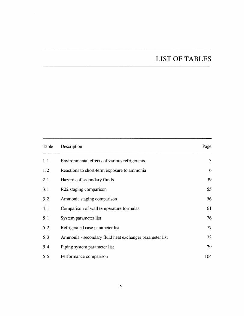
LIST OF TABLES
Table Description Page
1.1 Environmental effects of various refrigerants 3
1.2 Reactions to short-term exposure to ammonia 6
2.1 Hazards of secondary fluids 39
3.1 R22 staging comparison 55
3.2 Ammonia staging comparison 56
4.1 Comparison of wall temperature formulas 61
5.1 System parameter list 76
5.2 Refrigerated case parameter list 77
5.3 Ammonia - secondary fluid heat exchanger parameter list 78
5.4 Piping system parameter list 79
5.5 Performance comparison 104
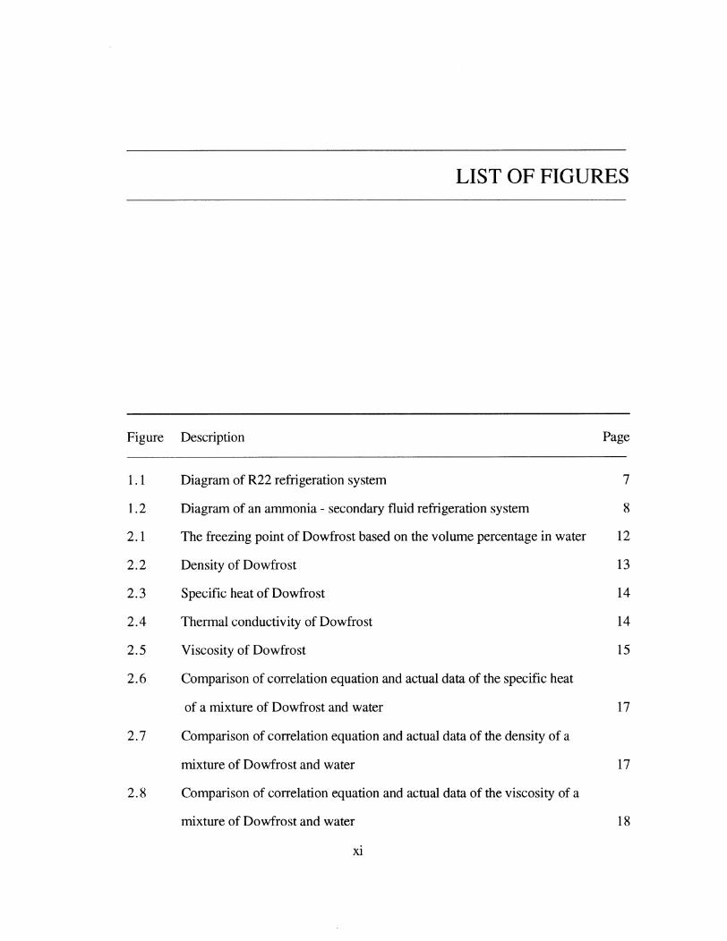
LIST OF FIGURES
Figure Description Page
1.1 Diagram of R22 refrigeration system 7
1.2 Diagram of an ammonia - secondary fluid refrigeration system 8
2.1 The freezing point of Dowfrost based on the volume percentage in water 12
2.2 Density of Dowfrost 13
2.3 Specific heat of Dowfrost 14
2.4 Thermal conductivity of Dowfrost 14
2.5 Viscosity of Dowfrost 15
2.6 Comparison of correlation equation and actual data of the specific heat
of a mixture of Dowfrost and water 17
2.7 Comparison of correlation equation and actual data of the density of a
mixture of Dowfrost and water 17
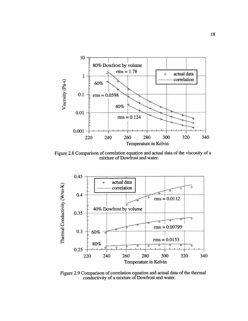
2.8 Comparison of correlation equation and actual data of the viscosity of a
mixture of Dowfrost and water 18
xi
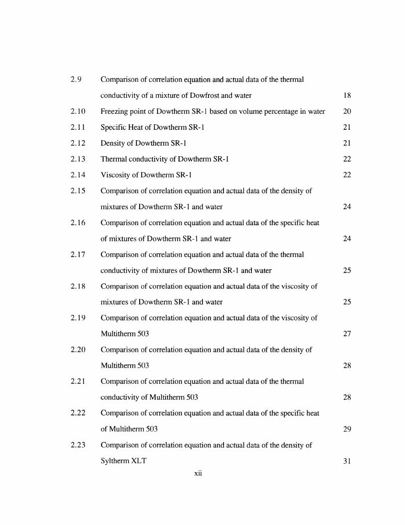
2.9 Comparison of correlation equation and actual data of the thermal
conductivity of a mixture of Dowfrost and water 18
2.10 Freezing point of Dowtherm SR- I based on volume percentage in water 20
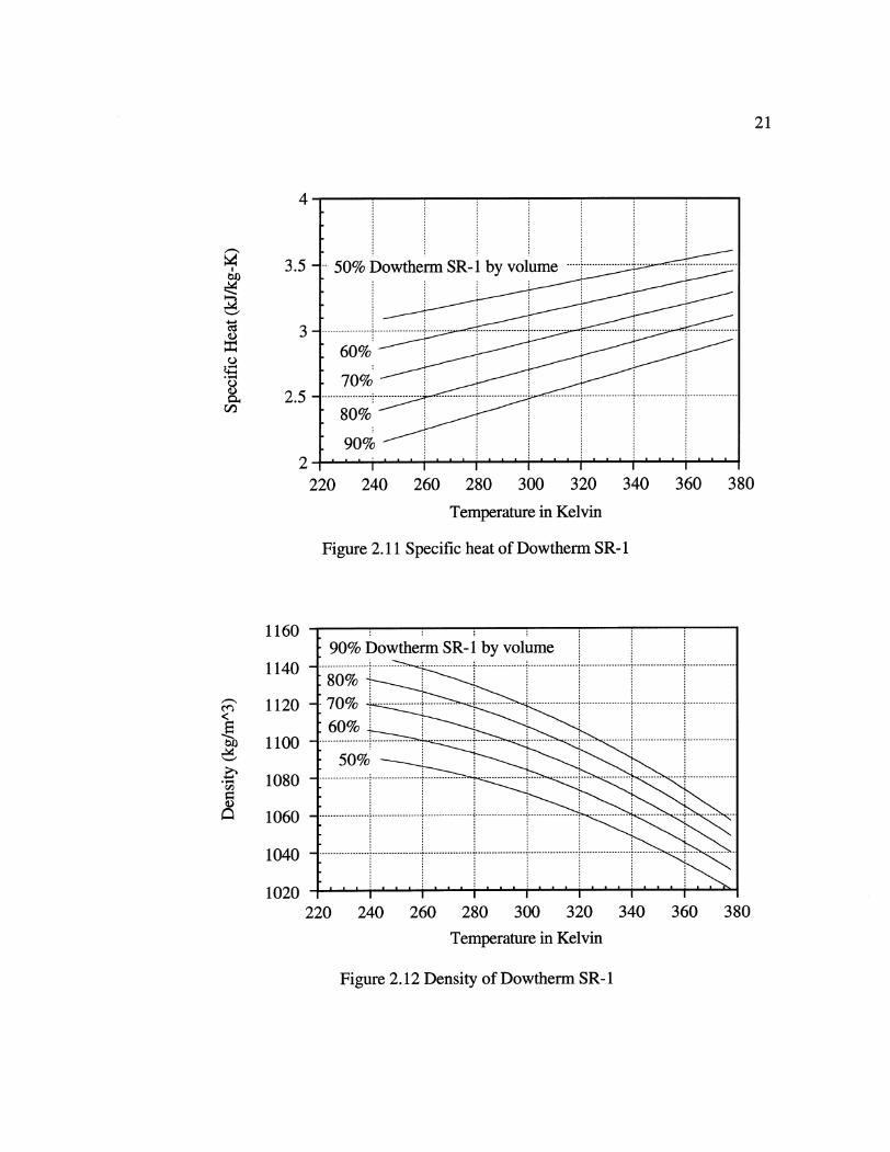
2.11 Specific Heat of Dowtherm SR-1 21
2.12 Density of Dowtherm SR-1 21
2.13 Thermal conductivity of Dowtherm SR-1 22
2.14 Viscosity of Dowtherm SR-1 22
2.15 Comparison of correlation equation and actual data of the density of
mixtures of Dowtherm SR-I and water 24
2.16 Comparison of correlation equation and actual data of the specific heat
of mixtures of Dowtherm SR-I and water 24
2.17 Comparison of correlation equation and actual data of the thermal
conductivity of mixtures of Dowtherm SR-I and water 25
2.18 Comparison of correlation equation and actual data of the viscosity of
mixtures of Dowtherm SR-I and water 25
2.19 Comparison of correlation equation and actual data of the viscosity of
Multitherm 503 27
2.20 Comparison of correlation equation and actual data of the density of
Multitherm 503 28
2.21 Comparison of correlation equation and actual data of the thermal
conductivity of Multitherm 503 28
2.22 Comparison of correlation equation and actual data of the specific heat
of Multitherm 503 29
2.23 Comparison of correlation equation and actual data of the density of
Syltherm XLT 31
xii
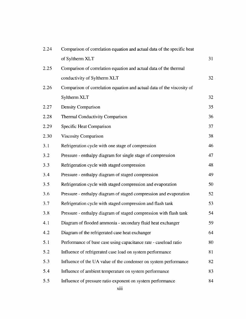
2.24 Comparison of correlation equation and actual data of the specific heat
of Syltherm XLT 31
2.25 Comparison of correlation equation and actual data of the thermal
conductivity of Syltherm XLT 32
2.26 Comparison of correlation equation and actual data of the viscosity of
Syltherm XLT 32
2.27 Density Comparison 35
2.28 Thermal Conductivity Comparison 36
2.29 Specific Heat Comparison 37
2.30 Viscosity Comparison 38
3.1 Refrigeration cycle with one stage of compression 46
3.2 Pressure - enthalpy diagram for single stage of compression 47
3.3 Refrigeration cycle with staged compression 48
3.4 Pressure - enthalpy diagram of staged compression 49
3.5 Refrigeration cycle with staged compression and evaporation 50
3.6 Pressure - enthalpy diagram of staged compression and evaporation 52
3.7 Refrigeration cycle with staged compression and flash tank 53
3.8 Pressure - enthalpy diagram of staged compression with flash tank 54
4.1 Diagram of flooded ammonia - secondary fluid heat exchanger 59
4.2 Diagram of the refrigerated case heat exchanger 64
5.1 Performance of base case using capacitance rate - caseload ratio 80
5.2 Influence of refrigerated case load on system performance 81
5.3 Influence of the UA value of the condenser on system performance 82
5.4 Influence of ambient temperature on system performance 83
5.5 Influence of pressure ratio exponent on system performance 84
xii
5.6 Influence of the temperature leaving the refrigerated case on system
performance 85
5.7 Influence of the number of pipes in the case heat exchanger on system
performance 86
5.8 Influence of the radius of the pipes in the case heat exchanger on system
performance 87
5.9 Influence of the length of the pipes in the case heat exchanger on system
performance 88
5.10 Influence of the velocity of the air through the refrigerated case heat
exchanger on system performance 89
5.11 Influence of the cross sectional area that the air flows through in the
refrigerated case heat exchanger on system performance 90
5.12 Influence of the number of pipes in the ammonia - secondary fluid
heat exchanger on system performance 91
5.13 Influence of the radius of the pipes in the ammonia - secondary fluid
heat exchanger on system performance 92
5.14 Influence of the length of the pipes in the ammonia - secondary fluid
heat exchanger on system performance 93
5.15 Influence of the length of the pipe to the refrigerated case on system
performance 94
5.16 Influence of the length of the pipe from the refrigerated case on system
performance 95
5.17 Influence of the length of the pipes to and from the refrigerated case on
system performance 96
xiv
5.18 Influence of the diameter of the pipe to the refrigerated case on system
performance 97
5.19 Influence of the diameter of the pipe from the refrigerated case on system
performance 98
5.20 Influence of the diameter of the pipes to and from the refrigerated case
on system performance 99
5.21 Influence of the thickness of the insulation on the pipes to the refrigerated
case on system performance 100
5.22 Influence of the thickness of the insulation on the pipes from the
refrigerated case on system performance 101
5.23 Influence of the store temperature on system performance 102
6.1 Performance comparison of the secondary fluids ignoring thermal losses
and pumping power at a refrigerated case temperature of 267 'K 108
6.2 Performance comparison of the secondary fluids ignoring thermal losses
and pumping power at a refrigerated case temperature of 244 °K 109
6.3 Performance comparison of the secondary fluids ignoring pumping power
at a refrigerated case temperature of 267 'K 110
6.4 Performance comparison of the secondary fluids ignoring pumping power
at a refrigerated case temperature of 244 'K 111
6.5 Performance comparison of the secondary fluids ignoring thermal losses
at a refrigerated case temperature of 267 'K 112
6.6 Performance comparison of the secondary fluids ignoring thermal losses
at a refrigerated case temperature of 244 0K 113
6.7 Performance compgarison of the secondary fluids at a refrigerated case
temperature of 267 0K 114
xv
6.8 Performance comparison of the secondary fluids at a refrigerated case
temperature of 244 'K 115
7.1 System performance as a function of compressor work - pump work ratio 119
7.2 Heat exchanger effectivenesses and system COP 121
7.3 System performance as a function of UA value ratio 122
7.4 Performance map with 0.01 m of insulation 124
7.5 Performance map with 0.02 m of insulation 125
7.6 Performance map with 0.03 m of insulation 126
xvi
NOMENCLATURE
ROMAN SYMBOLS
Symbol Definition
caseload refrigeration load met by refrigerated case
CFC chlorofluorocarbon
COP coefficient of performance
Cp specific heat
Cr capacitance rate ratio for heat exchangers
Csp empirical constant for pool boiling
D diameter
f friction factor
g acceleration of gravity
GWP global warming potential
h enthalpy
h heat transfer coefficient
xvii
HCFC non-fully halogenated clorofluorcarbon
head pressure head
hfg heat of fusion
J joule
K degrees Kelvin
k thermal conductivity
kg kilogram
Keq equivalent length for minor losses
L length
ri mass flow rate
m meter
m clearance ratio
n polytropic exponent
NTU number of transfer units
Nu Nusselt number
ODP ozone depletion potential
P pressure
Pa Pascal
percent volume percent of glycol
ppm parts per million
Pr Prandtl number
Q heat transfer
rms root mean square error
rp pressure ratio
xviii
s seconds
T temperature
ton ton of refrigeration
U overall heat transfer coefficient
UA loss coefficient
V Volume
v specific volume
v velocity
W work
W watts
x pressure ratio exponent
GREEK SYMBOLS
Symbol Definition
A difference
effectiveness
pipe roughness
TI1 efficiency
surface tension
p density
xix
SUBSCRIPTS
Symbol Definition
air air properties
ammonia ammonia properties
comp compressor
cond condenser
D diameter
disp displacement
evap evaporator
first stage first stage of compression
i inside
in into compressor
intercool used for intercooling between compressors
1 length
lrn log mean
o outside
out out of compressor
overall total pressure ratio
pipe properties of the pipes
ref refrigerant
sf secondary fluid
vol volume
wall surface between ammonia and secondary fluid in heat exchanger
xx
CHAPTER
ONE
INTRODUCTION
International agreements have been made that call for the gradual phasing-out of many
of the refrigerants currently in use. These include the refrigerants R12 and R502 which
are commonly used to provide the cooling for supermarket refrigerated cases. Suitable
replacements are needed for these refrigerants and both R22 and ammonia have been
proposed. The choice of refrigerant for use in supermarket refrigerated cases is important
because supermarkets consume approximately 4% of the national electrical power and
approximately 30 to 50% of this electrical power is used to store and display food
products. (Progressive Grocer 1985) Thus, it is important to chose a replacement
refrigerant that results in the most efficient refrigeration.
1.1 Agreements Concerning Refrigerants
With the growing concern about the environment, international agreements have been
struck to eliminate substances that cause both ozone depletion and global warming. This
includes many of the refrigerants currently being used. The refrigerants of most concern
are the fully halogenated chlorofluorocarbons (CFCs) and the non - fully halogenated
chlorofluorocarbons (HCFCs). As the CFCs and HCFCs migrate to the upper levels of
the atmosphere, ultraviolet radiation from the sun decomposes the compounds releasing
chlorine. The chlorine, in turn, chain reacts with the ozone reducing the concentration of
ozone in the stratosphere. The ozone layer has a role in filtering a portion of the sun's
ultraviolet radiation and the increase in ultraviolet radiation at ground level may affect
human health, as well as damage crops and aquatic life. There is also concern over the
trapping of some of the infrared radiation emitted from the earth's surface by atmospheric
gases known as the "greenhouse" effect. Many scientists predict that increases in
atmospheric concentrations of these "greenhouse" gases may result in a warming of the
atmosphere. The major "greenhouse" gas is carbon dioxide. However, many
refrigerants may contribute to the problem by being released into the atmosphere where
they absorb infrared radiation or by increasing energy consumption which, in turn,
increases the amount of carbon dioxide produced at fossil fuel power plants. (ASHRAE
1992)
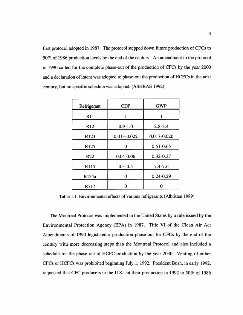
The World Meteorological Organization Global Ozone Research and Monitoring
Project has quantified the ozone depletion potential (ODP) and global warming potential
(GWP) of refrigerants. (Albritten 1989) Table 1.1 lists these potentials where the ODP
and GWP of refrigerant R11 is set as unity. The United Nations Environmental
Progamme (UNEP) established a mechanism for the international agreements concerning
the use of CFCs and HCFCs in the form of "protocols". The Montreal Protocol was the
3
first protocol adopted in 1987. The protocol stepped down future production of CFCs to
50% of 1986 production levels by the end of the century. An amendment to the protocol
in 1990 called for the complete phase-out of the production of CFCs by the year 2000
and a declaration of intent was adopted to phase-out the production of HCFCs in the next
century, but no specific schedule was adopted. (ASHRAE 1992)
Refrigerant ODP GWP
R11 1 1
R12 0.9-1.0 2.8-3.4
R123 0.013-0.022 0.017-0.020
R125 0 0.51-0.65
R22 0.04-0.06 0.32-0.37
R115 0.3-0.5 7.4-7.6
R134a 0 0.24-0.29
R717 0 0
Table 1.1 Environmental effects of various refrigerants (Albritten 1989)
The Montreal Protocol was implemented in the United States by a rule issued by the
Environmental Protection Agency (EPA) in 1987. Title VI of the Clean Air Act
Amendments of 1990 legislated a production phase-out for CFCs by the end of the
century with more decreasing steps than the Montreal Protocol and also included a
schedule for the phase-out of HCFC production by the year 2030. Venting of either
CFCs or HCFCs was prohibited beginning July 1, 1992. President Bush, in early 1992,
requested that CFC producers in the U.S. cut their production in 1992 to 50% of 1986
levels and to cease production, except for small amounts needed for service requirements,
by the end of 1995. This request represented an acceleration of the schedules of the
Clean Air Act and the Montreal Protocol. (ASHRAE 1992)
1.2 Supermarket Refrigerants
Currently supermarket refrigeration systems utilize either refrigerant R12 or R502.
R502 is an azeotropic mixture of 49% (by weight) of R22 and 51% of R115. Table 1.1
shows that R12 has a high ODP and GWP and that R115 has a lower ODP than R12 but
a higher GWP. Both R12 and R502 are scheduled to be phased-out in the Montreal
Protocol. The proposed replacement for both R12 and R502 in supermarket applications
is the refrigerant R22. Table 1.1 shows that R22 has a relatively low ODP and GWP,
however, it is a HCFC and according to current plans the production of HCFCs will be
phased-out before the year 2030. Another possible replacement refrigerant for
supermarket applications is ammonia (refrigerant R717).
The advantages of ammonia as a refrigerant are discussed by Stoecker. (Stoecker
1989) Ammonia is cheaper than either R22 or R502. In comparison to both R22 and
R502, ammonia has higher cycle efficiencies, higher heat transfer coefficients, and a
higher critical temperature. Because ammonia has a pungent odor, it is easy to detect
leaks in the system. Water is completely soluble in ammonia and will not freeze like it
can if it is mixed with other refrigerants. Water in the system could react with
compressor oils, even in an ammonia system, and should still be avoided. Oils are
completely insoluble in ammonia, while oils are completely soluble in halocarbon
refrigerants. So in ammonia systems, the ammonia will not foam in the crankcase of the
reciprocating compressor. Removing oil in the system with ammonia will involve
draining the oil off at an inactive point in the system. Table 1.1 shows that ammonia has
5
an ODP and a GWP of 0. Ammonia has no effect on the ozone layer because it reacts
with other chemicals in the air to form benign compounds.
There are drawbacks to the use of ammonia as a refrigerant. (Stoecker 1989) The
behavior of ammonia with oils can also be considered a disadvantage. Since ammonia
behaves differently with oils than other refrigerants, the method of removing oil from the
refrigerant in the system is different. This is an additional alteration needed to current
refrigeration systems. Ammonia is not compatible with copper and copper bearing alloys
so steel and aluminum must be used as the materials in system construction. Also
hermetically sealed compressors cannot be used with ammonia because the copper wiring
in the motors would be destroyed. Open compressors must be used instead. The
temperature of ammonia leaving the compressors of refrigeration systems is very high
and steps, such as cooling the heads of the compressor or by staging the compression,
need to be taken to reduce the temperature. However, the largest drawback to the use of
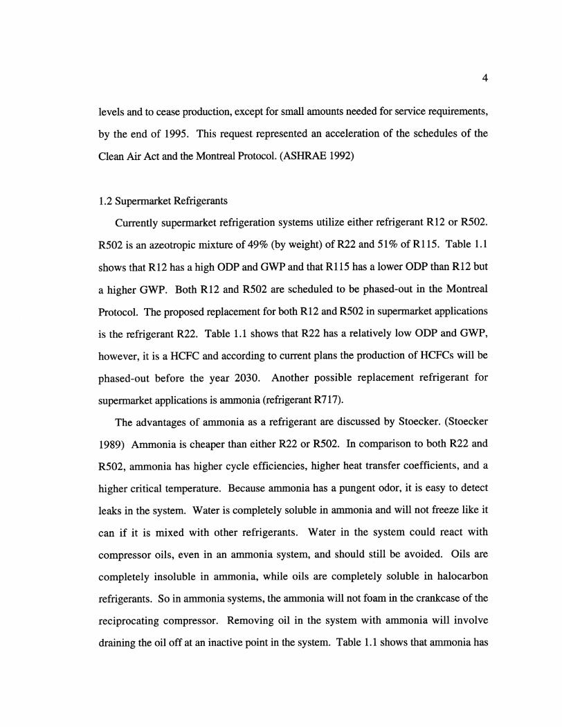
ammonia as a refrigerant is the low concentrations at which it is considered toxic.
Stoecker states that the threshold limits of ammonia are 25 parts per million (ppm) in a
time weighted average and 35 ppm for short time exposure limit. (Stoecker 1989) These
compare with 1000 ppm time weighted average and 1250 ppm short time exposure limit
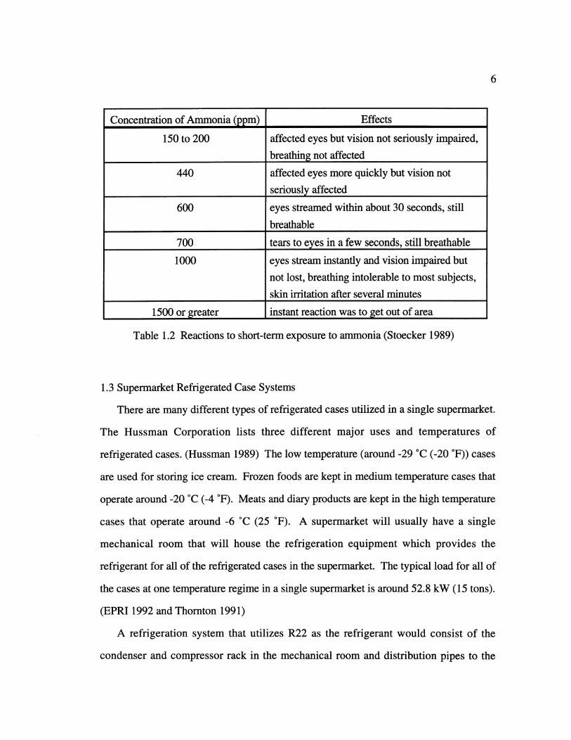
for R22. Table 1.2 shows the results of an informal test of reactions to short-term
exposure to ammonia.
6
Concentration of Ammonia (ppm) Effects
150 to 200 affected eyes but vision not seriously impaired,
breathing not affected
440 affected eyes more quickly but vision not
seriously affected
600 eyes streamed within about 30 seconds, still
breathable
700 tears to eyes in a few seconds, still breathable
1000 eyes stream instantly and vision impaired but
not lost, breathing intolerable to most subjects,
skin irritation after several minutes
1500 or greater instant reaction was to get out of area
Table 1.2 Reactions to short-term exposure to ammonia (Stoecker 1989)
1.3 Supermarket Refrigerated Case Systems
There are many different types of refrigerated cases utilized in a single supermarket.
The Hussman Corporation lists three different major uses and temperatures of
refrigerated cases. (Hussman 1989) The low temperature (around -29 'C (-20 F)) cases
are used for storing ice cream. Frozen foods are kept in medium temperature cases that
operate around--20 'C (-4 F). Meats and diary products are kept in the high temperature
cases that operate around -6 "C (25 F). A supermarket will usually have a single
mechanical room that will house the refrigeration equipment which provides the
refrigerant for all of the refrigerated cases in the supermarket. The typical load for all of
the cases at one temperature regime in a single supermarket is around 52.8 kW (15 tons).
(EPRI 1992 and Thornton 1991)
A refrigeration system that utilizes R22 as the refrigerant would consist of the
condenser and compressor rack in the mechanical room and distribution pipes to the
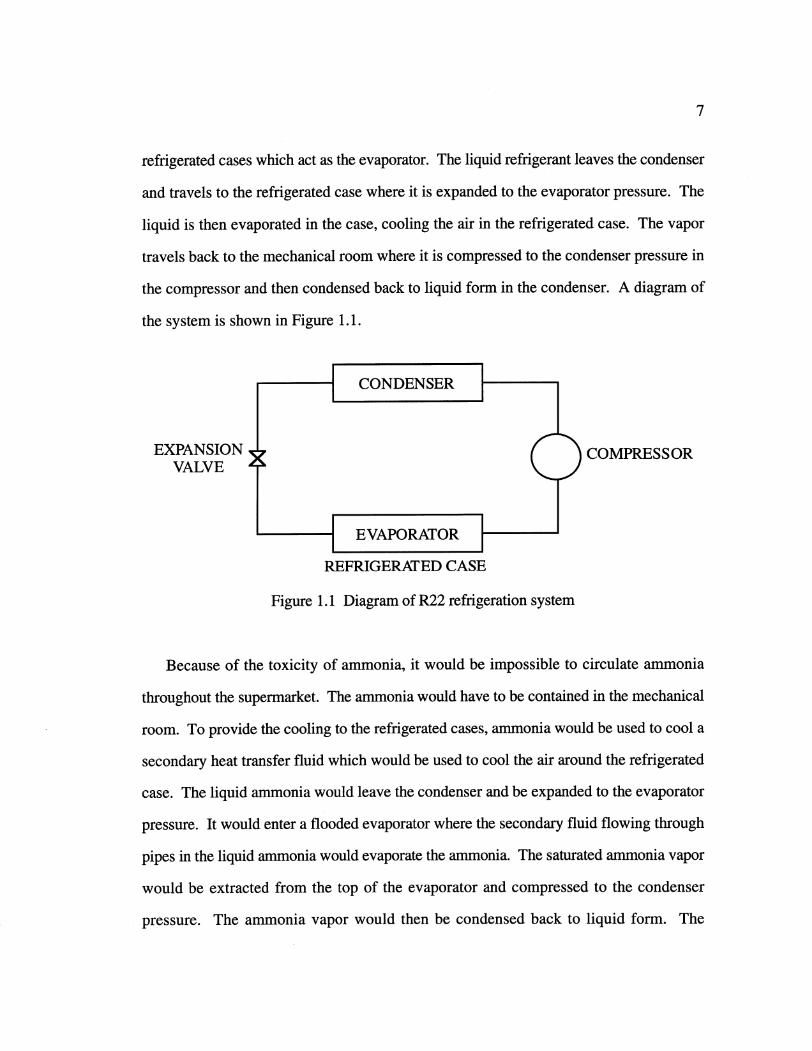
refrigerated cases which act as the evaporator. The liquid refrigerant leaves the condenser
and travels to the refrigerated case where it is expanded to the evaporator pressure. The
liquid is then evaporated in the case, cooling the air in the refrigerated case. The vapor
travels back to the mechanical room where it is compressed to the condenser pressure in
the compressor and then condensed back to liquid form in the condenser. A diagram of
the system is shown in Figure 1.1.
CONDENSER
EXPANSION COMPRESSORVALV E
EVAPORATOR
REFRIGERATED CASE
Figure 1.1 Diagram of R22 refrigeration system
Because of the toxicity of ammonia, it would be impossible to circulate ammonia
throughout the supermarket. The ammonia would have to be contained in the mechanical
room. To provide the cooling to the refrigerated cases, ammonia would be used to cool a
secondary heat transfer fluid which would be used to cool the air around the refrigerated
case. The liquid ammonia would leave the condenser and be expanded to the evaporator
pressure. It would enter a flooded evaporator where the secondary fluid flowing through
pipes in the liquid ammonia would evaporate the ammonia. The saturated ammonia vapor
would be extracted from the top of the evaporator and compressed to the condenser
pressure. The ammonia vapor would then be condensed back to liquid form. The
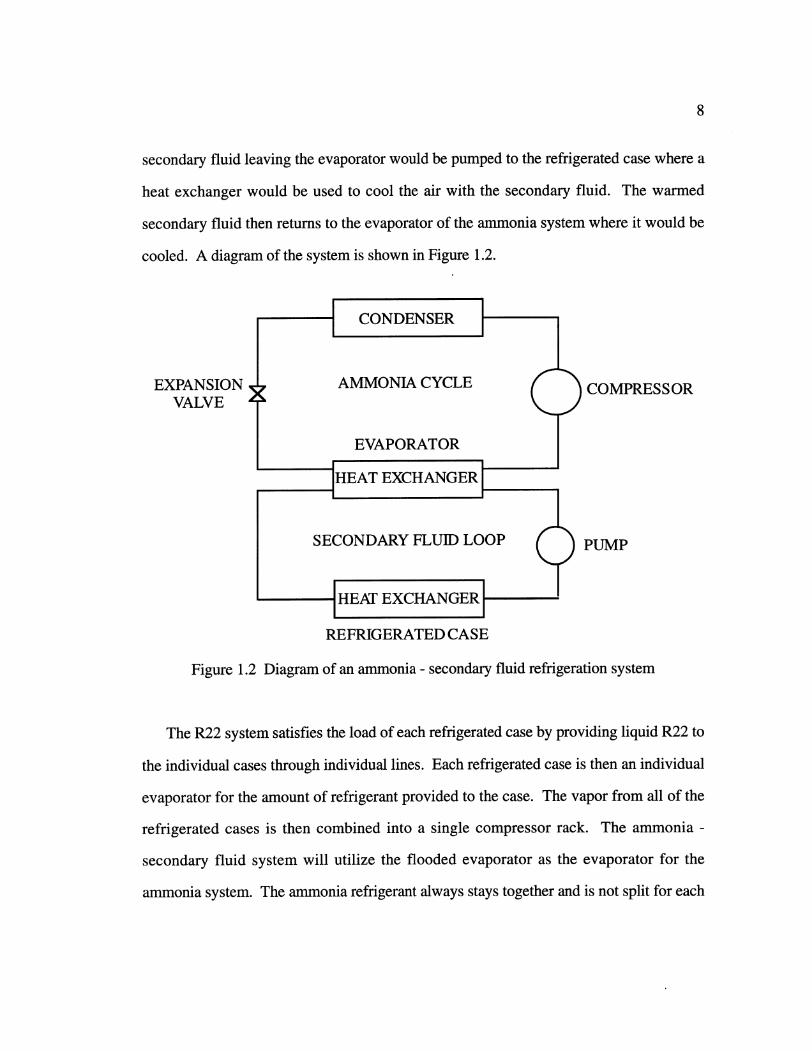
secondary fluid leaving the evaporator would be pumped to the refrigerated case where a
heat exchanger would be used to cool the air with the secondary fluid. The warmed
secondary fluid then returns to the evaporator of the ammonia system where it would be
cooled. A diagram of the system is shown in Figure 1.2.
EXPANSIONVALVE
COMPRESSOR
PUMP
REFRIGERATED CASE
Figure 1.2 Diagram of an ammonia - secondary fluid refrigeration system
The R22 system satisfies the load of each refrigerated case by providing liquid R22 to
the individual cases through individual lines. Each refrigerated case is then an individual
evaporator for the amount of refrigerant provided to the case. The vapor from all of the
refrigerated cases is then combined into a single compressor rack. The ammonia -
secondary fluid system will utilize the flooded evaporator as the evaporator for the
ammonia system. The ammonia refrigerant always stays together and is not split for each
9
of the refrigerated cases. The secondary fluid is divided as it is piped to the individual
cases and then is recombined before it reenters the flooded heat exchanger.
1.4 Refrigerant Comparison
Because of the new laws which phase-out refrigerants currently used to provide the
cooling of the refrigerated cases in supermarkets, it is necessary to select alternatives for
use in supermarkets. R22 and ammonia are two refrigerants that are already in use in
other applications that could be used in the supermarkets. However, R22 is likely to be
phased-out in the future. Therefore, it is important to determine the best method of
designing an ammonia - secondary fluid refrigeration system and comparing the
performance of such a system with the performance of a system utilizing R22. This
study uses computer models to evaluate ammonia - secondary fluid systems and compare
the performance to the performance to R22 systems.
10
CHAPTER
TWO
SECONDARY FLUIDS
There are many different fluids available for heat transfer applications. Some work well in
applications at high temperatures and some at low temperatures. For supermarket
applications it is necessary to find a fluid that balances low temperature heat transfer
performance with non-flammability and non-toxicity. In order to determine the best
secondary fluid for this application, the thermodynamic and transport properties of six
different secondary fluids were compared.
11
2.1 Secondary Fluid Descriptions
The important properties and information pertaining to toxicity and corrosiveness of
the six different secondary fluids compared for use in the supermarket system are
discussed in this section.
2.1.1 Propylene Glycol
Many chemical companies produce propylene glycol for use in heat transfer
applications. Propylene glycol-water solutions are used in applications where oral
toxicity is a concern, such as applications where contact with drinking water is possible
or in food processing applications where accidental contact with food or beverage
products is possible. These solutions can be inhibited to reduce the corrosiveness of
normal propylene glycol. The propylene glycol solution produced by the Dow Chemical
Company, called Dowfrost, was the solution considered in this application. (Dow
Chemical Company [1]) Dowfrost consists of 95.5 percent propylene glycol with
dipotassium phosphate and water, and has an operating temperature range of -46 to 121
'C (-50 to 250 F). In solutions with water, Dowfrost provides freeze protection to
below -51 °C (-60 °F) and prevents pipes from bursting to below -73 "C (-100 F). The
U.S. Department of Agriculture (USDA) lists Dowfrost as chemically acceptable for both
defrosting refrigeration coils and for immersion freezing of wrapped meats, poultry and
meats, and the FDA recognizes both propylene glycol and dipotassium phosphate as safe
food additives under parts 182 and 184 of the Food Additive Regulations. Standard
system materials can be used with Dowfrost. Steel, cast iron, copper, brass, bronze,
solder, and most plastic piping materials are generally acceptable for use, as well as
normal pipe fittings, valves, and pumps. When Dowfrost is mixed with water it is not
flammable, as long as the percentage of propylene-glycol remains less than 80%.
12
Dowfrost contains inhibitors that prevent corrosion by passivating the surface of metals to
prevent acids from attacking it and by buffering acids formed from glycol oxidation.
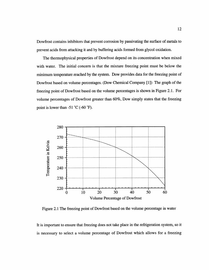
The thermophysical properties of Dowfrost depend on its concentration when mixed
with water. The initial concern is that the mixture freezing point must be below the
minimum temperature reached by the system. Dow provides data for the freezing point of
Dowfrost based on volume percentages. (Dow Chemical Company [ 1 ]) The graph of the
freezing point of Dowfrost based on the volume percentages is shown in Figure 2.1. For
volume percentages of Dowfrost greater than 60%, Dow simply states that the freezing
point is lower than -51 'C (-60 F).
cI)
SF-
280
270
260
250
240
230
2200 10
.... .. .... ... . ... .. ... .. ... ... --- --- --- --- --- -- --- --- --- --- --- --- ----. --- --. --- --- --- --- -
20 30 40Volume Percentage of Dowfrost
60
Figure 2.1 The freezing point of Dowfrost based on the volume percentage in water
It is important to ensure that freezing does not take place in the refrigeration system, so it
is necessary to select a volume percentage of Dowfrost which allows for a freezing
50
13
temperature 10 to 15 C below the lowest anticipated temperature. For the supermarket
application studied here, a volume percentage of 60% is necessary to ensure the proper
safety against freezing in the lines.
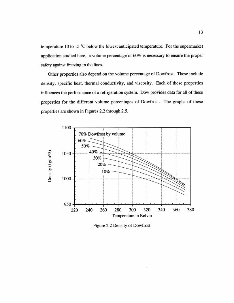
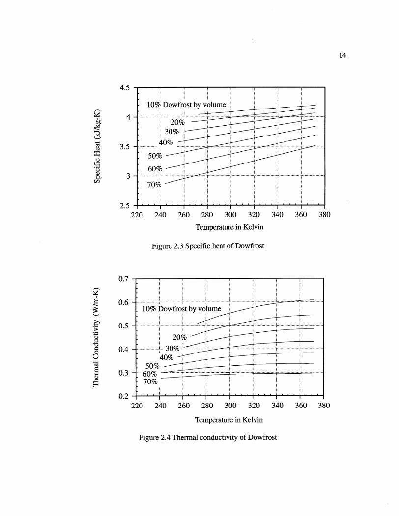
Other properties also depend on the volume percentage of Dowfrost. These include
density, specific heat, thermal conductivity, and viscosity. Each of these properties
influences the performance of a refrigeration system. Dow provides data for all of these
properties for the different volume percentages of Dowfrost. The graphs of these
properties are shown in Figures 2.2 through 2.5.
110070% Dowfrost by volume
0%0%
10 5 0 . ................. ---
1000
950220
20% i
...................................... .......
------------ -----------------------------------
240 260 280 300 320 340 360 380Temperature in Kelvin
Figure 2.2 Density of Dowfrost
I
3. -
3.5-
I I I I I I I
220 240 260 280 300 320 340 360 380
Temperature in Kelvin
Figure 2.3 Specific heat of Dowfrost
0.7
0.6
0.5
0.4
00.3
0.2 -4I I T
220 240 260 280 300 320 340 360 380
Temperature in Kelvin
Figure 2.4 Thermal conductivity of Dowfrost
4.5
A
14
0
00
10% Dowfrost by volume
--- -.- ... .... --- -- -.- -- -- -- -............... . . - - - - - -- ----.. .. .
30%3o40%........ ... --- -- --- -- --
50%
*60%
70%
_____________ b ~. ~ d ~** *** ____________2.5
10%. lODowfros by voum------ ----- ---.. ..... ............ ..... ............. ..... ........... .... .... .. ......-- -- -- ------ ---......--- ----- -
* 20%
* 40%... ... .. ... .. ..... .....
50%"- 6 0 % ..........................
70%,
.................. -------------
..............
........ ....... -------------------------- -----
................. .................. ---------------------------------------------------------- . ------------------.........-------------------------- -------------- --------------------- ................-1.
I I I ! I I II
.................. --.................................. ------------------ J-
15
00r.I~
0.1
0.01
0.001
0.0001220 240 260 280 300 320 340
Temperature in Kelvin
360 380
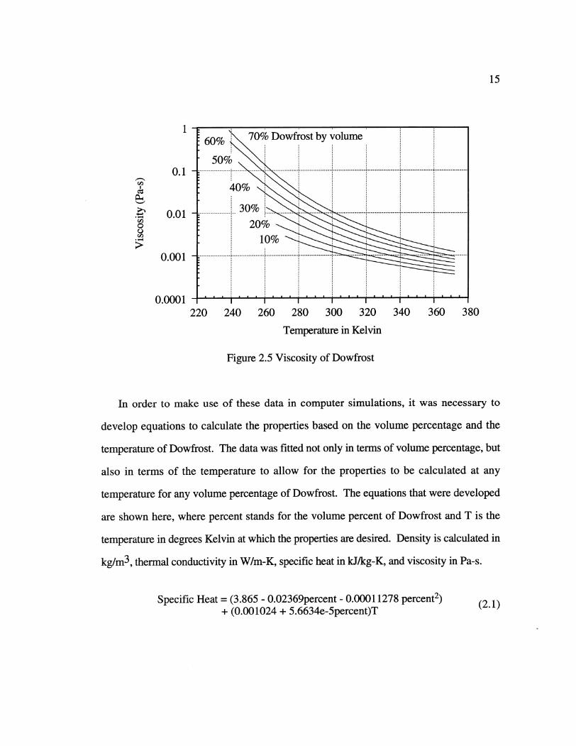
Figure 2.5 Viscosity of Dowfrost
In order to make use of these data in computer simulations, it was necessary to
develop equations to calculate the properties based on the volume percentage and the
temperature of Dowfrost. The data was fitted not only in terms of volume percentage, but
also in terms of the temperature to allow for the properties to be calculated at any
temperature for any volume percentage of Dowfrost. The equations that were developed
are shown here, where percent stands for the volume percent of Dowfrost and T is the
temperature in degrees Kelvin at which the properties are desired. Density is calculated in
kg/m3 , thermal conductivity in W/m-K, specific heat in kJ/kg-K, and viscosity in Pa-s.
Specific Heat = (3.865 - 0.02369percent - 0.00011278 percent2) (2.1)+ (0.001024 + 5.6634e-5percent)T
60 70% Dowfrost by volume
-------- ... ..... . ................. .................. .................. .................... ................. ...................
---------- 3 o0 % .... .... I .. .... .. ....... .... .............. i.... ............. ].... .............. .
-20%10%
-- - -- --- --.I- - - - - -- ---..-- - - - - - -- - - - - - - - . ... . . . .. . . . . . . .. . .
....
16
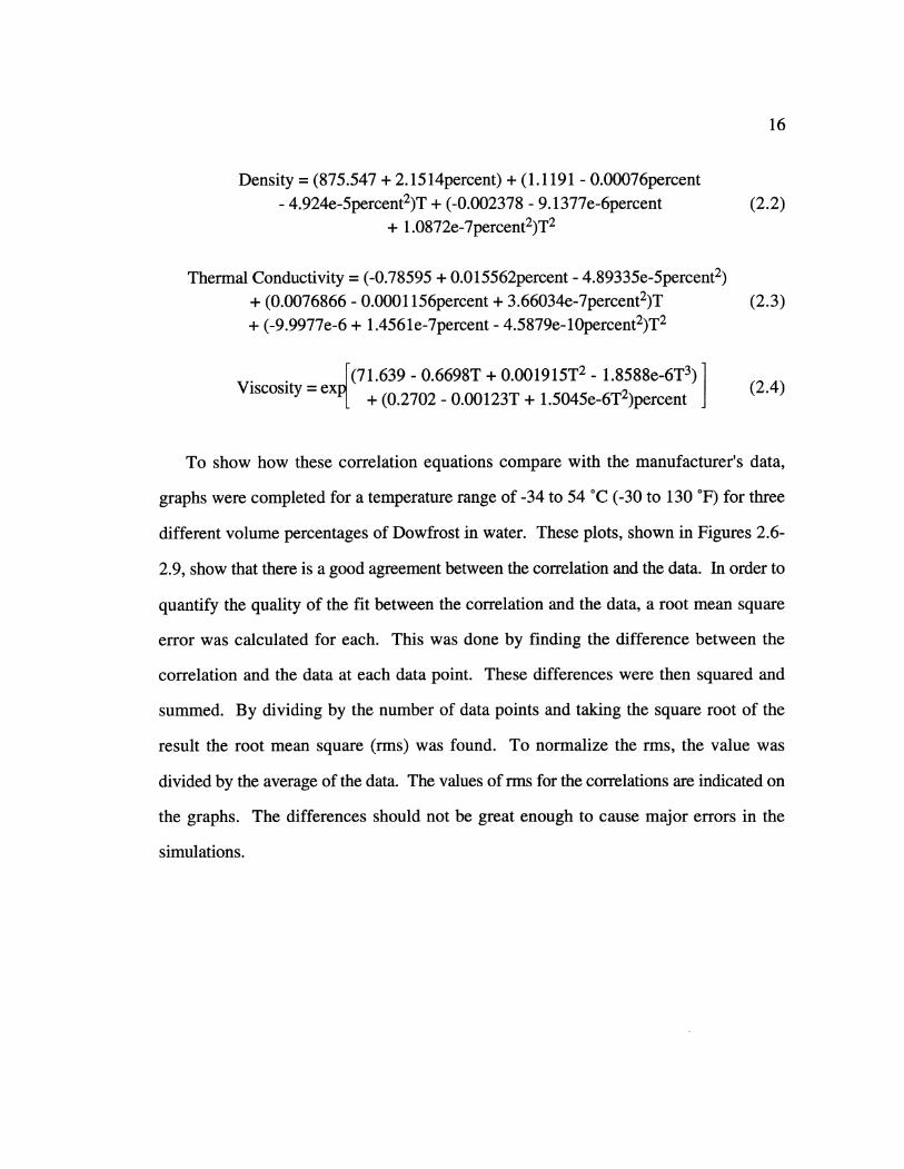
Density = (875.547 + 2.1514percent) + (1.1191 - 0.00076percent- 4.924e-5percent 2)T + (-0.002378 - 9.1377e-6percent (2.2)
+ 1.0872e-7percent2)T2
Thermal Conductivity = (-0.78595 + 0.015562percent - 4.89335e-5percent 2)
+ (0.0076866 - 0.0001156percent + 3.66034e-7percent 2)T (2.3)+ (-9.9977e-6 + 1.456 le-7percent - 4.5879e- 10percent2)T2
Viscosity =ex (7 1.639 - 0.6698T + 0.001915T 2 - 1.8588e-6T3)] (2.4)L[ + (0.2702 - 0.00123T + 1.5045e-6T 2)percent-J
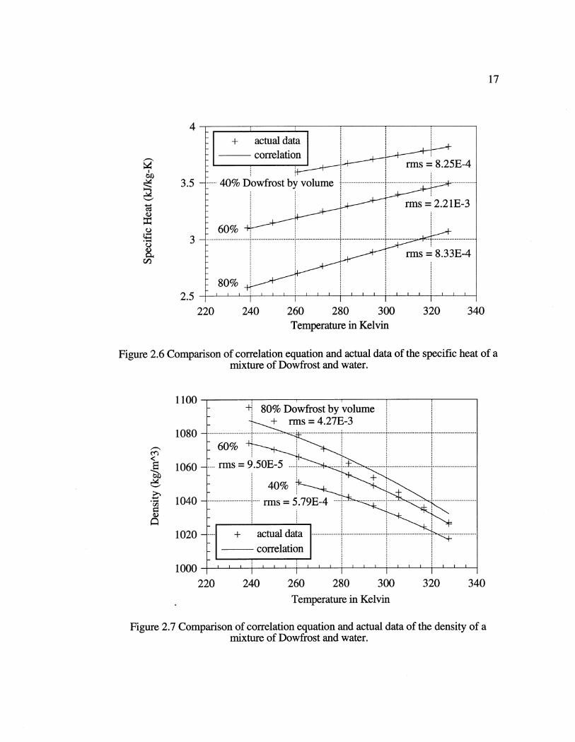
To show how these correlation equations compare with the manufacturer's data,
graphs were completed for a temperature range of -34 to 54 C (-30 to 130 F) for three
different volume percentages of Dowfrost in water. These plots, shown in Figures 2.6-
2.9, show that there is a good agreement between the correlation and the data. In order to
quantify the quality of the fit between the correlation and the data, a root mean square
error was calculated for each. This was done by finding the difference between the
correlation and the data at each data point. These differences were then squared and
summed. By dividing by the number of data points and taking the square root of the
result the root mean square (rms) was found. To normalize the rms, the value was
divided by the average of the data. The values of rms for the correlations are indicated on
the graphs. The differences should not be great enough to cause major errors in the
simulations.
17
4-actual datacorrelation
rms 8.25E-4
3.5 40% D ow frost by volum e .................. . . . ..... .........
rms 2.21E-3
060% 3 ....................... .. ........................----.....................I ........................-- ................. ..-- .-........................
€ rms 8.33E-4
80%2.5
220 240 260 280 300 320 340Temperature in Kelvin
Figure 2.6 Comparison of correlation equation and actual data of the specific heat of amixture of Dowfrost and water.
1100 1 0- 80% Dowfrost by volume_- + ..=..4.27E-3; .. ................. ........... .. ....................... ......................... ,........................ ........................
1080 -. 0%16 60%
S 1060 ..... rm s 9.50E-5 ....... .............+--------
" 10 0 ........................ r s 5 7 E -... .. .... ....... .... .. ..... ...........-------S1040- rms 5.79E-4..
1020 - "- + actual data ................ ........................................... .............
correlation10 0 0 ' ' ' ' ' ' ' ' ' ' ' ' ' ' ' ' '
220 240 260 280 300 320 340Temperature in Kelvin
Figure 2.7 Comparison of correlation equation and actual data of the density of amixture of Dowfrost and water.
18
10
1
0.1
0.01
0.001220 240 260 280 300 320 340
Temperature in Kelvin
Figure 2.8 Comparison of correlation equation and actual data of the viscosity of amixture of Dowfrost and water.
0.45
0.4
0.35
0.3
0.25220 240 260 280 300
Temperature in Kelvin320 340
Figure 2.9 Comparison of correlation equation and actual data of the thermalconductivity of a mixture of Dowfrost and water.
00.
80% Dowfrost by volume
- ~~rms-178 + actualdata.. ....... 4 --.--- ---- -... ....
60%
T ............... ................ .......... . ... .. .....!......... -----------.............--------------rms0.124
I
0
0u3
r-.
actual data
correlation... .................................... .... ... ---- --------.. ..........rms 0.0112
40% Dowfrost by volume. ............... ................................. ........................ ................................................. .........................
-......................F nns=0.00799
80% rms:0.015380% _ _ _ + + + ++,I i - '- ± 1+' ± +± ±
19
2.1.2 Ethylene Glycol
Ethylene glycol is another popular heat transfer fluid that is manufactured by many
different chemical companies. Since ethylene glycol is less viscous than propylene glycol,
it generally provides greater heat transfer efficiencies and better low temperature
performance. It is, however, moderately oral toxic and should be used with caution where
accidental contact with food can occur. The Dow Chemical Company manufactures a
family of inhibited ethylene glycol under the name of Dowtherm. (Dow Chemical
Company [2]) Dowtherm SR-1 consists of 95.4% ethylene glycol along with inhibitors
and has an operating range of -51 to 121 °C (-60 to 250 OF). In solutions with water, it
provides freeze protection to below -51 °C (-60 OF) and burst protection to below -73 °C (-
100 OF). Dowtherm SR-1 is listed as chemically acceptable by the U.S. Department of
Agriculture (USDA) for defrosting refrigeration coils in food processing plants assuming
that good manufacturing practices are used to prevent direct or indirect contact of the
ethylene glycol fluid with edible products. The construction material restrictions for
Dowtherm SR-1 are almost exactly the same as for Dowfrost. Steel, cast iron, copper,
brass, bronze, solder and most plastics are generally acceptable. Aluminum can be used
at temperatures below 66 °C (150 OF) and pipe fittings and valves can be made of ordinary
steel or ductile iron. Dowtherm SR-I is only flammable in volume percentages greater
than 80%. The inhibitors against corrosion used in Dowtherm SR-1 work by first
passivating the surface of metals to prevent acids from attacking it and second, by
buffering any acids formed from glycol oxidation.
The thermophysical properties of Dowtherm SR-1 depend on the concentration of the
mixture with water. The freezing point of the mixture is a great concern in the cold
temperature applications studied here, and it is necessary to utilize a volume percentage of
20
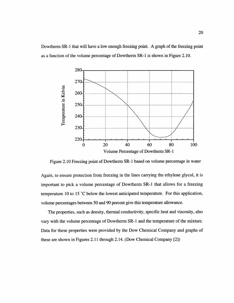
Dowtherm SR-1 that will have a low enough freezing point. A graph of the freezing point
as a function of the volume percentage of Dowtherm SR-I is shown in Figure 2.10.
280___
270-
t 26.-
S 250
S 240.
23-
220. r
0 20 40 60 80 100
Volume Percentage of Dowtherm SR-1
Figure 2.10 Freezing point of Dowtherm SR-i based on volume percentage in water
Again, to ensure protection from freezing in the lines carrying the ethylene glycol, it is
important to pick a volume percentage of Dowtherm SR-i that allows for a freezing
temperature 10 to 15 0C below the lowest anticipated temperature. For this application,
volume percentages between 50 and 90 percent give this temperature allowance.
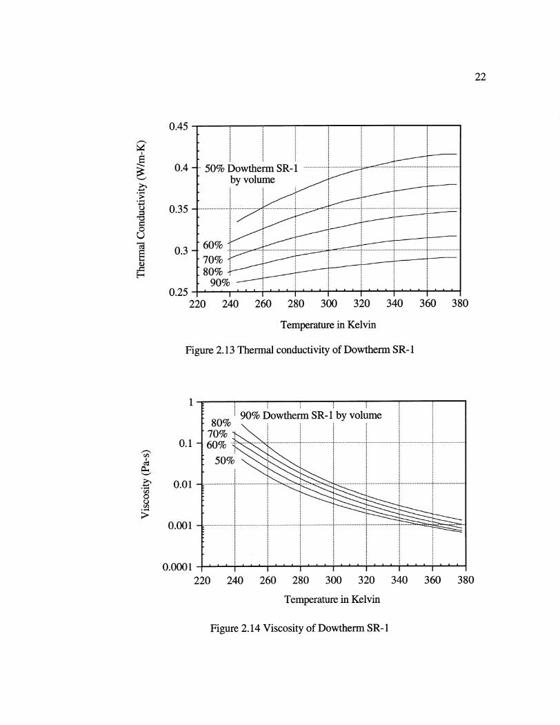
The properties, such as density, thermal conductivity, specific heat and viscosity, also
vary with the volume percentage of Dowtherm SR-i and the temperature of the mixture.
Data for these properties were provided by the Dow Chemical Company and graphs of
these are shown in Figures 2.11 through 2.14. (Dow Chemical Company [2])
4
3.5
C4
3
$:1 2.5
2
220 240 260 280 300 320 340 360 380
Temperature in Kelvin
Figure 2.11 Specific heat of Dowtherm SR- I
I T I I 1
220 240 260 280 300 320 340 360 380
Temperature in Kelvin
Figure 2.12 Density of Dowtherm SR-1
21
-50% Dowtherm SR-1 by volume
60%
70%
80%
90%
1160
1140
S 1120
b 1100
1080
S 1060
1040
IUzU
90% Dowtherm SR-1 by volume
:80%;70 ................ ............... ...........
.................. !................ [ ..................... ..........---- .......... ...-------..... ....----..... ................. .............---- ---- --- .... ... .... ......... ................... ................. .......... ................... ....... ...... ....... 1.. . . . . . . . - - -
------------------------------------- .................lm
I
Temperature in Kelvin
Figure 2.13 Thermal conductivity of Dowtherm SR-I
220 240 260 280 300 320
Temperature in Kelvin
Figure 2.14 Viscosity of Dowtherm SR-1
22
0.45
0.4
0.35
0.3
0.25
0 ,-
0
380
0
0 ,-
0.1
0.01
0.001
0.0001
90% Dowtherm SR-1 by volume80%
70%
7 %. ............... .................. .... ..... ... .. ... ................. .................. .................. U...................-60%
T I I Ir
340 360 380
23
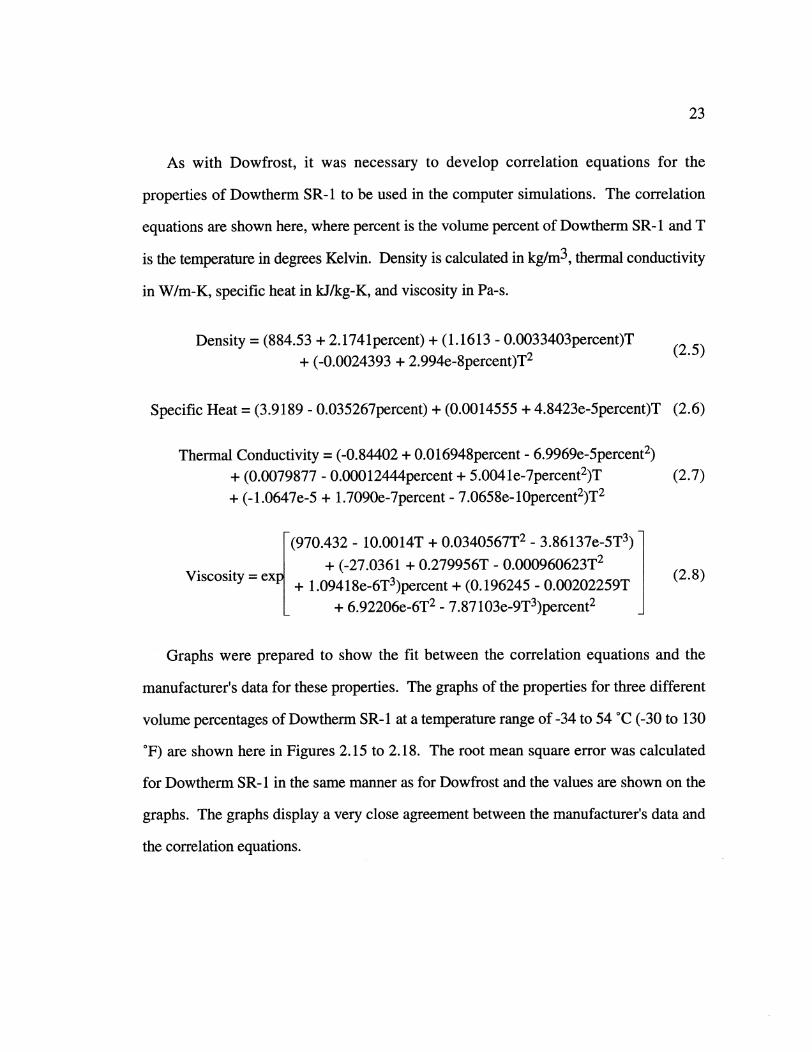
As with Dowfrost, it was necessary to develop correlation equations for the
properties of Dowtherm SR-1 to be used in the computer simulations. The correlation
equations are shown here, where percent is the volume percent of Dowtherm SR-1 and T
is the temperature in degrees Kelvin. Density is calculated in kg/m3, thermal conductivity
in W/m-K, specific heat in kJ/kg-K, and viscosity in Pa-s.
Density = (884.53 + 2.1741percent) + (1.1613 - 0.0033403percent)T (2.5)+ (-0.0024393 + 2.994e-8percent)T 2
Specific Heat = (3.9189 - 0.035267percent) + (0.0014555 + 4.8423e-5percent)T (2.6)
Thermal Conductivity = (-0.84402 + 0.016948percent - 6.9969e-5percent 2)
+ (0.0079877 - 0.00012444percent + 5.004le-7percent 2)T (2.7)
+ (-1.0647e-5 + 1.7090e-7percent - 7.0658e-10percent 2)T2
L(970.432 - 10.0014T + 0.0340567T 2 - 3.86137e-5T 3)
Viscosity = exp + (-27.0361 + 0.279956T - 0.000960623T 2 ] (2.8)+ 1.09418e-6T3 )percent + (0.196245 - 0.00202259T
+ 6.92206e-6T 2 - 7.87103e-9T 3)percent2
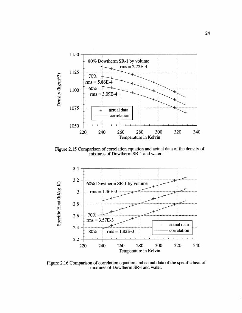
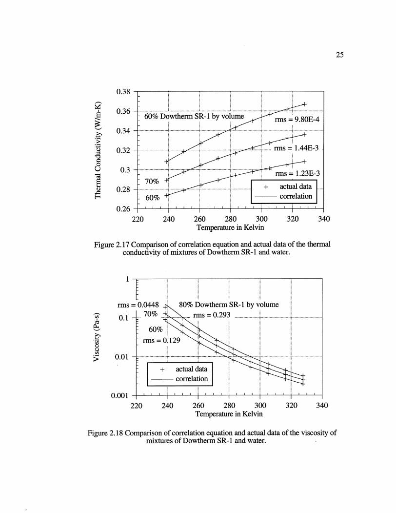
Graphs were prepared to show the fit between the correlation equations and the
manufacturer's data for these properties. The graphs of the properties for three different
volume percentages of Dowtherm SR-1 at a temperature range of -34 to 54 C (-30 to 130
*F) are shown here in Figures 2.15 to 2.18. The root mean square error was calculated
for Dowtherm SR-I in the same manner as for Dowfrost and the values are shown on the
graphs. The graphs display a very close agreement between the manufacturer's data and
the correlation equations.
1150
S 1125
1100
1075
1050220 240 260 280 300
Temperature in Kelvin
Figure 2.15 Comparison of correlation equation and actual data of the density ofmixtures of Dowtherm SR-1 and water.
3.4
3.2
3
2.8
2.6
2.4
2.2220 240 260 280 300 320 340
Temperature in Kelvin
Figure 2.16 Comparison of correlation equation and actual data of the specific heat ofmixtures of Dowtherm SR- land water.
24
80% Dowtherm SR-1 by volume-m 2..7.2E-4-. ...... ... -o-- ,-.. .... ..--. .. ... .... ....-.. ... .... ... ..
70%rms-= .86E-4 .-rms=3.09E-4 i .
-.. . . . .. . ..- -- - -. .-- - -- -- - -- -- --t -- - - -- - -- - - -- - -- -- -- - - .- -
correlation
I I 1
320 340
0o
0D
60% Dowtherm SR- iby volume
80%. rms 12E 3 correlation. ...... .................................... -. ..... ........ .....................
25
0.38
0.36
0.34
0.32
0.3
0.28
0.26220 240 260 280 300 320
Temperature in Kelvin340
Figure 2.17 Comparison of correlation equation and actual data of the thermalconductivity of mixtures of Dowtherm SR-I and water.
rms
0.1
0.01
0.001220 240 260 280 300 320
Temperature in Kelvin340
Figure 2.18 Comparison of correlation equation and actual data of the viscosity ofmixtures of Dowtherm SR-1 and water.
0
0
Q
H
0,t
0
26
2.1.3 Mineral Oil
A third common heat transfer fluid is mineral oil. There are many different
substances that fall under the name mineral oil and each has different properties. The
Multitherm Corporation produces a large family of mineral oil fluids for heat transfer
purposes. (Multitherm Corporation) Their low temperature fluid, which is
polyalphaolefin, is produced under the name Multitherm 503. It is a non-toxic substance
that meets the FDA regulation 21CRF178.3620(b) for use as a synthetic white mineral oil
for non-food articles in contact with food. It can be specified for many food, beverage,
and pharmaceutical applications. It is also non-corrosive, so it can be used with all
construction materials. Multitherm 503 does not irritate eyes or skin, should not present
an inhalation hazard at ambient temperatures, and ingestion is non-toxic. However, it
does act as a laxative when ingested. The flash point of Multitherm 503 is 160 °C (320
F) and the autoignition point is 324 *C (615 F). Fires must be extinguished with a dry
chemical or foam rather than water. Combustion of Multitherm 503 will produce carbon
monoxide and other asphyxiates. However, the fire hazard rating of Multitherm 503 is
slight.
The Multitherm Corporation has provided property data for Multitherm 503.
(Multitherm Corporation) Multitherm 503 is considered pumpable down to -58 °C (-72
F). As with Dowfrost and Dowtherm SR-1, correlation equations were written for the
data for use in computer simulations. The properties of Multitherm 503 depend only on
the temperature of the fluid and are shown here where T stands for temperature in degrees
Kelvin. Density is calculated in kg/m3 , thermal conductivity in W/m-K, specific heat in
kJl/kg-K, and viscosity in Pa-s.
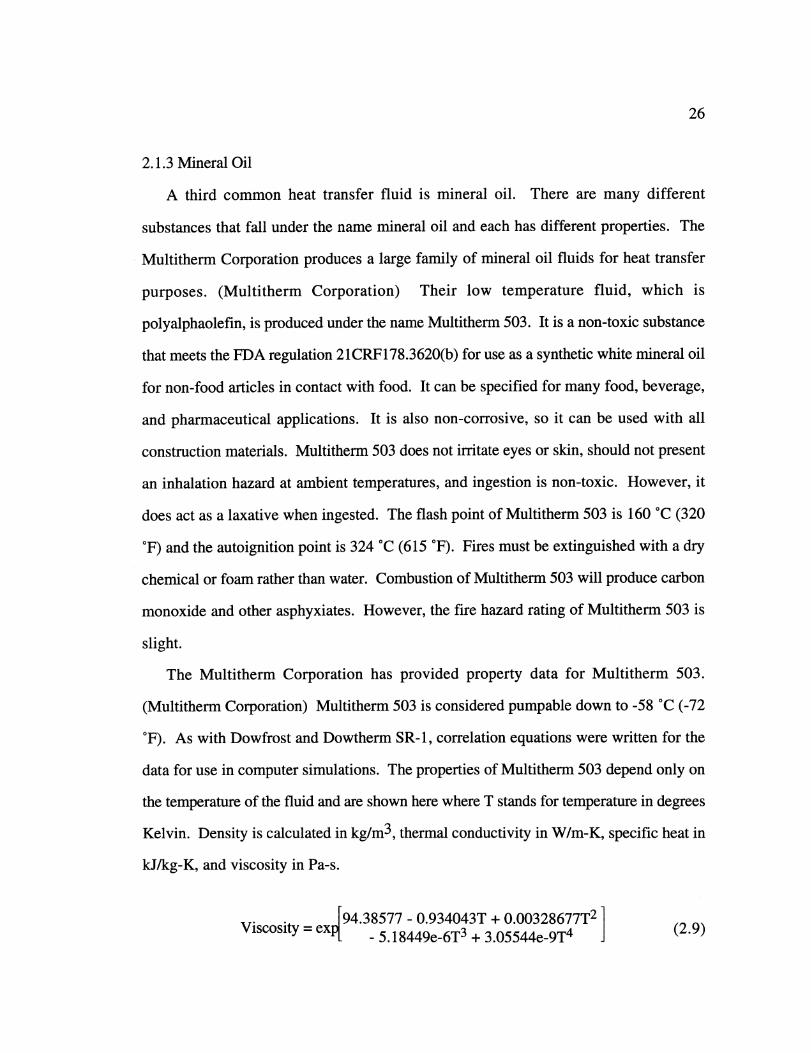
[94.38577 - 0.934043T + 0.00328677T2 1Viscosity = exp[ _ 518449e-6T3 + 3.05544e_9T 4 J (2.9)
27
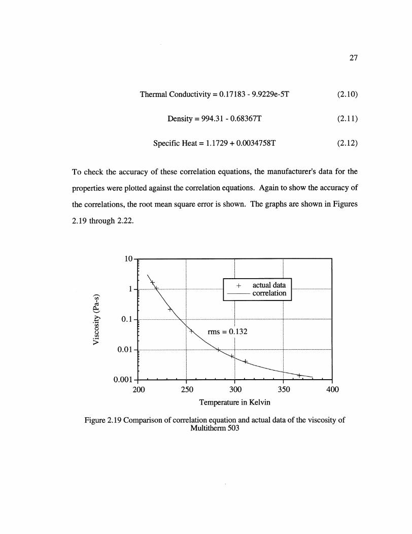
Thermal Conductivity = 0.17183 - 9.9229e-5T
Density = 994.31 - 0.68367T
(2.10)
(2.11)
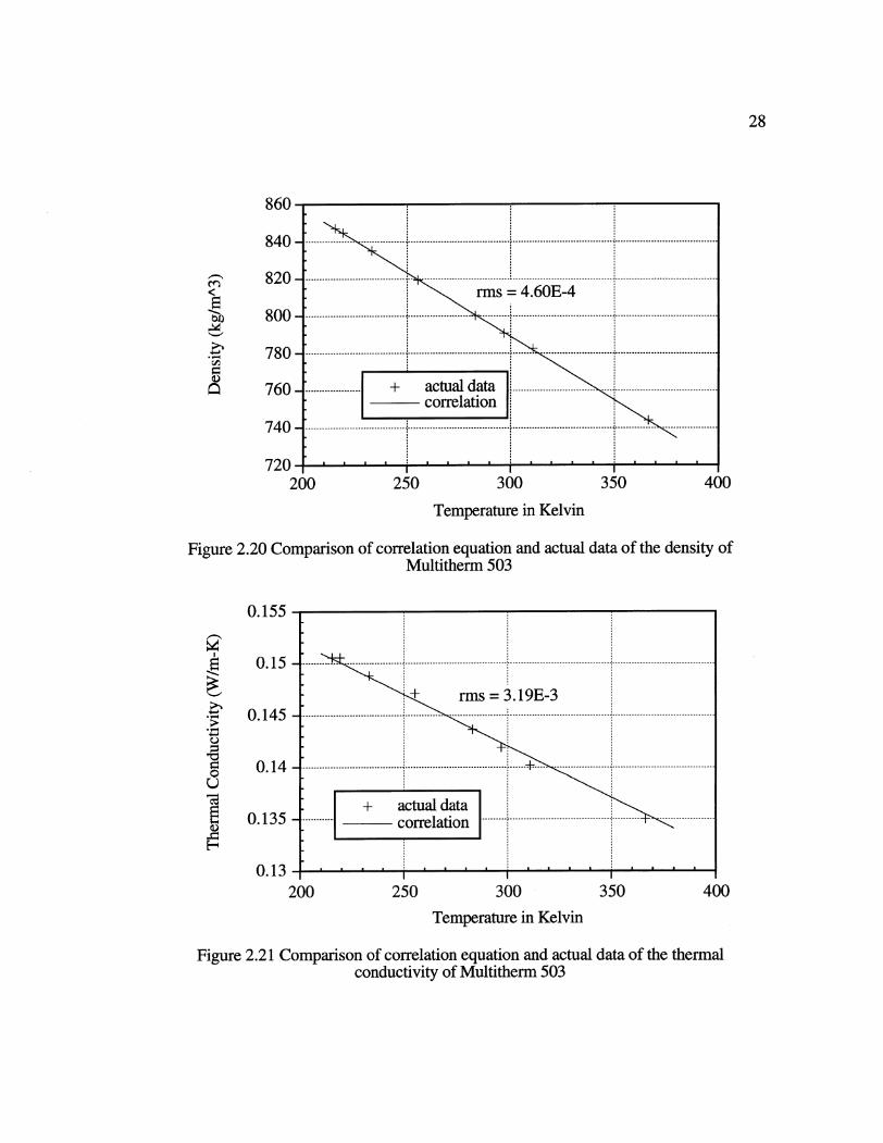
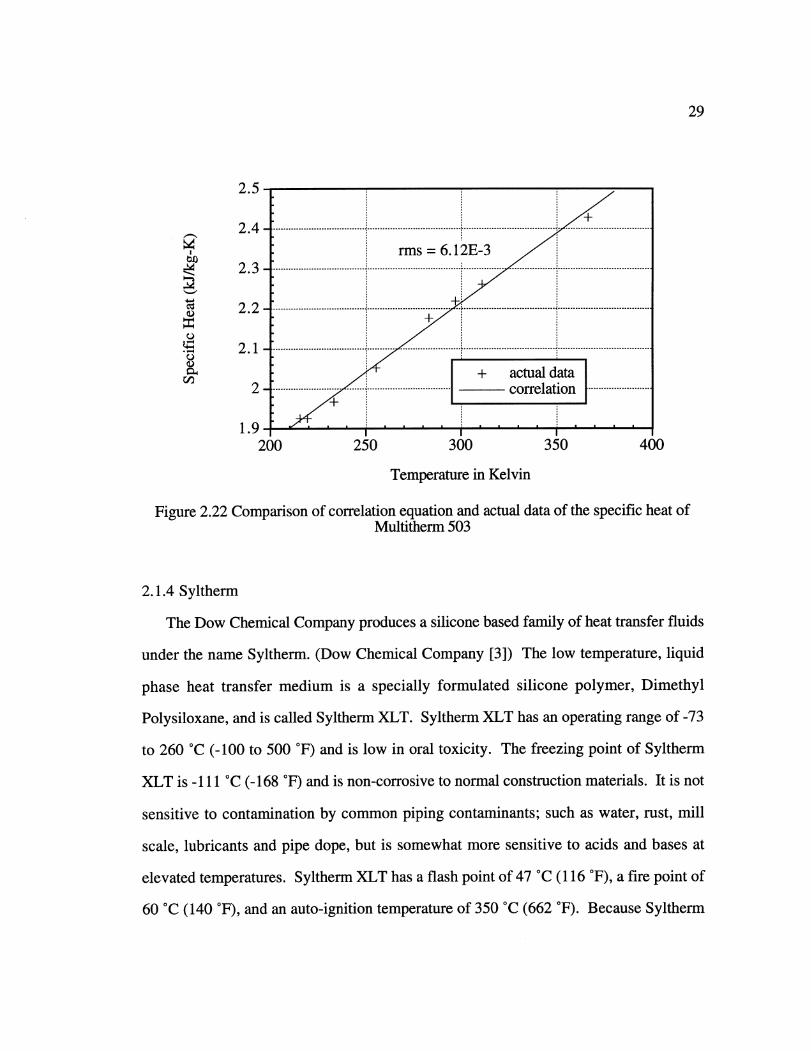
(2.12)Specific Heat = 1.1729 + 0.0034758T
To check the accuracy of these correlation equations, the manufacturer's data for the
properties were plotted against the correlation equations. Again to show the accuracy of
the correlations, the root mean square error is shown. The graphs are shown in Figures
2.19 through 2.22.
0.10C3
Cj
0.01
0.001 .
200 250 300 350 400
Temperature in Kelvin
Figure 2.19 Comparison of correlation equation and actual data of the viscosity ofMultitherm 503
28
860
840
820
800
780
760
740
T79 -
200 2503300 350 400
Temperature in Kelvin
Figure 2.20 Comparison of correlation equation and actual data of the density ofMultitherm 503
0.155
0.15
0.145
0.14
0.135
0.13 --200 250 300 350 400
Temperature in Kelvin
Figure 2.21 Comparison of correlation equation and actual data of the thermalconductivity of Multitherm 503
................... ................ ..................................... .................................... ....................................
71. .< _ ..
U!.=
0 -,
U
-------------------------------------------------------------------------
....... ........................... ....................................
.............................. .........................................-------- ......................
.......................................------------------------------------- ..............-------------------- actual data
correlation
29
2.5
2.4-
rms =6.12E32.3-
2.2- +.i2 .3 ." .................................... ......................... ......... .................. .................. i ....................................
2.1-...2 2 ----------------- .......................... ..... .................................. .. ..........n ..........................
+ actual data12-1 Loelatn ....
1.9-200 250 300 350 400
Temperature in Kelvin
Figure 2.22 Comparison of correlation equation and actual data of the specific heat ofMultitherm 503
2.1.4 Syltherm
The Dow Chemical Company produces a silicone based family of heat transfer fluids
under the name Syltherm. (Dow Chemical Company [3]) The low temperature, liquid
phase heat transfer medium is a specially formulated silicone polymer, Dimethyl
Polysiloxane, and is called Syltherm XLT. Syltherm XLT has an operating range of -73
to 260 °C (-100 to 500 °F) and is low in oral toxicity. The freezing point of Syltherm
XLT is -111 °C (-168 F) and is non-corrosive to normal construction materials. It is not
sensitive to contamination by common piping contaminants; such as water, rust, mill
scale, lubricants and pipe dope, but is somewhat more sensitive to acids and bases at
elevated temperatures. Syltherm XLT has a flash point of 47 °C (116 F), a fire point of
60 °C (140 °F), and an auto-ignition temperature of 350 °C (662 °F). Because Syltherm
30
XLT is a poor electrical conductor, static charges can build up and discharge static
electricity. Therefore, it is necessary to exclude oxygen from the headspace of the
expansion tank. Syltherm XLT has been studied for acute toxicology under the Federal
Hazardous Substance Act (FSHA) guidelines. It was classified as non-toxic with regard
to acute oral ingestion and dermal absorption and having minimal potential for eye or skin
irritation. Studies also indicate that repeated, prolonged skin contact should not result in
irritation. Syltherm XLT has minimal odor and no airborne exposure limits, however,
vapors released into the air at temperatures above 149 C (300 F) may cause temporary
eye and/or respiratory irritation.
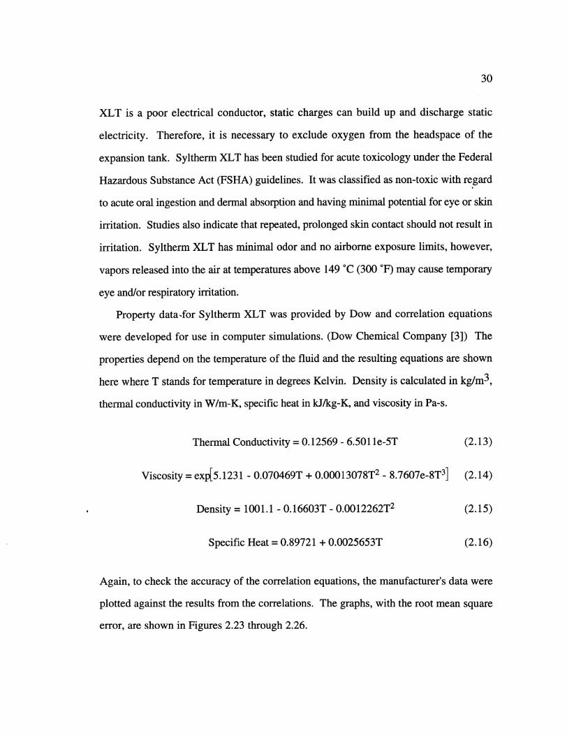
Property datafor Syltherm XLT was provided by Dow and correlation equations
were developed for use in computer simulations. (Dow Chemical Company [3]) The
properties depend on the temperature of the fluid and the resulting equations are shown
here where T stands for temperature in degrees Kelvin. Density is calculated in kg/m 3 ,
thermal conductivity in W/m-K, specific heat in kJ/kg-K, and viscosity in Pa-s.
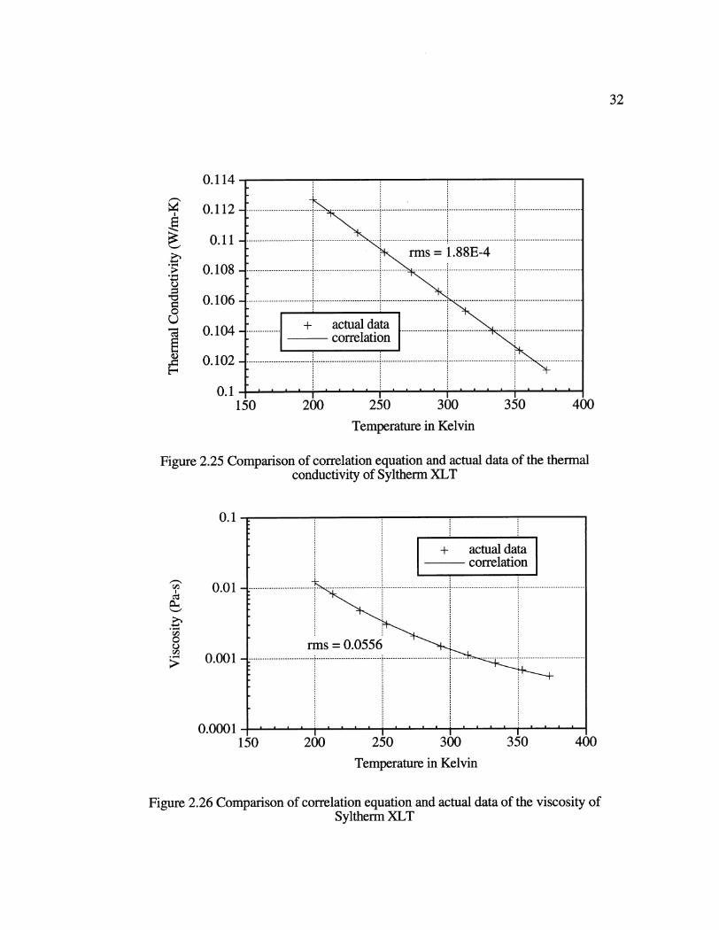
Thermal Conductivity = 0.12569 - 6.501 le-5T (2.13)
Viscosity = exp[5.1231 - 0.070469T + 0.00013078T 2 - 8.7607e-8T3] (2.14)
Density = 1001.1 - 0.16603T - 0.0012262T2 (2.15)
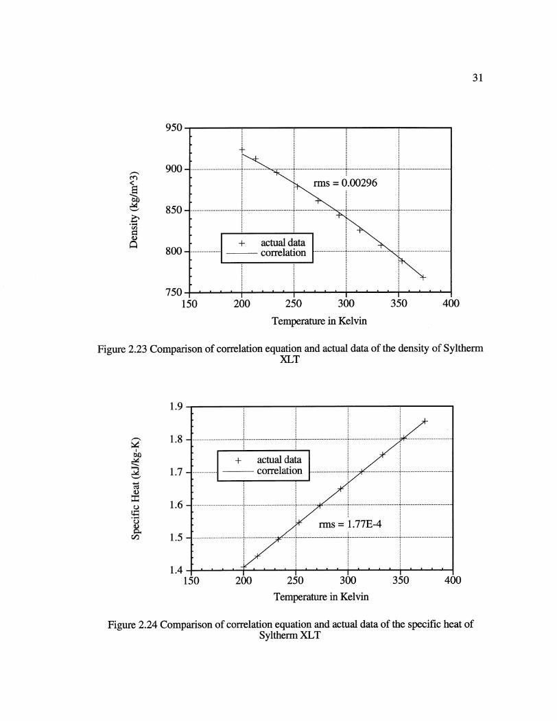
Specific Heat = 0.89721 + 0.0025653T (2.16)
Again, to check the accuracy of the correlation equations, the manufacturer's data were
plotted against the results from the correlations. The graphs, with the root mean square
error, are shown in Figures 2.23 through 2.26.
31
950
9 0 0 -.-.-- ----------- ----------- -- ---- ------------.. .. .... .. ... .- ------.. .......... .. .. .. --.. ... ... .. ..... ......... ....... .. ..... ----.. ..... ..... .... .. .....
rms 0.00296
actu data8 0 0 ~. ................. c-------............--................ ..-...................800 oreatioj ---------------------
750i
150 200 250 300 350 400
Temperature in Kelvin
Figure 2.23 Comparison of correlation equation and actual data of the density of SylthermXLT
1.9
1.8
1.7
1.6
1.5
1.4
0
0
C-,
Temperature in Kelvin
Figure 2.24 Comparison of correlation equation and actual data of the specific heat ofSyltherm XLT
oU,
0
UD
0.114
0.112
0.11
0.108
0.106
0.104
0.102
0.1 - n150 200 250 300 350 400
Temperature in Kelvin
Figure 2.25 Comparison of correlation equation and actual data of the thermalconductivity of Syltherm XLT
0.1
0•0,,,4-
0.01
0.001
0.0001
+ actual datacorrelation
....... .............. .. ........................... ............................. A ........ .. ................ j .............................
150 200 250 300 350 400
Temperature in Kelvin
Figure 2.26 Comparison of correlation equation and actual data of the viscosity ofSyltherm XLT
32
33
2.1.5 Ethanol
Ethanol, or ethyl alcohol, is a common heat transfer fluid. Rather than use the
properties of ethanol from a chemical company, the correlations were developed from
data taken from Liley, Yaws, and Natarajan. (Liley 1970, Yaws 1992, and Natarajan
1989) It is also important to note that ethanol is both flammable and explosive. When
denatured, toxicity with ethanol is not a concern. The correlation equations used for
ethanol are shown here, where T stands for temperature in Kelvin.
Thermal Conductivity = 0.25715 - 0.00030645T (2.17)
Viscosity= exp{11.664554604 - 0.057902271482T + 6.356133171le-5T2] (2.18)1000
Density = 0.2567e3*0.240 -1- 518(2.19)
Specific Heat - 100.92 - 111.839e-3T + 498.54e-6T 2 (2.20)46
2.1.6 Propane
Propane is a refrigerant that can also be used as a secondary fluid. It is necessary
with propane to ensure that the pressure is high enough that the propane remains in liquid
form throughout the system. Propane is also a highly flammable and explosive substance
and needs to be used with caution. The equation solving program that was used to run
the computer simulations, EES, calculates the properties of refrigerants, including
propane. (Klein 1993) The properties are calculated using data from the ASHRAE
handbook of fundamentals and the Martin-Hou equation of state. (ASHRAE 1989 and
Martin 1955) These were used for the properties for propane.
34
2.2 Comparison of Properties of Secondary Fluids
The first step in determining the best secondary coolant for use in the supermarket
system is to compare the properties of the different secondary coolants. Density, thermal
conductivity, specific heat and viscosity were calculated for the six fluids for temperatures
between 230 and 315 OK.
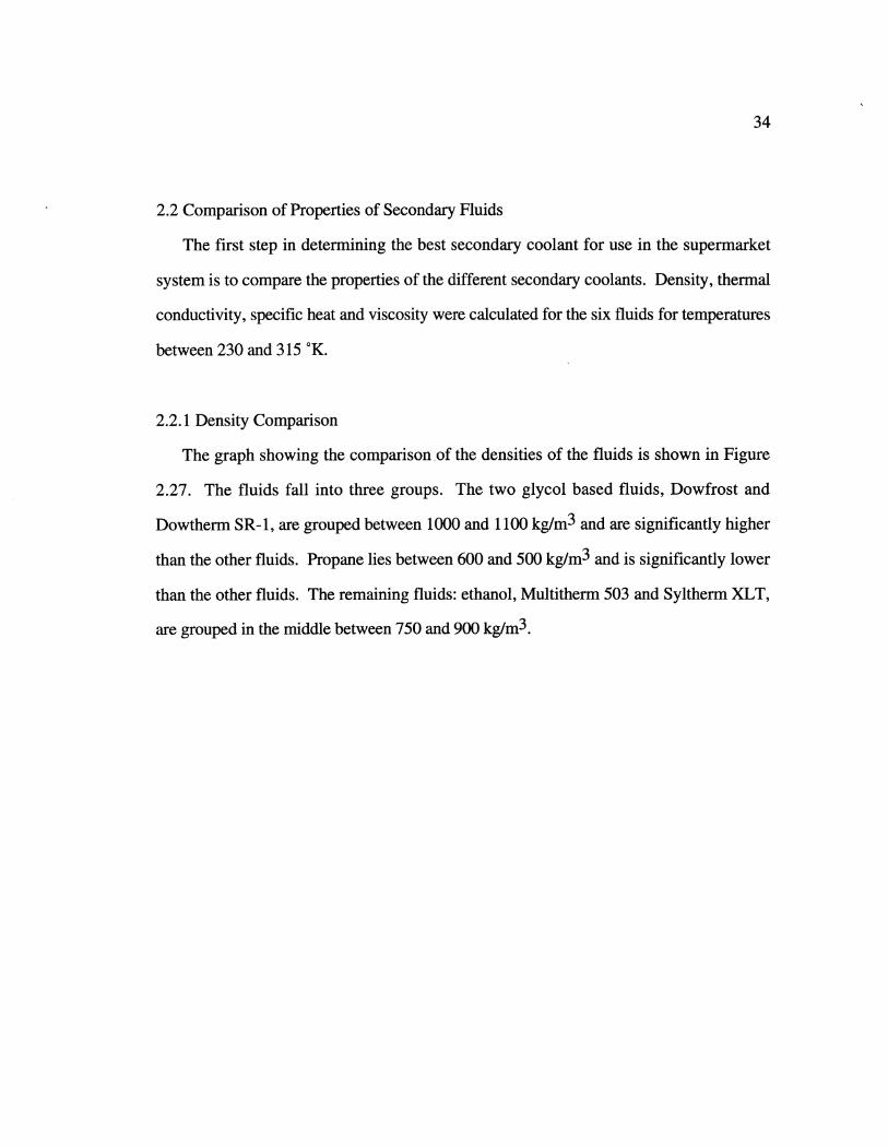
2.2.1 Density Comparison
The graph showing the comparison of the densities of the fluids is shown in Figure
2.27. The fluids fall into three groups. The two glycol based fluids, Dowfrost and
Dowtherm SR-1, are grouped between 1000 and 1100 kg/m3 and are significantly higher
than the other fluids. Propane lies between 600 and 500 kg/m3 and is significantly lower
than the other fluids. The remaining fluids: ethanol, Multitherm 503 and Syltherm XLT,
are grouped in the middle between 750 and 900 kg/m3 .
.- .... ... ... ... ... ... ... .. ". .. ... ... ... ... ... ... ... ... ..-- -- --- --- --- --- -
. ....................._...... ............................... ,............................... ............................... . ..............................
. - .. . ... . . . . ---- ---- ---- -----__ .i --- -- -- -- -- -- -- -- -- -- --- -- -- -- -- -- -- -- -- --.. --- -- -- -- -- -- -- -- -- -
- - - - -- - .-- -----
.. . ............................ . .............................. . ............................... ,..............................................................
- --------------------------------------------------------- --------------------------------------
260 280Temperature in Kelvin
-... -Ethanol PropaneDowtherm SR-1 - Dowfrost
...... Multitherm 530.........Syltherm XLT
Figure 2.27 Density comparison
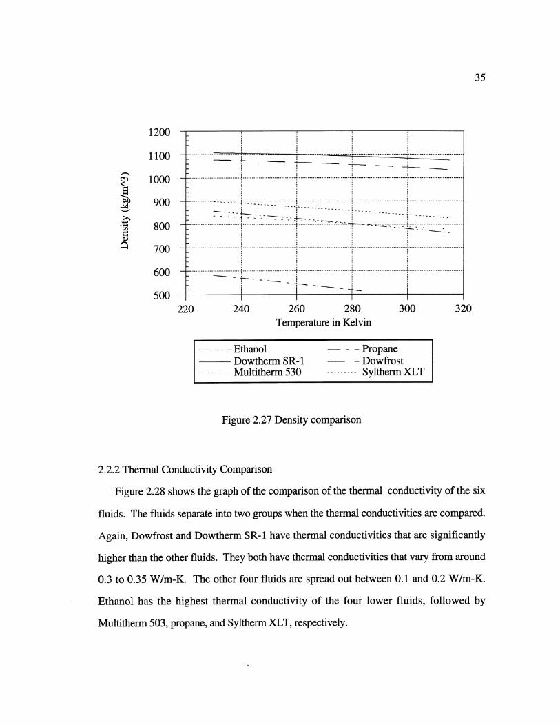
2.2.2 Thermal Conductivity Comparison
Figure 2.28 shows the graph of the comparison of the thermal conductivity of the six
fluids. The fluids separate into two groups when the thermal conductivities are compared.
Again, Dowfrost and Dowtherm SR-1 have thermal conductivities that are significantly
higher than the other fluids. They both have thermal conductivities that vary from around
0.3 to 0.35 W/m-K. The other four fluids are spread out between 0.1 and 0.2 W/m-K.
Ethanol has the highest thermal conductivity of the four lower fluids, followed by
Multitherm 503, propane, and Syltherm XLT, respectively.
35
c-*
<iPa
0,-
1200
1100
1000
900
800
700
600
500220 240 300 320
36
0.4
0
0.35
0.3
0.25
0.2
0.15
0.1220 240 260 280
Temperature in Kelvin300 320
-.... Ethanol Propane
Dowtherm SR-I - DowfrostMultitherm 503.......Syltherm XLT
Figure 2.28 Thermal conductivity comparison
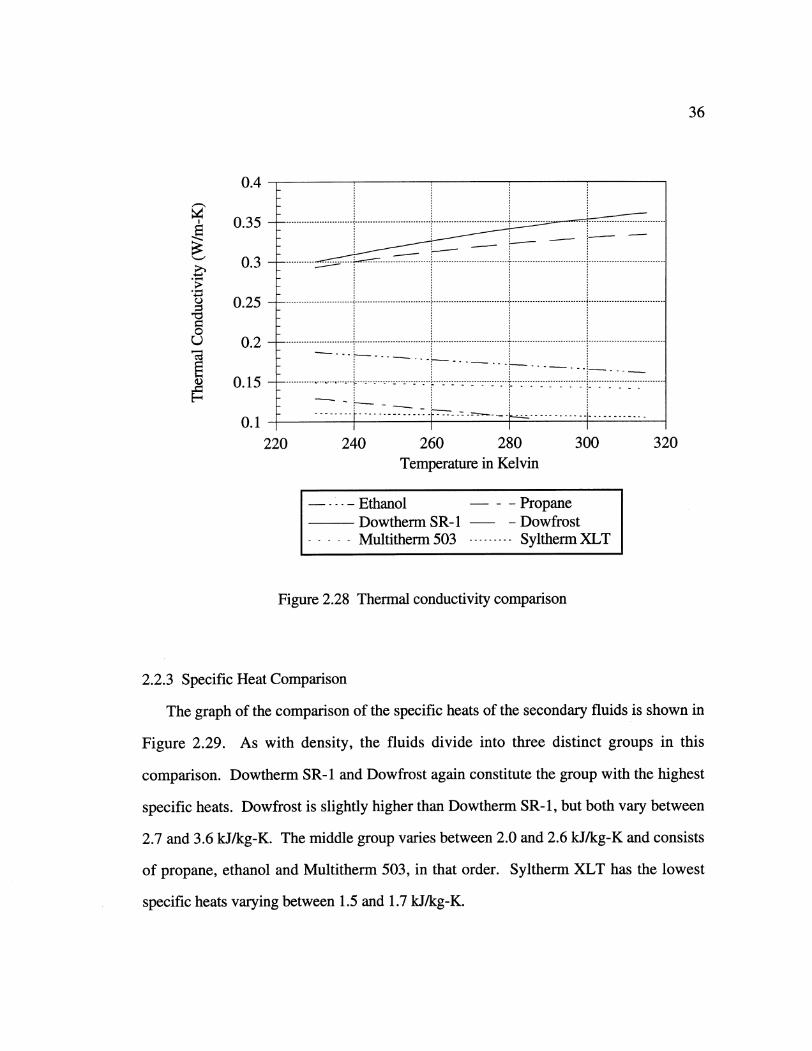
2.2.3 Specific Heat Comparison
The graph of the comparison of the specific heats of the secondary fluids is shown in
Figure 2.29. As with density, the fluids divide into three distinct groups in this
comparison. Dowtherm SR-1 and Dowfrost again constitute the group with the highest
specific heats. Dowfrost is slightly higher than Dowtherm SR-1, but both vary between
2.7 and 3.6 kJ/kg-K. The middle group varies between 2.0 and 2.6 kJ/kg-K and consists
of propane, ethanol and Multitherm 503, in that order. Syltherm XLT has the lowest
specific heats varying between 1.5 and 1.7 kJ/kg-K.
- -. ...................... ....... ............. .:............................ .......................... ..............................
............... . . ...... ............. ..I . . . .. . . . . . .I. . . . . .
37
0 ,
3.5
3
2.5
2
1.5
220
- - -- ----- - - - .. ... ... ... ... . --- --- --- --- --- --
. ... ......... .:' -. . . ..'. .... ........... ...... ...........................- "-................................ ...........
240 260 280Temperature in Kelvin
300 320
Ethanol PropaneDowtherm SR-1 - DowfrostMultitherm 503.......Syltherm XLT
Figure 2.29 Specific heat comparison
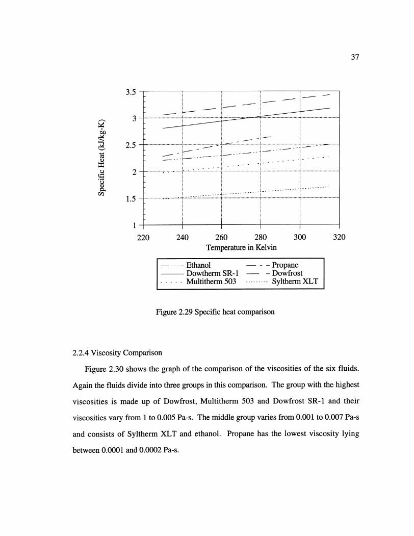
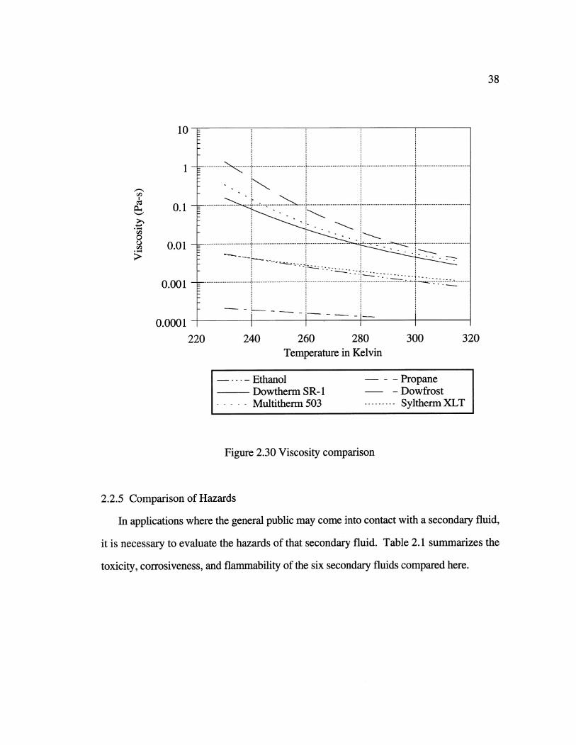
2.2.4 Viscosity Comparison
Figure 2.30 shows the graph of the comparison of the viscosities of the six fluids.
Again the fluids divide into three groups in this comparison. The group with the highest
viscosities is made up of Dowfrost, Multitherm 503 and Dowfrost SR-1 and their
viscosities vary from 1 to 0.005 Pa-s. The middle group varies from 0.001 to 0.007 Pa-s
and consists of Syltherm XLT and ethanol. Propane has the lowest viscosity lying
between 0.0001 and 0.0002 Pa-s.
10
1
g- 0.1
0.01
0.001
0.0001220 240 260 280
Temperature in Kelvin
-. --- Ethanol PropaneDowtherm SR-1 - DowfrostMultitherm 503 Syltherm XLT
Figure 2.30 Viscosity comparison
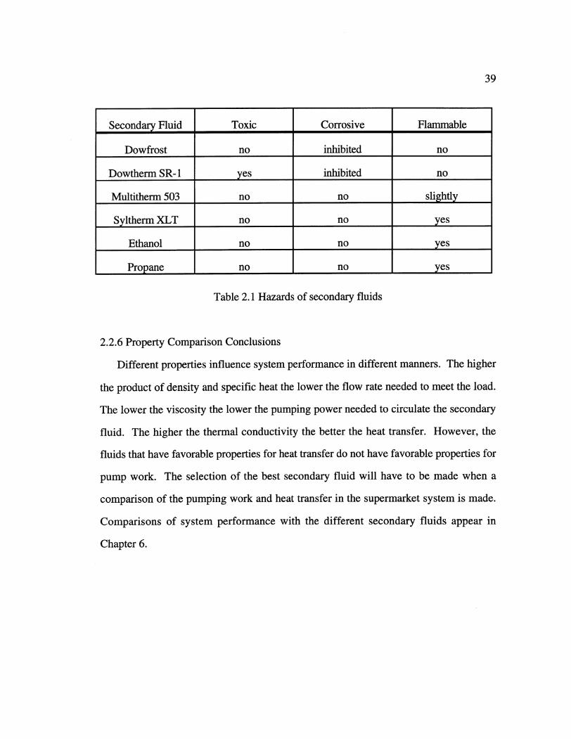
2.2.5 Comparison of Hazards
In applications where the general public may come into contact with a secondary fluid,
it is necessary to evaluate the hazards of that secondary fluid. Table 2.1 summarizes the
toxicity, corrosiveness, and flammability of the six secondary fluids compared here.
38
------- ------------------- -------------- ---------------°--------------
............. ..... .......... ...................................... ..................
.. . ...-. . . . .. .. . .. . . ..--- ------------T --------- -------I- -----------
-- --°-- - - --- °-------- ------ -----------------------
300 320
39
Secondary Fluid Toxic Corrosive Flammable
Dowfrost no inhibited no
Dowtherm SR- I yes inhibited no
Multitherm 503 no no slightly
Syltherm XLT no no yes
Ethanol no no yes
Propane no no yes
Table 2.1 Hazards of secondary fluids
2.2.6 Property Comparison Conclusions
Different properties influence system performance in different manners. The higher
the product of density and specific heat the lower the flow rate needed to meet the load.
The lower the viscosity the lower the pumping power needed to circulate the secondary
fluid. The higher the thermal conductivity the better the heat transfer. However, the
fluids that have favorable properties for heat transfer do not have favorable properties for
pump work. The selection of the best secondary fluid will have to be made when a
comparison of the pumping work and heat transfer in the supermarket system is made.
Comparisons of system performance with the different secondary fluids appear in
Chapter 6.
40
CHAPTER
THREE
REFRIGERANT CYCLE
The basis of the supermarket refrigeration system is the vapor compression cycle which
cools the refrigerated case with a direct expansion coil, or by cooling a secondary fluid
which in turn cools the refrigerated case. The first step in analyzing the supermarket
system is to determine how to configure the system involving the vapor compression
refrigeration cycle without the secondary fluid. This analysis was carried out for both
R22 and ammonia. Because both of these refrigerants have high discharge temperatures,
it is necessary to use staged compression for both refrigerants to reduce the temperatures.
Three different methods of staging the compression were evaluated to determine the best
method for each refrigerant.
41
3.1 Model Description
A computer model was written for the refrigeration cycles using the equation solving
program EES. (Klein 1993) Each component of the system (evaporator, condenser,
compressor, and expansion valve) was modeled using fundamental equations for each
type of apparatus.
3.1.1 Condenser
The condenser model is representative of an air-cooled condenser. The flow rate of
air is calculated using 0.14 kg/s of air per kW of cooling. This method of determining the
flow rate is from the ASHRAE handbook of fundamentals. (ASHRAE 1989) The UA
value for the condenser is a design input and is used to calculate the number of transfer
units (NTU) of the condenser.
UA = rhairCpairNTU (3.1)
The NTU can then be used to calculated the effectiveness of the condenser. The
refrigerant entering the condenser is a superheated vapor. First the condenser brings the
superheated refrigerant vapor to a saturated vapor and then condenses the vapor to a
saturated fluid. The total heat transfer in the process includes both the desuperheating and
the condensing. However, the calculation of heat transfer during desuperheating is
complex and a simplifying assumption is that the heat transfer in the desuperheating
process is small compared with the heat transfer in the condensing process. With this
assumption, the process is isothermal on the refrigerant side of the heat exchanger and the
effectiveness-NTU equation for an isothermal phase change can be used.
42
= 1- exp(-NTU) (3.2)
The heat transferred in the condenser can be calculated from the temperature difference
between the ambient air and the refrigerant flowing through the condenser.
Q =CfiairCpair(Tref - Tamb) (3.3)
The calculated heat transfer can be used to calculate the temperature change in the air
through the condenser.
Q -rhairCpairATair (3.4)
Then the heat transfer can also be used with the flow rate of the refrigerant to calculate the
enthalpy change of the refrigerant in the condenser.
Q = iAlrefAhref (3.5)
3.1.2 Evaporator
The desired temperature of the refrigerated case is the temperature of the evaporator.
It is assumed that the temperature of the refrigerant is constant across the evaporator and
that the refrigerant leaves the evaporator with a specified amount of superheat. The
number of degrees of superheat is a parameter of the model. The pressure in the
evaporator is the pressure at which the refrigerant would be vapor at the evaporator
temperature, and it is assumed that the pressure is constant. Then, knowing the
43
temperature and the pressure of the refrigerant leaving the evaporator, the properties of the
refrigerant are set at this state.
3.1.3 Expansion
The expansion valve for the refrigeration system is assumed to be isenthalpic. This
means that the enthalpy of the refrigerant does not change between the evaporator and the
condenser.
3.1.4 Compression
The compression method is different depending on the method of staged compression
chosen, and will be discussed in Section 3.2. The individual compressor model is the
same in each staged compression method. Originally, the compressor was modeled using
an isentropic model and an isentropic efficiency. This type of model can give accurate
results for a particular compressor, but it does not include the physical dimensions of the
compressor itself. Instead, a polytropic model based on the physical dimensions of the
compressor was used. The techniques and the equations used is this model are from
Threlkeld and Chlumsky. (Threlkeld 1970 and Chlumsky 1965) The refrigerant enters
the compressor at a certain pressure and specific volume. The polytropic model uses the
polytropic exponent (n) of the refrigerant to determine the relationship between the
entering state and exiting state of the refrigerant.
Pinvin n = PoutVoutn (3.6)
The displacement volume of the compressor depends on the bore and stroke of the
cylinder and the number of cylinders being operated.
44
Vdisp= (number of cylinders)( (bore)2 stroke) (3.7)
The volumetric efficiency of the compressor is based on the clearance ratio(m) of the
compressor, as well as the pressure ratio and the polytropic exponent.
TV m WtOutW1 _- - i [(Pn - 1(3.8)
The flow rate of the refrigerant through the compressor is dependent on the displacement
volume, the speed of the compressor, and the volumetric efficiency.
rilref= IV'n] Vdisp [speed] Tivol (3.9)
The power used by the compressor can be calculated from the flow rate of the refrigerant,
the enthalpy change in the refrigerant, and the polytropic efficiency of the compressor.
Wcomp = rilrefAhref (3.10)7ipolytropic
The reason that a polytropic efficiency needs to be used is that when the ideal polytropic
exponent is used, the result is an isentropic model. An isentropic model will under-predict
the amount of compressor work needed because the entropy of the refrigerant in the
compressor is not constant. To reduce this under-prediction, it is necessary to either alter
the polytropic exponent, or utilize a polytropic efficiency. In this manner an accurate
45
value of the compressor work is calculated. The outgoing pressure of the refrigerant from
the compressor is the same as the condenser pressure.
3.1.5 Other Equations
The refrigerant mass flow rate is dependent on the heat transfer rate of the refrigerated
cases (caseload) of the system and the enthalpy change of the refrigerant through the
evaporator.
=ilref - caseload (3.11)Ahref
For refrigeration cycles, a measure of the performance of a system is the coefficient of
performance (COP), which is defined as the caseload divided by the work done by the
compressor.
Cop - caseload (3.12)Wcomp
3.2 Compression Methods
Because both ammonia and R22 have high discharge temperatures in refrigeration
cycles, it is necessary to evaluate different compression staging methods for each. High
discharge temperatures are a problem because of the increased superheating that they
cause in the compressors. This increased superheating increases the work done by the
compressor. Staging the compression reduces the discharge temperatures by allowing
intercooling between the stages of compression. Three different methods of staging were
modeled along with the cycle with no staging. These models are discussed here.
46
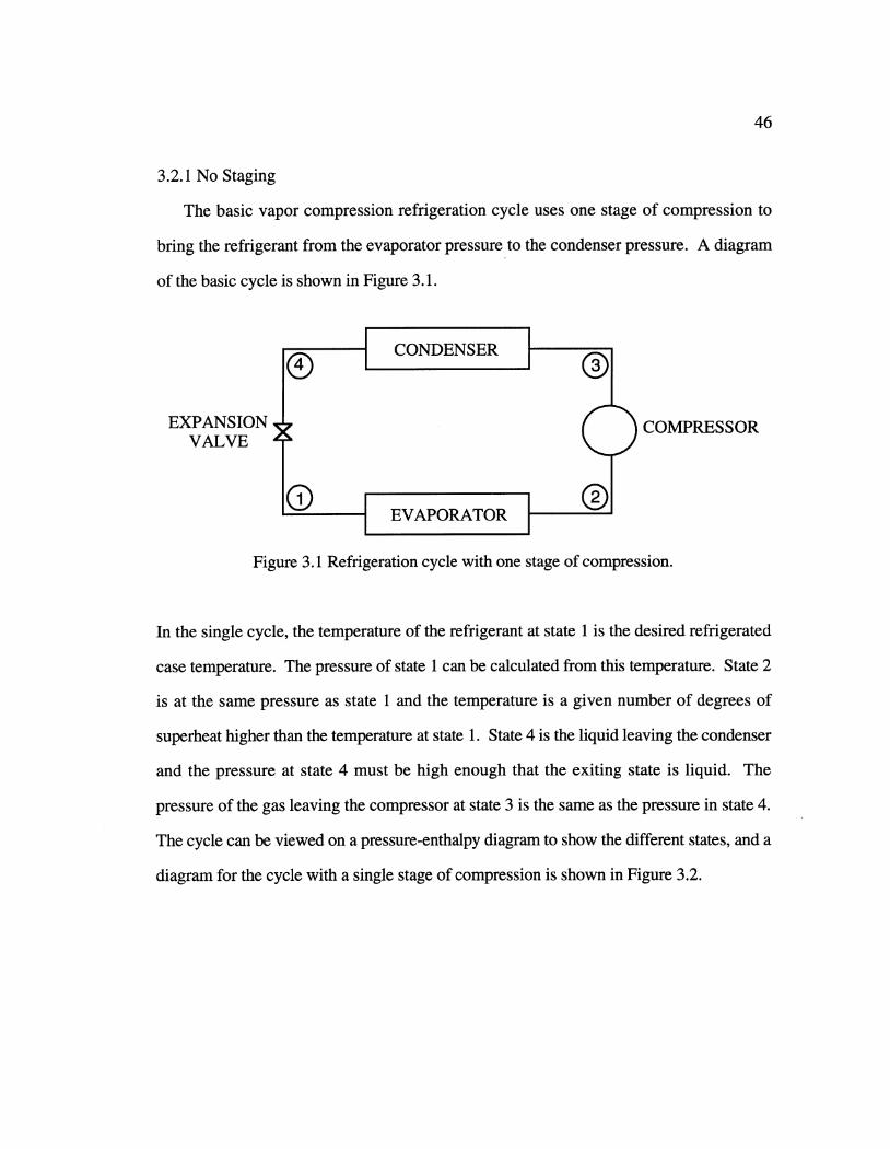
3.2.1 No Staging
The basic vapor compression refrigeration cycle uses one stage of compression to
bring the refrigerant from the evaporator pressure to the condenser pressure. A diagram
of the basic cycle is shown in Figure 3.1.
CONDENSER
EXPANSION COMPRESSORVALVE
Q EVAPORATOR
Figure 3.1 Refrigeration cycle with one stage of compression.
In the single cycle, the temperature of the refrigerant at state 1 is the desired refrigerated
case temperature. The pressure of state 1 can be calculated from this temperature. State 2
is at the same pressure as state 1 and the temperature is a given number of degrees of
superheat higher than the temperature at state 1. State 4 is the liquid leaving the condenser
and the pressure at state 4 must be high enough that the exiting state is liquid. The
pressure of the gas leaving the compressor at state 3 is the same as the pressure in state 4.
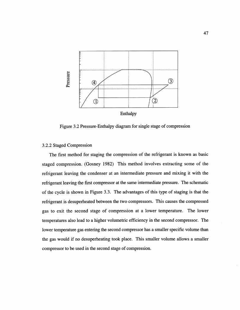
The cycle can be viewed on a pressure-enthalpy diagram to show the different states, and a
diagram for the cycle with a single stage of compression is shown in Figure 3.2.
47
Enthalpy
Figure 3.2 Pressure-Enthalpy diagram for single stage of compression
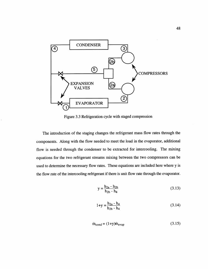
3.2.2 Staged Compression
The first method for staging the compression of the refrigerant is known as basic
staged compression. (Gosney 1982) This method involves extracting some of the
refrigerant leaving the condenser at an intermediate pressure and mixing it with the
refrigerant leaving the first compressor at the same intermediate pressure. The schematic
of the cycle is shown in Figure 3.3. The advantages of this type of staging is that the
refrigerant is desuperheated between the two compressors. This causes the compressed
gas to exit the second stage of compression at a lower temperature. The lower
temperatures also lead to a higher volumetric efficiency in the second compressor. The
lower temperature gas entering the second compressor has a smaller specific volume than
the gas would if no desuperheating took place. This smaller volume allows a smaller
compressor to be used in the second stage of compression.
48
Figure 3.3 Refrigeration cycle with staged compression
The introduction of the staging changes the refrigerant mass flow rates through the
components. Along with the flow needed to meet the load in the evaporator, additional
flow is needed through the condenser to be extracted for intercooling. The mixing
equations for the two refrigerant streams mixing between the two compressors can be
used to determine the necessary flow rates. These equations are included here where y is
the flow rate of the intercooling refrigerant if there is unit flow rate through the evaporator.
= h2 a - h2b (3.13)
h2b -N
1+y = h2a- h4 (3.14)h2b- h4
micond = (1 +y)AIevap (3.15)
49
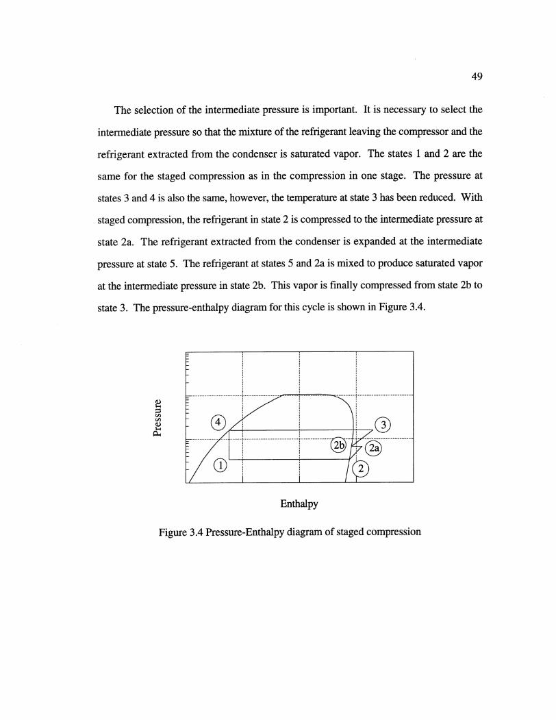
The selection of the intermediate pressure is important. It is necessary to select the
intermediate pressure so that the mixture of the refrigerant leaving the compressor and the
refrigerant extracted from the condenser is saturated vapor. The states 1 and 2 are the
same for the staged compression as in the compression in one stage. The pressure at
states 3 and 4 is also the same, however, the temperature at state 3 has been reduced. With
staged compression, the refrigerant in state 2 is compressed to the intermediate pressure at
state 2a. The refrigerant extracted from the condenser is expanded at the intermediate
pressure at state 5. The refrigerant at states 5 and 2a is mixed to produce saturated vapor
at the intermediate pressure in state 2b. This vapor is finally compressed from state 2b to
state 3. The pressure-enthalpy diagram for this cycle is shown in Figure 3.4.
a .)
Enthalpy
Figure 3.4 Pressure-Enthalpy diagram of staged compression
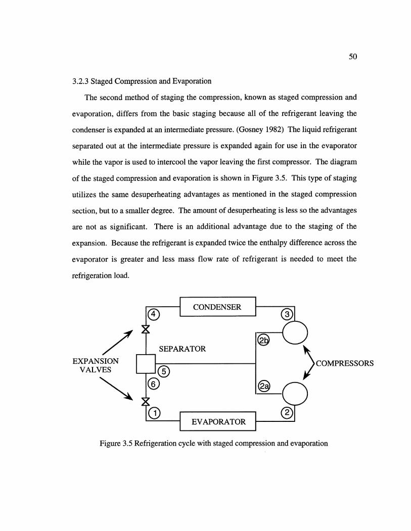
50
3.2.3 Staged Compression and Evaporation
The second method of staging the compression, known as staged compression and
evaporation, differs from the basic staging because all of the refrigerant leaving the
condenser is expanded at an intermediate pressure. (Gosney 1982) The liquid refrigerant
separated out at the intermediate pressure is expanded again for use in the evaporator
while the vapor is used to intercool the vapor leaving the first compressor. The diagram
of the staged compression and evaporation is shown in Figure 3.5. This type of staging
utilizes the same desuperheating advantages as mentioned in the staged compression
section, but to a smaller degree. The amount of desuperheating is less so the advantages
are not as significant. There is an additional advantage due to the staging of the
expansion. Because the refrigerant is expanded twice the enthalpy difference across the
evaporator is greater and less mass flow rate of refrigerant is needed to meet the
refrigeration load.
~CONDENSER
zoo SEPARATOR
EXPANSION COMPRESS1VALVES I 5,o o ®c)
Figure 3.5 Refrigeration cycle with staged compression and evaporation
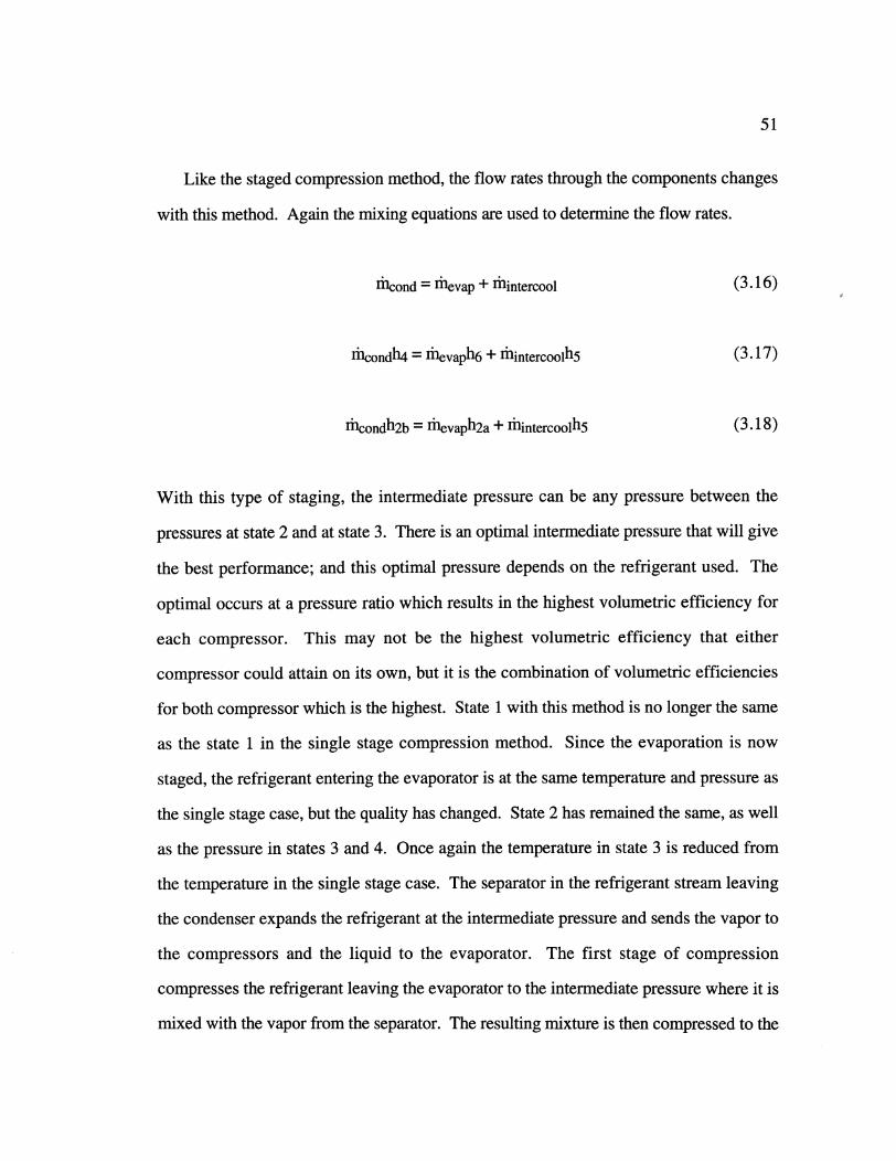
51
Like the staged compression method, the flow rates through the components changes
with this method. Again the mixing equations are used to determine the flow rates.
rhcond = hevap + rhintercool (3.16)
rlcondh4 = rhevaph6 + ihintercoolh5 (3.17)
icondh2b = ievaph2a + ihintercoolh5 (3.18)
With this type of staging, the intermediate pressure can be any pressure between the
pressures at state 2 and at state 3. There is an optimal intermediate pressure that will give
the best performance; and this optimal pressure depends on the refrigerant used. The
optimal occurs at a pressure ratio which results in the highest volumetric efficiency for
each compressor. This may not be the highest volumetric efficiency that either
compressor could attain on its own, but it is the combination of volumetric efficiencies
for both compressor which is the highest. State 1 with this method is no longer the same
as the state 1 in the single stage compression method. Since the evaporation is now
staged, the refrigerant entering the evaporator is at the same temperature and pressure as
the single stage case, but the quality has changed. State 2 has remained the same, as well
as the pressure in states 3 and 4. Once again the temperature in state 3 is reduced from
the temperature in the single stage case. The separator in the refrigerant stream leaving
the condenser expands the refrigerant at the intermediate pressure and sends the vapor to
the compressors and the liquid to the evaporator. The first stage of compression
compresses the refrigerant leaving the evaporator to the intermediate pressure where it is
mixed with the vapor from the separator. The resulting mixture is then compressed to the
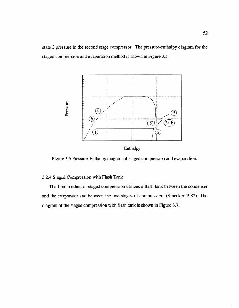
52
state 3 pressure in the second stage compressor. The pressure-enthalpy diagram for the
staged compression and evaporation method is shown in Figure 3.5.
Enthalpy
Figure 3.6 Pressure-Enthalpy diagram of staged compression and evaporation.
3.2.4 Staged Compression with Flash Tank
The final method of staged compression utilizes a flash tank between the condenser
and the evaporator and between the two stages of compression. (Stoecker 1982) The
diagram of the staged compression with flash tank is shown in Figure 3.7.
53
COMPRESSOR
Figure 3.7 Refrigeration cycle with staged compression and flash tank
This method is similar to the staged compression and evaporation because the refrigerant
leaving the condenser is expanded at an intermediate pressure and the resulting liquid is
used in the evaporator. The vapor resulting from the expansion of the refrigerant leaving
the condenser is not used to intercool the compressors directly in this method. Instead,
the liquid and vapor from the expansion are held in a flash tank. Some of the liquid is
extracted and used in the evaporator and once the refrigerant leaves the evaporator it is
compressed back to the intermediate pressure. The refrigerant leaving the compressor is
bubbled through the remaining liquid and vapor from the expansion of the refrigerant
leaving the condenser. The saturated vapor in the flash tank is then compressed to the
condenser pressure. This method of staged compression combines the advantages of
both the first two methods. The refrigerant is desuperheated to the saturation point as in
the staged compression method. This means that it has all of the same advantages of
increased volumetric efficiency and decreased size as the staged compression method.
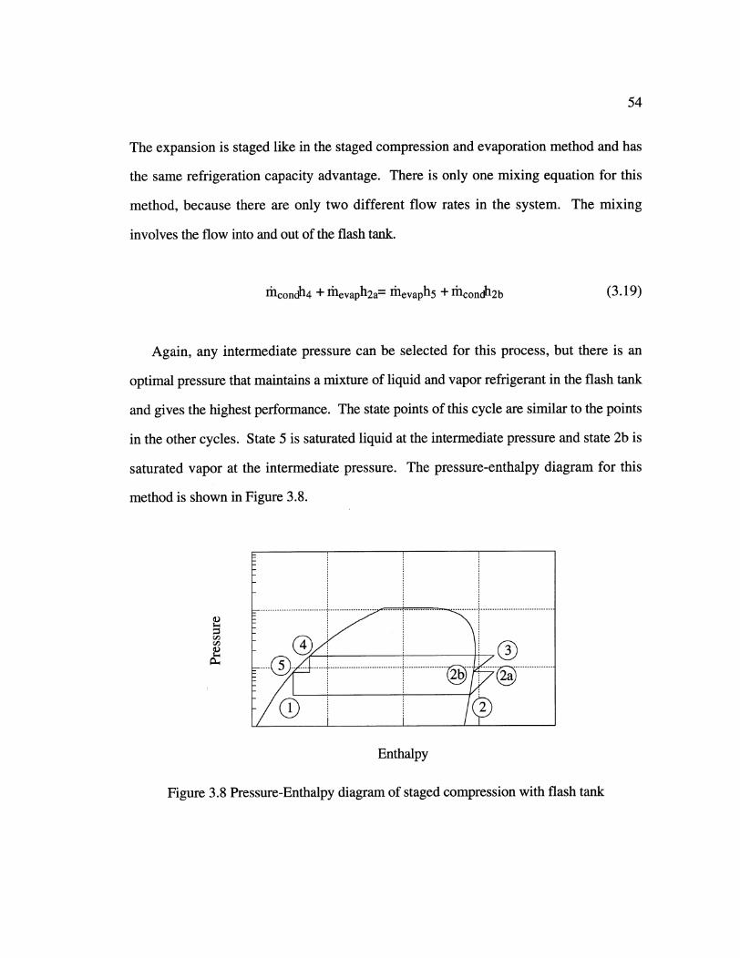
54
The expansion is staged like in the staged compression and evaporation method and has
the same refrigeration capacity advantage. There is only one mixing equation for this
method, because there are only two different flow rates in the system. The mixing
involves the flow into and out of the flash tank.
hcondh4 + rhevaph2a = levaph5 + nicondh2b (3.19)
Again, any intermediate pressure can be selected for this process, but there is an
optimal pressure that maintains a mixture of liquid and vapor refrigerant in the flash tank
and gives the highest performance. The state points of this cycle are similar to the points
in the other cycles. State 5 is saturated liquid at the intermediate pressure and state 2b is
saturated vapor at the intermediate pressure. The pressure-enthalpy diagram for this
method is shown in Figure 3.8.
Enthalpy
Figure 3.8 Pressure-Enthalpy diagram of staged compression with flash tank
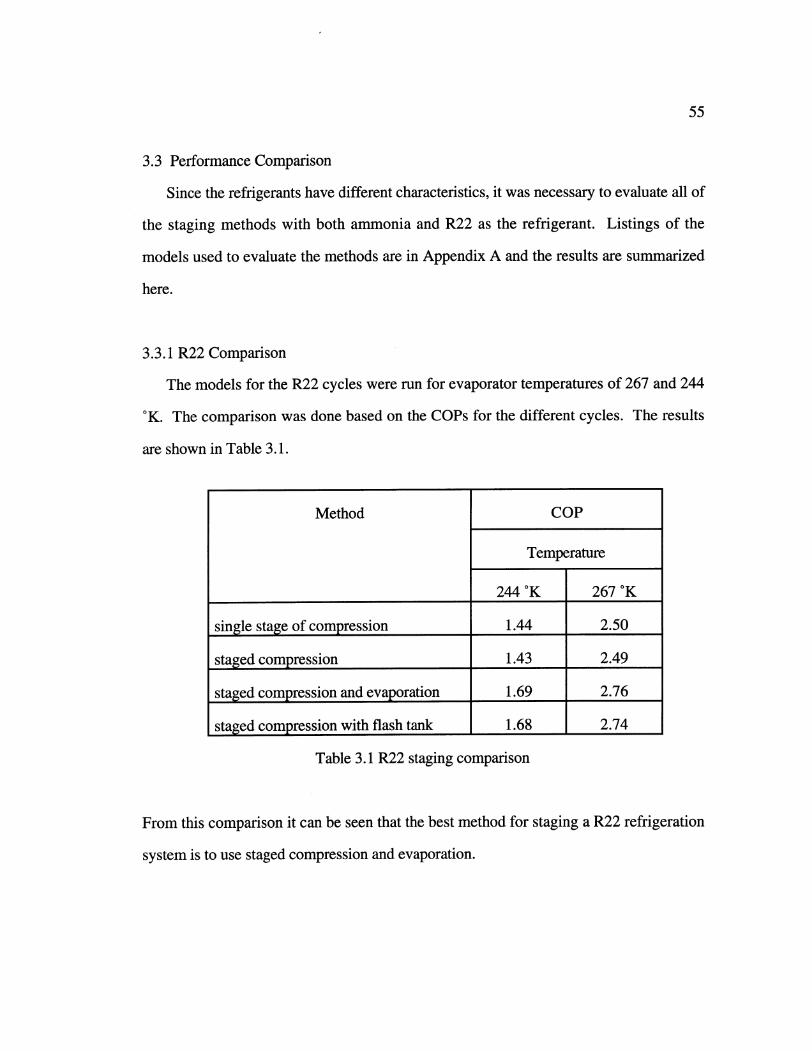
55
3.3 Performance Comparison
Since the refrigerants have different characteristics, it was necessary to evaluate all of
the staging methods with both ammonia and R22 as the refrigerant. Listings of the
models used to evaluate the methods are in Appendix A and the results are summarized
here.
3.3.1 R22 Comparison
The models for the R22 cycles were run for evaporator temperatures of 267 and 244
'K. The comparison was done based on the COPs for the different cycles. The results
are shown in Table 3.1.
Method COP
Temperature
244 OK 267 OK
single stage of compression 1.44 2.50
staged compression 1.43 2.49
staged compression and evaporation 1.69 2.76
staged compression with flash tank 1.68 2.74
Table 3.1 R22 staging comparison
From this comparison it can be seen that the best method for staging a R22 refrigeration
system is to use staged compression and evaporation.
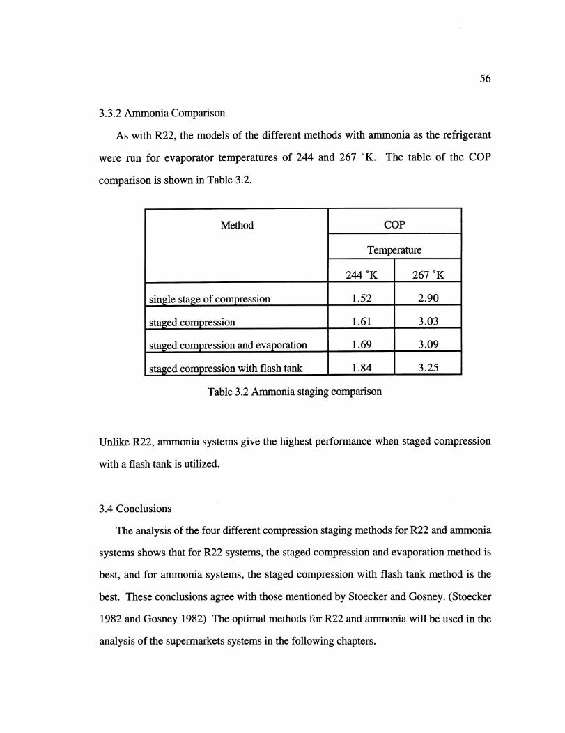
56
3.3.2 Ammonia Comparison
As with R22, the models of the different methods with ammonia as the refrigerant
were run for evaporator temperatures of 244 and 267 K. The table of the COP
comparison is shown in Table 3.2.
Method COP
Temperature
244 OK 267 OK
single stage of compression 1.52 2.90
staged compression 1.61 3.03
staged compression and evaporation 1.69 3.09
staged compression with flash tank 1.84 3.25
Table 3.2 Ammonia staging comparison
Unlike R22, ammonia systems give the highest performance when staged compression
with a flash tank is utilized.
3.4 Conclusions
The analysis of the four different compression staging methods for R22 and ammonia
systems shows that for R22 systems, the staged compression and evaporation method is
best, and for ammonia systems, the staged compression with flash tank method is the
best. These conclusions agree with those mentioned by Stoecker and Gosney. (Stoecker
1982 and Gosney 1982) The optimal methods for R22 and ammonia will be used in the
analysis of the supermarkets systems in the following chapters.
57
CHAPTER
FOUR
AMMONIA WITH SECONDARY FLUID SYSTEM
The addition of a secondary fluid to the refrigeration system increases the complexity
of the model necessary to simulate the performance. The evaporator for the vapor
compression cycle is replaced with an heat exchanger and the components needed for the
secondary fluid are added. This chapter discusses these components and how they are
modeled.
58
4.1 Evaporator Heat Exchanger Model
The model of the vapor compression part of the ammonia-secondary fluid system is
very similar to the models used for the single cycle comparison discussed in Chapter 3.
The staged compression with flash tank method was used and the model of the individual
compressor was the same. The condenser was also air-cooled and used the same
ASHRAE equations as shown in Equation 3.1 to 3.5. (ASHRAE 1989) All expansion
valves were modeled as isenthalpic.
The evaporator in the ammonia-secondary fluid system is completely different than
the evaporator used in the single cycle system. In the single cycle system, the evaporator
for the refrigerant is the refrigerated case, and in the ammonia-secondary fluid system, the
evaporator is a heat exchanger that uses the ammonia to cool the secondary fluid. The
model of that heat exchanger is discussed here.
The heat exchanger is a flooded, shell and tube heat exchanger with the secondary
fluid flowing through the tubes and ammonia in the shell. A diagram of the heat
exchanger is shown in Figure 4.1. The secondary fluid enters the tube bundle of the heat
exchanger after leaving the refrigerated case. It is cooled by the ammonia and then
circulated to the refrigerated case. The ammonia enters as liquid after leaving the
condenser and the expansion valve. As the ammonia cools the secondary fluid, it
evaporates and the saturated ammonia vapor collects in the top of the heat exchanger.
This vapor is removed and compressed.
For the computer model, it is necessary to determine the heat transferred in the
evaporation process. The initial idea for the model was to specify the effectiveness of the
heat exchanger and use this to calculate the heat transfer. The problem with this type of
model is that when the flow rates of the fluids change in an heat exchanger the
effectiveness of the heat exchanger changes because of the change in the capacitance rate
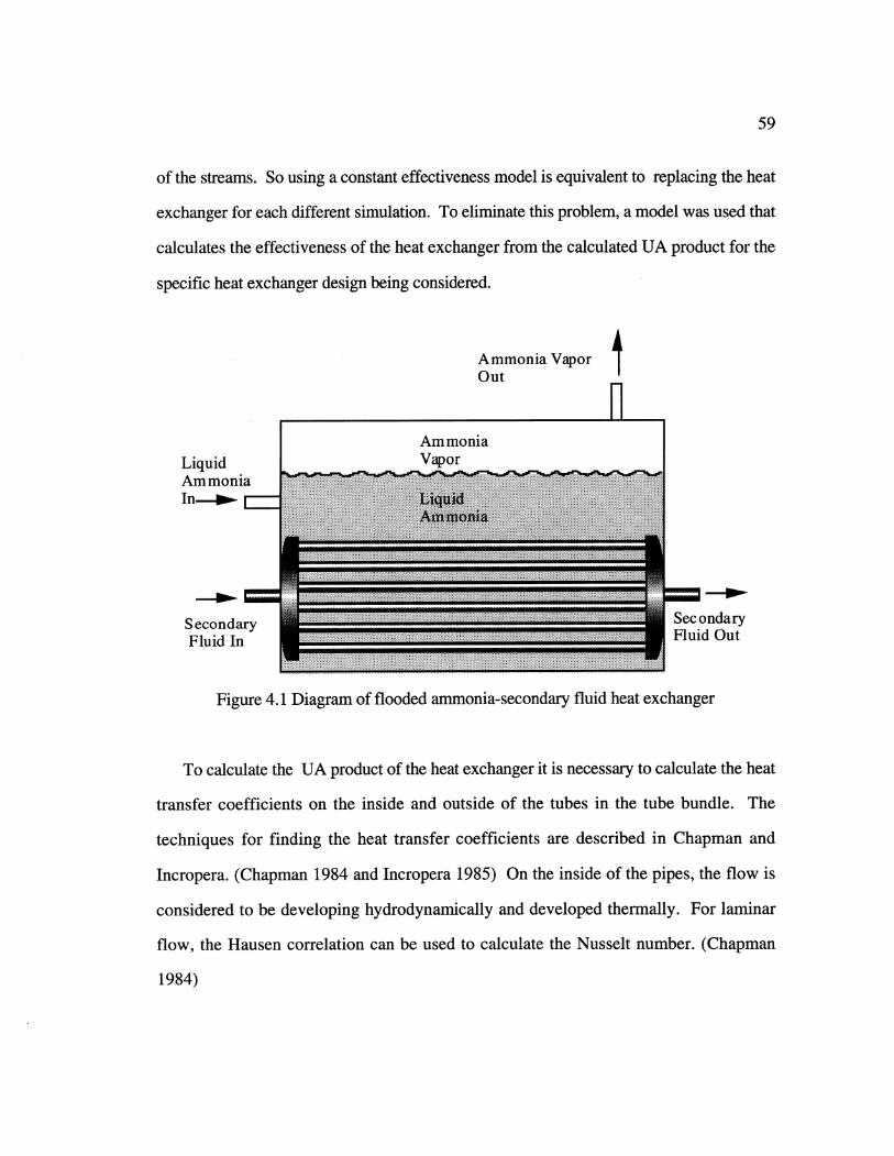
59
of the streams. So using a constant effectiveness model is equivalent to replacing the heat
exchanger for each different simulation. To eliminate this problem, a model was used that
calculates the effectiveness of the heat exchanger from the calculated UA product for the
specific heat exchanger design being considered.
Ammonia Vapor
Out
AmmoniaLiquid VaporAmmoniaIn --- , J ~~iiiiii~iii~ i ::::. ..... . ...... : : : :::: : :::: : : :::: : :.............. ........iiiiiiiiiii i ii iiiii~ i ii iiiiiiiiiiiiiiiiiiiiiiiiii l i i i iiiiiiiiiiiiiiiiiiiiiiiiil~~iiiiii iii
.. .. .. .Secondary..e... nda.Fluid... ... luid.Out
.. ..... ........... : :.. : ::::::::::::::::::::::::::::::::: :::::::::::::::::::::::::::................ ........
Figur 4.1Diagam o flooed amoni-s.... ary..ui.hea.excange
To clcuatetheUA rodct f th het echagerit.s.ncessry.o clcuatetheheatranfer oeficiets o th insde ad otsid of he ubesin.te.tbe.bndle.Th
techniues f........... ..attra.se ...... icX et- %r descrbed.i Chap an.anIncropea. (Chpman 194 and.ncropea 1985 .On.t. insde.o the..pesthe.f.w.iconsieredto bedeveopin hydrdynaicall anddeveoped hermlly..or.lmina
flowthe ausencorrlatio.canbe.usd.tocalcuate he.Nuseltnumbe..(Capma... ..9...4.....
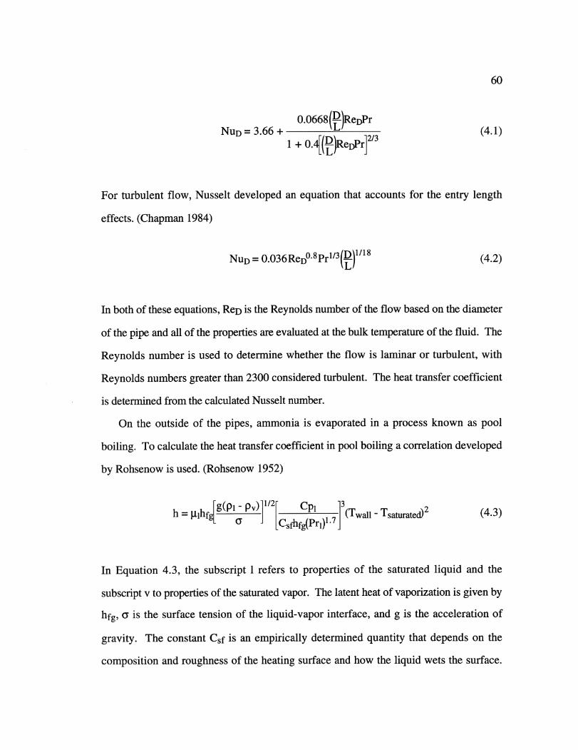
60
0.0668(Da eDPrNUD= 3.66 + -.68( ) /3r(4.1)
1 + 0.4 (D)ReDPr]
For turbulent flow, Nusselt developed an equation that accounts for the entry length
effects. (Chapman 1984)
NUD = 0.036ReDO.8Pr1/3(I)(1/18 (4.2)
In both of these equations, ReD is the Reynolds number of the flow based on the diameter
of the pipe and all of the properties are evaluated at the bulk temperature of the fluid. The
Reynolds number is used to determine whether the flow is laminar or turbulent, with
Reynolds numbers greater than 2300 considered turbulent. The heat transfer coefficient
is determined from the calculated Nusselt number.
On the outside of the pipes, ammonia is evaporated in a process known as pool
boiling. To calculate the heat transfer coefficient in pool boiling a correlation developed
by Rohsenow is used. (Rohsenow 1952)
h -=lhfgg(P1 Pv) 1 /2 - CP)--- J3(Twall - Tsaturated) 2 (4.3)G Csfhfg(Prl)1._
In Equation 4.3, the subscript 1 refers to properties of the saturated liquid and the
subscript v to properties of the saturated vapor. The latent heat of vaporization is given by
hfg, a is the surface tension of the liquid-vapor interface, and g is the acceleration of
gravity. The constant Csf is an empirically determined quantity that depends on the
composition and roughness of the heating surface and how the liquid wets the surface.
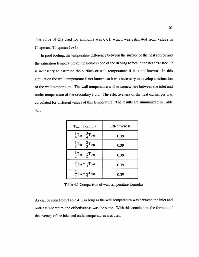
61
The value of Csf used for ammonia was 0.01, which was estimated from values in
Chapman. (Chapman 1984)
In pool boiling, the temperature difference between the surface of the heat source and
the saturation temperature of the liquid is one of the driving forces in the heat transfer. It
is necessary to estimate the surface or wall temperature if it is not known. In this
simulation the wall temperature is not known, so it was necessary to develop a estimation
of the wall temperature. The wall temperature will be somewhere between the inlet and
outlet temperature of the secondary fluid. The effectiveness of the heat exchanger was
calculated for different values of this temperature. The results are summarized in Table
4.1.
Table 4.1 Comparison of wall temperature formulas
As can be seen from Table 4.1, as long as the wall temperature was between the inlet and
outlet temperature, the effectiveness was the same. With this conclusion, the formula of
the average of the inlet and outlet temperatures was used.
Twall Formula Effectiveness
1Tin +-3Tout 0.39
1-Tin + Tout 0.393 3
2 Tin + Tout 0.39
3 Tin + Tout 0.39
62
Twall 1=Tin + 1To (4.4)2 2
Once the heat transfer coefficient on the inside of the pipes and on the outside of the
pipes is calculated, the overall heat transfer coefficient can be determined.
U = 1 (4.5)rolnroI
ro+ + ri+ 1rihi kpipe ho
In Equation 4.5, the subscript i refers to the inside of the pipes, the subscript o refers to
the outside of the pipes, r stands for the radii, h for the heat transfer coefficients, and kpipe
is the thermal conductivity of the pipes. The UA product for the heat exchanger is
determined by multiplying the overall heat transfer coefficient by the total area that is
utilized for heat transfer.
Once the UA product is determined, the heat transfer and temperature changes are
calculated using the effectiveness-NTU method. (Chapman 1984) The NTU can be
calculated from the UA product and the minimum capacitance rate of the two streams.
Since the ammonia side of the heat exchanger has an infinite specific heat, the minimum
capacitance rate is the secondary fluid flow.
NTU- UA (4.6)rnsfCpsf
Also, since the ammonia side of the heat exchanger involves a phase change, the
effectiveness-NTU equation for one fluid changing phase is used.
63
e = 1- exp(-NTU) (4.7)
It is possible to write the effectiveness of the heat exchanger as a combination of the inlet
and outlet temperatures of the two streams. The specific combination depends on which
of the streams has the minimum capacitance rate. In this case, the secondary fluid has the
minimum capacitance rate and the ammonia is at a constant temperature because the
ammonia evaporates and is extracted as a saturated vapor.
Tsfin - Tsfout
Tsf,in - Tammonia
Equation 4.8 determines the temperatures in the heat exchanger and the heat transfer can
be calculated from the capacitance rate and temperature change of the secondary fluid
stream.
Q = lilsfCpsf(Tsf,out - Tsfin ) (4.9)
4.2 Secondary Fluid System
The components of the system that are unique to the use of a secondary fluid were
also modeled. These components include the heat exchanger in the refrigerated case and
the thermal losses and required pump work from the piping system.
4.2.1 Refrigerated Case
In Chapter 3, the refrigerated case was the evaporator of the vapor compression cycle
and it was modeled by specifying the required case temperature and the amount of super
heating of the refrigerant. With a secondary fluid, the refrigerated case is a heat
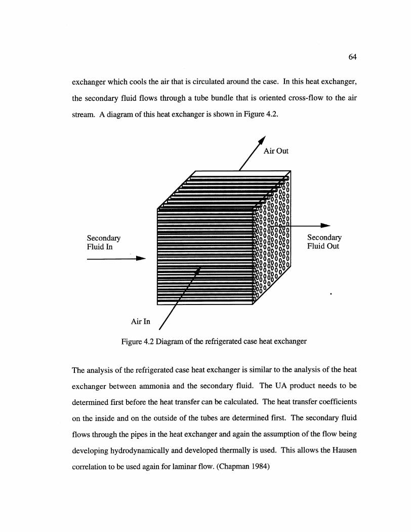
64
exchanger which cools the air that is circulated around the case. In this heat exchanger,
the secondary fluid flows through a tube bundle that is oriented cross-flow to the air
stream. A diagram of this heat exchanger is shown in Figure 4.2.
SecondaryFluid In
Air In
SecondaryFluid Out
Figure 4.2 Diagram of the refrigerated case heat exchanger
The analysis of the refrigerated case heat exchanger is similar to the analysis of the heat
exchanger between ammonia and the secondary fluid. The UA product needs to be
determined first before the heat transfer can be calculated. The heat transfer coefficients
on the inside and on the outside of the tubes are determined first. The secondary fluid
flows through the pipes in the heat exchanger and again the assumption of the flow being
developing hydrodynamically and developed thermally is used. This allows the Hausen
correlation to be used again for laminar flow. (Chapman 1984)
65
NUD = 3.66 + 0.0668(!)ReDPr (4.10)1+ 0.4 L)ReDPr
2/3
With turbulent flow, the Nusselt correlation was used. (Chapman 1984)
NUD = 0.036ReDO.8Pr1/3(L)D1/ 18 (4.11)
In both of these equations, ReD is the Reynolds number of the flow based on the diameter
of the pipe and all of the properties are evaluated at the average of the inlet and outlet
temperature of the fluid. The Reynolds number is used to determine whether the flow is
laminar or turbulent, with Reynolds numbers greater than 2300 considered turbulent.
From the calculated Nusselt number the heat transfer coefficient is determined. Air is
circulated on the outside of the pipes, resulting in heat transfer by forced convection over
horizontal tubes. It is assumed that the tubes do not have extended surfaces on the
outside. Churchill and Bernstein developed a correlation equation for this type of heat
transfer. (Chapman 1984)
NuD =0.3+ 0.62ReD" 2P 13 + ReD 5j/(4.12)[I + (0.4/Pr)2P31 1/4 L 2.82 x 10⁵ -
ReD is the Reynolds number based on the diameter and all of the properties are evaluated
at the mean temperature. The heat transfer coefficients are calculated from the Nusselt
numbers and then the overall heat transfer coefficient can be calculated.
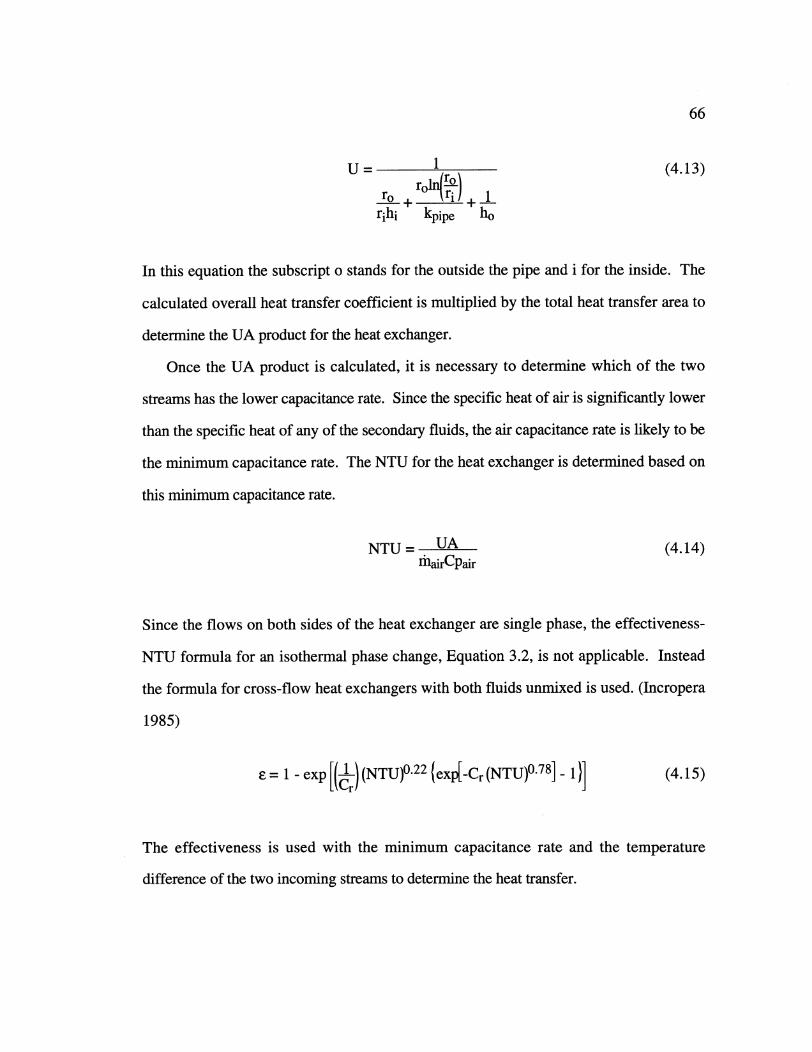
66
U = 1 (4.13)ro+ l )r(Ao + ri / 1
rihi kpipe ho
In this equation the subscript o stands for the outside the pipe and i for the inside. The
calculated overall heat transfer coefficient is multiplied by the total heat transfer area to
determine the UA product for the heat exchanger.
Once the UA product is calculated, it is necessary to determine which of the two
streams has the lower capacitance rate. Since the specific heat of air is significantly lower
than the specific heat of any of the secondary fluids, the air capacitance rate is likely to be
the minimum capacitance rate. The NTU for the heat exchanger is determined based on
this minimum capacitance rate.
NTU- UA (4.14)rhairCpair
Since the flows on both sides of the heat exchanger are single phase, the effectiveness-
NTU formula for an isothermal phase change, Equation 3.2, is not applicable. Instead
the formula for cross-flow heat exchangers with both fluids unmixed is used. (Incropera
1985)
e=1 - exp [(rr) (NTU)0 22 (exp[-Cr (NTU)078] - 1 (4.15)
The effectiveness is used with the minimum capacitance rate and the temperature
difference of the two incoming streams to determine the heat transfer.
67
Q = EhairCpair (Tair,in - Tsfin) (4.16)
This heat transfer can then be used to calculate the temperature change of the air and
secondary fluid streams.
Q rhairCpairATair (4.17)
Q =rsfCpsfATsf (4.18)
The calculated heat transfer in the case heat exchanger is the same as the load met by the
refrigerated case. Either the temperature change of the fluid can be given to calculate the
load met, or the required load can be given to determine the necessary temperature change.
4.2.2 Thermal Losses from Piping System
The secondary fluid needs to be distributed from the heat exchanger where it is cooled
by the ammonia to the refrigerated case where it provides the cooling to the air. The
piping system involves both thermal losses and pumping requirements. In order to
determine the thermal losses to the environment, it is necessary to calculate the overall heat
transfer coefficient of the piping system. The secondary fluid inside the pipes is assumed
to be fully developed both hydrodynamically and thermally and to be in turbulent flow.
The heat transfer coefficient on the inside of the pipes can be calculated using the Dittus-
Boelter correlation. (Incropera 1985)
Nui = 0.023ReD° 8Pr0 4(4.19)
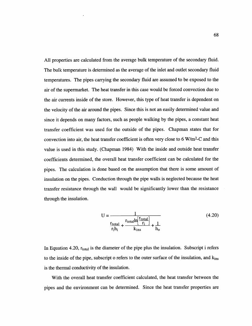
68
All properties are calculated from the average bulk temperature of the secondary fluid.
The bulk temperature is determined as the average of the inlet and outlet secondary fluid
temperatures. The pipes carrying the secondary fluid are assumed to be exposed to the
air of the supermarket. The heat transfer in this case would be forced convection due to
the air currents inside of the store. However, this type of heat transfer is dependent on
the velocity of the air around the pipes. Since this is not an easily determined value and
since it depends on many factors, such as people walking by the pipes, a constant heat
transfer coefficient was used for the outside of the pipes. Chapman states that for
convection into air, the heat transfer coefficient is often very close to 6 W/m 2-C and this
value is used in this study. (Chapman 1984) With the inside and outside heat transfer
coefficients determined, the overall heat transfer coefficient can be calculated for the
pipes. The calculation is done based on the assumption that there is some amount of
insulation on the pipes. Conduction through the pipe walls is neglected because the heat
transfer resistance through the wall would be significantly lower than the resistance
through the insulation.
U1 (4.20)_ _ r [rtotal]
rtotal +total ri + 1rihi+ kins ho
In Equation 4.20, rtotal is the diameter of the pipe plus the insulation. Subscript i refers
to the inside of the pipe, subscript o refers to the outer surface of the insulation, and kins
is the thermal conductivity of the insulation.
With the overall heat transfer coefficient calculated, the heat transfer between the
pipes and the environment can be determined. Since the heat transfer properties are
69
transfer from the pipes to the environment, both an energy balance and a heat transfer rate
equation are necessary to determine the inlet and outlet temperatures and the heat transfer.
The heat transfer rate is based on the log mean temperature difference of the secondary
fluid and air temperatures.
ATim Tsfout - Tsfin (4.21)mlm I Tair - Tsfin 1
-Tair - Tsfout _
This log mean temperature difference is used with the overall heat transfer coefficient and
the total heat transfer area to determine the heat transfer.
Q = UAATIm (4.22)
The heat transfer area (A) is the surface area of the insulation exposed to the supermarket
air. The energy balance of the secondary fluid stream can be expressed.
Q = rnisfCpsfATsf (4.23)
With these two different equations, it is possible to determine the thermal losses of the
piping system to the environment.
4.2.3 Pump Work
To circulate the secondary fluid through the piping system, it is necessary to overcome
the pressure drops from friction in the pipes. The first step in determining the pump work
is to calculate the head losses in the pipes. The head losses arise from the friction losses
and the minor losses due to bends and valves. The friction losses are calculated using the
70
friction factor (f) from the Moody diagram. (White 1986) The correlation equations of
the Moody diagram depend on whether the flow is laminar or turbulent. For laminar flow,
the friction factor is inversely proportional to the Reynolds number.
f= 64 (4.24)ReD
ReD is the Reynolds number based on the diameter. For turbulent flow, a correlation
equation developed by Haaland is utilized. (White 1986)
fl'2 -l 8log[6.9 +(F)111 (4.25)fl/2 e 7)
ReD is the Reynolds number based on diameter, , is the roughness of the pipe, and D is
the diameter of the pipe. The frictional head losses can be calculated once the friction
factor has been determined.
head = f (L) (v2) (4.26)
L is the length of the pipe, D is the diameter, v is the velocity of the fluid flow through the
pipes, and g is the acceleration due to gravity.
The head losses from the minor losses due to bends and valves in the piping system
depend on the number and type of the bends and valves. The method for determining the
minor losses is outlined by White. (White 1986) Each bend and valve is assigned an
equivalent loss coefficient (Keq) and then the total equivalent loss coefficient is the sum of
all of the equivalent loss coefficients from all of the bends and valves. This total
equivalent loss coefficient is then used to calculate the head losses from the minor losses.
71
head = Keq(V21) (4.27)
The total head loss is the sum of the losses due to friction and the minor losses. With the
total head losses, the pressure drop through the pipes can be calculated.
AP =(head) pg (4.28)
Where head is the total head losses, g is the acceleration of gravity, and p is the density of
the fluid flowing through the pipes.
Once the pressure drop is determined, the pump work needed can be calculated.
Wpump = risf ( %) (4.29)
The pump work is calculated for pressure drop in the distribution lines, as well as through
each component that the secondary fluid flow through. Thus, there is pump work
associated with the distribution lines, the heat exchanger in the refrigerated case, and the
heat exchanger with ammonia. The pump work is calculated using motor and mechanical
efficiencies of one. The addition of pump work into the system model alters the
coefficient of performance (COP) equation. The pump work is added to the compressor
work to penalize the additional circulation needed.
COP = caseload (4.30)Wcompressor + Wpump
72
CHAPTER
FIVE
PARAMETRIC STUDY
The computer model written to simulate the performance of the supermarket refrigeration
system utilizes many design parameters that influence the performance of the system.
The highest COP means the refrigeration load is met by the least amount of compressor
and pump power. It is necessary to determine the influence that each of these parameters
has on the performance of the whole system. In order to evaluate the influence, a
parametric study of the system was performed by first determining a base case of all of
the parameters and then varying the parameters one at a time to observe how the system
performance is affected.
73
5.1 Parameter List
Each of the components in the system model have parameters that would be specified
by the system designer and these parameters are described here. The parameters have
been divided according to the component group which they influence.
5.1.1 System Parameters
The first set of parameters affect the system as a whole and not an individual
component. The total refrigeration load met by the system is the first parameter. The
overall heat transfer coefficient (UA) value of the condenser is a specified variable that
primarily depends on the size and design of the condenser. The ambient air temperature
is used to determine the performance of the condenser. The performance of the staged
compression depends on the pressure ratio of the compressors. The intermediate
pressure is usually specified by giving a pressure ratio for the first compressor that is
some power of the overall pressure ratio. The equation for determining the pressure ratio
(rp) of the first stage of compression from the overall pressure ratio of the system is
shown here, where x is the exponent (between 0.0 and 1.0) that is specified. (Chlumsky
1965)
rPfirst stage = (rPoverall)x (5.1)
The mass flow rate of the secondary fluid is the last system parameter in the model. The
flow rate will determine the necessary temperature drops in the heat exchangers and the
piping system losses.
74
5.1.2 Refrigerated Case Parameters
The refrigerated case is modeled as an air to secondary fluid cross-flow heat
exchanger. The physical dimensions of the heat exchanger are necessary for the
calculations. The temperature of the air leaving the heat exchanger is the desired
temperature of the refrigerated case. Values for the output air of refrigerated cases can be
obtained from the manufacturers of refrigerated cases. The values used in this study were
determined from data from the Hussman Corporation that gave the output air
temperatures for the Hussman refrigerated cases using R22 and R502 as the refrigerants.
(Hussman 1989) On the air side of the heat exchanger, it is necessary to specify the air
velocity and the cross sectional area of the heat exchanger that the air passes through.
The air velocity in the cases can also be found in the case manufacturer's data The heat
exchanger cross sectional area depends on the case design. The number, the inside
diameter, the thickness, and the length of the pipes used to carry the secondary fluid
through the air stream are all specified in the model. Finally, the thermal conductivity of
the material used for the pipes and the Keq of the heat exchanger need to be specified. As
discussed in Section 4.2.3, the Keq is used to determine the minor losses of the flow
through the heat exchanger that are part of the pressure drop calculations.
5.1.3 Ammonia-Secondary Fluid Heat Exchanger Parameters
The parameters for this flooded heat exchanger are similar to the ones for the case
heat exchanger discussed above. Again the dimensions of the pipes used need to be
specified. These dimensions are the number, length, inside radius, and thickness of the
pipes. Also the thermal conductivity of the pipe material and the Keq of the heat
exchanger for minor losses need to be specified.
75
5.1.4 Piping System Parameters
A piping system is used to supply and return the secondary fluid from the ammonia-
secondary fluid heat exchanger to the case heat exchanger. For the piping system used in
this model, parameters are provided separately for the supply and return piping to allow
the system to be modeled with different pipes and insulation for the two different pipe
runs. For the pipes themselves, the length and the inside diameter need to be specified.
The amount of insulation, as well as the thermal conductivity of the insulation, are
parameters. In order to determine the losses to the store environment, the store
temperature needs to be provided. The roughness of the pipe material is needed for the
pump work calculations and the Keq for each pipe run must again be specified.
5.1.5 Compressor Parameters
Since two stage compression is used in this system model, two sets of compressor
parameters are needed. The bore and stroke of the piston in the compressor are
parameters, as well as the speed at which the compressor operates and the clearance ratio.
The polytropic model used for the compressors requires a polytropic exponent and
polytropic efficiency. Finally, the number of cylinders of the compressor can be
specified, but does not need to be. In the system parameters discussed in Section 5.1.1,
the pressure ratio and secondary fluid flow rate parameters are discussed. If these two
parameters are specified, then the number of cylinders being used is determined. If the
number of cylinders being used is given, then the pressure ratio and the flow rate are
calculated.
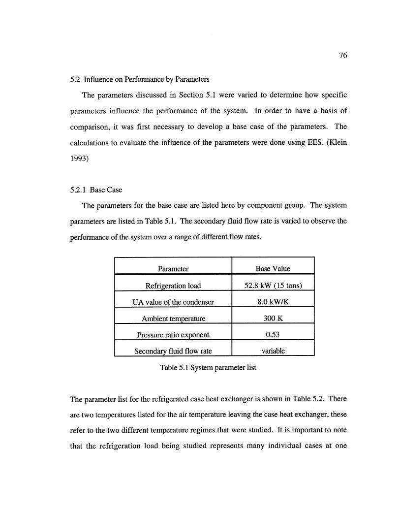
76
5.2 Influence on Performance by Parameters
The parameters discussed in Section 5.1 were varied to determine how specific
parameters influence the performance of the system. In order to have a basis of
comparison, it was first necessary to develop a base case of the parameters. The
calculations to evaluate the influence of the parameters were done using EES. (Klein
1993)
5.2.1 Base Case
The parameters for the base case are listed here by component group. The system
parameters are listed in Table 5.1. The secondary fluid flow rate is varied to observe the
performance of the system over a range of different flow rates.
Parameter Base Value
Refrigeration load 52.8 kW (15 tons)
UA value of the condenser 8.0 kW/K
Ambient temperature 300 K
Pressure ratio exponent 0.53
Secondary fluid flow rate variable
Table 5.1 System parameter list
The parameter list for the refrigerated case heat exchanger is shown in Table 5.2. There
are two temperatures listed for the air temperature leaving the case heat exchanger, these
refer to the two different temperature regimes that were studied. It is important to note
that the refrigeration load being studied represents many individual cases at one
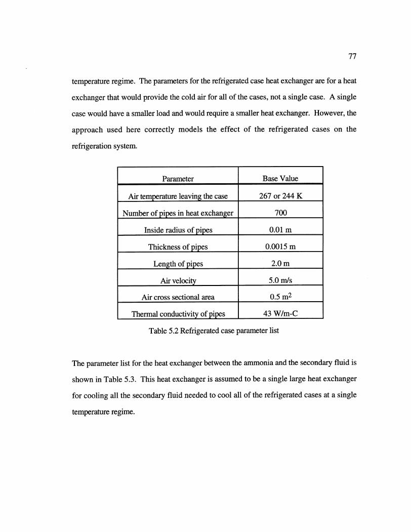
77
temperature regime. The parameters for the refrigerated case heat exchanger are for a heat
exchanger that would provide the cold air for all of the cases, not a single case. A single
case would have a smaller load and would require a smaller heat exchanger. However, the
approach used here correctly models the effect of the refrigerated cases on the
refrigeration system.
Parameter Base Value
Air temperature leaving the case 267 or 244 K
Number of pipes in heat exchanger 700
Inside radius of pipes 0.01 m
Thickness of pipes 0.0015 m
Length of pipes 2.0 m
Air velocity 5.0 m/s
Air cross sectional area 0.5 m2
Thermal conductivity of pipes 43 W/m-C
Table 5.2 Refrigerated case parameter list
The parameter list for the heat exchanger between the ammonia and the secondary fluid is
shown in Table 5.3. This heat exchanger is assumed to be a single large heat exchanger
for cooling all the secondary fluid needed to cool all of the refrigerated cases at a single
temperature regime.
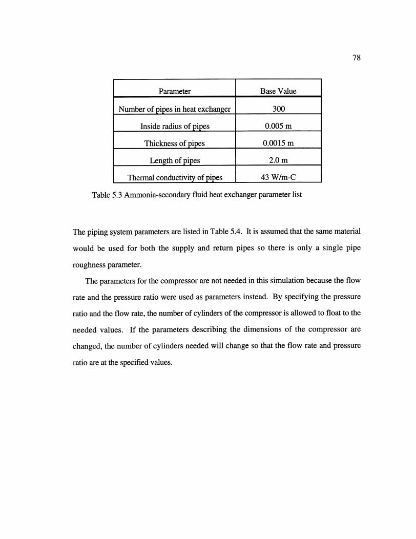
78
Parameter Base Value
Number of pipes in heat exchanger 300
Inside radius of pipes 0.005 m
Thickness of pipes 0.0015 m
Length of pipes 2.0 m
Thermal conductivity of pipes 43 W/m-C
Table 5.3 Ammonia-secondary fluid heat exchanger parameter list
The piping system parameters are listed in Table 5.4. It is assumed that the same material
would be used for both the supply and return pipes so there is only a single pipe
roughness parameter.
The parameters for the compressor are not needed in this simulation because the flow
rate and the pressure ratio were used as parameters instead. By specifying the pressure
ratio and the flow rate, the number of cylinders of the compressor is allowed to float to the
needed values. If the parameters describing the dimensions of the compressor are
changed, the number of cylinders needed will change so that the flow rate and pressure
ratio are at the specified values.
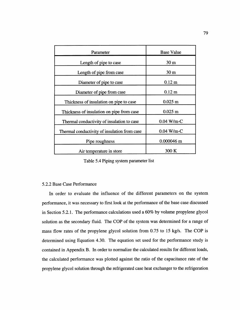
79
Parameter Base Value
Length of pipe to case 30 m
Length of pipe from case 30 m
Diameter of pipe to case 0.12 m
Diameter of pipe from case 0.12 m
Thickness of insulation on pipe to case 0.025 m
Thickness of insulation on pipe from case 0.025 m
Thermal conductivity of insulation to case 0.04 W/m-C
Thermal conductivity of insulation from case 0.04 W/m-C
Pipe roughness 0.000046 m
Air temperature in store 300 K
Table 5.4 Piping system parameter list
5.2.2 Base Case Performance
In order to evaluate the influence of the different parameters on the system
performance, it was necessary to first look at the performance of the base case discussed
in Section 5.2.1. The performance calculations used a 60% by volume propylene glycol
solution as the secondary fluid. The COP of the system was determined for a range of
mass flow rates of the propylene glycol solution from 0.75 to 15 kg/s. The COP is
determined using Equation 4.30. The equation set used for the performance study is
contained in Appendix B. In order to normalize the calculated results for different loads,
the calculated performance was plotted against the ratio of the capacitance rate of the
propylene glycol solution through the refrigerated case heat exchanger to the refrigeration
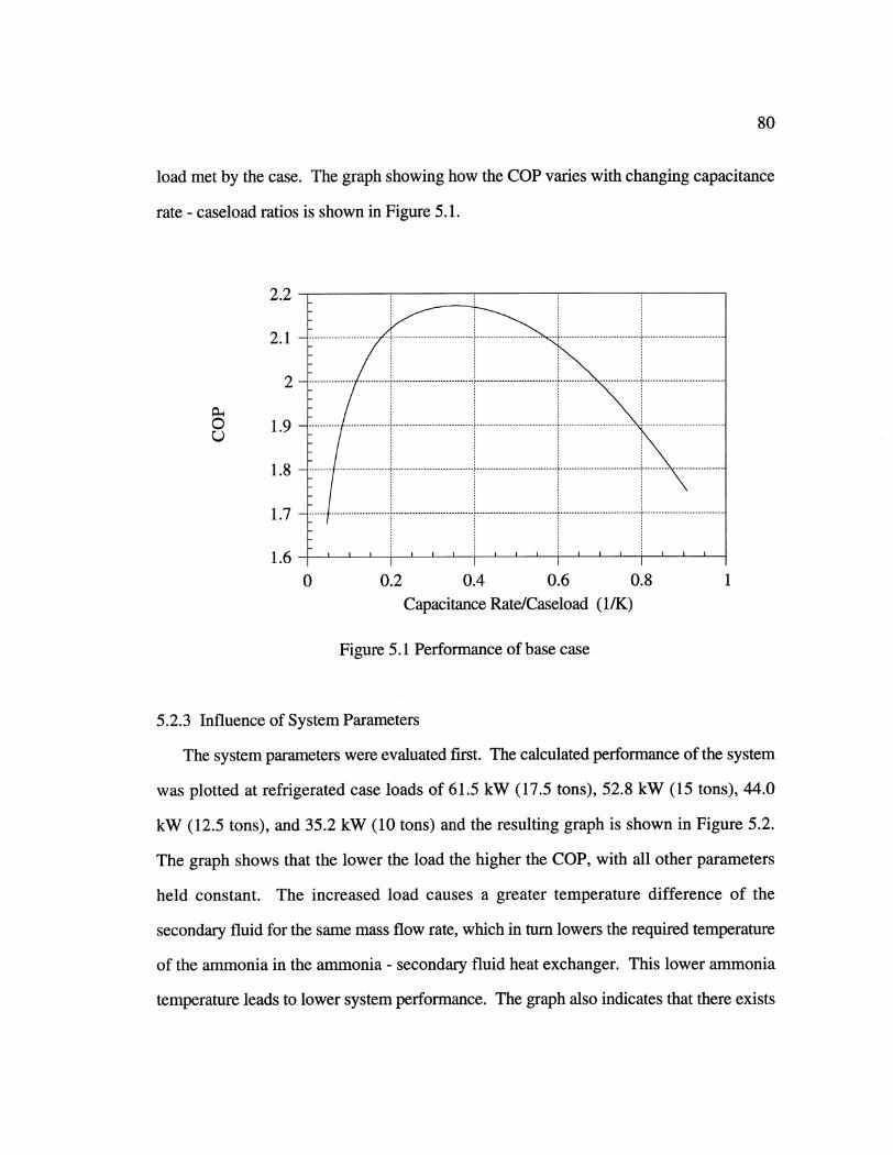
80
load met by the case. The graph showing how the COP varies with changing capacitance
rate - caseload ratios is shown in Figure 5.1.
2.2
2.1
2
0 1.9
1.8
1.7
1.60 0.2 0.4 0.6 0.8
Capacitance Rate/Caseload (I/K)
Figure 5.1 Performance of base case
5.2.3 Influence of System Parameters
The system parameters were evaluated first. The calculated performance of the system
was plotted at refrigerated case loads of 61.5 kW (17.5 tons), 52.8 kW (15 tons), 44.0
kW (12.5 tons), and 35.2 kW (10 tons) and the resulting graph is shown in Figure 5.2.
The graph shows that the lower the load the higher the COP, with all other parameters
held constant. The increased load causes a greater temperature difference of the
secondary fluid for the same mass flow rate, which in turn lowers the required temperature
of the ammonia in the ammonia - secondary fluid heat exchanger. This lower ammonia
temperature leads to lower system performance. The graph also indicates that there exists
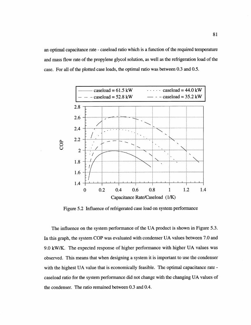
81
an optimal capacitance rate- caseload ratio which is a function of the required temperature
and mass flow rate of the propylene glycol solution, as well as the refrigeration load of the
case. For all of the plotted case loads, the optimal ratio was between 0.3 and 0.5.
caseload = 61.5 kW- - -caseload = 52.8 kW
2.8 -
2.4 ..
2.2
2 /
1.6
1.4 '
caseload = 44.0 kWcaseload = 35.2 kW
0 0.2 0.4 0.6 0.8 1
Capacitance Rate/Caseload (1/K)
1.2 1.4
Figure 5.2 Influence of refrigerated case load on system performance
The influence on the system performance of the UA product is shown in Figure 5.3.
In this graph, the system COP was evaluated with condenser UA values between 7.0 and
9.0 kW/K. The expected response of higher performance with higher UA values was
observed. This means that when designing a system it is important to use the condenser
with the highest UA value that is economically feasible. The optimal capacitance rate -
caseload ratio for the system performance did not change with the changing UA values of
the condenser. The ratio remained between 0.3 and 0.4.
0u
2 M "

UA = 9.0 kW/KUA=8.5 kW/KUA= 8.0kW/K
2.3
2 .2 - ..... ----------..... .... ..... .= ......
22--2.1
2 ...... ..... ,:......... . ............. .............1 .79 .. ....... ...... .......... .....
1.7
1.6 ~ ' T' ' '
UA = 7.5 kW/KUA= 7.0 kW/K
0 0.2 0.4 0.6 0.8 1Capacitance Rate/Caseload (1/K)
Figure 5.3 Influence of the UA value of the condenser on system performance
The influence of the ambient temperature on the system performance was calculated
using temperatures from 270 to 310 *K (26.3 to 98.3 *F) and the results are shown in
Figure 5.4. The COP of the system increases as the ambient temperature decreases, as
expected. The ambient temperature influences the performance of the condenser so these
results suggest that it is possible to increase the performance of the system by using a
water-cooled or evaporative condenser rather than the air-cooled condenser assumed in
this system analysis. The change in ambient temperature has only a minor influence on
the optimal capacitance rate - caseload ratio, as the ratio remains between 0.3 and 0.4
regardless of the ambient temperature.
82
0u
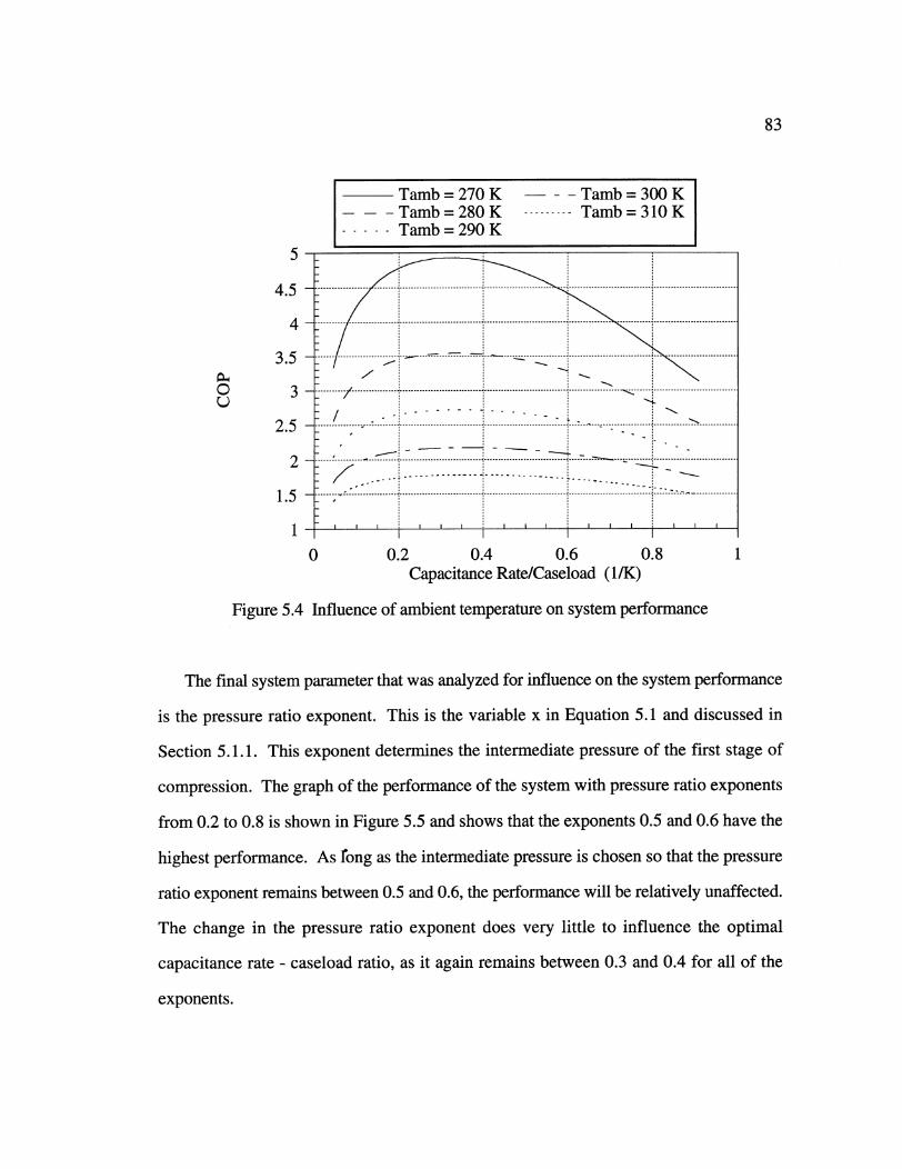
83
Tamb = 270 K Tamb = 300 KTamb=280 K .........- Tamb=310 KTamb=290 K
5
2.-
1.5 ---
- I0 02----04-- 0.6---08---1
......... 7"................................ .......... .....................................-" --..... --..........................3 .5) -----------------
2 .5 -_ --------./. ---------------.. ............................. ............................. ................' -.. --.... ......................... .
.. .... .. .. .. ............................. ............................ ----.... ............. i... ..........................--
2--_
... .................. .. ............................. i............................. i............................. '.. ....:. ..............1.5 - ,---------, 0--, ,
0 0 .2 0.4 0.6 0.8 1
Capacitance Rate/Caseload (1/K)
Figure 5.4 Influence of ambient temperature on system performance
The final system parameter that was analyzed for influence on the system performance
is the pressure ratio exponent. This is the variable x in Equation 5.1 and discussed in
Section 5.1.1. This exponent determines the intermediate pressure of the first stage of
compression. The graph of the performance of the system with pressure ratio exponents
from 0.2 to 0.8 is shown in Figure 5.5 and shows that the exponents 0.5 and 0.6 have the
highest performance. As fong as the intermediate pressure is chosen so that the pressure
ratio exponent remains between 0.5 and 0.6, the performance will be relatively unaffected.
The change in the pressure ratio exponent does very little to influence the optimal
capacitance rate - caseload ratio, as it again remains between 0.3 and 0.4 for all of the
exponents.
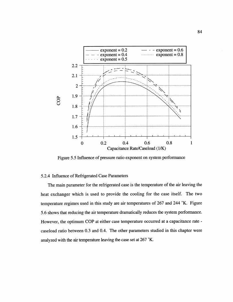
84
2.2 - ____
2 1 - ------------- ----------- --- ---... - . ....---------------
2 - ---- ----- ----- Y ---
-. ............ .. .... .. .......... ........-- ----------.................... ...... ....................................................
2.1-....._.. 'i
0------------9......................................------------------........... ..........
.... .......... ................ ................------ 1 ..... ..............
1.6
1.50 0.2 0.4 0.6 0.8 1
Capacitance Rate/Caseload (1/K)
Figure 5.5 Influence of pressure ratio exponent on system performance
5.2.4 Influence of Refrigerated Case Parameters
The main parameter for the refrigerated case is the temperature of the air leaving the
heat exchanger which is used to provide the cooling for the case itself. The two
temperature regimes used in this study are air temperatures of 267 and 244 K. Figure
5.6 shows that reducing the air temperature dramatically reduces the system performance.
However, the optimum COP at either case temperature occurred at a capacitance rate -
caseload ratio between 0.3 and 0.4. The other parameters studied in this chapter were
analyzed with the air temperature leaving the case set at 267 K.
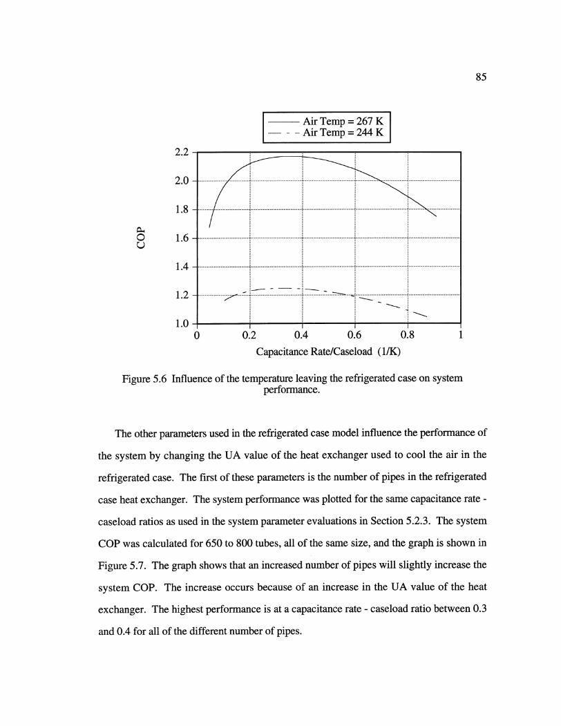
85
Air Temp = 267 KAir Temp = 244 K
0
2.2
2.0
1.8
1.6
1.4
1.2
1.00.2 0.4 0.6 4
Capacitance Rate/Caseload (1/K)
Figure 5.6 Influence of the temperature leaving the refrigerated case on systemperformance.
The other parameters used in the refrigerated case model influence the performance of
the system by changing the UA value of the heat exchanger used to cool the air in the
refrigerated case. The first of these parameters is the number of pipes in the refrigerated
case heat exchanger. The system performance was plotted for the same capacitance rate -
caseload ratios as used in the system parameter evaluations in Section 5.2.3. The system
COP was calculated for 650 to 800 tubes, all of the same size, and the graph is shown in
Figure 5.7. The graph shows that an increased number of pipes will slightly increase the
system COP. The increase occurs because of an increase in the UA value of the heat
exchanger. The highest performance is at a capacitance rate - caseload ratio between 0.3
and 0.4 for all of the different number of pipes.
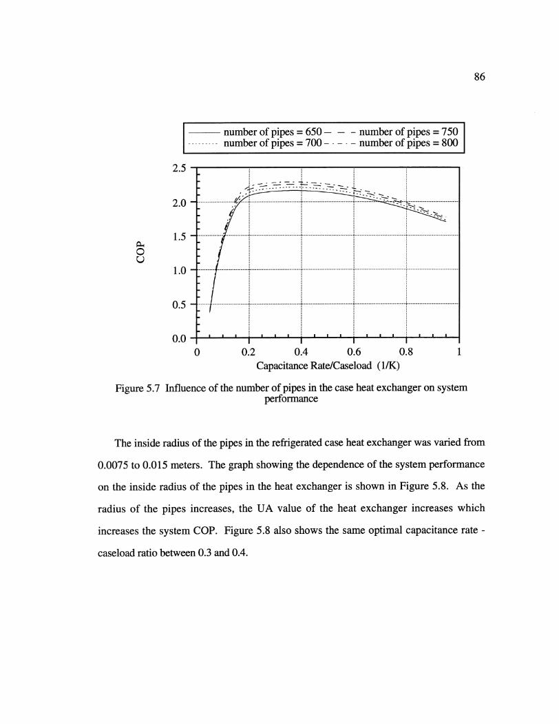
86
number of pipes = 650- - - number of pipes = 750number of pipes = 700 -... number of pipes - 800
2.5
2 .0 . .... ..... ........ ............ ..... ... ... ............................2 ., -- -- -- -- -- -- --- -- - ------. . -- - -- --- -- -
0u
Figure 5.7
1.5
1.0
0 .5 ... .[ ... ............ .-----------------------------...---------------. -------------..------------.-------...........----.. ........................
I II
0 0.2 0.4 0.6 0.8 1Capacitance Rate/Caseload (1/K)
Influence of the number of pipes in the case heat exchanger on systemperformance
The inside radius of the pipes in the refrigerated case heat exchanger was varied from
0.0075 to 0.015 meters. The graph showing the dependence of the system performance
on the inside radius of the pipes in the heat exchanger is shown in Figure 5.8. As the
radius of the pipes increases, the UA value of the heat exchanger increases which
increases the system COP. Figure 5.8 also shows the same optimal capacitance rate -
caseload ratio between 0.3 and 0.4.

87
radius = 0.0075 m radius = 0.0125 mradius = 0.0100 m-----radius = 0.0150 m
0Q
2.5
2.0
1.5
1.0
0.5
0.00 0.2 0.4 0.6 0.8
Capacitance Rate/Caseload (1/K)
Figure 5.8 Influence of the radius of the pipes in the case heat exchanger on systemperformance
The analysis of the thickness of the pipes showed that if the pipes are of the same
material (steel was used for these calculations) the thickness of the pipes in the
refrigerated case heat exchanger has essentially no effect on the system performance. The
influence of the length on the system performance is shown in Figure 5.9. The lengths
of the pipes in the refrigerated case heat exchanger ranged from 1.75 to 2.75 meters. The
system COP increases as the length is increased. The increase occurs because of an
increase in UA value without an equivalent increase in required pumping power. As with
the other parameters, the optimal capacitance rate - caseload ratio is between 0.3 and 0.4
for the length of the pipes.
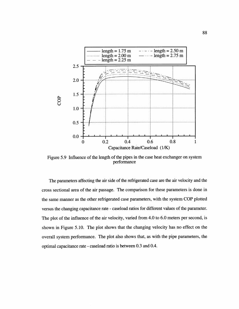
length = 1.75 mlength = 2.00 mlength = 2.25 m
.... -length=2.50 m-.... length=2.75 m
0
2.5
2.0
1.5
1.0
... ......... .............................................................--............................. ---..... . . . ..................
o o. ' i ' ' , * * * * * I0 0.2 0.4 0.6 0.8 1
Capacitance Rate/Caseload (1/K)
Figure 5.9 Influence of the length of the pipes in the case heat exchanger on systemperformance
The parameters affecting the air side of the refrigerated case are the air velocity and the
cross sectional area of the air passage. The comparison for these parameters is done in
the same manner as the other refrigerated case parameters, with the system COP plotted
versus the changing capacitance rate - caseload ratios for different values of the parameter.
The plot of the influence of the air velocity, varied from 4.0 to 6.0 meters per second, is
shown in Figure 5.10. The plot shows that the changing velocity has no effect on the
overall system performance. The plot also shows that, as with the pipe parameters, the
optimal capacitance rate - caseload ratio is between 0.3 and 0.4.
88
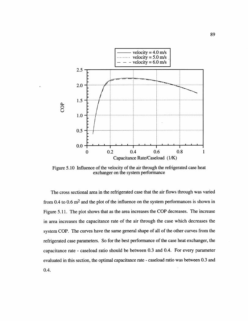
89
velocity = 4.0 m/svelocity = 5.0 m/svelocity =6.0 m/s
0u
Figure 5.10
2.5
2.0
1.5
1.0
0 ..... .................. ......................... ............................. .... ...........................--...........................0 .
0 0.2 0.4 0.6 0.8 1Capacitance Rate/Caseload (1/K)
Influence of the velocity of the air through the refrigerated case heatexchanger on the system performance
The cross sectional area in the refrigerated case that the air flows through was varied
from 0.4 to 0.6 m2 and the plot of the influence on the system performances is shown in
Figure 5.11. The plot shows that as the area increases the COP decreases. The increase
in area increases the capacitance rate of the air through the case which decreases the
system COP. The curves have the same general shape of all of the other curves from the
refrigerated case parameters. So for the best performance of the case heat exchanger, the
capacitance rate - caseload ratio should be between 0.3 and 0.4. For every parameter
evaluated in this section, the optimal capacitance rate - caseload ratio was between 0.3 and
0.4.
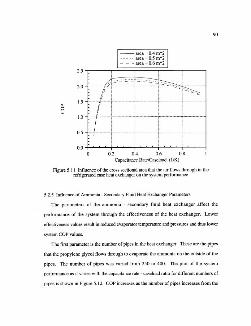
90
area = 0.4 mA2- --------- area = 0.5 mA2
area = 0.6 mA2
2. - .... .....__ __ __ _ __ __ __ _ __ __ _
2.0
1.0---- -
10 . .. ...... .................. ............................. ............................ ............................. ..............................
0 0.2 0.4 0.6 0.8 1Capacitance Rate/Caseload (1/K)
Figure 5.11 Influence of the cross sectional area that the air flows through in therefrigerated case heat exchanger on the system performance
5.2.5 Influence of Ammonia - Secondary Fluid Heat Exchanger Parameters
The parameters of the ammonia - secondary fluid heat exchanger affect the
performance of the system through the effectiveness of the heat exchanger. Lower
effectiveness values result in reduced evaporator temperature and pressures and thus lower
system COP values.
The first parameter is the number of pipes in the heat exchanger. These are the pipes
that the propylene glycol flows through to evaporate the ammonia on the outside of the
pipes. The number of pipes was varied from 250 to 400. The plot of the system
performance as it varies with the capacitance rate - caseload ratio for different numbers of
pipes is shown in Figure 5.12. COP increases as the number of pipes increases from the
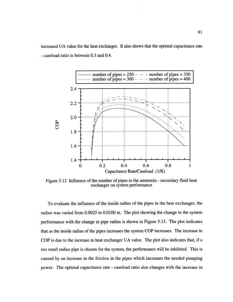
91
increased UA value for the heat exchanger. It also shows that the optimal capacitance rate
- caseload ratio is between 0.3 and 0.4.
number of pipes = 250- - - number of pipes = 350
number of pipes = 300 -... number of pipes = 400
2.4 , I
0
Figure 5.12
2.2
2.0
1.8
1 6 ............. ".. .......... '... ..........................----- .------------------ .---------- ..---------------- .- ........--- ...................--- --.....
1.4f0 0.2 0.4 0.6 0.8 1
Capacitance Rate/Caseload (1/K)
Influence of the number of pipes in the ammonia - secondary fluid heatexchanger on system performance
To evaluate the influence of the inside radius of the pipes in the heat exchanger, the
radius was varied from 0.0025 to 0.0100 m. The plot showing the change in the system
performance with the change in pipe radius is shown in Figure 5.13. The plot indicates
that as the inside radius of the pipes increases the system COP increases. The increase in
COP is due to the increase in heat exchanger UA value. The plot also indicates that, if a
too small radius pipe is chosen for the system, the performance will be inhibited. This is
caused by an increase in the friction in the pipes which increases the needed pumping
power. The optimal capacitance rate - caseload ratio also changes with the increase in
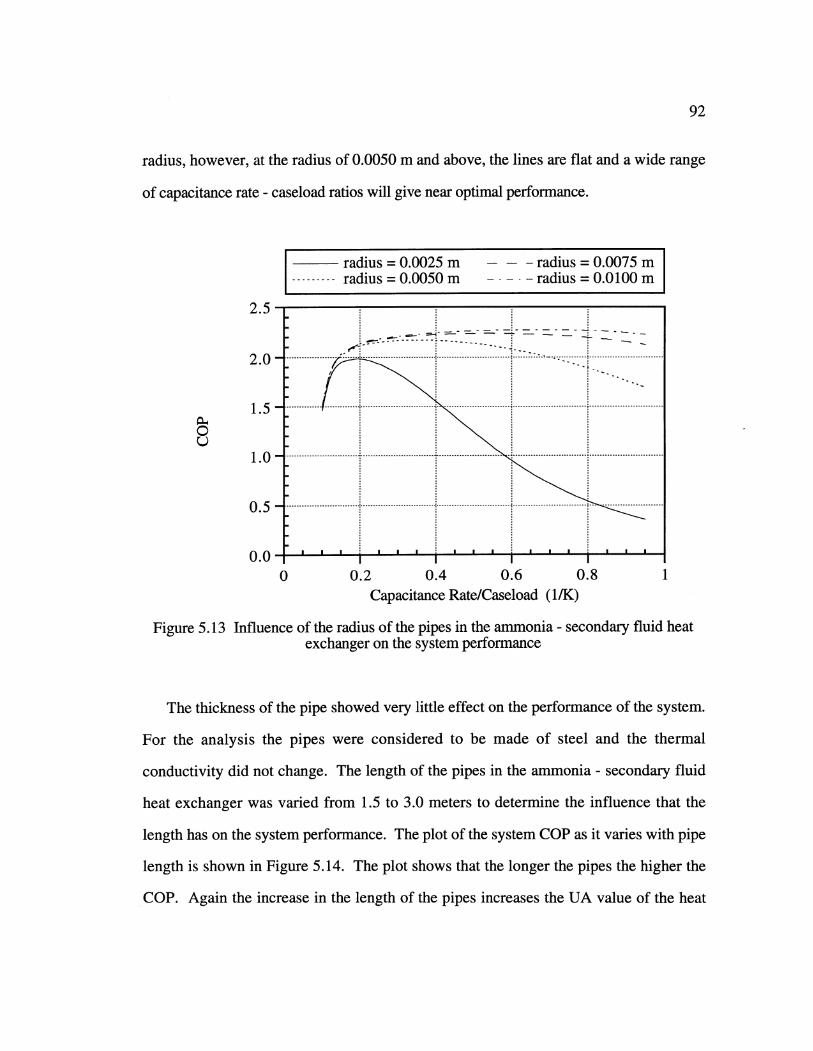
92
radius, however, at the radius of 0.0050 m and above, the lines are flat and a wide range
of capacitance rate - caseload ratios will give near optimal performance.
2.5
2.0
1.5
1.0
0.5
0.0
Figure 5.13
radius = 0.0025 m - - - radius = 0.0075 mradius = 0.0050 m -.... radius = 0.0100 m
.............. .....................-- -------------- --j....... .----- ------- :'------- ---------
-................ .. ................. ............ i..................I. ........... !...... :..... .... .............................-- -------------
.(
.. - --
0 0.2 0.4 0.6 0.8 1Capacitance Rate/Caseload (1/K)
Influence of the radius of the pipes in the ammonia - secondary fluid heatexchanger on the system performance
The thickness of the pipe showed very little effect on the performance of the system.
For the analysis the pipes were considered to be made of steel and the thermal
conductivity did not change. The length of the pipes in the ammonia - secondary fluid
heat exchanger was varied from 1.5 to 3.0 meters to determine the influence that the
length has on the system performance. The plot of the system COP as it varies with pipe
length is shown in Figure 5.14. The plot shows that the longer the pipes the higher the
COP. Again the increase in the length of the pipes increases the UA value of the heat
0U..
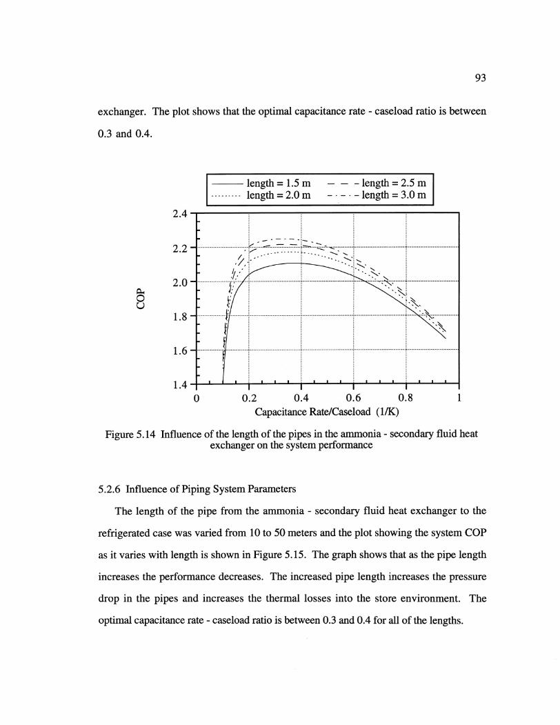
93
exchanger. The plot shows that the optimal capacitance rate - caseload ratio is between
0.3 and 0.4.
length = 1.5m - length=2.5 mlength = 2.0 m --- length=3.Om
0
Figure 5.14
2.4
2.2
2.0
1.8
1 .6 . .. ...... ... -----..... ..... ........................... --------------. --------.... ... ----......... ................ .--............ ...............
1.4 ' ' '' '' '' '0 0.2 0.4 0.6 0.8 1
Capacitance Rate/Caseload (1/K)
Influence of the length of the pipes in the ammonia - secondary fluid heatexchanger on the system performance
5.2.6 Influence of Piping System Parameters
The length of the pipe from the ammonia - secondary fluid heat exchanger to the
refrigerated case was varied from 10 to 50 meters and the plot showing the system COP
as it varies with length is shown in Figure 5.15. The graph shows that as the pipe length
increases the performance decreases. The increased pipe length increases the pressure
drop in the pipes and increases the thermal losses into the store environment. The
optimal capacitance rate - caseload ratio is between 0.3 and 0.4 for all of the lengths.
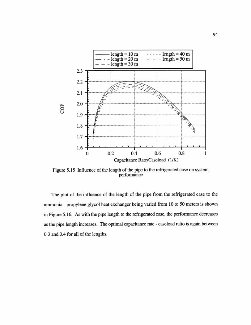
0
Figure 5.15
2.3 - __ _ _ _ _ _ _ _ _ __ _ _ _ _ _ _ _
2.2 -!°°
2.1-
2.0-
1.9..............
1.8.. ...............
1.7
1.6 - 10 0.2 0.4 0.6 0.8 1
Capacitance Rate/Caseload (1/K)
Influence of the length of the pipe to the refrigerated case on systemperformance
The plot of the influence of the length of the pipe from the refrigerated case to the
ammonia - propylene glycol heat exchanger being varied from 10 to 50 meters is shown
in Figure 5.16. As with the pipe length to the refrigerated case, the performance decreases
as the pipe length increases. The optimal capacitance rate - caseload ratio is again between
0.3 and 0.4 for all of the lengths.
94
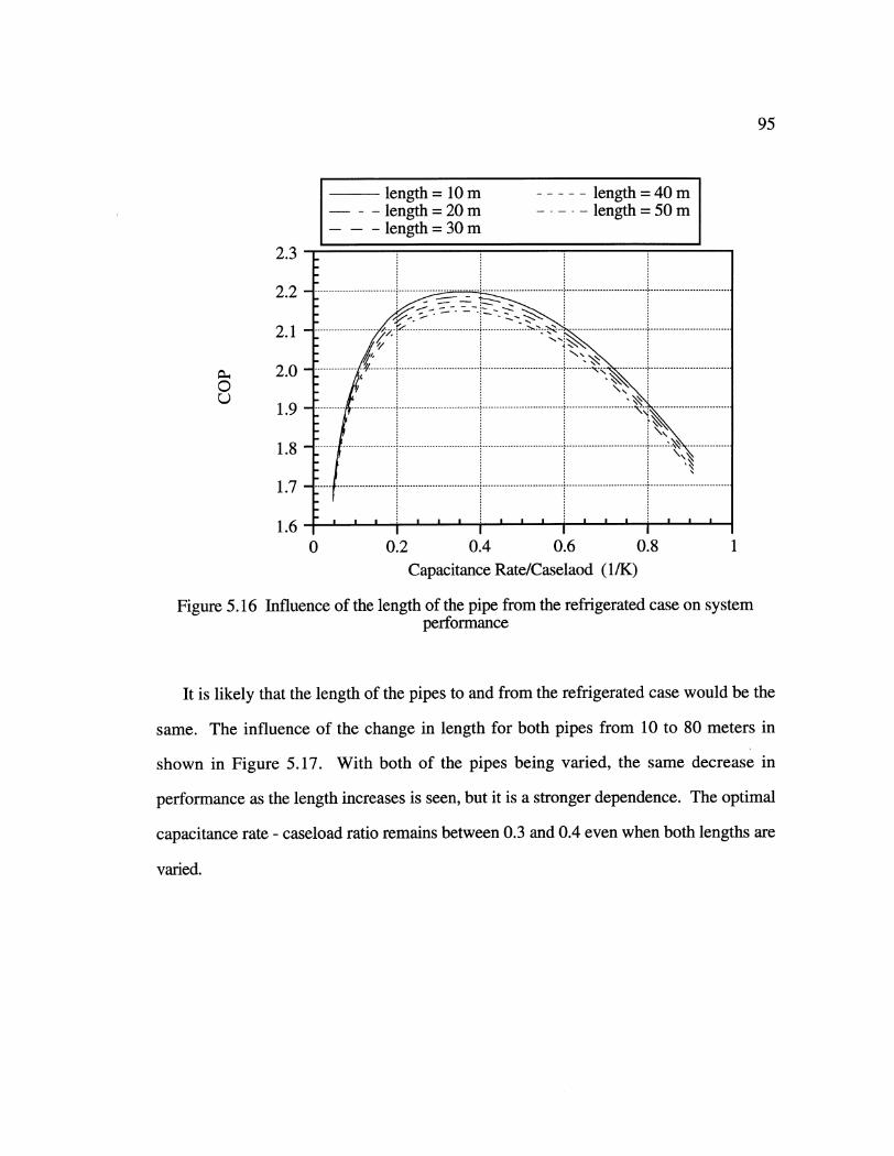
0
Figure 5.16
2.3 - __ _ _ _ _ _ _ _
2.2-
2.2 ~ ~......................2.1-/
2.0-.....--
1.9
1 .8 --- ---------
1.8- ... ...........................1.7
0 0.2 0.4 0.6 0.8 1
Capacitance Rate/Caselaod (1/K)
Influence of the length of the pipe from the refrigerated case on systemperformance
It is likely that the length of the pipes to and from the refrigerated case would be the
same. The influence of the change in length for both pipes from 10 to 80 meters in
shown in Figure 5.17. With both of the pipes being varied, the same decrease in
performance as the length increases is seen, but it is a stronger dependence. The optimal
capacitance rate - caseload ratio remains between 0.3 and 0.4 even when both lengths are
varied.
95
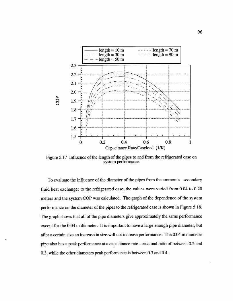
96
length= 10 mlength =30 mlength=50 m
0
Figure 5.17
2.3
2.2
2.1
2.0
1.9
1.8
1.7
1.6
1.5
length =70 mlength = 90 m
0 0.2 0.4 0.6 0.8 1Capacitance Rate/Caseload (1/K)
Influence of the length of the pipes to and from the refrigerated case onsystem performance
To evaluate the influence of the diameter of the pipes from the ammonia - secondary
fluid heat exchanger to the refrigerated case, the values were varied from 0.04 to 0.20
meters and the system COP was calculated. The graph of the dependence of the system
performance on the diameter of the pipes to the refrigerated case is shown in Figure 5.18.
The graph shows that all of the pipe diameters give approximately the same performance
except for the 0.04 m diameter. It is important to have a large enough pipe diameter, but
after a certain size an increase in size will not increase performance. The 0.04 m diameter
pipe also has a peak performance at a capacitance rate - caseload ratio of between 0.2 and
0.3, while the other diameters peak performance is between 0.3 and 0.4.
5 W"M""
MMMMEMMI
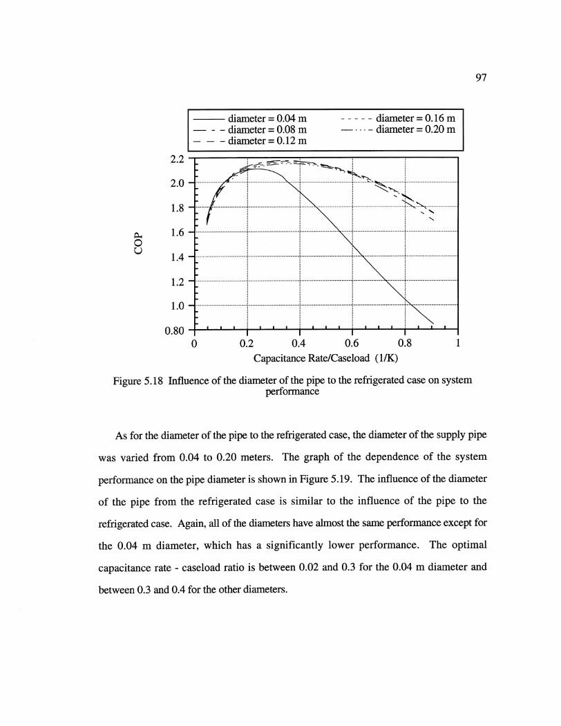
0u
2.2
2.0
1.8
1.6
1.4
1.2
1.0
0.80
diameter = 0.04 mdiameter = 0.08 mdiameter = 0.12 m
. .................................. I -- -
I
diameter = 0.16 mdiameter= 0.20 m
0 0.2 0.4 0.6 0.8 1Capacitance Rate/Caseload (1/K)
Figure 5.18 Influence of the diameter of the pipe to the refrigerated case on systemperformance
As for the diameter of the pipe to the refrigerated case, the diameter of the supply pipe
was varied from 0.04 to 0.20 meters. The graph of the dependence of the system
performance on the pipe diameter is shown in Figure 5.19. The influence of the diameter
of the pipe from the refrigerated case is similar to the influence of the pipe to the
refrigerated case. Again, all of the diameters have almost the same performance except for
the 0.04 m diameter, which has a significantly lower performance. The optimal
capacitance rate - caseload ratio is between 0.02 and 0.3 for the 0.04 m diameter and
between 0.3 and 0.4 for the other diameters.
97
I
I
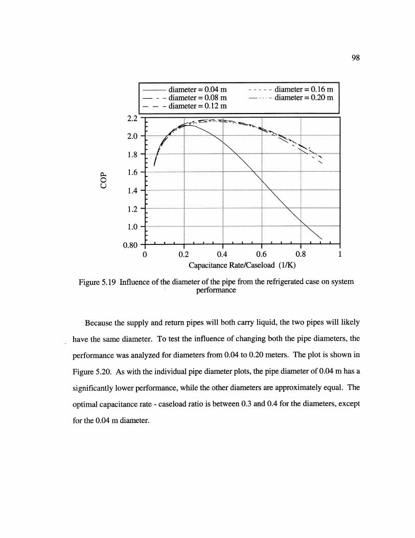
98
2.2-
2.0-
1.8 -
1.6-
1.4-
1.2-
1.0-
0.80-
F
Figure 5.19
diameter = 0.04 mdiameter = 0.08 mdiameter = 0.12 m
1,,-_.J.. -."--
diameter=0.16 m-.... diameter= 0.20 m
0 0.2 0.4 0.6 0.8 1Capacitance Rate/Caseload (1/K)
Influence of the diameter of the pipe from the refrigerated case on systemI performance
Because the supply and return pipes will both carry liquid, the two pipes will likely
have the same diameter. To test the influence of changing both the pipe diameters, the
performance was analyzed for diameters from 0.04 to 0.20 meters. The plot is shown in
Figure 5.20. As with the individual pipe diameter plots, the pipe diameter of 0.04 m has a
significantly lower performance, while the other diameters are approximately equal. The
optimal capacitance rate - caseload ratio is between 0.3 and 0.4 for the diameters, except
for the 0.04 m diameter.
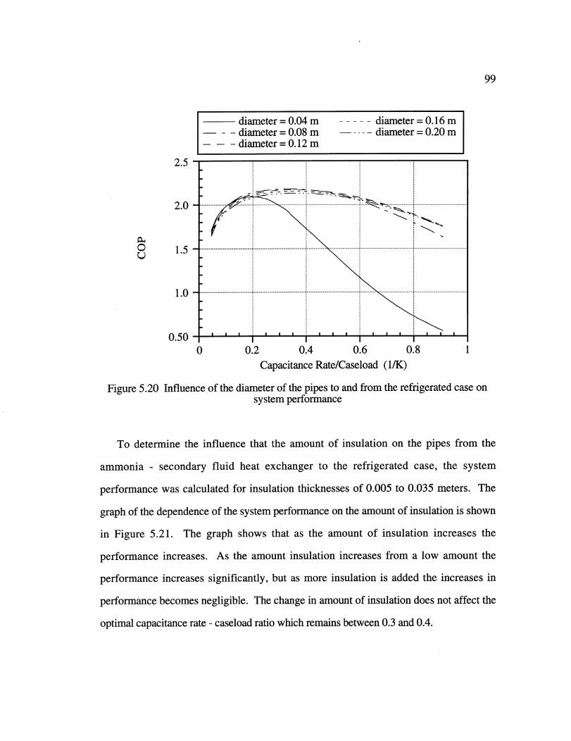
99
diameter = 0.04 mdiameter = 0.08 mdiameter = 0.12 m
2.5
2.0
0Q
Figure 5.20
1.5
diameter = 0.16 mdiameter = 0.20 m
0.50*
u.U- I I
0 0.2 0.4 0.6 0.8 1
Capacitance Rate/Caseload (1/K)
Influence of the diameter of the pipes to and from the refrigerated case onsystem performance
To determine the influence that the amount of insulation on the pipes from the
ammonia - secondary fluid heat exchanger to the refrigerated case, the system
performance was calculated for insulation thicknesses of 0.005 to 0.035 meters. The
graph of the dependence of the system performance on the amount of insulation is shown
in Figure 5.21. The graph shows that as the amount of insulation increases the
performance increases. As the amount insulation increases from a low amount the
performance increases significantly, but as more insulation is added the increases in
performance becomes negligible. The change in amount of insulation does not affect the
optimal capacitance rate - caseload ratio which remains between 0.3 and 0.4.
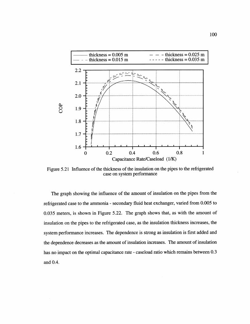
thickness = 0.005 m- - -thickness = 0.015 m
2.2 _L _
thickness = 0.025 mthickness = 0.035 m
0
Figure 5.21
2.1
2.0
1.9
1 .8 . ...... .................. I ............................. [ ....................... [......... -------- ................. ...- ........1.8
1 . .. ............... ----........ ................ .. ----........... ................I -.............................-- ........................... --.1.7 ..... -----
1.6 4 'I• I
0 0.2 0.4 0.6 0.8 1Capacitance Rate/Caseload (1/K)
Influence of the thickness of the insulation on the pipes to the refrigeratedcase on system performance
The graph showing the influence of the amount of insulation on the pipes from the
refrigerated case to the ammonia - secondary fluid heat exchanger, varied from 0.005 to
0.035 meters, is shown in Figure 5.22. The graph shows that, as with the amount of
insulation on the pipes to the refrigerated case, as the insulation thickness increases, the
system performance increases. The dependence is strong as insulation is first added and
the dependence decreases as the amount of insulation increases. The amount of insulation
has no impact on the optimal capacitance rate - caseload ratio which remains between 0.3
and 0.4.
L.
100
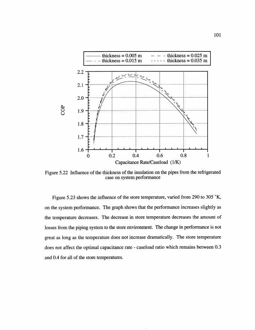
101
thickness = 0.005 m thickness = 0.025 mthickness = 0.015 m-thickness =0.035 m
0u
2.2
2.1
2.0
1.9
1.7
1.6
0 0.2 0.4 0.6 0.8 1Capacitance Rate/Caseload (1/K)
Figure 5.22 Influence of the thickness of the insulation on the pipes from the refrigeratedcase on system performance
Figure 5.23 shows the influence of the store temperature, varied from 290 to 305 °K,
on the system performance. The graph shows that the performance increases slightly as
the temperature decreases. The decrease in store temperature decreases the amount of
losses from the piping system to the store environment. The change in performance is not
great as long as the temperature does not increase dramatically. The store temperature
does not affect the optimal capacitance rate - caseload ratio which remains between 0.3
and 0.4 for all of the store temperatures.
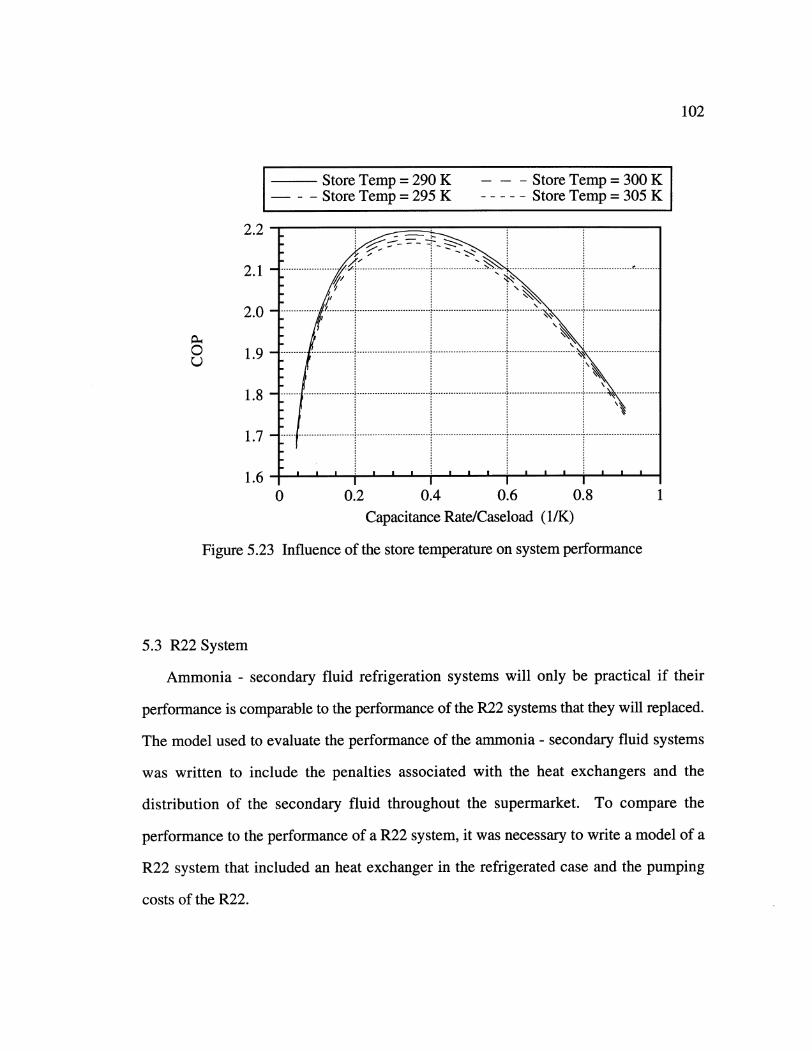
2.2
2.1
2.0
1.90
Store Temp= 290 KStore Temp = 295 K
Store Temp = 300 KStore Temp = 305 K
1 8 ....... ................. --------------.-..-.- ..-.-.---- .. ..... ...... ..... ..... .... ..... ...... ..... ..... ...... ... .. .....1 .78 ....... .... .. . . . . .. . . . .. . . . . .. . . . . . . . . .. . . . .. . . . . . . . . . .. . . . . .. . . . . .. . . ..17
1.6
0 0.2 0.4 0.6 0.8
Capacitance Rate/Caseload (1/K)
Figure 5.23 Influence of the store temperature on system performance
5.3 R22 System
Ammonia - secondary fluid refrigeration systems will only be practical if their
performance is comparable to the performance of the R22 systems that they will replaced.
The model used to evaluate the performance of the ammonia - secondary fluid systems
was written to include the penalties associated with the heat exchangers and the
distribution of the secondary fluid throughout the supermarket. To compare the
performance to the performance of a R22 system, it was necessary to write a model of a
R22 system that included an heat exchanger in the refrigerated case and the pumping
costs of the R22.
102
I
103
5.3.1 R22 Base Case
The equations used to calculate the thermal losses and the pressure drops in the
supply and return lines for the refrigerated case in the R22 system model are identical to
the equations used in the ammonia - secondary fluid system model. These equations are
discussed in Sections 4.2.2 and 4.2.3. The refrigerated case is assumed to have the R22
circulated in a tube bundle oriented cross-flow to the air stream. The heat transfer
coefficients of the air flow on the outside of the pipes are calculated in the same manner
as in the ammonia - secondary fluid model and shown in Equation 4.12. The R22 flow
in the pipes is changing phase and the correlation equations become confounded by the
forced convection and the phase change. An assumption was made that the inside heat
transfer coefficient would be an order of magnitude greater than the heat transfer
coefficient of the outside of the tubes due to the phase change of the R22 on the inside of
the pipes. The heat transfer coefficients are used to calculate the overall heat transfer
coefficient and the UA product for the heat exchanger. The effectiveness of the heat
exchanger is determined using the effectiveness - NTU equation for heat exchangers with
one stream changing phase, as shown in Equation 4.7.
5.3.2 R22 and Ammonia Performance Comparison
The models of the ammonia - secondary fluid system and the R22 system contain the
same penalties for the refrigerated case heat exchangers and the piping of the fluids. The
models are includes in Appendix C. The performance of the R22 system and the
ammonia with Dowfrost system were compared at a refrigerated case temperature of 267
'K. The results of the comparison are shown in Table 8.1. The system COP for the R22
system is around 4% higher than the system COP for the ammonia with Dowfrost
system. This is a small difference between the two system and improvements in the heat
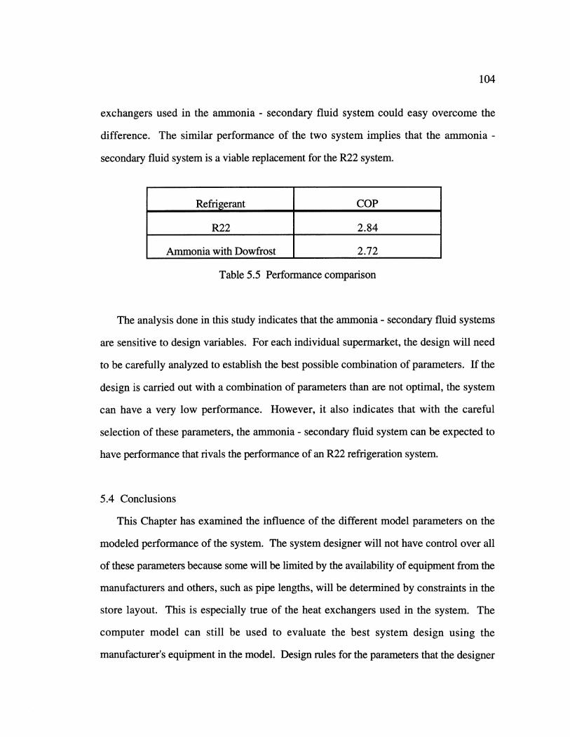
104
exchangers used in the ammonia - secondary fluid system could easy overcome the
difference. The similar performance of the two system implies that the ammonia -
secondary fluid system is a viable replacement for the R22 system.
Refrigerant COP
R22 2.84
Ammonia with Dowfrost 2.72
Table 5.5 Performance comparison
The analysis done in this study indicates that the ammonia - secondary fluid systems
are sensitive to design variables. For each individual supermarket, the design will need
to be carefully analyzed to establish the best possible combination of parameters. If the
design is carried out with a combination of parameters than are not optimal, the system
can have a very low performance. However, it also indicates that with the careful
selection of these parameters, the ammonia - secondary fluid system can be expected to
have performance that rivals the performance of an R22 refrigeration system.
5.4 Conclusions
This Chapter has examined the influence of the different model parameters on the
modeled performance of the system. The system designer will not have control over all
of these parameters because some will be limited by the availability of equipment from the
manufacturers and others, such as pipe lengths, will be determined by constraints in the
store layout. This is especially true of the heat exchangers used in the system. The
computer model can still be used to evaluate the best system design using the
manufacturer's equipment in the model. Design rules for the parameters that the designer

105
will have the most control over are presented in Chapter 7. With the use of these rules, a
carefully designed ammonia - secondary fluid system can have a performance that is
comparable with the performance of a R22 system.
106
CHAPTER
SIX
SECONDARY FLUID PERFORMANCE COMPARISON
The six different secondary fluids analyzed in the study were discussed in Chapter 2.
The properties and the hazards of each fluid were enumerated. However, the
performance of the ammonia - secondary fluid system for each of the different fluids was
not discussed. To analyze the overall system performance, the correlation equations for
the properties were entered into the base case model and the performance of the ammonia
- secondary fluid refrigeration system was calculated for each secondary fluid.
107
6.1 Secondary Fluid Comparison
The secondary fluid correlation equations from Chapter 2 were entered into the base
case computer model for the ammonia - secondary fluid system and the performance of
the system was evaluated using EES[l]. The comparison of the performance was done
for each fluid in four different manners: ignoring thermal losses and required pump
work, with thermal losses and without pump work, with pump work and without thermal
losses, and with both pump work and thermal losses. Using the base case parameters as
listed in Section 5.2.1, the comparison was done at refrigerated case temperatures of 267
and 244 K. The model equation sets are included in Appendix D.
6.1.1 Performance Comparison without thermal losses and pump work
This comparison did not include thermal losses of the piping system to the store
environment or the pumping power needed to circulate the secondary fluid in order to
isolate the effects of the two heat exchangers on the secondary fluid distribution system.
The plots of the performance of the different secondary fluids are shown in Figures 6.1
and 6.2. At a refrigerated case temperature of 267 'K, propane yields the highest
performance. Ethanol, Dowfrost, and Dowtherm SR-1 have about the same performance
and Syltherm XLT and Multitherm 503 have the lowest performance. Since all other
factors except for the heat exchangers are neglected here it is necessary to look at the
performance of the two heat exchangers to determine the reason that propane has the
highest performance. The Reynolds numbers of the secondary fluid flows through the
ammonia - secondary fluid heat exchanger are around 100 for Dowfrost, 400 for
Dowtherm SR-I, 45000 for propane, and 3000 for ethanol. This means that Dowfrost
and Dowtherm SR-i are laminar flow, ethanol is transitional flow, and propane is
turbulent flow. The heat transfer in turbulent flow is much higher than the heat transfer
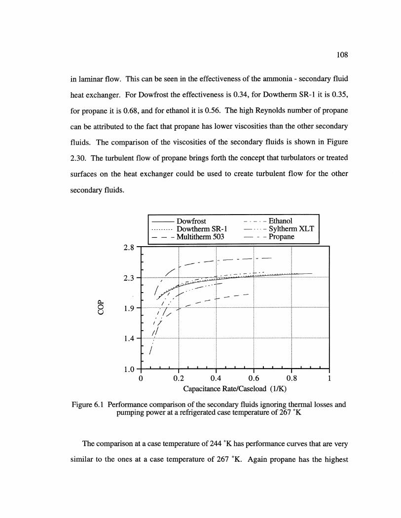
108
in laminar flow. This can be seen in the effectiveness of the ammonia - secondary fluid
heat exchanger. For Dowfrost the effectiveness is 0.34, for Dowtherm SR-1 it is 0.35,
for propane it is 0.68, and for ethanol it is 0.56. The high Reynolds number of propane
can be attributed to the fact that propane has lower viscosities than the other secondary
fluids. The comparison of the viscosities of the secondary fluids is shown in Figure
2.30. The turbulent flow of propane brings forth the concept that turbulators or treated
surfaces on the heat exchanger could be used to create turbulent flow for the other
secondary fluids.
Dowfrost . -Ethanol
--------- Dowtherm SR-1 - -Syltherm XLTMultitherm 503 Propane
2.8
.......-----------" .. ..... .... ...... _. .......,:.. . ......................-- ----2.3 - ---- '-
CO© 9 - . I ' [ .. ... .... ... ... ..; ... ....................... ........................... .. ...........................--- ............................."1.9 ---U
1.0
-//
0 0.2 0.4 0.6 0.8 1Capacitance Rate/Caseload (1/K)
Figure 6.1 Performance comparison of the secondary fluids ignoring thermal losses andpumping power at a refrigerated case temperature of 267 OK
Th1cm p rio ata. ae. em e atr.o.24.K hs.ero m a c curves........................that............ are...............very..............
siia oth nsa a aetmeaueo 6 K gin rpn a h ihs
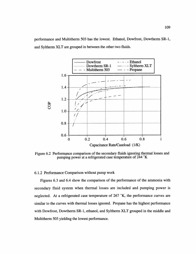
109
performance and Multitherm 503 has the lowest. Ethanol, Dowfrost, Dowtherm SR-1,
and Syltherm XLT are grouped in between the other two fluids.
Dowfrost .... -Ethanol
........ Dowtherm SR- -1.... Syltherm XLTMultitherm 503 - - - Propane
1.61
1.4
1.2
0
1.0
0.8
I.
/ 7.............................. ...................... . ..... i -.............. .. ..... .. ... .. ... .. .
... .. .. ..... ------------. ..... ..-..... ............. .................... ............................. ............................
../ , - -........... ... ........... ..........//
./
V. U II I I
0 0.2 0.4 0.6 0.8 1
Capacitance Rate/Caseload (1/K)
Figure 6.2 Performance comparison of the secondary fluids ignoring thermal losses andpumping power at a refrigerated case temperature of 244 *K
6.1.2 Performance Comparison without pump work
Figures 6.3 and 6.4 show the comparison of the performance of the ammonia with
secondary fluid system when thermal losses are included and pumping power is
neglected. At a refrigerated case temperature of 267 'K, the performance curves are
similar to the curves with thermal losses ignored. Propane has the highest performance
with Dowfrost, Dowtherm SR-1, ethanol, and Syltherm XLT grouped in the middle and
Multitherm 503 yielding the lowest performance.
..................... ............................. ............................. ...........................
.......... .. ... ..... ... ..... ... ----- -- --- --- -- --- -- - - --- ----- -- ------ -- -- -- --- --- -- ----- --- --
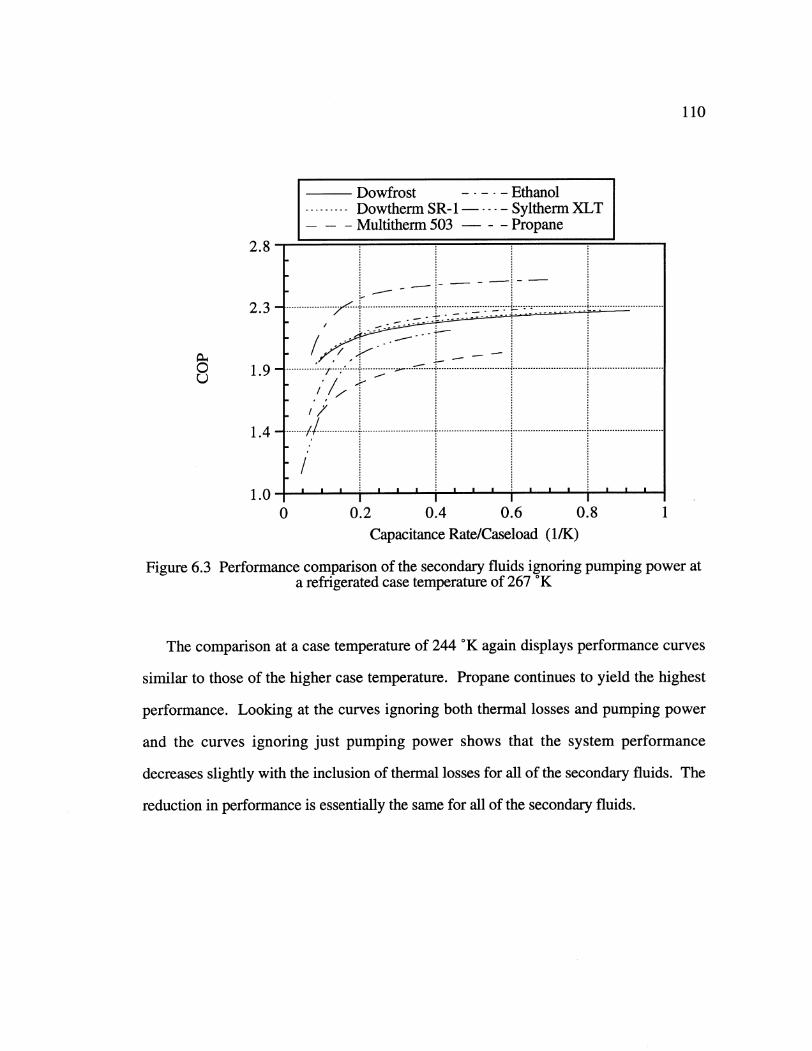
110
Dowfrost ... Ethanol-----Dowtherm SR- 1... Syltherm XLT
Multitherm 503 -- Propane
2.8
2 . 3 ------- ----- °" "
........ ... .... ....-----.---.. ... .... ... .... .... ..-,--..... ... .... ... .... ...--.. .--- --.. ... .... ... ....---.... .... .... ... .... ...1 .9_- ---------- -----7.... ------------------
1 .4 ......... .. ..---------
a refrigerated case temperature of 267 K
The comparison at a case temperature of 244 *K again displays performance curves
similar to those of the higher case temperature. Propane continues to yield the highest
performance. Looking at the curves ignoring both thermal losses and pumping power
and the curves ignoring just pumping power shows that the system performance
decreases slightly with the inclusion of thermal losses for all of the secondary fluids. The
reduction in performance is essentially the same for all of the secondary fluids.
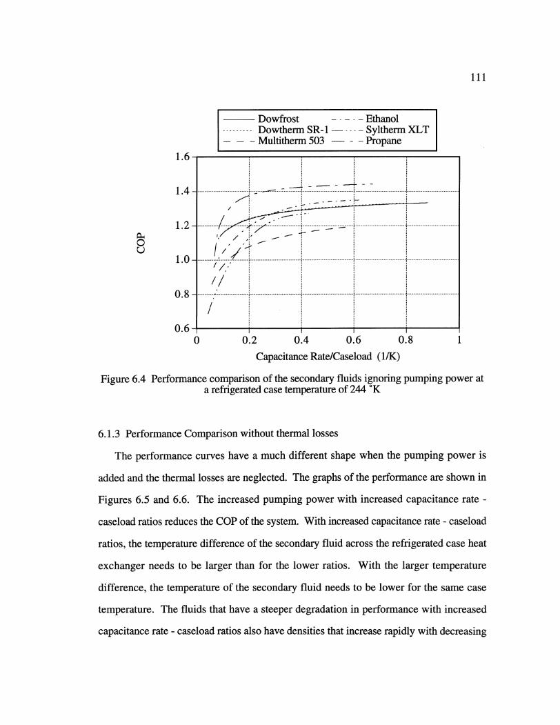
0
111
Dowfrost .... -Ethanol
Dowtherm SR-1- .... Syltherm XLTMultitherm 503 - - Propane
1 1
1.
1.
1.
1.
0.
0.
0-0
------- ---. . -... . .. . .. . .. . . .. . .. . .. . . .. . .. . .. . .
- -----------. .. ... ... . ... . .... ....... ..... ........................... ................................ ...........................
8- ..- . ..0 ---- -------- ............ ........................ ...........................................................
..... ..... .". ..... ..... ... ............................. ......................................................................................
/
6- r T
0 0.2 0.4 0.6 0.8 1
Capacitance Rate/Caseload (1/K)
Figure 6.4 Performance comparison of the secondary fluids ignoring pumping power ata refrigerated case temperature of 244 'K
6.1.3 Performance Comparison without thermal losses
The performance curves have a much different shape when the pumping power is
added and the thermal losses are neglected. The graphs of the performance are shown in
Figures 6.5 and 6.6. The increased pumping power with increased capacitance rate -
caseload ratios reduces the COP of the system. With increased capacitance rate - caseload
ratios, the temperature difference of the secondary fluid across the refrigerated case heat
exchanger needs to be larger than for the lower ratios. With the larger temperature
difference, the temperature of the secondary fluid needs to be lower for the same case
temperature. The fluids that have a steeper degradation in performance with increased
capacitance rate - caseload ratios also have densities that increase rapidly with decreasing
I
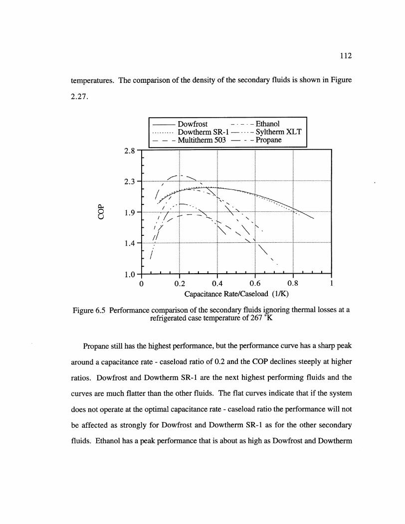
112
temperatures. The comparison of the density of the secondary fluids is shown in Figure
2.27.
Dowfrost .... -Ethanol
Dowtherm SR-I .... Syltherm XLTMultitherm 503 - - -Propane
2.8
1.- N !
.. ....... ........................ ................. ............................. ...........................
---------. .- ---.. ... ........... .. ............................ .- -. .- ---------------------
©1 .49 -----... ... ......- ---------------- ............ ... ...... % .......................... .'.. ......................... .
0 0.2 0.4 0.6 0.8 1Capacitance Rate/Caseload (1/K)
Figure 6.5 Performance comparison of the secondary fluids ignoring thermal losses at arefrigerated case temperature of 267 *K
Propane still has the highest performance, but the performance curve has a sharp peak
around a capacitance rate - caseload ratio of 0.2 and the COP declines steeply at higher
ratios. Dowfrost and Dowtherm SR-i are the next highest performing fluids and the
curves are much flatter than the other fluids. The flat curves indicate that if the system
does not operate at the optimal capacitance rate - caseload ratio the performance will not
be affected as strongly for Dowfrost and Dowtherm SR- I as for the other secondary
flid.Etaolha pa pefomnc .ta isaota iha ofotadDwhr
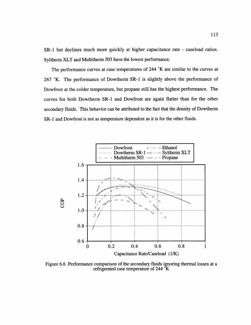
113
SR-I but declines much more quickly at higher capacitance rate - caseload ratios.
Syltherm XLT and Multitherm 503 have the lowest performance.
The performance curves at case temperatures of 244 'K are similar to the curves at
267 'K. The performance of Dowtherm SR-1 is slightly above the performance of
Dowfrost at the colder temperature, but propane still has the highest performance. The
curves for both Dowtherm SR-I and Dowfrost are again flatter than for the other
secondary fluids. This behavior can be attributed to the fact that the density of Dowtherm
SR-I and Dowfrost is not as temperature dependent as it is for the other fluids.
Dowfrost EthanolDowtherm SR-1 - Syltherm XLTMultitherm 503 Propane
1.6 _
1 .44 . .................--- ------------..-- -- ........... ................. ........................ ........................ .......................
1 .4 -. ....... :-.\............1 .2 ------ !....... ......
1.000
0 0.2 0.4 0.6 0.8 1
Capacitance Rate/Caseload (l/K)
Figure 6.6 Performance comparison of the secondary fluids ignoring thermal losses at arefrigerated case temperature of 244 *K
---- --..... . -------------... ... .. .. ... .. ... ................................ ---------------.............................................. ---------------
I5--Q
I
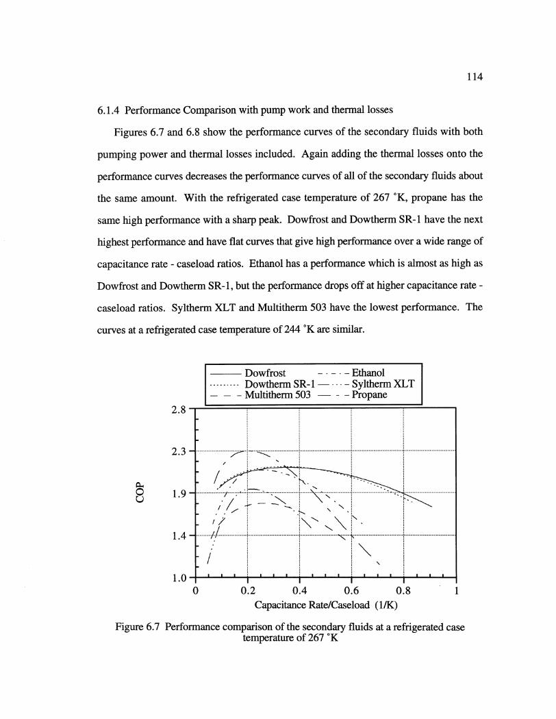
114
6.1.4 Performance Comparison with pump work and thermal losses
Figures 6.7 and 6.8 show the performance curves of the secondary fluids with both
pumping power and thermal losses included. Again adding the thermal losses onto the
performance curves decreases the performance curves of all of the secondary fluids about
the same amount. With the refrigerated case temperature of 267 'K, propane has the
same high performance with a sharp peak. Dowfrost and Dowtherm SR-1 have the next
highest performance and have flat curves that give high performance over a wide range of
capacitance rate - caseload ratios. Ethanol has a performance which is almost as high as
Dowfrost and Dowtherm SR-1, but the performance drops off at higher capacitance rate -
caseload ratios. Syltherm XLT and Multitherm 503 have the lowest performance. The
curves at a refrigerated case temperature of 244 'K are similar.
Dowfrost . -Ethanol
--------- Dowtherm SR-i -... Syltherm XLTMultitherm 503 - -Propane
2.8-
:... ........ ... ----------------
N
© 1 9 . .. ... .. ... .. ... : .. .!... .. ... . .. ....... . ...... ...... ................. . ................. --- -- --- --- ...........................
1-/0... ... ... ... ... ... ... .... ... ... ... .... ... ... ... ...
1.4-0
0 02 04 06 08 1Capacitance Rate/Caseload (1/K)
Figure 6.7 Performance comparison of the secondary fluids at a refrigerated casetemperature of 267 0K
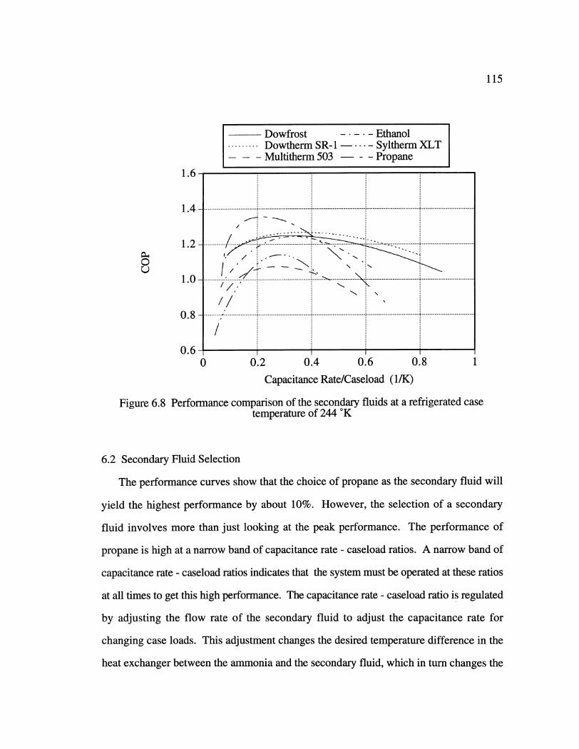
115
Dowfrost EthanolDowtherm SR- - Syltherm XLTMultitherm 503 Propane
. .............................--- .............................- -............. ............... . --............................. I -...........................
1.6
1.4
1.2
0u,.1.4
0.8
Figure 6.8
()I
/
.. ..... ...
S I, ,i
/ - ,-
/7
/
N
w . I I I I I
0 0.2 0.4 0.6 0.8 1
Capacitance Rate/Caseload (1/K)
Performance comparison of the secondary fluids at a refrigerated casetemperature of 244 'K
6.2 Secondary Fluid Selection
The performance curves show that the choice of propane as the secondary fluid will
yield the highest performance by about 10%. However, the selection of a secondary
fluid involves more than just looking at the peak performance. The performance of
propane is high at a narrow band of capacitance rate - caseload ratios. A narrow band of
capacitance rate - caseload ratios indicates that the system must be operated at these ratios
at all times to get this high performance. The capacitance rate - caseload ratio is regulated
by adjusting the flow rate of the secondary fluid to adjust the capacitance rate for
changing case loads. This adjustment changes the desired temperature difference in the
heat exchanger between the ammonia and the secondary fluid, which in turn changes the
... .. .. -... .. .. ..- _ - .. ..... . . ..... . . ..... . . ..... . ... ... .. o . ........... . . - . . . . . . . . . . . . . . . . . . . . . . . . . . .
_...........................
---- ---- ----f . ... -- -------- -- -----... .... ... .... ...- - .. ...
-- - - - - - - - - - ---------------------------- ............................... .. ... .. ...----... .. ... .. .----... .. .. ... .. ... .. ... .. .. ... .. ... .. ... .. ..
-. .......... ------------------. f -----------------------------. I.-----------------------------. ---------------------------------------------------.........
---- - -- - -- -- ---- -- -
ki
I-I
116
required flow rate of the ammonia. This flow rate is adjusted by increasing or decreasing
the number of cylinders of the compressor being used. Fine adjustments in the ammonia
flow rate cannot be accomplished in this manner. Thus secondary fluids that have
performance that does not change as much with changing capacitance rate - caseload
ratios will yield better performance at off-design conditions. Both Dowfrost and
Dowtherm SR-1 exhibit this type of behavior. Another concern is the toxicity and
flammability of the secondary fluid. As discussed in Chapter 2, propane is both
flammable and explosive. Dowfrost and Dowtherm SR-I are both considered non-
flammable. Dowfrost is non-toxic and Dowtherm SR-1 is orally toxic.
When the performance curves and the toxicity and flammability concerns are
considered, different choices for the secondary fluid are possible. Propane gives the
highest design, or peak, performance, Dowtherm SR-1 and Dowfrost yield the highest
performance over a range of capacitance rate - caseload ratios, and Dowfrost yields the
highest, safest performance. For an application as public as a supermarket, the safety
concern is very high and Dowfrost would likely be the best choice of the six secondary
fluids examined here.
117
CHAPTERSEVEN
DESIGN RULES
An accurate prediction of a supermarket ammonia - secondary fluid system can only be
accomplished with a complete analysis of the entire system. Some of the choices in the
design will be controlled by the availability of materials from the manufacturers. Design
rules that involve the design parameters which the system designer will have the most
control in selecting can be developed to simply the choices. By using these design rules,
the selection of some of the optimal parameters can be made without modeling the
complete system.
118
7.1 Ammonia Cycle Design
The ammonia vapor compression cycle is the backbone of the ammonia - secondary
fluid system. As discussed in Chapter 3, ammonia has a high discharge temperature from
the compressor and it is necessary to utilize staged compression to reduce the
temperature. Three different staging methods are described in Section 3.2 and a
performance comparison is shown in Section 3.3. Table 3.2 presents the results of the
performance comparison and shows that, with ammonia as the refrigerant, the staged
compression with flash tank method will give the highest performance. A diagram of this
system is shown in Figure 3.7.
7.2 Secondary Fluid Selection
Six different secondary fluids were compared in this study. Dowfrost, Dowtherm
SR-1, Multitherm 503, Syltherm XLT, ethanol, and propane are described in detail in
Chapter 2. The descriptions include a comparison of the properties of the fluids. The
property comparison is inconclusive because one fluid does not have the best properties
for high heat transfer and low pumping costs. In Chapter 6, a comparison of the
performance of the ammonia - secondary fluid system with the six different fluids is
documented. Figures 6.7 and 6.8 show the performance comparison at refrigerated case
temperatures of 267 and 244 'K, respectively. Both of these graphs indicated that propane
has a performance that is about 10% higher than both Dowfrost and Dowtherm SR-1.
However, since a supermarket refrigeration system is an application where the general
public may come in accidental contact with the secondary fluid, the flammability and
toxicity of the fluids is a concern. Table 2.1 indicates that propane is both flammable and
explosive and Dowtherm SR-i is orally toxic. Dowfrost is neither flammable nor toxic
and with the safety concerns of the supermarket system would likely be the best choice of
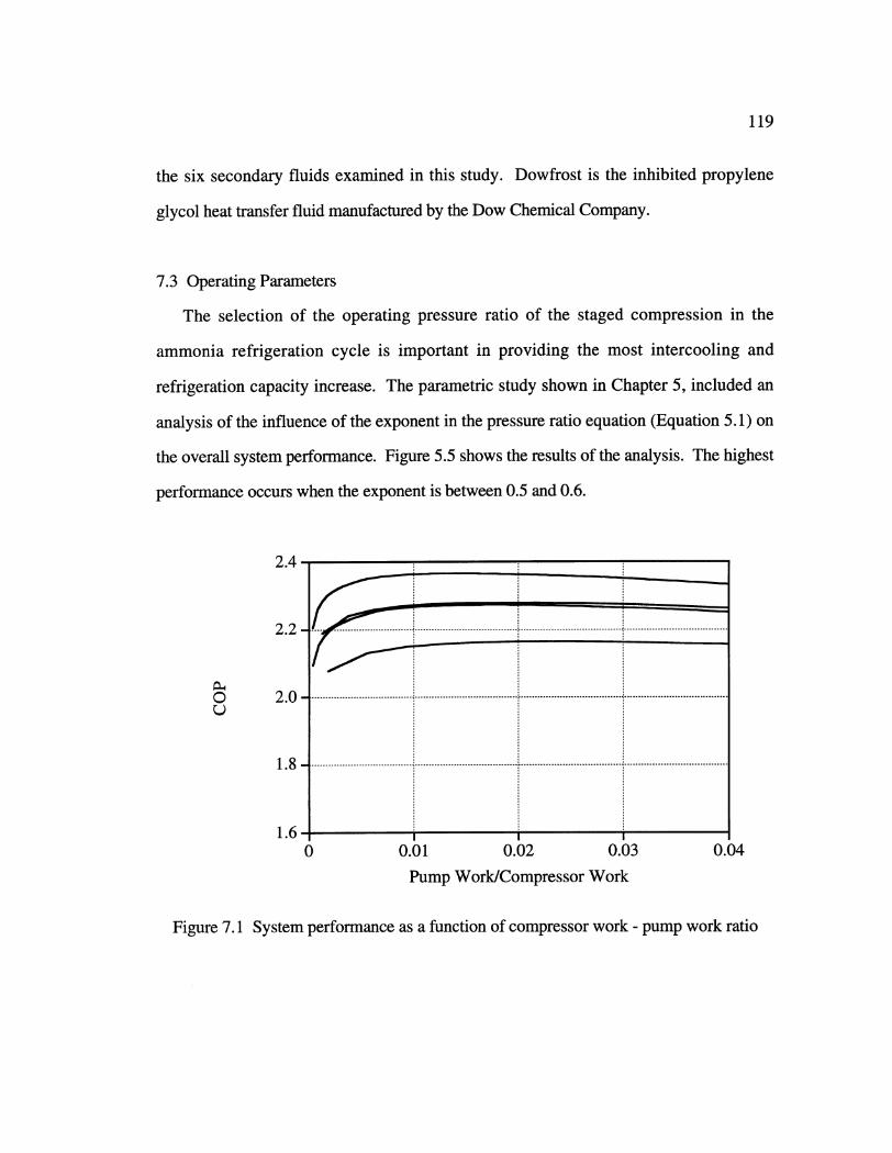
119
the six secondary fluids examined in this study. Dowfrost is the inhibited propylene
glycol heat transfer fluid manufactured by the Dow Chemical Company.
7.3 Operating Parameters
The selection of the operating pressure ratio of the staged compression in the
ammonia refrigeration cycle is important in providing the most intercooling and
refrigeration capacity increase. The parametric study shown in Chapter 5, included an
analysis of the influence of the exponent in the pressure ratio equation (Equation 5.1) on
the overall system performance. Figure 5.5 shows the results of the analysis. The highest
performance occurs when the exponent is between 0.5 and 0.6.
2.4
0 2 .0 ............................................................................ .................................... .....................................
1 .8 ...................................................................................................................................................
1.6
Pump Work/Compressor Work
Figure 7.1 System performance as a function of compressor work - pump work ratio
120
The optimal capacitance rate - caseload ratio provides another design rule. The ratio
influences the system performance by changing the ratio between the amount of
compressor work and the pump work needed. The influence of the ratio of the
compressor work and the pump work was calculated and the graph is shown in Figure
7.1. The graph indicates that the highest overall system performance occurs when the
ratio of pump work to compressor work is around 0.02. When selecting the operating
capacitance rate - caseload ratio, it is important that the compressor work - pump work
ratio is in this neighborhood to ensure that the highest system performance possible is
achieved.
7.4 Heat Exchangers
The supermarket refrigerated case system with ammonia and a secondary fluid utilizes
two heat exchangers to provide the cooling. The first is between the ammonia and the
secondary coolant and the second is in the refrigerated case. In a system with one heat
exchanger, the design mass flow rate of a system is selected to be at the point where the
highest heat exchanger effectiveness would be achieved. This would be true with a
system involving two heat exchangers only if both heat exchangers have the highest
effectiveness at the same flow rate.
In the supermarket system, the heat exchangers do not have the same behavior with
changing flow rate. For the base case system described in Chapter 5, Figure 7.2 shows
the changing effectiveness with changing flow rate. The flow rate is normalized by using
the capacitance rate - caseload ratio. Figure 7.2 shows that as the capacitance rate -
caseload ratio increases, the effectiveness of the refrigerated case heat exchanger
increases and the effectiveness of the ammonia - secondary fluid heat exchanger
decreases. The maximum COP for this parameter set occurs at a capacitance rate -
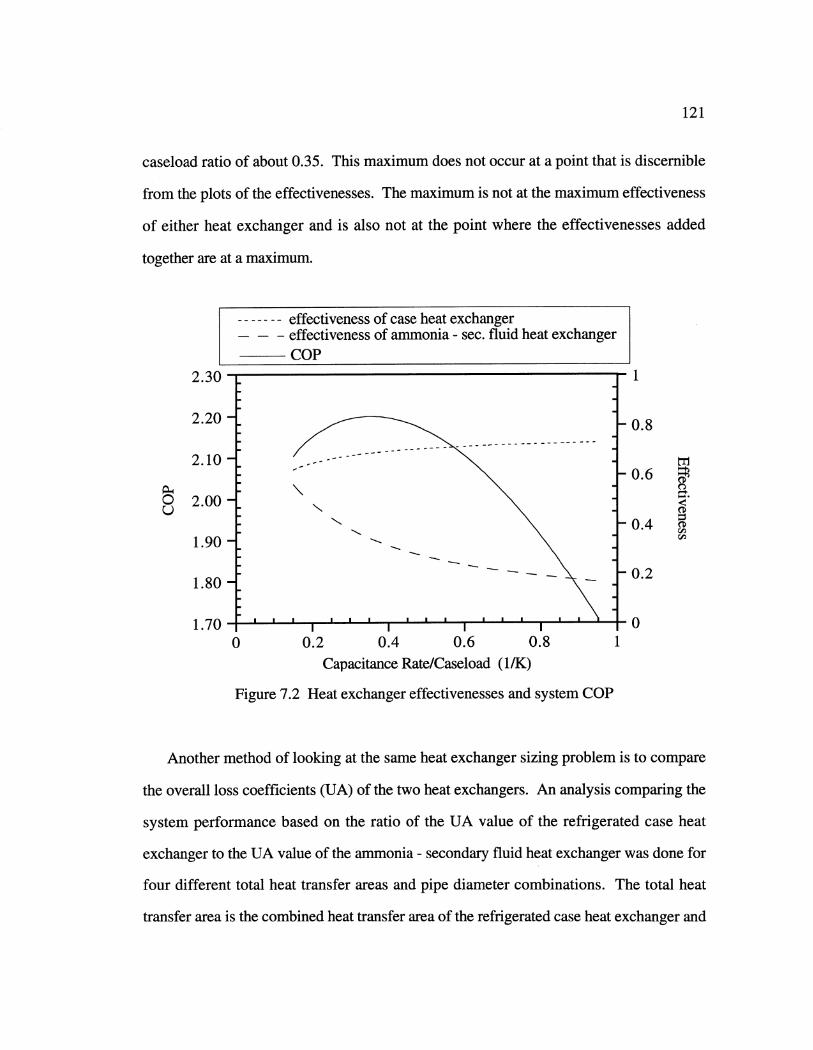
121
caseload ratio of about 0.35. This maximum does not occur at a point that is discernible
from the plots of the effectivenesses. The maximum is not at the maximum effectiveness
of either heat exchanger and is also not at the point where the effectivenesses added
together are at a maximum.
-- effectiveness of case heat exchanger- - effectiveness of ammonia - sec. fluid heat exchanger
COP
2.30 -1
2.20 -. 0.8
2.10."0.6
0 2.0004 n
1.90 -. 4
1.80 -. 2
1.70- -'00 0.2 0.4 0.6 0.8 1
Capacitance Rate/Caseload (l/K)
Figure 7.2 Heat exchanger effectivenesses and system COP
Another method of looking at the same heat exchanger sizing problem is to compare
the overall loss coefficients (UA) of the two heat exchangers. An analysis comparing the
system performance based on the ratio of the UA value of the refrigerated case heat
exchanger to the UA value of the ammonia - secondary fluid heat exchanger was done for
four different total heat transfer areas and pipe diameter combinations. The total heat
transfer area is the combined heat transfer area of the refrigerated case heat exchanger and

122
the ammonia - secondary fluid heat exchanger. The results of the comparison are shown
in Figure 7.2. The highest system performance occurs when the UA ratio is around
0.475. The heat exchangers should be sized in such a manner that the UA value for the
ammonia - secondary fluid heat exchanger is about 0.45 to 0.5 times the UA value of the
refrigerated case heat exchanger.
0u
2.6
2.5
2.4
2.3
2.2
2.1
0.2 0.3 0.4 0.5 0.6Ratio of the Heat Exchanger UA Values
0.7
Figure 7.3 System performance as a function of UA value ratio
7.5 Secondary Fluid Piping System
The system designer will have the most control in the design of the secondary fluid
supply and return pipes. The length of the pipes, the diameter of the pipes, and the
amount of insulation on the pipes will all be selected by the system designer. Since the
supply and return pipes will both carry liquid secondary fluid, it is reasonable to assume
that the same length, diameter, and amount of insulation will be used for both pipes. The
- - - -- - - - - -- - - - - -- - - - - -- - - - - -- --- - - -- - - - - -- - - --°- - - - - - - -- - - - - -............................. .............................. ............................. i............................. !................................ .. .. ... .. .. ... .. --- --- -- -- --- -- -- - .. ..... ..... ...... .. ...... ........ ..... .... .... ..... ..... .....
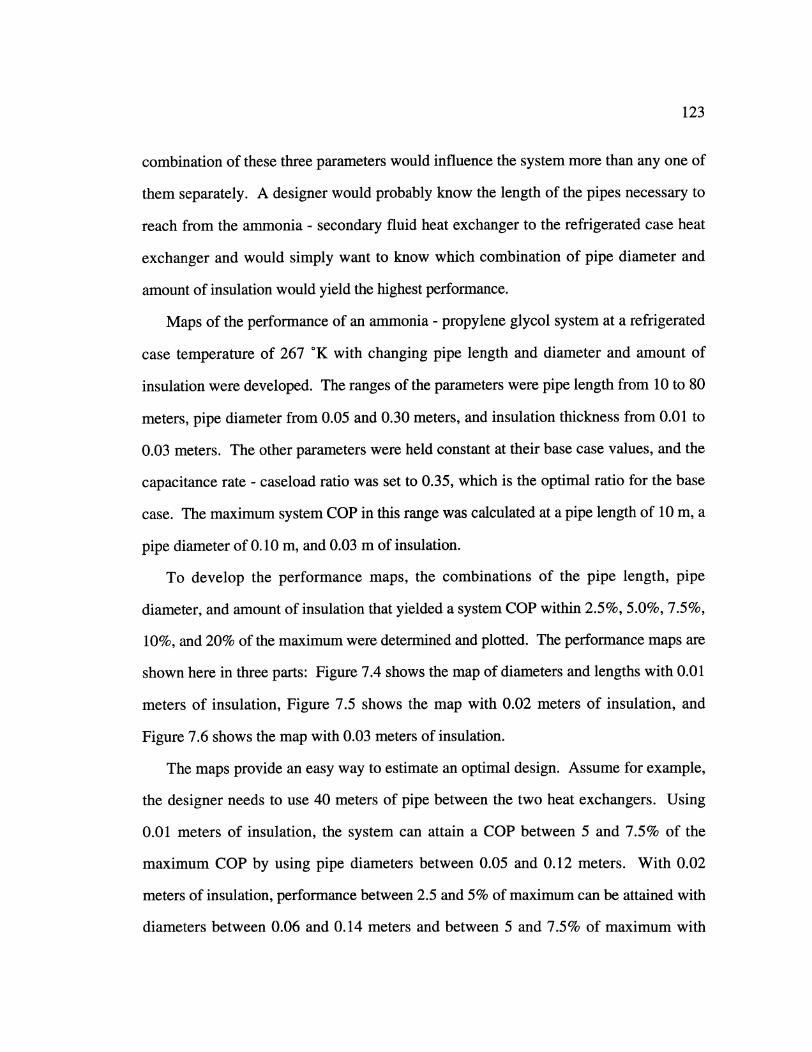
123
combination of these three parameters would influence the system more than any one of
them separately. A designer would probably know the length of the pipes necessary to
reach from the ammonia - secondary fluid heat exchanger to the refrigerated case heat
exchanger and would simply want to know which combination of pipe diameter and
amount of insulation would yield the highest performance.
Maps of the performance of an ammonia - propylene glycol system at a refrigerated
case temperature of 267 *K with changing pipe length and diameter and amount of
insulation were developed. The ranges of the parameters were pipe length from 10 to 80
meters, pipe diameter from 0.05 and 0.30 meters, and insulation thickness from 0.01 to
0.03 meters. The other parameters were held constant at their base case values, and the
capacitance rate - caseload ratio was set to 0.35, which is the optimal ratio for the base
case. The maximum system COP in this range was calculated at a pipe length of 10 m, a
pipe diameter of 0.10 m, and 0.03 m of insulation.
To develop the performance maps, the combinations of the pipe length, pipe
diameter, and amount of insulation that yielded a system COP within 2.5%, 5.0%, 7.5%,
10%, and 20% of the maximum were determined and plotted. The performance maps are
shown here in three parts: Figure 7.4 shows the map of diameters and lengths with 0.01
meters of insulation, Figure 7.5 shows the map with 0.02 meters of insulation, and
Figure 7.6 shows the map with 0.03 meters of insulation.
The maps provide an easy way to estimate an optimal design. Assume for example,
the designer needs to use 40 meters of pipe between the two heat exchangers. Using
0.01 meters of insulation, the system can attain a COP between 5 and 7.5% of the
maximum COP by using pipe diameters between 0.05 and 0.12 meters. With 0.02
meters of insulation, performance between 2.5 and 5% of maximum can be attained with
diameters between 0.06 and 0.14 meters and between 5 and 7.5% of maximum with
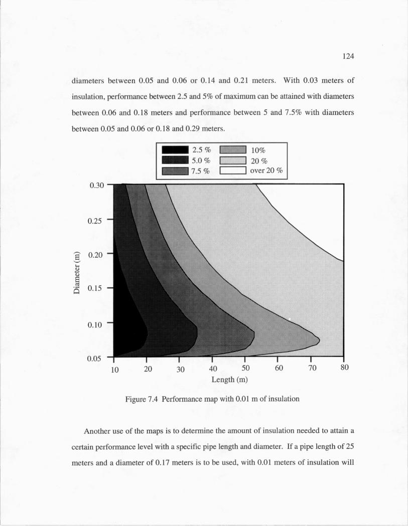
124
diameters between 0.05 and 0.06 or 0. 14 and 0.21 meters. With 0.03 meters of
insulation, performance between 2.5 and 5% of maximum can be attained with diameters
between 0.06 and 0. 18 meters and performance between 5 and 7.5% with diameters
between 0.05 and 0.06 or 0. 18 and 0.29 meters.
2.5 % 10%...........................................................................................................................................5.0 % 11 * I ' "Ill ' "I "" I "'I'll ' 20%
7.5 % I over 20 %0 - I.................................... .......................... ! .. ............ .............................. ....................................................................... .:.:.:,L0 .3 0 ,...,.:.::.:.:.:.:.:.:.:.:.:.:.:.:.:.:.:.:.:.:.:.:.:.:.,..''..,.....,.*.,.,.*.''.'.'.'.'.............................................................,.............................."..::."."."."."..."-"-"-'.-'.................................................................................................................................................,.,.,....................''"""""""'."""'""""""""'i ii ix........................................................:.:.:.:::.:.:.:.:.:.:.:.:.:.:.:.:.:.::.:.::::,......,.,.....,.,.,.'',..*.,.,....*.................................................................................................................................................................................................................................................."''.,::.:.:::.%,............................... ... ............................................................... * * *...............................................................,...........................................................................................................,.........,.............................::.:.::.:.:.'L... ......................... .. .... ............................................. ..... ...... .. ....... .............................. ....... -......... .......................... .. ...... .............................................................................................................................................................................,................................................,.,.,.:.:.:.:.:.:.:.:..,L................................................................. ................................................-.-.-.-..................................................................................,.,.,.,.*.,.:.:.:.:.:.:.,L......................................................................................................................... .. ............ ... ................. ...................... .. I ... ........................................................................................................................................................................................................................................... .. ..............................................................................................-.-: :i: :: .:!:,:: : : '.X........................................................................................................................................................................................................................................................................................................... ......"....,..........%.......................................................................................................................................................................................................................................................................... .,*::.................................................,...................................................................,.................................-.-.-......:::::::.:.::.:.:.:,..L....... .. ............................................... .. ... ....... .........................................................................................................................................................'..........................,.................. .......*.*.*.,.,.::: .."::: i ii i i'..X......................................................................................................................................................................................................................... .......... ... ...................................... ............................. .. .* . ............................ .. .. ......................... ........................................................................ ........................................... .................. .............,.....,. , ..... ..................................::,.................................................................................................................................................................,........::::.,. :::::::::::::::............... .................. ........................ ....................... ...' . . ............................... ..... ....................................... ... ... ................................ L ................................................................................................................................................................................. ................. .......................::,:.:.......................................... .... ...................................... .. .... ................................... ................... ................... ................................... .. .. ... ..... ............................ ----......................... .. ................................... ........... ......... ................... - .......:-:-:-:-:-:-:-:-:-:-:-:-:-:-:-:-:-:-::-:-::.,...,.*.,..,.,.,..,.'.'.'.'.'.'.'.'.*.'...........................,................................... ........................................,....... , I " ..............:-:-:-:-:-:-:-:-:-:-:-:-:-:-:-:-:-:-:-: :.:.,.,.,.,.,.,.,.,.,.'.'.'.'.'.'.'.'.'.*.'.'.*.'.'.*.*.*.'.'.'.*.'.'.'.'.'.'.'.'.'.*.'..'.'..'.'.'.'.'.'.'.'.'.'.'.'.'.'..'.*..'.'.*.*.'.'.*..' ". .............* ..... * -** ...... ** ..... * ................ * ..... ** ..... * ............. * I ..................................................:.................................................................................,................. ............................................ ' ' I ............................................... .- 11 .............................. I I - ....... ....... ...... ... :.:.:.:.:.:.:.:.:.:.:.:.:.:.:.:.:.::-:: :::.:::.:.::.:.:.:.:.:.::::.:.:.:.;.:.:.:.:.:.:.:.:.,.,.,.,.,.'.''.'.'*'.''.'.'''''" 'LLLLLLLLL L ......... ............. ...... ..... ... '*** * '' L L L ...................... ... ..... ... ****,*,*,* .......... ... .... ... ......... ..................,.....,................:.:.:.:.:.:.:.:.:.:.:.:.::.:.::.:.::.::::.::.*.''.,.,..,..,.,.,.''.".'.,**..,.*.,.,.,.,.,.,-.................................................................................................. .. ....... ... ................................. ......... ................ ................... ... .. I ..... .... .. .. .. ......... ... .. .. I .................................................................................. .... .... ... ..... .. ........ ...... ... ...................... ... .............. * .. ............................. ... ..... .... .. .... .. .,.:.::.:.:.:.:.:.:.:.:.:.::.:::.:'' ,* -....... .* ... * ........ ....* ... *'*'* ... * ............. ..... * ... .... ....... ............................ :.:.:.:.:.:.:.:.:.:.:.:.:.:.:.:.:.:.:.:.:.:.:::.,.,.''.,.,..........,...*.....,...,.,...,.,.,.,.*.*.,.,.,.,.*.,.,.,.,*.,.,,.,..,.,..''., .., *. ,- ......................... ......................................... ...................................... .................... ...I ....... ... .. ........................................
.......... ..... ................................ I ...... I ....... --I ...... ..... ... ...
.............................. ............................ ........................... .... ... .. 11 .... .. ... ..... .. ..... .. ................................. ....... .............................................. ... I ......... ............. ... .. ....... .................................................................................................................................* ......................... .* ... * ...... ... .. ................. --' ' ' ''*''*'* ...... * ............ ' '' '.:::::::::::::::::::::::::::::::;,.,..'.'..'.'....,..,....,..-......,....,....*..,..,..,.,.,.,.,.,.,,..,..."......,."..,.,..' .,..,..,..,..,..*..,..'........,....,..,....*..*..,..,..*..,..*..,...,.,.,*''.,..,..,..,..,..,..,..'..,..'..,..,....,..,..'..'....'.. .'..' .,..,..,.. ..' .....'..' ...........'.*................... ;.:.:.:.:.:.:.:.:.:.:.:.::.:.::.:.:.:.:.:.:.::., .,.,...........,.,..,.*.,.,.,.,.,.,.,.,.,.,.,.,.,,.,.''.'''*. * '.' I................................ ......... ...................................................... ..................... ..... .... -............................ ....... ... .. .......................... ..... I ........ .... .... .............................. ...... ................................. .... ... ........................... .. I ....... ........ ... .... .................................... -............................ I ..... .... ................................ .... .......... ..... ......................... .......... ................................ .. ............................................................................................,..,......................................................................I .......................... .... ... .. - .:::::::::........... --... ... .............. ........................................................................................,.. ........................................................ ... . ..................... '-'-::::::::: ' :-:::::::........ .. .. I .......................... .... ......................................... .... .. ... ......................... .... I ..... ....................... ..................................... ..... ............. .... .... ................. " '...................................................:. .: ,- ..0 .2 5 .............. :.:.:.:.:.:.:.::.:.:.:.::.::.:.:.:.::.:.:.:::.:.::.:.:.:.:.:.:.:.:.:.:.:.:.:.:.:.:.:.:.:.:.::'""',".",",.,.,,*,... ....................................... ,.................... ................... ............................ ... ... .. .-1 1 .............................. :::::............. .. .. .. ... .. .............................. ...........................................................................................................................' '''" .,.................... ......... ..........................., :::. .......... .... ............... ,........................ ................... :.::::.:.:.::.:.:.:.:.:.:.:.:.:.:.:.:.:.:.:.:.:.'.'.'." '." '.'.L ... L. . .. :::q :::... .. ... I......................... ..................................::::.:: ,................ ..... ..... ......... ... .. I ............ .................... ................... ............ ............. .. ....................................... ::::::: : .11,11................... .. ................ ....................... I ........................ :::::::.: ::::::................................................................ ..... ..... ... I ....................... 1,.......... .... ................... ........... ......... ............ - L . 11......................................................... ...... .. .. .I I .................... ... .......................... .- ................................... ......... ... .. .. ... I.................................................... ... .: I I........................................................................ ....... ................................,....................... ........ ......'.............................. ................................- .: :.: .. .............. ........ ...... ... ..... .. ....................................... . .. I .. ................ .. .I.I.I........ .""""" " ...... ....................................................................... ....... I ...... ....... :::; .:.. I --.:::..,..,..,..,..,..,..,.........,..I ........... ..,.,.,................................:.:::.::.:.:.::.:.:.:::.:.:.:.:.::.:.:.:.:."","","","," """"""'"'"""' .".*.'.*.,*. : . .......,. ................................................ ..............................,........ --............................................ .::. ::.. .., .. ................ ................. : . ... ........ ................................................ .... .. ..... ... .......................................... ... . I .... .... ....................................................................................................................................."................................................................... :..:.:.:...... ... -.......................................... -.................................. --............................... .... . ................................................................ ....... .. ........ ........................................... ... .. .-..... ........... ............................................. .... .... I ... .......... ............................................ ... ... ...... ................ ................................................... .. ... .... .............. * ..... * ........ .* ..... '' ' - ...................:.:.:.:.:.:.:,:.:.:.:.:.:.:.:.:.:.:.:.:.:.:.:.::..,.,.,.,.,.,.,.,.''.,.*.....,....,.,.,.,....,. .....:.:.:.:.:.:.:.::.::.::.:::.:.::.::.:.:.:.:.'..,..,..,....,..,....,......,..,....,........,..,....,....,..,..,..'..,..,..*..*..,..,..,....,...,....,.,..,..''..''..*...*....,....... ... . ........... .................. .......................... ... ...... ............ ............................................ ..... .. ................................................................ ............. ............................................... ......... L ..... ................ ... ....................................................... ................................................................. .. .. ... .. .. ................................................................................................................................................................................................................................................................................................ ...... .................... ........................ .......... ................................................... .. ........... ..... ............... .............................................. ......... ....... ....... I ......................................... ......... ...... ................................................................................................................................................................ I .. ...... ........... ........................................ ... I .............................................. .......... .... ..... .I .. ........ ....................... ............................. .. ... .. ... .. .. ............................................ ........... .. .................,...................................................................................................................,.......................................................................................................,....,.............. ...... ....... :::::::::....... .................... -. '* ' '.'.*.'.'.'.'.'.'........................... :.:.:.:.:.:.:.:.:.:.:.:.:.:.:.:.:::.:.:.::.:.:,.,.''.'.'.'.''.....*.....'.''.'.,.,. ....." ...'.'.'.'.*...,.,.,...,.,.,.,.,,.,.,.,.,..,.,.,.,..,.,..,..,,..,....,.,.,..,...,.,....,.,..,*",.*......... ....................................... ............... :.:::::::::::::::::::::::::::::::::.... .. ... ................................................ .. .... ...................................... .... .................................................................................,..............................,...,..................,.......................................................................................".''''-,:.:..................................."............................................................ ... ........................... .................................................................. .::::;:::::::::::::::::::::::::::::::::... .............I ............ .... ................. ............ ......... .......................................................... -........................................... ........ .. ..... .............. ............. I ......... ......... ................ : ..............,................... ................. ................... ...... ........ ..................................................................... ::: :::::::::::::::::::::::::::::::::::::.I .................................................................. ................ I ..... I ............................................. ::: ... ... ........... ... ................... .................... ... ......... ........... ................................................................ .... .. I ....... ..... ................... .......................... ... ................... I ..................................................... ......... ............ ... ........................................................................................................................................................................................... .. ..... I .................. I ................. ......................................... .-......... 1.* 1* 111........................................................................................................................................................................................................................................................................................................................................................................ ..............................,.....................................,.........::.......................................................................................................................................................................................................................................... .. ..................... ................ .. ............ .. .. ... ............................................. ... .. ...... ............. .......................................................... .. ... ....... .. .... ................................... ................ ........... ::-:-:-::-::-:-:-:-:-:-:-:.:." .''.'.'.'.'''- ''. '. --''.::::-:::-:-:::-:::-:-::-:-:::-::-:: ......... ... .'...'....'.'.'..'.'........... ..................................... ... . .1 ......... .. -................... ..:.:.:.:.:.:.:.:.:.:.:.:.:.:.,....*....,..,..,..,..,..,..,..*..,..,..,....,....,........,..*....,..,..,..,..,.,.,.,.,.,.,....,....,..,..,..,..'..,..,..,.,..*..,..,..,..."..,..........,....,..,........,..,..,..,..,..."..'..,.,.,.,.,.,.,.,.,,..* .. .... *,.,.'*.,.,.,..,.,.,.,..,.,.'.'' L' '...,.,.,.,.,.,...,,..' '.,.,.''*.,.,.,.,.., ''** * * ..... '' ' * ....... ' * '' '* .......................................................... ........................................................................ ........ ... .................................................. ... ... ... ... ... ... ................................................................. ..... -...... .... ................. ,:.:.:.:.:.:.:.:.:.:.:.:.::.:....,..,.,.*...,.*.'.''..''...'.''.... " ...'.'.'.,.,...,.,.,.,.,...,..*.*.*.,.,.,.,,.,...**.*.,.,...,.... ..*.,.''.,.,.,.,.,.,.,.,.,..................-.-.-.-.-.-.-.-.-.-.-.-.-.-.-.-.-.-.-.--, ' ' .'.'.'.'. .'...............................-* . ......................... .... .............. ... ......... L ....../ 0 -IN .. , :::.,.,.,.,.,.,.,.,...."...,.,.,...,..........................................................,.,.............. ................................ ...................................................................................I ..................................................,..................... ................................. ......................................... . -...... ...... .................................... I .................... .... ........ .................. I ....................................... .. ...... ..................... ........................................... ................................ I ...................................... ..... I ....... .... ...... I ............. .................................... -............................... .......................................... . .. ....... ... ................... .. ................................. ..' ..... ......................... .I ......................................... ' L ......... .. ... ...................- ,.:.:.:.:.:.:.:.:.::.:.,.,.,.,.,.*.*.,.,.''.'.'.'''" I .. .....................................,....".................... .................................................................................. 1 . ........................................................................ .... ..................... . I ......................................... .... ... ............ .... ............. I ................. ..... ..................... ....................................... .. I .. ................E j 0 .2 0 . .. ,.:.:.:.:.:.:.:., .,.,.,.,.,.,.,.,.,.,.,.,.*,- I .................,..................,............." .. .................................................................................''I I. ....... 11 ...........................................-- - .. ... .. .. .. ............. I ............................. ........... I .... I ............... .. ............. I ... ... .......... .. ..... .............. ..................................... .. ... ................ .................. ...... ........... ....... --............. ............................ ... ......... ... ..... .. .............. .................. ... .. ............. .. .... ...- ............ ............................... .... ... .. - ... .. I I ........ .... .. ...... ....... ..................... I ....... -................. ..................... ....................... ... .. I .......... ... .. ....... ............ .............. ..... ... ...... .. .......... ....................................... I ............... ....... .....:::::::::::::.,.,.,.,.,.,.,...'.-''-...- ...... ... ................ .............,....I ......................................................... .. ............. ... .' .......,.................,..................... ........... . I --- - .... --........................................ I . 1.. . ... ............ . .. -.......................... ... .. .............. .. .''............... .- ... ..... ...........-......... .........N % -,/ .. .:.:':':I:':"'-"'-" "'-''""''"L L I I.... .......................,................................................. ........ ................. I I ............. .. ..........., ................................... I .. ........ I ......................... .. .... -.. .... .. I ............. .... .... .. ........................... I -....................................... .... -....... ... .. ............ ...... ....... .... ........ .......................... I I ....................................................... .. I - . ................. .... .. ................................... - - ................................................... ............ ... ...................... ........ .......... 1 1 ........................................................ .. ............... ..... ........... ........ ................ .. ...................................... ............. ........... .... ...... .......... ............................................. I I I ..' I..............,.,..................................................................................... I .............................' ..... ............................... ................. I I I -11 ............................................. -.... ......... .. ..... .... ............ ....... ................ I .. ... ............................................. ....... ..... I I -........ ..... ... -... ......... .- 4 ................................................. I ............................................................................................................. ......... I .................- ..... . .................. ..... ..... ..... ..... I I I I I ' L L ...... ..... ..... ..... ..... ..... ..... ..... ..... ..... ..... ..... . I I . ........... I ............ ..... ..... ..... .. ..... ...... ..... ..... ..... ..... ..... ..... ..... ..... ..... ..... .... .... ............. I I . ............................ .. ...... ..... ..... ..... ..... ..... ..... ..... ..... ..... ..... ..... . . ........ .. I ........... ..... ..... ..... .. I I .............................................................. I ........ .. .............. ..... ..... .. I ..... ..... ..... ..... ..... ..... ..... ..... ..... ..... ..... .. I ....... . I ...I I ...................... , . ..................................................... .I ........ , .......... ..... ..... ..... .. ... ..... ...... .. I I I ........I .I I I ... I .
a ) ..................... .. I I .......................................................................... . ..... ..... ..... I ..... ...... . I I I I ........... ............... L . I ............ ............ .............. ...... ... .. .- .. ...
._ ................... I . ............................................. ..... .. .... ........ ... I ...... .............. ............... . I I . . .I .......................................................... I I I I ................................. .. . . .......................................................... I , I I , I I ....... .+ - j ....................................................... ,.,.....,....................................................................................... ......................... I I . . I I . . I ,........................................ ... .. .............. .............. ......... .. ....... . . I .. . I ..... ...................... ... .... I ................................................ ........... ...... ........................ .... .......................................................... I I ....... ..................... .. ... .......................................... .. ........... .. I ...... ....................... I ...................................................... - I - ....................... .. .I I ......................................... ... ... ......... . ..... ....................... . I .I ............................................. I I I ....... ................................ .... . , .......................................... ..................... - ... .. ......... ....................................................... I . ..... .. .................. .. ... . I .... ............................................. . . ..... I ..................... .. . ................................................... I I I I I I I ..... .................... ... I ......................... ........... .. ..... ... . I
.....
.............. ..... .. , ................................................... I I I I I .... ................... I . . . I .......................................... .. .... ................... ...... ........................................ ... ..... I .... .................... .....................................
.... -.....
............. .. .. .. . ......................................... .... .... ...... ........... .. .. ... .I .......................................... .......... .. ...... ................... .. .......................................... .... ...... .. I ...... ............... ... ....................................................... ....
......... .. ...... I -............................................... ... I I I I .... I .............. .. ....................................................... I I . I .... .............................. I ..... . .... ......... ............................................................................. I I . 1. I I 11 , I .1 . I I ........ ............ .. ... .. ............................................. .... . I I I , I . .I I I ....
........... .. ... ........................................ ... .. - . I . I I I I ............. ... .. ... ..I .I ............................................... ... I . .I . . ....... ............. ....................................................... I I .I I I I ....I I I . I .I ........I . ... I ............ ...........W ., -.. . I............... .... ......... ..................................... ....... I I I I , I ............ ......... I I .. ....I .C ld .... I . ................. ....... ........................ ........................ .... ........ . I............... .................... ................ ... ... ...,.......... I I I ......... I..... I I ............ -.......................
..
.. ..... .. ....................... ....... .. ...... .... ... .... T- 4 ...... L ' L L ................................................... --... .... I ....... I.......... ........................................................... .. I - .11 I ... ............... I .................................................. ....... .... I . I . ... I . I ............... ... .......................................................... .. . , I I - I I .1 ................................................................... - -..... I , I ................. .. .... .. ..................................................
......
I . ......
................................................................... I - - . , I , - -............. ............................................................ I 11 I . ................................................................... ...... . I I .1 . I ..............0 .1 5 ............................................................................................................. .... '... ..... .... . I I I - ....................................................................................... I I . ... .......... .......................................................... ...... ... .. .... ............................................................................. - I . .1 - ..... ............................................................................. -I I - 11 .............................. ................... ... I ' '. I .... .......a ) ................................................................................................ .... .......................................................................... I -....................................... .................................. ... I .... ........ ,.:.::::::::::::::::::::::,.,.,.,.,.'',.....,,.,....,.'',.,.,.,.,-'-'-'-,...'.,...........,.''......-........-......-.-.- - - - . ........' ............................................................................ -1 1 I - ----................ ............ .. ........ .... -1 1 1 '' ....- I ................................. ..................................... .... I , .. ..................................................................... ........ -.. .. ----...... ....... .. ..... ......... .... ........................... .......... ... - I ..................... ....... ......... .. ............. I ........... -.............. ................... ........ .................................... ... ........ ... - I I .......................... .................................... ... ............ .. . ......................... .. ..................................... I .............. I ........... ......... ... ..................................... ... ................ ........ .. .. ..... .... ....... .... ..... ........................... I ............... . - . I .......... ... .... ...... .. .. ... .... ............... I ............... I ................ ......... ....... ...... ....... .. ... .............. ............. .. ................. .............. .... ...... .. .. .I ............................... .. ........... I .... . I ......... ...... ........ ........................... ............. .................. . ... ....... ....... .......... ... ..... ............................... .................. .. .. I ....... ................................. I .............................. -.................. - - -... -............ ..... .. ... ..... .... ................................. ................ .. .... . ..... ... ........ .... ........... .. ..... ....... .......... ... ................ ............... .... .. .. ......... ............................................................................... .- I -.................................................................................... .- - I .................. ... ..... .... ..... .. .................................. ............. ... ......... .......... I .................................................................... .- - -................ ........... ... ... ... ........... I ................... ... ........... ... I I I .... .... .. ...... .... ............................ ............... .I , I .... ... .......................... ... .......... .................... .............. .... ............. ........ ... ... .......... ................... .... ........... . .... .... ..... .....:.:.:.:.:.:.:.:.:.:.:.:.:.::.::....................-.-.-.-.-.-.-..-...-..-.-.-.-...-....-... .-.-..-..-.-..-..-...-.. ................................... ........... ............ ..................... ............ - .... ......... .......................... .......... ................... .. .............. .. I I ..... .......... ........... .......... ............. ... ................ ................. ..... .......... ................... ... ............................... ................ -... .......... .. ........... ......... .......... .. .I ............... .. .. ............ .. I -.. ....... ... ....................... ....... ... .... ............. .... ............. I ..... ......... .. .............................................. -............. - . .. ........................................................................... - .. ........ ..................... ... ... I ...................... ................ I ... ........... ........... .. .. ........... ................ .. ................. .... .......... .. ......... ..... ....... .. .. .... .. ............. .. ... ............. I 1 1 ....... .......... ............ ...... ...... ... .. ................. ............... ....... ............. ............ ..... I .... ... .......... .. .............. ..... ..... ...... .......... .. .......... ..... ....... L ... .... ........... ... ................. ......... ... ........ .. ...... ..... .. I ...... ... .................... ............... .... .I ....... ............. ....... . ... .. .. .............. .. ............... ..... ...... .......... ........... .. .. ..... .... .... ................. ... ............... I ....... ... .......... ...... ..... ....... ... .................. .................. .. ....... ........... .. ............................... ........................................................................................................................................ .. ........ ...... ............ .. ................... .... ....... ............ ... .... ..... ..... ................... ................. .11 1. 1111. 11 ............. ... ..... ....... .. ................ ................... .... ........... ....... .. .. .... .... ................ ................ ... .I I. ... ........ ........ ..... .... .. ............... .................. 1 , .. ........... ...... ...... ... ................. .. ............... .. ........ .. .. ............. ............... .. ... ................ ... .... ............ ... .... ...... .. ............... ................. .. .. ... ... ......... ......... ... ... ............... .. .. ............... ..... ....... .. ...........- ..... ......................... . .:.::: ::::::::::...,....,.,.,.,.,.,.,.,.,.,-'-*-'-'.....,.,.,.,.,-'-'-'-*-'-'-'-.-.-.-.. ......................................... ........... .. .. ................. ... ... .. ....... ... .............. ... .. .............. .I .... .. ......... ....... .. .... ............ ... ............. -...... ............ ............... .... ................ ..... .... ....... ............................ ..... - --.............. . ................................................................ I.. . . ..................................... ... ................ ,. ........... ............... ................... ... ... ......... .. I................................ - .................................... - I .................... ................... .. .. ........ -.... .................. ... ... I ......... .......... ............. -'. .. I .. .......... .0 .1 0 ................................................,... I .. I I I -...............,.,......... .I ............... .I I I ........... ..... ................. .1 1 ....... ........................ -I ..... -....... ............ ... I .1 1 ....... ...... .......... ... .. I .......... ................... - -......... .......... .. .. ........ .................. -.......... ... ............. I ...... .. .....................'..'.....- 11 I '......- ...4................. ... ....... ................. ......... ............. . ...... .... ........... . ...... -......1 - .....................' I ........' '.......'.'.'.'. '.'.'.',,,',""""',""LLLLLL""",""LL,"-'-'-*-*-'."'.'.'.*.'..: .......................................................... ...... ...................... .. .. ....-.. -................ ................... .... .. ........... .....- ........., ....... ........"...........................................................................................................:...,..,.,.................................,-.................. .......... ..... ......................... ........ .......... ........ .I ......... ......... ...... ........... ........ I ...... ..... .. .............................................................................................................................................................................................................. ....... ......... ................... .......... ....................................................................................................................................I ... ........ ....... ......... .............................................. .. .. ....... ..... ........ .. .. .......: .. % ......... .......,...,........,..............,............... ....................... .... ............... ... ... ... ...... I , .......................................................................................110 . " I , .................................,............................................................................................................................ ... ............ ........ ....... .....................................I .............I ........... ............... ................... .... ... ......... . - ......'',-,-.-.-................................,............,................................................................ ....................................................................................................................................................... ... ............ I ... .................. .. ....... ............................................................... ......................................... .......................................................................
125
give performance between 5 and 7.5% of the maximum, with 0.02 meters of insulation
between 2.5 and 5%, and with 0.03 meters of insulation within 2.5% of maximum.
By utilizing these performance maps, the system designer can determine the piping
system that will give the highest performance. However, if an accurate determination of
the actual performance of the system is desired or if the basic system being utilized is
different from the one modeled to produce these performance maps, then the designer
should model the entire system to ensure that the behavior is similar to the behavior of the
system used here.
2.5 % %
105,0% 20%7*5 % over 20 %
.................... ........................................................................................................................... .. ....................... .... '' ... ........ ....... .............. ... ..... ... ......... ....... ..... ........ ................................ ... ..................... ........................0 .3 0 .. ...... .... .... . ............ ................ ......... .. ..... .. .... ............................... .. ............. --.......... ........ .... . ....... ..................... I .... ..... ....................... ...... .... . ...... ........................... ... ..... ............... .......... ...... ........ ...... .......... ....... ...... .. ................. .... .. ... ...... ........ ....... ......... .. .................. ..... .......... --......... ........... ........... .. ................. ..................... .... ........ ..................... .. .. ..................... .. ........ ......... .............. ..................... .... ...... .............. ... ........ .. ........ .......... ........... .... ...... ................................... .. ........................................... .... ... ..... ..................... ... ............ .. .. .... ....................... ... ................. ... ... ..................... -..... ... ... ............ .... ......................... ... ............ ... .... I ................... ... ........ ... ......................................................... .. ......... ............... ........... ....................... ........................... .................... ......................... ..... ..................... ............. ... .. .. ........................ ....................................................................... .............. ................. ...................... .................... . ........ ...................... .. ............. ...................... .................. ..... .. ....... .................... ..... . ...................... -... ......................... ................. ..... . ....... ....... .. ............ . ......... .. .... .... ... ........ ..................... ................. ..... ....... .................... ......... .0.25 ..... ...... ............................ .. ... .... ................ .... .. ........... .......... . ...... ................ .................... . ........................... ........ ........ .. ....... . ............... ........ ......... ..... ....... ..................... .................................. ........ ...... ...... ............. ....... .... ............ .................................. ....... ............................................................... .. ..... .... .. ................... . ...................... ... ........ ... .. .............................................. .............................. .................... .............. . ...... .. .................................. .... ...... ........................................................................................................................... ....................... ................................................................................. ... .................................... ......................................................................................................... ... ......................................................... ....... ............. I ................... ..................................... . ...... .... ............ ....... ................... ........... ..... I I ... .. ........ .. ... ... ............... .............. ..... ................. ...... .... ........................ .. . ..... .......... .. .... .... ...... ............... ............ -... .............. ... ................................................ ...... .......... .... .... ...... .......................... .. ...... .............. .... ..... .. ..................... ...... ... ... ... .. .. .... .. ......... .. .. ........... ..... ....... ...... ....................... ......... ... .... I ............ ......... .. ... .. .................. ....... ... ............... ..... ... .... .. ........... .. ..0.20 ............. - ............. ........................... ................ .. .... ........... .. ........ ......... .. .. ......... .... .... .. .......... ...... ........... I ..... ...... .I ................... ........... ... ... .......... .. .. .................. ........... ........ .. ............... ... ... .... ... .. ............. .. .. ..... ........ .... ......... ........... .. ............... .. -.. .... ...... ............ ........ -.......... .. ...... ............ .. ............... ..... ... ............. ...... .. .............. ........ ....................... ........................................................................ ..... ........ ... ............ ...... .................. ........ .......................................................................................................... ............... ... .......... .. .. ............. .. ........ ....... .. ........ -..... I .............. ............. ... ............... ........ ................................... .. ............ ............... ... .I ... .......... .. ....................... ..... ............ .. ............ .. ........ ............................... -... .... ......... ... -..... ... ... ........... ....................... ... ...... ......... .......... .................. ....... .......... .. ........... -.... ............ ...................... ... .. ........... .. ...... ....... ...... ............ ......................... ... .. ........ .. ......... I ...... I ... .. ... ...... -........................... .. .......... ............... ..... .......... .................... ..... .. ............ ............ .. .. ..... .I ........... ..................... .. .............. ...... ........ ..... ............. ..................... ..... ............ .............. ......... .......................... .. .............. ............. ....... ........... ................. .. ............ ............... ...... ......... ................ ... .I ........ .......... ...... - ............................. ... ....... ........... ..... .. ... ........................ ......... . ........ ......... ...................... ... ............ ... ...... ........ .. ................... ... .......... ........... ........ .......... ... ......... .......... ... ...... ....... ...... .... ......
. ........ ... ............ ... .......... ... .. .... ............ ....... .. ............. .. ... ...... ..... ..... .. .................... ........... .... .. . ...... ...... ........ ................. .. ............. ..... ............. .. .... ... .. ....... .......................... .................. - ....... - ......... .............. ... .. ............. ........ .... ...... ..... .. ............... .. ............. .. ...... ........... .... .. ........... .... .................. ... ............................................................................................................................................................. ................................................................................................................................................................................................................................................... .. .... I I ............ .......... ......... ...... .. I ............. .. ....... I ............ ............................................................. ... I ... ........ .. ..................................................... .. I ...... ...................... ....... ................................................................................................................................. I ........ ..............................................0. 15 ................................................................................................................
0.10
X ..........SEN...........................................................................................................................
0 .0 5 ..................... i .......................................
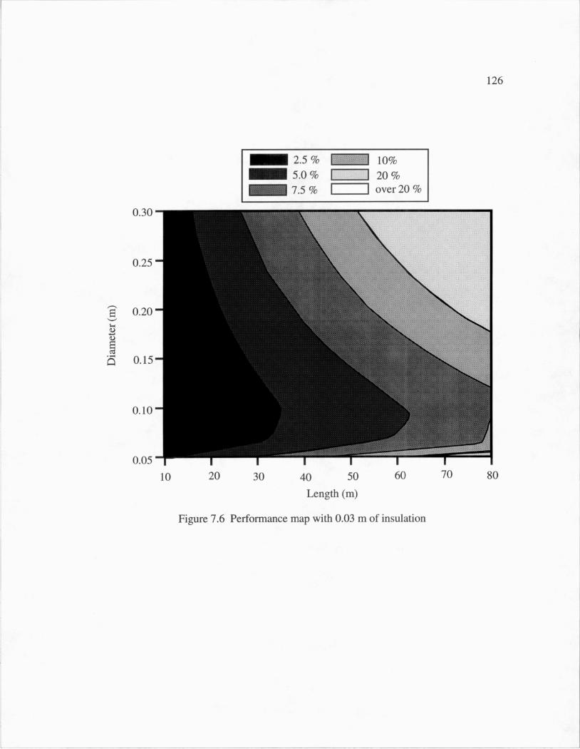
126
- 2.5% i 10%-5.0% EIZI 20%75 IzI over 20%
0.30 "
0.25 -
0.20 -
0.15"
0.10 "
0.05 -1r10
I I I I U U 1
20 30 40 50 60 70 80
Length (m)
Figure 7.6 Performance map with 0.03 m of insulation
127
CHAPTER
EIGHT
CONCLUSIONS AND RECOMMENDATIONS
The implementation of ammonia - secondary fluid supermarket refrigeration system will
require careful design considerations. It is important to ensure that the installed system
will be designed well enough to provide optimal performance. This study has looked at
the basic refrigeration systems. Further system alterations might make the use of
ammonia - secondary fluid systems more attractive.
128
8.1 Design Guidelines
In Chapter 7 the guidelines for the design of an ammonia - secondary fluid
supermarket refrigeration system were discussed in depth. It is important to use these
guidelines to ensure that the highest performance possible is attained. These guidelines
include the ratio of refrigerated case heat exchanger UA value to ammonia - secondary
fluid heat exchanger UA value of 0.475, the correct intermediate pressure selection, the
use of Dowfrost or a similar propylene glycol solution as the secondary fluid, and a
capacitance rate - caseload ratio that yields a pump work to compressor work ratio of
around 0.02. It is also important to utilize the performance maps in Chapter 7 to
determine the secondary fluid piping system that gives the highest performance.
If the design guidelines outlined in Chapter 7 are utilized and a system is constructed
which produces the highest performance possible, the ammonia - secondary fluid system
should have a performance which is comparable to the R22 refrigeration systems that
would be replaced.
8.2 Future Research
There are some additional modifications that could be made to the ammonia -
secondary fluid system that might increase the overall performance of the system. One
such modification is to produce two temperatures of secondary fluid with a single
ammonia system. This is accomplished by adding a second ammonia - secondary fluid
heat exchanger between the flash tank and the second compressor in the ammonia
system. The temperature requirements of the second heat exchanger would determine the
pressure ratio that could be used in the staged compression. If the pressure ratio that is
needed to produce the correct temperature for the additional secondary fluid is different
enough from the optimal pressure ratio, the performance of the two secondary fluid
129
system could be lower than the performance of two individual ammonia - secondary fluid
systems.
The addition of mechanical sub-cooling would increase the performance of the
system. In mechanical sub-cooling a second vapor compression cycle is added that
utilizes a heat exchanger to further cool the refrigerant as it leaves the evaporator.
Mechanical sub-cooling has been proven to increase performance and is used in many
applications. However, it can be added to a R22 refrigeration system, as well as the
ammonia - secondary fluid system. The performance of both system will be higher with
the mechanical sub-cooling, however, without quantifying the increase, it is impossible
to know if the improvement will be greater for one of the systems.
The replacement of the air-cooled condenser with an evaporative or water-cooled
condenser should increase the performance of the ammonia cycle. It may also be
beneficial to utilize some of the secondary fluid in a heat exchanger that would condense
the ammonia. The reduction in condenser temperature will increase the ammonia system
performance, but the increased amount of secondary fluid needed may reduce the
performance enough to negate the increase.
Storage of the secondary fluid is another possibility to increase to performance of the
ammonia - secondary fluid system. The ammonia cycle would be run at night and all of
the secondary fluid stored to provide the needed cooling of the refrigerated cases during
the day. The performance of the system will increase slightly because the condenser will
be more efficient in the colder temperatures and will decrease with increased storage
losses. However, the advantage of storage is that the electrical load is shifted to the night
time hours where electrical demand charges are less, lowering the cost of operating the
system. The storage could be accomplished by either storing all of the secondary fluid at
one temperature to provide the cooling for all of the refrigerated cases or by storing
130
different temperature secondary fluids for each of the temperature regimes needed in the
supermarket.
In a supermarket, the refrigeration system and the air conditioning systems are closely
linked. The use of the ammonia - secondary fluid system to provide the air conditioning
for the supermarket in addition to providing cooling for the refrigeration cases needs to be
analyzed. Changing the store conditions changes the refrigeration loads and the
refrigeration loads influence the needed air conditioning for the store. Simulations that
link the performance of the two systems could be used to determine if certain changes in
either system improve the combined performance of the two systems
131
APPENDIX A
COMPRESSION METHOD MODELS
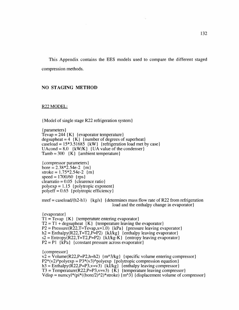
132
This Appendix contains the EES models used to compare the different staged
compression methods.
NO STAGING METHOD
R22 MODEL:
(Model of single stage R22 refrigeration system)
{parameters)Tevap = 244 (K) I evaporator temperature Idegsupheat =4 (K) Inumber of degrees of superheat)caseload = 15*3.51685 {kW) {refrigeration load met by case)UAcond = 8.0 (kW/K) {UA value of the condenser)Tamb = 300 { K) {ambient temperature)
( compressor parameters)Ibore = 2.38*2.54e-2 {m)stroke = 1.75*2.54e-2 (m)speed = 1700/60 {rps)clearratio = 0.05 { clearence ratio)Ipolyexp = 1.15 { polytropic exponent)polyeff = 0.65 { polytropic efficiency)I
mref = caseload/(h2-h 1) (kg/s (Idetermines mass flow rate of R22 from refrigerationload and the enthalpy change in evaporator)
(evaporator)Tl = Tevap (K) (Itemperature entering evaporator)T2 = Tl + degsupheat (K) (temperature leaving the evaporator)P2 = Pressure(R22,T=Tevap,x= 1.0) (kPa) (Ipressure leaving evaporator)h2 = Enthalpy(R22,T=T2,P=P2) (kJ/kg) (enthalpy leaving evaporator)s2 = Entropy(R22,T=T2,P=P2) (kJ/kg-K) (entropy leaving evaporator)P2 = P1 (kPa) (Iconstant pressure across evaporator)I
(compressor)v2 = Volume(R22,P=P2,h=h2) (mA3/kg) (specific volume entering compressor)P2*(v2)Apolyexp = P3*(v3)Apolyexp (polytropic compression equation)h3 = Enthalpy(R22,P=P3,v=v3) (kJ/kg) (enthalpy leaving compressor)T3 = Temperature(R22,P=P3,v=v3) (K) (temperature leaving compressor)Vdisp = numcyl*(pi*((bore/2)^2)*stroke) ( mA3) ( displacement volume of compressor)
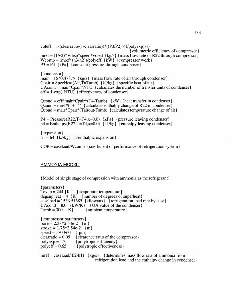
133
voleff = 1-(clearratio/(1-clearratio))*((P3/P2)A(1/polyexp)- 1)( volumetric efficiency of compressor)
mref = (1/v2)*Vdisp*speed*voleff I(kg/sI (I{mass flow rate of R22 through compressor)Wcomp = (mref*(h3-h2))/polyeff (kW} {compressor work)P3 = P4 {kPa) (Iconstant pressure through condenser)
{ condensor)mair = 15*0.47879 (kg/s) (mass flow rate of air through condenser)Cpair = SpecHeat(Air,T=Tamb) { kJ/kg) ( Ispecific heat of air)UAcond = mair*Cpair*NTU (calculates the number of transfer units of condenser)eff = 1-exp(-NTU) (effectiveness of condenser)
Qcond = eff*mair*Cpair*(T4-Tamb) (kW) (heat transfer in condenser)Qcond = mref*(h3-h4) ( calculates enthalpy change of R22 in condenser)Qcond = mair*Cpair*(Tairout-Tamb) (calculates temperature change of air)
P4 = Pressure(R22,T=T4,x=0.0) {kPa) (pressure leaving condenser)h4 = Enthalpy(R22,T=T4,x=0.0) { kJ/kg} { enthalpy leaving condenser)
(expansion)h 1 = h4 I(kJ/kg) ({Iisenthalpic expansion)
COP = caseload/Wcomp (coefficient of performance of refrigeration system)
AMMONIA MODEL:
(Model of single stage of compression with ammonia as the refrigerant)
(parameters)ITevap = 244 (K) (evaporator temperature)degsupheat = 4 ( K) (Inumber of degrees of superheat)Icaseload = 15*3.51685 (kilowatts) (refrigeration load met by case)UAcond = 8.0 (kW/K) (IUA value of the condenser)Tamb = 300 ( K) ( Iambient temperature)
( compressor parameters)Ibore = 2.38*2.54e-2 (m)stroke - 1.75*2.54e-2 imspeed = 1700/60 (rpm)clearratio = 0.05 {clearence ratio of the compressor)polyexp = 1.3 (polytropic efficiency)Ipolyeff = 0.65 (tpolytropic effectiveness)}
mnref = caseload/(h2-hl) (kg/sI (determines mass flow rate of ammonia fromrefrigeration load and the enthalpy change in condenser)
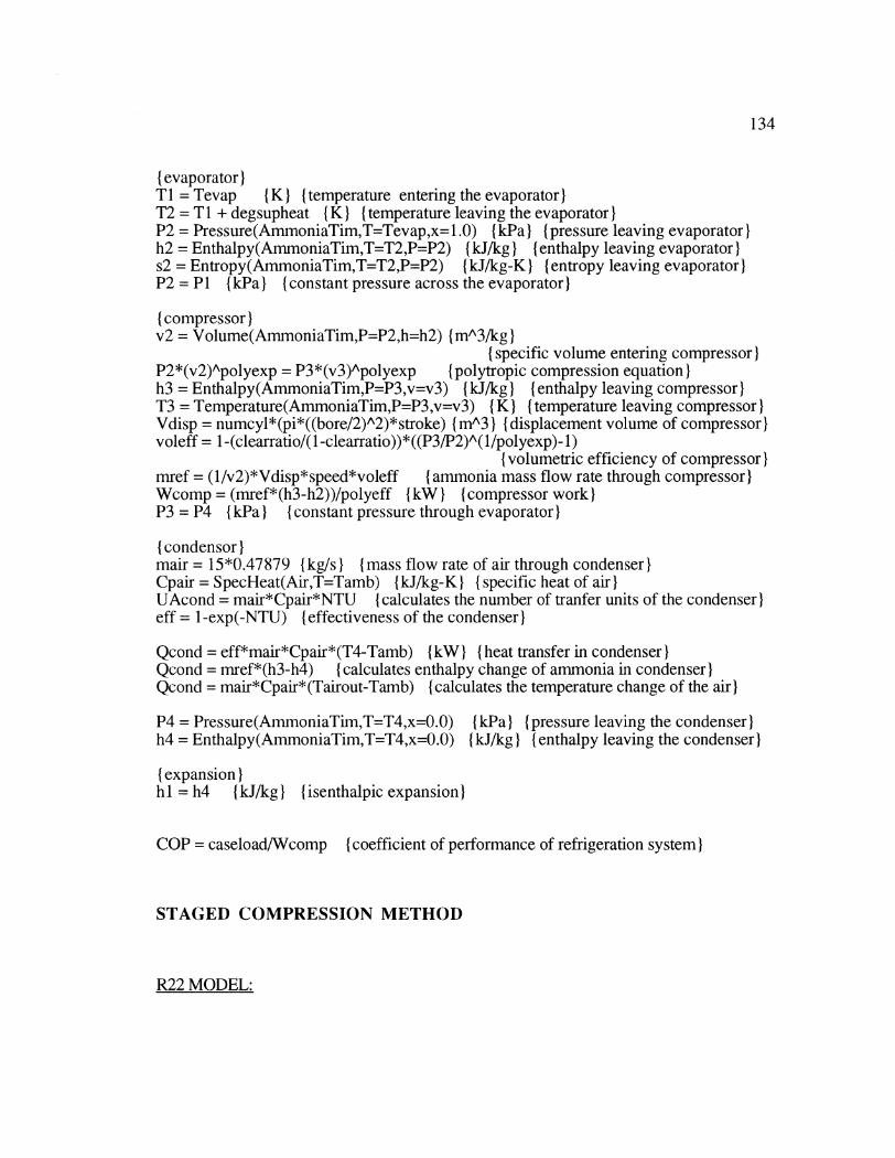
134
{ evaporator)ITI = Tevap { K) { temperature entering the evaporator)IT2 = TI + degsupheat (K }(temperature leaving the evaporator)P2 = Pressure(AmmoniaTim,T=Tevap,x= 1.0) { kPa) (pressure leaving evaporator)h2 = Enthalpy(AmmoniaTim,T=T2,P=P2) { kJ/kg { {enthalpy leaving evaporator)Is2 = Entropy(AmmoniaTim,T=T2,P=P2) I(kJ/kg-K) {entropy leaving evaporator)P2 = P1 {kPa) { constant pressure across the evaporator)
(compressor)v2 = Volume(AmmoniaTim,P=P2,h=h2) { mA3/kg)I
{ specific volume entering compressor)P2*(v2)Apolyexp = P3*(v3)Apolyexp (polytropic compression equation)h3 = Enthalpy(AmmoniaTim,P=P3,v=v3) IkJ/kgI (enthalpy leaving compressor)T3 = Temperature(AmmoniaTim,P=P3,v=v3) (K) { temperature leaving compressor)IVdisp = numcyl*(pi*((bore/2)A2)*stroke) { m"3) (Idisplacement volume of compressor)voleff = 1-(clearratio/(1-clearratio))*((P3/P2)A(1/polyexp)- 1)
{ volumetric efficiency of compressor)mref = (1/v2)*Vdisp*speed*voleff (ammonia mass flow rate through compressor)Wcomp = (mref*(h3-h2))/polyeff (kW) {compressor work)P3 = P4 {kPa) (constant pressure through evaporator)
(condensor)mair = 15*0.47879 (kg/s) {mass flow rate of air through condenser)Cpair = SpecHeat(Air,T=Tamb) (kJ/kg-K} (specific heat of air)UAcond = mair*Cpair*NTU (calculates the number of tranfer units of the condenser)eff = 1-exp(-NTU) ( effectiveness of the condenser)I
Qcond = eff*mair*Cpair*(T4-Tamb) (kW) (heat transfer in condenser)Qcond = mref*(h3-h4) (calculates enthalpy change of ammonia in condenser)Qcond = mair*Cpair*(Tairout-Tamb) (calculates the temperature change of the air)
P4 = Pressure(AmmoniaTim,T=T4,x=0.0) (kPa) (pressure leaving the condenser)h4 = Enthalpy(AmmoniaTim,T=T4,x=0.0) (kJ/kg) (enthalpy leaving the condenser)
( expansion)hl = h4 (kJ/kg) (Iisenthalpic expansion)
COP = caseload/Wcomp ( coefficient of performance of refrigeration system)I
STAGED COMPRESSION METHOD
R22 MODEL:
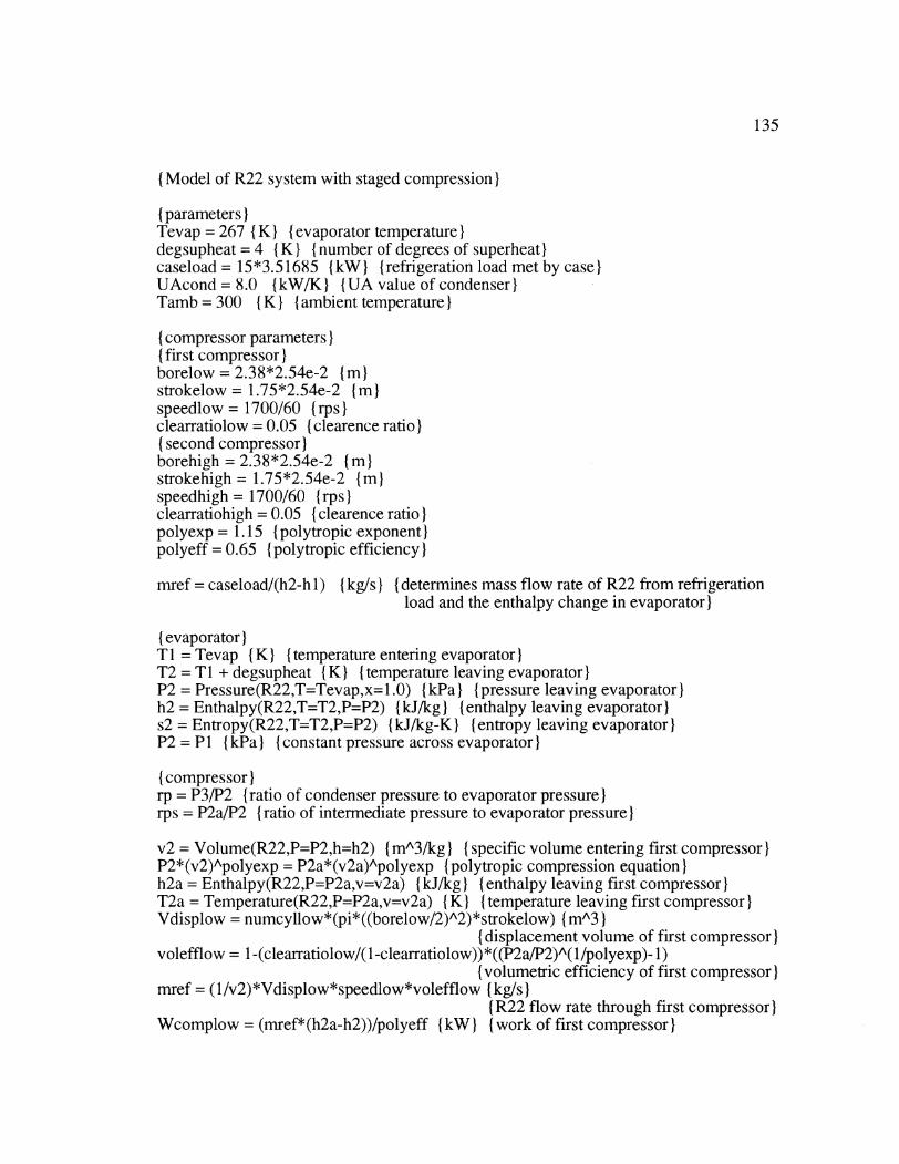
135
(Model of R22 system with staged compression)
(parameters)Tevap = 267 (K) (evaporator temperature)degsupheat = 4 { K) (number of degrees of superheat)caseload = 15*3.51685 (kW) (refrigeration load met by case)UAcond = 8.0 {kW/K) (IUA value of condenser)ITamb = 300 ( K)I { ambient temperature)I
( compressor parameters)I( first compressor)Iborelow = 2.38*2.54e-2 imstrokelow = 1.75*2.54e-2 (in)speedlow = 1700/60 {(rps)Iclearratiolow = 0.05 (clearence ratio)I( second compressor)borehigh = 2.38*2.54e-2 (m)strokehigh = 1.75*2.54e-2 (m)speedhigh = 1700/60 (1rps)Iclearratiohigh = 0.05 (clearence ratio)Ipolyexp = 1.15 ( polytropic exponent)Ipolyeff = 0.65 (polytropic efficiency)I
mref = caseload/(h2-h 1) (kg/s }(determines mass flow rate of R22 from refrigerationload and the enthalpy change in evaporator)I
{evaporator)T 1 = Tevap (K) (temperature entering evaporator)IT2 = T 1 + degsupheat ( K) ({Itemperature leaving evaporator)IP2 = Pressure(R22,T=Tevap,x=1.0) (kPa (pressure leaving evaporator)h2 = Enthalpy(R22,T=T2,P=P2) (kJ/kg) (fenthalpy leaving evaporator)Is2 = Entropy(R22,T=T2,P=P2) (kJ/kg-K) (Ientropy leaving evaporator)IP2 = P1 (kPa) (Iconstant pressure across evaporator)
(compressor)rp = P3/P2 (ratio of condenser pressure to evaporator pressure)rps = P2a/P2 (ratio of intermediate pressure to evaporator pressure)
v2 = Volume(R22,P=P2,h=h2) (mA3/kg) ( Ispecific volume entering first compressor)P2*(v2)Apolyexp = P2a*(v2a)Apolyexp (polytropic compression equation)h2a = Enthalpy(R22,P=P2a,v=v2a) I(kJ/kg) (enthalpy leaving first compressor)IT2a = Temperature(R22,P=P2a,v=v2a) (K) (temperature leaving first compressor)Vdisplow = numcyllow*(pi*((borelow/2)A2)*strokelow) (mA3)
(displacement volume of first compressor)voleffiow = 1-(clearratiolow/( 1-clearratiolow))*((P2a/P2)A(l/polyexp)- 1)
( volumetric efficiency of first compressor)}mref = (1/v2)*Vdisplow*speedlow*volefflow ( kg/s)}
{R22 flow rate through first compressor)}Wcomplow = (mref*(h2a-h2))/polyeff {(kW) ( work of first compressor)}
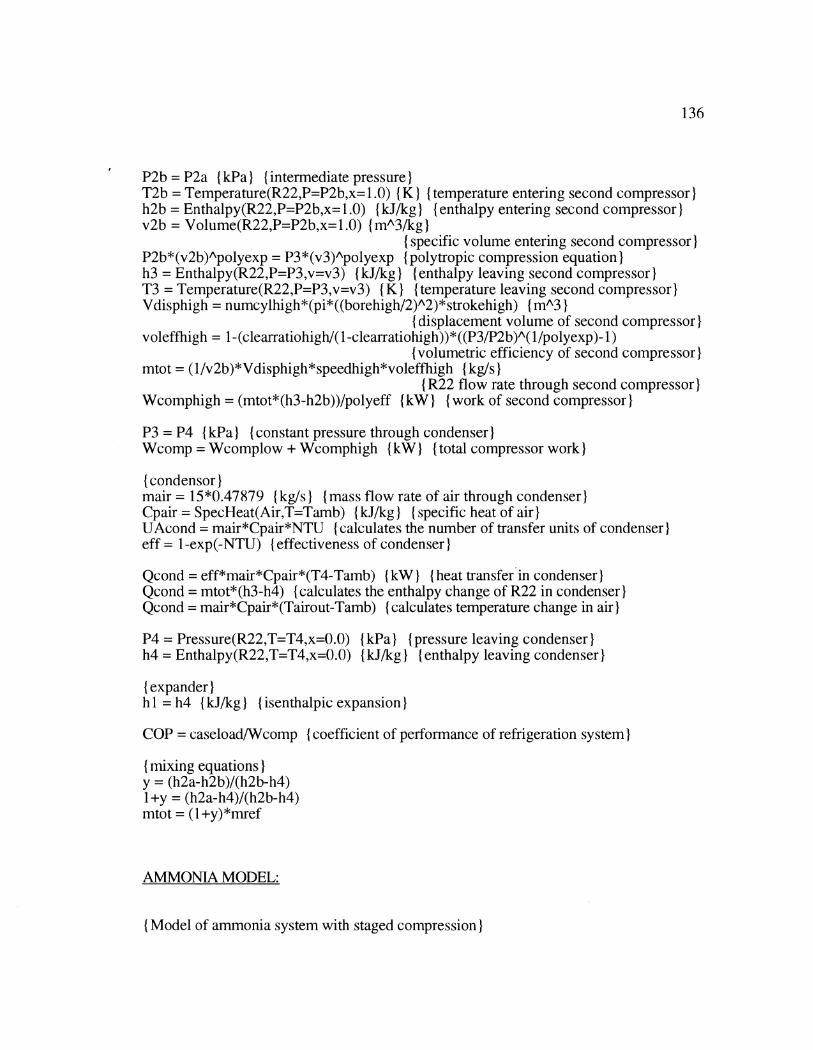
136
P2b = P2a {kPa) {intermediate pressure)IT2b = Temperature(R22,P=P2b,x=1.0) {K) {temperature entering second compressor)h2b = Enthalpy(R22,P=P2b,x= 1.0) {kJ/kgI} { enthalpy entering second compressor)Iv2b = Volume(R22,P=P2b,x= 1.0) ( mA3/kg}
(specific volume entering second compressor)P2b*(v2b)Apolyexp = P3*(v3)Apolyexp (polytropic compression equation)Ih3 = Enthalpy(R22,P=P3,v=v3) {kJ/kg) (enthalpy leaving second compressor)T3 = Temperature(R22,P=P3,v=v3) (K) (temperature leaving second compressor)Vdisphigh = numcylhigh*(pi*((borehigh/2)A2)*strokehigh) (mA3)
(displacement volume of second compressor)Ivoleffhigh = 1-(clearratiohigh/( 1-clearratiohigh))*((P3/P2b)A(1/polyexp)- 1)
(volumetric efficiency of second compressor)mtot = (1/v2b)*Vdisphigh*speedhigh*voleffhigh (kg/s)
I(R22 flow rate through second compressor)Wcomphigh = (mtot*(h3-h2b))/polyeff (kW) (work of second compressor)
P3 = P4 ( kPa) (Iconstant pressure through condenser)Wcomp = Wcomplow + Wcomphigh {kW} (Itotal compressor work)I
(condensor)Imair = 15*0.47879 (kg/s) (mass flow rate of air through condenser)Cpair = SpecHeat(Air,T=Tamb) I(kJ/kg) ({Ispecific heat of air)UAcond = mair*Cpair*NTU ( calculates the number of transfer units of condenser)Ieff = 1-exp(-NTU) ( effectiveness of condenser)I
Qcond = eff*mair*Cpair*(T4-Tamb) (kW) (heat transfer in condenser)Qcond = mtot*(h3-h4) (calculates the enthalpy change of R22 in condenser)Qcond = mair*Cpair*(Tairout-Tamb) (calculates temperature change in air)I
P4 = Pressure(R22,T=T4,x=0.0) (kPa) (pressure leaving condenser)h4 =Enthalpy(R22,T=T4,x=0.0) (kJ/kg) (enthalpy leaving condenser)
(expander)
h 1 = h4 {kJ/kg) (isenthalpic expansion)
COP = caseload/Wcomp ( coefficient of performance of refrigeration system)I
( mixing equations)Iy = (h2a-h2b)/(h2b-h4)Il+y = (h2a-h4)/(h2b-h4)mtot = (1+y)*mref
AMMONIA MODEL:
(Model of ammonia system with staged compression)I
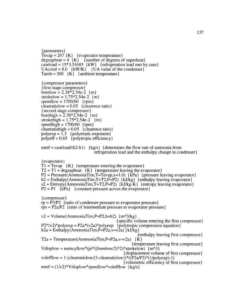
137
( parameters)ITevap = 267 { K) (evaporator temperature)degsupheat = 4 {K) (number of degrees of superheat)caseload = 15*3.51685 {kW) (refrigeration load met by case)UAcond = 8.0 (kW/K) {UA value of the condenser)Tamb = 300 1K) (Iambient temperature)I
( compressor parameters)I( first stage compressor)borelow = 2.38*2.54e-2 (imstrokelow = 1.75*2.54e-2 (m)speedlow = 1700/60 (rpm)clearratiolow = 0.05 ( clearence ratio)I(second stage compressor)borehigh = 2.38*2.54e-2 {imstrokehigh = 1.75*2.54e-2 Imspeedhigh = 1700/60 (rpm)clearratiohigh = 0.05 ( clearence ratio)Ipolyexp = 1.3 (polytropic exponent)polyeff = 0.65 (polytropic efficiency)
mref = caseload/(h2-h 1) (kg/s) (determines the flow rate of ammonia fromrefrigeration load and the enthalpy change in condenser)
( evaporator)IT1 = Tevap (K) (temperature entering the evaporator)T2 = Ti + degsupheat (K) (Itemperature leaving the evaporator)IP2 = Pressure(AmmoniaTim,T=Tevap,x=1.0) (kPa) ({pressure leaving evaporator)h2 = Enthalpy(AmmoniaTim,T=T2,P=P2) (kJ/kg) (enthalpy leaving evaporator)s2 = Entropy(AmmoniaTim,T=T2,P=P2) (kJ/kg-K) (Ientropy leaving evaporator)IP2 = P1 (kPa) (Iconstant pressure across the evaporator)
(compressor)rp = P3/P2 (ratio of condenser pressure to evaporator pressure)rps = P2a/P2 ( ratio of intermediate pressure to evaporator pressure)
v2 = Volume(AmnmoniaTim,P=P2,h=h2) {mA3/kg)I(specific volume entering the first compressor)
P2*(v2)Apolyexp = P2a*(v2a)Apolyexp (polytropic compression equation)h2a = Enthalpy(AnmmoniaTim,P=P2a,v=v2a) {IkJ/kg)I
(enthalpy leaving first compressor)T2a = Temperature(AmmoniaTim,P=P2a,v=v2a) (IK)
( temperature leaving first compressor)Vdisplow = numcyllow*(pi*((borelow/2)A2)*strokelow) (mA3)}
(displacement volume of first compressor)volefflow - 1 -(clearratiolow/( 1-clearratiolow))*((P2a/P2)A(1l/polyexp)- 1)(volumetric efficiency of first compressor)
mnref = (1/v2)*Vdisplow*speedlow*volefflow ( kg/s)}
138
( ammonia flow rate through first compressor)Wcomplow = (mref*(h2a-h2))/polyeff (kW) (work of first compressor)
P2b = P2a Iintermediate pressure)IT2b = Temperature(AmmoniaTim,P=P2b,x= 1.0) { K)
(temperature entering second compressor)h2b = Enthalpy(AmmoniaTim,P=P2b,x= 1.0) (kJ/kg)
t{enthalpy entering second compressor)v2b = Volume(AmmoniaTim,P=P2b,x= 1.0) { mA3/kg)I
{specific volume entering second compressor)P2b*(v2b)Apolyexp = P3*(v3)Apolyexp (polytropic compression equation)h3 = Enthalpy(AmmoniaTim,P=P3,v=v3) {kJ/kg)I
I enthalpy leaving second compressor)T3 = Temperature(AmmoniaTim,P=P3,v=v3) (K)
(temperature leaving second compressor)Vdisphigh = numcylhigh*(pi*((borehigh/2)A2)*strokehigh) { mA3)
{displacement volume of second compressor)voleffhigh = 1-(clearratiohigh/(1-clearratiohigh))*((P3/P2b)A( l/polyexp)- 1)
(volumetric efficiency of second compressor)mtot = (1/v2b)*Vdisphigh*speedhigh*voleffhigh { kg/s)I
{mass flow rate through second compressor)Wcomphigh = (mtot*(h3-h2b))/polyeff (kW) (work of second compressor)
P3 = P4 (kPa) (Iconstant pressure through evaporator)Wcomp = Wcomplow + Wcomphigh (kW } (total compressor work)
(condensorImair = 15*0.47879 (kg/s) (mass flow rate of air though the condenser)Cpair = SpecHeat(Air,T=Tamb) I(kJ/kg-K) ( Ispecific heat of air)UAcond = mair*Cpair*NTU ( calculates the number of transfer units of condenser)eff = 1-exp(-NTU) ( effectiveness of condenser)I
Qcond = eff*mair*Cpair*(T4-Tamb) (kW }(heat transfer in condenser)Qcond = mtot*(h3-h4) (calculates enthalpy change of ammonia in condenser)Qcond = mair*Cpair*(Tairout-Tamb) (calculates the temperature change of air)
P4 = Pressure(AmmoniaTim,T=T4,x=0.0) {kPa) ({pressure leaving the condenser)Ih4 = Enthalpy(AmmoniaTim,T=T4,x=0.0) (kJ/kg) (Ienthalpy leaving the condenser)I
(expansion)h I = h4 {kJ/kg) ({Iisenthalpic expansion)
COP = caseload/Wcomp ( coefficient of performance of refrigeration system)I
(mixing equations for intercooling)y = (h2a-h2b)/(h2b-h4)1l+y = (h2a-h4)I(h2b-h4)mtot = (1l+y)*mref
139
STAGED COMPRESSION AND EVAPORATION METHOD
R22 MODEL:
(Model of R22 system with staged compression and evaporation)
(parameters)ITevap = 244 (K) (evaporator temperature)degsupheat = 4 (K) {number of degrees of superheat)caseload = 15*3.51685 {kW)I {refrigeration load met by case)UAcond = 8.0 (kW/K) (UA value of condenser)Tamb = 300 { K) (ambient temperature)
{ compressor parameters)I{ first compressor)Iborelow = 2.38*2.54e-2 {m)strokelow = 1.75*2.54e-2 (In)
speedlow = 1700/60 (1rps)Iclearratiolow = 0.05 { clearence ratio)I( second compressor)borehigh = 2.38*2.54e-2 (m)strokehigh = 1.75*2.54e-2 (m)
speedhigh = 1700/60 (rps)clearratiohigh = 0.05 (clearence ratio)Ipolyexp = 1.15 ( polytropic exponent)Ipolyeff = 0.65 (polytropic efficiency)I
mref = caseload/(h2-h 1) 1(kg/s) (Idetermines mass flow rate of R22 from refrigerationload and the enthalpy change in evaporator)
( evaporator)IT 1 = Tevap ( K) ({Itemperature entering evaporator)T2 = T 1 + degsupheat (K) (temperature leaving evaporator)P2 = Pressure(R22,T=Tevap,x=l.0) (kPa) (pressure leaving evaporator)h2 = Enthalpy(R22,T=T2,P=P2) I(kJ/kg) ({Ienthalpy leaving evaporator)s2 = Entropy(R22,T=T2,P=P2) (entropy leaving evaporator)P2 = P1 (kPa) (Iconstant pressure across evaporator)
(compressor)rp = P3/P2 (ratio of condenser pressure to evaporator pressure)rps = rpAx (relationship between pressure ratios)rps = P2a/P2 ( ratio of intermediate pressure to evaporator pressure)
v2 = Volume(R22,P=P2,h=h2) {(m^3/kg) ({specific volume entering first compressor)}
140
P2*(v2)Apolyexp = P2a*(v2a)Apolyexp {polytropic compression equation)h2a = Enthalpy(R22,P=P2a,v=v2a) I(kJ/kg) { enthalpy leaving first compressor)T2a = Temperature(R22,P=P2a,v=v2a) { K) (temperature leaving first compressor)Vdisplow = numcyllow*(pi*((borelow/2)A2)*strokelow) (mA3}
(displacement volume of first compressor)volefflow = 1-(clearratiolow/( 1-clearratiolow))*((P2a/P2)A(l/polyexp)- 1)
( volumetric efficiency of first compressor)mref = (1/v2)*Vdisplow*speedlow*volefflow { kg/s)
{ R22 flow rate through first compressor)Wcomplow = (nref*(h2a-h2))/polyeff { kW (work of first compressor)
P2b = P2a { kPa) { intermediate pressure)T2b = Temperature(R22,P=P2bh=h2b) ( K) I(temperature entering second compressor)v2b = Volume(R22,P=P2b,h=h2b) { mA3/kg)
(specific volume entering second compressor)P2b*(v2b)Apolyexp = P3*(v3)Apolyexp ( polytropic compression equation)Ih3 = Enthalpy(R22,P=P3,v=v3) {kJ/kg) (enthalpy leaving second compressor)T3 = Temperature(R22,P=P3,v=v3) (K) }Itemperature leaving second compressor)IVdisphigh = numcylhigh*(pi*((borehigh/2)A2)*strokehigh) { mA3)
(displacement volume of second compressor)Ivoleffhigh = 1-(clearratiohigh/(1-clearratiohigh))*((P3/P2b)A(1/polyexp)- 1)
(volumetric efficiency of second compressor)mtot = (1/v2b)*Vdisphigh*speedhigh*voleffhigh (kg/s)
{R22 flow rate through second compressor)Wcomphigh = (mtot*(h3-h2b))/polyeff {kW) (work of second compressor)
P3 = P4 (kPa} {constant pressure through condenser)Wcomp = Wcomplow + Wcomphigh {kW) (Itotal compressor work)
(condensor)mair = 15*0.47879 (kg/s) (mass flow rate of air through condenser)Cpair = SpecHeat(Air,T=Tamb) I(kJ/kg) ({Ispecific heat of air)IUAcond = mair*Cpair*NTU ( calculates the number of transfer units of the condenser)eff = 1-exp(-NTU) ( effectiveness of condenser)I
Qcond = eff*mair*Cpair*(T4-Tamb) (kW) (Iheat transfer in condenser)Qcond = mtot*(h3-h4) (calculates the enthalpy change of R22 in condenser)Qcond = mair*Cpair*(Tairout-Tamb) (calculates temperature change of air)
P4 = Pressure(R22,T=T4,x=0.0) (kPa) (pressure leaving condenser)h4 = Enthalpy(R22,T=T4,x=0.0) (kJ/kg) (enthalpy leaving condenser)
( expansion)IP5 = P2a ( kPa) (intermediate pressure)P6 = P2a ( kPa) (intermediate pressure)h5 = Enthalpy(R22,P=P5,x= 1.0) {(kJ/kg) ({enthalpy of ammonia vapor for intercoling)}h6 = Enthalpy(R22,P=P6,x=0.0) {(kJ/kg)} { enthalpy of liquid ammonia forevaporation)hl1 = h6 ( kJ/kg) ({isenthalpic expansion)}
141
COP = caseload/Wcomp ( coefficient of performance of refrigeration system)
(mixing equations for separator and intercooling)mtot = mref + mvapmtot*h4 = mref*h6 + mvap*h5mtot*h2b = mref*h2a + mvap*h5
AMMONIA MODEL:
(Model of ammonia system with staged compression and evaporation)
{ parameters)ITevap = 267 { K) (evaporator temperature)degsupheat =4 { K) (number of degrees of superheat)caseload = 15*3.51685 (kW) (refrigeration load met by case)UAcond = 8.0 (kW/K) {UA value of the condenser)Tamb = 300 (K) (Iambient temperature)I
( compressor parameters)( first compressor)Iborelow = 2.38*2.54e-2 imstrokelow = 1.75*2.54e-2 imspeedlow = 1700/60 (1rps)Iclearratiolow = 0.05 (clearence ratio)I( second compressor)borehigh = 2.38*2.54e-2 Imstrokehigh = 1.75*2.54e-2 (im)speedhigh = 1700/60 (rps)Iclearratiohigh = 0.05 (clearence ratio)Ipolyexp = 1.3 (polytropic exponent)polyeff = 0.65 (polytropic efficiency)
mref = caseload/(h2-h 1) (kg/s) (determines mass flow rate of ammonia fromrefrigeration load and the enthalpy change in evaporator)
( evaporator)ITi = Tevap (K) (Itemperature entering the evaporator)T2 = Ti + degsupheat (K) temperature leaving the evaporator)P2 = Pressure(AmmoniaTim,T=Tevap,x=1.0) (kPa) (pressure leaving evaporator)h2 = Enthalpy(AmmoniaTim,T=T2,P=P2) (kJ/kg) (enthalpy leaving evaporator)s2 = Entropy(AmmoniaTim,T=T2,P=P2) (kJ/kg-K) (entropy leaving evaporator)P2 = P1 (kPa) (constant pressure in evaporator)
( compressor)}rp = P3/P2 (ratio of condenser pressure to evaporator pressure)}
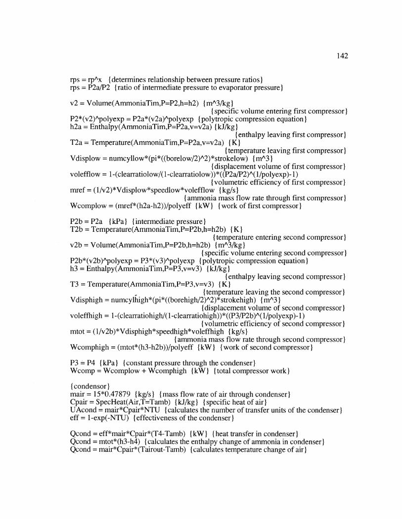
142
rps = rpAX {determines relationship between pressure ratios)Irps = P2a/P2 ( ratio of intermediate pressure to evaporator pressure)
v2 = Volume(AmmoniaTim,P=P2,h=h2) (mA3/kg)I{specific volume entering first compressor)
P2*(v2)Apolyexp = P2a*(v2a)Apolyexp (polytropic compression equation)h2a = Enthalpy(AmmoniaTim,P=P2a,v=v2a) {IkJ/kg)I
{ enthalpy leaving first compressor)T2a = Temperature(AmmoniaTim,P=P2a,v=v2a) { K)
( temperature leaving first compressor)Vdisplow = numcyllow*(pi*((borelow/2)A2)*strokelow) {(mA3)}
( displacement volume of first compressor)Ivolefflow = 1-(clearratiolow/( 1-clearratiolow))*((P2a/P2)A( 1/polyexp)- 1)
( volumetric efficiency of first compressor)mref = (1/v2)*Vdisplow*speedlow*volefflow (kg/s)
(ammonia mass flow rate through first compressor)Wcomplow = (mref*(h2a-h2))/polyeff (kW) (Iwork of first compressor)
P2b = P2a (kPa) (intermediate pressure)T2b = Temperature(AmmoniaTim,P=P2b,h=h2b) (K)
( temperature entering second compressor)v2b = Volume(AmmoniaTim,P=P2b,h=h2b) (mA3/kg)
( specific volume entering second compressor)P2b*(v2b)Apolyexp = P3*(v3)Apolyexp (polytropic compression equation)h3 = Enthalpy(AmmoniaTim,P=P3,v=v3) {kJ/kg)I
(enthalpy leaving second compressor)T3 = Temperature(AmmoniaTim,P=P3,v=v3) (K)
( temperature leaving the second compressor)IVdisphigh = numcylhigh*(pi*((borehigh/2)A2)*strokehigh) (mA3)
( displacement volume of second compressor)Ivoleffhigh = 1-(clearratiohigh/( 1-clearratiohigh))*((P3/P2b)A( 1/polyexp)- 1)
( volumetric efficiency of second compressor)mtot = (1/v2b)*Vdisphigh*speedhigh*voleffhigh (kg/s)
(ammonia mass flow rate through second compressor)Wcomphigh = (mtot*(h3-h2b))/polyeff {kW) (work of second compressor)
P3 = P4 (kPa) (constant pressure through the condenser)Wcomp = Wcomplow + Wcomphigh (kW) (Itotal compressor work)
{condensor)mair = 15*0.47879 (kg/s) (mass flow rate of air through condenser)Cpair = SpecHeat(Air,T=Tamb) I(kJ/kg) ( Ispecific heat of air)UAcond = mair*Cpair*NTU ( calculates the number of transfer units of the condenser)eff = 1-exp(-NTU) ( effectiveness of the condenser)I
Qcond = eff*mair*Cpair*(T4-Tamb) (kW) (heat transfer in condenser)Qcond = mtot*(h3-h4) (calculates the enthalpy change of ammonia in condenser)Qcond = mair*Cpair*(Tairout-Tamb) (calculates temperature change of air)
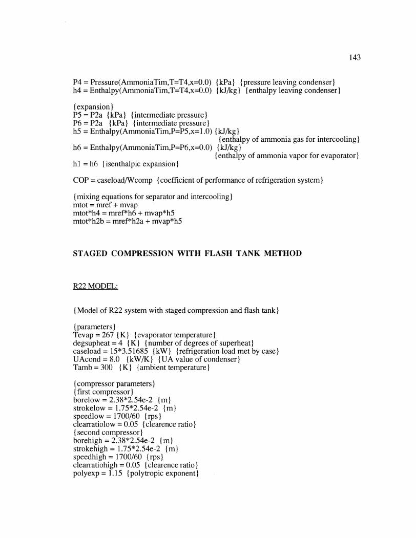
143
P4 = Pressure(AmmoniaTim,T=T4,x=0.0) (kPa) (pressure leaving condenser)Ih4 = Enthalpy(AmmoniaTim,T=T4,x=0.0) kJ/kg) (enthalpy leaving condenser)
{ expansion)IP5 = P2a I(kPa) (intermediate pressure)P6 = P2a {kPa) (intermediate pressure)h5 = Enthalpy(AmmoniaTim,P=P5,x=1.0) {kJ/kg)
(enthalpy of ammonia gas for intercooling)h6 = Enthalpy(AmmoniaTim,P=P6,x=0.0) {kJ/kg)I
{ enthalpy of ammonia vapor for evaporator)h I = h6 { isenthalpic expansion)I
COP = caseload/Wcomp ( coefficient of performance of refrigeration system)
(mixing equations for separator and intercooling)mtot = mref + mvapmtot*h4 = mref*h6 + mvap*h5mtot*h2b = mref*h2a + mvap*h5
STAGED COMPRESSION WITH FLASH TANK METHOD
R22 MODEL:
(Model of R22 system with staged compression and flash tank)
(parameters)Tevap = 267 (K) (evaporator temperature)degsupheat = 4 (K) (number of degrees of superheat)caseload = 15*3.51685 (kW) (refrigeration load met by case)UAcond = 8.0 (kW/K) ({IUA value of condenser)ITamb = 300 ( K) ( Iambient temperature)I
( compressor parameters)I( first compressor)Iborelow = 2.38*2.54e-2 imstrokelow = 1.75*2.54e-2 (mspeedlow - 1700/60 (1rps)Iclearratiolow = 0.05 (clearence ratio)I( second compressor)borehigh = 2.38*2.54e-2 imstrokehigh = 1.75"2.54e-2 (in)
speedhigh = 1700/60 ( rps)}clearratiohigh = 0.05 ( clearence ratio)}polyexp = 1.15 ( polytropic exponent)}
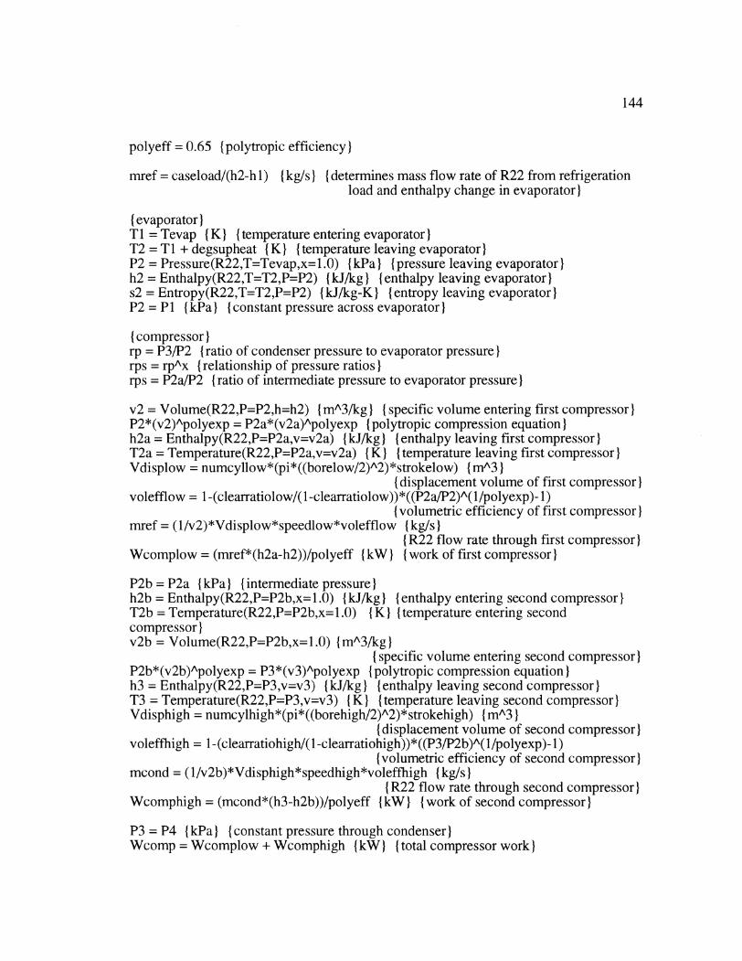
144
polyeff = 0.65 (polytropic efficiency)I
mref = caseload/(h2-h 1) { kg/s) { determines mass flow rate of R22 from refrigerationload and enthalpy change in evaporator)
(evaporator)ITI = Tevap (K) (temperature entering evaporator)T2 = T I + degsupheat ( K)} { temperature leaving evaporator}P2 = Pressure(R22,T=Tevap,x= 1.0) {kPa) {pressure leaving evaporator)h2 = Enthalpy(R22,T=T2,P=P2) I(kJ/kg) ({Ienthalpy leaving evaporator)Is2 = Entropy(R22,T=T2,P=P2) { kJ/kg-K) { entropy leaving evaporator)P2 = P1 {kPa) {constant pressure across evaporator)
(compressor)rp = P3/P2 (ratio of condenser pressure to evaporator pressure)rps = rpAx (relationship of pressure ratios)rps = P2a/P2 ( ratio of intermediate pressure to evaporator pressure)
v2 = Volume(R22,P=P2,h=h2) (mA3/kg) (Ispecific volume entering first compressor)P2*(v2)Apolyexp = P2a*(v2a)Apolyexp (polytropic compression equation)h2a = Enthalpy(R22,P=P2a,v=v2a) (kJ/kg) ({Ienthalpy leaving first compressor)IT2a = Temperature(R22,P=P2a,v=v2a) (K) (Itemperature leaving first compressor)Vdisplow = numcyllow*(pi*((borelow/2)A2)*strokelow) (mA3)
( displacement volume of first compressor)Ivolefflow = 1-(clearratiolow/( 1-clearratiolow))*((P2a/P2)A(l/polyexp)- 1)
( volumetric efficiency of first compressor)mref = (1/v2)*Vdisplow*speedlow*volefflow (kg/s)
( R22 flow rate through first compressor)Wcomplow = (mref*(h2a-h2))/polyeff (kW) (Iwork of first compressor)
P2b = P2a (kPa) (Iintermediate pressure)Ih2b = Enthalpy(R22,P=P2b,x= 1.0) (kJ/kg) (Ienthalpy entering second compressor)T2b = Temperature(R22,P=P2b,x= 1.0) (K) (temperature entering secondcompressor)v2b = Volume(R22,P=P2b,x= 1.0) 1mA3/kg)
(specific volume entering second compressor)P2b*(v2b)Apolyexp = P3*(v3)Apolyexp (polytropic compression equation)Ih3 = Enthalpy(R22,P=P3,v=v3) (kJ/kg) (enthalpy leaving second compressor)T3 = Temperature(R22,P=P3,v=v3) (K) (Itemperature leaving second compressor)Vdisphigh = numcylhigh*(pi*((borehigh/2)A2)*strokehigh) I(mA3)
(displacement volume of second compressor)voleffhigh = 1-(clearratiohigh/(1-clearratiohigh))*((P3/P2b)A(1/polyexp)- 1)
(volumetric efficiency of second compressor)mcond = (1/v2b)*Vdisphigh*speedhigh*voleffhigh (kg/s)
(R22 flow rate through second compressor)Wcomphigh = (mcond*(h3-h2b))/polyeff (kW) ( work of second compressor)}
P3 = P4 ( kPa) ({constant pressure through condenser)Wcomp - Wcomplow + Wcomphigh (kW) ({total compressor work)
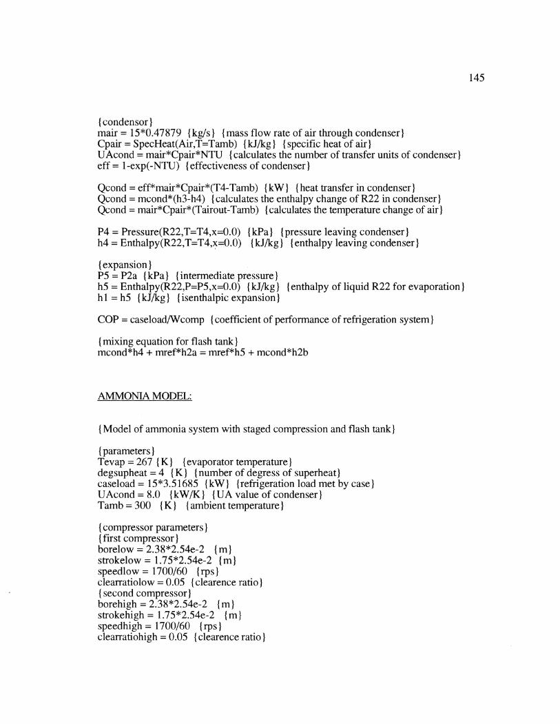
145
(condensor)mair = 15*0.47879 {kg/s) {mass flow rate of air through condenser)Cpair = SpecHeat(Air,T=Tamb) { kJ/kg) ( Ispecific heat of air)UAcond = mair*Cpair*NTU ( calculates the number of transfer units of condenser)Ieff = 1-exp(-NTU) ( effectiveness of condenser)I
Qcond = eff*mair*Cpair*(T4-Tamb) {kW) (heat transfer in condenser)Qcond = mcond*(h3-h4) (calculates the enthalpy change of R22 in condenser)Qcond = mair*Cpair*(Tairout-Tamb) {calculates the temperature change of air)I
P4 = Pressure(R22,T=T4,x=0.0) {kPa) {pressure leaving condenser)Ih4 = Enthalpy(R22,T=T4,x=0.0) {kJ/kg) (enthalpy leaving condenser)
{expansion)P5 = P2a ( kPa) (intermediate pressure)h5 = Enthalpy(R22,P=P5,x=0.0) { kJ/kg} { enthalpy of liquid R22 for evaporation)hl = h5 (kJ/kg) (isenthalpic expansion)
COP = caseload/Wcomp ( coefficient of performance of refrigeration system)
( mixing equation for flash tank)Imcond*h4 + mref*h2a = mref*h5 + mcond*h2b
AMMONIA MODEL:
(Model of ammonia system with staged compression and flash tank)
(parameters)Tevap = 267 (K) (evaporator temperaturedegsupheat = 4 (K) (number of degress of superheat)caseload = 15*3.51685 (kW) (refrigeration load met by case)UAcond = 8.0 {kW/K {IUA value of condenser)ITamb = 300 ( K) (Iambient temperature)I
( compressor parameters)I( first compressor)Iborelow = 2.38*2.54e-2 imstrokelow = 1.75*2.54e-2 imspeedlow = 1700/60 (rps)clearratiolow = 0.05 (clearence ratio)I( second compressor)borehigh = 2.38"2.54e-2 )mstrokehigh = 1.75"2.54e-2 (in)
speedhigh = 1700/60 (rps)}clearratiohigh = 0.05 ( clearence ratio)}
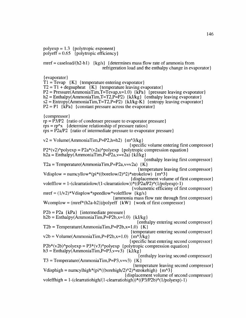
146
polyexp = 1.3 (polytropic exponent)polyeff = 0.65 (polytropic efficiency)
mref = caseload/(h2-h 1) (kg/s) (Idetermines mass flow rate of ammonia fromrefrigeration load and the enthalpy change in evaporator)
{ evaporator)ITI = Tevap (K) (temperature entering evaporator)T2 = Ti + degsupheat (K) (temperature leaving evaporator)P2 = Pressure(AmmoniaTim,T=Tevap,x= 1.0) (kPa) (Ipressure leaving evaporator)h2 = Enthalpy(AmmoniaTim,T=T2,P=P2) (kJ/kg} { enthalpy leaving evaporator)s2 = Entropy(AmmoniaTim,T=T2,P=P2) (kJ/kg-K} { entropy leaving evaporator)P2 = P1 {kPa) {constant pressure across the evaporator)
(compressor)rp = P3/P2 (ratio of condenser pressure to evaporator pressure)Irps = rpAx (Idetermine relationship of pressure ratios)rps = P2a/P2 (ratio of intermediate pressure to evaporator pressure)I
v2 = Volume(AmmoniaTim,P=P2,h=h2) (mA3/kg)I(specific volume entering first compressor)I
P2*(v2)Apolyexp = P2a*(v2a)Apolyexp (polytropic compression equation)h2a = Enthalpy(AmmoniaTim,P=P2a,v=v2a) {IkJ/kg)I
( enthalpy leaving first compressor)T2a = Temperature(AmmoniaTim,P=P2a,v=v2a) (IK)
(temperature leaving first compressor)Vdisplow = numcyllow*(pi*((borelow/2)A2)*strokelow) {mA3 }
(displacement volume of first compressor)volefflow = 1-(clearratiolow/( 1-clearratiolow))*((P2a/P2)A( l/polyexp)- 1)
( volumetric efficieny of first compressor)mref = (1/v2)*Vdisplow*speedlow*volefflow (kg/s)
(ammonia mass flow rate through first compressor)Wcomplow = (mref*(h2a-h2))/polyeff (kW) (Iwork of first compressor)
P2b = P2a {kPa) (intermediate pressure)Ih2b = Enthalpy(AmmoniaTim,P=P2b,x=1.0) {kJ/kg)
(enthalpy entering second compressor)T2b = Temperature(AmmoniaTim,P=P2b,x= 1.0) ( K)I
( temperature entering second compressor)v2b= Volume(AmmoniaTim,P=P2b,x=l.0) {mA3/kg)I
(specific heat entering second compressor)P2b*(v2b)Apolyexp = P3*(v3)Apolyexp (polytropic compression equation)h3 = Enthalpy(AmmoniaTim,P=P3,v=v3) (kJ/kg)I
(enthalpy leaving second compressor)T3 = Temperature(AmmoniaTimP=P3,v=v3) ( K)}
( temperature leaving second compressor)Vdisphigh = numcylhigh*(pi*((borehigh/2)^2)*strokehigh) { mA3)}
(displacement volume of second compressor)}volefffhigh = 1 -(clearratiohigh/( 1-clearratiohigh))*((P3/P2b)^(l/polyexp)- 1 )
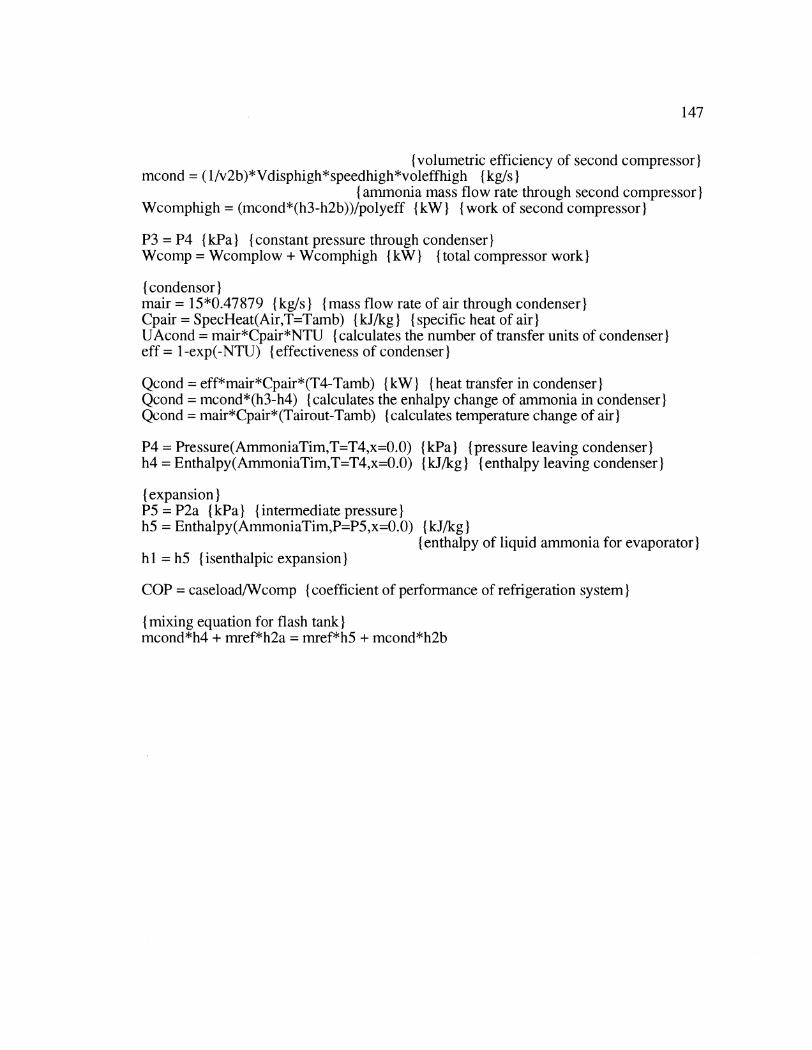
147
(volumetric efficiency of second compressor)mcond = (1/v2b)*Vdisphigh*speedhigh*voleffhigh {kg/s}
(ammonia mass flow rate through second compressor)Wcomphigh = (mcond*(h3-h2b))/polyeff f(kWI (I{work of second compressor)I
P3 = P4 {kPa) {constant pressure through condenser)Wcomp = Wcomplow + Wcomphigh {kW) (Itotal compressor work)
(condensor)mair = 15*0.47879 (kg/s) (mass flow rate of air through condenser)Cpair = SpecHeat(Air,T=Tamb) I(kJ/kg) { specific heat of air)IUAcond = mair*Cpair*NTU (calculates the number of transfer units of condenser)eff = 1-exp(-NTU) ( effectiveness of condenser)I
Qcond = eff*mair*Cpair*(T4-Tamb) (kW } (heat transfer in condenser)IQcond = mcond*(h3-h4) (calculates the enhalpy change of ammonia in condenser)Qcond = mair*Cpair*(Tairout-Tamb) (calculates temperature change of air)
P4 = Pressure(AmmoniaTim,T=T4,x=0.0) {kPa) (pressure leaving condenser)h4 = Enthalpy(AmmoniaTim,T=T4,x=0.0) {kJ/kg) (enthalpy leaving condenser)
{expansion)P5 = P2a I(kPa) (intermediate pressure)h5 = Enthalpy(AmmoniaTim,P=P5,x=0.0) (kJ/kg)
(enthalpy of liquid ammonia for evaporator)h 1 = h5 (isenthalpic expansion)
COP = caseload/Wcomp ( coefficient of performance of refrigeration system)
( mixing equation for flash tank)Imcond*h4 + mref*h2a = mref*h5 + mcond*h2b
148
APPENDIX B
BASE CASE MODEL
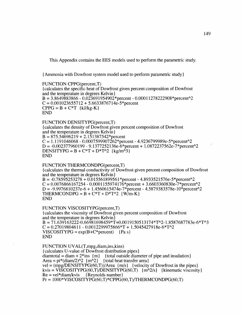
149
This Appendix contains the EES models used to perform the parametric study.
{ Ammonia with Dowfrost system model used to perform parametric study)
FUNCTION CPPG(percent,T)( calculates the specific heat of Dowfrost given percent composition of Dowfrostand the temperature in degrees Kelvin)IB = 3.8649883866 - 0.023691954902*percent - 0.0001 1278222908*percentA2C = 0.001023655712 + 5.6633876714e-5*percentCPPG = B + C*T (kJ/kg-K)END
FUNCTION DENSITYPG(percent,T)( calculates the density of Dowfrost given percent composition of Dowfrostand the temperature in degrees Kelvin)IB = 875.54696219 + 2.15 1387542*percentC = 1.1191046068 - 0.0007599907262*percent - 4.9236799989e-5*percentA2D = -0.002377960199 - 9.1377252136e-6*percent + 1.0872237562e-7*percentA2DENSITYPG = B + C*T + D*TA2 {kg/mA3)END
FUNCTION THERMCONDPG(percent,T)(calculates the thermal conductivity of Dowfrost given percent composition of Dowfrostand the temperature in degrees Kelvin)B = -0.78595253278 + 0.015561899561*percent - 4.8933521576e-5*percentA2C = 0.0076866167254 - 0.0001155974176*percent + 3.6603360830e-7*percentA2D = -9.9976810237e-6 + 1.4560615474e-7*percent - 4.5879383578e-10*percentA2THERMCONDPG = B + C*T + D*TA2 {W/m-K}END
FUNCTION VISCOSITYPG(percent,T)( calculates the viscosity of Dowfrost given percent composition of Dowfrostand the temperature in degrees Kelvin)IB = 71.639163222-0.66981698459*T+0.0019150513174*TA2 - 1.8587687783e-6*TA3C = 0.27019804611 - 0.0012299975866*T + 1.5045427918e-6*TA2VISCOSITYPG = exp(B+C*percent) (Pa siEND
FUNCTION UVAL(T,mpg,diam,ins,kins)( calculates U-value of Dowfrost distribution pipes)diamtotal = diam + 2*ins (i) (total outside diameter of pipe and insulation)Area = pi*(diam/2)A2 (mA2) (total heat transfer area)vel = (mpg/DENSITYPG(60,T))/Area (m/s) (Ivelocity of Dowfrost in the pipes)kvis = VISCOSITYPG(60,T)/DENSITYPG(60,T) (fmA2/s) (kinematic viscosity)Re = vel*diam/kvis ( Reynolds number)Pr = 1 000*VISCOSITYPG(60,T)*CPPG(60,T)/THERMCONDPG(60,T)
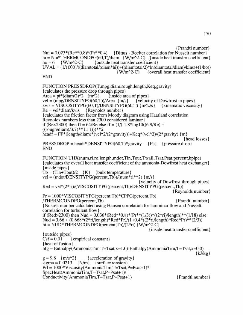
150
( Prandtl number)Nui = 0.023*(Re**0.8)*(Pr**0.4) { Dittus - Boelter correlation for Nusselt number)hi = Nui*THERMCONDPG(60,T)/diam {W/mA2-C) { inside heat transfer coefficient)ho = 6 { W/mA2-CI (I{outside heat transfer coefficient)UVAL = (1/1000)/((diamtotal/(diam*hi))+((diamtotal/2)*ln(diamtotal/diam)/kins)+(1/ho))
{ W/mA2-C) (overall heat transfer coefficient)END
FUNCTION PRESSDROP(T,mpg,diam,rough,length,Keq,gravity)(calculates the pressure drop through pipes)Area = pi*(diam/2)A2 {mA2) (Iinside area of pipes)vel = (mpg/DENSITYPG(60,T))/Area {m/sI {velocity of Dowfrost in pipes)kvis = VISCOSITYPG(60,T)/DENSITYPG(60,T) I(mA2/s) (kinematic viscosity)Re = vel*diamnkvis {Reynolds number)( calculates the friction factor from Moody diagram using Haarland correlationReynolds numbers less than 2300 considered laminar)if (Re<2300) then ff = 64/Re else ff = (1/(-1.8*log10((6.9/Re) +((rough/diam)/3.7)** 1.11)))**2headf = FF*(length/diam)*(velA2/(2*gravity))+Keq*(velA2)/(2*gravity) (m)
( head losses)PRESSDROP = headf*DENSITYPG(60,T)*gravity (Pa) (pressure drop)END
FUNCTION UHX(num,ri,ro,length,mdot,Tin,Tout,Twall,Tsat,Psat,percent,kpipe)(calculates the overall heat transfer coefficient of the ammonia-Dowfrost heat exchanger)(inside pipes)ITb = (Tin+Tout)/2 (K) (bulk temperature)vel = (mdot/DENSITYPG(percent,Th))/(num*ri**2) (m/s)
( velocity of Dowfrost through pipes)Red = vel* (2*ri)/(VISCOS ITYPG(percent,Tb)/DENSITYPG(percent,Tb))
( Reynolds number)Pr = 1000*VISCOSITYPG(percent,Tb)*CPPG(percent,Tb)/THERMCONDPG(percent,Tb) ( Prandtl number)( Nusselt number calculated using Hausen correlation for lamminar flow and Nusseltcorrelation for turbulent flow)Iif (Red>2300) then Nud = 0.036*(Red**0.8)*(Pr**(1/3))*((2*ri)/length)**(1/18) elseNud = 3.66 + (0.668*(2*ri/length)*Red*Pr)/(1 +0.4*((2*ri/length)*Red*Pr)**(2/3))hi = NUD*THERMCONDPG(percent,Tb)/(2*ri) {W/mA2-C)I
(inside heat transfer coefficient)(outside pipes)Csf = 0.01 (empirical constant)( heat of fusion)Ihfg = Enthalpy(AmmoniaTim,T=Tsat,x=1.0)-Enthalpy(AmmoniaTim,T=Tsat,x=0.0)
(kJ/kg)g = 9.8 {(m/sA2) ({acceleration of gravity)sigma = 0.0213 (N/in) (surface tension)}Prl = 1 000*Viscosity(AmmoniaTim,T=Tsat,P=Psat+ 1 )*S pecHeat(ArmmoniaTim,T=Ts at,P=Psat+ 1 )/Conductivity(AmnmoniaTim,T=Tsat,P=Psat+ 1) ( Prandtl number)

151
Area = 2*pi*ro*length*num {total heat transfer area){ boiling heat transfer coefficient from Rohsenow correlation)ho = 1000*Viscosity(AmmoniaTim,T=Tsat,P=Psat+ 1)*hfg*((g*(l/Volume(AmmoniaTim,T=Tsat,x=0.0)-l/Volume(AmmoniaTim,T=Tsat,x= 1.0))/sigma)**0.5)*((SpecHeat(AmmoniaTim,T=Tsat,P=Psat- 1)/(Csf*hfg*Prl** 1.7))**3)*(Twall-Tsat)**2
(W/mA2-CI(UvalueIUHX = (1/1000)/((ro/(ri*hi))+(ro*ln(ro/ri)/kpipe) + (1/ho)) {W/mA2-C}
{overall heat transfer coefficient)END
FUNCTION UCASE(num,ri,ro,length,mdot,airvel,airarea,Tref,percent,Tair,kpipe)(calculates the overall heat transfer coefficient of the refrigerated case heat exchanger)(inside pipe)Ivel = (mdot/DENSITYPG(percent,Tref))/(num*ri**2) {m/s}
( velocity of Dowfrost through pipes)Redi = vel*(2*ri)/(VISCOSITYPG(percent,Tref)/DENSITYPG(percent,Tref))( Reynolds number)Pri = 1000*VIS COS ITYPG(percent,Tref)*CPPG(percent,Tref)/THERMCONDPG(percent,Tref) ( Prandtl number)( Nusselt number calculated using Hausen correlation for laminar flow and Nusseltcorrelation for turbulent flow)Iif (Redi>2300) then Nudi = 0.036*(Redi**0.8)*(Pri**(1/3))*((2*ri)/length)**(1/18)else Nudi = 3.66 +(0.668*(2*ri/length)*Redi*Pri)/(1 +0.4*((2*ri/length)*Redi*Pri)**(2/3))hi = NUDI*THERMCONDPG(percent,Tref)/(2*ri) {W/mA2-C)I
(inside heat transfer coefficient)(outside pipes)Redo = airvel* (2*ro)/(Viscosity(Air,T=Tair)/(l/Volume(Air,T=Tair,P= 101.325)))(Reynolds number)Pro = 1000*Viscosity(Air,T=Tair)*SpecHeat(Air,T=Tair)/Conductivity(Air,T=Tair)(Prandtl number)(Nusselt number using Churchill Bernstein correlation)Nudo = 0.3+((0.62*Redo**(1/2)*Pro** (1/3))/((1 +(0.4/Pro)**(2/3))** (1/4)))*(1 +(Redo/2.82e5)** (5/8))** (4/5)ho = Nudo*Conductivity(Air,T=Tair)/(2*ro) {W/mA2-C)I
(outside heat transfer coefficient)UCASE = (1/((ro/(ri*hi))+(ro*ln(ro/ri)/kpipe) + (1/ho)))/1000 (W/mA2-C}
(overall heat transfer coefficient)END
( The equation set begins here}
(parameters)Tairout = 267 ( K) (temperature of air leaving refrigerated case)caseload = 15({tons)}'3.5 1685 (kW) ({refrigeration load met by the case)}UAcond = 8.00 (kW/K} ( UA value of the condenser)}Tamb = 300 ( K) ({ambient temperature)}
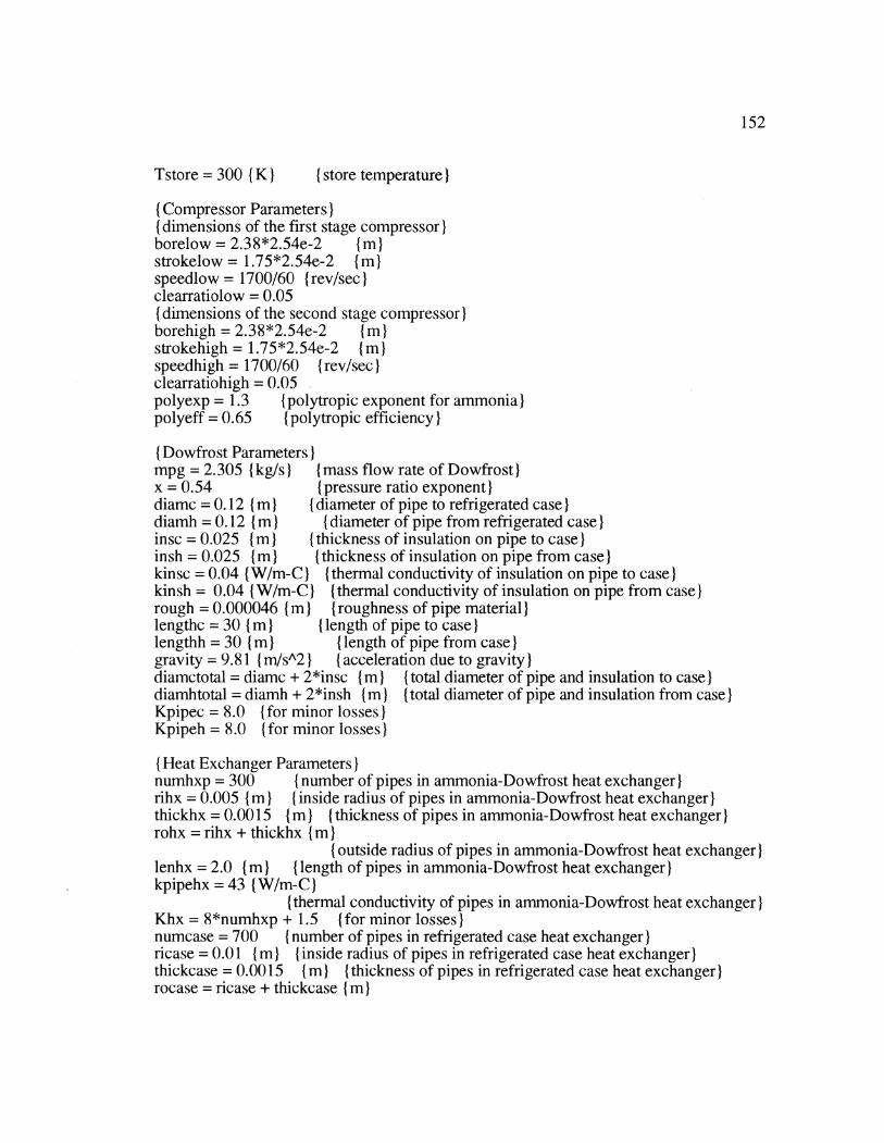
152
Tstore = 300 ( K)} { store temperature)
(Compressor Parameters)I{ dimensions of the first stage compressor)borelow = 2.38*2.54e-2 {m)strokelow = 1.75*2.54e-2 {m)speedlow = 1700/60 (rev/sec}clearratiolow = 0.05(dimensions of the second stage compressor)borehigh = 2.38*2.54e-2 {m)strokehigh = 1.75*2.54e-2 imspeedhigh = 1700/60 (rev/sec)clearratiohigh = 0.05polyexp = 1.3 ( polytropic exponent for ammonia)polyeff = 0.65 (polytropic efficiency)
( Dowfrost Parameters)Impg = 2.305 {kg/s} {mass flow rate of Dowfrost)x = 0.54 (pressure ratio exponent)Idiamc = 0.12 { m) (Idiameter of pipe to refrigerated case)diamh = 0.12 { m) { diameter of pipe from refrigerated case)insc = 0.025 {m) I { thickness of insulation on pipe to case)Iinsh = 0.025 (i) (thickness of insulation on pipe from case)kinsc = 0.04 (W/m-C) (thermal conductivity of insulation on pipe to case)kinsh = 0.04 (W/m-C) (thermal conductivity of insulation on pipe from case)rough = 0.000046 ( m roughness of pipe material)lengthc = 30 (i m(length of pipe to case)Ilengthh = 30 (in (}length of pipe from case)gravity = 9.81 {(m/sA2) (acceleration due to gravity)diamctotal = diamc + 2*insc I) (m{total diameter of pipe and insulation to case)diamhtotal = diamh + 2*insh i m (total diameter of pipe and insulation from case)Kpipec = 8.0 (for minor losses)IKpipeh = 8.0 ( for minor losses)
( Heat Exchanger Parameters)Inumhxp = 300 (number of pipes in ammonia-Dowfrost heat exchanger)rihx = 0.005 (in m (inside radius of pipes in ammonia-Dowfrost heat exchanger)thickhx = 0.0015 { m) (thickness of pipes in ammonia-Dowfrost heat exchanger)rohx = rihx + thickhx ( mI
(outside radius of pipes in ammonia-Dowfrost heat exchanger)lenhx = 2.0 ( m (length of pipes in ammonia-Dowfrost heat exchanger)kpipehx = 43 {(W/m-C)I
( thermal conductivity of pipes in ammonia-Dowfrost heat exchanger)Khx = 8*numhxp + 1.5 (for minor losses)numcase = 700 (number of pipes in refrigerated case heat exchanger)Iricase = 0.01 (in ( {inside radius of pipes in refrigerated case heat exchanger)}thickcase = 0.0015 (in (}{thickness of pipes in refrigerated case heat exchanger)}rocase-= ricase + thickcase (in)
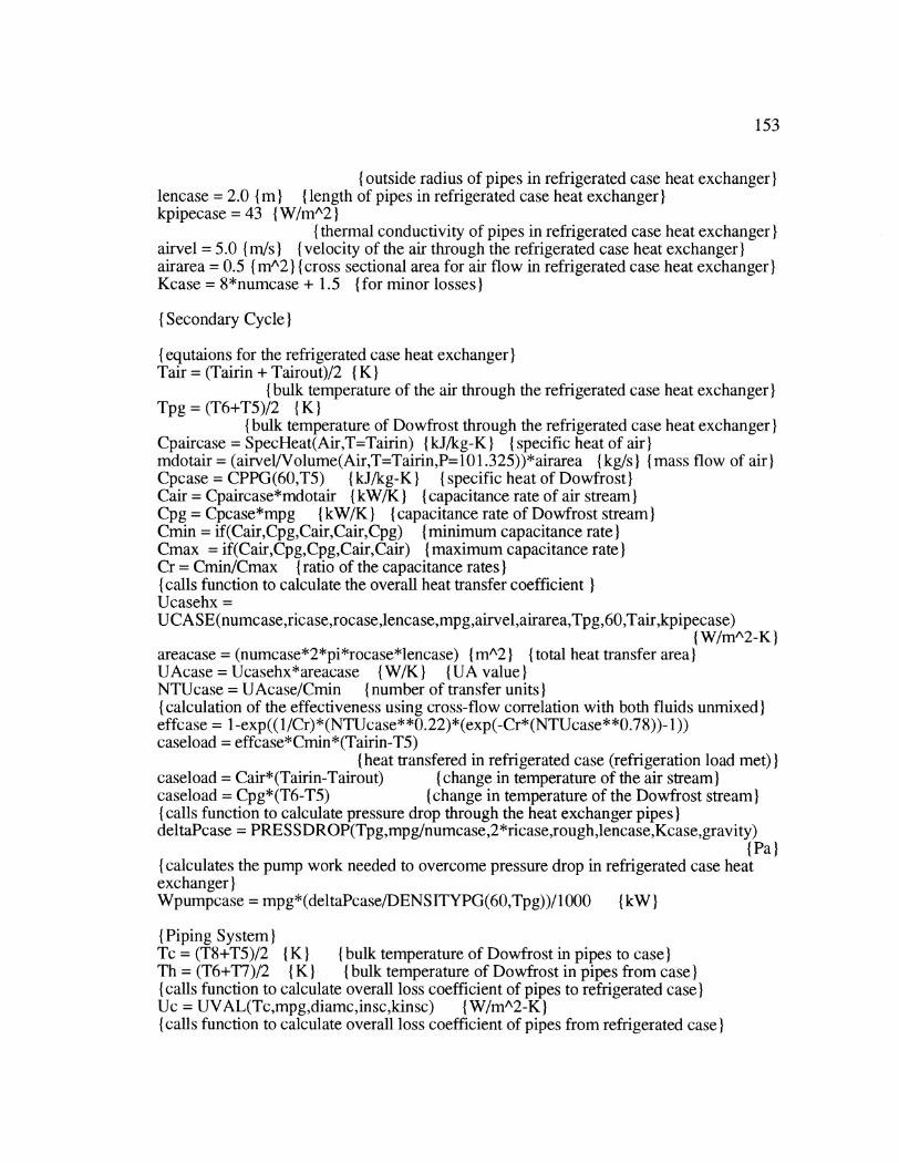
153
{outside radius of pipes in refrigerated case heat exchanger)lencase = 2.0 { m) (length of pipes in refrigerated case heat exchanger)kpipecase = 43 {W/mA2)
( thermal conductivity of pipes in refrigerated case heat exchanger)airvel = 5.0 (m/s) (velocity of the air through the refrigerated case heat exchanger)Iairarea = 0.5 {(mA2 (I{cross sectional area for air flow in refrigerated case heat exchanger)Kcase = 8*numcase + 1.5 (for minor losses)
(Secondary Cycle)I
(equtaions for the refrigerated case heat exchanger)Tair = (Tairin + Tairout)/2 (K)
(bulk temperature of the air through the refrigerated case heat exchanger)Tpg = (T6+T5)/2 (IK)
( bulk temperature of Dowfrost through the refrigerated case heat exchanger)Cpaircase = SpecHeat(Air,T=Tairin) I(kJ/kg-KI (I{specific heat of air)mdotair = (airvel/Volume(Air,T=Tairin,P= 101.325))*airarea (kg/s) ( Imass flow of air)Cpcase = CPPG(60,T5) (kJ/kg-K) (Ispecific heat of Dowfrost)Cair = Cpaircase*mdotair (kW/K) (Icapacitance rate of air stream)Cpg = Cpcase*mpg (kW/K) (Icapacitance rate of Dowfrost stream)Cmin = if(Cair,Cpg,Cair,Cair,Cpg) (minimum capacitance rate)Cmax = if(Cair,Cpg,Cpg,Cair,Cair) (maximum capacitance rate)Cr = Cmin/Cmax (ratio of the capacitance rates)( calls function to calculate the overall heat transfer coefficient)Ucasehx =UCASE(numcase,ricase,rocase,lencase,mpg,airvel,airarea,Tpg,60,Tair,kpipecase)
{W/mA2-K)areacase = (numcase*2*pi*rocase*lencase) (mA2) (Itotal heat transfer area)UAcase = Ucasehx*areacase (W/K) (UA value)NTUcase = UAcase/Cmin ( number of transfer units)(calculation of the effectiveness using cross-flow correlation with both fluids unmixed)effcase = 1-exp((1/Cr)*(NTUcase**0.22)*(exp(-Cr*(NTUcase**0.78))- 1))caseload = effcase*Cmin*(Tairin-T5)
( heat transfered in refrigerated case (refrigeration load met))caseload = Cair*(Tairin-Tairout) (change in temperature of the air stream)caseload = Cpg*(T6-T5) (change in temperature of the Dowfrost stream)( calls function to calculate pressure drop through the heat exchanger pipes)IdeltaPcase = PRESSDROP(Tpg,mpg/numcase,2*ricase,rough,lencase,Kcase,gravity)
(Pa)(calculates the pump work needed to overcome pressure drop in refrigerated case heatexchanger)Wpumpcase - mpg*(deltaPcase/DENSITYPG(60,Tpg))/1000 (kW)
( Piping System)ITc = (T8+T5)/2 (K) (bulk temperature of Dowfrost in pipes to case)Th = (T6+T7)/2 ( K) ( bulk temperature of Dowfrost in pipes from case)}(calls function to calculate overall loss coefficient of pipes to refrigerated case)Uc = UVAL(Tc,mpg,diamc,insc,kinsc) ( W/m^2-K)( calls function to calculate overall loss coefficient of pipes from refrigerated case)}

154
Uh = UVAL(Th,mpg,diamh,insh,kinsh) (W/mA2-K){ calls function to determine pressure drop in pipes to refrigerated case)IdeltaPc = PRES SDROP(Tc,mpg,diamc,rough,lengthc,Kpipec,gravity) { Pa)( calls function to determine pressure drop in pipes from refrigerated case)deltaPh = PRESSDROP(Th,mpg,diamh,rough,lengthh,Kpipeh,gravity) (Pa)
densityc = DENSITYPG(60,Tc) {kg/mA3)} {density of Dowfrost in pipes to case)densityh = DENSITYPG(60,Th) {kg/mA3} {density of Dowfrost inpipes from case)(Pump work necessary to overcome pressure drop in pipes to and from case)IWpumppipe = mpg*(deltaPc/densityc + deltaPh/densityh)/1000 {kW)
(calculates thermal losses of piping system)IAc = pi*diamctotal*lengthc { mA2) (Itotal heat transfer area of pipes to case)Ah = pi*diamhtotal*lengthh { mA2) (Itotal heat transfer are of pipes from case)Cpc = CPPG(60,Tc) {kJ/kg-K) (Ispecific heat of Dowfrost in pipes to case)Cph = CPPG(60,Th) (kJ/kg-K} { specific heat of Dowfrost in pipes from case)Qc = mpg*Cpc*(T5-T8) {kW) {heat loss of Dowfrost stream in pipes to case)Qh = mpg*Cph*(T7-T6) {kW) {heat loss of Dowfrost stream in pipes from case)deltatlmc = (T5-T8)/(ln((Tstore-T8)/(Tstore-T5)))
( log mean temperature difference of pipes to case)deltatlmh = (T7-T6)/(ln((Tstore-T6)/(Tstore-T7)))
( log mean temperature difference of pipes to case)Qc = Uc*Ac*deltatlmc {kW) (heat loss from pipes to case)Qh = Uh*Ah*deltatlmh (kW) (heat loss from pipes from case)NTUc = Uc*Ac/(mpg*Cpc) (number of transfer units in flow to case)NTUh = Uh*Ah/(mpg*Cph) (number of transfer units in flow from case)
( equation for the heat exchanger between Dowfrost and Ammonia)ITwall = T7-(T7-T8)/2 (K) (surface temperature of pipes in the ammonia)( calls function to calculate the overall heat transfer coefficient of heat exchanger)IU = UHX(numhxp,rihx,rohx,lenhx,mpg,T7,T8,Twall,T1,P 1,60,kpipehx) I(W/mA2-K)Iareahx = (2*rohx*pi*lenhx*numhxp) (mA2) (Itotal heat transfer area of heat exchanger)UAhx = U*areahx ( W/K) (IUA value of the heat exchanger)INTUhx = UAhx/(mpg*CPPG(60,T7)) (number of transfer units of heat exchanger)effhx = 1-exp(-NTUhx) (effectiveness of the heat exchanger)effhx = (T7-T8)/(T7-Tl)
(using effectiveness to calculate the temperatures in the heat exchanger)IQhx = mpg*CPPG(60,T7)*(T7-T8) (kW) (heat transfer in heat exchanger)Tmid = (T7+T8)/2 (K) (bulk temperature in Dowfrost in heat exchanger)T1 = T2 (K) (tconstant ammonia temperature in heat exchanger)mref = Qhx/(h2-h1) {1kg/s)I
{calculates necessary ammonia mass flow rate to meet the load)(calls function to determine pressure drop of flow through the heat exchanger)IdeltaPhx = PRES SDROP(Tmid,mpg/numhxp,2*rihx,rough,lenhx,Khx,gravity) (Pa)( calculates pump work needed to overcome pressure drop in heat exchanger)Wpumphx = mpg*(deltaPhxIDENSITYPG(60,Tmid))/l1000 {kW)
P2 = Pressure(AmmoniaTim,T=Tl1,x=l1.0) ( kPa)}(pressure of ammonia leaving heat exchanger)
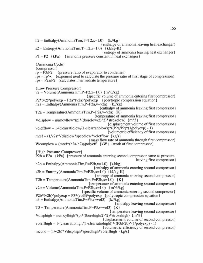
155
h2 = Enthalpy(AmmoniaTim,T=T2,x= 1.0) {kJ/kg)(enthalpy of ammonia leaving heat exchanger)
s2 = Entropy(AmmoniaTim,T=T2,x= 1.0) { kJ/kg-K)(entropy of ammonia leaving heat exchanger)
P1 = P2 {kPa) (ammonia pressure constant in heat exchanger)I
(Ammonia Cycle){compressor)rp = P3/P2 {pressure ratio of evaporator to condenser)rps = rpAX { exponent used to calculate the pressure ratio of first stage of compression)Irps = P2a/P2 {calculates intermediate temperature)I
(Low Pressure Compressor)Iv2 = Volume(AmmoniaTim,P=P2,x=l.0) (mA3/kg)I
( specific volume of ammonia entering first compressor)P2*(v2)Apolyexp = P2a*(v2a)Apolyexp Ipolytropic compression equation)h2a = Enthalpy(AmmoniaTim,P=P2a,v=v2a) (kJ/kg)I
(enthalpy of ammonia leaving first compressor)T2a = Temperature(AmmoniaTim,P=P2a,v=v2a) I K)
I(temperature of ammonia leaving first compressor)Vdisplow = numcyllow*(pi*((borelow/2)A2)*strokelow) { mA3)
(displacement volume of first compressor)volefflow = 1-(clearratiolow/(1-clearratiolow))*((P2a/P2)A(1/polyexp) - 1)
(volumetric efficiency of first compressor)mref = (1/v2)*Vdisplow*speedlow*volefflow (kg/s)
(mass flow rate of ammonia through first compressor)Wcomplow = (mref*(h2a-h2))/polyeff {kW ([work of first compressor)
( High Pressure Compressor)IP2b = P2a (kPa) (pressure of ammonia entering second compressor same as pressure
leaving first compressor)h2b = Enthalpy(AmmoniaTim,P=P2b,x= 1.0) {kJ/kg)I
{ enthalpy of ammonia entering second compressor)s2b = Entropy(AmmoniaTim,P=P2b,x=l .0) {kJ/kg-K)
( entropy of ammonia entering second compressor)T2b = Temperature(AmmoniaTim,P=P2b,x= 1.0) ( K)
( temperature of ammonia entering second compressor)v2b = Volume(AmmoniaTim,P=P2b,x=1.0) {mA3/kg)
(specific volume of ammonia entering second compressor)P2b*(v2b)Apolyexp = P3*(vol3)Apolyexp (polytropic compression equation)h3 = Enthalpy(AmmoniaTim,P=P3,v=vol3) {kJ/kg)I
(enthalpy leaving second compressor)T3 = Temperature(AmmoniaTim,P=P3,v=vol3) ( K)
( temperature leaving second compressor)Vdisphigh = numcylhigh*(pi*((borehigh/2)A2)*strokehigh) { mA3)
(displacement volume of second compressor)}voleffhigh = 1-(clearratiohigh/(1-clearratiohigh))*((P3/P2b)A( 1/polyexp) - 1)
( volumetric efficiency of second compressor)}mcond = (1/v2b)*Vdisphigh*speedhigh*voleffhigh {(kg/s)}
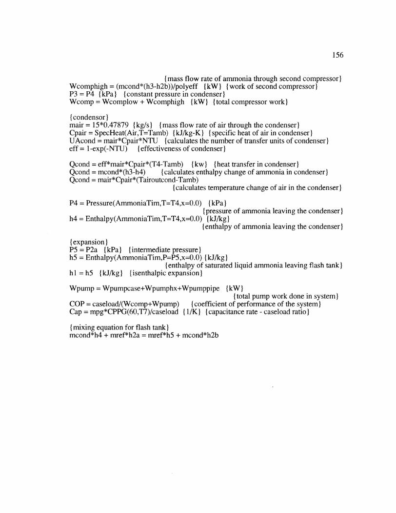
156
(mass flow rate of ammonia through second compressor)Wcomphigh = (mcond*(h3-h2b))/polyeff {kW) (work of second compressor)P3 = P4 {kPa) (constant pressure in condenser)Wcomp = Wcomplow + Wcomphigh {kW) (total compressor work)
(condensor)mair = 15*0.47879 (kg/s) (mass flow rate of air through the condenser)Cpair = SpecHeat(Air,T=Tamb) I(kJ/kg-KI (I{specific heat of air in condenser)IUAcond = mair*Cpair*NTU (calculates the number of transfer units of condenser)eff = 1-exp(-NTU) (effectiveness of condenser)
Qcond = eff*mair*Cpair*(T4-Tamb) (kw) (heat transfer in condenser)Qcond = mcond*(h3-h4) (calculates enthalpy change of ammonia in condenser)Qcond = mair*Cpair*(Tairoutcond-Tamb)
(calculates temperature change of air in the condenser)
P4 = Pressure(AmmoniaTim,T=T4,x=0.0) (kPa)(pressure of ammonia leaving the condenser)
h4 = Enthalpy(AmmoniaTim,T=T4,x=0.0) (kJ/kg)(enthalpy of ammonia leaving the condenser)
(expansion)P5 = P2a (kPa) (intermediate pressure)h5 = Enthalpy(AmmoniaTim,P=P5,x=0.0) {kJ/kg)
(enthalpy of saturated liquid ammonia leaving flash tank)hl = h5 (kJ/kg) (isenthalpic expansion)
Wpump = Wpumpcase+Wpumphx+Wpumppipe (kW)(total pump work done in system)
COP = caseload/(Wcomp+Wpump) (coefficient of performance of the system)Cap = mpg*CPPG(60,T7)/caseload (1/K) (capacitance rate - caseload ratio)I
(mixing equation for flash tank)mcond*h4 + mref*h2a = mref*h5 + mcond*h2b
APPENDIX
157
C
R22 - AMMONIA COMPARISON MODELS
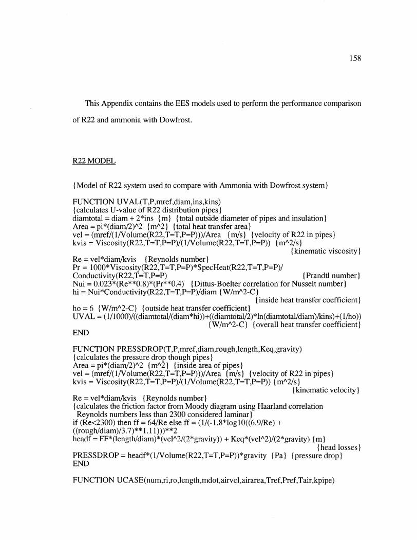
158
This Appendix contains the EES models used to perform the performance comparison
of R22 and ammonia with Dowfrost.
R22 MODEL
{ Model of R22 system used to compare with Ammonia with Dowfrost system)
FUNCTION UVAL(T,P,mref,diam,ins,kins){ calculates U-value of R22 distribution pipes)Idiamtotal= diam + 2*ins { m) (total outside diameter of pipes and insulation)Area = pi*(diam/2)A2 {mA2} { total heat transfer area)Ivel = (mref/(1/Volume(R22,T=T,P=P)))/Area I(m/s) ({Ivelocity of R22 in pipes)Ikvis = Viscosity(R22,T=T,P=P)/(I/Volume(R22,T=T,P=P)) { mA2/s)
(kinematic viscosity)Re = vel*diam/kvis ( Reynolds number)Pr = 1000*Viscosity(R22,T=T,P=P)*SpecHeat(R22,T=T,P=P)/Conductivity(R22,T=T,P=P) I(Prandtl number)Nui = 0.023*(Re**0.8)*(Pr**0.4) (Dittus-Boelter correlation for Nusselt number)hi = Nui*Conductivity(R22,T=T,P=P)/diam I(W/m^12-C)
( inside heat transfer coefficient)ho = 6 {W/m^2-C) (Ioutside heat transfer coefficient)UVAL = (1/1000)/((diamtotal/(diam*hi))+((diamtotal/2)*ln(diamtotal/diam)/kins)+(1/ho))
(W/mA2-C) (overall heat transfer coefficient)END
FUNCTION PRES SDROP(T,P,mref,diamrough,length,Keq,gravity)(calculates the pressure drop though pipes)IArea = pi*(diam/2)A2 {(mA2) (finside area of pipes)vel = (mref/(1/Volume(R22,T=T,P=P)))/Area ( m/s) ({Ivelocity of R22 in pipes)kvis = Viscosity(R22,T=T,P=P)/(1/Volume(R22,T=T,P=P)) (mA2/s)
( kinematic velocity)Re = vel*diamlkvis (Reynolds number)(calculates the friction factor from Moody diagram using Haarland correlationReynolds numbers less than 2300 considered laminar)
if (Re<2300) then ff = 64/Re else ff = (1/(-1.8*logl0((6.9/Re) +((rough/diam)/3.7)** 1.11)))**2headf = FF*(length/diam)*(velA2/(2*gravity)) + Keq*(velA2)/(2*gravity) (m
( head losses)PRESSDROP = headf*(I1/Volume(R22,T=T,P=P))*gravity (Pa) (pressure drop)END
FUNCTION UCA SE(num,ri,ro,length,mdot, airvel,airarea,Tref, Pref, Tair,kpipe)
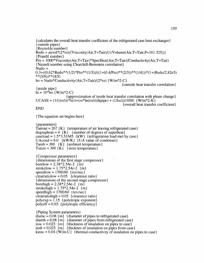
159
{calculates the overall heat transfer coefficient of the refrigerated case heat exchanger){ outside pipes)I{ Reynolds number)Redo = airvel*(2*ro)/(Viscosity(Air,T=Tair)/(l/Volume(Air,T=Tair,P= 101.325)))I Prandtl number)IPro = 1000*Viscosity(Air,T=Tair)*SpecHeat(Air,T=Tair)/Conductivity(Air,T=Tair)( Nusselt number using Churchill-Bernstein correlation)Nudo =0.3+((0.62*Redo**( 1/2)*Pro**( 1/3))/(( 1 +(0.4/Pro)** (2/3))**( 1/4)))*(1 +(Redo/2.82e5)**(5/8))**(4/5)ho = Nudo*Conductivity(AirT=Tair)/(2*ro) I(W/mA12-C)
(outside heat transfer correlation)(inside pipe)hi = 10*ho {W/mA2-C)I
(approximation of inside heat transfer correlation with phase change)UCASE = (1/((ro/(ri*hi))+(ro*ln(ro/ri)/kpipe) + (1/ho)))/1000 {W/mA2-K)I
{ overall heat transfer coefficient)END
{ The equation set begins here)I
( parameters)ITairout = 267 ( K) (temperature of air leaving refrigerated case)Idegsupheat = 4 (K) (number of degrees of superheat)caseload = 1.5*3.51685 (kW) (refrigeration load met by case)UAcond = 8.0 (kW/K) (IUA value of condenser)Tamb = 300 (K) { ambient temperature)ITstore = 300 (1K) (store temperature)
( Compressor parameters)I(dimensions of the first stage compressor)Iborelow = 2.38*2.54e-2 imstrokelow = 1.75*2.54e-2 imspeedlow= 1700/60 (rev/sec)clearratiolow = 0.05 (clearence ratio)( dimensions of the second stage compressor)Iborehigh = 2.38*2.54e-2 (m)strokehigh = 1.75*2.54e-2 imspeedhigh = 1700/60 (rev/sec)Iclearratiohigh = 0.05 (clearence ratio)polyexp = 1.15 ( polytropic exponent)polyeff = 0.65 (polytropic efficiency)
( Piping System parameters)Idiamc = 0.08 (i {diameter of pipes to refrigerated case)diamnh = 0.08 (in ( {diameter of pipes from refrigerated case)}insc = 0.025 (in ( thickness of insulation on pipes to case)}insh = 0.025 (in ( {thicknes of insulation on pipes from case)}kinsc = 0.04 (W/m-C) (thermal conductivity of insulation on pipes to case)
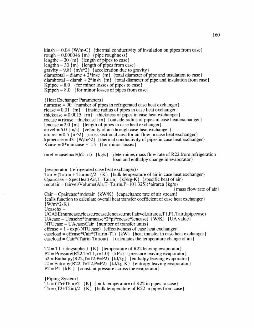
160
kinsh = 0.04 (W/m-C) (thermal conductivity of insulation on pipes from case)rough = 0.000046 {m) {pipe roughness)Ilengthc = 30 ( m (length of pipes to case)lengthh = 30 ( m (length of pipes from case)gravity = 9.81 {rm/sA2} { acceleration due to gravity)diamctotal = diamc + 2*insc { mI { total diameter of pipe and insulation to case)diamhtotal = diamh + 2*insh { m} { total diameter of pipe and insulation from case)Kpipec = 8.0 (for minor losses of pipes to case)IKpipeh = 8.0 (for minor losses of pipes from case)
( Heat Exchanger Parameters)Inumcase = 90 (number of pipes in refrigerated case heat exchanger)ricase = 0.01 ( m ({Iinside radius of pipes in case heat exchanger)Ithickcase = 0.0015 (I (Ithickness of pipes in case heat exchanger)rocase = ricase +thickcase I) (m}outside radius of pipes in case heat exchanger)lencase = 2.0 im (length of pipes in case heat exchanger)airvel = 5.0 (m/s) (velocity of air through case heat exchanger)airarea = 0.5 {(mA21 (Icross sectional area for air flow in case heat exchanger)kpipecase = 43 (W/mA2) (Ithermal conductivity of pipes in case heat exchanger)Kcase = 8*numcase + 1.5 (for minor losses)
mref = caseload/(h2-h 1) (kg/s) (Idetermines mass flow rate of R22 from refrigerationload and enthalpy change in evaporator)
(evaporator (refrigerated case heat exchanger))Tair = (Tairin + Tairout)/2 (K) (bulk temperature of air in case heat exchanger)Cpaircase = SpecHeat(Air,T=Tairin) (kJ/kg-K) (Ispecific heat of air)mdotair = (airvellVolume(Air,T=Tairin,P=101.325))*airarea (kg/s)
(mass flow rate of air)Cair = Cpaircase*mdotair {(kW/K) ({Icapacitance rate of air stream)I( calls function to calculate overall heat transfer coefficient of case heat exchanger){W/mA2-K)Ucasehx =UCASE(numcase,ricase,rocase,lencase,mref,airvel,airarea,T 1 ,P 1 ,Tair,kpipecase)UAcase = Ucasehx*(numcase*2*pi*rocase*lencase) (W/K) (UA value)NTUcase = UAcase/Cair (number of transfer units)Ieffcase = 1 - exp(-NTUcase) ( effectiveness of case heat exchanger)caseload = effcase*Cair*(Tairin-T1) (kW) (Iheat transfer in case heat exchanger)caseload = Cair*(Tairin-Tairout) (calculates the temperature change of air)
T2 = T1 + degsupheat (K }(temperature of R22 leaving evaporator)P2 = Pressure(R22,T=T1,x= 1.0) (kPa) (Ipressure leaving evaporator)h2 = Enthalpy(R22,T=T2,P=P2) (kJ/kg) (enthalpy leaving evaporator)s2 = Entropy(R22,T=T2,P=P2) (kJ/kg-K) (Ientropy leaving evaporator)IP2 = P1 (kPa (constant pressure across the evaporator)}
( Piping System)}Tc = (T6+T6in)/2 (K) ( {bulk temperature of R22 in pipes to case)}Th = (T2+T2in)/2 (K) (bulk temperature of R22 in pipes from case)
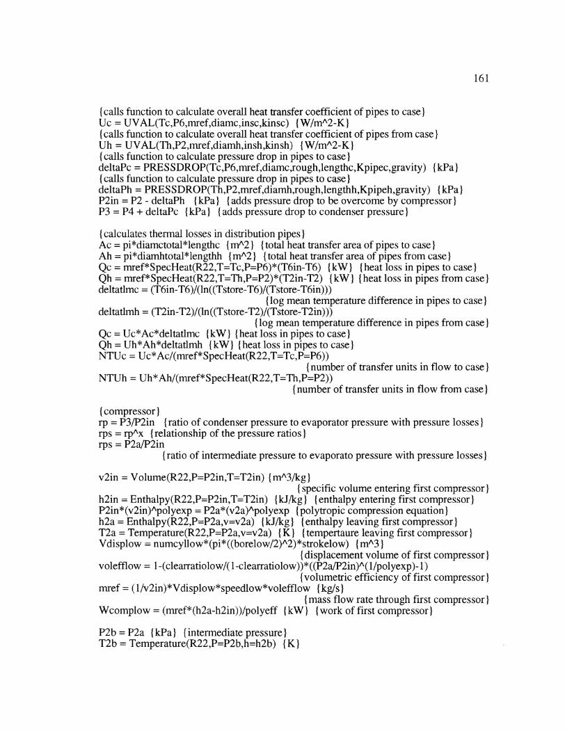
161
{ calls function to calculate overall heat transfer coefficient of pipes to case)Uc = UVAL(Tc,P6,mref,diamc,insc,kinsc) {W/mA2-K)I( calls function to calculate overall heat transfer coefficient of pipes from case)IUh = UVAL(Th,P2,mref,diamh,insh,kinsh) {W/mA2-K)I{ calls function to calculate pressure drop in pipes to case)IdeltaPc = PRESSDROP(Tc,P6,mref,diamc,rough,lengthc,Kpipec,gravity) (kPa)( calls function to calculate pressure drop in pipes to case)IdeltaPh = PRES SDROP(Th,P2,mref,diamh,rough,lengthh,Kpipeh,gravity) (kPa)P2in = P2 - deltaPh {kPa) { adds pressure drop to be overcome by compressor)P3 = P4 + deltaPc {kPa) (adds pressure drop to condenser pressure)
{ calculates thermal losses in distribution pipes)IAc = pi*diamctotal*lengthc (m^12) (Itotal heat transfer area of pipes to case)Ah = pi*diamhtotal*lengthh {mA2) ({total heat transfer area of pipes from case)Qc = mref*SpecHeat(R22,T=Tc,P=P6)*(T6in-T6) {kW) (heat loss in pipes to case)Qh = mref*SpecHeat(R22,T=Th,P=P2)*(T2in-T2) (kW }(heat loss in pipes from case)deltatlmc = (T6in-T6)/(ln((Tstore-T6)/(Tstore-T6in)))
(log mean temperature difference in pipes to case)deltatlmh = (T2in-T2)/(ln((Tstore-T2)/(Tstore-T2in)))
(log mean temperature difference in pipes from case)Qc = Uc*Ac*deltatlmc (kW) (heat loss in pipes to case)IQh = Uh*Ah*deltatlmh (kW) (heat loss in pipes to case)NTUc = Uc*Ac/(rnref*SpecHeat(R22,T=Tc,P=P6))
(number of transfer units in flow to case)NTUh = Uh*Ah/(mref*SpecHeat(R22,T=Th,P=P2))
(number of transfer units in flow from case)
(compressor)rp = P3/P2in (ratio of condenser pressure to evaporator pressure with pressure losses)rps = rpAx (Irelationship of the pressure ratios)rps = P2a/P2in
( ratio of intermediate pressure to evaporato pressure with pressure losses)
v2in = Volume(R22,P=P2in,T=T2in) (mA3/kg)I(specific volume entering first compressor)
h2in = Enthalpy(R22,P=P2in,T=T2in) (kJ/kg) ({Ienthalpy entering first compressor)P2in*(v2in)Apolyexp = P2a*(v2a)Apolyexp (polytropic compression equation)h2a = Enthalpy(R22,P=P2a,v=v2a) (kJ/kg) (Ienthalpy leaving first compressor)IT2a = Temperature(R22,P=P2a,v=v2a) (K) (Itempertaure leaving first compressor)IVdisplow = numcyllow*(pi*((borelow/2)A2)*strokelow) (mA3)
( displacement volume of first compressor)Ivolefflow = 1-(clearratiolow/( 1-clearratiolow))*((P2a/P2in)A(l/polyexp)- 1)
(volumetric efficiency of first compressor)Imref = (1/v2in)*Vdisplow*speedlow*volefflow (kg/s)
( mass flow rate through first compressor)Wcomplow = (mref*(h2a-h2in))/polyeff ( kW) ( work of first compressor)}
P2b = P2a {(kPa) ( intermediate pressure)}T2b = Temperature(R22,P=P2b,h=h2b) (K)}
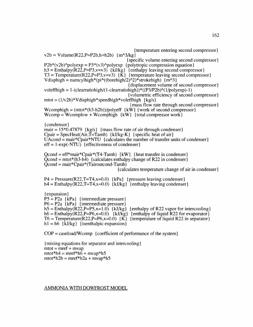
162
(temperature entering second compressor)v2b = Volume(R22,P=P2b,h=h2b) { m^3/kg)I
(specific volume entering second comlressorIP2b*(v2b)Apolyexp = P3*(v3)Apolyexp ( polytropic compression equation)Ih3 = Enthalpy(R22,P=P3,v=v3) { kJ/kgI (I{enthalpy leaving second compressor)IT3 = Temperature(R22,P=P3,v=v3) (K) (temperature leaving second compressor)Vdisphigh = numcylhigh*(pi*((borehigh/2)A2)*strokehigh) { mA3)
(displacement volume of second compressor)voleffhigh = 1-(clearratiohigh/(1-clearratiohigh))*((P3/P2b)A(1/polyexp)- 1)
(volumetric efficiency of second compressor)mtot = (1/v2b)*Vdisphigh*speedhigh*voleffhigh (kg/s)
{mass flow rate through second compressor)Wcomphigh = (mtot*(h3-h2b))/polyeff {kW) (work of second compressor)Wcomp = Wcomplow + Wcomphigh {kW) (total compressor work)
(condensor)mair = 15*0.47879 {kg/s) (mass flow rate of air through condenser)Cpair = SpecHeat(Air,T=Tamb) I(kJ/kg-K) ( Ispecific heat of air)IUAcond = mair*Cpair*NTU ( calculates the number of transfer units of condenser)eff = 1-exp(-NTU) ( effectiveness of condenser)I
Qcond = eff*mair*Cpair*(T4-Tamb) {kW) (heat transfer in condenser)Qcond = mtot*(h3-h4) (calculates enthalpy change of R22 in condenser)Qcond = mair*Cpair*(Tairoutcond-Tamb)
(calculates temperature change of air in condenser)
P4 = Pressure(R22,T=T4,x=0.0) {kPa) (pressure leaving condenser)h4 = Enthalpy(R22,T=T4,x=0.0) (kJ/kg) (Ienthalpy leaving condenser)
( expansion)IP5 = P2a (kPa) ( Iintermediate pressure)IP6 = P2a (kPa) (Iintermediate pressure)h5 = Enthalpy(R22,P=P5,x=1.0) 1(kJ/kg) }{Ienthalpy of R22 vapor for intercooling)Ih6 = Enthalpy(R22,P=P6,x=0.0) (kJ/kg) (enthalpy of liquid R22 for evaporator)T6 = Temperature(R22,P=P6,x=0.0) ( K) ({Itemperature of liquid R22 in separator)Ih 1 = h6 {kJ/kg) (Iisenthalpic expansion)I
COP = caseload/Wcomp (coefficient of performance of the system)
(mixing equations for separator and intercooling)Imtot = mref + mvapmtot*h4 = mref*h6 + mvap*h5mtot*h2b = mref*h2a + mvap*h5
AMMONIA WITH DOWFROST MODEL
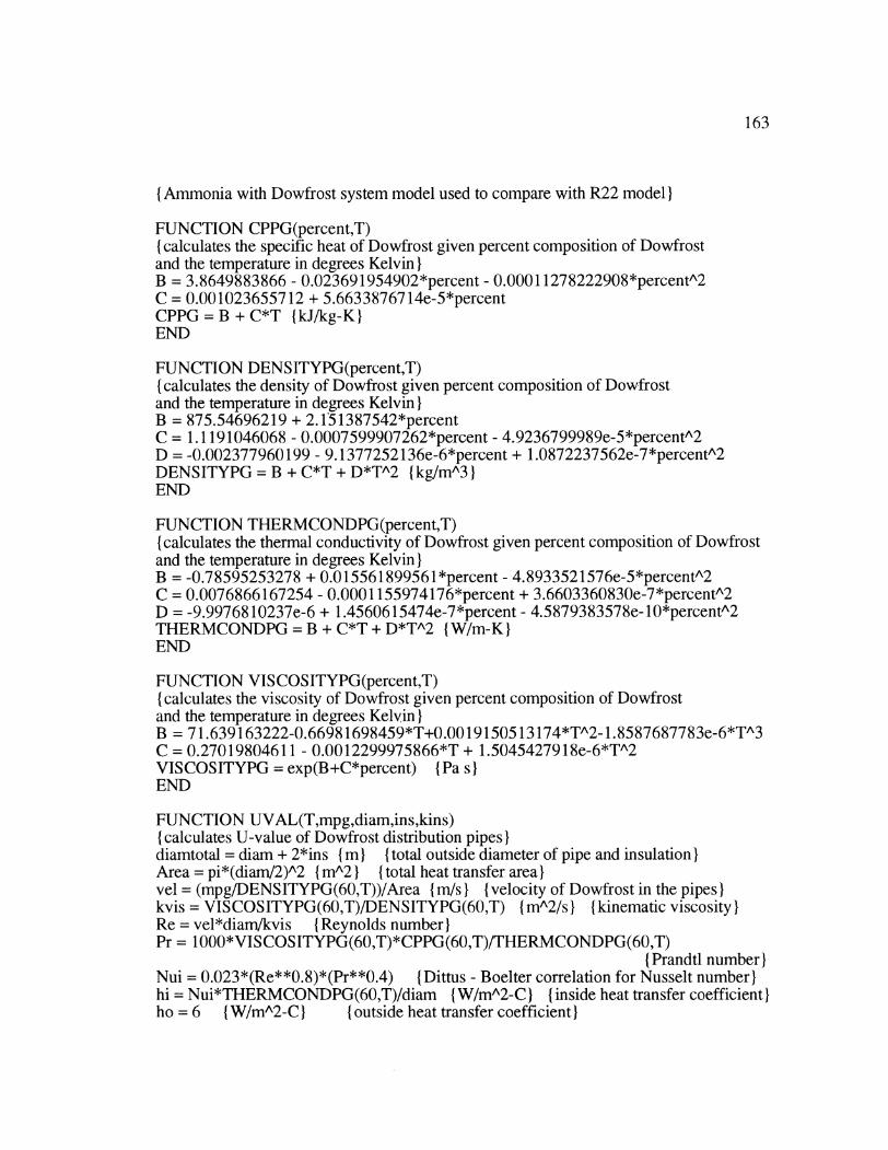
163
{ Ammonia with Dowfrost system model used to compare with R22 model }
FUNCTION CPPG(percent,T)( calculates the specific heat of Dowfrost given percent composition of Dowfrostand the temperature in degrees Kelvin)IB = 3.8649883866 - 0.023691954902*percent - 0.00011278222908*percentA2C = 0.001023655712 + 5.6633876714e-5*percentCPPG = B + C*T {kJ/kg-K}END
FUNCTION DENSITYPG(percent,T)( calculates the density of Dowfrost given percent composition of Dowfrostand the temperature in degrees Kelvin)IB = 875.54696219 + 2.15 1387542*percentC = 1.1191046068 - 0.0007599907262*percent - 4.9236799989e-5*percentA2D = -0.002377960199 - 9.1377252136e-6*percent + 1.0872237562e-7*percentA2DENSITYPG = B + C*T + D*TA2 (kg/mA3)END
FUNCTION THERMCONDPG(percent,T)( calculates the thermal conductivity of Dowfrost given percent composition of Dowfrostand the temperature in degrees Kelvin IB = -0.78595253278 + 0.01556189956 1*percent - 4.8933521576e-5*percentA2C = 0.0076866167254 - 0.0001155974176*percent + 3.6603360830e-7*percentA2D = -9.9976810237e-6 + 1.4560615474e-7*percent - 4.5879383578e-10*percentA2THERMCONDPG = B + C*T + D*TA2 {W/m-K}END
FUNCTION VISCOSITYPG(percent,T)( calculates the viscosity of Dowfrost given percent composition of Dowfrostand the temperature in degrees Kelvin)B = 71.639163222-0.66981698459*T+0.0019150513174*TA2 -1.8587687783e-6*TA3C = 0.27019804611 - 0.0012299975866*T + 1.5045427918e-6*TA2VISCOSITYPG = exp(B+C*percent) (Pa s)END
FUNCTION UVAL(T,mpg,diam,ins,kins)( calculates U-value of Dowfrost distribution pipes)diamtotal = diam + 2*ins i) m total outside diameter of pipe and insulation)Area = pi*(diam/2)A2 (mA2 }(total heat transfer area)vel = (mpg/DENSITYPG(60,T))/Area (m/s) (Ivelocity of Dowfrost in the pipes)Ikvis = VISCOSITYPG(60,T)/DENSITYPG(60,T) (mA2/sI} (kinematic viscosity)Re = vel*diamnkvis ( Reynolds number)Pr = 1000*VISCOSITYPG(60,T)*CPPG(60,T)/THERMCONDPG(60,T)
(Prandtl number)Nui = 0.023*(Re**0.8)*(Pr**0.4) (Dittus - Boelter correlation for Nusselt number)hi = Nui*THERMCONDPG(60,T)/diam {(W/m^2-C) ( inside heat transfer coefficient)}ho = 6 {(W/m^2-C) ({outside heat transfer coefficient)
164
UVAL = (1/1000)/((diamtotal/(diam*hi))+((diamtotal/2)*ln(diamtotal/diam)/kins)+(1/ho)){W/mA2-C)} { overall heat transfer coefficient)
END
FUNCTION PRESS DROP(T,mp g,diam,rough,length,Keq,gravity)(calculates the pressure drop through pipes)IArea = pi*(diam/2)A2 {mA2) (Iinside area of pipes)vel = (mpg/DENSITYPG(60,T))/Area ( m/s) (Ivelocity of Dowfrost in pipes)kvis = VISCOSITYPG(60,T)/DENSITYPG(60,T) { mA2/s) (kinematic viscosity)Re = vel*diam/kvis (IReynolds number)( calculates the friction factor from Moody diagram using Haarland correlationReynolds numbers less than 2300 considered laminar)if (Re<2300) then ff = 64/Re else ff = (1/(-1.8*logl0((6.9/Re) +((rough/diam)/3.7)** 1.11)))**2headf = FF*(length/diam)*(velA2/(2*gravity))+Keq*(velA2)/(2*gravity) (m)
( head losses)PRESSDROP = headf*DENSITYPG(60,T)*gravity (Pa) (pressure drop)END
FUNCTION UHX(numri,ro,length,mdot,Tin,Tout,Twall,Tsat,Psat,percent,kpipe)(calculates the overall heat transfer coefficient of the ammonia-Dowfrost heat exchanger)(inside pipes)ITb = (Tin+Tout)/2 (K) { bulk temperature)vel = (mdot/DENSITYPG(percent,Th))/(num*ri**2) (Im/s)
( velocity of Dowfrost through pipes)Red = vel*(2*ri)/(VISCOSITYPG(percent,Tb)/DENSITYPG(percent,Th))
I Reynolds number)Pr = 1000*VISCOSITYPG(percent,Tb)*CPPG(percent,Th)/THERMCONDPG(percent,Th) (IPrandtl number)( Nusselt number calculated using Hausen correlation for lamminar flow and Nusseltcorrelation for turbulent flow)Iif (Red>2300) then Nud = 0.036*(Red**0.8)*(Pr**(1/3))*((2*ri)/length)**(1/18) elseNud = 3.66 + (0.668*(2*ri/length)*Red*Pr)/(1 +0.4*((2*ri/length)*Red*Pr)**(2/3))hi = NUD*THERMCONDPG(percent,Tb)/(2*ri) {W/m^2-C)
(inside heat transfer coefficient)(outside pipes)Csf = 0.01 (empirical constant)( heat of fusion)hfg = Enthalpy(AmmoniaTim,T=Tsatx=1.0)-Enthalpy(AmmoniaTim,T=Tsat,x=0.0)
(kJ/kg)g = 9.8 {(m/sA2) (Iacceleration of gravity)sigma = 0.0213 (N/m (surface tension)IPrl = 1000*Viscosity(AmmoniaTim,T=Tsat,P=Psat+ 1)*SpecHeat(AmmoniaTim,T=Tsat,P=Psat+ 1)/Conductivity(AmmoniaTimT=Tsat,P=Psat+ 1) (Prandtl number)Area = 2*pi*ro*length*num ( total heat transfer area)}(boiling heat transfer coefficient from Rohsenow correlation)}ho = 1 000*Viscosity(AmmoniaTim,T=Tsat, P=Psat+ 1 )*hfg*((g* ( 1/Volume(Ammo ni aTim, T=Tsat,x =0.0)-
165
1/Volume(AmmoniaTim,T=Tsat,x= 1.0))/sigma)**0.5)*((SpecHeat(AmmoniaTim,T=Tsat,P=Psat- 1)/(Csf*hfg*Prl** 1.7))**3)*(Twall-Tsat)**2
(W/mA2-C)(Uvalue)UHX = (1/1000)/((ro/(ri*hi))+(ro*ln(ro/ri)/kpipe) + (1/ho)) {W/mA2-C}
( overall heat transfer coefficient)END
FUNCTION UCASE(num,ri,ro,length,mdot,airvel,airarea,Tref,percent,Tair,kpipe)(calculates the overall heat transfer coefficient of the refrigerated case heat exchanger){inside pipe)Ivel = (mdot/DENSITYPG(percent,Tref))/(num*ri**2) {m/s)
( velocity of Dowfrost through pipes)Redi = vel*(2*ri)/(VISCOSITYPG(percent,Tref)/DENSITYPG(percent,Tref))( Reynolds number)Pri = 1000*VIS COSITYPG(percent,Tref)*CPPG(percent,Tref)/THERMCONDPG(percent,Tref) I(Prandtl number){ Nusselt number calculated using Hausen correlation for laminar flow and Nusseltcorrelation for turbulent flow)Iif (Redi>2300) then Nudi = 0.036*(Redi**0.8)*(Pri**(1/3))*((2*ri)/length)**(1/18)else Nudi = 3.66 +(0.668*(2*ri/length)*Redi*Pri)/(1 +0.4*((2*ri/length)*Redi*Pri)**(2/3))hi = NUDI*THERMCONDPG(percent,Tref)/(2*ri) (W/m^2-C)I
(inside heat transfer coefficient)(outside pipes)Redo = airvel*(2*ro)/(Viscosity(AirT=Tair)/(l/Volume(Air,T=Tair, P= 101.325)))( Reynolds number)Pro = 1000*Viscosity(Air,T=Tair)*SpecHeat(Air,T=Tair)/Conductivity(Air,T=Tair)(Prandtl number)I(Nusselt number using Churchill Bernstein correlation)Nudo = 0.3+((0.62*Redo**(1/2)*Pro**(1/3))/((1 +(0.4/Pro)**(2/3))** (1/4)))*(1 +(Redo/2.82e5)**(5/8))**(4/5)ho = Nudo*Conductivity(Air,T=Tair)/(2*ro) {W/m^2-C)
( outside heat transfer coefficient)UCASE = (1/((ro/(ri*hi))+(ro*ln(ro/ri)/kpipe) + (1/ho)))/1000 (W/m^2-C)
(overall heat transfer coefficient)END
(The equation set begins here)
(parameters)Tairout = 267 (K) (temperature of air leaving refrigerated case)caseload = 15({tons)}*3.51685 {(kW) ( Irefrigeration load met by the case)UAcond = 8.00 (kW/K) (UA value of the condenser)Tamb = 300 (K) ({Iambient temperature)}Tstore = 300 ( K) ({store temperature)}
( Compressor Parameters)}( dimensions of the first stage compressor)}
166
borelow = 2.38*2.54e-2 {m)strokelow = 1.75*2.54e-2 (m)
speedlow = 1700/60 {rev/sec)clearratiolow = 0.05{ dimensions of the second stage compressor)borehigh = 2.38*2.54e-2 {m)strokehigh = 1.75*2.54e-2 imspeedhigh = 1700/60 (rev/sec)clearratiohigh = 0.05polyexp = 1.3 ( polytropic exponent for ammonia)Ipolyeff = 0.65 ( polytropic efficiency)I
{ Dowfrost Parameters)Impg = 2.305 {kg/s) ({Imass flow rate of Dowfrost)x = 0.54 (pressure ratio exponent)diamc = 0.12 (i) ({diameter of pipe to refrigerated case)Idiamh = 0.12 () ({diameter of pipe from refrigerated case)Iinsc = 0.025 (I (thickness of insulation on pipe to case)Iinsh = 0.025 (I (Ithickness of insulation on pipe from case)Ikinsc = 0.04 (W/m-C) (thermal conductivity of insulation on pipe to case)kinsh = 0.04 (W/m-C) (thermal conductivity of insulation on pipe from case)rough = 0.000046 im) (roughness of pipe material)lengthc = 30 (I (I{length of pipe to case)Ilengthh = 30 ( mlength of pipe from case)Igravity = 9.81 {(m/sA2) (Iacceleration due to gravity)Idiamctotal = diamc + 2*insc i) m total diameter of pipe and insulation to case)diamhtotal = diamh + 2*insh (i) ({total diameter of pipe and insulation from case)Kpipec = 8.0 (for minor losses)Kpipeh = 8.0 (for minor losses)
( Heat Exchanger Parameters)Inumhxp = 300 ( number of pipes in ammonia-Dowfrost heat exchanger)Irihx = 0.005 (i) (inside radius of pipes in ammonia-Dowfrost heat exchanger)thickhx = 0.0015 (i) ({thickness of pipes in ammonia-Dowfrost heat exchanger)rohx = rihx + thickhx ( mI
(outside radius of pipes in ammonia-Dowfrost heat exchanger)Ilenhx = 2.0 (I (Ilength of pipes in ammonia-Dowfrost heat exchanger)kpipehx = 43 {(W/m-}C)
( thermal conductivity of pipes in ammonia-Dowfrost heat exchanger)IKhx = 8*numhxp + 1.5 (for minor losses)numcase = 700 (number of pipes in refrigerated case heat exchanger)Iricase = 0.01 (m){inside radius of pipes in refrigerated case heat exchanger)thickcase = 0.0015 i m (thickness of pipes in refrigerated case heat exchanger)rocase = ricase + thickcase (m}I
(outside radius of pipes in refrigerated case heat exchanger)Ilencase = 2.0 (in ( {length of pipes in refrigerated case heat exchanger)}kpipecase = 43 (W/mA2)}
(thermal conductivity of pipes in refrigerated case heat exchanger)}
167
airvel = 5.0 (m/s) (velocity of the air through the refrigerated case heat exchanger)airarea = 0.5 { mA2 } { cross sectional area for air flow in refrigerated case heat exchanger)Kcase = 8*numcase + 1.5 {for minor losses)
( Secondary Cycle)I
( equtaions for the refrigerated case heat exchanger)Tair = (Tairin + Tairout)/2 {K)
( bulk temperature of the air through the refrigerated case heat exchanger)ITpg = (T6+T5)/2 (IK)
(bulk temperature of Dowfrost through the refrigerated case heat exchanger)ICpaircase = SpecHeat(Air,T=Tairin) (kJ/kg-K) {specific heat of air)mdotair = (airvel/Volume(Air,T=Tairin,P= 101.325))*airarea ( kg/s) (mass flow of air)Cpcase = CPPG(60,T5) (kJ/kg-K) (Ispecific heat of Dowfrost)Cair = Cpaircase*mdotair (kW/K) (Icapacitance rate of air stream)Cpg = Cpcase*mpg (kW/K} (capacitance rate of Dowfrost stream)Cmin = if(Cair,Cpg,Cair,Cair,Cpg) (minimum capacitance rate)ICmax = if(Cair,Cpg,Cpg,Cair,Cair) (maximum capacitance rate)Cr = Cmin/Cmax (ratio of the capacitance rates)I( calls function to calculate the overall heat transfer coefficient)IUcasehx =UCASE(numcase,ricase,rocase,1lencase,mpg,airvel,airarea,Tpg,60,Tair,kpipecase)
{W/mA2-K)areacase = (numcase*2*pi*rocase*lencase) (mA2) (Itotal heat transfer area)UAcase = Ucasehx*areacase (W/K) (UA value)NTUcase = UAcase/Cmin ( number of transfer units)(calculation of the effectiveness using cross-flow correlation with both fluids unmixed)Ieffcase = 1-exp((1/Cr)*(NTUcase**0.22)*(exp(-Cr*(NTUcase**0.78))- 1))caseload = effcase*Cmin*(Tairin-T5)
(heat transfered in refrigerated case (refrigeration load met))caseload = Cair*(Tairin-Tairout) ( change in temperature of the air stream)caseload = Cpg*(T6-T5) (change in temperature of the Dowfrost stream)( calls function to calculate pressure drop through the heat exchanger pipes)IdeltaPcase = PRESSDROP(Tpg,mpg/numcase,2*ricase,rough,lencase,Kcase,gravity)
(Pa)(calculates the pump work needed to overcome pressure drop in refrigerated case heatexchanger)Wpumpcase = mpg*(deltaPcase/DENSITYPG(60,Tpg))/l000 (kW)
( Piping System)ITc = (T8+T5)/2 (K) (bulk temperature of Dowfrost in pipes to case)Th = (T6+T7)/2 (K) (bulk temperature of Dowfrost in pipes from case)( calls function to calculate overall loss coefficient of pipes to refrigerated case)Uc = UVAL(Tc,mpg,diamc,insc,kinsc) {W/mA2-K (calls function to calculate overall loss coefficient of pipes from refrigerated case)}Uh = UVAL(Th,mpg,diamh,insh,kinsh) {(W/mA2-K }( calls function to determine pressure drop in pipes to refrigerated case)}deltaPc = PRES SDROP(Tc,mpg,diamc,rough,lengthc,Kpipec,gravity) ( Pa)( calls function to determine pressure drop in pipes from refrigerated case)}
168
deltaPh = PRESSDROP(Th,mpg,diamh,rough,lengthh,Kpipeh,gravity) (Pal
densityc = DENSITYPG(60,Tc) {kg/mA3) (Idensity of Dowfrost in pipes to case)densityh = DENSITYPG(60,Th) (kg/mA3) (density of Dowfrost inpipes from case)(Pump work necessary to overcome pressure drop in pipes to and from case)Wpumppipe = mpg*(deltaPc/densityc + deltaPh/densityh)/1000 {kW)
(calculates thermal losses of piping system)Ac = pi*diamctotal*lengthc { mA2 (I{total heat transfer area of pipes to case)Ah = pi*diamhtotal*lengthh (mA2 }(total heat transfer are of pipes from case)Cpc = CPPG(60,Tc) (kJ/kg-K) (Ispecific heat of Dowfrost in pipes to case)Cph = CPPG(60,Th) (kJ/kg-K) (specific heat of Dowfrost in pipes from case)Qc = mpg*Cpc*(T5-T8) (kW) (heat loss of Dowfrost stream in pipes to case)Qh = mpg*Cph*(T7-T6) (kW) (heat loss of Dowfrost stream in pipes from case)deltatlmc = (T5-T8)/(ln((Tstore-T8)/(Tstore-T5)))
( log mean temperature difference of pipes to case)deltatlmh = (T7-T6)/(ln((Tstore-T6)/(Tstore-T7)))
( log mean temperature difference of pipes to case)Qc = Uc*Ac*deltatlmc (kW) { heat loss from pipes to case)Qh = Uh*Ah*deltatlmh (kW) (heat loss from pipes from case)NTUc = Uc*Ac/(mpg*Cpc) (number of transfer units in flow to case)NTUh = Uh*Ah/(mpg*Cph) (number of transfer units in flow from case)
( equation for the heat exchanger between Dowfrost and Ammonia)Twall = T7-(T7-T8)/2 (K) (surface temperature of pipes in the ammonia)( calls function to calculate the overall heat transfer coefficient of heat exchanger)IU = UHX(numhxp,rihx,rohx,lenhx,mpg,T7,T8,Twall,T1,P 1,60,kpipehx) I(W/mA2-K}areahx = (2*rohx*pi*lenhx*numhxp) I(mA2) (Itotal heat transfer area of heat exchanger)UAhx = U*areahx (W/K) (UA value of the heat exchanger)NTUhx = UAhx/(mpg*CPPG(60,T7)) ( number of transfer units of heat exchanger)effhx = 1-exp(-NTUhx) (effectiveness of the heat exchanger)effhx = (T7-T8)/(T7-Tl)
(using effectiveness to calculate the temperatures in the heat exchanger)Qhx = mpg*CPPG(60,T7)*(T7-T8) (kW) (heat transfer in heat exchanger)Tmid = (T7+T8)/2 (K) (Ibulk temperature in Dowfrost in heat exchanger)T1 = T2 (K) (Iconstant ammonia temperature in heat exchanger)Imref = Qhx/(h2-h1) (1kg/s)I
(calculates necessary ammonia mass flow rate to meet the load)( calls function to determine pressure drop of flow through the heat exchanger)IdeltaPhx = PRES SDROP(Tmid,mpg/numhxp,2*rihx,rough,lenhx,Khx,gravity) (Pa)( calculates pump work needed to overcome pressure drop in heat exchanger)IWpumphx = mpg*(deltaPhx/DENSITYPG(60,Tmid))/l1000 (kWJ
P2 = Pressure(AmmoniaTim,T=Tl1,x= 1.0) 1(kPa)I(pressure of ammonia leaving heat exchanger)
h2 = Enthalpy(AmmoniaTim,T=T2,x=l.0) (kJ/kg)}(enthalpy of ammonia leaving heat exchanger)
s2 = Entropy(AmmoniaTim,T=T2,x=l1.0) {(kJ/kg-K)}(entropy of ammonia leaving heat exchanger)
169
P1 = P2 {kPa) (ammonia pressure constant in heat exchanger)
(Ammonia Cycle)(compressor)rp = P3/P2 {pressure ratio of evaporator to condenser)rps = rpAx { exponent used to calculate the pressure ratio of first stage of compression)rps = P2a/P2 (calculates intermediate temperature)
{ Low Pressure Compressor)Iv2 = Volume(AmmoniaTim,P=P2,x=l.0) {mA3/kg }
{specific volume of ammonia entering first compressor)IP2*(v2)Apolyexp = P2a*(v2a)Apolyexp (polytropic compression equation)h2a = Enthalpy(AmmoniaTim,P=P2a,v=v2a) {kJ/kg)I
{enthalpy of ammonia leaving first compressor)IT2a = Temperature(AmmoniaTim,P=P2a,v=v2a) I K)
I temperature of ammonia leaving first compressor)Vdisplow = numcyllow*(pi*((borelow/2)A2)*strokelow) { mA3)
1{displacement volume of first compressor)volefflow = 1-(clearratiolow/(1-clearratiolow))*((P2a/P2)A( 1/polyexp) - 1)
{volumetric efficiency of first compressor)mref = (1/v2)*Vdisplow*speedlow*volefflow (kg/s)
( mass flow rate of ammonia through first compressor)Wcomplow = (mref*(h2a-h2))/polyeff {kW) Iwork of first compressor)
(High Pressure Compressor)P2b = P2a {kPa) (pressure of ammonia entering second compressor same as pressure
leaving first compressor)h2b = Enthalpy(AmmoniaTim,P=P2b,x= 1.0) { kJ/kg)
{enthalpy of ammonia entering second compressor)s2b = Entropy(AmmoniaTim,P=P2b,x=l.0) {kJ/kg-K)
(entropy of ammonia entering second compressor)T2b = Temperature(AmmoniaTim,P=P2b,x= 1.0) (1K)
( temperature of ammonia entering second compressor)v2b = Volume(AmmoniaTim,P=P2b,x= 1.0) {m^3/kg)
( specific volume of ammonia entering second compressor)P2b*(v2b)Apolyexp = P3*(vol3)Apolyexp (polytropic compression equation)h3 = Enthalpy(AmmoniaTim,P=P3,v=vol3) (kJ/kg)I
(enthalpy leaving second compressor)T3 = Temperature(AmmoniaTim,P=P3,v=vol3) (IK)
(temperature leaving second compressor)Vdisphigh = numcylhigh*(pi*((borehigh/2)A2)*strokehigh) { mA3)
(displacement volume of second compressor)voleffhigh = 1-(clearratiohigh/(1 -clearratiohigh))*((P3/P2b)A(1l/polyexp) - 1)
(volumetric efficiency of second compressor)mcond = (1/v2b)*Vdisphigh*speedhigh*voleffhigh (kg/s }
(mass flow rate of ammonia through second compressor)Wcomphigh = (mcond*(h3-h2b))/polyeff (kW) (work of second compressor)P3 = P4 (kPa) ({constant pressure in condenser)Wcomp = Wcomplow + Wcomphigh (kW) (total compressor work)
170
(condensor)mair = 15*0.47879 {kg/s) (mass flow rate of air through the condenser)Cpair = SpecHeat(Air,T=Tamb) { kJ/kg-K) ( Ispecific heat of air in condenser)UAcond = mair*Cpair*NTU (calculates the number of transfer units of condenser)eff = 1-exp(-NTU) ( effectiveness of condenser)I
Qcond = eff*mair*Cpair*(T4-Tamb) (kw) (heat transfer in condenser)Qcond = mcond*(h3-h4) (calculates enthalpy change of ammonia in condenser)Qcond = mair*Cpair*(Tairoutcond-Tamb)
(calculates temperature change of air in the condenser)
P4 = Pressure(AmmoniaTim,T=T4,x=0.0) (kPa)I(pressure of ammonia leaving the condenser)
h4 = Enthalpy(AmmoniaTim,T=T4,x=0.0) {kJ/kg}(enthalpy of ammonia leaving the condenser)
(expansion)P5 = P2a (kPa) (intermediate pressure)h5 = Enthalpy(AmmoniaTim,P=P5,x=0.0) I(kJ/kg)
( enthalpy of saturated liquid ammonia leaving flash tank)h 1 = h5 (kJ/kg) (isenthalpic expansion)
Wpump = Wpumpcase+Wpumphx+Wpumppipe (kW}(total pump work done in system)
COP = caseload/(Wcomp+Wpump) ( coefficient of performance of the system)Cap = mpg*CPPG(60,T7)/caseload (1/K) (capacitance rate - caseload ratio)
( mixing equation for flash tank)Imcond*h4 + mref*h2a = mref*h5 + mcond*h2b
171
APPENDIX D
SECONDARY FLUID COMPARISON MODELS
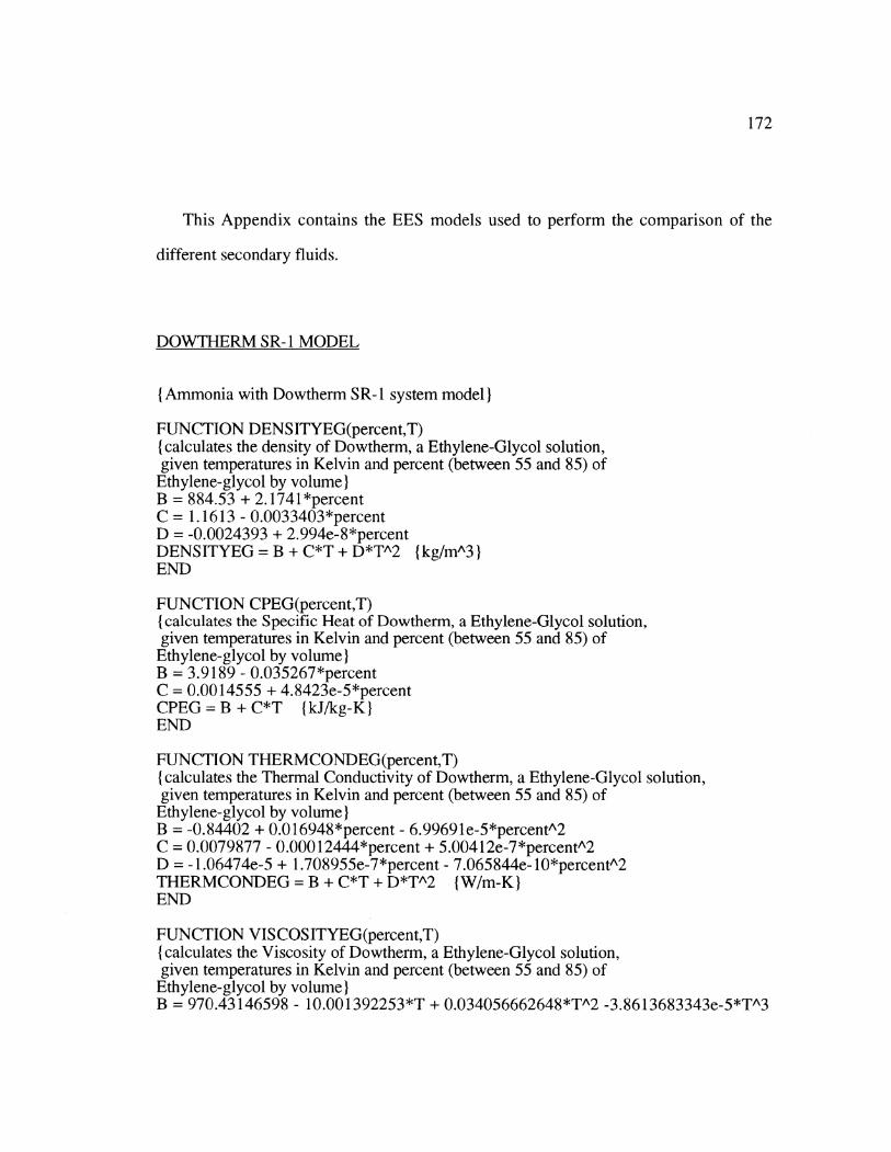
172
This Appendix contains the EES models used to perform the comparison of the
different secondary fluids.
DOWTHERM SR- I MODEL
(Ammonia with Dowtherm SR-I system model)
FUNCTION DENSITYEG(percent,T){ calculates the density of Dowtherm, a Ethylene-Glycol solution,given temperatures in Kelvin and percent (between 55 and 85) of
Ethylene-glycol by volume)IB = 884.53 + 2.1741*percentC = 1.1613 - 0.0033403*percentD = -0.0024393 + 2.994e-8*percentDENSITYEG = B + C*T + D*TA2 {kg/mA3)END
FUNCTION CPEG(percent,T)( calculates the Specific Heat of Dowtherm, a Ethylene-Glycol solution,given temperatures in Kelvin and percent (between 55 and 85) ofEthylene-glycol by volume)IB = 3.9189 - 0.035267*percentC = 0.0014555 + 4.8423e-5*percentCPEG = B + C*T {kJ/kg-K)END
FUNCTION THERMCONDEG(percent,T)( calculates the Thermal Conductivity of Dowtherm, a Ethylene-Glycol solution,given temperatures in Kelvin and percent (between 55 and 85) of
Ethylene-glycol by volume)IB = -0.84402 + 0.016948*percent - 6.99691e-5*percentA2C = 0.0079877 - 0.00012444*percent + 5.00412e-7*percentA2D = -1.06474e-5 + 1.708955e-7*percent - 7.065844e- 10*percentA2THERMCONDEG = B + C*T + D*TA2 {W/m-K)END
FUNCTION VIS COSITYEG(percent,T)( calculates the Viscosity of Dowtherm, a Ethylene-Glycol solution,given temperatures in Kelvin and percent (between 55 and 85) ofEthylene-glycol by volume)}B = 970.43 146598 - l0.001392253*T + 0.034056662648"T^2 -3.8613683343e-5*T^3
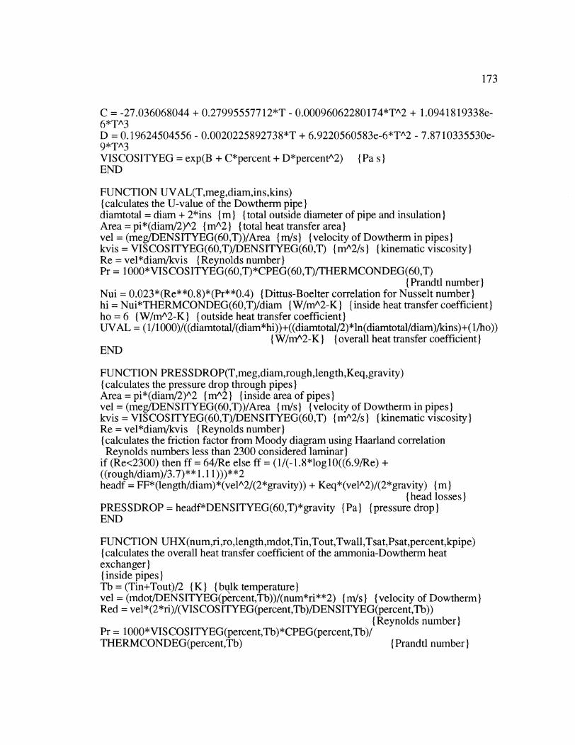
173
C = -27.036068044 + 0.27995557712*T - 0.00096062280174*TA2 + 1.0941819338e-6*TA3D = 0.19624504556 - 0.0020225892738*T + 6.9220560583e-6*TA2 - 7.8710335530e-9*TA3VISCOSITYEG = exp(B + C*percent + D*percentA2) { Pa s)END
FUNCTION UVAL(T,meg,diam,ins,kins){ calculates the U-value of the Dowtherm pipe)diamtotal = diam + 2*ins m) { total outside diameter of pipe and insulation)Area = pi*(diam/2)A2 {mA2 }(total heat transfer area)vel = (meg/DENSITYEG(60,T))/Area {m/s} {velocity of Dowtherm in pipes)kvis = VISCOSITYEG(60,T)/DENSITYEG(60,T) { mA2/s) (Ikinematic viscosity)IRe = vel*diam/kvis (Reynolds number)Pr = 1000*VISCOSITYEG(60,T)*CPEG(60,T)/THERMCONDEG(60,T)
I(Prandtl number)Nui = 0.023*(Re**0.8)*(Pr**0.4) (Dittus-Boelter correlation for Nusselt number)hi = Nui*THERMCONDEG(60,T)/diam (W/mA2-K} {inside heat transfer coefficient)ho = 6 (W/mA2-K (I{outside heat transfer coefficient]UVAL = (1/1000)/((diamtotal/(diam*hi))+((diamtotal/2)*ln(diamtotaldiam)/kins)+(1/ho))
{W/m^2-K) (overall heat transfer coefficient)END
FUNCTION PRES SDROP(T,meg,diam,rough,length,Keq,gravity)( calculates the pressure drop through pipes)IArea = pi*(diam/2)A2 { mA2 }I inside area of pipes)vel = (meg/DENSITYEG(60,T))/Area {m/s (velocity of Dowtherm in pipes)kvis = VISCOSITYEG(60,T)/DENSITYEG(60,T) I mA2/s) I kinematic viscosity)IRe = vel*diamlkvis (Reynolds number)( calculates the friction factor from Moody diagram using Haarland correlationReynolds numbers less than 2300 considered laminar)
if (Re<2300) then ff = 64/Re else ff = (1/(-1.8*logl0((6.9/Re) +((rough/diam)/3.7)** 1.11)))**2headf = FF*(length/diam)*(velA2/(2*gravity)) + Keq*(velA2)/(2*gravity) { m)
( head losses)PRESS DROP = headf*DENSITYEG(60,T)*gravity (Pa) (pressure drop)END
FUNCTION UHX(numri,ro,length,mdot,Tin,Tout,Twall,Tsat,Psat,percent,kpipe)( calculates the overall heat transfer coefficient of the ammonia-Dowtherm heatexchanger)( inside pipes)Tb = (Tin+Tout)/2 (K) (bulk temperature)vel = (mdot/DENSITYEG(percent,Tb))/(num*ri**2) (mi/s) velocity of Dowtherm)Red = vel*(2*ri)/(VISCOSITYEG(percent,Th)/DENSITYEG(percent,Th))
( Reynolds number)}Pr = l000*VISCOSITYEG(percent, Tb)*CPEG(percent, Tb)/THERMCoNDEG(percent,Tb) ( Prandtl number)}
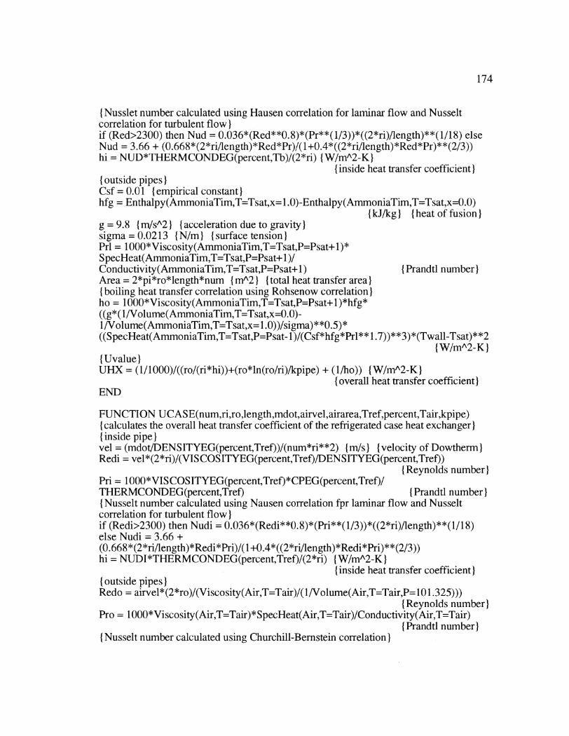
174
( Nusslet number calculated using Hausen correlation for laminar flow and Nusseltcorrelation for turbulent flow)if (Red>2300) then Nud = 0.036*(Red**0. 8)*(Pr**( 1/3))*((2*ri)/length)**(1/18) elseNud = 3.66 + (0.668*(2*ri/length)*Red*Pr)/(l+0.4*((2*ri/length)*Red*Pr)**(2/3))hi = NUD*THERMCONDEG(percent,Tb)/(2*ri) { W/m"A2-K)
{inside heat transfer coefficient)(outside pipes)Csf = 0.01 (1empirical constant)hfg = Enthalpy(AmmoniaTim,T=Tsat,x= 1.0)-Enthalpy(AmmoniaTim,T=Tsat,x=0.0)
{kJ/kg) (heat of fusion)g = 9.8 {m/sA2) (Iacceleration due to gravity)sigma = 0.0213 { N/m ( {surface tension)Prl = 1000*Viscosity(AmmoniaTim,T=Tsat,P=Psat+ 1)*SpecHeat(AmmoniaTim,T=Tsat,P=Psat+ 1)/Conductivity(AmmoniaTim,T=Tsat,P=Psat+ 1) (Prandtl number)Area = 2*pi*ro*length*num (mA2) (total heat transfer area)( boiling heat transfer correlation using Rohsenow correlation)ho = 1000*Viscosity(AmmoniaTim,T=Tsat,P=Psat+ 1)*hfg*((g*(1/Volume(AmmoniaTim,T=Tsat,x=0.0)-1/Volume(AmmoniaTim,T=Tsat,x= 1.0))/sigma)**0.5)*((SpecHeat(AmmoniaTim,T=Tsat,P=Psat- 1)/(Csf*hfg*Prl** 1.7))**3)*(Twall-Tsat)**2
(W/mA2-K)(Uvalue)UHX = (1/1000)/((ro/(ri*hi))+(ro*ln(ro/ri)/kpipe) + (1/ho)) {W/mA2-K}
(overall heat transfer coefficient)END
FUNCTION UCASE(num,ri,ro,length,mdot,airvel,airarea,Tref,percent,Tair,kpipe)(calculates the overall heat transfer coefficient of the refrigerated case heat exchanger)(inside pipe)Ivel = (mdot/DENSITYEG(percent,Tref))/(num*ri**2) (m/s) (velocity of Dowtherm)Redi = vel*(2*ri)/(VIS COSITYEG(percent,Tref)/DENSITYEG(percent,Tref))
( Reynolds number)Pri = 1000*VISCOSITYEG(percent,Tref)*CPEG(percentTref)/THERMCONDEG(percent,Tref) ( Prandtl number)( Nusselt number calculated using Nausen correlation fpr laminar flow and Nusseltcorrelation for turbulent flow)if (Redi>2300) then Nudi = 0.036*(Redi**0.8)*(Pri**(1/3))*((2*ri)/length)**(1/18)else Nudi = 3.66 +(0.668*(2*ri/length)*Redi*Pri)/(1 +0.4*((2*ri/length)*Redi*Pri)**(2/3))hi = NUDI*THERMCONDEG(percent,Tref)/(2*ri) (W/mA2-K)
( inside heat transfer coefficient)I( outside pipes)IRedo = airvel*(2*ro)/(Viscosity(Air,T=Tair)/(1/Volume(Air,T=Tair,P= 101.325)))
(Reynolds number)Pro = 1 000*Viscosity(Air,T=Tair)* SpecHeat(Air,T=Tair)/Conductivity(Air,T=Tair)
{Prandtl number)(Nusselt number calculated using Churchill-Bernstein correlation)}
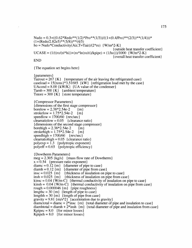
175
Nudo = 0.3+((0.62*Redo**(1/2)*Pro**(1/3))/(( 1+(0.4/Pro)**(2/3))** (1/4)))*(1 +(Redo/2.82e5)** (5/8))** (4/5)ho = Nudo*Conductivity(Air,T=Tair)/(2*ro) (W/mA2-K)
( outside heat transfer coefficient)UCASE = (1/((ro/(ri*hi))+(ro*ln(ro/ri)/kpipe) + (1/ho)))/1000 {W/mA2-K}
( overall heat transfer coefficient)IEND
(The equation set begins here)I
( parameters)ITairout = 267 (K) (temperature of the air leaving the refrigerated case)Icaseload = 15({tons)}*3.51685 (kW) (refrigeration load met by the case)UAcond = 8.00 {(kW/K) ({IUA value of the condenser)ITamb = 300 (1K) (Iambient temperature)ITstore = 300 (1K) ( {store temperature)I
( Compressor Parameters)I(dimensions of the first stage compressor)borelow = 2.38*2.54e-2 (mstrokelow = 1.75*2.54e-2 (m)speedlow = 1700/60 (rev/sec)clearratiolow = 0.05 (clearance ratio)( dimensions of the second stage compressor)borehigh = 2.38*2.54e-2 (mstrokehigh = 1.75*2.54e-2 (m)speedhigh = 1700/60 (rev/sec)clearratiohigh = 0.05 (clearance ratio)Ipolyexp = 1.3 (polytropic exponent)polyeff = 0.65 (polytropic efficiency)
( Dowtherm Parameters)Imeg = 2.305 (kg/s) (Imass flow rate of Dowtherm)x = 0.54 (pressure ratio exponent)diamc = 0.12 () ({diameter of pipe to case)Idiamh = 0.12 (I (Idiameter of pipe from case)Iinsc = 0.025 (I (Ithickness of insulation on pipe to case)insh = 0.025 (I (Ithickness of insulation on pipe from case)Ikinsc =0.04 {W/m-C) (thermal conductivity of insulation on pipe to case)kinsh = 0.04 (W/m-C) (Ithermal conductivity of insulation on pipe from case)rough = 0.000046 (im (pipe roughness)Ilengthc = 30 (I (Ilength of pipe to case)Ilengthh = 30 (I (Ilength of pipe fron case)Igravity = 9.81 ( m/sA2) ({Iacceleration due to gravity)Idiamctotal = diamc + 2*insc () m (total diameter of pipe and insulation to case)}diamnhtotal = diamnh + 2*insh (in ( {total diameter of pipe and insulation from case)}Kpipec = 8.0 ( for minor losses)}Kpipeh = 8.0 ( for minor losses)}
176
{ Heat Exchanger Parameters)Inumhxp = 300 {number of pipes in ammonia-Dowtherm heat exchanger)rihx = 0.005 (I (I{inside radius of pipes in ammonia-Dowtherm heat exchanger)thickhx = 0.0015 (in) (thickness of pipes in ammonia-Dowtherm heat exchanger)rohx = rihx + thickhx { m) { outside radius of pipes in ammonia-Dowtherm heatexchanger)lenhx = 2.0 (m { length of pipes in ammonia-Dowtherm heat exchanger)kpipehx = 43 (W/m-C)
{ thermal conductivity of pipes in ammonia-Dowtherm heat exchanger)Khx = 8*numhxp + 1.5 {for minor losses)numcase = 700 (number of pipes in refrigerated case heat exchanger)ricase = 0.01 { m} { inside radius of pipes in refrigerated case heat exchanger)thickcase = 0.0015 (in) { thickness of pipes in refrigerated case heat exchanger)rocase = ricase + thickcase { m)I
( outside radius of pipes in refrigerated case heat exchanger)lencase = 2.0 (m) (Ilength of pipes in refrigerated case heat exchanger)airvel = 5.0 {(m/s) (air velocity in refrigerated case heat exchanger)airarea = 0.5 {mA2)
{cross sectional area for air flow in refrigerated case heat exchanger)kpipecase = 43 (W/mA2)
I(thermal conductivity of pipes in refrigerated case heat exchanger)Kcase = 8*numcase + 1.5 {for minor losses)
(Secondary Cycle)I(equations for the refrigerated case heat exchanger)Tair = (Tairin + Tairout)/2 (K) bulk temperature of air in case heat exchanger)TEG = (T6+T5)/2 ( K) ( Ibulk temperature of Dowtherm in case heat exchanger)Cpaircase = SpecHeat(Air,T=Tairin) { kJ/kg-K) ({Ispecific heat of air)Imdotair = (airvel/Volume(Air,T=Tairin,P= 101.325))*airarea ( kg/s) (mass flow of air)Cpcase = CPEG(60,T5) {kJ/kg-K) ( Ispecific heat of Dowtherm)Cair = Cpaircase*mdotair (kW/K) (capacitance rate of air)CEG = Cpcase*meg I(kW/K) ({Icapacitance rate of Dowtherm)Cmin = if(Cair,CEG,Cair,Cair,CEG) (minimum capacitance rate)Cmax = if(Cair,CEG,CEG,Cair,Cair) (maximum capacitance rate)Cr = Cmin/Cmax (capacitance rate ratio)(calls function to calculate the overall heat transfer coefficient) }W/mA2-K)Ucasehx =UCASE(numcase,ricase,rocase,lencase,meg,airvel,airarea,TEG,60,Tair,kpipecase)UAcase = Ucasehx*(numcase*2*pi*rocase*lencase) ( W/K) ({IUA value of case)INTUcase = UAcase/Cmin ( number of transfer units of case heat exchanger)(calculates the effectiveness using cross-flow correlation with both streams unmixed)effcase = 1-exp((1/Cr)*(NTUcase**0.22)*(exp(-Cr*(NTUcase**0.78))- 1))caseload = effcase*Cmin*(Tairin-T5) (kW)
(heat transfer in case (refrigeration load met))caseload = Cair*(Tairin-Tairout) (change in temperature of the air stream)caseload = CEG*(T6-T5) (change in temperature of the Dowtherm)(calls function to calculate pressure drop through refrigerated case) ({Pa)}deltaPcase = PRES SDROP(TEG,meg/numcase,2*ricase,rough,lencase,Kcase,gravity)( calculates the pump work needed to overcome pressure drop in case)}

177
Wpumpcase = meg*(deltaPcase/DENSITYEG(60,TEG))/1000 (kW)
{Piping System)Tc = (T8+T5)/2 ( K) { bulk temperature of Dowtherm in pipes to case)Th = (T6+T7)/2 (K) (bulk temperature of Dowtherm in pipes from case){ calls function to calculate overall heat transfer coefficient of pipes to case)Uc = UVAL(Tc,meg,diamc,insc,kinsc) {W/mA2-K)( calls function to calculate overall heat transfer coefficient of pipes from case)Uh = UVAL(Th,meg,diamh,insh,kinsh) { W/mA2-K)I{ calls function to calculate pressure drop of pipes to case)IdeltaPc = PRESSDROP(Tc,meg,diamc,rough,lengthc,Kpipec,gravity) (Pa)(calls function to calculate pressure drop of pipes to case)IdeltaPh = PRESSDROP(Th,meg,diamh,rough,lengthh,Kpipeh,gravity) (Pa)
densityc = DENSITYEG(60,Tc) (kg/mA3) (density of Dowtherm in pipes to case)densityh = DENSITYEG(60,Th) (kg/mA3 } (density of Dowtherm in pipes from case)( calculates pump necessary to overcome pressure drop in piping system)Wpumppipe = meg*(deltaPc/densityc + deltaPh/densityh)/1000 {kW)
(calculates thermal losses of piping system)Ac = pi*diamctotal*lengthc (mA2) ({total heat transfer area of pipes to case)Ah = pi*diamhtotal*lengthh (mA2) (total heat transfer area of pipes from case)ICpc = CPEG(60,Tc) (kJ/kg-K) (specific heat of Dowtherm in pipes to case)Cph = CPEG(60,Th) (kJ/kg-K) (specific heat of Dowtherm in pipes from case)Qc = meg*Cpc*(T5-T8) (kW) (heat loss of Dowtherm in pipes to case)Qh = meg*Cph*(T7-T6) (kW) (heat loss of Dowtherm in pipes from case)deltatlmc = (T5-TX)/(ln((Tstore-T8)/(Tstore-T5)))
( log mean temperature difference of pipes to case)deltatlmh = (T7-T6)/(ln((Tstore-T6)/(Tstore-T7)))
(log mean temperature difference of pipes from case)Qc = Uc*Ac*deltatlmc (kW) (heat loss of pipes to case)IQh = Uh*Ah*deltatlmh (kW) (heat loss of pipes from case)NTUc = Uc*Ac/(meg*Cpc) (number of transfer units of pipes to case)NTUh = Uh*Ah/(meg*Cph) (number of transfer units of pipes from case)
(equations for heat exchanger between Dowtherm and Ammonia)ITwall = T7-(T7-T8)/2 (K) (surface temperature of pipes in ammonia)(calls function to calculate overall heat transfer coefficient) (W/m^2-K}U = UHX(numhxp,rihx,rohx,lenhx,meg,T7,T8,Twall,T 1 ,P 1,60,kpipehx)UAhx = U*(2*rohx*pi*lenhx*numhxp) (W/K) (UA value of heat exchanger)NTUhx = UAhx/(meg*CPEG(60,T7)) (number of transfer units of heat exchanger)effhx = 1-exp(-NTUhx) (effectiveness of heat exchanger)effhx = (T7-T8)/(T7-T1)
( using effectiveness to calculate temperatures in heat exchanger)Qhx = meg*CPEG(6OT7)*(T7-T8) (kW) (heat transfer in heat exchanger)Tmid = (T7+T8)/2 (K) (bulk temperature of Dowtherm in heat exchanger)T 1 = T2 (K) (constant ammonia temperature in heat exchanger)mref = Qhx/(h2-h 1) ( kg/s) ( calculates necessary ammonia flow rate to meet load)}( calls function to calculate the pressure drop in heat exchanger)}
178
deltaPhx = PRESSDROP(Tmid,neg/numhxp,2*rihx,rough,lenhx,Khx,gravity) (Pa){ calculates pump work necessary to overcome pressure drop in heat exchanger)Wpumphx = meg*(deltaPhx/DENSITYEG(60,Tmid))/1000 { kW)
P2 = Pressure(AmmoniaTim,T=Tl,x=l.0) {kPa)(pressure of ammonia leaving heat exchanger)
h2 = Enthalpy(AmmoniaTim,T=T2,x=l.0) {kJ/kg)(enthalpy of ammonia leaving heat exchanger)
s2 = Entropy(AmmoniaTim,T=T2,x= 1.0) { kJ/kg-K)I(entropy of ammonia leaving heat exchanger)
P 1 = P2 {kPa) { ammonia pressure constant in heat exchanger)I
(Ammonia Cycle)I(compressor)rp = P3/P2 (pressure ratio of evaporator to condenser)Irps = rpAx (pressure ratio relationship)rps = P2a/P2 (calculates intermediate pressure)
( Low Pressure Compressor)Iv2 = Volume(AmmoniaTim,P=P2,x= 1.0) (mA3/kg)I
( specific volume of ammonia entering first compressor)P2*(v2)Apolyexp = P2a*(v2a)Apolyexp (polytropic compression equation)Ih2a = Enthalpy(AmmoniaTim,P=P2a,v=v2a) {IkJ/kg)I
( enthalpy of ammonia leaving first compressor)T2a = Temperature(AmmoniaTim,P=P2a,v=v2a) (IK)I
{ temperature of ammonia leaving first compressor)Vdisplow = numcyllow*(pi*((borelow/2)A2)*strokelow) (mA3)
( displacement volume of first compressor)Ivolefflow = 1-(clearratiolow/(1-clearratiolow))*((P2a/P2)A(l/polyexp) - 1)
( volumetric efficiency of first compressor)mref = (1/v2)*Vdisplow*speedlow*volefflow (kg/s)
(mass flow of ammonia through first compressor)Wcomplow = (mref*(h2a-h2))/polyeff (kW) (Iwork of first compressor)I
(High Pressure Compressor)IP2b = P2a {kPa) (Iintermediate pressure)Ih2b = Enthalpy(AmmoniaTim,P=P2b,x=1.0) {kJ/kg)
(enthalpy of ammonia entering second compressor)Is2b = Entropy(AmmoniaTim,P=P2b,x=l.0) {kJ/kg-K)
( entropy of ammonia entering second compressor)T2b = Temperature(AmmoniaTim,P=P2b,x= 1.0) ( K)
(temperature of ammonia entering second compressor)Iv2b = Volume(AmmoniaTim,P=P2b,x= 1.0) {mA3/kg)I
Ifspecific heat of ammonia entering second compressor)P2b*(v2b)Apolyexp = P3*(vO13)Apolyexp (polytropic compression equation)h3 = Enthalpy(AmmoniaTim,P=P3,v=vol3) {kJ/kg)}
(enthalpy of ammonia leaving second compressor)T3 = Temperature(AmmoniaTim,P=P3,v=vol3) ( K)
(temperature of ammonia leaving second compressor)}
179
Vdisphigh = numcylhigh*(pi*((borehigh/2)A2)*strokehigh) {mA3}(displacement volume of second compressor)
voleffhigh = 1-(clearratiohigh/( 1-clearratiohigh))*((P3/P2b)A(1/polyexp) - 1)(volumetric effciciency of second compressor)
mcond = (1/v2b)*Vdisphigh*speedhigh*voleffhigh { kg/s)( mass flow of ammonia through second compressor)
Wcomphigh = (mcond*(h3-h2b))/polyeff {kW }(work of second compressor)P3 = P4 (kPa) (constant pressure across condenser)Wcomp = Wcomplow + Wcomphigh (kW) (total compression work)
(condensor)Imair = 15*0.47879 {kg/s) (flow rate of air through condenser)Cpair = SpecHeat(Air,T=Tamb) I(kJ/kg-K) ( Ispecific heat of air)UAcond = mair*Cpair*NTU (calculates number of transfer units of condenser)eff = 1-exp(-NTU) (effectiveness of condenser)
Qcond = eff*mair*Cpair*(T4-Tamb) (kW) (Iheat transfer in condenser)Qcond = mcond*(h3-h4) (calculates enthalpy change of ammonia in condenser)Qcond = mair*Cpair*(Tairoutcond-Tamb) ( calculates temperature change of air)
P4 = Pressure(AmmoniaTim,T=T4,x=0.0) I(kPa)(pressure of ammonia leaving condenser)
h4 = Enthalpy(AmmoniaTim,T=T4,x=0.0) (kJ/kg)I( enthalpy of ammonia leaving condenser)
(expansion)P5 = P2a ( kPa) (intermediate pressure)h5 = Enthalpy(AmmoniaTim,P=P5,x=0.0) I(kJ/kg)I
( enthalpy of saturated liquid ammonia leaving the flash tank)Ih I = h5 I(kJ/kg) ({Iisenthalpic expansion)I
Wpump = Wpumpcase+Wpumphx+Wpumppipe (kW) (total pump work done bysystem)ICOP = caseload/(Wcomp+Wpump) (coefficient of performance of refrigeration system)Cap = meg*CPEG(60,T7)/caseload (l/K) (capacitance rate - caseload ratio)
( mixing equation for flash tank)mcond*h4 + mref*h2a = mref*h5 + mcond*h2b
DOWFROST MODEL
( Ammonia with Dowfrost system model)}
FUNCTION CPPG(percent,T)
180
( calculates the specific heat of Dowfrost given percent composition of Dowfrostand the temperature in degrees Kelvin)IB = 3.8649883866 - 0.023691954902*percent - 0.00011278222908*percentA2C = 0.001023655712 + 5.6633876714e-5*percentCPPG = B + C*T {kJ/kg-K)END
FUNCTION DENSITYPG(percent,T)( calculates the density of Dowfrost given percent composition of Dowfrostand the temperature in degrees Kelvin)IB = 875.54696219 + 2.15 1387542*percentC = 1.1191046068 - 0.0007599907262*percent - 4.9236799989e-5*percentA2D = -0.002377960199 - 9.1377252136e-6*percent + 1.0872237562e-7*percentA2DENSITYPG = B + C*T + D*TA2 (kg/mA3)END
FUNCTION THERMCONDPG(percent,T)( calculates the thermal conductivity of Dowfrost given percent composition of Dowfrostand the temperature in degrees Kelvin)IB = -0.78595253278 + 0.015561899561 *percent - 4.8933521576e-5*percentA2C = 0.0076866167254 - 0.0001155974176*percent + 3.6603360830e-7*percentA2D = -9.9976810237e-6 + 1.4560615474e-7*percent - 4.5879383578e-10*percentA2THERMCONDPG = B + C*T + D*TA2 {W/m-K)END
FUNCTION VISCOSITYPG(percent,T)( calculates the viscosity of Dowfrost given percent composition of Dowfrostand the temperature in degrees Kelvin)IB = 71.639163222-0.66981698459*T+0.0019150513174TA2 - 1.8587687783e-6*TA3C = 0.27019804611 - 0.0012299975866*T + 1.5045427918e-6*TA2VISCOSITYPG = exp(B+C*percent) (Pa s)END
FUNCTION UVAL(T,mpg,diam,ins,kins)(calculates U-value of Dowfrost distribution pipes)diamtotal = diam + 2*ins I (m}Itotal outside diameter of pipe and insulation)Area = pi*(diam/2)A2 (mA2) (total heat transfer area)vel = (mpg/DENSITYPG(60,T))/Area (m/s) (Ivelocity of Dowfrost in the pipes)kvis = VISCOSITYPG(60,T)/DENSITYPG(60,T) (mA2/s) (kinematic viscosity)Re = vel*diam/kvis (Reynolds number)Pr = 1000*VISCOSITYPG(60,T)*CPPG(60,T)/THERMCONDPG(60,T)
( Prandtl number)Nui = 0.023*(Re**0.8)*(Pr**0.4) (Dittus - Boelter correlation for Nusselt number)hi = Nui*THERMCONDPG(60,T)/diam (W/mA2-C) (inside heat transfer coefficient)ho = 6 fW/mA2-C (outside heat transfer coefficient)IUVAL = (1/1 000)/((diamtotal/(diam*hi))+((diamtotal/2)*ln(diamtotal/diam)/kins)+( 1/ho))
( W/mA2-C) ({overall heat transfer coefficient)}END
181
FUNCTION PRESS DROP(T,mpg,diam,rough,length,Keq,gravity)( calculates the pressure drop through pipes)IArea = pi*(diam/2)A2 { mA21 { inside area of pipes)vel = (mpg/DENSITYPG(60,T))/Area I(m/sI (I{velocity of Dowfrost in pipes)kvis = VISCOSITYPG(60,T)/DENSITYPG(60,T) { mA2/s) (kinematic viscosity)Re = vel*diam/kvis ( Reynolds number){ calculates the friction factor from Moody diagram using Haarland correlationReynolds numbers less than 2300 considered laminar)if (Re<2300) then ff = 64/Re else ff = (1/(-1.8*log10((6.9/Re) +((rough/diam)/3.7)** 1.11)))**2headf = FF*(length/diam)*(velA2/(2*gravity))+Keq*(velA2)/(2*gravity) (m
( head losses)PRESSDROP = headf*DENSITYPG(60,T)*gravity (Pa) (pressure drop)END
FUNCTION UHX(num,ri,ro,length,mdot,Tin,Tout,Twall,Tsat,Psat,percent,kpipe)(calculates the overall heat transfer coefficient of the ammonia-Dowfrost heat exchanger)(inside pipes)ITh = (Tin+Tout)/2 (K) (bulk temperature)vel = (mdot/DENSITYPG(percent,Tb))/(num*ri**2) (m/s)
( velocity of Dowfrost through pipes)IRed = vel* (2*ri)/(VI SCOS ITYPG(percent,Tb)/DENS ITYPG(percent,Th))
( Reynolds number)Pr = 1000*VISCOSITYPG(percent,Tb)*CPPG(percent,Tb)/THERMCONDPG(percent,Th) (IPrandtl number)( Nusselt number calculated using Hausen correlation for lamminar flow and Nusseltcorrelation for turbulent flow)if (Red>2300) then Nud = 0.036*(Red**0. 8)*(Pr**( 1/3))*((2*ri)/length)**(1/18) elseNud = 3.66 + (0.668*(2*ri/length)*Red*Pr)/(l+0.4*((2*ri/length)*Red*Pr)**(2/3))hi = NUD*THERMCONDPG(percent,Tb)/(2*ri) {W/mA2-C)I
(inside heat transfer coefficient)( outside pipes)ICsf = 0.01 ( empirical constant)( heat of fusion)Ihfg = Enthalpy(AmmoniaTim,T=Tsat,x= 1.0)-Enthalpy(AmmoniaTim,T=Tsat,x=0.0)
(kJ/kg)g = 9.8 {(m/sA2) (Iacceleration of gravity)Isigma = 0.0213 (N/mI (Isurface tension)Prl = 1000*Viscosity(AmmoniaTim,T=Tsat,P=Psat+ 1)*SpecHeat(AmmoniaTim,T=Tsat,P=Psat+ 1 )/Conductivity(AmmoniaTim,T=Tsat,P=Psat+ 1) ( Prandtl number)Area = 2*pi*ro*length*num ( total heat transfer area)I(boiling heat transfer coefficient from Rohsenow correlation)Iho = 1000*Viscosity(AmmoniaTim,T=Tsat,P=Psat+ 1)*hfg*((g*(1 /Volume(AmmoniaTimT=Tsat,x=0.0)-1/Volume( Ammo niaTim,T=T sat, x= 1 .0) )/sigma) **0.5) *((SpecHeat(AmnmoniaTim,T=Tsat,P=Psat- 1)/(Csf*hfg*Prl** 1 .7))**3)*(Twall-Tsat)**2
(W/mA2-C)( Uvalue }
182
UHX = (1/1000)/((ro/(ri*hi))+(ro*ln(ro/ri)/kpipe) + (1/ho)) {W/mA2-C}( overall heat transfer coefficient)
END
FUNCTION UCASE(num,ri,ro,length,rndot,airvel,airarea,Tref,percent,Tair,kpipe){ calculates the overall heat transfer coefficient of the refrigerated case heat exchanger)(inside pipe)Ivel = (mdot/DENSITYPG(percent,Tref))/(num*ri**2) (m/s)
( velocity of Dowfrost through pipes)Redi = vel*(2*ri)/(VISCOSITYPG(percent,Tref)/DENSITYPG(percent,Tref)){ Reynolds number)IPri = 1000*VISCOSITYPG(percent,Tref)*CPPG(percent,Tref)/THERMCONDPG(percent,Tref) ( Prandtl number)( Nusselt number calculated using Hausen correlation for laminar flow and Nusseltcorrelation for turbulent flow)Iif (Redi>2300) then Nudi = 0.036*(Redi**0.8)*(Pri**(1/3))*((2*ri)/length)**(1/18)else Nudi = 3.66 +(0.668*(2*ri/length)*Redi*Pri)/(1 +0.4*((2*ri/length)*Redi*Pri)**(2/3))hi = NUDI*THERMCONDPG(percent,Tref)/(2*ri) {W/mA2-C)I
(inside heat transfer coefficient)I( outside pipes)IRedo = airvel*(2*ro)/(Viscosity(Air,T=Tair)/(1/Volume(Air,T=Tair,P= 101.325)))( Reynolds number)Pro = 1000*Viscosity(Air,T=Tair)*SpecHeat(Air,T=Tair)/Conductivity(Air,T=Tair)(Prandtl number)I(Nusselt number using Churchill Bernstein correlation)Nudo = 0.3+((0.62*Redo**(1/2)*Pro**(1/3))/((1 +(0.4/Pro)**(2/3))** (1/4)))*(I +(Redo/2.82e5)** (5/8))** (4/5)ho = Nudo*Conductivity(Air,T=Tair)/(2*ro) {W/mA2-C)
( outside heat transfer coefficient)UCASE = (1/((ro/(ri*hi))+(ro*ln(ro/ri)/kpipe) + (1/ho)))/1000 (W/mA2-C)
(overall heat transfer coefficient)END
(The equation set begins here)
( parameters)ITairout = 267 (K) (temperature of air leaving refrigerated case)caseload = 15(tons)*3.51685 (kW) (refrigeration load met by the case)UAcond = 8.00 (kW/K) (UA value of the condenser)Tamb = 300 (K) (ambient temperature)Tstore = 300 (K) (store temperature)
( Compressor Parameters)I( dimensions of the first stage compressor)Iborelow = 2.38"2.54e-2 (in)}strokelow = 1.75"2.54e-2 (in)speedlow = 1700/60 ( rev/sec)}clearratiolow = 0.05
183
(dimensions of the second stage compressor)borehigh = 2.38*2.54e-2 Im)strokehigh - 1.75*2.54e-2 (m)speedhigh = 1700/60 {rev/sec}clearratiohigh = 0.05polyexp = 1.3 {polytropic exponent for ammonia)Ipolyeff = 0.65 ( polytropic efficiency)
{ Dowfrost Parameters)Impg = 2.305 {kg/s) ({Imass flow rate of Dowfrost)Ix = 0.54 {pressure ratio exponent)diamc = 0.12 i) m diameter of pipe to refrigerated case)diamh = 0.12 { Im (diameter of pipe from refrigerated case)Iinsc = 0.025 {m) {thickness of insulation on pipe to case)insh = 0.025 (mI (thickness of insulation on pipe from case)kinsc = 0.04 {W/m-C) (thermal conductivity of insulation on pipe to case)kinsh = 0.04 (W/m-C) {thermal conductivity of insulation on pipe from case)rough = 0.000046 im) { roughness of pipe material)lengthc = 30 { m) (length of pipe to case)Ilengthh = 30 ( m({length of pipe from case)gravity = 9.81 ( m/sA2) (Iacceleration due to gravity)Idiamctotal = diamc + 2*insc i) m total diameter of pipe and insulation to case)Idiamhtotal = diamh + 2*insh (i) ({total diameter of pipe and insulation from case)Kpipec = 8.0 (for minor losses)Kpipeh = 8.0 (for minor losses)
( Heat Exchanger Parameters)Inumhxp = 300 ( number of pipes in ammonia-Dowfrost heat exchanger)Irihx = 0.005 (m (inside radius of pipes in ammonia-Dowfrost heat exchanger)thickhx = 0.0015 (i) ({thickness of pipes in ammonia-Dowfrost heat exchanger)Irohx = rihx + thickhx ( mI
( outside radius of pipes in ammonia-Dowfrost heat exchanger)lenhx = 2.0 m) (Ilength of pipes in ammonia-Dowfrost heat exchanger)kpipehx = 43 {(W/m-C)I
( thermal conductivity of pipes in ammonia-Dowfrost heat exchanger)Khx = 8*numhxp + 1.5 (for minor losses)numcase = 700 (number of pipes in refrigerated case heat exchanger)Iricase = 0.01 im (inside radius of pipes in refrigerated case heat exchanger)Ithickcase = 0.0015 i) m thickness of pipes in refrigerated case heat exchanger)Irocase= ricase + thickcase (m}I
( outside radius of pipes in refrigerated case heat exchanger)lencase = 2.0 (im (length of pipes in refrigerated case heat exchanger)kpipecase = 43 (W/mA2)
( thermal conductivity of pipes in refrigerated case heat exchanger)airvel = 5.0 (m/s) (velocity of the air through the refrigerated case heat exchanger)airarea = 0.5 {(mA2) ( cross sectional area for air flow in refrigerated case heat exchanger)}Kcase- =8*nuincase + 1.5 (for minor losses)
184
{Secondary Cycle)I
{ equtaions for the refrigerated case heat exchanger)Tair = (Tairin + Tairout)/2 (K)
(bulk temperature of the air through the refrigerated case heat exchanger)Tpg = (T6+T5)/2 {K)
(bulk temperature of Dowfrost through the refrigerated case heat exchanger)Cpaircase = SpecHeat(Air,T=Tairin) IkJ/kg-K} (specific heat of air)mdotair = (airvel/Volume(Air,T=Tairin,P= 101.325))*airarea ( kg/si { mass flow of air)Cpcase = CPPG(60,T5) {kJ/kg-K) (Ispecific heat of Dowfrost)Cair = Cpaircase*mdotair {kW/K) (Icapacitance rate of air stream)Cpg = Cpcase*mpg { kW/K) (Icapacitance rate of Dowfrost stream)ICmin = if(Cair,Cpg,Cair,Cair,Cpg) (minimum capacitance rate)Cmax = if(Cair,Cpg,Cpg,Cair,Cair) (maximum capacitance rate)Cr = Cmin/Cmax (ratio of the capacitance rates)(calls function to calculate the overall heat transfer coefficient)Ucasehx =UCASE(numcase,ricase,rocase,lencase,mpg,airvel,airarea,Tpg,60,Tair,kpipecase)
{W/mA2-KIareacase = (numcase*2*pi*rocase*lencase) (mA2) (Itotal heat transfer area)UAcase = Ucasehx*areacase (W/K) (UA value)NTUcase = UAcase/Cmin ( number of transfer units)(calculation of the effectiveness using cross-flow correlation with both fluids unmixed)Ieffcase = 1-exp((1/Cr)*(NTUcase**0.22)*(exp(-Cr*(NTUcase**0.78))- 1))caseload = effcase*Cmin*(Tairin-T5)
(heat transfered in refrigerated case (refrigeration load met))caseload = Cair*(Tairin-Tairout) (change in temperature of the air stream)caseload = Cpg*(T6-T5) ( change in temperature of the Dowfrost stream)( calls function to calculate pressure drop through the heat exchanger pipes)IdeltaPcase = PRESS DROP(Tpg,mpg/numcase,2*ricase,rough,lencase,Kcase,gravity)
(Pa)(calculates the pump work needed to overcome pressure drop in refrigerated case heatexchanger)Wpumpcase = mpg*(deltaPcase/DENSITYPG(60,Tpg))/1000 (kW)
(Piping System)Tc = (T8+T5)/2 (K) (bulk temperature of Dowfrost in pipes to case)Th = (T6+T7)/2 ( K) (bulk temperature of Dowfrost in pipes from case)( calls function to calculate overall loss coefficient of pipes to refrigerated case)Uc = UVAL(Tc,mpg,diamc,insc,kinsc) (W/mA2-K)I(calls function to calculate overall loss coefficient of pipes from refrigerated case)IUh = UVAL(Th,mpg,diamh,insh,kinsh) (W/mA2-K)I(calls function to determine pressure drop in pipes to refrigerated case)IdeltaPc = PRESSDROP(Tc,mpg,diamc,rough,lengthc,Kpipec,gravity) ( Pa)(calls function to determine pressure drop in pipes from refrigerated case)}deltaPh = PRESSDROP(Th,mpg,diamh,rough,lengthh,Kpipeh,gravity) (Pa)
densityc = DENSITYPG(60,Tc) (kg/mA3) ( density of Dowfrost in pipes to case)densityh = DENSITYPG(60,Th) (kg/mA3) ( density of Dowfrost inpipes from case)}
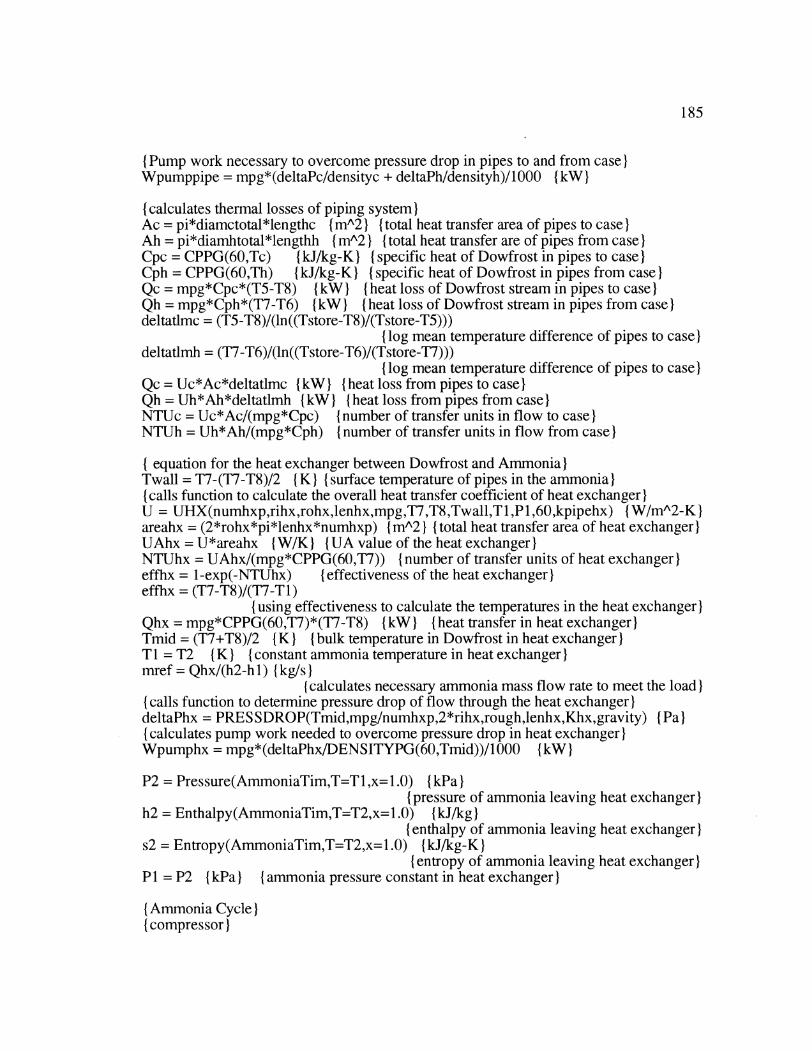
185
( Pump work necessary to overcome pressure drop in pipes to and from case)Wpumppipe = mpg*(deltaPc/densityc + deltaPh/densityh)/1000 {kW)
{ calculates thermal losses of piping system)Ac = pi*diamctotal*lengthc { m^2 }I{total heat transfer area of pipes to case)Ah = pi*diamhtotal*lengthh (mA2) (total heat transfer are of pipes from case)ICpc = CPPG(60,Tc) (kJ/kg-K) (Ispecific heat of Dowfrost in pipes to case)Cph = CPPG(60,Th) (kJ/kg-K) (specific heat of Dowfrost in pipes from case)Qc = mpg*Cpc*(T5-T8) (kW) { heat loss of Dowfrost stream in pipes to case)Qh = mpg*Cph*(T7-T6) (kW) { heat loss of Dowfrost stream in pipes from case)deltatlmc = (T5-T8)/(ln((Tstore-T8)/(Tstore-T5)))
( log mean temperature difference of pipes to case)deltatlmh = (T7-T6)/(ln((Tstore-T6)/(Tstore-T7)))
{ log mean temperature difference of pipes to case)Qc = Uc*Ac*deltatlmc {kW) (heat loss from pipes to case)Qh = Uh*Ah*deltatlmh (kW) (heat loss from pipes from case)NTUc = Uc*Ac/(mpg*Cpc) (number of transfer units in flow to case)NTUh = Uh*Ah/(mpg*Cph) (number of transfer units in flow from case)I
{ equation for the heat exchanger between Dowfrost and Ammonia)ITwall = T7-(T7-T8)/2 ( K) ({Isurface temperature of pipes in the ammonia)I( calls function to calculate the overall heat transfer coefficient of heat exchanger)U = UHX(numhxp,rihx,rohx,lenhx,mpg,T7,T8,Twall,T1,P 1,60,kpipehx) I(W/mA2-K)areahx = (2*rohx*pi*lenhx*numhxp) {mA2} { total heat transfer area of heat exchanger)UAhx = U*areahx (W/K) (UA value of the heat exchanger)NTUhx = UAhx/(mpg*CPPG(60,T7)) ( number of transfer units of heat exchanger)effhx = l-exp(-NTUhx) {effectiveness of the heat exchanger)effhx = (T7-T8)/(T7-T1)
(using effectiveness to calculate the temperatures in the heat exchanger)Qhx = mpg*CPPG(60,T7)*(T7-T8) (kW) (heat transfer in heat exchanger)Tmid = (T7+T8)/2 (K) (bulk temperature in Dowfrost in heat exchanger)T1 = T2 (K) (Iconstant ammonia temperature in heat exchanger)mref = Qhx/(h2-h 1) ( kg/s)I
(calculates necessary ammonia mass flow rate to meet the load)I( calls function to determine pressure drop of flow through the heat exchanger)deltaPhx = PRES SDROP(Tmid,mpg/numhxp,2*rihx,rough,lenhx,Khx,gravity) (Pa)(calculates pump work needed to overcome pressure drop in heat exchanger)Wpumphx = mpg*(deltaPhx/DENSITYPG(60,Tmid))/1000 (kW)
P2 = Pressure(AmmoniaTim,T=Tl,x=1.0) ( kPa)I(pressure of ammonia leaving heat exchanger)
h2 = Enthalpy(AmmoniaTim,T=T2,x=1.0) (kJ/kg)( enthalpy of ammonia leaving heat exchanger)I
s2 = Entropy(AmmoniaTim,T=T2,x=1.0) (kJ/kg-K)(entropy of ammonia leaving heat exchanger)
P1 = P2 (kPa) (ammonia pressure constant in heat exchanger)
( Ammonia Cycle)}(compressor)
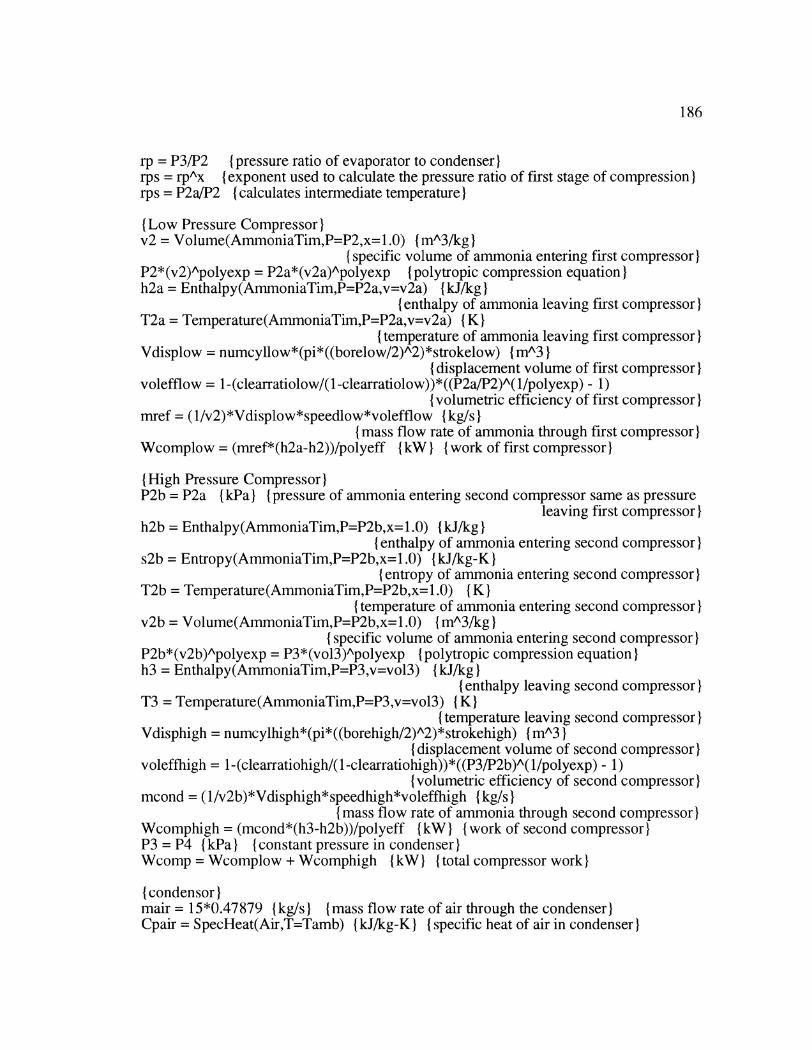
186
rp = P3/P2 (pressure ratio of evaporator to condenser)rps = rpAx { exponent used to calculate the pressure ratio of first stage of compression)rps = P2a/P2 ( calculates intermediate temperature)
(Low Pressure Compressor)Iv2 = Volume(AmmoniaTim,P=P2,x= 1.0) {mA3/kg)I
{specific volume of ammonia entering first compressor)P2*(v2)Apolyexp = P2a*(v2a)Apolyexp (polytropic compression equation)h2a = Enthalpy(AmmoniaTim,P=P2a,v=v2a) {kJ/kg)I
{enthalpy of ammonia leaving first compressor)T2a = Temperature(AmmoniaTim,P=P2a,v=v2a) (K)
( temperature of ammonia leaving first compressor)Vdisplow = numcyllow*(pi*((borelow/2)A2)*strokelow) { mA3)
( displacement volume of first compressor)Ivolefflow = 1-(clearratiolow/(1-clearratiolow))*((P2a/P2)A(l/polyexp) - 1)
( volumetric efficiency of first compressor)mref = (1/v2)*Vdisplow*speedlow*volefflow (kg/s)
(mass flow rate of ammonia through first compressor)Wcomplow = (mref*(h2a-h2))/polyeff (kW) (Iwork of first compressor)
(High Pressure Compressor)P2b = P2a (kPa) (pressure of ammonia entering second compressor same as pressure
leaving first compressor)h2b = Enthalpy(AmmoniaTim,P=P2b,x= 1.0) (kJ/kg }
(enthalpy of ammonia entering second compressor)s2b = Entropy(AmmoniaTim,P=P2b,x=l.0) (kJ/kg-K)
( entropy of ammonia entering second compressor)T2b = Temperature(AmmoniaTim,P=P2b,x= 1.0) ( K)I
( temperature of ammonia entering second compressor)v2b = Volume(AmmoniaTim,P=P2b,x=l.0) I(mA3/kg)
(specific volume of ammonia entering second compressor)P2b*(v2b)Apolyexp = P3*(vol3)Apolyexp (polytropic compression equation)h3 = Enthalpy(AmmoniaTim,P=P3,v=vol3) (kJ/kgI
(enthalpy leaving second compressor)T3 = Temperature(AmmoniaTim,P=P3,v=vol3) ( K)
(temperature leaving second compressor)Vdisphigh = numcylhigh*(pi*((borehigh/2)A2)*strokehigh) I(mA3)
(displacement volume of second compressor)voleffhigh = 1-(clearratiohigh/( 1-clearratiohigh))*((P3/P2b)A(1l/polyexp) - 1)
(volumetric efficiency of second compressor)mcond = (1/v2b)*Vdisphigh*speedhigh*voleffhigh (kg/s)
(mass flow rate of ammonia through second compressor)Wcomphigh = (mcond*(h3-h2b))/polyeff (kW) (Iwork of second compressor)P3 = P4 (kPa) (Iconstant pressure in condenser)Wcomp = Wcomplow + Wcomphigh (kW) (total compressor work)
(condensor)}mair = 15*0.47879 (kg/s) (mass flow rate of air through the condenser)Cpair = SpecHeat(Air,T=Tamb) {(kJ/kg-K) ({specific heat of air in condenser)}
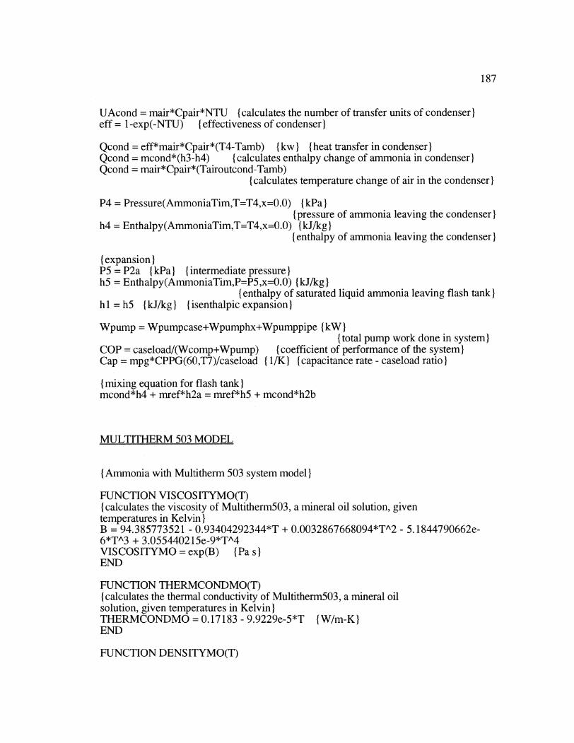
187
UAcond = mair*Cpair*NTU {calculates the number of transfer units of condenser)eff = 1-exp(-NTU) {effectiveness of condenser)
Qcond = eff*mair*Cpair*(T4-Tamb) {kw) {heat transfer in condenser)Qcond = mcond*(h3-h4) (calculates enthalpy change of ammonia in condenser)Qcond = mair*Cpair*(Tairoutcond-Tamb)
( calculates temperature change of air in the condenser)
P4 = Pressure(AmmoniaTim,T=T4,x=0.0) (kPa){pressure of ammonia leaving the condenser)
h4 = Enthalpy(AmmoniaTimT=T4,x=0.0) {kJ/kg)I(enthalpy of ammonia leaving the condenser)
{ expansion)P5 = P2a (kPa) (intermediate pressure)h5 = Enthalpy(AmmoniaTim,P=P5,x=0.0) {kJ/kg)
Ienthalpy of saturated liquid ammonia leaving flash tank)h I = h5 (kJ/kg) }Iisenthalpic expansion)
Wpump = Wpumpcase+Wpumphx+Wpumppipe { kW)I( total pump work done in system)
COP = caseload/(Wcomp+Wpump) (coefficient of performance of the system)Cap = mpg*CPPG(60,T7)/caseload (l/K) (capacitance rate - caseload ratio)
( mixing equation for flash tank)mcond*h4 + mref*h2a = mref*h5 + mcond*h2b
MULTITHERM 503 MODEL
(Ammonia with Multitherm 503 system model)
FUNCTION VISCOSITYMO(T)( calculates the viscosity of Multitherm503, a mineral oil solution, giventemperatures in Kelvin)IB = 94.385773521 - 0.93404292344*T + 0.0032867668094*TA2 - 5.1844790662e-6*TA3 + 3.055440215e-9*TA4VISCOSITYMO = exp(B) (Pa s)END
FUNCTION THERMCONDMO(T)(calculates the thermal conductivity of Multitherm503, a mineral oilsolution, given temperatures in Kelvin)ITHERMCoNDMO = 0. 17183 - 9.9229e-5*T {W/m-K)END
FUNCTION DENSITYMO(T)
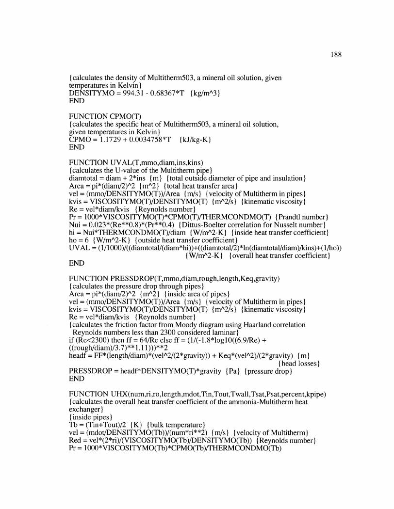
188
{ calculates the density of Multitherm503, a mineral oil solution, giventemperatures in Kelvin)IDENSITYMO = 994.31 - 0.68367*T (kg/mA3}END
FUNCTION CPMO(T){ calculates the specific heat of Multitherm503, a mineral oil solution,given temperatures in Kelvin)ICPMO= 1.1729+0.0034758*T (kJ/kg-K}END
FUNCTION UVAL(T,mmo,diam,ins,kins)(calculates the U-value of the Multitherm pipe)diamtotal = diam + 2*ins { m) ( Itotal outside diameter of pipe and insulation)Area = pi*(diam/2)A2 mA2I) { total heat transfer area)vel = (mmo/DENSITYMO(T))/Area I m/s) ({Ivelocity of Multitherm in pipes)kvis = VISCOSITYMO(T)/DENSITYMO(T) I(mA2/s) (Ikinematic viscosity)Re = vel*diam/kvis (Reynolds number)Pr = 1000*VISCOSITYMO(T)*CPMO(T)iTERMCONDMO(T) {Prandtl number)Nui = 0.023*(Re**0.8)*(Pr**0.4) (Dittus-Boelter correlation for Nusselt number)hi = Nui*THERMCONDMO(T)/diam {W/mA2-K) (Iinside heat transfer coefficient)ho = 6 (W/mA2-K) (Ioutside heat transfer coefficient)UVAL = (1/1000)/((diamtotal/(diam*hi))+((diamtotal/2)*ln(diamtotal/diam)/kins)+(1/ho))
(W/mA2-K) (overall heat transfer coefficient)END
FUNCTION PRES SDROP(T,mmo,diam,rough,length,Keq,gravity)(calculates the pressure drop through pipes)IArea = pi*(diam/2)A2 (mA2) (Iinside area of pipes)vel = (mmo/DENSITYMO(T))/Area (m/s }(velocity of Multitherm in pipes)kvis = VISCOSITYMO(T)/DENSITYMO(T) (mA2/s ({kinematic viscosity)Re = vel*diam/kvis (Reynolds number)(calculates the friction factor from Moody diagram using Haarland correlationReynolds numbers less than 2300 considered laminar)I
if (Re<2300) then ff = 64/Re else ff = (1/(-1.8*logl0((6.9/Re) +((rough/diam)/3.7)** 1.11)))**2headf = FF*(length/diam)*(velA2/(2*gravity)) + Keq*(velA2)/(2*gravity) (m)
( head losses)PRESSDROP = headf*DENSITYMO(T)*gravity (Pa) (pressure drop)END
FUNCTION UHX(numri,ro,length,mdot,Tin,Tout,Twall,Tsat,Psat,percent,kpipe)( calculates the overall heat transfer coefficient of the ammonia-Multitherm heatexchanger)( inside pipes)ITh = (Tin+Tout)/2 ( K) ({bulk temperature)}vel = (mdot/DENSITYMO(Th))/(num*ri**2) (mis) ( velocity of Multitherm)Red = vel*(2*ri)/(VISCOSITYMO(Tb)/DENSITYMO(Th)) ( Reynolds number)}Pr = 1 000*VISCOSITYMO(Tb)*CPMO(Tb)/THERMCoNDMO(Th)

189
I Prandtl number INusslet number calculated using Hausen correlation for laminar flow and Nusselt
correlation for turbulent flow)Iif (Red>2300) then Nud = 0.036*(Red**0.8)*(Pr**( 1/3))*((2*ri)/length)**(1/18) elseNud = 3.66 + (0.668*(2*ri/length)*Red*Pr)/(1 +0.4*((2*ri/length)*Red*Pr)**(2/3))hi = NUD*THERMCONDMO(Tb)/(2*ri) {W/mA2-KI (I{inside heat transfer coefficient)I{ outside pipes)ICsf = 0.01 ( empirical constant)hfg = Enthalpy(AmmoniaTim,T=Tsat,x= 1.0)-Enthalpy(AmmoniaTim,T=Tsat,x=0.0)
{kJ/kg) ({Iheat of fusion)Ig = 9.8 {m/sA2} (Iacceleration due to gravity)Isigma = 0.0213 { N/m ({Isurface tension)IPrl = 1000*Viscosity(AmmoniaTim,T=Tsat,P=Psat+ 1)*SpecHeat(AmmoniaTim,T=Tsat,P=Psat+ 1)/Conductivity(AmmoniaTim,T=Tsat,P=Psat+ 1) { Prandtl number)IArea = 2*pi*ro*length*num {m^2} (total heat transfer area)( boiling heat transfer correlation using Rohsenow correlation)ho = 1000*Viscosity(AmmoniaTim,T=Tsat,P=Psat+ 1)*hfg*((g*(1/Volume(AmmoniaTim,T=Tsat,x=0.0)- 1/Volume(AmmoniaTim,T=Tsat,x= 1.0))/sigma)**0.5)* ((SpecHeat(AmmoniaTim,T=Tsat,P=Psat- 1)/(Csf*hfg*Prl** 1.7))**3)*(Twall-Tsat)**2 {W/mA\2-K)(Uvalue)UHX = (1/1000)/((ro/(ri*hi))+(ro*ln(ro/ri)/kpipe) + (1/ho)) {W/mA2-K)
(overall heat transfer coefficient)END
FUNCTION UCASE(num,ri,ro,length,mdot,airvel,airarea,Tref,percent,Tair,kpipe)(calculates the overall heat transfer coefficient of the refrigerated case heat exchanger)(inside pipe)Ivel = (mdot/DENSITYMO(Tref))/(num*ri**2) (m/s) (velocity of Multitherm)Redi = vel*(2*ri)/(VISCOSITYMO(Tref)/DENSITYMO(Tref)) (Reynolds number)Pri = 1000*VISCOSITYMO(Tref)*CPMO(Tref)/THERMCONDMO(Tref)
{ Prandtl number)(Nusselt number calculated using Nausen correlation fpr laminar flow and Nusseltcorrelation for turbulent flow)Iif (Redi>2300) then Nudi = 0.036*(Redi**0.8)*(Pri**(1/3))*((2*ri)/length)**(1/18)else Nudi = 3.66 +(0.668* (2*ri/length)*Redi*Pri)/(l +0.4*((2*ri/length)*Redi*Pri)** (2/3))hi = NUDI*THERMCONDMO(Tref)/(2*ri) (W/mA2-K}
( inside heat transfer coefficient)(outside pipes)Redo = airvel*(2*ro)/(Viscosity(Air,T=Tair)/(l/Volume(Air,T=Tair,P= 101.325)))
(Reynolds number)Pro = 1000*Viscosity(Air,T=Tair)*SpecHeat(Air,T=Tair)/Conductivity(Air,T=Tair)
{ Prandtl number)( Nusselt number calculated using Churchill-Bernstein correlation)}Nudo = 0.3+((0.62*Redo**(1l/2)*Pro**( 1/3))/(( 1 +(0.4/Pro)**(2/3))**(1/4)))*( 1+ (Redo/2.82e5)** (5/8))** (4/5)
190
ho = Nudo*Conductivity(Air,T=Tair)/(2*ro) {W/mA12-K)I{outside heat transfer coefficient)
UCASE = (1/((ro/(ri*hi))+(ro*ln(ro/ri)/kpipe) + (1/ho)))/1000 (W/mA2-K)I(overall heat transfer coefficient)
END
(The equation set begins here)
(parameters)Tairout = 267 }K) (temperature of the air leaving the refrigerated case)caseload = 151{tons)}*3.51685 {kW) (refrigeration load met by the case)UAcond = 8.00 ( kW/K)} { UA value of the condenser)Tamb = 300 (K) (ambient temperature)Tstore = 300 ( K) (store temperature)
(Compressor Parameters)I(dimensions of the first stage compressor)borelow = 2.38*2.54e-2 Im)strokelow = 1.75*2.54e-2 imspeedlow = 1700/60 (rev/sec)Iclearratiolow = 0.05 (clearance ratio)(dimensions of the second stage compressor)borehigh = 2.38*2.54e-2 IM)strokehigh = 1.75*2.54e-2 (m)speedhigh = 1700/60 (rev/sec)Iclearratiohigh = 0.05 (clearance ratio)Ipolyexp = 1.3 (polytropic exponent)polyeff = 0.65 (polytropic efficiency)
( Multitherm Parameters)Immo = 2.305 ( kg/s) ({Imass flow rate of Multitherm)Ix = 0.54 (pressure ratio exponent)diamc = 0.12 (I (I{diameter of pipe to case)Idiamh = 0.12 (I (I{diameter of pipe from case)Iinsc = 0.025 (I (Ithickness of insulation on pipe to case)Iinsh = 0.025 (I (Ithickness of insulation on pipe from case)Ikinsc = 0.04 ( W/m-C) ({Ithermal conductivity of insulation on pipe to case)Ikinsh = 0.04 (W/m-C) (thermal conductivity of insulation on pipe from case)rough = 0.000046 ( m(Ipipe roughness)Ilengthc = 30 (I (length of pipe to case)Ilengthh = 30 () (length of pipe fron case)Igravity = 9.81 {(m/sA2) (acceleration due to gravity)diamctotal = diamc + 2*insc Im (total diameter of pipe and insulation to case)diamhtotal = diamh + 2*insh I) (m}total diameter of pipe and insulation from case)Kpipec = 8.0 (for minor losses)IKpipeh = 8.0 ( for minor losses)
( Heat Exchanger Parameters)}numhxp = 300 ( number of pipes in ammonia-Multitherm heat exchanger)
191
rihx = 0.005 { m) ( Iinside radius of pipes in ammonia-Multitherm heat exchanger)Ithickhx = 0.0015 (in) (thickness of pipes in ammonia-Multitherm heat exchanger)rohx = rihx + thickhx (mI
(outside radius of pipes in ammonia-Multitherm heat exchanger)lenhx = 2.0 im (length of pipes in ammonia-Multitherm heat exchanger)kpipehx = 43 {W/m-CI
(thermal conductivity of pipes in anmonia-Multitherm heat exchanger)Khx = 8*numhxp + 1.5 (for minor losses)numcase = 700 (number of pipes in refrigerated case heat exchanger)ricase = 0.01 i) m inside radius of pipes in refrigerated case heat exchanger)thickcase = 0.0015 i) m thickness of pipes in refrigerated case heat exchanger)rocase = ricase + thickcase ( mI
( outside radius of pipes in refrigerated case heat exchanger)lencase = 2.0 (m}{length of pipes in refrigerated case heat exchanger)airvel = 5.0 (m/s) (air velocity in refrigerated case heat exchanger)airarea = 0.5 1mA2)}
(cross sectional area for air flow in refrigerated case heat exchanger)kpipecase = 43 (W/mA2)
( thermal conductivity of pipes in refrigerated case heat exchanger)Kcase = 8*numcase + 1.5 (for minor losses)
(Secondary Cycle)I(equations for the refrigerated case heat exchanger)Tair = (Tairin + Tairout)/2 (K) (bulk temperature of air in case heat exchanger)TMO = (T6+T5)/2 (K) (Ibulk temperature of Multitherm in case heat exchanger)Cpaircase = SpecHeat(Air,T=Tairin) (kJ/kg-K) (Ispecific heat of air)mdotair = (airvellVolume(Air,T=Tairin,P=101.325))*airarea (kg/s) (mass flow of air)Cpcase = CPMO(T5) (kJ/kg-K (I{specific heat of Multitherm)Cair = Cpaircase*mdotair (kW/K }(capacitance rate of air)ICMO = Cpcase*mmo ( kW/K (capacitance rate of Multitherm)Cmin = if(Cair,CMO,Cair,Cair,CMO) ( minimum capacitance rate)Cmax = if(Cair,CMO,CMO,Cair,Cair) ( maximum capacitance rate)Cr = Cmin/Cmax ( capacitance rate ratio)I(calls function to calculate the overall heat transfer coefficient) }IW/mA2-K)Ucasehx =UCASE(numcase,ricase,rocase,lencase,mmo,airvel,airarea,TMO,60,Tair,kpipecase)UAcase = Ucasehx*(numcase*2*pi*rocase*lencase) (W/K) (UA value of case)NTUcase = UAcase/Cmin ( number of transfer units of case heat exchanger)(calculates the effectiveness using cross-flow correlation with both streams unmixed)effcase = 1-exp((1/Cr)*(NTUcase**0.22)*(exp(-Cr*(NTUcase**0.78))- 1))caseload = effcase*Cmin*(Tairin-T5) (kW)
(heat transfer in case (refrigeration load met))caseload = Cair*(Tairin-Tairout) (change in temperature of the air stream)caseload = CMO*(T6-T5) (change in temperature of the Multitherm)( calls function to calculate pressure drop through refrigerated case) ({Pa)}deltaPcase = PRES S DROP(TMO,mmo/numcase,2*ricase,rough,lencase,Kcase,gravity)(calculates the pump work needed to overcome pressure drop in case)Wpumpcase = mmo*(deltaPcase/DENSITYMO(TMO))/1000 ( kW)}
192
{ Piping System)ITc = (T8+T5)/2 {K) bulk temperature of Multitherm in pipes to case)Th = (T6+T7)/2 { K) (bulk temperature of Multitherm in pipes from case)( calls function to calculate overall heat transfer coefficient of pipes to case)Uc = UVAL(Tc,mmo,diamcinsckinsc) {W/mA2-K)( calls function to calculate overall heat transfer coefficient of pipes from case)IUh = UVAL(Th,mmo,diamh,insh,kinsh) (W/mA2-K)( calls function to calculate pressure drop of pipes to case)IdeltaPc = PRESSDROP(Tc,mmo,diamc,rough,lengthc,Kpipec,gravity) ( Pa)I( calls function to calculate pressure drop of pipes to case)IdeltaPh = PRES SDROP(Th,mmo,diamh,rough,lengthh,Kpipeh,gravity) (Pa)
densityc = DENSITYMO(Tc) I(kg/mA3) (Idensity of Multitherm in pipes to case)densityh = DENSITYMO(Th) (kg/mA3) (Idensity of Multitherm in pipes from case)( calculates pump necessary to overcome pressure drop in piping system)Wpumppipe = mmo*(deltaPc/densityc + deltaPh/densityh)/1000 {kW}
(calculates thermal losses of piping system)IAc = pi*diamctotal*lengthc (mA2) ({total heat transfer area of pipes to case)Ah = pi*diamhtotal*lengthh (mA2) (Itotal heat transfer area of pipes from case)Cpc = CPMO(Tc) (kJ/kg-K) (specific heat of Multitherm in pipes to case)Cph = CPMO(Th) (kJ/kg-K) (specific heat of Multitherm in pipes from case)Qc = mmo*Cpc*(T5-T8) (kW) (heat loss of Multitherm in pipes to case)Qh = mmo*Cph*(T7-T6) (kW) (heat loss of Multitherm in pipes from case)deltatlmc = (T5-T8)/(ln((Tstore-T8)/(Tstore-T5)))
( log mean temperature difference of pipes to case)deltatlmh = (T7-T6)/(In((Tstore-T6)/(Tstore-T7)))
( log mean temperature difference of pipes from case)Qc = Uc*Ac*deltatlmc (kW) (heat loss of pipes to case)IQh = Uh*Ah*deltatlmh (kW) (heat loss of pipes from case)NTUc = Uc*Ac/(mmo*Cpc) (number of transfer units of pipes to case)NTUh = Uh*Ah/(mmo*Cph) (number of transfer units of pipes from case)
( equations for heat exchanger between Multitherm and Ammonia)Twall = T7-(T7-T8)/2 (K) (surface temperature of pipes in ammonia)(calls function to calculate overall heat transfer coefficient) }{W/mA2-K}U = UHX(numhxp,rihx,rohx,lenhx,mmo,T7,T8,Twall,T 1 ,P 1,60,kpipehx)UAhx = U*(2*rohx*pi*lenhx*numhxp) ( W/K) ({IUA value of heat exchanger)NTUhx = UAhx/(mmo*CPMO(T7)) (number of transfer units of heat exchanger)effhx = 1-exp(-NTUhx) (effectiveness of heat exchanger)effhx = (T7-T8)/(T7-T1)
( using effectiveness to calculate temperatures in heat exchanger)Qhx = mmo*CPMO(T7)*(T7-T8) (kW) (heat transfer in heat exchanger)Tmid = (T7+T8)/2 (K) bulk temperature of Multitherm in heat exchanger)T1 = T2 ( K) ( constant ammonia temperature in heat exchanger)mref = Qhx/(h2-h 1) ( kg/s) ({calculates necessary ammonia flow rate to meet load)}( calls function to calculate the pressure drop in heat exchanger)}deltaPhx = PRESSDROP(Tmid,mmo/numhxp,2*rihx,rough,lenhx,Khx,gravity) ( Pa)( calculates pump work necessary to overcome pressure drop in heat exchanger)}
193
Wpumphx = mmo*(deltaPhx/DENSITYMO(Tmid))/1000 (kW)
P2 = Pressure(AmmoniaTim,T=T1,x=1.0) {kPa)(pressure of ammonia leaving heat exchanger)
h2 = Enthalpy(AmmoniaTim,T=T2,x= 1.0) { kJ/kg)(enthalpy of ammonia leaving heat exchanger)
s2 = Entropy(AmmoniaTim,T=T2,x= 1.0) {kJ/kg-K){entropy of ammonia leaving heat exchanger)I
P1 = P2 I(kPa)} { ammonia pressure constant in heat exchanger)I
{ Ammonia Cycle)I(compressor)rp = P3/P2 (pressure ratio of evaporator to condenser)Irps = rpAx (pressure ratio relationship)Irps = P2a/P2 (calculates intermediate pressure)
( Low Pressure Compressor)Iv2 = Volume(AmmoniaTim,P=P2,x=l.0) (mA3/kg)
( specific volume of ammonia entering first compressor)P2*(v2)Apolyexp = P2a*(v2a)Apolyexp ( polytropic compression equation)Ih2a = Enthalpy(AmmoniaTim,P=P2a,v=v2a) (kJ/kg)I
( enthalpy of ammonia leaving first compressor)T2a = Temperature(AmmoniaTim,P=P2a,v=v2a) (IK)I
(temperature of ammonia leaving first compressor)IVdisplow = numcyllow*(pi*((borelow/2)A2)*strokelow) (mA3)}
( displacement volume of first compressor)volefflow = 1-(clearratiolow/(1-clearratiolow))*((P2a/P2)A(1/polyexp) - 1)
( volumetric efficiency of first compressor)mref = (1/v2)*Vdisplow*speedlow*volefflow (kg/s)
(mass flow of ammonia through first compressor)Wcomplow = (mref*(h2a-h2))/polyeff (kW) (Iwork of first compressor)
(High Pressure Compressor)P2b = P2a {kPa) (Iintermediate pressure)Ih2b = Enthalpy(AmmoniaTim,P=P2b,x= 1.0) (kJ/kg)
(enthalpy of ammonia entering second compressor)s2b = Entropy(AmmoniaTim,P=P2b,x=l.0) (kJ/kg-K)
(entropy of ammonia entering second compressor)T2b = Temperature(AmmoniaTim,P=P2b,x= 1.0) ( K)I
(temperature of ammonia entering second compressor)v2b = Volume(AmmoniaTim,P=P2b,x=1.0) {mA3/kg)I
( specific heat of ammonia entering second compressor)IP2b*(v2b)Apolyexp = P3*(vo13)Apolyexp ( polytropic compression equation)Ih3 = Enthalpy(AmmoniaTim,P=P3,v=vol3) (kJ/kg)I
(enthalpy of ammonia leaving second compressor)T3 = Temperature(AmmoniaTim,P=P3,v=vol3) ( K)(temperature of ammonia leaving second compressor)
Vdisphigh = numcylhigh*(pi*((borehigh/2)A2)*strokehigh) {(mA3)}(displacement volume of second compressor)
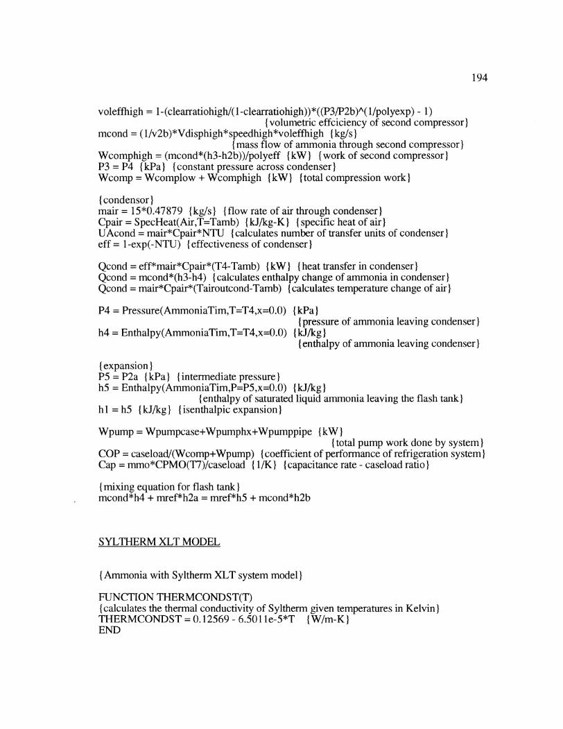
194
voleffhigh = 1-(clearratiohigh/(1-clearratiohigh))*((P3/P2b)A( 1/polyexp) - 1)(volumetric effciciency of second compressor)
mcond = (1/v2b)*Vdisphigh*speedhigh*voleffhigh {kg/s){mass flow of ammonia through second compressor)
Wcomphigh = (mcond*(h3-h2b))/polyeff {kW) (work of second compressor)P3 = P4 {kPa) {constant pressure across condenser)Wcomp = Wcomplow + Wcomphigh {kW) {total compression work)
(condensor)mair = 15*0.47879 (kg/s) (flow rate of air through condenser)Cpair = SpecHeat(Air,T=Tamb) I(kJ/kg-K) ({Ispecific heat of air)UAcond = mair*Cpair*NTU (calculates number of transfer units of condenser)eff = 1-exp(-NTU) ( effectiveness of condenser)
Qcond = eff*mair*Cpair*(T4-Tamb) (kW) (heat transfer in condenser)Qcond = mcond*(h3-h4) ( calculates enthalpy change of ammonia in condenser)Qcond = mair*Cpair*(Tairoutcond-Tamb) (calculates temperature change of air)
P4 = Pressure(AmmoniaTim,T=T4,x=0.0) I(kPa)(pressure of ammonia leaving condenser)
h4 = Enthalpy(AmmoniaTim,T=T4,x=0.0) I(kJ/kg)( enthalpy of ammonia leaving condenser)
( expansion)IP5 = P2a ( kPa) (Iintermediate pressure)Ih5 = Enthalpy(AmmoniaTim,P=P5,x=0.0) I(kJ/kg)
(enthalpy of saturated liquid ammonia leaving the flash tank)h I = h5 I(kJ/kg) ({Iisenthalpic expansion)
Wpump = Wpumpcase+Wpumphx+Wpumppipe (kW)I(total pump work done by system)
COP = caseload/(Wcomp+Wpump) (coefficient of performance of refrigeration system)Cap = mmo*CPMO(T7)/caseload (1/K) (Icapacitance rate - caseload ratio)
( mixing equation for flash tank)Imcond*h4 + mref*h2a = mref*h5 + mcond*h2b
SYLTHERM XLT MODEL
( Ammonia with Syltherm XLT system model)
FUNCTION THERMCONDST(T)( calculates the thermal conductivity of Syltherm given temperatures in Kelvin)}THERMCONDST = 0.12569 - 6.501 1le-5*T {(W/m-K)}END
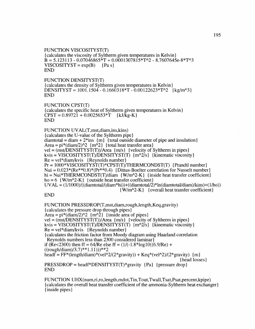
195
FUNCTION VISCOSITYST(T)(calculates the viscosity of Syltherm given temperatures in Kelvin)B = 5.123113 - 0.07046865*T + 0.0001307815*TA2 - 8.7607645e-8*TA3VISCOSITYST = exp(B) (Pa s}END
FUNCTION DENSITYST(T){ calculates the density of Syltherm given temperatures in Kelvin)DENSITYST = 1001.1504 - 0.1660318*T - 0.00122623*TA2 (kg/mA3)END
FUNCTION CPST(T)( calculates the specific heat of Syltherm given temperatures in Kelvin)CPST = 0.89721 + 0.0025653*T {kJ/kg-K)END
FUNCTION UVAL(T,mst,diam,ins,kins)( calculates the U-value of the Syltherm pipe)diamtotal = diam + 2*ins i) m total outside diameter of pipe and insulation)Area = pi*(diam/2)A2 (mA2) (total heat transfer area)vel = (mst/DENSITYST(T))/Area (m/s) (velocity of Syltherm in pipes)kvis = VISCOSITYST(T)/DENSITYST(T) (mA2/s) (Ikinematic viscosity)IRe = vel*diam/kvis (Reynolds number)Pr = 1000*VISCOSITYST(T)*CPST(T)/THERMCONDST(T) (Prandtl number)Nui = 0.023*(Re**0.8)*(Pr**0.4) (Dittus-Boelter correlation for Nusselt number)hi = Nui*THERMCONDST(T)/diam (W/mA2-K) (inside heat transfer coefficient)ho = 6 {W/mA2-K) (Ioutside heat transfer coefficient)UVAL = (1/1000)/((diamtotal/(diam*hi))+((diamtotal/2)*ln(diamtotal/diam)/kins)+(1/ho))
(W/m^2-K) (overall heat transfer coefficient)END
FUNCTION PRES SDROP(T,mst,diam,rough,length,Keq,gravity)( calculates the pressure drop through pipes)Area = pi*(diam/2)A2 ( mA2) ( Iinside area of pipes)vel = (mst/DENSITYST(T))/Area (m/s) (velocity of Syltherm in pipes)kvis = VISCOSITYST(T)/DENSITYST(T) (mA2/s) (Ikinematic viscosity)Re = vel*diam/kvis (Reynolds number)(calculates the friction factor from Moody diagram using Haarland correlationReynolds numbers less than 2300 considered laminar)
if (Re<2300) then ff = 64/Re else ff = (1/(-1.8*logl0((6.9/Re) +((rough/diam)/3.7)** 1.11)))**2headf = FF*(length/diam)*(velA2/(2*gravity)) + Keq*(velA2)/(2*gravity) (m
( head losses)PRESSDROP = headf*DENSITYST(T)*gravity (Pa (pressure drop)END
FUNCTION UHX(num,ri,ro,length,mdot,Tin,Tout,Twall,Tsat,Psat,percent,kpipe)(calculates the overall heat transfer coefficient of the ammonia-Syltherm heat exchanger)}( inside pipes)}

196
Tb = (Tin+Tout)/2 { K) ({Ibulk temperature)Ivel = (mdot/DENSITYST(Tb))/(num*ri**2) (m/s) (velocity of Syltherm)Red = vel*(2*ri)/(VISCOSITYST(Tb)/DENSITYST(Tb)) (Reynolds number)Pr = 1000*VISCOSITYST(Th)*CPST(Tb)/THERMCONDST(Th) { Prandtl number)(Nusslet number calculated using Hausen correlation for laminar flow and Nusseltcorrelation for turbulent flow)Iif (Red>2300) then Nud = 0.036*(Red**0. 8)*(Pr**( 1/3))*((2*ri)/length)**(1/18) elseNud = 3.66 + (0.668*(2*ri/length)*Red*Pr)/(1 +0.4*((2*ri/length)*Red*Pr)**(2/3))hi = NUD*THERMCONDST(Tb)/(2*ri) IW/mA2-K (inside heat transfer coefficient)( outside pipes)ICsf = 0.01 ( empirical constant)hfg = Enthalpy(AmmoniaTim,T=Tsat,x= 1.0)-Enthalpy(AmmoniaTim,T=Tsat,x=0.0)
I(kJ/kg) (heat of fusion)g = 9.8 (m/sA2) (Iacceleration due to gravity)sigma = 0.0213 (N/m } (surface tension)Prl = 1000*Viscosity(AmmoniaTim,T=Tsat,P=Psat+l )*SpecHeat(AmmoniaTim,T=Tsat,P=Psat+ 1)/Conductivity(AmmoniaTim,T=Tsat,P=Psat+ 1) (Prandtl number)Area = 2*pi*ro*length*num (mA2) ({Itotal heat transfer area)( boiling heat transfer correlation using Rohsenow correlation)Iho = 1000*Viscosity(AmmoniaTim,T=Tsat,P=Psat+ 1)*hfg*((g*(1/Volume(AmmoniaTim,T=Tsat,x=0.0)- 1/Volume(AmmoniaTim,T=Tsat,x= 1.0))/sigma)**0.5)* ((SpecHeat(AmmoniaTim,T=Tsat,P=Psat- 1)/(Csf*hfg*Prl** 1.7))**3)*(Twall-Tsat)**2 {W/mA2-K)(Uvalue)UHX = (1/1000)/((ro/(ri*hi))+(ro*ln(ro/ri)/kpipe) + (1/ho)) (W/mA2-K)
(overall heat transfer coefficient)END
FUNCTION UCASE(num,ri,ro,length,mdot,airvel,airarea,Tref,percent,Tair,kpipe)(calculates the overall heat transfer coefficient of the refrigerated case heat exchanger)(inside pipe)Ivel = (mdot/DENSITYST(Tref))/(num*ri**2) (m/s) (velocity of Syltherm)Redi = vel*(2*ri)/(VISCOSITYST(Tref)/DENSITYST(Tref)) ( Reynolds number)Pri = 1000*VISCOS ITYST(Tref)*CPST(Tref)/THERMCONDST(Tref)
( Prandtl number)(Nusselt number calculated using Nausen correlation fpr laminar flow and Nusseltcorrelation for turbulent flow)Iif (Redi>2300) then Nudi = 0.036*(Redi**0.8)*(Pri**(1/3))*((2*ri)/length)**(1/18)else Nudi = 3.66 +(0.668*(2*ri/length)*Redi*Pri)/(1 +0.4*((2*ri/length)*Redi*Pri)**(2/3))hi = NUDI*TIIERMCONDST(Tref)/(2*ri) (W/mA2-K)
(inside heat transfer coefficient)(outside pipes)Redo = airvel*(2*ro)/(Viscosity(Air,T=Tair)/(1/Volume(Air,T=Tair,P= 101.325)))
( Reynolds number)}Pro = 1 000"*Viscosity(Air,T=Tair)* SpecHeat(Air,T=Tair)/Conductivity(Air,T=Tair)
( Prandtl number)}( Nusselt number calculated using Churchill-Bernstein correlation)}

197
Nudo = 0.3+((0.62*Redo**(1/2)*Pro**(1/3))/((1 +(0.4/Pro)**(2/3))** (1/4)))*( 1+(Redo/2.82e5)**(5/8))**(4/5)ho = Nudo*Conductivity(Air,T=Tair)/(2*ro) {W/m^2-K}
{ outside heat transfer coefficient)UCASE = (1/((ro/(ri*hi))+(ro*ln(ro/ri)/kpipe) + (1/ho)))/1000 (W/m^2-K)
(overall heat transfer coefficient)END
{The equation set begins here)
(parameters)Tairout = 267 }K) (temperature of the air leaving the refrigerated case)caseload = 151{tons)}*3.51685 {kW) (refrigeration load met by the case)UAcond = 8.00 (kW/K) {UA value of the condenser)Tamb = 300 { K) (ambient temperature)Tstore = 300 (K) { store temperature)
(Compressor Parameters)I(dimensions of the first stage compressor)borelow = 2.38*2.54e'2 Im)strokelow = 1.75*2.54e-2 imspeedlow = 1700/60 (rev/sec)Iclearratiolow = 0.05 (clearance ratio)(dimensions of the second stage compressor)borehigh = 2.38*2.54e-2 [m)strokehigh = 1.75*2.54e-2 (m)speedhigh = 1700/60 (rev/sec)clearratiohigh = 0.05 (clearance ratio)Ipolyexp = 1.3 (polytropic exponent)polyeff = 0.65 (polytropic efficiency)
( Syltherm Parameters)Imst = 2.305 ( kg/s) ( Imass flow rate of Syltherm)x = 0.54 {pressure ratio exponent)diamc = 0.12 (I (diameter of pipe to case)Idiamh = 0.12 (I (Idiameter of pipe from case)Iinsc = 0.025 (I (Ithickness of insulation on pipe to case)insh = 0.025 (I (Ithickness of insulation on pipe from case)Ikinsc = 0.04 {(W/m-C) ({Ithermal conductivity of insulation on pipe to case)Ikinsh = 0.04 (W/m-C) (thermal conductivity of insulation on pipe from case)Irough = 0.000046 ( m ({pipe roughness)Ilengthc = 30 ( m ({length of pipe to case)Ilengthh = 30 (I (length of pipe fron case)Igravity = 9.81 {(m/sA2) (acceleration due to gravity)diamctotal = diamc + 2*insc i m (total diameter of pipe and insulation to case)diamhtotal = dianmh + 2*insh (in ( {total diameter of pipe and insulation from case)}Kpipec = 8.0 (for minor losses)Kpipeh = 8.0 (for minor losses)
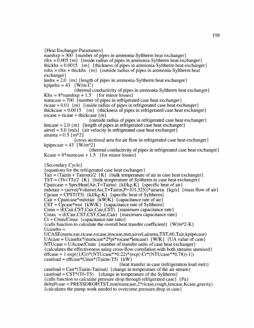
198
{ Heat Exchanger Parameters)Inumhxp = 300 (number of pipes in ammonia-Syltherm heat exchanger)rihx = 0.005 {m} (inside radius of pipes in ammonia-Syltherm heat exchanger)thickhx = 0.0015 (m (thickness of pipes in ammonia-S yltherm heat exchanger)rohx = rihx + thickhx (m (outside radius of pipes in ammonia-Syitherm heatexchanger)lenhx = 2.0 (in) (length of pipes in ammonia-Syitherm heat exchanger)Ikpipehx = 43 {W/m-C)
{thermal conductivity of pipes in ammonia-Syltherm heat exchanger)Khx = 8*numhxp + 1.5 {for minor losses)numcase = 700 (number of pipes in refrigerated case heat exchanger)Iricase = 0.01 (m (inside radius of pipes in refrigerated case heat exchanger)thickcase = 0.0015 i) m thickness of pipes in refrigerated case heat exchanger)Irocase = ricase + thickcase ( MI
( outside radius of pipes in refrigerated case heat exchanger)Ilencase = 2.0 (m)Ilength of pipes in refrigerated case heat exchanger)Iairvel = 5.0 (m/s) (Iair velocity in refrigerated case heat exchanger)Iairarea = 0.5 {1mA2)}
( cross sectional area for air flow in refrigerated case heat exchanger)Ikpipecase = 43 (W/mA2)
( thermal conductivity of pipes in refrigerated case heat exchanger)Kcase = 8*numcase + 1.5 (for minor losses)
( Secondary Cycle)I( equations for the refrigerated case heat exchanger)ITair = (Tairin + Tairout)/2 (K) (bulk temperature of air in case heat exchanger)TST = (T6+T5)/2 (K) (Ibulk temperature of Syltherm in case heat exchanger)Cpaircase = SpecHeat(Air,T=Tairin) (kJ/kg-K) (Ispecific heat of air)mdotair = (airvel/Volume(Air,T=Tairin,P=101.325))*airarea (kg/s) (mass flow of air)Cpcase = CPST(T5) (kJ/kg-K) (Ispecific heat of Syltherm)Cair = Cpaircase*mdotair {kW/K) (capacitance rate of air)CST = Cpcase*mst (kW/K) ( Icapacitance rate of Syltherm)Cmin = if(Cair,CST,Cair,Cair,CST) (minimum capacitance rate)Cmax = if(Cair,CST,CST,Cair,Cair) ( maximum capacitance rate)ICr = Cmin/Cmax (capacitance rate ratio)(calls function to calculate the overall heat transfer coefficient) (IW/mA2-K)Ucasehx =UCASE(numcase,ricase,rocase,lencase,mst,airvel,airarea,TST,60,Tair,kpipecase)UAcase = Ucasehx*(numcase*2*pi*rocase*lencase) (W/K) (UA value of case)NTUcase = UAcase/Cmin ( number of transfer units of case heat exchanger)(calculates the effectiveness using cross-flow correlation with both streams unmixed)Ieffcase = 1-exp((l/Cr)*(NTUcase**0.22)*(exp(-Cr*(NTUcase**0.78))- 1))caseload = effcase*Cmin*(Tairin-T5) (kW)
(heat transfer in case (refrigeration load met))caseload = Cair*(Tairin-Tairout) ( change in temperature of the air stream)caseload = CST*(T6-T5) (change in temperature of the Syltherm)( calls function to calculate pressure drop through refrigerated case) ({Pa)}deltaPcase = PRESS DR OP(TST,mst/numcase,2*ricase,rough,lencase,Kcase,gravity)(calculates the pump work needed to overcome pressure drop in case)}
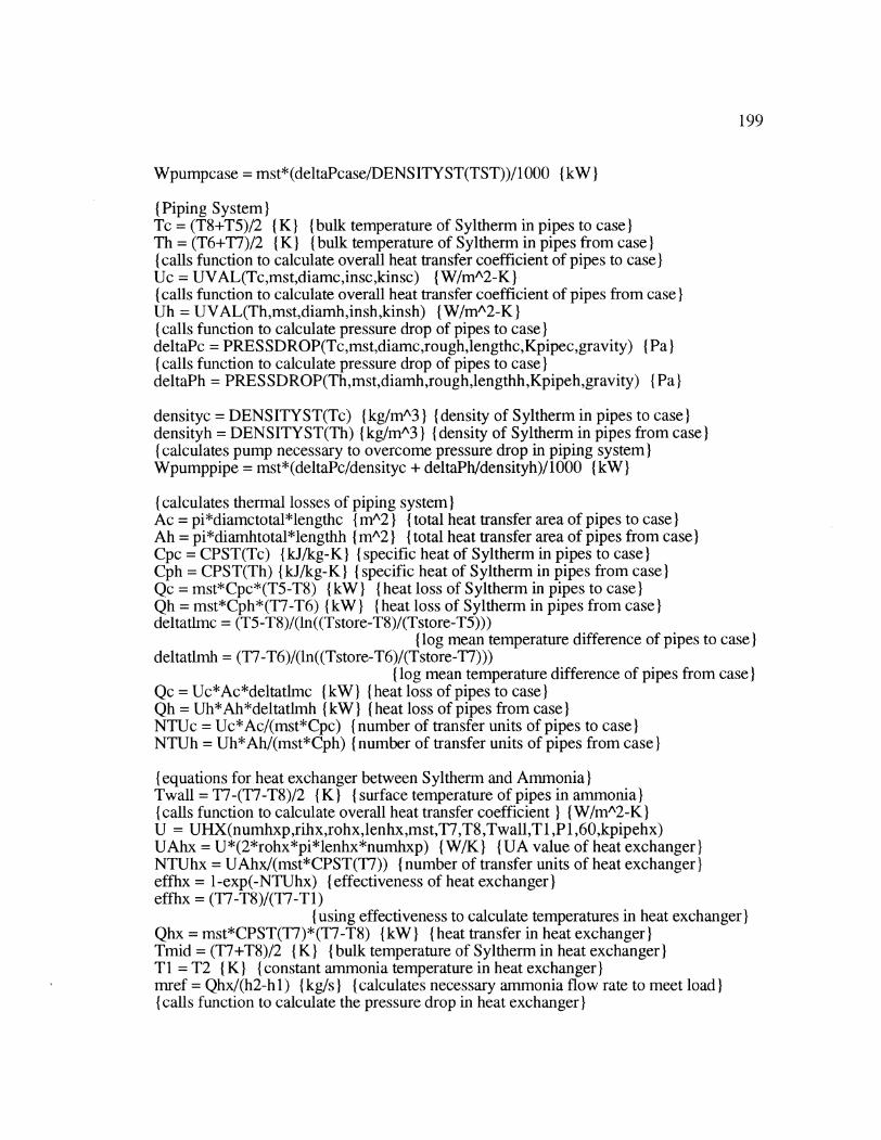
199
Wpumpcase = mst*(deltaPcase/DENSITYST(TST))/1000 {kW)
{ Piping System)ITc = (T8+T5)/2 (K) (bulk temperature of Syltherm in pipes to case)Th = (T6+T7)/2 (K) (bulk temperature of Syltherm in pipes from case)( calls function to calculate overall heat transfer coefficient of pipes to case)IUc = UVAL(Tc,mst,diamc,insc,kinsc) (W/mA2-K)( calls function to calculate overall heat transfer coefficient of pipes from case)IUh = UVAL(Th,mst,diamh,insh,kinsh) (W/mA2-K)I(calls function to calculate pressure drop of pipes to case)deltaPc = PRES SDROP(Tcmst,diamcrough,lengthcKpipecgravity) (Pa)( calls function to calculate pressure drop of pipes to case)IdeltaPh = PRES SDROP(Th,mst,diamh,rough,lengthh,Kpipeh,gravity) (Pa)
densityc = DENSITYST(Tc) (kg/mA3) ({density of Syltherm in pipes to case)densityh = DENSITYST(Th) I(kg/mA3) ({Idensity of Syltherm in pipes from case)( calculates pump necessary to overcome pressure drop in piping system)Wpumppipe = mst*(deltaPc/densityc + deltaPh/densityh)/1000 (kW)
(calculates thermal losses of piping system)Ac = pi*diamctotal*lengthc {(m^2) (ftotal heat transfer area of pipes to case)Ah = pi*diamhtotal*lengthh (mA2) ({total heat transfer area of pipes from case)Cpc = CPST(Tc) (kJ/kg-K) (specific heat of Syltherm in pipes to case)ICph = CPST(Th) (kJ/kg-K) (specific heat of Syltherm in pipes from case)Qc = mst*Cpc*(T5-T8) (kW) (heat loss of Syltherm in pipes to case)Qh = mst*Cph*(T7-T6) (kW) (heat loss of Syltherm in pipes from case)deltatlmc = (T5-T8)/(ln((Tstore-T8)/(Tstore-T5)))
(log mean temperature difference of pipes to case)deltatlmh = (T7-T6)/(ln((Tstore-T6)/(Tstore-T7)))
(log mean temperature difference of pipes from case)Qc = Uc*Ac*deltatlmc (kW) (Iheat loss of pipes to case)IQh = Uh*Ah*deltatlmh (kW) (Jheat loss of pipes from case)NTUc = Uc*Ac/(mst*Cpc) (number of transfer units of pipes to case)NTUh = Uh*Ah/(mst*Cph) (number of transfer units of pipes from case)
(equations for heat exchanger between Syltherm and Ammonia)Twall = T7-(T7-T8)/2 (K) (surface temperature of pipes in ammonia)(calls function to calculate overall heat transfer coefficient) }IW/mA2-K)U = UHX(numhxp,rihx,rohx,lenhx,mst,T7,T8,Twall,T 1,P 1,60,kpipehx)UAhx = U*(2*rohx*pi*lenhx*numhxp) I(W/K) ({IUA value of heat exchanger)NTUhx = UAhx/(mst*CPST(T7)) ( number of transfer units of heat exchanger)effhx = 1-exp(-NTUhx) ( effectiveness of heat exchanger)Ieffhx = (T7-T8)/(T7-T1)
( using effectiveness to calculate temperatures in heat exchanger)IQhx = mst*CPST(T7)*(T7-T8) (kW) (heat transfer in heat exchanger)Tmid = (T7+T8)/2 ( K) ({bulk temperature of Syltherm in heat exchanger)TI = T2 (K) (constant ammonia temperature in heat exchanger)mref = Qhx/(h2-h 1) ( kg/s) ({calculates necessary ammonia flow rate to meet load)}( calls function to calculate the pressure drop in heat exchanger)}

200
deltaPhx = PRES SDROP(Tmid,mst/numhxp,2*rihx,rough,lenhx,Khx,gravity) (Pa)(calculates pump work necessary to overcome pressure drop in heat exchanger)Wpumphx = mst*(deltaPhxIDENSITYST(Tmid))/1000 {kW)
P2 = Pressure(AmmoniaTim,T=T1,x=l.0) {kPa)(pressure of ammonia leaving heat exchanger)
h2 = Enthalpy(AinmoniaTim,T=T2,x=1.0) {kJ/kg)( enthalpy of ammonia leaving heat exchanger)
s2 = Entropy(AmmoniaTim,T=T2,x=l.0) {kJ/kg-K)I( entropy of ammonia leaving heat exchanger)I
P1 = P2 (kPa) ({Iammonia pressure constant in heat exchanger)I
( Ammonia Cycle)I(compressor)rp = P3/P2 ( pressure ratio of evaporator to condenser)Irps = rpAx (pressure ratio relationship)rps = P2a/P2 (calculates intermediate pressure)
(Low Pressure Compressor)Iv2 = Volume(AmmoniaTim,P=P2,x=1.0) {rmA3/kg)I
( specific volume of ammonia entering first compressor)IP2*(v2)Apolyexp = P2a*(v2a)Apolyexp (polytropic compression equation)Ih2a = Enthalpy(AmmoniaTim,P=P2a,v=v2a) {IkJ/kg)I
( enthalpy of ammonia leaving first compressor)T2a = Temperature(AmmoniaTim,P=P2a,v=v2a) (IK)I
(temperature of ammonia leaving first compressor)Vdisplow = numcyllow*(pi*((borelow/2)A2)*strokelow) {(m^3 }
(displacement volume of first compressor)Ivolefflow = 1-(clearratiolow/(1 -clearratiolow))*((P2a/P2)A(l/polyexp) - 1)
(volumetric efficiency of first compressor)mref = (1/v2)*Vdisplow*speedlow*volefflow (kg/s)
(mass flow of ammonia through first compressor)Wcomplow = (mref*(h2a-h2))/polyeff (kW) (Iwork of first compressor)
(High Pressure Compressor)P2b = P2a I(kPa) ( {intermediate pressure)h2b = Enthalpy(AmmoniaTim,P=P2b,x=l.0) 1(kJ/kg)I
( enthalpy of ammonia entering second compressor)s2b = Entropy(AmmoniaTim,P=P2b,x=l.0) {kJ/kg-K)
(entropy of ammonia entering second compressor)T2b = Temperature(AmmoniaTim,P=P2b,x= 1.0) ( K)I
(temperature of ammonia entering second compressor)Iv2b = Volume(AmmoniaTim,P=P2b,x= 1.0) {mA3/kg)I
( specific heat of ammonia entering second compressor)IP2b*(v2b)Apolyexp = P3*(vol3)Apolyexp (polytropic compression equation)h3 = Enthalpy(AmmoniaTim,P=P3,v=vol3) {(kJ/kg)}
(enthalpy of ammonia leaving second compressor)T3 = Temperature(AmmoniaTim,P=P3,v=vol3) ( K)
(temperature of ammonia leaving second compressor)}
201
Vdisphigh = numcylhigh*(pi*((borehigh/2)A2)*strokehigh) (mA3){ displacement volume of second compressor)
voleffhigh = 1-(clearratiohigh/(1-clearratiohigh))*((P3/P2b)A(1/polyexp) - 1){volumetric effciciency of second compressor)
mcond = (1/v2b)*Vdisphigh*speedhigh*voleffhigh { kg/s)(mass flow of ammonia through second compressor)
Wcomphigh = (mcond*(h3-h2b))/polyeff { kW) (work of second compressor)P3 = P4 {kPa) {constant pressure across condenser)Wcomp = Wcomplow + Wcomphigh (kW) {total compression work)
(condensor)mair = 15*0.47879 {kg/s) (flow rate of air through condenser)Cpair = SpecHeat(Air,T=Tamb) I(kJ/kg-K)} { specific heat of air)UAcond = mair*Cpair*NTU (calculates number of transfer units of condenser)eff = 1-exp(-NTU) { effectiveness of condenser)
Qcond = eff*mair*Cpair*(T4-Tamb) (kW) (Iheat transfer in condenser)Qcond = mcond*(h3-h4) (calculates enthalpy change of ammonia in condenser)Qcond = mair*Cpair*(Tairoutcond-Tamb) (calculates temperature change of air)
P4 = Pressure(AmmoniaTim,T=T4,x=0.0) (kPa)(pressure of ammonia leaving condenser)
h4 = Enthalpy(AmmoniaTim,T=T4,x=0.0) IkJ/kg)I( enthalpy of ammonia leaving condenser)
(expansion)P5 = P2a (kPa) (intermediate pressure)h5 = Enthalpy(AmmoniaTim,P=P5,x=0.0) (kJ/kg)
(enthalpy of saturated liquid ammonia leaving the flash tank)h I = h5 ( kJ/kg) ({Iisenthalpic expansion)I
Wpump = Wpumpcase+Wpumphx+Wpumppipe (kW)( total pump work done by system)I
COP = caseload/(Wcomp+Wpump) (coefficient of performance of refrigeration system)Cap = mst*CPST(T7)/caseload (1/K) (capacitance rate - caseload ratio)
( mixing equation for flash tank)Imcond*h4 + mref*h2a = mref*h5 + mcond*h2b
ETHANOL MODEL
( Ammonia with ethanol system model)
FUNCTION THERMCoNDEA(T)(calculates the thermal conductivity of Ethanol given temperatures in Kelvin)}THERMCoNDEA = 0.257 15 - 0.00030645"T ( W/m-K)
202
END
FUNCTION VISCOSITYEA(T){ calculates the viscosity of Ethanol given temperatures in Kelvin)B = 11.664554604 - 0.057902271482*T + 6.356133171le-5*TA2VISCOSITYEA = exp(B)/e3 (Pa s)END
FUNCTION DENSITYEA(T)( calculates the density of Ethanol given temperatures in Kelvin)DENSITYEA = 0.2567e3*(0.240A(-(1 -T/515.8)A(2/7))) {kg/mA3}END
FUNCTION CPEA(T){ calculates the specific heat of Ethanol given temperatures in Kelvin)CPEA = (100.92 -111.839e-3*T + 498.54e-6*TA2)/46 (kJ/kg-K)END
FUNCTION UVAL(T,mea,diam,ins,kins)( calculates the U-value of the Ethanol pipe)diamtotal = diam + 2*ins i m (total outside diameter of pipe and insulation)Area = pi*(diam/2)A2 { mA2) (Itotal heat transfer area)vel = (mea/DENSITYEA(T))/Area (m/s) (Ivelocity of Ethanol in pipes)kvis = VISCOSITYEA(T)/DENSITYEA(T) I(mA2/s) (kinematic viscosity)Re = vel*diam/kvis (Reynolds number)Pr 1000*VISCOSITYEA(T)*CPEA(T)/THERMCONDEA(T) (Prandtl number)Nui = 0.023*(Re**0.8)*(Pr**0.4) (Dittus-Boelter correlation for Nusselt number)hi = Nui*THERMCONDEA(T)/diam (W/mA2-KI (inside heat transfer coefficient)ho = 6 (W/mA2-K) (Ioutside heat transfer coefficient)UVAL = (1/1000)/((diamtotal/(diam*hi))+((diamtotal/2)*ln(diamtotal/diam)/kins)+(1/ho))
(W/mA2-K) (overall heat transfer coefficient)END
FUNCTION PRES SDROP(T,mea,diam,rough,length,Keq, gravity)( calculates the pressure drop through pipes)Area = pi*(diam/2)A2 (mA2) (Iinside area of pipes)vel = (mea/DENSITYEA(T))/Area (m/s) (velocity of Ethanol in pipes)kvis = VISCOSITYEA(T)/DENSITYEA(T) (mA2/s) (kinematic viscosity)Re = vel*diam/kvis (Reynolds number)(calculates the friction factor from Moody diagram using Haarland correlationReynolds numbers less than 2300 considered laminar)
if (Re<2300) then ff = 64/Re else ff = (1/(-1.8*logl0((6.9/Re) +((rough/diam)/3.7)** 1.11)))**2headf = FF*(length/diam)*(velA2/(2*gravity)) + Keq*(velA2)/(2*gravity) (in)
(head losses)}PRES SDROP = headf*DENSITYEA(T)*gravity ( Pa) (pressure drop)}END
FUNCTION UHX(num,ri,ro,length,mdot,Tin,Tout,Twall,Tsat, Psat,percent,kpipe)

203
(calculates the overall heat transfer coefficient of the ammonia-Ethanol heat exchanger)(inside pipes)ITh = (Tin+Tout)/2 (K) (bulk temperature)vel = (mdot/DENSITYEA(Th))/(num*ri**2) {m/s) (velocity of Ethanol)Red = vel*(2*ri)/(VISCOSITYEA(Tb)/DENSITYEA(Tb)) (Reynolds number)Pr = 1000*VISCOSITYEA(Tb)*CPEA(Tb)/THERMCONDEA(Th) (Prandtl number)(Nusslet number calculated using Hausen correlation for laminar flow and Nusseltcorrelation for turbulent flow)if (Red>2300) then Nud = 0.036*(Red**0. 8)*(Pr**(l/3))*((2*ri)/length)**(1/18) elseNud = 3.66 + (0.668*(2*ri/length)*Red*Pr)/(l+0.4*((2*ri/length)*Red*Pr)**(2/3))hi = NUD*THERMCONDEA(Tb)/(2*ri) {W/mA2-K) (Iinside heat transfer coefficient)( outside pipes)ICsf = 0.01 ( empirical constant)Ihfg = Enthalpy(AmmoniaTim,T=Tsat,x=1.0)-Enthalpy(AmmoniaTim,T=Tsat,x=0.0)
I(kJ/kg) ({Iheat of fusion)Ig = 9.8 { m/sA2) (Iacceleration due to gravity)Isigma = 0.0213 (N/m ( {Isurface tension)IPrl = 1000*Viscosity(AmmoniaTim,T=Tsat,P=Psat+ l)*SpecHeat(AmmoniaTim,T=Tsat,P=Psat+ 1)/Conductivity(AmmoniaTim,T=Tsat,P=Psat+ 1) (Prandtl number)Area = 2*pi*ro*length*num (mA2) (Itotal heat transfer area)(boiling heat transfer correlation using Rohsenow correlation)ho = 1000*Viscosity(AmmoniaTim,T=Tsat,P=Psat+ l)*hfg*((g*(1/Volume(AmmoniaTim,T=Tsat,x=0.0)- 1/Volume(AmmoniaTim,T=Tsat,x= 1.0))/sigma)**0.5)* ((SpecHeat(AmmoniaTim,T=Tsat,P=Psat- 1)/(Csf*hfg*Prl** 1.7))**3)*(Twall-Tsat)**2 {W/mA2-K)I(Uvalue)UHX = (1/1000)/((ro/(ri*hi))+(ro*ln(ro/ri)/kpipe) + (1/ho)) {W/m^2-K)
(overall heat transfer coefficient)IEND
FUNCTION UCASE(num,ri,ro,length,mdot,airvel,airarea,Tref,percent,Tair,kpipe)(calculates the overall heat transfer coefficient of the refrigerated case heat exchanger)(inside pipe)Ivel = (mdot/DENSITYEA(Tref))/(num*ri**2) (m/s) (velocity of Ethanol)Redi = vel*(2*ri)/(VISCOSITYEA(Tref)/DENSITYEA(Tref)) ( Reynolds number)Pri = 1000*VISCOSITYEA(Tref)*CPEA(Tref)/THERMCONDEA(Tref)
( Prandtl number)(Nusselt number calculated using Nausen correlation fpr laminar flow and Nusseltcorrelation for turbulent flow)Iif (Redi>2300) then Nudi = 0.036*(Redi**0.8)*(Pri**(1/3))*((2*ri)/length)**(1/18)else Nudi = 3.66 +(0.668*(2*ri/length)*Redi*Pri)/(1 +0.4*((2*ri/length)*Redi*Pri)**(2/3))hi = NUDI*THERMCONDEA(Tref)/(2*ri) {W/m^2-K)
( inside heat transfer coefficient)I( outside pipes)}Redo = airvel* (2*ro)/(Viscosity(Air,T=Tair)/( 1/Volume(Air,T=Tair,P= 101.325)))
( Reynolds number)Pro = 1 000"*Viscosity(Air,T=Tair)* SpecHeat(Air,T=Tair)/Conductivity(Air,T=Tair)
204
I(Prandtl number){ Nusselt number calculated using Churchill-Bernstein correlation)INudo = 0.3+((0.62*Redo**(1/2)*Pro**(1/3))/((1 +(0.4/Pro)**(2/3))** (1/4)))*(1 +(Redo/2.82e5)** (5/8))** (4/5)ho = Nudo*Conductivity(Air,T=Tair)/(2*ro) {W/m^2-K)
{outside heat transfer coefficient)UCASE = (1/((ro/(ri*hi))+(ro*ln(ro/ri)/kpipe) + (1/ho)))/1000 {W/m^2-K}
{ overall heat transfer coefficient)END
{ The equation set begins here)
{parameters)Tairout = 267 (K) (temperature of the air leaving the refrigerated case)caseload = 151{tons)}*3.51685 {kW) {refrigeration load met by the case)UAcond = 8.00 {kW/K) (UA value of the condenser)Tamb = 300 (1K) { ambient temperature)ITstore = 300 (K) { store temperature)I
{ Compressor Parameters)II dimensions of the first stage compressor)Iborelow = 2.38*2.54e-2 {m)strokelow = 1.75*2.54e-2 (m)speedlow = 1700/60 {rev/sec)clearratiolow = 0.05 {clearance ratio)(dimensions of the second stage compressor)Iborehigh = 2.38*2.54e-2 Im)strokehigh = 1.75*2.54e-2 (mspeedhigh = 1700/60 (rev/sec)clearratiohigh = 0.05 (clearance ratio)polyexp = 1.3 (polytropic exponent)polyeff = 0.65 (polytropic efficiency)
{ Ethanol Parameters)Imea = 2.305 (kg/s) {mass flow rate of Ethanol)x = 0.54 (pressure ratio exponent)diamc = 0.12 ( m (diameter of pipe to case)diamh = 0.12 {m) (diameter of pipe from case)insc = 0.025 {m) (thickness of insulation on pipe to case)insh = 0.025 ( m (thickness of insulation on pipe from case)kinsc = 0.04 (W/m-C) (thermal conductivity of insulation on pipe to case)kinsh - 0.04 (W/m-C) (thermal conductivity of insulation on pipe from case)rough = 0.000046 (im (pipe roughness)lengthc = 30 (I (I{length of pipe to case)lengthh = 30 (in ({length of pipe fron case)}gravity = 9.81 {(m/s^2) ( acceleration due to gravity)}diamctotal = diamc + 2*insc (in ( total diameter of pipe and insulation to case)}diamhtotal = diamh + 2*insh (in ( {total diameter of pipe and insulation from case)}Kpipec = 8.0 (for minor losses)
205
Kpipeh = 8.0 {for minor losses)
(Heat Exchanger Parameters)numhxp = 300 {number of pipes in ammonia-Ethanol heat exchanger)rihx = 0.005 (in ({inside radius of pipes in ammonia-Ethanol heat exchanger)thickhx = 0.0015 (in) (thickness of pipes in ammonia-Ethanol heat exchanger)rohx = rihx + thickhx (n)I
{ outside radius of pipes in ammonia-Ethanol heat exchanger)lenhx = 2.0 { m) (length of pipes in ammonia-Ethanol heat exchanger)kpipehx = 43 { W/m-C)I
(thermal conductivity of pipes in ammonia-Ethanol heat exchanger)Khx = 8*numhxp + 1.5 (for minor losses)numcase = 700 {number of pipes in refrigerated case heat exchanger)ricase = 0.01 { m) ({Iinside radius of pipes in refrigerated case heat exchanger)thickcase = 0.0015 (in) (Ithickness of pipes in refrigerated case heat exchanger)rocase = ricase + thickcase ( mI
( outside radius of pipes in refrigerated case heat exchanger)lencase = 2.0 im ( {length of pipes in refrigerated case heat exchanger)airvel = 5.0 ( m/s) ( {air velocity in refrigerated case heat exchanger)airarea = 0.5 (1mA2}
(cross sectional area for air flow in refrigerated case heat exchanger)kpipecase = 43 (W/mA2)
( thermal conductivity of pipes in refrigerated case heat exchanger)Kcase = 8*numcase + 1.5 (for minor losses)
(Secondary Cycle)I(equations for the refrigerated case heat exchanger)Tair = (Tairin + Tairout)/2 (K) (bulk temperature of air in case heat exchanger)TEA = (T6+T5)/2 ( K) ( Ibulk temperature of Ethanol in case heat exchanger)Cpaircase = SpecHeat(Air,T=Tairin) I(kJ/kg-K) ( Ispecific heat of air)Imdotair = (airvellVolume(Air,T=Tairin,P=101.325))*airarea (kg/s (mass flow of air)Cpcase = CPEA(T5) (IkJ/kg-K) ( Ispecific heat of Ethanol)Cair = Cpaircase*mdotair (kW/K) (Icapacitance rate of air)CEA = Cpcase*mea I(kW/K) ({Icapacitance rate of Ethanol)Cmin = if(Cair,CEA,Cair,Cair,CEA) (minimum capacitance rate)Cmax = if(Cair,CEA,CEA,Cair,Cair) (maximum capacitance rate)Cr = Cmin/Cmax (capacitance rate ratio)I(calls function to calculate the overall heat transfer coefficient) (W/mA2-K}Ucasehx =UCASE(numcase,ricase,rocase,lencase,mea,airvel,airarea,TEA,60,Tair,kpipecase)UAcase = Ucasehx*(numcase*2*pi*rocase*lencase) (W/K) (UA value of case)NTUcase = UAcase/Cmin ( number of transfer units of case heat exchanger)(calculates the effectiveness using cross-flow correlation with both streams unmixed)effcase = 1-exp((1/Cr)*(NTUcase**0.22)*(exp(-Cr*(NTUcase**0.78))- 1))caseload = effcase*Cmin*(Tairin-T5) {(kW)
(heat transfer in case (refrigeration load met))caseload = Cair*(Tairin-Tairout) ( change in temperature of the air stream)caseload = CEA*(T6-T5) (change in temperature of the Ethanol)(calls function to calculate pressure drop through refrigerated case) (Pa)
206
deltaPcase = PRESSDROP(TEA,mea/numcase,2*ricase,rough,lencase,Kcase,gravity){ calculates the pump work needed to overcome pressure drop in case)Wpumpcase = mea*(deltaPcase/DENSITYEA(TEA))/1000 {kW)
(Piping System)Tc = (T8+T5)/2 (K) (bulk temperature of Ethanol in pipes to case)Th = (T6+T7)/2 {K) (bulk temperature of Ethanol in pipes from case)( calls function to calculate overall heat transfer coefficient of pipes to case)IUc = UVAL(Tc,mea,diamc,insc,kinsc) {W/mA2-K)( calls function to calculate overall heat transfer coefficient of pipes from case)IUh = UVAL(Thmeadiamhinshkinsh) { W/mA2-K)(calls function to calculate pressure drop of pipes to case)deltaPc = PRESSDROP(Tc,mea,diamc,rough,lengthc,Kpipec,gravity) (Pa)( calls function to calculate pressure drop of pipes to case)IdeltaPh = PRES SDROP(Th,mea,diamh,rough,lengthh,Kpipeh,gravity) (Pa)
densityc = DENSITYEA(Tc) (kg/mA3 (I{density of Ethanol in pipes to case)densityh = DENSITYEA(Th) (kg/mA3) (Idensity of Ethanol in pipes from case)(calculates pump necessary to overcome pressure drop in piping system)Wpumppipe = mea*(deltaPc/densityc + deltaPh/densityh)/1000 (kW)
( calculates thermal losses of piping system)Ac = pi*diamctotal*lengthc (mA2) ({total heat transfer area of pipes to case)IAh = pi*diamhtotal*lengthh { mA2) (total heat transfer area of pipes from case)ICpc = CPEA(Tc) (kJ/kg-K) (specific heat of Ethanol in pipes to case)Cph = CPEA(Th) I(kJ/kg-K) ({Ispecific heat of Ethanol in pipes from case)Qc = mea*Cpc*(T5-T8) (kW) (heat loss of Ethanol in pipes to case)Qh = mea*Cph*(T7-T6) (kW) (heat loss of Ethanol in pipes from case)deltatlmc = (T5-T8)/(ln((Tstore-T8)/(Tstore-T5)))
(log mean temperature difference of pipes to case)deltatlmh = (T7-T6)/(ln((Tstore-T6)/(Tstore-T7)))
(log mean temperature difference of pipes from case)Qc = Uc*Ac*deltatlmc (kW) (heat loss of pipes to case)Qh = Uh*Ah*deltatlmh (kW} (heat loss of pipes from case)NTUc = Uc*Ac/(mea*Cpc) (number of transfer units of pipes to case)NTUh = Uh*Ah/(mea*Cph) (number of transfer units of pipes from case)
(equations for heat exchanger between Ethanol and Ammonia)Twall = T7-(T7-T8)/2 (K) (surface temperature of pipes in ammonia)(calls function to calculate overall heat transfer coefficient) {W/mA2-K)U = UHX(numhxp,rihx,rohx,lenhx,mea,T7 ,T8,Twall,T 1 ,P 1,60,kpipehx)UAhx = U*(2*rohx*pi*lenhx*numhxp) (W/K) (UA value of heat exchanger)NTUhx = UAhx/(mea*CPEA(T7)) ( number of transfer units of heat exchanger)effhx = 1-exp(-NTUhx) (effectiveness of heat exchanger)effhx = (T7-T8)/(T7-T1)
(using effectiveness to calculate temperatures in heat exchanger)}Qhx = mea*CPEA(T7)*(T7-T8) (kW} (heat transfer in heat exchanger)Tmid = (T7+T8)12 (K) (bulk temperature of Ethanol in heat exchanger)T 1 = T2 (K) (constant ammonia temperature in heat exchanger)}
207
mref = Qhx/(h2-h 1) (1kg/s) ({Icalculates necessary ammonia flow rate to meet load)(calls function to calculate the pressure drop in heat exchanger)deltaPhx = PRESSDROP(Tmid,mea/numhxp,2*rihx,rough,lenhx,Khx,gravity) (Pa)(calculates pump work necessary to overcome pressure drop in heat exchanger)Wpumphx = mea*(deltaPhx/DENSITYEA(Tmid))/1000 { kW)
P2 = Pressure(AmmoniaTim,T=T1,x=1.0) (kPa)(pressure of ammonia leaving heat exchanger)
h2 = Enthalpy(AmmoniaTim,T=T2,x= 1.0) (kJ/kg){enthalpy of ammonia leaving heat exchanger)
s2 = Entropy(AmmoniaTimT=T2,x= 1.0) 1(kJ/kg-K)I(entropy of ammonia leaving heat exchanger)
P1 = P2 (kPa) (Iammonia pressure constant in heat exchanger)
(Ammonia Cycle)(compressor)rp = P3/P2 (pressure ratio of evaporator to condenser)rps = rpAx (pressure ratio relationship)rps = P2a/P2 (calculates intermediate pressure)
(Low Pressure Compressor)Iv2 = Volume(AmmoniaTim,P=P2,x= 1.0) (mA3/kg)I
( specific volume of ammonia entering first compressor)P2*(v2)Apolyexp = P2a*(v2a)Apolyexp (polytropic compression equation)h2a = Enthalpy(AmmoniaTim,P=P2a,v=v2a) IkJ/kg)I
( enthalpy of ammonia leaving first compressor)T2a = Temperature(AmmoniaTim,P=P2a,v=v2a) (IK)I
( temperature of ammonia leaving first compressor)Vdisplow = numcyllow*(pi*((borelow/2)A2)*strokelow) (mA3)}
( displacement volume of first compressor)Ivolefflow = 1-(clearratiolow/(1-clearratiolow))*((P2a/P2)A(1l/polyexp) - 1)
( volumetric efficiency of first compressor)mref = (1/v2)*Vdisplow*speedlow*voleffow (kg/s)
( mass flow of ammonia through first compressor)Wcomplow = (mref*(h2a-h2))/polyeff (kW ([work of first compressor)
( High Pressure Compressor)IP2b = P2a (kPa (Iintermediate pressure)h2b = Enthalpy(AmmoniaTim,P=P2b,x= 1.0) (kJ/kg)
( enthalpy of ammonia entering second compressor)s2b = Entropy(AmmoniaTim,P=P2b,x= 1.0) (kJ/kg-K)
(entropy of ammonia entering second compressor)T2b = Temperature(AmmoniaTim,P=P2b,x= 1.0) ( K)I
(temperature of ammonia entering second compressor)Iv2b = Volume(AmmoniaTimP=P2bx=1.0) (ImA3/kg)I
( specific heat of ammonia entering second compressor)}P2b*(v2b)Apolyexp = P3*(VOl3)Apolyexp (polytropic compression equation)h3 = Enthalpy(AmmoniaTim,P=P3,v=vol3) (kJ/kg)}
(enthalpy of ammonia leaving second compressor)
208
T3 = Temperature(AmmoniaTim,P=P3,v=vol3) ( K)( temperature of ammonia leaving second compressor)
Vdisphigh = numcylhigh*(pi*((borehigh/2)A2)*strokehigh) { mA 31(displacement volume of second compressor)
voleffhigh = 1-(clearratiohigh/( 1-clearratiohigh))*((P3/P2b)A( 1/polyexp) - 1){ volumetric effciciency of second compressor)
mcond = (1/v2b)*Vdisphigh*speedhigh*voleffhigh { kg/s)(mass flow of ammonia through second compressor)
Wcomphigh = (mcond*(h3-h2b))/polyeff {(kW) ({Iwork of second compressor)P3 = P4 {kPa} (constant pressure across condenser)Wcomp = Wcomplow + Wcomphigh {kW) (Itotal compression work)I
{condensor)Imair = 15*0.47879 {kg/s) (flow rate of air through condenser)Cpair = SpecHeat(Air,T=Tamb) { kJ/kg-K) { specific heat of air)IUAcond = mair*Cpair*NTU (calculates number of transfer units of condenser)eff = 1-exp(-NTU) ( effectiveness of condenser)I
Qcond = eff*mair*Cpair*(T4-Tamb) (kW) (heat transfer in condenser)Qcond = mcond*(h3-h4) (calculates enthalpy change of ammonia in condenser)Qcond = mair*Cpair*(Tairoutcond-Tamb) (calculates temperature change of air)I
P4 = Pressure(AmmoniaTim,T=T4,x=0.0) (kPa)(pressure of ammonia leaving condenser)
h4 = Enthalpy(AmmoniaTim,T=T4,x=0.0) (kJ/kg)(enthalpy of ammonia leaving condenser)
(expansion)P5 = P2a I(kPa) (intermediate pressure)h5 = Enthalpy(AmmoniaTim,P=P5,x=0.0) (kJ/kg)
(enthalpy of saturated liquid ammonia leaving the flash tank)h I = h5 (kJ/kg) (isenthalpic expansion)I
Wpump = Wpumpcase+Wpumphx+Wpumppipe (kW)( total pump work done by system)
COP = caseload/(Wcomp+Wpump) (coefficient of performance of refrigeration system)Cap = mea*CPEA(T7)/caseload (1/K) (capacitance rate - caseload ratio)
(mixing equation for flash tank)mcond*h4 + mref*h2a = mref*h5 + mcond*h2b
PROPANE MODEL
(Ammonia with propane system model)
FUNCTION UVAL(T,mpr,diam,ins,kins)
209
( calculates the U-value of the propane distribution pipes)density = l/Volume(Propane,T=T,P=700) {kg/mA3) (density of propane)diamtotal = diam + 2*ins (m (total outside diameter of pie and insulation)IArea = pi*(diam/2)A2 {mA21 (Itotal heat transfer area)vel = (mpr/density)/Area (m/s) (Ivelocity of propane)kvis = Viscosity(Propane,T=T,P=700)/density { mA2/s) (Ikinematic viscosity)Re = vel*diam/kvis ( Reynolds number)Pr = 1000*Viscosity(Propane,T=T,P=700)*SpecHeat(Propane,T=T,P=700)/Conductivity(Propane,T=T,P=700) ( Prandtl number)Nui = 0.023*(Re**0.8)*(Pr**0.4) (Dittus-Boelter correlation for Nusselt number)hi = Nui*Conductivity(Propane,T=T,P=700)/diam {W/mA2-K}
( inside heat transfer coefficient)Iho = 6 (W/mA2-K) ({outside heat transfer coefficient)UVAL = (1/1000)/((diamtotal/(diam*hi))+((diamtotal/2)*ln(diamtotal/diam)/kins)+(1/ho))
(W/mA2-K) (overall heat transnfer coefficient)END
FUNCTION PRESSDROP(T,mpr,diam,rough,length,Keq,gravity)( calculate the pressure drop through pipes)density = l/Volume(Propane,T=T,P=700) (kg/mA3) (density of propane)Area = pi*(diam/2)A2 (mA2) }(inside area of pipes)Ivel = (mpr/density)/Area ( m/s) (Ivelocity of propane)kvis = Viscosity(Propane,T=T,P=700)/density (mA2/s) (kinematic viscosity)Re = vel*diam/kvis (Reynolds number)(calculates the friction factor from Moody diagram using Haarland correlationReynolds numbers less than 2300 considered laminar)
if (Re<2300) then ff = 64/Re else ff = (1/(-1.8*log10((6.9/Re) +((rough/diam)/3.7)** 1.11)))**2headf = FF*(length/diam)*(velA2/(2*gravity)) + Keq*(velA2)/(2*gravity) (m
( head losses)PRESSDROP = headf*density*gravity (Pa) (pressure drop)END
FUNCTION UHX(num,ri,ro,length,mdot,Tin,Tout,Twall,Tsat,Psat,percent,kpipe)(calculates the overall heat transfer coefficient of the ammonia-propane heat exchanger)(inside pipes)ITb = (Tin+Tout)/2 (K) (bulk temperature of propane)vel = (mdot/(l/Volume(Propane,T=Tb,P=700)))/(num*ri**2) (m/s)
(velocity of propane)Red = vel*(2*ri)/(Viscosity(Propane,T=Tb,P=700)/(1/Volume(Propane,T=Tb,P=700)))
( Reynolds number)Pr = 1000*Viscosity(Propane,T=Tb,P=700)*SpecHeat(Propane,T=Tb,P=700)/Conductivity(Propane,T=Tb,P=700) ( Prandtl number)( Nusselt number calculated using Hausen correlation for laminar flow and Nusseltcorrelation for turbulent flow)if (Red>2300) then Nud = 0.036*(Red**0.8)*(Pr**(l/3))*((2*ri)/length)**(1118) elseNud = 3.66 + (0.668*(2*ri/length)*Red*Pr)/( 1 +0.4*((2*ri/length)*Red*Pr)**(2/3))hi = NUD*Conductivity(Propane,T=Tb,P=700)/(2*ri) {(W/mA2-K)}
( inside heat transfer coefficient)}

210
( outside pipes)ICsf = 0.01 {empirical constant)hfg = Enthalpy(AmmoniaTim,T=Tsat,x=1.0)-Enthalpy(AmmoniaTim,T=Tsat,x=0.0)
I(kJ/kg} {heat of fusion)g = 9.8 { m/sA2) (acceleration due to gravity)sigma = 0.0213 (N/m { surface tension)Prl = 1000*Viscosity(AmmoniaTim,T=Tsat,P=Psat+ 1)*SpecHeat(AmmoniaTim,T=Tsat,P=Psat+ 1)/Conductivity(AmmoniaTim,T=Tsat,P=Psat+ 1) ( Prandtl number)IArea = 2*pi*ro*length*num { mA2) (Itotal heat transfer area)( boiling heat transfer coefficient calculated using Rohsenow correlation)Iho = 1000*Viscosity(AmmoniaTim,T=Tsat,P=Psat+ 1)*hfg*((g*(1/Volume(AmmoniaTim,T=Tsat,x=0.0)- 1/Volume(AmmoniaTim,T=Tsat,x= 1.0))/sigma)**0.5)*((SpecHeat(AmmoniaTim,T=Tsat,P=Psat- 1)/(Csf*hfg*Prl** 1.7))**3)*(Twall-Tsat)**2
{W/mA2-K}(Uvalue)UHX = (1/1000)/((ro/(ri*hi))+(ro*ln(ro/ri)/kpipe) + (1/ho)) (W/mA2-K)
(overall heat transfer coefficient)END
FUNCTION UCASE(num,ri,ro,length,mdot,airvel,airarea,Tref,percent,Tair,kpipe)(calculates the overall heat transfer coefficient of the refrigerated case heat exchanger)(inside pipe)Ivel = (mdot/(1/Volume(Propane,T=Tref,P=700)))/(num*ri**2) (rn/s)
( velocity of propane)Redi = vel*(2*ri)/(Viscosity(Propane,T=TrefP=700)/(1/Volume(Propane,T=Tref,P=700))) ( Reynolds number)Pri = 1000*Viscosity(Propane,T=Tref,P=700)*SpecHeat(Propane,T=Tref,P=700)/Conductivity(Propane,T=Tref,P=700) ( Prandtl number)( Nusselt number calculated using Hausen correlation for laminar flow and Nusseltcorrelation for turbulent flow)Iif (Redi>2300) then Nudi = 0.036*(Redi**0.8)*(Pri**(1/3))*((2*ri)/length)**(1/18)else Nudi = 3.66 +(0.668*(2*ri/length)*Redi*Pri)/(1 +0.4*((2*ri/length)*Redi*Pri)**(2/3))hi = NUDI*Conductivity(Propane,T=TrefP=700)/(2*ri) (W/mA2-K
( inside heat transfer coefficient)I( outside pipes)IRedo = airvel*(2*ro)/(Viscosity(Air,T=Tair)/(1/Volume(Air,T=Tair,P= 101.325)))
( Reynolds number)Pro = 1000*Viscosity(Air,T=Tair)*SpecHeat(Air,T=Tair)/Conductivity(Air,T=Tair)
( Prandtl number)(Nusselt number calculated using Churchill-Bernstein correlation)INudo = 0.3+((0.62*Redo**(1/2)*Pro**(1/3))/((1 +(0.4/Pro)**(2/3))**(1/4)))*( 1 +(Redo/2.82e5)**(5/8))**(4/5)ho = Nudo*Conductivity(Air,T=Tair)/(2*ro) (W/mA2-K}
( outside heat transfer coefficient)IUCASE = (l/((ro/(ri*hi))+(ro*ln(ro/ri)/kpipe) + (1/ho)))/1 000 (W/mA2-K}
( overall heat transfer coefficient)END
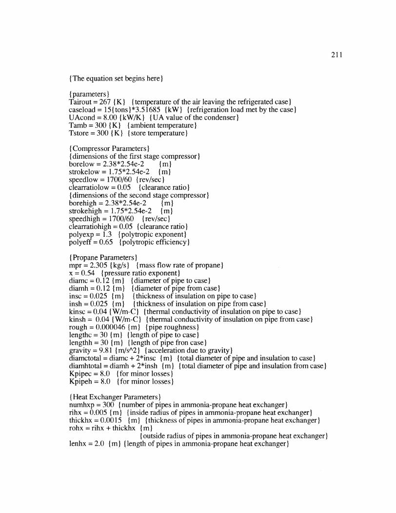
211
{ The equation set begins here)
{parameters)Tairout = 267 {K) (temperature of the air leaving the refrigerated case)caseload = 151(tons)}*3.51685 {kW) (refrigeration load met by the case)UAcond = 8.00 (kW/K) }{IUA value of the condenser)Tamb = 300 1 K) (ambient temperature)Tstore = 300 { K) (store temperature)
(Compressor Parameters)I(dimensions of the first stage compressor)borelow = 2.38*2.54e-2 (m)strokelow = 1.75*2.54e-2 imspeedlow= 1700/60 (rev/sec)clearratiolow = 0.05 (clearance ratio)( dimensions of the second stage compressor)borehigh = 2.38*2.54e-2 Im)strokehigh = 1.75*2.54e-2 imspeedhigh = 1700/60 (rev/sec)clearratiohigh = 0.05 (clearance ratio)Ipolyexp = 1.3 (polytropic exponent)polyeff = 0.65 (polytropic efficiency)
( Propane Parameters)Impr = 2.305 ( kg/s) ({Imass flow rate of propane)Ix = 0.54 (pressure ratio exponent)diamc = 0.12 (I (Idiameter of pipe to case)diamh = 0.12 (I (Idiameter of pipe from case)Iinsc = 0.025 ( (}I{Ithickness of insulation on pipe to case)Iinsh = 0.025 i m ( {thickness of insulation on pipe from case)kinsc = 0.04 (W/m-C }(thermal conductivity of insulation on pipe to case)kinsh = 0.04 (W/m-C) (Ithermal conductivity of insulation on pipe from case)rough = 0.000046 (m I{pipe roughness)lengthc = 30 (I (tlength of pipe to case)lengthh = 30 (mI (length of pipe fron case)gravity = 9.81 ( m/sA2 (acceleration due to gravity)diamctotal = diamc + 2*insc (im) (total diameter of pipe and insulation to case)Idiamhtotal = diamh + 2*insh (i) ({total diameter of pipe and insulation from case)Kpipec = 8.0 (for minor losses)Kpipeh = 8.0 (for minor losses)
( Heat Exchanger Parameters)numhxp = 300 (number of pipes in ammonia-propane heat exchanger)rihx = 0.005 (I (I{inside radius of pipes in ammonia-propane heat exchanger)Ithickhx = 0.0015 i) m thickness of pipes in ammonia-propane heat exchanger)rohx = rihx + thickhx (in)}
( outside radius of pipes in ammonia-propane heat exchanger)lenhx = 2.0 (in ( length of pipes in ammonia-propane heat exchanger)
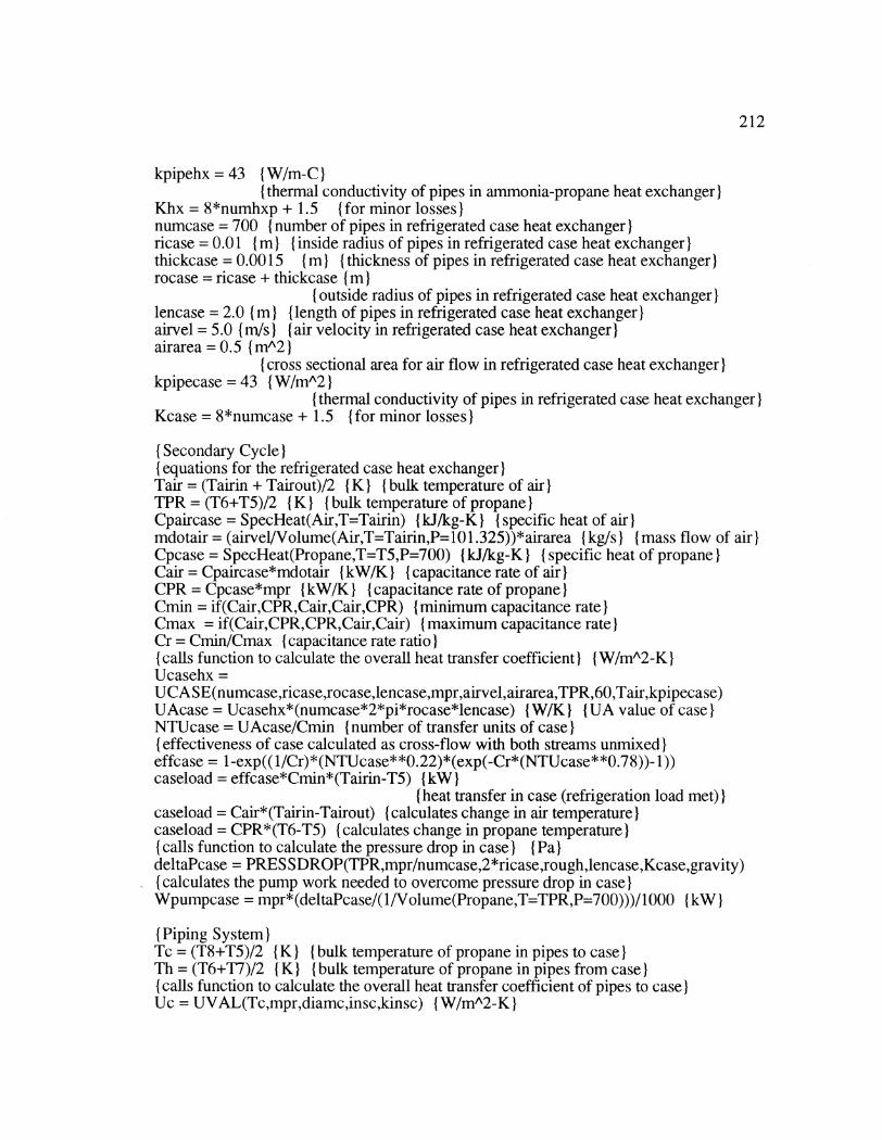
212
kpipehx = 43 {W/m-C}(thermal conductivity of pipes in ammonia-propane heat exchanger)
Khx = 8*numhxp + 1.5 (for minor losses)numcase = 700 (number of pipes in refrigerated case heat exchanger)ricase = 0.01 (I (I{inside radius of pipes in refrigerated case heat exchanger)thickcase = 0.0015 i) m thickness of pipes in refrigerated case heat exchanger)rocase = ricase + thickcase ( mI
(outside radius of pipes in refrigerated case heat exchanger)lencase = 2.0 (m) length of pipes in refrigerated case heat exchanger)airvel = 5.0 ( m/s) ({Iair velocity in refrigerated case heat exchanger)airarea = 0.5 (1mA2)
(cross sectional area for air flow in refrigerated case heat exchanger)kpipecase = 43 (W/mA2)
( thermal conductivity of pipes in refrigerated case heat exchanger)Kcase = 8*numcase + 1.5 (for minor losses)
(Secondary Cycle)I(equations for the refrigerated case heat exchanger)Tair = (Tairin + Tairout)/2 (K) (bulk temperature of air)TPR = (T6+T5)/2 ( K) (Ibulk temperature of propane)ICpaircase = SpecHeat(Air,T=Tairin) I(kJ/kg-K) (Ispecific heat of air)mdotair = (airvel/Volume(Air,T=Tairin,P= 101.325))*airarea ( kg/s) (mass flow of air)Cpcase = SpecHeat(Propane,T=T5,P=700) I(kJ/kg-K) ({Ispecific heat of propane)Cair = Cpaircase*mdotair (kW/KI (I{capacitance rate of air)CPR = Cpcase*mpr (kW/K) ( Icapacitance rate of propane)Cmin = if(Cair,CPR,Cair,Cair,CPR) (minimum capacitance rate)Cmax = if(Cair,CPR,CPR,Cair,Cair) (maximum capacitance rate)Cr = Cmin/Cmax (capacitance rate ratio)I(calls function to calculate the overall heat transfer coefficient) {W/m^2-K)Ucasehx =UCASE(numcase,ricase,rocase,lencase,mpr,airvel,airarea,TPR,60,Tair,kpipecase)UAcase = Ucasehx*(numcase*2*pi*rocase*lencase) (W/K) (UA value of case)NTUcase = UAcase/Cmin (number of transfer units of case)I( effectiveness of case calculated as cross-flow with both streams unmixed)effcase = 1-exp((1/Cr)*(NTUcase**0.22)*(exp(-Cr*(NTUcase**0.78))- 1))caseload = effcase*Cmin*(Tairin-T5) I(kW)I
(heat transfer in case (refrigeration load met))caseload = Cair*(Tairin-Tairout) (calculates change in air temperature)caseload = CPR*(T6-T5) (calculates change in propane temperature)(calls function to calculate the pressure drop in case) (Pa)deltaPcase = PRES S DROP(TPR,mpr/numcase,2*ricase,rough,lencase,Kcase,gravity)(calculates the pump work needed to overcome pressure drop in case)Wpumpcase = mpr*(deltaPcase/(l/Volume(Propane,T=TPR,P=700)))/1000 (kW)
(Piping System)Tc = (T8+T5)/2 (K) (bulk temperature of propane in pipes to case)Th = (T6+T7)/2 (K) (bulk temperature of propane in pipes from case)( calls function to calculate the overall heat transfer coefficient of pipes to case)}Uc = UVAL(Tc,mpr,diamc,insc,kinsc) {(W/m^2-K)
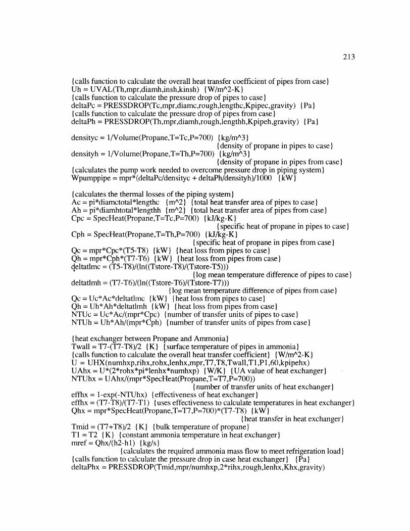
213
{ calls function to calculate the overall heat transfer coefficient of pipes from case)Uh = UVAL(Th,mpr,diamh,insh,kinsh) { W/mA2-K}( calls function to calculate the pressure drop of pipes to case)deltaPc = PRESSDROP(Tc,mpr,diamc,rough,lengthc,Kpipec,gravity) (Pa)(calls function to calculate the pressure drop of pipes from case)IdeltaPh - PRES SDROP(Th,mpr,diamh,rough,lengthh,Kpipeh,gravity) { Pa)
densityc = 1/Volume(Propane,T=Tc,P=700) {kg/mA3){density of propane in pipes to case)
densityh - 1/Volume(Propane,T=Th,P=700) (kg/mA3)( density of propane in pipes from case)
(calculates the pump work needed to overcome pressure drop in piping system)Wpumppipe = mpr*(deltaPc/densityc + deltaPh/densityh)/1000 (kW)
( calculates the thermal losses of the piping system)IAc = pi*diamctotal*lengthc {mA2) (total heat transfer area of pipes to case)Ah = pi*diamhtotal*lengthh (mA2) (Itotal heat transfer area of pipes from case)ICpc = SpecHeat(Propane,T=Tc,P=700) { kJ/kg-K)
{specific heat of propane in pipes to case)Cph = SpecHeat(Propane,T=Th,P=700) {kJ/kg-K)
(specific heat of propane in pipes from case)IQc = mpr*Cpc*(T5-T8) {kW) (heat loss from pipes to case)Qh = mpr*Cph*(T7-T6) {kW) (heat loss from pipes from case)deltatlnc = (T5-T8)/(ln((Tstore-T8)/(Tstore-T5)))( log mean temperature difference of pipes to case)deltatlmh = (T7-T6)/(ln((Tstore-T6)/(Tstore-T7)))
I(log mean temperature difference of pipes from case)Qc = Uc*Ac*deltatlmc (kW) (heat loss from pipes to case)Qh = Uh*Ah*deltatlmh (kW) (heat loss from pipes from case)NTUc = Uc*Ac/(mpr*Cpc) (number of transfer units of pipes to case)NTUh = Uh*Ah/(mpr*Cph) (number of transfer units of pipes from case)
(heat exchanger between Propane and Ammonia)ITwall = T7-(T7-T8)/2 (K) (Isurface temperature of pipes in ammonia)I(calls function to calculate the overall heat transfer coefficient) {W/mA2-K}U = UHX(numhxp,rihx,rohx,lenhx,mpr,T7 ,T8,Twall,T 1 ,P 1,60,kpipehx)UAhx = U*(2*rohx*pi*lenhx*numhxp) (W/K) (UA value of heat exchanger)NTUhx = UAhx/(mpr*SpecHeat(Propane,T=T7,P=700))
( number of transfer units of heat exchanger)effhx = 1-exp(-NTUhx) ( effectiveness of heat exchanger)Ieffhx = (T7-T8)/(T7-T1) (uses effectiveness to calculate temperatures in heat exchanger)Qhx = mpr*SpecHeat(Propane,T=T7,P=700)*(T7-T8) (kW)
( heat transfer in heat exchanger)ITmid = (T7+T8)/2 (K) (bulk temperature of propane)T1 = T2 (K) (constant ammonia temperature in heat exchanger)rnref = Qhx/(h2-hl1) ( kg/s)}
(calculates the required ammonia mass flow to meet refrigeration load)(calls function to calculate the pressure drop in case heat exchanger) (Pa)deltaPhx = PRES SDROP(Tmid,mpr/numhxp,2*rihx,rough,lenhx,Khx,gravity)
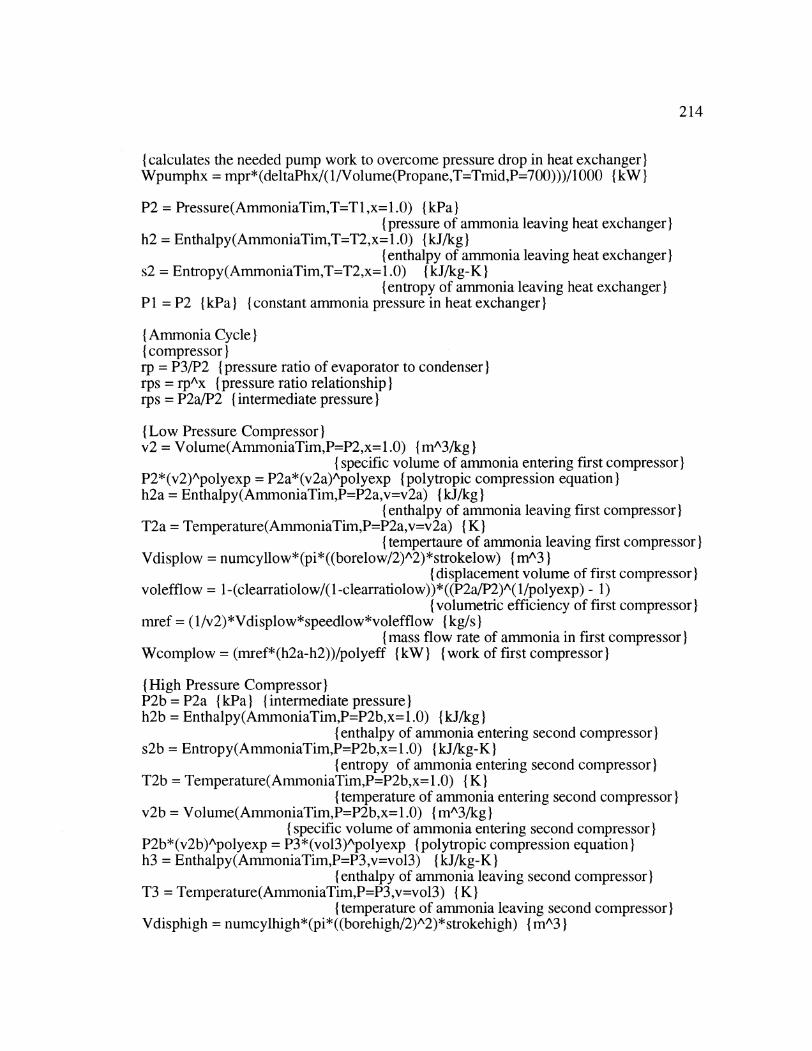
214
(calculates the needed pump work to overcome pressure drop in heat exchanger)Wpumphx = mpr*(deltaPhx/(1/Volume(Propane,T=Tmid,P=700)))/1000 { kW)
P2 = Pressure(AmmoniaTim,T=Tl,x=1.0) (kPa}(pressure of ammonia leaving heat exchanger)
h2 = Enthalpy(AmmoniaTim,T=T2,x= 1.0) {kJ/kg){enthalpy of ammonia leaving heat exchanger)
s2 = Entropy(AmmoniaTim,T=T2,x= 1.0) {IkJ/kg-K){ entropy of ammonia leaving heat exchanger)
P1 = P2 {kPa) (constant ammonia pressure in heat exchanger)
{ Ammonia Cycle){compressor)rp = P3/P2 {pressure ratio of evaporator to condenser)rps = rpAx (pressure ratio relationship)rps = P2a/P2 ( intermediate pressure)
{Low Pressure Compressor)v2 = Volume(AmmoniaTim,P=P2,x=1.0) { mA3/kg)
( specific volume of ammonia entering first compressor)P2*(v2)Apolyexp = P2a*(v2a)Apolyexp (polytropic compression equation)h2a = Enthalpy(AmmoniaTim,P=P2a,v=v2a) {IkJ/kg)I
(enthalpy of ammonia leaving first compressor)T2a = Temperature(AmmoniaTim,P=P2a,v=v2a) (K)
( tempertaure of ammonia leaving first compressor)Vdisplow = numcyllow*(pi*((borelow/2)A2)*strokelow) (mA3)}
(displacement volume of first compressor)volefflow = 1-(clearratiolow/(1-clearratiolow))*((P2a/P2)A(l/polyexp) - 1)
( volumetric efficiency of first compressor)mref = (1/v2)*Vdisplow*speedlow*volefflow (kg/s)
(mass flow rate of ammonia in first compressor)Wcomplow = (mref*(h2a-h2))/polyeff (kW) (work of first compressor)
(High Pressure Compressor)P2b = P2a I(kPa) { intermediate pressure)h2b = Enthalpy(AmmoniaTim,P=P2b,x= 1.0) (kJ/kg)
( enthalpy of ammonia entering second compressor)s2b = Entropy(AmmoniaTim,P=P2b,x= 1.0) (kJ/kg-K)
(entropy of ammonia entering second compressor)T2b = Temperature(AmmoniaTim,P=P2b,x=1.0) ( K)
( temperature of ammonia entering second compressor)v2b = Volume(AmmoniaTim,P=P2b,x= 1.0) {mA3/kg)
( specific volume of ammonia entering second compressor)IP2b*(v2b)Apolyexp = P3*(vol3)Apolyexp (polytropic compression equation)h3 = Enthalpy(AmmoniaTim,P=P3,v=vol3) (kJ/kg-K)
(enthalpy of ammonia leaving second compressor)T3 = Temperature(AmmoniaTim,P=P3,v=vol3) ( K)
(temperature of ammonia leaving second compressor)}Vdisphigh = numcylhigh*(pi*((borehigh/2)A2)*strokehigh) {(mA3)}
215
( displacement volume of second compressor)voleffhigh = 1-(clearratiohigh/(1-clearratiohigh))*((P3/P2b)A(1/polyexp) - 1)
(volumetric efficiency of second compressor)mcond = (1/v2b)*Vdisphigh*speedhigh*voleffhigh (kg/s)
(mass flow of ammonia through second compressor)Wcomphigh = (mcond*(h3-h2b))/polyeff {kW) (work of second compressor)P3 = P4 {kPa)} {constant pressure in condenser)Wcomp = Wcomplow + Wcomphigh {kW) (Itotal compression work)
{ condensor)mair = 15*0.47879 {kg/s) (mass flow of air in condenser)Cpair = SpecHeat(Air,T=Tamb) { kJ/kg-K) ( Ispecific heat of air)UAcond = mair*Cpair*NTU (calculates the number of transfer units of condenser)eff = 1-exp(-NTU) ( effectiveness of condenser)I
Qcond = eff*mair*Cpair*(T4-Tamb) (kW) (Iheat transfer in condenser)Qcond = mcond*(h3-h4) (calculates enthalpy change of ammonia in condenser)Qcond = mair*Cpair*(Tairoutcond-Tamb) (calculates the change in air temperature)
P4 = Pressure(AmmoniaTim,T=T4,x=0.0) (kPa)(pressure of ammonia leaving condenser)
h4 = Enthalpy(AmmoniaTim,T=T4,x=0.0) (kJ/kg)I(enthalpy of ammonia leaving condenser)
(expansion)P5 = P2a ( kPa) (intermediate pressure)h5 = Enthalpy(AmmoniaTim,P=P5,x=0.0) (kJ/kg)
( enthalpy of saturated liquid ammonia leaving the flash tank)h I = h5 (kJ/kg) (isenthalpic expansion)I
Wpump = Wpumpcase+Wpumphx+Wpumppipe (kW) (total pump work in system)COP = caseload/(Wcomp+Wpump) ( coefficient of performance of refrigeration system)Cap = mpr*SpecHeat(Propane,T=T7,P=700)/caseload (1l/K)
(capacitance rate - caseload ratio)
(mixing equation for flash tank)mcond*h4 + mref*h2a = mref*h5 + mcond*h2b
216
REFERENCES
Albritten, T and Hughes, B.M. (Assessment Co-chairs), Scientific Assessment ofStratospheric Ozone: 1989, World Meteorological Organization Global OzoneResearch and Monitoring Project - Report No. 20, Vol.1.
Analysis of Supermarket Dehumidification Alternatives, EPRI Project 2891-03,November 1992, Prepared by University of Wisconsin - Madison.
ASHRAE Handbook, Fundamentals Volume, 1989, American Society of Heating,Refrigeration, and Air-Conditioning Engineers Inc., Atlanta, Georgia
Case Performance Data, Hussman Corporation, Bridgeton, MO, 1989.
Chapman, Alan J., Heat Transfer, Macmillan Publishing Company, New York, 1984
Chlumsky, Vladimir, Reciprocating and Rotary Compressors, SNTL--Publishers ofTechnical Literature, Prague, 1965.
Engineering and Operating Guide for Dowfrost and Dowfrost HD, Form No.180-1286-1190 AMS, The Dow Chemical Company, Midland, Michigan
Engineering and Operating Guide for Dowtherm SR-i and Dowtherm 4000Form No. 180-1190-992 AMS, The Dow Chemical Company, Midland,Michigan
Gosney, W.B., Principles of Refrigeration, Cambridge University Press, Cambridge,1982
Implications of the Restrictions on Production and Use of Ozone-DepletingSubstances on Air Conditioning and Refrigeration, American Society of Heating,Refrigeration, and Air-Conditioning Engineers Inc., 1992, Atlanta, Georgia.
Incropera, Frank P, and Dewitt, David P., Introduction to Heat Transfer, JohnWiley & Sons, New York, 1985
217
Klein, S.A. and Alvarado, F.L., EES: Engineering Equation Solver, F-chart Software,Middleton, WI, 1993
Liley, P.E., Touloukian, Y.S., Saxena, S.C., Thermophysical Properties of MatterVolume 3, IFI/Plenum, New York, 1970, p. 169
Martin, J.J., and Hou, Y.C., Development of an Equation of State for Gases,A.I.Ch.E. Journal, no. 1, vol. 2, June 1955, pp. 142-151
Multitherm 503, Bulletin 503 990, Multitherm Corporation, Colwyn, Pennsylvania
Natarajan, G. and Viswanath, D.S., Data Book on the Viscosity of Liquids, HemispherePublishing Company, New York, 1989, pp. 295-297
Rohsenow, W. M., "A Method of Correlating Heat Transfer Data for SurfaceBoiling Liquids," Transactions of the ASME, vol. 74, 1952, p. 969
Stoecker, W.F., Opportunities for Ammonia Refrigeration, Heating/Piping/AirConditioning, September 1989, pp. 93-108.
Stoecker, W.F., and Jones, J.W., Refrigeration and Air Conditioning, McGraw-HillInc., New York, 1982
Syltherm XLT Heat Transfer Fluid Product Technical Data, Form No. 176-01434- 793AMS, The Dow Chemical Company, Midland, Michigan
Thornton, J.W., "Supermarket Refrigeration Options", M.S. Thesis, University ofWisconsin - Madison, 1991.
Threlkeld, James L., Thermal Environmental Engineering, 2nd edition, Prentice-HallInc., New Jersey, 1970
White, Frank M., Fluid Mechanics, McGraw-Hill Book Company, New York, 1986
Yaws, Carl L., Thermodynamic and Physical Property Data, Gulf PublishingCompany, Houston, 1992, pp. 43 and 97
52nd Annual Report of the Grocery Industry, Progressive Grocer, April 1985,pp. 23-98.


