INVESTIGATION OF THE STABILITY AND STEADY STATE RESPONSE OF ASYMMETRIC ROTORS, USING FINITE ELEMENT FORMULATION

Journal of Sound and <ibration (2001) 245(2), 303}328doi:10.1006/jsvi.2001.3570, available online at http://www.idealibrary.com on

INVESTIGATION OF THE STABILITY AND STEADY STATERESPONSE OF ASYMMETRIC ROTORS, USING FINITE

ELEMENT FORMULATION

F. ONCESCU, A. A. LAKIS AND G. OSTIGUY

Department of Mechanical Engineering, ED cole Polytechnique de Montre&al, P.O. Box 6079,Station Centre-ville, Montre&al, QueHbec, Canada, H3C 3A7. E-mail: [email protected]

(Received 28 April 2000, and in ,nal form 22 January 2001)

The motion of a rotor of which both the bearings and the shaft cross-section areasymmetric is generally governed by ordinary di!erential equations with periodiccoe$cients. In this paper, modi"cations are made to incorporate the e!ect of shaftasymmetry into an existing "nite element procedure developed for rotors with symmetricshaft. The model for the elastic asymmetric shaft takes into account rotary inertia andgyroscopic inertia. In addition, this paper describes an existing method of investigating thestability of a general system of di!erential equations with periodic coe$cients, and evaluatesits e$ciency when applied to asymmetric rotors. The method described is based on Floquet'stheory and involves the computation of a transfer matrix over one period of motion. Thedetailed presentation of the equations of motion, both in a rotating frame of reference and ina "xed one, is accompanied by an analysis of speci"c cases. The equations of motion fora simpler model are obtained by modal expansion. Numerical examples are given in order toshow the "nite element formulation and the transfer matrix method as applied toasymmetric rotors. Due to the use of linear equations, the results shown in this paper havelimited practical utility, but they are useful tools in analyzing the behavior of periodicsystems with weak non-linearities. ( 2001 Academic Press

1. INTRODUCTION

It is important to distinguish between the asymmetry of the rotating part and theasymmetry of the "xed part of a rotor. If only one of the two is asymmetric, it is possible toestablish a frame of reference in which the coe$cients of the equations of motion areconstant. If both parts are asymmetric, the system equations will, in the majority of cases,have periodic coe$cients.

The principal methods used to investigate the stability of systems with periodiccoe$cients fall into three groups: perturbation methods [1], variants of Hill's in"nitedeterminant method [2, section 7.6, 3], and methods combining the use of Floquet's theory[2, section 7.2] with numerical computation of the transfer matrix at the end of one period[4}6].

The main advantage of the methods from the third group, here called &&transfer matrixmethods'', is their high degree of generality. It is not necessary for the equations of motionto satisfy restrictive conditions (as is the case with the perturbation methods, where theperiodic coe$cients need to be expressed in terms of a small parameter), nor are complexpreparatory steps required before numerical procedures can be applied (as is the case withboth the perturbation and the in"nite determinant methods). The main disadvantage of

0022-460X/01/320303#26 $35.00/0 ( 2001 Academic Press

304 F. ONCESCU E¹ A¸.

these methods is the high computational e!ort required to obtain the transfer matrix overone period, while the stability of the motion can be evaluated for only one point in theparameter's space at a given time.

Many studies deal with rotors having partial asymmetry: either bearing asymmetry ordisk and shaft asymmetry. Typical studies are by El-Marhomy [7], for bearing asymmetry,and Arday"o and Frohrib [8], for shaft and disk asymmetry. In this case, it is possible todescribe the movement of the rotor using a system of di!erential equations with constantcoe$cients.

Amongst the papers dealing with rotors having full asymmetry, the majority considersimple models, such as a massless shaft of uniform cross-section, a disk usually in planemotion, one or two identical elastic bearings, and environmental damping acting on thedisk. Typical studies using Hill's in"nite determinant method to analyze the motion stabilityare those by Brosens and Crandall [9], and Kotera and Yano [10]. Perturbation methodsare used, for example, by Black and McTernan [11], and also Iwatsubo et al. [12]. Thetransfer matrix method is considered by Guilhen et al. [13], for a speci"c model with rigidbearings at the shaft ends, one elastic bearing and one rigid disk, attached to the shaft atdi!erent stations.

The adoption of simple models of asymmetric rotors facilitates the understanding of thebehavior of such dynamic systems, but the practical use of these studies remains limited.Nelson and McVaugh [14] developed a "nite element model for a rotor-bearing systemwith asymmetric bearings and symmetric shaft, which means a rotor with partialasymmetry. Their procedure is presented also in reference [15, chapter 3]. Inagaki et al. [16]studied a multi-disk fully asymmetric rotor with longitudinal variation of the shaft cross-section. The temporal equations of motion were obtained using the transfer matrix method(&&transfer'' between two stations of the shaft). The unbalance response is deduced by theharmonic balance method. Genta [17] applied the "nite element method to fullyasymmetric rotors, using complex co-ordinates, in order to reduce the size of the problem,and analyzed the stability of the motion using Hill's in"nite determinant method. Kanget al. [18] also applied the "nite element method to fully asymmetric rotors, studying theunbalanced response using the harmonic balance method. Neither of the two studies givesthe elements of the matrices related to the shaft asymmetry.

In this paper, the "nite element procedure for rotors with asymmetric bearings andsymmetric shaft by Nelson and McVaugh [14] is extended to include shaft asymmetry. Themotion stability and the unsteady response are analyzed using the method developed byFriedmann and associates [4, 5]. The elements of all matrices involved in the equations ofmotion are included in Appendix A.

2. TRANSFER MATRIX METHOD

Rotor systems are constrained by bearings, dampers, seals, etc., to very small lateralmotion. Generally, these mechanisms are dynamic systems with weak non-linearities, andtheir motion is governed by ordinary di!erential equations with periodic coe$cients,represented in a "rst order state variable form as follows:

MxR N"[A (t)]MxN#M f (t)N#MN1(MxN, t)N#MN

2(MxN, MxR N, t)N, (1)

with matrix [A(t)] and vectors M f N, MN1N and MN

2N periodic, of common period ¹.

An e!ective approach [5] to deal with the weak non-linearities combined in vectors MN1N

and MN2N of system (1) is quasilinearization, consisting in an iterative evaluation of the

ASYMMETRIC ROTOR RESPONSE 305

periodic response of system (1), as a solution of linear periodic systems. This procedure isinitiated with an initial estimation of the solution, obtained from system (1) after droppingthe non-linear terms MN

1N and MN

2N.

In this paper, the discussion will center on n-degree-of-freedom dynamic systemsgoverned by the linear system of m"2n "rst order di!erential equations and m unknownfunctions,

[xR N"[A(t)]MxN#M f (t)N, (2)

where Mx(t)N is the state variable vector, [A (t)] is the system matrix, and vectorM f (t)N describes time-dependent forces, both [A(t)] and M f (t)N being periodic, of commonperiod ¹.

It is of major interest to "nd the steady state response of system (2), i.e., the periodicsolution, and to evaluate its stability.

2.1. STABILITY

The study of the stability of the steady state solution of system (2) can be reduced (seereference [2, Chapter 7]) to the study of the stability of the trivial solution of the associatedhomogeneous system:

MxR N"[A(t)]MxN. (3)

It should be noted that this result is more general, being valid for system (2) replaced witha non-autonomous system

MxR N"MX (MxN, t)N (2b)

with the functions Xi

being periodic, of period ¹ and system (3) replaced with thevariational system attached to system (2b) and to its periodic solution Mp (t)N,

MyR N"[a (t)]MyN, (3b)

where My (t)N contains the small perturbations from Mp(t)N, and matrix [a(t)] is periodic, ofperiod ¹.

For system (3), the time transfer matrix is de"ned as an m]m matrix [U (t)] with itscolumns consisting of a set of linearly independent solutions.

Since matrix [A(t)] is periodic, of period ¹, an extension of Floquet's theory (see reference[2, Chapter 7]) shows that [U (t)] is fully known when its variation during one period ¹ isknown. Furthermore, it is shown that the stability of the trivial solution of equation (3) isfully de"ned by the eigenvalues of the transfer matrix over one period [U(¹)], known as thecharacteristic multipliers of system (3). The trivial solution is asymptotically stable if themodulus of all m eigenvalues is less than one, and is unstable if the modulus of at least one ofthe eigenvalues is greater than one.

2.2. STEADY-STATE RESPONSE

For non-homogeneous system (2), without considering the periodicity of matrix [A (t)]and vector M f (t)N, the general solution is given by (see reference [2, Chapter 6])

Mx(t)N"[U (t)]Mx (0)N#Pt

0

[U (t, s)]M f (s)Nds, (4)


in which [U(t)] is the transfer matrix of the homogeneous system satisfying the initialconditions [U(0)]"[I

m], and matrix [U(t, s)] is given by

[U(t, s)]"[U (t)] [U (s)]~1. (5)

It is clear that the "rst term on the right-hand side of expression (4) is the general solutionof the homogeneous system (3), denoted by Mx

h(t)N. Matrix [U(t, s)] makes the transfer

between the values at moments &&t'' and &&s'' of Mxh(t)N:

Mxh(t)N"[U(t, s)] Mx

h(s)N. (6)

If matrix [A(t)] and vector M f (t)N are periodic, of common period ¹, and if the modulus ofevery characteristic multiplier of the corresponding homogeneous system (3) is di!erentfrom one, system (2) has one and only one periodic solution [3]. This periodic solution is thesteady state response of the periodic non-homogeneous system only if the associatedperiodic homogeneous system is stable, that is to say, only if the modulus of everycharacteristic multiplier is less than one.

To obtain the initial conditions corresponding to the steady state response, conditionMx(¹)N"Mx (0)N is substituted into equation (4). An algebraic system for Mx(0)N is derived:

([Im]![U(¹)])Mx(0)N"P

T

0

[U (t, s)]M f (s)Nds. (7)

The steady state response can be obtained by taking the initial conditions Mx (0)N given byequation (7) and numerically integrating system (2) over one period. If Mx(¹)N is not closeenough to Mx(0)N, the integration is continued over another few periods, until the desiredconvergence is obtained.

In order to calculate the transfer matrix over one period [U(¹)], Friedmann et al. [4]considered the division of the period ¹ into a number of equal parts. By denoting thedivision points as

0"t0(t

1(2(t

N~1(t

N"¹, (8)

a useful relation can be derived from equation (6):

[U (¹, ti)]"[U (¹, t

i`1)] [U(t

i`1, t

i)]. (9)

Matrix [U(¹)]"[U(¹, 0)] is generated by an iterative calculation, based on relation (9)and starting with [U(¹, t

N)]"[I

m]. The elementary transfer matrix [U (t

i`1, t

i)] is obtained

by numerically integrating the homogeneous system (3) over the corresponding elementaryinterval. The iterative calculation not only gives matrix [U (¹)], to be used in the stabilityevaluation, but also matrices [U(¹, t

i)], appearing in the right-hand term of the algebraic

system (7) for the initial condition Mx (0)N, if an integration scheme using division points (8) isconsidered.

It has been shown in reference [4] that a very e$cient way to obtain the elementary transfermatrix is by considering the fourth order Runge}Kutta scheme with Gill coe$cients.

3. CONFIGURATION

The mathematical model (Figure 1) consists of a #exible horizontal shaft, one or morerigid disks and two or more #exible bearings.

Figure 1. General model of the rotor.

Figure 2. (a) Co-ordinate systems: OX>Z and Oxyz, "xed and rotating frames of reference; Cx@y@z@, system ofprincipal axes of inertia of shaft cross-section. (b) Mass unbalance and external damping.


The shaft cross-section is asymmetric, having di!erent principal moments of inertia, andvaries step-by-step along the longitudinal axis (Figure 2(a)). However, the principaldirections of inertia of the cross-section do not vary along the shaft.

The mathematical model for a bearing is a massless spring}damper system (Figure 3). Itscharacteristics (sti!ness and damping) in horizontal and vertical directions are di!erent.The cross-coupled characteristics in the horizontal and vertical directions are alsoconsidered. This linear and anisotropic model with eight coe$cients (four for sti!ness andfour for viscous damping) is the same as in reference [14].

We analyze the unbalance response using concentrated masses placed on disks (pointB in Figure 2(b)) and we consider an environmental viscous damping acting on the disks(Figure 2(b)).

Two co-ordinate systems can be seen in Figure 2(a). On the "xed system OX>Z, the>-axis is along the unde#ected horizontal shaft and the Z-axis is oriented vertically upward.The rotating system Oxyz has the y-axis coincidental with the >-axis of the "xed system,and x- and z-axis parallel with the principal axes x@ and z@ of the shaft cross-section (if theangular de#ections are neglected).

The "nite element procedure for rotors with symmetric shaft, developed by Nelson andMcVaugh [14], will be considered. Modi"cations will be made to accommodate the e!ect ofshaft asymmetry. The shaft model includes the e!ect of rotary inertia and the gyroscopice!ect. Shear of the cross-section and internal damping will be neglected.

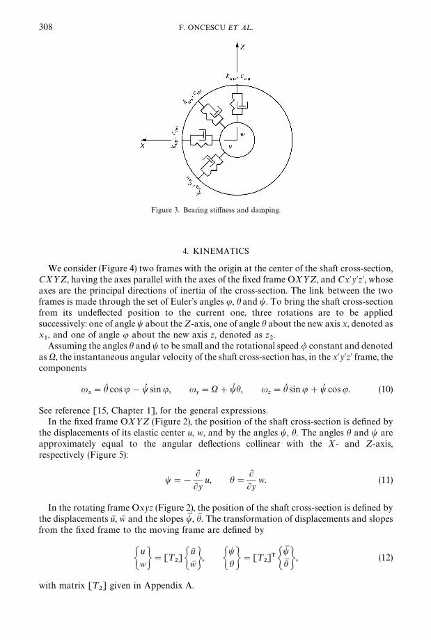
Figure 3. Bearing sti!ness and damping.


4. KINEMATICS

We consider (Figure 4) two frames with the origin at the center of the shaft cross-section,CX>Z, having the axes parallel with the axes of the "xed frame OX>Z, and Cx@y@z@, whoseaxes are the principal directions of inertia of the cross-section. The link between the twoframes is made through the set of Euler's angles u, h and t. To bring the shaft cross-sectionfrom its unde#ected position to the current one, three rotations are to be appliedsuccessively: one of angle t about the Z-axis, one of angle h about the new axis x, denoted asx1, and one of angle u about the new axis z, denoted as z

2.

Assuming the angles h and t to be small and the rotational speed uR constant and denotedas X, the instantaneous angular velocity of the shaft cross-section has, in the x@y@z@ frame, thecomponents

ux"hQ cosu!tQ sinu, u

y"X#tQ h, u

z"hQ sinu#tQ cosu. (10)

See reference [15, Chapter 1], for the general expressions.In the "xed frame OX>Z (Figure 2), the position of the shaft cross-section is de"ned by

the displacements of its elastic center u, w, and by the angles t, h. The angles h and t areapproximately equal to the angular de#ections collinear with the X- and Z-axis,respectively (Figure 5):

t"!

LLy

u, h"LLy

w. (11)

In the rotating frame Oxyz (Figure 2), the position of the shaft cross-section is de"ned bythe displacements uN , wN and the slopes tM , hM . The transformation of displacements and slopesfrom the "xed frame to the moving frame are de"ned by

Gu

wH"[¹2]G

uNwN H, G

thH"[¹

2]T G

tMhM H , (12)

with matrix [¹2] given in Appendix A.

Figure 4. Euler's angles.

Figure 5. Displacements of the shaft elastic axis.


5. EQUATIONS OF MOTION OF ROTOR ELEMENTS

5.1. DISKS

The center of mass of the rigid disk coincides with the elastic center of the shaftcross-section. The nodal displacements vector of the disk in "xed co-ordinates is given by

Md0N"Mu

0w

0t0

h0NT,

its components being the displacements of the shaft at disk attachment.

5.1.1. Equations of motion of disk in ,xed frame

The kinetic energy of the disk has the expression

¹"12m(uR 2

0#wR 2

0)#1

2(J

xu2

x#J

yu2

y#J

zu2

z), (13)


where ux, u

yand u

zare the angular velocities given by equation (10), while m, J

x"J

zand

Jyare the mass and the moments of inertia of the disk.By substituting equation (10) into equation (13), and also considering the e!ect of the

unbalance, we obtain

¹D"1

2m(uR 2

0#wR 2

0)#1

2Jx(hQ 2

0#tQ 2

0)#J

yXtQ

0h0

#mudX[uR

0cos(Xt#b)!wR

0sin (Xt#b)], (14)

where X is the angular speed of the rotor, muis the unbalance mass (assumed to be small if

compared with m), d and b are the radius and the angle de"ning the location of theunbalance.

The four terms in equation (14) give, in order, the translating inertia e!ect, the rotaryinertia e!ect, the gyroscopic e!ect, and the unbalance e!ect.

The virtual work of the disk weight and of damping forces acting on the disk can bewritten as

d¸D"!mgdw

0!cuR

0du

0!cwR

0dw

0, (15)

where c is the damping coe$cient, m is the mass of the disk, and g is the gravitationalacceleration.

The application of Lagrange's equations for the disk only gives

[MD]MdG

0N#[C

DNMdQ

0N"MQ

DN#MQ

LN, (16)

where [MD] and [C

D] are the mass and damping matrices of the disk, MQ

DN is the load

vector and MQLN is the vector of liaison forces which will disappear at the assembly of the

elementary matrices.Matrices [M

D] and [C

D], and also vector MQ

DN are given in Appendix A.

5.1.2. Equations of motion of disk in rotating frame

The nodal displacements in "xed co-ordinates are related to those in rotatingco-ordinates by the transformation equation

Md0N"[¹

4] MdM

0N, (17)

with the matrix [¹4] given in Appendix A. The substitution of equation (17) into equation

(16), yields the equations of motion in rotating co-ordinates as

[MMD]MdMG

0N#[CM

D] MdMQ

0N#[KM

D]MdM

0N"MQM

DN#MQM

LN, (18)

where [MMD]"[M

D], [CM

D]"2X[M

D][H

4]#[¹

4]T[C

D] [¹

4], [KM

D]"!X2[M

D]

#X[¹4]T [C

D][¹

4][H

4] and MQM

DN"[¹

4]TMQ

DN, with matrices [¹

4] and [H

4] given in

Appendix A. MQMLN contains liaison forces that will disappear at the assembly of

the elementary matrices. Matrices [KMD] and [CM

D], and also vector MQM

DN are given in

Appendix A.

5.2. THE SHAFT

While the shaft element has two nodes, the nodal displacement vector includes fourdisplacements and four slopes. Its expression in "xed co-ordinates is Md

eN"


Mu1

w1

t1

h1

u2

w2

t2

h2NT. The nodal displacements in "xed co-ordinates are related to

those in rotating co-ordinates by the transformation equation:

MdeN"[¹g]MdM

eN. (19)

with matrix [¹g] given in Appendix A.In "xed co-ordinates, the displacements and the slopes along the shaft elements are

represented by shape functions as

Gu

wH"[N (y)]MdeN (20)

and

GthH"G

!

LLy

u

LLy

w H"C!1 0

0 1D [D(y)]MdeN, (21)

where [N] is the matrix of shape functions

[N]"CN

10 !N

20 N

30 !N

40

0 N1

0 N2

0 N3

0 N4D and [D]"C

LLy

ND.N

i(y) are the typical displacement functions of a beam in bending:

N1(y)"1!3yN 2#2yN 3, N

2(y)"¸yN (1!2yN #yN 2), N

3(y)"3yN 2!2yN 3,

N4(y)"¸ (!yN 2#yN 3), with yN "y/¸. (22)

5.2.1. Kinetic energy

The kinetic energy for the shaft element has a form similar to the one derived for the diskand is

¹A"

1

2oAP

L

0

(uR 2#wR 2) dy#12oP

L

0

(Ixu2

x#I

pu2

y#I

zu2

z) dy, (23)

where ux, u

yand u

zare the angular velocities given by equation (10), I

xand I

zare the

second moments of area about principal axes x@ and z@ of the shaft, Ip"I

x#I

zis the polar

moment of area, A, ¸ and o are the cross-section, the length, and the density of the shaftelement.

By introducing equation (10) in equation (23), we obtain

¹A"¹

t#¹

r#¹

d,ccos(2Xt)#¹

d,ssin (2Xt)#¹g , (24)

where ¹t"1

2oA :L

0(uR 2#wR 2) dy, is the translating term, ¹

r"1

2oI

m:L0(hQ 2#tQ 2) dy is the

rotatory term), ¹d,c"1

2oI

d:L0(tQ 2#hQ 2) dy is the deviatory-cosine term, ¹

d,s"oI

d:L0tQ hdy is


the deviatory-sine term and ¹g"oIpX :L

0tQ hdy is the gyroscopic term, with

Im"1

2(I

z#I

x), I

d"1

2(I

z!I

x) and I

p"2I

m.

5.2.2. Strain energy

If the shear deformations are neglected, the strain energy of the shaft element is

;"

1

2 PL

0

[EIz(uN A)2#EI

x(wN A)2] dy, (25)

where u6 and wN are the displacements of the center of the cross-section in rotating co-ordinates, I

xand I

zare the second moments of area about principal axes, E is Young's

modulus, ¸ is the length of the shaft element, ( ) )A"(L2/Ly2) ( ) ), and u6 A and wN A are thede#ections of bending in the directions of the principal axes.

Substituting the transformation equation (12) into equation (25), the strain energy can beexpressed as

;"

1

2 PL

0

EIm[(uA)2#(wA)2] dy#

1

2PL

0

EIdS[(uA)2!(wA)2] cos(2Xt)!2uAwA sin(2Xt)Tdy,

(26)

where u and w are the displacements of the center of the cross-section in "xed co-ordinates,Im

and Idare the mean and the deviatory area moments, and X is the angular speed of the

rotor.

5.2.3. <irtual work of the shaft weight

The virtual work of the shaft weight has the expression

d¸A"!g P

L

0

(oAdw) dy

"!ogAAdw1 P

L

0

N1dy#dh

1 PL

0

N2dy#dw

2 PL

0

N3dy#dh

2 PL

0

N4dyB, (27)

where Nk(y) are the shape functions given by equation (22), A, ¸ and o are the cross-section,

the length and the density of the shaft element, and g is the gravitational acceleration.

5.2.4. Equations of motion of shaft in ,xed frame

Upon substituting equations (20) and (21) into the expressions (24), (26) and (27),Lagrange's equations provide the system

[MA(t)] MdG

eN#[C

A] MdQ

eN#[K

A(t)]Md

eN"MQ

AN#MQ

LN, (28)

with [MA(t)] and [K

A(t)] being periodic matrices of period n/X, and [C

A] being a constant

matrix, given by

[MA(t)]"[M

t]#[M

r]#[M

d,c] cos(2Xt)#[M

d,s] sin(2Xt), (29)

[CA]"X[G], [K

A(t)]"[K

m]#xK

d,cy cos(2Xt)#xK

d,sy sin(2Xt). (30, 31)


In equation (28), vector MQAN represents the shaft weight, while vector MQ

LN contains the

liaison forces that will disappear when the elementary matrices are assembled.The gyroscopic matrix, mass matrices and sti!ness matrices of equations (29)}(31) may be

expressed as

[G]"12oI

p PL

0

[D]TC0 !1

1 0 D[D]dy,

[Mt]"oA P

L

0

[N]T[N] dy, [Mr]"oI

mPL

0

[D]T[D] dy,

[Md,c

]"oId P

L

0

[D]TC1 0

0 !1D[D] dy, [Md,s

]"!oId P

L

0

[D]TC0 1

1 0D [D] dy, (32)

[Km]"EI

m PL

0

[B]T[B] dy, [Kd,c

]"EId P

L

0

[B]TC1 0

0 !1D[B] dy,

[Kd,s

]"EId P

L

0

[B]TC0 1

1 0D[B] dy,

with [N], the matrix of shape functions, [D]"[(L/Ly)N] and [B]"(L2/Ly2) [N].The elements of the matrices de"ned by the above equations, and also of vector MQ

AN are

shown in Appendix A.Matrices [M

d,c], [M

d,s], [K

d,c] and [K

d,s] are proportional to the deviatory moment of

area of the shaft Id, and will vanish for a symmetric shaft. Matrices [M

t], [M

r], [K

m] and

[G], speci"c for a symmetric shaft, can be found also in reference [14].

5.2.5. Equations of motion of shaft in rotating frame

Substituting transformation equation (19) into equation (28), we obtain

[MMA] MdM G

eN#[CM

A]MdMQ

eN#[KM

A] MdM

eN"MQM

A(t)N#MQM

LN, (33)

where [MMA], [CM

A] and [KM

A] are constant matrices given by

[MMA]"[M

t]#[M

r]#[M

d], [ CM

A]"2X[MM

A] [H

8]#X[G], (34, 35)

[KMA]"[K

m]#[K

d]!X2[MM

A]#X2[G][H

8], (36)

with matrix [H8] given in Appendix A.

In equation (33), the weight vector MQMA(t)N is periodic, of period 2n/X. Its elements are

shown in Appendix A. Vector MQMLN contains the liaison forces.

In equations (34)}(36), matrices [Mt], [M

r], [K

m] and [G] are as de"ned by equation (32),

while matrices [Md] and [K

d] are given by [M

d]"[M

d,c] and [K

d]"[K

d,c], with [M

d,c]

and [Kd,c

] as de"ned by equation (32).


5.3. BEARINGS

The nodal displacement vector of the bearing in "xed co-ordinates is given by

MdpN"Mu

pwpNT,

its components being the displacements of the shaft center at bearing attachment.

5.3.1. Equations of motion of bearing in ,xed frame

The virtual work of the forces acting on the shaft can be written as

d¸p"!k

uuupdu

p!k

uwwpdu

p!k

wuupdw

p!k

www

pdw

p

!cuu

uRpdu

p!c

uwwRpdu

p!c

wuuRpdw

p!c

wwwR

pdw

p, (37)

where kuu, k

uw, k

wuand k

wware the sti!ness coe$cients, and c

uu, c

uw, c

wuand c

wware the

damping coe$cients.The application of Lagrange's equations gives

[CP]MdQ

pN#[K

P]Md

pN"MQ

LN, (38)

where [KP] and [C

P] are the sti!ness and damping matrices of the bearing, and MQ

LN is

a vector containing the liaison forces between bearing and shaft. Matrices [KP] and [C

P]

are given in Appendix A.

5.3.2. Equations of motion of bearing in rotating frame

The nodal displacements in "xed co-ordinates are related to those in rotating co-ordinates by the transformation equation

MdpN"[¹

2]MdM

pN (39)

with the matrix [¹2] given in Appendix A.

Substituting equation (39) into equation (38), we obtain

[CMP(t)]MdMQ

pN#[KM

P(t)]MdM

pN"MQM

LN, (40)

where [CMP(t)] and [KM

P(t)] are periodic matrices, of period n/X, given by

[CMP]"[¹

2]T[C

P][¹

2], [KM

P]"[¹

2]T[K

P][¹

2]#X[CM

P][H

2], (41, 42)

with matrices [¹2] and [H

2] given in Appendix A. The vector MQM

LN contains the liaison

forces between bearing and shaft. Matrices [CMP(t)] and [KM

P(t)] are given in Appendix A.

There are particular cases when these two matrices are constant, the most general case beingde"ned by the conditions

kuu"k

ww, k

wu"!k

uw, c

uu"c

ww"0 and c

wu"!c

uw.


6. GLOBAL EQUATIONS OF MOTION

6.1. GENERAL CASE

By assembling the elementary matrices of shaft elements, disks and bearings, we obtaina system of 4N

nsecond order di!erential equations and 4N

nunknown functions, where

Nnis the number of nodes of the shaft partition. The global equations of motion in "xed

co-ordinates are

[M(t)]MdG N#[C]MdQ N#[K (t)]MdN"MQu(t)N#MQ

wN , (43)

where [M(t)] and [K (t)] are periodic matrices of period ¹1"n/X, for which the time

dependency is due to the shaft asymmetry, matrix [C] is constant, MQu(t)N, the unbalance

vector, is periodic, of period ¹2"2n/X, and MQ

wN, the weight vector, is constant.

In equation (43), MdN is the vector of global DOF in "xed reference frame, given as

MdN"Mu1

w1

t1

u1

2 uNn

wNn

tNn

uNn

NT.

In rotating co-ordinates, the assembled global equations are

[MM ]MdMG N#[CM (t)]MdMQ N#[KM (t)]MdM N"MQMuN#MQM

w(t)N, (44)

where [MM ] is a constant matrix, [CM (t)] and [KM (t)] are periodic matrices of period ¹1"n/X,

for which the time dependency is due to bearing asymmetry, MQMuN, the unbalance vector, is

constant, and MQMw(t)N, the weight vector, is periodic of period ¹

2"2n/X.

Each of the above systems can be transformed into a "rst order di!erential system, with8N

nequations and 8N

nunknown functions. From a numerical point of view, it is more

convenient to consider the equations of motion in rotating co-ordinates, because massmatrix [MM ] is constant. Substituting also u"Xt for the variable t, system (44) can beexpressed as

d

duGMdN

Md@NH"[A(u)]GMdN

Md@NH#M f (u)N , (45)

with

[A(u)]"

[0] [1]

!

1

X2[MM ]~1[KM (u)] !

1

X[MM ]~1[CM (u)]

, M f(u)N"

igjgk

M0N

1

X2[MM ]~1MQM (u)N

egfgh

.

Matrix [A (u)] has a periodic variation with frequency of p, due to bearing asymmetry,while vector M f (u)N has a periodic variation with frequency of 2p, due to rotor weight.

To study only the stability of the motion, the transfer matrix [U(¹)], with ¹"n, iscalculated using the method described in section 2, and its 8N

neigenvalues are evaluated.

In order to study the stability and to obtain the steady state response at the same time,the period to be considered is ¹"2n. Calculated values of matrix [U(¹, u)] at the divisionpoints of the period ¹ are used to build the algebraic system of type (7) for the initialconditions Mx(0)N. If the periodic non-homogeneous system (45) is integrated usingSimpson's rule, the number of intervals per period N must be even.


6.2. MASSLESS SHAFT, ASSOCIATED WITH UNDAMPED BEARINGS

If the shaft mass is ignored, matrix [M] in equation (43) becomes constant. Reorderingthe equations of system (43) and also the elements of the global DOF vector MdN, we canhighlight the contribution of the N

ddisks, as follows:

C[M

dd] [0

dr]

[0rd] [0

rr]D G

MdGdN

MdGrNH#C

[Cdd] [0

dr]

[0rd] [C

rr]D G

MdQdN

MdQrNH#C

[Kdd] [K

dr]

[KrdN MK

rr]D G

MddN

MdrNH"G

MQdN

M0rN H ,(46)

where index &&d'' refers to disks, and index &&r'' refers to the rest of the rotor. Vector MddN

contains the 4Nd

displacements associated with the Nd

disks.If the damping of the bearings is also ignored, we have [C

rr]"[0

rr] and the last

4(Nn!N

d) equations of system (46) give

MdrN"![K

rr]~1[K

rd]Md

dN. (47)

Consequently, the "rst 4Ndequations (46) become

[Mdd]MdG

dN#[C

dd]MdQ

dN#[K*

dd(t)]Md

dN"MQ

dN, (48)

with

[K*dd

(t)]"[Kdd]![K

dr(t)] [K

rr(t)]~1[K

rd(t)]. (49)

In equations (48) and (49), the variable matrices are periodic, of period ¹1"n/X, and the

time dependency is due to the shaft asymmetry.System (48) can be transformed into a "rst order di!erential system of type (45), with 8N

dequations and 8N

dunknown functions. The advantage of this formulation is the capability

to re"ne the "nite element partition of the shaft, without increasing the size of the motionequations system.

6.3. SYMMETRIC SHAFT

If the shaft cross-section is symmetric, matrices [M] and [K] from equations (43) areconstant, and the motion is governed by a linear system with constant coe$cients, de"nedas

[M]MdG N#[C]MdQ N#[K]MdN"MQu(t)N#MQ

wN. (50)

To evaluate the motion stability, we have only to analyze the eigenvalues of a constantmatrix. The evaluation of the steady state response, with its components, the weightresponse and the unbalance response, is given below. The weight response is the solution ofthe algebraic system de"ned as

[K]MdwN"MQ

wN . (51)

To obtain the unbalance response, we express the unbalance vector from equation (50) asMQ

u(t)N"Re(M<Ne*(Xt#b) ), where M<N is a constant vector with complex elements. It is easy


to show that the unbalance response will be obtained as

Mdu(t)N"Re(Mz

0N e*Xt ), (52)

where Mz0N is a constant vector with complex elements, de"ned as the solution of the

algebraic system

([K]!X2[M]#iX[C])Mz0N"M<Ne*b . (53)

7. EQUATIONS OF MOTION, BY MODAL EXPANSION

In order to test the "nite element formulation, the equations of motion for a simplermodel will be obtained using the Rayleigh}Ritz method.

The new model consists of a #exible horizontal shaft, a rigid disk and two #exiblebearings (Figure 6). The shaft is of uniform cross-section along its longitudinal axis and hastwo di!erent sti!nesses along its two principal directions (Figure 2(a)). Its mass is supposedto be small compared with that of the disk, and consequently negligible. For bearings, onlythe direct sti!nesses, denoted as k

uand k

w, are considered. The unbalance is de"ned as

shown in Figure 2(b). The only damping considered is the external one, acting on the disk(Figure 2(b)).

The shaft displacements in the x and z directions can be expressed as

u(y, t)"A1!y

¸B u1(t)#

y

¸

u2(t)#f (y)q

x(t), w (y, t)"A1!

y

¸Bw1(t)

#

y

¸

w2(t)#f (y)q

z(t) , (54)

where ¸ is the shaft length, u1, w

1, u

2and w

2, are the displacements of the shaft ends, q

xand

qw

are generalized independent co-ordinates, and f (y) is the displacement function.

Figure 6. Simpli"ed model of the rotor: (a) location of the disk, (b) bearing sti!ness.


By substituting equations (54) into equation (11), we obtain the slopes of the shaft axis:

h (y, t)"w2!w

1¸

#

Lf

Lyqz

and t (y, t)"!

u2!u

1¸

!

Lf

Lyqx. (55)

For y"y0, the four equations (54) and (55) provide the displacements of the shaft ends

(u1, w

1, u

2, w

2) as functions of the displacements of the center of the disk (u

0, w

0, t

0, h

0) and

of the generalized co-ordinates (qx, q

z):

u1"u

0#y

0t0!( f

0!y

0g0)q

x,

u2"u

0!(¸!y

0)t

0![ f

0#(¸!y

0)g

0]q

x,

w1"w

0!y

0h0!( f

0!y

0g0)q

z,

w2"w

0#(¸!y

0)h

0![ f

0#(¸!y

0)g

0]q

z, (56)

where f0"f (y

0) and g

0"(df/dy) (y

0).

The kinetic energy of the disk and the strain energy of the shaft are given by theexpressions (14) and (26) respectively.

By introducing equations (54) in equation (26), the strain energy may be expressed as

;"12km(q2

x#q2

z)#1

2kd[(q2

x!q2

z) cos(2Xt)!2q

xqzsin(2Xt)], (57)

where km

and kd

are the mean and the deviatoric sti!nesses of the shaft, given by

km"EI

mPL

0

f A (y)2dy and kd"EI

d PL

0

f A (y)2dy.

Assuming the displacement function to be the "rst mode shape in the bending of a beamwith constant cross-section, simply supported at both ends, i.e., f (y)"sin(ny/¸), thesti!nesses become

km"

n4

2

EIm

¸3and k

d"

n4

2

EId

¸3.

The expression for the virtual work is

d¸"!ku1

u1du

1!k

w1w1dw

1!k

u2u2du

2!k

w2w2dw

2!cuR

0du

0!cwR

0dw

0!mgdw

0,

(58)

where u1, w

1, u

2and w

2, are the displacements of the shaft ends, u

0and w

0are the

displacements of the center of the disk, ku1

, kw1

, ku2

and kw2

are the sti!ness coe$cients ofthe bearings, c is the damping coe$cient, m is the mass of the disk, and g is the gravitationalacceleration. Substituting equations (56) into equation (58), the virtual work becomesa function of the disk displacements u

0, w

0, t

0, h

0and generalized co-ordinates q

x, q

z.

Considering the expressions for the kinetic energy, strain energy and virtual work, theapplication of Lagrange's equations gives

C[M] [0

42]

[024

] [022

]D GMdG

0N

MdGqNH#C

[C] [042

]

[024

] [022

]D GMdQ

0N

MdQqNH#C

[K0] [K

0q]

[Kq0

] [Kq]D G

Md0N

MdqNH"G

MQN

M02NH ,(59)


where matrices [M], [C] and vector MQN are identical to [MD], [C

D] and MQ

DN, respectively,

from equation (16):

Md0N"Mu

0w

0t0

h0NT, Md

qN"Mq

xqzNT,

[K0]"

ku1#k

u20 k

u1y0!k

u2(¸!y

0) 0

kw1

#kw2

0 !kw1

y0#k

w2(¸!y

0)

ku1

y20#k

u2(¸!y

0)2 0

(sym) kw1

y20#k

w2(¸!y

0)2

,

[Kq(t)]"

ku1

( f0!y

0g0)2

#ku2

[ f0#(¸!y

0)g

0]2

0

0

kw1

( f0!y

0g0)2

#kw2

[ f0#(¸!y

0)g

0]2

#kmC

1 0

0 1D#kd C

cos 2Xt !sin 2Xt

!sin 2Xt !cos 2XtD ,

[K0q

]"[Kq0

]T"

!ku1

( f0!y

0g0)

!ku2

[ f0#(¸!y

0)g

0]

0

!ku1

y0( f

0!y

0g0)

#ku2

(¸!y0) [ f

0#(¸!y

0)g

0]

0

0

!kw1

( f0!y

0g0)

!kw2

[ f0#(¸!y

0)g

0]

0

kw1

y0( f

0!y

0g0)

!kw2

(¸!y0) [ f

0#(¸!y

0)g

0]

The last two equations of system (59) give

MdqN"![K

q(t)]~1[K

q0]Md

0N ,

and therefore, the "rst four equations provide the system, and

[M]MdG0N#[C]MdQ

0N#[K(t)]Md

0N"MQ (t)N , (60)

where

[K (t)]"[K0]![K

0q][K

q(t)]~1 [K

q0].

System (60) gives a "rst order di!erential system of type (45), with eight equations andeight unknown functions.


8. NUMERICAL RESULTS

Two models are used for testing the "nite element method and the transfer matrix methodas applied to asymmetrical rotors. Model 1 is as shown in Figure 6, but the mass of the shaftis not neglected, and the bearings are as shown in Figure 3. The "xed characteristics ofmodel 1 are given in Table 1. The variable parameter is the factor of shaft asymmetry,de"ned as the rate between the deviatory and the mean area moments of the shaftcross-section, I

d/I

m. Model 2 is similar to model 1, only the bearing damping is replaced by

an external damping of coe$cient c"50 N s/m, and the sti!ness cross-coe$cients of thebearings are neglected.

Using the "nite element formulation, the shaft is simulated by two elements, delimited bydisk station and shaft ends. It was proven that when using four elements (dividing each ofthe previous elements by two), the e!ect on calculated critical speeds and steady stateresponse is insigni"cant.

The number of intervals per period was set at N"90 for stability analysis and N"360for steady state response evaluation. These values were established as the minimumacceptable by testing the convergence of numerical calculations. The response amplitude isobserved at the disk-to-shaft attachment.

If the shaft is symmetric, the motion of the rotor can be observed in both the "xed and therotating frames of reference. In the "rst case, the steady state response is obtained as thesolution of a system of di!erential equations with constant coe$cients (see section 6.3),while in the second case we are dealing with the numerical integration of a periodic system(see section 6.1). Figure 7 gives the results obtained by the two methods, for model 1. Therotational speed was varied from 75 to 300 rad/s, in increments of 5 rad/s. As can beobserved, there are two peaks, corresponding to principal critical speeds excited by the massunbalance. The relative error has an average value of 1)3% and a maximum value of 3)4%(at 75 rad/s). The accuracy of the algorithm used to "nd the steady state solution ofa periodic system is veri"ed by this example.

The e!ect of shaft asymmetry on the steady state response is studied next, using model 1,and the results are plotted in Figure 8(a), for a rotational speed increment of 5 rad/s, and inFigure 8(b), for a rotational speed increment of 1 rad/s. As can be observed from Figure 8(a),when the factor of shaft asymmetry passes from 0 to 0)2, each one of the two peaks fromFigure 7 splits into two other peaks. Additionally, there are two new peaks, correspondingto secondary critical speeds excited by the rotor weight (at 105 and 115 rad/s). Tounderstand this behavior, we need to analyze the stability of the motion.

TABLE 1

Details of model 1

Element Details

Disk m"2 kg, Jx"J

z"0)005 kgm2, J

y"0)01 kgm2

mud"0)004 kgm, b"453

Shaft y0"0)4 m, ¸"1 m, E"2]1011 Nm2, o"7750 kg/m3

Im"4]10~8 m4, A"0)693]10~3m2

Bearing*y"0[K

p]"C

3)5

!1

!1

5)5 D]105 N/m, [CP]"C

26

!8

!8

20DNs/m

Bearing*y"¸

[Kp]"C

4)5

!1

!1

3D]105 N/m, [CP]"C

24

!4

!4

30DNs/m

Figure 7. Steady state response for model 1, with symmetric cross-section of shaft. Comparison between theresponses obtained using the autonomous system of motion in "xed frame of reference and the periodic system ofmotion in rotating frame of reference: **, "xed frame; m, rotating frame.

Figure 8. Steady state response for model 1. (a) E!ect of shaft asymmetry:**, symmetrical; } } } } }, factor ofshaft asymmetry 0)2. (b) Detail of the region of main critical speeds.


Figure 9 gives the regions of instability obtained for model 1, for factors of shaftasymmetry varying from 0 to 0)3, with increments of 0)05. The results were obtained byvarying the rotational speed between 75 and 300 rad/s, in increments of 1 rad/s. For thesymmetric shaft, no instability interval has been identi"ed. For the asymmetric shaft, thereare three regions of instability, of widths increasing with the shaft asymmetry until joininginto a single band. For a factor of shaft asymmetry of 0)2, the 6 critical speeds delimiting thethree regions of instability are 200, 210, 213, 223, 226 and 239 rad/s. Consequently, the splitof the two peaks observed in Figures 8(a) and (b) indicates two regions of instability. Theevaluation of the steady state response could not identify the middle region of instability.One may note that the periodic solution is meaningless inside the instability regions.

The response amplitudes of models 1 and 2 are compared next, for a factor of shaftasymmetry of 0.2. For model 2, Figure 10 shows two peaks corresponding to principalcritical speeds excited by the mass unbalance and one peak for a secondary critical speedexcited by the rotor weight. A stability analysis shows a single instability region, boundedby the speeds of the two principal peaks. The di!erent behavior for model 1 is due basicallyto the bearing cross-sti!ness. Replacing the bearing damping with the external damping

Figure 9. Instability regions for model 1; e!ect of shaft asymmetry.

Figure 10. Steady state response, for a factor of shaft asymmetry of 0)2. Comparison between models 1 and 2:))))))), model 1; **, model 2; } } } } }, model 2, massless shaft.


c"50 N s/m has a smaller e!ect, while the direct damping of the two bearings equals theexternal damping (c"c

u1#c

u2"c

w1#c

w2).

Figure 10 shows also that if we ignore the mass of the shaft, the instability region of model2 passes from 210}235 rad/s to 345}385 rad/s. This e!ect is very big because the mass of theshaft is 2)7 times larger than the mass of the disk (see Table 1).

The response amplitudes obtained by "nite element formulation are compared next withthose obtained by the Rayleigh}Ritz method. Two factors of shaft asymmetry are used formodel 2. As can be observed from Figure 11, the results obtained by the two methods arevery close, which validates the "nite element formulation developed for asymmetric rotor-bearing systems.

9. CONCLUSIONS

In this paper, a "nite element procedure for rotor-bearing systems is generalized toinclude the e!ects of the shaft asymmetry. In order to deal with the particular form of the

Figure 11. Steady state response for model 2. Comparison between the responses obtained using the "niteelement method (FEM) and the Rayleigh}Ritz method (RRM), for two factors of shaft asymmetry (fsa): **,FEM, fsa 0)2; )))))), RRM, fsa 0)2; } } } } }, RRM, fsa 0)4.


equations of motion (ordinary di!erential equations with periodic coe$cients), the "niteelement method is applied in conjunction with a time-transfer matrix method, based onFloquet's theory. The time-transfer matrix method was tested by observing the motion ofa rotor with symmetric shaft in both "xed and rotating frames of reference. The "niteelement procedure was compared, for a rotor-bearing system with a massless shaft andundamped bearings, with a modal expansion method.

Numerical examples have shown that the "nite element method in conjunction with thetime-transfer matrix method is a convenient way to predict the behavior of asymmetricrotors.

REFERENCES

1. A. H. NAYFEH 1981 Introduction to Perturbation ¹echniques. New York: John Wiley.2. L. MEIROVITCH 1970 Methods of Analytical Dynamics. New York: McGraw-Hill Book Co.3. S. T. NOAH and G. R. HOPKINS 1982 Journal of Applied Mechanics 49, 217}223. A generalized

Hill's method for the stability analysis of parametrically excited dynamic systems.4. P. FRIEDMANN, C. E. HAMMOND and T. H. WOO 1977 International Journal for Numerical

Methods in Engineering 11, 1117}1136. E$cient numerical treatment of periodic systems withapplications to stability problems.

5. P. FRIEDMANN 1990 Computers and Structures 35, 329}347. Numerical methods for the treatmentof periodic systems with applications to structural dynamics and helicopter rotor dynamics.

6. S. C. SINHA, R. PANDIYAN and J. S. BIBB 1996 Journal of <ibration and Acoustics 118, 209}219.Liapunov}Floquet transformation: computation and applications to periodic systems.

7. A. A. EL-MARHOMY 1991 Journal of Applied Mechanics 58, 1056}1063. Dynamic stability ofelastic rotor-bearing systems via Liapunov's direct method.

8. D. ARDAYFIO and D. A. FROHRIB 1976 Journal of Engineering for Industry 98, 1161}1165.Instabilities of an asymmetric rotor with asymmetric shaft mounted on symmetric elasticsupports.

9. P. J. BROSENS and S. H. CRANDALL 1961 Journal of Applied Mechanics 28, 355}362. Whirling ofunsymmetrical rotors.

10. T. KOTERA and S. YANO 1980 Bulletin of the Japan Society of Mechanical Engineers 23,1194}1199. Instability of motion of a disc supported by an asymmetric shaft in asymmetricbearings (in#uence of external damping).


11. H. F. BLACK and A. J. MCTERNAN 1968 Journal of Mechanical Engineering Science 10, 252}261.Vibration of a rotating asymmetric shaft supported in asymmetric bearings.

12. T. IWATSUBO, R. KAWAI and T. MIYAJI 1980 Bulletin of the Japan Society of Mechanical Engineers23, 934}937. On the stability of a rotating asymmetric shaft supported by asymmetric bearings.

13. P. M. GUILHEN, P. BERTHIER, G. FERRARIS and M. LALANNE 1988 Journal of <ibration,Acoustics, Stress and Reliability in Design 110, 288}294. Instability and unbalance response ofdissymmetric rotor-bearing systems.

14. H. D. NELSON and J. M. MCVAUGH 1976 Journal of Engineering for Industry 98, 593}600. Thedynamics of rotor-bearing systems using "nite elements.

15. M. LALANNE and G. FERRARIS 1990 Rotordynamics Prediction in Engineering. New York: JohnWiley.

16. T. INAGAKI, H. KANKI and K. SHIRAKI 1980 Journal of Mechanical Design 102, 147}157. Responseanalysis of a general asymmetric rotor-bearing system.

17. G. GENTA 1988 Journal of Sound and <ibration 124, 27}53. Whirling of unsymmetrical rotors:a "nite element approach based on complex coordinates.

18. Y. KANG, Y.-P. SHIH and A.-C. LEE 1992 Journal of <ibration and Acoustics 114, 194}208.Investigation on the steady-state responses of asymmetric rotors.

APPENDIX A: MATRICES

A.1. TRANSFORMATION MATRICES

[¹2]"C

cosXt sinXt

!sinXt cosXtD , [¹4]"C

[¹2]

[¹2]TD , [¹

8]"C

[¹4]

[¹4]D .

(A.1}3)

[H2]"C

0 1

!1 0D , [H4]"C

[H2]

[H2]TD , [H

8]"C

[H4]

[H4]D .

(A.4}6)

A.2. DISK MATRICES

[MD]"

m

m

Jx

Jx

, [CD]"

c

c

0 JyX

!JyX 0

, (A.7, 8)

MQDN"m

udX2

igjgk

sin(Xt#b)

cos(Xt#b)

0

0

egfgh

!mg

igjgk

0

1

0

0

egfgh

, (A.9)

[CMD]"

c 2Xm

!2Xm c

0 X(Jy!2J

x)

!X(Jy!2J

x) 0

, (A.10)


[KMD]"

!X2m Xc

!Xc !X2m

X2(Jy!J

x)

X2 (Jy!J

x)

, (A.11)

MQMDN"m

udX2

igjgk

sin(b)

cos(b)

0

0

egfgh

#mg

igjgk

sin (Xt)

cos (Xt)

0

0

egfgh

. (A.12)

A.3. SHAFT ELEMENT MATRICES

[Mt]"

oA¸

420

156 0 !22¸ 0 54 0 13¸ 0

156 0 22¸ 0 54 0 !13¸

4¸2 0 !13¸ 0 !3¸2 0

4¸2 0 13¸ 0 !3¸2

156 0 22¸ 0

(sym) 156 0 !22¸

4¸2 0

4¸2

, (A.13)

[Mr]"

oIm

30¸

36 0 !3¸ 0 !36 0 !3¸ 0

36 0 3¸ 0 !36 0 3¸

4¸2 0 3¸ 0 !¸2 0

4¸2 0 !3¸ 0 !¸2

36 0 3¸ 0

(sym) 36 0 !3¸

4¸2 0

4¸2

, (A.14)

[Md,c

]"[Md]"

oId

30¸

36 0 !3¸ 0 !36 0 !3¸ 0

!36 0 !3¸ 0 36 0 !3¸

4¸2 0 3¸ 0 !¸2 0

!4¸2 0 3¸ 0 ¸2

36 0 3¸ 0

(sym) !36 0 3¸

4¸2 0

!4¸2

,

(A.15)


[Md,s

]"oI

d30¸

0 !36 0 !3¸ 0 36 0 !3¸

0 3¸ 0 36 0 3¸ 0

0 4¸2 0 !3¸ 0 !¸2

0 3¸ 0 !¸2 0

0 !36 0 3¸

(sym) 0 !3¸ 0

0 4¸2

0

, (A.16)

[G]"oI

p30¸

0 !36 0 !3¸ 0 36 0 !3¸

0 !3¸ 0 !36 0 !3¸ 0

0 4¸2 0 !3¸ 0 !¸2

0 !3¸ 0 ¸2 0

0 !36 0 3¸

(skew}sym) 0 3¸ 0

0 4¸2

0

, (A.17)

[Km]"

EIm

¸3

12 0 !6¸ 0 !12 0 !6¸ 0

12 0 6¸ 0 !12 0 6¸

4¸2 0 6¸ 0 2¸2 0

4¸2 0 !6¸ 0 2¸2

12 0 6¸ 0

(sym) 12 0 !6¸

4¸2 0

4¸2

, (A.18)

[Kd,c

]"[Kd]"

EId

¸3

12 0 !6¸ 0 !12 0 !6¸ 0

!12 0 !6¸ 0 12 0 !6¸

4¸2 0 6¸ 0 2¸2 0

!4¸2 0 6¸ 0 !2¸2

12 0 6¸ 0

(sym) !12 0 6¸

4¸2 0

!4¸2

,

(A.19)


[Kd,s

]"EI

d¸3

0 !12 0 !6¸ 0 12 0 !6¸

0 6¸ 0 12 0 6¸ 0

0 4¸2 0 !6¸ 0 2¸2

0 6¸ 0 2¸2 0

0 !12 0 6¸

(sym) 0 !6¸ 0

0 4¸2

0

, (A.20)

MQAN"1

2ogA¸

igggjgggk

0

1

0

16¸

0

1

0

!16¸

egggfgggh

, MQMAN"!1

2ogA¸

igggjgggk

!sinXt

cosXt

16¸ sin Xt

16¸ cos Xt

!sinXt

cosXt

!16¸ sinXt

!16¸ cosXt

egggfgggh

. (A.21, 22)

A.4. BEARING MATRICES

[KP]"C

kuu

kwu

kuw

kwwD , [C

P]"C

Cuu

Cwu

Cuw

CwwD , (A.23, 24)

[KMP]"A

kuu#k

ww2

!Xcuw!c

wu2 BC

1

0

0

1D#Akuw#k

wu2

!Xcuu!c

ww2 BC

0

!1

1

0D#A

kuu!k

ww2

#Xcuw!c

wu2 BC

cos(2Xt)

sin(2Xt)

sin(2Xt)

!cos(2Xt)D#A

kuw#k

wu2

#Xcuu!c

ww2 BC

!sin(2Xt)

cos(2Xt)

cos(2Xt)

sin(2Xt)D , (A.25)

[CMP]"

cuu#c

ww2 C

1

0

0

1D#cuw!c

wu2 C

0

!1

1

0D#cuu!c

ww2 C

cos(2Xt)

sin(2Xt)

sin(2Xt)

!cos(2Xt)D#

cuw#c

wu2 C

!sin(2Xt)

cos(2Xt)

cos(2Xt)

sin(2Xt)D. (A.26)

APPENDIX B: NOMENCLATURE

A cross-section area of the shaft[A(t)] periodic matrix of dimension m]m[B(y)] matrix de"ned by [B]"(L2/Ly2) [N]


c external damping coe$cientcuu, c

uw, c

wu, c

wwdamping coe$cients of the bearings, Figure 3

[C] damping matrix (subscripts D, A, P: disk, shaft, bearing)d radius de"ning the unbalance position, Figure 2[D(y)] matrix given by [D]"[(L/Ly)N]E Young's modulusf (y) displacement functionM f N force vector of dimension mg gravitational acceleration[G] gyroscopic matrixxH

jy

,j/2,4,8constant transformation matrices, Appendix A

[Im] m]m unity matrix

I second moments of area for shaft (subscripts x, z, m, d, p: along x@- and z@-axis,mean, deviatoric, polar)

J moment of inertia of the disk (subscripts x, y: transverse, polar)kuu

, kuw

, kwu

, kww

sti!ness coe$cients of the bearings, Figure 3km, k

dmean and deviatory sti!ness of the shaft

[K] sti!ness matrix (subscripts D, A, P: disk, shaft, bearing)¸ length of a shaft element, also shaft lengthd¸ virtual work of external forces (subscripts D, A, P: disk, shaft, bearing)m mass of the diskm

umass of the unbalance

[M] damping matrix (subscripts D, A, P: disk, shaft, bearing)N number of intervals in a periodN

d, N

nnumber of disks, number of nodes of the shaft partition

[N(y)] matrix of shape functions for shaft elementsq generalized displacements (subscripts x, z: along X- and Z-axis)MQN forces vector (subscripts D, A, P, ¸, u, w: disk, shaft, bearing, liaison, unbalance,

weight)t time¹ period¹ kinetic energy (subscripts D, A: disk, shaft)x¹

jy

,j/2,4,8periodic transformation matrices, Appendix A

u, w lateral de#ections of the shaft in the in "xed frame; strain energyMxN vector of dimension m, containing displacements and velocities(xyz) rotating frame(x@y@z@) principal axes of the shaft cross-section(X>Z) "xed reference framey axial distance along shaft element or shaftb angle de"ning the unbalance position, Figure 2MdN nodal displacements vector (subscripts 0, e, p: disk, shaft element, bearing)h, t angular de#ections of the shafto mass per unit volume for shaftu angle of rotation of the rotoru, h, t Euler's angles[U(t)], [U(t, s)] transfer matrix of system (1)u

x, u

yand u

zangular velocities of the shaft cross-section

X rotational speed of the rotor

Special symbols

xR "dx/dt di!erentiation with respect to timex@"dx/du di!erentiation with respect to angle of rotationxN , MxN N, [XM ] with reference to the rotating frame (for scalars, vectors or matrices)

Documents

INVESTIGATION OF THE STABILITY AND STEADY STATE RESPONSE OF ASYMMETRIC ROTORS, USING FINITE ELEMENT FORMULATION