Embed Size (px)
Citation preview
Ministry of Higher Education and
Scientific Research
University of Technology
Computer Engineering Department
Iraqi Rivers Pollution Monitoring
System Based on Underwater Wireless
Sensor Networks
A Thesis
Submitted to the Computer Engineering Department University of Technology in Partial Fulfillment of the Requirements for the Degree of Master of Science in
"Computer Engineering"
By
Ahmed Mosa Dinar
(B.Sc. 2007)
Supervised by
Assist.Prof. Dr Mohammed Najm Abdallah
Nov. 2013 Muh. 1434

يرفع الل�ه ال�ذين آمنوا منكم ﴿
﴾وال�ذين أوتوا العلم درجات
( 11: المجادلة )

DEDICATION
This Thesis is dedicated to:
My Mother
and every mother…
My Father
and every father…
Ahmed Mosa
November / 2013
ACKNOWLEDGEMENTS
All praises and thanks are due to Almighty "Allah" who
enabled me to complete this task successfully.
My appreciation goes first to my supervisor Assist. Prof. Dr.
Mohammed Najm Abdallah for giving me advices and guidance
for the completion of this thesis.
I would like to thank the staff of the Computer
Engineering Department for the great help they have introduced
to me.
Thanks for the Environmental Research Center at the
University of Technology and the Environmental Baghdad
Department at ministry of environment for helping me and
giving me useful information.
Last, I would like to thank my family and friends for their
support during my study.
Ahmed Mosa
November / 2013
Supervisors Certification
I certify that this thesis entitled (Pollution Monitoring System Based on
Underwater Wireless Sensor Networks) was prepared by (Ahmed Mosa
Dinar) under my supervision at the Computer Engineering Department /
University of Technology in partial fulfillment of the requirements for the
degree of Master of Science in " Computer Engineering" .
Signature:
Name: Dr. Mohammed Najm Abdallah
Title: Assistant Professor
Position: Supervisor
Date: / 9 / 2013
In view of the available recommendation, I forward this thesis for debate by the examination committee.
Signature:
Name: Prof.DR. Salih M. Al-Qarraawi
Title: Head of Department
Date: / 9 / 2013
V
Linguistic Certification
This to certify that this thesis entitled (Pollution Monitoring System
Based on Underwater Wireless Sensor Networks) was prepared by
(Ahmed Mosa Dinar) under my linguistic supervision.
Its language was a mended to meet the style of English language.
Prof. Dr. Arkan KH. Husain Al -Taie
Linguistic Supervisor
22/9/2013

Certificate of the Examination Committee
We certify, as an examination committee, that we have read the thesis
entitled " Iraqi Rivers Pollution Monitoring System Based on
Underwater Wireless Sensor Networks" , and examined the student
" Ahmed Mosa Dinar" and found that the thesis meets the standard for
the degree of Master of Science in Computer Engineering.
Approval of the College of Computer Engineering
Signature: Title : Assist. Prof. Name : Dr. Mohammed Najim Abdallah
(Supervisor) Date : / /2013
Signature: Title : Assist. Prof. Name : Dr. Mohammed Yousif Hassan (Member) Date : / /2013
Signature: Title : Professor Name : Dr. Sideeq Yousif Ameen
(Chairman) Date : / /2013
Signature: Title : Professor Name : Dr. Salih M. Al-Qarraawi (Dean) Date : / /2013
Signature: Title : Lecturer Name : Dr. Muayad Sadik Croock
(Member) Date : / /2013
I
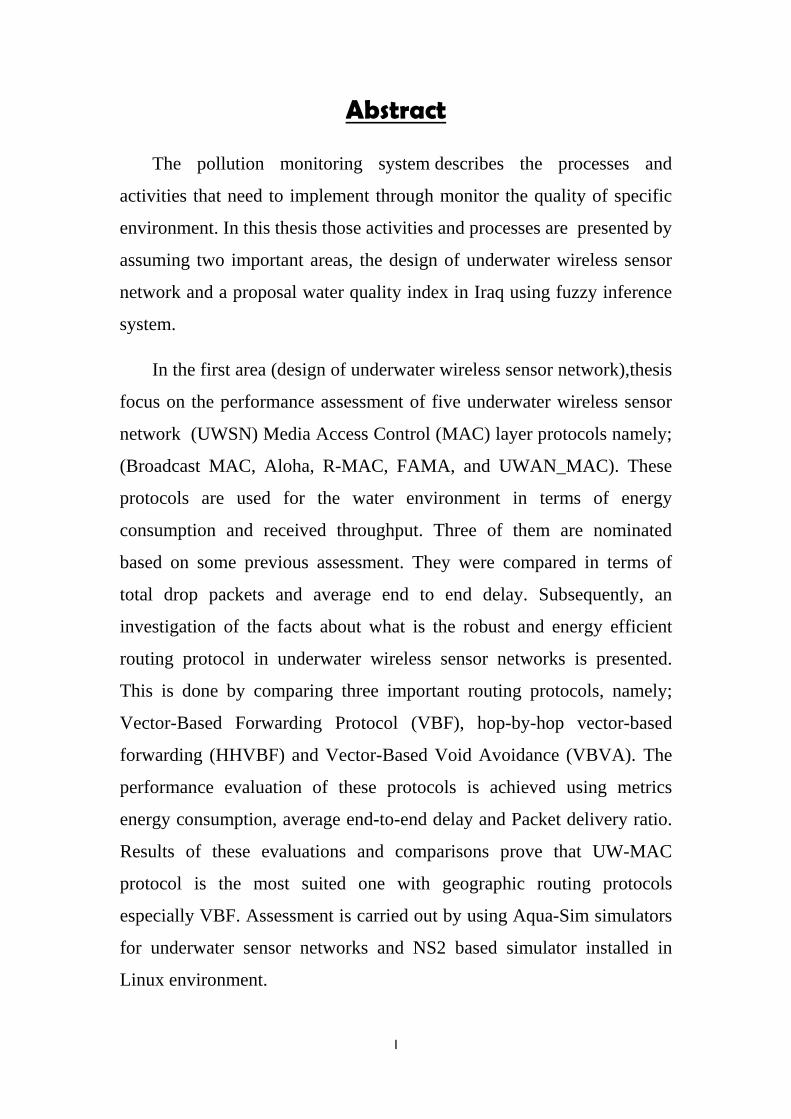
Abstract
The pollution monitoring system describes the processes and
activities that need to implement through monitor the quality of specific
environment. In this thesis those activities and processes are presented by
assuming two important areas, the design of underwater wireless sensor
network and a proposal water quality index in Iraq using fuzzy inference
system.
In the first area (design of underwater wireless sensor network),thesis
focus on the performance assessment of five underwater wireless sensor
network (UWSN) Media Access Control (MAC) layer protocols namely;
(Broadcast MAC, Aloha, R-MAC, FAMA, and UWAN_MAC). These
protocols are used for the water environment in terms of energy
consumption and received throughput. Three of them are nominated
based on some previous assessment. They were compared in terms of
total drop packets and average end to end delay. Subsequently, an
investigation of the facts about what is the robust and energy efficient
routing protocol in underwater wireless sensor networks is presented.
This is done by comparing three important routing protocols, namely;
Vector-Based Forwarding Protocol (VBF), hop-by-hop vector-based
forwarding (HHVBF) and Vector-Based Void Avoidance (VBVA). The
performance evaluation of these protocols is achieved using metrics
energy consumption, average end-to-end delay and Packet delivery ratio.
Results of these evaluations and comparisons prove that UW-MAC
protocol is the most suited one with geographic routing protocols
especially VBF. Assessment is carried out by using Aqua-Sim simulators
for underwater sensor networks and NS2 based simulator installed in
Linux environment.
II
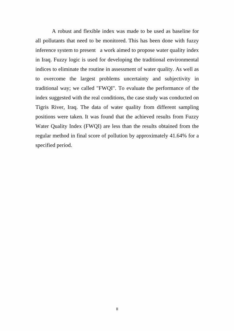
A robust and flexible index was made to be used as baseline for
all pollutants that need to be monitored. This has been done with fuzzy
inference system to present a work aimed to propose water quality index
in Iraq. Fuzzy logic is used for developing the traditional environmental
indices to eliminate the routine in assessment of water quality. As well as
to overcome the largest problems uncertainty and subjectivity in
traditional way; we called "FWQI". To evaluate the performance of the
index suggested with the real conditions, the case study was conducted on
Tigris River, Iraq. The data of water quality from different sampling
positions were taken. It was found that the achieved results from Fuzzy
Water Quality Index (FWQI) are less than the results obtained from the
regular method in final score of pollution by approximately 41.64% for a
specified period.
III
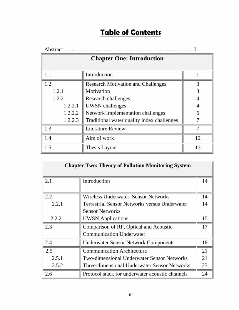
Table of Contents
Abstract ……………...………………………………....................... I
Chapter One: Introduction
1.1 Introduction 1
1.2 1.2.1 1.2.2 1.2.2.1 1.2.2.2 1.2.2.3
Research Motivation and Challenges Motivation Research challenges UWSN challenges Network Implementation challenges Traditional water quality index challenges
3 3 4 4 6 7
1.3 Literature Review 7
1.4 Aim of work 12
1.5 Thesis Layout 13
Chapter Two: Theory of Pollution Monitoring System
2.1 Introduction 14
2.2 2.2.1 2.2.2
Wireless Underwater Sensor Networks Terrestrial Sensor Networks versus Underwater Sensor Networks UWSN Applications
14 14
15
2.3 Comparison of RF, Optical and Acoustic Communication Underwater
17
2.4 Underwater Sensor Network Components 18
2.5 2.5.1 2.5.2
Communication Architecture Two-dimensional Underwater Sensor Networks Three-dimensional Underwater Sensor Networks
21 21 23
2.6 Protocol stack for underwater acoustic channels 24
IV
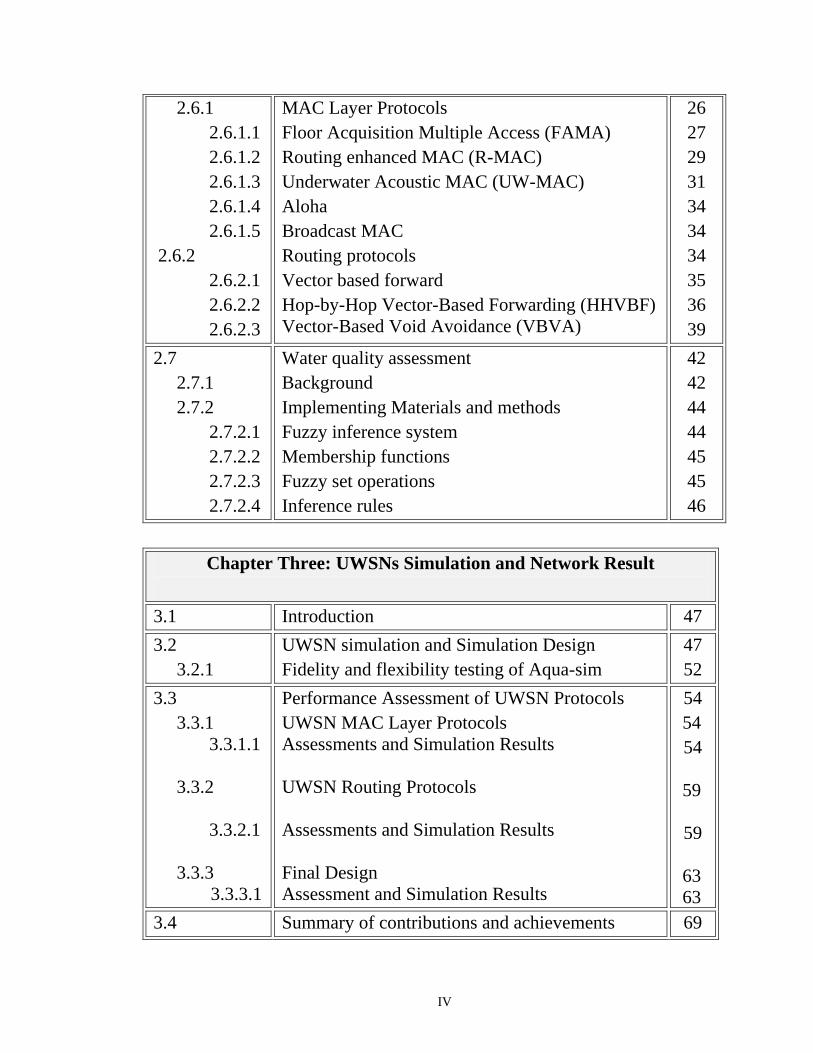
2.6.1 2.6.1.1 2.6.1.2 2.6.1.3 2.6.1.4 2.6.1.5 2.6.2 2.6.2.1 2.6.2.2 2.6.2.3
MAC Layer Protocols Floor Acquisition Multiple Access (FAMA) Routing enhanced MAC (R-MAC) Underwater Acoustic MAC (UW-MAC) Aloha Broadcast MAC Routing protocols Vector based forward Hop-by-Hop Vector-Based Forwarding (HHVBF) Vector-Based Void Avoidance (VBVA)
26 27 29 31 34 34 34 35 36 39
2.7 2.7.1 2.7.2 2.7.2.1 2.7.2.2 2.7.2.3 2.7.2.4
Water quality assessment Background Implementing Materials and methods Fuzzy inference system Membership functions Fuzzy set operations Inference rules
42 42 44 44 45 45 46
Chapter Three: UWSNs Simulation and Network Result
3.1 Introduction 47
3.2 3.2.1
UWSN simulation and Simulation Design Fidelity and flexibility testing of Aqua-sim
47 52
3.3 3.3.1 3.3.1.1 3.3.2 3.3.2.1 3.3.3 3.3.3.1
Performance Assessment of UWSN Protocols UWSN MAC Layer Protocols Assessments and Simulation Results UWSN Routing Protocols Assessments and Simulation Results Final Design Assessment and Simulation Results
54 54 54
59 59
63 63
3.4 Summary of contributions and achievements 69
V
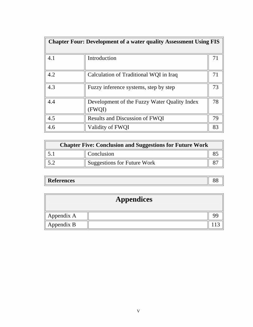
Chapter Four: Development of a water quality Assessment Using FIS
4.1 Introduction
71
4.2 Calculation of Traditional WQI in Iraq 71
4.3
Fuzzy inference systems, step by step 73
4.4 Development of the Fuzzy Water Quality Index (FWQI)
78
4.5 Results and Discussion of FWQI 79
4.6 Validity of FWQI 83
Chapter Five: Conclusion and Suggestions for Future Work
5.1 Conclusion 85
5.2 Suggestions for Future Work 87
References 88
Appendices
Appendix A 99
Appendix B 113
XI
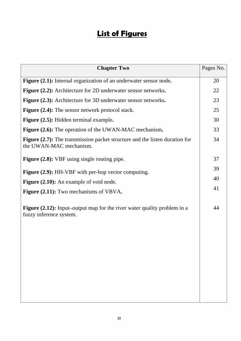
List of Figures
Chapter Two Pages No.
Figure (2.1): Internal organization of an underwater sensor node.
Figure (2.2): Architecture for 2D underwater sensor networks.
Figure (2.3): Architecture for 3D underwater sensor networks.
Figure (2.4): The sensor network protocol stack.
Figure (2.5): Hidden terminal example.
Figure (2.6): The operation of the UWAN-MAC mechanism.
Figure (2.7): The transmission packet structure and the listen duration for the UWAN-MAC mechanism. Figure (2.8): VBF using single routing pipe. Figure (2.9): HH-VBF with per-hop vector computing.
Figure (2.10): An example of void node.
Figure (2.11): Two mechanisms of VBVA.
Figure (2.12): Input–output map for the river water quality problem in a fuzzy inference system.
20
22
23
25
30
33
34
37
39
40
41
44
XII
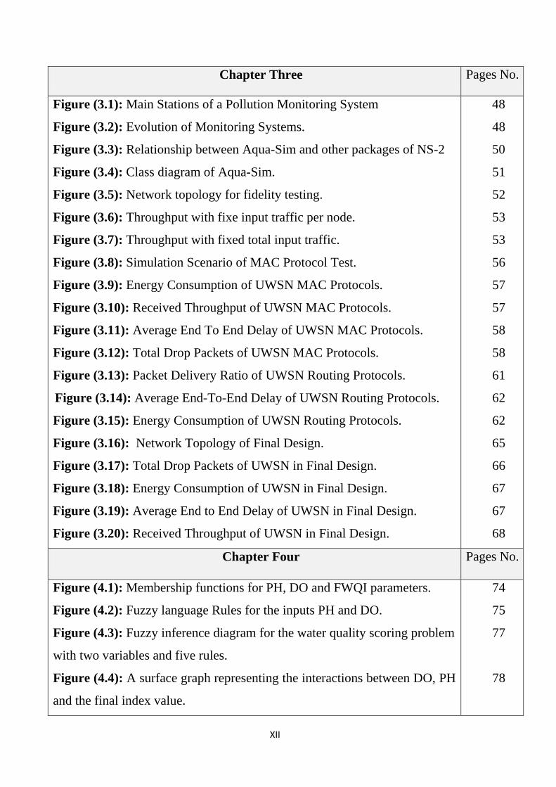
Chapter Three Pages No.
Figure (3.1): Main Stations of a Pollution Monitoring System
Figure (3.2): Evolution of Monitoring Systems.
Figure (3.3): Relationship between Aqua-Sim and other packages of NS-2
Figure (3.4): Class diagram of Aqua-Sim.
Figure (3.5): Network topology for fidelity testing.
Figure (3.6): Throughput with fixe input traffic per node.
Figure (3.7): Throughput with fixed total input traffic.
Figure (3.8): Simulation Scenario of MAC Protocol Test.
Figure (3.9): Energy Consumption of UWSN MAC Protocols.
Figure (3.10): Received Throughput of UWSN MAC Protocols.
Figure (3.11): Average End To End Delay of UWSN MAC Protocols.
Figure (3.12): Total Drop Packets of UWSN MAC Protocols.
Figure (3.13): Packet Delivery Ratio of UWSN Routing Protocols.
Figure (3.14): Average End-To-End Delay of UWSN Routing Protocols.
Figure (3.15): Energy Consumption of UWSN Routing Protocols.
Figure (3.16): Network Topology of Final Design.
Figure (3.17): Total Drop Packets of UWSN in Final Design.
Figure (3.18): Energy Consumption of UWSN in Final Design.
Figure (3.19): Average End to End Delay of UWSN in Final Design.
Figure (3.20): Received Throughput of UWSN in Final Design.
48
48
50
51
52
53
53
56
57
57
58
58
61
62
62
65
66
67
67
68
Chapter Four Pages No.
Figure (4.1): Membership functions for PH, DO and FWQI parameters.
Figure (4.2): Fuzzy language Rules for the inputs PH and DO.
Figure (4.3): Fuzzy inference diagram for the water quality scoring problem
with two variables and five rules.
Figure (4.4): A surface graph representing the interactions between DO, PH
and the final index value.
74
75
77
78
XIII
Figure (4.5): Results for water quality indexes for Tigris River within Baghdad city from 2004-2010 Figure (4.6): Comparative between indexes in June 2007.
Figure (4.7): Comparative between indexes in August 2007.
Figure (4.8): Comparative between indexes in January 2008.
81
82
82
83
XIV
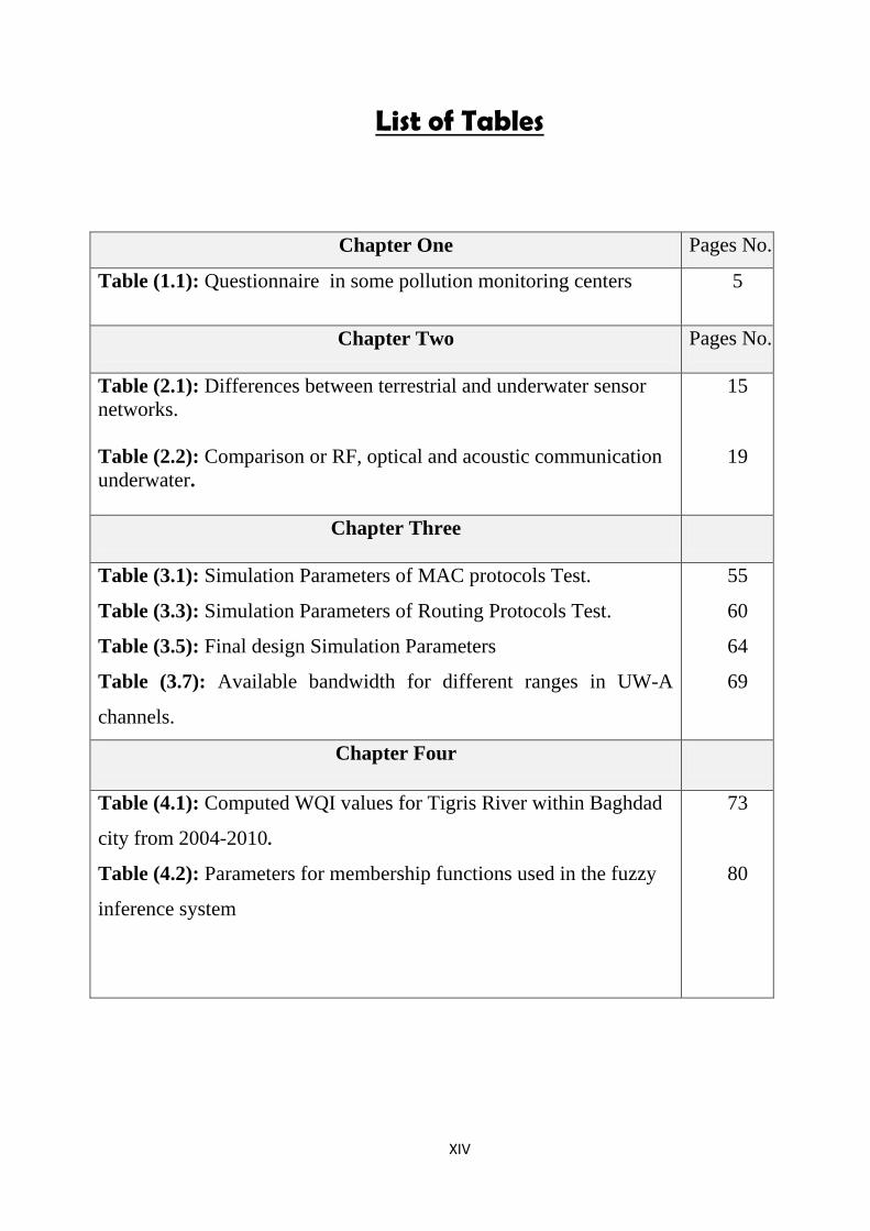
List of Tables
Chapter One Pages No.
Table (1.1): Questionnaire in some pollution monitoring centers 5
Chapter Two Pages No.
Table (2.1): Differences between terrestrial and underwater sensor networks. Table (2.2): Comparison or RF, optical and acoustic communication underwater.
15
19
Chapter Three
Table (3.1): Simulation Parameters of MAC protocols Test.
Table (3.3): Simulation Parameters of Routing Protocols Test.
Table (3.5): Final design Simulation Parameters
Table (3.7): Available bandwidth for different ranges in UW-A
channels.
55
60
64
69
Chapter Four
Table (4.1): Computed WQI values for Tigris River within Baghdad
city from 2004-2010.
Table (4.2): Parameters for membership functions used in the fuzzy
inference system
73
80
XV
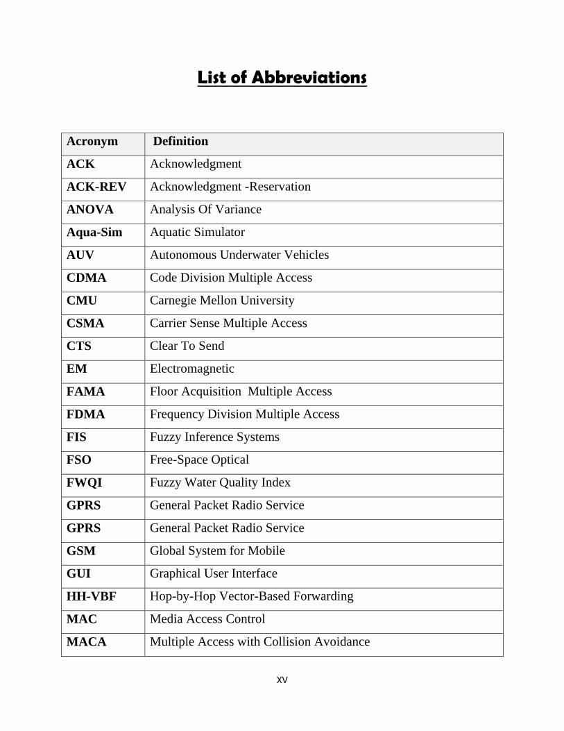
List of Abbreviations
Acronym Definition
ACK Acknowledgment
ACK -REV Acknowledgment -Reservation
ANOVA Analysis Of Variance
Aqua-Sim Aquatic Simulator
AUV Autonomous Underwater Vehicles
CDMA Code Division Multiple Access
CMU Carnegie Mellon University
CSMA Carrier Sense Multiple Access
CTS Clear To Send
EM Electromagnetic
FAMA Floor Acquisition Multiple Access
FDMA Frequency Division Multiple Access
FIS Fuzzy Inference Systems
FSO Free-Space Optical
FWQI Fuzzy Water Quality Index
GPRS General Packet Radio Service
GPRS General Packet Radio Service
GSM Global System for Mobile
GUI Graphical User Interface
HH-VBF Hop-by-Hop Vector-Based Forwarding
MAC Media Access Control
MACA Multiple Access with Collision Avoidance
XVI
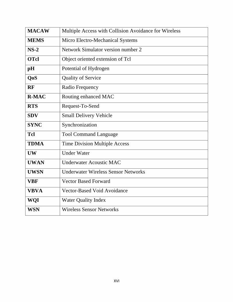
MACAW Multiple Access with Collision Avoidance for Wireless
MEMS Micro Electro-Mechanical Systems
NS-2 Network Simulator version number 2
OTcl Object oriented extension of Tcl
pH Potential of Hydrogen
QoS Quality of Service
RF Radio Frequency
R-MAC Routing enhanced MAC
RTS Request-To-Send
SDV Small Delivery Vehicle
SYNC Synchronization
Tcl Tool Command Language
TDMA Time Division Multiple Access
UW Under Water
UWAN Underwater Acoustic MAC
UWSN Underwater Wireless Sensor Networks
VBF Vector Based Forward
VBVA Vector-Based Void Avoidance
WQI Water Quality Index
WSN Wireless Sensor Networks

Chapter One
Introduction

Chapter One……………………………………….…………………….Introduction
1
Chapter One
Introduction
1.1 Introduction
Sensing is a technique used to collect information about a physical object or
process, including the happening of events such as changes in state like dropping in
temperature or pressure. An object performing a sensing task is called a sensor. For
example, the human body is supplied with sensors that can capture optical
information from the environment (eyes), acoustic information such as sounds (ears),
and smells (nose). These are examples of remote sensors, i.e. they do not require
touching the monitored object to gather information. From a technical view, a sensor
is a device that translates events or parameters in the real world into signals that can
be determined and analyzed [1].
With the new developments in micro electro-mechanical systems (MEMS)
technology, in addition to wireless communications, and digital electronics, the
design and development of cheap, low-power, multifunctional sensor; tiny nodes that
communicate untethered in short distances are applied. The continuously increasing
capabilities of these small sensor nodes, including sensing, data processing, and
communicating, enable the realization of wireless sensor networks (WSNs) based on
the effort of a large number of sensor nodes [2].
So, a WSN is a self-configured network that is composed of a large number of
small sensor nodes. The fields of WSNs influence the world with their potential to
enhance human lives. A WSN is able to sense information, processing, and transmit
information to other nodes through proper communication. Sensor nodes were
developed for deployment on land, and there are no native nodes for underwater
environment until now. Terrestrial nodes enclosed in specially designed containers
deploy the nodes in water but they do not exploit underwater circumstances. These
waterproof nodes are susceptible to issues such as localization, communication
Chapter One……………………………………….…………………….Introduction
2
overhead (i.e. electromagnetic waves are vulnerable over long distances in
underwater environment), bandwidth, dynamic topology, and node flexibility.
Henceforth, using nodes bounded in containers is not a perfect solution to monitor
the underwater environment and is not recommended for placement in underwater
environments [3].
Lately, wireless sensor networks were suggested for placement in underwater
environments where a lot of applications like aquiculture, pollution monitoring,
offshore investigation, etc. would advantage from this technology.
Design and construction of UWSNs as a communication network is extremely
difficult. As a value, that is valid for earthly WSNs are perhaps not valid for
UWSNs. So, an overall examination of the total network construction is necessary to
supply a suitable network service for observing the system such as routing and MAC
protocols, range of each node, network topography and all network necessities.
On the other hand and after the arrival of data from the wireless sensor
network; it will be processed. There is an important challenge to assess this data,
make it ready, and pass it to the concerned authorities. This is useful to monitor
environmental pollution in this area. For example, if the water quality is good,
weak, average or bad etc. Then, make the right decision to deal with this condition
of water. The second part is not essential, but very important in the completion of
an integrated pollution monitoring system. There is no need to bring other systems
that might complicate it. Water quality assessment is an evaluation of the water
body conditions using biological surveys, chemical-specific analyses of pollutants
in water bodies, and toxicity tests.
There are several ways to assess the quality of water using empirical equations
multiplying the indicators by certain weights depending on the degree of
importance. The latest method to assess the quality of water is the use of fuzzy
logic discovered by Lotfi Zadeh in 1965, which allows for using knowledge with
Chapter One……………………………………….…………………….Introduction
3
expertise in the processes to eliminate uncertainty and subjectivity contained in
traditional systems.
1.2 Research Motivation and Challenges
Two important concepts of research motivation and research challenges are
presented in this section. It introduces the traditional pollution monitoring research
motivation in its general form, then looks at the traditional way in Iraq. Challenges
are classified into two parts, challenges facing UWSNs and implementation of
networks.
1.2.1 Motivation
The old approach for monitoring is to allocate underwater sensors that record
data during the monitoring task, then mend the instruments. This approach has the
following disadvantages [4]:
1. No immediate monitoring: The recorded data can not read until the instruments
are mended. This may last for days, weeks, or months after starting the
monitoring task. In observation or environmental monitoring applications such
as seismic monitoring, instantaneous data retrieval is crucial.
2. No connected system reconfiguration: Collaboration between onshore control
systems and the monitoring devices are not possible. This does not obstruct any
adaptive regulation of the devices; nor is it possible to reconfigure the system
after specific events happening.
3. No failure discovery: If failures or misconfigurations happen, it might not be
possible to be discover them before the devices are recovered. This can easily
lead to the broad failure of a monitoring task.
4. Inadequate storage capacity: The quantity of data that can be recorded during the
monitoring task by every sensor is limited by the capacity of the aboard storage
devices (memories, hard disks).
Chapter One……………………………………….…………………….Introduction
4
These disadvantages of old underwater monitoring techniques bound the possible
applications for this atmosphere. Alternatively, the distributed sensor network model
may provide capabilities meaningfully exceed the existing underwater applications.
Therefore, there is a necessity to position underwater networks that enable
immediate monitoring of particular ocean areas, distant configuration and interaction
with onshore human operatives. All this can be gained by joining underwater
instruments by means of wireless links and forming underwater sensor networks.
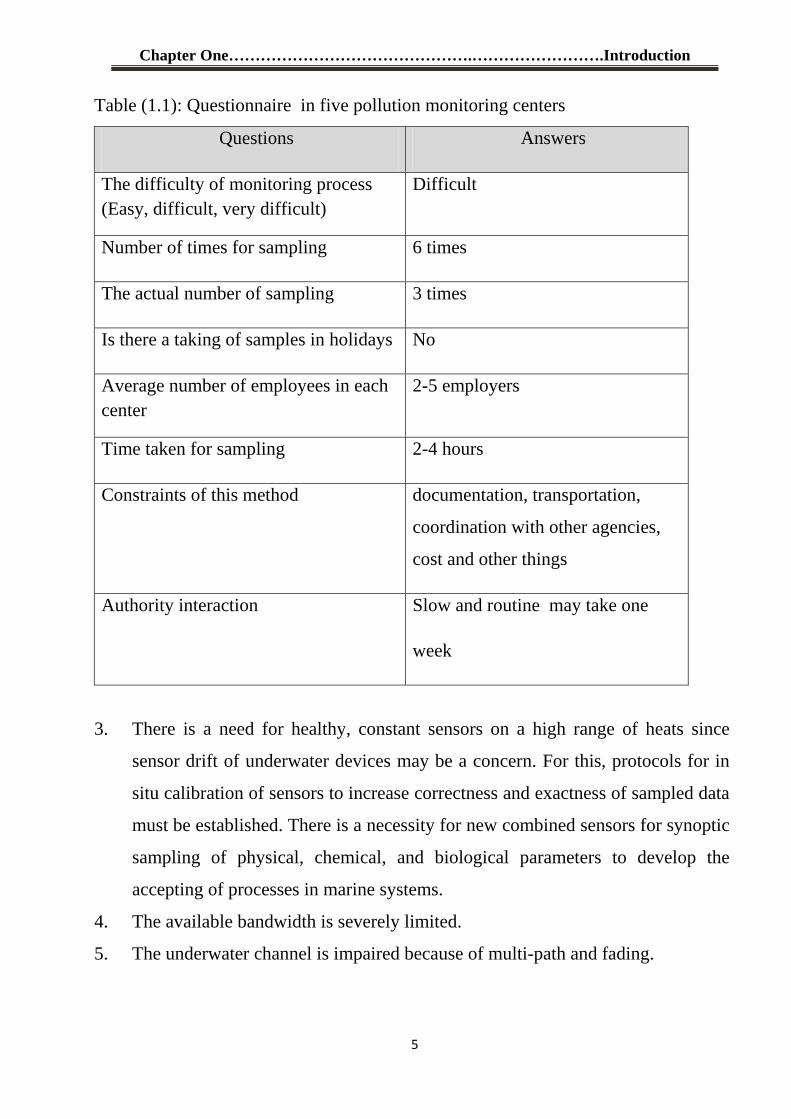
In Iraq, and through a questionnaire conducted in a number of environment and
health centers involved in the control of pollution in the water, especially those
located in remote places and it was found that the monitoring process routine used is
a process tired, slow and contains all the disadvantages mentioned above. The
questionnaire to summarize system specifications approach is shown in Table (1.1).
1.2.2 Research challenges
The research challenges are classified into three categories; UWSN, network
implementation, and traditional water quality index challenges.
1.2.2.1 UWSN challenges
The major challenges encountered in the design of underwater acoustic
networks are listed as follows [5], [6] and [7]:
1. It is necessary to develop less expensive, robust nano-sensors, e.g., sensors
based on nanotechnology, which contains development of supplies and systems
at the nuclear, molecular, or macromolecular ranks in the dimension range of
about 1–500 nm.
2. It is essential to develop the mechanisms of scheduled by cleaning against
weathering and fouling, which may affect the lifespan of underwater devices.
Chapter One……………………………………….…………………….Introduction
5
Table (1.1): Questionnaire in five pollution monitoring centers
Questions Answers
The difficulty of monitoring process (Easy, difficult, very difficult)
Difficult
Number of times for sampling 6 times
The actual number of sampling 3 times
Is there a taking of samples in holidays No
Average number of employees in each center
2-5 employers
Time taken for sampling 2-4 hours
Constraints of this method documentation, transportation,
coordination with other agencies,
cost and other things
Authority interaction Slow and routine may take one
week
3. There is a need for healthy, constant sensors on a high range of heats since
sensor drift of underwater devices may be a concern. For this, protocols for in
situ calibration of sensors to increase correctness and exactness of sampled data
must be established. There is a necessity for new combined sensors for synoptic
sampling of physical, chemical, and biological parameters to develop the
accepting of processes in marine systems.
4. The available bandwidth is severely limited.
5. The underwater channel is impaired because of multi-path and fading.
Chapter One……………………………………….…………………….Introduction
6
6. Propagation postponement in subsurface is five orders of magnitude higher than
in Radio Frequency (RF) terrestrial channels, and variable.
7. High bit fault amounts and short-term losses of connectivity (shadow zones)
can be practiced.
8. Underwater sensors are categorized by high cost because of extra protecting
sheaths needed for sensors and also rather small numbers of suppliers (i.e., not
much reduced of scale) are available.
9. Battery power is restricted and usually batteries cannot be recharged, as solar
energy cannot be broken.
10. Underwater sensors are more disposed to failures because of entangling and
corrosion.
1.2.2.2 Network Implementation challenges
The difficulty and cost of providing professional laboratory for a real test lead
to the use of simulators. The major challenge is to find a suitable simulator to offer
all or most of the requirements of this underwater network. The challenges
encountered in the application of this network and the differences from those
worldly networks are:
1. audio communication is the usual conventional method for underwater
environments, while the broadcast speed of audio signal under water is very slow
(about 1500 m/s), considerably different from that of radio signal.
2. The audio signal decrease model is radically different from that of radio signal,
and thus audio channel models should be unified.
3. Underwater sensor networks are usually positioned in a three-dimensional place,
while these simulators usually only support two-dimensional placement. Thus,
the unique features of underwater sensor networks make the existing network
simulators unsuitable.
Chapter One……………………………………….…………………….Introduction
7
1.2.2.3 Traditional water quality index challenges
The use of these traditional indices raises many challenges:
1. Some parameters in the index equations can influence dramatically the final
score without valid justification, while their formulations are rather elementary,
and the number of variables involved is too limited. [8].
2. This leads to an unclear distinction between each mode of the index and
causes inaccuracies and ambiguity when making decisions about boundary
values [9].
3. The most critical deficiency of these indexes is the lack of dealing with
uncertainty and subjectivity [10].
1.3 Literature Review
The related works of wireless sensor networks simulation are discussed in
this section.
In [11], the author proved that low-cost sensors are usable in underwater
sensor networks and the Microsoft Windows CE may be used in the Intel Xscale
PXA270 board for signal processing. A high-level programming language like
C++, C# or VB.Net used for programming the applications that read real-time
sensor data and convey sensor data between a sensor node and a super-node. He
presented that the sensor data can be read by the Intel Xscale PXA270 board via
its analog to digital (A/D) converter. The sensor data can be conveyed from a
sensor node to a super-node in real time throughout an 802.11 wireless sensor
network
In [12], an original alternative opportunity of time-critical underwater
communication using short-range (50 – 500 m) low-cost sensors was presented.
Their chief goal is that the modem must be cheap to make it possible to buy and
position many underwater sensor nodes. Multi-hop routing over many separate
nodes can reach long-range communication. Actually, concentrating on short-
Chapter One……………………………………….…………………….Introduction
8
range communication means can increase the obtainable audio bandwidth and
also escape many of the challenges of long-range underwater communication
and henceforth, really make simpler the modem design. In addition, the
researcher has planned a novel management protocol that confirms total volume
coverage, advance the QoS; in addition to enhance the lifetime of the entire
network.
In [13], the authors introduced the adjacent of network nodes form
cluster.in which, each node sends the data to the main node of the cluster. The
main node compresses the data and sends it to the Sink node. Actually, sink
node is the gateway nodes, responsible of the network beginning, repairs, data
gathering and send data to the control center. The monitor center is responsible
of data processing and network management. There is some specific software on
the control center that does the job of data processing and makes choice. As
woodland is a place that human can easily reach, so artificial split farmland can
be split into multiple regions, each region is a cluster of network topology. And
inside each cluster a head node responsible of the communication with gateway
is assigned. And meanwhile the agricultural environment may not have standard
cable network, so they are considered as two communication structures. (a) The
gateway communicates with the Server control center through the cable
network. (b) In the mobile networks such as Global System for Mobile
Communications (GSM) or Code division multiple access (CDMA) coverage
area can be used as a broadcast medium. The sink node sends the data to main
stations, and the main station data is then transmitted to the monitoring center.
In [14], the authors explained and illustrated a new design of water
environment monitoring system, based on a WSN. The system generally
includes three divisions: hardware and software of data monitoring nodes,
hardware and software of the data main station, in addition to software for the
distant monitoring center. The system efficiently achieves an on line auto
Chapter One……………………………………….…………………….Introduction
9
monitoring of the water temperature and pH environment of a non-natural lake.
Sensors were appropriate to alter water quality that can be installed at the node
to meet the monitoring requirements in various water environments and to attain
various parameters.
In [15], the authors developed and compared different sensor network
construction designs that can be used for monitoring underwater pipeline
foundations. These constructions were underwater wired sensor networks,
underwater audio wireless sensor networks, RF (Radio Frequency) wireless
sensor networks, combined wired/audio wireless sensor networks, and integrated
wired/RF wireless sensor networks. The researchers also discussed the
dependability challenges and enhancement methods for these network
constructions. The dependability evaluation, features, compensations, and
shortcomings among these constructions were argued and matched. Three
reliability factors were used for the discussion and comparison: the network
connectivity, the endurance of power supply for the network, and the physical
network security. In addition, they developed and evaluated a graded sensor
network framework for underwater pipeline monitoring.
In [16], Based on wireless sensor networks (WSN), reported a new
observation system using underwater multisensory information. After processing
the multisensory data from each sensor, the system transmits it to a hub node
through WSN, and then transmits it to a land data center through a general
packet radio service (GPRS) wireless network. In order to check the basic
performance of this system, they completed a node positioning experiment
based on a GPS module, and a communication experiment based on ZigBee.
This article reported the design of the hardware and the experimental results
[16].
Chapter One……………………………………….…………………….Introduction
10
In [17], the author introduced a thesis focused on node lifetime extension
based on energy management. While some constraints and results might hold
true from a more general perspective. The main application target involves
environmental measurement systems based on Wireless Sensor Networks.
Lifetime extension possibilities, which were the result of application
characteristics, by (i) reducing energy consumption and (ii) utilizing energy
harvesting were to be presented. For energy consumption, he showed how
precise task scheduling due to node synchronization, combined with methods
such as duty cycling and power domains, can optimize the overall energy use.
With reference to the energy supply, the focus lies on solar-based solutions with
special attention placed on their feasibility at locations with limited solar
radiation. Further dimensioning of these systems was addressed [17].
In [18], the authors developed an underwater sensor network for
monitoring water quality and pollution to keep heat and pH as the parameters
which were being monitored by the jots and communicated through data main
station and GPRS modems to the data monitoring center. This can serve as a
prolonged solution for ecological control and monitoring of physical
environments therefore making pollution monitoring less complex and age
group of reports on fixed basis upholding a close check on the amount of
impurities through monitoring acidity in the samples of water under monitoring
[18].
In [19], the author presented a thesis about general framework in water
quality monitoring system. The real-time values of analytical instruments are
necessary to the wireless data acquisition terminal, the data processed and
packaged, and sent to the data center through a wireless network. After
decrypting, the system does the data analysis, storage, display and alarm
automatically by management information system (MIS) and geographic
information system (GIS). It then publishes the data to the upper network
Chapter One……………………………………….…………………….Introduction
11
control and management system Via TCP / IP protocol and exchange data with
other control centers. At last, the center sent the command to the sub-stations
and summaries the feedback through GSM/GPRS communication. In short
range, Zigbee and Wi-Fi frequently are used in water monitoring area. For
sensor cost wireless networking protocol are targeted towards automation. On
the other hand, GSM/GPRS are applied for long range communication [19].
In [20], the authors identified a need for an autonomous and
collaborative mechanism, based on targeted wireless sensor technologies.
Furthermore, they concluded that for effective and integrated water quality
monitoring and management at a catchment scale, a system of individually
networked activities is needed. This is likely to take the form of a combination
of networks that have been installed for local monitoring purposes (e.g. at farm
scale, primarily to provide local information for that farm), and some specific
networks aimed at filling in information gaps in the catchment. This system of
networks should be able to share information about critical parameters for
events, such as rain, or floods, that could trigger consequences, such as
contaminants runoff. It requires a higher level application to make use of this
information, and that the individual networks are aware of similar networks
nearby capable of passing information to them. This inevitably led them to some
form of standardization of communication protocol and data representation
between enabled environmental networks [20].
By looking carefully at the pollution monitoring systems mentioned
above, the following disadvantages are noted:-
1. It can be seen that the above researches did not contain physical comparison
between the types of communications in terms of facing the UWSN challenges
then select the appropriate one. For example the comparison between acoustic,
electromagnetic and optical communication.
Chapter One……………………………………….…………………….Introduction
12
2. The lack of a comparative study between MAC and routing protocols to find the
most appropriate one. This comparison is done through specific metrics such as
(energy consumption, received throughput, packet delivery ratio, total drop
packet and etc.).
3. The number of nodes used is not taken into consideration the possible number
that is optimum to get an efficient system by using specific metrics.
4. Lack of a comprehensive study on the importance of the pollutants to be
monitored, is it sensitive information or not? Can it be delaying or not? And
other then decide on any routing protocols will use depending on type of the
system.
5. No focus on important aspect especially, Integrated Systems in terms of the
design of monitoring systems, data processing, water quality assessment, make
decision when there is an increase or decrease in limits of indicators and
reporting to the competent authorities.
This is evident through the research, conducted in a number of scientific
papers related to the terms "Monitoring", "underwater wireless sensor network"
and "ns2". There are 1250 papers on this matter. While for the terms
"Monitoring", "underwater wireless sensor network", "ns2" and "fuzzy water
quality" only 12 papers were found that simply deal with these concepts as an
integrated system.
1.4 Aim of work
The aim of presented work is to overcome the gaps in literature mentioned
above and obtain preferred and integrated monitoring system.
1. These works is design and implement the UWSN to monitor some of the
pollutants in the Iraqi rivers.
2. Through this design, several comparisons between communication channels,
MAC protocols and routing protocols is presented to obtain the results for most
appropriate one for this work from the point of view of several metrics.
Chapter One……………………………………….…………………….Introduction
13
3. To develop a novel water quality index in Iraq based on fuzzy inference system,
that is, a comprehensive artificial intelligence (AI) approach to the development
of traditional environmental indices for routine assessment of water quality,
particularly for human drinking purposes.
1.5 Thesis Layout
This thesis is organized to 5 chapters. Chapter 2 presents the overview of
UWSN as architecture of sensor, communication medium, MAC protocols and
routing protocols including a quick comparison between the terrestrial WSN and
UWSN. It additionally presents a compaction between the present simulators and
candidate the appropriate one to face the implementation challenges. It also
presents a background about water quality indices and presents the material tools
for developing the traditional way used in Iraq used to assess water quality.
Chapter 3 presents Performance Assessment of MAC Layer Protocols in UWSN
by using the specific metrics (energy consumption, received throughput, total drop
packets and average end to end delay) and elects the appropriate one based on
present system requirements and the UWSN routing protocol. It also conducts a
comparative study of them in terms of energy consumption, average end-to-end
delay and Packet delivery ratio to choose the most appropriate. Additionally,
Chapter 3 provides the final evaluation of the system in terms of the metrics that
are adopted.
Chapter 4 presents the details of the traditional way to assess water quality and
compare it with a novel way in Iraq that use fuzzy inference system. The use of
FIS step by step, the development of index and result of compression will also be
introduced in this chapter, together with the validation of the new fuzzy index.
Chapter 5 summarizes the thesis and conclusion with a suggestion of future work
trends.

Chapter One……………………………………….…………………….Introduction
14

Chapter Two
Theory of Pollution
Monitoring
Systems
Chapter Two ….…………………….…… Theory of Pollution Monitoring Systems
14
Chapter Two
Theory of Pollution Monitoring Systems
2.1 Introduction
In this chapter, the theoretical background of the pollution monitoring system
is discussed. This background contains two categories. The first one is an
overview of UWSNs which include UWSN definition, differences between
terrestrial (normal networks) and underwater Sensor Networks, UWSN
applications, important comparison between all UWSN communication channels.
In addition, it describes in details all aspect of UWSN as components and
communication architecture. At last, the Protocol stacks for underwater acoustic
channels are presented with a highlight of MAC and Routing protocols.
The second one is water quality indices and the implementation material tools
and methods to develop the traditional way used in Iraq to assess water quality by
using fuzzy inference system.
2.2 Wireless Underwater Sensor Networks
Underwater sensor networks are planned to enable applications for
oceanographic data gathering, pollution checking, offshore examination, disaster
avoidance, aided navigation and strategic investigation applications [21].
2.2.1 Terrestrial Sensor Networks versus Underwater Sensor Networks
Several features of networking in water have correspondences with the
terrestrial sensor networks. There are many differences that need communication
protocols to be custom-made for underwater sensor networks. The
communication procedures and the variances are clarified in details in section 2.
Chapter Two ….…………………….…… Theory of Pollution Monitoring Systems
15
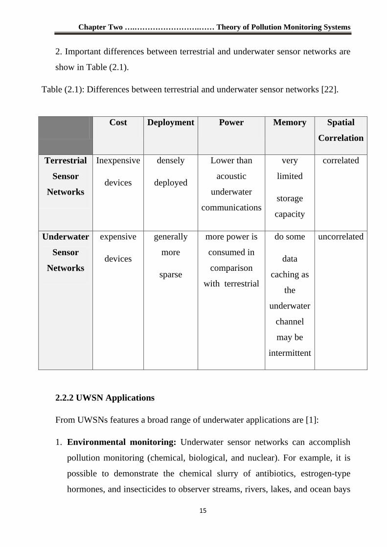
2. Important differences between terrestrial and underwater sensor networks are
show in Table (2.1).
Table (2.1): Differences between terrestrial and underwater sensor networks [22].
2.2.2 UWSN Applications
From UWSNs features a broad range of underwater applications are [1]:
1. Environmental monitoring: Underwater sensor networks can accomplish
pollution monitoring (chemical, biological, and nuclear). For example, it is
possible to demonstrate the chemical slurry of antibiotics, estrogen-type
hormones, and insecticides to observer streams, rivers, lakes, and ocean bays
Cost Deployment Power Memory Spatial
Correlation
Terrestrial
Sensor
Networks
Inexpensive
devices
densely
deployed
Lower than
acoustic
underwater
communications
very
limited
storage
capacity
correlated
Underwater
Sensor
Networks
expensive
devices
generally
more
sparse
more power is
consumed in
comparison
with terrestrial
do some
data
caching as
the
underwater
channel
may be
intermittent
uncorrelated
Chapter Two ….…………………….…… Theory of Pollution Monitoring Systems
16
(water quality in-situ examination) [23]. Monitoring ocean streams and
winds, enhanced weather forecast, discovering climate change, understanding
and expecting the influence of human actions on naval ecosystems,
biological monitoring such as tracing fishes or microorganisms, are other
potential uses.
2. Undersea explorations: Underwater sensor networks can detect underwater
oilfields or reservoirs, determine routes for resting underwater cables, and
help in the investigation for valued minerals.
3. Assisted navigation: Sensors can be used to recognize threats on the seabed,
to locate dangerous rocks or shoals in shallow waters, mooring locations, and
flooded collisions, and to perform bathymetry summarizing.
4. Distrib uted tactical surveillance: AUVs and fixed underwater sensors can
cooperatively monitor zones for investigation, inspection, targeting, and
intrusion discovery systems. A good example, a 3-D underwater sensor
network can recognize a strategic investigation system that is able to sense
and categorize submarines, small delivery vehicles (SDVs), and divers built
on the sensed data from mechanical, radiation, magnetic, and audio micro
sensors. With respect to old-style radar/sonar systems, underwater sensor
networks can reach an advanced correctness, advanced coverage, and
forcefulness as well as allow discovery and cataloguing of low-signature
targets by joining measures from different kinds of sensors.
5. Mine reconnaissance: The concurrent action of various AUVs with audio
and optical sensors can be used to make quick environmental calculation and
discover mine-like objects.
Chapter Two ….…………………….…… Theory of Pollution Monitoring Systems
17
2.3 Comparison between RF, Optical and Acoustic Underwater Communication
Effective underwater communication among units or nodes in a UWSN is
one of the utmost essential and serious issues in the entire network system
design [24].
Current underwater communication systems include the transmission of
information in the form of sound, electromagnetic (EM), or optical waves. All of
these techniques have benefits and boundaries. Audio communication is the
most multipurpose and broadly used technique in underwater settings because of
the low reduction of sound under water. This is particularly true in thermally
constant, deep-water environment. Alternatively, the use of audio waves in thin
water can be badly affected by heat rises, surface ambient noise, and multipath
broadcast because of reflection and refraction. The slower speed of audio
propagation in water, about 1500 m/s (meters per second), compared with that of
electromagnetic and optical waves, and forms another restrictive factor for
effective communication and networking. Nonetheless, the present promising
technology for underwater communication is upon audibility.
On the front of using electromagnetic (EM) waves in radio frequencies,
conventional radio does not work well in an underwater environment due to the
conducting nature of the medium, especially in the case of seawater. However, if
EM could be working underwater, even in a short distance, its much faster
propagating speed is definitely a great advantage for faster and efficient
communication among nodes.
Free-space optical (FSV) waves are used as wireless communication
carriers are commonly restricted to very small distances since the severe water
absorption is at the optical frequency bands that produce strong backscatter from
hanging particles. Even the purest water has 1000 times the reduction of clear
air, and muddled water has more than 100 times the reduction of the heaviest
Chapter Two ….…………………….…… Theory of Pollution Monitoring Systems
18
fog [24]. Underwater FSV, specifically in the blue-green wavelengths,
compromises a real choice for high-bandwidth communication (10-150 Mbps)
over reasonable ranges (10-100 meters). This communication range is much
desired in port examination, oil-rig repairs, and connecting submarines to land,
these are just names of few of the demands on this front [24].
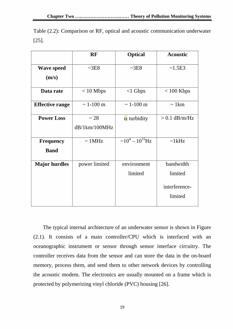
Table (2.2) summarizes and compares the characteristics of radio, optical,
and acoustic communication underwater. All three physical wave fields have
their own advantages and limitations for acting as an underwater wireless
communications carrier; radio waves can provide high data rates, but are subject
to strong attenuation by the conductivity of sea water, optical waves provide
even higher data rates, but are subject to attenuation by the turbidity of sea
water, acoustic waves provide long transmission distances but support relatively
low data rates and are subject to multipath. As our sensor network applications
require low data rates and transmission distances greater than 100 meters,
acoustics remains the most robust and feasible carrier to date for wireless
communication in these underwater sensor networks. As acoustics have been
widely used in underwater communications and we have selected acoustics for
our monitoring system.
2.4 Underwater Sensor Network Components
The design difficulties and the sole features of underwater sensor networks
need different components for the understanding of these networks. In this
section, we designate these apparatuses of the underwater sensors that are used
to gather information about the underwater setting.
Chapter Two ….…………………….…… Theory of Pollution Monitoring Systems
19
Table (2.2): Comparison or RF, optical and acoustic communication underwater
[25].
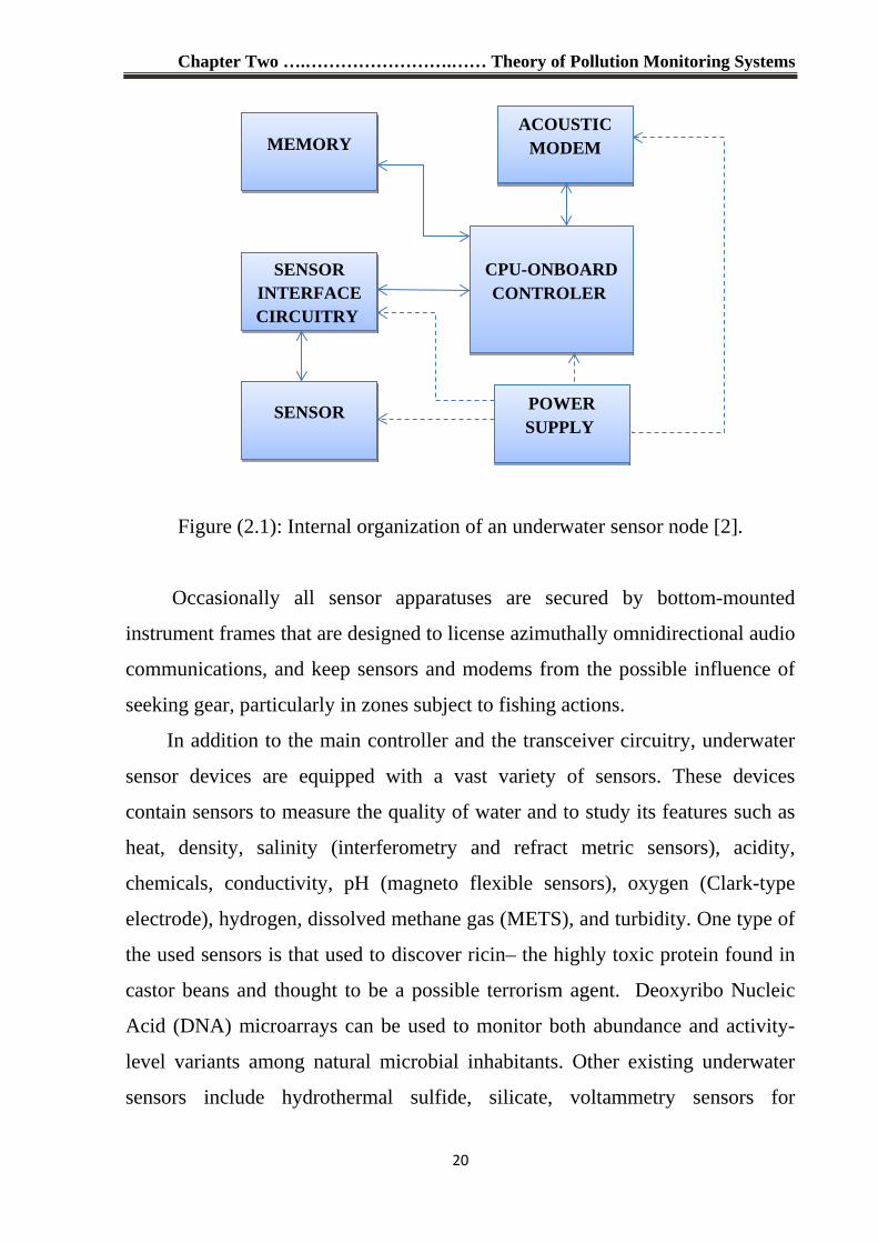
The typical internal architecture of an underwater sensor is shown in Figure
(2.1). It consists of a main controller/CPU which is interfaced with an
oceanographic instrument or sensor through sensor interface circuitry. The
controller receives data from the sensor and can store the data in the on-board
memory, process them, and send them to other network devices by controlling
the acoustic modem. The electronics are usually mounted on a frame which is
protected by polymerizing vinyl chloride (PVC) housing [26].
RF Optical Acoustic
Wave speed
(m/s)
~3E8 ~3E8 ~1.5E3
Data rate < 10 Mbps <1 Gbps < 100 Kbps
Effective range ~ 1-100 m ~ 1-100 m ~ 1km
Power Loss ~ 28
dB/1km/100MHz
α turbidity > 0.1 dB/m/Hz
Frequency
Band
~ 1MHz ~104 – 1015Hz ~1kHz
Major hurdles power limited environment
limited
bandwidth
limited
interference-
limited
Chapter Two ….…………………….…… Theory of Pollution Monitoring Systems
20
Figure (2.1): Internal organization of an underwater sensor node [2].
Occasionally all sensor apparatuses are secured by bottom-mounted
instrument frames that are designed to license azimuthally omnidirectional audio
communications, and keep sensors and modems from the possible influence of
seeking gear, particularly in zones subject to fishing actions.
In addition to the main controller and the transceiver circuitry, underwater
sensor devices are equipped with a vast variety of sensors. These devices
contain sensors to measure the quality of water and to study its features such as
heat, density, salinity (interferometry and refract metric sensors), acidity,
chemicals, conductivity, pH (magneto flexible sensors), oxygen (Clark-type
electrode), hydrogen, dissolved methane gas (METS), and turbidity. One type of
the used sensors is that used to discover ricin– the highly toxic protein found in
castor beans and thought to be a possible terrorism agent. Deoxyribo Nucleic
Acid (DNA) microarrays can be used to monitor both abundance and activity-
level variants among natural microbial inhabitants. Other existing underwater
sensors include hydrothermal sulfide, silicate, voltammetry sensors for
ACOUSTIC MODEM
SENSOR INTERFACE CIRCUITRY
MEMORY
SENSOR
CPU-ONBOARD CONTROLER
POWER SUPPLY
Chapter Two ….…………………….…… Theory of Pollution Monitoring Systems
21
spectrophotometry, gold-amalgam electrode sensors for sediment measurements
of metal ions (ion-selective analysis), aerometric micro sensors for H2S
capacities for studies of an oxygenic photosynthesis, sulfide oxidation, and
sulfate reduction of sediments [2].
2.5 Communication Architecture
In this section, we describe the communication architectures of underwater
acoustic sensor networks. In particular, we introduce reference architectures for
two-dimensional and three-dimensional underwater networks.
Underwater monitoring missions can be extremely expensive due to the high
cost of underwater devices. Henceforth, it is significant that the positioned
network be highly dependable, to avoid failure of monitoring tasks due to failure
of single or multiple devices. For example, it is vital to evade designing the
network topology with sole points of failure, which could compromise the total
operational of the network. The network capability is also affected by the
network topology. Since the capacity of the underwater channel is severely
limited it is very important to organize the network topology in such a way that
no communication bottleneck is introduced [27].
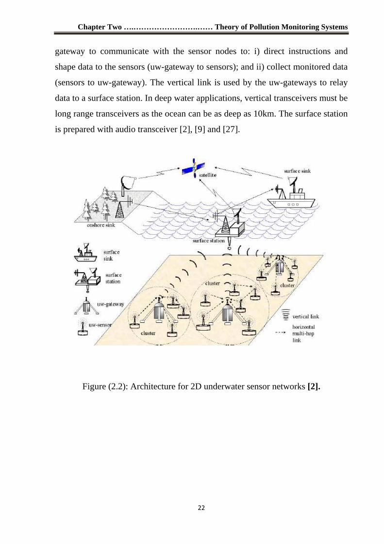
2.5.1 Two-dimensional Underwater Sensor Networks
Position construction for two-dimensional underwater networks is shown
in Figure (2.2). A group of sensor nodes is attached to the bottommost of the
ocean with deep ocean anchors. Underwater sensor nodes are interrelated to one
or more underwater gateways (uw-gateways) via wireless audio links. UW-
gateways, as presented in Figure (2.2). These are network devices responsible of
spreading data from the ocean bottom network to a surface station. To attain this
goal, uw-gateways are prepared with two audio transceivers, namely a vertical
and a horizontal transceiver. The horizontal transceiver is used by the uw-
Chapter Two ….…………………….…… Theory of Pollution Monitoring Systems
22
gateway to communicate with the sensor nodes to: i) direct instructions and
shape data to the sensors (uw-gateway to sensors); and ii) collect monitored data
(sensors to uw-gateway). The vertical link is used by the uw-gateways to relay
data to a surface station. In deep water applications, vertical transceivers must be
long range transceivers as the ocean can be as deep as 10km. The surface station
is prepared with audio transceiver [2], [9] and [27].
Figure (2.2): Architecture for 2D underwater sensor networks [2].
Chapter Two ….…………………….…… Theory of Pollution Monitoring Systems
23
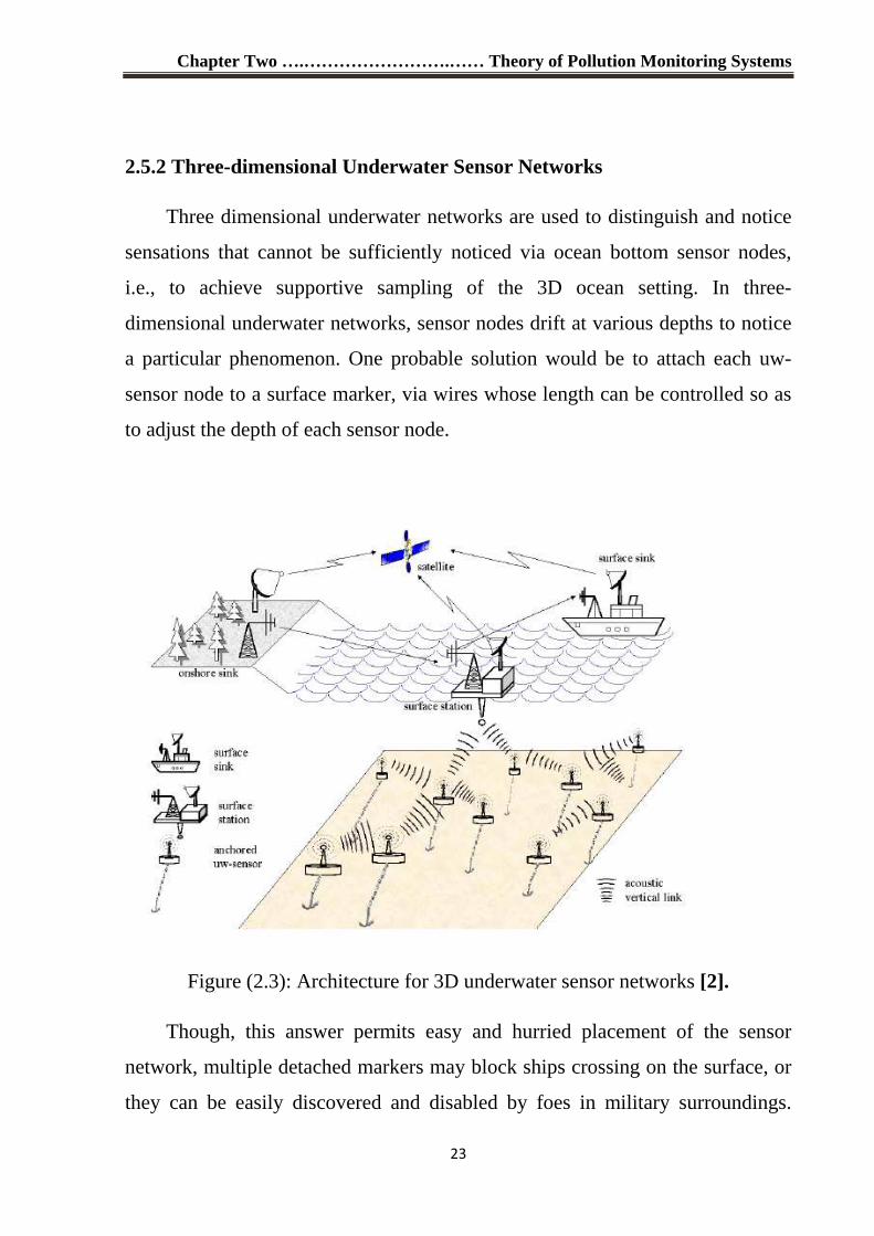
2.5.2 Three-dimensional Underwater Sensor Networks
Three dimensional underwater networks are used to distinguish and notice
sensations that cannot be sufficiently noticed via ocean bottom sensor nodes,
i.e., to achieve supportive sampling of the 3D ocean setting. In three-
dimensional underwater networks, sensor nodes drift at various depths to notice
a particular phenomenon. One probable solution would be to attach each uw-
sensor node to a surface marker, via wires whose length can be controlled so as
to adjust the depth of each sensor node.
Figure (2.3): Architecture for 3D underwater sensor networks [2].
Though, this answer permits easy and hurried placement of the sensor
network, multiple detached markers may block ships crossing on the surface, or
they can be easily discovered and disabled by foes in military surroundings.
Chapter Two ….…………………….…… Theory of Pollution Monitoring Systems
24
Additionally, floating markers are defenseless to weather and tampering or
stealing. For these details, a different way can be used to anchor sensor devices
to the bottom of the ocean. In this construction, depicted in Figure (2.3), each
sensor is anchored to the ocean bottom and prepared with a floating marker that
can be inflated by a pump. The marker pushes the sensor in the direction of the
ocean surface. The depth of the sensor can then be controlled by correcting the
length of the wire that attaches the sensor to the anchor, via an electronically
controlled engine that exists on the sensor. A challenge is faced in such
construction that is the effect of ocean flows on the described mechanism to
regulate the depth of the sensors.
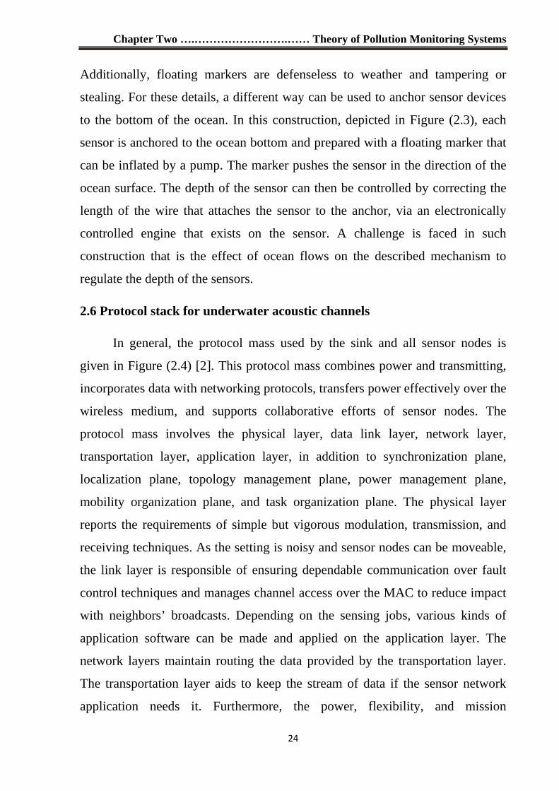
2.6 Protocol stack for underwater acoustic channels
In general, the protocol mass used by the sink and all sensor nodes is
given in Figure (2.4) [2]. This protocol mass combines power and transmitting,
incorporates data with networking protocols, transfers power effectively over the
wireless medium, and supports collaborative efforts of sensor nodes. The
protocol mass involves the physical layer, data link layer, network layer,
transportation layer, application layer, in addition to synchronization plane,
localization plane, topology management plane, power management plane,
mobility organization plane, and task organization plane. The physical layer
reports the requirements of simple but vigorous modulation, transmission, and
receiving techniques. As the setting is noisy and sensor nodes can be moveable,
the link layer is responsible of ensuring dependable communication over fault
control techniques and manages channel access over the MAC to reduce impact
with neighbors’ broadcasts. Depending on the sensing jobs, various kinds of
application software can be made and applied on the application layer. The
network layers maintain routing the data provided by the transportation layer.
The transportation layer aids to keep the stream of data if the sensor network
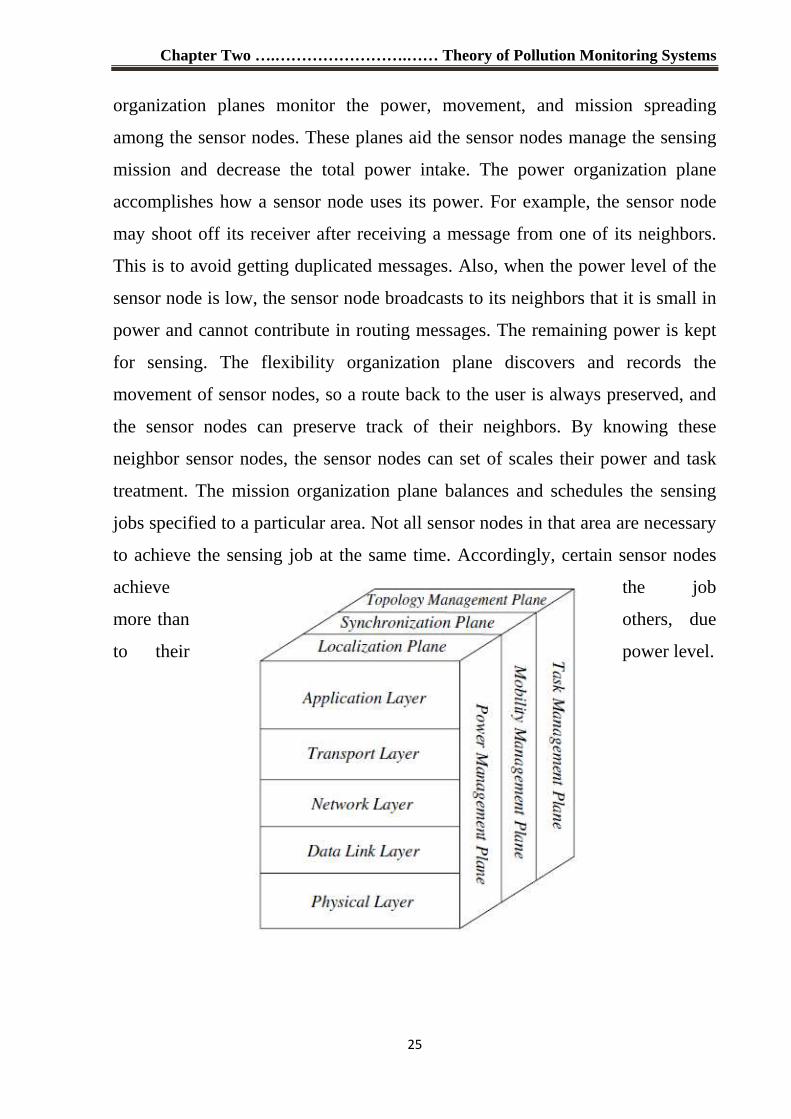
application needs it. Furthermore, the power, flexibility , and mission
Chapter Two ….…………………….…… Theory of Pollution Monitoring Systems
25
organization planes monitor the power, movement, and mission spreading
among the sensor nodes. These planes aid the sensor nodes manage the sensing
mission and decrease the total power intake. The power organization plane
accomplishes how a sensor node uses its power. For example, the sensor node
may shoot off its receiver after receiving a message from one of its neighbors.
This is to avoid getting duplicated messages. Also, when the power level of the
sensor node is low, the sensor node broadcasts to its neighbors that it is small in
power and cannot contribute in routing messages. The remaining power is kept
for sensing. The flexibility organization plane discovers and records the
movement of sensor nodes, so a route back to the user is always preserved, and
the sensor nodes can preserve track of their neighbors. By knowing these
neighbor sensor nodes, the sensor nodes can set of scales their power and task
treatment. The mission organization plane balances and schedules the sensing
jobs specified to a particular area. Not all sensor nodes in that area are necessary
to achieve the sensing job at the same time. Accordingly, certain sensor nodes
achieve the job
more than others, due
to their power level.
Chapter Two ….…………………….…… Theory of Pollution Monitoring Systems
26
Figure (2.4): The sensor network protocol stack [2].
These organization planes are required so that sensor nodes can work together in
a power-effective way, route data in a moveable sensor network, and share
resources between sensor nodes. Without them, every sensor node will just work
alone. From the position of the entire sensor network, it is more effective if
sensor nodes can cooperate with each other, so the lifespan of the sensor
networks can be extended.
The next two sections present a detailed explanation of MAC and routing layer
protocols in UWSN. It is considered that the most important challenge facing
the network is this layer.
2.6.1 MAC Layer Protocols
In UAWSN, MAC constitutes one of the major challenges in sensor
networks [28]. Such as available bandwidth is severely limited, Propagation
delay in underwater is five orders of magnitude higher than in Radio Frequency
(RF) terrestrial channels and Battery power is limited and usually batteries
cannot be recharged as solar energy cannot be exploited [29].
The main task of MAC protocols is to provide efficient and reliable access
to the shared physical medium in terms of throughput, delay, error rates and
energy consumption [30]. However, several drawbacks are faced with the
suitability of the terrestrial MAC solutions for the aquatic environment, because
of the different nature of the underwater environment. The Frequency Division
Multiple Access (FDMA) is narrow bandwidth available in underwater acoustic
channels, and the vulnerability of limited band systems to fading and multipath
effects. Also, Time Division Multiple Access (TDMA) shows restricted
Chapter Two ….…………………….…… Theory of Pollution Monitoring Systems
27
bandwidth efficiency because of the long time guards required in the underwater
acoustic channel [31].
There are two categories suitable for UAWSN as Carrier Sense Multiple
Access (CSMA) and Code Division Multiple Access (CDMA). In general,
CSMA-based protocols are vulnerable to both hidden and exposed terminal
problems. In order to decrease the effects of hidden terminals MAC proposals
should include techniques similar to those used in terrestrial networks like
MACA [32], which uses RTS/CTS/DATA packets to reduce the hidden terminal
problem. And MACAW [33], which adds to the previous one an ACK packet at
the link-layer that can be profitable in an unreliable underwater channel. FAMA
[34] extends the duration of RTS and CTS packets so as to avoid data packet
collisions, thus, contention is managed at both sender and receiver sides before
data packets are sent. The efficiency of these protocols is heavily impacted by
propagation delays due to their multiple handshakes. CDMA-based protocols
are not useful for acoustic networks because these protocols have some
problems such as synchronization and near far problem [28].
Underwater MAC layer protocols should also assume node mobility, low
bandwidth, energy efficiency and long propagation delay. Due to the long
propagation delay, node mobility and other underwater environment constraints,
distributed topologies are used more than centralized topologies. Thus,
contention based protocols like Broadcast MAC, Aloha; R-MAC, FAMA, and
UWAN_MAC are useful for such topologies.
2.6.1.1 Floor Acquisition Multiple A ccess (FAMA)
FAMA is proposed by Chane and Garcia [34]. The objective of a FAMA
protocol is to allow a station to acquire control of the channel (the floor)
dynamically, and in such a way that the data packets never collide with any
other packet. This can be viewed as a form of dynamic reservations; however, in
Chapter Two ….…………………….…… Theory of Pollution Monitoring Systems
28
contrast to prior approaches to dynamic reservations, which are also referred to
collision avoidance schemes the FAMA protocols presented requires no separate
control sub-channels or preambles to reserve the channel. Instead, a FAMA
protocol involves a station who wishes to send one or more packets to acquire
the floor before transmitting the packet train. The floor is acquired using control
packets that are multiplexed together with the data packets in the same channel
in such a way that, although control packets may collide with others, data
packets are always free of collisions.
A floor acquisition strategy based on an RTS-CTS exchange is particularly
attractive in the control of packet- radio networks due to its ability to provide a
building block to solve the hidden-terminal problem that arises in CSMA.
Within the context of using an RTS-CTS exchange for floor acquisition, there
are many ways in which such control packets can be transmitted. Two variants
are interest in this work; namely:
• RTS-CTS exchange with no carrier sensing.
• RTS-CTS exchange with non-persistent carrier sensing.
The first variant corresponds to using the ALOHA protocol for the
transmission of RTS packets. While the second is consists of using the non-
persistent CSMA protocol to transmit RTS packets. We choose to consider non-
persistent carrier sensing over persistent carrier sensing, because the throughput
of non-persistent CSMA is much higher under high load and only slightly lower
under low load than the throughput of p-persistent CSMA. Despite that the
original motivation for MACA was to solve the hidden-terminal problem of
CSMA, the basic RTS-CTS dialogue of MACA and even a four way handshake
(RTS, CTS, data, acknowledgment) does not solve all hidden- terminal
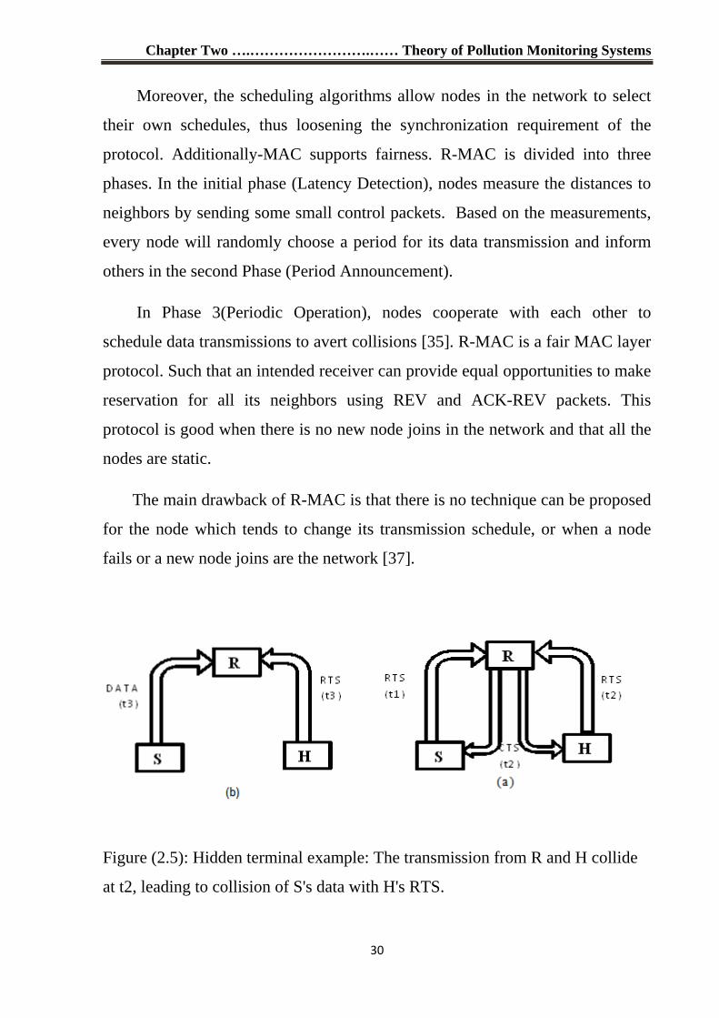
problems. For example, as Figure (2.5) shows, three given stations S, R and H.
If H is “hidden” from S (i.e., S and H cannot hear each other's transmissions) it
Chapter Two ….…………………….…… Theory of Pollution Monitoring Systems
29
could happen that S sends an RTS to R in the clear and R sends a CTS to S. The
problem occurs when H transmits an RTS to R, or another station that can hear
R and H, at the same time that R transmits its CTS to S. If this is the case, then S
will send data packets to R, and H may transmit an RTS that R can hear and
collide with S’s data packets. Obviously, an ad-hoc solution would make H wait
a very long time before trying to retransmit, but that would degrade the network
throughput. The four-way handshake advocated in the IEEE 802.11 only helps
detecting hidden-terminal interference after it occurs, but, does not prevent it.
The RTS-CTS dialogue can be used as the building block to reduce the
hidden-terminal problem. However, this work focuses only on using such a
dialogue to establish a floor acquisition discipline, and focuses on single-hop
networks in which hidden terminals does not exist. The design of FAMA
protocols for multi-hop packet-radio networks is addressed elsewhere. The basis
for such protocols is the use of additional feedback from the receiver, in the
form of CTSs and partial acknowledgments to packet trains.
The drawbacks of FAMA are the following [36]:-
- Difficulty in configuring FAMA protocol when a new node come in or
moves out of network system.
- It is hard to implement FAMA protocol in a distributed mode.
2.6.1.2 Routing enhanced MAC (R-MAC )
The major design objectives of R-MAC are energy efficiency and fairness.
R-MAC schedules the transmissions of control packets and data packets to avoid
data packet collision completely. The scheduling algorithms does not only save
energy but also solve the exposed terminal problem inherited in RTS/CTS-based
protocols.
Chapter Two ….…………………….…… Theory of Pollution Monitoring Systems
30
Moreover, the scheduling algorithms allow nodes in the network to select
their own schedules, thus loosening the synchronization requirement of the
protocol. Additionally-MAC supports fairness. R-MAC is divided into three
phases. In the initial phase (Latency Detection), nodes measure the distances to
neighbors by sending some small control packets. Based on the measurements,
every node will randomly choose a period for its data transmission and inform
others in the second Phase (Period Announcement).
In Phase 3(Periodic Operation), nodes cooperate with each other to
schedule data transmissions to avert collisions [35]. R-MAC is a fair MAC layer
protocol. Such that an intended receiver can provide equal opportunities to make
reservation for all its neighbors using REV and ACK-REV packets. This
protocol is good when there is no new node joins in the network and that all the
nodes are static.
The main drawback of R-MAC is that there is no technique can be proposed
for the node which tends to change its transmission schedule, or when a node
fails or a new node joins are the network [37].
Figure (2.5): Hidden terminal example: The transmission from R and H collide
at t2, leading to collision of S's data with H's RTS.
Chapter Two ….…………………….…… Theory of Pollution Monitoring Systems
31
2.6.1.3 Underwater Acoustic MAC (UW-MAC)
UWAN-MAC [38], also deploys CSMA-based MAC and has been
primarily developed for high density UWSNs. Rather than bandwidth
optimization, UWAN-MAC focuses on energy efficiency by introducing sleep
schedules similar to its terrestrial counterparts. Each node has a sleep schedule
such that each node wakes up periodically in the network to transmit its data. At
the beginning of each cycle, a node broadcasts a SYNC packet indicating its
period of the sleep schedule. And as a result, the neighbor nodes that receive this
packet wake up at the next scheduled time to listen to the node. Consequently,
every node wakes up for each of its neighbors to receive data in addition to its
scheduled wakeup time to transmit data. Note that since relative time
information is exchanged by the SYNC packets, UWAN-MAC propagation
delay is not required to be known by other nodes.
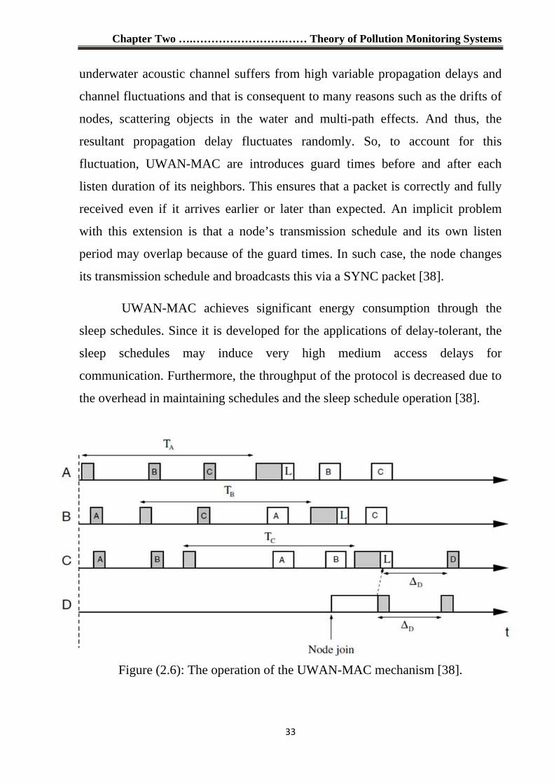
The operation of the UWAN-MAC synchronization mechanism is shown
in Figure (2.6). When node a broadcasts a SYNC packet; it indicates its sleep
period as TA. Accordingly, when node A’s neighbors receive this SYNC packet,
they schedule to wake up TA seconds after reception of the SYNC packet.
Similarly, node A also receives SYNC packets from its neighbors and schedules
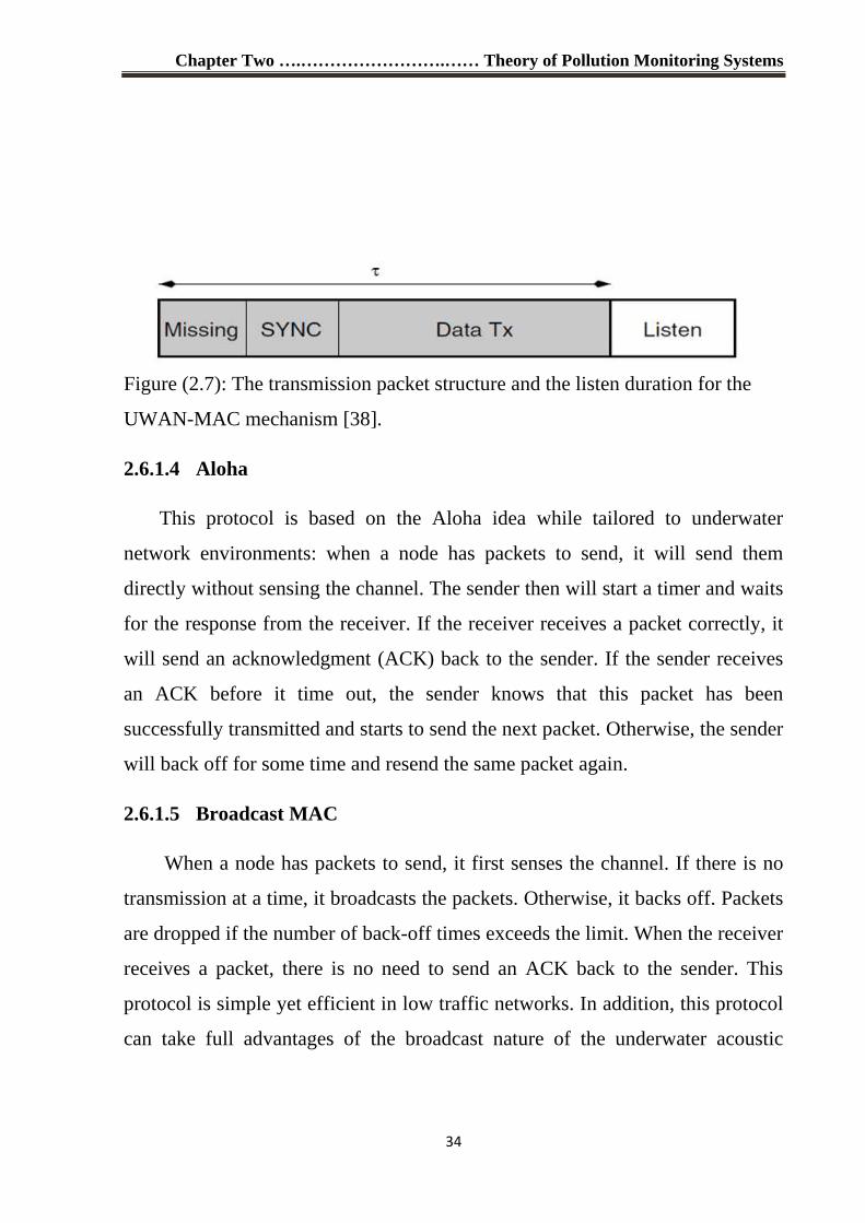
wakeup times for them. The data transmission packet structure of each node is
shown in Figure (2.7), which consists of Missing, SYNC, Data Tx, and Listen
periods. The SYNC period is used to broadcast SYNC packets as explained
before, while Data Tx is used to transmit the DATA packets. Since each of the
Chapter Two ….…………………….…… Theory of Pollution Monitoring Systems
32
neighbors of node A is listening to the transmission period of the node, it can
transmit its DATA without any collisions. The missing and listening periods are
used to handle node failures/removals and node joins. At each sleep period, a
node collects the list of its own neighbors that it has received SYNC messages
from. In case that there is a change in this list (a SYNC
message from a certain node is not received), the node creates a missing node
list and broadcasts this information during the Missing period shown in Figure
(2.7). This list serves as notification to the nodes in the missing list that a
communication error may have occurred earlier. If a node does not hear from its
neighbors in the missing list for a couple of consecutive cycles, it deletes this
node from its neighbor list. On the other hand, the node that is in the missing list
replies back to the sender of the SYNC message as if it is a newcomer node. The
procedure for newcomer nodes is explained next.
The listening period in the transmission period shown in Figure (2.7) is
used to comprise newcomers to the network. This situation is illustrated in
Figure (2.6) where node D joins the network while node C is transmitting a
SYNC packet. When node D joins the network, it listens to the channel for the
SYNC packets from its neighbors. When it receives a SYNC packet from node
C, it makes a reply to this packet with a HELLO packet to indicate its existence.
The Listen period at the end of each transmission period ensures that node C
receives this HELLO packet. Then, node C includes the newcomer node D in its
list of neighbors. In the HELLO packet, node F also indicates the time left for its
next wakeup time, i.e. Node C can then wake up for the scheduled wakeup time
of node D and receive its SYNC packet as shown in Figure (2.6) Node D
indicates its schedule to other nodes in the same manner [38].
The operation of UWAN-MAC so far assumes that the propagation delay
between two nodes does not change. This enables the relative wakeup
announcements by the SYNC packets to synchronize nodes. However, the
Chapter Two ….…………………….…… Theory of Pollution Monitoring Systems
33
underwater acoustic channel suffers from high variable propagation delays and
channel fluctuations and that is consequent to many reasons such as the drifts of
nodes, scattering objects in the water and multi-path effects. And thus, the
resultant propagation delay fluctuates randomly. So, to account for this
fluctuation, UWAN-MAC are introduces guard times before and after each
listen duration of its neighbors. This ensures that a packet is correctly and fully
received even if it arrives earlier or later than expected. An implicit problem
with this extension is that a node’s transmission schedule and its own listen
period may overlap because of the guard times. In such case, the node changes
its transmission schedule and broadcasts this via a SYNC packet [38].
UWAN-MAC achieves significant energy consumption through the
sleep schedules. Since it is developed for the applications of delay-tolerant, the
sleep schedules may induce very high medium access delays for
communication. Furthermore, the throughput of the protocol is decreased due to
the overhead in maintaining schedules and the sleep schedule operation [38].
Figure (2.6): The operation of the UWAN-MAC mechanism [38].
Chapter Two ….…………………….…… Theory of Pollution Monitoring Systems
34
Figure (2.7): The transmission packet structure and the listen duration for the
UWAN-MAC mechanism [38].
2.6.1.4 Aloha
This protocol is based on the Aloha idea while tailored to underwater
network environments: when a node has packets to send, it will send them
directly without sensing the channel. The sender then will start a timer and waits
for the response from the receiver. If the receiver receives a packet correctly, it
will send an acknowledgment (ACK) back to the sender. If the sender receives
an ACK before it time out, the sender knows that this packet has been
successfully transmitted and starts to send the next packet. Otherwise, the sender
will back off for some time and resend the same packet again.
2.6.1.5 Broadcast MAC
When a node has packets to send, it first senses the channel. If there is no
transmission at a time, it broadcasts the packets. Otherwise, it backs off. Packets
are dropped if the number of back-off times exceeds the limit. When the receiver
receives a packet, there is no need to send an ACK back to the sender. This
protocol is simple yet efficient in low traffic networks. In addition, this protocol
can take full advantages of the broadcast nature of the underwater acoustic
Chapter Two ….…………………….…… Theory of Pollution Monitoring Systems
35
channel and are suitable for geo-routing protocols such as vector based forward
(VBF) [39].
2.6.2 Routing protocols
The network layer function is finding a way from source to the destination
taking into account many characteristics of the channel such as long propagation
delay and energy of the nodes. There was an extensive study to find the path
from the source to the destination in various gateways of the UWSNs. These
protocols can be classified into three different groups: proactive, reactive and
geographical routing [28]. From [40], [41] and [42] an appropriate proactive and
reactive protocol with UWSNs is too weak, for memory, energy reasons and
incompatibility of proactive protocol with UWSN. Reactive protocols are
unsuitable for underwater networks because of high latency, asymmetrical links
and topology and so the higher delay to create the path, being further amplified
in this environment because the slower propagation in acoustic signals. Thus,
the geographical routing protocols are energy efficient and scalable. For these
reasons the most suitable approach using in UWSNs is geographical routing
protocols. A brief on some routing protocols designed to UWSNs topologies
will presented later. Most of them take into consideration the limitation in
energy [43].
2.6.2.1 Vector based forward (VBF)
VBF is robust, scalable and energy efficient [44]. This is mainly in "routing
pipe" approach. There is no need for Information Service on the nodes, except
only a small part of them. Also, the packets pass through repeated and
dovetailed paths from source to sink; therefore VBF is robust against losing
packets and frailer can occur on nodes.
The routing in VBF routing protocol
Chapter Two ….…………………….…… Theory of Pollution Monitoring Systems
36
In VBF, each packet holds the location of the sender (SP), the destination
(TP) and forwarder (FP). Each packet contains a RANGE field. The packet that
reaches the area defined by its TP, that packet is controlled by the RANGE field.
The routing pipe is the vector from the sender (SP) to the destination (TP) and
the radius of the pipe is illustrated in the RADIUS field. Routing in VBF is
embarked by query packets. VBF routes various queries in deferent ways [44]:
i. Sink Initiated Query :-
Two types of such queries: location-dependent query, in this type the sink is
interested in some limited area and knows the position of that area. The other
type of this query is location-based query, in which the sink needs to know some
types of data or information regardless of its position.
ii. Source Initiated Query:-
When a source is starting to transmit, firstly sets a coordinate system for
itself and floods a packet called "DATA READY" to the network. Thus, each
node and sink can calculate its position in the source-based coordinate system.
The sink sends source location to its coordinate system, and sends a location-
based packet to source to give it permission for computing its location in the
sink-based coordinate system for following communications.
VBF Algorithm
A node receiving packet calculates its position and checks if it is in the
routing pipe. If so; the node holds the packet for a time called Tadaptation. This
is determined as follows [44]:
Tadaptation = √α × tdelay + (r-d/υ0) (2.1)
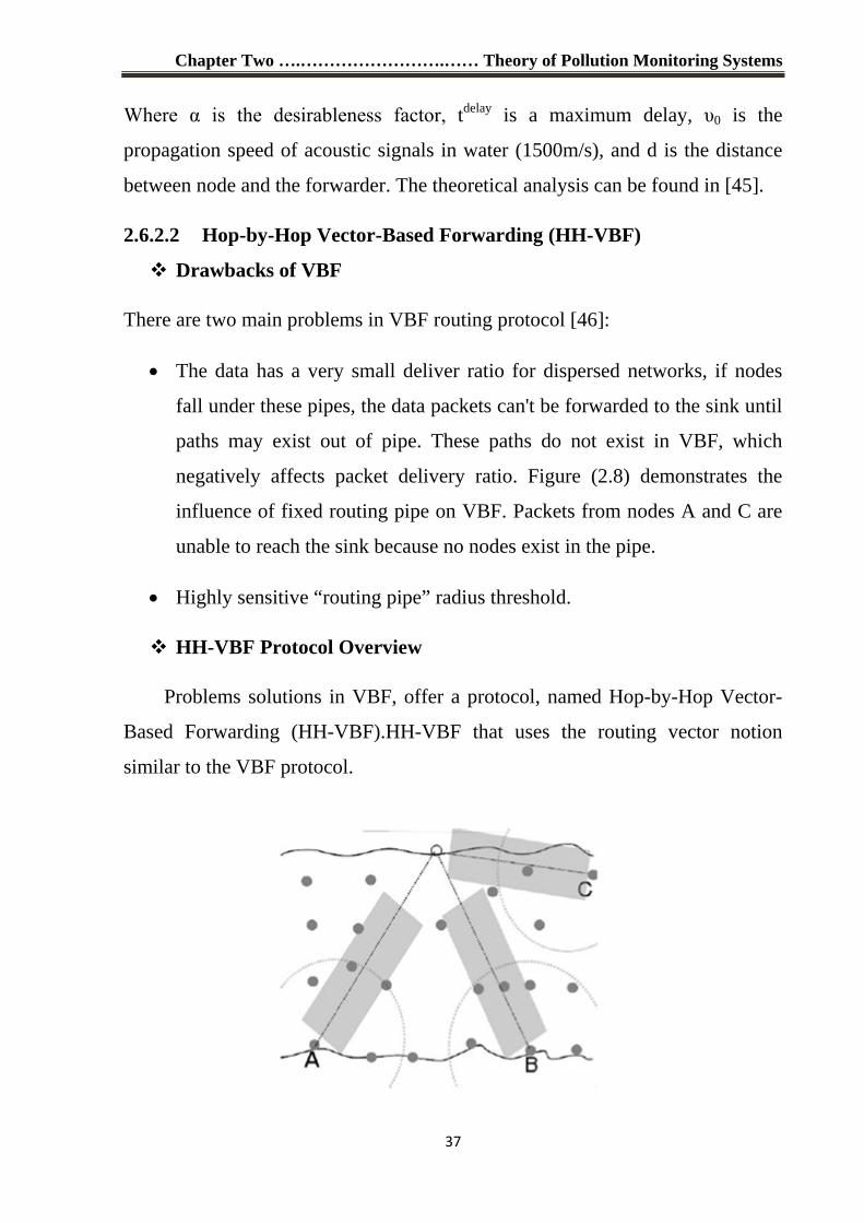
Chapter Two ….…………………….…… Theory of Pollution Monitoring Systems
37
Where α is the desirableness factor, tdelay is a maximum delay, υ0 is the
propagation speed of acoustic signals in water (1500m/s), and d is the distance
between node and the forwarder. The theoretical analysis can be found in [45].
2.6.2.2 Hop-by-Hop Vector-Based Forwarding (HH-VBF)
Drawbacks of VBF
There are two main problems in VBF routing protocol [46]:
• The data has a very small deliver ratio for dispersed networks, if nodes
fall under these pipes, the data packets can't be forwarded to the sink until
paths may exist out of pipe. These paths do not exist in VBF, which
negatively affects packet delivery ratio. Figure (2.8) demonstrates the
influence of fixed routing pipe on VBF. Packets from nodes A and C are
unable to reach the sink because no nodes exist in the pipe.
• Highly sensitive “routing pipe” radius threshold.
HH-VBF Protocol Overview
Problems solutions in VBF, offer a protocol, named Hop-by-Hop Vector-
Based Forwarding (HH-VBF).HH-VBF that uses the routing vector notion
similar to the VBF protocol.
Chapter Two ….…………………….…… Theory of Pollution Monitoring Systems
38
Figure (2.8): VBF using single routing pipe
But, HH-VBF uses various virtual pipes from forwarders nodes to the sink
instead of use of single vector in VBF. Thus, each node can make the adaptation
for the packet routing decisions depending on its current position. From these
characteristics the following interests are made:-
• No need to increase the radius of pipe after the transmission range to
enhance performance in routing, because of there is routing pipe for
each node.
• HH-VBF Strengthens packet delivery ratio compared with VBF,
because of dispersed networks. While the number of nodes qualified is
small. HH-VBF can find a data delivery path as long as it exists. Also,
HH-VBF is less than VBF in sensitivity to routing pipe radius
threshold.
Routing In HH -VBF Protocol
In HH-VBF [45], the routing pipe is redefined to be a virtual pipe from
source to sink instead of single vector pipe. This policy allows for finding a
routing path in expanded manner when compared with VBF. Suppose a node N
receives a packet from the source or any through node S, after receiving the
packet, the N calculates the vector from the S to the sink. That offers to the
forwarding pipe changing each hop in the network. For this reason it is named
hop-by-hop vector based forwarding (HH-VBF). Upon a reception it calculates
the vector from its sender to the sink, and computes its distance to that vector. If
the distance is less than the predefined threshold, it will drop the packet. Time
period is represents the time a node carries the packet before forwarding it. The
self-adaption algorithm in HH-VBF is different from that in the original VBF.
Due to effective suppression strategy package approved in VBF, it can select
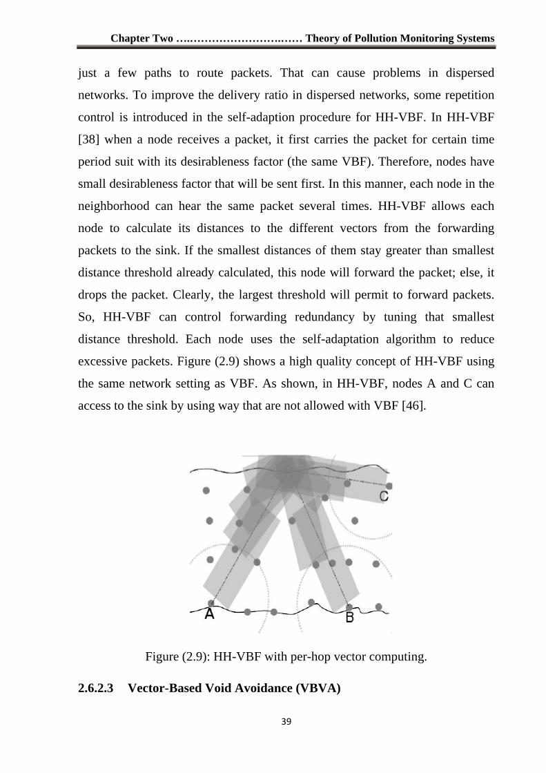
Chapter Two ….…………………….…… Theory of Pollution Monitoring Systems
39
just a few paths to route packets. That can cause problems in dispersed
networks. To improve the delivery ratio in dispersed networks, some repetition
control is introduced in the self-adaption procedure for HH-VBF. In HH-VBF
[38] when a node receives a packet, it first carries the packet for certain time
period suit with its desirableness factor (the same VBF). Therefore, nodes have
small desirableness factor that will be sent first. In this manner, each node in the
neighborhood can hear the same packet several times. HH-VBF allows each
node to calculate its distances to the different vectors from the forwarding
packets to the sink. If the smallest distances of them stay greater than smallest
distance threshold already calculated, this node will forward the packet; else, it
drops the packet. Clearly, the largest threshold will permit to forward packets.
So, HH-VBF can control forwarding redundancy by tuning that smallest
distance threshold. Each node uses the self-adaptation algorithm to reduce
excessive packets. Figure (2.9) shows a high quality concept of HH-VBF using
the same network setting as VBF. As shown, in HH-VBF, nodes A and C can
access to the sink by using way that are not allowed with VBF [46].
Figure (2.9): HH-VBF with per-hop vector computing.
2.6.2.3 Vector-Based Void Avoidance (VBVA )
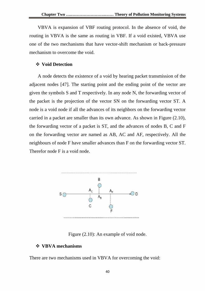
Chapter Two ….…………………….…… Theory of Pollution Monitoring Systems
40
VBVA is expansion of VBF routing protocol. In the absence of void, the
routing in VBVA is the same as routing in VBF. If a void existed, VBVA use
one of the two mechanisms that have vector-shift mechanism or back-pressure
mechanism to overcome the void.
Void Detection
A node detects the existence of a void by hearing packet transmission of the
adjacent nodes [47]. The starting point and the ending point of the vector are
given the symbols S and T respectively. In any node N, the forwarding vector of
the packet is the projection of the vector SN on the forwarding vector ST. A
node is a void node if all the advances of its neighbors on the forwarding vector
carried in a packet are smaller than its own advance. As shown in Figure (2.10),
the forwarding vector of a packet is ST, and the advances of nodes B, C and F
on the forwarding vector are named as AB, AC and AF, respectively. All the
neighbours of node F have smaller advances than F on the forwarding vector ST.
Therefor node F is a void node.
Figure (2.10): An example of void node.
VBVA mechanisms
There are two mechanisms used in VBVA for overcoming the void:
Chapter Two ….…………………….…… Theory of Pollution Monitoring Systems
41
1. Vector-Shift Mechanism
When a node identifies the void node for a packet, it will try to avoid the
void by shifting the forwarding vector of the packet. To accomplish this, it will
send a broadcast message containing a vector-shift packet by node to all its
neighbor nodes. Upon receiving this message; each node outside the forwarding
pipe will try to forward its data packet to a new vector from them to the sink.
Figure (2.11 (a)) shows this mechanism [47].
2. Back-Pressure Mechanism
A node that found to be end node will send a controlling packet, called
BP (Back Pressure) packet. Upon receiving a BP packet, every neighboring
Node tries to shift the forwarding vector of the corresponding packet if it has
never shifted the forwarding vector of this packet before. Otherwise, the node
broadcasts the BP packet again. The BP packet routed in reverse side move
from the sink until it reaches a source node that can act on the vector shifting
it to pass the packet towards sink. Figure (2.11 (b)) shows an example for the
back-pressure process.
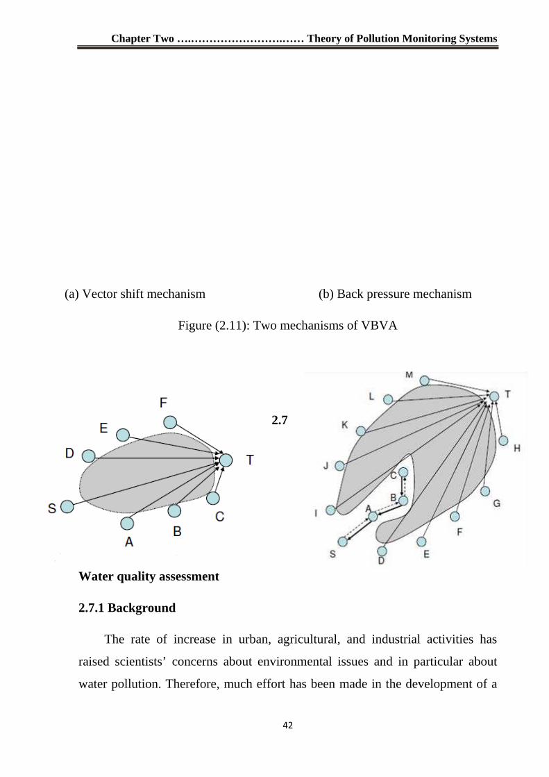
Chapter Two ….…………………….…… Theory of Pollution Monitoring Systems
42
(a) Vector shift mechanism (b) Back pressure mechanism
Figure (2.11): Two mechanisms of VBVA
2.7
Water quality assessment
2.7.1 Background
The rate of increase in urban, agricultural, and industrial activities has
raised scientists’ concerns about environmental issues and in particular about
water pollution. Therefore, much effort has been made in the development of a
Chapter Two ….…………………….…… Theory of Pollution Monitoring Systems
43
comprehensive index that is representative of the overall water quality. Several
authors have integrated water quality variables into indices, technically called
water quality indices (WQIs) ([48], [49], [50] and [51]). Most are based in a
concept developed by the U.S. National Sanitation Foundation [52].
Since, several modified water quality indices (WQI) have been developed
based on the WQI. The WQI is obtained by adding the multiplication of the
respective weight factor by an appropriated quality-value for each parameter.
The WQI index consists of nine parameters: dissolved oxygen (0.17), fecal
coliforms (0.16), biochemical oxygen demand (0.11), pH (0.11), temperature
change (0.1), phosphates (0.10), nitrates (0.10), turbidity (0.08) and total solids
(0.07). In parentheses are given the weight factors according to the importance
of the parameters [8].
However, use of these traditional indices raises many problems. One of the
most important problems is that values with different distances from a limit have
the same effect on the final index score [9]. This leads to an unclear distinction
between each mode of the index and causes inaccuracies and ambiguity when
making decisions about boundary values [8]. The most critical deficiency of
these indexes is the lack of dealing with uncertainty and subjectivity present in
this complex environmental problem [10].
In recent years, artificial intelligence (AI) computational methods such as
knowledge-based systems, neural networks, genetic algorithms, and fuzzy logic,
have been increasingly applied to environmental issues [53]. Fuzzy logic was
introduced by Zadeh (1965) and has become one of the most common
approaches in the field of AI. It is believed to be appropriate for developing
environmental indices, because it has the ability to reflect human thoughts and
expertise in the indices, enabling them to deal with non-linear, uncertain,
ambiguous and subjective information. It also enables us to include parameters
Chapter Two ….…………………….…… Theory of Pollution Monitoring Systems
44
with different values and meanings in the index, including both qualitative and
quantitative variables. Furthermore, it is a reliable method for reporting the
results of an assessment in linguistic terms, which are understandable for the
public, managers, decision-makers, and non-experts in general [54].
The use of linguistic variables to describe and assess complex systems has
already been extensively elaborated by computer scientists, the fuzzy logic. One
of the main advantages of fuzzy logic is the ability to model expert human
knowledge, a necessary feature to be considered in the complex process of
environmental management.
The term fuzzy inference system embraces a wide set of diverse
methodologies intended to deal with uncertainty and subjectivity. Since its
introduction in 1965 by Lofti Zadeh, fuzzy inference system has been applied to
many research areas. The interest in fuzzy is still growing through years from
2002 to 2011. The number of papers related to “fuzzy inference system” for
2002 to 2011was 1700 papers while the two terms "fuzzy" and "water quality"
together was only 98 papers. This indicates that it used only 5.7 % of the total
1700 in the field of water quality. Further scientific advances within this field
and their widespread acceptance and use are expected to follow.
2.7.2 Implementing Materials and methods
2.7.2.1 Fuzzy inference system
Fuzzy set theory has been developed for modeling complex systems in
uncertain and imprecise environment [55]. Fuzzy logic uses sets with unclear
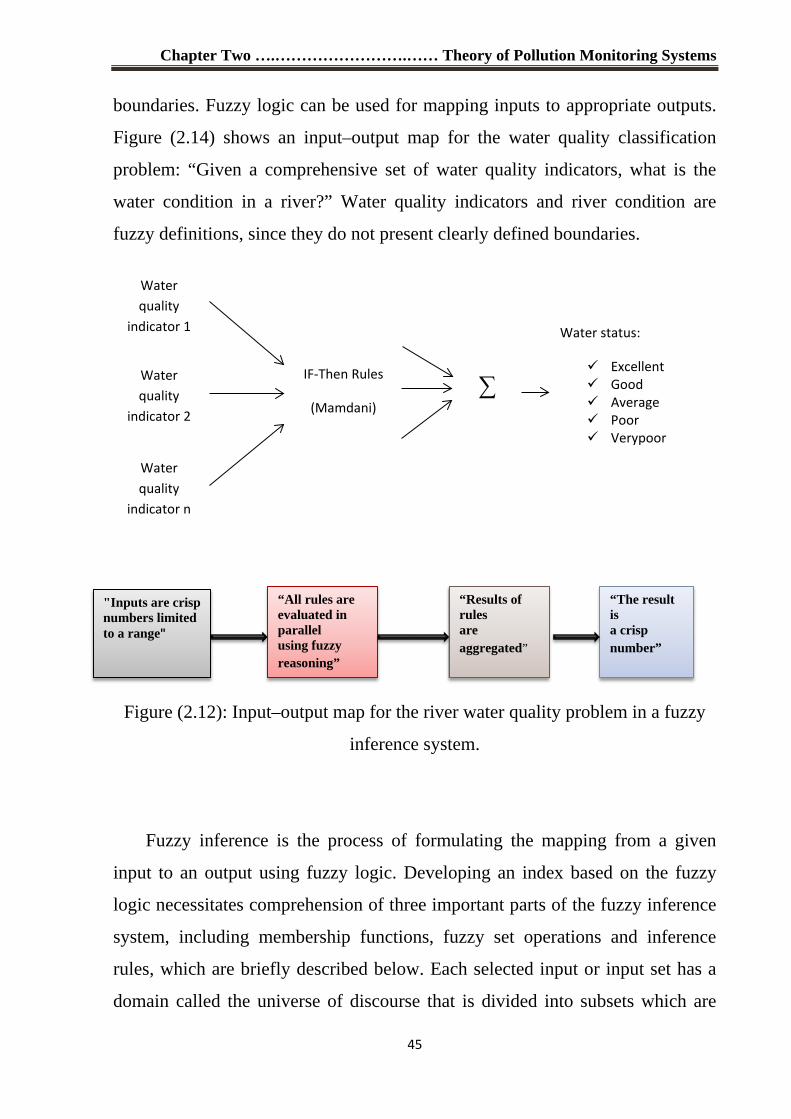
Chapter Two ….…………………….…… Theory of Pollution Monitoring Systems
45
boundaries. Fuzzy logic can be used for mapping inputs to appropriate outputs.
Figure (2.14) shows an input–output map for the water quality classification
problem: “Given a comprehensive set of water quality indicators, what is the
water condition in a river?” Water quality indicators and river condition are
fuzzy definitions, since they do not present clearly defined boundaries.
Figure (2.12): Input–output map for the river water quality problem in a fuzzy
inference system.
Fuzzy inference is the process of formulating the mapping from a given
input to an output using fuzzy logic. Developing an index based on the fuzzy
logic necessitates comprehension of three important parts of the fuzzy inference
system, including membership functions, fuzzy set operations and inference
rules, which are briefly described below. Each selected input or input set has a
domain called the universe of discourse that is divided into subsets which are
Water
quality
indicator 1
Water
quality
indicator 2
Water
quality
indicator n
∑
Water status:
Excellent
Good
Average
Poor
Verypoor
IF-Then Rules
(Mamdani)
“All rules are evaluated in parallel using fuzzy reasoning”
" Inputs are crisp numbers limited to a range"
“Results of rules are aggregated”
“The result is a crisp number”
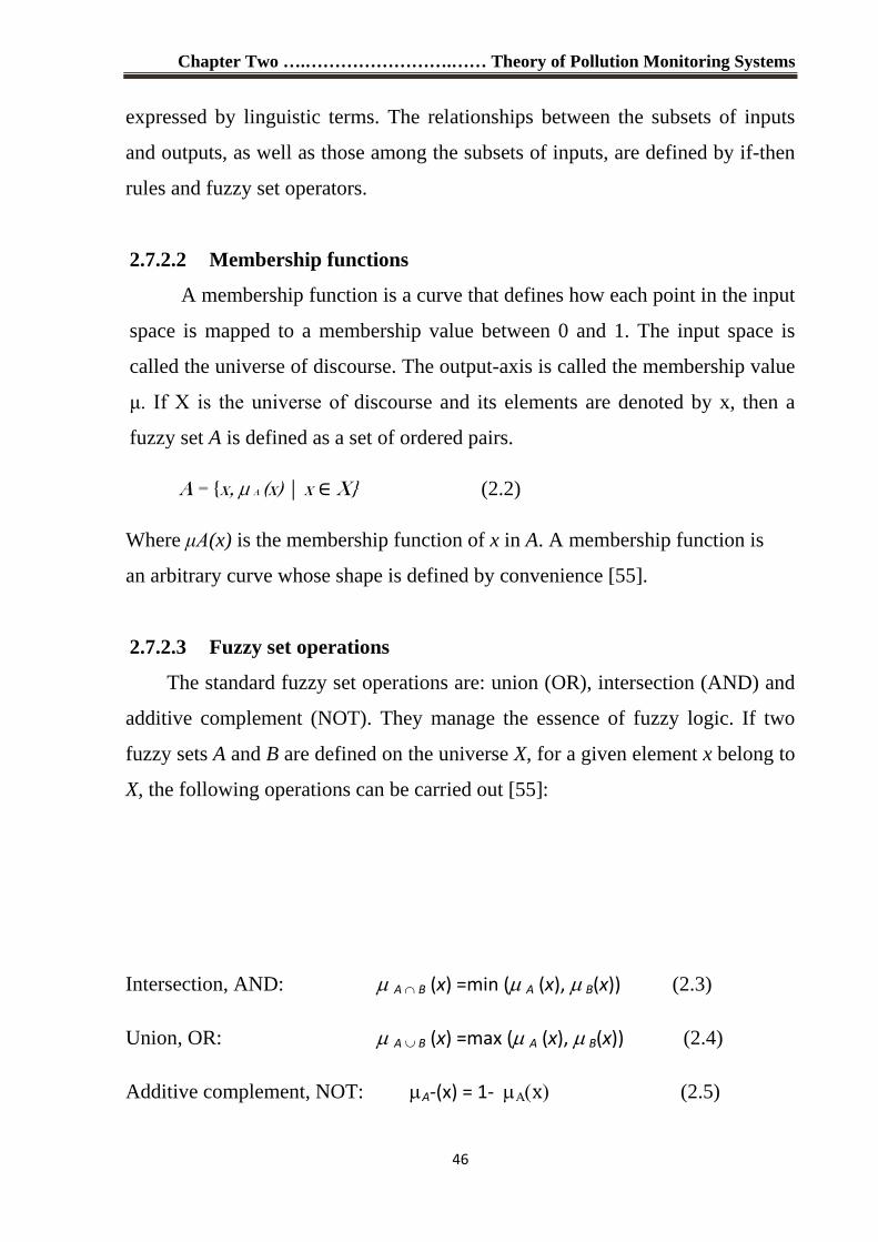
Chapter Two ….…………………….…… Theory of Pollution Monitoring Systems
46
expressed by linguistic terms. The relationships between the subsets of inputs
and outputs, as well as those among the subsets of inputs, are defined by if-then
rules and fuzzy set operators.
2.7.2.2 Membership functions
A membership function is a curve that defines how each point in the input
space is mapped to a membership value between 0 and 1. The input space is
called the universe of discourse. The output-axis is called the membership value
μ. If X is the universe of discourse and its elements are denoted by x, then a
fuzzy set A is defined as a set of ordered pairs.
A = {x, µ A (x) | x ∈ X} (2.2)
Where μA(x) is the membership function of x in A. A membership function is
an arbitrary curve whose shape is defined by convenience [55].
2.7.2.3 Fuzzy set operations
The standard fuzzy set operations are: union (OR), intersection (AND) and
additive complement (NOT). They manage the essence of fuzzy logic. If two
fuzzy sets A and B are defined on the universe X, for a given element x belong to
X, the following operations can be carried out [55]:
Intersection, AND: µ A ∩ B (x) =min (µ A (x), µ B(x)) (2.3)
Union, OR: µ A ∪ B (x) =max (µ A (x), µ B(x)) (2.4)
Additive complement, NOT: µA-(x) = 1- µΑ(x) (2.5)
Chapter Two ….…………………….…… Theory of Pollution Monitoring Systems
47
2.7.2.4 Inference rules
Inference rules define the relationships among the subsets of the inputs and
outputs. This process is carried out by if-then rules which generate a new output
subset. Each rule consists of two parts including an “if-” part, which is called the
antecedent, and a “then-” part, which is called the consequent. The if-then rules
are written in the following way:
IF A is a THEN C is c.
IF B is b THEN C is c.
Where a, b, and c are the linguistic terms for the subsets defined for sets A,
B, and C, respectively [55].
Chapter
Three
UWSNs Simulation
and Network
Results
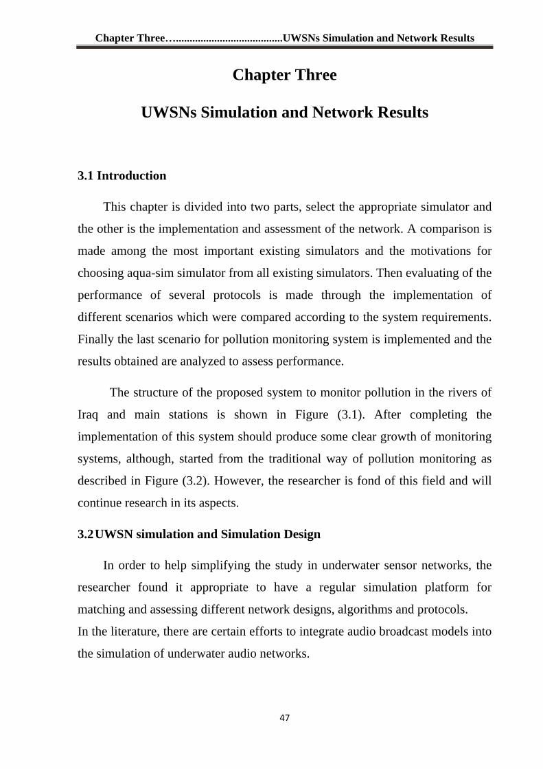
Chapter Three….......................................UWSNs Simulation and Network Results
47
Chapter Three
UWSNs Simulation and Network Results
3.1 Introduction
This chapter is divided into two parts, select the appropriate simulator and
the other is the implementation and assessment of the network. A comparison is
made among the most important existing simulators and the motivations for
choosing aqua-sim simulator from all existing simulators. Then evaluating of the
performance of several protocols is made through the implementation of
different scenarios which were compared according to the system requirements.
Finally the last scenario for pollution monitoring system is implemented and the
results obtained are analyzed to assess performance.
The structure of the proposed system to monitor pollution in the rivers of
Iraq and main stations is shown in Figure (3.1). After completing the
implementation of this system should produce some clear growth of monitoring
systems, although, started from the traditional way of pollution monitoring as
described in Figure (3.2). However, the researcher is fond of this field and will
continue research in its aspects.
3.2 UWSN simulation and Simulation Design
In order to help simplifying the study in underwater sensor networks, the
researcher found it appropriate to have a regular simulation platform for
matching and assessing different network designs, algorithms and protocols.
In the literature, there are certain efforts to integrate audio broadcast models into
the simulation of underwater audio networks.
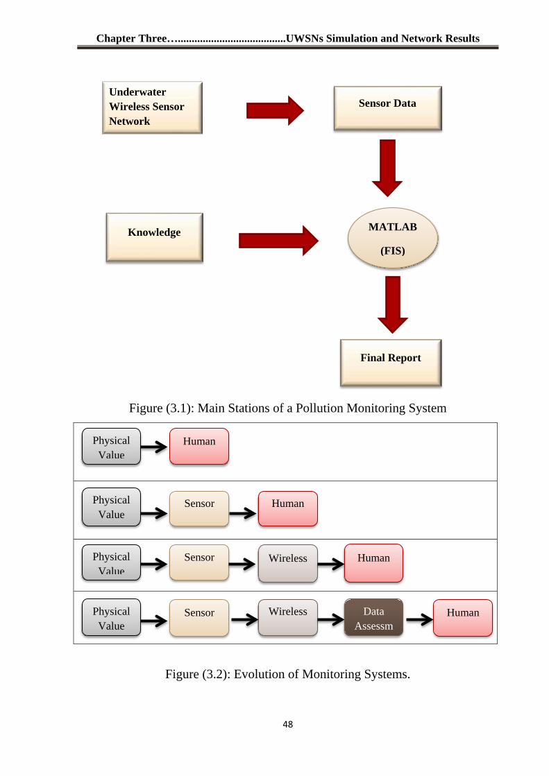
Chapter Three….......................................UWSNs Simulation and Network Results
48
Figure (3.1): Main Stations of a Pollution Monitoring System
Figure (3.2): Evolution of Monitoring Systems.
Underwater Wireless Sensor Network
Final Report
Knowledge
Sensor Data
MATLAB
(FIS)
Physical Value
Human
Physical Value
Sensor Human
Physical Value
Sensor Wireless Human
Physical Value
Human Data Assessm
Wireless
Sensor
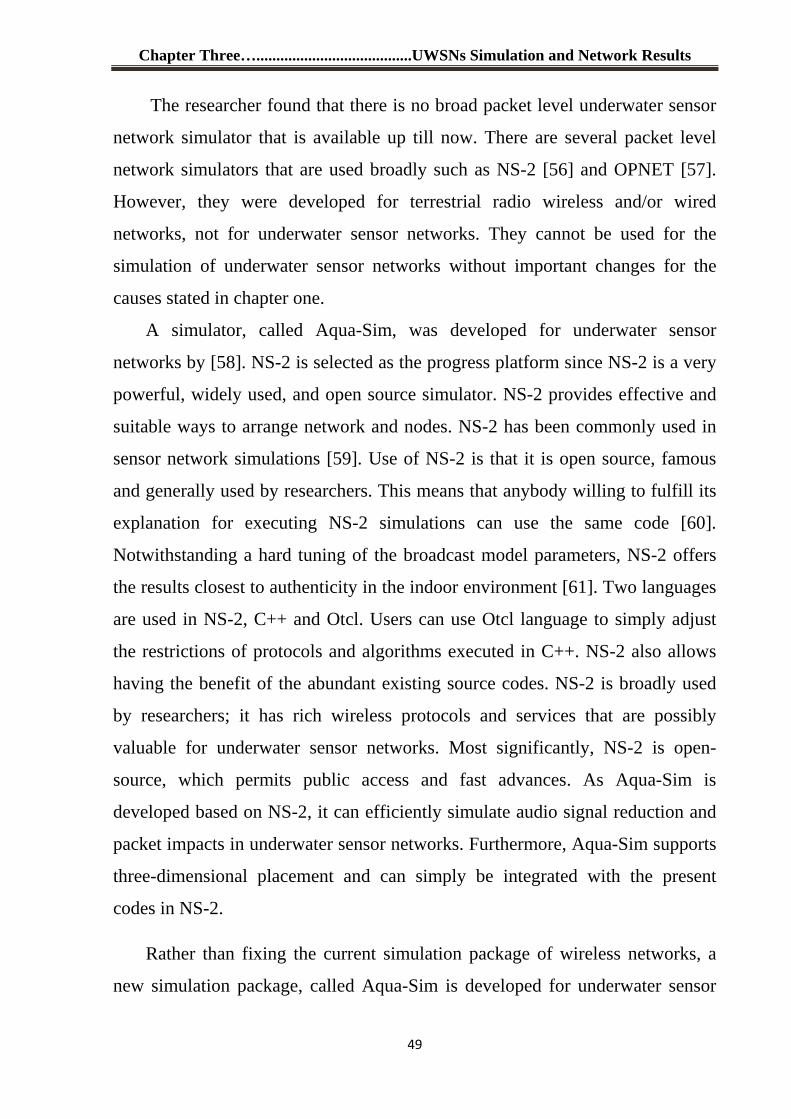
Chapter Three….......................................UWSNs Simulation and Network Results
49
The researcher found that there is no broad packet level underwater sensor
network simulator that is available up till now. There are several packet level
network simulators that are used broadly such as NS-2 [56] and OPNET [57].
However, they were developed for terrestrial radio wireless and/or wired
networks, not for underwater sensor networks. They cannot be used for the
simulation of underwater sensor networks without important changes for the
causes stated in chapter one.
A simulator, called Aqua-Sim, was developed for underwater sensor
networks by [58]. NS-2 is selected as the progress platform since NS-2 is a very
powerful, widely used, and open source simulator. NS-2 provides effective and
suitable ways to arrange network and nodes. NS-2 has been commonly used in
sensor network simulations [59]. Use of NS-2 is that it is open source, famous
and generally used by researchers. This means that anybody willing to fulfill its
explanation for executing NS-2 simulations can use the same code [60].
Notwithstanding a hard tuning of the broadcast model parameters, NS-2 offers
the results closest to authenticity in the indoor environment [61]. Two languages
are used in NS-2, C++ and Otcl. Users can use Otcl language to simply adjust
the restrictions of protocols and algorithms executed in C++. NS-2 also allows
having the benefit of the abundant existing source codes. NS-2 is broadly used
by researchers; it has rich wireless protocols and services that are possibly
valuable for underwater sensor networks. Most significantly, NS-2 is open-
source, which permits public access and fast advances. As Aqua-Sim is
developed based on NS-2, it can efficiently simulate audio signal reduction and
packet impacts in underwater sensor networks. Furthermore, Aqua-Sim supports
three-dimensional placement and can simply be integrated with the present
codes in NS-2.
Rather than fixing the current simulation package of wireless networks, a
new simulation package, called Aqua-Sim is developed for underwater sensor
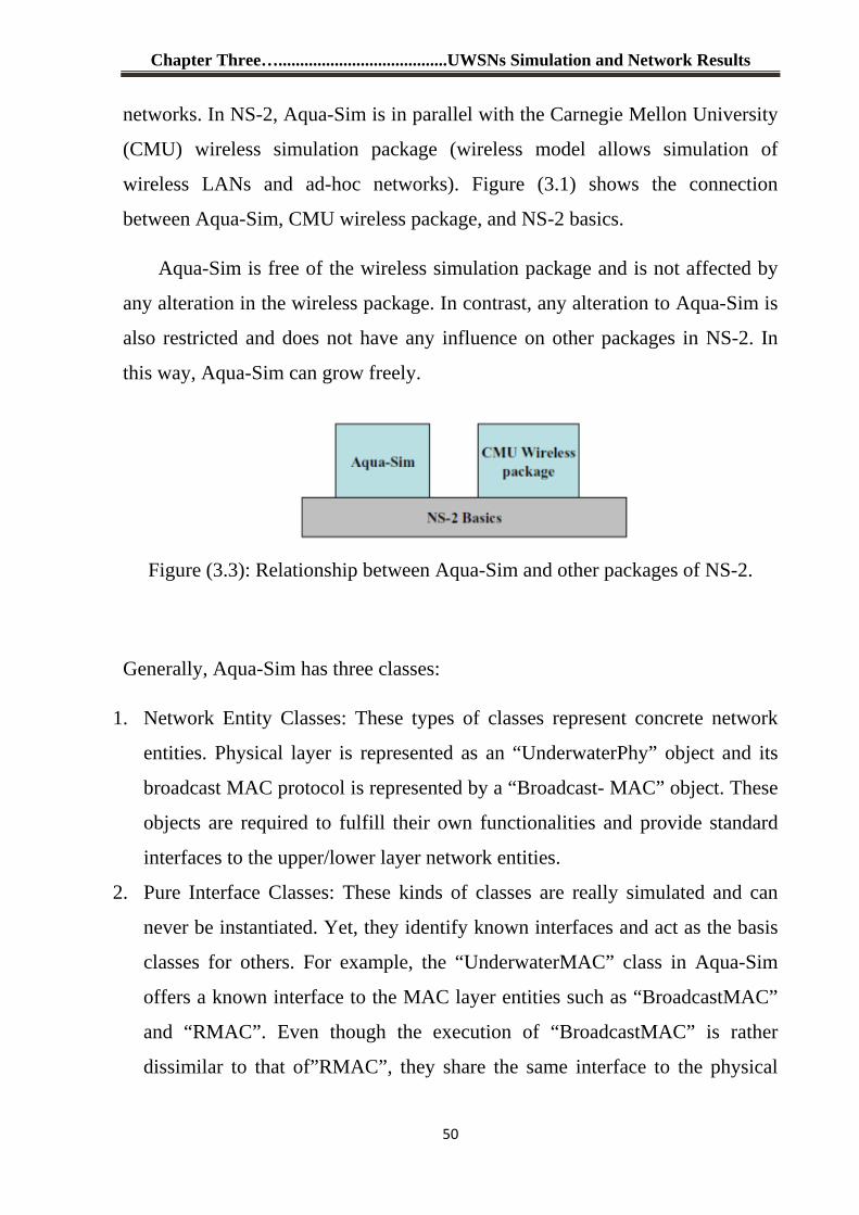
Chapter Three….......................................UWSNs Simulation and Network Results
50
networks. In NS-2, Aqua-Sim is in parallel with the Carnegie Mellon University
(CMU) wireless simulation package (wireless model allows simulation of
wireless LANs and ad-hoc networks). Figure (3.1) shows the connection
between Aqua-Sim, CMU wireless package, and NS-2 basics.
Aqua-Sim is free of the wireless simulation package and is not affected by
any alteration in the wireless package. In contrast, any alteration to Aqua-Sim is
also restricted and does not have any influence on other packages in NS-2. In
this way, Aqua-Sim can grow freely.
Figure (3.3): Relationship between Aqua-Sim and other packages of NS-2.
Generally, Aqua-Sim has three classes:
1. Network Entity Classes: These types of classes represent concrete network
entities. Physical layer is represented as an “UnderwaterPhy” object and its
broadcast MAC protocol is represented by a “Broadcast- MAC” object. These
objects are required to fulfill their own functionalities and provide standard
interfaces to the upper/lower layer network entities.
2. Pure Interface Classes: These kinds of classes are really simulated and can
never be instantiated. Yet, they identify known interfaces and act as the basis
classes for others. For example, the “UnderwaterMAC” class in Aqua-Sim
offers a known interface to the MAC layer entities such as “BroadcastMAC”
and “RMAC”. Even though the execution of “BroadcastMAC” is rather
dissimilar to that of”RMAC”, they share the same interface to the physical
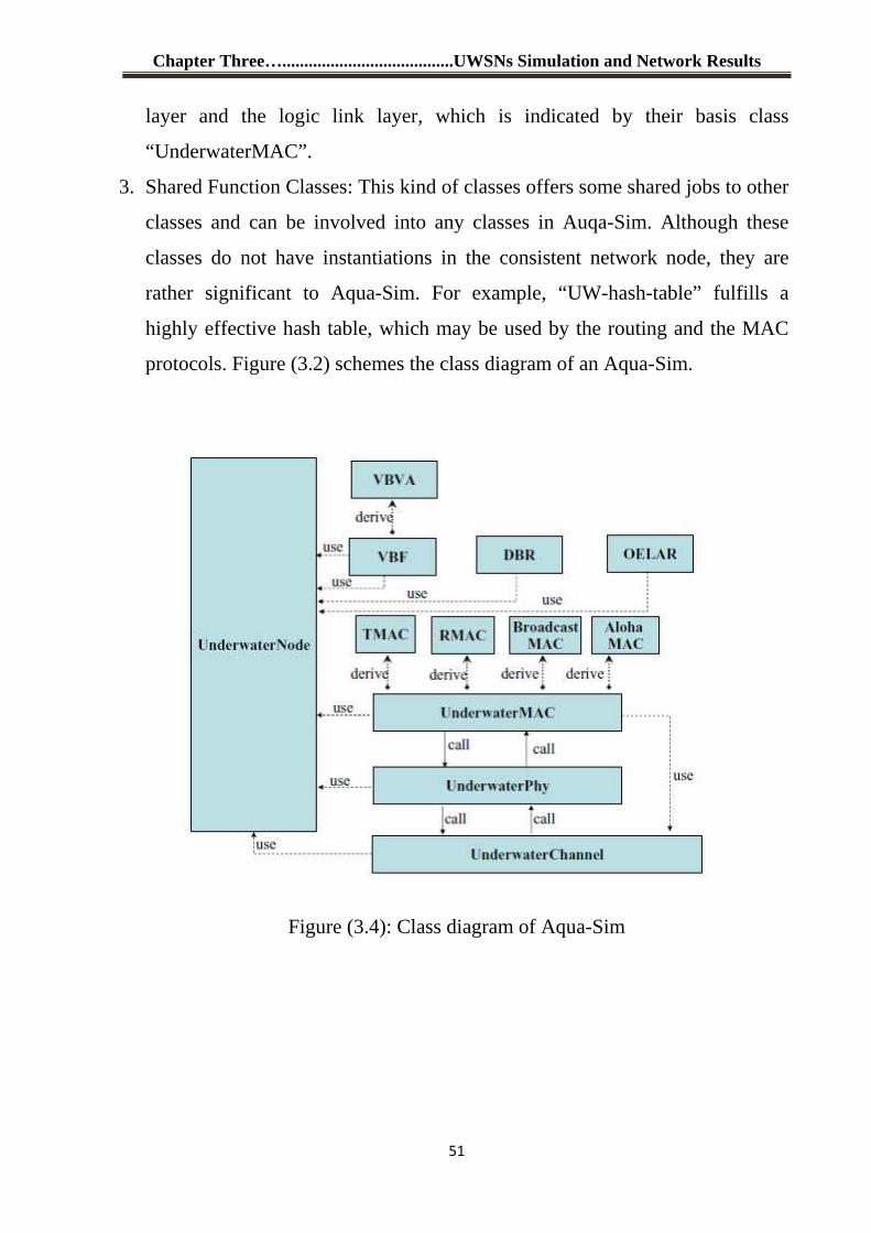
Chapter Three….......................................UWSNs Simulation and Network Results
51
layer and the logic link layer, which is indicated by their basis class
“UnderwaterMAC”.
3. Shared Function Classes: This kind of classes offers some shared jobs to other
classes and can be involved into any classes in Auqa-Sim. Although these
classes do not have instantiations in the consistent network node, they are
rather significant to Aqua-Sim. For example, “UW-hash-table” fulfills a
highly effective hash table, which may be used by the routing and the MAC
protocols. Figure (3.2) schemes the class diagram of an Aqua-Sim.
Figure (3.4): Class diagram of Aqua-Sim
Chapter Three….......................................UWSNs Simulation and Network Results
52
3.2.1 Fidelity and flexibility testing of Aqua-sim
In order to test the fidelity of Aqua-Sim, we design experiments to compare
simulation results with real test bed results. The actual tests are achieved in
Aqua-Lab, a lab test bed developed by the Underwater Sensor Network Lab
[62].Figure (3.5) shows the network topology for both simulation and real test.
Figure (3.5): Network topology for fidelity testing
Node 6 is configured as the receiver and all other nodes send data to node 6.
This gives a one hop, multi-source and single-sink topology. Micro-modem [63]
used in Aqua-Lab provides a data rate at 80bps which is used also in the
simulations.
Aloha protocol was implemented for both Aqua-Lab and Aqua-Sim. The
packet length and the ACK message are set to 32 bytes. The maximal number of
retransmissions is 3 and the input traffic of every node follows an exponential
distribution. Two experiments are conducted to compare the simulations and
real tests. In the first experiment, the average input traffic of every node is set to
0.02 packets per second and change the number of data senders from 1 to 5. In
the second experiment, the total average input traffic is 0.1 packets per second
and change the number of data senders (n). Thus, the input traffic of every node
is 0.1 n. The results are plotted in Figure (3.6) and Figure (3.7). These figures
show clearly that Aqua-Sim can closely approximate the results of the real tests
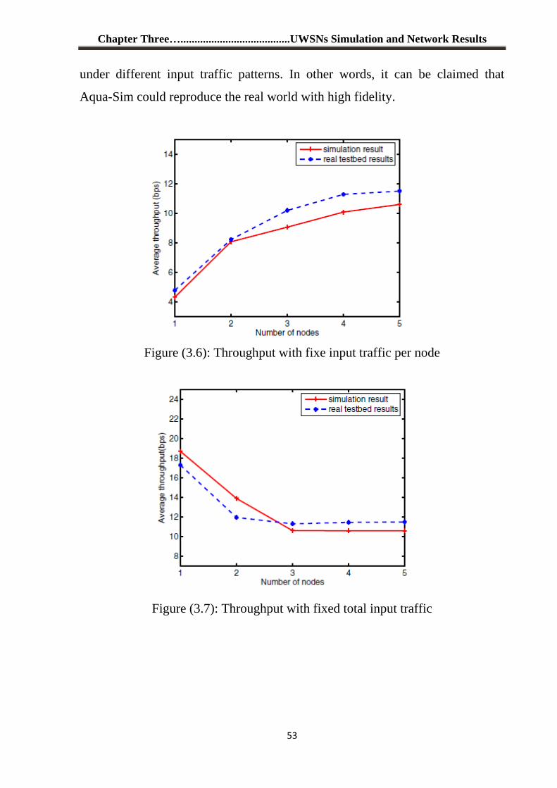
Chapter Three….......................................UWSNs Simulation and Network Results
53
under different input traffic patterns. In other words, it can be claimed that
Aqua-Sim could reproduce the real world with high fidelity.
Figure (3.6): Throughput with fixe input traffic per node
Figure (3.7): Throughput with fixed total input traffic
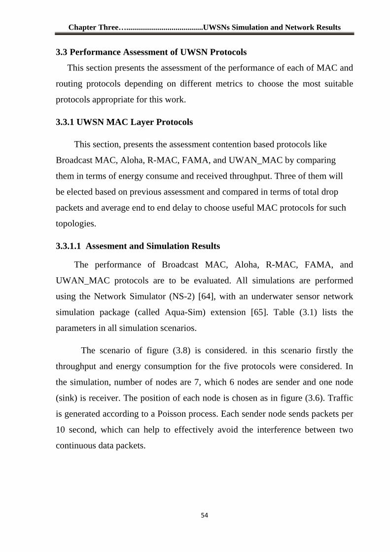
Chapter Three….......................................UWSNs Simulation and Network Results
54
3.3 Performance Assessment of UWSN Protocols
This section presents the assessment of the performance of each of MAC and
routing protocols depending on different metrics to choose the most suitable
protocols appropriate for this work.
3.3.1 UWSN MAC Layer Protocols
This section, presents the assessment contention based protocols like
Broadcast MAC, Aloha, R-MAC, FAMA, and UWAN_MAC by comparing
them in terms of energy consume and received throughput. Three of them will
be elected based on previous assessment and compared in terms of total drop
packets and average end to end delay to choose useful MAC protocols for such
topologies.
3.3.1.1 Assesment and Simulation Results
The performance of Broadcast MAC, Aloha, R-MAC, FAMA, and
UWAN_MAC protocols are to be evaluated. All simulations are performed
using the Network Simulator (NS-2) [64], with an underwater sensor network
simulation package (called Aqua-Sim) extension [65]. Table (3.1) lists the
parameters in all simulation scenarios.
The scenario of figure (3.8) is considered. in this scenario firstly the
throughput and energy consumption for the five protocols were considered. In
the simulation, number of nodes are 7, which 6 nodes are sender and one node
(sink) is receiver. The position of each node is chosen as in figure (3.6). Traffic
is generated according to a Poisson process. Each sender node sends packets per
10 second, which can help to effectively avoid the interference between two
continuous data packets.
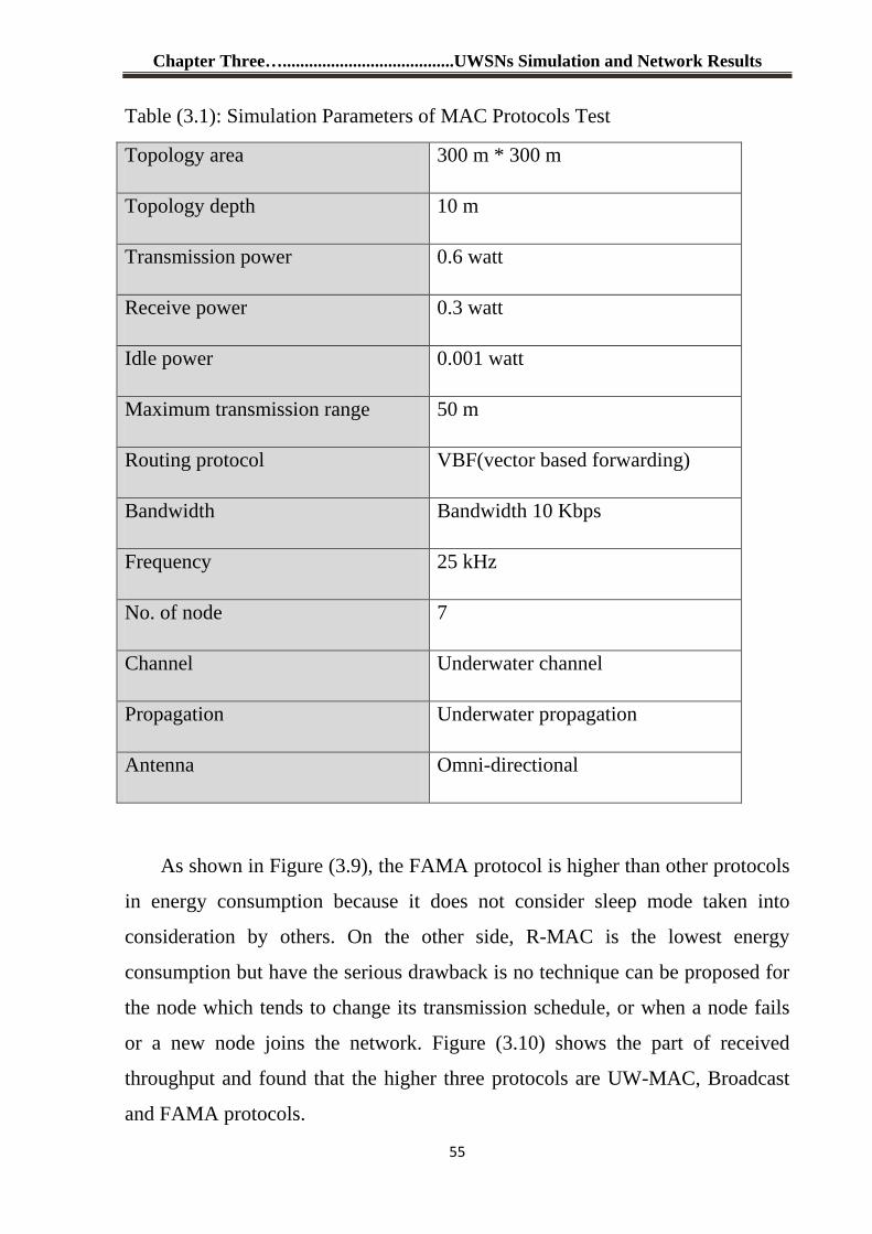
Chapter Three….......................................UWSNs Simulation and Network Results
55
Table (3.1): Simulation Parameters of MAC Protocols Test
Topology area 300 m * 300 m
Topology depth 10 m
Transmission power 0.6 watt
Receive power 0.3 watt
Idle power 0.001 watt
Maximum transmission range 50 m
Routing protocol VBF(vector based forwarding)
Bandwidth Bandwidth 10 Kbps
Frequency 25 kHz
No. of node 7
Channel Underwater channel
Propagation Underwater propagation
Antenna Omni-directional
As shown in Figure (3.9), the FAMA protocol is higher than other protocols
in energy consumption because it does not consider sleep mode taken into
consideration by others. On the other side, R-MAC is the lowest energy
consumption but have the serious drawback is no technique can be proposed for
the node which tends to change its transmission schedule, or when a node fails
or a new node joins the network. Figure (3.10) shows the part of received
throughput and found that the higher three protocols are UW-MAC, Broadcast
and FAMA protocols.
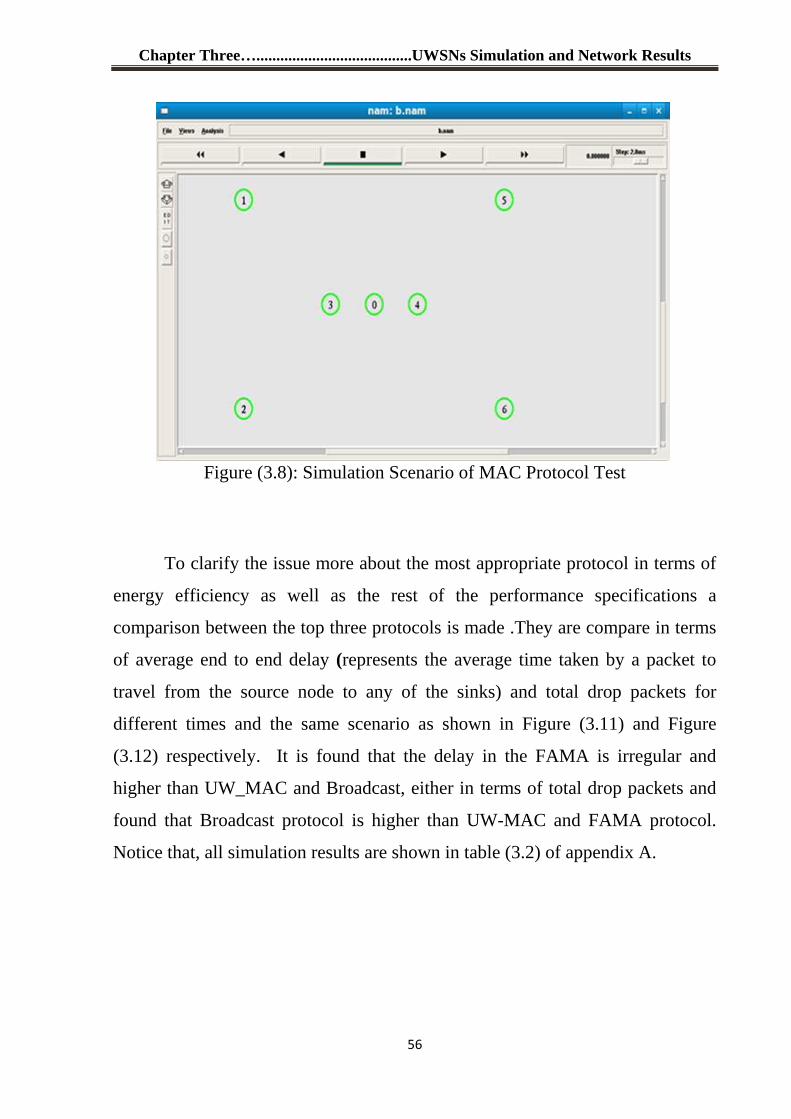
Chapter Three….......................................UWSNs Simulation and Network Results
56
Figure (3.8): Simulation Scenario of MAC Protocol Test
To clarify the issue more about the most appropriate protocol in terms of
energy efficiency as well as the rest of the performance specifications a
comparison between the top three protocols is made .They are compare in terms
of average end to end delay (represents the average time taken by a packet to
travel from the source node to any of the sinks) and total drop packets for
different times and the same scenario as shown in Figure (3.11) and Figure
(3.12) respectively. It is found that the delay in the FAMA is irregular and
higher than UW_MAC and Broadcast, either in terms of total drop packets and
found that Broadcast protocol is higher than UW-MAC and FAMA protocol.
Notice that, all simulation results are shown in table (3.2) of appendix A.
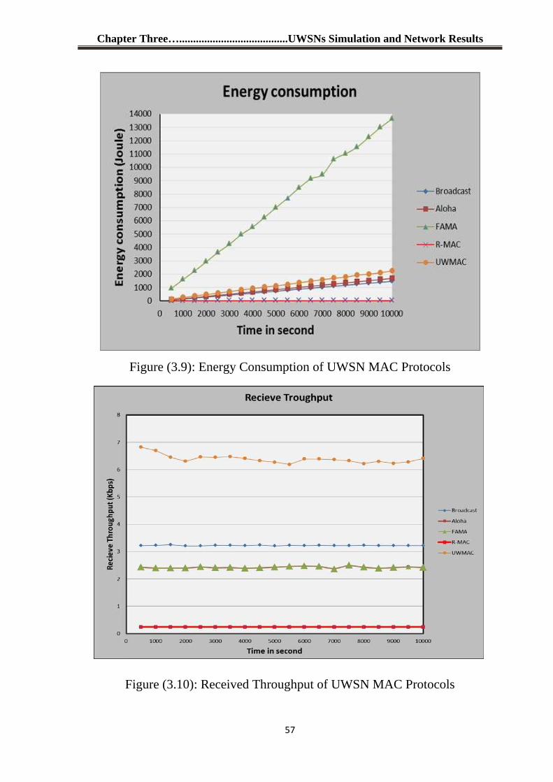
Chapter Three….......................................UWSNs Simulation and Network Results
57
Figure (3.9): Energy Consumption of UWSN MAC Protocols
Figure (3.10): Received Throughput of UWSN MAC Protocols
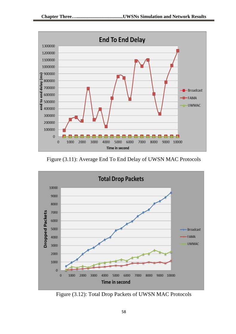
Chapter Three….......................................UWSNs Simulation and Network Results
58
Figure (3.11): Average End To End Delay of UWSN MAC Protocols
Figure (3.12): Total Drop Packets of UWSN MAC Protocols
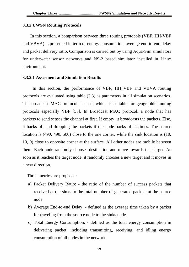
Chapter Three….......................................UWSNs Simulation and Network Results
59
3.3.2 UWSN Routing Protocols
In this section, a comparison between three routing protocols (VBF, HH-VBF
and VBVA) is presented in term of energy consumption, average end-to-end delay
and packet delivery ratio. Comparison is carried out by using Aqua-Sim simulators
for underwater sensor networks and NS-2 based simulator installed in Linux
environment.
3.3.2.1 Assesment and Simulation Results
In this section, the performance of VBF, HH_VBF and VBVA routing
protocols are evaluated using table (3.3) as parameters in all simulation scenarios.
The broadcast MAC protocol is used, which is suitable for geographic routing
protocols especially VBF [58]. In Broadcast MAC protocol, a node that has
packets to send senses the channel at first. If empty, it broadcasts the packets. Else,
it backs off and dropping the packets if the node backs off 4 times. The source
location is (490, 490, 500) close to the one corner, while the sink location is (10,
10, 0) close to opposite corner at the surface. All other nodes are mobile between
them. Each node randomly chooses destination and move towards that target. As
soon as it reaches the target node, it randomly chooses a new target and it moves in
a new direction.
Three metrics are proposed:
a) Packet Delivery Ratio: - the ratio of the number of success packets that
received at the sinks to the total number of generated packets at the source
node.
b) Average End-to-end Delay: - defined as the average time taken by a packet
for traveling from the source node to the sinks node.
c) Total Energy Consumption: - defined as the total energy consumption in
delivering packet, including transmitting, receiving, and idling energy
consumption of all nodes in the network.
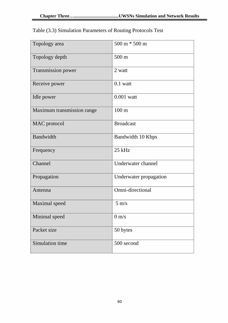
Chapter Three….......................................UWSNs Simulation and Network Results
60
Table (3.3) Simulation Parameters of Routing Protocols Test
Topology area 500 m * 500 m
Topology depth 500 m
Transmission power 2 watt
Receive power 0.1 watt
Idle power 0.001 watt
Maximum transmission range 100 m
MAC protocol Broadcast
Bandwidth Bandwidth 10 Kbps
Frequency 25 kHz
Channel Underwater channel
Propagation Underwater propagation
Antenna Omni-directional
Maximal speed 5 m/s
Minimal speed 0 m/s
Packet size 50 bytes
Simulation time 500 second
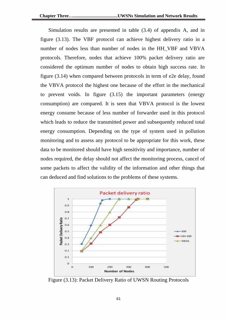
Chapter Three….......................................UWSNs Simulation and Network Results
61
Simulation results are presented in table (3.4) of appendix A, and in
figure (3.13). The VBF protocol can achieve highest delivery ratio in a
number of nodes less than number of nodes in the HH_VBF and VBVA
protocols. Therefore, nodes that achieve 100% packet delivery ratio are
considered the optimum number of nodes to obtain high success rate. In
figure (3.14) when compared between protocols in term of e2e delay, found
the VBVA protocol the highest one because of the effort in the mechanical
to prevent voids. In figure (3.15) the important parameters (energy
consumption) are compared. It is seen that VBVA protocol is the lowest
energy consume because of less number of forwarder used in this protocol
which leads to reduce the transmitted power and subsequently reduced total
energy consumption. Depending on the type of system used in pollution
monitoring and to assess any protocol to be appropriate for this work, these
data to be monitored should have high sensitivity and importance, number of
nodes required, the delay should not affect the monitoring process, cancel of
some packets to affect the validity of the information and other things that
can deduced and find solutions to the problems of these systems.
Figure (3.13): Packet Delivery Ratio of UWSN Routing Protocols
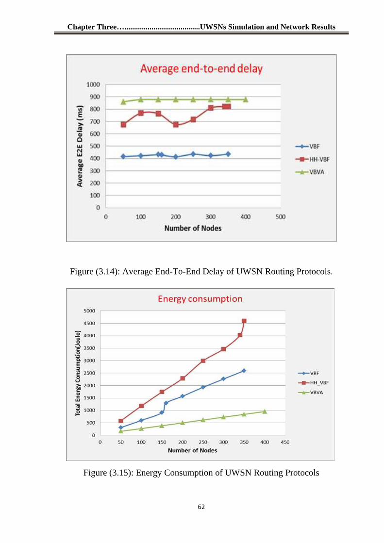
Chapter Three….......................................UWSNs Simulation and Network Results
62
Figure (3.14): Average End-To-End Delay of UWSN Routing Protocols.
Figure (3.15): Energy Consumption of UWSN Routing Protocols
Chapter Three….......................................UWSNs Simulation and Network Results
63
3.3.3 Final Design
In this section, the final design of UWSN will be assessed for pollution
monitoring system in terms of energy consume, received throughput, total drop
packets and average end to end delay.
3.3.3.1 Assessment and Simulation Results
This section presents the evaluation of the performance of the final design
of UWSN for pollution monitoring system. Figure (3.16) represents the structure
of the network consisting of the two networks are UWSN and the terrestrial
network. UWSN is composed of 7 nodes, 6 of them will be sent and one
represents sink node to collect data or values of pollutants and then passed to the
terrestrial network through the antenna outside of the water surface. The
terrestrial network is represented by the on shore or base station linked by
satellite to the pollution center where data is processed and monitored. Using
table (3.5), as parameters in simulation scenario, the steps to implement the
network in the simulator, as well as full source code are available in Appendix
A.
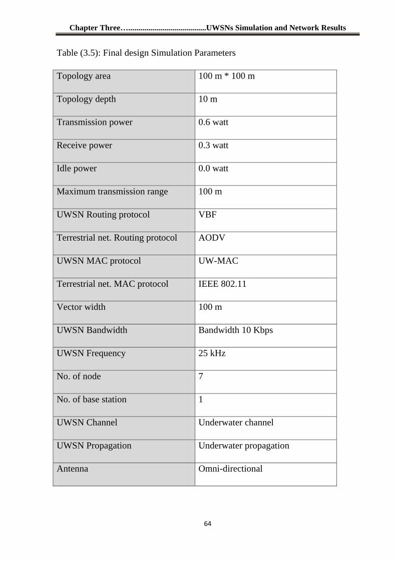
Chapter Three….......................................UWSNs Simulation and Network Results
64
Table (3.5): Final design Simulation Parameters
Topology area 100 m * 100 m
Topology depth 10 m
Transmission power 0.6 watt
Receive power 0.3 watt
Idle power 0.0 watt
Maximum transmission range 100 m
UWSN Routing protocol VBF
Terrestrial net. Routing protocol AODV
UWSN MAC protocol UW-MAC
Terrestrial net. MAC protocol IEEE 802.11
Vector width 100 m
UWSN Bandwidth Bandwidth 10 Kbps
UWSN Frequency 25 kHz
No. of node 7
No. of base station 1
UWSN Channel Underwater channel
UWSN Propagation Underwater propagation
Antenna Omni-directional
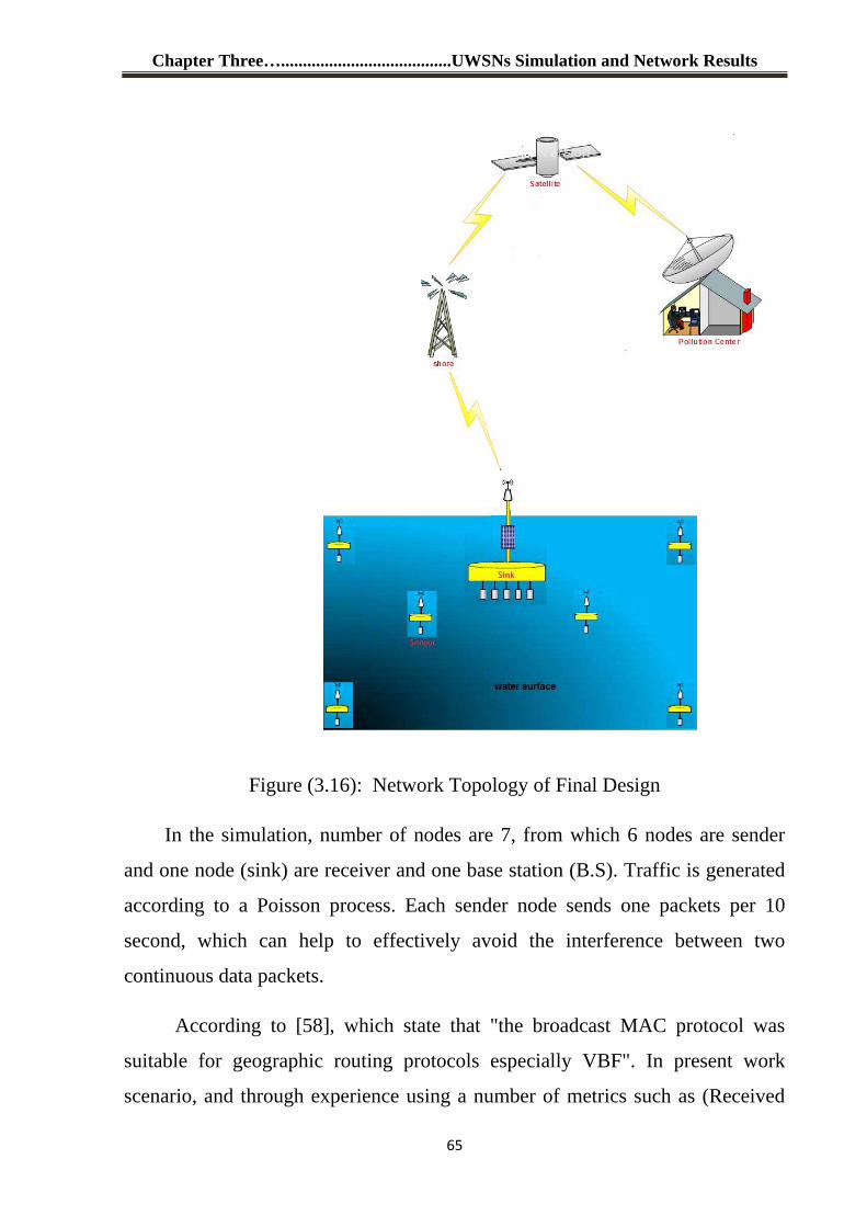
Chapter Three….......................................UWSNs Simulation and Network Results
65
Figure (3.16): Network Topology of Final Design
In the simulation, number of nodes are 7, from which 6 nodes are sender
and one node (sink) are receiver and one base station (B.S). Traffic is generated
according to a Poisson process. Each sender node sends one packets per 10
second, which can help to effectively avoid the interference between two
continuous data packets.
According to [58], which state that "the broadcast MAC protocol was
suitable for geographic routing protocols especially VBF". In present work
scenario, and through experience using a number of metrics such as (Received
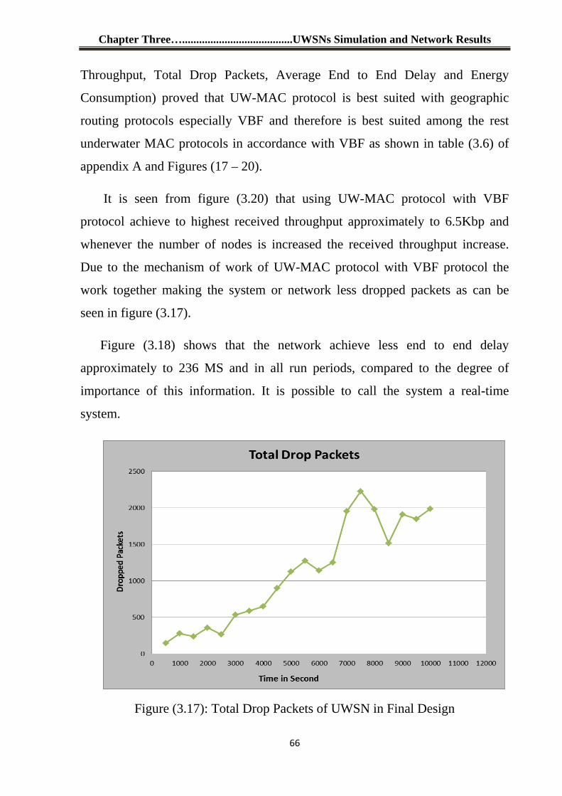
Chapter Three….......................................UWSNs Simulation and Network Results
66
Throughput, Total Drop Packets, Average End to End Delay and Energy
Consumption) proved that UW-MAC protocol is best suited with geographic
routing protocols especially VBF and therefore is best suited among the rest
underwater MAC protocols in accordance with VBF as shown in table (3.6) of
appendix A and Figures (17 – 20).
It is seen from figure (3.20) that using UW-MAC protocol with VBF
protocol achieve to highest received throughput approximately to 6.5Kbp and
whenever the number of nodes is increased the received throughput increase.
Due to the mechanism of work of UW-MAC protocol with VBF protocol the
work together making the system or network less dropped packets as can be
seen in figure (3.17).
Figure (3.18) shows that the network achieve less end to end delay
approximately to 236 MS and in all run periods, compared to the degree of
importance of this information. It is possible to call the system a real-time
system.
Figure (3.17): Total Drop Packets of UWSN in Final Design
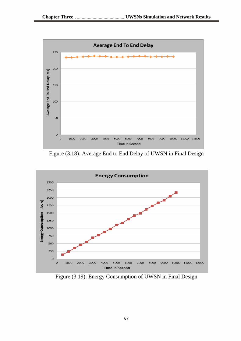
Chapter Three….......................................UWSNs Simulation and Network Results
67
Figure (3.18): Average End to End Delay of UWSN in Final Design
Figure (3.19): Energy Consumption of UWSN in Final Design
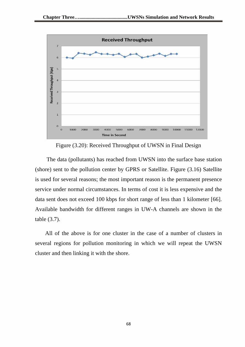
Chapter Three….......................................UWSNs Simulation and Network Results
68
Figure (3.20): Received Throughput of UWSN in Final Design
The data (pollutants) has reached from UWSN into the surface base station
(shore) sent to the pollution center by GPRS or Satellite. Figure (3.16) Satellite
is used for several reasons; the most important reason is the permanent presence
service under normal circumstances. In terms of cost it is less expensive and the
data sent does not exceed 100 kbps for short range of less than 1 kilometer [66].
Available bandwidth for different ranges in UW-A channels are shown in the
table (3.7).
All of the above is for one cluster in the case of a number of clusters in
several regions for pollution monitoring in which we will repeat the UWSN
cluster and then linking it with the shore.
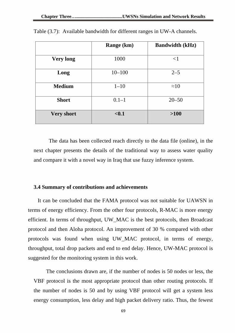
Chapter Three….......................................UWSNs Simulation and Network Results
69
Table (3.7): Available bandwidth for different ranges in UW-A channels.
Bandwidth (kHz) Range (km)
<1 1000 Very long
2–5 10–100 Long
≈10 1–10 Medium
20–50 0.1–1 Short
>100 <0.1 Very short
The data has been collected reach directly to the data file (online), in the
next chapter presents the details of the traditional way to assess water quality
and compare it with a novel way in Iraq that use fuzzy inference system.
3.4 Summary of contributions and achievements
It can be concluded that the FAMA protocol was not suitable for UAWSN in
terms of energy efficiency. From the other four protocols, R-MAC is more energy
efficient. In terms of throughput, UW_MAC is the best protocols, then Broadcast
protocol and then Aloha protocol. An improvement of 30 % compared with other
protocols was found when using UW_MAC protocol, in terms of energy,
throughput, total drop packets and end to end delay. Hence, UW-MAC protocol is
suggested for the monitoring system in this work.
The conclusions drawn are, if the number of nodes is 50 nodes or less, the
VBF protocol is the most appropriate protocol than other routing protocols. If
the number of nodes is 50 and by using VBF protocol will get a system less
energy consumption, less delay and high packet delivery ratio. Thus, the fewest
Chapter Three….......................................UWSNs Simulation and Network Results
70
number of nodes will be used to achieve approximately 100% success rate
thereby obtaining a less expensive system that overcomes the problems of using
redundant node to achieve the same purpose.
But if the data monitored is sensitive in terms of delay then VBVA and HH-
VBF protocols are more suitable than VBF protocol. If the monitoring systems
have a large number of nodes, it is best to use VBVA Protocol to overcome the
problem of charging and recharge for long periods as VBVA Protocol is high
energy-efficient. Thus, for the monitoring system, VBF routing protocol is
suggested.
There is a slight difference in energy consumption compared with using
broadcast protocol with VBF protocol. This difference will decay when the
number of nodes is increased making the system more efficient in terms of
energy consumption. However, if the number of nodes is increased, the system
will bring 100% packet delivery ratio in less number of nodes and therefore the
system becomes more efficient in energy consumption than other systems.
Energy consumption of the pollution monitoring system .
Chapter
Four
Development of a
water quality
Assessment Using
FIS
Chapter Four …………. Development of a water quality Assessment Using FIS
71
Chapter Four
Development of a water quality Assessment Using FIS
4.1 Introduction
The present work aims at developing a proposed water quality index in Iraq
based on fuzzy inference system. That is, comprehensive artificial intelligence
(AI) approaches to the development of environmental indices for routine
assessment of water quality, particularly for human drinking purposes. Multiple
parameters were included based on their critical importance for the overall water
quality and their potential impact on human health. To assess the performance of
the proposed index under actual conditions, a case study was conducted at Tigris
River, Iraq, employing water quality data of various sampling sites in the water.
4.2 Calculations of Traditional WQI in Iraq
The WQI was calculated using the Weighted Arithmetic Index method. The
quality rating scale for each parameter (qi) was calculated by using equation (1)
[51]:
qi = �CiSi� ∗ 100 (4.1)
A quality rating scale (qi) for each parameter is assigned by dividing its
observed concentration (Ci) in each water sample by its respective standard
value (Si) for each sample (i) and the result is multiplied by 100. Relative
weight (wi) was calculated by a value inversely proportional to the
recommended standard value (Si) of the corresponding parameter using equation
(2) [51]: �i = 1�� (4.2)
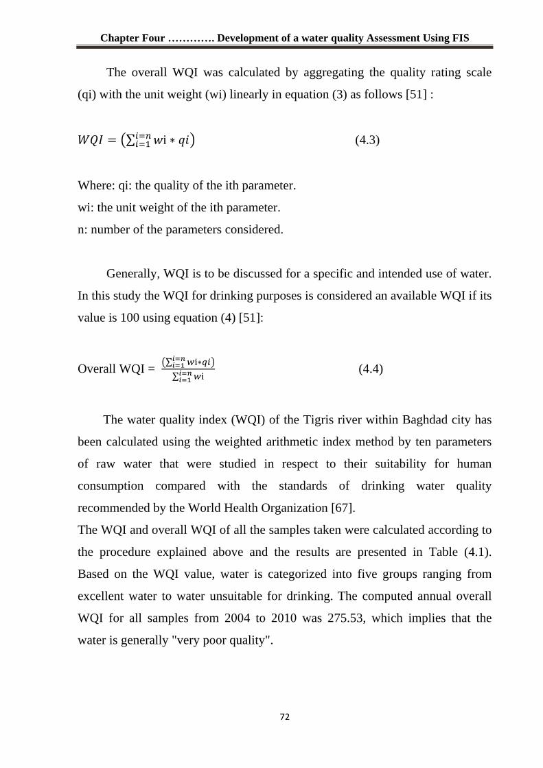
Chapter Four …………. Development of a water quality Assessment Using FIS
72
The overall WQI was calculated by aggregating the quality rating scale
(qi) with the unit weight (wi) linearly in equation (3) as follows [51] :
��� = �∑ �i ∗ ���=��=1 � (4.3)
Where: qi: the quality of the ith parameter.
wi: the unit weight of the ith parameter.
n: number of the parameters considered.
Generally, WQI is to be discussed for a specific and intended use of water.
In this study the WQI for drinking purposes is considered an available WQI if its
value is 100 using equation (4) [51]:
Overall WQI = �∑ �i∗���=��=1 �∑ �i�=��=1 (4.4)
The water quality index (WQI) of the Tigris river within Baghdad city has
been calculated using the weighted arithmetic index method by ten parameters
of raw water that were studied in respect to their suitability for human
consumption compared with the standards of drinking water quality
recommended by the World Health Organization [67].
The WQI and overall WQI of all the samples taken were calculated according to
the procedure explained above and the results are presented in Table (4.1).
Based on the WQI value, water is categorized into five groups ranging from
excellent water to water unsuitable for drinking. The computed annual overall
WQI for all samples from 2004 to 2010 was 275.53, which implies that the
water is generally "very poor quality".
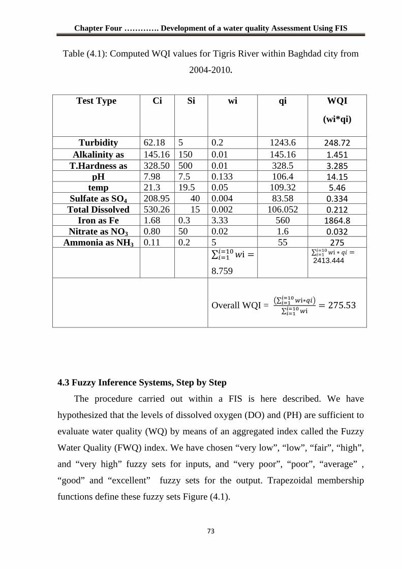
Chapter Four …………. Development of a water quality Assessment Using FIS
73
4.3 Fuzzy Inference Systems, Step by Step
The procedure carried out within a FIS is here described. We have
hypothesized that the levels of dissolved oxygen (DO) and (PH) are sufficient to
evaluate water quality (WQ) by means of an aggregated index called the Fuzzy
Water Quality (FWQ) index. We have chosen “very low”, “low”, “fair ” , “high”,
and “very high” fuzzy sets for inputs, and “very poor”, “poor”, “average” ,
“good” and “excellent” fuzzy sets for the output. Trapezoidal membership
functions define these fuzzy sets Figure (4.1).
Table (4.1): Computed WQI values for Tigris River within Baghdad city from
2004-2010.
Test Type Ci Si wi qi WQI
(wi*qi)
Turbidity 62.18 5 0.2 1243.6 248.72
Alkalinity as 145.16 150 0.01 145.16 1.451
T.Hardness as 328.50 500 0.01 328.5 3.285
pH 7.98 7.5 0.133 106.4 14.15
temp 21.3 19.5 0.05 109.32 5.46
Sulfate as SO4 208.95 40 0.004 83.58 0.334
Total Dissolved 530.26 15 0.002 106.052 0.212
Iron as Fe 1.68 0.3 3.33 560 1864.8
Nitrate as NO3 0.80 50 0.02 1.6 0.032
Ammonia as NH3 0.11 0.2 5 55 275 ∑ �i =�=10�=1
8.759
∑ �i ∗ ���=10�=1 =
2413.444
Overall WQI = �∑ �i∗���=10�=1 �∑ �i�=10�=1 = 275.53
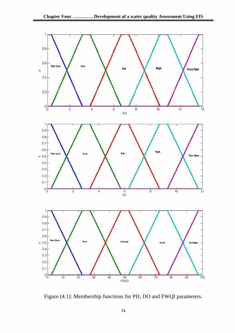
Chapter Four …………. Development of a water quality Assessment Using FIS
74
Figure (4.1): Membership functions for PH, DO and FWQI parameters.
Chapter Four …………. Development of a water quality Assessment Using FIS
75
In water quality assessment, the expressions are frequently used by the
experts: “if the levels of PH in a river are low, and the levels or dissolved
oxygen are low, then the expected water quality is poor”. In fuzzy language, it
could be enunciated as figure (4.2).
Figure (4.2): Fuzzy language Rules for the inputs PH and DO.
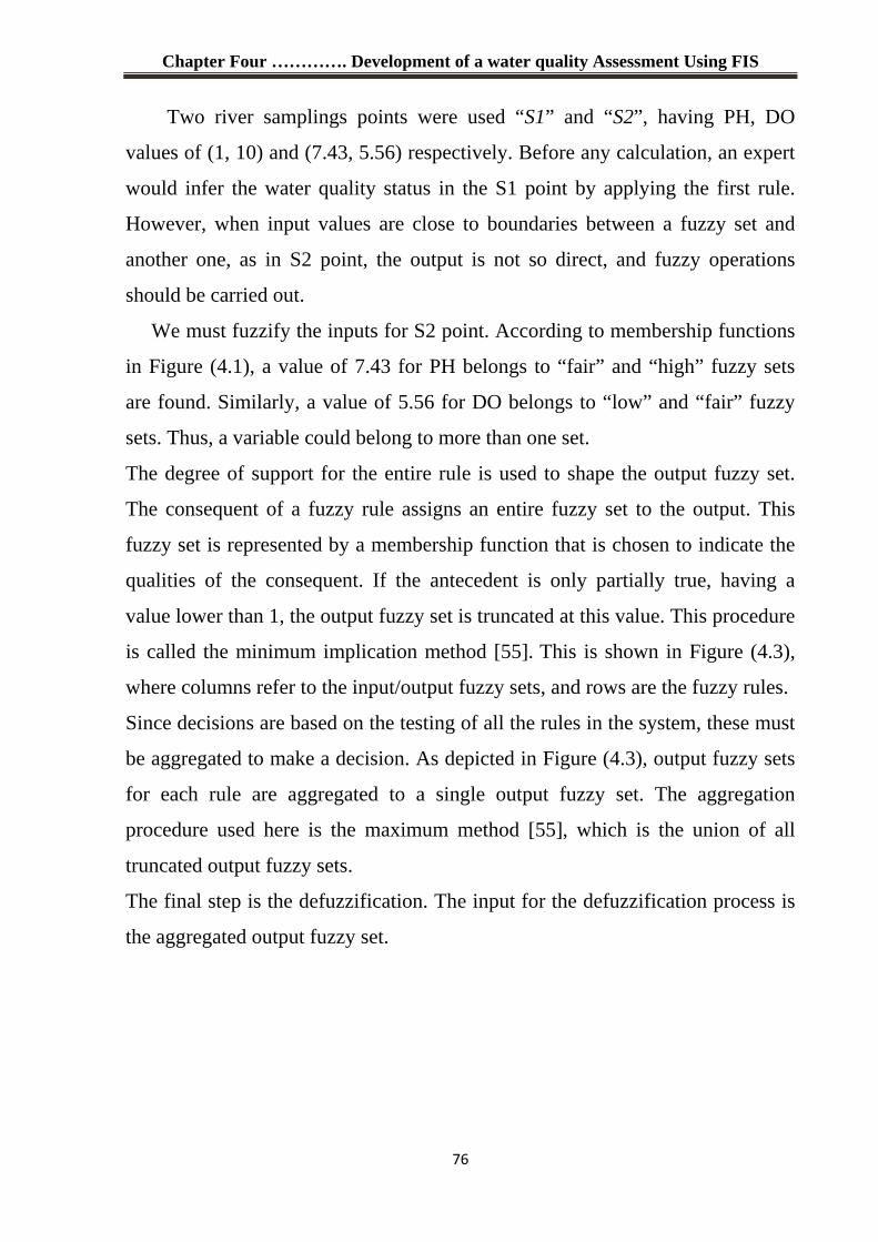
Chapter Four …………. Development of a water quality Assessment Using FIS
76
Two river samplings points were used “S1” and “S2”, having PH, DO
values of (1, 10) and (7.43, 5.56) respectively. Before any calculation, an expert
would infer the water quality status in the S1 point by applying the first rule.
However, when input values are close to boundaries between a fuzzy set and
another one, as in S2 point, the output is not so direct, and fuzzy operations
should be carried out.
We must fuzzify the inputs for S2 point. According to membership functions
in Figure (4.1), a value of 7.43 for PH belongs to “fair” and “high” fuzzy sets
are found. Similarly, a value of 5.56 for DO belongs to “low” and “fair” fuzzy
sets. Thus, a variable could belong to more than one set.
The degree of support for the entire rule is used to shape the output fuzzy set.
The consequent of a fuzzy rule assigns an entire fuzzy set to the output. This
fuzzy set is represented by a membership function that is chosen to indicate the
qualities of the consequent. If the antecedent is only partially true, having a
value lower than 1, the output fuzzy set is truncated at this value. This procedure
is called the minimum implication method [55]. This is shown in Figure (4.3),
where columns refer to the input/output fuzzy sets, and rows are the fuzzy rules.
Since decisions are based on the testing of all the rules in the system, these must
be aggregated to make a decision. As depicted in Figure (4.3), output fuzzy sets
for each rule are aggregated to a single output fuzzy set. The aggregation
procedure used here is the maximum method [55], which is the union of all
truncated output fuzzy sets.
The final step is the defuzzification. The input for the defuzzification process is
the aggregated output fuzzy set.
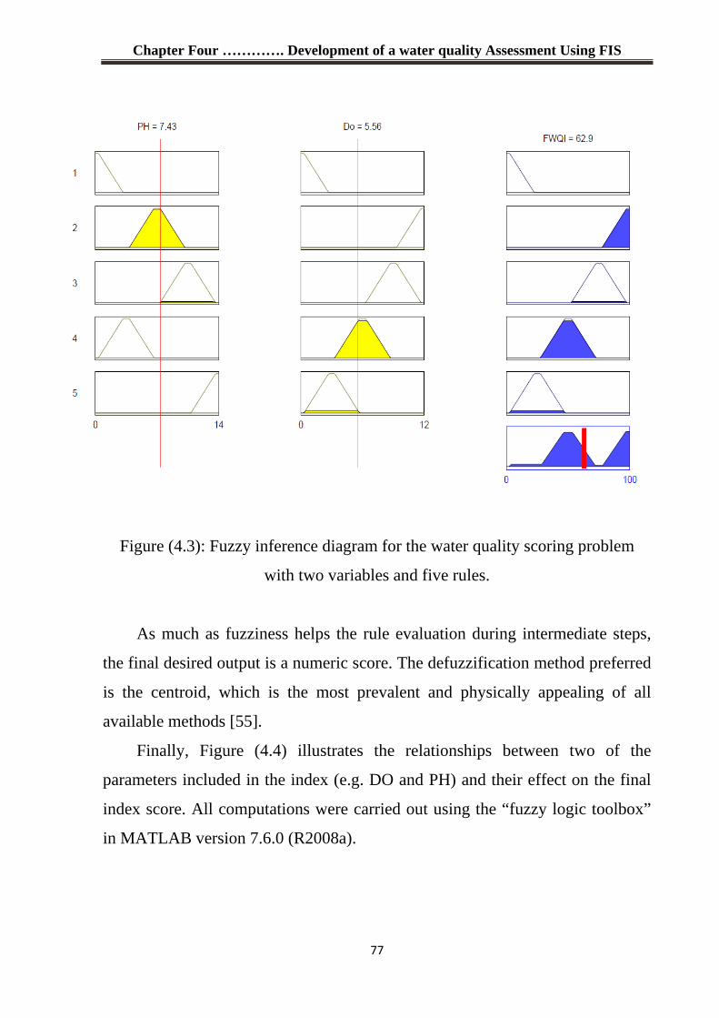
Chapter Four …………. Development of a water quality Assessment Using FIS
77
Figure (4.3): Fuzzy inference diagram for the water quality scoring problem
with two variables and five rules.
As much as fuzziness helps the rule evaluation during intermediate steps,
the final desired output is a numeric score. The defuzzification method preferred
is the centroid, which is the most prevalent and physically appealing of all
available methods [55].
Finally, Figure (4.4) illustrates the relationships between two of the
parameters included in the index (e.g. DO and PH) and their effect on the final
index score. All computations were carried out using the “fuzzy logic toolbox”
in MATLAB version 7.6.0 (R2008a).
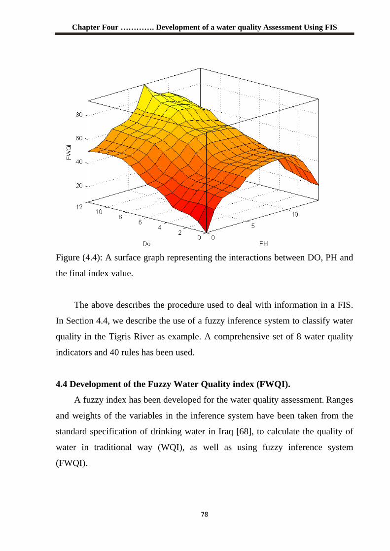
Chapter Four …………. Development of a water quality Assessment Using FIS
78
Figure (4.4): A surface graph representing the interactions between DO, PH and
the final index value.
The above describes the procedure used to deal with information in a FIS.
In Section 4.4, we describe the use of a fuzzy inference system to classify water
quality in the Tigris River as example. A comprehensive set of 8 water quality
indicators and 40 rules has been used.
4.4 Development of the Fuzzy Water Quality index (FWQI).
A fuzzy index has been developed for the water quality assessment. Ranges
and weights of the variables in the inference system have been taken from the
standard specification of drinking water in Iraq [68], to calculate the quality of
water in traditional way (WQI), as well as using fuzzy inference system
(FWQI).
Chapter Four …………. Development of a water quality Assessment Using FIS
79
Ten variables taken for the years from 2004 to 2010 for the eight sites in
the Tigris River to calculate the overall WQI in the traditional way, as well as
using FWQI.
To calculate the FWQI eight variables were taken from five sites in three
months, the indicators are the following:
Dissolved oxygen (DO), pH, Turbidity, total Hardness, Iron as Fe, Temperature,
Mn and Cu.
Trapezoidal membership functions were used to represent “very low”, “low”,
“Fair”, “ high” and “very high” for input and “very poor”, “poor”, “average ”,
“good” and “excellent” for output fuzzy sets.
The membership function parameters are a, b, c, and d. A list of these
parameters is summarized in Table. Ranges for fuzzy sets were based on the
Standard Specification of drinking water in Iraq and guidelines for drinking-
water quality [68] and [67] respectively. These ranges are also shown in Table
(4.2).
4.5 Results and discussion of FWQI
The water condition for the Tigris River has been assessed with the FWQ
index. Input data extracted from public databases have been used to assess water
quality between 2004 and 2010 to assess the performance of these years, and to
compare between traditional WQI and present method FWQI, then to compare
between them in multiple sites through three varying months and different in
terms of geographical climate [69].
The results for the global FWQ index calculated according to the FIS and
traditional WQI from 2004 to 2010 are shown in Figure (4.5). A comparison
between the proposed FWQ index and the reputed WQI index through three
months (June, august 2007 and January 2008) is shown in Figures (4.6, 4.7 and
4.8). The FWQI obtained from section 4.2 for calculating the quality of water
for two indicators (PH and DO) is also observed that the result of FWQI is 62.9.
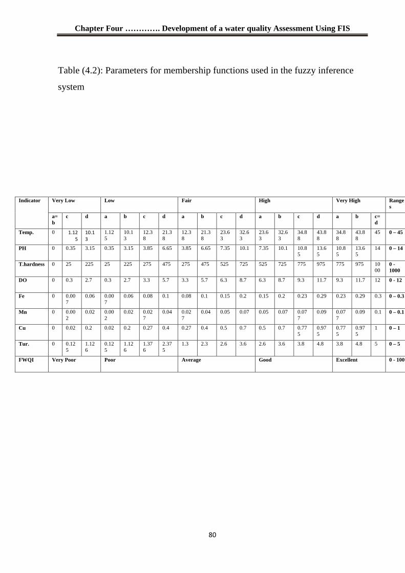
Chapter Four …………. Development of a water quality Assessment Using FIS
80
Table (4.2): Parameters for membership functions used in the fuzzy inference
system
Indicator Very Low
Low Fair High Very High Ranges
a=b
c d a b c d a b c d a b c d a b c=d
Temp. 0 1.12
5 10.1
3
1.125
10.13
12.38
21.38
12.38
21.38
23.63
32.63
23.63
32.63
34.88
43.88
34.88
43.88
45 0 – 45
PH 0 0.35 3.15 0.35 3.15 3.85 6.65 3.85 6.65 7.35 10.1 7.35 10.1 10.85
13.65
10.85
13.65
14 0 – 14
T.hardness 0 25 225 25 225 275 475 275 475 525 725 525 725 775 975 775 975 1000
0 -1000
DO 0 0.3 2.7 0.3 2.7 3.3 5.7 3.3 5.7 6.3 8.7 6.3 8.7 9.3 11.7 9.3 11.7 12 0 - 12
Fe 0 0.007
0.06 0.007
0.06 0.08 0.1 0.08 0.1 0.15 0.2 0.15 0.2 0.23
0.29 0.23 0.29 0.3 0 – 0.3
Mn 0 0.002
0.02 0.002
0.02 0.027
0.04 0.027
0.04 0.05 0.07 0.05 0.07 0.077
0.09 0.077
0.09 0.1 0 – 0.1
Cu 0 0.02 0.2 0.02 0.2 0.27 0.4 0.27 0.4 0.5 0.7 0.5 0.7 0.775
0.975
0.775
0.975
1 0 – 1
Tur. 0 0.125
1.126
0.125
1.126
1.376
2.375
1.3 2.3 2.6 3.6 2.6 3.6 3.8 4.8 3.8 4.8 5 0 – 5
FWQI Very Poor Poor Average Good Excellent 0 - 100
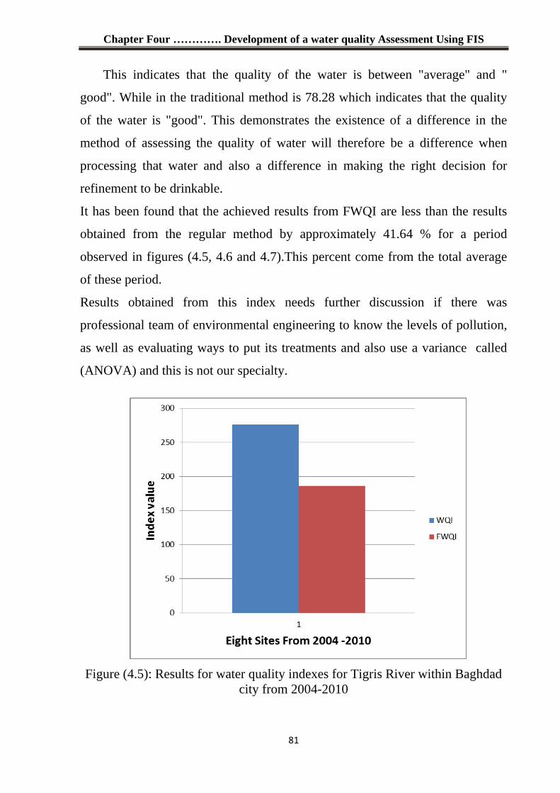
Chapter Four …………. Development of a water quality Assessment Using FIS
81
This indicates that the quality of the water is between "average" and "
good". While in the traditional method is 78.28 which indicates that the quality
of the water is "good". This demonstrates the existence of a difference in the
method of assessing the quality of water will therefore be a difference when
processing that water and also a difference in making the right decision for
refinement to be drinkable.
It has been found that the achieved results from FWQI are less than the results
obtained from the regular method by approximately 41.64 % for a period
observed in figures (4.5, 4.6 and 4.7).This percent come from the total average
of these period.
Results obtained from this index needs further discussion if there was
professional team of environmental engineering to know the levels of pollution,
as well as evaluating ways to put its treatments and also use a variance called
(ANOVA) and this is not our specialty.
Figure (4.5): Results for water quality indexes for Tigris River within Baghdad city from 2004-2010
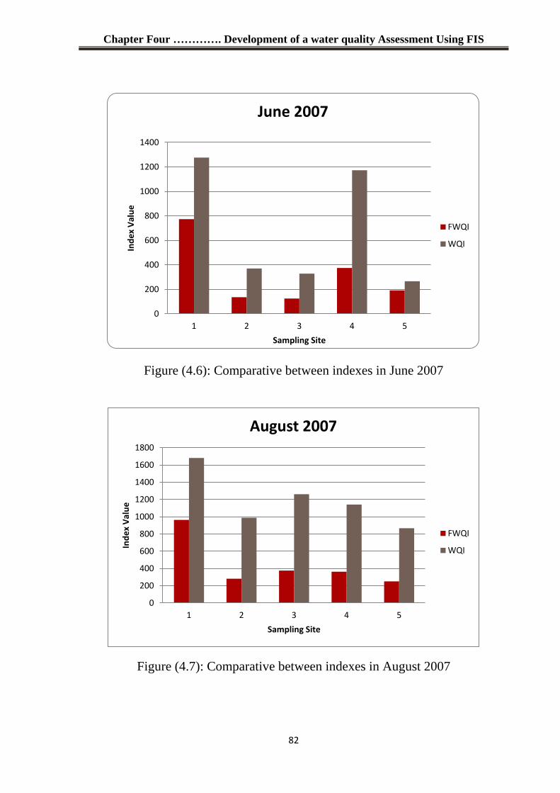
Chapter Four …………. Development of a water quality Assessment Using FIS
82
0
200
400
600
800
1000
1200
1400
1 2 3 4 5
Ind
ex
Va
lue
Sampling Site
June 2007
FWQI
WQI
0
200
400
600
800
1000
1200
1400
1600
1800
1 2 3 4 5
Ind
ex
Va
lue
Sampling Site
August 2007
FWQI
WQI
Figure (4.6): Comparative between indexes in June 2007
Figure (4.7): Comparative between indexes in August 2007
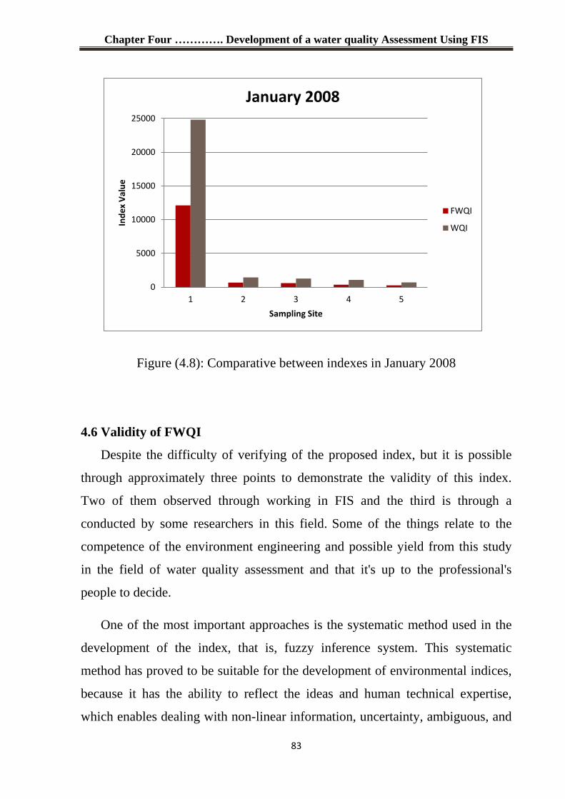
Chapter Four …………. Development of a water quality Assessment Using FIS
83
Figure (4.8): Comparative between indexes in January 2008
4.6 Validity of FWQI
Despite the difficulty of verifying of the proposed index, but it is possible
through approximately three points to demonstrate the validity of this index.
Two of them observed through working in FIS and the third is through a
conducted by some researchers in this field. Some of the things relate to the
competence of the environment engineering and possible yield from this study
in the field of water quality assessment and that it's up to the professional's
people to decide.
One of the most important approaches is the systematic method used in the
development of the index, that is, fuzzy inference system. This systematic
method has proved to be suitable for the development of environmental indices,
because it has the ability to reflect the ideas and human technical expertise,
which enables dealing with non-linear information, uncertainty, ambiguous, and
0
5000
10000
15000
20000
25000
1 2 3 4 5
Ind
ex
Va
lue
Sampling Site
January 2008
FWQI
WQI
Chapter Four …………. Development of a water quality Assessment Using FIS
84
subjectivity. Additionally, the index is based on the linguistic terminology and
results becoming more understandable for the public, managers and non-experts
peoples. The second approach addresses the inclusion of the parameters in the
index. The presented index can include all of the parameters that were
considerable importance for the overall quality of drinking water and can greatly
affect to health of human. And this is an indication of the necessity for
containing all of these parameters should be included in the index if it is to be
representative of the overall water quality.
Finally, according to Ref. [53], the robustness of the index is
approximately similar to the index that has been presented by a sensitivity
analysis. For this purpose the final rule set of the index is considered as the
baseline, and then measurement of the changes/deviations, were intentionally
made, from the baseline as the percentage of change/variation in the rule sets of
different stages. In fact, the presence of change in the rules of each stage is
obtained by calculating the number of rules that differ from that of the baseline
rule set. For instance, considering a total of 25 rules in the rule set of the final
stage, if 5 rules had been manipulated in the rule set of this stage, the percent of
change/variation would have been 20%. This suggests that the changes in the
rules of different stages of the fuzzy-based index do not significantly change the
index outputs. Implying that the index is quite robust against changes.

Chapter Five
Conclusion and
Suggestions for
Future Work
Chapter Five ……………………. Conclusion and Suggestions for Future Work
85
Chapter Five
Conclusion and Suggestions for Future Work
5.1 Conclusion
The proposition of a system for pollution monitoring in water by using
underwater wireless sensor networks presented. Then, design a methodology to
assess the data collected from this network. The work is divided into two parts;
firstly performance assessment of UWSN through comparing multiple MAC and
routing protocols using specific metrics as energy consumption, received
throughput, total drop packets, average end to end delay and Packet delivery ratio
then elected the appropriate one based on system requirements. The second part
presents a novel way in Iraq that use fuzzy inference system to assess water quality
on data collected from our UWSN.
The conclusions are drawn from the obtained results of simulation that deals
with UWSN as follows:
1. The simulation Aqua-Sim can efficiently simulate audio signal reduction
and packet impacts in underwater sensor networks. Also, Aqua-Sim can
simply be integrated with the present codes in NS-2.
2. The FAMA protocol is not suitable for UAWSN in terms of energy
efficiency. The rest four protocols, R-MAC protocol is more energy
efficient. In terms of throughput, UW_MAC is the best protocols, then
Broadcast protocol then Aloha protocol. Thus, improvement of 30 %
compared with other protocols has been found when using UW_MAC
protocol, in terms of energy, throughput, total drop packets and end to end
delay.
3. If the number of nodes is 50 nodes or less, the VBF protocol is the most
appropriate one. If the number of nodes is 50 then using VBF protocol get a
Chapter Five ……………………. Conclusion and Suggestions for Future Work
86
system less energy consumption, less delay and high packet delivery ratio.
Thus, the fewest number of nodes will be used to achieve approximately
100% success rate. A less expensive system that overcomes the problem of
use redundant node to achieve the same purpose is obtained.
4. Due to the mechanism of work of UW-MAC protocol with VBF protocol the
work together making the system or network less dropped packets. Also, it
achieved less end to end delay approximately to 236 MS and in all run
periods, which can be assumed as a real-time system.
5. Broadcast protocol with VBF protocol is slightly less than using UW_MAC
protocol with VBF protocol. This difference can decay when comparing
highly success rate has been obtained from final design.
The conclusions observed from using fuzzy inference system to develop a water
quality index are as follows:
1. A robust decision making tool has been presented for water assessment and
management in the form of an index called fuzzy water quality index
(FWQI).
2. Fuzzy inference system that has flexibility in its work to develop
classification models should be recommended in the development of similar
environmental indexes.
3. FIS can put a baseline index to be used with other parameters with simple
changes thereby do not change the score of index significantly, but in the
same number of parameters of baseline.
4. FIS is a reliable method for reporting the results of the monitoring system in
linguistic terms, which are understandable for the public and non-experts
people to decide.
Chapter Five ……………………. Conclusion and Suggestions for Future Work
87
5.2 Suggestions for Future Work
The monitoring system has been proposed has many points as suggestion
for future work that makes a pollution monitoring systems more efficient. These
points are summarized as follows:
1. The information needs to transmit is decided according to water quality
grade which is quantitatively analyzed directly by using fuzzy
comprehensive evaluation rather than transmitting large amount of raw
data to the monitoring center therapy solve the problem of high energy
consumption.
2. Plan to manipulate the VBVA protocol to make it higher packet delivery
ratio and less end to end delay to achieve more energy efficient and high
data rate routing protocol at the same time.
3. Development of a DBR routing protocol in Aqua-sim simulator by using
the network programing tools represented by using TCL language and
C++.
4. Formation of a working group with the engineering environment or the
number of specialists in the field of pollution to set effective limits for
indicators and consistent with the Iraq's water environment and therapy.
There will be a high level of water quality assessment using fuzzy,
because the degree of knowledge will be increased.
5. Design of different GUI to add on pollution monitoring system by using
GUI in MATLAB to alert when the indicator limits exceed.
88
REFRENCES
[1] X. (Sherman) Shen, Y. Pan, "Fundamentals of Wireless Sensor
Networks", Book chapter, John Wiley & Sons Ltd, 2010.
[2] I. F. Akyildiz, M. Can ,"Wireless Sensor Networks ", Book chapter,
John Wiley & Sons Ltd.2010.
[3] B. Kishore,"Muti-Metric Adaptive Routing Algorithm for Underwater
Wireless Sensor Networks", Master thesis, Texas A&M University, 2011.
[4] D. Pompili, T. Melodia,"An architecture for ocean bottom Under
Water Acoustic Sensor Networks," poster presentation, in Proc. of the
Mediterranean Ad Hoc Networking Workshop (MedHocNet), Bodrum,
Turkey, July 2004
[5] U.Devee Prasan, Dr. S. Murugappan," Underwater Sensor Networks
:Architecture, Research Challenges and Potential Applications ",
International Journal of Engineering Research and Applications, Vol. 2,
Issue 2,Mar-Apr 2012.
[6] Jun-Hong Cui, Jiejun Kong, Mario Gerla, Shengli Zhou," Challenges:
Building Scalable Mobile Underwater Wireless Sensor Networks for
Aquatic Applications", IEEE Network, Special Issue on Wireless
Sensor Networking, Vol. 20, No. 3, pp. 12-18, May/June 2006.
89
[7] M.P. Malumbres, P. Pablo Garrido, Carlos T. Calafate,Jose Oliver,"
Underwater Wireless Networking Technologies ", Progress In
Electromagnetics Research, Vol. 95, pages 219-239, 2008.
[8] Andre Lermontov, Lıdia Yokoyama , Mihail Lermontov , Maria
Augusta," River quality analysis using fuzzy water quality index: Ribeira
do Iguape river watershed, Brazil", Ecological Indicators, Volume: 9
Issue: 6 Pages: 1188-1197, 2009.
[9] Gabrielle Thie´baut, Guillaume Tixier, Franc¸ois Gue´rold,Serge
Muller," Comparison of different biological indices for the assessment of
river quality:application to the upper river Moselle (France)",
Hydrobiologia, Volume: 570 Issue: 1 Pages: 159-164, Springer, 2006.
[10] William Andrés Ocampo Duque," the development of decision-
making systems based on fuzzy models to assess water quality in rivers",
PhD Thesis, Department of Chemical Engineering Universitat Rovira i
Virgili,Tarragona – 2008.
[11] Feng Zhang," Underwater Sensor Networks for Water Quality
Monitoring" Project Final Report, 2008
[12] Arijit Khan, Lawrence Jenkins," Undersea wireless sensor network
for ocean pollution prevention", International Conference on
Communication Systems Software and Middleware, Pages: 2-8 Provider:
IEEE، Bangalore, 2008.
[13] WANG W., LIN Y.," The Application of Wireless Sensor Network
on Regional Environmental Protection", Conference on Regional
90
Economy and Sustainable Development, ISBN: 978-0-646-50352-3,
Nov. 2008.
[14] Peng J. , Hongbo X. , Zhiye H. and Zheming W.," Design of a Water
Environment Monitoring System Based on Wireless Sensor Networks ",
Sensors , Volume: 9 Issue: 8 Pages: 6411-6434, 2009.
[15] Nader M. , Imad J., Jameela J. and Liren Z.," Sensor Network
Architectures for Monitoring Underwater Pipelines ", Sensors , Volume:
11 Issue: 11 Pages: 10738-10764, 2011.
[16] Chunhu Liu ,Bin Fu ,Han Zhang, Lian Lian." Construction and basic
performance tests of an underwater monitoring network", Artificial Life
and Robotics, Volume: 16, Issue: 1, Pages: 98-101, Provider: Springer,
2011.
[17] Sebastian B. ," Enabling Autonomous Environmental Measurement
Systems with Low-Power Wireless Sensor Networks", Master Thesis,
Mid Sweden University, 2011.
[18] Mustafa S., Mahmood A., Shahzad A. Malik, Izhar-ul-Haq," Design
of Underwater Sensor Networks for Water Quality Monitoring", World
Applied Sciences Journal, Vol. 17 ,page 1441-1444,2012.
[19] Teng Wang," Water Quality Monitoring System based on WSN",
Master Thesis,Royal Institute of Technology,2012.
91
[20] Huma Zia, Nick R. Harris, Geoff V. Merrett , Mark Rivers , Neil
Coles," The impact of agricultural activities on water quality: A case for
collaborative catchment-scale management using integrated wireless
sensor networks", Computers and Electronics in Agriculture , Volume: 96
, Pages: 126-138 Provider: Elsevier,2013.
[21] Ian F. Akyildiz, Dario P., Tommaso M.," Underwater acoustic
sensor networks: research challenges", Ad Hoc Networks, Volume: 3,
Issue: 3, Pages: 257-279, Provider: Elsevier, 2005.
[22] Ian F. Akyildiz, Dario Pompili, Tommaso Melodia," State-of-the-art
in Protocol Research for Underwater Acoustic Sensor Networks", ACM
Mobile Computing and Communication Review by citeseer, 2007.
[23] Xiping Yang, Keat G. Ong, William R. Dreschel, Kefeng Zeng,
Casey S. Mungle, Craig A. Grimes," Design of a Wireless Sensor
Network for Long-term, In-Situ Monitoring of an Aqueous Environment"
, Sensors , Volume: 2, Issue: 11, Pages: 455-472, November 2002.
[24] Lanbo Liu, Shengli Zhou, Jun-Hong Cui," Prospects and Problems
of Wireless Communication for Underwater Sensor Networks ", Wireless
Communications and Mobile Computing, Volume: 8, Issue: 8, Pages:
977-994, Provider: Wiley, 2008.
[25] Bridget Benson," Design of a Low-cost Underwater Acoustic
Modem for Short-Range Sensor Networking Applications", Ph.D. Thesis,
University of California, San Diego, 2010.
92
[26] Daniel L. Codiga, Joseph A. Rice, Paul A. Baxely," Networked
Acoustic Modems for Real-Time Data Delivery from Distributed
Subsurface Instruments in the Coastal Ocean: Initial System
Development and Performance", Oceanic Tech., Vol. 22,page 704-720 ,
2005.
[27] Dario Pompili," Efficient Communication Protocols for Underwater
Acoustic Sensor Networks ", Ph.D. Thesis, Georgia Institute of
Technology, August 2007.
[28] Ian F. Akyildiz, Mehmet Can Vuran," Wireless sensor networks",
Book chapter , A John Wiley and Sons, Ltd, Publication, 2010.
[29]Manjula.R.B, Sunilkumar S. Manvi," Issues in Underwater Acoustic
Sensor Networks", International Journal of Computer and Electrical
Engineering, Vol.3, No.1, February, 2011.
[30] Holger Karl, Andreas Willig, "Protocols and Architectures for
Wireless Sensor Networks", Book chapter, John Wiley & Sons, Ltd.2005.
[31] M.P. Malumbres, P. Pablo Garrido, Carlos T. Calafate, Jose Oliver,"
Underwater Wireless Networking Technologies ", Progress In
Electromagnetics Research, Vol. 95, pages 219-239, 2008, 2008.
[32]Phil Karn," MACA: A New Channel Access Method for Packet
Radio", the proceedings of the 9th ARRL Computer Networking
Conference, London, Ontario, Canada, 1990.
93
[33] Vaduvur B., Alan D., Scott S., Lixia Z.," MACAW: A Media Access
Protocol for Wireless LAN’s", by citeseer Journal, 2009.
[34]Chane L.Fullmer, J.J Garcia-Luna-Aceves, "Floor Acquisition
Multiple Access (FAMA) for Packet Radio Networks", by citeseer
Journal, 1998.
[35] Peng Xie, Jun-Hong Cui," R-MAC: An Energy-Efficient MAC
Protocol for Underwater Sensor Networks", International Conference on
Wireless Algorithms, Systems and Applications , ISBN: 076952981X ,
Pages: 187-198, Provider: IEEE, 2007 .
[36] Asoke K. Talukdar," Mobile Computing ", Book chapter, Chapter
21,page 607, Edition 2, Tata McGraw-Hill Education, Jul 10, 2010.
[37] Farizah Yunus, Sharifah H. S. Ariffin, Yasser Zahedi," A Survey of
Existing Medium Access Control (MAC) for Underwater Wireless
Sensor Network (UWSN)", 2010 Fourth Asia International Conference
on Mathematical/Analytical Modeling and Computer Simulation , Pages:
544-549, Provider: IEEE, 2010.
[38]Min Kyoung Park, Volkan Rodoplu,"UWAN-MAC: An Energy
efficient MAC-Protocol for Underwater Acoustic Wireless Sensor
Networks", IEEE Journal of Oceanic Engineering, Volume: 32, Issue: 3,
Pages: 710-720, Provider: IEEE, July 2007.
[39] Peng Xie, Jun-Hong Cui, Li Lao," VBF: Vector-Based Forwarding
Protocol for Underwater Sensor Networks", In Proc. of IFIP Networking
by citeseer Journal,2005.
94
[40] Charles E. Perkins, Pravin Bhagwat," Highly Dynamic Destination-
Sequenced Distance-Vector Routing (DSDV) for Mobile Computers", by
citeseer Journal, 1994.
[41]P.Jacquet,P.Muhlethaler,T.Clausen,A.Laouiti,A.Qayyum,L.Viennot,"
Optimized Link-State Routing Protocol for AD hoc Networks", Multi
Topic Conference, 2001. IEEE INMIC 2001. Technology for the 21st
Century, Pages: 62-68, Provider: IEEE 2001.
[42] Ian F. Akyildiz, Dario Pompili, Tommaso Melodia," State of the Art
in Protocol Research for Underwater Acoustic Sensor Networks", ACM
Mobile Computing and Communication Review by citeseer Journal,
2007.
[43] Tommaso Melodia, Dario Pompili, Ian E Akyildiz," Optimal Local
Topology Knowledge for Energy Efficient Geographical Routing in
Sensor Networks", IEEE INFOCOM, Volume: 3, Pages: 1705-1716,
Provider: IEEE, 2004.
[44] Peng Xie,Jun-Hong Cui, Li Lao,"VBF: Vector-Based Forwarding
Protocol for Underwater Sensor Networks", In Proc. of IFIP Networking
by citeseer Journal,2009.
[45] Peng Xie, Zhong Zhou, Zheng Peng, Jun-Hong Cui, Zhijie Shi,"
Void Avoidance in Three-Dimensional Mobile Underwater Sensor
Networks", by citeseer Journal, 2010.
95
[46] Nicolas Nicolaou, Andrew See, Peng Xie, Jun-Hong Cui, Dario
Maggiorini," Improving the Robustness of Location-Based Routing for
Underwater Sensor Networks", Conference in OCEANS 2007 - Europe ,
Pages: 1-6, Provider: IEEE, 2007.
[47] Peng Xie, Jun-Hong Cui, Li Lao," VBF: Vector-Based Forwarding
Protocol for Underwater Sensor Networks", International Conference on
Multimedia Information Networking and Security, Pages: 178-181,
Provider: IEEE, February 2006.
[48] Jesus Cabezas Flores," Comments to the use of water quality indices
to verify the impact of C!ordoba City (Argentina) on Suquıa river", Water
Research, Vol.36 , pages 4664–4666, 2002.
[49] Shiow-Mey Liou, Shang-Lien Lo,Shan-Hsien Wang," A Generalized
Water Quality Index For Taiwan", Environmental Monitoring and
Assessment, Volume 96, Issue 1-3, pp 35-52, August 2004
[50]Ahmed Said, David K. Stevens, Gerald Sehlke, "Environmental
Assessment: An Innovative Index for Evaluating Water Quality in
Streams", Environmental Management Vol. 34, No. 3, pp. 406–414,
2004.
[51] Dr. Basim Hussein khudair," Assessment of Water Quality Index
and Water Suitability of the Tigris River for drinking water within
Baghdad City, Iraq", Journal of Engineering, Number 6, Volume 19, June
2013.
96
[52] [NSF] National Sanitation Foundation International, 2007. Available
in: <http://www.nsf.org> (Accessed on October of 2007).
[53] Hamed Gharibi , Amir Hossein Mahvi, Ramin Nabizadeh , Hossein
Arabalibeik ,Masud Yunesian , Mohammad Hossein Sowlat," A novel
approach in water quality assessment based on fuzzy logic", Journal of
Environmental Management , Volume: 112, Pages: 87-95, Provider:
Elsevier ,2012.
[54] Thomas E. McKone, Ashok W. Deshpande," Can Fuzzy Logic Bring
Complex Problems into Focus? Modeling Imprecise Factors in
Environmental Policy", IEEE International Conference on Granular
Computing, Pages: 11-17, Provider: IEEE Aug. 2010.
[55] Timothy J. Ross," Fuzzy Logic with Engineering Applications",
Book chapter , John Wiley & Sons, Ltd,2010.
[56] Geoffrey Xie, John Gibson Leopoldo ,Diaz-Gonzalez,"
Incorporating Realistic Acoustic Propagation Models in Simulation of
Underwater Acoustic Networks:A Statistical Approach", IEEE Journal
of OCEANS , Pages: 1-9, September 2006.
[57] Ethem M. Sozer, Milica Stojanovic, John G. Proakis," Design and
Simulation of an Underwater Acoustic Local Area Network", by citeseer
Journal, 2009.
[58] Peng Xie, Zhong Zhou, Zheng Peng, Hai Yan, Tiansi Hu,Jun-Hong
Cui, Zhijie Shi, Yunsi Fei, Shengli Zhou, "Aqua-Sim: An NS-2 Based
97
Simulator for Underwater Sensor Networks" IEEE Journal of OCEANS,
Pages: 1-7, Oct. 2009.
[59] Yunjiao Xue, Ho Sung Lee, Ming Yang, Priyantha Kumarawadu,
Hamada H. Ghenniwa, Weiming Shen," Performance Evaluation of NS-2
Simulator for Wireless Sensor Networks ", Canadian Conference on
Electrical and Computer Engineering , Pages: 1372-1375, Provider:
IEEE, 2007.
[60] Chiara Petrioli,Roberto Petroccia, Jon Shusta ,Lee Freitag," From
underwater simulation to at-sea testing using the ns-2 network simulator
", IEEE Journal of OCEANS ,Spain , Pages: 1-9, 2011.
[61] Stéphane Lohier, Abderrezak Rachedi, Erwan Livolant, Ismail
Salhi," Wireless Sensor Network Simulators Relevance compared to a
real IEEE 802.15.4 Testbed ", International Wireless Communications
and Mobile Computing Conference , Pages: 1347-1352, Provider: IEEE,
2011.
[62] Zheng Peng, Jun-Hong Cui, Bing Wang, Keenan Ball, Lee Freitag,"
An Underwater Network Testbed: Design, Implementation and
Measurement", OCEANS MTS/IEEE Conference and Exhibition,
Volume: 2, Pages: 797-802, 2008.
[63] Lee Freitag, Matthew Grund, Sandipa Singh, James Partan, Peter
Koski, Keenan Ball," The WHOI Micro-Modem: An Acoustic
Communications and Navigation System for Multiple Platforms ",
OCEANS, Proceedings of MTS/IEEE , Volume: 1, Pages: 1086-1092,
Sep. 2005.
98
[64] The ns2 simulator manual.
http://www.isi.edu/nsnam/ns/doc/index.html.
[65] The WEP of Aqua-Sim simulator (http://uwsn.engr.uconn.edu).
[66] Tommaso Melodia, Hovannes Kulhandjian, Li-Chung Kuo, Emrecan
Demirors,"Communication Architecture", Book Chapter, Chapter 23,
First Edition, John Wiley & Sons, Inc., 2012.
[67] "Guidelines for Drinking-water Quality", Vol. 1, World Health
Organization, 2004.
[68] Standard methods for the examination of Drinking water in Iraq no.
(417) first update, ICS :13.060.20, 2001.
[69] Nigar A. Aziz, Sabah M. Salih, Nizar Y. Hama-Salh," Pollution of
Tanjero River by Some Heavy Metals Generated from Sewage Wastwater
and Industrial Wastewater in Sulaimani District ", Journal of Kirkuk
University –Scientific Studies, vol.7, No.1, 2012.
Appendix A
1A-
A. Parameters Definitions and its Source Code
1. Parameters definition
There are five parameters used in performance assessment of protocols
are:-
-Total Energy Consumption: - defined as the total energy consumption
in delivering packet, including transmitting, receiving, and idling energy
consumption of all nodes in the network.
-Average End-to-end Delay: - defined as the average time taken by a
packet for traveling from the source node to the sinks node.
Packet Delivery Ratio: - the ratio of the number of success packets that
received at the sinks to the total number of generated packets at the
source node.
Received Throughput:- In communication networks, such
as Ethernet or packet radio, throughput or network throughput is the
average rate of successful message delivery over a communication
channel. This data may be delivered over a physical or logical link, or
pass through a certain network node. The throughput is usually measured
in bits per second (bit/s or bps), and sometimes in data packets per second
or data packets per time slot.
The system throughput or aggregate throughput is the sum of the data
rates that are delivered to all terminals in a network.
The throughput can be analyzed mathematically by means of queuing
theory, where the load in packets per time unit is denoted arrival rate λ,
and the throughput in packets per time unit is denoted departure rate μ.
Appendix A
2A-
Throughput is essentially synonymous to digital bandwidth consumption.
Total Drop Packets: - drop packet or Packet loss occurs when one or
more packets of data travelling across a network fail to reach their
destination. Packet loss is distinguished as one of the three main error
types encountered in digital communications; the other two being bit
error and spurious packets caused due to noise.
2. Source Code of parameters
NS simulator can provide a lot of detailed data on events that occur at the
network. If we wish to analyze the data we may need to extract relevant
information from traces and to manipulate them.
One can of course write programs in any programming language (TCL
and C++) that can handle data files. Yet several tools that seem
particularly adapted for these purposes already exist and are freely
available under various operating systems (unix, linux, windows, etc.).All
they require is to write short scripts that are interpreted and executed
without need for compilation.
Hear, I used awk tool to Processing data or trace file. The awk utility
allows us to do simple operations on data files such as averaging the
values of a given column, summing or multiplying term by term between
several columns, all data- reformatting tasks, etc.
After write the program to compute any parameters or any operation use
the short script to get the result as bellow for example:
awk -f suma.awk Conn4.tr > outfile
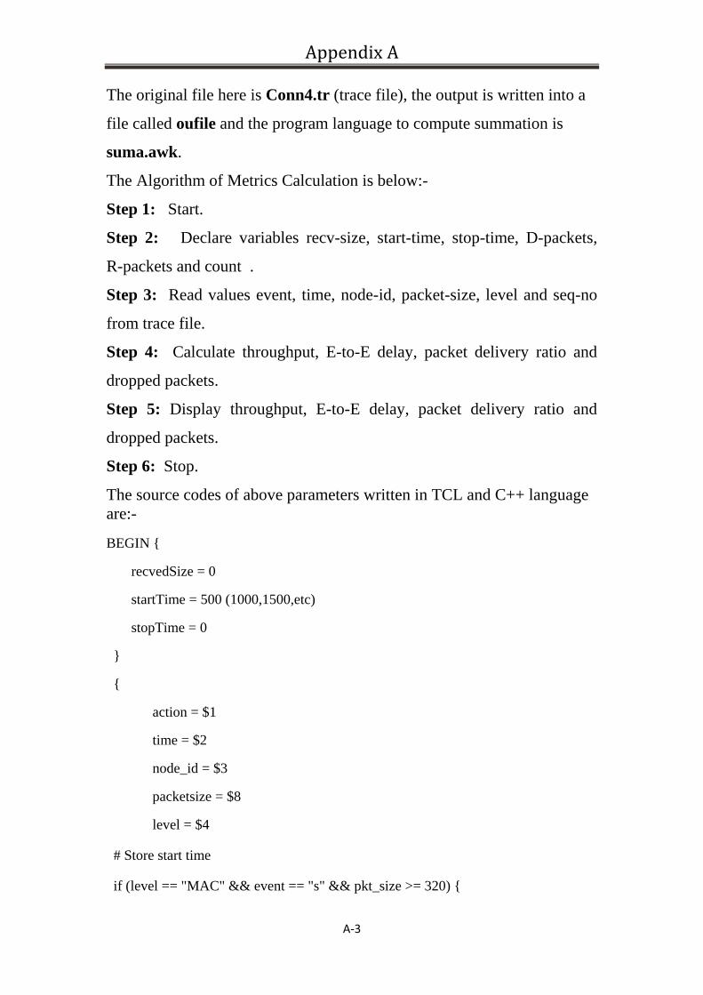
Appendix A
3A-
The original file here is Conn4.tr (trace file), the output is written into a
file called oufile and the program language to compute summation is
suma.awk.
The Algorithm of Metrics Calculation is below:-
Step 1: Start.
Step 2: Declare variables recv-size, start-time, stop-time, D-packets,
R-packets and count .
Step 3: Read values event, time, node-id, packet-size, level and seq-no
from trace file.
Step 4: Calculate throughput, E-to-E delay, packet delivery ratio and
dropped packets.
Step 5: Display throughput, E-to-E delay, packet delivery ratio and
dropped packets.
Step 6: Stop.
The source codes of above parameters written in TCL and C++ language are:-
BEGIN {
recvedSize = 0
startTime = 500 (1000,1500,etc)
stopTime = 0
}
{
action = $1
time = $2
node_id = $3
packetsize = $8
level = $4
# Store start time
if (level == "MAC" && event == "s" && pkt_size >= 320) {
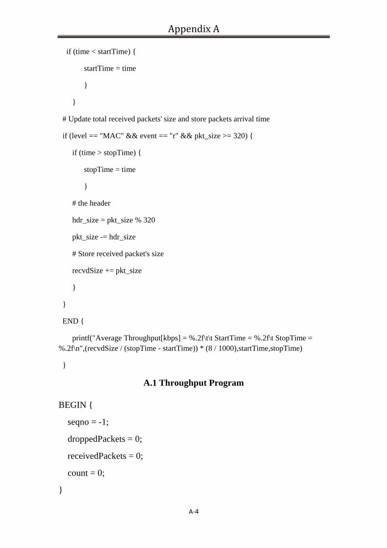
Appendix A
4A-
if (time < startTime) {
startTime = time
}
}
# Update total received packets' size and store packets arrival time
if (level == "MAC" && event == "r" && pkt_size >= 320) {
if (time > stopTime) {
stopTime = time
}
# the header
hdr_size = pkt_size % 320
pkt_size -= hdr_size
# Store received packet's size
recvdSize += pkt_size
}
}
END {
printf("Average Throughput[kbps] = %.2f\t\t StartTime = %.2f\t StopTime = %.2f\n",(recvdSize / (stopTime - startTime)) * (8 / 1000),startTime,stopTime)
}
A.1 Throughput Program
BEGIN {
seqno = -1;
droppedPackets = 0;
receivedPackets = 0;
count = 0;
}
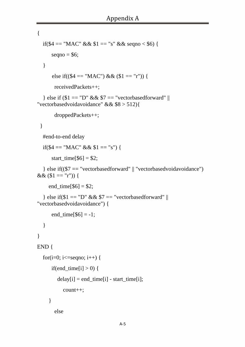
Appendix A
5A-
{
if($4 == "MAC" && $1 == "s" && seqno < $6) {
seqno = $6;
}
else if(($4 == "MAC") && ($1 == "r")) {
receivedPackets++;
} else if ($1 == "D" && $7 == "vectorbasedforward" || "vectorbasedvoidavoidance" && $8 > 512){
droppedPackets++;
}
#end-to-end delay
if($4 == "MAC" && $1 == "s") {
start_time[$6] = $2;
} else if(($7 == "vectorbasedforward" || "vectorbasedvoidavoidance") && ($1 == "r")) {
end_time[$6] = $2;
} else if($1 == "D" && $7 == "vectorbasedforward" || "vectorbasedvoidavoidance") {
end_time[$6] = -1;
}
}
END {
for(i=0; i<=seqno; i++) {
if(end_time[i] > 0) {
delay[i] = end_time[i] - start_time[i];
count++;
}
else
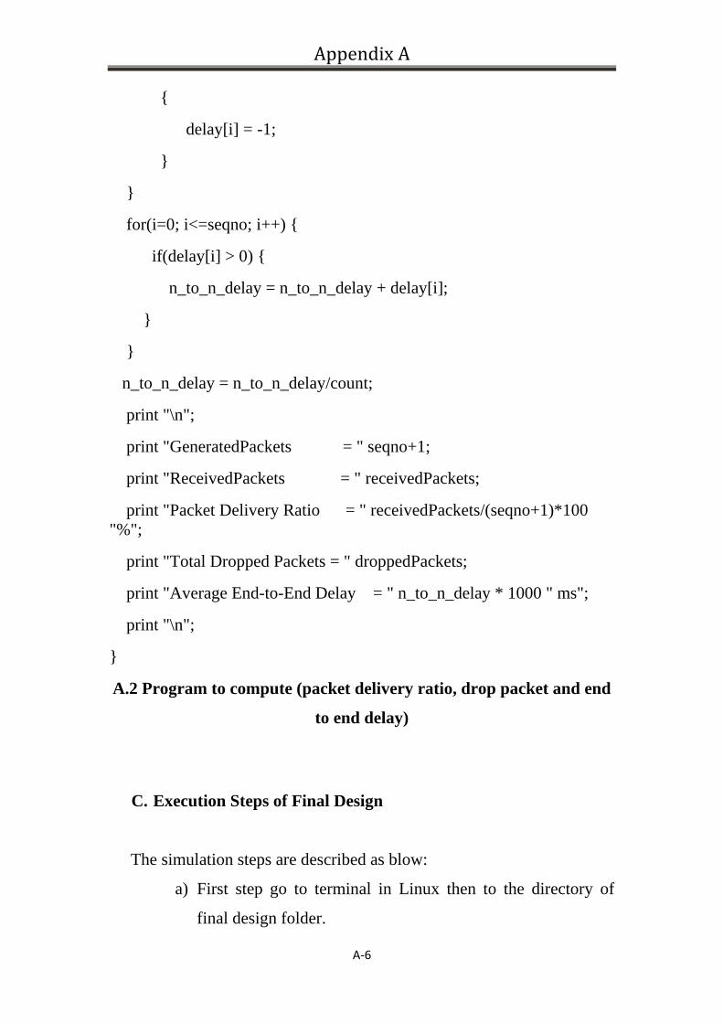
Appendix A
6A-
{
delay[i] = -1;
}
}
for(i=0; i<=seqno; i++) {
if(delay[i] > 0) {
n_to_n_delay = n_to_n_delay + delay[i];
}
}
n_to_n_delay = n_to_n_delay/count;
print "\n";
print "GeneratedPackets = " seqno+1;
print "ReceivedPackets = " receivedPackets;
print "Packet Delivery Ratio = " receivedPackets/(seqno+1)*100 "%";
print "Total Dropped Packets = " droppedPackets;
print "Average End-to-End Delay = " n_to_n_delay * 1000 " ms";
print "\n";
}
A.2 Program to compute (packet delivery ratio, drop packet and end
to end delay)
C. Execution Steps of Final Design
The simulation steps are described as blow:
a) First step go to terminal in Linux then to the directory of
final design folder.
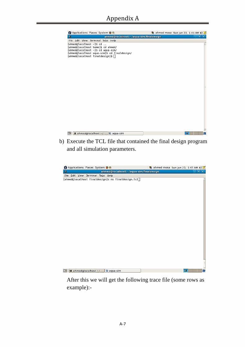
Appendix A
7A-
b) Execute the TCL file that contained the final design program and all simulation parameters.
After this we will get the following trace file (some rows as example):-
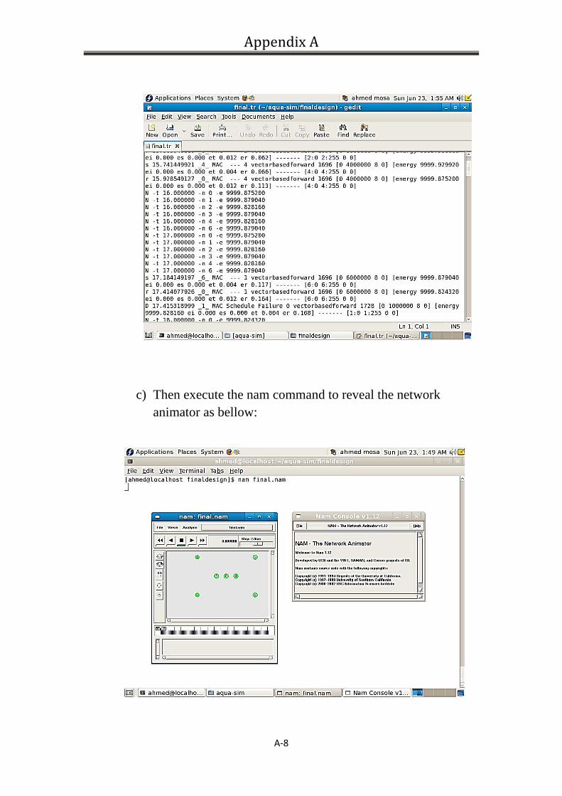
Appendix A
8A-
c) Then execute the nam command to reveal the network animator as bellow:
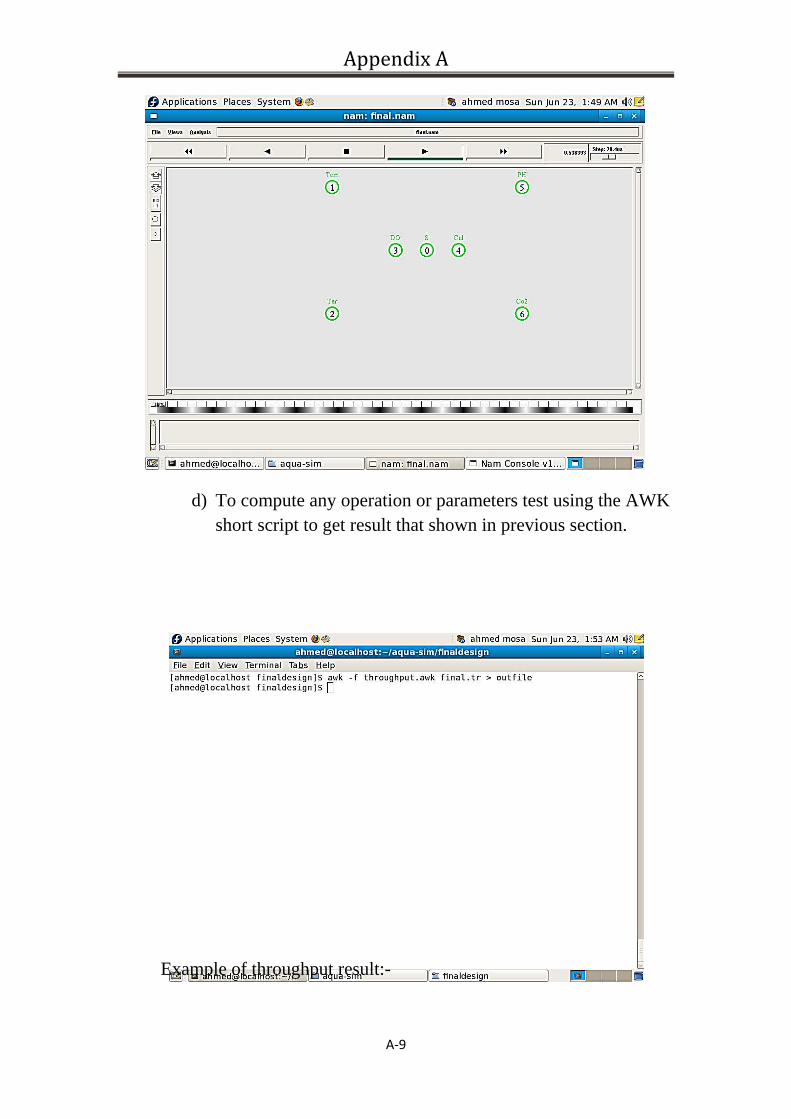
Appendix A
9A-
d) To compute any operation or parameters test using the AWK short script to get result that shown in previous section.
Example of throughput result:-
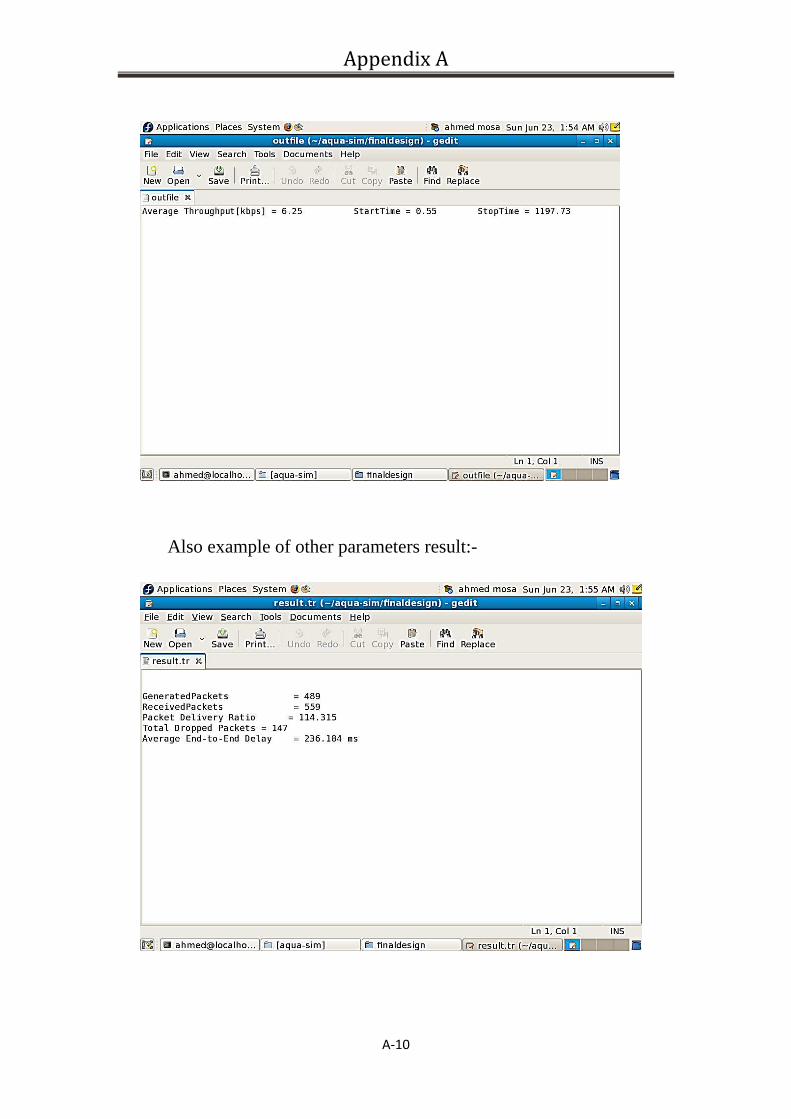
Appendix A
10A-
Also example of other parameters result:-
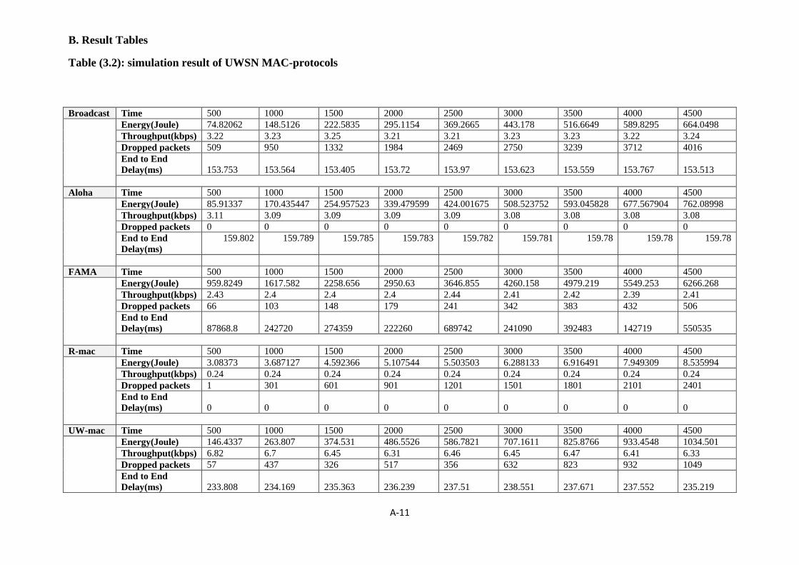
B. Result Tables
Table (3.2): simulation result of UWSN MAC-protocols
11A-
Broadcast Time 500 1000 1500 2000 2500 3000 3500 4000 4500 Energy(Joule) 74.82062 148.5126 222.5835 295.1154 369.2665 443.178 516.6649 589.8295 664.0498
Throughput(kbps) 3.22 3.23 3.25 3.21 3.21 3.23 3.23 3.22 3.24 Dropped packets 509 950 1332 1984 2469 2750 3239 3712 4016 End to End Delay(ms) 153.753 153.564 153.405 153.72 153.97 153.623 153.559 153.767 153.513
Aloha Time 500 1000 1500 2000 2500 3000 3500 4000 4500 Energy(Joule) 85.91337 170.435447 254.957523 339.479599 424.001675 508.523752 593.045828 677.567904 762.08998
Throughput(kbps) 3.11 3.09 3.09 3.09 3.09 3.08 3.08 3.08 3.08 Dropped packets 0 0 0 0 0 0 0 0 0 End to End Delay(ms)
159.802 159.789 159.785 159.783 159.782 159.781 159.78 159.78 159.78
FAMA Time 500 1000 1500 2000 2500 3000 3500 4000 4500 Energy(Joule) 959.8249 1617.582 2258.656 2950.63 3646.855 4260.158 4979.219 5549.253 6266.268
Throughput(kbps) 2.43 2.4 2.4 2.4 2.44 2.41 2.42 2.39 2.41 Dropped packets 66 103 148 179 241 342 383 432 506 End to End Delay(ms) 87868.8 242720 274359 222260 689742 241090 392483 142719 550535
R-mac Time 500 1000 1500 2000 2500 3000 3500 4000 4500 Energy(Joule) 3.08373 3.687127 4.592366 5.107544 5.503503 6.288133 6.916491 7.949309 8.535994
Throughput(kbps) 0.24 0.24 0.24 0.24 0.24 0.24 0.24 0.24 0.24 Dropped packets 1 301 601 901 1201 1501 1801 2101 2401 End to End Delay(ms) 0 0 0 0 0 0 0 0 0
UW-mac Time 500 1000 1500 2000 2500 3000 3500 4000 4500 Energy(Joule) 146.4337 263.807 374.531 486.5526 586.7821 707.1611 825.8766 933.4548 1034.501
Throughput(kbps) 6.82 6.7 6.45 6.31 6.46 6.45 6.47 6.41 6.33 Dropped packets 57 437 326 517 356 632 823 932 1049 End to End Delay(ms) 233.808 234.169 235.363 236.239 237.51 238.551 237.671 237.552 235.219
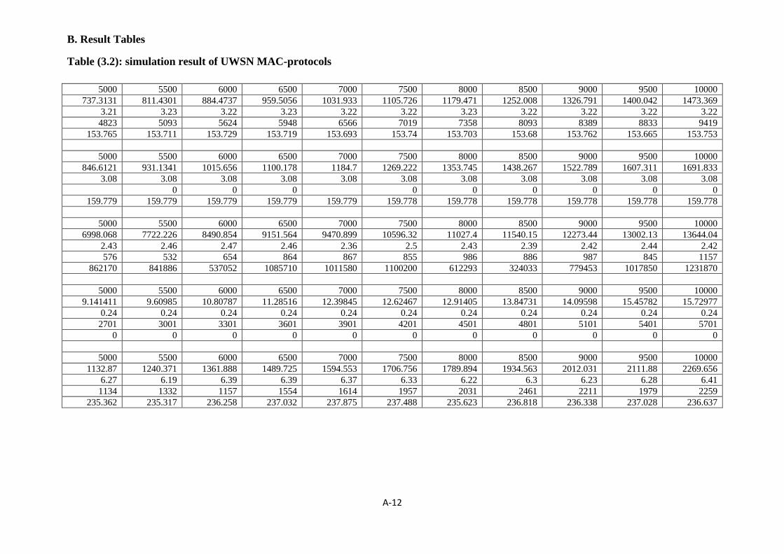
B. Result Tables
Table (3.2): simulation result of UWSN MAC-protocols
12A-
5000 5500 6000 6500 7000 7500 8000 8500 9000 9500 10000 737.3131 811.4301 884.4737 959.5056 1031.933 1105.726 1179.471 1252.008 1326.791 1400.042 1473.369
3.21 3.23 3.22 3.23 3.22 3.22 3.23 3.22 3.22 3.22 3.22 4823 5093 5624 5948 6566 7019 7358 8093 8389 8833 9419
153.765 153.711 153.729 153.719 153.693 153.74 153.703 153.68 153.762 153.665 153.753
5000 5500 6000 6500 7000 7500 8000 8500 9000 9500 10000 846.6121 931.1341 1015.656 1100.178 1184.7 1269.222 1353.745 1438.267 1522.789 1607.311 1691.833
3.08 3.08 3.08 3.08 3.08 3.08 3.08 3.08 3.08 3.08 3.08 0 0 0 0 0 0 0 0 0
159.779 159.779 159.779 159.779 159.779 159.778 159.778 159.778 159.778 159.778 159.778
5000 5500 6000 6500 7000 7500 8000 8500 9000 9500 10000 6998.068 7722.226 8490.854 9151.564 9470.899 10596.32 11027.4 11540.15 12273.44 13002.13 13644.04
2.43 2.46 2.47 2.46 2.36 2.5 2.43 2.39 2.42 2.44 2.42 576 532 654 864 867 855 986 886 987 845 1157
862170 841886 537052 1085710 1011580 1100200 612293 324033 779453 1017850 1231870
5000 5500 6000 6500 7000 7500 8000 8500 9000 9500 10000 9.141411 9.60985 10.80787 11.28516 12.39845 12.62467 12.91405 13.84731 14.09598 15.45782 15.72977
0.24 0.24 0.24 0.24 0.24 0.24 0.24 0.24 0.24 0.24 0.24 2701 3001 3301 3601 3901 4201 4501 4801 5101 5401 5701
0 0 0 0 0 0 0 0 0 0 0
5000 5500 6000 6500 7000 7500 8000 8500 9000 9500 10000 1132.87 1240.371 1361.888 1489.725 1594.553 1706.756 1789.894 1934.563 2012.031 2111.88 2269.656
6.27 6.19 6.39 6.39 6.37 6.33 6.22 6.3 6.23 6.28 6.41 1134 1332 1157 1554 1614 1957 2031 2461 2211 1979 2259
235.362 235.317 236.258 237.032 237.875 237.488 235.623 236.818 236.338 237.028 236.637
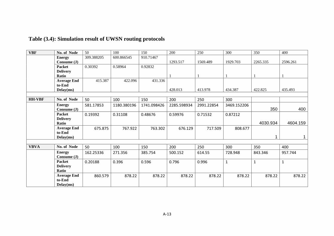
13A-
Table (3.4): Simulation result of UWSN routing protocols
VBF No. of Node 50 100 150 200 250 300 350 400 Energy
Consume (J) 309.388205 600.866545 910.71467
1293.517 1569.489 1929.703 2265.335 2596.261 Packet Delivery Ratio
0.30392 0.58964 0.92832
1 1 1 1 1 Average End to-End Delay(ms)
415.387 422.096 431.336
428.013 413.978 434.387 422.825 435.493 HH-VBF No. of Node 50 100 150 200 250 300 Energy
Consume (J) 581.17853 1180.380196 1741.098426 2285.598934 2991.22854 3469.152206
350 400 Packet Delivery Ratio
0.19392 0.31108 0.48676 0.59976 0.71532 0.87212
4030.934 4604.159 Average End to-End Delay(ms)
675.875 767.922 763.302 676.129 717.509 808.677
1 1 VBVA No. of Node 50 100 150 200 250 300 350 400
Energy Consume (J)
162.25336 271.356 385.754 500.152 614.55 728.948 843.346 957.744
Packet Delivery Ratio
0.20188 0.396 0.596 0.796 0.996 1 1 1
Average End to-End Delay(ms)
860.579 878.22 878.22 878.22 878.22 878.22 878.22 878.22
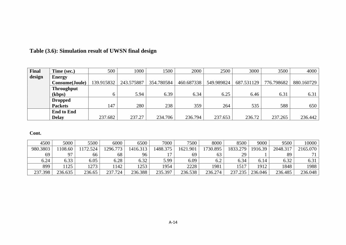
14A-
Table (3.6): Simulation result of UWSN final design
Final design
Time (sec.) 500 1000 1500 2000 2500 3000 3500 4000 Energy Consume(Joule) 139.915832 243.575887 354.780584 460.687338 549.989824 687.531129 776.798682 880.160729 Throughput (kbps) 6 5.94 6.39 6.34 6.25 6.46 6.31 6.31 Dropped Packets 147 280 238 359 264 535 588 650
End to End Delay 237.682 237.27 234.706 236.794 237.653 236.72 237.265 236.442
Cont.
4500 5000 5500 6000 6500 7000 7500 8000 8500 9000 9500 10000 980.3803
69 1108.60
97 1172.524
66 1296.773
68 1416.313
96 1488.375
17 1621.901
69 1730.895
63 1833.279
29 1916.39
1 2048.317
89 2165.070
71 6.24 6.33 6.05 6.28 6.32 5.99 6.09 6.2 6.34 6.14 6.32 6.31 899 1125 1273 1142 1253 1954 2228 1981 1517 1912 1848 1988
237.398 236.635 236.65 237.724 236.388 235.397 236.538 236.274 237.235 236.046 236.485 236.048
Appendix B
15B-
Publication arises from project
1. Mohammed N. and Ahmed M. "Performance Assessment of MAC
Layer Protocols Based on Underwater Wireless Sensor Networks ",
Journal of Global Research in Computer Science, Volume 4, No. 3,
March 2013.
2. Mohammed N. and Ahmed M. " Comparative Study of Routing
Protocols in Pollution Monitoring System Based on Underwater
Wireless Sensor Networks " Oriental Journal of Computer Since &
Technology, Vol. 6, No. 2, June 2013
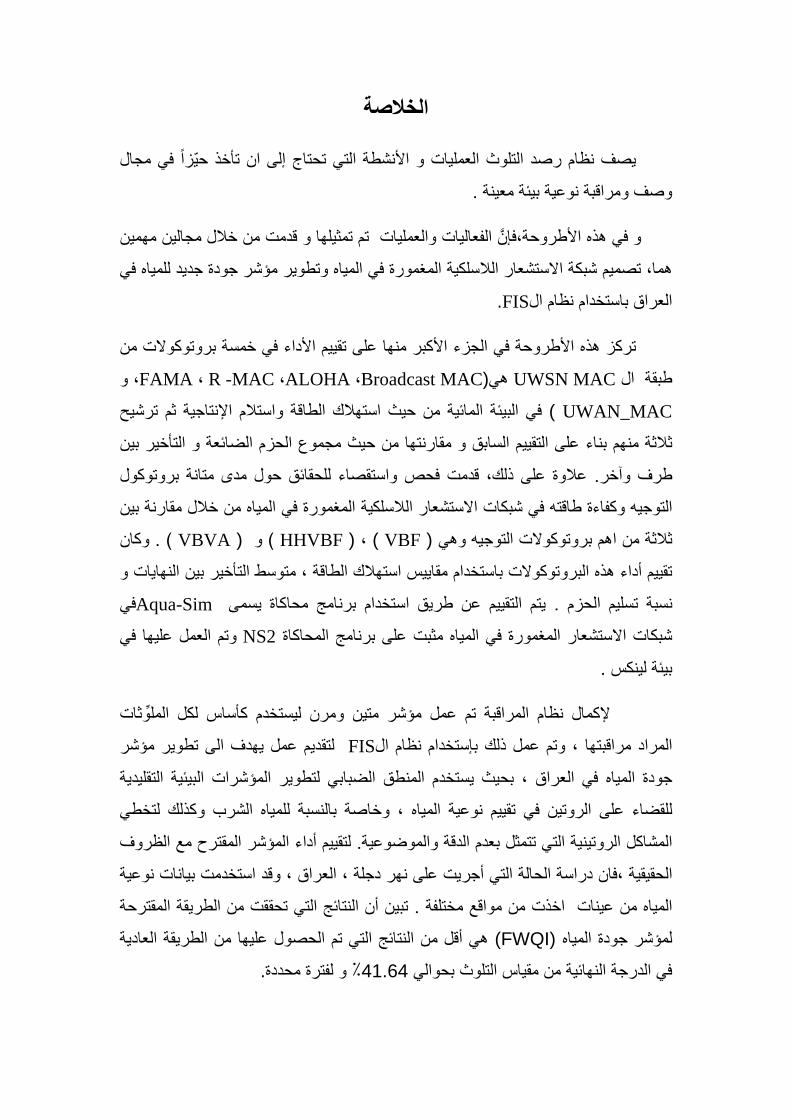
الخالصة
إلى ان تأخذ حيزا في مجالنشطة التي تحتاج يصف نظام رصد التلوث العمليات و األ
نوعية بيئة معينة .مراقبة و وصف
مجالين مهمين خاللو قدمت من تم تمثيلها العمليات الفعاليات و ،فإن في هذه األطروحة و
في جديد للمياه مؤشر جودة تطويروفي المياه مغمورةال، تصميم شبكة االستشعار الالسلكية هما
.FISراق باستخدام نظام الالع
من بروتوكوالتخمسة فياألكبر منها على تقييم األداء الجزء فيتركز هذه األطروحة
، و Broadcast MAC ،ALOHA ،R -MAC ،FAMA(هي UWSN MACال طبقة
UWAN_MAC ( اإلنتاجية ثم ترشيح استالمحيث استهالك الطاقة وئية من البيئة المافي
التأخير بين و الضائعة الحزم مجموعم السابق و مقارنتها من حيث ثالثة منهم بناء على التقيي
بروتوكول دى متانةللحقائق حول م فحص واستقصاء. عالوة على ذلك، قدمت طرف وآخر
من خالل مقارنة بين المغمورة في المياه ت االستشعار الالسلكيةفي شبكا تهطاق كفاءةوالتوجيه
) . وكان VBVA( ) و VBF (، )HHVBF( وهيالتوجيه تبروتوكوالمن اهم ثالثة
و بين النهايات التأخير تقييم أداء هذه البروتوكوالت باستخدام مقاييس استهالك الطاقة ، متوسط
في Aqua-Sim برنامج محاكاة يسمى . يتم التقييم عن طريق استخدام نسبة تسليم الحزم
في وتم العمل عليها NS2المحاكاة مثبت على برنامج المغمورة في المياهشبكات االستشعار
بيئة لينكس .
ثات لمراقبةإلكمال نظام ا تم عمل مؤشر متين ومرن ليستخدم كأساس لكل الملو
الى تطوير مؤشر فيهدلتقديم عمل FISالوتم عمل ذلك بإستخدام نظام ، المراد مراقبتها
التقليدية بيئيةالمؤشرات ال بحيث يستخدم المنطق الضبابي لتطويرالعراق ، المياه في جودة
وكذلك لتخطي مياه الشرب نوعية المياه ، وخاصة بالنسبة لل للقضاء على الروتين في تقييم
قترح مع الظروف الم. لتقييم أداء المؤشر التي تتمثل بعدم الدقة والموضوعية المشاكل الروتينية
يانات نوعية ، العراق ، وقد استخدمت ب نهر دجلةسة الحالة التي أجريت على درا ،فانالحقيقية
الطريقة المقترحة من تحققت التي النتائج أن تبينمختلفة . قع ااخذت من مو ت المياه من عينا
العادية طريقةال من عليها الحصول تم التي النتائج من أقل هي) FWQI( المياه جودة لمؤشر
.محددة لفترةو ٪ 41.64 بحوالي التلوثمقياس من النهائية الدرجة في

وزارة التعليم العالي والبحث العلمي
الجامعة التكنولوجة
قسم هندسة الحاسوب
رســـالة
كجزء قسم هندسة الحاسوب في الجامعة التكنولوجيةمقدمة الى
الحاسوبفي هندسة علومماجستيرال شهادةمن متطلبات نيل
من قبل
احمد موسى ديناراحمد موسى دينار
)2007(بكالوريوس
بإشراف
األستاذ المساعد الدكتور محمد نجم عبدهللا
1435محرم تشرين الثاني 2013
على على في االنهار العراقيةفي االنهار العراقية التلوثالتلوث مراقبةمراقبةنظام نظام المغمورة في المغمورة في تشعار الالسلكية تشعار الالسلكية أساس شبكات االسأساس شبكات االس
الماءالماء


