BioMed CentralBMC Health Services Research

ss

Open AcceResearch articleIs there much variation in variation? Revisiting statistics of small area variation in health services researchBerta Ibáñez1,2, Julián Librero3, Enrique Bernal-Delgado*3, Salvador Peiró4,3, Beatriz González López-Valcarcel5, Natalia Martínez3 and Felipe Aizpuru6,2

Address: 1Fundación Vasca de Innovación e Investigación Sanitarias (BIOEF), Bilbao, Spain, 2CIBER Epidemiología y Salud Pública (CIBERESP), Spain, 3Instituto Aragonés de Ciencias de la Salud (IACS), Zaragoza, Spain, 4Centro Superior de Investigaciones en Salud Pública (CSISP), Conselleria de Sanitat, Valencia, Spain, 5Departamento de Métodos Cuantitativos, Universidad de Las Palmas de Gran Canaria, Las Palmas, Spain and 6Unidad de Investigación, Hospital Txagorritxu, Vitoria, Spain

Email: Berta Ibáñez - ibanez@bioef.org; Julián Librero - julian.librero@uv.es; Enrique Bernal-Delgado* - ebernal.iacs@aragon.es; Salvador Peiró - peiro_bor@gva.es; Beatriz González López-Valcarcel - bvalcarcel@dmc.ulpgc.es; Natalia Martínez - nmartinez.iacs@aragon.es; Felipe Aizpuru - faizpuru@htxa.osakidetza.net

* Corresponding author

AbstractBackground: The importance of Small Area Variation Analysis for policy-making contrasts withthe scarcity of work on the validity of the statistics used in these studies. Our study aims at 1)determining whether variation in utilization rates between health areas is higher than would beexpected by chance, 2) estimating the statistical power of the variation statistics; and 3) evaluatingthe ability of different statistics to compare the variability among different procedures regardlessof their rates.

Methods: Parametric bootstrap techniques were used to derive the empirical distribution for eachstatistic under the hypothesis of homogeneity across areas. Non-parametric procedures were usedto analyze the empirical distribution for the observed statistics and compare the results in sixsituations (low/medium/high utilization rates and low/high variability). A small scale simulation studywas conducted to assess the capacity of each statistic to discriminate between different scenarioswith different degrees of variation.

Results: Bootstrap techniques proved to be good at quantifying the difference between the nullhypothesis and the variation observed in each situation, and to construct reliable tests andconfidence intervals for each of the variation statistics analyzed. Although the good performanceof Systematic Component of Variation (SCV), Empirical Bayes (EB) statistic shows better behaviourunder the null hypothesis, it is able to detect variability if present, it is not influenced by theprocedure rate and it is best able to discriminate between different degrees of heterogeneity.

Conclusion: The EB statistics seems to be a good alternative to more conventional statistics usedin small-area variation analysis in health service research because of its robustness.

Published: 2 April 2009

BMC Health Services Research 2009, 9:60 doi:10.1186/1472-6963-9-60

Received: 15 September 2008Accepted: 2 April 2009

This article is available from: http://www.biomedcentral.com/1472-6963/9/60

© 2009 Ibáñez et al; licensee BioMed Central Ltd. This is an Open Access article distributed under the terms of the Creative Commons Attribution License (http://creativecommons.org/licenses/by/2.0), which permits unrestricted use, distribution, and reproduction in any medium, provided the original work is properly cited.

Page 1 of 12(page number not for citation purposes)

BMC Health Services Research 2009, 9:60 http://www.biomedcentral.com/1472-6963/9/60

BackgroundSmall Area Variation Analysis (SAVA) is a method used inhealth services research to describe how rates of health-care utilization vary across geographic areas [1]. While uti-lization rates can be calculated to summarize non-binaryevents (hospital days, costs), they are usually computed torepresent counts (procedures, hospital admissions). Stud-ies based on SAVA have documented dramatic variationsacross areas in the use of medical and surgical procedures,showing that the amount and type of medical care that theindividuals of a population receive depend on where theylive. The principal finding of these studies remainsunchanged: for medical care, geography is destiny [2].SAVA methods are, thus, used extensively to characterizemedical care, assuming that high variability conditionsare associated with higher uncertainty and supply-sensi-tive care [3], and Wennberg constructed an influentialgeneral theory describing how to detect physician uncer-tainty from the variation in small area analysis [4].

The importance of these studies in terms of their impacton policy-making contrasts with the dearth of work test-ing the validity of the SAVA statistics themselves. Very lit-tle has been done to determine whether higher thanrandomly expected variability across areas is in factdetected, or whether certain procedures are more variablethan others [5-12]. Not surprisingly, statistical analysis ofarea variations in health service research is often informal,consisting of plots and maps illustrating admission or sur-gery rates by healthcare area, and statistics with importantstatistical limitations [13,14].

Two groups of statistics of variation are commonly used:those that describe the distribution of rates (based onstandardization by direct method) and those that use dif-ferences between expected and observed cases (based onindirect standardization). Statistics among the formerusually include the high-low ratio or extremal quotient(EQ, maximum rate divided by minimum rate) [5,7], andthe unweighted (CV) and weighted (CVw) coefficients ofvariation.[7] Among the latter, the systematic componentof variation (SCV) proposed by McPherson et al, [15] andthe chi-squared statistic (χ2) [7,10] are the most fre-quently used. Through simulations studies, these statisticshave been shown to be sensitive to specific characteristics,such as the prevalence of the procedure or condition, thepossibility of multiple admissions, the number of areasconsidered, and the population size of small areas [7].Simulation studies have also shown that the expected var-iation, when the hypothesis of homogeneity in rates istrue, can be surprisingly large; especially, in low-incidenceprocedures or when readmissions are frequent [8]. There-fore, it is important to assess how far variation estimatesare from the null hypothesis, and how precise the statisticsare in each particular situation.

Several studies conducted by Diehr and her colleagues,including work assessing the power of the tests applied[9], the effect of multiple admissions [10], and the com-parison of variability between procedures [11], have con-tributed extraordinarily to the advance in SAVAmethodology. Nevertheless, these authors were "unable torecommend a single good descriptive for small-area analysis"[8]. Additionally, SAVA statistics methodology has stilllimitations. The simulation procedure constructed byDiehr et al did not take into account the well-known ageand sex variability of most health conditions (althoughthese authors developed an interesting approach in oneappendix) [7]. On the other hand, it is important to studynot only the behaviour of the statistics under the nullhypothesis along with their power, but also to evaluatetheir capacity to discriminate between procedures withdifferent variability. Finally, Diehr carried out the analysesusing a setting with a small number of geographic areas,and where utilization rates were several times higher thanthe usual rates observed in the Spanish context.

Our work has pursued three objectives: 1) to determinewhether variation in rates between areas is higher thanwould be expected by chance, complementing the studyunder the null hypothesis of homogeneity by constructingconfidence intervals for the observed statistics based onnon-parametric bootstrap techniques; 2) to estimate thepower of the variation statistics; and 3) to evaluate theability of different statistics to compare variability amongprocedures regardless of their rates. Additionally, weextended the simulation procedure to other barely usedstatistics, such as the empirical Bayes (EB) statistic, thatwas first proposed in this context by Shwartz et al.[12].The EB focuses on estimating rates rather than on testingsignificance, and the model underlying this statistic hasbeen applied in some SAVA papers [16,17]. We also con-sidered the Dean (DT) [18], and Bohning statistics (BT)[19], which have been used to test if geographical varia-tion in rates is larger than that assumed under homogene-ity in mortality studies [20], but have not been applied yetin health-services research variation analysis.

MethodsDatabase, small geographic areas and procedures under studyWe used data from the Atlas of Variations in Medical Prac-tice in the Spanish National Health System (NHS) [21], aresearch project designed to inform Spanish decision-makers on differences in such parameters as hospitaladmissions or surgery for specific conditions across geo-graphic areas (see: http://www.atlasvpm.org). The Span-ish Atlas emulates the Dartmouth Atlas of Health CareProject [22]. Hospital Discharge Administrative Databasesin 2002 (calendar year), with additional data from ambu-latory surgery registries, were used to build the numerator

Page 2 of 12(page number not for citation purposes)

BMC Health Services Research 2009, 9:60 http://www.biomedcentral.com/1472-6963/9/60

of the rates. These administrative databases, produced byevery acute care hospital in the Spanish NHS, provide thefollowing information from every single admission: age,sex, admission and discharge dates, diagnosis and proce-dure codes [International Classification of Diseases 9th

revision Clinical Modification codes (ICD9CM)], andpostal codes identifying the patient's area of residence.This latter was used to assign every patient admitted in ahospital to the Healthcare Area in which he lives.

Denominators to calculate population rates came fromthe Municipal Register of Inhabitants of the SpanishNational Institute of Statistics' for 2002. The small geo-graphic areas used corresponded to the "HealthcareAreas" defined by the Health Departments of the 14Autonomous Regions which participated in the AtlasProject. In total, 147 areas including 75% of the 2002Spanish population were used. Table 1 shows the popula-tion distribution across the Healthcare Areas: 27% of thecountry's Healthcare areas had less than 100,000 peopleand only 4% had over a million.

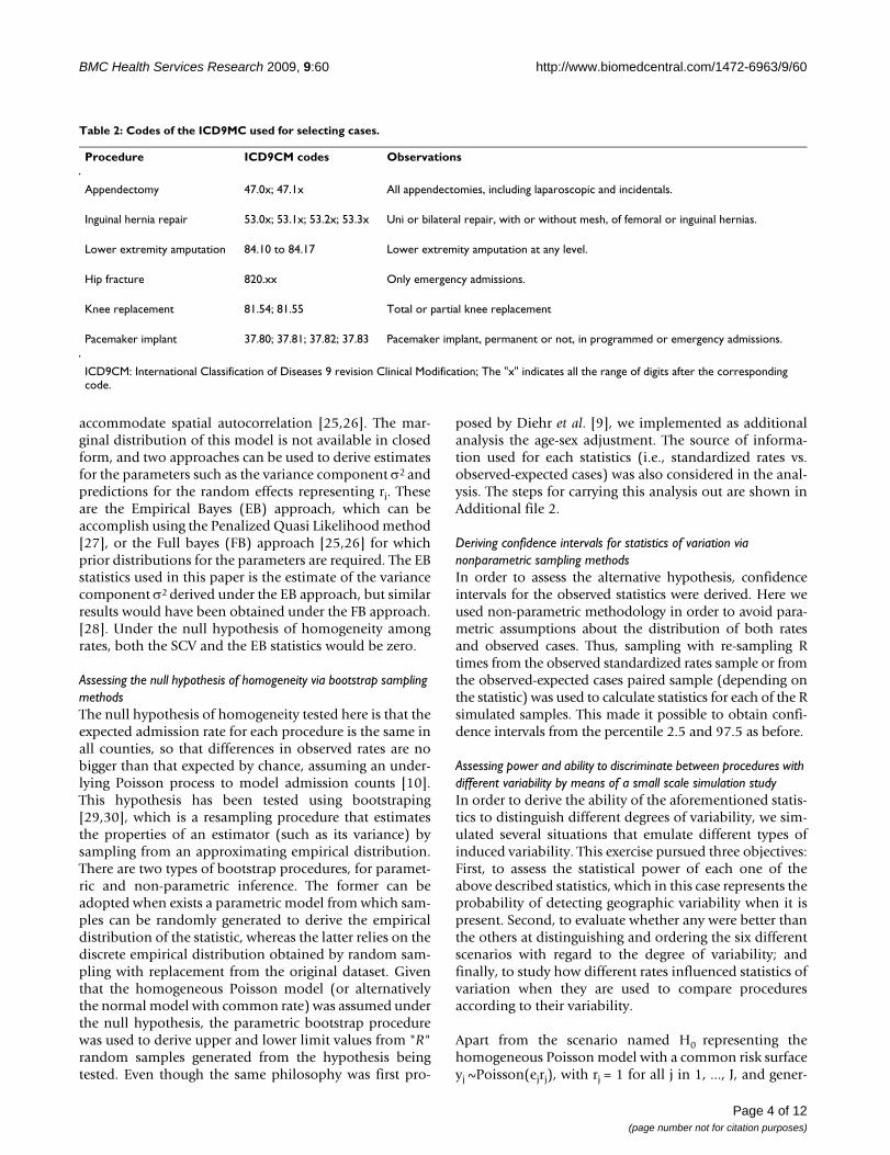
We chose six procedures (pacemakers implant, appendec-tomy, admission for hip fracture, lower extremity amputa-tion, inguinal hernia repair and knee replacement) takinginto account both their utilization rate and their variabil-ity. We labelled them as low or high-variation procedures,and as performed at high, medium or low utilization rate.This classification was carried using as reference the wholeset of procedures analyzed in the Spanish Atlas project,which add up a total of 35. Hence, by combining the twodimensions, we were able to reproduce six different situa-tions that embrace all of the major cases concerning SAVAstudies. ICD9CM codes and inclusion criteria for definingnumerators are shown in Table 2.

AnalysisExtremal Quotient [7], Coefficient of Variation [7],Weighted Coefficient of Variation [11], Systematic Com-

ponent of Variation [15], Empirical Bayes variance com-ponent [12], χ2 statistic [11], Dean statistic [18], andBohning statistic [19] were all studied. Because some ofthe Spanish Atlas' calculations exclude the 5% of extremestandardized rates for each tie [21], we have also elimi-nated the outliers beyond of the 5–95 percentiles, andlabelled our statistics as EQ5–95, CV5–95; CVW5–95 andSCV5–95. The formulation of the statistics is given in Addi-tional file 1. The EQ, CV and CVw use direct age-standard-ized rates for each i-th Healthcare Area, denoted by DSRifor i = 1, ..., I, and all three are well-known measures ofvariation in general contexts. The remaining statistics usethe observed and expected cases per area, denoted by yiand ei respectively. These expected cases were derivedbased on the age-specific rate for 8 groups (0–24, 25–44,45–64, 65–69, 70–74, 75–79, 80–84, 85 years and over)and the sex stratum in the standard population, whichwas the population from the 147 healthcare areas understudy. More precisely, ei = ∑j, knijk Rjk, where nijk is the pop-ulation in area i, age group j and sex stratum k, and Rjk isthe age-sex specific rate for the whole region under study.Hence, the quotient of the observed to the expectednumber of cases is the indirect Standardized UtilizationRatio, SURi = yi/ei for the i-th Healthcare Area. This quo-tient is in fact the maximum-likelihood estimator of ri, theunknown relative risk of suffering a given surgical proce-dure in the area, under the assumption that yi ~Pois-son(eiri) independently for each i-th Health Area. ThePoisson distribution is frequently adopted because theBernoulli process at the individual level (surgery vs nonsurgery) becomes a Binomial process at the area level,which can be approximated by the Poisson distributionwhen rare events are modelled [10]. Hence, the nullhypothesis indicating an homogenous risk surface for thewhole region can be represented by the model yi~Pois-son(eir), with r the common risk. The X2, DT and BT ver-sions applied here were derived to detect heterogeneitywith respect to this homogeneous Poisson model. Finally,the SCV and the EB statistics are derived under a more gen-eral framework where the number of admissions per areais modelled hierarchically in a two-step procedure. Thefirst step assumes that, conditional on the risk ri, thenumber of counts yi follows a Poisson distribution, yi|ri~Poisson(eiri), whereas in the second one, heterogeneityin rates is modelled adopting a common distribution π forthe risk ri (or for its logarithm), ri~ π(r|θ), with θ the vectorof parameters of the density function. Whereas the deriva-tion of the SCV does not require a parametric form for π,as the SCV is precisely the moment estimator of the vari-ance in the distribution of π [15], the EB statistics is basedon the assumption that the log-relative risks are normallyand identically distributed, log(ri) ~N(μ, σ2). This lastmodel, called multivariate Poisson log-normal model orexchangeable model, is widely used in the disease map-ping literature [23,24], and can be easily extended to

Table 1: Population distribution of the geographical areas

Inhabitants Frequency Percentage

10,000 – 49,999 9 6.1%50,000 – 99,999 31 21.1%100,000 – 149,999 29 19.7%150,000 – 199,999 13 8.8%200,000 – 249,999 14 9.5%250,000 – 299,999 18 12.3%300,000 – 399,999 17 11.6%400,000 – 499,999 10 6.8%500,000 – 999,999 0 0.0%1,000,000 – 1,500,000 6 4.1%

Total 147 100%

Page 3 of 12(page number not for citation purposes)

BMC Health Services Research 2009, 9:60 http://www.biomedcentral.com/1472-6963/9/60

accommodate spatial autocorrelation [25,26]. The mar-ginal distribution of this model is not available in closedform, and two approaches can be used to derive estimatesfor the parameters such as the variance component σ2 andpredictions for the random effects representing ri. Theseare the Empirical Bayes (EB) approach, which can beaccomplish using the Penalized Quasi Likelihood method[27], or the Full bayes (FB) approach [25,26] for whichprior distributions for the parameters are required. The EBstatistics used in this paper is the estimate of the variancecomponent σ2 derived under the EB approach, but similarresults would have been obtained under the FB approach.[28]. Under the null hypothesis of homogeneity amongrates, both the SCV and the EB statistics would be zero.

Assessing the null hypothesis of homogeneity via bootstrap sampling methodsThe null hypothesis of homogeneity tested here is that theexpected admission rate for each procedure is the same inall counties, so that differences in observed rates are nobigger than that expected by chance, assuming an under-lying Poisson process to model admission counts [10].This hypothesis has been tested using bootstraping[29,30], which is a resampling procedure that estimatesthe properties of an estimator (such as its variance) bysampling from an approximating empirical distribution.There are two types of bootstrap procedures, for paramet-ric and non-parametric inference. The former can beadopted when exists a parametric model from which sam-ples can be randomly generated to derive the empiricaldistribution of the statistic, whereas the latter relies on thediscrete empirical distribution obtained by random sam-pling with replacement from the original dataset. Giventhat the homogeneous Poisson model (or alternativelythe normal model with common rate) was assumed underthe null hypothesis, the parametric bootstrap procedurewas used to derive upper and lower limit values from "R"random samples generated from the hypothesis beingtested. Even though the same philosophy was first pro-

posed by Diehr et al. [9], we implemented as additionalanalysis the age-sex adjustment. The source of informa-tion used for each statistics (i.e., standardized rates vs.observed-expected cases) was also considered in the anal-ysis. The steps for carrying this analysis out are shown inAdditional file 2.

Deriving confidence intervals for statistics of variation via nonparametric sampling methodsIn order to assess the alternative hypothesis, confidenceintervals for the observed statistics were derived. Here weused non-parametric methodology in order to avoid para-metric assumptions about the distribution of both ratesand observed cases. Thus, sampling with re-sampling Rtimes from the observed standardized rates sample or fromthe observed-expected cases paired sample (depending onthe statistic) was used to calculate statistics for each of the Rsimulated samples. This made it possible to obtain confi-dence intervals from the percentile 2.5 and 97.5 as before.

Assessing power and ability to discriminate between procedures with different variability by means of a small scale simulation studyIn order to derive the ability of the aforementioned statis-tics to distinguish different degrees of variability, we sim-ulated several situations that emulate different types ofinduced variability. This exercise pursued three objectives:First, to assess the statistical power of each one of theabove described statistics, which in this case represents theprobability of detecting geographic variability when it ispresent. Second, to evaluate whether any were better thanthe others at distinguishing and ordering the six differentscenarios with regard to the degree of variability; andfinally, to study how different rates influenced statistics ofvariation when they are used to compare proceduresaccording to their variability.

Apart from the scenario named H0 representing thehomogeneous Poisson model with a common risk surfaceyj ~Poisson(ejrj), with rj = 1 for all j in 1, ..., J, and gener-

Table 2: Codes of the ICD9MC used for selecting cases.

Procedure ICD9CM codes Observations

Appendectomy 47.0x; 47.1x All appendectomies, including laparoscopic and incidentals.

Inguinal hernia repair 53.0x; 53.1x; 53.2x; 53.3x Uni or bilateral repair, with or without mesh, of femoral or inguinal hernias.

Lower extremity amputation 84.10 to 84.17 Lower extremity amputation at any level.

Hip fracture 820.xx Only emergency admissions.

Knee replacement 81.54; 81.55 Total or partial knee replacement

Pacemaker implant 37.80; 37.81; 37.82; 37.83 Pacemaker implant, permanent or not, in programmed or emergency admissions.

ICD9CM: International Classification of Diseases 9 revision Clinical Modification; The "x" indicates all the range of digits after the corresponding code.

Page 4 of 12(page number not for citation purposes)

BMC Health Services Research 2009, 9:60 http://www.biomedcentral.com/1472-6963/9/60

ated as described in Additional file 2, six additional sce-narios with different degrees of variability were designed.The population structure was based on that observed inthe real geographical pattern with I = 147 areas, whereasthe expected counts were derived using the overall age-sexspecific rates for the most frequent (hip fracture) and theleast frequent (lower extremity amputation) procedure.While most of the regions were assumed to have homoge-neous rates, an artificially elevated risk was induced in arandomly selected group of areas. These was carried outusing two sources of additional variation: incrementingthe risks of the selected areas to rj = 1.2 (S1–S3) or rj = 1.6(S4–S6) (and equivalently their mean rates in 1.2p and1.6p respectively), and varying the number of these areaswith induced elevated risk, being 10 (S1 and S4), 20 (S2and S5), and 40 Healthcare Areas (S3 and S6) out of the147. Counts in all background areas (all but these 10, 20or 40 respectively) were generated from the null modelwith a common underlying rate aforementioned. Hence,the scenarios were numbered from the lowest to the high-est expected variability S1<S2<S3<S4<S5<S6.

Once the scenarios were designed, 2000 samples weresimulated from the null distribution following the proce-dure previously described and named H0. The criticalvalue of the tests was estimated using the 95-th percentileof the empirical distribution of the statistics, whereas con-fidence interval limits were obtained form the same distri-bution using percentiles 2.5 and 97.5. Another 2000samples were simulated from each scenario S1–S6, and theempirical distribution of the statistics was derived. Thisallowed us to obtain not only the empirical statisticalpower of the test for each scenario, by calculating the pro-portion of values greater than the critical values obtainedin H0 (the proportion of times that the null hypothesis issurpassed in each scenario), but also the confidence inter-vals for the statistics in each scenario using percentiles 2.5and 97.5 of the empirical distribution.

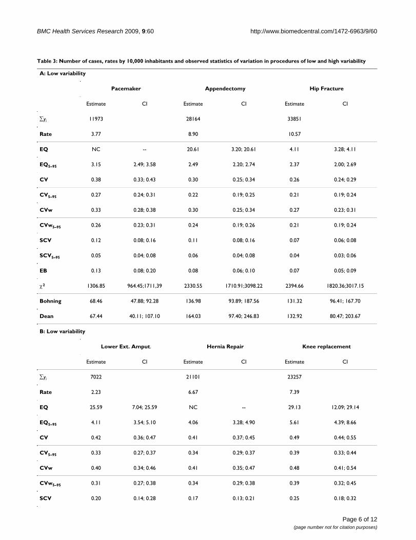
ResultsReal case study resultsTable 3 shows the rates and the observed statistics of vari-ation for the six procedures under study. Rates varied from3.77 pacemaker implants to 10.57 hip fracture admis-sions per 10,000 inhabitants in procedures presumed toshow low variation, and from 2.33 lower extremity ampu-tations to 7.39 knee replacements per 10,000 inhabitants,in procedures presumed to have high variation. We couldnot calculate the EQ for some of the procedures becausesome of the Healthcare Areas had 0 cases. For this reasonwe excluded the EQ (not the EQ5–95) from the simulationprocedures. The exclusion of 5% of outlying areas on eachside of the distribution notoriously reduced the value ofpractically all the statistics, including the SCV. Thisoccurred in procedures with low and high variation, notdepending on prevalence rates. Some statistics, such as the

χ2, and the Dean and Bohning tests, tended to have highervalues as the overall rate increases, regardless of the under-lying variability.

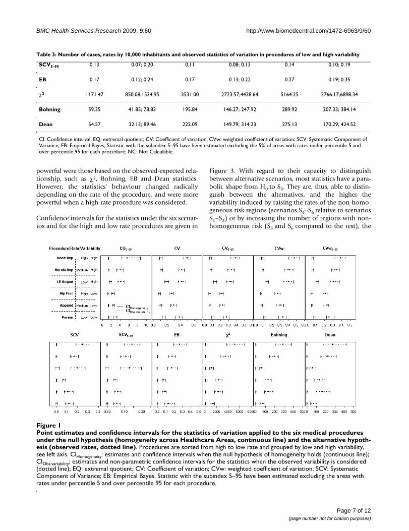
Figure 1 presents the point estimates for each procedure,together with the parametric confidence intervals whenthe null hypothesis of homogeneity holds (continuousline), and the non-parametric confidence intervals for theobserved statistic (dotted line). This figure shows thatunder the assumed null hypothesis, behaviour differsdepending on whether the statistics of variation are basedon rates (upper row) or on observed-expected cases (lowerrow). In particular, the former present wider confidenceintervals for the procedures with the lowest rates (lowerextremity amputation and pacemaker implant); further-more, they are "shifted to the right" for these procedures.In contrast, for those statistics based on the observed-expected cases, no apparent differences related with theunderlying rate are found, with the exception of the SCV,with a notably wider interval for the less frequent proce-dure. In these cases, the χ2, the Dean and the Bohning sta-tistics show narrow confidence intervals.

Regarding the observed variation, confidence intervals forthe observed statistics are wider than their null counter-parts, and these discrepancies in amplitude are higher inthe statistics based on the observed-expected comparisonsthan in the rate-based statistics. Of note is the agreementamong the statistics in detecting which is the most varia-ble procedure, all suggesting that knee replacement hasthe highest point and the widest confidence interval esti-mates, being very far removed from the null hypothesis.However, this agreement is not observed when trying toelucidate which procedure presents the lowest variability.While most statistics detect that admissions for hip frac-ture and appendectomy seem to have the lowest pointestimates, the χ2, Bohning and Dean tests suggest thatpacemaker implant or lower extremity amputation, thetwo procedures with the lowest rates, appear to have lowerpoint estimates than those obtained for the rest of the pro-cedures. Representing together confidence intervals of thestatistics and those obtained under homogeneity in thesame graph allows us to derive more reliable conclusionsregarding the underlying variability. Specifically, thecloser they are, the less probability for systematic variation(i.e., beyond chance). Note also that excluding the 5% ofextreme rates in some statistics seems negligible withregard to the comparison between null and observedintervals, because the expected variability depicted islower when excluding them both under the null hypothe-sis and under the observed variability.

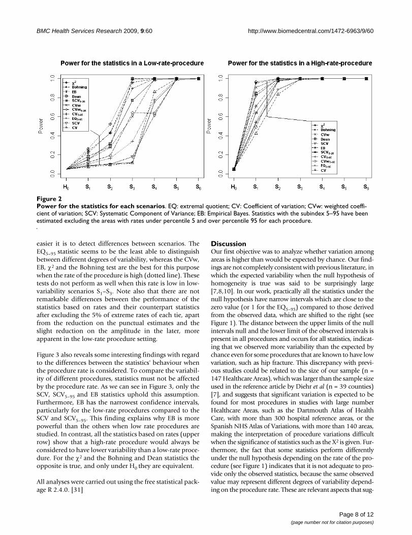
Small scale simulation study resultsThe empirical power of the statistics is presented in Figure2 for a high-rate (hip fracture) and a low-rate (lowerextremity amputation) procedure. In both cases, the most

Page 5 of 12(page number not for citation purposes)

BMC Health Services Research 2009, 9:60 http://www.biomedcentral.com/1472-6963/9/60

Table 3: Number of cases, rates by 10,000 inhabitants and observed statistics of variation in procedures of low and high variability

A: Low variability

Pacemaker Appendectomy Hip Fracture

Estimate CI Estimate CI Estimate CI

∑yi 11973 28164 33851

Rate 3.77 8.90 10.57

EQ NC -- 20.61 3.20; 20.61 4.11 3.28; 4.11

EQ5–95 3.15 2.49; 3.58 2.49 2.20; 2.74 2.37 2.00; 2.69

CV 0.38 0.33; 0.43 0.30 0.25; 0.34 0.26 0.24; 0.29

CV5–95 0.27 0.24; 0.31 0.22 0.19; 0.25 0.21 0.19; 0.24

CVw 0.33 0.28; 0.38 0.30 0.25; 0.34 0.27 0.23; 0.31

CVw5–95 0.26 0.23; 0.31 0.24 0.19; 0.26 0.21 0.19; 0.24

SCV 0.12 0.08; 0.16 0.11 0.08; 0.16 0.07 0.06; 0.08

SCV5–95 0.05 0.04; 0.08 0.06 0.04; 0.08 0.04 0.03; 0.06

EB 0.13 0.08; 0.20 0.08 0.06; 0.10 0.07 0.05; 0.09

χ2 1306.85 964.45;1711,39 2330.55 1710.91;3098.22 2394.66 1820.36;3017.15

Bohning 68.46 47.88; 92.28 136.98 93.89; 187.56 131.32 96.41; 167.70

Dean 67.44 40.11; 107.10 164.03 97.40; 246.83 132.92 80.47; 203.67

B: Low variability

Lower Ext. Amput. Hernia Repair Knee replacement

Estimate CI Estimate CI Estimate CI

∑yi 7022 21101 23257

Rate 2.23 6.67 7.39

EQ 25.59 7.04; 25.59 NC -- 29.13 12.09; 29.14

EQ5–95 4.11 3.54; 5.10 4.06 3.28; 4.90 5.61 4.39; 8.66

CV 0.42 0.36; 0.47 0.41 0.37; 0.45 0.49 0.44; 0.55

CV5–95 0.33 0.27; 0.37 0.34 0.29; 0.37 0.39 0.33; 0.44

CVw 0.40 0.34; 0.46 0.41 0.35; 0.47 0.48 0.41; 0.54

CVw5–95 0.31 0.27; 0.38 0.34 0.29; 0.38 0.39 0.32; 0.45

SCV 0.20 0.14; 0.28 0.17 0.13; 0.21 0.25 0.18; 0.32

Page 6 of 12(page number not for citation purposes)

BMC Health Services Research 2009, 9:60 http://www.biomedcentral.com/1472-6963/9/60

powerful were those based on the observed-expected rela-tionship, such as χ2, Bohning, EB and Dean statistics.However, the statistics' behaviour changed radicallydepending on the rate of the procedure, and were morepowerful when a high-rate procedure was considered.

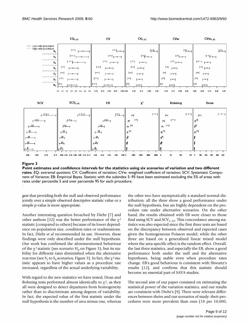
Confidence intervals for the statistics under the six scenar-ios and for the high and low rate procedures are given in

Figure 3. With regard to their capacity to distinguishbetween alternative scenarios, most statistics have a para-bolic shape from H0 to S6. They are, thus, able to distin-guish between the alternatives, and the higher thevariability induced by raising the rates of the non-homo-geneous risk regions (scenarios S4–S6 relative to scenariosS1–S3) or by increasing the number of regions with non-homogeneous risk (S3 and S6 compared to the rest), the

SCV5–95 0.13 0.07; 0.20 0.11 0.08; 0.13 0.14 0.10; 0.19

EB 0.17 0.12; 0.24 0.17 0.13; 0.22 0.27 0.19; 0.35

χ2 1171.47 850.08;1534.95 3531.00 2723.57;4438.64 5164.25 3766.17;6898.34

Bohning 59.35 41.85; 78.83 195.84 146.27; 247.92 289.92 207.33; 384.14

Dean 54.57 32.13; 89.46 222.09 149.79; 314.23 275.13 170.29; 424.52

CI: Confidence interval; EQ: extremal quotient; CV: Coefficient of variation; CVw: weighted coefficient of variation; SCV: Systematic Component of Variance; EB: Empirical Bayes; Statistic with the subindex 5–95 have been estimated excluding the 5% of areas with rates under percentile 5 and over percentile 95 for each procedure; NC: Not Calculable.

Table 3: Number of cases, rates by 10,000 inhabitants and observed statistics of variation in procedures of low and high variability

Point estimates and confidence intervals for the statistics of variation applied to the six medical procedures under the null hypothesis (homogeneity across Healthcare Areas, continuous line) and the alternative hypothesis (observed rates, dotted line)Figure 1Point estimates and confidence intervals for the statistics of variation applied to the six medical procedures under the null hypothesis (homogeneity across Healthcare Areas, continuous line) and the alternative hypoth-esis (observed rates, dotted line). Procedures are sorted from high to low rate and grouped by low and high variability, see left axis. CIHomogeneity: estimates and confidence intervals when the null hypothesis of homogeneity holds (continuous line); CIObs.variability; estimates and non-parametric confidence intervals for the statistics when the observed variability is considered (dotted line); EQ: extremal quotient; CV: Coefficient of variation; CVw: weighted coefficient of variation; SCV: Systematic Component of Variance; EB: Empirical Bayes. Statistic with the subindex 5–95 have been estimated excluding the areas with rates under percentile 5 and over percentile 95 for each procedure.

Page 7 of 12(page number not for citation purposes)

BMC Health Services Research 2009, 9:60 http://www.biomedcentral.com/1472-6963/9/60

easier it is to detect differences between scenarios. TheEQ5–95 statistic seems to be the least able to distinguishbetween different degrees of variability, whereas the CVw,EB, χ2 and the Bohning test are the best for this purposewhen the rate of the procedure is high (dotted line). Thesetests do not perform as well when this rate is low in low-variability scenarios S1–S3. Note also that there are notremarkable differences between the performance of thestatistics based on rates and their counterpart statisticsafter excluding the 5% of extreme rates of each tie, apartfrom the reduction on the punctual estimates and theslight reduction on the amplitude in the later, moreapparent in the low-rate procedure setting.

Figure 3 also reveals some interesting findings with regardto the differences between the statistics' behaviour whenthe procedure rate is considered. To compare the variabil-ity of different procedures, statistics must not be affectedby the procedure rate. As we can see in Figure 3, only theSCV, SCV5–95 and EB statistics uphold this assumption.Furthermore, EB has the narrowest confidence intervals,particularly for the low-rate procedures compared to theSCV and SCV5–95. This finding explains why EB is morepowerful than the others when low rate procedures arestudied. In contrast, all the statistics based on rates (upperrow) show that a high-rate procedure would always beconsidered to have lower variability than a low-rate proce-dure. For the χ2 and the Bohning and Dean statistics theopposite is true, and only under H0 they are equivalent.

All analyses were carried out using the free statistical pack-age R 2.4.0. [31]

DiscussionOur first objective was to analyze whether variation amongareas is higher than would be expected by chance. Our find-ings are not completely consistent with previous literature, inwhich the expected variability when the null hypothesis ofhomogeneity is true was said to be surprisingly large[7,8,10]. In our work, practically all the statistics under thenull hypothesis have narrow intervals which are close to thezero value (or 1 for the EQ5–95) compared to those derivedfrom the observed data, which are shifted to the right (seeFigure 1). The distance between the upper limits of the nullintervals null and the lower limit of the observed intervals ispresent in all procedures and occurs for all statistics, indicat-ing that we observed more variability than the expected bychance even for some procedures that are known to have lowvariation, such as hip fracture. This discrepancy with previ-ous studies could be related to the size of our sample (n =147 Healthcare Areas), which was larger than the sample sizeused in the reference article by Diehr et al (n = 39 counties)[7], and suggests that significant variation is expected to befound for most procedures in studies with large numberHealthcare Areas, such as the Dartmouth Atlas of HealthCare, with more than 300 hospital reference areas, or theSpanish NHS Atlas of Variations, with more than 140 areas,making the interpretation of procedure variations difficultwhen the significance of statistics such as the X2 is given. Fur-thermore, the fact that some statistics perform differentlyunder the null hypothesis depending on the rate of the pro-cedure (see Figure 1) indicates that it is not adequate to pro-vide only the observed statistics, because the same observedvalue may represent different degrees of variability depend-ing on the procedure rate. These are relevant aspects that sug-

Power for the statistics for each scenariosFigure 2Power for the statistics for each scenarios. EQ: extremal quotient; CV: Coefficient of variation; CVw: weighted coeffi-cient of variation; SCV: Systematic Component of Variance; EB: Empirical Bayes. Statistics with the subindex 5–95 have been estimated excluding the areas with rates under percentile 5 and over percentile 95 for each procedure.

Page 8 of 12(page number not for citation purposes)

BMC Health Services Research 2009, 9:60 http://www.biomedcentral.com/1472-6963/9/60

gest that providing both the null and observed performancejointly over a simple observed descriptive statistic value or asimple p-value is more appropriate.

Another interesting question broached by Diehr [7] andother authors [32] was the better performance of the χ2

statistic (compared to others) because of its lower depend-ence on population size, condition rates or readmissions.In fact, Diehr et al recommended its use. However, thesefindings were only described under the null hypothesis.Our work has confirmed the aforementioned behaviourof the χ2 statistic (see scenario H0 on Figure 3), but its sta-bility for different rates diminished when the alternativewas true (see S1 to S6 scenarios, Figure 3). In fact, the χ2 sta-tistic appears to have higher values as a procedure rateincreased, regardless of the actual underlying variability.

With regard to the new statistics we have tested, Dean andBohning tests performed almost identically to χ2, as theyall were designed to detect departures from homogeneityrather than to discriminate among degrees of variability.In fact, the expected value of the first statistic under thenull hypothesis is the number of area minus one, whereas

the other two have asymptotically a standard normal dis-tribution; all the three show a good performance underthe null hypothesis, but are highly dependent on the pro-cedure rate under alternative scenarios. On the otherhand, the results obtained with EB were closer to thosefind using SCV and SCV5–95. This concordance among sta-tistics was also expected since the first three tests are basedon the discrepancy between observed and expected casesgiven the homogeneous Poisson model, while the otherthree are based on a generalized linear mixed modelwhere the area-specific effect is the random effect. Overall,the last three statistics, and especially the EB, show a goodperformance both under the null and the alternativehypotheses, being stable even when procedure rateschange. EB's good behaviour is consistent with Shwartz'sresults [12], and confirms that this statistic shouldbecome an essential part of SAVA studies.

The second aim of our paper consisted on estimating thestatistical power of the variation statistics, and our resultsare consistent with Diehr's [9]. There were relevant differ-ences between theirs and our scenarios of study: their pro-cedures were more prevalent than ours (18 per 10,000,

Point estimates and confidence intervals for the statistics using six scenarios of variation and two different ratesFigure 3Point estimates and confidence intervals for the statistics using six scenarios of variation and two different rates. EQ: extremal quotient; CV: Coefficient of variation; CVw: weighted coefficient of variation; SCV: Systematic Compo-nent of Variance; EB: Empirical Bayes. Statistic with the subindex 5–95 have been estimated excluding the 5% of areas with rates under percentile 5 and over percentile 95 for each procedure.

Page 9 of 12(page number not for citation purposes)

BMC Health Services Research 2009, 9:60 http://www.biomedcentral.com/1472-6963/9/60

while ours ranged from 2.2 to 10.6 per 10,000 dependingon conditions) and their sample size was smaller (39counties compared to our 147 Healthcare Areas). In spiteof this, the outcomes of both studies point in the samedirection: the χ2 test appears to have the most statisticalpower, and the CV and EQ the least. Nevertheless, Diehr'swork did not evaluate other statistics such as the EB,which has practically the same power that the widely rec-ommended χ2 and performs better in terms of stabilityunder the alternative hypothesis.

With regard to our third objective, our work sought tocompare variation profiles between different procedures.Traditionally, this objective in SAVA studies is pursued byusing simple dot plots, descriptive statistics without sig-nificance testing or ratios between the SCV of the revisedprocedures and the SCV of hospitalization for hip frac-ture, a known low-variation condition [22,33,34]. In ourwork, all the statistics evaluated seem to agree when theprocedure or condition presents high variability. Thisfinding is important because it confirms that conditionsidentified as highly variable remain consistent across sta-tistics, suggesting that SAVA analysis is a useful methodfor targeting conditions for intervention or further study.Moreover, it is important to be aware that the sensitivityto low-rate procedure of the χ2 statistic (and the Dean andBohning tests) may suggest low variability, as seems tohave happened in the case of lower extremity amputation.Because of this problem, the χ2 statistic appears not to bethe best choice in SAVA studies.

In order to truly compare variation among procedures,SAVA studies must use reliable statistics that are able todetect variability when it exists. These statistics must per-form robustly when there are differences in utilization ratesamong the procedures, and when small-sized samples arestudied. The main conclusion of our study is that the SCVand, mainly, the EB statistic have been shown to be thebest, because they do not seem to be influenced by the uti-lization rates of the conditions or procedures under study(a relevant advantage when conditions of very differentrates are compared), and because it is able to accurately dis-criminate between different degrees of heterogeneity (seeconfidence intervals in S1 to S6, Figure 3).

Our work has not included all the statistics suggested inthe literature, but has concentrated on those most widelyused, and those that are commonly used in other contexts,such as mortality analysis. Diehr et al proposed the use ofthe CVA [7], which was recommended when procedureshad high prevalence rates. They showed that the CVA,which is derived from an analysis of variance where theresponse variable is the number of admissions for eachperson in each area and the area is the random effect, donot correlate with the procedure rate in contrast to otherestimates of variation (CV, CVw). Our study corroborates

the influence of prevalence in the latter statistics and alsoshows that neither the SCV nor the EB have this limita-tion. Furthermore, the underlying Poisson distributionassumed for SCV and EB statistics [12] was consideredmore appropriate than normal assumptions with equalvariances needed for the CVA calculations. In particular,the peculiarities of the model underlying the EB computa-tion, that takes into account the reliability of each area toweight the information each of them gives to the pooledvariation, encouraged us to prefer the properties of the EBto be used in these studies. Smoothing techniques such asthe EB are now dominating the literature in disease map-ping, and can be easily programmed using standard soft-ware such as R.

Our work has several limitations. First, we have notaddressed the analysis considering recurrent events (i.e.readmissions). Although the six procedures under studyare not likely to have recurrent events in a one-year period(with the exception of lower extremity amputation) it isimportant to note that the possibility of multiple countsin recurrent events violates the assumption of independ-ence of Poisson events. The variance may be higher andthe standard approaches may not account for the extravariation, underestimating variability [7,10,35]. Differentapproaches to overcome this problem have been pro-posed in the literature. These include the Multiple Admis-sion Factor [10], or the use of other distributions ratherthan Poisson. Additionally, the assumed null model doesnot consider the variability that may be present due to dis-ease prevalence variation. This could have been incorpo-rated with models accounting for overdispersion andestimated if reliable outpatient registers had been availa-ble. Although some interesting attempts are being carriedout in this direction [16,36], at present these registers arenot reliable enough in our setting. The approach pre-sented here has neither taken into account the spatialautocorrelation that may exist in the data, because a com-parison of smoothing techniques incorporating it did notsuggest that its inclusion would lead to different results,given the high populated regions usually considered inhealth service research studies. Nevertheless, the EB esti-mate can easily be extended to account for spatial correla-tion [20] and it provides estimates close to the full-Bayescounterparts [28,37], so that we recommend SAVA studiesto go in this direction to be of benefit for the advancesproduced in disease mapping studies. Another limitationis related with the simulation study, where only two vari-ation sources were used, the number of heterogeneousareas above the overall level (10, 20 or 40) and the mag-nitude of differences (RR = 1.6 or RR = 1.2), and two dif-ferent procedure rates were considered. It may happenthat other settings with different number of regions, dif-ferent rates, different population distributions or differentdegrees of induced variability could have led to differentresults.

Page 10 of 12(page number not for citation purposes)

BMC Health Services Research 2009, 9:60 http://www.biomedcentral.com/1472-6963/9/60

Despite the importance of our findings, some questionsremained unsolved. With the exception of the EQ, theremaining statistics assessed in this work do not provideinformation easily translated into action. Unfortunately,while the EQ appears to be the most intuitive statistic, it isalso the worst one in terms of sensitivity and robustness.It is, further, also difficult to build when considering areaswith no cases. As Coory and Gibberd note [38], we neednew measures for reporting the magnitude and impact ofsmall-area variation in rates. In the meantime, it is worthdrawing health services researchers' attention to theimportance of using adequate measures of its estimation.

ConclusionFor this reason, and in conclusion, we recommend: 1) touse bootstrap techniques to obtain a joint picture of theobserved variability and that obtained under homogene-ity, as they provide a complete and reliable measure of themagnitude of variation; 2) to be careful with the interpre-tation of some statistic estimates, particularly for the rate-based statistics, as their performance differ even underhomogeneity depending on the procedure rate: and 3)when variability of different procedures needs to be com-pared, SCV and specially, EB statistic, are the most robustmeasures, overcoming problems derived from differencesin procedures prevalence rates.

Competing interestsThe authors declare that they have no competing interests.

Authors' contributionsBI, EBD and SP are guarantors of the study, had full accessto all the data, and take responsibility for the integrity andthe accuracy of the analysis and results. BI, JL, EBD, SP andFAB contributed to the conception and the design of thearticle. NML acted as data-manager of the study. BI, JL andBGLV contributed to the study analysis. BI, SP, JL and EBDinterpreted the results, and drafted the article. All theauthors read and approved the final manuscript.

Additional material

AcknowledgementsThis research is part of the "Atlas of Medical Practice Variation in the Spanish National Health System" a Project funded by the Institute for Health, Ministry of Health, Spain (Grants G03/202, PI05/2490, PI06/1673, CIBERESP) and IBERCAJA.

References1. Diehr P: Small Area Variation Analysis. In Encyclopedia of Biosta-

tistics 2nd edition. Edited by: Armitage P, Colton T. Chichester: JohnWiley & Sons; 2005.

2. Wennberg DE: Variation in the delivery of health care: thestakes are high. Ann Intern Med 1998, 128:866-8.

3. Fisher ES, Wennberg JE: Health care quality, geographic varia-tions, and the challenge of supply-sensitive care. Perspect BiolMed 2003, 46:69-79.

4. Wennberg JE: Small area analysis and the medical care out-come problem. Edited by: Sechrest L, Perrin E, Binker J. Researchmethodology: Strengthening causal interpretations of non-experi-mental data. Rockville, MD: U.S. Dept. of Health and Human Services;1990:177-206.

5. Kazandjian VA, Durance PW, Schork MA: The extremal quotientin small-area variation analysis. Health Serv Res 1989, 24:665-84.

6. Diehr P: Small area analysis: the medical care outcome prob-lem. Edited by: Sechrest L, Perrin E, Binker J. Research methodology:Strengthening causal interpretations of non-experimental data. Rock-ville, MD: U.S. Dept. of Health and Human Services; 1990:207-13.

7. Diehr P, Cain K, Connell F, Volinn E: What is too much variation?The null hypothesis in small-area analysis. Health Serv Res 1990,24:741-71.

8. Diehr P, Grembowski D: A small area simulation approach todetermining excess variation in dental procedure rates. AmJ Public Health 1990, 80:1343-8.

9. Diehr P, Cain KC, Kreuter W, Rosenkranz S: Can small-area anal-ysis detect variation in surgery rates? The power of small-area variation analysis. Med Care 1992, 30(6):484-502.

10. Cain KC, Diehr P: Testing the null hypothesis in small areaanalysis. Health Serv Res 1992, 27:267-94.

11. Diehr P, Cain K, Ye Z, Abdul-Salam F: Small area variation analy-sis. Methods for comparing several diagnosis-related groups.Med Care 1993, 31(5 Suppl):YS45-53.

12. Shwartz M, Ash AS, Anderson J, Iezzoni LI, Payne SM, Restuccia JD:Small area variations in hospitalization rates: how much yousee depends on how you look. Med Care 1994, 32(3):189-201.

13. Diehr P: Small area statistics: large statistical problems. Am JPublic Health 1984, 74:313-4.

14. Julious SA, Nicholl J, George S: Why do we continue to usestandardized mortality ratios for small area comparisons? JPublic Health Med 2001, 23:40-6. Erratum in: J Public Health Med.2006; 28:399.

15. McPherson K, Wennberg JE, Hovind OB, Clifford P: Small-area var-iations in the use of common surgical procedures: an inter-national comparison of New England, England, and Norway.N Engl J Med 1982, 307:1310-4.

16. Shwartz M, Peköz EA, Ash AS, Posner MA, Restuccia JD, Iezzoni LI:Do variations in disease prevalence limit the usefulness ofpopulation-based hospitalization rates for studying varia-tions in hospital admissions? Med Care 2005, 43:4-11.

17. Havranek EP, Wolfe P, Masoudi FA, Rathore SS, Krumholz HM, OrdinDL: Provider and hospital characteristics associated withgeographic variation in the evaluation and management ofelderly patients with heart failure. Arch Intern Med 2004,164:1186-91.

18. Dean CB: Testing for overdispersion in Poisson and binomialregression models. J Am Stat Assoc 1992, 87:451-7.

19. Böhning D: Computer-assisted analysis of mixtures and appli-cations: Meta-analysis, disease mapping, and others. BocaRaton: Chapman & Hall; 2000.

20. Ugarte MD, Ibáñez B, Militino AF: Modelling risks in disease map-ping. Statistical Methods in Medical Research 2006, 15(1):21-35.

21. Librero J, Rivas F, Peiró S, Allepuz A, Montes Y, Bernal-Delgado E, etal.: Metodología en el Atlas VPM. Atlas Var Pract Med Sist NacSalud 2005, 1:43-48.

22. Wennberg JE, Cooper MM: Dartmouth Atlas of Health Care inthe United States. Chicago: American Hospital Association; 1996.

Additional File 1Table s1. Formulation of the descriptive statistic.Click here for file[http://www.biomedcentral.com/content/supplementary/1472-6963-9-60-S1.doc]

Additional File 2Table s2. Schematic Diagram of Simulation under the null hypothesis of homogeneity*.Click here for file[http://www.biomedcentral.com/content/supplementary/1472-6963-9-60-S2.doc]

Page 11 of 12(page number not for citation purposes)

BMC Health Services Research 2009, 9:60 http://www.biomedcentral.com/1472-6963/9/60

Publish with BioMed Central and every scientist can read your work free of charge

"BioMed Central will be the most significant development for disseminating the results of biomedical research in our lifetime."

Sir Paul Nurse, Cancer Research UK

Your research papers will be:

available free of charge to the entire biomedical community

peer reviewed and published immediately upon acceptance

cited in PubMed and archived on PubMed Central

yours — you keep the copyright

Submit your manuscript here:http://www.biomedcentral.com/info/publishing_adv.asp

BioMedcentral

23. Lawson AB, Biggeri AB, Bohning D, Lesaffre E, VIel JF, Clark A,Schlattmann P, Divino F: Disease mapping models: an empiricalevaluation. Statistics in Medicine 2000, 19:2217-2241.

24. Wakefield J: Disease mapping and spatial regression withcount data. Biostastistcs 2007, 8:158-183.

25. Besag J, York J, Mollié A: Bayesian image restoration with twoapplications in spatial statistics. Annals of the Institute of StatisticalMathematics 1991, 43:1-59.

26. Richardson S, Thomson A, Best N, Elliot P: Interpreting PosteriorRelative Risk Estimates in Disease-Mapping Studies. Environ-mental Health Perspectives 2004, 112(9):1016-1025.

27. Breslow NE, Clayton DG: Approximate inference in general lin-ear mixed models. J Am Stat Assoc 1993, 88:9-25.

28. MacNab YC, Farrell PJ, Gustafson P, Wen S: Estimation in Baye-sian Disease Mapping. Biometrics 2004, 60:865-873.

29. Efron B, Tibshirani RJ: An Introduction to the Bootstrap. NewYork: Chapman & Hall; 1993.

30. Davison AC, Hinkley DV: Bootstrap Methods and Their Appli-cation. London: Cambridge University Press; 1997.

31. R Development Core Team: R: A language and environment forstatistical computing. 2007 [http://www.R-project.org]. R Foun-dation for Statistical Computing, Vienna, Austria ISBN 3-900051-07-0

32. Carriere KC, Roos LL: A method of comparison for standard-ized rates of low-incidence events. Med Care 1997, 35:57-69.

33. Birkmeyer JD, Sharp SM, Finlayson SR, Fisher ES, Wennberg JE: Var-iation profiles of common surgical procedures. Surgery 1998,124:917-23.

34. Wennberg JE, Cooper MM: The Dartmouth Atlas of HealthCare in the United States 1999. Chicago: American HospitalAssoc; 1999.

35. Carriere KC, Roos LL: Comparing standardized rates ofevents. Am J Epidemiol 1994, 140:472-82.

36. Peköz EA, Shwartz M, Iezzoni LI, Ash AS, Posner MA, Restuccia JD:Comparing the importance of disease rate versus practicestyle variations in explaining differences in small area hospi-talization rates for two respiratory conditions. Stat Med 2003,22:1775-86.

37. MacNab YC, Kmetic A, Gustafson P, Sheps S: An innovative appli-cation of Bayesian disease mapping methods to patientsafety research: A Canadian adverse medical event study.Stat Med 2006, 25:3960-3980.

38. Carriere KC, Roos LL: Comparing standardized rates ofevents. Am J Epidemiol 1994, 140:472-82.

39. Coory M, Gibberd R: New measures for reporting the magni-tude of small-area variation in rates. Stat Med 1998,17:2625-34.

Pre-publication historyThe pre-publication history for this paper can be accessedhere:

http://www.biomedcentral.com/1472-6963/9/60/prepub

Page 12 of 12(page number not for citation purposes)