Embed Size (px)
Citation preview

Comput Mech (2008) 43:3–37DOI 10.1007/s00466-008-0315-x
ORIGINAL PAPER
Isogeometric fluid-structure interaction: theory, algorithms,and computations
Y. Bazilevs · V. M. Calo · T. J. R. Hughes · Y. Zhang
Received: 25 May 2008 / Accepted: 16 June 2008 / Published online: 6 August 2008© Springer-Verlag 2008
Abstract We present a fully-coupled monolithicformulation of the fluid-structure interaction of an incom-pressible fluid on a moving domain with a nonlinear hyper-elastic solid. The arbitrary Lagrangian–Eulerian descriptionis utilized for the fluid subdomain and the Lagrangiandescription is utilized for the solid subdomain. Particularattention is paid to the derivation of various forms of theconservation equations; the conservation properties of thesemi-discrete and fully discretized systems; a unified pre-sentation of the generalized-α time integration method forfluid-structure interaction; and the derivation of the tangentmatrix, including the calculation of shape derivatives. ANURBS-based isogeometric analysis methodology is usedfor the spatial discretization and three numerical examplesare presented which demonstrate the good behavior of themethodology.
Keywords Blood flow · Cardiovascular modeling ·Fluid-structure interaction · Hyperelastic solids ·Incompressible fluids · Isogeometric analysis ·Mesh movement · Moving domains · NURBS ·Shape derivatives · Space-time Piola transformation
Y. Bazilevs (B)Department of Structural Engineering,University of California, San Diego9500 Gilman Drive, La Jolla, CA 92093, USAe-mail: [email protected]
V. M. Calo · T. J. R. HughesInstitute for Computational Engineering and Sciences,The University of Texas at Austin, 201 East 24th Street,1 University Station C0200, Austin, TX 78712, USA
Y. ZhangMechanical Engineering, Carnegie Mellon University, Scalfe Hall303, 5000 Forbes Avenue, Pittsburgh, PA 15213, USA
Contents
1 Introduction . . . . . . . . . . . . . . . . . . . . . . . . 32 Conservation laws on moving domains . . . . . . . . . . 5
2.1 Space-time mapping and Piola transform . . . . . 52.2 Master balance laws . . . . . . . . . . . . . . . . 72.3 Discussion of discretization choices for balance laws
on moving domains . . . . . . . . . . . . . . . . . 82.4 Specific forms of solid and fluid equations . . . . . 10
3 Variational formulation of the coupled fluid-structure inter-action problem at the continuous level . . . . . . . . . . 113.1 Solid problem . . . . . . . . . . . . . . . . . . . . 123.2 Motion of the fluid subdomain . . . . . . . . . . . 123.3 Fluid problem . . . . . . . . . . . . . . . . . . . . 133.4 Coupled problem . . . . . . . . . . . . . . . . . . 13
4 Formulation of the fluid-structure interaction problem atthe discrete level . . . . . . . . . . . . . . . . . . . . . . 144.1 Approximation spaces and enforcement of kinematic
compatibility conditions . . . . . . . . . . . . . . 144.2 Semi-discrete problem . . . . . . . . . . . . . . . 154.3 Discussion of conservation . . . . . . . . . . . . . 164.4 Time integration of the fluid-structure interaction
system . . . . . . . . . . . . . . . . . . . . . . . . 175 Linearization of the fluid-structure interaction equations: a
methodology for computing shape derivatives . . . . . . 196 NURBS-based isogeometric analysis . . . . . . . . . . . 237 Numerical examples: selected benchmark computations . 23
7.1 Flow over an elastic beam attached to a fixed squareblock . . . . . . . . . . . . . . . . . . . . . . . . 23
7.2 Inflation of a balloon . . . . . . . . . . . . . . . . 248 Computation of vascular flows . . . . . . . . . . . . . . 26
8.1 Construction of the arterial geometry . . . . . . . 268.2 Investigation of the solid model for a range of
physiological stresses . . . . . . . . . . . . . . . . 298.3 Flow in a patient-specific abdominal aortic aneurysm 30
9 Conclusions . . . . . . . . . . . . . . . . . . . . . . . . 32Appendix A: A note on exterior calculus . . . . . . . . . . . 33
1 Introduction
There are two major classes of discrete fluid-structure inter-action (FSI) formulations: staggered and monolithic, which
123

4 Comput Mech (2008) 43:3–37
are also referred to as loosely- and strongly-coupled, respec-tively.
In staggered approaches, the fluid, solid and mesh move-ment equations are solved sequentially, in uncoupled fashion.This enables the use of existing well-validated fluid andstructural solvers, a significant motivation for adopting thisapproach. In addition, for many problems the staggeredapproach works well and is very efficient. However, diffi-culties in the form of lack of convergence have been noted ina number of situations and considerable recent literature hasbeen devoted to a discussion of these problems and attemptsto circumvent them. It seems that “light” structures interac-ting with “heavy” fluids are particularly problematic (see,e.g., [50,52,53]). Another situation that has proved difficultis when an incompressible fluid region is fully contained bya solid, such as for the filling of a balloon with water [42].In cases like this, special modifications need to be introdu-ced to achieve success. On the other hand, Farhat et al. [18]has reported consistent success for staggered approaches tocompressible fluids. As of this writing, these claims have notbeen fully reconciled with those for incompressible fluids.It is somewhat puzzling because incompressible flows maybe thought of as limiting phenomena within a compressibleformulation.
In monolithic approaches, the fluid, solid and mesh move-ment equations are solved simultaneously in fully-coupledfashion. The main advantage is that monolithic solvers tendto be more robust. Many of the problems encountered with thestaggered approach are completely avoided with the mono-lithic approach. Of course, there is a price to pay in that themonolithic approach necessitates writing a fully-integratedfluid-structure solver, precluding the use of existing fluidand structure software. However, recent attempts have beenmade to design schemes that could in principle use existingfluid and structure software in the context of fully-coupledapproaches [24].
Our aim in this work was to develop a robust isogeometricanalysis formulation for fluid-structure interaction. Conse-quently, we opted for a monolithic approach, but we notevarious staggered techniques can also be obtained from thefully-coupled formulation at the linearization stage by remo-ving certain blocks from the tangent matrix and employinga fixed, small number of Newton steps (see, e.g., [49]).
Isogeometric analysis was introduced in Hughes et al.[30] and further developed in [2–5,13,14,16,74]. Isogeome-tric analysis is based on the technologies used in enginee-ring design, animation, graphic art, and visualization. It is ageneralization of finite element analysis and it is a relativelysimple matter to develop an isogeometric code from an exis-ting finite element code. The main change involves writing anew shape function routine (see Hughes [28, Chap. 3]). It alsorequires an element routine that is written in a parameteri-zed way, in particular, the number of degrees-of-freedom per
element needs to be a parameter. The element routines des-cribed in Hughes [28] possess this property. Some additionalsimple data structures are also required. We plan to describethese implementational aspects in detail in future work. Inaddition to including finite element analysis as a special case,isogeometric analysis offers the following possibilities:Precise and efficient geometry modeling; simplified meshrefinement and order elevation procedures; superior approxi-mation properties; smooth basis functions with compact sup-port; and, ultimately, the integration of geometric design andanalysis.
In Sect. 2, we begin with a presentation of general conti-nuum mechanics on domains undergoing arbitrary motion.The motion is described in terms of a space-time mapping ofan arbitrary reference domain. The description is specializedfor the cases of interest, namely, the Lagrangian descriptionof a solid and the arbitrary Lagrangian–Eulerian (ALE) des-cription of the fluid [32]. In the ALE description the domain isin motion but the motion does not coincide with the motionof material particles. The material particles are in relativemotion with respect to the motion of the referential domain(mobilis mobili). In the derivations, it is found helpful toemploy a space-time Piola transformation. Several usefulforms of the conservation equations are presented, specifi-cally, the advective, conservative and mixed forms.
The mixed form seems to be the preferred one for imple-menting the ALE description in the semi-discrete format.A key relation is identified that influences the ability of theformulation to conserve momentum in the discrete case. Spe-cific forms of the fluid and solid equations used in the sequelare presented.
In Sect. 3 the variational formulation is described. Theconstituent formulations for the solid, fluid, mesh motion,and coupled problems are presented. In Sect. 4 the discretespaces and continuity conditions at the fluid-structure inter-face are described. The semi-discrete problem is then intro-duced and a discussion of conservation properties follows.The conservation laws of interest are mass, momentum, andthe so-called geometric conservation law. It is argued that allthese are satisfied in the semi-discrete case, and the mass andgeometric conservation laws also hold in the fully-discretecase. Momentum conservation in the fully discrete casedepends on whether or not the time integrator preserves thekey relation alluded to previously. If it does not, then themomentum is conserved up to the truncation errors introdu-ced by the time integration algorithm in this key relation. Thetime integration is performed by the generalized-α method[12,36]. We present, apparently for the first time, a subfa-mily of the generalized-α family of methods that is dissipa-tive, second-order accurate, and unconditionally stable forthe coupled fluid-structure case. In Sect. 5 the linearizationof the system is presented including a discussion of the cal-culation of shape derivatives, that is, derivatives taken with
123

Comput Mech (2008) 43:3–37 5
respect to the motion of the reference domain, namely, themesh motion. The tangent that is derived contains all termsin the consistent tangent except ones involving derivatives ofstabilization parameters appearing in the fluid subproblem.This is a common practice in the solution of stabilized for-mulations and does not seem to adversely affect convergenceof the nonlinear problem in each time step.
Some specific aspects of isogeometric analysis are des-cribed in Sect. 6. Two benchmark calculations are presen-ted in Sect. 7, flow over an elastic beam attached to a fixedsquare block and the inflation of a balloon. The inflation ofa balloon is a particularly stringent test for a fluid-structureformulation. In Sect. 8 the application of NURBS-based iso-geometric analysis to patient-specific arterial configurationsis described. A simple finite-deformation constitutive lawis studied for arterial applications and justified on the basisof an elementary equilibrium analysis of a simple arterialconfiguration. This model is then used in the fluid-structureinteraction analysis of a patient-specific abdominal aorticaneurysm. Conclusions are drawn in Sect. 9. The derivationof some fundamental relations used in Sect. 2 by exteriorcalculus methodology is presented in Appendix A.
2 Conservation laws on moving domains
We begin by introducing the concept of a space-time map-ping and the associated mathematical apparatus. In particular,a space-time Piola transformation (see, e.g., [46,47] for back-ground) emerges as a key concept. We then turn our attentionto generic scalar and vector balance laws and make use ofthe space-time Piola transformation to derive their variousforms.
2.1 Space-time mapping and Piola transform
Let�y ∈ R3 be an open and bounded domain, referred to as
the referential domain. Let r denote a time coordinate and let]0, T [ be a time interval of interest. We define a space-timereferential domain as Qy = �y×]0, T [⊂ R
4.
Let φ(4) : Qy → Qx ⊂ R
4 be a space-time mapping ontoa space-time spatial domain, given by
Qx=((x, t)|
{tx
}=φ
(4)( y, r)=
{r
φ( y, r)
}∀( y, r)∈Qy
)
(1)
where φ : �y → �x ⊂ R3 denotes a mapping of the refe-
rential domain onto its spatial counterpart. (See Fig. 1 for anillustration.) Note that in (1), t = r , that is the spatial andreferential clocks are synchronized.
Remark 2.1 It is convenient to think of Qy , Qx , �y , and�x |t = φ(�y, r = t) as differential manifolds. Despite the
Fig. 1 The space-time mapping of the referential domain onto thespatial domain. Note that, in all cases, the referential domain �y isfixed for all r ∈]0, T [ in contrast with the spatial domain
fact that we take t = r , it is important to distinguish bet-ween the differential operators ∂/∂r and ∂/∂t , because inthe former case we are assuming points y ∈ �y are beingheld fixed, whereas in the latter case we are assuming pointsx ∈ �x |t are being held fixed.
Remark 2.2 The spatial description is often referred to as theEulerian description.
The deformation gradient associated with φ(4)
becomes
F(4) = Dφ
(4) =[∂t∂r
∂t∂ y
∂φ∂r
∂φ∂ y
]=[
1 0T
v F
], (2)
where 0 ∈ R3 is the zero vector, F ∈ R
3×3 is the usualdeformation gradient associated with φ, and v ∈ R
3 is thereferential velocity vector, defined as,
v = ∂ u∂r, (3)
where u is the displacement of a point in the referentialdomain,
u( y, r) = φ( y, r)− y, (4)
and ∂∂r is the derivative with respect to the referential time
variable taken with y held fixed.
The inverse of F(4)
may be computed as
F(4) −1 =
[1 0T
−F−1
v F−1
], (5)
and its transpose is
F(4) −T =
[1 −v
T F−T
0 F−T
]. (6)
123

6 Comput Mech (2008) 43:3–37
The following relationship is also easily verified
J (4) ≡ det F(4) = J ≡ det F, (7)
that is, the determinants of F(4)
and F are equal, a conse-quence of time synchronization.
Let γ(4)x : Qx → R
4 denote a space-time flux vectorfield defined on the spatial configuration. In order to preservethe conservation structure in the reference configuration, wedefine γ
(4)y , a space-time flux vector field in the referential
configuration, as
γ (4)y = J (4) F(4) −1γ (4)x . (8)
This is the space-time Piola transformation. With (8), we canprove the following space-time integral theorem:∫Qx
∇(4)x · γ (4)x d Qx =
∫Qy
∇(4)y · γ (4)y d Qy, (9)
where
∇(4)x ≡
(∂∂t∇x
)(10)
∇(4)y ≡
(∂∂r∇y
)(11)
are the space-time gradient operators. The proof of (9) isbased on the Piola identity, namely,
∇(4)y ·
(J (4) F
(4) −1)
= 0, (12)
the transformation formula for volume elements,
d Qx = J (4)d Qy, (13)
and straightforward calculations.One must be careful in analysis on a space-time manifold
because many commonly invoked results depend on the exis-tence of a Riemannian metric, which in the present case doesnot exist. For example, there is no well-defined unit normalvector to the boundary of ∂Qx , in contrast with ∂Qy , forwhich there is a well-defined unit outward normal vector.However, many important results can be obtained withoutthe existence of a Riemannian metric, or any metric for thatmatter. The subject of analysis on manifolds without metricstructure (i.e., differential topology) is well-developed (see,Flanders [21], Spivak [57], Lang [44,45], Guillermin andPollack [23], Bishop and Goldberg [8], Marsden and Hughes[47]). A proof of (9) using exterior calculus methodology ispresented in Appendix A.
A way to understand (8) is to assume Cartesian coordinatecharts on both Qx and Qy . We will denote these charts as{xa} and {yA}, respectively. We use lower case indices (i.e.,a, b, c, . . .) to denote the current configuration and uppercase indices (i.e., A, B,C, . . .) to denote the reference confi-guration. All the indices run over the range 0, 1, 2, 3 with 0
referring to the time coordinate, and 1, 2, 3 referring to thespace coordinates. Summation over the range of the indicesis implied for repeated indices. With these one can computeas follows:
∂( J (4) F (4)Aa−1)
∂yA= ∂ J (4)
∂yAF (4)Aa
−1 + J (4)∂ F (4)Aa
−1
∂yA(14)
∂ J (4)
∂yA= ∂ J (4)
∂ F (4)bB
∂ F (4)bB
∂yA
= cofF (4)bB
∂2φ(4)b
∂yA∂yB
= J (4) F (4)bB−T ∂2φ
(4)b
∂yA∂yB(15)
∂ F (4)Ca−1
∂yA= −F (4)Cb
−1 ∂ F (4)bB
∂yAF (4)Ba
−1
= −F (4)Cb−1 ∂
2φ(4)b
∂yA∂yBF (4)Ba
−1 (16)
∂ F (4)Aa−1
∂yA= −F (4)Ab
−1 ∂2φ(4)b
∂yA∂yBF (4)Ba
−1 (17)
∂( J (4) F (4)Aa−1)
∂yA= J (4)
∂2φ(4)b
∂yA∂yBF (4)Bb
−1 F (4)Aa−1
− J (4)∂2φ
(4)b
∂yA∂yBF (4)Ab
−1 F (4)Ba−1
= J (4)∂2φ
(4)b
∂yA∂yB
(F (4)Bb
−1 F (4)Aa−1
− F (4)Ab−1 F (4)Ba
−1)
= 0. (18)
This is the component form of (12). The last line of (18)
follows from the fact that∂2φ
(4)b
∂yA∂yBis symmetric in A and B,
and the term in parenthesis is skew-symmetric in A and B.The referential domain can take on several interpreta-
tions. In fluid-structure interaction, it is usually taken to bethe initial configuration of the problem domain. When thefluid domain moves, it becomes the so-called arbitraryLagrangian–Eulerian (ALE) description. The material des-cription is often utilized for the solid domain. By virtue ofthe fact that the referential domain is arbitrary, it can be spe-cialized for the material description. This representation isalso important for deriving material forms of the conserva-tion laws. A summary of notations and important results forthe material description follows. We set y = X ∈ �X ⊂ R
3,a “particle” in the material domain, and r = s ∈ ]0, T [,the material time. As before, the differential operator ∂/∂s,needs to be distinguished from ∂/∂r and ∂/∂t . In the caseof ∂/∂s, known as the material time derivative, the materialpoint (i.e., particle) X ∈ �X is held fixed. The material des-cription is often referred to as the Lagrangian description.
123

Comput Mech (2008) 43:3–37 7
The material and referential clocks are also synchronized.Let Q X = �X×]0, T [⊂ R
4 and φ(4) : Q X → Qx , where
Qx =((x, t)|
{tx
}= φ(4)(X, s)
={
sφ(X, s)
}∀(X, s) ∈ Qs
)(19)
F(4) = Dφ(4) =⎡⎣
∂t∂s
∂t∂X
∂φ∂s
∂φ
∂X
⎤⎦ =
[1 0T
v F
], (20)
F = ∂φ
∂X(deformation gradient), (21)
u(X, s) = φ(X, s)− X(particle displacement), (22)
v = ∂φ
∂s= ∂u∂s(particle velocity), (23)
F(4) −1 =[
1 0T
−F−1v F−1
], (24)
F(4) −T =[
1 −vT F−T
0 F−T
]. (25)
J (4) ≡ det F(4) = J ≡ det F, (26)
γ(4)X
T = Jγ (4)xT F(4) −T . (27)∫
Qx
∇(4)x · γ (4)x d Qx =
∫Q X
∇(4)X · γ
(4)X d Q X , (28)
∇(4)X ≡
(∂∂s∇X
)(29)
2.2 Master balance laws
In this section we derive generic master balance laws forvectors and scalars, and present their various forms in thespatial and referential domains.
The following master balance laws hold on the spatialdomain �x (see, e.g., [47] for background):Scalar case
d
dt
∫�x
α d�x =∫∂�x
γ Tx nx d ∂�x +
∫�x
β d�x , (30)
Vector case
d
dt
∫�x
α d�x =∫∂�x
�x nx d∂�x +∫�x
β d�x . (31)
In the above equations α, a scalar, and α, a vector, are theconserved quantities of interest, β, a scalar, and β, a vector,are the volumetric source terms, and γ T
x n, a scalar, and �x n,a vector, are the surface fluxes. n is the unit outward normalto ∂�x , the boundary of �x , γ x is a vector, and �x is asecond-rank tensor. Note that the unit outward normal vectorto the 3-dimensional spatial slices is well defined. Recall
that the domain�x changes with time and this must be takeninto account in the time differentiation of the left-hand sides.Standard procedures (see [47]) yield the following:∫�x
∂α
∂td�x =
∫∂�x
(γ x − αv)T nx d ∂�x +∫�x
β d�x (32)
and∫�x
∂α
∂td�x =
∫∂�x
(�x −α ⊗ v)nx d ∂�x +∫�x
β d�x , (33)
where the partial time derivative ∂/∂t is taken with the spatialcoordinate x held fixed. Note that the boundary terms aremodified by the fluxes involving the material particle velocityv. Employing the divergence theorem on the boundary termsin (32) and (33) gives∫�x
∂α
∂t+ ∇x · (αv − γ x )− β d�x = 0 (34)
and∫�x
∂α
∂t+ ∇x · (α ⊗ v − �x )− β d�x = 0. (35)
Equations (34) and (35) represent the scalar and vector masterbalance laws on the spatial domain written in a divergenceform. We are going to employ Eq. (10) in (34) and (35) toobtain the same balance laws on the referential space-timedomain, also in the divergence form. For this purpose weintegrate (34) and (35) in time∫Qx
∂α
∂t+ ∇x · (αv − γ x )− β d Qx = 0 (36)
∫Qx
∂α
∂t+ ∇x · (α ⊗ v − �x )− β d Qx = 0, (37)
and then change variables, using (10)–(13),
∫Qy
∂ Jα
∂r+∇y ·
(Jα F
−1(v−v)− J F
−1γ x
)− Jβ d Qy = 0
(38)∫Qy
∂ Jα
∂r+ ∇y ·
(J(α ⊗ (v − v)
)F
−T
− J�x F−T)
− Jβ d Qy = 0. (39)
The advantage of these forms of the master balance law is thatone is free to choose any referential domain that is convenientfor a given problem.
Particularly useful forms of (38) and (39) are obtained bychoosing the reference domain to be the material domain. In
123

8 Comput Mech (2008) 43:3–37
this case, we set y = X , v = v, F = F, and J = J , in (38)and (39), and obtain, respectively,∫Q X
∂ Jα
∂s− ∇X ·
(J F−1γ x
)− Jβ d Q X = 0 (40)
and∫Q X
∂ Jα
∂s− ∇X ·
(J�x F−T
)− Jβ d Q X = 0. (41)
As may be noted, this results in a simplification of the generalcase due to the fact that v − v = 0. This is an advantage ofthe Lagrangian description.
Remark 2.3 In order to obtain local forms of the balancelaws, we assume the integrands of any of the previous inte-gral balance laws are continuous and the domain may betaken arbitrarily small about any space-time point. In thiscase, using standard arguments (see [47]), it follows that theintegrands must vanish pointwise. This is referred to as thelocalization argument.
We can also state the mixed form of the master balancelaws, where “mixed” refers to the fact that time and spacederivatives are associated with different descriptions. Thisform is often used as a staring point of ALE formulations ofbalance laws. We first recognize that both
∫Qy
= ∫T
∫�y
and�y do not change in time. Furthermore, using time synchro-nization and a localization argument with respect to time in(38) and (39) leads to∫�y
∂ Jα
∂r+∇y ·
(Jα F
−1(v−v)− J F
−1γ x
)− Jβ d�y = 0
(42)
and∫�y
∂ Jα
∂r+ ∇y ·
(J(α ⊗ (v − v)
)F
−T
− J�x F−T)
− Jβ d�y = 0, (43)
which hold at every time instant. Changing variables∫�y
→∫�x
and using Eq. (10) and (13) yields
∫�x
J−1 ∂ Jα
∂r+ ∇x · (α(v − v)− γ x )− β d�x = 0 (44)
and∫�x
J−1 ∂ Jα
∂r+ ∇x · (α ⊗ (v − v)− �x
)− β d�x = 0. (45)
Note that in (44) and (45), partial time derivatives are leftwith respect to the referential time variable, while the spatial
derivatives are taken with respect to spatial coordinates,leading to a mixed representation. These equations may besimplified further. Assuming sufficient smoothness of thefields, we compute
J−1 ∂ Jα
∂r= J−1
(α∂ J
∂r+ J
∂α
∂r
)
= J−1(α J∇x · v + J
∂α
∂r
)
= α∇x · v + ∂α
∂r, (46)
where, going from the first to the second line, we have usedthe key identity
∂ J
∂r= J∇x · v, (47)
which we will discuss further in Sect. 4.3. Also note that
∇x · α(v − v) = (v − v) · ∇xα + α∇x · v −α∇x · v . (48)
Similarly, for a vector quantity, we get
J−1 ∂ Jα
∂r= α∇x · v + ∂α
∂r, (49)
and
∇x · (α ⊗ (v − v)) = (v − v) · ∇xα + α∇x · v −α∇x · v .
(50)
Substituting (46) and (48) in (44), and (49) and (50) in (45)leads to simplified forms of the integral balance statementsin the vector and scalar cases,∫�x
∂α
∂r+ (v − v) · ∇xα + α∇x · v − ∇x · γ x − β d�x = 0
(51)
and∫�x
∂α
∂r+ (v − v) · ∇xα + α∇x · v − ∇x · �x−β d�x = 0
(52)
respectively. It is important to note the disappearance in (51)and (52) of α∇x · v and α∇x · v [i.e., the boxed terms in(46), (48)–(50)]. This cancellation is due to (47). In the fully-discrete case, (47) may not be satisfied identically, which hasimplications to the discrete conservation of momentum. Wewill return to this point in Sect. 4.3.
2.3 Discussion of discretization choices for balance lawson moving domains
In the previous section we have derived integral balance lawson the referential and spatial domains. At the continuous or
123

Comput Mech (2008) 43:3–37 9
infinite-dimensional level, all the instantiations of these lawsare completely equivalent. The situation changes when onetries to numerically approximate the equations emanatingfrom the balance laws. In this section we discuss the suitabi-lity of the existing computational approaches for partial diffe-rential equations arising from different forms of the balancelaws. We focus on ALE and space-time methods (see, e.g.,[31,34,41,64,65,69]).
In the space-time finite element method the approximationspace consists of basis functions that explicitly depend onspace and time, denoted NA(x, t), where A spans the indexset I of functions on a space-time mesh defined on Qx . Let-ting u = u(x, t) denote a generic space-time field, its partialtime and spatial derivatives are expressed as follows:
u(x, t) =∑A∈I
UA NA(x, t) (53)
∂u
∂t(x, t) =
∑A∈I
UA∂NA
∂t(x, t) (54)
and
∂u
∂x(x, t) =
∑A∈I
UA∂NA
∂x(x, t) (55)
where the UA’s are real coefficients. Note that the partial timederivative in (54) is, by definition, taken with x fixed. Withthis observation, the forms of the balance equations given by(36) and (37) are well-suited for space-time treatment.
One may also employ the space-time technique for discre-tizing the balance equations on the referential domain, (38)and (39). Just as before, let NA( y, r) be the basis functionsassociated with the space-time discretization of Qy . Nowthe solution field and its partial time and space derivativesbecome
u( y, r) =∑A∈I
UA NA( y, r) (56)
∂ u
∂r( y, r) =
∑A∈I
UA∂ NA
∂r( y, r) (57)
and
∂ u
∂ y( y, r) =
∑A∈I
UA∂ NA
∂ y( y, r). (58)
As before, the UA’s are real coefficients, but the partial timederivative in (57) is now taken with the referential coordinatey held fixed.
The mixed form of the balance laws, as expressed byEq. (44) and (45), is not amenable to space-time discreti-zation because partial time and space derivatives employedin the formulation of the conservation equations are takenwith respect to different descriptions, namely, the referen-tial and spatial description, respectively. In this case, the
following approach is taken. On the referential domain �y
one defines basis functions NA( y), A ∈ I , and assumes thefollowing expansion for the solution variable as a functionof the referential domain variables
u( y, r) =∑A∈I
UA(r)NA( y), (59)
which, in turn, results in the following expression for thereferential time derivative
∂ u( y, r)∂r
=∑A∈I
∂UA(r)
∂rNA( y). (60)
The basis in the spatial configuration�x is the push forwardof NA( y) defined by
NA(x, t) ≡ NA(φ−1(x, t)) = NA ◦ φ
−1(x, t) (61)
In the spatial configuration, a solution field is now defined as
u(x, t) = u(φ−1(x, t), t) =
∑A∈I
UA(t)NA(φ−1(x, t))
=∑A∈I
UA(t)NA(x, t), (62)
and its gradient with respect to the spatial coordinates is easilycomputed as
∂u(x, t)
∂x=∑A∈I
UA(t)∂NA(x, t)
∂x(63)
Finally, on the spatial domain, the referential time derivativeof the solution field becomes
∂ u
∂r(φ
−1(x, t), t) =
∑A∈I
∂UA(t)
∂rNA ◦ φ
−1(x, t)
=∑A∈I
∂UA(t)
∂tNA(x, t) (64)
In (44) and (45) the spatial gradient and the referential timederivative are evaluated according to (63) and (64), respecti-vely. This is the essence of the discrete ALE approach. Theseparticularly simple expressions explain in part the popularityof ALE methods for moving domain problems. Comparingexpressions (62) and (64) we note that a referential timederivative of the solution in the spatial configuration maybe obtained by simply taking a time derivative of its coeffi-cients, thus rendering the semi-descrete equations amenableto finite-difference-in-time treatment. As a result, we maythink of ALE as an extension of the classical semi-discreteapproach to moving domain problems.
The semi-discrete approach may also be applied to theequations emanating from the master balance law writtenwith respect to the referential domain [see Eqs. (42) and (43)].An expression of the form (59) may be employed in this case
123

10 Comput Mech (2008) 43:3–37
due to the orthogonality of space and time in the referentialdescription.
2.4 Specific forms of solid and fluid equations
Although we fully recognize the elegance and power of thespace-time approaches, in this work we opt for a numericalimplementation in the semi-discrete setting. This, in turn,dictates the forms of the balance laws at the continuous levelthat we take as a point of departure for designing discreteformulations. In what follows, we use the developments ofthe previous sections to derive strong forms of the solid andfluid partial differential equations employed in this work.
2.4.1 Formulation of the solid problem
We adopt the material description for the solid and utilizeEqs. (40) and (41). Setting α = ρ, the mass density of thesolid, and γ = 0 and β = 0 in (40), we arrive at∫Q X
∂ Jρ
∂sd Q X = 0. (65)
By the localization argument,
∂ Jρ
∂s= 0, (66)
implying that Jρ is a function of material particles alone,that is, Jρ(X, s) = Jρ(X). Assuming the initial configura-tion is the material configuration, that is φ(X, 0) = X , thenF(X, 0) = I and J (X, 0) = 1. Denoting by ρ0 the massdensity of the solid in the initial configuration, we obtain thefollowing point-wise statement of the conservation of mass
Jρ = ρ0. (67)
Balance of linear momentum follows from setting α = ρv,the linear momentum density, �x = σ , the “true” or Cauchystress tensor, and β = ρ f , the force density per unit volume,in (41):∫Q X
∂ Jρv
∂s− ∇X ·
(Jσ F−T
)− Jρ f d Q X = 0. (68)
Localizing (68) to a point in space-time and substituting (67)we obtain a point-wise statement of balance of linear momen-tum
ρ0∂v
∂s− ∇X ·
(Jσ F−T
)= ρ0 f . (69)
Note that if f = 0, momentum is conserved.To complete the specification of the solid problem we first
introduce the displacement u, such that v = ∂u/∂s, anddefine P and S, the first and second Piola–Kirchhoff stress
tensors, respectively, as
P = Jσ F−T (70)
and
S = F−1 P = J F−1σ F−T (71)
With these definitions, the solid problem takes a familiarform, namely
ρ0∂2u∂s2 − ∇X · (FS) = ρ0 f (72)
Note that in this Lagrangian setting, provided the initial dis-tribution of mass densityρ0 is given, the mass density is deter-mined by the displacement, that is,ρ = ρ0/J = ρ0/ det F =ρ0/ det(I + ∇X u).
The details of the constitutive model used in this work areas follows. We use the generalized neo–Hookean model withpenalty given in Simo and Hughes [55]. S derives from thegradient of an elastic potential ψ as
S = 2∂ψ
∂C(73)
where C is the Cauchy–Green deformation tensor, definedas
C = FT F (74)
The elastic potential is given by a sum decomposition
ψ = ψiso + ψdil (75)
where ψiso is the energy associated with the volume-preserving or isochoric part of the motion, while ψdil isthe energy of the volume-changing or dilatational part ofthe deformation. This decomposition expresses the fact thatmany materials respond differently in bulk and in shear. Weperform the following multiplicative decomposition of thedeformation gradient F (see [16] and references therein):
F = J 1/3 F (76)
where F = J−1/3 F. Note that detF = 1, hence F is asso-ciated with the volume-preserving part of the motion, whileJ 1/3 is the volume-changing part. Let
C = FT
F (77)
in direct analogy with (74). Then,
ψiso = 1
2µs(trC − 3) (78)
and
ψdil = 1
2κs(
1
2(J 2 − 1)− lnJ
). (79)
Note that this model fulfills all the normalization conditionsnecessary for well-poseness (see Marsden and Hughes [47],Holzapfel [27]). In particular, the lnJ term in the definition
123

Comput Mech (2008) 43:3–37 11
of ψdil precludes material instabilities for states of strongcompression. For this definition of the elastic potential, thesecond Piola-Kirchhoff stress tensor becomes
S = µs J−2/3(
I − 1
3trC C−1
)+ 1
2κs(J 2 − 1)C−1, (80)
and the fourth-order tensor of elastic moduli is
C = 4∂2ψ
∂C∂C=(
2
9µs J−2/3trC + κs J 2
)C−1 ⊗ C−1
+(
2
3µs J−2/3trC − κs(J 2 − 1)
)C−1 C−1
− 2
3µs J−2/3(I ⊗ C−1 + C−1 ⊗ I). (81)
In (81) the ⊗ symbol is used to denote the outer product oftwo second-rank tensors, that is,
(C−1 ⊗ C−1)IJKL ≡ (C−1)IJ (C−1)KL , (82)
and
(C−1 C−1)IJKL≡(C−1)IK (C−1)JL + (C−1)IL(C−1)JK
2(83)
Parameters µs and κs may be determined by the Laméconstants of the linear elastic model, denoted µl and λl , byconsidering the case when the current and the reference confi-gurations coincide. Then, by inspection,
µs = µl (84)
κs = λl + 2
3µl . (85)
Thus, µs and κs are the classical shear and bulk moduli,respectively.
2.4.2 Formulation of the fluid problem
While the solid problem is written using a Lagrangian des-cription, an ALE approach is adopted for the fluid problem.Although ALE is widely used for fluid flow in movingdomains, the authors wish to point out the recent works on theParticle Finite Element Method (PFEM, see, e.g., [35] andreferences therein), which makes use of a Lagrangian des-cription of fluid mechanics, enabling straight-forward solu-tion of very complicated flows and fluid-structure interactionproblems. To arrive at the formulation of the fluid problememployed in this work, Eq. (51) and (52) are taken as a depar-ture point. Note that we work with the so-called advectiveforms of the master balance laws rather than their conserva-tive counterparts given by (44) and (45). We will show laterin this paper that our final semi-descrete formulation satis-fies global conservation of mass and linear momentum. Fur-thermore, the advantage of the advective form is that, when
discretized, it trivially satisfies the so-called Discrete Geo-metric Conservation Law (DGCL). The DGCL states that inthe absence of body forces and surface tractions, the discretescheme must preserve a constant velocity solution. For a dis-cussion of the importance of conservation and satisfaction ofthe DGCL for moving domain problems see [17,22,46].
Substituting α = ρ, γ = 0 and β = 0 in (50), we arriveat∫�x
∂ρ
∂r+ (v − v) · ∇xρ + ρ∇x · v d�x = 0. (86)
Assuming that the fluid has constant mass density (i.e., theflow is incompressible) and localizing the above equation toa point in space and time, we obtain the following form ofthe mass conservaton equation,
∇x · v = 0, (87)
which manifests the incompressibility constraint. To arriveat the conservation of linear momentum we use (52) and setα = ρv, � = σ , and β = ρ f∫�x
∂ρv
∂r+ (v − v) · ∇xρv
+ ρv∇x · v − ∇x · σ − ρ f d�x = 0. (88)
Using the assumption of constant mass density, (87) and loca-lizing the result to a point in space and time, we obtain
ρ∂v
∂r+ ρ(v − v) · ∇xv − ∇x · σ = ρ f . (89)
To complete the specification of the fluid problem, we assumethat the flow is Newtonian with the following definition ofthe Cauchy stress tensor
σ = −p I + 2µ∇sxv, (90)
where p is the pressure, µ is the dynamic viscosity, I is thesecond-rank identity tensor, and ∇s
x = 1/2(∇x + ∇Tx ) is the
symmetric gradient.
Remark 2.4 We note that if f = 0 and σ · n = 0 on ∂�x ,then v = constant identically satisfies (88).
3 Variational formulation of the coupled fluid-structureinteraction problem at the continuous level
Let �0 ≡ �y ⊂ Rd , d = 2, 3, represent the combined
fluid and solid domain in the initial configuration, whichserves simultaneously as the reference configuration. Letφ : �0 → �t ≡ �x |t ⊂ R
d denote the motion of thefluid-solid domain, as before.
The domain �0 admits the decomposition
�0 = �f0 ∪�s
0, (91)
123

12 Comput Mech (2008) 43:3–37
Fig. 2 Abstract setting for the fluid-structure interaction problem.Depiction of the initial and the current configurations related throughthe ALE mapping. The initial configuration also serves as the referenceconfiguration
where � f0 is the subset of �0 occupied by the fluid, and �s
0is the subset of�0 occupied by the solid. The decompositionis non-overlapping, that is
�f0 ∩�s
0 = ∅. (92)
Likewise,
�t = �ft ∪�s
t , (93)
with
�ft ∩�s
t = ∅. (94)
Let f s0 denote the interface between the fluid and the
solid regions in the initial configuration, and, analogously,let f s
t be its counterpart in the current configuration. Thesetup is illustrated in Fig. 2. It is important to emphasize thatthe motion of the fluid domain is not the particle motion ofthe fluid. It does, however, conform to the particle motion ofthe solid at the fluid-solid interface because the Lagrangiandescription is adopted for the solid.
3.1 Solid problem
This section gives a weak formulation of the solid in theLagrangian description. Let Vs = Vs(�s
0) denote the trialsolution space for displacements and let Ws = Ws(�s
0)
denote the trial weighting space for the linear momentumequations. Let u denote the displacement of the solid withrespect to the initial configuration and let ws be the weightingfunction for the momentum equation. We also assume thatthe displacement satisfies the boundary condition, u = gs on
s,D0 , the Dirichlet part of the solid domain boundary. The
variational formulation is stated as follows: Find u ∈ Vs suchthat ∀ws ∈ Ws ,
Bs(ws, u) = Fs(ws) (95)
where
Bs(ws, u) =(
ws, ρs0∂2u∂s2
)�s
0
+ (∇Xws, FS)�s
0, (96)
and
Fs(ws) = (ws, ρs0 f s)�s
0+ (ws, hs)
s,N0, (97)
where s,N0 is the Neumann part of the solid boundary, hs is
the boundary traction vector, ρs0 is the density of the solid in
the initial configuration, f s is the body force per unit mass,and (·, ·)D is the L2 inner product with respect to domain D.The above relations are written over the initial configuration�s
0, which is also the material configuration. The subscriptX on the partial derivative operators indicates that the deri-vatives are taken with respect to the material coordinates X .
3.2 Motion of the fluid subdomain
This section gives a weak formulation of the motion of thefluid subdomain. Partial differential equations of linear elas-tostatics subject to Dirichlet boundary conditions comingfrom the displacements of the solid region are employed todefine the ALE mapping φ( y, r) of the fluid domain. For pre-cise conditions on the regularity of the ALE map, see Nobile[51]. In the discrete setting, the fluid subdomain motion pro-blem is referred to as “mesh moving.” The fluid subdomainmotion problem may be thought of as a succession of ficti-tious linear elastic boundary-value problems designed simplyto produce a smooth evolution of the fluid mesh.
We write φr ( y) = φ( y, r). Consequently, φr : �0 → �r
and φ−1r : �r → �0. Likewise, we define the displacement
of the reference domain as
u( y, r) = φ( y, r)− y (98)
and write ur ( y) = u( y, r). Note that ur is defined on�0 andrepresents the displacement of the reference configuration attime r .
Let �t be the configuration of �0 at t < t . We think ofthis as a configuration “nearby” �t that in numerical com-putations will typically represent the final configuration ofthe previous time step. We wish to push forward the func-tions defined on �0 to �t . We write φ t : �0 → �t and
φ−1t : �t → �0. Then ut ◦ φ
−1t and ut ◦ φ
−1t are the dis-
placements of the reference domain at time t and t , respec-tively, but both are defined with respect to the configurationof the reference domain at time t , namely �t . We writex = φ t ( y) ∈ �t . To determine φt we will construct a linear
elastic boundary problem for ut ◦ φ−1t and utilize
φt ( y) = φ t ( y)+(
ut ◦ φ−1t
) (φ t ( y)
)(99)
123

Comput Mech (2008) 43:3–37 13
We would like to remind the reader that φ t and ut are consi-
dered known when we solve for ut ◦ φ−1t .
Let Vm = Vm(�ft) denote the trial solution space of dis-
placements and let Wm = Wm(�ft) denote the weighting
space for the elastic equilibrium equations. As usual, kine-matic boundary conditions are built into the definitions of thespaces, namely,
Vm ={
um | um ∈(
H1(�ft))d, um = ut ◦ φ
−1t on f s
t
}
(100)
Wm ={wm | wm ∈
(H1(�
ft))d, wm = 0 on f s
t
}(101)
where ut is the particle displacement at time t . Note that inour formulation ut will be an unknown and will be solvedfor simultaneously along with ut in a coupled fashion. Thevariational formulation of the problem is stated as follows:
Find ut ◦ φ−1t ∈ Vm such that ∀wm ∈ Wm ,
Bm(wm, ut ◦ φ−1t ) = Fm(wm), (102)
where
Bm(wm, um) = (∇sxw
m, 2µm∇sx um)
�ft
+ (∇x · wm, λm∇x · um)�
ft, (103)
Fm(wm) = Bm(wm, ut ◦ φ−1t ), (104)
and ∇x is the gradient operator on �t , ∇sx is its symmetri-
zation, and µm and λm are the Lamé parameters of the fic-titious linear elastic model characterizing the motion of thefluid domain. In the discrete setting µm and λm should beselected (as it was demonstrated in [37]) such that the fluidmesh quality is preserved for as long as possible. In parti-cular, mesh quality can be preserved by dividing the elas-tic coefficients by the Jacobian determinant of the elementmapping, effectively increasing the stiffness of the smallerelements [37,48,70], which are typically placed at fluid-solid interfaces. For advanced mesh moving techniques see[38,39,58,59]. Parts of the boundary of the fluid region mayalso have motion prescribed independent of the motion ofthe solid region. This is handled in a standard way as a Diri-chlet boundary condition. The remainder of the fluid regionboundary is typically subjected to a “zero stress” Neumannboundary condition.
As a result of the above construction, the ALE mappingfor the entire domain may be defined in a piece-wise fashion.Recall that this means for the solid domain that we take y =X , r = s, φ = φ, and u = u. We write
φ( y, r) ={
X + u(X, s) ∀X ∈ �s0, s ∈ (0, T )
y + u( y, r) ∀ y ∈ � f0 , r ∈ (0, T )
(105)
Note that due to (100), the ALE map φ in (105) is continuousat the fluid-solid interface. Recall also that the velocity of thefluid domain is obtained by taking a partial time derivativeof u with y held fixed, that is, v = ∂ u/∂r .
3.3 Fluid problem
In this section we give a weak formulation of the incompres-sible Navier–Stokes fluid on a moving domain in the ALEdescription. The motion of the fluid domain was construc-ted in the previous section. Let V f = V f (�
ft ) denote the
trial solution space of velocities and pressures and let W f =W f (�
ft ) denote the trial weighting space for the momen-
tum and continuity equations. Let {v, p} denote the particlevelocity-pressure pair and {w f , q f } the weighting functionsfor the momentum and continuity equations. We also assumethat the fluid particle velocity field satisfies the boundarycondition, v = g f on f,D
t , the Dirichlet part of the fluidboundary. The variational formulation is stated as follows:Find {v, p} ∈ V f such that ∀{w f , q f } ∈ W f ,
B f ({w f , q f }, {v, p}; v) = F f ({w f , q f }) (106)
where
B f ({w f , q f }, {v, p}; v)
=(
w f , ρ f ∂v
∂r
)�
ft
+(w f , ρ f (v − v) · ∇xv
)�
ft
+(q f ,∇x · v)�
ft
− (∇x · w f , p)�
ft
+(∇s
xwf , 2µ f ∇s
xv)�
ft
, (107)
and
F f ({w f , q f }) = (w f , ρ f f f )�
ft
+ (w f , h f )
f,Nt, (108)
where f,Nt is the Neumann part of the fluid domain boun-
dary, h f is the boundary traction vector, f f is the body forceper unit mass, and ρ f and µ f are the density and the dyna-mic viscosity of the fluid, respectively. The above equationsare written with respect to the current configuration �t , ∇x
is the gradient operator on �t , and ∇sx is its symmetrization.
3.4 Coupled problem
In this section we present the coupled fluid-structure interac-tion problem, which is based on the individual subproblemsintroduced previously. The variational formulation for thecoupled problem is stated as: Find {v, p} ∈ V f , u ∈ Vs ,and u ∈ Vm such that ∀{w f , q f } ∈ W f , ∀ws ∈ Ws , and∀wm ∈ Wm ,
B f ({w f , q f }, {v, p}; v)− F f ({w f , q f })+ Bs(ws, u)
− Fs(ws) + Bm(wm, u)− Fm(wm) = 0. (109)
123

14 Comput Mech (2008) 43:3–37
with the following auxiliary relations holding in the sense oftraces:
v
∣∣∣∣ f st
= ∂u∂t
◦ φ−1∣∣∣∣
f st
, (110)
w f∣∣∣
f st
= ws ◦ φ−1∣∣∣
f st
. (111)
Relationship (110), the kinematic constraint, equates the fluidparticle velocity with that of the solid at the fluid-solid boun-dary. Equation (111) leads to the compatibility of the Cauchystress vector at the fluid-solid interface. To demonstrate thisfact, we first set wm = 0 and focus on the fluid and solidparts of the coupled problem (109). Integrating by parts in(109) and assuming sufficient regularity of the solution fieldsgives
0 =(w f ,L f (v, p; v)− ρ f f f
)�
ft
+(
q f ,∇x · v)�
ft
+(w f ,σσσ f n f
t − h f)
f,Nt
+(w f ,σσσ f n f
t
)
f st
+ (ws,Ls(u)− ρs
0 f s)�s
0+ (ws, Pns
0 − hs)
s,N0
+ (ws, Pns
0
)
f s0, (112)
where n ft and ns
0 are the unit outward normal vectors to thefluid and solid domains, in the current and reference confi-gurations, respectively. In (112) the following definitions areused:
L f (v, p; v)=ρ f ∂v
∂r+ρ f (v − v) · ∇xv − ∇x · σσσ f , (113)
σσσ f = −∇x p I + 2µ f ∇sxv, (114)
Ls(u) = ρs0∂2u∂s2 − ∇X · P . (115)
P = FS, (116)
Standard variational arguments imply that the fluid and thesolid momentum equations and the fluid incompressibilityconstraint hold in the interior of the appropriate subdomains.The Neumann boundary conditions are also satisfied on theappropriate parts of the fluid and solid domain boundaries.Selecting test functions that vanish everywhere in the domain,except at the fluid-solid interface in (112), gives(
w f ,σσσ f n ft
)
f st
+ (ws, Pns0
)
f s0
= 0. (117)
Transforming the second term in (117) to the current confi-guration, yields(
w f ,σσσ f n ft
)
f st
+(ws ◦ φ
−1,σσσ s ns
t
)
f st
= 0. (118)
Using (111) we arrive at the weak continuity of surface trac-tions at the fluid-solid interface(
w f ,σσσ f n ft + σσσ s ns
t
)
f st
= 0, (119)
which, together with (110), produces proper fluid-solid inter-face conditions.
4 Formulation of the fluid-structure interactionproblem at the discrete level
In this section we give a formulation of the fluid-structureinteraction Eq. (109) in the discrete setting. We begin bydefining the spatial discretization of the problem. It is exactlythe same for finite elements and NURBS-based isogeome-tric analysis. Having defined the semi-discrete forms, wepresent the time stepping algorithm, which is the generalized-α method of Chung and Hulbert [12].
4.1 Approximation spaces and enforcement of kinematiccompatibility conditions
We begin by considering the discretization of the referencedomain�0. Here, and in what follows, we will use the samenotation for the discrete objects as for their continuous coun-terparts to simplify the presentation. Let NA denote a set ofbasis functions defined on�0, as in Sect. 2.3, and let I denotethe index set of all basis functions defined on�0. These func-tions do not depend on time, they are “fixed” in space on thereference domain. Consider a discrete ALE mapping φ( y, r)which can be expressed as
φ( y, r)=∑A∈I
φA(r)NA( y)=∑A∈I
(U A(r)+ yA)NA( y) (120)
The mapping pertains to the entire fluid-structure domain.The motion of the fluid subdomain is obtained from (120) byrestricting the index set to the fluid control variables (or nodalvariables in the case of finite elements). We write I = I f ∪ Is ,where I f and Is are the index sets of the fluid and solidcontrol variables, respectively. Note that I f ∩ Is = ∅ due tothe kinematic continuity conditions imposed at the fluid-solidinterface.
The displacement field of the solid is written as
u(X, s) =∑A∈Is
U A(s)NA(X), (121)
We assume that all basis functions in the reference configura-tion are at least C0-continuous, which automatically makesthem H1-conforming. In this work, we also require that thediscretization at the fluid-solid interface is conforming, thatis, NA’s are C0-continuous across f s
0 .In contrast to the solid problem, the fluid problem (106)
is posed over the current configuration with unknown fieldsexpressed as functions of the spatial coordinates x. In orderto approximate the unknown fields in the current domain,
we employ {NA(x, t) = NA ◦ φ−1t (x)}A∈I f , as defined in
Sect. 2.3, Eq. (61), to approximate the fluid velocity and
123

Comput Mech (2008) 43:3–37 15
pressure as
v(x, t) =∑A∈I f
V A(t)NA(x, t), (122)
p(x, t) =∑A∈I f
PA(t)NA(x, t) (123)
The fluid domain motion problem (106) is posed overa configuration at time t . As a result, in order to approxi-mate the fluid mesh displacement, we make use of the basisdefined on that configuration, namely, {NA(x, t) = NA ◦φ
−1t (x)}A∈I f . The fluid mesh displacement, as a function of
the x configuration variables, becomes
u(x, t) =∑A∈I f
U A(t)NA(x, t), (124)
and, as a function of the current configuration variables,
u(x, t) =∑A∈I f
U A(t)NA(x, t). (125)
The fluid mesh velocity in the current configuration becomes[see (64)]:
v(x, t) =∑A∈I f
∂U A
∂t(t)NA(x, t). (126)
The kinematic compatibility conditions (100) and (110),as well as conditions on the weighting spaces, (101) and(111), are essential for the continuous fluid-structure interac-tion problem (109) to ensure proper coupling. In the discretesetting there are a variety of ways of incorporating them intothe formulation. For example, condition (110) may be impo-sed weakly (see, e.g., [6,7]) by constructing additional termson the fluid-solid interface using ideas emanating from dis-continuous Galerkin methods. As a result, incompatible fluidand solid discretizations may be employed. This approach isnot adopted here. Instead, in our discrete formulation, wechoose to satisfy the above mentioned conditions strongly asdescribed in the following.
Continuity of the discrete ALE mapping at the fluid-solidinterface is ensured as follows. Let I f s = I f ∩ Is denote theindex set of basis functions (and the associated geometry andsolution degrees of freedom) associated with the fluid-solidinterface. Then, setting U A = U A ∀A ∈ I f s gives
u|
f s0
=∑
A∈I f s
U A NA|
f s0
=∑
A∈I f s
U A(NA ◦ φ t )| f s0
= u ◦ φ t | f s0, (127)
which is precisely the compatibility condition given in (100).Continuity of the ALE mapping, together with continuity ofthe basis in the reference configuration, assures that the basis
functions in the current configuration are at leastC0-continuous, and thus, H1-conforming. The kinematiccompatibility condition (110), which ensures that the fluidparticles adhere to the fluid-solid boundary, is satisfied bysetting V A = ∂U A/∂t ∀A ∈ I f s and carrying out the samecomputation as in (127). The fluid-solid interface conditionin (101) is satisfied by setting to zero the weighting func-tions for the mesh motion problem supported on the fluid-solid interface, while a unique set of basis functions at thefluid-solid interface guarantees (111).
Remark 4.1 In the theoretical developments and the compu-tations reported in this paper, the same basis functions areused for the pressure as for the fluid particle velocity andthe displacement of the fluid region. Unequal-order velocity-pressure discretization may also be employed in order tosatisfy the Babuška–Brezzi condition at the discrete level(see [9,56]). This will not be an issue in our formulationbecause our variational multiscale formulation attains stabi-lity, circumventing the Babuška–Brezzi condition.
4.2 Semi-discrete problem
Let V fh ,Vs
h,Vmh and W f
h ,Wsh,Wm
h be the finite dimensionalsubspaces corresponding to their infinite dimensional coun-terparts. We approximate the coupled fluid-structure interac-tion problem (109) as follows: Find {v, p} ∈ V f
h , u ∈ Vsh ,
and u ∈ Vmh such that ∀{w f , q f } ∈ W f
h , ∀ws ∈ Wsh , and
∀wm ∈ Wmh ,
B fM S({w f , q f }, {v, p}; v)− F f
M S({w f , q f })+ Bs(ws, u)
− Fs(ws)+ Bm(wm, u)− Fm(wm) = 0, (128)
where
B fM S({w f , q f }, {v, p}; v) = B f ({w f , q f }, {v, p}; v)
+((v − v) · ∇xw
f , v′)�
ft
+(
∇x q f ,1
ρ fv′)�
ft
+ (∇x · w f ρ f τC ,∇x · v)�
ft
− (w f , v′ · ∇xv)� ft
−(
∇xwf ,
1
ρ fv′ ⊗ v′
)�
ft
+ (v′ · ∇xwf τ , v′ · ∇xv)� f
t
(129)
and
F fM S({w f , q f }) = F f ({w f , q f }). (130)
123
16 Comput Mech (2008) 43:3–37
The following definitions are employed in (129):
v′ = τM (L f (v, p; v)− ρ f f f ) (131)
τM =(
Ct
t2 + (v − v) · G(v − v)
+CI
(µ f
ρ f
)2
G : G )−1/2 (132)
τC = (τMg · g)−1 (133)
τ = (v′ · Gv′)−1/2 (134)
Gi j =d∑
k=1
∂ξk
∂xi
∂ξk
∂x j(135)
G : G =d∑
i, j=1
Gi j Gi j (136)
(v − v) · G(v − v) =d∑
i, j=1
(vi − vi )Gi j (v j − v j ) (137)
gi =d∑
j=1
∂ξ j
∂xi, (138)
g · g = gigi . (139)
In the above, ∂ξ∂x is the inverse Jacobian of the mapping bet-
ween the isoparametric, or parent, and physical domains, tis the time step size, and CI is a positive constant, inde-pendent of the mesh size, derived from an element-wiseinverse estimate (see, e.g., Johnson [40]). In (128) the sym-bol � f
t is used to denote the fact that integrals are taken overelement interiors.
Galerkin’s method is employed for the solid and meshmotion problems. The fluid formulation (129) emanates fromthe variational multiscale residual-based turbulence mode-ling paradigm [2,4,7,11,29]. The residual-based formulationof fluid flow may be viewed as an extension of well-knownstabilized methods, such as SUPG [10]. However, the lastterm of (129) is not motivated by multiscale arguments, butmerely provides additional residual-based stabilization (seeTaylor et al. [61]).
4.3 Discussion of conservation
In this section we focus on the semi-discrete formulation(128) restricted to the fluid. We show that the formulationsatisfies the discrete geometric conservation law and is glo-bally mass-conservative. We also show that our formulationglobally conserves momentum under semi-discretization.
The discrete geometric conservation law is satisfied if theformulation preserves a constant fluid velocity in space andtime when there are no body forces and the stress tensoris self-equilibrating. Indeed, if a constant particle velocityfield is assumed, it is easily seen to satisfy (128) identically.
We note that selecting the advective form was an impor-tant constituent in obtaining this result. Furthermore, assu-ming that a time integrator is chosen such that it “respects”a constant solution, that is, if the velocity field is constantin time, the discrete approximation to the time derivative iszero, then the formulation satisfies the geometric conserva-tion law at a fully discrete level. Any consistent time integra-tor, including the one employed in this work and describedin the following section, should satisfy this condition.
To demonstrate global mass conservation, we set w f = 0,ws = 0, wm = 0, and q f = 1 in (128). This choice leavesus with
(1,∇x · v)�
ft
= (1, v · n f )
ft
= 0, (140)
which is precisely the statement of global mass conservationon the fluid domain. Note that in the solid region the mass-conservation is satisfied a priori due to the choice of theLagrangian description.
Let ei , i = 1, 2, 3, be the i th Cartesian basis vector.To show global momentum conservation, we set w f =ei ,ws=ei , wm=0 in (128) and assume that there are no body orsurface forces present. In this case (128) reduces to
(ei , ρ
s0∂2u∂s2
)�s
0
+(
ei , ρf ∂v
∂r
)�
ft
+(
ei , ρf (v − v) · ∇xv
)�
ft
+(ei , v′ · ∇xv)� f
t= 0 (141)
(q f ,∇x · v)�
ft
+(
∇x q f ,1
ρ fv′)�
ft
= 0 (142)
Integration-by-parts in the third term of (141) gives
(ei , ρ
s0∂2u∂s2
)�s
0
+(
ei , ρf ∂v
∂r
)�
ft
+(
ei , ρf {(v − v) · n f }v
)
ft
−(
ei , ρf {∇x · (v − v)}v
)�
ft
+ (ei , v′ · ∇xv)� f
t= 0 (143)
Using (142) with a specific choice of the test function q f =ρ f vi gives
(ei , ρf {∇x · v}v)
�ft
+ (ei , v′ · ∇xv)� f
t= 0 (144)
which, in turn, simplifies (143) to
(ei , ρ
s0∂2u∂s2
)�s
0
+(
ei , ρf ∂v
∂r
)�
ft
+(
ei , ρf {(v − v) · n f }v
)
ft
+(
ei , ρf {∇x · v}v
)�
ft
= 0 (145)
123

Comput Mech (2008) 43:3–37 17
Note that q f = ρ f vi is a valid choice because velocity andpressure are approximated by the same discrete spaces. Thiswould not be the case if V p
h = W ph ⊃ Vvh component-wise.
We proceed by changing variables in the second and fourthterms of Eq. (145) to the referential description as(
ei , ρs0∂2u∂s2
)�s
0
+(
ei , ρf ∂v
∂rJ
)�
f0
+(
ei , ρf {(v − v) · n f }v
)
ft
+(
ei , ρf { J∇x · v}v
)�
f0
= 0 (146)
Recognizing that J∇x · v = ∂ J/∂r [see also Eq. (47)] andcombining the second and fourth terms in (146) gives(
ei , ρs0∂2u∂s2
)�s
0
+(
ei , ρf ∂v J
∂r
)�
f0
+(
ei , ρf {(v − v) · n f }v
)
ft
= 0 (147)
Defining u = ∂u/∂s to be the velocity of the solid, takingthe partial time derivative outside of the inner product andchanging variables back to the spatial domain in the first twoterms of (147) gives
d
dt
(ei , ρ
s0 J−1u
)�s
t
+ d
dt(ei , ρ
f v)�
ft
+(
ei , ρf {(v − v) · n f }v
)
ft
= 0 (148)
By conservation of mass in the Lagrangian description,ρs
0 J−1 = ρst [see also Eq. (67)]. Also note that v = v on
f s
t . With these observations we arrive at
d
dt
((ei , ρ
st u)�s
t+ (ei , ρ
f v)�
ft
)
+(
ei , ρf {(v − v) · n f }v
)
ft − f s
t
= 0 (149)
which precisely states that the rate of change of the glo-bal momentum of the coupled system is balanced by themomentum flux through the boundary of the fluid domain.The momentum flux through the solid boundary is zero dueto the choice of the Lagrangian description.
Remark 4.2 The term (w f , v′ · ∇xv)� ft
was first presen-
ted in [61]. For a stationary fluid domain, the conservation-restoring property of this term was shown in [33], where itwas pointed out that conservation can be obtained for stabi-lized methods, but not for Galerkin methods satisfying theBabuška–Brezzi condition [9,56].
Remark 4.3 The identity ∂ J/∂r = J∇x · v plays a criticalrole in proving momentum conservation. This identity holdstrue when a functional representation in space and time issimultaneously employed, for example, when space-time
finite elements are employed. On the other hand, lack of satis-faction of the identity induced by a time-integration methodwill, in general, prevent us from obtaining (147) from (146)and in this case momentum may not be conserved in thefully-discrete case.
4.4 Time integration of the fluid-structure interactionsystem
In this section, we present the time integration algorithm forsemi-discrete Eq. (128). The method is the generalized-αalgorithm proposed by Chung and Hulbert [12] for the equa-tions of structural dynamics, and extended to the equations offluid mechanics by Jansen et al. [36]. In the context of fluid-structure interaction, the generalized-α method was used in[15,43]. In this section we give details of the method as itapplies to the semi-discrete formulation (128).
Let U , U , U , and P denote the vectors of nodal or controlvariable degrees of freedom of displacements, velocities,velocity time derivatives, and pressure, respectively, of thefluid-structure system. Let V , V , and V denote the vectors ofnodal or control variable degrees of freedom of mesh displa-cements, velocities, and accelerations, respectively. Note thatthere is no “fluid displacement” in our formulation; U andU are simply labels that we chose for fluid time derivativedegrees of freedom. Also note that fluid and solid degrees offreedom are combined in one solution vector. We define threeresidual vectors corresponding to the momentum, continuity,and mesh motion equations by substituting individual basisfunctions in place of w f , ws , q f , and wm in (128) as follows:
Rmom = [RmomA,i ] (150)
RmomA,i = B f
M S({NAei , 0}, {v, p}; v)− F fM S({NAei , 0})
+ Bs(NAei , u)− Fs(NAei ) (151)
Rcont = [RcontA ] (152)
RcontA = B f
M S({0, NA}, {v, p}; v)− F fM S({0, NA}) (153)
Rmesh = [RmeshA,i ] (154)
RmeshA,i = Bm(NAei , u) (155)
Note that in the above Rmom is the combined fluid and solidresidual of the linear momentum equations.
The genealized-α time integration algorithm is stated asfollows: given (Un , Un , Un , V n , V n , V n), find (Un+1, Un+1,Un+1, Pn+1, V n+1, V n+1, V n+1, Un+α f , Un+α f , Un+αm ,V n+α f , V n+α f , V n+αm ), such that
Rmom(Un+α f , Un+α f , Un+αm , Pn+1,
×V n+α f , V n+α f , V n+αm ) = 0, (156)
Rcont(Un+α f , Un+α f , Un+αm , Pn+1,
×V n+α f , V n+α f , V n+αm ) = 0, (157)
123

18 Comput Mech (2008) 43:3–37
Rmesh(Un+α f , Un+α f , Un+αm ,
×Pn+1, V n+α f , V n+α f , V n+αm ) = 0, (158)
Un+α f = Un + α f (Un+1 − Un), (159)
Un+α f = Un + α f (Un+1 − Un), (160)
Un+αm = Un + αm(Un+1 − Un), (161)
V n+α f = V n + α f (V n+1 − V n), (162)
V n+α f = V n + α f (V n+1 − V n), (163)
V n+αm = V n + αm(V n+1 − V n), (164)
Un+1 = Un + t ((1 − γ )Un + γ Un+1), (165)
Un+1 = Un+ tUn+ t2
2((1−2β)Un+2βUn+1), (166)
V n+1 = V n+ t ((1−γ )V n+γ V n+1), (167)
V n+1 = V n+ t V n+ t2
2((1−2β)V n+2β V n+1), (168)
where t = tn+1 − tn is the time step, α f , αm , γ , and βare real-valued parameters that define the method and areselected to ensure second-order accuracy and unconditionalstability. For a second-order linear ordinary differential equa-tion system with constant coefficients, which is related to thesolid and the mesh parts of the fluid-structure interactionproblem, Chung and Hulbert [12] showed that second-orderaccuracy is attained if
γ = 1
2− α f + αm, (169)
and
β = 1
4(1 − α f + αm)
2, (170)
while unconditional stability requires
αm ≥ α f ≥ 1
2. (171)
Results (169) and (171) were also shown by Jansen et al.[36] to hold true for a first order linear ordinary differentialequation system with constant coefficients, which is relatedto the fluid part of the fluid-structure interaction problem.Condition (170) is only applicable to the second-order case.In order to have strict control over high frequency damping,αm and α f are parameterized by ρ∞, the spectral radius ofthe amplification matrix at infinitely large time step. Opti-mal high frequency damping occurs when all the eigenvaluesof the amplification matrix take on the same value, namely,−ρ∞. In this case, for the second-order system, Chung andHulbert [12] derive
αcm = 2 − ρc∞
1 + ρc∞, (172)
αcf = 1
1 + ρc∞,
while for the first order system Jansen et al. [36] give
αjm = 1
2
(3 − ρ
j∞1 + ρ
j∞
), (173)
αjf = 1
1 + ρj∞,
where superscripts distinguish the quantities coming fromtwo different methods. The above equations show that forthe same values of ρ∞ (that is, ρc∞ = ρ
j∞) there is a mis-match between αc
m and αcj . This inconsistency may be eli-
minated by setting ρc∞ = ρj∞ = 1, the case of zero high
frequency damping corresponding to the midpoint rule, butthis is not sufficiently robust for practical calculations. Inthis work, we adopt expressions (173), making the fluid partof the problem optimally damped, and determine the eigen-values of the amplification matrix for a second-order linearordinary differential equation system at infinitely large timestep, given by an expression obtained in [12]:
lim t→∞ λ=
⎧⎨⎩
−1+(α jm − α
jf )
1 + (αjm − α
jf ),−1 + (α
jm − α
jf )
1 + (αjm − α
jf ), 1− 1
αjf
⎫⎬⎭ .
(174)
Substituting (173) into (174), we obtain
lim t→∞ λ =
{−1 − 3ρ j∞
3 + ρj∞,−1 − 3ρ j∞
3 + ρj∞,−ρ j∞
}. (175)
The first two eigenvalues are different from −ρ j∞, but it isa simple matter to show that they are monotone decreasingfunctions of ρ j∞ and
1
3≤∣∣∣∣∣−1 − 3ρ j∞
3 + ρj∞
∣∣∣∣∣ ≤ 1 ∀|ρ j∞| ≤ 1. (176)
This, in turn, implies that the spectral radius of the amplifi-cation matrix never exceeds unity in magnitude and no insta-bilities are incurred for a second-order system. Note that thischoice of parameters maintains second-order accuracy andunconditional stability because conditions (169)–(171) stillhold true.
To solve the nonlinear system of Eqs. (156)–(168), weemploy Newton’s method, which can be viewed as a two-stage predictor–multicorrector algorithm.
123

Comput Mech (2008) 43:3–37 19
Predictor stage. Set
Un+1,(0) = Un, (177)
Un+1,(0) = (γ − 1)
γUn, (178)
Un+1,(0) = Un + tUn + t2
2((1 − 2β)Un
+ 2βUn+1,(0)), (179)
Pn+1,(0) = Pn, (180)
V n+1,(0) = V n (181)
V n+1,(0) = (γ − 1)
γV n (182)
V n+1,(0) = V n + t V n
+ t2
2((1 − 2β)V n + 2β V n+1,(0)). (183)
The subscript 0 on the left-hand side quantities is the ite-ration index. Note that the predictor is consistent with thegeneralized-α Eq. (165)–(168).Multi-corrector stage. Repeat the following steps forl = 1, 2, . . . , lmax.
(1) Evaluate iterates at the intermediate time levels as
Un+α f ,(l) = Un + α f (Un+1,(l−1) − Un) (184)
Un+α f ,(l) = Un + α f (Un+1,(l−1) − Un) (185)
Un+αm ,(l) = Un + αm(Un+1,(l−1) − Un) (186)
V n+α f ,(l) = V n + α f (V n+1,(l−1) − V n) (187)
V n+α f ,(l) = V n + α f (V n+1,(l−1) − V n) (188)
V n+αm ,(l) = V n + αm(V n+1,(l−1) − V n) (189)
Pn+1,(l) = Pn+1,(l−1) (190)
(2) Use the intermediate solutions to assemble the residualsof the continuity and momentum equations and the cor-responding matrices in the linear system
∂Rmom
∂Un+1 Un+1,(l) + ∂Rmom
∂ Pn+1 Pn+1,(l)
+ ∂Rmom
∂ V n+1 V n+1,(l) = −Rmom
(l) (191)
∂Rcon
∂Un+1 Un+1,(l) + ∂Rcon
∂ Pn+1 Pn+1,(l)
+ ∂Rcon
∂ V n+1 V n+1,(l) = −Rcon
(l) (192)
∂Rmesh
∂Un+1 Un+1,(l) + ∂Rmesh
∂ Pn+1 Pn+1,(l)
+ ∂Rmesh
∂ V n+1 V n+1,(l) = −Rmesh
(l) (193)
Solve this linear system using a preconditioned GMRESalgorithm (see Saad and Schultz [54]) to a specifiedtolerance.
(3) Having solved the linear system, update the iterates as
Un+1,(l) = Un+1,(l−1) + Un+1,(l) (194)
Un+1,(l) = Un+1,(l−1) + γ t Un+1,(l) (195)
Un+1,(l) = Un+1,(l−1) + β( t)2 Un+1,(l) (196)
Pn+1,(l) = Pn+1,(l−1) + Pn+1,(l) (197)
V n+1,(l) = V n+1,(l−1) + V n+1,(l) (198)
V n+1,(l) = V n+1,(l−1) + γ t V n+1,(l) (199)
V n+1,(l) = V n+1,(l−1) + β( t)2 V n+1,(l) (200)
Remark 4.4 In the context of solution strategies employedto solve the coupled fluid-structural equations, Tezduyar andco-workers (see, e.g., [71]) introduced the following termi-nology: the block-iterative solution strategy refers to the casewhen the solution for the three fields (i.e., the solid, fluid andmesh) is obtained in a fully segregated manner; the quasi-direct solution strategy refers to the case when the fluid andsolid equations are solved in a coupled fashion, while themesh motion is solved for separately; finally, the direct stra-tegy refers to the case when the three fields are solved forin a coupled fashion and all the influences of the fields oneach other are reflected in the tangent matrix. Adopting theterminology of Tezduyar, the method outlined in this sectionmay be classified as a direct solution strategy.
5 Linearization of the fluid-structure interactionequations: a methodology for computing shapederivatives
Derivatives of the momentum, continuity, and mesh motionresiduals with respect to solution variables define the so-called tangent matrices. In particular, derivatives of themomentum and continuity residuals with respect to the meshmotion variables are referred to as shape derivatives. Thecomputation of shape derivative matrices, required for aconsistent linearization of the fluid-structure system, has notbeen extensively studied in the fluid-structure interaction lite-rature, although recently a few references have appeared onthe subject (see, e.g., [15,19]). In this section, we presenta detailed methodology for deriving shape derivatives andprovide their explicit expressions. Although presented in theALE context, this methodology is applicable to other fluid-structure formulations.
We begin by introducing notation. Let x = x(ξ) denotethe isoparametric mapping at a particular time instant. Let ∂x
∂ξ
be the Jacobian of this mapping, let ∂ξ∂x = ∂x
∂ξ
−1denote its
123
20 Comput Mech (2008) 43:3–37
inverse, and let Jξ = det ∂x∂ξ
be its determinant. A Cartesian
basis will be used throughout and operations on vectors andtensors will be expressed through operations on their com-ponents in the Cartesian basis. Let xi and ξi denote the i thcomponent of x and ξ , respectively, and [ ∂x
∂ξ]i j = ∂xi
∂ξ j, and
[ ∂ξ∂x ]i j = ∂ξi
∂x jbe the components of the Jacobian and its
inverse, respectively. The following identities are standard innonlinear continuum mechanics (see, e.g., Holzapfel [27]),and will be used in the sequel:
D(∂ξi
∂x j
)= − ∂ξi
∂xlD(∂xl
∂ξk
)∂ξk
∂x j, (201)
and
DJξ = Jξ∂ξ j
∂xiD(∂xi
∂ξ j
), (202)
where D denotes a general derivative operator. Summationconvention on repeated indices is used throughout. Makinguse of Eq. (201) and (202) and the chain rule, we obtain
D(
Jξ∂ξi
∂x j
)= Jξ
(∂ξl
∂xkD(∂xk
∂ξl
)∂ξi
∂x j
− ∂ξi
∂xlD(∂xl
∂ξk
)∂ξk
∂x j
), (203)
and, furthermore,
D(
Jξ∂ξi
∂x j
∂ξm
∂xn
)
= Jξ
{∂ξl
∂xkD(∂xk
∂ξl
)∂ξi
∂x j− ∂ξi
∂xlD(∂xl
∂ξk
)∂ξk
∂x j
}∂ξm
∂xn
− Jξ∂ξi
∂x j
∂ξm
∂xlD(∂xl
∂ξk
)∂ξk
∂xn. (204)
Our task is to derive expressions for shape derivatives in aterm-by-term fashion. We will treat several terms in detail soas to make the underlying procedures clear. Results for therest of the terms will be stated without derivation. We firstconsider a derivative of the discrete residual of the momen-tum equation with respect to mesh acceleration degrees offreedom,
∂Rmom
∂ V, (205)
which we re-express in component form for convenience as
∂RmomA,i
∂ VB, j. (206)
In (205), time step and iteration superscripts are omitted inthe interest of a concise exposition. This derivative is activein the fluid region only, so we consider just the Navier–Stokescontributions to the discrete residual.
Acceleration termWe begin with the acceleration contribution to the shape
derivative matrix, that is
∂∑Nel
e=1
∫�e
NA ρf ∂vi∂t d�e
∂ VB, j. (207)
In (207) Nel is the number of elements in the fluid mesh and�e is the domain of the spatial element.
Taking the partial derivative operator inside the sum overthe elements, for a given element e we obtain
∂∫�e
NAρf ∂vi∂t d�e
∂ VB, j. (208)
In (208) we cannot take the partial derivative operator insidethe integral, as the region of integration directly depends onthe mesh motion, that is,�e = �e(V ). In order to circumventthis difficulty, we change variables, x → ξ . With this, (208)becomes∫
�e
NA ρf ∂vi
∂t
∂ Jξ∂ VB, j
d�e, (209)
where �e is the parent domain of the element.Note that the basis functions, and particle density and
acceleration in the parent domain are independent of the meshmotion variables, hence the partial derivative only affects theJacobian determinant. Using expression (202) in (209) gives
∫
�e
NA ρf ∂vi
∂t
∂(∂xk∂ξl
)∂ VB, j
∂ξl
∂xkJξ d�e (210)
The term∂(∂xk∂ξl)
∂ VB, j
∂ξl∂xk
is analyzed as follows. Recall the defi-
nition of xk ,
xk = uk + yk, (211)
where yk are the reference configuration coordinates of anduk are the mesh displacements. Then,
∂xk
∂ξl= ∂ uk
∂ξl+ ∂yk
∂ξl, (212)
and
∂(∂xk∂ξl
)∂ VB, j
=∂(∂ uk∂ξl
)∂ VB, j
, (213)
as the second term on the right-hand side of (212) is inde-pendent of the mesh motion. The mesh displacement uk isdefined as a linear combination of mesh displacement coef-ficients and basis functions, that is
uk =Ndof∑A=1
VA,k NA, (214)
123

Comput Mech (2008) 43:3–37 21
where Ndof is the number of element degrees of freedom.The above implies
∂(∂xk∂ξl
)∂ VB, j
∂ξl
∂xk= α f β t2 ∂NB
∂ξl
∂ξl
∂x j. (215)
In (215) we made use of Newmark update formulas (164) and(168). Inserting (215) into (210), changing variables back tothe physical domain, and summing over the elements of thefluid mesh, we finally get
Nel∑e=1
α f β t2∫�e
NAρf ∂vi
∂t
∂NB
∂x jd�e. (216)
Matrix (216) is the contribution to the shape derivative matrix(205) from the acceleration term present in the discretemomentum equations of the incompressible Navier–Stokessystem. It is form-identical to and has the same sparsity struc-ture of the matrices that contribute to the tangents in the ana-lysis of fluids and solids, and its implementation in finiteelement and isogeometric codes is standard.Advection term
In the acceleration term the coupling between the momen-tum residual and mesh motion variables occurs through Jξ .Other terms of the discrete incompressible Navier–Stokessystem exhibit more complex coupling. For example, consi-der the advective contribution to the momentum residual
Nel∑e=1
∫�e
NA ρf (vk − vk)
∂vi
∂xkd�e
=Nel∑e=1
∫�e
NA ρf vk
∂vi
∂xkd�e −
Nel∑e=1
∫�e
NA ρf vk
∂vi
∂xkd�e.
(217)
Restricting the sum to a single element, changing variablesto the parent domain, and taking the derivative with respectto the mesh acceleration degrees of freedom gives
∫
�e
NA ρf (vk − vk)
∂vi
∂ξl
∂(∂ξl∂xk
Jξ)
∂ VB, jd�e
−∫
�e
NA ρf ∂vi
∂ξl
∂ξl
∂xk
∂vk
∂ VB, jJξ d�e (218)
Using relation (203) in the first term of (218) gives
∫
�e
NA ρf (vk − vk)
∂vi
∂ξl
⎛⎝∂ξm
∂xn
∂(∂xn∂ξm
)∂ VB, j
∂ξl
∂xk
− ∂ξl
∂xn
∂(∂xn∂ξm
)∂ VB, j
∂ξm
∂xk
⎞⎠ Jξ d�e (219)
Changing variables back to the physical domain, taking thesum over the elements in the fluid mesh, and accounting forthe second term of (218), we get
Nel∑e=1
α f β t2∫�e
NA ρf (vk − vk)
∂vi
∂xk
∂NB
∂x jd�e
−Nel∑e=1
α f β t2∫�e
NA ρf (vk − vk)
∂vi
∂x j
∂NB
∂xkd�e
−Nel∑e=1
α f γ t∫�e
NA ρf ∂vi
∂x jNB d�e. (220)
Pressure stabilization termAs a final example we present the derivation of the shape
derivative contribution from the discrete continuity equation,that is
∂RcontA
∂ VB, j. (221)
Consider the pressure contribution from the stabilizing terms,that is
Nel∑e=1
∫�e
∂NA
∂xi
τM
ρ f
∂p
∂xid�e. (222)
As in previous developments, restricting to a single elementand changing variables in (222) gives∫
�e
∂NA
∂ξk
∂ξk
∂xi
τM
ρ f
∂p
∂ξl
∂ξl
∂xiJξ d�e. (223)
Taking the derivative with respect to the acceleration degreesof freedom and isolating terms that are independent of themesh motion in (223) we get
∫
�e
∂NA
∂ξk
1
ρ f
∂p
∂ξl
∂(τM
∂ξk∂xi
∂ξl∂xi
Jξ)
∂ VB, jd�e (224)
=∫
�e
∂NA
∂ξk
τM
ρ f
∂p
∂ξl
∂(∂ξk∂xi
∂ξl∂xi
Jξ)
∂ VB, jd�e
+∫
�e
∂NA
∂ξk
1
ρ f
∂p
∂ξl
∂ξk
∂xi
∂ξl
∂xiJξ∂τM
∂ VB, jd�e.
The last term on the right-hand side of the above expressioninvolves the derivative of τM with respect to the mesh acce-leration degrees of freedom. It is, in principle, present in thetangent matrix and is computable, but in this work it is omit-ted. In order to handle the first term on the right-hand side of
123

22 Comput Mech (2008) 43:3–37
(224) we employ relation (204) to obtain
∫
�e
∂NA
∂ξk
τM
ρ f
∂p
∂ξl
⎛⎝∂ξm
∂xn
∂(∂xn∂ξm
)∂ VB, j
∂ξk
∂xi
∂ξl
∂xi
− ∂ξl
∂xn
∂(∂xn∂ξm
)∂ VB, j
∂ξm
∂xi
∂ξk
∂xi
− ∂ξk
∂xn
∂(∂xn∂ξm
)∂ VB, j
∂ξm
∂xi
∂ξl
∂xi
⎞⎠ Jξ d�e. (225)
Changing variables back to the physical domain and sum-ming over the fluid domain elements gives the followingcontribution to the shape derivative
Nel∑e=1
α f β t2∫�e
∂NA
∂xi
τM
ρ f
∂p
∂xi
∂NB
∂x jd�e
−Nel∑e=1
α f β t2∫�e
∂NA
∂xi
τM
ρ f
∂p
∂x j
∂NB
∂xid�e
−Nel∑e=1
α f β t2∫�e
∂NA
∂x j
τM
ρ f
∂p
∂xi
∂NB
∂xid�e. (226)
As before, these matrices and their implementation in a finiteelement/isogeometric FSI solver are standard. In what fol-lows, we give, without derivation, expressions for shape deri-vative contributions from some of the remaining terms in theformulation.Pressure gradient term
−∂∑Nel
e=1
∫�e
∂NA∂xi
p d�e
∂ VB, j
= −Nel∑e=1
α f β t2∫�e
∂NA
∂xip∂NB
∂x j− ∂NA
∂x jp∂NB
∂xid�e.
(227)
Viscous stress term
∂∑Nel
e=1
∫�e
∂NA∂xk
µ f(∂vi∂xk
+ ∂vk∂xi
)d�e
∂ VB, j
=Nel∑e=1
α f β t2∫�e
∂NA
∂xkµ f(∂vi
∂xk+ ∂vk
∂xi
)∂NB
∂x j
− ∂NA
∂x jµ f(∂vi
∂xk+ ∂vk
∂xi
)∂NB
∂xk
− ∂NA
∂xkµ f ∂vi
∂x j
∂NB
∂xk− ∂NA
∂xkµ f ∂vk
∂x j
∂NB
∂xid�e. (228)
Body force term
∂∑Nel
e=1
∫�e
NAρf f f
i d�e
∂ VB, j
=Nel∑e=1
∫�e
NAρf ∂ f f
i
∂ VB, j+ α f β t2 NAρ
f f fi∂NB
∂x jd�e.
(229)
Continuity constraint term
∂∑Nel
e=1
∫�e
NA∂vi∂xi
d�e
∂ VB, j
=Nel∑e=1
α f β t2∫�e
NA
(∂vi
∂xi
∂NB
∂x j− ∂vi
∂x j
∂NB
∂xi
)d�e.
(230)
Continuity least-squares term
∂∑Nel
e=1
∫�e
∂NA∂xiτC
∂vk∂xk
d�e
∂ VB, j
=Nel∑e=1
α f β t2∫�e
∂NA
∂xiτC∂vk
∂xk
∂NB
∂x j
− ∂NA
∂x jτC∂vk
∂xk
∂NB
∂xi− ∂NA
∂xiτC∂vk
∂x j
∂NB
∂xkd�e. (231)
Streamline diffusion stabilization term
∂∑Nel
e=1
∫�e(vk − vk)
∂NA∂xk
τM (vl − vl)∂vi∂xl
d�e
∂ VB, j
= −Nel∑e=1
α f γ t∫�e
∂NA
∂x jτM (vk − vk)
∂vi
∂xkNB
+ ∂NA
∂xkτM (vk − vk)
∂vi
∂x jNB d�e
+Nel∑e=1
α f β t2∫�e
(vl − vl)∂NA
∂xlτM (vk − vk)
∂vi
∂xk
∂NB
∂x j
− ∂NA
∂x jτM (vl − vl)
∂vi
∂xl(vk − vk)
∂NB
∂xk
− (vl − vl)∂NA
∂xlτM
∂vi
∂x j(vk − vk)
∂NB
∂xkd�e (232)
Contributions to the shape derivative matrix given in this sec-tion are implemented in our software. With these contribu-tions to the tangent matrix we observed satisfactory nonlinearconvergence of the FSI system within the time step. Includingadditional terms in the tangent matrix may possibly lead to abetter performance of the nonlinear solver for other problemclasses of interest.
123

Comput Mech (2008) 43:3–37 23
6 NURBS-based isogeometric analysis
In NURBS-based isogeometric analysis, a physical domainin R
d , d = 2, 3, is defined as a union of subdomains, alsoreferred to as patches. A patch, denoted by �, is an imageunder a NURBS mapping of a parametric domain (0, 1)d ,that is
� = {x ∈ Rd | x = F(ξ), ∀ξ ∈ (0, 1)d}. (233)
The geometrical mapping F(ξ) is defined as a linear combi-nation of rational basis functions and real coefficients as
F(ξ) =∑i∈I
Ri (ξ)Ci . (234)
In (234), Ci ∈ Rd are the control points, I is the index set of
control points, and their multi-linear interpolation is referredto as the control mesh. The basis functions Ri (ξ) have thefollowing structure:
Ri (ξ) = Bi (ξ)
w(ξ), (235)
where the Bi (ξ)’s are tensor-product B-spline basis functionsdefined on (0, 1)d ,
w(ξ) =∑i∈I
wi Bi (ξ) (236)
is the so-called weighting function, and the wi ’s are thestrictly positive weights. Due to the point-wise non-negativityof the B-spline functions and the strict positivity of theweights, w(ξ) is strictly positive.
In isogeometric analysis the geometry generation stepentails constructing the initial control mesh, which, inconjunction with the underlying basis functions, defines the“exact geometry” parametrically. For purposes of analysis,the isoparametric concept is invoked (see [28]). The basisfor the solution space in the physical domain, denoted byφi (x), is defined through a “push-forward” of the rationalbasis functions in (235) to the physical domain, namely
Ni (x) = Ri (F−1(x)) = Ri ◦ F−1(x). (237)
This construction guarantees that all rigid body modes andconstant strain states are represented exactly in the discretespace, which, in turn, is critical for structural analysis. Coef-ficients of the basis functions in (237), defining the solutionfields in question (e.g., displacement, velocity, etc.), are cal-led control variables.
There are NURBS analogues of finite element h- and p-refinement, and there is also a variant of p-refinement, whichis termed k-refinement, in which the continuity of functionsis systematically increased. This seems to have no analoguein traditional finite element analysis but is a feature shared bysome meshless methods. As a consequence of the parame-tric definition of the “exact” geometry at the coarsest level of
discretization, mesh refinement can be performed automa-tically without changing the geometry and its parameteri-zation, and without further communication with an externaldescription of the geometry (e.g., CAD). From the standpointof analysis, these are significant benefits. For the details ofthe analysis framework based on NURBS, the correspondingmathematical theory, and mesh refinement and degree eleva-tion algorithms, the reader is referred to [5,30].
7 Numerical examples: selected benchmarkcomputations
In this section we present two numerical examples, computedusing the NURBS-based discretization. In these cases we userelatively thin structures for which we employ solid elementswith four C1-continuous quadratic basis functions in thethrough-thickness direction. For modeling shell-like struc-tures with solid NURBS elements, see [30].
7.1 Flow over an elastic beam attached to a fixed squareblock
Our first example is a two-dimensional flow over a thinelastic beam attached to a rigid and fixed square block. Thisbenchmark was proposed by Wall [73] in order to test accu-racy and robustness of newly emerging fluid-structure inter-action procedures. The problem setup is illustrated in Fig. 3.The flow is driven by a uniform velocity of magnitude51.3 cm/s prescribed at the inflow. Lateral boundaries areassigned zero normal velocity and zero tangential traction.A zero traction boundary condition is applied at the outflow.The fluid density and viscosity are set to 1.18 × 10⁻³ g/cm3
and 1.82 × 10⁻⁴ g/(cm s), respectively, resulting in a flowat Reynolds number Re = 100 based on the edge lengthof the square block. The density of the elastic beam is0.1 g/cm3, and the Young’s modulus and Poisson’s ratioare 2.5 × 10⁶ g/(cm s2) and 0.35, respectively. Problem
Fig. 3 Flow over an elastic beam attached to a fixed square block.Problem setup
123

24 Comput Mech (2008) 43:3–37
Fig. 4 Flow over an elasticbeam attached to a fixed squareblock. Fluid domain meshemployed in the computations
Fig. 5 Flow over an elastic beam attached to a fixed square block.Through-thickness discretization of the beam
dimensions, material, and boundary data are taken from theoriginal reference.
The mesh for this example is comprised of 6936 quadra-tic NURBS elements and is shown in Fig. 4. The through-thickness discretization of the beam is shown in Fig. 5. Themesh is allowed to move everywhere in the flow domainexcept at the inflow and around the square block, where it isheld fixed, and also at the lateral boundaries and the outflowboundary where the mesh is constrained not to move in thenormal direction.
Figure 6 shows velocity vectors and pressure contours ofthe solution at various times. The flow features are characte-ristic of Re = 100 flow. Vortices that are being shed from thesquare block are impinging on the bar eventually forcing itinto an oscillating motion. The bar experiences large defor-mations necessitating careful mesh movement. The fictitiouselastic Lamé parameters for the mesh motion problem aredefined as
µm = Em
2(1 + νm)(238)
λm = νm Em
(1 + νm)(1 − 2νm), (239)
where Em and νm are the mesh Young’s modulus and Pois-son’s ratio, respectively. For this computation we take νm =
0.3 and define the mesh Young’s modulus to be
Em = Em0 J−1
ξ , (240)
where, as in the previous section, Jξ is the Jacobian determi-nant of the isoparametric element mapping and Em
0 is set tounity. Expression (240) represents the so-called Jacobian stif-fening procedure (see, e.g., [48,70]), which preserves goodmesh quality throughout the entire simulation (see the smal-ler frames in Fig. 6).
The onset of vortex shedding in a numerical calculationdepends on many factors, such as convergence tolerances,round-off, etc., some of which are very difficult or evenimpossible to conrol. As a result, meaningful comparisonswith other computations are only possible when the flowreaches a stable periodic state. Comparison with the resultsof Wall [73] for a periodic flow regime is shown in Fig. 7.As may be inferred from the figure, the amplitude of thetip displacement is between 1 and 1.5 cm, and the period isapproximately 0.33 s. These results are in agreement withthose of Wall [73], despite the differences in discretizationsand solid modeling. Wall used bilinear finite elements for thefluid discretization, biquadratic finite elements with one ele-ment through the thickness for the solid discretization, andincompatible meshes at the fluid-solid interface. In our com-putations, a compatible quadratic NURBS mesh is employedwith a similar number of degrees of freedom as that of Wall.The St. Venant–Kirchhoff model for the elastic beam wasused in [73], in contrast to a neo-Hookean with penalty for-mulation employed here.
7.2 Inflation of a balloon
This three-dimensional benchmark example, proposed byTezduyar and Sathe [66], belongs to a class of problemsknown as flows in enclosed domains. In this case, the boun-dary of the fluid subdomain is composed of two parts: aninflow and a fluid-solid interface. For incompressible fluidsthis imposes the following condition: the inflow flow ratemust equal the rate of change of the fluid domain volume
123
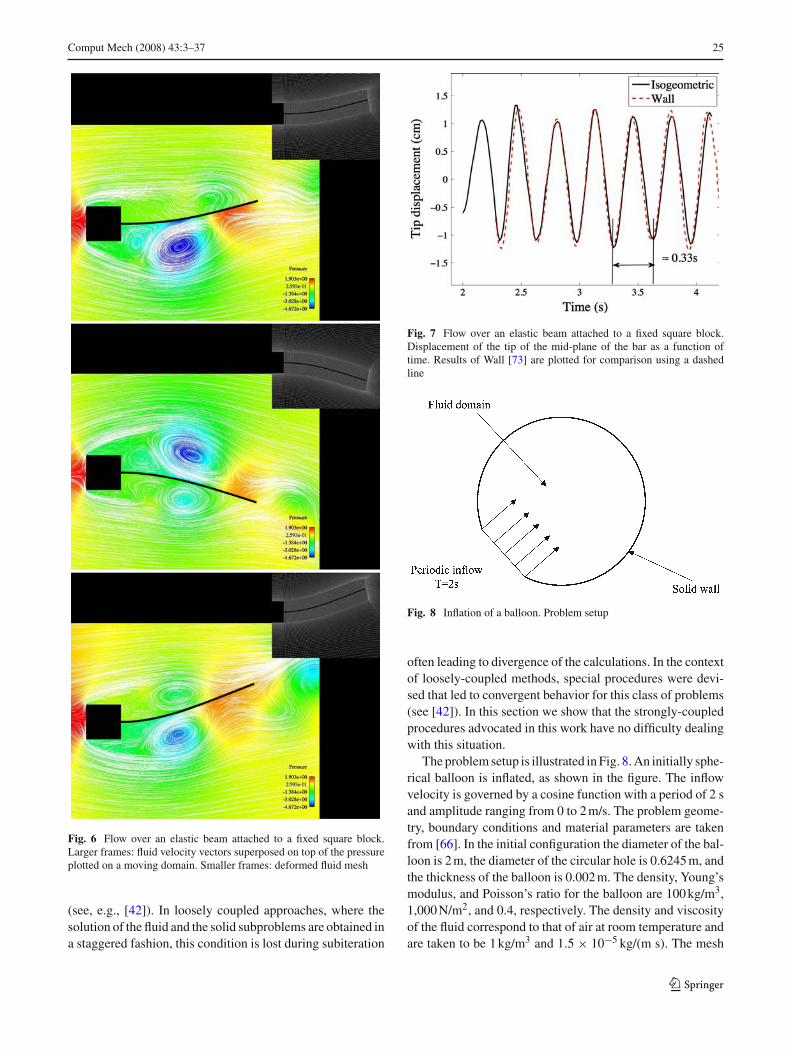
Comput Mech (2008) 43:3–37 25
Fig. 6 Flow over an elastic beam attached to a fixed square block.Larger frames: fluid velocity vectors superposed on top of the pressureplotted on a moving domain. Smaller frames: deformed fluid mesh
(see, e.g., [42]). In loosely coupled approaches, where thesolution of the fluid and the solid subproblems are obtained ina staggered fashion, this condition is lost during subiteration
Fig. 7 Flow over an elastic beam attached to a fixed square block.Displacement of the tip of the mid-plane of the bar as a function oftime. Results of Wall [73] are plotted for comparison using a dashedline
Fig. 8 Inflation of a balloon. Problem setup
often leading to divergence of the calculations. In the contextof loosely-coupled methods, special procedures were devi-sed that led to convergent behavior for this class of problems(see [42]). In this section we show that the strongly-coupledprocedures advocated in this work have no difficulty dealingwith this situation.
The problem setup is illustrated in Fig. 8. An initially sphe-rical balloon is inflated, as shown in the figure. The inflowvelocity is governed by a cosine function with a period of 2 sand amplitude ranging from 0 to 2 m/s. The problem geome-try, boundary conditions and material parameters are takenfrom [66]. In the initial configuration the diameter of the bal-loon is 2 m, the diameter of the circular hole is 0.6245 m, andthe thickness of the balloon is 0.002 m. The density, Young’smodulus, and Poisson’s ratio for the balloon are 100 kg/m3,1,000 N/m2, and 0.4, respectively. The density and viscosityof the fluid correspond to that of air at room temperature andare taken to be 1 kg/m3 and 1.5 × 10⁻⁵ kg/(m s). The mesh
123

26 Comput Mech (2008) 43:3–37
Fig. 9 Inflation of a balloon. NURBS mesh of the balloon in both topand bottom views
of the initial configuration, comprised of 10,336 quadraticNURBS elements, is shown in Fig. 9. Note that, becauseNURBS are used to define the analysis-suitable geometry,the spherical balloon is represented exactly.
For the purposes of mesh motion, we take advantage of theparametric definition of the geometry. We take Em [i.e., theelastic modulus of the mesh motion problem; see Eq. (238)–(239)] to be an exponentially increasing function of the para-meter defining the radial direction, thus effectively “stiffe-ning” the fluid elements near the fluid-solid boundary.
The computation is advanced for 14 inflow cycles, duringwhich the volume of the balloon grows by a factor of approxi-mately five with respect to its initial value. Figures 10–12show snapshots of fluid velocity vectors superposed on thepressure contours at a planar cut through the diameter ofthe sphere. The flow starts out as being radially symmetric,although it is apparent that the symmetry of the solutionbreaks down towards the end of the computation. This isnot surprizing as the Reynolds number of the flow, based onthe initial diameter of the balloon and the maximum inflowspeed, is 4 × 10⁵, which is quite high. For the purposes ofplotting the results, the geometry and solution variables areinterpolated with linear hexahedral finite elements at knotsand midpoints of knot intervals. The meshes displayed inFigs. 10, 11 and 12 correspond to the linear hexahedral repre-sentation.
Figure 13a shows the inflow flowrate versus the rate ofchange of the fluid domain volume, which are expected tobe the same. On the scale of the plot they are indistingui-shable. A closer examination of the error between the inflowflowrate and the rate of change of the fluid domain volumereveals that the relative error in the quantities is on the orderof 10−4 − 10−3, which is attributable to the fact that thenonlinear equations are solved to a tolerance (see Fig. 13b).Note that the results are, on average, slightly less accurateduring the last few periods of the simulation, which is attri-butable to the loss of radial symmetry in the solution. Alsonote that the error has the same sign, that is, the rate ofchange of the fluid domain volume is always greater than
Fig. 10 Inflation of a balloon. Mesh deformation and fluid velocityvectors superposed on the pressure plotted on a planar cut through thediameter of the balloon
the inflow flow rate. This suggests that in the discrete set-ting there is a tendency of the balloon to expand slightlyfaster (i.e., overcompensate) than dictated by the inflow flo-wrate.
8 Computation of vascular flows
In this section we describe the construction of arterial geo-metries. We then make an assessment of the solid model[presented in (75)–(80)] in describing the behavior of arterialwall tissue. Finally, we present results of the fluid-structureinteraction calculation of a patient-specific abdominal aorticaneurysm.
8.1 Construction of the arterial geometry
Blood vessels are tubular objects and so we employ a swee-ping method to construct meshes for isogeometric analysis.
123

Comput Mech (2008) 43:3–37 27
Fig. 11 Inflation of a balloon. Mesh deformation and fluid velocityvectors superposed on the pressure plotted on a planar cut through thediameter of the balloon
A solid NURBS description of a single arterial branch isobtained by extrusion of a circular curve along the vesselpath and filling the volume radially inward. Arterial systemsengender various branchings and intersections, which arehandled with a template-based approach described in detail in[74]. Application of these procedures generate multi-patch,trivariate descriptions of patient-specific arterial geometriesthat are also analysis suitable.
A central feature of our approach is a construction of anarterial cross-section template that is based on the NURBSdefinition of the circular surface. Here we focus on theconstruction of the cross-section template as it relates to fluid-structure interaction analysis of arterial blood flow. We iden-tify the area occupied by the blood, or the fluid region, and thearterial wall, or the solid region. Fluid and solid regions areseparated by the luminal surface, or the fluid-solid boundary.Figure 14 shows an example of a NURBS mesh of a circu-lar cross-section with both fluid and solid regions present.NURBS elements are defined as areas enclosed between
Fig. 12 Inflation of a balloon. Mesh deformation and fluid velocityvectors superposed on the pressure plotted on a planar cut through thediameter of the balloon
isoparametric lines. Note that the isoparametric lines corres-pond to radial and circumferential directions. For purposesof analysis we separate the fluid and the solid region by a C0
line as the solution is not expected to have regularity beyondC0 at the interface.
Human arteries are not exactly circular, hence projec-tion of the template onto the true surface is necessary. Onlycontrol points that govern the cross-section geometry areinvolved in the projection process, while the underlying para-metric description of the cross-section stays unchanged. Theend result of this construction is shown in Fig. 14, whichillustrates the mapping of the template cross-section ontothe patient-specific geometry. Here the isoparametric linesare somewhat distorted so as to conform to the true geome-try, while the topology of the fluid and solid subdomains ispreserved along with their interface. It is worth noting thatcross-sections of healthy arteries are nearly circular, so in this
123

28 Comput Mech (2008) 43:3–37
Fig. 13 Inflation of a balloon.(a) Plot of the volumetric inflowrate (solid line) versus the rateof change of the fluid domainvolume (circles). (b) Plot of therelative error in the flow ratesthat is attributable toconvergence tolerancesemployed in the calculations
0 4 8 12 16 20 24 28
0
0.2
0.4
0.6
Time (s)F
low
rate
(cm
3 /s)
0 4 8 12 16 20 24 28
0
2
4
6
8
10x 10−4
Time(s)
(dV f
/dt−
Oin
)/m
ax(Q
in)
(a)
(b)
Fig. 14 Arterial cross-section template based on a NURBS mesh ofa circle that is subsequently mapped onto a subject-specific geometry.Fluid and solid regions are identified and separated by an interface.For analysis purposes, basis functions are made C0-continuous at thefluid-solid boundary. Note that the topology of the fluid and the solidsubdomains remains unchanged
case little distortion of the template is required to accuratelycapture the true geometry.
Compared to the standard finite element method, the des-cribed method has significant benefits for analysis of bloodflow in arteries, both in terms of accuracy and implementa-tional convenience. It is well known in fluid mechanics thatsteady, laminar, incompressible flow in a straight circular
pipe that is driven by a constant pressure gradient developsa parabolic profile in the radial direction and has no depen-dence on the circumferential or axial directions. NURBS dis-cretizations proposed in this paper, in contrast to standardfinite element discretizations, are capable of exactly repre-senting this solution profile.
Parametric definition of the geometry is not only attractivefrom the mesh refinement point of view, is also beneficial inarterial blood flow applications for the following reasons:
(1) In the fluid region structured boundary layer meshesnear arterial walls may be constructed. This is crucialfor overall accuracy of the fluid-structural simulation aswell as for obtaining accurate wall quantities, such asshear stress, which plays an important role in predictingthe onset and development of vascular disease.
(2) In the solid region it allows for a natural representationof material anisotropy of the arterial wall because theparametric coordinates are aligned with the axial, cir-cumferential and wall-normal directions. See [26] forarterial wall material modeling which accounts for ani-sotropic behavior.
(3) Fluid-structure interaction applications involve motionof the fluid domain. As described previously, this istypically done by solving an auxiliary fictitious elasticboundary value problem for mesh movement (see, e.g.,[37,3]). Parametric mesh definition in the fluid region
123

Comput Mech (2008) 43:3–37 29
Fig. 15 Setup for a uniaxial stress state
allows for a straightforward specification of these elasticmesh parameters. For example, for problems of this typewe “stiffen” the mesh in the radial direction so as topreserve boundary layer elements during mesh motion.
8.2 Investigation of the solid model for a range ofphysiological stresses
We begin by examining the behavior of the material modelpresented in (75)–(80) on a simple state of uniaxial stress. Wefirst consider a bar with an applied stress in the x-direction,denoted by σ , and zero stress in the the orthogonal directions,as illustrated in Fig. 15. We will then relate this situation tothat of a pre-stressed artery in the physiologically relevantrange. For this type of loading, the deformation tensors Fand C are constant and diagonal, that is
F=⎡⎣ F11 0 0
0 F22 00 0 F33
⎤⎦=
⎡⎣ lx/ l0x 0 0
0 ly/ l0y 00 0 lz/ l0z
⎤⎦ (241)
and
C = FT F =⎡⎣C11 0 0
0 C22 00 0 C33
⎤⎦
=⎡⎣ (lx/ l0x )
2 0 00 (ly/ l0y)
2 00 0 (lz/ l0z)
2
⎤⎦ (242)
where lx , ly, lz are the current lengths of the bar and l0x , l0y,
l0z are the original lengths of the bar in the x ,y andz-directions, respectively. We assume that l0y = l0z andly = lz due to symmetry, and use this assumption in theupcoming developments.
From considerations of equilibrium, the Cauchy stress ten-sor becomes
σ =⎡⎣σ 0 0
0 0 00 0 0
⎤⎦ (243)
and, by the transformation of stress formula (71),
S = J F−1σ F−T =⎡⎣ Jσ F−2
11 0 00 0 00 0 0
⎤⎦
=⎡⎣ JσC−1
11 0 00 0 00 0 0
⎤⎦ , (244)
with J = F11 F22 F33 = F11 F222 = (C11C2
22)1/2, where we
used the assumption of symmetry in the second equality.Substituting (244) into (80) and rearranging terms, we arriveat the following 2 × 2 system of nonlinear equations
σ = µsC1/611 C−5/3
22 (1 − 1/3(C11 + 2C22)C−111 )
+ 1/2κs(C11C222 − 1)C−1/2
11 C−122 (245)
0 = µsC−1/311 C−2/3
22 (1 − 1/3(C11 + 2C22)C−122 )
+ 1/2κs(C11C222 − 1)C−1
22 . (246)
The shear and bulk moduli µs and κs are computed fromEq. (84) as
µs = µl (247)
κs = λl + 2
3µl , (248)
where
µl = E
2(1 + ν)(249)
λl = νE
(1 + ν)(1 − 2ν)(250)
are the Lamé coefficients: E is Young’s modulus, and ν isPoisson’s ratio. We set E = 4.144 × 10⁶ dyn/cm 2 = 3.11 ×10³ mmHg and ν = 0.45.
The relevant values of σ corresponding to the physiologi-cally-realistic range of intramural pressure are obtained usingthe following analysis. We approximate the arterial cross-section as a hollow cylinder. Let Ri and Ro denote its innerand outer radii. We also assume that a pressure of magni-tude p0 is applied at the inner wall of the cylinder, as shownin Fig. 16. We assume an approximately constant state ofstress through the thickness, as shown in Fig. 16. From forceequilibrium considerations it follows that
2Ri p0 = 2σ t (251)
where t = Ro − Ri is the thickness of the arterial wall.Solving for σ , we get
σ = p0 Ri/t. (252)
123

30 Comput Mech (2008) 43:3–37
Fig. 16 Equilibrium on a cylinder with imposed internal pressure
Assuming a thickness-to-radius ratio of 15% and p0 varyingfrom 80 mmHg to 120 mmHg, we get the physiologically-realistic stress ranging from approximately 530 mmHg to800 mmHg.
As a part of this analysis we also extract effective tangentmoduli at different levels of deformation as follows. The tan-gent modulus is defined as
C = ∂σ
∂ε, (253)
with ε defined as
ε = lx − l0x
lx= 1 − F−1
11 = 1 − C−1/211 . (254)
We solve (245) and (246) numerically for C11 and C22
for σ ranging from 0 mmHg to 2500 mmHg, and computethe strain according to (254). The plot of stress σ versusstrain ε is shown in Fig. 17. Physiological ranges of stressesand strains due to intramural pressure are indicated in thefigure by dashed lines. Note that the stress-strain curve exhi-bits convex behavior throughout the range of loadings consi-dered, showing stiffening with deformation. Also note thatfor the physiological range of stresses the deviation from alinearized stress-strain relationship is not significant. We alsocompute a numerical derivative of σ with respect to ε in orderto evaluate the effective tangent modulus. Note that the equi-valent tangent stiffness is higher at the level of deformationcaused by the physiological stress as compared to the tangentstiffness in the undeformed configuration. Also note that, asexpected, the value of the tangent stiffness in the undeformedconfiguration is exactly the value of Young’s modulus used todefine the solid model parameters. Figure 18 shows the plotof elastic energy ψ versus strain ε. We believe that this ana-lysis justifies using the model in fluid-structure interactionanalysis of arteries. We also feel that it supports the hypo-theses behind the coupled momentum method of Figueroa etal. [20]. Obviously, significant improvements are possible.
However, the present model is both qualitatively and quanti-tatively reasonable for the following application.
8.3 Flow in a patient-specific abdominal aortic aneurysm
Patient-specific geometry is obtained from 64-slice CT angio-graphy courtesy of T. Kvamsdal and J.H. Kaspersen of SIN-TEF, Norway. The geometrical model, which contains mostmajor branches of a typical abdominal aorta, is shown inFig. 19a . Note that one of the renal arteries is missing inthe model indicating that the patient has only one kidney.The fluid properties are: ρ f = 1.06 g/cm3, µ f = 0.04 g/cms. The solid has the density ρs = 1 g/cm3, Young’s modu-lus, E = 4.144×10⁶ dyn/cm2, and Poisson’s ratio, ν= 0.45.The model coefficientsµs and κs are obtained using relation-ships from the previous section. The computational mesh,consisting of 44892 quadratic NURBS elements, is shownin Fig. 19c. Two quadratic NURBS elements and four C1-
0 0.05 0.1 0.15 0.2 0.25 0.3 0.35 0.4 0.450
1000
1500
2000
2500
533
800
Strain: (lx−l0x)/lx
Cau
chy
stre
ss (
mm
Hg)
Physiological stress range due to intramural pressure
Tangent modulus at zero stress: 4.14x10⁶ dyn/cm2 or 3.11x10³ mmHg
Tangent modulus at physiological stress:6.00x10⁶ dyn/cm2 or 4.50x10³ mmHg
Fig. 17 Cauchy stress plotted against strain for the material modelused in the abdominal aorta simulation. Physiological range of stressesand strains due to intramural pressure are indicated by dashed lines
0 0.05 0.1 0.15 0.2 0.25 0.3 0.35 0.4 0.45 0
200
300
400
500
600
42.3
91.3
Strain: (l x −l 0x )/l x
Ela
stic
ene
rgy
(mm
Hg)
Elastic energy at physiological stress due to intramural pressure
Fig. 18 Elastic energy plotted against strain for the material modelused in the abdominal aorta simulation. Physiological range of energiesand strains due to intramural pressure are indicated by dashed lines
123

Comput Mech (2008) 43:3–37 31
Fig. 19 Flow in apatient-specific abdominal aortawith aneurysm.a Patient-specific imaging data;b Skeleton of the NURBS mesh;c Smoothed and truncatedNURBS model and mesh. In c,every NURBS patch is assigneda different color. For moredetails of geometrical modelingfor isogeometric analysis ofblood flow the reader is referredto [74]
continuous basis functions are used for through-thicknessresolution of the arterial wall. For the purposes of meshmotion, parametric stiffening in the radial direction isemployed as for the inflation of a balloon problem.
8.3.1 Imposition of initial and boundary conditions
A periodic flow waveform, with period T = 1.05 s, is appliedat the inlet of the aorta, while resistance boundary conditionsare applied at all outlets. The solid is fixed at the inlet and atall outlets. Material and flow rate data, as well as resistancevalues are taken from Figueroa et al. [20]. Wall thickness forthis model is taken to be 15% of the nominal radius of eachcross-section of the fluid domain model.
In order to ensure medically-realistic response, resistanceboundary conditions must be applied in such a way thatphysiological pressure levels are present in the system atall times. This is accomplished by making use of the fol-lowing variant of the resistance boundary condition (see alsoFigueroa et al. [20], Vignon-Clementel et al. [72], andHeywood et al. [25]). At every outlet face a we set
nT σ n = Ca
∫a
v · nda + p0, (255)
τ T1 σ n = 0, (256)
τ T2 σ n = 0 (257)
where n is the outward unit normal, and τ 1 and τ 2 aremutually orthogonal unit tangent vectors on the outlet face.The above boundary conditions state that normal stress onthe outlet face is a linear function of the flowrate through theface, while both tangential stresses are zero. The Ca’s are theso-called resistance constants. They are positive, and are, inprinciple, different from outlet to outlet, reflecting the resis-tance of different blood vessels. p0 in (255) is responsiblefor imposing physiologically realistic pressure level in thevessels, even at zero flow through the outlet faces. For thecomputations reported in this section p0 is set to 85 mmHg,as in [20]. We impose boundary conditions (255) weaklyby adding the following terms to the variational formula-tion (109)
+∑
a
{(∫a
w f · nda
)(Ca
∫a
v · nda + p0
)}
where the sum is taken over all the outlet faces with prescri-bed resistance conditions.
We initialize our computations as follows. We start withan un-pressurized configuration, set and maintain the inflow
123

32 Comput Mech (2008) 43:3–37
velocity consistent with the inflow flowrate at t = 0, and gra-dually increase the pressure level in the system by raising p0
in (255) from zero to the physiologically realistic value of 85mmHg. This is done for one or two cycles. Once the physio-logical pressure level is attained, we begin computing withthe time-varying inflow boundary condition until periodic-in-time response is attained. This usually takes four or fivecycles.
Remark 8.1 Recent efforts to increase the efficiency of arte-rial FSI computations by performing a series of so-called“pre-FSI” computations were reported in [67].
Remark 8.2 In reference [68] the authors propose a strategyto compute the so-called “estimated zero-pressure arterialgeometry.” This is done in an effort to reconcile the factthat the patient-specific arterial geometry, often times takenas the reference geometry, corresponds to to the pressurizedconfiguration, while in the majority of the proposed materialmodels the reference configuration is assumed to be stress-free.
8.3.2 Numerical results
After a nearly periodic-in-time solution was attained,simulation data was collected for postprocessing. Figures 20and 21 show snapshots of the velocity field plotted on themoving domain at various times during the heart cycle. Theflow field is quite complex and fully three-dimensional, espe-cially in diastole. Velocity magnitude is largest near the inflowand is significantly lower in the aneurysm region. This occursin part due to the fact that a significant percentage of the flowgoes to the upper branches of the abdominal aorta. Thereis also an increase in the cross-sectional area of the vesselassociated with the aneurysm, resulting in a decreased flowvelocity in this region.
Figure 22 shows the magnitude of the wall shear stress(i.e., the tangential component of the fluid or solid tractionvector) averaged over a cycle. Note that the wall shear stressis significantly lower in the aneurysm region than in the upperportion of the aorta and at branches. Also note the smoothnessof the stress contours due to the NURBS representation ofthe geometry and solution fields.
Figure 23 shows the oscillatory shear index (OSI) at theluminal surface. OSI is defined as (see, e.g., [62,63]),
OSI = 1
2
(1 − τmean
τabs
), (258)
where, denoting by τ s the wall shear stress vector,
τmean =∣∣∣∣∣∣
1
T
T∫0
τ sdt
∣∣∣∣∣∣ , (259)
Fig. 20 Flow in a patient-specific abdominal aorta with aneurysm.Large frame: fluid velocity vectors colored by their magnitude in thevicinity of the celiac and superior mesenteric arteries. Left small frame:volume rendering of the velocity magnitude. Right small frame: fluidvelocity isosurfaces
and
τabs = 1
T
T∫0
|τ s |dt. (260)
Note that, in contrast to the wall shear stress, OSI is largestin the aneurysm region, especially along the posterior wall,suggesting that wall shear stress is highly oscillatory theredue to the recirculating flow. Low time-averaged wall shearstress, in combination with high shear stress temporal oscil-lations, as measured by the OSI, are indicators of the regionsof high probability of occurrence of atherosclerotic disease.Figure 24 shows the distribution of flow among the branches.The outflow lags the inflow due to the distensibility of thearterial wall. The overall flow distribution and the time lagare in qualitative agreement with results in [3,20].
9 Conclusions
We have presented a monolithic isogeometric fluid-structure interaction formulation. The fluid subdomain wasassumed to be governed by the incompressible Navier–Stokesequations and the solid subdomain was assumed to be
123
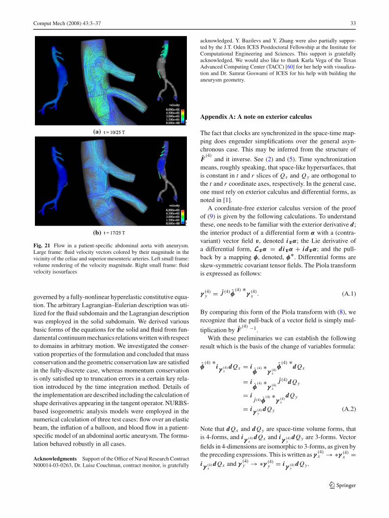
Comput Mech (2008) 43:3–37 33
Fig. 21 Flow in a patient-specific abdominal aorta with aneurysm.Large frame: fluid velocity vectors colored by their magnitude in thevicinity of the celiac and superior mesenteric arteries. Left small frame:volume rendering of the velocity magnitude. Right small frame: fluidvelocity isosurfaces
governed by a fully-nonlinear hyperelastic constitutive equa-tion. The arbitrary Lagrangian–Eulerian description was uti-lized for the fluid subdomain and the Lagrangian descriptionwas employed in the solid subdomain. We derived variousbasic forms of the equations for the solid and fluid from fun-damental continuum mechanics relations written with respectto domains in arbitrary motion. We investigated the conser-vation properties of the formulation and concluded that massconservation and the geometric conservation law are satisfiedin the fully-discrete case, whereas momentum conservationis only satisfied up to truncation errors in a certain key rela-tion introduced by the time integration method. Details ofthe implementation are described including the calculation ofshape derivatives appearing in the tangent operator. NURBS-based isogeometric analysis models were employed in thenumerical calculation of three test cases: flow over an elasticbeam, the inflation of a balloon, and blood flow in a patient-specific model of an abdominal aortic aneurysm. The formu-lation behaved robustly in all cases.
Acknowledgments Support of the Office of Naval Research ContractN00014-03-0263, Dr. Luise Couchman, contract monitor, is gratefully
acknowledged. Y. Bazilevs and Y. Zhang were also partially suppor-ted by the J.T. Oden ICES Postdoctoral Fellowship at the Institute forComputational Engineering and Sciences. This support is gratefullyacknowledged. We would also like to thank Karla Vega of the TexasAdvanced Computing Center (TACC) [60] for her help with visualiza-tion and Dr. Samrat Goswami of ICES for his help with building theaneurysm geometry.
Appendix A: A note on exterior calculus
The fact that clocks are synchronized in the space-time map-ping does engender simplifications over the general asyn-chronous case. This may be inferred from the structure of
F(4)
and it inverse. See (2) and (5). Time synchronizationmeans, roughly speaking, that space-like hypersurfaces, thatis constant in t and r slices of Qx and Qy are orthogonal tothe t and r coordinate axes, respectively. In the general case,one must rely on exterior calculus and differential forms, asnoted in [1].
A coordinate-free exterior calculus version of the proofof (9) is given by the following calculations. To understandthese, one needs to be familiar with the exterior derivative d;the interior product of a differential form α with a (contra-variant) vector field v, denoted ivα; the Lie derivative ofa differential form, Lvα = divα + i dvα; and the pull-back by a mapping φ, denoted, φ∗. Differential forms areskew-symmetric covariant tensor fields. The Piola transformis expressed as follows:
γ (4)y = J (4)φ(4) ∗
γ (4)x . (A.1)
By comparing this form of the Piola transform with (8), werecognize that the pull-back of a vector field is simply mul-
tiplication by F(4) −1.
With these preliminaries we can establish the followingresult which is the basis of the change of variables formula:
φ(4) ∗
iγ (4)x
d Qx = iφ(4) ∗
γ (4)x
φ(4) ∗
d Qx
= iφ(4) ∗
γ (4)x
J (4)d Qy
= iJ (4)φ
(4) ∗γ (4)
x
d Qy
= iγ (4)y
d Qy (A.2)
Note that d Qx and d Qy are space-time volume forms, thatis 4-forms, and iγ (4)
xd Qx and iγ (4)
yd Qy are 3-forms. Vector
fields in 4-dimensions are isomorphic to 3-forms, as given bythe preceding expressions. This is written as γ
(4)x → ∗γ (4)x =
iγ (4)x
d Qx and γ(4)y → ∗γ (4)y = iγ (4)
yd Qy .
123

34 Comput Mech (2008) 43:3–37
Fig. 22 Flow in apatient-specific abdominal aortawith aneurysm. Magnitude ofwall shear stress averaged over acycle plotted in three differentviews
Fig. 23 Flow in apatient-specific abdominal aortawith aneurysm. Oscillatoryshear index (OSI) plotted inthree different views
With these preliminaries we have
∇(4)y · γ (4)y d Qy = Lγ (4)
yd Qy
= d(iγ (4)y
d Qy)
= d(φ(4) ∗
iγ (4)x
d Qx )
= φ(4) ∗
d(iγ (4)x
d Qx )
= φ(4) ∗Lγ (4)
xd Qx
= φ(4) ∗
(∇(4)x · γ (4)x d Qx )
= ∇(4)x · γ (4)x ◦ φ
(4)φ(4) ∗
d Qx
= ∇(4)x · γ (4)x ◦ φ
(4)J (4)d Qy . (A.3)
This results and the change of variables formula yields (9).
In the above we have utilized the commutativity of pull-back and exterior differentiation, and the fact that the exte-rior derivative of a 4-form, closed in four dimensions, iszero. That Lγ (4)
yd Qy = ∇(4)
y · γ(4)y d Qy can be proved by
assuming cartesian coordinates on R4 ⊃ Qy and d Qy =
dy0 ∧ dy1 ∧ dy2 ∧ dy3, where ∧ is the wedge product. Like-wise, the same construct can be used to prove Lγ (4)
xd Qx =
∇(4)x ·γ (4)x d Qx . Curvilinear spatial coordinates can be accom-
modated by using the usual tensor transformation formulason these coordinates (see Marsden and Hughes [47]). Thetime coordinate is unaffected in this case.
Remark A.1 With differential forms, correct boundary inte-gral expressions can be obtained without the necessity of unitnormal vectors by using Stokes theorem and the change of
123

Comput Mech (2008) 43:3–37 35
Fig. 24 Flow in apatient-specific abdominal aortawith aneurysm. Flow ratedistribution among the arterialbranches during a heart cycle
variables formula. For example,∫∂Qy
iγ (4)y
d Qy =∫
Qy
d(iγ (4)y
d Qy)
=∫
Qy
φ(4) ∗
d(iγ (4)x
d Qx )
=∫
φ(4)(Qy)
d(iγ (4)x
d Qx )
=∫
Qx
d(iγ (4)x
d Qx )
=∫∂Qx
iγ (4)x
d Qx . (A.4)
Remark A.2 The notations d Qx and d Qy are used under theintegration sign in the main body of the paper, in contrast withthe differential form notations to represent volume elements,
d Qx and d Qy , respectively, in keeping with the standardusage.
References
1. Abedi P, Patracovici B, Haber RB (2006) A spacetime discon-tinuous Galerkin method for linearized elastodynamics withelement-wise momentum balance. Comput Methods Appl MechEng 195:3247–3273
2. Akkerman I, Bazilevs Y, Calo VM, Hughes TJR, HulshoffS (2008) The role of continuity in residual-based variational mul-tiscale modeling of turbulence. Comput Mech 41:371–378
3. Bazilevs Y, Calo VM, Zhang Y, Hughes TJR (2006) Isogeometricfluid-structure interaction analysis with applications to arterialblood flow. Comput Mech 38:310–322
4. Bazilevs Y, Calo VM, Cottrell JA, Hughes TJR, Reali A, ScovazziG (2007) Variational multiscale residual-based turbulence mode-ling for large eddy simulation of incompressible flows. ComputMethods Appl Mech Eng 197:173–201
5. Bazilevs Y, Beiraoda Veiga L, Cottrell JA, Hughes TJR, SangalliG (2006) Isogeometric analysis: approximation, stability and errorestimates for h-refined meshes. Math Models Methods Appl Sci16:1031–1090
123

36 Comput Mech (2008) 43:3–37
6. Bazilevs Y, Hughes TJR (2007) Weak imposition of Dirichletboundary conditions in fluid mechanics. Comput Fluids 36:12–26
7. Bazilevs Y, Michler C, Calo VM, Hughes TJR (2007) Weak Diri-chlet boundary conditions for wall-bounded turbulent flows. Com-put Methods Appl Mech Eng 196:4853–4862
8. Bishop R, Goldberg S (1980) Tensor analysis on manifolds. Dover,New York
9. Brezzi F, Fortin M (1991) Mixed and hybrid finite elementmethods. Springer, Berlin
10. Brooks AN, Hughes TJR (1982) Streamline upwind/Petrov-Galerkin formulations for convection dominated flows with par-ticular emphasis on the incompressible Navier–Stokes equations.Comput Methods Appl Mech Eng 32:199–259
11. Calo VM (2004) Residual-based multiscale turbulence mode-ling: finite volume simulation of bypass transistion. Ph.D. The-sis, Department of Civil and Environmental Engineering, StanfordUniversity
12. Chung J, Hulbert GM (1993) A time integration algorithm forstructural dynamics with improved numerical dissipation: Thegeneralized-α method. J Appl Mech 60:371–75
13. Cottrell JA, Reali A, Bazilevs Y, Hughes TJR (2006) Isogeometricanalysis of structural vibrations. Comput Methods Appl Mech Eng195:5257–5297
14. Cottrell JA, Reali A, Hughes TJR (2007) Studies of refinement andcontinuity in isogeometric structural analysis. Comput MethodsAppl Mech Eng 196:4160–4183
15. Dettmer W, Peric D (2006) A computational framework for fluid-structure interaction: finite element formulation and applications.Comput Methods Appl Mech Eng 195:5754–5779
16. Elguedj T, Bazilevs Y, Calo VM, Hughes TJR (2008) B-bar andF-bar projection methods for nearly incompressible linear and non-linear elasticity and plasticity using higher-order NURBS elements.Comput Methods Appl Mech Eng 197:2732–2762
17. Farhat C, Geuzaine P, Grandmont C (2001) The discrete geometricconservation law and the nonlinear stability of ALE schemes forthe solution of flow problems on moving grids. J Comput Phys174(2):669–694
18. Farhat C, van der Zee K, Geuzaine P (2006) Provably second-ordertime-accurate loosely-coupled solution algorithms for transientnonlinear computational aeroelasticity. Comput Methods ApplMech Eng 195:1973–2001
19. Fernandez MA, Moubachir M (2005) A Newton method usingexact jacobians for solving fluid-structure coupling. Comput Struct83:127–142
20. Figueroa A, Vignon-Clementel IE, Jansen KE, Hughes TJR, TaylorCA (2006) A coupled momentum method for modeling blood flowin three-dimensional deformable arteries. Comput Methods ApplMech Eng 195:5685–5706
21. Flanders H (1963) Differential forms with applications to the phy-sical sciences. Academic Press, London
22. Formaggia L, Nobile F (2005) Stability analysis of second-ordertime accurate schemes for ALE-FEM. Comput Methods ApplMech Eng 193:4097–4116
23. Guillermin V, Pollack A (1974) Differential topology. Prentice-Hall, Englewood Cliffs
24. Heil M, Hazel A, Boyle J (2008) Solvers for large-displacementfluid-structure interaction problems: segregated vs. monolithicapproaches. Comput Mech. doi:10.1007/s00466-008-0270-6
25. Heywood JG, Rannacher R, Turek S (1996) Artificial boundariesand flux and pressure conditions for the incompressible Navier-Stokes equations. Int J Numer Methods Fluids 22:325–352
26. Holzapfel GA (2004) Computational biomechanics of soft biologi-cal tissue. In: Stein E, De Borst R, Hughes TJR (eds) Encyclopediaof computational mechanics, Solids and structures, chap 18, vol 2.Wiley, London
27. Holzapfel GA (2000) Nonlinear solid mechanics, a continuumapproach for engineering. Wiley, Chichester
28. Hughes TJR (2000) The finite element method: linear static anddynamic finite element analysis. Dover Publications, Mineola
29. Hughes TJR, Calo VM, Scovazzi G (2004) Variational and multis-cale methods in turbulence. In: Gutkowski W, Kowalewski TA (eds)In Proceedings of the XXI International Congress of Theoreticaland Applied Mechanics (IUTAM), Kluwer, pp 153–163
30. Hughes TJR, Cottrell JA, Bazilevs Y (2005) Isogeometric analysis:CAD, finite elements, NURBS, exact geometry, and mesh refine-ment. Comput. Methods Appl Mech Eng 194:4135–4195
31. Hughes TJR, Hulbert GM (1988) Space-time finite elementmethods for elastodynamics: formulations and error estimates.Comput Methods Appl Mech Eng 66:339–363
32. Hughes TJR, Liu WK, Zimmermann TK (1981) Lagrangian–Eulerian finite element formulation for incompressible viscousflows. Comput Methods Appl Mech Eng 29:329–349
33. Hughes TJR, Wells GN (2005) Conservation properties for theGalerkin and stabilised forms of the advection-diffusion andincompressible Navier-Stokes equations. Comput Methods ApplMech Eng 194:1141–1159
34. Hulbert GM, Hughes TJR (1990) Space-time finite elementmethods for second order hyperbolic equations. Comput MethodsAppl Mech Eng 84:327–348
35. Idelsohn SR, Oñate E, Del Pin F, Calvo N (2006) Fluid-structureinteraction using the particle finite element method. ComputMethods Appl Mech Eng 195:2100–2123
36. Jansen KE, Whiting CH, Hulbert GM (1999) A generalized-αmethod for integrating the filtered Navier-Stokes equations witha stabilized finite element method. Comput Methods Appl MechEng 190:305–319
37. Johnson AA, Tezduyar TE (1994) Mesh update strategies in paral-lel finite element computations of flow problems with movingboundaries and interfaces. Comput Methods Appl Mech Eng119:73–94
38. Johnson AA, Tezduyar TE (1997) Parallel computation of incom-pressible flows with complex geometries. Int J Numer MethodsFluids 24:1321–1340
39. Johnson AA, Tezduyar TE (1999) Advanced mesh generation andupdate methods for 3D flow simulations. Comput Mech 23:130–141
40. Johnson C (1987) Numerical solution of partial differential equa-tions by the finite element method. Cambridge University Press,Sweden
41. Johnson C, Nävert U, Pitkäranta J (1984) Finite element methodsfor linear hyperbolic problems. Comput Methods Appl Mech Eng45:285–312
42. Küttler U, Förster C, Wall WA (2006) A solution for the incom-pressibility dilemma in partitioned fluid-structure interaction withpure Dirichlet fluid domains. Comput Mech 38:417–429
43. Kuhl E, Hulshoff S, de Borst R (2003) An arbitrary LagrangianEulerian finite element approach for fluid-structure interaction phe-nomena. Int J Numer Methods Eng 57:117–142
44. Lang S (1972) Differential manifolds. Addison-Wesley, Reading45. Lang S (1995) Differential and riemannian manifolds (graduate
texts in mathematics, vol. 160). Springer, Heidelberg46. Le Tallec P, Mouro J (2001) Fluid structure interaction with
large structural displacements. Comput Methods Appl Mech Eng190:3039–3068
47. Marsden JE, Hughes TJR (1993) Mathematical foundations ofelasticity. Dover Publications Inc., New York
48. Masud A, Hughes TJR (1997) A space-time Galerkin/least-squares finite element formulation of the Navier-Stokes equationsfor moving domain problems. Comput Methods Appl Mech Eng148:91–126
123

Comput Mech (2008) 43:3–37 37
49. Michler C, van Brummelen EH, de Borst R (2006) Error-amplification analysis of subiteration-preconditioned GMRES forfluid-structure interaction. Comput Methods Appl Mech Eng195:2124–2148
50. Michler C, van Brummelen EH, Hulshoff SJ, de BorstR (2003) The relevance of conservation for stability and accu-racy of numerical methods for fluid-structure interaction. ComputMethods Appl Mech Eng 192:4195–4215
51. Nobile F (2001) Numerical Approximation of Fluid-StructureInteraction Problems with Application to Haemodynamics. Ph.D.Thesis, EPFL
52. Piperno S, Farhat C (2001) Partitined procedures for the transientsolution of coupled aeroelastic problems. Part II: Energy trans-fer analysis and three-dimensional applications. Comput MethodsAppl Mech Eng 190:3147–3170
53. Piperno S, Farhat C, Larrouturou B (1995) Partitined proceduresfor the transient solution of coupled aeroelastic problems. Part I:Model problem, theory and two-dimensional application. ComputMethods Appl Mech Eng 124:79–112
54. Saad Y, Schultz MH (1986) GMRES: A generalized minimal resi-dual algorithm for solving nonsymmetric linear systems. SIAM JSci Stat Comput 7:856–869
55. Simo JC, Hughes TJR (1998) Computational inelasticity. Springer,New York
56. Babuska I (1973) The finite element method with Lagrange multi-pliers. Numer Math 20:179–192
57. Spivak M (1965) Calculus on manifolds. Benjamin, New York58. Stein K, Tezduyar T, Benney R (2003) Mesh moving techniques
for fluid-structure interactions with large displacements. J ApplMech 70:58–63
59. Stein K, Tezduyar TE, Benney R (2004) Automatic mesh updatewith the solid-extension mesh moving technique. Comput MethodsAppl Mech Eng 193:2019–2032
60. Texas Advanced Computing Center (TACC). http://www.tacc.utexas.edu
61. Taylor CA, Hughes TJR, Zarins CK (1998) Finite element mode-ling of blood flow in arteries. Comput Methods Appl Mech Eng158:155–196
62. Taylor CA, Hughes TJR, Zarins CK (1998) Finite element mode-ling of three-dimensional pulsatile flow in the abdominal aorta:relevance to atherosclerosis. Ann Biomed Eng 26:975–987
63. Taylor CA, Hughes TJR, Zarins CK (1999) Effect of exercise onhemodynamic conditions in the abdominal aorta. J Vasc Surg29:1077–1089
64. Tezduyar TE, Behr M, Liou J (1992) A new strategy for finiteelement computations involving moving boundaries and inter-faces. The deforming-spatial-domain/space-time procedure. I. Theconcept and the preliminary numerical tests. Comput MethodsAppl Mech Eng 94:339–351
65. Tezduyar TE, Behr M, Mittal S, Liou J (1992) A new strategyfor finite element computations involving moving boundaries andinterfaces. The deforming-spatial-domain/space-time procedure.II. Computation of free-surface flows, two-liquid flows, and flowswith drifting cylinders. Comput Methods Appl Mech Eng 94:353–371
66. Tezduyar TE, Sathe S (2007) Modelling of fluid-structure interac-tions with the space-time finite elements: solution techniques. IntJ Numer Methods Fluids 54:855–900
67. Tezduyar TE, Sathe S, Cragin T, Nanna B, Conklin BS, Pause-wang J, Schwaab M (2007) Modelling of fluid-structure interac-tions with the space-time finite elements: Arterial fluid mechanics.Int J Numer Methods Fluids 54:901–922
68. Tezduyar TE, Sathe S, Schwaab M, Conklin BS (2008) Arterialfluid mechanics modeling with the stabilized space-time fluid-structure interaction technique. Int J Numer Methods Fluids57:601–629
69. Tezduyar TE (2003) Computation of moving boundaries and inter-faces and stabilization parameters. Int J Numer Methods Fluids43:555–575
70. Tezduyar TE, Behr M, Mittal S, Johnson AA (1992) Computationof unsteady incompressible flows with the stabilized finite elementmethods—space–time formulations, iterative strategies and massi-vely parallel implementations. In: New methods in transient ana-lysis, pVP, vol 246/AMD, vol 143. ASME, New York, pp 7–24
71. Tezduyar TE, Sathe S, Keedy R, Stein K (2006) Space-time finiteelement techniques for computation of fluid-structure interactions.Comput Methods Appl Mech Eng 195:2002–2027
72. Vignon-Clementel IE, Figueroa CA, Jansen KE, TaylorCA (2006) Outflow boundary conditions for three-dimensionalfinite element modeling of blood flow and pressure in arteries.Comput Methods Appl Mech Eng 195:3776–3796
73. Wall W (1999) Fluid-Struktur-Interaktion mit stabilisierten FinitenElementen. Ph.D. Thesis, Institut für Baustatik, Universität Stutt-gart
74. Zhang Y, Bazilevs Y, Goswami S, Bajaj C, HughesTJR (2007) Patient-specific vascular NURBS modeling forisogeometric analysis of blood flow. Comput Methods Appl MechEng 196:2943–2959
123


