Embed Size (px)
Citation preview

INTERNATIONAL JOURNAL FOR NUMERICAL METHODS IN ENGINEERINGInt. J. Numer. Meth. Engng 2011; 88:126–156Published online 7 March 2011 in Wiley Online Library (wileyonlinelibrary.com). DOI: 10.1002/nme.3167
Isogeometric finite element data structures based on Bézierextraction of T-splines
Michael A. Scott1,∗,†, Michael J. Borden1,2, Clemens V. Verhoosel3,Thomas W. Sederberg4 and Thomas J. R. Hughes1
1Institute for Computational Engineering and Sciences, The University of Texas at Austin, 1 University StationC0200, Austin, TX 78712, U.S.A.
2Sandia National Laboratories, Albuquerque, NM 87185, U.S.A.3Department of Mechanical Engineering, Eindhoven University of Technology,
5600 MB Eindhoven, The Netherlands4Department of Computer Science, Brigham Young University, 3361 TMCB PO Box 26576, Provo,
Utah 84602, U.S.A.
SUMMARY
We develop finite element data structures for T-splines based on Bézier extraction generalizing our previouswork for NURBS. As in traditional finite element analysis, the extracted Bézier elements are defined interms of a fixed set of polynomial basis functions, the so-called Bernstein basis. The Bézier elementsmay be processed in the same way as in a standard finite element computer program, utilizing exactly thesame data processing arrays. In fact, only the shape function subroutine needs to be modified while allother aspects of a finite element program remain the same. A byproduct of the extraction process is theelement extraction operator. This operator localizes the topological and global smoothness information tothe element level, and represents a canonical treatment of T-junctions, referred to as ‘hanging nodes’ infinite element analysis and a fundamental feature of T-splines. A detailed example is presented to illustratethe ideas. Copyright � 2011 John Wiley & Sons, Ltd.
Received 3 November 2010; Revised 19 January 2011; Accepted 20 January 2011
KEY WORDS: Bézier extraction; isogeometric analysis; T-splines; finite elements
1. INTRODUCTION
Isogeometric analysis was introduced in [1] and has been described in detail in [2]. In the isoge-ometric framework the basis which describes the geometry is also used as the basis for analysis.Investigations using simple tensor product NURBS constructions have shown that the use of asmooth basis in analysis provides computational advantages over standard finite elements in manyareas, including turbulence [3–6], fluid–structure interaction [7–10], incompressibility [11–13],structural analysis [14, 15], plates and shells [16–20], phase-field analysis [21, 22], large defor-mation with mesh distortion [23], shape optimization [24–27], and electromagnetics [28]. Thissuccess has in turn stimulated efforts within the Computer Aided Geometric Design (CAGD)community to develop and integrate analysis-suitable geometric technologies and isogeometricanalysis [29–35].
T-splines, which emanate from CAGD, overcome the tensor product restriction inherent inNURBS [36]. In fact, NURBS form a restricted subset of T-splines. Additionally, T-splines
∗Correspondence to: Michael A. Scott, Institute for Computational Engineering and Sciences, The University ofTexas at Austin, 1 University Station C0200, Austin, TX 78712, U.S.A.
†E-mail: [email protected]
Copyright � 2011 John Wiley & Sons, Ltd.

ISOGEOMETRIC FINITE ELEMENT DATA STRUCTURES FOR T-SPLINES 127
Q = C P
N = CB
Figure 1. Schematic representation of Bézier extraction for a B-spline curve. B-spline basis functions andcontrol points are denoted by N and P, respectively. Bernstein polynomials and control points are denoted
by B and Q, respectively. The curve T (n)=PTN(n)=QTB(n).
can be locally refined [37] and can generate analysis-suitable models of arbitrary topologicalcomplexity [38]. This makes T-splines an ideal basis for isogeometric analysis. The extensionof the isogeometric framework to the more advanced T-spline setting was initiated in [39, 40].T-spline discretizations have been successfully applied to fracture and damage [41, 42]. In theseapplications, efficient local refinement plays an important role. Initial investigations extendingT-spline-based isogeometric analysis to the arbitrary topology setting in the context of shells havealso been promising [18].
In this paper we develop T-splines from the finite element point-of-view, utilizing Bézier extrac-tion. Bézier extraction for T-splines was briefly mentioned in the context of geometric design in[36]. The application of Bézier extraction to isogeometric analysis for the special case of NURBSwas detailed in [43]. The idea is to extract the linear operator which maps the Bernstein polynomialbasis on Bézier elements to the global T-spline basis. This is referred to as Bézier extraction. Thelinear transformation is defined by a matrix referred to as the extraction operator. The transposeof the extraction operator maps the control points of the global T-spline to the control points ofthe Bernstein polynomials. Figure 1 illustrates the idea for a B-spline curve. This provides a finiteelement representation of T-splines, and facilitates the incorporation of T-splines into existing finiteelement programs. Only the shape function subroutine needs to be modified. All other aspects ofthe finite element program remain the same. Additionally, Bézier extraction is automatic and canbe applied to any T-spline regardless of topological complexity or polynomial degree. In particular,it represents an elegant treatment of T-junctions, referred to as ‘hanging nodes’ in finite elementanalysis. The centrality of Bézier extraction in unifying common CAD representations and FEAis illustrated in Figure 2.
This paper is organized as follows. Basic T-spline concepts are reviewed in Section 2. The funda-mental finite element structure underlying T-splines is developed in Section 3. Section 4 describesBézier extraction of T-splines. T-splines and element extraction operators are then integrated intostandard finite element programs in Section 5. This paper is written specifically in terms of bicubicT-splines, although the concepts apply to any degree. T-splines of arbitrary degree are discussedin [39, 44]. This paper is also focused on surfaces, although the ideas extend directly to solids.
2. T-SPLINE FUNDAMENTALS
We first present fundamental concepts underlying T-spline technology. We illustrate our develop-ments using the physical domain �⊂R2 shown in Figure 3. Throughout this paper we use p to
Copyright � 2011 John Wiley & Sons, Ltd. Int. J. Numer. Meth. Engng 2011; 88:126–156DOI: 10.1002/nme

128 M. A. SCOTT ET AL.
T-splines
NURBS
IsogeometricAnalysis
FEABézier
Extraction
k-refinement
h-, p-refinement
Figure 2. A schematic diagram illustrating the central role played by Bézierextraction in unifying CAGD and FEA.
Figure 3. The domain �⊂R2 for a bivariate (dp =2), cubic (p=3) T-spline. The curved boundaries areexact quarter circles. The hash marks on the left indicate homogeneous Dirichlet boundary conditions.
indicate polynomial degree, dp to indicate the number of parametric dimensions, and ds to indicatethe number of spatial dimensions.
2.1. The T-mesh
A T-spline is constructed from a T-mesh, denoted by T. For surfaces, i.e. dp =2, the T-mesh is amesh of quadrilateral elements‡ which permit T-junctions. In finite element parlance, a T-junctionis analogous to a ‘hanging node.’ An element with T-junctions is composed of four corner verticesand any number of additional vertices on any side. The spatial representation of a T-mesh is calleda T-spline control mesh. In this paper we use T-mesh and T-spline control mesh interchangeably.Every vertex in the T-mesh is assigned a control point, PA ∈Rds , and control weight, wA ∈R,where the index A is used to denote a global control point number.
A T-mesh for the domain � in Figure 3 is shown in Figure 4. The circles are T-mesh verticesor, equivalently, control points (see Appendix A for values of the control points and weights). TheT-junctions in Figure 4 are the large circles P25 and P33. This T-mesh will be used throughout thepaper to illustrate the concept of Bézier extraction in finite element analysis. However, we notethat this simple geometry could be represented more concisely with NURBS or T-splines. In thecase of NURBS, as few as 6 control points are capable of representing the exact geometry, andfor bicubic T-splines, as few as 16 are required. The additional control points in the T-mesh of
‡What we refer to as T-mesh ‘elements’ are usually referred to as T-mesh ‘faces’ in the CAGD literature [36].
Copyright � 2011 John Wiley & Sons, Ltd. Int. J. Numer. Meth. Engng 2011; 88:126–156DOI: 10.1002/nme

ISOGEOMETRIC FINITE ELEMENT DATA STRUCTURES FOR T-SPLINES 129
1
25
24
23
22
21
20
19
1817
16
15
14
13
12
11109
8
7
6
5
4
32
31
3029
28
27
26
36
35
34
33
32
54
53
5251
44 45
46
47
48
49
5043
42
41
40
39
3837
57
56
55
Figure 4. A T-mesh defining a bicubic T-spline geometry. The large circles are the T-junctions for thisT-mesh. The indexing identifies the T-mesh control points.
0.5
0.5
1
1
1
= 0
= 0.5
= 1
Figure 5. A valid knot interval configuration for the bicubic T-mesh in Figure 4. The triangles correspondto a knot interval of 0, the squares correspond to a knot interval of 1
2 , and the pentagons correspondto a knot interval of 1. A valid knot interval configuration for a T-mesh element is shown in the element
callout. Note that the knot intervals along opposing sides of the element sum to the same value.
Figure 4 is representative of the fact that finite element analysis will typically require many moredegrees of freedom than geometric design.
A T-mesh does not contain enough information to define a T-spline basis. A valid knot intervalconfiguration must also be assigned. Knot intervals [45] provide a way to assign local parametricinformation to a T-mesh. A knot interval is a non-negative real number assigned to an edge. Avalid knot interval configuration requires that the knot intervals on opposite sides of every T-meshelement sum to the same value.
A valid knot interval configuration for the T-mesh in Figure 4 is shown in Figure 5. Note that anouter ring of zero-length knot intervals has been assigned to the T-mesh. These zero-length knotintervals play a similar role to open knot vectors in NURBS and ease the imposition of boundaryconditions.
Copyright � 2011 John Wiley & Sons, Ltd. Int. J. Numer. Meth. Engng 2011; 88:126–156DOI: 10.1002/nme

130 M. A. SCOTT ET AL.
= 1
= 0= 0.5
1
1
1
1 100
0
1
1
1
18
^
18
P
18
Figure 6. The construction of T-spline basis function N18 which is associated with T-meshvertex P18. Starting at the upper left and going clockwise we have: Inference of the localknot vectors from the T-mesh, the resulting local basis function mesh, the local basis function
domain, and the T-spline basis function.
2.2. The T-spline basis§
T-spline basis functions can be inferred from a T-mesh with a valid knot interval configuration.A T-spline basis function is associated with each vertex in the T-mesh. We illustrate the constructionof the T-spline basis functions associated with P18 and P33 in Figures 6 and 7, respectively.
2.2.1. Local knot interval vectors. The first step in constructing a T-spline basis function is inferringsequences of knot intervals from the T-mesh in the neighborhood of the associated vertex. Theseknot intervals are organized into local knot interval vectors. A local knot interval vector is asequence of knot intervals, ��={��1,��2, . . . ,��p+1}, such that ��i =�i+1 −�i , and a localknot vector, derivable from any ��, is a non-decreasing knot sequence, �={�1,�2, . . . ,�p+2}.A local knot interval vector possesses all the information in a local knot vector except an origin.For example, if a knot interval vector is {1,3,2,1}, then we can set the origin to zero and thecorresponding local knot vector is {0,1,4,6,7}. If instead we are given a local knot vector, then thelocal knot interval vector is simply the difference between adjacent knots. In general, for T-splines,knot intervals are the method of choice for assigning and retrieving parameter information to andfrom the T-mesh since no origin is required. It should be noted that all classical B-spline algorithmscan be rewritten in terms of knot intervals [47].
To every vertex, A, in the T-mesh we assign a set of local knot interval vectors, DNA ={��iA}dp
i=1,
from which a corresponding set of local knot vectors, NA ={�iA}dp
i=1, can be derived. The localknot interval vectors DNA are constructed by marching through the T-mesh in each topologicaldirection, starting at the vertex A, until p−1 vertices or perpendicular edges are intersected. Ifa vertex or perpendicular edge is encountered, the knot interval distance traversed since the lastintersection is placed in the local knot interval vector. If a T-mesh boundary is crossed before p−1knot intervals are encountered, knot intervals are appended to complete the knot interval vector.
§The mathematical term ‘basis’ implies linear independence. The proof that T-spline blending functions in factconstitute a basis has recently been given for a class of T-splines [46].
Copyright � 2011 John Wiley & Sons, Ltd. Int. J. Numer. Meth. Engng 2011; 88:126–156DOI: 10.1002/nme

ISOGEOMETRIC FINITE ELEMENT DATA STRUCTURES FOR T-SPLINES 131
= 1
= 0= 0.5
P
1
1
1
10.5 0.5
0.5
0.5
N33
1 10.5 0.5
1
1
0.5
0.5
33
33
^
Figure 7. The construction of T-spline basis function N33 which is associated with the T-junctionT-mesh vertex P33. Starting at the upper left and going clockwise we have: Inference of the localknot vectors from the T-mesh, the resulting local basis function mesh, the local basis function
domain, and the T-spline basis function.
In analysis these appended knot intervals are often chosen to be equal to zero to create an openknot vector structure along the boundary of the T-mesh.
In Figure 6, in the upper left corner, the knot intervals used to construct the local knot vectorsfor T-mesh vertex P18 are shown. Note that this vertex is near the boundary of the T-mesh. Whenmarching to the left only a single knot interval is encountered before reaching the boundary of theT-mesh. As a result an additional zero knot interval is added to the front of the local knot intervalvector. The knot interval vectors for P18 are given by
DN18 =[
0,0,1,1
0,1,1,1
].
In Figure 7, in the upper left corner, the knot intervals used to construct the local knot intervalvectors for T-mesh vertex P33 are shown. Note that this is a T-junction vertex. In this case,T-mesh elements must be traversed to form the local knot interval vectors. When an element istraversed the knot interval sum associated with the sides of the element which are parallel to thetraversal direction are inserted into the local knot interval vector. For P33, the knot interval vectorsare given by
DN33 =[
1, 12 , 1
2 ,1
12 , 1
2 ,1,1
].
2.2.2. The local basis function domain. Each set of local knot vectors NA defines a local basisfunction domain, �A ⊂Rdp , over which a single T-spline basis function is defined. The local basisfunction domain is defined as
�A =dp⊗
i=1
�iA, (1)
Copyright � 2011 John Wiley & Sons, Ltd. Int. J. Numer. Meth. Engng 2011; 88:126–156DOI: 10.1002/nme

132 M. A. SCOTT ET AL.
where �iA = [0,��i
1 +��i2 +��i
3 +��i4]⊂R. Each local basis function domain carries a coordinate
system nA = (�1A,�2
A)= (�A,�A). This coordinate system is called the basis coordinate system.Local basis function domains �18 and �33 are shown in the bottom right corners of Figures 6
and 7, respectively. In the case of �18 we have that �118 = [0,2] and �
218 = [0,3]. In the case of
�33 we have that �133 = [0,3] and �
233 = [0,3].
2.2.3. T-spline basis functions. Over each local basis function domain �A we define a singleT-spline basis function, NA : �A →R+∪0. This is done by forming the tensor product of the
univariate basis functions {N iA(�i
A|�iA)}dp
i=1 as
NA(nA|NA)≡dp∏
i=1N i
A(�iA|�i
A). (2)
The univariate T-spline basis function, N iA : �
iA →R+∪0, is defined using a recurrence relation,
starting with the piecewise constant (p=0) basis function
N iA(�i
A|�iA,1,�
iA,2)=
{1 if �i
A,1��iA<�i
A,2,
0 otherwise,(3)
where �iA,k is the kth knot value in the localized knot vector �i
A. For p>0, the basis function isdefined using the Cox–de Boor recursion formula:
N iA(�i
A|�iA,1,�
iA,2, . . . ,�i
A,p+2) = �iA −�i
A,1
�iA,p+1 −�i
A,1
N iA(�i
A|�iA,1,�
iA,2, . . . ,�i
A,p+1)
+ �iA,p+2 −�i
A
�iA,p+2 −�i
A,2
N iA(�i
A|�iA,2,�
iA,3, . . . ,�i
A,p+2). (4)
The T-spline basis functions N18 and N33 are shown in the lower left corner of Figures 6 and 7,respectively. It should be noted that while algorithms exist for computing T-spline basis functionsaccording to (4) (see [48]), using the recursive definition in finite element shape function routinesis expensive when compared with the extracted element technology introduced in Section 4 of thispaper. Between knots, the one-dimensional basis functions (4) are C∞ continuous. At knots thecontinuity is reduced [2].
3. THE T-SPLINE ELEMENT STRUCTURE
We now develop the finite element structure underlying T-splines. A T-spline element �e ⊂Rds is aregion in physical space which is bounded by knot lines, which are lines of reduced continuity in theT-spline basis. We use the terminologies knot lines and lines of reduced continuity interchangeablythroughout this paper. The basis functions restricted to the interior of the T-spline element are C∞.
3.1. The local basis function mesh
From any set of local knot interval vectors DNA (and corresponding local knot vectors NA) a localbasis function mesh, TA, can be defined as the tensor product mesh representation of the localknot vectors
TA =dp⊗
i=1
�iA. (5)
Each edge in TA continues to carry the appropriate knot interval from DNA.
Copyright � 2011 John Wiley & Sons, Ltd. Int. J. Numer. Meth. Engng 2011; 88:126–156DOI: 10.1002/nme

ISOGEOMETRIC FINITE ELEMENT DATA STRUCTURES FOR T-SPLINES 133
1
25
24
23
22
21
20
191817
16
15
14
13
12
11109
8
7
6
5
4
32
313029
28
27
26
36
35
34
33
32
54
535251
44 4546
47
48
49
5043
42
41
40
393837
57
56
55
Figure 8. The mapping of T33 onto the global T-mesh T. The dashed edges correspond to lines of reducedcontinuity from T33 which are not in T.
1
12
11
10
9
8
7
6
5
4
3
2
24
18
1914
13
20
15 21
16
22
17
23
Figure 9. The T-spline elements in the elemental T-mesh T f of T.
Figure 6, in the upper right corner, shows the local basis function mesh, T18, generated fromDN18. The shaded region indicates the local basis function mesh elements with positive parametricarea. Figure 7, in the upper right corner, shows the local basis function mesh, T33, generated fromDN33. In this case every element has positive parametric area.
3.2. The elemental T-mesh
A T-mesh element does not necessarily have a one-to-one correspondence with a T-spline element.We recall that a T-mesh element is a quadrilateral in the T-mesh or T-spline control mesh andthe T-spline element is a region of the T-spline surface bounded by lines of reduced continuity inthe T-spline basis. This can be seen by drawing the local basis function mesh T33 on top of theT-mesh, as in Figure 8. The dashed lines in Figure 8 indicate edges which exist in T33 but notin T. Each knot line in the T-spline basis is present in at least one basis function. However, notall these knot lines are represented by corresponding lines in the T-mesh. We form the elemental
Copyright � 2011 John Wiley & Sons, Ltd. Int. J. Numer. Meth. Engng 2011; 88:126–156DOI: 10.1002/nme
134 M. A. SCOTT ET AL.
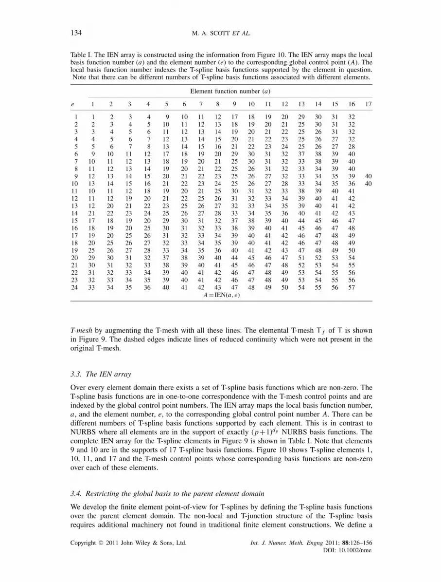
Table I. The IEN array is constructed using the information from Figure 10. The IEN array maps the localbasis function number (a) and the element number (e) to the corresponding global control point (A). Thelocal basis function number indexes the T-spline basis functions supported by the element in question.Note that there can be different numbers of T-spline basis functions associated with different elements.
Element function number (a)
e 1 2 3 4 5 6 7 8 9 10 11 12 13 14 15 16 17
1 1 2 3 4 9 10 11 12 17 18 19 20 29 30 31 322 2 3 4 5 10 11 12 13 18 19 20 21 25 30 31 323 3 4 5 6 11 12 13 14 19 20 21 22 25 26 31 324 4 5 6 7 12 13 14 15 20 21 22 23 25 26 27 325 5 6 7 8 13 14 15 16 21 22 23 24 25 26 27 286 9 10 11 12 17 18 19 20 29 30 31 32 37 38 39 407 10 11 12 13 18 19 20 21 25 30 31 32 33 38 39 408 11 12 13 14 19 20 21 22 25 26 31 32 33 34 39 409 12 13 14 15 20 21 22 23 25 26 27 32 33 34 35 39 40
10 13 14 15 16 21 22 23 24 25 26 27 28 33 34 35 36 4011 10 11 12 18 19 20 21 25 30 31 32 33 38 39 40 4112 11 12 19 20 21 22 25 26 31 32 33 34 39 40 41 4213 12 20 21 22 23 25 26 27 32 33 34 35 39 40 41 4214 21 22 23 24 25 26 27 28 33 34 35 36 40 41 42 4315 17 18 19 20 29 30 31 32 37 38 39 40 44 45 46 4716 18 19 20 25 30 31 32 33 38 39 40 41 45 46 47 4817 19 20 25 26 31 32 33 34 39 40 41 42 46 47 48 4918 20 25 26 27 32 33 34 35 39 40 41 42 46 47 48 4919 25 26 27 28 33 34 35 36 40 41 42 43 47 48 49 5020 29 30 31 32 37 38 39 40 44 45 46 47 51 52 53 5421 30 31 32 33 38 39 40 41 45 46 47 48 52 53 54 5522 31 32 33 34 39 40 41 42 46 47 48 49 53 54 55 5623 32 33 34 35 39 40 41 42 46 47 48 49 53 54 55 5624 33 34 35 36 40 41 42 43 47 48 49 50 54 55 56 57
A= IEN(a,e)
T-mesh by augmenting the T-mesh with all these lines. The elemental T-mesh T f of T is shownin Figure 9. The dashed edges indicate lines of reduced continuity which were not present in theoriginal T-mesh.
3.3. The IEN array
Over every element domain there exists a set of T-spline basis functions which are non-zero. TheT-spline basis functions are in one-to-one correspondence with the T-mesh control points and areindexed by the global control point numbers. The IEN array maps the local basis function number,a, and the element number, e, to the corresponding global control point number A. There can bedifferent numbers of T-spline basis functions supported by each element. This is in contrast toNURBS where all elements are in the support of exactly (p+1)dp NURBS basis functions. Thecomplete IEN array for the T-spline elements in Figure 9 is shown in Table I. Note that elements9 and 10 are in the supports of 17 T-spline basis functions. Figure 10 shows T-spline elements 1,10, 11, and 17 and the T-mesh control points whose corresponding basis functions are non-zeroover each of these elements.
3.4. Restricting the global basis to the parent element domain
We develop the finite element point-of-view for T-splines by defining the T-spline basis functionsover the parent element domain. The non-local and T-junction structure of the T-spline basisrequires additional machinery not found in traditional finite element constructions. We define a
Copyright � 2011 John Wiley & Sons, Ltd. Int. J. Numer. Meth. Engng 2011; 88:126–156DOI: 10.1002/nme

ISOGEOMETRIC FINITE ELEMENT DATA STRUCTURES FOR T-SPLINES 135
Indicates T-spline basis functions that are supported by the highlighted element
1
25
24
23
22
21
20
191817
16
15
14
13
12
11109
8
7
6
5
4
32
313029
28
27
26
36
35
34
33
32
54
535251
44 4546
47
48
49
5043
42
41
40
393837
57
56
55
1
25
24
23
22
21
20
191817
16
15
14
13
12
11109
8
7
6
5
4
32
313029
28
27
26
36
35
34
33
32
54
535251
44 4546
47
48
49
5043
42
41
40
393837
57
56
55
T-mesh element 1 T-mesh element 10
T-mesh element 11 T-mesh element 17
1
25
24
23
22
21
20
191817
16
15
14
13
12
11109
8
7
6
5
4
32
313029
28
27
26
36
35
34
33
32
54
535251
44 4546
47
48
49
5043
42
41
40
393837
57
56
55
1
25
24
23
22
21
20
191817
16
15
14
13
12
11109
8
7
6
5
4
32
313029
28
27
26
36
35
34
33
32
54
535251
44 4546
47
48
49
5043
42
41
40
393837
57
56
55
Figure 10. T-mesh elements 1, 10, 11, and 17 in the elemental T-mesh and the T-mesh control pointswhose corresponding T-spline basis functions are non-zero over these T-spline elements.
set, Se ={�e,{�e
a}nea=1}, of affine mappings for the element under consideration where
• �e
: �→ �e
is a one-to-one and onto affine map from the parent element domain onto theelement domain:
ne = �e(n). (6)
• �ea : �
e → �A, for a =1, . . . ,ne is a one-to-one affine mapping from the element domain intothe local basis function domain for basis function A= IEN(a,e):
nA = �ea(ne). (7)
These mappings can be determined using the elemental T-mesh and the IEN array and are usedto map from the parent element into each local basis function domain which corresponds to a
Copyright � 2011 John Wiley & Sons, Ltd. Int. J. Numer. Meth. Engng 2011; 88:126–156DOI: 10.1002/nme

136 M. A. SCOTT ET AL.
Local basis function domains
Element domain
Parent domain
Figure 11. The mappings between parent, element, and basis function coordinate systems for element 17.
For simplicity only some of the mappings are shown. �17
maps from the parent coordinate system into
the element coordinate system. �17a maps from the element coordinate system of local basis function
number a into the basis function coordinate system of global control point A= IEN(a,17). The solid dot(•) on element 17 shows the rotations incorporated in the mappings.
T-spline basis function which is non-zero over element e. The action of some but not all of theaffine maps in S17 is shown in Figure 11.
Using Se and the IEN array we can define a localized, element-based definition for the globalT-spline basis functions as
NA(nA)|e = NA(�ea(ne))|e = NA(�
ea(�
e(n)))|e = N e
a (n), (8)
where |e indicates restriction to the domain of element number e.
3.5. The T-spline element geometric map
With the basis functions defined over the parent element by Equation (8), we now define theelement geometric map, xe : �→�e, from the parent element domain onto the physical domain as
xe(n)=∑ne
a=1 Peawe
a N ea (n)
W e(n)=
ne∑a=1
Pea Re
a(n), (9)
Copyright � 2011 John Wiley & Sons, Ltd. Int. J. Numer. Meth. Engng 2011; 88:126–156DOI: 10.1002/nme

ISOGEOMETRIC FINITE ELEMENT DATA STRUCTURES FOR T-SPLINES 137
where
W e(n)=ne∑
a=1we
a N ea (n) (10)
is the element weight function, and Pea =PIEN(a,e) and we
a =wIEN(a,e) are the control point andweight, respectively, corresponding to the ath T-spline basis function over element e. Re
a is therational form of the T-spline basis function because it includes the weight function in its denomi-nator. Defining the element weight vector we ={we
a}nea=1, the diagonal weight matrix We =diag(we),
and element control points Pe as a matrix of dimension ne ×ds ,
Pe =
⎡⎢⎢⎢⎢⎢⎢⎣Pe,1
1 Pe,21 · · · Pe,ds
1
Pe,12 Pe,2
2 · · · Pe,ds2
......
...
Pe,1ne
Pe,2ne
· · · Pe,dsne
⎤⎥⎥⎥⎥⎥⎥⎦ , (11)
we can generate the corresponding matrix representation of the geometric map as
xe(n) = 1
(we)TNe(n)(Pe)TWeNe(n) (12)
= (Pe)TRe(n), (13)
where Ne ={N ea }ne
a=1 and Re ={Rea}ne
a=1 are the vectors of polynomial and rational T-spline basisfunctions, respectively, which are non-zero over element e.
4. BÉZIER EXTRACTION FOR T-SPLINES
The T-spline element construction presented in Section 3 can be further simplified using Bézierextraction. For each element, Bézier extraction generates an element extraction operator. This oper-ator is a simple, compact, algebraic representation of the topological and smoothness informationstored in the elemental T-mesh and T-spline basis. This operator can be easily integrated into thefinite element framework, analogous to what was presented for NURBS in [43]. This should notbe a surprise since NURBS form a restricted subset of T-splines. In fact, a finite element codecapable of handling extraction operators can easily incorporate both NURBS and T-splines.
4.1. The element extraction operator and the Bézier element
Bézier extraction for T-splines determines the exact representation of the T-spline basis over eachT-spline element e in terms of a set of Bernstein polynomials, B(n). Every localized T-spline basisfunction, N e
a (n), can be written as a linear combination of these Bernstein polynomials. In otherwords, for each localized T-spline basis function, N e
a (n), there exists coefficients, cea,b such that¶
N ea (n)=
(p+1)dp∑b=1
cea,b Bb(n) (14)
over element e. In matrix-vector form (14) is written as
Ne(n)=CeB(n), (15)
¶Note that the element basis functions are numbered b=1,2, . . . , (p+1)dp . This convention is typical in finite elementanalysis, but different than that used in CAGD in which it is standard for the indexing to begin with 0.
Copyright � 2011 John Wiley & Sons, Ltd. Int. J. Numer. Meth. Engng 2011; 88:126–156DOI: 10.1002/nme

138 M. A. SCOTT ET AL.
where Ce is the element extraction operator. We call the element defined by the Bernstein poly-nomials the Bézier element.
Note that, in contrast with the T-spline basis functions Ne and Re, there are the same number ofBernstein basis functions for all the elements. Also, the use of the operator allows us to standardizethe form of the element basis on the parent domain. In other words, each Bézier element is definedin terms of the exact same set of Bernstein basis functions. This may be contrasted with the T-splinebasis defined over each T-spline element in which the structure of the basis changes from elementto element.
4.2. The Bernstein basis
The Bernstein polynomials form a basis for the Bézier element. The univariate Bernstein basisfunctions are defined over the biunit interval [−1,1] as
Bki,p(�
k)= 1
2p
(p
i −1
)(1− �
k)p−(i−1)(1+ �
k)i−1, (16)
where the binomial coefficient(
pi−1
)= p!/(i −1)!(p+1−i)!, 1�i�p+1. In CAGD, the Bernstein
polynomials are usually defined over the unit interval [0,1], but in finite element analysis the biunitinterval is preferred to take advantage of the usual domains for Gauss quadrature. The univariateBernstein basis functions for p=1,2, and 3 are plotted in Figure 12. The univariate Bernsteinbasis has the following properties:
• Partition of unity:
p+1∑i=1
Bki,p(�
k)=1 ∀�
k ∈ [−1,1]. (17)
• Pointwise non-negativity:
Bki,p(�
k)�0 ∀�
k ∈ [−1,1]. (18)
• Endpoint interpolation:
Bk1,p(−1)= Bk
p+1,p(1)=1. (19)
• Symmetry:
Bki,p(�
k)= Bk
p+1−i,p(−�k) ∀�
k ∈ [−1,1]. (20)
The multivariate Bernstein basis functions of degree p, Ba,p : �→R+∪0, with a =1, . . . , (p+1)dp ,are formed as the tensor product of univariate basis functions Bk
i,p : [−1,1]→R+∪0, with i =1, . . . , p+1. In the bivariate case we have
Ba(i, j),p(n)= B1i,p(�
1)B2
j,p(�2) (21)
with
a(i, j)= (p+1)( j −1)+i. (22)
Recall that n= (�1, �
2)= (�, �) is the coordinate system assigned to the parent element. From the
formulas, it is clear that the basis functions are numbered from left to right in one dimension. Intwo dimensions each row is numbered from left to right, starting with the bottom row and movingupward (Figure 13).
Copyright � 2011 John Wiley & Sons, Ltd. Int. J. Numer. Meth. Engng 2011; 88:126–156DOI: 10.1002/nme
ISOGEOMETRIC FINITE ELEMENT DATA STRUCTURES FOR T-SPLINES 139
0
0.2
0.4
0.6
0.8
1
-1 -0.6 -0.2 0.2 0.6 1
0
0.2
0.4
0.6
0.8
1
-1 -0.6 -0.2 0.2 0.6 1
0
0.2
0.4
0.6
0.8
1
-1 -0.6 -0.2 0.2 0.6 1
1 2 12
3 12 3
4
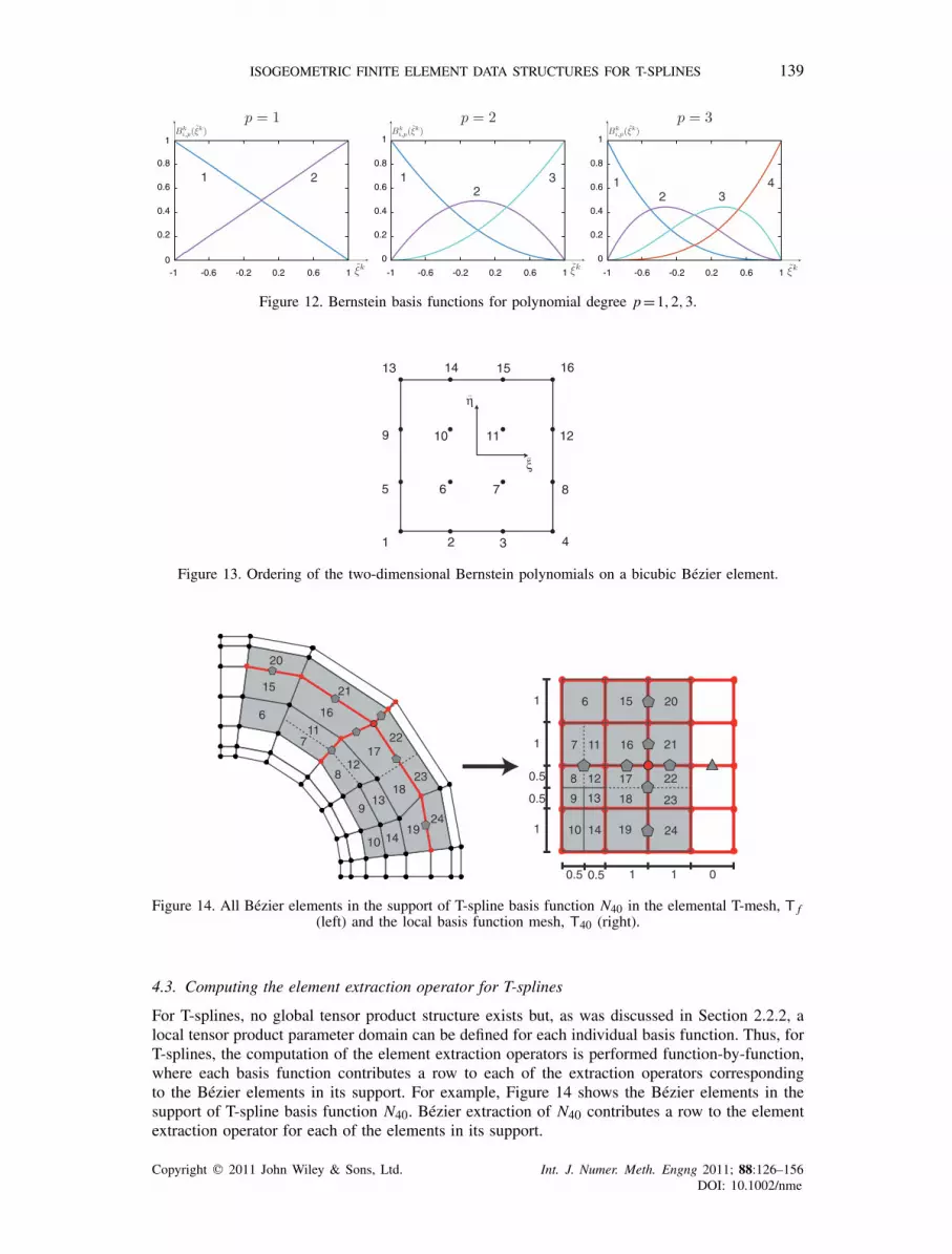
Figure 12. Bernstein basis functions for polynomial degree p=1,2,3.
ξ
η
1 2
16151413
1211109
8765
43
Figure 13. Ordering of the two-dimensional Bernstein polynomials on a bicubic Bézier element.
1
1
1
0.5
1 1 0
0.5
0.5 0.5
6
15
20
711
16
21
2217
128 23
1813
924
191410
10 14 19 24
9 13 18 23
8 12 17 22
7 11 16 21
6 15 20
Figure 14. All Bézier elements in the support of T-spline basis function N40 in the elemental T-mesh, T f(left) and the local basis function mesh, T40 (right).
4.3. Computing the element extraction operator for T-splines
For T-splines, no global tensor product structure exists but, as was discussed in Section 2.2.2, alocal tensor product parameter domain can be defined for each individual basis function. Thus, forT-splines, the computation of the element extraction operators is performed function-by-function,where each basis function contributes a row to each of the extraction operators correspondingto the Bézier elements in its support. For example, Figure 14 shows the Bézier elements in thesupport of T-spline basis function N40. Bézier extraction of N40 contributes a row to the elementextraction operator for each of the elements in its support.
Copyright � 2011 John Wiley & Sons, Ltd. Int. J. Numer. Meth. Engng 2011; 88:126–156DOI: 10.1002/nme

140 M. A. SCOTT ET AL.
N1
N2N3 N5 N6
N7
N4
0 321 4
Figure 15. A univariate T-spline basis function (solid line) with local knot vector �={0,1,2,3,4}. Theextended knot vector �={0,0,0,0,1,2,3,4,4,4,4} adds the additional functions (dashed lines) that will
be used to construct the basis functions for the Bézier elements.
4.3.1. Comparing extraction for NURBS and T-splines. Similar to NURBS, multivariate extractionoperators for T-splines can be computed as products of univariate extraction operators. A majordifference between NURBS and T-splines is that where NURBS have a global parameterization,T-splines have a local parameterization. This leads to two differences in how the extraction operatorsare computed. First, with T-splines, we work with local knot vectors that are, in general, not open,i.e. the first and last knots may have multiplicity less than p+1. Second, since the local knotvectors correspond to individual functions, as a local knot vector is processed, we compute a singlerow for each of the corresponding element extraction operators, as opposed to computing the entireelement extraction operator at once. Additionally, since there may be T-junctions in a T-spline,knots may need to be inserted into the knot spans of the local knot vector as part of the extractionprocess.
4.3.2. The extended knot vector. To handle the local knot vectors we introduce the extended knotvector, �A. The extended knot vector is constructed by repeating the first and last knots in the localknot vector until they have a multiplicity equal to p+1. The extended knot vector does not changethe parametric description of the original T-spline basis function, but it adds functions to the localbasis function domain. For example, Figure 15 shows the univariate T-spline basis function (solidline) with local knot vector �={0,1,2,3,4} and the additional basis functions (dashed lines) addedby the extended knot vector �={0,0,0,0,1,2,3,4,4,4,4}. When the functions are numberedfrom left to right the T-spline basis function will be numbered nt +1, where nt is the number ofknots added to the front of the local knot vector when constructing the extended knot vector.
4.3.3. Univariate extraction. We now describe how the univariate extraction operators arecomputed for T-splines. Once the extended knot vector has been constructed for the originalT-spline basis function, the corresponding rows of the univariate extraction operators can becomputed. These extraction operator rows are computed by performing knot insertion on theextended knot vector. Conceptually, the process is similar to computing the extraction operator forNURBS [43]. For example, if the extended knot vector for the function in Figure 15 is consideredas a knot vector for a NURBS curve, Bézier extraction would produce the basis functions as shownin Figure 16, which are the same basis functions that are produced by extraction for the T-splinebasis function. The difference between extraction for NURBS and T-splines is that for T-splineswe only compute a single row of the operator. For comparison, Table II shows the full extractionoperators that would be computed in the case of NURBS with the rows corresponding to theT-spline basis function from Figure 15 (highlighted). The extraction operator rows are computedby Algorithm 1, which is a modified version of the algorithm presented for NURBS in [43].
As a result of the extraction process we have a representation of each T-spline function in termsof the basis functions of the Bézier elements. This can be seen by considering Bézier element e inthe support of the T-spline basis function A. The T-spline basis function A restricted to element
Copyright � 2011 John Wiley & Sons, Ltd. Int. J. Numer. Meth. Engng 2011; 88:126–156DOI: 10.1002/nme

ISOGEOMETRIC FINITE ELEMENT DATA STRUCTURES FOR T-SPLINES 141
B1
B2
B3
B4
B5
B6
B7
B8
B9
B10
B11
B12
B13
1 2 3 40
Figure 16. The resulting basis functions of the Bézier elements after knot insertion and refinement of thebasis functions shown in Figure 15.
Table II. The action of extraction operators on the Bézier elementbasis computed from the extended knot vector from Figure 15. Thefull operators would be computed in the case of NURBS, but only
the highlighted rows for the T-spline basis function.
⎧⎪⎪⎪⎨⎪⎪⎪⎩N1
N2
N3
N4
⎫⎪⎪⎪⎬⎪⎪⎪⎭=
⎡⎢⎢⎢⎢⎣1 0 0 0
0 1 12
14
0 0 12
712
0 0 0 16
⎤⎥⎥⎥⎥⎦⎧⎪⎪⎪⎨⎪⎪⎪⎩
B1
B2
B3
B4
⎫⎪⎪⎪⎬⎪⎪⎪⎭,
⎧⎪⎪⎪⎨⎪⎪⎪⎩N2
N3
N4
N5
⎫⎪⎪⎪⎬⎪⎪⎪⎭=
⎡⎢⎢⎢⎢⎢⎣14 0 0 0
712
23
13
16
16
13
23
23
0 0 0 16
⎤⎥⎥⎥⎥⎥⎦⎧⎪⎪⎪⎨⎪⎪⎪⎩
B4
B5
B6
B7
⎫⎪⎪⎪⎬⎪⎪⎪⎭,
⎧⎪⎪⎪⎨⎪⎪⎪⎩N3
N4
N5
N6
⎫⎪⎪⎪⎬⎪⎪⎪⎭=
⎡⎢⎢⎢⎢⎢⎣16 0 0 0
23
23
13
16
16
13
23
712
0 0 0 14
⎤⎥⎥⎥⎥⎥⎦⎧⎪⎪⎪⎨⎪⎪⎪⎩
B7
B8
B9
B10
⎫⎪⎪⎪⎬⎪⎪⎪⎭,
⎧⎪⎪⎪⎨⎪⎪⎪⎩N4
N5
N6
N7
⎫⎪⎪⎪⎬⎪⎪⎪⎭=
⎡⎢⎢⎢⎢⎣16 0 0 0
712
12 0 0
14
12 1 0
0 0 0 1
⎤⎥⎥⎥⎥⎦⎧⎪⎪⎪⎨⎪⎪⎪⎩
B10
B11
B12
B13
⎫⎪⎪⎪⎬⎪⎪⎪⎭
e is related to the Bernstein basis functions by
NA(nA)|e = N ea (n)=eT
a Ne(n)=eTa CeB(n)=ce T
a B(n), (23)
where ea is a unit vector which is equal to 1 in entry a and 0 elsewhere. The vector cea extracts
basis function A= IEN(a,e) from Bézier element e.
4.3.4. Multivariate extraction. Multivariate Bézier extraction operators Ce for a T-spline element eare constructed as products of univariate Bézier extraction operators. In the bivariate case, T-splinebasis function NA restricted to element e can be decomposed into two univariate T-spline basisfunctions as
NA(nA)|e = N ea (n)= N e,1
a (�1)N e,2
a (�2), (24)
where a and e are such that A= IEN(a,e) and the superscripts indicate the local parametricdirection. Using the extraction procedure outlined above for univariate T-spline basis functions, we
can construct extraction operators for the basis functions N e,1a (�
1) and N e,2
a (�2). By substituting
Equation (23) into (24) we obtain
N ea (n)= [ce,1T
a B1(�1)][ce,2T
a B2(�2)]. (25)
Using the index mapping from Equation (22) it can be shown that this becomes
N ea (n)=ce T
a B(n), (26)
Copyright � 2011 John Wiley & Sons, Ltd. Int. J. Numer. Meth. Engng 2011; 88:126–156DOI: 10.1002/nme

142 M. A. SCOTT ET AL.
ce,1a ce,2
a
Figure 17. The extraction of a single T-spline basis function. Extraction is decoupled into twounivariate extraction operations and then reassembled into a single row of Ce. (The T-spline basisfunction is the one associated with control point 40, and element e corresponds to element 13 in
the elemental T-mesh shown in Figure 9.)
where cea corresponds to the ath row of the bivariate element extraction operator Ce in Equation
(15). This process is repeated for each T-spline basis function supported by element e to generatethe full extraction operator for the element. Importantly, once the element extraction operators arecomputed, a finite element code never needs to know anything about T-mesh topology to processthe global T-spline basis.
The process and result of extracting N40(n40) over an element e in its support are shown inFigures 17 and 18, respectively. In Figure 17 the univariate components of the T-spline basisfunction are shown on the left and right. Note that in both cases a knot interior to a knot span of theextended knot vector must be inserted p times to compute the extraction operator for element e. InFigure 18 we show the resulting extraction coefficients. In Appendix C, full extraction operatorscorresponding to elements 1, 10, 11, and 17 are presented.
4.4. A Bézier extraction algorithm for T-splines
A Bézier extraction algorithm for T-splines consists of the following steps:
1. Infer the T-spline basis from the T-mesh, see Section 2.2.2. Refine the T-mesh to construct the elemental T-mesh, see Section 3.2.3. For a T-spline basis function determine the Bézier elements which are in its support, see
Section 4.3.4. For a T-spline basis function perform Bézier extraction, see Sections 4.3.3 and 4.3.4.5. Repeat steps 3 and 4 for each T-spline basis function.
Copyright � 2011 John Wiley & Sons, Ltd. Int. J. Numer. Meth. Engng 2011; 88:126–156DOI: 10.1002/nme

ISOGEOMETRIC FINITE ELEMENT DATA STRUCTURES FOR T-SPLINES 143
Figure 18. The result of extracting N40(n40) over element e, where e=13. On the top left, the position ofelement 13 in the local basis function space of N40(n40) is shown. On the top right, Bézier extraction ofN40 over element e (see Figure 17) generates c13T
14 where 14 is the local index of global control point 40for element 13. In other words, 40= IEN(14,13). Note that this represents a single row of the elementextraction operator C13. On the bottom left, N40(n40) is plotted. The shaded region is the restriction ofN40(n40) to the domain of element 13. On the bottom right, a close-up of element e is shown whichportrays graphically the relationship between the extraction coefficients and Bernstein basis functions.
Note that N40(n40)|13 =c13T14 B(n). See Equation (26).
We note that the topological characterization of a T-mesh described in Section 2.1 is analogousto a quadrilateral mesh with hanging nodes. Thus, traditional quadrilateral meshing data structuresand refinement schemes that allow hanging nodes are compatible with T-splines and can be usedto perform the first three steps of the algorithm.
The fourth step is the most critical and is not mesh dependent. The primary operation in thisstep is the univariate extraction of the extended local knot vectors for a T-spline basis function asdescribed in Section 4.3.3. This routine is presented in Algorithm 1.
Algorithm 1 An algorithm to compute the univariate extraction operator rows corresponding toa single univariate T-spline basis function.
input Knot vector, � ={�1, . . . ,�p+2}Interior knots to be inserted into �, U ={�1, . . . , �m}Knot spans in � where new knots will be inserted, spans ={s1, . . . , sm}Number of interior knots, mCurve degree, p
output Element extraction operator rows ce, e=1,2, . . . ,p+1+m
// Construct the extended knot vector and count the// number of knots added to the front of the knot vector.call compute_extended_knot_vector
input: �
Copyright � 2011 John Wiley & Sons, Ltd. Int. J. Numer. Meth. Engng 2011; 88:126–156DOI: 10.1002/nme

144 M. A. SCOTT ET AL.
output: Ubar, nt
// Initialization variables:a = p+1;b = a+1;nb = 1;c1 = 0;c1(nt+1) = 1;mbar = p + 2 + nt + m;ki = 1;si = 1;while b < mbar do
cnb+1 = 0; // Initialize the next extraction operator row.
// Count multiplicity of the knot at location b.add = 0;if si <= m && spans(si) = ki domult = 0;add = 1;// Add the new knot to the knot vector.Ubar(b+1:mbar+p-m+si) = Ubar(b:mbar+p-m+si-1);Ubar(b) = U(si);si = si + 1;
elseki = ki+1;i = b;while b < m && Ubar(b+1) == Ubar(b) do b = b+1;mult = b-i+1;
end
if mult < p donumer = Ubar(b)-Ubar(a);for j = p,p-1,. . .,mult+1 do
alphas(j-mult) = numer / (Ubar(a+j+add)-Ubar(a));endr = p-mult;// Update the matrix coefficients for r new knotsfor j=1,2,. . .,r do
save = r-j+1;s = mult+j;for k=p+1,p,. . .,s+1 do
alpha = alphas(k-s);cnb(k) = alpha*cnb(k) + (1.0-alpha)*cnb(k-1);
endif b < m do// Update overlapping coefficients of the next operator row.cnb+1(save) = cnb(p+1);
endendnb = nb + 1; // Finished with the current operator.if b < m do// Update indices for the next operator.a = b;
Copyright � 2011 John Wiley & Sons, Ltd. Int. J. Numer. Meth. Engng 2011; 88:126–156DOI: 10.1002/nme

ISOGEOMETRIC FINITE ELEMENT DATA STRUCTURES FOR T-SPLINES 145
b = b+1;end
endend
5. INCORPORATING Ce INTO THE FINITE ELEMENT FORMULATION
Bézier extraction of T-splines generates a set of Bézier elements (written in terms of the Bernsteinbasis), the corresponding element extraction operators, Ce, and the IEN array. This structure isidentical to what was derived for NURBS in [43] and can be incorporated into a finite elementformulation in an analogous fashion. Starting with an abstract weak formulation,
(W )
{Given f, find u ∈S such that for all w∈V,
a(w,u)= (w, f ),(27)
where a(·, ·) is a bilinear form and (·, ·) is the L2 inner product, and S and V are the trial solutionspace and space of weighting functions, respectively. Galerkin’s method consists of constructingfinite-dimensional approximations of S and V. In isogeometric analysis these finite-dimensionalsubspaces Sh ⊂S and Vh ⊂V are constructed from the T-spline basis which describes thegeometry. The Galerkin formulation is then
(G)
{Given f, find uh ∈Sh such that for all wh ∈Vh,
a(wh,uh)= (wh, f ).(28)
In isogeometric analysis, the isoparametric concept is invoked, that is, the field in question isrepresented in terms of the geometric T-spline basis. We can write uh and wh as
wh =n∑
A=1cA RA, (29)
uh =n∑
B=1dB RB, (30)
where cA and dB are control variables. Substituting these into (28) yields the matrix form of theproblem
Kd=F, (31)
where
K = [K AB], (32)
F = {FA}, (33)
d = {dB}, (34)
K AB = a(RA, RB), (35)
FA = (RA, f ). (36)
The preceding formulation applies to scalar-valued partial differential equations, such as the heatconduction equation. The generalization to vector-valued partial differential equations, such aselasticity, follows standard procedures as described in [49].
5.1. The element shape function routine
As in standard finite elements, the global stiffness matrix, K, and force vector, F, can be constructedby performing integration over the Bézier elements to form element stiffness matrices and force
Copyright � 2011 John Wiley & Sons, Ltd. Int. J. Numer. Meth. Engng 2011; 88:126–156DOI: 10.1002/nme

146 M. A. SCOTT ET AL.
vectors, ke and fe, respectively, and assembling these into their global counterparts. The elementform of (35) and (36) is
keab = ae(Re
a, Reb), (37)
f ea = (Re
a, f )e, (38)
where ae(·, ·) denotes the bilinear form restricted to the element, (·, ·)e is the L2 inner productrestricted to the element, and Re
a are the element shape functions. The integration is usuallyperformed by Gaussian quadrature. Since T-splines are not, in general, defined over a globalparametric domain, all integrals are pulled back directly to the bi-unit parent element domain. Nointermediate parametric domain is employed. This requires the evaluation of the global T-splinebasis functions, their derivatives, and the Jacobian determinant of the pullback from the physicalspace to the parent element at each quadrature point in the parent element. These evaluations aredone in an element shape function routine. Employing the element extraction operators we have that
Re(n)=WeCe B(n)
W e(n), (39)
where
W e(n)= (we)TCeB(n). (40)
The derivatives of Re with respect to the local parent coordinates, �i, are
�Re(n)
��i
=WeCe �
��i
(B(n)
W e(n)
)=WeCe
(1
W e(n)
�B(n)
��i
− �W e(n)
��i
B(n)
(W e(n))2
). (41)
To compute the derivatives with respect to the physical coordinates, (x e1, x e
2, x e3), we apply the chain
rule to get
�Re(n)
�x ei
=3∑
j=1
�Re(n)
��j
��j
�x ei
. (42)
To compute �n/�xe we first compute �xe/�n using (13) and (41) and then take its inverse. Sincewe are integrating over the parent element we must also compute the Jacobian determinant, J e,of the mapping from the parent element to the physical space. It is computed as
J e =∣∣∣∣�xe
�n
∣∣∣∣ . (43)
Higher order derivatives can also be computed as described in [2].
5.2. Finite element data structures
To employ an extracted T-spline in an existing finite element framework requires, in addition tothe IEN array and extraction operators, the ID array and Bézier mesh. It is also useful to constructthe LM array, which can be defined directly from the IEN and ID arrays.
RemarkThe IEN, ID, and LM arrays are standard data processing arrays in finite element programs (see [49]for a full discussion). The acronyms mean ‘element nodes’, ‘destination’, and ‘location matrix’,respectively. The I’s in IEN and ID are indicating that the arrays are integer valued, correspondingto the implicit typing convention frequently used in FORTRAN programs. The implicit typingconvention defines all variable names beginning with I, J, K, L, M, and N as integer valued, hence,LM is automatically integer valued. For the reader familiar with FORTRAN these remarks areunnecessary. However, FORTRAN is not common in CAGD, and many younger programmersare unfamiliar with it and its conventions. It is still widely utilized in computational mechanics,although the trend is toward C++.
Copyright � 2011 John Wiley & Sons, Ltd. Int. J. Numer. Meth. Engng 2011; 88:126–156DOI: 10.1002/nme

ISOGEOMETRIC FINITE ELEMENT DATA STRUCTURES FOR T-SPLINES 147
5.2.1. Constructing the ID array. The ID array for the example domain � in Figure 3 is shownin Figure 19, where two degrees of freedom are assigned to every control point. This array mapsthe degree-of-freedom number (e.g. the direction index of a displacement component) and globalcontrol point number to the corresponding equation number in the global system. A zero valueindicates a degree of freedom that is specified by the boundary conditions and for which theequation has been removed from the global system. For the domain � the horizontal and verticaldisplacements of control points 1, 9, 17, 29, 37, 44, and 51 are assumed to be specified.
5.2.2. Computing the Bézier mesh. Once the IEN array and element extraction operators have beencomputed, the control points for the Bézier elements can be computed by combining Equations (9)and (15). In general, we obtain the Bézier control points Qe and Bézier weights wb,e for element e as
Qe = (Wb,e)−1(Ce)TWePe, (44)
wb,e = (Ce)Twe, (45)
1
25
24
23
22
21
20
191817
16
15
14
13
12
11109
8
7
6
5
4
32
313029
28
27
26
36
35
34
33
32
54
535251
44 4546
47
48
49
5043
42
41
40
393837
57
56
55
Global control point number ( )1 2 3 4 5 6 7 8 9 10 11 12 13 14 15
Degree-of-freedom 1 0 1 3 5 7 9 11 13 0 15 17 19 21 23 25number ( ) 2 0 2 4 6 8 10 12 14 0 16 18 20 22 24 26
16 17 18 19 20 21 22 23 24 25 26 27 28 29 3027 0 29 31 33 35 37 39 41 43 45 47 49 0 5128 0 30 32 34 36 38 40 42 44 46 48 50 0 52
31 32 33 34 35 36 37 38 39 40 41 42 43 44 4553 55 57 59 61 63 0 65 67 69 71 73 75 0 7754 56 58 60 62 64 0 66 68 70 72 74 76 0 78
46 47 48 49 50 51 52 53 54 55 56 5779 81 83 85 87 0 89 91 93 95 97 9980 82 84 86 88 0 90 92 94 96 98 100
Figure 19. The ID array maps the degree-of-freedom number (i.e. direction index of the displace-ment component) and global control point number to the corresponding equation number in the globalsystem. For this example the horizontal and vertical displacements of control points 1, 9, 17, 29, 37,44, and 51 are specified by boundary conditions. The global equations corresponding to these degreesof freedom are removed from the system through the ID array. The LM array is computed as follows:
P =LM(i,a,e)= ID(i, IEN(a,e)).
Copyright � 2011 John Wiley & Sons, Ltd. Int. J. Numer. Meth. Engng 2011; 88:126–156DOI: 10.1002/nme

148 M. A. SCOTT ET AL.
Bezier control element 1 Bezier control element 10
Bezier control element 11 Bezier control element 17
Figure 20. The extraction operators and IEN array can be used to construct the Bézier control elements.For each control element e the symbol ‘◦’ indicates the global T-spline control points which influencethe location of Bézier control points, indicated by the symbol ‘•’. The global control points thatinfluence each control element are determined by the IEN array, and the location of the element control
points is computed with the element extraction operator Ce.
where Pe are the T-spline control points, Wb,e is the diagonal matrix of Bézier weights, and We isthe diagonal matrix of T-spline weights, we. Figure 20 shows the result of (44) for Bézier elements1, 10, 11, 17 (see Appendix B for the element control point coordinates). The T-spline controlpoints which contribute to the location of the Bézier element control points are indicated by thesymbol ◦. Each T-spline element (see Section 3.5) has an equivalent representation as an extractedBézier element. In other words
xe(n)= xb,e(n)= 1
W b,e(n)(Qe)TWb,eB(n), (46)
where W b,e(n)=wb,e TB(n). We have defined three ‘meshes’ for the T-spline example in Figure 3—the elemental T-mesh, the Bézier control mesh, and the Bézier physical mesh. Figure 21 shows arepresentative element in each of these meshes and how they are related using Ce. It is importantto remember that the Bézier physical mesh defines the set of finite elements used in computations.The extraction operator corresponding to each of these elements is then used to constrain theBézier degrees of freedom such that the original smoothness of the T-spline is present in the finiteelement solution.
We have implemented a finite element code that incorporates Bézier elements and the extractionoperator, and have tested this approach extensively. In all cases where a comparison exists, it givesidentical results to those obtained using isogeometric implementations which do not utilize T-splineextraction. We have also found that this approach greatly reduces finite element assembly times andreduces the complexity of parallelizing isogeometric codes. Another important practical advantage
Copyright � 2011 John Wiley & Sons, Ltd. Int. J. Numer. Meth. Engng 2011; 88:126–156DOI: 10.1002/nme

ISOGEOMETRIC FINITE ELEMENT DATA STRUCTURES FOR T-SPLINES 149
T-spline control mesh
e
e
Bézier control mesh
Bézier physical mesh
Algorithm 1
Element extraction operator
Input
T-mesh:- Topology
- Knot intervals
Figure 21. Various ‘meshes’ of the T-spline example.
to this approach is that it allows an analyst to compute with T-splines without understanding thedetails of T-spline technology. The extraction paradigm provides a simple interface which is readilyaccessible to most finite element practitioners.
6. CONCLUSION
We have used Bézier extraction to develop a local finite element representation of a global T-spline.The global topological and smoothness information is contained in element extraction operators,which facilitate an elegant implementation of T-junctions, known as ‘hanging nodes’ in finiteelement analysis. Each element basis has the same form in terms of Bernstein polynomials. Thechanges necessary to standard finite element programs are confined to shape function subroutines.Element formation routines and overall architecture are unaffected. The assembly of global arraysuses the same data processing arrays as finite element programs (e.g. the IEN, ID, and LMarrays; see Hughes [49]). Existing finite element programs can be easily generalized to performisogeometric analysis with T-splines using the methodology described.
APPENDIX A: T-SPLINE CONTROL POINTS FOR THE T-SPLINE EXAMPLE
Table AI lists the global T-spline control point coordinates for the geometry in Figure 3.
Copyright � 2011 John Wiley & Sons, Ltd. Int. J. Numer. Meth. Engng 2011; 88:126–156DOI: 10.1002/nme

150 M. A. SCOTT ET AL.
Table AI. The control point (P) coordinates (x, y) and weights (w).
Control point x y w
1 0.0000 1.5000 1.00002 0.1858 1.5000 0.95123 0.5746 1.4288 0.87804 1.0022 1.1497 0.84755 1.2637 0.8275 0.85976 1.4477 0.4714 0.89637 1.5000 0.1858 0.95128 1.5000 0.0000 1.00009 0.0000 1.6250 1.0000
10 0.2013 1.6250 0.951211 0.6224 1.5479 0.878012 1.0857 1.2455 0.847513 1.3690 0.8964 0.859714 1.5683 0.5107 0.896315 1.6250 0.2013 0.951216 1.6250 0.0000 1.000017 0.0000 1.8750 1.000018 0.2323 1.8750 0.951219 0.7182 1.7860 0.878020 1.2527 1.4371 0.847521 1.5270 0.9999 0.859722 1.7493 0.5696 0.896323 1.8425 0.2246 0.951224 1.8425 0.0000 1.000025 1.7376 1.1378 0.859726 1.9906 0.6482 0.896327 2.0625 0.2555 0.951228 2.0625 0.0000 1.000029 0.0000 2.2500 1.000030 0.2788 2.2500 0.951231 0.8618 2.1432 0.878032 1.5033 1.7245 0.847533 1.9516 1.2194 0.789534 2.2319 0.7268 0.896335 2.3125 0.2865 0.951236 2.3125 0.0000 1.000037 0.0000 2.6250 1.000038 0.3252 2.6250 0.951239 1.0055 2.5004 0.878040 1.9100 1.9100 0.841341 2.5004 1.0055 0.878042 2.6250 0.3252 0.951243 2.6250 0.0000 1.000044 0.0000 2.8750 1.000045 0.3562 2.8750 0.951246 1.1012 2.7386 0.878047 2.0919 2.0919 0.841348 2.7386 1.1012 0.878049 2.8750 0.3562 0.951250 2.8750 0.0000 1.000051 0.0000 3.0000 1.000052 0.3717 3.0000 0.951253 1.1491 2.8576 0.878054 2.1829 2.1829 0.841355 2.8576 1.1491 0.878056 3.0000 0.3717 0.951257 3.0000 0.0000 1.0000
Copyright � 2011 John Wiley & Sons, Ltd. Int. J. Numer. Meth. Engng 2011; 88:126–156DOI: 10.1002/nme

ISOGEOMETRIC FINITE ELEMENT DATA STRUCTURES FOR T-SPLINES 151
APPENDIX B: BÉZIER ELEMENT CONTROL POINTS FOR THE T-SPLINE EXAMPLE
Table BI lists the Bézier element control points for elements 1, 10, 11, and 17 from the geometryin Figure 3.
Table BI. Bézier element control points for elements 1, 10, 11, and 17, as shown inFigure 10. The array a(i, j) is defined in (22).
a(i, j) x y w a(i, j) x y w
e=1 e=101 0.5521 1.3947 0.8902 1 1.8750 0.0000 1.00002 0.5982 1.5109 0.8902 2 1.9375 0.0000 1.00003 0.6442 1.6271 0.8902 3 2.0000 0.0000 1.00004 0.6902 1.7433 0.8902 4 2.0625 0.0000 1.00005 0.3724 1.4658 0.9146 5 1.8750 0.2323 0.95126 0.4035 1.5880 0.9146 6 1.9375 0.2401 0.95127 0.4345 1.7101 0.9146 7 2.0000 0.2478 0.95128 0.4655 1.8323 0.9146 8 2.0625 0.2555 0.95129 0.1858 1.5000 0.9512 9 1.8323 0.4655 0.9146
10 0.2013 1.6250 0.9512 10 1.8934 0.4810 0.914611 0.2168 1.7500 0.9512 11 1.9544 0.4966 0.914612 0.2323 1.8750 0.9512 12 2.0155 0.5121 0.914613 0.0000 1.5000 1.0000 13 1.7433 0.6902 0.890214 0.0000 1.6250 1.0000 14 1.8015 0.7132 0.890215 0.0000 1.7500 1.0000 15 1.8596 0.7362 0.890216 0.0000 1.8750 1.0000 16 1.9177 0.7592 0.8902
a(i, j) x y w a(i, j) x y w
e=11 e=171 1.4584 1.4584 0.8536 1 1.8832 1.2312 0.86272 1.5026 1.5026 0.8536 2 1.9879 1.2996 0.86273 1.5468 1.5468 0.8536 3 2.0925 1.3680 0.86274 1.5910 1.5910 0.8536 4 2.1971 1.4364 0.86275 1.2570 1.6598 0.8536 5 1.7985 1.3608 0.85666 1.2951 1.7101 0.8536 6 1.8985 1.4364 0.85667 1.3332 1.7604 0.8536 7 1.9984 1.5120 0.85668 1.3713 1.8107 0.8536 8 2.0983 1.5876 0.85669 1.0202 1.8143 0.8658 9 1.7008 1.4811 0.8536
10 1.0512 1.8693 0.8658 10 1.7953 1.5634 0.853611 1.0821 1.9243 0.8658 11 1.8898 1.6457 0.853612 1.1130 1.9793 0.8658 12 1.9843 1.7280 0.853613 0.7592 1.9177 0.8902 13 1.5910 1.5910 0.853614 0.7822 1.9758 0.8902 14 1.6794 1.6794 0.853615 0.8052 2.0339 0.8902 15 1.7678 1.7678 0.853616 0.8282 2.0920 0.8902 16 1.8561 1.8561 0.8536
APPENDIX C: BÉZIER ELEMENT EXTRACTION OPERATORS FOR THET-SPLINE EXAMPLE
The extraction operators for elements 1, 10, 11 and 17 are listed below. These operators can beused to retrieve the Bézier control points listed in Appendix B from the global T-spline controlpoints in Appendix A using (44). We note that because most extraction operators have many zeroentries it is important to employ a sparse matrix storage format (see [50] and references therein).
Copyright � 2011 John Wiley & Sons, Ltd. Int. J. Numer. Meth. Engng 2011; 88:126–156DOI: 10.1002/nme

152 M. A. SCOTT ET AL.
C1 =
⎡⎢⎢⎢⎢⎢⎢⎢⎢⎢⎢⎢⎢⎢⎢⎢⎢⎢⎢⎢⎢⎢⎢⎢⎢⎢⎣
0.0000 0.0000 0.0000 0.0000 0.0000 0.0000 0.0000 0.00000.2500 0.0000 0.0000 0.0000 0.5000 0.0000 0.0000 0.00000.5500 0.0000 0.0000 0.0000 0.5000 0.0000 0.0000 0.00000.2000 0.0000 0.0000 0.0000 0.0000 0.0000 0.0000 0.00000.0000 0.0000 0.0000 0.0000 0.0000 0.0000 0.0000 0.00000.0000 0.2500 0.1250 0.0625 0.0000 0.5000 0.2500 0.12500.0000 0.5500 0.2750 0.1375 0.0000 0.5000 0.2500 0.12500.0000 0.2000 0.1000 0.0500 0.0000 0.0000 0.0000 0.00000.0000 0.0000 0.0000 0.0000 0.0000 0.0000 0.0000 0.00000.0000 0.0000 0.1250 0.1458 0.0000 0.0000 0.2500 0.29170.0000 0.0000 0.2750 0.3208 0.0000 0.0000 0.2500 0.29170.0000 0.0000 0.1000 0.1167 0.0000 0.0000 0.0000 0.00000.0000 0.0000 0.0000 0.0000 0.0000 0.0000 0.0000 0.00000.0000 0.0000 0.0000 0.0417 0.0000 0.0000 0.0000 0.08330.0000 0.0000 0.0000 0.0917 0.0000 0.0000 0.0000 0.08330.0000 0.0000 0.0000 0.0333 0.0000 0.0000 0.0000 0.0000
0.0000 0.0000 0.0000 0.0000 1.0000 0.0000 0.0000 0.00001.0000 0.0000 0.0000 0.0000 0.0000 0.0000 0.0000 0.00000.0000 0.0000 0.0000 0.0000 0.0000 0.0000 0.0000 0.00000.0000 0.0000 0.0000 0.0000 0.0000 0.0000 0.0000 0.00000.0000 0.0000 0.0000 0.0000 0.0000 1.0000 0.5000 0.25000.0000 1.0000 0.5000 0.2500 0.0000 0.0000 0.0000 0.00000.0000 0.0000 0.0000 0.0000 0.0000 0.0000 0.0000 0.00000.0000 0.0000 0.0000 0.0000 0.0000 0.0000 0.0000 0.00000.0000 0.0000 0.0000 0.0000 0.0000 0.0000 0.5000 0.58330.0000 0.0000 0.5000 0.5833 0.0000 0.0000 0.0000 0.00000.0000 0.0000 0.0000 0.0000 0.0000 0.0000 0.0000 0.00000.0000 0.0000 0.0000 0.0000 0.0000 0.0000 0.0000 0.00000.0000 0.0000 0.0000 0.0000 0.0000 0.0000 0.0000 0.16670.0000 0.0000 0.0000 0.1667 0.0000 0.0000 0.0000 0.00000.0000 0.0000 0.0000 0.0000 0.0000 0.0000 0.0000 0.00000.0000 0.0000 0.0000 0.0000 0.0000 0.0000 0.0000 0.0000
⎤⎥⎥⎥⎥⎥⎥⎥⎥⎥⎥⎥⎥⎥⎥⎥⎥⎥⎥⎥⎥⎥⎥⎥⎥⎥⎦
C10 =
⎡⎢⎢⎢⎢⎢⎢⎢⎢⎢⎢⎢⎢⎢⎢⎢⎢⎢⎢⎢⎢⎢⎢⎢⎢⎢⎢⎢⎣
0.0000 0.0000 0.0000 0.0000 0.0000 0.0000 0.0000 0.00000.0000 0.0000 0.0000 0.0000 0.0000 0.0000 0.0000 0.00000.0000 0.0000 0.0000 0.0000 0.1111 0.0000 0.0000 0.00000.1111 0.0000 0.0000 0.0000 0.0000 0.0000 0.0000 0.00000.0000 0.0000 0.0000 0.0000 0.0000 0.0000 0.0000 0.00000.0000 0.0000 0.0000 0.0000 0.0000 0.0000 0.0000 0.00000.0000 0.0000 0.0000 0.0000 0.5556 0.5000 0.2500 0.12500.5556 0.5000 0.2500 0.1250 0.0000 0.0000 0.0000 0.00000.0000 0.0000 0.0000 0.0000 0.0000 0.0000 0.0000 0.00000.0000 0.0000 0.0000 0.0000 0.0000 0.0000 0.0000 0.00000.0000 0.0000 0.0000 0.0000 0.3333 0.5000 0.7500 0.75000.3333 0.5000 0.7500 0.7500 0.0000 0.0000 0.0000 0.00000.0000 0.0000 0.0000 0.0000 0.0000 0.0000 0.0000 0.00000.0000 0.0000 0.0000 0.0000 0.0000 0.0000 0.0000 0.00000.0000 0.0000 0.0000 0.0000 0.0000 0.0000 0.0000 0.12500.0000 0.0000 0.0000 0.1250 0.0000 0.0000 0.0000 0.00000.0000 0.0000 0.0000 0.0000 0.0000 0.0000 0.0000 0.0000
Copyright � 2011 John Wiley & Sons, Ltd. Int. J. Numer. Meth. Engng 2011; 88:126–156DOI: 10.1002/nme

ISOGEOMETRIC FINITE ELEMENT DATA STRUCTURES FOR T-SPLINES 153
0.0000 0.0000 0.0000 0.0000 0.0370 0.0000 0.0000 0.00000.0741 0.0000 0.0000 0.0000 0.0617 0.0000 0.0000 0.00000.0370 0.0000 0.0000 0.0000 0.0123 0.0000 0.0000 0.00000.0000 0.0000 0.0000 0.0000 0.0000 0.0000 0.0000 0.00000.0000 0.0000 0.0000 0.0000 0.1852 0.1667 0.0833 0.04170.3704 0.3333 0.1667 0.0833 0.3086 0.2778 0.1389 0.06940.1852 0.1667 0.0833 0.0417 0.0617 0.0556 0.0278 0.01390.0000 0.0000 0.0000 0.0000 0.0000 0.0000 0.0000 0.00000.0000 0.0000 0.0000 0.0000 0.1111 0.1667 0.2500 0.25000.2222 0.3333 0.5000 0.5000 0.1852 0.2778 0.4167 0.41670.1111 0.1667 0.2500 0.2500 0.0370 0.0556 0.0833 0.08330.0000 0.0000 0.0000 0.0000 0.0000 0.0000 0.0000 0.00000.0000 0.0000 0.0000 0.0000 0.0000 0.0000 0.0000 0.04170.0000 0.0000 0.0000 0.0833 0.0000 0.0000 0.0000 0.06940.0000 0.0000 0.0000 0.0417 0.0000 0.0000 0.0000 0.01390.0000 0.0000 0.0000 0.0000 0.0000 0.0000 0.0000 0.00000.0000 0.0000 0.0000 0.0000 0.0000 0.0000 0.0000 0.0035
⎤⎥⎥⎥⎥⎥⎥⎥⎥⎥⎥⎥⎥⎥⎥⎥⎥⎥⎥⎥⎥⎥⎥⎥⎥⎥⎥⎥⎦
C11 =
⎡⎢⎢⎢⎢⎢⎢⎢⎢⎢⎢⎢⎢⎢⎢⎢⎢⎢⎢⎢⎢⎢⎢⎢⎢⎢⎣
0.0000 0.0000 0.0000 0.0000 0.0000 0.0000 0.0000 0.00000.0021 0.0000 0.0000 0.0000 0.0063 0.0000 0.0000 0.00000.0188 0.0000 0.0000 0.0000 0.0250 0.0000 0.0000 0.00000.0000 0.0000 0.0000 0.0000 0.0000 0.0000 0.0000 0.00000.0312 0.0250 0.0167 0.0111 0.0937 0.0750 0.0500 0.03330.2812 0.2250 0.1500 0.1000 0.3750 0.3000 0.2000 0.13330.0417 0.0000 0.0000 0.0000 0.0000 0.0000 0.0000 0.00000.2500 0.2500 0.1667 0.1111 0.0000 0.0000 0.0000 0.00000.0000 0.0000 0.0000 0.0000 0.0000 0.0000 0.0000 0.00000.0319 0.0389 0.0444 0.0444 0.0958 0.1167 0.1333 0.13330.2875 0.3500 0.4000 0.4000 0.3833 0.4667 0.5333 0.53330.0417 0.0833 0.1667 0.2000 0.0000 0.0000 0.0000 0.00000.0000 0.0000 0.0000 0.0000 0.0000 0.0000 0.0000 0.00000.0035 0.0069 0.0139 0.0278 0.0069 0.0139 0.0278 0.05560.0139 0.0278 0.0556 0.1111 0.0139 0.0278 0.0556 0.11110.0000 0.0000 0.0000 0.0111 0.0000 0.0000 0.0000 0.0000
0.0000 0.0000 0.0000 0.0000 0.0078 0.0000 0.0000 0.00000.0187 0.0000 0.0000 0.0000 0.0172 0.0000 0.0000 0.00000.0125 0.0000 0.0000 0.0000 0.0063 0.0000 0.0000 0.00000.0000 0.0000 0.0000 0.0000 0.1172 0.0937 0.0625 0.04170.2812 0.2250 0.1500 0.1000 0.2578 0.2063 0.1375 0.09170.1875 0.1500 0.1000 0.0667 0.0938 0.0750 0.0500 0.03330.0000 0.0000 0.0000 0.0000 0.0000 0.0000 0.0000 0.00000.0000 0.0000 0.0000 0.0000 0.0000 0.0000 0.0000 0.00000.0000 0.0000 0.0000 0.0000 0.1198 0.1458 0.1667 0.16670.2875 0.3500 0.4000 0.4000 0.2635 0.3208 0.3667 0.36670.1917 0.2333 0.2667 0.2667 0.0958 0.1167 0.1333 0.13330.0000 0.0000 0.0000 0.0000 0.0000 0.0000 0.0000 0.00000.0000 0.0000 0.0000 0.0000 0.0052 0.0104 0.0208 0.04170.0139 0.0278 0.0556 0.1111 0.0122 0.0243 0.0486 0.09720.0069 0.0139 0.0278 0.0556 0.0035 0.0069 0.0139 0.02780.0000 0.0000 0.0000 0.0000 0.0000 0.0000 0.0000 0.0000
⎤⎥⎥⎥⎥⎥⎥⎥⎥⎥⎥⎥⎥⎥⎥⎥⎥⎥⎥⎥⎥⎥⎥⎥⎥⎥⎦Copyright � 2011 John Wiley & Sons, Ltd. Int. J. Numer. Meth. Engng 2011; 88:126–156
DOI: 10.1002/nme
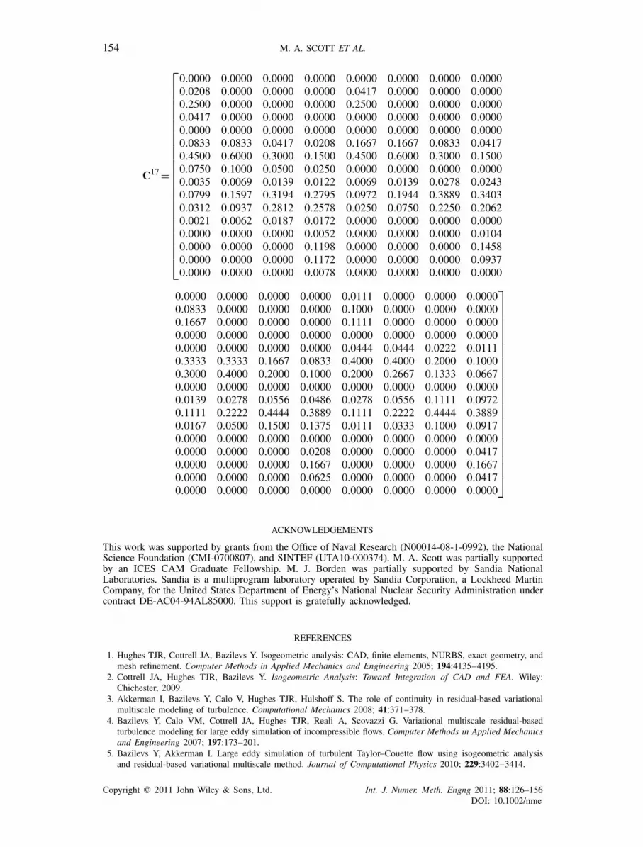
154 M. A. SCOTT ET AL.
C17 =
⎡⎢⎢⎢⎢⎢⎢⎢⎢⎢⎢⎢⎢⎢⎢⎢⎢⎢⎢⎢⎢⎢⎢⎢⎢⎢⎣
0.0000 0.0000 0.0000 0.0000 0.0000 0.0000 0.0000 0.00000.0208 0.0000 0.0000 0.0000 0.0417 0.0000 0.0000 0.00000.2500 0.0000 0.0000 0.0000 0.2500 0.0000 0.0000 0.00000.0417 0.0000 0.0000 0.0000 0.0000 0.0000 0.0000 0.00000.0000 0.0000 0.0000 0.0000 0.0000 0.0000 0.0000 0.00000.0833 0.0833 0.0417 0.0208 0.1667 0.1667 0.0833 0.04170.4500 0.6000 0.3000 0.1500 0.4500 0.6000 0.3000 0.15000.0750 0.1000 0.0500 0.0250 0.0000 0.0000 0.0000 0.00000.0035 0.0069 0.0139 0.0122 0.0069 0.0139 0.0278 0.02430.0799 0.1597 0.3194 0.2795 0.0972 0.1944 0.3889 0.34030.0312 0.0937 0.2812 0.2578 0.0250 0.0750 0.2250 0.20620.0021 0.0062 0.0187 0.0172 0.0000 0.0000 0.0000 0.00000.0000 0.0000 0.0000 0.0052 0.0000 0.0000 0.0000 0.01040.0000 0.0000 0.0000 0.1198 0.0000 0.0000 0.0000 0.14580.0000 0.0000 0.0000 0.1172 0.0000 0.0000 0.0000 0.09370.0000 0.0000 0.0000 0.0078 0.0000 0.0000 0.0000 0.0000
0.0000 0.0000 0.0000 0.0000 0.0111 0.0000 0.0000 0.00000.0833 0.0000 0.0000 0.0000 0.1000 0.0000 0.0000 0.00000.1667 0.0000 0.0000 0.0000 0.1111 0.0000 0.0000 0.00000.0000 0.0000 0.0000 0.0000 0.0000 0.0000 0.0000 0.00000.0000 0.0000 0.0000 0.0000 0.0444 0.0444 0.0222 0.01110.3333 0.3333 0.1667 0.0833 0.4000 0.4000 0.2000 0.10000.3000 0.4000 0.2000 0.1000 0.2000 0.2667 0.1333 0.06670.0000 0.0000 0.0000 0.0000 0.0000 0.0000 0.0000 0.00000.0139 0.0278 0.0556 0.0486 0.0278 0.0556 0.1111 0.09720.1111 0.2222 0.4444 0.3889 0.1111 0.2222 0.4444 0.38890.0167 0.0500 0.1500 0.1375 0.0111 0.0333 0.1000 0.09170.0000 0.0000 0.0000 0.0000 0.0000 0.0000 0.0000 0.00000.0000 0.0000 0.0000 0.0208 0.0000 0.0000 0.0000 0.04170.0000 0.0000 0.0000 0.1667 0.0000 0.0000 0.0000 0.16670.0000 0.0000 0.0000 0.0625 0.0000 0.0000 0.0000 0.04170.0000 0.0000 0.0000 0.0000 0.0000 0.0000 0.0000 0.0000
⎤⎥⎥⎥⎥⎥⎥⎥⎥⎥⎥⎥⎥⎥⎥⎥⎥⎥⎥⎥⎥⎥⎥⎥⎥⎥⎦
ACKNOWLEDGEMENTS
This work was supported by grants from the Office of Naval Research (N00014-08-1-0992), the NationalScience Foundation (CMI-0700807), and SINTEF (UTA10-000374). M. A. Scott was partially supportedby an ICES CAM Graduate Fellowship. M. J. Borden was partially supported by Sandia NationalLaboratories. Sandia is a multiprogram laboratory operated by Sandia Corporation, a Lockheed MartinCompany, for the United States Department of Energy’s National Nuclear Security Administration undercontract DE-AC04-94AL85000. This support is gratefully acknowledged.
REFERENCES
1. Hughes TJR, Cottrell JA, Bazilevs Y. Isogeometric analysis: CAD, finite elements, NURBS, exact geometry, andmesh refinement. Computer Methods in Applied Mechanics and Engineering 2005; 194:4135–4195.
2. Cottrell JA, Hughes TJR, Bazilevs Y. Isogeometric Analysis: Toward Integration of CAD and FEA. Wiley:Chichester, 2009.
3. Akkerman I, Bazilevs Y, Calo V, Hughes TJR, Hulshoff S. The role of continuity in residual-based variationalmultiscale modeling of turbulence. Computational Mechanics 2008; 41:371–378.
4. Bazilevs Y, Calo VM, Cottrell JA, Hughes TJR, Reali A, Scovazzi G. Variational multiscale residual-basedturbulence modeling for large eddy simulation of incompressible flows. Computer Methods in Applied Mechanicsand Engineering 2007; 197:173–201.
5. Bazilevs Y, Akkerman I. Large eddy simulation of turbulent Taylor–Couette flow using isogeometric analysisand residual-based variational multiscale method. Journal of Computational Physics 2010; 229:3402–3414.
Copyright � 2011 John Wiley & Sons, Ltd. Int. J. Numer. Meth. Engng 2011; 88:126–156DOI: 10.1002/nme

ISOGEOMETRIC FINITE ELEMENT DATA STRUCTURES FOR T-SPLINES 155
6. Bazilevs Y, Michler C, Calo VM, Hughes TJR. Isogeometric variational multiscale modeling of wall-boundedturbulent flows with weakly enforced boundary conditions on unstretched meshes. Computer Methods in AppliedMechanics and Engineering 2010; 199(13–16):780–790.
7. Bazilevs Y, Calo VM, Zhang Y, Hughes TJR. Isogeometric fluid–structure interaction analysis with applicationsto arterial blood flow. Computational Mechanics 2006; 38:310–322.
8. Bazilevs Y, Calo VM, Hughes TJR, Zhang Y. Isogeometric fluid–structure interaction: theory, algorithms, andcomputations. Computational Mechanics 2008; 43:3–37.
9. Zhang Y, Bazilevs Y, Goswami S, Bajaj C, Hughes TJR. Patient-specific vascular NURBS modeling forisogeometric analysis of blood flow. Computer Methods in Applied Mechanics and Engineering 2007; 196:2943–2959.
10. Bazilevs Y, Gohean JR, Hughes TJR, Moser RD, Zhang Y. Patient-specific isogeometric fluid-structure interactionanalysis of thoracic aortic blood flow due to implantation of the Jarvik 2000 left ventricular assist device.Computer Methods in Applied Mechanics and Engineering 2009; 198(45–46):3534–3550.
11. Auricchio F, da Veiga LB, Lovadina C, Reali A. The importance of the exact satisfaction of the incompressibilityconstraint in nonlinear elasticity: mixed FEMs versus NURBS-based approximations. Computer Methods inApplied Mechanics and Engineering 2010; 199:314–323.
12. Auricchio F, da Veiga LB, Buffa A, Lovadina C, Reali A, Sangalli G. A fully ‘locking-free’ isogeometric approachfor plane linear elasticity problems: a stream function formulation. Computer Methods in Applied Mechanics andEngineering 2007; 197:160–172.
13. Elguedj T, Bazilevs Y, Calo VM, Hughes TJR. B and F projection methods for nearly incompressible linear andnon-linear elasticity and plasticity using higher-order NURBS elements. Computer Methods in Applied Mechanicsand Engineering 2008; 197:2732–2762.
14. Cottrell JA, Hughes TJR, Reali A. Studies of refinement and continuity in isogeometric analysis. ComputerMethods in Applied Mechanics and Engineering 2007; 196:4160–4183.
15. Cottrell JA, Reali A, Bazilevs Y, Hughes TJR. Isogeometric analysis of structural vibrations. Computer Methodsin Applied Mechanics and Engineering 2006; 195:5257–5296.
16. Benson DJ, Bazilevs Y, Hsu MC, Hughes TJR. Isogeometric shell analysis: the Reissner–Mindlin shell. ComputerMethods in Applied Mechanics and Engineering 2010; 199(5–8):276–289.
17. Benson DJ, Bazilevs Y, Hsu MC, Hughes TJR. A large deformation, rotation-free, isogeometric shell. InternationalJournal for Numerical Methods in Engineering 2010. DOI: 10.1016/j.cma.2010.12.003.
18. Benson DJ, Bazilevs Y, De Luycker E, Hsu MC, Scott MA, Hughes TJR, Belytschko T. A generalized finiteelement formulation for arbitrary basis functions: from isogeometric analysis to XFEM. International Journalfor Numerical Methods in Engineering 2010; 83:765–785.
19. Echter R, Bischoff M. Numerical efficiency, locking and unlocking of NURBS finite elements. Computer Methodsin Applied Mechanics and Engineering 2010; 199(5–8):374–382.
20. Kiendl J, Bazilevs Y, Hsu MC, Wuechner R, Bletzinger KU. The bending strip method for isogeometric analysisof Kirchhoff-Love shell structures comprised of multiple patches. Computer Methods in Applied Mechanics andEngineering 2010; 199(37–40):2403–2416.
21. Gomez H, Calo VM, Bazilevs Y, Hughes TJR. Isogeometric analysis of the Cahn–Hilliard phase-field model.Computer Methods in Applied Mechanics and Engineering 2008; 197:4333–4352.
22. Gomez H, Hughes TJR, Nogueira X, Calo VM. Isogeometric analysis of the isothermal Navier–Stokes–Kortewegequations. Computer Methods in Applied Mechanics and Engineering 2010; 199(25–28):1828–1840.
23. Lipton S, Evans JA, Bazilevs Y, Elguedj T, Hughes TJR. Robustness of isogeometric structural discretizationsunder severe mesh distortion. Computer Methods in Applied Mechanics and Engineering 2010; 199(5–8):357–373.
24. Wall WA, Frenzel MA, Cyron C. Isogeometric structural shape optimization. Computer Methods in AppliedMechanics and Engineering 2008; 197:2976–2988.
25. Qian X. Full analytical sensitivities in NURBS based isogeometric shape optimization. Computer Methods inApplied Mechanics and Engineering 2010; 199(29–32):2059–2071.
26. Nagy AP, Abdalla MM, Gurdal Z. Isogeometric sizing and shape optimisation of beam structures. ComputerMethods in Applied Mechanics and Engineering 2010; 199(17–20):1216–1230.
27. Nagy AP, Abdalla MM, Gurdal Z. On the variational formulation of stress constraints in isogeometric design.Computer Methods in Applied Mechanics and Engineering 2010; 199(41–44):2687–2696.
28. Buffa A, Sangalli G, Vazquez R. Isogeometric analysis in electromagnetics: B-splines approximation. ComputerMethods in Applied Mechanics and Engineering 2010; 199(17–20):1143–1152.
29. Cohen E, Martin T, Kirby RM, Lyche T, Riesenfeld RF. Analysis-aware modeling: understanding qualityconsiderations in modeling for isogeometric analysis. Computer Methods in Applied Mechanics and Engineering2010; 199(5–8):334–356.
30. Lu J. Circular element: isogeometric elements of smooth boundary. Computer Methods in Applied Mechanicsand Engineering 2009; 198(30–32):2391–2402.
31. Kim HJ, Seo YD, Youn SK. Isogeometric analysis for trimmed CAD surfaces. Computer Methods in AppliedMechanics and Engineering 2009; 198(37–40):2982–2995.
32. Costantini P, Manni C, Pelosi F, Sampoli ML. Quasi-interpolation in isogeometric analysis based on generalizedB-splines. Computer Aided Geometric Design 2010; 27(8):656–668.
Copyright � 2011 John Wiley & Sons, Ltd. Int. J. Numer. Meth. Engng 2011; 88:126–156DOI: 10.1002/nme

156 M. A. SCOTT ET AL.
33. Aigner M, Heinrich C, Juettler B, Pilgerstorfer E, Simeon B, Vuong AV. Swept volume parameterization forisogeometric analysis. In Mathematics of Surfaces XIII, Lecture Notes in Computer Science, vol. 5654, HancockER, Martin RR, Sabin MA (eds). Springer: Berlin, 2009; 19–44.
34. Martin T, Cohen E, Kirby RM. Volumetric parameterization and trivariate B-spline fitting using harmonicfunctions. Computer Aided Geometric Design 2009; 26(6):648–664.
35. Wang W, Zhang Y. Wavelets-based NURBS simplification and fairing. Computer Methods in Applied Mechanicsand Engineering 2010; 199(5–8):290–300. DOI: 10.1016/j.cma.2009.04.003.
36. Sederberg TW, Zheng J, Bakenov A, Nasri A. T-splines and T-NURCCSs. ACM Transactions on Graphics 2003;22(3):477–484.
37. Sederberg TW, Cardon DL, Finnigan GT, North NS, Zheng J, Lyche T. T-spline simplification and local refinement.ACM Transactions on Graphics 2004; 23(3):276–283.
38. Sederberg TW, Finnigan GT, Li X, Lin H. Watertight trimmed NURBS. ACM Transactions on Graphics 2008;27(3):Article no. 79.
39. Bazilevs Y, Calo VM, Cottrell JA, Evans JA, Hughes TJR, Lipton S, Scott MA, Sederberg TW. Isogeometricanalysis using T-splines. Computer Methods in Applied Mechanics and Engineering 2010; 199(5–8):229–263.
40. Dörfel M, Jüttler B, Simeon B. Adaptive isogeometric analysis by local h-refinement with T-splines. ComputerMethods in Applied Mechanics and Engineering 2009; 199(5–8):264–275.
41. Verhoosel CV, Scott MA, de Borst R, Hughes TJR. An isogeometric approach to cohesive zone modeling.International Journal for Numerical Methods in Engineering, 2010; DOI: 10.1002/nme.3061.
42. Verhoosel CV, Scott MA, Hughes TJR, de Borst R. An isogeometric analysis approach to gradient damagemodels. International Journal for Numerical Methods in Engineering, 2010; DOI: 10.1002/nme.3050.
43. Borden MJ, Scott MA, Evans JA, Hughes TJR. Isogeometric finite element data structures based on Bézierextraction of NURBS. International Journal for Numerical Methods in Engineering 2010; DOI: 10.1002/nme.2968.
44. Finnigan GT. Arbitrary degree T-splines. Master’s Thesis, Brigham Young University, August 2008.45. Sederberg TW, Zheng J, Song X. Knot intervals and multi-degree splines. Computer Aided Geometric Design
2003; 20:455–468.46. Li X, Zheng J, Sederberg TW, Hughes TJR, Scott MA. On the linear independence of T-splines.
Computer Aided Geometric Design 2010; submitted for publication, see also ICES Report 10-40 athttp://www.ices.utexas.edu/research/reports.
47. Sederberg TW. Computer-Aided Geometric Design: Course Notes, 2010. Available from: http://www.tsplines.com/educationportal.html.
48. Piegl L, Tiller W. The NURBS Book (Monographs in Visual Communication) (2nd edn). Springer: New York,1997.
49. Hughes TJR. The Finite Element Method: Linear Static and Dynamic Finite Element Analysis. Dover Publications:Mineola, NY, 2000.
50. Saad Y. Iterative Methods for Sparse Linear Systems. PWS Pub. Co.: Albany, NY, 1996.
Copyright � 2011 John Wiley & Sons, Ltd. Int. J. Numer. Meth. Engng 2011; 88:126–156DOI: 10.1002/nme


