Embed Size (px)
Citation preview

Universidade de Aveiro Departamento de Engenharia Mecânica 2018
Jeronimo Gonzalez Agudelo
Desenvolvimento de ferramenta de gestão, monitorização e controlo de sistemas de abastecimento de água Development of a tool for management, monitoring and control of water supply systems Dissertação apresentada à Universidade de Aveiro para cumprimento dos requisitos necessários à obtenção do grau de Mestre em Engenharia e automação Industrial, realizada sob a orientação científica do Doutor António Gil d'Orey de Andrade Campos, Professor Auxiliar do Departamento de Engenharia Mecânica da Universidade de Aveiro, do Doutor José Paulo Oliveira Santos, Professor Auxiliar do Departamento de Engenharia Mecânica da Universidade de Aveiro
Apoio financeiro dos projetos UID/EMS/00481/2013-FCT e CENTRO-01-0145-FEDER-022083

2
À mi princesa.

3
o júri
presidente
Prof. Doutor Jorge Augusto Fernandes Ferreira Professor Auxiliar, Universidade de Aveiro Mestre Miguel da Silva Oliveira Assistente Convidado, Universidade de Aveiro Prof. Doutor António Gil D'Orey de Andrade Campos Professor Auxiliar, Universidade de Aveiro (orientador)

4
agradecimentos
A realização do presente trabalho não teria sido possível sem o apoio dos meus amigos e familiares, Aberlardo meu pai, Mateo meu irmão e Margarita minha tia. Um agradecimento sincero à minha namorada Lorena.

5
palavras-chave Sistemas de abastecimento de água, operação de bombagem, controlo, modelação do sistema hidráulico, eficiência energética, sistemas em tempo real, otimização.
resumo
Nos dias atuais, grande parte das empresas de abastecimento de água realiza as operações de bombagem com elevados custos operacionais e de forma empírica, sem levar em conta fatores como as tarifas elétricas, a eficiência da bomba e a disponibilidade de água. Este trabalho tem como objetivo propor e validar uma metodologia que inclui as etapas de monitorização, gestão e controle dos sistemas de abastecimento de água, reduzindo os custos operacionais e custos relacionados com a energia. O estágio de monitorização inclui o uso de um sistema de instrumentação que reúne informações do sistema de água, como caudais, níveis dos tanques de água e pressões de tubagem. O sistema de monitorização também é usado para prever os consumos de água. O estágio de gestão é responsável por encontrar o cronograma de operação da bomba para reduzir os custos de energia. Neste trabalho, o sistema de água é modelado através de três métodos: (a) um método empírico desenvolvido pelo autor; (b) usando equações de balanço de caudal de água e (c) usando o simulador hidráulico EPANET. O cenário ótimo de operação da bomba é encontrado usando um algoritmo genético binário. A metodologia foi implementada usando a linguagem de programação python. Os resultados obtidos mostram que a metodologia desenvolvida e implementada conduz a uma redução nos custos de energia de bombagem e pode ser usada para a etapa de controle.

6
keywords Water supply system, pumping operation, control, system modelling, energy efficiency, real-time systems, optimization
abstract In current days, a large part of the water supply companies performs the pumping operation in an empirical way without taking into account factors such as the electric tariff, the efficiency of the pump, and water availability, having large operating costs. This work aims to propose and validate a methodology that includes the monitoring, manage and control stages of the water supply systems reducing the operational and energy-related costs. The monitoring stage includes the use of an instrumentation support system that gathers information of the water system such as flow rates, water tank levels and pipe pressure. The monitoring system is also used to forecast water demands. The management stage is responsible to find the pump operation schedule in order to reduce energy costs. In this work, the water system is modelled through 3 methods: (a) an empirical method developed by the author; (b) using water flow balance equations and (c) using the hydraulic simulator EPANET. The optimum pump operational schedule is found using a binary genetic algorithm. The methodology was implemented using python code. The results obtained show that the methodology developed and implemented lead to a reduction in pumping energy-costs and can be used for the control stage. This work was done with the collaboration of the SCUBIC company.

7
Contents I. LIST OF FIGURES. 10 II. LIST OF TABLES. 11 1. INTRODUCTION. 13 1.1. Problems in WSS System. 13
1.1.1. Operation 13 1.1.2. Calibration 14
1.2. Objectives of this work. 14 1.3. Reading Guide. 15 2. STATE OF THE ART REVIEW. 17 2.1. Components of process of a water supply system, power consumption and forecasting. 17
2.1.1. Components of a WSS system 17 2.1.3. Real Infrastructure of a water supply system. 22 2.1.4. Impact and benefits of forecast. 24
2.2. Platform for water management 24 2.2.1. SCUBIC company actual state. 24 2.2.2. Other platforms. 26 2.2.3. Comparison of platforms. 27
2.3. Hydraulic Simulators. 28 2.4. Optimization by metaheuristic methods. 29
2.4.1. Genetic algorithms (GA). 30 2.4.2. Convergence of the algorithm. 32
2.5. Processing system. 32 2.6. Instrumentation. 33 3. METHODOLOGY. 35 3.1. Minimization of the energy-cost in the WSS operation 35 3.2. Simulation of a WSS system. 35 3.2.1. Empirical equations. 35
3.2.2. Hydraulic analysis by Epanet. 36 3.3. Methods of optimization of pumping operation 36
3.3.1. General Constraints that a pumping operation optimal must meet. 37 3.3.2. Genetic algorithm for optimizing the operation of the pump 37
3.4. Features of the instrumented support system for reading pressure and flow. 38

8
3.4.1. Calibration of the flow sensor 38 3.4.2. Calibration of the pressure sensor 39
4. IMPLEMENTATION. 41 4.1. Case - study of INOVA 41 4.2. Module for the optimization of the pumping operation. 42 4.3. Data collection for processing 43 4.4. Simulation of the water supply system. 44
4.4.1. Implementation of the hydraulic analytical equations. 44 4.4.2. Hydraulic simulation implementation of the study case. 46
4.5. Implementation of the optimization models for the pumping operation 49 4.5.1. Empirical methodology of optimization by constraint 49 4.5.2. Genetic algorithm (GA). 50
4.6. Optimization of the pumping operation using empirical constraint and simulation with empirical hydraulic equations. 56 4.7. Optimization of the pumping operation using GA and simulation with empirical hydraulic equations. 57 4.8. Optimization of the pumping operation using GA and the hydraulic simulator. 59 4.9. Communication between modules and database update 61 4.10. Implementation of the instrumentation support system 61
4.10.1. Hardware 61 4.10.2. Firmware 65
5. RESULTS 70 5.1. Pumping operation by INOVA 70 5.2. Results of the pumping operation using empirical constraint and simulating the network with hydraulic equations 70
5.2.1. Algorithm validation. 71 5.3. Results of the pumping operation using GA and simulating the network with hydraulic equations. 73
5.3.1. Parameter calibration of the genetic algorithm. 74 5.3.2. Algorithm validation. 75
5.4. Results of the pumping operation using GA and the hydraulic simulator. 76 5.4.1. Algorithm validation. 78
5.5. Result of the instrumentation support system. 79 6. CONCLUSIONS. 81 REFERENCES. 82 7. APPENDIX. 83

9
7.1. Python language. 83 7.2. Complementary modules of the SCUBIC platform 83
7.2.1. Reporting’s module. 83 7.2.2. Calendar’s module. 83 7.2.3. Alarm Modulo. 84
7.3. Additional information of Epanet tool kit. 84 7.3.1. API functions. 86 7.3.2. Main functions of Epanet tookit and how to use 86 7.3.3 Main functions for simulation with Epanet tool kit with python. 87
7.4. Instrumentation support system specifications 91 7.4.1. The ESP 8266 module. 91 7.4.2. The NodeMCU microprocessor. 92 7.4.3. HK1100C - Pressure Sensor. 93 7.4.4. YF-S201 - Flow Sensor. 93

10
I. List of Figures.
Figure 1. Communication scheme of the SCUBIC platform. ....................................................................................... 14 Figure 2. INOVA water supply system. ...................................................................................................................... 24 Figure 3. The software architecture of SCUBIC. ......................................................................................................... 26 Figure 4. WATENER platform example. ...................................................................................................................... 27 Figure 5. Flow diagram of the genetic algorithm. ...................................................................................................... 30 Figure 6. P805 microprocessor. .................................................................................................................................. 32 Figure 7. Arduino D1mini. ........................................................................................................................................... 32 Figure 8. Fontinha reservatory - study case. .............................................................................................................. 35 Figure 9. General scheme of the instrumented support system. ............................................................................... 38 Figure 10. The flow of the demand points. Information supplied by INOVA. ............................................................ 41 Figure 11. Electric tariff, information supplied by INOVA. ......................................................................................... 42 Figure 12. General scheme of the module of optimization. ....................................................................................... 42 Figure 13. Connection between the INOVA SCADA and the SCUBIC platform. ......................................................... 44 Figure 14. Structure of the simulation module. ......................................................................................................... 47 Figure 15. Structure of the INOVA water supply network. ........................................................................................ 47 Figure 16.Flow diagram of the GA algorithm ............................................................................................................. 55 Figure 17. GA reproduction method diagram. ........................................................................................................... 55 Figure 18.Flow diagram of the GA mutation algorithm. ............................................................................................ 56 Figure 19. Flow diagram of the optimization algorithm by constraints. .................................................................... 57 Figure 20. Flow diagram of the optimization algorithm by GA. ................................................................................. 58 Figure 21. Flow diagram of the optimization algorithm by GA. ................................................................................. 60 Figure 22. 5Vdc source circuit. ................................................................................................................................... 63 Figure 23. 3.3 Vdc source circuit................................................................................................................................. 63 Figure 24. Voltage divider circuit. ............................................................................................................................... 64 Figure 25. New voltage outputs after applying a voltage divider. ............................................................................. 64 Figure 26. final circuit scheme. ................................................................................................................................... 65 Figure 27. Database and tables created ..................................................................................................................... 65 Figure 28. Columns of the historical table. ................................................................................................................. 66 Figure 29. Columns of the supervision table. ............................................................................................................. 66 Figure 30. Frontend of the server. .............................................................................................................................. 67 Figure 31. Flow diagram of the instrumentation support system algorithm. ............................................................ 68 Figure 32. Empirical pumping operation by INOVA .................................................................................................... 70 Figure 33. Pumping operation optimized by constraints. Initial level = 4.91m. ......................................................... 71 Figure 34. Pumping operation optimized by constraints. Initial level = 2.5m. ........................................................... 72 Figure 35. Pumping operation optimized by constraints. Initial level = 7.5m. ........................................................... 72 Figure 36. Pumping operation optimized by GA. Initial level = 4.91m. ...................................................................... 73 Figure 37. Convergence of the genetic algorithm. ..................................................................................................... 74 Figure 38. Pumping operation optimized by GA. Initial level = 2.5m ......................................................................... 75 Figure 39. Pumping operation optimized by GA. Initial level = 7.5m ......................................................................... 76 Figure 40. Pumping operation optimized by GA. Initial level = 4.91m. ...................................................................... 77 Figure 41. Pumping operation optimized by GA. Initial level = 2.5m. ........................................................................ 78 Figure 42. Pumping operation optimized by GA. Initial level = 7.5m. ........................................................................ 79 Figure 43. Real assembly of the instrumentation support system. ............................................................................ 79 Figure 44. Website where the measures are presented ............................................................................................ 80 Figure 45. Main Pages of the SCUBIC platform. ......................................................................................................... 84 Figure 46. Page of the SSOLVE module. ..................................................................................................................... 84

11
Figure 47. EPANET toolbox files. ................................................................................................................................. 85 Figure 48. Keywords of EPANET functions ................................................................................................................. 85 Figure 49. ESP 8266 module. ...................................................................................................................................... 92 Figure 50. NodeMCU electronic card integrated with module ESP8266. .................................................................. 93 Figure 51. Pressure sensor HK1100C. ......................................................................................................................... 93 Figure 52. Flow Sensor YF-S201. ................................................................................................................................. 94 II. List of tables.
Table 1. Use of energy in WSS systems ...................................................................................................................... 17 Table 2. Aspects that affect the energy consumption in the WSS system ................................................................. 18 Table 3. Improvement of the efficiency of the pump from the curve ....................................................................... 22 Table 4. Comparison of the SCUBIC and WATENER platforms. .................................................................................. 27 Table 5. Advantage and disadvantages of heuristic methods. ................................................................................... 29 Table 6. Main characteristics to choose a sensor. ...................................................................................................... 33 Table 7. Types of pressure sensors ............................................................................................................................. 33 Table 8. types of flow sensors .................................................................................................................................... 34 Table 9. Number of values in the input vectors according to the period. .................................................................. 43 Table 10. Minimum periods of the switch on of the pump. ....................................................................................... 43 Table 11. Inputs and output of the function for the calculation pump's elevation flow. .......................................... 44 Table 12. Inputs and output of the function for the calculation of tank level. .......................................................... 45 Table 13. Inputs and output of the function for the calculation of pump efficiency. ................................................ 45 Table 14. Inputs and output of the function for the calculation of pump energy consumption. .............................. 46 Table 15. Inputs and output of the function for the calculation of the cost of energy consumption. ...................... 46 Table 16. Elevation of the nodes of the WSS system of INOVA. ................................................................................ 48 Table 17. Pipes characteristics of the WSS system. .................................................................................................... 48 Table 18. The piping diameters of the WSS system. .................................................................................................. 48 Table 19. Input and output of the function for the calculation of period by the input vectors. ............................... 49 Table 20. Example for the assignment of weights in the tariff vector. ...................................................................... 50 Table 21.Inputs and outputs of the function to calculate the permissive to switch on the pump. ........................... 50 Table 22. Inputs and outputs to simulate the WSS system. ....................................................................................... 51 Table 23. Input and output of the function to calculate the penalties by minimum periods of the switch on the pump. .......................................................................................................................................................................... 51 Table 24. Filter list to calculate the correlation. ......................................................................................................... 52 Table 25. Filters that are used to calculate the correlation according to the period. ................................................ 52 Table 26. Values of the correlation result for each filter. .......................................................................................... 52 Table 27. Cost of the penalty for example 2 for different periods. ............................................................................ 53 Table 28. Number of individuals of the population according to each period........................................................... 54 Table 29. Inputs and outputs of the function of selection and reproduction of GA .................................................. 54 Table 30. Supply voltages for the microprocessor and sensors. ................................................................................ 62 Table 31. Output voltages of the sensors. .................................................................................................................. 63 Table 32. Main commands in php for the management of the database. ................................................................. 67 Table 33. GA values used in optimization processes. ................................................................................................. 73 Table 34. Optimization costs of the pumping operation by simulation with equations hydraulic. ........................... 73 Table 35. Simulation results for different values of the number of interactions and percentage of mutation ........ 75 Table 36. Simulation results for different values of the selection parameter. .......................................................... 75 Table 37. Optimization costs of the pumping operation by the hydraulic simulator ................................................ 77 Table 38. List of EPANET toolbox functions ............................................................................................................... 86 Table 39. Functions to open an Epanet file. ............................................................................................................... 87

12
Table 40. Input and outputs of the function to open an Epanet file. ......................................................................... 87 Table 41. Functions to count the nodes of the network. ........................................................................................... 87 Table 42. Outputs of the function to count the network's nodes. ............................................................................. 87 Table 43. Functions to count the links of the network. .............................................................................................. 88 Table 44. Outputs of the function to count the network's links. ............................................................................... 88 Table 45. Functions to open the Epanet simulator. ................................................................................................... 88 Table 46. Functions to start the Epanet simulation. .................................................................................................. 88 Table 47. Input and outputs of the function to start the Epanet simulation. ............................................................ 88 Table 48. Functions to run the Epanet simulation. .................................................................................................... 89 Table 49. Input and outputs of the function to run the Epanet simulation. .............................................................. 89 Table 50. Functions to get the demands forecast. ..................................................................................................... 89 Table 51. Input and outputs of the function to get the demands forecast. ............................................................... 89 Table 52. Input and outputs of the function to set the demands forecast ................................................................ 89 Table 53. Functions to get the pump state................................................................................................................. 90 Table 54. Input and outputs of the function to get the pump state. ......................................................................... 90 Table 55. Functions to set the pump state. ................................................................................................................ 90 Table 56. Functions to get the power consumed. ...................................................................................................... 90 Table 57. Input and outputs of the function to get the power consumed................................................................. 90 Table 58. Functions to get the tank level. .................................................................................................................. 91 Table 59. Input and outputs of the function to get the tank level. ............................................................................ 91 Table 60. Input and outputs of the function to simulate the network. ..................................................................... 91

13
Chapter 1. 1. INTRODUCTION.
Water supply systems (WSS) are engineering structures that allow to transport drinking water from its natural or artificial place (source) to the consumption destination, such as homes of a city or a relatively dense town area. Rural supply systems are usually simple, instead of urban supply systems that are complex systems and have a series of components. These systems require some electrical power for its operation. The most complex WSS require adequate systems for their operation in the phases of: water collection, water filtration, water storage, water pumping solution, water pipes for transportation. Within these systems, it is possible to find equipment such as: centrifugal pumps (for pressure), valves, instrumentation, junction control, electric panel, and electric systems. This is the reason that these systems present a high-energy consumption. The development of a software becomes necessary for the previously mentioned problems, for the reduction of electrical consumption with an optimal sequence in the operation of these systems. Within this case, it is estimated that the WSS consumptions represent the 7% of all the global energy consumed [1]. On the other hand, within a given process, there are several variables that determine the conditions of the system. These variations affect directly the process, making the inputs or outputs dependent on temperature, pressure, flow, and viscosity that are the most common variables within the WSS industry. These variables are generally monitored and controlled through Industrial instrumentation The measurement of processes is fundamental to generate the best possible results regarding the use of resources, machines, performance, profitability, environmental protection, and safety, in a productive unit. The WSS system are networks that can be located in remote areas. For this reason, it becomes necessary to have an instrumented system that has the possibility of sending data via GSM to the server where the information is available. This type of system reduces the installation cost because it does not require cables for its connection and it also decreasing maintenance costs.
1.1. Problems in WSS System. 1.1.1. Operation
The water demands of the consumption points must be complied, requiring a precise operation of WSS systems. A non optimal strategy for the operation of these systems leads to inefficiency, increasing the energy costs for water supply and distribution. In general, WSS systems are operated according to the level in the reserve tank, performing inefficient on-off control, limited by the minimum value and maximum level, in which the pumps are only activated to full the tank. The previous procedure is done periodically without taking into account the electricity tariff in the operating period and the forecasted demands. Therefore, the pumps are the equipment that most contribute to the energy consumption of the system. Additionally, the power consumption when switching on the pump is equal to three times its nominal power consumption. Due to the above, it is clear that it is necessary to know how many times to switch on the pump during the day, and the running time conditioned to the low electricity tariff. The possible solutions for increasing efficiency of WSS in terms of energy and costs go through simple monitoring of the system by the operator to more complex solutions, such as developing mathematical models that calculate future demand in periods of time of (24h-48h forecasting), and with this information and the energy tariff table, the operation planning of the WSS. All these procedures must always guaranteeing the existence of minimum water in the tank. A final solution could be the implementation of variable speed drives for soft starts of the pumps. In this way, the energy consumption is reduced in addition to avoiding over pressures in the system. Furthermore, according to Gellings [1], these drives can save 10–20% of the total pumping energy and Kiselychnyk [1] indicates a possible energy reduction of 27% only with a 10% of pump speed decrease.

14
1.1.2. Calibration For the calibration of a hydraulic model, it is necessary to have real data of the system. Initially, the sensors already installed in this system are used in the calibration tests, but the results generally are not the expected. After doing some analysis of the data it was found that the data that have inconsistent measurements of pressures and flows. One of the possible causes of the erroneous measurements can be the low or null maintenance that these instruments received after their installation. These are instruments located in remote areas and of difficult access. It is required devices and systems that allow the reading of variables from sensors in the field, without the need for wires and thus be sent the readings to a database which can be consulted in anywhere in the world. For this reason, it is necessary to develop an instrumentation support system that can read data in the field which can send the readings wirelessly to a database and that this information can be consulted from a web browser.
1.2. Objectives of this work. The main goal of this work is listed in the followings points:
I. The work to be developed is mainly based on the creation and improvement of the modules of the platform of SCUBIC1, concentrating mainly on energy optimization strategies for WSS. As the first work, it is to develop an application that uses continuous equations describing the behaviour of a water supply system or a hydraulic specialized software, to generate the simulation of the WSS system and, with the result of the simulation, calculate the best pumping operation that optimize the energy consumption and cost in the network. This application uses the demand forecast information of the WSS system generated by the forecasting module of SCUBIC and electricity tariff. The module to develop should to guarantees the minimum demand conditions in the consumption points.
II. Develop an instrumentation support system for any type of sensors, or system variables, that through an IP connection with a router, send and record in the database the readings taken in the system, that be consulted in a web browser anywhere in the world.
III. As the general objective, it is proposed to give support to the implementation of a new solution for optimization algorithms and communication of the platform. This includes the development and creation of custom tools and protocols of communication for simulation of water demand and the optimization of demand forecast, that belong to the SSENSE and SSOLVE modules.
Within this work, the SCUBIC platform is made up of the following modules, as shown in figure 1.
Figure 1. Communication scheme of the SCUBIC platform.
The calculation module calculates the forecast of the future demand of water in the points of consumption. The optimization module uses the forecasts and the network’s information and tries to come up with the optimal
1 SCUBIC is a water management Company. Please see pag. 24.

15
operation schedule (pumping operation). The complementary modules are (i) a database where all the information of the system is stored, and (ii) the communication module for the interaction between them.
1.3. Reading Guide. In section 2, the main components of a WSS system are exposed and the main reasons why WSS have a high energy consumption and what are the methods to reduce this cost are also presented. The general algorithm of the metaheuristic optimization methods and which of these can be used to solve the problem of optimization of the operating cost of WSS systems are also exposed. In the first part of section 3, the reasons for using the genetic algorithm as a means of optimization are given, as well as an empirical method developed to optimize and compare their results. In the second part of section 3, the methods that are used to perform the simulation of the water supply system will be described. In the section 4, the information and tools necessary for the implementation of the optimization algorithm for the operation of the pump are described, as well as the assembly of the instrumentation support system. In the section 5, it is presented and analysed the pumping operations already optimized given the information provided by the water utilities company INOVA2 and that were the result of the algorithms implemented. It is also done a validation of parameters for the percentage of mutation and number of iterations for the genetic algorithm. Finally, the final scheme of the instrumentation support system and a preview of the web browser developed to present the measurements taken by the applications is shown.
2 INOVA is a water utilities company. Please see the pag. 22

16
17
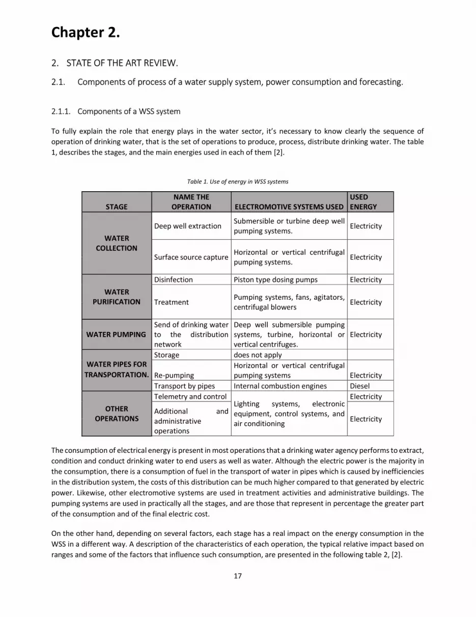
Chapter 2. 2. STATE OF THE ART REVIEW. 2.1. Components of process of a water supply system, power consumption and forecasting. 2.1.1. Components of a WSS system To fully explain the role that energy plays in the water sector, it’s necessary to know clearly the sequence of operation of drinking water, that is the set of operations to produce, process, distribute drinking water. The table 1, describes the stages, and the main energies used in each of them [2].
Table 1. Use of energy in WSS systems
STAGE NAME THE OPERATION ELECTROMOTIVE SYSTEMS USED USED ENERGY
WATER COLLECTION Deep well extraction Submersible or turbine deep well pumping systems. Electricity
Surface source capture Horizontal or vertical centrifugal pumping systems. Electricity
WATER PURIFICATION Disinfection Piston type dosing pumps Electricity Treatment Pumping systems, fans, agitators, centrifugal blowers Electricity
WATER PUMPING Send of drinking water to the distribution network Deep well submersible pumping systems, turbine, horizontal or vertical centrifuges. Electricity
WATER PIPES FOR TRANSPORTATION.
Storage does not apply Re-pumping Horizontal or vertical centrifugal pumping systems Electricity Transport by pipes Internal combustion engines Diesel
OTHER OPERATIONS Telemetry and control Lighting systems, electronic equipment, control systems, and air conditioning
Electricity Additional and administrative operations
Electricity
The consumption of electrical energy is present in most operations that a drinking water agency performs to extract, condition and conduct drinking water to end users as well as water. Although the electric power is the majority in the consumption, there is a consumption of fuel in the transport of water in pipes which is caused by inefficiencies in the distribution system, the costs of this distribution can be much higher compared to that generated by electric power. Likewise, other electromotive systems are used in treatment activities and administrative buildings. The pumping systems are used in practically all the stages, and are those that represent in percentage the greater part of the consumption and of the final electric cost. On the other hand, depending on several factors, each stage has a real impact on the energy consumption in the WSS in a different way. A description of the characteristics of each operation, the typical relative impact based on ranges and some of the factors that influence such consumption, are presented in the following table 2, [2].

18
Table 2. Aspects that affect the energy consumption in the WSS system
STAGE NAME THE OPERATION BASIC DESCRIPTION IMPACT ON THE GLOBAL ENERGY CONSUMPTION (%)
COMMENTS ON ENERGY CONSUMPTION
WATER COLLECTION
Deep well collection Extract the water to the surface by pumping the raw water from the dynamic level of a deep well
30 - 60% The energy cost depends on the depth of the well.
Surface source collection Capture water from a river intake, spring or other surface source 0 - 10%
The energy indices of this catchment, in kWh / m3, due to the dynamic height
WATER PURIFICATION
Disinfection It implies chlorine dosing or other process such as ozonation 1 - 2% The energetic consumption of the dosage is quantified in the treatment or in the extraction
Treatment Involves processing raw water with a primary or secondary treatment 5 - 10 %
The consumption is linked to the amount of organic contamination and other types of particles and their size
WATER PUMPING Send the drinking water to the distribution network
Pumping of drinking water from water treatment plants to regulating tanks or to the distribution network 0 - 60%
In some cases it is done by gravity, which does not imply energy consumption. In cases where the surface source predominates, the impact on global consumption may be very high, especially in pumping systems Storage does not apply
19
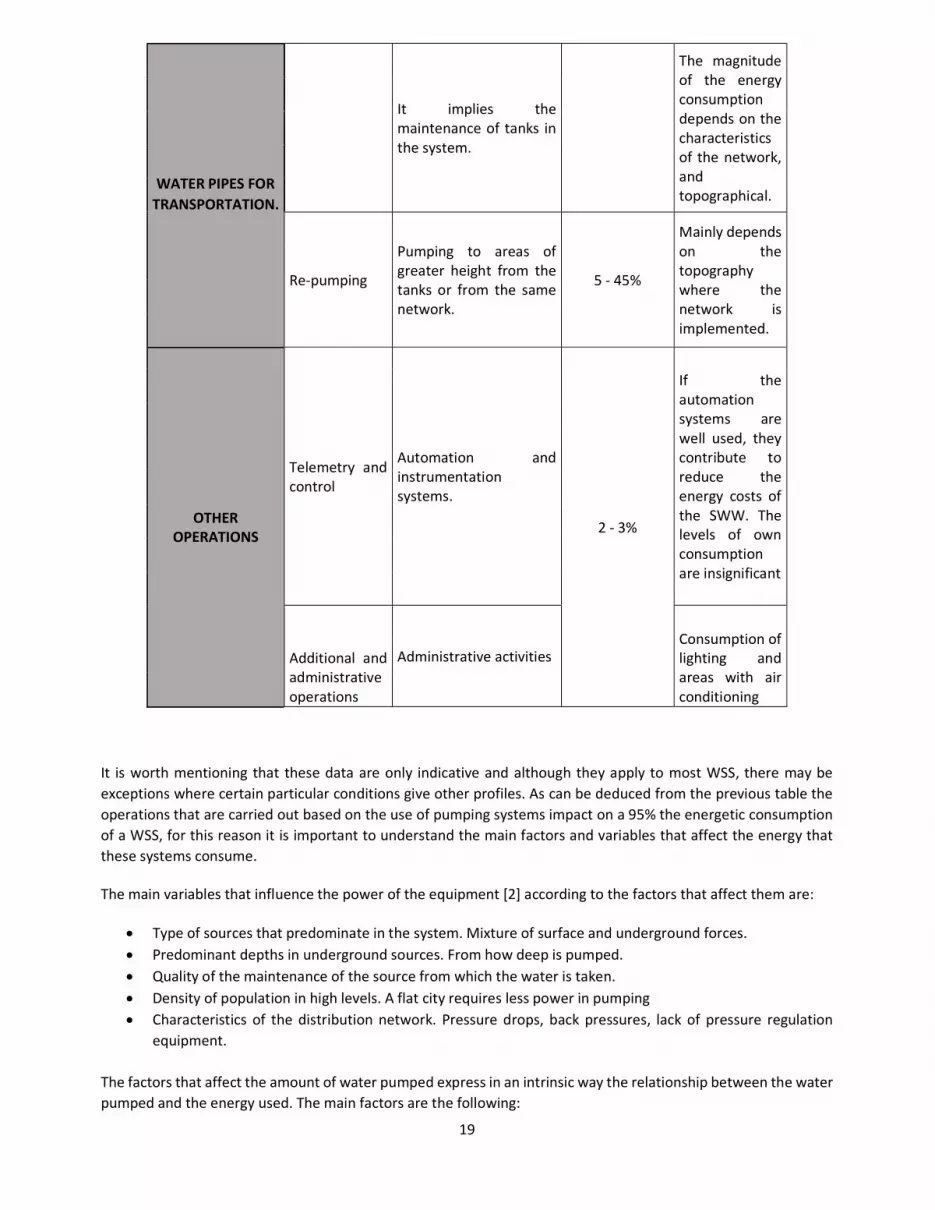
WATER PIPES FOR TRANSPORTATION.
It implies the maintenance of tanks in the system.
The magnitude of the energy consumption depends on the characteristics of the network, and topographical.
Re-pumping Pumping to areas of greater height from the tanks or from the same network.
5 - 45% Mainly depends on the topography where the network is implemented.
OTHER OPERATIONS
Telemetry and control Automation and instrumentation systems.
2 - 3%
If the automation systems are well used, they contribute to reduce the energy costs of the SWW. The levels of own consumption are insignificant
Additional and administrative operations Administrative activities Consumption of lighting and areas with air conditioning
It is worth mentioning that these data are only indicative and although they apply to most WSS, there may be exceptions where certain particular conditions give other profiles. As can be deduced from the previous table the operations that are carried out based on the use of pumping systems impact on a 95% the energetic consumption of a WSS, for this reason it is important to understand the main factors and variables that affect the energy that these systems consume. The main variables that influence the power of the equipment [2] according to the factors that affect them are:
Type of sources that predominate in the system. Mixture of surface and underground forces. Predominant depths in underground sources. From how deep is pumped. Quality of the maintenance of the source from which the water is taken. Density of population in high levels. A flat city requires less power in pumping Characteristics of the distribution network. Pressure drops, back pressures, lack of pressure regulation
equipment.
The factors that affect the amount of water pumped express in an intrinsic way the relationship between the water pumped and the energy used. The main factors are the following:

20
Size of the population to which it is supplied. If it is of a residential, commercial and industrial type and its specific weight on the total population.
Climate. In general, in warm climates, the demand per inhabitant tends to be higher. Level of losses. At lower levels of losses, greater flow of pumping and therefore greater consumption. Each
liter of water that passes through the system represents a significant energy cost. The loss of water in the form of leaks, theft and waste of consumers, directly affect the amount of energy consumed. In general, the waste of water leads to a waste of energy.
Number of hours of operation. The flow that is pumped and the energy consumed are directly proportional to the number of hours pumped. In general, to greater number of hours of service greater energetic consumption.
Efficiency in the hydraulic operation and pressure control. Levels of automation. Absence of automation systems (SCADA systems and telemetry), inadequate manual
control of the operation leads to high energy consumption. Coverage. The greater water supply coverage, the greater energy consumption.
The measures for the energy saving of a supply network are:
Optimization of the electromechanical power factor and efficiency. Control of the demand and pumping in peak hour according to the energy tariff. Savings for the optimization of the hydraulic operation. reduction due to mechanical losses.
2.1.2. Problems and barriers in the WSS The low efficiency of the pumping systems in most of the cases studied it’s mainly due to factors such as: poor preventive maintenance of equipment and associated systems, lack of procedures ordered for the selection of the same, ignorance of norms and lack of technical training of operative personnel. Besides this, the inadequate pumping operation schemes, lack of pressure control and leakage in the distribution networks among others, they substantially increase the energy indices with which these systems operate. These factors can be framed in the following concepts:
High demand due to high percentage of leaks. Little or no control of pressure in the network. Empirical operation of the network. Sub-used installed infrastructure. Little use of appropriate technology.
2.1.2.1. Aspects to improve energy efficiency. In general, the actions are aimed at controlling and optimizing the variables that affect energy consumption and cost. The actions to improve efficiency are as follows:
Predict the flow that is required to supply. The load that the distribution lines support, when the water is pumping. Buy equipment that has a better efficiency. Change of technology hydraulic, electrical and electronic. Design a pumping operation. Optimize the time of the pumping equipment without affecting the demand
The description and their respective theoretical bases as well as the criteria used to evaluate the application of these measures are described below.
1) Actions related to the energy tariff:

21
An area of opportunity for savings, always attractive in the pumping systems, consists of changing the rate contracted with the electricity supplier company, for some other that is more profitable. The stages to carry out the study are the following:
Stage 1: Identify the tariffs in which all operating services are located. Stage 2: Evaluation of the possibilities of saving in the cost of electric power with the different applicable
tariffs, according to the systems connected to low, medium and high power. 2) Control of the demand.
In installations where the electricity supply is hired in hourly rate, it is recommended to analyze the alternatives for the implementation of a demand control system. Essentially, it is about reducing the hydraulic load in operation during peak hours, to lower the amount of billed demand and consequently the electrical cost. The control of the demand can be made with the following methods:
Modify operating procedures to reduce the load during peak hours. Install timers to stop equipment before the start of peak hours and put them into operation at the end
of this time. Implement an automatic control system to regulate equipment according to demand and other
parameters of the process, such as pressure or level. It is important to keep in mind that the pumping operation must be intrinsically linked to guaranteeing the demand to be supplied without losing control over the main variables of the system such as tank level control and system pressure.
3) Actions for the reduction of losses in electrical installations. These actions are focused on its main components: transformers, power factor and drivers. Below is a brief description of the measures that could be applied for these cases.
Improve the cooling of the transformers: Measurements of the temperatures recorded in the transformer must be made to find ranges that are out of normal, this can produce significant losses of electricity. To correct this, must be evaluate the cost of maintenance or ultimately if it’s more viable to make a change of the transformer.
Increase the caliber of the transmission cables In case it has been detected that the cable gauges are not the size required by the pumping equipment, must to select a cable that not only meets the standard, but also saves energy.
Optimize the power factor. The objective of this measure is to eliminate the problems caused by a low power factor. According to experience, a value below 96% deserves to take actions to compensate and achieve better values of power factors. If the low power factor is caused by oversized motors or working in bad conditions, these motors must be replaced by new high efficiency motors that operate around 75% load. This problem could also be solved by compensating the power factor with capacitor banks.
Actions to increase the efficiency of the pumps. a.) Suitability of the pumping equipment to the actual operating point:

22
In this action the procedure consists in defining two points of operation of load vs. expense where the pumping equipment operates, table 3.
Table 3. Improvement of the efficiency of the pump from the curve
TYPE OF PUMP LOCATION OF THE POINT OF OPERATION CORRECTIVE ACTION
MULTI-STAGE VERTICAL PUMP
Above the curve of the pump
Increase stages, until the pump curve is passed through the point of operation Replace the impellers with new ones of greater diameter whenever possible.
Below the curve of the pump
Eliminate stages, until manage to pass the curve of the pump by the point of operation Trim the impellers to the required size, so that the curve of the pump passes through the point of operation
HORIZONTAL PUMP
Above the curve of the pump Replace the impellers with new impellers of greater diameter Below the curve of the pump
Trim the impellers to the required size, so that the curve of the pump passes through the point of operation
b.) Replacement of the pump - motor assembly: This action is recommended when the electromechanical efficiency has been low and the potential for energy savings has resulted by low of 30%. Selection a pump that meets the hydraulic load operation point (s), so that present a reasonably high efficiency.
4) Leakage reduction The objective of leakage control is to reduce to a minimum the time that elapses between the follow-up of a leak and its elimination, through the revision and continuous adjustment of procedures and actions, in order to increase the efficiency of the conservation and maintenance of the distribution network. The control of water leaks is a continuous activity where the processes are established to coordinate the actions of location and elimination, supported by continuous monitoring of the network, reports of leaks detected by users, systematic search programs, periodic preparation of balances and sampling. The field sampling and statistical data is elaborated a loss evaluation and a water balance in order to estimate the percentage of water to be reduced. On the other hand, the cause of the occurrence of water losses must be determined, indicating the main problems to be corrected in the short and medium term.
2.1.3. Real Infrastructure of a water supply system. In general terms, the services [3] that the company INOVA provides are the following:
Management and exploration of public water supply systems, urban wastewater sanitation

23
Management of public cleaning systems. Creation, management and exploration of an urban and local public transport network.
As the work to be developed is based on the scope of the water supply systems, a brief description of the configuration and operation of the company is made The collection system is located in “Olhos de fervença”. The system is autonomous in terms of collection, providing service for neighboring such as: Mira, Montemos o velho and Coimbra. A summary of the existing infrastructure [3] of the WSS are the followings:
Water collection: 3 facilities with a capacity of 19.008 m3 / day Treatment: 5 facilities with the capacity of 10.968 m3 / day Water pumping stations: 12 facilities Water pipe for transport: 139.2 km. Tanks: 21 installations with capacity of 14000 m3 Distribution network: 461.2 km.
The distribution system of drinking water is divided into zones. From the central of “Olhos da Fervença” are supplied the main sectors of Cantanhede, Tocha, Febres and Mira. There are also other sub-sectors that are supplied. They are: Montemor, Velho and Coimbra. In these sectors and subsectors are installed distribution networks supported by storage, pressurizing and other equipment. The high system, is sub-divided into the collection, treatment, adaptation and storage of water. water collection, water purification, water storage, water pumping solution, water pipes for transportation.
Water collection: The water collection is done in “Olhos da Ferveça”, and it has underground origins. There are 8 wells with depths of 4m and 8m each one, with a diameter of 1m and have a capacity of 25 L/s and 50 L/s. The supply from this catchment began in 1970. These wells have a maximum flow of 180 L/s in the month of May.
Water purification: Water treatment is applied at 5 different points.
Fercença station, a disinfection is done with the addition of hypochlorite.
Fontinha, Tocha, Cantanhede and Murtede stations, sodium hypochlorite is added.
Water transportation and storage. The reserve system is characterized by 120 km of ducts [3]. The tanks for reservoir of water are located in: Fervença, Fontinha, Cantanhede, and Tocha, these complete a total capacity of 3.900 m3, figure 2.

24
Figure 2. INOVA water supply system.
The INOVA company, is committed to the development of the SCUBIC platform. It provided information as dimensions of the WSS network, flows of the distribution for the lines of Fervença, Covões e Vilamar, system demand, tank levels, and electricity tariff for a given month of the year. 2.1.4. Impact and benefits of forecast. Prediction methods are highly diversified in vast areas of knowledge. The prediction is used to predict the evolution of economic models, to interpret natural events such as rains, storms or earthquakes, help in medicine to provide information about the progress of a vaccine medication in humans, or to chronologically date the degeneration of an illness. These kinds of forecasts are only possible due to today’s innovative mathematical techniques and computational processing power [4]. Due to the high population growth in large and small cities, it is necessary to have highly efficient WSS systems in terms that guarantee water supply, as well as systems that use the necessary resources for their operation. The optimal functioning of a WSS system is that which guarantees the water demand of the population when it uses the minimum resources for said area, in this way low operating costs are obtained bringing as benefits the no overload in the work in the equipments that make up the WSS; additional to this gives properties to the system to be scalable, this means that the system can be enlarged as the population grows. Bad management leads to high operating costs, limiting investments in terms of improvement or expansion of the system. Knowing the consumption patterns of a region –forecasting -, as well as the behavior of the WSS system in a period of time is significantly important. In the first instance it allows the projects designers of WSS to develop networks supply systems that adjust to the demand of the region or population, in this way there is no oversizing of the system, which would lead to an un-utilization of equipment which would represent a loss of materials for the company. In the second instance, the management of the information provided by the forecast is the engine to establish an efficient administration in the operation while is guaranteed the existence of water in the storage tanks while adjusting the power consumption of the entire network [4]. 2.2. Platform for water management 2.2.1. SCUBIC company actual state. The existing water supply management software developed within SCUBIC, has several modules: prediction and calculations, database management, interface, and communication. The software SCUBIC was developed with the

25
main objective of improving energy consumption in WSS besides the management of this systems too. The main information that SCUBIC needs to manage and administer the WSS are: flows rates in the network, volumes, pressures, water level in tanks, environment condition (temperature, humidity chance of precipitation, past water demand, energy price rate, start of operation, end of operation, duration of operation. The methodology that SCUBIC uses to obtain low consumption in the WSS is the calculation of the forecast of the future consumption to give an approximation in the time and the moment that the pumps must be connected to meet the consumption demands in the network while optimizing the energy consumption of the elements of the system as they are: pumps, valves, electrical panels, control systems, instrumentation and complementary systems. SCUBIC counts as 4 modules of which the main ones are: SSENCE and SSOLVE. 2.2.1.1. SSENSE’s Module. This module is responsible for reading information, processing, and writing information of data coming from databases of servers or other platforms that provide all the necessary information. This module is divided into two submodules that perform the calculation of the forecast according to the information received in a period of time. Each submodule contains mathematical methods and models that have been implemented and tested in previous work. The methods used are: Statistics described by ARIMA and Heuristic models described by BAKKER's models, and Machine Learning, commonly known as neural networks. 2.2.1.2. SSOLVE’s Module. The SSOLVE module allows to see the approximate simulation of the calculations coming from the SSENSE module, and with the help of the EPANET platform, a hydraulic modeling system for water supply networks, have an approximate response in the time of the system with the calculated forecast, in this way to analyze and take the necessary decisions to improve the energy efficiency, having lower consumption in the WSS. Other modules that complement the SSCUBIC software are: Reports, Calendar and Alarms. These last modules allow the management of the information provided by the two previous modules, thus complementing mechanisms that are available to the user during the development and analysis of the system of water supply and energy optimization. 2.2.1.3. Software Architecture. SCUBIC's software is developed on the following platforms:
Databases: Redis DB; SQL DB. Webservice (JavaScript, HTML, CSS) Calculation of Forecast (Python) Module Simulation and optimization (Epanet, C ++) Communications between Webservice and DBs.
Figure 3 describes the modules that make up the SCUBIC platform and how it interacts with each other.

26
Figure 3. The software architecture of SCUBIC.
2.2.2. Other platforms. Currently in the industry it can already find tools for the administration and optimization of the energy resources for the water supply systems WSS. To achieve excellent development of the management tool, is must look at other systems and reflect on their work and how this can improve the failures in the SCUBIC platform. So in this way to stay with a robust product that meets the specifications and standards required by the market and current systems.
1) WATENER. One of the tools that is possible to find in the market is WATENER of INCLAM’ GRUPO of Spain. The WATENER [5], is a specialized technical response to evaluate problems to systems or companies in the sector hydraulic and hydrological issues. The INCLAM Group has extensive experience in the information technology sector and in the development of software oriented to both product and service. He has successfully participated in the implementation of solutions that facilitate the management of information, the optimization of processes and support efficient decisions. Bet heavily on free software and the use of standards, allowing the customer to save costs. Figure 4 shows one of the main pages of the competition – watener-. WATENER: “WatEner is an TIC solution that helps to improve comprehensively and intelligently the management and operation of drinking water networks, providing the tools and the ideal working environment to increase efficiency in the water-energy field, reducing costs and providing benefits in the social, environmental and quality of service areas.”

27
Figure 4. WATENER platform example.
2.2.3. Comparison of platforms. In table 4 presents the comparison between the simulation platforms SCUBIC and WATENER
Table 4. Comparison of the SCUBIC and WATENER platforms. TOOLS SSCUBIC WATENER Module 1. Display Consultation of global network information with functional schemes. Integration of hydraulic modules and mapping tools. ? Incorporation of real and simulated data in GIS environment. Query of elements and segments of the network. Measured and simulated time series. Module 2. Monitoring Presentation of anomalies in the elements of the system. ? Alarm Management. Timeline view in GIS environment. ? Search management by severity level topology of the elements in the network Module 3. Simulation. Presentation of daily demand forecast information in each sector or segment in the WSS network Management of the methods of calculation and manipulation of Parameters. ? Management of calculation methods. Generation of method of pre-finished form. Training of the methods with different conditions of the maximum and minimum permissible in the system. ? Custom planning of the daily pumping sequences. Improved energy efficiency.

28
Configuration of calculation methods. One method or hybrids, several methods. Which of these gives a better result in the simulation. Thus reduction in energy consumption Module 4. Reports. Analysis of network behaviors with indicators of industry standards. ? Operational panels that facilitate monitoring and decision making in water and energy issues. Management panels for scheduling tasks in the short and long term, with management commands. ? Consult panels for business objectives, with financial measures and charts. ? Generation of reports for internal consultation or information to the general public ?
As analysed from the table, the SCUBIC platform can be improved in the following aspects: to include map integration, to include presentation of anomalies of system elements, develop different ways of simulating WSS systems, analyse the behaviours with the international standards of WSS systems, establish an integration with the business platform of the WSS system, among others. 2.3. Hydraulic Simulators. 2.3.1. EPANET. The Epanet [6] software, allows to do hydraulic and water quality simulations of a supply network. Has become in the most popular tool and used worldwide by the companies or municipalities that operate and manage the networks of WSS. This is because the application is free to use and open source. EPANET [6], in addition to answering this need functioning as a standalone application with its own interface graphic to build the model of the network and analyze the results, also allows connect their calculation library, or Toolkit as it is usually known, to any another application or graphic interface, thus opening a huge field of possibilities for any technician or researcher who wants to go beyond what is currently said application offers. The Epanet Toolkit can be integrated into any native programming environment or in the programming tools themselves that offer many packages of proprietary software, as: Excel, AutoCad, ArcGIS, etc or free as OpenOffice, gvSIG, QSIG, etc. The Epanet calculation library [6] has a large number of functions that they help us to recover and modify certain parameters of the network model, before and after performing a hydraulic simulation. Also allowing control the process of simulation step by step. EPANET has been conceived as a research tool to improve our knowledge about the progress and final destination of the various substances transported by water, while it runs through the distribution network. Among its different applications can be cited the design of sampling programs, the calibration of a hydraulic model. For the case of study, the most important management that EPANET can perform is directed to the analysis and decision making to modify the pumping regime, or filling and emptying the deposits. 2.3.2. Toolkit – EPANET. Toolkit de EPANET [7], is a set of files that made up the dynamic library (dll), and four header files that allow to link the written functions in the dynamic library, depending on the programming environment that is used. With these functions is can access the information contained in the EPANET input file, in INP format, and to the results generated after performing a simulation. The EPANET API is a dynamic library, a file with the .dll extension, which is distributed together with the other files that make up the box tools for programmers (Toolkit). This bookstore is
29
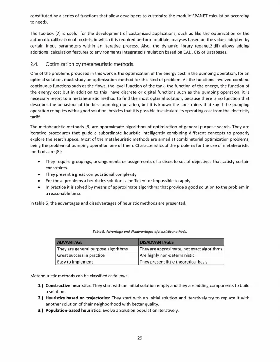
constituted by a series of functions that allow developers to customize the module EPANET calculation according to needs. The toolbox [7] is useful for the development of customized applications, such as like the optimization or the automatic calibration of models, in which it is required perform multiple analyses based on the values adopted by certain Input parameters within an iterative process. Also, the dynamic library (epanet2.dll) allows adding additional calculation features to environments integrated simulation based on CAD, GIS or Databases. 2.4. Optimization by metaheuristic methods. One of the problems proposed in this work is the optimization of the energy cost in the pumping operation, for an optimal solution, must study an optimization method for this kind of problem. As the functions involved combine continuous functions such as the flows, the level function of the tank, the function of the energy, the function of the energy cost but in addition to this have discrete or digital functions such as the pumping operation, it is necessary resort to a metaheuristic method to find the most optimal solution, because there is no function that describes the behaviour of the best pumping operation, but it is known the constraints that say if the pumping operation complies with a good solution, besides that it is possible to calculate its operating cost from the electricity tariff. The metaheuristic methods [8] are approximate algorithms of optimization of general purpose search. They are iterative procedures that guide a subordinate heuristic intelligently combining different concepts to properly explore the search space. Most of the metaheuristic methods are aimed at combinatorial optimization problems, being the problem of pumping operation one of them. Characteristics of the problems for the use of metaheuristic methods are [8]:
They require groupings, arrangements or assignments of a discrete set of objectives that satisfy certain constraints.
They present a great computational complexity For these problems a heuristics solution is inefficient or impossible to apply In practice it is solved by means of approximate algorithms that provide a good solution to the problem in
a reasonable time. In table 5, the advantages and disadvantages of heuristic methods are presented.
Table 5. Advantage and disadvantages of heuristic methods. ADVANTAGE DISADVANTAGES They are general purpose algorithms They are approximate, not exact algorithms Great success in practice Are highly non-deterministic Easy to implement They present little theoretical basis
Metaheuristic methods can be classified as follows:
1.) Constructive heuristics: They start with an initial solution empty and they are adding components to build a solution.
2.) Heuristics based on trajectories: They start with an initial solution and iteratively try to replace it with another solution of their neighborhood with better quality.
3.) Population-based heuristics: Evolve a Solution population iteratively.

30
2.4.1. Genetic algorithms (GA). Genetic algorithms (GAs) [9] are adaptive methods that can be used to solve optimization problems. They are based on the genetic process of living organisms. Throughout generations, populations evolve in nature in accordance with the principles of natural selection and survival. By imitating this process, genetic algorithms are able to create solutions for real problems. The evolution of these solutions towards optimal values of the problem, depends on an adequate selection or constraints created so that the best populations can move and generate a new solution equal or better than the previous one. Genetic algorithms [9] analogically use the same natural behaviour. Initially a population of individuals is created, each of them represents a feasible solution to a given problem. Each individual is assigned a value, this value is given according to the constraints that the solution of the problem must have, between more constraints the individual fulfills, the value assigned to it will be much higher. The greater the adaptation of an individual to the problem, the greater the probability that it will be selected to reproduce, crossing and mutate his genetic material with another individual selected in the same way. The crossing produce new individuals descendants of the previous ones, who share some of the characteristics of their parents. In this way a new population of possible solutions is produced, this replaces the previous one, being able to assure that they contain a greater proportion of good characteristics of compliance to the constraints of the problem in comparison with the previous population. If the genetic algorithm has been well designed, after crossing and mutating the individuals the population will converge towards an optimal solution of the problem. The power of the genetic algorithms comes from the fact that it is a robust technique and that can successfully deal with a wide variety of problems in different areas. Although it is not guaranteed that the genetic algorithm finds the optimal solution to the problem, but there is empirical evidence of the solutions found are of an acceptable level, in a competitive time. The figure 5, a flow diagram of the genetic algorithm [9] is shown. The genetic algorithms [9] are based on integrating and efficiently implementing two ideas: simple representations as binary strings of the solution of the problem and the realization of simple transformation to modify and improve these representations.
Figure 5. Flow diagram of the genetic algorithm.

31
This last data is very important for our work since the representation of the pumping operation is a matrix formed by zeros and ones, having to be combined with each other to reach the pumping operation that optimizes the electric consumption and the operation cost. Was for this that it decided to study and use this heuristic method to find a possible solution to problem of the pumping operation in the WSS systems. The elements to keep in mind in the implementation of a genetic algorithm are [9]:
Creation of an individual - chromosomal representation Formation of an initial population Measure of evaluation - constraints of compliance of the solution Selection criteria Parental selection criterial One or several mutation operations.
The handling of the operations [9] named above depends on the type of representation, whether they are binary strings or if they are continuous functions. The use of binary string has an advantage over the others, this easily allows the operation of crossing and mutation, in addition allows the results of convergence are much more feasible in comparison with the use of continuous representations.
1) Initial population: It is generated randomly. However, lately, heuristic methods have been used to generate initial solutions of good quality, thus allowing the genetic algorithm to improve them. It is important to guarantee the structural diversity of the first population or solutions in order to avoid the premature convergence of the algorithm.
2) Size of the population: One of the characteristics where there is more doubt, is in choosing the appropriate size of the population that is iterated in each evolution in the algorithm, but there are studies that have shown that small populations run the risk of not adequately covering the search space, while working with large populations can lead to an excess computational cost or even to lead that the solution does not converge. Goldberg (1989) [9], made a theoretical study in which he concluded that the optimal size of the population must be equal to the length of an individual. Alexander (1992) [9], based on empirical evidence suggests that a population size between the length of an individual or twice this of is enough to successfully attack a given problem.
3) Measure of evaluation: Usually use the objective function to maximize or minimize. To this function, it can add a penalty factor to control the infeasibility of the solution - solutions not tolerable. Commonly, this measure is called fitness [9].
4) Selection criteria. The selection of parents is given by studying the measure that is given to each individual of the population - fitness. As fitness is the degree of satisfaction of the solution for the given problem, it is normal to take the parents among the individuals who have a greater fitness
5) Cross of parents. The most used crossing operators are: By one point: A breaking point is randomly chosen in the parents and their bits are exchanged By two points: two breakpoints are chosen at random to exchange their bits Uniform: In each bit a parent is chosen randomly so that it contributes with their bit to the child. Sophisticated methods. Are operators in which the random mix is used, of the operators described
above.
6) Mutation. The simplest and most used operation for this process is to replace with a certain probability the value of a bit. It should be noted that the role played by the mutation, is to introduce a factor of diversification [9], so that the genetic algorithm doesn’t have premature convergence stuck in a local optima point. Another way to introduce new elements in a population is to recombine elements taken at random without considering their fitness.

32
2.4.2. Convergence of the algorithm. The concept of convergence [9] is related to the progression towards uniformity: a gene has converged when at least 95% of individuals in the population share the same value. It is said that the population converges when all the genes have converged. This definition can be generalized to the case in which at least a % of the individuals in the population have converged. As the number of generations increases, the average convergence is more likely to approximate to the best individual. It is important to note that the percentage of mutation is a value that may or may not accelerate the convergence to a solution, so it is very important to know how to choose this value, since through a percentage high mutation is possible generate great diversity, this will not allow a timely convergence. 2.5. Processing system. Within the current technologies, several options of embedded systems that could be used for the project is found. Between them is Arduino and the Microcontrollers. 2.5.1. Microcontrollers. The microcontroller [10] was invented by Texas Instruments in the 1970s. Microcontrollers are microprocessors with a memory function, with RAM (Random Access Memory) and ROM(read-only memory). Modern microcontrollers are specialized for products in sectors such as automotive, mobile phones, lighting, industrial control, communications and low power consumption devices, since they are small and powerful in terms of processing. The importance of microcontrollers is because they have the possibility to integrate with different devices in various types of communications, as they are. RS-232, RS-484, I2C, ISP, TCP/IP and others. The figure 6 shows a microprocessor.
Figure 6. P805 microprocessor.
2.5.2. Arduino. Arduino [11] started in 2006 as a student project at the Institute of IVREA - Italy with the goal of developing a programming platform that would be compatible with platforms like MacOSX, Windows, and GNU / Linux. Once the platform was finished they developed a "Wiring" electronic card, which is light, economical, available to the community of the institute, in open source. After the project was successful, Google entered the project developing the ADK Kit (Accessory Development Kit) an Arduino board capable of communicating with smartphones under the Android operating system so that the phones could control lighting, motors, and sensors. Figure 8, shows an example of the ARDUINO equipment.
Figure 7. Arduino D1mini.
Advantages of Microcontrollers:

33
Learn to program in C / C ++, modifying internal registers which allow a better knowledge of the hardware, which gives greater flexibility and optimization in the development of the applications.
Greater flexibility in dedicated projects. There is a high range of devices according to the type of project. The Microcontroller supports higher frequencies. It has more possibilities to configure the outputs and
inputs as Analog or digital signals. It has pins that provide PWM signals. Can be programmed for CAM industrial communication.
Advantages of Arduino: The learning curve is much faster for the type of programming. Availability of web resources, op-source community, take advantage of projects already developed, be
improved and thus share in the community again. Use of Bootloader, that makes it easier to load the programming in Arduino. In the market, there are many devices compatible with Arduino such as: Modules Wifi, module android,
GSM module, Bluetooth module, among others. It is a low-cost device, which makes it very accessible to students while learning, but with the ability to be
programmed for complex applications in the industry. 2.6. Instrumentation. One of the most important aspects in the area of industrial automation is the instrumentation [12], which play a fundamental role in the productive system. A sensor is a transducer which is used to convert variations of the mechanical, magnetic, thermal, optical or chemical type in electrical type signals. The most common sensors [12] in the industrial are: Temperature, pressure, flow, level, ph, weight, current, voltage, radiation, luminance. To choose a sensor, it is important to know the process that is measured, and the operating conditions in which it is installed. The following are the general parameters that must be taken into account when choosing the sensor, table 6:
Table 6. Main characteristics to choose a sensor.
FEATUREST TO CHOOSE A SENSOR Operating pressure Chemical compatibility with the working fluid.
Operation flow Output type (analog or digital) Bursting pressure. Process connection method, (flanges, threaded connection, etc.)
Accuracy Method of electrical connection, (soldering, special connectors, etc.) Work temperature. Linearity
Sensor type. Speed of response. Sensor response curve. Sensor cost
2.6.1. Types of Pressure Sensors. The main types of sensors to measure pressure [13] are presented below, which is one of the variables of interest for instrumentation support system.
Table 7. Types of pressure sensors PRESSURE SENSORS:
Burdon Nozzle pallet system. Piezoelectric Resistive Diaphragm Magnetic
Bellows Capacitive

34
2.6.2. Types of Flow Sensors. The main types of sensors to measure flow [14] are presented below, which is one of the variables of interest for instrumentation support system.
Table 8. types of flow sensors FLOW SENSORS:
Ultrasonic flowmeter Flowmeter with oval wheels. Mass flowmeter Rotmeters
Oscillating disk type meter Vortex flowmeter Electromagnetic flowmeter Turbine type

35
Chapter 3. 3. METHODOLOGY. 3.1. Minimization of the energy-cost in the WSS operation After having mentioned some methods for reducing energy costs in section 2.1.1, having each one a high saving rate, the development for the optimization of the energy of a WSS is focus on the generation of an optimal pumping operation that reduces the operation's cost. This method has the highest impact in the cost reduction for these systems. An adequate planning of the hours on which a pump must be on or off according to the demand and the peak hours of the electrical tariff has a 65% impact on the reduction of the energy. 3.2. Simulation of a WSS system. For the simulation of the water supply system, two methods are used. The first method uses the empirical hydraulic equations developed by the SCUBIC group, these equations are derived from a mass balance in the network. The second method performs the hydraulic simulation of the network using the EPANET simulation package, which is a specialized software for hydraulic systems. 3.2.1. Empirical equations. The SCUBIC group developed a system of equations that describe the hydraulic behavior of the system, particularly for the case study of the water subsupply system of ferveça, covões and Vilamar, that is schematically presented in figure 8.
Figure 8. Fontinha reservatory - study case.
The figure 8 is the hydraulic system that is composed by the main tank, the inputs and outputs of the flows. In this case, these are Qc (flow of covões), Qf (flow of ferveça), Qv (flow of vilamar), and Qo (pump flow). The mass balance equation that describes the behavior of the system is as follows:
+ + − = ∆∆ (1)
= 0 ,1 , State pump The flow Qo provided by the pump depends on the hydraulic parameters (length, diameter and roughness of the pipe, discharge height and accessories present in the network). Based on the mathematical model of the analysed

36
network, it is possible to establish a linear relationship between the flow rate pumped and the level in the tank. The following equation is proposed:
(ℎ) = 182.21 − 3.262 ℎ . (2) h is given in meter and the flow Qo in m3/h. The flow of Ferveça – fontinha Qf is equivalent to 40% of the flow of Covões Qc and has a similar consumption, as described by equation 3:
= 0.4 (3) A linear relationship between the efficiency of the pump and the flow in the working range is given by the equation:
( ) = 0.58 + 0.001 (4) The above equations are used for the empirical implementation of the simulation of the system that is presented in section 4. 3.2.2. Hydraulic analysis by Epanet. The method that Epanet uses to solve the equations of continuities in the nodes is an analysis of nodes and meshes [6 ]. Using the equations of the gradient, the components of an Epanet network are the following: N nodes, NF height nodes, tanks and deposits. The relationship between the loss of load for a pipe going from node i to j, and the flow of step Qij, is as follows:
+ = ℎ = + , (5) where H = height in the node, h = headloss, r = resistance coefficient, Q =flow rate, n = flow exponent and m = minor loss coefficient. For pumps, the headloss [6] can be represented by a power law of the form:
ℎ = − (ℎ − ( / ) ) , (6) Where ho is the shutoff head for the pump, w is a relative speed setting, and r and n are the pump curve coefficients. The second set of equations that must be satisfied is flow continuity around all nodes [6]: ∑ − = 0 for i = 1,……N, (7) where Di is the flow demand at node i and by convention, flow into a node is positive. For a set of known heads at the fixed grade nodes, we seek a solution for all heads Hi and flows Qij that satisfy Eqs. (1) and (3). The Gradient solution method [6] begins with an initial estimate of flows in each pipe that may not necessarily satisfy flow continuity. At each iteration of the method, new nodal heads are found by solving the matrix equation: AH= F (8) where A = an (NxN) Jacobian matrix, H = an (Nx1) vector of unknown nodal heads, and F = an (Nx1) vector of right hand side terms. 3.3. Methods of optimization of pumping operation The main characteristics that an optimal pumping operation should have is presented in this section. From these characteristics, the constraints of the pumping operation are defined to be able to reach an optimal operation that minimizes the energy cost. These constraints are used in the proposed optimization methods to carry out the development of the module.

37
3.3.1. General Constraints that a pumping operation optimal must meet. 1) The tank's level can't exceed the maximum or the minimum allowed, for each period in the calculation of
the pumping operation.
2) If the pump is switched on, it must remain in this state for a minimum of some consecutive periods.
3) The programming algorithm should try to give priority of switch on the pump in the two lowest electrical tariff during the day.
4) The optimization algorithm search that the final level being equal or greats to the initial level of the tank. 3.3.2. Genetic algorithm for optimizing the operation of the pump As was mentioned in the state of art, there are metaheuristic algorithms to solve optimization complex problems like this, that combine continuous signals such as the level of the tank, flow, energy consumption, energy consumption cost. On the other hand, it has signals that do not have a theoretical basis as is the pumping operation, in addition, is a binary signal. For this reason, it was developed through metaheuristic optimization methods, a binary genetic algorithm. The reasons to use a genetic algorithm as an optimization method are the following:
1) The pumping operation is a vector of 1 and 0, that describes when the pump should be on or off during a period of the day. Since this matrix does not have an exact function that describes its behaviour, it only have the possibility of calculating its energetic cost, and the tank level, according with the pump's state. These are the main characteristics that are used to find the best method for its optimization.
2) It would be easy to think that is possible to implement an algorithm that tests all the combinations of 0 or 1 in this matrix to find the one with the lowest cost. This could be a possible solution, but with a very large computational cost, because with a pumping operation with n periods, the possible combinations would be equal 2n (the power of the number of periods). For example, if have a period of 15 min, the pump operation matrix would have a length of 96 terms, therefore the possible combinations that would have to be tested would be.
Possiblecombinations = 2n =7.9x1028 (9) Knowing that the average time of execution of a program is 0.00020 seg, to carry out this process the program would take 4.4x10²¹ days to try all the combinations, which is something impossible to hope.
The genetic algorithm has the possibility of creating solutions randomly, discriminating the best ones according to the fulfilment of the characteristics or constraints that was described above. The genetic algorithm gives a weight to each solution called “fitness”, and it is with this value that the genetic algorithm knows if it is an optimal solution, to take into account in the processes of selection, reproduction, and mutation, as it was described in the state of art. The genetic algorithm has some penalties for the pumping operation, these are: (i) minimum of periods of operation of the pump, (ii) exceed the maximum or minimum level of the tank, and (iii) continuity of the final level vs the initial level of the tank. The cost of the penalties is added to the operating cost of the pumping operation. In this way, it ensures that in the evolution of the genetic algorithm the pumping operations that have a high operating cost are not taken into account for the selection, reproduction and mutation and thus the algorithm can converge to the solution most optimal.

38
3.4. Features of the instrumented support system for reading pressure and flow. The system to be designed has its following main component: the microprocessor, that the objective is to read in its analog and digital inputs, the signals coming from the pressure and flow sensors respectively, and it must establish a communication TCP / IP via wifi with a remote server (PC) where a database (BD) is housed. There is a server programmed that acts as an intermediary to communicate with the database and the NodeMCU. The readings taken by the microprocessor are stored in the database after these are sent to the server. In addition to the previous process, a WEB page is developed to present in a graphic way the values stored in the database. Figure 9 shows a general scheme of the implemented system. 3.4.1. Calibration of the flow sensor To calibrate the flow sensor, it is required to do the following proceeding.
With a known quantity of water - 1 l - to pass through of the flow sensor. Take the # of pulses counted by the program. (#Pulsesxliter). Take the time in that the pulses were taken, sampling time. ( )
After having a number of pulses per liter, the following equations to calculate the flow rate in L / min is used: # = #
# (10)
( ) = 1000 ( ) ∗ 60( ) ∗ # (11)
Figure 9. General scheme of the instrumented support system.

39
3.4.2. Calibration of the pressure sensor In the specifications of NodeMCU, an analog input with a resolution of 10 bit is defined. Therefore, when the analog input has a maximum input voltage of 3.3Vdc, the microprocessor reads the values as 1024 (210). As known, the pressure sensor is a linear sensor. Consequently, the following process must carry out to find the function that describes the behaviour of the sensor:
To have connected the sensor to the Analog input A0 of 10 Bit resolution. First let the sensor in the air (0 PSI) to know what is of the value that is read in the microprocessor in 10-bit
resolution (#bitpress_min). It can read with a pneumatic pressure system linking to the sensor in the maximum range, in this case 174.5
PSI, to read the bit number that is received by the microprocessor for this pressure (#bitPress_max). Using the slope equation, the pressure growth rate per bit is calculated as
= .
# # = (12)
Using the slope point equation 13, it is calculated a linear function that describes the pressure sensor when it is read by the microprocessor: ã = (# − # ) . (13)

40

41
Chapter 4. 4. IMPLEMENTATION. 4.1. Case - study of INOVA For the development of the program that calculate an optimal pumping operation, INOVA supplied an initial information of flows and demand of the regions of: Covões, Vilamar, Fervença. These are represented in figure 10. It should be noted that after the development of the application, the real forecasts will be used per day to calculate the optimal pumping operation.
Figure 10. The flow of the demand points. Information supplied by INOVA.
The second information required, leading to the calculation of the pumping operation, is the electric tariff during the day. It should also be noted that this is the information for the development of the application, after being developed the module. The real daily tariffs should be used. These tariffs are changing according to the lists of companies that provide electricity. For this case, in figure 11, the cost of kWh is plotted. From this, it can be deduced that the on-peak day hours in that it has the highest cost tariffs (On –peak day) is between 10-13 h and between 18-22h. On the other hand, the lowest tariff (off –peak day) times are in the early hours of day. Therefore, the program should give priority to switch on the pump in these hours, always taking into a count of tank’s level. The program should have the ability to perform a verification of level so that this does not exceed the maximum or minimum allowed by the company INOVA. In this way, the level remains within the allowed ranges while the demand is met, with a low operating cost of the pump. All information provided by INOVA is given by data arrangements taken every 15 min for 24 hours. Therefore, this information is defined as vectors composed of 96 values for one day.
0,0010,0020,0030,0040,0050,0060,0070,00
0:00 4:48 9:36 14:24 19:12 0:00
Flow CovõesFlow VilamarFlow Fervença-Fontinha

42
Figure 11. Electric tariff, information supplied by INOVA.
4.2. Module for the optimization of the pumping operation. The modules developed in this work aim to complement the SCUBIC platform. Currently, SCUBIC platform integrates programming languages such as C ++, java and database in REDIS. As the programming language to use must be compatible with the previous programming languages, Python is an easy compilation language, it can be integrated with other languages or software and this programming code can be executed from others software. For these reasons and for the clear advantages that Python have over other languages, the applications developed in this work are programmed in this language. In the block diagram of figure12, the general scheme of the composition of this module is presented.
Figure 12. General scheme of the module of optimization.
4.2.1. Inputs data. In general, the inputs of the module are: (i) the forecast of the demand or flows of the system, (ii) electricity tariff and (iii) initial level of the tank that is equal to the last level of the previous day. The demands and the tariff are matrices composed of n values, where n is the number of periods in 24 hours. The program has the ability to process the following periods of time that are shown in table 9. In table 10, the number of minimum periods that the pump should be switched on is presented.
00,05
0,10,15
0,20,25
0:00 4:48 9:36 14:24 19:12 0:00
Price kW/h

43
Table 9. Number of values in the input vectors according to the period.
# OF PERIODS (n) PERIOD IN MINUTES (min) 288 5 144 10 96 15 48 30 32 45 24 60 12 120
Table 10. Minimum periods of the switch on of the pump.
PERIOD (m) MINIMUM CONSECUTIVE PERIODS IN WHICH THE PUMP SHOULD BE ON 5 6
10 6 15 4 30 3 45 3 60 1
periods > 60 1 4.2.2. Outputs data The outputs are the following: (i) the pumping operation that is a vector composed of n values of binary 0 or 1, where “0” means that the pump is switched off, and “1” means that the pump is switched on. The other output is the vector of the tank level during the day according to the pumping operation and the demand. This vector is composed of n values too. The information of the levels of the tank can be used by the end user to carry out a traceability and to compare with the real daily tank levels with the forecast calculated by the algorithm, thus evaluate the quality of calculations made. Finally, the final cost of the pumping operation for the calculated day is calculated. 4.3. Data collection for processing The data is collected from the SCADA system (the INOVA SCADA system) to a database initially developed by SCUBIC. This database presents a Redis and MySql structure. The interaction of these modules can be seen in Figure 13.

44
Figure 13. Connection between the INOVA SCADA and the SCUBIC platform.
4.4. Simulation of the water supply system. The two ways in that the WSS is simulated are described: (1) simplified equations and (2) using a hydraulic simulation (Epanet). 4.4.1. Implementation of the hydraulic analytical equations. The following equations describe the hydraulic behaviour of the supply system. These equations were developed by the SCUBIC group. The equations for the calculation of the power consumed by the pump and its cost according to the electricity tariff are also be described.
1) Calculation of Fervença's demand According with the studies done by the SCUBIC's group, it found the following relationship to calculate the flow of Ferveça from the demand of Covões:
ç = ∗ (14) 2) Calculation of the pump's elevation flow.
This function calculates the elevation flow of the pump if it is on or off, according to equation 15, the inputs and outputs are presented in the table 11.
_ = ∗ i − ∗ ∗ i (15)
i = 1,…….. nperiods Table 11. Inputs and output of the function for the calculation pump's elevation flow.
INPUT DESCRIPTION leveli Current level of the tank for the iteration i
Si Current state of the pump, on or off during the period m, b they are hydraulic constants of the system
OUTPUT elevationflow_pump The elevation flow of the pump
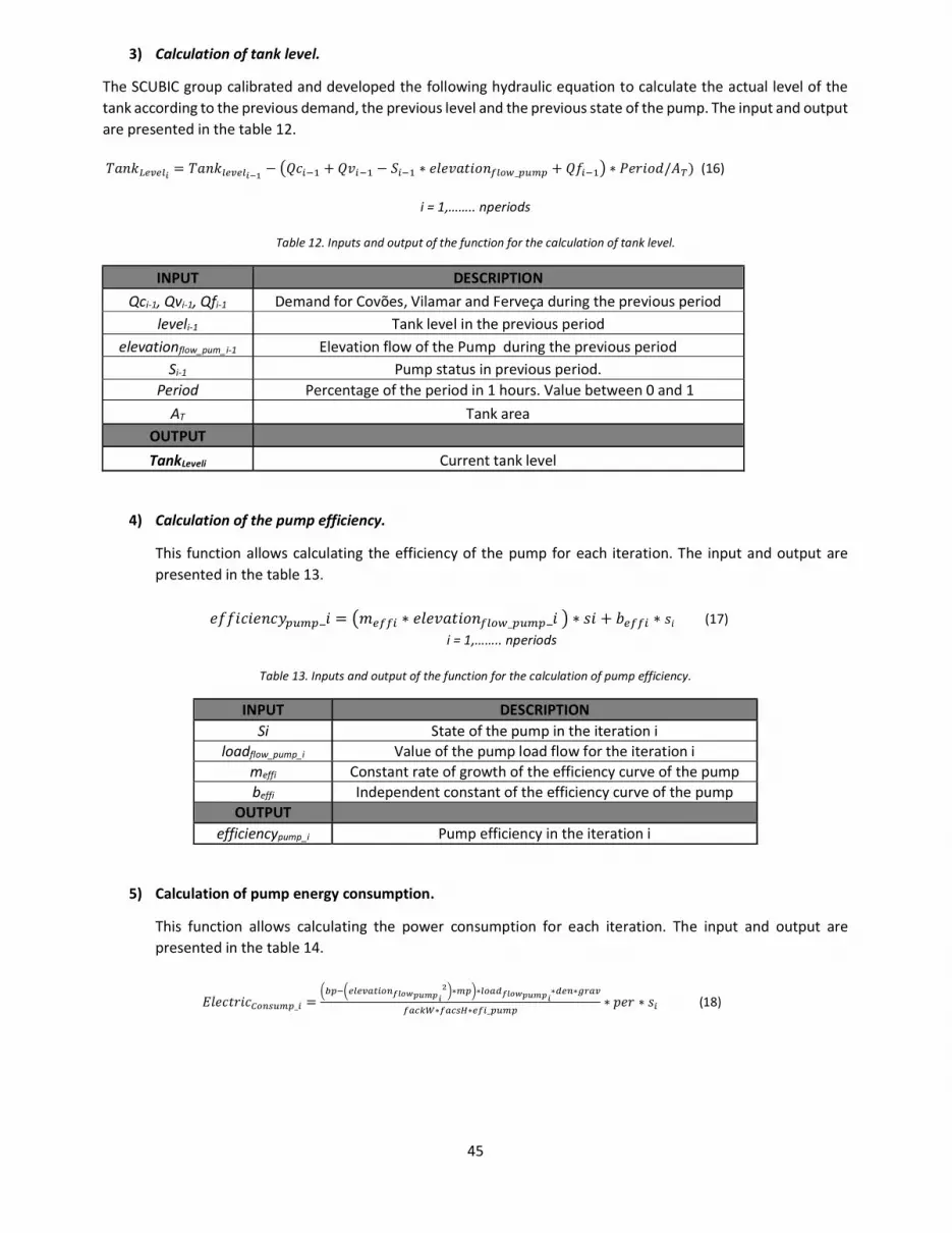
45
3) Calculation of tank level. The SCUBIC group calibrated and developed the following hydraulic equation to calculate the actual level of the tank according to the previous demand, the previous level and the previous state of the pump. The input and output are presented in the table 12. = − + − ∗ _ + ∗ / ) (16)
i = 1,…….. nperiods Table 12. Inputs and output of the function for the calculation of tank level.
INPUT DESCRIPTION Qci-1, Qvi-1, Qfi-1 Demand for Covões, Vilamar and Ferveça during the previous period
leveli-1 Tank level in the previous period elevationflow_pum_i-1 Elevation flow of the Pump during the previous period
Si-1 Pump status in previous period. Period Percentage of the period in 1 hours. Value between 0 and 1
AT Tank area OUTPUT TankLeveli Current tank level
4) Calculation of the pump efficiency.
This function allows calculating the efficiency of the pump for each iteration. The input and output are presented in the table 13. _ = ∗ _ _ ∗ + ∗ (17)
i = 1,…….. nperiods Table 13. Inputs and output of the function for the calculation of pump efficiency.
INPUT DESCRIPTION Si State of the pump in the iteration i
loadflow_pump_i Value of the pump load flow for the iteration i meffi Constant rate of growth of the efficiency curve of the pump beffi Independent constant of the efficiency curve of the pump
OUTPUT efficiencypump_i Pump efficiency in the iteration i
5) Calculation of pump energy consumption.
This function allows calculating the power consumption for each iteration. The input and output are presented in the table 14. _ = ∗ ∗ ∗ ∗
∗ ∗ _ ∗ ∗ (18)

46
Table 14. Inputs and output of the function for the calculation of pump energy consumption. INPUT DESCRIPTION
Si State of the pump in the iteration i elevationflow_pump_i Constant describing the curve of the pump
efficiencypump_i Value of the efficiency of the pump calculated for the iteration i mp Constant rate of growth of the efficiency curve of the pump bp Constant describing the curve of the pump
den Density of water. grav: Universal constant of gravity.
Period Percentage that represents the period in 1 hour fackW: Conversion factor from W (watts) to kW (kilowatts) facsH: Hours conversion factor for seconds
OUTPUT EnergyConsump_i The power consumption of the pump in the interaction i
According to the previous equation, as the term of the pump's state Si is multiplying the whole equation, it can be concluded that if the pump is off, the power consumption is 0 and, therefore, the energy cost is also zero.
6) Calculation of the cost of energy consumption. This function calculates the cost of the electric consumption for each iteration. The input and output are presented in the table 15. _ = _ ∗ (19)
Table 15. Inputs and output of the function for the calculation of the cost of energy consumption. INPUT DESCRIPTION
ElectricConsump_i Energy consumption in the period i Tariffi Electrical tariff for the period i
OUTPUT ElectricCost_i Electrical cost of the pump for the period i
7) Calculation of the total cost of operation.
For calculating the final cost of the pump operation " _ ”, all values of the cost vector per period “ElectricCost ” are added. 4.4.2. Hydraulic simulation implementation of the study case. The Epanettoolkit tool for Python allows simulating water supply networks easily and robustly without having to use the software directly. This is a great help for the development of online simulation platforms of these systems, requiring only to performe the simulations by calling the Epanet functions for python. In this section, a brief description of the installation and configuration of the hydraulic software (Epanettoolkit) is made for the simulation of these systems. 4.4.2.1. Description of the software configuration. Is necessary to know that the Epanet tool kit tool runs on the python platform 3.3. Therefore, it is required to

47
Install the version of python 3.3.0 Install the version of epanettoolkit Epanet2 0.4.0.1dev for python Install the Epanet software. In this way, the Epanet functions can be called by the functions of epanet toolkit
for Python. Import the functions of Epanet toolkit into python using the python command “import epanet.epanet”
After making the correct installation, the Epanet toolkit package is available to carry out WSS system simulations Must clarify that to simulate a water supply network, it is must have the network configured in an input file, where the network configuration is hosted and has the information necessary for the simulation. 4.4.2.2. Module in python for the simulation with EPANET. In figure 14, the structure of the module to be developed in the Python platform is presented. It has an input text file where the network structure and the forecast of the consumption demand in the network are stored. This data is loaded into the program so that it is called by the EPANET toolkit functions to perform the configuration and the simulation of the system. After the simulation of the network and the optimization of the pumping operation, the final outputs of the module are sent to the database and to the frontend of the SCUBIC platform.
Figure 14. Structure of the simulation module.
4.4.2.3. Configuration of the network. To make the simulation of the network, is must have configured the water supply network in the EPANET software, and export the .inp file. This input file is called by a python function, which at the same time calls a function of epanet toolkit to open the file from Python and in this way be available within the programming code to perform the simulation of the network. it must be clarified that the demand point of Fervença are all the consumption point located between node 3 and node 4. The network was designed in this way to simplify all the consumption points. The configuration of the network is presented in figure 15.
Figure 15. Structure of the INOVA water supply network.

48
Characteristics of the supply network
1) Elevation: Table 16 shows the elevation of the nodes.
Table 16. Elevation of the nodes of the WSS system of INOVA. NODE ELEVATION
Node 1 37 m Node 2 32 m Node 3 36 m
Fervença demand point 29 m Node 4 74 m
Fontinha tank 90 m Covões demand point 35 m Vilamar demand point 25m
2) Characteristics of the pipes: Table 17 shows the characteristics of the pipes.
Table 17. Pipes characteristics of the WSS system. SECTION CHARACTERISTIC
Water collection olhos fervença - Node 1 Diameter 300 cm Roughness 100
Node 2 - Node 3 Diameter 300 cm Roughness 100
Node 3 - Fervença demand point Diameter 110 cm Roughness 140
Node 3 - Node 4 Diameter 300 cm Roughness 100
Node 4 - Fontinha tank Diameter 300 cm Roughness 100
Node 4 - Covões demand point Diameter 160 cm Roughness 140
Node 4 - Vilamar demand point Diameter 200 cm Roughness 140
3) Length: Table 18 shows the lengths of the pipes
Table 18. The piping diameters of the WSS system. SECTION LENGTH
Water collection olhos fervença - Node 1 5 m Node 2 - Node 3 761 m
Node 3 - Fervença demand point 294 m Node 3 - Node 4 8400 m
Node 4 - Fontinha tank 5 m Node 4 - Covões demand point 5870 m Node 4 - Vilamar demand point 7366
As the consumptions and the state of the pump change according to the period that is being iterated, these are configured within the simulation calling EPANET functions through the Epanet toolkit. After having configured the network, it can export the .inp file that is called from python to simulate the network according to the demands

49
and of the pump state in each period. The main functions for simulation with Epanet tool kit with python can be found in appendix 7.3.3. 4.5. Implementation of the optimization models for the pumping operation In this section, the implementation of the two chosen methodologies in order to optimize the pumping operation are explained. 4.5.1. Empirical methodology of optimization by constraint
1) Maximum level and minimum tank. This function does a verification of the level for each iteration, and not allow that the pumping operation to exceed the maximum level or the minimum allowed for the tank.
Levelmax = 8 m Levelmin = 2 m 2) Calculation of periods.
This function first verifies that the input vectors have the same length, then it calculates the period in minutes which the measurements were taken. In this way, the length of the matrices is known. Table 41 present the inputs and outputs of this function.
Table 19. Input and output of the function for the calculation of period by the input vectors. INPUT DESCRIPTION Qc, Qv Demand forecast vectors of Covões and Vilamar during the day Tariff Electric tariff vector during the day.
OUTPUT totalperiods length of the vectors is equal to the number of periods during the day
Period The period in which the samples were taken, given in minutes numberindividual Number of individuals of the GA population
In addition to the previous output, the number of individuals that the population must have is also given for the genetic algorithm.
3) Calculation of the tariffs weights. This function gives a weight to each tariff's value from 0 to #_tariff in the tariff vector, with 0 being the lowest tariff and #_tariff the highest tariff. The given values are integers. An example can be seen below to creation of the weight matrix of the tariffs.
Example 1: Being the tariff vector that describes the cost in euros of kW / h for each period the day.
Tariff = [ 0.0738, 0.06608, 0.06608, 0.0738, 0.10004, 0.10004, 0.10004, 0.20595, 0.20595, 0.20595, 0.10004, 0.20595, 0.20595, 0.10004, 0.10004 ]
This example has 4 different prices in the vector, to each one it is assigned a weight from the lowest to the most, according to the number of repeated tariffs found. According to the order that the values are found in the tariff matrix, the assignment of weight is shown in the following table 42:

50
Table 20. Example for the assignment of weights in the tariff vector.
TARIFF WEIGHT ACCORDING TO ITS VALUE IF > OR < 0.0738 1
0.06608 0 0.10004 2 0.20595 3
Finally, it is built the weight vector according to the order in that they are in the tariffs vector. The vector final result is the following:
Weight_vector_tariff = [1, 0, 0, 1, 2, 2, 2, 3, 3, 3, 2, 3, 3, 2, 2, ] In this way, it is better for the program to know if in each iteration the tariff it is high or low according to the weight. So, in this way, the program makes the decision whether to switch the pump on or off. It is clear that the input for this function is the tariff vector given by the electric provider, according to the number of periods that are being iterated.
4) Permissive calculation to switch off the pump. This function calculates the permissive to switch off the pump when it is on, according to the number of minimum periods in which it must be switched on according to the total length of the input vectors, as it was described in table 43. The input and the output of this function are also in table 43.
Table 21.Inputs and outputs of the function to calculate the permissive to switch on the pump. INPUT DESCRIPTION
Pumpingplan_i Pumping operation calculated up to iteration i. minperiods Minimum of periods that the pump should switch on. OUTPUT
Permissive_off_pump 1, permissive to switch off the pump for the next iteration. 0, the pump must remain switch on for the next iteration. The function extracts from the vector of the pumping operation, from the last position, the number of minimum periods, and then adds all the values, if the result of this sum is equal to the number of consecutive minimum periods. Then, the program gives the permissive to switch off the pump for the next iteration. Otherwise the pump must remain on. The above functions allow to calculate a pumping operation based on constraints according to the needs of INOVA, hoping that in addition to meeting the demand, optimize the electric consumption and therefore the operating cost per day. 4.5.2. Genetic algorithm (GA). Within a genetic algorithm, it is required to know the cost function (fitness) that must be optimized. This function is the weighting given by the algorithm for each solution generated by the GA. Therefore, the fitness is defined as the weight that has possible solution within the GA, and evaluate if the solution is better than the actual one. For this reason, if the cost of the pumping operation is high, then it is a bad solution. On the other hand, if the pumping operation has a low cost, then this operation is a possible solution.

51
4.5.2.1. Fitness calculation for an individual. The aim of the genetic algorithm is to minimize the energy cost of the pumping operation. Therefore, the fitness is defined as the cost of the pumping operation:
= _ (20) 1) Calculation of the total cost of operation.
This function was created to use the methods explained in the previous section to perform the simulation of the network: (1) empirical hydraulic equations and (2) hydraulic software EPANET. This function has the ability to calculate the total cost of operation of a pumping operation generated by the genetic algorithm. The table 44 present the inputs and outputs of this function.
Table 22. Inputs and outputs to simulate the WSS system. INPUT DESCRIPTION
InitalLevel Initial level of the tank PumpingPlan Vector of the pumping operation, generated by the genetic algorithm.
Tariff Electric tariff vector during the day OUTPUT
TankLevel Vector of tank levels in each period TotalCost_oper Total cost of operation of the pumping operation (Fitness)
In the same way, as some constraints were defined to validate a solution, also for the genetic algorithm, the calculation of penalties like a method of constraints to discard solutions that do not satisfy the solution to the problem was defined. The cost of the penalties is added to the cost of operation (fitness) if the pumping operation fails to meet certain parameters. 4.5.2.2. Penalties for solution constraints Within the genetic algorithm that is defined later, the solution that meets the requirements of operation and has the lowest possible cost must be found. The penalties are a cost for non-compliance with the requirements that the solution must have. These penalties increase the cost of the solution, leaving it with a low percentage of possibility to be an adequate solution. Thus, the genetic algorithm not take it into account this solution in order to perform in futures calculations. The penalties for non-compliance with the solution are as follows:
1. Minimum of periods that the pump should be switched on. A function that calculates the penalties by minimum periods of the switch on the pump was created. In the table 45, the inputs and outputs are presented.
Table 23. Input and output of the function to calculate the penalties by minimum periods of the switch on the pump. INPUT DESCRIPTION
PumpingPlan Vector of the pumping operation, generated by the genetic algorithm. ListFilter Array that contains all the filters described above.
minperiods Minimum of periods that the pump should switch on OUTPUT
Num_Totalpenalties Total number of penalties
According to table 9 presented in the section 3.3.1, there should be a minimum of periods that the pump should be on. In this case, a vector that represents each individual (pumping operation) is analysed. The algorithm must

52
look within of the pumping operation for the cases that the minimum of the switch on periods is not fulfilled. For the tests carried out, with a period of 15 min, the minimum of periods in which the pump should be on are 4. The calculation of the minimum periods in that the pump must be switched on, in general, is done by the correlation of the pumping operation with filters that are vectors that describe the behavior of the switch on. The correlation is a calculation that gives the relationship between two statistical variables. The filters that describe the switch on by periods are shown in the table 46.
Table 24. Filter list to calculate the correlation. Periods of switch on Filter
1 period Filter 1 = [10, 1, 10] 2 periods Filter 2 = [10, 1, 1, 10] 3 periods Filter 3 = [10, 1, 1, 1, 10] 4 periods Filter 4 = [10, 1, 1, 1, 1, 10] 5 periods Filter 5 = [10, 1, 1, 1, 1, 1, 10] 6 periods Filter 6 = [10, 1, 1, 1, 1, 1, 1, 10]
The function calculates the correlation of the pumping operation with the number of filters needed according to the period. The table 47 shows the filters that must be calculated according to the period. The following table 48 shows the result of the correlation given a pumping operation in an iteration.
Table 25. Filters that are used to calculate the correlation according to the period.
PERIOD (min) FILTERS TO CALCULATE MINIMUM CONSECUTIVE PERIODS IN THAT THE PUMP SHOULD BE ON 5 Filter1 , Filter2 , Filter3 , Filter4 , Filter5 6
10 Filter1 , Filter2 , Filter3 , Filter4 , Filter5 6 15 Filter1 , Filter2 , Filter3 4 30 Filter1 , Filter2 3 45 Filter1 , Filter2 3 60 None 2
periods > 60 min None 1
Table 26. Values of the correlation result for each filter.
Filter RESULT OF THE CORRELATION Filter1 1 Filter2 2 Filter3 3 Filter4 4 Filter5 5 Filter6 6
The result of the calculation of the correlation is a vector that saves where statistically occurs the transition of each filter. Finally, it is counted the times the same result is presented in the correlation made.
Example2: Given the following pumping operation, the correlation with all filters is calculated. = , , , , , , , , , , , , , , , , , , , , , , , , , , ,

53
= , , , , , , , , , , , , , , , , , , , , , , , , , , , , , , , , , , , , , , , ,
After the correlation is calculated, the events are counted and this result increase the total cost of operation, by each event in a value of 1 Euro.
Example3: The table 49 shows the total value of the penalty that is increased in the total cost of operation by a given period, for the pumping operation of example 2.
Table 27. Cost of the penalty for example 2 for different periods.
PERIOD (min) TOTAL PENALTY 5 5 €
10 5 € 15 3 € 30 2 € 45 2€ 60 No penalize
periods > 60 No penalize
2. Penalty for exceeding minimum or maximum level. As mentioned in previous sections, the maximum and minimum tank level for this system is:
= =
One available information after of calculation of the operation cost of the pumping operation is the vector that contains the values of the tank level “ “ calculated for each period. This function is analysed and this vector finds the values that exceed the limits given for the tank. Every time the value of the level exceeds the maximum level or overpasses the minimum level, the total cost of operation of the pumping operation is increased in a penalty of 50 €. In this way, it ensures that the pumping operation is not taken into account by the genetic algorithm for next generations. 3. Penalty for level continuity This function analyze the vector of tank level too “ “. This penalty ensures that the final level of the tank is greater or equal to the initial level of the tank. The difference between the initial level and the final level is multiplied by 50 €, and the result is the value of the penalty. Given the above, the larger the difference between the levels, the greater the cost of the penalty. However, if the difference is small or close to 0, the value of the penalty is null, giving the possibility of the genetic algorithm to take into account this solution for future populations. Described the previous penalties, the total fitness for each pumping operation is given by:
= + _ + _ _ + _ (21)
4.5.2.3. Main functions of the GA. Already having defined how it is intended to calculate the total cost (fitness) for each individual or pumping operation, the functions necessary to implement a genetic algorithm are defined.

54
1. Creation of an individual (Pumping operation) An individual, in a genetic algorithm, is a possible solution for the problem of optimization. In this case, the solution is the operation for the pump during the periods of the day. A pumping operation is a vector composed of binary numbers that describe if the pump is on or off during a certain period. In this way, it is must create a vector composed of "1" or "0" with a length equal to the number of periods during the day. Using the Python “random” function, initially, a vector with "1" or "0" is randomly created, with a length equal to the total periods in the day, and finally this vector is the pumping operation (individual).
2. Creation of a population As was mentioned in the state of art, studies have already been carried out to define the size of a population (see section 2.4.2). The population size must be equal to the length of an individual, in this case, the pumping operation. In table 50, the size of the population is defined according to the period.
Table 28. Number of individuals of the population according to each period PERIOD (min) LENGTH OF SOLUTION AMOUNT OF THE POPULATION
5 288 300 10 144 150 15 96 100 30 48 50 45 32 35 60 24 25
120 12 15 The value of the number of individuals that the population must have is calculated within the function 2 of the section 4.6.1. A function that create a population of individuals equal to “numberindividuals” with a total length of each individual of “totalperiod” is defined. The output of this function is the “Population{ }” matrix that is an array that contains the first population. 3. Selection and reproduction. The following function table 51 was defined to perform the selection and reproduction process. In the following figure 16 the implemented algorithm is presented for this function.
Table 29. Inputs and outputs of the function of selection and reproduction of GA INPUT DESCRIPTION
Population Array which contains the pumping operations to be analysed. demands Vector that contains the demands or flows of consumption of: Covões, Vilamar and Fervença. InitialLevel The value of the initial level to calculate the hydraulic simulation
ListFilter Array that contains the list of filters to analyze the penalty in each pumping operation for minimum periods that the pump must be switched on. Levelmax, Levelmin Values of the maximum and minimum level of the tank level to calculate penalty for exceeding these levels. Selection The number of individuals that are chosen for reproduction. OUTPUT
Population New population for the next iteration

55
Figure 16.Flow diagram of the GA algorithm
From the figure 16, it should be noted the following: As was described in section 4.5, the simulation of the network is carried out by the two methods proposed.
The output of the simulation is the operating cost of each pumping operation that is the fitness for each solution.
As was mentioned, the calculation of the fitness includes the sum of the penalties. This ensures that the unwanted solutions remain at a high cost. In this way the algorithm does not have into account these solutions for the selection and reproduction procedure.
After reorganizing the array of the population (vectors of pumping operations) according to the cost, the pumping operations that have the lowest cost are selected like parents. The number of individuals selected is given by the value “selection”.
Within the selected parents are randomly chosen two of them, of the two pumping operations, the genetic material is crossed according to the method mentioned in the state of art: By one point. This method consists of choosing a random point of the parents, from this point the genetic material is exchanged. This process is repeated in the same number of times as the value of "selection" so in this way the children are part of the array of the new population.
An example of the method of “By one point” is shown in the following figure 17.
Figure 17. GA reproduction method diagram.
4. Mutation. As it was explained in the state of the art, the mutation process changes the value of a certain position within the individual. This position is chosen randomly, ensuring that the new value is different from the current value. This

56
process is done for all the individuals except the parents chosen in the previous process, thus it gives a certain diversification to find new solutions in the pumping operation that can be taken into account in future generations. In the flow diagram of the figure 18 it is described the mutation algorithm. The program calculates a random value. This value is compared with the percentage of mutation. If this value is less or equal, then there is a mutation, if it is not met, then there is no mutation. In this way it is ensured that all individuals are not mutated, avoiding creating diversification in the population, which can lead to the solution not converging. The percentage of mutation is a parameter that makes the genetic algorithm very sensitive, at this time it cannot be specified, therefore is done a tests to find a suitable value in the sections of the results.
Figure 18.Flow diagram of the GA mutation algorithm.
The process of reproduction and selection and the mutation process is housed within a "for" cycle, converging to a solution that meets the proper characteristics of an optimal solution. The number of times that these two processes is performed is defined as “numinteractions” 4.6. Optimization of the pumping operation using empirical constraint and simulation with
empirical hydraulic equations. For this solution the pumping operation is optimized based on the constraints and simulating by empirical equations hydraulics. It is not the most efficient solution but gives a reference in the first instance to arrive at the most optimal solution. The main constraints that describe an optimal solution for a pumping operation were explained in the section 4.6.1, and are used for developing the programming code. The code developed in each iteration defines the pumping operation according to the constraints, and, with the help of the functions described in section 4.5.1, the program simulates the network and calculates the energy consumption and its cost for each period. This program has a low computational cost, which allows having the result in less than 0.5 sec. In figure 19, the flowchart of the programming code is shown.

57
Figure 19. Flow diagram of the optimization algorithm by constraints.
4.7. Optimization of the pumping operation using GA and simulation with empirical hydraulic
equations. The objective is developing a genetic algorithm able to find an optimal pumping operation and able to improve the first solution found. The operation cost of the first solution found is a starting point for the genetic algorithm, serving as a point of comparison to evaluate the individuals that the algorithm generates while evolving in the iterations. The following figure 20 is the flow diagram of the implemented algorithm.

58
Figure 20. Flow diagram of the optimization algorithm by GA.
The developed algorithm uses the hydraulic equations that describe the behavior of the system, to perform the simulation of the network. Initially, the genetic algorithm randomly creates solutions (pumping operations). The number of solutions created is related to the period, as described in table 50. All the pumping operations are simulated and their operation cost is calculated. Then, the pumping operations go into the module of selection and reproduction of the genetic algorithm and the pumping operation that have the lowest cost are chosen like parents to cross their solutions. The method for to reproduce the parents is explained in the section 4.6.2.3. The number of pumping operations that are chosen depends on the input value of "selection". Finally, the pumping operations that were not chosen in the previous process are mutated in a randomly chosen point by the genetic algorithm, as it was explained in the section 4.6.2.3. The resulting final population, after completing these processes, is the input for the next iteration in the selection and reproduction module, doing the whole process again until the number of iterations is completed (evolution of the genetic algorithm).

59
According to the flow diagram, after completing the iterations corresponding to the evolution of the genetic algorithm, it is within the last population where the algorithm looks for the pumping operation that had the lowest operating cost. This pumping operation is the solution and complies with the constraints mentioned in the section 3.3.1. 4.8. Optimization of the pumping operation using GA and the hydraulic simulator. For the development of the two previous modules, the hydraulic equations that the SCUBIC group developed for the network of INOVA were taken into account. Unlike the previous module, this new module performs the simulation of the water supply network system using the hydraulic simulator through the Epanet toolkit for python, and, in this way, call the functions used by the Epanet software to simulate the system. The optimization method of the pumping operation is the genetic algorithm explained in the previous sections. The flow diagram of the figure 21 describes the implementation of the simulation of the network with the Epanet toolkit. This function opens the file where the network is configured. Then, it makes the configuration of the level with that the simulation starts. After this, the commands to start the simulation are used. As the simulation of the network is for a given pumping operation, this enters the "for" cycle to simulate the network for each period during the day. In this cycle, the demands and the pump's state in each iteration are configurated in the network. Then, the pump's power consumption and the tanks level are recovered. Finally, in each iteration, the vectors the level of the tank, the power consumption of the pump and the electric cost for the period are updated. The final operation cost “TotalCost_oper” is the add of all the values of the vector " "ElectCost [ ]” using the function "sum" by Python.

60
Figure 21. Flow diagram of the optimization algorithm by GA.

61
4.9. Communication between modules and database update
4.10. Implementation of the instrumentation support system 4.10.1. Hardware
1) Microprocessor For the development of the application, the processing system provided by Espressif Systems the NodeMCU has been chosen, because it is a hardware that can to be programmed by the free platform IDE of Arduino, and is compatible with any system, besides is of low cost and makes it an important option because does not generate an additional cost for the company SCUBIC. The all specification of the NodeMCU are in the section 7.3.2. On the other hand, going more background of the application that is intended to develop, the integrated microprocessor, the ESP 8266 module has the possibility of establishing TCP / IP connections with other devices, which is of interest to this project.
2) Sensors. For the development of the project the sensors are used to measure pressure and flow in the piping in a network of a raw water supply system. Therefore, it is possible to define some main parameters for the choice of these.
Pressure Sensor. The selection criteria for the pressure sensor, according to the specifications of the WSS system are:
Pressure requirements: 0 - 150 PIS Accuracy: High Working temperature: Ambient Chemical compatibility with working fluid: Water. Output Type: Analog Output 0 - 3.3 Vdc preferably. According to the analog input A0 of the NodeMCU
microprocessor Working current. < 8mA, NodeMCU working current Method of electrical connection: Cables Sensor cost: Low Linearity: High Response speed: <2ms Sensor response curve: Linear.
As the application is for a not corrosive fluid, a very robust sensor is not needed. In the market, can be found a piezoresistive sensors of linear response for pressures not very high. The average pressure of a water supply system is 150 PSI, however, it cannot make the choice of the sensor with this same range, since the working pressure would be very close to the rupture pressure of the sensor. Therefore, it is advisable to make the choice of the sensor with a 35% more safety in the working pressure, to ensure that the system never reach the maximum pressure of the sensor in this way it protects the sensor element. According to the previous explanation, a sensor with a range of 0 to 175 PSI should be searched. For the development of the application, the HK 1100C sensor was chosen. The specifications of this sensor can be found in the appendix in section 7.3.3.
Flow Sensor. The selection criteria for the flow sensor, according to the specifications of the WSS system are: System working pressure: 0 – 150 PSI Maximum and minimum flow: Proces systems. Accuracy: High Working temperature: Ambient temperature

62
Chemical compatibility with working fluid: Raw water Orientation: Horizontal Tube type: PVC or other. Sensor type: Differential pressure, Ultrasonic, Paddles. Output type: analog or digital Method of electrical connection, (soldering, special connectors, etc.): Cable Sensor response curve: Linear Diameter: 1/2 "NPS Sensor cost: Low.
In the industrial, for the measurement of flow is common to use sensors of pressure differential, ultrasonic or pallets type. The ultrasonic sensor has a high accuracy, therefore, the cost is very high in comparison with other technologies. This sensor is used for the processes where the measurement with a high accuracy is required. For our case, the reading should be accurate, but not with the accuracy of this sensor. Also is found the differential pressure sensor, this sensor is very good for flow measurements in processes where the pressure is very high, but the cameras of this sensor must be checked constantly because they can calibrate the zero of the sensor due to variations in the element sensor, for this must be disassembled to calibrate the zero newly. This sensor has a rate of the maintenance high, for this would not be a good solution for the application. The palette sensor, that is a mechanical type sensor by Hall effect, which according to the passage of water the voltage shifts from 0Vdc (logic 0) to + Vcc (logic 1), generating pulses. The number of the pulses in a sampling time is the relation of the flow measurement. This sensor has a linear response curve with a good accuracy. It is a sensor easily find in the market of several diameters for different voltage outputs. The most common are the peak voltages of 5 Vdc. For the development of the application, the YF – S201 flow sensor was chosen. The specifications of this sensor can be found in the appendix in section 7.3.4.
3) Power Supplies. Once have been defined the components that are used to develop the application, it is necessary to determine the power supplies for them. The equipments must have a power source, as is presented in table 52.
Table 30. Supply voltages for the microprocessor and sensors. EQUIPMENT POWER VOLTAGE (Vin)
NodeMCU 3.3 Vdc supply voltage, with a consumption < 8mA Pressure Sensor 5.0 Vdc Supply voltage, with consumption <10 mA
Flow Sensor from 5 to 18 Vdc Supply voltage, with a consumption < mA According to the above, 2 regulated voltage sources are needed; one to feed the sensors and the other to feed the Microprocessor.
Power Supplies of 5 Vdc. To design the power supply is used the semiconductor LM7805 – figure 22, positive voltage regulator commonly used to power TTL technology circuits as is the flow sensor; this regular has an output voltage of 5Vdc.

63
Figure 22. 5Vdc source circuit.
Power Supplies of 3.3 Vdc. Many electronic devices not powered at standard 5 Vdc voltages, due many of them operate at a regulated voltage of 3.3 Vdc, which makes the circuitry consume less power, and can be connected to of low consumption portable batteries, which makes them have a longer duration. To design the power supply is used the semiconductor LD117V33 that is shown in figure 23, this regular has an output voltage of 3.3Vdc. It is important to note that this regulator supply with 5Vdc, that is the output of the regulator LM7805.
Figure 23. 3.3 Vdc source circuit.
4) Signal conditioning. According to the characteristics of NodeMCU, it has analogical and the digital input, that are designed to receive voltages from 0 to 3.3Vdc. On the other hand, the voltage outputs of the sensors are as follows, table 53.
Table 31. Output voltages of the sensors. EQUIPMENT OUTPUT VOLTAGE (Vo)
Pressure Sensor 0.5 to 4.5. Vdc (Analog sinal ) Flow Sensor 0 or 5 Vdc (Digital sinal )
From the foregoing information, it is deduced that a transformation of the output signals from the sensors to voltages that can be supported by the microprocessor must be done. This transformation of the signal can be doing in several ways with different schemes, which are studied in the areas of power electronics, this are: Semiconductors, Instrumentation amplifier, Voltage divider. For the transformation of the signals is used the simplest scheme but with good electronic result.
Voltage Divider.

64
The simplest and most cost-effective way to do signal transformation is to use a voltage divider. It's a simple circuit that with two series resistors and an input voltage, an output voltage equivalent to a fraction of the input voltage can be obtained. This circuit is shown in figure24, and is fundamental in the area of electronics.
Figure 24. Voltage divider circuit.
The general formula for the voltage divider is as follows: = ∗
(22) In this way, having the previous equation it possible to find the relationship of the resistances that causes that the output of this circuit being 3.3 Vdc, that is the voltage that allows the microprocessor. If it is assumed that the resistance in R1 = 10K Ω, by developing the equation for R2, in terms of the rest of the variables is possible to arrive at the following expression:
= ∗ (23)
Finally, it is calculated the resistance R2, and this would have a value of R2 = 20KΩ. In the figure 25 it is defined the outputs resulting from the sensors after the voltage divider is applied, so have.
Figure 25. New voltage outputs after applying a voltage divider.
The new signals resulting after the voltage divider is applied are within the constraint conditions for the inputs to the NodeMCU. In this way is designed two voltage dividers for each signal, in the final scheme. After explaining each of the components of the system, a scheme for the integration of all the equipment is done, figure 26.

65
Figure 26. final circuit scheme.
4.10.2. Firmware
1) Data Base A database is a set of related information that is structured. This is stored on disks that allow direct access to them and there are one or more programs that manipulate this dataset. The database programs organize the information in such a way that the tables are indexed so the users can consult these. Is possible to find different software for data management, among them are: Access, Visual FoxPro, MySQL Database, SQL server, Oracle, among others. For the application, is used the MySQL Data base tool, due to that this software that can work on multiple platforms, including LINUX and Windows. The server allows multiple users to access multiple DB tables. Finally, this is a database compatible with other software thus allowing integration with other applications. In the MySQL Workbenk software the following database was created: Database: sist_supply_water, figure 27.
Figure 27. Database and tables created
2) Tables.

66
History_wss: This table have the following columns, with the following configuration parameters, figure 28. In the history table is stored the data coming from the microprocessor, with a date and time of reading.
Figure 28. Columns of the historical table.
Supervisory_wss: This table have the following columns, with the following configuration parameters,
figure 29. In the supervision table only the last data measured by the microprocessor is stored.
Figure 29. Columns of the supervision table.
The database was structured in the software Mysql Workbench free enterprise version. 3) Database server
To manage a database, it is must know the tools that help in managing them. A simple way is to query using web resources as is php. Php is an open source language especially suitable for website development that can be included in html code. What distinguishes php, is that it can runs on the server, generating by html and sending to the client, in addition, php has many advanced functions that allow interaction for professional programs like MySql databases. To establish a connection with the database is should mainly have into account the following:
Have database created Localhost: Indicates where are going to connect to the DB. If the connection is from another server, is must
include the IP of the server and it must have the connections open. User. Mysqul generates a username and password to access the BDs Password. Associated with Mysql user Name of DB. Name of DB tables.

67
To make a connection from the server to the database was used the following commands in php code, table 54: Table 32. Main commands in php for the management of the database.
FUNCTION OF SERVER Declaration of variables. Saves the value sent by the client.
$Y0=$_GET[ 'VARIABLE' ] Connection to the database. The communication is made by port 81.
$link = mysql_connect("localhost = 81", "user ", "pass word”) mysql_select_db("name of the BD").
Updating the record in the database. For this case in the supervision table. $query = "UPDATE supervisory_wss SET pressure='". $Y0 . "', ...... WHERE Read=1";
$result = mysql_query($query). To insert a new value into the database. For this case in the historical table.
$query = "INSERT INTO history_wss ( pressure, .....flow) VALUES('$Y0', ....,'$Y1')"; $result = mysql_query($query).
To query the database. For this case read the current value of the supervision table. $query = "SELECT * FROM supervisory_wss"; echo "<BR>"."Pressure: ".$linha1['presao'];
The previous programming functions was used to perform the database server, this is called by the clients who need to write in the DB. The final result of the development of the web server called from a browser is presented in the following figure 30.
Figure 30. Frontend of the server.
4) Software NodeMCU.
The NodeMCU is the microprocessor that recovers the readings made by the sensors, and are sent to the database using the server described above. This makes a TCP / IP connection with the equipment where the database server is housed and send the records of the sensors. As the NodeMCU has to connect to a router to call the IP of the site where the server is located, is must have all the permissions, such as users and passwords of the router and the server, to pass each layer in the sending of the data.
Plataform IDE.

68
IDE- is an integrated development environment, a computer program composed of a set of programming tools. It has been bundled as an application program, which consists of a code editor, compiler, debugger and a module for drawing interfaces. It also incorporates tools to load the compiled program into the flash memory of the hardware.
NodeMCU Software. The programming of the application was developed in the platform IDE, due the microprocessor has the faculty to be compatible with this platform. In the figure 31, is gave a brief description of the code developed, In the appendix of this work is appended the code to be consulted in more detail.
Figure 31. Flow diagram of the instrumentation support system algorithm.

69
In the last lines of the programming of NODEMCU makes a connection with the server and send the measurement of the sensor, and this sends the values of the readings through the code php to the data base updating the values in the table of “supervisory_wss” and “history_wss”. The values in the table supervisory_wss are saved in a new line of the table.

70
Chapter 5. 5. RESULTS 5.1. Pumping operation by INOVA Currently, the company INNOVA performs a pumping operation in an empirical way without taking into account the electricity tariff. This was the main reason for improvement of the electrical consumption of this equipment and reducing the final cost of operation. An example of how the pumping operation is done by INOVA is presented in figure 32.
Figure 32. Empirical pumping operation by INOVA
The INOVA pumping operation is a reference for comparison of the solutions that are presented in this work. Therefore, the proposed solutions are presented in accordance with the savings obtained in comparison with the cost of the current pumping operation used by INOVA. 5.1.1. Characteristics of the current INOVA pumping operation From figure 32, it is possible to infer the following characteristics.
1. The operation pattern of the pump is the same throughout the day. 2. According operation pattern, the result is an oscillating level control, having a minimum value of 4.9 and a
maximum value of 5.8, that gives as results that initial level and the final level be approximately the same. 3. The switch on pattern does not give relevance to the electricity tariff. Therefore, the same pattern is used
when the electrical tariff is low or high. This generates that the pump's operation cost is high. 4. As the pumping operation does not take into account the electricity tariff, it can be assumed that the
operation cost is high, in comparison with some other pumping operation that has this information into account.
5. According to the information provided by INOVA, the current pumping operation have a cost of 81,53 €/day. If it is assumed a constant demand and that the operation of the pump is performed in the same way during the year, it is possible to have an approximate operation cost of 29.760,05 €/ year.
5.2. Results of the pumping operation using empirical constraint and simulating the network with hydraulic equations
After developing the algorithm proposed in the section 4.7, the following pumping operation was obtained by the empirical method. In figure 33, the pumping operation, the level of the tank, and the electricity tariff during a period of 24 hours is presented.
-1,000,001,002,003,004,005,006,007,00
0:00 4:48 9:36 14:24 19:12 0:00
LEVEL TANKStatus Pump

71
Figure 33. Pumping operation optimized by constraints. Initial level = 4.91m.
The following can be analysed from the previous pumping operation. The minimum periods of the switch on of the pump is met, which in this case are 4 since the length of the
input data is 96, having a period of 15 min, as it was mentioned in the table 9. The calculated of the pumping operation does not exceed the level maximum nor the minimum of the tank,
which in this case is 8 m and 2 m respectively. The algorithm managed to give continuity to the end level of the tank in comparison with the initial value.
These values are approximately equal. The algorithm gave priority to the two lowest values in the vector of electricity tariff to switch on the pump.
As it can be seen, the lowest tariffs are in the early hours of the day, where the algorithm switches on the pump to full the tank, allowing it to evacuate in the highest tariffs while the pump is switched off, having to switch on the pump again to recover the level. The cost of daily operation for this pumping operation is 78.14 €. This pumping operation is less expensive in comparison with the empirical method with that INOVA pump is operating currently, that has a cost of 81.53 €/day.
Although the saving is of 5%, this not representative, but it proves that it is possible to optimize the pumping operation and their cost. The target now is to improve the algorithm to have representative saving for the INOVA company or for any company that wishes to optimize its pumping operation. 5.2.1. Algorithm validation. Using the same demands and tariff, simulations with different initial levels are performed to analyse the response of the algorithm and to verify the compliance of the constraints.
Initial Level = 2.5 m

72
Figure 34. Pumping operation optimized by constraints. Initial level = 2.5m.
Initial Level = 7.5 m
Figure 35. Pumping operation optimized by constraints. Initial level = 7.5m.
For the two pumping operations the minimum number of periods of the switch on for the pump is met. These solutions have a different operating cost due to the initial level. The initial level of 7.5 m required a high energy expenditure to maintain this level and give continuity in comparison with the pumping operation with an initial level of 2.5m. It is possible to see that for the pumping operation with the initial level of 2.5, the solution tries to full the tank at the lowest tariffs and then to use the water at the higher tariffs, which is the main objective of the optimization of the pumping operation. The two pumping operations keep the level between the limits while meeting the demand of the consumption points.

73
5.3. Results of the pumping operation using GA and simulating the network with hydraulic equations.
After of the implementation of the genetic algorithm, it was obtained the following results. In the figure 36, the pumping operation, the level of the tank, and the electricity tariff during a period of 24 hours are plotted. For the solution of the pumping operation by the genetic algorithm, the GA characteristics values were listed in table 55.
Table 33. GA values used in optimization processes. GENETIC ALGORITHM SIMULATION'S VALUE Period = 15 min Mutationpercentage = 0.5 totalperiods = 96 numberindividuals = 100 selection = 10 numinteractions = 1500
Figure 36. Pumping operation optimized by GA. Initial level = 4.91m. The pumping operation calculated by the genetic algorithm has the characteristics listed in table 56.
Table 34. Optimization costs of the pumping operation by simulation with equations hydraulic. PUMPING OPERATION COST
Total cost of operation of the pump 64,01 € Penalties for minimum periods of the switch on of the pump 0,00 € Penalty for exceeding the max or min level 0,00 € Penalty for continuity of the final level vs initial level 0,18 € Total cost plus penalties 64,43 €
The genetic algorithm managed to improve the solution until reaching an optimal solution for the pumping operation. It is evident that the previously exposed constraints are fulfilled in totality by this method. From figure 36 it can be analysed and concluded the following:
First, the minimum periods of the switch-on of the pump are met, which in this case are 4 given that length of the input data is 96, having a period of 15 min, as it was mentioned in the table 9.
The pumping operation does not exceed the maximum level nor the minimum level of the tank, which in this case are 8 m and 2 m units respectively.
The program gave continuity to the initial level of the tank in comparison with the end value. These values are approximately equal. For this solution, the level difference is 0.18 m
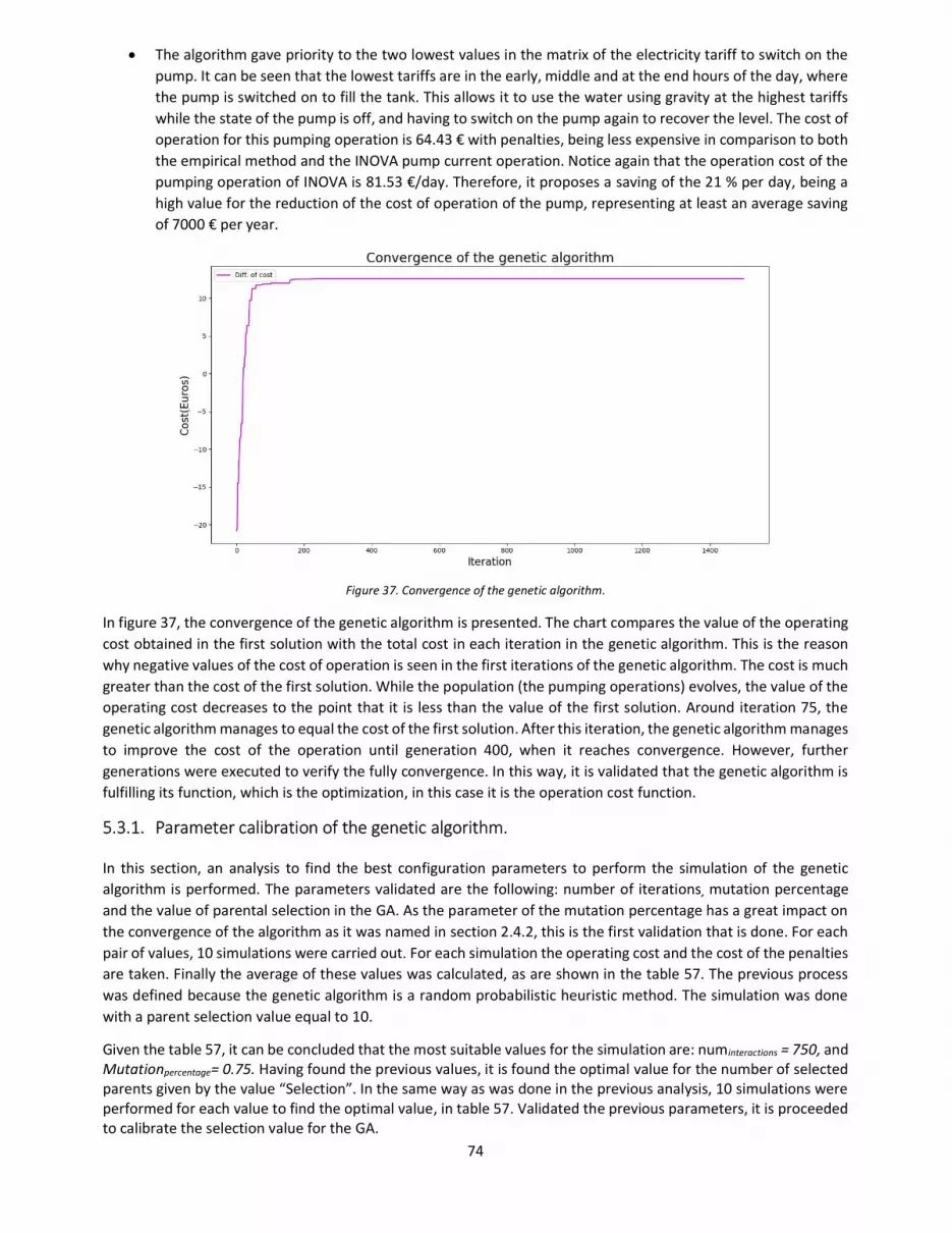
74
The algorithm gave priority to the two lowest values in the matrix of the electricity tariff to switch on the pump. It can be seen that the lowest tariffs are in the early, middle and at the end hours of the day, where the pump is switched on to fill the tank. This allows it to use the water using gravity at the highest tariffs while the state of the pump is off, and having to switch on the pump again to recover the level. The cost of operation for this pumping operation is 64.43 € with penalties, being less expensive in comparison to both the empirical method and the INOVA pump current operation. Notice again that the operation cost of the pumping operation of INOVA is 81.53 €/day. Therefore, it proposes a saving of the 21 % per day, being a high value for the reduction of the cost of operation of the pump, representing at least an average saving of 7000 € per year.
Figure 37. Convergence of the genetic algorithm.
In figure 37, the convergence of the genetic algorithm is presented. The chart compares the value of the operating cost obtained in the first solution with the total cost in each iteration in the genetic algorithm. This is the reason why negative values of the cost of operation is seen in the first iterations of the genetic algorithm. The cost is much greater than the cost of the first solution. While the population (the pumping operations) evolves, the value of the operating cost decreases to the point that it is less than the value of the first solution. Around iteration 75, the genetic algorithm manages to equal the cost of the first solution. After this iteration, the genetic algorithm manages to improve the cost of the operation until generation 400, when it reaches convergence. However, further generations were executed to verify the fully convergence. In this way, it is validated that the genetic algorithm is fulfilling its function, which is the optimization, in this case it is the operation cost function. 5.3.1. Parameter calibration of the genetic algorithm. In this section, an analysis to find the best configuration parameters to perform the simulation of the genetic algorithm is performed. The parameters validated are the following: number of iterations, mutation percentage and the value of parental selection in the GA. As the parameter of the mutation percentage has a great impact on the convergence of the algorithm as it was named in section 2.4.2, this is the first validation that is done. For each pair of values, 10 simulations were carried out. For each simulation the operating cost and the cost of the penalties are taken. Finally the average of these values was calculated, as are shown in the table 57. The previous process was defined because the genetic algorithm is a random probabilistic heuristic method. The simulation was done with a parent selection value equal to 10. Given the table 57, it can be concluded that the most suitable values for the simulation are: numinteractions = 750, and Mutationpercentage= 0.75. Having found the previous values, it is found the optimal value for the number of selected parents given by the value “Selection”. In the same way as was done in the previous analysis, 10 simulations were performed for each value to find the optimal value, in table 57. Validated the previous parameters, it is proceeded to calibrate the selection value for the GA.

75
Table 35. Simulation results for different values of the number of interactions and percentage of mutation
numiterations Values 375 750 1125 1500
Mutati
on perce
ntage v
alues 0.25 TC=65.58 TC =66.11 TC =64.89 TC =65.46
PC = 0.16 PC = 0.25 PC = 0.21 PC = 0.23 0.5 TC =64.54 TC =64.48 TC =64.72 TC =64.69
PC = 0.43 PC = 0.21 PC = 0.42 PC = 0.23 0.75 TC =64.76 TC =62.71 TC =63.89 TC =63.29
PC = 0.41 PC = 0.94 PC = 0.45 PC = 0.46 1 TC =64.79 TC =64.47 TC =64.68 TC =64.85
PC = 0.22 PC = 0.62 PC = 0.67 PC = 0.26 Where: = _ : Is the average of the operating costs obtained. = : Is the average of the costs of the penalties obtained
Table 36. Simulation results for different values of the selection parameter. Selection values
1 2 3 4 5 TC 65.94 62.95 63.86 63.73 63.26 PC 0 0.49 0.42 1.43 0.42
6 7 8 9 10 TC 60.06 63.39 65.0 62.39 63.54 PC 3.94 0.46 0.22 2.63 0.42
Given the previous table 58, it can be concluded that the most suitable value for the simulation is: Selection = 5 5.3.2. Algorithm validation. Using the same demands and tariff, simulations with different initial levels are performed to analyse the response of the algorithm and to verify the compliance of the constraints. For this simulation the calibrated parameters previously found were used.
Initial Level = 2.5 m.
Figure 38. Pumping operation optimized by GA. Initial level = 2.5m

76
Initial Level = 7.5 m.
Figure 39. Pumping operation optimized by GA. Initial level = 7.5m
For the initial level of 2.5 m, the pumping operation calculated by the genetic algorithm in figure 38 in comparison with the operation of the first solution by constraints figure 34, a saving of 15% was achieved, that is a considerable saving. As it is intended, the genetic algorithm managed to find a pumping operation that fills the tank in the lowest tariffs to then be able to evacuate the water in the highest tariffs. This operation complies with all operating constraints defined with a total of penalties of 0.34 € that is the difference between the final level and the initial level. For the initial level of 7.5 m, the pumping operation calculated by the genetic algorithm figure 39 in comparison with the operation of the first solution by constraints figure 35, an approximate saving of 28% was achieved, that is a considerable saving. As it is intended, the genetic algorithm managed to find a pumping operation that keep the tank full in the lowest tariffs to then be able to evacuate the water at the highest tariffs. This pumping operation complies with all operating constraints defined with a total of penalties of 0.93 € that is the difference between the final level and the initial level. 5.4. Results of the pumping operation using GA and the hydraulic simulator. After of the implementation of the genetic algorithm using the simulation of the network with the Epanet toolkit, it was obtained the following results. In the figure 40, the pumping operation, the level of the tank, and the electricity tariff during a period of 24 hours are plotted. For the solution of the pumping operation by the genetic algorithm, the calibrated values found in above section were used. The pumping operation calculated by the genetic algorithm simulating the network through the Epanet toolkit tool has the following characteristics, presented in table 59.

77
Figure 40. Pumping operation optimized by GA. Initial level = 4.91m.
Table 37. Optimization costs of the pumping operation by the hydraulic simulator PUMPING OPERATION COST
Cost of operation of the pump. 207,71 € Penalties for minimum periods of switch on of the pump. 0,00 € Penalty for exceeding the max or min level. 0,00 € Penalty for continuity of the final level vs initial level. 0,84 € Total cost plus penalties. 208,55 €
The genetic algorithm managed to evolve in the number of iterations until reaching an optimal solution for the pumping operation, in this, it is evident that the constraints exposed in above sections are fulfilled in totality by this method. From figure 40 can analyse the following:
The minimum periods of the switch on of the pump is met, which in this case is 4 given that length of the input data is 96, having a period of 15 min, as it was mentioned in the table 9.
The pumping operation does not exceed the maximum level nor the minimum level of the tank. The GA gave continuity to the initial level of the tank in comparison with the end value. The difference
between the initial level and the final level is 0.84 m. This means that the values of the levels are approximately equal.
The GA gave priority to the two lowest values in the matrix of electricity tariff to switch on the pump, this can be seen that the lowest tariffs are in the early and the end hours of the day, that is where the program switches on the pump to fill the tank, allowing it to evacuate the water in the highest tariffs while the pump is the switch off, having to switch on the pump again to recover the level.
For the pumping operation calculated by this solution using the Epanet simulation, it can be observed a great similarity with the pumping operation calculated by the second solution that used the continue equations that describe the behaviour of the network.
The simulation through of the Epanet software which is a specialized software for water supply systems, it can largely validate the continuous equations developed by the SCUBIC group to describe the behaviour of the supply network, given the similarity of the operation operations obtained.

78
5.4.1. Algorithm validation. Using the same demands and tariff, is performed simulations with different initial levels figure 41 and figure42, to see what is the response of the algorithm and verify the compliance of the constraints. For this simulation the calibration parameters found were used. In general, the two pumping operations meet the constraints of an optimal pumping operation, they also meet the demand, and finally they have a low cost. There is a difference in the calculation of electrical consumption and therefore in the electric cost, this is because the two methods of simulation use different ways of calculating this consumption. Therefore, the real power consumption must be validated when pumping operations are implemented in the real system.
Initial Level = 2.5 m.
Figure 41. Pumping operation optimized by GA. Initial level = 2.5m.
Initial Level = 7.5 m.
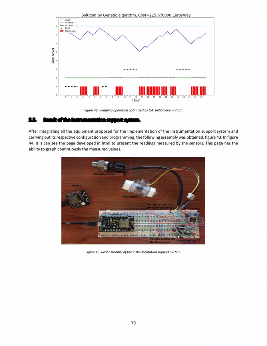
79
Figure 42. Pumping operation optimized by GA. Initial level = 7.5m.
5.5. Result of the instrumentation support system. After integrating all the equipment proposed for the implementation of the instrumentation support system and carrying out its respective configuration and programming, the following assembly was obtained, figure 43. In figure 44, it is can see the page developed in html to present the readings measured by the sensors. This page has the ability to graph continuously the measured values.
Figure 43. Real assembly of the instrumentation support system.
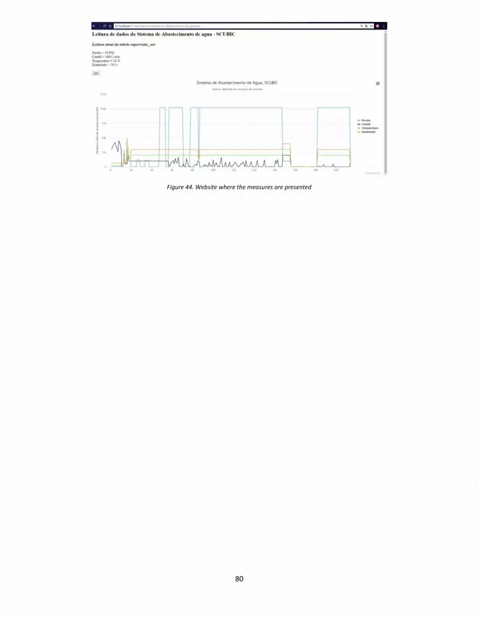
80
Figure 44. Website where the measures are presented

81
Chapter 6. 6. CONCLUSIONS.
1. The objective of optimizing the pumping operation was achieved, as could be demonstrated in the results chapter. The pumping operations found comply with the operation requirements while the demand of the consumption points is guaranteed, in addition that is optimized of the energy consumption and its cost. 2. It is important to be clear about the objective function to be optimized within a genetic algorithm. In addition to this, knowing the constraints that an optimal solution must fulfil is vital to define the penalties within the genetic algorithm and thus ensure that only the solutions that comply with all the characteristics in the evolution of the algorithm are taken into account. Nonetheless, some remarks on the use of the presented genetic algorithm arise. Although it was found a better result of the pumping operation in comparison with the empirical form that the company INOVA does this operation, it is not guaranteed that for new data this model will maintain its performance due to the randomness of the method. 3. For the work developed, it could be proven that the genetic algorithm can explore the solution space in multiple directions, given by the number of combinations the pumping operation. As it is a random process, if a path does not turn out to be a good solution space, it can eliminate it and continue its evolution in other more promising spaces, giving a greater probability in each iteration to find the solution. 4. Within the genetic algorithm it was helpful to define the penalties, which is an additional cost when some characteristics of an optimal pumping plan is not fulfilled. Thus, the fitness parameter is increased so that the genetic algorithm does not take into account the solutions that have a value very high. So, the GA can reduce the search space that is where the optimal solution is found after your evolution. 5. Two methods of simulating the WSS system were defined. For the method that uses the empirical equations, developed by the SCUBIC group, an equation was proposed for calculating the pump's energy consumption and calculating the pump's operating cost. On the other hand, the Epanet simulator uses a weighting of the nominal power consumed by the pump. Since the two simulation methods use different ways to calculate the consumed power of the pump, for this reason, different values were obtained in the final cost of operation. Therefore, this cost has to be validated with the real implementation of a pumping operation to compare the values obtained to calibrate the equations and methods used to calculate the power consumption of the pump within of the algorithm. 6. The computational cost of the simulation by the hydraulic software is much greater than the simulation with the empirical equations, this is because the software performs more calculations like lost by load, lost in the pipes among others, which makes it take more time in solving the equations. 7. Concerning the development of the application of the instrumentation support system, it is very important to have clear the elements to be used and to have the available information of the technical characteristics to make a correct integration of the elements.

82
REFERENCES.
1. Coelho, B.; Andrade-Campos, A. Efficiency achievement in water supply systems–A review. Renew. Sustain. Energy Rev. 2018, 60–63. 2. Estudio integral de sistemas de bombeo de agua potable municipal [Online]. Availablefrom: ⟨http://www.bivica.org/upload/sistemas-bombeo-agua.pdf⟩; [accessed 2018]. 3. INOVA [Online]. Availablefrom: ⟨ https://www.inova-em.pt/⟩; [accessed 2018]. 4. A. Martins Antunes. Energetic Analysis of water supply systems: demand forecasting using artificial intelligence techniques 2017; Cap # 1, 1–4. 5. WATENER [Online]. Availablefrom: ⟨ http://watener.com/?lang=es⟩; [accessed 2018]. 6. EPANET user manual [Online]. Availablefrom: ⟨ https://www.innovyze.com/products/epanet/download/P1007WWU.pdf⟩; [accessed 2018]. 7. EPANET Programmer's Toolkit [Online]. Availablefrom: ⟨ http://lopez-ibanez.eu/doc/toolkit_help.pdf⟩; [accessed 2018]. 8. Procedimientos metaheurísticos en optimizacíon combinatorial. [Online]. Availablefrom: ⟨ https://www.uv.es/rmarti/paper/docs/heur1.pdf⟩; [accessed 2018]. 9. ALGORITMOS GENETICOS [Online]. Availablefrom: ⟨ http://www.sc.ehu.es/ccwbayes/docencia/mmcc/docs/temageneticos.pdf⟩; [accessed 2018]. 10. Microprocessor [Online]. Availablefrom: ⟨ https://en.wikipedia.org/wiki/Microprocessor⟩; [accessed 2018]. 11. ARDUINO [Online]. Availablefrom: ⟨ https://www.arduino.cc/⟩; [accessed 2018]. 12. A. Creus; Instrumentacíon Industrial - 8th edition. Rev. 2018, 63–91. 13. A. Creus; Instrumentacíon Industrial - 8th edition. Rev. 2018, 91–100. 14. A. Creus; Instrumentacíon Industrial - 8th edition. Rev. 2018, 105–193.

83
Chapter 7. 7. APPENDIX. In this section additional information is presented, that was helpful to develop the optimization modules of the pumping operation and to develop the instrumentation support system. 7.1. Python language. The origin of the Python language dates back to the early nineties. It was in the Netherlands when Guido van Rossun decided to create a new language for the project he worked on called Amoeba, which was a new distributed operating system. the first version of the language came out on the market in 1991, but it was in 2000 when version 1.6 was released with a GNU license (General Public License), by the company created called Python Software Foundation. Below are defined some advantages for the use of this language.
1. Is easy to learn: Do not need to be a programming expert to start programming on it, is a simple language, focused on functionality that allows anyone to understand the programming commands, language and structure.
2. It is versatile: It can be used in any development project and in different scenarios. Therefore, any technology company could design its solutions in Python. It is used for solutions in the cloud, web developments, database management in SQL and even to create machine learning algorithms for artificial intelligence among other applications.
3. It is robust: Python has 85,000 libraries among modules and programs for anyone can use in their own developments, for example, there is NumPy, that is to analyse data, and Tweepy, that allows to manage Twitter among others.
4. Data management: Managing data is one of the most common jobs in companies so Python is characterized by being one of the most used languages for these tasks due that is compatible with the most database servers such as MYSQL, SQL, REDIS, among others.
5. It is open source and multiplatform: It works on Linux, on Windows, and on MacOS. Since its creation the programmers were in charge of improving and correcting errors, converting it into a solid language highly used currently.
6. Code lines: Thanks to the use of common expressions, Python requires fewer lines of code to perform basic tasks. On average, the code written in Python is three to five times shorter than Java and five to 10 times shorter than C ++.
Given the advantages of using this language, are the reasons that have led to having the highest growths in programming and application development, positioning it as a benchmark in industrial highly used. 7.2. Complementary modules of the SCUBIC platform 7.2.1. Reporting’s module. The reports module generates the information available in the databases of SCUBIC like the simulation of the hydraulic system, the forecast of the demands and the pumping operation over time. In this way, it is can make the analysis of behaviours of the variables in the network with the indicators of satisfaction. The reports provide vital information for making decisions in areas of demand and optimization of energy. In addition, this allow analysing the objectives reached by the simulation of the system given by the SSENSE's module in the short and long term. This module has filters for better management by the user. 7.2.2. Calendar’s module. The calendar module presents in a graphical way for days or months the detailed information of the data hosted on the servers, it can also be filtered for better management of the information. The calendar tool also enables the

84
user to improve energy efficiency through intelligent operation and adjustment of pumping schedules according to the price of energy on a given day. 7.2.3. Alarm Modulo. The alarms module allows an easy access to the elements and segments of the network, this module alert the elements of the network that have a behaviour not expected by the forecasting of the supply system. Also in this module, it is can detect disturbances of the system, such as pressures, level or flow that are outside the measurement range. This module has alarms to notify the user of closing and opening of valves, in addition to when is switch on or switch off a pump in the system of supply. Figure 45 shows the main page.
Figure 45. Main Pages of the SCUBIC platform.
Figure 46. Page of the SSOLVE module.
7.3. Additional information of Epanet tool kit. The Epanet Toolkit or toolbox is made up of seven files, which are shown below in the figure 47.

85
Figure 47. EPANET toolbox files.
Description of the files that make up the EPANET Toolkit [7]: Epanet2.bas : Declarations module for use with Visual Basic 6.0 Epanet2.dll: dynamic library Epanet2.h: Header file to use functions with C / C ++ 5.0 Epanet2.lib: LIB file to use functions with Borland C / ++ 5.0 or Microsoft Visual C / C ++ 6.0 Epanet2.pas: Unit to import to use functions with Delphi 5.0 (Object Pascal) Readme: Describe the content of the tool module Toolkit: Help file for Windows that describes how to use the module tools The header files, contain variables and functions, that can be incorporated in the programming environments that work on the 32-bit or 64 bit for Windows OS as C / C ++, Delphi Pascal, Visual Basic, phyton, or any other language that allows the call to functions incorporated into a Windows DLL. The file, with extension .dll, included in the toolbox, is called epanet2.dll and is distributed together with the EPANET application, that contains 55 functions that allow to open a data file, read and modify different design parameters and operation of the network, run simulations in extended period step by step, access to the results as they are generated, save these in a file, or write certain results in a text file under a certain format [7]. To perform simulations with the epanet package for python must it is have an input file with extension * .INP (ASCII text file) or * .NET (file binary) where it is configured all the necessary information that have the network model. The data of the input file are grouped into different categories, each one preceded by a label (keyword enclosed in brackets) that allows to clearly identify it. The figure 48 describes the key words of the functions that integrate the EPANET toolkit.
Figure 48. Keywords of EPANET functions
The order in which the different sections in the file are written is irrelevant. The only consideration to keep in mind is that when a section is reference to a node or line, this must have been previously declared in the following parameters: [JUNCTIONS], [RESERVOIRS], [TANKS], [PIPES], [PUMPS], or [VALVES]. Therefore, it is recommended to locate these sections at the beginning of the file, just after the [TITLE] section.

86
7.3.1. API functions. The EPANET dynamic library, also called to the API, that is written in ANSI C language and has modules of separate codes for: the processing of input data, hydraulic analysis, the analysis of water quality, the resolution of the system of linear equations with scattered matrices and the generation of reports. It consists of 55 functions and 104 variables that are used with the functions as input parameters, which are named in table 60.
Table 38. List of EPANET toolbox functions Assignment Function Run a complete simulation in one Command line ENepanet Open and close dynamic Epanet library Enopen ENclose Retrieve information about knots of the network Engetnodeindex Engetnodeid Engetnodetype Engetnodevalue Retrieve information about the lines of the network
Engetlinkindex Engetlinkvalue Engetlinktype Engetlinknodes Engetlinkid
Retrieve information from the curves of modulation ENpatpatternid Engetpatternindex Engetpatternlen Engetpatternvalue Obtain other information from the network Engetcontrol Engetqualtype Engetoption Engetversion
ENgetcount ENgetflowunits Engettimeparam
Set new values for the parameters network ENsetcontrol ENsetnodevalue ENsetlinkvalue ENaddpattern Ensetpattern
ENserpatternvalue ENsetqualtype ENsettimeparam Ensetoption Save and use result files of hydraulic analysis Ensavehydfile ENusehyfile Ejecutar un análisis hidráulico ENsolveH ENopenH ENinitH
ENrunH ENnextH ENcloseH Generate an exit report
ENsaveH ENsaveinpfile ENreport Enresetreport
ENsetreport ENsetstatusreport ENgeterror Enwriteline
7.3.2. Main functions of Epanet tookit and how to use 1. Use the ENopen function to open the Epanet library, and be able to use the rest of the functions included
in the said file (Epanet.dll). 2. Use the ENsetxxx functions to change the properties of the elements or characteristics of the network to
be analyzed or the ENgetxxx functions for retrieve data from the network stored in the input file (file with INP extension).
3. For a complete simulation use the ENsolveH function (this function automatically save the results in a result file hydraulic), or if is wanted to perform a step-by-step simulation, use the following sequence of functions: ENopenH, ENinitH, ENrunH, ENnextH, ENcloseH, and access the results through the series of ENgetxxx functions.
4. If is wanted to run new analyzes, go back to step 2, or use the function ENreport to save the results report. 5. Call the ENclose function to close the open Epanet file initially and free the occupied memory of the
computer.

87
7.3.3 Main functions for simulation with Epanet tool kit with python. Below are presented the functions developed in python to use the Epanettookit functions that allow to simulate the network:
1) Open an Epanet file. This function table 19, opens the Epanet toolkit in python to analyse a particular supply network. The table 20 present the inputs and outputs of this function.
Table 39. Functions to open an Epanet file. FUNCTIONS
Python function funENopen (file.inp, file.rpt, file.out) Epanet tool kit function err = epa.ENopen(inpstr,rptstr,outstr)
Table 40. Input and outputs of the function to open an Epanet file.
INPUT DESCRIPTION File.inp File where the network is configured, is of type string and must contain the location on the server. File.str File where is saved the reports generated by epanettooklkit.
File .out File where is saved the outputs of the simulation generated by epanettooklkit. OUTPUT
Err Numbering of the type of error generated by the simulation If this function opens correctly the files, the error "err" is equal 0, otherwise "err" is equal to the error code of EPANET.
2) Count nodes in a network. After opening the Epanet network, this function table 21, obtaining the number of nodes that make up the network. It does not have a specific input, but it has a special command "EN_NODECOUNT " that determines which is the characteristic that is intended to be obtained, in this case the nodes table 22.
Table 41. Functions to count the nodes of the network. FUNCTIONS
Python function funEngetcount_nodes( ) Epanet tool kit function (err,numNodos)=epa.ENgetcount(epa.EN_NODECOUNT)
Table 42. Outputs of the function to count the network's nodes. OUTPUT DESCRIPTION
NumNodes Number of nodes in the network err Numbering of the type of error generated by the simulation
If the function correctly obtains the number of nodes " numNodos”, the error "err" is equal 0, otherwise "err" is equal to the error code of EPANET.
3) Count links in a network.

88
After opening the Epanet network, this function table 23, obtaining the number of Links that make up the network. It does not have a specific input, but it has a special command "EN_LINKCOUNT" that determines which is the characteristic that is intended to be obtained, in this case the links table 24.
Table 43. Functions to count the links of the network. FUNCTIONS
Python function funEngetcount_links( ) Epanet tool kit function (err,numLinks) = epa.ENgetcount(epa.EN_LINKCOUNT)
Table 44. Outputs of the function to count the network's links.
OUTPUT DESCRIPTION numLinks Number of links in the network
err Numbering of the type of error generated by the simulation If the function correctly obtains the number of links " numLinks ", the error "err" is equal 0, otherwise the "err" is equal to the error code of EPANET.
4) Open the Epanet simulator. After opening the Epanet network, this function table 25, opens the hydraulics analysis system. It does not have a specific entry.
Table 45. Functions to open the Epanet simulator. FUNCTIONS
Python function fun_ENopenH_open_solver( ) Epanet tool kit function err = epa.ENopenH( )
If this function opens correctly the hydraulic analysis, the error "err" is equal 0, otherwise the “err" is equal to the error code of EPANET.
5) Start the epanet simulation Depending on the input of the variable “flag”, the function table 25, starts the simulation. The table 27 present the inputs and outputs of this function.
Table 46. Functions to start the Epanet simulation. FUNCTIONS
Python function fun_ENinitH_start_hydraulic( ) Epanet tool kit function err = epa.ENinitH ( flag )
Table 47. Input and outputs of the function to start the Epanet simulation.
INPUT DESCRIPTION flag=00 do not re-initialise flows, do not save results to file. flag=01 do not re-initialise flows, save results to file. flag=10 re-initialise flows, do not save results to file. flag=11 re-initialise flows, save results to file (should be set for quality analysis). OUTPUT
Err Numbering of the type of error generated by the simulation

89
If this function starts correctly start the hydraulic analysis, the error "err" is equal 0, otherwise the "err" is equal to the error code of EPANET.
6) Run the Epanet simulation After starting the simulation of the network, this function table 28, runs the simulation, in this way it has as output the length of time “ClockT” that is going to be iterate. The table 29 present the inputs and outputs of this function.
Table 48. Functions to run the Epanet simulation. FUNCTIONS
Python function fun_ENrunH_run_hydraulic_anal( ) Epanet tool kit function ( err, ClockT ) = epa.ENrunH( )
Table 49. Input and outputs of the function to run the Epanet simulation.
OUTPUT DESCRIPTION ClockT Length of time that is iterated
err Numbering of the type of error generated by the simulation If this function run correctly the hydraulic analysis, the error "err" is equal 0, otherwise "err" is equal to the error code of EPANET.
7) Get the demands's forecast. This python function table 30, allows to obtain the value of the demand in a certain period " i ", inside of the flow vectors of Covões, Ferveça e Vilamar. The table 31 present the inputs and outputs of this function.
Table 50. Functions to get the demands forecast. FUNCTIONS
Python function fun_get_demands(Qc,Qv,Qf, i)”
Table 51. Input and outputs of the function to get the demands forecast. INPUT DESCRIPTION
Qc, Qv, Qf Demand Vector for Covoções, Vilamar and Ferveça during the previous period i Value of the iterated period
OUTPUT dem_Qci, dem_Qvi, dem_Qfi Demand´s value in the iterated period “i”
8) Set the demands within Epanet. }
These functions table 32, allow to configure the value of the demand for each consumption point within the simulation of EPANET with the corresponding value in each iteration “i”.
Table 52. Input and outputs of the function to set the demands forecast FUNCTIONS
Python function fun_set_demands_nodos(dem_qci,dem_qvi,dem_qfi) Epanet tool kit function err = epa.ENsetnodevalue( node_pointfervença, epa.EN_BASEDEMAND, dem_qfi) Epanet tool kit function err = epa.ENsetnodevalue( node_pointcovões, epa.EN_BASEDEMAND, dem_qci) Epanet tool kit function err = epa.ENsetnodevalue( node_pointVilamar, epa.EN_BASEDEMAND, dem_qvi)

90
If this function configures correctly the demand within the node, the error "err" is equal 0, otherwise "err" is equal to the error code of EPANET.
9) Get the status of the pump. This python function table 33, allows to obtain the value of the state of the pump “statepumpi” in a certain period " i ", inside of each pumping operation. The table 34 present the inputs and outputs of this function.
Table 53. Functions to get the pump state. FUNCTIONS
Python function fun_get_state_pump(pumpingplan[], i )
Table 54. Input and outputs of the function to get the pump state. INPUT DESCRIPTION
pumpingplan Vector of the pumping operation i Value of the iterated period
OUTPUT statepumpi state of the pump in period i
10) Set the pump's status inside Epanet.
After obtaining the value of the state of the pump in a given period within the pumping operation, it is proceeds to configure this state within the simulation of EPANET with the function table 35.
Table 55. Functions to set the pump state. FUNCTIONS
Python function fun_set_state_pump( statepumpi )” Epanet tool kit function err= epa.ENsetlinkvalue( LinkPump, epa.EN_STATUS, statepumpi)
If this function configures correctly the current state of the pump inside of link, the error "err" is equal 0, otherwise "err" is equal to the error code of EPANET.
11) Get the power consumed by the pump. This function table 36, the Epanet tool kit allows to obtain the value of the electric consumption of the pump “pumppoweri” in the period “i” that is being iterated according to the current pump status. The table 37 present the inputs and outputs of this function.
Table 56. Functions to get the power consumed. FUNCTIONS
Epanet tool kit function (err pumppoweri ) = epa.ENgetlinkvalue( LinkPump , epa.EN_ENERGY)
Table 57. Input and outputs of the function to get the power consumed. INPUT DESCRIPTION
LinkPump Link where the pump is located OUTPUT
pumppoweri Power consumed by the pump in period i Err Numbering of the type of error generated by the simulation

91
If this function obtains correctly of the current electric consumption of the pump, the error "err" is equal 0, otherwise "err" is equal to the error code of EPANET.
12) Get the current level of the tank. This function table 38, of Epanet tool kit allows to obtain the value of the level of the tank “leveli” in the period “i” that is being iterated according to the current demands. The table 39 present the inputs and outputs of this function.
Table 58. Functions to get the tank level. FUNCTIONS
Epanet tool kit function (err, leveli) = epa.ENgetnodevalue( NodeTank ,epa.EN_PRESSURE)
Table 59. Input and outputs of the function to get the tank level. INPUT DESCRIPTION
NodeTank Node where the tank is located epa.EN_PRESSURE Special command of Epanet toolkit for to get the tank level
OUTPUT Leveli Tank level in the periodo i
Err Numbering of the type of error generated by the simulation If this function obtains correctly of the current level of tank, the error "err" is equal 0, otherwise "err" is equal to the error code of EPANET.
13) Simulation of a WSS system. A function for Python was developed to perform the simulation of a supply network, this function uses the previous Epanet functions explained. The table 40 present the inputs and outputs of this function.
Table 60. Input and outputs of the function to simulate the network. INPUT DESCRIPTION
InitalLevel Initial level of the tank PumpingPlan Vector of the pumping operation, generated by the genetic algorithm.
Tariff Electric tariff vector during the day numLinks Number of links in the network
numNodes Number of nodes in the network OUTPUT
TankLevel Vector of tank levels in each period TotalCost_oper Total cost of operation of the pumping operation (Fitness)
The output of this function is the vector that contains the levels in each period, in addition to the total cost of operation. The operation cost vector is the parameter to minimize with the described optimization methods. 7.4. Instrumentation support system specifications 7.4.1. The ESP 8266 module. The ESP 8266, figure 49, module of radio frequency communication in the wifi band TCP & IP management and communicates with the arduino IDE platform by the serial port. The module uses text commands via the port that could be configured for different communication speeds. (baud). Once is connected the module with a WIFI

92
network, this can send information through the serial port to an IP address or a port wished. When it comes to receiving, the module clears all the TCP/IP packaging and only received the clean data information through the serial port. The module has the following characteristics:
Wireless protocol, native 802b / g / n Wifi Output power 19.5dB Integrated StackTCP / IP Microprocessor PC PCB Antenna One led 16Mbit Flash Memory. Power supply 3Vdc, with a consumption of 8mA
Figure 49. ESP 8266 module.
7.4.2. The NodeMCU microprocessor. Nowadays, is possible to find in the market a microprocessor integrated with the module ESP 8266. The NodeMCU figure 50, was one of the first boards to include the ESP8266 module. Is a microcontroller of easy programming with IDE of Arduino that can load any firmware. Its design integrates electronics necessary to be a totally efficient device with all tools to develop an application besides establishing communications between devices through a WiFi network. Its attribute is to have USB connection. Although it does not have the capability of connecting multiple inputs or outputs like digital or analog, it is possible to find integrated circuits that can be used as expansion modules for inputs and outputs. This microprocessor has the following characteristics: NodeMCU Features:
Integration with the ESP8266 WIFI Processor module 32-bit RISC architecture 4Mb flash memory 64Kb for instructions 96Kb for data 11 digital input and output pins from 0 - 3.3Vdc 1 analog input port of 0 - 3.3Vdc. 10 bit resolution 5 Vdc non-tolerant pins 2 buttons: Reset and other to GPIO0 which allows to activate the firwamre load mode. GPIO 1 and 3, Tx and Rx serial port. Power supply via micro USB 3.3V Programmable via USB or WiFi (OTA) Compatible with Arduino IDE Firmware load speed 115200 bps.

93
Figure 50. NodeMCU electronic card integrated with module ESP8266.
7.4.3. HK1100C - Pressure Sensor. The sensor HK1100C figure 51, piezoresistive type have the following characteristics:
Operating voltage: 5.0 VDC Output voltage: 0.5 - 4.5 Vdc Working current: <= 10 mA Pressure Range: 0-1.2 MPa / 0 - 174.5 PSI. (Within the range that was calculated) Maximum pressure: 2.4 MPa Destruction pressure: 3.0 MPa Working temperature: 0-85 Degrees Celsius. (Within system range, ambient temp) Storage Temperature: 0-100 Degrees Celsius Measurement error: + _ 1.5% FSO Temperature Error Range: + _ 3.5% FSO Response time: <= 2.0 MS Life cycle: 500,000 units
Figure 51. Pressure sensor HK1100C.
7.4.4. YF-S201 - Flow Sensor. The YF-S201 figure 52, palette type sensor have the following characteristics:
Operating voltage: 5V - 18Vdc Output Type: 5V TTL Operating current: 15mA (5Vdc) Load capacity: 10mA (5 Vdc) Operating temperature: -25ºC to 80ºC Maximum operating pressure: 1.75MPa (253 PSI) Operating range: 1-30L / min Accuracy: ± 10% Upload time: 0.04us

94
Down time: 0.18us Pulse rate: Frequency (Hz) = 6.67Hz per 1 L / min External thread: 1/2 "NPS Average volume per pulse: 2.25mL Sensor cost: Low
Figure 52. Flow Sensor YF-S201.


