Embed Size (px)
Citation preview
National Vehicle and Fuel Emissions Laboratory
Office of Transportation and Air Quality
U.S. Environmental Protection Agency
Office of International Policy, Fuel Economy, and Consumer Programs National Highway Traffic Safety Administration U.S. Department of Transportation
EPA-420-R-10-901
Joint Technical Support Document:
Rulemaking to Establish Light-Duty Vehicle
Greenhouse Gas Emission Standards and Corporate
Average Fuel Economy Standards
April 2010
ii
TABLE OF CONTENTS
Executive Summary iv
CHAPTER 1: The Baseline and Reference Vehicle Fleet 1-1
1.1 Why do the agencies establish a baseline and reference vehicle fleet? 1-1
1.2 The 2008 baseline vehicle fleet 1-2
1.2.1 Why did the agencies choose 2008 as the baseline model year? 1-2
1.3 The MY 2011-2016 Reference Fleet 1-13
1.3.1 On what data is the reference vehicle fleet based? 1-13
1.3.2 How do the agencies develop the reference vehicle fleet? 1-15
1.3.3 How has the reference fleet changed from the NPRM to the Final Rule? 1-24
1.3.4 What are the sales volumes and characteristics of the reference fleet? 1-26
1.3.5 How is the development of the baseline and reference fleet for this final rule
different from NHTSA’s historical approach and why is this approach
preferable? 1-30
1.3.6 How does manufacturer product plan data factor into the baseline used in this
final rule? 1-31
CHAPTER 2: What Are the Attribute-Based Curves the Agencies Are Using, and How
Were They Developed? 2-1
2.1 Standards are attribute-based and are defined by a mathematical function 2-1
2.2 What attribute do the agencies use, and why? 2-5
2.3 What mathematical function do the agencies use, and why? 2-6
CHAPTER 3: Technologies Considered in the Agencies’ Analysis 3-1
3.1 How do the agencies decide which technologies to include in the analysis? 3-1
3.1.1 Reports and papers in the literature 3-1
3.1.2 Fuel economy certification data 3-2
3.2 Which technologies will be applicable during the model years to which the
rules apply? 3-3
3.3 What technology assumptions have the agencies used for the final rule? 3-7
3.3.1 How are the technologies applied in the agencies’ respective models? 3-7
3.3.2 How did the agencies develop technology cost and effectiveness estimates for
the final rule? 3-9
3.4 Specific technologies considered and estimates of costs and effectiveness 3-20
3.4.1 What data sources did the agencies evaluate? 3-20
3.4.2 Individual technology descriptions and cost/effectiveness estimates 3-20
3.5 Cost and effectiveness tables 3-83
3.5.1 NHTSA cost and effectiveness tables 3-83
3.5.2 EPA cost and effectiveness tables 3-91
Appendix 3.A 3-96
CHAPTER 4: Economic Assumptions Used in the Agencies’ Analysis 4-1
4.1 How the Agencies use the economic assumptions in their analyses 4-1
4.2 What economic assumptions do the agencies use? 4-2
4.2.1 The on-road fuel economy “gap” 4-2

iii
4.2.2 Fuel prices and the value of saving fuel 4-3
4.2.3 Vehicle survival and use assumptions 4-6
4.2.4 Accounting for the fuel economy rebound effect 4-16
4.2.5 Benefits from increased vehicle use 4-23
4.2.6 Added costs from increased vehicle use 4-23
4.2.7 Petroleum and energy security impacts 4-24
4.2.8 Air pollutant emissions 4-36
4.2.9 Reductions in emissions of greenhouse gases 4-45
iv
Executive Summary
The Environmental Protection Agency (EPA) and the National Highway Traffic
Safety Administration (NHTSA) are issuing a joint final rulemaking which establishes
new standards for light-duty highway vehicles that will reduce greenhouse gas emissions
and improve fuel economy. The joint final rulemaking is consistent with the National
Fuel Efficiency Policy announced by President Obama on May 19, 2009, responding to
the country’s critical need to address global climate change and to reduce oil
consumption. EPA is finalizing greenhouse gas emissions standards under the Clean Air
Act, and NHTSA is finalizing Corporate Average Fuel Economy standards under the
Energy Policy and Conservation Act, as amended. These standards apply to passenger
cars, light-duty trucks, and medium-duty passenger vehicles, covering model years 2012
through 2016. They require these vehicles to meet an estimated combined average
emissions level of 250 grams of CO2 per mile in MY 2016 under EPA’s GHG program,
and 34.1 mpg in MY 2016 under NHTSA’s CAFE program and represent a harmonized
and consistent national program (National Program). These standards are designed such
that compliance can be achieved with a single national vehicle fleet whose emissions and
fuel economy performance improves each year from MY2012 to 2016. This document
describes the supporting technical analysis for areas of these jointly finalized rules which
are consistent between the two agencies.
NHTSA and EPA have coordinated closely to create a nationwide joint fuel
economy and GHG program based on consistent compliance structures and technical
assumptions. To the extent permitted under each Agency’s statutes, NHTSA and EPA
have incorporated the same compliance flexibilities, such as averaging, banking, and
trading of credits, and the same testing protocol for determining the agencies’ respective
fleet-wide average standards. In addition, the agencies have worked together to create a
common baseline fleet and to harmonize most of the costs and benefit inputs used in the
agencies’ respective modeling processes for this joint finalized rule.
Chapter 1 of this document provides an explanation of the agencies’ new
methodology used to develop the baseline and reference case vehicle fleets, including the
technology composition of these fleets, and how the agencies projected vehicle sales into
the future. One of the fundamental features of this technical analysis is the development
of these fleets, which are used by both agencies in their respective models. In order to
determine technology costs associated with this joint rulemaking, it is necessary to
consider the vehicle fleet absent a rulemaking as a “business as usual” comparison. In
past CAFE rulemakings, NHTSA has used confidential product plans submitted by
vehicle manufacturers to develop the reference case fleet. In responding to comments
from these previous rulemakings that the agencies make these fleets available for public
review, the agencies created a new methodology for creating baseline and reference fleets
using data, the vast majority of which is publicly available.
Chapter 2 of this document discusses how NHTSA and EPA developed the
mathematical functions which provide the bases for manufacturers’ car and truck
v
standards. NHTSA and EPA worked together closely to develop regulatory approaches
that are fundamentally the same, and have chosen to use an attribute-based program
structure based on the footprint attribute, like NHTSA’s current Reformed CAFE
program. The agencies revisited other attributes as candidates for the standard functions,
but concluded that footprint remains the best option for balancing the numerous technical
and social factors. However, the agencies did adjust the shape of the footprint curve, in
contrast to the 2011 CAFE rule, the CO2 or fuel consumption curve is a piecewise linear
or constrained linear function, rather than a constrained logistic function. In determining
the shape of the footprint curve, the agencies considered factors such as the magnitudes
of CO2 reduction and fuel savings, how much that shape may entice manufacturers to
comply in a manner which circumvents the overall goals of the joint program, whether
the standards’ stringencies are technically attainable, and the mathematical flexibilities
inherent to such a function
Chapter 3 contains a detailed analysis of NHTSA and EPA’s technology
assumptions on which the finalized regulations were based. Because the majority of
technologies that reduce GHG emissions and improve fuel economy are identical, it was
crucial that NHTSA and EPA use common assumptions for values pertaining to
technology availability, cost, and effectiveness. The agencies collaborated closely in
determining which technologies would be considered in the rulemaking, how much these
technologies would cost the manufacturers (directly) in the time frame of the rules, how
these costs will be adjusted for learning as well as for indirect cost multipliers, and how
effective the technologies are at accomplishing the goals of improving fuel efficiency and
GHG emissions.
Chapter 4 of this TSD provides a full description and analysis of the economic
factors considered in this joint final rulemaking. EPA and NHTSA harmonized many of
the economic and social factors, such as the discount rates, fuel prices, the magnitude of
the rebound effect, the value of refueling time, and the social cost of importing oil and
fuel.

The Baseline and Reference Vehicle Fleet
1-1
CHAPTER 1: The Baseline and Reference Vehicle Fleet
The passenger cars and light trucks sold currently in the United States, and those
which are anticipated to be sold in the MY 2012-2016 timeframe, are highly varied and
satisfy a wide range of consumer needs. From two-seater miniature cars to 11-seater
passenger vans to large extended cab pickup trucks, American consumers have a great
number of vehicle options to accommodate their utility needs and preferences. Recent
volatility in oil prices and the state of the economy have demonstrated that consumer
demand and choice of vehicles within this wide range can be sensitive to these factors.
Although it is impossible for anyone or any organization to precisely predict the future, a
characterization and quantification of the future fleet are required to assess the impacts of
rules which would affect that future fleet. In order to do this, the various leading
publicly-available sources are examined, and a series of models are relied upon that help
us to project the composition of a reference fleet. This chapter describes the process for
accomplishing this.
Most of the public comments to the NPRM supported this methodology for
developing the inputs to the rule's analysis. Because the input sheets can be made public,
stakeholders can verify and check EPA’s and NHTSA’s modeling, and perform their own
analyses with these datasets. Many commenters stated that creating a transparent fleet
from public sources was a significant improvement over previous rulemakings, although
other commenters raised accuracy issues with regard to the continuation in the agencies’
analysis of MY 2008 vehicles into the future model years covered by the rulemaking.
There were no comments on methodology, but GM did comment that they believe the
agencies had projected more full size trucks and full size vans than they believe would be
produced. EPA had already noticed, after the NPRM had been published, that the
standard CSM forecast included heavy duty class 2b and class 3 vehicles. EPA requested
that CSM make a custom forecast with these vehicles removed for the final rulemaking.
1.1 Why do the agencies establish a baseline and reference vehicle fleet?
In order to calculate the impacts of the EPA and NHTSA final rule, it is necessary to
estimate the composition of the future vehicle fleet absent the final CAFE/GHG standards
in order to conduct comparisons. EPA in consultation with NHTSA has developed a
comparison fleet in two parts. The first step was to develop a baseline fleet based on
model year 2008 data. EPA and NHTSA create a baseline fleet in order to track the
volumes and types of fuel economy-improving and CO2-reducing technologies which are
already present in today’s fleet. Creating a baseline fleet helps to keep, to some extent,
the agencies’ models from adding technologies to vehicles that already have these
technologies, which would result in “double counting” of technologies’ costs and
benefits. The second step was to project the baseline fleet sales into MYs 2011-2016.
This is called the reference fleet, and it represents the fleet that would exist in MYs 2011-
2016 absent any change from current regulations. The third step was to add technologies
to that fleet such that each manufacturer’s average car and truck CO2 levels are in
Joint Technical Support Document
1-2
compliance with their MY 2011 CAFE standards. This final “reference fleet” is the light
duty fleet estimated to exist in MYs 2012-2016 without the final CAFE/GHG standards.
All of the agencies’ estimates of emission reductions/fuel economy improvements, costs,
and societal impacts are developed in relation to the respective reference fleets. The
chapter describes the first two steps of the development of the baseline and reference
fleets. The third step of technology addition is developed separately by each agency as
the outputs of the OMEGA and Volpe models. The process is described in section II of
the preamble and in each agency’s respective RIAs.
1.2 The 2008 baseline vehicle fleet
1.2.1 Why did the agencies choose 2008 as the baseline model year?
The baseline vehicle fleet developed by EPA in consultation with NHTSA and is
comprised of model year 2008 data. MY 2008 was used as the basis for the baseline
vehicle fleet, because it is the most recent model year for which a complete set of data is
publicly available. Vehicle manufacturers have 90 days after their last vehicle is
produced to submit their CAFE data to EPA.1 Most manufacturers interpret this to mean
90 days after the end of the calendar year. For example, in calendar year 2007, model
year 2008 vehicles were tested and certified by the EPA. These MY 2008 vehicles were
then sold in the latter part (often fall) of 2007 until the following fall of 2008. In early
2009 (calendar year), the manufacturers then submit their total sales of MY 2008
vehicles. After these sales figures were submitted, EPA and NHTSA combined the sales
with the previously measured and reported fuel economies to calculate the sales-weighted
average fleet fuel economy. Even though the fuel economies (and some other
specifications) of the MY 2009 vehicles were known, since they were tested earlier, the
sales were not yet known for each company exactly. Full MY 2009 sales data is not
available until April 2010, due to the fact that manufacturers have 90 days after the end
of the model year to submit their data.a Therefore, the agencies chose to use MY 2008 as
the baseline since it was the latest complete transparent data set available.
1.2.1.1 On what data is the baseline vehicle fleet based?
As part of the CAFE program, EPA measures vehicle CO2 emissions and converts
them to mpg and generates and maintains the federal fuel economy database. Most of the
information about the 2008 vehicle fleet was gathered from EPA’s emission certification
and fuel economy database, most of which is available to the public. The data obtained
from this source included vehicle production volume, fuel economy, carbon dioxide
emissions, fuel type, number of engine cylinders, displacement, valves per cylinder,
engine cycle, transmission type, drive, hybrid type, and aspiration. However, EPA’s
certification database does not include a detailed description of the types of fuel
economy-improving/CO2-reducing technologies considered in this final rule, because this
level of information is not necessary for emission certification or fuel economy testing.
Thus, the agency augmented this description with publicly-available data which includes
a § 600.512-08 Model Year Report
The Baseline and Reference Vehicle Fleet
1-3
more complete technology descriptions from Ward’s Automotive Group.2,b
In a few
instances when required vehicle information was not available from these two sources
(such as vehicle footprint), this information was obtained from publicly-accessible
internet sites such as Motortrend.com, Edmunds.com and other sources to a lesser extent
(such as articles about specific vehicles revealed from internet search engine research.3,c
The baseline vehicle fleet for the analysis in this rule is comprised of publicly-
available data to the largest extent possible. However, a few relatively low-impact
technologies were added based on confidential information provided from some
manufacturers (within their product plan submissions to NHTSA and EPA). This was
done because the data were not available from any other source. These technologies
include low friction lubricants, electric power steering, improved accessories, and low
rolling resistance tires. This confidential information has been excised from the baseline
data submitted to the docket, though the summary results are still used, so that any
specific information cannot be traced back to any specific manufacturer. This
discrepancy between the public baseline and the one used by the agencies is relatively
minor and results in only result small differences in the outputs of the Volpe and
OMEGA models for certain manufacturers.
Creating the 2008 baseline fleet Excel file was an extremely labor intensive
process. EPA in consultation with NHTSA first considered using EPA’s CAFE
certification data, which contains most of the required information. However, since the
deadline for manufacturers to report this data did not allow enough time for early
modeling review, it was necessary to start this process using an alternative data source.
The agencies next considered using EPA’s vehicle emissions certification data,
which contains much of the required information, however it lacked the production
volumes that are necessary for the OMEGA and Volpe models. The data set also
contains some vehicle models manufacturers have certified, but not produced. A second
data source which would supply production volumes and eliminate extraneous vehicles
was needed. Data from a paid subscription to Ward’s Automotive Group was used as the
second source for data, which contains production volumes and vehicle specifications.
The vehicle emissions certification dataset came in two parts, an engine file and a
vehicle file. Since there was a common index in the two files, the engine and vehicle
data were easily combined into one spreadsheet. The agencies had hoped to supplement
this dataset with production volume data from Ward’s Automotive Group but the Ward’s
data does not have production volumes for individual vehicles down to the resolution of
the specific engine and transmission level. Although production volumes from Ward’s
Automotive Group could not be used, the subscription did provide specific details on
individual vehicles and engines. The Ward’s data used came in two parts (engine file and
vehicle file), and also required mapping. In this case, mapping was more difficult since
there was no common index between the two files. A new index was implanted in the
engine file and a search equation in the vehicle file, which identified most of the vehicle
b Note that WardsAuto.com is a fee-based service, but all information is public to subscribers.
c Motortrend.com and Edmunds.com are free, no-fee internet sites.
Joint Technical Support Document
1-4
and engine combinations. Each vehicle and engine combination was reviewed and
corrections were made manually when the search routine failed to give the correct engine
and vehicle combination. The combined Ward’s data was then mapped to the vehicle
emissions certification data by creating a new index in the combined Ward’s data and
using the same process that was used to combine the Ward’s engine and vehicle files. In
the next step, CAFE certification data had to be merged in order to fill out the needed
production volumes.
NHTSA and EPA reviewed the CAFE certification data for model year 2008 as it
became available. The CAFE certification dataset could have been used with the Ward’s
data without the vehicle emission certification dataset, but was instead appended to the
combined Ward’s and vehicle certification dataset. The two former datasets were then
mapped into the CAFE dataset using the same Excel mapping technique described above.
Finally, EPA and NHTSA obtained the remaining attribute and technology data, such as
footprint, curb weight, and others (for a complete list of data with sources see Table 1-1
below) from other sources (such as the internet and the confidential product plan data),
thus completing the baseline dataset.
This was the first time a baseline fleet was created using this method. Given the
long delay before the CAFE certification data became available, EPA explored creating
the alternative dataset. It is possible to create the same baseline with CAFE certification
data, the Ward’s engine data, a limited amount of product plan data, and some internet
searches.
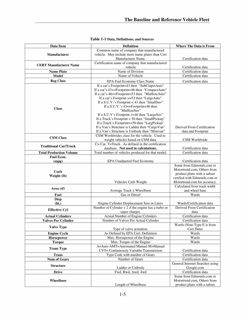
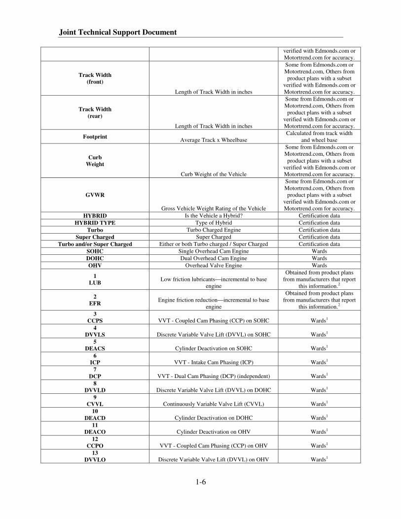
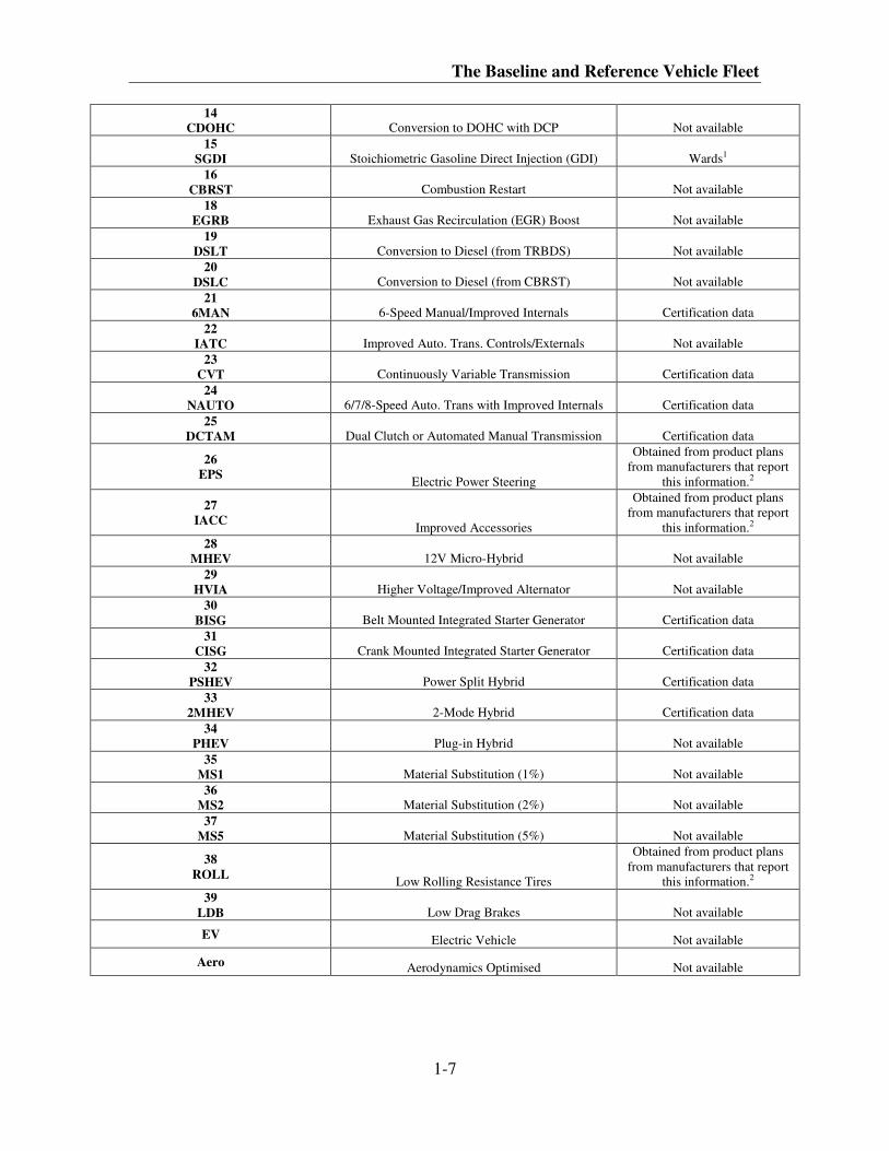
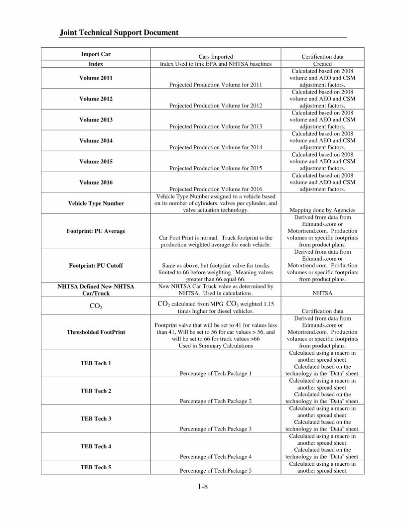
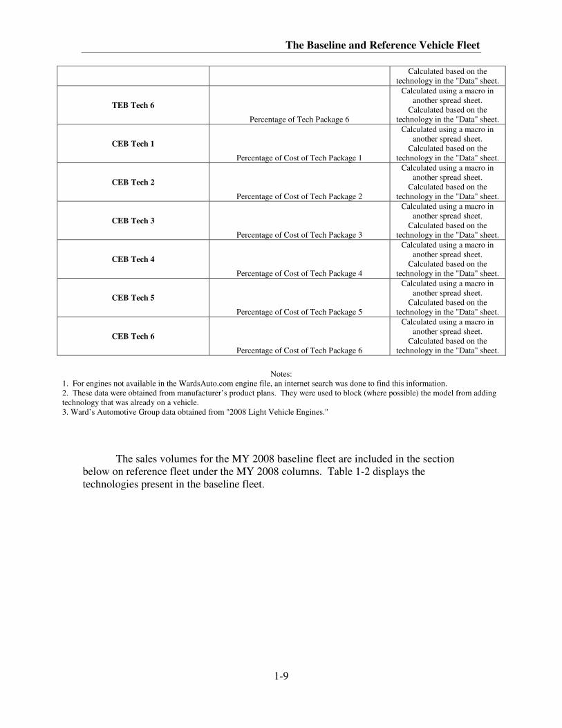
Table 1-1 below shows the columns of the complete fleet file, which includes the
2008 MY baseline data that was compiled. Each column has its name, definition
(description) and source. The EV and Aero columns were added to the fleet file to more
accurately describe vehicles for the final rule. The data that is marked “not available” is
data NHTSA would normally get from product plans. As mentioned above, some of the
desired model inputs, such as the presence of low rolling resistance tires, reduced engine
friction, improved accessories, etc., are not available from public sources and the
agencies had to rely on manufacturers’ confidential product plans. The Technology
Effectiveness Basis and the Cost Effectiveness Basis values reflect the percent of a
technology package’s effectiveness and cost present in the baseline fleet, and they are
described in further detail in chapters 3.1 and 3.5, respectively. Those technologies that
are not accounted for in the baseline—that is, the ones marked “not available”—run the
risk of getting double counted by the agencies’ models, but those effects are expected to
be small.
The Baseline and Reference Vehicle Fleet
1-5
Table 1-1 Data, Definitions, and Sources
Data Item Definition Where The Data is From
Manufacturer
Common name of company that manufactured
vehicle. May include more name plates than Cert
Manufacturer Name. Certification data
CERT Manufacturer Name Certification name of company that manufactured
vehicle Certification data
Name Plate Name of Division Certification data
Model Name of Vehicle Certification data
Reg Class EPA Fuel Economy Class Name Certification data
Class
If a car’s Footprint<43 then "SubCmpctAuto"
If a car’s 43<=Footprint<46 then "CompactAuto"
If a car’s 46<=Footprint<53 then "MidSizeAuto”
If a car’s Footprint >=53 then “LargeAuto”
If a S.U.V.’s Footprint < 43 then “SmallSuv”
If a S.U.V.’s 43<=Footprint<46 then
"MidSizeSuv”
If a S.U.V’s Footprint >=46 then “LargeSuv”
If a Truck’s Footprint < 50 then “SmallPickup”
If a Truck’s Footprint>=50 then “LargPickup”
If a Van’s Structure is Ladder then “CargoVan”
If a Van’s Structure is Unibody then “Minivan”
Derived From Certification
data and Footprint
CSM Class CSM Worldwides class for the vehicle. Used to
weight vehicles based on CSM data. CSM Worldwide
Traditional Car/Truck C= Car, T=Truck. As defined in the certification
database. Not used in calculations. Certification data
Total Production Volume Total number of vehicles produced for that model. Certification data
Fuel Econ.
(mpg) EPA Unadjusted Fuel Economy Certification data
Curb
Weight (lb)
Vehicles Curb Weight
Some from Edmonds.com or
Motortrend.com, Others from
product plans with a subset
verified with Edmonds.com or
Motortrend.com for accuracy.
Area (sf) Average Track x Wheelbase
Calculated from track width
and wheel base
Fuel Gas or Diesel Wards
Disp
(lit.) Engine Cylinder Displacement Size in Liters Wards/Certification data
Effective Cyl Number of Cylinder + 2 if the engine has a turbo or
super charger.
Derived From Certification
data.
Actual Cylinders Actual Number of Engine Cylinders Certification data
Valves Per Cylinder Number of Valves Per Actual Cylinder Certification data
Valve Type Type of valve actuation.
Wards (Note:Type E is from
Cert Data)
Engine Cycle As Defined by EPA Cert. Definition Wards
Horsepower Max. Horsepower of the Engine Wards
Torque Max. Torque of the Engine Wards
Trans Type A=Auto AMT=Automated Manual M=Manual
CVT= Continuously Variable Transmission Certification data
Trans Type Code with number of Gears Certification data
Num of Gears Number of Gears Certification data
Structure Ladder or Unibody
General Internet Searches using
Google.com
Drive Fwd, Rwd, Awd, 4wd Certification data
Wheelbase
Length of Wheelbase
Some from Edmonds.com or
Motortrend.com, Others from
product plans with a subset
Joint Technical Support Document
1-6
verified with Edmonds.com or
Motortrend.com for accuracy.
Track Width
(front)
Length of Track Width in inches
Some from Edmonds.com or
Motortrend.com, Others from
product plans with a subset
verified with Edmonds.com or
Motortrend.com for accuracy.
Track Width
(rear)
Length of Track Width in inches
Some from Edmonds.com or
Motortrend.com, Others from
product plans with a subset
verified with Edmonds.com or
Motortrend.com for accuracy.
Footprint Average Track x Wheelbase
Calculated from track width
and wheel base
Curb
Weight
Curb Weight of the Vehicle
Some from Edmonds.com or
Motortrend.com, Others from
product plans with a subset
verified with Edmonds.com or
Motortrend.com for accuracy.
GVWR
Gross Vehicle Weight Rating of the Vehicle
Some from Edmonds.com or
Motortrend.com, Others from
product plans with a subset
verified with Edmonds.com or
Motortrend.com for accuracy.
HYBRID Is the Vehicle a Hybrid? Certification data
HYBRID TYPE Type of Hybrid Certification data
Turbo Turbo Charged Engine Certification data
Super Charged Super Charged Certification data
Turbo and/or Super Charged Either or both Turbo charged / Super Charged Certification data
SOHC Single Overhead Cam Engine Wards
DOHC Dual Overhead Cam Engine Wards
OHV Overhead Valve Engine Wards
1
LUB Low friction lubricants—incremental to base
engine
Obtained from product plans
from manufacturers that report
this information.2
2
EFR Engine friction reduction—incremental to base
engine
Obtained from product plans
from manufacturers that report
this information.2
3
CCPS VVT - Coupled Cam Phasing (CCP) on SOHC Wards1
4
DVVLS Discrete Variable Valve Lift (DVVL) on SOHC Wards1
5
DEACS Cylinder Deactivation on SOHC Wards1
6
ICP VVT - Intake Cam Phasing (ICP) Wards1
7
DCP VVT - Dual Cam Phasing (DCP) (independent) Wards1
8
DVVLD Discrete Variable Valve Lift (DVVL) on DOHC Wards1
9
CVVL Continuously Variable Valve Lift (CVVL) Wards1
10
DEACD Cylinder Deactivation on DOHC Wards1
11
DEACO Cylinder Deactivation on OHV Wards1
12
CCPO VVT - Coupled Cam Phasing (CCP) on OHV Wards1
13
DVVLO Discrete Variable Valve Lift (DVVL) on OHV Wards1
The Baseline and Reference Vehicle Fleet
1-7
14
CDOHC Conversion to DOHC with DCP Not available
15
SGDI Stoichiometric Gasoline Direct Injection (GDI) Wards1
16
CBRST Combustion Restart Not available
18
EGRB Exhaust Gas Recirculation (EGR) Boost Not available
19
DSLT Conversion to Diesel (from TRBDS) Not available
20
DSLC Conversion to Diesel (from CBRST) Not available
21
6MAN 6-Speed Manual/Improved Internals Certification data
22
IATC Improved Auto. Trans. Controls/Externals Not available
23
CVT Continuously Variable Transmission Certification data
24
NAUTO 6/7/8-Speed Auto. Trans with Improved Internals Certification data
25
DCTAM Dual Clutch or Automated Manual Transmission Certification data
26
EPS Electric Power Steering
Obtained from product plans
from manufacturers that report
this information.2
27
IACC Improved Accessories
Obtained from product plans
from manufacturers that report
this information.2
28
MHEV 12V Micro-Hybrid Not available
29
HVIA Higher Voltage/Improved Alternator Not available
30
BISG Belt Mounted Integrated Starter Generator Certification data
31
CISG Crank Mounted Integrated Starter Generator Certification data
32
PSHEV Power Split Hybrid Certification data
33
2MHEV 2-Mode Hybrid Certification data
34
PHEV Plug-in Hybrid Not available
35
MS1 Material Substitution (1%) Not available
36
MS2 Material Substitution (2%) Not available
37
MS5 Material Substitution (5%) Not available
38
ROLL Low Rolling Resistance Tires
Obtained from product plans
from manufacturers that report
this information.2
39
LDB Low Drag Brakes Not available
EV Electric Vehicle Not available
Aero Aerodynamics Optimised Not available
Joint Technical Support Document
1-8
Import Car Cars Imported Certification data
Index Index Used to link EPA and NHTSA baselines Created
Volume 2011
Projected Production Volume for 2011
Calculated based on 2008
volume and AEO and CSM
adjustment factors.
Volume 2012
Projected Production Volume for 2012
Calculated based on 2008
volume and AEO and CSM
adjustment factors.
Volume 2013
Projected Production Volume for 2013
Calculated based on 2008
volume and AEO and CSM
adjustment factors.
Volume 2014
Projected Production Volume for 2014
Calculated based on 2008
volume and AEO and CSM
adjustment factors.
Volume 2015
Projected Production Volume for 2015
Calculated based on 2008
volume and AEO and CSM
adjustment factors.
Volume 2016
Projected Production Volume for 2016
Calculated based on 2008
volume and AEO and CSM
adjustment factors.
Vehicle Type Number
Vehicle Type Number assigned to a vehicle based
on its number of cylinders, valves per cylinder, and
valve actuation technology. Mapping done by Agencies
Footprint: PU Average
Car Foot Print is normal. Truck footprint is the
production weighted average for each vehicle.
Derived from data from
Edmunds.com or
Motortrend.com. Production
volumes or specific footprints
from product plans.
Footprint: PU Cutoff Same as above, but footprint valve for trucks
limited to 66 before weighting. Meaning valves
greater than 66 equal 66.
Derived from data from
Edmunds.com or
Motortrend.com. Production
volumes or specific footprints
from product plans.
NHTSA Defined New NHTSA
Car/Truck
New NHTSA Car Truck value as determined by
NHTSA. Used in calculations. NHTSA
CO2 CO2 calculated from MPG. CO2 weighted 1.15
times higher for diesel vehicles. Certification data
Thresholded FootPrint
Footprint valve that will be set to 41 for values less
than 41, Will be set to 56 for car values > 56, and
will be set to 66 for truck values >66
Used in Summary Calculations
Derived from data from
Edmunds.com or
Motortrend.com. Production
volumes or specific footprints
from product plans.
TEB Tech 1
Percentage of Tech Package 1
Calculated using a macro in
another spread sheet.
Calculated based on the
technology in the "Data" sheet.
TEB Tech 2
Percentage of Tech Package 2
Calculated using a macro in
another spread sheet.
Calculated based on the
technology in the "Data" sheet.
TEB Tech 3
Percentage of Tech Package 3
Calculated using a macro in
another spread sheet.
Calculated based on the
technology in the "Data" sheet.
TEB Tech 4
Percentage of Tech Package 4
Calculated using a macro in
another spread sheet.
Calculated based on the
technology in the "Data" sheet.
TEB Tech 5 Percentage of Tech Package 5
Calculated using a macro in
another spread sheet.
The Baseline and Reference Vehicle Fleet
1-9
Calculated based on the
technology in the "Data" sheet.
TEB Tech 6
Percentage of Tech Package 6
Calculated using a macro in
another spread sheet.
Calculated based on the
technology in the "Data" sheet.
CEB Tech 1
Percentage of Cost of Tech Package 1
Calculated using a macro in
another spread sheet.
Calculated based on the
technology in the "Data" sheet.
CEB Tech 2
Percentage of Cost of Tech Package 2
Calculated using a macro in
another spread sheet.
Calculated based on the
technology in the "Data" sheet.
CEB Tech 3
Percentage of Cost of Tech Package 3
Calculated using a macro in
another spread sheet.
Calculated based on the
technology in the "Data" sheet.
CEB Tech 4
Percentage of Cost of Tech Package 4
Calculated using a macro in
another spread sheet.
Calculated based on the
technology in the "Data" sheet.
CEB Tech 5
Percentage of Cost of Tech Package 5
Calculated using a macro in
another spread sheet.
Calculated based on the
technology in the "Data" sheet.
CEB Tech 6
Percentage of Cost of Tech Package 6
Calculated using a macro in
another spread sheet.
Calculated based on the
technology in the "Data" sheet.
Notes:
1. For engines not available in the WardsAuto.com engine file, an internet search was done to find this information.
2. These data were obtained from manufacturer’s product plans. They were used to block (where possible) the model from adding
technology that was already on a vehicle.
3. Ward’s Automotive Group data obtained from "2008 Light Vehicle Engines."
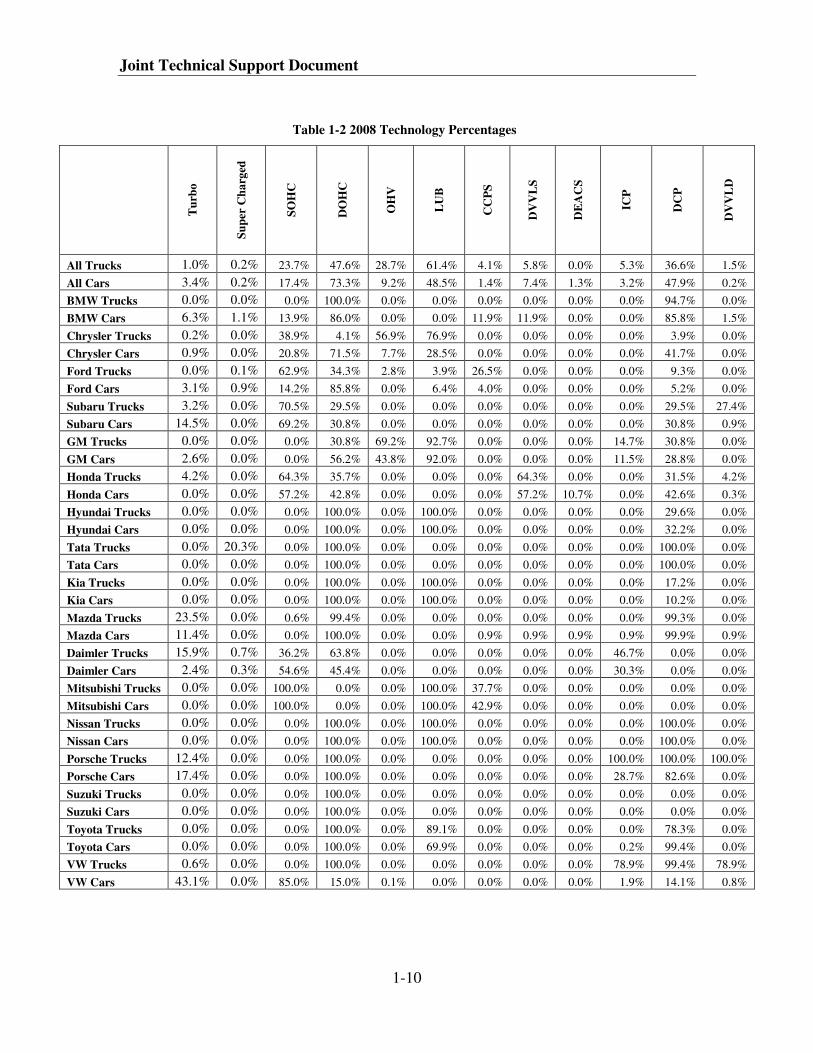
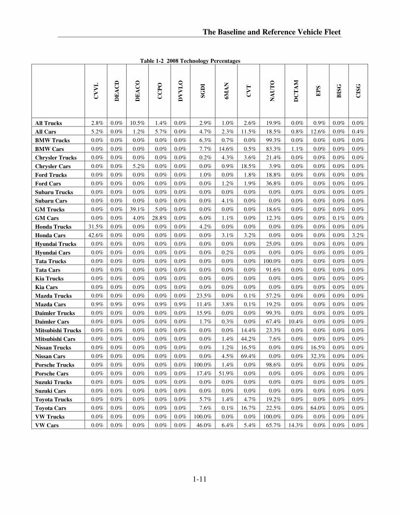
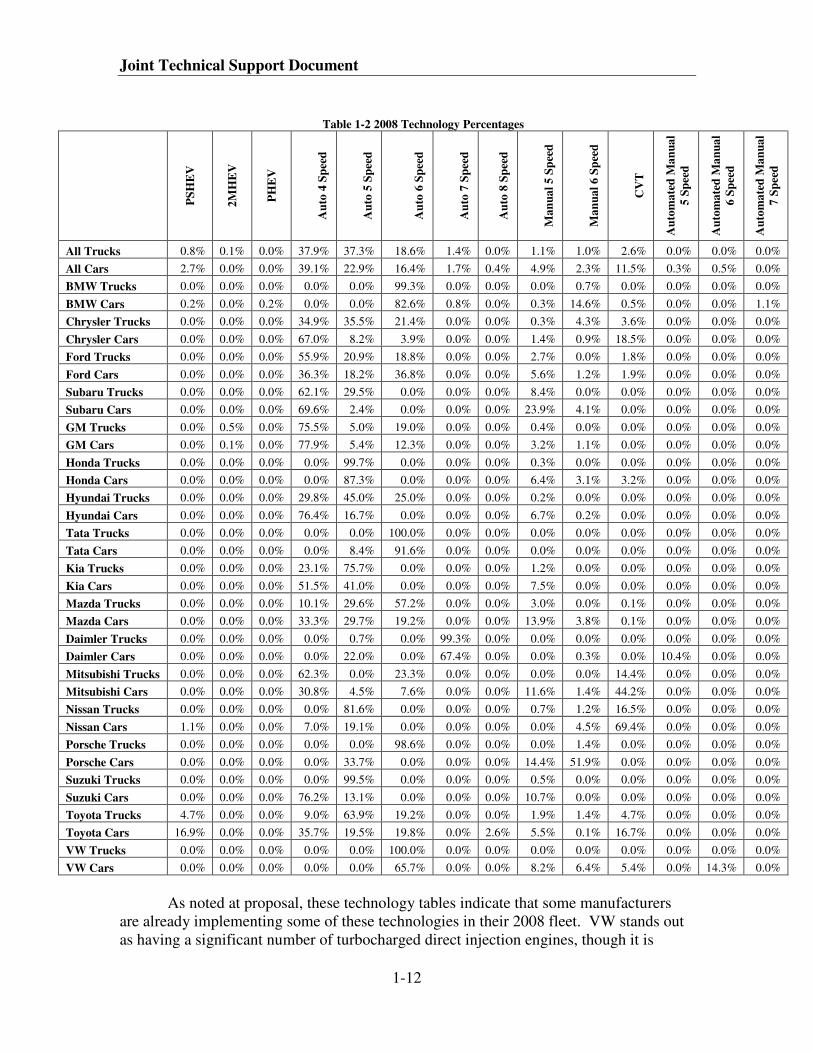
The sales volumes for the MY 2008 baseline fleet are included in the section
below on reference fleet under the MY 2008 columns. Table 1-2 displays the
technologies present in the baseline fleet.
Joint Technical Support Document
1-10
Table 1-2 2008 Technology Percentages
Tu
rbo
Su
per
Ch
arg
ed
SO
HC
DO
HC
OH
V
LU
B
CC
PS
DV
VL
S
DE
AC
S
ICP
DC
P
DV
VL
D
All Trucks 1.0% 0.2% 23.7% 47.6% 28.7% 61.4% 4.1% 5.8% 0.0% 5.3% 36.6% 1.5%
All Cars 3.4% 0.2% 17.4% 73.3% 9.2% 48.5% 1.4% 7.4% 1.3% 3.2% 47.9% 0.2%
BMW Trucks 0.0% 0.0% 0.0% 100.0% 0.0% 0.0% 0.0% 0.0% 0.0% 0.0% 94.7% 0.0%
BMW Cars 6.3% 1.1% 13.9% 86.0% 0.0% 0.0% 11.9% 11.9% 0.0% 0.0% 85.8% 1.5%
Chrysler Trucks 0.2% 0.0% 38.9% 4.1% 56.9% 76.9% 0.0% 0.0% 0.0% 0.0% 3.9% 0.0%
Chrysler Cars 0.9% 0.0% 20.8% 71.5% 7.7% 28.5% 0.0% 0.0% 0.0% 0.0% 41.7% 0.0%
Ford Trucks 0.0% 0.1% 62.9% 34.3% 2.8% 3.9% 26.5% 0.0% 0.0% 0.0% 9.3% 0.0%
Ford Cars 3.1% 0.9% 14.2% 85.8% 0.0% 6.4% 4.0% 0.0% 0.0% 0.0% 5.2% 0.0%
Subaru Trucks 3.2% 0.0% 70.5% 29.5% 0.0% 0.0% 0.0% 0.0% 0.0% 0.0% 29.5% 27.4%
Subaru Cars 14.5% 0.0% 69.2% 30.8% 0.0% 0.0% 0.0% 0.0% 0.0% 0.0% 30.8% 0.9%
GM Trucks 0.0% 0.0% 0.0% 30.8% 69.2% 92.7% 0.0% 0.0% 0.0% 14.7% 30.8% 0.0%
GM Cars 2.6% 0.0% 0.0% 56.2% 43.8% 92.0% 0.0% 0.0% 0.0% 11.5% 28.8% 0.0%
Honda Trucks 4.2% 0.0% 64.3% 35.7% 0.0% 0.0% 0.0% 64.3% 0.0% 0.0% 31.5% 4.2%
Honda Cars 0.0% 0.0% 57.2% 42.8% 0.0% 0.0% 0.0% 57.2% 10.7% 0.0% 42.6% 0.3%
Hyundai Trucks 0.0% 0.0% 0.0% 100.0% 0.0% 100.0% 0.0% 0.0% 0.0% 0.0% 29.6% 0.0%
Hyundai Cars 0.0% 0.0% 0.0% 100.0% 0.0% 100.0% 0.0% 0.0% 0.0% 0.0% 32.2% 0.0%
Tata Trucks 0.0% 20.3% 0.0% 100.0% 0.0% 0.0% 0.0% 0.0% 0.0% 0.0% 100.0% 0.0%
Tata Cars 0.0% 0.0% 0.0% 100.0% 0.0% 0.0% 0.0% 0.0% 0.0% 0.0% 100.0% 0.0%
Kia Trucks 0.0% 0.0% 0.0% 100.0% 0.0% 100.0% 0.0% 0.0% 0.0% 0.0% 17.2% 0.0%
Kia Cars 0.0% 0.0% 0.0% 100.0% 0.0% 100.0% 0.0% 0.0% 0.0% 0.0% 10.2% 0.0%
Mazda Trucks 23.5% 0.0% 0.6% 99.4% 0.0% 0.0% 0.0% 0.0% 0.0% 0.0% 99.3% 0.0%
Mazda Cars 11.4% 0.0% 0.0% 100.0% 0.0% 0.0% 0.9% 0.9% 0.9% 0.9% 99.9% 0.9%
Daimler Trucks 15.9% 0.7% 36.2% 63.8% 0.0% 0.0% 0.0% 0.0% 0.0% 46.7% 0.0% 0.0%
Daimler Cars 2.4% 0.3% 54.6% 45.4% 0.0% 0.0% 0.0% 0.0% 0.0% 30.3% 0.0% 0.0%
Mitsubishi Trucks 0.0% 0.0% 100.0% 0.0% 0.0% 100.0% 37.7% 0.0% 0.0% 0.0% 0.0% 0.0%
Mitsubishi Cars 0.0% 0.0% 100.0% 0.0% 0.0% 100.0% 42.9% 0.0% 0.0% 0.0% 0.0% 0.0%
Nissan Trucks 0.0% 0.0% 0.0% 100.0% 0.0% 100.0% 0.0% 0.0% 0.0% 0.0% 100.0% 0.0%
Nissan Cars 0.0% 0.0% 0.0% 100.0% 0.0% 100.0% 0.0% 0.0% 0.0% 0.0% 100.0% 0.0%
Porsche Trucks 12.4% 0.0% 0.0% 100.0% 0.0% 0.0% 0.0% 0.0% 0.0% 100.0% 100.0% 100.0%
Porsche Cars 17.4% 0.0% 0.0% 100.0% 0.0% 0.0% 0.0% 0.0% 0.0% 28.7% 82.6% 0.0%
Suzuki Trucks 0.0% 0.0% 0.0% 100.0% 0.0% 0.0% 0.0% 0.0% 0.0% 0.0% 0.0% 0.0%
Suzuki Cars 0.0% 0.0% 0.0% 100.0% 0.0% 0.0% 0.0% 0.0% 0.0% 0.0% 0.0% 0.0%
Toyota Trucks 0.0% 0.0% 0.0% 100.0% 0.0% 89.1% 0.0% 0.0% 0.0% 0.0% 78.3% 0.0%
Toyota Cars 0.0% 0.0% 0.0% 100.0% 0.0% 69.9% 0.0% 0.0% 0.0% 0.2% 99.4% 0.0%
VW Trucks 0.6% 0.0% 0.0% 100.0% 0.0% 0.0% 0.0% 0.0% 0.0% 78.9% 99.4% 78.9%
VW Cars 43.1% 0.0% 85.0% 15.0% 0.1% 0.0% 0.0% 0.0% 0.0% 1.9% 14.1% 0.8%
The Baseline and Reference Vehicle Fleet
1-11
Table 1-2 2008 Technology Percentages
CV
VL
DE
AC
D
DE
AC
O
CC
PO
DV
VL
O
SG
DI
6M
AN
CV
T
NA
UT
O
DC
TA
M
EP
S
BIS
G
CIS
G
All Trucks 2.8% 0.0% 10.5% 1.4% 0.0% 2.9% 1.0% 2.6% 19.9% 0.0% 0.9% 0.0% 0.0%
All Cars 5.2% 0.0% 1.2% 5.7% 0.0% 4.7% 2.3% 11.5% 18.5% 0.8% 12.6% 0.0% 0.4%
BMW Trucks 0.0% 0.0% 0.0% 0.0% 0.0% 6.3% 0.7% 0.0% 99.3% 0.0% 0.0% 0.0% 0.0%
BMW Cars 0.0% 0.0% 0.0% 0.0% 0.0% 7.7% 14.6% 0.5% 83.3% 1.1% 0.0% 0.0% 0.0%
Chrysler Trucks 0.0% 0.0% 0.0% 0.0% 0.0% 0.2% 4.3% 3.6% 21.4% 0.0% 0.0% 0.0% 0.0%
Chrysler Cars 0.0% 0.0% 5.2% 0.0% 0.0% 0.0% 0.9% 18.5% 3.9% 0.0% 0.0% 0.0% 0.0%
Ford Trucks 0.0% 0.0% 0.0% 0.0% 0.0% 1.0% 0.0% 1.8% 18.8% 0.0% 0.0% 0.0% 0.0%
Ford Cars 0.0% 0.0% 0.0% 0.0% 0.0% 0.0% 1.2% 1.9% 36.8% 0.0% 0.0% 0.0% 0.0%
Subaru Trucks 0.0% 0.0% 0.0% 0.0% 0.0% 0.0% 0.0% 0.0% 0.0% 0.0% 0.0% 0.0% 0.0%
Subaru Cars 0.0% 0.0% 0.0% 0.0% 0.0% 0.0% 4.1% 0.0% 0.0% 0.0% 0.0% 0.0% 0.0%
GM Trucks 0.0% 0.0% 39.1% 5.0% 0.0% 0.0% 0.0% 0.0% 18.6% 0.0% 0.0% 0.0% 0.0%
GM Cars 0.0% 0.0% 4.0% 28.8% 0.0% 6.0% 1.1% 0.0% 12.3% 0.0% 0.0% 0.1% 0.0%
Honda Trucks 31.5% 0.0% 0.0% 0.0% 0.0% 4.2% 0.0% 0.0% 0.0% 0.0% 0.0% 0.0% 0.0%
Honda Cars 42.6% 0.0% 0.0% 0.0% 0.0% 0.0% 3.1% 3.2% 0.0% 0.0% 0.0% 0.0% 3.2%
Hyundai Trucks 0.0% 0.0% 0.0% 0.0% 0.0% 0.0% 0.0% 0.0% 25.0% 0.0% 0.0% 0.0% 0.0%
Hyundai Cars 0.0% 0.0% 0.0% 0.0% 0.0% 0.0% 0.2% 0.0% 0.0% 0.0% 0.0% 0.0% 0.0%
Tata Trucks 0.0% 0.0% 0.0% 0.0% 0.0% 0.0% 0.0% 0.0% 100.0% 0.0% 0.0% 0.0% 0.0%
Tata Cars 0.0% 0.0% 0.0% 0.0% 0.0% 0.0% 0.0% 0.0% 91.6% 0.0% 0.0% 0.0% 0.0%
Kia Trucks 0.0% 0.0% 0.0% 0.0% 0.0% 0.0% 0.0% 0.0% 0.0% 0.0% 0.0% 0.0% 0.0%
Kia Cars 0.0% 0.0% 0.0% 0.0% 0.0% 0.0% 0.0% 0.0% 0.0% 0.0% 0.0% 0.0% 0.0%
Mazda Trucks 0.0% 0.0% 0.0% 0.0% 0.0% 23.5% 0.0% 0.1% 57.2% 0.0% 0.0% 0.0% 0.0%
Mazda Cars 0.9% 0.9% 0.9% 0.9% 0.9% 11.4% 3.8% 0.1% 19.2% 0.0% 0.0% 0.0% 0.0%
Daimler Trucks 0.0% 0.0% 0.0% 0.0% 0.0% 15.9% 0.0% 0.0% 99.3% 0.0% 0.0% 0.0% 0.0%
Daimler Cars 0.0% 0.0% 0.0% 0.0% 0.0% 1.7% 0.3% 0.0% 67.4% 10.4% 0.0% 0.0% 0.0%
Mitsubishi Trucks 0.0% 0.0% 0.0% 0.0% 0.0% 0.0% 0.0% 14.4% 23.3% 0.0% 0.0% 0.0% 0.0%
Mitsubishi Cars 0.0% 0.0% 0.0% 0.0% 0.0% 0.0% 1.4% 44.2% 7.6% 0.0% 0.0% 0.0% 0.0%
Nissan Trucks 0.0% 0.0% 0.0% 0.0% 0.0% 0.0% 1.2% 16.5% 0.0% 0.0% 16.5% 0.0% 0.0%
Nissan Cars 0.0% 0.0% 0.0% 0.0% 0.0% 0.0% 4.5% 69.4% 0.0% 0.0% 32.3% 0.0% 0.0%
Porsche Trucks 0.0% 0.0% 0.0% 0.0% 0.0% 100.0% 1.4% 0.0% 98.6% 0.0% 0.0% 0.0% 0.0%
Porsche Cars 0.0% 0.0% 0.0% 0.0% 0.0% 17.4% 51.9% 0.0% 0.0% 0.0% 0.0% 0.0% 0.0%
Suzuki Trucks 0.0% 0.0% 0.0% 0.0% 0.0% 0.0% 0.0% 0.0% 0.0% 0.0% 0.0% 0.0% 0.0%
Suzuki Cars 0.0% 0.0% 0.0% 0.0% 0.0% 0.0% 0.0% 0.0% 0.0% 0.0% 0.0% 0.0% 0.0%
Toyota Trucks 0.0% 0.0% 0.0% 0.0% 0.0% 5.7% 1.4% 4.7% 19.2% 0.0% 0.0% 0.0% 0.0%
Toyota Cars 0.0% 0.0% 0.0% 0.0% 0.0% 7.6% 0.1% 16.7% 22.5% 0.0% 64.0% 0.0% 0.0%
VW Trucks 0.0% 0.0% 0.0% 0.0% 0.0% 100.0% 0.0% 0.0% 100.0% 0.0% 0.0% 0.0% 0.0%
VW Cars 0.0% 0.0% 0.0% 0.0% 0.0% 46.0% 6.4% 5.4% 65.7% 14.3% 0.0% 0.0% 0.0%
Joint Technical Support Document
1-12
Table 1-2 2008 Technology Percentages
PS
HE
V
2M
HE
V
PH
EV
Au
to 4
Sp
eed
Au
to 5
Sp
eed
Au
to 6
Sp
eed
Au
to 7
Sp
eed
Au
to 8
Sp
eed
Ma
nu
al
5 S
pee
d
Ma
nu
al
6 S
pee
d
CV
T
Au
tom
ate
d M
an
ua
l
5 S
pee
d
Au
tom
ate
d M
an
ua
l
6 S
pee
d
Au
tom
ate
d M
an
ua
l
7 S
pee
d
All Trucks 0.8% 0.1% 0.0% 37.9% 37.3% 18.6% 1.4% 0.0% 1.1% 1.0% 2.6% 0.0% 0.0% 0.0%
All Cars 2.7% 0.0% 0.0% 39.1% 22.9% 16.4% 1.7% 0.4% 4.9% 2.3% 11.5% 0.3% 0.5% 0.0%
BMW Trucks 0.0% 0.0% 0.0% 0.0% 0.0% 99.3% 0.0% 0.0% 0.0% 0.7% 0.0% 0.0% 0.0% 0.0%
BMW Cars 0.2% 0.0% 0.2% 0.0% 0.0% 82.6% 0.8% 0.0% 0.3% 14.6% 0.5% 0.0% 0.0% 1.1%
Chrysler Trucks 0.0% 0.0% 0.0% 34.9% 35.5% 21.4% 0.0% 0.0% 0.3% 4.3% 3.6% 0.0% 0.0% 0.0%
Chrysler Cars 0.0% 0.0% 0.0% 67.0% 8.2% 3.9% 0.0% 0.0% 1.4% 0.9% 18.5% 0.0% 0.0% 0.0%
Ford Trucks 0.0% 0.0% 0.0% 55.9% 20.9% 18.8% 0.0% 0.0% 2.7% 0.0% 1.8% 0.0% 0.0% 0.0%
Ford Cars 0.0% 0.0% 0.0% 36.3% 18.2% 36.8% 0.0% 0.0% 5.6% 1.2% 1.9% 0.0% 0.0% 0.0%
Subaru Trucks 0.0% 0.0% 0.0% 62.1% 29.5% 0.0% 0.0% 0.0% 8.4% 0.0% 0.0% 0.0% 0.0% 0.0%
Subaru Cars 0.0% 0.0% 0.0% 69.6% 2.4% 0.0% 0.0% 0.0% 23.9% 4.1% 0.0% 0.0% 0.0% 0.0%
GM Trucks 0.0% 0.5% 0.0% 75.5% 5.0% 19.0% 0.0% 0.0% 0.4% 0.0% 0.0% 0.0% 0.0% 0.0%
GM Cars 0.0% 0.1% 0.0% 77.9% 5.4% 12.3% 0.0% 0.0% 3.2% 1.1% 0.0% 0.0% 0.0% 0.0%
Honda Trucks 0.0% 0.0% 0.0% 0.0% 99.7% 0.0% 0.0% 0.0% 0.3% 0.0% 0.0% 0.0% 0.0% 0.0%
Honda Cars 0.0% 0.0% 0.0% 0.0% 87.3% 0.0% 0.0% 0.0% 6.4% 3.1% 3.2% 0.0% 0.0% 0.0%
Hyundai Trucks 0.0% 0.0% 0.0% 29.8% 45.0% 25.0% 0.0% 0.0% 0.2% 0.0% 0.0% 0.0% 0.0% 0.0%
Hyundai Cars 0.0% 0.0% 0.0% 76.4% 16.7% 0.0% 0.0% 0.0% 6.7% 0.2% 0.0% 0.0% 0.0% 0.0%
Tata Trucks 0.0% 0.0% 0.0% 0.0% 0.0% 100.0% 0.0% 0.0% 0.0% 0.0% 0.0% 0.0% 0.0% 0.0%
Tata Cars 0.0% 0.0% 0.0% 0.0% 8.4% 91.6% 0.0% 0.0% 0.0% 0.0% 0.0% 0.0% 0.0% 0.0%
Kia Trucks 0.0% 0.0% 0.0% 23.1% 75.7% 0.0% 0.0% 0.0% 1.2% 0.0% 0.0% 0.0% 0.0% 0.0%
Kia Cars 0.0% 0.0% 0.0% 51.5% 41.0% 0.0% 0.0% 0.0% 7.5% 0.0% 0.0% 0.0% 0.0% 0.0%
Mazda Trucks 0.0% 0.0% 0.0% 10.1% 29.6% 57.2% 0.0% 0.0% 3.0% 0.0% 0.1% 0.0% 0.0% 0.0%
Mazda Cars 0.0% 0.0% 0.0% 33.3% 29.7% 19.2% 0.0% 0.0% 13.9% 3.8% 0.1% 0.0% 0.0% 0.0%
Daimler Trucks 0.0% 0.0% 0.0% 0.0% 0.7% 0.0% 99.3% 0.0% 0.0% 0.0% 0.0% 0.0% 0.0% 0.0%
Daimler Cars 0.0% 0.0% 0.0% 0.0% 22.0% 0.0% 67.4% 0.0% 0.0% 0.3% 0.0% 10.4% 0.0% 0.0%
Mitsubishi Trucks 0.0% 0.0% 0.0% 62.3% 0.0% 23.3% 0.0% 0.0% 0.0% 0.0% 14.4% 0.0% 0.0% 0.0%
Mitsubishi Cars 0.0% 0.0% 0.0% 30.8% 4.5% 7.6% 0.0% 0.0% 11.6% 1.4% 44.2% 0.0% 0.0% 0.0%
Nissan Trucks 0.0% 0.0% 0.0% 0.0% 81.6% 0.0% 0.0% 0.0% 0.7% 1.2% 16.5% 0.0% 0.0% 0.0%
Nissan Cars 1.1% 0.0% 0.0% 7.0% 19.1% 0.0% 0.0% 0.0% 0.0% 4.5% 69.4% 0.0% 0.0% 0.0%
Porsche Trucks 0.0% 0.0% 0.0% 0.0% 0.0% 98.6% 0.0% 0.0% 0.0% 1.4% 0.0% 0.0% 0.0% 0.0%
Porsche Cars 0.0% 0.0% 0.0% 0.0% 33.7% 0.0% 0.0% 0.0% 14.4% 51.9% 0.0% 0.0% 0.0% 0.0%
Suzuki Trucks 0.0% 0.0% 0.0% 0.0% 99.5% 0.0% 0.0% 0.0% 0.5% 0.0% 0.0% 0.0% 0.0% 0.0%
Suzuki Cars 0.0% 0.0% 0.0% 76.2% 13.1% 0.0% 0.0% 0.0% 10.7% 0.0% 0.0% 0.0% 0.0% 0.0%
Toyota Trucks 4.7% 0.0% 0.0% 9.0% 63.9% 19.2% 0.0% 0.0% 1.9% 1.4% 4.7% 0.0% 0.0% 0.0%
Toyota Cars 16.9% 0.0% 0.0% 35.7% 19.5% 19.8% 0.0% 2.6% 5.5% 0.1% 16.7% 0.0% 0.0% 0.0%
VW Trucks 0.0% 0.0% 0.0% 0.0% 0.0% 100.0% 0.0% 0.0% 0.0% 0.0% 0.0% 0.0% 0.0% 0.0%
VW Cars 0.0% 0.0% 0.0% 0.0% 0.0% 65.7% 0.0% 0.0% 8.2% 6.4% 5.4% 0.0% 14.3% 0.0%
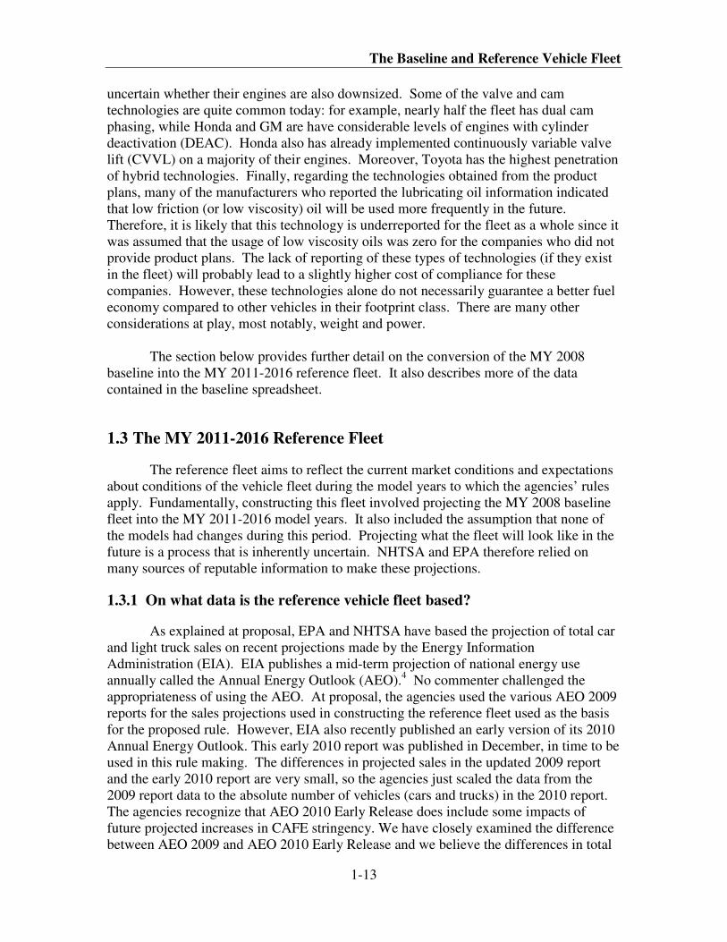
As noted at proposal, these technology tables indicate that some manufacturers
are already implementing some of these technologies in their 2008 fleet. VW stands out
as having a significant number of turbocharged direct injection engines, though it is
The Baseline and Reference Vehicle Fleet
1-13
uncertain whether their engines are also downsized. Some of the valve and cam
technologies are quite common today: for example, nearly half the fleet has dual cam
phasing, while Honda and GM are have considerable levels of engines with cylinder
deactivation (DEAC). Honda also has already implemented continuously variable valve
lift (CVVL) on a majority of their engines. Moreover, Toyota has the highest penetration
of hybrid technologies. Finally, regarding the technologies obtained from the product
plans, many of the manufacturers who reported the lubricating oil information indicated
that low friction (or low viscosity) oil will be used more frequently in the future.
Therefore, it is likely that this technology is underreported for the fleet as a whole since it
was assumed that the usage of low viscosity oils was zero for the companies who did not
provide product plans. The lack of reporting of these types of technologies (if they exist
in the fleet) will probably lead to a slightly higher cost of compliance for these
companies. However, these technologies alone do not necessarily guarantee a better fuel
economy compared to other vehicles in their footprint class. There are many other
considerations at play, most notably, weight and power.
The section below provides further detail on the conversion of the MY 2008
baseline into the MY 2011-2016 reference fleet. It also describes more of the data
contained in the baseline spreadsheet.
1.3 The MY 2011-2016 Reference Fleet
The reference fleet aims to reflect the current market conditions and expectations
about conditions of the vehicle fleet during the model years to which the agencies’ rules
apply. Fundamentally, constructing this fleet involved projecting the MY 2008 baseline
fleet into the MY 2011-2016 model years. It also included the assumption that none of
the models had changes during this period. Projecting what the fleet will look like in the
future is a process that is inherently uncertain. NHTSA and EPA therefore relied on
many sources of reputable information to make these projections.
1.3.1 On what data is the reference vehicle fleet based?
As explained at proposal, EPA and NHTSA have based the projection of total car
and light truck sales on recent projections made by the Energy Information
Administration (EIA). EIA publishes a mid-term projection of national energy use
annually called the Annual Energy Outlook (AEO).4 No commenter challenged the
appropriateness of using the AEO. At proposal, the agencies used the various AEO 2009
reports for the sales projections used in constructing the reference fleet used as the basis
for the proposed rule. However, EIA also recently published an early version of its 2010
Annual Energy Outlook. This early 2010 report was published in December, in time to be
used in this rule making. The differences in projected sales in the updated 2009 report
and the early 2010 report are very small, so the agencies just scaled the data from the
2009 report data to the absolute number of vehicles (cars and trucks) in the 2010 report.
The agencies recognize that AEO 2010 Early Release does include some impacts of
future projected increases in CAFE stringency. We have closely examined the difference
between AEO 2009 and AEO 2010 Early Release and we believe the differences in total
Joint Technical Support Document
1-14
sales and the car/truck split attributed to considerations of the standard in the final rule
are small. 5
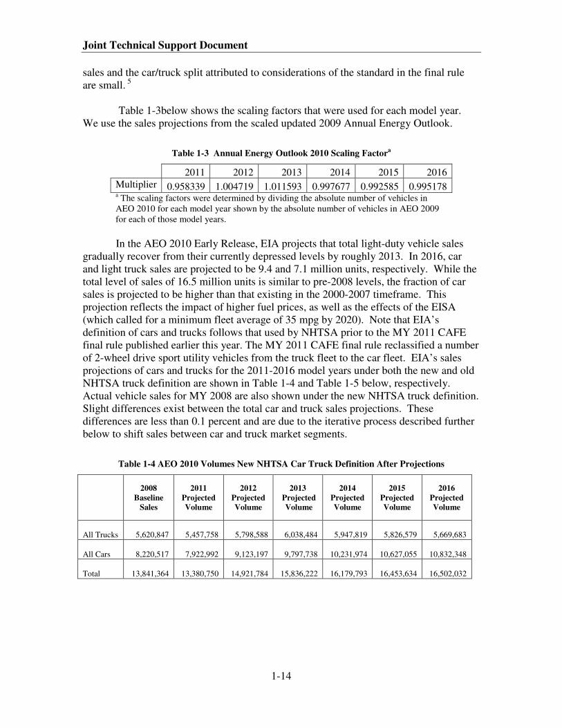
Table 1-3below shows the scaling factors that were used for each model year.
We use the sales projections from the scaled updated 2009 Annual Energy Outlook.
Table 1-3 Annual Energy Outlook 2010 Scaling Factora
2011 2012 2013 2014 2015 2016
Multiplier 0.958339 1.004719 1.011593 0.997677 0.992585 0.995178 a The scaling factors were determined by dividing the absolute number of vehicles in
AEO 2010 for each model year shown by the absolute number of vehicles in AEO 2009
for each of those model years.
In the AEO 2010 Early Release, EIA projects that total light-duty vehicle sales
gradually recover from their currently depressed levels by roughly 2013. In 2016, car
and light truck sales are projected to be 9.4 and 7.1 million units, respectively. While the
total level of sales of 16.5 million units is similar to pre-2008 levels, the fraction of car
sales is projected to be higher than that existing in the 2000-2007 timeframe. This
projection reflects the impact of higher fuel prices, as well as the effects of the EISA
(which called for a minimum fleet average of 35 mpg by 2020). Note that EIA’s
definition of cars and trucks follows that used by NHTSA prior to the MY 2011 CAFE
final rule published earlier this year. The MY 2011 CAFE final rule reclassified a number
of 2-wheel drive sport utility vehicles from the truck fleet to the car fleet. EIA’s sales
projections of cars and trucks for the 2011-2016 model years under both the new and old
NHTSA truck definition are shown in Table 1-4 and Table 1-5 below, respectively.
Actual vehicle sales for MY 2008 are also shown under the new NHTSA truck definition.
Slight differences exist between the total car and truck sales projections. These
differences are less than 0.1 percent and are due to the iterative process described further
below to shift sales between car and truck market segments.
Table 1-4 AEO 2010 Volumes New NHTSA Car Truck Definition After Projections
2008
Baseline
Sales
2011
Projected
Volume
2012
Projected
Volume
2013
Projected
Volume
2014
Projected
Volume
2015
Projected
Volume
2016
Projected
Volume
All Trucks
5,620,847
5,457,758
5,798,588
6,038,484
5,947,819
5,826,579
5,669,683
All Cars
8,220,517
7,922,992
9,123,197
9,797,738
10,231,974
10,627,055
10,832,348
Total
13,841,364
13,380,750
14,921,784
15,836,222
16,179,793
16,453,634
16,502,032
The Baseline and Reference Vehicle Fleet
1-15
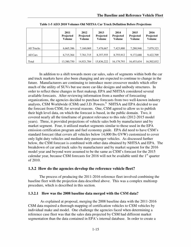
Table 1-5 AEO 2010 Volumes Old NHTSA Car Truck Definition Before Projections
2011
Projected
Volume
2012
Projected
Volume
2013
Projected
Volume
2014
Projected
Volume
2015
Projected
Volume
2016
Projected
Volume
All Trucks
6,665,386
7,160,069
7,478,667
7,423,880
7,280,946
7,079,323
All Cars
6,715,364
7,761,715
8,357,555
8,755,912
9,172,688
9,422,709
Total
13,380,750
14,921,784
15,836,222
16,179,793
16,453,634
16,502,032
In addition to a shift towards more car sales, sales of segments within both the car
and truck markets have also been changing and are expected to continue to change in the
future. Manufacturers are continuing to introduce more crossover models which offer
much of the utility of SUVs but use more car-like designs and unibody structures. In
order to reflect these changes in fleet makeup, EPA and NHTSA considered several
available forecasts. After reviewing information from a number of forecasting
organizations, the agencies decided to purchase forecasts from two well-known industry
analysts, CSM Worldwide (CSM) and J.D. Powers.6 NHTSA and EPA decided to use
the forecast from CSM, for several reasons. One, CSM agreed to allow us to publish
their high level data, on which the forecast is based, in the public domain. Two, it
covered nearly all the timeframe of greatest relevance to this rule (2012-2015 model
years). Three, it provided projections of vehicle sales both by manufacturer and by
market segment. Four, it utilized market segments similar to those used in the EPA
emission certification program and fuel economy guide. EPA did need to have CSM’s
standard forecast (that covers all vehicles below 14,000 lbs GVW) customized to cover
only light duty vehicles and medium duty passenger vehicles. As discussed further
below, the CSM forecast is combined with other data obtained by NHTSA and EPA. The
breakdown of car and truck sales by manufacturer and by market segment for the 2016
model year and beyond were assumed to be the same as CSM’s forecast for the 2015
calendar year, because CSM forecasts for 2016 will not be available until the 1st quarter
of 2010.
1.3.2 How do the agencies develop the reference vehicle fleet?
The process of producing the 2011-2016 reference fleet involved combining the
baseline fleet with the projection data described above. This was a complex multistep
procedure, which is described in this section.
1.3.2.1 How was the 2008 baseline data merged with the CSM data?
As explained at proposal, merging the 2008 baseline data with the 2011-2016
CSM data required a thorough mapping of certification vehicles to CSM vehicles by
individual make and model. One challenge the agencies faced when determining a
reference case fleet was that the sales data projected by CSM had different market
segmentation than the data contained in EPA’s internal database. In order to create a
Joint Technical Support Document
1-16
common segmentation between the two databases, side-by-side comparison of the
specific vehicle models in both datasets was performed, and an additional “CSM
segment” modifier in the spreadsheet was created, thus mapping the two datasets. The
reference fleet sales based on the “CSM segmentation” was then projected.
The baseline data and reference fleet volumes are available to the public. The
baseline Excel spreadsheet in the docket is the result of the merged files.7 It provides
specific details on the sources and definitions for the data. The Excel file contains
several tabs. They are: “Data”, “Data Tech Definitions”, “SUM”, “SUM Tech
Definitions”, “Truck Vehicle Type Map”, and “Car Vehicle Type Map”. “Data” is the
tab with the raw data. “Data Tech Definitions” is the tab where each column is defined
and its data source named. “SUM” is the tab where the raw data is processed to be used
in the OMEGA and Volpe models. The “SUM” tab minus columns A-F and minus the
Generic vehicles is the input file for the models. The “Generic” manufacturer (shown in
the “SUM” tab) is the sum of all manufacturers and is calculated as a reference, and for
data verification purposes. It is used to validate the manufacturers’ totals. It also gives
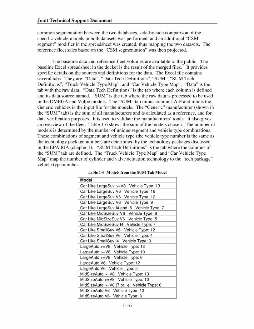
an overview of the fleet. Table 1-6 shows the sum of the models chosen. The number of
models is determined by the number of unique segment and vehicle type combinations.
These combinations of segment and vehicle type (the vehicle type number is the same as
the technology package number) are determined by the technology packages discussed
in.the EPA RIA (chapter 1). “SUM Tech Definitions” is the tab where the columns of
the “SUM” tab are defined. The “Truck Vehicle Type Map” and “Car Vehicle Type
Map” map the number of cylinder and valve actuation technology to the “tech package”
vehicle type number.
Table 1-6 Models from the SUM Tab Model
Model
Car Like LargeSuv >=V8 Vehicle Type: 13
Car Like LargeSuv V6 Vehicle Type: 16
Car Like LargeSuv V6 Vehicle Type: 12
Car Like LargeSuv V6 Vehicle Type: 9
Car Like LargeSuv I4 and I5 Vehicle Type: 7
Car Like MidSizeSuv V6 Vehicle Type: 8
Car Like MidSizeSuv V6 Vehicle Type: 5
Car Like MidSizeSuv I4 Vehicle Type: 7
Car Like SmallSuv V6 Vehicle Type: 12
Car Like SmallSuv V6 Vehicle Type: 4
Car Like SmallSuv I4 Vehicle Type: 3
LargeAuto >=V8 Vehicle Type: 13
LargeAuto >=V8 Vehicle Type: 10
LargeAuto >=V8 Vehicle Type: 6
LargeAuto V6 Vehicle Type: 12
LargeAuto V6 Vehicle Type: 5
MidSizeAuto >=V8 Vehicle Type: 13
MidSizeAuto >=V8 Vehicle Type: 10
MidSizeAuto >=V8 (7 or >) Vehicle Type: 6
MidSizeAuto V6 Vehicle Type: 12
MidSizeAuto V6 Vehicle Type: 8
The Baseline and Reference Vehicle Fleet
1-17
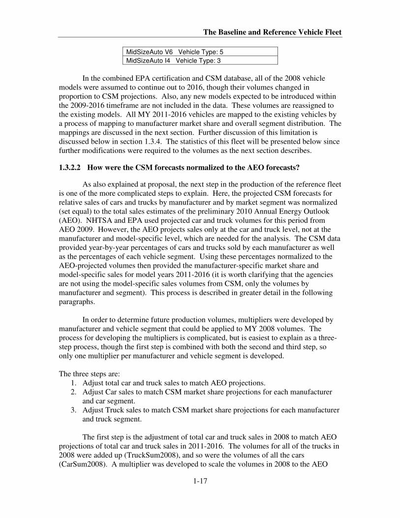
MidSizeAuto V6 Vehicle Type: 5
MidSizeAuto I4 Vehicle Type: 3
In the combined EPA certification and CSM database, all of the 2008 vehicle
models were assumed to continue out to 2016, though their volumes changed in
proportion to CSM projections. Also, any new models expected to be introduced within
the 2009-2016 timeframe are not included in the data. These volumes are reassigned to
the existing models. All MY 2011-2016 vehicles are mapped to the existing vehicles by
a process of mapping to manufacturer market share and overall segment distribution. The
mappings are discussed in the next section. Further discussion of this limitation is
discussed below in section 1.3.4. The statistics of this fleet will be presented below since
further modifications were required to the volumes as the next section describes.
1.3.2.2 How were the CSM forecasts normalized to the AEO forecasts?
As also explained at proposal, the next step in the production of the reference fleet
is one of the more complicated steps to explain. Here, the projected CSM forecasts for
relative sales of cars and trucks by manufacturer and by market segment was normalized
(set equal) to the total sales estimates of the preliminary 2010 Annual Energy Outlook
(AEO). NHTSA and EPA used projected car and truck volumes for this period from
AEO 2009. However, the AEO projects sales only at the car and truck level, not at the
manufacturer and model-specific level, which are needed for the analysis. The CSM data
provided year-by-year percentages of cars and trucks sold by each manufacturer as well
as the percentages of each vehicle segment. Using these percentages normalized to the
AEO-projected volumes then provided the manufacturer-specific market share and
model-specific sales for model years 2011-2016 (it is worth clarifying that the agencies
are not using the model-specific sales volumes from CSM, only the volumes by
manufacturer and segment). This process is described in greater detail in the following
paragraphs.
In order to determine future production volumes, multipliers were developed by
manufacturer and vehicle segment that could be applied to MY 2008 volumes. The
process for developing the multipliers is complicated, but is easiest to explain as a three-
step process, though the first step is combined with both the second and third step, so
only one multiplier per manufacturer and vehicle segment is developed.
The three steps are:
1. Adjust total car and truck sales to match AEO projections.
2. Adjust Car sales to match CSM market share projections for each manufacturer
and car segment.
3. Adjust Truck sales to match CSM market share projections for each manufacturer
and truck segment.
The first step is the adjustment of total car and truck sales in 2008 to match AEO
projections of total car and truck sales in 2011-2016. The volumes for all of the trucks in
2008 were added up (TruckSum2008), and so were the volumes of all the cars
(CarSum2008). A multiplier was developed to scale the volumes in 2008 to the AEO
Joint Technical Support Document
1-18
projections. The example equation below shows the general form of how to calculate a
car or truck multiplier. The AEO projections are shown above in Table 1-4.
Example Equation :
TruckMultiplier(Year X) = AEOProjectionforTrucks(Year X) / TruckSum2008
CarMultiplier(Year X) = AEOProjectionforCars(Year X) / CarSum2008
Where: Year X is the model year of the multiplier.
The AEO projection is different for each model year. Therefore, the multipliers
are different for each model year. The multipliers can be applied to each 2008 vehicle as
a first adjustment, but multipliers based solely on AEO have limited value since it can
only give an adjustment that will give the correct total numbers of cars and trucks without
the correct market share or vehicle mix. A correction factor based on the CSM data,
which does contain market share and vehicle segment mix, is therefore necessary, so
combining the AEO multiplier with CSM multipliers (one per manufacturer, segment,
and model year) will give the best multipliers.
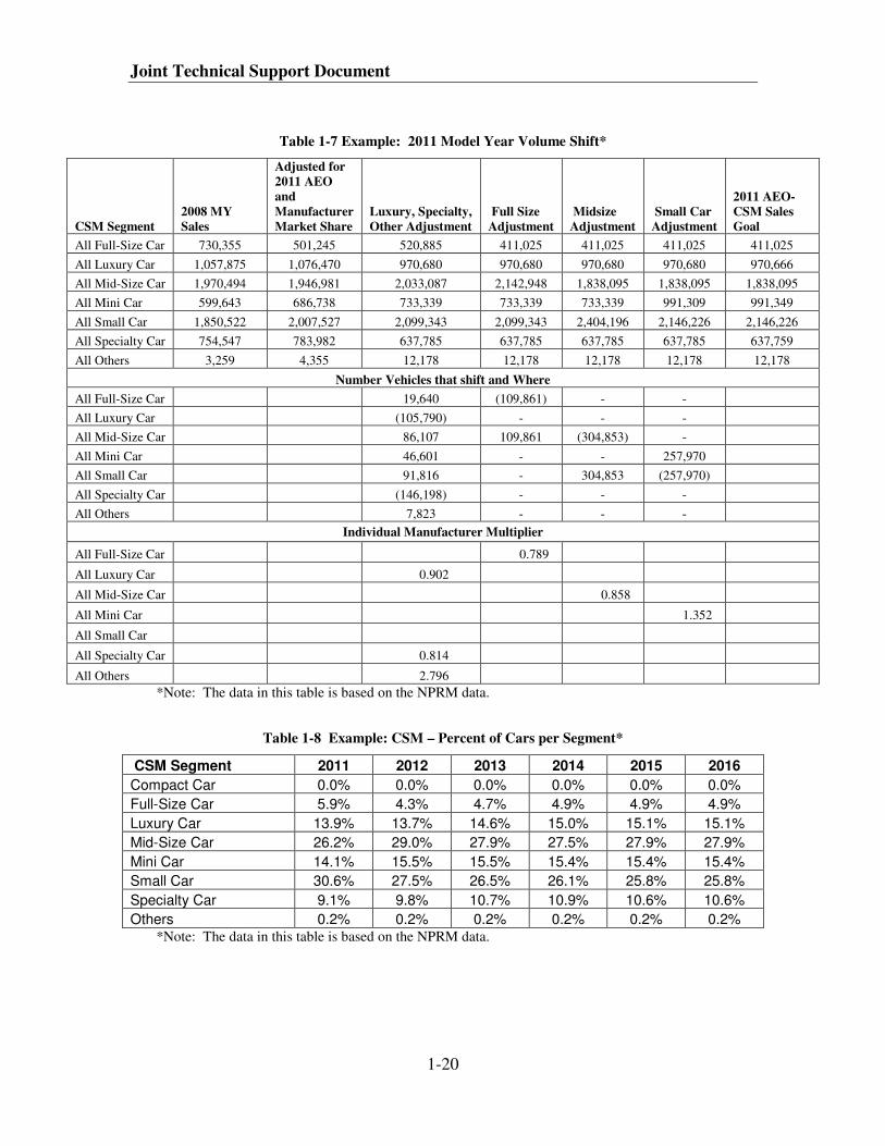
There were several steps in developing an adjustment for Cars based on the CSM
data. CSM provided data on the market share and vehicle segment distribution. The first
step in determining the adjustment for Cars was to total the number of Cars in each
vehicle segment by manufacturer in MY 2008. A total for all manufacturers in each
segment was also calculated. The next step was to multiply the volume of each segment
for each manufacturer by the CSM market share. The AEO multiplier was also applied at
this time. This gave projected volumes with AEO total volumes and market share
correction for Cars. This is shown in the “Adjusted for 2011 AEO and Manufacturer
Market Share” column of Table 1-7.
The next step is to adjust the sales volumes for CSM vehicle segment distribution.
The process for adjusting for vehicle segment is more complicated than a simple one step
multiplication. In order to keep manufacturers’ volumes constant and still have the
correct vehicle segment distribution, vehicles need to move from segment to segment
while maintaining constant manufacturers’ totals. Six rules and one assumption were
applied to accomplish the shift. The assumption (based on the shift in vehicle sales in the
last year) is that people are moving to smaller vehicles in the rulemaking time frame. A
higher level (less detailed) example of this procedure is provided in the preamble section
II.
1. Vehicles from CSM’s “Luxury Car,” “Specialty Car,” and “Other Car” segments,
if reduced will be equally distributed to the remaining four categories (“Full-Size
Car,” “Mid-Size Car,” “Small Car,” “Mini Car”). If these sales increased, they
were taken from the remaining four categories so that the relative sales in these
four categories remained constant.
2. Vehicles from CSM’s “Luxury Car,” “Specialty Car,” and “Other Car” segments,
if increased will take equally from the remaining categories (“Full-Size Car,”
“Mid-Size Car,” “Small Car,” “Mini Car”).
The Baseline and Reference Vehicle Fleet
1-19
3. All manufacturers have the same multiplier for a given segment shift based on
moving all vehicles in that segment to achieve the CSM distribution. Table 1-7
shows how the 2011 vehicles moved and the multipliers that were created for
each adjustment. This does not mean that new vehicle segments will be added
(except for Generic Mini Car described in the next step) to manufacturers that do
not produce them. Vehicles within each manufacturer will be shifted as close to
the distribution as possible given the other rules. Table 1-8 has the percentages of
Cars per CSM segment. These percentages are multiplied by the total number of
vehicles in a given year to get the total sales in the segment. Table 1-7 shows the
totals for 2011 in the “2011 AEO-CSM Sales Goal” column.
4. When “Full-Size Car,” “Mid-Size Car,” “Small Car” are processed, if vehicles
need to move in or out of the segment, they will move into or out of the next
smaller segment. So, if Mid-Size Cars are being processed they can only move to
or be taken from Small Cars. Note: In order to accomplish this, a “Generic Mini
Car” segment was added to manufacturers who did not have a Mini (type) Car in
production in 2008, but needed to shift down vehicles from the Small Car
segment.
5. The data must be processed in the following order: “Luxury Car,” “Specialty
Car,” “Other Car,” “Full-Size Car,” “Mid-Size Car,” “Small Car.” The “Mini
Car” does not need to be processed separately. By using this order, it works out
that vehicles will always move toward the correct distribution. There are two
exceptions, BMW and Porsche only have “Luxury Car,” “Specialty Car,” and
“Other Car” vehicles, so their volumes were not changed or shifted since these
rules did not apply to them.
6. When an individual manufacturer multiplier is applied for a segment, the vehicles
move to or from the appropriate segments as specified in the previous rules and as
shown in Table 1-7.
Joint Technical Support Document
1-20
Table 1-7 Example: 2011 Model Year Volume Shift*
CSM Segment
2008 MY
Sales
Adjusted for
2011 AEO
and
Manufacturer
Market Share
Luxury, Specialty,
Other Adjustment
Full Size
Adjustment
Midsize
Adjustment
Small Car
Adjustment
2011 AEO-
CSM Sales
Goal
All Full-Size Car 730,355 501,245 520,885 411,025 411,025 411,025 411,025
All Luxury Car 1,057,875 1,076,470 970,680 970,680 970,680 970,680 970,666
All Mid-Size Car 1,970,494 1,946,981 2,033,087 2,142,948 1,838,095 1,838,095 1,838,095
All Mini Car 599,643 686,738 733,339 733,339 733,339 991,309 991,349
All Small Car 1,850,522 2,007,527 2,099,343 2,099,343 2,404,196 2,146,226 2,146,226
All Specialty Car 754,547 783,982 637,785 637,785 637,785 637,785 637,759
All Others 3,259 4,355 12,178 12,178 12,178 12,178 12,178
Number Vehicles that shift and Where
All Full-Size Car 19,640 (109,861) - -
All Luxury Car (105,790) - - -
All Mid-Size Car 86,107 109,861 (304,853) -
All Mini Car 46,601 - - 257,970
All Small Car 91,816 - 304,853 (257,970)
All Specialty Car (146,198) - - -
All Others 7,823 - - -
Individual Manufacturer Multiplier
All Full-Size Car 0.789
All Luxury Car 0.902
All Mid-Size Car 0.858
All Mini Car 1.352
All Small Car
All Specialty Car 0.814
All Others 2.796
*Note: The data in this table is based on the NPRM data.
Table 1-8 Example: CSM – Percent of Cars per Segment*
CSM Segment 2011 2012 2013 2014 2015 2016
Compact Car 0.0% 0.0% 0.0% 0.0% 0.0% 0.0%
Full-Size Car 5.9% 4.3% 4.7% 4.9% 4.9% 4.9%
Luxury Car 13.9% 13.7% 14.6% 15.0% 15.1% 15.1%
Mid-Size Car 26.2% 29.0% 27.9% 27.5% 27.9% 27.9%
Mini Car 14.1% 15.5% 15.5% 15.4% 15.4% 15.4%
Small Car 30.6% 27.5% 26.5% 26.1% 25.8% 25.8%
Specialty Car 9.1% 9.8% 10.7% 10.9% 10.6% 10.6%
Others 0.2% 0.2% 0.2% 0.2% 0.2% 0.2% *Note: The data in this table is based on the NPRM data.
The Baseline and Reference Vehicle Fleet
1-21
Mathematically, an individual manufacturer multiplier is calculated by making the
segment the goal and dividing by the previous total for the segment (shown in Table 1-7).
If the number is greater than 1, the vehicles are entering the segment, and if the number is
less than 1, the vehicles are leaving the segment. So, for example, if Luxury Cars have
an adjustment of 1.5, then for a specific manufacturer who has Luxury Cars, a multiplier
of 1.5 is applied to its luxury car volume, and the total number of vehicles that shifted
into the Luxury segment is subtracted from the remaining segments to maintain that
company’s market share. On the other hand, if Large Cars have an adjustment of 0.7,
then for a specific manufacturer who has Large Cars, a multiplier of 0.7 is applied to its
Large Cars, and the total number of vehicles leaving that segment is transferred into that
manufacturer’s Mid-Size Cars.
After the vehicle volumes are shifted using the above rules, a total for each
manufacturer and vehicle segment is maintained. The total for each manufacturer
segment for a specific model year (e.g., 2011 General Motors Luxury Cars) divided by
the MY 2008 total for that manufacturer segment (e.g., 2008 General Motors Luxury
Cars) is the new multiplier used to determine the future vehicle volume for each vehicle
model. This is done by taking the multiplier (which is for a specific manufacturer and
segment) times the MY 2008 volume for the specific vehicle model (e.g., 2008 General
Motors Luxury Car Cadillac CTS). This process is repeated for each model year (2011-
2016).
The method used to adjust CSM Trucks to the AEO market share was different
than the method used for Cars. The process for Cars is different than Trucks because it is
not possible to predict how vehicles would shift between segments based on current
market trends. This is because of the added utility of some trucks that makes their sales
more insensitive to factors like fuel price. Again, CSM provided data on the market
share and vehicle segment distribution. The process for having the fleet match CSM’s
market share and vehicle segment distribution was iterative.
The following totals were determined:
• The total number of trucks for each manufacturer in 2008 model year.
• The total number of trucks in each truck segment in 2008 model year.
• The total number of truck in each segment for each manufacturer in 2008 model
year.
• The total number of trucks for each manufacturer in a specific future model year
based on the AEO and CSM data. This is the goal for market share.
• The total number of trucks in each truck segment in a specific future model year
based on the AEO and CSM data. This is the goal for vehicle segment
distribution. Table 1-9 has the percentages of Trucks per CSM segment
Joint Technical Support Document
1-22
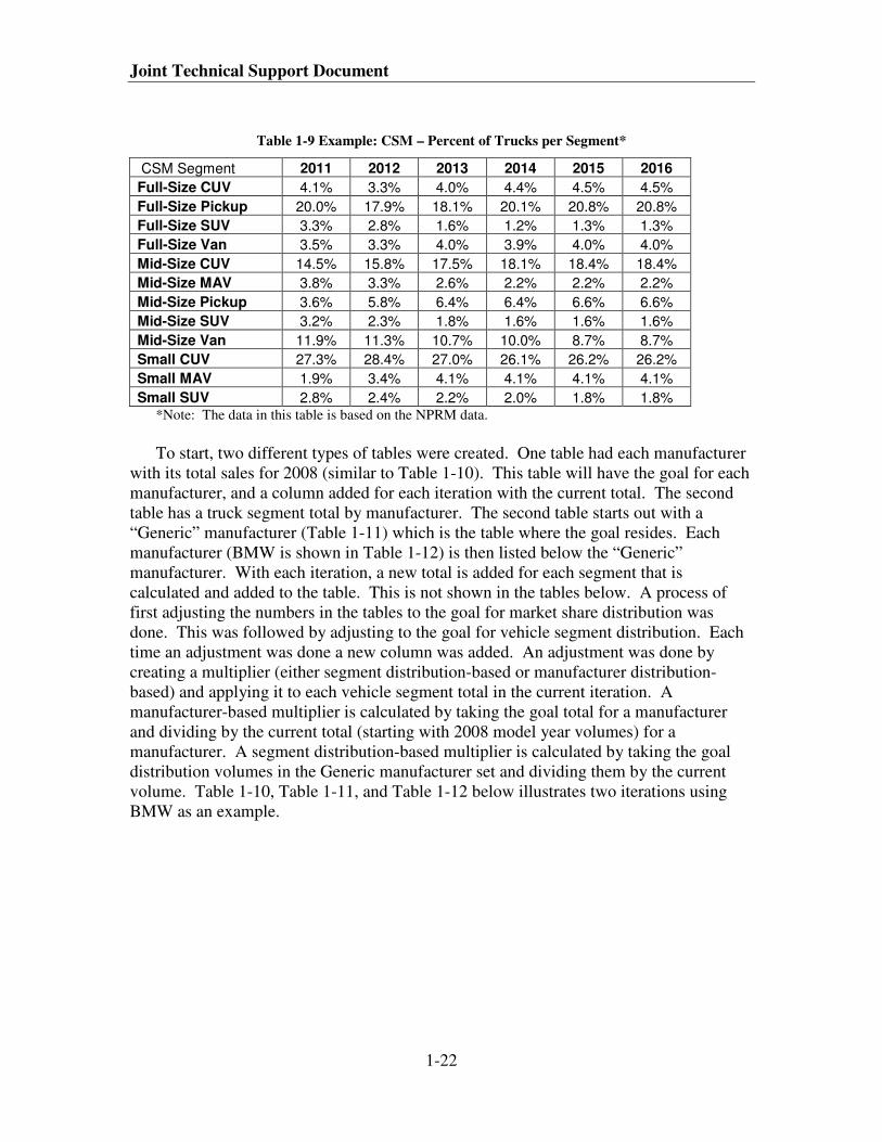
Table 1-9 Example: CSM – Percent of Trucks per Segment*
CSM Segment 2011 2012 2013 2014 2015 2016
Full-Size CUV 4.1% 3.3% 4.0% 4.4% 4.5% 4.5%
Full-Size Pickup 20.0% 17.9% 18.1% 20.1% 20.8% 20.8%
Full-Size SUV 3.3% 2.8% 1.6% 1.2% 1.3% 1.3%
Full-Size Van 3.5% 3.3% 4.0% 3.9% 4.0% 4.0%
Mid-Size CUV 14.5% 15.8% 17.5% 18.1% 18.4% 18.4%
Mid-Size MAV 3.8% 3.3% 2.6% 2.2% 2.2% 2.2%
Mid-Size Pickup 3.6% 5.8% 6.4% 6.4% 6.6% 6.6%
Mid-Size SUV 3.2% 2.3% 1.8% 1.6% 1.6% 1.6%
Mid-Size Van 11.9% 11.3% 10.7% 10.0% 8.7% 8.7%
Small CUV 27.3% 28.4% 27.0% 26.1% 26.2% 26.2%
Small MAV 1.9% 3.4% 4.1% 4.1% 4.1% 4.1%
Small SUV 2.8% 2.4% 2.2% 2.0% 1.8% 1.8% *Note: The data in this table is based on the NPRM data.
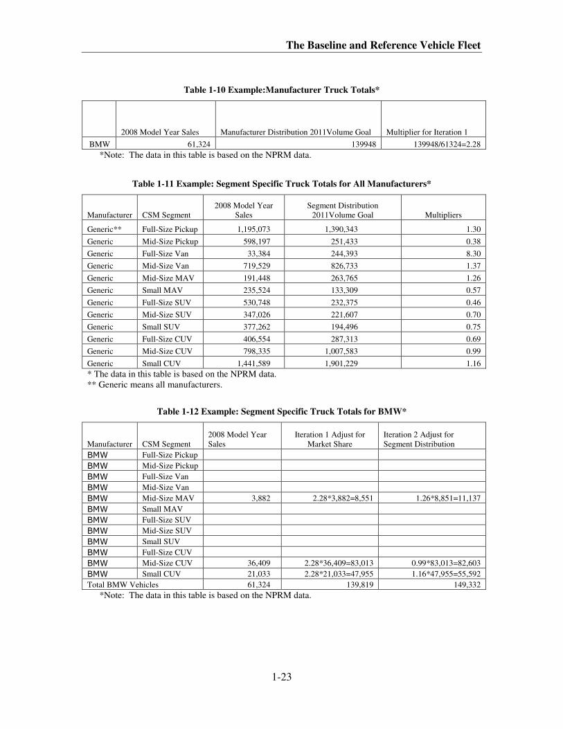
To start, two different types of tables were created. One table had each manufacturer
with its total sales for 2008 (similar to Table 1-10). This table will have the goal for each
manufacturer, and a column added for each iteration with the current total. The second
table has a truck segment total by manufacturer. The second table starts out with a
“Generic” manufacturer (Table 1-11) which is the table where the goal resides. Each
manufacturer (BMW is shown in Table 1-12) is then listed below the “Generic”
manufacturer. With each iteration, a new total is added for each segment that is
calculated and added to the table. This is not shown in the tables below. A process of
first adjusting the numbers in the tables to the goal for market share distribution was
done. This was followed by adjusting to the goal for vehicle segment distribution. Each
time an adjustment was done a new column was added. An adjustment was done by
creating a multiplier (either segment distribution-based or manufacturer distribution-
based) and applying it to each vehicle segment total in the current iteration. A
manufacturer-based multiplier is calculated by taking the goal total for a manufacturer
and dividing by the current total (starting with 2008 model year volumes) for a
manufacturer. A segment distribution-based multiplier is calculated by taking the goal
distribution volumes in the Generic manufacturer set and dividing them by the current
volume. Table 1-10, Table 1-11, and Table 1-12 below illustrates two iterations using
BMW as an example.
The Baseline and Reference Vehicle Fleet
1-23
Table 1-10 Example:Manufacturer Truck Totals*
2008 Model Year Sales Manufacturer Distribution 2011Volume Goal Multiplier for Iteration 1
BMW 61,324 139948 139948/61324=2.28
*Note: The data in this table is based on the NPRM data.
Table 1-11 Example: Segment Specific Truck Totals for All Manufacturers*
Manufacturer CSM Segment
2008 Model Year
Sales
Segment Distribution
2011Volume Goal Multipliers
Generic** Full-Size Pickup 1,195,073 1,390,343 1.30
Generic Mid-Size Pickup 598,197 251,433 0.38
Generic Full-Size Van 33,384 244,393 8.30
Generic Mid-Size Van 719,529 826,733 1.37
Generic Mid-Size MAV 191,448 263,765 1.26
Generic Small MAV 235,524 133,309 0.57
Generic Full-Size SUV 530,748 232,375 0.46
Generic Mid-Size SUV 347,026 221,607 0.70
Generic Small SUV 377,262 194,496 0.75
Generic Full-Size CUV 406,554 287,313 0.69
Generic Mid-Size CUV 798,335 1,007,583 0.99
Generic Small CUV 1,441,589 1,901,229 1.16
* The data in this table is based on the NPRM data.
** Generic means all manufacturers.
Table 1-12 Example: Segment Specific Truck Totals for BMW*
Manufacturer CSM Segment
2008 Model Year
Sales
Iteration 1 Adjust for
Market Share
Iteration 2 Adjust for
Segment Distribution
BMW Full-Size Pickup
BMW Mid-Size Pickup
BMW Full-Size Van
BMW Mid-Size Van
BMW Mid-Size MAV 3,882 2.28*3,882=8,551 1.26*8,851=11,137
BMW Small MAV
BMW Full-Size SUV
BMW Mid-Size SUV
BMW Small SUV
BMW Full-Size CUV
BMW Mid-Size CUV 36,409 2.28*36,409=83,013 0.99*83,013=82,603
BMW Small CUV 21,033 2.28*21,033=47,955 1.16*47,955=55,592
Total BMW Vehicles 61,324 139,819 149,332
*Note: The data in this table is based on the NPRM data.
Joint Technical Support Document
1-24
Using this process, the numbers will get closer to the goal of matching CSM’s market
share for each manufacturer and distribution for each vehicle segment after each of the
iterations. The iterative process is carried out until the totals nearly match the goals.
After 19 iterations, all numbers were within 0.01% of CSM’s distributions. The
calculation iterations could have been stopped sooner, but they were continued to observe
how the numbers would converge.
After the market share and segment distribution were complete, the totals need to be
used to create multipliers that could be applied to the original individual 2008 model year
vehicle volumes (each unique manufacture models volume). The total for each
manufacturer segment divided by the 2008 model year total for each manufacturer
segment gives a multiplier that can be applied to each vehicle based on its manufacturer
and segment.
The above process is done for each model year needed (2011-2016). The multipliers
are then applied to each vehicle in 2008 model year, which gives a volume for each
vehicle in 2011 through 2016 model year. The “reference case” (which is the technology
being applied to 2012-2016 fleet to meet the 2011 cafe standard) is discussed below in
section 4.1, with the results being presented in section 4.2.
1.3.3 How has the reference fleet changed from the NPRM to the Final Rule?
The agencies updated the projected reference (2011-2016) fleet file for the final
rule, though the baseline fleet (MY 2008) remains unchanged. The NPRM reference
fleet used CSM Worldwide’s second quarter, 2009 projections and the April 2009 Annual
Energy Outlook. The reference for the final rule uses a filtered version of CSM
Worldwide’s fourth quarter, 2009 projections, and (as noted above) an early version of
the 2010 Annual Energy Outlook that was released in December of 2009.
CSM Worldwide’s standard forecast includes heavy duty class 2b and heavy duty
class 3 vehicles. Including these extra vehicles in the second quarter forecast caused the
baseline to have an increased number of full size trucks and full size vans. EPA did not
discover this discrepancy between CSM’s definition of heavy truck and the one used by
NHTSA/EPA until after the proposal had been published. For the final rule, the EPA
requested CSM to filter their 4th quarter projections to only include light duty and
medium duty passenger vehicles. The filtered CSM data allowed the agencies to produce
a more accurate projection of future sales.
Table 1-13 and Table 1-14 below show the difference in volumes per each CSM
segment in the final rule baseline and the NPRM reference. The significant decrease in
the number of full size vans can be attributed to the new filtered version of the CSM data.
Full size trucks show some decrease, but did not have as obvious an impact from the data
filtering since CSM increase their predicted volume for full size trucks. The overall
decrease in cars and trucks for some of the year in the 2011-2016 time frame is due to the
decreased volumes projected in the 2010 Annual Energy Outlook.
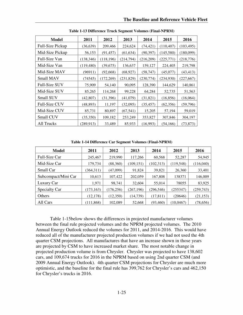
The Baseline and Reference Vehicle Fleet
1-25
Table 1-13 Difference Truck Segment Volumes (Final-NPRM)
Model 2011 2012 2013 2014 2015 2016
Full-Size Pickup (36,639) 209,466 224,624 (74,421) (110,407) (103,495)
Mid-Size Pickup 56,153 (91,457) (61,634) (90,397) (145,580) (180,099)
Full-Size Van (138,346) (118,196) (214,794) (216,209) (225,771) (218,776)
Mid-Size Van (119,480) (39,675) 136,637 159,127 224,405 219,798
Mid-Size MAV (96911) (92,668) (68,927) (58,747) (45,077) (43,413)
Small MAV (74545) (172,269) (231,829) (230,774) (234,930) (227,667)
Full-Size SUV 75,909 54,140 90,095 128,390 144,629 140,861
Mid-Size SUV 85,265 114,268 99,228 64,284 52,735 51,563
Small SUV (42,807) (31,396) (41,079) (31,821) (16,856) (16,064)
Full-Size CUV (48,893) 11,197 (32,095) (35,457) (62,356) (59,796)
Mid-Size CUV 85,731 80,897 (67,541) 15,205 57,194 59,019
Small CUV (35,350) 109,182 253,249 353,827 307,846 304,197
All Trucks (289,913) 33,489 85,933 (16,993) (54,166) (73,873)
Table 1-14 Difference Car Segment Volumes (Final-NPRM)
Model 2011 2012 2013 2014 2015 2016
Full-Size Car 245,467 219,990 117,266 60,568 52,287 54,945
Mid-Size Car 179,734 (88,360) (109,151) (102,313) (119,548) (116,040)
Small Car (364,311) (47,099) 91,824 39,821 26,360 33,401
Subcompact/Mini Car 10,613 107,422 202,059 167,808 138371 146,009
Luxury Car 1,971 98,741 32,604 55,014 78055 83,925
Specialty Car (173,163) (176,256) (267,196) (296,546) (255347) (259,743)
Others (12,178) (12,350) (14,739) (17,811) (20646) (21,153)
All Cars (111,868) 102,089 52,668 (93,460) (10,0467) (78,656)
Table 1-15below shows the differences in projected manufacturer volumes
between the final rule projected volumes and the NPRM projected volumes. The 2010
Annual Energy Outlook reduced the volumes for 2011, and 2014-2016. This would have
reduced all of the manufacturer projected production volumes if we had not used the 4th
quarter CSM projections. All manufactures that have an increase shown in those years
are projected by CSM to have increased market share. The most notable change in
projected production volume is from Chrysler. Chrysler was projected to have 138,602
cars, and 109,674 trucks for 2016 in the NPRM based on using 2nd quarter CSM (and
2009 Annual Energy Outlook). 4th quarter CSM projections for Chrysler are much more
optimistic, and the baseline for the final rule has 399,762 for Chrysler’s cars and 462,150
for Chrysler’s trucks in 2016.
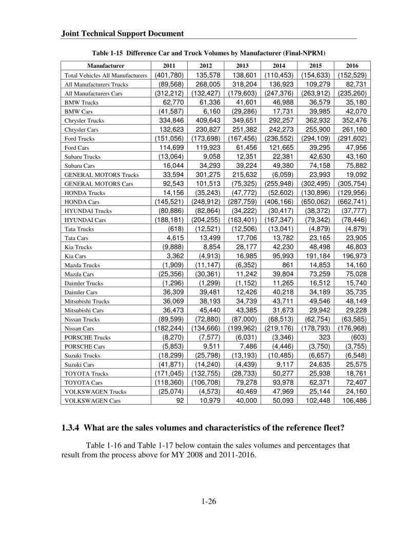
Joint Technical Support Document
1-26
Table 1-15 Difference Car and Truck Volumes by Manufacturer (Final-NPRM)
Manufacturer 2011 2012 2013 2014 2015 2016
Total Vehicles All Manufacturers (401,780) 135,578 138,601 (110,453) (154,633) (152,529)
All Manufacturers Trucks (89,568) 268,005 318,204 136,923 109,279 82,731
All Manufacturers Cars (312,212) (132,427) (179,603) (247,376) (263,912) (235,260)
BMW Trucks 62,770 61,336 41,601 46,988 36,579 35,180
BMW Cars (41,587) 6,160 (29,286) 17,731 39,985 42,070
Chrysler Trucks 334,846 409,643 349,651 292,257 362,932 352,476
Chrysler Cars 132,623 230,827 251,382 242,273 255,900 261,160
Ford Trucks (151,056) (173,698) (167,456) (236,552) (294,109) (291,602)
Ford Cars 114,699 119,923 61,456 121,665 39,295 47,956
Subaru Trucks (13,064) 9,058 12,351 22,381 42,630 43,160
Subaru Cars 16,044 34,293 39,224 49,380 74,158 75,882
GENERAL MOTORS Trucks 33,594 301,275 215,632 (6,059) 23,993 19,092
GENERAL MOTORS Cars 92,543 101,513 (75,325) (255,948) (302,495) (305,754)
HONDA Trucks 14,156 (35,243) (47,772) (52,602) (130,896) (129,956)
HONDA Cars (145,521) (248,912) (287,759) (406,166) (650,062) (662,741)
HYUNDAI Trucks (80,886) (82,864) (34,222) (30,417) (38,372) (37,777)
HYUNDAI Cars (188,181) (204,255) (163,401) (167,347) (79,342) (78,446)
Tata Trucks (618) (12,521) (12,506) (13,041) (4,879) (4,879)
Tata Cars 4,615 13,499 17,706 13,782 23,165 23,905
Kia Trucks (9,888) 8,854 28,177 42,230 48,498 46,803
Kia Cars 3,362 (4,913) 16,985 95,993 191,184 196,973
Mazda Trucks (1,909) (11,147) (6,352) 861 14,853 14,160
Mazda Cars (25,356) (30,361) 11,242 39,804 73,259 75,028
Daimler Trucks (1,296) (1,299) (1,152) 11,265 16,512 15,740
Daimler Cars 36,309 39,481 12,426 40,218 34,189 35,735
Mitsubishi Trucks 36,069 38,193 34,739 43,711 49,546 48,149
Mitsubishi Cars 36,473 45,440 43,385 31,673 29,942 29,228
Nissan Trucks (89,599) (72,880) (87,000) (68,513) (62,754) (63,585)
Nissan Cars (182,244) (134,666) (199,962) (219,176) (178,793) (176,968)
PORSCHE Trucks (8,270) (7,577) (6,031) (3,346) 323 (603)
PORSCHE Cars (5,853) 9,511 7,486 (4,446) (3,750) (3,755)
Suzuki Trucks (18,299) (25,798) (13,193) (10,485) (6,657) (6,548)
Suzuki Cars (41,871) (14,240) (4,439) 9,117 24,635 25,575
TOYOTA Trucks (171,045) (132,755) (28,733) 50,277 25,938 18,761
TOYOTA Cars (118,360) (106,708) 79,278 93,978 62,371 72,407
VOLKSWAGEN Trucks (25,074) (4,573) 40,469 47,969 25,144 24,160
VOLKSWAGEN Cars 92 10,979 40,000 50,093 102,448 106,486
1.3.4 What are the sales volumes and characteristics of the reference fleet?
Table 1-16 and Table 1-17 below contain the sales volumes and percentages that
result from the process above for MY 2008 and 2011-2016.
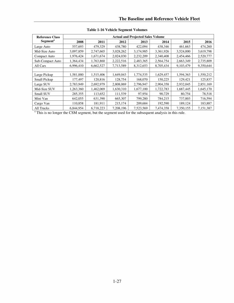
The Baseline and Reference Vehicle Fleet
1-27
Table 1-16 Vehicle Segment Volumes
Actual and Projected Sales Volume Reference Class
Segmenta 2008 2011 2012 2013 2014 2015 2016
Large Auto 557,693 479,329 438,780 422,094 438,346 461,663 474,260
Mid-Size Auto 3,097,859 2,747,665 3,028,262 3,174,985 3,361,926 3,524,000 3,619,798
Compact Auto 1,976,424 1,671,674 2,024,030 2,232,209 2,340,408 2,454,466 2,520,777
Sub-Compact Auto 1,364,434 1,763,860 2,222,516 2,483,365 2,564,754 2,663,349 2,735,809
All Cars 6,996,410 6,662,527 7,713,589 8,312,653 8,705,434 9,103,479 9,350,644
Large Pickup 1,581,880 1,515,406 1,649,043 1,774,535 1,629,457 1,594,363 1,550,212
Small Pickup 177,497 120,816 128,754 168,070 150,225 129,421 125,837
Large SUV 2,783,949 2,692,979 2,808,069 2,796,947 2,904,358 2,932,045 2,851,169
Mid-Size SUV 1,263,360 1,462,069 1,630,310 1,677,100 1,722,783 1,687,445 1,645,170
Small SUV 285,355 113,652 111,539 97,954 90,729 80,754 78,518
Mini Van 642,055 631,390 665,307 799,280 784,215 737,003 716,594
Cargo Van 110,858 181,911 215,174 209,684 192,590 189,124 183,887
All Trucks 6,844,954 6,718,223 7,208,196 7,523,569 7,474,358 7,350,155 7,151,387 a This is no longer the CSM segment, but the segment used for the subsequent analysis in this rule.
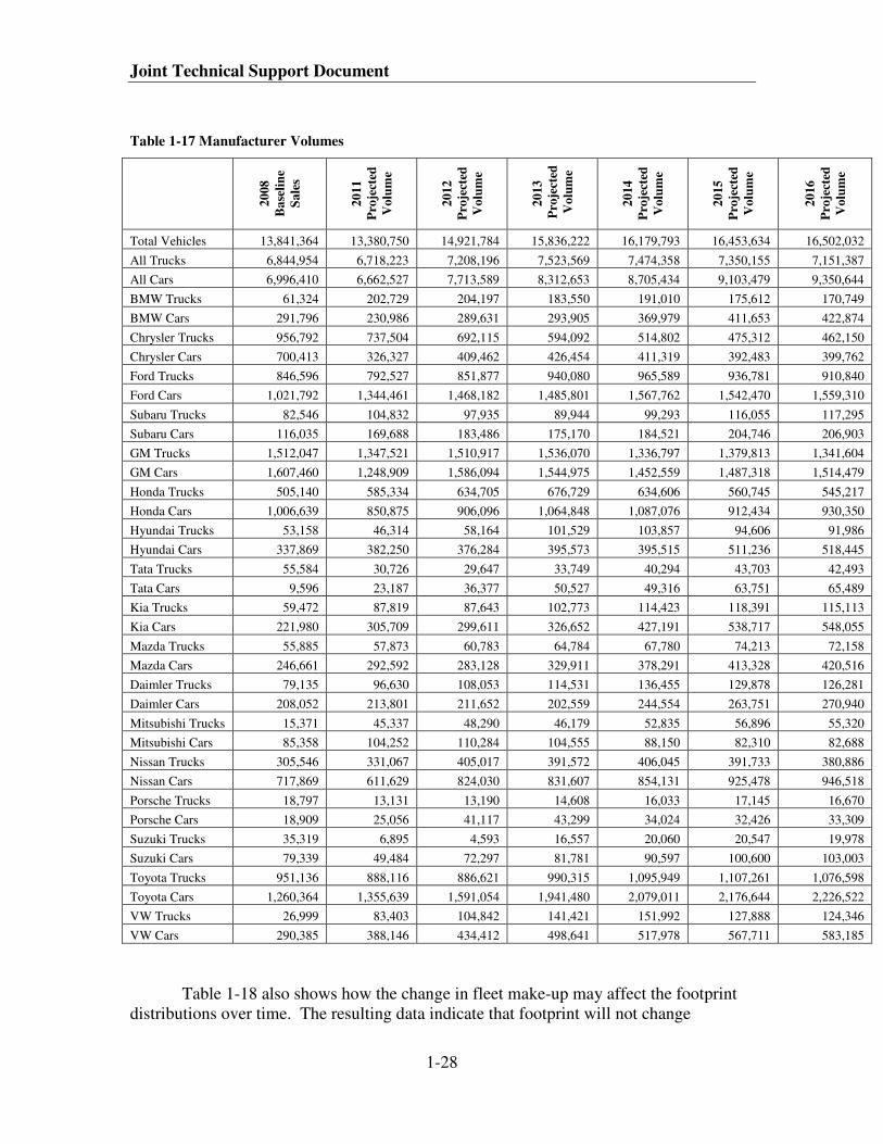
Joint Technical Support Document
1-28
Table 1-17 Manufacturer Volumes
20
08
Ba
seli
ne
Sa
les
20
11
Pro
ject
ed
Vo
lum
e
20
12
Pro
ject
ed
Vo
lum
e
20
13
Pro
ject
ed
Vo
lum
e
20
14
Pro
ject
ed
Vo
lum
e
20
15
Pro
ject
ed
Vo
lum
e
20
16
Pro
ject
ed
Vo
lum
e
Total Vehicles 13,841,364 13,380,750 14,921,784 15,836,222 16,179,793 16,453,634 16,502,032
All Trucks 6,844,954 6,718,223 7,208,196 7,523,569 7,474,358 7,350,155 7,151,387
All Cars 6,996,410 6,662,527 7,713,589 8,312,653 8,705,434 9,103,479 9,350,644
BMW Trucks 61,324 202,729 204,197 183,550 191,010 175,612 170,749
BMW Cars 291,796 230,986 289,631 293,905 369,979 411,653 422,874
Chrysler Trucks 956,792 737,504 692,115 594,092 514,802 475,312 462,150
Chrysler Cars 700,413 326,327 409,462 426,454 411,319 392,483 399,762
Ford Trucks 846,596 792,527 851,877 940,080 965,589 936,781 910,840
Ford Cars 1,021,792 1,344,461 1,468,182 1,485,801 1,567,762 1,542,470 1,559,310
Subaru Trucks 82,546 104,832 97,935 89,944 99,293 116,055 117,295
Subaru Cars 116,035 169,688 183,486 175,170 184,521 204,746 206,903
GM Trucks 1,512,047 1,347,521 1,510,917 1,536,070 1,336,797 1,379,813 1,341,604
GM Cars 1,607,460 1,248,909 1,586,094 1,544,975 1,452,559 1,487,318 1,514,479
Honda Trucks 505,140 585,334 634,705 676,729 634,606 560,745 545,217
Honda Cars 1,006,639 850,875 906,096 1,064,848 1,087,076 912,434 930,350
Hyundai Trucks 53,158 46,314 58,164 101,529 103,857 94,606 91,986
Hyundai Cars 337,869 382,250 376,284 395,573 395,515 511,236 518,445
Tata Trucks 55,584 30,726 29,647 33,749 40,294 43,703 42,493
Tata Cars 9,596 23,187 36,377 50,527 49,316 63,751 65,489
Kia Trucks 59,472 87,819 87,643 102,773 114,423 118,391 115,113
Kia Cars 221,980 305,709 299,611 326,652 427,191 538,717 548,055
Mazda Trucks 55,885 57,873 60,783 64,784 67,780 74,213 72,158
Mazda Cars 246,661 292,592 283,128 329,911 378,291 413,328 420,516
Daimler Trucks 79,135 96,630 108,053 114,531 136,455 129,878 126,281
Daimler Cars 208,052 213,801 211,652 202,559 244,554 263,751 270,940
Mitsubishi Trucks 15,371 45,337 48,290 46,179 52,835 56,896 55,320
Mitsubishi Cars 85,358 104,252 110,284 104,555 88,150 82,310 82,688
Nissan Trucks 305,546 331,067 405,017 391,572 406,045 391,733 380,886
Nissan Cars 717,869 611,629 824,030 831,607 854,131 925,478 946,518
Porsche Trucks 18,797 13,131 13,190 14,608 16,033 17,145 16,670
Porsche Cars 18,909 25,056 41,117 43,299 34,024 32,426 33,309
Suzuki Trucks 35,319 6,895 4,593 16,557 20,060 20,547 19,978
Suzuki Cars 79,339 49,484 72,297 81,781 90,597 100,600 103,003
Toyota Trucks 951,136 888,116 886,621 990,315 1,095,949 1,107,261 1,076,598
Toyota Cars 1,260,364 1,355,639 1,591,054 1,941,480 2,079,011 2,176,644 2,226,522
VW Trucks 26,999 83,403 104,842 141,421 151,992 127,888 124,346
VW Cars 290,385 388,146 434,412 498,641 517,978 567,711 583,185
Table 1-18 also shows how the change in fleet make-up may affect the footprint
distributions over time. The resulting data indicate that footprint will not change
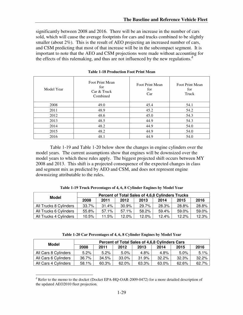
The Baseline and Reference Vehicle Fleet
1-29
significantly between 2008 and 2016. There will be an increase in the number of cars
sold, which will cause the average footprints for cars and trucks combined to be slightly
smaller (about 2%). This is the result of AEO projecting an increased number of cars,
and CSM predicting that most of that increase will be in the subcompact segment. It is
important to note that the AEO and CSM projections were made without accounting for
the effects of this rulemaking, and thus are not influenced by the new regulations.d
Table 1-18 Production Foot Print Mean
Model Year
Foot Print Mean
for
Car & Truck
Combined
Foot Print Mean
for
Car
Foot Print Mean
for
Truck
2008 49.0 45.4 54.1
2011 48.9 45.2 54.2
2012 48.6 45.0 54.3
2013 48.5 44.9 54.3
2014 48.2 44.9 54.0
2015 48.2 44.9 54.0
2016 48.1 44.9 54.0
Table 1-19 and Table 1-20 below show the changes in engine cylinders over the
model years. The current assumptions show that engines will be downsized over the
model years to which these rules apply. The biggest projected shift occurs between MY
2008 and 2013. This shift is a projected consequence of the expected changes in class
and segment mix as predicted by AEO and CSM, and does not represent engine
downsizing attributable to the rules.
Table 1-19 Truck Percentages of 4, 6, 8 Cylinder Engines by Model Year
Percent of Total Sales of 4,6,8 Cylinders Trucks Model
2008 2011 2012 2013 2014 2015 2016
All Trucks 8 Cylinders 33.7% 31.4% 30.9% 29.7% 28.3% 28.8% 28.8%
All Trucks 6 Cylinders 55.8% 57.1% 57.1% 58.2% 59.4% 59.0% 59.0%
All Trucks 4 Cylinders 10.5% 11.5% 12.0% 12.0% 12.4% 12.2% 12.3%
Table 1-20 Car Percentages of 4, 6, 8 Cylinder Engines by Model Year
Percent of Total Sales of 4,6,8 Cylinders Cars Model
2008 2011 2012 2013 2014 2015 2016
All Cars 8 Cylinders 5.2% 5.2% 5.0% 4.8% 4.8% 5.0% 5.1%
All Cars 6 Cylinders 36.7% 34.5% 33.0% 31.9% 32.2% 32.3% 32.2%
All Cars 4 Cylinders 58.1% 60.3% 62.0% 63.3% 63.0% 62.6% 62.7%
d Refer to the memo to the docket (Docket EPA-HQ-OAR-2009-0472) for a more detailed description of
the updated AEO2010 fleet projection.
Joint Technical Support Document
1-30
1.3.5 How is the development of the baseline and reference fleet for this final
rule different from NHTSA’s historical approach and why is this
approach preferable?
As described in detail at the opening of this chapter, and as explained at proposal,
NHTSA has historically based its analysis of potential new CAFE standards on detailed
product plans the agency has requested from manufacturers planning to produce light
vehicles for sale in the United States. Although the agency has never compelled
manufacturers to submit such information, most major manufacturers and some smaller
manufacturers have voluntarily provided it when requested.
As in other prior rulemakings, NHTSA has requested extensive and detailed
information regarding the models that manufacturers plan to offer, as well as
manufacturers’ estimates of the volume of each model they expect to produce for sale in
the U.S. NHTSA’s recent requests have sought information regarding a range of
engineering and planning characteristics for each vehicle model (e.g., fuel economy,
engine, transmission, physical dimensions, weights and capacities, redesign schedules),
each engine (e.g., fuel type, fuel delivery, aspiration, valvetrain configuration, valve
timing, valve lift, power and torque ratings), and each transmission (e.g., type, number of
gears, logic).
The information that manufacturers have provided in response to this request has
varied in completeness and detail. Some manufacturers have submitted nearly all of the
information NHTSA has requested, for most or all of the model years covered by
NHTSA’s requests, and have closely followed NHTSA’s guidance regarding the
structure of the information. Other manufacturers have submitted partial information,
information for only a few model years, and/or information in a structure less amenable
to analysis. Still other manufacturers have not responded to NHTSA’s requests or have
responded on occasion, usually with partial information.
One of the primary reasons for the request for data in 2009 was to obtain
permission from the manufacturers to make public their product plan information for
model years 2010 and 2011. There are a number of reasons that this could be
advantageous in the development of a reference fleet. First some changes to the fleet
may not be captured by this approach of solely using publicly available information. For
example, the agencies’ current market forecast includes some vehicles for which
manufacturers have announced plans for elimination or drastic production cuts such as
the Chevrolet Trailblazer, the Chrysler PT Cruiser, the Chrysler Pacifica, the Dodge
Magnum, the Ford Crown Victoria, the Hummer H2, the Mercury Sable, the Pontiac
Grand Prix, and the Pontiac G5. These vehicle models appear explicitly in market inputs
to NHTSA’s analysis, and are among those vehicle models included in the aggregated
vehicle types appearing in market inputs to EPA’s analysis.
Second, the agencies’ market forecast does not include some forthcoming vehicle
models, such as the Chevrolet Volt, the Chevrolet Camaro, the Ford Fiesta and several
publicly announced electric vehicles, including the announcements from Nissan. Nor
The Baseline and Reference Vehicle Fleet
1-31
does it include several MY 2009 and 2010 vehicles, such as the Honda Insight, the
Hyundai Genesis and the Toyota Venza, as the starting point for vehicle definitions was
MY 2008. Additionally, the market forecast does not account for publicly-announced
technology introductions, such as Ford’s EcoBoost system, whose product plans specify
which vehicles and how many are planned to have this technology. Were the agencies to
rely on manufacturers’ product plans, this market forecast would account for not only
these specific examples, but also for similar examples that have not yet been announced
publicly.
Finally, some technical information manufacturers that have provided in product
plans regarding specific vehicle models is, at least as far as NHTSA and EPA have been
able to determine, not available from public or commercial sources. While such gaps do
not bear significantly on the agencies’ analysis, the diversity of pickup configurations
necessitated utilizing a sales-weighted average footprint value7 for many manufacturers’
pickups. Since the modeling only utilizes footprint in order to estimate each
manufacturer’s CO2 or fuel economy standard and all the other vehicle characteristics are
available for each pickup configuration, this approximation has no practical impact on the
projected technology or cost associated with compliance with the various standards
evaluated. The only impact which could arise would be if the relative sales of the various
pickup configurations changed, or if the agencies were to explore standards with a
different shape or attribute. This would necessitate recalculating the average footprint
value in order to maintain accuracy.
In an effort to update the 2008 baseline to account for the expected changes in the
fleet in the near-term model years 2009-2011 described above, NHTSA requested
permission from the manufacturers to make this limited product plan information public.
Unfortunately, virtually no manufacturers agreed to allow the use of their data after the
2009 model year. A few manufacturers stated we could use their 2009 product plan data
after the end of production (December 31). Unfortunately, this does not afford us
sufficient time to do the analysis for the final rule. Also, the 2009 product plan data that
was permitted to be used was not consistent with the data already in the baseline, and in
some cases was determined to be inaccurate. Since the agencies were unable to obtain
consistent updates, the baseline and reference fleets were not updated beyond 2008 model
year for this final rule. The 2008 baseline fleet and projections were instead updated
using the latest AEO and CSM data, as explained above.
7 A full-size pickup might be offered with various combinations of cab style (e.g., regular, extended, crew)
and box length (e.g., 5½’, 6½’, 8’) and, therefore, multiple footprint sizes. CAFE compliance data for
MY2008 data does not contain footprint information, and does not contain information that can be used to
reliably identify which pickup entries correspond to footprint values estimable from public or commercial
sources. Therefore, the agencies have used the known production levels of average values to represent all
variants of a given pickup line (e.g., all variants of the F-150 and the Sierra/Silverado) in order to calculate
the sales-weighted average footprint value for each pickup family. Again, this has little impact on the
results of the modeling effort. In the extreme, one single footprint value could be used for every vehicle
sold by a single manufacturer as long as the fuel economy standard associated with this footprint value
represented the sales-weighted, harmonic average of the fuel economy standards associated with each
vehicle’s footprint values.
Joint Technical Support Document
1-32
1.3.6 How does manufacturer product plan data factor into the baseline used
in this final rule?
In the spring and fall of 2009, many manufacturers submitted product plans in
response to NHTSA’s recent requests that they do so. NHTSA and EPA both have
access to these plans, and both agencies have reviewed them in detail. A small amount of
product plan data was used in the development of the baseline. The specific pieces of
data are:
• Wheelbase
• Track Width Front
• Track Width Rear
• EPS (Electric Power Steering)
• ROLL (Reduced Rolling Resistance)
• LUB (Advance Lubrication i.e. low weight oil)
• IACC (Improved Electrical Accessories)
• Curb Weight
• GVWR (Gross Vehicle Weight Rating)
The track widths, wheelbase, curb weight, and GVWR for vehicles could have
been looked up on the internet (159 were), but were taken from the product plans when
available for convenience. To ensure accuracy, a sample from each product plan was
used as a check against the numbers available from Motortrend.com. These numbers will
be published in the baseline file since they can be easily looked up on the internet. On
the other hand, EPS, ROLL, LUB, and IACC are difficult to determine without using
manufacturer’s product plans. These items will not be published in the baseline file, but
the data has been aggregated into the agencies’ baseline in the technology effectiveness
and cost effectiveness for each vehicle in a way that allows the baseline for the model to
be published without revealing the manufacturers data.
The Baseline and Reference Vehicle Fleet
1-33
References
All references can be found in the EPA DOCKET: EPA-HQ-OAR-2009-0472.
1 CFEIS (Certification Fuel Emissions Information System) Database: CFEIS is an EPA database system.
2 WardsAuto.com: Used as a source for engine specifications.
3 Motortrend.com and Edmunds.com: Used as a source for foot print and vehicle weight data.
4 Energy Information Administration’s 2009 Annual Energy Outlook.
5 The agencies have also looked at the impact of the rule in EIA’s projection, and concluded that the impact
was small. EPA and NHTSA have evaluated the differences between the AEO 2010 (early draft) and AEO
2009 and found little difference in the fleet projections (or fuel prices). This analysis can be found in the
memo to the docket: (Docket EPA-HQ-OAR-2009-0472).
6 CSM World Wide, CSM World Wide is a paid service provider; J.D. Power Automotive Forecasting, J.D. Power
Automotive Forecasting is a paid service provider.
7 The baseline Excel file (“2008-2016 Production Summary Data _Definitions Docket 08_27_2009”) is
available in the docket (Docket EPA-HQ-OAR-2009-0472).
What are the Attribute-Based Curves the Agencies are Using, and How Were They Developed?
2-1
CHAPTER 2: What are the Attribute-Based Curves the Agencies
are Using, and How Were They Developed?
2.1 Standards are attribute-based and are defined by a mathematical
function
As discussed in Section II.B of the final rule preamble, NHTSA and EPA are setting
attribute-based CAFE and CO2 standards for MYs 2012-2016 passenger cars and light trucks,
which are expressed by a mathematical function. EPCA, as amended by EISA, expressly
requires that CAFE standards for passenger cars and light trucks be based on one or more
vehicle attributes related to fuel economy, and be expressed in the form of a mathematical
function.1 The CAA has no such requirement, although such an approach is permissible
under section 202 (a) and EPA has used the attribute-based approach in issuing standards
under analogous provisions of the CAA (e.g., standards for non-road diesel engines using
engine size as the attribute). Given the advantages of using attribute-based standards for light
duty vehicles, and given the goal of coordinating and harmonizing CO2 standards promulgated
under the CAA and CAFE standards promulgated under CAA and EPCA, as expressed by
President Obama in his announcement of the new National Program and by the agencies in
the joint NOI and NPRM, EPA is also finalizing standards that are attribute-based and
expressed as mathematical functions.
Under an attribute-based standard approach, each vehicle model has a fuel economy
(mpg) or CO2 target, the stringency of which depends on the value of the attribute for the
vehicle model. Thus, fuel economy and CO2 targets are set for individual vehicles, and vary
directly with the attribute, i.e., becoming more stringent as the attribute decreases and vice
versa. For example, size-based (i.e., size-indexed) standards assign higher fuel economy
targets (lower CO2 targets) to smaller vehicles and lower fuel economy targets (higher CO2
targets) to larger vehicles. However, we emphasize that the targets themselves are not
standards. The CAFE or fleet-wide average CO2 level required of a particular manufacturer is
actually determined by calculating the production-weighted average of the applicable model-
specific fuel economy or CO2 targets.
The form of the fuel economy or CO2 standard can have a dramatic effect on the level
of improvement required from various types of vehicles and on the relative stringency of the
standard for various manufacturers. These disparate impacts derive from two facts
concerning the current automotive market: 1) consumers currently demand a wide variety of
vehicle types and sizes, and 2) individual manufacturers focus their product offerings on
different portions of this demand. Therefore, a comparison of the advantages and
disadvantages of attribute-based and flat (universal) standards needs to consider both of these
factors.
Methods to reduce the CO2 emissions from and increase the fuel economy of
individual vehicles can be generally grouped into four main categories: 1) reducing vehicle
size, 2) reducing vehicle performance and/or utility, 3) increasing the efficiency of the
Joint Technical Support Document
2-2
powertrain and accessories while maintaining constant performance and utility, and 4)
reducing weight and aerodynamic drag while maintaining vehicle size and utility.a Stringent
flat standards encourage all four of these methods. However, the level of encouragement
differs between manufacturers. Manufacturers of generally larger vehicles face a more
difficult task in meeting a flat standard than those of generally smaller vehicles. Thus, the
stringency of flat standards will tend to be limited by the capabilities of the manufacturers of
larger vehicles. Conversely, manufacturers of smaller vehicles will tend to face lower
compliance costs and may not even need to change their vehicles at all.b Thus, the overall
level of achieved stringency of a flat standard may be limited. A flat standard will encourage
smaller, less powerful vehicles, as these vehicles face the least compliance costs. Sales will
tend to be shifted to manufacturers of generally smaller vehicles as their overall compliance
costs will be lower than those of manufacturers of average or larger vehicles. Finally, because
smaller vehicles face lower costs than larger vehicles, consumers will be encouraged to
purchase smaller vehicles. Or, to avoid these outcomes, the standard may not be of sufficient
stringency to result in significant fuel economy improvements or emission reductions.
Attribute-based fuel economy and CO2 standards are preferable to universal industry-
wide average standards for several reasons. First, if the shape is chosen properly, every
manufacturer is more likely to be required to continue adding more fuel efficient technology
each year, because the level of the compliance obligation of each manufacturer is based on its
own particular product mix.
Second, attribute-based standards minimize the incentive for manufacturers to respond
to CAFE and CO2 standards in ways that may be harmful to safety.2 Because each vehicle
model has its own target based on the attribute chosen, attribute-based standards can,
depending on the corresponding mathematical function (i.e., the shape of the attribute based
standards), reduce or eliminate the incentive to build smaller vehicles simply to meet a fleet-
wide average. Since smaller vehicles are subject to more stringent fuel economy targets, a
manufacturer’s increasing its proportion of smaller vehicles would not necessarily ease its
compliance obligation. For the purposes of this rule, the agencies believe that setting
attribute-based standards with careful attention to the slope of the target curves will not
encourage wholesale changes in fleet mix to either smaller or larger vehicles.
Third, attribute-based standards provide a more equitable regulatory framework for
different vehicle manufacturers.3 A flat industry-wide average standard imposes
disproportionate compliance obligations on (full-line) manufacturers that need to significantly
a Another method of increasing fleet fuel economy is to increase the number of high-fuel-economy vehicles and
reduce production of low-fuel-economy vehicles, for instance, by changing their relative prices. EPA and
NHTSA believe that existing technologies allow automakers to meet the requirements of the rules without
changing the mix of vehicles produced (although the rules do not prohibit such changes in mix). b Trading of credits could encourage fuel economy improvements or CO2 emission reductions from
manufacturers of smaller vehicles. This would probably create a shift of wealth between the two sets of
manufacturers. However, most manufacturers have indicated that they would be unlikely to trade credits with
their direct competitors. In addition, EPCA does not permit NHTSA, in determining maximum feasible CAFE
standards, to consider manufacturers’ ability to earn, transfer, trade, and use CAFE credits.
What are the Attribute-Based Curves the Agencies are Using, and How Were They Developed?
2-3
change their product plans and little obligation on those manufacturers that have minimal
need to change their plans because, for example, they may build smaller vehicles. Attribute-
based standards that have the proper shape spread the regulatory cost burden for fuel economy
more broadly across all of the vehicle manufacturers within the industry.
And fourth, attribute-based standards respect economic conditions and consumer
choice. Manufacturers are required to invest in technologies that improve the fuel economy
of their fleets, regardless of vehicle mix. Thus the consumer is likely to enjoy the same wide
range of vehicles to choose from in 2016 as they do now. The difference will be, of course,
that the vehicles will be more fuel efficient.
The agencies recognize that, because manufacturers’ compliance obligations under
attribute-based standards are based in part on the mix of vehicles that they produce, the fuel
savings and emissions reductions produced under attribute-based standards can vary
depending on market conditions. For example, fuel prices lower than those anticipated at the
time of rulemaking could tend to shift consumer demand toward larger vehicles. If
manufacturers sell a greater number of larger vehicles than the agencies anticipate, fuel
savings and CO2 reductions would be lower than anticipated. In contrast, if fuel prices rise
significantly, more fuel savings and CO2 reductions than anticipated should be likely.
One potential way to mitigate the variability of results under attribute-based standards
due to market conditions is through the use of a universal standard—that is, an average
standard set at a (single) absolute level below which manufacturers’ fuel economy/CO2
standards may not drop/exceed. This is often described as a “backstop standard.” For
purposes of the CAFE program, EISA expressly requires a backstop for domestically-
manufactured passenger cars—a universal minimum, non-attribute-based standard of either
“27.5 mpg or 92 percent of the average fuel economy projected by the Secretary of
Transportation for the combined domestic and non-domestic passenger automobile fleets
manufactured for sale in the United States by all manufacturers in the model year…”4,
whichever is greater. Backstops are generally permissible under section 202(a) of the CAA
(as are universal standards generally).
For purposes of the CAFE and CO2 standards proposed in the NPRM, NHTSA and
EPA recognized that the risk, even if small, does exist that low fuel prices in MYs 2012-2016
might lead indirectly to less than currently anticipated fuel savings and emissions reductions.
The NPRM sought comment on whether backstop standards, or any other method within the
agencies’ statutory authority, should and can be implemented for the import and light truck
fleets in order to achieve the fuel savings that attribute-based standards might not absolutely
guarantee.
As discussed in Section II.C of the final rule preamble, the agencies have reviewed the
comments received on this issue and have made the policy choice not to adopt backstop
standards for MYs 2012-2016 other than those for domestic passenger cars, as required by
EISA. EPA and NHTSA remain confident that their projections of the future fleet mix are
reliable, and that future changes in the fleet mix of footprints and sales are not likely to lead to
more than modest changes in projected emissions reductions or fuel savings. Both agencies
Joint Technical Support Document
2-4
remain confident in these fleet projections and the resulting emissions reductions and fuel
savings from the standards. As explained in section II.B of the preamble and chapter 1 of the
TSD, the agencies’ projections of the future fleet are based on the best, transparent data
obtained to date. In addition, there are only a relatively few model years at issue. Moreover,
market trends today are consistent with the agencies’ estimates showing shifts from light
trucks to passenger cars and increased emphasis on fuel economy. Finally, the shapes of the
curves, including the “flattening” at the largest footprint values, tend to avoid or minimize
regulatory incentives for a manufacturer to upsize their fleet to change their compliance
burden.
At the same time, adding another backstop standard would directionally impose
increased costs for some manufacturers, with greater costs commensurate with more stringent
backstops. This would occur unless the backstop standard was relatively weak, in which case
it would have a minimal effect. It would be difficult to establish the level of a backstop
standard such that costs are likely to be imposed on manufacturers only when there is a failure
to achieve the projected reductions across the industry as a whole. An example of this could
be when there is a significant shift to larger vehicles across the industry as a whole, or if there
is a general market shift from cars to trucks. The problem the agencies are concerned about is
not with respect to any single manufacturer, but rather is based on concerns over shifts across
the fleet as a whole, as compared to shifts in one manufacturer's fleet that may be more than
offset by shifts the other way in another manufacturer's fleet. However a backstop does not
directly deal with fleetwide trends because it acts as a manufacturer specific standard. The
concept of a ratchet mechanism recognizes this issue, and aims to impose the new more
stringent standard only when the problem arises across the industry as a whole. However, this
approach fails to provide the lead time necessary for making vehicle changes to meet a new,
more stringent standard.
In addition, we do not believe that the risk of vehicle upsizing or changing vehicle
offerings to “game” the passenger car and light truck definitions is as great as commenters
imply for the model years in question. The changes that commenters suggest manufacturers
might make are neither so simple nor so likely to be accepted by consumers. For example,
4WD versions of vehicles tend to be more expensive and, other things being equal, have
inherently lower fuel economy than their 2WD equivalent models. Therefore, many
consumers may not desire to purchase 4WD vehicles because of the cost premium;
conversely, many manufacturers often require the 2WD option to satisfy demand for base
vehicle models. Additionally, increasing the footprint of vehicles requires platform changes,
which usually requires a product redesign phase (the agencies estimate that this occurs on
average once every 5 years for a model). Alternatively, turning many 2WD SUVs into
(2WD) light trucks would require manufacturers to squeeze a third row of seats in or
significantly increase their GVWR, which also requires a significant change in the vehicle.
For these reasons, and in the interest of harmonization and given that neither EISA nor
the CAA provide specific directives on this issue plus the agencies’ belief that backstops are
not the only mechanisms to ensure fuel savings and emissions reductions, the agencies have
reached the conclusion not to incorporate backstops in these final rules but will consider the
issue further if the evidence warrants. The agencies discuss this issue further in the final rule
preamble.
What are the Attribute-Based Curves the Agencies are Using, and How Were They Developed?
2-5
2.2 What attribute do the agencies use, and why?
Consistent with the MY 2011 CAFE standards, EPA and NHTSA are using footprint
as the attribute for the MY 2012-2016 CAFE standards and CO2 emissions standards. There
are several policy reasons why the agencies believe that footprint is the most appropriate
attribute on which to base the standards, as discussed below.
It is important that the CAFE and CO2 standards be set in a way that does not
encourage manufacturers to respond by selling vehicles that are in any way less safe.
Although NHTSA’s research also indicates that certain types of reductions in vehicle mass
tend to compromise vehicle safety, footprint-based standards provide an incentive to use new
and advanced lightweight materials and structures that could be otherwise discouraged by
weight-based standards, because manufacturers can use them to improve a vehicle’s fuel
economy without their use necessarily resulting in a change in the vehicle’s target level of
fuel economy or CO2 emissions and without a substantial impact on the safety (in terms of
crashworthiness) of that vehicle.
Further, although the agencies recognize the point raised by some commenters that
weight is better correlated with fuel economy and CO2 emissions than is footprint, the
agencies continue to believe that there is less risk of “gaming” (artificial manipulation of the
attribute(s) to achieve a more favorable target) by increasing footprint under footprint-based
standards than by increasing vehicle mass under weight-based standards—it is relatively easy
for a manufacturer to add enough weight to a vehicle to decrease its applicable fuel economy
target by a significant amount, as compared to increasing vehicle footprint. For a
manufacturer to change a vehicle’s footprint, a significant redesign of the chassis and many
components would be required. (See the related discussion of this issue above in the
discussion of whether to adopt universal backstop standards.) In addition, despite requests
from some manufacturers that the agencies consider multi-attribute standards, or adjust the
target curves to “accommodate” other attributes like towing/hauling capability, the agencies
continue to agree with concerns raised in 2008 by some commenters to NHTSA’s MY 2011
CAFE rulemaking that there would be greater potential for gaming under multi-attribute
standards, such as standards under which targets would also depend on attributes such as
weight, torque, power, towing capability, and/or off-road capability. Standards that
incorporate such attributes in conjunction with footprint would not only be significantly more
complex, but by providing degrees of freedom with respect to more easily-adjusted attributes,
they would make it less certain that the future fleet would actually achieve the average fuel
economy improvement and CO2 reduction levels projected by the agencies.
2.3 What mathematical function do the agencies use, and why?
The MY 2011 CAFE standards are defined by a continuous, constrained logistic
function, which takes the form of an S-curve, and is defined according to the following
formula:
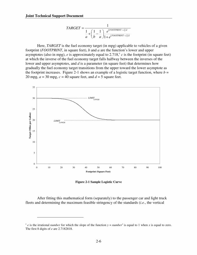
Joint Technical Support Document
2-6
( )
( )
1
1 1 1
1
FOOTPRINT c d
FOOTPRINT c d
TARGET
e
a b a e
−
−
=
+ −
+
Here, TARGET is the fuel economy target (in mpg) applicable to vehicles of a given
footprint (FOOTPRINT, in square feet), b and a are the function’s lower and upper
asymptotes (also in mpg), e is approximately equal to 2.718,c c is the footprint (in square feet)
at which the inverse of the fuel economy target falls halfway between the inverses of the
lower and upper asymptotes, and d is a parameter (in square feet) that determines how
gradually the fuel economy target transitions from the upper toward the lower asymptote as
the footprint increases. Figure 2-1 shows an example of a logistic target function, where b =
20 mpg, a = 30 mpg, c = 40 square feet, and d = 5 square feet.
0
5
10
15
20
25
30
35
0 10 20 30 40 50 60 70 80 90 100
Footprint (Square Feet)
Targ
et
(Mil
es p
er G
all
on
)
LIMITUPPER
LIMITLOWER
Figure 2-1 Sample Logistic Curve
After fitting this mathematical form (separately) to the passenger car and light truck
fleets and determining the maximum feasible stringency of the standards (i.e., the vertical
c e is the irrational number for which the slope of the function y = number
x is equal to 1 when x is equal to zero.
The first 8 digits of e are 2.7182818.
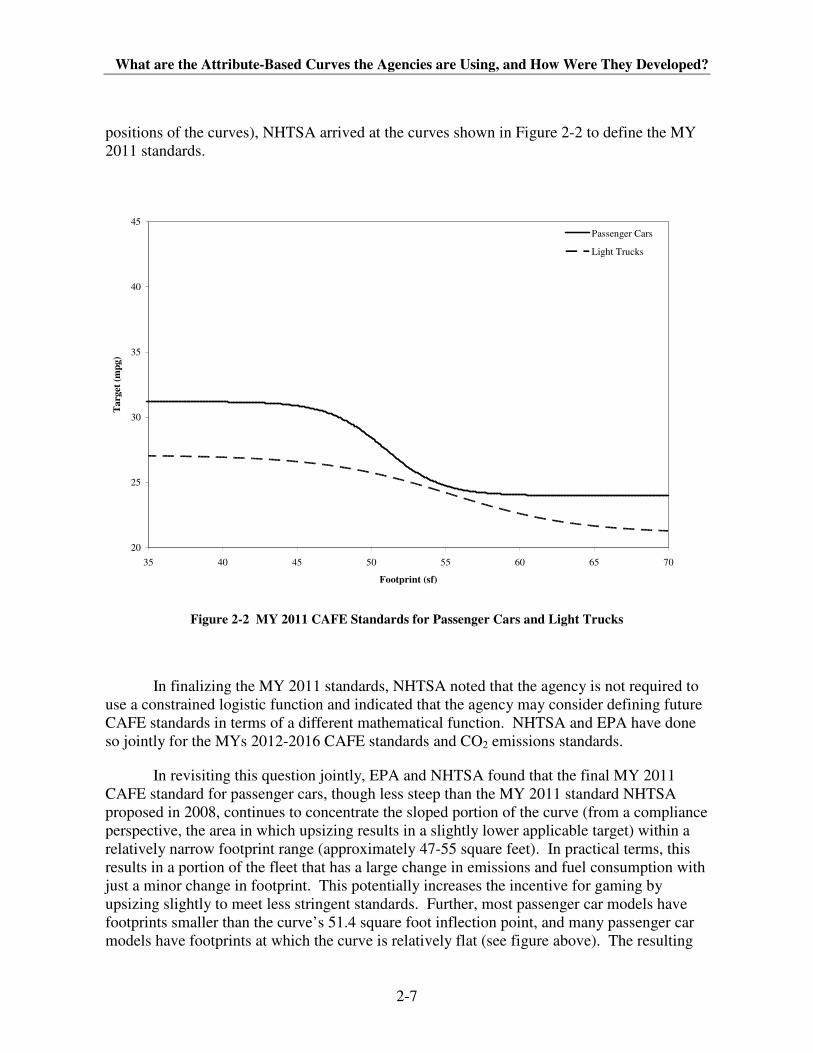
What are the Attribute-Based Curves the Agencies are Using, and How Were They Developed?
2-7
positions of the curves), NHTSA arrived at the curves shown in Figure 2-2 to define the MY
2011 standards.
20
25
30
35
40
45
35 40 45 50 55 60 65 70
Footprint (sf)
Target
(m
pg)
Passenger Cars
Light Trucks
Figure 2-2 MY 2011 CAFE Standards for Passenger Cars and Light Trucks
In finalizing the MY 2011 standards, NHTSA noted that the agency is not required to
use a constrained logistic function and indicated that the agency may consider defining future
CAFE standards in terms of a different mathematical function. NHTSA and EPA have done
so jointly for the MYs 2012-2016 CAFE standards and CO2 emissions standards.
In revisiting this question jointly, EPA and NHTSA found that the final MY 2011
CAFE standard for passenger cars, though less steep than the MY 2011 standard NHTSA
proposed in 2008, continues to concentrate the sloped portion of the curve (from a compliance
perspective, the area in which upsizing results in a slightly lower applicable target) within a
relatively narrow footprint range (approximately 47-55 square feet). In practical terms, this
results in a portion of the fleet that has a large change in emissions and fuel consumption with
just a minor change in footprint. This potentially increases the incentive for gaming by
upsizing slightly to meet less stringent standards. Further, most passenger car models have
footprints smaller than the curve’s 51.4 square foot inflection point, and many passenger car
models have footprints at which the curve is relatively flat (see figure above). The resulting
Joint Technical Support Document
2-8
fit to the data was forced by choice of asymptotes defining the constrained logistic function.
The agencies discuss below the alternative function that seeks to prevent this from occurring.
For both passenger cars and light trucks, a mathematical function that has some slope
at most footprints where vehicles are produced is advantageous in terms of fairly balancing
regulatory burdens among manufacturers, and in terms of providing a disincentive to respond
to new standards by downsizing vehicles in ways that compromise vehicle safety. For
example, a flat standard has drawbacks discussed above: it may be very difficult for a full-line
manufacturer to meet, while requiring very little of a manufacturer concentrating on small
vehicles, and a flat standard may provide an incentive to manufacturers to downsize certain
vehicles, in order to “balance out” other vehicles subject to the same standard.
As a potential alternative to the constrained logistic function, NHTSA had, in
proposing MY 2011 standards, presented information regarding a constrained linear function
(or piecewise linear function). As shown in the 2008 NPRM, a constrained linear function
has the potential to avoid creating a localized region (in terms of vehicle footprint) over which
the slope of the function is relatively steep. Although NHTSA did not receive public
comments on this option, the agency indicated that it still believed a linear function
constrained by upper (on a gpm basis) and possibly lower limits could merit reconsideration
in future CAFE rulemakings.
Having re-examined a piecewise linear function or constrained linear function for
purposes of the proposed standards, NHTSA and EPA tentatively concluded that for both
passenger cars and light trucks, it remained important to maintain a function with a
meaningfully sloped section covering a wide footprint range, thereby providing a well-
distributed disincentive to downsize vehicles in ways that could compromise highway safety.
Also, the function proposed was not so steeply sloped that it would provide a strong incentive
to increase vehicle size in order to obtain a lower CAFE requirement and higher CO2 limit,
thereby compromising energy and environmental benefits. Therefore, the CAFE and CO2
emissions standards proposed in the NPRM were defined by constrained linear or piecewise
linear functions.
The NHTSA constrained linear function was defined according to the following
formula:
1
1 1, ,
TARGET
MIN MAX c FOOTPRINT da b
=
× +
Here, TARGET is the fuel economy target (in mpg) applicable to vehicles of a given
footprint (FOOTPRINT, in square feet), b and a are the function’s lower and upper
asymptotes (also in mpg), respectively, c is the slope (in gpm per square foot) of the sloped
portion of the function, and d is the intercept (in gpm) of the sloped portion of the function
(that is, the value the sloped portion would take if extended to a footprint of 0 square feet.
The MIN and MAX functions take the minimum and maximum, respectively of the included
values; for example, MIN(1,2) = 1, MAX(1,2) = 2, and MIN[MAX(1,2),3)]=2. Figure 2-3
shows an example of a linear target function, where a = 0.0241 gpm (41.6 mpg), b = 0.032
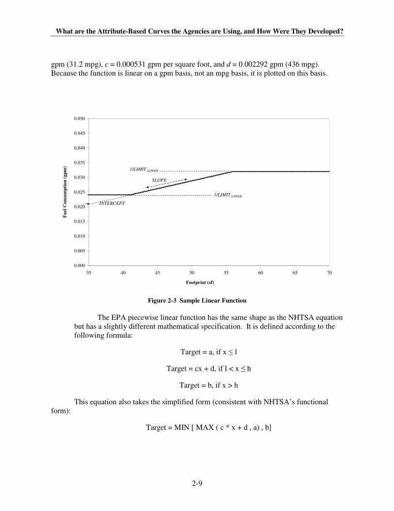
What are the Attribute-Based Curves the Agencies are Using, and How Were They Developed?
2-9
gpm (31.2 mpg), c = 0.000531 gpm per square foot, and d = 0.002292 gpm (436 mpg).
Because the function is linear on a gpm basis, not an mpg basis, it is plotted on this basis.
0.000
0.005
0.010
0.015
0.020
0.025
0.030
0.035
0.040
0.045
0.050
35 40 45 50 55 60 65 70
Footprint (sf)
Fu
el C
on
sum
pti
on
(gp
m)
1/LIMITUPPER
1/LIMITLOWER
INTERCEPT
SLOPE
Figure 2-3 Sample Linear Function
The EPA piecewise linear function has the same shape as the NHTSA equation
but has a slightly different mathematical specification. It is defined according to the
following formula:
Target = a, if x ≤ l
Target = cx + d, if l < x ≤ h
Target = b, if x > h
This equation also takes the simplified form (consistent with NHTSA’s functional
form):
Target = MIN [ MAX ( c * x + d , a) , b]
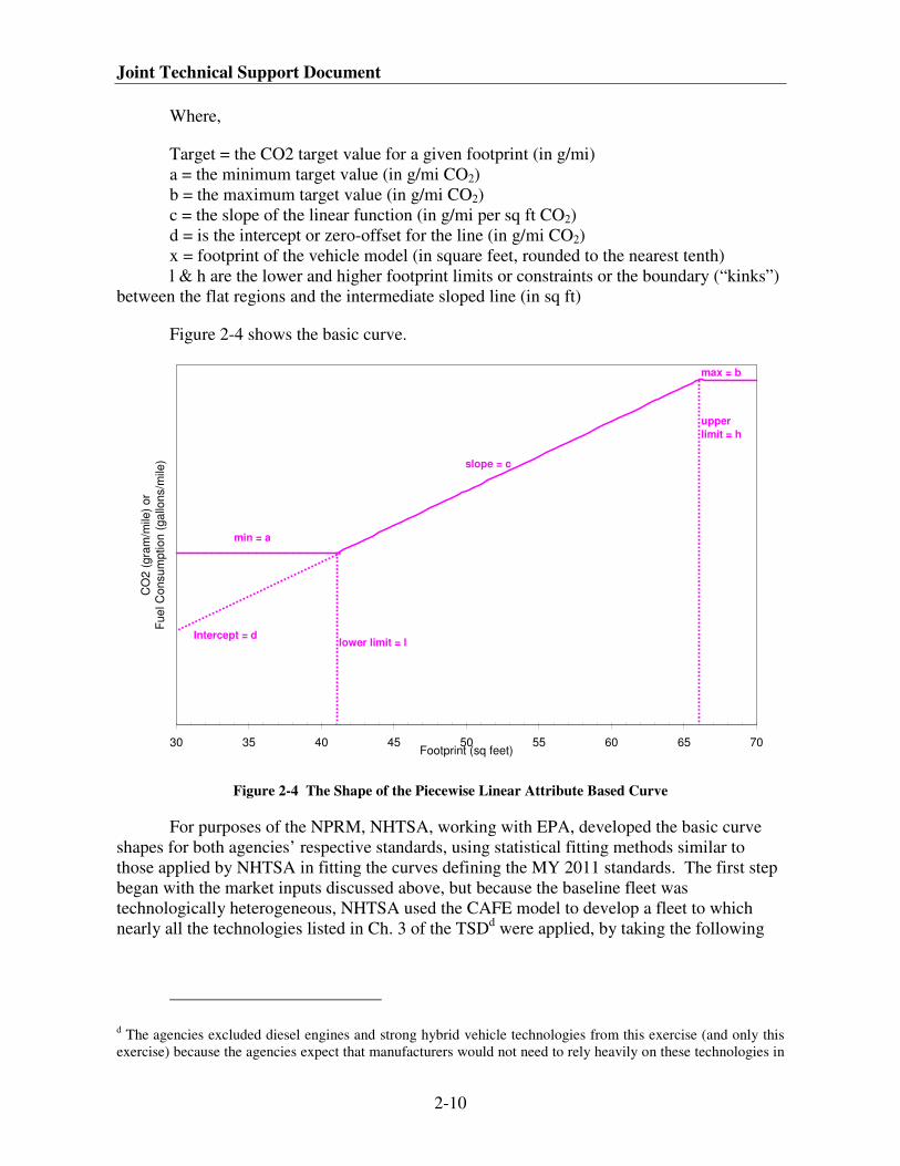
Joint Technical Support Document
2-10
Where,
Target = the CO2 target value for a given footprint (in g/mi)
a = the minimum target value (in g/mi CO2)
b = the maximum target value (in g/mi CO2)
c = the slope of the linear function (in g/mi per sq ft CO2)
d = is the intercept or zero-offset for the line (in g/mi CO2)
x = footprint of the vehicle model (in square feet, rounded to the nearest tenth)
l & h are the lower and higher footprint limits or constraints or the boundary (“kinks”)
between the flat regions and the intermediate sloped line (in sq ft)
Figure 2-4 shows the basic curve.
30 35 40 45 50 55 60 65 70Footprint (sq feet)
CO
2 (
gra
m/m
ile)
or
Fue
l C
onsum
ption (
gallo
ns/m
ile)
lower limit = lIntercept = d
upper
limit = h
slope = c
min = a
max = b
Figure 2-4 The Shape of the Piecewise Linear Attribute Based Curve
For purposes of the NPRM, NHTSA, working with EPA, developed the basic curve
shapes for both agencies’ respective standards, using statistical fitting methods similar to
those applied by NHTSA in fitting the curves defining the MY 2011 standards. The first step
began with the market inputs discussed above, but because the baseline fleet was
technologically heterogeneous, NHTSA used the CAFE model to develop a fleet to which
nearly all the technologies listed in Ch. 3 of the TSDd were applied, by taking the following
d The agencies excluded diesel engines and strong hybrid vehicle technologies from this exercise (and only this
exercise) because the agencies expect that manufacturers would not need to rely heavily on these technologies in
What are the Attribute-Based Curves the Agencies are Using, and How Were They Developed?
2-11
steps: (1) applying all non-diesel and non-hybrid technologies to each vehicles according to
their applicability, (2) treating all manufacturers as unwilling to pay civil penalties rather than
applying technology, (3) applying any technology at any time, irrespective of scheduled
vehicle redesigns or freshening, and (4) ignoring “phase-in caps” that constrain the overall
amount of technology that can be applied by the model to a given manufacturer’s fleet. These
steps helped to increase technological parity among vehicle models, thereby providing a better
basis (than the baseline fleet) for estimating the statistical relationship between vehicle size
and fuel economy. In other words, this process normalized the fleet such that differences in
technology had a minimal contribution to the variation (scatter) in the data. This process also
served to eliminate the influence of differing degrees of pre-existing fuel-saving technology at
various footprint values. This slightly flattened the slope of the line, indicating that a
regression without adjusting for different 2008 vehicle technologies would not only have
overestimated the dependence of fuel economy on footprint, but would also have provided an
inappropriate incentive to upsize vehicles.
In fitting the curves, EPA and NHTSA also continued to apply constraints to limit the
function’s value for both the smallest and largest vehicles. Without a limit at the smallest
footprints, the function—whether logistic or linear—can reach values that would be unfairly
burdensome for a manufacturer that elects to focus on the market for small vehicles;
depending on the underlying data, an unconstrained form could apply targets to the smallest
vehicles that are simply unachievable. Limiting the function’s value for the smallest vehicles
thus assures that the function remains technologically achievable and economically
practicable for manufacturers focusing on small vehicles. Obviously, passenger
compartments can only become so small; this means, among other things, that a vehicle’s
frontal area—a key determinant of aerodynamic drag—can only become so small. Also, as
vehicle size decreases, complying with federal motor vehicle safety standards can necessitate
the addition of structural elements that add mass and thereby reduce fuel economy and
increase CO2 emissions. On the other side of the function, without a limit at the largest
footprints, the function may provide no floor on required fuel economy. Also, the safety
considerations that support the provision of a disincentive for downsizing as a compliance
strategy apply weakly—if at all—to the very largest vehicles. Limiting the function’s value
for the largest vehicles leads to a function with an inherent absolute minimum level of fuel
economy (or maximum emissions), while remaining consistent with safety considerations.
Before fitting the sloped portion of the constrained linear form, NHTSA and EPA
selected footprints above and below which to apply constraints (i.e., minimum and maximum
values) on the function. For passenger cars, the agencies noted that several manufacturers
offer small and, in some cases, sporty coupes below 41 square feet, examples including the
BMW Z4 and Mini, Saturn Sky, Honda Fit and S2000, Hyundai Tiburon, Mazda MX-5
Miata, Suzuki SX4, Toyota Yaris, and Volkswagen New Beetle. Because such vehicles
represent a small portion (less than 10 percent) of the passenger car market, yet often have
order to comply with the standards. NHTSA and EPA did include diesel engines and strong hybrid vehicle
technologies in all other portions of their analyses.
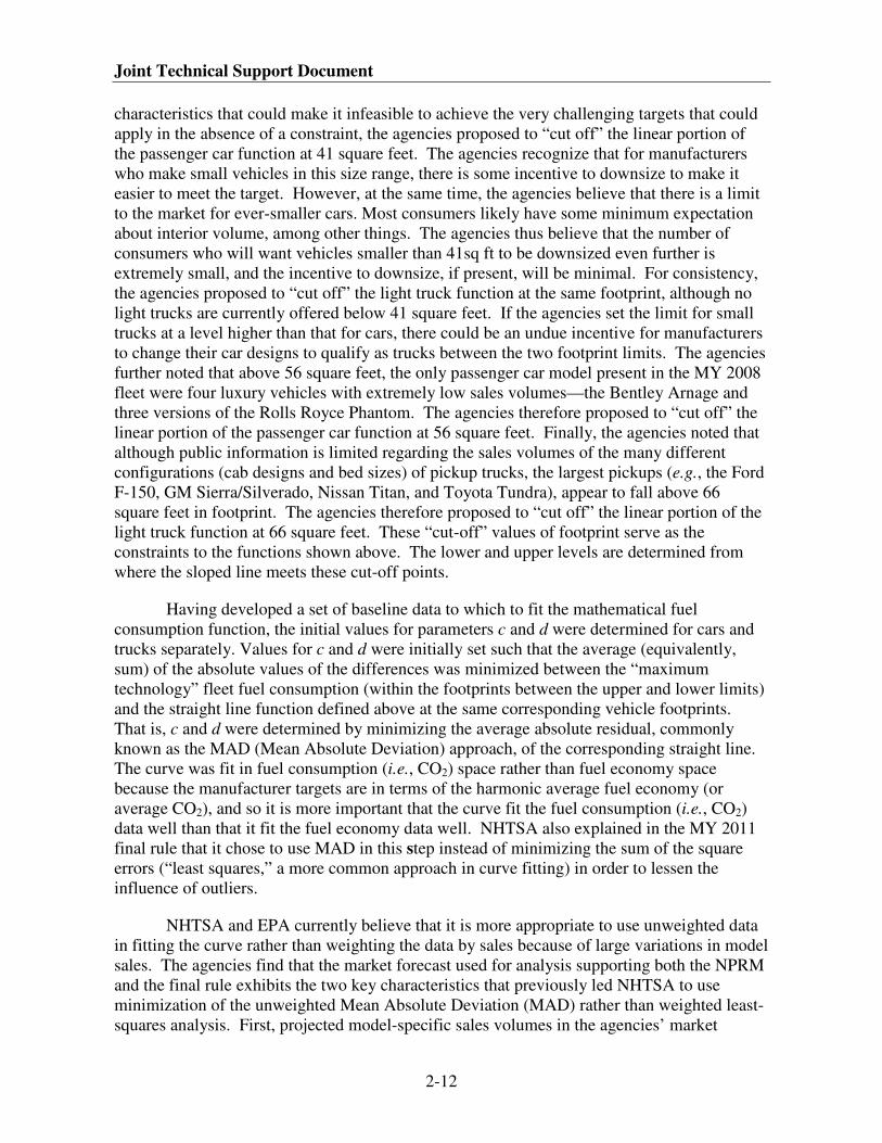
Joint Technical Support Document
2-12
characteristics that could make it infeasible to achieve the very challenging targets that could
apply in the absence of a constraint, the agencies proposed to “cut off” the linear portion of
the passenger car function at 41 square feet. The agencies recognize that for manufacturers
who make small vehicles in this size range, there is some incentive to downsize to make it
easier to meet the target. However, at the same time, the agencies believe that there is a limit
to the market for ever-smaller cars. Most consumers likely have some minimum expectation
about interior volume, among other things. The agencies thus believe that the number of
consumers who will want vehicles smaller than 41sq ft to be downsized even further is
extremely small, and the incentive to downsize, if present, will be minimal. For consistency,
the agencies proposed to “cut off” the light truck function at the same footprint, although no
light trucks are currently offered below 41 square feet. If the agencies set the limit for small
trucks at a level higher than that for cars, there could be an undue incentive for manufacturers
to change their car designs to qualify as trucks between the two footprint limits. The agencies
further noted that above 56 square feet, the only passenger car model present in the MY 2008
fleet were four luxury vehicles with extremely low sales volumes—the Bentley Arnage and
three versions of the Rolls Royce Phantom. The agencies therefore proposed to “cut off” the
linear portion of the passenger car function at 56 square feet. Finally, the agencies noted that
although public information is limited regarding the sales volumes of the many different
configurations (cab designs and bed sizes) of pickup trucks, the largest pickups (e.g., the Ford
F-150, GM Sierra/Silverado, Nissan Titan, and Toyota Tundra), appear to fall above 66
square feet in footprint. The agencies therefore proposed to “cut off” the linear portion of the
light truck function at 66 square feet. These “cut-off” values of footprint serve as the
constraints to the functions shown above. The lower and upper levels are determined from
where the sloped line meets these cut-off points.
Having developed a set of baseline data to which to fit the mathematical fuel
consumption function, the initial values for parameters c and d were determined for cars and
trucks separately. Values for c and d were initially set such that the average (equivalently,
sum) of the absolute values of the differences was minimized between the “maximum
technology” fleet fuel consumption (within the footprints between the upper and lower limits)
and the straight line function defined above at the same corresponding vehicle footprints.
That is, c and d were determined by minimizing the average absolute residual, commonly
known as the MAD (Mean Absolute Deviation) approach, of the corresponding straight line.
The curve was fit in fuel consumption (i.e., CO2) space rather than fuel economy space
because the manufacturer targets are in terms of the harmonic average fuel economy (or
average CO2), and so it is more important that the curve fit the fuel consumption (i.e., CO2)
data well than that it fit the fuel economy data well. NHTSA also explained in the MY 2011
final rule that it chose to use MAD in this step instead of minimizing the sum of the square
errors (“least squares,” a more common approach in curve fitting) in order to lessen the
influence of outliers.
NHTSA and EPA currently believe that it is more appropriate to use unweighted data
in fitting the curve rather than weighting the data by sales because of large variations in model
sales. The agencies find that the market forecast used for analysis supporting both the NPRM
and the final rule exhibits the two key characteristics that previously led NHTSA to use
minimization of the unweighted Mean Absolute Deviation (MAD) rather than weighted least-
squares analysis. First, projected model-specific sales volumes in the agencies’ market
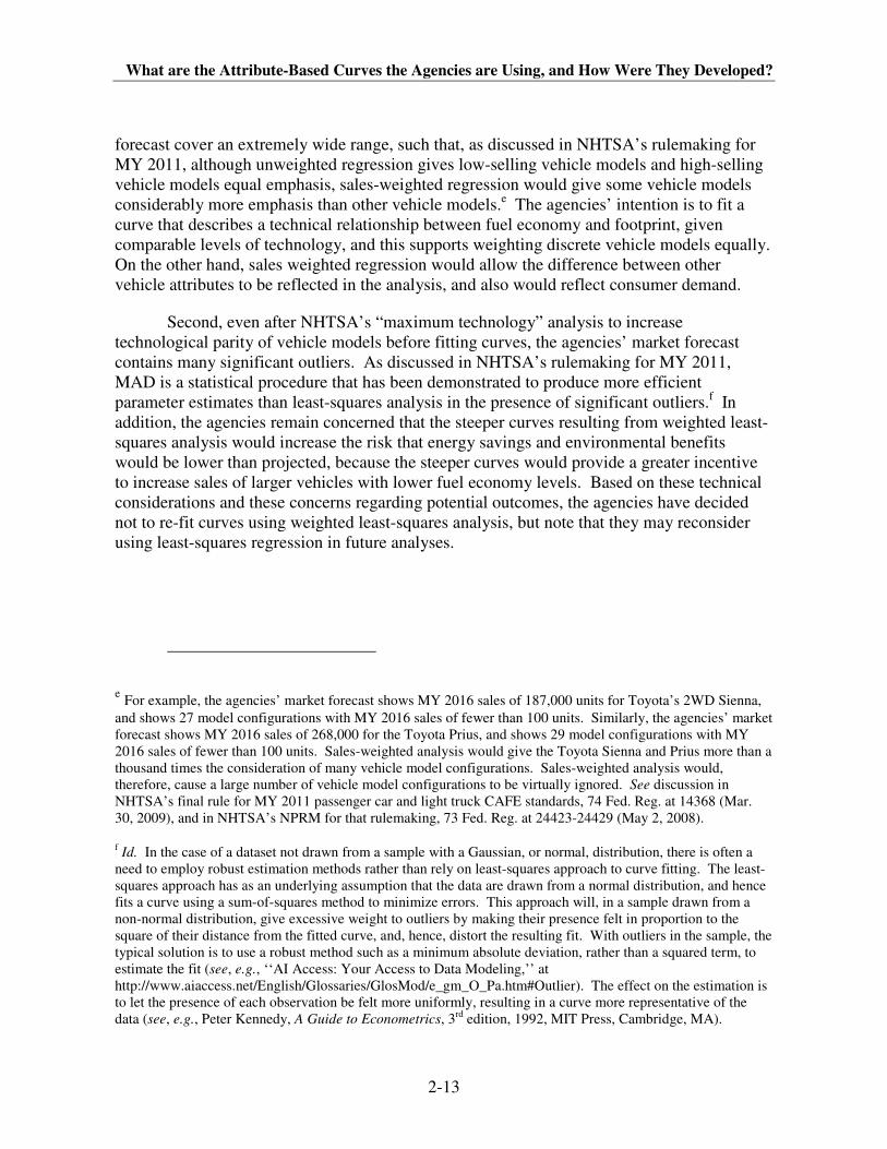
What are the Attribute-Based Curves the Agencies are Using, and How Were They Developed?
2-13
forecast cover an extremely wide range, such that, as discussed in NHTSA’s rulemaking for
MY 2011, although unweighted regression gives low-selling vehicle models and high-selling
vehicle models equal emphasis, sales-weighted regression would give some vehicle models
considerably more emphasis than other vehicle models.e The agencies’ intention is to fit a
curve that describes a technical relationship between fuel economy and footprint, given
comparable levels of technology, and this supports weighting discrete vehicle models equally.
On the other hand, sales weighted regression would allow the difference between other
vehicle attributes to be reflected in the analysis, and also would reflect consumer demand.
Second, even after NHTSA’s “maximum technology” analysis to increase
technological parity of vehicle models before fitting curves, the agencies’ market forecast
contains many significant outliers. As discussed in NHTSA’s rulemaking for MY 2011,
MAD is a statistical procedure that has been demonstrated to produce more efficient
parameter estimates than least-squares analysis in the presence of significant outliers.f In
addition, the agencies remain concerned that the steeper curves resulting from weighted least-
squares analysis would increase the risk that energy savings and environmental benefits
would be lower than projected, because the steeper curves would provide a greater incentive
to increase sales of larger vehicles with lower fuel economy levels. Based on these technical
considerations and these concerns regarding potential outcomes, the agencies have decided
not to re-fit curves using weighted least-squares analysis, but note that they may reconsider
using least-squares regression in future analyses.
e For example, the agencies’ market forecast shows MY 2016 sales of 187,000 units for Toyota’s 2WD Sienna,
and shows 27 model configurations with MY 2016 sales of fewer than 100 units. Similarly, the agencies’ market
forecast shows MY 2016 sales of 268,000 for the Toyota Prius, and shows 29 model configurations with MY
2016 sales of fewer than 100 units. Sales-weighted analysis would give the Toyota Sienna and Prius more than a
thousand times the consideration of many vehicle model configurations. Sales-weighted analysis would,
therefore, cause a large number of vehicle model configurations to be virtually ignored. See discussion in
NHTSA’s final rule for MY 2011 passenger car and light truck CAFE standards, 74 Fed. Reg. at 14368 (Mar.
30, 2009), and in NHTSA’s NPRM for that rulemaking, 73 Fed. Reg. at 24423-24429 (May 2, 2008).
f Id. In the case of a dataset not drawn from a sample with a Gaussian, or normal, distribution, there is often a
need to employ robust estimation methods rather than rely on least-squares approach to curve fitting. The least-
squares approach has as an underlying assumption that the data are drawn from a normal distribution, and hence
fits a curve using a sum-of-squares method to minimize errors. This approach will, in a sample drawn from a
non-normal distribution, give excessive weight to outliers by making their presence felt in proportion to the
square of their distance from the fitted curve, and, hence, distort the resulting fit. With outliers in the sample, the
typical solution is to use a robust method such as a minimum absolute deviation, rather than a squared term, to
estimate the fit (see, e.g., ‘‘AI Access: Your Access to Data Modeling,’’ at
http://www.aiaccess.net/English/Glossaries/GlosMod/e_gm_O_Pa.htm#Outlier). The effect on the estimation is
to let the presence of each observation be felt more uniformly, resulting in a curve more representative of the
data (see, e.g., Peter Kennedy, A Guide to Econometrics, 3rd
edition, 1992, MIT Press, Cambridge, MA).
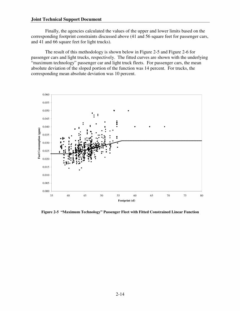
Joint Technical Support Document
2-14
Finally, the agencies calculated the values of the upper and lower limits based on the
corresponding footprint constraints discussed above (41 and 56 square feet for passenger cars,
and 41 and 66 square feet for light trucks).
The result of this methodology is shown below in Figure 2-5 and Figure 2-6 for
passenger cars and light trucks, respectively. The fitted curves are shown with the underlying
“maximum technology” passenger car and light truck fleets. For passenger cars, the mean
absolute deviation of the sloped portion of the function was 14 percent. For trucks, the
corresponding mean absolute deviation was 10 percent.
0.000
0.005
0.010
0.015
0.020
0.025
0.030
0.035
0.040
0.045
0.050
0.055
0.060
35 40 45 50 55 60 65 70 75 80
Footprint (sf)
Fu
el C
on
sum
pti
on
(gp
m)
Figure 2-5 “Maximum Technology” Passenger Fleet with Fitted Constrained Linear Function
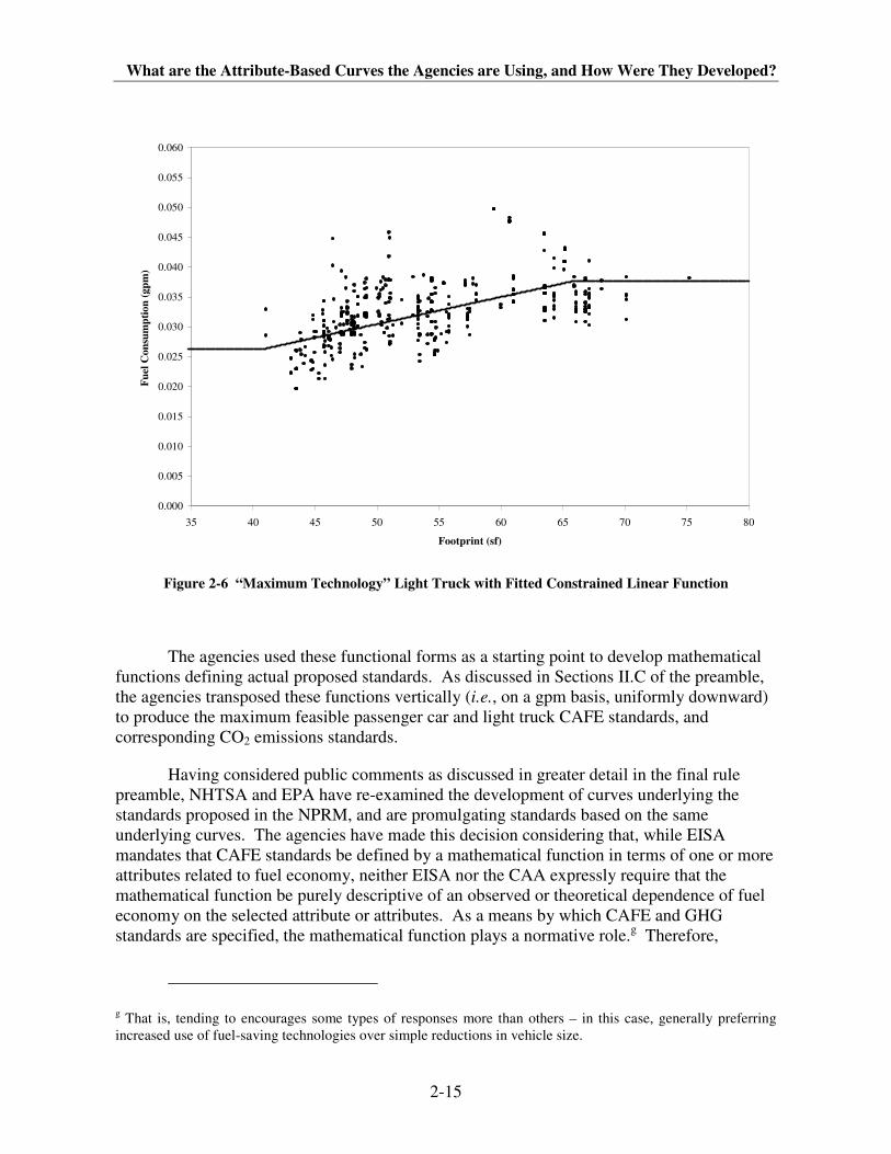
What are the Attribute-Based Curves the Agencies are Using, and How Were They Developed?
2-15
0.000
0.005
0.010
0.015
0.020
0.025
0.030
0.035
0.040
0.045
0.050
0.055
0.060
35 40 45 50 55 60 65 70 75 80
Footprint (sf)
Fu
el C
on
sum
pti
on
(gp
m)
Figure 2-6 “Maximum Technology” Light Truck with Fitted Constrained Linear Function
The agencies used these functional forms as a starting point to develop mathematical
functions defining actual proposed standards. As discussed in Sections II.C of the preamble,
the agencies transposed these functions vertically (i.e., on a gpm basis, uniformly downward)
to produce the maximum feasible passenger car and light truck CAFE standards, and
corresponding CO2 emissions standards.
Having considered public comments as discussed in greater detail in the final rule
preamble, NHTSA and EPA have re-examined the development of curves underlying the
standards proposed in the NPRM, and are promulgating standards based on the same
underlying curves. The agencies have made this decision considering that, while EISA
mandates that CAFE standards be defined by a mathematical function in terms of one or more
attributes related to fuel economy, neither EISA nor the CAA expressly require that the
mathematical function be purely descriptive of an observed or theoretical dependence of fuel
economy on the selected attribute or attributes. As a means by which CAFE and GHG
standards are specified, the mathematical function plays a normative role.g Therefore,
g That is, tending to encourages some types of responses more than others – in this case, generally preferring
increased use of fuel-saving technologies over simple reductions in vehicle size.
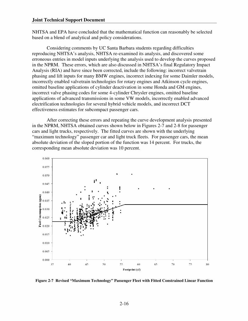
Joint Technical Support Document
2-16
NHTSA and EPA have concluded that the mathematical function can reasonably be selected
based on a blend of analytical and policy considerations.
Considering comments by UC Santa Barbara students regarding difficulties
reproducing NHTSA’s analysis, NHTSA re-examined its analysis, and discovered some
erroneous entries in model inputs underlying the analysis used to develop the curves proposed
in the NPRM. These errors, which are also discussed in NHTSA’s final Regulatory Impact
Analysis (RIA) and have since been corrected, include the following: incorrect valvetrain
phasing and lift inputs for many BMW engines, incorrect indexing for some Daimler models,
incorrectly enabled valvetrain technologies for rotary engines and Atkinson cycle engines,
omitted baseline applications of cylinder deactivation in some Honda and GM engines,
incorrect valve phasing codes for some 4-cylinder Chrysler engines, omitted baseline
applications of advanced transmissions in some VW models, incorrectly enabled advanced
electrification technologies for several hybrid vehicle models, and incorrect DCT
effectiveness estimates for subcompact passenger cars.
After correcting these errors and repeating the curve development analysis presented
in the NPRM, NHTSA obtained curves shown below in Figures 2-7 and 2-8 for passenger
cars and light trucks, respectively. The fitted curves are shown with the underlying
“maximum technology” passenger car and light truck fleets. For passenger cars, the mean
absolute deviation of the sloped portion of the function was 14 percent. For trucks, the
corresponding mean absolute deviation was 10 percent.
Figure 2-7 Revised “Maximum Technology” Passenger Fleet with Fitted Constrained Linear Function
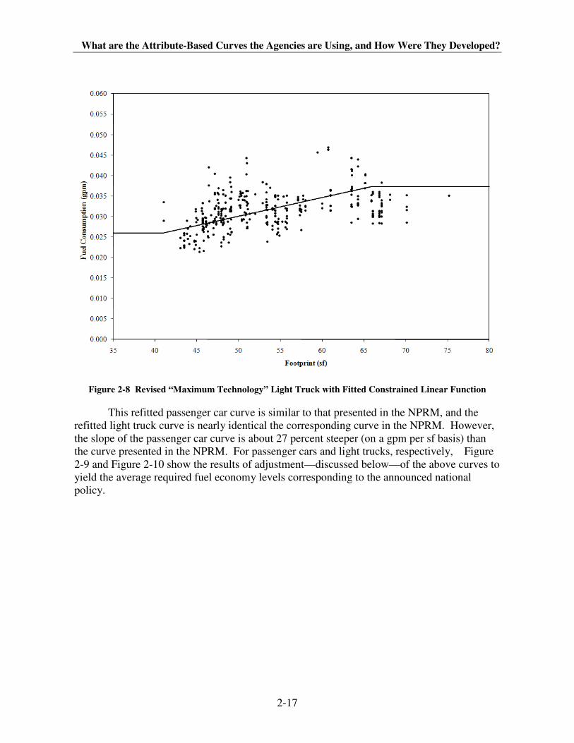
What are the Attribute-Based Curves the Agencies are Using, and How Were They Developed?
2-17
Figure 2-8 Revised “Maximum Technology” Light Truck with Fitted Constrained Linear Function
This refitted passenger car curve is similar to that presented in the NPRM, and the
refitted light truck curve is nearly identical the corresponding curve in the NPRM. However,
the slope of the passenger car curve is about 27 percent steeper (on a gpm per sf basis) than
the curve presented in the NPRM. For passenger cars and light trucks, respectively, Figure
2-9 and Figure 2-10 show the results of adjustment—discussed below—of the above curves to
yield the average required fuel economy levels corresponding to the announced national
policy.
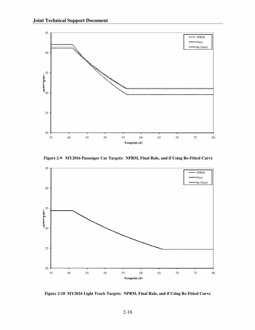
Joint Technical Support Document
2-18
20
25
30
35
40
45
35 40 45 50 55 60 65 70 75 80
Target (mpg)
Footprint (sf)
NPRM
Final
Re-Fitted
Figure 2-9 MY2016 Passenger Car Targets: NPRM, Final Rule, and if Using Re-Fitted Curve
20
25
30
35
40
45
35 40 45 50 55 60 65 70 75 80
Target (mpg)
Footprint (sf)
NPRM
Final
Re-Fitted
Figure 2-10 MY2016 Light Truck Targets: NPRM, Final Rule, and if Using Re-Fitted Curve
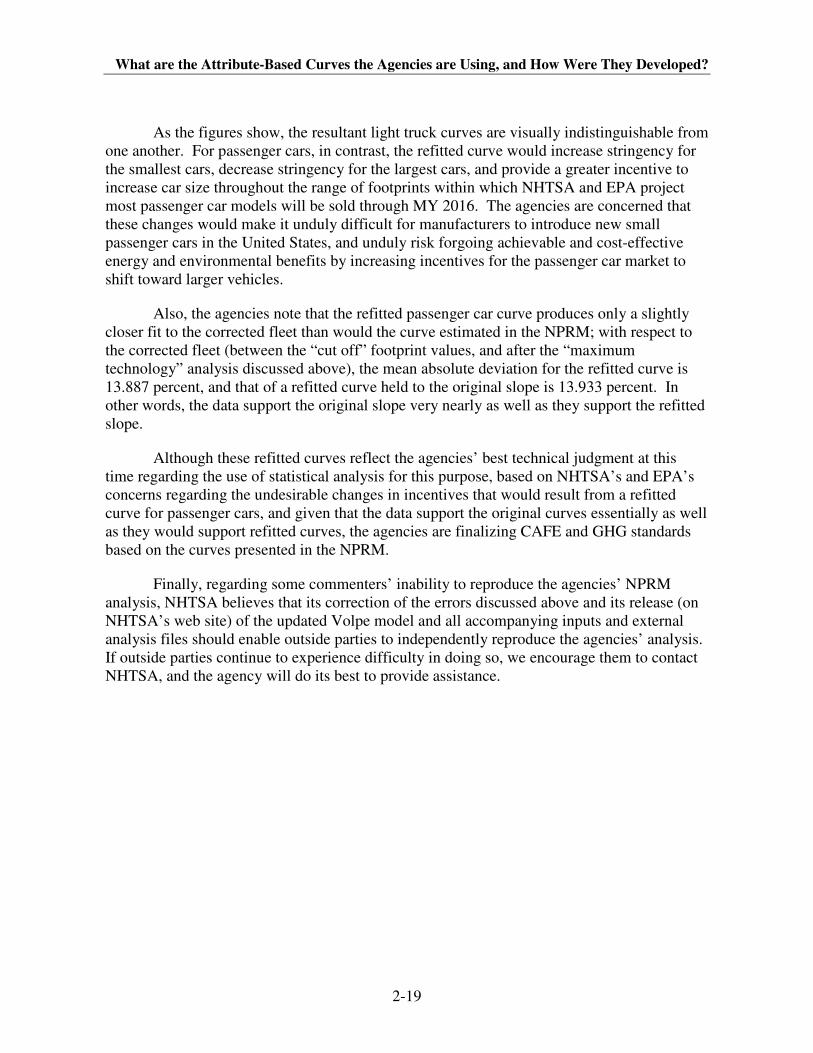
What are the Attribute-Based Curves the Agencies are Using, and How Were They Developed?
2-19
As the figures show, the resultant light truck curves are visually indistinguishable from
one another. For passenger cars, in contrast, the refitted curve would increase stringency for
the smallest cars, decrease stringency for the largest cars, and provide a greater incentive to
increase car size throughout the range of footprints within which NHTSA and EPA project
most passenger car models will be sold through MY 2016. The agencies are concerned that
these changes would make it unduly difficult for manufacturers to introduce new small
passenger cars in the United States, and unduly risk forgoing achievable and cost-effective
energy and environmental benefits by increasing incentives for the passenger car market to
shift toward larger vehicles.
Also, the agencies note that the refitted passenger car curve produces only a slightly
closer fit to the corrected fleet than would the curve estimated in the NPRM; with respect to
the corrected fleet (between the “cut off” footprint values, and after the “maximum
technology” analysis discussed above), the mean absolute deviation for the refitted curve is
13.887 percent, and that of a refitted curve held to the original slope is 13.933 percent. In
other words, the data support the original slope very nearly as well as they support the refitted
slope.
Although these refitted curves reflect the agencies’ best technical judgment at this
time regarding the use of statistical analysis for this purpose, based on NHTSA’s and EPA’s
concerns regarding the undesirable changes in incentives that would result from a refitted
curve for passenger cars, and given that the data support the original curves essentially as well
as they would support refitted curves, the agencies are finalizing CAFE and GHG standards
based on the curves presented in the NPRM.
Finally, regarding some commenters’ inability to reproduce the agencies’ NPRM
analysis, NHTSA believes that its correction of the errors discussed above and its release (on
NHTSA’s web site) of the updated Volpe model and all accompanying inputs and external
analysis files should enable outside parties to independently reproduce the agencies’ analysis.
If outside parties continue to experience difficulty in doing so, we encourage them to contact
NHTSA, and the agency will do its best to provide assistance.
Joint Technical Support Document
2-20
References
1 49 U.S.C. 32902(a)(3)(A).
2 The 2002 NAS Report described at length and quantified the potential safety problem with average fuel
economy standards that specify a single numerical requirement for the entire industry. See NAS Report at 5,
finding 12. Docket EPA-HQ-OAR-2009-0472-0147.
3 Id. at 4-5, finding 10. Docket EPA-HQ-OAR-2009-0472-0147.
4 49 U.S.C. 32902(b)(4).
Technologies Considered in the Agencies’ Analysis
3-1
CHAPTER 3: Technologies Considered in the Agencies’
Analysis
This Chapter of the joint TSD describes the technologies NHTSA and EPA
evaluated as potential inputs in their respective models and provides estimates of the
technologies’ costs, effectiveness and availability. This Chapter also describes, in general
terms, how the agencies use these inputs in their respective models. For greater detail on
this subject, please see Section V of NHTSA’s FRIA and Chapter 4 of EPA’s RIA.
3.1 How do the agencies decide which technologies to include in the
analysis?
Technology assumptions, i.e., assumptions about their availability, cost,
effectiveness, and the rate at which they can be incorporated into new vehicles, are often
very controversial as they have a significant impact on the levels of the standards.
Agencies must, therefore, take great care in developing and justifying these
assumptions. In developing technology inputs for MY 2012-2016 standards the agencies
reviewed the technology assumptions that NHTSA used in setting the MY 2011
standards, the agencies reviewed the technology input assumptions identified in EPA’s
2008 Staff Technical Report,1 the comments that NHTSA received in response to its May
2008 Notice of Proposed Rulemaking, and the comments that the agencies received in
response to its September 2009 Notice of Proposed Rulemaking. In addition, the
agencies supplemented their review with information from the sources described in the
following section.
3.1.1 Reports and papers in the literature
NHTSA and EPA have done extensive research in identifying the most credible
sources of information. These sources included: the 2002 NAS report on the effectiveness
and impact of CAFE standards;2 the 2004 study done by NESCCAF;
3 the California Air
Resources Board (CARB) Initial Statement of Reasons in support of their carbon
rulemaking;4 a 2006 study done by Energy and Environmental Analysis (EEA) for the
Department of Energy;5 a study done by the Martec Group for the Alliance of
Automobile Manufacturers, and an update by the Martec Group to that study;6 and
vehicle fuel economy certification data. Both agencies also reviewed the published
technical literature which addressed the issue of CO2 emission control and fuel economy,
such as papers published by the Society of Automotive Engineers and the American
Society of Mechanical Engineers, as well as papers submitted by commenters (for
example, the Aluminum Association) to the agencies’ joint NPRM. In addition,
confidential data submitted by vehicle manufacturers in response to NHTSA’s request for
product plans,7 and confidential information shared by automotive industry component
suppliers in meetings with EPA and NHTSA staff held during the second half of the 2007
calendar year were used as a cross check of the public data mentioned above and not as a
significant basis for this rulemaking.
Joint Technical Support Document
3-2
EPA also has a contracted study ongoing with FEV that consists of complete
system tear-downs to evaluate technologies down to the nuts and bolts to arrive at very
detailed estimates of the costs associated with manufacturing them. For the NPRM, the
agencies used a completed analysis to estimate costs of turbocharging with downsizing
for I4 engines only. The NPRM stated that tear-down cost estimates from FEV for
additional engine and transmission technologies became available shortly before the
release of the NPRM, but not in time to be incorporated into the agencies’ cost analysis
of the proposed standards. These preliminary results were made available for review and
the agencies stated they would consider this information for use in the final rule analysis.8
The NPRM also stated that a detailed report would be submitted to the docket on these
additional technologies during the public comment period for the proposal. That deadline
was not met but all additional technologies for which cost study tear downs have been
completed from this study with FEV (studies have now been completed on turbocharging
and downsizing for V6 and V8 engines, stoichiometric gasoline direct injection, 6/7/8-
speed automatic transmission and dual clutch transmission technologies) have been
considered for the final rule and details are contained in two reports placed in the
docket.9,10
EPA and NHTSA reviewed all of the above information in order to develop
the best estimates of availability, cost and effectiveness of these fuel-saving/CO2-
reducing technologies.
The agencies would also like to note that per the Energy Independence and
Security Act (EISA), the National Academies of Sciences has been conducting a study
for NHTSA to update chapter 3 of their 2002 NAS Report, which presents technology
effectiveness estimates for light-duty vehicles. The update takes a fresh look at that list
of technologies and their associated cost and effectiveness values. The updated NAS
report was expected to be available on September 30, 2009, but has not been completed
and released to the public. The results from this study thus are unavailable for this
rulemaking. The agencies look forward to considering the results from this study as part
of the next round of rulemaking for CAFE/GHG standards.
3.1.2 Fuel economy certification data
Where available, data from recent model years of EPA’s Fuel Economy
Certification Data were used for helping to determine the effectiveness of specific
technologies. CO2 and fuel consumption reduction estimates were estimated from EPA’s
fuel economy database on the two-cycle (FTP city & highway) fuel economy test results.
During the standard fuel economy test cycles, direct measurements of CO2 emissions are
made. This data, along with other measurements, are then used to calculate the estimated
fuel economy performance in gallons of fuel consumed per mile. Vehicle certification
data are an obviously reliable source for determination of the CO2 and fuel consumption
reduction potential when a directly comparable vehicle was offered both with and without
the specific CO2 and fuel consumption reducing technology, because a comparison
between the emissions data between the two vehicles directly reflect the application of
the technologies on the vehicle test cycles. Where possible, technology-specific
effectiveness numbers were extracted for vehicles where only the specific technology
would be changed from a reference vehicle, in order to eliminate any confounding of
Technologies Considered in the Agencies’ Analysis
3-3
values across several technologies. In some hybrid vehicle cases, the exact same vehicle
may not be offered, and a similar vehicle was selected for comparison.
3.2 Which technologies will be applicable during the model years to
which the rules apply?
One of the key factors that NHTSA and EPA considered in developing the
standards for each model year is the availability and feasibility of fuel-saving/CO2-
reducing technologies. A variety of technologies can be used to reduce fuel consumption
and CO2 emissions, whether they be engine-related (e.g., turbocharging), transmission-
related (e.g., six forward gears in place of four), accessory-related (e.g., electric power
steering), or vehicle-related (e.g., low rolling resistance tires). In taking a fresh look at
the availability and feasibility of technologies for purposes of setting the MYs 2012-2016
standards, the agencies reviewed NHTSA’s MY 2011 CAFE final rule and EPA’s 2008
Staff Report, as well as the public comments to the proposed rule and updated the
assumptions based on the most current information. As a check on this new analysis,
NHTSA and EPA also reviewed the product plans submitted by manufacturers to the
agencies in response to NHTSA’s November 2009 request for product plans.
Many technologies considered by the agencies, such as variable valve timing
(VVT), low rolling resistance tires, etc., are well known and readily available during the
rulemaking time period, and could be incorporated into vehicles once production
decisions are made. The agencies did not consider technologies in the research stage,
such as homogeneous charge compression ignition (HCCI), lean-burn direct injection
technology, etc., because their effectiveness and/or cost estimates contain a high level of
uncertainty.
The technologies considered by the NHTSA and EPA models are briefly
described below. They fall under the five broad categories of engine, transmission,
vehicle, electrification/accessory, and hybrid technologies. A more detailed description
of each technology, and the technology’s costs and effectiveness, is described in greater
detail in section 3.5 of this TSD.
Types of engine technologies that improve fuel economy and reduce CO2
emissions include the following:
• Low-friction lubricants – low viscosity and advanced low friction lubricants
oils are now available with improved performance and better lubrication.
• Reduction of engine friction losses – can be achieved through low-tension
piston rings, roller cam followers, improved material coatings, more optimal
thermal management, piston surface treatments, and other improvements in
the design of engine components and subsystems that improve engine
operation.
Joint Technical Support Document
3-4
• Conversion to dual overhead cam with dual cam phasing – as applied to
overhead valves designed to increase the air flow with more than two valves
per cylinder and reduce pumping losses.
• Cylinder deactivation – deactivates the intake and exhaust valves and prevents
fuel injection into some cylinders during light-load operation. The engine
runs temporarily as though it were a smaller engine which substantially
reduces pumping losses
• Variable valve timing – alters the timing or phase of the intake valve, exhaust
valve, or both, primarily to reduce pumping losses, increase specific power,
and control residual gases.
• Discrete variable valve lift – increases efficiency by optimizing air flow over
a broader range of engine operation which reduces pumping losses.
Accomplished by controlled switching between two or more cam profile lobe
heights.
• Continuous variable valve lift – is an electromechanically controlled system in
which cam period and phasing is changed as lift height is controlled. This
yields a wide range of performance optimization and volumetric efficiency,
including enabling the engine to be valve throttled.
• Stoichiometric gasoline direct-injection technology – injects fuel at high
pressure directly into the combustion chamber to improve cooling of the
air/fuel charge within the cylinder, which allows for higher compression ratios
and increased thermodynamic efficiency.
• Combustion restart – can be used in conjunction with gasoline direct-injection
systems to enable idle-off or start-stop functionality. Similar to other start-
stop technologies, additional enablers, such as electric power steering,
accessory drive components, and auxiliary oil pump, might be required.
• Turbocharging and downsizing – increases the available airflow and specific
power level, allowing a reduced engine size while maintaining performance.
This reduces pumping losses at lighter loads in comparison to a larger engine.
• Exhaust-gas recirculation boost – increases the exhaust-gas recirculation used
in the combustion process to increase thermal efficiency and reduce pumping
losses.
• Diesel engines – have several characteristics that give superior fuel efficiency,
including reduced pumping losses due to lack of (or greatly reduced)
throttling, and a combustion cycle that operates at a higher compression ratio,
with a very lean air/fuel mixture, than an equivalent-performance gasoline
engine. This technology requires additional enablers, such as NOx trap
catalyst after-treatment or selective catalytic reduction NOx after-treatment.
Technologies Considered in the Agencies’ Analysis
3-5
Types of transmission technologies considered include:
• Improved automatic transmission controls – optimizes shift schedule to
maximize fuel efficiency under wide ranging conditions, and minimizes losses
associated with torque converter slip through lock-up or modulation.
• Six-, seven-, and eight-speed automatic transmissions – the gear ratio spacing
and transmission ratio are optimized to enable the engine to operate in a more
efficient operating range over a broader range of vehicle operating conditions.
• Dual clutch or automated shift manual transmissions – are similar to manual
transmissions, but the vehicle controls shifting and launch functions. A dual-
clutch automated shift manual transmission uses separate clutches for even-
numbered and odd-numbered gears, so the next expected gear is pre-selected,
which allows for faster and smoother shifting.
• Continuously variable transmission – commonly uses V-shaped pulleys
connected by a metal belt rather than gears to provide ratios for operation.
Unlike manual and automatic transmissions with fixed transmission ratios,
continuously variable transmissions can provide fully variable and an infinite
number of transmission ratios that enable the engine to operate in a more
efficient operating range over a broader range of vehicle operating conditions.
• Manual 6-speed transmission – offers an additional gear ratio, often with a
higher overdrive gear ratio, than a 5-speed manual transmission.
Types of vehicle technologies considered include:
• Low-rolling-resistance tires – have characteristics that reduce frictional losses
associated with the energy dissipated in the deformation of the tires under
load, therefore reducing the energy needed to move the vehicle.
• Low-drag brakes – reduce the sliding friction of disc brake pads on rotors
when the brakes are not engaged because the brake pads are pulled away from
the rotors.
• Front or secondary axle disconnect for four-wheel drive systems – provides a
torque distribution disconnect between front and rear axles when torque is not
required for the non-driving axle. This results in the reduction of associated
parasitic energy losses.
• Aerodynamic drag reduction – is achieved by changing vehicle shape or
reducing frontal area, including skirts, air dams, underbody covers, and more
aerodynamic side view mirrors.
• Mass reduction and material substitution – Mass reduction encompasses a
variety of techniques ranging from improved design and better component
Joint Technical Support Document
3-6
integration to application of lighter and higher-strength materials. Mass
reduction is further compounded by reductions in engine power and ancillary
systems (transmission, steering, brakes, suspension, etc.).
Types of electrification/accessory and hybrid technologies considered include:
• Electric power steering (EPS) – is an electrically-assisted steering system that
has advantages over traditional hydraulic power steering because it replaces a
continuously operated hydraulic pump, thereby reducing parasitic losses from
the accessory drive.
• Improved accessories (IACC) – may include high efficiency alternators,
electrically driven (i.e., on-demand) water pumps and cooling fans. This
excludes other electrical accessories such as electric oil pumps and electrically
driven air conditioner compressors.
• Air Conditioner Systems – These technologies include improved hoses,
connectors and seals for leakage control. They also include improved
compressors, expansion valves, heat exchangers and the control of these
components for the purposes of improving tailpipe CO2 emissions as a result
of A/C use. These technologies are covered separately in the EPA RIA.
• 12-volt micro-hybrid (MHEV) – also known as idle-stop or start stop and
commonly implemented as a 12-volt belt-driven integrated starter-generator,
this is the most basic hybrid system that facilitates idle-stop capability. Along
with other enablers, this system replaces a common alternator with an
enhanced power starter-alternator, both belt driven, and a revised accessory
drive system.
• Higher Voltage Stop-Start/Belt Integrated Starter Generator (BISG) –
provides idle-stop capability and uses a high voltage battery with increased
energy capacity over typical automotive batteries. The higher system voltage
allows the use of a smaller, more powerful electric motor and reduces the
weight of the motor, inverter, and battery wiring harnesses. This system
replaces a standard alternator with an enhanced power, higher voltage, higher
efficiency starter-alternator, that is belt driven and that can recover braking
energy while the vehicle slows down (regenerative braking).
• Integrated Motor Assist (IMA)/Crank integrated starter generator (CISG) –
provides idle-stop capability and uses a high voltage battery with increased
energy capacity over typical automotive batteries. The higher system voltage
allows the use of a smaller, more powerful electric motor and reduces the
weight of the motor, inverter, and battery wiring harnesses. This system
replaces a standard alternator with an enhanced power, higher voltage, higher
efficiency starter-alternator that is crankshaft mounted and can recover
braking energy while the vehicle slows down (regenerative braking).
Technologies Considered in the Agencies’ Analysis
3-7
• 2-mode hybrid (2MHEV) – is a hybrid electric drive system that uses an
adaptation of a conventional stepped-ratio automatic transmission by
replacing some of the transmission clutches with two electric motors that
control the ratio of engine speed to vehicle speed, while clutches allow the
motors to be bypassed. This improves both the transmission torque capacity
for heavy-duty applications and reduces fuel consumption and CO2 emissions
at highway speeds relative to other types of hybrid electric drive systems.
• Power-split hybrid (PSHEV) – a hybrid electric drive system that replaces the
traditional transmission with a single planetary gearset and a motor/generator.
This motor/generator uses the engine to either charge the battery or supply
additional power to the drive motor. A second, more powerful
motor/generator is permanently connected to the vehicle’s final drive and
always turns with the wheels. The planetary gear splits engine power between
the first motor/generator and the drive motor to either charge the battery or
supply power to the wheels.
• Plug-in hybrid electric vehicles (PHEV) – are hybrid electric vehicles with the
means to charge their battery packs from an outside source of electricity
(usually the electric grid). These vehicles have larger battery packs with more
energy storage and a greater capability to be discharged. They also use a
control system that allows the battery pack to be substantially depleted under
electric-only or blended mechanical/electric operation.
• Electric vehicles (EV) – are vehicles with all-electric drive and with vehicle
systems powered by energy-optimized batteries charged primarily from grid
electricity.
3.3 What technology assumptions have the agencies used for the final
rule?
3.3.1 How are the technologies applied in the agencies’ respective models?
Although both NHTSA and EPA are basing their fuel economy and emission
modeling on the same baseline vehicle fleet and cost and effectiveness estimates for
control technologies, differences in the Volpe and OMEGA models require that this
common information be processed in different ways prior to their use in the respective
models.. With respect to the vehicle fleet, the Volpe Model evaluates the addition of
technology to individual vehicle configurations or models, while the OMEGA model
does so for vehicle platforms broken down further by engine size. Thus, NHTSA used
the vehicle sales estimates described above directly, while EPA combined the sales of
certain vehicle models. The Volpe Model evaluates technologies individually. This,
coupled with the modeling of individual vehicle models, means that only the presence or
absence of any particular technology needs to be indicated, as described above. OMEGA
Joint Technical Support Document
3-8
applies technology in combinations or packages. This, plus the grouping of individual
vehicle models, requires that the total effectiveness of the technology already applied in
the baseline fleet must be calculated and must be reflected as a percentage of the various
technology packages available to be added to those vehicles.
With respect to the cost and effectiveness of technologies, as mentioned above,
the Volpe Model applies technologies individually. It does this following certain
specified pathways for several categories of technologies (e.g., engine, transmission,
accessories, etc.). The Volpe Model applies technology incrementally, so the
effectiveness of each subsequent technology needs to be determined relative to the
previous one. The same is true for cost. In addition, because of interaction in the
effectiveness of certain technologies, herein referred to as the synergy/dis-synergy, any
such interaction between the next technology on a specified pathway with those which
have already been potentially applied in other pathways must be determined. For
example, the incremental effectiveness of switching from a six-speed automatic
transmission to a dual clutch transmission will depend on the level of engine technology
already applied (e.g., intake cam phasing on a port-fuel injected engine or a down-sized,
turbocharged, direct injection engine).
EPA’s OMEGA model applies technologies in packages and according to a fixed
sequence for any particular group of vehicles. This requires that the overall cost and
effectiveness of each package be determined first, considering any and all dis-synergies
which may exist. Then, the incremental cost and effectiveness of each subsequent
package is determined relative to the prior one.
Thus, while the same baseline vehicle fleet and cost and effectiveness estimates
for technologies are being used in both the Volpe and OMEGA models, the form of the
actual inputs to the model will appear to be different. For more information on EPA’s
and NHTSA’s unique approaches to modeling, please refer to each agency’s respective
final RIA.
In order to estimate both technology costs and fuel consumption/CO2 reduction
estimates, it is necessary for each agency to describe the baseline vehicle characteristics
from which the estimates can be compared. This “baseline” is different from the usage in
Chapter 1 of this joint TSD. In Chapter 1, the baseline fleet is the projected fleet in MY
2016 before accounting for technologies needed to meet the MY 2011 CAFE standards
and before accounting for changes in fleet composition attributable to that rule (those
later steps accounted for independently by each agency in developing their separate
reference fleets). In the present context, it indicates the vehicle types and technologies
that will be used for comparison from a strict cost and effectiveness point of view. These
baselines may be slightly different for the two agencies. For EPA, unless noted
elsewhere, the baseline vehicle is defined as a vehicle with a port-fuel injected, naturally
aspirated gasoline engine with two intake and two exhaust valves and fixed valve timing
and lift. The baseline transmission is a 4-speed automatic, and the vehicle has no hybrid
systems. For NHTSA, unless noted elsewhere, the baseline vehicle is the actual vehicle
as it exists in the baseline fleet, because NHTSA models each unique vehicle separately.
Technologies Considered in the Agencies’ Analysis
3-9
For details on how the technology cost and effectiveness estimates presented below are
used in each agency’s model, refer to each agency’s respective final RIA.
3.3.2 How did the agencies develop technology cost and effectiveness estimates for
the final rule?
3.3.2.1 Considerations that affect technology effectiveness
As mentioned above, regarding estimates for technology effectiveness, NHTSA
and EPA’s primary approach was to reexamine the estimates from NHTSA’s MY 2011
CAFE final rule and EPA’s ANPRM and Staff Technical Report, which largely mirrored
NHTSA’s NPRM estimates in the 2008 proposal to establish CAFE standards for MYs
2011-2015. The agencies also reconsidered other sources such as the 2002 NAS Report,
the 2004 NESCCAF report, recent CAFE compliance data (comparing similar vehicles
with different technologies against each other in fuel economy testing, such as a Honda
Civic Hybrid versus a directly comparable Honda Civic conventional drive), and
confidential manufacturer estimates of technology effectiveness. Using the BOM
framework utilized in the MY 2011 CAFE final rule, NHTSA and EPA engineers
reviewed effectiveness information from the multiple sources for each technology.
Together, they compared the multiple estimates and assessed their validity, taking care to
ensure that common BOM definitions and other vehicle attributes such as performance,
refinement, and drivability were taken into account. However, because the agencies’
respective models employ different numbers of vehicle subclasses and use different
technology decision trees to arrive at the standards, direct comparison of BOMs was
somewhat more complicated. To address this and to assure an apples-to-apple
comparison, NHTSA and EPA developed mapping techniques, devising technology
packages and corresponding incremental technology estimates. This approach helped
compare incremental and packaged estimates and derive results that are consistent and
could be translated into the respective models of the agencies. In general, most
effectiveness estimates used in the 2008 EPA Staff Report, the MY 2011 CAFE final rule
and the MY 2012-2016 joint NPRM were determined to be accurate and were carried
forward without significant change into the analysis for this final rule. When NHTSA
and EPA’s estimates for effectiveness diverged slightly due to differences in how the
agencies apply technologies to vehicles in their respective models, the agencies report the
ranges for the effectiveness values used in each model, as well as the reasons why the
range is reasonable. There were only a few comments on technology effectiveness. For
the most part, the non-confidential comments were consistent with the range of
effectiveness reported in this rule. Where there were differences, EPA and NHTSA did
not see sufficient evidence to warrant a change in the technology effectiveness. Further
details can be found in EPA’s Response to Comments document (section 4.4) and
Chapter V of NHTSA’s FRIA.
3.3.2.1.1 Technology synergies
The benefits of these technologies are generally but not always additive. That is,
adding cylinder deactivation to dual cam phasing does not necessarily result in a 10
percent improvement. This is true because some of the technologies address the same
Joint Technical Support Document
3-10
shortcomings of the internal combustion engine, although in different ways. Where that
is the case, negative (or dis-) synergies are said to exist between two (or more)
technologies. It is also true that combining some technologies can provide more benefit
than a simple additive effect. In those cases, positive synergies are said to exist. The
analysis accounts for these positive and negative synergies wherever appropriate so as to
ensure no double or insufficient counting of effects. Synergies are discussed in more
detail in each agency’s respective final RIA.
3.3.2.2 Technology Cost Considerations
As a general matter, NHTSA and EPA believe the best way to derive technology
cost estimates is to conduct real-world tear down studies. This position is supported by
commenters and we received no comments to the contrary.a These studies are based to a
large degree on tear downs of vehicles or vehicle systems that employ the new
technologies, and of similar vehicles or systems without the new technologies. Analysts
with expertise in automotive design, materials, and manufacturing then compare the tear
down components and evaluate the differences. Using databases for materials, labor,
manufacturing overhead, and mark-up costs, the overall costs to manufacture individual
parts are calculated and summed into final results. However, as such, tear down studies
require a significant amount of time and are very costly. EPA has begun conducting tear
down studies to assess the costs of 4-5 technologies under a contract with FEV Inc., an
independent engine and powertrain systems research, design and development company.
To date, four technologies (downsizing and turbocharging, stoichiometric gasoline direct-
injection, dual clutch transmission and 6-speed automatic transmission) have been
evaluated. The tear down study has been peer-reviewed and the report for these tear
down studies and the peer-review report have been made public in the rulemaking
docket.11
The agencies have considered these studies and the comments received on
them, as practicable and appropriate, in developing technology cost assumptions for this
final rule.
These recently completed tear-downs include the following technologies:
1. 3.0L V6 port fuel-injected (PFI) downsized and turbocharged to a 2.0L I4
gasoline direct injection (GDI)
2. 5.4L V8 PFI downsized and turbocharged to a 3.0L V6 twin-turbo GDI
3. 5-speed automatic transmission to 6-speed automatic transmission
4. 6-speed automatic transmission to 6-speed wet dual-clutch transmission
A comparison between costs reported in the NPRM and the final rule can be found in
Table 3-1 below.
Table 3-1 A comparison of NPRM costs and the final rule for five updated technologies ($2007 in
2012).
Technology Incremental To NPRM Direct Final Rule Direct Change
a See comments from ICCT (EPA-HQ-OAR-2009-0472-7156), CARB (EPA-HQ-OAR-2009-0472-7189),
NESCAUM (EPA-HQ-OAR-2009-0472-7235)
Technologies Considered in the Agencies’ Analysis
3-11
Manufacturing
Cost
Manufacturing
Cost
2.0L I4 Turbo GDI 3.0L V6 MPFI $248 $152 -$96
3.0L V6 twin-turbo GDI 5.4L V8 MPFI $1,081 $964 -$117
5-speed auto trans 4-speed auto trans $91 $91 $0
6-speed auto trans 4-speed auto trans $153 $101 -$52
6-speed auto trans 5-speed auto trans $62 * $9 -$53
6-speed dual-clutch trans (wet) 6-speed auto trans $126 -$11 -$137
* Calculated as the difference between the 4 to 6 speed trans ($153) and the 4 to 5 speed trans ($91).
Most notable in Table 3-1 is the change in costs for the 6-speed dual-clutch
transmission relative to the 6-speed automatic transmission. We discuss this change in
more detail in section 3.4.2.2.5, FEV’s tear down work found that a wet clutch DCT is
$147 less costly than a 6 speed auto transmission (see table 3-15). This cost savings is
not unexpected when one considers that the DCT is less complex than an auto
transmission. However, FEV tear down cost analysis studies were conducted based on
the assumption that the analyzed technologies and the manufacturing for those
technologies were both fully “mature,” in that designs and manufacturing processes have
been reasonably optimized. The studies also assumed that manufacturing facilities have
annual production levels of 450,000 units. EPA and NHTSA recognize that in early
implementation years, designs and manufacturing processes may not be optimized to that
extent, and investment cost may exceed those of fully mature technologies. To account
for higher cost in the earlier implementation years of the rulemaking period, NHTSA and
EPA estimated MY 2012 costs as the average of the FEV tear down study cost and the
NPRM cost for technologies for which there were completed FEV tear down studies.
Time-based learning is used to reflect cost in later years. This approach is applied to
downsizing and turbocharging for V6 and V8, stoichiometric gasoline direct-injection for
V6 and V8, dual clutch transmission and 6-speed automatic transmission. In the NPRM,
the costs for turbocharging, downsizing and SGDI for I4 engines were based on an FEV
teardown cost study that was completed prior to release of the NPRM. For the final rule,
these costs were carefully reviewed and updated to better account for early year
implementation costs. We discuss all of the costs presented in Table 3-1 in greater detail
in section 3.4.2 of this joint TSD.
Regarding the other technologies, because tear down studies were not yet
available, the agencies decided to continue the BOM approach as outlined in NHTSA’s
MY 2011 final rule and EPA’s 2008 Staff Report. This approach was recommended to
NHTSA by Ricardo, an international engineering consulting firm retained by NHTSA to
aid in the analysis of public comments on its proposed standards for MYs 2011-2015
because of its expertise in the area of fuel economy technologies. A BOM approach is
similar in concept to the approach used in tear down studies. The difference is that under
a BOM approach, the build up of cost estimates is conducted based on a review of cost
and effectiveness estimates for each component from available literature. To the extent
that the agencies departed from the MY 2011 CAFE final rule and the 2008 Staff Report
estimates, the agencies have explained the reasons and provided supporting analyses. For
example, while NHTSA and Ricardo engineers had relied considerably in the MY 2011
Joint Technical Support Document
3-12
final rule on the 2008 Martec Report for costing contents of some technologies, upon
further joint review and for purposes of the MY 2012-2016 standards, the agencies
decided that some of the costing information in that report was no longer accurate due to
downward trends in commodity prices since the publication of that report. The agencies
reviewed, revalidated or updated cost estimates for individual components based on new
information.
The subsequent sections describe the costs associated with the new vehicle
technologies. The costs represent the piece costs for an individual piece of hardware or
system, e.g., an intake cam phaser to provide variable valve timing. Costs are presented
in terms of their hardware incremental compliance cost. This means that they include all
potential costs associated with their application on vehicles, not just the cost of their
physical parts. As discussed, the basis for the piece costs presented here is NHTSA’s
MY 2011 CAFE final rule and EPA’s 2008 Staff Report.12,1
In those analyses, piece
costs were estimated based on a number of sources for cost related information. The
objective was to use those sources of information considered to be most credible for
projecting the costs of individual vehicle technologies. As a result of almost daily
meetings between EPA and NHTSA staff during 2009, where both piece costs and fuel
consumption efficiencies were discussed in detail, cost estimates have been adjusted
slightly. Where estimates differ between sources, engineering judgment was used to
arrive at what is believed to be the best cost estimate available today, and explained the
basis for that exercise of judgment.
Note that EPA’s 2008 Staff Report presented costs in terms of 2006 dollars. For
this analysis, costs are expressed in terms of 2007 dollars. Any costs presented here that
are based on costs expressed in 2006 dollars have been adjusted to reflect 2007 dollars
using the Gross Domestic Product price deflator (see Appendix 3.A).13,b
The following
discussion summarizes the piece cost estimates and how these data sources were used to
arrive at the best estimate of piece costs for individual technologies, as well as their
respective effectiveness estimates. For purposes of this joint TSD, these estimates were
developed jointly by NHTSA and EPA. Due to differences in the modeling and
technology application methodologies employed by the two agencies, the estimates used
by each agency may not match exactly but will be consistent given the different modeling
tools used. Additional details are also provided in each agency’s respective final RIAs.
3.3.2.2.1 Direct manufacturing costs
Building on NHTSA’s estimates developed for the MY 2011 CAFE final rule
and EPA’s Advanced Notice of Proposed Rulemaking, which relied on the 2008 Staff
Technical Report, 1
the agencies took a fresh look at technology cost and effectiveness
values for purposes of the joint final rule under the National Program. For costs, the
agencies reconsidered both the direct or “piece” costs and indirect costs of individual
components of technologies. For the direct costs, the agencies generally followed a bill
of materials (BOM) approach as noted above. A bill of materials, in a general sense, is a
list of components that make up a system—in this case, an item of fuel economy-
b The adjustment used to convert from 2006 dollars to 2007 dollars was 1.03.
Technologies Considered in the Agencies’ Analysis
3-13
improving technology. In order to determine what a system costs, one of the first steps is
to determine its components and what they cost.
NHTSA and EPA estimated these components and their costs based on a number
of sources for cost-related information. The objective was to use those sources of
information considered to be most credible for projecting the costs of individual vehicle
technologies. As discussed above, the agencies reviewed, revalidated or updated cost
estimates for individual components based on new information. Thus although NHTSA
and EPA found that much of the cost information used in NHTSA’s MY 2011 CAFE
final rule and EPA’s staff report was consistent, the agencies, in reconsidering
information from many sources (such as the new FEV cost studies), ultimately revised
several component costs of several major technologies (turbocharging downsizing, mild
and strong hybrids, diesels, SGDI, Valve Train Lift Technologies, DCT and 6-speed
automatic transmissions).14
These are discussed at length below. For turbocharging
downsizing, SGDI, DCT and 6-speed automatic transmission, the agencies relied, to the
extent possible, on the tear down data available and scaling methodologies used in EPA’s
ongoing study with FEV. As discussed above in detail in Section 3.3.2.2, this study
consists of complete system tear down to evaluate technologies down to the nuts and
bolts to arrive at very detailed estimates of the costs associated with manufacturing
them.15
The confidential information provided by manufacturers under their product plan
submissions to the agencies or discussed in meetings between the agencies and the
manufacturers and suppliers served largely as a check on publicly-available data.
Once costs were determined, they were adjusted to ensure that they were all
expressed in 2007 dollars using the GDP price deflator as described in Appendix 3.A.
Indirect costs were accounted for using a new approach developed by EPA for this
rulemaking and explained below rather than using the Retail Price Equivalent (RPE)
multiplier of 1.5 as was done in NHTSA’s MY 2011 final rule and EPA’s 2008 Staff
Report. NHTSA and EPA also considered how costs should be adjusted to reflect
manufacturer learning as discussed below. Lastly, costs were adjusted by modifying or
scaling content assumptions to account for differences across the range of vehicle sizes
and functional requirements, and adjusted the associated material cost impacts to account
for the revised content, although these adjustments were different for each agency due to
the different vehicle subclasses used in their respective models.
3.3.2.2.2 Cost markups to account for indirect costs
Indirect costs include production-related costs (research, development, and other
engineering), business-related costs (corporate salaries, pensions, and manufacturer
profits), and retail-sales-related costs (dealer support, marketing, and dealer profits). For
this analysis, direct cost estimates were first developed for each technology or system at
the auto manufacturer level, i.e., the price paid by the manufacturer to a Tier 1
component supplier. To these costs, an indirect cost markup factor was then applied that
varied by the best estimate of the particular technology’s complexity. This section
describes the approach to determining the indirect cost multipliers (ICM) used in this
analysis and the specific multipliers used for each piece of technology.
Joint Technical Support Document
3-14
3.3.2.2.3 Concept behind and development of indirect cost multipliers
If all desirable data were available, when a new technology is implemented, the
costs of that technology would include the direct and indirect costs particular to that
technology. For instance, some changes may involve new tooling, while others may not;
some may affect the way the car is marketed, while others are of limited interest to
consumers. In a world of full information, the indirect costs of a new technology would
be calculated specifically for that technology. In practice, though, it is often difficult, if
not impossible, to identify the indirect costs specific to a particular new technology.
The automotive industry, EPA, and NHTSA have commonly used retail price
equivalent (RPE) multipliers to approximate the indirect costs associated with a new
technology. The RPE is a ratio of total revenues to direct manufacturing costs. Because,
by definition, total revenues = direct costs + indirect costs + profit, the RPE is the factor
that, when multiplied by direct manufacturing costs, recovers total revenue.c This
multiplication is accurate only in the aggregate; it does not in reality apply to any specific
technology. The RPE is a way to estimate indirect costs on the assumption that indirect
costs are constant across all technologies and processes in a company. In the MY 2011
CAFE final rule NHTSA utilized a 1.5 RPE multiplier.
In fact, however, the indirect costs of new technologies vary, both with the
complexity of the technology and with the time frame. For instance, a hybrid-electric
engine is likely to involve greater research and development and marketing costs per
dollar of direct costs than low-rolling-resistance tires; the research and development costs
of any technology are likely to decrease over time. In recognition of this concern, EPA
contracted with RTI International to provide a current estimate of the RPE multiplier and
to examine whether the indirect costs of new technologies are likely to vary across
technologies. The report “Automobile Industry Retail Price Equivalent and Indirect Cost
Multipliers,” by Alex Rogozhin, Michael Gallaher, and Walter McManus,16
calculates the
RPE multiplier as 1.46 in 2007. The report then develops indirect cost (IC) multipliers
that vary with the complexity of technology and the time frame. While any multiplier is
only an approximation of the true indirect costs of a new technology, the IC multipliers in
this report move away from the assumption that the proportion of indirect costs is
constant across all technologies and take into account some of the variation in these costs.
The multipliers developed in this report are presented in Table 3-2.
The indirect cost multipliers used adjustment factors, developed by a team of EPA
engineers with expertise in the auto industry, which accounted for the differences in
complexity of the specific technologies under study. To examine the sensitivity of the
results to different technologies of the same complexity, and to provide more detailed
documentation of the development of the adjustment factors, EPA convened a second
panel,17
with NHTSA’s input, to develop adjustment factors for three different
technologies. This latter process allowed for estimates of the variation in adjustment
c Note that unlike the RPE, the ICM does not include profits.
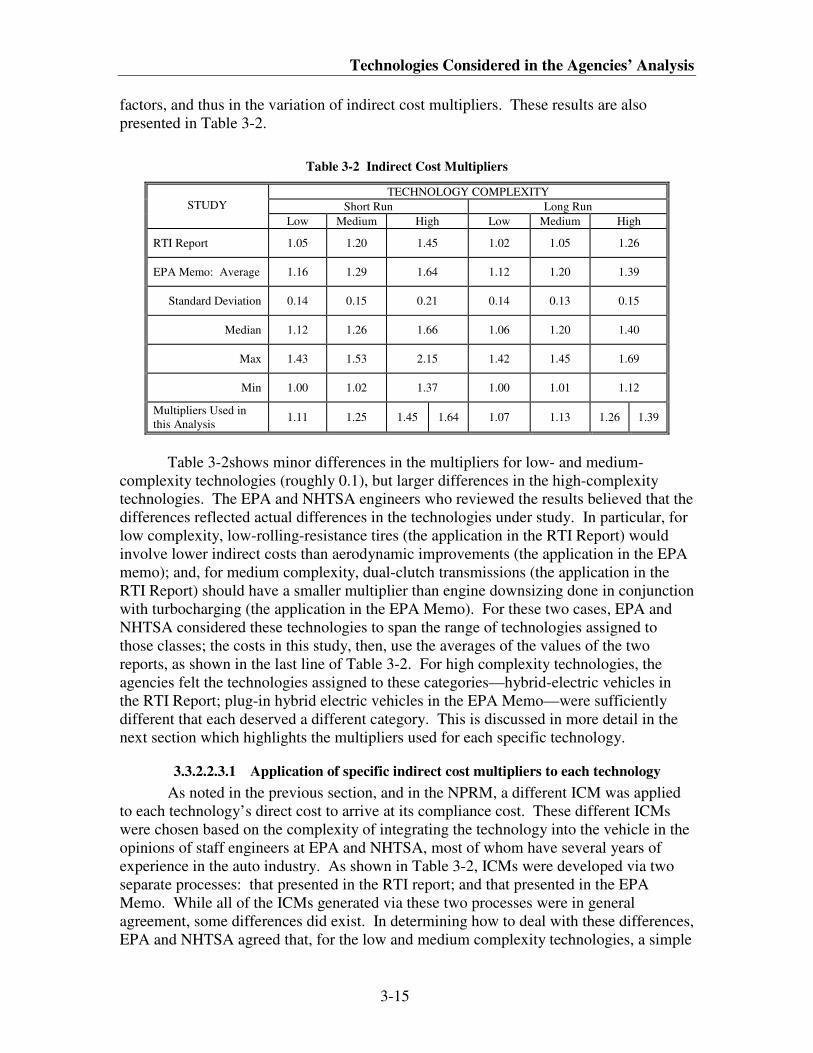
Technologies Considered in the Agencies’ Analysis
3-15
factors, and thus in the variation of indirect cost multipliers. These results are also
presented in Table 3-2.
Table 3-2 Indirect Cost Multipliers
TECHNOLOGY COMPLEXITY
Short Run Long Run STUDY
Low Medium High Low Medium High
RTI Report 1.05 1.20 1.45 1.02 1.05 1.26
EPA Memo: Average 1.16 1.29 1.64 1.12 1.20 1.39
Standard Deviation 0.14 0.15 0.21 0.14 0.13 0.15
Median 1.12 1.26 1.66 1.06 1.20 1.40
Max 1.43 1.53 2.15 1.42 1.45 1.69
Min 1.00 1.02 1.37 1.00 1.01 1.12
Multipliers Used in
this Analysis 1.11 1.25 1.45 1.64 1.07 1.13 1.26 1.39
Table 3-2shows minor differences in the multipliers for low- and medium-
complexity technologies (roughly 0.1), but larger differences in the high-complexity
technologies. The EPA and NHTSA engineers who reviewed the results believed that the
differences reflected actual differences in the technologies under study. In particular, for
low complexity, low-rolling-resistance tires (the application in the RTI Report) would
involve lower indirect costs than aerodynamic improvements (the application in the EPA
memo); and, for medium complexity, dual-clutch transmissions (the application in the
RTI Report) should have a smaller multiplier than engine downsizing done in conjunction
with turbocharging (the application in the EPA Memo). For these two cases, EPA and
NHTSA considered these technologies to span the range of technologies assigned to
those classes; the costs in this study, then, use the averages of the values of the two
reports, as shown in the last line of Table 3-2. For high complexity technologies, the
agencies felt the technologies assigned to these categories—hybrid-electric vehicles in
the RTI Report; plug-in hybrid electric vehicles in the EPA Memo—were sufficiently
different that each deserved a different category. This is discussed in more detail in the
next section which highlights the multipliers used for each specific technology.
3.3.2.2.3.1 Application of specific indirect cost multipliers to each technology
As noted in the previous section, and in the NPRM, a different ICM was applied
to each technology’s direct cost to arrive at its compliance cost. These different ICMs
were chosen based on the complexity of integrating the technology into the vehicle in the
opinions of staff engineers at EPA and NHTSA, most of whom have several years of
experience in the auto industry. As shown in Table 3-2, ICMs were developed via two
separate processes: that presented in the RTI report; and that presented in the EPA
Memo. While all of the ICMs generated via these two processes were in general
agreement, some differences did exist. In determining how to deal with these differences,
EPA and NHTSA agreed that, for the low and medium complexity technologies, a simple
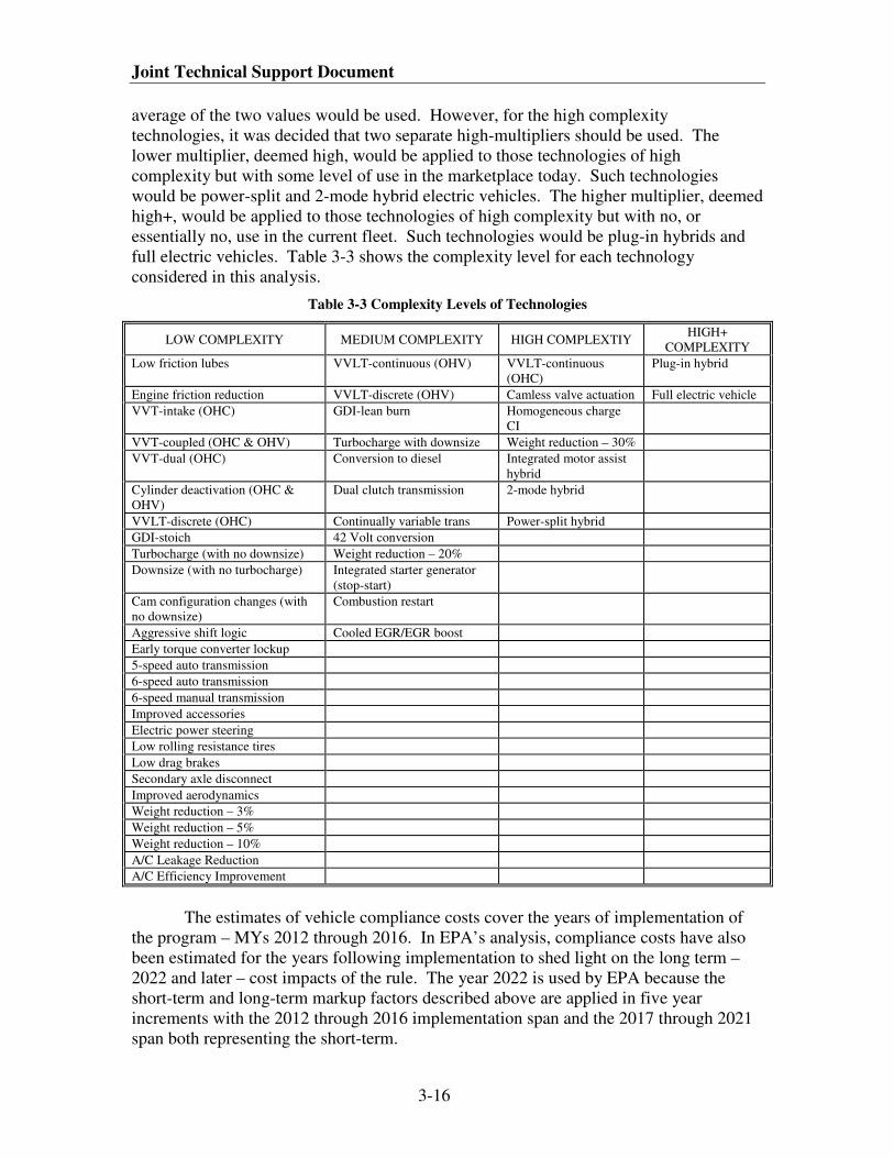
Joint Technical Support Document
3-16
average of the two values would be used. However, for the high complexity
technologies, it was decided that two separate high-multipliers should be used. The
lower multiplier, deemed high, would be applied to those technologies of high
complexity but with some level of use in the marketplace today. Such technologies
would be power-split and 2-mode hybrid electric vehicles. The higher multiplier, deemed
high+, would be applied to those technologies of high complexity but with no, or
essentially no, use in the current fleet. Such technologies would be plug-in hybrids and
full electric vehicles. Table 3-3 shows the complexity level for each technology
considered in this analysis.
Table 3-3 Complexity Levels of Technologies
LOW COMPLEXITY MEDIUM COMPLEXITY HIGH COMPLEXTIY HIGH+
COMPLEXITY
Low friction lubes VVLT-continuous (OHV) VVLT-continuous
(OHC)
Plug-in hybrid
Engine friction reduction VVLT-discrete (OHV) Camless valve actuation Full electric vehicle
VVT-intake (OHC) GDI-lean burn Homogeneous charge
CI
VVT-coupled (OHC & OHV) Turbocharge with downsize Weight reduction – 30%
VVT-dual (OHC) Conversion to diesel Integrated motor assist
hybrid
Cylinder deactivation (OHC &
OHV)
Dual clutch transmission 2-mode hybrid
VVLT-discrete (OHC) Continually variable trans Power-split hybrid
GDI-stoich 42 Volt conversion
Turbocharge (with no downsize) Weight reduction – 20%
Downsize (with no turbocharge) Integrated starter generator
(stop-start)
Cam configuration changes (with
no downsize)
Combustion restart
Aggressive shift logic Cooled EGR/EGR boost
Early torque converter lockup
5-speed auto transmission
6-speed auto transmission
6-speed manual transmission
Improved accessories
Electric power steering
Low rolling resistance tires
Low drag brakes
Secondary axle disconnect
Improved aerodynamics
Weight reduction – 3%
Weight reduction – 5%
Weight reduction – 10%
A/C Leakage Reduction
A/C Efficiency Improvement
The estimates of vehicle compliance costs cover the years of implementation of
the program – MYs 2012 through 2016. In EPA’s analysis, compliance costs have also
been estimated for the years following implementation to shed light on the long term –
2022 and later – cost impacts of the rule. The year 2022 is used by EPA because the
short-term and long-term markup factors described above are applied in five year
increments with the 2012 through 2016 implementation span and the 2017 through 2021
span both representing the short-term.
Technologies Considered in the Agencies’ Analysis
3-17
Commenters in general agreed with this methodology for determining indirect
cost multipliers, though there was some disagreement as to the magnitude of the
multipliers.
3.3.2.2.4 Cost reduction through manufacturer learning
For some of the technologies considered in this analysis, manufacturer learning
effects would be expected to play a role in the actual end costs. The “learning curve” or
“experience curve” describes the reduction in unit production costs as a function of
accumulated production volume. In theory, the cost behavior it describes applies to
cumulative production volume measured at the level of an individual manufacturer,
although it is often assumed—as both agencies have done in past regulatory analyses—to
apply at the industry-wide level, particularly in industries that utilize many common
technologies and component supply sources.18
Both agencies believe there are indeed
many factors that cause costs to decrease over time. Research in the costs of
manufacturing has consistently shown that, as manufacturers gain experience in
production, they are able to apply innovations to simplify machining and assembly
operations, use lower cost materials, and reduce the number or complexity of component
parts. All of these factors allow manufacturers to lower the per-unit cost of production
(i.e., the manufacturing learning curve).19
NHTSA has a detailed description of the learning effect in the MY 2011 CAFE
final rule, and EPA has a detailed description of the learning effect in the 2008 Staff
Report and in several past rules.20
The description here is focused on how the learning
effect has been used in the analyses support each agency’s rule.
Most studies of the effect of experience or learning on production costs appear to
assume that cost reductions begin only after some initial volume threshold has been
reached, but not all of these studies specify this threshold volume. The rate at which
costs decline beyond the initial threshold is usually expressed as the percent reduction in
average unit cost that results from each successive doubling of cumulative production
volume, sometimes referred to as the learning rate. Many estimates of experience curves
do not specify a cumulative production volume beyond which cost reductions would no
longer occur, instead depending on the asymptotic behavior of the effect for learning
rates below 100 percent to establish a floor on costs.
In past rulemaking analyses, as noted above, both agencies have used a learning
curve factor of 20 percent for each doubling of production volume. NHTSA has used
this approach in analyses supporting recent CAFE rules. In its analysis, EPA has
simplified the approach by using an “every two years” based learning progression rather
than a pure production volume progression (i.e., after two years of production it was
assumed that production volumes would have doubled and, therefore, costs would be
reduced by 20 percent).
In the MY 2011 CAFE final rule, NHTSA considered not only this volume-based
learning as described above, but also “time-based” learning. Time-based learning,
estimated by NHTSA at three percent per year, occurs in years following the volume-
Joint Technical Support Document
3-18
based learning steps and represents the smaller scale learning that occurs as
manufacturers continue to innovate. The time-based learning is, in effect, represented by
the flattened out, asymptotic portion of the learning curve.
For this analysis, each agency has employed both volume-based and time-based
learning effects. In NHTSA’s analysis, volume-based learning is estimated to result in 20
percent lower costs as production volumes of the given technology reach 300,000 units
and again when they reach 600,000 units within the entire industry. The count of
production units begins in the 2012 model year and/or with the first units produced,
whichever is earlier. In EPA’s analysis, as noted above, volume-based learning is
estimated to result in 20 percent lower costs after two full years of implementation (i.e.,
the 2014 MY costs are 20 percent lower than the 2012 and 2013 model year costs). In
each agency’s analysis, time-based learning is estimated to result in 3 percent lower costs
in each year following first introduction of a given technology. Once two volume-based
learning steps have occurred, or once the five year time-based learning period is
completed, learning is assumed to be complete, at least for purposes of the analyses done
to support each agency’s rule.
Both agencies considered learning impacts on most but not all of the technologies
expected to be used because some of the expected technologies are already used rather
widely in the industry and, presumably, learning impacts have already occurred.
Volume-based learning was considered for only a handful of technologies that are
considered to be new or emerging technologies such as the hybrids and electric vehicles.
Most technologies have been considered to be more established given their current use in
the fleet and, hence, the lower time-based learning has been applied. The learning effects
applied to each technology are summarized in Table 3-4.
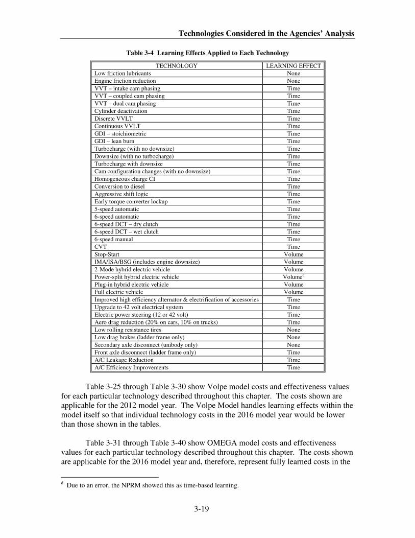
Technologies Considered in the Agencies’ Analysis
3-19
Table 3-4 Learning Effects Applied to Each Technology
TECHNOLOGY LEARNING EFFECT
Low friction lubricants None
Engine friction reduction None
VVT – intake cam phasing Time
VVT – coupled cam phasing Time
VVT – dual cam phasing Time
Cylinder deactivation Time
Discrete VVLT Time
Continuous VVLT Time
GDI – stoichiometric Time
GDI – lean burn Time
Turbocharge (with no downsize) Time
Downsize (with no turbocharge) Time
Turbocharge with downsize Time
Cam configuration changes (with no downsize) Time
Homogeneous charge CI Time
Conversion to diesel Time
Aggressive shift logic Time
Early torque converter lockup Time
5-speed automatic Time
6-speed automatic Time
6-speed DCT – dry clutch Time
6-speed DCT – wet clutch Time
6-speed manual Time
CVT Time
Stop-Start Volume
IMA/ISA/BSG (includes engine downsize) Volume
2-Mode hybrid electric vehicle Volume
Power-split hybrid electric vehicle Volumed
Plug-in hybrid electric vehicle Volume
Full electric vehicle Volume
Improved high efficiency alternator & electrification of accessories Time
Upgrade to 42 volt electrical system Time
Electric power steering (12 or 42 volt) Time
Aero drag reduction (20% on cars, 10% on trucks) Time
Low rolling resistance tires None
Low drag brakes (ladder frame only) None
Secondary axle disconnect (unibody only) None
Front axle disconnect (ladder frame only) Time
A/C Leakage Reduction Time
A/C Efficiency Improvements Time
Table 3-25 through Table 3-30 show Volpe model costs and effectiveness values
for each particular technology described throughout this chapter. The costs shown are
applicable for the 2012 model year. The Volpe Model handles learning effects within the
model itself so that individual technology costs in the 2016 model year would be lower
than those shown in the tables.
Table 3-31 through Table 3-40 show OMEGA model costs and effectiveness
values for each particular technology described throughout this chapter. The costs shown
are applicable for the 2016 model year and, therefore, represent fully learned costs in the
d Due to an error, the NPRM showed this as time-based learning.
Joint Technical Support Document
3-20
context of EPA’s analysis. For technologies added in years prior to MY 2016, EPA has
backed out the learning effects relative to the costs shown in the tables. For example,
Table 3-33 shows the small car stop-start vehicle cost as $351 in 2016. In the 2012
model year, this cost would be higher since the volume-based learning reflected in the
2016 cost would not have occurred yet. Backing out two volume-based learning steps
(i.e., dividing $351 by 80% twice) would result in a 2012 cost estimate of $548.
The different handling of learning effects across the two analyses (that done by
EPA and that by NHTSA) would have little impact on the overall results of the analyses.
NHTSA handles learning effects in the CAFE model. EPA handles learning effects
outside of the OMEGA model since OMEGA is run for only one model year - 2016.
Because the CAFE model adds technology on a year-by-year basis, it applies volume-
based learning effects once the applicable production volume thresholds have been
exceeded. In contrast, EPA would not apply volume-based learning until year 3
(assumed to be the point at which initial production volumes have doubled). Most
technologies in both analyses are subject to time-based learning which is applied on an
annual basis in the same way by both agencies (with the exception that NHTSA applies
time-based learning in the CAFE model while EPA applies it outside the OMEGA
model). Importantly, by the 2016 model year, both agencies will have applied two
volume-based learning steps to the appropriate technologies (hybrid and electric vehicles
only) and four time-based learning steps to the appropriate technologies (most other
technologies) to arrive at the same technology costs.
3.4 Specific technologies considered and estimates of costs and
effectiveness
It is important to note that the cost and effectiveness values presented by NHTSA
and EPA in this Final TSD are used when creating input files for the agencies’ respective
models, but are not literally the inputs themselves. The Docket to this final rule contains
the specific input files EPA and NHTSA used when modeling the technology cost.
3.4.1 What data sources did the agencies evaluate?
Refer to section 3.1 for a discussion of the specific data sources and reference
material used for the analysis of this rulemaking.
3.4.2 Individual technology descriptions and cost/effectiveness estimates
The sections that follow describe the technologies applied by both EPA and
NHTSA. It is important to note that there are distinct differences between the agencies in
how cost and effectiveness estimations are reported and applied.
EPA reports the total cost and effectiveness associated with a respective
technology. The technologies are then applied to a vehicle type as a package. To
calculate a cost for a vehicle package, the individual technologies are summed. To
estimate the overall effectiveness, the lumped parameter method is applied.
Technologies Considered in the Agencies’ Analysis
3-21
NHTSA applies cost and effectiveness through a series of decision trees. The
progressive nature of this methodology results in conditions for which a portion of a
technology has already been added. In this case, NHTSA would add an incremental
value which is the difference between the total cost of a technology and the portion
already existing. An example of this is cylinder deactivation. At the point in the decision
tree that it is applied, valvetrain technologies which could enable this feature have
already been added. NHTSA will add the delta in cost, which in this example accounts
for the NVH attributes.
3.4.2.1 Engine Technologies
NHTSA and EPA have reviewed the engine technology estimates used in
NHTSA’s MY 2011 CAFE final rule and EPA’s 2008 Staff Report and available
comments to the NPRM. In doing so NHTSA and EPA reconsidered all available
sources and updated the estimates as appropriate. The section below describes each of
the engine technologies considered for this rulemaking.
3.4.2.1.1 Low Friction Lubricants (LUB)
One of the most basic methods of reducing fuel consumption in gasoline engines
is the use of lower viscosity engine lubricants. More advanced multi-viscosity engine
oils are available today with improved performance in a wider temperature band and with
better lubricating properties. This can be accomplished by changes to the oil base stock
(e.g., switching engine lubricants from a Group I base oils to lower-friction, lower
viscosity Group III synthetic) and through changes to lubricant additive packages (e.g.,
friction modifiers and viscosity improvers). The use of 5W-30 motor oil is now
widespread and auto manufacturers are introducing the use of even lower viscosity oils,
such as 5W-20 and 0W-20, to improve cold-flow properties and reduce cold start friction.
However, in some cases, changes to the crankshaft, rod and main bearings and changes to
the mechanical tolerances of engine components may be required. In all cases, durability
testing would be required to ensure that durability is not compromised. The shift to lower
viscosity and lower friction lubricants will also improve the effectiveness of valvetrain
technologies such as cylinder deactivation, which rely on a minimum oil temperature
(viscosity) for operation.
Several manufacturers have previously commented confidentially, that low
friction lubricants could have an effectiveness value between 0 to 1 percent. For
purposes of this final rule, NHTSA and EPA are using effectiveness estimates within this
range. Therefore 0.5 percent was used in both models.
The 2002 NAS study estimated the low friction lubricant RPE at $8 to $11 using a
1.4 markup factor. The NESCCAF study showed an RPE of $5 to $15 with a 1.4
markup. The EEA report to DOE showed manufacturer costs of $10 to $20 with no
markup. Confidential Business Information (CBI) data estimates an average incremental
cost of $3 for the use of low friction lubricants. EPA’s 2008 Staff Report also confirms
this $3 cost (2006$). Both NHTSA and EPA believe that manufacturer’s estimates are
Joint Technical Support Document
3-22
the most accurate, and thus continue to believe that the $3 cost estimate is appropriate
and independent of vehicle class since the engineering work required should apply to any
engine size. Applying an indirect cost multiplier (ICM) of 1.11, for a low complexity
technology, results in a compliance cost of $3 per vehicle (2007$) for a MY 2012 through
MY 2016 vehicle (learning effects are not applied to low friction lubes).e
3.4.2.1.2 Engine Friction Reduction (EFR)
In addition to low friction lubricants, manufacturers can also reduce friction and
improve fuel consumption by improving the design of engine components and
subsystems. Approximately 10 percent of the energy consumed by a vehicle is lost to
friction, and just over half is due to frictional losses within the engine.21
Examples
include improvements in low-tension piston rings, piston skirt design, roller cam
followers, improved crankshaft design and bearings, material coatings, material
substitution, more optimal thermal management, and piston and cylinder surface
treatments. Additionally, as computer-aided modeling software continues to improve,
more opportunities for evolutionary friction reductions may become available.
All reciprocating and rotating components in the engine are potential candidates
for friction reduction, and minute improvements in several components can add up to a
measurable fuel economy improvement. The 2002 NAS, NESCCAF and EEA reports as
well as confidential manufacturer data suggested a range of effectiveness for engine
friction reduction to be between 1 to 3 percent. NHTSA and EPA continue to believe
that this range is accurate. Because of the incremental nature of the CAFE model,
NHTSA needed to continue to use the narrower range of 1-2 percent, which was also
used in the MY 2011 CAFE final rule.
In the MY 2011 CAFE final rule, NHTSA estimated a range from $13 to $49
using a 1.5 RPE on a per cylinder basis, or $9 to $33 without RPE (2007$). In the 2008
NPRM engine friction reduction was estimated to cost up to $14 without RPE on a per
cylinder basis (2006$). EPA’s 2008 Staff Report estimated this at $11 using a 1.5 RPE
on a per cylinder basis, or $7 without RPE (2006$). After review, NHTSA and EPA
believe that the cost estimate is closer to the lower end of the MY 2011 CAFE final rule
range and thus for this rulemaking is $13 per cylinder compliance cost (2007$), including
the low complexity ICM markup value of 1.11, for a MY 2012 through MY 2016 vehicle
(learning effects are not applied to engine friction reduction). This cost is multiplied by
the number of engine cylinders.
3.4.2.1.3 Variable Valve Timing (VVT)
Variable valve timing (VVT) classifies a family of valve-train designs that alter
the timing of the intake valve, exhaust valve, or both, primarily to reduce pumping losses,
increase specific power, and control the level of residual gases in the cylinder. VVT
reduces pumping losses when the engine is lightly loaded by controlling valve timing
closer to an optimum needed to sustain horsepower and torque. VVT can also improve
volumetric efficiency at higher engine speeds and loads. Additionally, VVT can be used
e Note that the costs developed for low friction lubes for this analysis reflect the costs associated with any
engine changes that would be required as well as any durability testing that may be required.
Technologies Considered in the Agencies’ Analysis
3-23
to alter (and optimize) the effective compression ratio where it is advantageous for
certain engine operating modes (e.g., in the Atkinson Cycle).
VVT has now become a widely adopted technology: in MY 2007, over half of all
new cars and light trucks had engines with some method of variable valve timing.22
Manufacturers are currently using many different types of variable valve timing, which
have a variety of different names and methods. The three major types of VVT are listed
below.
Each of the three implementations of VVT uses a cam phaser to adjust the
camshaft angular position relative to the crankshaft position, referred to as “camshaft
phasing.” The phase adjustment results in changes to the pumping work required by the
engine to accomplish the gas exchange process. The majority of current cam phaser
applications use hydraulically-actuated units, powered by engine oil pressure and
managed by a solenoid that controls the oil pressure supplied to the phaser.
3.4.2.1.3.1 Intake Cam Phasing (ICP)
Valvetrains with ICP, which is the simplest of the cam phasing technologies, can
modify the timing of the inlet valves by phasing the intake camshaft while the exhaust
valve timing remains fixed. This requires the addition of a cam phaser on each bank of
intake valves on the engine. An in-line 4-cylinder engine has one bank of intake valves,
while V-configured engines have two banks of intake valves.
NHTSA’s MY 2011 CAFE final rule and EPA 2008 Staff Report estimated an
effectiveness of 1 to 2 percent for ICP, which was supported by the NESCCAF report and
a majority of confidential manufacturer comments. The agencies have found no
additional sources to suggest strongly that this estimate is inaccurate, and so have
employed it for this rulemaking.
As for costs, NHTSA’s MY 2011 CAFE final rule estimated a $61 RPE ($41 non-
RPE) cost per cam phaser, based on the 2008 Martec Report and confidential
manufacturer data (2007$). In the 2008 staff report, EPA estimated this at $59 using a
1.5 RPE or $40 without RPE (2006$). NHTSA and EPA believe that this estimate
remains accurate. Using the new indirect cost multiplier of 1.11, for a low complexity
technology, the compliance cost per cam phaser would be $45 per bank , yielding a $45
cost for and in-line engine configurations and $90 for V-engine configurations for a MY
2012 vehicle (2007$). Time-based learning is applied to ICP so the MY 2016 cost would
be $40 for in in-line engine and $80 for the V-engine (2007$).
3.4.2.1.3.2 Coupled Cam Phasing (CCPS and CCPO)
Valvetrains with coupled (or coordinated) cam phasing can modify the timing of
both the inlet valves and the exhaust valves an equal amount by phasing the camshaft of a
single overhead cam (SOHC) engine or an overhead valve (OHV) engine.f For overhead
f Although CCP appears only in the SOHC and OHV branches of the decision tree, it is noted that a single
phaser with a secondary chain drive would allow CCP to be applied to DOHC engines. Since this would
Joint Technical Support Document
3-24
cam engines, this requires the addition of a cam phaser on each bank of the engine. Thus,
an in-line 4-cylinder engine has one cam phaser, while SOHC V-engines have two cam
phasers. For overhead valve (OHV) engines, which have only one camshaft to actuate
both inlet and exhaust valves, CCP is the only VVT implementation option available and
requires only one cam phaser.g
Based on NHTSA’s MY 2011 CAFE final rule, previously-received confidential
manufacturer data, and the NESCCAF report, NHTSA and EPA estimated the
effectiveness of CCP to be between 1 to 4 percent. NHTSA and EPA reviewed this
estimate for purposes of the final rule, and continue to find it accurate.
The same cam phaser has been assumed for ICP and CCP applications, thus CCPs
cost per cam phaser is identical to ICPs. This results in a cost of $45 for in-line SOHC
and OHV engines and $90 for SOHC V-engine configurations for a MY 2012 vehicle
(2007$). With time-based learning applied, these costs for a 2016 MY vehicle would be
$40 and $80, respectively (2007$).
3.4.2.1.3.3 Dual Cam Phasing (DCP)
The most flexible VVT design is dual (independent) cam phasing, where the
intake and exhaust valve opening and closing events are controlled independently. This
option allows the option of controlling valve overlap, which can be used as an internal
EGR strategy. At low engine loads, DCP creates a reduction in pumping losses, resulting
in improved fuel consumption/reduced CO2 emissions. Increased internal EGR also
results in lower engine-out NOX emissions. The amount by which fuel consumption is
improved and CO2 emissions are reduced depends on the residual tolerance of the
combustion system. Additional improvements are observed at idle, where low valve
overlap could result in improved combustion stability, potentially reducing idle fuel
consumption.
NHTSA MY 2011 CAFE final rule estimated the effectiveness of DCP to be
between 3 to 5 percent relative to a base engine or 2 to 3 relative to an engine with ICP.
NHTSA and EPA believe that this estimate remains applicable for the final rule.
As above, the same cam phaser has been assumed for ICP and DCP applications.
Thus, DCP’s cost per cam phaser is identical to ICP’s. DCP requires two cam phasers
per cylinder bank, one to control the intake valves and one to control the exhaust valves.
This results in a cost of $90, relative to an engine without ICP, or $45 relative to an
engine with ICP, minus $6 for the removal of the EGR valve, ultimately yielding costs of
$84 and $39 respectively for in-line DOHC configurations (all in 2007$). For V-
configuration engines, the cost is $180 relative to an engine without ICP, or $90 relative
to an engine with ICP, minus $6 for the removal of the EGR valve, ultimately yielding
potentially be adopted on a limited number of DOHC engines NHTSA did not include it in that branch of
the decision tree. g It is also noted that coaxial camshaft developments would allow other VVT options to be applied to OHV
engines. However, since they would potentially be adopted on a limited number of OHV engines NHTSA
did not include them in the decision tree.
Technologies Considered in the Agencies’ Analysis
3-25
costs of $174 and $84, respectively (all in 2007$). These costs are appropriate for a MY
2012 vehicle. With time-based learning applied, these costs for a 2016 MY vehicle
would be $157 and $73, respectively (2007$).
3.4.2.1.4 Variable Valve Lift (VVL)
Controlling the lift of the valves provides a potential for further efficiency
improvements. By optimizing the valve-lift profile for specific engine operating regions,
the pumping losses can be reduced by reducing the amount of throttling required to
produce the desired engine power output. By moving the throttling losses further
downstream of the throttle valve, the heat transfer losses that occur from the throttling
process are directed into the fresh charge-air mixture just prior to compression, delaying
the onset of knock-limited combustion processes. Variable valve lift control can also be
used to induce in-cylinder mixture motion, which improves fuel-air mixing and can result
in improved thermodynamic efficiency. Variable valve lift control can also potentially
reduce overall valvetrain friction. At the same time, such systems may also incur
increased parasitic losses associated with their actuation mechanisms. A number of
manufacturers have already implemented VVL into their fleets (Toyota, Honda, and
BMW), but overall this technology is still available for most of the fleet. There are two
major classifications of variable valve lift, described below:
3.4.2.1.4.1 Discrete Variable Valve Lift (DVVLS, DVVLD, DVVLO)
DVVL systems allow the selection between two or three discrete cam profiles by
means of a hydraulically-actuated mechanical system. By optimizing the cam profile for
specific engine operating regions, the pumping losses can be reduced by reducing the
amount of throttling required to produce the desired engine power output. This increases
the efficiency of the engine. These cam profiles consist of a low and a high-lift lobe, and
may include an inert or blank lobe to incorporate cylinder deactivation (in the case of a 3-
step DVVL system). DVVL is normally applied together with VVT control. DVVL is
also known as Cam Profile Switching (CPS). DVVL is a mature technology with low
technical risk.
NHTSA’s MY 2011 CAFE final rule, previously-received confidential
manufacturer data, and the NESCCAF report, all estimate the effectiveness of DVVL to
be between 1 to 4 percent above that realized by VVT systems. NHTSA and EPA
believe this estimate continues to be applicable for the final rule.
In the MY 2011 CAFE final rule, NHTSA estimated an RPE (1.5 markup factor)
of $201 for an inline 4-cylinder engine, $306 for a V6 engine and $396 for a V8 engine
or without the RPE markup $134, $204, $264, respectively (all in 2007$). In the 2008
Staff Report, EPA estimated this at $169, $246, and $322, respectively, using a 1.5 RPE
factor (2006$) or $113, $164 and $215, respectively without markup (all in 2006$). For
this analysis, the agencies have estimated the compliance costs, including $25 for
controls and using a 1.11 ICM for a low complexity technology, at $141 for an inline 4-
cylinder engine, $205 for a V6 engine and $293 for a V8 for a 2012 MY vehicle (2007$).
With time-based learning applied, these costs would be $125, $181, and $259,
respectively for a 2016 MY vehicle (2007$).
Joint Technical Support Document
3-26
3.4.2.1.4.2 Continuously Variable Valve Lift (CVVL)
In CVVL systems, valve lift is varied by means of a mechanical linkage, driven
by an actuator controlled by the engine control unit. The valve opening and phasing vary
as the lift is changed and the relation depends on the geometry of the mechanical system.
BMW has considerable production experience with CVVL systems and has sold port-
injected “Valvetronic” engines since 2001. CVVL allows the airflow into the engine to
be regulated by means of intake valve opening reduction, which improves engine
efficiency by reducing pumping losses from throttling the intake system further upstream
as with a conventionally throttled engine.
Variable valve lift gives a further reduction in pumping losses compared to that
which can be obtained with cam phase control only, with CVVL providing greater
effectiveness than DVVL, since it can be fully optimized for all engine speeds and loads,
and is not limited to a two or three step compromise. There may also be a small
reduction in valvetrain friction when operating at low valve lift, resulting in improved
low load fuel consumption for cam phase control with variable valve lift as compared to
cam phase control only. Most of the fuel economy effectiveness is achieved with
variable valve lift on the intake valves only. CVVL is only applicable to double overhead
cam (DOHC) engines.
NHTSA’s MY 2011 CAFE final rule estimated the effectiveness for CVVL at 1.5
to 3.5 percent over an engine with DCP, but also recognize that it could go up as high as
5 percent above and beyond DCP to account for the implementation of more complex
CVVL systems such as BMW’s “Valvetronic” engines. This coincides with EPA Staff
Report estimates of the contribution of CVVL, which were based on the NESCCAF
report, in which CVVL could improve effectiveness by 4 percent (minivans) and up to 6
percent (large cars) over dual cam phasing. Thus, the effectiveness range for CVVL in
this joint TSD ranges from 1.5 to 6 percent depending on the complexity level of the
application. However, due to the complexity and cost of this technology, the GHG model
did not consider it and the CAFE model projected no application of the less complex
version of this technology. The most recent submission of manufacturers’ product plans
confirmed that this technology will not be applied by most manufacturers.
In the MY 2011 CAFE final rule, NHTSA estimated and RPE (1.5 factor) of
continuously variable valve lift to be $306 for an inline 4-cylinder engine, $432 for a V6
engine and $582 for a V8 engine or without RPE $204, $287, $388, respectively. In the
2008 Staff Report, EPA estimated this at $254, $466, and $508, respectively, using a 1.5
RPE factor (2006$) or $169, $311 and $339, respectively without markup (all in 2006$)
For this analysis, the agencies have estimated the compliance costs, using a 1.45 ICM for
a high complexity technology, at $277 for an inline 4-cylinder engine, $509 for a V6
engine and $554 for a V8 engine for a MY 2012 vehicle (2007$). With time-based
learning applied, these costs would become $245, $449, and $489, respectively for a MY
2016 vehicle (2007$).
Technologies Considered in the Agencies’ Analysis
3-27
3.4.2.1.5 Cylinder Deactivation (DEACS, DEACD, DEACO)
In conventional spark-ignited engines throttling the airflow controls engine torque
output. At partial loads, efficiency can be improved by using cylinder deactivation
instead of throttling. Cylinder deactivation (DEAC) can improve engine efficiency by
disabling or deactivating (usually) half of the cylinders when the load is less than half of
the engine’s total torque capability – the valves are kept closed, and no fuel is injected –
as a result, the trapped air within the deactivated cylinders is simply compressed and
expanded as an air spring, with reduced friction and heat losses. The active cylinders
combust at almost double the load required if all of the cylinders were operating.
Pumping losses are significantly reduced as long as the engine is operated in this “part-
cylinder” mode.
Cylinder deactivation control strategy relies on setting maximum manifold
absolute pressures or predicted torque within which it can deactivate the cylinders. Noise
and vibration issues reduce the operating range to which cylinder deactivation is allowed,
although manufacturers are exploring vehicle changes that enable increasing the amount
of time that cylinder deactivation might be suitable. Some manufacturers may choose to
adopt active engine mounts and/or active noise cancellations systems to address NVH
concerns and to allow a greater operating range of activation. Manufacturers have stated
that use of DEAC on 4 cylinder engines would cause unacceptable NVH; therefore
cylinder deactivation has not been applied to 4-cylinder engines.
Cylinder deactivation has seen a recent resurgence thanks to better valvetrain
designs and engine controls. General Motors and Chrysler Group have incorporated
cylinder deactivation across a substantial portion of their V8-powered lineups. Honda
(Odyssey, Pilot) offers V6 models with cylinder deactivation.
Effectiveness improvements scale roughly with engine displacement-to-vehicle
weight ratio: the higher displacement-to-weight vehicles, operating at lower relative loads
for normal driving, have the potential to operate in part-cylinder mode more frequently.
NHTSA and EPA reviewed the MY 2011 CAFE final rule estimate and confirmed
a range of 0.5 to 6 percent depending on the valvetrain configuration and other existing
technologies. The OMEGA model, which is based on packages, applies 6 percent
reduction in CO2 emissions in all applications. The CAFE model, due to its incremental
nature, uses a range depending on the engine valvetrain configuration. For example, for
DOHC engines which are already equipped with DCP and DVVLD, there is little benefit
that can be achieved from adding cylinder deactivation since the pumping work has
already been minimized and internal Exhaust Gas Recirculation (EGR) rates are
maximized, so the effectiveness is only up to 0.5 percent for DEACD. For SOHC
engines which have CCP and DVVLS applied, effectiveness ranged from 2.5 to 3 percent
for DEACS. For OHV engines, without VVT or VVL technologies, the effectiveness for
DEACO ranged from 3.9 to 5.5 percent.
Joint Technical Support Document
3-28
NHTSA and EPA considered a range of $170 to $190 (or $28 to $190 depending
on whether an engine already has lost motion devices, oil control valves and camshaft
position sensors). This is a departure from NHTSA’s MY 2011 CAFE final rule, which
used a range of $306 to $400. That range was primarily based on the 2008 Martec
Report and applied a higher RPE value. In reviewing these assumptions, NHTSA and
EPA amended the MY 2011 CAFE final rule estimates and adjusted the estimates to
include the new ICM low complexity markup of 1.11. The EPA Staff Report estimated
this ranging from $203 to $229 (RPE using a 1.5 factor) or $135 to $153 without RPE
(2006$). NHTSA’s MYs 2011-2015 NPRM showed estimates of a $170 for a 6-cylinder
engine and $190 for an 8-cylinder engine—when adjusted for 2007 dollars and using the
new ICM multipliers— for engines that do not have lost motion devices. These numbers
were within the ranges described by the 2002 NAS and NESCCAF reports. The $170
and $190 costs are appropriate of a MY 2012 vehicle (2007$). With time-based learning
applied, these would become $150 and $169, respectively, for a MY 2016 vehicle
(2007$).
If lost motion devices are on the engine, the cost of DEAC as applied to SOHC
and DOHC engines could be as low as $28.h This $28
i accounts for the potential
additional application of active engine mounts on SOHC and DOHC engines and can
only be applied on 50 percent of the vehicles. Further, this SOHC and DOHC engine
estimate is relevant to the CAFE model only because the OMEGA model does not apply
technologies in the same incremental fashion as the CAFE model.
3.4.2.1.6 Conversion to Double Overhead Camshaft Engine with Dual Cam Phasing
(CDOHC)
Double overhead camshaft engines achieve increased airflow at high engine
speeds, improve volumetric efficiency and reductions of the valvetrain’s moving mass.
Such engines typically develop higher power at high engine speeds. Manufacturers may
choose to replace OHV engines with DOHC engine designs with dual cam phasing
(DCP). EPA and NHTSA reviewed the analysis of effectiveness for CDOHC in the MY
2011 CAFE final rule and found no information to indicate that these estimates were
inaccurate. EPA and NHTSA estimate the effectiveness to be between 1 to 2.5 percent.
As for costs, NHTSA’s MY 2011 CAFE final rule assumed that CDOHC would
have an RPE of $746 ($497 non-RPE) for a V8 engine, $590 ($393 non-RPE) for a V6
engine and $373 ($249 non-RPE) for inline 4-cylinder engine (2007$). In the 2008 Staff
Report, EPA did not estimate a cost for this specific technology. For purposes of this
rulemaking, NHTSA revised the costs only by identifying this technology as a low
complexity technology and applying an indirect cost multiplier of 1.11 resulting in a
compliance cost of $552 for V8 engine, $436 for a V6 and $276 for an inline 4-cylinder
engine. The above costs are for a MY 2012 vehicle and with the application of time-
based learning will be slightly lower for MY 2016 vehicle
h The $28 is an adjustment from the $75 estimate used in the MY 2011 final rule to account for the new
ICM markup factor and the fact that it could only be applied on up to 50 percent of the vehicles.
Technologies Considered in the Agencies’ Analysis
3-29
3.4.2.1.7 Stoichiometric Gasoline Direct Injection (SGDI)
Stoichiometric gasoline direct injection (SGDI), or Spark Ignition Direct injection
(SIDI), engines inject fuel at high pressure directly into the combustion chamber (rather
than the intake port in port fuel injection). SGDI requires changes to the injector design,
an additional high pressure fuel pump, new fuel rails to handle the higher fuel pressures
and changes to the cylinder head and piston crown design. Direct injection of the fuel
into the cylinder improves cooling of the air/fuel charge within the cylinder, which allows
for higher compression ratios and increased thermodynamic efficiency without the onset
of combustion knock. Recent injector design advances, improved electronic engine
management systems and the introduction of multiple injection events per cylinder firing
cycle promote better mixing of the air and fuel, enhance combustion rates, increase
residual exhaust gas tolerance and improve cold start emissions. SGDI engines achieve
higher power density and match well with other technologies, such as boosting and
variable valvetrain designs.
Several manufacturers have recently introduced vehicles with SGDI engines,
including VW/Audi, BMW, Toyota (Lexus IS 350) and General Motors (Chevrolet
Impala and Cadillac CTS 3.6L). BMW, GM, Ford and VW/Audi have announced their
plans to increase dramatically the number of SGDI engines in their portfolios.
NHTSA’s MY 2011 CAFE final rule estimated the effectiveness of SGDI to be
between 2 and 3 percent. NHTSA and EPA reviewed estimates from the Alliance of
Automobile Manufactures, which projects 3 percent gains in fuel efficiency and a 7
percent improvement in torque. The torque increase provides the opportunity to
downsize the engine allowing an increase in efficiency of up to a 5.8 percent. NHTSA
and EPA also reviewed other published literature, reporting 3 percent effectiveness for
SGDI.23
Another source reports a 5 percent improvement on the NEDC drive cycle.24
Confidential manufacturer data reported an efficiency effectiveness range of 1 to 2
percent. NHTSA and EPA determined that the range of 2 to 3 percent continues to be
appropriate. Combined with other technologies (i.e., boosting, downsizing, and in some
cases, cooled EGR), SGDI can achieve greater reductions in fuel consumption and CO2
emissions compared to engines of similar power output.
The NHTSA and EPA cost estimates for SGDI take into account the changes
required to the engine hardware, engine electronic controls, ancillary and Noise Vibration
and Harshness (NVH) mitigation systems. Through contacts with industry NVH
suppliers, and manufacturer press releases, the agencies believe that the NVH treatments
will be limited to the mitigation of fuel system noise, specifically from the injectors and
the fuel lines. In the final rule, the agencies have revised the SGDI costs based on the
FEV work that was not yet available for the NPRM. Focusing on direct manufacturing
costs, the NPRM estimates, the FEV values, and the final values are shown in Table 3-5.
FEV did not directly estimate the SGDI costs shown here. Instead, FEV estimated costs
associated with downsizing and turbocharging a V8 and V6 engine to a V6 and I4 engine,
respectively, and simultaneously converting the PFI fuel system to a SGDI fuel system.
The agencies, working closely with FEV, then “binned” the costs into three distinct bins:
downsize, turbocharge, and SGDI. As such, the FEV results shown in Table 3-5 cannot
Joint Technical Support Document
3-30
be found in the FEV reports, but instead are detailed in a memo to the docket which also
provides details of this binning process.25
Because the methodology used by FEV
presumes high volume production, instead of using the FEV results directly the agencies
have averaged those results with the NPRM results to estimate the final values (this is
noted in section 3.3.2.2, 3.4.2.1.9, and 3.4.2.2.5). Note that the costs for the I3 and I4
engines have changed since the NPRM but have not been averaged with the NPRM
values. The costs changed based on a more rigorous binning process than that conducted
for the NPRM, but were not averaged because they are based on the I4 to I4 teardown
conducted by FEV which was, in fact, used in the NPRM. While the final value of $213
is lower than the NPRM value of $226, the $13 difference has simply been shifted from
SGDI to the downsizing bin.
Table 3-5 Direct Manufacturing Costs for SGDI (2007$ in 2012)
Technology NPRM FEV Results Final Rule
I3 $226 $213 $213
I4 $226 $213 $213
V6 $293 $321 $307
V8 $317 $386 $352
For the final rule marked up costs, the agencies estimate SGDI costs at $236 for
an inline 4-cylinder and $341 for V6 and $390 for V8 including the low complexity ICM
markup value of 1.11 (2007$ in 2012). With time-based learning applied, these costs
would be $209, $301, and $346 for a MY 2016 vehicle (2007$). As noted above, all of
these costs differ slightly from those used in the NPRM analysis as shown in Table 3-6.
These costs were not changed in response to public comments, but instead were changed
due to updated information from the FEV teardown studies.26
Table 3-6 Marked up Costs for Stoichiometric GDI (2007$ in 2012)
Technology NPRM Final Rule
I3 $251 $236
I4 $251 $236
V6 $326 $341
V8 $353 $390
3.4.2.1.8 Combustion Restart (CBRST)
Combustion restart allows “start-stop” functionality of DI engines through the
implementation of an upgraded starter with bi-directional rotation to allow precise
crankshaft positioning prior to subsequent fuel injection and spark ignition, allowing
engine restart. This method of implementing engine stop/start functionality allows not
only the fuel savings from not idling the engine, but also reduces fuel consumption as the
engine speeds up to its operational speed. A Direct Injection (DI) fuel system is required
for implementation of this technology.
Technologies Considered in the Agencies’ Analysis
3-31
NHTSA reviewed the MY 2011 CAFE final rule assumptions and determined that
due to technical risks implementation of combustion restart would likely not be feasible
prior to MY 2014. Some of the risks are associated with unresolved issues regarding the
impact of very high or very low ambient air temperatures on the ability to start the engine
in the described manner. Although the starter motor can provide fail-safe starting
capability in these temperature limited areas, strategies must be developed to manage the
transitions. Other risks relate to production readiness.
Additional hardware is required to implement combustion restart, beyond SGDI.
This includes a battery sensor, incremental wiring and high current switching, an
incremental crank position sensor, and, in the case of an automatic transmission
applications, a transmission oil pump to allow for torque converter continuity.
BMW has published a 3.5 percent fuel consumption effectiveness over the NEDC
drive cycle for combustion restart,27
and AVL a 4.8 percent effectiveness.28
However,
these reported effectiveness levels could potentially be reduced significantly on the EPA
combined drive cycle, as combustion restart does not save fuel on the highway drive
cycle. Therefore, NHTSA estimates the fuel consumption effectiveness for CBRST to
range from 2 to 2.5 percent.
Regarding the cost estimate, NHTSA determined that the estimate of $118 from
the 2008 Martec Report cost estimates for individual pieces was the best available. The
total RPE cost (excluding transmission pump) is $141 at high volumes, which includes
$70 for upgrading the starter, $10 for a battery sensor and wiring, $10 for high current
switch and $4 for crank sensor a totaling $94 (non-RPE) cost. Applying an indirect cost
multiplier of 1.25, for a medium complexity technology, results in a compliance cost of
$118 for a MY 2012 vehicle and will be reduced in future years with the application of
time-based learning.
3.4.2.1.9 Turbocharging and Downsizing (TRBDS)
The specific power of a naturally aspirated engine is primarily limited by the rate
at which the engine is able to draw air into the combustion chambers. Turbocharging and
supercharging (grouped together here as boosting) are two methods to increase the intake
manifold pressure and cylinder charge-air mass above naturally aspirated levels.
Boosting increases the airflow into the engine, thus increasing the specific power level,
and with it the ability to reduce engine displacement while maintaining performance.
This effectively reduces the pumping losses at lighter loads in comparison to a larger,
naturally aspirated engine.
Almost every major manufacturer currently markets a vehicle with some form of
boosting. While boosting has been a common practice for increasing performance for
several decades, turbocharging has considerable potential to improve fuel economy and
reduce CO2 emissions when the engine displacement is also reduced. Specific power
levels for a boosted engine often exceed 100 hp/L, compared to average naturally
aspirated engine power densities of roughly 70 hp/L. As a result, engines can
conservatively be downsized roughly 30 percent to achieve similar peak output levels. In
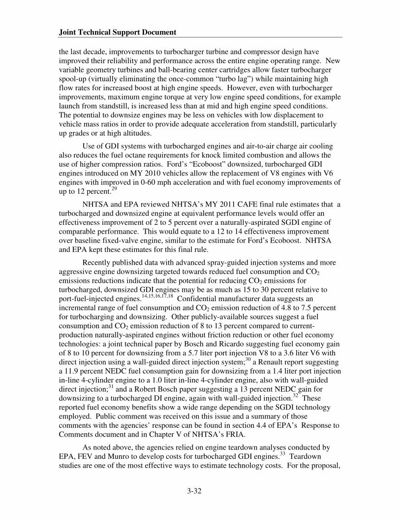
Joint Technical Support Document
3-32
the last decade, improvements to turbocharger turbine and compressor design have
improved their reliability and performance across the entire engine operating range. New
variable geometry turbines and ball-bearing center cartridges allow faster turbocharger
spool-up (virtually eliminating the once-common “turbo lag”) while maintaining high
flow rates for increased boost at high engine speeds. However, even with turbocharger
improvements, maximum engine torque at very low engine speed conditions, for example
launch from standstill, is increased less than at mid and high engine speed conditions.
The potential to downsize engines may be less on vehicles with low displacement to
vehicle mass ratios in order to provide adequate acceleration from standstill, particularly
up grades or at high altitudes.
Use of GDI systems with turbocharged engines and air-to-air charge air cooling
also reduces the fuel octane requirements for knock limited combustion and allows the
use of higher compression ratios. Ford’s “Ecoboost” downsized, turbocharged GDI
engines introduced on MY 2010 vehicles allow the replacement of V8 engines with V6
engines with improved in 0-60 mph acceleration and with fuel economy improvements of
up to 12 percent.29
NHTSA and EPA reviewed NHTSA’s MY 2011 CAFE final rule estimates that a
turbocharged and downsized engine at equivalent performance levels would offer an
effectiveness improvement of 2 to 5 percent over a naturally-aspirated SGDI engine of
comparable performance. This would equate to a 12 to 14 effectiveness improvement
over baseline fixed-valve engine, similar to the estimate for Ford’s Ecoboost. NHTSA
and EPA kept these estimates for this final rule.
Recently published data with advanced spray-guided injection systems and more
aggressive engine downsizing targeted towards reduced fuel consumption and CO2
emissions reductions indicate that the potential for reducing CO2 emissions for
turbocharged, downsized GDI engines may be as much as 15 to 30 percent relative to
port-fuel-injected engines.14,15,16,17,18
Confidential manufacturer data suggests an
incremental range of fuel consumption and CO2 emission reduction of 4.8 to 7.5 percent
for turbocharging and downsizing. Other publicly-available sources suggest a fuel
consumption and CO2 emission reduction of 8 to 13 percent compared to current-
production naturally-aspirated engines without friction reduction or other fuel economy
technologies: a joint technical paper by Bosch and Ricardo suggesting fuel economy gain
of 8 to 10 percent for downsizing from a 5.7 liter port injection V8 to a 3.6 liter V6 with
direct injection using a wall-guided direct injection system;30
a Renault report suggesting
a 11.9 percent NEDC fuel consumption gain for downsizing from a 1.4 liter port injection
in-line 4-cylinder engine to a 1.0 liter in-line 4-cylinder engine, also with wall-guided
direct injection;31
and a Robert Bosch paper suggesting a 13 percent NEDC gain for
downsizing to a turbocharged DI engine, again with wall-guided injection.32
These
reported fuel economy benefits show a wide range depending on the SGDI technology
employed. Public comment was received on this issue and a summary of those
comments with the agencies’ response can be found in section 4.4 of EPA’s Response to
Comments document and in Chapter V of NHTSA’s FRIA.
As noted above, the agencies relied on engine teardown analyses conducted by
EPA, FEV and Munro to develop costs for turbocharged GDI engines.33
Teardown
studies are one of the most effective ways to estimate technology costs. For the proposal,
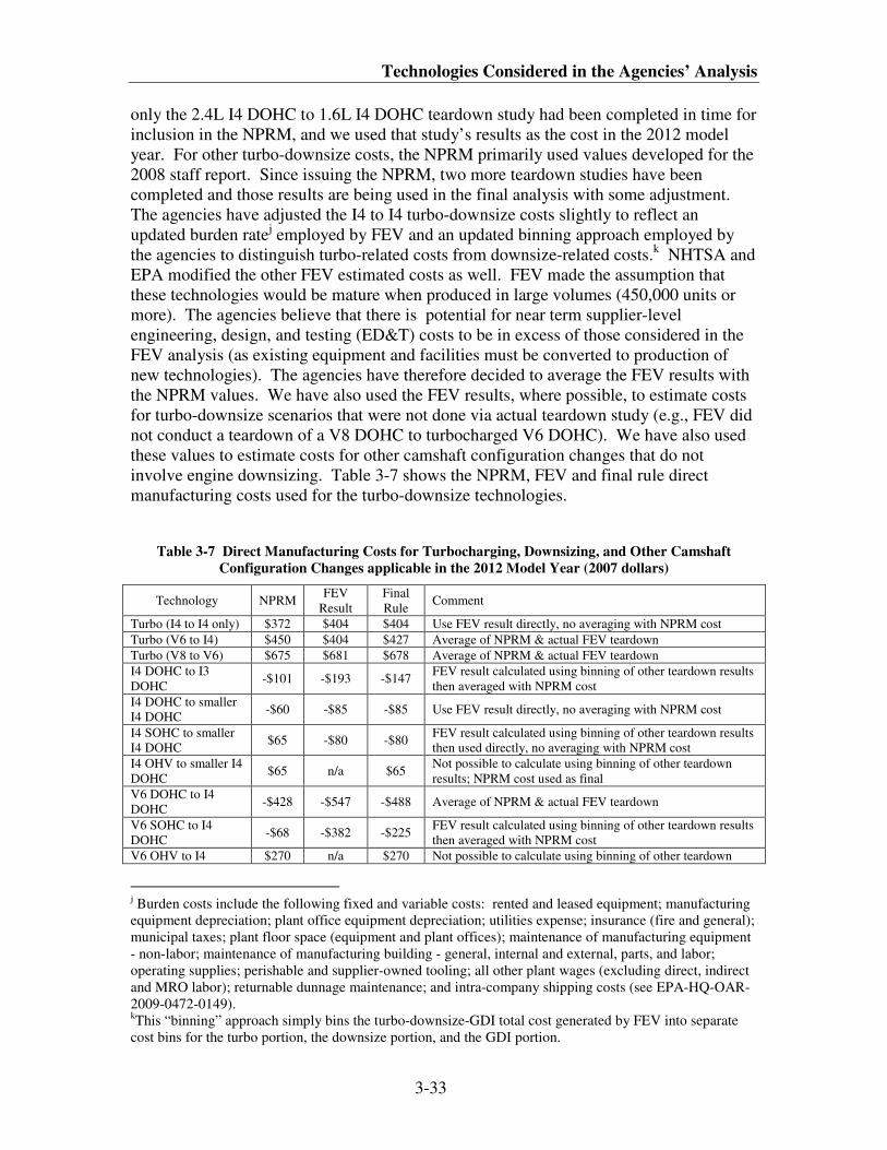
Technologies Considered in the Agencies’ Analysis
3-33
only the 2.4L I4 DOHC to 1.6L I4 DOHC teardown study had been completed in time for
inclusion in the NPRM, and we used that study’s results as the cost in the 2012 model
year. For other turbo-downsize costs, the NPRM primarily used values developed for the
2008 staff report. Since issuing the NPRM, two more teardown studies have been
completed and those results are being used in the final analysis with some adjustment.
The agencies have adjusted the I4 to I4 turbo-downsize costs slightly to reflect an
updated burden ratej employed by FEV and an updated binning approach employed by
the agencies to distinguish turbo-related costs from downsize-related costs.k NHTSA and
EPA modified the other FEV estimated costs as well. FEV made the assumption that
these technologies would be mature when produced in large volumes (450,000 units or
more). The agencies believe that there is potential for near term supplier-level
engineering, design, and testing (ED&T) costs to be in excess of those considered in the
FEV analysis (as existing equipment and facilities must be converted to production of
new technologies). The agencies have therefore decided to average the FEV results with
the NPRM values. We have also used the FEV results, where possible, to estimate costs
for turbo-downsize scenarios that were not done via actual teardown study (e.g., FEV did
not conduct a teardown of a V8 DOHC to turbocharged V6 DOHC). We have also used
these values to estimate costs for other camshaft configuration changes that do not
involve engine downsizing. Table 3-7 shows the NPRM, FEV and final rule direct
manufacturing costs used for the turbo-downsize technologies.
Table 3-7 Direct Manufacturing Costs for Turbocharging, Downsizing, and Other Camshaft
Configuration Changes applicable in the 2012 Model Year (2007 dollars)
Technology NPRM FEV
Result
Final
Rule Comment
Turbo (I4 to I4 only) $372 $404 $404 Use FEV result directly, no averaging with NPRM cost
Turbo (V6 to I4) $450 $404 $427 Average of NPRM & actual FEV teardown
Turbo (V8 to V6) $675 $681 $678 Average of NPRM & actual FEV teardown
I4 DOHC to I3
DOHC -$101 -$193 -$147
FEV result calculated using binning of other teardown results
then averaged with NPRM cost
I4 DOHC to smaller
I4 DOHC -$60 -$85 -$85 Use FEV result directly, no averaging with NPRM cost
I4 SOHC to smaller
I4 DOHC $65 -$80 -$80
FEV result calculated using binning of other teardown results
then used directly, no averaging with NPRM cost
I4 OHV to smaller I4
DOHC $65 n/a $65
Not possible to calculate using binning of other teardown
results; NPRM cost used as final
V6 DOHC to I4
DOHC -$428 -$547 -$488 Average of NPRM & actual FEV teardown
V6 SOHC to I4
DOHC -$68 -$382 -$225
FEV result calculated using binning of other teardown results
then averaged with NPRM cost
V6 OHV to I4 $270 n/a $270 Not possible to calculate using binning of other teardown
j Burden costs include the following fixed and variable costs: rented and leased equipment; manufacturing
equipment depreciation; plant office equipment depreciation; utilities expense; insurance (fire and general);
municipal taxes; plant floor space (equipment and plant offices); maintenance of manufacturing equipment
- non-labor; maintenance of manufacturing building - general, internal and external, parts, and labor;
operating supplies; perishable and supplier-owned tooling; all other plant wages (excluding direct, indirect
and MRO labor); returnable dunnage maintenance; and intra-company shipping costs (see EPA-HQ-OAR-
2009-0472-0149). kThis “binning” approach simply bins the turbo-downsize-GDI total cost generated by FEV into separate
cost bins for the turbo portion, the downsize portion, and the GDI portion.
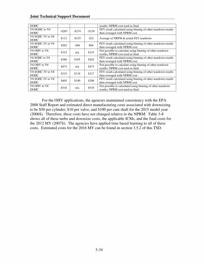
Joint Technical Support Document
3-34
DOHC results; NPRM cost used as final
V8 DOHC to V6
DOHC -$203 -$274 -$238
FEV result calculated using binning of other teardown results
then averaged with NPRM cost
V8 SOHC 3V to V6
DOHC $113 -$155 -$21 Average of NRPM & actual FEV teardown
V8 SOHC 2V to V6
DOHC $203 -$84 $60
FEV result calculated using binning of other teardown results
then averaged with NPRM cost
V8 OHV to V6
DOHC $315 n/a $315
Not possible to calculate using binning of other teardown
results; NPRM cost used as final
V6 SOHC to V6
DOHC $360 $165 $262
FEV result calculated using binning of other teardown results
then averaged with NPRM cost
V6 OHV to V6
DOHC $473 n/a $473
Not possible to calculate using binning of other teardown
results; NPRM cost used as final
V8 SOHC 3V to V8
DOHC $315 $119 $217
FEV result calculated using binning of other teardown results
then averaged with NPRM cost
V8 SOHC 2V to V8
DOHC $405 $190 $298
FEV result calculated using binning of other teardown results
then averaged with NPRM cost
V8 OHV to V8
DOHC $518 n/a $518
Not possible to calculated using binning of other teardown
results; NPRM cost used as final
For the OHV applications, the agencies maintained consistency with the EPA
2008 Staff Report and estimated direct manufacturing costs associated with downsizing
to be $50 per cylinder, $10 per valve, and $100 per cam shaft for the 2015 model year
(2006$). Therefore, these costs have not changed relative to the NPRM. Table 3-8
shows all of these turbo and downsize costs, the applicable ICMs, and the final costs for
the 2012 MY (2007$). The agencies have applied time based learning to all of these
costs. Estimated costs for the 2016 MY can be found in section 3.5.2 of this TSD.
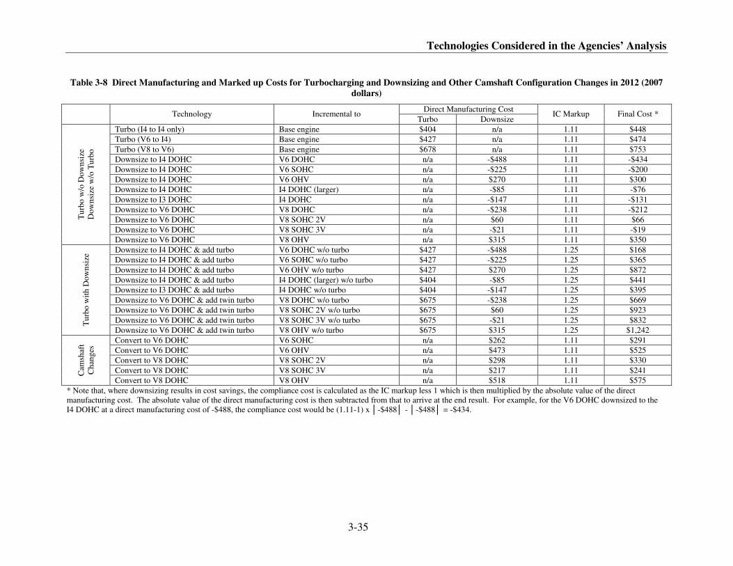
Technologies Considered in the Agencies’ Analysis
3-35
Table 3-8 Direct Manufacturing and Marked up Costs for Turbocharging and Downsizing and Other Camshaft Configuration Changes in 2012 (2007
dollars)
Direct Manufacturing Cost Technology Incremental to
Turbo Downsize IC Markup Final Cost *
Turbo (I4 to I4 only) Base engine $404 n/a 1.11 $448
Turbo (V6 to I4) Base engine $427 n/a 1.11 $474
Turbo (V8 to V6) Base engine $678 n/a 1.11 $753
Downsize to I4 DOHC V6 DOHC n/a -$488 1.11 -$434
Downsize to I4 DOHC V6 SOHC n/a -$225 1.11 -$200
Downsize to I4 DOHC V6 OHV n/a $270 1.11 $300
Downsize to I4 DOHC I4 DOHC (larger) n/a -$85 1.11 -$76
Downsize to I3 DOHC I4 DOHC n/a -$147 1.11 -$131
Downsize to V6 DOHC V8 DOHC n/a -$238 1.11 -$212
Downsize to V6 DOHC V8 SOHC 2V n/a $60 1.11 $66
Downsize to V6 DOHC V8 SOHC 3V n/a -$21 1.11 -$19
Tu
rbo
w/o
Do
wn
size
Do
wn
size
w/o
Tu
rbo
Downsize to V6 DOHC V8 OHV n/a $315 1.11 $350
Downsize to I4 DOHC & add turbo V6 DOHC w/o turbo $427 -$488 1.25 $168
Downsize to I4 DOHC & add turbo V6 SOHC w/o turbo $427 -$225 1.25 $365
Downsize to I4 DOHC & add turbo V6 OHV w/o turbo $427 $270 1.25 $872
Downsize to I4 DOHC & add turbo I4 DOHC (larger) w/o turbo $404 -$85 1.25 $441
Downsize to I3 DOHC & add turbo I4 DOHC w/o turbo $404 -$147 1.25 $395
Downsize to V6 DOHC & add twin turbo V8 DOHC w/o turbo $675 -$238 1.25 $669
Downsize to V6 DOHC & add twin turbo V8 SOHC 2V w/o turbo $675 $60 1.25 $923
Downsize to V6 DOHC & add twin turbo V8 SOHC 3V w/o turbo $675 -$21 1.25 $832 Tu
rbo
wit
h D
ow
nsi
ze
Downsize to V6 DOHC & add twin turbo V8 OHV w/o turbo $675 $315 1.25 $1,242
Convert to V6 DOHC V6 SOHC n/a $262 1.11 $291
Convert to V6 DOHC V6 OHV n/a $473 1.11 $525
Convert to V8 DOHC V8 SOHC 2V n/a $298 1.11 $330
Convert to V8 DOHC V8 SOHC 3V n/a $217 1.11 $241 Cam
shaf
t
Ch
ang
es
Convert to V8 DOHC V8 OHV n/a $518 1.11 $575
* Note that, where downsizing results in cost savings, the compliance cost is calculated as the IC markup less 1 which is then multiplied by the absolute value of the direct
manufacturing cost. The absolute value of the direct manufacturing cost is then subtracted from that to arrive at the end result. For example, for the V6 DOHC downsized to the
I4 DOHC at a direct manufacturing cost of -$488, the compliance cost would be (1.11-1) x │-$488│ - │-$488│ = -$434.
Joint Technical Support Document
3-36
3.4.2.1.10 Cooled Exhaust Gas Recirculation/EGR Boost (EGRB)
Cooled exhaust gas recirculation (cooled EGR) or EGR Boost is a combustion
concept that involves utilizing EGR as a charge dilutant for controlling combustion
temperatures and cooling the EGR prior to its introduction to the combustion system.
Higher exhaust gas residual levels at part load conditions reduce pumping losses for
increased fuel economy. Cooled EGR reduces knock sensitivity which enables the use of
more optimal spark advance or enables compression ratio to be increased for improved
thermal efficiency, and increased fuel economy. Currently available turbo, charge air
cooler, and EGR cooler technologies are sufficient to demonstrate the feasibility of this
concept.
However, this remains a technology with a number of issues that still need to be
addressed and for which there is no production experience. EGR system fouling
characteristics could be potentially worse than diesel EGR system fouling, due to the
higher HC levels found in gasoline exhaust. Turbocharger compressor contamination
may also be an issue for low pressure EGR systems. Additionally, transient controls of
boost pressure, EGR rate, cam phasers and intake charge temperature to exploit the
cooled EGR combustion concept will require development beyond what has already been
accomplished by the automotive industry. These are all “implementation readiness”
issues that must be resolved prior to putting EGR Boost into high volume production.
NHTSA has concluded that these implementation issues could be resolved
and this technology could be brought to production by MY 2013. Supporting this
conclusion, MEMA has previously suggested a 5 to 7 percent effectiveness for
cooled EGR systems, although without boosting.34
Two public sources indicate a 10 to 20 percent fuel consumption
effectiveness for a downsized DI engine with cooled EGR compared to a naturally
aspirated baseline engine35
and a 4 percent fuel consumption effectiveness for
cooled EGR compared to a conventional downsized DI turbocharged engine.36
Based on the data from these reports, NHTSA estimates the incremental reduction
in fuel consumption for EGR Boost to be 4 percent over a turbocharged and
downsized DI engine. Thus, if TRBDS precedes EGRB, adding the 12 percent gain
from TRBDS to the 4 percent gain from EGRB results in total fuel consumption
reduction of 16 percent. This is in agreement with the range suggested in the Lotus
report.
Regarding costs, the addition of EGR cooler and EGR valve were estimated in
NHTSA’s MY 2011 rule to have an incremental RPE cost impact of approximately $173
based on confidential individual component cost data from 2008 Martec describing EGR
cooler costs of $75, EGR valve costs of $20 and associated piping costs of $20, totaling
$115 (non-RPE). For purposes of this rulemaking, NHTSA found no information to
indicate that these estimates were inaccurate. To that end, NHTSA applied an indirect
Technologies Considered in the Agencies’ Analysis
3-37
cost multiplier of 1.25, for a medium complexity technology, resulting in a compliance
cost of $144 for MY 2012 vehicles with time-based learning applied.
3.4.2.1.11 Diesel Engine Technologies
Diesel engines have several characteristics that give them superior fuel efficiency
compared to conventional gasoline, spark-ignited engines. Pumping losses are much
lower due to lack of (or greatly reduced) throttling. The diesel combustion cycle operates
at a higher compression ratio, with a very lean air/fuel mixture, and turbocharged light-
duty diesels typically achieve much higher torque levels at lower engine speeds than
equivalent-displacement naturally-aspirated gasoline engines. Additionally, diesel fuel
has a higher energy content per gallon.l However, diesel fuel also has a higher carbon to
hydrogen ratio, which increases the amount of CO2 emitted per gallon of fuel used by
approximately 15 percent over a gallon of gasoline.
Diesel engines have emissions characteristics that present challenges to meeting
federal Tier 2 NOx emissions standards. It is a significant systems-engineering challenge
to maintain the fuel consumption advantage of the diesel engine while meeting U.S.
emissions regulations. Fuel consumption can be negatively impacted by emissions
reduction strategies depending on the combination of strategies employed. Emission
compliance strategies for diesel vehicles sold in the U.S. are expected to include a
combination of combustion improvements and aftertreatment. These emission control
strategies are being introduced on Tier 2 light-duty diesel vehicles today
To achieve U.S. Tier 2 emissions limits, roughly 45 to 65 percent more NOx
reduction is required compared to the Euro VI standards. Additionally, as discussed
below, there may be a fuel consumption penalty associated with diesel aftertreatment
since extra fuel is needed for the aftertreatment, and this extra fuel is not used in the
combustion process of the engine that provides torque to propel the vehicle.
Light-duty diesel emissions control systems capable of meeting Tier 2 Bin 5
emission standards are already in production. Several key advances in diesel technology
have made it possible to reduce emissions coming from the engine prior to aftertreatment.
These technologies include improved fuel systems (higher injection pressure and
multiple-injection capability), advanced controls and sensors to optimize combustion and
emissions performance, higher EGR levels and EGR cooling to reduce NOx, and
advanced turbocharging systems.
On the aftertreatment side, the traditional 3-way catalyst aftertreatment found on
gasoline-powered vehicles is ineffective due to the lean-burn combustion of a diesel. All
diesels will require a diesel particulate filter (DPF) or catalyzed diesel particulate filter
(CDPF), a diesel oxidation catalyst (DOC), and a NOx reduction strategy to comply with
Tier 2 emissions standards. The most common NOx reduction strategies include the use
of lean NOx traps (LNT) or selective catalytic reduction (SCR), which are outlined
below.
l Burning one gallon of diesel fuel produces about 15 percent more carbon dioxide than gasoline due to the
higher density and carbon to hydrogen ratio.
Joint Technical Support Document
3-38
3.4.2.1.11.1 Diesel Engine with Lean NOx Trap (LNT) Catalyst After-treatment
A lean NOx trap operates, in principle, by oxidizing NO to NO2 in the exhaust
and storing NO2 on alkali sorbent material. When the control system determines (via
mathematical model or a NOx sensor) that the trap is saturated with NOx, it switches the
engine into a rich operating mode or may in some cases inject fuel directly into the
exhaust stream to produce excess hydrocarbons that act as a reducing agent to convert the
stored NOx to N2 and water, thereby “regenerating” the LNT and opening up more
locations for NOx to be stored. LNTs preferentially store sulfate compounds from the
fuel, which can reduce catalytic performance. The system must undergo periodic
desulfurization by operating at a net-fuel-rich condition at high temperatures in order to
retain NOx trapping efficiency.
NHTSA and EPA have concluded that diesel engines on small vehicles would be
LNT-based. In the proposed rule, we did not include a diesel option for small vehicles
because it did not appear to be a cost effective solution. Based on comments received we
are including a diesel option for small vehicles in the final rule, and we are allowing the
respective models to choose whether to apply the technology.
3.4.2.1.11.2 Diesel Engine with Selective Catalyst Reduction (SCR) After-treatment
An SCR aftertreatment system uses a reductant (typically, ammonia derived from
urea) that is injected into the exhaust stream ahead of the SCR catalyst. Ammonia
combines with NOx in the SCR catalyst to form N2 and water. The hardware
configuration for an SCR system is more complicated than that of an LNT, due to the
onboard urea storage and delivery system (which requires a urea pump and injector to
inject urea into the exhaust stream). While a rich engine-operating mode is not required
for NOx reduction, the urea is typically injected at a rate of approximately 3 percent of
the fuel consumed. Manufacturers designing SCR systems intend to align urea tank
refills with standard maintenance practices such as oil changes. As is the case with LNT-
based diesels, EPA and NHTSA project that SCR-based diesel engines will be available
within the next couple of years. Mercedes-Benz recently introduced two 2009 model
year vehicles R320 and GL320, both of which are certified to Tier 2, Bin 5 emission
standards. Based on public announcements from several other companies, an increased
number of product offerings from multiple companies are expected over the next few
years.
In order to maintain equivalent performance to comparable gasoline-engine
vehicles, an in-line 4-cylinder diesel engine, with displacement varying around 2.0 liters
was assumed to replace an I4 gasoline base engine for Subcompact, Compact, and
Midsize Passenger Car, Performance Subcompact Car and Small Light Truck. An in-line
4-cylinder diesel engine, with displacement varying around 2.8 liters was assumed to
replace a V6 gasoline base engine for Performance Compact, Performance Midsize,
Large Passenger Car, Minivan, and Midsize Truck for the CAFE model. A V6 diesel
engine, with displacement varying around 4.0 liters to meet vehicle performance
requirements, was assumed to replace a V8 gasoline base engine for Large Truck and
Technologies Considered in the Agencies’ Analysis
3-39
Performance Large Car vehicle classes for the CAFE model. It was also assumed that
diesel engines for these classes would utilize SCR aftertreatment systems.
Confidential manufacturer and non-confidential comment data submitted in
response to NHTSA’s past rulemaking for diesel engines showed a fuel consumption
reduction in the range of 16.7 to 26.7 percent or a 15 to 23 percent CO2 emission
reduction over a baseline gasoline engine. NHTSA’s MY 2011 CAFE final rule, which
was supported by confidential manufacturer data, estimated the fuel consumption
reduction of a SCR-based diesel engine to be between 19 to 25 percent over a baseline
gasoline engine. NHTSA and EPA have revisited these values and found them to be
reasonable. EPA estimates a 15 to 26 percent CO2 reduction for light-duty diesels
equipped with SCR.
Diesel engines are more costly than port-injected spark-ignition gasoline engines.
These higher costs result from:
• Fuel systems (higher pressures and more responsive injectors);
• Controls and sensors to optimize combustion and emissions performance;
• Engine design (higher cylinder pressures require a more robust engine, but
higher torque output means diesel engines can have reduced displacement);
• Turbocharger(s);
• Aftertreatment systems, which tend to be more costly for diesels;
Due to a significant decrease in platinum group metal prices since NHTSA’s MY
2011 CAFE final rule analysis, the agencies chose to re-analyze diesel costs. In EPA’s
2008 Staff Report, costs were considered for two types of diesel systems: one using a
lean-NOX trap (LNT) along with a diesel particulate filter (DPF); and one using a
selective catalytic reduction (SCR) system along with a DPF. In that report, EPA
estimated direct manufacturing costs to range from $1,860 for the small car (LNT plus
DPF) to $2,710 for the large truck (SCR plus DPF). For comparison, the NESCCAF
study showed direct manufacturing costs of $1,500 to $1,950. More recently, NHTSA’s
MY 2011 CAFE final rule showed direct manufacturing costs of $2,670 for a 4-cylinder
engine using a LNT plus DPF system, $3,735 for a 6-cylinder engine using a SCR plus
DPF system, and $4,668 for an 8-cylinder engine using a SCR plus DPF system.
NHTSA noted that estimates in the MY 2011 CAFE final rule were higher than those
shown in this rule due largely to the spike in platinum group metal prices that had
occurred in the months just prior to issuing the 2011 CAFE final rule.
The following diesel engine costs were developed by first taking a look back at
EPA’s 2008 Staff Report, which reveals a couple of factors that resulted in somewhat
misleading costs. First, the engine costs estimated there did not take into account the
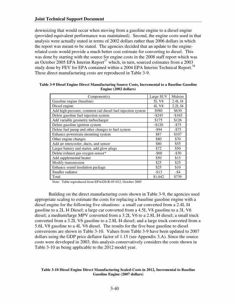
Joint Technical Support Document
3-40
downsizing that would occur when moving from a gasoline engine to a diesel engine
(provided equivalent performance was maintained). Second, the engine costs used in that
analysis were actually stated in terms of 2002 dollars rather than 2006 dollars in which
the report was meant to be stated. The agencies decided that an update to the engine-
related costs would provide a much better cost estimate for converting to diesel. This
was done by starting with the source for engine costs in the 2008 staff report which was
an October 2005 EPA Interim Report37
which, in turn, sourced estimates from a 2003
study done by FEV for EPA contained within a 2004 EPA Interim Technical Report.38
These direct manufacturing costs are reproduced in Table 3-9.
Table 3-9 Diesel Engine Direct Manufacturing Source Costs, Incremental to a Baseline Gasoline
Engine (2002 dollars)
Component(s) Large SUV Midsize
Gasoline engine (baseline) 5L V8 2.4L I4
Diesel engine 4L V8 2.2L I4
Add high-pressure, common rail diesel fuel injection system $980 $630
Delete gasoline fuel injection system -$245 -$165
Add variable geometry turbocharger $175 $126
Delete gasoline ignition system -$120 -$75
Delete fuel pump and other changes to fuel system -$94 -$75
Enhance powertrain mounting system $87 $107
Other engine changes $80 $70
Add air intercooler, ducts, and sensor $80 $55
Larger battery and starter, add glow plugs $72 $50
Delete exhaust gas oxygen sensor* -$60 -$30
Add supplemental heater $50 $15
Modify transmission $25 $25
Enhance sound insulation package $25 $10
Smaller radiator -$13 -$4
Total $1,042 $739
Note: Table reproduced from EPA420-R-05-012, October 2005
Building on the direct manufacturing costs shown in Table 3-9, the agencies used
appropriate scaling to estimate the costs for replacing a baseline gasoline engine with a
diesel engine for the following five situations: a small car converted from a 2.4L I4
gasoline to a 2L I4 Diesel; a large car converted from a 4.5L V8 gasoline to a 3L V6
diesel; a medium/large MPV converted from a 3.2L V6 to a 2.8L I4 diesel; a small truck
converted from a 3.2L V6 gasoline to a 2.8L I4 diesel; and a large truck converted from a
5.6L V8 gasoline to a 4L V6 diesel. The results for the five base gasoline to diesel
conversions are shown in Table 3-10. Values from Table 3-9 have been updated to 2007
dollars using the GDP price deflator factor of 1.15 (see Appendix 3.A). Since the source
costs were developed in 2003, this analysis conservatively considers the costs shown in
Table 3-10 as being applicable to the 2012 model year.
Table 3-10 Diesel Engine Direct Manufacturing Scaled-Costs in 2012, Incremental to Baseline
Gasoline Engine (2007 dollars)
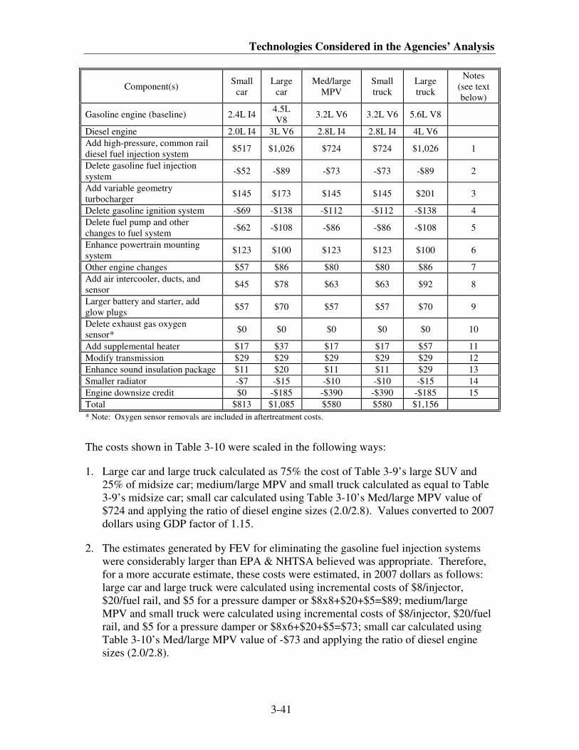
Technologies Considered in the Agencies’ Analysis
3-41
Component(s) Small
car
Large
car
Med/large
MPV
Small
truck
Large
truck
Notes
(see text
below)
Gasoline engine (baseline) 2.4L I4 4.5L
V8 3.2L V6 3.2L V6 5.6L V8
Diesel engine 2.0L I4 3L V6 2.8L I4 2.8L I4 4L V6
Add high-pressure, common rail
diesel fuel injection system $517 $1,026 $724 $724 $1,026 1
Delete gasoline fuel injection
system -$52 -$89 -$73 -$73 -$89 2
Add variable geometry
turbocharger $145 $173 $145 $145 $201 3
Delete gasoline ignition system -$69 -$138 -$112 -$112 -$138 4
Delete fuel pump and other
changes to fuel system -$62 -$108 -$86 -$86 -$108 5
Enhance powertrain mounting
system $123 $100 $123 $123 $100 6
Other engine changes $57 $86 $80 $80 $86 7
Add air intercooler, ducts, and
sensor $45 $78 $63 $63 $92 8
Larger battery and starter, add
glow plugs $57 $70 $57 $57 $70 9
Delete exhaust gas oxygen
sensor* $0 $0 $0 $0 $0 10
Add supplemental heater $17 $37 $17 $17 $57 11
Modify transmission $29 $29 $29 $29 $29 12
Enhance sound insulation package $11 $20 $11 $11 $29 13
Smaller radiator -$7 -$15 -$10 -$10 -$15 14
Engine downsize credit $0 -$185 -$390 -$390 -$185 15
Total $813 $1,085 $580 $580 $1,156
* Note: Oxygen sensor removals are included in aftertreatment costs.
The costs shown in Table 3-10 were scaled in the following ways:
1. Large car and large truck calculated as 75% the cost of Table 3-9’s large SUV and
25% of midsize car; medium/large MPV and small truck calculated as equal to Table
3-9’s midsize car; small car calculated using Table 3-10’s Med/large MPV value of
$724 and applying the ratio of diesel engine sizes (2.0/2.8). Values converted to 2007
dollars using GDP factor of 1.15.
2. The estimates generated by FEV for eliminating the gasoline fuel injection systems
were considerably larger than EPA & NHTSA believed was appropriate. Therefore,
for a more accurate estimate, these costs were estimated, in 2007 dollars as follows:
large car and large truck were calculated using incremental costs of $8/injector,
$20/fuel rail, and $5 for a pressure damper or $8x8+$20+$5=$89; medium/large
MPV and small truck were calculated using incremental costs of $8/injector, $20/fuel
rail, and $5 for a pressure damper or $8x6+$20+$5=$73; small car calculated using
Table 3-10’s Med/large MPV value of -$73 and applying the ratio of diesel engine
sizes (2.0/2.8).
Joint Technical Support Document
3-42
3. Large car calculated as the average of Table 3-9’s large SUV and midsize car;
medium/large MPV and small truck calculated as equal to Table 3-9’s midsize car,
and large truck calculated as equal to Table 3-9’s large SUV; small car calculated as
equal to medium/large MPV. Values converted to 2007 dollars using GDP factor of
1.15.
4. Medium/large MPV and small truck calculated as the average of Table 3-9’s large
SUV and midsize car; Large car and large truck calculated as equal to Table 3-9’s
large SUV; small car calculated as equal to half of Table 3-10’s large truck value of -
$138. Values converted to 2007 dollars using GDP factor of 1.15.
5. Medium/large MPV and small truck calculated as equal to Table 3-9’s midsize car;
Large car and large truck calculated as equal to Table 3-9’s large SUV; small car
calculated using Table 3-10’s Med/large MPV value of -$86 and applying the ratio of
diesel engine sizes (2.0/2.8). Values converted to 2007 dollars using GDP factor of
1.15.
6. Medium/large MPV and small truck calculated as equal to Table 3-9’s large SUV;
Large car and large truck calculated as equal to Table 3-9’s midsize car; small car
calculated as equal to medium/large MPV. Values converted to 2007 dollars using
GDP factor of 1.15.
7. Medium/large MPV and small truck calculated as equal to Table 3-9’s midsize car;
Large car and large truck calculated as the average of Table 3-9’s large SUV and
midsize car; small car calculated using Table 3-10’s Med/large MPV value of $80
and applying the ratio of diesel engine sizes (2.0/2.8). Values converted to 2007
dollars using GDP factor of 1.15.
8. Medium/large MPV and small truck calculated as equal to Table 3-9’s midsize car;
Large car calculated as the average of Table 3-9’s large SUV and midsize car; Large
truck calculated as equal to Table 3-9’s large SUV; small car calculated using Table
3-10’s Med/large MPV value of $63 and applying the ratio of diesel engine sizes
(2.0/2.8). Values converted to 2007 dollars using GDP factor of 1.15.
9. Medium/large MPV and small truck calculated as equal to Table 3-9’s midsize car;
Large car and large truck calculated as the average of Table 3-9’s large SUV and
midsize car; small car calculated as equal to medium/large MPV. Values converted
to 2007 dollars using GDP factor of 1.15.
10. Oxygen sensor costs are included in the aftertreatment costs discussed below.
11. Medium/large MPV and small truck calculated as equal to Table 3-9’s midsize car;
Large car calculated as the average of Table 3-9’s large SUV and midsize car; Large
truck calculated as equal to Table 3-9’s large SUV; small car calculated as equal to
medium/large MPV. Values converted to 2007 dollars using GDP factor of 1.15.
12. Values from Table 3-9 converted to 2007 dollars using GDP factor of 1.15.
Technologies Considered in the Agencies’ Analysis
3-43
13. Medium/large MPV and small truck calculated as equal to Table 3-9’s midsize car;
Large car calculated as the average of Table 3-9’s large SUV and midsize car; Large
truck calculated as equal to Table 3-9’s large SUV; small car calculated as equal to
medium/large MPV. Values converted to 2007 dollars using GDP factor of 1.15.
14. Medium/large MPV and small truck calculated as the average of Table 3-9’s large
SUV and midsize car; Large car and large truck calculated as equal to Table 3-9’s
large SUV; small car calculated using Table 3-10’s Med/large MPV value of -$10
and applying the ratio of diesel engine sizes (2.0/2.8). Values converted to 2007
dollars using GDP factor of 1.15.
15. Based on the approach presented in the turbocharging/downsizing section (see section
3.5.2.1.11), the savings associated with downsizing the gasoline engine were
calculated by estimating the cost in 2007 dollars of each cylinder at $51, each valve at
$10, and each cam at $103.m
Therefore, the large car and large truck, which each lose
two cylinders (-$102), eight valves (-$82) and no cams realize a $185 savings. The
medium/large MPV and small truck would each lose two cylinders (-$102) and eight
valves (-$82) and two cams (-$205) for a savings of $390. The small car downsizing
credit was left at $0 given the small displacement change and lack of cylinder or
valve removals.
For the diesel aftertreatment systems, the approach taken is consistent with the
approach taken in EPA’s 2007/2010 Highway Diesel rule and EPA’s recent locomotive
and marine rule.39
For platinum group metal (PGM) costs, monthly average prices as of
March 2009 as reported by Johnson-Matthey were used.40,n
Those values were
$1,085/troy ounce for platinum and $1,169/troy ounce for rhodium. Aftertreatment
devices were sized according to the diesel engine displacement with a 1:1 ratio for both
the SCR catalyst and the DPF, and a 0.5:1 ratio for the DOC (i.e., the DOC is half the
displacement of the engine). The end result for aftertreatment devices, including a urea
dosing unit, urea tank and necessary brackets and heaters, are shown in Table 3-11. Also
shown in Table 3-11 are the savings associated with removal of the gasoline catalyst.
Note that the gasoline catalyst was sized according to the gasoline engine that served as
the baseline engine.
m These are the correct costs for the 2015MY in 2007$. But, they are used here erroneously as 2012MY
values. Technically, 3 years of time-based learning should have been backed out to get 2012MY values.
So, the 2012MY costs are slightly underestimated by roughly $10. This was true in the proposed analysis
and, because it has no meaningful impact on the analysis (1-2% of the estimated diesel costs), continues to
be true in the final analysis. n These are the PGM prices used in the NPRM. As precious metals, PGM prices swing widely year-to-year
and even month-to-month. Given economic conditions during the past year and the tendency of investors
during tough economic times to invest in valuable metals such as gold and PGMs, PGM prices have
increased considerably since the NPRM. Were the January 2010 PGM prices used, the diesel costs
presented here would increase on the order of 10-20 percent. That would serve to make diesels less cost
effective options for improving fuel economy or reducing GHGs. Since diesels comprise such a small
percentage of each agency’s analysis from a technology penetration standpoint, even using the lower March
2009 PGM prices, the choice of what PGM prices to use is of little consequence to the analytical results for
purposes of this rulemaking.
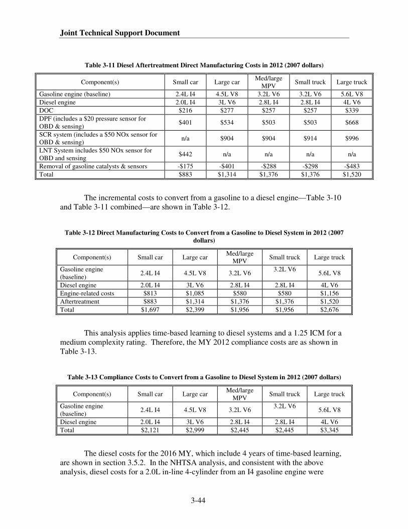
Joint Technical Support Document
3-44
Table 3-11 Diesel Aftertreatment Direct Manufacturing Costs in 2012 (2007 dollars)
Component(s) Small car Large car Med/large
MPV Small truck Large truck
Gasoline engine (baseline) 2.4L I4 4.5L V8 3.2L V6 3.2L V6 5.6L V8
Diesel engine 2.0L I4 3L V6 2.8L I4 2.8L I4 4L V6
DOC $216 $277 $257 $257 $339
DPF (includes a $20 pressure sensor for
OBD & sensing) $401 $534 $503 $503 $668
SCR system (includes a $50 NOx sensor for
OBD & sensing) n/a $904 $904 $914 $996
LNT System includes $50 NOx sensor for
OBD and sensing $442 n/a n/a n/a n/a
Removal of gasoline catalysts & sensors -$175 -$401 -$288 -$298 -$483
Total $883 $1,314 $1,376 $1,376 $1,520
The incremental costs to convert from a gasoline to a diesel engine—Table 3-10
and Table 3-11 combined—are shown in Table 3-12.
Table 3-12 Direct Manufacturing Costs to Convert from a Gasoline to Diesel System in 2012 (2007
dollars)
Component(s) Small car Large car Med/large
MPV Small truck Large truck
Gasoline engine
(baseline) 2.4L I4 4.5L V8 3.2L V6
3.2L V6 5.6L V8
Diesel engine 2.0L I4 3L V6 2.8L I4 2.8L I4 4L V6
Engine-related costs $813 $1,085 $580 $580 $1,156
Aftertreatment $883 $1,314 $1,376 $1,376 $1,520
Total $1,697 $2,399 $1,956 $1,956 $2,676
This analysis applies time-based learning to diesel systems and a 1.25 ICM for a
medium complexity rating. Therefore, the MY 2012 compliance costs are as shown in
Table 3-13.
Table 3-13 Compliance Costs to Convert from a Gasoline to Diesel System in 2012 (2007 dollars)
Component(s) Small car Large car Med/large
MPV Small truck Large truck
Gasoline engine
(baseline) 2.4L I4 4.5L V8 3.2L V6
3.2L V6 5.6L V8
Diesel engine 2.0L I4 3L V6 2.8L I4 2.8L I4 4L V6
Total $2,121 $2,999 $2,445 $2,445 $3,345
The diesel costs for the 2016 MY, which include 4 years of time-based learning,
are shown in section 3.5.2. In the NHTSA analysis, and consistent with the above
analysis, diesel costs for a 2.0L in-line 4-cylinder from an I4 gasoline engine were
Technologies Considered in the Agencies’ Analysis
3-45
estimated to be $2,121 in MY 2012. A 2.8L in-line 4-cylinder from a V6 gasoline engine
were estimated to be $2,445 in MY 2012. A MY 2012 cost of $3,345 was estimated for a
conversion to 4.0L V6 diesel from a V8 gasoline engine. These MY 2012 estimates were
obtained using the in-line 4-cylinder 2.0L cost of $1,697, the in-line 4-cylinder 2.8L cost
of $1956 and V6 cost of $2,676, from Table 3-12, and multiplying them by the medium
complexity ICM markup of 1.25 and are eligible for time-based learning cost reductions.
3.4.2.2 Transmission Technologies
NHTSA and EPA have also reviewed the transmission technology estimates used
in the MY 2011 CAFE final rule. In doing so, NHTSA and EPA considered or
reconsidered all available sources and updated the estimates as appropriate. The section
below describes each of the transmission technologies considered for this rulemaking.
3.4.2.2.1 Improved Automatic Transmission Control (IATC) (Aggressive Shift Logic
and Early Torque Converter Lockup)
Calibrating the transmission shift schedule to upshift earlier and quicker, and to
lock-up or partially lock-up the torque converter under a broader range of operating
conditions can reduce fuel consumption and CO2 emissions. However, this operation can
result in a perceptible degradation in noise, vibration, and harshness (NVH). The degree
to which NVH can be degraded before it becomes noticeable to the driver is strongly
influenced by characteristics of the vehicle, and although it is somewhat subjective, it
always places a limit on how much fuel consumption can be improved by transmission
control changes. Given that the Aggressive Shift Logic and Early Torque Converter
Lockup are best optimized simultaneously due to the fact that adding both of them
primarily requires only minor modifications to the transmission or calibration software,
these two technologies are combined in the modeling.
3.4.2.2.2 Aggressive Shift Logic
During operation, an automatic transmission’s controller manages the operation of
the transmission by scheduling the upshift or downshift, and locking or allowing the
torque converter to slip based on a preprogrammed shift schedule. The shift schedule
contains a number of lookup table functions, which define the shift points and torque
converter lockup based on vehicle speed and throttle position, and other parameters such
as temperature. Aggressive shift logic (ASL) can be employed in such a way as to
maximize fuel efficiency by modifying the shift schedule to upshift earlier and inhibit
downshifts under some conditions, which reduces engine pumping losses and engine
friction. The application of this technology does require a manufacturer to confirm that
drivability, durability, and NVH are not significantly degraded.
The agencies have estimated the effectiveness of aggressive shift logic at 1 to 2
percent, as explained below. The agencies have estimated the cost at $32 for a MY 2012
Joint Technical Support Document
3-46
vehicle, regardless of size (2007$).o With time-based learning applied, this cost would be
$28 for a MY 2016 vehicle (2007$) based on the 2002 NAS report.
3.4.2.2.3 Early Torque Converter Lockup
A torque converter is a fluid coupling located between the engine and
transmission in vehicles with automatic transmissions and continuously-variable
transmissions (CVT). This fluid coupling allows for slip so the engine can run while the
vehicle is idling in gear (as at a stop light), provides for smoothness of the powertrain,
and also provides for torque multiplication during acceleration, and especially launch.
During light acceleration and cruising, the inherent slip in a torque converter causes
increased fuel consumption, so modern automatic transmissions utilize a clutch in the
torque converter to lock it and prevent this slippage. Fuel consumption can be further
reduced by locking up the torque converter at lower vehicle speeds, provided there is
sufficient power to propel the vehicle, and noise and vibration are not excessive.p If the
torque converter cannot be fully locked up for maximum efficiency, a partial lockup
strategy can be employed to reduce slippage. Early torque converter lockup is applicable
to all vehicle types with automatic transmissions. Some torque converters will require
upgraded clutch materials to withstand additional loading and the slipping conditions
during partial lock-up. As with aggressive shift logic, confirmation of acceptable
drivability, performance, durability and NVH characteristics is required to successfully
implement this technology.
Regarding the effectiveness of Improved Automatic Transmission Control, the
MY 2011 CAFE final rule, which was supported by the 2002 NAS and NESCCAF
reports as well as confidential manufacturer data, estimated an effectiveness
improvement of 1 to 2 percent for aggressive shift logic and 0.5 percent for early torque
converter lockup. These estimates are in agreement with the values stated in the
NESCCAF report and confidential manufacturer data. For the purpose of this final rule,
NHTSA and EPA concluded that the combined estimated effectiveness is 1.5 to 2.5
percent reduction in CO2 emissions and fuel consumption.
Regarding cost estimates, the agencies estimate the cost at $29, regardless of
vehicle size and including a low complexity ICM of 1.11 for a MY 2012 vehicle (2007$).
With time-based learning, this cost would be $25 for a MY 2016 vehicle (2007$). For
IATC (or the combination of aggressive shift logic and early torque converter lockup),
the cost, including the 1.11 ICM, would be $60 for a MY 2012 vehicle and $53 for a MY
2016 vehicle after time-based learning (2007$).
3.4.2.2.4 Automatic 6-, 7- and 8-Speed Transmissions (NAUTO)
Manufacturers can also choose to replace 4- and 5-speed transmission with 6-, 7-,
or 8-speed automatic transmissions. Additional ratios allow for further optimization of
engine operation over a wider range of conditions, but this is subject to diminishing
o This reflects a revisiting of component costs for NHTSA since the MY 2011 CAFE final rule.
p Although only modifications to the transmission calibration software are considered as part of this
technology, very aggressive early torque converter lock up may require an adjustment to damper stiffness
and hysteresis inside the torque converter.
Technologies Considered in the Agencies’ Analysis
3-47
returns as the number of speeds increases. As additional planetary gear sets are added
(which may be necessary in some cases to achieve the higher number of ratios),
additional weight and friction are introduced. Also, the additional shifting of such a
transmission can be perceived as bothersome to some consumers, so manufacturers need
to develop strategies for smooth shifts. Some manufacturers are replacing 4- and 5-speed
automatics with 6-speed automatics, and 7- and 8-speed automatics have also entered
production, albeit in lower-volume applications in luxury and performance oriented cars.
As discussed in the MY 2011 CAFE final rule, confidential manufacturer data
projected that 6-speed transmissions could incrementally reduce fuel consumption by 0 to
5 percent from a baseline 4-speed automatic transmission, while an 8-speed transmission
could incrementally reduce fuel consumption by up to 6 percent from a baseline 4-speed
automatic transmission. GM has publicly claimed a fuel economy improvement of up to
4 percent for its new 6-speed automatic transmissions.41
The 2008 EPA Staff Technical
Report found a 4.5 to 6.5 percent fuel consumption improvement for a 6-speed over a 4-
speed automatic transmission.42
Based on this information, NHTSA estimated in the MY
2011 rule, that the conversion to a 6-,7- and 8-speed transmission (NAUTO) from a 4 or
5-speed automatic transmission with IATC would have an incremental fuel consumption
benefit of 1.4 percent to 3.4 percent, for all vehicle classes. From a baseline 4 or 5 speed
transmission without IATC, the incremental fuel consumption benefit would be
approximately 3 to 6 percent, which is consistent with the EPA Staff Report estimate.
NHTSA and EPA reviewed these effectiveness estimates and concluded that they
remain accurate. While the CAFE model follows the incremental approach discussed
above, the GHG model estimates the packaged effectiveness of 4.5 to 6.5 percent.
In the NPRM, NHTSA and EPA reviewed the cost estimates from the MY 2011
CAFE final rule which used cost estimates from 2008 Martec report and the 2008 EPA
Staff Report (which assumed use of a Lepelletier gear set) and concluded that some but
not all 6-speed automatic transmissions would be equipped with Lepelletier gear set. As
such, the estimates were revised to establish the cost for the 6 speed transmission to be
equally divided between application using Lepelletier, and application of a standard
planetary gear set 6-speed automatic transmission as estimated in the 2008 Martec Report
(and the MY 2011 CAFE final rule). The 2008 Martec report estimated a cost of $323
with RPE adjustment and $215 without RPE adjustment for converting a 4-speed to a 6-
speed transmission and a cost of $638 with RPE adjustment or $425 without RPE
adjustment for converting a 4-speed to an 8-speed transmission. As a result, the final
incremental cost estimate in the NPRM was $170, independent of vehicle type and size
and including a low complexity 1.11 ICM (2007$). In the CAFE model, due to the
structure of the vehicle classes used, an additional $102 (2007$) was included to account
for performance vehicle classes and for medium and large trucks. This is because for
performance classes, additional gear ratios, such as 7 and 8 speed transmissions may be
utilized, and for medium and large trucks heavier duty transmissions are required. These
estimates represented MY 2012 vehicle costs
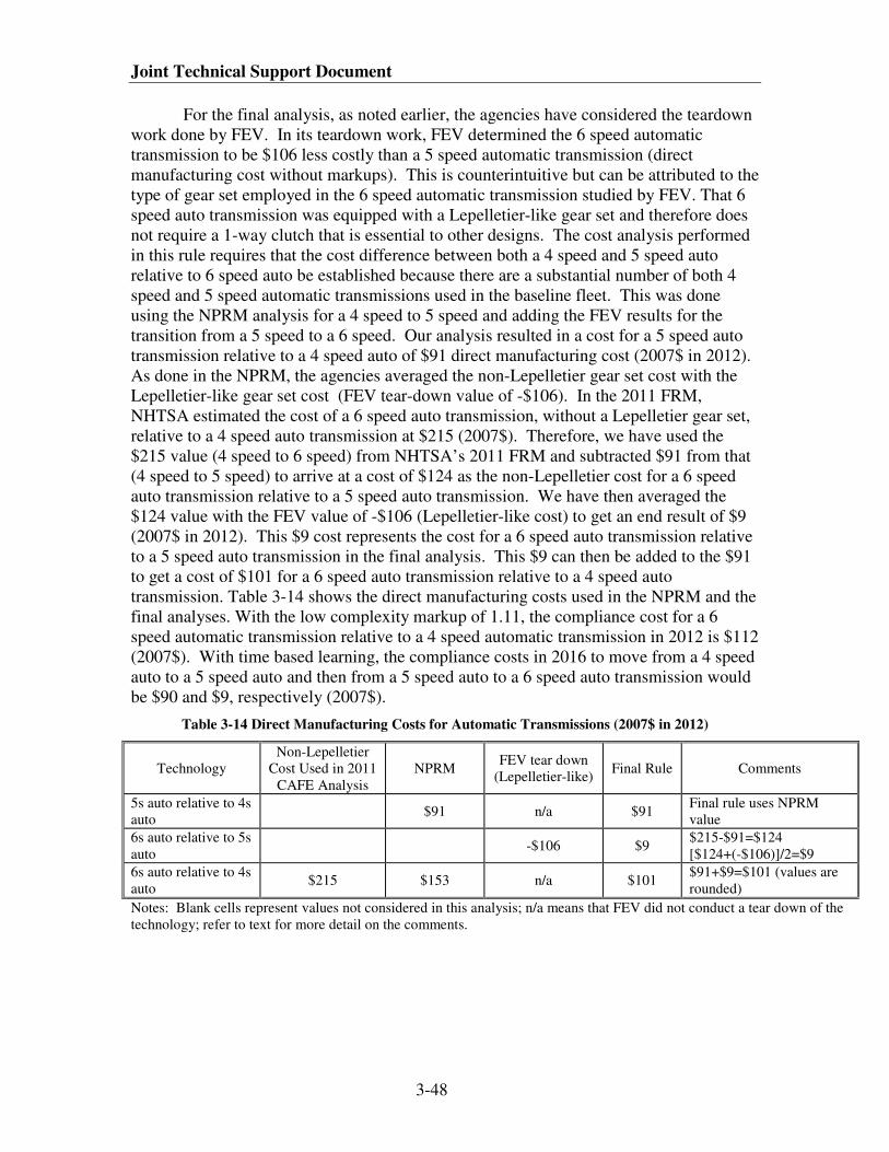
Joint Technical Support Document
3-48
For the final analysis, as noted earlier, the agencies have considered the teardown
work done by FEV. In its teardown work, FEV determined the 6 speed automatic
transmission to be $106 less costly than a 5 speed automatic transmission (direct
manufacturing cost without markups). This is counterintuitive but can be attributed to the
type of gear set employed in the 6 speed automatic transmission studied by FEV. That 6
speed auto transmission was equipped with a Lepelletier-like gear set and therefore does
not require a 1-way clutch that is essential to other designs. The cost analysis performed
in this rule requires that the cost difference between both a 4 speed and 5 speed auto
relative to 6 speed auto be established because there are a substantial number of both 4
speed and 5 speed automatic transmissions used in the baseline fleet. This was done
using the NPRM analysis for a 4 speed to 5 speed and adding the FEV results for the
transition from a 5 speed to a 6 speed. Our analysis resulted in a cost for a 5 speed auto
transmission relative to a 4 speed auto of $91 direct manufacturing cost (2007$ in 2012).
As done in the NPRM, the agencies averaged the non-Lepelletier gear set cost with the
Lepelletier-like gear set cost (FEV tear-down value of -$106). In the 2011 FRM,
NHTSA estimated the cost of a 6 speed auto transmission, without a Lepelletier gear set,
relative to a 4 speed auto transmission at $215 (2007$). Therefore, we have used the
$215 value (4 speed to 6 speed) from NHTSA’s 2011 FRM and subtracted $91 from that
(4 speed to 5 speed) to arrive at a cost of $124 as the non-Lepelletier cost for a 6 speed
auto transmission relative to a 5 speed auto transmission. We have then averaged the
$124 value with the FEV value of -$106 (Lepelletier-like cost) to get an end result of $9
(2007$ in 2012). This $9 cost represents the cost for a 6 speed auto transmission relative
to a 5 speed auto transmission in the final analysis. This $9 can then be added to the $91
to get a cost of $101 for a 6 speed auto transmission relative to a 4 speed auto
transmission. Table 3-14 shows the direct manufacturing costs used in the NPRM and the
final analyses. With the low complexity markup of 1.11, the compliance cost for a 6
speed automatic transmission relative to a 4 speed automatic transmission in 2012 is $112
(2007$). With time based learning, the compliance costs in 2016 to move from a 4 speed
auto to a 5 speed auto and then from a 5 speed auto to a 6 speed auto transmission would
be $90 and $9, respectively (2007$).
Table 3-14 Direct Manufacturing Costs for Automatic Transmissions (2007$ in 2012)
Technology
Non-Lepelletier
Cost Used in 2011
CAFE Analysis
NPRM FEV tear down
(Lepelletier-like) Final Rule Comments
5s auto relative to 4s
auto $91 n/a $91
Final rule uses NPRM
value
6s auto relative to 5s
auto -$106 $9
$215-$91=$124
[$124+(-$106)]/2=$9
6s auto relative to 4s
auto $215 $153 n/a $101
$91+$9=$101 (values are
rounded)
Notes: Blank cells represent values not considered in this analysis; n/a means that FEV did not conduct a tear down of the
technology; refer to text for more detail on the comments.
Technologies Considered in the Agencies’ Analysis
3-49
3.4.2.2.5 Dual Clutch Transmissions / Automated Manual Transmissions (DCTAM)
An Automated Manual Transmission (AMT) is mechanically similar to a
conventional manual transmission, but shifting and launch functions are automatically
controlled by the electronics. There are two basic types of AMTs, single-clutch and dual-
clutch (DCT). A single-clutch AMT is essentially a manual transmission with automated
clutch and shifting. Because of shift quality issues with single-clutch designs, DCTs will
likely be far more common in the U.S. and are the basis of the estimates that follow. A
DCT uses separate clutches (and separate gear shafts) for the even-numbered gears and
odd-numbered gears. In this way, the next expected gear is pre-selected, which allows
for faster and smoother shifting. For example, if the vehicle is accelerating in third gear,
the shaft with gears one, three and five has gear three engaged and is transmitting power.
The shaft with gears two, four, and six is idle, but has gear four engaged. When a shift is
required, the controller disengages the odd-gear clutch while simultaneously engaging the
even-gear clutch, thus making a smooth shift. If, on the other hand, the driver slows
down instead of continuing to accelerate, the transmission will have to change to second
gear on the idling shaft to anticipate a downshift. This shift can be made quickly on the
idling shaft since there is no torque being transferred on it.
In addition to single-clutch and dual-clutch AMTs, there are also wet clutch and
dry clutch designs which are used for different types of vehicle applications. Wet clutch
AMTs offer a higher torque capacity that comes from the use of a hydraulic system that
cools the clutches. Wet clutch systems are less efficient than the dry clutch systems due
to the losses associated with hydraulic pumping. Additionally, wet AMTs have a higher
cost due to the additional hydraulic hardware required.
Overall, DCTs likely offer the greatest potential for effectiveness improvements
among the various transmission options presented in this report because they offer the
inherently lower losses of a manual transmission with the efficiency and shift quality
advantages of electronic controls. The lower losses stem from the elimination of the
conventional lock-up torque converter, and a greatly reduced need for high pressure
hydraulic circuits to hold clutches or bands to maintain gear ratios (in automatic
transmissions) or hold pulleys in position to maintain gear ratio (in Continuously
Variable Transmissions). However, the lack of a torque converter will affect how the
vehicle launches from rest, so a DCT will most likely be paired with an engine that offers
sufficient torque at low engine speeds to allow for adequate launch performance.
For the MY 2011 CAFE final rule, NHTSA estimated a 5.5 to 9.5 percent
improvement in fuel consumption over a baseline 4/5-speed automatic transmission for a
wet clutch DCT, which was assumed for all but the smallest of vehicle subclasses,
Subcompact and Compact cars and small LT. This results in an incremental effectiveness
estimate of 2.7 to 4.1 percent over a 6-speed automatic transmission with IATC. For
Subcompact and Compact Cars and small LT, which were assumed to use a dry clutch
DCT, NHTSA estimated an 8 to 13 percent fuel consumption improvement over a
baseline 4/5-speed automatic transmission, which equates to a 5.5 to 7.5 percent
incremental improvement over the 6-speed transmission. This is consistent with the EPA
Staff Report, which estimated that these transmissions offer an effectiveness of 9.5 to
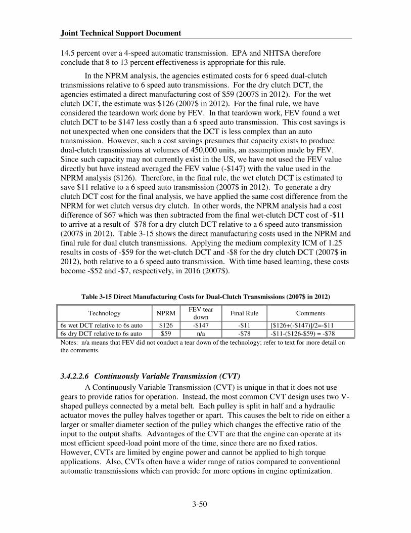
Joint Technical Support Document
3-50
14.5 percent over a 4-speed automatic transmission. EPA and NHTSA therefore
conclude that 8 to 13 percent effectiveness is appropriate for this rule.
In the NPRM analysis, the agencies estimated costs for 6 speed dual-clutch
transmissions relative to 6 speed auto transmissions. For the dry clutch DCT, the
agencies estimated a direct manufacturing cost of $59 (2007$ in 2012). For the wet
clutch DCT, the estimate was $126 (2007$ in 2012). For the final rule, we have
considered the teardown work done by FEV. In that teardown work, FEV found a wet
clutch DCT to be $147 less costly than a 6 speed auto transmission. This cost savings is
not unexpected when one considers that the DCT is less complex than an auto
transmission. However, such a cost savings presumes that capacity exists to produce
dual-clutch transmissions at volumes of 450,000 units, an assumption made by FEV.
Since such capacity may not currently exist in the US, we have not used the FEV value
directly but have instead averaged the FEV value (-$147) with the value used in the
NPRM analysis ($126). Therefore, in the final rule, the wet clutch DCT is estimated to
save $11 relative to a 6 speed auto transmission (2007$ in 2012). To generate a dry
clutch DCT cost for the final analysis, we have applied the same cost difference from the
NPRM for wet clutch versus dry clutch. In other words, the NPRM analysis had a cost
difference of $67 which was then subtracted from the final wet-clutch DCT cost of -$11
to arrive at a result of -$78 for a dry-clutch DCT relative to a 6 speed auto transmission
(2007$ in 2012). Table 3-15 shows the direct manufacturing costs used in the NPRM and
final rule for dual clutch transmissions. Applying the medium complexity ICM of 1.25
results in costs of -$59 for the wet-clutch DCT and -$8 for the dry clutch DCT (2007$ in
2012), both relative to a 6 speed auto transmission. With time based learning, these costs
become -$52 and -$7, respectively, in 2016 (2007$).
Table 3-15 Direct Manufacturing Costs for Dual-Clutch Transmissions (2007$ in 2012)
Technology NPRM FEV tear
down Final Rule Comments
6s wet DCT relative to 6s auto $126 -$147 -$11 [$126+(-$147)]/2=-$11
6s dry DCT relative to 6s auto $59 n/a -$78 -$11-($126-$59) = -$78
Notes: n/a means that FEV did not conduct a tear down of the technology; refer to text for more detail on
the comments.
3.4.2.2.6 Continuously Variable Transmission (CVT)
A Continuously Variable Transmission (CVT) is unique in that it does not use
gears to provide ratios for operation. Instead, the most common CVT design uses two V-
shaped pulleys connected by a metal belt. Each pulley is split in half and a hydraulic
actuator moves the pulley halves together or apart. This causes the belt to ride on either a
larger or smaller diameter section of the pulley which changes the effective ratio of the
input to the output shafts. Advantages of the CVT are that the engine can operate at its
most efficient speed-load point more of the time, since there are no fixed ratios.
However, CVTs are limited by engine power and cannot be applied to high torque
applications. Also, CVTs often have a wider range of ratios compared to conventional
automatic transmissions which can provide for more options in engine optimization.
Technologies Considered in the Agencies’ Analysis
3-51
While CVTs by definition are fully continuous, some automakers choose to emulate
conventional stepped automatic operation because some drivers are not used to the
sensation of the engine speed operating independently of vehicle speed.
Considering the confidential data together with independent review, NHTSA has
estimated the fuel consumption effectiveness for CVTs at 2.2 to 4.5 percent over a 4/5-
speed automatic transmission, which translates into a 0.7 to 2.0 incremental effectiveness
improvement over an automatic transmission with the IATC technology. EPA and
NHTSA reviewed these estimates and found them to be accurate.
The agencies adjusted the original estimates used in the MY 2011 CAFE final
rule to account for medium complexity ICM of 1.25. This resulted in estimated
incremental compliance cost of $250 for the MY 2012 vehicles. In the Volpe model, this
technology was only applied to vehicles manufactured with unibody construction
methods. CVTs are an established and readily available technology, so time based
learning is applied.
3.4.2.2.7 6-Speed Manual Transmissions (6MAN)
Manual transmissions are entirely dependent upon driver input to shift gears: the
driver selects when to perform the shift and which gear to select. This is the most
efficient transfer of energy of all transmission layouts, because it has the lowest internal
gear losses, with a minimal hydraulic system, and the driver provides the energy to
actuate the clutch. From a systems viewpoint, however, vehicles with manual
transmissions have the drawback that the driver may not always select the optimum gear
ratio for fuel economy. Nonetheless, increasing the number of available ratios in a
manual transmission can improve fuel economy by allowing the driver to select a ratio
that optimizes engine operation more often. Typically, this is achieved through adding
overdrive ratios to reduce engine speed at cruising velocities (which saves fuel through
reduced engine pumping losses) and pushing the torque required of the engine towards
the optimum level. However, if the gear ratio steps are not properly designed, this may
require the driver to change gears more often in city driving, resulting in customer
dissatisfaction. Additionally, if gear ratios are selected to achieve improved launch
performance instead of to improve fuel economy, then no fuel saving effectiveness is
realized.
NHTSA’s MY 2011 CAFE final rule estimated an effectiveness increase of 0.5
percent for replacing a 5-speed manual with a 6-speed manual transmission, which was
derived from confidential manufacturer data. NHTSA and EPA have found no evidence
to dispute this estimate and chosen to use 0.5 percent reduction in CO2 emissions and fuel
consumption for replacing a 5-speed manual with a 6-speed manual transmission for this
rule.
NHTSA updated costs to reflect the ICM low complexity markup of 1.11 which
resulted in a incremental compliance cost of $250 as compared to $338 for MY 2012,
with lower costs in later MYs due to the application of time-based learning factors. In
the 2008 Staff Report, EPA estimated this RPE (1.5 RPE factor) at $107 (2006$) relative
to a 5-speed manual transmission and for a MY 2015 vehicle. EPA updated this value to
Joint Technical Support Document
3-52
2007$ and used a 1.11 ICM to get costs of $89 for a MY 2012 vehicle and $69 for a MY
2016 vehicle, both relative to a 5-speed manual transmission (2007$).
3.4.2.3 Hybrid and Electrification/Accessory Technologies
A Hybrid is a vehicle that combines two or more sources of propulsion energy,
where one uses a consumable fuel (like gasoline), and one is rechargeable (during
operation, or by another energy source). Hybrid technology is established in the U.S.
market and more manufacturers are adding hybrid models to their lineups. Hybrids
reduce fuel consumption through three major mechanisms:
• The internal combustion engine can be optimized (through downsizing,
modifying the operating cycle, or other control techniques) to operate at or
near its most efficient point more of the time. Power loss from engine
downsizing can be mitigated by employing power assist from the secondary
power source.
• Some of the energy normally lost as heat while braking can be captured and
stored in the energy storage system for later use.
• The engine is turned off when it is not needed, such as when the vehicle is
coasting or when stopped.
Hybrid vehicles utilize some combination of the three above mechanisms to
reduce fuel consumption and CO2 emissions. A fourth mechanism to reduce petroleum
fuel consumption, available only to plug-in hybrids, is by substituting the petroleum fuel
energy with energy from another source, such as the electric grid. The effectiveness of
fuel consumption and CO2 reduction depends on the utilization of the above mechanisms
and how aggressively they are pursued. One area where this variation is particularly
prevalent is in the choice of engine size and its effect on balancing fuel economy and
performance. Some manufacturers choose not to downsize the engine when applying
hybrid technologies. In these cases, performance is vastly improved, while fuel
efficiency improves significantly less than if the engine was downsized to maintain the
same performance as the conventional version. While this approach has been used in
cars such as the Honda Accord Hybrid (now discontinued), it is more likely to be used for
vehicles like trucks where towing and/or hauling is an integral part of their performance
requirements. In these cases, if the engine is downsized, the battery can be quickly
drained during a long hill climb with a heavy load, leaving only a downsized engine to
carry the entire load. Because towing capability is currently a heavily-marketed truck
attribute, manufacturers are hesitant to offer a truck with downsized engine which can
lead to a significantly diminished towing performance with a low battery, and therefore
engines are traditionally not downsized for these vehicles.
Although hybrid vehicles using other energy storage concepts (flywheel,
hydraulic) have been developed, the systems currently in production in the U.S. for
passenger cars and light trucks use battery storage and electric drive systems. Hybrid
Technologies Considered in the Agencies’ Analysis
3-53
electric vehicles (HEV) are part of a continuum of vehicles using systems with differing
levels of electric drive and electric energy storage. This range of vehicles includes
relatively basic engine start/stop systems, HEV systems with varying degrees of electric
storage and electric drive system capability, plug-in hybrid electric vehicles (PHEV) with
differing degrees of all electric range and battery electric vehicles (EV) that rely entirely
on electric drive and battery electric energy storage.
Different HEV, PHEV and EV concepts utilize these mechanisms differently, so
they are treated separately for the purposes of this analysis. Below is a discussion of
battery energy storage and the major hybrid concepts that were determined to be
available in the near term. In many applications, particularly with PHEV and EV, the
battery represents the most costly and system-limiting sub-component of the hybrid
system. Currently, there are many battery chemistries being developed and refined for
hybrid applications that are expected to enhance the performance of future hybrid
vehicles.
3.4.2.3.1 Batteries for MHEV, HEV, PHEV and EV Applications
The design of battery secondary cells can vary considerably between MHEV,
HEV, PHEV and EV applications.
MHEV batteries: Due to their lower voltage (12-42 VDC) and reduced power
and energy requirements, MHEV systems will likely continue to use lead-acid batteries.
MHEV battery designs differ from those of current starved-electrolyte (typical
maintenance free batteries) or flooded-electrolyte (the older style lead-acid batteries
requiring water “top-off”) batteries used for starting, lighting and ignition (SLI) in
automotive applications. Standard SLI batteries are primarily designed to provide high-
current for engine start-up and then recharge immediately after startup via the vehicle’s
charging system. Deeply discharging a standard SLI battery will greatly shorten its life.
MHEV applications are expected to use:
• Extended-cycle-life flooded (ELF) lead-acid batteries
• Absorptive glass matt, valve-regulated lead-acid (AGM/VRLA) batteries –
or –
• Asymmetric lead-acid battery/capacitor hybrids (e.g., flooded
ultrabatteries)
MHEV systems using electrolytic double-layer capacitors are also under development.
HEV batteries: HEV applications operate in a narrow, short-cycling, charge-
sustaining state of charge (SOC). Energy capacity in HEV applications is somewhat
limited by the ability of the battery and power electronics to accept charge and by space
and weight constraints within the vehicle design. HEV battery designs tend to be
optimized for high power density rather than high energy density, with thinner cathode
and anode layers and more numerous current collectors and separators (Figure 3-1).
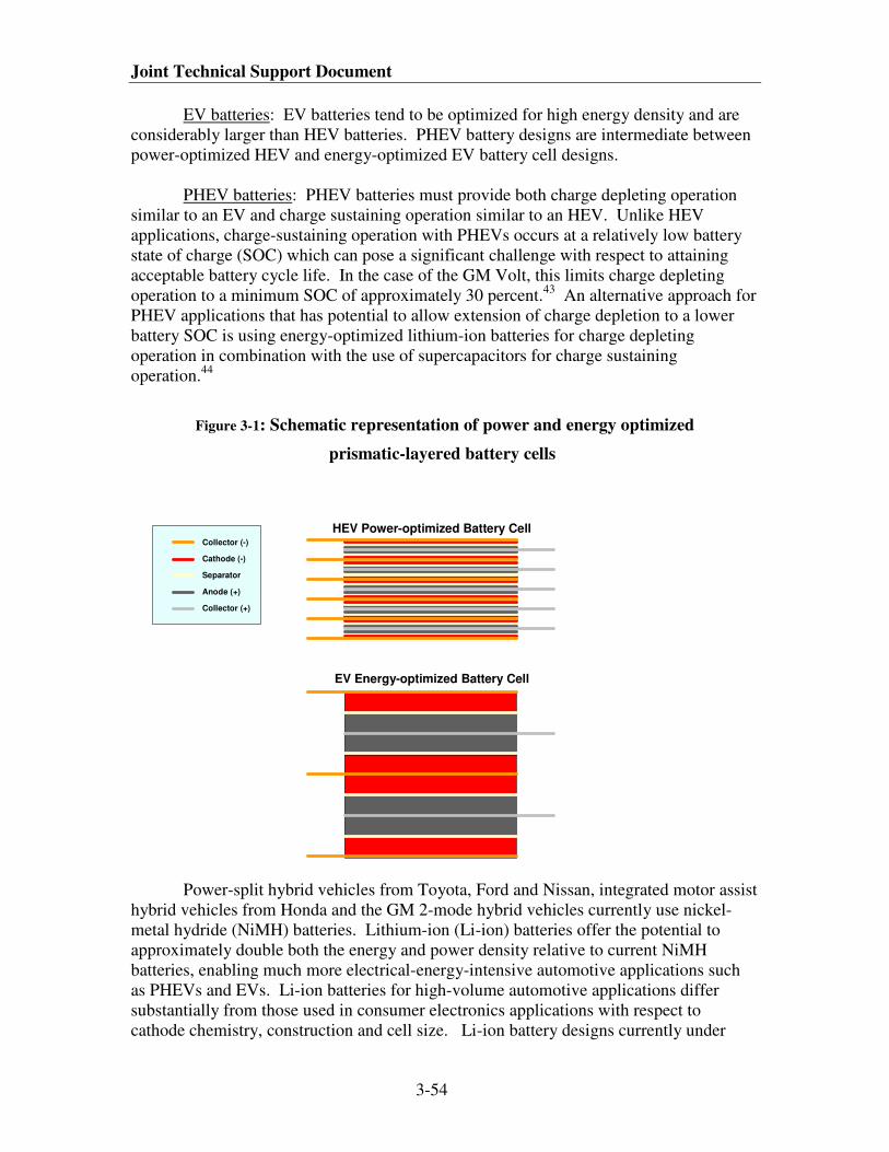
Joint Technical Support Document
3-54
EV batteries: EV batteries tend to be optimized for high energy density and are
considerably larger than HEV batteries. PHEV battery designs are intermediate between
power-optimized HEV and energy-optimized EV battery cell designs.
PHEV batteries: PHEV batteries must provide both charge depleting operation
similar to an EV and charge sustaining operation similar to an HEV. Unlike HEV
applications, charge-sustaining operation with PHEVs occurs at a relatively low battery
state of charge (SOC) which can pose a significant challenge with respect to attaining
acceptable battery cycle life. In the case of the GM Volt, this limits charge depleting
operation to a minimum SOC of approximately 30 percent.43
An alternative approach for
PHEV applications that has potential to allow extension of charge depletion to a lower
battery SOC is using energy-optimized lithium-ion batteries for charge depleting
operation in combination with the use of supercapacitors for charge sustaining
operation.44
Figure 3-1: Schematic representation of power and energy optimized
prismatic-layered battery cells
Collector (-)
Cathode (-)
Separator
Anode (+)
Collector (+)
HEV Power-optimized Battery Cell
EV Energy-optimized Battery Cell
Power-split hybrid vehicles from Toyota, Ford and Nissan, integrated motor assist
hybrid vehicles from Honda and the GM 2-mode hybrid vehicles currently use nickel-
metal hydride (NiMH) batteries. Lithium-ion (Li-ion) batteries offer the potential to
approximately double both the energy and power density relative to current NiMH
batteries, enabling much more electrical-energy-intensive automotive applications such
as PHEVs and EVs. Li-ion batteries for high-volume automotive applications differ
substantially from those used in consumer electronics applications with respect to
cathode chemistry, construction and cell size. Li-ion battery designs currently under
Technologies Considered in the Agencies’ Analysis
3-55
development by CPI (LG-Chem) for the GM Volt PHEV and by AESC, GS-Yuasa and
A123 Systems (respectively) for the upcoming Nissan, Mitsubishi and Chrysler EVs use
large-format, layered-prismatic cells assembled into battery modules. The modules are
then combined into battery packs.
Cathodes for large-format, automotive Li-ion batteries are becoming increasingly
focused on two chemistries – LiMn2O4-spinel (CPI, GS-Yuasa, AESC) and LiFePO4
(A123 Systems).
In addition to the purely hybrid technologies, which decrease the proportion of
propulsion energy coming from the fuel by increasing the proportion of that energy
coming from electricity, there are other steps that can be taken to improve the efficiency
of auxiliary functions (e.g., power-assisted steering or air-conditioning) which also
reduce CO2 emissions and fuel consumption. These steps, together with the hybrid
technologies, are collectively referred to as “vehicle electrification” because they
generally use electricity instead of engine power. In order to achieve consistency
between the two modeling techniques, and to improve the number and range of
technology offerings, the CAFE model was revised to include one additional mild hybrid
technology. The high voltage or improved efficiency alternator (HVIA) technology,
which was used in the MY 2011 CAFE final rule, is no longer represented as a separate
technology and has instead been incorporated into this new mild hybrid technology, as
discussed further below.
3.4.2.3.2 Hybrid System Sizing and Cost Estimating Methodology
NHTSA and EPA reviewed estimates of cost and effectiveness for hybrid and
related electrical technologies and adjusted them as appropriate. Both agencies found the
hybrid technology cost estimating methodology that Ricardo and NHTSA developed
during the MY 2011 CAFE final rule to be reasonable and used it to estimate hybrid
systems costs and account for variation in component sizing across both the hybrid types
and vehicle subclasses. That method utilizes four pieces of data: (1) key component
sizes for a midsize car by hybrid system type; (2) normalized costs for each key
component; (3) component scaling factors that are applied to each vehicle class/subclass
by hybrid system type; and (4) vehicle characteristics for the subclasses which are used as
the basis for the scaling factors. During development of the methodology, NHTSA and
Ricardo made several assumptions:
1) Hybrid controls hardware varies with the level of functionality offered by the
hybrid technology. Assumed hybrid controls complexity for a 12V micro
hybrid (MHEV) and belt integrated starter generator (BISG) was 25 percent of
a strong hybrid controls system and the complexity for a Crank Integrated
Starter Generator (CISG) was 50 percent. These ratios were estimates based
on the directional need for increased functionality as system complexity
increases.
2) Li-ion batteries for hybrid electric vehicles are currently entering production,
including a 2010 MY Mercedes and Hyundai. One estimate from Anderman
indicates that Li-ion market penetration will achieve 35 percent by 2015.45
Joint Technical Support Document
3-56
However, as was discussed above, significant development effort is underway
by a number of battery producers which could impact cost and overcome other
technical concerns. Therefore it was assumed that mild hybrids (MHEV,
BISG, CISG) and strong hybrids (PSHEV, 2MHEV, PHEV) will use either
Li-ion or NiMH batteries, depending on cost considerations. However, plug-
in hybrids will use Li-ion batteries only. Battery usage is discussed further
below.
3) The plug-in hybrid battery pack was sized for a mid-sized car by assuming:
the vehicle has a 20 mile all electric range and consumes an average of 300
W-hr per mile; the battery pack can be discharged down to 30 percent depth of
discharge;q and the capacity of a new battery pack is 20 percent greater than at
end of life (i.e., range on a new battery pack is 24 miles).
4) All hybrid systems included a DC/DC converter which was sized to
accommodate vehicle electrical loads appropriate for increased vehicle
electrification in the time frame considered.
5) High voltage wiring scaled with hybrid vehicle functionality and could be
represented as a fraction of strong hybrid wiring. These ratios were estimates
based on the directional need for increased functionality as system complexity
increases.
6) All hybrid systems included a supplemental heater to provide vehicle heating
when the engine is stopped; however, in this analysis, it is assumed that only
half of the vehicles will adapt this technology, as discussed further below.
Only the strong hybrids included electric air conditioning to enable engine
stop/start when vehicle air conditioning was requested by the operator.
Furthermore, NHTSA and Ricardo recognized that some strong hybrid systems
replaced a conventional transmission with a hybrid-specific transmission, resulting in a
cost offset (i.e., a cost credit) for the removal of a portion of the clutches and gear sets
within the transmission. In the MY 2011 CAFE final rule, the transmission cost in Table
3-16 below expressed hybrid transmission costs as a percentage of traditional automatic
transmission cost, as described in the 2008 Martec Report, at $850 direct manufacturing
costs (non-RPE/ICM). The method assumed that the mechanical aspect of a power-split
transmission with a reduced number of gear sets and clutches resulted in a cost savings of
50 percent ($425) over a conventional transmission with torque converter. For a 2-mode
hybrid, the mechanical aspects of the transmission are similar in complexity to a
conventional transmission, so no cost savings was appropriate. The plug-in hybrid
assumed a highly simplified transmission for electric motor drive, thus 25 percent of the
base vehicle transmission cost was applied (resulting in a $638 credit).
The NHTSA MY 2011 CAFE final rule discusses in detail how the hybrid cost
estimating methodology uses the information provided in the tables below to calculate
costs for each of the strong hybrid systems used in this analysis. It also includes a step-
by-step example for the midsize vehicle mild hybrid systems used in the MY 2011 CAFE
q The GM Volt operates between 30% DOD and 85% DOD. So there is 55% useable DOD, but charge
sustaining operation starts at 30% and cycles between 30 and 35% DOD.
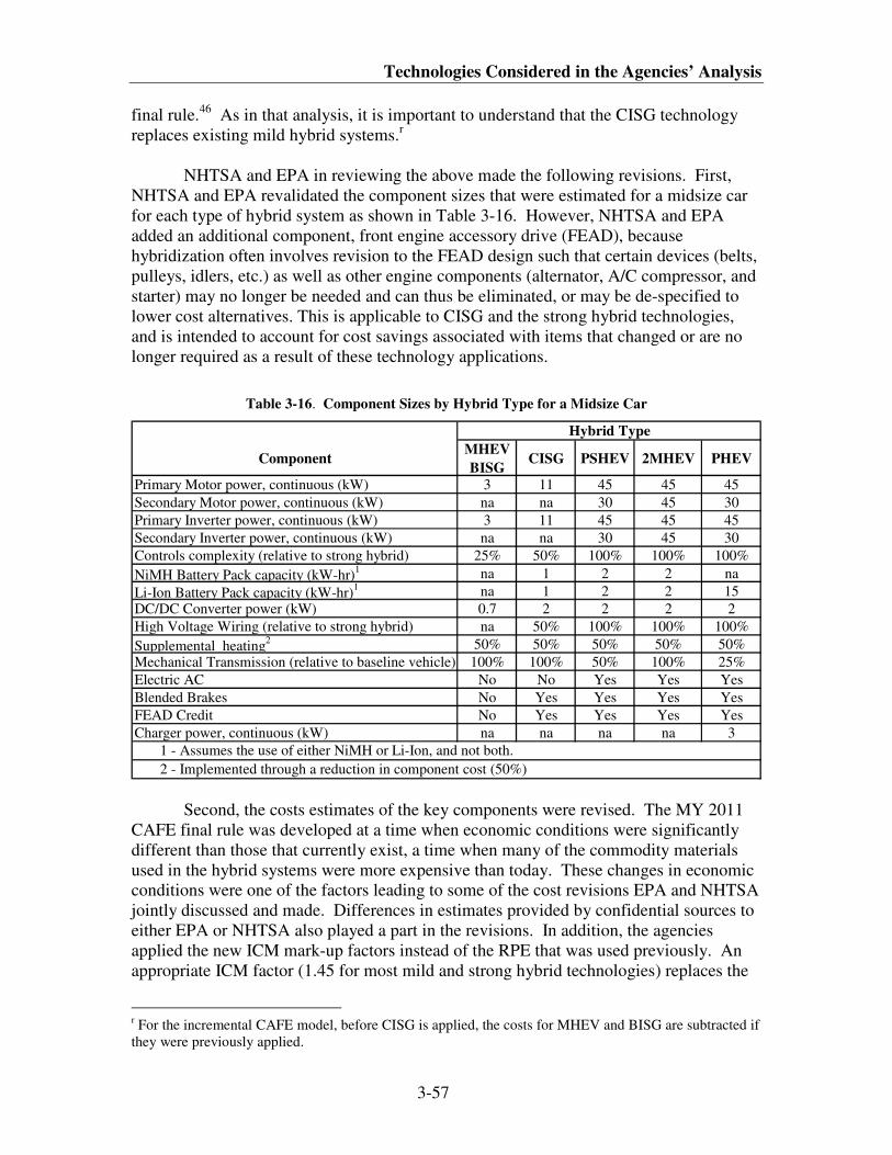
Technologies Considered in the Agencies’ Analysis
3-57
final rule.46
As in that analysis, it is important to understand that the CISG technology
replaces existing mild hybrid systems.r
NHTSA and EPA in reviewing the above made the following revisions. First,
NHTSA and EPA revalidated the component sizes that were estimated for a midsize car
for each type of hybrid system as shown in Table 3-16. However, NHTSA and EPA
added an additional component, front engine accessory drive (FEAD), because
hybridization often involves revision to the FEAD design such that certain devices (belts,
pulleys, idlers, etc.) as well as other engine components (alternator, A/C compressor, and
starter) may no longer be needed and can thus be eliminated, or may be de-specified to
lower cost alternatives. This is applicable to CISG and the strong hybrid technologies,
and is intended to account for cost savings associated with items that changed or are no
longer required as a result of these technology applications.
Table 3-16. Component Sizes by Hybrid Type for a Midsize Car
ComponentMHEV
BISGCISG PSHEV 2MHEV PHEV
Primary Motor power, continuous (kW) 3 11 45 45 45
Secondary Motor power, continuous (kW) na na 30 45 30
Primary Inverter power, continuous (kW) 3 11 45 45 45
Secondary Inverter power, continuous (kW) na na 30 45 30
Controls complexity (relative to strong hybrid) 25% 50% 100% 100% 100%
NiMH Battery Pack capacity (kW-hr)1 na 1 2 2 na
Li-Ion Battery Pack capacity (kW-hr)1 na 1 2 2 15
DC/DC Converter power (kW) 0.7 2 2 2 2
High Voltage Wiring (relative to strong hybrid) na 50% 100% 100% 100%
Supplemental heating2 50% 50% 50% 50% 50%
Mechanical Transmission (relative to baseline vehicle) 100% 100% 50% 100% 25%
Electric AC No No Yes Yes Yes
Blended Brakes No Yes Yes Yes Yes
FEAD Credit No Yes Yes Yes Yes
Charger power, continuous (kW) na na na na 3
2 - Implemented through a reduction in component cost (50%)
1 - Assumes the use of either NiMH or Li-Ion, and not both.
Hybrid Type
Second, the costs estimates of the key components were revised. The MY 2011
CAFE final rule was developed at a time when economic conditions were significantly
different than those that currently exist, a time when many of the commodity materials
used in the hybrid systems were more expensive than today. These changes in economic
conditions were one of the factors leading to some of the cost revisions EPA and NHTSA
jointly discussed and made. Differences in estimates provided by confidential sources to
either EPA or NHTSA also played a part in the revisions. In addition, the agencies
applied the new ICM mark-up factors instead of the RPE that was used previously. An
appropriate ICM factor (1.45 for most mild and strong hybrid technologies) replaces the
r For the incremental CAFE model, before CISG is applied, the costs for MHEV and BISG are subtracted if
they were previously applied.
Joint Technical Support Document
3-58
previous RPE factor (1.5), as discussed in section 3.3.2.2.2. Specifically, the primary and
secondary inverter cost per kilowatt were revised downward from $10 to $7, the controls
cost was revised upward from $100 to $115, the DC/DC converter costs were revised
from $100 to $88, the blended brake system that was revised from $400 to $310, and
finally the fully learned, high volume production, cost per kilowatt hour (kW-hr) for
NiMH batteries was revised from $350 to $320 to match the updated costs for Li-ion
batteries discussed below.s
The cost for Li-ion batteries was also revised. As previously stated, Li-ion
batteries are being implemented in series production in model year 2010. Battery
technology is changing rapidly in the marketplace today, as discussed above, and is
expected to continue along this path throughout the rulemaking period. OEMs are now
forming relationships with battery manufacturers in an effort to research and develop not
only new and improved battery technology, but also more efficient manufacturing
processes capable of supporting high volume production. Accordingly, as shown in
Table 3-17, the $600 per kW-hr used in the MY 2011 CAFE final rule was revised
downward to $320 per kW-hr. The revision downward from $600/kW-hr in the MY
2011 CAFE final rule to $320/kW-hr in this analysis was done based a study by Deutsche
Bank that estimated Li-ion battery costs at 300-400 €/kW-hr.47
This was converted to
$500/kW-hr then learned twice using volume-based learning to arrive at the $320/kW-hr
applicable in the 2015 timeframe.
Li-ion batteries were originally restricted to plug-in hybrids only. Recent vehicle
introductions confirm either battery technology can be used in any mild or strong HEV
application. However, manufacturers are likely to consider cost highly in their selection
of battery technology. If Li-ion battery prices remain high, NiMH would be the default
battery technology for all hybrid electric vehicles. For plug-in hybrids Li-ion would
continue to be required because plug-in hybrids demand higher energy density than
NiMH can provide. Neither the CAFE nor OMEGA model predicts a high penetration of
plug-in technology in achieving the standards.
Finally, the agencies assessed the cost savings associated with the FEAD credit
discussed above. This cost was not previously represented in the hybrid cost model. As
shown in Table 3-17 below, a $100 credit is shown which offsets directly the costs of the
other components specified. This is the best approximation of the value of these items,
based on NHTSA and EPA engineering assessment.
Estimates of each key component are shown in Table 3-17 below along with the
sources of those estimates. The cost basis estimates assume fully learned, high-volume
(greater than 1.2 million units per annum) production, and the costs shown are direct
manufacturing costs that are not RPE or ICM adjusted. This table does not show a cost
applicable to the belt integrated starter generator system (BISG) since it is a fixed cost
that, like the automatic transmission pump cost, is not scaled by subclass as described
later.
s In the MY 2011 final rule NHTSA had misstated this $350 per kW-hr cost as $50 per kW-hr due to a
typographical error.
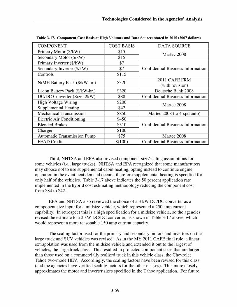
Technologies Considered in the Agencies’ Analysis
3-59
Table 3-17. Component Cost Basis at High Volumes and Data Sources stated in 2015 (2007 dollars)
COMPONENT COST BASIS DATA SOURCE
Primary Motor ($/kW) $15
Secondary Motor ($/kW) $15 Martec 2008
Primary Inverter ($/kW) $7
Secondary Inverter ($/kW) $7
Controls $115
Confidential Business Information
NiMH Battery Pack ($/kW-hr.) $320 2011 CAFE FRM
(with revision)
Li-ion Battery Pack ($/kW-hr.) $320 Deutsche Bank 2008
DC/DC Converter (Size: 2kW) $88 Confidential Business Information
High Voltage Wiring $200
Supplemental Heating $42 Martec 2008
Mechanical Transmission $850 Martec 2008 (to 4-spd auto)
Electric Air Conditioning $450
Blended Brakes $310
Charger $100
Confidential Business Information
Automatic Transmission Pump $75 Martec 2008
FEAD Credit $(100) Confidential Business Information
Third, NHTSA and EPA also revised component size/scaling assumptions for
some vehicles (i.e., large trucks). NHTSA and EPA recognized that some manufacturers
may choose not to use supplemental cabin heating, opting instead to continue engine
operation in the event heat demand occurs; therefore supplemental heating is specified for
only half of the vehicles. Table 3-17 above indicates the 50 percent application rate
implemented in the hybrid cost estimating methodology reducing the component cost
from $84 to $42.
EPA and NHTSA also reviewed the choice of a 3 kW DC/DC converter as a
component size input for a midsize vehicle, which represented a 250 amp current
capability. In retrospect this is a high specification for a midsize vehicle, so the agencies
revised the estimate to a 2 kW DC/DC converter, as shown in Table 3-17 above, which
would represent a more reasonable 150 amp current capacity.
The scaling factor used for the primary and secondary motors and invertors on the
large truck and SUV vehicles was revised. As in the MY 2011 CAFE final rule, a linear
extrapolation was used from the midsize vehicle and extended it out to the largest of
vehicles, the large truck class. This resulted in projected component sizes that are larger
than those used on a commercially realized truck in this vehicle class, the Chevrolet
Tahoe two-mode HEV. Accordingly, the scaling factors have been revised for this class
(and the agencies have verified scaling factors for the other classes). This more closely
approximates the motor and inverter sizes specified in the Tahoe application. For future
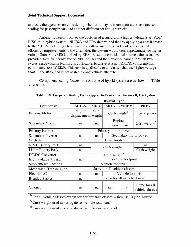
Joint Technical Support Document
3-60
analysis, the agencies are considering whether it may be more accurate to use one set of
scaling for passenger cars and another different set for light trucks.
Another revision involves the addition of a stand-alone higher voltage Start-Stop/
BISG mild hybrid system. NHTSA and EPA determined that by applying a cost increase
to the MHEV technology to allow for a voltage increase (lead acid batteries) and
efficiency improvements to the alternator, the system would then approximate the higher
voltage Start-Stop/BISG applied by EPA. Based on confidential sources, the estimates
provided were first converted to 2007 dollars and then reverse-learned through two
cycles, since volume learning is applicable, to arrive at a non-RPE/ICM incremental
compliance cost of $229. This cost is applicable to all classes that use higher voltage
Start-Stop/BISG, and is not scaled by any vehicle attribute.
Component scaling factors for each type of hybrid system are as shown in Table
3-18 below.
Table 3-18. Component Scaling Factors applied to Vehicle Class for each Hybrid System
Component MHEV CISG PSHEV 2MHEV PHEV
Primary MotorEngine
displacement
Curb
weightEngine power
Secondary Motor na na Curb weight2
Primary Inverter
Secondary Inverter na na
Controls
NiMH Battery Pack na na
Li-Ion Battery Pack na Curb weight
DC/DC Converter
High Voltage Wiring na
Supplemental heating
Mechanical Transmission
Electric AC na na
Blended Brakes na
Charger na na na naSame for all
vehicle classes
(1) For all vehicle classes except for performance classes which use Engine Torque
(2) Curb weight used as surrogate for vehicle road load
(3) Curb weight used as surrogate for vehicle electrical load
Same for all vehicle classes
Hybrid Type
Engine
displacement
Curb weight1
Curb weight3
Vehicle footprint
Same for all vehicle classes
Vehicle footprint
Vehicle footprint
Primary motor power
Secondary motor power
Complexity
Curb weight
Technologies Considered in the Agencies’ Analysis
3-61
Regarding the market data file from the MY 2011 CAFE final rule, NHTSA and
EPA did not make any revisions to the average vehicle characteristics for each vehicle
subclass as shown in Table 3-19, which defines the average vehicle characteristics for
each vehicle subclass. These characteristics were used as the basis of the scaling factors
in the CAFE and OMEGA models. EPA used these vehicle specifications solely for the
purpose of scaling hybrid vehicle attributes in order to remain consistent with the
NHTSA methodology.
Table 3-19. Key Vehicle Characteristics For Each Vehicle Subclass for CAFE Model
Vehicle Subclass
Curb
Weight
(lbs)
Footprint
(ft2)
Engine
Disp. (L)
Engine
Power
(hp)
Torque
(ft-lb)
Subcompact Car 2795 41 1.9 134 133
Compact Car 3359 44 2.2 166 167
Midsize Car 3725 47 2.9 205 206
Large Car 4110 50 3.4 258 248
Performance Subcompact Car 3054 40 2.7 260 260
Performance Compact Car 3516 44 3.0 269 260
Performance Midsize Car 3822 47 3.9 337 318
Performance Large Car 4189 51 4.8 394 388
Minivan 4090 50 3.3 247 242
Small Truck 3413 45 2.6 178 185
Medium Truck 4260 50 3.6 250 256
Large Truck 5366 63 5.0 323 352
3.4.2.3.3 Electrical Power Steering (EPS)
Electric power steering (EPS) provides a potential reduction in CO2 emissions and
fuel consumption over hydraulic power steering because of reduced overall accessory
loads. This eliminates the parasitic losses associated with belt-driven power steering
pumps which consistently draw load from the engine to pump hydraulic fluid through the
steering actuation systems even when the wheels are not being turned. EPS is an enabler
for all vehicle hybridization technologies since it provides power steering when the
engine is off. EPS may be implemented on most vehicles with a standard 12V system.
Some heavier vehicles may require a higher voltage system which may add cost and
complexity.
In the MY 2011 CAFE final rule, NHTSA estimated a 1 to 2 percent effectiveness
based on the 2002 NAS report, a Sierra Research report, and confidential manufacturer
Joint Technical Support Document
3-62
data. NHTSA and EPA reviewed these effectiveness estimates and found them to be
accurate, thus they have been retained for this final rule.
Regarding costs, in the MY 2011 CAFE final rule, NHTSA estimated EPS at
$105-120 at 1.5 RPE mark-up factor. NHTSA and EPA adjusted the EPS cost for the
current rulemaking based on a review of the specification of the system. Adjustments
were made to include potentially higher voltage or heavier duty system operation, such as
would be required on some hybrid trucks. Accordingly, higher costs were estimated for
systems with higher capability. After accounting for the differences in system capability
and applying the ICM markup of low complexity technology of 1.11, the estimated costs
for this rulemaking are $106 for a MY 2012 vehicle (2007$). With time-based learning,
this cost would be $94 for a MY 2016 vehicle (2007$). As EPS systems are in
widespread usage today, time-based learning is deemed applicable.
3.4.2.3.4 Improved Accessories (IACC)
The accessories on an engine, including the alternator, coolant and oil pumps are
traditionally mechanically-driven. A reduction in CO2 emissions and fuel consumption
can be realized by driving them electrically, and only when needed (“on-demand”).
Electric water pumps and electric fans can provide better control of engine
cooling. For example, coolant flow from an electric water pump can be reduced and the
radiator fan can be shut off during engine warm-up or cold ambient temperature
conditions which will reduce warm-up time, reduce warm-up fuel enrichment, and reduce
parasitic losses.
Indirect benefit may be obtained by reducing the flow from the water pump
electrically during the engine warm-up period, allowing the engine to heat more rapidly
and thereby reducing the fuel enrichment needed during cold starting of the engine.
Further benefit may be obtained when electrification is combined with an improved,
higher efficiency engine alternator. Intelligent cooling can more easily be applied to
vehicles that do not typically carry heavy payloads, so larger vehicles with towing
capacity present a challenge, as these vehicles have high cooling fan loads.t
The agencies considered whether to include electric oil pump technology for the
rulemaking. Because it is necessary to operate the oil pump any time the engine is
running, electric oil pump technology has insignificant effect on efficiency. Therefore,
the agencies decided to not include electric oil pump technology for this rulemaking.
NHTSA and EPA jointly reviewed the estimates of 1 to 2 percent effectiveness
estimates used in the MY 2011 CAFE final rule and found them to be accurate for
Improved Electrical Accessories. For its analysis, NHTSA simply adjusted the MY 2011
CAFE final rule costs to reflect the new ICM markup of low complexity value of 1.11,
resulting in a cost estimate for this rulemaking of $128 at MY 2012 (2007$). Improved
t In the CAFE model, IACC refers solely to improved engine cooling. However, EPA has included a high
efficiency alternator in this category, as well as improvements to the cooling system.
Technologies Considered in the Agencies’ Analysis
3-63
accessory systems are in production currently and thus time-based learning is applied.
For its analysis, EPA considered both an accessory upgrade to a 12 Volt system and a
combined accessory upgrade with conversion to a 42 Volt system. The accessory
upgrade itself is estimated to cost $86 in MY 2012 and $76 in MY 2016 (with time-based
learning; both in 2007$). The conversion to a 42 Volt electrical system is estimated to
cost $97 for a MY 2012 vehicle and $86 for a MY 2016 vehicle (again with time-based
learning; both in 2007$).
3.4.2.3.5 12V Micro Hybrid (MHEV)
12V Micro-Hybrid (MHEV) systems are the most basic of hybrid systems and
offer only the ability to turn the engine off when the vehicle is stopped or potentially
during deceleration (i.e., idle stop). Their low cost and adaptability to existing
powertrains and platforms can make them attractive for some applications. The
conventional belt-driven alternator is replaced with a belt-driven, enhanced power
starter-alternator and a redesigned front-end accessory drive system. A conventional
12V gear-reduction starter is retained to ensure reliable cold-weather starting. Also,
during idle-stop, some functions such as power steering and automatic transmission
hydraulic pressure are lost, so electric power steering and an auxiliary transmission
pump are needed.
Although EPA does not use the 12 V version of this stop-start technology,
NHTSA and EPA jointly reviewed the assumptions. The effectiveness estimates for this
technology ranged from 2.0 to 4.0 percent, depending on whether the vehicle is equipped
with a 4-, 6- or 8-cylinder engine, with the 4-cylinder engine having the lowest range and
the 8-cylinder having the highest. The estimates reflect the limited capability of 12 volt
systems; sources citing higher estimates typically involve higher voltage systems that
have increased capability.
For this final rule, the system specifications assumed in the MY 2011 CAFE final
rule were applied (i.e., use of a 3 kW motor and a DC/DC converter) and the hybrid
technology cost method produced costs like those in MY 2011 final rule; however, the
use of new ICM markups resulted in costs ranging from $288 for Subcompact subclass to
$410 for the Large Performance subclass. This technology is not applied to the Large
Truck and SUV subclass due to the heavy duty utility requirements of these vehicles.
Time-based learning is considered applicable, and a schematic of the MHEV system is
shown in Figure 3-2.
Figure 3-2 Schematic of MHEV type System [Husted, 2003]
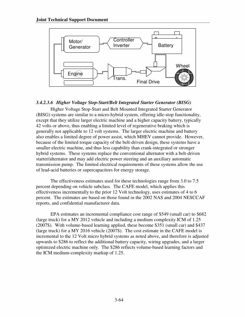
Joint Technical Support Document
3-64
3.4.2.3.6 Higher Voltage Stop-Start/Belt Integrated Starter Generator (BISG)
Higher Voltage Stop-Start and Belt Mounted Integrated Starter Generator
(BISG) systems are similar to a micro-hybrid system, offering idle-stop functionality,
except that they utilize larger electric machine and a higher capacity battery, typically
42 volts or above, thus enabling a limited level of regenerative braking which is
generally not applicable to 12 volt systems. The larger electric machine and battery
also enables a limited degree of power assist, which MHEV cannot provide. However,
because of the limited torque capacity of the belt-driven design, these systems have a
smaller electric machine, and thus less capability than crank-integrated or stronger
hybrid systems. These systems replace the conventional alternator with a belt-driven
starter/alternator and may add electric power steering and an auxiliary automatic
transmission pump. The limited electrical requirements of these systems allow the use
of lead-acid batteries or supercapacitors for energy storage.
The effectiveness estimates used for these technologies range from 3.0 to 7.5
percent depending on vehicle subclass. The CAFE model, which applies this
effectiveness incrementally to the prior 12 Volt technology, uses estimates of 4 to 6
percent. The estimates are based on those found in the 2002 NAS and 2004 NESCCAF
reports, and confidential manufacturer data.
EPA estimates an incremental compliance cost range of $549 (small car) to $682
(large truck) for a MY 2012 vehicle and including a medium complexity ICM of 1.25
(2007$). With volume-based learning applied, these become $351 (small car) and $437
(large truck) for a MY 2016 vehicle (2007$). The cost estimate in the CAFE model is
incremental to the 12 Volt micro hybrid systems as noted above, and therefore is adjusted
upwards to $286 to reflect the additional battery capacity, wiring upgrades, and a larger
optimized electric machine only. The $286 reflects volume-based learning factors and
the ICM medium-complexity markup of 1.25.
Engine
Motor/ Generator
Trans.
Controller Inverter
Final Drive
Wheel
+ - Battery
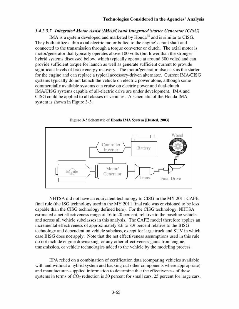
Technologies Considered in the Agencies’ Analysis
3-65
3.4.2.3.7 Integrated Motor Assist (IMA)/Crank Integrated Starter Generator (CISG)
IMA is a system developed and marketed by Honda48
and is similar to CISG.
They both utilize a thin axial electric motor bolted to the engine’s crankshaft and
connected to the transmission through a torque converter or clutch. The axial motor is
motor/generator that typically operates above 100 volts (but lower than the stronger
hybrid systems discussed below, which typically operate at around 300 volts) and can
provide sufficient torque for launch as well as generate sufficient current to provide
significant levels of brake energy recovery. The motor/generator also acts as the starter
for the engine and can replace a typical accessory-driven alternator. Current IMA/CISG
systems typically do not launch the vehicle on electric power alone, although some
commercially available systems can cruise on electric power and dual-clutch
IMA/CISG systems capable of all-electric drive are under development. IMA and
CISG could be applied to all classes of vehicles. A schematic of the Honda IMA
system is shown in Figure 3-3.
Figure 3-3 Schematic of Honda IMA System [Husted, 2003]
NHTSA did not have an equivalent technology to CISG in the MY 2011 CAFE
final rule (the ISG technology used in the MY 2011 final rule was envisioned to be less
capable than the CISG technology defined here). For the CISG technology, NHTSA
estimated a net effectiveness range of 16 to 20 percent, relative to the baseline vehicle
and across all vehicle subclasses in this analysis. The CAFE model therefore applies an
incremental effectiveness of approximately 8.6 to 8.9 percent relative to the BISG
technology and dependent on vehicle subclass, except for large truck and SUV in which
case BISG does not apply. Note that the net effectiveness assumptions used in this rule
do not include engine downsizing, or any other effectiveness gains from engine,
transmission, or vehicle technologies added to the vehicle by the modeling process.
EPA relied on a combination of certification data (comparing vehicles available
with and without a hybrid system and backing out other components where appropriate)
and manufacturer-supplied information to determine that the effectiveness of these
systems in terms of CO2 reduction is 30 percent for small cars, 25 percent for large cars,
Final Drive
Engine Motor/
Generator Trans.
+ -
Battery Controller
Inverter
Wheel
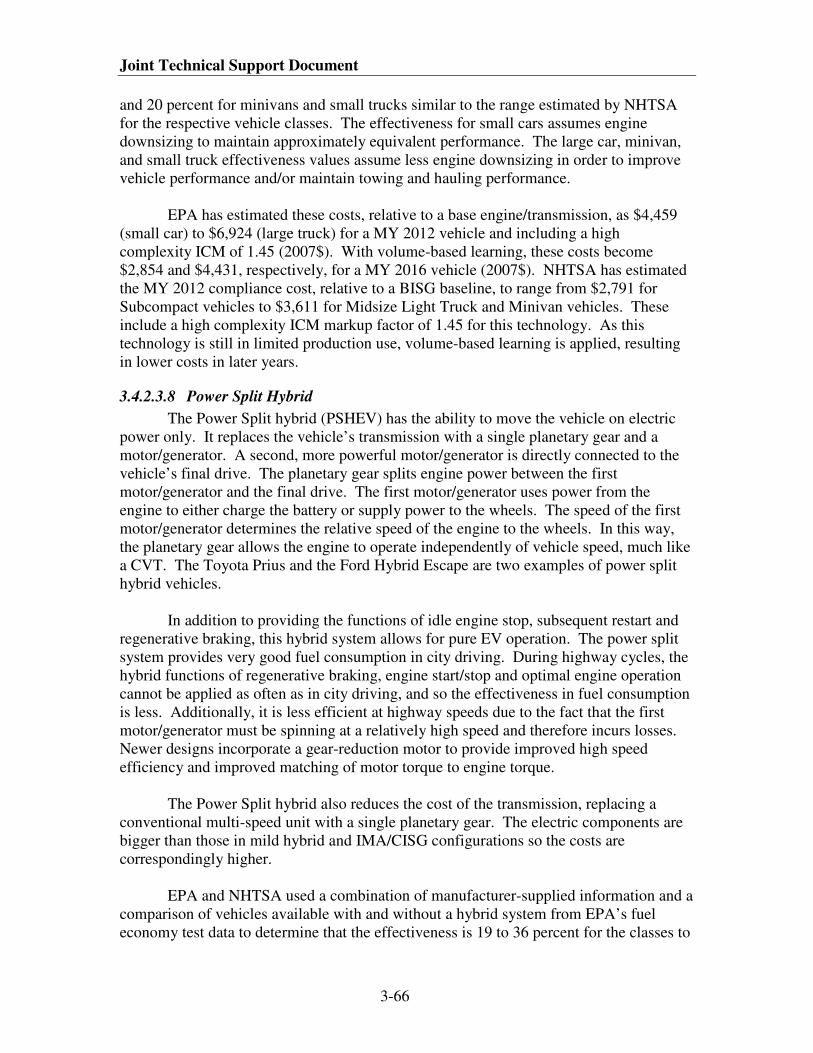
Joint Technical Support Document
3-66
and 20 percent for minivans and small trucks similar to the range estimated by NHTSA
for the respective vehicle classes. The effectiveness for small cars assumes engine
downsizing to maintain approximately equivalent performance. The large car, minivan,
and small truck effectiveness values assume less engine downsizing in order to improve
vehicle performance and/or maintain towing and hauling performance.
EPA has estimated these costs, relative to a base engine/transmission, as $4,459
(small car) to $6,924 (large truck) for a MY 2012 vehicle and including a high
complexity ICM of 1.45 (2007$). With volume-based learning, these costs become
$2,854 and $4,431, respectively, for a MY 2016 vehicle (2007$). NHTSA has estimated
the MY 2012 compliance cost, relative to a BISG baseline, to range from $2,791 for
Subcompact vehicles to $3,611 for Midsize Light Truck and Minivan vehicles. These
include a high complexity ICM markup factor of 1.45 for this technology. As this
technology is still in limited production use, volume-based learning is applied, resulting
in lower costs in later years.
3.4.2.3.8 Power Split Hybrid
The Power Split hybrid (PSHEV) has the ability to move the vehicle on electric
power only. It replaces the vehicle’s transmission with a single planetary gear and a
motor/generator. A second, more powerful motor/generator is directly connected to the
vehicle’s final drive. The planetary gear splits engine power between the first
motor/generator and the final drive. The first motor/generator uses power from the
engine to either charge the battery or supply power to the wheels. The speed of the first
motor/generator determines the relative speed of the engine to the wheels. In this way,
the planetary gear allows the engine to operate independently of vehicle speed, much like
a CVT. The Toyota Prius and the Ford Hybrid Escape are two examples of power split
hybrid vehicles.
In addition to providing the functions of idle engine stop, subsequent restart and
regenerative braking, this hybrid system allows for pure EV operation. The power split
system provides very good fuel consumption in city driving. During highway cycles, the
hybrid functions of regenerative braking, engine start/stop and optimal engine operation
cannot be applied as often as in city driving, and so the effectiveness in fuel consumption
is less. Additionally, it is less efficient at highway speeds due to the fact that the first
motor/generator must be spinning at a relatively high speed and therefore incurs losses.
Newer designs incorporate a gear-reduction motor to provide improved high speed
efficiency and improved matching of motor torque to engine torque.
The Power Split hybrid also reduces the cost of the transmission, replacing a
conventional multi-speed unit with a single planetary gear. The electric components are
bigger than those in mild hybrid and IMA/CISG configurations so the costs are
correspondingly higher.
EPA and NHTSA used a combination of manufacturer-supplied information and a
comparison of vehicles available with and without a hybrid system from EPA’s fuel
economy test data to determine that the effectiveness is 19 to 36 percent for the classes to
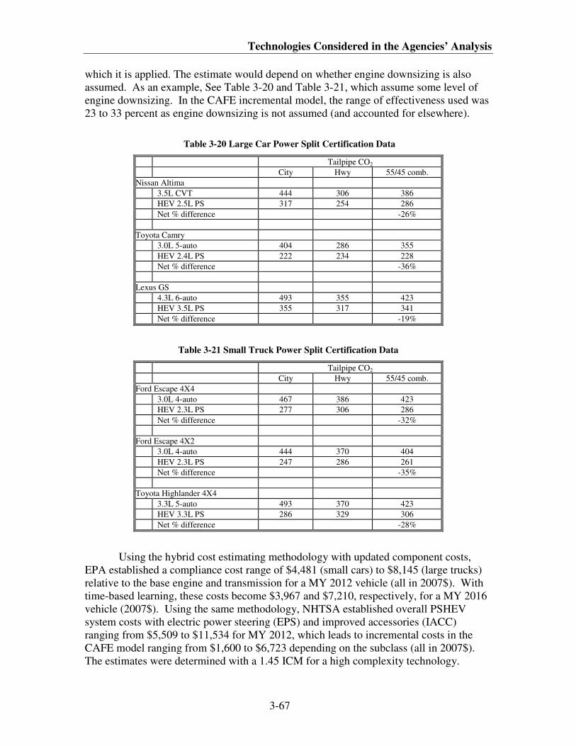
Technologies Considered in the Agencies’ Analysis
3-67
which it is applied. The estimate would depend on whether engine downsizing is also
assumed. As an example, See Table 3-20 and Table 3-21, which assume some level of
engine downsizing. In the CAFE incremental model, the range of effectiveness used was
23 to 33 percent as engine downsizing is not assumed (and accounted for elsewhere).
Table 3-20 Large Car Power Split Certification Data
Tailpipe CO2
City Hwy 55/45 comb.
Nissan Altima
3.5L CVT 444 306 386
HEV 2.5L PS 317 254 286
Net % difference -26%
Toyota Camry
3.0L 5-auto 404 286 355
HEV 2.4L PS 222 234 228
Net % difference -36%
Lexus GS
4.3L 6-auto 493 355 423
HEV 3.5L PS 355 317 341
Net % difference -19%
Table 3-21 Small Truck Power Split Certification Data
Tailpipe CO2
City Hwy 55/45 comb.
Ford Escape 4X4
3.0L 4-auto 467 386 423
HEV 2.3L PS 277 306 286
Net % difference -32%
Ford Escape 4X2
3.0L 4-auto 444 370 404
HEV 2.3L PS 247 286 261
Net % difference -35%
Toyota Highlander 4X4
3.3L 5-auto 493 370 423
HEV 3.3L PS 286 329 306
Net % difference -28%
Using the hybrid cost estimating methodology with updated component costs,
EPA established a compliance cost range of $4,481 (small cars) to $8,145 (large trucks)
relative to the base engine and transmission for a MY 2012 vehicle (all in 2007$). With
time-based learning, these costs become $3,967 and $7,210, respectively, for a MY 2016
vehicle (2007$). Using the same methodology, NHTSA established overall PSHEV
system costs with electric power steering (EPS) and improved accessories (IACC)
ranging from $5,509 to $11,534 for MY 2012, which leads to incremental costs in the
CAFE model ranging from $1,600 to $6,723 depending on the subclass (all in 2007$).
The estimates were determined with a 1.45 ICM for a high complexity technology.
Joint Technical Support Document
3-68
Based on Toyota Prius and Ford Escape/Mariner market sales, PSHEV technology with
NiMH battery is considered mature from the perspective of cost learning, and time-based
learning is applicable. However, the Li-ion battery technology is undergoing rapid
development and it is expected that some manufacturers may choose to use Li-ion
batteries on PSHEV applications during this rulemaking period. Because this
combination of technology is new, volume-based learning would be appropriate for such
applications. For cost analysis in the NPRM and final rule, volume-based learning is
used for PSHEV which assumes use of Li-ion batteries. This volume-based learning for
Li-ion is supported by the 2008 Deutsche Bank study.
3.4.2.3.9 2-Mode Hybrid
The 2-Mode Hybrid (2MHEV) uses an adaptation of a conventional stepped-ratio
automatic transmission which replaces some of the transmission clutches with two
electric motor/generators, allowing the transmission to act like a CVT. The
motor/generators control the ratio of engine speed to vehicle speed. The clutches allow
the motors to be bypassed improving the transmission’s torque capacity and the
efficiency for improved fuel economy at highway speeds. This type of system is used in
the Chevrolet Tahoe Hybrid.
In addition to providing the hybrid functions of engine stop and subsequent restart
and regenerative braking, the 2MHEV allows for pure EV operation. The two
motor/generators allow the engine to be run in efficient operating zones. The 2-mode
system provides significantly reduced CO2 emissions and fuel consumption. The primary
motor/generator is comparable in size to that in the PSHEV system, but the secondary
motor/generator is larger. The 2-mode system cost is greater than that for the power split
system due to the additional transmission complexity and secondary motor sizing.
The battery pack for 2MHEV is assumed to be 300V NiMH as is used in current
2MHEV systems today, however GM recently announced an agreement with Hitachi to
provide Li-ion battery packs for 2012 and later 2MHEVs.
For this rule the CAFE model considered a range of 23 to 33 percent with a
midpoint of 28 percent, assuming no engine downsizing to preserve the utility nature of
medium and large trucks (e.g., maintaining full towing capability even in situations with
low battery charge) and EPA estimates CO2 emissions reduction effectiveness to be 25
percent for large trucks (LDT3 and LDT4 categories) based on vehicle certification data.
EPA estimates an effectiveness of 40 percent for smaller vehicles.
EPA and NHTSA estimated MY 2012 costs using the updated component costs
and scaling factors in the hybrid cost estimating methodology discussed above. EPA
estimated the compliance cost to range from $5,469 for large car to $7,236 for large
truck/SUV relative to the base engine/transmission (all in 2007$). NHTSA determined
incremental cost estimates ranging from $3,521 to $5,779 for light-duty truck
applications in the CAFE model. These include the 1.45 ICM markup value for high
complexity technology. Given that the CAFE and OMEGA models classify vehicles
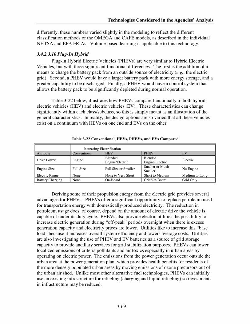
Technologies Considered in the Agencies’ Analysis
3-69
differently, these numbers varied slightly in the modeling to reflect the different
classification methods of the OMEGA and CAFE models, as described in the individual
NHTSA and EPA FRIAs. Volume-based learning is applicable to this technology.
3.4.2.3.10 Plug-In Hybrid
Plug-In Hybrid Electric Vehicles (PHEVs) are very similar to Hybrid Electric
Vehicles, but with three significant functional differences. The first is the addition of a
means to charge the battery pack from an outside source of electricity (e.g., the electric
grid). Second, a PHEV would have a larger battery pack with more energy storage, and a
greater capability to be discharged. Finally, a PHEV would have a control system that
allows the battery pack to be significantly depleted during normal operation.
Table 3-22 below, illustrates how PHEVs compare functionally to both hybrid
electric vehicles (HEV) and electric vehicles (EV). These characteristics can change
significantly within each class/subclass, so this is simply meant as an illustration of the
general characteristics. In reality, the design options are so varied that all these vehicles
exist on a continuum with HEVs on one end and EVs on the other.
Table 3-22 Conventional, HEVs, PHEVs, and EVs Compared
Increasing Electrification
Attribute Conventional HEV PHEV EV
Drive Power Engine Blended
Engine/Electric
Blended
Engine/Electric Electric
Engine Size Full Size Full Size or Smaller Smaller or Much
Smaller No Engine
Electric Range None None to Very Short Short to Medium Medium to Long
Battery Charging None On-Board Grid/On-Board Grid Only
Deriving some of their propulsion energy from the electric grid provides several
advantages for PHEVs. PHEVs offer a significant opportunity to replace petroleum used
for transportation energy with domestically-produced electricity. The reduction in
petroleum usage does, of course, depend on the amount of electric drive the vehicle is
capable of under its duty cycle. PHEVs also provide electric utilities the possibility to
increase electric generation during “off-peak” periods overnight when there is excess
generation capacity and electricity prices are lower. Utilities like to increase this “base
load” because it increases overall system efficiency and lowers average costs. Utilities
are also investigating the use of PHEV and EV batteries as a source of grid storage
capacity to provide ancillary services for grid stabilization purposes. PHEVs can lower
localized emissions of criteria pollutants and air toxics especially in urban areas by
operating on electric power. The emissions from the power generation occur outside the
urban area at the power generation plant which provides health benefits for residents of
the more densely populated urban areas by moving emissions of ozone precursors out of
the urban air shed. Unlike most other alternative fuel technologies, PHEVs can initially
use an existing infrastructure for refueling (charging and liquid refueling) so investments
in infrastructure may be reduced.
Joint Technical Support Document
3-70
In analyzing the impacts of grid-connected vehicles like PHEVs and EVs, the
emissions from the electrical generation can be accounted for if a full upstream and
downstream analysis is desired. While this issue is being studied on an on-going basis,
upstream CO2 emissions are not unique to grid-connected technologies and so are not
included in this analysis.
PHEVs will be considerably more costly than conventional vehicles and some
other advanced technologies. To take advantage of their capability, consumers would
have to be willing to charge the vehicles nightly, and would need access to electric power
where they park their vehicles. For many urban dwellers who may park on the street, or
in private or public lots or garages, charging may not be practical. Charging may be
possible at an owner’s place of work, but that would increase grid loading during peak
hours which would eliminate some of the benefits to utilities of off-peak charging versus
on-peak. Oil savings will still be the same in this case assuming the vehicle can be
charged fully.
The effectiveness potential of PHEVs depends on many factors, the most
important being the energy storage capacity designed into the battery pack. To estimate
the fuel consumption and tailpipe CO2 reduction potential of PHEVs, EPA has developed
an in-house vehicle energy model (PEREGRIN) to estimate the fuel consumption/CO2
emissions reductions of PHEVs. This model is based on the PERE (Physical Emission
Rate Estimator) physics-based model used as a fuel consumption input for EPA’s
MOVES mobile source emissions model.
The PHEV small car, large car, minivan and small trucks were modeled using
parameters from a midsize car similar to today’s hybrids and scaled to each vehicle’s
weight. The large truck PHEV was modeled separately assuming no engine downsizing.
PHEVs can have a wide variation in the All Electric Range (AER) that they offer. Some
PHEVs are of the “blended” type where the engine is on during most of the vehicle
operation, but the proportion of electric energy that is used to propel the vehicle is
significantly higher than that used in a PSHEV or 2MHEV. Each PHEV was modeled
with enough battery capacity for a 20-mile-equivalent AER and a power requirement to
provide similar performance to a hybrid vehicle. 20 miles was selected because it offers
a good compromise for vehicle performance, weight, battery packaging and cost. Given
expected near-term battery capability, a 20 mile range represents the likely capability that
will be seen in PHEVs in the near-to-mid term.
To calculate the total energy use of a PHEV, the PHEV can be thought of as
operating in two distinct modes, electric (EV) mode, and hybrid (HEV) mode. At the
tailpipe, the CO2 emissions during EV operation are zero. The EV mode fuel economy
can then be combined with the HEV mode fuel economy using the Utility Factor
calculation in SAE J1711 to determine a total MPG value for the vehicle. (See Table
3-23)
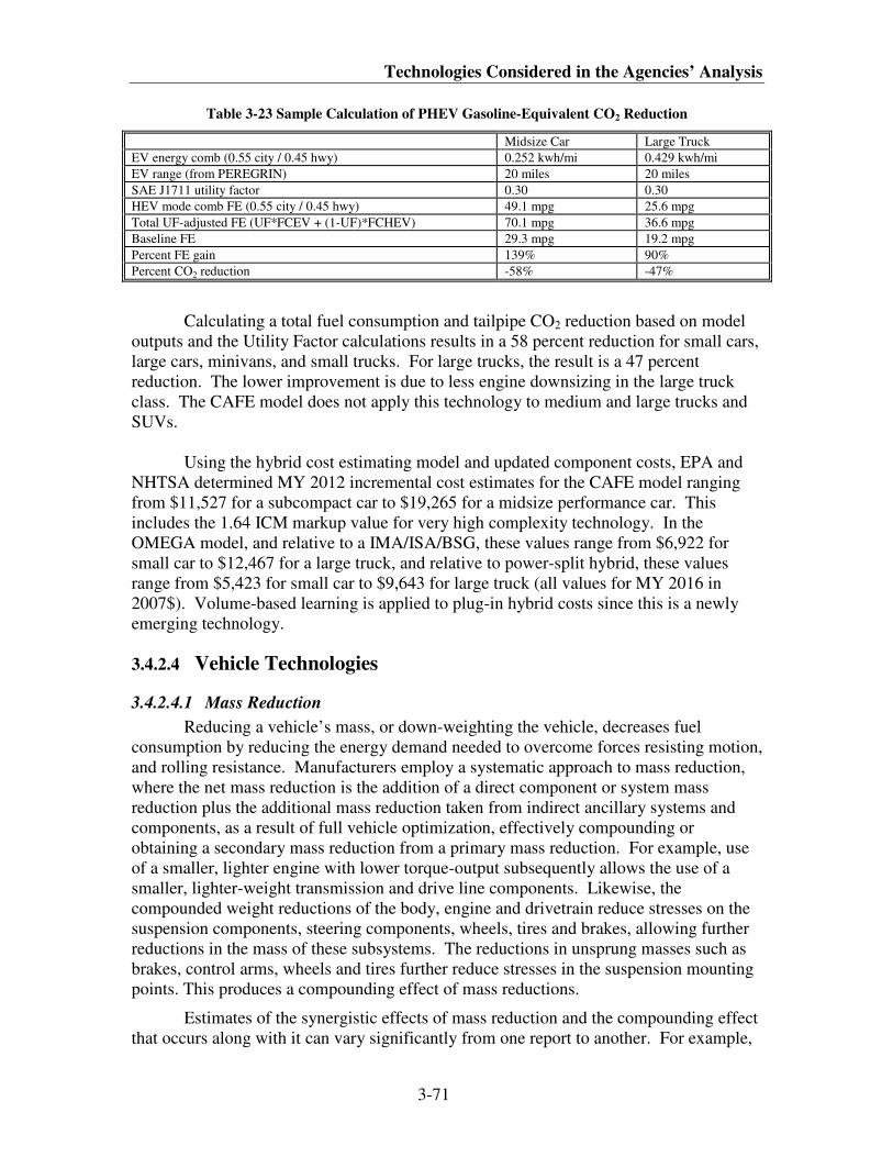
Technologies Considered in the Agencies’ Analysis
3-71
Table 3-23 Sample Calculation of PHEV Gasoline-Equivalent CO2 Reduction
Midsize Car Large Truck
EV energy comb (0.55 city / 0.45 hwy) 0.252 kwh/mi 0.429 kwh/mi
EV range (from PEREGRIN) 20 miles 20 miles
SAE J1711 utility factor 0.30 0.30
HEV mode comb FE (0.55 city / 0.45 hwy) 49.1 mpg 25.6 mpg
Total UF-adjusted FE (UF*FCEV + (1-UF)*FCHEV) 70.1 mpg 36.6 mpg
Baseline FE 29.3 mpg 19.2 mpg
Percent FE gain 139% 90%
Percent CO2 reduction -58% -47%
Calculating a total fuel consumption and tailpipe CO2 reduction based on model
outputs and the Utility Factor calculations results in a 58 percent reduction for small cars,
large cars, minivans, and small trucks. For large trucks, the result is a 47 percent
reduction. The lower improvement is due to less engine downsizing in the large truck
class. The CAFE model does not apply this technology to medium and large trucks and
SUVs.
Using the hybrid cost estimating model and updated component costs, EPA and
NHTSA determined MY 2012 incremental cost estimates for the CAFE model ranging
from $11,527 for a subcompact car to $19,265 for a midsize performance car. This
includes the 1.64 ICM markup value for very high complexity technology. In the
OMEGA model, and relative to a IMA/ISA/BSG, these values range from $6,922 for
small car to $12,467 for a large truck, and relative to power-split hybrid, these values
range from $5,423 for small car to $9,643 for large truck (all values for MY 2016 in
2007$). Volume-based learning is applied to plug-in hybrid costs since this is a newly
emerging technology.
3.4.2.4 Vehicle Technologies
3.4.2.4.1 Mass Reduction
Reducing a vehicle’s mass, or down-weighting the vehicle, decreases fuel
consumption by reducing the energy demand needed to overcome forces resisting motion,
and rolling resistance. Manufacturers employ a systematic approach to mass reduction,
where the net mass reduction is the addition of a direct component or system mass
reduction plus the additional mass reduction taken from indirect ancillary systems and
components, as a result of full vehicle optimization, effectively compounding or
obtaining a secondary mass reduction from a primary mass reduction. For example, use
of a smaller, lighter engine with lower torque-output subsequently allows the use of a
smaller, lighter-weight transmission and drive line components. Likewise, the
compounded weight reductions of the body, engine and drivetrain reduce stresses on the
suspension components, steering components, wheels, tires and brakes, allowing further
reductions in the mass of these subsystems. The reductions in unsprung masses such as
brakes, control arms, wheels and tires further reduce stresses in the suspension mounting
points. This produces a compounding effect of mass reductions.
Estimates of the synergistic effects of mass reduction and the compounding effect
that occurs along with it can vary significantly from one report to another. For example,
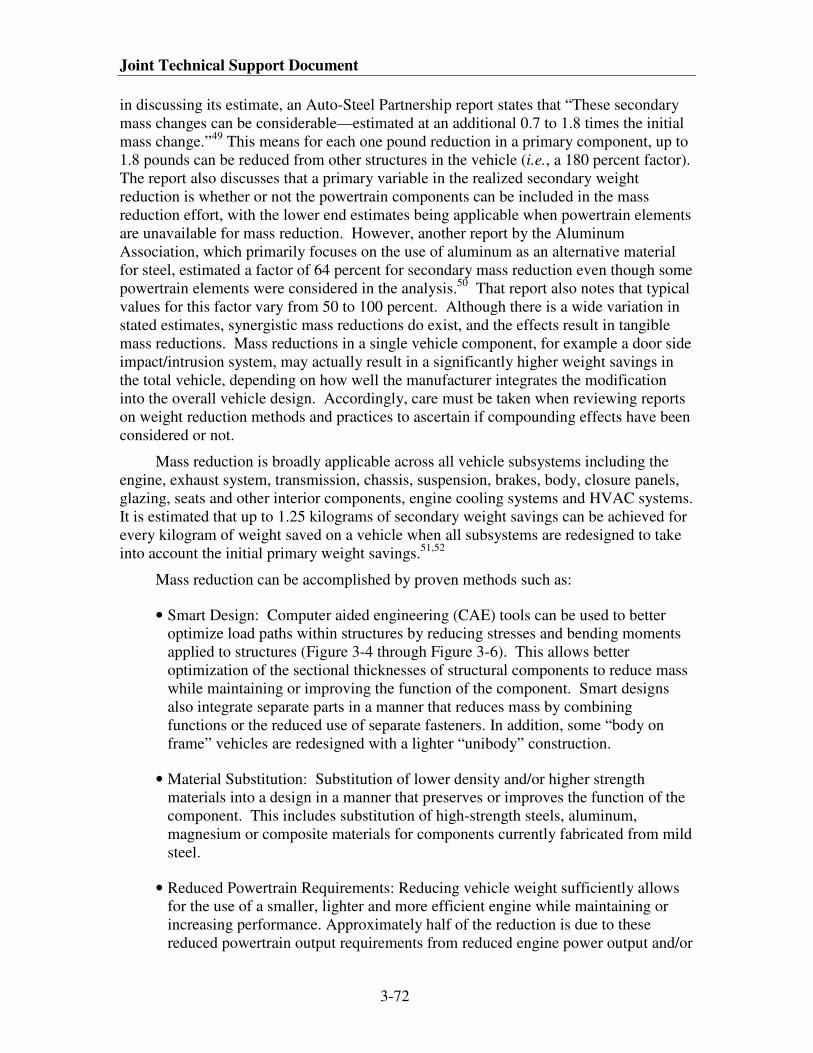
Joint Technical Support Document
3-72
in discussing its estimate, an Auto-Steel Partnership report states that “These secondary
mass changes can be considerable—estimated at an additional 0.7 to 1.8 times the initial
mass change.”49
This means for each one pound reduction in a primary component, up to
1.8 pounds can be reduced from other structures in the vehicle (i.e., a 180 percent factor).
The report also discusses that a primary variable in the realized secondary weight
reduction is whether or not the powertrain components can be included in the mass
reduction effort, with the lower end estimates being applicable when powertrain elements
are unavailable for mass reduction. However, another report by the Aluminum
Association, which primarily focuses on the use of aluminum as an alternative material
for steel, estimated a factor of 64 percent for secondary mass reduction even though some
powertrain elements were considered in the analysis.50
That report also notes that typical
values for this factor vary from 50 to 100 percent. Although there is a wide variation in
stated estimates, synergistic mass reductions do exist, and the effects result in tangible
mass reductions. Mass reductions in a single vehicle component, for example a door side
impact/intrusion system, may actually result in a significantly higher weight savings in
the total vehicle, depending on how well the manufacturer integrates the modification
into the overall vehicle design. Accordingly, care must be taken when reviewing reports
on weight reduction methods and practices to ascertain if compounding effects have been
considered or not.
Mass reduction is broadly applicable across all vehicle subsystems including the
engine, exhaust system, transmission, chassis, suspension, brakes, body, closure panels,
glazing, seats and other interior components, engine cooling systems and HVAC systems.
It is estimated that up to 1.25 kilograms of secondary weight savings can be achieved for
every kilogram of weight saved on a vehicle when all subsystems are redesigned to take
into account the initial primary weight savings.51,52
Mass reduction can be accomplished by proven methods such as:
• Smart Design: Computer aided engineering (CAE) tools can be used to better
optimize load paths within structures by reducing stresses and bending moments
applied to structures (Figure 3-4 through Figure 3-6). This allows better
optimization of the sectional thicknesses of structural components to reduce mass
while maintaining or improving the function of the component. Smart designs
also integrate separate parts in a manner that reduces mass by combining
functions or the reduced use of separate fasteners. In addition, some “body on
frame” vehicles are redesigned with a lighter “unibody” construction.
• Material Substitution: Substitution of lower density and/or higher strength
materials into a design in a manner that preserves or improves the function of the
component. This includes substitution of high-strength steels, aluminum,
magnesium or composite materials for components currently fabricated from mild
steel.
• Reduced Powertrain Requirements: Reducing vehicle weight sufficiently allows
for the use of a smaller, lighter and more efficient engine while maintaining or
increasing performance. Approximately half of the reduction is due to these
reduced powertrain output requirements from reduced engine power output and/or
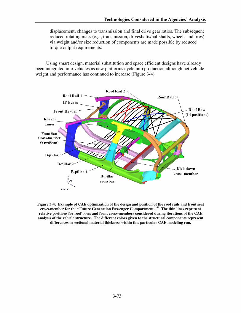
Technologies Considered in the Agencies’ Analysis
3-73
displacement, changes to transmission and final drive gear ratios. The subsequent
reduced rotating mass (e.g., transmission, driveshafts/halfshafts, wheels and tires)
via weight and/or size reduction of components are made possible by reduced
torque output requirements.
Using smart design, material substitution and space efficient designs have already
been integrated into vehicles as new platforms cycle into production although net vehicle
weight and performance has continued to increase (Figure 3-4).
Figure 3-4: Example of CAE optimization of the design and position of the roof rails and front seat
cross-member for the “Future Generation Passenger Compartment.”53
The thin lines represent
relative positions for roof bows and front cross-members considered during iterations of the CAE
analysis of the vehicle structure. The different colors given to the structural components represent
differences in sectional material thickness within this particular CAE modeling run.
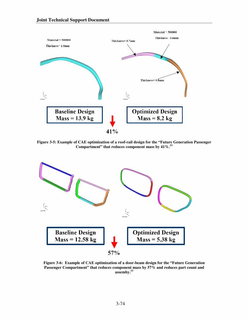
Joint Technical Support Document
3-74
Figure 3-5: Example of CAE optimization of a roof-rail design for the “Future Generation Passenger
Compartment” that reduces component mass by 41%.53
Figure 3-6: Example of CAE optimization of a door-beam design for the “Future Generation
Passenger Compartment” that reduces component mass by 57% and reduces part count and
assemby.53
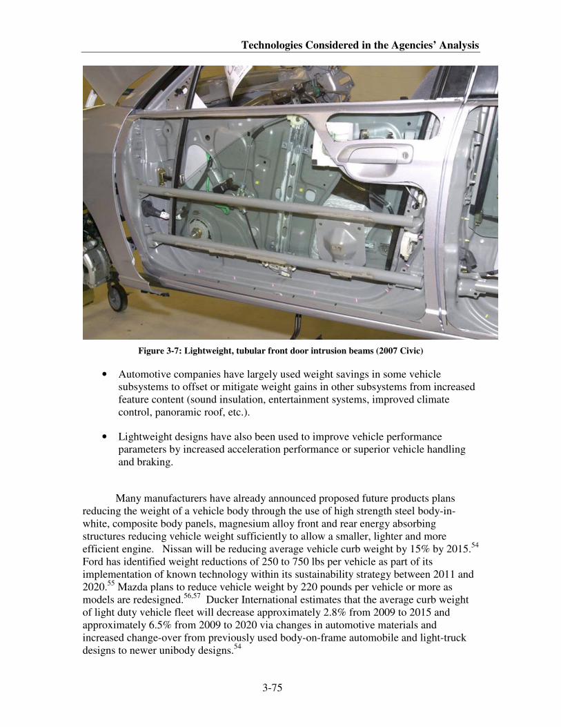
Technologies Considered in the Agencies’ Analysis
3-75
Figure 3-7: Lightweight, tubular front door intrusion beams (2007 Civic)
• Automotive companies have largely used weight savings in some vehicle
subsystems to offset or mitigate weight gains in other subsystems from increased
feature content (sound insulation, entertainment systems, improved climate
control, panoramic roof, etc.).
• Lightweight designs have also been used to improve vehicle performance
parameters by increased acceleration performance or superior vehicle handling
and braking.
Many manufacturers have already announced proposed future products plans
reducing the weight of a vehicle body through the use of high strength steel body-in-
white, composite body panels, magnesium alloy front and rear energy absorbing
structures reducing vehicle weight sufficiently to allow a smaller, lighter and more
efficient engine. Nissan will be reducing average vehicle curb weight by 15% by 2015.54
Ford has identified weight reductions of 250 to 750 lbs per vehicle as part of its
implementation of known technology within its sustainability strategy between 2011 and
2020.55
Mazda plans to reduce vehicle weight by 220 pounds per vehicle or more as
models are redesigned.56,57
Ducker International estimates that the average curb weight
of light duty vehicle fleet will decrease approximately 2.8% from 2009 to 2015 and
approximately 6.5% from 2009 to 2020 via changes in automotive materials and
increased change-over from previously used body-on-frame automobile and light-truck
designs to newer unibody designs.54
Joint Technical Support Document
3-76
NHTSA in the CAFE model has used a tiered approach in material substitution to
reduce mass without considering other means of vehicle mass reduction. MS1, a 1.5
percent mass reduction, is applicable in any year at refresh or redesign. MS2, a 3.5 to 8.5
percent mass reduction incremental to MS1, is only available in MY 2014 and beyond in
an attempt to mimic manufacturers’ planned applications of mass reduction/material
substitution in later years. For smaller vehicles, MS2 was limited to a 3.5 percent mass
reduction of mass reduction/material substitution, but for larger cars and trucks up to 8.5
percent mass reduction was allowed.
In the CAFE model, MS2 is cumulative to MS1, as it is only applied after MS1;
therefore the maximum weight reduction that can occur for smaller subclass vehicles is 5
percent, while large cars, truck, and SUVs could experience up to a 10 percent weight
reduction. Making the MS2 technology unavailable until MY 2014 is intended to
recognize the lead time required to implement platform redesigns that would be necessary
for these levels of weight reduction.
NHTSA and EPA estimate that a 10 percent mass reduction with engine
downsizing results in a 6.5 percent reduction in fuel consumption while maintaining
equivalent vehicle performance (i.e., 0-60 mph time, towing capacity, etc.) which is
consistent with estimates in the 2002 NAS report. For small amounts of mass reduction,
such as the 1.5 percent used at vehicle refresh in NHTSA’s modeling, no engine
downsizing will be used and a 10 percent mass reduction without engine downsizing will
result in a 3.5 percent reduction in fuel consumption. 58,59,60
NHTSA and EPA have reviewed three studies of mass reduction/material
substitution and the associated cost. The 2002 NAS,Report estimated that vehicle weight
could be reduced for approximately $1.50 per pound, along with 3 to 4 percent reductions
in fuel consumption, without engine downsizing, from a 5 percent reduction in vehicle
weight, at a cost of $210-$350. This translates into $1.50 per pound, assuming a 3,800
pound base vehicle and using the midpoint cost. Additionally, Sierra Research estimated
that a 10 percent reduction, with compounding, could be accomplished for a cost of $1.01
per pound.61
Finally, an MIT study62
estimated that the weight of a vehicle could be
reduced by 14 percent, with no compounding, for a cost of $1.36 per pound. The final
cost estimate is $1.32 per pound and is based on the average of the three referenced
studies. Applying an ICM factor of 1.11 for a low complexity technology results in a
compliance cost of $1.48 per pound. For the vehicle mass reduction technologies, neither
volume-based nor time-based cost reductions are applied, since many of the materials
under consideration are commodity based.
3.4.2.4.2 Low Drag Brakes (LDB)
Low drag brakes reduce the sliding friction of disc brake pads on rotors when the
brakes are not engaged because the brake pads are pulled away from the rotating disc
either by mechanical or electric methods. While most passenger cars have already
adopted this technology with the standardization of electronic brake control, there are
indications that this technology is still available for body-on-frame trucks and for some
large passenger cars.
Technologies Considered in the Agencies’ Analysis
3-77
NHTSA’s MY 2011 CAFE final rule estimated the effectiveness of LDB to be as
much as 1 percent, based on confidential manufacturer data. NHTSA and EPA have
reviewed this estimate and believe it to be applicable for this final rule.
NHTSA and EPA have reviewed the cost estimates from the MY 2011 CAFE
final rule and have not found any evidence to suggest that this cost is not a valid cost and
have chosen to maintain this estimate. However, the agencies adjusted the costs to apply
the ICM of 1.11, for a low-complexity technology. The compliance cost for LDB is
estimated to be $63 for MY 2012 through MY 2016 vehicles as no learning effects are
applied to this technology.
3.4.2.4.3 Low Rolling Resistance Tires (ROLL)
Tire rolling resistance is the frictional loss associated mainly with the energy
dissipated in the deformation of the tires under load and thus influences fuel economy
and CO2 emissions. Other tire design characteristics (e.g., materials, construction, and
tread design) influence durability, traction (both wet and dry grip), vehicle handling, and
ride comfort in addition to rolling resistance. A typical low rolling resistance tire’s
attributes would include: increased tire inflation pressure, material changes, and tire
construction with less hysteresis, geometry changes (e.g., reduced aspect ratios), and
reduction in sidewall and tread deflection. These changes would generally be
accompanied with additional changes to suspension tuning and/or suspension design.
EPA and NHTSA estimated a 1 to 2 percent increase in effectiveness with a 10
percent reduction in rolling resistance, which was based on the 2002 NAS report findings
and consistent with NHTSA’s MY 2011 CAFE final rule estimate. NHTSA and EPA
still believe that this NAS effectiveness estimate is valid for this final rule. Lower rolling
resistance tires are widely available today.
Based on NHTSA’ MY 2011 CAFE final rule and the 2006 NAS/NRC report, the
agencies have estimated the cost for low rolling resistance tires to be $6 per vehicle.63
This is based on a cost of $1 per tire as estimated by NAS/NRC 2006 report, which is $5
per vehicle, including the spare tire. When applying the ICM low complexity markup
factor, of 1.11, results in compliance cost of $6 per vehicle for MY 2012 through MY
2016 vehicles (2007$).u Due to the commodity-based nature of this technology, cost
learning is not applied.
3.4.2.4.4 Front or Secondary Axle Disconnect for Four-Wheel Drive Systems (SAX)
Energy is required to continually drive the front, or secondary, axle in a four-
wheel drive system even when the system is not required during most operating
conditions. This energy loss directly results in increased fuel consumption and CO2
emissions. Many part-time four-wheel drive systems use some type of front axle
disconnect to provide shift-on-the-fly capabilities. The front axle disconnect is normally
part of the front differential assembly. As part of a shift-on-the-fly four-wheel drive
u Note that the costs developed for low rolling resistance tires for this analysis do not include the increase in
lifetime costs that would be expected at each tire replacement. Instead, the analysis includes only the
upfront increase in costs.
Joint Technical Support Document
3-78
system, the front axle disconnect serves two basic purposes. First, in two-wheel drive
mode, it disengages the front axle from the front driveline so the front wheels do not turn
the front driveline at road speed, saving wear and tear. Second, when shifting from two-
to four-wheel drive “on the fly” (while moving), the front axle disconnect couples the
front axle to the front differential side gear only when the transfer case’s synchronizing
mechanism has spun the front driveshaft up to the same speed as the rear driveshaft.
Four-wheel drive systems that have a front axle disconnect typically do not have either
manual- or automatic-locking hubs. To isolate the front wheels from the rest of the front
driveline, front axle disconnects use a sliding sleeve to connect or disconnect an axle
shaft from the front differential side gear. NHTSA and EPA are not aware of any
manufacturer offering this technology in the U.S. today on unibody frame vehicles;
however, it is possible this technology could be introduced by manufacturers within the
rulemaking time period.
Based on confidential manufacturer data, NHTSA’s MY 2011 CAFE final rule
estimated an effectiveness improvement of 1.0 to 1.5 percent for axle disconnect.
NHTSA and EPA believe this to still be an accurate estimate for this rulemaking.
Regarding costs, the agencies believe that the incremental compliance cost from
NHTSA’s MY 2011 final rule is an accurate estimate. However, for this final rule, this
estimate was revised by applying the new ICM factor markup, for a low complexity
technology, of 1.11. Thus, the compliance cost estimate for this final rule, is $87 for a
MY 2012 vehicle (2007$). With time-based learning this cost would be $84 for a MY
2016 vehicle (2007$).
3.4.2.4.5 Aerodynamic Drag Reduction (AERO)
Many factors affect a vehicle’s aerodynamic drag and the resulting power
required to move it through the air. While these factors change with air density and the
square and cube of vehicle speed, respectively, the overall drag effect is determined by
the product of its frontal area and drag coefficient. Reductions in these quantities can
therefore reduce fuel consumption and CO2 emissions. Although frontal areas tend to be
relatively similar within a vehicle class (mostly due to market-competitive size
requirements), significant variations in drag coefficient can be observed. Significant
changes to a vehicle’s aerodynamic performance may need to be implemented during a
redesign (e.g., changes in vehicle shape). However, shorter-term aerodynamic
reductions, with a somewhat lower effectiveness, may be achieved through the use of
revised exterior components (typically at a model refresh in mid-cycle) and add-on
devices that currently being applied. The latter list would include revised front and rear
fascias, modified front air dams and rear valances, addition of rear deck lips and
underbody panels, and lower aerodynamic drag exterior mirrors.
The MY 2011 CAFE final rule estimated that a fleet average of 10 to 20 percent
total aerodynamic drag reduction is attainable (with a caveat for “high-performance”
vehicles described below) which equates to incremental reductions in fuel consumption
and CO2 emissions of 2 to 3 percent for both cars and trucks. These numbers are
generally supported by confidential manufacturer data and public technical literature and
Technologies Considered in the Agencies’ Analysis
3-79
therefore NHTSA and EPA are retaining these estimates, as confirmed by joint review,
for the purposes of this final rule.
In the MY 2011 CAFE final rule, NHTSA estimated a range from $60 to $116
(1.5 RPE); $40 to $75 (without RPE). NHTSA and EPA reviewed these estimates and
updated these estimates to reflect the new ICM markup factor of 1.11 for a low
complexity technology. In addition, given its low complexity and the facility of its
implementation during design and refresh cycles, NHTSA and EPA believe that a cost
estimate at the lower end of the range is more appropriate. Thus, the cost estimate used
in this rulemaking is $48, including the 1.11 ICM markup value, for a low complexity
technology (2007$). This compliance cost is for a MY 2012 vehicle. With time-based
learning, this cost would be $42 for a MY 2016 vehicle (2007$)
3.4.2.5 Technologies considered but not included in the final rule
analysis
NHTSA and EPA have identified six technologies that will not be available in the
time frame considered under this rulemaking. These technologies while considered were
not made available in the CAFE and OMEGA models. They are: electric vehicles,
camless valve actuation (CVA), lean burn gasoline direct injection (LBDI), homogeneous
charge compression ignition (HCCI), and electric assist turbocharging and full series
hydraulic hybrids (HHV). While electric vehicles are likely become available in small
numbers in the near future, the costs for this technology (as estimated by the agencies)
are non-competitive with the more conventional technologies listed above. Therefore,
the OMEGA and Volpe model analysis would preclude their selection, when estimating
the costs of the rule. Lean Burn direct injection engines are currently available in
Europe, however, these vehicles cannot be designed at this time to be both efficient and
meet the NOx standards in the United States with the current sulfur levels in the fuels.
The other technologies listed are still in the research phase of development. NHTSA and
EPA will continue to monitor the industry and system suppliers for progress on these
technologies, and should they become more available, consider them for use in future
rulemaking activity. More details are described below.
3.4.2.5.1 Electric Vehicles
The recent intense interest in Hybrid vehicles and the development of Hybrid
vehicle battery and motor technology has helped make Electric Vehicle technology more
viable than it has ever been. Electric Vehicles (EVs) require much larger batteries than
either HEVs or PHEVs, but the batteries must be of a high-energy and lower-power
design to deliver an appropriate amount of power over the useful charge of the battery.
These high-energy batteries are generally less expensive per kilowatt-hour than high-
power batteries required for hybrids, but the size of the battery pack still incurs a
considerable cost.
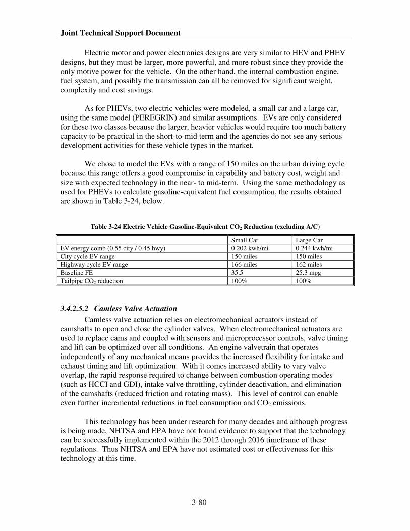
Joint Technical Support Document
3-80
Electric motor and power electronics designs are very similar to HEV and PHEV
designs, but they must be larger, more powerful, and more robust since they provide the
only motive power for the vehicle. On the other hand, the internal combustion engine,
fuel system, and possibly the transmission can all be removed for significant weight,
complexity and cost savings.
As for PHEVs, two electric vehicles were modeled, a small car and a large car,
using the same model (PEREGRIN) and similar assumptions. EVs are only considered
for these two classes because the larger, heavier vehicles would require too much battery
capacity to be practical in the short-to-mid term and the agencies do not see any serious
development activities for these vehicle types in the market.
We chose to model the EVs with a range of 150 miles on the urban driving cycle
because this range offers a good compromise in capability and battery cost, weight and
size with expected technology in the near- to mid-term. Using the same methodology as
used for PHEVs to calculate gasoline-equivalent fuel consumption, the results obtained
are shown in Table 3-24, below.
Table 3-24 Electric Vehicle Gasoline-Equivalent CO2 Reduction (excluding A/C)
Small Car Large Car
EV energy comb (0.55 city / 0.45 hwy) 0.202 kwh/mi 0.244 kwh/mi
City cycle EV range 150 miles 150 miles
Highway cycle EV range 166 miles 162 miles
Baseline FE 35.5 25.3 mpg
Tailpipe CO2 reduction 100% 100%
3.4.2.5.2 Camless Valve Actuation
Camless valve actuation relies on electromechanical actuators instead of
camshafts to open and close the cylinder valves. When electromechanical actuators are
used to replace cams and coupled with sensors and microprocessor controls, valve timing
and lift can be optimized over all conditions. An engine valvetrain that operates
independently of any mechanical means provides the increased flexibility for intake and
exhaust timing and lift optimization. With it comes increased ability to vary valve
overlap, the rapid response required to change between combustion operating modes
(such as HCCI and GDI), intake valve throttling, cylinder deactivation, and elimination
of the camshafts (reduced friction and rotating mass). This level of control can enable
even further incremental reductions in fuel consumption and CO2 emissions.
This technology has been under research for many decades and although progress
is being made, NHTSA and EPA have not found evidence to support that the technology
can be successfully implemented within the 2012 through 2016 timeframe of these
regulations. Thus NHTSA and EPA have not estimated cost or effectiveness for this
technology at this time.
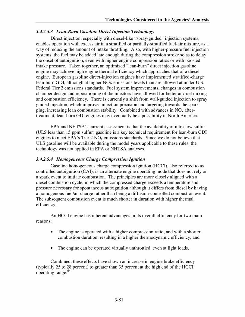
Technologies Considered in the Agencies’ Analysis
3-81
3.4.2.5.3 Lean-Burn Gasoline Direct Injection Technology
Direct injection, especially with diesel-like “spray-guided” injection systems,
enables operation with excess air in a stratified or partially-stratified fuel-air mixture, as a
way of reducing the amount of intake throttling. Also, with higher-pressure fuel injection
systems, the fuel may be added late enough during the compression stroke so as to delay
the onset of autoignition, even with higher engine compression ratios or with boosted
intake pressure. Taken together, an optimized “lean-burn” direct injection gasoline
engine may achieve high engine thermal efficiency which approaches that of a diesel
engine. European gasoline direct-injection engines have implemented stratified-charge
lean-burn GDI, although at higher NOx emissions levels than are allowed at under U.S.
Federal Tier 2 emissions standards. Fuel system improvements, changes in combustion
chamber design and repositioning of the injectors have allowed for better air/fuel mixing
and combustion efficiency. There is currently a shift from wall-guided injection to spray
guided injection, which improves injection precision and targeting towards the spark
plug, increasing lean combustion stability. Combined with advances in NOx after-
treatment, lean-burn GDI engines may eventually be a possibility in North America.
EPA and NHTSA’s current assessment is that the availability of ultra-low sulfur
(ULS less than 15 ppm sulfur) gasoline is a key technical requirement for lean-burn GDI
engines to meet EPA’s Tier 2 NOx emissions standards. Since we do not believe that
ULS gasoline will be available during the model years applicable to these rules, the
technology was not applied in EPA or NHTSA analyses.
3.4.2.5.4 Homogeneous Charge Compression Ignition
Gasoline homogeneous charge compression ignition (HCCI), also referred to as
controlled autoignition (CAI), is an alternate engine operating mode that does not rely on
a spark event to initiate combustion. The principles are more closely aligned with a
diesel combustion cycle, in which the compressed charge exceeds a temperature and
pressure necessary for spontaneous autoignition although it differs from diesel by having
a homogenous fuel/air charge rather than being a diffusion-controlled combustion event.
The subsequent combustion event is much shorter in duration with higher thermal
efficiency.
An HCCI engine has inherent advantages in its overall efficiency for two main
reasons:
• The engine is operated with a higher compression ratio, and with a shorter
combustion duration, resulting in a higher thermodynamic efficiency, and
• The engine can be operated virtually unthrottled, even at light loads,
Combined, these effects have shown an increase in engine brake efficiency
(typically 25 to 28 percent) to greater than 35 percent at the high end of the HCCI
operating range.64
Joint Technical Support Document
3-82
Criteria pollutant emissions are very favorable during HCCI operation. Lower
peak in-cylinder temperatures (due to high dilution) keep engine-out NOx emissions to a
minimum – realistically below Tier 2 levels without aftertreatment – and particulates are
low due to the homogeneous nature of the premixed charge.
Due to the inherent difficulty in maintaining combustion stability without
encountering engine knock, HCCI is difficult to control, requiring feedback from in-
cylinder pressure sensors and rapid engine control logic to optimize combustion timing,
especially considering the transient nature of operating conditions seen in a vehicle. Due
to the highly dilute conditions under which gasoline-HCCI combustion is stable, the
range of engine loads achievable in a naturally-aspirated engine is somewhat limited.
Because of this, it is likely that any commercial application would operate in a “dual-
mode” strategy between HCCI and spark ignition combustion modes, in which HCCI
would be utilized for best efficiency at light engine loads and spark ignition would be
used at higher loads and at idle. This type of dual-mode strategy has already been
employed in diesel HCCI engines in Europe and Asia (notably the Toyota Avensis D-Cat
and the Nissan light-duty “MK” combustion diesels).
Until recently, gasoline-HCCI technology was considered to still be in the
research phase. However, most manufacturers have made public statements about the
viability of incorporating HCCI into light-duty passenger vehicles, and have significant
vehicle demonstration programs aimed at producing a viable product within the next 5-10
years.
There is widespread optimism as to the CO2 reduction potential for HCCI in the
literature. Based on confidential manufacturer information, EPA and NHTSA believe
that a gasoline HCCI / GDI dual-mode engine might achieve 10 to 12 percent reduction
in CO2, compared to a comparable SI engine. Despite its promise, application of HCCI
in light duty vehicles is not yet ready for the market. It is not anticipated to be seen in
volume for at least the next 5-10 years, which is concurrent with many manufacturers’
public estimates. NHTSA also noted in its MY 2011 CAFE final rule that the technology
will not be available within the time frame considered based on a review of confidential
product plan information.
3.4.2.5.5 Electric Assist Turbocharging
The Alliance commented in NHTSA’s previous rulemaking that global
development of electric assist turbocharging has not demonstrated the fuel efficiency
effectiveness of a 12V EAT up to 2kW power levels since the 2004 NESCCAF study,
and stated that it saw remote probability of its application over the next decade. While
hybrid vehicles lower the incremental hardware requirements for higher-voltage, higher-
power EAT systems, NHTSA and EPA agree that significant developmental work is
required to demonstrate effective systems and that implementation in significant volumes
will not occur in the 2012 to 2016 time frame considered in this rulemaking. Thus, this
technology was not included in the final rule.
Technologies Considered in the Agencies’ Analysis
3-83
3.4.2.5.6 Full Series Hydraulic Hybrid
A Full Series Hydraulic Hybrid Vehicle (HHV) is somewhat similar in concept to
a full series electric hybrid vehicle, except that the energy is stored in the form of
compressed nitrogen gas and the power is transmitted in the form of hydraulic fluid.
Series HHV technology currently under development by EPA is capable of a 40 percent
decrease in tailpipe CO2 emissions in the small car, large car, minivan, and small truck
classes. In the large truck class, a 30 percent CO2 reduction is possible. The large truck
benefit is somewhat lower than the other classes because it is assumed that a large truck
requires a larger engine to maintain towing and hauling performance after the energy in
the high pressure hydraulic accumulator is exhausted. This technology is still under
development and not yet commercialized, however there are technology demonstration
vehicles in service with UPS in daily package delivery service.
3.5 Cost and effectiveness tables
The tables representing the Volpe model input files for incremental technology
costs by vehicle subclass are presented below. The tables have been divided into
passenger cars, performance passenger cars, and light trucks to make them easier to read.
It should be noted that the Volpe model input files define costs for MY 2012 and learn
down costs for subsequent years.
3.5.1 NHTSA cost and effectiveness tables
Table 3-25 Technology Incremental Cost Estimates for Volpe model, Passenger Cars in 2012
VEHICLE TECHNOLOGY ICM COSTS PER VEHICLE (2007$) BY VEHICLE
SUBCLASS - PASSENGER CARS
Subcompact Compact Midsize Large
Car Car Car Car
Nominal Baseline Engine (For Cost Basis) Inline 4 Inline 4 Inline 4 V6
Low Friction Lubricants 3 3 3 3
Engine Friction Reduction EFR 50 50 50 75
VVT - Coupled Cam Phasing (CCP) on SOHC CCPS 45 45 45 90
Discrete Variable Valve Lift (DVVL) on SOHC DVVLS 142 142 142 205
Cylinder Deactivation on SOHC DEACS n.a. n.a. n.a. 0 - 56
VVT - Intake Cam Phasing (ICP) ICP 45 45 45 90
VVT - Dual Cam Phasing (DCP) DCP 38 38 38 83
Discrete Variable Valve Lift (DVVL) on DOHC DVVLD 142 142 142 205
Continuously Variable Valve Lift (CVVL) CVVL 277 277 277 509
Cylinder Deactivation on DOHC DEACD n.a. n.a. n.a. 0 - 56
Cylinder Deactivation on OHV DEACO n.a. n.a. n.a. 170
VVT - Coupled Cam Phasing (CCP) on OHV CCPO 45 45 45 45
Discrete Variable Valve Lift (DVVL) on OHV DVVLO 142 142 142 0 - 56
Conversion to DOHC with DCP CDOHC 276 276 276 436
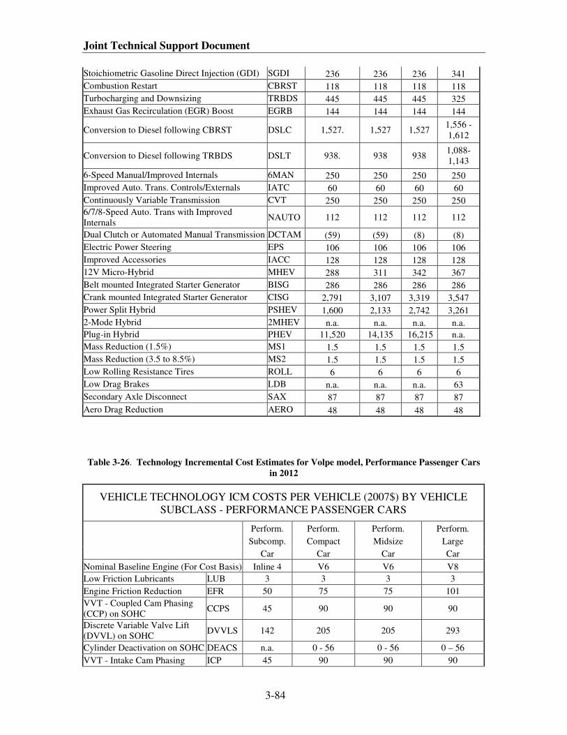
Joint Technical Support Document
3-84
Stoichiometric Gasoline Direct Injection (GDI) SGDI 236 236 236 341
Combustion Restart CBRST 118 118 118 118
Turbocharging and Downsizing TRBDS 445 445 445 325
Exhaust Gas Recirculation (EGR) Boost EGRB 144 144 144 144
Conversion to Diesel following CBRST DSLC 1,527. 1,527 1,527 1,556 -
1,612
Conversion to Diesel following TRBDS DSLT 938. 938 938 1,088-
1,143
6-Speed Manual/Improved Internals 6MAN 250 250 250 250
Improved Auto. Trans. Controls/Externals IATC 60 60 60 60
Continuously Variable Transmission CVT 250 250 250 250
6/7/8-Speed Auto. Trans with Improved
Internals NAUTO 112 112 112 112
Dual Clutch or Automated Manual Transmission DCTAM (59) (59) (8) (8)
Electric Power Steering EPS 106 106 106 106
Improved Accessories IACC 128 128 128 128
12V Micro-Hybrid MHEV 288 311 342 367
Belt mounted Integrated Starter Generator BISG 286 286 286 286
Crank mounted Integrated Starter Generator CISG 2,791 3,107 3,319 3,547
Power Split Hybrid PSHEV 1,600 2,133 2,742 3,261
2-Mode Hybrid 2MHEV n.a. n.a. n.a. n.a.
Plug-in Hybrid PHEV 11,520 14,135 16,215 n.a.
Mass Reduction (1.5%) MS1 1.5 1.5 1.5 1.5
Mass Reduction (3.5 to 8.5%) MS2 1.5 1.5 1.5 1.5
Low Rolling Resistance Tires ROLL 6 6 6 6
Low Drag Brakes LDB n.a. n.a. n.a. 63
Secondary Axle Disconnect SAX 87 87 87 87
Aero Drag Reduction AERO 48 48 48 48
Table 3-26. Technology Incremental Cost Estimates for Volpe model, Performance Passenger Cars
in 2012
VEHICLE TECHNOLOGY ICM COSTS PER VEHICLE (2007$) BY VEHICLE
SUBCLASS - PERFORMANCE PASSENGER CARS
Perform. Perform. Perform. Perform.
Subcomp. Compact Midsize Large
Car Car Car Car
Nominal Baseline Engine (For Cost Basis) Inline 4 V6 V6 V8
Low Friction Lubricants LUB 3 3 3 3
Engine Friction Reduction EFR 50 75 75 101
VVT - Coupled Cam Phasing
(CCP) on SOHC CCPS 45 90 90 90
Discrete Variable Valve Lift
(DVVL) on SOHC DVVLS 142 205 205 293
Cylinder Deactivation on SOHC DEACS n.a. 0 - 56 0 - 56 0 – 56
VVT - Intake Cam Phasing ICP 45 90 90 90
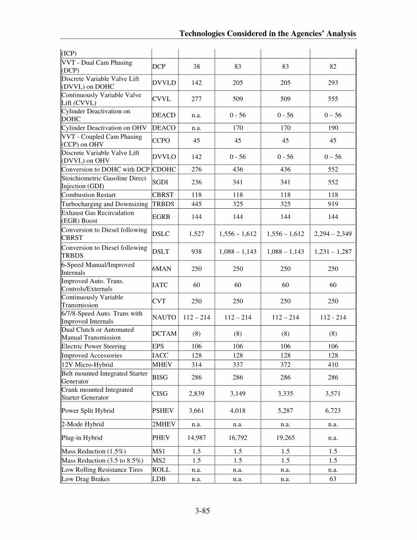
Technologies Considered in the Agencies’ Analysis
3-85
(ICP)
VVT - Dual Cam Phasing
(DCP) DCP 38 83 83 82
Discrete Variable Valve Lift
(DVVL) on DOHC DVVLD 142 205 205 293
Continuously Variable Valve
Lift (CVVL) CVVL 277 509 509 555
Cylinder Deactivation on
DOHC DEACD n.a. 0 - 56 0 - 56 0 – 56
Cylinder Deactivation on OHV DEACO n.a. 170 170 190
VVT - Coupled Cam Phasing
(CCP) on OHV CCPO 45 45 45 45
Discrete Variable Valve Lift
(DVVL) on OHV DVVLO 142 0 - 56 0 - 56 0 – 56
Conversion to DOHC with DCP CDOHC 276 436 436 552
Stoichiometric Gasoline Direct
Injection (GDI) SGDI 236 341 341 552
Combustion Restart CBRST 118 118 118 118
Turbocharging and Downsizing TRBDS 445 325 325 919
Exhaust Gas Recirculation
(EGR) Boost EGRB 144 144 144 144
Conversion to Diesel following
CBRST DSLC 1,527 1,556 – 1,612 1,556 – 1,612 2,294 – 2,349
Conversion to Diesel following
TRBDS DSLT 938 1,088 – 1,143 1,088 – 1,143 1,231 – 1,287
6-Speed Manual/Improved
Internals 6MAN 250 250 250 250
Improved Auto. Trans.
Controls/Externals IATC 60 60 60 60
Continuously Variable
Transmission CVT 250 250 250 250
6/7/8-Speed Auto. Trans with
Improved Internals NAUTO 112 – 214 112 – 214 112 – 214 112 - 214
Dual Clutch or Automated
Manual Transmission DCTAM (8) (8) (8) (8)
Electric Power Steering EPS 106 106 106 106
Improved Accessories IACC 128 128 128 128
12V Micro-Hybrid MHEV 314 337 372 410
Belt mounted Integrated Starter
Generator BISG 286 286 286 286
Crank mounted Integrated
Starter Generator CISG 2,839 3,149 3,335 3,571
Power Split Hybrid PSHEV 3,661 4,018 5,287 6,723
2-Mode Hybrid 2MHEV n.a. n.a. n.a. n.a.
Plug-in Hybrid PHEV 14,987 16,792 19,265 n.a.
Mass Reduction (1.5%) MS1 1.5 1.5 1.5 1.5
Mass Reduction (3.5 to 8.5%) MS2 1.5 1.5 1.5 1.5
Low Rolling Resistance Tires ROLL n.a. n.a. n.a. n.a.
Low Drag Brakes LDB n.a. n.a. n.a. 63
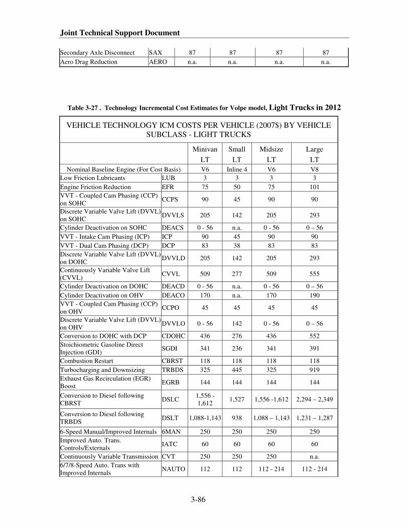
Joint Technical Support Document
3-86
Secondary Axle Disconnect SAX 87 87 87 87
Aero Drag Reduction AERO n.a. n.a. n.a. n.a.
Table 3-27 . Technology Incremental Cost Estimates for Volpe model, Light Trucks in 2012
VEHICLE TECHNOLOGY ICM COSTS PER VEHICLE (2007$) BY VEHICLE
SUBCLASS - LIGHT TRUCKS
Minivan Small Midsize Large
LT LT LT LT
Nominal Baseline Engine (For Cost Basis) V6 Inline 4 V6 V8
Low Friction Lubricants LUB 3 3 3 3
Engine Friction Reduction EFR 75 50 75 101
VVT - Coupled Cam Phasing (CCP)
on SOHC CCPS 90 45 90 90
Discrete Variable Valve Lift (DVVL)
on SOHC DVVLS 205 142 205 293
Cylinder Deactivation on SOHC DEACS 0 - 56 n.a. 0 - 56 0 – 56
VVT - Intake Cam Phasing (ICP) ICP 90 45 90 90
VVT - Dual Cam Phasing (DCP) DCP 83 38 83 83
Discrete Variable Valve Lift (DVVL)
on DOHC DVVLD 205 142 205 293
Continuously Variable Valve Lift
(CVVL) CVVL 509 277 509 555
Cylinder Deactivation on DOHC DEACD 0 - 56 n.a. 0 - 56 0 – 56
Cylinder Deactivation on OHV DEACO 170 n.a. 170 190
VVT - Coupled Cam Phasing (CCP)
on OHV CCPO 45 45 45 45
Discrete Variable Valve Lift (DVVL)
on OHV DVVLO 0 - 56 142 0 - 56 0 – 56
Conversion to DOHC with DCP CDOHC 436 276 436 552
Stoichiometric Gasoline Direct
Injection (GDI) SGDI 341 236 341 391
Combustion Restart CBRST 118 118 118 118
Turbocharging and Downsizing TRBDS 325 445 325 919
Exhaust Gas Recirculation (EGR)
Boost EGRB 144 144 144 144
Conversion to Diesel following
CBRST DSLC
1,556 -
1,612 1,527 1,556 -1,612 2,294 – 2,349
Conversion to Diesel following
TRBDS DSLT 1,088-1,143 938 1,088 – 1,143 1,231 – 1,287
6-Speed Manual/Improved Internals 6MAN 250 250 250 250
Improved Auto. Trans.
Controls/Externals IATC 60 60 60 60
Continuously Variable Transmission CVT 250 250 250 n.a.
6/7/8-Speed Auto. Trans with
Improved Internals NAUTO 112 112 112 - 214 112 - 214
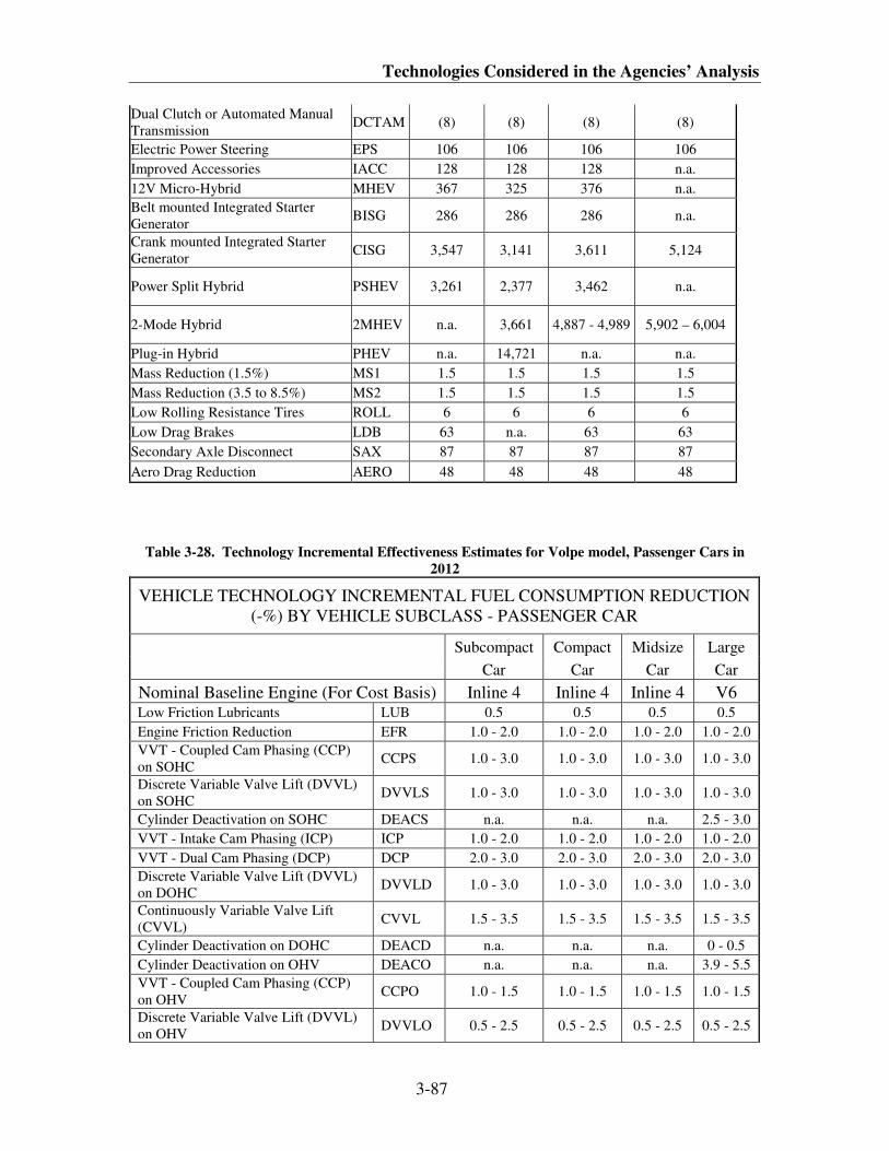
Technologies Considered in the Agencies’ Analysis
3-87
Dual Clutch or Automated Manual
Transmission DCTAM (8) (8) (8) (8)
Electric Power Steering EPS 106 106 106 106
Improved Accessories IACC 128 128 128 n.a.
12V Micro-Hybrid MHEV 367 325 376 n.a.
Belt mounted Integrated Starter
Generator BISG 286 286 286 n.a.
Crank mounted Integrated Starter
Generator CISG 3,547 3,141 3,611 5,124
Power Split Hybrid PSHEV 3,261 2,377 3,462 n.a.
2-Mode Hybrid 2MHEV n.a. 3,661 4,887 - 4,989 5,902 – 6,004
Plug-in Hybrid PHEV n.a. 14,721 n.a. n.a.
Mass Reduction (1.5%) MS1 1.5 1.5 1.5 1.5
Mass Reduction (3.5 to 8.5%) MS2 1.5 1.5 1.5 1.5
Low Rolling Resistance Tires ROLL 6 6 6 6
Low Drag Brakes LDB 63 n.a. 63 63
Secondary Axle Disconnect SAX 87 87 87 87
Aero Drag Reduction AERO 48 48 48 48
Table 3-28. Technology Incremental Effectiveness Estimates for Volpe model, Passenger Cars in
2012
VEHICLE TECHNOLOGY INCREMENTAL FUEL CONSUMPTION REDUCTION
(-%) BY VEHICLE SUBCLASS - PASSENGER CAR
Subcompact Compact Midsize Large
Car Car Car Car
Nominal Baseline Engine (For Cost Basis) Inline 4 Inline 4 Inline 4 V6 Low Friction Lubricants LUB 0.5 0.5 0.5 0.5
Engine Friction Reduction EFR 1.0 - 2.0 1.0 - 2.0 1.0 - 2.0 1.0 - 2.0
VVT - Coupled Cam Phasing (CCP)
on SOHC CCPS 1.0 - 3.0 1.0 - 3.0 1.0 - 3.0 1.0 - 3.0
Discrete Variable Valve Lift (DVVL)
on SOHC DVVLS 1.0 - 3.0 1.0 - 3.0 1.0 - 3.0 1.0 - 3.0
Cylinder Deactivation on SOHC DEACS n.a. n.a. n.a. 2.5 - 3.0
VVT - Intake Cam Phasing (ICP) ICP 1.0 - 2.0 1.0 - 2.0 1.0 - 2.0 1.0 - 2.0
VVT - Dual Cam Phasing (DCP) DCP 2.0 - 3.0 2.0 - 3.0 2.0 - 3.0 2.0 - 3.0
Discrete Variable Valve Lift (DVVL)
on DOHC DVVLD 1.0 - 3.0 1.0 - 3.0 1.0 - 3.0 1.0 - 3.0
Continuously Variable Valve Lift
(CVVL) CVVL 1.5 - 3.5 1.5 - 3.5 1.5 - 3.5 1.5 - 3.5
Cylinder Deactivation on DOHC DEACD n.a. n.a. n.a. 0 - 0.5
Cylinder Deactivation on OHV DEACO n.a. n.a. n.a. 3.9 - 5.5
VVT - Coupled Cam Phasing (CCP)
on OHV CCPO 1.0 - 1.5 1.0 - 1.5 1.0 - 1.5 1.0 - 1.5
Discrete Variable Valve Lift (DVVL)
on OHV DVVLO 0.5 - 2.5 0.5 - 2.5 0.5 - 2.5 0.5 - 2.5
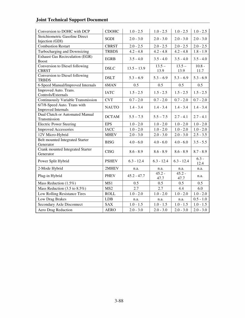
Joint Technical Support Document
3-88
Conversion to DOHC with DCP CDOHC 1.0 - 2.5 1.0 - 2.5 1.0 - 2.5 1.0 - 2.5
Stoichiometric Gasoline Direct
Injection (GDI) SGDI 2.0 - 3.0 2.0 - 3.0 2.0 - 3.0 2.0 - 3.0
Combustion Restart CBRST 2.0 - 2.5 2.0 - 2.5 2.0 - 2.5 2.0 - 2.5
Turbocharging and Downsizing TRBDS 4.2 - 4.8 4.2 - 4.8 4.2 - 4.8 1.8 - 1.9
Exhaust Gas Recirculation (EGR)
Boost EGRB 3.5 - 4.0 3.5 - 4.0 3.5 - 4.0 3.5 - 4.0
Conversion to Diesel following
CBRST DSLC 13.5 – 13.9
13.5 –
13.9
13.5 –
13.9
10.8 -
11.7
Conversion to Diesel following
TRBDS DSLT 5.3 – 6.9 5.3 – 6.9 5.3 – 6.9 5.3 - 6.9
6-Speed Manual/Improved Internals 6MAN 0.5 0.5 0.5 0.5
Improved Auto. Trans.
Controls/Externals IATC 1.5 - 2.5 1.5 - 2.5 1.5 - 2.5 1.5 - 2.5
Continuously Variable Transmission CVT 0.7 - 2.0 0.7 - 2.0 0.7 - 2.0 0.7 - 2.0
6/7/8-Speed Auto. Trans with
Improved Internals NAUTO 1.4 - 3.4 1.4 - 3.4 1.4 - 3.4 1.4 - 3.4
Dual Clutch or Automated Manual
Transmission DCTAM 5.5 – 7.5 5.5 – 7.5 2.7 - 4.1 2.7 - 4.1
Electric Power Steering EPS 1.0 - 2.0 1.0 - 2.0 1.0 - 2.0 1.0 - 2.0
Improved Accessories IACC 1.0 - 2.0 1.0 - 2.0 1.0 - 2.0 1.0 - 2.0
12V Micro-Hybrid MHEV 2.0 - 3.0 2.0 - 3.0 2.0 - 3.0 2.5 - 3.5
Belt mounted Integrated Starter
Generator BISG 4.0 - 6.0 4.0 - 6.0 4.0 - 6.0 3.5 - 5.5
Crank mounted Integrated Starter
Generator CISG 8.6 - 8.9 8.6 - 8.9 8.6 - 8.9 8.7 - 8.9
Power Split Hybrid PSHEV 6.3 - 12.4 6.3 - 12.4 6.3 - 12.4 6.3 -
12.4
2-Mode Hybrid 2MHEV n.a. n.a. n.a. n.a.
Plug-in Hybrid PHEV 45.2 - 47.7 45.2 -
47.7
45.2 -
47.7 n.a.
Mass Reduction (1.5%) MS1 0.5 0.5 0.5 0.5
Mass Reduction (3.5 to 8.5%) MS2 2.7 2.7 4.4 6.0
Low Rolling Resistance Tires ROLL 1.0 - 2.0 1.0 - 2.0 1.0 - 2.0 1.0 - 2.0
Low Drag Brakes LDB n.a. n.a. n.a. 0.5 - 1.0
Secondary Axle Disconnect SAX 1.0 - 1.5 1.0 - 1.5 1.0 - 1.5 1.0 - 1.5
Aero Drag Reduction AERO 2.0 - 3.0 2.0 - 3.0 2.0 - 3.0 2.0 - 3.0
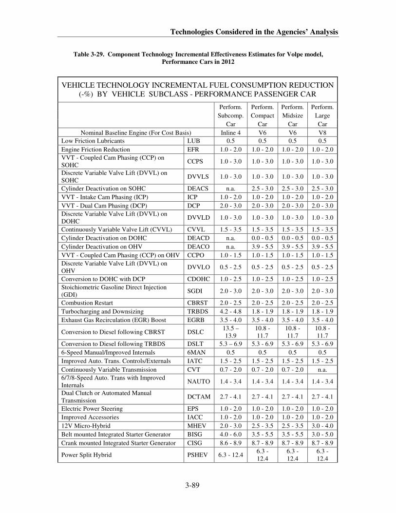
Technologies Considered in the Agencies’ Analysis
3-89
Table 3-29. Component Technology Incremental Effectiveness Estimates for Volpe model,
Performance Cars in 2012
VEHICLE TECHNOLOGY INCREMENTAL FUEL CONSUMPTION REDUCTION
(-%) BY VEHICLE SUBCLASS - PERFORMANCE PASSENGER CAR
Perform. Perform. Perform. Perform.
Subcomp. Compact Midsize Large
Car Car Car Car
Nominal Baseline Engine (For Cost Basis) Inline 4 V6 V6 V8
Low Friction Lubricants LUB 0.5 0.5 0.5 0.5
Engine Friction Reduction EFR 1.0 - 2.0 1.0 - 2.0 1.0 - 2.0 1.0 - 2.0
VVT - Coupled Cam Phasing (CCP) on
SOHC CCPS 1.0 - 3.0 1.0 - 3.0 1.0 - 3.0 1.0 - 3.0
Discrete Variable Valve Lift (DVVL) on
SOHC DVVLS 1.0 - 3.0 1.0 - 3.0 1.0 - 3.0 1.0 - 3.0
Cylinder Deactivation on SOHC DEACS n.a. 2.5 - 3.0 2.5 - 3.0 2.5 - 3.0
VVT - Intake Cam Phasing (ICP) ICP 1.0 - 2.0 1.0 - 2.0 1.0 - 2.0 1.0 - 2.0
VVT - Dual Cam Phasing (DCP) DCP 2.0 - 3.0 2.0 - 3.0 2.0 - 3.0 2.0 - 3.0
Discrete Variable Valve Lift (DVVL) on
DOHC DVVLD 1.0 - 3.0 1.0 - 3.0 1.0 - 3.0 1.0 - 3.0
Continuously Variable Valve Lift (CVVL) CVVL 1.5 - 3.5 1.5 - 3.5 1.5 - 3.5 1.5 - 3.5
Cylinder Deactivation on DOHC DEACD n.a. 0.0 - 0.5 0.0 - 0.5 0.0 - 0.5
Cylinder Deactivation on OHV DEACO n.a. 3.9 - 5.5 3.9 - 5.5 3.9 - 5.5
VVT - Coupled Cam Phasing (CCP) on OHV CCPO 1.0 - 1.5 1.0 - 1.5 1.0 - 1.5 1.0 - 1.5
Discrete Variable Valve Lift (DVVL) on
OHV DVVLO 0.5 - 2.5 0.5 - 2.5 0.5 - 2.5 0.5 - 2.5
Conversion to DOHC with DCP CDOHC 1.0 - 2.5 1.0 - 2.5 1.0 - 2.5 1.0 - 2.5
Stoichiometric Gasoline Direct Injection
(GDI) SGDI 2.0 - 3.0 2.0 - 3.0 2.0 - 3.0 2.0 - 3.0
Combustion Restart CBRST 2.0 - 2.5 2.0 - 2.5 2.0 - 2.5 2.0 - 2.5
Turbocharging and Downsizing TRBDS 4.2 - 4.8 1.8 - 1.9 1.8 - 1.9 1.8 - 1.9
Exhaust Gas Recirculation (EGR) Boost EGRB 3.5 - 4.0 3.5 - 4.0 3.5 - 4.0 3.5 - 4.0
Conversion to Diesel following CBRST DSLC 13.5 –
13.9
10.8 -
11.7
10.8 -
11.7
10.8 -
11.7
Conversion to Diesel following TRBDS DSLT 5.3 – 6.9 5.3 - 6.9 5.3 - 6.9 5.3 - 6.9
6-Speed Manual/Improved Internals 6MAN 0.5 0.5 0.5 0.5
Improved Auto. Trans. Controls/Externals IATC 1.5 - 2.5 1.5 - 2.5 1.5 - 2.5 1.5 - 2.5
Continuously Variable Transmission CVT 0.7 - 2.0 0.7 - 2.0 0.7 - 2.0 n.a.
6/7/8-Speed Auto. Trans with Improved
Internals NAUTO 1.4 - 3.4 1.4 - 3.4 1.4 - 3.4 1.4 - 3.4
Dual Clutch or Automated Manual
Transmission DCTAM 2.7 - 4.1 2.7 - 4.1 2.7 - 4.1 2.7 - 4.1
Electric Power Steering EPS 1.0 - 2.0 1.0 - 2.0 1.0 - 2.0 1.0 - 2.0
Improved Accessories IACC 1.0 - 2.0 1.0 - 2.0 1.0 - 2.0 1.0 - 2.0
12V Micro-Hybrid MHEV 2.0 - 3.0 2.5 - 3.5 2.5 - 3.5 3.0 - 4.0
Belt mounted Integrated Starter Generator BISG 4.0 - 6.0 3.5 - 5.5 3.5 - 5.5 3.0 - 5.0
Crank mounted Integrated Starter Generator CISG 8.6 - 8.9 8.7 - 8.9 8.7 - 8.9 8.7 - 8.9
Power Split Hybrid PSHEV 6.3 - 12.4 6.3 -
12.4
6.3 -
12.4
6.3 -
12.4
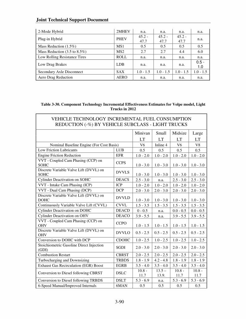
Joint Technical Support Document
3-90
2-Mode Hybrid 2MHEV n.a. n.a. n.a. n.a.
Plug-in Hybrid PHEV 45.2 -
47.7
45.2 -
47.7
45.2 -
47.7 n.a.
Mass Reduction (1.5%) MS1 0.5 0.5 0.5 0.5
Mass Reduction (3.5 to 8.5%) MS2 2.7 2.7 4.4 6.0
Low Rolling Resistance Tires ROLL n.a. n.a. n.a. n.a.
Low Drag Brakes LDB n.a. n.a. n.a. 0.5 - 1.0
Secondary Axle Disconnect SAX 1.0 - 1.5 1.0 - 1.5 1.0 - 1.5 1.0 - 1.5
Aero Drag Reduction AERO n.a. n.a. n.a. n.a.
Table 3-30. Component Technology Incremental Effectiveness Estimates for Volpe model, Light
Trucks in 2012
VEHICLE TECHNOLOGY INCREMENTAL FUEL CONSUMPTION
REDUCTION (-%) BY VEHICLE SUBCLASS - LIGHT TRUCKS
Minivan Small Midsize Large
LT LT LT LT
Nominal Baseline Engine (For Cost Basis) V6 Inline 4 V6 V8
Low Friction Lubricants LUB 0.5 0.5 0.5 0.5
Engine Friction Reduction EFR 1.0 - 2.0 1.0 - 2.0 1.0 - 2.0 1.0 - 2.0
VVT - Coupled Cam Phasing (CCP) on
SOHC CCPS
1.0 - 3.0 1.0 - 3.0 1.0 - 3.0 1.0 - 3.0
Discrete Variable Valve Lift (DVVL) on
SOHC DVVLS
1.0 - 3.0 1.0 - 3.0 1.0 - 3.0 1.0 - 3.0
Cylinder Deactivation on SOHC DEACS 2.5 - 3.0 n.a. 2.5 - 3.0 2.5 - 3.0
VVT - Intake Cam Phasing (ICP) ICP 1.0 - 2.0 1.0 - 2.0 1.0 - 2.0 1.0 - 2.0
VVT - Dual Cam Phasing (DCP) DCP 2.0 - 3.0 2.0 - 3.0 2.0 - 3.0 2.0 - 3.0
Discrete Variable Valve Lift (DVVL) on
DOHC DVVLD
1.0 - 3.0 1.0 - 3.0 1.0 - 3.0 1.0 - 3.0
Continuously Variable Valve Lift (CVVL) CVVL 1.5 - 3.5 1.5 - 3.5 1.5 - 3.5 1.5 - 3.5
Cylinder Deactivation on DOHC DEACD 0 - 0.5 n.a. 0.0 - 0.5 0.0 - 0.5
Cylinder Deactivation on OHV DEACO 3.9 - 5.5 n.a. 3.9 - 5.5 3.9 - 5.5
VVT - Coupled Cam Phasing (CCP) on
OHV CCPO
1.0 - 1.5 1.0 - 1.5 1.0 - 1.5 1.0 - 1.5
Discrete Variable Valve Lift (DVVL) on
OHV DVVLO 0.5 - 2.5 0.5 - 2.5 0.5 - 2.5 0.5 - 2.5
Conversion to DOHC with DCP CDOHC 1.0 - 2.5 1.0 - 2.5 1.0 - 2.5 1.0 - 2.5
Stoichiometric Gasoline Direct Injection
(GDI) SGDI 2.0 - 3.0 2.0 - 3.0 2.0 - 3.0 2.0 - 3.0
Combustion Restart CBRST 2.0 - 2.5 2.0 - 2.5 2.0 - 2.5 2.0 - 2.5
Turbocharging and Downsizing TRBDS 1.8 - 1.9 4.2 - 4.8 1.8 - 1.9 1.8 - 1.9
Exhaust Gas Recirculation (EGR) Boost EGRB 3.5 - 4.0 3.5 - 4.0 3.5 - 4.0 3.5 - 4.0
Conversion to Diesel following CBRST DSLC 10.8 -
11.7
13.5 –
13.9.
10.8 -
11.7
10.8 -
11.7
Conversion to Diesel following TRBDS DSLT 5.3 - 6.9 n.a. 5.3 - 6.9 5.3 - 6.9
6-Speed Manual/Improved Internals 6MAN 0.5 0.5 0.5 0.5
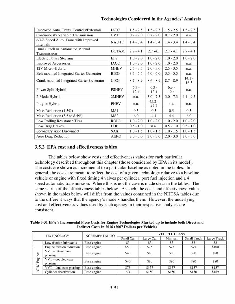
Technologies Considered in the Agencies’ Analysis
3-91
Improved Auto. Trans. Controls/Externals IATC 1.5 - 2.5 1.5 - 2.5 1.5 - 2.5 1.5 - 2.5
Continuously Variable Transmission CVT 0.7 - 2.0 0.7 - 2.0 0.7 - 2.0 n.a.
6/7/8-Speed Auto. Trans with Improved
Internals NAUTO 1.4 - 3.4 1.4 - 3.4 1.4 - 3.4 1.4 - 3.4
Dual Clutch or Automated Manual
Transmission DCTAM 2.7 - 4.1 2.7 -4.1 2.7 - 4.1 2.7 - 4.1
Electric Power Steering EPS 1.0 - 2.0 1.0 - 2.0 1.0 - 2.0 1.0 - 2.0
Improved Accessories IACC 1.0 - 2.0 1.0 - 2.0 1.0 - 2.0 n.a.
12V Micro-Hybrid MHEV 2.5 - 3.5 2.0 - 3.0 2.5 - 3.5 n.a.
Belt mounted Integrated Starter Generator BISG 3.5 - 5.5 4.0 - 6.0 3.5 - 5.5 n.a.
Crank mounted Integrated Starter Generator CISG 8.7 - 8.9 8.6 - 8.9 8.7 - 8.9 14.1 -
16.3
Power Split Hybrid PSHEV 6.3 -
12.4
6.3 -
12.4
6.3 -
12.4 n.a.
2-Mode Hybrid 2MHEV n.a. 3.0 - 7.3 3.0 - 7.3 4.1 - 9.5
Plug-in Hybrid PHEV n.a. 45.2 -
47.7 n.a. n.a.
Mass Reduction (1.5%) MS1 0.5 0.5 0.5 0.5
Mass Reduction (3.5 to 8.5%) MS2 6.0 4.4 4.4 6.0
Low Rolling Resistance Tires ROLL 1.0 - 2.0 1.0 - 2.0 1.0 - 2.0 1.0 - 2.0
Low Drag Brakes LDB 0.5 - 1.0 n.a. 0.5 - 1.0 0.5 - 1.0
Secondary Axle Disconnect SAX 1.0 - 1.5 1.0 - 1.5 1.0 - 1.5 1.0 - 1.5
Aero Drag Reduction AERO 2.0 - 3.0 2.0 - 3.0 2.0 - 3.0 2.0 - 3.0
3.5.2 EPA cost and effectiveness tables
The tables below show costs and effectiveness values for each particular
technology described throughout this chapter (those considered by EPA in its model).
The costs are shown as incremental to a particular baseline as noted in the tables. In
general, the costs are meant to reflect the cost of a given technology relative to a baseline
vehicle or engine with fixed timing 4 valves per cylinder, port fuel injection and a 4
speed automatic transmission. Where this is not the case is made clear in the tables. The
same is true of the effectiveness tables below. As such, the costs and effectiveness values
shown in the tables below will differ from the values contained in the NHTSA tables due
to the different ways that the agency’s models handles them. However, the underlying
cost and effectiveness values used by each agency in their respective analyses are
consistent.
Table 3-31 EPA’s Incremental Piece Costs for Engine Technologies Marked up to include both Direct and
Indirect Costs in 2016 (2007 Dollars per Vehicle)
VEHICLE CLASS TECHNOLOGY INCREMENTAL TO
Small Car Large Car Minivan Small Truck Large Truck
Low friction lubricants Base engine $3 $3 $3 $3 $3
Engine friction reduction Base engine $50 $75 $75 $75 $100
VVT – intake cam
phasing Base engine $40 $80 $80 $80 $80
VVT – coupled cam
phasing Base engine $40 $80 $80 $80 $80
VVT – dual cam phasing Base engine $73 $157 $157 $157 $157
OH
C E
ng
ines
Cylinder deactivation Base engine n/a $150 $150 $150 $169
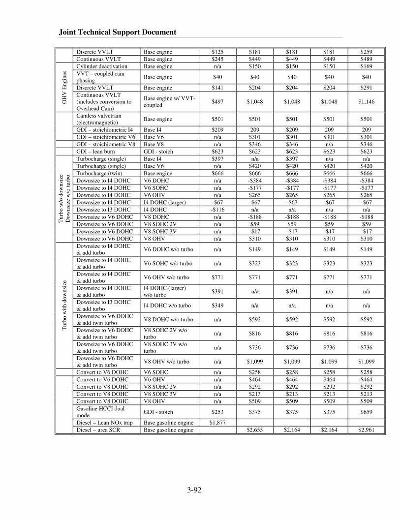
Joint Technical Support Document
3-92
Discrete VVLT Base engine $125 $181 $181 $181 $259
Continuous VVLT Base engine $245 $449 $449 $449 $489
Cylinder deactivation Base engine n/a $150 $150 $150 $169
VVT – coupled cam
phasing Base engine $40 $40 $40 $40 $40
Discrete VVLT Base engine $141 $204 $204 $204 $291
OH
V E
ng
ines
Continuous VVLT
(includes conversion to
Overhead Cam)
Base engine w/ VVT-
coupled $497 $1,048 $1,048 $1,048 $1,146
Camless valvetrain
(electromagnetic) Base engine $501 $501 $501 $501 $501
GDI – stoichiometric I4 Base I4 $209 209 $209 209 209
GDI – stoichiometric V6 Base V6 n/a $301 $301 $301 $301
GDI – stoichiometric V8 Base V8 n/a $346 $346 n/a $346
GDI – lean burn GDI - stoich $623 $623 $623 $623 $623
Turbocharge (single) Base I4 $397 n/a $397 n/a n/a
Turbocharge (single) Base V6 n/a $420 $420 $420 $420 Turbocharge (twin) Base engine $666 $666 $666 $666 $666
Downsize to I4 DOHC V6 DOHC n/a -$384 -$384 -$384 -$384
Downsize to I4 DOHC V6 SOHC n/a -$177 -$177 -$177 -$177
Downsize to I4 DOHC V6 OHV n/a $265 $265 $265 $265
Downsize to I4 DOHC I4 DOHC (larger) -$67 -$67 -$67 -$67 -$67
Downsize to I3 DOHC I4 DOHC -$116 n/a n/a n/a n/a
Downsize to V6 DOHC V8 DOHC n/a -$188 -$188 -$188 -$188
Downsize to V6 DOHC V8 SOHC 2V n/a $59 $59 $59 $59
Downsize to V6 DOHC V8 SOHC 3V n/a -$17 -$17 -$17 -$17
Tu
rbo
w/o
do
wn
size
Do
wn
size
w/o
tu
rbo
Downsize to V6 DOHC V8 OHV n/a $310 $310 $310 $310
Downsize to I4 DOHC
& add turbo V6 DOHC w/o turbo n/a $149 $149 $149 $149
Downsize to I4 DOHC
& add turbo V6 SOHC w/o turbo n/a $323 $323 $323 $323
Downsize to I4 DOHC
& add turbo V6 OHV w/o turbo $771 $771 $771 $771 $771
Downsize to I4 DOHC
& add turbo
I4 DOHC (larger)
w/o turbo $391 n/a $391 n/a n/a
Downsize to I3 DOHC
& add turbo I4 DOHC w/o turbo $349 n/a n/a n/a n/a
Downsize to V6 DOHC
& add twin turbo V8 DOHC w/o turbo n/a $592 $592 $592 $592
Downsize to V6 DOHC
& add twin turbo
V8 SOHC 2V w/o
turbo n/a $816 $816 $816 $816
Downsize to V6 DOHC
& add twin turbo
V8 SOHC 3V w/o
turbo n/a $736 $736 $736 $736
Tu
rbo
wit
h d
ow
nsi
ze
Downsize to V6 DOHC
& add twin turbo V8 OHV w/o turbo n/a $1,099 $1,099 $1,099 $1,099
Convert to V6 DOHC V6 SOHC n/a $258 $258 $258 $258
Convert to V6 DOHC V6 OHV n/a $464 $464 $464 $464
Convert to V8 DOHC V8 SOHC 2V n/a $292 $292 $292 $292
Convert to V8 DOHC V8 SOHC 3V n/a $213 $213 $213 $213
Convert to V8 DOHC V8 OHV n/a $509 $509 $509 $509
Gasoline HCCI dual-
mode GDI - stoich $253 $375 $375 $375 $659
Diesel – Lean NOx trap Base gasoline engine $1,877
Diesel – urea SCR Base gasoline engine $2,655 $2,164 $2,164 $2,961
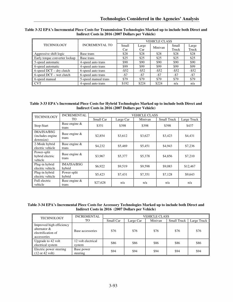
Technologies Considered in the Agencies’ Analysis
3-93
Table 3-32 EPA’s Incremental Piece Costs for Transmission Technologies Marked up to include both Direct and
Indirect Costs in 2016 (2007 Dollars per Vehicle)
VEHICLE CLASS TECHNOLOGY INCREMENTAL TO Small
Car
Large
Car Minivan
Small
Truck
Large
Truck
Aggressive shift logic Base trans $28 $28 $28 $28 $28
Early torque converter lockup Base trans $25 $25 $25 $25 $25
5-speed automatic 4-speed auto trans $90 $90 $90 $90 $90
6-speed automatic 4-speed auto trans $99 $99 $99 $99 $99
6-speed DCT – dry clutch 6-speed auto trans -$52 -$52 -$52 -$52 -$52
6-speed DCT – wet clutch 6-speed auto trans -$7 -$7 -$7 -$7 -$7
6-speed manual 5-speed manual trans $79 $79 $79 $79 $79
CVT 4-speed auto trans $192 $224 $224 n/a n/a
Table 3-33 EPA’s Incremental Piece Costs for Hybrid Technologies Marked up to include both Direct and
Indirect Costs in 2016 (2007 Dollars per Vehicle)
VEHICLE CLASS TECHNOLOGY
INCREMENTAL
TO Small Car Large Car Minivan Small Truck Large Truck
Stop-Start Base engine &
trans $351 $398 $398 $398 $437
IMA/ISA/BSG
(includes engine
downsize)
Base engine &
trans $2,854 $3,612 $3,627 $3,423 $4,431
2-Mode hybrid
electric vehicle
Base engine &
trans $4,232 $5,469 $5,451 $4,943 $7,236
Power-split
hybrid electric
vehicle
Base engine &
trans $3,967 $5,377 $5,378 $4,856 $7,210
Plug-in hybrid
electric vehicle
IMA/ISA/BSG
hybrid $6,922 $9,519 $9,598 $9,083 $12,467
Plug-in hybrid
electric vehicle
Power-split
hybrid $5,423 $7,431 $7,351 $7,128 $9,643
Full electric
vehicle
Base engine &
trans $27,628 n/a n/a n/a n/a
Table 3-34 EPA’s Incremental Piece Costs for Accessory Technologies Marked up to include both Direct and
Indirect Costs in 2016 (2007 Dollars per Vehicle)
VEHICLE CLASS TECHNOLOGY
INCREMENTAL
TO Small Car Large Car Minivan Small Truck Large Truck
Improved high efficiency
alternator &
electrification of
accessories
Base accessories $76 $76 $76 $76 $76
Upgrade to 42 volt
electrical system
12 volt electrical
system $86 $86 $86 $86 $86
Electric power steering
(12 or 42 volt)
Base power
steering $94 $94 $94 $94 $94
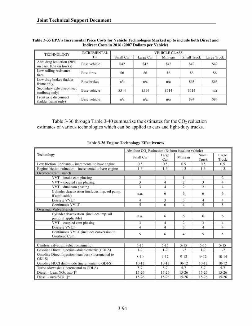
Joint Technical Support Document
3-94
Table 3-35 EPA’s Incremental Piece Costs for Vehicle Technologies Marked up to include both Direct and
Indirect Costs in 2016 (2007 Dollars per Vehicle)
VEHICLE CLASS TECHNOLOGY
INCREMENTAL
TO Small Car Large Car Minivan Small Truck Large Truck
Aero drag reduction (20%
on cars, 10% on trucks) Base vehicle $42 $42 $42 $42 $42
Low rolling resistance
tires Base tires $6 $6 $6 $6 $6
Low drag brakes (ladder
frame only) Base brakes n/a n/a n/a $63 $63
Secondary axle disconnect
(unibody only) Base vehicle $514 $514 $514 $514 n/a
Front axle disconnect
(ladder frame only) Base vehicle n/a n/a n/a $84 $84
Table 3-36 through Table 3-40 summarize the estimates for the CO2 reduction
estimates of various technologies which can be applied to cars and light-duty trucks.
Table 3-36 Engine Technology Effectiveness
Absolute CO2 Reduction (% from baseline vehicle) Technology
Small Car Large
Car Minivan
Small
Truck
Large
Truck
Low friction lubricants – incremental to base engine 0.5 0.5 0.5 0.5 0.5
Engine friction reduction – incremental to base engine 1-3 1-3 1-3 1-3 1-3
Overhead Cam Branch
VVT – intake cam phasing 2 1 1 1 2
VVT – coupled cam phasing 3 4 2 3 4
VVT – dual cam phasing 3 4 2 2 4
Cylinder deactivation (includes imp. oil pump,
if applicable) n.a. 6 6 6 6
Discrete VVLT 4 3 3 4 4
Continuous VVLT 5 6 4 5 5
Overhead Valve Branch
Cylinder deactivation (includes imp. oil
pump, if applicable) n.a. 6 6 6 6
VVT – coupled cam phasing 3 4 2 3 4
Discrete VVLT 4 4 3 4 4
Continuous VVLT (includes conversion to
Overhead Cam) 5 6 4 5 5
Camless valvetrain (electromagnetic) 5-15 5-15 5-15 5-15 5-15
Gasoline Direct Injection–stoichiometric (GDI-S) 1-2 1-2 1-2 1-2 1-2
Gasoline Direct Injection–lean burn (incremental to
GDI-S) 8-10 9-12 9-12 9-12 10-14
Gasoline HCCI dual-mode (incremental to GDI-S) 10-12 10-12 10-12 10-12 10-12
Turbo+downsize (incremental to GDI-S) 5-7 5-7 5-7 5-7 5-7
Diesel – Lean NOx trap[]* 15-26 15-26 15-26 15-26 15-26
Diesel – urea SCR []* 15-26 15-26 15-26 15-26 15-26
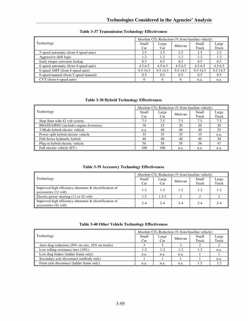
Technologies Considered in the Agencies’ Analysis
3-95
Table 3-37 Transmission Technology Effectiveness
Absolute CO2 Reduction (% from baseline vehicle) Technology Small
Car
Large
Car Minivan
Small
Truck
Large
Truck
5-speed automatic (from 4-speed auto) 2.5 2.5 2.5 2.5 2.5
Aggressive shift logic 1-2 1-2 1-2 1-2 1-2
Early torque converter lockup 0.5 0.5 0.5 0.5 0.5
6-speed automatic (from 4-speed auto) 4.5-6.5 4.5-6.5 4.5-6.5 4.5-6.5 4.5-6.5
6-speed AMT (from 4-speed auto) 9.5-14.5 9.5-14.5 9.5-14.5 9.5-14.5 9.5-14.5
6-speed manual (from 5-speed manual) 0.5 0.5 0.5 0.5 0.5
CVT (from 4-speed auto) 6 6 6 n.a. n.a.
Table 3-38 Hybrid Technology Effectiveness
Absolute CO2 Reduction (% from baseline vehicle) Technology Small
Car
Large
Car Minivan
Small
Truck
Large
Truck
Stop-Start with 42 volt system 7.5 7.5 7.5 7.5 7.5
IMA/ISA/BSG (includes engine downsize) 30 25 20 20 20
2-Mode hybrid electric vehicle n.a. 40 40 40 25
Power-split hybrid electric vehicle 35 35 35 35 n.a.
Full-Series hydraulic hybrid 40 40 40 40 30
Plug-in hybrid electric vehicle 58 58 58 58 47
Full electric vehicle (EV) 100 100 n.a. n.a. n.a.
Table 3-39 Accessory Technology Effectiveness
Absolute CO2 Reduction (% from baseline vehicle) Technology Small
Car
Large
Car Minivan
Small
Truck
Large
Truck
Improved high efficiency alternator & electrification of
accessories (12 volt) 1-2 1-2 1-2 1-2 1-2
Electric power steering (12 or 42 volt) 1.5 1.5-2 2 2 2
Improved high efficiency alternator & electrification of
accessories (42 volt) 2-4 2-4 2-4 2-4 2-4
Table 3-40 Other Vehicle Technology Effectiveness
Absolute CO2 Reduction (% from baseline vehicle) Technology Small
Car
Large
Car Minivan
Small
Truck
Large
Truck
Aero drag reduction (20% on cars, 10% on trucks) 3 3 3 2 2
Low rolling resistance tires (10%) 1-2 1-2 1-2 1-2 n.a.
Low drag brakes (ladder frame only) n.a. n.a. n.a. 1 1
Secondary axle disconnect (unibody only) 1 1 1 1 n.a.
Front axle disconnect (ladder frame only) n.a. n.a. n.a. 1.5 1.5
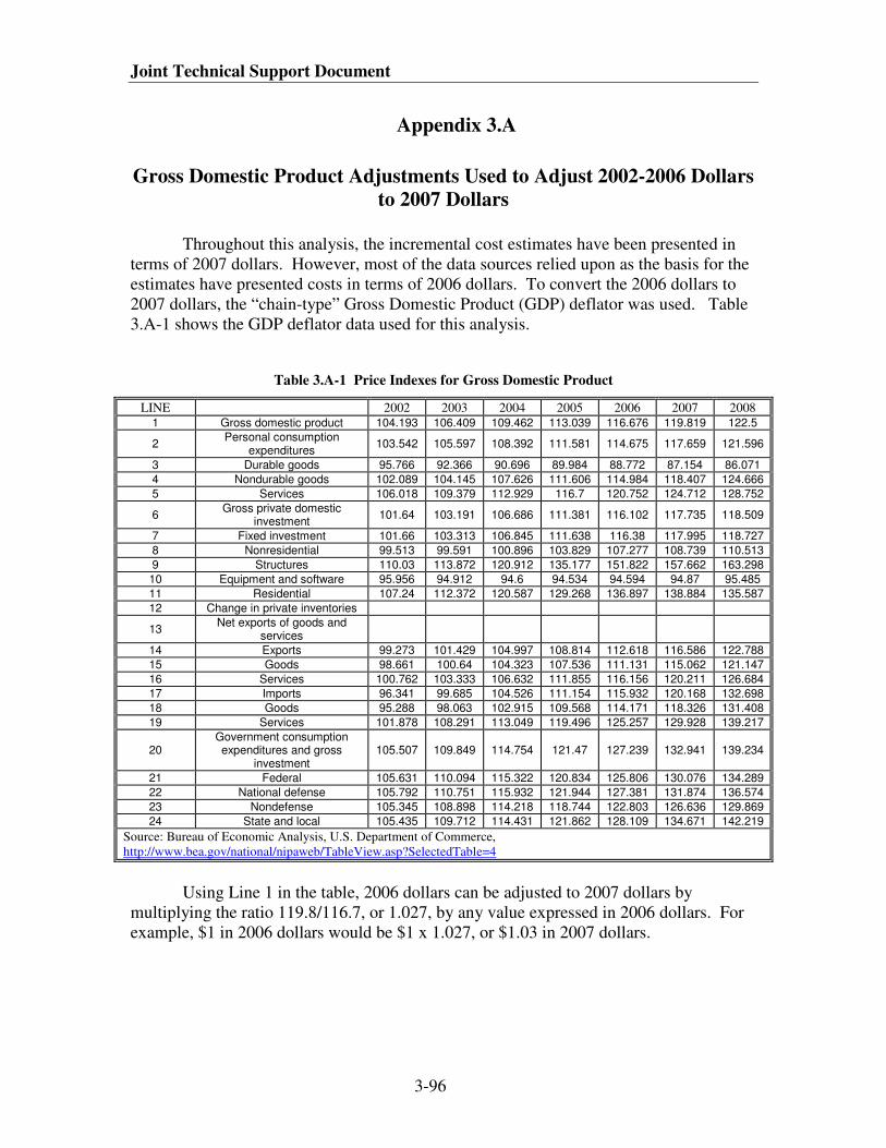
Joint Technical Support Document
3-96
Appendix 3.A
Gross Domestic Product Adjustments Used to Adjust 2002-2006 Dollars
to 2007 Dollars
Throughout this analysis, the incremental cost estimates have been presented in
terms of 2007 dollars. However, most of the data sources relied upon as the basis for the
estimates have presented costs in terms of 2006 dollars. To convert the 2006 dollars to
2007 dollars, the “chain-type” Gross Domestic Product (GDP) deflator was used. Table
3.A-1 shows the GDP deflator data used for this analysis.
Table 3.A-1 Price Indexes for Gross Domestic Product
LINE 2002 2003 2004 2005 2006 2007 2008
1 Gross domestic product 104.193 106.409 109.462 113.039 116.676 119.819 122.5
2 Personal consumption
expenditures 103.542 105.597 108.392 111.581 114.675 117.659 121.596
3 Durable goods 95.766 92.366 90.696 89.984 88.772 87.154 86.071
4 Nondurable goods 102.089 104.145 107.626 111.606 114.984 118.407 124.666
5 Services 106.018 109.379 112.929 116.7 120.752 124.712 128.752
6 Gross private domestic
investment 101.64 103.191 106.686 111.381 116.102 117.735 118.509
7 Fixed investment 101.66 103.313 106.845 111.638 116.38 117.995 118.727
8 Nonresidential 99.513 99.591 100.896 103.829 107.277 108.739 110.513
9 Structures 110.03 113.872 120.912 135.177 151.822 157.662 163.298
10 Equipment and software 95.956 94.912 94.6 94.534 94.594 94.87 95.485
11 Residential 107.24 112.372 120.587 129.268 136.897 138.884 135.587
12 Change in private inventories
13 Net exports of goods and
services
14 Exports 99.273 101.429 104.997 108.814 112.618 116.586 122.788
15 Goods 98.661 100.64 104.323 107.536 111.131 115.062 121.147
16 Services 100.762 103.333 106.632 111.855 116.156 120.211 126.684
17 Imports 96.341 99.685 104.526 111.154 115.932 120.168 132.698
18 Goods 95.288 98.063 102.915 109.568 114.171 118.326 131.408
19 Services 101.878 108.291 113.049 119.496 125.257 129.928 139.217
20 Government consumption expenditures and gross
investment 105.507 109.849 114.754 121.47 127.239 132.941 139.234
21 Federal 105.631 110.094 115.322 120.834 125.806 130.076 134.289
22 National defense 105.792 110.751 115.932 121.944 127.381 131.874 136.574
23 Nondefense 105.345 108.898 114.218 118.744 122.803 126.636 129.869
24 State and local 105.435 109.712 114.431 121.862 128.109 134.671 142.219
Source: Bureau of Economic Analysis, U.S. Department of Commerce,
http://www.bea.gov/national/nipaweb/TableView.asp?SelectedTable=4
Using Line 1 in the table, 2006 dollars can be adjusted to 2007 dollars by
multiplying the ratio 119.8/116.7, or 1.027, by any value expressed in 2006 dollars. For
example, $1 in 2006 dollars would be $1 x 1.027, or $1.03 in 2007 dollars.
Technologies Considered in the Agencies’ Analysis
3-97
References
1 “EPA Staff Technical Report: Cost and Effectiveness Estimates of Technologies Used to Reduce Light-
duty Vehicle Carbon Dioxide Emissions,” EPA420-R-08-008, March 2008, Docket EPA-HQ-OAR-2009-
0472-0132.
2 “Effectiveness and Impact of Corporate Average Fuel Economy (CAFE) Standards,” National Research
Council, National Academy of Sciences, 2002, Docket EPA-HQ-OAR-2009-0472-0147.
3 “Reducing Greenhouse Gas Emissions from Light-Duty Motor Vehicles,” Northeast States Center for a
Clean Air Future, September 2004, Docket EPA-HQ-OAR-2009-0472-0148.
4 “Staff Report: Initial Statement of Reasons for Proposed Rulemaking,” California Environmental
Protection Agency, Air Resources Board, Regulations to Control Greenhouse Gas Emissions from Motor
Vehicles, August 6, 2004, Docket EPA-HQ-OAR-2009-0472-0134.
5 “Technology to Improve the Fuel Economy of Light Duty Trucks to 2015,” Energy and Environmental
Analysis, Inc., May 2006, Docket EPA-HQ-OAR-2009-0472-0136.
6 “Variable Costs of Fuel Economy Technologies,” prepared for The Alliance of Automobile
Manufacturers, June 1, 2008, Docket EPA-HQ-OAR-2009-0472-0144; and, “Variable Costs of Fuel
Economy Technologies,” prepared for The Alliance of Automobile Manufacturers, June 1, 2008, Amended
December 10, 2008, Docket EPA-HQ-OAR-2009-0472-0145.
7 National Highway Traffic Safety Administration, Request for Product Plan Information, 74 FR 48192,
September 22, 2009.
8 Memorandum from Don Kopinski, U.S. EPA, Docket No. EPA-HQ-OAR-2009-0472-0217, dated
September 11, 2009.
9 U.S. Environmental Protection Agency, “Draft Report – Light-Duty Technology Cost Analysis Pilot
Study,” Contract No. EP-C-07-069, Work Assignment 1-3, September 3, 2009, Docket EPA-HQ-OAR-
2009-0472-0149; EPA-420-R-09-020, EPA docket number EPA-HQ-OAR-2009-0472-11282.
10 “Light-duty Technology Cost Analysis – Report on Additional Case Studies,” EPA-420-R-10-010.
11 U.S. Environmental Protection Agency, “Light-Duty Technology Cost Analysis Pilot Study,” Contract
No. EP-C-07-069, Work Assignment 1-3, December 2009, EPA-420-R-09-020, Docket EPA-HQ-OAR-
2009-0472-0149; peer review report dated November 6, 2009, is at EPA-HQ-OAR-2009-0472-11285;
“Light-duty Technology Cost Analysis – Report on Additional Case Studies,” EPA-420-R-10-010..
12 NHTSA’s 2011 CAFE final rule at 74 FR 14196.
13 National Income and Product Accounts Table 1.1.4: Price Indexes for Gross Domestic Product;
downloaded on 6/25/2009 At 12:00:25 PM, Last Revised June 25, 2009; Bureau of Economic Analysis,
U.S. Department of Commerce, www.bea.gov.
14 The 2002 NAS Report, Docket EPA-HQ-OAR-2009-0472-0147; the 2004 study done by NESCCAF,
Docket EPA-HQ-OAR-2009-0472-0148; the California Air Resources Board (CARB) Initial Statement of
Reasons in support of their carbon rulemaking, Docket EPA-HQ-OAR-2009-0472-0134; a 2006 study done
Joint Technical Support Document
3-98
by Energy and Environmental Analysis (EEA) for the Department of Energy, Docket EPA-HQ-OAR-2009-
0472-0136; a study done by Martec for the Alliance of Automobile Manufacturers, Docket EPA-HQ-OAR-
2009-0472-0144, and the 2008 Martec Report which updated that study, Docket EPA-HQ-OAR-2009-
0472-0145; and vehicle fuel economy certification data, and confidential data submitted by manufacturers
in response to the March and November 2009 requests for product plans.
15 U.S. Environmental Protection Agency, “Draft Report – Light-Duty Technology Cost Analysis Pilot
Study,” Contract No. EP-C-07-069, Work Assignment 1-3, September 3, 2009, Docket EPA-HQ-OAR-
2009-0472-0149.
16 Rogozhin, Alex, Michael Gallaher, and Walter McManus, “Automobile Industry Retail Price Equivalent
and Indirect Cost Multipliers,” EPA 420-R-09-003, Docket EPA Docket EPA-HQ-OAR-2009-0472-0142,
February 2009, http://epa.gov/otaq/ld-hwy/420r09003.pdf.
17 “Memorandum: Documentation of the Development of Indirect Cost Multipliers for Three Automotive
Technologies,” Gloria Helfand and Todd Sherwood, Office of Transportation and Air Quality, U.S.
Environmental Protection Agency, August 2009, Docket EPA-HQ-OAR-2009-0472-0158.
18 “Final Regulatory Analysis: Control of Emissions from Nonroad Diesel Engines,” EPA420-R-04-007,
May 2004, Docket EPA-HQ-OAR-2009-0472-0140; “Regulatory Impact Analysis: Control of Emissions
of Air Pollution from Locomotive Engines and Marine Compression-Ignition Engines Less than 30 Liters
per Cylinder,” EPA420-D-08-001a, May 2008, Docket EPA-HQ-OAR-2009-0472-0139; NHTSA 2011
CAFE final rule at 74 FR 14196.
19 “Learning Curves in Manufacturing,” Linda Argote and Dennis Epple, Science, February 23, 1990, Vol.
247, pp. 920-924, Docket EPA-HQ-OAR-2009-0472-0143.
20 NHTSA 2011 CAFE final rule at 74 FR 14196; “EPA Staff Technical Report: Cost and Effectiveness
Estimates of Technologies Used to Reduce Light-Duty Vehicle Carbon Dioxide Emissions,” EPA420-R-
08-008, March 2008, Docket EPA-HQ-OAR-2009-0472-0132; “Final Regulatory Analysis: Control of
Emissions from Nonroad Diesel Engines,” EPA420-R-04-007, May 2004, Docket EPA-HQ-OAR-2009-
0472-0140; “Regulatory Impact Analysis: Control of Emissions of Air Pollution from Locomotive Engines
and Marine Compression-Ignition Engines Less than 30 Liters per Cylinder,” EPA420-D-08-001a, May
2008, Docket EPA-HQ-OAR-2009-0472-0139.
21 “Impact of Friction Reduction Technologies on Fuel Economy,” Fenske, G. Presented at the March 2009
Chicago Chapter Meeting of the ‘Society of Tribologists and Lubricated Engineers’ Meeting, March 18th,
2009. Available at: http://www.chicagostle.org/program/2008-
2009/Impact%20of%20Friction%20Reduction%20Technologies%20on%20Fuel%20Economy%20-
%20with%20VGs%20removed.pdf (last accessed July 9, 2009).
22 “Light-Duty Automotive Technology and Fuel Economy Trends: 1975 Through 2007”, EPA420-S-07-
001, September 2007, Docket EPA-HQ-OAR-2009-0472-0137. Available at
http://www.epa.gov/oms/cert/mpg/fetrends/fetrends-archive.htm (last accessed July 9, 2009).
23 Paul Whitaker, Ricardo, Inc., “Gasoline Engine Performance And Emissions – Future Technologies and
Optimization,” ERC Symposium, Low Emission Combustion Technologies for Future IC Engines,
Madison, WI, June 8-9, 2005, Docket EPA-HQ-OAR-2009-0472-0155. Available at
http://www.erc.wisc.edu/symposiums/2005_Symposium/June%208%20PM/Whitaker_Ricardo.pdf (last
accessed Nov. 9, 2008).
24 Stefan Trampert, FEV Motorentechnik GmbH, “Engine and Transmission Development Trends - Rising
Fuel Cost Pushes Technology,” Symposium on International Automotive Technology, Pune, India, January
2007.
Technologies Considered in the Agencies’ Analysis
3-99
25
“Binning of FEV Costs to GDI, Turbo-charging, and Engine Downsizing,” memorandum to Docket
EPA-HQ-OAR-2009-0472, from Michael Olechiw, U.S. EPA, dated March 25, 2010.
26 “Binning of FEV Costs to GDI, Turbo-charging, and Engine Downsizing,” memorandum to Docket
EPA-HQ-OAR-2009-0472, from Michael Olechiw, U.S. EPA, dated March 25, 2010.
27 Stefan Wolff, Dirk Abendroth, Werner Weigl, Claus-Peter Linner, Rupert Neudecker, Michael
Schneider, Wolfgang Huber, and Andreas Rau, BMW, “Introducing The Automatic Start-Stop (ASS)
Function In Series Models,” 7th Stuttgart Automotive Vehicle and Engine Symposium, Organised by
FKFS, Mar 2007, Vol. 1.
28 G.K. Fraidl, P.E. Kapus, and H. Friedl, AVL List GmbH, “Future Gasoline Engine Technologies for 130
g/Km CO2,” VKM-THD 11th Symposium on the Working Process of Combustion Engines, TU Graz,
Sept. 2007.
29 “Development and Optimization of the Ford 3.5L V6 EcoBoost Combustion System,” Yi,J., Wooldridge,
S., Coulson, G., Hilditch, J. Iyer, C.O., Moilanen, P., Papaioannou, G., Reiche, D. Shelby, M.,
VanDerWege, B., Weaver, C. Xu, Z., Davis, G., Hinds, B. Schamel, A. SAE Technical Paper No. 2009-01-
1494, 2009, Docket EPA-HQ-OAR-2009-0472-2860.
30 David Woldring and Tilo Landenfeld of Bosch, and Mark J. Christie of Ricardo, “DI Boost: Application
of a High Performance Gasoline Direct Injection Concept,” SAE 2007-01-1410. Available at
http://www.sae.org/technical/papers/2007-01-1410 (last accessed Nov. 9, 2008)
31 Yves Boccadoro, Loïc Kermanac’h, Laurent Siauve, and Jean-Michel Vincent, Renault Powertrain
Division, “The New Renault TCE 1.2L Turbocharged Gasoline Engine,” 28th Vienna Motor Symposium,
April 2007.
32 Tobias Heiter, Matthias Philipp, Robert Bosch, “Gasoline Direct Injection: Is There a Simplified, Cost-
Optimal System Approach for an Attractive Future of Gasoline Engines?” AVL Engine & Environment
Conference, September 2005.
33 U.S. Environmental Protection Agency, “Draft Report – Light-Duty Technology Cost Analysis Pilot
Study,” Contract No. EP-C-07-069, Work Assignment 1-3, September 3, 2009, Docket EPA-HQ-OAR-
2009-0472-0149.
34 Docket No. NHTSA-2008-0089-0193.1
35 Cairns et al., Lotus, “Low Cost Solutions for Improved Fuel Economy in Gasoline Engines,” Global
Powertrain Congress September 27-29, 2005, vol. 33. Available at http://www.gpc-
icpem.org/pages/publications.html (last accessed Nov. 9, 2008).
36 Tim Lake, John Stokes, Richard Murphy, and Richard Osborne of Ricardo and Andreas Schamel of
Ford-Werke, “Turbocharging Concepts for Downsized DI Gasoline Engines,” VKA/ika Aachen
Colloquium 2003. Available at http://cat.inist.fr/?aModele=afficheN&cpsidt=16973598 (last accessed
Nov. 9, 2008).
37 “Interim Report: New Powertrain Technologies and Their Projected Costs,” October 2005, EPA420-R-
05-012, Docket EPA-HQ-OAR-2009-0472-0138.
38 “Cost and Fuel Economy Comparison of Diesel and Gasoline Powertrains in Passenger Cars and Light
Trucks,” submitted by FEV Engine Technology, Inc., April 23, 2003, contained as Appendix I within EPA
Interim Technical Report EPA420-R-04-002, Docket EPA-HQ-OAR-2009-0472-0141.
Joint Technical Support Document
3-100
39
EPA’s 2007/2010 diesel heavy-duty highway final rule at66 FR 5002; EPA’s Locomotive and Marine
final rule at 73 FR 37096.
40 http://www.platinum.matthey.com/ (web page printout is contained in Docket EPA-HQ-OAR-2009-0472
as “Johnson-Matthey PGM data for March 2009.pdf”).
41 General Motors, news release, “From Hybrids to Six-Speeds, Direct Injection And More, GM’s 2008
Global Powertrain Lineup Provides More Miles with Less Fuel” (released Mar. 6, 2007). Available at
http://www.gm.com/experience/fuel_economy/news/2007/adv_engines/2008-powertrain-lineup-082707.jsp
(last accessed Sept. 18, 2008).
42 “EPA Staff Technical Report: Cost and Effectiveness Estimates of Technologies Used to Reduce Light-
duty Vehicle Carbon Dioxide Emissions” Environmental Protection Agency, EPA420-R-08-008, March
2008, at page 17, Docket EPA-HQ-OAR-2009-0472-0132.
43 “Latest Chevrolet Volt Battery Pack and Generator Details and Clarifications.” Lyle Dennis interview
of Rob Peterson (GM) regarding the all-electric drive range of the GM Volt, August 29, 2007. Accessed on
the Internet on June 30, 2009 at: http://gm-volt.com/2007/08/29/latest-Chevrolet-volt-battery-pack-and-
generator-details-and-clarifications/
44 “Active Combination of Ultracapacitorsand Batteries for PHEV ESS.” Bohn, T. U.S. Department of
Energy 2009 Vehicle Technologies Merit Review, May 20, 2009, Docket EPA-HQ-OAR-2009-0472-0163.
45 Anderman, Advanced Automotive Battery Conference, May 2008. Proceedings available for purchase at
http://www.advancedautobat.com/Proceedings/index.html (last accessed October 17, 2008).
46 74 FR 14291 (Mar. 30, 2009)
47 “Electric Cars: Plugged In, Batteries must be included,” Deutsche Bank Global Markets Research
Company, June 9, 2008, Docket EPA-HQ-OAR-2009-0472-0154.
48 http://automobiles.honda.com/insight-hybrid/features.aspx?Feature=ima (last accessed on March 29,
2010; web page printout is contained in Docket EPA-HQ-OAR-2009-0472 as “Honda IMA webpage.pdf”).
49 “Preliminary Vehicle Mass Estimation Using Empirical Subsystem Influence Coefficients,” Malen, D.E.,
Reddy, K. Auto-Steel Partnership Report, May 2007, Docket EPA-HQ-OAR-2009-0472-0169. Accessed
on the Internet on May 30, 2009 at: http://www.a-sp.org/database/custom/Mass%20Compounding%20-
%20Final%20Report.pdf
50 “Benefit Analysis: Use of Aluminum Structures in Conjunction with Alternative Powertrain
Technologies in Automobiles,” Bull, M. Chavali, R., Mascarin, A., Aluminum Association Research
Report, May 2008, Docket EPA-HQ-OAR-2009-0472-0168. Accessed on the Internet on April 30, 2009
at: http://www.autoaluminum.org/downloads/IBIS-Powertrain-Study.pdf
51 “Future Generation Passenger Compartment-Validation (ASP 241)” Villano, P.J., Shaw, J.R.,
Polewarczyk, J., Morgans, S., Carpenter, J.A., Yocum, A.D., in “Lightweighting Materials – FY 2008
Progress Report,” U.S. Department of Energy, Office of Energy Efficiency and Renewable Energy, Vehicle
Technologies Program, May 2009, Docket EPA-HQ-OAR-2009-0472-0190.
52 “Preliminary Vehicle Mass Estimation Using Empirical Subsystem Influence Coefficients,” Malen, D.E.,
Reddy, K. Auto-Steel Partnership Report, May 2007, Docket EPA-HQ-OAR-2009-0472-0169. Accessed
on the Internet on May 30, 2009 at: http://www.a-sp.org/database/custom/Mass%20Compounding%20-
%20Final%20Report.pdf
Technologies Considered in the Agencies’ Analysis
3-101
53
“Future Generation Passenger Compartment – Final Report,” Auto-Steel Partnership Report, June 2007.
Accessed on the Internet on May 30, 2009 at: http://www.a-sp.org/database/custom/FGPC%20Phase
%201%20Final%20Report.pdf
54 “Lighten Up!,” Brooke, L., Evans, H. Automive Engineering International, Vol. 117, No. 3, March 2009.
55 “2008/9 Blueprint for Sustainability,” Ford Motor Company. Available at: http://
www.ford.com/go/sustainability (last accessed February 8, 2010).
56 “Mazda to cut vehicle fuel consumption 30 percent by 2015,” Mazda press release, June 23, 2009.
Available at: http://www.mazda.com/publicity/release/2008/200806/080623.html (last accessed February
8, 2010).
57 “Mazda: Don’t believe hot air being emitted by hybrid hype,” Greimel, H. Automotive News, March 30,
2009.
58 “Factor of Two: Halving the Fuel Consumption of New U.S. Automobiles by 2035,” Cheah, L., Evans,
C., Bandivadekar, A., Heywood, J., Massachusetts Institute of Technology, Publication No. LFEE 2007-04
RP, October 2007, Docket EPA-HQ-OAR-2009-0472-0174.
59 “FY 2007 Progress Report for Lightweighting Materials”, Davis, P., Sullivan, R., Carpenter, J., U.S.
Department of Energy Office of Vehicle Technologies, December 2008, Docket EPA-HQ-OAR-2009-
0472-0165. Accessed on the Internet on April 30, 2009 at:
http://www1.eere.energy.gov/vehiclesandfuels/resources/vt_lm_fy07.html
60 “Benefit Analysis: Use of Aluminum Structures in Conjunction with Alternative Powertrain
Technologies in Automobiles,” Bull, M. Chavali, R., Mascarin, A., Aluminum Association Research
Report, May 2008, Docket EPA-HQ-OAR-2009-0472-0168. Accessed on the Internet on April 30, 2009
at: http://www.autoaluminum.org/downloads/IBIS-Powertrain-Study.pdf
61 “Basic Analysis of the Cost and Long-Term Impact of the Energy Independence and Security Act Fuel
Economy Standards” Sierra Research Report No. SR2008-04-01, Docket EPA-HQ-OAR-2009-0472-0173.
62 “Factor of Two: Halving the Fuel Consumption of New U.S. Automobiles by 2035” L. Cheah, C. Evans,
A. Bandivadekar and J. Heywood, Publication No. LFEE 2007-04 RP, October 2007, Docket EPA-HQ-
OAR-2009-0472-0174.
63 “Tires and Passenger Vehicle Fuel Economy,” Transportation Research Board Special Report 286,
National Research Council of the National Academies, 2006, Docket EPA-HQ-OAR-2009-0472-0146.
64 “An HCCI Engine Power Plant for a Hybrid Vehicle,” Sun, R., R. Thomas and C. Gray, Jr., SAE
Technical Paper No. 2004-01-0933, 2004.
Economic Assumptions Used in the Agencies’ Analysis
4-1
CHAPTER 4: Economic Assumptions Used in the Agencies’ Analysis
4.1 How the agencies use the economic assumptions in their analyses
Improving new vehicles’ fuel efficiency and reducing greenhouse gas (GHG) emissions
provides direct benefits to their buyers and users by reducing fuel consumption and fuel costs
throughout those vehicles’ lifetimes, stimulating increased vehicle use through the fuel economy
rebound effect, and increasing vehicles’ driving range so that they require less frequent refueling.
At the same time, the reduction in fuel use that results from requiring higher fuel economy and
reducing GHGs also produces wider benefits to the U.S. economy by lowering the cost of
economic externalities that result from U.S. petroleum consumption and imports, including
reducing the price of petroleum, lowering the potential costs from disruption in the flow of oil
imports, and possibly reducing federal outlays to secure imported oil supplies and cushion the
U.S. economy against their potential interruption. Reducing fuel consumption and GHGs also
lowers the economic costs of environmental externalities resulting from fuel production and use,
including reducing the impacts on human health from emissions of criteria air pollutants, and
reducing future economic damages from potential changes in the global climate caused by
greenhouse gas emissions.
These benefits are partly offset by the increase in fuel use that results from added vehicle
use due to the fuel economy rebound effect, as well as by added costs from the increased
congestion, crashes, and noise caused by increased vehicle use. They might also be offset by any
loss in the utility that new vehicles provide to their buyers (and subsequent owners) if
manufacturers include reductions in vehicles’ performance, carrying capacity, or comfort as part
of their strategies to comply with higher fuel economy requirements and GHG standards.
Nevertheless, the total economic benefits from requiring higher fuel economy and reducing
GHGs are likely to be substantial, and the EPA and NHTSA have attempted to develop detailed
estimates of the economic benefits from adopting more stringent standards.
This section discusses the common economic values used by both NHTSA and EPA.
These economic inputs incorporate a range of forecast information, economic estimates, and
input parameters. This section describes the sources that EPA and NHTSA have relied upon for
this information, the rationale underlying each assumption, and the agencies’ estimates of
specific parameter values. These common economic values are then used as inputs into each
Agencies’ respective modeling and other analyses of the economic benefits and costs of the EPA
and NHTSA programs. While the underlying economic input values are common to both
Agencies, it is the differences in the way each Agency assesses its program that result in
differing benefits estimates. This issue is discussed further in Section I.C of the preamble to the
joint rulemaking.
Joint Technical Support Document
4-2
4.2 What economic assumptions do the agencies use?
4.2.1 The on-road fuel economy “gap”
Actual fuel economy levels achieved by vehicles in on-road driving fall significantly
short of their levels measured under the laboratory-like test conditions used under the CAFE
program to establish its published fuel economy ratings for different models. In analyzing the
fuel savings from passenger car and light truck fuel efficiency and GHG standards, the agency
adjusts the actual fuel economy performance of each passenger car and light truck model
downward from its rated value to reflect the expected size of this on-road fuel economy “gap.”
In December 2006, EPA adopted changes to its regulations on fuel economy labeling, which
were intended to bring vehicles’ rated fuel economy levels closer to their actual on-road fuel
economy levels.1
Comparisons of on-road and CAFE fuel economy levels developed by EPA as part of its
Final Rule implementing new fuel economy labeling requirements for new vehicles indicate that
actual on-road fuel economy for light-duty vehicles averages 20 percent lower than published
fuel economy levels.2 While there is great heterogeneity between individual drivers, as
discussed in the referenced material, 20% represents an accurate average for modeling a fleet.
For example, if the overall EPA fuel economy rating of a light truck is 20 mpg, the on-road fuel
economy actually achieved by a typical driver of that vehicle is expected to be 16 mpg (20*.80).
In its analysis supporting the Final Rule establishing CAFE standards for MY 2011, NHTSA
employed EPA’s revised estimate of this on-road fuel economy gap in its analysis of the fuel
savings resulting from alternative fuel efficiency standards.
An analysis conducted by NHTSA confirmed that EPA’s estimate of a 20 percent gap
between test and on-road fuel economy is well-founded. The agency used data on the number of
passenger cars and light trucks of each model year that were in service (registered for use) during
each calendar year from 2000 through 2006, average fuel economy for passenger cars and light
trucks produced during each model year, and estimates of average miles driven per year by cars
and light trucks of different ages during each calendar year over that period. These data were
combined to develop estimates of the usage-weighted average fuel economy that the U.S.
passenger car and light truck fleets would have achieved during each year from 2000 through
2006 under test conditions.
Table 4-1 compares NHTSA’s estimates of fleet-wide average fuel economy under test
conditions for 2000 through 2006 to the Federal Highway Administration’s (FHWA) published
estimates of actual on-road fuel economy achieved by passenger cars and light trucks during
each of those years. As it shows, FHWA’s estimates of actual fuel economy for passenger cars
ranged from 21 percent to 23 percent lower than NHTSA’s estimates of its fleet-wide average
value under test conditions over this period. Similarly, FHWA’s estimates of actual fuel
economy for light trucks ranged from 16 percent to 18 percent lower than NHTSA’s estimates of
average light truck fuel economy under test conditions. Thus, these results appear to confirm
that the 20 percent on-road fuel economy discount or gap represents a reasonable estimate for
use in evaluating the fuel savings likely to result from alternative fuel efficiency standards for
MY 2012-2016 vehicles.
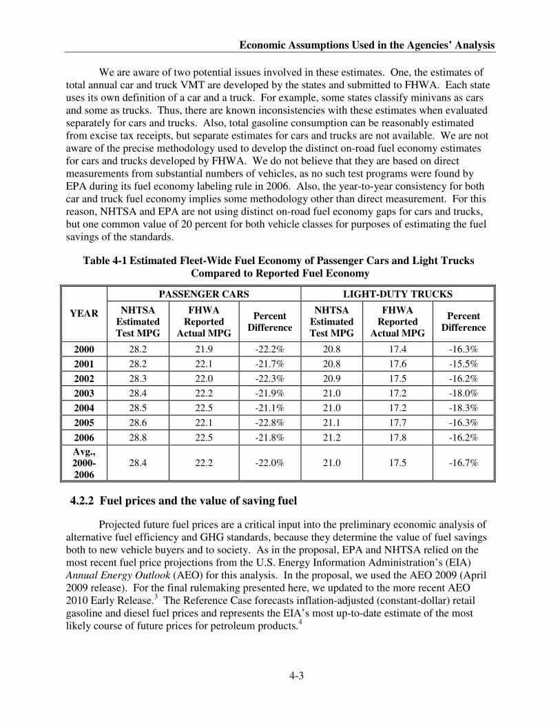
Economic Assumptions Used in the Agencies’ Analysis
4-3
We are aware of two potential issues involved in these estimates. One, the estimates of
total annual car and truck VMT are developed by the states and submitted to FHWA. Each state
uses its own definition of a car and a truck. For example, some states classify minivans as cars
and some as trucks. Thus, there are known inconsistencies with these estimates when evaluated
separately for cars and trucks. Also, total gasoline consumption can be reasonably estimated
from excise tax receipts, but separate estimates for cars and trucks are not available. We are not
aware of the precise methodology used to develop the distinct on-road fuel economy estimates
for cars and trucks developed by FHWA. We do not believe that they are based on direct
measurements from substantial numbers of vehicles, as no such test programs were found by
EPA during its fuel economy labeling rule in 2006. Also, the year-to-year consistency for both
car and truck fuel economy implies some methodology other than direct measurement. For this
reason, NHTSA and EPA are not using distinct on-road fuel economy gaps for cars and trucks,
but one common value of 20 percent for both vehicle classes for purposes of estimating the fuel
savings of the standards.
Table 4-1 Estimated Fleet-Wide Fuel Economy of Passenger Cars and Light Trucks
Compared to Reported Fuel Economy
PASSENGER CARS LIGHT-DUTY TRUCKS
YEAR NHTSA
Estimated
Test MPG
FHWA
Reported
Actual MPG
Percent
Difference
NHTSA
Estimated
Test MPG
FHWA
Reported
Actual MPG
Percent
Difference
2000 28.2 21.9 -22.2% 20.8 17.4 -16.3%
2001 28.2 22.1 -21.7% 20.8 17.6 -15.5%
2002 28.3 22.0 -22.3% 20.9 17.5 -16.2%
2003 28.4 22.2 -21.9% 21.0 17.2 -18.0%
2004 28.5 22.5 -21.1% 21.0 17.2 -18.3%
2005 28.6 22.1 -22.8% 21.1 17.7 -16.3%
2006 28.8 22.5 -21.8% 21.2 17.8 -16.2%
Avg.,
2000-
2006
28.4 22.2 -22.0% 21.0 17.5 -16.7%
4.2.2 Fuel prices and the value of saving fuel
Projected future fuel prices are a critical input into the preliminary economic analysis of
alternative fuel efficiency and GHG standards, because they determine the value of fuel savings
both to new vehicle buyers and to society. As in the proposal, EPA and NHTSA relied on the
most recent fuel price projections from the U.S. Energy Information Administration’s (EIA)
Annual Energy Outlook (AEO) for this analysis. In the proposal, we used the AEO 2009 (April
2009 release). For the final rulemaking presented here, we updated to the more recent AEO
2010 Early Release.3 The Reference Case forecasts inflation-adjusted (constant-dollar) retail
gasoline and diesel fuel prices and represents the EIA’s most up-to-date estimate of the most
likely course of future prices for petroleum products.4
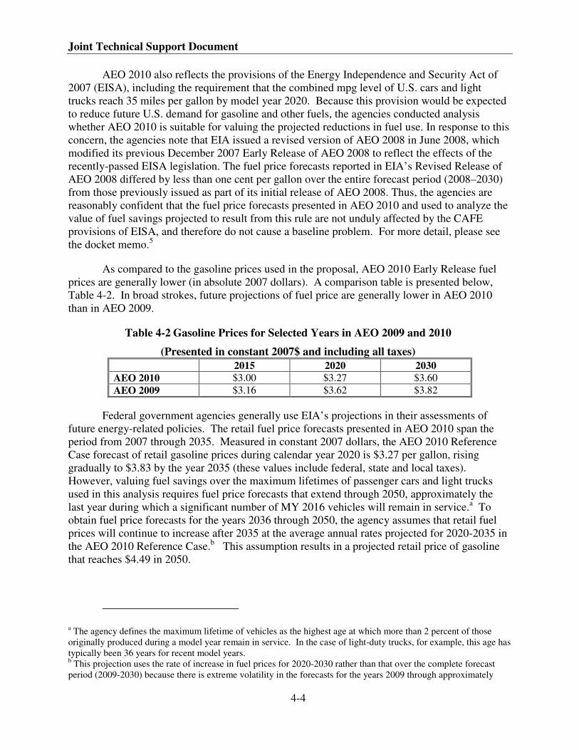
Joint Technical Support Document
4-4
AEO 2010 also reflects the provisions of the Energy Independence and Security Act of
2007 (EISA), including the requirement that the combined mpg level of U.S. cars and light
trucks reach 35 miles per gallon by model year 2020. Because this provision would be expected
to reduce future U.S. demand for gasoline and other fuels, the agencies conducted analysis
whether AEO 2010 is suitable for valuing the projected reductions in fuel use. In response to this
concern, the agencies note that EIA issued a revised version of AEO 2008 in June 2008, which
modified its previous December 2007 Early Release of AEO 2008 to reflect the effects of the
recently-passed EISA legislation. The fuel price forecasts reported in EIA’s Revised Release of
AEO 2008 differed by less than one cent per gallon over the entire forecast period (2008–2030)
from those previously issued as part of its initial release of AEO 2008. Thus, the agencies are
reasonably confident that the fuel price forecasts presented in AEO 2010 and used to analyze the
value of fuel savings projected to result from this rule are not unduly affected by the CAFE
provisions of EISA, and therefore do not cause a baseline problem. For more detail, please see
the docket memo.5
As compared to the gasoline prices used in the proposal, AEO 2010 Early Release fuel
prices are generally lower (in absolute 2007 dollars). A comparison table is presented below,
Table 4-2. In broad strokes, future projections of fuel price are generally lower in AEO 2010
than in AEO 2009.
Table 4-2 Gasoline Prices for Selected Years in AEO 2009 and 2010
(Presented in constant 2007$ and including all taxes)
2015 2020 2030
AEO 2010 $3.00 $3.27 $3.60
AEO 2009 $3.16 $3.62 $3.82
Federal government agencies generally use EIA’s projections in their assessments of
future energy-related policies. The retail fuel price forecasts presented in AEO 2010 span the
period from 2007 through 2035. Measured in constant 2007 dollars, the AEO 2010 Reference
Case forecast of retail gasoline prices during calendar year 2020 is $3.27 per gallon, rising
gradually to $3.83 by the year 2035 (these values include federal, state and local taxes).
However, valuing fuel savings over the maximum lifetimes of passenger cars and light trucks
used in this analysis requires fuel price forecasts that extend through 2050, approximately the
last year during which a significant number of MY 2016 vehicles will remain in service.a To
obtain fuel price forecasts for the years 2036 through 2050, the agency assumes that retail fuel
prices will continue to increase after 2035 at the average annual rates projected for 2020-2035 in
the AEO 2010 Reference Case.b This assumption results in a projected retail price of gasoline
that reaches $4.49 in 2050.
a The agency defines the maximum lifetime of vehicles as the highest age at which more than 2 percent of those
originally produced during a model year remain in service. In the case of light-duty trucks, for example, this age has
typically been 36 years for recent model years. b This projection uses the rate of increase in fuel prices for 2020-2030 rather than that over the complete forecast
period (2009-2030) because there is extreme volatility in the forecasts for the years 2009 through approximately
Economic Assumptions Used in the Agencies’ Analysis
4-5
The value of fuel savings resulting from improved fuel economy and GHG emissions to
buyers of light-duty vehicles is determined by the retail price of fuel, which includes federal,
state, and any local taxes imposed on fuel sales. Total taxes on gasoline, including federal, state,
and local levies averaged $0.42 per gallon during 2008, while those levied on diesel averaged
$0.50. Because fuel taxes represent transfers of resources from fuel buyers to government
agencies, however, rather than real resources that are consumed in the process of supplying or
using fuel, their value must be deducted from retail fuel prices to determine the value of fuel
savings resulting from more stringent fuel efficiency and GHG standards to the U.S. economy as
a whole.
In estimating the economy-wide value of fuel savings from improved fuel efficiency
standards and GHG emission standards, EPA and NHTSA follow the assumptions used by EIA
in AEO 2010 that state and local gasoline taxes will keep pace with inflation in nominal terms,
and thus remain constant when expressed in constant 2007 dollars.c In contrast, EIA assumes
that federal gasoline taxes will remain unchanged in nominal terms, and thus decline throughout
the forecast period when expressed in constant 2007 dollars. These differing assumptions about
the likely future behavior of federal and state/local fuel taxes are consistent with recent historical
experience, which reflects the fact that federal as well as most state motor fuel taxes are specified
on a cents-per-gallon basis, and typically require legislation to change. The projected value of
total taxes is deducted from each future year’s forecast of retail gasoline and diesel prices
reported in AEO 2010 to determine the economic value of each gallon of fuel saved during that
year as a result of improved fuel economy. Subtracting fuel taxes results in a projected value for
saving gasoline of $2.89 per gallon during 2020, rising to $3.48 per gallon by the year 2035.
EIA is widely-recognized as an impartial and authoritative source of analysis and
forecasts of U.S. energy production, consumption, and prices. The agency has published annual
forecasts of energy prices and consumption levels for the U.S. economy since 1982 in its AEOs.
These forecasts have been widely relied upon by federal agencies for use in regulatory analysis
and for other purposes. Since 1994, EIA’s annual forecasts have been based upon the agency’s
National Energy Modeling System (NEMS), which includes detailed representation of supply
pathways, sources of demand, and their interaction to determine prices for different forms of
energy.
From 1982 through 1993, EIA’s forecasts of world oil prices – the primary determinant
of prices for gasoline, diesel, and other transportation fuels derived from petroleum –
consistently overestimated actual prices during future years, often very significantly. Of the total
of 119 forecasts of future world oil prices for the years 1985 through 2005 that EIA reported in
its 1982-1993 editions of AEO, 109 overestimated the subsequent actual values for those years,
on average exceeding their corresponding actual values by 75 percent.
2020. Using the average rate of change over the complete 2009-2030 forecast period would result in projections of
declining fuel prices after 2030. c To calculate economy-wide impacts, the agencies value fuel savings at pre-tax prices, since this measures the value
of the resources that are saved when less fuel is produced and consumed. The economy-wide value of saving fuel
includes this plus the reductions in economic and environmental externalities that result from consuming less fuel,
importing less petroleum, and so on.
Joint Technical Support Document
4-6
Since that time, however, EIA’s forecasts of future world oil prices show a more mixed
record for accuracy. The 1994-2005 editions of AEO reported 91 separate forecasts of world oil
prices for the years 1995-2005, of which 33 have subsequently proven too high while the
remaining 58 have underestimated actual prices. The average absolute error (i.e., regardless of
its direction) of these forecasts has been 21 percent, but over- and underestimates have tended to
offset one another, so that on average EIA’s more recent forecasts have underestimated actual
world oil prices by 7 percent. Although both its overestimates and underestimates of future
world oil prices for recent years have often been large, the most recent editions of AEO have
significantly underestimated petroleum prices during those years for which actual prices are now
available.
However, EPA and NHTSA does not regard EIA’s recent tendency to underestimate
future prices for petroleum and refined products or the high level of current fuel prices as
adequate justification to employ forecasts that differ from the Reference Case forecast presented
in the AEO 2010 Reference Case. This is particularly the case because both the AEO 2009 and
AEO 2010 Reference Cases forecast significantly higher future prices than those projected in the
initial release of AEO 2008, which in turn represented a major upward revision from EIA’s fuel
price forecast reported previously in AEO 2007. Comparing recent forecasts of world oil prices
also shows that EIA’s Reference Case forecast reported in AEO 2009 is among the highest of all
six publicly-available forecasts of world oil prices over the 2010-30 time horizon.6 Because
world petroleum prices are the primary determinant of retail prices for refined petroleum
products such as transportation fuels, this suggests that the Reference Case forecast of U.S. fuel
prices reported in AEO 2010 is likely to be the highest of those projected by major forecasting
services.
In the estimates of costs and benefits presented in the Preamble and the agencies’ RIAs,
the agencies have included the full fuel savings over vehicles’ expected lifetimes, discounted to
their present values using both 3 and 7 percent discount rates. More detailed discussion of this
approach can be found in Preamble Sections III.H.1 and IV.G.6, in Section 8.1 of EPA’s RIA,
and in Chapter VIII of NHTSA’s RIA.
4.2.3 Vehicle survival and use assumptions
The agencies’ analyses of fuel savings and related benefits from adopting higher fuel
efficiency standards and establishing GHG emission standards for MY 2012-2016 passenger cars
and light trucks begin by estimating the resulting changes in fuel use over the entire lifetimes of
these vehicles. The change in total fuel consumption by vehicles produced during each of these
model years is calculated as the difference in their lifetime fuel use under the baseline
assumption that the CAFE standard previously established for model year 2011 remains in effect,
and under the alternative assumption that CAFE and GHG emissions standards improve for each
model year from 2012-2016.
The first step in estimating lifetime fuel consumption by vehicles produced during a
model year is to calculate the number of those vehicles that is expected to remain in service
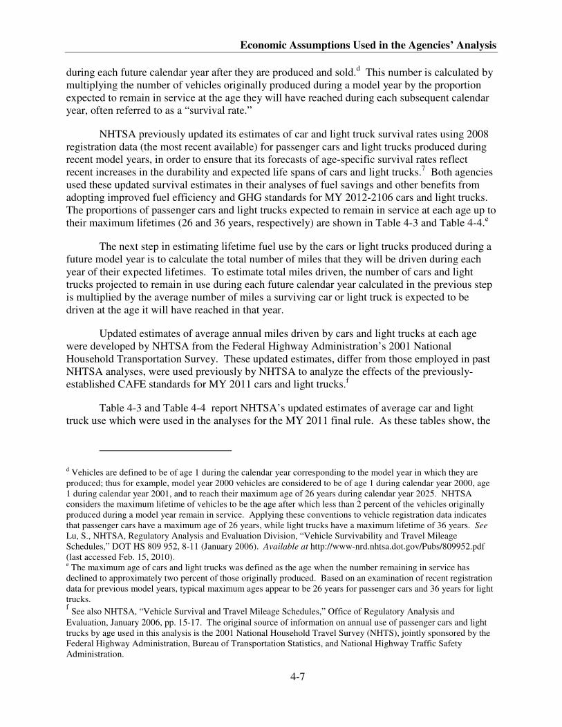
Economic Assumptions Used in the Agencies’ Analysis
4-7
during each future calendar year after they are produced and sold.d This number is calculated by
multiplying the number of vehicles originally produced during a model year by the proportion
expected to remain in service at the age they will have reached during each subsequent calendar
year, often referred to as a “survival rate.”
NHTSA previously updated its estimates of car and light truck survival rates using 2008
registration data (the most recent available) for passenger cars and light trucks produced during
recent model years, in order to ensure that its forecasts of age-specific survival rates reflect
recent increases in the durability and expected life spans of cars and light trucks.7 Both agencies
used these updated survival estimates in their analyses of fuel savings and other benefits from
adopting improved fuel efficiency and GHG standards for MY 2012-2106 cars and light trucks.
The proportions of passenger cars and light trucks expected to remain in service at each age up to
their maximum lifetimes (26 and 36 years, respectively) are shown in Table 4-3 and Table 4-4.e
The next step in estimating lifetime fuel use by the cars or light trucks produced during a
future model year is to calculate the total number of miles that they will be driven during each
year of their expected lifetimes. To estimate total miles driven, the number of cars and light
trucks projected to remain in use during each future calendar year calculated in the previous step
is multiplied by the average number of miles a surviving car or light truck is expected to be
driven at the age it will have reached in that year.
Updated estimates of average annual miles driven by cars and light trucks at each age
were developed by NHTSA from the Federal Highway Administration’s 2001 National
Household Transportation Survey. These updated estimates, differ from those employed in past
NHTSA analyses, were used previously by NHTSA to analyze the effects of the previously-
established CAFE standards for MY 2011 cars and light trucks.f
Table 4-3 and Table 4-4 report NHTSA’s updated estimates of average car and light
truck use which were used in the analyses for the MY 2011 final rule. As these tables show, the
d Vehicles are defined to be of age 1 during the calendar year corresponding to the model year in which they are
produced; thus for example, model year 2000 vehicles are considered to be of age 1 during calendar year 2000, age
1 during calendar year 2001, and to reach their maximum age of 26 years during calendar year 2025. NHTSA
considers the maximum lifetime of vehicles to be the age after which less than 2 percent of the vehicles originally
produced during a model year remain in service. Applying these conventions to vehicle registration data indicates
that passenger cars have a maximum age of 26 years, while light trucks have a maximum lifetime of 36 years. See
Lu, S., NHTSA, Regulatory Analysis and Evaluation Division, “Vehicle Survivability and Travel Mileage
Schedules,” DOT HS 809 952, 8-11 (January 2006). Available at http://www-nrd.nhtsa.dot.gov/Pubs/809952.pdf
(last accessed Feb. 15, 2010). e The maximum age of cars and light trucks was defined as the age when the number remaining in service has
declined to approximately two percent of those originally produced. Based on an examination of recent registration
data for previous model years, typical maximum ages appear to be 26 years for passenger cars and 36 years for light
trucks. f See also NHTSA, “Vehicle Survival and Travel Mileage Schedules,” Office of Regulatory Analysis and
Evaluation, January 2006, pp. 15-17. The original source of information on annual use of passenger cars and light
trucks by age used in this analysis is the 2001 National Household Travel Survey (NHTS), jointly sponsored by the
Federal Highway Administration, Bureau of Transportation Statistics, and National Highway Traffic Safety
Administration.

Joint Technical Support Document
4-8
resulting survival-weighted mileages calculated for that rule over the 26-year maximum lifetime
of passenger cars is 161,847 miles, while that over the 36-year maximum lifetime of light trucks
is 190,066 miles. It should be noted, however, that survival-weighted mileage is extremely low
(less than 1,000 miles per year) after age 20 for cars and after age 25 for light trucks, and thus
has little impact on lifetime fuel savings or other benefits from higher fuel economy, particularly
after discounting those benefits to their present values.
The survival and annual mileage estimates reported in the tables reflect the convention
that vehicles are defined to be of age 1 during the calendar year that coincides with their model
year Thus for example, model year 2012 vehicles will be considered to be of age 1 during
calendar year 2012. This convention is used in order to account for the fact that vehicles
produced during a model year typical are first offered for sale in June through September of the
preceding calendar year (for example, sales of a model year typically begin in June through
September of the previous calendar year, depending on manufacturer). Thus virtually all of the
vehicles produced during a model year will be in use for some or all of the calendar year
coinciding with their model year, and they are considered to be of age 1 during that year.g
g As an illustration, virtually the entire production of model year 2012 cars and light trucks will have been sold by
the end of calendar year 2012, so those vehicles are defined to be of age 1 during calendar year 2012. Model year
2012 vehicles are subsequently defined to be of age 2 during calendar year 2013, age 3 during calendar year 2014,
and so on. One complication arises because registration data are typically collected for July 1 of each calendar year,
so not all vehicles produced during a model year will appear in registration data until the calendar year when they
have reached age 2 (and sometimes age 3) under this convention.
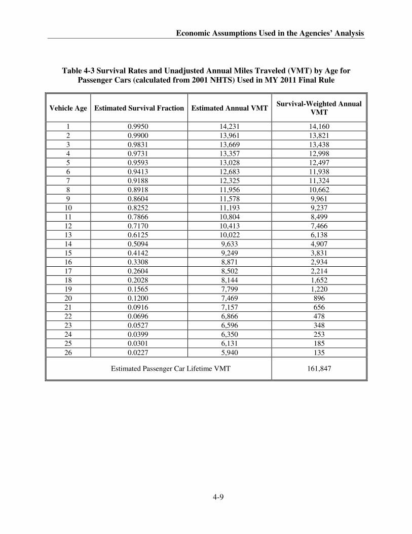
Economic Assumptions Used in the Agencies’ Analysis
4-9
Table 4-3 Survival Rates and Unadjusted Annual Miles Traveled (VMT) by Age for
Passenger Cars (calculated from 2001 NHTS) Used in MY 2011 Final Rule
Vehicle Age Estimated Survival Fraction Estimated Annual VMT Survival-Weighted Annual
VMT
1 0.9950 14,231 14,160
2 0.9900 13,961 13,821
3 0.9831 13,669 13,438
4 0.9731 13,357 12,998
5 0.9593 13,028 12,497
6 0.9413 12,683 11,938
7 0.9188 12,325 11,324
8 0.8918 11,956 10,662
9 0.8604 11,578 9,961
10 0.8252 11,193 9,237
11 0.7866 10,804 8,499
12 0.7170 10,413 7,466
13 0.6125 10,022 6,138
14 0.5094 9,633 4,907
15 0.4142 9,249 3,831
16 0.3308 8,871 2,934
17 0.2604 8,502 2,214
18 0.2028 8,144 1,652
19 0.1565 7,799 1,220
20 0.1200 7,469 896
21 0.0916 7,157 656
22 0.0696 6,866 478
23 0.0527 6,596 348
24 0.0399 6,350 253
25 0.0301 6,131 185
26 0.0227 5,940 135
Estimated Passenger Car Lifetime VMT 161,847
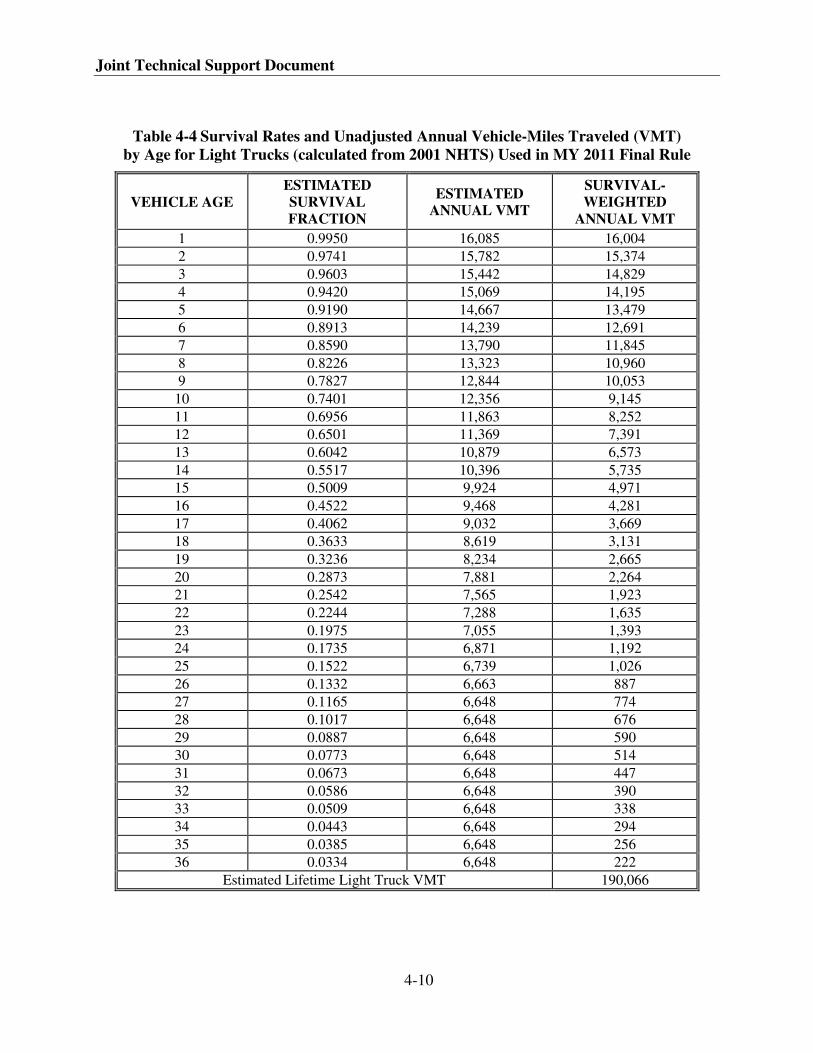
Joint Technical Support Document
4-10
Table 4-4 Survival Rates and Unadjusted Annual Vehicle-Miles Traveled (VMT)
by Age for Light Trucks (calculated from 2001 NHTS) Used in MY 2011 Final Rule
VEHICLE AGE
ESTIMATED
SURVIVAL
FRACTION
ESTIMATED
ANNUAL VMT
SURVIVAL-
WEIGHTED
ANNUAL VMT
1 0.9950 16,085 16,004
2 0.9741 15,782 15,374
3 0.9603 15,442 14,829
4 0.9420 15,069 14,195
5 0.9190 14,667 13,479
6 0.8913 14,239 12,691
7 0.8590 13,790 11,845
8 0.8226 13,323 10,960
9 0.7827 12,844 10,053
10 0.7401 12,356 9,145
11 0.6956 11,863 8,252
12 0.6501 11,369 7,391
13 0.6042 10,879 6,573
14 0.5517 10,396 5,735
15 0.5009 9,924 4,971
16 0.4522 9,468 4,281
17 0.4062 9,032 3,669
18 0.3633 8,619 3,131
19 0.3236 8,234 2,665
20 0.2873 7,881 2,264
21 0.2542 7,565 1,923
22 0.2244 7,288 1,635
23 0.1975 7,055 1,393
24 0.1735 6,871 1,192
25 0.1522 6,739 1,026
26 0.1332 6,663 887
27 0.1165 6,648 774
28 0.1017 6,648 676
29 0.0887 6,648 590
30 0.0773 6,648 514
31 0.0673 6,648 447
32 0.0586 6,648 390
33 0.0509 6,648 338
34 0.0443 6,648 294
35 0.0385 6,648 256
36 0.0334 6,648 222
Estimated Lifetime Light Truck VMT 190,066
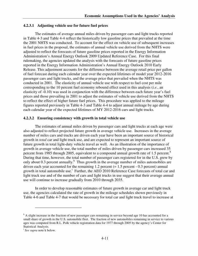
Economic Assumptions Used in the Agencies’ Analysis
4-11
4.2.3.1 Adjusting vehicle use for future fuel prices
The estimates of average annual miles driven by passenger cars and light trucks reported
in Table 4-3 and Table 4-4 reflect the historically low gasoline prices that prevailed at the time
the 2001 NHTS was conducted. To account for the effect on vehicle use of subsequent increases
in fuel prices in the proposal, the estimates of annual vehicle use derived from the NHTS were
adjusted to reflect the forecasts of future gasoline prices reported in the Energy Information
Administration’s Annual Energy Outlook 2009 Updated Reference Case. For this final
rulemaking, the agencies updated the analysis with the forecasts of future gasoline prices
reported in the Energy Information Administration’s Annual Energy Outlook 2010 Early
Release. This adjustment accounts for the difference between the average retail price per gallon
of fuel forecast during each calendar year over the expected lifetimes of model year 2012-2016
passenger cars and light trucks, and the average price that prevailed when the NHTS was
conducted in 2001. The elasticity of annual vehicle use with respect to fuel cost per mile
corresponding to the 10 percent fuel economy rebound effect used in this analysis (i.e., an
elasticity of -0.10) was used in conjunction with the difference between each future year’s fuel
prices and those prevailing in 2001 to adjust the estimates of vehicle use derived from the NHTS
to reflect the effect of higher future fuel prices. This procedure was applied to the mileage
figures reported previously in Table 4-3 and Table 4-4 to adjust annual mileage by age during
each calendar year of the expected lifetimes of MY 2012-2016 cars and light trucks.
4.2.3.2 Ensuring consistency with growth in total vehicle use
The estimates of annual miles driven by passenger cars and light trucks at each age were
also adjusted to reflect projected future growth in average vehicle use. Increases in the average
number of miles cars and trucks are driven each year have been an important source of historical
growth in total car and light truck use, and are expected to represent an important source of
future growth in total light-duty vehicle travel as well. As an illustration of the importance of
growth in average vehicle use, the total number of miles driven by passenger cars increased 35
percent from 1985 through 2005, equivalent to a compound annual growth rate of 1.5 percent.8
During that time, however, the total number of passenger cars registered for in the U.S. grew by
only about 0.3 percent annually.h Thus growth in the average number of miles automobiles are
driven each year accounted for the remaining 1.2 percent (= 1.5 percent - 0.3 percent) annual
growth in total automobile use.i Further, the AEO 2010 Reference Case forecasts of total car and
light truck use and of the number of cars and light trucks in use suggest that their average annual
use will continue to increase gradually from 2010 through 2035.
In order to develop reasonable estimates of future growth in average car and light truck
use, the agencies calculated the rate of growth in the mileage schedules shown previously in
Table 4-6 and Table 4-7 that would be necessary for total car and light truck travel to increase at
h A slight increase in the fraction of new passenger cars remaining in service beyond age 10 has accounted for a
small share of growth in the U.S. automobile fleet. The fraction of new automobiles remaining in service to various
ages was computed from R.L. Polk vehicle registration data for 1977 through 2005 by the agency’s Center for
Statistical Analysis. i See supra note k below.
Joint Technical Support Document
4-12
the rate forecast in the AEO 2010 Reference Case. This calculated rate is also consistent with
future changes in the overall size and age distributions of the U.S. passenger car and light truck
fleets that are implied by the agency’s forecasts of total car and light truck sales and the survival
rates reported in Table 4-3 and Table 4-4. The growth rate in average annual car and light truck
use produced by this calculation is approximately 1.15 percent per year.j This rate was applied
to the mileage figures reported previously in Table 4-3 and Table 4-4 to estimate annual mileage
by age during each calendar year of the expected lifetimes of MY 2012-2016 cars and light
trucks.k
Table 4-6 and Table 4-7 report the results of applying the adjustments for both future fuel
prices and annual growth in car and light truck use to the mileage schedules reported previously
in Table 4-2 and Table 4-3. Separate adjustments for projected fuel prices and growth in car and
light truck use were made for each calendar year from 2012 through 2030. Because the effects
of both fuel prices and cumulative growth in average vehicle use vary by year, these adjustments
result in differing VMT schedules for each future year. The adjusted annual VMT estimates
reported in Table 4-4 and Table 4-5 and their lifetime totals represent the averages of the
adjusted values of annual car and light truck use by age for calendar years 2012-2030. However,
the estimates of fuel savings and other impacts of improved fuel efficiency for individual
calendar years over the lifetimes of model year 2012-16 cars and light trucks employ the
adjusted values of car and light truck use by age during those specific calendar years.
While the adjustment for future fuel prices reduces average mileage at each age from the
values shown previously, the adjustment for expected future growth in average vehicle use
increases it. Comparing the mileage estimates in Table 4-6 and Table 4-7 to those shown
previously in Table 4-2 and Table 4-3 shows that the net effect of these two adjustments is to
increase expected lifetime mileage significantly. As an illustration, expected lifetime mileage for
passenger cars, this figure rises to 195,264 miles from the 161,847 miles reported previously in
Table 4-3 (or by 21 percent), while expected lifetime mileage for light trucks increases from the
190,066 miles reported previously in Table 4-4 to 225,865 miles (19 percent). As previously
noted, the estimates of survival-weighted mileage decline to less than 1,000 miles per year after
age 20 for cars and after age 27 for light trucks. Thus they have relatively little impact on
j It was not possible to estimate separate growth rates in average annual use for cars and light trucks, because of the
significant reclassification of light truck models as passenger cars discussed previously. k The agency has also identified an unintentional discrepancy between the estimates of expected lifetime VMT used
by EPA and NHTSA in their respective analyses of proposed GHG and CAFE standards reported in the NPRM.
EPA’s estimates of expected lifetime VMT for model year 2012-26 vehicles reflect the shared assumption that the
average number of miles driven annually by cars and light trucks of all ages would grow at a rate of 1.15 percent per
year beginning in 2001. Although NHTSA’s description of the procedures used to calculate its estimates of
expected lifetime VMT for passenger cars and light trucks indicated that it had also adjusted the base-year estimates
of vehicle use to account for annual growth (see Preliminary Regulatory Impact Assessment, Chapter VIII, p. 367),
this adjustment was not in fact applied in NHTSA’s analysis of the effects of proposed increases in CAFE standards
for model years 2012-16. This omission caused the estimates of expected lifetime VMT for passenger cars and light
trucks that NHTSA actually used in its NPRM analysis of CAFE standards for model years 2012-16 to be lower than
those used by EPA. This error has been corrected by NHTSA, and this correction is reflected in its analysis of the
impacts of CAFE standards for model year 2012-16 passenger cars and light trucks reported in the Final Rule. This
error did not occur in the analysis of environmental impacts of alternative increases in CAFE standards reported in
the agency’s recent Draft Environmental Impact Statement.
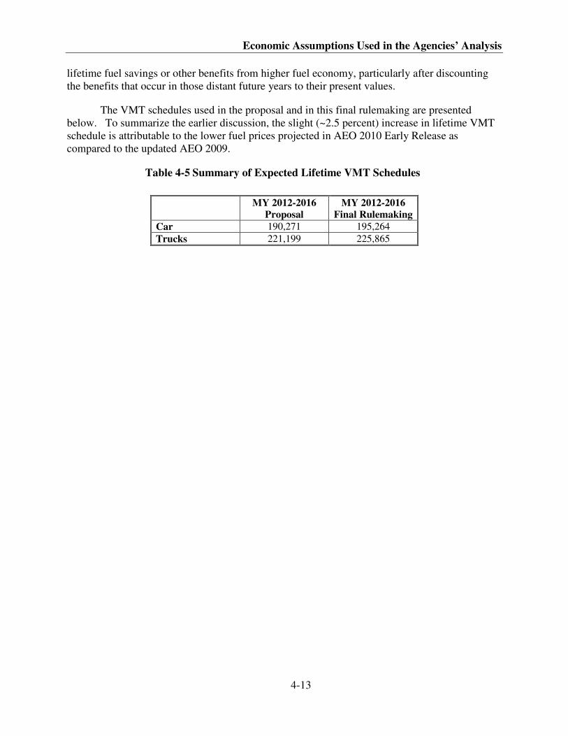
Economic Assumptions Used in the Agencies’ Analysis
4-13
lifetime fuel savings or other benefits from higher fuel economy, particularly after discounting
the benefits that occur in those distant future years to their present values.
The VMT schedules used in the proposal and in this final rulemaking are presented
below. To summarize the earlier discussion, the slight (~2.5 percent) increase in lifetime VMT
schedule is attributable to the lower fuel prices projected in AEO 2010 Early Release as
compared to the updated AEO 2009.
Table 4-5 Summary of Expected Lifetime VMT Schedules
MY 2012-2016
Proposal
MY 2012-2016
Final Rulemaking
Car 190,271 195,264
Trucks 221,199 225,865
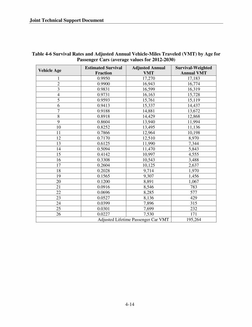
Joint Technical Support Document
4-14
Table 4-6 Survival Rates and Adjusted Annual Vehicle-Miles Traveled (VMT) by Age for
Passenger Cars (average values for 2012-2030)
Vehicle Age Estimated Survival
Fraction
Adjusted Annual
VMT
Survival-Weighted
Annual VMT
1 0.9950 17,270 17,183
2 0.9900 16,943 16,774
3 0.9831 16,599 16,319
4 0.9731 16,163 15,728
5 0.9593 15,761 15,119
6 0.9413 15,337 14,437
7 0.9188 14,881 13,672
8 0.8918 14,429 12,868
9 0.8604 13,940 11,994
10 0.8252 13,495 11,136
11 0.7866 12,964 10,198
12 0.7170 12,510 8,970
13 0.6125 11,990 7,344
14 0.5094 11,470 5,843
15 0.4142 10,997 4,555
16 0.3308 10,543 3,488
17 0.2604 10,125 2,637
18 0.2028 9,714 1,970
19 0.1565 9,307 1,456
20 0.1200 8,891 1,067
21 0.0916 8,546 783
22 0.0696 8,285 577
23 0.0527 8,136 429
24 0.0399 7,896 315
25 0.0301 7,699 232
26 0.0227 7,530 171
Adjusted Lifetime Passenger Car VMT 195,264
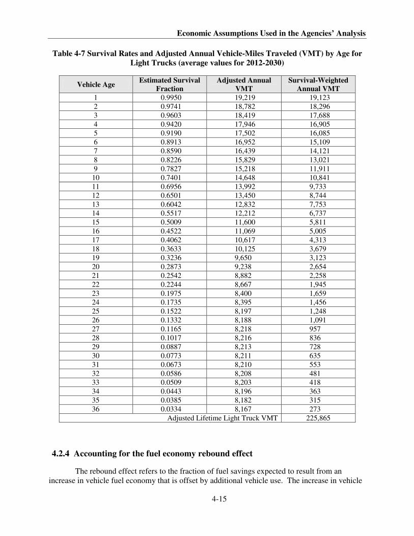
Economic Assumptions Used in the Agencies’ Analysis
4-15
Table 4-7 Survival Rates and Adjusted Annual Vehicle-Miles Traveled (VMT) by Age for
Light Trucks (average values for 2012-2030)
Vehicle Age Estimated Survival
Fraction
Adjusted Annual
VMT
Survival-Weighted
Annual VMT
1 0.9950 19,219 19,123
2 0.9741 18,782 18,296
3 0.9603 18,419 17,688
4 0.9420 17,946 16,905
5 0.9190 17,502 16,085
6 0.8913 16,952 15,109
7 0.8590 16,439 14,121
8 0.8226 15,829 13,021
9 0.7827 15,218 11,911
10 0.7401 14,648 10,841
11 0.6956 13,992 9,733
12 0.6501 13,450 8,744
13 0.6042 12,832 7,753
14 0.5517 12,212 6,737
15 0.5009 11,600 5,811
16 0.4522 11,069 5,005
17 0.4062 10,617 4,313
18 0.3633 10,125 3,679
19 0.3236 9,650 3,123
20 0.2873 9,238 2,654
21 0.2542 8,882 2,258
22 0.2244 8,667 1,945
23 0.1975 8,400 1,659
24 0.1735 8,395 1,456
25 0.1522 8,197 1,248
26 0.1332 8,188 1,091
27 0.1165 8,218 957
28 0.1017 8,216 836
29 0.0887 8,213 728
30 0.0773 8,211 635
31 0.0673 8,210 553
32 0.0586 8,208 481
33 0.0509 8,203 418
34 0.0443 8,196 363
35 0.0385 8,182 315
36 0.0334 8,167 273
Adjusted Lifetime Light Truck VMT 225,865
4.2.4 Accounting for the fuel economy rebound effect
The rebound effect refers to the fraction of fuel savings expected to result from an
increase in vehicle fuel economy that is offset by additional vehicle use. The increase in vehicle
Joint Technical Support Document
4-16
use that stems from improved fuel economy occurs because vehicle owners respond to the
resulting reduction in vehicle fuel consumption and operating costs by driving slightly more.
The magnitude of the rebound effect is one of the determinants of the actual fuel savings
that are likely to result from adopting stricter fuel economy or emissions standards, and thus an
important parameter affecting EPA’s and NHTSA’s evaluation of alternative standards for future
model years. It can be measured directly by estimating the elasticity of vehicle use with respect
to fuel economy itself, or indirectly by the elasticity of vehicle use with respect to fuel cost per
mile driven.l When expressed as a positive percentage, either of these parameters gives the
fraction of fuel savings that would otherwise result from adopting stricter standards, but is offset
by the increase in fuel consumption that results when vehicles with increased fuel economy are
driven more.
The fuel economy rebound effect for light-duty vehicles has been the subject of a large
number of studies since the early 1980s. Although they have reported a wide range of estimates
of its exact magnitude, these studies generally conclude that a significant rebound effect occurs
when vehicle fuel efficiency improves.m The most common approach to estimating its
magnitude has been to analyze household survey data on vehicle use, fuel consumption, fuel
prices (often obtained from external sources), and other determinants of household travel
demand to isolate the response of vehicle use to higher fuel economy. Other studies have relied
on econometric analysis of annual U.S. data on vehicle use, fuel economy, fuel prices, and other
variables to identify the response of total or average vehicle use to changes in fleet-wide average
fuel economy and its effect of fuel cost per mile driven. Two recent studies analyzed yearly
variation in vehicle ownership and use, fuel prices, and fuel economy among individual states
over an extended time period in order to measure the response of vehicle use to changing fuel
economy.n
This section surveys these previous studies, summarizes recent work on the rebound
effect, and explains the basis for the 10 percent rebound effect EPA and NHTSA are using in this
rulemaking.9
4.2.4.1 Summary of historical literature on rebound effect
It is important to note that a majority of the studies previously conducted on the rebound
effect rely on data from the 1950-1990s. While these older studies provide valuable information
on the potential magnitude of the rebound effect, studies that include more recent information
(e.g., data within the last decade) may provide more reliable estimates of how this rule will affect
l Fuel cost per mile is equal to the price of fuel in dollars per gallon divided by fuel economy in miles per gallon, so
this figure declines when a vehicle’s fuel economy increases. m Some studies estimate that the long-run rebound effect is significantly larger than the immediate response to
increased fuel efficiency. Although their estimates of the adjustment period required for the rebound effect to reach
its long-run magnitude vary, this long-run effect is most appropriate for evaluating the fuel savings and emissions
reductions resulting from stricter standards that would apply to future model years. n In effect, these studies treat U.S. states as a data “panel” by applying appropriate estimation procedures to data
consisting of each year’s average values of these variables for the separate states.
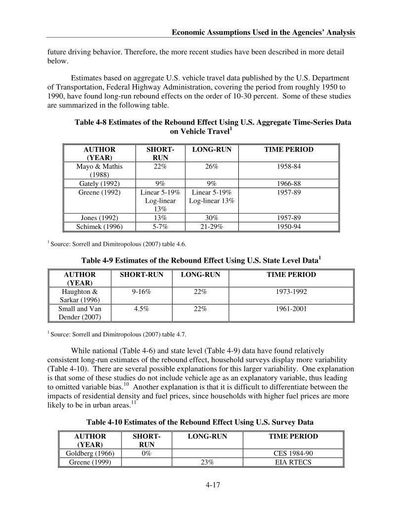
Economic Assumptions Used in the Agencies’ Analysis
4-17
future driving behavior. Therefore, the more recent studies have been described in more detail
below.
Estimates based on aggregate U.S. vehicle travel data published by the U.S. Department
of Transportation, Federal Highway Administration, covering the period from roughly 1950 to
1990, have found long-run rebound effects on the order of 10-30 percent. Some of these studies
are summarized in the following table.
Table 4-8 Estimates of the Rebound Effect Using U.S. Aggregate Time-Series Data
on Vehicle Travel1
AUTHOR
(YEAR)
SHORT-
RUN
LONG-RUN TIME PERIOD
Mayo & Mathis
(1988)
22% 26% 1958-84
Gately (1992) 9% 9% 1966-88
Greene (1992) Linear 5-19%
Log-linear
13%
Linear 5-19%
Log-linear 13%
1957-89
Jones (1992) 13% 30% 1957-89
Schimek (1996) 5-7% 21-29% 1950-94
1 Source: Sorrell and Dimitropolous (2007) table 4.6.
Table 4-9 Estimates of the Rebound Effect Using U.S. State Level Data1
AUTHOR
(YEAR)
SHORT-RUN LONG-RUN TIME PERIOD
Haughton &
Sarkar (1996)
9-16% 22% 1973-1992
Small and Van
Dender (2007)
4.5% 22% 1961-2001
1 Source: Sorrell and Dimitropolous (2007) table 4.7.
While national (Table 4-6) and state level (Table 4-9) data have found relatively
consistent long-run estimates of the rebound effect, household surveys display more variability
(Table 4-10). There are several possible explanations for this larger variability. One explanation
is that some of these studies do not include vehicle age as an explanatory variable, thus leading
to omitted variable bias.10
Another explanation is that it is difficult to differentiate between the
impacts of residential density and fuel prices, since households with higher fuel prices are more
likely to be in urban areas.11
Table 4-10 Estimates of the Rebound Effect Using U.S. Survey Data
AUTHOR
(YEAR)
SHORT-
RUN
LONG-RUN TIME PERIOD
Goldberg (1966) 0% CES 1984-90
Greene (1999) 23% EIA RTECS
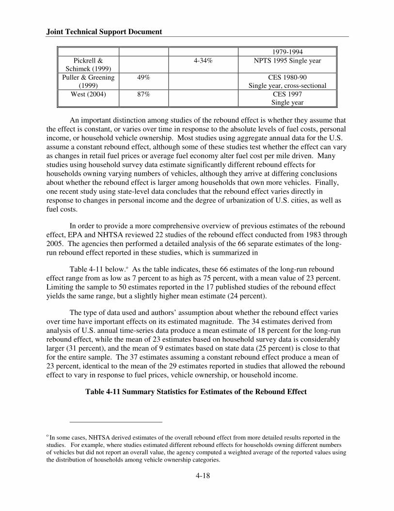
Joint Technical Support Document
4-18
1979-1994
Pickrell &
Schimek (1999)
4-34% NPTS 1995 Single year
Puller & Greening
(1999)
49% CES 1980-90
Single year, cross-sectional
West (2004) 87% CES 1997
Single year
An important distinction among studies of the rebound effect is whether they assume that
the effect is constant, or varies over time in response to the absolute levels of fuel costs, personal
income, or household vehicle ownership. Most studies using aggregate annual data for the U.S.
assume a constant rebound effect, although some of these studies test whether the effect can vary
as changes in retail fuel prices or average fuel economy alter fuel cost per mile driven. Many
studies using household survey data estimate significantly different rebound effects for
households owning varying numbers of vehicles, although they arrive at differing conclusions
about whether the rebound effect is larger among households that own more vehicles. Finally,
one recent study using state-level data concludes that the rebound effect varies directly in
response to changes in personal income and the degree of urbanization of U.S. cities, as well as
fuel costs.
In order to provide a more comprehensive overview of previous estimates of the rebound
effect, EPA and NHTSA reviewed 22 studies of the rebound effect conducted from 1983 through
2005. The agencies then performed a detailed analysis of the 66 separate estimates of the long-
run rebound effect reported in these studies, which is summarized in
Table 4-11 below.o As the table indicates, these 66 estimates of the long-run rebound
effect range from as low as 7 percent to as high as 75 percent, with a mean value of 23 percent.
Limiting the sample to 50 estimates reported in the 17 published studies of the rebound effect
yields the same range, but a slightly higher mean estimate (24 percent).
The type of data used and authors’ assumption about whether the rebound effect varies
over time have important effects on its estimated magnitude. The 34 estimates derived from
analysis of U.S. annual time-series data produce a mean estimate of 18 percent for the long-run
rebound effect, while the mean of 23 estimates based on household survey data is considerably
larger (31 percent), and the mean of 9 estimates based on state data (25 percent) is close to that
for the entire sample. The 37 estimates assuming a constant rebound effect produce a mean of
23 percent, identical to the mean of the 29 estimates reported in studies that allowed the rebound
effect to vary in response to fuel prices, vehicle ownership, or household income.
Table 4-11 Summary Statistics for Estimates of the Rebound Effect
o In some cases, NHTSA derived estimates of the overall rebound effect from more detailed results reported in the
studies. For example, where studies estimated different rebound effects for households owning different numbers
of vehicles but did not report an overall value, the agency computed a weighted average of the reported values using
the distribution of households among vehicle ownership categories.
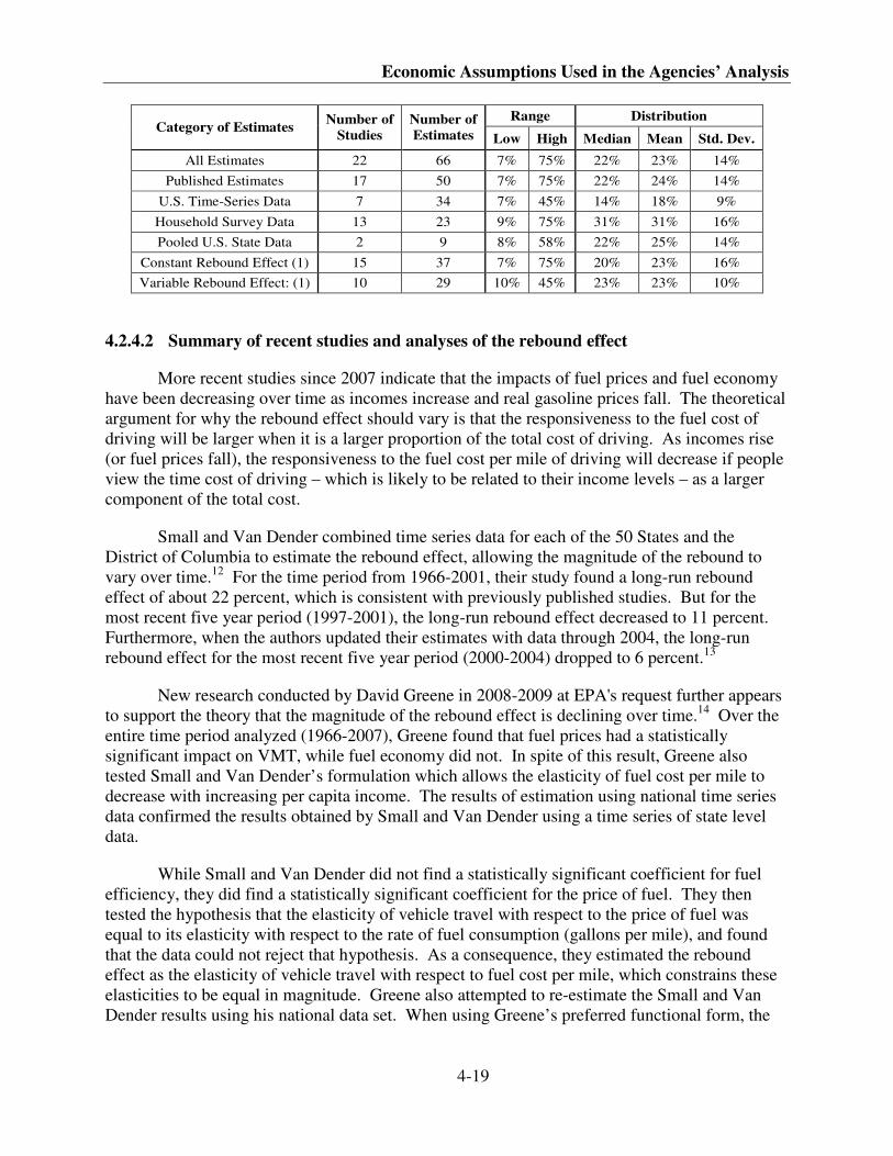
Economic Assumptions Used in the Agencies’ Analysis
4-19
Range Distribution Category of Estimates
Number of
Studies
Number of
Estimates Low High Median Mean Std. Dev.
All Estimates 22 66 7% 75% 22% 23% 14%
Published Estimates 17 50 7% 75% 22% 24% 14%
U.S. Time-Series Data 7 34 7% 45% 14% 18% 9%
Household Survey Data 13 23 9% 75% 31% 31% 16%
Pooled U.S. State Data 2 9 8% 58% 22% 25% 14%
Constant Rebound Effect (1) 15 37 7% 75% 20% 23% 16%
Variable Rebound Effect: (1) 10 29 10% 45% 23% 23% 10%
4.2.4.2 Summary of recent studies and analyses of the rebound effect
More recent studies since 2007 indicate that the impacts of fuel prices and fuel economy
have been decreasing over time as incomes increase and real gasoline prices fall. The theoretical
argument for why the rebound effect should vary is that the responsiveness to the fuel cost of
driving will be larger when it is a larger proportion of the total cost of driving. As incomes rise
(or fuel prices fall), the responsiveness to the fuel cost per mile of driving will decrease if people
view the time cost of driving – which is likely to be related to their income levels – as a larger
component of the total cost.
Small and Van Dender combined time series data for each of the 50 States and the
District of Columbia to estimate the rebound effect, allowing the magnitude of the rebound to
vary over time.12
For the time period from 1966-2001, their study found a long-run rebound
effect of about 22 percent, which is consistent with previously published studies. But for the
most recent five year period (1997-2001), the long-run rebound effect decreased to 11 percent.
Furthermore, when the authors updated their estimates with data through 2004, the long-run
rebound effect for the most recent five year period (2000-2004) dropped to 6 percent.13
New research conducted by David Greene in 2008-2009 at EPA's request further appears
to support the theory that the magnitude of the rebound effect is declining over time.14
Over the
entire time period analyzed (1966-2007), Greene found that fuel prices had a statistically
significant impact on VMT, while fuel economy did not. In spite of this result, Greene also
tested Small and Van Dender’s formulation which allows the elasticity of fuel cost per mile to
decrease with increasing per capita income. The results of estimation using national time series
data confirmed the results obtained by Small and Van Dender using a time series of state level
data.
While Small and Van Dender did not find a statistically significant coefficient for fuel
efficiency, they did find a statistically significant coefficient for the price of fuel. They then
tested the hypothesis that the elasticity of vehicle travel with respect to the price of fuel was
equal to its elasticity with respect to the rate of fuel consumption (gallons per mile), and found
that the data could not reject that hypothesis. As a consequence, they estimated the rebound
effect as the elasticity of vehicle travel with respect to fuel cost per mile, which constrains these
elasticities to be equal in magnitude. Greene also attempted to re-estimate the Small and Van
Dender results using his national data set. When using Greene’s preferred functional form, the
Joint Technical Support Document
4-20
projected rebound effect is approximately 12 percent in 2007, and drops to 10 percent in 2010, 9
percent in 2016 and 8 percent in 2030.
4.2.4.3 NHTSA analysis of the rebound effect
To provide additional insight into the rebound effect for the purposes of this rulemaking,
NHTSA developed several new estimates of its magnitude. These estimates were developed by
estimating and testing several econometric models of the relationship between vehicle miles-
traveled and factors that influence it, including household income, fuel prices, vehicle fuel
efficiency, road supply, the number of vehicles in use, vehicle prices, and other factors.
As the study by Small and Van Dender pointed out, it is important to account for the
effect of fuel prices when attempting to estimate the rebound effect. Failing to control for
changes in fuel prices is likely to bias estimates of the rebound effect. Therefore, changes in fuel
prices are taken into account in Volpe’s analysis of the rebound effect. Several different
approaches were used to estimate the fuel economy rebound effect for light duty vehicles,
including single equation OLS regressions, multiple equation systems estimated using two- and
three-stage least squares regression, vector autoregression, and vector error-correction models.
With the exception of single-equation regressions estimated using OLS, all of these procedures
attempt to account for the endogenous relationship of fuel efficiency to fuel prices.
The results from each of these approaches are presented in Table 4-12 below. The table
reports the value of the rebound effect calculated over the entire period from 1950 through 2006,
as well as for the final year of that period. In addition, the table presents forecasts of the average
rebound effect between 2010 and 2030, which utilize forecasts of personal income, fuel prices,
and fuel efficiency from EIA’s AEO 2009 Reference Case.
The results of NHTSA’s analysis are broadly consistent with the findings from previous
research summarized above. The historical average long-run rebound effect is estimated to range
from 16-30 percent, and comparing these estimates to its calculated values for 2006 (which range
from 8-14 percent) gives some an indication that it is declining in magnitude. The forecast
values of the rebound effect shown in the table also suggest that this decline is likely to continue
through 2030, as they range from 4-16 percent.
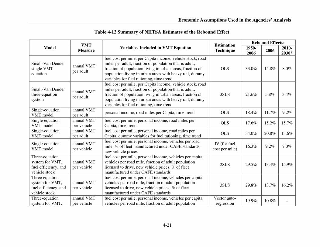
Economic Assumptions Used in the Agencies’ Analysis
4-21
Table 4-12 Summary of NHTSA Estimates of the Rebound Effect
Rebound Effects:
Model VMT
Measure Variables Included in VMT Equation
Estimation
Technique 1950-
2006 2006
2010-
2030*
Small-Van Dender
single VMT
equation
annual VMT
per adult
fuel cost per mile, per Capita income, vehicle stock, road
miles per adult, fraction of population that is adult,
fraction of population living in urban areas, fraction of
population living in urban areas with heavy rail, dummy
variables for fuel rationing, time trend
OLS 33.0% 15.8% 8.0%
Small-Van Dender
three-equation
system
annual VMT
per adult
fuel cost per mile, per Capita income, vehicle stock, road
miles per adult, fraction of population that is adult,
fraction of population living in urban areas, fraction of
population living in urban areas with heavy rail, dummy
variables for fuel rationing, time trend
3SLS 21.6% 5.8% 3.4%
Single-equation
VMT model
annual VMT
per adult personal income, road miles per Capita, time trend OLS 18.4% 11.7% 9.2%
Single-equation
VMT model
annual VMT
per vehicle
fuel cost per mile, personal income, road miles per
Capita, time trend OLS 17.6% 15.2% 15.7%
Single-equation
VMT model
annual VMT
per adult
fuel cost per mile, personal income, road miles per
Capita, dummy variables for fuel rationing, time trend OLS 34.0% 20.8% 13.6%
Single-equation
VMT model
annual VMT
per vehicle
fuel cost per mile, personal income, vehicles per road
mile, % of fleet manufactured under CAFE standards,
new vehicle prices
IV (for fuel
cost per mile) 16.3% 9.2% 7.0%
Three-equation
system for VMT,
fuel efficiency, and
vehicle stock
annual VMT
per vehicle
fuel cost per mile, personal income, vehicles per capita,
vehicles per road mile, fraction of adult population
licensed to drive, new vehicle prices, % of fleet
manufactured under CAFE standards
2SLS 29.5% 13.4% 15.9%
Three-equation
system for VMT,
fuel efficiency, and
vehicle stock
annual VMT
per vehicle
fuel cost per mile, personal income, vehicles per capita,
vehicles per road mile, fraction of adult population
licensed to drive, new vehicle prices, % of fleet
manufactured under CAFE standards
3SLS 29.8% 13.7% 16.2%
Three-equation
system for VMT,
annual VMT
per vehicle
fuel cost per mile, personal income, vehicles per capita,
vehicles per road mile, fraction of adult population
Vector auto-
regression 19.9% 10.8% --
Joint Technical Support Document
4-22
4.2.4.4 Basis for rebound effect used by EPA and NHTSA in this rule
As the preceding discussion indicates, there is a wide range of estimates for both the
historical magnitude of the rebound effect and its projected future value, and there is some
evidence that the magnitude of the rebound effect appears to be declining over time.
Nevertheless, NHTSA requires a single point estimate for the rebound effect as an input to its
analysis, although a range of estimates can be used to test the sensitivity to uncertainty about its
exact magnitude. For the final rulemaking, the agencies chose to use 10 percent as their primary
estimate of the rebound effect, with a range of 5-15 percent for use in sensitivity testing.
As Tables 4-10 and 4-11 indicate, the 10 percent figure is well below those reported in
almost all previous research, and Table 4-12 shows that it is also below most estimates of the
historical and current magnitude of the rebound effect developed by NHTSA. However, other
recent research – particularly that conducted by Small and Van Dender and by Greene – reports
persuasive evidence that the magnitude of the rebound effect is likely to be declining over time,
and the forecasts developed by NHTSA and reported in Table 4-12 also suggest that this is likely
to be the case. As a consequence, the agencies concluded that a value below the historical
estimates reported in Tables 4-10, 4-11, and 4-12 is likely to provide a more reliable estimate of
its magnitude during the future period spanned by the agencies’ analyses of the impacts of this
rule. The 10 percent estimate meets this condition, since it lies below the 15-30 percent range of
estimates for the historical rebound effect reported in most previous research, and at the upper
end of the 5-10 percent range of estimates for the future rebound effect reported in the recent
studies by Small and Van Dender and by Greene. As Table 4-12 shows, it also lies within the 3-
16 percent range of forecasts of the future magnitude of the rebound effect developed by
NHTSA in its recent research. In summary, the 10 percent value was not derived from a single
point estimate from a particular study, but instead represents a reasonable compromise between
the historical estimates and the projected future estimates. The Agencies will continue to review
the estimate of the rebound effect for future rulemakings.
In their proposed rules, the agencies sought comment on other alternatives for estimating
the rebound effect. As one illustration, under the assumption that drivers respond similarly to
changes in the cost of driving whether they are caused by variation in fuel prices or fuel
economy, the short-run price elasticity of demand for gasoline – which measures the sensitivity
of gasoline consumption to changes in its price per gallon – may provide some indication about
the magnitude of the rebound effect itself. Thus, the agencies sought comment on whether it
would be appropriate to use the price elasticity of demand for gasoline, or other alternative
approaches, to guide their choice of a value for the rebound effect.
During the public comment period, EPA and NHTSA did not receive new data or
analysis on the level of the rebound effect, but did receive some supportive comments on the 10
percent level. Hence, EPA and NHTSA have elected to continue to use the 10 percent estimate
of the rebound effect in the analyses supporting this final rule.
4.2.5 Benefits from increased vehicle use
The increase in vehicle use from the rebound effect provides additional benefits to their
owners, who may make more frequent trips or travel farther to reach more desirable destinations.
Economic Assumptions Used in the Agencies’ Analysis
4-23
This additional travel provides benefits to drivers and their passengers by improving their access
to social and economic opportunities away from home. As evidenced by their decisions to make
more frequent or longer trips when improved fuel economy reduces their costs for driving, the
benefits from this additional travel exceed the costs drivers and passengers incur in making more
frequent or longer trips.
The analysis estimates the economic benefits from increased rebound-effect driving as
the sum of fuel costs drivers incur plus the consumer surplus they receive from the additional
accessibility it provides.p Because the increased in travel depend on the extent of improvement
in fuel economy, the value of benefits it provides differs among model years and alternative
CAFE standards. Under even those alternatives that would impose the highest standards,
however, the magnitude of these benefits represents a small fraction of total benefits.
4.2.6 Added costs from increased vehicle use
Although it provides some benefits to drivers, increased vehicle use associated with the
rebound effect also contributes to increased traffic congestion, motor vehicle accidents, and
highway noise. Depending on how the additional travel is distributed over the day and on where
it takes place, additional vehicle use can contribute to traffic congestion and delays by increasing
traffic volumes on facilities that are already heavily traveled during peak periods. These added
delays impose higher costs on drivers and other vehicle occupants in the form of increased travel
time and operating expenses. Because drivers do not take these added costs into account in
deciding when and where to travel, they must be accounted for separately as a cost of the added
driving associated with the rebound effect.
Increased vehicle use due to the rebound effect may also increase the costs associated
with traffic accidents. Drivers may take account of the potential costs they (and their passengers)
face from the possibility of being involved in an accident when they decide to make additional
trips. However, they probably do not consider all of the potential costs they impose on
occupants of other vehicles and on pedestrians when accidents occur, so any increase in these
“external” accident costs must be considered as another cost of additional rebound-effect driving.
Like increased delay costs, any increase in these external accident costs caused by added driving
is likely to depend on the traffic conditions under which it takes place, since accidents are more
frequent in heavier traffic (although their severity may be reduced by the slower speeds at which
heavier traffic typically moves).
Finally, added vehicle use from the rebound effect may also increase traffic noise. Noise
generated by vehicles causes inconvenience, irritation, and potentially even discomfort to
occupants of other vehicles, to pedestrians and other bystanders, and to residents or occupants of
surrounding property. Because these effects are unlikely to be taken into account by the drivers
whose vehicles contribute to traffic noise, they represent additional externalities associated with
motor vehicle use. Although there is considerable uncertainty in measuring their value, any
p The consumer surplus provided by added travel is estimated as one-half of the product of the decline in fuel cost
per mile and the resulting increase in the annual number of miles driven.
Joint Technical Support Document
4-24
increase in the economic costs of traffic noise resulting from added vehicle use must be included
together with other increased external costs from the rebound effect.
EPA and NHTSA rely on estimates of congestion, accident, and noise costs caused by
automobiles and light trucks developed by the Federal Highway Administration to estimate the
increased external costs caused by added driving due to the rebound effect.15
NHTSA employed
these estimates previously in its analysis accompanying the MY 2011 final rule, and continues to
find them appropriate for this NPRM after reviewing the procedures used by FHWA to develop
them and considering other available estimates of these values. They are intended to measure the
increases in costs from added congestion, property damages and injuries in traffic accidents, and
noise levels caused by automobiles and light trucks that are borne by persons other than their
drivers (or “marginal” external costs).
Updated to 2007 dollars, FHWA’s “Middle” estimates for marginal congestion, accident,
and noise costs caused by automobile use amount to 5.2 cents, 2.3 cents, and 0.1 cents per
vehicle-mile (for a total of 7.6 cents per mile), while those for pickup trucks and vans are 4.7
cents, 2.5 cents, and 0.1 cents per vehicle-mile (for a total of 7.3 cents per mile).16, q
These costs
are multiplied by the annual increases in automobile and light truck use from the rebound effect
to yield the estimated increases in congestion, accident, and noise externality costs during each
future year.
4.2.7 Petroleum and energy security impacts
4.2.7.1 Impact on U.S. petroleum imports
In 2008, U.S. petroleum import expenditures represented 21 percent of total U.S. imports
of all goods and services.17
In 2008, the United States imported 66 percent of the petroleum it
consumed, and the transportation sector accounts for 70 percent of total U.S. petroleum
consumption. This compares roughly to 37 percent of petroleum from imports and 55 percent
consumption of petroleum in the transportation sector in 1975.18
It is clear that petroleum
imports have a significant impact on the U.S. economy. Requiring lower-GHG vehicle
technology and improved fuel economy in the U.S. is expected to lower U.S. petroleum imports.
4.2.7.2 Background on U.S. energy security
U.S. energy security is broadly defined as protecting the U.S. economy against
circumstances that threaten significant short- and long-term increases in energy costs. Most
discussion of U.S. energy security revolves around the topic of the economic costs of U.S.
dependence on oil imports. The problem is that the U.S. relies on sources of imported oil from
q The Federal Highway Administration’s estimates of these costs agree closely with some other recent estimates.
For example, recent published research conducted by Resources for the Future (RFF) estimates marginal congestion
and external accident costs for increased light-duty vehicle use in the U.S. to be 3.5 and 3.0 cents per vehicle-mile in
year-2002 dollars. See Ian W.H. Parry and Kenneth A. Small, “Does Britain or the U.S. Have the Right Gasoline
Tax?” Discussion Paper 02-12, Resources for the Future, 19 and Table 1 (March 2002). Available at
http://www.rff.org/rff/Documents/RFF-DP-02-12.pdf (last accessed Feb. 15, 2010).
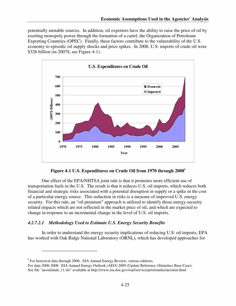
Economic Assumptions Used in the Agencies’ Analysis
4-25
potentially unstable sources. In addition, oil exporters have the ability to raise the price of oil by
exerting monopoly power through the formation of a cartel, the Organization of Petroleum
Exporting Countries (OPEC). Finally, these factors contribute to the vulnerability of the U.S.
economy to episodic oil supply shocks and price spikes. In 2008, U.S. imports of crude oil were
$326 billion (in 2007$, see Figure 4-1).
U.S. Expenditures on Crude Oil
0
100
200
300
400
500
600
700
1970 1975 1980 1985 1990 1995 2000 2005
Year
(20
07
$ B
illi
on
s)
Domestic
Imported
Figure 4-1 U.S. Expenditures on Crude Oil from 1970 through 2008r
One effect of the EPA/NHTSA joint rule is that it promotes more efficient use of
transportation fuels in the U.S. The result is that it reduces U.S. oil imports, which reduces both
financial and strategic risks associated with a potential disruption in supply or a spike in the cost
of a particular energy source. This reduction in risks is a measure of improved U.S. energy
security. For this rule, an “oil premium” approach is utilized to identify those energy-security
related impacts which are not reflected in the market price of oil, and which are expected to
change in response to an incremental change in the level of U.S. oil imports.
4.2.7.2.1 Methodology Used to Estimate U.S. Energy Security Benefits
In order to understand the energy security implications of reducing U.S. oil imports, EPA
has worked with Oak Ridge National Laboratory (ORNL), which has developed approaches for
r For historical data through 2006: EIA Annual Energy Review, various editions.
For data 2006-2008: EIA Annual Energy Outlook (AEO) 2009 (Update Reference (Stimulus) Base Case).
See file "aeostimtab_11.xls" available at http://www.eia.doe.gov/oiaf/servicerpt/stimulus/aeostim.html
Joint Technical Support Document
4-26
evaluating the social costs and energy security implications of oil use. The energy security
estimates provide below are based upon a methodology developed in a peer-reviewed study
entitled, “The Energy Security Benefits of Reduced Oil Use, 2006-2015,” completed in March
2008. This recent study is included as part of the docket for this rulemaking.19
This ORNL
study is an update version of the approach to estimating the energy security benefits of U.S. oil
import reductions developed in an ORNL 1997 Report by Leiby, Paul N., Donald W. Jones, T.
Randall Curlee, and Russell Lee, entitled “Oil Imports: An Assessment of Benefits and Costs.”
When conducting this recent analysis, ORNL considered the full cost of importing
petroleum into the U.S. The full economic cost is defined to include two components in addition
to the purchase price of petroleum itself. These are: (1) the higher costs for oil imports resulting
from the effect of U.S. import demand on the world oil price and on OPEC market power (i.e.,
the “demand” or “monopsony” costs); and (2) the risk of reductions in U.S. economic output and
disruption of the U.S. economy caused by sudden disruptions in the supply of imported oil to the
U.S. (i.e., macroeconomic disruption/adjustment costs). Maintaining a U.S. military presence to
help secure stable oil supply from potentially vulnerable regions of the world was not included in
this analysis because its attribution to particular missions or activities is difficult (as discussed
further below).
Section III.H of the preamble contains a detailed discussion of how the monopsony and
macroeconomic disruption/adjustment components were treated for this analysis. As that
discussion indicates, the monopsony cost represents a transfer of resources from consumers of
petroleum products to oil producers, and does not involve the consumption of real economic
resources. Reducing the magnitude of the monopsony cost does not produce a savings in
economic resources, although it does reduce the value of resources transferred from U.S.
consumers of petroleum products to foreign suppliers of petroleum. In contrast, the
macroeconomic disruption and adjustment costs that arise from U.S. petroleum imports do
represent real economic costs, and reductions in their magnitude do represent real economic
benefits from reducing U.S. consumption and imports of petroleum. Therefore, the remainder of
this discussion focuses on estimating the magnitude of the macroeconomic disruption and
adjustment costs.
As part of the process for using the ORNL energy security estimates, EPA sponsored an
independent-expert peer review of this ORNL study. A report compiling the peer reviewers’
comments is provided in the docket.20
In addition, EPA has worked with ORNL to address
comments raised in the peer review and to develop estimates of the energy security benefits
associated with a reduction in U.S. oil imports for this rule. In response to peer reviewer
comments, ORNL modified its model by changing several key parameters involving OPEC
supply behavior, the responsiveness of oil demand and supply to a change in the world oil price,
and the responsiveness of U.S. economic output to a change in the world oil price.
For this rule, ORNL further updated the energy security premium by incorporating the
most recent oil price forecast and energy market trends in AEO 2009 into its model. In order for
the energy security premium estimated to be used in EPA’s VECTOR model, ORNL developed
energy security estimates for a number of different years; i.e., 2015, 2020, 2030, and 2040.
NHTSA used just the 2015 estimates to estimate the energy security benefits associated with this
rule.
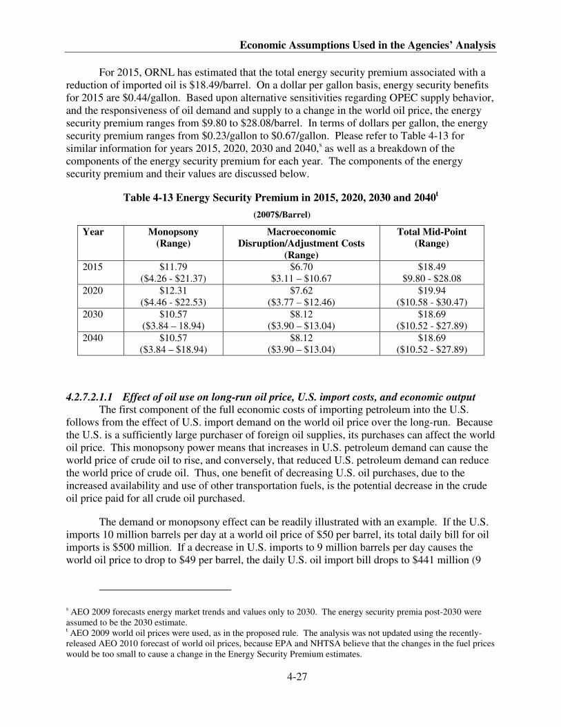
Economic Assumptions Used in the Agencies’ Analysis
4-27
For 2015, ORNL has estimated that the total energy security premium associated with a
reduction of imported oil is $18.49/barrel. On a dollar per gallon basis, energy security benefits
for 2015 are $0.44/gallon. Based upon alternative sensitivities regarding OPEC supply behavior,
and the responsiveness of oil demand and supply to a change in the world oil price, the energy
security premium ranges from $9.80 to $28.08/barrel. In terms of dollars per gallon, the energy
security premium ranges from $0.23/gallon to $0.67/gallon. Please refer to Table 4-13 for
similar information for years 2015, 2020, 2030 and 2040,s as well as a breakdown of the
components of the energy security premium for each year. The components of the energy
security premium and their values are discussed below.
Table 4-13 Energy Security Premium in 2015, 2020, 2030 and 2040t
(2007$/Barrel)
Year
Monopsony
(Range)
Macroeconomic
Disruption/Adjustment Costs
(Range)
Total Mid-Point
(Range)
2015 $11.79
($4.26 - $21.37)
$6.70
$3.11 – $10.67
$18.49
$9.80 - $28.08
2020 $12.31
($4.46 - $22.53)
$7.62
($3.77 – $12.46)
$19.94
($10.58 - $30.47)
2030 $10.57
($3.84 – 18.94)
$8.12
($3.90 – $13.04)
$18.69
($10.52 - $27.89)
2040 $10.57
($3.84 – $18.94)
$8.12
($3.90 – $13.04)
$18.69
($10.52 - $27.89)
4.2.7.2.1.1 Effect of oil use on long-run oil price, U.S. import costs, and economic output The first component of the full economic costs of importing petroleum into the U.S.
follows from the effect of U.S. import demand on the world oil price over the long-run. Because
the U.S. is a sufficiently large purchaser of foreign oil supplies, its purchases can affect the world
oil price. This monopsony power means that increases in U.S. petroleum demand can cause the
world price of crude oil to rise, and conversely, that reduced U.S. petroleum demand can reduce
the world price of crude oil. Thus, one benefit of decreasing U.S. oil purchases, due to the
increased availability and use of other transportation fuels, is the potential decrease in the crude
oil price paid for all crude oil purchased.
The demand or monopsony effect can be readily illustrated with an example. If the U.S.
imports 10 million barrels per day at a world oil price of $50 per barrel, its total daily bill for oil
imports is $500 million. If a decrease in U.S. imports to 9 million barrels per day causes the
world oil price to drop to $49 per barrel, the daily U.S. oil import bill drops to $441 million (9
s AEO 2009 forecasts energy market trends and values only to 2030. The energy security premia post-2030 were
assumed to be the 2030 estimate. t AEO 2009 world oil prices were used, as in the proposed rule. The analysis was not updated using the recently-
released AEO 2010 forecast of world oil prices, because EPA and NHTSA believe that the changes in the fuel prices
would be too small to cause a change in the Energy Security Premium estimates.
Joint Technical Support Document
4-28
million barrels times $49 per barrel). While the world oil price only declines $1, the resulting
decrease in oil purchase payments of $59 million per day ($500 million minus $441 million) is
equivalent to an incremental benefit of $59 per barrel of oil imports reduced, or $10 more than
the newly-decreased world price of $49 per barrel. This additional $10 per barrel “import cost
premium” represents the incremental external benefits to the U.S. for avoided import costs
beyond the price paid oil purchases. This additional benefit arises only to the extent that
reduction in U.S. oil imports affects the world oil price. ORNL estimates this component of the
energy security benefit in 2015 to be $11.79/barrel, with a range of $4.26 – $21.37/barrel of
imported oil reduced.
4.2.7.2.1.2 Short-run disruption premium from expected costs of sudden supply disruptions The second component of the oil import premium, the “macroeconomic
disruption/adjustment costs premium,” arises from the effect of oil imports on the expected cost
of disruptions. A sudden increase in oil prices triggered by a disruption in world oil supplies has
two main effects: (1) it increases the costs of imports in the short run, further expanding the
transfer of U.S. wealth to foreign producers, and (2) it can lead to macroeconomic contraction,
dislocation and Gross Domestic Product (GDP) losses. ORNL estimates the composite estimate
of these two factors that comprise the macroeconomic disruption/adjustment costs premium to be
$6.70/barrel in 2015, with a range of $3.11 – $10.67/barrel of imported oil reduced.
4.2.7.2.1.2.1 Higher costs of oil imports during shocks During oil price shocks, the higher price of imported oil causes increased payments for
imports from the U.S to oil exporters. This increased claim on U.S. economic output is a loss to
the U.S. that is separate from and additional to any reduction in economic output due to the
shock. The increased oil payments during shocks are counted as a loss to the degree that the
expected price increase is not anticipated and internalized by oil consumers.
4.2.7.2.1.2.2 Macroeconomic costs: potential output loss and dislocation/adjustment costs Macroeconomic losses during price shocks reflect both aggregate output losses and
“allocative” losses. The former are a reduction in the level of output that the U.S. economy can
produce fully using its available resources; and the latter stem from temporary dislocation and
underutilization of available resources due to the shock, such as labor unemployment and idle
plant capacity. The aggregate output effect, a reduction in “potential” economic output, will last
so long as the price is elevated. It depends on the extent and duration of any disruption in the
world supply of oil, since these factors determine the magnitude of the resulting increase in
prices for petroleum products, as well as whether and how rapidly these prices return to their pre-
disruption levels.
In addition to the aggregate contraction, there are “allocative” or “adjustment” costs
associated with dislocated energy markets. Because supply disruptions and resulting price
increases occur suddenly, empirical evidence shows they also impose additional costs on
businesses and households which must adjust their use of petroleum and other productive factors
more rapidly than if the same price increase had occurred gradually. Dislocational effects
include the unemployment of workers and other resources during the time needed for their
intersectoral or interregional reallocation, and pauses in capital investment due to uncertainty.
These adjustments temporarily reduce the level of economic output that can be achieved even
below the “potential” output level that would ultimately be reached once the economy’s
Economic Assumptions Used in the Agencies’ Analysis
4-29
adaptation to higher petroleum prices was complete. The additional costs imposed on businesses
and households for making these adjustments reflect their limited ability to adjust prices, output
levels, and their use of energy, labor and other inputs quickly and smoothly in response to rapid
changes in prices for petroleum products.
Since future disruptions in foreign oil supplies are an uncertain prospect, each of the
disruption cost components must be weighted by the probability that the supply of petroleum to
the U.S. will actually be disrupted. Thus, the “expected value” of these costs – the product of the
probability that a supply disruption will occur and the sum of costs from reduced economic
output and the economy’s abrupt adjustment to sharply higher petroleum prices – is the relevant
measure of their magnitude. Further, when assessing the energy security value of a policy to
reduce oil use, it is only the change in the expected costs of disruption that results from the
policy that is relevant. The expected costs of disruption may change from lowering the normal
(i.e., pre-disruption) level of domestic petroleum use and imports, from any induced alteration in
the likelihood or size of disruption, or from altering the short-run flexibility (e.g., elasticity) of
petroleum use.
In summary, the steps needed to calculate the disruption or security premium are: 1)
determine the likelihood of an oil supply disruption in the future; 2) assess the likely impacts of a
potential oil supply disruption on the world oil price; 3) assess the impact of the oil price shock
on the U.S. economy (in terms of import costs and macroeconomic losses); and 4) determine
how these costs change with oil imports. The value of price spike costs avoided by reducing oil
imports becomes the oil security portion of the premium.
In the energy security literature, the macroeconomic disruption component of the energy
security premium traditionally has included both (1) increased payments for petroleum imports
associated with a rapid increase in world oil prices, and (2) the GDP losses and adjustment costs
that result from projected future oil price shocks. One commenter suggested that the increased
payments associated with rapid increases in petroleum prices (i.e., price increases in a disrupted
market) represent transfers from U.S. oil consumers to petroleum suppliers rather than real
economic costs, and therefore, should not be counted as a benefit.
This approach would represent a significant departure from how the macroeconomic
disruption costs associated with oil price shocks have been quantified in the broader energy
security literature, and the Agencies believe it should be analyzed in more detail before being
applied in a regulatory context. In addition, the Agencies also believe that there are compelling
reasons to treat higher oil import costs during oil supply disruptions differently than simple
wealth transfers that reflect the exercise of market power by petroleum sellers or consumers.
According to the OMB definition of a transfer: “Benefit and cost estimates should reflect real
resource use. Transfer payments are monetary payments from one group to another that do not
affect total resources available to society…The net reduction in the total surplus (consumer plus
producer) is a real cost to society, but the transfer from buyers to sellers resulting from a higher
price is not a real cost since the net reduction automatically accounts for the transfer from buyers
Joint Technical Support Document
4-30
to sellers.”u In other words, pure transfers do not lead to changes in the allocation or
consumption of economic resources, whereas changes in the resource allocation or use produce
real economic costs or benefits.
While price increases during oil price disruptions can result in large transfers of wealth,
they also result in a combination of real resource shortages, costly short-run shifts in energy
supply, behavioral and demand adjustments by energy users, and other response costs. Unlike
pure transfers, the root cause of the disruption price increase is a real resource supply reduction
due, for example, to disaster or war. Regions where supplies are disrupted (i.e., the U.S.) suffer
very high costs. Businesses’ and households’ emergency responses to supply disruptions and
rapid price increases are likely to consume some real economic resources, in addition to causing
financial losses to the U.S. economy that are matched by offsetting gains elsewhere in the global
economy.
While households and businesses can reduce their petroleum consumption, invest in fuel
switching technologies, or use futures markets to insulate themselves in advance against the
potential costs of rapid increases in oil prices, when deciding how extensively to do so, they are
unlikely to account for the effect of their petroleum consumption on the magnitude of costs that
supply interruptions and accompanying price shocks impose on others. As a consequence, the
U.S. economy as a whole will not make sufficient use of these mechanisms to insulate itself from
the real costs of rapid increases in energy prices and outlays that usually accompany oil supply
interruptions.v Therefore, the ORNL estimate of macroeconomic disruption and adjustment
costs that the Agencies use to value energy security benefits includes the increased oil import
costs stemming from oil price shocks that are unanticipated and not internalized by advance
actions of U.S. consumers of petroleum products. The Agencies believe that, as the ORNL
analysis argues, the uninternalized oil import costs that occur during oil supply interruptions
represents a real cost associated with U.S. petroleum consumption and imports, and that reducing
its value by lowering domestic petroleum consumption and imports thus represents a real
economic benefit from lower fuel consumption.
4.2.7.2.2 Cost of existing U.S. energy security policies The last often-identified component of the full economic costs of U.S. oil imports is the
costs to the U.S. taxpayers of existing U.S. energy security policies. The two primary examples
are maintaining a military presence to help secure a stable oil supply from potentially vulnerable
regions of the world and maintaining the Strategic Petroleum Reserve (SPR). The SPR is the
largest stockpile of government-owned emergency crude oil in the world. Established in the
aftermath of the 1973-74 oil embargo, the SPR provides the U.S. a response option should a
u OMB Circular A-4, September 17, 2003. See
http://www.whitehouse.gov/omb/assets/omb/circulars/a004/a-4.pdf v For a more complete discussion of the reasons why the oil import cost component of the
macroeconomic disruption and adjustment costs includes some real costs and does not represent
a pure transfer, see Paul N. Leiby, Estimating the Energy Security Benefits of Reduced U.S. Oil
Imports: Final Report, ORNL-TM-2007-028, Oak Ridge National Laboratory, March 14, 2008,
pp. 21-25.
Economic Assumptions Used in the Agencies’ Analysis
4-31
disruption in commercial oil supplies threaten the U.S. economy. It also allows the U.S. to meet
part of its International Energy Agency obligation to maintain emergency oil stocks, and it
provides a national defense fuel reserve.
U.S. military costs are excluded from the analysis performed by ORNL because their
attribution to particular missions or activities is difficult. Most military forces serve a broad
range of security and foreign policy objectives. Attempts to attribute some share of U.S. military
costs to oil imports are further challenged by the need to estimate how those costs might vary
with incremental variations in U.S. oil imports. Similarly, while the costs for building and
maintaining the SPR are more clearly related to U.S. oil use and imports, historically these costs
have not varied in response to changes in U.S. oil import levels. Thus, while SPR is factored
into the ORNL analysis, the cost of maintaining the SPR is excluded.
4.2.7.2.3 Modifications to analysis based upon peer reviewer comments The EPA commissioned ORNL to conduct a number of sensitivity analyses to address the
comments of the peer reviewers. Based upon the peer reviewer comments, key parameters that
influence the “oil import” premium were assessed. Since not all the comments were in
agreement with each other, several ranges of different parameters were developed for the
analyses. These sensitivities used the most recent price forecasts and energy market trends
available at the time the peer review was being conducted and completed, the AEO 2007
Reference Case. Thus, the results presented below are suggestive of how the energy security
premium is influenced by alternative assumptions of key parameters that influence world oil
markets. A summary of the results of the analyses are shown in Table 4-14.
Three key parameters were varied in order to assess their impacts on the oil import
premium: (1) the response of OPEC supply, (2) the combined response of non-U.S., non-OPEC
demand and supply and (3) the GDP response to a change in the world oil as a result of reduced
U.S. oil imports. The cases used updated supply/demand elasticities for non-U.S./non-OPEC
region after considering more recent estimates than those used in 1997 study. As a result, the
total market responsiveness is greater than previous ORNL estimates. Only small changes to the
world oil price are anticipated from a substantial reduction in U.S. demand, on average, about
$0.70/barrel for every million-barrels-per-day reduction in demand.
In the ORNL framework, OPEC-behavior is treated parametrically, with a wide range of
possible responses represented by a range of supply elasticities. Case One in Table 4-14 below
refers to the AEO 2007 estimates of energy market trends and uses the elasticity parameters from
the original 1997 ORNL study. In Case Two, the OPEC supply elasticities range for 0.25 to 6
with a mean elasticity of 1.7. Case Three alters the distribution of the OPEC supply elasticities
so that the mean elasticity is 2.2 instead of 1.7. With the more elastic OPEC oil supply in Case
Three, the oil premium is lower. Alternatively, a candidate rule for OPEC strategic response
behavior, adapted from a lead article on what behavior maximizes OPEC’s long run net revenue
in a robust way,21
would have OPEC responding to preserve its worldwide oil market share.
This is presented as Case Seven. Application of this rule instead of the range of OPEC supply
responses used leads to an estimate of the oil import premium that is between Case Two and
Case Three.
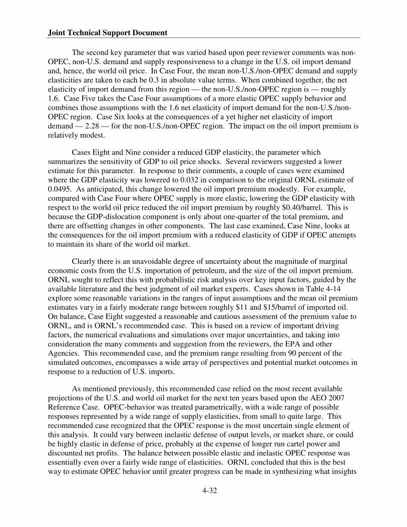
Joint Technical Support Document
4-32
The second key parameter that was varied based upon peer reviewer comments was non-
OPEC, non-U.S. demand and supply responsiveness to a change in the U.S. oil import demand
and, hence, the world oil price. In Case Four, the mean non-U.S./non-OPEC demand and supply
elasticities are taken to each be 0.3 in absolute value terms. When combined together, the net
elasticity of import demand from this region — the non-U.S./non-OPEC region is — roughly
1.6. Case Five takes the Case Four assumptions of a more elastic OPEC supply behavior and
combines those assumptions with the 1.6 net elasticity of import demand for the non-U.S./non-
OPEC region. Case Six looks at the consequences of a yet higher net elasticity of import
demand — 2.28 — for the non-U.S./non-OPEC region. The impact on the oil import premium is
relatively modest.
Cases Eight and Nine consider a reduced GDP elasticity, the parameter which
summarizes the sensitivity of GDP to oil price shocks. Several reviewers suggested a lower
estimate for this parameter. In response to their comments, a couple of cases were examined
where the GDP elasticity was lowered to 0.032 in comparison to the original ORNL estimate of
0.0495. As anticipated, this change lowered the oil import premium modestly. For example,
compared with Case Four where OPEC supply is more elastic, lowering the GDP elasticity with
respect to the world oil price reduced the oil import premium by roughly $0.40/barrel. This is
because the GDP-dislocation component is only about one-quarter of the total premium, and
there are offsetting changes in other components. The last case examined, Case Nine, looks at
the consequences for the oil import premium with a reduced elasticity of GDP if OPEC attempts
to maintain its share of the world oil market.
Clearly there is an unavoidable degree of uncertainty about the magnitude of marginal
economic costs from the U.S. importation of petroleum, and the size of the oil import premium.
ORNL sought to reflect this with probabilistic risk analysis over key input factors, guided by the
available literature and the best judgment of oil market experts. Cases shown in Table 4-14
explore some reasonable variations in the ranges of input assumptions and the mean oil premium
estimates vary in a fairly moderate range between roughly $11 and $15/barrel of imported oil.
On balance, Case Eight suggested a reasonable and cautious assessment of the premium value to
ORNL, and is ORNL’s recommended case. This is based on a review of important driving
factors, the numerical evaluations and simulations over major uncertainties, and taking into
consideration the many comments and suggestion from the reviewers, the EPA and other
Agencies. This recommended case, and the premium range resulting from 90 percent of the
simulated outcomes, encompasses a wide array of perspectives and potential market outcomes in
response to a reduction of U.S. imports.
As mentioned previously, this recommended case relied on the most recent available
projections of the U.S. and world oil market for the next ten years based upon the AEO 2007
Reference Case. OPEC-behavior was treated parametrically, with a wide range of possible
responses represented by a wide range of supply elasticities, from small to quite large. This
recommended case recognized that the OPEC response is the most uncertain single element of
this analysis. It could vary between inelastic defense of output levels, or market share, or could
be highly elastic in defense of price, probably at the expense of longer run cartel power and
discounted net profits. The balance between possible elastic and inelastic OPEC response was
essentially even over a fairly wide range of elasticities. ORNL concluded that this is the best
way to estimate OPEC behavior until greater progress can be made in synthesizing what insights
Economic Assumptions Used in the Agencies’ Analysis
4-33
are available from the evolving strategic game-theoretic and empirical research on OPEC
behavior, and advancing that research. An alternative would have been to use OPEC strategic
response behavior to maximize long-run net revenue, which may well correspond to market-
share preservation behavior (e.g., Case Seven), and a somewhat higher premium value.
Finally, ORNL’s recommended case used a GDP elasticity range, the parameter which
summarizes the sensitivity of GDP to oil price shocks, which is reduced compared to earlier
estimates, and compared to the full range of historically-based estimates. This helped address
the concerns of those who either question the conclusions of past empirical estimates or expect
that the impacts of oil shocks may well be declining.
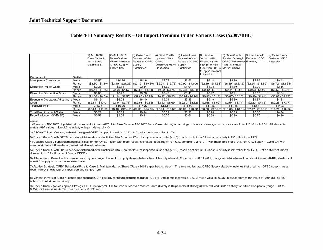
Joint Technical Support Document
4-34
Table 4-14 Summary Results – Oil Import Premium Under Various Cases ($2007/BBL)
Component Statistic
1) AEO2007
Base Outlook,
1997 Study
Elasticities
2) AEO2007
Base Outlook,
Wider Range of
OPEC Supply
Elasticities
3) Case 2 with
Revised Wider
Range of OPEC
Supply
Elasticities
4) Case 2 with
Updated Non-
OPEC
Supply/Demand
Elasticities
5) Case 4 plus
Revised Wider
Range of OPEC
Supply
Elasticities
6) Case 4
Variant with
Wider, Higher
Range of Non-
U.S./Non-OPEC
Supply/Demand
Elasticities
7) Case 6 with
Applied Strategic
OPEC Behavioral
Rule: Maintain
Market Share
8) Case 4 with
Reduced GDP
Elasticity
9) Case 7 with
Reduced GDP
Elasticity
Mean $5.57 $10.26 $8.16 $7.77 $6.52 $6.44 $9.36 $7.86 $9.42
Range ($3.60 - $8.19) ($3.10 - $21.22) ($3.12 - $19.30) ($2.94 - $13.75) ($2.90 - $13.06) ($2.69 - $11.33) ($6.69 - $12.42) ($2.94 - $13.89) ($6.72 - $12.54)
Mean $2.36 $2.33 $2.34 $1.92 $1.94 $1.93 $1.89 $2.20 $2.16
Range ($0.51 - $4.66) ($0.58 - $4.57) ($0.66 - $4.61) ($0.39 - $3.75) ($0.38 - $3.84) ($0.42 - $3.70) ($0.44 - $3.66) ($0.63 - $4.07) ($0.62 - $3.96)
Mean $3.83 $3.70 $3.76 $3.42 $3.45 $3.47 $3.41 $2.67 $2.64
Range ($1.06 - $6.69) ($1.04 - $6.57) ($1.06 - $6.74) ($0.92 - $6.23) ($0.94 - $6.10) ($0.92 - $6.13) ($0.87 - $6.26) ($0.90 - $4.84) ($0.87 - $4.87)
Mean $6.19 $6.03 $6.10 $5.34 $5.39 $5.40 $5.30 $4.87 $4.81
Range ($2.94 - $10.01) ($2.94 - $9.75) ($2.91 - $9.85) ($2.53 - $8.69) ($2.60 - $8.62) ($2.58 - $8.92) ($2.54 - $8.74) ($2.23 - $7.85) ($2.25 - $7.77)
Mean $11.75 $16.29 $14.27 $13.11 $11.90 $11.86 $14.65 $12.71 $14.23
Range ($8.04 - $15.96) ($8.10 - $27.42) ($7.90 - $25.49) ($7.26 - $19.59) ($6.96 - $18.62) ($6.79 - $17.23) ($11.03 - $18.61) ($7.07 - $19.02) ($10.76 - $18.25)
Total Premium, in $/Gallon Mean $0.28 $0.39 $0.34 $0.31 $0.28 $0.28 $0.35 $0.30 $0.34
Price Reduction ($/MMBD) Mean $0.52 $1.04 $0.81 $0.75 $0.61 $0.60 $0.90 $0.75 $0.90
Cases
7) Applied Strategic OPEC Behavioral Rule to Case 6: Maintain Market Share (Gately 2004 paper best strategy). This rule implies that OPEC Supply elasticity matches that of all non-OPEC supply. As a
result non-U.S. elasticity of import demand ranges from
8) Variant on version Case 4, considered reduced GDP elasticity for future disruptions (range -0.01 to -0.054; midcase value -0.032; mean value is -0.032, reduced from mean value of -0.0495). OPEC-
behavior treated parametrically.
9) Revise Case 7 (which applied Strategic OPEC Behavioral Rule to Case 6: Maintain Market Share (Gately 2004 paper best strategy)) with reduced GDP elasticity for future disruptions (range -0.01 to -
0.054; midcase value -0.032; mean value is -0.032, reduc
3) Revise Case 2, with OPEC behavior distributed over elasticities 0 to 6, so that 25% of response is inelastic (< 1.0), mode elasticity is 2.0 (mean elasticity is 2.2 rather than 1.76)
4) Updated Case 2 supply/demand elasticities for non-OPEC region with more recent estimates. Elasticity of non-U.S. demand -0.2 to -0.4, with mean and mode -0.3, non-U.S. Supply = 0.2 to 0.4, with
mean and mode 0.3, implying (mode) net elasticity of impo
5) Revise Case 4, with OPEC behavior distributed over elasticities 0 to 6, so that 25% of response is inelastic (< 1.0), mode elasticity is 2.0 (mean elasticity is 2.2 rather than 1.76). Net elasticity of import
demand is -1.6 for the non-U.S./non-OPEC r
6) Alternative to Case 4 with expanded (and higher) range of non-U.S. supply/demand elasticities. Elasticity of non-U.S. demand = -0.3 to -0.7, triangular distribution with mode -0.4 mean -0.467, elasticity of
non-U.S. supply = 0.2 to 0.6, mode 0.3 and m
Economic Disruption/Adjustment
Costs
Total Mid-Point
1) Based on AEO2007. Updated oil market outlook from AEO1994 Base Case to AEO2007 Base Case. Among other things, this means average crude price rises from $20.33 to $48.34. All elasticities
match 1997 values. Non-U.S. elasticity of import demand = -0.
2) AEO2007 Base Outlook, with wider range of OPEC supply elasticities, 0.25 to 6.0 and a mean elasticity of 1.76.
Monopsony Component
Disruption Import Costs
Disruption Dislocation Costs
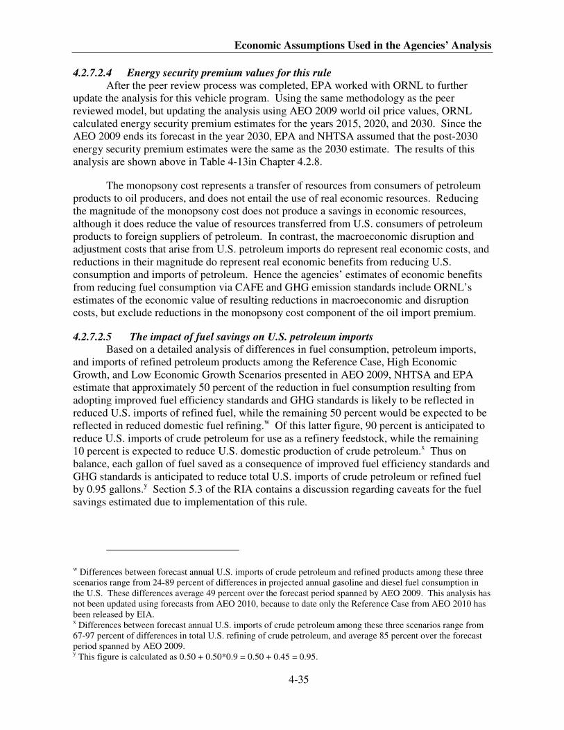
Economic Assumptions Used in the Agencies’ Analysis
4-35
4.2.7.2.4 Energy security premium values for this rule After the peer review process was completed, EPA worked with ORNL to further
update the analysis for this vehicle program. Using the same methodology as the peer
reviewed model, but updating the analysis using AEO 2009 world oil price values, ORNL
calculated energy security premium estimates for the years 2015, 2020, and 2030. Since the
AEO 2009 ends its forecast in the year 2030, EPA and NHTSA assumed that the post-2030
energy security premium estimates were the same as the 2030 estimate. The results of this
analysis are shown above in Table 4-13in Chapter 4.2.8.
The monopsony cost represents a transfer of resources from consumers of petroleum
products to oil producers, and does not entail the use of real economic resources. Reducing
the magnitude of the monopsony cost does not produce a savings in economic resources,
although it does reduce the value of resources transferred from U.S. consumers of petroleum
products to foreign suppliers of petroleum. In contrast, the macroeconomic disruption and
adjustment costs that arise from U.S. petroleum imports do represent real economic costs, and
reductions in their magnitude do represent real economic benefits from reducing U.S.
consumption and imports of petroleum. Hence the agencies’ estimates of economic benefits
from reducing fuel consumption via CAFE and GHG emission standards include ORNL’s
estimates of the economic value of resulting reductions in macroeconomic and disruption
costs, but exclude reductions in the monopsony cost component of the oil import premium.
4.2.7.2.5 The impact of fuel savings on U.S. petroleum imports Based on a detailed analysis of differences in fuel consumption, petroleum imports,
and imports of refined petroleum products among the Reference Case, High Economic
Growth, and Low Economic Growth Scenarios presented in AEO 2009, NHTSA and EPA
estimate that approximately 50 percent of the reduction in fuel consumption resulting from
adopting improved fuel efficiency standards and GHG standards is likely to be reflected in
reduced U.S. imports of refined fuel, while the remaining 50 percent would be expected to be
reflected in reduced domestic fuel refining.w Of this latter figure, 90 percent is anticipated to
reduce U.S. imports of crude petroleum for use as a refinery feedstock, while the remaining
10 percent is expected to reduce U.S. domestic production of crude petroleum.x Thus on
balance, each gallon of fuel saved as a consequence of improved fuel efficiency standards and
GHG standards is anticipated to reduce total U.S. imports of crude petroleum or refined fuel
by 0.95 gallons.y Section 5.3 of the RIA contains a discussion regarding caveats for the fuel
savings estimated due to implementation of this rule.
w Differences between forecast annual U.S. imports of crude petroleum and refined products among these three
scenarios range from 24-89 percent of differences in projected annual gasoline and diesel fuel consumption in
the U.S. These differences average 49 percent over the forecast period spanned by AEO 2009. This analysis has
not been updated using forecasts from AEO 2010, because to date only the Reference Case from AEO 2010 has
been released by EIA. x Differences between forecast annual U.S. imports of crude petroleum among these three scenarios range from
67-97 percent of differences in total U.S. refining of crude petroleum, and average 85 percent over the forecast
period spanned by AEO 2009. y This figure is calculated as 0.50 + 0.50*0.9 = 0.50 + 0.45 = 0.95.
Joint Technical Support Document
4-36
The energy security analysis conducted for this rule estimates that the world price of
oil will fall modestly in response to lower U.S. demand for refined fuel. One potential result
of this decline in the world price of oil would be an increase in the consumption of petroleum
products outside the U.S., which would in turn lead to a modest increase in emissions of
greenhouse gases, criteria air pollutants, and airborne toxics from their refining and use.
While additional information would be needed to analyze this “leakage effect” in detail,
NHTSA provides a sample estimate of its potential magnitude in its Final EIS.z This analysis
indicates that the leakage effect is likely to offset only a modest fraction of the reductions in
emissions projected to result from the rule.
4.2.8 Air pollutant emissions
Car and light truck use, fuel refining, and fuel distribution and retailing also generate
emissions of certain criteria air pollutants, including carbon monoxide (CO), hydrocarbon
compounds (usually referred to as “volatile organic compounds,” or VOC), nitrogen oxides
(NOx), fine particulate matter (PM2.5), and sulfur dioxide (SO2). Emissions of most of these
pollutants are associated with the number of vehicle miles driven, rather than with the
quantity of fuel consumed. While reductions in fuel refining and distribution that result from
lower fuel consumption will reduce emissions of criteria pollutants, additional vehicle use
associated with the rebound effect from higher fuel economy will increase emissions of most
of these pollutants. Sulfur dioxide is an exception, as described below.
Thus the net effect of stricter fuel efficiency and GHG standards on total emissions of
each criteria pollutant depends on the relative magnitudes of reduced emissions in fuel
refining and distribution, and increases in emissions from vehicle use. Because the
relationship between emission rates (emissions per gallon refined of fuel or mile driven) in
fuel refining and vehicle use is different for each criteria pollutant, the net effect of fuel
savings from increased fuel efficiency and GHG standards on total emissions of each
pollutant is likely to differ.
4.2.8.1 Reductions in emissions of criteria air pollutants
For the analysis of criteria emissions over the lifetime of the model years covered by
this rule, EPA and NHTSA estimate the increases in emissions of each criteria air pollutant
from additional vehicle use by multiplying the increase in total miles driven by cars and light
trucks of each model year and age by their estimated emission rates per vehicle-mile of each
pollutant. These emission rates differ between cars and light trucks as well as between
gasoline and diesel vehicles, and both their values for new vehicles and the rates at which they
increase with age and accumulated mileage can vary among model years. With the exception
of SO2, the agencies calculated the increase in emissions of these criteria pollutants from
added car and light truck use by multiplying the estimated increases in their vehicles’ use
z NHTSA Final Environmental Impact Statement: Corporate Average Fuel Economy Standards, Passenger Cars
and Light Trucks, Model Years 2012-2016, February 2010, page 3-14.
Economic Assumptions Used in the Agencies’ Analysis
4-37
during each year over their expected lifetimes by per-mile emission rates appropriate to each
vehicle type, fuel used, model year, and age as of that future year.
These emission rates were estimated by U.S. EPA using its newly updated Motor
Vehicle Emission Simulator (MOVES2010). For the proposal, emission rates were estimated
using Draft MOVES2009.
The MOVES model assumes that the per-mile rates at which these pollutants are
emitted are determined by EPA regulations and the effectiveness of catalytic after-treatment
of engine exhaust emissions, and are thus unaffected by changes in car and light truck fuel
economy. As a consequence, the effects of required increases in fuel economy on emissions
of these pollutants from car and light truck use are determined entirely by the increases in
driving that result from the fuel economy rebound effect. As discussed in the EPA RIA,
anticipated changes in the fuel supply composition will also affect criteria pollutant emissions.
Emission factors in the MOVES database are expressed in the form of grams per
vehicle-hour of operation. To convert these emission factors to grams per mile for use in EPA
and NHTSA’s calculations, MOVES was run for the year 2050, and was programmed to
report aggregate emissions from vehicle starting and running exhaust operation. EPA analysts
selected the year 2050 in order to generate emission factors that were representative of
lifetime average emission rates for vehicles meeting the agency’s Tier 2 emission standard.aa
Separate estimates were developed for each vehicle type and model year, as well as for each
state and month, in order to reflect the effects of regional and temporal variation in
temperature and other relevant variables on emissions.
The MOVES emissions estimates were then summed to the model year level and
divided by average distance traveled in order to produce per-mile emission factors for each
pollutant. The resulting emission rates represent average values across the nation, and
incorporate typical temperature variations over an entire calendar year. These national
average rates also reflect county-specific differences in fuel composition, as well as in the
presence and type of vehicle inspection and maintenance programs.bb
Emission rates for the criteria pollutant SO2 were calculated by EPA and NHTSA
using average fuel sulfur content estimates supplied by EPA, together with the assumption
that the entire sulfur content of fuel is emitted in the form of SO2. These calculations assumed
that national average gasoline and diesel sulfur levels would remain at current levels.cc
aa Because all light-duty emission rates in MOVES2010 are assumed to be invariant after MY 2010, a calendar-
year 2050 run produced a full set of emission rates that reflect anticipated deterioration in the effectiveness of
vehicles’ emission control systems with increasing age and accumulated mileage for post-MY 2010 vehicles. bb
The national mix of fuel types includes county-level market shares of conventional and reformulated gasoline,
as well as county-level variation in sulfur content, ethanol fractions, and other fuel properties.
Inspection/maintenance programs at the county level account for detailed program design elements such as test
type, inspection frequency, and program coverage by vehicle type and age. cc
These are 30 and 15 parts per million (ppm, measured on a mass basis) for gasoline and diesel respectively,
which produces emission rates of 0.17 grams of SO2 per gallon of gasoline and 0.10 grams per gallon of diesel.
Joint Technical Support Document
4-38
There, unlike many other criteria pollutants, sulfur dioxide emissions from vehicle use
decrease proportionally to the decrease in fuel consumption.
Emissions of criteria air pollutants also occur during each phase of fuel production and
distribution, including crude oil extraction and transportation, fuel refining, and fuel storage
and transportation. The reduction in emissions during each of these phases depends on the
extent to which fuel savings result in lower imports of refined fuel, or in reduced domestic
fuel refining. To a lesser extent, they also depend on whether reductions in domestic gasoline
refining are reflected in reduced imports of crude oil or in reduced domestic extraction of
petroleum.
Both EPA’s and NHTSA’s analyses assume that reductions in imports of refined fuel
would reduce criteria pollutant emissions during fuel storage and distribution only.
Reductions in domestic fuel refining using imported crude oil as a feedstock are assumed to
reduce emissions during fuel refining, storage, and distribution, because each of these
activities would be reduced. Finally, reduced domestic fuel refining using domestically-
produced crude oil is assumed to reduce emissions during all four phases of fuel production
and distribution.dd
EPA estimated the reductions in criteria pollutant emissions from producing and
distributing fuel that would occur with alternative fuel efficiency and GHG standards using
emission rates obtained from Argonne National Laboratories’ Greenhouse Gases and
Regulated Emissions in Transportation (GREET) model.22 The GREET model provides
separate estimates of air pollutant emissions that occur in four phases of fuel production and
distribution: crude oil extraction, crude oil transportation and storage, fuel refining, and fuel
distribution and storage.ee EPA modified the GREET model to change certain assumptions
about emissions during crude petroleum extraction and transportation, as well as to update its
emission rates to reflect adopted and pending EPA emission standards. EPA also
incorporated emission factors for the air toxics estimated in this analysis: benzene, 1,3-
butadiene, acetaldehyde, acrolein, and formaldehyde. The resulting emission factors are
shown in Table 4-15.
dd In effect, this assumes that the distances crude oil travels to U.S. refineries are approximately the same
regardless of whether it travels from domestic oilfields or import terminals, and that the distances that gasoline
travels from refineries to retail stations are approximately the same as those from import terminals to gasoline
stations. ee
Emissions that occur during vehicle refueling at retail gasoline stations (primarily evaporative emissions of
volatile organic compounds, or VOCs) are already accounted for in the “tailpipe” emission factors used to
estimate the emissions generated by increased light truck use. GREET estimates emissions in each phase of
gasoline production and distribution in mass per unit of gasoline energy content; these factors are then converted
to mass per gallon of gasoline using the average energy content of gasoline.
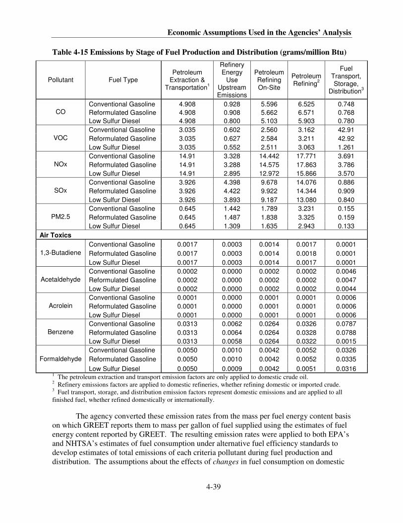
Economic Assumptions Used in the Agencies’ Analysis
4-39
Table 4-15 Emissions by Stage of Fuel Production and Distribution (grams/million Btu)
Pollutant Fuel Type Petroleum
Extraction & Transportation
1
Refinery Energy
Use Upstream Emissions
Petroleum Refining On-Site
Petroleum Refining
2
Fuel Transport, Storage,
Distribution3
Conventional Gasoline 4.908 0.928 5.596 6.525 0.748
Reformulated Gasoline 4.908 0.908 5.662 6.571 0.768 CO
Low Sulfur Diesel 4.908 0.800 5.103 5.903 0.780
Conventional Gasoline 3.035 0.602 2.560 3.162 42.91
Reformulated Gasoline 3.035 0.627 2.584 3.211 42.92 VOC
Low Sulfur Diesel 3.035 0.552 2.511 3.063 1.261
Conventional Gasoline 14.91 3.328 14.442 17.771 3.691
Reformulated Gasoline 14.91 3.288 14.575 17.863 3.786 NOx
Low Sulfur Diesel 14.91 2.895 12.972 15.866 3.570
Conventional Gasoline 3.926 4.398 9.678 14.076 0.886
Reformulated Gasoline 3.926 4.422 9.922 14.344 0.909 SOx
Low Sulfur Diesel 3.926 3.893 9.187 13.080 0.840
Conventional Gasoline 0.645 1.442 1.789 3.231 0.155
Reformulated Gasoline 0.645 1.487 1.838 3.325 0.159 PM2.5
Low Sulfur Diesel 0.645 1.309 1.635 2.943 0.133
Air Toxics
Conventional Gasoline 0.0017 0.0003 0.0014 0.0017 0.0001
Reformulated Gasoline 0.0017 0.0003 0.0014 0.0018 0.0001 1,3-Butadiene
Low Sulfur Diesel 0.0017 0.0003 0.0014 0.0017 0.0001
Conventional Gasoline 0.0002 0.0000 0.0002 0.0002 0.0046
Reformulated Gasoline 0.0002 0.0000 0.0002 0.0002 0.0047 Acetaldehyde
Low Sulfur Diesel 0.0002 0.0000 0.0002 0.0002 0.0044
Conventional Gasoline 0.0001 0.0000 0.0001 0.0001 0.0006
Reformulated Gasoline 0.0001 0.0000 0.0001 0.0001 0.0006 Acrolein
Low Sulfur Diesel 0.0001 0.0000 0.0001 0.0001 0.0006
Conventional Gasoline 0.0313 0.0062 0.0264 0.0326 0.0787
Reformulated Gasoline 0.0313 0.0064 0.0264 0.0328 0.0788 Benzene
Low Sulfur Diesel 0.0313 0.0058 0.0264 0.0322 0.0015
Conventional Gasoline 0.0050 0.0010 0.0042 0.0052 0.0326
Reformulated Gasoline 0.0050 0.0010 0.0042 0.0052 0.0335 Formaldehyde
Low Sulfur Diesel 0.0050 0.0009 0.0042 0.0051 0.0316 1 The petroleum extraction and transport emission factors are only applied to domestic crude oil.
2 Refinery emissions factors are applied to domestic refineries, whether refining domestic or imported crude.
3 Fuel transport, storage, and distribution emission factors represent domestic emissions and are applied to all
finished fuel, whether refined domestically or internationally.
The agency converted these emission rates from the mass per fuel energy content basis
on which GREET reports them to mass per gallon of fuel supplied using the estimates of fuel
energy content reported by GREET. The resulting emission rates were applied to both EPA’s
and NHTSA’s estimates of fuel consumption under alternative fuel efficiency standards to
develop estimates of total emissions of each criteria pollutant during fuel production and
distribution. The assumptions about the effects of changes in fuel consumption on domestic
Joint Technical Support Document
4-40
and imported sources of fuel supply discussed above were then employed to calculate the
effects of reductions in fuel use from alternative fuel efficiency and GHG standards on
changes in domestic emissions of each criteria pollutant.
Finally, EPA and NHTSA calculated the net changes in domestic emissions of each
criteria pollutant by summing the increases in its emissions projected to result from increased
vehicle use, and the reductions in emissions anticipated to result from lower domestic fuel
refining and distribution.ff As indicated previously, the effect of adopting improved fuel
efficiency and GHG standards on total emissions of each criteria pollutant depends on the
relative magnitudes of the resulting reduction in emissions from fuel refining and distribution,
and the increase in emissions from additional vehicle use. Although these net changes vary
significantly among individual criteria pollutants, we project that on balance, adopting
improved fuel efficiency and GHG standards would reduce emissions of all criteria air
pollutants except carbon monoxide (CO). The analysis of criteria emissions during specific
calendar years is described independently in NHTSA’s Environmental Impact Statement and
EPA’s RIA.
4.2.8.2 Estimated values of reducing PM related emissions in the model year analysis
In this analysis, EPA and NHTSA estimate the economic value of the human health
benefits associated with reducing exposure to PM2.5 using benefit-per-ton estimates for the
analysis of PM-related benefits over the lifetime of specific model years. Due to analytical
limitations, the estimated benefit-per-ton values do not include comparable benefits related to
reductions in other criteria pollutants (such as ozone, NO2 or SO2) or toxic air pollutants, nor
do they monetize all of the potential health and welfare effects associated with PM2.5 or the
other criteria pollutants. As a result these values underestimate the benefits associated with
reductions of these pollutants. Note that EPA conducted full-scale photochemical air quality
modeling for the calendar year analysis. Please refer to Chapter 7.2 of the RIA for a
description of EPA’s air quality modeling results and to Chapter 7.3 for a description of the
quantified and monetized PM- and ozone-related health impacts of the FRM.
The analysis of PM-related benefits over the lifetime of specific model years uses a
“benefit-per-ton” method to estimate selected PM2.5-related health benefits. These PM2.5-
related benefit-per-ton estimates provide the total monetized human health benefits (the sum
of premature mortality and premature morbidity) of reducing one ton of directly emitted
PM2.5, or one ton of a pollutant that contributes to secondarily-formed PM2.5 (such as NOx,
SOx, and VOCs) from a specified source. Ideally, the human health benefits would be
estimated based on changes in ambient PM2.5 concentrations and population exposure, as
determined by full-scale air quality and exposure modeling.
The dollar-per-ton estimates for reductions in PM2.5 emissions used in this analysis are
provided in Table 4-16.
ff All emissions from increased vehicle use are assumed to occur within the U.S., since fuel efficiency standards
would apply only to vehicles produced for sale in the U.S.
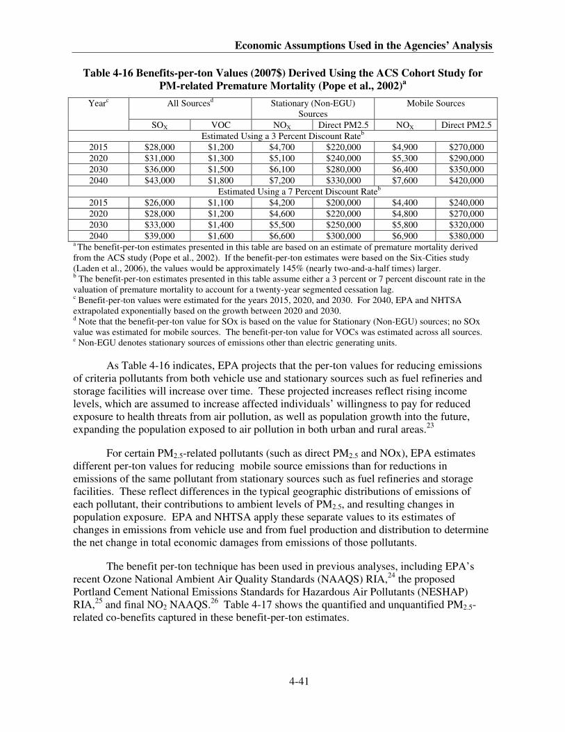
Economic Assumptions Used in the Agencies’ Analysis
4-41
Table 4-16 Benefits-per-ton Values (2007$) Derived Using the ACS Cohort Study for
PM-related Premature Mortality (Pope et al., 2002)a
All Sourcesd
Stationary (Non-EGU)
Sources
Mobile Sources Yearc
SOX VOC NOX Direct PM2.5 NOX Direct PM2.5
Estimated Using a 3 Percent Discount Rateb
2015 $28,000 $1,200 $4,700 $220,000 $4,900 $270,000
2020 $31,000 $1,300 $5,100 $240,000 $5,300 $290,000
2030 $36,000 $1,500 $6,100 $280,000 $6,400 $350,000
2040 $43,000 $1,800 $7,200 $330,000 $7,600 $420,000
Estimated Using a 7 Percent Discount Rateb
2015 $26,000 $1,100 $4,200 $200,000 $4,400 $240,000
2020 $28,000 $1,200 $4,600 $220,000 $4,800 $270,000
2030 $33,000 $1,400 $5,500 $250,000 $5,800 $320,000
2040 $39,000 $1,600 $6,600 $300,000 $6,900 $380,000 a The benefit-per-ton estimates presented in this table are based on an estimate of premature mortality derived
from the ACS study (Pope et al., 2002). If the benefit-per-ton estimates were based on the Six-Cities study
(Laden et al., 2006), the values would be approximately 145% (nearly two-and-a-half times) larger. b The benefit-per-ton estimates presented in this table assume either a 3 percent or 7 percent discount rate in the
valuation of premature mortality to account for a twenty-year segmented cessation lag. c Benefit-per-ton values were estimated for the years 2015, 2020, and 2030. For 2040, EPA and NHTSA
extrapolated exponentially based on the growth between 2020 and 2030. d Note that the benefit-per-ton value for SOx is based on the value for Stationary (Non-EGU) sources; no SOx
value was estimated for mobile sources. The benefit-per-ton value for VOCs was estimated across all sources. e Non-EGU denotes stationary sources of emissions other than electric generating units.
As Table 4-16 indicates, EPA projects that the per-ton values for reducing emissions
of criteria pollutants from both vehicle use and stationary sources such as fuel refineries and
storage facilities will increase over time. These projected increases reflect rising income
levels, which are assumed to increase affected individuals’ willingness to pay for reduced
exposure to health threats from air pollution, as well as population growth into the future,
expanding the population exposed to air pollution in both urban and rural areas.23
For certain PM2.5-related pollutants (such as direct PM2.5 and NOx), EPA estimates
different per-ton values for reducing mobile source emissions than for reductions in
emissions of the same pollutant from stationary sources such as fuel refineries and storage
facilities. These reflect differences in the typical geographic distributions of emissions of
each pollutant, their contributions to ambient levels of PM2.5, and resulting changes in
population exposure. EPA and NHTSA apply these separate values to its estimates of
changes in emissions from vehicle use and from fuel production and distribution to determine
the net change in total economic damages from emissions of those pollutants.
The benefit per-ton technique has been used in previous analyses, including EPA’s
recent Ozone National Ambient Air Quality Standards (NAAQS) RIA,24
the proposed
Portland Cement National Emissions Standards for Hazardous Air Pollutants (NESHAP)
RIA,25
and final NO2 NAAQS.26
Table 4-17 shows the quantified and unquantified PM2.5-
related co-benefits captured in these benefit-per-ton estimates.
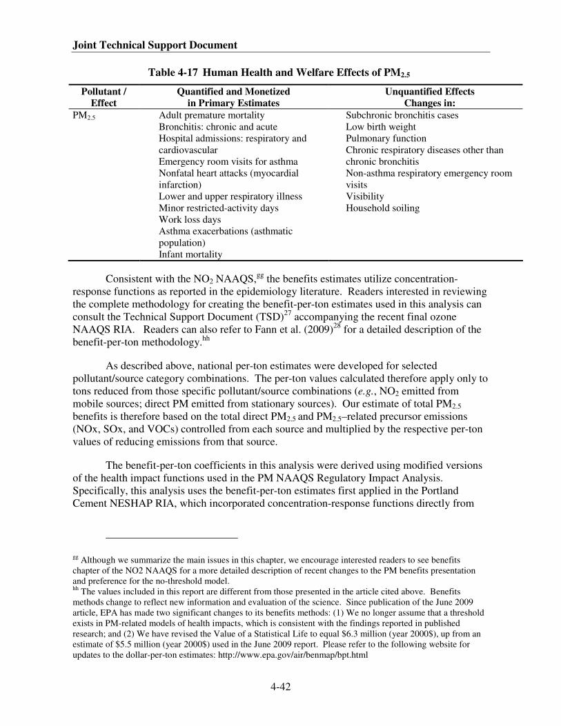
Joint Technical Support Document
4-42
Table 4-17 Human Health and Welfare Effects of PM2.5
Pollutant /
Effect
Quantified and Monetized
in Primary Estimates
Unquantified Effects
Changes in:
PM2.5 Adult premature mortality
Bronchitis: chronic and acute
Hospital admissions: respiratory and
cardiovascular
Emergency room visits for asthma
Nonfatal heart attacks (myocardial
infarction)
Lower and upper respiratory illness
Minor restricted-activity days
Work loss days
Asthma exacerbations (asthmatic
population)
Infant mortality
Subchronic bronchitis cases
Low birth weight
Pulmonary function
Chronic respiratory diseases other than
chronic bronchitis
Non-asthma respiratory emergency room
visits
Visibility
Household soiling
Consistent with the NO2 NAAQS,gg
the benefits estimates utilize concentration-
response functions as reported in the epidemiology literature. Readers interested in reviewing
the complete methodology for creating the benefit-per-ton estimates used in this analysis can
consult the Technical Support Document (TSD)27
accompanying the recent final ozone
NAAQS RIA. Readers can also refer to Fann et al. (2009)28
for a detailed description of the
benefit-per-ton methodology.hh
As described above, national per-ton estimates were developed for selected
pollutant/source category combinations. The per-ton values calculated therefore apply only to
tons reduced from those specific pollutant/source combinations (e.g., NO2 emitted from
mobile sources; direct PM emitted from stationary sources). Our estimate of total PM2.5
benefits is therefore based on the total direct PM2.5 and PM2.5–related precursor emissions
(NOx, SOx, and VOCs) controlled from each source and multiplied by the respective per-ton
values of reducing emissions from that source.
The benefit-per-ton coefficients in this analysis were derived using modified versions
of the health impact functions used in the PM NAAQS Regulatory Impact Analysis.
Specifically, this analysis uses the benefit-per-ton estimates first applied in the Portland
Cement NESHAP RIA, which incorporated concentration-response functions directly from
gg Although we summarize the main issues in this chapter, we encourage interested readers to see benefits
chapter of the NO2 NAAQS for a more detailed description of recent changes to the PM benefits presentation
and preference for the no-threshold model. hh
The values included in this report are different from those presented in the article cited above. Benefits
methods change to reflect new information and evaluation of the science. Since publication of the June 2009
article, EPA has made two significant changes to its benefits methods: (1) We no longer assume that a threshold
exists in PM-related models of health impacts, which is consistent with the findings reported in published
research; and (2) We have revised the Value of a Statistical Life to equal $6.3 million (year 2000$), up from an
estimate of $5.5 million (year 2000$) used in the June 2009 report. Please refer to the following website for
updates to the dollar-per-ton estimates: http://www.epa.gov/air/benmap/bpt.html
Economic Assumptions Used in the Agencies’ Analysis
4-43
the epidemiology studies, without any adjustment for an assumed threshold. Removing the
threshold assumption is a key difference between the method used in this analysis to estimate
PM co-benefits and the methods used in analyses prior to EPA’s Portland Cement NESHAP.
As a consequence, the benefit-per-ton estimates used in this analysis include incremental
benefits of reductions in PM2.5 concentrations down to their lowest modeled levels.
Reductions in PM-related mortality provide the majority of the monetized value in
each benefit-per-ton estimate. Typically, the premature mortality-related effect coefficients
that underlie the benefits-per-ton estimates are drawn from epidemiology studies that examine
two large population cohorts: the American Cancer Society cohort (Pope et al., 2002)29
and
the Harvard Six Cities cohort (Laden et al., 2006).30
The concentration-response (C-R)
function developed from the extended analysis of American Cancer Society (ACS) cohort, as
reported in Pope et al. (2002), has previously been used by EPA to generate its primary
benefits estimate. The extended analysis of the Harvard Six Cities cohort, as reported by
Laden et al (2006), was published after the completion of the Staff Paper for the 2006 PM2.5
NAAQS and has been used as an alternative estimate in the PM2.5 NAAQS RIA and PM2.5 co-
benefits estimates in analyses completed since the PM2.5 NAAQS.
These studies provide logical choices for anchor points when presenting PM-related
benefits because, while both studies are well designed and peer-reviewed, there are strengths
and weaknesses inherent in each. Although this argues for using both studies to generate
benefits estimates, due to the analytical limitations associated with this analysis, EPA and
NHTSA have chosen to use the benefit-per-ton value derived from the ACS study. The
agencies note that benefits would be approximately 145 percent (or nearly two-and-a-half
times) larger if the per-ton benefit values based on the Harvard Six Cities were used instead.
As is the nature of benefits analyses, assumptions and methods evolve over time to
reflect the most current interpretation of the scientific and economic literature. For a period
of time (2004-2008), EPA’s Office of Air and Radiation (OAR) valued mortality risk
reductions using a value of statistical life (VSL) estimate derived from a limited analysis of
some of the available studies. OAR arrived at a VSL using a range of $1 million to $10
million (2000$) consistent with two meta-analyses of the wage-risk literature.
The $1 million value represented the lower end of the interquartile range from the
Mrozek and Taylor (2002)31
meta-analysis of 33 studies. The $10 million value represented
the upper end of the interquartile range from the Viscusi and Aldy (2003)32
meta-analysis of
43 studies. The mean estimate of $5.5 million (2000$) was also consistent with the mean
VSL of $5.4 million estimated in the Kochi et al. (2006)33
meta-analysis. However, the
Agency neither changed its official guidance on the use of VSL in rule-makings nor subjected
the interim estimate to a scientific peer-review process through the Science Advisory Board
(SAB) or other peer-review group.
Until updated guidance is available, EPA determined that a single, peer-reviewed
estimate applied consistently best reflects the SAB-EEAC advice it has received. Therefore,
Joint Technical Support Document
4-44
EPA has decided to apply the VSL that was vetted and endorsed by the SAB in the Guidelines
for Preparing Economic Analyses (U.S. EPA, 2000)34
while they continue efforts to update
their guidance on this issue.ii This approach calculates a mean value across VSL estimates
derived from 26 labor market and contingent valuation studies published between 1974 and
1991. The mean VSL across these studies is $6.3 million (2000$). The dollar-per-ton
estimates used in this analysis are based on this revised VSL.
The benefit-per-ton estimates are subject to a number of assumptions and
uncertainties.
a. They do not reflect local variability in population density, meteorology, exposure,
baseline health incidence rates, or other local factors that might lead to an
overestimate or underestimate of the actual benefits of controlling fine particulates in
specific locations. EPA conducted full-scale air quality modeling for the calendar year
analysis in an effort to capture this variability. Please refer to Chapter 7.2 of the RIA
for a description of EPA’s air quality modeling results and to Chapter 7.3 for the
description of the agency’s quantification and monetization of PM- and ozone-related
health impacts for the FRM.
b. This analysis assumes that all fine particles, regardless of their chemical composition,
are equally potent in causing premature mortality. This is an important assumption,
because PM2.5 produced via transported precursors emitted from stationary sources
may differ significantly from direct PM2.5 released from engines and other industrial
sources. At the present time, however, no clear scientific grounds exist for supporting
differential effects estimates by particle type.
c. This analysis assumes that the health impact function for fine particles is linear within
the range of ambient concentrations under consideration. Thus, the estimates include
health benefits from reducing fine particles in areas with varied initial concentrations
of PM2.5, including both regions that are in attainment with fine particle standard and
those that do not meet the standard, down to the lowest modeled concentrations.
d. There are several health benefits categories that EPA and NHTSA were unable to
quantify due to limitations associated with using benefits-per-ton estimates, several of
which could be substantial. Because NOX and VOC emissions are also precursors to
ozone, changes in NOX and VOC would also impact ozone formation and the health
effects associated with ozone exposure. Benefits-per-ton estimates for ozone do not
exist due to issues associated with the complexity of the atmospheric air chemistry and
nonlinearities associated with ozone formation. The PM-related benefits-per-ton
estimates also do not include any human welfare or ecological benefits. Please refer to
Chapter 7.3 of the RIA for a description of the quantification and monetization of both
PM- and ozone-related health impacts for the FRM and a description of the
unquantified co-pollutant benefits associated with this rulemaking.
ii In the (draft) update of the Economic Guidelines (U.S. EPA, 2008c), EPA retained the VSL endorsed by the
SAB with the understanding that further updates to the mortality risk valuation guidance would be forthcoming
in the near future. Therefore, this report does not represent final agency policy. The draft update of the
Economic Guidelines is available on the Internet at <http://yosemite.epa.gov/ee/epa/eermfile.nsf/vwAN/EE-
0516-01.pdf/$File/EE-0516-01.pdf>.
Economic Assumptions Used in the Agencies’ Analysis
4-45
As mentioned above, emissions changes and benefits-per-ton estimates alone are not a
good indication of local or regional air quality and health impacts, as the localized impacts
associated with the rulemaking may vary significantly. Additionally, the atmospheric
chemistry related to ambient concentrations of PM2.5, ozone and air toxics is very complex.
Full-scale photochemical modeling is therefore necessary to provide the needed spatial and
temporal detail to more completely and accurately estimate the changes in ambient levels of
these pollutants and their associated health and welfare impacts. For the final rule, EPA
conducted a national-scale air quality modeling analysis in 2030 to analyze the impacts of the
standards on PM2.5, ozone, and selected air toxics.
4.2.9 Reductions in emissions of greenhouse gases
Emissions of carbon dioxide and other greenhouse gases (GHGs) occur throughout the
process of producing and distributing transportation fuels, as well as from fuel combustion
itself. By reducing the volume of fuel consumed by passenger cars and light trucks, higher
fuel efficiency standards will thus reduce GHG emissions generated by fuel use, as well as
throughout the fuel supply cycle. Lowering these emissions is likely to slow the projected
pace and reduce the ultimate extent of future changes in the global climate, thus reducing
future economic damages that changes in the global climate are otherwise expected to cause.
Further, by reducing the probability that climate changes with potentially catastrophic
economic or environmental impacts will occur, lowering GHG emissions may also result in
economic benefits that exceed the resulting reduction in the expected future economic costs
caused by gradual changes in the earth’s climatic systems. Quantifying and monetizing
benefits from reducing GHG emissions is thus an important step in estimating the total
economic benefits likely to result from establishing improved fuel efficiency and GHG
standards.
4.2.9.1 Estimating reductions in GHG emissions
The agencies estimated emissions of carbon dioxide (CO2) from passenger car and
light truck use by multiplying the number of gallons of each type of fuel (gasoline and diesel)
they are projected to consume with each alternative CAFE standard in effect by the quantity
or mass of CO2 emissions released per gallon of fuel consumed. This calculation assumes
that the entire carbon content of each fuel is ultimately converted to CO2 emissions during the
combustion process. The weighted average CO2 content of gasoline is estimated to be
approximately 8,900 grams per gallon, while that of diesel fuel is estimated to be
approximately 10,200 grams per gallon. For details, please see EPA’s RIA and NHTSA’s
RIA.
Although carbon dioxide emissions account for nearly 95 percent of total GHG
emissions that result from fuel combustion during vehicle use, emissions of other GHGs are
potentially significant as well because of their higher “potency” as GHGs than that of CO2
itself. EPA and NHTSA estimated the increases in emissions of methane (CH4) and nitrous
oxide (N2O) from additional vehicle use by multiplying the increase in total miles driven by
cars and light trucks of each model year and age by emission rates per vehicle-mile for these
GHGs. These emission rates, which differ between cars and light trucks as well as between
gasoline and diesel vehicles, were estimated by EPA using its recently-developed Motor
Joint Technical Support Document
4-46
Vehicle Emission Simulator (Draft MOVES 2009), as subsequently updated for use in this
analysis.
The MOVES model assumes that the per-mile rates at which cars and light trucks emit
these GHGs are determined by the efficiency of fuel combustion during engine operation and
chemical reactions that occur during catalytic after-treatment of engine exhaust, and are thus
independent of vehicles’ fuel consumption rates. Thus MOVES emission factors for these
GHGs, which are expressed per mile of vehicle travel, are assumed to be unaffected by
changes in fuel economy.
Increases in emissions of non-CO2 GHGs are converted to equivalent increases in CO2
emissions using estimates of the Global Warming Potential (GWP) of methane and nitrous
oxide. These GWPs are one way of accounting for the higher radiative forcing capacity and
differing lifetimes of methane and nitrous oxide when they are released into the earth’s
atmosphere, measured relative to that of CO2 itself. Because these gases differ in atmospheric
lifetimes, their relative damages are not constant over time. Impacts other than temperature
change also vary across gases in ways that are not captured by GWP. For instance, CO2
emissions, unlike methane and other greenhouse gases, contribute to ocean acidification.
Methane contributes to health and ecosystem effects arising from increases in tropospheric
ozone, while damages from methane emissions are not offset by the positive effect of CO2
fertilization. Noting these caveats, the CO2 equivalents of increases in emissions of these
gases are then added to the increases in emissions of CO2 itself to summarize the effect of the
total increase in CO2-equivalent GHG emissions from vehicle use. However, only the CO2
emissions were monetized for purposes of valuing benefits of the rule.
4.2.9.2 Economic benefits from reducing GHG emissions
NHTSA and EPA have taken the economic benefits of reducing CO2 emission into
account in this rulemaking, both in developing alternative CAFE standards and in assessing
the economic benefits of each alternative that was considered. Specifically, EPA and NHTSA
assigned a dollar value to reductions in CO2 emissions using the marginal dollar value (i.e.,
cost) of climate-related damages resulting from carbon emissions, also referred to as “social
cost of carbon” (SCC). The SCC is intended to measure the monetary value society places on
impacts resulting from increased GHGs, such as property damage from sea level rise, forced
migration due to dry land loss, and mortality changes associated with vector-borne diseases.
Published estimates of the SCC vary widely as a result of uncertainties about future economic
growth, climate sensitivity to GHG emissions, procedures used to model the economic
impacts of climate change, and the choice of discount rates.
EPA and NHTSA developed new SCC estimates through an interagency modeling
exercise. The modeling exercise involved running three integrated assessment models using
inputs agreed upon by the interagency group for climate sensitivity, socioeconomic and
emissions trajectories, and discount rates. A more complete discussion of SCC, including the
revised estimates and underlying methodology, can be found in the SCC TSD, Social Cost of
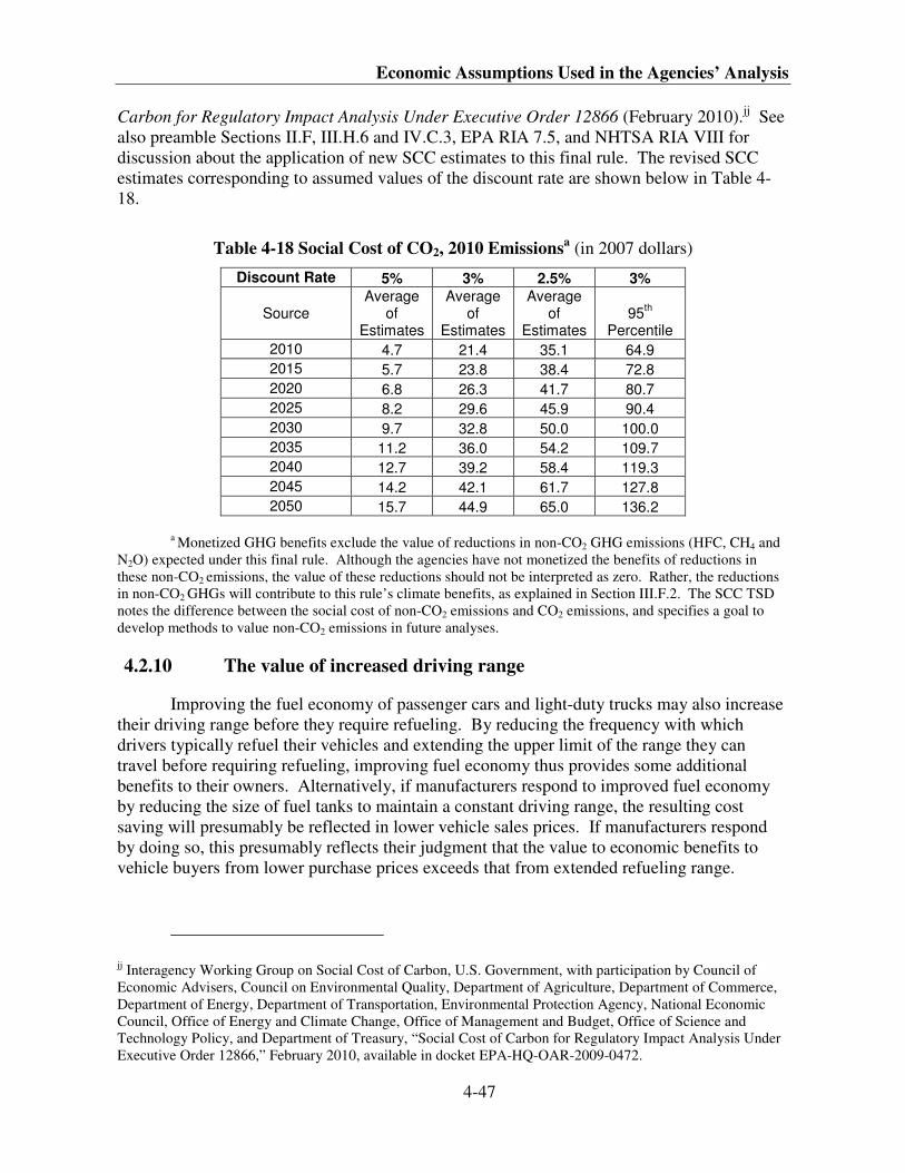
Economic Assumptions Used in the Agencies’ Analysis
4-47
Carbon for Regulatory Impact Analysis Under Executive Order 12866 (February 2010).jj See
also preamble Sections II.F, III.H.6 and IV.C.3, EPA RIA 7.5, and NHTSA RIA VIII for
discussion about the application of new SCC estimates to this final rule. The revised SCC
estimates corresponding to assumed values of the discount rate are shown below in Table 4-
18.
Table 4-18 Social Cost of CO2, 2010 Emissionsa (in 2007 dollars)
Discount Rate 5% 3% 2.5% 3%
Source Average
of Estimates
Average of
Estimates
Average of
Estimates 95
th
Percentile
2010 4.7 21.4 35.1 64.9
2015 5.7 23.8 38.4 72.8
2020 6.8 26.3 41.7 80.7
2025 8.2 29.6 45.9 90.4
2030 9.7 32.8 50.0 100.0
2035 11.2 36.0 54.2 109.7
2040 12.7 39.2 58.4 119.3
2045 14.2 42.1 61.7 127.8
2050 15.7 44.9 65.0 136.2
a Monetized GHG benefits exclude the value of reductions in non-CO2 GHG emissions (HFC, CH4 and
N2O) expected under this final rule. Although the agencies have not monetized the benefits of reductions in
these non-CO2 emissions, the value of these reductions should not be interpreted as zero. Rather, the reductions
in non-CO2 GHGs will contribute to this rule’s climate benefits, as explained in Section III.F.2. The SCC TSD
notes the difference between the social cost of non-CO2 emissions and CO2 emissions, and specifies a goal to
develop methods to value non-CO2 emissions in future analyses.
4.2.10 The value of increased driving range
Improving the fuel economy of passenger cars and light-duty trucks may also increase
their driving range before they require refueling. By reducing the frequency with which
drivers typically refuel their vehicles and extending the upper limit of the range they can
travel before requiring refueling, improving fuel economy thus provides some additional
benefits to their owners. Alternatively, if manufacturers respond to improved fuel economy
by reducing the size of fuel tanks to maintain a constant driving range, the resulting cost
saving will presumably be reflected in lower vehicle sales prices. If manufacturers respond
by doing so, this presumably reflects their judgment that the value to economic benefits to
vehicle buyers from lower purchase prices exceeds that from extended refueling range.
jj Interagency Working Group on Social Cost of Carbon, U.S. Government, with participation by Council of
Economic Advisers, Council on Environmental Quality, Department of Agriculture, Department of Commerce,
Department of Energy, Department of Transportation, Environmental Protection Agency, National Economic
Council, Office of Energy and Climate Change, Office of Management and Budget, Office of Science and
Technology Policy, and Department of Treasury, “Social Cost of Carbon for Regulatory Impact Analysis Under
Executive Order 12866,” February 2010, available in docket EPA-HQ-OAR-2009-0472.
Joint Technical Support Document
4-48
No direct estimates of the value of extended vehicle range are readily available, so the
agencies’ analyses calculate the reduction in the annual number of required refueling cycles
that results from improved fuel economy, and applies DOT-recommended values of travel
time savings to convert the resulting time savings to their economic value.35 As a coarse
illustration of how the value of extended refueling range is estimated, a typical small light
truck model has an average fuel tank size of approximately 20 gallons.kk
Based on a
California Air Resources Board Study, the average fuel purchase is approximately 55% of
tank volume.36
Therefore, increasing this model’s actual on-road fuel economy from 24 to 25
mpg would extend its driving range from 216 miles (= 9 gallons x 24 mpg) to 225 miles (= 9
gallons x 25 mpg). Assuming that this vehicle is driven 12,000 miles/year, this reduces the
number of times it needs to be refueled each year from 55.5 (= 12,000 miles per year / 216
miles per refueling) to 53.3 (= 12,000 miles per year / 225 miles per refueling), or by 2.2
refuelings per year.
Weighted by the nationwide mix of urban (about 2/3) and rural (about 1/3) driving and
average vehicle occupancy for all driving trips (1.6 persons), the DOT-recommended value of
travel time per vehicle-hour is $24.00 (in 2006 dollars).ll Assuming that locating a station and
filling up requires five minutes, the annual value of time saved as a result of less frequent
refueling amounts to $4.40 (calculated as 5/60 x 2.2 x $24.00). This calculation is repeated
for each future calendar year that light trucks of each model year affected by the alternative
fuel economy standards considered in this rule would remain in service. Like fuel savings
and other benefits, however, the value of this benefit declines over a model year’s lifetime,
because a smaller number of vehicles originally produced during that model year remain in
service each year, and those remaining in service are driven fewer miles. The detailed values
used in this calculation by each agency are available in EPA’s RIA and NHTSA’s FRIA
respectively.
The agencies’ estimate of benefits from less frequent refueling is subject to several
sources of uncertainty. First, this analysis assumes that manufacturers will not adjust fuel tank
capacities downward (from the current average of 19.3 gallons) when they improve the fuel
economy of their vehicle models, so that the entire increase in fuel economy will be reflected
in increased driving range.
Should manufacturers choose to downsize fuel tanks, and all other factors have been
estimated with no error, the current estimates of refueling benefits would be overstated.
Should manufacturers downsize tanks to fully offset any increase in vehicle range, there
would be no extension in driving range and no resultant benefit to consumers. However,
kk Based on the Volpe Model Market Data file for Model Year 2011, average tank volumes for cars and trucks
are 16.6 gallons and 23.0 gallons, respectively. This produces a production weighted average of 19.3 gallons. ll The hourly wage rate during 2006 is estimated to be $24.00. Personal travel (94.4 percent of urban travel) is
valued at 50 percent of the hourly wage rate. Business travel (5.6 percent of urban travel) is valued at 100
percent of the hourly wage rate. For intercity travel, personal travel (87 percent) is valued at 70 percent of the
wage rate, while business travel (13 percent) is valued at 100 percent of the wage rate. The resulting values of
travel time are $12.67 for urban travel and $17.66 for intercity travel, and must be multiplied by vehicle
occupancy (1.6) to obtain the estimate value of time per vehicle hour.
Economic Assumptions Used in the Agencies’ Analysis
4-49
should fuel tank sizes be reduced, vehicle space, utility and value would increase and vehicle
weight and production costs would decrease, improving fuel economy and CO2 emissions.
A larger fuel tank size requires additional manufacturing costs (if for nothing more
than increased materials or increased molding costs to squeeze more tank volume in unusually
shaped spaces underbody), adds weight (thus, reduces fuel economy and increases CO2
emissions) and takes up potentially usable vehicle space. It also increases vehicle range (a
widely advertised vehicle attribute), which reduces the frequency of vehicle refueling for at
least some owners and (less frequently) increases peace of mind when operating a vehicle in
areas with limited refueling options. Given this clear trade-off, manufacturers must use some
type of optimization schema to determine the appropriate tank size for each vehicle. If
manufacturers choose to retain the current fuel tank size, then the impact on manufacturing
costs is obvious: zero. At least some portion of the driving public will save a considerable
amount of time with some value. Given range is a widely publicized vehicle attribute,
manufacturers will only reduce tank size if it lowers production costs sufficiently to overcome
the loss in vehicle desirability. Thus, either consumers save time or production costs go
down. Much as the agencies assume that cost increases are passed through to consumers, the
agencies assume that cost savings from reducing fuel tank size (by reducing engineering
complexity and materials required) would be passed through to consumers.
Further, the agencies assume that manufacturers operate in a manner that maintains or
increases the desirability of a vehicle. Consequently, should a manufacturer choose to reduce
fuel tank size, this option should provide welfare gains equivalent to or greater than the loss in
welfare from reducing driving range. In the context of the rule, the improvement in CO2 or
fuel economy from downsizing a fuel tank will additionally decrease a manufacturers cost of
compliance with the standards. The weight reduction estimates modeled in OMEGA and the
CAFE Model do not include any reduction in the size and weight of fuel tanks, excluding
potential light weight materials substitution which would not affect fuel volume, thus this
benefit has not been counted elsewhere.
Second, the agencies’ analysis assumes that fuel purchases average 55 percent of fuel
tank capacity. However, as shown in the California Air Resource Board (CARB) report,
refueling patterns vary. Moreover, the 55 percent estimate implies that drivers, on average,
are either refueling when nearly a half tank of gas remains in their vehicles, or that they are
habitually not filling their tanks. Since many drivers only refuel when their tanks are very
low, and since many drivers habitually refuel, this in turn implies that many drivers in the
CARB study are refueling when their tanks are still well above 50 percent full. While based
on field data, this estimate may thus overestimate the impact of refueling benefits.
For the primary analysis in both the proposal and this final rulemaking, the agencies
assume that 100 percent of all refueling is demand-based; i.e., that every gallon of fuel which
is saved would reduce the need to return to the refueling station. Based on anecdotal
evidence, this value is potentially an overestimate. As an example, some people may refuel
every Sunday morning at the same time as they buy their newspaper and chewing gum.
Barring unusually long trips, these people would not benefit from an increased driving range.
Joint Technical Support Document
4-50
In order to understand how sensitive the overall estimate of the refueling benefit is to
this specific input, we provide the following example. If 25 percent of gallons are refueled on
a habitual rather than demand-based schedule, and the rest of the assumptions remain
constant, the value of increased driving range decreases by 25 percent. There would be no
value of increased driving range derived from these gallons. Returning to the example light
truck discussed above, which generated a value of increased driving range worth $4.40 in the
first year, if this owner refilled ¼ of his annual fuel on a habitual rather than demand based
schedule, the value of increased driving range would decrease to $3.30. Unfortunately, the
agencies do not have a basis for this 25 percent value, thus this example is for illustrative
purposes only. However, as noted below, DOT is undertaking a new survey which may
provide a data-based basis for revising our 100 percent assumption for future analysis.
Third, the agencies’ estimate of refueling benefits assumes that refueling stops involve
the same number of vehicle occupants as the overall average for all vehicle trips (1.6 persons).
To the extent that drivers refuel while doing other errands or in advance of picking up
passengers, this figure may overestimate the typical vehicle occupancy during refueling, and
thus the total savings in refueling time. Similarly, the hourly value used to estimate the
economic value of savings in refueling time reflects the typical mix of personal and business
travel purposes, and drivers are likely to assign different values to their time when traveling
for these different purposes. To the extent that drivers seek to refuel when traveling for
purposes that typically use less valuable time, the hourly value used in the agencies’ analysis
may overstate the benefits from saving refueling time.
Finally, the agencies assume that both finding and using a refueling station takes, on
average, five minutes. There are few, if any, data sources on average refueling time, and this
estimate is subject to significant uncertainty.
For these reasons, the agencies’ estimate of savings in refueling time is uncertain. To
reduce the uncertainty, a new project is being planned by DOT which will include a detailed
study of refueling events, using a random sample of refueling stations across the U.S. It is
projected to include ~7,000 observations (time to refuel, # gallons refueled, etc.) and ~5,000
surveys of refueling participants. The agencies anticipate that this will provide a robust data
set on which to revise many of the key inputs to the refueling benefit calculation. Some of the
specific data categories which will be surveyed are listed below:
• Miles driven and time out of way to get to gas station
• Fuel gage level before and after refueling
• # gallons purchased
• # people in vehicle, above and below 16 years old
• Reasons for travel
• Reason for stopping at gas station (e.g., fuel level too low, or other)
While the study results are not available in time for this final rulemaking, it is
anticipated that the data will improve future estimations of the value of increased driving
range.
Economic Assumptions Used in the Agencies’ Analysis
4-51
4.2.11 Discounting future benefits and costs
Discounting future fuel savings and other benefits is intended to account for the
reduction in their value to society when they are deferred until some future date, rather than
received immediately. The discount rate expresses the percent decline in the value of these
benefits – as viewed from current perspective – for each year they are deferred into the future.
In evaluating the benefits from alternative increases in fuel economy and GHG standards for
MY 2012-2016 passenger cars and light trucks, EPA and NHTSA consider a discount rate of
both 3 and 7 percent per year.
Three percent may be the appropriate rate for discounting future benefits from
increased fuel economy and GHG standards because most or all of vehicle manufacturers’
costs for complying with improved fuel economy and GHG standards are likely to be
reflected in higher sales prices for their new vehicle models. By increasing sales prices for
new cars and light trucks, CAFE regulation will thus primarily affect vehicle purchases and
other private consumption decisions.
Both economic theory and OMB guidance on discounting indicate that the future
benefits and costs of regulations that mainly affect private consumption should be discounted
at the consumption rate of time preference.37
OMB guidance indicates that savers appear to
discount future consumption at an average real (that is, adjusted to remove the effect of
inflation) rate of about 3 percent when they face little risk about its likely level, which makes
it a reasonable estimate of the consumption rate of time preference.38
Thus EPA and NHTSA
have employed the 3 percent rate to discount projected future benefits and costs resulting
from improved fuel economy and GHG standards for MY 2012-2016 passenger cars and light
trucks.
Because there is some uncertainty about the extent to which vehicle manufacturers
will be able to recover their costs for complying with improved fuel economy and GHG
standards by increasing vehicle sales prices, however, the use of a higher percent discount rate
may also be appropriate. OMB guidance indicates that the real economy-wide opportunity
cost of capital is the appropriate discount rate to apply to future benefits and costs when the
primary effect of a regulation is “…to displace or alter the use of capital in the private sector,”
and estimates that this rate currently averages about 7 percent.39
Thus the agencies estimate
net present values using both 3 and 7 percent discount rates.
One important exception to these values are the rates used to discount benefits from
reducing CO2 emissions from the years in which reduced emissions occur, which span the
lifetimes of model year 2012-16 cars and light trucks, to their present values. In order to
ensure consistency in the derivation and use of the interagency group’s estimates of the unit
values of reducing CO2 emissions, the total benefits from reducing those emissions during
each future year are discounted using the same rates that were used to derive the alternative
values of reducing each ton of CO2 emissions. As described previously in Section 4.2.10.2,
these rates are 2.5, 3.0, and 5.0 percent.
Joint Technical Support Document
4-52
References
1 EPA, Fuel Economy Labeling of Motor Vehicles: Revisions To Improve Calculation of Fuel Economy
Estimates; Final Rule, 40 CFR Parts 86 and 600, Federal Register, December 27, 2006, pp. 77872-77969,
http://www.epa.gov/fedrgstr/EPA-AIR/2006/December/Day-27/a9749.pdf.
2 EPA, Final Technical Support Document: Fuel Economy Labeling of Motor Vehicle Revisions to Improve
Calculation of Fuel Economy Estimates, Office of Transportation and Air Quality EPA420-R-06-017 December
2006, Chapter II, http://www.epa.gov/fueleconomy/420r06017.pdf.
3 Energy Information Administration, Annual Energy Outlook 2010, Early Release Reference Case (December
2009), Table 12. Available at http://www.eia.doe.gov/oiaf/servicerpt/stimulus/excel/aeostimtab_12.xls
4 Energy Information Administration, Annual Energy Outlook 2009, Revised Updated Reference Case (April
2009), Table 12. Available at http://www.eia.doe.gov/oiaf/servicerpt/stimulus/excel/aeostimtab_12.xls (last
accessed July 26, 2009). EIA’s Updated Reference Case reflects the effects of the American Reinvestment and
Recovery Act of 2009, as well as the most recent revisions to the U.S. and global economic outlook.
5 Kahan, A. and Pickrell D. “Energy Information Administration’s Annual Energy Outlook 2009 and 2010”
Memo to Docket EPA-HQ-OAR-2009-0472 and NHTSA–2009–0059.
6 http://www.eia.doe.gov/oiaf/aeo/forecast.html (last accessed July 26, 2009), and Table 16,
http://www.eia.doe.gov/oiaf/aeo/pdf/table16.pdf (last accessed July 26, 2009).
7 Lu, S., NHTSA, Regulatory Analysis and Evaluation Division, “Vehicle Survivability and Travel Mileage
Schedules,” DOT HS 809 952, 8-11 (January 2006). Available at http://www-nrd.nhtsa.dot.gov/pdf/nrd-
30/NCSA/Rpts/2006/809952.pdf (last accessed Feb. 15, 2010). These updated survival rates suggest that the
expected lifetimes of recent-model passenger cars and light trucks are 13.8 and 14.5 years.
8 FHWA, Highway Statistics, Summary to 1995, Table vm201at
http://www.fhwa.dot.gov/ohim/summary95/vm201a.xlw , and annual editions 1996-2005, Table VM-1 at
http://www.fhwa.dot.gov/policy/ohpi/hss/hsspubs.htm (last accessed Feb. 15, 2010).
9 Sorrell, S. and J. Dimitropoulos, 2007. “UKERC Review of Evidence for the Rebound Effect, Technical Report
2: Econometric Studies”, UKERC/WP/TPA/2007/010, UK Energy Research Centre, London, October and
Greening, L.A., D.L. Greene and C. Difiglio, 2000. “Energy Efficiency and Consumption – The Rebound Effect
– A Survey”, Energy Policy, vol. 28, pp. 389-401.
10 Greening et al. 2000.
11 Pickrell, D. and P. Schimek, 1999. “Growth in Motor Vehicle Ownership and Use: Evidence from the
Nationwide Personal Transportation Survey”, Journal of Transportation and Statistics, vol. 2, no. 1, pp. 1-17.
12 Small, K. and K. Van Dender, 2007a. “Fuel Efficiency and Motor Vehicle Travel: The Declining Rebound
Effect”, The Energy Journal, vol. 28, no. 1, pp. 25-51.
13 Small, K. and K. Van Dender, 2007b. "Long Run Trends in Transport Demand, Fuel Price Elasticities and
Implications of the Oil Outlook for Transport Policy," OECD/ITF Joint Transport Research Centre Discussion
Papers 2007/16, OECD, International Transport Forum.
14 Revised Report by David Greene of Oak Ridge National Laboratory to EPA,“Rebound 2007: Analysis of
National Light-Duty Vehicle Travel Statistics,” February 9, 2010 (Docket EPA-HQ-OAR-2009-0472-0220).
This paper has been accepted for an upcoming special issue of Energy Policy, although the publication date has
not yet been determined.
15 FHWA. 1997 Federal Highway Cost Allocation Study; http://www.fhwa.dot.gov/policy/hcas/final/index.htm
(last accessed July 29, 2009).
Economic Assumptions Used in the Agencies’ Analysis
4-53
16 Federal Highway Administration, 1997 Federal Highway Cost Allocation Study,
http://www.fhwa.dot.gov/policy/hcas/final/index.htm, Tables V-22, V-23, and V-24 (last accessed Feb. 15,
2010).
17 U.S. Bureau of Economic Analysis, U.S. International Transactions Accounts Data, as shown on June 24,
2009.
18 U.S. Department of Energy, Annual Energy Review 2008, Report No. DOE/EIA-0384(2008), Tables 5.1 and
5.13c, June 26, 2009.
19 Leiby, Paul N. "Estimating the Energy Security Benefits of Reduced U.S. Oil Imports," Oak Ridge National
Laboratory, ORNL/TM-2007/028, Final Report, 2008.
20 Peer Review Report Summary: Estimating the Energy Security Benefits of Reduced U.S. Oil Imports, ICF,
Inc., September 2007.
21 Gately, Dermot 2004. "OPEC's Incentives for Faster Output Growth," The Energy Journal, 25(2):75-96,
"What Oil Export Levels Should We Expect From OPEC?" The Energy Journal, 28(2):151-173, 2007 22
Argonne National Laboratories, The Greenhouse Gas and Regulated Emissions from Transportation (GREET)
Model, Version 1.8, June 2007, available at http://www.transportation.anl.gov/software/GREET/index.html
(last accessed April 20, 2008). 23
The issue is discussed in more detail in the PM NAAQS RIA from 2006. See U.S. Environmental Protection
Agency. 2006. Final Regulatory Impact Analysis (RIA) for the Proposed National Ambient Air Quality
Standards for Particulate Matter. Prepared by: Office of Air and Radiation. October 2006. Available at
http://www.epa.gov/ttn/ecas/ria.html.
24 U.S. Environmental Protection Agency (U.S. EPA). 2008. Regulatory Impact Analysis, 2008 National
Ambient Air Quality Standards for Ground-level Ozone, Chapter 6. Office of Air Quality Planning and
Standards, Research Triangle Park, NC. March. Available at <http://www.epa.gov/ttn/ecas/regdata/RIAs/6-
ozoneriachapter6.pdf>. EPA-HQ-OAR-2009-0472-0238
25 U.S. Environmental Protection Agency (U.S. EPA). 2009. Regulatory Impact Analysis: National Emission
Standards for Hazardous Air Pollutants from the Portland Cement Manufacturing Industry. Office of Air
Quality Planning and Standards, Research Triangle Park, NC. April. Available on the Internet at
<http://www.epa.gov/ttn/ecas/regdata/RIAs/portlandcementria_4-20-09.pdf>. EPA-HQ-OAR-2009-0472-0241
26 U.S. Environmental Protection Agency (U.S. EPA). 2010. Final NO2 NAAQS Regulatory Impact Analysis
(RIA). Office of Air Quality Planning and Standards, Research Triangle Park, NC. April. Available on the
Internet at http://www.epa.gov/ttn/ecas/regdata/RIAs/FinalNO2RIAfulldocument.pdf. Accessed March 15,
2010. EPA-HQ-OAR-2009-0472-0237
27 U.S. Environmental Protection Agency (U.S. EPA). 2008. Technical Support Document: Calculating Benefit
Per-Ton estimates, Ozone NAAQS Docket #EPA-HQ-OAR-2007-0225-0284. Office of Air Quality Planning
and Standards, Research Triangle Park, NC. March. Available on the Internet at <http://www.regulations.gov>.
EPA-HQ-OAR-2009-0472-0228 28
Fann, N. et al. (2009). The influence of location, source, and emission type in estimates of the human health
benefits of reducing a ton of air pollution. Air Qual Atmos Health. Published online: 09 June, 2009. EPA-HQ-
OAR-2009-0472-0229
29 Pope, C.A., III, R.T. Burnett, M.J. Thun, E.E. Calle, D. Krewski, K. Ito, and G.D. Thurston. 2002. “Lung
Cancer, Cardiopulmonary Mortality, and Long-term Exposure to Fine Particulate Air Pollution.” Journal of the
American Medical Association 287:1132-1141. EPA-HQ-OAR-2009-0472-0263
30 Laden, F., J. Schwartz, F.E. Speizer, and D.W. Dockery. 2006. “Reduction in Fine Particulate Air Pollution
and Mortality.” American Journal of Respiratory and Critical Care Medicine 173:667-672. Estimating the
Joint Technical Support Document
4-54
Public Health Benefits of Proposed Air Pollution Regulations. Washington, DC: The National Academies Press.
EPA-HQ-OAR-2009-0472-1661
31 Mrozek, J.R., and L.O. Taylor. 2002. “What Determines the Value of Life? A Meta-Analysis.” Journal of
Policy Analysis and Management 21(2):253-270. EPA-HQ-OAR-2009-0472-1677
32 Viscusi, V.K., and J.E. Aldy. 2003. “The Value of a Statistical Life: A Critical Review of Market Estimates
throughout the World.” Journal of Risk and Uncertainty 27(1):5-76. EPA-HQ-OAR-2009-0472-0245
33 Kochi, I., B. Hubbell, and R. Kramer. 2006. An Empirical Bayes Approach to Combining Estimates of the
Value of Statistical Life for Environmental Policy Analysis. Environmental and Resource Economics. 34: 385-
406. EPA-HQ-OAR-2009-0472-0235
34 U.S. Environmental Protection Agency (U.S. EPA). 2000. Guidelines for Preparing Economic Analyses.
EPA 240-R-00-003. National Center for Environmental Economics, Office of Policy Economics and
Innovation. Washington, DC. September. Available on the Internet at
<http://yosemite.epa.gov/ee/epa/eed.nsf/webpages/Guidelines.html/$file/cover.pdf>. EPA-HQ-OAR-2009-0472-
0226 35
See http://ostpxweb.dot.gov/policy/Data/VOT97guid.pdf and
http://ostpxweb.dot.gov/policy/Data/VOTrevision1_2-11-03.pdf
36 California Environmental Protection Agency, Air Resources Board. Draft Assessment of the Real-World
Impacts of Commingling California Phase 3 Reformulated Gasoline. August 2003
37 Id.
38 Office of Management and Budget, Circular A-4, “Regulatory Analysis,” September 17, 2003, 33. Available
at http://www.whitehouse.gov/omb/circulars/a004/a-4.pdf (last accessed July 24, 2009).
39 Id.


