arX

iv:1

505.

0317

0v1

[phy

sics

.che

m-p

h] 1

2 M

ay 2

015

Jost function description of near threshold resonances forcoupled-channel scattering

I. Simbotin, R. Cote∗

Department of Physics, University of Connecticut, 2152 Hillside Rd., Storrs, CT 06269, USA

Abstract

We study the effect of resonances near the threshold of low energy (ε) reactive scattering processes, and find an anomalous behaviorof thes-wave cross sections. For reaction and inelastic processes, the cross section exhibits the energy dependenceσ ∼ ε−3/2 insteadof the standard Wigner’s law threshold behaviorσ ∼ ε−1/2. Wigner’s law is still valid asε → 0, but in a narrow range of energies.We illustrate these effects with two reactive systems, a low-reactive system (H2 + Cl) and a more reactive one (H2 + F). Weprovide analytical expressions, and explain this anomalous behavior using the properties of the Jost functions. We also discuss theimplication of the reaction rate coefficients behaving asK ∼ 1/T at low temperatures, instead of the expected constant rate of theWigner regime in ultracold physics and chemistry.

Keywords: threshold resonances, ultracold chemistry, reactive scattering

1. Introduction

Ultracold gases allow a high level of control over the inter-action by using Feshbach resonances [1] or by orienting ultra-cold molecules [2, 3]. In addition to the study of phenomena indegenerate quantum gases ranging from the BEC-BCS cross-over regime to solitons and multi-component condensates [4,5], such control also permits the investigation of exotic three-body Efimov states [6]. In parallel, the rapid advances in form-ing cold molecules [7, 8, 9, 10, 11] have made possible studiesof cold chemical reactions [2, 12] and their control [13], withapplication to a growing range of fields, such as quantum in-formation processing [14, 15, 16]. A key ingredient for theseinvestigations are resonances near the scattering threshold. Al-though such resonances have been theoretically [17] and exper-imentally [18, 19, 20] explored in the chemistry of low temper-ature systems, their effect on reaction rates is however not fullytaken into account.

In this article, we investigate how reaction and inelasticprocesses are affected by near threshold resonances (NTR) inthe entrance channel of a reactive scattering system. We focusour attention on two benchmark systems containing hydrogen,namely H2+Cl and H2+F. We note that alkali hydrides [21], be-cause of their small mass, would also be interesting systemstoinvestigate. By varying the mass of H, explore the modifica-tion of the behavior of the reaction cross sectionσreact from theWigner’s threshold lawσreact ∝ ε−1/2 [22, 23] at ultralow en-ergyε. We generalize our initial treatment [24] of the effect ofresonances in low energy collisions originally analyzed innu-clear [25] and atomic [26] collisions, to include a multi-channelformalism using Jost functions.

∗Corresponding authorEmail address: rcote@phys.uconn.edu (R. Cote)

In Section 2, we review the general theory of reactive scat-tering and discuss the two benchmark systems H2+Cl and H2+F,and present the results of our calculations in Section 3 for bothsystems. In Section 4, we give an explanation of those resultsbased on the S-matrix, followed by an alternative descriptionbased on Jost functions in Section 5. Finally, we describe theequivalence of both approaches in Section 6 and give a simplephysical picture in Section 7, before concluding in Section8.

2. Reactive scattering at low energies

In this section, we review briefly the theory of low energyreactive scattering, and describe the two benchmark systemsthat we use to study the effect of s-wave near threshold reso-nances.

2.1. General theory

The scattering cross section from an initial internal statei toa final statef is given by [27]

σ f←i(εi) =π

k2i

∞∑

J=0

(

2J + 12 j + 1

)

∑

ℓ

∑

ℓ′

∣

∣

∣δ f i − S Jf i

∣

∣

∣

2, (1)

where ℓ = |J − j|, . . . , J + j and ℓ′ = |J − j′|, . . . , J + j′;J = j+ℓ = j′+ℓ′ is the total angular momentum, with molecu-lar rotational momentumj and orbital angularℓ in the entrancechanneli, and corresponding quantum numbersJ, j, andℓ (theprimes indicate the exit channelf ). Here,εi = ~

2k2i /2µ is the

kinetic energy with respect to the entrance channel threshold, ki

the wave number, andµ−1= m−1

H2+m−1

A the reduced mass in theentrance arrangement (with A standing for Cl or F). We are fo-cusing on the effect of resonances at ultralow temperatures, andso consider onlys-wave scattering withℓ = 0, which requiresJ = j and thus (2J + 1)/(2 j + 1) = 1. In addition, we limit

Preprint submitted to Chemical Physics May 14, 2015

ourselves to molecules initially in their rotational ground state( j = 0), such that we only need considerJ = 0; consequently,the sum

∑

ℓ′ in (1) reduces to a single term:ℓ′ = j′. Hence,equation (1) simplifies significantly, and it now reads:

σ f←i(εi) =π

k2i

∣

∣

∣δ f i − S J=0f i (ki)

∣

∣

∣

2. (2)

It is well known [28] that in the zero-energy limit the crosssections can be expressed in terms of the complex scatteringlengthai = αi − iβi,

σreacti (ε) ≡

∑

f,i

σ f←i(ε) → 4πβi

k,

σelasti (ε) ≡ σi←i(ε) → 4π(α2

i + β2i ).

(3)

We obtain energy dependent rate coefficients by multiplying thecross sections with the relative velocityvrel = ~k/µ,

Kreacti (ε) ≡ ~k

µ

∑

f,i

σ f←i(ε) → 4π~µβi,

Kelasti (ε) ≡ ~k

µσi←i(ε) → 4π~k

µ(α2

i + β2i ),

(4)

which can be thermally averaged over a Maxwellian velocitydistribution to yield the true rate constantK(T ). Note that thesum

∑

f,i in Eqs. (3) and (4) includes all possible final states,i.e., both reaction channels to form the products and quenching(inelastic) channels for the reactant. Thus,σreact andKreact de-fined above include all non-elastic outcomes of the scatteringprocess, i.e., reaction plus quenching. We shall simplify ournotation by omitting the channel subscripti (for εi, ki, αi, βi,etc.) and we also omit the superscriptJ in S J

f i throughout theremainder of this article.

0.4

0.6

0.8

1.0

1.2

Ene

rgy

(eV

)

HCl H2

barr

ier

Cl + H2(v=1, j=0)

v=0

v=1

v=2

v=0

v=1

j=02

4

6

8

j=02

4

6

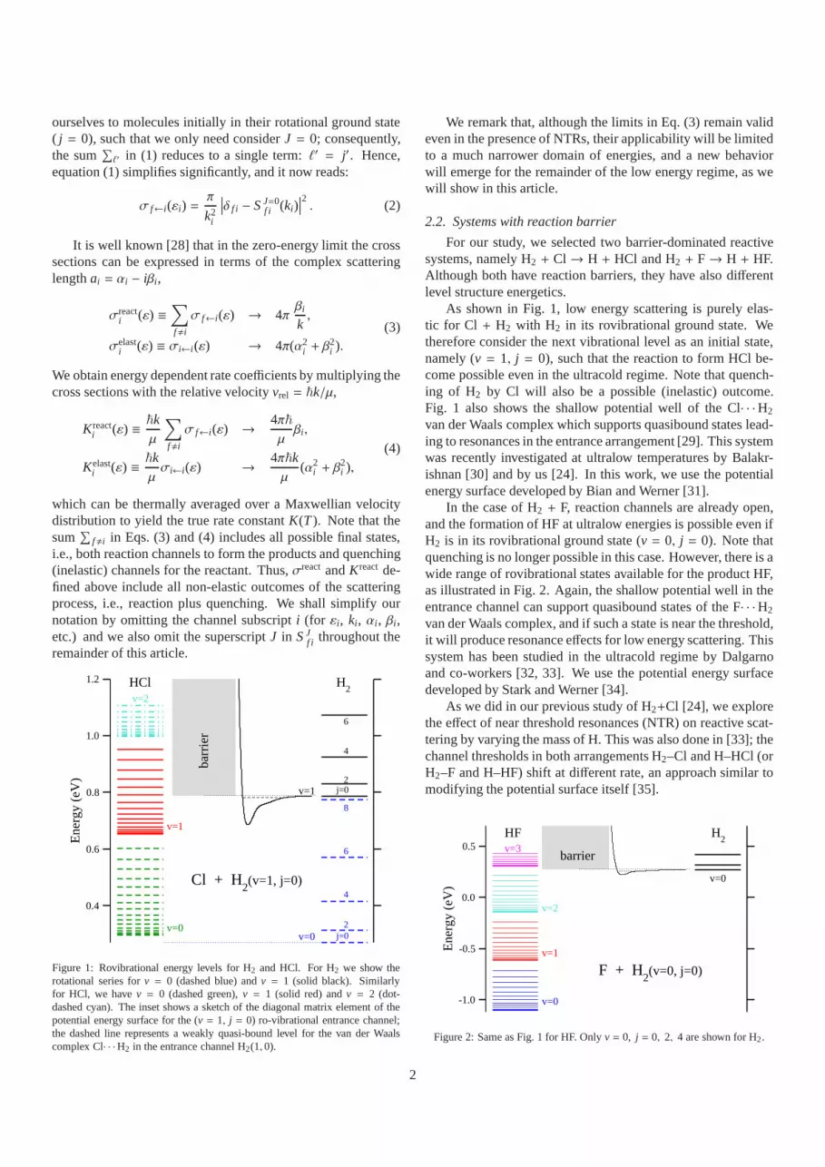
Figure 1: Rovibrational energy levels for H2 and HCl. For H2 we show therotational series forv = 0 (dashed blue) andv = 1 (solid black). Similarlyfor HCl, we havev = 0 (dashed green),v = 1 (solid red) andv = 2 (dot-dashed cyan). The inset shows a sketch of the diagonal matrixelement of thepotential energy surface for the (v = 1, j = 0) ro-vibrational entrance channel;the dashed line represents a weakly quasi-bound level for the van der Waalscomplex Cl· · ·H2 in the entrance channel H2(1, 0).

We remark that, although the limits in Eq. (3) remain valideven in the presence of NTRs, their applicability will be limitedto a much narrower domain of energies, and a new behaviorwill emerge for the remainder of the low energy regime, as wewill show in this article.

2.2. Systems with reaction barrier

For our study, we selected two barrier-dominated reactivesystems, namely H2 + Cl→ H + HCl and H2 + F→ H + HF.Although both have reaction barriers, they have also differentlevel structure energetics.

As shown in Fig. 1, low energy scattering is purely elas-tic for Cl + H2 with H2 in its rovibrational ground state. Wetherefore consider the next vibrational level as an initialstate,namely (v = 1, j = 0), such that the reaction to form HCl be-come possible even in the ultracold regime. Note that quench-ing of H2 by Cl will also be a possible (inelastic) outcome.Fig. 1 also shows the shallow potential well of the Cl· · ·H2

van der Waals complex which supports quasibound states lead-ing to resonances in the entrance arrangement [29]. This systemwas recently investigated at ultralow temperatures by Balakr-ishnan [30] and by us [24]. In this work, we use the potentialenergy surface developed by Bian and Werner [31].

In the case of H2 + F, reaction channels are already open,and the formation of HF at ultralow energies is possible evenifH2 is in its rovibrational ground state (v = 0, j = 0). Note thatquenching is no longer possible in this case. However, thereis awide range of rovibrational states available for the product HF,as illustrated in Fig. 2. Again, the shallow potential well in theentrance channel can support quasibound states of the F· · ·H2

van der Waals complex, and if such a state is near the threshold,it will produce resonance effects for low energy scattering. Thissystem has been studied in the ultracold regime by Dalgarnoand co-workers [32, 33]. We use the potential energy surfacedeveloped by Stark and Werner [34].

As we did in our previous study of H2+Cl [24], we explorethe effect of near threshold resonances (NTR) on reactive scat-tering by varying the mass of H. This was also done in [33]; thechannel thresholds in both arrangements H2–Cl and H–HCl (orH2–F and H–HF) shift at different rate, an approach similar tomodifying the potential surface itself [35].

-1.0

-0.5

0.0

0.5

Ene

rgy

(eV

)

HF H2

barrier

F + H2(v=0, j=0)

v=0

v=1

v=2

v=3

v=0

Figure 2: Same as Fig. 1 for HF. Onlyv = 0, j = 0, 2, 4 are shown for H2.

2

3. Results and discussion

The results we present here were obtained using theabc

reactive scattering code of Manolopoulos and coworkers [36],which we have optimized for ultralow energies in previous stud-ies of H2+D [37, 38, 39], and H2+Cl [24].

-50

0

50

100

150

α (a

.u.)

0.5 1.0 1.5 2.0Mass of H (u)

10-6

10-3

100

103

β (a

.u.)

Figure 3: Real (α) and imaginary (β) components of the scattering length asfunctions of the mass of the hydrogen atomm for H2+Cl. The true masses ofhydrogen and deuterium are indicated by circles.

3.1. Results for H2 + Cl→ HCl + H

Figure 3 shows the real and imaginary parts of the scatteringlength for H2(v = 1, j = 0)+Cl as a function of the massm ofH, with the open circles indicating the true masses of H and D.We note that H is located on the wing of a resonance, visible asa sharp increase forβ.

The top panel of Fig. 4 shows the reaction cross sectionas a function ofm for a few energies (in Kelvin). The simpleσ ∝ k−1 ∝ ε−1/2 scaling in Eq. (3) implies equidistant curvesfor the energies chosen in the logarithmic scale. We find thistobe true except near the resonances. This is more clearly illus-trated in the lower panel of Fig. 4 in which the rate constant isplotted; from Eq.(4), we expect curves to coincide for all thosefour low energies, which is the case away from the resonances.However, as we near a resonance, the difference between thecurves become more pronounced.

In order to analyze this behavior, we selected three massesnear the resonance, namelym = 1.0078u= mH (true mass),1.038 u, and 1.042 u; they appear as dashed vertical lines in theinset of the top panel of Fig. 4. We focus our attention on thesethree masses, and we analyze in detail the energy dependenceof the cross sections. Fig. 5(a) shows the low energy behaviorof σreact: asε → 0, σreact reaches the Wigner regime, scalingasε−1/2 for all three masses, but for masses closer to the reso-nance, the scaling changes toε−3/2. Fig. 5(b) shows the elasticcross sectionsσelast for the same masses; the Wigner regime’sconstant cross section asε → 0 changes to the expectedε−1

scaling form near a resonance.

For the sake of completeness, the corresponding rate con-stants are plotted in Figs. 6(a) and (b). Asm nears the reso-nance,Kreact is significantly enhanced, scaling asT−1 until T issmall enough that the Wigner regime is reached andKreact be-comes constant. The corresponding scaling forKelast changesfrom T−1/2 for NTR to T 1/2 for Wigner’s regime.

10-3

100

103

106

109

σreac

t (a.

u.)

1 1.05

0.5 1 1.5 2Mass of H (u)

10-16

10-13

10-10

10-7

Kre

act (

cm3 /s

)1 nK1 µK

1 mK1 K

1 nK1 µΚ

1 mKE/kB = 1 K

Figure 4: Top panel: Reaction cross section for H2+Cl as a function of massmof H for different scattering energies in units of Kelvin. The inset showsσreactinthe vicinity of the resonance with the vertical dashed linescorresponding tom =1.0078 u= mH (true mass, in black), 1.038 u (red), and 1.042 u (blue), fromleftto right respectively. Bottom panel: Rate constant for the same energies.

3.2. Results for H2 + F→ HF + H

The results for the F+ H2(0, 0) reaction contain resonantfeatures that are similar to those described above for the Cl+

H2(1, 0) system. Figure 7 shows the reaction rate constant atT = 0, which is directly related toβ, see Eq. (4). AlthoughFig. 7 and Fig. 3 are similar, only two pronounced resonancesare found for H2 + F, even though the mass of H varies over awider range. Note that the real mass of H is again on the wingof a resonance. Dalgarno and co-workers [33] have obtainedsimilar results, but their work has explored a limited mass range(only up tom = 1.5 u, with one additional data point form =mD ≈ 2 u) and they only found one resonance (nearm = 1.1 u).

The reaction cross section and rate constant follow the samebehavior as the mass gets closer to the resonance. This is illus-trated in Fig. 8 forσreact, with the NTR scaling (ε−3/2) becom-ing more apparent asm gets closer to the resonance, while theWigner regime (withε−1/2 scaling) is pushed to lower energies.The corresponding behavior for the rate constant is shown inFig. 9.

To explain the appearance of the NTR regime, we turn ourattention to the analytical properties of theS -matrix.

3

100

103

106

109

σreac

t (a.

u.)

10-9

10-6

10-3

100

Kinetic energy (K)

100

103

106

109

σelas

t (a.

u.)

m = 1.042m = 1.038

m = mH

m = mH

m = 1.038

m = 1.042

σ ~ k -1

σ ~ k -3

(a)

(b)

σ ~ k -2

σ = const.

Figure 5: Energy dependence of the reaction cross section (a) and elastic crosssection (b). The results shown are for the entrance channel H2(v=1, j=0) + Cl→ H + HCl, and they correspond to different masses of H, as indicated for eachcurve.

4. S-matrix approach for ℓ = 0

The anomalous behavior of the cross sections shown above—an abrupt increase followed by a gradual transition into theWigner regime, as the energy decreases—is due to the presenceof a resonance pole near the threshold of the entrance channel.To understand this, we pay attention to theS matrix. Recallingthe unitarity condition,

∑

f |S f i|2 = |S ii|2 +∑

f,i |S f i|2 = 1, andusing Eq. (2), we rewrite the cross sections in Eq. (3) explicitlyin terms of the diagonal elementS ii(k):

σreact(k) =π

k2

(

1− |S ii(k)|2)

, (5)

σelast(k) =π

k2|1− S ii(k)|2. (6)

In this section we use the single channel case heuristicallyto guide our analysis ofS ii(k), while in the next section we willpresent a more rigorous approach based on Jost matrices for thegeneral case of a many channel problem.

4.1. Pole factorization; single channel case

For a single channel problem, we express the S matrix for agiven partial waveℓ, in terms of the Jost functionFℓ:

S ℓ(k) =Fℓ(−k)Fℓ(k)

. (7)

Thus, the properties ofS ℓ(k) follow from those of the Jost func-tion [40]; here, we shall make use of the fact that ifFℓ(k) has azero located atk = p (in the complex plane of the momentum),then theS -matrix has a pole atk = p and a zero atk = −p.Note that for any partial waveℓ ≥ 1, two poles will approach

10-12

10-11

10-10

10-9

10-8

K r

eact (

cm3 /s

)

10-8

10-6

10-4

10-2

100

Temperature (K)

10-13

10-12

10-11

10-10

10-9

K e

last (

cm3 /s

)

K ~ T -1

K ~ const.

K ~ T -1/2

K ~ T 1/2

(a)

(b)

Figure 6: Temperature dependence of rate coefficients for reaction (a) and elas-tic scattering (b) corresponding to the cross sections shown in Fig. 5.

the threshold and collide atk = 0, while for s-wave (ℓ = 0) onlya single pole at a time may reach the threshold. In this paper weanalyze the case of s-wave scattering, for which it is convenientto factor out the effect of the pole atk = p and its accompanyingzero atk = −p. Thus, we can write

S (k) =p + kp − k

S (k), (8)

and we assume the background contributionS (k) is a slowlyvarying function ofk. Note that we shall omit the subscriptℓ,as we only discuss the case ofℓ = 0.

As is well known [40], for purely elastic scattering in partialwaveℓ = 0, a polep which is sufficiently close tok = 0 will belocated on the imaginary axis; thus, we can write

p = iκ, (9)

with κ real valued; whenκ > 0 the pole corresponds to a boundstate, while forκ < 0 it corresponds to a virtual (or anti-bound)state. Since we are interested in near threshold resonances, weshall focus our attention on a short segment of the trajectory ofthe pole along the imaginary axis neark = 0. From Eqs. (9) and(8) it is clear that the resonant contributionS res(k) ≡ p+k

p−k =iκ+kiκ−k

is explicitly unitary for real values ofk. The full S matrix isalso unitary for realk, and thus the background part has to beunitary, and both of them can be written in the usual fashion,i.e.,S = e2iδ andS = e2iδ. The full phaseshiftδ is a sum of thebackground phaseshiftδ and the resonant contribution,

δ(k) = δ(k) − arctan(

kκ

)

.

Hence, the elastic cross section,σelast=

4πk2 sin2 δ, reads

σelast(k) =4πk2

(k cosδ − κ sinδ)2

k2 + κ2.

4

1 2 3Mass of H (u)

10-14

10-13

10-12

10-11

10-10

10-9

10-8

K r

eact

T=

0 (cm

3 /s)

Figure 7: Mass dependence of the reaction rate coefficient for F+ H2(0,0)→HF + H at T = 10−6K.

At low energy we use the approximation sinδ ≈ δ(k) ≈ −ka(and cosδ ≈ 1) to further simplify the expression above:

σelast(k) ≈ 4π(1+ κa)2

k2 + κ2= 4πa2 κ2

k2 + κ2, (10)

wherea is the background scattering length, anda = a + 1κ

thefull scattering length. We remark that the Lorentzian expres-sion in the equation above is a function of themomentum k.Thus, although Eq. (10) is similar to the Breit–Wigner formula,we recall that the latter has the familiar Lorentz-typeenergydependence. Moreover, since the lineshape in Eq. (10) is cen-tered on the threshold (k = 0) itself, only thek > 0 half canbe probed in elastic scattering, which is specific to the caseof anear threshold resonance for partial waveℓ = 0 in the entrancechannel.

When the resonant pole crosses the threshold, the scatteringlength diverges:

a = a + κ−1 κ→±0−−−−−−→ ±∞. (11)

Hence, the behavior of the cross section will be affected dramat-ically; indeed, whenκ is vanishingly small, the denominator inEq. (10) will give rise to two different types of behavior insidethe low energy domain, depending on the relative magnitude ofκ andk. Whenk ≪ |κ| we recover the familiar result for theWigner regime,

σelast(k)k→0−−−−−→ 4πa2,

while for the remainder of the low energy domain,κ becomesnegligible whenk ≫ |κ|, and we obtain

σelast(k) −−−−−→k≫|κ|

4π(1+ κa)2

k2−−−−→κ≈ 0

4πk2,

which we refer to asNTR-regime behavior. From our discus-sion, it is clear that the extent of the NTR regime is specifiedapproximately by the inequalities|κ| / k / |a|−1.

We emphasize that although the Wigner regime can be dis-placed towards the extreme low energy domain, Wigner’s thresh-old law is always recovered whenk → 0, except in the critical

10-6

10-5

10-4

10-3

10-2

10-1

100

101

Energy (kelvin)

100

102

104

106

108

σreac

t (a.

u.)

m = 1.120m = 1.115m = 1.1m = 1.0078 (true)m = 0.9 u

σ ∼ E -3/2 (NTR regime)

σ ∼ E-1/2(Wigner regime)

Figure 8: Energy dependence of the reaction cross section for F + H2(0, 0) fordifferent masses of H.

case ofκ = 0, which corresponds to a bona fide zero-energyresonance. Only in this special case, could the Wigner behav-ior be lost, andσelast(k) would diverge atk = 0, since it wouldfollow the NTR-regime behavior throughout the entire low-kregime. As we shall see in the next section, the special caseof a zero-energy resonance is only possible for purely elasticscattering, because any additional (inelastic or reactive) openchannels—which are coupled, however feebly, to the entrancechannel—will push the resonance pole away from the imagi-nary axis; hence, the pole will be kept away fromk = 0, butstill possibly close enough to produce a significant resonanceeffect.

4.2. Pole factorization; many channel caseWe consider first the reaction cross section, followed by the

elastic cross section.

4.2.1. The reaction cross sectionWe now extend the analysis of the single channelS matrix

to the many channel case; namely, we focus on the diagonal el-ementS ii(k) corresponding to the entrance channel. It is impor-tant to note that the factorization employed in the single channel

10-6

10-5

10-4

10-3

10-2

10-1

100

101

Energy (kelvin)

10-13

10-12

10-11

10-10

10-9

10-8

K r

eact (

cm3 /s

)

m = 1.120m = 1.115m = 1.1m = 1.0078 (true)m = 0.9 u

K ~ E -1 (NTR regime)

K ~ constant(Wigner regime)

Figure 9: Energy dependence of the reaction rate constant for F + H2(0, 0) fordifferent masses of H.

5

case in Eq. (8) also holds for the diagonal element correspond-ing to the entrance channel; indeed, the general propertiesof theS matrix ensure that a pole atk = p is always accompanied bya zero ofS ii(k) at k = −p [41]. Thus, for a NTR in the entrancechanneli, we write

S ii(k) =p + kp − k

S ii(k). (12)

The background contributionS ii(k) = e2iδi is again assumed tobe a slowly varying function ofk. However, unlike the single-channel case, the background phase shiftδi is now a complexquantity (owing to the nonzero reactivity of the system). More-over, the polep is no longer on the imaginary axis, as will beillustrated by our results, and can be explained by the fact that aquasi-bound state of the van der Waals complex near the thresh-old of the entrance channel can decay in all available (open)channels, and thus has a finite lifetime and a finite decay rate.Should the pole be located on the imaginary axis in the momen-tum plane, it would then be located on the real energy axis inthe energy plane, implying a zero width (decay rateΓ = 0) andthus an infinite lifetime of complex, which would contradicttheassumption of nonzero reactivity.

Our results will show that Re(p) is always negative; thus,we write explicitly:

p = −q + iκ,

with q > 0. The nonzero value ofq stems from the nonzeroreactivity (inelasticity) of the system, as argued above. Hence,the eigen-energyEp = p2/2µ associated with the pole is nowa complex quantity, with Re(Ep) = (q2 − κ2)/2µ and Im(Ep) =−qκ/µ. The algebraic sign ofκ will determine if the pole repre-sents a virtual state or a quasi-bound state of the van der Waalscomplex; indeed, just as in the single channel case,κ > 0 corre-sponds to the latter, whileκ < 0 to the former. We remark thatthe decay rateΓ = −2 Im(Ep) = 2qκ/µ is positive for a quasi-bound van der Waals complex, while for a virtual state we haveΓ < 0 (unphysical).

At low energy, we employ the usual parametrization of thebackground contribution,δi(k) ≈ −kai, where the backgroundscattering length ˜ai = αi − iβi is now a complex quantity. Usingsimilar parametrizations, the resonant part and the full S matrixelement in Eq. (12) can be linearized whenk → 0. Thus wehaveS res

ii (k) = p+kp−k ≈ 1 − 2iares

i k, andS ii(k) = S resii (k)S ii(k) ≈

1 − 2iaik, and we can extract the resonant contribution to thescattering length,ares

i =ip =

κ−iqq2+κ2 , and the full scattering length

ai = ai + aresi = ai +

ip . Omitting the channel subscript, the real

and imaginary parts of the scattering length read:

Re(a) ≡ α = α + κ

q2 + κ2, (13)

− Im(a) ≡ β = β + qq2 + κ2

. (14)

We now return to theunapproximated expression of theresonant contribution in Eq. (12),S res(k) = p+k

p−k , and the full

S matrix element,S (k) = p+kp−k e−2ika, which are valid for the

entire low-energy domain, namelyk / |a|. Making use of

0 0.002 0.004 0.006Momentum k (a.u.)

0

0.2

0.4

0.6

0.8

10-9

10-6

10-3

100

Energy (kelvin)

10-4

10-3

10-2

10-1

100

Tot

al r

eact

ion

prob

abili

ty

m=mH

m=1.038

m=1.041

m=1.042

Wign

er

NTR

Figure 10: Low energy behavior of the total reaction probability for m = 1.042 uin H2+Cl. The horizontal dashed line marks the unitarity limit. Inset: linear-scale plot ofPreact(k) for different masses (as indicated). The data points fromthe full (exact) computation are shown as symbols, while thecontinuous lineswere obtained by fitting using Eq. (20).

|S (k)|2 ≈ |e−2ika|2 = e−4kβ, and substituting Eq. (12) in Eq. (5),the reaction cross section reads:

σreact=π

k2

2e−2kβ

|p − k|2[

(k2+ |p|2) sinh 2kβ + 2qk cosh 2kβ)

]

,

(15)Assuming low reactivity, i.e.,β → 0, this result can be furthersimplified:

σreact(k) ≈ 4πβ

k

∣

∣

∣

∣

∣

pp − k

∣

∣

∣

∣

∣

2

, (16)

with β given in Eq. (14). Finally, if one neglectsβ entirely, onecan substituteβ ≈ βres

= q|p|−2 in the equation above, whichcan be recast as

σreact(k) ≈ 4πk

q(q + k)2 + κ2

. (17)

This expression only contains two parameters (q andκ) whichare sufficient to describe a prominent NTR (whenβ is small).Note that the full expression given in Eq. (15) includes the back-ground contributionβ as a third parameter, which allows forslight deviations from the simplek-dependence in Eq. (17).

Recall that we are interested in the case when|p| is verysmall, such that the energy associated with the pole,|Ep| =12µ~

2|p|2, is well within the ultracold domain. Consequently,there will be two different types of behavior at lowk, depend-ing on the relative values ofk and|p|. Indeed, fork ≪ |p|, werecover Wigner’s threshold law,

σreact −−−−−→k→ 0

4πβ

k, (18)

6

while for k ≫ |p|, Eq. (17) reduces to

σreact −−−−−→k≫|p|

4πqk3, (19)

which we named NTR-regime behavior.We emphasize that the simple expression in Eq. (17) cap-

tures both types of behavior, including the transition betweenthe two regimes, and we can employ it to fit our computeddata. Specifically, we use a more convenient quantity than thecross section shown in Fig. 5(a), namely the reaction probabil-ity, Preact≡ 1−|S ii|2 = k2

πσreact(k), which is bound between zero

and one. Hence, our fitting procedure employs the expression

Preact(k) = 4qk

(q + k)2 + κ2, (20)

which is equivalent with Eq. (17). The asymmetrical profile ofPreact(k) is clearly illustrated by the linear-scale plot shown as aninset in Fig. 10, which contains results for various masses,rang-ing from the true mass of hydrogen (m = mH) to m = 1.042u.The results for one of the strongly resonant cases (m = 1.042u)are also shown on a log-log scale (see the main plot in Fig. 10),which emphasizes the good agreement between the numericalresults and the simple analytical expression in Eq. (20). Also,the two power-laws in Eqs. (18) and (19) are easily recognizedon the log-log plot in Fig. 10; indeed, we havePreact(k) ∼ k inthe Wigner regime, andPreact(k) ∼ k−1 in the NTR regime.

From Eq. (20) it follows thatPreact(k) reaches its maximumvalue atkmax = |p|, which marks the transition between the tworegimes; in terms of energy, the maximum ofPreact is located atEmax = |Ep| = 1

2µ (q2+ κ2). Although it is tempting to interpret

the location of the maximum ofPreact(k) as the position of theresonance, one has to resist this temptation. Indeed, basedonEq. (20), we suggest that it is more appropriate to assignk = −qas the position of the resonance, instead ofk = kmax = |p|.

We remark that the unitarity limit (Preact= 1) can only be

reached in the special case withκ = 0, when the pole is situatedon the negative real axis atp = −q, and the diagonal elementof S corresponding to the entrance channel has a zero on thepositive real axis atk = −p = q. Namely, we haveS ii(q) = 0,see Eq. (12), which guarantees thatPreact(q) = 1. Figure 11shows the pole trajectory in the complex plane as a functionof the parameterm, and makes it apparent that the trajectoryp(m) crosses the real axis whenm reaches a critical (resonant)valuem = mres. We note that in the special case ofm = mres,when the unitarity limitPreact(k) = 1 is reached atk = q(mres),the NTR regime extends to the lowest possible energies intothe ultracold regime:k / |p(mres)| = q(mres). Whenm movesgradually away frommres the NTR regime shrinks gradually,and it spans a narrower range of energies (as seen in Figs. 5,6, 8, and 9). Eventually, the NTR regime disappears when thepole p(m) is no longer in the vicinity ofk = 0.

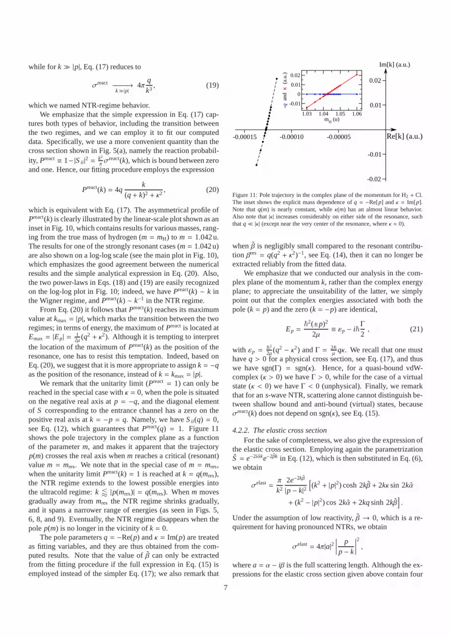
The pole parametersq = −Re(p) andκ = Im(p) are treatedas fitting variables, and they are thus obtained from the com-puted results. Note that the value ofβ can only be extractedfrom the fitting procedure if the full expression in Eq. (15) isemployed instead of the simpler Eq. (17); we also remark that

1.03 1.04 1.05 1.06m

H (u)

-0.01

0

0.01

0.02

-qan

d κ

(a.u

.)

-0.00015 -0.00010 -0.00005

-0.02

-0.01

0.01

0.02

Im[k] (a.u.)

Re[k] (a.u.)

Figure 11: Pole trajectory in the complex plane of the momentum for H2 + Cl.The inset shows the explicit mass dependence ofq = −Re[p] and κ = Im[p].Note thatq(m) is nearly constant, whileκ(m) has an almost linear behavior.Also note that|κ| increases considerably on either side of the resonance, suchthatq ≪ |κ| (except near the very center of the resonance, whereκ ≈ 0).

whenβ is negligibly small compared to the resonant contribu-tion βres

= q(q2+ κ2)−1, see Eq. (14), then it can no longer be

extracted reliably from the fitted data.We emphasize that we conducted our analysis in the com-

plex plane of the momentumk, rather than the complex energyplane; to appreciate the unsuitability of the latter, we simplypoint out that the complex energies associated with both thepole (k = p) and the zero (k = −p) are identical,

Ep =~

2(±p)2

2µ≡ εp − i~

Γ

2, (21)

with εp =~

2

2µ (q2 − κ2) andΓ = 2~µ

qκ. We recall that one musthaveq > 0 for a physical cross section, see Eq. (17), and thuswe have sgn(Γ) = sgn(κ). Hence, for a quasi-bound vdW-complex (κ > 0) we haveΓ > 0, while for the case of a virtualstate (κ < 0) we haveΓ < 0 (unphysical). Finally, we remarkthat for ans-wave NTR, scattering alone cannot distinguish be-tween shallow bound and anti-bound (virtual) states, becauseσreact(k) does not depend on sgn(κ), see Eq. (15).

4.2.2. The elastic cross sectionFor the sake of completeness, we also give the expression of

the elastic cross section. Employing again the parametrizationS = e−2iαke−2βk in Eq. (12), which is then substituted in Eq. (6),we obtain

σelast=π

k2

2e−2kβ

|p − k|2[

(k2+ |p|2) cosh 2kβ + 2kκ sin 2kα

+ (k2 − |p|2) cos 2kα + 2kq sinh 2kβ]

.

Under the assumption of low reactivity,β → 0, which is a re-quirement for having pronounced NTRs, we obtain

σelast= 4π|a|2

∣

∣

∣

∣

∣

pp − k

∣

∣

∣

∣

∣

2

,

wherea = α − iβ is the full scattering length. Although the ex-pressions for the elastic cross section given above containfour

7

parameters ( ˜α, β, q andκ), only two of them are needed whenthe resonance pole is very close to the threshold (p ≈ 0). In-deed, if the pole contribution is dominant, we can neglect ˜a, andusea ≈ ares

=ip in the equation above, which we rewrite as

σelast=

4π(q + k)2 + κ2

. (22)

Note the similarity between this result for the elastic cross sec-tion and Eq. (17) for the reactive cross section; thus, in thelimitk → 0 we recover again the familiar Wigner behavior,

σelast −−−−−→k→0

4π|a|2,

and for the NTR regime we obtain

σelast −−−−−→k≫|p|

4πk2.

5. Jost-function approach

We now describe an alternative approach, based on the useof the Jost function, to obtain the anomalousk−3 scaling of thereaction cross section for the NTR regime described in the pre-vious section. We shall first give the key concepts for the caseof single channel and short-range interactionV(R), and gener-alize the results to the multi-channel case afterward.

5.1. Single channel case

The regular solution of the radial equation,

d2

dR2φk =

[

2µV(R) − k2]

φk(R),

is uniquely specified by initial-value type conditions:φk = 0and d

dRφk = 1 atR = 0. Recall that we are discussing only thecase of s-wave (ℓ = 0) scattering; for higher partial waves, theinitial boundary condition reads:φk,ℓ(R) ∼ Rℓ+1. The asymp-totic behavior of the regular solution can be written as

φk(R)R→∞−−−−−→ 1

k[

A(k) sinkR + B(k) coskR]

. (23)

If k is real valued, and assumingV(R) is real, then we canchooseφk to be real; hence,A(k) andB(k) are real valued. Re-casting Eq. (23) in terms of the free solutions exp(±ikR), wehave

φk(R)R→∞−−−−−→ i

2k

[

(A − iB)e−ikR − (A + iB)e+ikR]

, (24)

and following the convention used in Refs. [40, 42], we definethe Jost function:

F (k) ≡ A(k) − iB(k). (25)

Conversely, if one introducedF in the usual manner, i.e., bystarting with the asymptotic behavior ofφk written as

φk(R)R→∞−−−−−→ i

2k

[

F (k)e−ikR − F ∗(k)e+ikR]

, (26)

one could identifyA = Re(F ) andB = −Im(F ), provided thatboth k andV(R) are real valued. Note that if one allows fora complex valuedk, see [40], a fully general definition of theJost function can be obtained by replacingF ∗(k) with F (−k)in Eq. (26). In this article we use real and positivek, unlessotherwise specified; when needed, we can allowk to be com-plex without any difficulty, because we restrict ourselves to thecase of short-range interactions. We remark that our analysisof the S matrix in the previous section (done in the complexk plane) would be difficult to justify rigorously for the case oflong-range interactions. However, as we shall see in this sec-tion, the approach based on the Jost function (for real argumentk) circumvents this obstacle, because it makes it possible toac-count for the NTR phenomenon without referring to the polesof theS matrix in the complex plane. Moreover, when it is pos-sible to define the Jost function for complexk, it is easily seenthat the two approaches are equivalent.

Regarding our preference for analyzingA(k) and B(k) in-stead ofF (k) itself, we point out that although the two solutionsχ±k (R) ∼ e±ikR are linearly independent in the strict sense, theywill become linearly dependent in the limitk → 0 (from thenumerical point of view) simply becausee−ikR ≈ eikR ≈ 1 whenkR ≪ 1. Thus, it is desirable to replaceχ±k with a set of solu-tions which are more suitable at lowk, namely fk(R) ∼ sin(kR)andgk(R) ∼ cos(kR). Since we assume thatφk, fk, gk andχ±k areexact solutions of the radial equation, the matching conditions(23) and (26) can be recast as equalities:kφk = A fk + Bgk,and 2ikφk = F ∗χ+k − F χ−k respectively. As is well known,the Jost function can be expressed asF = W[χk, φk], whereW[u, v] = uv′−u′v denotes the Wronskian. Similarly, forA andB we haveA = W[gk, φk] and B = −W[ fk, φk], which can beused in practice to computeA(k) andB(k).

We now shift our attention to the (normalized) physical so-lution ψk(R), which is regular atR = 0. Hence, the physicaland regular solutions only differ by a multiplicative constant,which can be easily found by comparing the asymptotic bound-ary condition obeyed by the physical solution [43],

ψk(R)R→∞−−−−−→ eiδ sin(kR + δ) =

i2

(

e−ikR − e2iδeikR)

, (27)

to the asymptotic behavior in Eq. (26). Indeed, we find

ψk(R) =kF (k)

φk(R), (28)

and we can also identify theS matrix,S = e2iδ= F ∗F −1. We

recall the well known relationship between the phase shiftδ(k)in Eq. (27) and the Jost function; namely,δ = − arg(F ), whichcan also be written as tanδ = B/A, see Eqs. (23, 25, 27). Alsonote that if we make use ofF = |F |e−iδ, then Eq. (25) can beexpressed asA = |F | cosδ andB = |F | sinδ.

We emphasize that scattering resonances will affect stronglythe k dependence of the normalization constantk[F (k)]−1 inEq. (28). Special attention has to be paid to the denominatorF = A − iB, which could vanish neark = 0, and thus producea near threshold resonance. Hence, we proceed to analyze thelow k behavior of the Jost function. Under the assumption of a

8

short-range potential, it is possible to expandA(k) andB(k) aspower series. Indeed, given that the regular solution, as well ascos(kR), are analytic ink2 [44], and that sin(kR) is analytic inkand is an odd function ofk, we can write:

A(k) = A0 + A2k2+ A4k4

+ · · · (29)

B(k) = B1k + B3k3+ B5k5

+ · · · (30)

For a finite-range potential, these power series can be rigorouslydeduced in a straightforward manner, and their validity canalsobe extended to the case of short-range potentials. However,forlong-range potentials, e.g.,V(R) = −Cn/Rn for R → ∞, A(k)and B(k) are no longer analytic functions; theirk dependenceis rather complicated, as shown by Willner and Gianturco [45].Nevertheless, even in the case of long-range interactions,bothA(k) andB(k), and henceF (k) are generally well behaved, al-beit nonanalytic; thus, we subscribe to the point of view advo-cated by Willner and Gianturco [45], that the low-k expansionfor the Jost function is simpler, more elegant, and more practi-cal than the corresponding expression for tanδ(k) or the famil-iar effective range expansion fork cotδ(k). We argue that oneshould employ the low-k expansions forA(k) and B(k) of theJost functionF (k) = A(k)− iB(k) rather than lowk power seriesexpansion of the phase shift (and all other physical quantities,such as the cross section). For example,

tanδ(k) =B(k)A(k)

=B1k + B3k3

+ · · ·A0 + A2k2 + · · ·

should be kept as a fraction, rather than attempting to expandit consistently toO(k2) or higher. Indeed, such an expansionwould become unsuitable ifA0 were vanishingly small, as itsvalidity would be restricted to an extremely narrow range, namelyk2 ≪ |A0/A2|, while the expression above remains valid anduseful for a much wider range. Alternatively, we have

k cotδ =A0 + A2k2

+ · · ·B1 + B3k2 + · · · ,

which could be expanded as a power series to give the familiareffective range expansion,

k cotδ ≈ −1a+

reff

2k2,

with a = −B1/A0 the scattering length, andreff = 2(A2/B1 −A0B3/B2

1) = (2/B1)(A2 + B3/a) the effective range. WhenA0

vanishes, we havea → ±∞ andreff → 2A2/B1, and the effec-tive range expansion remains valid, taking a simplified form:k cotδ ≈ 1

2reffk2. However, ifB1 is vanishingly small, we havea ≈ 0 andreff → ±∞, and thus the effective range expansion isrendered useless.

We now analyze the elastic cross section in terms of the Jostfunction:

σelast(k) =π

k2|1− S (k)|2,

where the S matrix is expressed as

S (k) = e2iδ=

A + iBA − iB

.

Thus, the elastic cross section reads

σelast(k) =4πk2

B2(k)A2(k) + B2(k)

. (31)

In the limit k → 0, and provided thatA(0) , 0, we recover thewell known Wigner law for s-wave elastic scattering, which issimply the lowest order approximation,

σelast−−−−→k→0

4π

(

B1

A0

)2

= 4πa2.

The domain of validity for Wigner’s threshold law defines theso called Wigner regime; its extent is governed by the lowestor-der coefficientsA0 andB1 in the Jost function expansions (29,30). When neitherA0 nor B1 is small, the Wigner regime willcover the entire low energy domain. Conversely, if eitherA0

or B1 is vanishingly small, Wigner’s threshold law will be re-stricted to a narrow domain neark = 0, because the higher or-der terms in (29, 30) become dominant ask increases, and thek-dependence of the cross section in Eq. (31) changes dramati-cally.

Here, we are especially interested in the case of vanish-ingly small A0, which corresponds to a NTR, and we estab-lish the domain of validity for Wigner’s law as follows: inEq. (31) it is necessary that bothA(k) and B(k) be replacedby Eqs. (29, 30) truncated to the lowest order, i.e., we requirek ≪ |A0A−1

2 |1/2 andk ≪ |B1B−13 |1/2. The former inequality is

stronger than the latter, sinceB1 is typically finite whenA0→ 0.Moreover, theB2(k) term in the denominator of Eq. (31) hasto remain negligible; hence, we impose yet another inequality,k ≪ |A0B−1

1 | = |a|−1, which is much stronger than either ofthe two inequalities above, and thus dictates the extent of theWigner regime.

Since the Wigner regime is displaced towards extremelylow energies whenA0 ≈ 0, we need to analyze the behaviorof the elastic cross section for the remainder of the low energydomain. Thus, we considerk outside the Wigner regime, butstill inside the low energy domain, such that Eq. (30) can betruncated to the first term, and Eq. (29) to the second term. Ask increases gradually,A0 becomes negligible compared to bothA2k2 andB1k. Moreover, only the latter term survives, as wehave|B1|k ≫ |A2|k2 throughout the low energy domain. Con-sequently, the termA2(k) in the denominator of Eq. (31) can beneglected entirely, and we recover the NTR-regime behavior,

σelast(k) ≈ 4πk2.

In summary, using the Jost function description, the elasticcross section can parametrized in a simple way at low energy;namely, according to our discussion above, we keep only therelevant terms in Eqs. (29, 30) to approximate Eq. (31) as

σelast(k) = 4πB2

1

A20 + B2

1k2= 4π

1k2 + (1/a)2

, (32)

wherea = −B1/A0 is the full scattering length. The simpleexpression above makes it clear that the the gradual transition

9

from Wigner’s threshold law to the NTR-regime behavior takesplace neark ≈ |a|−1, where the two terms in the denominatorare comparable. We remark that Eq. (32) is in agreement withEq. (10) obtained in the previous section using the pole factor-ization of theS matrix, and we shall discuss their equivalencein Sec. 6.

5.2. Multi-channel case

In the case ofN coupled channels, the regular solutionΦis anN × N matrix with elementsφi j satisfying the system ofcoupled radial equations,

d2

dR2Φ(k,R) + K2

Φ(k,R) =2µ~2

V(R)Φ(k,R), (33)

with k ≡ (k1, k2, . . . , kN) and kn =√

2µ(E − εn)/~2 the mo-menta corresponding to channel threshold energiesεn. For sim-plicity we consider all channels open, with allkn real valuedandkn > 0. K is a diagonal matrix with elementsknδnm, whileV(R) is a full matrix containing the couplingsVnm(R). Note thatthe diagonal elements ofV also include centrifugal terms of theform ℓn(ℓn + 1)R−2.

The regular solution is uniquely specified by initial-valuetype conditions atR = 0,

φnm(R)R→0−−−−−→ δnmRℓn+1.

Assuming that the coupling matrixV is real, we extract two realvalued matrices (A andB) from the asymptotic behavior of theregular solution,

ΦR→∞−−−−−→ K−ℓ−1(jA + nB),

whereK−ℓ−1= diag{k−ℓn−1

n }, and the diagonal matricesj andn contain the free solutions, i.e., the Riccati–Bessel functionsjℓ(knR) andnℓ(knR) for each channel. Note that, although theasymptotic behavior in the last equation was written in matrixnotation, the coefficientsAnm andBnm (i.e., the matrix elementsof A andB) are extracted independently for each pair of indices(n,m). Indeed, for each component (n) of any column solution(m) contained inΦ, we write the asymptotic behavior explicitly,

kℓn+1n φnm(R)

R→∞−−−−−→ Anm jℓn (knR) + Bnmnℓn(knR).

Employing this matching condition forφnm (together with asimilar equation fordφnm/dR) at R = Rmax in the asymptoticregion, we obtain

Anm = −kℓnn W[φnm, nℓn ] (34)

Bnm = +kℓnn W[φnm, jℓn ] (35)

whereW[. . . ] stands for the Wronskian. The Jost matrix is de-fined in terms of the matricesA andB as

F = A − i B, (36)

which is a direct generalization of Eq. (25). The factorkℓn+1n

in the equations above was used for convenience, such that the

Jost matrix is well behaved whenkn → 0. In this paper werestrict our discussion to s-wave scattering, i.e.,ℓ = 0 in theentrance channel; note that only the centrifugal term in theen-trance channel is relevant for analyzing the threshold behavior.The values ofℓn in all other channels can be arbitrary (as al-lowed by the specifics of any given scattering problem). How-ever, we setℓn = 0 in all channels to simplify our notation; thus,the asymptotic behavior of the regular solution reads

knφnm(R)R→∞−−−−−→ Anm sin(knR) + Bnm cos(knR),

which is identical to the single channel version, see Eq. (23).Equivalently, the asymptotic behavior ofΦ can be written interms of Jost matrix elementsFnm = Anm − iBnm as

2i

knφnm(R)R→∞−−−−−→ e−iknRFnm − e+iknRF∗nm,

whereF∗nm = Anm + iBnm is the complex conjugate ofFnm.The normalized (physical) solutionΨ can be written in terms

of the regular solutionΦ,

Ψ(R) = Φ(R)F−1K, (37)

and it has the well known asymptotic behavior,

ψnm(R)R→∞−−−−−→ i

2

[

e−iknRδnm − e+iknR(

k−1/2n S nmk1/2

m

)]

, (38)

whereS nm are the elements of the S matrix,

S = K−1/2(F)∗(F)−1K1/2. (39)

Equations (37) and (39) contain the inverse of the Jost matrix,which we write explicitely as

F−1=

1det(F)

[Cof(F)]T , (40)

with [Cof(F)]T the transpose of the matrix of cofactors ofF,and det(F) the determinant ofF.

As in the single-channel case, we focus our attention onthe denominator, i.e., the determinant of the Jost matrix. Weare interested in the situation when det(F) is vanishingly small,such that the scattering cross sections are resonantly enhanced;if Tnm are the elements of the T matrix,T = 1 − S, we have

σ(n← m) ∼ π

k2m|Tnm|2 ∼ | det(F)|−2.

Although the determinant of the Jost matrix cannot vanish onthe real axis [46], it canalmost reach zero. Also, recall that weonly consider the case of a scattering problem without closedchannels, thus eliminating the possibility of Feshbach resonances.Therefore, by extrapolation from the single-channel case,theonly remaining possibility is that of a potential resonanceat lowenergy; such a resonance would correspond to a quasi-boundstate near the threshold of the channel with the highest energyasymptote, which we take as our entrance channel (n = 1). Forclarity, we assumeE > ε1 > ε2 > · · · > εn > · · · > εN .

10

When det(F) ≈ 0 at a channel threshold, the factor| det(F)|−2

in the equation above will be responsible for a resonance en-hancement, and will also affect the threshold behavior of crosssections. We now give a detailed analysis of a NTR in the en-trance channel,n = 1, and we start by using a cofactor expan-sion of the determinant along the first row,

det(F) =N

∑

m=1

F1mC1m, (41)

whereC1m is the cofactor corresponding to the element (1,m).Next, we extractC11 outside the sum, and we isolate the firstterm (i.e., the diagonal elementF11) to recast det(F) as

det(F) = C11 (F11+ f11) , (42)

where

f11 ≡1

C11

∑

m,1

F1mC1m. (43)

Separating the real and imaginary parts of the last factor inEq. (42), namelyF11 + f11 = A− iB, and defining

D ≡ |F11+ f11|2 = A2+ B2,

we can write

| det(F)|2 = |C11|2|A − iB|2 = |C11|2D. (44)

Under the assumption thatf11 is suitably small, and pro-vided thatC11 0 0, only the factorD ≈ |F11|2 = A2

11 + B211 can

be responsible for NTRs. In order to clarify these assumptions,we recall that, as we explained in Sec. 4, due to the coupling ofthe entrance channel with other open channels, the resonancepole will be pushed away from the threshold; thus, in the limitof strong coupling, the existence of a near threshold resonancewill become highly unlikely. Conversely, the appearance ofaprominent NTR requires the entrance channel be weakly cou-pled to all other open channels. To simplify, one can use acoupling strength parameterλ to redefine these particular cou-plings (V1n = Vn1 → λVn1) which will become vanishinglysmall whenλ → 0. Hence, we assume the regular solutionmatrix Φ is almost block diagonal, with a small 1× 1 blockcontainingφ11 and a large (N − 1)× (N − 1) block correspond-ing to all other open channels. The remaining elements, i.e.,φ1m with m , 1 in the first row, andφn1 with n , 1 in the firstcolumn are vanishingly small whenλ→ 0. Consequently, fromEqs. (34, 35, 36) we have (forn , 1) Fn1 = O(λ) whenλ → 0,and thusC1m = O(λ) for m , 1. Note thatC11 is independentof λ in zeroth order, and hence we assumeC11 = O(1). Finally,we also haveF1m = O(λ) for m , 1, and from Eq. (43) we havef11 = O(λ2) whenλ→ 0.

Regarding the caveat of an accidental vanishing ofC11 nearthe threshold of the entrance channel, recall that in the limitλ → 0 the channeln = 1 becomes decoupled from the remain-ing N − 1 channels, and we have limλ→0 C11 = det

[

F(N−1)],whereF(N−1) is the Jost matrix for the scattering problem withN − 1 channels. Thus, det

[

F(N−1)] cannot be vanishingly smallfor collision energiesE > ε1, sinceE is very high aboveε2

(which is the highest threshold for the scattering problem withN − 1 channels). Indeed, as we assumeε1 − ε2 is much largerthan the generic low-energy scale of the scattering problem;thus, it is safe to factor outC11 = O(1) as a background contri-bution, as we already anticipated in the equations above.

Denotingk = k1, we now focus on thek dependence ofD(k)in Eq. (44), which stems from the behavior ofF11(k) and f11(k).We emphasize that all quantities are analyzed as functions ofthe single variablek. All other momenta, i.e.,kn for channelsn = 2, 3, . . . ,N, can be easily expressed in terms of the entrancechannel momentum: usingk2

n = 2µ(E − εn), we write

kn =√

∆n + k2,

with ∆n = 2µ(ε1 − εn). In the ultracold limit (k → 0) we havek2 ≪ ∆n for all n , 1, and we use a power series expansion:

kn(k2) ≈√

∆n + O(k2).

Moreover, the regular solutionΦ is a function ofk2 (rather thank itself), and we deduce from Eqs. (34, 35) that except for thefirst row, all matrix elementsAnm andBnm are also functions ofk2. Thus, whenk → 0 we have

Fnm(k2) = Fnm(0)+ O(k2), for n , 1,

Similarly, the cofactors corresponding to the first row ofF canbe written as

C1m(k2) = C1m(0)+ O(k2), for all m,

which ensures that the ratioscm ≡ C1m/C11 in Eq. (43) can beexpanded in a similar fashion:

cm(k2) = cm(0)+ O(k2).

Rewriting Eq. (43) as

f11 =

∑

m,1

F1mcm, (45)

and separating its real and imaginary parts, we have

Re(f11) =∑

m,1

[

A1m(k)Recm(k) + B1m(k)Imcm(k)]

, (46)

Im( f11) =∑

m,1

[

A1m(k)Imcm(k) − B1m(k)Recm(k)]

. (47)

In these equations, special attention has to be paid toA1m(k) andB1m(k). From Eqs. (34, 35) we obtain the expansions:

A1m(k) = A1m(0)+ k2A(2)1m + O(k4), (48)

B1m(k) = kB(1)1m + k3B(3)

1m + O(k5). (49)

Since the series ofB1m(k) contains odd powers, andcm(k) inEq. (45) are complex quantities, the power series in Eqs. (46,47) contain both odd and even powers ofk,

Re(f11) = a(0)+ ka(1)+ k2a(2)

+ O(k3), (50)

Im( f11) = b(0)+ kb(1)+ k2b(2)

+ O(k3). (51)

11

Thus, the power series ofA(k) andB(k) will also contain allpossible terms, i.e., both odd and even powers:

A(k) = A0 + kA1 + k2A2 + · · · , (52)

B(k) = B0 + kB1 + k2B2 + · · · (53)

The coefficientsAν andBν will be expressed in terms ofA(ν)1m,

B(ν)1m, a(ν) and b(ν). Indeed, recall thatA = Re(F11 + f11) =

A11 + Re(f11) andB = −Im(F11 + f11) = B11 − Im( f11). Fromthe equations above, we obtain for the coefficients up to orderν = 2,

A0 = A(0) = a(0)+ A11(0)

A1 = a(1)

A2 = a(2)+ A(2)

11

and

B0 = B(0) = −b(0)

B1 = −b(1)+ B(1)

11

B2 = −b(2).

Under the assumption of weak coupling (λ → 0), we havef11 = O(λ2) → 0. Thus, alla(ν) andb(ν) are negligibly small;however, their presence in the equations above is necessary, be-cause they limit the effects caused by near threshold resonances.Indeed, note thatA0 andB0 cannot vanish simultaneously; inother words, one cannot have:A11(0) = 0 anda(0) = 0 andb(0) = 0. Were that the case,D(k) and hence det(F) wouldvanish atk = 0, which is impossible (as we mentioned earlier).Nevertheless, whenλ is small, so area(0) andb(0). Also, asin the single-channel case, it is possible thatA11(0) ≈ 0. Thus,although the quantityD(k = 0) = A2

0 + B20 cannot vanish, it

could reach very small values (which is the signature of NTR).Finally, we analyze the threshold behavior of cross sections

in the presence of a NTR; from Eqs. (39, 40) we obtain

S nm = δnm +

√

km

kn

2i∑

j Bn jCm j

det(F).

We only consider scattering from the ultracold channelm = 1to all final channelsn = 1, 2, 3, . . . ,N; thus, using the notationk = k1, the cross sections read

σ(n← 1) ∼ π

k2|Tn1(k)|2 ∼

|∑ j Bn jC1 j|2

kkn|C11|2D(k).

Except forD(k), all other quantities are finite whenk → 0, andcan be replaced by their values atk = 0, i.e., Bn j(0), C1 j(0),C11(0) andkn(0), which amount to an overall (n dependent)constant. This allows us to simplify the expression above; forreactive (or inelastic) scattering,n , 1, we obtain

σreact(n← 1) ∼ const(n)D(k)

k−1, (54)

while for elastic scattering, we havekn = k andB1 j(k) ∼ k, andthe cross section reads

σelast(1← 1) ∼ const′

D(k). (55)

RecallD(k) = A2(k) + B2(k), which is expanded at lowk,

D(k) = D0 + kD1 + k2D2 + · · · , (56)

with

D0 = D(0) = [b(0)]2 + [a(0)+ A11(0)]2,

D1 = 2[−b(0)B1 + a(1)A0],

D2 = B21 + [a(1)]2

+ 2[A0A2 + b(0)b(2)].

As argued above,D0 cannot vanish identically; however,D0

is small in the case of a NTR, and hence it is the most impor-tant parameter characterizing the NTR. Note that the first orderterm in Eq. (56) can be neglected when both the weak coupling(λ → 0) assumption and the NTR assumption (A11(0) ≈ 0) arevalid; indeed, we haveD1 ≈ −2b(0)B(1)

11 = O(λ). Thus, evenfor a pronounced NTR, i.e., whenD0 approaches its minimumvalue,D0 ≈ Dmin ≈ [b(0)]2 = O(λ2), the linear term will be-come negligible compared toD0 for k ≪ D0/|D1| ≈ |b(0)/B(1)

11|.In the ultracold limit (k → 0) the quadratic term in Eq. (56)can be neglected as well; specifically, the requirement isk ≪√

D0/D2. Making use of the approximationsD0 ≈ [b(0)]2 andD2 ≈ [B(1)

11]2, we have√

D0/D2 ≈ |b(0)/B(1)11|. Hence, the strong

inequalityk ≪√

D0/D2 defines the Wigner regime, since wecan ignore both the linear and quadratic terms in Eq. (56). In-deed, we haveD(k) ≈ D0, and we recover Wigner’s thresholdlaws:σreact∼ k−1 andσelast≈ constant.

The linear term in Eq. (56) can also be neglected outsidethe Wigner regime, i.e., for the remainder of the lowk domain;indeed, whenk ≫ |b(0)/B(1)

11|, we havek2D2 ≫ kD1 and alsok2D2 ≫ D0, which ensures thatD(k) ≈ k2D2. Thus, discardingthe linear term altogether in Eq. (56), we simplify Eqs. (54)and(55), and we obtain

k0,1σelast, react∼ 1D0 + k2D2

, (57)

where the prefactorsk0= 1 andk correspond to elastic and

reactive scattering, respectively. We emphasize that thisex-pression is a good approximation throughout the entire low-kregime, and despite its simplicity, it accounts for the combinedWigner and NTR-regime behavior. For reactive scattering wehave

σreact∼{

k−1, Wigner regime fork ≪√

D0/D2

k−3, NTR regime fork ≫√

D0/D2,

while for elastic scattering,

σelast∼{

k0, Wigner regimek−2, NTR regime,

According to Eq. (57) there is a smooth transition between thetwo types of behavior (Wigner and NTR) which takes placearoundk =

√D0/D2, where all three terms in Eq. (56) are

comparable. Thus, the linear term in Eq. (56) only plays a mi-nor role near the transition, while becoming negligible forbothWigner and NTR regimes.

We remark that when the coupling strengthλ increases, andthe system becomes more reactive,a(ν) andb(ν) will increase;

12

10-9

10-6

10-3

100

Energy (kelvin)

10-4

10-3

10-2

10-1

100

P =

1 -

|Si,i

|2

1st resonance

3rd resonance

2nd resonance

β~ incr

ease

s

q increases

2 31

Figure 12: Comparison of reaction probabilities for the resonances of H2 + Cl.The imaginary part of the scattering length (β, see Fig. 3) is shown in the insetto help identify the resonances. The three solid curves correspond to the threecritical values ofm (for the first, second and third resonance, which are shownin red, green and blue, respectively). The dashed curves correspond to valuesof m near the first and third resonance. The arrows indicate the increase ofreactivity, and the increase ofβ andq, asm decreases.

hence,D0 andD1 will become large (even ifA0 ≈ 0 still holds)and the NTR regime will be pushed to higher values ofk, wherehigher-order terms will become dominant. Eventually, the sig-nature of the NTR will disappear, as suggested in Fig. 12, whichshows that for the lowest reactivityβ corresponding to the thirdresonance, the pole is located at very lowk, and the NTR regimeextends to a sizable range for largerk. The extent of the NTRregime is smaller for the second resonance corresponding toalargerβ, and smaller still for the first resonance with the largestreactivity β. Thus, in the limit of strong coupling, the very ex-istence of a quasi-bound state of the atom–dimer complex be-comes unlikely, since such a complex will be short lived; conse-quently, NTRs cannot exist (or are less pronounced) for highlyreactive systems.

6. Equivalence between different approaches

In the case of purely elastic scattering (single channel), theequivalence of the two approaches is based on the simple rela-tionship between theS matrix and the Jost function, see Eq. (7).The expressions (8) and (29, 30) merely give different parametriza-tions for theS matrix, and hence for the elastic cross section.To elucidate their equivalence, we first note that the pole fac-torization (8) relies on the power series expansion of the Jostfunction around its zero (atk = p). Recall that we assume ashort range potential, such thatF (k) is analytic in the entirecomplexk plane, or at least inside a wide region containing thethresholdk = 0. We thus write

F (k) =∞∑

n=1

Fn(p − k)n,

where the coefficientsFn are complex numbers. The absenceof the term forn = 0 in the sum above makes it explicit thatF (p) = 0, and allows for the factorizationF (k) = (p − k)F(k).

The background contributionF(k) is also analytic, and assum-ing it to be slowly varying within a small domain containingbothk = p andk = 0, we can truncate its power series in thelow energy domain:

F(k) ≈ F0 + F1k.

Note that forF(k) we employ a power series expansion aroundk = 0, which is more convenient. Hence, theS matrix reads

S (k) =F (−k)F (k)

=p + kp − k

F(−k)

F(k),

and we recognize the background contribution, see Eq. (8),

S (k) =F(−k)

F(k),

which is slowly varying neark = 0, due to the smooth behaviorof F(k). Truncating the power series ofS to first order, we haveS (k) ≈ 1 − 2iak. The unitarity ofS on the real axis ensuresthat the coefficient of the first order term in this expansion ispurely imaginary, and we have used the customary notation,namely the background scattering length ˜a. Thus, in the polefactorization approach, the fullS matrix at lowk reads

S (k) ≈ p + kp − k

(1− 2iak).

We now compare this result with the equivalent expressionobtained in the explicit Jost function approach, namely in termsof F (k) = A(k) − iB(k). We emphasize thatA(k) andB(k) areexpanded in power series aroundk = 0 only, and we remarkthat for a short range potential, the power series ofA(k) andB(k) remain valid whenk takes complex values; moreover, theexpansion coefficientsAn andBn in Eqs. (29, 30) remain realnumbers. Therefore, if a zero of the Jost function (i.e., a poleof theS matrix) is located on the imaginary axis,p = iκ, thenκis a real valued solution of the equation

A0 + B1κ − A2κ2 − B3κ

3+ · · · = 0,

with all coefficients real. In the case of a NTR,A0 is vanishinglysmall, and to a good approximation we have

κ ≈ −A0

B1=

1a,

wherea is the full scattering length, which agrees with Eq. (11).As we discussed in Sec. 5.1, theS matrix is simply written as

S (k) =A0 + iB1k + A2k2

+ · · ·A0 − iB1k + A2k2 − · · · .

When the resonance polep = iκ is very close tok = 0, this ex-pression truncated to second order becomes equivalent withthesimilar expression from the pole factorization approach, whichhas the advantage of using the exact value of the resonance pole(extracted as a fitting parameter from the computed scatteringcross section, as it was done in Sec. 4). However, for complexk, the very definition of theS matrix becomes problematic, as

13

it imposes strict requirements for the asymptotic behaviorofthe interaction potential. Hence, the direct approach based onJost functions for realk has the advantage of being fully gen-eral. We also emphasize that the Jost function has a smoothk-dependence, and it can be easily interpolated on a rather coarsek-mesh, which is very convenient in practice; nevertheless,thisadvantage has remained largely overlooked, despite being rec-ognized more than four decades ago by Heller and Reinhardt[47].

Regarding the coupled-channel case, we remark that Eq. (57)obtained in the Jost function approach represents a parametriza-tion which is identical to Eq. (17) from the pole factorizationtreatment, provided we simplify the latter to readkσreact(k) =4πq(k2

+ |p|2)−2. We can thus identifyD0/D2 = |p|2 = q2+ κ2

in the denominator, and we regardq in the numerator as anoverall measure of background reactivity (due to the couplingsVn1 = V1n between the entrance channel and all other channels).

7. Qualitative interpretation based on the wave function am-plitude

A very simple picture emerges from the treatment using theJost function; indeed, as noted for the single-channel discus-sion in Sec. 5.1, the amplitude of the physical wave functionis modulated by the inverse of the Jost functionF −1(k), seeEq. (28). This scaling property is especially useful in the lowenergy domain, i.e., fork / |a|−1, when the regular solutionin the short range (R / |a|) region is nearlyk-independent:φk(R) ≈ φ0(R). Hence, within the short-range region, Eq. (28)readsψk(R) ≈ kF −1(k)φ0(R), and thek dependence of the phys-ical solution is driven entirely by the scaling factorkF −1(k).

In the absence of NTRs, the Jost function can also be re-placed by its value atk = 0, F (0) = A0, and we obtain thewell known linear scaling of the short-range amplitude of thephysical wave function,ψk(R) ≈ kA−1

0 φ0(R), characteristic tothe Winger regime. However, whenF (0) = A0 is vanishinglysmall, it produces a resonance enhancement forψk(R), and alsothe anomalous NTR behavior,

|ψk(R)|2 ≈ k2

A20 + B2

1k2|φk(R)|2 . (58)

We remark that this simple expression for the single-channelcase already contains the main result, Eq. (57), obtained rig-orously in Sec. 5.2 for the coupled-channel case. This can bejustified qualitatively, if we rely on the following physical ar-gument; under the assumption of small couplings, the entrance-channel component (ψ1) of the physical wave function followsthe same scaling as in the single-channel case, see Eq. (37).Thisk-dependence in the equation above will be imprinted (viathe couplingsVnm) on all the other componentsψn. Althoughthe entrance-channel component obeys Eq. (58) only at shortrange, all other components will obey it for allR (including thelong-range region). Thus, according to Eq. (38) form = 1, weextract the matrix elementsS n1 from the asymptotic behavior

of ψn(R), and we obtain forn , 1

kkn|S n1|2 ∝ |ψn|2 ∝

k2

A20 + B2

1k2,

where we usedk = k1 for the entrance channel, andkn(k) ≈√∆n is constant. Finally, we obtain for the reaction cross sec-

tion,

kσreact(n← 1) ∝ 1

A20 + B2

1k2,

which is the same result obtained in Eq. (57), withD0 ≈ A20 and

D2 ≈ B21.

8. Conclusions

In conclusion, we found that a near threshold resonance willaffect dramatically the behavior of thes-wave cross section atlow energy. In fact, the low energy domain will be divided intwo distinct regimes: the Wigner regime with the well knownscaling (σreact∝ k−1) and the NTR regime with the anomalousscalingσreact ∝ k−3. We derived simple analytical expressionsfor both elastic and reaction (inelastic) cross sections, which de-pend on the position of the pole of theS matrix, and found verygood agreement with results obtained numerically for the fullreactive scattering problem. We explained the anomalous NTR-regime behavior using two different approaches—one based onthe pole factorization of theS matrix, and a more general treat-ment based on the low energy expansion of the Jost function.

We remark that thek−3 NTR-regime behavior (for s-wave)is a general feature, and it can be a rather common occurrencein scattering problems; however, unless the resonance poleisvery close tok = 0, the presence of the NTR can be somewhatinconspicuous, or it can be masked by higher partial wave con-tributions. Although previous work hinted at such anomalousresonant behavior—which was explored either by using mass-scaling [33, 48], or external fields [49]—the new NTR-regimebehavior shown in Eq. (15) was discussed only recently [24].These studies explored the effects of mass-scaling or magneticfield scanning at fixed scattering energy, e.g., see [50]. In ourwork, we revealed the effect of NTRs in two benchmark atom-diatom reactive scattering systems by mass-scaling (H2+Cl andH2+F), but it also appears in any system with a zero-energyresonance, such as in photoassociation at ultralow temperatures[51, 52], ultracold collisions in general [53], or spin-relaxationin ultracold atomic samples [54]. The modified (k−3) behaviorof the reaction (inelastic) cross section will play a role intheinterpretation of experiments such as [20], and also for theo-ries based on Wigner’s threshold law developed to account forresonances in ultracold molecular systems [17].

This work was partially supported by the US Department ofEnergy, Office of Basic Energy Sciences (RC), and the ArmyResearch Office Chemistry Division (I. S.).

References

[1] C. Chin, R. Grimm, P. Julienne, and E. Tiesinga, Rev. Mod.Phys.82,1225 (2010).

14

[2] M. H. G. de Miranda, A. Chotia, B. Neyenhuis, D. Wang, G. Quemener,S. Ospelkaus, J. L. Bohn, J. Ye, and D. S. Jin, Nature Phys.7, 502 (2011).

[3] J. N. Byrd, J. A. Montgomery, Jr., and R. Cote, Phys. Rev. Lett. 109,083003 (2012).

[4] F. Dalfovo, S. Giorgini, L. P. Pitaevskii, and S. Stringari, Rev. Mod. Phys.71, 463 (1999); A. J. Leggett, Rev. Mod. Phys.73, 307 (2001).

[5] S. Giorgini, L. P. Pitaevskii, and S. Stringari, Rev. Mod. Phys.80, 1215(2008).

[6] T. Kraemer, M. Mark, P. Waldburger, J. G. Danzl, C. Chin, B. Engeser,A. D. Lange, K. Pilch, A. Jaakkola, H.-C. Nagerl, and R. Grimm, Nature440, 315 (2006).

[7] L. Carr, D. DeMille, R. Krems, and J. Ye, New J. Phys.11, 055049(2009).

[8] O. Dulieu, R. Krems, M. Weidemuller, and S. Willitsch, Phys. Chem.Chem. Phys.13, 18703 (2011).

[9] D. S. Jin and J. Ye, Chem. Rev.112, 4801 (2012), and references therein.[10] R. Cote and A. Dalgarno, J. Mol. Spectrosc.195, 236 (1999).[11] E. Kuznetsova, M. Gacesa, P. Pellegrini, S. F. Yelin, and R. Cote, New J.

Phys.11, 055028 (2009).[12] B. C. Sawyer, B. K. Stuhl, M. Yeo, T. V. Tscherbul, M. T. Hummon, Y.

Xia, J. Klos, D. Patterson, J. M. Doyle, and J. Ye, Phys. Chem.Chem.Phys.13, 19059 (2011).

[13] G. Quemener and P. Julienne, Chem. Rev.112, 4949 (2012).[14] D. DeMille, Phys. Rev. Lett.88, 067901 (2002).[15] S. F. Yelin, K. Kirby, and R. Cote, Phys. Rev. A74, 050301 (2006).[16] E. Kuznetsova, R. Cote, K. Kirby, and S. F. Yelin, Phys. Rev. A 78,

012313 (2008).[17] M. Mayle, G. Quemener, B. P. Ruzic, and J. L. Bohn, Phys. Rev. A 87,

012709 (2013).[18] S. Chefdeville, T. Stoecklin, A. Bergeat, K. M. Hickson, C. Naulin, and

M. Costes, Phys. Rev. Lett.109, 023201 (2012).[19] M. Lara, S. Chefdeville, K. M. Hickson, A. Bergeat, C. Naulin, J.-M.

Launay, and M. Costes, Phys. Rev. Lett.109, 133201 (2012).[20] A. B. Henson, S. Gersten, Y. Shagam, J. Narevicius, and E. Narevicius,

Science338, 234 (2012).[21] N. Geum, G.-H. Jeung, A. Derevianko, R. Cote, and A. Dalgarno, J.

Chem. Phys.115, 5984 (2001).[22] E. P. Wigner, Phys. Rev.73, 1002 (1948).[23] H. R. Sadeghpour, J. L. Bohn, M. J. Cavagnero, B. D. Esry,I. I. Fabrikant,

J. H. Macek, and A. R. P. Rau, J. Phys. B33, R93 (2000).[24] I. Simbotin, S. Ghosal, and R. Cote, Phys. Rev. A,89, 040701 (2014).[25] H. A. Bethe, Phys. Rev.47, 747 (1935).[26] U. Fano, Phys. Rev.124, 1866 (1961).[27] N. Balakrishnan, R. C. Forrey, and A. Dalgarno, Phys. Rev. Lett.80, 3224

(1998).[28] N. Balakrishnan, V. Kharchenko, R. C. Forrey, and A. Dalgarno, Chem.

Phys. Lett.280, 5 (1997).[29] E. Garand, J. Zhou, D. E. Manolopoulos, M. H. Alexander,and D. M.

Neumark, Science319, 72 (2008).[30] N. Balakrishnan, J. Chem. Sci.124, 311 (2012).[31] W. Bian and H.-J. Werner, J. Chem. Phys.112, 220 (2000).[32] N. Balakrishnan and A. Dalgarno, Chem. Phys. Lett.341, 652 (2001).[33] E. Bodo, F. A. Gianturco, N. Balakrishnan, and A. Dalgarno, J. Phys. B

37, 3641 (2004).[34] K. Stark and H.-J. Werner, J. Chem. Phys.104, 6515 (1996).[35] M. T. Cvitas, P. Soldan, J. M. Hutson, P. Honvault, and J.-M. Launay, J.

Chem. Phys.127, 074302 (2007).[36] D. Skouteris, J. F. Castillo, and D. E. Manolopoulos, Comp. Phys. Comm.

133, 128 (2000).[37] I. Simbotin, S. Ghosal, and R. Cote, Phys. Chem. Chem.Phys.13, 19148

(2011).[38] I. Simbotin and R. Cote, New J. Phys., in press (2015).[39] J. Wang, J. N. Byrd, I. Simbotin, and R. Cote, Phys. Rev. Lett. 113,

025302 (2014).[40] J. R. Taylor,Scattering Theory (Dover Publications, Mineola, NY, 2006).[41] See page 523 in Ref. [42].[42] R. G. Newton,Scattering Theory of waves and particles (Dover Publica-

tions, Mineola, NY, 2002).[43] See page 343 in Ref. [42].[44] See page 335 in Ref. [42].[45] K. Willner and F. A. Gianturco, Phys. Rev. A74, 052715 (2006).

[46] See page 528 in Ref. [42].[47] E. J. Heller and W. P. Reinhardt, Phys. Rev. A5, 757 (1972).[48] J. L. Nolte, B. H. Yang, P. C. Stancil, T.-G. Lee, N. Balakrishnan, R. C.

Forrey, and A. Dalgarno, Phys. Rev. A81, 014701 (2010).[49] J. M. Hutson, M. Beyene, and M. L. Gonzalez-Martınez,Phys. Rev. Lett.

103, 163201 (2009).[50] J. M. Hutson, New J. Phys.9, 152 (2007).[51] A. Crubellier and E. Luc-Koenig, J. Phys. B39, 1417 (2006).[52] P. Pellegrini, M. Gacesa, and R. Cote, Phys. Rev. Lett. 101, 053201

(2008).[53] M. Arndt, M. Ben Dahan, D. Guery-Odelin, M. W. Reynolds, and J. Dal-

ibard, Phys. Rev. Lett.79, 625 (1997).[54] J. Soding, D. Guery-Odelin, P. Desbiolles, G. Ferrari, and J. Dalibard,

Phys. Rev. Lett.80, 1869 (1998).

15