Embed Size (px)
Citation preview

Jukka Väätäinen
Inventories and company’s financial performance
Vaasa 2021
School of Technology and InnovationsMaster’s Thesis in Industrial Management
Master’s Programme in Industrial Management

2
UNIVERSITY OF VAASASchool of Technology and InnovationsAuthor: Jukka VäätäinenTitle of the Thesis: Inventories and company’s financial performanceDegree: Master of Science in Economics and Business AdministrationMajor: Industrial managementSupervisor: Petri HeloYear of graduation: 2021 Pages: 99
ABSTRACT:In recent times working capital management has emerged in both the academic literature andoperational business. Several companies aim to optimize their working capital levels in a waythat working capital wouldn’t be tied into daily business. Effective working capital managementfor instance improves company’s liquidity position and increases the return on investment ra-tios. Working capital management is involved in various stages of company’s operations chain,from the procurement of raw materials through inventories to the sale of goods to the end cus-tomer. In a larger context, working capital management can be seen from the perspective ofwhole value chain or supply chain, in which working capital should be optimized in a supply chainlevel in a way that liquidity in whole supply chain improves and also return on investment ratio.Inventories are a key component of working capital that often tie significant amount of a com-pany’s working capital.
The purpose of this thesis is study relationship between value of stock and company’s financialperformance. The theoretical framework of the thesis is based on academic literature and aca-demic research of working capital. The thesis aim to determine the statistical relationship be-tween the value of inventory and several key indicators of company’s performance, such as prof-itability and inventory turnover. In this thesis the data was collected from financial statementsin seven industries and from two countries: Finland and United States of America. The data usedin this study is between years 2011 and 2019. In order to achieve the research objectives, datafrom different industries and different countries was analyzed, and the correlation and regres-sion between key variables was studied.
As a managerial implications of this thesis show the statistical relationship between the value ofinventory to selected variables from seven different industries and between selected industriesbetween Finnish and US companies. The results show, for example, that US companies havestronger positive statistical correlation between value of the inventories and business profita-bility than Finnish companies. In addition, based on the study, the values of inventories has in-creased an average during the period under review in both countries Finland and in the USA.The results also observe that in most industries studied, an increase in the value of inventoryslows down inventory turnover.
KEYWORDS: Working capital, financial performance, inventories, EBIT, turnover, stock turn-over
3
VAASAN YLIOPISTOAkateeminen yksikköTekijä: Jukka VäätäinenTutkielman nimi: Inventories and company’s financial performanceTutkinto: Kauppatieteiden maisteriOppiaine: TuotantotalousTyön ohjaaja: Petri HeloValmistumisvuosi: 2021 Sivumäärä: 99
TIIVISTELMÄ:Käyttöpääoman hallinta on noussut viime vuosina esille sekä akateemisessa kirjallisuudessa ettäkäytännön yritystoiminnassa. Useat yritykset pyrkivät optimoimaan käyttöpääomansa hallinnansiten, että liiketoimintaan sitoutuu mahdollisimman vähän käyttöpääomia. Tehokas käyttöpää-oman hallinta esimerkiksi parantaa yrityksen likviditeettiä ja maksuvalmiutta sekä nostaa sijoi-tetun pääoman tuottoa. Käyttöpääoman hallinta liittyy yrityksen tuotantoketjun eri vaiheisiin,alkaen raaka-aineiden hankinnasta, varastoinnin kautta hyödykkeen myymiseen loppuasiak-kaalle. Isommassa kontekstissa käyttöpääoman hallintaa voi ajatella yrityksen koko toimitusket-jun tai arvoketjun näkökulmasta, jolloin käyttöpääomaa tulisi optimoida siten, että yrityksenkoko toimitusketjun likviditeetin määrä kasvaa ja sijoitetun pääoman tuotto paranee. Varastotovat keskeinen käyttöpääoman komponentti joka usein sitoo merkittävän määrän yrityksenkäyttöpääomaa.
Tämän tutkielman tarkoituksena on selvittää varaston arvon yhteyttä yrityksen taloudelliseensuorituskykyyn. Tutkimuksen teoreettinen viitekehys nojaa käyttöpääomaa käsittelevään aka-teemiseen kirjallisuuteen sekä akateemisiin tutkimuksiin. Tutkimus pyrki selvittämään varastonarvon tilastollisen yhteyden useisiin yrityksen keskeisiin mittareihin kuten kannattavuuteen sekävaraston kierron nopeuteen. Tutkimuksessa käytettiin seitsemän eri toimialan tilinpäätöstietojakahdesta eri maasta: Suomesta ja Yhdysvalloista. Tutkimuksessa käytetty aineisto on vuosilta2011 – 2019. Tutkimustuloksen saavuttamiseksi data eri toimialoita ja maista analysoidaan jatutkitaan korrelaatiota ja regressiota eri mittareiden välillä.
Tutkielman tulokset osoittavat varaston arvon tilastollisen yhteyden valittuihin mittareihin seit-semältä eri toimialalta sekä suomalaisten ja yhdysvaltalaisten yritysten väliltä valituilta toimi-aloilta. Tulokset osoittavat esimerkiksi yhdysvaltalaisilla yrityksillä olevan suurimpi positiivinenkorrelaatio varaston arvon ja liiketoiminnan kannattavuuden välillä kuin suomalaisilla yrityksillä.Lisäksi tutkimuksen perusteella varaston arvo on keskimäärin noussut tarkasteltuna ajanjaksonasekä Suomessa että Yhdysvalloissa. Tutkimuksesta selvisi myös, että useimmilla toimialoilla va-raston arvon kasvu hidastaa varaston kiertoa.
AVAINSANAT: Käyttöpääoma, taloudellinen suorituskyky, varastot, EBIT, liikevaihto, varastonkierto

4
Table of contents1 Introduction 10
1.1 Research objectives and research questions 11
1.2 Limitations and restrictions 12
1.3 Structure of the Thesis 13
2 Working capital management and financing options 14
2.1 Definition of working capital management 16
2.1.1 Accounts payables 16
2.1.2 Accounts receivables 17
2.1.3 Inventories 17
2.2 Working capital optimization 18
2.2.1 Traditional school 21
2.2.2 Alternative school 21
2.2.3 Progressive school 22
2.2.4 Supply Chain Finance-oriented school 23
2.3 Working capital and profitability 24
2.4 The cash conversion cycle 27
2.5 Financing options 30
3 Data and research methodology 31
4 Empirical findings 34
4.1 Empirical findings for all Finnish and US companies 34
4.2 Industry 16 – manufacture of wood and of products of wood 47
4.3 Industry 17 – manufacture of paper and paper products 54
4.4 Industry 22 – industry rubber and plastic 60
4.5 Industry 23 – manufacture of vehicles, trailers and semi-trailers 66
4.6 Industry 24 – manufacture of basic metals 72
4.7 Industry 26 – manufacture of computer, electrical and optical products 78
4.8 Industry 27 – manufacture of electrical equipment 84
5 Conclusions 92

5
5.1 Managerial implications 93
5.2 Limitations and implications for future research 95
References 97

6
Tables
Table 1. Data sample by industry 33
Table 2. Correlogram, Finland 36
Table 3. Correlogram, USA. 37
Table 4. Inventory turnover histogram, Finland (2019). 38
Table 5. Inventory turnover histogram, USA (2019). 39
Table 6. EBIT histogram, Finland (2019). 40
Table 7. EBIT histogram, USA (2019). 41
Table 8. Value of stock histogram, Finland (2019). 42
Table 9. Value of stock histogram, USA (2019). 43
Table 10. Total assets histogram, Finland (2019). 44
Table 11. Total assets histogram, USA (2019). 45
Table 12. Turnover histogram, Finland (2019). 46
Table 13. Turnover histogram, USA (2019). 47
Table 14. Average stock turnover in Finland and USA, period 2011-2019, industry 16.
48
Table 15. Stock average and total assets average, industry 16, Finland. 49
Table 16. Stock turnover and total assets in average, industry 16, USA 49
Table 17. Regression statistics, industry 16, Finland. 51
Table 18. Stock scatter, industry 16, Finland. 51
Table 19. Regression statistics, industry 16, USA. 52
Table 20. Stock scatter, industry 16, USA. 53
Table 21. Average stock turnover in Finland and USA, period 2011-2019, industry 17.
55
Table 22. Stock average and total assets average, industry 17, Finland 56
Table 23. Stock average and total assets average, industry 17, USA. 56
Table 24. Regression statistics, industry 17, Finland. 57
Table 25. Stock scatter, industry 17, Finland. 58
Table 26. Regression statistics, industry 17, USA 59
Table 27. Stock scatter, industry 17, USA. 60
7
Table 28. Average stock turnover in Finland and USA, period 2011-2019, industry 22.
61
Table 29. Stock average and total assets average, industry 22, Finland. 62
Table 30. Stock average and total assets average, industry 22, USA. 62
Table 31. Regression statistics, industry 22, Finland. 63
Table 32. Stock scatter, industry 22, Finland. 64
Table 33. Regression statistics, industry 22, USA. 65
Table 34. Stock scatter, industry 22, USA 66
Table 35. Average stock turnover in Finland and USA, period 2011-2019, industry 23.
67
Table 36. Stock average and total assets average, industry 23, Finland. 67
Table 37. Stock average and total assets average, industry 23, USA. 68
Table 38. Regression statistics, industry 23, Finland. 69
Table 39. Stock scatter, industry 23, Finland. 70
Table 40. Regression statistics, industry 23, USA. 71
Table 41. Stock scatter, industry 23, USA. 72
Table 42. Average stock turnover in Finland and USA, period 2011-2019, industry 24.
73
Table 43. Stock average and total assets average, industry 24, Finland. 74
Table 44. Stock average and total assets average, industry 24, USA. 74
Table 45. Regression statistics, industry 24, Finland. 75
Table 46. Stock scatter, industry 24, Finland. 76
Table 47. Regression statistics, industry 24, USA. 77
Table 48. Stock scatter, industry 24, USA. 78
Table 49. Average stock turnover in Finland and USA, period 2011-2019, industry 26.
79
Table 50. Stock average and total assets average, industry 26, Finland. 80
Table 51. Stock average and total assets average, industry 26 USA. 80
Table 52. Regression statistics, industry 26, Finland. 81
Table 53. Stock scatter, industry 26, Finland. 82

8
Table 54. Regression statistics, industry 26, USA. 83
Table 55. Stock scatter, industry 26, USA. 84
Table 56. Average stock turnover in Finland and USA, period 2011-2019, industry 27.
85
Table 57. Stock average and total assets average, industry 27, Finland. 86
Table 58. Stock average and total assets average, industry 27, USA. 87
Table 59. Regression statistics, industry 27, Finland. 88
Table 60. Stock scatter, industry 27, Finland. 89
Table 61. Regression statistics, industry 27, USA. 90
Table 62. Stock scatter, industry 27, USA. 91

9
Abbreviations
IFRS = International Financial Reporting StandardsCCC = Cash Conversion CycleDIO = Days of Inventory OutstandingDPO = Days of Payables OutstandingDSO = Days of Sales OutstandingSCM = Supply Chain ManagementWACC = Weighted Average Cost of CapitalWCM = Working Capital ManagementWIP = Work in Progress

10
1 Introduction
Inventories represent major share of firm’s assets. More precisely, it can be considered
as a semi-liquid asset because converting inventory into sales typically takes time (Wu,
Muthuraman & Seshadri, 2017). At the same time firms are under continuous competi-
tion in global markets and aim to achieve even more favourable profits. Inventory is rec-
ognised as a one of the major working capital items or assets, in addition to account
payables and account receivables. Several academic articles (e.g. Knauer & Wöhrmann,
2013) have highlighted that working capital management (WCM) is very important to a
company’s success.
Several studies have found a connection between working capital and firm’s profitability.
By lowering working capital level a company should achieve more profits. Thus, compa-
nies’ should continuously follow-up their inventory levels and determine optimal inven-
tory strategy. Different financing solutions for a single-company and among supply chain
are able to support companies to determine optimal inventory strategy that enables
companies’ to keep their daily operations running (avoid stock-outs) with a smallest pos-
sible cost.
Companies usually have several major financial metrics that they follow-up. Some of the
most common ones are revenues that show how much in currency company can sell its
goods or products. The more company can sell in currency, e.g. in euros the higher the
revenues for the company are. Another important aspect for company’s financial situa-
tion is their ability to generate profit. Companies can not operate long if they are not
financially solid. Companies can secure their financial situation with external finance (e.g.
loans or bonds) but that is not sustainable solution in a long term. Thus companies need
to operate in way that their operations are profitable. One of the most common metric
that companies use to follow-up their financial situation is earnings before interest and
taxes (EBIT).

11
This thesis focuses to understand relationship between value of stock to other major
financial metrics: EBIT, turnover, total assets and stock turnover in several industries and
in two countries in USA and Finland. This might help companies to understand how in-
crease or decrease of this metrics affect to each other and overall to company’s perfor-
mance in a global competition field.
1.1 Research objectives and research questions
The main research objective for this master’s thesis is to identify how to value of stock
affect to other key variables: EBIT, total assets, stock turnover and turnover.
To be able to reach the research objective theory working capital management needs to
be evaluated. Working capital managements theory includes the definition of working
capital management, different optimization models, theory about working capital man-
agement and profitability and cash conversion cycle.
To reach the main research objective, working capital management theory and collabo-
rative supply chain management practices needs to be studied and evaluated. Also data
from seven industries and two countries needs to be studied and evaluated. To conduct
this study, following research questions will be established:
1. Is there correlation between major financial aspects: stock, EBIT, turnover, total assets
and stock turnover.
2. Is there any differences in correlation between Finland and USA?
3. Is there differences between industries in Finland and in the USA, in terms of regres-
sion between value of stock and other studied variables?
12
1.2 Limitations and restrictions
This thesis focuses to understand the relationship between major financial aspects. To
achieve this target data needs to be gathered from different industries and in different
countries.
To receive comparison between countries, two countries Finland and USA were selected
to further analysis. The findings of this thesis are applicable only in Finland and in the
USA, industries selected.
Seven different industries were selected. Definition in industries is based on NACE rev. 2
classification. The findings are applicable only in the industries selected and cannot be
noticed as a universal truth applicable in all industries worldwide. Industries selected are:
1) Manufacture of wood and products of wood and cork, except furniture; manu-
facture of articles of straw and plaiting materials (NACE rev. 2 classification: 16).
2) Manufacture of paper and products of paper (NACE rev. 2 classification: 17).
3) Manufacture of rubber and plastic products (NACE rev. 2 classification: 22).
4) Manufacture of other non-metallic mineral products (NACE rev. 2 classification:
23).
5) Manufacture of basic metals (NACE rev. 2 classification: 24).
6) Manufacture of computer, electronic and optical products (NACE rev. 2 classifica-
tion: 26).
7) Manufacture of electrical equipment (NACE rev. 2 classification: 27).
Data was gathered for years between and including 2011 and 2019. Thus, the results and
findings are applicable only within that time period. Globalisation changes business all
the time so results based on that timeframe might not be applicable in any other time
period.

13
1.3 Structure of the Thesis
This thesis is divided into eight chapters in order to provide clear and extensive structure.
First structure is introduction chapter to the topic and defines research objectives and
research questions. First chapter provides information of key concepts, limitation and
restriction as well, in a way that reader would be familiar about the concept of this thesis.
Second chapter is theoretical chapter that provides comprehensive theoretical frame-
work around the subject. Second chapter will focus on theory around working capital
management. Inventories are one of the key assets in working capital and thus, working
capital management theory will be introduced and discussed. The chapter will focus on,
for instance, working capital optimization and working capital and firm’ s profitability. In
addition, also working capital financing solutions will be introduced.
After the theoretical chapters, the third chapter will introduce and present data and re-
search methodologies related to the empirical part of the thesis. fourth chapter focuses
on empirical findings based on the data. It shows empirical findings based on correlation
analysis in Finland and in the USA and compares the findings. After that each industry is
studied separately for Finnish companies and for US companies. Validity and reliability
of the results is also discussed in this chapter.
Last chapter focuses on conclusions and concludes this thesis. The purpose of this chap-
ter is to summarize theoretical and empirical findings into managerial implications and
provide suggestions to new research in this field.
14
2 Working capital management and financing options
Working capital is money needed to run and finance company’s daily operations (Kra-
jewski et al. 2019: 530). Whereas supply chain management typically focuses on flows
of goods and services, working capital management represents management of financial
flows (Lind, Pirttilä, Viskari, Schupp & Kärri, 2012). Into key working capital assets include:
accounts payables, accounts receivables and inventories. Accounts receivables and in-
ventories represent tied-up capital and accounts payables decrease tied-up capital levels.
Ding, Guariglia and Knight (2013) defined working capital as difference of company’s cur-
rent assets and current liabilities. Current assets include accounts receivables, invento-
ries and cash, and current liabilities include accounts payables and other short-term debt.
Working capital can also be representing the source and use of short-term capital. Also
Chauhan (2019) notes that working capital decisions are in often considered as short-
term financial decisions. That is because main components (payables, receivables and
inventories) of WCM are related to short-term cycles .Working capital is often acknowl-
edged as one of the key indicators to measure and control company’s financial situation.
Companies need cash to make the required payments. That is the reason why it is essen-
tial for companies to efficiently manage its short-term liabilities. (Jalal & Khaksari, 2019).
Knauer & Wöhrmann (2013) state that managing company’s working capital items (cur-
rent assets and current liabilities) is very important to the success of company. Authors
even highlight that working capital management is main task of day-to-day management.
Working capital management is especially important in countries, such as China, where
companies have limited access to long-term capital markets. Those companies need to
focus on efficient short-term capital management, including WCM overall and some
other objects such as trade credit. (Knauer et al. 2013) (Ding et al. 2013).
Working capital is widely noted in academic literature and corporate finance textbooks.
At the end of 2011 working capital (defined in this study as receivables plus inventories)
accounted 24 % of sales and above 18 % of assets (book value), total amount of working
capital was 4,2 trillion dollars. Net operating working capital amounted to 2,5 trillion
dollars and compared to working capital, it was adjusted by accounts payables.

15
High working capital levels means that company has invested its capital to working cap-
ital assets. Any investment into working capital assets generates cost of capital (Zeidan
& Shapir, 2017). High working capital level is often correlated with higher additional fi-
nancing expenses. In addition, companies do always have other opportunities where to
invest. Thus, opportunity cost is closely associated with working capital.
Company have to always consider several trade-offs regarding working capital manage-
ment. In addition optimal working capital level depends on several company-specific fac-
tors for instance as size, capital intensity, global engagement and output volatility (Ding
et al. 2013). A common example of trade-off is between liquidity and profitability. Liquid-
ity is requirement for company to guarantee that company is able to meet its short-term
liabilities (Ding et al. 2013). As Enqvist et al. (2014) notes high investments into working
capital, e.g. by terms of high inventories or cash discounts given for the customers might
lead to decrease in firms profitability. On the other hand, high inventory levels might
help to avoid costly stock-outs in firms operations. Commonly, literature has provided
two opposite views of working capital management: one view observes that high work-
ing capital level may increase company’s value because high working capital level makes
possible to give e.g. trade discounts that may increase company’s sales. Under second
view, high working capital value requires financing that increases financing costs that in
the end decrease company’s value (Banos-Caballero, Garcia-Teruel & Martinez-Solano,
2014). However, as we see in below paragraphs, academical literature has actually found
four different working capital schools. (Enqvist et al. 2014).
Working capital is commonly used to measure company’s liquidity (Ding et al. 2013).
Liquidity measures are used to provide information regarding company’s liquidity (cash).
In other words, liquidity ratios measure company’s short-term financing situation and
indicate how sufficiently company is able to cover its short-term liabilities. Ding et al.
(2013) notes that working capital management requires to balancing between liquidity
and profitability to maximize the value of the company. Two of the common working

16
capital and liquidity ratios that are used to measure company’s liquidity are current ratio
and quick ratio. Current ratio is calculated as current assets divided by current liabilities
and quick ratio is divided by current assets minus inventory divided by current liabilities.
More precise, in terms of mathematic, current ratio and quick ratio are calculated as
=
=ℎ + ℎ − +
Current ratio is a measure of short-term liquidity. That is because short-term liabilities
and assets are converted to cash within 12 months. Compared to current ratio, quick
ratio takes into account inventory. Both of these measures are static by their nature.
2.1 Definition of working capital management
2.1.1 Accounts payables
Accounts payables refer to payables that company needs to pay to e.g. its suppliers. If
company receives a good or service but has not paid it, the sum will be accounted and
booked as a accounts payable in its balance sheet. It can be said that accounts payables
involve contracts with suppliers. In perspective of working capital management the
higher accounts payable level benefits company because it already has received the
goods or services but needs to pay it later. In other words, once company has purchased
raw materials in credit it will be booked as a accounts payable in balance sheet. Credit
can be made for the time service or good is made or even longer. Common metric how
accounts payables can be calculated in working capital management context is days pay-
ables outstanding (DPO). DPO is correlated with company’s operating cycle measure
(CCC, cash-conversion cycle). (R. P. Boisjoly, Conine Jr. & McDonald IV., 2020).
17
2.1.2 Accounts receivables
In addition to accounts payables and inventories, also accounts receivables are consid-
ered as a major component of working capital. Accounts receivables involve contract
with end customers. One of the key metrics how accounts receivables are calculated in
working capital context is DSO i.e. days sales outstanding. DSO is created by selling fin-
ished goods inventory to end customer with credit extended. An example of this kind of
extended credit can be for instance net 30 days that means that customer pays the re-
ceived goods or services within 30 days. Accounts receivables are booked in company’s
balance sheet. (Boisjoly et al. 2020).
2.1.3 Inventories
Inventory is recognized as a one key working capital asset, in addition to account paya-
bles and account receivables. Several inventory measures, such as inventory turns and
weeks of inventory are associated and reflected in working capital. If company is able to
decrease its inventory levels by increasing inventory turns or reducing weeks of inventory,
it will have a positive effect in working capital, because less capital is tied to finance in-
ventories. (Krajewski et al. 2019: 530). Inventory in general is comprised of three com-
ponents: raw material inventory, work-in-process (WIP) inventory and finished goods in-
ventory (Boisjoly et al, 2020). Each of these inventories is associated with different sup-
ply chain stages (Bendig et al. 2018). Inventory is between accounts payables and ac-
count receivables. Once company purchases raw material with credit, it is recognized as
account payables. After that, when the product is produced and after that as finished
good, it is recognized as a inventory. Once a good is sold to the customer with credit, it
is recognized as a accounts payable. In perspective of working capital management, in-
ventory turnover is often calculated as a DIO, meaning days inventory outstanding. From
working capital perspective, the shorter the DIO is for the company the better working
capital ratio is has. However, in addition to purely working capital perspective companies
should take into account e.g. safety margin in inventory to avoid possible costly stockouts.

18
Bougheas et al. (2009) studied that inventories have a notable negative effect on account
receivables.
2.2 Working capital optimization
Generally, it can be said that research associated with working capital management con-
sists of two opposite perspectives: from single-company perspective and from interor-
ganizational or supply chain perspective. Single-company perspective is more extensive
in financial literature and research, while interorganizational perspective has emerged
recently to financial literature and research. (Wetzel & Hofmann, 2019).
A single-company perspective can be further divided into three categories how the re-
search is categorized. First group has analysed what kind of strategies and practices com-
panies have implemented to manage their working capital. Second research group has
focused on analysing factors that affect the nature of working capital and what kind of
outcome those factors have in working capital management. Examples of working capital
determinants that second group have analysed are industry or size of the company. Third
group has focused on analysing the connection between working capital management
and company’s profitability. Based on the three academic research groups, the single-
company WCM perspective can be divided into three different working capital manage-
ment schools: traditional WCM school, alternative WCM school and progressive WCM
school. (Wetzel & Hofmann, 2019).
An interorganizational working capital management perspective has emerged recently.
This perspective is often referred also as Supply Chain Finance (SCF). SCF perspective
highlights that in working capital management should take into account also upstream
and downstream supply chain partners and working capital should be optimized in sup-
ply chain or, in other words, interorganizational level. Some SCF research define that in-
terorganizational working capital management in supply chains increase value for all the

19
participants. Interorganizational working capital management perspective can be also
called Supply Chain Finance-oriented working capital management school. (Wetzel &
Hofmann, 2019).
Different schools in WCM have different view on what kind of relationship corporate
performance and investment into working capital assets have.
Especially smaller suppliers often accepted longer and unfavourable payment terms
from their customers. This often worsens their financial situation because capital is tied
into operations and thus, working capital levels are weaker. However, often weaker pay-
ment terms and payment delays are accepted by the terms of trade credit and can be
compensated by various types of Supply Chain Finance instruments, such as factoring.
(Bian et al. 2018).
As previously noted, working capital management is connected to short-term financing
decisions, because main components (payables, receivables and inventories) of working
capital management are short-term by nature. However, Chauhan (2019) found in his
article that high or low working capital allocations often remain in same often over 15
years. This indicates that although main WCM components are short-term by nature, the
WCM level is usually not short-term, more long-term activity. This finding is generality
and dependent on industries company operates. Chauhan’s article will be represented
more in-depth in below paragraph but the author notes that for typical company work-
ing capital allocation is not short-term by nature, relative to other assets. Traditionally,
literature assumes that optimal allocation of working capital is U-shaped. U-shaped
curve is related to alternative WCM school that is introduced in below paragraph. (Chau-
han, 2019).
Several cross-sectional factors have been recognized to have an effect to working capital
allocations. These factors include but is not limited to for instance following cross-sec-
tional determinants: asset profile, sales profile, assets utilization, financing constraints

20
and perceived risk. Assets profile indicates that the differences in working capital alloca-
tions for companies in same industries indicate that their asset profile also differ. For
sales profile academic literature indicate that high sales growth directs to higher alloca-
tions of working capital. The explanation is that high sales growth might require larger
temporary inventories and flexibility on payment terms (slower DPO cycle). Also sales
volatility that could have an effect to working capital levels. Asset utilization is one de-
terminant because high working capital allocations may provide flexibility for a company
to manage its overall assets. Also companies with high working capital may operate with
smaller amount of cash holdings. Financing constraints are closely related to working
capital allocations because companies with more financial constraints may use their
working capital more efficiently. Traditional financing constraints are company’s size and
age. Perceived risk is also considered as a important determinant of working capital al-
location because companies with high working capital allocation may be less riskier com-
pared to other end. That is because literature has found operating leverage to be posi-
tively correlated with company’s business risk. (Chauhan, 2019).
Chauhan (2019) studied working capital allocations in non-financial US companies, ex-
cluding utilities and real estate industries and divided those into different industry cate-
gories. The data included years between 1984 and 2014 and the metric studied was net
operating working capital to total assets. Overall 228 companies survived during the
whole analysis. Chauhan found systematic differences in working capital allocations be-
tween companies in different industries. Key finding Chauhan had was that, as opposed
to general literature, working capital allocations tend to continue long time, often over
15 years. Literature often indicates that working capital allocations are short-term activ-
ities due to that WCM assets are in general short-term by nature, so Chauhan’s study
proves opposite. This kind of steadfastness makes impossible to use working capital as a
tactical tool for create value for companies. Accordingly Chauhan findings recommends
that companies should not tactically use WCM as a tool for create value for company.
One reason for continuity in working capital allocations might be that companies face
adjustments cost for changing their working capital allocations and thus, are not

21
enthusiastic to change their working capital allocations. Nevertheless, Chauhan observes
that any adjustments costs should not prevent companies to change their working capi-
tal allocations. As well, adjustments costs are likely to rebalance over long time. (Chau-
han, 2019).
2.2.1 Traditional school
Traditional school suggest that between investment into working capital assets and cor-
porate performance is linear negative relationship. Simplistically this means that the
higher working capital level a company has, the worse is the profitability of the company.
Academic research related to traditional school of taught have used profitability
measures such as ROE (Return on Equity) and ROA (Return on Assets) to measure prof-
itability of the company. ROA is calculated as net income divided by total assets averaged
over years. Higher ROA indicates higher assets efficiency so ROA can also be considered
as measure of efficiency (Eroglu & Hofer, 2011). (Wetzel et al. 2019).
According to studies, e.g. Bian et al. (2018), associated with traditional WCM school of
taught, propose that lower working capital level lowers financing costs (e.g. interest
costs) and thus, have connection to profitability. Lower financing costs lead to higher net
income. Other studies associated to traditional school indicate that high working capital
levels potentially lead to rejecting other value-enhancing projects because capital is tied
into WCM assets. (Wetzel et al. 2019).
2.2.2 Alternative school
Alternative school proposes that there is linear positive relationship between firm prof-
itability and the level of working capital. Simplistically this means that the more company
invest into working capital assets, the more profitable the company is.
Eroglu & Hofer (2011) studied relationship between lean production philosophy and
company’s profitability. Lean production philosophy aims to minimize waste in produc-
tion operations, this includes inventory that in lean philosophy should be minimized.

22
Smaller inventory has correlation to lower working capital level, because capital is not
tied up into inventory. Eroglu & Hofer found that at some point relationship between
lean and company’s performance become negative, this might be because of certain
supply or demand characteristics. Anyhow, should be noted that their study has e.g. in-
dustry-specific limitations. According to Wetzel & Hofmann (2019) some other studies
confirm Eroglu et al. (2011) result and indicate that higher inventory level reduces risk
for e.g. stock-out’s that might be harmful and costly for company’s operations and sales.
Other issue that support alternative WCM schools point-of-view is e.g. that grading ex-
tended payment term for customer may lead to stronger relationship with customer.
(Eroglu et al. 2011) (Wetzel et al. 2019).
2.2.3 Progressive school
Progressive WCM school of taught is developed from traditional and alternative WCM
schools basis. Traditional and alternative WCM schools suggest that both high and low
working capital levels have a positive relationship to company’s profitability. Progressive
WCM schools perspective is that, working capital is an investment that keeps a com-
pany’s operations on the track and every company needs to optimize and decide working
capital level and manage the trade-off between too high tied-up capital level and too
small working capital levels, which might be harmful for company’s daily business. There-
fore, progressive WCM school suggest that between profitability and working capital
level in the company is inverted U-shaped relationship. (Wetzel et al. 2019).
For instance, Banos-Caballero et als. (2014) results in their study indicate that there is
an inverter U-shaped relationship between company’s profitability and working capital.
It means that low working capital level is connecter to high profitability of company and
high working capital level is connected to low profitability of company. U-shaped rela-
tionship between working capital and profitability indicates that optimal level of working
capital exists and that the optimal level balances costs and benefits and that yields to
maximal performance of company. (Banos-Caballero et al. 2014).
23
U-shaped relationship supports idea that at lower levels of working capital company
should prefer possibility to increase working capital levels that may yield to higher sales
and discounts received from suppliers related to early payments. On the other hand, in
higher working capital levels company should target to lower it in order to decrease in-
terest expenses and other financing costs related to high working capital level. High in-
terest expenses and other financing costs are connected to e.g. higher possibility to
bankruptcy. As a conclusion company should keep the working capital level as close to
the optimal as possible in order to avoid destroying company’s value. Some studies sug-
gest that working capital is sensitive to company’s access to the capital markets. Bonas-
Caballero et al. observes that optimal level of working capital always exist but it is more
likely that optimal level is lower for financially constrained companies than less con-
strained companies. So, in other words, optimal investment level into working capital
depends on financing constraints. Low level of working capital is closely connected to
lower need for external financing. Overall, Banos-Caballero et al. highlight that compa-
nies should target to the optimal level of working capital in order to avoid any costs that
appear outside of the optimal working capital level. This kind of costs are e.g. additional
financing costs or costs from lost sales. (Banos-Caballero et al. 2014).
2.2.4 Supply Chain Finance-oriented school
The supply chain finance-oriented WCM school is the newest WCM school. It is devel-
oped on the basis of other (traditional, alternative & progressive) WCM schools perspec-
tives. SCF-oriented school proposes that working capital management affects directly to
supply chain partners as well. In other words, SCF-oriented perspective acknowledges
that working capital management should be managed in supply chain level, not just from
single-company perspective. SCF-oriented school broadens especially progressive WCM
view by accepting that between working capital level and profitability is U-shaped rela-
tionship but the scope is supply chain, not a single company.

24
The main difference between SCF-oriented school and other WCM schools is that SCF
notices that working capital assets affect to cross-organizational financing relationships
within supply chain. Wetzel and Hofmann point out that if a (focal) company make self-
serving working capital improvements those are potentially made by an expense of other
supply chain members. Studies related to SCF-oriented school have found e.g. that col-
laborative working capital management lowers financing costs on the value chain and
also that average level of working capital is higher in upstream supply chain partners
than in downstream. (Wetzel et al. 2019).
Trade credit is one of the most popular financing options in supply chains. In UK, over
80 % of business-to-business are conducted with trade credit (Yang, Zhuo & Shao, 2017).
2.3 Working capital and profitability
Idea that working capital management affects to company’s profitability enjoy expansive
acceptance in academic literature (Banos-Caballero et al. 2014) Several studies have rec-
ognized a connection between firms profitability and working capital management. For
example, Knauer et al. (2013) note that empirical studies have in general found a con-
nection between company’s profitability and working capital management. As discussed
above, four working capital oriented-schools have a different opinion what is the rela-
tionship like, but all agree that relationship between working capital and company’s prof-
itability exists. (Banos-Caballero et al. 2014).
Deloof studied relation between corporate profitability and working capital manage-
ment in 2003. His sample included 1009 large Belgian non-financial companies between
years 1992 and 1996. He found that companies can increase their profitability by reduc-
ing inventory levels and days of accounts receivable outstanding. He also found that less
profitable companies wait longer to pay their invoices, i.e. days of accounts payables
outstanding is longer for less profitable companies. Also, Aktas et al. (2015) have simial
understanding while noting that high working capital might reduce the opportunities to
invest in more profitable or value-enhancing projects. Academic literature has indicated

25
also opposite findings. Chauhan (2019) found that there be limited value addition from
changing working capital allocations over different time periods, thus according to Chau-
han, economic importance of relationship between working capital and company’s prof-
itability is limited. According to Banos-Caballero et al. (2014) it is found that keeping in-
ventories high, indicating high working capital levels, may secure supply towards cus-
tomers. (Chauhan, 2019) (Deloof, 2003).
In his study Deloof (2003) defined profitability as a gross operating income. Gross oper-
ating income (GOI) is calculated as
=−
−
Deloof found that negative relation between WCM and profitability exist. Author noted
that one reasonable explanation for negative relationship between profitability and days
of accounts payables outstanding is that less profitable companies wait longer before
they pay their invoices. He observers also that negative relationship between profitabil-
ity and inventory levels can be caused by falling sales, yielding to lower profits and higher
inventory levels. As a conclusion, Deloof (2003) found a significant negative statistical
relationship between corporate profitability, defined as gross operating income, and the
number of day’s inventories, accounts payable and accounts receivable. Inference is that
a company can create value for its shareholders by managing working capital more effi-
cient way. Techniques for that are for example, reducing days of inventory outstanding
and accounts receivable outstanding to reasonable minimum. (Deloof, 2003).
Enqvist et al. (2014) studied companies listed on the Helsinki Stock Exchange in period
of 18 years, between 1990 and 2008. The aim of their study was to examine the effect
of the business cycle on the link between working capital and corporate performance.
According to authors of that study Finnish companies tend to react powerfully to the
changes of business cycles, an example of that can be measured by terms of volatility in
Helsinki Stock Exchange.

26
Tsuruta (2019) studied relationship between working capital management and firm’s
profitability in Japanese companies during global financial crisis (years between 2007
and 2010). As a comparison period they used years between 2003 and 2006. They de-
fined working capital requirements (WCR) as the sum of account receivables and inven-
tories minus account payables divided by total sales ((AR + Inventory - AP) / total sales).
Tsuruta found that immoderate amount of working capital worsened company’s perfor-
mance. This was especially founded in large companies (over 300 employees). For small
companies (less that 300 employees) Tsuruta did not find any statistically significant re-
sults. Reason for difference between large and small companies he find to be that
smaller companies can adjust excess working capital by reducing levels of account re-
ceivables. So, in other words, adjustment speed of working capital is faster for smaller
companies that larger companies, that have slow working capital adjustment speed, and
that is why the negative effects on company’s performance are minor. Ding et al. (2013)
studied relationship between profitability and working capital management in Chinese
firms. Data included over 116 000 Chinese companies between years 2000 and 2007.
They did similar findings that smaller and younger companies are able to adjust their
working capital levels more compared to larger companies. On the other hand, larger
companies are likely to adjust their fixed assets investments (Ding et al. 2013) (Tsuruta,
2019).
Slow working capital adjustment speed indicates that larger companies act as liquidity
providers for smaller companies. According to Tsuruta, this is the reason why smaller
companies decrease their account receivable levels because they benefit from large
companies that provide liquidity for smaller ones. His finding that large companies de-
crease payable levels to decrease excess working capital can be explained by that the
large companies optimize their working capital levels often in short timeframe. He found
also that this negative effect continues up to two years. However, it should be under-
stood that Tsuruta’s data included only Japanese companies and that is why the data is
unbiased. (Tsuruta, 2019).

27
Aktas et al. (2015) studied relationship between working capital management and com-
pany’s performance in study of US companies between years 1982 and 2011. Sample
size was 15 541 companies in total. They noted that NWC to sales ratio was notable de-
creased from 1982 to 2011 in average. They found that an optimal level of working cap-
ital exists. They observe that companies whose working capital level differs from this
optimal should increase or decrease their investments into working capital to improve
their operative performance and also stock performance. Their finding was statistically
significant and observed that positive excess of NWC is negatively correlated with com-
pany’s performance, stock and corporate investments. However, positive excess of NWC
is not statistically significant with company’s risk. This finding indicates that if company
reduces excess cash does not yield to increased company’s risk. Companies should utilise
their not utilised working capital more efficiently such to fund their growth investments.
They also found that companies should focus on maximizing utility of companies’ assets,
especially to avoid holding too much cash and that way target to optimal level of working
capital.
2.4 The cash conversion cycle
Cash is needed in any organization to cover short-term liabilities. Activities that bring
cash are termed sources of cash. Activities that use cash are named uses of cash.
The cash-conversion cycle (CCC), or cash-to-cash cycle (C2C) consist of three components:
Accounts payables, accounts receivables and inventory. CCC combines accounts payables
cycle, accounts receivables cycle and inventory cycle. CCC is the lapse of time between
purchasing raw materials for producing goods and collection of account receivables of
finished goods. Investment into working capital is bigger if the lapse of time is longer in
CCC. (Deloof, 2003). In other words, short CCC indicates that company is managing its
working capital efficiently. Company can minimize CCC by efficient management of ac-
counts receivables, accounts payables and inventory (Jalal et al. 2019). According to
Deloof (2003) some studies have found that a company can create value for its share-
holders by reducing length of CCC to a tolerable minimum. Enqvist, Graham & Nikkinen

28
(2014) point the same; efficient working capital management aims to reduce the length
of CCC to reasonable minimum that optimize the levels that best corresponds to the
requirements of the particular company. In practice, short CCC often indicates that pay-
ment towards suppliers’ are lengthen while receivables are collected promptly. (Ding et
al. 2013).
CCC is mathematically defined as
= + −
Where DIO correspond to days of inventory outstanding. DSO equals to days of sales
outstanding and DPO equals to days of payment outstanding. DIO is calculated as aver-
age inventory outstanding divided by COGS that corresponds to cost of goods and ser-
vices sold. COGS points direct costs associated to producing goods and services sold by
a company. Formally DIO is defined as
=
In other words, DIO is a measure for inventory management. The faster the inventory
turnover is the better working capital efficiency it indicates because goods are not stored
on the shelves long time. (Ding et al. 2013).
On the other hand, DPO is a measure of accounts payables. Is defines average number
of days that a company waits before it pays invoices received. Practically DPO is calcu-
lated as:
According to Ding et al. (2013) high DPO is in terms of working capital management ben-
eficial for the company. It indicates that company has negotiated good payment terms
towards its suppliers’. On the other hand slow payment towards suppliers’ can be also
sign of problems in liquidity and working capital management.

29
Third component of cash-conversion-cycle, DSO, is a measure of account receivables. It
defines average number of days that a company wait before receives monies from buyer,
in other words, is able to clear its receivables. Practically, DSO is calculated as:
A high DSO indicates that company is not managing working capital efficiently. High DSO
indicates that company is not collecting its receivables promptly. This might lead to
short-term liquidity challenges, because of the longer cash conversion cycle (Ding et al.
2013).
Academic research has found that reducing CCC increases profitability of the company.
In general can be said, that reducing of CCC means streamlining company’s operations.
In practice, shorter CCC improves profitability e.g. because lower CCC lowers costs re-
lated to inventory and credit sales (Jalal et al. 2019). Some of the constraints for stream-
lining operations are operating margin and cash flow considerations. It is also found that
investments into working capital assets do not often cover the cost of capital. According
to Zeidan et al. (2017) there are two possible reasons for this. First, there are no general
accepted model to optimize working capital investments. And secondly, the difference
between theory and actual decisions done by managers may be uncontrolled. (Zeidan &
Shapir, 2017).
Jalal and Khaksari studied regarding cash cycle, around 42 250 firms from 79 countries.
They found that there are notable deviations in cash cycles between industries. They
found that companies in hi-tech and consumer industries have shorter cash cycle com-
pared to companies in other industries. In other end of the scale, Jalal and Khaksari
found that companies in manufacturing and healthcare industries have longest cash cy-
cle. (Jalal & Khaksari, 2019).
Also from value chain perspective CCC is important metric because it connects purchas-
ing activities with suppliers to sales activities with customers and also internal supply
chain activities. Lind et al. (2012) analysed working capital management in value chain

30
in the years 2006-2008 in automotive industry and pulp and paper industry. They found
that CCC was positive in each stage of value chain meaning that working capital was tied-
up. Average CCC in automotive industry was 67 days for researched period. They found
that difference in CCC in years 2006 and 2008 was small, observing that relation between
working capital and sales is almost fixed. Although, the CCC level remained almost con-
stant its components DPO and DSO changed notable, while DIO remained almost con-
stant. Because the changes in DPO and DSO often offset each other, authors observed
that the change in DIO is usually driver in CCC changes. Changes in DIO more on the
inventory management and policy of production that purchase and sales. This was
proved in findings in changes of DSO and DPO. (Lind et al. 2012).
2.5 Financing options
Several metrics that are critical to company’s operations are closely related to working
capital management. These metrics include previously introduced metrics such as DPO
(account payables) that are connected to supplier operations in terms of contract nego-
tiations, DIO that is connected to inventory operations (raw material inventory, work-in-
process and finished goods inventory) and DSO that is related to end customer opera-
tions. All of these metrics are corresponded with each other and to cash conversion cycle
(CCC) as well. This correlation is confirmed for instance in Boisjoly et al.’s study (2020).
(Boisjoly et al. 2020).
According to Wu et al. (2019) it is typical for companies’ to finance their inventory jointly
by cash, trade credit and bank credit (Wu et al. 2019).
In inventory financing, inventory itself is often recognized as a pledge for the purpose to
limit or lower risk level. Pledged inventory, however, is not guaranteed to keep its value
over time. Inventory financing is important especially for small and medium sized com-
panies (SME) by allowing them e.g. to improve cash flows. Generally, different inventory
financing solutions are provided banks and financial institutions.

31
3 Data and research methodology
Data to this thesis was gathered from Orbis (Bureau van Dijk, a Moody’s Analytics com-
pany) database. In addition to Orbis part of the data was validated e.g. from companies’
annual reports. Orbis database has information on more than 365 million companies in
worldwide. All of parameters used in this thesis: turnover, EBIT, working capital, total
assets, stock and stock turnover were visible in Orbis database.
Sample to the empirical part was gathered in a sample between years from 2011 to 2019.
Data was gathered from seven industries in total. NACE rev. 2 code 16 industry repre-
sents companies in manufacture of wood and products of wood and cork, except furni-
ture; manufacture of articles of straw and plaiting materials product sectors. NACE rev.
2 code 17 industry represents companies in manufacture of paper and products of paper
products sector. NACE rev. 2 code 22 industry represents companies in manufacture of
rubber and plastic products sector. NACE rev. 2 code 23 industry represents companies
in manufacture of other non-metallic mineral products sector. NACE rev. 2 code 24 in-
dustry represents companies in manufacture of basic metals industry. NACE rev. 2 code
26 represents companies in manufacture of computer, electronic and optical products
sector, while NACE rev. 2 code 27 represents companies in manufacture electrical equip-
ment sector.
In this study five key financial variables were selected to statistical analysis. Those key
variables are:
1) Value of stock (stock)
2) Earnings before interest and taxes (EBIT)
3) Total assets
4) Turnover
5) Stock turnover (inventory turnover)

32
Data was gathered from two countries, Finland and USA. From Orbis this selection was
defined in location search step. In total data from 8910 companies was used of which
2947 companies were selected to further analysis. Industry was specified by utilizing
NACE Rev. 2 metrics. Data was analyzed by using R-software and eviews-software.
There were some limitations that resulted that not all of the companies of those indus-
tries were selected to further analysis. First of all, only active companies were selected
because non-active companies didn’t have all sufficient data in place. Secondly, if com-
pany didn’t have sufficient data for the reference period it wasn’t included to study, thus
from the USA mainly public listed companies were included to the study, whereas for
Finnish companies the data was available also for the smaller ones. Below is statistics of
companies studied. Total amount includes all companies (also non-active companies)
that don’t have any data, thus companies studied is not 100 % of all companies in indus-
try. Analyzed data was between 15,68 % and 73,34 % of total sample, depending of in-
dustry.
Companies in total Companies studied % of totalNACE: 16 Finland 3565 559 15,68 %NACE: 16 USA 22 14 63,64 %
NACE: 17 Finland 299 135 45,15 %NACE: 17 USA 30 20 66,67 %
NACE: 22 Finland 835 432 51,74 %NACE: 22 USA 51 36 70,59 %
NACE: 23 Finland 1295 394 30,42 %NACE: 23 USA 26 19 73,08 %
NACE: 24 Finland 217 83 38,25 %NACE: 24 USA 185 63 34,05 %
NACE: 26 Finland 1048 417 39,79 %NACE: 26 USA 588 433 73,64 %
NACE: 27 Finland 650 277 42,62 %NACE: 27 USA 99 65 65,66 %

33
Table 1. Data sample by industry
The following empirical part of the thesis includes regression model. As a dependent
variable value of stock was used. Value of stock indicates in euro-terms how much goods
company has in its balance sheet. As a independent variables, EBIT, inventory turnover
(stock turnover), total assets and turnover were used. EBIT describes earnings before
interest and taxes, turnover describes how much company has sold its goods or services
and total assets describes value of assets in balance sheet.
Inventory turnover is calculated as
= ( )
It is a ratio that shows how many times inventory is sold or used and replaced during
given time period. In this thesis the time period is one year. For instance, UPM-Kymmene
Oyj had inventory turnover 6,43 in fiscal year 2018 it means that inventory is sold or used
6,43 times in year 2018. Descriptive statistics is presented in chapter 4.
Correlation test was made by using correlogram correlation method. In practice correlo-
gram is a graphical output of correlation matrix. It shows the correlation value and high-
lights the most or least correlated variables.

34
4 Empirical findings
In this chapter five, the main findings of the empirical part are presented. First the chap-
ter introduces descriptive statistics, correlation matrix (correlogram) and results of re-
gression analysis, for Finnish companies and US companies respectively, and the findings
are presented and analysed. Currency in all graphs and tables is EUR so companies op-
erating in USD are converted into euros.
Data was gathered from seven industries, respectively. The studied industries are:
8) Manufacture of wood and products of wood and cork, except furniture; manu-
facture of articles of straw and plaiting materials (NACE rev. 2 classification: 16).
9) Manufacture of paper and products of paper (NACE rev. 2 classification: 17).
10) Manufacture of rubber and plastic products (NACE rev. 2 classification: 22).
11) Manufacture of other non-metallic mineral products (NACE rev. 2 classification:
23).
12) Manufacture of basic metals (NACE rev. 2 classification: 24).
13) Manufacture of computer, electronic and optical products (NACE rev. 2 classifica-
tion: 26).
14) Manufacture of electrical equipment (NACE rev. 2 classification: 27).
4.1 Empirical findings for all Finnish and US companies
Below is two correlograms, one for Finnish companies and one for US companies. All
companies and all observations from reference period are grouped and visible in corre-
logram, countries separately. Correlogram analyses the relationship between two se-
lected variables in a dataset. In two correlograms below all five key variables are ana-
lysed against each other. It shows how the variables move in relation to each other. Be-
low correlograms are colour coded, the more red the square is the more there is negative
35
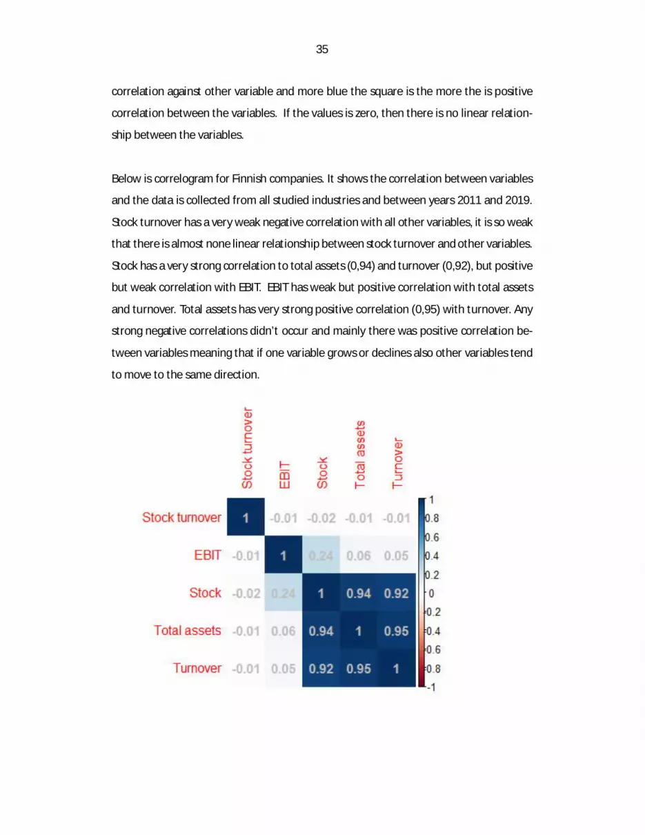
correlation against other variable and more blue the square is the more the is positive
correlation between the variables. If the values is zero, then there is no linear relation-
ship between the variables.
Below is correlogram for Finnish companies. It shows the correlation between variables
and the data is collected from all studied industries and between years 2011 and 2019.
Stock turnover has a very weak negative correlation with all other variables, it is so weak
that there is almost none linear relationship between stock turnover and other variables.
Stock has a very strong correlation to total assets (0,94) and turnover (0,92), but positive
but weak correlation with EBIT. EBIT has weak but positive correlation with total assets
and turnover. Total assets has very strong positive correlation (0,95) with turnover. Any
strong negative correlations didn’t occur and mainly there was positive correlation be-
tween variables meaning that if one variable grows or declines also other variables tend
to move to the same direction.

36
Table 2. Correlogram, Finland
Below is correlogram for US companies based on US data. It includes all studied seven
industries and gathered between the reference period 2011 and 2019. Stock turnover
has very weak positive correlation to total assets, turnover and EBIT, and very weak neg-
ative correlation to stock turnover. Stock and stock turnover don’t almost have a linear
relationship at all, because the correlation is so weak. This finding was almost aligned to
Finnish data where stock turnover has also very weak, almost non-linear correlation to
other variables. Stock has medium, 0,45, correlation to EBIT, but strong correlation to
turnover (0,65) and total assets (0,64) meaning that if value of stock increase also com-
pany’s turnover and total assets tend to increase; those variables have relatively strong
relationship. In addition to previously mentioned, total assets have very strong (0,96)
relationship with turnover and very strong relationship with EBIT. So if total assets in-
crease also turnover and EBIT tend to increase, in practice this is logical because for most
of the companies big value of total assets mean that company is big also in other metrics
(correlation is causation). Turnover has a strong correlation (0,91) to EBIT, meaning that
if turnover increases also EBIT tend to increase and vice versa.

37
Table 3. Correlogram, USA.
Basic data is formatted to histograms. Histograms are based on year 2019 data. In histo-
grams all variables studied (EBIT, turnover, total assets, stock turnover and value of stock)
are presented in own histograms separately and also countries from where data was
gathered, Finland and USA, were presented separately. Histograms following in below
are frequency histograms meaning that in vertical column frequencies are visible (and
also in top of each bin), there are also no caps between the bars. On the horizontal axis
value values of interval are visible.
First histogram is inventory turnover histogram, describing Finnish companies in 2019.
Stock turnover shows how many times company can sold and replace its inventory in a
year. Width of the bin is 5 and metric is 1x (inventory turns in a year). Histogram is limited
to 50 meaning that all values over 50 (inventory turns over 50 times in a year) are
grouped to the last bin. Number of companies exceeding 50x inventory turns in a year is
88. Inventory turnover histogram is skewed on right, i.e. the tail is going off in the right.
Majority of companies have inventory turnover between 0x – 15x in 2019.

38
Table 4. Inventory turnover histogram, Finland (2019).
Inventory turnover histogram (USA, fiscal year 2019) is shown in below. Width of bin is
same as in Finland (5) and histogram is limited to 50 (all values exceeding 50 are grouped
into last bin). Number of companies in USA within examined industries in 2019 that have
inventory turnover over 50 is 10 companies. As in Finland, also in the USA, histogram is
skewed on right, meaning that it has a positive skew. The shape of US histogram is similar
to Finnish histogram, most of the companies in studied industries had inventory turnover
between 0-15x in 2019.

39
Table 5. Inventory turnover histogram, USA (2019).
EBIT histogram below represents frequencies companies are divided based on their EBIT
levels. EBIT shows earnings before interest and taxes by a company. As we can see, most
of the companies have EBIT between 0 and 1 MEUR, so based on their EBIT levels, most
of the companies are relatively small. Width of a bin is 1 MEUR and all values over
20MEUR are grouped to the last bin. EBIT histogram for Finnish companies within the
examined industries in 2019 is relatively asymmetric. There are few companies that have
negative EBIT levels meaning that their operations are not profitable from EBIT point of
view.

40
Table 6. EBIT histogram, Finland (2019).
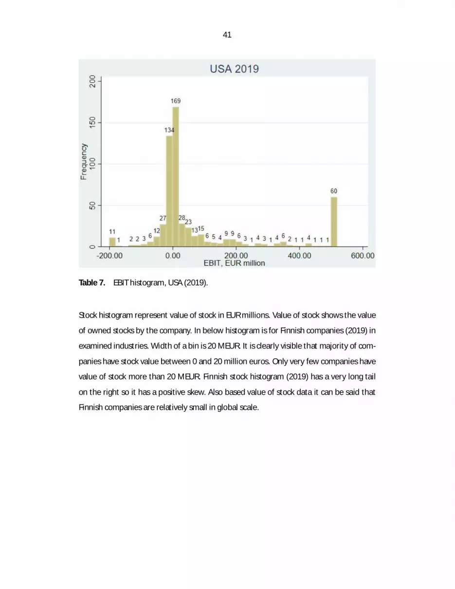
EBIT histogram for US companies within the studied industries in 2019 is different com-
pared to Finnish peers. First of all, width of the bin is 20 MEUR because the tails are
much longer for the US EBIT histogram compared to Finnish EBIT histogram. Most of the
companies are in 0 – 10 MEUR bin, number of companies in this bin are 169. In general
it can be said that from EBIT point of view, US companies are bigger compared to Finnish
peers. All of the companies that had EBIT more than 500 million euros in 2019 are
grouped into last bin and number of those companies is 60.
41
Table 7. EBIT histogram, USA (2019).
Stock histogram represent value of stock in EUR millions. Value of stock shows the value
of owned stocks by the company. In below histogram is for Finnish companies (2019) in
examined industries. Width of a bin is 20 MEUR. It is clearly visible that majority of com-
panies have stock value between 0 and 20 million euros. Only very few companies have
value of stock more than 20 MEUR. Finnish stock histogram (2019) has a very long tail
on the right so it has a positive skew. Also based value of stock data it can be said that
Finnish companies are relatively small in global scale.

42
Table 8. Value of stock histogram, Finland (2019).
Value of stock histogram for US companies (2019) in studied industries has a positive
skew and a long tail to the right, i.e. it skewed to the right. Width of a bin is 25 MEUR
and majority of companies, 339 companies, had value of stock between 0 and 25 million
euros. Companies those value of stock is more than 1000 million euros are grouped in
last bin, number of those companies is 32. Based on the value of stock data it can be said
that US companies are in average bigger compared to Finnish companies. As it was visi-
ble in correlograms if value of stock increases also value of turnover tend to increase,
and turnover is often used as a metric of company’s size.

43
’
Table 9. Value of stock histogram, USA (2019).
Histogram in below describes value of total assets for Finnish companies in studied in-
dustries (2019). Total assets shows the value of assets owned by the company. Width of
a bin is 50 MEUR and majority of companies, 1929 companies, have total assets between
0 and 50 million euros. Only very few companies of studied sample (4,8 %) have total
assets more than 50 million euros. Histogram is skewed to the right. Those Finnish com-
panies in studied industries that have total assets more that 1000 million euros are
grouped into last bin, the number of those companies is 13. Findings from total assets
histograms are well aligned to other histograms; Finnish companies are relatively small
in general.

44
Table 10. Total assets histogram, Finland (2019).
Total assets histogram (in below) for US companies has similar long tail to the right and
skewness as Finnish companies. Majority of the companies are in the first bin. Width of
the bin is 500 million euros so the companies have in average more assets compared to
the Finnish peers within same industries. Those US companies that have total assets
more than 10 000 million euros are grouped into the last bin and the number of those
companies is 37. Comparison to Finnish total assets histogram highlights previously find-
ings that in studied data US companies are bigger compared to Finnish companies.

45
Table 11. Total assets histogram, USA (2019).
Last histogram is turnover histogram. Turnover, i.e. sales, shows how much revenues
company receive from its operations. Histogram for Finnish companies has a positive
skewness. Most of the companies are in the first bin (1848 companies or 94% of total
sample) so have revenues between 0 and 50 million euros. Companies that have reve-
nues more that 1000 million are grouped into last bin. 15 Finnish companies within stud-
ied sample have revenues more that 1000 million euros.

46
Table 12. Turnover histogram, Finland (2019).
Turnover histogram for US companies (below) has similar positive skewness to the right
as Finnish peers. However, contrary to histogram for Finnish peers, width of the bin is
different (100 million euros) and histogram is limited to 5 000 million meaning that all
companies that have revenues more than 5 000 million euros are grouped to the last bin.
Number of companies in US sample that have revenues more than 5000 euros is 49 (and
8,2% of total sample). Number of companies in first bin is 283 (and 48 % of total sample).
Compared to Finnish peer it seems that US companies generate more revenues in aver-
age in studied population.

47
Table 13. Turnover histogram, USA (2019).
4.2 Industry 16 – manufacture of wood and of products of wood
Sample in industry NACE Rev. 2: 16 – manufacture of wood and of products of wood and
cork, expect furniture; manufacture of articles of straw and and plainting materials con-
sists of 3587 companies of which 573 companies were selected to review, 559 companies
from Finland and 14 companies from the United States of America. Rest of the compa-
nies did not have data available or were no longer in operation.
Between period 2012 and 2019 average inventory turnover (in rounds) for Finnish com-
panies is higher compared to US companies. In 2011 inventory turnover was higher for
US companies compared to Finnish companies. In 2019 average inventory turnover for
Finnish companies was 20,05x and for US companies 9,95x. Lower average inventory
turnover for US companies may indicate e.g. that they have overstock but also lower
possibility to shortages if inventory overall is saleable.
48
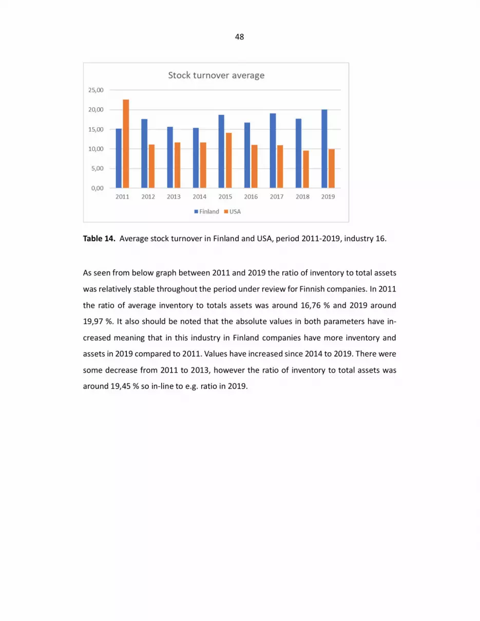
Table 14. Average stock turnover in Finland and USA, period 2011-2019, industry 16.
As seen from below graph between 2011 and 2019 the ratio of inventory to total assets
was relatively stable throughout the period under review for Finnish companies. In 2011
the ratio of average inventory to totals assets was around 16,76 % and 2019 around
19,97 %. It also should be noted that the absolute values in both parameters have in-
creased meaning that in this industry in Finland companies have more inventory and
assets in 2019 compared to 2011. Values have increased since 2014 to 2019. There were
some decrease from 2011 to 2013, however the ratio of inventory to total assets was
around 19,45 % so in-line to e.g. ratio in 2019.

49
Table 15. Stock average and total assets average, industry 16, Finland.
For US companies the ratio of inventory to total assets has slightly increased from 5,85 %
in 2011 to 7,68 % in 2019. As in Finland also in the USA the absolute values of both
variables have increased during the period under review. Compared to Finnish compa-
nies the ratio of inventory to total assets in US companies in this industry is lower mean-
ing that inventories represent smaller share of total assets than in Finland.
Table 16. Stock turnover and total assets in average, industry 16, USA

50
Below is statistics for Finnish companies in manufacture of wood and products of wood
industry between studied years 2011 - 2019. Data has in total 4021 observations. Value
of stock is dependent variable. R-squared is 0,915. Stock has statistically significant re-
gression to EBIT, total assets and turnover with 99% confidence level. In practice that
means that if company increases its value of stock also EBIT, total assets and turnover
increases. Stock is part of total assets so this finding might indicate that stock represents
considerable share of total assets in this industry. However, although stock positive re-
gression to EBIT, the regression is not as big as between stock to total assets or to turn-
over. Theory supports this evidence because if value/amount of stock increases it usually
slows stock turnover so company is not handling its working capital as efficiently as pos-
sible, i.e. there is a lack of WCM efficiency. Once value of stock increases it is logical that
also turnover increases. Otherwise company is not selling its stock or sells it with dis-
count. Stock has also negative regression to stock turnover with 99% confidence interval,
meaning that it value of stock increases then stock turnover decreases.
51
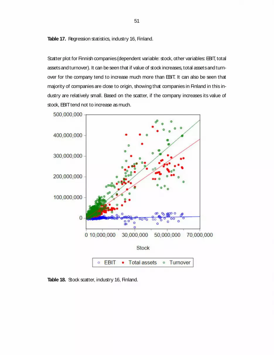
Table 17. Regression statistics, industry 16, Finland.
Scatter plot for Finnish companies (dependent variable: stock, other variables: EBIT, total
assets and turnover). It can be seen that if value of stock increases, total assets and turn-
over for the company tend to increase much more than EBIT. It can also be seen that
majority of companies are close to origin, showing that companies in Finland in this in-
dustry are relatively small. Based on the scatter, if the company increases its value of
stock, EBIT tend not to increase as much.
Table 18. Stock scatter, industry 16, Finland.

52
Below is statistics for the USA in manufacture of wood and products of wood industry
between 2011 and 2019. Data has 98 observations. R-squared is 0,960. Results show
that stock has statistically strong positive regression with turnover where coefficient is
0,1265. This data for US companies also show that stock has statistically negative regres-
sion with total assets. Regression between stock and turnover and between stock and
total assets are with 99 % confidence interval. Turnover tend to increase if value of stock
increases because company needs to sell its inventory in order to be profitable. In this
data stock didn’t have statistically significant regression to EBIT, that might indicate that
EBIT levels decrease or remain in same level if value of stock increases with 99% confi-
dence interval. Stock did have negative regression with EBIT in 95 % confidence interval
where coefficient was -0,1359. Stock did have also negative regression with stock turn-
over with 90 % confidence interval.
Table 19. Regression statistics, industry 16, USA.

53
Scatter from US data (below) has similar effect to Finnish scatter. If the value of stock
increases turnover and total assets tend to increase more than EBIT. Based on the scatter
there seems to be some correlation between stock and total assets. This is logical be-
cause stock is accounted as part of total assets. Also statistical regression model found a
relationship between stock and total assets in USA in this industry.
Table 20. Stock scatter, industry 16, USA.

54
4.3 Industry 17 – manufacture of paper and paper products
Sample of industry manufacture of paper and paper products (NACE Rev. 2. classification:
17) consists of 329 companies of which 155 companies were selected to further review
(135 companies from Finland and 20 companies from the USA). Rest of the companies
did not have the data available or were no longer in operation.
Inventory turnover in average was higher for Finnish companies compared to US peer
during the whole reference period between 2011 and 2019 indicating better working
capital management in terms of inventories. Average inventory turnover fluctuated rel-
atively much in both countries within this industry. In Finland decreasing trend can be
seen between 2016 and 2019 whereas in the US trend can be seen to be increasing be-
tween years 2017 and 2019. In this data there is no clear evidence why the trend has
opposite in recent years in Finland and in the US. In 2019 the average inventory turnover
in Finland was 12.9x and in the US 12,1x. Highest inventory turnover average in Finland
was 18,0x in 2012 and highest figure in the US was 12,1 in 2019. Although trend has
been opposite during recent years, it can be said that Finnish companies are more effi-
cient compared to US companies in terms of stock turnover during the reference period.
However, it should be noted that US companies are stock listed i.e. bigger in average
compared to Finnish data where majority of the companies are not stock listed.
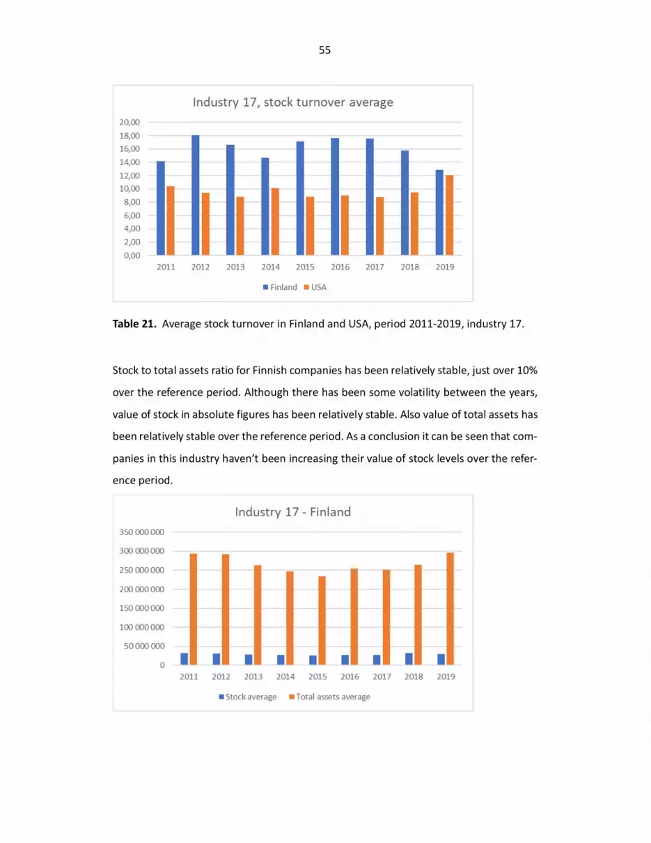
55
Table 21. Average stock turnover in Finland and USA, period 2011-2019, industry 17.
Stock to total assets ratio for Finnish companies has been relatively stable, just over 10%
over the reference period. Although there has been some volatility between the years,
value of stock in absolute figures has been relatively stable. Also value of total assets has
been relatively stable over the reference period. As a conclusion it can be seen that com-
panies in this industry haven’t been increasing their value of stock levels over the refer-
ence period.

56
Table 22. Stock average and total assets average, industry 17, Finland
Value of stock in average to value of total assets in average has been relatively stable
also for the US companies over the reference period. Value of stock in average to value
of total assets in average ratio has been for US companies just below 10 % so slightly
lower than for Finnish peers. Absolute values of average stock level and for total assets
have increased during the reference period. Average stock value ended up in 2019 to
566,4 million euros whereas for Finnish companies it was around 29,7 million euros at
the end of 2019.
Table 23. Stock average and total assets average, industry 17, USA.
Below are results for statistical regression analysis for Finnish companies. In total there
was 922 observations that formed the results. Dependent variable was value of stock
and r-squared is 0,9937. Based on data there was strong regression between stock and
EBIT (coefficient: 0,0524), stock and total assets (coefficient: 0,0326) and between stock
and turnover (coefficient: 0,0896) with 99 confidence interval. This finding indicates that
for Finnish companies in industry 17 between years 2011 and 2019 is value of stock in-
creases also EBIT, total assets and turnover tend to increase. Value of stock has a negative
regression with stock turnover with 90 % confidence interval.
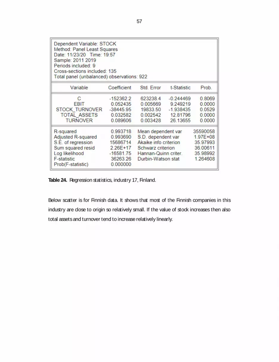
57
Table 24. Regression statistics, industry 17, Finland.
Below scatter is for Finnish data. It shows that most of the Finnish companies in this
industry are close to origin so relatively small. If the value of stock increases then also
total assets and turnover tend to increase relatively linearly.

58
Table 25. Stock scatter, industry 17, Finland.
Statistical regression data for US companies in industry 17 consists of total 171 observa-
tions. Dependent variable is value of stock and r-squared is 0,9757. Based on the analysis
value of stock has statistically strong positive relationship with total assets (coefficient
0,0167) and turnover (coefficient: 0,0922) with 99 % confidence interval. Value of stock
has statistically negative regression to stock turnover with 99 % confidence interval
meaning that if value of stock increases stock turnover tend to decrease that leads to
slower efficiency in terms of working capital efficiency.

59
Table 26. Regression statistics, industry 17, USA
From the US scatter below it is visible that is value of stock increases total assets and
turnover increases the most. Amount of EBIT increases as well but not as much as total
assets and turnover. These findings are similar to Finnish scatter from the same industry.

60
Table 27. Stock scatter, industry 17, USA.
4.4 Industry 22 – industry rubber and plastic
Sample in manufacture of rubber and plastic products -industry (Nace. Rev. 2: 22) con-
sists of 871 companies in total. 432 companies from Finland and 36 companies from the
United States of America were selected to further review.
Inventory turnover in average has been better in Finland compared to the USA. Especially
during the years 2017-2019 inventory turnover has been higher in Finland compared to
the USA. In 2019 Finland stand in around 14x and USA just below 8x. However, it should
be noted that both have been in decreasing trend from 2017 to 2019. Stock turnover
overall in average has fluctuated during the reference period.

61
Table 28. Average stock turnover in Finland and USA, period 2011-2019, industry 22.
Data from Finnish companies between years 2011 and 2019 shows that value of inven-
tory to value of total assets has increased during the sample period. In absolute values
both of the indicators, values of inventory and value of total assets, increased during the
reference period. In the USA total value of inventory to value of total assets has de-
creased during the reference period. However, as in Finland, also in the USA absolute
values of both indicators have increased during the reference period.

62
Table 29. Stock average and total assets average, industry 22, Finland.
For US companies the value of stock ratio to total assets has been decreasing during the
reference period. Main reason for that is significant increase in value of total assets in
average. However, also value of stock in average has increased during the reference pe-
riod. In 2019 value of inventory to value of total assets ratios was 12,48 %.
Table 30. Stock average and total assets average, industry 22, USA.

63
Below is statistic for Finnish companies in industry 22. It is formed from 3071 observa-
tions. R-squared is 0,992. Value of stock as a dependent variable has strong positive re-
gression with EBIT (coefficient: 0,048), with total assets (coefficient : 0,141) and with
turnover (coefficient: 0,017). This finding shows that in rubber and plastic industry if
value of stock increases also EBIT, total assets and turnover tend to increase. All of those
findings are at 99 % confidence interval. Stock and stock turnover have strong but nega-
tive regression showing that if the value of inventory increases then stock turnover tend
to decrease. This result is at 90 % confidence interval.
Table 31. Regression statistics, industry 22, Finland.
Below scatter is based on Finnish data. It shows that most of the Finnish companies are
close to origin in terms of value of stock, value of total assets or turnover, so Finnish

64
companies in this industry are relatively small. Scatter clearly show that if the value of
stock increases then also company’s turnover and total assets increase more than EBIT.
Table 32. Stock scatter, industry 22, Finland.
Regression model for US companies in industry 22 consists of 273 observations. Depend-
ent variable is stock and r-squared is 0,9716. Based on this data, value of stock has a
positive strong regression with total assets (coefficient: 0,0173) and with turnover (co-
efficient: 0,1421). These finding are with 99 % confidence interval. From statistical point
of view there was no significant statistical findings between value of stock and EBIT or
with value of stock and stock turnover.

65
Table 33. Regression statistics, industry 22, USA.
Scatter from US data for industry 22 (below) shows that if the value of stock increases
turnover and total assets tend to increase much more than EBIT.

66
Table 34. Stock scatter, industry 22, USA
4.5 Industry 23 – manufacture of vehicles, trailers and semi-trailers
Sample of manufacture of vehicles, trailers and semi-trailers (NACE Rev. 2 classification:
23) consist of 1295 Finnish companies and 26 companies registered in the USA (1321
companies in total). From this sample 394 Finnish companies and 19 US companies were
selected to further review. Rest of the companies were no longer active or didn’t have
sufficient data.
In industry 23 stock turnover in average has been clearly higher for Finnish companies
compared to US during the reference period. Only exception is year 2011 when stock
turnover in average was higher for US companies. For US companies trend has been rel-
atively stable, around 9x – 10x between 2012 and 2019. For Finnish companies trend has
been slightly increasing between 2013 and 2019 (around 20x – 23x).

67
Table 35. Average stock turnover in Finland and USA, period 2011-2019, industry 23.
In Finland the absolute value of inventories in this industry has increased during the ref-
erence period 2011-2019. Also value of the inventory to value of total assets has in-
creased during the sample period. At the end of 2019 the ratio was 13,59 %.
Table 36. Stock average and total assets average, industry 23, Finland.

68
For the US companies absolute values for value of stock and total assets have increased
during the reference period. The ratios has been relatively stable. At the end of 2011 it
was 11,07 % and at the end of 2019 it was 9,51 %. Overall during the reference period it
has been close to 10 %.
Table 37. Stock average and total assets average, industry 23, USA.
Below is statistics of Finland between years 2011 and 2019 in manufacture of vehicles,
trailers and semi-trailers industry. It consists of 2777 observations. R-squared is 0,844.
Stock is dependent variable and its regression was measured against other variables.
Value of stock has significant statistical positive regression with turnover (coefficient:
0,1219) and positive statistical regression with EBIT (coefficient: 0,1387) and total assets
(coefficient: 0,0168) with 99 % confidence interval. Value of stock has also negative re-
gression with stock turnover meaning that if values of stock increases stock turnover
tend to decrease.

69
Table 38. Regression statistics, industry 23, Finland.
Below scatter based on Finnish data shows that if value of stock increases then turnover
for the company and total assets tend to be bigger compared to the EBIT.

70
Table 39. Stock scatter, industry 23, Finland.
For US data there was 144 observations in total between years 2011 and 2019. Depend-
ent variable is stock and r-squared is 0,9942. Value of stock has a statistically positive
regression with turnover (coefficient: 0,1216) and total assets (coefficient: 0,0276) with
confidence interval 99 %. Stock has statistically negative regression with EBIT (coefficient:
-0,1388) with confidence interval 99 %. Between stock and stock turnover there was no
statistically significant findings.

71
Table 40. Regression statistics, industry 23, USA.
Scatter below shows that in USA sample in industry 23 if value of stock increases then
value of total assets and turnover tend to increase more than EBIT.

72
Table 41. Stock scatter, industry 23, USA.
4.6 Industry 24 – manufacture of basic metals
Sample in manufacture of basic metals industry (NACE Rev. 2. classification: industry 24
– manufacture of basic metals) consist of 217 companies from Finland and 185 compa-
nies from the United States of America (in total 402 companies). Of this sample 83 com-
panies from Finland and 63 companies from the USA were selected to further review.
Other companies didn’t have sufficient data available.
Stock turnover in average has been bigger for Finnish companies compared to US peers
during the reference period. However, the trend for Finnish companies has been
decreasing whereas for US companies the trend has been increasing. At the end of 2019

73
inventory turnover in average for Finnish companies was 13,87x and for US companies
it was 10,53x.
Table 42. Average stock turnover in Finland and USA, period 2011-2019, industry 24.
For Finnish companies both, values of inventory in average and total assets have been
stable during the reference period. There are some fluctuations but nothing major. At
the end of 2011 the ratio was 15,12 % and at the end of 2019 17,43 %.

74
Table 43. Stock average and total assets average, industry 24, Finland.
For the USA companies value of total assets has increased steadily during the reference
period. Also absolute values of inventories are increased. The value of stock to total as-
sets ratio is lower for US companies compared to Finnish peers. At the end of 2011 it was
11,44 % and at the end of 2019 11,81 %.
Table 44. Stock average and total assets average, industry 24, USA.
There was in total 573 observations for Finnish companies between year 2011 and 2019.
Dependent variable is stock and r-squared is 0,8545. There was no significant statistical
findings between stock and EBIT and between stock and stock turnover. Between stock
and total assets there was statistically significant regression (coefficient: 0,1519) and also
between stock and turnover (coefficient: 0,0378) with confidence interval 99 %.

75
Table 45. Regression statistics, industry 24, Finland.
Based on the scatter for Finnish companies in below, if value of stock increases then
turnover and value of total assets tend to increase more than EBIT. This finding is aligned
with similar data in other industries.
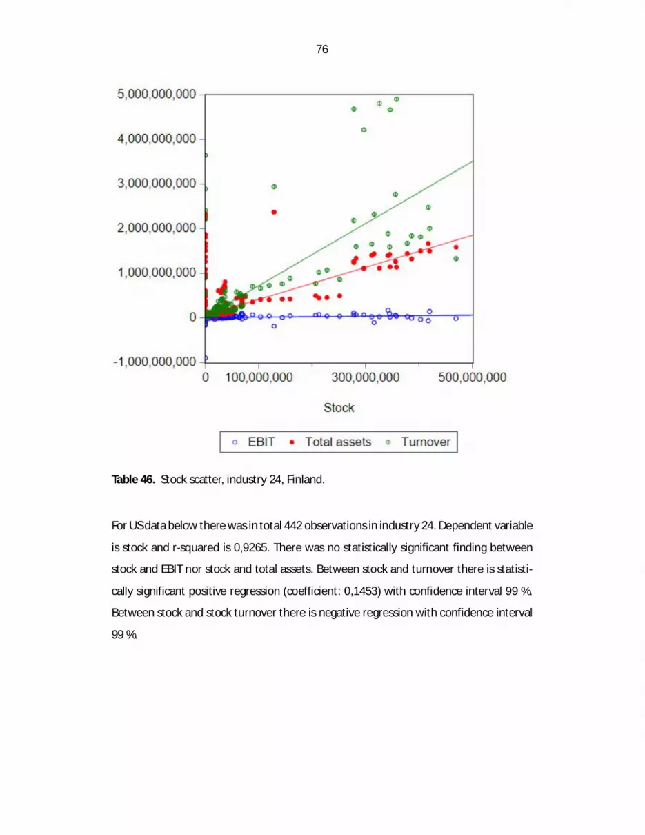
76
Table 46. Stock scatter, industry 24, Finland.
For US data below there was in total 442 observations in industry 24. Dependent variable
is stock and r-squared is 0,9265. There was no statistically significant finding between
stock and EBIT nor stock and total assets. Between stock and turnover there is statisti-
cally significant positive regression (coefficient: 0,1453) with confidence interval 99 %.
Between stock and stock turnover there is negative regression with confidence interval
99 %.

77
Table 47. Regression statistics, industry 24, USA.
Scatter for US based companies indicates that the larger the value of stock is then total
assets and turnover tend to increase more than EBIT.

78
Table 48. Stock scatter, industry 24, USA.
4.7 Industry 26 – manufacture of computer, electrical and optical prod-
ucts
Sample of manufacture of computer, electrical and optical products consist of 1048 Finn-
ish companies and 588 companies from the USA (i.e. 16632companies in total). From
this sample 417 Finnish companies and 433 companies from the USA were selected to
further analysis.
In Finland the stock turnover in average is more efficient compared to US peers. During
the reference period only exception is 2014 when stock turnover in average was 13,83x

79
in the USA and 12,53x in Finland. During other years in reference period stock turnover
in average has been higher in Finland compared to the USA. However, between 2011 and
2015 the difference in this ratio has not been very high between the countries. From
2016 to 2019 stock turnover in average has been higher in Finland compared to the USA
indicating that companies in Finland in this industry have been e.g. more efficient in
terms of working capital perspective in stock.
Table 49. Average stock turnover in Finland and USA, period 2011-2019, industry 26.
In Finland total value of inventories to total assets ratio was slightly higher compared to
US peers during the reference period. In 2019 the total value of inventory to total assets
ratio in Finland around 6,67 %. In the USA the total value of inventory to total assets ratio
at the end of 2019 was 5,24 % so slightly lower compared to Finland. However, in both
countries the value of inventory to total assets ratio is low compared to any other indus-
try reviewed in this thesis.

80
Table 50. Stock average and total assets average, industry 26, Finland.
Table 51. Stock average and total assets average, industry 26 USA.

81
From statistical point of view it is visible that in Finland stock has statistically significant
positive correlation to EBIT (coefficient: 0,1023) and to total assets (coefficient: 0,062)
with confidence interval 99%. Stock did not have statistical significant findings to other
variables, stock turnover and turnover. This finding in Finland within manufacture of
computer, electrical and optical industry indicates that companies can speed up their
sales in way that they don’t necessary need to increase their inventories, if they are more
efficient in terms on inventory turnover. That way they might be able also to release tight
capital in their operations.
Table 52. Regression statistics, industry 26, Finland.
From below graph we can see that if value of stock increases then also other variables
increase. Amount of total assets increase most, then total assets and EBIT as a third.

82
Table 53. Stock scatter, industry 26, Finland.
In the USA statistically significant positive regression was visible between stock and total
assets (coefficient: 0,0229) and between stock and turnover (coefficient: 0,0321) with
99 % confidence interval. In practice this indicates that if the companies within this in-
dustry increase their sales or total assets also value of the stock increases. Stock did also
have statistically significant but negative regression to EBIT (coefficient: -0,1459) and in-
ventory turnover with 99 % confidence interval. This finding points out that if companies
increase their value of inventory it leads to worse inventory turnover. In practice this
indicates that there should be room for efficiency improvements in inventory turnover.
From working capital perspective it would be better that if value of stock increases it
wouldn’t have statistically significant correlation to inventory turnover. Statistically

83
significant negative correlation between stock and EBIT also indicates that companies
are not working with their stock in most efficient way from working capital point of view.
This finding shows that companies are not able to turn their increased stock volumes to
profit in best way possible. R-squared is 0,5677).
Table 54. Regression statistics, industry 26, USA.
From below graph can be seen that if value of stock increases the also values of total
assets, turnover and EBIT increases. Graph indicates that, compared to Finnish peers,
EBIT seems to increase more for the US companies.

84
Table 55. Stock scatter, industry 26, USA.
4.8 Industry 27 – manufacture of electrical equipment
Sample of manufacture of electrical equipment industry consist of 650 companies from
Finland and 99 companies from the USA, so in total 749 companies. 277 companies from
Finland and 65 companies from the USA were selected to further review. Other compa-
nies didn’t enough sufficient data to be analyzed further.
Below graph describes stock turnover in average in the USA and in Finland during the
reference period 2011 – 2019. Based on the data and diagram below US companies
within studied industry have enhanced its stock turnover in average compared to Finnish
peers. At the end of 2019 US companies value of stock turnover in average stood in

85
15,29x while for Finnish companies the number was 11,20x. If we look only Finnish com-
panies within this industry, data shows that their stock turnover in average has actually
decreased during the reference period (at the end of 2011 it was 12,04x and at the end
of 2019 11,20x). This might indicate weaker working capital management and yield to
weaker EBIT. Especially between 2017 and 2019 trend of stock turnover in average has
been decreasing for Finnish companies in manufacture of electrical equipment industry.
Table 56. Average stock turnover in Finland and USA, period 2011-2019, industry 27.
Below graph describes how value of stock in average and value of totals assets in average
have developed during the period considered in Finland in manufacture of electrical
equipment industry. The value of inventory to value of totals has increased during the
reference period. At the end of 2019 it was 21,80 %. Both variables have increased from
2011 to 2019.

86
Table 57. Stock average and total assets average, industry 27, Finland.
Below is same graph for US companies in manufacture of electrical industry. It can be
seen that value of total assets in average has increased during the reference period. Also
value of inventories in average has increased during the reference period but not as
much as the values of total assets. This leads to that the value of inventories in average
to value of total assets in average ratio has decreased during the reference period. At
the end of 2011 it was 13,75 % and at the end of 2019 it was 11,94 %. Compared to
Finnish data value of inventories in average to value of total assets in average ratio has
been around 6-7 percentage points lower in the USA compared to Finnish peers in this
industry.

87
Table 58. Stock average and total assets average, industry 27, USA.
Below is main statistics for Finnish companies in manufacture of electrical equipment
industry between years 2011 and 2019. Data has in total 1895 observations and r-
squared is 0,9069. Below regression model shows that stock has a statistical significant
regression EBIT (coefficient: 0,2954) and total assets (coefficient: 0,1701) and negative
regression with turnover (coefficient: -0,0402). R-square is over 0,5 so predictor variable
stock explains very well the response variables EBIT, stock turnover, total assets and turn-
over. There was no statistical significant regression between stock and stock turnover.

88
Table 59. Regression statistics, industry 27, Finland.
Below stock scatter observes that if value of stock in big then also total assets and turn-
over tend to be big. EBIT also increases but not with as sharp slope.

89
Table 60. Stock scatter, industry 27, Finland.
Below is statistics for US companies in manufacture of electrical equipment industry in
reference period 2011 – 2019. Total number of observations found was 404. R-square is
around 0,97 so predictor variable explains very well response variables EBIT, stock turn-
over, total assets and turnover. There is strong statistical regression between stock (pre-
dictor variable) and turnover (coefficient: 0,0935), and also between stock and total as-
sets (coefficient: 0,0432) with 99 % confidence interval. Between value of stock and EBIT
there was negative regression with 90% confidence interval. There was no significant
statistical findings between stock and stock turnover.

90
Table 61. Regression statistics, industry 27, USA.
Below stock scatter for US companies observes that if value of stock increases then slope
for turnover and total assets is bigger compared to slope of EBIT.

91
Table 62. Stock statistics, industry 27, USA.

92
5 Conclusions
The objective of this master’s thesis was to study how company’s stock values affect to
other key variables (EBIT, total assets, turnover and stock turnover) and study this topic
especially from working capital point of view. To achieve this objective theoretical back-
ground related to working capital management and supply chain management, was
studied in second chapter of thesis. Theoretical framework was studied based on aca-
demic journals and sources and literature.
After the theory review, in the second part of the thesis, empirical research methodolo-
gies were presented. Empirical research was based on quantitative research methods.
Data to the empirical part was gathered from Orbis database. Due to the big amount of
data, the data has several limitations: only two countries were selected (USA and Fin-
land), reference period was limited to years 2011 – 2019 and seven industries (based on
NACE rev. 2 classification) was studied. Empirical part focused to answer to the research
questions that what is the correlation and regression between stock and selected finan-
cial variables, is there differences between industries overall and differences between
industries in Finland and the USA and finally is there any visible differences between
Finland and USA in selected industries in terms of selected variables.
Correlation analysis was done in correlogram. In correlogram Finnish companies in all
studied industries were grouped and compared against US peers. From Finland the ma-
jor finding was that correlation between value of stock and EBIT was 0,24 meaning that
correlations between those variables is weak. In practice that means that in general the
EBIT doesn’t grow as fast as the value of stock. Academic literature support this finding
from working capital point of view. Higher value of stock needs to be financed and the
capital is tied into stock. Also, based on the academic literature, high value of stock have
also other possible disadvantages, e.g. increased possibility to write-downs, if stock is
not any more saleable. Instead of investing into inventories companies could invest the
capital into other operations that would grow its EBIT. However, it should be noticed that
higher value of stock is not necessary poor thing for the companies; with high levels of

93
inventories companies can supply its customers also if there are any kind of disturbance
in the markets and normal supply in the chain is not working as it should. Between other
variables there was strong correlation between stock and total assets and between stock
and turnover. Stock turnover did have very weak negative correlation to all variables.
Correlogram based on data from US companies had fairly parallel findings as Finnish data.
Between stock and EBIT the correlation was 0,45 so it was stronger than Finnish compa-
nies had but still weak correlation in absolute terms. So if value of inventory also EBIT
tends to increase but less than the value of stock. However, seems that US companies
can turn increased values of inventories more better into profit than Finnish peers can.
Other findings were also similar as Finnish data; total assets had strong correlation to
EBIT and turnover, turnover did have strong correlation to EBIT. Stock did have over 0,5
correlation to total assets (0,64) and to turnover (0,65), these correlations were weaker
than Finnish peers. Stock turnover did have very weak but positive correlation to all var-
iables.
5.1 Managerial implications
Based on the theoretical review of working capital management, academic research and
literature and empirical research this part of the thesis provides author provides sugges-
tions and implications regarding inventories and company’s financial performance.
Based on the statistical analysis and supported by academic research companies should
not target to increase stock levels. Based on the statistical analysis, if value of stock in-
creases also EBIT tend to increase but lower slope. Companies should target to optimize
their inventory level to the point where they can avoid possible costly stock-outs but
where it does not tie working capital more than necessary into inventories. Based on the
data used in this thesis Finnish companies have positive correlation between value of
stock and EBIT (0,24) and so also does US companies (0,45). However, correlation below
0,5 (but over 0) can be considered as a weak correlation. That indicates that companies
should not target to increase their inventory levels over reasonable level where they can

94
secure their supply to the end customers. From correlogram it was found also that stock
and stock turnover does not have linear relationship between each other. From correlo-
gram it can also be highlighted that US companies had weak positive (0,12) correlation
between stock turnover and EBIT. So, this might indicate that faster inventory turns ben-
efit also profitability of the companies. Also academic literature has found that higher
efficiency in inventory turns will benefit working capital levels that have relationship to
the profitability of the company.
There was no big variations between industries. High value of stock tend to have strong
positive regression especially to turnover and total assets. That is logical because if com-
pany afford to have invested to value of stock it needs to finance it and operative cash
flow comes from sales, i.e. turnover. Also if company is able to sell produced goods, the
goods are first accounted in inventory. Inventory is booked in total assets so regression
between those variables is also logical. It was seen that inventory values during the ref-
erence period have increased. Companies may have for instance higher their safety mar-
gins to avoid costly stock-outs. From working capital perspective however, the increase
is not beneficial from profitability perspective. Companies may should consider to avoid
any further increase in values of inventory but instead try to put efforts to optimize the
goods flow in whole supply chain.
Inventory turnovers were overall in average higher for Finnish companies compared to
US peers. In the data analyzed US companies were larger in terms of turnover and EBIT
for instance. This indicated that smaller companies are more agile to handle their inven-
tories. Academic literature shows that one negative aspect for slow inventory turnover
is increased risk to inventory write-offs. Relationship between inventory turnover and
inventory write-downs was not studied in this thesis.
In some industries was found negative regression between EBIT and value of inventories.
Between studied countries there were no major differences. This finding is something
companies should understand in operative business. However, this finding was
95
dependent by business. In industries where there seems to be negative regression be-
tween value of stock and EBIT, companies should target to decrease their inventory lev-
els and that way released tied capital into other operations. Reduce of tied capital should
positively affect to company’s return on investment ratio and also improve liquidity po-
sition.
5.2 Limitations and implications for future research
This research was conducted as a quantitative research with several limitations and
therefore the results and implications are only applicable only if all limitations are taken
into consideration within the scope of the thesis. Empirical part was studied in seven
industries. Thus, the results and implications are applicable only in those industries and
cannot be extended to all industries available. An other major limitation is that compa-
nies only two countries, Finland and USA, were studied, thus, considerations from this
thesis cannot be extended to other countries. In USA only public companies were stud-
ied and that should be taken also into account when analyzing and reading the results.
This limitation needed to be done in order to have sufficient data for all companies, i.e.
for non-public US companies the data was not available. Third major limitations is related
to reference period, the data was gathered for years 2011 – 2019, thus the findings might
not be valid for other reference periods.
During the thesis, some recommendations for future research were observed. Based on
the academic literature there might be a room for a study that would analyze more ac-
curate that would it be beneficial for a supply chain, in terms of overall quality, that
stronger companies would finance weaker ones in terms of faster payment (terms). If
weaker companies would that way have a faster in-flow in cash, would it increase the
quality and speed of its deliveries and that way benefit all companies in supply chain in
terms of higher overall quality in whole supply chain. Also related to supply chain context,
future research could study how stock levels could be optimized in a supply chain in a
way that the price of a having stock would be as low as possible in supply chain context
but also secure the deliveries. Also it would be interesting to see research related to

96
relationship between value of inventory, inventory safety margin and company’s profit-
ability. I.e. if companies would lower their value of inventory and that way also inventory
safety margin, would it have positive or negative impact on company’s profitability. Fur-
ther studies could also focus on relationship between inventory turnover and inventory
write-offs more deeply, i.e. does slow inventory turnover lead significantly more inven-
tory write-downs or not.
This thesis mainly focused on major metrics related to stock and company’s financial
performance. To extend this research future research would focus on smaller metrics
and take also into account how accounts payables and accounts receivables would affect
to EBIT and stock. It would be interesting to see would changes in accounts payables and
account receivables affect to value of stock and EBIT. Also more comprehensive study
between different countries or between different industries would bring more under-
standing how stock is related to different metrics. In order to understand more deeply,
why there are differences between industries future research could focus for example in
very few industries and go more deep into industries financials, compare them and re-
search if there are some mechanism why other industries have more correlation be-
tween value of stock and e.g. EBIT.
97
References
Aktas, N., Croci, E. & Petmezas, D. (2015). Is working capital management value-
enhancing? Evidence from firm performance and investments. Journal of
Corporate Finance, 30, 98-113. https://doi.org/10.1016/j.jcorpfin.2014.12.008
Banos-Caballero, S., Garcia-Teruel, P. & Martinez-Solano, P. (2014). Working capital
management, corporate performance, and financial constraints. Journal of
Business Research, 67(3), 332-338.
https://doi.org/10.1016/j.jbusres.2013.01.016
Bendig, D., Brettel, M. & Downar, B. (2018). Inventory component volatility and its
relation to returns. International Journal of Production Economics, 200, 37-49.
https://doi.org/10.1016/j.ijpe.2018.03.012
Bian, Y., Lemoine, D., Yeung, T., Bostel, N., Hovelaque, V., Viviani, J-L & Gayraud, F. (2018).
A dynamic lot-sizing-based profit maximization discounted cash flow model
considering working capital requirement cost with infinite production capacity.
International Journal of Production Economics, 196, 319-332.
https://doi.org/10.1016/j.ijpe.2017.12.002
Boisjoly, R., Conine Jr, T. & McDonald IV, M. (2020). Working capital management:
Financial and valuation impacts. Journal of Business Research, 108, 1-8.
https://doi.org/10.1016/j.jbusres.2019.09.025
Chauhan, G. (2019). Are working capital decisions truly short-term in nature? Journal of
Business Research, 99, 238-253. https://doi.org/10.1016/j.jbusres.2019.02.032
Deloof, M. (2003). Does Working Capital Management Affect Profitability of Belgian
Firms? Journal of Business Finance & Accounting, 30(3), 573-587. https://doi-
org.proxy.uwasa.fi/10.1111/1468-5957.00008
Ding, S., Guariglia, A. & Knight, J. (2013). Investment and financing constraints in China:
Does working capital management make a difference? Journal of Banking &
Finance, 37(5), 1490-1507. https://doi.org/10.1016/j.jbankfin.2012.03.025

98
Engblom, J., Solakivi, T., Töyli, J. & Ojala, L. (2012). Multiple-method analysis of logistics
costs. International Journal of Production Economics, 137(1), 29-35.
https://doi.org/10.1016/j.ijpe.2012.01.007
Enqvist, J., Graham, M. & Nikkinen, J. (2014). The impact of working capital management
on firm profitability in different business cycles: Evidence from Finland. Research
in International Business and Finance, 34, 36-49.
https://doi.org/10.1016/j.ribaf.2014.03.005
Eroglu, C. & Hofer, C. (2010). Lean, leaner, too lean? The inventory-performance link
revisited. Journal of Operations Management, 29, 356-369.
https://doi.org/10.1016/j.jom.2010.05.002
Jalal, A. & Khaksari, S. (2019). Cash cycle: A cross-country analysis. Financial
Management, 1-37. https://doi.org/10.1111/fima.12273
Jones, C. & Tuzel, S. (2013). Inventory investment and the cost of capital. Journal of
Financial Economics, 107, 557-579.
https://doi.org/10.1016/j.jfineco.2012.09.001
Krajewski, L.; Malhotra, M. & Ritzman, L. (2019). Operations Management - Processes
and Supply Chains. Harlow: Pearson Education Limited.
Kim, K. (2020). Inventory, fixed capital, and the cross-section of corporate investment.
Journal of Corporate Finance, 60, 101528.
https://doi.org/10.1016/j.jcorpfin.2019.101528
Lind, L., Pirttilä, M., Viskari, S., Schupp, F. & Kärri, T. (2012). Working capital management
in the automotive industry: Financial value chain analysis. Journal of Purchasing
and Supply Management, 18(2), 92-100.
https://doi.org/10.1016/j.pursup.2012.04.003
Moser, P., Isaksson, O., & Seifert, R. (2017). Inventory dynamics in process industries: An
empirical investigation. International Journal of Production Economics, 191, 253-
266. https://doi.org/10.1016/j.ijpe.2017.06.019
Plaza, M., David, I. & Shirazi, F. (2018). Management of inventory under market
fluctuations the case of Canadian high tech company. International Journal of
Production Economics, 205, 215-227. https://doi.org/10.1016/j.ijpe.2018.09.007

99
Ross, S., Westerfield, R. & Jordan, B. (2019). Corporate Finance Fundamentals. McGraw-
Hill /Irwin. Eight edition. 864 p.
Tsuruta, D. (2019). Working capital management during the global financial crisis:
Evidence from Japan. Japan & The World Economy, 49, 206-219.
https://doi.org/10.1016/j.japwor.2019.01.002
Wetzel, P. & Hofmann, E. (2019). Supply chain finance, financial constraints and
corporate performance: An explorative network analysis and future research
agenda. International Journal of Economics, 216, 364-383.
https://doi.org/10.1016/j.ijpe.2019.07.001
Wu, Q., Muthuraman, K., & Seshadri, S. (2019). Effect of Financing Costs and Constraints
on Real Investments: The Case of Inventories. Production and Operations Man-
agement, 28(10), 2573-2593. https://doi.org/10.1111/poms.13062
Yang, H., Zhuo, W. & Shao, L. (2017). Equilibrium evolution in a two-echelon supply chain
with financially constrained retailers: The impact of equity financing.
International Journal of Production Economics, 185, 139-149.
https://doi.org/10.1016/j.ijpe.2016.12.027
Zeidan, R. & Shapir, O. (2017). Cash conversion cycle and value-enhancing operations:
Theory and evidence for a free lunch. Journal of Corporate Finance, 45, 203-219.
https://doi.org/10.1016/j.jcorpfin.2017.04.014
Zhi, B., Wang, X. & Xu, F. (2020). Impawn rate optimisation in inventory financing: A
canonical vine copula-based approach. International Journal of Production
Economics, 227, 107659. https://doi.org/10.1016/j.ijpe.2020.107659