Journal of Economic Behavior & Organization 81 (2012) 644– 663

Contents lists available at SciVerse ScienceDirect

Journal of Economic Behavior & Organization

j our na l ho me p age: www.elsev ier .com/ locate / jebo

Evolution of subjective hurricane risk perceptions: A Bayesianapproach�

David L. Kellya,∗, David Letsonb, Forrest Nelsonc, David S. Nolanb, Daniel Solísb

a Department of Economics, University of Miami, Box 248126, Coral Gables, FL 33146, United Statesb Rosenstiel School of Marine and Atmospheric Science, University of Miami, 4600 Rickenbacker Causeway, Miami, FL 33149, United Statesc Department of Economics, Henry B. Tippie College of Business Administration, University of Iowa, Iowa City, IA 52242, United States

a r t i c l e i n f o

Article history:

Received 30 April 2010Received in revised form22 September 2011Accepted 7 October 2011Available online 20 October 2011

Keywords:

Risk perceptionsCorrelated informationBayesian learningEvent marketsPrediction marketsFavorite-longshot biasHurricanes

a b s t r a c t

How do decision makers weight private and official information sources which are cor-related and differ in accuracy and bias? This paper studies how traders update subjectiverisk perceptions after receiving expert opinions, using a unique data set from a predictionmarket, the Hurricane Futures Market (HFM). We derive a theoretical Bayesian frameworkwhich predicts how traders update the probability of a hurricane making landfall in a cer-tain range of coastline, after receiving correlated track forecast information from officialand unofficial sources. Our results suggest that traders behave in a way not inconsistentwith Bayesian updating but this behavior is based on the perceived quality of the informa-tion received. Official information sources are discounted when a perception of bias andcredible alternatives exist.

© 2011 Elsevier B.V. All rights reserved.

1. Introduction

Consider a decision maker who solicits advice from several experts, including an official government source, regardingthe probability that an adverse event will occur. Such problems are ubiquitous. A stock trader may look at the Securities andExchange Commission (SEC) and private information sources for balance sheet information to determine the probability ofbankruptcy. A bond buyer may consider information from officially-sanctioned rating agencies as well as private sourcesregarding the probability of default. An individual making nutritional choices may examine government advice (e.g., the USDAfood pyramid) and private nutrition books. A regulator may solicit private sector opinions and an internal study regardingthe probability of environmental damage. An individual considering evacuation from a hurricane may consult official andprivate track forecasts to determine the probability that a hurricane will make landfall near the individual. Expert opinionsare likely to be correlated, given that each expert observes overlapping data sets. Further, private and official information

� Research support grants from the University of Miami Abess Center for Ecosystems Science and Policy, and the University of Miami School of BusinessAdministration are gratefully acknowledged. We would like to thank three anonymous referees, Nuray Akin, Ralphael Boleslavsky, Richard Howarth, OscarMitnik, Elizabeth Witham, Nick Vriend, and seminar participants at the American Meteorological Society Meetings, the University of Miami RosenstielSchool of Marine and Atmospheric Science, the Eleventh Occasional Workshop on Environmental and Resource Economics, the Conference on Uncertaintyand Learning in the Management of Environmental and Resource Economics at UC-Santa Barbara, and the Wharton Center for Risk Management at theUniversity of Pennsylvania for comments and suggestions. We also thank two anonymous traders for discussing their trading strategies with us in interviews.

∗ Corresponding author. Tel.: +1 305 284 3725; fax: +1 305 284 2985.E-mail addresses: dkelly@miami.edu (D.L. Kelly), dletson@rsmas.miami.edu (D. Letson), Forrest-nelson@uiowa.edu (F. Nelson),

dnolan@rsmas.miami.edu (D.S. Nolan), d.solis@miami.edu (D. Solís).

0167-2681/$ – see front matter © 2011 Elsevier B.V. All rights reserved.doi:10.1016/j.jebo.2011.10.004

D.L. Kelly et al. / Journal of Economic Behavior & Organization 81 (2012) 644– 663 645

sources likely have different objectives and incentives. How do decision makers weight private and official informationsources which are correlated and differ in accuracy and bias?

Here we use data from a prediction market to study how traders react to official and non-official risk information sources.In particular, we study how traders update beliefs about the probability that a hurricane will make landfall in a certain area(“hurricane risk perceptions”) in response to official and non-official hurricane track forecast information.1 We find thattraders were able to spot biases in official information, and used weights not inconsistent with Bayesian updating for twoinformation sources. However, traders discounted information from a third source, which was overall the least accurate, butnonetheless provided information that was relatively uncorrelated with the other sources. Information in the third sourcetherefore had a high marginal value.

Because of the difficulty of directly measuring a decision maker’s posterior risk perceptions following the solicitation ofexpert opinion, researchers typically use survey or hedonic methods. Survey research shows that prior perception of risk(Smith et al., 2001), outside information (Viscusi, 1997; Cameron, 2005), credibility of the source of information (Cameron,2005; Viscusi and O’Connor, 1984), socio-economic characteristics (Dominitz and Manski, 1997; Flynn et al., 1994), amongother factors, affect risk perceptions. For hurricanes, Baker (1995) uses surveys to study responses to hurricane track forecastsand evacuation notices and finds that updates of official warnings play a major role in shifting stated responses.

Surveys require well-designed monetary payments, or scoring rules, to insure that survey responses accord with actualindividual beliefs (for example, Hanson, 2007 contrasts the costs of scoring rules with market-based alternatives). Still,surveys are typically designed with a single information event in mind. Researchers measure respondents’ risk perceptionsafter presenting an information set and associated precision of the information set. Consequently, respondents do not getthe opportunity to learn over time which forecasts perform better. Further, the information sources we study are correlated,and so far research using survey methods examines only uncorrelated information. We find that traders give little weight toinformation that is less accurate but nonetheless valuable since it is relatively uncorrelated with other information sources.

The main alternatives to surveys are hedonic methods, whereby researchers use changes in market prices to revealchanges in risk perceptions. Hallstrom and Smith (2005) and Bin and Polasky (2004) are two prominent studies that usechanges in housing prices to infer changes in hurricane risk perceptions subsequent to a hurricane event. Such studies musttry to control for confounding influences on prices following an adverse event. First, individuals may take on adaptations,such as installing hurricane proof windows, to insulate themselves from future risk. Second, the econometrician may notobserve individual heterogeneity in exposure to adverse events or in risk aversion. That is, individuals may be willing topay different amounts to avoid an adverse event that occurs with a probability that all agree upon. Finally, governmentregulatory policy may distort prices away from those which represent risk perceptions, by creating a moral hazard problem.This occurs two ways. First, state legislatures may pass regulation which suppresses windstorm insurance premia, ex ante.Second, a disaster declaration from the president may provide reimbursement, ex post. In both cases, the change in saleprices will not fully reflect the increase in risk perceptions. Some hedonic studies attempt to control for these factors. Inparticular, Hallstrom and Smith (2005) use a near miss hurricane to ensure that rebuilding will not be substantial and find adecrease in housing prices which they attribute to changes in risk perceptions. However, Hallstrom and Smith (2005) muststill underestimate changes in risk perceptions to some degree, since some homeowners undertake adaptations even if ahurricane is a near miss (especially since the near miss they consider was Hurricane Andrew, a category five hurricane).

The present study proposes an alternative approach to study risk perceptions based on data from a prediction market. Inparticular, we use the Hurricane Futures Market (HFM) prediction market at the University of Miami. HFM creates securitieswhose payoffs depend on whether or not a hurricane makes landfall in a specific range of coastline. Traders then trade thesesecurities in an online market.2 HFM operated during the latter half of the 2005 hurricane season in collaboration with theIowa Electronic Market (IEM) project at the University of Iowa. The markets ran on the IEM system with traders recruitedby HFM. Payoffs are designed so that the price of the security represents the traders’ subjective belief of the probability thatthe event occurs.3 Hence, the price of the security equals the traders’ risk perception.

Prediction markets are well suited to reveal risk perceptions. Because traders win or lose real dollars, they have a strongincentive to reveal, through their trades, their true risk perceptions. Further, by design prediction markets are free of con-founding influences from other aspects of risk, such as adaptations or moral hazard. In addition, with hedonic studies, a fallin a sale price may overestimate changes in risk perceptions, because the seller may instead be very risk averse with respectto a small increase in risk. In contrast, losses are small with a prediction market (maximum of $100 in HFM), so approximaterisk neutrality is more plausible.

Forty five participants made at least one trade in HFM. Like most prediction markets (and survey populations), HFM tradersare not a representative of the general population. In fact, all traders have some interest in hurricanes and/or meteorology(many were undergraduate or graduate students in meteorology). The general population may react differently to new

1 Hurricanes are the most costly natural disaster in the U.S. To mitigate the costs and loss of life of extreme weather, federal agencies have financedweather research programs aiming to improve the accuracy of weather forecasting and to enhance the dissemination of usable weather information (NOAA,2005).

2 See Wolfers and Zitzewitz (2004) for a survey and introduction to prediction markets.3 In particular, we are assuming payoffs are small enough so that risk neutrality is a reasonable approximation, that the discount rate is close to one, and

security payoffs are not correlated with traders’ marginal utility of wealth. See Wolfers and Zitzewitz (2006) for a formal justification.

646 D.L. Kelly et al. / Journal of Economic Behavior & Organization 81 (2012) 644– 663

information. Of course, some of the examples given in the first paragraph pertain to experienced decision makers, and somehurricane decision makers (e.g., broadcast meteorologists, traffic engineers) are experienced as well.4

Lee and Moretti (2009) study the impact of polls on a presidential election prediction market within a Bayesian learningcontext. Like our paper, they find evidence in favor of Bayesian learning. In particular, they find more precise polls receivemore weight by traders. Our results extend upon their study by considering correlated information sources and a (potentiallybiased) government information source. In addition, although they find that polls, rather than outside information, are theprimary drivers of risk perceptions, information revelation is more controlled with hurricanes since new information isrevealed only every 6 h, when track forecasts are released. Finally, we consider multiple prediction markets and are thusable to control for hurricane-specific fixed effects.

Other studies focus on environmental risk perceptions. Oberholzer and Mitsunari (2006) find that Toxic Release Inventoryreports of toxic emissions a moderate distance from a home cause the price to fall, which they attribute to upward adjust-ments of risk perceptions. A series of papers by Viscusi (Viscusi and O’Connor, 1984; Viscusi and Magat, 1992; Viscusi, 1997;and others) study various environmental risks. For example, Viscusi (1997) studies air pollution and cancer and finds indi-viduals give too much weight to forecasts indicating a high risk of cancer, which they call ‘alarmist’ learning. Cameron (2005)asks students to forecast future temperatures and studies how risk perceptions change after introducing new information.Students come close to Bayesian learning but place too much weight on priors when forecasts diverge.

Cameron (2005) and Viscusi (1997) consider government and private information sources. Cameron (2005) finds thatperception of bias leads to lower weight placed on a particular information source, while Viscusi (1997) finds neithergovernment nor industry sources were more credible. In contrast, we find that traders in our prediction market discountthe official National Hurricane Center (NHC) forecast, when it is likely to be biased. In particular, traders discounted theNHC forecast when the NHC forecast landfall close to an urban area, concluding the NHC was biased to avoid type II (falsenegative) error.

In general, we find traders behave in a way not inconsistent with Bayesian updating with respect to two forecasts, butessentially ignore a third forecast. The third forecast is the least accurate forecast, and yet provides useful informationbecause it is relatively uncorrelated with the other forecasts.5 Thus, while we confirm previous results that indicate traderscan appropriately weight information sources according to their accuracy, we show this result does not extend to weightinginformation sources according to their correlation structure, which is more complex.

Overall, traders are remarkably accurate forecasters. Indeed, traders correctly predict a hurricane will or will not makelandfall in one of eight Gulf or Atlantic regions with 84% accuracy. The most accurate forecast, the NHC forecast, correctlypredicts whether or not a hurricane will make landfall in one of eight regions with 81% accuracy. Traders are more accuratethan the NHC for storms more than five days from landfall (69% to 54%), but less accurate for storms two days or less fromlandfall (90% versus 100%).

Finally, we conduct an ex post test of market efficiency by grouping securities with similar prices and measuring thefraction of securities in the group which eventually payoff (see for example Tetlock, 2004). We find that although price andaverage payoff are close, a ‘favorite-longshot’ bias exists in that traders could mildly profit by buying securities with a pricenear one. The favorite-longshot bias is also evident from the relatively poor performance of the traders for storms close tolandfall, which typically have a price very close to one. Jullien and Salanie (2000) and others find the favorite-longshot biasin sports wagering prediction markets, but Tetlock (2004) finds no favorite-longshot bias in financial prediction marketsand argues that one possible explanation is that those who bet on sports may be inexperienced with prediction markets.Our results are consistent with this argument in that our traders, while experts in meteorology, have little experience withprediction markets.

The rest of this article is organized as follows. The next section gives an overview of the Bayesian approach in studying riskperception updating analysis, followed by a description of the data and the empirical model. Then, we present and discussthe empirical results. The last section presents some concluding remarks along with some suggestions for further research.The appendices analyze a number of important assumptions: that our approximation of the Bayesian posterior is close tothe true posterior, that payoffs are uncorrelated with traders’ marginal utility of wealth, and that traders have an improperprior.

2. Risk perception updating model: The case of hurricanes

In the Bayesian framework, new information causes traders to update the probability that a certain hypothesis (a hurricanemakes landfall in a certain area in our case) is true.6 Assume the true probability of hurricane h of type k making first landfall incoastline range j is P*.7 Note that all of the parameters below and P* will depend on j and k, but we suppress this dependence

4 One disadvantage may be a lack of liquidity in the market, but Tetlock (2007) argues that uninformed traders in thick markets inhibit informationrevelation.

5 The third forecast uses statistical information from previous hurricanes, while the other forecasts use mainly physics equations. Thus the third forecastcontains different information.

6 See Bolstad (2004) for a detailed review of the Bayesian theory.7 Hurricane type characteristics may include Atlantic versus Gulf storm, wind speed, and/or the day of the year when the storm formed.

D.L. Kelly et al. / Journal of Economic Behavior & Organization 81 (2012) 644– 663 647

where no confusion is possible. The true probability is unknown to traders. Since a hurricane of type k will either makelandfall in range j or not,8 traders can view this event as a Bernoulli distributed random variable. That is, each hurricane oftype k is a draw from a Bernoulli urn in which P* is the probability of ‘success,’ in that the hurricane does make landfall inrange j. Traders have prior beliefs that P* ∼ beta(˛,ˇ). The beta distribution is particularly advantageous since it allows fora wide variety of density function shapes. The mean of the beta distribution is ˛/( + ˇ), meaning the prior distribution isequivalent to ˛ out of + ˇ draws indicating success. If the prior was formed from previous, similar hurricanes, then theprior indicates ˛/( + ˇ) fraction of hurricanes of type k ended up making first landfall in range j.

Next, suppose traders receive hurricane track forecast information at time t. We can view t in 6 h increments, since alltrack forecasts are released every 6 h. Each track forecast i contains a set of predicted latitude and longitude positions overtime. Let zit = z(˝it) be the traders’ belief of the probability of landfall in range j given the latitude and longitude information˝it of track forecast i at time t.9 We can view zit as the fraction of nit draws from the Bernoulli urn which indicate success,where nit = q(˝it)zit(1 − zit) and q(˝it) is the precision (or inverse of the variance) of zit.10 Each track forecast is therefore arealization, zitnit, of a binomial random variable with parameters P* and nit. The precision varies by track and the time thetrack forecast was released. Track forecasts vary in their accuracy, and all track forecasts become more accurate at predictingwhether a hurricane will make first landfall in a security range as hurricanes approach the coastline. Given our distributionaland information assumptions, it is well known (see for example DeGroot, 1970) that, if the track forecasts are independent,the posterior distribution is also beta, with:

˛t = +I∑i=1

zitnit, ˇt = ˇ + Nt −I∑i=1

zitnit (1)

Pt = E[P∗|H] = +

I∑i=1

zitnit

+ + Nt(2)

Here Pt is the expectation of P* conditional on the track forecast information at time t, I is the total number of track

forecasts and Nt =I∑i=1

nit represents the information contained within the track forecasts. Eq. (2) may be decomposed into

a linear weighted average of the priors and the information provided by each track forecast, with the weights being equal tothe relative information content of each track forecast. Let Dt = + + Nt be the total precision of the prior and track forecastinformation. Then:

Pt = + ˇ

Dt· ˛

+ ˇ+ n1t

Dtz1t + ... + nIt

DtzIt (3)

Eq. (3) shows that the information within each track forecast implies a predicted probability that the hurricane will makefirst landfall in range j, and that the posterior probability is a weighted average of the predicted probabilities. The weightsequal the relative information content of each track forecast.

Eq. (3) assumes the track forecasts are independent. In fact, the NHC forecast is an expert opinion forecast which explicitlyconsiders other track information. Suppose a known fraction mijt of the draws that tracks i and j made from the urn arecommon (which draws are common is unknown). We therefore have overlapping information sets (see for example Clemen,1987 and Zeckhauser, 1971). We can interpret mijt as a correlation measure, since the correlation between zit and zjt ismijt/

√nit

√njt . Clemen (1987) shows that, when information sources are correlated binomial random variables and the

prior is uninformative, the posterior is a mixture of beta distributions. Estimation of mixture distributions is possible (Leroux,1992), but especially complicated here since each observation has potentially a different mixture of betas. Viscusi (1997)suggests weighting binomial information sources as if the information sources were draws from a correlated multivariatenormal distribution. He speculates that the difference between using the weights of the normal distribution and the weightsobtained by applying Bayes rule when the prior is beta and the information sources are correlated binomial draws is likelysmall. We show in Appendix A that, for values of Nt typically in our data, that in fact the errors are small and therefore adoptViscusi’s suggestion. That is, let Dt = e′Vt−1e, where e is a unit vector and Vt is the covariance matrix:

Vt =

⎡⎢⎣

1/( + ˇ) 0 0 00 1/n1t m12t/n1tn2t m13t/n1tn3t0 m12t/n1tn2t 1/n2t m23t/n2tn3t0 m13t/n1tn3t m23t/n2tn3t 1/n3t

⎤⎥⎦ , e =

⎡⎢⎣

1111

⎤⎥⎦

8 Because storms may straddle more than one range, we define as our trigger event the location where the storm center makes its first U.S. landfall.9 We specify z(˝it) precisely in Section 3, but the theoretical model only requires that a function z exists.

10 We are thus assuming the information content of each track forecast is known (indeed the only uncertain parameter is P*). This assumption is standardin the literature (e.g. Viscusi, 1997), but of course the trader’s actual environment is likely considerably more uncertain.

648 D.L. Kelly et al. / Journal of Economic Behavior & Organization 81 (2012) 644– 663

Table 1Summary statistics for the 2005 Atlantic hurricane season.

Number of tropical and subtropical storms 28Number of hurricanes 15Number of major hurricanes (Cat. 3–5) 7

We assume new track information is uncorrelated with the prior. Thus, if information sets are overlapping, and assumingthe underlying distribution is normal, the weights are computed via:

Pt = 1

Dte′V−1

t ·[˛/(˛ + ˇ), z1t , ..., zIt

]′

Pt = w0t · ˛/( + ˇ) + w1t · z1t + ... + wIt · zIt (4)

Here [w0t , ..., wIt] = e′V−1t /Dt are the weights on the prior and track information of security j for hurricane h at time t.

The conditional expectation remains a linear weighted average of the priors and track forecasts, but the weights account forthe probability that information is redundant.

Eq. (4) is closely related to Clemen (1987) and Viscusi (1997), who study beta-binomial models. However, all empiricalpapers assume independent information events. In Section 4 we estimate a version of Eq. (4) with non-zero correlations,with maximum likelihood, using private and official track forecast data, and prediction market data for the conditionalprobability Pt. In particular, the price of a security which pays $1 if a hurricane makes landfall in range j trades at price equalto Pt, since otherwise a trader could make positive expected profits by buying the security if the price was less than Pt, orselling if the price was greater than Pt. Appendix B discusses the required conditions for the trade price to equal the trader’sconditional probability.

3. Data

To analyze hurricane risk perceptions, we use data gathered from the Hurricane Futures Market (HFM) project at theUniversity of Miami. When the NHC officially names a tropical storm, HFM creates a market for the storm, which allowstraders to buy and sell ten securities whose payoff is conditional on where the storm makes landfall. If the storm is northof a dividing line,11 the storm is considered in the Atlantic region. Otherwise the storm is in the Gulf region. For an Atlanticregion storm, eight securities (labeled A1–A8) pay one dollar if a hurricane makes first landfall within a particular rangeof U.S. coastline.12 Securities represent disjoint coastline ranges, and the union of ranges for all securities is the entire U.S.Atlantic coastline from Florida to Maine. Additionally, an ‘expires’ security, AX, pays one dollar if the storm expires withoutmaking U.S. landfall,13 and a final security, AN, pays one dollar if the storm moves southwest into the Gulf region. For Gulfregion storms, eight securities (G1–G8) have coastline ranges which cover the U.S. Gulf coast from Florida to Texas. Anexpires security, GX, pays if the storm expires at sea or makes landfall in mainland Central America outside the U.S., anda final security, GN, pays if the storm moves North into the Atlantic region. Coastline ranges were computed so that since1949 an approximately equal number of tropical storms or hurricanes made first landfall in each coastline range. Fig. 1 is amap of the Eastern U.S. coastline which shows the landfall range of each security and the dividing line.

HFM creates multiple markets if more than one storm is present, and creates more than one market for an individualstorm if the storm crosses the dividing line or returns to the ocean after making an initial landfall.

HFM data cover storms for later half of the 2005 season. Many storms and securities elicited little or no trading activity.In such storms the price of a particular security is close or equal to one dollar, and the other securities have a price near zero.Traders put probability near or equal to one on a particular security paying off (typically the “expires” security). Since suchstorms apparently have no subjective risk, we exclude them from the sample. Our rule is to exclude storms with less than 20trades. This leaves 4 usable storms, 13 securities, and 445 trades.14 Thirty two traders made at least one trade in one of the13 usable securities. Tables 1–3 present summary statistics for the 2005 Atlantic hurricane season and for security prices.

Consider as an example the storm Ophelia, for which a market was created September 7, 2005 and which expired withoutmaking landfall on September 16, 2005. Fig. 2 presents the evolution of the two securities most likely to payoff: A5 pays onedollar if first landfall occurs in a range of coastline which includes part of North and South Carolina (see Fig. 1), and AX paysone dollar if Ophelia expires without making landfall. Initially, A5 traded at a price equal to $0.10, indicating that traders’subjective risk assessment was that Ophelia would make first landfall in A5 with probability equal to 0.1. New information

11 Atlantic storms are those located north and east of the imaginary line extending from Key Largo, Florida (25.25◦N, 80.30◦W) through the LesserAntilles (15◦N, 65◦W) and beyond. Specifically, a storm is designated an Atlantic storm if it forms east of 80.3◦W and its latitude satisfies the inequality:latitude > 10.25 (longitude – 65)/15.3 + 15.0. Gulf storms are those forming west of 80.3◦W or south of that same line when they are named.

12 NHC provides an exact latitude and longitude corresponding to the site where the center of the hurricane first lands.13 A storm is defined to ‘expire’ if it has not made U.S. landfall or crossed the dividing line and the NHC issues its final advisory for that storm when it is

still over the ocean, or over non-U.S. land.14 Our data set is of similar size to other estimates of risk perceptions using survey data (see for example, Viscusi, 1997 or Cameron, 2005).

D.L. Kelly et al. / Journal of Economic Behavior & Organization 81 (2012) 644– 663 649

Fig. 1. Map of HFM landfall ranges.

Table 2HFM trade data for year 2005: Summary statistics. Hurricanes can potentially have multiple landfalls and thus multiple markets. Forty five tradersparticipated, of which 32 made at least one trade in the subset of securities with at least 20 trades. All traders began with $100.

Summary statistic Number

Storms with markets 11Securities with >20 trades 13Storms with >20 trades 5

Summary statistic Mean Standard deviation Maximum Minimum

Contracts 730.6 1059.9 4150.0 9.0Ending balance ($) 103.0 52.6 207.6 0.0

from track forecasts then arrived, indicating that it was more likely Ophelia would make landfall in A5. Traders then revisedtheir subjective beliefs upward, eventually to a peak of 0.85 on September 13, as Ophelia neared the Carolina coast. However,Ophelia then turned Northeast and went out to sea, resulting in a decrease in the subjective risk of Ophelia making landfallin A5 to zero by September 15.

Regarding the operational details of HFM, the market consisted of 45 traders. Each trader began with $100 of researchfunding in their account. No minimum number of trades was required, so traders could make no trades and receive $100.All traders made at least one trade, however. A set of all securities, which pays $1 with probability one, may be purchasedat any time from HFM for $1. The securities purchased from HFM form the supply of securities. Traders may also post limitorders to buy or sell a security at a specific price. Traders see the highest buy and lowest sell order, and may accept an offerto buy or sell, creating a trade. HFM records the time, date and price of each trade. Only one trader lost the full $100, andwas then out of the market, since traders could not use their own funds. At the end of the season, traders received checksequal to their account value. For more details on HFM, see http://hurricanefutures.miami.edu/.

For the information sources, we collected latitude and longitude data for three standard track forecasts. These trackforecasts become available about every 6 h, being released to the public either shortly before or at the times of midnight,

650 D.L. Kelly et al. / Journal of Economic Behavior & Organization 81 (2012) 644– 663

Table 3Summary statistics for transaction prices by storm and security.

Storm (Intensity) Trades Mean Standard deviation Maximum Minimum

Katrina-Atlantic (Cat 1)Security A2 20 0.456 0.215 0.700 0.020

Katrina-Gulf (Cat 5)Security G3 22 0.894 0.063 0.980 0.730Security G4 39 0.400 0.161 0.700 0.001

Ophelia (Cat 1)Security A5 29 0.235 0.218 0.750 0.001Security AX 46 0.420 0.198 0.895 0.050

Rita (Cat 5)Security G1 36 0.379 0.162 0.700 0.015Security G2 73 0.766 0.150 0.990 0.150Security G3 63 0.168 0.145 0.600 0.001

Wilma (Cat 5)Security G7 26 0.247 0.148 0.440 0.010Security G8 27 0.736 0.182 0.990 0.350Security GN 32 0.176 0.079 0.350 0.010

09/07 09/08 09/09 09/10 09/11 09/12 09/13 09/14 09/15 09/160

0.1

0.2

0.3

0.4

0.5

0.6

0.7

0.8

0.9

Average Prices of Carolinas (A5) and Expires (AX) Securities For Hurricane Ophelia, September 7-16, 2005

$ P

rice=

Pro

babi

lity

A5AX

Fig. 2. Trade-weighted average daily prices of Carolina (A5) and Expires (AX) Securities for Hurricane Ophelia, September 7–16, 2005.

6 am, noon, 6 pm, Greenwich Mean Time (GMT). All times reported in this paper are GMT. Thus, unlike presidential racesor stock markets, information events are easily identified as occurring every 6 h. The first track forecast is NOAA’s NationalHurricane Center forecast, denoted NHC. As few as four NHC hurricane experts consider data from many separate trackforecasts (including both of our other track forecasts), and through consensus create the NHC track forecast. Thus, the NHCforecast is a standard expert opinion-type forecast and is also the official government forecast that competes with privateforecasts. NHC forecasts have become increasingly accurate over the years, due to computational advances, more data, andimproved physical models (Franklin et al., 2003). A three-day track forecast today is about as accurate as a two-day trackforecast 20 years ago. The mean absolute error for a five-day track forecast is 283.7 nautical miles, which improves to 108.6nautical miles for a two-day forecast, and 59.6 nautical miles for a one-day forecast (60 nautical miles equals 1◦ latitude).

The second track forecast is the NOAA/Geophysical Fluid Dynamics Laboratory (GFDL) forecast model (Bender et al.,2007). The GFDL model is a structural model (known as a ‘dynamic model’ in the hurricane literature). Structural modelsuse numerical solutions to physics equations. GFDL forecasts are widely available on the web.

The third track forecast is the Climatology and Persistence (CLP5) forecast model (Aberson, 1998). CLP5 is a purelystatistical regression model that forecasts using direction of motion, location, storm intensity, and day of the year information,using parameters estimated from data on previous hurricanes. CLP5 also proxies for basic information about a storm suchas the storms current position and heading. CLP5 is widely available in tracking software and on the internet.

Consequently, our data contain three representative models: one expert forecast, one structural model, and one statisti-cal model. Although other models are available (see http://www.nhc.noaa.gov/modelsummary.shtml for details), they aretypically either structural, statistical, or a combination of both, and are thus unlikely to add much in the way of informationnot contained in the models we use. Interviews with the traders revealed that they were using GFDL and were aware ofCLP5. Traders seemed to regard CLP5 as too inaccurate to pay much attention to, yet traders did claim to pay attention tothe storms’ position, heading, speed, and other characteristics upon which CLP5 is based.

D.L. Kelly et al. / Journal of Economic Behavior & Organization 81 (2012) 644– 663 651

Table 4Standard deviation of longitude and latitude distance error in km by track and hours ahead.

Track Hours ahead

0 12 24 36 48 72 96 120

GFDL 64.6 112.1 177.1 257.7 353.6 486.9 552.1 896.3NHC 17.8 89.6 156.1 219.0 284.4 422.2 558.9 743.1CLP5 31.3 131.2 270.8 446.0 596.9 872.7 1088 1297

Source: authors’ calculations from data published by NHC (2008).

Each track forecast contains a set of predicted latitude and longitude positions over time. Each predicted latitude andlongitude position is an l-hour ahead forecast. Tracks vary in the number of hour-ahead forecasts they report, but no forecastsare greater than 126 h ahead. Table 4 reports forecast accuracy up to 120 h ahead in 12 h increments.

As noted in Section 2, traders must convert the point forecasts into probabilities of landfall, with associated precision.Appendix C shows how we calculate these probabilities. The probabilities depend closely on the accuracy of the pointforecasts and the implied landfall locations. The probability z rises as the predicted landfall location nears the center ofrange j. If the predicted landfall location is in range j, then the probability rises with the accuracy of the point forecast.Similarly, precisions vary by track and time since track forecasts vary in their accuracy, and all track forecasts become moreaccurate as hurricanes approach landfall. Table 5 gives summary statistics for the probability data.

As an example, Fig. 3a–c plot the track forecasts for Hurricane Wilma, from October 17 to 23, 2005. In the graph, themost Northeast marker (square, circle, or plus) is the five-day ahead forecast. From the graphs, on October 17 all three five-day forecasts agreed that Wilma would still be in the Gulf of Mexico. However, the next day GFDL predicted Wilma wouldland in G7. NHC and CLP5 predicted Wilma would still be at sea, but CLP5 moved closer to the G8 coastline. The impliedlandfall probability of G7 for GFDL was only 0.24, however. For all tracks, five-day forecasts have large errors. Indeed, thestandard deviation of the GFDL five-day forecast error is more than 4.5◦, enough to move the landfall to nearly the borderbetween Alabama and Florida. Traders were apparently considerably more confident than the historical accuracy of theGFDL forecast implies, however, since the trade price indicated Wilma would hit G7 with probability 0.40 and G8 with

Table 5Summary statistics for track forecasts.

Storm Distance to security range (km) Probability of landfall in security range Predicted hours to landfall

GFDL NHC CLP5 GFDL NHC CLP5 GFDL NHC CLP5

Katrina-AtlanticSecurity A2 136.8 126.3 119.1 0.10 0.22 0.27 33.0 26.5 42.0

114.1 123.4 136.9 0.02 0.09 0.17 19.6 16.8 38.5Katrina-Gulf

Security G3 119.3 127.5 150.9 0.74 0.80 0.55 34.0 36.0 52.0122.2 130.1 142.5 0.13 0.09 0.20 11.8 10.7 19.6

Security G4 73.3 75.5 109.8 0.12 0.11 0.05 34.0 36.0 52.060.9 72.8 74.3 0.05 0.04 0.02 11.8 10.7 19.6

OpheliaSecurity A5 117.0 126.1 142.8 0.22 0.23 0.18 54.0 52.8 43.4

110.8 120.6 130.2 0.16 0.18 0.18 32.7 39.3 27.2Security AX 174.9 185.2 192.7 0.27 0.37 0.42 54.0 52.8 43.4

99.5 105.6 100.2 0.20 0.24 0.23 32.7 39.3 27.2Rita

Security G1 617.7 610.9 634.0 0.18 0.19 0.10 45.2 43.4 49.8339.2 331.9 343.8 0.14 0.19 0.08 22.4 20.5 20.1

Security G2 365.1 359.8 383.1 0.56 0.62 0.30 45.2 43.4 49.8300.0 290.0 301.1 0.15 0.19 0.25 22.4 20.5 20.1

Security G3 79.7 72.0 84.8 0.23 0.18 0.40 45.2 43.4 49.8127.9 124.9 135.3 0.08 0.08 0.18 22.4 20.5 20.1

WilmaSecurity G7 307.5 291.5 322.7 0.18 0.18 0.08 85.5 77.1 109.3

136.6 131.3 144.4 0.10 0.08 0.06 36.9 34.5 30.9Security G8 332.8 317.2 343.1 0.38 0.46 0.14 85.5 77.1 109.3

183.1 170.1 187.3 0.24 0.25 0.17 36.9 34.5 30.9Security GN 492.0 468.2 498.5 0.22 0.21 0.15 85.5 77.1 109.3

243.3 240.7 250.1 0.10 0.11 0.09 36.9 34.5 30.9

The top number in each cell is the mean and the bottom number is the standard deviation. For columns 2–4, each row considers all 12 h ahead trackforecasts occurring between the start and end of trading for the security given in the first column. Columns 2–4 give the average distance in km to theclosest point in the range of coastline given by the security listed in the rows. If the 12 h ahead forecast is over land, the distance is set to zero. For AX,the distance is the average minimum distance to the US coastline. For track forecasts that eventually cross the coastline, columns 8–10 are computed byinterpolating between the hour ahead forecast that is last over water and the first hour ahead track over land. If the 120 h ahead forecast does not crossland, the track forecast is interpolated forward. If the forecast predicts the storm will expire at sea, the hour ahead forecast closest to landfall is used

652 D.L. Kelly et al. / Journal of Economic Behavior & Organization 81 (2012) 644– 663

Fig. 3. (a) GFDL track forecasts for Hurricane Wilma, October 17–24, 2005. (b) NHC track forecasts for Hurricane Wilma, October 17–24, 2005. (c) CLP5track forecasts for Hurricane Wilma, October 17–24, 2005.

probability 0.45 (GFDL predicted G8 with probability 0.23). The next day, the NHC forecast predicted G8 (specifically, theprobability of G8 rose from 0.28 to 0.37) and GFDL predicted the storm would be just off the G8 coastline. The price ofG8 rose to 0.7, while the price of G7 dropped to 0.25. Again, traders were considerably more confident than the historicalaccuracy of the forecasts implied. The price eventually neared one as Wilma neared the G8 coastline, where it eventuallymade landfall. It is interesting to note that traders appeared overconfident, and yet their forecasts proved correct in thiscase. Interviews with traders subsequent to the 2005 season indicated traders did not view track forecasts of five days ormore ahead as informative, yet their trades indicated surprising confidence. In Section 5 we estimate whether or not tradersare systematically overconfident.

Fig. 4a–c presents a second example, track forecasts for Hurricane Rita for the dates during which trades occurred(September 21–23, 2005). Rita is interesting because the three September 21, 12 pm forecasts predicted landfall in locationscovered by three different securities (the orange lines). The NHC forecast predicted G1 (zNHC,t = 0.49), GFDL predicted G2

D.L. Kelly et al. / Journal of Economic Behavior & Organization 81 (2012) 644– 663 653

Fig. 4. (a) GFDL track forecasts for Hurricane Rita, September 21–23, 2005. (b) NHC track forecasts for Hurricane Rita, September 21–23, 2005. (c) CLP5track forecasts for Hurricane Rita, September 21–23, 2005.

(zGFDL,t = 0.41), and CLP5 predicted G3 (zCLP5,t = 0.40). The forecasts predicted the storm was approximately three days fromlandfall, yet the landfall predictions are relatively close to borders between securities, and so the probabilities are relativelyclose to one half.

One hour subsequent to the release of these forecasts, the prices were PG1 = 0.4, PG2 = 0.6, and PG3 = 0.03, indicatingtraders gave the GFDL forecast the highest weight. Traders apparently discounted CLP5, which predicted G3.15 Indeed, allthe forecasts had a higher probability of G3 than the traders. So traders were considerably more confident in G2 than theforecasts implied. Twelve hours later (green lines), the NHC forecast moved to G2 (zNHC,t = 0.55), GFDL continued to predictedG2 (zGFDL,t = 0.46), and CLP5 predicted G3 (zCLP5,t = 0.49). At this point, the price of G1 fell to 0.1, G2 increased to 0.85, andG3 was 0.05. Thus traders placed more weight on the forecasts (GFDL and NHC) that turned out to be correct, because thehurricane made landfall in G2.16 Further, traders were more confident than the forecasts would suggest, given the forecastspredicted the storm was still more than two days from landfall.

These examples indicate traders can make sophisticated decisions and look at diverse information. They also indicatesome possibility of overconfidence. Although these examples are suggestive, a formal statistical model is needed to ascertainexact weights placed on each forecast, and to test whether or not such weights are optimal in a Bayesian sense.

4. Empirical model and hypotheses

We estimate an empirical version of Eq. (4) with three track forecasts:

Phjt = ˇ0 + ˇ0h · sht + ˇ1

(w0,hjt

˛

+ ˇ

)+

3∑i=1

ˇi+1

(wi,hjtzi,hjt

)(5)

15 The weights for CLP5 implied from Eq. (4) are all above 0.29.16 That the prices in a few cases sum to greater than one most likely occurs due to thinness in the market. In addition, the data are last trade data, and so

trades do not occur at exactly the same time.

654 D.L. Kelly et al. / Journal of Economic Behavior & Organization 81 (2012) 644– 663

Here = [ˇ0, ˇ0k, ˇ1, ..., ˇ4] is a vector of parameters to be estimated, and sht is a hurricane-specific dummy.17 FurtherPhjt is the conditional probability of hurricane h making landfall in range j, at the time t that a track forecast was released,equal to the price of security hj at time t.

Eq. (5) requires values for the priors and ˇ. We considered both the initial CLP5 forecast and an uninformative (improper)prior ( = ˇ = 0). If = ˇ = 0, then from Eq. (4):

w0,hjt˛

+ ˇ= + ˇ

D· ˛

+ ˇ= ˛

D= 0. (6)

The uninformative prior provides no information (no draws) about P* and thus the prior receives zero weight. Hence, theˇ1 term drops out of the regression. The remaining weights simplify to [w1t , w2t , w3t] = e′V−1

t /Dt , where Dt = e′V−1t e and

Vt is the matrix Vt excluding the first row and column, and e is now a 3 × 1 unit vector. The results are virtually identicalfor both the uninformed and initial CLP5 forecast prior, so we report results using the uninformed prior. One could alsoestimate the priors via empirical or hierarchal Bayesian methods (Bernardo and Smith, 2000), rather than assuming a fixedprior, which is the standard Bayesian methodology used here. We consider this possibility in Appendix D. 18

As in Eq. (4), the data in Eq. (5) vary by hurricane, security, and over time. Our calculation of the track forecast probabilitiesin Appendix C accounts for security- and time-specific information. For example, if a hurricane is forecast to make landfall atthe border between securities, the security with the longer coastline will consequently have a higher probability. In addition,probabilities are relatively large if the forecast predicts landfall in a short period of time within the security range. However,it is possible that we have not considered all hurricane-specific information. For example, one track forecast may be moreaccurate in Gulf versus Atlantic storms, leading to different weights for different storms. Hence we use hurricane-specificfixed effects, which control for unobserved heterogeneity in the hurricane-specific information traders are exploiting thatwe have not modeled.

Our dependent variable, Phjt, lies on the [0,1] interval. However, direct maximum likelihood estimation of Eq. (5) isgenerally not feasible since predicted values of Phjt outside the unit interval have beta probability equal to zero. Thus, thelikelihood function is not differentiable at 0 and 1, ruling out gradient based likelihood maximization algorithms. For thisreason, we follow the literature (see for example, Ferrari and Cribari-Neto, 2004 or Paulino, 2001) and use a logit functionto transform the conditional mean to the unit interval. By using this approach, our beta distribution model can now beestimated by maximum likelihood. In particular, we rewrite Eq. (1), defining the beta distribution as a function of the meanand sample size, and then maximize the log of the likelihood function:

max�,

⎧⎨⎩

∑h,j,t

log[beta(Phjt, g(� · xhjt), g( · xhjt))

]⎫⎬⎭ ,

xhjt = [1, sht, w1,hjtz1,hjt, w2,hjtz2,hjt, w3,hjtz3,hjt]′,

g(z) = 11 + exp[−z] .

(7)

However, the transformation makes Phjt = g(� · x0) a non-linear function of the regressors, which is inconsistent with thetheoretical model outlined in Section 2. We therefore present a linear approximation of the regression results using first-order Taylor series approximations of the nonlinear density:19 Phjt ≈ (g(� · x0) − �g ’ (� · x0)) + �g ’ (� · x0) · x = ˇx, where x0 isthe mean of the independent variables.

Eqs. (4) and (5) imply that traders are Bayesian if ˇ2 = ... = ˇ4 = 1, so a test for Bayesian updating corresponds to a testof this restriction. If the constant term is positive and significant, then the price exceeds the Bayesian weighted average offorecasts. This signals either that traders have additional information, or that traders are overconfident. If the constant termis positive and significant but traders predictions are less accurate than the prices imply, then traders are overconfident (forexample if, when the price is 0.8, hurricanes make landfall in range j less than 80% of the time).

5. Results and discussion

5.1. Bayesian updating test

Table 6 summarizes the regression results. From Table 6, column 1, the coefficients for GFDL and NHC are highly significantand close to one, the theoretical value consistent with Bayesian updating. The CLP5 coefficient is nearly zero, indicatingtraders are ignoring CLP5 information, which is consistent with the statements from traders mentioned in Section 3 indicatingtheir belief that CLP5 was too inaccurate to be useful. However, from a Bayesian perspective, traders are underweighting

17 Adding a dummy for the first day of trading had little effect on the results.18 Neither Viscusi (1997) nor Lee and Moretti (2009) estimate the priors. Cameron (2005) takes and directly from survey data.19 The logistic function is relatively linear in the unit interval, so the errors are small. Using a linear approximation of the density function is also standard

in the literature (see for example, Lee and Moretti, 2009).

D.L. Kelly et al. / Journal of Economic Behavior & Organization 81 (2012) 644– 663 655

Table 6Maximum likelihood estimation, all storms.

Econometric Specification

Coefficient 1 2 3 4 5 6 7 8

Constant 0.27*** 0.27*** 0.26*** 0.27*** 0.27*** 0.27*** 0.28*** 0.25**(0.02) (0.02) (0.05) (0.05) (0.06) (0.05) (0.03) (0.11)

GFDL 1.13*** 1.13*** 1.17*** 1.12*** 1.14*** 1.06*** 1.11*** 1.19***(0.13) (0.13) (0.13) (0.12) (0.13) (0.13) (0.13) (0.07)

NHC 0.89*** 0.90*** 0.95*** 0.81*** 0.92*** 1.05*** 0.88*** 0.80***(0.11) (0.10) (0.11) (0.11) (0.11) (0.14) (0.11) (0.06)

CLP5 0.00 0.00 0.00 −0.17 −0.02 −0.05 0.00 −0.16(0.12) (0.12) (0.12) (0.13) (0.12) (0.12) (0.12) (0.12)

OPHxNHC −0.33(0.27)

WILxNHC −0.57***(0.19)

KATxNHC −0.14(0.36)

RITAxNHC −0.26(0.17)

DummyAX −0.08

(0.15)˛ 0.71**

(0.25)� 0.34

(0.20)Log 155.90 184.69 185.42 188.99 184.76 184.88 184.72 169.18Likelihood�2 98.11*** 91.14*** 92.62*** 92.62*** 91.29*** 95.53*** 91.21*** 93.32***

Column 2 is random effects, all other columns include hurricane-specific fixed effects (implemented using dummy variables). Columns 3–6 include interac-tion terms, column 7 includes a dummy variable for AX trades, and column 8 estimates the prior parameters using empirical Bayesian methods. Independentvariables equal zit , i = CLP5, GFDL, NHC.**, *** indicates significance at the 5% and 1% level, respectively, and standard errors are in parenthesis. Except for and ˇ, we report first-order Taylorseries approximations of the mean of the density. All regressions have 417 observations.

CLP5. Forecast CLP5 is indeed the least accurate, but the low accuracy is somewhat offset by the low correlation CLP5 haswith other forecasts. Thus, the information CLP5 does provide has relatively high marginal value. Our results using the entiredata set reject strict Bayesian updating. However, the results are not inconsistent with traders who are Bayesians but areunaware of the value of the CLP5 forecast: the hypothesis ˇ2 = ˇ3 = ˇ4 = 1 is rejected with �2 = 92.5 (p-value = 0.00) and thehypothesis ˇ2 = ˇ3 = 1 is not rejected with �2 = 2.43 (p-value = 0.22). The constant term is positive and significant, indicatingeither overconfidence or that traders are using other information besides the three track forecasts.

Hurricane Ophelia illustrates how traders ignored CLP5 information. Inspection of Figs. 2 and 5a–c reveals that the priceof AX closely followed the NHC and CLP5 forecasts throughout much of the trading. For example, on September 13, both NHCand CLP5 predicted the Ophelia make first landfall in range A5, whereas on September 14, both predicted Ophelia wouldexpire at sea. As expected, the price of A5 fell from $0.85 to $0.24. However, during September 8–10, the price of AX fellwhile the CLP5 forecast was moving east (increasing the probability of AX) and the NHC forecast was moving northwest(increasing the probability of A5). Traders apparently put more weight on the NHC forecast during this period, and a traderwould have earned more by assigning more weight to CLP5, since AX eventually paid off. Using data only for Ophelia andexcluding trades from September 9–10 results in the CLP5 coefficient being positive and not significantly different from one,supporting the idea that traders ignored CLP5 during these dates.

Subsequent to the trading season, we interviewed several traders. They indicated that CLP5 was a better predictor forOphelia because Ophelia was a slow moving storm and CLP5 forecasts well for slow moving storms. Furthermore, in theiropinion, the NHC did not maximize forecast accuracy, because it faces different penalties for type I (false positive) and typeII (false negative) errors. In their opinion, the NHC predicts landfall too often and predicts storms will land near or on anurban center too often.20 For Ophelia, traders we interviewed felt the NHC was predicting landfall because it feared theconsequences of predicting that Ophelia would go out to sea, only to see it make landfall in the Carolinas.

To test this idea, in Table 6, column 3, we interact the Ophelia dummy with the NHC forecast. The coefficient is notsignificant, indicating traders did not give the NHC forecast significantly less weight for Ophelia. Overall then, even though

20 Powell and Aberson (2001) examine NHC forecasts between 1976 and 2000 and find a bias to avoid type II errors, which they call a “least regret”forecast. Note that while it may be entirely appropriate for the NHC to bias forecasts in this way, our interest is in how traders react to a potentially biasedforecast.

656 D.L. Kelly et al. / Journal of Economic Behavior & Organization 81 (2012) 644– 663

Fig. 5. (a) GFDL track forecasts for Hurricane Ophelia, September 7–16, 2005. (b) NHC track forecasts for Hurricane Ophelia, September 7–16, 2005. (c)CLP5 track forecasts for Hurricane Ophelia, September 7–16, 2005.

some traders felt the NHC forecast was biased for Ophelia and CLP5 was predicting AX, traders went with the NHC forecast(especially during September 8–10) because they did not view the CLP5 as providing valuable information.

Wilma provides another test case, this time between GFDL and the NHC. From Fig. 3, the NHC consistently forecast G8,whereas GFDL forecast G7 on October 17–18, but switched to G8 on October 19, and then trended south towards GN.21 TheNHC forecast was very close to Tampa, a large urban center, whereas GFDL trended south to a less populated area. Pricesappeared to closely follow GFDL. The price of G7 declined from $0.44 to trade in the range of $0.10–$0.25 after October 18,before declining to near zero as GFDL trended towards GN. Similarly, the price of GN increased briefly to $0.35 at the end ofthe day on October 19 as GFDL began to drift south of Tampa. From October 20 to 23, the probability of GN for GFDL declinedbecause the effect of the standard error of the forecast narrowing as the storm approached the coast outweighed the effectof the forecast nearing the GN border. The price of GN also declined during the period from October 20–23. The prices aretherefore consistent with traders’ favoring GFDL over NHC. Interviews with the traders indicated they discounted the NHCforecast because they felt the NHC was compelled to predict landfall near Tampa.22

In Table 6, column 4, we formally test this idea by including a term which interacts the Wilma dummy with the NHCforecast. The coefficient is negative and significant as expected, indicating that traders discounted the NHC forecast in favor

21 Traders discounted CLP5, which predicted mainly G5 and G6 until the very end.22 Regional weather patterns indicated there was almost no chance of a landfall near Tampa. Thus traders could effectively rule out model uncertainty as

a reason for divergence of the forecasts.

D.L. Kelly et al. / Journal of Economic Behavior & Organization 81 (2012) 644– 663 657

Fig. 6. (a) GFDL track forecasts for Hurricane Katrina, August 27–28, 2005. (b) NHC track forecasts for Hurricane Katrina, August 27–28, 2005. (c) CLP5 trackforecasts for Hurricane Katrina, August 27–28, 2005.

of GFDL for Wilma.23 Overall then, the results for Ophelia and Wilma indicate that traders discount the official forecast whenthey perceive bias and when they perceive the alternative information source is credible.

Turning next to Katrina, although CLP5 and GFDL briefly turned towards G4 very early on (Fig. 6a–c), all three forecastsconsistently predicted G3, the eventual winner. Traders also favored G3, whose probability never fell below 0.73. Nonetheless,traders seemed to favor G4, assigning G4 probabilities as high as 0.7 during trading,24 despite the fact that no forecast hadthe probability of G4 above 0.07 during the period of trading. Katrina made landfall in G3, but extremely close to the borderof G4. Close enough, in fact, that it took a couple of days to determine the winning security. The true probability of G4 is ofcourse unobserved, but most likely greater than the probability indicated by the track forecasts. For consistency, in Table 6,column 5, we included a term which interacted the NHC forecast with the Katrina dummy. As expected the coefficient wasnot significant, since the forecasts were all in agreement that Katrina would make landfall near an urban area.

Turning next to Rita, from Fig. 4a–c, GFDL and NHC generally predicted G2, whereas CLP5 generally predicted G3. Pricesappeared to closely track GFDL and NHC, which was correct ex post since Rita eventually made landfall in G2. In Table 6,column 6, we included a term which interacted the NHC forecast with the Rita dummy. As expected, the term was notsignificant. GFDL was generally closer than the NHC to the urban center Houston, so no perception of bias existed.

Overall then, our results indicate some support for Bayesian updating with respect to GFDL and NHC, but with CLP5being generally underweighted. Furthermore, traders perceived the NHC forecast was biased in cases where the NHC

23 We can reject the hypothesis that the sum of the NHC coefficients equals one at the 5% level of significance.24 The sum of the last trade prices was greater than one for about one day. This may reflect illiquidity in the market. In addition, Katrina was the first

hurricane with active trading. Therefore, there was probably quite a bit of learning during Katrina trading.

658 D.L. Kelly et al. / Journal of Economic Behavior & Organization 81 (2012) 644– 663

Table 7Forecast accuracy of HFM traders and track forecasts. A trade price or forecast is correct if the probability of a hurricane making landfall in j is greater than(less than) or equal to 0.5, and the hurricane makes (does not make) landfall in j.

Days from HFM Forecast observations Fraction correct

Landfall Trades GFDL NHC CLP5 HFM GFDL NHC CLP5

All trades 433 418 431 431 0.84 0.79 0.81 0.62>5 days 108 95 108 108 0.69 0.60 0.54 0.58≤5 days 325 323 323 323 0.89 0.85 0.90 0.64≤4 days 303 301 301 301 0.89 0.86 0.91 0.63≤3 days 270 268 268 268 0.90 0.89 0.94 0.63≤2 days 181 179 179 179 0.90 1.00 1.00 0.61≤1 day 66 65 65 65 0.98 1.00 1.00 0.97

predicted landfall near an urban center and when an alternative information source perceived to be credible predictedlandfall elsewhere.

Government information dissemination faces difficult tradeoffs in its principal-agent problem. If the information is unbi-ased, then the government agency may face a high penalty for not predicting an adverse event that occurs, while if theagency submits biased information it may be ignored. Here, the NHC apparently leans towards releasing biased informationto ensure that type II errors will not occur (Powell and Aberson, 2001). Our results indicate that the NHC bias crept into theprice of Ophelia AX, even though some traders were aware of it. However, the NHC bias did not affect Wilma security prices,as traders discounted the NHC forecast in favor of GFDL.

5.2. Accuracy

Consider as a measure of accuracy the fraction of trades for which Phjt ≥ (<)0.5 and the hurricane made (did not make)landfall in range j. Table 7 indicates that, by this measure, traders forecast with an 84% success rate. When a hurricane isthree days or less from landfall, the percentage rises to better than 90%. Traders are remarkably accurate in their forecasts.For forecasts, we similarly measure the fraction of forecasts for which zhjt ≥ (<)0.5 and the hurricane made (did not make)landfall in range j. Table 7 indicates that, as expected, the official NHC forecast is the most accurate forecast, whereas CLP5is the least accurate. Traders are more accurate than the NHC for storms greater than three days from landfall, whereas theNHC is more accurate for storms less than or equal to two days from landfall. Overall traders are slightly more accurate thanthe NHC.

One possible reason why traders are less accurate for storms near landfall is a ‘favorite-longshot bias’ (see for exampleTetlock, 2004). The favorite-longshot bias occurs when expected returns from betting increase with the probability of win-ning. Traders could mildly profit by buying securities for which the hurricane is near landfall and forecast to make landfallin the security range. Such securities have a high price and are thus ‘favorites.’ Additional evidence of a favorite-longshotbias is presented below.

In Table 7, each trade counts as one observation of trader beliefs. That is, when a buyer and seller agree on a trade price,we take the trade price as a proxy for the average beliefs of the two traders. However, new information is released onlyevery six hours, so trades in the same six hour window at very different prices might reflect illiquidity in the market, ratherthan new information. For example, 11 trades for Rita, security G3, occurred within three hours of 12 noon on September23. The average price was $0.32, while the forecasts ranged from 0.17 to 0.20. However, one trade was at $0.60. In a moreliquid market with less price dispersion, trades would be closer to the mean trade, as the buyer would be able to find a sellerfor a price less than $0.60.

In Table 8, we group trades by the nearest forecast release. In particular, since forecasts are released every six hours,each trade is matched to a set of forecasts no more than plus or minus three hours from the trade. We then average allprices that are matched to the same set of forecasts. If a six hour period has no trades, we have no observation for that timeinterval. Table 8 reveals that the NHC forecast accuracy falls slightly, while the HFM forecast accuracy improves considerably

Table 8Forecast accuracy of HFM traders and track forecasts, identical forecast times. For each track forecast release, we compute the average security prices duringthe next six hours. Six trades for which no forecasts are available are removed from the sample.

Days from Observations Fraction correct

Landfall HFM GFDL NHC CLP5

All trades 111 0.94 0.75 0.77 0.68>5 days 39 0.92 0.56 0.56 0.62≤5 days 72 0.94 0.85 0.89 0.71≤4 days 65 0.94 0.88 0.92 0.72≤3 days 52 0.96 0.94 0.96 0.71≤2 days 38 0.95 1.00 1.00 0.68≤1 day 19 1.00 1.00 1.00 0.95

D.L. Kelly et al. / Journal of Economic Behavior & Organization 81 (2012) 644– 663 659

0 0.1 0.2 0.3 0.4 0.5 0.6 0.7 0.8 0.9 10

0.1

0.2

0.3

0.4

0.5

0.6

0.7

0.8

0.9

1

Frac

tion

mak

ing

land

fall

in s

ecur

ity ra

nge

HFM Trade Price

Ex Post Accuracy of Traders: 45 Deg. Line Is Ideal. 20 bins.

Price vs. ProbabilityLinear FitIdeal

Fig. 7. Ex post forecast accuracy, all storms.

to 94%. Averaging the trades reduces the impact of some less accurate trades that probably would not occur in a more liquidmarket. HFM still outperforms all three track forecasts. Indeed, we computed HFM forecasts a number of ways and HFMoutperformed all track forecasts with the exception of storms very close to landfall. The primary advantage of HFM is inOphelia and Wilma, when the storms were more than five days from landfall. Thus, as noted in Section 5.1, traders are moreaccurate in situations where the NHC faces a large penalty for type II error.

Still, Tables 7 and 8 do not provide a test of market efficiency. For example, it may be that 94% of storms of type k makefirst landfall in range j, but traders only assess a probability of 0.7. In that case Table 7 would indicate 94% accuracy, buttraders would be consistently underestimating the probability of success, and traders could make positive expected profitof $0.24 by buying the security for $0.70, with expected payout of $0.94. Market efficiency implies the current price is theconditional probability, based on current public information, that the hurricane will make landfall in range j. Unfortunately,the true conditional probability is unobserved. Instead, we observe only whether or not the security paid off. However, bygrouping securities with similar prices, we can estimate the true conditional probability with the fraction of securities thateventually payoff. Therefore we grouped nearby trade prices into 20 equal sized bins,25 and then for each bin compare themidpoint of the range of prices in the bin with the percentage of actual successes for all trades in the bin’s price range. Marketefficiency implies the relationship between price and the percentage of actual successes is the 1:1 line.26

Fig. 7 shows that most observations are near the 1:1 line, but the slope is greater than one. Traders could mildly profit bybetting on storms with a high price and selling securities with a low price (buying favorites, selling long shots).27,28 HenceFig. 7 is consistent with a favorite-longshot bias. These results must be interpreted with caution because of the difficulty ofestimating an event with a probability near one without a large data set. Even grouping all trade prices greater than or equalto 0.8 to increase the sample size, however, gives a slope greater than one.

6. Concluding remarks

This study is the first to use prediction market data to study hurricane risk perceptions. Our regression model estimateshow individuals update their subjective risk perceptions in response to private and official sources of hurricane track forecastinformation. An important issue that we address is how much weight individuals place on competing information sources,as well as their own prior beliefs, as they update their subjective beliefs about hurricane landfalls. We find traders behave ina manner not inconsistent with Bayesian updating with respect to the official (NHC) forecast and a structural forecast model(GFDL), but underweight a statistical model (CLP5).

25 The bins are of equal size ($0.01–$0.05, $0.06–$0.10, etc) and the results are not very sensitive to the number of bins used.26 Assuming a discount factor of one, risk neutrality, that payoffs are uncorrelated with wealth, and no transactions costs.27 Interestingly, one trader we interviewed noticed the bias and made significant profits selling securities with a low price. These trades apparently did

not completely eliminate the bias, however.28 Jullien and Salanie (2000) and others find evidence of a favorite-longshot bias in horse racing, but Tetlock (2004) finds a reverse longshot bias for the

case of sports prediction markets and no bias for financial prediction markets.

660 D.L. Kelly et al. / Journal of Economic Behavior & Organization 81 (2012) 644– 663

CLP5 is the least accurate forecast, but receives significant weight in the Bayesian forecast because it is relatively uncor-related with the other forecasts. Since the value of CLP5 is subtle, it is perhaps not surprising that boundedly rational traderswere unable to see the value of CLP5 information. Nonetheless, our results indicate differences between uncorrelated and(until now not examined in the literature) correlated information sources, since the value of correlated information sourcesis more difficult to ascertain.

Traders display remarkable skill. Traders correctly predict whether a hurricane will or will not make landfall in one of8 regions for 84% of their trades. If the hurricane is 3 days or less from landfall, the percentage rises to over 90%. Whencomparing average forecasts made by traders with track forecasts on the same hurricane at roughly the same time, thetraders forecast with 94% accuracy compared to 77% accuracy of the best available track forecast (NHC).

Nonetheless, the NHC forecast outperformed traders for storms less than or equal to three days from landfall. Trackforecasts are highly accurate when storms are near landfall. Hence, security prices should be near one if the storm is projectedto make landfall in the security range and near zero otherwise. But security prices tended to be too low when the landfallprobability was near one and too high when the landfall probability was near zero. This behavior is consistent with afavorite-longshot bias.

With regard to official versus private information, traders believed the NHC forecast was biased to avoid type II errors.For Wilma, traders discounted the NHC forecast in favor of GFDL (which turned out to be correct), but for Ophelia tradersdid not discount the NHC forecast in favor of CLP5 (which turned out to be correct). Traders perceived bias in both cases, butwere only willing to discount the NHC forecast when the alternative forecast was perceived as credible.

Several caveats are in order. First, HFM is a thin market. Due to the lack of trades, we cannot introduce other trackforecasts traders may be watching, including official forecasts with different time lags. Nonetheless, it is unclear if addingadditional noise traders would help or hinder information revelation. Second, our traders are mostly meteorologists, so itis unclear if the results generalize to the general population. Still, a wide variety of experienced decision makers consultpossibly correlated and competing official and unofficial information sources.

Our results indicate official information agencies such as the NHC face a difficult tradeoff. Penalties for type II error maylead information agencies to bias information dissemination, but biased official information may be ignored, at least byexperienced decision makers, in the face of credible alternatives. It would be interesting to see if this tradeoff extends toother information agencies. We leave this question to future research.

Appendix A. Normal approximation

Here we show that the approximation of the posterior distribution of P* used in the paper is a reasonable approximationof the actual distribution. The approximation is equal to beta(Pt,Nt − Pt), where Pt is as in Eq. (4), while Clemen (1987) showsthe actual distribution is a mixture of beta distributions. Intuitively the normal approximation works for two reasons. First,all information sources (track forecasts) provide unbiased estimates of the true probability. Therefore, the track forecaststend to converge on the true value for large N and the weights become irrelevant.

Second, Clemen (1987) shows the mixture of distributions arises from the decision maker (trader) inferring the totalsuccesses for all track forecasts by the reports of each track forecast. The total successes, s, is unknown since for exampleif two track forecasts have m12 = 1 and report one success in four draws (zi = 1/4), then either both saw one shared draw(s = 1) or each saw one successful private draw (s = 2). In contrast, the approximation does not infer the total successes, butinstead just constructs a weighted average of the track forecasts. Therefore, the variance of the estimate of P* is higher.However, with large N the posterior is a mixture of many beta distributions, the weighted average of which tends to be closeto normal.

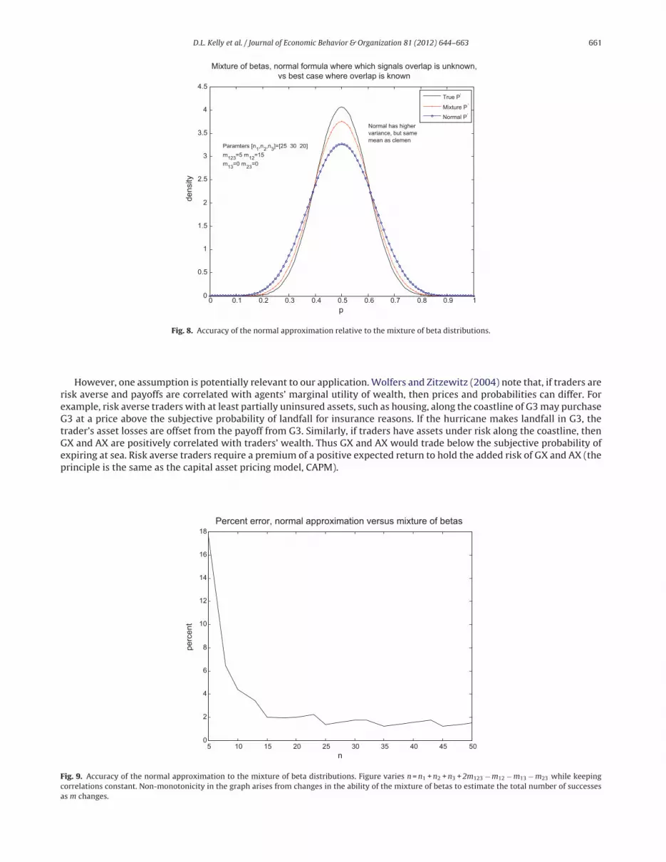
Fig. 8 gives an average of 50,000 posterior distributions each of which draws random zi’s from a binomial distributionwhere the true value is 0.5, and n1 = 25, n2 = 30, n3 = 20, and m12 = 15, m13 = 0, m23 = 0, and m123 = 5. The solid line is a theoreticalbest case posterior supposing the trader knew the total successes, which has the smallest variance. The mixture of betasis unbiased, but has a higher variance since the trader estimates the total number of successes. The variance of the normalapproximation is 1.5% higher still, since the normal distribution does not try to infer the total successes. Fig. 9 shows howthe approximation error decreases with the total number of draws n = n1 + n2 + n3 + 2m123 − m12 − m13 − m23. For n > 15, stillwell below n for even five day track forecasts, the variance is less than 2% higher than the variance of the mixture of betas.Thus the approximation is reasonably accurate.

Appendix B. Correlation between security payoff and marginal utility of wealth

A number of papers give sufficient conditions for prediction market prices to be equal to the traders’ subjective probabilitythat the event occurs. Clearly risk neutrality is sufficient (Wolfers and Zitzewitz, 2004). Wolfers and Zitzewitz (2006) showthat if the distribution of beliefs is symmetric and demand is symmetric around the point where price equals probability,then prices equal probabilities even if traders are risk averse. These papers have a number of other implicit assumptions,such as no transaction costs and a discount factor equal to one. These assumptions are relatively innocuous in our case: thesmall stakes make risk neutrality a reasonable assumption, and the security pays off within a week or so of trading, so thediscount factor is near one.

D.L. Kelly et al. / Journal of Economic Behavior & Organization 81 (2012) 644– 663 661

0 0.1 0.2 0.3 0.4 0.5 0.6 0.7 0.8 0.9 10

0.5

1

1.5

2

2.5

3

3.5

4

4.5

p

dens

ity

Mixture of betas, normal formula where which signals overlap is unknown, vs best case where overlap is known

Normal has highervariance, but samemean as clemen

Paramters [n1,n 2,n 3]=[25 30 20]m123 =5 m12 =15m13 =0 m23=0

True Pʹ

Mixture P ʹ

Normal Pʹ

Fig. 8. Accuracy of the normal approximation relative to the mixture of beta distributions.

However, one assumption is potentially relevant to our application. Wolfers and Zitzewitz (2004) note that, if traders arerisk averse and payoffs are correlated with agents’ marginal utility of wealth, then prices and probabilities can differ. Forexample, risk averse traders with at least partially uninsured assets, such as housing, along the coastline of G3 may purchaseG3 at a price above the subjective probability of landfall for insurance reasons. If the hurricane makes landfall in G3, thetrader’s asset losses are offset from the payoff from G3. Similarly, if traders have assets under risk along the coastline, thenGX and AX are positively correlated with traders’ wealth. Thus GX and AX would trade below the subjective probability ofexpiring at sea. Risk averse traders require a premium of a positive expected return to hold the added risk of GX and AX (theprinciple is the same as the capital asset pricing model, CAPM).

5 10 15 20 25 30 35 40 45 500

2

4

6

8

10

12

14

16

18Percent error, normal approximation versus mixture of betas

n

perc

ent

Fig. 9. Accuracy of the normal approximation to the mixture of beta distributions. Figure varies n = n1 + n2 + n3 + 2m123 − m12 − m13 − m23 while keepingcorrelations constant. Non-monotonicity in the graph arises from changes in the ability of the mixture of betas to estimate the total number of successesas m changes.

662 D.L. Kelly et al. / Journal of Economic Behavior & Organization 81 (2012) 644– 663

To see this precisely, let q(k) be trader k’s subjective probability of GX or AX, yx(k) be the wealth of trader k if the hurricaneexpires at sea, and y0(k) = ıyx(k) be the expected wealth of trader k if the hurricane makes landfall. Following the logic of Eq.(5) in Wolfers and Zitzewitz (2006) we have for log utility:

Pt =∫q(k)

y0(k)yF(k)dk

y =∫

(q(k)y0(k) + (1 − q(k))yx(k)) F(k)dk

That is, traders with more wealth at risk than the ex ante average expected wealth demand relatively less of a security whosepayoff is positively correlated with their wealth, decreasing the price. We assume no correlation exists between traders’wealth at risk and subjective beliefs.29 Hence, rewriting gives:

Pt = ı

1 − (1 − ı)E[q]E[q]

Thus Pt < E[q], since the probability for each trader is less than one.We therefore test Pt < E[q] for the security AX,30 by including a dummy variable equal to one if the trade was an AX

security. The null hypothesis is that the coefficient on the dummy is negative. The price should be lower for securitiespositively correlated with assets at risk.

As shown in Table 6, we can reject the hypothesis that the coefficient is negative at the five percent level. We thereforereject that traders are using HFM to hedge wealth at risk from hurricanes.

Appendix C. Computing the probabilities and precisions

Every 6 h, institutions release track forecasts, which give point forecasts of the storm’s position at various times in thefuture. Thus the information in track forecast i released at time t, ˝it, consists of a set of Li pairs of position coordinates, so˝it = {Latitl,Lonitl}, l = 1. . .Li. Tracks vary in the number of point forecasts issued at each release. Each trader must at leastimplicitly convert the information ˝it into a probability of first landfall in range j, zijt, upon which the price of the securityis based. Here we explain how we compute the probability, based on the point forecasts and historical mean forecast errors.

The first step is to compute the standard deviation of the point forecast errors. NHC (2008) gives historical mean predictionerrors by track and time to landfall. Hurricane track forecasts have become increasingly accurate, thus we consider only the2000–06 mean absolute errors (2002–06 for CLP5). It is straightforward to show (proof available on request) that, if thelatitude and longitude point forecast errors are normally distributed with mean zero and if the variance of the latitude errorequals the variance of the longitude error, then the standard deviation in each direction, �il, is related to the mean absoluteEuclidean distance error, MAE, according to: �il∼

√2/� · MAEil . For example, the third point on the black line of Fig. 6c is

the 36 h ahead forecast of the August 28, 12 pm CLP5 Katrina forecast. Thirty six hour ahead CLP5 forecasts have a meanabsolute distance error of 315.4 km, which corresponds to a standard deviation of the longitude error of 251.7 km.

We next compute the probability of landfall in range j via a Monte Carlo procedure. The simulated longitude position, citl ,is a normally distributed random variable with mean equal to the point forecast Lonitl and standard deviation �il. However,errors are positively serially correlated over point forecasts. That is, if the hurricane is west of the one day ahead forecast,the hurricane is likely to be west of the two day ahead forecast as well. We model the serial correlation as:

cit1 = N(Lonit1, �2il

)citl = cit,l−1 + N(Lonitl − Lonit,l−1, �2

il− �2

i−1,l) i = 2...Li

Hence, citl − Lonitl is mean zero with standard deviation �il, but is positively serially correlated over i. A simulated latitudeis computed in an identical manner.

Next, for each simulated track, cit = {cit1, ..., citL} and the same for latitude, we compute the first landfall, by interpolatingbetween the simulated positions, accounting for the curvature of the earth. The first landfall coordinate is the first intersectionbetween the coastline (including the dividing line) and the line formed by interpolating the simulated actual positions. If allforecasts are at sea (over land), the track forecast is extrapolated forward (backward) using the last (first) two forecasts. Ifall simulated positions and the forward extrapolation are at sea, the simulated track is said to predict the storm will expireat sea. The probability is thus equal to the fraction of a large number (1000) of simulated tracks which make first landfall inrange j.

To compute the precision of the probability, q(˝it), we use a bootstrap procedure. For each track forecast, we have 1000simulations which either made landfall in range j or did not. From this set, we draw a large number (1000) of samples with

29 It is possible that traders with more wealth at risk also have an incentive to acquire more accurate priors, but unlikely that traders with morewealth at risk systematically believe hurricanes are less likely to make landfall. In fact, though, Pt < E[q] as long as the covariance satisfies: cov(q,yx) < (1 − ı)E[q](1 − E[q])E[yx]/(ı + (1 − ı)E[q]).

30 We have no trades for the GX security.

D.L. Kelly et al. / Journal of Economic Behavior & Organization 81 (2012) 644– 663 663

replacement of 1000 simulations each and compute the fraction which make landfall in range j. We then have a set of 1000probabilities. The precision is the inverse of the variance of the set of probabilities.

Our methodology requires some fairly sophisticated computations. However, traders are at least aware of the varioustrack forecasts, and how their error varies across tracks and as the hurricane approaches landfall. More straightforwardmethods of computing probabilities from track forecast information should produce similar regression results.

Appendix D. Estimation of the priors

Our empirical results assume priors are uninformative, or = = 0. Another possibility is to estimate the priors whichbest fit the data. Estimation of priors is known as empirical Bayesian methods. Another alternative we do not consider ishierarchical Bayesian methods, in which the econometrician has priors over and ˇ.

To estimate the priors, we take ˛ and ˇ in Eq. (7) as parameters to be estimated, rather than assuming = ˇ = 0. Column8 of Table 6 details the results. The estimate of ˛+ˇ=1.05 is close to one. The estimated precision of the prior is then equalto about one draw. Thus the econometric results show that the traders priors are not very informative, providing somejustification for our assumption of an uninformative prior. The estimate of ˛/( + ˇ) = 0.68 indicates the prior amounts to avery noisy prediction that the hurricane makes landfall in the coastline range 68% of the time. The �2 value drops with theaddition of and ˇ, indicating that estimating the priors has not significantly improved the fit of the model.

As for the weights on the track forecasts, the weight on GFDL increases slightly and the weight on NHC decreases slightlyand the standard error of both weights decreases, so we can now reject the joint hypothesis that both weights are equal toone. However, the results remain qualitatively unchanged in that traders still put essentially no weight on CLP5, and thatthe GFDL and NHC weights remain close to one.

References

Aberson, Sim D., 1998. Five-day tropical cyclone track forecasts in the North Atlantic basin. Weather Forecast. 13, 1005–1015.Baker, E., 1995. Public response to hurricane probability forecasts. Prof. Geogr. 47, 137–147.Bender, M.A., Ginis, I., Tuleya, R.E., Thomas, B., Marchok, T., 2007. The operational GFDL coupled hurricane – ocean prediction system and a summary of its

performance. Monthly Weather Rev. 135, 3965–3989.Bernardo, J., Smith, A., 2000. Bayesian Theory. John Wiley & Sons, Inc, New York.Bin, O., Polasky, S., 2004. Effects of flood hazards on property values: evidence before and after hurricane floyd. Land Econ. 73, 490–500.Bolstad, W., 2004. Introduction to Bayesian Statistics. John Wiley & Sons, Inc, Hoboken.Cameron, T., 2005. Updating subjective risks in the presence of conflicting information: an application to climate change. J. Risk Uncertain. 30, 63–97.Clemen, R., 1987. Combining overlapping information. Manage. Sci. 33, 373–380.DeGroot, M., 1970. Optimal Statistical Decisions. McGraw-Hill, New York.Dominitz, J., Manski, C., 1997. Using expectations data to study subjective income expectations. J. Am. Stat. Assoc. 92, 855–867.Ferrari, S., Cribari-Neto, F., 2004. Beta regression for modelling rates and proportions. J. Appl. Stat. 31, 799–815.Flynn, J., Slovic, P., Mertz, C., 1994. Gender, race, and perception of environmental-health risks. Risk Anal. 14, 1101–1108.Franklin, J., McAdie, C., Lawrence, M., 2003. Trends in track forecasting for tropical cyclones threatening the United States, 1970–2001. Bull. Am. Meteor.

Soc. 84 (9), 1197–1203.Hallstrom, D., Smith, V., 2005. Market Responses to Hurricanes. J. Environ. Econ. Manage. 50, 541–561.Hanson, R., 2007. Logarithmic market scoring rules for modular combinatorial information aggregation. J. Predict. Markets 1, 3–15.Jullien, B., Salanie, B., 2000. Estimating preferences under risk: the case of racetrack bettors. J. Polit. Econ. 108, 503–530.Lee, D., Moretti, E., 2009. Bayesian learning and the pricing of new information: evidence from prediction markets. Am. Econ. Rev. 99, 330–336.Leroux, B.G., 1992. Consistent estimation of a mixing distribution. Ann. Stat. 20, 1350–1360.NHC (National Hurricane Center), 2008. Hurricane Season Tropical Cyclone Reports (all reports from 2000-6), http://www.nhc.noaa.gov/pastall.shtml.NOAA (National Oceanic and Atmospheric Administration), 2005. New Priorities for the 21st Century – NOAA’s Strategic Plan , Washington, DC.Oberholzer, F., Mitsunari, M., 2006. Information regulation: do the victims of externalities pay attention? J. Regul. Econ. 30, 141–158.Paulino, P., 2001. Maximum likelihood estimation of models with beta-distributed dependent variables. Polit. Anal. 9, 325–346.Powell, M., Aberson, S., 2001. Tropical cyclone landfall forecasts in the Atlantic basin (1976–2000). Bull. Am. Meteor. Soc. 82, 2749–2767.Smith, V., Taylor, D., Sloan, F., 2001. Longevity expectations and death: can people predict their own demise? Am. Econ. Rev. 91, 1126–1134.Tetlock, P., 2004. How efficient are information markets? Evidence from an online exchange , University of Texas, Department of Finance, Working Paper.Tetlock, P., 2007. Does liquidity affect securities market efficiency? University of Texas, Department of Finance, Working Paper.Viscusi, W., 1997. Alarmist decisions with divergent risk information. Econ. J. 107, 1657–1670.Viscusi, W., Magat, W., 1992. Bayesian decisions with ambiguous belief aversion. J. Risk Uncertain. 5, 371–387.Viscusi, W., O’Connor, C., 1984. Adaptive responses to chemical labeling: are workers bayesian decision makers? Am. Econ. Rev. 74, 942–956.Wolfers, J., Zitzewitz, E., 2004. Prediction markets. J. Econ. Perspect. 18, 107–126.Wolfers, J., Zitzewitz, E., 2006. Interpreting prediction market prices as probabilities. In: NBER Working Paper number, p. 12200.Zeckhauser, R., 1971. Combining overlapping information. J. Am. Stat. Assoc. 66, 91–92.