Embed Size (px)
Citation preview
Washington University in St. Louis Washington University in St. Louis
Washington University Open Scholarship Washington University Open Scholarship
Arts & Sciences Electronic Theses and Dissertations Arts & Sciences
Spring 5-15-2015
Labor Force Participation and Crime among Serious and Violent Labor Force Participation and Crime among Serious and Violent
Former Prisoners Former Prisoners
Nora Ellen Wikoff Washington University in St. Louis
Follow this and additional works at: https://openscholarship.wustl.edu/art_sci_etds
Part of the Social Work Commons
Recommended Citation Recommended Citation Wikoff, Nora Ellen, "Labor Force Participation and Crime among Serious and Violent Former Prisoners" (2015). Arts & Sciences Electronic Theses and Dissertations. 446. https://openscholarship.wustl.edu/art_sci_etds/446
This Dissertation is brought to you for free and open access by the Arts & Sciences at Washington University Open Scholarship. It has been accepted for inclusion in Arts & Sciences Electronic Theses and Dissertations by an authorized administrator of Washington University Open Scholarship. For more information, please contact [email protected].
WASHINGTON UNIVERSITY IN ST. LOUIS
Brown School of Social Work
Dissertation Examination Committee:
Carrie Pettus-Davis, Chair
Michael Sherraden, Co-Chair
Derek Brown
Shanta Pandey
Juan Pantano
Labor Force Participation and Crime among Serious and Violent Former Prisoners
by
Nora Ellen Wikoff
A dissertation presented to the
Graduate School of Arts & Sciences
of Washington University in
partial fulfillment of the
requirements for the degree
of Doctor of Philosophy
May 2015
St. Louis, Missouri

Copyright by
Nora Wikoff
2015

ii
Table of Contents List of Figures ................................................................................................................................ vi
List of Tables ................................................................................................................................ vii
List of Abbreviations ................................................................................................................... viii
Acknowledgments.......................................................................................................................... ix
ABSTRACT OF THE DISSERTATION ..................................................................................... xii
Chapter 1: Specific Aims ................................................................................................................ 1
1.1 State of Current Knowledge ............................................................................................. 3
1.1.1 Labor Force Participation Before and After Prison .............................................................. 4
1.1.2 Labor Force Participation and the Desistance Process ......................................................... 5
1.1.3 Interventions to Increase Labor Force Participation ............................................................. 6
1.2 Gaps in Existing Research................................................................................................ 9
Chapter 2: Theoretical Perspectives .............................................................................................. 11
2.1 Rational Choice Theoretical Framework ....................................................................... 11
2.1.1 Objections to the Basic Model ............................................................................................ 12
2.2 Dynamic Human Capital Model of Criminal Activity ................................................... 13
2.2.1 Human Capital Investment .................................................................................................. 14
2.2.2 Social Capital Accumulation .............................................................................................. 14
2.2.3 Criminal Capital Accumulation .......................................................................................... 15
2.3 Proposed Conceptual Model .......................................................................................... 16
Chapter 3: Methodology ............................................................................................................... 21
3.1 Overview ........................................................................................................................ 21
3.2 Research Hypotheses...................................................................................................... 21
3.3 Research Design ............................................................................................................. 23
3.3.1 Data Collection ................................................................................................................... 23
3.3.2 Sample ................................................................................................................................. 24
3.3.3 Missing Data Analysis ........................................................................................................ 27
3.4 Measures......................................................................................................................... 31
3.4.1 Main Outcome Variables .................................................................................................... 31
3.4.2 Group-Based Trajectory Model .......................................................................................... 32
iii
3.4.3 Multilevel Logit Participation Model.................................................................................. 33
3.4.4 Duration Models ................................................................................................................. 34
3.4.5 Structural Equation Modeling ............................................................................................. 36
3.5 Data Analysis Plan ......................................................................................................... 40
3.5.1 Group-Based Trajectory Model .......................................................................................... 40
3.5.2 Multilevel Logit Participation Model.................................................................................. 41
3.5.3 Propensity Score Matching ................................................................................................. 44
3.5.4 Duration Models ................................................................................................................. 47
3.5.5 Structural Equation Modeling ............................................................................................. 47
Chapter 4: Results ......................................................................................................................... 53
4.1 Overview ........................................................................................................................ 53
4.2 Descriptive Results ......................................................................................................... 55
4.2.1 Demographic Characteristics at Baseline ............................................................................ 55
4.3 Assessing Initial Bias before Matching .......................................................................... 59
4.3.1 Bivariate Statistics before Matching ................................................................................... 59
4.3.2 Hypothesis 1: Participants Differ from Nonparticipants ..................................................... 60
4.4 Group-Based Trajectory Model ..................................................................................... 61
4.4.1 Pre-SVORI Arrest Rates ..................................................................................................... 61
4.4.2 Group-Based Trajectory Model Results.............................................................................. 62
4.4.3 Trajectory Group Characteristics ........................................................................................ 66
4.5 Propensity Score Matching ............................................................................................ 72
4.5.1 Multilevel Logit Model Results .......................................................................................... 72
4.5.2 Nearest Neighbor Matching with Caliper ........................................................................... 74
4.5.3 Bivariate Statistics after Matching ...................................................................................... 74
4.6 Duration Models ............................................................................................................. 78
4.6.1 Post-Release Arrest Rates ................................................................................................... 78
4.6.2 Employment Programs Increase Labor Force Participation ............................................... 78
4.6.3 Hypothesis 2: Employment Programs Reduce Recidivism................................................. 79
4.6.4 Duration Model Results ...................................................................................................... 80
4.6.5 Hypothesis 3: Increased Participation has Diminishing Benefits ....................................... 85
4.7 Structural Equation Modeling ........................................................................................ 86
4.7.1 Outcome variables............................................................................................................... 86
iv
4.7.2 Confirmatory Factor Model ................................................................................................ 87
4.7.3 Structural Equation Path Model .......................................................................................... 95
4.7.4 Hypothesis 4: Criminal Activity Reduces Human and Social Capital ................................ 96
4.7.5 Hypothesis 5: Human and Social Capital Increases Employment ...................................... 96
4.7.6 Hypothesis 6: Labor Force Participation Increases Job Quality ......................................... 97
4.7.7 Hypothesis 7: Quality Jobs Reduce Men’s Financial Needs............................................. 101
4.7.8 Hypothesis 8: Financial Needs Increase the Probability of Reoffending .......................... 101
4.7.9 Hypothesis 9: Financial Needs Increase Psychological Distress ...................................... 101
4.7.10 Hypothesis 10: Psychological Distress Contributes to Reoffending ................................. 102
4.7.11 Work-Crime Association .................................................................................................. 102
4.7.12 Trimmed Pathways from the Final Longitudinal SEM ..................................................... 103
4.7.13 Significant Covariates ....................................................................................................... 104
4.8 Conclusion .................................................................................................................... 104
Chapter 5: Discussion ................................................................................................................. 106
5.1 Summary of Findings ................................................................................................... 106
5.1.1 Identifying Selection Processes into Treatment ................................................................ 107
5.1.2 Balancing across Trajectory Groups ................................................................................. 109
5.1.3 Maintenance of the Status Quo ......................................................................................... 112
5.1.4 Understanding Why Employment Programs do not Work ............................................... 112
5.1.5 Structural Factors Trump Human Capital Factors ............................................................ 119
5.1.6 Limited Support for Causal Theories of Work and Crime ................................................ 123
5.1.7 Testing Theoretical Concepts ............................................................................................ 124
5.1.8 Fostering Desistance among Former Prisoners ................................................................. 125
5.2 Challenges and Limitations .......................................................................................... 128
5.2.1 Group-Based Trajectory Model ........................................................................................ 128
5.2.2 Defining Participation Status ............................................................................................ 128
5.2.3 Duration Models ............................................................................................................... 129
5.2.4 Structural Equation Modeling ........................................................................................... 130
Chapter 6: Implications and Conclusion ..................................................................................... 135
6.1 Implications for Policy ................................................................................................. 135
6.1.1 Logic Models and Program Evaluations ........................................................................... 135
6.1.2 Policy Changes to Improve Correctional Programming ................................................... 135
v
6.1.3 Policy Changes to Increase Labor Force Attachment ....................................................... 136
6.2 Implications for Future Research ................................................................................. 137
6.2.1 Improving Research Designs using Observational Data ................................................... 137
6.2.2 Testing Theoretical Concepts ............................................................................................ 140
6.2.3 Validating Self-Report Crime Measures ........................................................................... 141
6.3 Conclusion .................................................................................................................... 142
References ................................................................................................................................... 144
Appendices .................................................................................................................................. 156
vi
List of Figures Figure 2.1: Program Participation, Labor Force Attachment, and Desistance...………………...17
Figure 2.2: General Panel Model of Post-Release Labor Force Attachment and Recidivism.......19
Figure 3.1: Sample Selection Flowchart for Duration Models......................................................26
Figure 3.2: Parameter Labels for Four Time Points: The Configural Invariance Model..............49
Figure 3.3: Parameter Labels for Four Time Points: The Weak Invariance Model......................50
Figure 3.4: Parameter Labels for Four Time Points: The Strong Invariance Model.....................51
Figure 3.5: Initial Longitudinal Structural Equation Path Model..................................................52
Figure 4.1: Pre-SVORI Arrest Rates by Offense Type..................................................................60
Figure 4.2: Pre-SVORI Arrest Rates by Racial/Ethnic Status.......................................................61
Figure 4.3: Pre-SVORI Drug Arrest Rates by Racial/Ethnic Status..............................................62
Figure 4.4: Pre-SVORI Property Arrest Rates by Racial/Ethnic Status........................................63
Figure 4.5: Pre-SVORI Violent Arrest Rates by Racial/Ethnic Status..........................................63
Figure 4.6: Arrest Trajectories during Years Preceding SVORI Prison Term..............................65
Figure 4.7: Rearrest Rates by Participation Status after Release from SVORI Prison Term........81
Figure 4.8: Parameter Estimates for Four Time Points: The Configural Invariance Model..........88
Figure 4.9: Parameter Estimates for Four Time Points: The Weak Invariance Model..................90
Figure 4.10: Parameter Estimates for Four Time Points: The Strong Invariance Model..............94
Figure 4.11: Final Longitudinal Structural Equation Path Model.................................................95
vii
List of Tables Table 3.1: Variable Descriptions by Analysis………………………………………………….29
Table 3.2: Interview and Data Collection Periods for Structural Equation Path Model…….....37
Table 4.1 Demographic Characteristics at Baseline…………………………………………...54
Table 4.2: Demographic Characteristics of Program Participants before Matching…………...56
Table 4.3: Group-Based Trajectory Model Results…………………………………………….64
Table 4.4: Demographic Characteristics of Three Trajectory Groups………………………....67
Table 4.5: Logit Participation Model Results………………………………………………......73
Table 4.6: Demographic Characteristics of Program Participants after Matching……………..75
Table 4.7: Post-Release Arrest Rates by Participant Status …………………………………...80
Table 4.8: Duration Model: Nested Results for Time to Arrest with Repeated Failures……....82
Table 4.9: Duration Models: Results for Time to First Arrest by Offense Type ……………...84
Table 4.10: Post-Release Labor Force Attachment by Participant Status ………………………86
Table 4.11: Model Fit Statistics for the Tests of Configural Invariance over Four Waves……...87
Table 4.12: Comparison of Parameter Estimates across the Levels of Invariance………………91
Table 4.13: Longitudinal Structural Equation Model Results…………………………………...98
Table 4.14: Odds Ratios for Work, Crime, and Recidivism………………………………........100

viii
List of Abbreviations
AIC Aikaike Information Criterion
AFQT Armed Forces Qualifying Test
B Unstandardized Coefficient
BIC Bayesian Information Criterion
CEO Center for Employment Opportunities
CFA Confirmatory Factor Analysis
CFI Comparative Fit Index
CI Confidence Interval
DM Duration Models
DF Degrees of freedom
FBI Federal Bureau of Investigation
FIML Full-Information Maximum Likelihood
GED General Education Development (General Equivalency Diploma)
GSI Global Severity Index
GTM Group-Based Trajectory Model
HR Hazard Ratio
HSD High School Diploma
LSEM Longitudinal Structural Equation Model
ML Maximum Likelihood
M Mean
MH/AOD Mental Health, Alcohol, or Drug
NCIC National Crime Information Center
OR Odds Ratio
PSM Propensity Score Methods
RMSEA Root Mean Square Error of Approximation
RNR Risk-Need-Responsivity
SD Standard Deviation
SE Standard Errors
SEM Structural Equation Modeling
SR Self-Report
SVORI Serious and Violent Offender Reentry Initiative
TABE Tests of Adult Basic Education
TANF Temporary Assistance to Needy Families
TLI/NNFI Tucker-Lewis Index (Non-Normed Fit Index)

ix
Acknowledgments This dissertation would not have been possible without the support of many people. I wish to
express my enormous gratitude for the advice, encouragement, and support that my advisors
Carrie Pettus-Davis, PhD (dissertation co-chair) and Michael Sherraden, PhD (dissertation co-
chair) so generously offered to me throughout my time at the Brown School. My work on
prisoner reentry would not have been possible without Michael’s consistent support and interest
in the topic. His questions spurred me to look at research questions in a new light, and his
sanguine confidence has buoyed me through difficult periods in the research process.
My doctoral research has taken an entirely different, and better, trajectory from what I could
have hoped for, as a result of working with Carrie during the final years in the doctoral program.
Before Carrie had even started her position at Washington University, she had met with me
several times to offer her guidance and experience on criminal justice research. I appreciate her
patience as I have evolved in my thinking about employment, prisoner reentry, and the
desistance process.
I want to express a special gratitude to Shanta Pandey, PhD, for her service on my area statement
and dissertation committees, and for early support during the MSW program. I would not have
been prepared to enter doctoral study had it not been for completing the MSW Research Seminar
under her tutelage. At each stage of the MSW and PhD programs, her thoughtful suggestions
have improved my research and writing skills. To my other dissertation committee members,
Derek Brown, PhD, and Juan Pantano, PhD, I am grateful for your insight, support, and
skepticism. The dissertation is a stronger body of work as a result of your service on my
committee.

x
I have been fortunate to receive statistical training from excellent instructors. In addition to
Shanta Pandey, I would like to thank Shenyang Guo, PhD, and Ramesh Raghavan, PhD, for
inculcating a respect for rigorous statistical methodology. I am thankful to have had the
opportunity to develop these skills as a Research Associate at the Center for Social
Development.
The National Institute of Justice (2013-IJ-CX-0042) provided financial support for this research.
I am also grateful to the School of Social Work for fellowship, research, and travel funding. I
want to thank PhD Program Administrators Lucinda Cobb and Marissa Hardwrict for
shepherding me through each stage of the doctoral program.
Finally, I thank my husband, Zach Hoskins, for his patience, good humor, and steadfast support.
My journey to St. Louis, and to doctoral research in Social Work, can only be understood in this
light.
Nora Wikoff
Washington University in St. Louis
May 2015

xi
Dedicated to my husband.
xii
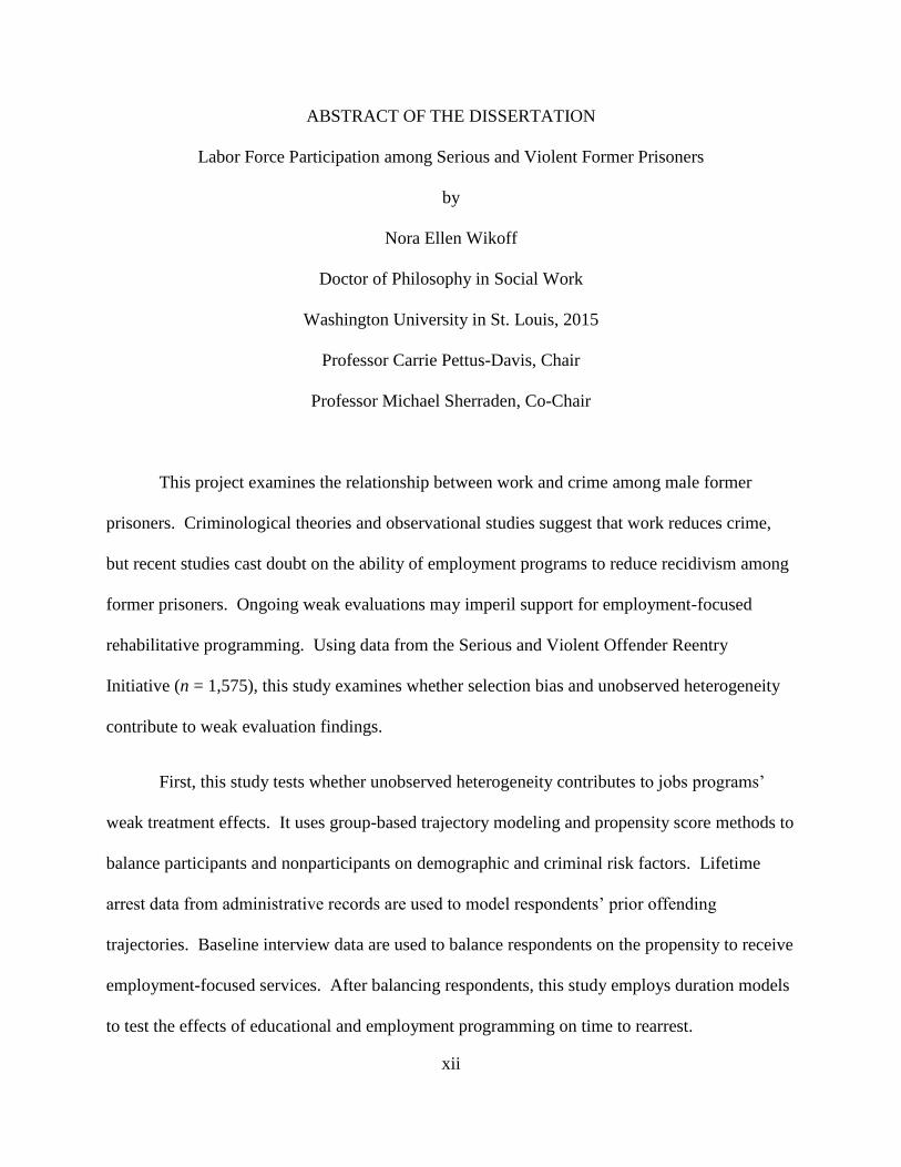
ABSTRACT OF THE DISSERTATION
Labor Force Participation among Serious and Violent Former Prisoners
by
Nora Ellen Wikoff
Doctor of Philosophy in Social Work
Washington University in St. Louis, 2015
Professor Carrie Pettus-Davis, Chair
Professor Michael Sherraden, Co-Chair
This project examines the relationship between work and crime among male former
prisoners. Criminological theories and observational studies suggest that work reduces crime,
but recent studies cast doubt on the ability of employment programs to reduce recidivism among
former prisoners. Ongoing weak evaluations may imperil support for employment-focused
rehabilitative programming. Using data from the Serious and Violent Offender Reentry
Initiative (n = 1,575), this study examines whether selection bias and unobserved heterogeneity
contribute to weak evaluation findings.
First, this study tests whether unobserved heterogeneity contributes to jobs programs’
weak treatment effects. It uses group-based trajectory modeling and propensity score methods to
balance participants and nonparticipants on demographic and criminal risk factors. Lifetime
arrest data from administrative records are used to model respondents’ prior offending
trajectories. Baseline interview data are used to balance respondents on the propensity to receive
employment-focused services. After balancing respondents, this study employs duration models
to test the effects of educational and employment programming on time to rearrest.
xiii
Second, this study tests whether financial problems mediate the work-crime relationship.
Longitudinal structural equation modeling is used to model men’s labor force attachment, job
quality, financial needs, and emotional wellbeing. Models test whether financial problems
diminish the crime-reducing effects of employment for men who remain weakly attached to the
labor force. Multiple indicators for each latent construct reduce bias due to measurement error.
Results of this study show that education and employment programs in United States
prisons have limited effects on the likelihood that participants maintain employment and avoid
criminal justice involvement. Male prisoners recruited into the Serious and Violent Offender
Reentry Initiative faced multiple barriers to employment before entering prison, due to extensive
criminal records, low educational attainment, and limited work experience. Before matching
men on the probability of receiving employment-focused services, program participants differed
from nonparticipants across an array of demographic and risk factors. The group-based
trajectory model derived three latent trajectory groups from the sample that exhibited distinctive
demographic characteristics and pre-prison offending trajectories. Due to significant variation at
the state-level, a multilevel logit model was used to model the probability of receiving education
and employment services. Nearest neighbor matching with caliper resulted in a sample that
exhibited balance across multiple demographic, criminal record, employment, and health
measures.
After matching, employment program participants were slightly more likely than
education participants and nonparticipants to maintain stable employment, and employment
program participants exhibited lower rates of rearrest during the first 9 months after release.
After that point, there were no significant differences between employment-focused program
participants and nonparticipants in labor force and criminal activity.

xiv
The longitudinal structural equation model results show that criminal activity has
cascading effects on financial and emotional wellbeing, subsequent labor force activity, and
ongoing criminal justice involvement. Engagement in crime during the early months of release
reduced labor force participation, limited men’s ability to obtain higher-quality employment, and
increased their financial needs and feelings of psychological distress. In contrast, stable
employment led to improved job quality and reduced financial needs over time. Employment
did not reduce men’s later involvement in criminal activity, however. In fact, employment
during the first 9 months of release was associated with increased odds of reporting committing
new crimes during the subsequent 6-month period. Overall, the path model results provide no
evidence to suggest that stable employment reduces criminal activity among serious and violent
former prisoners.
The results of this study cast doubt on theories of crime that presuppose causal
associations between work and crime. Observational studies that show associations between
stable labor force participation and desistance from crime may be capturing maturation effects
that simultaneously directed individuals toward legal work and away from crime. If desistance
from crime actually precedes stable labor force attachment for most former prisoners, this may
explain the weak empirical evidence for prison-based employment programs. The findings may
inform modifications to employment and transitional jobs programs to identify participants on
the path to desistance who may be most responsive to these services.
1
Chapter 1: Specific Aims This study examines the relationship between work and crime among newly released former
prisoners. Criminological theories propose various mechanisms by which work reduces crime: It
limits opportunities for deviant behavior, strengthens prosocial attachments, and reduces
financial incentives to engage in crime (Grogger, 1998; Hirschi, 1969; Latessa, 2012).
Observational studies provide empirical support for these claims, suggesting that even among
active offenders, work has a weak causal effect on crime (Bushway, 2011). This lends credence
to employment-focused prison programs: If work reduces crime, then increasing employment
among reentering former prisoners should reduce recidivism. Unfortunately, jobs programs
show limited success in helping many prisoners gain job skills, find and maintain work, and
reduce their involvement in crime (Bushway & Apel, 2012; Farabee, Zhang, & Wright, 2014;
Lattimore et al., 2012; J. A. Wilson & Davis, 2006).
Strengthening our understanding of the relationship between work and crime is critical to
designing effective employment programs for low-skilled, low-educated former prisoners with
limited formal work experience. Interventions may not reduce recidivism rates if work, although
correlated, is not causally related to reduced crime among former prisoners (Farabee et al., 2014;
Grogger, 1998; D. B. Wilson, Gallagher, & MacKenzie, 2000). Employment may reduce
individuals’ incentives to engage in economically motivated crimes, but it may have limited
effects on other crimes (Aaltonen, Macdonald, Martikainen, & Kivivuori, 2013; Felson, Osgood,
Horney, & Wiernik, 2012). Former prisoners who find work may continue to engage in criminal
activity (Horney, Osgood, & Marshall, 1995), especially when workplace settings provide new
opportunities for crime (Lochner, 2004).
2
This study examines the effects of employment-focused programs on prisoners’ post-release
labor force participation, job quality, and criminal involvement. Its findings will contribute
knowledge to three broad questions at the heart of current scholarship on crime and economics:
Does employment have a causal effect on offending among former prisoners? What factors
contribute to the relationship between work and crime among former prisoners? What factors
explain why employment programs have limited effects on labor activity and recidivism?
I first investigate whether mixed and negative outcomes for employment programs result from
selection effects in who receives employment services (Chamberlain, 2012; Heckman & Hotz,
1989; Sedgley, Scott, Williams, & Derrick, 2010). First, if treatment participants have fewer job
skills than do people in the comparison group, then post-release outcomes in part reflect pre-
existing differences that selected people into treatment (Chamberlain, 2012; Heckman & Hotz,
1989). Second, when prison programs are offered à la carte to prisoners—rather than as bundled
sets of programs—the comparison group for employment programs includes both true
nonparticipants and people who participated in education programs or prison work. This
unmodeled contamination may bias estimates of the intervention under evaluation (Sedgley et
al., 2010). After controlling for observed heterogeneity in treatment status, I examine whether
participation in educational or employment programs increase men’s time in the community
(Brewster & Sharp, 2002; Farabee et al., 2014; Kim & Clark, 2013; Sedgley et al., 2010).
Next, I use structural equation modeling (SEM) to study men’s labor force and criminal activities
during the first 15 months of release from prison. The cross-lagged panel model examines
whether crime weakens men’s attachment to the labor force (Thornberry & Christenson, 1984).
The longitudinal structural equation model (LSEM) includes factors that shape men’s incentives
to work, to identify whether labor force participation signals men’s likelihood of reoffending

3
(Bushway, 2011; Bushway & Apel, 2012). Finally, I examine whether financial and
psychological stressors mediate the relationship between work and crime. The LSEM results
provide information about interpersonal and financial challenges that men face following release
from prison (Bollen & Brand, 2010; Bucklen & Zajac, 2009; Price, Choi, & Vinokur, 2002).
1.1 State of Current Knowledge By 2008, 1 in 100 Americans were in jail or prison on any given day. Risk of incarceration is
exponentially higher for young, racial and ethnic minority men with less than a high school
diploma (Beck et al., 1993; Pew Center on the States, 2008). African Americans and Hispanics
compose nearly 60% of prisoners incarcerated in state and federal prisons1 (Pettit & Western,
2004; Western & Wildeman, 2009). To put this in context, African American men were six
times as likely as White men to be imprisoned in state and federal prisons in 2013 (Carson,
2014). African American males are now twice as likely to have been incarcerated as to have
bachelor’s degrees, and they are more likely to be incarcerated than to be employed (37% vs.
26%) (Western & Wildeman, 2009).
Nearly all of these prisoners are released from prison (95%), but many of them are returned to
prison as well (Piehl & Useem, 2011). During their first 3 years of release, more than two-thirds
of prisoners are rearrested, nearly half are returned to prison for any reason, and almost one-
quarter are imprisoned for a new crime (Durose, Cooper, & Snyder, 2014; Langan & Levin,
2002). Between 1980 and 2006, the proportion of state prisoners admitted for parole violations
doubled from 17% to 35% (Sabol & Couture, 2008). By 2013, this percentage had stabilized to
9% of federal prisoners and 28% of state prisoners (Carson, 2014). Parolees are responsible for
1 Non-Hispanic Whites comprise only 32% of the state and federal prison population (Asians, American Indians and
Alaskan Natives, and people of two are more races comprise the remaining 8%).
4
roughly 20% of the violent and property offenses that lead to arrests (Rosenfeld, Wallman, &
Fornango, 2005).
1.1.1 Labor Force Participation Before and After Prison
Appendix A summarizes important studies on post-release employment and crime. Prisoners
exhibit significant education and job skills deficits that diminish their job prospects and expected
earnings (Lattimore et al., 2012). Minorities face additional barriers to employment, due to
racial discrimination, weak local labor markets, and macro-level structural conditions, including
recessions and structural unemployment (Bellair & Kowalski, 2011). Time spent out of the labor
market while in prison reduces opportunities for men to develop prosocial ties to employment
networks (Apel & Sweeten, 2010b; Hagan, 1993). While incarcerated, few men participate in
education and job training programs, due to the lack of availability of programming and other
systemic issues, so they have limited opportunities to acquire job skills (Chamberlain, 2012;
Harlow, 2003; Piehl & Useem, 2011).
Despite this, high rates of joblessness among former prisoners reflect labor force
nonparticipation, not just unemployment (Apel & Sweeten, 2010b; Bucklen & Zajac, 2009;
Chamberlain, 2012; Sugie, 2014). For most men, the difficulty lies in keeping jobs, not in
finding jobs (Aaltonen et al., 2013; Bucklen & Zajac, 2009; Sugie, 2014; van der Geest,
Bijleveld, & Blokland, 2011). Data consistently show that men exhibit short-term boosts in post-
release employment and earnings (Apel & Sweeten, 2010b; Nagin & Waldfogel, 1998). Over
time, declining external pressures from parole officers and family members to find work, and
increasing frustration with low-wage work, leads former prisoners to withdraw from the labor
market (Sugie, 2014). Post-release employment and earnings eventually decline to pre-prison
5
levels as men supplement income through illegal activity (Apel & Sweeten, 2010b; Nagin &
Waldfogel, 1998; Pettit & Lyons, 2009).
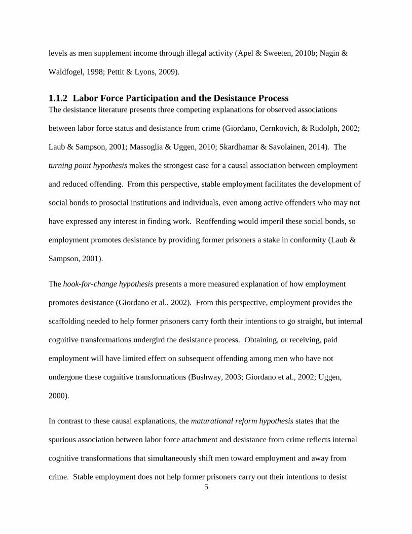
1.1.2 Labor Force Participation and the Desistance Process
The desistance literature presents three competing explanations for observed associations
between labor force status and desistance from crime (Giordano, Cernkovich, & Rudolph, 2002;
Laub & Sampson, 2001; Massoglia & Uggen, 2010; Skardhamar & Savolainen, 2014). The
turning point hypothesis makes the strongest case for a causal association between employment
and reduced offending. From this perspective, stable employment facilitates the development of
social bonds to prosocial institutions and individuals, even among active offenders who may not
have expressed any interest in finding work. Reoffending would imperil these social bonds, so
employment promotes desistance by providing former prisoners a stake in conformity (Laub &
Sampson, 2001).
The hook-for-change hypothesis presents a more measured explanation of how employment
promotes desistance (Giordano et al., 2002). From this perspective, employment provides the
scaffolding needed to help former prisoners carry forth their intentions to go straight, but internal
cognitive transformations undergird the desistance process. Obtaining, or receiving, paid
employment will have limited effect on subsequent offending among men who have not
undergone these cognitive transformations (Bushway, 2003; Giordano et al., 2002; Uggen,
2000).
In contrast to these causal explanations, the maturational reform hypothesis states that the
spurious association between labor force attachment and desistance from crime reflects internal
cognitive transformations that simultaneously shift men toward employment and away from
crime. Stable employment does not help former prisoners carry out their intentions to desist
6
from crime; it is the natural result of cognitive changes that led men away from criminal activity
in the first place (Skardhamar & Savolainen, 2014).
1.1.3 Interventions to Increase Labor Force Participation
Appendix B summarizes evaluations of employment-focused interventions. The following
paragraphs highlight noteworthy findings from these evaluations. Education programs show
greater reductions in recidivism than vocational and work programs do, but neither type of
program significantly improves labor force outcomes (Brewster & Sharp, 2002; Lattimore et al.,
2012; D. B. Wilson et al., 2000). Prison education programs prioritize remedial education and
General Education Development (GED) courses over postsecondary courses that would improve
prisoners’ employability and wages (Brown, 2015; Chamberlain, 2012). Passing the GED test
can increase wages among prisoners who fare worst in the labor market, but GED holders’
earnings often resemble high school dropouts’ earnings more closely than high school graduates’
earnings (Apel & Sweeten, 2010b; Heckman & LaFontaine, 2006; Heckman & Rubinstein,
2001; Tyler & Kling, 2007).
Employment readiness programs for prisoners often have limited impacts on post-release
employment and recidivism (Bushway, 2003; Farabee et al., 2014; Lattimore et al., 2012).
Commonly cited reasons for negative program evaluations include poor program designs, weak
program fidelity, and selection bias (manifested by voluntary enrollment and treatment
noncompliance) (Farabee et al., 2014; D. B. Wilson et al., 2000). Programs are rarely designed
and equipped to provide the comprehensive services needed to improve participants’ job
prospects (e.g., vocational training, postsecondary education) (Bushway, 2003). Employment
programs vary widely in quality, content, and intensity; for example, classes that teach interview
7
skills and provide advice on discussing the criminal record are included in the same category as
vocational training (Lattimore et al., 2012).
Selection bias due to voluntary enrollment is commonly assumed to produce upwardly biased
treatment estimates (D. B. Wilson et al., 2000). However, selection bias that results from
treatment group dropout and comparison group substitution may produce downwardly biased
estimates: Mandated programs serve prisoners who have no interest in the topics presented, so
the content has limited impact on treatment members’ later job searches (Bushway, 2003;
Bushway & Apel, 2012). At the same time, the comparison condition for most voluntary and
randomized prison interventions permits access to treatment as usual, which often means access
to services that are similar to the treatment services being evaluated (Farabee et al., 2014;
Heckman, Hohmann, Smith, & Khoo, 2000; Sedgley et al., 2010). In evaluations with high rates
of dropout and substitution, observed differences in outcomes between the treatment and
comparison groups reveal the effect of the program (e.g., the particular intervention being
offered to treatment participants), not the effect of the treatment (e.g., employment services for
former prisoners) (Farabee et al., 2014). These attenuated estimates contribute to findings that
employment and jobs programs do not work (Heckman et al., 2000).
Program designs, implementation difficulties, and selection bias may have contributed to
negative findings for employment programs implemented as part of the Severe and Violent
Offender Reentry Initiative (SVORI). This large, multi-site reentry initiative provided states
funding to expand existing services for reentering prisoners to be more comprehensive and to
begin prior to release into the community. Although SVORI programs increased the number of
services that participants received, the programs did not appear to increase employment or
reduce recidivism (Lattimore et al., 2012; Lattimore & Steffey, 2009). Most men received no
8
education or employment assistance in prison, despite high rates of men indicating that they
needed help with education and employment (Lattimore & Steffey, 2009; Lattimore, Steffey, &
Visher, 2009).
SVORI employment programs varied widely in terms of content, intensity, and duration
(Lattimore & Steffey, 2009; D. B. Wilson et al., 2000), but limited data on services and
participation kept evaluators from differentiating programs by quality (Lattimore et al., 2012).
Employment program nonparticipants likely worked in prison or received education assistance in
place of employment services (Chamberlain, 2012; Lattimore et al., 2012; Lattimore et al.,
2009). To the extent that education programs improve prisoners’ human capital and soft skills,
educational programs provide a competing treatment to employment programs. When
employment program nonparticipants within the comparison group opt for educational services
(in place of no treatment), this unobserved participation in comparable services contaminates the
sample, often reducing the observed effect of employment programs on work and recidivism
outcomes (Bushway & Apel, 2012; Lattimore et al., 2012; Sedgley et al., 2010).
Initial evaluations suggested that SVORI participants exhibited slightly better employment
outcomes than non-SVORI participants, regardless of participation in education or employment
programs: In general, SVORI participants received more services than did non-SVORI
participants, so these short-term effects may have reflected the cumulative benefit of receiving
bundled services that addressed an array of needs. At each post-release interview, SVORI
participants were more likely to hold jobs with benefits than non-SVORI participants were. By
the final 15-month follow-up interview, SVORI participation increased men’s probability of
supporting themselves through employment. Despite these beneficial outcomes, SVORI
participation did not increase the average number of months that men worked between interview
9
reference periods (two-thirds of months), and SVORI participants were no more likely than non-
SVORI participants to maintain employment throughout each of the 3- to 6-month interview
reference periods (Lattimore et al., 2009).
Subtle improvements in SVORI participants’ labor force outcomes did not translate into reduced
rearrest and reincarceration (i.e., recidivism) during men’s first 24 months following release.
SVORI and non-SVORI participants showed equivalent rates of recidivism during each post-
release quarter (Lattimore et al., 2009). Multiple logistic regression models that included men’s
SVORI status and indicators for participation in education, employment, and other reentry
services provide limited support for education programs, and almost no support for employment
services. Education programs were weakly associated with improved labor outcomes over the
follow-up waves, but they did not significantly reduce men’s odds of rearrest or reincarceration.
Conversely, employment services were not associated with post-release employment status or
job quality but were associated with shortened time to first rearrest (Lattimore et al., 2012).
1.2 Gaps in Existing Research Employment and education programs implicitly, if not explicitly, assume that jobs function as
crime-prevention levers for former prisoners (Bushway & Apel, 2012; Farabee et al., 2014;
Redcross, Millenky, Rudd, & Levshin, 2012). By increasing participants’ job skills, these
services should increase labor force activity and reduce offending (Bushway, 2003). Research is
needed to confirm that associations between post-release work and desistance do not simply
reflect an underlying common cause (e.g., maturational reform) (Maruna, 2001; Skardhamar &
Savolainen, 2014). Prisoners who maintain employment may differ systematically from
persistently unemployed prisoners in ways that contribute to observed differences in recidivism
(Flinn & Heckman, 1983). Most observational studies that suggest employment reduces
10
recidivism among former prisoners provide correlational support (D. B. Wilson et al., 2000). In
contrast, findings from some experimental and randomized studies suggest that selection bias
explains the observed negative relationship between work and crime among former offenders
(Bushway & Apel, 2012; Skardhamar & Telle, 2012).
Intermittent labor force detachment may reflect the cumulative impact of institutional barriers
and personal characteristics that lead former prisoners to perceive that there are no jobs available
for them (Apel & Sweeten, 2010b). Persistent labor force detachment may identify men who are
least committed to finding work, but only a few studies have examined whether labor force exit
is associated with increased recidivism risk (Apel & Sweeten, 2010b; Crutchfield & Pitchford,
1997). Related to this, studies have not examined whether consistent attachment to the labor
force—whether in the form of stable employment at one job, stable employment over time, or
committed job-seeking efforts—functions as a reliable signal of offenders’ desistance from crime
(Bushway, 2003; Bushway & Apel, 2012). Finally, research and theory suggest that
characteristics associated with “good” jobs (e.g., employment stability, decent wages, and fringe
benefits) are responsible for the crime-reducing benefits of regular employment (Mocan, Billups,
& Overland, 2005; Uggen, 1999; van der Geest et al., 2011). Few studies provide detailed
information about the jobs prisoners find in terms of wages, fringe benefits, and opportunities for
growth (Crutchfield & Pitchford, 1997; Grogger, 1998; Uggen, 1999; van der Geest et al., 2011).

11
Chapter 2: Theoretical Perspectives This chapter introduces the rational choice perspective that underpins microeconomic models of
crime (Becker, 1968; Coleman, 1988; Ehrlich, 1973; Heckman, 1976; Heckman, Stixrud, &
Urzua, 2006; Lochner, 2004; Sickles & Williams, 2008). The first section presents the rational
choice model of crime as work (Becker, 1968). The second section illustrates how scholars have
integrated human, social, and criminal capital into a dynamic model of crime that explains
variations in men’s level of offending over time (Coleman, 1988; Ehrlich, 1973; Heckman, 1976;
Heckman et al., 2006; Lochner, 2004; Mocan et al., 2005; Sickles & Williams, 2008). The last
section presents the current study’s proposed conceptual model.
2.1 Rational Choice Theoretical Framework Rational choice models presume that people behave rationally in pursuing ends that maximize
subjective expected utility (Apel, 2013; Becker, 1968; Ehrlich, 1973; Mocan et al., 2005).
Individuals select an optimal balance of work and crime to maximize consumption and leisure
(Grogger, 1998; Mocan et al., 2005). Crime and legal work are equivalent in that both produce
income and limit time available to pursue other activities (Grogger, 1998; Mocan et al., 2005;
Thornberry & Christenson, 1984). Criminal activity offers marginal offenders an alternative to
legal work (Bushway, 2011; Thornberry & Christenson, 1984).
Men enter the labor force and seek market employment when their market wage exceeds their
reservation wage. Men’s reservation wage can be estimated by the marginal rate of substitution
for their first hour of work, the point at which all time is allocated to leisure. Their marginal rate
of substitution is a function of their market wages, hours spent in market work, hours spent in

12
criminal activity and available sources of non-labor income (Ehrlich, 1973; Grogger, 1998;
Williams & Sickles, 2002).
Non-labor income reduces men’s incentives to seek wage employment, whether earned illegally
or acquired legally in the form of savings and investments, family assistance, or social benefits
(Grogger, 1998; Skardhamar & Telle, 2012). Men commit crimes when the returns on their first
hour of crime are expected to exceed their market wage. Men will engage in crime up to the
point at which their marginal returns to crime no longer exceed their market wage (Becker, 1968;
Fagan & Freeman, 1999; Grogger, 1998; Williams & Sickles, 2002).
2.1.1 Objections to the Basic Model
The basic microeconomic model describes incentives that lead people to engage in financially
motivated crimes, for which returns to crime can be monetized (e.g., drug sales, prostitution,
property offenses) (Ehrlich, 1973; Grogger, 1998). However, on the surface many crimes do not
meet this criterion, even if financial considerations played a role (e.g., domestic violence
exacerbated by financial problems in the home). Strict utility maximization can be relaxed to
include non-financial considerations: Perpetrators derive non-financial benefits from crime,
including stress relief and social respect (Mocan et al., 2005; Sickles & Williams, 2008). Non-
pecuniary considerations that influence individuals’ assessments of the relative utility of crime
include emotional wellbeing, interpersonal relationships, and social standing in the community
(Ehrlich, 1973; Grogger, 1998; Sickles & Williams, 2008; Thornberry & Christenson, 1984).
Describing offenders’ decision-making processes as rational may seem a fundamental
mischaracterization, as ample evidence shows that most current and former prisoners assess
situations poorly (Apel, 2013; Bucklen & Zajac, 2009; Nagin, 2007). Expected benefits are
more salient than perceived risks, and many people are poorly equipped to estimate both the
13
probability that they will be caught and the amount of pain they will feel if caught and punished.
In light of uncertainty about their realistic job prospects, former prisoners employ heuristics to
estimate perceived benefits from employment in determining whether to look for work (Apel,
2013; Bucklen & Zajac, 2009). Heightened emotional states reduce the extent to which they
consider relevant costs of crime (Bucklen & Zajac, 2009; Nagin, 2007).
Nonetheless, choices that current and former prisoners make are rational in the sense that men’s
choices are informed by this general utility-maximization framework. Cognitive limitations,
emotional distress, and drug use may reduce the accuracy with which former prisoners assess
available opportunities, but these situational conditions do not undermine the basic assumption
that men use means-end reasoning to bring about the best consequences for themselves (Apel,
2013; Bucklen & Zajac, 2009; Clarke & Cornish, 1985; Felson et al., 2012).
Heckman (1976) cautions against interpreting rational choice theoretical models literally. His
savings model includes human capital investment, labor income, and leisure time as distinct
activities, even though work hours and time spent on human capital investment overlap when
people receive on-the-job training (Heckman, 1976). Similarly, time spent in criminal activity
may overlap with leisure time without significant challenges to the general theoretical model.
Nonetheless, this overlap may have implications for men’s probability of recidivism. Men who
consider criminal activity to be a form of leisure, as well as a form of work, may derive increased
utility from crime, and this should strengthen their resolve to persist in criminal activity.
2.2 Dynamic Human Capital Model of Criminal Activity Individuals vary in their skill levels, learning ability, social networks, and criminal ability
(Lochner, 2004; Mocan et al., 2005). These endowments influence men’s later decisions to

14
engage in crime, work, and human capital investment. Individuals with high learning ability will
enjoy greater returns to human capital investment than less-skilled individuals will (Mocan et al.,
2005). Criminal ability should not influence the return on legal human capital investment, but it
should influence the likelihood that men invest in human capital (Lochner, 2004).
2.2.1 Human Capital Investment
Human capital investment should increase men’s incentives to enter the labor market and resist
crime (Lochner, 2004). Men invest in education or job skills training to maximize lifetime
earnings through skills acquisition. These investments initially reduce the time available for men
to engage in crime or work. However, improved earnings prospects reduces future criminal
involvement because men perceive that they have more to lose from crime if detected (Lochner,
2004; Mocan et al., 2005). Even criminally involved men may decide to reallocate income from
consumption toward savings when they perceive larger potential gains from legal employment
than ongoing criminal activity. Voluntarily reallocating a portion of current income from
consumption to savings reduces men’s dependence on crime in the future and facilitates later
investments in legal human capital (Mocan et al., 2005).
2.2.2 Social Capital Accumulation
Social capital is a resource, akin to human capital, that accumulates over time and can help men
obtain desired goods (Williams & Sickles, 2002). Unlike human capital, it is not held within an
individual but is instead stored in men’s relationships with other people (Coleman, 1988; Sickles
& Williams, 2008). As a result, this socially embedded resource both facilitates and constrains
men’s actions. Men who maintain close attachments to prosocial individuals and institutions
benefit from access to financial resources and emotional support in times of need (Coleman,
1988). However, these embedded social networks entail obligations from men. Failure to live

15
up to these expectations causes men to experience more serious social sanctions than if they had
not been embedded in social support networks (Coleman, 1988; Sickles & Williams, 2008;
Williams & Sickles, 2002).
Men with more prosocial social capital risk greater losses from crime due to detection and
punishment, and this process of embeddedness into prosocial networks strengthens men’s
commitment to conformity (Sampson & Laub, 2003; Sickles & Williams, 2008). Social norms,
personal attachments to family and friends, and stigmatizing processes (e.g., depreciated social
capital and loss of social support following arrest) increase the disutility from crime in
proportion to men’s accumulated social capital and the anticipated severity of punishment
(Sickles & Williams, 2008).
2.2.3 Criminal Capital Accumulation
Men acquire criminal capital in the course of engaging in crime. Extensive criminal involvement
increases men’s criminal capital more quickly, and skilled offenders who avoid detection
accumulate more capital than offenders who do not evade detection (Mocan et al., 2005).
Involvement in licit and illicit activity permits men to build human and criminal capital
simultaneously, and criminal activity may enhance men’s legal human capital separate from any
criminal capital gains. As with human capital, criminal capital deteriorates over time (Lochner,
2004; Mocan et al., 2005).
Extensive criminal capital increases the amount of time men invest in criminal activity. Criminal
human capital reduces men’s relative risk of incarceration, but this is offset by increased risk of
detection as their involvement in crime increases. Criminal capital may increase while men are
imprisoned if they learn skills from spending time with other prisoners; for other men, criminal
capital declines during that time due to the reduction in available criminal opportunities. Men
16
who leave prison with higher levels of criminal than legal human capital have greater incentives
to engage in crime over legal employment. Prison programs that increase men’s legal human
capital increase men’s incentives to engage in legal employment (Mocan et al., 2005).
Increasing former prisoners’ expected benefits from employment, thereby increasing the
opportunity cost of crime, may reduce recidivism upon release (Mocan et al., 2005; Nagin,
Cullen, & Jonson, 2009).
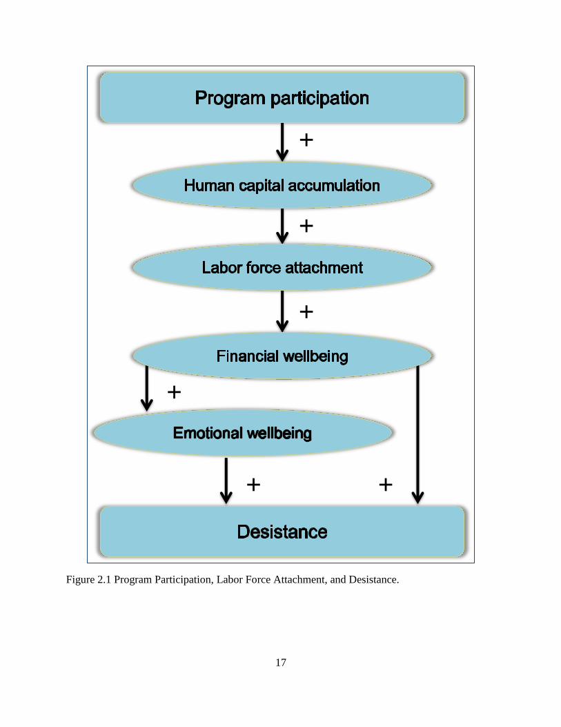
2.3 Proposed Conceptual Model Figure 2.1 depicts pathways by which prison education and employment programs strive to
reduce recidivism by strengthening men’s attachments to the labor force (Farabee et al., 2014;
Redcross et al., 2012; Saylor & Gaes, 1997). Education and employment programs improve
men’s job prospects through job skills training and the acquisition of education credentials
(Duwe & Clark, 2014; Steurer, Smith, & Tracy, 2001; Tyler & Kling, 2007; D. B. Wilson et al.,
2000). Human capital accumulation improves men’s wage prospects and increases their
incentives to take legal work (Thornberry & Christenson, 1984). Full-time employment in the
formal labor market provides men with living wages, benefits, and opportunities for growth and
career advancement (Bloom, 2006; Hagan, 1993).
Ongoing stable employment enhances men’s financial wellbeing. Jobs that pay living wages
alleviate financial strains that can lead men to commit economic crimes (Felson et al., 2012;
Skardhamar & Telle, 2012). Financial wellbeing contributes to enhanced emotional wellbeing
(Harris, Evans, & Beckett, 2010). Sustained emotional and financial wellbeing facilitate
desistance among former prisoners who find and maintain work (Bucklen & Zajac, 2009; Felson
et al., 2012).
17
Figure 2.1 Program Participation, Labor Force Attachment, and Desistance.
+
+
+
+
+ +
18
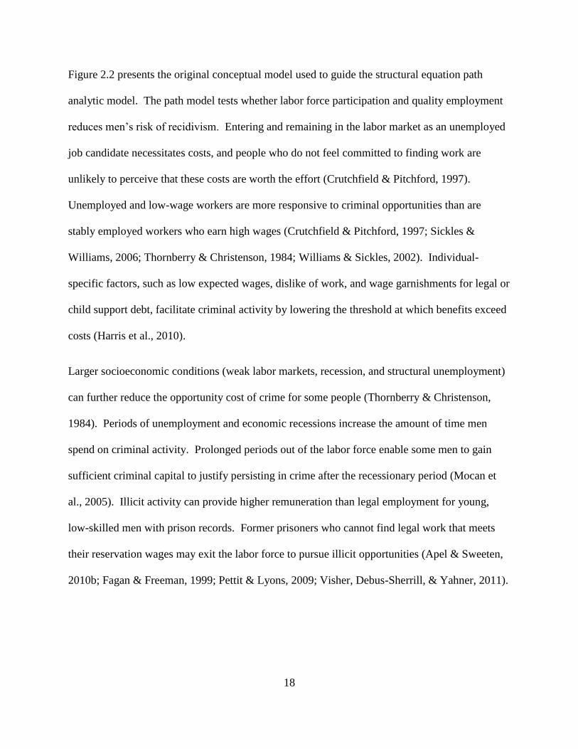
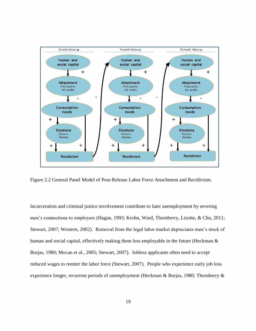
Figure 2.2 presents the original conceptual model used to guide the structural equation path
analytic model. The path model tests whether labor force participation and quality employment
reduces men’s risk of recidivism. Entering and remaining in the labor market as an unemployed
job candidate necessitates costs, and people who do not feel committed to finding work are
unlikely to perceive that these costs are worth the effort (Crutchfield & Pitchford, 1997).
Unemployed and low-wage workers are more responsive to criminal opportunities than are
stably employed workers who earn high wages (Crutchfield & Pitchford, 1997; Sickles &
Williams, 2006; Thornberry & Christenson, 1984; Williams & Sickles, 2002). Individual-
specific factors, such as low expected wages, dislike of work, and wage garnishments for legal or
child support debt, facilitate criminal activity by lowering the threshold at which benefits exceed
costs (Harris et al., 2010).
Larger socioeconomic conditions (weak labor markets, recession, and structural unemployment)
can further reduce the opportunity cost of crime for some people (Thornberry & Christenson,
1984). Periods of unemployment and economic recessions increase the amount of time men
spend on criminal activity. Prolonged periods out of the labor force enable some men to gain
sufficient criminal capital to justify persisting in crime after the recessionary period (Mocan et
al., 2005). Illicit activity can provide higher remuneration than legal employment for young,
low-skilled men with prison records. Former prisoners who cannot find legal work that meets
their reservation wages may exit the labor force to pursue illicit opportunities (Apel & Sweeten,
2010b; Fagan & Freeman, 1999; Pettit & Lyons, 2009; Visher, Debus-Sherrill, & Yahner, 2011).
19
Figure 2.2 General Panel Model of Post-Release Labor Force Attachment and Recidivism.
Incarceration and criminal justice involvement contribute to later unemployment by severing
men’s connections to employers (Hagan, 1993; Krohn, Ward, Thornberry, Lizotte, & Chu, 2011;
Stewart, 2007; Western, 2002). Removal from the legal labor market depreciates men’s stock of
human and social capital, effectively making them less employable in the future (Heckman &
Borjas, 1980; Mocan et al., 2005; Stewart, 2007). Jobless applicants often need to accept
reduced wages to reenter the labor force (Stewart, 2007). People who experience early job loss
experience longer, recurrent periods of unemployment (Heckman & Borjas, 1980; Thornberry &
20
Christenson, 1984). This reduces the number of hours worked in the formal labor market and
flattens long-term earnings trajectories (Stewart, 2007).
Labor force detachment and unemployment expose former prisoners to financial and
psychological strains that may explain much of the relationship between work and crime. The
stress associated with looking for work compounds as the length of unemployment increases
(Krueger, Mueller, Davis, & Sahin, 2011; Sugie, 2014; Young, 2012). Repeated job rejections
diminish applicants’ self-confidence and reduce their motivation to continue looking for work
(Krueger et al., 2011; Sugie, 2014; Young, 2012). Ongoing financial and emotional stressors
trigger a cascade of negative emotional states that reduce men’s sense of personal mastery and
increase their risk of recidivism (Halvorsen, 1998; Maruna, 2001; Price et al., 2002; Visher et al.,
2011).
21
Chapter 3: Methodology
3.1 Overview Prior SVORI evaluations concluded that employment services failed to improve participants’
reentry outcomes, and in some cases appeared to increase recidivism risk (Lattimore et al., 2012;
Lattimore et al., 2009). I first examine whether unobserved heterogeneity contributes to
inconsistent estimates of the effects of employment-focused programs on post-release
employment and crime (Heckman et al., 2000; Sedgley et al., 2010). Group-based trajectory
modeling (GTM) and propensity score techniques (PSM) use men’s baseline interviews and
criminal history records to control for characteristics that differentially select individuals into
treatment (Haviland, Nagin, & Rosenbaum, 2007).
Second, I use duration models to examine whether education and employment programs effect
participants’ time to first rearrest (Sedgley et al., 2010). Third, I examine whether increased
labor force attachment leads to higher quality employment (Stewart, 2007), increased financial
and emotional wellbeing (Price et al., 2002), and reduced offending (Thornberry & Christenson,
1984). The structural equation model use follow-up interview and administrative arrest data to
test whether quality jobs increase men’s financial and emotional wellbeing and reduce their risk
of recidivism (Thornberry & Christenson, 1984).
3.2 Research Hypotheses The first set of hypotheses examines the effects of participation in employment-focused prison
programs on men’s time to rearrest. The services included in this definition are educational
programs and job training/vocational education programs (Heckman, 2001; Sedgley et al., 2010).

22
1. Men who participate in vocational education, job training, or other education programs
exhibit distinct pre-release characteristics from men who do not receive these services.
2. After controlling for observed heterogeneity between nonparticipants and participants,
program participants exhibit lower recidivism rates than similar nonparticipants.
3. Participation in more than one type of employment-focused program has diminishing
marginal benefits on recidivism.
The second set of hypotheses examine the effects of labor force attachment and job quality on
men’s financial and emotional wellbeing, and their risk of recidivism during the early reentry
period (Bucklen & Zajac, 2009; Price et al., 2002; Skardhamar & Telle, 2012; Stewart, 2007;
Thornberry & Christenson, 1984).
4. Criminal justice involvement (e.g., arrest during the prior wave) reduces men’s stock of
human and social capital.
5. Men who have high levels of human and social capital are more likely to participate in
the labor market than men with low levels of capital are.
6. Increased labor force participation leads to improved job quality.
7. High quality employment reduces men’s experience of financial strain (e.g., unmet
consumption needs).
8. Unmet consumption needs increase the probability that men reoffend.
9. Financial strain, characterized by unmet consumption needs, diminishes emotional
wellbeing (e.g., psychological distress, personal mastery).
10. Diminished emotional wellbeing increases the likelihood that men reoffend.

23
3.3 Research Design
3.3.1 Data Collection
The study uses data on adult male prisoners from the Serious and Violent Offender Reentry
Initiative (SVORI) multi-site evaluation (n = 1,697). This collaborative federal effort provided
grant funds to 69 state agencies to design comprehensive reentry services targeting serious and
violent offenders under 35 years old. The SVORI evaluation tested the success of this federal
funding stream in motivating states to develop comprehensive reentry services that reduce
recidivism. SVORI programs varied widely in design, curriculum, activities, intensity, and
timeframe because agencies receiving SVORI funds could tailor services to fit the local context
without following a specific reentry-programming model (Lattimore et al., 2012; Lattimore &
Steffey, 2009).
The evaluation used an intent-to-treat design, in which respondents were classified as
participants and nonparticipants based on enrollment in SVORI programs or residence in
facilities offering SVORI programs. Sites recruited otherwise eligible individuals into the non-
SVORI comparison sample from facilities that did not provide SVORI programs. They also
recruited otherwise eligible individuals returning to communities without SVORI programs. Not
all SVORI participants received reentry services, and non-SVORI participants receiving
“treatment as usual” could participate in similar non-SVORI services (Lattimore & Steffey,
2009). Data on program participation were not available from all SVORI sites and for all
SVORI nonparticipants, so the evaluation uses men’s responses at the baseline interview
(Lattimore et al., 2012).
The 12 states offering SVORI-funded services to adult men that participated in the SVORI
evaluation were responsible for recruiting SVORI participants and comparable nonparticipants
24
into the study. Only two states randomly assigned men to the treatment and comparison groups.
The remaining 10 states enrolled eligible and interested men into SVORI programs and then
enrolled otherwise similar individuals into the comparison group. The initial pool of eligible
adult male prisoners included 2,564 adult men returning home from adult prisons between July
2004 and November 2005. Twelve percent of eligible men refused to participate in the study (n
= 295), 21% were released from prison before completing the baseline interview (n = 538), and
1% were ruled ineligible due to language or cognitive limitations (n = 34) (Lattimore & Steffey,
2009).
Men completed baseline interviews roughly 1 month before release from prison, and evaluators
contacted the men at 3, 9, and 15 months after release to complete follow-up interviews. The
follow-up interviews were completed from October 2004-April 2006, April 2005-October 2006,
and October 2005-April 2007. Men received financial incentives for follow-up interviews
completed in the community: $35 at the 3-month interview, $40 at the 9-month interview, and
$50 at the final 15-month interview. They received an additional $5 if they called a toll-free
number to schedule follow-up interviews. Men who were incarcerated at the time of follow-up
interviews completed interviews in prison. When possible, respondents who completed
interviews while institutionalized received the same financial compensations. Study participants
who completed all four interviews received an additional $50 at the end of the study (Lattimore
& Steffey, 2009).
3.3.2 Sample
The original SVORI evaluation sample included 1,697 men who were recruited from prison sites
in 12 US states. As part of the original evaluation, the Federal Bureau of Investigation (FBI)
National Crime Information Center (NCIC) provided lifetime arrest data for men in 11 of 12
25
states (n = 1,575). Arrest data spanned men’s full criminal history up to 36 months after release
from the SVORI status incarceration. The NCIC provided the dates of each arrest as well as the
charge and conviction offense associated with the arrest. SVORI evaluators calculated the time
from arrest to release from prison for each arrest recorded in the NCIC database (Lattimore et al.,
2012; Lattimore & Steffey, 2009).
Roughly 58% of these men completed the 3-month interview (n = 919), 61% completed the 9-
month interview (n = 957), and 65% completed the 15-month interview (n = 1,030). However,
only 43% of men interviewed at the pre-release baseline interview completed all three waves (n
= 670) and 21% of men completed no interviews after the pre-release interview (n = 330)
(Lattimore et al., 2012; Lattimore & Steffey, 2009).1
The initial sample for this study comprises 1,575 cases that had valid pre-SVORI arrests
recorded in the NCIC arrest records files. These men were included in the group-based
trajectory model (n = 1,575) and logit participation model (n = 1,571). Cases that were
successfully matched using propensity scores were included in the duration models (n = 1,521).
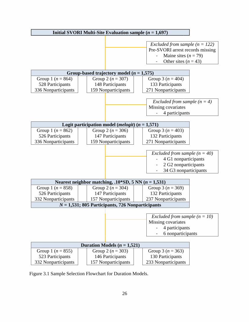
Figure 3.1 presents the sample selection process used to identify latent trajectory groups, model
participation status, and select appropriate matches among participants and nonparticipants.
The longitudinal structural equation model uses responses from three follow-up interviews.
Individuals who completed one or more follow-up interviews were retained in the longitudinal
structural equation model (n = 1,245).
1 The original SVORI sample included 122 individuals who had no pre-SVORI arrests recorded in the NCIC arrest
records file. Nearly all of these men were imprisoned in Maine (n = 79), which does not report arrests to the
National Crime Information Center. The remaining men with no NCIC-reported arrests were released from the
other states’ sites. The attrition rates from the follow-up interviews for the non-NCIC sample were virtually
indistinguishable from the NCIC sample, suggesting that attrition was not necessarily associated with state-level
factors.
26
Initial SVORI Multi-Site Evaluation sample (n = 1,697)
Excluded from sample (n = 122)
Pre-SVORI arrest records missing
- Maine sites (n = 79)
- Other sites (n = 43)
Group-based trajectory model (n = 1,575)
Group 1 (n = 864)
528 Participants
336 Nonparticipants
Group 2 (n = 307)
148 Participants
159 Nonparticipants
Group 3 (n = 404)
133 Participants
271 Nonparticipants
Excluded from sample (n = 4)
Missing covariates
- 4 participants
Logit participation model (melogit) (n = 1,571)
Group 1 (n = 862)
526 Participants
336 Nonparticipants
Group 2 (n = 306)
147 Participants
159 Nonparticipants
Group 3 (n = 403)
132 Participants
271 Nonparticipants
Excluded from sample (n = 40)
- 4 G1 nonparticipants
- 2 G2 nonparticipants
- 34 G3 nonparticipants
Nearest neighbor matching, .10*SD, 5 NN (n = 1,531)
Group 1 (n = 858)
526 Participants
332 Nonparticipants
Group 2 (n = 304)
147 Participants
157 Nonparticipants
Group 3 (n = 369)
132 Participants
237 Nonparticipants
N = 1,531; 805 Participants, 726 Nonparticipants
Excluded from sample (n = 10)
Missing covariates
- 4 participants
- 6 nonparticipants
Duration Models (n = 1,521)
Group 1 (n = 855)
523 Participants
332 Nonparticipants
Group 2 (n = 303)
146 Participants
157 Nonparticipants
Group 3 (n = 363)
130 Participants
233 Nonparticipants
Figure 3.1 Sample Selection Flowchart for Duration Models.
27
3.3.3 Missing Data Analysis
Indicators for Missing Data on Baseline Covariates
Certain key demographic variables that had limited numbers of missing data were recoded to
retain cases with intermittent missing data. Two individuals who had missing data for
racial/ethnic status were included in a combined category: Hispanic, biracial/multiracial, other
racial/ethnic status, or missing. Nine individuals who were missing data on number of times
previously imprisoned were included in the category for no previous prison terms, due to their
young ages when entering prison to complete their SVORI-related sentences.
Group-Based Trajectory Model
The trajectory model retained cases that had missing data for some observation periods (in cases
where men were too young to have been eligible for arrest), but these cases contributed fewer
observation periods to the fitting of the trajectory model. Approximately half of the time-
invariant explanatory variables included in the trajectory model were created using lifetime arrest
records. The remaining time-invariant explanatory variables come from the baseline interview,
which was completed by all of the men recruited into the sample. However, most items had little
or no missing data. Categorical variables that had missing data for a small number of cases (e.g.,
racial/ethnic status, previous imprisonments) were recoded as described above to retain cases.
Propensity Score Matching and Duration Models
The indicator for participation status had no missing data (n = 1,575): One man did not indicate
whether he had received vocational education/job training, but all of the men provided
information on educational service receipt. The duration models use data from official arrest
records that were compiled for all men in the original sample (n = 1,575). The multilevel logit
model and duration models used listwise deletion, due to incidental patterns of missing data for
items collected at the baseline interview. These models include race and prison variables that
28
were recoded to retain cases with missing data, as described previously. The logit participation
model eliminates four cases with missing data on covariates in the model (n = 1,571). The
duration models exclude 10 cases from the matched sample that had missing data on covariates
(n = 1,521).
Confirmatory Factor Analysis
The maximum likelihood (ML) estimation procedure retained cases with incidental missing data
patterns, although cases with extensive missing data (e.g., attriters from all three follow-up
interviews) were excluded from the sample.
Structural Equation Modeling
This study uses full-information maximum likelihood (FIML) estimation for the structural
equation models, which assumes that data are missing at random (Allison, 2003; Yuan, Yang-
Wallentin, & Bentler, 2012). FIML estimation using the full sample is preferable to statistical
techniques that use complete cases when data are not completely missing at random (Allison,
2003). Listwise deletion introduces the possibility of bias into estimates, while the reduced
sample size increases the size of standard errors and reduces the power of hypothesis tests
(Allison, 2003). FIML generates parameter estimates that are often more efficient than multiple
imputation techniques and do not rely on multiple random draws of data sets (Allison, 2003,
2012; Larsen, 2011). Because FIML addresses missing data as part of the estimation process, the
parameter estimates, standard errors, and test statistics are stable and do not vary (Allison, 2012).
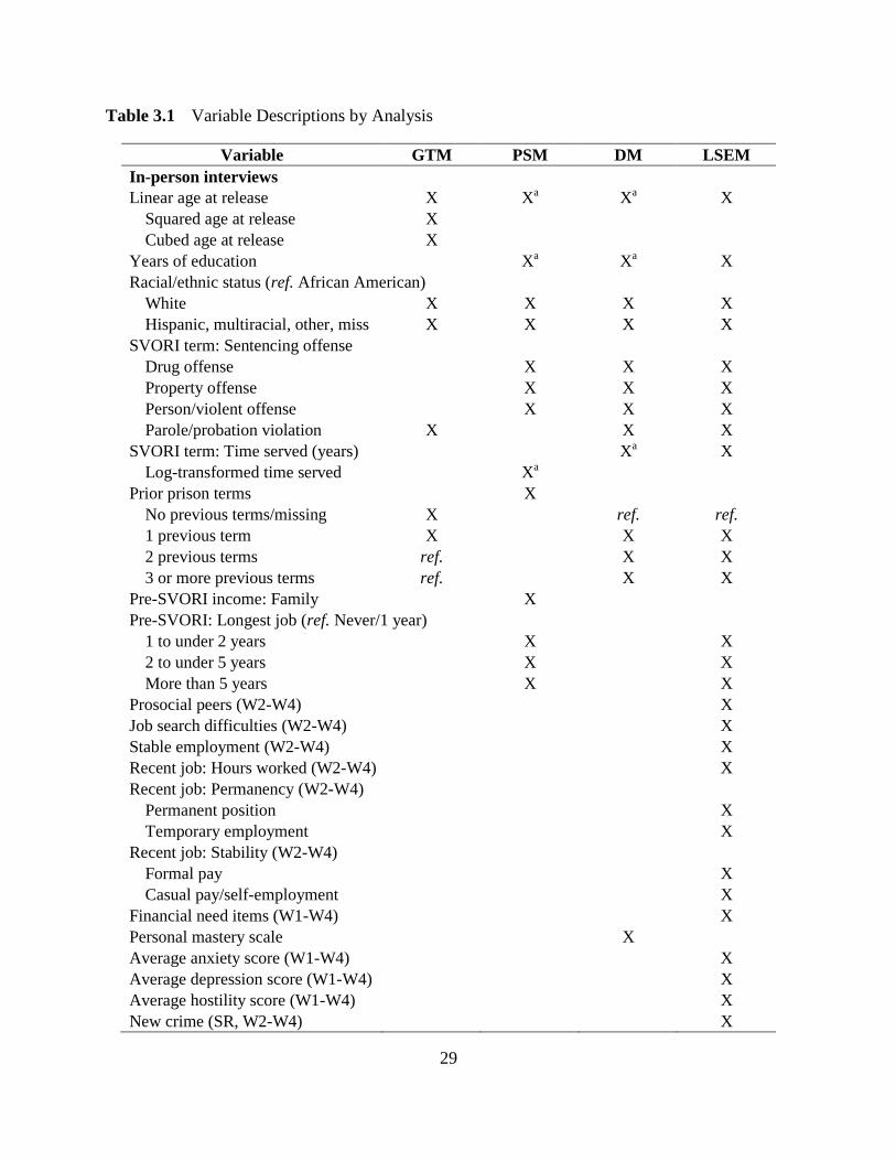
29
Table 3.1 Variable Descriptions by Analysis
Variable GTM PSM DM LSEM
In-person interviews
Linear age at release X Xa Xa X
Squared age at release X
Cubed age at release X
Years of education Xa Xa X
Racial/ethnic status (ref. African American)
White X X X X
Hispanic, multiracial, other, miss X X X X
SVORI term: Sentencing offense
Drug offense X X X
Property offense X X X
Person/violent offense X X X
Parole/probation violation X X X
SVORI term: Time served (years) Xa X
Log-transformed time served Xa
Prior prison terms X
No previous terms/missing X ref. ref.
1 previous term X X X
2 previous terms ref. X X
3 or more previous terms ref. X X
Pre-SVORI income: Family X
Pre-SVORI: Longest job (ref. Never/1 year)
1 to under 2 years X X
2 to under 5 years X X
More than 5 years X X
Prosocial peers (W2-W4) X
Job search difficulties (W2-W4) X
Stable employment (W2-W4) X
Recent job: Hours worked (W2-W4) X
Recent job: Permanency (W2-W4)
Permanent position X
Temporary employment X
Recent job: Stability (W2-W4)
Formal pay X
Casual pay/self-employment X
Financial need items (W1-W4) X
Personal mastery scale X
Average anxiety score (W1-W4) X
Average depression score (W1-W4) X
Average hostility score (W1-W4) X
New crime (SR, W2-W4) X
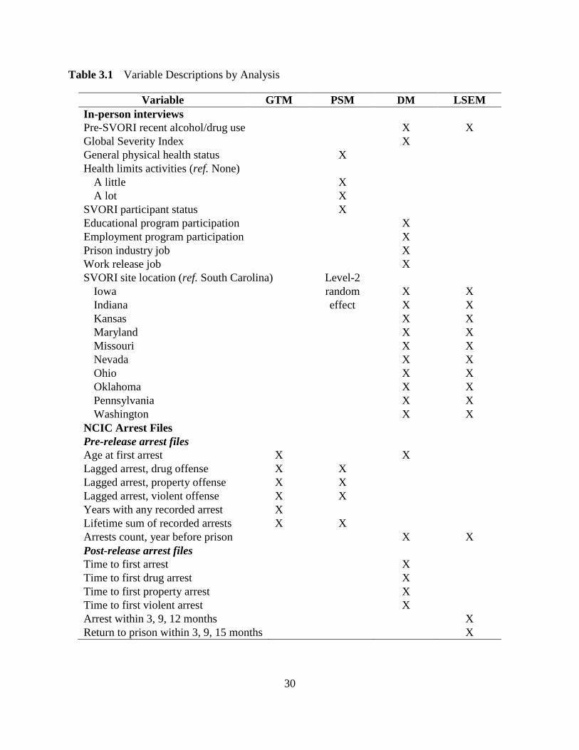
30
Table 3.1 Variable Descriptions by Analysis
Variable GTM PSM DM LSEM
In-person interviews
Pre-SVORI recent alcohol/drug use X X
Global Severity Index X
General physical health status X
Health limits activities (ref. None)
A little X
A lot X
SVORI participant status X
Educational program participation X
Employment program participation X
Prison industry job X
Work release job X
SVORI site location (ref. South Carolina) Level-2
Iowa random X X
Indiana effect X X
Kansas X X
Maryland X X
Missouri X X
Nevada X X
Ohio X X
Oklahoma X X
Pennsylvania X X
Washington X X
NCIC Arrest Files
Pre-release arrest files
Age at first arrest X X
Lagged arrest, drug offense X X
Lagged arrest, property offense X X
Lagged arrest, violent offense X X
Years with any recorded arrest X
Lifetime sum of recorded arrests X X
Arrests count, year before prison X X
Post-release arrest files
Time to first arrest X
Time to first drug arrest X
Time to first property arrest X
Time to first violent arrest X
Arrest within 3, 9, 12 months X
Return to prison within 3, 9, 15 months X

31
Table 3.1 Variable Descriptions by Analysis
Variable GTM PSM DM LSEM
Model-Generated Variables
Trajectory group (ref. Group 1)
Group 2 X X X
Group 3 X X X
Linear age*Trajectory group Xa
Education*Trajectory group Xa
Prison terms*Trajectory group X
Prob. participation, Education/Employment services X
Probability of participation* Trajectory group X
Note: GTM = Group-based trajectory model. LSEM = Longitudinal Structural Equation Model. NCIC =
National Crime Information Center. PSM = Propensity score methods. DM = Duration Models. SR = Self-
report. SVORI = Serious and Violent Offender Reentry Initiative. In-person interview items were collected
at baseline unless noted. “a” indicates continuous variables centered on state means.
3.4 Measures This section first describes the main outcomes variables for the study. It next describes the
explanatory and outcome variables for each set of analyses in detail. Table 3.1 presents the
variables included in each type of analysis. Variables included in the analyses can be divided
into three categories: in-person interview items, variables created from the NCIC arrest record
files, and model-generated variables. Most covariates from the in-person interview were
measured at the baseline interview; variables that were obtained from the follow-up interviews
are noted in Table 3.1.
3.4.1 Main Outcome Variables
This study use official records and men’s self-reported information from follow-up interviews to
measure criminal activity and criminal justice involvement. Arrests (for any offense and by
specific offenses) are measured using the NCIC arrest records, and self-reported criminal activity
(offenses committed during the 3-6 month reference period for each follow-up wave) is
32
measured using responses from each follow-up interview (Loeffler, 2013; Zweig, Yahner, &
Redcross, 2011).
3.4.2 Group-Based Trajectory Model
Measures included in the trajectory model were obtained from NCIC arrest records data and
from the baseline pre-release interview.
Outcome Variables
The key outcome variables (e.g., indicators of annual arrests) are derived from the NCIC arrest
record files. The trajectory model uses indicators of annual arrests during the 14 years leading
up to the SVORI status incarceration to chart prisoners’ prior offending trajectories (Haviland &
Nagin, 2005; Haviland et al., 2007; Thornberry & Christenson, 1984).
Explanatory Variables
The trajectory model includes time-varying and time-invariant measures created from the
longitudinal arrest record files. Linear, squared, and cubed forms of age at the time of the arrest
were included to model the nonlinear effect of age on risk of arrest. Age at arrest was estimated
using men’s age at release from the SVORI status offense. Time-varying covariates included in
the model were binary indicators of drug, property, or violent arrests during the prior year (e.g.,
three lagged indicators for each year, indicating the presence of a drug, property, or violent arrest
the previous year).
Additional covariates for criminal history were included in the model to control for false
desistance, observed during periods when men were imprisoned, and to control for the fact that
the 14-year observation period excluded some men’s complete criminal records. Time-invariant
covariates that were created using NCIC arrest records include age at first NCIC arrest
33
(continuous), number of pre-SVORI years with any arrests (continuous), and lifetime number of
arrests before SVORI prison term (continuous).
Other time-invariant covariates were obtained from the baseline in-person interview. To control
for the possibility of false desistance during previous periods of imprisonment, the model
includes self-report indicators for number of times imprisoned (1 = first imprisonment or
missing, 2 = second imprisonment, ref. two or more previous imprisonments) and for parole or
probation violation leading to the SVORI prison term (Eggleston, Laub, & Sampson, 2004).
Racial/ethnic status is included in the model to control for differential policing practices and
unobserved state-level differences (1 = Caucasian, 2 = African American (ref.), 3 = Hispanic,
biracial/multiracial, other racial/ethnic status, or missing).
3.4.3 Multilevel Logit Participation Model
The propensity score model includes pre-release indicators of men’s demographic
characteristics, prior employment, criminal history, and structural factors that may be correlated
with men’s decision to participate in employment-focused prison programs (Apel & Sweeten,
2010a; Haviland et al., 2007). Measures included in the logit participation model were obtained
from NCIC arrest record files and from the baseline pre-release interview.
Outcome Variables
Participation status was measured as participation in educational services or specific employment
programs while imprisoned. Educational services ranged from literacy tutoring and GED
courses to higher education (n = 717). Employment programs included vocational education or
job training programs (n = 208). Some participants received both educational and employment
services (n = 116). Nearly half of the sample did not participate in either type of program (n =
766).
34
Explanatory Variables
SVORI site location (US states) is included in the model as a level-2 random effect. Individuals
are nested within states from which they had been released from prison.
Level-1 variables measure individuals’ characteristics. Demographic variables were age at
release (continuous), education (continuous), racial/ethnic status (ref. African American), and
previous family income support (1 = yes). Four items reflected the SVORI status offense:
number of years in prison for the SVORI status offense (log-transformed) and three indicators
for drug, property, and violent conviction. Several items captured pre-SVORI criminal justice
involvement: previous imprisonments, indicators for drug, property, or violent arrests during the
year preceding prison entry (1 = yes), and total number of arrests that year (continuous).
Other explanatory variables included SVORI participation status (1 = yes), general physical
health (health limits moderate activity: 1 = a lot, 2 = a little, ref. not at all), and general emotional
wellbeing (e.g., feeling calm and peaceful). Trajectory group membership was included in the
model as dummy variables (ref. Group 1) and as interaction terms for age, education, and
continuous number of previous imprisonments. Age at release, education, and prison sentence
length were centered on state means to account for state-level differences.
3.4.4 Duration Models
Measures included in the duration models were obtained from NCIC arrest records data and from
the baseline pre-release interview.
Outcome Variables
The main outcome measure for the duration models was time to rearrest for any offense, using
post-release arrest records obtained from the NCIC arrest files. Time to arrest was measured in
days since release from the SVORI prison term. The parametric duration models measure time
35
to arrest in five different formats: time to arrest within the first 3 years, with repeated failures
permitted; time to first arrest for any offense; and time to first arrest for three offense subtypes
(drug, property, and violent offense). Prior to fitting the models, the five continuous arrest
measures were log-transformed to normalize their distributions and improve the fit of the
models. The duration models use the log-transformed continuous arrest measures as outcome
variables. In each case, model residuals indicate that the models fit most of the observations
well.
Explanatory Variables
Variables included in the duration models include indicators of program participation, men’s pre-
release demographic characteristics, work experience, prior offenses, and predicted trajectory
group membership (Brewster & Sharp, 2002; Sedgley et al., 2010; Skardhamar & Telle, 2012).
The duration models presented exclude interaction terms for engagement in both types of
employment-focused programs, but results of models that include interaction terms are not
substantively different.
The main predictor variables were educational programming, employment programming,
trajectory group membership, and predicted probability of participation. Demographic and
human capital measures included age at release (continuous), education (continuous), longest
time employed at one job (1 = 1-2 years, 2 = 3-5 years, 3 = 5 or more years, ref. less than 1 year),
work release employment (1 = yes), and prison industry employment (1 = yes). Measures for the
SVORI status offense included three indicators for having been convicted of drug, property, and
violent offenses, an indicator for parole or probation violations leading to the SVORI prison
term, and prison sentence length (continuous).

36
Recent criminal history was captured using men’s age at first NCIC arrest (continuous), total
number of arrests the year preceding prison entry, and number of previous imprisonments (1 =
one previous imprisonment, 2 = two or more previous imprisonments, ref. first imprisonment or
missing). Physical and mental health items included personal mastery (continuous parcel
averaging responses from eight baseline interview items), Global Severity Index (GSI) at
baseline, and an indicator of alcohol or drug use during the month preceding the SVORI prison
term (1 = yes). Racial/ethnic status (ref. African American) and state location (ref. South
Carolina) are included in the model as controls for social structural context. Age at release,
education, and prison sentence length were centered on state means to account for state-level
differences.
3.4.5 Structural Equation Modeling
The model includes five analysis periods: the baseline interview (before release), the first 3
months following release, months 4-9, months 10-15, and recidivism measures for months 3-21.
Table 3.2 presents the interview and data collection periods used to create the items included in
the path models.
Indicators and measures included in the structural equation model come from the baseline
interview, three follow-up interviews, and NCIC post-release arrest files. The LSEM uses
measures from waves 2-4 for labor force participation, job quality, financial needs, psychological
distress, and criminal activity (Krohn et al., 2011).
Latent Factors
Financial need (Time 1, 2, 3, & 4). The latent financial need factors were modeled using
responses to six items at each interview period. Men stated the extent to which they needed
financial assistance at the time (0 = not at all, 1 = a little, 2 = a lot). These ordinal-scale items

37
were combined to form two parcels, the first of which averaged men’s responses to three items
(place to live, clothing banks/food pantries, financial assistance). The second parcel averaged
men’s responses to the following three items (transportation, public financial assistance, public
healthcare insurance).
Table 3.2 Interview and Data Collection Periods for Longitudinal Structural Equation Model
Data source Wave 1 Wave 2 Wave 3 Wave 4 NCIC files
Reference period Month
of release
Months
1-3
Months
4-9
Months
10-15
Months
1-21
Constructs
Stable employment/
Job quality
Since
release
Since date
of last
interview
Since date
of last
interview
Financial needs Date of
interview
Date of
interview
Date of
interview
Date of
interview
Psychological
distress
7 days
preceding
interview
7 days
preceding
interview
7 days
preceding
interview
7 days
preceding
interview
Self-reported
criminal activity
Since
release
Since date
of last
interview
Since date
of last
interview
Rearrest/
Return to prison
Within first
3 months
Within first
9 months
Within first
12 months
Within first
21 months
Control variables Date of
interview
NCIC files
Analysis periods 1 2 3 4 5
Post-release months 0 1-3 4-9 10-15 16-21
Psychological Distress (Time 1, 2, 3, & 4). Psychological distress was measured for each time
point using responses to 15 items measuring respondents’ feelings of anxiety, depression, and
hostility during the previous week (1-5 scale). The five items within each subscale were first
averaged to create three parcels for each analysis period (before release, 3 months, 9 months, and

38
15 months after release). These parcels were then log-transformed to normalize their
distributions.
Labor force attachment (Time 2, 3, & 4). Three items were used to model men’s labor force
attachment during the reference periods preceding each follow-up interview (van der Geest et al.,
2011). The first item is included in the model as an observed indicator for labor force
participation, and is not an indicator of the latent construct for job quality. The binary indicator
of labor force participation measures stable employment since the date of the last interview (1 =
having worked at least once during each month that men had been living in the community).
Men who worked intermittently during the 3-6 month reference period were coded as 0, as were
men either who did not work at all or who were not living in the community at any point during
the observation period.
The latent construct for job quality is measured using two standardized items collected at each of
the three follow-up interviews. The first item reflected the average number of hours men had
worked each week at their last place of employment (centered and scaled to M 0, SD 1). The
second item was an index of primary sector employment. The initial score ranged from 0-6 and
was created by summing men’s responses to three questions (Job permanency: 0 = no recent job,
1 = temporary pay, 2 = permanent employment; Job stability: 0 = no recent job, 1 = casual
pay/self-employment, 2 = formal pay; Job benefits: 1 = receive paid time off, 1 = receive health
insurance from work). This 6-point index was centered and scaled to M 0, SD 1.
Observed Variables
Criminal activity is measured by self-reported criminal behavior during the months leading up to
each follow-up interview (Sickles & Williams, 2008; Williams & Sickles, 2002). Criminal
involvement was measured at three time points. The first item recorded any crime committed
39
since release from prison (W2, at approximately 3 months following release), the second
reported crimes that occurred between the second and third interviews (W3, approximately 3-9
months after release), and the third recorded crimes committed since the third interview (W4,
months 10-15). To supplement findings using self-reported criminal involvement, the model
includes indicators for arrest within 12 months and return to prison within the first 21 months
(Thornberry & Christenson, 1984).
Explanatory Variables
Control variables that were collected at baseline include age at release, educational attainment,
racial/ethnic status (ref. African American), and longest time employed at one job (1 = 1-2 years,
2 = 3-5 years, 3 = 5 or more years, ref. less than 1 year). Measures for the SVORI status offense
include three indicators for having been convicted of drug, property, and violent offenses, an
indicator for parole or probation violations leading to the SVORI prison term, and prison
sentence length (continuous). Criminal risk measures include trajectory group membership (ref.
Group 1), total number of arrests the year preceding prison entry, number of previous
imprisonments (1 = one previous imprisonment, 2 = two or more previous imprisonments, ref.
first imprisonment or missing), and an indicator of alcohol or drug use during the month
preceding the SVORI prison term (1 = yes). Dummies are included to control for state-specific
characteristics (ref. South Carolina).
Covariates collected at follow-up waves capture men’s recent human and social capital. These
included parcels measuring the average number of job search difficulties respondents had faced
during the reference period, and positive peer influences (proportion of friends employed,
proportion of friends who stay out of trouble). Criminal justice indicators measure rearrests and
returns to prison within the first 9 months of release from prison.

40
3.5 Data Analysis Plan Persistent, chronic, and more serious offenders are less likely to have acquired work skills before
prison entry and to pursue legal employment after release (Apel et al., 2007; Brame, Paternoster,
& Piquero, 2012; Nagin & Tremblay, 2005). This study employs techniques that control for
heterogeneity in treatment (program participation, labor force attachment) and in prior
observations of the outcome (recidivism) that can bias estimates of the average treatment effect
(Heckman, 2001; Heckman, Ichimura, & Todd, 1997). Group-based trajectory modeling and
propensity score matching control for pre-SVORI factors that shaped men’s access to services
and informed their participation decisions (Apel et al., 2007; Haviland et al., 2007; Haviland,
Rosenbaum, Nagin, & Tremblay, 2008; Heckman et al., 1997). Propensity score matching and
duration models are used to test the first three hypotheses presented at the beginning of the
chapter.
Structural equation modeling is used to test the remaining hypotheses (4-10). The structural
equation model employs a cross-lagged recursive panel design to assess 1) whether labor force
attachment is associated with self-reported criminal activity during the next interview period, and
2) whether self-reported criminal activity is associated with labor force attachment during the
next interview period.
3.5.1 Group-Based Trajectory Model
The Stata user-written command traj was used to derive latent groups within the sample, using
men’s pre-SVORI arrest records. The trajectory modeling procedure uses time-varying outcome
measures (binary indicators for any arrest within a given year) to identify distinct arrest
trajectories. Time-varying covariates are included in the longitudinal component of the model,
as these covariates may alter the shapes of the trajectories for certain groups. Time-invariant
41
covariates are included in the multinomial component of the model; these characteristics
differentiate members assigned probabilistically to each derived trajectory group. Men are
assigned probabilistically to one group, based on their observed characteristics. Models’ Akaike
information criterion (AIC) and Bayesian information criterion (BIC) values were used to
compare competing non-nested models to determine which one provided the best fit to the data.
Appendix C provides detailed information about the estimation process.
Fitting the Trajectory Model
Age is the primary time-varying predictor in the model; it was included in the final model in
linear, squared, and cubed terms. Including linear, squared, and cubed terms for age at time of
arrest provided superior fit to models that included only the linear or squared terms. Time-
varying lagged indicators for drug, property, and violent arrests were included in the model
because their coefficients were significant for two of the three derived latent groups. Other time-
invariant covariates were retained in the model because they improved the fit of the model and
controlled for differences in criminal records that were not captured by the arrest records (e.g.,
prior jail/prison terms, juvenile system involvement, and lengthy criminal records that exceeded
the 14-year pre-SVORI observation period).
3.5.2 Multilevel Logit Participation Model
This study uses propensity score techniques to balance individuals on the likelihood that they
engage in employment programs (Haviland et al., 2007). Propensity score matching should
address violations of two key assumptions required to compare treatment and comparison group
outcomes (Heckman et al., 1997). The conditional independence assumption requires that the
outcome for untreated men does not influence their participation: Men’s probability of rearrest or
reincarceration does not influence their selection into employment-focused programming. The

42
overlap assumption specifies that for any value of x, 0 < 𝑃𝑟𝑜𝑏((𝑑1 = 1|𝑥)) < 1. At any level
of x, there should be a similar mix of nonparticipants and participants in the sample, such that
there is a nonparticipant who is similar to each participant in the sample (Apel & Sweeten,
2010a; Greene, 2012; Haviland et al., 2007; Heckman et al., 1997).
Defining Program Participation
The original analysis plan had included prison industry work and work release employment in
the definition of program participation, based on the expectation that prison industry work and
work release employment provided relevant work skills (e.g., competing treatments to vocational
education/job training). Unfortunately, sample members holding work release/prison industry
jobs were significantly different from the rest of the sample; they were older, more educated,
serving shorter prison sentences, and were less likely to have been convicted of a violent offense
(results not presented). Diagnostic tests (traditional bivariate statistics and standardized bias
estimates) revealed that lingering biases resulted from the inclusion of prison industry work and
work release employment in the definition of employment-focused program participation.2
Furthermore, half of the men holding these industry/work release jobs had not received any other
educational/employment services. Defining prison industry/work release jobholders as
participants, many of whom had received no other employment-focused services, led to poor
matching results. The matched participants who held prison industry/work release employment
remained persistently different from nonparticipants, but also from other participants. As a
2 Pre- and post-matching standardized bias tests using this original participation definition are available upon
request. Mean and median standardized biases after matching were smaller than before matching, but bivariate tests
show that the matching process retained large differences between individuals who held work release/prison
industry employment and the other sample members (nonparticipant and participant alike) who did not.

43
result, matched participants receiving the main treatments of interest (vocational education/job
training) remained significantly different from the matched nonparticipant sample.
Upon realizing this problem, participation was redefined to fit the narrower criteria described in
the Measures subsection of this chapter: educational services of any kind and/or vocational
education/job training programs. Because roughly half of the prison industry/work-release
jobholders also received some form of education or job training services, this group divided
evenly among participants and nonparticipants.
Estimating the Logit Participation Model
Several logit models were fit to reduce standardized biases to an acceptable level (mean
standardized bias under 5%; maximum standardized bias under 20%). These models included a
1-level logit model that included individual-level characteristics, SVORI participant status, and
state dummies; a 2-level logit model, in which individuals were nested within SVORI participant
status; a kitchen-sink logit model that included multiple measures for each construct
(demographics, employment history, criminal history, health status, substance use, attitudinal
measures); and a an expanded version of the kitchen-sink model that included squared, cubed,
and interaction terms for significant predictors. These models did not effectively capture the
state-level variations in participation, so they were discarded in favor of the 2-level logit model
that nests individuals within SVORI sites (US states).
Fitting the Multilevel Logit Model
The multilevel logit model (Stata13 melogit) estimates men’s predicted probability of
participation in educational services, vocational education, or job training programs. Individuals
were nested within state sites to control for substantial state-level variation in prisoners’
demographic characteristics, criminal histories, and access to educational or employment-
44
focused services. State SVORI site is included in the model as a level-2 random effect, and
baseline demographic and risk characteristics are included in the model as level-1 covariates.
Items from the baseline interview that reflected men’s pre-prison characteristics were included in
the logit model, and these self-report interview items were supplemented by variables that had
been created from the NCIC arrest records. Continuous covariates are included in the model
after centering observations on mean values for each state. Trajectory group membership is
included in the model as dummy variables and as interactions with state-centered age at release,
state-centered level of education (in years), and number of previous imprisonments. These
individual-level characteristics do not completely remove the state-level variation in participation
status. The final multilevel logit model reveals that 16% of the variation in participation status
occurred at the state level.
3.5.3 Propensity Score Matching
Steps to Assess Covariate Balance
Propensity scores that effectively remove imbalances along potential confounders satisfy the
conditional independence assumption (Apel & Sweeten, 2010a). Two methods assess whether
the PSM has achieved covariate balance. First, the distribution of scores within treatment and
comparison groups can be compared to determine whether there is common support across levels
of x. Insignificant differences across most to all covariates within each bin provide supporting
evidence that the model has achieved covariate balance (Apel & Sweeten, 2010a).
Second, estimates of the standardized bias before and after matching can be used to compare the
results derived from various matching methods. Standardized bias estimates that exceed 20
indicate covariate imbalance (Apel & Sweeten, 2010a; Rosenbaum & Rubin, 1985). To meet the
overlap assumption, propensity scores for cases in each treatment condition should overlap, with
45
few off-support cases in tails of the score distribution and ideally common support across all
values between 0 and 1 (Apel & Sweeten, 2010a; Heckman et al., 1997).
Matching Estimation Techniques
Nearest neighbor matching is the simplest method, and it permits matching to single or multiple
cases, with or without replacement. Matching to multiple nonparticipants reduces variance but
can increase bias because some matches are less accurate. Matching without replacement works
well when untreated and treated cases are located along the whole propensity score distribution.
Matching with replacement permits treated cases to be matched to the same untreated cases; this
can improve the quality of the matches, although it reduces the effective sample size. This loss
of efficiency is preferred to the potential increase in bias that can occur when using matching
without replacement (Apel & Sweeten, 2010a).
Caliper matching sets an additional parameter to the nearest neighbor matching technique; the
caliper sets the maximum area from which untreated cases can be matched to treated cases. This
helps ensure that matched pairs have similar propensity scores (Apel & Sweeten, 2010a). The
initial caliper width proposed for use in the matching model was 0.2 of the standard deviation of
the propensity score logit (Rosenbaum & Rubin, 1985).
Kernel matching techniques may be preferred in cases where untreated and treated cases are less
evenly distributed. The finite probability distribution function used as a kernel weights untreated
cases by their distance from the treated case. If a uniform kernel is used, this method can
increase the number of untreated cases to which treated cases are matched, as it matches treated
cases to all untreated cases within a given radius. The Epanechnikov kernel matches treated
cases to all untreated cases located within a pre-specified bandwidth (Apel & Sweeten, 2010a).

46
Propensity Score Estimation Methods
The Stata user-written psmatch2 command was used to implement various matching estimators.
Matches were restricted to regions of common support. Prior to matching, the Stata user-written
pscore command was used to divide the sample into 5 bins of equal size. The program showed
that there were no significant differences between participants and nonparticipants within the
same bin. The pstest command was used to assess standardized biases for key predictors before
and after matching.
Results from multiple matching estimators were evaluated to assess which estimator produced
optimal matches (Apel & Sweeten, 2010b). Nearest neighbor matching with caliper, and
permitting various numbers of matches, was used as the primary matching technique. To
supplement results derived from nearest neighbor matching techniques, this study implemented a
second set of models that use kernel matching. Various forms of kernel matching estimators
(Epanechnikov, Gaussian, tricube and uniform kernels) were considered, but these alternatives
resulted in greater loss of cases without any corresponding improvement in balance.
Implementing Propensity Score Matching
The dissertation proposal initially specified that matches would be restricted to individuals
within the same trajectory group (Haviland & Nagin, 2005; Haviland et al., 2007; Haviland et al.,
2008). When efforts were made to restrict matching to within the same trajectory group,
participants and nonparticipants in the high-rate trajectory groups (Groups 1 and 3) showed
adequate balance using most matching techniques. Despite this, mean standardized biases
exceeded 5% for all matching methods, and standardized biases for key predictors exceeded 10%
(e.g., age at release, SVORI prison term). Matching estimators failed to achieve balance when
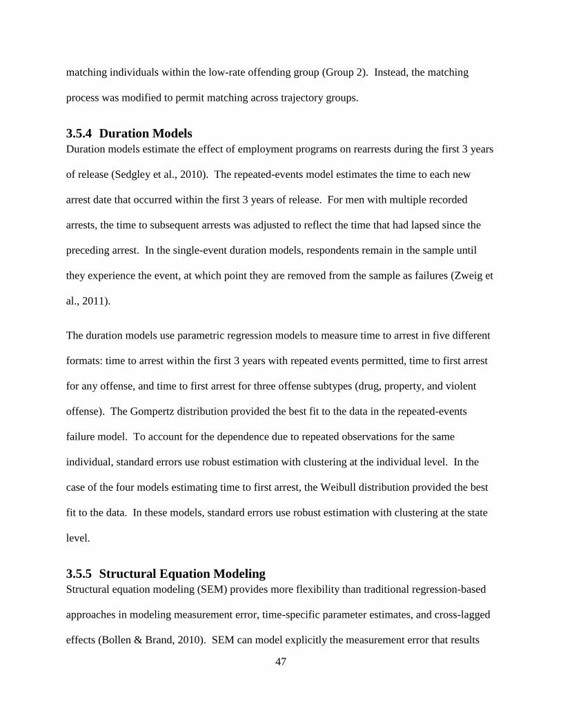
47
matching individuals within the low-rate offending group (Group 2). Instead, the matching
process was modified to permit matching across trajectory groups.
3.5.4 Duration Models
Duration models estimate the effect of employment programs on rearrests during the first 3 years
of release (Sedgley et al., 2010). The repeated-events model estimates the time to each new
arrest date that occurred within the first 3 years of release. For men with multiple recorded
arrests, the time to subsequent arrests was adjusted to reflect the time that had lapsed since the
preceding arrest. In the single-event duration models, respondents remain in the sample until
they experience the event, at which point they are removed from the sample as failures (Zweig et
al., 2011).
The duration models use parametric regression models to measure time to arrest in five different
formats: time to arrest within the first 3 years with repeated events permitted, time to first arrest
for any offense, and time to first arrest for three offense subtypes (drug, property, and violent
offense). The Gompertz distribution provided the best fit to the data in the repeated-events
failure model. To account for the dependence due to repeated observations for the same
individual, standard errors use robust estimation with clustering at the individual level. In the
case of the four models estimating time to first arrest, the Weibull distribution provided the best
fit to the data. In these models, standard errors use robust estimation with clustering at the state
level.
3.5.5 Structural Equation Modeling
Structural equation modeling (SEM) provides more flexibility than traditional regression-based
approaches in modeling measurement error, time-specific parameter estimates, and cross-lagged
effects (Bollen & Brand, 2010). SEM can model explicitly the measurement error that results
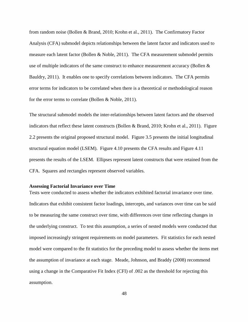
48
from random noise (Bollen & Brand, 2010; Krohn et al., 2011). The Confirmatory Factor
Analysis (CFA) submodel depicts relationships between the latent factor and indicators used to
measure each latent factor (Bollen & Noble, 2011). The CFA measurement submodel permits
use of multiple indicators of the same construct to enhance measurement accuracy (Bollen &
Bauldry, 2011). It enables one to specify correlations between indicators. The CFA permits
error terms for indicators to be correlated when there is a theoretical or methodological reason
for the error terms to correlate (Bollen & Noble, 2011).
The structural submodel models the inter-relationships between latent factors and the observed
indicators that reflect these latent constructs (Bollen & Brand, 2010; Krohn et al., 2011). Figure
2.2 presents the original proposed structural model. Figure 3.5 presents the initial longitudinal
structural equation model (LSEM). Figure 4.10 presents the CFA results and Figure 4.11
presents the results of the LSEM. Ellipses represent latent constructs that were retained from the
CFA. Squares and rectangles represent observed variables.
Assessing Factorial Invariance over Time
Tests were conducted to assess whether the indicators exhibited factorial invariance over time.
Indicators that exhibit consistent factor loadings, intercepts, and variances over time can be said
to be measuring the same construct over time, with differences over time reflecting changes in
the underlying construct. To test this assumption, a series of nested models were conducted that
imposed increasingly stringent requirements on model parameters. Fit statistics for each nested
model were compared to the fit statistics for the preceding model to assess whether the items met
the assumption of invariance at each stage. Meade, Johnson, and Braddy (2008) recommend
using a change in the Comparative Fit Index (CFI) of .002 as the threshold for rejecting this
assumption.
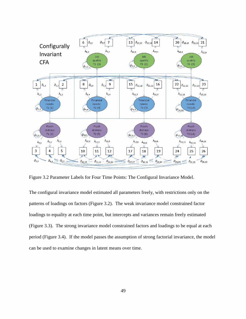
49
Figure 3.2 Parameter Labels for Four Time Points: The Configural Invariance Model.
The configural invariance model estimated all parameters freely, with restrictions only on the
patterns of loadings on factors (Figure 3.2). The weak invariance model constrained factor
loadings to equality at each time point, but intercepts and variances remain freely estimated
(Figure 3.3). The strong invariance model constrained factors and loadings to be equal at each
period (Figure 3.4). If the model passes the assumption of strong factorial invariance, the model
can be used to examine changes in latent means over time.
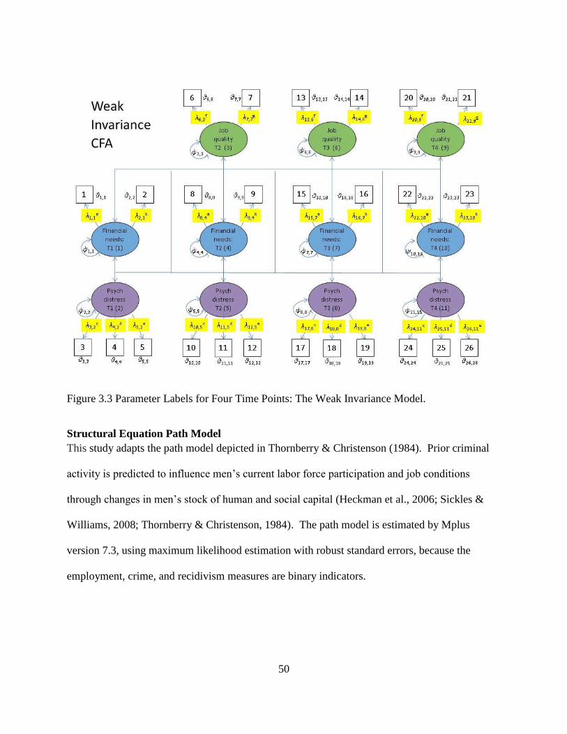
50
Figure 3.3 Parameter Labels for Four Time Points: The Weak Invariance Model.
Structural Equation Path Model
This study adapts the path model depicted in Thornberry & Christenson (1984). Prior criminal
activity is predicted to influence men’s current labor force participation and job conditions
through changes in men’s stock of human and social capital (Heckman et al., 2006; Sickles &
Williams, 2008; Thornberry & Christenson, 1984). The path model is estimated by Mplus
version 7.3, using maximum likelihood estimation with robust standard errors, because the
employment, crime, and recidivism measures are binary indicators.
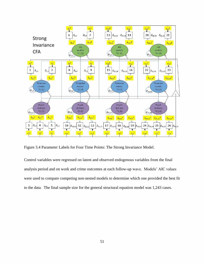
51
Figure 3.4 Parameter Labels for Four Time Points: The Strong Invariance Model.
Control variables were regressed on latent and observed endogenous variables from the final
analysis period and on work and crime outcomes at each follow-up wave. Models’ AIC values
were used to compare competing non-nested models to determine which one provided the best fit
to the data. The final sample size for the general structural equation model was 1,243 cases.
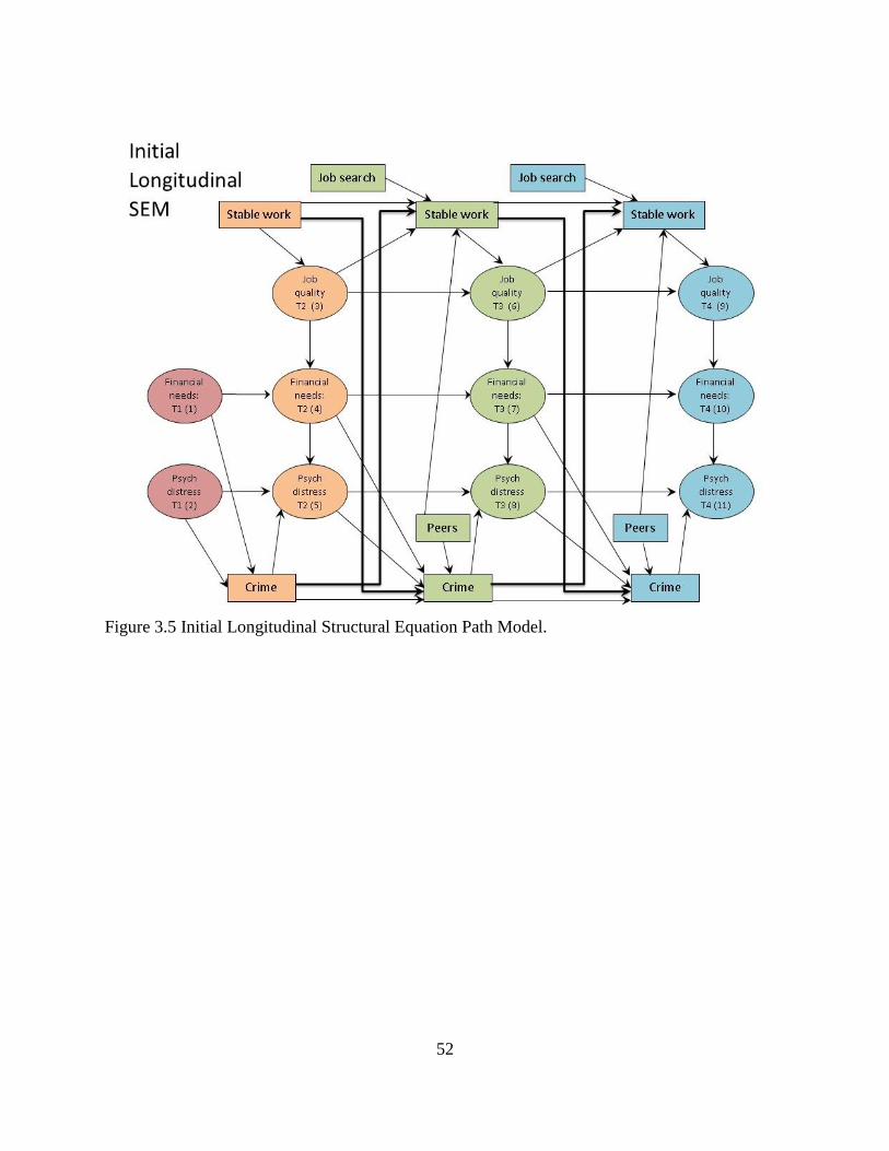
52
Figure 3.5 Initial Longitudinal Structural Equation Path Model.

53
Chapter 4: Results
4.1 Overview This chapter presents results of the trajectory group modeling, propensity score matching,
duration models, and structural equation modeling. This chapter begins by presenting
descriptive characteristics of the study sample at the time of the baseline interview. This chapter
next presents results of the trajectory group model, propensity score matching process, and
duration models, all of which are used to test the effect of employment programs on arrest
outcomes following release from prison. Information from the trajectory group model is
included in the logit model used to model the probability of receiving employment-focused
services. The matched sample obtained from propensity score matching is used to model time to
rearrest in the repeated-event and single-event failure models.
The second half of the chapter presents results of the longitudinal structural equation model. The
CFA model is tested for invariance over time, and the best-fitting model meets the assumptions
of strong invariance over time. Using the strong invariant CFA model, the longitudinal SEM
includes four interview waves. The best-fitting model regresses all endogenous constructs and
observed variables on covariates from the baseline interview and NCIC arrest record files.
Primary outcome measures are presented at the beginning of each analysis section: pre-SVORI
arrests are used to fit the group-based trajectory model, employment-focused service receipt is
used in the logit participation model, several time-based rearrest measures are included in
duration models, and work and crime outcomes at each follow-up interview are included in the
structural equation model.
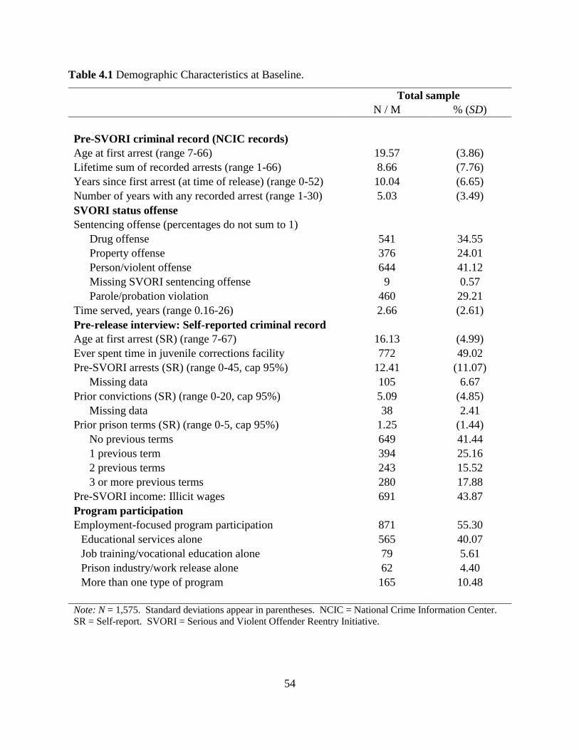
54
Table 4.1 Demographic Characteristics at Baseline.
Total sample
N / M % (SD)
Pre-SVORI criminal record (NCIC records)
Age at first arrest (range 7-66) 19.57 (3.86)
Lifetime sum of recorded arrests (range 1-66) 8.66 (7.76)
Years since first arrest (at time of release) (range 0-52) 10.04 (6.65)
Number of years with any recorded arrest (range 1-30) 5.03 (3.49)
SVORI status offense
Sentencing offense (percentages do not sum to 1)
Drug offense 541 34.55
Property offense 376 24.01
Person/violent offense 644 41.12
Missing SVORI sentencing offense 9 0.57
Parole/probation violation 460 29.21
Time served, years (range 0.16-26) 2.66 (2.61)
Pre-release interview: Self-reported criminal record
Age at first arrest (SR) (range 7-67) 16.13 (4.99)
Ever spent time in juvenile corrections facility 772 49.02
Pre-SVORI arrests (SR) (range 0-45, cap 95%) 12.41 (11.07)
Missing data 105 6.67
Prior convictions (SR) (range 0-20, cap 95%) 5.09 (4.85)
Missing data 38 2.41
Prior prison terms (SR) (range 0-5, cap 95%) 1.25 (1.44)
No previous terms 649 41.44
1 previous term 394 25.16
2 previous terms 243 15.52
3 or more previous terms 280 17.88
Pre-SVORI income: Illicit wages 691 43.87
Program participation
Employment-focused program participation 871 55.30
Educational services alone 565 40.07
Job training/vocational education alone 79 5.61
Prison industry/work release alone 62 4.40
More than one type of program 165 10.48
Note: N = 1,575. Standard deviations appear in parentheses. NCIC = National Crime Information Center.
SR = Self-report. SVORI = Serious and Violent Offender Reentry Initiative.
55
4.2 Descriptive Results
4.2.1 Demographic Characteristics at Baseline Table 4.1 presents data on baseline characteristics of the sample. Men’s average age at first
arrest was 16 years old; by release, men were 30 years old on average and had served nearly 3
years in prison. Minorities composed 70% of the sample (55% African American, 33% White,
4% Hispanic, and 8% other). At the time of the baseline interview, 40% of men reported that
they were currently married or involved in a steady relationship (n = 628). Sixty percent of men
(n = 947) reported that they were fathers of minor children; and 30% of them held child support
orders before entering prison (Lattimore et al., 2012; Lattimore & Visher, 2009).
Four in ten respondents left prison with less than a twelfth-grade education, having not
completed the GED while incarcerated (n = 633). Men were more likely to have received GEDs
than to have graduated from high school (29% vs. 14%), indicating the possible completion of
the GED during the current (or previous) prison sentence. Two-thirds of men had been
employed at some point during the 6 months leading up to prison (n = 1,040). Those
predominantly full-time positions paid average hourly wages of $10.51 (SD 7.62). However,
most men had not held consistent employment before prison, as 60% of men had never held a job
for more than 2 years.
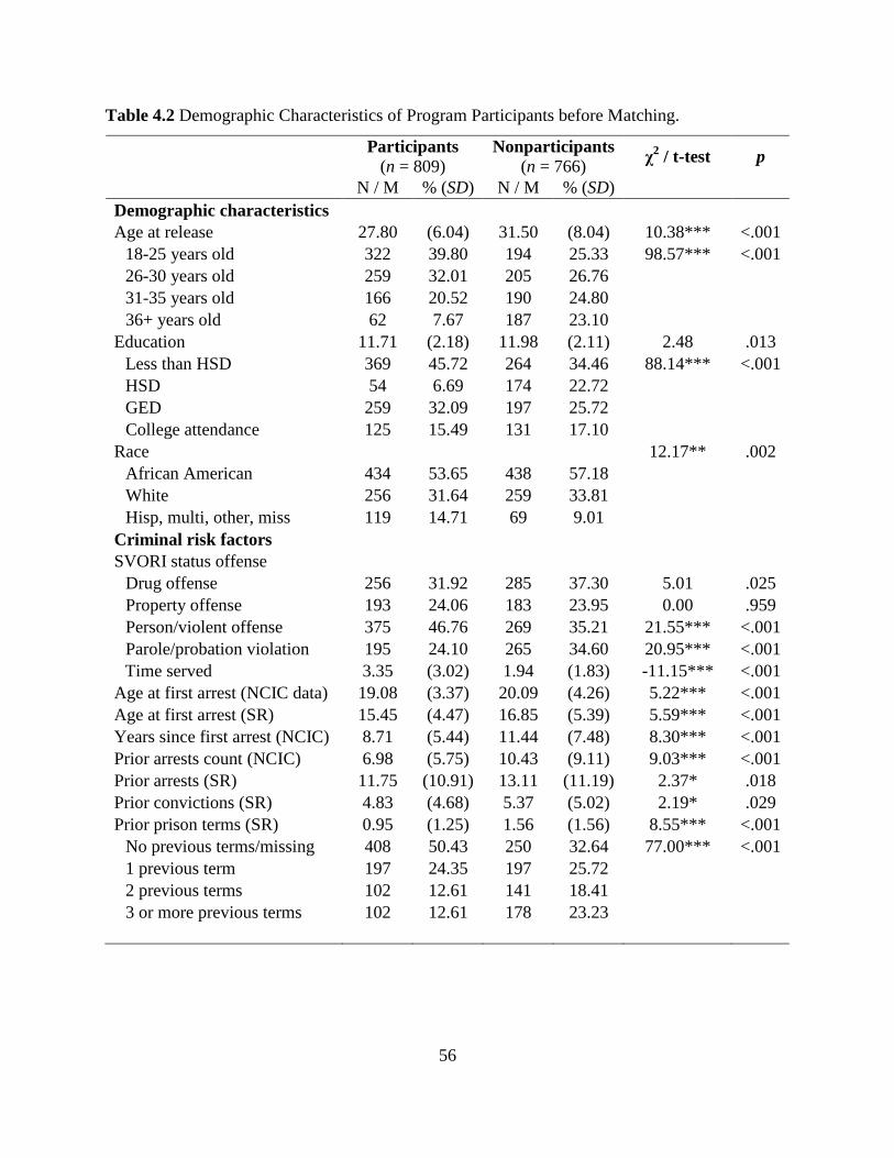
56
Table 4.2 Demographic Characteristics of Program Participants before Matching.
Participants
(n = 809) Nonparticipants
(n = 766) χ
2 / t-test p
N / M % (SD) N / M % (SD)
Demographic characteristics
Age at release 27.80 (6.04) 31.50 (8.04) 10.38*** <.001
18-25 years old 322 39.80 194 25.33 98.57*** <.001
26-30 years old 259 32.01 205 26.76
31-35 years old 166 20.52 190 24.80
36+ years old 62 7.67 187 23.10
Education 11.71 (2.18) 11.98 (2.11) 2.48 .013
Less than HSD 369 45.72 264 34.46 88.14*** <.001
HSD 54 6.69 174 22.72
GED 259 32.09 197 25.72
College attendance 125 15.49 131 17.10
Race
12.17** .002
African American 434 53.65 438 57.18
White 256 31.64 259 33.81
Hisp, multi, other, miss 119 14.71 69 9.01
Criminal risk factors
SVORI status offense
Drug offense 256 31.92 285 37.30 5.01 .025
Property offense 193 24.06 183 23.95 0.00 .959
Person/violent offense 375 46.76 269 35.21 21.55*** <.001
Parole/probation violation 195 24.10 265 34.60 20.95*** <.001
Time served 3.35 (3.02) 1.94 (1.83) -11.15*** <.001
Age at first arrest (NCIC data) 19.08 (3.37) 20.09 (4.26) 5.22*** <.001
Age at first arrest (SR) 15.45 (4.47) 16.85 (5.39) 5.59*** <.001
Years since first arrest (NCIC) 8.71 (5.44) 11.44 (7.48) 8.30*** <.001
Prior arrests count (NCIC) 6.98 (5.75) 10.43 (9.11) 9.03*** <.001
Prior arrests (SR) 11.75 (10.91) 13.11 (11.19) 2.37* .018
Prior convictions (SR) 4.83 (4.68) 5.37 (5.02) 2.19* .029
Prior prison terms (SR) 0.95 (1.25) 1.56 (1.56) 8.55*** <.001
No previous terms/missing 408 50.43 250 32.64 77.00*** <.001
1 previous term 197 24.35 197 25.72
2 previous terms 102 12.61 141 18.41
3 or more previous terms 102 12.61 178 23.23
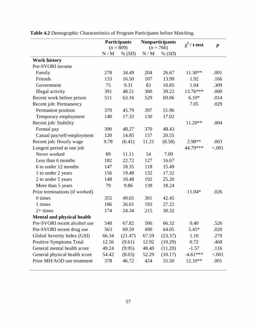
57
Table 4.2 Demographic Characteristics of Program Participants before Matching.
Participants
(n = 809) Nonparticipants
(n = 766) χ
2 / t-test p
N / M % (SD) N / M % (SD)
Work history
Pre-SVORI income
Family 278 34.49 204 26.67 11.30** .001
Friends 133 16.50 107 13.99 1.92 .166
Government 75 9.31 83 10.85 1.04 .309
Illegal activity 391 48.51 300 39.22 13.76*** .000
Recent work before prison 511 63.16 529 69.06 6.10* .014
Recent job: Permanency 7.05 .029
Permanent position 370 45.79 397 51.96
Temporary employment 140 17.33 130 17.02
Recent job: Stability 11.20** .004
Formal pay 390 48.27 370 48.43
Casual pay/self-employment 120 14.85 157 20.55
Recent job: Hourly wage 9.78 (6.41) 11.21 (8.58) 2.98** .003
Longest period at one job
44.79*** <.001
Never worked 89 11.11 54 7.09
Less than 6 months 182 22.72 127 16.67
6 to under 12 months 147 18.35 118 15.49
1 to under 2 years 156 19.48 132 17.32
2 to under 5 years 148 18.48 192 25.20
More than 5 years 79 9.86 139 18.24
Prior terminations (if worked) 11.04* .026
0 times 355 49.65 301 42.45
1 times 186 26.01 193 27.22
2+ times 174 24.34 215 30.32
Mental and physical health
Pre-SVORI recent alcohol use 548 67.82 506 66.32 0.40 .526
Pre-SVORI recent drug use 563 69.59 490 64.05 5.45* .020
Global Severity Index (GSI) 66.34 (21.47) 67.59 (23.37) 1.10 .270
Positive Symptoms Total 12.56 (9.61) 12.92 (10.29) 0.72 .468
General mental health score 49.24 (9.95) 48.40 (11.20) -1.57 .116
General physical health score 54.42 (8.03) 52.29 (10.17) -4.61*** <.001
Prior MH/AOD use treatment 378 46.72 424 55.50 12.10** .001
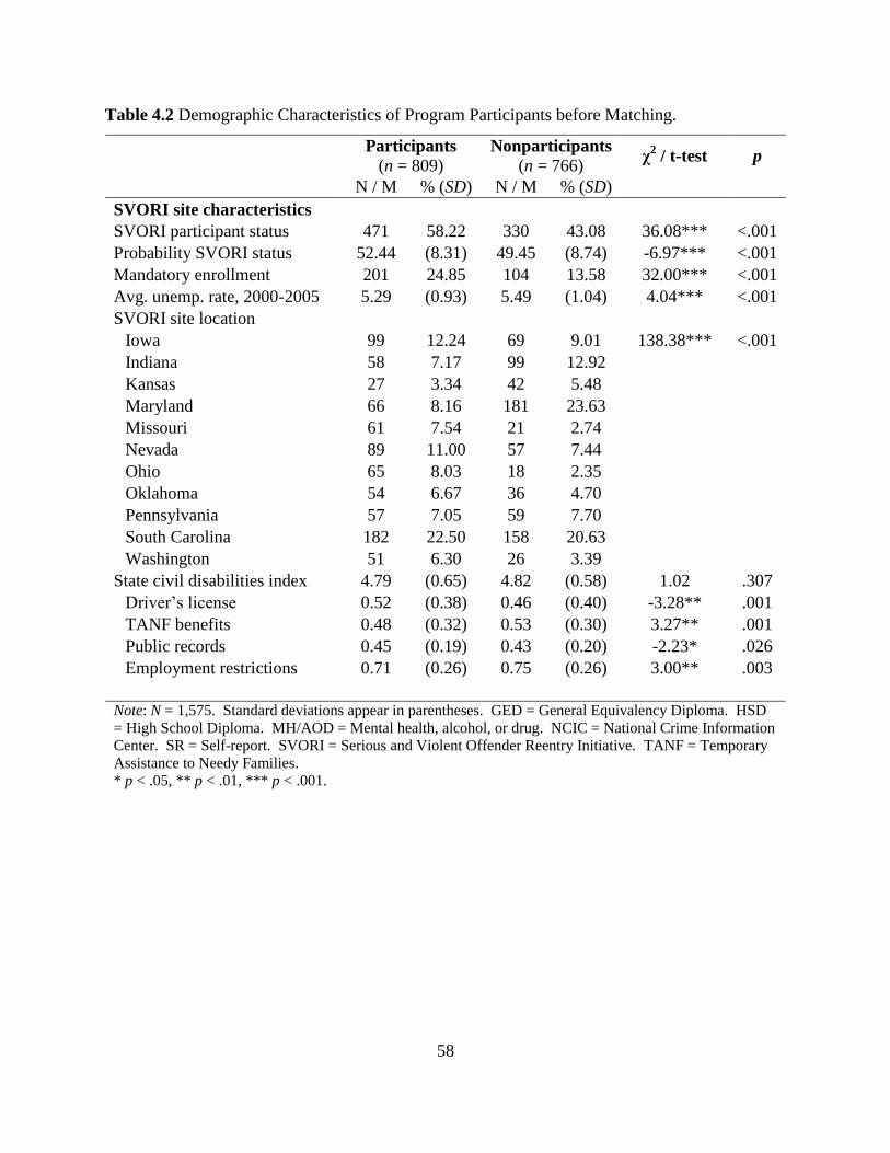
58
Table 4.2 Demographic Characteristics of Program Participants before Matching.
Participants
(n = 809) Nonparticipants
(n = 766) χ
2 / t-test p
N / M % (SD) N / M % (SD)
SVORI site characteristics
SVORI participant status 471 58.22 330 43.08 36.08*** <.001
Probability SVORI status 52.44 (8.31) 49.45 (8.74) -6.97*** <.001
Mandatory enrollment 201 24.85 104 13.58 32.00*** <.001
Avg. unemp. rate, 2000-2005 5.29 (0.93) 5.49 (1.04) 4.04*** <.001
SVORI site location
Iowa 99 12.24 69 9.01 138.38*** <.001
Indiana 58 7.17 99 12.92
Kansas 27 3.34 42 5.48
Maryland 66 8.16 181 23.63
Missouri 61 7.54 21 2.74
Nevada 89 11.00 57 7.44
Ohio 65 8.03 18 2.35
Oklahoma 54 6.67 36 4.70
Pennsylvania 57 7.05 59 7.70
South Carolina 182 22.50 158 20.63
Washington 51 6.30 26 3.39
State civil disabilities index 4.79 (0.65) 4.82 (0.58) 1.02 .307
Driver’s license 0.52 (0.38) 0.46 (0.40) -3.28** .001
TANF benefits 0.48 (0.32) 0.53 (0.30) 3.27** .001
Public records 0.45 (0.19) 0.43 (0.20) -2.23* .026
Employment restrictions 0.71 (0.26) 0.75 (0.26) 3.00** .003
Note: N = 1,575. Standard deviations appear in parentheses. GED = General Equivalency Diploma. HSD
= High School Diploma. MH/AOD = Mental health, alcohol, or drug. NCIC = National Crime Information
Center. SR = Self-report. SVORI = Serious and Violent Offender Reentry Initiative. TANF = Temporary
Assistance to Needy Families.
* p < .05, ** p < .01, *** p < .001.
59
4.3 Assessing Initial Bias before Matching
4.3.1 Bivariate Statistics before Matching Table 4.2 presents baseline characteristics by participation status before matching. Education
and employment program participants were significantly younger than nonparticipants were
(Mpart = 27.80, SDpart = 6.04; Mnon = 31.50, SDnon = 8.04; t = 10.38, p < .001) and were less likely
to have completed high school (6.69% of participants vs. 22.72% of nonparticipants).
Participants were also more likely than were nonparticipants to have been convicted of a violent
offense (46.76% and 35.21%, respectively) and to report having recently earned income from
illegal activity (48.51% vs. 39.22%). Reflecting their youth, participants were more likely to be
completing their first prison term and less likely to be completing a sentence for a technical
parole/probation violation. They had also acquired shorter work histories than nonparticipants
had, and a higher percentage reported having received financial support from family members
before entering prison (34.49% of participants, compared to 26.67% of nonparticipants).
Using data from official arrest records, participants had acquired shorter criminal records than
nonparticipants had, in terms of prior arrests (Mpart = 6.98, SDpart = 5.75; Mnon = 10.43, SDnon =
9.11; t = 9.03, p < .001) and years since first arrest (Mpart = 8.71, SDpart = 5.44; Mnon = 11.44,
SDnon = 7.48; t = 8.30, p < .001). Despite this, average age at first arrest was younger among
participants (Mpart = 19.08, SDpart = 3.37; Mnon = 20.09, SDnon = 4.26; t = 5.22, p < .001), and
they had acquired nearly the same number of convictions as nonparticipants, albeit within a
shorter timeframe (Mpart = 4.83, SDpart = 4.68; Mnon = 5.37, SDnon = 5.02; t = 5.22, p < .001).
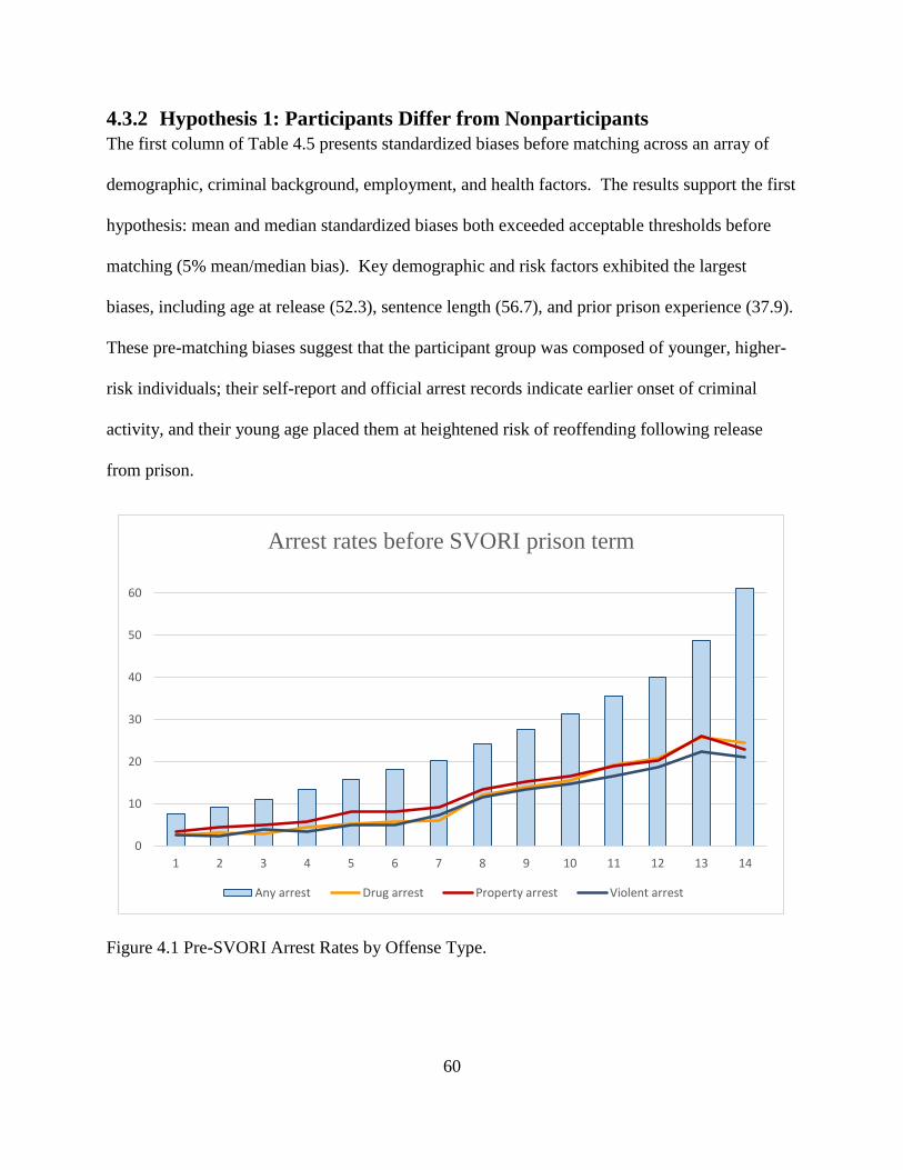
60
4.3.2 Hypothesis 1: Participants Differ from Nonparticipants
The first column of Table 4.5 presents standardized biases before matching across an array of
demographic, criminal background, employment, and health factors. The results support the first
hypothesis: mean and median standardized biases both exceeded acceptable thresholds before
matching (5% mean/median bias). Key demographic and risk factors exhibited the largest
biases, including age at release (52.3), sentence length (56.7), and prior prison experience (37.9).
These pre-matching biases suggest that the participant group was composed of younger, higher-
risk individuals; their self-report and official arrest records indicate earlier onset of criminal
activity, and their young age placed them at heightened risk of reoffending following release
from prison.
Figure 4.1 Pre-SVORI Arrest Rates by Offense Type.
0
10
20
30
40
50
60
1 2 3 4 5 6 7 8 9 10 11 12 13 14
Arrest rates before SVORI prison term
Any arrest Drug arrest Property arrest Violent arrest
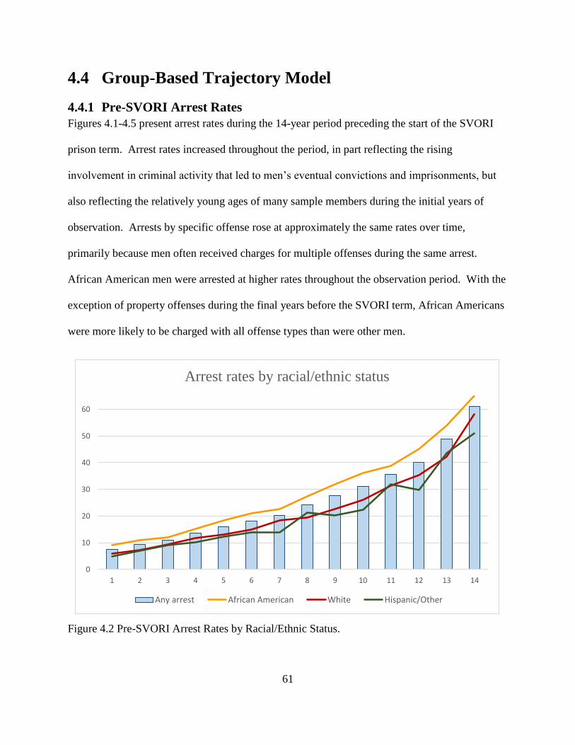
61
4.4 Group-Based Trajectory Model
4.4.1 Pre-SVORI Arrest Rates
Figures 4.1-4.5 present arrest rates during the 14-year period preceding the start of the SVORI
prison term. Arrest rates increased throughout the period, in part reflecting the rising
involvement in criminal activity that led to men’s eventual convictions and imprisonments, but
also reflecting the relatively young ages of many sample members during the initial years of
observation. Arrests by specific offense rose at approximately the same rates over time,
primarily because men often received charges for multiple offenses during the same arrest.
African American men were arrested at higher rates throughout the observation period. With the
exception of property offenses during the final years before the SVORI term, African Americans
were more likely to be charged with all offense types than were other men.
Figure 4.2 Pre-SVORI Arrest Rates by Racial/Ethnic Status.
0
10
20
30
40
50
60
1 2 3 4 5 6 7 8 9 10 11 12 13 14
Arrest rates by racial/ethnic status
Any arrest African American White Hispanic/Other
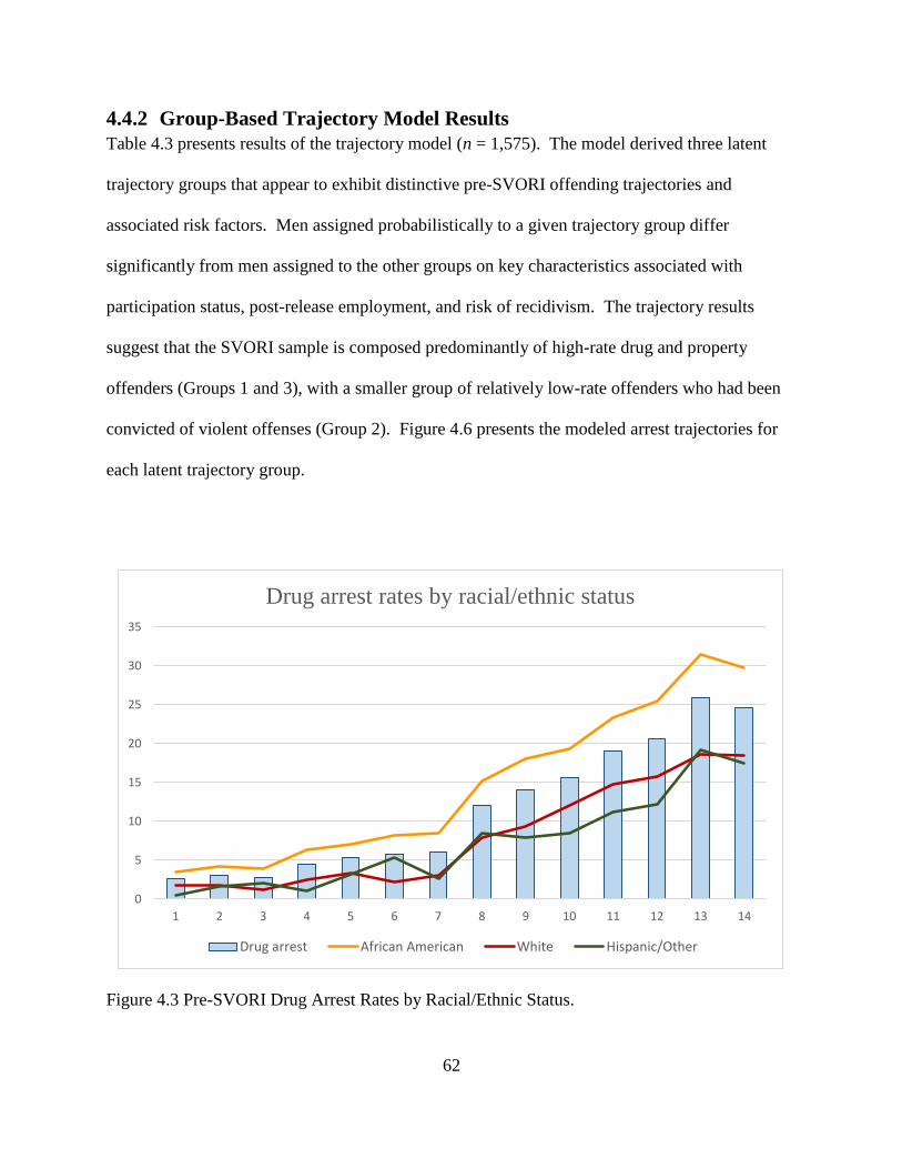
62
4.4.2 Group-Based Trajectory Model Results
Table 4.3 presents results of the trajectory model (n = 1,575). The model derived three latent
trajectory groups that appear to exhibit distinctive pre-SVORI offending trajectories and
associated risk factors. Men assigned probabilistically to a given trajectory group differ
significantly from men assigned to the other groups on key characteristics associated with
participation status, post-release employment, and risk of recidivism. The trajectory results
suggest that the SVORI sample is composed predominantly of high-rate drug and property
offenders (Groups 1 and 3), with a smaller group of relatively low-rate offenders who had been
convicted of violent offenses (Group 2). Figure 4.6 presents the modeled arrest trajectories for
each latent trajectory group.
Figure 4.3 Pre-SVORI Drug Arrest Rates by Racial/Ethnic Status.
0
5
10
15
20
25
30
35
1 2 3 4 5 6 7 8 9 10 11 12 13 14
Drug arrest rates by racial/ethnic status
Drug arrest African American White Hispanic/Other
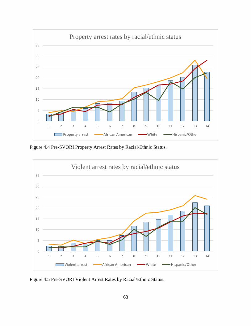
63
Figure 4.4 Pre-SVORI Property Arrest Rates by Racial/Ethnic Status.
Figure 4.5 Pre-SVORI Violent Arrest Rates by Racial/Ethnic Status.
0
5
10
15
20
25
30
35
1 2 3 4 5 6 7 8 9 10 11 12 13 14
Property arrest rates by racial/ethnic status
Property arrest African American White Hispanic/Other
0
5
10
15
20
25
30
35
1 2 3 4 5 6 7 8 9 10 11 12 13 14
Violent arrest rates by racial/ethnic status
Violent arrest African American White Hispanic/Other
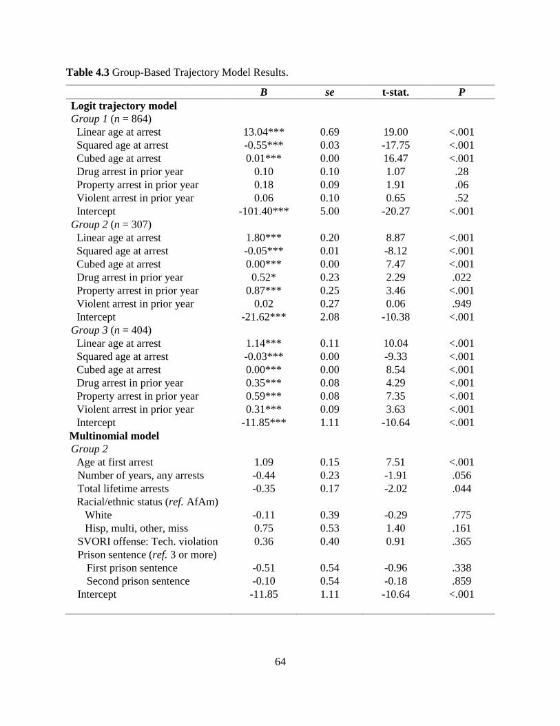
64
Table 4.3 Group-Based Trajectory Model Results.
B se t-stat. P
Logit trajectory model
Group 1 (n = 864)
Linear age at arrest 13.04*** 0.69 19.00 <.001
Squared age at arrest -0.55*** 0.03 -17.75 <.001
Cubed age at arrest 0.01*** 0.00 16.47 <.001
Drug arrest in prior year 0.10 0.10 1.07 .28
Property arrest in prior year 0.18 0.09 1.91 .06
Violent arrest in prior year 0.06 0.10 0.65 .52
Intercept -101.40*** 5.00 -20.27 <.001
Group 2 (n = 307)
Linear age at arrest 1.80*** 0.20 8.87 <.001
Squared age at arrest -0.05*** 0.01 -8.12 <.001
Cubed age at arrest 0.00*** 0.00 7.47 <.001
Drug arrest in prior year 0.52* 0.23 2.29 .022
Property arrest in prior year 0.87*** 0.25 3.46 <.001
Violent arrest in prior year 0.02 0.27 0.06 .949
Intercept -21.62*** 2.08 -10.38 <.001
Group 3 (n = 404)
Linear age at arrest 1.14*** 0.11 10.04 <.001
Squared age at arrest -0.03*** 0.00 -9.33 <.001
Cubed age at arrest 0.00*** 0.00 8.54 <.001
Drug arrest in prior year 0.35*** 0.08 4.29 <.001
Property arrest in prior year 0.59*** 0.08 7.35 <.001
Violent arrest in prior year 0.31*** 0.09 3.63 <.001
Intercept -11.85*** 1.11 -10.64 <.001
Multinomial model
Group 2
Age at first arrest 1.09 0.15 7.51 <.001
Number of years, any arrests -0.44 0.23 -1.91 .056
Total lifetime arrests -0.35 0.17 -2.02 .044
Racial/ethnic status (ref. AfAm)
White -0.11 0.39 -0.29 .775
Hisp, multi, other, miss 0.75 0.53 1.40 .161
SVORI offense: Tech. violation 0.36 0.40 0.91 .365
Prison sentence (ref. 3 or more)
First prison sentence -0.51 0.54 -0.96 .338
Second prison sentence -0.10 0.54 -0.18 .859
Intercept -11.85 1.11 -10.64 <.001
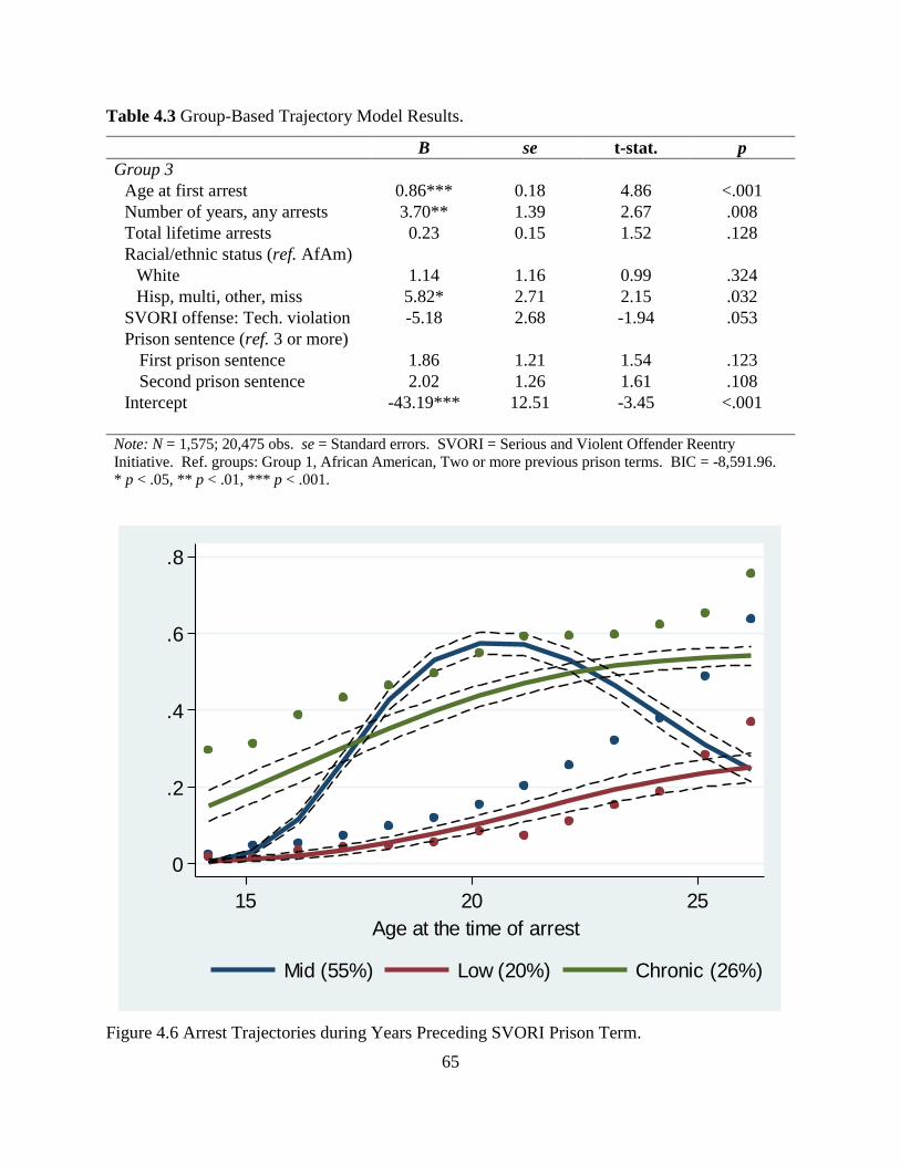
65
Table 4.3 Group-Based Trajectory Model Results.
B se t-stat. p
Group 3
Age at first arrest 0.86*** 0.18 4.86 <.001
Number of years, any arrests 3.70** 1.39 2.67 .008
Total lifetime arrests 0.23 0.15 1.52 .128
Racial/ethnic status (ref. AfAm)
White 1.14 1.16 0.99 .324
Hisp, multi, other, miss 5.82* 2.71 2.15 .032
SVORI offense: Tech. violation -5.18 2.68 -1.94 .053
Prison sentence (ref. 3 or more)
First prison sentence 1.86 1.21 1.54 .123
Second prison sentence 2.02 1.26 1.61 .108
Intercept -43.19*** 12.51 -3.45 <.001
Note: N = 1,575; 20,475 obs. se = Standard errors. SVORI = Serious and Violent Offender Reentry
Initiative. Ref. groups: Group 1, African American, Two or more previous prison terms. BIC = -8,591.96.
* p < .05, ** p < .01, *** p < .001.
Figure 4.6 Arrest Trajectories during Years Preceding SVORI Prison Term.
0
.2
.4
.6
.8
Pro
ba
bility o
f a
rre
st
15 20 25
Age at the time of arrest
Mid (55%) Low (20%) Chronic (26%)
66
4.4.3 Trajectory Group Characteristics Table 4.4 presents bivariate statistics comparing differences by trajectory group. The results
show large differences between groups for most demographic characteristics, criminal risk
factors, employment history, and SVORI site characteristics. The high-rate offenders in Groups
1 and 3 differ from each other in the length of their criminal histories; men in Group 3 were
chronic high-rate offenders, and their arrest records and interview responses revealed extensive
criminal involvement over several years. In contrast, the men in Group 1 had only recently
embarked on criminal activity; their high pre-prison arrest rates reflected escalating criminal
involvement during the last few years leading up to their prison term.
Group 1
The first, largest group (n = 864) is composed of men who exhibited a relatively recent onset into
criminal activity. These individuals had the highest predicted probability of being enrolled in
SVORI-funded services (52.57% vs. 48.55-49.73% for the other groups). As a result, Group 1
members had the highest participation rates in education (55.09%) and employment (15.97%)
programs, and men in this group exhibited many characteristics that distinguished participants
from nonparticipants. Men in this group were significantly younger (MG1 = 26.10, SDG1 = 4.34)
than men in groups 2 and 3 were (MG2 = 31.08, SDG2 = 7.98; MG3 = 35.95, SDG3 = 7.21; F =
382.04, p < .001). They were significantly more likely than were men in other groups to have
received income from illegal activity before prison entry (48.84% of G1 men vs. 35.50% and
39.60% of G2 and G3 men).
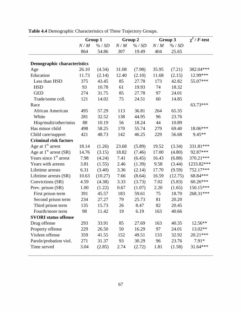
67
Table 4.4 Demographic Characteristics of Three Trajectory Groups.
Group 1 Group 2 Group 3 χ
2 / F-test
N / M % / SD N / M % / SD N / M % / SD
864 54.86 307 19.49 404 25.65
Demographic characteristics
Age 26.10 (4.34) 31.08 (7.98) 35.95 (7.21) 382.04***
Education 11.73 (2.14) 12.40 (2.10) 11.68 (2.15) 12.99***
Less than HSD 375 43.45 85 27.78 173 42.82 55.07***
HSD 93 10.78 61 19.93 74 18.32
GED 274 31.75 85 27.78 97 24.01
Trade/some coll. 121 14.02 75 24.51 60 14.85
Race 63.73***
African American 495 57.29 113 36.81 264 65.35
White 281 32.52 138 44.95 96 23.76
Hisp/multi/other/miss 88 10.19 56 18.24 44 10.89
Has minor child 498 58.25 170 55.74 279 69.40 18.06***
Child care/support 421 48.73 142 46.25 229 56.68 9.45**
Criminal risk factors
Age at 1st arrest 18.14 (1.26) 23.68 (5.89) 19.52 (3.34) 331.81***
Age at 1st arrest (SR) 14.76 (3.15) 18.82 (7.46) 17.00 (4.80) 92.87***
Years since 1st arrest 7.98 (4.24) 7.41 (6.45) 16.43 (6.88) 370.21***
Years with arrests 3.81 (1.55) 2.46 (1.39) 9.58 (3.44) 1233.82***
Lifetime arrests 6.31 (3.40) 3.36 (2.14) 17.70 (9.59) 752.17***
Lifetime arrests (SR) 10.63 (10.27) 7.66 (8.64) 16.59 (12.75) 68.84***
Convictions (SR) 4.59 (4.38) 3.33 (3.73) 7.02 (5.83) 60.26***
Prev. prison (SR) 1.00 (1.22) 0.67 (1.07) 2.20 (1.65) 150.15***
First prison term 391 45.57 183 59.61 75 18.70 268.31***
Second prison term 234 27.27 79 25.73 81 20.20
Third prison term 135 15.73 26 8.47 82 20.45
Fourth/more term 98 11.42 19 6.19 163 40.66
SVORI status offense
Drug offense 293 33.91 85 27.69 163 40.35 12.56**
Property offense 229 26.50 50 16.29 97 24.01 13.02**
Violent offense 359 41.55 152 49.51 133 32.92 20.21***
Parole/probation viol. 271 31.37 93 30.29 96 23.76 7.91*
Time served 3.04 (2.85) 2.74 (2.72) 1.81 (1.58) 31.64***
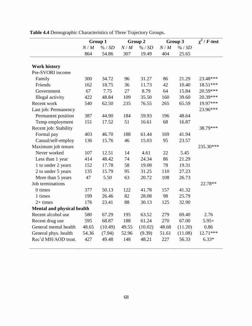
68
Table 4.4 Demographic Characteristics of Three Trajectory Groups.
Group 1 Group 2 Group 3 χ
2 / F-test
N / M % / SD N / M % / SD N / M % / SD
864 54.86 307 19.49 404 25.65
Work history
Pre-SVORI income
Family 300 34.72 96 31.27 86 21.29 23.48***
Friends 162 18.75 36 11.73 42 10.40 18.51***
Government 67 7.75 27 8.79 64 15.84 20.59***
Illegal activity 422 48.84 109 35.50 160 39.60 20.39***
Recent work 540 62.50 235 76.55 265 65.59 19.97***
Last job: Permanency 23.96***
Permanent position 387 44.90 184 59.93 196 48.64
Temp employment 151 17.52 51 16.61 68 16.87
Recent job: Stability 38.79***
Formal pay 403 46.70 188 61.44 169 41.94
Casual/self-employ 136 15.76 46 15.03 95 23.57
Maximum job tenure 235.30***
Never worked 107 12.51 14 4.61 22 5.45
Less than 1 year 414 48.42 74 24.34 86 21.29
1 to under 2 years 152 17.78 58 19.08 78 19.31
2 to under 5 years 135 15.79 95 31.25 110 27.23
More than 5 years 47 5.50 63 20.72 108 26.73
Job terminations 22.78**
0 times 377 50.13 122 41.78 157 41.32
1 times 199 26.46 82 28.08 98 25.79
2+ times 176 23.41 88 30.13 125 32.90
Mental and physical health
Recent alcohol use 580 67.29 195 63.52 279 69.40 2.76
Recent drug use 595 68.87 188 61.24 270 67.00 5.95+
General mental health 48.65 (10.49) 49.55 (10.02) 48.68 (11.20) 0.86
General phys. health 54.36 (7.94) 52.96 (9.39) 51.61 (11.08) 12.71***
Rec’d MH/AOD treat. 427 49.48 148 48.21 227 56.33 6.33*
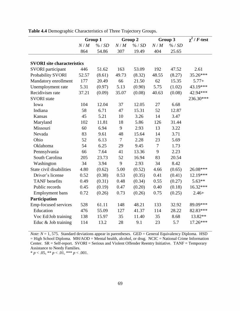
69
Table 4.4 Demographic Characteristics of Three Trajectory Groups.
Group 1 Group 2 Group 3 χ
2 / F-test
N / M % / SD N / M % / SD N / M % / SD
864 54.86 307 19.49 404 25.65
SVORI site characteristics
SVORI participant 446 51.62 163 53.09 192 47.52 2.61
Probability SVORI 52.57 (8.61) 49.73 (8.32) 48.55 (8.27) 35.26***
Mandatory enrollment 177 20.49 66 21.50 62 15.35 5.77+
Unemployment rate 5.31 (0.97) 5.13 (0.90) 5.75 (1.02) 43.19***
Recidivism rate 37.21 (0.09) 35.07 (0.08) 40.63 (0.08) 42.94***
SVORI state 236.30***
Iowa 104 12.04 37 12.05 27 6.68
Indiana 58 6.71 47 15.31 52 12.87
Kansas 45 5.21 10 3.26 14 3.47
Maryland 102 11.81 18 5.86 126 31.44
Missouri 60 6.94 9 2.93 13 3.22
Nevada 83 9.61 48 15.64 14 3.71
Ohio 52 6.13 7 2.28 23 5.69
Oklahoma 54 6.25 29 9.45 7 1.73
Pennsylvania 66 7.64 41 13.36 9 2.23
South Carolina 205 23.73 52 16.94 83 20.54
Washington 34 3.94 9 2.93 34 8.42
State civil disabilities 4.80 (0.62) 5.00 (0.52) 4.66 (0.65) 26.08***
Driver’s license 0.52 (0.38) 0.53 (0.35) 0.41 (0.41) 12.19***
TANF benefits 0.49 (0.31) 0.48 (0.34) 0.55 (0.27) 5.63**
Public records 0.45 (0.19) 0.47 (0.20) 0.40 (0.18) 16.32***
Employment bans 0.72 (0.26) 0.73 (0.26) 0.75 (0.25) 2.46+
Participation
Emp-focused services 528 61.11 148 48.21 133 32.92 89.09***
Education 476 55.09 127 41.37 114 28.22 82.83***
Voc Ed/Job training 138 15.97 35 11.40 35 8.68 13.82**
Educ & Job training 114 13.2 28 9.1 23 5.7 17.26***
Note: N = 1, 575. Standard deviations appear in parentheses. GED = General Equivalency Diploma. HSD
= High School Diploma. MH/AOD = Mental health, alcohol, or drug. NCIC = National Crime Information
Center. SR = Self-report. SVORI = Serious and Violent Offender Reentry Initiative. TANF = Temporary
Assistance to Needy Families.
* p < .05, ** p < .01, *** p < .001.
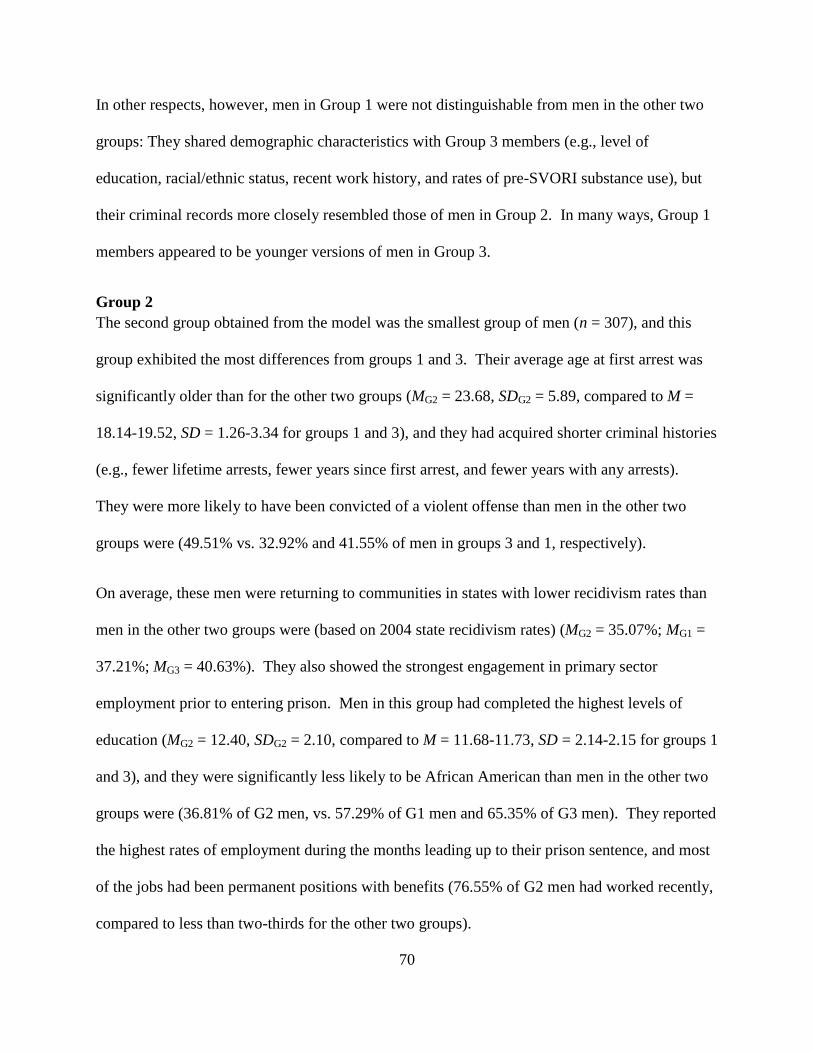
70
In other respects, however, men in Group 1 were not distinguishable from men in the other two
groups: They shared demographic characteristics with Group 3 members (e.g., level of
education, racial/ethnic status, recent work history, and rates of pre-SVORI substance use), but
their criminal records more closely resembled those of men in Group 2. In many ways, Group 1
members appeared to be younger versions of men in Group 3.
Group 2
The second group obtained from the model was the smallest group of men (n = 307), and this
group exhibited the most differences from groups 1 and 3. Their average age at first arrest was
significantly older than for the other two groups (MG2 = 23.68, SDG2 = 5.89, compared to M =
18.14-19.52, SD = 1.26-3.34 for groups 1 and 3), and they had acquired shorter criminal histories
(e.g., fewer lifetime arrests, fewer years since first arrest, and fewer years with any arrests).
They were more likely to have been convicted of a violent offense than men in the other two
groups were (49.51% vs. 32.92% and 41.55% of men in groups 3 and 1, respectively).
On average, these men were returning to communities in states with lower recidivism rates than
men in the other two groups were (based on 2004 state recidivism rates) (MG2 = 35.07%; MG1 =
37.21%; MG3 = 40.63%). They also showed the strongest engagement in primary sector
employment prior to entering prison. Men in this group had completed the highest levels of
education (MG2 = 12.40, SDG2 = 2.10, compared to M = 11.68-11.73, SD = 2.14-2.15 for groups 1
and 3), and they were significantly less likely to be African American than men in the other two
groups were (36.81% of G2 men, vs. 57.29% of G1 men and 65.35% of G3 men). They reported
the highest rates of employment during the months leading up to their prison sentence, and most
of the jobs had been permanent positions with benefits (76.55% of G2 men had worked recently,
compared to less than two-thirds for the other two groups).

71
Group 3
The third group included chronic offenders who had acquired lengthy criminal records during the
years preceding the SVORI status offense (n = 404). Longer time had passed on average since
first arrest among Group 3 members (MG3 = 16.43, SDG3= 6.88), relative to men in the other
groups (MG1 = 7.98, SDG1 = 4.24; MG2 = 7.41, SDG2 = 6.45; F = 370.21, p < .001). At the time of
the baseline interview, they were the oldest group on average (MG3 = 35.95, SDG3 = 7.21), and
they had acquired the most lifetime arrests (MG3 = 17.70, SDG3 = 9.59). They also had the lowest
average level of education, with most indicating that they had completed fewer than 12 years of
education. On average, they had been imprisoned more times in the past than the men in the
other two groups had been, but technical violations of previous supervision did not explain their
recent return to prison (23.76% of G3 men had violated parole or probation requirements before
entering prison, in contrast to 31% of G1 and G2 men). These chronic offenders were more
likely to come from Maryland or South Carolina than from other states, and in general, they were
returning to states with higher mean recidivism rates than were men in the other groups (2004
rates).
Summary of Findings
Based on observed characteristics, men in Groups 1 and 3 exhibited more risk factors than did
the men in Group 2. The men in Group 3 had longer criminal records then men in Group 1, and
they could be described as chronic adult offenders who would be likely to remain engaged in
persistent criminal activity upon release. However, men in Group 1 were younger, more active
offenders, and their escalating rates of arrest before prison entry suggested the possibility of
more serious criminal activity upon release.

72
Men in Group 1 differed sharply from men in Group 3 in the likelihood of receiving
employment-focused services. Most Group 1 men received some form of employment-focused
programming, in contrast to men in the other two groups. Despite low educational attainment
and weak attachment to primary sector employment, men in Group 3 reported the lowest rates of
program participation.
The distinct compositions of the three trajectory groups may reflect the fact that prisons involved
in the SVORI evaluation used differing selection criteria when recruiting participants into the
study. There is evidence to suggest that the 3-group trajectory model diminished some of the
pre-existing differences between employment-focused program participants and nonparticipants
(reducing mean standardized bias to 10%). Despite this, participants in all three trajectory
groups continued to exhibit significant differences from nonparticipants, so propensity score
matching is used to reduce lingering observed heterogeneity.
4.5 Propensity Score Matching
4.5.1 Multilevel Logit Model Results Table 4.5 presents results of the multilevel logit model (n = 1,571). Individuals’ propensity
scores were calculated from the fitted (expected) value of this logit regression, which estimated
the probability of program participation based on the fixed- and random-level effects. The
resulting propensity score ranges from .02 to .98, with a mean of .64 for participants and .38 for
nonparticipants.
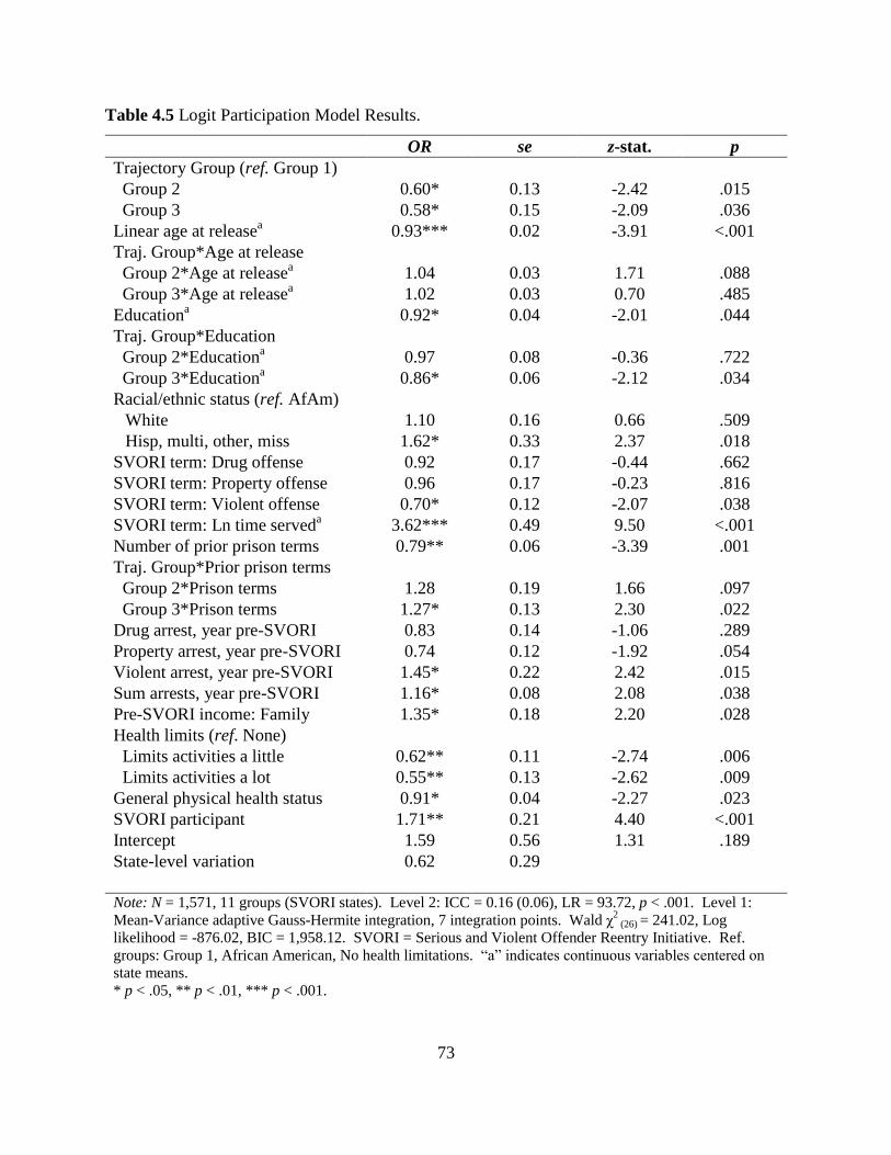
73
Table 4.5 Logit Participation Model Results.
OR se z-stat. p
Trajectory Group (ref. Group 1)
Group 2 0.60* 0.13 -2.42 .015
Group 3 0.58* 0.15 -2.09 .036
Linear age at releasea
0.93*** 0.02 -3.91 <.001
Traj. Group*Age at release
Group 2*Age at releasea 1.04 0.03 1.71 .088
Group 3*Age at releasea 1.02 0.03 0.70 .485
Educationa 0.92* 0.04 -2.01 .044
Traj. Group*Education
Group 2*Educationa 0.97 0.08 -0.36 .722
Group 3*Educationa 0.86* 0.06 -2.12 .034
Racial/ethnic status (ref. AfAm)
White 1.10 0.16 0.66 .509
Hisp, multi, other, miss 1.62* 0.33 2.37 .018
SVORI term: Drug offense 0.92 0.17 -0.44 .662
SVORI term: Property offense 0.96 0.17 -0.23 .816
SVORI term: Violent offense 0.70* 0.12 -2.07 .038
SVORI term: Ln time serveda 3.62*** 0.49 9.50 <.001
Number of prior prison terms 0.79** 0.06 -3.39 .001
Traj. Group*Prior prison terms
Group 2*Prison terms 1.28 0.19 1.66 .097
Group 3*Prison terms 1.27* 0.13 2.30 .022
Drug arrest, year pre-SVORI 0.83 0.14 -1.06 .289
Property arrest, year pre-SVORI 0.74 0.12 -1.92 .054
Violent arrest, year pre-SVORI 1.45* 0.22 2.42 .015
Sum arrests, year pre-SVORI 1.16* 0.08 2.08 .038
Pre-SVORI income: Family 1.35* 0.18 2.20 .028
Health limits (ref. None)
Limits activities a little 0.62** 0.11 -2.74 .006
Limits activities a lot 0.55** 0.13 -2.62 .009
General physical health status 0.91* 0.04 -2.27 .023
SVORI participant 1.71** 0.21 4.40 <.001
Intercept 1.59 0.56 1.31 .189
State-level variation 0.62 0.29
Note: N = 1,571, 11 groups (SVORI states). Level 2: ICC = 0.16 (0.06), LR = 93.72, p < .001. Level 1:
Mean-Variance adaptive Gauss-Hermite integration, 7 integration points. Wald χ2
(26) = 241.02, Log
likelihood = -876.02, BIC = 1,958.12. SVORI = Serious and Violent Offender Reentry Initiative. Ref.
groups: Group 1, African American, No health limitations. “a” indicates continuous variables centered on
state means.
* p < .05, ** p < .01, *** p < .001.

74
4.5.2 Nearest Neighbor Matching with Caliper Participants and nonparticipants were matched on their predicted probability of employment-
focused program participation using nearest neighbor matching with caliper. The caliper size
used was 0.1 times the standard deviation of the propensity score obtained from the multilevel
logit model. Replacement was permitted and up to five matches were permitted, although the
results were unchanged when fewer matches were permitted.
Nearest neighbor matching with caliper successfully reduced mean standardized biases to below
5%. Forty nonparticipants were excluded from the final sample, due to the inability to find
appropriate matches within the participant sample (34 nonparticipants from Group 3, 4 from
Group 1, and 2 nonparticipants from Group 2). The final sample consisted of 805 participants
and 726 nonparticipants (n = 1,531). Figure 3.1 presents the sample selection process used to
identify trajectory groups, model participation status, and match participants and nonparticipants.
4.5.3 Bivariate Statistics after Matching Table 4.6 presents pre- and post-matching standardized biases for key predictors of participation
and post-release rearrest. The nearest neighbor matching process eliminated much of the
observed bias. Mean standardized bias declined from 19.1 to 3.8, and the maximum
standardized bias for individual items declined from 56.7 to 18.2. Most importantly,
standardized bias for linear age at release declined from -52.3 to -1.7, and bias for time served,
which had exhibited the largest bias before matching, declined from 56.7 to 2.0. Other variables
that exhibited large reductions in imbalance include age at first arrest (from -26.3 to -0.3), years
since first arrest (-41.8 to -2.2), lifetime number of arrests (-45.6 to -3.7), and trajectory group
membership (44.1 to -0.3 among Group 1 members; -44.4 to 0.3 among Group 3 members).
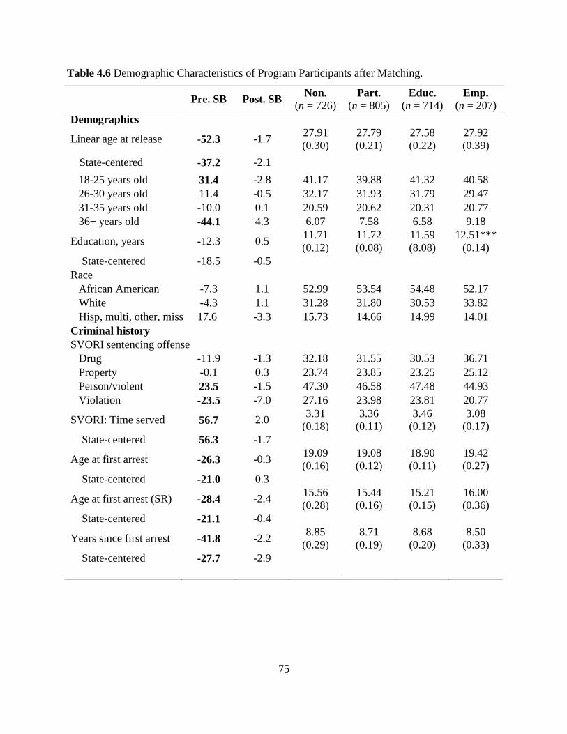
75
Table 4.6 Demographic Characteristics of Program Participants after Matching.
Pre. SB Post. SB
Non.
(n = 726) Part.
(n = 805) Educ.
(n = 714) Emp.
(n = 207)
Demographics
Linear age at release -52.3 -1.7 27.91
(0.30)
27.79
(0.21)
27.58
(0.22)
27.92
(0.39)
State-centered -37.2 -2.1
18-25 years old 31.4 -2.8 41.17 39.88 41.32 40.58
26-30 years old 11.4 -0.5 32.17 31.93 31.79 29.47
31-35 years old -10.0 0.1 20.59 20.62 20.31 20.77
36+ years old -44.1 4.3 6.07 7.58 6.58 9.18
Education, years -12.3 0.5 11.71
(0.12)
11.72
(0.08)
11.59
(8.08)
12.51***
(0.14)
State-centered -18.5 -0.5
Race
African American -7.3 1.1 52.99 53.54 54.48 52.17
White -4.3 1.1 31.28 31.80 30.53 33.82
Hisp, multi, other, miss 17.6 -3.3 15.73 14.66 14.99 14.01
Criminal history
SVORI sentencing offense
Drug -11.9 -1.3 32.18 31.55 30.53 36.71
Property -0.1 0.3 23.74 23.85 23.25 25.12
Person/violent 23.5 -1.5 47.30 46.58 47.48 44.93
Violation -23.5 -7.0 27.16 23.98 23.81 20.77
SVORI: Time served 56.7 2.0 3.31
(0.18)
3.36
(0.11)
3.46
(0.12)
3.08
(0.17)
State-centered 56.3 -1.7
Age at first arrest -26.3 -0.3 19.09
(0.16)
19.08
(0.12)
18.90
(0.11)
19.42
(0.27)
State-centered -21.0 0.3
Age at first arrest (SR) -28.4 -2.4 15.56
(0.28)
15.44
(0.16)
15.21
(0.15)
16.00
(0.36)
State-centered -21.1 -0.4
Years since first arrest -41.8 -2.2 8.85
(0.29)
8.71
(0.19)
8.68
(0.20)
8.50
(0.33)
State-centered -27.7 -2.9
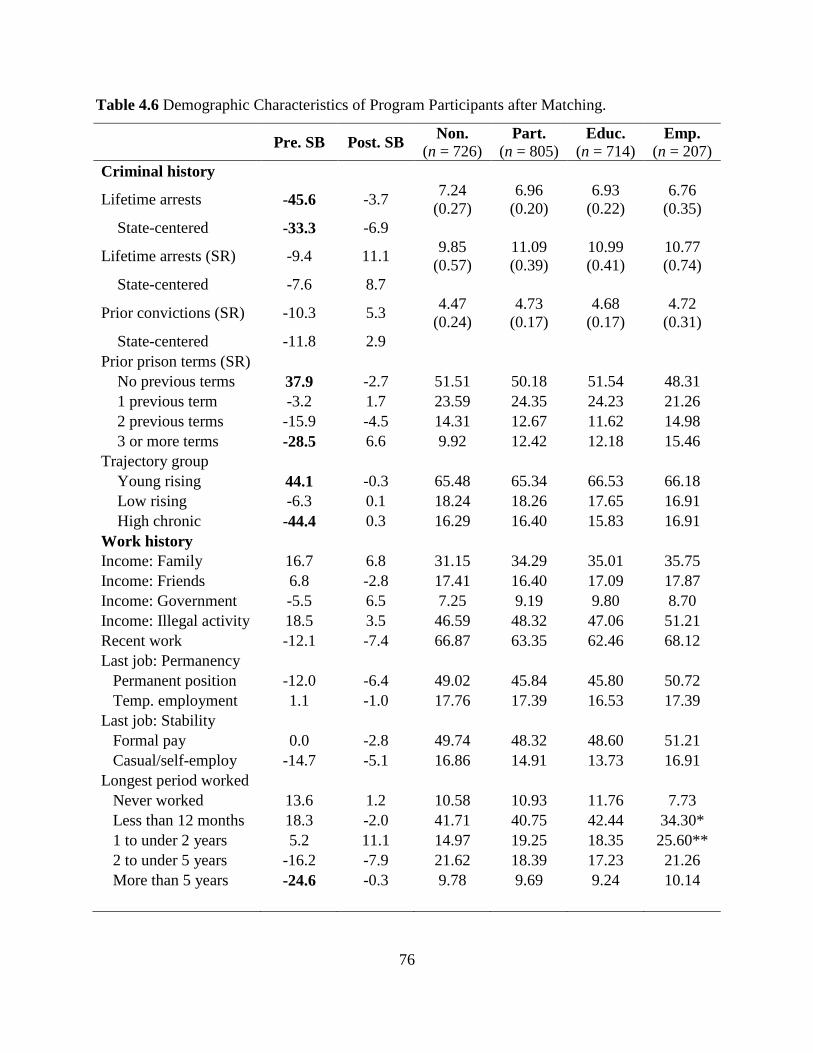
76
Table 4.6 Demographic Characteristics of Program Participants after Matching.
Pre. SB Post. SB
Non.
(n = 726) Part.
(n = 805) Educ.
(n = 714) Emp.
(n = 207)
Criminal history
Lifetime arrests -45.6 -3.7 7.24
(0.27)
6.96
(0.20)
6.93
(0.22)
6.76
(0.35)
State-centered -33.3 -6.9
Lifetime arrests (SR) -9.4 11.1 9.85
(0.57)
11.09
(0.39)
10.99
(0.41)
10.77
(0.74)
State-centered -7.6 8.7
Prior convictions (SR) -10.3 5.3 4.47
(0.24)
4.73
(0.17)
4.68
(0.17)
4.72
(0.31)
State-centered -11.8 2.9
Prior prison terms (SR)
No previous terms 37.9 -2.7 51.51 50.18 51.54 48.31
1 previous term -3.2 1.7 23.59 24.35 24.23 21.26
2 previous terms -15.9 -4.5 14.31 12.67 11.62 14.98
3 or more terms -28.5 6.6 9.92 12.42 12.18 15.46
Trajectory group
Young rising 44.1 -0.3 65.48 65.34 66.53 66.18
Low rising -6.3 0.1 18.24 18.26 17.65 16.91
High chronic -44.4 0.3 16.29 16.40 15.83 16.91
Work history
Income: Family 16.7 6.8 31.15 34.29 35.01 35.75
Income: Friends 6.8 -2.8 17.41 16.40 17.09 17.87
Income: Government -5.5 6.5 7.25 9.19 9.80 8.70
Income: Illegal activity 18.5 3.5 46.59 48.32 47.06 51.21
Recent work -12.1 -7.4 66.87 63.35 62.46 68.12
Last job: Permanency
Permanent position -12.0 -6.4 49.02 45.84 45.80 50.72
Temp. employment 1.1 -1.0 17.76 17.39 16.53 17.39
Last job: Stability
Formal pay 0.0 -2.8 49.74 48.32 48.60 51.21
Casual/self-employ -14.7 -5.1 16.86 14.91 13.73 16.91
Longest period worked
Never worked 13.6 1.2 10.58 10.93 11.76 7.73
Less than 12 months 18.3 -2.0 41.71 40.75 42.44 34.30*
1 to under 2 years 5.2 11.1 14.97 19.25 18.35 25.60**
2 to under 5 years -16.2 -7.9 21.62 18.39 17.23 21.26
More than 5 years -24.6 -0.3 9.78 9.69 9.24 10.14
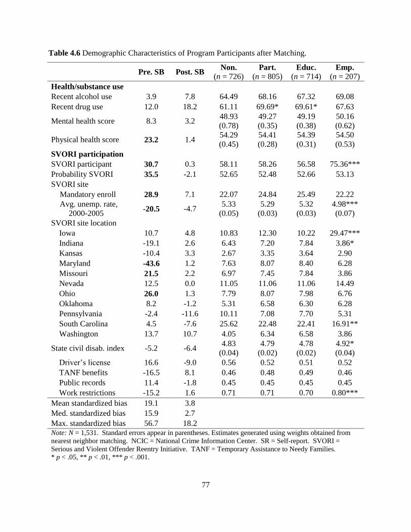
77
Table 4.6 Demographic Characteristics of Program Participants after Matching.
Pre. SB Post. SB
Non.
(n = 726) Part.
(n = 805) Educ.
(n = 714) Emp.
(n = 207)
Health/substance use
Recent alcohol use 3.9 7.8 64.49 68.16 67.32 69.08
Recent drug use 12.0 18.2 61.11 69.69* 69.61* 67.63
Mental health score 8.3 3.2 48.93
(0.78)
49.27
(0.35)
49.19
(0.38)
50.16
(0.62)
Physical health score 23.2 1.4 54.29
(0.45)
54.41
(0.28)
54.39
(0.31)
54.50
(0.53)
SVORI participation
SVORI participant 30.7 0.3 58.11 58.26 56.58 75.36***
Probability SVORI 35.5 -2.1 52.65 52.48 52.66 53.13
SVORI site
Mandatory enroll 28.9 7.1 22.07 24.84 25.49 22.22
Avg. unemp. rate,
2000-2005 -20.5 -4.7
5.33
(0.05)
5.29
(0.03)
5.32
(0.03)
4.98***
(0.07)
SVORI site location
Iowa 10.7 4.8 10.83 12.30 10.22 29.47***
Indiana -19.1 2.6 6.43 7.20 7.84 3.86*
Kansas -10.4 3.3 2.67 3.35 3.64 2.90
Maryland -43.6 1.2 7.63 8.07 8.40 6.28
Missouri 21.5 2.2 6.97 7.45 7.84 3.86
Nevada 12.5 0.0 11.05 11.06 11.06 14.49
Ohio 26.0 1.3 7.79 8.07 7.98 6.76
Oklahoma 8.2 -1.2 5.31 6.58 6.30 6.28
Pennsylvania -2.4 -11.6 10.11 7.08 7.70 5.31
South Carolina 4.5 -7.6 25.62 22.48 22.41 16.91**
Washington 13.7 10.7 4.05 6.34 6.58 3.86
State civil disab. index -5.2 -6.4 4.83
(0.04)
4.79
(0.02)
4.78
(0.02)
4.92*
(0.04)
Driver’s license 16.6 -9.0 0.56 0.52 0.51 0.52
TANF benefits -16.5 8.1 0.46 0.48 0.49 0.46
Public records 11.4 -1.8 0.45 0.45 0.45 0.45
Work restrictions -15.2 1.6 0.71 0.71 0.70 0.80***
Mean standardized bias 19.1 3.8
Med. standardized bias 15.9 2.7
Max. standardized bias 56.7 18.2 Note: N = 1,531. Standard errors appear in parentheses. Estimates generated using weights obtained from
nearest neighbor matching. NCIC = National Crime Information Center. SR = Self-report. SVORI =
Serious and Violent Offender Reentry Initiative. TANF = Temporary Assistance to Needy Families.
* p < .05, ** p < .01, *** p < .001.
78
The matching process did not eliminate all pre-matching differences, however. Four variables
exhibited lingering imbalance, with bias statistics that exceeded 10.0 after matching: These were
a dummy variable for longest job tenure before prison (11.1), the dummy variable for
Washington State (10.7), self-reported number of lifetime arrests (11.1), and self-reported drug
use during the month preceding prison entry (18.2).
4.6 Duration Models
4.6.1 Post-Release Arrest Rates
Rearrest rates among men in the SVORI sample closely resembled rearrest rates that have been
observed for state prison populations as a whole (Durose et al., 2014). Three-quarters of the men
were arrested at least once during the first 3 years of release (n = 1,129; 74%). On average, these
men were arrested 2.96 times (SD = 2.46). Thirty-five percent were arrested at least once for a
drug offense, 32% had one or more property arrests, and 28% were arrested for violent offenses.
Men were frequently charged with more than one type of offense during a single arrest, so these
percentages are not mutually exclusive.
4.6.2 Employment Programs Increase Labor Force Participation Table 4.10 presents post-release labor force activity by participation status. The results suggest
that employment-focused programs do have beneficial effects on employment, although results
do not persist over time. Men who participated in vocational education/job training programs
were significantly more likely to seek work during the first 9 months of release from prison than
were nonparticipants and participants receiving educational services alone. Enrollees in
vocational education/job training programs exhibited the lowest rates of labor force exit at the
first two follow-up interviews. Employment program participants also exhibited the highest

79
rates of stable employment (measured as having worked each month that they were living in the
community).
In contrast, men who received educational services alone exhibited similar rates of employment
as nonparticipants. Education participants were less likely to enter the labor force to seek work
than were employment program participants (13.75% vs. 5.00% at Wave 2; 15.88% vs. 11.29%
at Wave 3). Approximately the same proportion of education program participants held stable
employment during the first 3 months, as did nonparticipants (roughly 30% of each group).
By the time of the third interview (approximately 9 months after release), rates of labor force
entry and employment declined among employment participants, although they remained
significantly higher than for nonparticipants and education participants. By the time of the
fourth interview (approximately 15 months after release), there were no significant differences in
labor force activity by participation status.
4.6.3 Hypothesis 2: Employment Programs Reduce Recidivism
Findings provide limited support for the second hypothesis. Table 4.7 presents rearrest rates by
participation status during the first 3 years of release. The weighted percentages reflect the
proportion of each group within the matched sample who had been arrested at least once within
the given reference period. During the first 9 months of release, education and employment
program participants had significantly lower rates of rearrest than nonparticipants did.
Participants receiving vocational education/job training programs alone were least likely to have
been rearrested within that time (34.07%), compared to participants receiving education and
employment services (38.79%), participants receiving educational services alone (41.30%), and
nonparticipants (43.80%). These differences dwindled over time; by 1 year after release, the
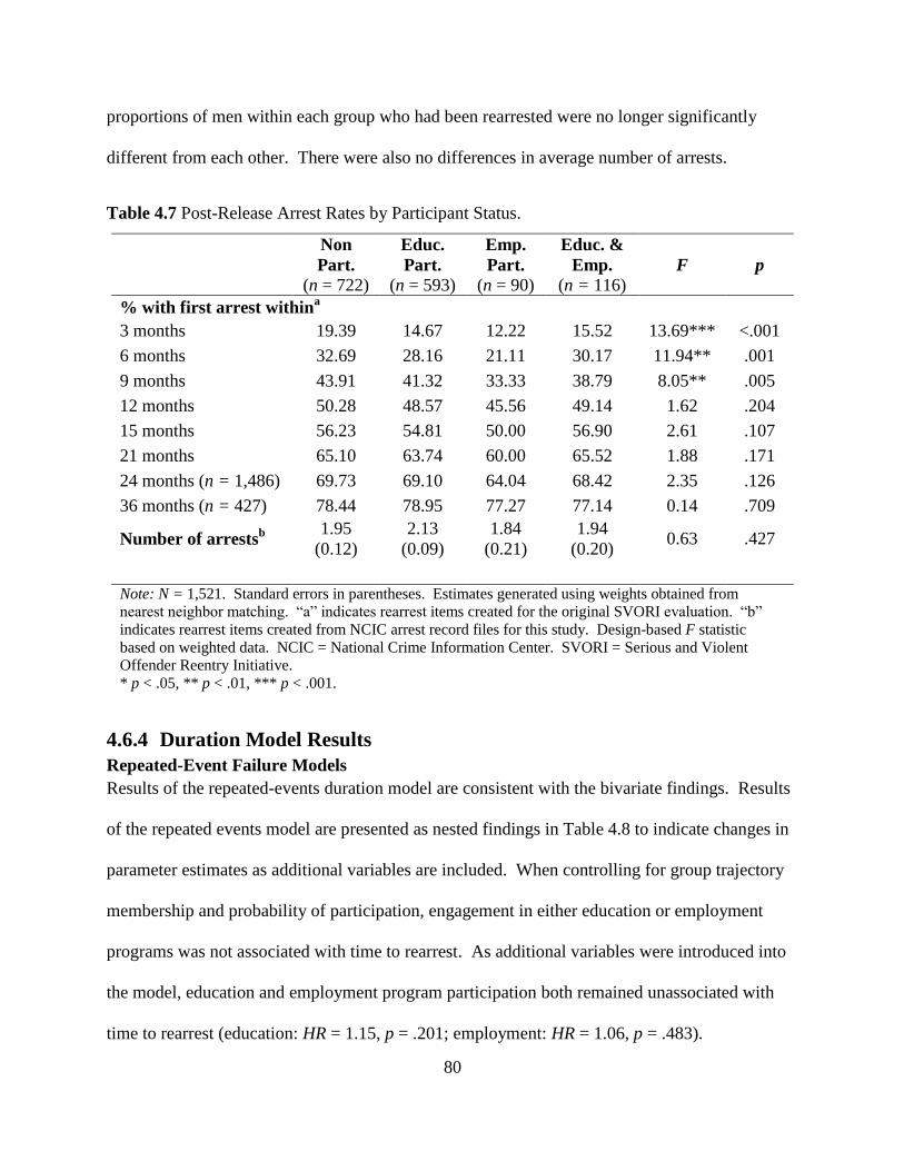
80
proportions of men within each group who had been rearrested were no longer significantly
different from each other. There were also no differences in average number of arrests.
Table 4.7 Post-Release Arrest Rates by Participant Status.
Non
Part.
(n = 722)
Educ.
Part.
(n = 593)
Emp.
Part.
(n = 90)
Educ. &
Emp.
(n = 116) F p
% with first arrest withina
3 months 19.39 14.67 12.22 15.52 13.69*** <.001
6 months 32.69 28.16 21.11 30.17 11.94** .001
9 months 43.91 41.32 33.33 38.79 8.05** .005
12 months 50.28 48.57 45.56 49.14 1.62 .204
15 months 56.23 54.81 50.00 56.90 2.61 .107
21 months 65.10 63.74 60.00 65.52 1.88 .171
24 months (n = 1,486) 69.73 69.10 64.04 68.42 2.35 .126
36 months (n = 427) 78.44 78.95 77.27 77.14 0.14 .709
Number of arrestsb
1.95
(0.12)
2.13
(0.09)
1.84
(0.21)
1.94
(0.20) 0.63 .427
Note: N = 1,521. Standard errors in parentheses. Estimates generated using weights obtained from
nearest neighbor matching. “a” indicates rearrest items created for the original SVORI evaluation. “b”
indicates rearrest items created from NCIC arrest record files for this study. Design-based F statistic
based on weighted data. NCIC = National Crime Information Center. SVORI = Serious and Violent
Offender Reentry Initiative.
* p < .05, ** p < .01, *** p < .001.
4.6.4 Duration Model Results
Repeated-Event Failure Models
Results of the repeated-events duration model are consistent with the bivariate findings. Results
of the repeated events model are presented as nested findings in Table 4.8 to indicate changes in
parameter estimates as additional variables are included. When controlling for group trajectory
membership and probability of participation, engagement in either education or employment
programs was not associated with time to rearrest. As additional variables were introduced into
the model, education and employment program participation both remained unassociated with
time to rearrest (education: HR = 1.15, p = .201; employment: HR = 1.06, p = .483).
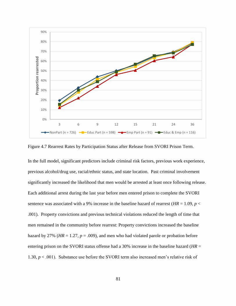
81
Figure 4.7 Rearrest Rates by Participation Status after Release from SVORI Prison Term.
In the full model, significant predictors include criminal risk factors, previous work experience,
previous alcohol/drug use, racial/ethnic status, and state location. Past criminal involvement
significantly increased the likelihood that men would be arrested at least once following release.
Each additional arrest during the last year before men entered prison to complete the SVORI
sentence was associated with a 9% increase in the baseline hazard of rearrest (HR = 1.09, p <
.001). Property convictions and previous technical violations reduced the length of time that
men remained in the community before rearrest: Property convictions increased the baseline
hazard by 27% (HR = 1.27, p = .009), and men who had violated parole or probation before
entering prison on the SVORI status offense had a 30% increase in the baseline hazard (HR =
1.30, p < .001). Substance use before the SVORI term also increased men’s relative risk of
0%
10%
20%
30%
40%
50%
60%
70%
80%
90%
3 6 9 12 15 21 24 36
Pro
po
rtio
n r
earr
este
d
NonPart (n = 726) Educ Part (n = 598) Emp Part (n = 91) Educ & Emp (n = 116)
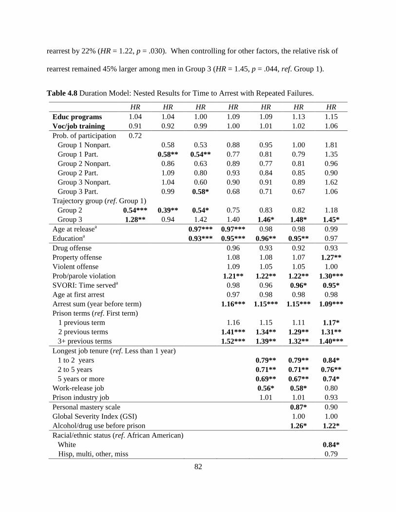
82
rearrest by 22% (HR = 1.22, p = .030). When controlling for other factors, the relative risk of
rearrest remained 45% larger among men in Group 3 (HR = 1.45, p = .044, ref. Group 1).
Table 4.8 Duration Model: Nested Results for Time to Arrest with Repeated Failures.
HR HR HR HR HR HR HR
Educ programs 1.04 1.04 1.00 1.09 1.09 1.13 1.15
Voc/job training 0.91 0.92 0.99 1.00 1.01 1.02 1.06
Prob. of participation 0.72
Group 1 Nonpart. 0.58 0.53 0.88 0.95 1.00 1.81
Group 1 Part. 0.58** 0.54** 0.77 0.81 0.79 1.35
Group 2 Nonpart. 0.86 0.63 0.89 0.77 0.81 0.96
Group 2 Part. 1.09 0.80 0.93 0.84 0.85 0.90
Group 3 Nonpart. 1.04 0.60 0.90 0.91 0.89 1.62
Group 3 Part. 0.99 0.58* 0.68 0.71 0.67 1.06
Trajectory group (ref. Group 1)
Group 2 0.54*** 0.39** 0.54* 0.75 0.83 0.82 1.18
Group 3 1.28** 0.94 1.42 1.40 1.46* 1.48* 1.45*
Age at releasea 0.97*** 0.97*** 0.98 0.98 0.99
Educationa 0.93*** 0.95*** 0.96** 0.95** 0.97
Drug offense 0.96 0.93 0.92 0.93
Property offense 1.08 1.08 1.07 1.27**
Violent offense 1.09 1.05 1.05 1.00
Prob/parole violation 1.21** 1.22** 1.22** 1.30***
SVORI: Time serveda 0.98 0.96 0.96* 0.95*
Age at first arrest 0.97 0.98 0.98 0.98
Arrest sum (year before term) 1.16*** 1.15*** 1.15*** 1.09***
Prison terms (ref. First term)
1 previous term 1.16 1.15 1.11 1.17*
2 previous terms 1.41*** 1.34** 1.29** 1.31**
3+ previous terms 1.52*** 1.39** 1.32** 1.40***
Longest job tenure (ref. Less than 1 year)
1 to 2 years 0.79** 0.79** 0.84*
2 to 5 years 0.71** 0.71** 0.76**
5 years or more 0.69** 0.67** 0.74*
Work-release job 0.56* 0.58* 0.80
Prison industry job 1.01 1.01 0.93
Personal mastery scale 0.87* 0.90
Global Severity Index (GSI) 1.00 1.00
Alcohol/drug use before prison 1.26* 1.22*
Racial/ethnic status (ref. African American)
White 0.84*
Hisp, multi, other, miss 0.79
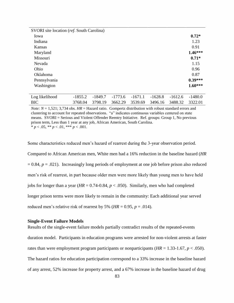
83
SVORI site location (ref. South Carolina)
Iowa 0.72*
Indiana 1.23
Kansas 0.91
Maryland 1.46***
Missouri 0.71*
Nevada 1.15
Ohio 0.96
Oklahoma 0.87
Pennsylvania 0.39***
Washington 1.60***
Log likelihood -1855.2 -1849.7 -1773.6 -1671.1 -1628.8 -1612.6 -1480.0
BIC 3768.04 3798.19 3662.29 3539.69 3496.16 3488.32 3322.01
Note: N = 1,521; 3,734 obs. HR = Hazard ratio. Gompertz distribution with robust standard errors and
clustering to account for repeated observations. “a” indicates continuous variables centered on state
means. SVORI = Serious and Violent Offender Reentry Initiative. Ref. groups: Group 1, No previous
prison term, Less than 1 year at any job, African American, South Carolina.
* p < .05, ** p < .01, *** p < .001.
Some characteristics reduced men’s hazard of rearrest during the 3-year observation period.
Compared to African American men, White men had a 16% reduction in the baseline hazard (HR
= 0.84, p = .021). Increasingly long periods of employment at one job before prison also reduced
men’s risk of rearrest, in part because older men were more likely than young men to have held
jobs for longer than a year (HR = 0.74-0.84, p < .050). Similarly, men who had completed
longer prison terms were more likely to remain in the community: Each additional year served
reduced men’s relative risk of rearrest by 5% (HR = 0.95, p = .014).
Single-Event Failure Models
Results of the single-event failure models partially contradict results of the repeated-events
duration model. Participants in education programs were arrested for non-violent arrests at faster
rates than were employment program participants or nonparticipants (HR = 1.33-1.67, p < .050).
The hazard ratios for education participation correspond to a 33% increase in the baseline hazard
of any arrest, 52% increase for property arrest, and a 67% increase in the baseline hazard of drug
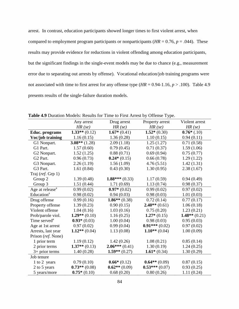
84
arrest. In contrast, education participants showed longer times to first violent arrest, when
compared to employment program participants or nonparticipants (HR = 0.76, p = .044). These
results may provide evidence for reductions in violent offending among education participants,
but the significant findings in the single-event models may be due to chance (e.g., measurement
error due to separating out arrests by offense). Vocational education/job training programs were
not associated with time to first arrest for any offense type (HR = 0.94-1.16, p > .100). Table 4.9
presents results of the single-failure duration models.
Table 4.9 Duration Models: Results for Time to First Arrest by Offense Type.
Any arrest Drug arrest Property arrest Violent arrest
HR (se) HR (se) HR (se) HR (se)
Educ. programs 1.33** (0.12) 1.67* (0.41) 1.52* (0.30) 0.76* (.10)
Voc/job training 1.16 (0.15) 1.36 (0.28) 1.10 (0.15) 0.94 (0.11)
G1 Nonpart. 3.08** (1.28) 2.09 (1.18) 1.25 (1.27) 0.71 (0.58)
G1 Part. 1.57 (0.60) 0.79 (0.45) 0.71 (0.37) 1.59 (1.06)
G2 Nonpart. 1.52 (1.25) 0.88 (0.71) 0.69 (0.94) 0.75 (0.77)
G2 Part. 0.96 (0.73) 0.24* (0.15) 0.66 (0.78) 1.29 (1.22)
G3 Nonpart. 2.26 (1.19) 1.56 (1.09) 4.76 (5.51) 1.42 (1.31)
G3 Part. 1.61 (0.84) 0.43 (0.30) 1.30 (0.95) 2.38 (1.67)
Traj (ref. Grp 1)
Group 2 1.39 (0.48) 1.88*** (0.33) 1.17 (0.59) 0.94 (0.49)
Group 3 1.51 (0.44) 1.71 (0.69) 1.13 (0.74) 0.98 (0.37)
Age at releasea 0.99 (0.02) 0.97* (0.02) 0.99 (0.02) 0.97 (0.02)
Educationa 0.98 (0.02) 0.94 (0.03) 0.98 (0.03) 1.01 (0.03)
Drug offense 0.99 (0.16) 1.86** (0.38) 0.72 (0.14) 0.77 (0.17)
Property offense 1.39 (0.23) 0.90 (0.15) 2.40** (0.61) 1.06 (0.18)
Violent offense 1.04 (0.16) 1.03 (0.16) 0.75 (0.20) 1.23 (0.21)
Prob/parole viol. 1.29** (0.10) 1.16 (0.25) 1.27* (0.15) 1.48** (0.21)
Time serveda 0.93* (0.03) 1.00 (0.04) 0.98 (0.03) 0.95 (0.03)
Age at 1st arrest 0.97 (0.02) 0.99 (0.04) 0.91*** (0.02) 0.97 (0.02)
Arrests, last year 1.12** (0.04) 1.13 (0.08) 1.10** (0.04) 1.00 (0.09)
Prison (ref. None)
1 prior term 1.19 (0.12) 1.42 (0.26) 1.08 (0.21) 0.85 (0.14)
2 prior terms 1.37** (0.13) 2.06*** (0.41) 1.30 (0.19) 1.24 (0.25)
3+ prior terms 1.40 (0.28) 1.59** (0.27) 1.61* (0.34) 1.30 (0.29)
Job tenure
1 to 2 years 0.79 (0.10) 0.66* (0.12) 0.64** (0.09) 0.87 (0.15)
2 to 5 years 0.73** (0.08) 0.62** (0.09) 0.53*** (0.07) 0.93 (0.25)
5 years/more 0.75* (0.10) 0.68 (0.20) 0.80 (0.26) 1.11 (0.24)
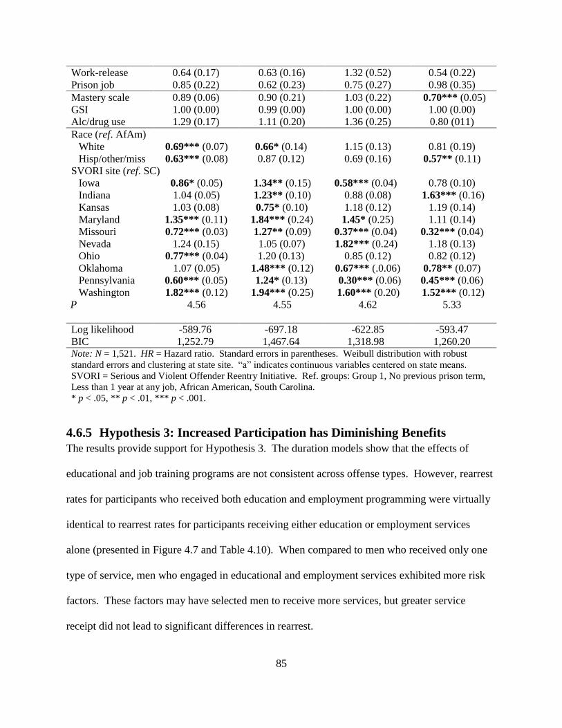
85
Work-release 0.64 (0.17) 0.63 (0.16) 1.32 (0.52) 0.54 (0.22)
Prison job 0.85 (0.22) 0.62 (0.23) 0.75 (0.27) 0.98 (0.35)
Mastery scale 0.89 (0.06) 0.90 (0.21) 1.03 (0.22) 0.70*** (0.05)
GSI 1.00 (0.00) 0.99 (0.00) 1.00 (0.00) 1.00 (0.00)
Alc/drug use 1.29 (0.17) 1.11 (0.20) 1.36 (0.25) 0.80 (011)
Race (ref. AfAm)
White 0.69*** (0.07) 0.66* (0.14) 1.15 (0.13) 0.81 (0.19)
Hisp/other/miss 0.63*** (0.08) 0.87 (0.12) 0.69 (0.16) 0.57** (0.11)
SVORI site (ref. SC)
Iowa 0.86* (0.05) 1.34** (0.15) 0.58*** (0.04) 0.78 (0.10)
Indiana 1.04 (0.05) 1.23** (0.10) 0.88 (0.08) 1.63*** (0.16)
Kansas 1.03 (0.08) 0.75* (0.10) 1.18 (0.12) 1.19 (0.14)
Maryland 1.35*** (0.11) 1.84*** (0.24) 1.45* (0.25) 1.11 (0.14)
Missouri 0.72*** (0.03) 1.27** (0.09) 0.37*** (0.04) 0.32*** (0.04)
Nevada 1.24 (0.15) 1.05 (0.07) 1.82*** (0.24) 1.18 (0.13)
Ohio 0.77*** (0.04) 1.20 (0.13) 0.85 (0.12) 0.82 (0.12)
Oklahoma 1.07 (0.05) 1.48*** (0.12) 0.67*** (.0.06) 0.78** (0.07)
Pennsylvania 0.60*** (0.05) 1.24* (0.13) 0.30*** (0.06) 0.45*** (0.06)
Washington 1.82*** (0.12) 1.94*** (0.25) 1.60*** (0.20) 1.52*** (0.12)
P 4.56 4.55 4.62 5.33
Log likelihood -589.76 -697.18 -622.85 -593.47
BIC 1,252.79 1,467.64 1,318.98 1,260.20 Note: N = 1,521. HR = Hazard ratio. Standard errors in parentheses. Weibull distribution with robust
standard errors and clustering at state site. “a” indicates continuous variables centered on state means.
SVORI = Serious and Violent Offender Reentry Initiative. Ref. groups: Group 1, No previous prison term,
Less than 1 year at any job, African American, South Carolina.
* p < .05, ** p < .01, *** p < .001.
4.6.5 Hypothesis 3: Increased Participation has Diminishing Benefits
The results provide support for Hypothesis 3. The duration models show that the effects of
educational and job training programs are not consistent across offense types. However, rearrest
rates for participants who received both education and employment programming were virtually
identical to rearrest rates for participants receiving either education or employment services
alone (presented in Figure 4.7 and Table 4.10). When compared to men who received only one
type of service, men who engaged in educational and employment services exhibited more risk
factors. These factors may have selected men to receive more services, but greater service
receipt did not lead to significant differences in rearrest.
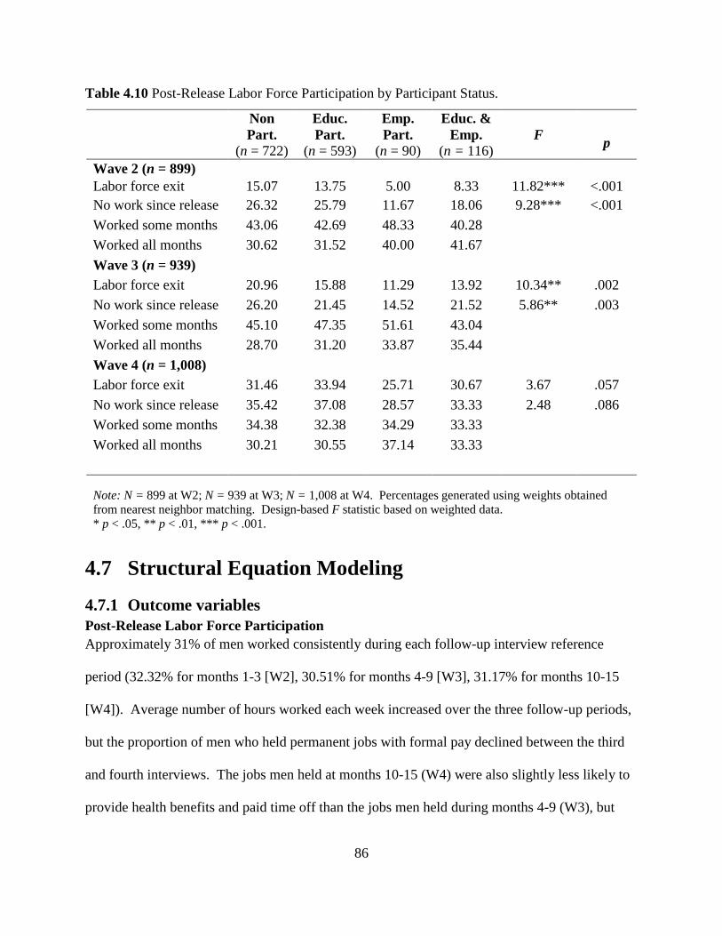
86
Table 4.10 Post-Release Labor Force Participation by Participant Status.
Non
Part.
(n = 722)
Educ.
Part.
(n = 593)
Emp.
Part.
(n = 90)
Educ. &
Emp.
(n = 116) F
p
Wave 2 (n = 899)
Labor force exit 15.07 13.75 5.00 8.33 11.82*** <.001
No work since release 26.32 25.79 11.67 18.06 9.28*** <.001
Worked some months 43.06 42.69 48.33 40.28
Worked all months 30.62 31.52 40.00 41.67
Wave 3 (n = 939)
Labor force exit 20.96 15.88 11.29 13.92 10.34** .002
No work since release 26.20 21.45 14.52 21.52 5.86** .003
Worked some months 45.10 47.35 51.61 43.04
Worked all months 28.70 31.20 33.87 35.44
Wave 4 (n = 1,008)
Labor force exit 31.46 33.94 25.71 30.67 3.67 .057
No work since release 35.42 37.08 28.57 33.33 2.48 .086
Worked some months 34.38 32.38 34.29 33.33
Worked all months 30.21 30.55 37.14 33.33
Note: N = 899 at W2; N = 939 at W3; N = 1,008 at W4. Percentages generated using weights obtained
from nearest neighbor matching. Design-based F statistic based on weighted data.
* p < .05, ** p < .01, *** p < .001.
4.7 Structural Equation Modeling
4.7.1 Outcome variables
Post-Release Labor Force Participation
Approximately 31% of men worked consistently during each follow-up interview reference
period (32.32% for months 1-3 [W2], 30.51% for months 4-9 [W3], 31.17% for months 10-15
[W4]). Average number of hours worked each week increased over the three follow-up periods,
but the proportion of men who held permanent jobs with formal pay declined between the third
and fourth interviews. The jobs men held at months 10-15 (W4) were also slightly less likely to
provide health benefits and paid time off than the jobs men held during months 4-9 (W3), but
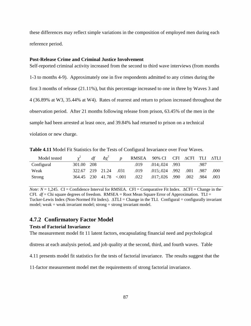
87
these differences may reflect simple variations in the composition of employed men during each
reference period.
Post-Release Crime and Criminal Justice Involvement
Self-reported criminal activity increased from the second to third wave interviews (from months
1-3 to months 4-9). Approximately one in five respondents admitted to any crimes during the
first 3 months of release (21.11%), but this percentage increased to one in three by Waves 3 and
4 (36.89% at W3, 35.44% at W4). Rates of rearrest and return to prison increased throughout the
observation period. After 21 months following release from prison, 63.45% of the men in the
sample had been arrested at least once, and 39.84% had returned to prison on a technical
violation or new charge.
Table 4.11 Model Fit Statistics for the Tests of Configural Invariance over Four Waves.
Model tested χ2
df ∆χ2 p RMSEA 90% CI CFI ∆CFI TLI ∆TLI
Configural 301.00 208
.019 .014;.024 .993
.987
Weak 322.67 219 21.24 .031 .019 .015;.024 .992 .001 .987 .000
Strong 364.45 230 41.78 <.001 .022 .017;.026 .990 .002 .984 .003
Note: N = 1,245. CI = Confidence Interval for RMSEA. CFI = Comparative Fit Index. ∆CFI = Change in the
CFI. df = Chi square degrees of freedom. RMSEA = Root Mean Square Error of Approximation. TLI =
Tucker-Lewis Index (Non-Normed Fit Index). ∆TLI = Change in the TLI. Configural = configurally invariant
model; weak = weak invariant model; strong = strong invariant model.
4.7.2 Confirmatory Factor Model Tests of Factorial Invariance
The measurement model fit 11 latent factors, encapsulating financial need and psychological
distress at each analysis period, and job quality at the second, third, and fourth waves. Table
4.11 presents model fit statistics for the tests of factorial invariance. The results suggest that the
11-factor measurement model met the requirements of strong factorial invariance.
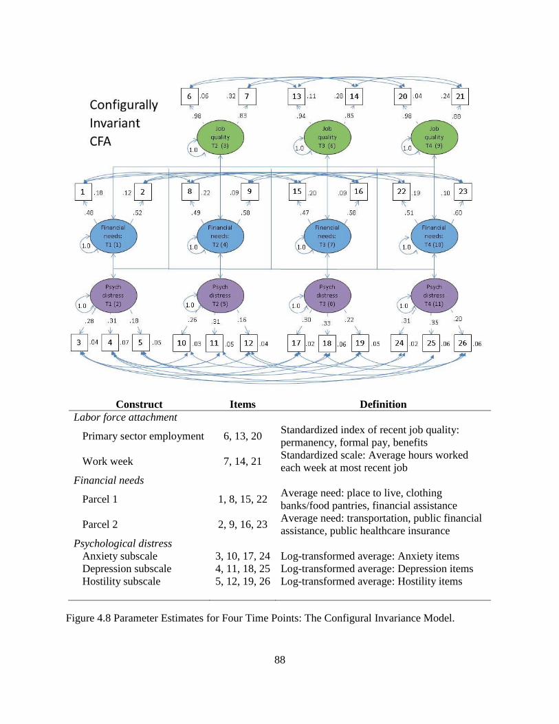
88
Construct Items Definition
Labor force attachment
Primary sector employment 6, 13, 20 Standardized index of recent job quality:
permanency, formal pay, benefits
Work week 7, 14, 21 Standardized scale: Average hours worked
each week at most recent job
Financial needs
Parcel 1 1, 8, 15, 22 Average need: place to live, clothing
banks/food pantries, financial assistance
Parcel 2 2, 9, 16, 23 Average need: transportation, public financial
assistance, public healthcare insurance
Psychological distress
Anxiety subscale 3, 10, 17, 24 Log-transformed average: Anxiety items
Depression subscale 4, 11, 18, 25 Log-transformed average: Depression items
Hostility subscale 5, 12, 19, 26 Log-transformed average: Hostility items
Figure 4.8 Parameter Estimates for Four Time Points: The Configural Invariance Model.

89
The configurally invariant model showed good model fit (RMSEA = .019 [.014;.024], CFI =
.993, TLI = .987). The items exhibited similar pattern loadings over time; for the financial needs
factor, the second item had the largest loading, the first item had the smallest loading, and the
third item was in the middle. Among psychological distress indicators, the depression parcel
loaded strongest on the latent factor, followed by the anxiety and hostility parcels. For the job
quality factors, the standardized primary sector employment item had larger loadings than did the
standardized workweek item. Figure 4.8 presents results of the configural invariance model.
The indicators and factors also passed the test for weak factorial invariance. When factor
loadings were constrained to equality at each wave, the fit statistics indicated no decline in the fit
of the overall model (RMSEA = .019 [.015;.024], CFI = .992, TLI = .987). Figure 4.9 presents
results of the weak factorial invariance model.
To test strong factorial invariance, the factor loadings and intercepts were constrained to equal
the values for the first observation period. The intercepts for financial need items at Wave 1
were slightly higher than intercepts at subsequent waves, so constraining the intercepts to equal
the Wave 1 items had the most notable effect on the change. Nonetheless, the model fit statistics
indicate that the strong invariance model showed good fit (RMSEA = .022 [.017;.026], CFI =
.990, TLI = .984), the change in CFI of .002 did not exceed the .002 maximum change that
Meade, Johnson, and Braddy (2008) recommend. Table 4.12 presents parameter estimates for
different levels of factorial invariance. Figure 4.10 presents the retained CFA model, and it is
used to build the longitudinal structural equation model.

90
Construct Items Definition
Labor force attachment
Primary sector employment 6, 13, 20 Standardized index of recent job quality:
permanency, formal pay, benefits
Work week 7, 14, 21 Standardized scale: Average hours worked
each week at most recent job
Financial needs
Parcel 1 1, 8, 15, 22 Average need: place to live, clothing
banks/food pantries, financial assistance
Parcel 2 2, 9, 16, 23 Average need: transportation, public financial
assistance, public healthcare insurance
Psychological distress
Anxiety subscale 3, 10, 17, 24 Log-transformed average: Anxiety items
Depression subscale 4, 11, 18, 25 Log-transformed average: Depression items
Hostility subscale 5, 12, 19, 26 Log-transformed average: Hostility items
Figure 4.9 Parameter Estimates for Four Time Points: The Weak Invariance Model.
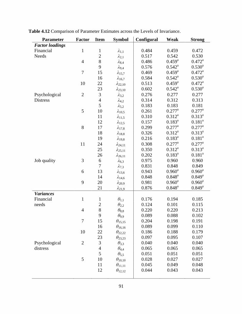
91
Table 4.12 Comparison of Parameter Estimates across the Levels of Invariance.
Parameter Factor Item Symbol Configural Weak Strong
Factor loadings
Financial 1 1 λ1,1 0.484 0.459 0.472
Needs 2 λ2,1 0.517 0.542 0.530
4 8 λ8,4 0.486 0.459a 0.472
a
9 λ9,4 0.576 0.542a 0.530
a
7 15 λ15,7 0.469 0.459a 0.472
a
16 λ16,7 0.584 0.542a 0.530
a
10 22 λ22,10 0.513 0.459a 0.472
a
23 λ23,10 0.602 0.542a 0.530
a
Psychological 2 3 λ3,2 0.276 0.277 0.277
Distress 4 λ4,2 0.314 0.312 0.313
5 λ5,2 0.183 0.183 0.181
5 10 λ10,5 0.261 0.277a 0.277
a
11 λ11,5 0.310 0.312a 0.313
a
12 λ12,5 0.157 0.183a 0.181
a
8 17 λ17,8 0.299 0.277a 0.277
a
18 λ18,8 0.326 0.312a 0.313
a
19 λ19,8 0.216 0.183a 0.181
a
11 24 λ24,11 0.308 0.277a 0.277
a
25 λ25,11 0.350 0.312a 0.313
a
26 λ26,11 0.202 0.183a 0.181
a
Job quality 3 6 λ6,3 0.975 0.960
0.960
7 λ7,3 0.831 0.848 0.849
6 13 λ13,6 0.943 0.960a 0.960
a
14 λ14,6 0.848 0.848a 0.849
a
9 20 λ20,9 0.981 0.960a 0.960
a
21 λ21,9 0.876 0.848a 0.849
a
Variances
Financial 1 1 θ1,1 0.176 0.194 0.185
needs 2 θ2,2 0.124 0.101 0.115
4 8 θ8,8 0.220 0.220 0.213
9 θ9,9 0.089 0.088 0.102
7 15 θ15,15 0.204 0.198 0.191
16 θ16,16 0.089 0.099 0.110
10 22 θ22,22 0.186 0.188 0.179
23 θ23,23 0.097 0.095 0.107
Psychological 2 3 θ3,3 0.040 0.040 0.040
distress 4 θ4,4 0.065 0.065 0.065
5 θ5,5 0.051 0.051 0.051
5 10 θ10,10 0.028 0.027 0.027
11 θ11,11 0.045 0.049 0.048
12 θ12,12 0.044 0.043 0.043
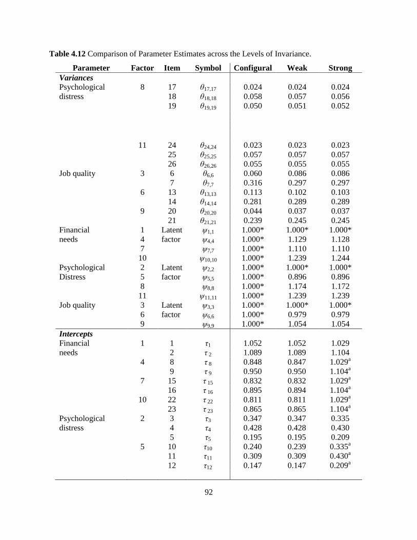
92
Table 4.12 Comparison of Parameter Estimates across the Levels of Invariance.
Parameter Factor Item Symbol Configural Weak Strong
Variances
Psychological 8 17 θ17,17 0.024 0.024 0.024
distress 18 θ18,18 0.058 0.057 0.056
19 θ19,19 0.050 0.051 0.052
11 24 θ24,24 0.023 0.023 0.023
25 θ25,25 0.057 0.057 0.057
26 θ26,26 0.055 0.055 0.055
Job quality 3 6 θ6,6 0.060 0.086 0.086
7 θ7,7 0.316 0.297 0.297
6 13 θ13,13 0.113 0.102 0.103
14 θ14,14 0.281 0.289 0.289
9 20 θ20,20 0.044 0.037 0.037
21 θ21,21 0.239 0.245 0.245
Financial 1 Latent ψ1,1 1.000* 1.000* 1.000*
needs 4 factor ψ4,4 1.000* 1.129 1.128
7 ψ7,7 1.000* 1.110 1.110
10 ψ10,10 1.000* 1.239 1.244
Psychological 2 Latent ψ2,2 1.000* 1.000* 1.000*
Distress 5 factor ψ5,5 1.000* 0.896 0.896
8 ψ8,8 1.000* 1.174 1.172
11 ψ11,11 1.000* 1.239 1.239
Job quality 3 Latent ψ3,3 1.000* 1.000* 1.000*
6 factor ψ6,6 1.000* 0.979 0.979
9 ψ9,9 1.000* 1.054 1.054
Intercepts
Financial 1 1 τ1 1.052 1.052 1.029
needs 2 τ 2 1.089 1.089 1.104
4 8 τ 8 0.848 0.847 1.029a
9 τ 9 0.950 0.950 1.104a
7 15 τ 15 0.832 0.832 1.029a
16 τ 16 0.895 0.894 1.104a
10 22 τ 22 0.811 0.811 1.029a
23 τ 23 0.865 0.865 1.104a
Psychological 2 3 τ3 0.347 0.347 0.335
distress 4 τ4 0.428 0.428 0.430
5 τ5 0.195 0.195 0.209
5 10 τ10 0.240 0.239 0.335a
11 τ11 0.309 0.309 0.430a
12 τ12 0.147 0.147 0.209a
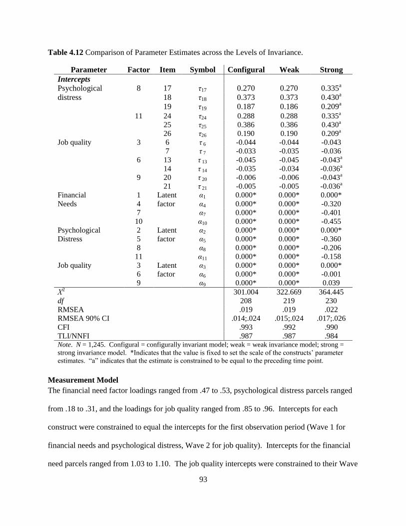
93
Table 4.12 Comparison of Parameter Estimates across the Levels of Invariance.
Parameter Factor Item Symbol Configural Weak Strong
Intercepts
Psychological 8 17 τ17 0.270 0.270 0.335a
distress 18 τ18 0.373 0.373 0.430a
19 τ19 0.187 0.186 0.209a
11 24 τ24 0.288 0.288 0.335a
25 τ25 0.386 0.386 0.430a
26 τ26 0.190 0.190 0.209a
Job quality 3 6 τ 6 -0.044 -0.044 -0.043
7 τ 7 -0.033 -0.035 -0.036
6 13 τ 13 -0.045 -0.045 -0.043a
14 τ 14 -0.035 -0.034 -0.036a
9 20 τ 20 -0.006 -0.006 -0.043a
21 τ 21 -0.005 -0.005 -0.036a
Financial 1 Latent α1 0.000* 0.000* 0.000*
Needs 4 factor α4 0.000* 0.000* -0.320
7 α7 0.000* 0.000* -0.401
10 α10 0.000* 0.000* -0.455
Psychological 2 Latent α2 0.000* 0.000* 0.000*
Distress 5 factor α5 0.000* 0.000* -0.360
8 α8 0.000* 0.000* -0.206
11 α11 0.000* 0.000* -0.158
Job quality 3 Latent α3 0.000* 0.000* 0.000*
6 factor α6 0.000* 0.000* -0.001
9 α9 0.000* 0.000* 0.039
Χ2 301.004 322.669 364.445
df 208 219 230
RMSEA .019 .019 .022
RMSEA 90% CI .014;.024 .015;.024 .017;.026
CFI .993 .992 .990
TLI/NNFI .987 .987 .984 Note. N = 1,245. Configural = configurally invariant model; weak = weak invariance model; strong =
strong invariance model. *Indicates that the value is fixed to set the scale of the constructs’ parameter
estimates. “a” indicates that the estimate is constrained to be equal to the preceding time point.
Measurement Model
The financial need factor loadings ranged from .47 to .53, psychological distress parcels ranged
from .18 to .31, and the loadings for job quality ranged from .85 to .96. Intercepts for each
construct were constrained to equal the intercepts for the first observation period (Wave 1 for
financial needs and psychological distress, Wave 2 for job quality). Intercepts for the financial
need parcels ranged from 1.03 to 1.10. The job quality intercepts were constrained to their Wave
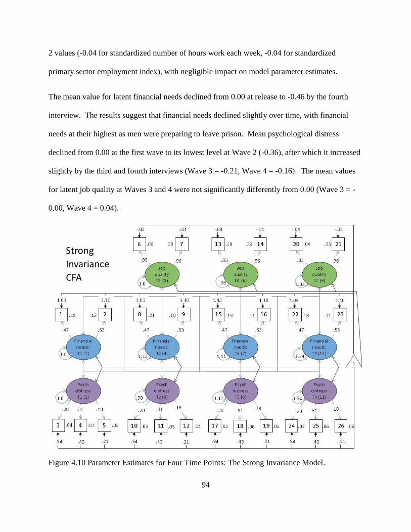
94
2 values (-0.04 for standardized number of hours work each week, -0.04 for standardized
primary sector employment index), with negligible impact on model parameter estimates.
The mean value for latent financial needs declined from 0.00 at release to -0.46 by the fourth
interview. The results suggest that financial needs declined slightly over time, with financial
needs at their highest as men were preparing to leave prison. Mean psychological distress
declined from 0.00 at the first wave to its lowest level at Wave 2 (-0.36), after which it increased
slightly by the third and fourth interviews (Wave 3 = -0.21, Wave 4 = -0.16). The mean values
for latent job quality at Waves 3 and 4 were not significantly differently from 0.00 (Wave 3 = -
0.00, Wave 4 = 0.04).
Figure 4.10 Parameter Estimates for Four Time Points: The Strong Invariance Model.
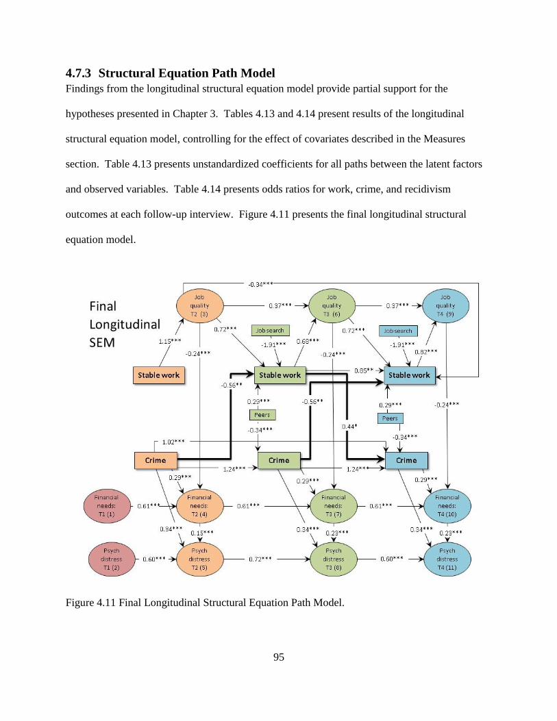
95
4.7.3 Structural Equation Path Model Findings from the longitudinal structural equation model provide partial support for the
hypotheses presented in Chapter 3. Tables 4.13 and 4.14 present results of the longitudinal
structural equation model, controlling for the effect of covariates described in the Measures
section. Table 4.13 presents unstandardized coefficients for all paths between the latent factors
and observed variables. Table 4.14 presents odds ratios for work, crime, and recidivism
outcomes at each follow-up interview. Figure 4.11 presents the final longitudinal structural
equation model.
Figure 4.11 Final Longitudinal Structural Equation Path Model.
96
4.7.4 Hypothesis 4: Criminal Activity Reduces Human and Social Capital
Results provide limited evidence to assess whether ongoing criminal involvement reduces men’s
stock of human and social capital. The final path includes paths from prosocial peer influences
to crime and criminal justice involvement, not from crime to later investments in human and
social capital. However, the path model shows an association between positive peer influences
(friends who work and do not get in trouble) and reduced odds of having committed crimes
recently. Compared to men who reported that most of their friends were positive influences,
men who said that all of them were had 29% lower odds of having committed crime during the
interview reference period (Waves 3 and 4: OR = 0.71, b = -0.34, p < .001). Similarly, prosocial
peer influences at the Wave 3 interview (months 3-9) reduced men’s odds of returning to prison
during the first 21 months of release (OR = 0.77, b = -0.27, p = .005).
Men who were arrested within the first 90 days were significantly less likely than other men to
remain employed during the subsequent 6-month period (OR = 0.47, b = -0.75, p < .001).
Arrests that occurred within the first 9 months had a similar effect of Wave 4 employment,
reducing the odds of remaining stably employed between months 10 and 15 by 53% (OR = 0.47,
b = -0.75, p < .001). Reincarceration further reduced men’s odds of maintaining stable
employment by the time of the Wave 4 interview (OR = 0.44, b = -0.83, p = .014).
4.7.5 Hypothesis 5: Human and Social Capital Increases Employment
Path model results support this hypothesis. Men who had worked at the same place for longer
than 1 year, at any point before entering prison, continued to have more success in maintaining
employment upon release, compared to men who had never worked anywhere for longer than a
year (OR = 1.81-3.32). Men who experienced greater job difficulties during each reference
period had reduced odds of maintaining stable employment. Men who reported experiencing all

97
six barriers to employment had 85-90% lower odds of working each month (OR = 0.15, b = -
1.91, p < .001). During each observation period, prosocial peer influences increased men’s labor
force attachment. Compared to men who reported that most of their friends were positive
influences, men who said all of them were had 30% higher odds of maintaining stable
employment (OR = 1.34, b = 0.29, p < .001).
4.7.6 Hypothesis 6: Labor Force Participation Increases Job Quality
Several pathways within the longitudinal structural equation model provide support for this
hypothesis. Consistent employment (e.g., working each month) was associated with improved
job quality within the same interview reference period. The largest coefficient for stable
employment was at the first follow-up interview (Wave 2, 3 months after release). Mean job
quality was 1 standard deviation increase higher among men who had worked each month since
release, in comparison to men who worked intermittently or not at all.
The association between stable employment and job quality was smaller at subsequent
interviews, although the effect of stable employment on job quality increased slightly from
months 4-9 (Wave 3) to months 10-15 (Wave 4). Men who worked consistently during the
Wave 3 reference period reported higher quality jobs than did men who had not maintained
stable employment during the same timeframe (b = 0.68, p < .001). During the subsequent 6
months (months 10-15), stable employment was associated with slightly larger improvements in
job quality (b = 0.82, p < .001).
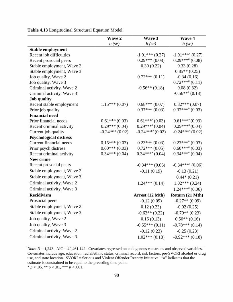
98
Table 4.13 Longitudinal Structural Equation Model.
Wave 2 Wave 3 Wave 4
b (se) b (se) b (se)
Stable employment
Recent job difficulties -1.91*** (0.27) -1.91***a (0.27)
Recent prosocial peers 0.29*** (0.08) 0.29***a (0.08)
Stable employment, Wave 2 0.39 (0.22) 0.33 (0.28)
Stable employment, Wave 3 0.85** (0.25)
Job quality, Wave 2 0.72*** (0.11) -0.34 (0.16)
Job quality, Wave 3 0.72***a (0.11)
Criminal activity, Wave 2 -0.56** (0.18) 0.08 (0.32)
Criminal activity, Wave 3 -0.56**a (0.18)
Job quality
Recent stable employment 1.15*** (0.07) 0.68*** (0.07) 0.82*** (0.07)
Prior job quality 0.37*** (0.03) 0.37***a (0.03)
Financial need
Prior financial needs 0.61*** (0.03) 0.61***
a (0.03) 0.61***
a (0.03)
Recent criminal activity 0.29*** (0.04) 0.29***
a (0.04) 0.29***
a (0.04)
Current job quality -0.24*** (0.02) -0.24***
a (0.02) -0.24***
a (0.02)
Psychological distress
Current financial needs 0.15*** (0.03) 0.23*** (0.03) 0.23***a (0.03)
Prior psych distress 0.60*** (0.03) 0.72*** (0.05) 0.60***a (0.03)
Recent criminal activity 0.34*** (0.04) 0.34***a (0.04) 0.34***
a (0.04)
New crime
Recent prosocial peers -0.34*** (0.06) -0.34***a (0.06)
Stable employment, Wave 2 -0.11 (0.19) -0.13 (0.21)
Stable employment, Wave 3 0.44* (0.21)
Criminal activity, Wave 2 1.24*** (0.14) 1.02*** (0.24)
Criminal activity, Wave 3 1.24***a (0.06)
Recidivism Arrest (12 Mth) Return (21 Mth)
Prosocial peers -0.12 (0.09) -0.27** (0.09)
Stable employment, Wave 2 0.12 (0.23) -0.02 (0.25)
Stable employment, Wave 3 -0.63** (0.22) -0.70** (0.23)
Job quality, Wave 2 0.16 (0.13) 0.50** (0.16)
Job quality, Wave 3 -0.55*** (0.11) -0.78*** (0.14)
Criminal activity, Wave 2 -0.12 (0.23) -0.25 (0.23)
Criminal activity, Wave 3 1.02*** (0.18) -0.92*** (0.18)
Note: N = 1,243. AIC = 40,461.142. Covariates regressed on endogenous constructs and observed variables.
Covariates include age, education, racial/ethnic status, criminal record, risk factors, pre-SVORI alcohol or drug
use, and state location. SVORI = Serious and Violent Offender Reentry Initiative. “a” indicates that the
estimate is constrained to be equal to the preceding time point.
* p < .05, ** p < .01, *** p < .001.
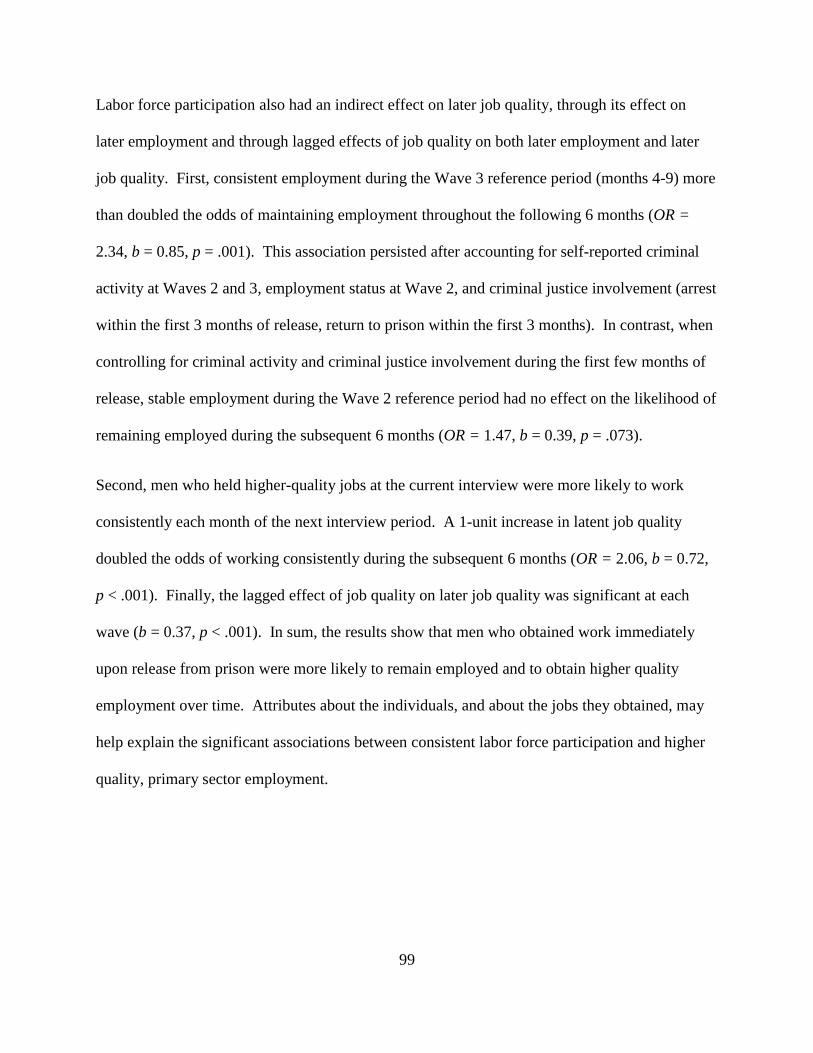
99
Labor force participation also had an indirect effect on later job quality, through its effect on
later employment and through lagged effects of job quality on both later employment and later
job quality. First, consistent employment during the Wave 3 reference period (months 4-9) more
than doubled the odds of maintaining employment throughout the following 6 months (OR =
2.34, b = 0.85, p = .001). This association persisted after accounting for self-reported criminal
activity at Waves 2 and 3, employment status at Wave 2, and criminal justice involvement (arrest
within the first 3 months of release, return to prison within the first 3 months). In contrast, when
controlling for criminal activity and criminal justice involvement during the first few months of
release, stable employment during the Wave 2 reference period had no effect on the likelihood of
remaining employed during the subsequent 6 months (OR = 1.47, b = 0.39, p = .073).
Second, men who held higher-quality jobs at the current interview were more likely to work
consistently each month of the next interview period. A 1-unit increase in latent job quality
doubled the odds of working consistently during the subsequent 6 months (OR = 2.06, b = 0.72,
p < .001). Finally, the lagged effect of job quality on later job quality was significant at each
wave (b = 0.37, p < .001). In sum, the results show that men who obtained work immediately
upon release from prison were more likely to remain employed and to obtain higher quality
employment over time. Attributes about the individuals, and about the jobs they obtained, may
help explain the significant associations between consistent labor force participation and higher
quality, primary sector employment.
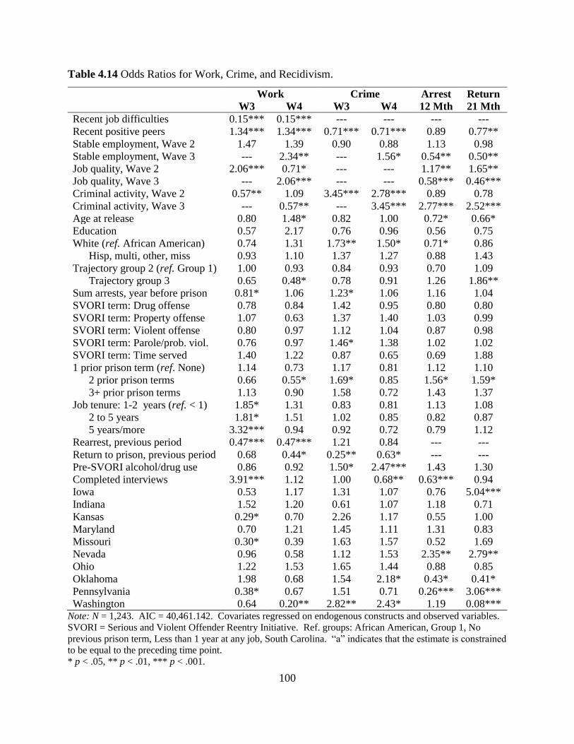
100
Table 4.14 Odds Ratios for Work, Crime, and Recidivism.
Work Crime Arrest Return
W3 W4 W3 W4 12 Mth 21 Mth
Recent job difficulties 0.15*** 0.15*** --- --- --- ---
Recent positive peers 1.34*** 1.34*** 0.71*** 0.71*** 0.89 0.77**
Stable employment, Wave 2 1.47 1.39 0.90 0.88 1.13 0.98
Stable employment, Wave 3 --- 2.34** --- 1.56* 0.54** 0.50**
Job quality, Wave 2 2.06*** 0.71* --- --- 1.17** 1.65**
Job quality, Wave 3 --- 2.06*** --- --- 0.58*** 0.46***
Criminal activity, Wave 2 0.57** 1.09 3.45*** 2.78*** 0.89 0.78
Criminal activity, Wave 3 --- 0.57** --- 3.45*** 2.77*** 2.52***
Age at release 0.80 1.48* 0.82 1.00 0.72* 0.66*
Education 0.57 2.17 0.76 0.96 0.56 0.75
White (ref. African American) 0.74 1.31 1.73** 1.50* 0.71* 0.86
Hisp, multi, other, miss 0.93 1.10 1.37 1.27 0.88 1.43
Trajectory group 2 (ref. Group 1) 1.00 0.93 0.84 0.93 0.70 1.09
Trajectory group 3 0.65 0.48* 0.78 0.91 1.26 1.86**
Sum arrests, year before prison 0.81* 1.06 1.23* 1.06 1.16 1.04
SVORI term: Drug offense 0.78 0.84 1.42 0.95 0.80 0.80
SVORI term: Property offense 1.07 0.63 1.37 1.40 1.03 0.99
SVORI term: Violent offense 0.80 0.97 1.12 1.04 0.87 0.98
SVORI term: Parole/prob. viol. 0.76 0.97 1.46* 1.38 1.02 1.02
SVORI term: Time served 1.40 1.22 0.87 0.65 0.69 1.88
1 prior prison term (ref. None) 1.14 0.73 1.17 0.81 1.12 1.10
2 prior prison terms 0.66 0.55* 1.69* 0.85 1.56* 1.59*
3+ prior prison terms 1.13 0.90 1.58 0.72 1.43 1.37
Job tenure: 1-2 years (ref. < 1) 1.85* 1.31 0.83 0.81 1.13 1.08
2 to 5 years 1.81* 1.51 1.02 0.85 0.82 0.87
5 years/more 3.32*** 0.94 0.92 0.72 0.79 1.12
Rearrest, previous period 0.47*** 0.47*** 1.21 0.84 --- ---
Return to prison, previous period 0.68 0.44* 0.25** 0.63* --- ---
Pre-SVORI alcohol/drug use 0.86 0.92 1.50* 2.47*** 1.43 1.30
Completed interviews 3.91*** 1.12 1.00 0.68** 0.63*** 0.94
Iowa 0.53 1.17 1.31 1.07 0.76 5.04***
Indiana 1.52 1.20 0.61 1.07 1.18 0.71
Kansas 0.29* 0.70 2.26 1.17 0.55 1.00
Maryland 0.70 1.21 1.45 1.11 1.31 0.83
Missouri 0.30* 0.39 1.63 1.57 0.52 1.69
Nevada 0.96 0.58 1.12 1.53 2.35** 2.79**
Ohio 1.22 1.53 1.65 1.44 0.88 0.85
Oklahoma 1.98 0.68 1.54 2.18* 0.43* 0.41*
Pennsylvania 0.38* 0.67 1.51 0.71 0.26*** 3.06***
Washington 0.64 0.20** 2.82** 2.43* 1.19 0.08*** Note: N = 1,243. AIC = 40,461.142. Covariates regressed on endogenous constructs and observed variables.
SVORI = Serious and Violent Offender Reentry Initiative. Ref. groups: African American, Group 1, No
previous prison term, Less than 1 year at any job, South Carolina. “a” indicates that the estimate is constrained to be equal to the preceding time point.
* p < .05, ** p < .01, *** p < .001.

101
4.7.7 Hypothesis 7: Quality Jobs Reduce Men’s Financial Needs
The structural equation path models provide support for this hypothesis. At each follow-up
analysis period, job quality was significantly associated with reduced financial needs (Waves 2-
4: b = -0.24, p < .001). Nonetheless, improved job quality did not fully address existing financial
needs, as previous financial need remained significantly associated with current need (b = 0.61, p
< .001).
4.7.8 Hypothesis 8: Financial Needs Increase the Probability of Reoffending
The results provide mixed evidence in support of this hypothesis. The original theoretical model
specified that financial needs predicted concurrent criminal involvement. The model was revised
to reflect the temporal ordering of financial need and crime items, so the paths go from prior
financial need to recent criminal involvement and from recent criminal involvement to current
financial needs.
The paths from recent criminal activity to current financial needs were significant at each follow-
up interview period (constrained to equality, b = 0.29, p < .001). The coefficient suggests that
current financial need was 1/2 standard deviation higher among those who had engaged in
criminal activity during the preceding 3-6 month period. The LSEM results presented exclude
the paths from prior financial need to recent self-reported criminal involvement, as these paths
were not significant and diminished model fit (higher AIC).
4.7.9 Hypothesis 9: Financial Needs Increase Psychological Distress
The 15 indicators for psychological distress (5 indicators of anxiety, 5 of distress, and 5 of
hostility) fit weakly on a latent factor. The hostility items exhibited the lowest factor loadings (λ
= 0.18), but the anxiety and depression parcels were also extremely low (λ = 0.27 and λ = 0.31,
respectively). The self-efficacy and locus of control items did not fit a CFA model at all. These

102
personal mastery items were excluded from the final model because they correlated more
strongly with other items (e.g., personal peer networks, psychological distress, and financial
needs) than with each other.
Despite these revisions, results support this hypothesis. Men who reported more unmet financial
needs also reported higher mean levels of psychological distress at each time point (Wave 2, b =
0.15, p < .001; constrained to equality at Waves 3 and 4, b = 0.23, p < .001). However, previous
psychological distress accounted for much of the variation in current psychological distress at
each follow-up period (Waves 2 & 4: b = 0.60, p < .001; Wave 3: b = 0.72, p < .001).
4.7.10 Hypothesis 10: Psychological Distress Contributes to Reoffending
The pathways from latent psychological distress to new crime within the next 3-6 months were
not significant at each wave and were excluded from the final model. However, men who
admitted to crime within the preceding 6 months reported heightened feelings of psychological
distress. At each follow-up interview, self-reported criminal activity was associated with a 0.34
increase in latent psychological distress (b = 0.34, p < .001). In contrast, involvement in the
criminal justice system during the months preceding each interview’s 6-month reference period
(for Wave 3, months 3-9: arrest or return to prison before 3 months; for Wave 4, months 10-15:
arrest or return to prison before 9 months) had no effect on men’s feelings of psychological
distress. Psychological distress was not associated with likelihood of rearrest within the first 12
months or return to prison within the first 21 months (paths omitted from the final model).
4.7.11 Work-Crime Association
The results provide limited support for unidirectional theories of work and crime. The effect of
work on crime varied across waves. Stable employment at Wave 2 was not associated with
criminal activity at Wave 3 (OR = 0.90, b = -0.11, p = .578) or at Wave 4 (OR = 0.88, b = -0.13,

103
p = .534). However, men who worked each month before the Wave 3 interview (months 4-9)
had a 56% increase in the odds of committing crimes during the fourth interview reference
period (months 10-15: OR = 1.56, b = 0.44, p = .033).
Criminal activity had a more consistent, persistent effect on later work and crime. Engaging in
crime more than tripled the odds of reoffending within the following interview period (Waves 3
and 4, constrained to equality: OR = 3.45, b = 1.24, p < .001). After accounting for previous
labor force and criminal activity, the lagged effect of Wave 2 crime on Wave 4 crime was nearly
as large (OR = 2.78, b = 1.02, p < .001). In contrast, engaging in crime was associated with a
43% decline in the odds of remaining employed during the next wave (OR = 0.57, b = -0.56, p =
.002). The effect of Wave 2 crime on later employment did not persist to Wave 4, when
controlling for criminal activity during Wave 3 (OR = 1.09, b = 0.08, p = .793).
Significant associations between stable employment and criminal justice involvement did
provide support for theories that link labor force participation to reduced recidivism. After
controlling for labor force and criminal activity during the first 9 months of release (Waves 2 and
3), consistent employment at Wave 3 was associated with a 46% reduction in the odds of arrest
during the first 12 months of release (OR = 0.54, b = -0.63, p = .005). Stable employment
during that period had a similar effect on the likelihood of returning to prison within the first 21
months (OR = 0.50, b = -0.70, p = .002).
4.7.12 Trimmed Pathways from the Final Longitudinal SEM
The final model excludes paths from employment status and the latent job quality factor to
psychological distress. These paths were not significant at any stage of model-fitting, and
overall fit of the model improved when these paths were eliminated (based on log-likelihood and
AIC values). Psychological distress was also not associated with subsequent labor force
104
participation or job quality. The other main paths that were eliminated from the model were
from prior job quality to current criminal activity. These paths were not significant at any wave.
4.7.13 Significant Covariates
Criminal Activity
Men who reported using alcohol or illicit drugs during the final month before their SVORI
prison term were significantly more likely to remain engaged in crime during the three follow-up
periods (Wave 3: OR = 1.50, b = 0.41, p = .047; Wave 4: OR = 2.47, b = 0.90, p < .001).
Whites were significantly more likely than African American men were to report having
committed crimes since release from prison: 73% higher odds at Wave 3 (OR = 1.73, b = 0.55, p
= .004) and 50% higher odds at Wave 4 (OR = 1.50, b = 0.40, p = .034). However, White men
had a decline of 29% in the odds of rearrest within the first 12 months, when compared to
African American men (OR = 0.71, b = -0.34, p = .047).
4.8 Conclusion Overall, the results show that the trajectory and propensity score models reduced pre-existing
differences that had biased the initial SVORI evaluation findings. After matching participants
and nonparticipants, the duration models show that education and employment programs have no
long-term effects on employment and rearrest. Employment program participants were slightly
more likely to seek and maintain employment during the first 9 months of release than other men
were, and they were less likely to be arrested during the same timeframe. Conversely, education
participants exhibited slightly increased risk of rearrest for certain crimes, but they showed
slightly reduced risk of rearrest for violent crimes. Educational programming did not appear to
improve men’s post-release work outcomes, when compared to nonparticipants.

105
The results of the longitudinal structural equation model help explain the null effects of
education and employment programming on recidivism. Criminal activity reduced the odds that
men would maintain employment during subsequent waves, and the effects of early criminal
involvement persisted over time. In contrast, employment did not appear to reduce the odds of
engaging in crime at any Wave; consistent employment during the third wave even appeared to
increase men’s risk of engaging in crime during the fourth wave. However, the overall results
suggest that the effects of criminal activity are more stable and persistent than are the effects of
work on criminal activity. These findings are discussed in greater detail in the following chapter.
106
Chapter 5: Discussion
5.1 Summary of Findings After controlling for pre-imprisonment characteristics and selection into employment-focused
programming, the results show that vocational education and job training services do not have
long-term effects on labor force participation or likelihood of rearrest. Men who received these
services exhibited short-term increases in employment, as well as short-term delays in rearrest,
but no significant differences persisted after the first 9 months of release. Furthermore, the five
duration models consistently showed that employment programs had no effect on times to
rearrest.
Results of the cross-lagged LSEM provide limited evidence to support theories of crime (or
program logic models) that link increased labor force activity to reductions in later offending.
When recidivism was measured as new arrest within 12 months, and as reincarceration within 21
months, increased labor force attachment was significantly associated with reductions in criminal
justice involvement. However, stable employment had either no effect, or a small significant
positive effect, on the likelihood of reoffending. Job quality was not associated with self-
reported criminal activity at any point, in contrast to previous research (Uggen, 1999; van der
Geest et al., 2011).
The final path model results reveal that, contrary to the original conceptual model (Figure 2.2),
criminal activity emerged as the key explanatory variable driving men’s labor force activity,
financial difficulties, psychological distress, and persistence in crime. Criminal activity had a
stable, persistent effect on later labor force and criminal activity, diminishing the odds that men
remained employed during subsequent interview periods and increasing the odds that they
107
persisted in criminal activity. Men who remained engaged in criminal activity experienced
heightened financial need and emotional reactivity, and they were less involved in the labor force
than were men who reported no criminal activity. In sum, the results suggest that, among active
offenders with extensive criminal records, the path from crime does not begin with employment
(van der Geest et al., 2011), but rather, the paths to employment and financial stability begin with
desistance from crime (Skardhamar & Savolainen, 2014).
5.1.1 Identifying Selection Processes into Treatment
The pre-matching statistics revealed significant differences between men in the sample who
engaged in educational, vocational or job training programs and men who had not received these
services while imprisoned. When programs targeted to high-risk prisoners successfully recruit a
high-risk treatment group, it can be difficult to locate nonparticipants in the prison who can form
an appropriate comparison sample (Braga, Piehl, & Hureau, 2009; Peters, Hochstetler, DeLisi, &
Kuo, 2015). Initial SVORI evaluations included propensity score weights that accounted for
differences between SVORI participants and nonparticipants (e.g., enrollment in SVORI-funded
reentry services) (Lattimore et al., 2012; Lattimore & Steffey, 2009). When applied to models
that evaluated the effectiveness of employment programs (Lattimore et al., 2012), these weights
did not adequately reduce observed differences between employment program participants and
nonparticipants. As a result, initial evaluations concluded that educational programs benefited
individuals who received those services, but that employment programs had detrimental effects
on participants’ subsequent labor force and criminal activity (Lattimore et al., 2012).
In the absence of randomization, observed treatment effects are subject to bias due to selection
into treatment (D. B. Wilson et al., 2000). Selection processes commonly favor individuals who
are predisposed to benefit from the treatment, as these individuals are often the most interested in

108
and motivated to receive the treatment (Davis et al., 2013). In the case of the programs evaluated
in this study, however, the factors that selected men into treatment favored men who exhibited
greater service needs. These pre-existing deficits (e.g., high school dropout, low educational
attainment, and limited work experience) suggest that enrollment in prison-based educational and
employment services identifies individuals who entered prison with the most serious human
capital deficits (Harlow, 2003). This selection process is troubling because low educational
attainment and limited work experience are causally related to the primary outcomes of interest
in evaluations of prison-based education and employment programs: post-release labor force
participation, reoffending, and recidivism (Bushway & Apel, 2012; Duwe, 2012; Latessa, 2012).
As a result, this study contributes to the literature on prison-based programming (Bushway,
2003; Bushway & Apel, 2012). It shows that selection into some forms of prison programming
reflects heightened need (Peters et al., 2015). However, it is more likely that nonparticipants in
this sample were able to select out of the treatment under study (i.e., programs providing
remedial education and job skills training), than that participants voluntarily opted to attend
educational and employment programs (Chamberlain, 2012; Heckman & Hotz, 1989).
The literature on prison programming provides evidence to support this conclusion (Brewster &
Sharp, 2002; Chamberlain, 2012; Harlow, 2003; Steurer et al., 2001). In many prisons, GED
classes are mandatory for all prisoners with less than a high school education (Duwe & Clark,
2014), so these classes are composed predominantly of men who are compelled to enroll in these
services in place of other alternatives (Heckman, Humphries, & Mader, 2011). Furthermore,
enrollment does not equate to regular attendance, let alone consistent attention and engagement.
In many cases, remedial education, job readiness, and GED programs function as silos that
contain the neediest prisoners, but which are not designed to deliver the intensive support needed

109
for these participants (Bushway, 2003). Finally, enrollees in these services are unlikely to show
responsivity to the treatment, given the compulsory nature of enrollment, limited ability to
compel participant engagement, and limited ability to individualize content to participants’ needs
(Andrews & Bonta, 2010).
In contrast, high school graduates, GED holders, and prisoners who have acquired sufficient
work experience before prison may be directed away from remedial education and job training
programs toward services that address other challenges these individuals may face, such as
substance abuse treatment or cognitive behavioral therapy. Certain prison programs, such as the
popular Puppies for Parole dog-training programs, include stringent enrollment criteria that
restrict participation to the most successful, model prisoners. Prisoners are often aware of which
programs available to them are viewed most favorably by prison staff and parole boards
(Brewster & Sharp, 2002; Steurer et al., 2001). In this case, selection out of education and
employment programs may in fact reflect selection into other programs among prisoners most
equipped to succeed upon release.
To some extent, this explanation remains speculative because men in this sample did not indicate
whether they were voluntary or mandatory enrollees. However, men who were imprisoned in
states that used mandatory enrollment into SVORI-funded services were more likely to report
educational or employment service receipt.
5.1.2 Balancing across Trajectory Groups
The propensity score matching process deviated from the proposed method in permitting
matches across trajectory groups. It is worth examining why matching across groups reduced
observed biases, and whether this modification casts doubt first, on the validity of the latent
groups, and second, on the quality of the matches.

110
The retained trajectory model included observations on arrests over a 14-year period preceding
the SVORI prison entry. Models that used shorter pre-SVORI observation periods (i.e., fewer
than 10 years), yielded two latent trajectory groups: a high-rate group and a low-rate group. The
high-rate groups derived from these 2-group models consisted of nearly all of the men assigned
to Groups 1 and 3 of the final 3-group model, whereas men in Group 2 populated most of the
low-rate groups in the 2-group models. A small proportion of the sample changed group
membership when trajectory models used shorter observation periods: Men shifted from low-
rate groups in 2-group models to the chronic offending group (group 3) of the 3-group model,
and conversely from the chronic offending group (group 3) of the 3-group model to the low-rate
groups in the 2-group models.
The stability in the pattern of these results suggests two important points. First, as has been
found in previous studies, longer observation periods yield additional latent trajectory groups.
Previous studies suggest that longer observation periods yield more accurate, stable trajectory
groupings, so the literature supports the retention of the 3-group model over shorter 2-group
models (Eggleston et al., 2004; Nagin & Tremblay, 2005).
This leads to the second point. The main effect of the longer observation period was to
distinguish Group 1 men from Group 3 men, by focusing more on the length of the criminal
history than on the level of involvement during the final years leading up to prison entry. The
bivariate statistics revealed many similarities between these two groups, most notably
demographic and criminal risk factors. They also exhibited similar post-release arrest rates,
despite significant differences in age and length of the criminal record.

111
The bivariate statistics do suggest that the men in Groups 1 and 3 were fundamentally different
from each other in certain risk factors relevant to the study of post-release work and crime.
Namely, group 1 and group 3 men appeared to be located at opposite points along the
hypothesized age-crime curve, with group 1 men entering the prime years of offending and
group 3 men expected to be in the process of desistance from crime. Given these groups’
opposing expected trajectories upon release, it would appear to be of paramount importance to
restrict matches across groups. However, the post-release arrest rates show that group 3 men
were hardly on the path toward desistance from crime; in fact, these men exhibited increased
hazard rates of rearrest. Across models, there is ample evidence to suggest that men in Group 3
remained persistently high-risk and marginalized, relative to men in Groups 1 and 2. As a result,
the trajectory groupings provide insight into the factors that led to men’s SVORI imprisonment
and enrollment in the sample, but there is limited reason to think that the groupings are
fundamentally distinct (Nagin & Tremblay, 2005).
Furthermore, the factors selecting men into treatment did not differ substantively for men in
Groups 1 and 3; men in Group 3 were less likely to receive services, but participant-
nonparticipant differences were comparable across these two groups. The same is not exactly
true for men in Group 2, as factors selecting men into treatment for this group were not exactly
identical to those for the other groups.
In this case, the use of the group-based trajectory modeling complemented the propensity score
matching process and appeared to improve the overall quality of the matches. At the very least,
the group-based trajectory model provided an efficient way to capture distinct pre-prison arrest
trajectories. The dummy variables for group membership (and related interaction terms with

112
age, education, and prison term) captured relevant differences among groups across multiple
domains.
5.1.3 Maintenance of the Status Quo Viewed as a whole, the significant coefficients in the duration models in this study provide
evidence to suggest that risk factors for rearrest reflect stable characteristics that existed before
men entered prison (Duwe, 2012; Horney et al., 1995). The significant positive coefficients in
the repeated-events duration model reflect stable criminal risk factors (e.g., previous prison
terms, violation of supervision); ongoing factors correlated with criminal activity (recent alcohol
or drug use), and structural factors that influence the likelihood and timing of rearrest (state
location, racial/ethnic status).
The significant negative coefficients for longest job tenure before prison and length of the
SVORI prison term suggest that maturational reform may account for differences in time to
rearrest. Men who had maintained jobs for longer periods before prison were less likely to be
rearrested than were men who had never worked or had only held jobs briefly before entering
prison. Similarly, longer prison terms were associated with reduced odds of rearrest. As age did
not influence the likelihood and timing of rearrest, it appears likely that job tenure and prison
term partially reflect the effect of aging out of crime. However, if maturational reform does
account for delays in rearrest among men who had previously held stable employment, then it is
clear that the process toward desistance had been underway prior to entering prison.
5.1.4 Understanding Why Employment Programs do not Work
The results generally show that men continue to engage in fundamentally the same behaviors that
they had exhibited prior to entering prison. From this perspective, it is easy to understand why
prison-based education and employment programs often have limited success in improving

113
men’s labor force outcomes. To use educational programming as an example, Adult Basic
Education and GED programs cover the same content that is covered in secondary schools, and
the teaching methods used replicate the traditional lecture-based classroom environments
common among American high schools. The high school dropouts enrolled in these programs
have essentially received, and not been responsive to, the educational treatment offered, so there
is limited reason to think that the programs will have a significant effect on their behavior. To
yield improved outcomes, the teaching methods used in remedial and GED programs may need
to undergo significant revisions to address participants’ specific needs and learning styles
(Andrews & Bonta, 2010).
Risk-Need-Responsivity Framework
Programs that target individuals with the highest risks of reoffending offer the potential for the
greatest returns on investment, in terms of reduced crime, victimization, and correctional costs
(Braga et al., 2009; Peters et al., 2015; Zweig et al., 2011). Zweig and colleagues (2011)
reanalyzed outcome data from the Center for Employment Opportunities (CEO), a subsidized
jobs program serving former prisoners in New York City. When the authors categorized
participants by risk of recidivism, they found that high-risk participants were most responsive to
the intervention (reducing the probability of arrests and convictions, and the frequency of arrests,
among high-risk participants). Participation had no corresponding effects on the low- and
medium-risk participants (Zweig et al., 2011).
Older studies provided partial support for job training and vocational programs (Saylor & Gaes,
1997; D. B. Wilson et al., 2000), but methodological weaknesses in some studies suggest that
observed benefits result from selection into treatment (Brewster & Sharp, 2002). Current studies
suggest that it is not the employment readiness or job training components of these programs that
114
reduce recidivism risk (Jacobs, 2012; Redcross et al., 2012; Zweig et al., 2011). In the case of
the CEO program noted above, the high-risk participants were no more likely to locate
unsubsidized employment than were the high-risk nonparticipants, so other programmatic factors
appear responsible for the recidivism reductions among the high-risk subgroup (Zweig et al.,
2011).
Intervention components that appear to reduce criminogenic risk factors include chemical
dependency treatment (Peters et al., 2015), mentorship (Braga et al., 2009; Redcross et al., 2012;
Zweig et al., 2011), case management (Braga et al., 2009; Zweig et al., 2011), and postsecondary
education (Duwe & Clark, 2014; Kim & Clark, 2013; D. B. Wilson et al., 2000). Interventions
that include therapeutic components and apply cognitive behavioral and social learning
techniques exhibit improved outcomes over programs that lack this therapeutic focus (Andrews
& Bonta, 2010).
Weak Program Design and Implementation
The weak effects of education and employment programs in this study may have resulted from
variations in the quality and intensity of services offered by each state (Andrews & Bonta, 2010;
Lowenkamp, Latessa, & Smith, 2006; Peters et al., 2015). Unfortunately, the SVORI evaluation
lacked the administrative data needed to evaluate whether some states provided higher quality
programs than other states did. As a result, it is difficult to assess whether null findings reflect
poor program design, mismatch to participants’ needs, or poor delivery (Bouffard, Taxman, &
Silverman, 2003; Lowenkamp et al., 2006; Peters et al., 2015; J. A. Wilson & Zozula, 2012).
Demonstration projects often yield much larger effect sizes than do comparable interventions
that are applied rigorously in correctional settings, suggesting that correctional systems face
logistical challenges in scaling up effective programs (Andrews & Bonta, 2010). Prison
115
administrators in the SVORI evaluation overestimated the extent to which prisoners had received
services before release from prison (Lattimore, Visher, & Steffey, 2011), and it is quite possible
that they overestimated how quickly they would be able to scale up existing programs or
introduce new services. Some states had limited existing reentry services in place for prisoners,
so correctional staff in these sites faced the additional hurdle of developing programs for SVORI
participants. States with existing services in place could focus their efforts on increasing access
to a greater range of services (Lattimore et al., 2011).
Failure to obtain buy-in from correctional staff may have hindered the effective delivery of
services to education and employment participants (Bonta, Rugge, Scott, Bourgon, & Yessine,
2008; Lowenkamp et al., 2006; Van Voorhis, Cullen, & Applegate, 1995). Staff may recruit
ineligible people into the treatment group, provide services to comparison group members,
and/or modify components of the intervention based on staff members’ perception of how the
program should work (Peters et al., 2015). The institutional culture in some prisons emphasizes
security and control over rehabilitative programming (Bushway, 2003), so newly designed
programs may have contradicted or challenged existing correctional procedures, leading
administrators to abandon essential components of the reentry model. Logistical challenges
often hamper participation, as when participants transfer abruptly to other correctional
institutions or leave prison at the completion of their sentence (Bushway, 2003; Steurer et al.,
2001).
Evaluators rarely conduct process evaluations during the early stages of an intervention, to
ensure that the program is being implemented as designed. Process evaluations may require that
prison staff collect data on program components that previously went unmeasured by prison
staff, including detailed information on program attendance, content, participant engagement,

116
and completion (Bouffard et al., 2003; Lattimore et al., 2011; Steurer et al., 2001). If these data
collection procedures are not integrated into existing tasks, prison staff may fail to collect data
consistently and reliably (Bouffard et al., 2003).
Work Doesn’t Work, and Perhaps It Never Did
If employment programs are going to be evaluated by their ability to reduce recidivism, the
literature suggests that employment services may need to be wrapped around the primary
intervention (e.g., chemical dependency treatment, postsecondary education) (Duwe & Clark,
2014; Kim & Clark, 2013; Peters et al., 2015). Observational data suggest that employment has,
at best, a weak causal effect on crime, so the potential benefits of even the strongest prison-based
employment program will be modest (Bushway, 2011; Farabee et al., 2014). Programs that
successfully increase participants’ labor force attachment may reduce overall recidivism rates,
but the observed reductions may be too small to be of statistical, let alone practical, significance
(Bushway & Apel, 2012; Lattimore, Steffey, & Visher, 2010).
Lattimore, Steffey, and Visher (2010) present the following example of an employment program
that boosts participants’ employment rate by 20% (to 60% from the baseline 50% rate for
nonparticipants). By helping participants gain employment, the intervention reduces their rate of
criminal involvement by 20% as well (to 40%, from the 50% baseline rate). However, these
sizable improvements may have only a small effect on rearrests, if the 20% reduction in
reoffending manifests as 1 fewer arrest per 100 participants (2.2% reduction in recidivism)
(Bushway & Apel, 2012). Indirect interventions, such as the one described by Lattimore and
colleagues (2010), may be more equipped to show their effectiveness by incorporating proximal
outcomes (e.g., skills gained, attitudinal changes, job search activities) that plausibly link
program completion to the key, often distal, outcomes (e.g., labor force participation,
117
reoffending) (Bushway & Apel, 2012; Farabee et al., 2014). Given the relative lack of support
for employment programs as currently provided, evaluations that assess whether programs
actually improve participants’ hard and soft skills, prior to release from prison, could provide
preliminary evidence to support programs that otherwise show limited effects on post-release
work and crime.
Weak Signals
The negligible observed effects of education and employment programming may have resulted
from the inability to identify men in the SVORI evaluation who completed programs and/or
received credentials while imprisoned (Bushway & Apel, 2012; Lowenkamp et al., 2006).
Successful completion of certain degree programs confers on graduates a credential that may
improve their employment prospects (Duwe & Clark, 2014). Completion status provides useful
information for evaluators as well; in many cases, unobserved risk factors influence the
likelihood of completing the program and of reoffending (Bushway & Apel, 2012; Miller, 2014;
Peters et al., 2015). Even where program designers believe that the program will improve
outcomes, regardless of completion status, knowledge of which participants achieve the
credential can be used to minimize unobserved variable bias (Peters et al., 2015).
Postsecondary education completion appears to provide the most useful credential for reentering
former prisoners (Brown, 2015; Duwe & Clark, 2014), but this option appears to have been out
of reach for most men in the SVORI evaluation. Education participants may not have been
academically prepared for college classes, as four in ten men had less than a high school
education at release from prison. Furthermore, only a minority of them likely resided in prisons
that offered post-secondary education. As of 2015, only 6 of the 11 states provided degree-

118
granting college education programs to select groups of individuals (Prison Studies Project,
2015).
In the case of prisoners enrolled in GED programs, it is unclear whether passing the GED test
actually provides a useful credential upon release (Heckman & LaFontaine, 2006; Heckman &
Rubinstein, 2001; Tyler, Murnane, & Willett, 2000). Among a sample of Minnesota state
prisoners, completing post-secondary education in prison significantly reduced the odds of
rearrest, reconviction, and return to prison (Duwe & Clark, 2014). Completing the GED or high
school diploma while imprisoned had no effect on recidivism outcomes (Duwe & Clark, 2014).
Other studies suggest that, absent pursuit of further education, GED completion does little to
improve labor force outcomes for GED holders, relative to high school dropouts (Brown, 2015;
Heckman et al., 2011).
From the perspective of potential employers, the GED credential may not offset former
prisoners’ negative credentials: their criminal records, removal from the labor market, and
lingering human capital deficits (Brown, 2015; Miller, 2014; Tyler & Kling, 2007; Tyler et al.,
2000). Holding a GED may even hinder employment prospects for some former prisoners, based
on comparisons among high school dropouts, GED graduates, and high school graduates. Based
on tests of cognitive ability, such as the Armed Forces Qualifying Test (AFQT), GED graduates
appear to be as intelligent as high school graduates who do not attend college, and more
intelligent than high school dropouts who do not obtain GED certification . However, when
controlling for cognitive skills and number of years in school (before dropout), GED holders
actually experience greater job instability, earn lower hourly wages, and accumulate less work
experience over time than do uncredentialed high school dropouts. These patterns hold even
when samples exclude former prisoners (Heckman & Rubinstein, 2001).

119
The paradoxical findings for GED completion suggest that noncognitive factors, such as internal
locus of control, self-esteem, and sociability, adversely differentiate GED holders from both high
school dropouts and high school graduates (Heckman & Rubinstein, 2001; Heckman et al.,
2006). Low-skill job markets prioritize noncognitive skills over cognitive skills, in contrast to
high-skill job markets, which value the latter over the former (Heckman et al., 2006). Lacking
postsecondary education or trade certification, GED holders remain unqualified for high-skilled
jobs, for which their low noncognitive skills would present less of a liability. However, in
attaining the GED credential, GED holders differentiate themselves from uncredentialed high
school dropouts, and this may explain GED holders’ disadvantaged position in the formal labor
market (Heckman & Rubinstein, 2001; Heckman et al., 2006).
5.1.5 Structural Factors Trump Human Capital Factors Social structures (e.g., racial/ethnic status, state of residence) appear to have stronger effects on
arrest outcomes among this sample than theoretically relevant predictors do, such as age and
level of education. When racial/ethnic status and SVORI site were excluded from the nested
duration models, higher levels of educational attainment increased the time that men remained in
the community before rearrest. Further education was no longer significantly associated with
rearrest when racial/ethnic status and state of residence were included in the model. These
findings may reflect state-level differences in arrest rates; it is not clear to what extent higher
rates of arrests among African Americans are the result of racial profiling or similar justice
practices (see Figures 4.1-4.6 for graphs of pre-SVORI arrest rates by racial/ethnic status; Tables
4.8 and 4.9 for duration model results).
120
Racial/Ethnic Differences in Rates of Offending and Arrest
Disproportionate minority involvement in the criminal justice system likely reflects real
differences in levels of policing, prosecutorial discretion, and criminal justice sanctioning,
especially for less serious crimes that may go unreported or unobserved by police (the
“differential criminal justice system selection hypothesis”) (Piquero & Brame, 2008). However,
racial/ethnic differences in arrest rates may also reflect differential rates of involvement, if
minorities are more likely to remain involved in criminal activity over the life course (the
“differential involvement hypothesis”) (Anderson, 1999; D’Alessio & Stolzenberg, 2003;
McNulty & Bellair, 2003; Piquero & Brame, 2008).
Between these two divergent perspectives, a middle position exists, which hypothesizes that
police and criminal justice processes discriminate against minorities, but that individual, social,
and structural factors contribute to higher rates of serious crime among minorities (Piquero &
Brame, 2008; Piquero, MacDonald, & Parker, 2002). For instance, racial differences between
African American and White male former prisoners in timing to first violent felony disappeared
when controlling for local unemployment rate and access to manufacturing jobs (Bellair &
Kowalski, 2011). The association between unemployment and violent offending has also been
observed among African American prisoners in Florida; for these men, rising African American
unemployment increased the likelihood of a new felony offense within 2 years of release (Mears,
Wang, & Bales, 2014).
The results of studies using self-reported information often differ from studies that use official
records, which consistently show higher arrest rates among African Americans and other
minorities than among Whites (Piquero & Brame, 2008). Ideally, self-report measures would
provide insight into the source of the racial disparities in criminal justice involvement.
121
Unfortunately, older studies that have collected official records and self-reported information on
official records revealed significant differences by racial/ethnic status in the accuracy of self-
reported information (Farrington, Stouthamer-Loeber, Van-Kammen, & Schmidt, 1996;
Hindelang, Hirschi, & Weis, 1981; Huizinga & Elliott, 1986). These original studies often used
adolescent samples that engaged in less serious forms of delinquent behavior, so the results may
not generalize to adult prisoners with extensive criminal records (Piquero & Brame, 2008).
Recent studies have provided mixed evidence to support the validity of self-report measures
(Jolliffe et al., 2003; Maxfield, Luntz Weiler, & Spatz Widom, 2000; Piquero & Brame, 2008;
Piquero, Schubert, & Brame, 2014; Sampson, Morenoff, & Raudenbush, 2005).
State-Level Differences in Arrest Rates
The duration and path models revealed significant differences in the odds of arrest by state
location. These differences likely reflect differential rates of criminal activity by individuals
within each state, although multiple potential sources of variation also exist at the local and state
levels. First, policing practices vary across localities and states, which in turn influence the
likelihood and timing of arrest. Second, prosecutorial discretion at the local level influences the
odds that an arrest leads to prosecution, conviction, and eventually imprisonment. The length of
time imprisoned for a given offense varies across states, as do prison conditions and access to
programming within prisons.
State recidivism rates reflect the cumulative impact of these local and statewide variations in
criminal justice practices, rendering it difficult to compare outcomes across states. In the case of
the repeated-events duration model, residents from two states (Maryland and Washington)
showed large increases in the baseline hazard of rearrest. Recidivism rates for these two states
were the second- and third-highest rates, respectively, of the 11 states included in the duration
122
models (Pew Center on the States, 2011; Rosenwald, 2011). The reduced time to first arrest for
Maryland and Washington prisoners therefore reflects, in part, the policing or supervision
practices in these states.
Finally, states appeared to recruit participants into the SVORI evaluation using different aspects
of the SVORI enrollment criteria. Several states enrolled high proportions of men with recent
drug convictions, most notably Iowa (58%) and Maryland (66%). Property offenders frequently
exhibit the highest rates of rearrest and return to prison, relative to drug and property offenders,
but none of the states appeared to use property convictions as criteria for enrollment into the
SVORI evaluation (Lattimore & Steffey, 2009).
States that enrolled the highest proportions of violent offenders included Kansas (61%), Nevada
(88%), Ohio (58%), and Washington (65%). Violent offenders often exhibit the lowest
recidivism rates, in comparison to drug and property offenders. This is born out for Nevada,
which had the lowest statewide recidivism rate in 2004, of the states in the sample (Sentencing
Project, 2010).
However, in the case of Washington State, the enrollment criteria were designed to recruit a
high-risk, high-needs sample (e.g., under 35 years old and fitting one or more categories
reflecting heightened risk or needs). Men from Washington State who fit these criteria and were
selected for the SVORI intervention were then mandated to receive services (Lattimore &
Steffey, 2009). The LSEM results showed that men from Washington State were significantly
more likely to have reoffended within each 6-month reference period, so policing practices do
not fully account for state-level differences in rearrest.
123
5.1.6 Limited Support for Causal Theories of Work and Crime The LSEM results generally refute the turning point hypothesis outlined in Section 1.1.3, but it is
not clear to what extent the findings may be interpreted as supporting maturational reform in
place of the hook-for-change hypothesis (Giordano et al., 2002; Laub & Sampson, 2001;
Skardhamar & Savolainen, 2014). Employment did not reduce the odds of later offending,
suggesting that the jobs attained by prisoners in this sample lacked the requisite qualities needed
to foster social bonds and reduce criminal activity (Laub & Sampson, 2001). The fact that stable
employment never reduced the odds of subsequent criminal activity (in fact, it predicted higher
odds of committing crime during the last interview wave) appears to suggest that maturational
reform had not yet taken place among men in this sample. The results do leave open the
possibility that stable employment could have provided the hooks-for-change needed to support
men’s path toward desistance, had men in this sample expressed (implicitly or explicitly)
intentions to “go straight” (Skardhamar & Savolainen, 2014).
Results from a longitudinal study that followed work and offending trajectories during early
adulthood among a sample of former juvenile delinquents provide a possible explanation for
stable employment’s negligible effects on crime in the LSEM. Among high-frequency offenders
in the sample, stable employment had no effect on convictions during the same 1-year period
(van der Geest et al., 2011). In a separate study that examined the timing of employment and
reoffending for a sample of serious offenders, steep declines in criminal activity preceded
employment spells for most men in the sample (Skardhamar & Savolainen, 2014). The delay
between prior offense and most entries into stable employment (lasting at least 6 months) was
extensive, spanning 2 years or more, lending credence to the conclusion that desistance precedes
stable employment (Skardhamar & Savolainen, 2014).
124
5.1.7 Testing Theoretical Concepts Strength of Weak Ties
Results of this study support human and social capital theories of work and crime. Odds of
maintaining stable employment, and resisting criminal activity, were higher among men who
reported social networks comprising higher proportions of employed and prosocial peers. The
opposite pattern emerged when items measuring time spent with employed and prosocial peers
were included in the model: Socializing with peers, even those who were employed and likely to
help men avoid trouble, reduced the odds that men maintained employment, and increased their
odds of reoffending.
Findings from a recent study examining parolees’ job search activities and emotional wellbeing
during the first 90 days of release provide insight into the role of social networks (Sugie, 2014).
As theorized by human and social capital theories, men who expanded their social networks
during the reentry period enjoyed greater success in finding work, and of finding work paying
more than a minimum wage. However, men who felt close to people in their post-release social
network spent more time unemployed. Strong ties to contacts also extended the time until men
located formal labor market employment and jobs paying more than the minimum wage (Sugie,
2014). Men who felt strong ties to people in their social network had likely maintained contact
with people they had known before entering prison, and these existing peer networks may not
have facilitated men’s connections to the labor market. Overall, the results suggest the
importance of weak ties (Granovetter, 1973), and the potential importance of replacing past peer
networks with new, possibly more prosocial peer networks (Hagan, 1993).
Managing Financial Needs During the Reentry Period
Results of this study suggest that greater focus should be paid to the financial and psychological
consequences of remaining engaged in criminal activity (Bucklen & Zajac, 2009; Felson et al.,

125
2012). When controlling for men’s prior levels of psychological distress, prior labor force
activity, and peer support networks, self-reported recent criminal activity was associated with
concurrent unmet financial needs and psychological distress. However, remaining engaged in
the labor force, or even finding higher-quality employment, had limited effects on men’s feelings
of financial and emotional wellbeing. For men in this sample, consistent employment led to
improved job quality, and higher quality jobs diminished men’s financial needs, but there were
no reciprocal paths leading from financial need or psychological distress to later labor force and
criminal activity.
Heightened financial need among men who persisted in criminal activity may reflect a
shortsighted inability, or lack of interest, in taking control of their finances. In a study that
examined factors influencing parolee success, Bucklen and Zajac (2009) observed that financial
management and coping strategies differentiated parole violators from parole successes (those
who had no parole violations or returns to prison during the first 3 years of release). Individuals
who eventually violated parole or returned to prison perceived significantly greater financial
difficulties than did parole successes, even though median debt levels were much lower among
parole violators than among parole successes.
5.1.8 Fostering Desistance among Former Prisoners The LSEM results provide limited evidence to suggest that men can work themselves into
desistance from crime. Previous sections in this chapter have noted the path dependent nature of
men’s post-release activities, which can be seen most clearly in the duration models, yet also
seems present in the path model results. Men in the sample had been involved in criminal
activity before entering prison, and many of them resumed quickly upon release. Similarly,
126
unstable unemployment characterized the majority of men’s labor force activity during the
months leading up to and following release from prison.
Findings from this and other recent studies refute long-standing assumptions about the crime-
reducing effect of employment that had been supported by studies using data from the mid- to
late-20th century (Laub & Sampson, 2001; Uggen, 2000). In previous decades, when union-
protected manufacturing jobs paid good wages to men with limited education and soft skills,
employment likely did reduce crime, by keeping men occupied on a regular basis and increasing
their stakes in conformity (Hirschi, 1969; Laub & Sampson, 2001). Studies have shown that,
even in the 21st century, postindustrial United States, former prisoners who live in areas with
higher levels of manufacturing jobs have lower odds of committing new violent offenses (Mears
et al., 2014). The loss of manufacturing jobs during the latter part of the 20th century has
decimated the low-skilled labor market, with predictable consequences for low-educated former
prisoners’ long-term employability.
Even though former prisoners in the SVORI sample exhibited no signs of desisting from crime
and only limited engagement with the labor force, it merits consideration whether men leaving
prison in coming years will be able to find the kinds of jobs that had once provided hooks-for-
change, if not also turning points, for former prisoners. It may be that these jobs simply do not
exist in sufficient quantities to provide viable options for former prisoners, especially when
people without criminal records are competing for the same positions.
Identity, Agency, and the Desistance Process
The relative absence of strong social factors that may foster desistance, such as high-quality
employment, means that subjective, internal factors play a large role in bolstering former
prisoners’ intentions to “go straight” (LeBel, Burnett, Maruna, & Bushway, 2008). As a result,

127
research on desistance from crime has increasingly focused on the personal, often private,
cognitive transformations that lead former prisoners to cast former friends aside, take on
previously ignored financial and personal responsibilities, and accept the inevitability of legal
work as their best long-term option (Bucklen & Zajac, 2009). Desistance scholars traditionally
envision personal agency as an intrinsic characteristic within individuals that shapes their
behavior and ability to carry out long-range plans. In many cases, persistent offending reflects
the fact that men feel they lack agency over their own behavior. Successful desisters seem better
equipped than do non-desisters to perceive a credible new self, and then to marshal internal
agentic forces toward pursuit of the imagined self (Healy, 2014; Maruna, 2001).
It may be possible to design reentry interventions that build upon former prisoners’ inherent
ability to redirect their own actions toward desired goals. Prisons have experimented with
entrepreneurial training programs for prisoners, as a way to overcome the informal and formal
restrictions on employment for people with felon records. Preliminary research suggests that
entrepreneurship training programs have the capacity to differentiate prisoners who enter the
program with the requisite “personal agency mind-set” needed for entrepreneurial success upon
release (Patzelt, Williams, & Shepherd, 2014). Case studies have shown that successful
completion of an entrepreneurial training program identifies prisoners who feel high levels of
self-efficacy and have taken responsibility for the actions that led them to prison. For these
individuals, the training program increases their orientation to the future, and this future
orientation is fostered through the use of program activities that provide participants with
opportunities to practice behaviors that will help them achieve their long-term goals (Patzelt et
al., 2014).
128
5.2 Challenges and Limitations
5.2.1 Group-Based Trajectory Model
The sample is composed of men who were completing prison sentences in 11 US prison systems.
Most of the men who were recruited into the sample began their prison terms months, even
years, before SVORI was designed and implemented. Although two states did randomly assign
men to participate in SVORI-funded programs, the other states selected their nonparticipant
samples from similar sites within their states (Lattimore & Steffey, 2009). The years preceding
men’s release from prison varied significantly, depending on the lengths of their prison term,
offense type, and characteristics about the states in which they were completing their prison
terms. As a result, the use of men’s pre-SVORI arrest records to identify latent trajectory groups
may have ignored or minimized important state-level differences.
5.2.2 Defining Participation Status
The baseline interview provided information on services men had received during their entire
SVORI-related prison terms, including services received before the design and implementation
of SVORI-funded services. Men who had served longer prison terms had greater access to
education and employment services, especially more intensive higher education and job training
programs. The lack of administrative data, and limited detail from respondents on program
participation, limits the extent to which this study can assess the quality of the services provided.
The SVORI evaluation did not obtain detailed information about the intensity, content, or
duration of the services men received, and men were not asked whether they had received any
certification or credentials while imprisoned. Despite this, the services men received are
comparable to the education and employment programs offered by most US prisons, and it is
worth noting that all of the services that nonparticipants received, and perhaps most of the
129
services received by nonparticipants, had been implemented in the absence of SVORI funding.
In this respect, service receipt by the serious and violent offenders in this sample is likely
representative of service receipt for comparable men in all US prisons.
5.2.3 Duration Models
The single- and repeated-event duration models use recorded dates from official arrest record
files to depict failure rates following release from prison. Rearrests are distal measures of
reoffending following release from prison, so duration models that included time to first self-
reported offense could provide stronger evidence about the short-term effects of program
participation (Davis et al., 2013).
Although the arrest records were cleaned to remove charges that preceded men’s release from
prison (e.g., arrests recorded on their day of release, which likely reflected pre-existing charges),
it is possible that the remaining arrest records included charges that had occurred prior to men’s
release date.1 It is also possible that states and local jurisdictions varied in the speed and
accuracy with which they arrested individuals and recorded the arrests. Furthermore, it is not
possible to assess whether the arrest records fairly reflect differences in individuals’ levels of
criminal activity following release. Most notably, significant differences in time to arrest by
racial/ethnic status may reflect differences in crime rates by racial/ethnic status, but they also
likely reflect differences in local policing, community crime rates, and state corrections systems.
1 Defining arrests that occurred on men’s first day of release (time 0) as having occurred before release resulted in
differences for six matched cases. The SVORI arrest indicators code these men as having been arrested within the
first 3 months of release, whereas the continuous time measures used in this study code them as never being
arrested. Three of the men were participants and three were nonparticipants; none had arrests recorded after their
day of release, so all six men are included in the sample as survivors during the first 3 years of release. In this sense,
they were not failures in that they were never arrested following the first day of release, but it may be that their
arrests led to new prison terms that prevented them from returning to the community during the 3-year period.

130
5.2.4 Structural Equation Modeling
Measures
Labor force participation. The main results of this study operationalize labor force participation
as stable employment, in which men worked each month that they were living in the community.
The general findings are supported when labor force participation is defined as a continuous
measure (proportion of months working) or categorical measure (none, some, or all months
working). However, the variable numbers of months in which men were living in the
community between interview periods may render these items less reliable than if men had been
in the community for the same lengths of time. It was also not possible to distinguish between
men who worked only once within a given month from men who worked consistently throughout
the month. The descriptive statistics indicate that when even this weak measure for stable
employment was used, less than 1/3 of respondents at each wave met the criteria.
Job quality. The CFA and LSEM included two scaled items for job quality. The items measure
features about respondents’ most recent jobs, whether they were currently employed or not:
hours worked during the average week and attributes of primary sector employment (van der
Geest et al., 2011). Other studies have measured job quality using mean job satisfaction scores
that reflect the objective desirability of given occupations (Uggen, 1999). The continuous hourly
wage items at each wave were not reliably measured and showed weak associations with the
other items and the latent factor for job quality.
Financial needs. This study hypothesized that financial strain was the key concept linking
employment to criminal activity. By reducing financial difficulties and the resulting
psychological distress that men experienced, stable employment would reduce the odds that men
persisted in criminal activity. Studies traditionally define financial strain by individuals’ self-

131
reported inabilities to afford basic goods and necessities in the present, and the extent to which
they anticipate financial constraints in the future. In contrast, the measures available from the
SVORI interviews indicate respondents’ self-assessed need for assistance in obtaining basic
goods and services.
It is possible that men’s responses would have been different if the questions had focused on
men’s ability to obtain goods and services on their own (or with the help of their family), not on
men’s need for assistance. Furthermore, the six financial needs items used in this study were
selected from a list of approximately 25 items that measured a range of service needs, from legal
assistance to anger management counseling. When answering these questions, men may have
considered their financial needs relative to other non-financial needs they may have had.
Psychological distress. The 15 psychological distress items did not fit strongly on one latent
factor, nor did items within subscales load unidimensionally on their own factors. In most
instances, the 5-level items approximated binary indicators, with most respondents reporting no
experiences of each symptom within the previous 7 days. As a result, the CFAs fit using the 15
original ordinal items showed poor fit, with only one or two items loading strongly on the latent
factor. Due to low cell counts for the top three categories within each item (especially for the
hostility indicators), new 3-level variables were created that collapsed these most serious
responses into one category. These new items also showed poor model fit when modeled as
ordinal-level items.
It is not clear whether the poor fit resulted from the use of a 7-day window, the phrasing of the
items and range of response options, or from sensitivity about the concepts being measured.
Research suggests that questions about general mental health overestimate the extent to which

132
former prisoners experience psychological distress, and underestimate the extent to which they
experience positive emotional states (Sugie, 2014). The use of interview items capturing
negative emotional states may not provide accurate measures of men’s general emotional
wellbeing.
It is also possible that the psychological distress items used in this study did not in fact measure
emotional states resulting from prior financial need and criminal involvement. Instead, these
parceled items may reflect individuals’ emotional reactivity, which in turn influenced their
financial wellbeing and likelihood to engage in crime. Nonetheless, the theoretical significance
of psychological distress, or emotional reactivity, drives home the need to validate indicators of
psychological functioning for use in large-scale prisoner studies.
Crime. The binary measures for any type of criminal involvement since the previous interview
limited the extent to which one can differentiate individuals who remained persistently engaged
in crime from those who had only offended once or twice since release. Indicators for specific
type of crimes committed, most notably property offenses, may have yielded significant results
for stable employment, as previous studies have found property offending to be associated with
unemployment and financial strain (Aaltonen et al., 2013; Felson et al., 2012). It was also not
possible to assess whether men answered the questions honestly, although men were often
forthcoming about illicit substance use and illicit earnings at each wave.
Results for criminal justice involvement show divergent results from findings for self-reported
criminal activity; this may reflect policing patterns or may reflect differences in the severity of
offenses committed. Previous research has suggested that racial/ethnic differences exist in the
validity of self-report delinquency and crime measures (Farrington et al., 1996; Hindelang et al.,

133
1981; Huizinga & Elliott, 1986). Recent studies provide contradictory evidence for invariance
by racial/ethnic status in the accuracy of self-report crime measures, especially among adult and
high-rate offender samples (Piquero et al., 2014). The results of this study may reflect the same
general pattern of African American males underreporting criminal activity, albeit among adult
male former prisoners. However, the results may reveal real differences by racial/ethnic status in
the association between crime and arrest.
Temporal ordering
The LSEM used a cross-lagged design, in which work and crime status were regressed on work
and crime status during the next 6-month period. This may not be the appropriate time lag for
either concept; the paths for employment status at Wave 2 to both work and crime at Wave 4
were not significant, so the effect of work may be short-lived. For instance, van der Geest and
colleagues (2011) observed that the effect of employment on offending among high frequency,
chronic offenders was instantaneous, with limited enduring effects. The 3- to 6-month lag
between employment status and crime used in this study may have been too long to capture
short-term changes in criminal activity that results from changes in employment status.
In contrast, early criminal involvement at Wave 2 remained significant at Wave 4, even when
controlling for Wave 3 crime and other predictors. Future research should use monthly measures
to assess whether the findings of this study hold when shorter lag periods are used.
Most of the paths in the LSEM specified directions from the preceding to current waves. The
phrasing of the questions at each follow-up interview informed the selection of paths from crime
to financial need, crime to psychological distress, and financial need to psychological distress. It
is possible that men’s psychological distress over the preceding 7 days was a fair representation
of their psychological wellbeing over a longer period. If that is the case, the path from crime to

134
psychological distress is misspecified. It is also possible that current financial need had actually
preceded criminal involvement during the same interview reference period. However, it is not
possible to make that assumption, due to the phrasing of the questions.
135
Chapter 6: Implications and Conclusion
6.1 Implications for Policy
6.1.1 Logic Models and Program Evaluations
The logic models underpinning most prison- and community-based employment programs link
employment services to increased labor force activity and reductions in criminal activity
(Farabee et al., 2014; Redcross et al., 2012). Theoretical models commonly suggest that
increased labor force participation reduces men’s involvement in criminal activity, but mounting
empirical evidence suggests that this association may be unfounded. At the very least, it appears
to be too optimistic (Hagan, 1993; Horney et al., 1995; Skardhamar & Savolainen, 2014). The
results of this study emphasize the need to unlink recidivism outcomes from employment
program evaluations (Bushway & Apel, 2012; Redcross et al., 2012).
Current employment programs rely on cost-reductions in crime and criminal justice involvement
to justify investments in employment training and assistance, so decoupling recidivism
reductions from program completion may complicate efforts to sustain funding for employment
programs. Including proximal measures that capture the intermediate effects of program
participation (e.g., attitudinal changes, cognitive gains, and job-seeking strategies) would
increase our understanding of how successful education and employment programs influence the
odds of later employment and crime. Including these short-term outcomes in evaluations could
help identify subgroups that are the most responsive to programming (Davis et al., 2013).
6.1.2 Policy Changes to Improve Correctional Programming
Evaluations should apply the Risk-Need-Responsivity (RNR) framework to the design,
implementation, and evaluation of correctional programs (Latessa, 2012; J. A. Wilson & Zozula,
136
2012). A growing body of evidence suggests that weak labor force attachment among former
prisoners reflects low levels of noncognitive skills more than the lack of cognitive ability
(Heckman & Rubinstein, 2001; Heckman et al., 2006; Lindqvist & Vestman, 2011). Low-skill
job markets prioritize noncognitive skills over cognitive abilities, an imbalance that leaves many
young, male former prisoners at a disadvantage when seeking employment. Employment
programs may need to be designed to emphasize the development of soft skills (e.g.,
noncognitive skills) while providing participants with opportunities to complete their education
or achieve job-training credentials (Heckman & Rubinstein, 2001; Lindqvist & Vestman, 2011;
Miller, 2014).
Correctional education programs may not be able to shift focus away from GED preparation,
given the high rates of prisoners with less than a high school education (Harlow, 2003; Heckman
et al., 2011). However, the literature shows that helping prisoners obtain the GED credential
alone is not sufficient to improve their reentry prospects (Brown, 2015; Heckman et al., 2011;
Tyler & Kling, 2007). Removing the restriction on Pell Grants for former prisoners would
increase the provision of postsecondary education programs in state prisons (Batiuk, Lahm,
Mckeever, Wilcox, & Wilcox, 2005; Brown, 2015). College degrees appear to diminish the
stigma associated with the criminal record, perhaps due to the shift in emphasis from
noncognitive to cognitive skills in high-skill job markets (Heckman et al., 2006).
6.1.3 Policy Changes to Increase Labor Force Attachment
Removing employment restrictions that are not justified by public safety interests would help
former prisoners find stable employment providing a living wage. Subsidized insurance and tax
credits for employers who hire former prisoners would increase employers’ willingness to
consider applicants with felon records. These incentives would have fewer unintended

137
consequences than policies that limit employers’ access to applicants’ criminal records. In the
absence of complete knowledge about applicants’ criminal backgrounds, employers already look
for markers to identify former felons, and these markers lead employers to discriminate against
young, minority men. This would likely increase if employers knew that they were legislatively
barred from learning about applicants’ criminal risk.
Correctional departments should develop systems, in partnership with local service agencies, to
share information about reentering prisoners’ job skills, program participation, and talents with
potential employers. This positive information could help offset information about prisoners’
criminal records that limit employers’ willingness to hire them.
6.2 Implications for Future Research
6.2.1 Improving Research Designs using Observational Data
Recent meta-analyses show that prison-based postsecondary education programs do reduce
recidivism rates, so it is not clear why education programs did not have any long-term effects on
participants’ ability to maintain employment or reduce criminal involvement (Davis et al., 2013;
Duwe & Clark, 2014). Null findings may reveal ineffective programs, but they may also reflect
low rates of participation among men receiving education and employment services. Future
research should examine program dosage, in terms of program intensity, duration, content, and
delivery method (Davis et al., 2013; Steurer et al., 2001). Existing studies have not consistently
differentiated education programs by type, so it is not clear whether some types of correctional
education yield more benefits than others (Steurer et al., 2001).
Regression Discontinuity
This study used propensity score weighting to balance participants and nonparticipants, but this
method only reduces observed heterogeneity. Regression discontinuity designs can diminish
138
observed and unobserved heterogeneity, thereby increasing the methodological rigor of future
program evaluations. To implement a regression discontinuity design, evaluators must have
access to a continuous measure, such as Tests of Basic Adult Education (TABE), that reliably
measures individuals’ latent ability. Evaluators then use a cut-point to assign respondents to the
treatment and comparison groups; scores that fall above the cut-point are included in the
treatment group and scores that fall above the cut-point are assigned to the comparison group. If
there is a linear association between latent ability (as measured by the continuous scale) and the
observed outcome, then the difference in outcomes for sample members above and below the
cut-point should reflect the true effect of the program (Davis et al., 2013).
Successful regression discontinuity designs may entail more planning during the research design
stage than do some propensity score methods, which can be implemented successfully at the
analysis stage. It can be difficult to find an appropriate continuous variable in administrative
records, so program evaluators may need to modify the sample selection process to include
testing. The internal validity of this method is reduced when program implementers violate the
assignment rule, so it is critical that practitioners faithfully apply the rule when assigning
participation status. Furthermore, poorly implemented or designed programs may not meet the
linearity assumption (Davis et al., 2013).
Use of Smartphones to Collect Data
Recent studies have experimented with the use of text messaging to collect data from
respondents on a more frequent basis (Gaggioli et al., 2013; Sugie, 2014). This technique has
been successfully implemented in a study following parolees during the first 3 months of release
from prison (Sugie, 2014). Compared to men who were assigned to the traditional interview
condition, men assigned to the smartphone condition were more likely to agree to participate in
139
the study (89% vs. 68%) and to remain involved in the project throughout the 3-month study
period (Sugie, 2014).1 The completion rate for men who entered the study (82%) is higher than
has been observed in other longitudinal studies following prisoners after release, including the
SVORI evaluation (58% completion rate for the 3-month follow-up interview).
Furthermore, the use of smartphones enabled the study investigators to collect data on
participants’ job search activities, work activity, and current mood each day. Participants
received two text messages daily, each of which took only a few minutes to complete. The first
was sent randomly between 9am and 6pm, and it included questions about participants’ current
activity and mood. The second text was sent at 7pm and the questions addressed participants’
activities and mood for the whole day. To encourage smartphone respondents to complete each
survey within an hour of receiving the text, participants received a $15 bonus for completing at
least 75% of the interviews each week. As a result, men answered approximately 78% of all
texts that they received, with two-thirds of the men reaching the 75% target completion rate. In
general, smartphone respondents preferred the use of text messaging to weekly interviews and
they enjoyed having access to a smartphone (Sugie, 2014).2
Most importantly, the smartphone interviews captured fine-grained data on changes in mood and
job search activity during the early reentry period (Sugie, 2014). The variables for labor force
participation, job search difficulties, and psychological distress were among the weakest
variables in the current study, due to the lag in measurement periods for employment, the weak
1 These percentages reflect participation and completion rates for the full sample of eligible individuals. Attrition
from the study was higher among smartphone participants than among interview participants (70% complete rate
among smartphone users who completed the initial interview, compared to 86% for those completing interviews
(Sugie, 2014). 2 Given the high use of no-contract cell phones among former prisoners, and the importance of maintaining a stable
contact number during the job search, the subsidized smartphone provided a form of reentry intervention that may
improve men’s likelihood of gaining employment (Sugie, 2014).
140
measure of labor force participation (e.g., worked at least once within a given month), and the
narrow 7-day reference period for psychological distress measures. Using smartphones to
capture men’s current status in non-research settings would provide far more reliable measures
of job search activities and mood than by use of retrospective interviews (Gaggioli et al., 2013;
Sugie, 2014). For instance, men reported higher levels of anger, sadness, and stress at the first
interview than were reported during smartphone interviews, and men’s daily happiness levels
showed substantial variability that was not captured by weekly interview responses (Sugie,
2014).
6.2.2 Testing Theoretical Concepts
Future research should examine the association between employment and crime using shorter
observation periods, to assess whether the findings of this study hold with changes in lagged
periods (Aaltonen et al., 2013; Horney et al., 1995; Skardhamar & Telle, 2012). Research that
used monthly observation periods would be better equipped to assess whether and how
employment reduces crime or crime reduces employment (van der Geest et al., 2011). Detailed
information on employment status, including the number of weeks worked, average number of
hours, type of job, and reasons for labor force exit, would provide insight into the associations
between labor force participation, job quality, and criminal activity (Sugie, 2014; van der Geest
et al., 2011).
Future research should examine the temporal association between financial need/strain, criminal
activity, and criminal justice involvement. The results of this study provide cautious support for
the negative effects of ongoing criminal activity on men’s financial status, psychological
wellbeing, and employment status. Despite this, the results provide limited support to suggest
that financial strain contributes to later criminal activity. The results presented also cannot
141
determine whether recent criminal activity was actually associated with current financial needs
and psychological distress, and not vice versa, as strain theories would predict. Future research
using shorter observation periods would provide stronger evidence in support of or against
existing theories of work, crime, and financial need.
Future research with prisoner populations should include validated financial strain measures in
surveys to be sure financial need/strain is being measured accurately. Research is also needed to
assess whether financial strain is a relevant concept among young former prisoners, who may
perceive limited need for goods and services commonly included in questions (e.g., inability to
pay bills on time, inability to obtain medical assistance). It may be necessary to modify financial
strain measures to reflect the social context faced by young and marginalized former prisoners.
6.2.3 Validating Self-Report Crime Measures
Future research should examine whether self-report measures are invariant across racial and
ethnic status (Jolliffe et al., 2003; Thornberry & Krohn, 2003). The ongoing inability to
adjudicate between competing explanations for disproportionate minority involvement in the
criminal justice system has blunted research using self-report offending measures (Hindelang et
al., 1981). Most existing studies ask respondents about delinquent and criminal activity, without
also asking about criminal justice involvement. Studies should ask men to report recent criminal
justice involvement as well as recent criminal involvement, so that their responses can be
compared to official measures (e.g., arrests, convictions, technical violations, and
institutionalizations). The correspondence between self-reported and official reports may
provide insight into the reliability of self-report measures. It would also provide researchers
opportunities to assess whether differential item functioning occurs by age, educational
attainment, gender, and racial/ethnic status.
142
Studies that examine the accuracy of self-reported information would have implications for
policy as well as for our theoretical understanding of delinquency and crime. In the case of this
study, if it could be determined that there were no differences in the accuracy of self-reporting by
racial/ethnic status, the interpretation of the findings here would change drastically. The
contradictory evidence for racial and ethnic status would have major implications for policing.
Namely, the duration models show that minorities had shorter times to rearrest, in comparison to
Whites. However, the results of the LSEM show that Whites were significantly more likely than
African Americans to have committed new crimes since release. In combination, these findings
would suggest that Whites are more likely than other minority groups to commit crimes, but
African Americans are still more likely to be arrested following release. This would provide
unassailable support for the existence of racial bias in policing and the criminal justice system.
Unfortunately, it is not clear to what extent one can draw these conclusions, absent further
research on the validity of self-report measures.
6.3 Conclusion This study has shown that previous employment program evaluations may have overstated the
effects of prison-based education and employment programming. After balancing a sample of
adult male prisoners on the probability of receiving employment-focused services in prison, the
results of this study showed that education and employment programs had no long-term effects
on labor force participation, crime, and rearrest. Null findings such as these may not appear
promising, but recent employment program evaluations had concluded that such programs might
have adverse consequences on participants’ labor force and criminal activity (Lattimore et al.,
2012). The results of this study suggest that selection effects may explain weak and negative
effects of similar employment-focused programs.

143
The results also cast doubt on the prospect of reducing criminal activity by increasing former
prisoners’ labor force participation. Criminal activity had a stronger negative effect on later
employment than employment had on later criminal activity. This reverses the directional effects
hypothesized by many program logic models. The findings suggest the need to revise the logic
models used to design and evaluate prison- and community-based employment programs for
reentering former prisoners.
The study findings do not diminish the importance of employment and job training programs for
men who have limited education and work experience (Bushway, 2003). Men’s labor force
status may not contribute to their decisions to engage in criminal activity following release from
prison (Skardhamar & Savolainen, 2014), but the results do show that criminal activity severs
men’s connections to the formal labor market.
Finally, this study identified significant racial differences in criminal activity and criminal justice
involvement after release. The findings reveal sizable differences in the likelihood of offending
and being arrested among African American and White men. In the wake of Ferguson and
related incidents of police brutality against young African American men, research on crime and
delinquency must address the institutionalized racism that contributes to high rates of
incarceration in the African American community. However, the limited ability to confirm that
the measures are valid limits the extent to which we can make conclusive statements about the
findings.
144
References Aaltonen, M., Macdonald, J. M., Martikainen, P., & Kivivuori, J. (2013). Examining the
generality of the unemployment-crime association. Criminology, 51(3), 561-594. doi:
10.1111/1745-9125.12012
Allison, P. D. (2003). Missing data techniques for structural equation modeling. Journal of
Abnormal Psychology, 112(4), 545-557. doi: 10.1037/0021-843x.112.4.545
Allison, P. D. (2012). Handling missing data by maximum likelihood. Paper presented at the SAS
Global Forum 2012.
Anderson, E. (1999). Code of the street: Decency, violence, and the moral life of the inner city.
New York: Norton.
Andrews, D. A., & Bonta, J. (2010). Rehabilitating criminal justice policy and practice.
Psychology Public Policy and Law, 16(1), 39-55. doi: 10.1037/a0018362
Apel, R. J. (2013). Sanctions, perceptions, and crime: Implications for criminal deterrence.
Journal of Quantitative Criminology, 29(1), 67-101. doi: 10.1007/s10940-012-9170-1
Apel, R. J., Bushway, S. D., Brame, R., Haviland, A. M., Nagin, D. S., & Paternoster, R. (2007).
Unpacking the relationship between adolescent employment and antisocial behavior: A
matched samples comparison. Criminology, 45(1), 67-97. doi: 10.1111/j.1745-
9125.2007.00072.x
Apel, R. J., & Sweeten, G. (2010a). Propensity score matching in criminology and criminal
justice. In A. R. Piquero & D. Weisburd (Eds.), Handbook of Quantitative Criminology
(pp. 543-562).
Apel, R. J., & Sweeten, G. (2010b). The impact of incarceration on employment during the
transition to adulthood. Social Problems, 57(3), 448-479. doi: 10.1525/sp.2010.57.3.448
Batiuk, M. E., Lahm, K. F., Mckeever, M., Wilcox, N., & Wilcox, P. (2005). Disentangling the
effects of correctional education: Are current policies misguided? An event history
analysis. Criminal Justice, 5(1), 55-74. doi: 10.1177/1466802505050979
Beck, A., Gilliard, D., Greenfeld, L., Harlow, C., Hester, T., Jankowski, L., . . . Morton, D.
(1993). Survey of state inmates, 1991. Washington, DC: Retrieved from
bjs.ojp.usdoj.gov/content/pub/pdf/SOSPI91.PDF.
Becker, G. S. (1968). Crime and punishment: An economic approach. Journal of Political
Economy, 76(2), 169-217.
Bellair, P. E., & Kowalski, B. R. (2011). Low-skill employment opportunity and African
American-White difference in recidivism. Journal of Research in Crime and
Delinquency, 48(2), 176-208. doi: 10.1177/0022427810391536
145
Berk, R. A., Lenihan, K. J., & Rossi, P. H. (1980). Crime and poverty: Some experimental
evidence from ex-offenders. American Sociological Review, 766-786.
Bloom, D. (2006). Employment-focused programs for ex-prisoners: What have we learned, what
are we learning and where should we go from here. Paper presented at the Research on
Prisoner Reentry: What Do We Know and What Do We Want to Know?, University of
Michigan, Ann Arbor.
Bollen, K. A., & Bauldry, S. (2011). Three Cs in measurement models: Causal indicators,
composite indicators, and covariates. Psychological Methods, 16(3), 265-284. doi:
10.1037/a0024448
Bollen, K. A., & Brand, J. E. (2010). A general panel model with random and fixed effects: A
structural equations approach. Social Forces, 89(1), 1-34.
Bollen, K. A., & Noble, M. D. (2011). Structural equation models and the quantification of
behavior. Proceedings of the National Academy of Sciences of the United States of
America, 108, 15639-15646. doi: 10.1073/pnas.1010661108
Bonta, J., Rugge, T., Scott, T.-L., Bourgon, G., & Yessine, A. K. (2008). Exploring the black
box of community supervision. Journal of Offender Rehabilitation, 47(3), 248-270.
Bouffard, J. A., Taxman, F. S., & Silverman, R. (2003). Improving process evaluations of
correctional programs by using a comprehensive evaluation methodology. Evaluation
and Program Planning, 26(2), 149-161. doi: 10.1016/s0149-7189(03)00010-7
Braga, A. A., Piehl, A. M., & Hureau, D. (2009). Controlling violent offenders released to the
community: An evaluation of the Boston Reentry Initiative. Journal of Research in
Crime and Delinquency, 46(4), 411-436. doi: 10.1177/0022427809341935
Brame, R., Paternoster, R., & Piquero, A. R. (2012). Thoughts on the analysis of group-based
developmental trajectories in criminology. Justice Quarterly, 29(4), 469-490. doi:
10.1080/07418825.2011.585994
Brewster, D. R., & Sharp, S. F. (2002). Educational programs and recidivism in Oklahoma:
Another look. Prison Journal, 82(3), 314-334.
Brown, C. (2015). Returns to postincarceration education for former prisoners. Social Science
Quarterly, 96(1), 161-175. doi: 10.1111/ssqu.12094
Bucklen, K. B., & Zajac, G. (2009). But some of them don't come back (to prison!) Resource
deprivation and thinking errors as determinants of parole success and failure. Prison
Journal, 89(3), 239-264. doi: 10.1177/0032885509339504
Bushway, S. D. (2003). Reentry and prison work programs. Paper presented at the Reentry
Roundtable, The Employment Dimensions of Prisoner Reentry: Understanding the Nexus
between Prisoner Reentry and Work, New York, NY.
146
Bushway, S. D. (2011). Labor markets and crime. In J. Q. Wilson & J. Petersilia (Eds.), Crime
and Public Policy (pp. 183-209). New York: Oxford University Press.
Bushway, S. D., & Apel, R. J. (2012). A signaling perspective on employment-based reentry
programming: Training completion as a desistance signal. Criminology & Public Policy,
11(1), 17-50. doi: 10.1111/j.1745-9133.2012.00786.x
Carson, E. A. (2014). Prisoners in 2013. Washington, DC: Retrieved from
http://www.bjs.gov/content/pub/pdf/p13.pdf.
Chamberlain, A. W. (2012). Offender rehabilitation: Examining changes in inmate treatment
characteristics, program participation, and institutional behavior. Justice Quarterly,
29(2), 183-228. doi: 10.1080/07418825.2010.549833
Clarke, R. V., & Cornish, D. B. (1985). Modeling offenders' decisions: A framework for
research and policy. Crime and Justice: A Review of Research, 6, 147-185.
Coleman, J. S. (1988). Social capital in the creation of human capital. American Journal of
Sociology, S95-S120.
Crutchfield, R. D., & Pitchford, S. R. (1997). Work and crime: The effects of labor stratification.
Social Forces, 76(1), 93-118. doi: 10.2307/2580319
Davis, L. M., Bozick, R., Steele, J. L., Saunders, J., Miles, J. N., Corporation, R., & America, U.
S. o. (2013). Evaluating the effectiveness of correctional education: A meta-analysis of
programs that provide education to incarcerated adults. Santa Monica, CA: Rand
Corporation.
Durose, M. R., Cooper, A. D., & Snyder, H. N. (2014). Recidivism of prisoners released in 30
states in 2005: Patterns from 2005 to 2010. U.S. Department of Justice, Office of Justice
Programs, Bureau of Justice Statistics Retrieved from
http://www.bjs.gov/content/pub/pdf/rprts05p0510.pdf.
Duwe, G. (2012). Evaluating the Minnesota Comprehensive Offender Reentry Plan (MCORP):
Results from a randomized experiment. Justice Quarterly, 29(3), 347-383. doi:
10.1080/07418825.2011.555414
Duwe, G., & Clark, V. (2014). The effects of prison-based educational programming on
recidivism and employment. The Prison Journal, 94(4), 454-478.
D’Alessio, S. J., & Stolzenberg, L. (2003). Race and the probability of arrest. Social Forces,
81(4), 1381-1397.
Eggleston, E. P., Laub, J. H., & Sampson, R. J. (2004). Methodological sensitivities to latent
class analysis of long-term criminal trajectories. Journal of Quantitative Criminology,
20(1), 1-26. doi: 10.1023/B:JOQC.0000016696.02763.ce

147
Ehrlich, I. (1973). Participation in illegitimate activities: A theoretical and empirical
investigation. The Journal of Political Economy, 521-565.
Fagan, J., & Freeman, R. B. (1999). Crime and work. Crime and Justice: A Review of Research,
25, 225-290. doi: 10.1086/449290
Farabee, D., Zhang, S. X., & Wright, B. (2014). An experimental evaluation of a nationally
recognized employment-focused offender reentry program. Journal of Experimental
Criminology, 10(3), 309-322. doi: 10.1007/s11292-014-9201-z
Farrington, D. P. L., R., Stouthamer-Loeber, M., Van-Kammen, W. B., & Schmidt, L. (1996).
Self-reported delinquency and a combined delinquency seriousness scale based on boys,
mothers, and teachers: Concurrent and predictive validity for African-Americans and
Caucasians. Criminology, 34(4), 493-518.
Felson, R. B., Osgood, D. W., Horney, J., & Wiernik, C. (2012). Having a bad month: General
versus specific effects of stress on crime. Journal of Quantitative Criminology, 28(2),
347-363. doi: 10.1007/s10940-011-9138-6
Flinn, C. J., & Heckman, J. J. (1983). Are unemployment and out of the labor-force behaviorally
distinct labor-force states? Journal of Labor Economics, 1(1), 28-42. doi:
10.1086/298002
Gaggioli, A., Pioggia, G., Tartarisco, G., Baldus, G., Corda, D., Cipresso, P., & Riva, G. (2013).
A mobile data collection platform for mental health research. Personal and Ubiquitous
Computing, 17(2), 241-251. doi: 10.1007/s00779-011-0465-2
Giordano, P. C., Cernkovich, S. A., & Rudolph, J. L. (2002). Gender, crime, and desistance:
Toward a theory of cognitive transformation. American Journal of Sociology, 107(4),
990-1064.
Granovetter, M. (1973). The strength of weak ties. American Journal of Sociology, 78(6), 1360-
1380. doi: 10.1086/225469
Greene, W. H. (2012). Econometric analysis (Vol. 7th edition): Pearson Education.
Grogger, J. (1998). Market wages and youth crime. Journal of Labor Economics, 16(4), 756-791.
doi: 10.1086/209905
Hagan, J. (1993). The social embeddedness of crime and unemployment. Criminology, 31(4),
465-491.
Halvorsen, K. (1998). Impact of re-employment on psychological distress among long-term
unemployed. Acta Sociologica, 41(3), 227-242.
Harlow, C. W. (2003). Education and correctional populations. Washington, DC: US
Department of Justice, Office of Justice Programs, Bureau of Justice Statistics.

148
Harris, A., Evans, H., & Beckett, K. (2010). Drawing blood from stones: Legal debt and social
inequality in the contemporary United States. American Journal of Sociology, 115(6),
1753-1799.
Haviland, A. M., & Nagin, D. S. (2005). Causal inferences with group-based trajectory models.
Psychometrika, 70(3), 557-578. doi: 10.1007/s11336-004-1261-y
Haviland, A. M., Nagin, D. S., & Rosenbaum, P. R. (2007). Combining propensity score
matching and group-based trajectory analysis in an observational study. Psychological
Methods, 12(3). doi: 10.1037/1082-989x.12.3.247
Haviland, A. M., Rosenbaum, P. R., Nagin, D. S., & Tremblay, R. E. (2008). Combining group-
based trajectory modeling and propensity score matching for causal inferences in
nonexperimental longitudinal data. Developmental Psychology, 44(2). doi: 10.1037/0012-
1649.44.2.422
Healy, D. (2014). Becoming a desister: Exploring the role of agency, coping and imagination in
the construction of a new self. British Journal of Criminology, 54(5), 873-891. doi:
10.1093/bjc/azu048
Heckman, J. J. (1976). Life-cycle model of earnings, learning, and consumption. Journal of
Political Economy, 84(4), S11-S44. doi: 10.1086/260531
Heckman, J. J. (2001). Accounting for heterogeneity, diversity and general equilibrium in
evaluating social programmes. Economic Journal, 111(475), F654-F699.
Heckman, J. J., & Borjas, G. J. (1980). Does unemployment cause future unemployment?
Definitions, questions and answers from a continuous time model of heterogeneity and
state dependence. Economica, 47(187), 247-283.
Heckman, J. J., Hohmann, N., Smith, J., & Khoo, M. (2000). Substitution and dropout bias in
social experiments: A study of an influential social experiment. Quarterly Journal of
Economics, 115(2), 651-694. doi: 10.1162/003355300554764
Heckman, J. J., & Hotz, V. J. (1989). Choosing among alternative nonexperimental methods for
estimating the impact of social programs: The case of manpower training. Journal of the
American Statistical Association, 84(408), 862-874. doi: 10.2307/2290059
Heckman, J. J., Humphries, J. E., & Mader, N. S. (2011). The GED. In E. A. Hanushek, S.
Machin, & L. W. oßmann (Eds.), Handbook of the Economics Of Education (Vol. 3, pp.
423-484). Amsterdam: North Holland.
Heckman, J. J., Ichimura, H., & Todd, P. E. (1997). Matching as an econometric evaluation
estimator: Evidence from evaluating a job training programme. Review of Economic
Studies, 64(4), 605-654. doi: 10.2307/2971733
Heckman, J. J., & LaFontaine, P. A. (2006). Bias-corrected estimates of GED returns. Journal of
Labor Economics, 24(3), 661-700. doi: 10.1086/504278

149
Heckman, J. J., & Rubinstein, Y. (2001). The importance of noncognitive skills: Lessons from
the GED testing program. American Economic Review, 91(2), 145-149. doi:
10.1257/aer.91.2.145
Heckman, J. J., Stixrud, J., & Urzua, S. (2006). The effects of cognitive and noncognitive
abilities on labor market outcomes and social behavior. Journal of Labor Economics,
24(3), 411-482. doi: 10.1086/504455
Hindelang, M. J., Hirschi, T., & Weis, J. G. (1981). Measuring delinquency. Beverly Hills, CA:
Sage.
Hirschi, T. (1969). Causes of delinquency. Berkeley,: University of California Press.
Horney, J., Osgood, D. W., & Marshall, I. H. (1995). Criminal careers in the short-term: Intra-
individual variability in crime and its relation to local life circumstances. American
Sociological Review, 655-673.
Huizinga, D. A., & Elliott, D. S. (1986). Reassessing the reliability and validity of self-report
delinquent measures. Journal of Quantitative Criminology, 24(4), 293-327.
Jacobs, E. (2012). Returning to work after prison. Final results from the Transitional Jobs
Reentry Demonstration. New York City: MDRC.
Jolliffe, D., Farrington, D. P., Hawkins, J. D., Catalano, R. F., Hill, K. G., & Kosterman, R.
(2003). Predictive, concurrent, prospective and retrospective validity of self-reported
delinquency. Criminal behaviour and mental health : CBMH, 13(3), 179-197. doi:
10.1002/cbm.541
Jones, B. L., & Nagin, D. S. (2007). Advances in group-based trajectory modeling and an SAS
procedure for estimating them. Sociological Methods & Research, 35(4), 542-571.
Kim, R. H., & Clark, D. (2013). The effect of prison-based college education programs on
recidivism: Propensity Score Matching approach. Journal of Criminal Justice, 41(3),
196-204. doi: 10.1016/j.jcrimjus.2013.03.001
Krohn, M. D., Ward, J. T., Thornberry, T. P., Lizotte, A. J., & Chu, R. (2011). The cascading
effects of adolescent gang involvement across the life course. Criminology, 49(4), 991-
1028. doi: 10.1111/j.1745-9125.2011.00250.x
Krueger, A. B., Mueller, A., Davis, S. J., & Sahin, A. (2011). Job search, emotional well-being,
and job finding in a period of mass unemployment: Evidence from high frequency
longitudinal data [with comments and discussion]. Brookings Papers on Economic
Activity, 1-81.
Langan, P. A., & Levin, D. J. (2002). Recidivism of prisoners released in 1994. Federal
Sentencing Reporter, 15(1), 58-65.
150
Larsen, R. (2011). Missing data imputation versus full information maximum likelihood with
second-level dependencies. Structural Equation Modeling: A Multidisciplinary Journal,
18(4), 649-662. doi: 10.1080/10705511.2011.607721
Latessa, E. J. (2012). Why work is important, and how to improve the effectiveness of
correctional reentry programs that target employment. Criminology & Public Policy,
11(1), 87-91. doi: 10.1111/j.1745-9133.2012.00790.x
Lattimore, P. K., Barrick, K., Cowell, A., Dawes, D., Steffey, D. M., Tueller, S., & Visher, C. A.
(2012). Prisoner reentry services: What worked for SVORI evaluation participants?
Available from http://www.ncjrs.gov/App/publications/abstract.aspx?ID=260257.
Lattimore, P. K., & Steffey, D. M. (2009). Multi-site evaluation of SVORI: Methodology and
analytic approach. Research Triangle Park, NC: RTI International.
Lattimore, P. K., Steffey, D. M., & Visher, C. A. (2009). Prisoner reentry experiences of adult
males: Characteristics, service receipt, and outcomes of participants in the SVORI Multi-
site Evaluation (Vol. 230419, pp. 2011). Research Triangle Park, NC: RTI International.
Lattimore, P. K., Steffey, D. M., & Visher, C. A. (2010). Prisoner reentry in the first decade of
the twenty-first century. Victims & Offenders, 5, 253–267.
Lattimore, P. K., & Visher, C. A. (2009). The multi-site evaluation of SVORI: Summary and
synthesis: Urban Institute.
Lattimore, P. K., Visher, C. A., & Steffey, D. M. (2011). Measuring gaps in reentry service
delivery through program director and participant reports. Justice Research and Policy,
13(1), 77-100.
Laub, J. H., & Sampson, R. J. (2001). Understanding desistance from crime. Crime and Justice:
A Review of Research, 28, 1-69.
LeBel, T. P., Burnett, R., Maruna, S., & Bushway, S. D. (2008). The 'chicken and egg' of
subjective and social factors in desistance from crime. European Journal of Criminology,
5(2), 131-159. doi: 10.1177/1477370807087640
Lindqvist, E., & Vestman, R. (2011). The labor market returns to cognitive and noncognitive
ability: Evidence from the Swedish Enlistment. American Economic Journal-Applied
Economics, 3(1), 101-128. doi: 10.1257/app.3.1.101
Lochner, L. (2004). Education, work, and crime: A human capital approach. International
Economic Review, 45(3), 811-843. doi: 10.1111/j.0020-6598.2004.00288.x
Loeffler, C. E. (2013). Does imprisonment alter the life course? Evidence on crime and
employment from a natural experiment Criminology, 51(1), 137-166.

151
Lowenkamp, C. T., Latessa, E. J., & Smith, P. (2006). Does correctional program quality really
matter? The impact of adhering to the principles of effective intervention. Criminology &
Public Policy, 5(3), 575-594.
Maruna, S. (2001). Making good: How ex-convicts reform and rebuild their lives. Washington,
D.C.: American Psychological Association.
Massoglia, M., & Uggen, C. (2010). Settling down and aging out: Toward an interactionist
theory of desistance and the transition to adulthood. American Journal of Sociology,
116(2), 543-582. doi: 10.1086/653835
Maxfield, M. G., Luntz Weiler, B., & Spatz Widom, C. (2000). Comparing self-reports and
official records of arrests. Journal of Quantitative Criminology, 16(1), 87-110.
McNulty, T. L., & Bellair, P. E. (2003). Explaining racial and ethnic differences in serious
adolescent violent behavior. Criminology, 41(3), 709-748.
Meade, A. W., Johnson, E. C., & Braddy, P. W. (2008). Power and sensitivity of alternative fit
indices in tests of measurement invariance. Journal of Applied Psychology, 93(3), 568-
592. doi: 10.1037/0021-9010.93.3.568
Mears, D. P., Wang, X., & Bales, W. D. (2014). Does a rising tide lift all boats? Labor market
changes and their effects on the recidivism of released prisoners. Justice Quarterly,
31(5), 822-851. doi: 10.1080/07418825.2012.677466
Miller, R. J. (2014). Devolving the carceral state: Race, prisoner reentry, and the micro-politics
of urban poverty management. Punishment & Society-International Journal of Penology,
16(3), 305-335. doi: 10.1177/1462474514527487
Mocan, H. N., Billups, S. C., & Overland, J. (2005). A dynamic model of differential human
capital and criminal activity. Economica, 72(288), 655-681. doi: 10.1111/j.1468-
0335.2005.00437.x
Nagin, D. S. (2005). Group-based modeling of development. Cambridge, Mass.: Harvard
University Press.
Nagin, D. S. (2007). Moving choice to center stage in criminological research and theory: The
American Society of Criminology 2006 Sutherland address. Criminology, 45(2), 259-
272.
Nagin, D. S., Cullen, F. T., & Jonson, C. L. (2009). Imprisonment and reoffending. In M. Tonry
(Ed.), Crime and Justice: A Review of Research (Vol. 38, pp. 115-200).
Nagin, D. S., & Tremblay, R. E. (2005). Developmental trajectory groups: Fact or a useful
statistical fiction? Criminology, 43(4), 873-904. doi: 10.1111/j.1745-9125.2005.00026.x
152
Nagin, D. S., & Waldfogel, J. (1998). The effect of conviction on income through the life cycle.
International Review of Law and Economics, 18(1), 25-40. doi: 10.1016/s0144-
8188(97)00055-0
Patzelt, H., Williams, T. A., & Shepherd, D. A. (2014). Overcoming the walls that constrain us:
The role of entrepreneurship education programs in prison. Academy of Management
Learning & Education, 13(4), 587-620. doi: 10.5465/amle.2013.0094
Peters, D. J., Hochstetler, A., DeLisi, M., & Kuo, H.-J. (2015). Parolee recidivism and successful
treatment completion: Comparing hazard models across propensity methods. Journal of
Quantitative Criminology, 31(1), 149-181. doi: 10.1007/s10940-014-9229-2
Pettit, B., & Lyons, C. J. (2009). Incarceration and the legitimate labor market: Examining age-
graded effects on employment and wages. Law & Society Review, 43(4), 725-756.
Pettit, B., & Western, B. (2004). Mass imprisonment and the life course: Race and class
inequality in US incarceration. American Sociological Review, 69(2), 151-169.
Pew Center on the States. (2008). One in 100: Behind bars in America 2008. Washington, DC:
The Pew Charitable Trusts.
Pew Center on the States. (2011). State of recidivism: The revolving door of America’s prisons
(April ed.). Washington, DC: The Pew Charitable Trusts.
Piehl, A. M., & Useem, B. (2011). Prisons. In J. Q. Wilson & J. Petersilia (Eds.), Crime and
Public Policy (pp. 532-558). New York: Oxford University Press.
Piquero, A. R., & Brame, R. W. (2008). Assessing the race-crime and ethnicity-crime
relationship in a sample of serious adolescent delinquents. Crime & Delinquency, 54(3),
390-422. doi: 10.1177/0011128707307219
Piquero, A. R., Farrington, D. P., Nagin, D. S., & Moffitt, T. E. (2010). Trajectories of offending
and their relation to life failure in late middle age: Findings from the Cambridge Study in
Delinquent Development. Journal of Research in Crime and Delinquency, 47(2), 151-
173. doi: 10.1177/0022427809357713
Piquero, A. R., MacDonald, J. M., & Parker, K. F. (2002). Race, local life circumstances, and
criminal activity. Social Science Quarterly, 83(3), 654-670. doi: 10.1111/1540-
6237.00107
Piquero, A. R., Schubert, C. A., & Brame, R. (2014). Comparing official and self-report records
of offending across gender and race/ethnicity in a longitudinal study of serious youthful
offenders. Journal of Research in Crime and Delinquency, 51(4), 526-556. doi:
10.1177/0022427813520445
Price, R. H., Choi, J. N., & Vinokur, A. D. (2002). Links in the chain of adversity following job
loss: how financial strain and loss of personal control lead to depression, impaired

153
functioning, and poor health. Journal of Occupational Health Psychology, 7(4), 302-312.
doi: 10.1037//1076-8998.7.4.302
Prison Studies Project. (2015). Directory. from http://prisonstudiesproject.org/directory/
Redcross, C., Millenky, M., Rudd, T., & Levshin, V. (2012). More than a job: Final results from
the evaluation of the Center for Employment Opportunities (CEO) transitional jobs
program. Washington, DC: Office of Planning, Research and Evaluation, Administration
for Children and Families, US Department of Health and Human Services.
Rosenbaum, P. R., & Rubin, D. B. (1985). Constructing a control-group using multivariate
matched sampling methods that incorporate the propensity score. American Statistician,
39(1), 33-38. doi: 10.2307/2683903
Rosenfeld, R., Wallman, J., & Fornango, R. (2005). The contribution of ex-prisoners to crime
rates. In J. Travis & C. Visher (Eds.), Prisoner reentry and crime in America. New York:
Cambridge University Press.
Rosenwald, M. S. (2011). Va. returning prisoners to jail at lower-than-average rate, study shows.
Washington Post. Retrieved from http://www.washingtonpost.com/local/va-returning-
prisoners-to-jail-at-lower-than-average-rate-study-
shows/2011/04/12/AFw7qbTD_story.html
Sabol, W. J., & Couture, H. (2008). Prison inmates at midyear 2007. Washington, DC.
Sampson, R. J., & Laub, J. H. (2003). Life-course desisters? Trajectories of crime among
delinquent boys followed to age 70. Criminology, 41(3), 555-592. doi: 10.1111/j.1745-
9125.2003.tb00997.x
Sampson, R. J., Morenoff, J. D., & Raudenbush, S. W. (2005). Social anatomy of racial and
ethnic disparities in violence. American Journal of Public Health, 95(2), 224-232.
Saylor, W. G., & Gaes, G. G. (1997). Training inmates through industrial work participation and
vocational and apprenticeship instruction. Corrections Management Quarterly, 1(2), 32-
43.
Sedgley, N. H., Scott, C. E., Williams, N. A., & Derrick, F. W. (2010). Prison's dilemma: Do
education and jobs programmes affect recidivism? Economica, 77(307), 497-517. doi:
10.1111/j.1468-0335.2008.00751.x
Sentencing Project. (2010). State recidivism studies. Retrieved April 22, 2015, from
http://sentencingproject.org/doc/publications/inc_StateRecidivismFinalPaginated.pdf
Sickles, R. C., & Williams, J. (2006). An intertemporal model of rational criminal choice.
Contributions to Economic Analysis, 274, 135-165.
Sickles, R. C., & Williams, J. (2008). Turning from crime: A dynamic perspective. Journal of
Econometrics, 145(1-2), 158-173. doi: 10.1016/j.jeconom.2008.05.014

154
Skardhamar, T., & Savolainen, J. (2014). Changes in criminal offending around the time of job
entry: A study of employment and desistance. Criminology, 52(2), 263-291. doi:
10.1111/1745-9125.12037
Skardhamar, T., & Telle, K. (2012). Post-release employment and recidivism in Norway.
Journal of Quantitative Criminology, 28(4), 629-649. doi: 10.1007/s10940-012-9166-x
Steurer, S. J., Smith, L. G., & Tracy, A. (2001). Three state recidivism study. Lanham, MD:
Correctional Education Association.
Stewart, M. B. (2007). The interrelated dynamics of unemployment and low-wage employment.
Journal of Applied Econometrics, 22(3), 511-531. doi: 10.1002/jae.922
Sugie, N. F. (2014). Finding work: A smartphone study of job searching, social contacts, and
wellbeing after prison (Doctoral dissertation). Retrieved from
https://www.ncjrs.gov/pdffiles1/nij/grants/248487.pdf
Thornberry, T. P., & Christenson, R. L. (1984). Unemployment and criminal involvement: An
investigation of reciprocal causal structures. American Sociological Review, 49(3), 398-
411. doi: 10.2307/2095283
Thornberry, T. P., & Krohn, M. D. (2003). Comparison of self-report and official data for
measuring crime. In J. Pepper & C. Petrie (Eds.), Measurement Problems in Criminal
Justice Research: Workshop Summary (pp. 43-94). Washington, DC: National
Academies Press.
Tyler, J. H., & Kling, J. R. (2007). Prison-based education and reentry into the mainstream labor
market. In S. Bushway, M. Stoll, & D. Weiman (Eds.), Barriers to reentry? The labor
market for released prisoners in post-industrial America (pp. 227-256). New York:
Russell Sage Foundation Press.
Tyler, J. H., Murnane, R. J., & Willett, H. (2000). Estimating the labor market signaling value of
the GED. Quarterly Journal of Economics, 115, 431–468.
Uggen, C. (1999). Ex-offenders and the conformist alternative: A job quality model of work and
crime. Social Problems, 46(1), 127-151. doi: 10.1525/sp.1999.46.1.03x0245k
Uggen, C. (2000). Work as a turning point in the life course of criminals: A duration model of
age, employment, and recidivism. American Sociological Review, 65(4), 529-546. doi:
10.2307/2657381
van der Geest, V. R., Bijleveld, C. C. J. H., & Blokland, A. A. J. (2011). The effects of
employment on longitudinal trajectories of offending: A follow-up of high-risk youth
from 18 to 32 years of age. Criminology, 49(4). doi: 10.1111/j.1745-9125.2011.00247.x
Van Voorhis, P., Cullen, F. T., & Applegate, B. (1995). Evaluating interventions with violent
offenders: A guide for practitioners and policymakers. Federal Probation, 59, 17.

155
Visher, C. A., Debus-Sherrill, S. A., & Yahner, J. (2011). Employment after prison: A
longitudinal study of former prisoners. Justice Quarterly, 28(5), 698-718. doi:
10.1080/07418825.2010.535553
Western, B. (2002). The impact of incarceration on wage mobility and inequality. American
Sociological Review, 67(4), 526-546. doi: 10.2307/3088944
Western, B., & Wildeman, C. (2009). The Black family and mass incarceration. Annals of the
American Academy of Political and Social Science, 621, 221-242. doi:
10.1177/0002716208324850
Williams, J., & Sickles, R. C. (2002). An analysis of the crime as work model: Evidence from
the 1958 Philadelphia birth cohort study. Journal of Human Resources, 479-509.
Wilson, D. B., Gallagher, C. A., & MacKenzie, D. L. (2000). A meta-analysis of corrections-
based education, vocation, and work programs for adult offenders. Journal of Research in
Crime and Delinquency, 37(4), 347-368. doi: 10.1177/0022427800037004001
Wilson, J. A., & Davis, R. C. (2006). Good intentions meet hard realities: An evaluation of the
Project Greenlight reentry program. Criminology & Public Policy, 5(2), 303-338.
Wilson, J. A., & Zozula, C. (2012). Risk, recidivism, and (re)habilitation: Another look at
Project Greenlight. Prison Journal, 92(2), 203-230. doi: 10.1177/0032885512438870
Young, C. (2012). Losing a job: The nonpecuniary cost of unemployment in the United States.
Social Forces, 91(2), 609-633. doi: 10.1093/sf/sos071
Yuan, K. H., Yang-Wallentin, F., & Bentler, P. M. (2012). ML versus MI for missing data with
violation of distribution conditions. Sociological Methods & Research, 41(4), 598-629.
doi: 10.1177/0049124112460373
Zweig, J., Yahner, J., & Redcross, C. (2011). For whom does a transitional jobs program work?
Examining the recidivism effects of the Center for Employment Opportunities program
on former prisoners at high, medium, and low risk of reoffending. Criminology & Public
Policy, 10(4), 945-972. doi: 10.1111/j.1745-9133.2011.00767.x
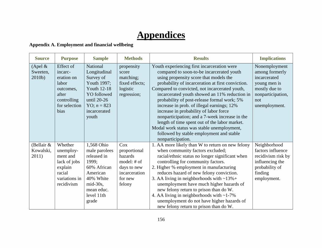
156
Appendices Appendix A. Employment and financial wellbeing
Source Purpose Sample Methods Results Implications
(Apel &
Sweeten,
2010b)
Effect of
incarc-
eration on
labor
outcomes,
after
controlling
for selection
bias
National
Longitudinal
Survey of
Youth 1997;
Youth 12-18
YO followed
until 20-26
YO; n = 823
incarcerated
youth
propensity
score
matching;
fixed effects;
logistic
regression;
Youth experiencing first incarceration were
compared to soon-to-be incarcerated youth
using propensity score that models the
probability of incarceration at first conviction.
Compared to convicted, not incarcerated youth,
incarcerated youth showed an 11% reduction in
probability of post-release formal work; 5%
increase in prob. of illegal earnings; 12%
increase in probability of labor force
nonparticipation; and a 7-week increase in the
length of time spent out of the labor market.
Modal work status was stable unemployment,
followed by stable employment and stable
nonparticipation.
Nonemployment
among formerly
incarcerated
young men is
mostly due to
nonparticipation,
not
unemployment.
(Bellair &
Kowalski,
2011)
Whether
unemploy-
ment and
lack of jobs
explain
racial
variations in
recidivism
1,568 Ohio
male parolees
released in
1999;
60% African
American
40% White
mid-30s,
mean educ.
level 11th
grade
Cox
proportional
hazards
model: # of
days to new
incarceration
for new
felony
1. AA more likely than W to return on new felony
when community factors excluded;
racial/ethnic status no longer significant when
controlling for community factors.
2. Higher % employment in manufacturing
reduces hazard of new felony conviction.
3. AA living in neighborhoods with ~13%+
unemployment have much higher hazards of
new felony return to prison than do W.
4. AA living in neighborhoods with ~1-7%
unemployment do not have higher hazards of
new felony return to prison than do W.
Neighborhood
factors influence
recidivism risk by
influencing the
probability of
finding
employment.
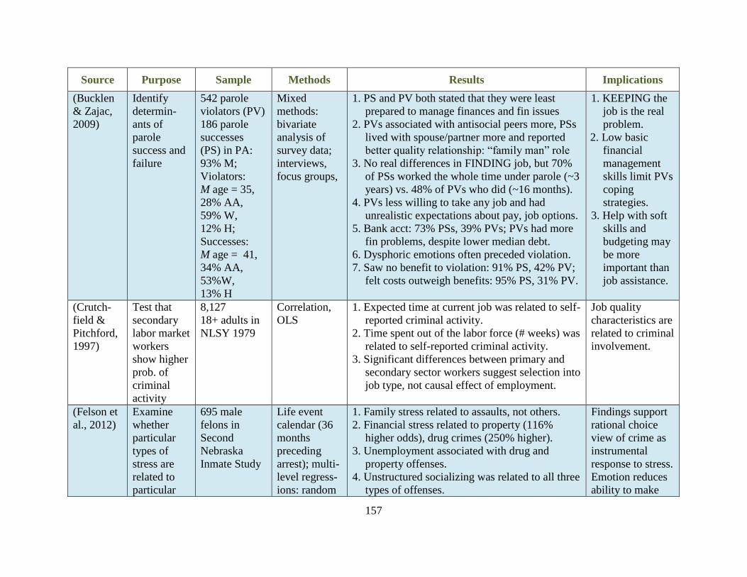
157
Source Purpose Sample Methods Results Implications
(Bucklen
& Zajac,
2009)
Identify
determin-
ants of
parole
success and
failure
542 parole
violators (PV)
186 parole
successes
(PS) in PA:
93% M;
Violators:
M age = 35,
28% AA,
59% W,
12% H;
Successes:
M age = 41,
34% AA,
53%W,
13% H
Mixed
methods:
bivariate
analysis of
survey data;
interviews,
focus groups,
1. PS and PV both stated that they were least
prepared to manage finances and fin issues
2. PVs associated with antisocial peers more, PSs
lived with spouse/partner more and reported
better quality relationship: “family man” role
3. No real differences in FINDING job, but 70%
of PSs worked the whole time under parole (~3
years) vs. 48% of PVs who did (~16 months).
4. PVs less willing to take any job and had
unrealistic expectations about pay, job options.
5. Bank acct: 73% PSs, 39% PVs; PVs had more
fin problems, despite lower median debt.
6. Dysphoric emotions often preceded violation.
7. Saw no benefit to violation: 91% PS, 42% PV;
felt costs outweigh benefits: 95% PS, 31% PV.
1. KEEPING the
job is the real
problem.
2. Low basic
financial
management
skills limit PVs
coping
strategies.
3. Help with soft
skills and
budgeting may
be more
important than
job assistance.
(Crutch-
field &
Pitchford,
1997)
Test that
secondary
labor market
workers
show higher
prob. of
criminal
activity
8,127
18+ adults in
NLSY 1979
Correlation,
OLS
1. Expected time at current job was related to self-
reported criminal activity.
2. Time spent out of the labor force (# weeks) was
related to self-reported criminal activity.
3. Significant differences between primary and
secondary sector workers suggest selection into
job type, not causal effect of employment.
Job quality
characteristics are
related to criminal
involvement.
(Felson et
al., 2012)
Examine
whether
particular
types of
stress are
related to
particular
695 male
felons in
Second
Nebraska
Inmate Study
Life event
calendar (36
months
preceding
arrest); multi-
level regress-
ions: random
1. Family stress related to assaults, not others.
2. Financial stress related to property (116%
higher odds), drug crimes (250% higher).
3. Unemployment associated with drug and
property offenses.
4. Unstructured socializing was related to all three
types of offenses.
Findings support
rational choice
view of crime as
instrumental
response to stress.
Emotion reduces
ability to make
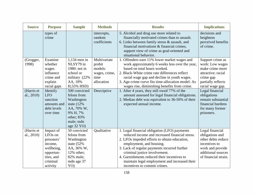
158
Source Purpose Sample Methods Results Implications
types of
crime
intercepts,
random
coefficients
5. Alcohol and drug use more related to
financially motivated crimes than to assault.
6. Links between family stress & assault, and
financial motivations & financial crimes,
support view of crime as goal-oriented and
situational behavior.
decisions and
heightens
perceived benefits
of crime.
(Grogger,
1998)
Examine
whether
wages
influence
crime and
explain
racial gaps
1,134 men in
NLSY79 in
1980: not in
school or
military (22%
AA, 18%
H,55% HSD)
Multivariate
probit
models:
wages, crime,
time
allocation
1. Offenders earn 11% lower market wages and
work approximately 6 weeks less over the year,
based on total hours worked.
2. Black-White crime rate differences reflect
racial wage gap and decline in youth wages.
3. Age-crime curve fits time-allocation model: As
wages rise, diminishing benefits from crime.
Support crime as
work: Low wages
make crime more
attractive; racial
crime gap
partially reflects
racial wage gap.
(Harris et
al., 2010)
Identify
LFO
sanction
amounts and
debt levels
over time
500 convicted
felons from
Washington
state (12%
AA, 70% W,
9% H, 7%
other; 83%
male; mdn
age 32 YO)
Descriptive 1. After 4 years, they still owed 77% of the
amount assessed for legal financial obligations.
2. Median debt was equivalent to 36-50% of their
expected annual income.
Legal financial
obligations
remain substantial
financial burdens
for many former
prisoners.
(Harris et
al., 2010)
Impact of
LFOs on
prisoners’
income,
wellbeing,
opportun-
ities, and
criminal
activity
50 convicted
felons from
Washington
state (52%
AA, 36% W,
12% other;
82% male;
mdn age 37
YO)
Qualitative 1. Legal financial obligation (LFO) payments
reduced income and increased financial stress.
2. LFOs impeded efforts to obtain education,
employment, and housing.
3. Lack of regular payments incurred further
criminal justice involvement.
4. Garnishments reduced their incentives to
maintain legal employment and increased their
incentives to commit crimes.
Legal financial
obligations and
other debts reduce
incentives to
work and provide
additional sources
of financial strain.
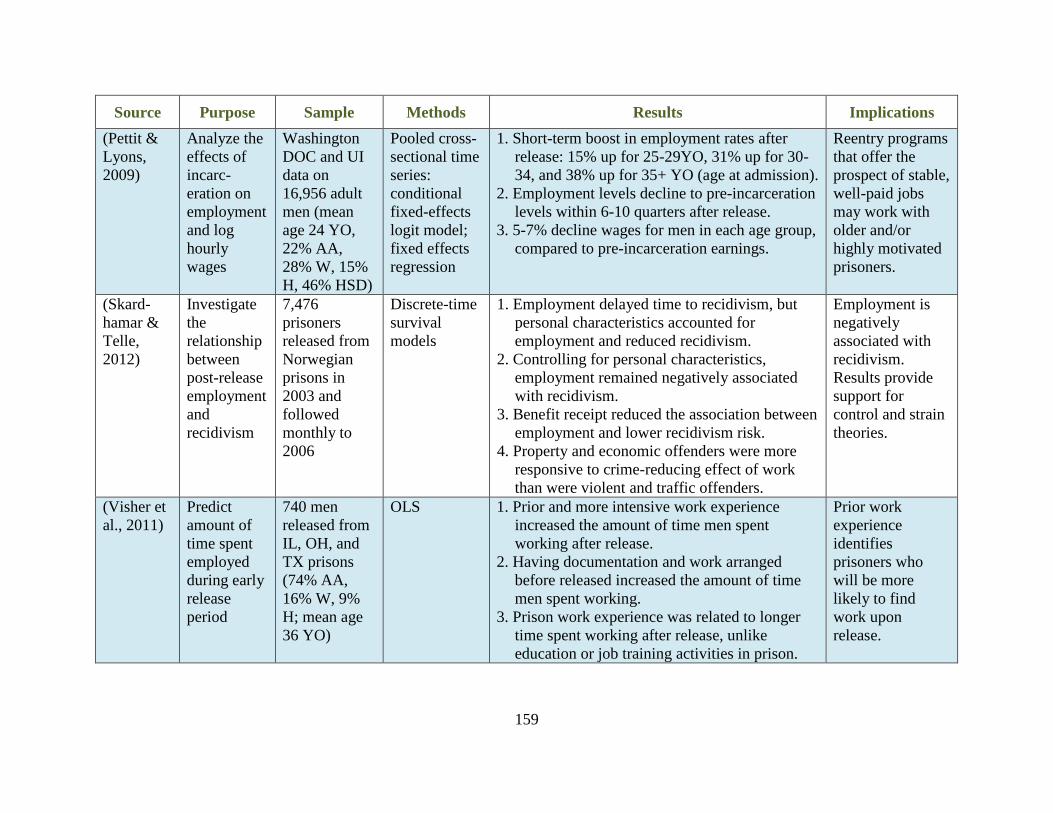
159
Source Purpose Sample Methods Results Implications
(Pettit &
Lyons,
2009)
Analyze the
effects of
incarc-
eration on
employment
and log
hourly
wages
Washington
DOC and UI
data on
16,956 adult
men (mean
age 24 YO,
22% AA,
28% W, 15%
H, 46% HSD)
Pooled cross-
sectional time
series:
conditional
fixed-effects
logit model;
fixed effects
regression
1. Short-term boost in employment rates after
release: 15% up for 25-29YO, 31% up for 30-
34, and 38% up for 35+ YO (age at admission).
2. Employment levels decline to pre-incarceration
levels within 6-10 quarters after release.
3. 5-7% decline wages for men in each age group,
compared to pre-incarceration earnings.
Reentry programs
that offer the
prospect of stable,
well-paid jobs
may work with
older and/or
highly motivated
prisoners.
(Skard-
hamar &
Telle,
2012)
Investigate
the
relationship
between
post-release
employment
and
recidivism
7,476
prisoners
released from
Norwegian
prisons in
2003 and
followed
monthly to
2006
Discrete-time
survival
models
1. Employment delayed time to recidivism, but
personal characteristics accounted for
employment and reduced recidivism.
2. Controlling for personal characteristics,
employment remained negatively associated
with recidivism.
3. Benefit receipt reduced the association between
employment and lower recidivism risk.
4. Property and economic offenders were more
responsive to crime-reducing effect of work
than were violent and traffic offenders.
Employment is
negatively
associated with
recidivism.
Results provide
support for
control and strain
theories.
(Visher et
al., 2011)
Predict
amount of
time spent
employed
during early
release
period
740 men
released from
IL, OH, and
TX prisons
(74% AA,
16% W, 9%
H; mean age
36 YO)
OLS 1. Prior and more intensive work experience
increased the amount of time men spent
working after release.
2. Having documentation and work arranged
before released increased the amount of time
men spent working.
3. Prison work experience was related to longer
time spent working after release, unlike
education or job training activities in prison.
Prior work
experience
identifies
prisoners who
will be more
likely to find
work upon
release.
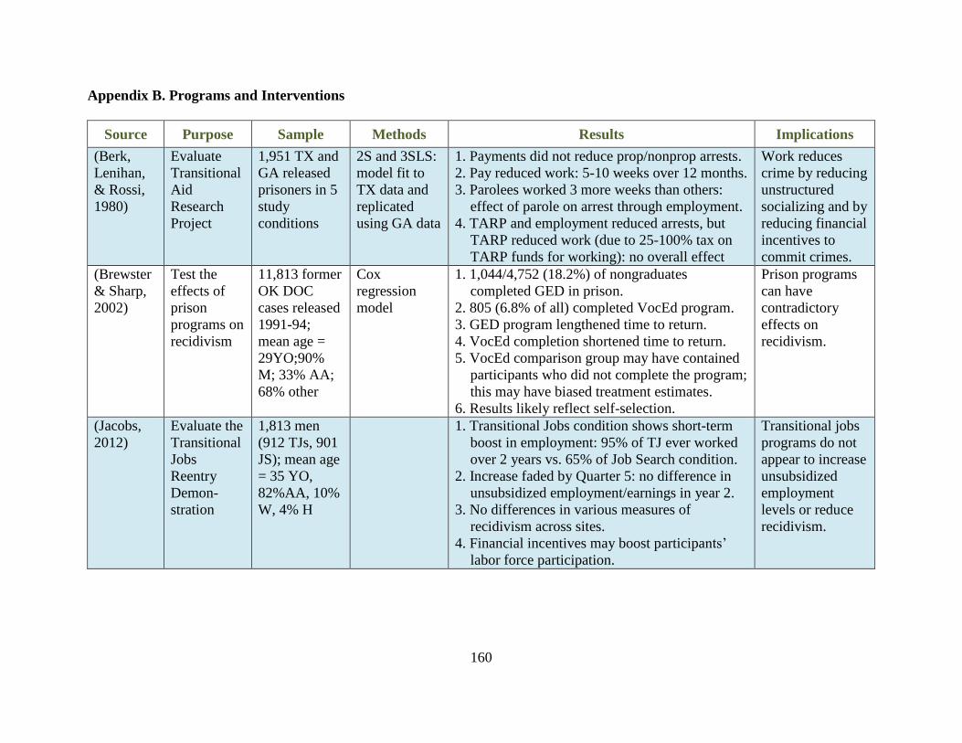
160
Appendix B. Programs and Interventions
Source Purpose Sample Methods Results Implications
(Berk,
Lenihan,
& Rossi,
1980)
Evaluate
Transitional
Aid
Research
Project
1,951 TX and
GA released
prisoners in 5
study
conditions
2S and 3SLS:
model fit to
TX data and
replicated
using GA data
1. Payments did not reduce prop/nonprop arrests.
2. Pay reduced work: 5-10 weeks over 12 months.
3. Parolees worked 3 more weeks than others:
effect of parole on arrest through employment.
4. TARP and employment reduced arrests, but
TARP reduced work (due to 25-100% tax on
TARP funds for working): no overall effect
Work reduces
crime by reducing
unstructured
socializing and by
reducing financial
incentives to
commit crimes.
(Brewster
& Sharp,
2002)
Test the
effects of
prison
programs on
recidivism
11,813 former
OK DOC
cases released
1991-94;
mean age =
29YO;90%
M; 33% AA;
68% other
Cox
regression
model
1. 1,044/4,752 (18.2%) of nongraduates
completed GED in prison.
2. 805 (6.8% of all) completed VocEd program.
3. GED program lengthened time to return.
4. VocEd completion shortened time to return.
5. VocEd comparison group may have contained
participants who did not complete the program;
this may have biased treatment estimates.
6. Results likely reflect self-selection.
Prison programs
can have
contradictory
effects on
recidivism.
(Jacobs,
2012)
Evaluate the
Transitional
Jobs
Reentry
Demon-
stration
1,813 men
(912 TJs, 901
JS); mean age
= 35 YO,
82%AA, 10%
W, 4% H
1. Transitional Jobs condition shows short-term
boost in employment: 95% of TJ ever worked
over 2 years vs. 65% of Job Search condition.
2. Increase faded by Quarter 5: no difference in
unsubsidized employment/earnings in year 2.
3. No differences in various measures of
recidivism across sites.
4. Financial incentives may boost participants’
labor force participation.
Transitional jobs
programs do not
appear to increase
unsubsidized
employment
levels or reduce
recidivism.
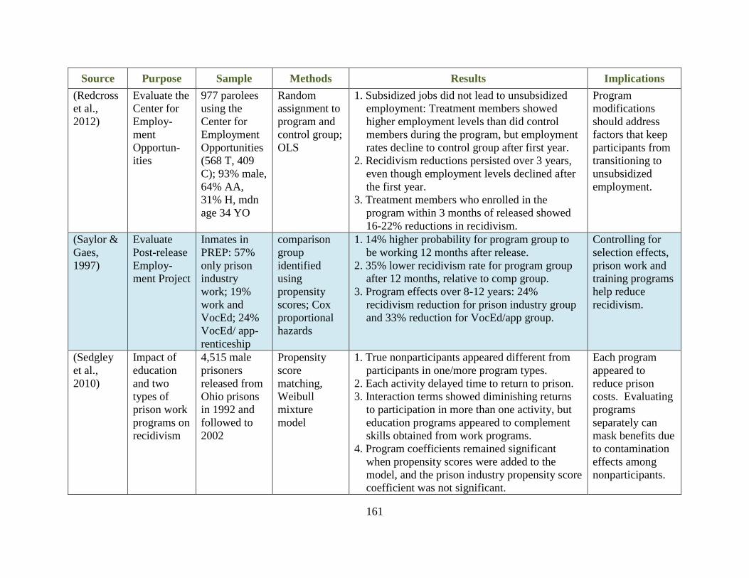
161
Source Purpose Sample Methods Results Implications
(Redcross
et al.,
2012)
Evaluate the
Center for
Employ-
ment
Opportun-
ities
977 parolees
using the
Center for
Employment
Opportunities
(568 T, 409
C); 93% male,
64% AA,
31% H, mdn
age 34 YO
Random
assignment to
program and
control group;
OLS
1. Subsidized jobs did not lead to unsubsidized
employment: Treatment members showed
higher employment levels than did control
members during the program, but employment
rates decline to control group after first year.
2. Recidivism reductions persisted over 3 years,
even though employment levels declined after
the first year.
3. Treatment members who enrolled in the
program within 3 months of released showed
16-22% reductions in recidivism.
Program
modifications
should address
factors that keep
participants from
transitioning to
unsubsidized
employment.
(Saylor &
Gaes,
1997)
Evaluate
Post-release
Employ-
ment Project
Inmates in
PREP: 57%
only prison
industry
work; 19%
work and
VocEd; 24%
VocEd/ app-
renticeship
comparison
group
identified
using
propensity
scores; Cox
proportional
hazards
1. 14% higher probability for program group to
be working 12 months after release.
2. 35% lower recidivism rate for program group
after 12 months, relative to comp group.
3. Program effects over 8-12 years: 24%
recidivism reduction for prison industry group
and 33% reduction for VocEd/app group.
Controlling for
selection effects,
prison work and
training programs
help reduce
recidivism.
(Sedgley
et al.,
2010)
Impact of
education
and two
types of
prison work
programs on
recidivism
4,515 male
prisoners
released from
Ohio prisons
in 1992 and
followed to
2002
Propensity
score
matching,
Weibull
mixture
model
1. True nonparticipants appeared different from
participants in one/more program types.
2. Each activity delayed time to return to prison.
3. Interaction terms showed diminishing returns
to participation in more than one activity, but
education programs appeared to complement
skills obtained from work programs.
4. Program coefficients remained significant
when propensity scores were added to the
model, and the prison industry propensity score
coefficient was not significant.
Each program
appeared to
reduce prison
costs. Evaluating
programs
separately can
mask benefits due
to contamination
effects among
nonparticipants.
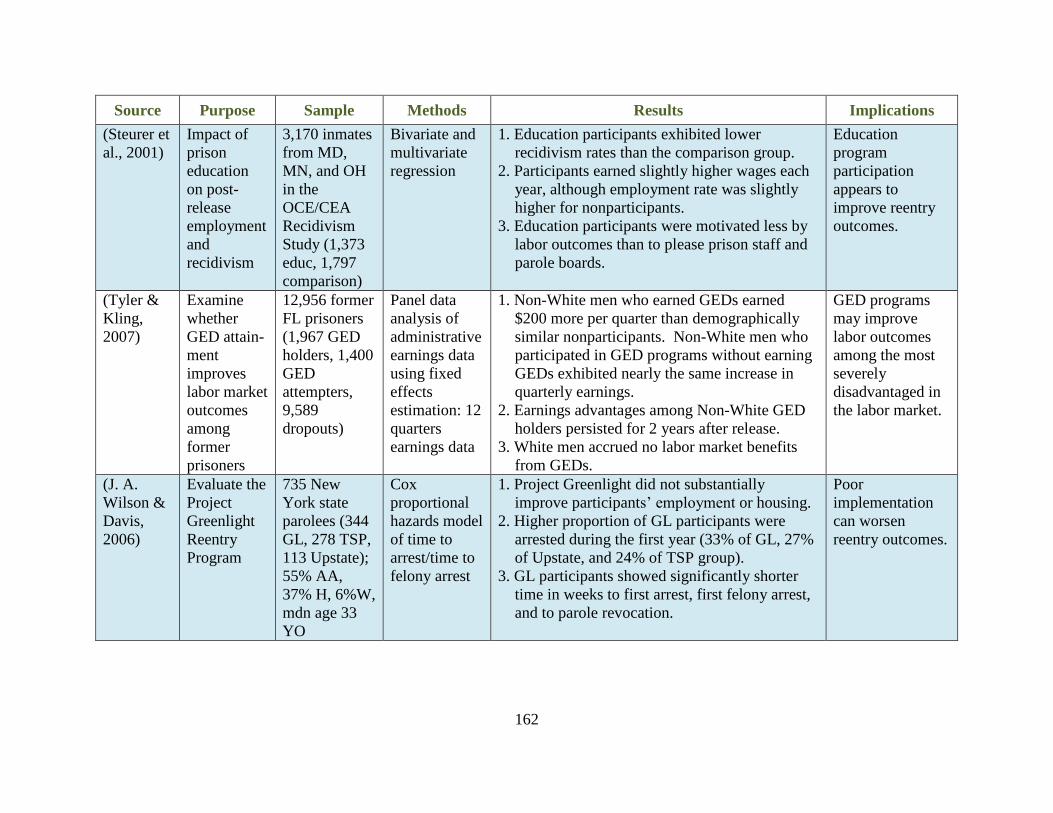
162
Source Purpose Sample Methods Results Implications
(Steurer et
al., 2001)
Impact of
prison
education
on post-
release
employment
and
recidivism
3,170 inmates
from MD,
MN, and OH
in the
OCE/CEA
Recidivism
Study (1,373
educ, 1,797
comparison)
Bivariate and
multivariate
regression
1. Education participants exhibited lower
recidivism rates than the comparison group.
2. Participants earned slightly higher wages each
year, although employment rate was slightly
higher for nonparticipants.
3. Education participants were motivated less by
labor outcomes than to please prison staff and
parole boards.
Education
program
participation
appears to
improve reentry
outcomes.
(Tyler &
Kling,
2007)
Examine
whether
GED attain-
ment
improves
labor market
outcomes
among
former
prisoners
12,956 former
FL prisoners
(1,967 GED
holders, 1,400
GED
attempters,
9,589
dropouts)
Panel data
analysis of
administrative
earnings data
using fixed
effects
estimation: 12
quarters
earnings data
1. Non-White men who earned GEDs earned
$200 more per quarter than demographically
similar nonparticipants. Non-White men who
participated in GED programs without earning
GEDs exhibited nearly the same increase in
quarterly earnings.
2. Earnings advantages among Non-White GED
holders persisted for 2 years after release.
3. White men accrued no labor market benefits
from GEDs.
GED programs
may improve
labor outcomes
among the most
severely
disadvantaged in
the labor market.
(J. A.
Wilson &
Davis,
2006)
Evaluate the
Project
Greenlight
Reentry
Program
735 New
York state
parolees (344
GL, 278 TSP,
113 Upstate);
55% AA,
37% H, 6%W,
mdn age 33
YO
Cox
proportional
hazards model
of time to
arrest/time to
felony arrest
1. Project Greenlight did not substantially
improve participants’ employment or housing.
2. Higher proportion of GL participants were
arrested during the first year (33% of GL, 27%
of Upstate, and 24% of TSP group).
3. GL participants showed significantly shorter
time in weeks to first arrest, first felony arrest,
and to parole revocation.
Poor
implementation
can worsen
reentry outcomes.
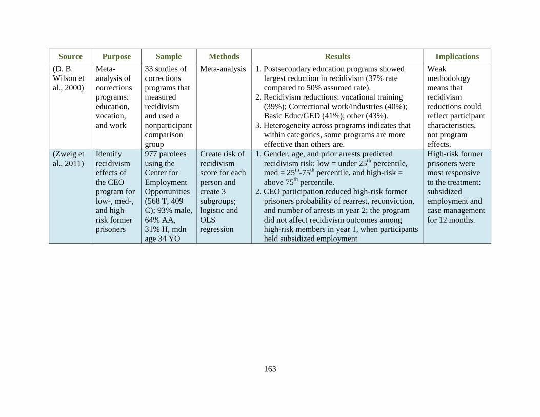
163
Source Purpose Sample Methods Results Implications
(D. B.
Wilson et
al., 2000)
Meta-
analysis of
corrections
programs:
education,
vocation,
and work
33 studies of
corrections
programs that
measured
recidivism
and used a
nonparticipant
comparison
group
Meta-analysis 1. Postsecondary education programs showed
largest reduction in recidivism (37% rate
compared to 50% assumed rate).
2. Recidivism reductions: vocational training
(39%); Correctional work/industries (40%);
Basic Educ/GED (41%); other (43%).
3. Heterogeneity across programs indicates that
within categories, some programs are more
effective than others are.
Weak
methodology
means that
recidivism
reductions could
reflect participant
characteristics,
not program
effects.
(Zweig et
al., 2011)
Identify
recidivism
effects of
the CEO
program for
low-, med-,
and high-
risk former
prisoners
977 parolees
using the
Center for
Employment
Opportunities
(568 T, 409
C); 93% male,
64% AA,
31% H, mdn
age 34 YO
Create risk of
recidivism
score for each
person and
create 3
subgroups;
logistic and
OLS
regression
1. Gender, age, and prior arrests predicted
recidivism risk: low = under 25th
percentile,
med = 25th
-75th
percentile, and high-risk =
above 75th
percentile.
2. CEO participation reduced high-risk former
prisoners probability of rearrest, reconviction,
and number of arrests in year 2; the program
did not affect recidivism outcomes among
high-risk members in year 1, when participants
held subsidized employment
High-risk former
prisoners were
most responsive
to the treatment:
subsidized
employment and
case management
for 12 months.

164
Appendix C. Group-Based Trajectory Model
This study models prior offending trajectories using annual arrest indicators for the years
preceding their SVORI prison term (Haviland & Nagin, 2005; Lattimore & Steffey, 2009; Nagin,
2005). The SVORI adult male sample is assumed to comprise a mixture of J underlying
trajectory groups. The composition of groups can be described by 𝑃(𝑌𝑖) = ∑ 𝜋𝑗𝑗 𝑃𝑗(𝑌𝑖), in
which 𝑌𝑖 is a longitudinal sequence of annual arrest counts from age at first arrest to the SVORI
term, 𝑃(𝑌𝑖) = the probability of 𝑌𝑖, 𝜋𝑗 = the probability of group j, and 𝑃𝑗(𝑌𝑖) = the probability
of 𝑌𝑖 given membership in group j. Conditional on group membership, subject i’s observations at
times 𝑡 = 1, 2, 3, … , 𝑇 are random independent variables. Probabilities of membership in each
group are modeled using a multinomial logit function 𝜋𝑗 = 𝑒𝜃𝑗 ∑ 𝑒𝜃𝑗𝐽1⁄ , where 𝜃1is set to 0 to
ensure that 𝜋𝑗is estimated such that men’s probability of membership in each trajectory group
falls between 0 and 1 (Jones & Nagin, 2007).
Men’s arrest indicators are assumed to follow the logistic distribution. The group-based
trajectory model (GTM) is depicted by the equation
ln(𝜆𝑖𝑡𝑗
) = 𝛽0𝑗
+ 𝛽1𝑗𝐴𝑔𝑒𝑖𝑡 + 𝛽2
𝑗𝐴𝑔𝑒𝑖𝑡
2 + 𝛽3𝑗𝐴𝑔𝑒𝑖𝑡
3 + 𝛽4𝑉𝑖𝑜𝑙𝑖𝑡 + 𝛽5𝑃𝑟𝑜𝑝𝑖𝑡 + 𝛽6𝐷𝑟𝑢𝑔𝑖𝑡 + 𝛽7𝑃𝑢𝑏𝑖𝑡,
in which 𝜆𝑖𝑡𝑗
= the expected number of arrests of subject i at time t in each year leading up the
SVORI status incarceration, given membership in group j, 𝐴𝑔𝑒𝑖𝑡 = subject i’s age at time t,
𝐴𝑔𝑒𝑖𝑡2 and 𝐴𝑔𝑒𝑖𝑡
3 = squared and cubed forms of 𝐴𝑔𝑒𝑖𝑡, and 𝑉𝑖𝑜𝑙𝑖𝑡, 𝑃𝑟𝑜𝑝𝑖𝑡, 𝐷𝑟𝑢𝑔𝑖𝑡, and 𝑃𝑢𝑏𝑖𝑡 are
each indicators of arrest type for arrests at time t. The model allows the vector of parameters
(𝛽𝑗) to vary freely across groups (Jones & Nagin, 2007).

165
The number of trajectories identified by the model can depend upon the length of the
observation period used to generate trajectories and the number of subjects in the sample (Nagin
& Tremblay, 2005). The GTM may identify groups even when all individuals in the sample are
homogenous with respect to criminal background and offending propensity (Brame et al., 2012;
Nagin, 2005; Nagin & Tremblay, 2005). By design, the model will fit the number of groups
specified, and it is the researcher’s responsibility to determine the appropriate number of groups
by comparing the fit of models identifying different numbers of groups (Brame et al., 2012).
The Bayesian (Schwarz) information criterion (BIC) is used to compare non-nested trajectory
group models, 𝐵𝐼𝐶 = −2 ln 𝐿 + 𝐾 ln 𝑛. The formula penalizes overfit models by increasing
their BIC value, so low BIC values identify models that provide better fit to the data than other
models. The most parsimonious model with an optimal BIC value is generally selected as the
best model (Brame et al., 2012; Nagin, 2005; Nagin & Tremblay, 2005).
Bayes theorem is used to generate for each individual a nonzero probability of
membership in each identified group j.
𝑃𝑟𝑜𝑏(𝑔𝑟𝑜𝑢𝑝 = 𝑗|𝑜𝑏𝑠𝑒𝑟𝑣𝑎𝑡𝑖𝑜𝑛 𝑖) =𝑓(𝑜𝑏𝑠𝑒𝑟𝑣𝑎𝑡𝑖𝑜𝑛 𝑖|𝑐𝑙𝑎𝑠𝑠 = 𝑗)𝑃𝑟𝑜𝑏(𝑐𝑙𝑎𝑠𝑠 𝑗)
∑ (𝑜𝑏𝑠𝑒𝑟𝑣𝑎𝑡𝑖𝑜𝑛 𝑖|𝑐𝑙𝑎𝑠𝑠 = 𝑗)𝐽𝑗=1 𝑃𝑟𝑜𝑏(𝑐𝑙𝑎𝑠𝑠 𝑗)
= 𝑤𝑖𝑗
These posterior predicted probabilities of group membership will be included in the propensity
score models as continuous measures (Jones & Nagin, 2007). For duration models, individuals
will be assigned to the group for which they have the highest posterior predicted probability of
membership. Predicted group membership will be used to examine whether missing data are
ignorable, for purposes of the longitudinal structural equation model sample using follow-up data
(Allison, 2012; Nagin, 2005; Piquero, Farrington, Nagin, & Moffitt, 2010).