Embed Size (px)
Citation preview

RESEARCHPAPER
Land-use drivers of forest fragmentationvary with spatial scaleLorenzo Cattarino1,2*, Clive A. McAlpine1,3 and Jonathan R. Rhodes1,3,4
1Landscape Ecology and Conservation Group,
School of Geography, Planning and
Environmental Management, The University
of Queensland, Brisbane, Qld 4072, Australia,2Australian Rivers Institute, Griffith University,
Nathan, Qld 4111, Australia, 3National
Environmental Research Program
Environmental Decisions Hub, The University
of Queensland, Brisbane, Qld 4072, Australia,4Australian Research Council Centre of
Excellence for Environmental Decisions, The
University of Queensland, Brisbane, Qld 4072,
Australia
ABSTRACT
Aim Improving our understanding of the drivers of forest fragmentation is fun-damental to mitigating the consequences of anthropogenic fragmentation for bio-diversity. Moreover, the impacts of fragmentation on biodiversity depend on thespatial scale at which fragmentation occurs. Therefore, understanding how theeffect of land use on fragmentation patterns varies across scales is critical to ensurethat fragmentation is managed at scales relevant to the ecology of target speciesor to land management. Here, we quantified the influence of land use on patternsof forest fragmentation at different scales using Queensland, Australia,as a case study.
Location North-eastern Australia.
Methods We combined fractal analysis with piecewise linear regression tomeasure patterns of forest fragmentation across a range of scales in 5309 landscapesof c. 50 km2, with different proportions of land used for cropping and grazing. Asignificant change in fragmentation patterns occurred at approximately 1 km2. Weused beta regression to quantify the impact of land use on the degree of fragmen-tation at scales finer and coarser than 1 km2.
Results The use of land for grazing tended to create more fragmented forestpatterns than use of land for cropping. This difference was more pronounced atcoarser than finer scales.
Main conclusions Our finding suggests that the choice of land use where con-servation actions, such as revegetation and retention of forest patches, are to beprioritized depends on the scale at which we measure fragmentation. This infor-mation contributes to reducing the risk of mismatches between the scale at whichfragmentation is managed and the scale at which fragmentation is measured, whichis often dictated by the scale of species movements or the scale of land management.Our finding also improves our capacity to discern between fragmentation patternsthat are typical of land-sharing and land-sparing conservation strategies, as spatialscale varies, thus aiding the implementation of land sparing and land sharing atscales relevant to biodiversity conservation and land management.
KeywordsAgriculture, Australia, fractal geometry, land sharing, land sparing, land-usechange, scale-dependent patterns, SLATS, thresholds, vegetation clearing.
*Correspondence: Lorenzo Cattarino, GriffithUniversity, Australian Rivers Institute, Nathan,Qld 4111, AustraliaE-mail: [email protected]
INTRODUCTION
Forest fragmentation, that is the breaking apart of forest as
opposed to a reduction in the amount of forest (i.e. forest
loss), is a key component of global change. Fragmentation is a
primary consequence of change in land use, such as agricultural
intensification, logging and urban development, and, at the
same time, is a main cause of the modification of natural
landscapes (Foley et al., 2005; Fischer & Lindenmayer, 2007).
Quantifying the impact of land use on the degree of dis-
aggregation of forest cover over large geographical extents
(‘macroecological’ fragmentation patterns; Brown, 1995) is
bs_bs_banner
Global Ecology and Biogeography, (Global Ecol. Biogeogr.) (2014)
© 2014 John Wiley & Sons Ltd DOI: 10.1111/geb.12187http://wileyonlinelibrary.com/journal/geb 1

necessary to understand the drivers of forest fragmentation
(Mertens & Lambin, 1997; Geist & Lambin, 2001; Lambin et al.,
2003), which is a fundamental issue for conservation (Sala et al.,
2000). Moreover, the impact of land use on fragmentation may
vary with spatial scale (Ewers & Laurance, 2006), with impor-
tant consequences for biodiversity (Cattarino et al., 2013).
Therefore, identifying the types of land use that drive forest
fragmentation at different scales is crucial for biodiversity con-
servation. However, there is currently little understanding of
how land use drives macroecological patterns of forest fragmen-
tation, and how this effect varies with spatial scale, despite a
recognition that land use is a major driver of fragmentation
(Riitters et al., 2002; Ewers & Laurance, 2006).
The impact of land use on patterns of forest fragmentation
depends on the spatial scale, or resolution, of the fragmentation
pattern, because different land uses create different fragmenta-
tion patterns at different scales. For example, urban development
and smallholder-based agriculture create forest patterns that are
more fragmented at fine than coarse scales (Ewers & Laurance,
2006; Girvetz et al., 2008), while clearing of large blocks of veg-
etation for large-scale farming tends to create forest patterns that
are more fragmented at coarse than fine scales (Fearnside, 2005).
Quantifying the impact of different land uses on patterns of
forest fragmentation at different scales is important for identify-
ing the drivers of fragmentation at each scale, and therefore the
conservation management actions that need to be implemented
to reduce fragmentation at each scale. For instance, better farm-
level management practices and land tenure reforms can be
employed to reduce fine-scale fragmentation, while broader
mechanisms, such as elimination of subsidies for large-scale
clearing, would be more suited to target coarse-scale fragmenta-
tion (Fearnside, 2005; Ewers & Laurance, 2006). Identifying the
scale at which to implement different land-use policies is impor-
tant to ensure that the scale at which fragmentation is managed
matches the scale of relevant ecological processes, such as the
scale of species dispersal, or the scale of land management (e.g.
local or regional administrative boundaries) (Pelosi et al., 2010;
Dudaniec et al., 2013). This is a critical issue for conservation,
because fragmentation at different scales has different effects on
biodiversity (Cattarino et al., 2013). Although previous studies
have measured forest fragmentation at different scales (Ewers &
Laurance, 2006), the relative effect of different land uses in
driving fragmentation patterns simultaneously at different scales
remains largely unexplored.
Understanding the link between land use and scale-
dependent fragmentation is important for implementing con-
servation strategies at scales relevant to the ecology of species
and to land management. Two contrasting conservation strat-
egies, land sharing and land sparing, have been proposed to
reconcile the conservation of biodiversity with agricultural land
use (Green et al., 2005). While land sparing consists of inten-
sively farming agricultural land and setting aside some land for
conservation, land sharing integrates agricultural production
and conservation on the same land by farming a larger area of
land at a lower intensity (Green et al., 2005). Driven by different
land uses, the two strategies create different fragmentation pat-
terns, which represent the extremes in a continuum of degrees
of fragmentation. While land sparing tends to create less frag-
mented patterns, by physically separating agricultural land (e.g.
crops) from land for conservation, land sharing creates more
fragmented patterns, by subdividing the landscape into a hete-
rogeneous mix of different land uses (e.g. crops, pasture and
forest) (Fischer et al., 2008). Land sharing and land sparing can
also be implemented at different scales. Matching the scale at
which land sharing and land sparing are implemented with the
scale at which species move, or at which land-use management
is conducted, is important for achieving effective outcomes for
biodiversity conservation and land management (Phalan et al.,
2011). However, avoiding scale mismatches requires us to first
understand whether land sparing becomes land sharing, or vice
versa, as scale varies (Phalan et al., 2011). Following Fischer’s
framework, this involves quantifying whether land use drives
changes in the degree of fragmentation across scales. While scale
is becoming an important aspect of the land sparing/land
sharing debate (Phalan et al., 2011; Chandler et al., 2013), how
different land uses drive patterns of land sharing and land
sparing at different scales has received relatively little attention.
In this study we address the following question: to what extent
does land use drive patterns of forest fragmentation and how
does this effect vary across spatial scales? To answer this ques-
tion, we conducted a multiscale analysis of forest fragmentation
for Queensland, Australia. The region, which covers an area
of 1.1 million km2, has undergone extensive deforestation
since European settlement of Australia (Seabrook et al., 2006;
McAlpine et al., 2009). We adopted a regression-based approach
derived from fractal geometry (Mandelbrot, 1983) to quantify
how patterns of forest fragmentation at different scales vary
with the proportion of different land uses. We show that the
impact of land use on patterns of forest fragmentation depends
on the scale at which we measure fragmentation. This suggests
that the choice of land use where conservation actions need to
be prioritized depends on the scale at which we are interested in
measuring fragmentation, such as the scale at which species of
conservation interest move or the scale at which land manage-
ment is conducted. This information will help to improve our
capacity to match the scale at which fragmentation should be
managed with the scale relevant to biodiversity conservation or
land management.
MATERIALS AND METHODS
Study region
We focused on seven Queensland bioregions from the interim
biogeographic regionalization for Australia (Thackway &
Cresswell, 1995): Brigalow Belt North, Brigalow Belt South,
Central Mackay Coast, Desert Uplands, Mulga Lands, South
Eastern Queensland and Wet Tropics (Fig. 1). The bioregions
cover an area of c. 72 million hectares. The climate ranges from
tropical to subtropical and semi-arid, with rainfall concentrated
in the north and central parts (Sattler & Williams, 1999). The
main vegetation communities include rain forest species in
L. Cattarino et al.
Global Ecology and Biogeography, © 2014 John Wiley & Sons Ltd2
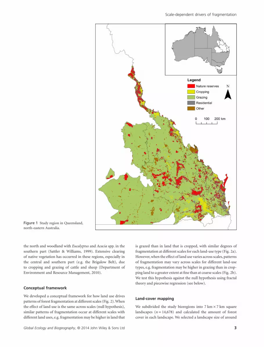
the north and woodland with Eucalyptus and Acacia spp. in the
southern part (Sattler & Williams, 1999). Extensive clearing
of native vegetation has occurred in these regions, especially in
the central and southern part (e.g. the Brigalow Belt), due
to cropping and grazing of cattle and sheep (Department of
Environment and Resource Management, 2010).
Conceptual framework
We developed a conceptual framework for how land use drives
patterns of forest fragmentation at different scales (Fig. 2). When
the effect of land use is the same across scales (null hypothesis),
similar patterns of fragmentation occur at different scales with
different land uses, e.g. fragmentation may be higher in land that
is grazed than in land that is cropped, with similar degrees of
fragmentation at different scales for each land-use type (Fig. 2a).
However, when the effect of land use varies across scales, patterns
of fragmentation may vary across scales for different land-use
types, e.g. fragmentation may be higher in grazing than in crop-
ping land to a greater extent at fine than at coarse scales (Fig. 2b).
We test this hypothesis against the null hypothesis using fractal
theory and piecewise regression (see below).
Land-cover mapping
We subdivided the study bioregions into 7 km × 7 km square
landscapes (n = 14,678) and calculated the amount of forest
cover in each landscape. We selected a landscape size of around
Figure 1 Study region in Queensland,north-eastern Australia.
Scale-dependent drivers of fragmentation
Global Ecology and Biogeography, © 2014 John Wiley & Sons Ltd 3

5000 ha to make sure we would capture the effect on fragmen-
tation patterns of processes operating within individual agricul-
tural properties (average size 7000 ha; Seabrook et al., 2008),
because vegetation clearing in Australia occurs mainly within
properties (Seabrook et al., 2007, 2008). Forest cover data for the
year 2009 were derived from the Statewide Landcover and Trees
Study (SLATS), derived from Landsat Thematic Mapper (TM)
and Enhanced Thematic Mapper Plus (ETM+) satellite imagery
(pixel size 30 m) (Department of Environment and Resource
Management, 2010). SLATS has mapped woody foliage pro-
jected cover (FPC) data over the entire state of Queensland
between the years 1999 and 2009. For our analysis, we only
considered values of FPC greater than 11% to be forest, which
according to the Kyoto Protocol corresponds to the definition of
forest cover (i.e. trees and shrubs above 2 m and approximately
20% canopy cover) (Kitchen et al., 2010).
For each landscape, we calculated the proportion of each
pixel occupied by cropping and grazing land uses, as these are
the major drivers of forest fragmentation in Queensland
(Department of Environment and Resource Management,
2010). Land-use data, in the form of a raster layer (pixel size
1000 m), were obtained from Land Use of Australia, version 4,
2005–06 (Australian Bureau of Agricultural and Resource
Economics and Sciences, 2010). As clearing of vegetation might
not be representative in nature reserves, we excluded them from
the analysis. At the end of the mapping process, a total of 12,134
landscapes (7 km × 7 km) were identified (Table 1).
Measure of forest fragmentation
We used fractal geometry (Mandelbrot, 1983) to measure pat-
terns of forest fragmentation at different scales. Fractal geom-
etry has been widely used to model the spatial heterogeneity of
resource distributions in real landscapes (Milne, 1992; Palmer,
1992; With, 1997). We define p(m,L) as the probability of
finding m forest pixels in a squared window of size L. According
to fractal theory, when the degree of forest fragmentation is the
same across scales, the slope of the log–log regression line of
the expectation of p(m,L), measured over a range of scales (i.e.
resolutions), versus scale is constant (Milne, 1992). The steeper
the slope, the more fragmented the forest pattern. However,
when the degree of fragmentation changes across scales, the
slope of the log–log regression line varies along the line. The
change in slope is often assumed to occur as a threshold, or
breakpoint. The number of breakpoints reflects the number of
times the degree of fragmentation varies across scales. We can
interpret the location of the breakpoint(s) as the scale at which
there is a transition between the degree of fragmentation at fine
scales (the slope before the breakpoint) and the degree of frag-
mentation at coarser scales (the slope after the breakpoint).
We constructed a probability distribution of the mean
amount of forest in a landscape, p(m,L), by counting the total
number of forest pixels, m, in a moving squared window of
length L centred on each forest pixel of our sample landscapes.
The probabilities satisfy the condition
Figure 2 Conceptual framework of how land uses drive patterns of forest fragmentation at different scales. The diagram shows differentspatial configurations of forest cover at coarse (large grey quadrats) and fine (small grey quadrats) scales, for cropping and grazing land use.When the effect of land use is the same across scales (null hypothesis), similar patterns of fragmentation occurs at different scales fordifferent land uses (a). However, when the effect of land use varies across scales, patterns of fragmentation may vary across scales fordifferent land uses (b).
Table 1 Number of landscapes in each bioregion.
Bioregion
No. of
landscapes
Brigalow Belt South 3903
Brigalow Belt North 2008
SEQ 1055
Mackay Central Coast 174
Wet Tropics 135
Mulga Land 3638
Desert Uplands 1221
Total 12,134
L. Cattarino et al.
Global Ecology and Biogeography, © 2014 John Wiley & Sons Ltd4

p m Lm
N L
,( ) ==
( )
∑1
1 (1)
which ensures that the sum of the probabilities of finding m
forest pixels in a window of length L is 1, where N(L) is the
number of different m values obtained for windows of size L.
Measurement of p(m,L) provides a statistic that describes the
aggregation of forest cover in a patch mosaic (Milne, 1992).
In order to minimize the effects of landscape boundaries, we
treated a landscape as a torus, where the bottom row adjoins
the top row and the right-most column adjoins the left-most
column (With et al., 1997).
The expectation, M(L), of p(m,L) was then calculated as
follows:
M L m p m Lm
N L
( ) = ( )=
( )
∑ , .1
(2)
Based on a general property of fractal objects (Mandelbrot,
1983), the expected average amount of forest, M(L), varies with
the length of the squared window, L, through the power-law
relationship M(L) = kLD, where k is a constant and D is the
fractal dimension of the land-cover pattern, which represents
the degree of forest fragmentation. The value of D, which ranges
from 1 to 2, increases as the degree of fragmentation increases
(Milne, 1992). We selected 100 values of L, ranging from 1 to 280
pixels, where L = 280 corresponds to the size of a landscape.
For each landscape, we calculated the expectation, M(L), for
each value of L. To reduce computational time, we calculated
M(L) for a random sample of 10% of the total number of forest
pixels in each landscape. The analysis was run for all land-
scapes in each bioregion. However, for those bioregions with a
large number of landscapes (> 1000), a random sample of 1000
landscapes was selected, limiting the analysis to a total of 5309
landscapes.
Statistical analysis
For each landscape, we modelled the mean M(L) as a function of
window length L. To investigate whether forest fragmentation
varied across scales, we tested for the existence of breakpoints in
the log–log regression line using linear and piecewise regression.
We fitted two alternative regression models: (1) a ‘null’ model –
linear regression (McCullagh & Nelder, 1989) – which refers to
the case where there is no difference in patterns of fragmenta-
tion across scales; and (2) a ‘threshold’ model – piecewise regres-
sion (Muggeo, 2003) – which refers to the case where different
patterns of fragmentation occurs at different scales. To assess the
significance of a breakpoint, we fitted threshold models for a
number of breakpoints ranging from 1 to 10. For each model,
we then calculated the Akaike information criterion (AIC) and
selected the model with the lowest AIC as the most parsi-
monious one, based on an information-theoretic approach
(Burnham & Anderson, 2002). A preliminary inspection
revealed that the threshold model with one breakpoint received
very strong support relative to the null model and the threshold
models with more than one breakpoint (Table 2). We assumed
that different degrees of fragmentation occurred at coarse and
fine spatial scales (i.e. coarse-scale and fine-scale fragmentation)
in landscapes for which the threshold model was the most par-
simonious one. For those models, we estimated the location of
the breakpoint and the fractal dimension of the forest patterns
on either side of the breakpoint.
We then applied beta regression models to quantify the
effect of land use in driving patterns of forest fragmentation at
coarse and fine scales. Beta regression is a common approach for
modelling variables bounded in the range 0–1, such as propor-
tions or rates (Ferrari & Cribari-Neto, 2004). We built two sepa-
rate models and fitted them to the degree of coarse-scale and
fine-scale fragmentation, which were treated as dependent vari-
ables. A value of 1 was subtracted from the raw values of the
dependent variables (bounded between 1 and 2) to fit the 0–1
range of the beta regression models. In order to include land use
as an independent variable, we first tested whether the pro-
portions of land used for cropping and grazing were correlated
using a Spearman’s correlation. The proportion of land used
for cropping was found to be negatively correlated with the
proportion of grazing land (r = −0.57). We therefore interpreted
the effect of cropping on patterns of fragmentation at different
scales to be the inverse of the effect of grazing, and discarded the
proportion of cropping land use from the models to reduce
collinearity. We also controlled for the effect of the amount of
Table 2 Total number of fitted models, proportion of threshold models with one breakpoint that had a better fit (based on Akaikeinformation criterion values) than the other models (null model and threshold models with more than one breakpoint), average values ofcoarse-scale (D1) and fine-scale (D2) fragmentation and breakpoint location (Bp), with standard error (SE), for each bioregion.
Bioregion
Total
models
Best threshold
models D1 (SE) D2 (SE) Bp (SE)
Brigalow Belt South 1000 0.989 1.700 (0.007) 1.863 (0.006) 3.684 (0.033)
Brigalow Belt North 1000 0.996 1.780 (0.006) 1.858 (0.004) 3.763 (0.029)
South East Queensland 1000 0.994 1.908 (0.004) 1.900 (0.003) 3.715 (0.033)
Mackay Central Coast 174 0.994 1.815 (0.013) 1.937 (0.005) 3.480 (0.075)
Wet Tropics 135 0.993 1.726 (0.018) 1.935 (0.005) 3.391 (0.076)
Mulga Land 1000 0.982 1.815 (0.005) 1.873 (0.005) 3.844 (0.031)
Desert Uplands 1000 0.988 1.843 (0.007) 1.879 (0.004) 3.379 (0.037)
Scale-dependent drivers of fragmentation
Global Ecology and Biogeography, © 2014 John Wiley & Sons Ltd 5

forest cover (Gardner et al., 1987) by including the amount of
forest cover as an independent variable in the models. We fitted
the following model:
logit Xμ βi i( ) = ′ (3)
where μi is the degree of coarse-scale or fine-scale fragmentation
in landscape i, β is a vector of regression coefficients and Xi is a
vector of independent variables. For each dependent variable,
we constructed a set of five competing models using combina-
tions of all the explanatory variables.
For each dependent variable, model comparison was done
using an information-theoretic approach (Burnham &
Anderson, 2002). We calculated the goodness of fit of each model
using R2. To reduce model selection bias, we calculated model
average parameter estimates, and the unconditional standard
error of each estimate, from all the fitted models. We also esti-
mated the relative importance of each explanatory variable by
ranking them according to the sum of the Akaike weights (Σwi) of
the models in which the variable occurred. The larger the sum of
the Akaike weights, the higher the importance of each variable is
relative to the other variables. All statistical analyses were con-
ducted using R version 2.14.0 (R Development Core Team, 2013).
RESULTS
In most of the landscapes, forest fragmentation was higher at
fine than at coarser scales (Fig. 3). This was more evident for
lower than higher amounts of forest cover (P < 0.5) and for
grazing than cropping land use. The average value of the
degree of coarse-scale fragmentation (D1 = 1.798 ± 0.009) was
significantly different from the average value of the degree
of fine-scale fragmentation (D2 = 1.892 ± 0.005) (Mann–
Whitney–Wilcoxon test, W = 130, P = 0.015) (Table 2). The
average value of the location of the breakpoint was 3.608 ± 0.045
(Table 2), which corresponded to c. 100 ha (1 km2).
The amount of forest cover and the proportion of grazing
land use were both included in the most parsimonious model
for coarse-scale fragmentation (AIC = −350.8, R2 = 0.71;
Table 3). However, the second best model also included the
interaction between the amount of forest cover and the pro-
portion of grazing land use (ΔAIC = 1.9). The sum of the Akaike
weights showed that the amount of forest cover and the propor-
tion of grazing land use were considerably more influential than
their interaction in affecting coarse-scale fragmentation (Fig. 4).
The most parsimonious model for fine-scale fragmentation
included the amount of forest cover, the proportion of grazing
land use and their interaction (AIC = −224.2, R2 = 0.84;
Table 4). The sum of the Akaike weights showed that the
amount of forest cover and the proportion of grazing land use
were more influential than their interaction in affecting both
coarse-scale and fine-scale fragmentation (Fig. 4).
The model-averaged coefficients showed that as the propor-
tion of grazing land use increased, forest fragmentation increased
(Fig. 5). The coefficients also indicated that, as the pro-
portion of cropping land use increased, forest fragmentation
declined, due to the negative correlation between cropping and
grazing land use. However, as the proportion of grazing land use
increased, forest fragmentation increased more at coarser than at
Figure 3 Bar chart showing the average degree of coarse-scaleand fine-scale fragmentation (± 1 SE), in landscapes with differentdominant land uses, for different amounts of forest cover (p). Theterm ‘cropping’ indicates landscapes with a higher proportion ofcropped land than grazed land, and vice versa for ‘grazing’.
Table 3 Summary of beta-regression models (model rank andvariables, Akaike information criterion (AIC) values, ΔAIC, AICweights and R2 goodness of fit) of coarse-scale fragmentation, asa function of the amount of forest cover (p), the proportion ofgrazing land use (g) and their interaction (pg).
Model
rank Variables AIC ΔAIC
AIC
weight (wi) R2
1 p + g −350.8 0.0 0.673 0.71
2 p + g + pg −348.9 1.9 0.259 0.71
3 p −346.2 4.6 0.067 0.71
4 g −59.6 291.2 0.000 0.00
5 Only intercept −58.7 292.2 0.000 0.00
Table 4 Summary of beta-regression models (model rank andvariables, Akaike information criterion (AIC) values, ΔAIC, AICweights and R2 goodness of fit) of fine-scale fragmentation, as afunction of the amount of forest cover (p), the proportion ofgrazing land use (g) and their interaction (pg).
Model
rank Variables AIC ΔAIC
AIC
weight (wi) R2
1 p + g + pg −224.2 0.0 0.539 0.84
2 p + g −223.9 0.3 0.459 0.81
3 p −212.3 11.9 0.001 0.85
4 g −14.5 209.7 0.000 0.03
5 Only intercept −16.3 207.9 0.000 0.00
L. Cattarino et al.
Global Ecology and Biogeography, © 2014 John Wiley & Sons Ltd6

finer scales. Moreover, as the amount of forest cover increased,
increasing the proportion of grazing land use reduced forest
fragmentation. However, this effect was greater at coarser than at
finer scales.
DISCUSSION
Our study contributes to improving the understanding of the
drivers of scale-dependent land-use change in human-modified
landscapes (Lambin et al., 2003; Ewers & Laurance, 2006). We
found that land use is a more important driver of fragmentation
at coarse spatial scales than at fine scales. Our findings suggest
that the choice of land use where conservation actions, such as
revegetation and retention of forest patches to reduce forest
fragmentation, are to be prioritized depends on the scale at
which we measure fragmentation patterns. This information
may improve our ability to match the scale at which fragmen-
tation is managed with the scale relevant to the ecology of
species of conservation concern or existing land management
(Pelosi et al., 2010). This is crucial for conservation, because
fragmentation at different scales has different effects on biodi-
versity (Cattarino et al., 2013). Our study also improves the
capacity to discern between fragmentation patterns that are
typical of different conservation strategies, i.e. land sharing or
land sparing, across different scales. This may aid the implemen-
tation of land sharing and land sparing at scales relevant to
biodiversity conservation and land management.
Drivers of fragmentation at different scales
In our study, grazing and cropping drive different fragmentation
patterns at fine and coarse scales. A transition between fragmen-
tation patterns at fine and coarse scales occurred at approxi-
mately 100 ha (1 km2), which is much smaller than the average
property size in Queensland, i.e. 7000 ha (Seabrook et al., 2008).
Our finding suggests that different drivers of clearing of native
vegetation determine different fragmentation patterns between
and within agricultural fields, in landscapes modified by differ-
ent land uses. For example, Seabrook et al. (2007) found that
cleared areas within agricultural properties were clustered
Figure 4 Relative importance of theexplanatory variables, for the modelsfor fine-scale and coarse-scalefragmentation, based on the sum of theAkaike weights (Σwi) of the modelswhere the variable occurred.
Figure 5 Coefficient averages from betaregression models explaining variationsin the degree of coarse-scale andfine-scale fragmentation, as a function ofthe amount of forest cover, theproportion of land used for grazing andtheir interaction.
Scale-dependent drivers of fragmentation
Global Ecology and Biogeography, © 2014 John Wiley & Sons Ltd 7

around particular landscape features (e.g. riparian vegetation)
and vegetation classes (e.g. dry eucalypt forests), which are indi-
cators of high soil productivity. This may explain why, at coarse
scales, cropping creates less fragmented patterns than grazing:
the spatial clustering of vegetation clearing in areas of high soil
fertility has a greater effect on the physical separation of agri-
cultural land (e.g. crop fields) from remnant vegetation in
cropped areas than in grazed ones.
At finer scales, such as within individual agricultural fields,
the processes driving clearing of vegetation in cropped and
grazed land are different from those at coarser scales. The
intense removal of standing native vegetation within agricul-
tural fields, through the use of agricultural machinery for crop
cultivation and irrigation (e.g. ploughing, sowing, harvest-
ing, irrigation systems) creates less fragmented patterns than
grazing, as remnant vegetation tends to be clumped in linear
strips and patches between cropped areas (Maron & Fitzsimons,
2007; Smith et al., 2013). On the other hand, clearing of isolated
patches of vegetation is less intense within grazed properties,
where all vegetation within an area of production is not
necessarily removed and regrowth of vegetation is common
(Fensham, 1997; Smith et al., 2013), thus creating more frag-
mented forest patterns than in cropped properties.
Interestingly, the breakpoint location we found here is smaller
than that reported by Ewers & Laurance (2006) for the Brazilian
Amazon (c. 1200 ha). Therefore, the scale at which there is a
transition between the impacts of different drivers of fragmen-
tation is coarser in Brazil than in Australia. This may be due to
different socio-economic factors. In Brazil, large-scale clearing,
mainly for cattle ranching, is a major source of deforestation,
and is a legacy of poor environmental policies and government
subsidies (Fearnside, 2005). The low fertility of forest soils has
also forced farmers to clear large areas of land to maintain
productivity. Moreover, agricultural properties are, on average,
larger than 10,000 ha, which makes coarse-scale fragmentation
patterns sensitive to macroeconomic factors, such as interest
rates and land prices (Walker et al., 2000; Fearnside, 2001). In
Queensland, on the other hand, clearing tends to be more local-
ized, as a result of stronger vegetation management policies, and
to occur more on fertile than infertile soil, and is also driven by
finer-scale mechanisms such as smaller property sizes and the
responses of individual land holders to vegetation management
policies (McAlpine et al., 2002; Seabrook et al., 2007, 2008).
These differences suggest that the scales at which different pro-
cesses of land-use change drive different fragmentation patterns
are also different in different regions.
Approach and limitations
We identified three main caveats in our modelling approach.
First, we assumed that land use did not change over the period of
time during which the clearing occurred, because the patterns
of fragmentation measured here reflect the cumulative effects of
past clearing processes and not necessarily the effect of current
ones. Land use may have changed during the time when clearing
determined the observed fragmentation patterns, thus causing a
potential scale mismatch between the time when the clearing
occurred and the time when the land-use data were acquired
(2005–06). Nevertheless, since most of the clearing occurred
recently and in a relatively short period of time (1990–2004)
(Department of Environment and Resource Management,
2010), we believe our results are still robust, because land use
may have not changed considerably over the time when the
majority of the clearing occurred.
Second, we assumed the transition between the degree of
fragmentation at different scales to be abrupt, i.e. it exhibited
a threshold. A range of statistical models, including polyno-
mial regressions and generalized additive models (Hastie &
Tibshirani, 1990), could be used to capture the nonlinear behav-
iour of the relationship between the expected average amount of
forest M(L) and the value of scale L. However, our aim was not
to understand the nature of the transition, but rather to assess
whether there was any significant change in patterns of frag-
mentation at different scales.
Finally, although forest fragmentation is a scale-dependent
process, it is possible that we failed to detect patterns at very fine
scales due to the coarse resolution of our thematic maps (30 m).
For example, processes of land-use change, such as the develop-
ment of infrastructure and agricultural intensification, cause
the removal of individual trees and small patches of vegetation
within agricultural fields (Maron & Fitzsimons, 2007), that we
may not have captured in our analysis. Therefore, the coarse
resolution of vegetation data may have contributed to the
weaker effect of land use on fragmentation patterns at finer
than at coarser scales. Future research may benefit from the use
of land-cover maps derived from higher-resolution satellite
imagery (e.g. SPOT, Worldview, Lidar), which may help to iden-
tify finer patterns of fragmentation and their drivers of change.
Implications for conservation and land management
The different scale-dependent effects of land use on patterns of
forest fragmentation suggest that the choice of land use where
conservation actions to reduce fragmentation need to be imple-
mented depends on the scale at which fragmentation is meas-
ured. For example, if fragmentation is measured at coarse scales,
conservation should promote revegetation and habitat restora-
tion across multiple agricultural fields or small properties (Smith
et al., 2013) on grazing land more than on cropping land. If
fragmentation is measured at fine scales, management may still
need to target grazed land more than cropped land by
incentivizing best farm management practices within properties,
such as retention of patches of vegetation and scattered paddock
trees (Harper et al., 2012). However, the need for conservation
actions targeting grazing may be greater at coarser than finer
scales, as the difference between the impacts of different land uses
on fragmentation patterns is smaller at finer than at coarser
scales. Thus, our findings are likely to be relevant for the conser-
vation of species that move large distances, as they are particu-
larly affected by coarse-scale fragmentation (Cattarino et al.,
2013), and in the case of management across multiple planning
units, such as local government areas (Dudaniec et al., 2013).
L. Cattarino et al.
Global Ecology and Biogeography, © 2014 John Wiley & Sons Ltd8

Our study advances our capacity to discern between the forest
patterns typical of land-sharing and land-sparing conservation
strategies as spatial scale varies. This may help identify the land-
use type where agricultural policies to achieve land sparing and
land sharing at different spatial scales should be implemented
(Phalan et al., 2011). For example, at coarse scales, forest pat-
terns resemble those typical of land sharing (high fragmenta-
tion), more in grazing than in cropping land use, and those
more typical of land sparing (low fragmentation), more in crop-
ping than in grazing land use. This suggest that, at coarse scales,
agricultural policies to implement land sharing should be
applied to grazing rather than cropping land use, as we found
higher fragmentation in grazing than in cropping land use. This
would involve the adoption of sustainable farming practices, for
example fencing and rotational grazing, and favouring native
perennial ground cover (Dorrough et al., 2007). However, to
implement land sparing, cropping land use would be a more
suitable target for policies and legislative mechanisms than
grazing land use, due to the lower fragmentation found in crop-
ping than in grazing land use. This could be achieved through
the protection of large patches of intact vegetation and planned
yield intensification (Fischer et al., 2008). The need to prioritize
the implementation of different policies for different land-use
types is likely to be smaller at finer than at coarser scales, as a
consequence of the smaller effect of land use on fragmentation
patterns. By identifying the land uses where different agricul-
tural policies should be implemented, our study provides guide-
lines for implementing land sparing versus land sharing at scales
relevant to species ecology or land management.
ACKNOWLEDGEMENTS
We thank Martine Maron and three anonymous referees for
their helpful comments on an earlier version of the manuscript.
This research was conducted with the support of funding from an
Endeavour International Postgraduate Research Scholarship (LC),
the Australian Government’s National Environmental Research
Program (J.R. and C.M.), the Australian Research Council’s Centre
of Excellence for Environmental Decisions (J.R.) and the Austral-
ian Research Council (Grant No. FT100100338 to C.M.).
REFERENCES
Australian Bureau of Agricultural and Resource Economics
and Sciences (2010) Land use of Australia, version 4: 2005–06.
Available at: <http://data.daff.gov.au/anrdl/metadata_files/
pa_luav4g9abl07811a00.xml> (accessed 10 February 2010).
Brown, J.H. (1995) Macroecology. University of Chicago Press,
Chicago.
Burnham, K.P. & Anderson, D.R. (2002) Model selection
and multimodel inference: a practical information-theoretic
approach, 2nd edn. Springer-Verlag, New York.
Cattarino, L., McAlpine, C.A. & Rhodes, J.R. (2013) The conse-
quences of interactions between dispersal distance and reso-
lution of habitat clustering for dispersal success. Landscape
Ecology, 28, 1321–1334.
Chandler, R.B., King, D.I., Raudales, R., Trubey, R., Chandler, C.
& Chavez, V.J.A. (2013) A small-scale land-sparing approach
to conserving biological diversity in tropical agricultural land-
scapes. Conservation Biology, 27, 785–795.
Department of Environment and Resource Management
(2010) Land cover change in Queensland 2008–09: a Statewide
Landcover and Trees Study (SLATS) report. Department of
Environment and Resource Management, Brisbane.
Dorrough, J., Moll, J. & Crosthwaite, J. (2007) Can intensifica-
tion of temperate Australian livestock production systems
save land for native biodiversity? Agriculture, Ecosystems and
Environment, 121, 222–232.
Dudaniec, R.Y., Rhodes, J.R., Wilmer, J.W., Lyons, M., Lee, K.E.,
McAlpine, C.A. & Carrick, F.N. (2013) Using multilevel
models to identify drivers of landscape-genetic structure
among management areas. Molecular Ecology, 22, 3752–3765.
Ewers, R.M. & Laurance, W.F. (2006) Scale-dependent patterns
of deforestation in the Brazilian Amazon. Environmental
Conservation, 33, 203–211.
Fearnside, P.M. (2001) Land-tenure issues as factors in environ-
mental destruction in Brazilian Amazonia: the case of South-
ern Para. World Development, 29, 1361–1372.
Fearnside, P.M. (2005) Deforestation in Brazilian Amazonia:
history, rates, and consequences. Conservation Biology, 19,
680–688.
Fensham, R.J. (1997) Options for conserving large vegetation
remnants in the Darling Downs, South East Queensland. Con-
servation outside nature reserves (ed. by P. Hale and D. Lamb),
pp. 419–423. Centre for Conservation Biology, University of
Brisbane, Brisbane.
Ferrari, S.L.P. & Cribari-Neto, F. (2004) Beta regression for
modelling rates and proportions. Journal of Applied Statistics,
31, 799–815.
Fischer, J. & Lindenmayer, D.B. (2007) Landscape modification
and habitat fragmentation: a synthesis. Global Ecology and
Biogeography, 16, 265–280.
Fischer, J., Brosi, B., Daily, G.C., Ehrlich, P.R., Goldman, R.,
Goldstein, J., Lindenmayer, D.B., Manning, A.D., Mooney,
H.A., Pejchar, L., Ranganathan, J. & Tallis, H. (2008) Should
agricultural policies encourage land sparing or wildlife-
friendly farming? Frontiers in Ecology and the Environment,
6, 382–387.
Foley, J.A., DeFries, R., Asner, G.P., Barford, C., Bonan, G.,
Carpenter, S.R., Chapin, F.S., Coe, M.T., Daily, G.C., Gibbs,
H.K., Helkowski, J.H., Holloway, T., Howard, E.A., Kucharik,
C.J., Monfreda, C., Patz, J.A., Prentice, I.C., Ramankutty, N. &
Snyder, P.K. (2005) Global consequences of land use. Science,
309, 570–574.
Gardner, R.H., Milne, B.T., Turner, M.G. & O’Neill, R.V. (1987)
Neutral models for the analysis of broad-scale landscape
patterns. Landscape Ecology, 1, 19–28.
Geist, H.J. & Lambin, E.F. (2001) What drives tropical deforesta-
tion? LUCC report series 4. Land-Use and Land-Cover Change
Project. CIACO, Louvain-la-Neuve, Belgium.
Girvetz, E.H., Thorne, J.H., Berry, A.M. & Jaeger, J.A.G. (2008)
Integration of landscape fragmentation analysis into regional
Scale-dependent drivers of fragmentation
Global Ecology and Biogeography, © 2014 John Wiley & Sons Ltd 9

planning: a statewide multi-scale case study from California,
USA. Landscape and Urban Planning, 86, 205–218.
Green, R.E., Cornell, S.J., Scharlemann, J.P.W. & Balmford, A.
(2005) Farming and the fate of wild nature. Science, 307,
550–555.
Harper, R.J., Okom, A.E.A., Stilwell, A.T., Tibbett, M., Dean, C.,
George, S.J., Sochacki, S.J., Mitchell, C.D., Mann, S.S. & Dods,
K. (2012) Reforesting degraded agricultural landscapes with
eucalypts: effects on carbon storage and soil fertility after 26
years. Agriculture, Ecosystems and Environment, 163, 3–13.
Hastie, T.J. & Tibshirani, R.J. (1990) Generalized additive models.
Chapman and Hall, London.
Kitchen, J., Armston, J., Clark, A., Danaher, T. & Scarth, P. (2010)
Operational use of annual Landsat-5 TM and Landsat-7
ETM+ image time-series for mapping wooded extent and
foliage projective cover in north-eastern Australia. Proceed-
ings of the 15th Australian Remote Sensing and
Photogrammetry Conference, Alice Springs, Northern Terri-
tory, Australia (ed. by B. Sparrow and G. Bhalia).
Lambin, E.F., Geist, H.J. & Lepers, E. (2003) Dynamics of land-
use and land-cover change in tropical regions. Annual Review
of Environment and Resources, 28, 205–241.
McAlpine, C.A., Fensham, R.J. & Temple-Smith, D.E. (2002)
Biodiversity conservation and vegetation clearing in Queens-
land: principles and thresholds. Rangeland Journal, 24, 36–55.
McAlpine, C.A., Etter, A., Fearnside, P.M., Seabrook, L. &
Laurance, W.F. (2009) Increasing world consumption of beef
as a driver of regional and global change: a call for policy
action based on evidence from Queensland (Australia),
Colombia and Brazil. Global Environmental Change–Human
and Policy Dimensions, 19, 21–33.
McCullagh, P. & Nelder, J.A. (1989) Generalized linear models.
Chapman and Hall, London.
Mandelbrot, B.B. (1983) The fractal geometry of nature. W. H.
Freeman, New York.
Maron, M. & Fitzsimons, J.A. (2007) Agricultural intensification
and loss of matrix habitat over 23 years in the West Wimmera,
south-eastern Australia. Biological Conservation, 135, 587–
593.
Mertens, B. & Lambin, E.F. (1997) Spatial modelling of deforesta-
tion in southern Cameroon – spatial disaggregation of diverse
deforestation processes. Applied Geography, 17, 143–162.
Milne, B.T. (1992) Spatial aggregation and neutral models in
fractal landscapes. The American Naturalist, 139, 32–57.
Muggeo, V.M.R. (2003) Estimating regression models with
unknown break-points. Statistics in Medicine, 22, 3055–3071.
Palmer, M.W. (1992) The coexistence of species in fractal land-
scapes. The American Naturalist, 139, 375–397.
Pelosi, C., Goulard, M. & Balent, G. (2010) The spatial scale
mismatch between ecological processes and agricultural man-
agement: do difficulties come from underlying theoretical
frameworks? Agriculture, Ecosystems and Environment, 139,
455–462.
Phalan, B., Balmford, A., Green, R.E. & Scharlemann, J.P.W.
(2011) Minimising the harm to biodiversity of producing
more food globally. Food Policy, 36, S62–S71.
R Development Core Team (2013) R: a language and environ-
ment for statistical computing. Available at: <http://www
.r-project.org/> (accessed 20 April 2011).
Riitters, K.H., Wickham, J.D., O’Neill, R.V., Jones, K.B., Smith,
E.R., Coulston, J.W., Wade, T.G. & Smith, J.H. (2002) Frag-
mentation of continental United States forests. Ecosystems, 5,
815–822.
Sala, O.E., Chapin, F.S., Armesto, J.J., Berlow, E., Bloomfield, J.,
Dirzo, R., Huber-Sanwald, E., Huenneke, L.F., Jackson, R.B.,
Kinzig, A., Leemans, R., Lodge, D.M., Mooney, H.A.,
Oesterheld, M., Poff, N.L., Sykes, M.T., Walker, B.H., Walker,
M. & Wall, D.H. (2000) Biodiversity – global biodiversity
scenarios for the year 2100. Science, 287, 1770–1774.
Sattler, P. & Williams, R. (1999) The conservation status of Queen-
sland’s bioregional ecosystems. Environmental Protection
Agency and Queensland National Parks Association, Brisbane.
Seabrook, L., McAlpine, C. & Fensham, R. (2006) Cattle, crops
and clearing: regional drivers of landscape change in the
Brigalow Belt, Queensland, Australia, 1840–2004. Landscape
and Urban Planning, 78, 373–385.
Seabrook, L., McAlpine, C. & Fensham, R. (2007) Spatial and
temporal analysis of vegetation change in agricultural land-
scapes: a case study of two brigalow (Acacia harpophylla)
landscapes in Queensland, Australia. Agriculture, Ecosystems
and Environment, 120, 211–228.
Seabrook, L., McAlpine, C. & Fensham, R. (2008) What influ-
ences farmers to keep trees? A case study from the Brigalow
Belt, Queensland, Australia. Landscape and Urban Planning,
84, 266–281.
Smith, F.P., Prober, S.M., House, A.P.N. & McIntyre, S. (2013)
Maximizing retention of native biodiversity in Australian
agricultural landscapes – the 10:20:40:30 guidelines. Agricul-
ture, Ecosystems and Environment, 166, 35–45.
Thackway, R. & Cresswell, I.D. (1995) An interim biogeographic
regionalisation for Australia: a framework for setting priorities
in the national reserves system cooperative program. Australian
Nature Conservation Agency, Canberra.
Walker, R., Moran, E. & Anselin, L. (2000) Deforestation and
cattle ranching in the Brazilian Amazon: external capital and
household processes. World Development, 28, 683–699.
With, K.A. (1997) The application of neutral landscape models
in conservation biology. Conservation Biology, 11, 1069–1080.
With, K.A., Gardner, R.H. & Turner, M.G. (1997) Landscape
connectivity and population distributions in heterogeneous
environments. Oikos, 78, 151–169.
BIOSKETCH
Lorenzo Cattarino is a post-doctoral research fellow
at the Australian Rivers Institute, Griffith University,
Australia. His research interests include movement
ecology, the mechanisms determining species
persistence in human-modified landscapes and
systematic conservation planning.
Editor: Martin Sykes
L. Cattarino et al.
Global Ecology and Biogeography, © 2014 John Wiley & Sons Ltd10


