GLOBAL LAND USE IMPACTS ON BIODIVERSITYAND ECOSYSTEM SERVICES IN LCA

Land use impacts on biodiversity in LCA: a global approach

Laura de Baan & Rob Alkemade & Thomas Koellner

Received: 7 July 2011 /Accepted: 13 March 2012# Springer-Verlag 2012

AbstractPurpose Land use is a main driver of global biodiversity lossand its environmental relevance is widely recognized in re-search on life cycle assessment (LCA). The inherent spatialheterogeneity of biodiversity and its non-uniform response toland use requires a regionalized assessment, whereas manyLCA applications with globally distributed value chains re-quire a global scale. This paper presents a first approach toquantify land use impacts on biodiversity across differentworld regions and highlights uncertainties and research needs.Methods The study is based on the United NationsEnvironment Programme (UNEP)/Society of EnvironmentalToxicology and Chemistry (SETAC) land use assessmentframework and focuses on occupation impacts, quantified asa biodiversity damage potential (BDP). Species richness of

different land use types was compared to a (semi-)naturalregional reference situation to calculate relative changes inspecies richness. Data on multiple species groups were de-rived from a global quantitative literature review and nationalbiodiversity monitoring data from Switzerland. Differencesacross land use types, biogeographic regions (i.e., biomes),species groups and data source were statistically analyzed. Fora data subset from the biome (sub-)tropical moist broadleafforest, different species-based biodiversity indicators werecalculated and the results compared.Results and discussion An overall negative land use impactwas found for all analyzed land use types, but results variedconsiderably. Different land use impacts across biogeo-graphic regions and taxonomic groups explained some ofthe variability. The choice of indicator also strongly influ-enced the results. Relative species richness was less sensi-tive to land use than indicators that considered similarity ofspecies of the reference and the land use situation. Possiblesources of uncertainty, such as choice of indicators andtaxonomic groups, land use classification and regionaliza-tion are critically discussed and further improvements aresuggested. Data on land use impacts were very unevenlydistributed across the globe and considerable knowledgegaps on cause–effect chains remain.Conclusions The presented approach allows for a firstrough quantification of land use impact on biodiversity inLCA on a global scale. As biodiversity is inherently hetero-geneous and data availability is limited, uncertainty of theresults is considerable. The presented characterization fac-tors for BDP can approximate land use impacts on biodi-versity in LCA studies that are not intended to directlysupport decision-making on land management practices. Forsuch studies, more detailed and site-dependent assessmentsare required. To assess overall land use impacts, transforma-tion impacts should additionally be quantified. Therefore,more accurate and regionalized data on regeneration times ofecosystems are needed.

Responsible editor: Roland Geyer

Electronic supplementary material The online version of this article(doi:10.1007/s11367-012-0412-0) contains supplementary material,which is available to authorized users.

L. de Baan (*)Institute for Environmental Decisions,Natural and Social Science Interface, ETH Zurich,Universitaetsstr. 22,8092 Zurich, Switzerlande-mail: laura.debaan@env.ethz.ch

R. AlkemadePBL Netherlands Environmental Assessment Agency,P. O. Box 303, 3720 AH Bilthoven, The Netherlands

R. AlkemadeEnvironmental Systems Analysis Group, Wageningen University,P. O. Box 47, 6700AAWageningen, The Netherlands

T. KoellnerProfessorship of Ecological Services, Faculty of Biology,Chemistry and Geosciences, University of Bayreuth,GEO II, Room 1.17, Universitaetsstr. 30,95440 Bayreuth, Germany

Int J Life Cycle AssessDOI 10.1007/s11367-012-0412-0

Author's personal copy

Keywords Biodiversity . Global characterizationfactors . Land use . LCIA . Regionalization

1 Introduction

During the last decades, global biodiversity loss has becomea major environmental concern. One of the main drivers ofcurrent and projected future biodiversity loss is habitatchange or land use (Alkemade et al. 2009; MillenniumEcosystem Assessment 2005; Pereira et al. 2010; Sala etal. 2000). Within research on life cycle impact assessment(LCIA), attempts have been made to quantify the impacts ofland use and other important drivers of biodiversity loss,such as climate change and pollution (for a review, seeCurran et al. 2011). Several approaches on how to quantifyland use-related biodiversity impacts have been proposed(Achten et al. 2008; Geyer et al. 2010; Kyläkorpi et al. 2005;Koellner 2000; Koellner et al. 2004; Koellner and Scholz2007; Lindeijer 2000a, b; Michelsen 2008; Müller-Wenk1998; Penman et al. 2010; Schenck 2001; Schmidt 2008;De Schryver et al. 2010; van der Voet 2001; Vogtländer et al.2004; Weidema and Lindeijer 2001), of which some havebeen operationalized in life cycle assessment (LCA) soft-ware for broad use by LCA practitioners (e.g., Goedkoopand Spriensma 1999; Goedkoop et al. 2008).

Although the environmental relevance of assessing land useimpacts on biodiversity in LCIA is widely recognized, the taskremains difficult. Biodiversity is a complex and multifacetedconcept, involving several hierarchical levels (i.e., genes, spe-cies, ecosystems), biological attributes (i.e., composition, struc-ture, function; Noss 1990) and a multitude of temporal andspatial dynamics (see, e.g., Rosenzweig 1995). Biodiversityassessments therefore have to simplify this complexity into afew facets, which are quantifiable with current knowledge anddata. Existing land use LCIA methods were mainly developedfor one specific region (often Europe) using species richness ofvascular plants as an indicator (e.g., Koellner and Scholz 2008;De Schryver et al. 2010). Weidema and Lindeijer (2001) pro-posed a first approach to assess land use impacts on biodiver-sity on a global scale, quantifying the biodiversity value ofreference habitat of different biomes based on vascular plantspecies richness, ecosystem scarcity, and ecosystem vulnera-bility. However, the reduction of the biodiversity value ofdifferent land use types was estimated based on assumptionby the authors and was not supported by empirical data (seeWeidema and Lindeijer 2001, p. 37). To quantify land useimpacts across global value chains more accurately, a region-alized global method is needed, based on a broader taxonomiccoverage. This is required due to the spatial heterogeneity ofbiodiversity and due to the non-uniform and variable reactionsof ecosystems and species to disturbances such as land use.Although plants are important components of terrestrial

ecosystems, they only make up an estimated 2 % of all species(Heywood and Watson 1995) and their reaction to land use isnot necessarily representative for the impacts on other speciesgroups.

In this paper, we propose a first approach to quantify biodi-versity impacts in LCIA in different world regions based onempirical data, focusing on the facet of species composition.We illustrate how global quantitative analysis of peer-reviewedbiodiversity surveys can be combined with national biodiver-sity monitoring data to assess land use impacts across multipletaxonomic groups and world regions, using a set of species-based biodiversity indicators. The indicator relative speciesrichness is used to calculate characterization factors for occu-pation impacts of terrestrial ecosystems expressed as a biodi-versity damage potential (BDP).

2 Methods

This study is based on the framework for LCIA of land use,developed by the United Nations Environment Programme(UNEP)/Society of Environmental Toxicology and Chemistry(SETAC) Life Cycle Initiative working group (LULCIA;Milà iCanals et al. 2007; Koellner et al. 2012b), which distinguishesthree types of land use impacts: transformation impacts (causedby land use change), occupation impacts (occurring during theland use activity), and permanent impacts (i.e., irreversibleimpacts on ecosystems, which occur when an ecosystem can-not fully recover after disturbance). For calculating transforma-tion and permanent impacts, reliable data on regenerationsuccess and times of the world’s ecosystems is required, whichwas not available for this study. Therefore, we only focused onoccupation impacts and, for modeling purpose, neglected thetemporal dynamics of biodiversity by assuming that we canassign a constant “biodiversity score” to occupied land (i.e., noreduction in biodiversity over time) and to a (semi)-naturalreference habitat. The impact of land use on biodiversity wasassessed by comparing the relative difference of biodiversity ofa land use i with a (semi-)natural reference situation. Spatialaspects were considered by using a site-specific reference situ-ation and by calculating impacts per biogeographic region. Asproposed in Koellner et al. (2012a) biomes defined by theWorld Wide Fund for Nature (WWF; see Olson et al. 2001)were used as spatial unit for biogeographic differentiation,which represent the world’s 14 major terrestrial habitat types.Land use was classified based on the UNEP/SETAC LULCIAproposal (Koellner et al. 2012a).

2.1 Calculation of characterization factors

Characterization factors of occupation impacts, CFOcc, werecalculated according to the UNEP/SETAC framework (Milài Canals et al. 2007; Koellner et al. 2012b), which is

Int J Life Cycle Assess

Author's personal copy

graphically illustrated in Fig. 1 of the Electronic supplemen-tary material (ESM). CFOcc are given as the differencebetween the ecosystem quality of a reference situation (ref;defined as 100 %01) and a land use type LUi per region j. Inthis study, ecosystem quality was expressed as biodiversity,measured as relative species richness (Srel; see Section 2.4).

CFOcc;LUi;j ! Srel;ref ;j " Srel;LUi;j ! 1" Srel;LUi;j #1$

The numerical value of CFOcc is normally between 0 and +1(representing a damaging impact on biodiversity), but negativevalues are also possible (denoting a beneficial impact). Tocalculate impact scores for land use occupation, CFOcc is mul-tiplied by the land use occupation flows from a life cycleinventory (given as time tOcc and areaAOcc required for a certainland use activity).

Occupation impact ! AOcc % tOcc# $ % CFOcc #2$

Transformation impacts scores are calculated accordingly(Eq. (3)). Here, the inventory flow is given as a transformedarea ATrans and the characterization factor CFTrans is calcu-lated based on Eq. (4), with treg being the time required foran ecosystem to recover after a disturbance.

Transformation impact ! ATrans % CFTrans #3$

CFTrans;LUi;j ! 0:5% Srel;ref ;j " Srel;LUi;j

! "% treg;LUi;j

! 0:5 % CFOcc;LUi;j % treg;LUi;j

#4$

As no reliable data on region and land use type-specificregeneration times of biodiversity treg was available fordifferent world regions, CFTrans were not calculated in thisstudy.

2.2 Reference situation

Ecosystems and biodiversity are changing over time due notonly to population, succession, and evolutionary dynamics,but also due to intended and unintended human impacts. Toquantify land use impacts on biodiversity on a global scale,a temporal baseline or reference situation for biodiversityhas to be defined, which lies either in the past, present, orfuture. Any choice of such a temporal reference involvesdifferent degrees of human impacts for different worldregions, as the human land use history varies from regionto region (see, e.g., Ramankutty and Foley 1999). Here, wechose the current, late-succession habitat stages as refer-ence, which are widely used as target for restoration ecologyand serve as a proxy for the Potential Natural Vegetation,i.e., hypothetical future ecosystems that would develop if allhuman activities would be removed at once (Chiarucci et al.2010). Such late-succession habitat stages experienced

different degrees of natural or human disturbances in thepast. In many tropical world regions, the past human influ-ence was low, so the chosen reference is, to a large extent,undisturbed by humans; whereas in many temperateregions, few or no undisturbed habitat exists. In Europe,for example, forests currently cover 35 % of the surface(SOER Synthesis 2010), whereas the natural post-glacialforest cover (i.e., without human land use) is estimated tobe 80–90 % (Stanners and Philippe 1995). Of the remainingforest area, only 5 % is considered as undisturbed forest(SOER Synthesis 2010). Thus, as the reference habitatschosen in this study do not necessarily represent prehuman,natural habitats, we use the term “(semi)-natural” to refer tothe reference situation. More details on the data used forquantifying biodiversity of the reference habitat is given inthe next section.

2.3 Data sources

Two data sources were combined in this study to quantifybiodiversity of different land use types and reference situationsfor different world regions: the GLOBIO3 database, which isbased on a quantitative review of literature (Alkemade et al.2009), and national biodiversity monitoring data of Switzerland(BDM 2004). The GLOBIO3 database was compiled for theGLOBIO3 model, which aims at assessing impacts of multipledrivers of biodiversity loss at regional and global scales(Alkemade et al. 2009). The database contains datasetsextracted from peer-reviewed empirical studies that comparebiodiversity of different land use types with an undisturbed orlittle disturbed reference situation within the same study site.Depending on data provided in each study, the impact of landuse is recorded as relative change in species richness or abun-dance of a range of different taxonomic groups. For each study,we additionally extracted the geographical coordinates of thestudy site to assign it to the corresponding WWF biome andecoregion. A total of 195 publications providing 644 datapoints on different land use types and 254 data points onreference situations from a total of nine out of 14 biomes wereincluded here, but the data was unevenly distributed. Due topublication bias and lack of undisturbed reference habitats inregions with long and intense human land use history, thedatabase contains many studies conducted in tropical regionsand less data in temperate and none in boreal zones (forgeographical distribution of data, see ESM Fig. 2 andTable 1). We therefore complemented our analysis withNational Biodiversity Monitoring Data of Switzerland (BDM2004) used in earlier land use LCIA methods (Koellner andScholz 2008). The used BDM indicator “species diversity inhabitats (Z9)” is based on a grid of 1,600 sampling pointsevenly distributed over Switzerland, covering two biomes (tem-perate broadleaf and mixed forests and temperate coniferousforests). In each of the 10 m2 sampling points, species richness

Int J Life Cycle Assess

Author's personal copy

of vascular plants, moss, and mollusks and the correspondingland use type are recorded. To make this dataset comparable tothe GLOBIO3 data, we first reclassified the land use type ofeach sampling point based on Koellner and Scholz (2008) intobroader land use classes (see ESM Table 6). We then groupedall sampling points into ecologically similar regions to defineregional (semi-)natural reference situations. We split the tenbiogeographic regions of Switzerland defined in BDM (2004)into three altitudinal zones (colline, below 800 m asl; montane,800–1,300 m; subalpine, 1,300–2,000 m; see Baltisberger2009) and excluded the high-elevation plots (alpine and nival,above 2,000 m). This resulted in 26 regions j acrossSwitzerland, as not all altitudinal zones occur in every biogeo-graphic region. For each of the 26 regions and for each of thethree sampled species groups, the average species richness ofall sampling points per land use type was calculated, resultingin totally 186 averaged data points for different land use types(see also ESM Table 1). All sampling points in (semi-)naturalhabitats (forests, grasslands, wetlands, bare areas, and waterbodies) were assigned as regional reference situation (for moredetails, see ESMTable 6). As for the land use types, the averagespecies richness per region and species group was calculatedfor the reference, resulting in 72 data points for the reference.To test the sensitivity of choice of reference situations, resultswere recalculated using an alternative reference habitat contain-ing only forest sampling points.

2.4 Indicator selection and calculation

As a primary indicator for biodiversity impacts, we choserelative changes in observed species richness Srel between a(semi-)natural reference and a specific land use type i. Foreach taxonomic group g and region j, the species richness ofeach land use type i, SLUi was divided by the speciesrichness of the reference situation (Sref) (Eq. (5)). For theBDM dataset, the regionally averaged species richness of

the land use types and the reference were used for calculat-ing the relative species richness.

Srel;LUi;j;g !SLUi;j;g

Sref j;g#5$

The selected indicator species richness is a simple andwidely applied indicator recording the number of species in ahabitat (also referred to as !-diversity or within habitat diver-sity; Hayek and Buzas 2010) and data availability is rather highcompared to other biodiversity indicators. The disadvantage ofusing species richness as a proxy for biodiversity is that it onlycontains limited information on the many facets of biodiversity.It only records the presence or absence of species within asampling area and gives equal weight to all species recorded ina sample, no matter how abundant or biologically distinct theyare (i.e., 10 individuals of an endemic species and one individ-ual of an invasive species are both recorded as one species).Species richness neither provides information on between-habitat diversity, i.e., species turnover or !-diversity (seeKoellner et al. 2004). This indicator is in addition affected byundersampling: the species richness of an ecosystem is oftenunderestimated as the number of species recorded highlydepends on sampling efforts.

Besides species richness, a wide range of diversity measureshave been developed, each quantifying other aspects of biodi-versity (see, e.g., Hayek and Buzas 2010; Purvis and Hector2000). To analyze the influence of choice of indicator on theresults, we calculated four additional, commonly used species-based biodiversity indicators: Fisher’s!, Shannon’s entropyH,Sørensen’s Ss, and mean species abundance of original species(MSA; see formulas in Table 1). Fisher’s ! (1943) is anindicator that corrects for incomplete sampling: it estimates“true” species richness from a sample, fitting the observedvalues of species richness (Sobs) and total number of individuals(Nobs) to a theoretical (empirically derived) relationship be-tween “true” species richness S and “true” number of

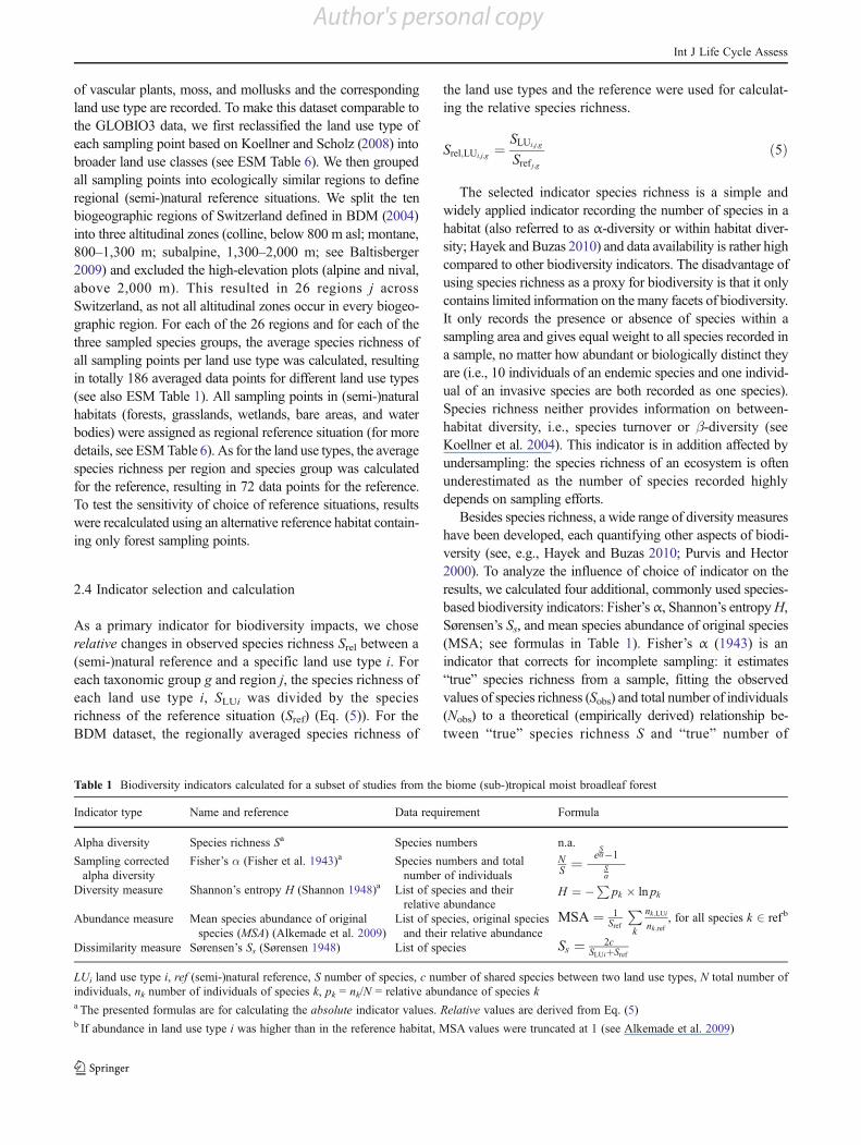
Table 1 Biodiversity indicators calculated for a subset of studies from the biome (sub-)tropical moist broadleaf forest

Indicator type Name and reference Data requirement Formula

Alpha diversity Species richness Sa Species numbers n.a.

Sampling correctedalpha diversity

Fisher’s " (Fisher et al. 1943)a Species numbers and totalnumber of individuals

NS ! e

Sa"1

! "Sa

Diversity measure Shannon’s entropy H (Shannon 1948)a List of species and theirrelative abundance

H ! "P

pk % ln pk

Abundance measure Mean species abundance of originalspecies (MSA) (Alkemade et al. 2009)

List of species, original speciesand their relative abundance

MSA ! 1Sref

Pk

nk;LUink;ref

, for all species k 2 ref b

Dissimilarity measure Sørensen’s Ss (Sørensen 1948) List of species Ss ! 2cSLUi&Sref

LUi land use type i, ref (semi-)natural reference, S number of species, c number of shared species between two land use types, N total number ofindividuals, nk number of individuals of species k, pk 0 nk/N 0 relative abundance of species ka The presented formulas are for calculating the absolute indicator values. Relative values are derived from Eq. (5)b If abundance in land use type i was higher than in the reference habitat, MSA values were truncated at 1 (see Alkemade et al. 2009)

Int J Life Cycle Assess

Author's personal copy

individuals N. Shannon’s entropy H (1948) combines informa-tion on species abundance and richness in one number andreaches a maximum when all species occurring in a sample areequally abundant. Sørensen’s Ss (1948) and MSA (Alkemadeet al. 2009) both compare the species composition of twosamples (here, the reference and land use type i). Sørensen’sSs reports howmany reference-habitat species occur in the landuse type i and reaches a maximum value of 1 if all of themoccur in the land use type i and aminimum value of 0 if none ofthe reference-habitat species occur in the land use type i. MSA,which has been developed for the GLOBIO3 model(Alkemade et al. 2009), assesses changes in abundance of eachreference-habitat species and thus reports changes in speciescomposition earlier than Sørensen’s Ss, which only indicates acomplete absence of a species from a site.

Besides the number of species S, these indicators allrequire additional information such as species identity (i.e.,checklist of species present) and/or abundance (number ofindividual organisms nk, per species k or total individualorganisms N per sample). This additional information com-plicates the process of data collection and was only availablein parts of the studies in the GLOBIO3 database. We there-fore performed this indicator comparison with a subset ofthe data: we chose all those studies from the biome (sub)-tropical moist broadleaf forest (i.e., “tropical rain forest”) inwhich a full species list indicating the abundance of eachspecies in different land use types and a (semi-)naturalreference was provided. The species abundance lists of thesestudies were extracted to Microsoft Excel to calculate theselected biodiversity indicators (see Table 1). Two indicators(MSA and Ss) directly calculate the relative change betweena land use type i and a reference, for the other three indica-tors (species richness, Shannon’s H, and Fisher’s !), therelative values per land use type LUi and taxonomic group gwithin each study j were calculated as follows:

Irel;LUi;j;g !ILUi;j;g

Iref j;g#6$

The numerical values range from 0 to 1 for the twoindicators MSA and Sørensen’s Ss, whereas Irel of the otherthree indicators species richness, Shannon’s H, and Fisher’s! allow values above 1. For studies containing data fromseveral reference situations, relative indicators were calcu-lated for all possible combinations of references and landuse types and also within references, giving an additionalestimate of uncertainty. Hence, the reference situation wasnot fixed at 1 as was the case for the data on Srel from the fulldataset (BDM and GLOBIO3 database), where multiplereference plots per study site were averaged before thecalculation of the relative indicator. This resulted in a finalnumber of 168 (pairwise) data points for the reference and atotal of 337 for all land use types.

2.5 Statistical analysis

Analysis of variance (ANOVA)was used to analyze the differ-ences in mean relative species richness Srel, depending on thefour factors land use type (LU), taxonomic group (taxa),biogeographic region (biome), and data source (i.e.,GLOBIO or BDM; data), including the interaction of factors(see Eq. (7)).

Srel ! f #LU; biome; taxa; data; LU% biome; LU% taxa;

biome% taxa; LU% data; biome% data;

taxa% data; LU% biome% taxa;

LU% biome% data; LU% taxa% data$

#7$

As the data did not follow the assumption of normal distri-bution, we additionally applied the Kruskal–Wallis test to testthe difference of medians of Srel of the four factors (withoutinteraction). Mann–WhitneyU test was conducted for pairwisecomparison of median Srel of different land use types.

For each of the five indicators Irel (see Table 1 andEq. (6)) calculated for a subset of data, the differences inmeans for the three factors LU, taxa, and biogeographicregion (realm) and their interactions were assessed withANOVA (see Eq. (8)).

Irel ! f #LU; taxa; realm; LU% taxa; LU% realm;

taxa% realm; LU% taxa% realm$

#8$

As with the total dataset, robustness of results wasassessed with nonparametric Kruskal–Wallis tests andMann–Whitney U tests. In addition, Pearson’s correlationbetween indicators was calculated. All data analysis was car-ried out using R statistical package v2.11 (R DevelopmentCore Team 2011).

3 Results

3.1 Land use impacts on biodiversity

Characterization factors of land occupation CFocc for BDPwere calculated according to Eq. (1) and are shown inTable 2 and in the Online Resource (see ESM Table 1).For easier interpretation of results, the biodiversity indicatorSrel is chosen for graphical display (Figs. 1, 2, and 3). Thecharacterization factors (CF) can be derived by subtractingthe median Srel from 1 (see Eq. 1).

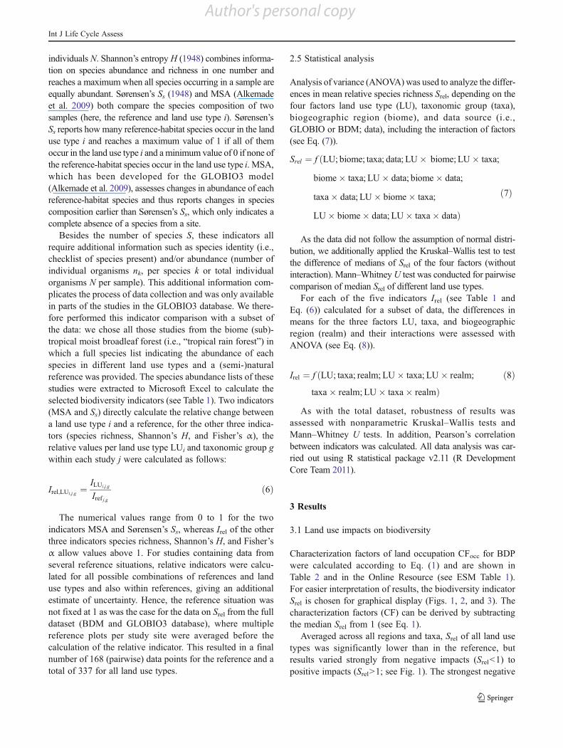
Averaged across all regions and taxa, Srel of all land usetypes was significantly lower than in the reference, butresults varied strongly from negative impacts (Srel<1) topositive impacts (Srel>1; see Fig. 1). The strongest negative

Int J Life Cycle Assess

Author's personal copy

impact was found in annual crops, where Srel was reducedby 60 %, followed by permanent crops and artificial areas(40 % decreased Srel). In pastures, the reduction of Srel wasaround 30 %, in secondary vegetation, used forests andagroforestry around 20 %. A pairwise comparison of thedifference of median Srel of different land use types is givenin ESM Table 2.

A significant effect on Srel of LU, taxa, and biome, and anonsignificant effect of the source of data (GLOBIO orBDM) were found for the full dataset both in ANOVA(Table 3) and Kruskal–Wallis test (results not shown). Inthe ANOVA, land use effects on Srel differed significantlybetween biomes (LU ! region) and taxa (LU ! taxa), but notbetween data source (LU ! data). The latter was supportedby Mann–Whitney U tests, which did not show any signif-icant difference (p<0.05) in Srel between the two data sour-ces for any land use type (results not shown).

3.2 Regionalization

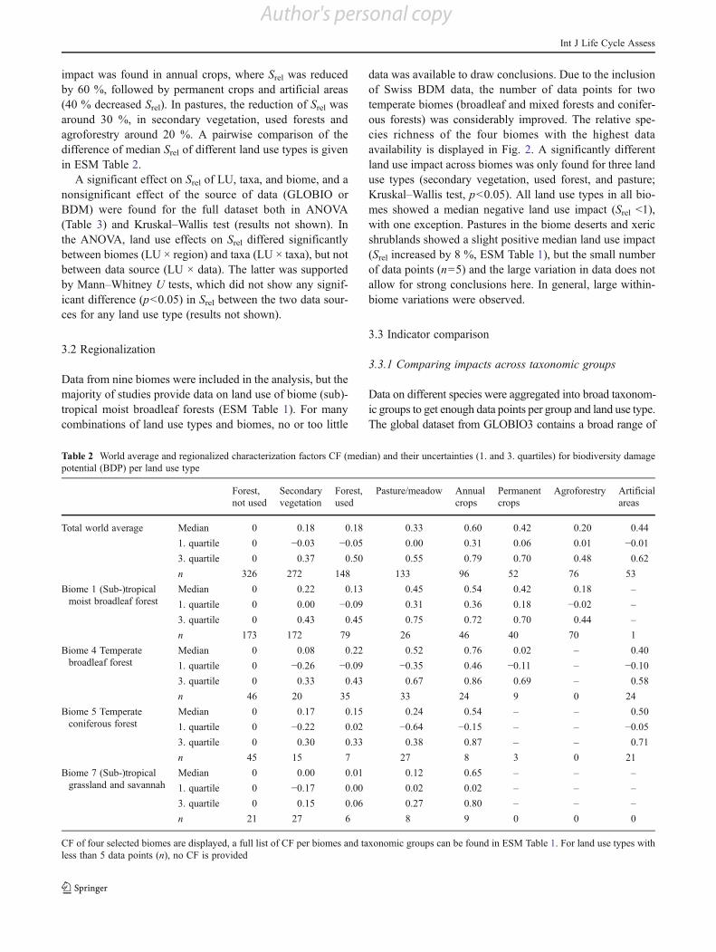
Data from nine biomes were included in the analysis, but themajority of studies provide data on land use of biome (sub)-tropical moist broadleaf forests (ESM Table 1). For manycombinations of land use types and biomes, no or too little

data was available to draw conclusions. Due to the inclusionof Swiss BDM data, the number of data points for twotemperate biomes (broadleaf and mixed forests and conifer-ous forests) was considerably improved. The relative spe-cies richness of the four biomes with the highest dataavailability is displayed in Fig. 2. A significantly differentland use impact across biomes was only found for three landuse types (secondary vegetation, used forest, and pasture;Kruskal–Wallis test, p<0.05). All land use types in all bio-mes showed a median negative land use impact (Srel <1),with one exception. Pastures in the biome deserts and xericshrublands showed a slight positive median land use impact(Srel increased by 8 %, ESM Table 1), but the small numberof data points (n05) and the large variation in data does notallow for strong conclusions here. In general, large within-biome variations were observed.

3.3 Indicator comparison

3.3.1 Comparing impacts across taxonomic groups

Data on different species were aggregated into broad taxonom-ic groups to get enough data points per group and land use type.The global dataset from GLOBIO3 contains a broad range of

Table 2 World average and regionalized characterization factors CF (median) and their uncertainties (1. and 3. quartiles) for biodiversity damagepotential (BDP) per land use type

Forest,not used

Secondaryvegetation

Forest,used

Pasture/meadow Annualcrops

Permanentcrops

Agroforestry Artificialareas

Total world average Median 0 0.18 0.18 0.33 0.60 0.42 0.20 0.44

1. quartile 0 !0.03 !0.05 0.00 0.31 0.06 0.01 !0.01

3. quartile 0 0.37 0.50 0.55 0.79 0.70 0.48 0.62

n 326 272 148 133 96 52 76 53

Biome 1 (Sub-)tropicalmoist broadleaf forest

Median 0 0.22 0.13 0.45 0.54 0.42 0.18 –

1. quartile 0 0.00 !0.09 0.31 0.36 0.18 !0.02 –

3. quartile 0 0.43 0.45 0.75 0.72 0.70 0.44 –

n 173 172 79 26 46 40 70 1

Biome 4 Temperatebroadleaf forest

Median 0 0.08 0.22 0.52 0.76 0.02 – 0.40

1. quartile 0 !0.26 !0.09 !0.35 0.46 !0.11 – !0.10

3. quartile 0 0.33 0.43 0.67 0.86 0.69 – 0.58

n 46 20 35 33 24 9 0 24

Biome 5 Temperateconiferous forest

Median 0 0.17 0.15 0.24 0.54 – – 0.50

1. quartile 0 !0.22 0.02 !0.64 !0.15 – – !0.05

3. quartile 0 0.30 0.33 0.38 0.87 – – 0.71

n 45 15 7 27 8 3 0 21

Biome 7 (Sub-)tropicalgrassland and savannah

Median 0 0.00 0.01 0.12 0.65 – – –

1. quartile 0 !0.17 0.00 0.02 0.02 – – –

3. quartile 0 0.15 0.06 0.27 0.80 – – –

n 21 27 6 8 9 0 0 0

CF of four selected biomes are displayed, a full list of CF per biomes and taxonomic groups can be found in ESM Table 1. For land use types withless than 5 data points (n), no CF is provided

Int J Life Cycle Assess

Author's personal copy

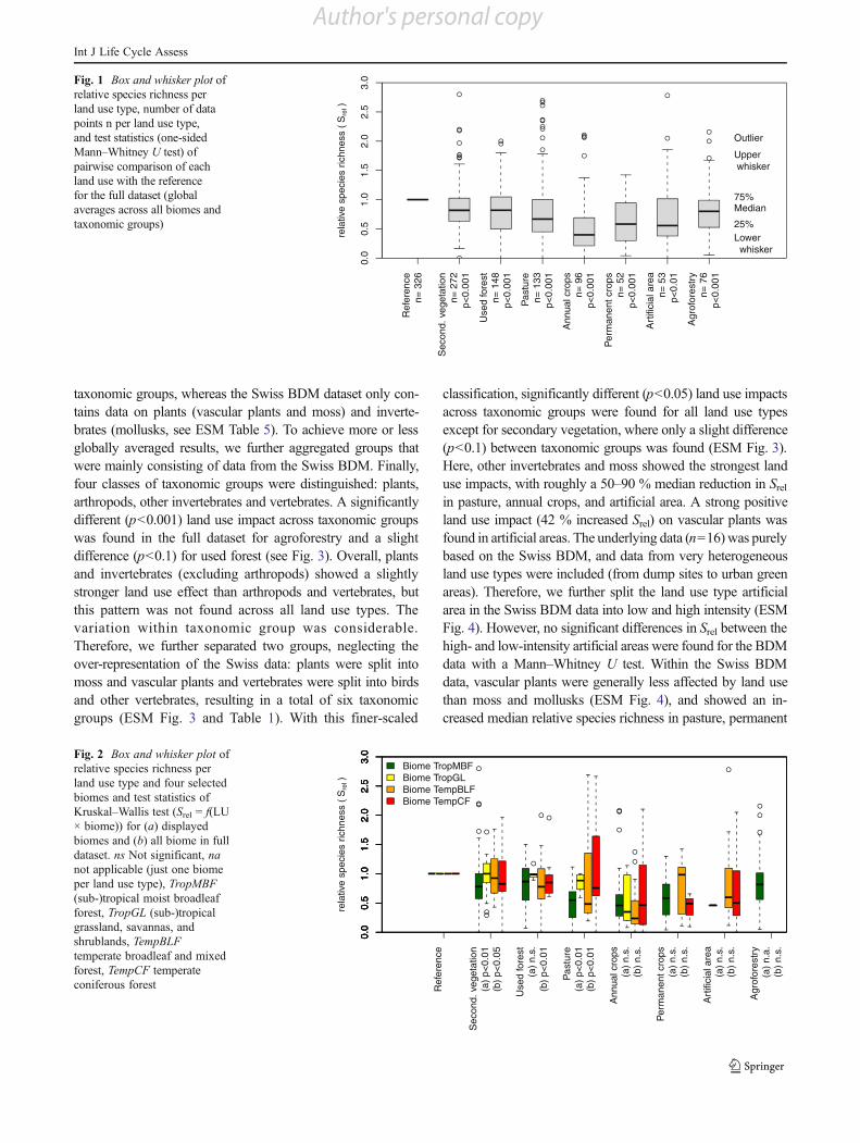
taxonomic groups, whereas the Swiss BDM dataset only con-tains data on plants (vascular plants and moss) and inverte-brates (mollusks, see ESM Table 5). To achieve more or lessglobally averaged results, we further aggregated groups thatwere mainly consisting of data from the Swiss BDM. Finally,four classes of taxonomic groups were distinguished: plants,arthropods, other invertebrates and vertebrates. A significantlydifferent (p<0.001) land use impact across taxonomic groupswas found in the full dataset for agroforestry and a slightdifference (p<0.1) for used forest (see Fig. 3). Overall, plantsand invertebrates (excluding arthropods) showed a slightlystronger land use effect than arthropods and vertebrates, butthis pattern was not found across all land use types. Thevariation within taxonomic group was considerable.Therefore, we further separated two groups, neglecting theover-representation of the Swiss data: plants were split intomoss and vascular plants and vertebrates were split into birdsand other vertebrates, resulting in a total of six taxonomicgroups (ESM Fig. 3 and Table 1). With this finer-scaled

classification, significantly different (p<0.05) land use impactsacross taxonomic groups were found for all land use typesexcept for secondary vegetation, where only a slight difference(p<0.1) between taxonomic groups was found (ESM Fig. 3).Here, other invertebrates and moss showed the strongest landuse impacts, with roughly a 50–90 % median reduction in Srelin pasture, annual crops, and artificial area. A strong positiveland use impact (42 % increased Srel) on vascular plants wasfound in artificial areas. The underlying data (n016) was purelybased on the Swiss BDM, and data from very heterogeneousland use types were included (from dump sites to urban greenareas). Therefore, we further split the land use type artificialarea in the Swiss BDM data into low and high intensity (ESMFig. 4). However, no significant differences in Srel between thehigh- and low-intensity artificial areas were found for the BDMdata with a Mann–Whitney U test. Within the Swiss BDMdata, vascular plants were generally less affected by land usethan moss and mollusks (ESM Fig. 4), and showed an in-creased median relative species richness in pasture, permanent

0.0

0.5

1.0

1.5

2.0

2.5

3.0

rela

tive

spec

ies

richn

ess

( Sre

l )

Ref

eren

ce

n=

326

Sec

ond.

veg

etat

ion

n=

272

p<0

.001

Use

d fo

rest

n

= 14

8 p

<0.0

01

Pas

ture

n

= 13

3 p

<0.0

01

Ann

ual c

rops

n

= 96

p

<0.0

01

Per

man

ent c

rops

n

= 52

p

<0.0

01

Art

ifici

al a

rea

n=

53

p<0

.01

Agr

ofor

estr

y n

= 76

p

<0.0

01

25%

Median75%

Outlier

Upper whisker

Lower whisker

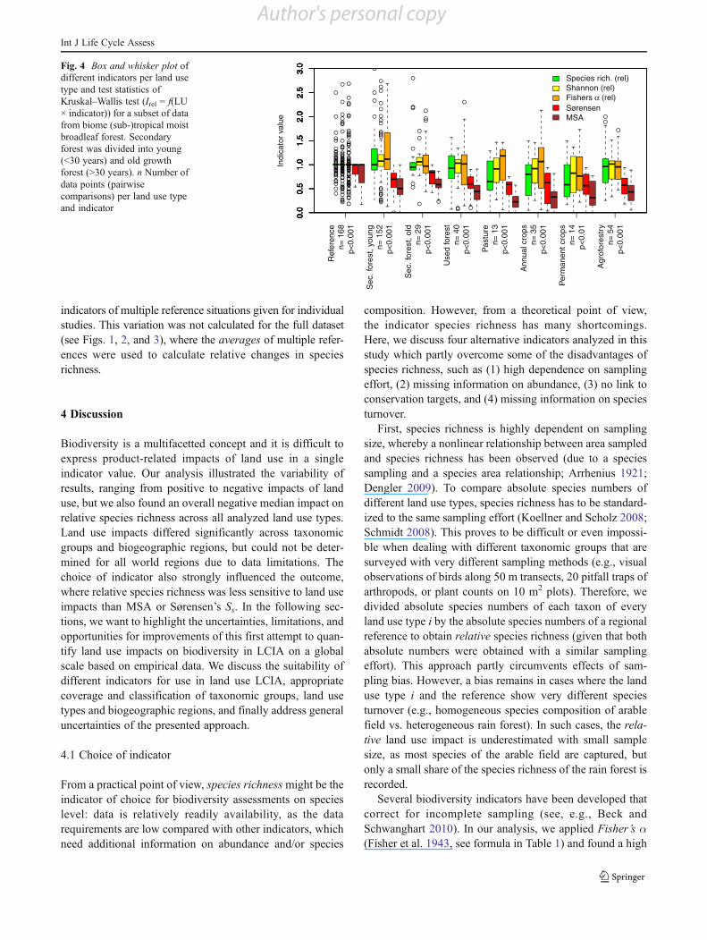
Fig. 1 Box and whisker plot ofrelative species richness perland use type, number of datapoints n per land use type,and test statistics (one-sidedMann–Whitney U test) ofpairwise comparison of eachland use with the referencefor the full dataset (globalaverages across all biomes andtaxonomic groups)

0.0

0.5

1.0

1.5

2.0

2.5

3.0

rela

tive

spec

ies

richn

ess

( Sre

l )

0.0

0.5

1.0

1.5

2.0

2.5

3.0

0.0

0.5

1.0

1.5

2.0

2.5

3.0

0.0

0.5

1.0

1.5

2.0

2.5

3.0

Ref

eren

ce

Sec

ond.

veg

etat

ion

(a)

p<0

.01

(b)

p<0

.05

Use

d fo

rest

(

a) n

.s.

(b)

p<0

.01

Pas

ture

(

a) p

<0.0

1 (

b) p

<0.0

1

Ann

ual c

rops

(

a) n

.s.

(b)

n.s

.

Per

man

ent c

rops

(

a) n

.s.

(b)

n.s

.

Art

ifici

al a

rea

(a)

n.s

. (

b) n

.s.

Agr

ofor

estr

y (

a) n

.a.

(b)

n.s

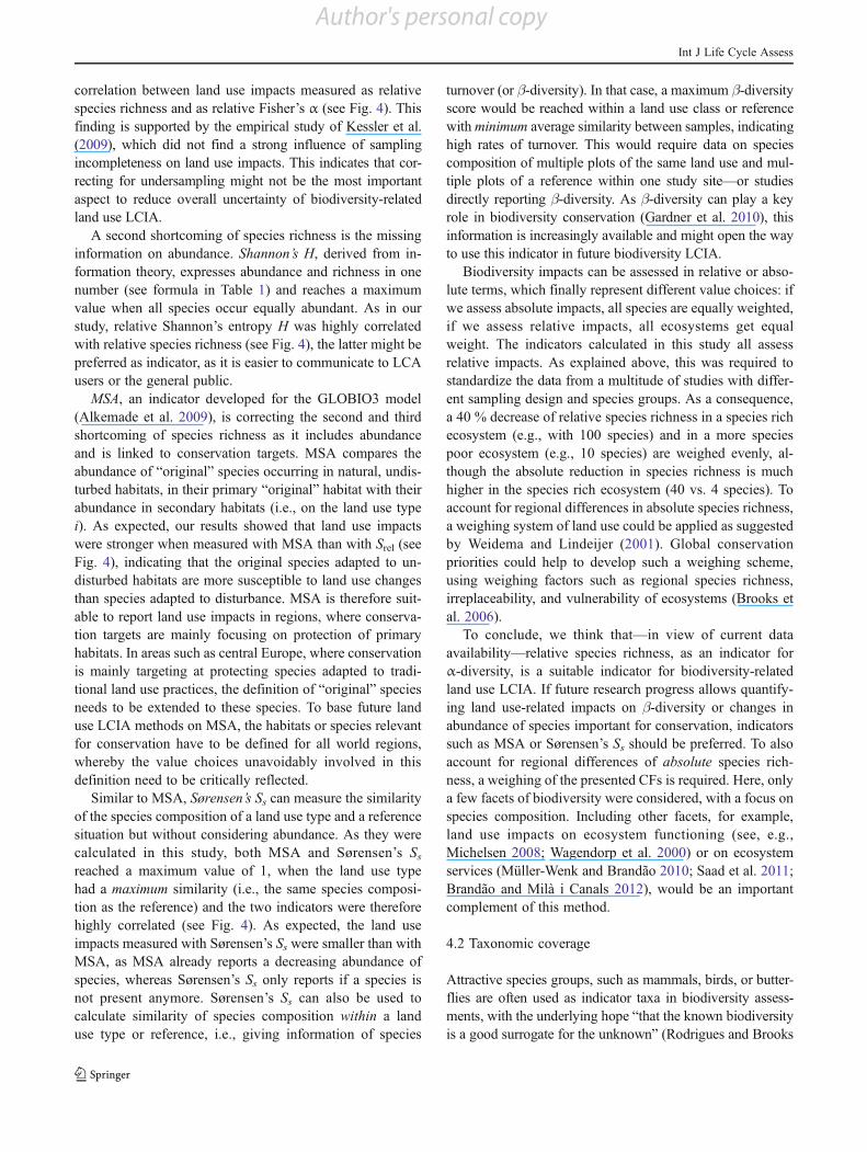
. Biome TropMBFBiome TropGLBiome TempBLFBiome TempCF

Fig. 2 Box and whisker plot ofrelative species richness perland use type and four selectedbiomes and test statistics ofKruskal–Wallis test (Srel 0 f(LU! biome)) for (a) displayedbiomes and (b) all biome in fulldataset. ns Not significant, nanot applicable (just one biomeper land use type), TropMBF(sub-)tropical moist broadleafforest, TropGL (sub-)tropicalgrassland, savannas, andshrublands, TempBLFtemperate broadleaf and mixedforest, TempCF temperateconiferous forest

Int J Life Cycle Assess

Author's personal copy

crops, and artificial areas. Moss and mollusks showed a de-creased relative species richness in all land use types.

3.3.2 Comparing impacts across biodiversity indicator

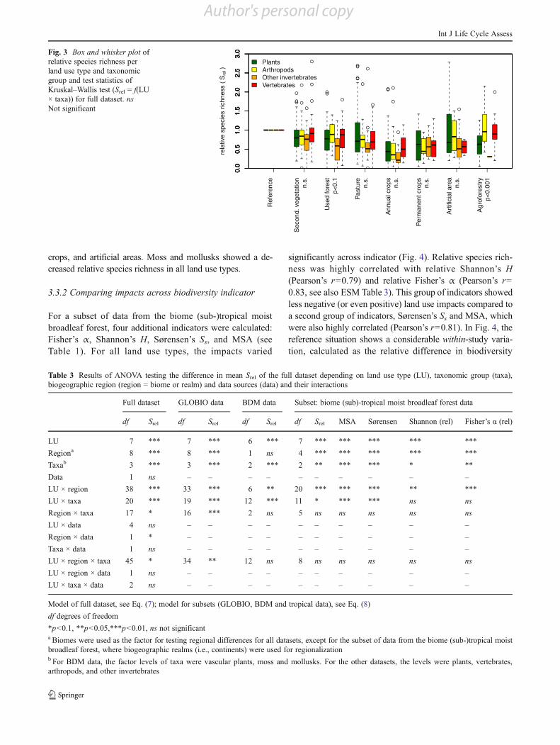
For a subset of data from the biome (sub-)tropical moistbroadleaf forest, four additional indicators were calculated:Fisher’s !, Shannon’s H, Sørensen’s Ss, and MSA (seeTable 1). For all land use types, the impacts varied

significantly across indicator (Fig. 4). Relative species rich-ness was highly correlated with relative Shannon’s H(Pearson’s r00.79) and relative Fisher’s ! (Pearson’s r00.83, see also ESM Table 3). This group of indicators showedless negative (or even positive) land use impacts compared toa second group of indicators, Sørensen’s Ss and MSA, whichwere also highly correlated (Pearson’s r00.81). In Fig. 4, thereference situation shows a considerable within-study varia-tion, calculated as the relative difference in biodiversity

0.0

0.5

1.0

1.5

2.0

2.5

3.0

rela

tive

spec

ies

richn

ess

( Sre

l )

0.0

0.5

1.0

1.5

2.0

2.5

3.0

0.0

0.5

1.0

1.5

2.0

2.5

3.0

0.0

0.5

1.0

1.5

2.0

2.5

3.0

Ref

eren

ce

Sec

ond.

veg

etat

ion

n.s

.

Use

d fo

rest

p

<0.1

Pas

ture

n

.s.

Ann

ual c

rops

n

.s.

Per

man

ent c

rops

n

.s.

Art

ifici

al a

rea

n.s

.

Agr

ofor

estr

y p

<0.0

01

PlantsArthropodsOther invertebratesVertebrates

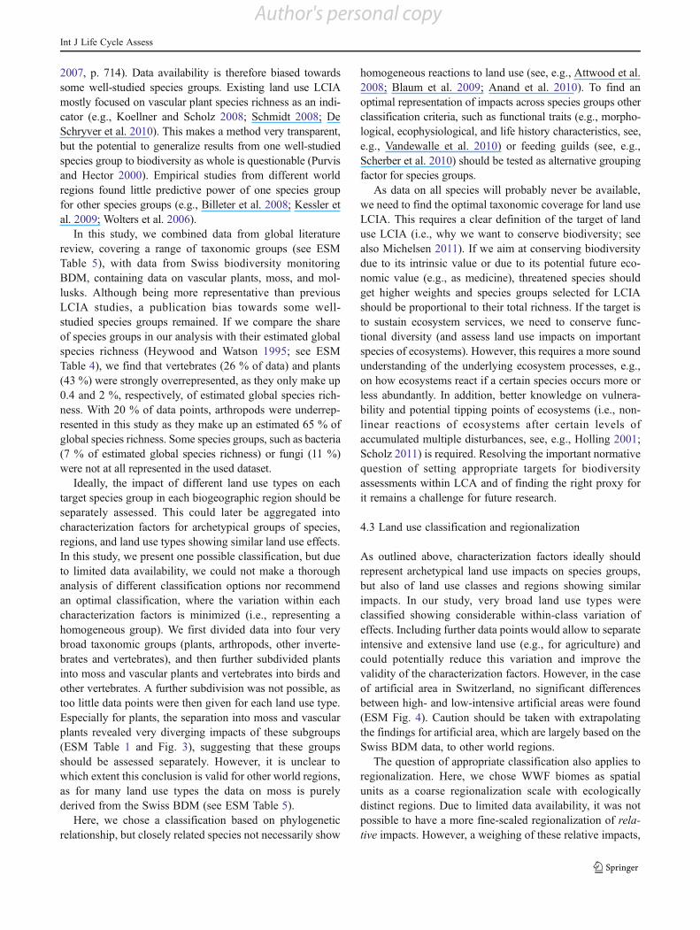
Fig. 3 Box and whisker plot ofrelative species richness perland use type and taxonomicgroup and test statistics ofKruskal–Wallis test (Srel 0 f(LU! taxa)) for full dataset. nsNot significant

Table 3 Results of ANOVA testing the difference in mean Srel of the full dataset depending on land use type (LU), taxonomic group (taxa),biogeographic region (region 0 biome or realm) and data sources (data) and their interactions

Full dataset GLOBIO data BDM data Subset: biome (sub)-tropical moist broadleaf forest data

df Srel df Srel df Srel df Srel MSA Sørensen Shannon (rel) Fisher’s ! (rel)

LU 7 *** 7 *** 6 *** 7 *** *** *** *** ***

Regiona 8 *** 8 *** 1 ns 4 *** *** *** *** ***

Taxab 3 *** 3 *** 2 *** 2 ** *** *** * **

Data 1 ns – – – – – – – – – –

LU ! region 38 *** 33 *** 6 ** 20 *** *** *** ** ***

LU ! taxa 20 *** 19 *** 12 *** 11 * *** *** ns ns

Region ! taxa 17 * 16 *** 2 ns 5 ns ns ns ns ns

LU ! data 4 ns – – – – – – – – – –

Region ! data 1 * – – – – – – – – – –

Taxa ! data 1 ns – – – – – – – – – –

LU ! region ! taxa 45 * 34 ** 12 ns 8 ns ns ns ns ns

LU ! region ! data 1 ns – – – – – – – – – –

LU ! taxa ! data 2 ns – – – – – – – – – –

Model of full dataset, see Eq. (7); model for subsets (GLOBIO, BDM and tropical data), see Eq. (8)

df degrees of freedom

*p<0.1, **p<0.05,***p<0.01, ns not significanta Biomes were used as the factor for testing regional differences for all datasets, except for the subset of data from the biome (sub-)tropical moistbroadleaf forest, where biogeographic realms (i.e., continents) were used for regionalizationb For BDM data, the factor levels of taxa were vascular plants, moss and mollusks. For the other datasets, the levels were plants, vertebrates,arthropods, and other invertebrates

Int J Life Cycle Assess

Author's personal copy

indicators of multiple reference situations given for individualstudies. This variation was not calculated for the full dataset(see Figs. 1, 2, and 3), where the averages of multiple refer-ences were used to calculate relative changes in speciesrichness.

4 Discussion

Biodiversity is a multifacetted concept and it is difficult toexpress product-related impacts of land use in a singleindicator value. Our analysis illustrated the variability ofresults, ranging from positive to negative impacts of landuse, but we also found an overall negative median impact onrelative species richness across all analyzed land use types.Land use impacts differed significantly across taxonomicgroups and biogeographic regions, but could not be deter-mined for all world regions due to data limitations. Thechoice of indicator also strongly influenced the outcome,where relative species richness was less sensitive to land useimpacts than MSA or Sørensen’s Ss. In the following sec-tions, we want to highlight the uncertainties, limitations, andopportunities for improvements of this first attempt to quan-tify land use impacts on biodiversity in LCIA on a globalscale based on empirical data. We discuss the suitability ofdifferent indicators for use in land use LCIA, appropriatecoverage and classification of taxonomic groups, land usetypes and biogeographic regions, and finally address generaluncertainties of the presented approach.

4.1 Choice of indicator

From a practical point of view, species richness might be theindicator of choice for biodiversity assessments on specieslevel: data is relatively readily availability, as the datarequirements are low compared with other indicators, whichneed additional information on abundance and/or species

composition. However, from a theoretical point of view,the indicator species richness has many shortcomings.Here, we discuss four alternative indicators analyzed in thisstudy which partly overcome some of the disadvantages ofspecies richness, such as (1) high dependence on samplingeffort, (2) missing information on abundance, (3) no link toconservation targets, and (4) missing information on speciesturnover.

First, species richness is highly dependent on samplingsize, whereby a nonlinear relationship between area sampledand species richness has been observed (due to a speciessampling and a species area relationship; Arrhenius 1921;Dengler 2009). To compare absolute species numbers ofdifferent land use types, species richness has to be standard-ized to the same sampling effort (Koellner and Scholz 2008;Schmidt 2008). This proves to be difficult or even impossi-ble when dealing with different taxonomic groups that aresurveyed with very different sampling methods (e.g., visualobservations of birds along 50 m transects, 20 pitfall traps ofarthropods, or plant counts on 10 m2 plots). Therefore, wedivided absolute species numbers of each taxon of everyland use type i by the absolute species numbers of a regionalreference to obtain relative species richness (given that bothabsolute numbers were obtained with a similar samplingeffort). This approach partly circumvents effects of sam-pling bias. However, a bias remains in cases where the landuse type i and the reference show very different speciesturnover (e.g., homogeneous species composition of arablefield vs. heterogeneous rain forest). In such cases, the rela-tive land use impact is underestimated with small samplesize, as most species of the arable field are captured, butonly a small share of the species richness of the rain forest isrecorded.

Several biodiversity indicators have been developed thatcorrect for incomplete sampling (see, e.g., Beck andSchwanghart 2010). In our analysis, we applied Fisher’s "(Fisher et al. 1943, see formula in Table 1) and found a high

0.0

0.5

1.0

1.5

2.0

2.5

3.0

Indi

cato

r va

lue

0.0

0.5

1.0

1.5

2.0

2.5

3.0

0.0

0.5

1.0

1.5

2.0

2.5

3.0

0.0

0.5

1.0

1.5

2.0

2.5

3.0

0.0

0.5

1.0

1.5

2.0

2.5

3.0

Ref

eren

ce

n=

168

p<0

.001

Sec

. for

est,

youn

g n

= 15

2 p

<0.0

01

Sec

. for

est,

old

n=

29

p<0

.001

Use

d fo

rest

n

= 40

p

<0.0

01

Pas

ture

n

= 13

p

<0.0

01

Ann

ual c

rops

n

= 35

p

<0.0

01

Per

man

ent c

rops

n

= 14

p

<0.0

1

Agr

ofor

estr

y n

= 54

p

<0.0

01

Species rich. (rel)Shannon (rel)Fishers ! (rel)SørensenMSA

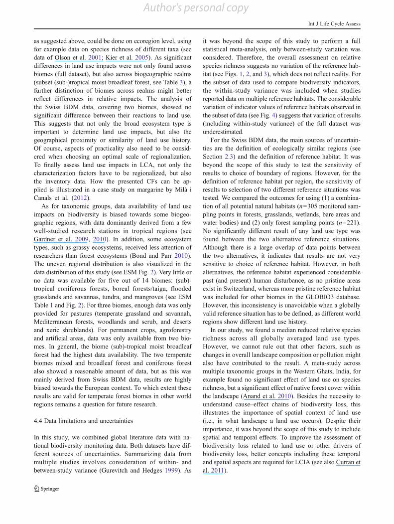
Fig. 4 Box and whisker plot ofdifferent indicators per land usetype and test statistics ofKruskal–Wallis test (Irel 0 f(LU! indicator)) for a subset of datafrom biome (sub-)tropical moistbroadleaf forest. Secondaryforest was divided into young(<30 years) and old growthforest (>30 years). n Number ofdata points (pairwisecomparisons) per land use typeand indicator

Int J Life Cycle Assess

Author's personal copy

correlation between land use impacts measured as relativespecies richness and as relative Fisher’s ! (see Fig. 4). Thisfinding is supported by the empirical study of Kessler et al.(2009), which did not find a strong influence of samplingincompleteness on land use impacts. This indicates that cor-recting for undersampling might not be the most importantaspect to reduce overall uncertainty of biodiversity-relatedland use LCIA.

A second shortcoming of species richness is the missinginformation on abundance. Shannon’s H, derived from in-formation theory, expresses abundance and richness in onenumber (see formula in Table 1) and reaches a maximumvalue when all species occur equally abundant. As in ourstudy, relative Shannon’s entropy H was highly correlatedwith relative species richness (see Fig. 4), the latter might bepreferred as indicator, as it is easier to communicate to LCAusers or the general public.

MSA, an indicator developed for the GLOBIO3 model(Alkemade et al. 2009), is correcting the second and thirdshortcoming of species richness as it includes abundanceand is linked to conservation targets. MSA compares theabundance of “original” species occurring in natural, undis-turbed habitats, in their primary “original” habitat with theirabundance in secondary habitats (i.e., on the land use typei). As expected, our results showed that land use impactswere stronger when measured with MSA than with Srel (seeFig. 4), indicating that the original species adapted to un-disturbed habitats are more susceptible to land use changesthan species adapted to disturbance. MSA is therefore suit-able to report land use impacts in regions, where conserva-tion targets are mainly focusing on protection of primaryhabitats. In areas such as central Europe, where conservationis mainly targeting at protecting species adapted to tradi-tional land use practices, the definition of “original” speciesneeds to be extended to these species. To base future landuse LCIA methods on MSA, the habitats or species relevantfor conservation have to be defined for all world regions,whereby the value choices unavoidably involved in thisdefinition need to be critically reflected.

Similar to MSA, Sørensen’s Ss can measure the similarityof the species composition of a land use type and a referencesituation but without considering abundance. As they werecalculated in this study, both MSA and Sørensen’s Ssreached a maximum value of 1, when the land use typehad a maximum similarity (i.e., the same species composi-tion as the reference) and the two indicators were thereforehighly correlated (see Fig. 4). As expected, the land useimpacts measured with Sørensen’s Ss were smaller than withMSA, as MSA already reports a decreasing abundance ofspecies, whereas Sørensen’s Ss only reports if a species isnot present anymore. Sørensen’s Ss can also be used tocalculate similarity of species composition within a landuse type or reference, i.e., giving information of species

turnover (or !-diversity). In that case, a maximum !-diversityscore would be reached within a land use class or referencewithminimum average similarity between samples, indicatinghigh rates of turnover. This would require data on speciescomposition of multiple plots of the same land use and mul-tiple plots of a reference within one study site—or studiesdirectly reporting !-diversity. As !-diversity can play a keyrole in biodiversity conservation (Gardner et al. 2010), thisinformation is increasingly available and might open the wayto use this indicator in future biodiversity LCIA.

Biodiversity impacts can be assessed in relative or abso-lute terms, which finally represent different value choices: ifwe assess absolute impacts, all species are equally weighted,if we assess relative impacts, all ecosystems get equalweight. The indicators calculated in this study all assessrelative impacts. As explained above, this was required tostandardize the data from a multitude of studies with differ-ent sampling design and species groups. As a consequence,a 40 % decrease of relative species richness in a species richecosystem (e.g., with 100 species) and in a more speciespoor ecosystem (e.g., 10 species) are weighed evenly, al-though the absolute reduction in species richness is muchhigher in the species rich ecosystem (40 vs. 4 species). Toaccount for regional differences in absolute species richness,a weighing system of land use could be applied as suggestedby Weidema and Lindeijer (2001). Global conservationpriorities could help to develop such a weighing scheme,using weighing factors such as regional species richness,irreplaceability, and vulnerability of ecosystems (Brooks etal. 2006).

To conclude, we think that—in view of current dataavailability—relative species richness, as an indicator for!-diversity, is a suitable indicator for biodiversity-relatedland use LCIA. If future research progress allows quantify-ing land use-related impacts on !-diversity or changes inabundance of species important for conservation, indicatorssuch as MSA or Sørensen’s Ss should be preferred. To alsoaccount for regional differences of absolute species rich-ness, a weighing of the presented CFs is required. Here, onlya few facets of biodiversity were considered, with a focus onspecies composition. Including other facets, for example,land use impacts on ecosystem functioning (see, e.g.,Michelsen 2008; Wagendorp et al. 2000) or on ecosystemservices (Müller-Wenk and Brandão 2010; Saad et al. 2011;Brandão and Milà i Canals 2012), would be an importantcomplement of this method.

4.2 Taxonomic coverage

Attractive species groups, such as mammals, birds, or butter-flies are often used as indicator taxa in biodiversity assess-ments, with the underlying hope “that the known biodiversityis a good surrogate for the unknown” (Rodrigues and Brooks

Int J Life Cycle Assess

Author's personal copy

2007, p. 714). Data availability is therefore biased towardssome well-studied species groups. Existing land use LCIAmostly focused on vascular plant species richness as an indi-cator (e.g., Koellner and Scholz 2008; Schmidt 2008; DeSchryver et al. 2010). This makes a method very transparent,but the potential to generalize results from one well-studiedspecies group to biodiversity as whole is questionable (Purvisand Hector 2000). Empirical studies from different worldregions found little predictive power of one species groupfor other species groups (e.g., Billeter et al. 2008; Kessler etal. 2009; Wolters et al. 2006).

In this study, we combined data from global literaturereview, covering a range of taxonomic groups (see ESMTable 5), with data from Swiss biodiversity monitoringBDM, containing data on vascular plants, moss, and mol-lusks. Although being more representative than previousLCIA studies, a publication bias towards some well-studied species groups remained. If we compare the shareof species groups in our analysis with their estimated globalspecies richness (Heywood and Watson 1995; see ESMTable 4), we find that vertebrates (26 % of data) and plants(43 %) were strongly overrepresented, as they only make up0.4 and 2 %, respectively, of estimated global species rich-ness. With 20 % of data points, arthropods were underrep-resented in this study as they make up an estimated 65 % ofglobal species richness. Some species groups, such as bacteria(7 % of estimated global species richness) or fungi (11 %)were not at all represented in the used dataset.

Ideally, the impact of different land use types on eachtarget species group in each biogeographic region should beseparately assessed. This could later be aggregated intocharacterization factors for archetypical groups of species,regions, and land use types showing similar land use effects.In this study, we present one possible classification, but dueto limited data availability, we could not make a thoroughanalysis of different classification options nor recommendan optimal classification, where the variation within eachcharacterization factors is minimized (i.e., representing ahomogeneous group). We first divided data into four verybroad taxonomic groups (plants, arthropods, other inverte-brates and vertebrates), and then further subdivided plantsinto moss and vascular plants and vertebrates into birds andother vertebrates. A further subdivision was not possible, astoo little data points were then given for each land use type.Especially for plants, the separation into moss and vascularplants revealed very diverging impacts of these subgroups(ESM Table 1 and Fig. 3), suggesting that these groupsshould be assessed separately. However, it is unclear towhich extent this conclusion is valid for other world regions,as for many land use types the data on moss is purelyderived from the Swiss BDM (see ESM Table 5).

Here, we chose a classification based on phylogeneticrelationship, but closely related species not necessarily show

homogeneous reactions to land use (see, e.g., Attwood et al.2008; Blaum et al. 2009; Anand et al. 2010). To find anoptimal representation of impacts across species groups otherclassification criteria, such as functional traits (e.g., morpho-logical, ecophysiological, and life history characteristics, see,e.g., Vandewalle et al. 2010) or feeding guilds (see, e.g.,Scherber et al. 2010) should be tested as alternative groupingfactor for species groups.

As data on all species will probably never be available,we need to find the optimal taxonomic coverage for land useLCIA. This requires a clear definition of the target of landuse LCIA (i.e., why we want to conserve biodiversity; seealso Michelsen 2011). If we aim at conserving biodiversitydue to its intrinsic value or due to its potential future eco-nomic value (e.g., as medicine), threatened species shouldget higher weights and species groups selected for LCIAshould be proportional to their total richness. If the target isto sustain ecosystem services, we need to conserve func-tional diversity (and assess land use impacts on importantspecies of ecosystems). However, this requires a more soundunderstanding of the underlying ecosystem processes, e.g.,on how ecosystems react if a certain species occurs more orless abundantly. In addition, better knowledge on vulnera-bility and potential tipping points of ecosystems (i.e., non-linear reactions of ecosystems after certain levels ofaccumulated multiple disturbances, see, e.g., Holling 2001;Scholz 2011) is required. Resolving the important normativequestion of setting appropriate targets for biodiversityassessments within LCA and of finding the right proxy forit remains a challenge for future research.

4.3 Land use classification and regionalization

As outlined above, characterization factors ideally shouldrepresent archetypical land use impacts on species groups,but also of land use classes and regions showing similarimpacts. In our study, very broad land use types wereclassified showing considerable within-class variation ofeffects. Including further data points would allow to separateintensive and extensive land use (e.g., for agriculture) andcould potentially reduce this variation and improve thevalidity of the characterization factors. However, in the caseof artificial area in Switzerland, no significant differencesbetween high- and low-intensive artificial areas were found(ESM Fig. 4). Caution should be taken with extrapolatingthe findings for artificial area, which are largely based on theSwiss BDM data, to other world regions.

The question of appropriate classification also applies toregionalization. Here, we chose WWF biomes as spatialunits as a coarse regionalization scale with ecologicallydistinct regions. Due to limited data availability, it was notpossible to have a more fine-scaled regionalization of rela-tive impacts. However, a weighing of these relative impacts,

Int J Life Cycle Assess

Author's personal copy

as suggested above, could be done on ecoregion level, usingfor example data on species richness of different taxa (seedata of Olson et al. 2001; Kier et al. 2005). As significantdifferences in land use impacts were not only found acrossbiomes (full dataset), but also across biogeographic realms(subset (sub-)tropical moist broadleaf forest, see Table 3), afurther distinction of biomes across realms might betterreflect differences in relative impacts. The analysis ofthe Swiss BDM data, covering two biomes, showed nosignificant difference between their reactions to land use.This suggests that not only the broad ecosystem type isimportant to determine land use impacts, but also thegeographical proximity or similarity of land use history.Of course, aspects of practicality also need to be consid-ered when choosing an optimal scale of regionalization.To finally assess land use impacts in LCA, not only thecharacterization factors have to be regionalized, but alsothe inventory data. How the presented CFs can be ap-plied is illustrated in a case study on margarine by Milà iCanals et al. (2012).

As for taxonomic groups, data availability of land useimpacts on biodiversity is biased towards some biogeo-graphic regions, with data dominantly derived from a fewwell-studied research stations in tropical regions (seeGardner et al. 2009, 2010). In addition, some ecosystemtypes, such as grassy ecosystems, received less attention ofresearchers than forest ecosystems (Bond and Parr 2010).The uneven regional distribution is also visualized in thedata distribution of this study (see ESM Fig. 2). Very little orno data was available for five out of 14 biomes: (sub)-tropical coniferous forests, boreal forests/taiga, floodedgrasslands and savannas, tundra, and mangroves (see ESMTable 1 and Fig. 2). For three biomes, enough data was onlyprovided for pastures (temperate grassland and savannah,Mediterranean forests, woodlands and scrub, and desertsand xeric shrublands). For permanent crops, agroforestryand artificial areas, data was only available from two bio-mes. In general, the biome (sub)-tropical moist broadleafforest had the highest data availability. The two temperatebiomes mixed and broadleaf forest and coniferous forestalso showed a reasonable amount of data, but as this wasmainly derived from Swiss BDM data, results are highlybiased towards the European context. To which extent theseresults are valid for temperate forest biomes in other worldregions remains a question for future research.

4.4 Data limitations and uncertainties

In this study, we combined global literature data with na-tional biodiversity monitoring data. Both datasets have dif-ferent sources of uncertainties. Summarizing data frommultiple studies involves consideration of within- andbetween-study variance (Gurevitch and Hedges 1999). As

it was beyond the scope of this study to perform a fullstatistical meta-analysis, only between-study variation wasconsidered. Therefore, the overall assessment on relativespecies richness suggests no variation of the reference hab-itat (see Figs. 1, 2, and 3), which does not reflect reality. Forthe subset of data used to compare biodiversity indicators,the within-study variance was included when studiesreported data on multiple reference habitats. The considerablevariation of indicator values of reference habitats observed inthe subset of data (see Fig. 4) suggests that variation of results(including within-study variance) of the full dataset wasunderestimated.

For the Swiss BDM data, the main sources of uncertain-ties are the definition of ecologically similar regions (seeSection 2.3) and the definition of reference habitat. It wasbeyond the scope of this study to test the sensitivity ofresults to choice of boundary of regions. However, for thedefinition of reference habitat per region, the sensitivity ofresults to selection of two different reference situations wastested. We compared the outcomes for using (1) a combina-tion of all potential natural habitats (n0305 monitored sam-pling points in forests, grasslands, wetlands, bare areas andwater bodies) and (2) only forest sampling points (n0221).No significantly different result of any land use type wasfound between the two alternative reference situations.Although there is a large overlap of data points betweenthe two alternatives, it indicates that results are not verysensitive to choice of reference habitat. However, in bothalternatives, the reference habitat experienced considerablepast (and present) human disturbance, as no pristine areasexist in Switzerland, whereas more pristine reference habitatwas included for other biomes in the GLOBIO3 database.However, this inconsistency is unavoidable when a globallyvalid reference situation has to be defined, as different worldregions show different land use history.

In our study, we found a median reduced relative speciesrichness across all globally averaged land use types.However, we cannot rule out that other factors, such aschanges in overall landscape composition or pollution mightalso have contributed to the result. A meta-study acrossmultiple taxonomic groups in the Western Ghats, India, forexample found no significant effect of land use on speciesrichness, but a significant effect of native forest cover withinthe landscape (Anand et al. 2010). Besides the necessity tounderstand cause–effect chains of biodiversity loss, thisillustrates the importance of spatial context of land use(i.e., in what landscape a land use occurs). Despite theirimportance, it was beyond the scope of this study to includespatial and temporal effects. To improve the assessment ofbiodiversity loss related to land use or other drivers ofbiodiversity loss, better concepts including these temporaland spatial aspects are required for LCIA (see also Curran etal. 2011).

Int J Life Cycle Assess

Author's personal copy

5 Conclusions and recommendations

Although uncertainties and data and knowledge gaps areconsiderable, human impacts on biodiversity are ongoing.Decisions how to adapt production towards being less harm-ful for biodiversity need to be taken urgently, and cannotwait until all data and knowledge gaps are filled. Based onempirical data, this study provides a first attempt to quantifyland use impacts on biodiversity within LCA across worldregions to support such decisions. Due to the mentionedchallenges to quantify biodiversity impacts, the presentedCF should be used with caution and remaining uncertaintiesshould be considered when LCA results are interpreted andcommunicated. In LCA studies, where the “user may notdirectly decide on the land management practices” (Milà iCanals et al. 2007, p. 13), our CF can serve as a firstscreening of potential land use impacts across global valuechains. For LCA studies aiming to support decisions ofspecific land management, a more detailed, site-dependentassessment, including additional region- or site-specific data,is indispensable (see, e.g., Geyer et al. 2010).

In this paper, occupation impacts of a range of land usetypes in many world regions could be assessed, but somedata gaps remain. Research priorities should be set to firstclose data gaps for environmentally important land useactivities (such as agri- and silviculture, construction, min-ing, and land filling) in economically important worldregions (e.g., by using regionalized global inventories suchas the inventory of global crop production from Pfister et al.2011). To assess total land use impacts on biodiversity, weneed to complement the presented CF of occupation withregionalized global estimates of transformation impacts.This requires more reliable information on regenerationtimes of ecosystems across the world, as transformationimpacts (calculated according to the UNEP/SETAC frame-work; Milà i Canals et al. 2007; Koellner et al. 2012b) arehighly sensitive to this parameter and currently availableestimates vary considerably (Schmidt 2008). Estimates ofregeneration times should ideally be based on empiricaldata, for example derived through meta-analysis of ecosystemregeneration studies.

In view of current data availability, the applied indicatorrelative species richness is suitable for biodiversity-relatedglobal land use LCIA. As ecological research evolves,LCIA methods should be complemented with indicatorsmeasuring other facets of biodiversity, such as conservationvalue, species abundance, or turnover. This applies not onlyto land use impacts, but also to other drivers of biodiversityloss, such as climate change, eutrophication, acidification,or ecotoxicity. To inform decision-makers about potentialtrade-offs of different drivers of biodiversity loss along thelife cycle, indicators need to be comparable across impactpathways (see also Curran et al. 2011). Finding a measure to

quantify impacts of concurrent multiple drivers of biodiver-sity loss in a globally applicable and spatially differentiatedway will be a challenge for future LCA research. As theimportance of halting global biodiversity loss is increasinglyrecognized in research, industry, and policy (e.g., formulat-ed as the 2020 targets of the Convention on BiologicalDiversity; CBD 2010), increased research efforts are madeto close some of the mentioned knowledge and data gaps.This will also open the way to improve the accuracy ofbiodiversity assessments within LCA and allow for morerobust and credible decision support.

Acknowledgments The authors wish to thank Biodiversity Monitor-ing Switzerland (BDM) and the team of GLOBIO for providing data.The research was funded by ETH Research Grant CH1-0308-3 and bythe project “Life Cycle Impact Assessment Methods for ImprovedSustainability Characterisation of Technologies” (LC-IMPACT), GrantAgreement No. 243827, funded by the European Commission underthe 7th Framework Programme. We appreciate helpful comments byM. Curran, S. Hellweg, J.P. Lindner, R. Müller-Wenk, A. Spörri, andtwo anonymous reviewers.

References

Achten WMJ, Mathijs E, Muys B (2008) Proposing a life cycle land useimpact calculationmethodology. In: 6th International Conference onLCA in the Agri-Food Sector, Zurich, Nov 12–14, 2008

Alkemade R, van Oorschot M, Miles L, Nellemann C, Bakkenes M,ten Brink B (2009) GLOBIO3: a framework to investigate optionsfor reducing global terrestrial biodiversity loss. Ecosystems 12(3):374–390

Anand M, Krishnaswamy J, Kumar A, Bali A (2010) Sustainingbiodiversity conservation in human-modified landscapes in theWestern Ghats: remnant forests matter. Biol Conserv 143:2363–2374

Arrhenius O (1921) Species and area. J Ecol 9(1):95–99Attwood SJ, Maron M, House APN, Zammit C (2008) Do arthropod

assemblages display globally consistent responses to intensifiedagricultural land use and management? Glob Ecol Biogeogr 17(5):585–599

Baltisberger M (2009) Systematische Botanik. Einheimische Farn- undSamenpflanzen. 3 edn. vdf Hochschulverlag AG, ETH, Zurich,Switzerland

BDM (2004) Biodiversity monitoring Switzerland. Indicator Z9: spe-cies diversity in habitats. Bundesamt für Umwelt, BAFU. http://www.biodiversitymonitoring.ch

Beck J, Schwanghart W (2010) Comparing measures of species diver-sity from incomplete inventories: an update. Methods Ecol Evol 1(1):38–44

Billeter R, Liira J, Bailey D, Bugter R, Arens P, Augenstein I, AvironS, Baudry J, Bukacek R, Burel F, Cerny M, De Blust G, De CockR, Diekotter T, Dietz H, Dirksen J, Dormann C, Durka W, FrenzelM, Hamersky R, Hendrickx F, Herzog F, Klotz S, Koolstra B,Lausch A, Le Coeur D, Maelfait JP, Opdam P, Roubalova M,Schermann A, Schermann N, Schmidt T, Schweiger O, SmuldersMJM, SpeelmansM, Simova P, Verboom J, vanWingerdenWKRE,Zobel M, Edwards PJ (2008) Indicators for biodiversity in agricul-tural landscapes: a pan-European study. J Appl Ecol 45(1):141–150

Blaum N, Seymour C, Rossmanith E, Schwager M, Jeltsch F (2009)Changes in arthropod diversity along a land use driven gradient of

Int J Life Cycle Assess

Author's personal copy

shrub cover in savanna rangelands: identification of suitable indica-tors. Biodivers Conserv 18(5):1187–1199

BondWJ, Parr CL (2010) Beyond the forest edge: ecology, diversity andconservation of the grassy biomes. Biol Conserv 143:2395–2404

Brandão M, Milà i Canals L (2012) Global characterisation factors toassess land use impacts on biotic production. Int J Life Cycle Assess(this issue)

Brooks T, Mittermeier R, da Fonseca G, Gerlach J, Hoffmann M,Lamoreux J, Mittermeier C, Pilgrim J, Rodrigues A (2006) Globalbiodiversity conservation priorities. Science 313(5783):58–61

CBD (2010) Aichi biodiversity targets. Convention on Biological Diver-sity. http://www.cbd.int/sp/targets/. Accessed 26 October 2011

Chiarucci A, Araujo MB, Decocq G, Beierkuhnlein C, Fernandez-Palacios JM (2010) The concept of potential natural vegetation:an epitaph? J Veg Sci 21(6):1172–1178

Curran M, de Baan L, De Schryver A, van Zelm R, Hellweg S,Koellner T, Sonnemann G, Huijbregts MAJ (2011) Toward mean-ingful end points of biodiversity in life cycle assessment. EnvironSci Technol 45(1):70–79

De Schryver AM, Goedkoop MJ, Leuven RSEW, Huijbregts MAJ(2010) Uncertainties in the application of the species area rela-tionship for characterisation factors of land occupation in lifecycle assessment. Int J Life Cycle Assess 15(7):682–691

Dengler J (2009) Which function describes the species–area relation-ship best? A review and empirical evaluation. J Biogeogr 36(4):728–744

Fisher R, Corbet A, Williams C (1943) The relation between thenumber of species and the number of individuals in a randomsample of an animal population. J Anim Ecol 12(1):42–58

Gardner TA, Barlow J, Chazdon R, Ewers RM, Harvey CA, Peres CA,Sodhi NS (2009) Prospects for tropical forest biodiversity in ahuman modified world. Ecol Lett 12(6):561–582

Gardner T, Barlow J, Sodhi N, Peres C (2010) A multi-region assessmentof tropical forest biodiversity in a human-modified world. BiolConserv 143:2293–2300

Geyer R, Lindner JP, Stoms DM, Davis FW, Wittstock B (2010)Coupling GIS and LCA for biodiversity assessments of landuse: Part 2: impact assessment. Int J Life Cycle Assess 15(7):692–703

Goedkoop M, Spriensma R (1999) The Eco-indicator 99. A damageoriented method for life cycle impact assessment. MethodologyReport. PRé Consultants, Amersfoort

Goedkoop M, Heijungs R, Huijbregts MAJ, De Schryver A, Struijs J,van Zelm R (2008) ReCiPe 2008. A life cycle impact assessmentmethod which comprises harmonised category indicators at themidpoint and the endpoint level; first edition Report I. Den Haag

Gurevitch J, Hedges L (1999) Statistical issues in ecological meta-analyses. Ecology 80(4):1142–1149

Hayek L-AC, Buzas MA (2010) Surveying natural populations. Quantita-tive tools for assessing biodiversity, 2nd edn. Columbia UniversityPress, New York

Heywood VH, Watson RT (1995) Global biodiversity assessment.Cambridge University Press, Cambridge

Holling CS (2001) Understanding the complexity of economic, eco-logical, and social systems. Ecosystems 4(5):390–405

Kessler M, Abrahamczyk S, Bos M, Buchori D, Putra DD, GradsteinSR, Hoehn P, Kluge J, Orend F, Pitopang R, Saleh S, Schulze CH,Sporn SG, Steffan-Dewenter I, Tjitrosoedirdjo S, Tscharntke T(2009) Alpha and beta diversity of plants and animals along atropical land-use gradient. Ecol Appl 19(8):2142–2156

Kier G, Mutke J, Dinerstein E, Ricketts T, Kuper W, Kreft H, Barthlott W(2005) Global patterns of plant diversity and floristic knowledge. JBiogeogr 32(7):1107–1116

Koellner T (2000) Species-pool effect potentials (SPEP) as a yardstickto evaluate land-use impacts on biodiversity. J Clean Prod 8:293–311

Koellner T, Scholz RW (2007) Assessment of land use impacts on thenatural environment. Part 1: an analytical framework for pure landoccupation and land use change. Int J Life Cycle Assess 12(1):16–23

Koellner T, Scholz RW (2008) Assessment of land use impacts on thenatural environment. Part 2: generic characterization factors forlocal species diversity in Central Europe. Int J Life Cycle Assess13(1):32–48

Koellner T, Hersperger A, Wohlgemuth T (2004) Rarefaction methodfor assessing plant species diversity on a regional scale. Ecography27:532–544

Koellner T, de Baan L, Beck T, Brandão M, Civit B, Goedkoop MJ,Margni M, Milà i Canals L, Müller-Wenk R, Weidema B, WittstockB (2012a) Principles for life cycle inventories of land use on a globalscale. Int J Life Cycle Assess (this issue)

Koellner T, de Baan L, Beck T, Brandão M, Civit B, Margni M, Milà iCanals L, Saad R, de Souza DM, Müller-Wenk R (2012b) UNEP-SETAC guideline on global land use impact assessment on bio-diversity and ecosystem services in LCA. Int J Life Cycle Assess(this issue)

Kyläkorpi K, Rydgren B, Ellegård A, Miliander S (2005) The BiotopeMethod 2005: a method to assess the impact of land use onbiodiversity. Vattenfall, Sweden

Lindeijer E (2000a) Biodiversity and life support impacts of land use inLCA. J Clean Prod 8:313–319

Lindeijer E (2000b) Review of land use impact methodologies. J CleanProd 8:273–281

Michelsen O (2008) Assessment of land use impact on biodiversity. IntJ Life Cycle Assess 13(1):22–31

Michelsen O (2011) Impacts on biodiversity from land use and landuse changes—did we forget the first fundamental question? In:ISIE Conference, University of California, Berkeley, June 7–10

Milà i Canals L, Rigarlsford G, Sim S (2012) Land use impact assessmentof margarine. Int J Life Cycle Assess (this issue)

Milà i Canals L, Bauer C, Depestele J, Dubreuil A, Freiermuth KnuchelR, Gaillard G,Michelsen O,Müller-Wenk R, Rydgren B (2007)Keyelements in a framework for land use impact assessment withinLCA. Int J Life Cycle Assess 12(1):5–15

Millennium Ecosystem Assessment (2005) Millennnium Ecosystem As-sessment. Ecosystems and human well-being: biodiversity synthesis.World Resources Institute, Washington

Müller-Wenk R (1998) Land use—the main threat to species, how toinclude land use in LCA. IWÖ—Diskussionsbeitrag Nr. 64. Institutfür Wirtschaft und Ökologie, Universität St. Gallen, St. Gallen

Müller-Wenk R, Brandão M (2010) Climatic impact of land use inLCA—carbon transfers between vegetation/soil and air. Int J LifeCycle Assess 15(2):172–182

Noss R (1990) Indicators for monitoring biodiversity—a hierarchicalapproach. Conserv Biol 4(4):355–364

Olson D, Dinerstein E, Wikramanayake E, Burgess N, Powell G,Underwood E, D’Amico J, Itoua I, Strand H, Morrison J, LoucksC, Allnutt T, Ricketts T, Kura Y, Lamoreux J, Wettengel W,Hedao P, Kassem K (2001) Terrestrial ecoregions of the worlds:a new map of life on Earth. BioScience 51(11):933–938

Penman TD, Law BS, Ximenes F (2010) A proposal for accounting forbiodiversity in life cycle assessment. Biodivers Conserv 19(11):3245–3254

Pereira H, Leadley P, Proença V, Alkemade R, Scharlemann JPW,Fernandez-Manjarrés JF, Araújo MB, Balvanera P, Biggs R,Cheung WWL, Chini L, Cooper HD, Gilman EL, Guénette S,Hurtt GC, Huntington HP, Mace GM, Oberdorff T, Revenga C,Rodrigues P, Scholes RJ, Sumaila UR, Walpole M (2010) Scenariosfor global biodiversity in the 21st century. Science 330(6010):1496–1501

Pfister S, Bayer P, Koehler A, Hellweg S (2011) Environmentalimpacts of water use in global crop production: hotspots andtrade-offs with land use. Environ Sci Technol 45:5761–5768

Int J Life Cycle Assess

Author's personal copy

Purvis A, Hector A (2000) Getting the measure of biodiversity. Nature405(6783):212–219

R Development Core Team (2011) R: a language and environment forstatistical computing. R Foundation for Statistical Computing,Vienna

Ramankutty N, Foley JA (1999) Estimating historical changes in globalland cover: croplands from 1700 to 1992. Glob Biogeochem Cycle13(4):997–1027

Rodrigues ASL, Brooks TM (2007) Shortcuts for biodiversity conser-vation planning: the effectiveness of surrogates. Annu Rev EcolEvol Syst 38:713–737

Rosenzweig ML (1995) Species diversity in space and time. CambridgeUniversity Press, Cambridge

Saad R, Margni M, Koellner T, Wittstock B, Deschênes L (2011)Assessment of land use impacts on soil ecological functions:development of spatially differentiated characterization factorswithin a Canadian context. Int J Life Cycle Assess 16:198–211

Sala O, Chapin F, Armesto J, Berlow E, Bloomfield J, Dirzo R, Huber-Sanwald E, Huenneke L, Jackson R, Kinzig A, Leemans R,Lodge D, Mooney H, Oesterheld M, Poff N, Sykes M, WalkerB, Walker M, Wall D (2000) Global biodiversity scenarios for theyear 2100. Science 287(5459):1770–1774

Schenck R (2001) Land use and biodiversity indicators for life cycleimpact assessment. Int J Life Cycle Assess 6(2):114–117

Scherber C, Eisenhauer N, Weisser WW, Schmid B, Voigt W, FischerM, Schulze E-D, Roscher C, Weigelt A, Allan E, Beßler H,Bonkowski M, Buchmann N, Buscot F, Clement LW, EbelingA, Engels C, Halle S, Kertscher I, Klein A-M, Koller R, Konig S,Kowalski E, Kummer V, Kuu A, Lange M, Lauterbach D,Middelhoff C, Migunova VD, Milcu A, Muller R, Partsch S,Petermann JS, Renker C, Rottstock T, Sabais A, Scheu S,Schumacher J, Temperton VM, Tscharntke T (2010) Bottom-upeffects of plant diversity on multitrophic interactions in a biodi-versity experiment. Nature 468:553–556

Schmidt J (2008) Development of LCIA characterisation factors forland use impacts on biodiversity. J Clean Prod 16:1929–1942

Scholz RW (2011) Environmental literacy in science and society. Fromknowledge to decisions. Cambridge University Press, Cambridge

Shannon CE (1948) A mathematical theory of communication. BellSystem Tech J 27:379–423

SOER Synthesis (2010) The European environment—state and outlook2010: synthesis. European Environment Agency, Copenhagen

Sørensen T (1948) A method of establishing groups of equal amplitudein plant sociology based on similarity of species content. K DanVidensk Selsk Biol Skr 5:1–34

Stanners D, Philippe B (1995) Europe’s environment—the Dobrisassessment. European Environment Agency, Copenhagen

van der Voet E (2001) Land use in LCA. CML-SSP Working Paper02.002, Leiden

Vandewalle M, de Bello F, Berg MP, Bolger T, Doledec S, Dubs F, FeldCK, Harrington R, Harrison PA, Lavorel S, da Silva PM, MorettiM, Niemela J, Santos P, Sattler T, Sousa JP, Sykes MT, VanbergenAJ, Woodcock BA (2010) Functional traits as indicators of bio-diversity response to land use changes across ecosystems andorganisms. Biodivers Conserv 19(10):2921–2947

Vogtländer J, Lindeijer E, Witte J, Hendriks C (2004) Characterizingthe change of land-use based on flora: application for EIA andLCA. J Clean Prod 12:47–57

Wagendorp T, Gulinck H, Coppin P, Muys B (2000) Land use impactevaluation in life cycle assessment based on ecosystem thermo-dynamics. Energy 31:112–125

Weidema B, Lindeijer E (2001) Physical impacts of land use in productlife cycle assessment. Final report of the EURENVIRON-LCAGAPS sub-project on land use. Department of ManufacturingEngineering and Management, Technical University of Denmark,Lyngby

Wolters V, Bengtsson J, Zaitsev AS (2006) Relationship among thespecies richness of different taxa. Ecology 87(8):1886–1895

Int J Life Cycle Assess

Author's personal copy