Lateral Torsional Buckling Resistance of Continuous Steel

Louisiana Tech University Louisiana Tech University

Louisiana Tech Digital Commons Louisiana Tech Digital Commons

Doctoral Dissertations Graduate School

Spring 5-2021

Lateral Torsional Buckling Resistance of Continuous Steel Lateral Torsional Buckling Resistance of Continuous Steel

Stringers in Existing Bridges Stringers in Existing Bridges

Dinesha Malky Kuruppuarachchi Kuruppuarachchi Appuhamilage Don

Follow this and additional works at: https://digitalcommons.latech.edu/dissertations

Part of the Civil Engineering Commons, and the Mechanical Engineering Commons

https://digitalcommons.latech.edu/

https://digitalcommons.latech.edu/dissertations

https://digitalcommons.latech.edu/graduate-school

https://digitalcommons.latech.edu/dissertations?utm_source=digitalcommons.latech.edu%2Fdissertations%2F900&utm_medium=PDF&utm_campaign=PDFCoverPages

http://network.bepress.com/hgg/discipline/252?utm_source=digitalcommons.latech.edu%2Fdissertations%2F900&utm_medium=PDF&utm_campaign=PDFCoverPages

http://network.bepress.com/hgg/discipline/293?utm_source=digitalcommons.latech.edu%2Fdissertations%2F900&utm_medium=PDF&utm_campaign=PDFCoverPages

LATERAL TORSIONAL BUCKLING RESISTANCE OF

CONTINUOUS STEEL STRINGERS

IN EXISTING BRIDGES

by

Kuruppuarachchi Appuhamilage Don

Dinesha Malky Kuruppuarachchi, B.S., M.S.

A Dissertation Presented in Partial Fulfillment

of the Requirements of the Degree

Doctor of Philosophy

May 2021

COLLEGE OF ENGINEERING AND SCIENCE

LOUISIANA TECH UNIVERSITY

iii

ABSTRACT

Some of the Louisiana’s bridges built in the 1950s and 1960s used two-girder or

truss systems, in which floorbeams are carried by main members and the continuous

(spliced) stringers are supported by the floorbeams. The main members are either two

edge (fascia) girders or trusses. When the flexural capacity of continuous stringers is

calculated, the moment gradient factor (Cb) is not accurately calculated considering the

lateral torsional buckling (LTB) at the negative moment section. In particular, the bracing

effect of the non-composite concrete deck is not accounted for, and as a result, the current

practice has underestimated the LTB strength of continuous stringers significantly, which

would cause either expensive bridge rehabilitation or unnecessary bridge postings. This

dissertation presents the re-assessment of methodology behind flexural capacity of

continuous stringers with the effort focusing on more realistic values for Cb. Theoretical

solution and finite element analyses were addressed to examine Cb in continuous

stringers. The analysis results were also calibrated using the lab testing data.

Recommendations were provided on how to determine Cb more accurately and load rate

the continuous stringers more reasonably.

Chapter 1 presents a literature review including various codes and specifications,

and relevant work by several researchers. Chapter 2 addresses a theoretical solution for

the LTB resistance of continuous stringers. Chapter 3 illustrates the finite element

analyses of the continuous stringers accounting for various bracing conditions and load

iv

cases. Chapter 4 addresses the lab testing findings and discusses the bracing effect due to

various types of bracings, including the intermediate steel diaphragms, timber ties, and

non-composite concrete deck. Chapter 5 presents the conclusions and recommendations

on load ratings of continuous stringers with non-composite deck.

GS Form 14

(8/10)

APPROVAL FOR SCHOLARLY DISSEMINATION

The author grants to the Prescott Memorial Library of Louisiana Tech University

the right to reproduce, by appropriate methods, upon request, any or all portions of this

Dissertation. It is understood that “proper request” consists of the agreement, on the part

of the requesting party, that said reproduction is for his personal use and that subsequent

reproduction will not occur without written approval of the author of this Dissertation.

Further, any portions of the Dissertation used in books, papers, and other works must be

appropriately referenced to this Dissertation.

Finally, the author of this Dissertation reserves the right to publish freely, in the

literature, at any time, any or all portions of this Dissertation.

Author _Kuruppuarachchi Appuhamilage Don Dinesha Malky Kuruppuarachchi__

Date ______4/19/2021_______________________

vi

DEDICATION

To my parents

vii

TABLE OF CONTENTS

ABSTRACT ....................................................................................................................... iii

APPROVAL FOR SCHOLARLY DISSEMINATION ..................................................... v

DEDICATION ................................................................................................................... vi

TABLE OF CONTENTS ................................................................................................... vi

LIST OF FIGURES ........................................................................................................... xi

LIST OF TABLES ........................................................................................................... xvi

ACKNOWLEDGMENTS .............................................................................................. xvii

CHAPTER 1 INTRODUCTION ........................................................................................ 1

1.1 Moment Gradient Factor ..................................................................................... 3

1.1.1 AASHTO LRFD Bridge Design Specifications, Seventh Edition, 2014 [1] .. 4

1.1.2 AISC Steel Construction Manual, 2016 [4] .................................................... 5

1.1.3 Canadian Highway Bridge Design Code, S6-14 [6] ....................................... 5

1.1.4 Australian Steel Code AS4100 [7] .................................................................. 6

1.1.5 British Standards Institution (BSI), Structural Use of Steelwork in Building,

BS 5950-1:2000 [8] ..................................................................................................... 6

1.1.6 Research by Lopez et al. [9] ........................................................................... 7

1.1.7 Research by Subramanian and White [10] ...................................................... 8

1.1.8 Research by Helwig et al. [14] ........................................................................ 9

1.1.9 Research by Salvadori [15] ........................................................................... 10

1.1.10 Research by Wong and Driver [16] ............................................................ 10

1.1.11 Research by Yura and Helwig [17] [18] ..................................................... 11

viii

1.1.12 Research Findings in Other References [19] to [53] .................................. 11

1.2 Lateral Bracing Effect of Bridge Decks ........................................................... 11

CHAPTER 2 THEORY BACKGROUND ....................................................................... 14

2.1 Finite Difference Method for Simple Beam ..................................................... 15

2.1.1 Taylor Series ................................................................................................. 16

2.1.2 Boundary Conditions .................................................................................... 17

2.1.3 Creating a Matrix .......................................................................................... 18

2.1.4 Smallest Positive Eigenvalue λ ..................................................................... 18

Constant Moment .................................................................................................. 19

Point Load at Midspan .......................................................................................... 19

2.1.5 MatLab Solution ........................................................................................... 20

2.2 Finite Difference Method for Continuous Beam .............................................. 21

2.2.1 Boundary Condition ...................................................................................... 21

2.2.2 One Span Loaded Case ................................................................................. 21

2.2.3 Two Spans Loaded Case ............................................................................... 22

2.2.4 Numerical Example ...................................................................................... 23

2.3 Finite Difference Method for Beams with Non-composite Concrete Deck ..... 25

CHAPTER 3 NUMERICAL ANALYSES ....................................................................... 27

3.1 Lab Testing ....................................................................................................... 27

3.2 Stress Components Corresponding to Strain Gauge Readings ......................... 34

3.3 Finite Element Analyses ................................................................................... 37

3.3.1 Element Type ................................................................................................ 38

3.3.2 Material ......................................................................................................... 38

3.3.3 Mesh .............................................................................................................. 39

3.3.4 Boundary Conditions .................................................................................... 41

ix

3.3.5 Load Cases .................................................................................................... 42

3.3.6 Stringer Models ............................................................................................. 42

3.3.7 Non-composite Concrete Deck ..................................................................... 43

3.3.8 Parametric Study ........................................................................................... 44

Lateral Stiffness at the Loading Frame ................................................................. 44

Geometry Imperfections ....................................................................................... 45

Friction between the Stringers and Floorbeam ..................................................... 46

Connections between the Stringer Ends and Diaphragms .................................... 47

3.4 Group I Results ................................................................................................. 47

3.5 Group II Results ................................................................................................ 50

3.6 Group III Results .............................................................................................. 53

3.7 Group IV Results .............................................................................................. 56

3.7.1 One Span Loaded Case ................................................................................. 56

3.7.2 Two Spans Loaded Case ............................................................................... 60

CHAPTER 4 LAB TESTING FINDINGS ....................................................................... 65

4.1.1 Effect of Connections between the Stringer and Floorbeam ........................ 65

4.1.2 Effect of Floorbeam Stiffness ....................................................................... 66

4.1.3 Bracing Effect of Intermediate Steel Diaphragms ........................................ 66

4.1.4 Bracing Effect of Timber Ties ...................................................................... 67

4.1.5 Bracing Effect of Non-composite Concrete Deck ........................................ 70

4.1.6 Moment Gradient Factor ............................................................................... 74

One Span Loaded Case ......................................................................................... 74

Two Spans Loaded Case ....................................................................................... 75

CHAPTER 5 CONCLUSIONS ........................................................................................ 78

APPENDIX A IMPLEMENTATION ............................................................................. 81

x

APPENDIX B THEORETICAL SOLUTION................................................................. 85

APPENDIX C COMMANDS USED IN ANSYS .......................................................... 89

ACRONYMS, ABBREVIATIONS, AND SYMBOLS ................................................... 92

REFERENCES ................................................................................................................. 92

xi

LIST OF FIGURES

Figure 1-1: Sample floor system, edge girder .................................................................... 2

Figure 1-2: Sample floor system, truss .............................................................................. 2

Figure 1-3: Basic form of I-section compression-flange flexural resistance

equations [1]........................................................................................................................ 3

Figure 2-1: LTB for a simple-span beam [63] ................................................................. 16

Figure 2-2: Equally spaced grid points in finite difference approximation [62] ............. 16

Figure 2-3: Boundary conditions [64] ............................................................................. 17

Figure 2-4: Critical buckling moment vs. span length ..................................................... 21

Figure 2-5: A continuous beam with one span loaded ..................................................... 22

Figure 2-6: A continuous beam with both spans loaded .................................................. 23

Figure 2-7: Buckled shape: one span loaded ................................................................... 24

Figure 2-8 : Buckled shape: two spans loaded ................................................................ 24

Figure 2-9: Critical buckling moment for continuous span ............................................. 25

Figure 3-1: Grillage system framing plan ........................................................................ 28

Figure 3-2: Grillage system section at floorbeam ............................................................ 28

Figure 3-3: Test setup mimicking rigid (stiff) floorbeam ................................................ 29

Figure 3-4: Test setup mimicking flexible floorbeam ..................................................... 29

Figure 3-5: Deck reinforcement plan ............................................................................... 29

Figure 3-6: Deck reinforcement plan ............................................................................... 30

Figure 3-7: Example Group I setup [66] .......................................................................... 31

Figure 3-8: Example Group II setup [66] ........................................................................ 33

xii

Figure 3-9: Example Group III setup [66] ....................................................................... 33

Figure 3-10: Example Group IV setup [66] ..................................................................... 33

Figure 3-11: Instrumentation plan view........................................................................... 34

Figure 3-12: Stress components ....................................................................................... 35

Figure 3-13: Stress components, Loc. 3 TN, Test Run #1............................................... 36

Figure 3-14: Stress components, Loc. 3 TS, Test Run #1 ............................................... 36

Figure 3-15: Stress components, Loc. 3 BN, Test Run #1 .............................................. 36

Figure 3-16: Stress components, Loc. 3 BS, Test Run #1 ............................................... 37

Figure 3-17: FEA models ................................................................................................ 37

Figure 3-18: Selected stress-strain diagram for structural steel ....................................... 39

Figure 3-19: Selected stress-strain diagram for concrete ................................................. 39

Figure 3-20: Typical meshes in the model....................................................................... 40

Figure 3-21: Model mesh sensitivity study...................................................................... 40

Figure 3-22: Boundary conditions at the stringers and floorbeam ................................... 41

Figure 3-23: Load cases ................................................................................................... 42

Figure 3-24: Flow chart of FEA modeling in ANSYS [71] ............................................ 42

Figure 3-25: Stringer model development using ANSYS ............................................... 43

Figure 3-26: Deck model setup using ANSYS ................................................................ 44

Figure 3-27: Spring placement in Test Run #3 ................................................................ 44

Figure 3-28: Effect of spring stiffness for a simply supported beam .............................. 45

Figure 3-29: Effect of geometry imperfections on LTB .................................................. 46

Figure 3-30: Interior stringer displacement at floorbeam location .................................. 47

Figure 3-31: Lateral deflection contour, Test Run #3 ..................................................... 48

Figure 3-32: Normal stress contour, Test Run #3 ............................................................ 48

Figure 3-33: Comparison of FEA and measured vertical deflections, Test Run #3 ........ 48

xiii

Figure 3-34: Comparison of FEA and measured deflections, Test Run #3 ..................... 49

Figure 3-35: Comparison of Loc. 3 normal stresses between analysis and test data,

Test Run #3 ....................................................................................................................... 49


Test Run #3 ....................................................................................................................... 49

Figure 3-37: Total deformation contour, both spans loaded ............................................ 50

Figure 3-38: Buckled shapes of the interior stringer for Group II tests when one

span is loaded .................................................................................................................... 51

Figure 3-39: Buckled shapes of the interior stringer for Group II tests when both

spans are loaded ................................................................................................................ 51

Figure 3-40: Comparison of FEA and measured vertical deflections, Test Run #15 ...... 52

Figure 3-41: Comparison of FEA and measured lateral deflections, Test Run #15 ........ 52

Figure 3-42: Comparison of Loc. 3 stresses between analysis and test data,

Test Run #15 ..................................................................................................................... 52

Figure 3-43: Comparison of Loc. 10 stresses between analysis and test data,

Test Run #15 ..................................................................................................................... 53

Figure 3-44: Group III ANSYS model ............................................................................ 54

Figure 3-45: LTB of Group III subjected to two-span loading........................................ 54

Figure 3-46: Vertical deflection contour, Test Run #33 .................................................. 54

Figure 3-47. Lateral deflection contour, Test Run #33 .................................................... 55

Figure 3-48: Comparison of FEA and measured vertical deflections, Test Run #33 ...... 55

Figure 3-49: Comparison of FEA and measured lateral deflections, Test Run #33 ........ 55


Test Run #33 ..................................................................................................................... 56


Test Run #33 ..................................................................................................................... 56

Figure 3-52: Stringer vertical deflection contour, Test Run #45 Failure 3 ...................... 57

Figure 3-53: Deck vertical deflection contour, Test Run #45 Failure 3 .......................... 57

Figure 3-54: Lateral deflection contour, Test Run #45 Failure 3 .................................... 58

xiv

Figure 3-55: Stringer longitudinal normal stress contour, Test Run #45 Failure 3 ......... 58

Figure 3-56: Deck longitudinal normal stress contour, Test Run #45 Failure 3 ............. 58

Figure 3-57: Comparison of FEA and measured vertical deflections, Test Run #45

Failure 3 ............................................................................................................................ 59

Figure 3-58: Comparison of FEA and measured lateral deflections, Test Run #45

Failure 3 ............................................................................................................................ 59

Figure 3-59: Comparison of FEA and measured axial strains, Loc. 10, Test Run #45

Failure 3 ............................................................................................................................ 59


Failure 3 ............................................................................................................................ 60


Failure 3 ............................................................................................................................ 60

Figure 3-62: Stringer vertical deflection contour, Test Run #46 ..................................... 61

Figure 3-63: Deck vertical deflection contour, Test Run #46 ......................................... 61

Figure 3-64: Lateral deflection contour, Test Run #46 ................................................... 61

Figure 3-65: Stringer longitudinal normal stress contour, Test Run #46 ........................ 62

Figure 3-66: Deck longitudinal normal stress contour, Test Run #46 ............................ 62

Figure 3-67: ANSYS vertical deflection results, Test Run #46 ...................................... 62

Figure 3-68: Lab test vertical deflection results, Test Run #46 ....................................... 63

Figure 3-69: ANSYS lateral deflection results, Test Run #46 ........................................ 63

Figure 3-70: Lab test lateral deflection results, Test Run #46 ......................................... 63

Figure 3-71: ANSYS applied load versus measured longitudinal strains results,

Test Run #46 ..................................................................................................................... 64

Figure 3-72: Lab test applied load versus measured longitudinal strains results,

Test Run #46 ..................................................................................................................... 64

Figure 3-73: ANSYS applied load versus measured longitudinal strains,

Test Run #46 ..................................................................................................................... 64

Figure 4-1: Effect of stringer to floorbeam fixity on loading capacity ............................ 66

Figure 4-2: Effect of floorbeam’s relative stiffness on loading capacity ........................ 66

xv

Figure 4-3: Intermediate steel diaphragm effect on LTB, stringer bolted to

floorbeam .......................................................................................................................... 67

Figure 4-4: Intermediate steel diaphragm effect on LTB, stringer unbolted to

floorbeam .......................................................................................................................... 67

Figure 4-5: Load-vertical deflection plot ......................................................................... 68

Figure 4-6: Load-lateral deflection plot ........................................................................... 69

Figure 4-7: Bracing effect of timber ties with rigid interior support ............................... 69

Figure 4-8: Bracing effect of timber ties with flexible interior support ........................... 70

Figure 4-9: Vertical displacement at Loc.3 in Group IV tests ......................................... 71

Figure 4-10: Lateral displacement at Loc. 3 in Group IV tests ....................................... 71

Figure 4-11: Strain diagrams at Loc. 3 due to 82 kips ..................................................... 72

Figure 4-12: Strain diagrams at Loc. 6 due to 82 kips (Load at Loc. 3) .......................... 72

Figure 4-13: Strain diagrams at Loc. 10 due to 82 kips (Load at Loc. 3) ........................ 72

Figure 4-14: Measured and modeled interior stringer Mx diagrams at an

applied load of 82 kips ...................................................................................................... 74

Figure 4-15: Measured and modeled interior stringer Mx diagrams at an

applied of 118.2 kips ......................................................................................................... 75

Figure 4-16: Strain diagrams, Loc. 3, maximum load of 186.6 kips at each span .......... 75

Figure 4-17: Strain diagrams, Loc. 10, maximum load of 186.6 kips at each span ......... 76

Figure 4-18: Mx diagram, 100 kips at each span .............................................................. 76

Figure 4-19: Lab test results - Applied load versus measured longitudinal strains,

Test Run #46 ..................................................................................................................... 77

Figure A-1: Framing plan, Bridge No. 610065 ................................................................ 80

Figure A-2: Cross section, Bridge No. 610065 ............................................................... 80

Figure A-3: Unfactored moment envelope due to HL-93 (unit in Kip-ft.) ...................... 81

Figure A-4: Unfactored concurrent moment due to HL-93 (unit in Kip-ft.) ................... 82

xvi

LIST OF TABLES

Table 2-1: Cb for continuous span using codes, lab testing and FDM ............................. 25

Table 3-1: Test Matrix ..................................................................................................... 32

Table 3-2: Four critical locations ..................................................................................... 34

Table 4-1: Group I test matrix.......................................................................................... 65

Table 4-2: Descriptions of Test Run Nos. 2, and 29 to 32 that are subjected to

loading at both spans ......................................................................................................... 68

Table 4-3: Test Run #57, 45, 81, and 69 .......................................................................... 71

Table A-1: List of moment from BrR using moment envelope approach ....................... 82

Table A-2: List of moment from RISA using concurrent moment approach .................. 83

Table A-3: Cb calculations using Yura and Helwig (2010) ............................................. 83

Table A-4: Moment gradient and load rating factors ....................................................... 83

xvii

ACKNOWLEDGMENTS

First and foremost, I wish to express my gratitude to my supervisor, Dr. Shawn

Sun, for his constant support, advice, and encouragement during the entire time of this

research. I consider myself very fortunate to have studied under his supervision. A

special thank you goes to Dr. Daniel Linzell and Dr. Jay Puckett for their leadership and

guidance in performing lab testing at the University of Nebraska-Lincoln. Furthermore, I

am deeply grateful to Dr. Jay Wang for his interest in my subject and his ideas during the

progress of my research. I would specially like to thank Dr. Shaurav Alam for his

continuous support and motivation. I am grateful to Dr. John Matthews for his

encouragement and guidance. Furthermore, I would like to thank Dr. Elizabeth

Matthews for her much appreciated input. Special thanks go to Dr. Ramu Ramachandran

and Dr. Collin Wick for their leadership during the course of my study.

I am grateful to my colleagues Tobi and Nahid for making this research possible.

Thank you for your support, friendship and encouragement during that challenging time.

I would also like to thank to Greta, Shams Arafat, Yemi, Arafat, Roksana, Sevda, Ishani

and Christy for their moral support, friendship, and all the memories we have shared.

Finally, my biggest gratitude goes to my parents, siblings, and their family, and whole

extended family for always being there for me.

1

CHAPTER 1

INTRODUCTION

Some of the bridges in Louisiana built in the 1950s and 1960s used two-girder or

truss systems, in which the main members carried floorbeams, and the floorbeams

supported continuous (spliced) I-stringers. The main members are either two edge

(fascia) girders Figure 1-1 or trusses Figure 1-2.

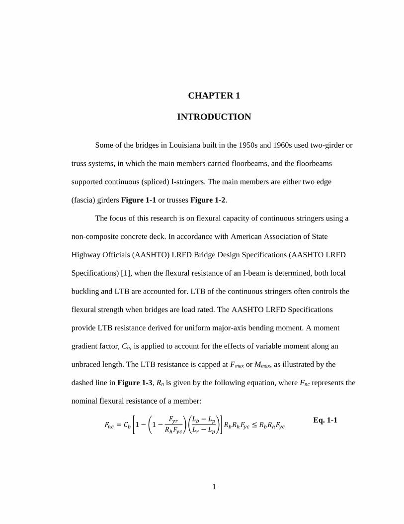
The focus of this research is on flexural capacity of continuous stringers using a

non-composite concrete deck. In accordance with American Association of State

Highway Officials (AASHTO) LRFD Bridge Design Specifications (AASHTO LRFD

Specifications) [1], when the flexural resistance of an I-beam is determined, both local

buckling and LTB are accounted for. LTB of the continuous stringers often controls the

flexural strength when bridges are load rated. The AASHTO LRFD Specifications

provide LTB resistance derived for uniform major-axis bending moment. A moment

gradient factor, Cb, is applied to account for the effects of variable moment along an

unbraced length. The LTB resistance is capped at Fmax or Mmax, as illustrated by the

dashed line in Figure 1-3, Rn is given by the following equation, where Fnc represents the

nominal flexural resistance of a member:

𝐹𝑛𝑐 = 𝐶𝑏 [1 − (1 −

𝐹𝑦𝑟

𝑅ℎ𝐹𝑦𝑐) (

𝐿𝑏 − 𝐿𝑝

𝐿𝑟 − 𝐿𝑝)] 𝑅𝑏𝑅ℎ𝐹𝑦𝑐 ≤ 𝑅𝑏𝑅ℎ𝐹𝑦𝑐

Eq. 1-1

2

As shown in this equation, Cb directly affects the flexural strength of the stringer.

As specified in AASHTO LRFD Specifications Appendix A6 [1], when flexural

resistance of non-composite I-sections is calculated, the contribution from the concrete

deck and longitudinal reinforcement is neglected at the negative moment section. This

underestimates the flexural capacity of the continuous stringer. The objective of this

research is to re-assess the flexural strength of a continuous stringer with a non-

composite deck and propose a reasonable approach to determine Cb.

Figure 1-1: Sample floor system, edge girder

Figure 1-2: Sample floor system, truss

3

Figure 1-3: Basic form of I-section compression-flange flexural resistance equations [1]

This chapter presents a literature review of Cb in accordance with a variety of

codes and specifications. Also presented is the significant work by several researchers. In

addition, there are reference summaries on the bracing effect of the bridge decks.

1.1 Moment Gradient Factor

The focus of this research is related to I-shaped stringers having doubly

symmetric sections and primarily subject to vertical loading. Several significant

references associated with the development of Cb and lateral bracing provided by bridge

decks are discussed herein. A number of specifications and codes are presented, including

the AASHTO LRFD Bridge Design Specifications, the AISC Steel Construction Manual,

the Canadian Highway Bridge Design Code, the Australian Steel Code, the British

Standards Structural Use of Steelwork in Building, and the Japanese Standard

Specifications for Steel and Composite Structures. In addition, works by several

significant researchers are included. Each section presents relevant background

4

discussions and equations for the moment gradient factor followed by definitions of the

primary parameters.

1.1.1 AASHTO LRFD Bridge Design Specifications, Seventh Edition, 2014 [1]

The LTB resistance equations in the AASHTO LRFD Bridge Design

Specifications provide predictions close to mean LTB resistances from uniform bending

experimental tests conducted by Galambos and Ravindra in 1978 [2]. For members

subject to a moment gradient, the factor is included primarily following research work

performed by Salvadori [3]. For continuous stringers supported by floorbeams, Cb can be

greater than 1.0 using Eq. 1-2.

𝐶𝑏 = 1.75 − 1.05 (𝑓1

𝑓2) + 0.3 (

𝑓1

𝑓2)

2

≤ 2.3 Eq. 1-2

where

f1 = stress without consideration of lateral bending at the brace point opposite to

the one corresponding to f2, calculated as the intercept of the most critical assumed linear

stress variation passing through f2 and either fmid or f0, whichever produces the smaller

value of Cb. When variations in the moment along the entire length between the brace

points are concave in shape, then 𝑓1 = 𝑓0 ; otherwise, 𝑓1 = 2𝑓𝑚𝑖𝑑 − 𝑓2 ≥ 𝑓0.

f2 = largest compressive stress without consideration of lateral bending at either

end of the unbraced length of the flange under consideration, calculated from the critical

moment envelope value. Due to the factored loads, f2 shall be positive. If the stress is

zero or the tensile in the flange under consideration at both ends of the unbraced length, f2

is zero.

5

1.1.2 AISC Steel Construction Manual, 2016 [4]

The AISC Steel Construction Manual provides the lateral-torsional buckling

modification factor, Cb, for non-uniform moment diagrams primarily based on the

research work by Kirby and Nethercot with slight modifications [5]. Cb is determined as

follows:

𝐶𝑏 =12.5𝑀𝑚𝑎𝑥

2.5𝑀𝑚𝑎𝑥 + 3𝑀𝐴 + 4𝑀𝐵 + 3𝑀𝑐 Eq. 1-3

where

Mmax = the absolute value of maximum moment in the unbraced segment;

MA = the absolute value of moment at the quarter point of the unbraced segment;

MB = the absolute value of moment at the center of the unbraced segment; and

MC = the absolute value of moment at the three-quarter point of the unbraced

segment.

1.1.3 Canadian Highway Bridge Design Code, S6-14 [6]

In accordance with the Canadian Highway Bridge Design Code, structural

sections shall be designated as Class 1, 2, 3, or 4, depending on width-to-thickness ratios

of the elements that make up the cross-section and on loading conditions. A Class 1

section is one that will attain the plastic moment capacity, adjusted for the presence of

axial force if necessary, and permit subsequent redistribution of bending moment. A

Class 2 section is one that will attain the plastic moment capacity, adjusted for the

presence of axial force if necessary, but not necessarily permit subsequent moment

redistribution. A Class 3 section is one that will attain the yield moment capacity,

adjusted for the presence of axial force if necessary. A Class 4 section is one in which the

slenderness of the elements making up the cross-section exceeds the limits of Class 3.

6

The moment gradient factor is calculated as:

𝑤2 =4𝑀𝑚𝑎𝑥

√𝑀𝑚𝑎𝑥2 + 4𝑀𝑎

2 + 7𝑀𝑏2 + 4𝑀𝑐

2

≤ 2.5 Eq. 1-4

where

Mmax = maximum absolute value of factored moment in the unbraced segment;

Ma = factored bending moment at one-quarter point of the unbraced segment;

Mb = factored bending moment at midpoint of the unbraced segment; and

Mc = factored bending moment at three-quarter point of the unbraced segment.

1.1.4 Australian Steel Code AS4100 [7]

AS4100 provides Eq. 1-5 to determine an equivalent uniform moment factor or

moment modification factor, αm, for stringers where β is the ratio of the two end

moments. It also allows simple approximation using Eq. 1-6 that applies to any bending

moment distribution:

𝛼𝑚 = 1.75 + 1.05𝛽 + 0.3𝛽2 ≤ 2.5 Eq. 1-5

𝛼𝑚 =1.7𝑀𝑚

√(𝑀2)2 + (𝑀3)2 + (𝑀4)2≤ 2.5 Eq. 1-6

where

Mm = maximum design bending moment;

M2, M4 = design bending moments at the quarter points; and

M3 = design bending moment at the midpoint of the segment.

1.1.5 British Standards Institution (BSI), Structural Use of Steelwork in Building,

BS 5950-1:2000 [8]

In the British code, the moment gradient factor of I-stringers with equal flanges

should satisfy the following:

7

𝑚𝐿𝑇 = 0.2 +0.15𝑀2 + 0.5𝑀3 + 0.15𝑀4

𝑀𝑚𝑎𝑥≥ 0.44

Eq. 1-7

Where, all moments are taken as positive. The moment M2 and M4 are the values at the

quarter points, M3 is the value at mid-length and Mmax is the maximum moment in the

segment.

1.1.6 Research by Lopez et al. [9]

Lopez et al. proposed a closed form expression for the equivalent uniform

moment factor, C1, applicable to any moment distribution. The proposed formula

incorporates end support conditions through a parameter related to the lateral torsional

buckling length of the stringer. For a general moment diagram, the coefficient C1 may be

obtained by:

𝐶1 =

√√𝑘𝐴1 + [(1 − √𝑘)𝐴2

2]

2

+(1 − √𝑘)𝐴2

2

𝐴1

Eq. 1-8

where

k depends on the lateral bending and warping condition coefficients k1 and k2 :

𝑘 = √𝑘1𝑘2 Eq. 1-9

and A1 and A2 are given by:

𝐴1 =𝑀𝑚𝑎𝑥

2 + 𝛼1𝑀12 + 𝛼2𝑀2

2 + 𝛼3𝑀32 + 𝛼4𝑀4

2 + 𝛼5𝑀52

(1 + 𝛼1 + 𝛼2 + 𝛼3 + 𝛼4 + 𝛼5)𝑀𝑚𝑎𝑥2

Eq. 1-10

𝐴2 = |𝑀1 + 2𝑀2 + 3𝑀3 + 2𝑀4 + 𝑀5

9𝑀𝑚𝑎𝑥|

Eq. 1-11

8

where

𝛼1 = 1 − 𝑘2; 𝛼2 = 5𝑘1

3

𝑘22 ; 𝛼3 = 5 (

1

𝑘1+

1

𝑘2) ;

𝛼4 = 5𝑘2

3

𝑘12 ; 𝛼5 = 1 − 𝑘1

Eq. 1-12

In Eq. 1-10 and Eq. 1-11, Mmax is the maximum moment, and M1, M2, M3, M4, and

M5 are the values of the moment at different sections of the stringer, each of them with

the corresponding sign.

1.1.7 Research by Subramanian and White [10]

The LTB curves in AASHTO and AISC are based in large part on unified

provisions proposed by White [11], which were in turn based largely on experimental

data compiled by White and Jung [12] and White and Kim [13]. A recent study by

Subramanian et al. demonstrated that rolled I-stringers may exhibit an inelastic Cb effect.

This essentially means that, when the inelastic LTB strength is scaled by the modification

factor Cb (where Cb is developed based on elastic buckling formulations), strength

estimates tend to be higher than the true inelastic LTB strength under a moment gradient.

Subramanian et al. concluded that when the maximum moment in a span occurs at a

braced location, the proposed LTB model for uniform moment, along with current

handling of Cb in the AASHTO and AISC, is satisfactory, and no modifications were

proposed for such cases. When the maximum moment occurs within an unbraced

segment of the stringer, the current AISC specification moment modifier in the inelastic

LTB region could be as much as 20% un-conservative. The SABRE2 computational tool

was developed to implicitly and rigorously capture moment gradient effects based on

applied loading as well as any unbraced length end-restraint effects.

9

1.1.8 Research by Helwig et al. [14]

Helwig et al. suggested multiplying the original equation for Cb from Kirby and

Nethercot [5] by the terms 1.42𝑦/ℎ to account for the effects of load height within the

cross-section and by R to account for the effects of I-section monosymmetry and reverse

curvature bending in prismatic members. The term 1.42𝑦/ℎ considers destabilizing or the

tipping effect of the loads applied transversely to the top flange, or the stabilizing or the

restoring effect of loads applied transversely to the bottom flange. If one or more

intermediate braces are provided within an ordinary or cantilever span in which the ends

are prevented from twisting, the load height effects do not need to be considered in the

calculation of Cb:

𝐶𝑏 =12.5𝑀𝑚𝑎𝑥

2.5𝑀𝑚𝑎𝑥 + 3𝑀𝐴 + 4𝑀𝐵 + 3𝑀𝑐(1.42𝑦/ℎ)𝑅 Eq. 1-13

where

Mmax = the absolute value of the maximum moment within the unbraced length;

MA, MB, and MC = the absolute values of the moments at the 1/4, middle, and 3/4 points

of the unbraced segment;

y = the distance from the mid-depth of the cross section to the point of the load

application, which is taken as negative for downward loads applied above mid-depth and

positive for downward loads applied below mid-depth;

h = the distance between the compression and tension flange centroids; and

R = 1.0 for beams with single-curvature bending.

For reverse-curvature bending,

𝑅 = 0.5 + 2(𝐼𝑦 𝑇𝑜𝑝

𝐼𝑦)2 Eq. 1-14

10

where

Iy Top = moment of inertia of the top flange on an axis in the plane of the web; and

Iy = moment of inertia of the entire section about an axis in the plane of the web.

1.1.9 Research by Salvadori [15]

Beginning with the 1961 AISC Manual and continuing through the 1986

AASHTO LRFD Specifications, Eq. 1-15 was used to adjust lateral-torsional buckling

equations for variations in the moment diagram within an unbraced length:

𝐶𝑏 = 1.75 + 1.05 (𝑀1

𝑀2) + 0.3 (

𝑀1

𝑀2)

2

≤ 2.3 Eq. 1-15

where

M1 = smaller moment at end of unbraced lengths;

M2 = larger moment at end of unbraced lengths; and

(M1/M2) is positive when moments cause reverse curvature and negative for single

curvature.

1.1.10 Research by Wong and Driver [16]

Wong and Driver reviewed several approaches and recommended the following

quarter-point equation for use with doubly symmetric I-shaped members:

𝐶𝑏 =4𝑀𝑚𝑎𝑥

√𝑀𝑚𝑎𝑥2 + 4𝑀𝐴

2 + 7𝑀𝐵2 + 4𝑀𝑐

2

Eq. 1-16

The equation gives improved predictions for several important cases, including

cases with moderately nonlinear moment diagrams. Also, the length between braces, not

the distance to inflection points, is used in all cases.

11

1.1.11 Research by Yura and Helwig [17] [18]

Many situations arise where a stringer is subjected to reverse curvature bending

with one of the flanges continuously braced laterally by closely spaced joists and/or light

gauge decking normally used for roofing or flooring systems. Although this type of

lateral bracing provides significant restraint to one of the flanges, the other flange can

still buckle laterally due to compression caused by the reverse curvature bending. For

gravity loaded, rolled I–section stringers with the top flange laterally restrained, the

following expression is applicable:

𝐶𝑏 = 3.0 −2

3(

𝑀1

𝑀0) −

8

3 [

𝑀𝐶𝐿

(𝑀1 + 𝑀0)∗] Eq. 1-17

where

M0 = moment at the end of the unbraced length that gives the largest compressive stress

in the bottom flange;

M1 = moment at the other end of the unbraced length;

MCL= moment at the middle of the unbraced length; and

(M0 + M1)* = M0, if M1 is positive, causing tension on the bottom flange.

1.1.12 Research Findings in Other References [19] to [53]

Additional references on the flexural strength accounting for lateral torsional

buckling and moment gradient factor were studied. Because the research findings in these

publications are similar or comparable to those listed above, they are not described

individually for brevity.

1.2 Lateral Bracing Effect of Bridge Decks

Bracing members are commonly classified as torsional (diaphragms or cross

frames) or lateral (top chord, upper and lower laterals or bridge decks). Both tests and

12

theoretical solutions have shown that cross section distortion has a significant effect on

torsional brace effectiveness [54]. A bridge deck has the potential to act as a lateral

and/or torsional brace. The friction that may be mobilized at the deck-stringer interface

acts as a lateral brace because it restrains lateral movement of the stringer top flange. A

number of researchers concluded that even if there is no mechanical connection between

the deck and the stringers, friction may still be adequate to develop the required deck

stiffness to act as a lateral brace at the contact area of the wheel load. Therefore, if a

stringer is non-composite and it is subject to positive moment, it might be considered

laterally supported at the wheel load location near the mid-span [55].

A full-size test on a five-girder short-span bridge conducted by Yura et al. showed

that timber decks not positively attached to the stringers can provide lateral bracing at

wheel load locations through friction [56]. Common timber decks have enough lateral

bracing stiffness to permit the stringers to reach yield without buckling. It can be inferred

that concrete decks provide greater lateral stiffness and have better friction resistance

than timber decks.

Kissane completed another study of bracing effects provided by bridge decks for

the New York State Department of Transportation in 1985 [57]. The objective was to

determine the effectiveness of a non-composite concrete bridge deck as a lateral brace for

the compression flange of the supporting stringers without any positive shear

connections. To complete the comparison, we conducted tests where the physical or

chemical bond between the concrete deck and the stringers was intentionally eliminated.

Kissane concluded that friction resistance between the concrete deck and the stringers

was sufficient to use the deck as a brace and allow the stringers to reach their full bending

13

capacity without buckling laterally. In addition, Linzell et al. conducted field-testing of a

riveted through-girder bridge in Pennsylvania and identified unintended composite action

under live loads [58].

When a stringer is made composite with a concrete deck slab or the top flange is

fully embedded in the deck slab, the top flange is considered to be fully braced if the

subject is connected to the positive moment (compression on top), and therefore, LTB is

not applicable. In the negative moment region, the bottom flange of the stringers is in

compression and shall be evaluated for LTB resistance. In past practices, points of contra

flexure sometimes have been considered as the brace points when the influence of

moment gradient is not included in LTB resistance equations. However, this practice

sometimes can lead to a substantially un-conservative estimate of the flexural resistance

[1]. The influence of moment gradient may be correctly accounted for using Cb and the

effect of restraint from adjacent unbraced segments may be accounted for by using an

effective length factor less than 1.0. Multiple researchers have proposed using a braced

column monograph as an acceptable analogy for obtaining the effective length of the

critical stringer [58, 59].

14

CHAPTER 2

THEORY BACKGROUND

This chapter presents the theory background of steel beams’ LTB resistance. It

summarizes different approaches of solving the LTB problem, including the finite

difference method (FDM). Several studies have been conducted to evaluate the LTB of

simple-span beams and different loading cases. This chapter discusses a theoretical

solution for Cb for continuous beams and addresses a comparison with the existing

methods.

Prandtl and Mitchell developed the first documentation about LTB in 1899,

accounting for a thin rectangular cross section. Timoshenko included the effect of

warping to Prandtl’s work in 1905, and introduced a fourth order differential equation for

LTB in 1961 [60] (See Eq. 2-1).

𝐸𝐶𝑤

𝑑4𝛷

𝑑𝑧4−

𝐺𝐽𝑑2𝛷

𝑑𝑧2−

𝑀𝑜2𝛷

𝐸𝐼𝑦= 0 Eq. 2-1

where

E - modulus of elasticity J - torsional constant

G - shear modulus Iy - moment of inertia in weak axis

Cw - warping constant Φ - twisting angle

𝑀𝑜 - bending moment in strong axis

15

LTB is affected by material properties (shear modulus and Young’s modulus),

cross-section properties (torsional constant, warping constant, second moment of inertia

about weak axis), geometric properties (unbraced length of the beam), boundary

conditions, load type (distributed versus concentrated loads) and point of load application

(top flange, shear center, bottom flange, etc.). LTB is likely to occur when the torsional

stiffness (GIt), warping stiffness(EIw), and flexural stiffness in weak axes are low. A

larger unbraced length and a higher loading position along the beam height (e.g., beam

top flange) also increase the risk of LTB. Eq. 2-1 is based on the following

assumptions [61]:

1. Beam has no initial geometric imperfections or residual stresses.

2. The beam is within the linear elastic range and has no distortion in the

cross section while loading.

3. Load acts in plane of the web.

2.1 Finite Difference Method for Simple Beam

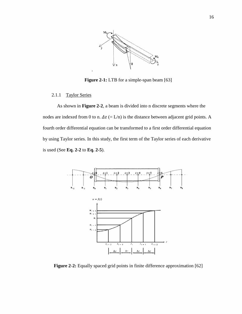
Suryaatmono et al. (2002) [62] investigated the use of FDM considering a few

load cases using a simple-span beam. Figure 2-1 shows a beam subjected to a constant

bending moment (Mo). Since the top flange of the beam is in compression, it tends to

displace laterally and rotate with a twisting angle of Φ. The major axis is indicated in the

x-direction and the minor axis in the y-direction.

16

.

Figure 2-1: LTB for a simple-span beam [63]

2.1.1 Taylor Series

As shown in Figure 2-2, a beam is divided into n discrete segments where the

nodes are indexed from 0 to n. 𝛥𝑧 (= L/n) is the distance between adjacent grid points. A

fourth order differential equation can be transformed to a first order differential equation

by using Taylor series. In this study, the first term of the Taylor series of each derivative

is used (See Eq. 2-2 to Eq. 2-5).

Figure 2-2: Equally spaced grid points in finite difference approximation [62]

17

𝛷𝑖′ =

1

2𝛥𝑧(−𝛷𝑖−1 + 𝛷𝑖+1) Eq. 2-2

𝛷𝑖′′ =

1

𝛥𝑧2(𝛷𝑖−1 − 2𝛷𝑖 + 𝛷𝑖+1) Eq. 2-3

𝛷𝑖′′′ =

1

2𝛥𝑧3(−𝛷𝑖−2 + 2𝛷𝑖−1 − 2𝛷𝑖+1 + 𝛷𝑖+2) Eq. 2-4

𝛷𝑖′′′′ =

1

𝛥𝑧4(𝛷𝑖−2 − 4𝛷𝑖−1 + 6𝛷𝑖 − 4𝛷𝑖+1 + 𝛷𝑖+2) Eq. 2-5

The transformed equation of Eq. 2-1 is as follows:

𝐸𝐶𝑤

𝛥𝑧4(𝛷𝑖−2 − 4𝛷𝑖−1 + 6𝛷𝑖 − 4𝛷𝑖+1 + 𝛷𝑖+2) +

𝐺𝐽

𝛥𝑧2(𝛷𝑖−1 − 2𝛷𝑖 + 𝛷𝑖+1)

+ 𝑀𝑜

2

𝐸𝐼𝑦𝛷𝑖 = 0 Eq. 2-6

2.1.2 Boundary Conditions

Figure 2-3 shows boundary conditions for simply supported, warping fixed,

lateral bending fixed, and completely fixed conditions [64]. Timoshenko equation is

created for simply supported case

.

Figure 2-3: Boundary conditions [64]

18

Using Taylor series these boundary conditions can be written as below

𝛷 = 0 → 𝛷𝑖 = 0 Eq. 2-7

𝑑2𝛷

𝑑𝑧2= 0 → 𝛷𝑖−1 − 2𝛷𝑖 + 𝛷𝑖+1 = 0 Eq. 2-8

𝑑𝛷

𝑑𝑧= 0 → −𝛷𝑖−1 + 𝛷𝑖+1 = 0 Eq. 2-9

2.1.3 Creating a Matrix

For example, if a beam has five grid points (i = 1,2,3,4 and 5), equations for each

node can be written as below. Boundary conditions introduce two equations at the

beginning and the ending nodes. There are nine unknowns and nine equations can solve

this matrix. Large number of nodes are suggested to achieve accurate results.

2.1.4 Smallest Positive Eigenvalue λ

The matrix is created by rearranging nodes and simplifying boundary conditions

according to Kaminski et al. (2016) [65]. In this example, five nodes (n =5) are used for

Eq. 2-10

Eq. 2-11

Eq. 2-12

Eq. 2-13

Eq. 2-14

Eq. 2-15

Eq. 2-16

Eq. 2-17

Eq. 2-18

19

the simply supported beam. All the elements are located on the main diagonal of the

matrix. The smallest positive eigenvalue (λ) that derives from Eq. 2-19 corresponds to

the critical buckling moment or force, depending on the load case.

[A-λI] Φ = 0 Eq. 2-19

Constant Moment

Matrix A is written for a simple span subjected to a constant moment. 𝜆 is the unknown,

and M is the critical buckling moment. Simple support boundary condition is applied.

λ = 𝑀2

𝐸𝐼𝑦 Eq. 2-20

Point Load at Midspan

Matrix B is written for a beam subjected to a point load at the midspan. Simple

support boundary conditions are applied. λ is arranged in a way that P, critical buckling

load, is the only unknown variable (See Eq. 2-21 and 2-22). The first half of the span is

shown in Eq. 2-23, and the other half of the span is shown in Eq. 2-24 because the

bending moment diagram consists of two lines with two slopes. Hence, there is a need for

two equations:

Φ[B-λ I] = 0 Eq. 2-21

λ =

𝑃2

𝐸𝐼𝑦

Eq. 2-22

A =

20

0 ≤ z < L/2 𝐸𝐶𝑤𝑑4𝛷

𝑑𝑧4−

𝐺𝐽𝑑2𝛷

𝑑𝑧2−

(𝑃𝑧/2)2𝛷

𝐸𝐼𝑦

= 0 Eq. 2-23

L/2 ≤ z ≤ L 𝐸𝐶𝑤𝑑4𝛷

𝑑𝑧4−

𝐺𝐽𝑑2𝛷

𝑑𝑧2−

(𝑃(𝐿 − 𝑧)

2)2𝛷

𝐸𝐼𝑦

= 0 Eq. 2-24

2.1.5 MatLab Solution

For example, a W16 x31 beam is considered. The span length varied from 12ft to

24ft. Following the steps above, a matrix is created for this beam assuming simply

supported and subjected to a uniform moment. The solution is compared with Eq. 2-25,

which is the smallest moment that satisfies Timoshenko equation (Eq. 2-1).

𝑀ocr =𝜋

𝐿√𝐸𝐼𝑦𝐺𝐽 + (

𝜋𝐸

𝐿)

2𝐼𝑦𝐶𝑤 Eq. 2-25

Figure 2-4 shows that Timoshenko solution and FDM solution are in good

agreement, which validates the developed Matlab [66] codes and allow the codes to be

upgraded for other cases. Figure 2-4 also shows the buckling moment variation when a

point load is applied at the mid-span of a beam.

B =

21

Figure 2-4: Critical buckling moment vs. span length

2.2 Finite Difference Method for Continuous Beam

2.2.1 Boundary Condition

At the interior support, when there is no steel diaphragm bracing, lateral

deflection curves of adjacent spans have the same tangent. When the steel diaphragms are

present at the interior supports the web restraints twisting, but flanges are free to warp.

(See Figure 2-3 -Type 3). Boundary conditions for continuous beam are as follow:

𝛷 = 0 → 𝛷𝑖 = 0 Eq. 2-26

𝑑2𝛷

𝑑𝑧2= 0 → 𝛷𝑖−1 − 2𝛷𝑖 + 𝛷𝑖+1 = 0 Eq. 2-27

2.2.2 One Span Loaded Case

Moment diagram is presented in Figure 2-6 and Matrix is shown in Appendix B.

Beam is loaded at one span only; therefore, the equations are as follows:

0 ≤ z < L/2 𝐸𝐶𝑤𝑑4𝛷

𝑑𝑧4−

𝐺𝐽𝑑2𝛷

𝑑𝑧2−

(13𝑃𝑧

32 )2𝛷

𝐸𝐼𝑦= 0 Eq. 2-28

0

50

100

150

200

12 16 20 24

Mcr

(k

ip-f

t)

Span Length (ft)

Critical Buckling Moment vs Span Length

MatLab solution for

point load

MatLab solution for

uniform load

Timoshenko solution

for uniform load

22

L/2 ≤ z < L 𝐸𝐶𝑤𝑑4𝛷

𝑑𝑧4−

𝐺𝐽𝑑2𝛷

𝑑𝑧2−

[𝑃13𝑧

32−𝑃(𝑧−

𝐿

2)]2𝛷

𝐸𝐼𝑦=0 Eq. 2-29

L ≤ z ≤ 2L 𝐸𝐶𝑤d4Φ

dz4−

𝐺𝐽d2Φ

dz2−

[𝑃𝟏𝟑𝑧

𝟑𝟐−𝑃(𝑧−

𝑳

𝟐)+

22

32𝑃(𝑧−𝐿)]𝟐Φ

𝐸𝐼𝑦=0 Eq. 2-30

Figure 2-5: A continuous beam with one span loaded

2.2.3 Two Spans Loaded Case

When a continuous beam is loaded at both spans, the equations are updated as

follows:

0 ≤ z < L/2 𝐸𝐶𝑤𝑑4𝛷

𝑑𝑧4−

𝐺𝐽𝑑2𝛷

𝑑𝑧2−

(𝟓

𝟏𝟔𝑷𝑧)𝟐𝛷

𝐸𝐼𝑦=0 Eq. 2-31

L/2 ≤ z < L 𝐸𝐶𝑤d4Φ

dz4−

𝐺𝐽d2Φ

dz2−

[𝑃5

16𝑧−𝑃(𝑧−

𝐿

2)]2Φ

𝐸𝐼𝑦=0 Eq. 2-32

L ≤ z < 3L/2 𝐸𝐶𝑤d4Φ

dz4−

𝐺𝐽d2Φ

dz2−

[P𝟓

𝟏𝟔z−P(z−

𝐋

𝟐)+P

11

8(z−L)]𝟐Φ

𝐸𝐼𝑦=0 Eq. 2-33

3L/2 ≤ z < 2L 𝐸𝐶𝑤d4Φ

dz4 −𝐺𝐽d2Φ

dz2 −[P

𝟓

𝟏𝟔z−P(z−

𝐋

𝟐)+P

11

8(z−L)−P(z−

3𝐋

𝟐)]𝟐Φ

𝐸𝐼𝑦=0 Eq. 2-34

23

.

Figure 2-6: A continuous beam with both spans loaded

2.2.4 Numerical Example

For discussion purpose, a two-span continuous beam is analyzed and the analysis

results using the FDM are compared with the AASHTO, AISC, and lab test data. The

following assumptions are made:

Beam type = W 16 x 31 Torsional constant (It) = 0.461 in4

Modulus elasticity (E) = 29000 ksi Span length (L) = 288 in

Warping constant (Iw) = 739 in6 Minor axis inertia (Iy) = 12.4 in4

Shear modulus (G) = 11154 ksi

Figure 2-7 and Figure 2-8 presents buckled shapes from FDM solution. In

Figure 2-8, “S”-shape is shown for illustration. Another mode can be determined

similarly. Lab testing [67] is discussed in Chapter 3. Results of two test runs that include

lateral bracing by steel diaphragms (Test Run #19 (one span loaded) and Test Run #20

(two spans loaded)) are presented for comparison purpose. The predicated LTB

resistance according to AASHTO, AISC, and lab testing consider point of load

application as the beam’s top flange. However, FDM considers point of load application

24

to be beam’s shear center. Therefore, FDM results are converted to top flange loading

position for comparison purpose.

Figure 2-7: Buckled shape: one span loaded

Figure 2-8: Buckled shape: two spans loaded

Figure 2-9 illustrates critical buckling moment for continuous span bridge

subjected to a point load at the midspan. The predicted buckling moment values from the

FDM are higher than the test data. This difference is attributed to the fact that FDM did

not account for geometry imperfections, and residual stresses. Cb in AASHTO and AISC

codes are presented in Eq. 1-1 and Eq. 1-2 respectively. The resultant Cb is multiplied by

Eq. 2-25 to find critical buckling moments (Mcr) that are shown Figure 2-10. The FDM

results for one span and both spans loaded are multiplied by 0.714 to count for the

25

loading position. [14]. Table 2-1 shows Cb results of all cases. FDM results shows a

higher critical moment for one span loaded case, and a lower critical moment for two

span loaded case. In two span loaded case, FDM results show a “S” buckled shape,

however, lab testing demonstrate a symmetric buckled shape. Therefore, buckling modes

are not exactly same to compare results.

Figure 2-9: Critical buckling moment for continuous span

Table 2-1: Cb for continuous span using codes, lab testing and FDM

Cb

One Span Loaded Two Spans Loaded

AASHTO 1.75 1.75

AISC 1.42 1.69

Lab Test 1.70 1.62

FDM 1.94 1.41

2.3 Finite Difference Method for Beams with Non-composite Concrete Deck

When a non-composite concrete deck is provided, the bracing effect of the deck

does not allow the beam’s top flange to move freely along the transverse direction

(perpendicular to the beam length). At the negative moment region, the beam’s bottom

26

flange is in compression and tends to buckle. Khelil et al. (2008) [68] studied the LTB of

beams that were continuously restrained at one flange. Their research used the Galaerkin

method in the finite difference method. The matrix consisted of three submatrices that

corresponded to rigidity (geometry), boundary conditions, and loading conditions.

Additional information on use of FDM for composite beams can be found in Durant

(1944), Wirianto (1979) and Ivan et al. (2015) [69 -71].

27

CHAPTER 3

NUMERICAL ANALYSES

As part of the research on the LTB resistance of continuous stringers, full-scale

lab testing [67] was conducted at the University of Nebraska – Lincoln. The lab testing

results served as a baseline to allow for calibrating the finite element analyses of the

continuous stringers, which is the focus of Chapter 3. The analyses matched a variety of

test setups accounting for different bracing conditions and load cases. The analysis results

were compared with the lab testing data, including the vertical and lateral deflections, and

strain readings at the representative sections of the stringers. A more accurate approach

was proposed to determine Cb to account for the bracing effect of the concrete deck.

3.1 Lab Testing

This test setup corresponded to a two-span structure, which involved three lines of

stringers, steel diaphragms at the ends for support, and a floorbeam as the interior

support. Lateral restraints provided three options (i.e. steel diaphragms, timber struts at

the top flange, and non-composite concrete deck). To investigate the effect of the

floorbeam’s relative stiffness for LTB, the floorbeam was supported as rigid and flexible.

To analyze variations of the connection restraint for LTB, the bottom of the stringers

were connected to the floorbeam with bolts and without bolts. One-span load case and

two-span load case were tested on the interior stringer.

28

Basic setup included a grillage system that involved three lines of 50 ft. long

W16 x 31 stringers, one 25-ft-long W24 x 68 floorbeam, and C12 x 20 end diagrams

bolted to the stringers. Figure 3-1 and Figure 3-2 show the framing plan and a section of

the grillage at the floorbeam, respectively. Each span was 24 ft. long and the stringers

were spaced at 4 ft. As shown in Figure 3-3 and Figure 3-4, stiff supports underneath the

floorbeam differentiated the rigid and flexible support conditions. The deck was 50 ft.

long by 10 ft. wide and 6 in. thick. The deck was conventionally reinforced using Grade

60 rebar. Figure 3-5 and Figure 3-6 present the deck plan and a typical section.

Figure 3-1: Grillage system framing plan

Figure 3-2: Grillage system section at floorbeam

29

Figure 3-3: Test setup mimicking rigid (stiff) floorbeam

Figure 3-4: Test setup mimicking flexible floorbeam

Figure 3-5: Deck reinforcement plan

30

Figure 3-6: Deck reinforcement plan

Table 3-1 provides the complete test matrix including categories; corresponding

configurations (i.e., test setups); stringer support conditions (i.e., floorbeam flexural

stiffness); loading and bracing conditions, including existence or absence of composite

action (i.e., C or NC); and test run identification numbers. Testing is categorized into four

general groups as listed below (See Figure 3-7 to Figure 3-10).

Group I

This category included stringers without any restraint at the top flange. Results

are shown when the bottom flange was bolted and not bolted, as well as when the

floorbeam was flexible and rigid. Spans were loaded either only one span or both spans.

Group II

In this group, intermediate steel diaphragms (C12x20) were placed at various

locations including the interior support, and L/2, L/8, L/4, and 3L/8 away from the interior

support (L = span). Bottom flange bolted and not bolted conditions were applied in this

group as well.

31

Group III

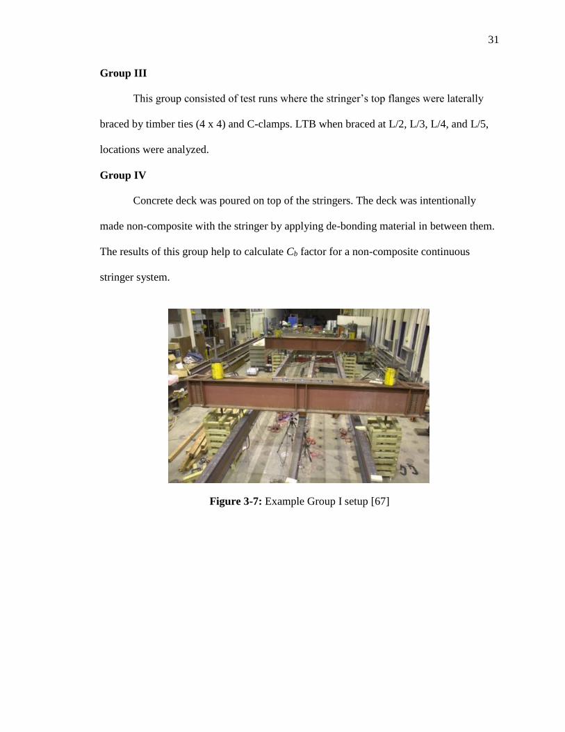
This group consisted of test runs where the stringer’s top flanges were laterally

braced by timber ties (4 x 4) and C-clamps. LTB when braced at L/2, L/3, L/4, and L/5,

locations were analyzed.

Group IV

Concrete deck was poured on top of the stringers. The deck was intentionally

made non-composite with the stringer by applying de-bonding material in between them.

The results of this group help to calculate Cb factor for a non-composite continuous

stringer system.

Figure 3-7: Example Group I setup [67]

32

Table 3-1: Test Matrix

Interior

support at

center stringer

Top flange of stringerBottom flange of

stringer

1 point load 1

2 point loads 21 point load 32 point loads 4

1 point load 5

2 point loads 6

1 point load 7

2 point loads 81 point load 9

2 point loads 10

1 point load 11

2 point loads 12

1 point load 13



2 point loads 18

1 point load 19

2 point loads 20

1 point load 21




2 point loads 28

Timber strut @ L/2, TF 2 point loads 29


TS @ L/4, L/2, L, L/2, L/4 2 point loads 30'





TS @ L/4, L/2, L, L/2, L/4 2 point loads 34'



TS @ L/8, L/4, L/2, L, L/8,

L/4, L/22 point loads 36'








Timber strut @ L/5, TF 2 point loads 441 point load 452 point loads 46

1 point load 57

1 point load 69

No. 3C Braced laterally by bolts 1 point load 81

IV

No Diaphragms

No Diaphragms

NC

Concrete

slab

cast to

stringer

top

flange

No. 3B

Flexible

Unbraced

Braced laterally by bolts

No. 3Rigid

Unbraced

No. 3A

No. 2A


No. 2B

Flexible

Unbraced

No. 2C Braced laterally by bolts

Diaphragms @ L/2

Diaphragms @ L/8 from Int.

SupportDiaphragms @ L/4 from Int.

SupportDiaphragms @ 3L/8 form

Int. Support

III

No. 2

NC

Rigid

Unbraced

Diaphragms @ L/2

Diaphragms @ L/8 from Int.

SupportDiaphragms @ L/4 from Int.

SupportDiaphragms @ 3L/8 form

Int. SupportII

No. 1'

NC

Rigid

Diaphragms @ Int. Support

Unbraced

No. 1'A Rigid

Diaphragms @ Int. Support


No. 1A Braced laterally by bolts

No. 1B

Flexible

Unbraced

No. 1C Braced laterally by bolts

I

No. 1

NC

Rigid

Unbraced

Unbraced

GroupTest

setupNC or C

Description of boundary conditions

Load condition Test Run #

33

Figure 3-8: Example Group II setup [67]

Figure 3-9: Example Group III setup [67]

Figure 3-10: Example Group IV setup [67]

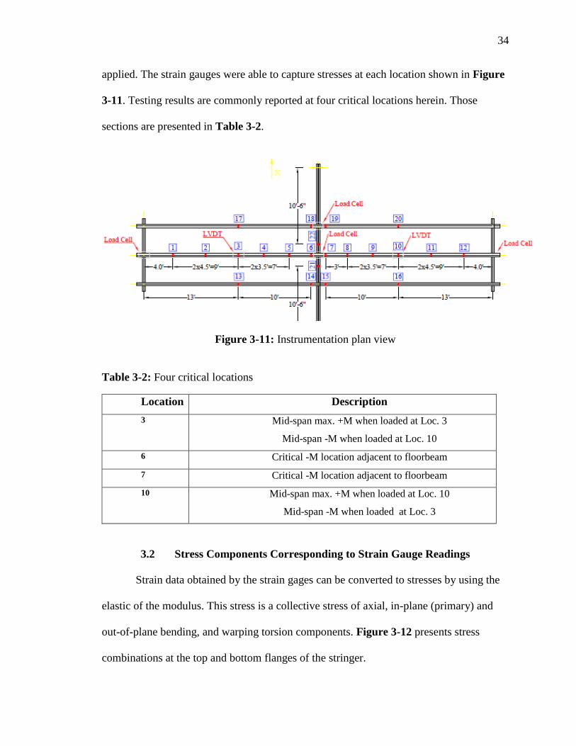
LVDTs are installed at mid-span of the interior stringer of both spans to capture

vertical and lateral deflections. Load and pressure cells were able to measure the force

34

applied. The strain gauges were able to capture stresses at each location shown in Figure

3-11. Testing results are commonly reported at four critical locations herein. Those

sections are presented in Table 3-2.

Location Description

3 Mid-span max. +M when loaded at Loc. 3

Mid-span -M when loaded at Loc. 10

6 Critical -M location adjacent to floorbeam

7 Critical -M location adjacent to floorbeam

10 Mid-span max. +M when loaded at Loc. 10

Mid-span -M when loaded at Loc. 3

3.2 Stress Components Corresponding to Strain Gauge Readings

Strain data obtained by the strain gages can be converted to stresses by using the

elastic of the modulus. This stress is a collective stress of axial, in-plane (primary) and

out-of-plane bending, and warping torsion components. Figure 3-12 presents stress

combinations at the top and bottom flanges of the stringer.

Figure 3-11: Instrumentation plan view

Table 3-2: Four critical locations

35

Figure 3-13 to Figure 3-16 provide load verses stress plots for each stress

component at Loc. 3 for Test Run #1. TN (top-north), TS (top-south), BN (bottom-north)

and BS (bottom-south) are the stresses at Location 3, which is 1 ft. from the loading

position for Test Run #1. Axial loads are typically zero. Weak axis bending and warping

torsion shows a gradual drop after peak load indicating LTB of the stringer. Note how

warping stress and weak axis bending moment at the top flange affect the total stress in

Figure 3-13 and Figure 3-14. On the other hand, warping and weak axis bending

moment at the stringer’s bottom flange act on opposite directions and therefore the sum

of them barely affects the total stress (See Figure 3-15 and Figure 3-16). The stress plots

sof Test Run #1 are provided for illustration purpose. The test results of the other test

runs are selectively shown when they are used to calibrate the finite element analyses

results.

Figure 3-12: Stress components

36

Figure 3-14: Stress components, Loc. 3 TS, Test Run #1

Figure 3-15: Stress components, Loc. 3 BN, Test Run #1

0

5

10

15

20

-20 -15 -10 -5 0 5 10 15

Lo

ad

(k

ips)

Stress(ksi)

TN

σa

σw

σx

0

5

10

15

20

-30 -25 -20 -15 -10 -5 0 5

Lo

ad

(k

ips)

Stress(ksi)

TS

σa

σw

σx

0

5

10

15

20

-10 -5 0 5 10 15 20

Lo

ad

(k

ips)

Stress(ksi)

BN

σa

σw

σx

Figure 3-13: Stress components, Loc. 3 TN, Test Run #1

37

Figure 3-16: Stress components, Loc. 3 BS, Test Run #1

3.3 Finite Element Analyses

Finite element analysis (FEA) simulated the stringer’s behavior while accounting

for various parameters, including geometric imperfections, various bracing

configurations, rigid and flexible interior supports, other loading conditions, etc. FEA

was completed using ANSYS R19 [72]. A combination of static, linear Eigenvalue

buckling, and non-linear buckling analyses were performed. The FEA model includes

three lines of stringers, end diaphragms, and the floorbeam and non-composite concrete

deck (see Figure 3-17).

Figure 3-17: FEA models

0

5

10

15

20

-10 -5 0 5 10 15 20

Lo

ad

(k

ips)

Stress(ksi)

BS

σa

σw

σx

σy

Total

38

3.3.1 Element Type

SHELL181 elements were used for the stringers, end and intermediate

diaphragms, and floorbeam. This shell element is a first-order element with 4 external

nodes and no internal nodes and six degrees of freedom at each node: translations in and

rotations about the x, y, and z axes.

The concrete deck in the linear analysis was modeled using SOLID185 elements.

This is a linear 3D eight-node element with only three (translational) degrees of freedom.

The deck has three layers of elements across the thickness and the element size in the

transverse and longitudinal directions is 4 in. In the nonlinear analysis, the SOLID185 are

substituted for CPT215 elements because SOLID185 elements are not compatible in non-

linear analyses. CPT215 is a coupled physics 3D eight-node suitable for the microplane

model used to capture the nonlinear behavior of the concrete. The element has

temperature, pressure, and nonlocal field values degrees of freedom in addition to three

translations at each node.

LINK180 elements were used to represent the reinforcing steel bars in the

concrete deck for both linear and nonlinear analyses. The element is a linear 3D spar with

two nodes and only translation degrees of freedom suitable for uniaxial tension or

compression. Similarly, this element was employed for the wood bracing at the top

flanges and at appropriate tests because it best represented the test data compared to

BEAM188, which resists load in bending.

3.3.2 Material

The selected structural steel stress-strain diagram is shown in Figure 3-18. The

elastic modulus of steel is assumed to be 29,000 ksi. The stringers and floorbeam were

39

Grade 50 steel, and the diaphragms Grade 36 steel. The concrete strength considered to

be 5,000 psi (f ’c).

Linear elastic concrete properties were used for the linear analysis and the

parameters were chosen to obtain the best imperfection for the stringers. A micro plane

model with coupled damage-plasticity was employed for the nonlinear analysis. This

material model accounts for the elasticity, plasticity, damage, and nonlocal interaction of

the concrete.

Figure 3-18: Selected stress-strain diagram for structural steel

Figure 3-19: Selected stress-strain diagram for concrete

3.3.3 Mesh

Each stringer flange consists of 4 elements along its width while the stringer web

is divided into 8 equal elements. A typical mesh of the stringer section is shown in

40

Figure 3-20. The element size along the length of the stringer at each span is 2 in. A

convergence study was performed to validate the mesh for both linear and nonlinear

analyses. Figure 3-21 shows a comparison among three mesh types (fine, finer, and

finest meshes) for Test Run #3 and indicates that the fine mesh type is sufficient to

capture the stringer’s behavior.

0

3

6

9

12

0.0 0.5 1.0 1.5 2.0 2.5 3.0 3.5

Lo

ad

(k

ips)

Lateral Deflection (in.)

Effect of Mesh Sizes

Fine mesh: 4 flange & 8 web divisions

Finer mesh: 6 flange & 12 web divisions

Finest mesh: 8 flange & 16 web divisions

Figure 3-20: Typical meshes in the model

Figure 3-21: Model mesh sensitivity study

41

3.3.4 Boundary Conditions

Boundary conditions of the models at various supports are illustrated in Figure

3-22. Ends of the stringers were connected with the steel diaphragms using the node

merge option in ANSYS. The floorbeam served as the interior supports (rigid or flexible

supports) for the stringers. For the case of the flexible floorbeam, the floorbeam was

laterally braced at every 3 ft. to ensure that the floorbeam could reach the plastic moment

without failing before the stringers fail. In Group IV, the non-composite deck is applied.

Figure 3-22: Boundary conditions at the stringers and floorbeam

42

3.3.5 Load Cases

As shown in Figure 3-23, the interior stringer was loaded at either one span or

both spans. An area load (6 in. diameter) was applied at the mid-span matching the test

setup.

Figure 3-23: Load cases

3.3.6 Stringer Models

A combination of static, linear Eigenvalue buckling, and non-linear buckling

analyses were performed. Figure 3-24 presents a flow chart of the FEA modeling in

ANSYS. Figure 3-25 shows the procedure of developing the FEA models in ANSYS

corresponding to Group III’s test setups.

Figure 3-24: Flow chart of FEA modeling in ANSYS [73]

43

Figure 3-25: Stringer model development using ANSYS

3.3.7 Non-composite Concrete Deck

Regarding the connection between the deck and stringers, initial model trials

assumed no friction between them along any direction while the stringer’s top flanges

were laterally braced by the deck at discrete points along the stringer’s length. After

calibrating the models with the test results, a frictional interface with a coefficient of 0.1

was selected along both transverse and longitudinal directions because it best matched the

testing data.

SOLID185 was tried initially for the deck, but it was incompatible in the non-

linear buckling analysis. Hence, CPT 215 element was adopted to maintain the same

mesh as the static analysis. Linear buckling and non-linear buckling models were not

connected because they used two different material elements. (See Figure 3-26) Instead,

linear buckling results were extracted using commands. ANSYS commands that helped

to attribute these elements and to implement non-linear behavior are shown in Appendix.

44

Figure 3-26: Deck model setup using ANSYS

3.3.8 Parametric Study

Lateral Stiffness at the Loading Frame

After numerous FEA model trials, use of a lateral spring with a stiffness of 1.0

kip/in. at the loading location best represent the load assembly’s lateral stiffness and

provide comparable results with the test data. The spring connected to midpoint of the top

flange, and explicitly constrained in a vertical direction (using a constraint equation), so

that stringer and spring have the same vertical movement (See Figure 3-27). Observed

lateral stiffness is attributable to friction between the load bearing plate and the interior

stringer, and lateral stiffness of the loading assembly largely provided by the two

threaded rods used to support the spreader beam in the lab tests. Figure 3-28 shows the

effect of the spring’s stiffness for a simple supported beam.

Figure 3-27: Spring placement in Test Run #3

45

Figure 3-28: Effect of spring stiffness for a simply supported beam

Geometry Imperfections

Stringer geometry measurements were collected using laser scans prior to the lab

tests. An initial imperfection for the interior stringer, approximately L/1,500 (L = span),

was accounted for in the non-linear analysis following the critical buckling mode. Figure

3-29 shows the lateral and vertical deflection variation in LTB due to imperfections.

0

1

2

3

4

5

6

7

8

9

10

0 0.5 1 1.5 2

Load

(ki

ps)

Vertical Displacement (in.)

without spring

0.05 kip/in spring

0.1 kip/in. spring

0.2 kip/in. spring

0

1

2

3

4

5

6

7

8

9

10

0 1 2 3 4

Load

(ki

ps.

)

Lateral Displacement (in.)

without spring

0.05 kip/in. spring

0.1 kip/in. spring

0.2 kip/in. spring

46

Figure 3-29: Effect of geometry imperfections on LTB

Friction between the Stringers and Floorbeam

In the test runs without bolt connection between the stringers and the floorbeam,

friction was assumed at the interface. Friction coefficient of 0.05, 0.1, 0.2, and 0.4 were

accounted for, and the interior stringer lateral movement at the floorbeam is shown in

Figure 3-30. After comparing the test results, the friction coefficient of 0.2 was chosen

for the models.

0

2

4

6

8

10

12

0 1 2 3 4

Load

(ki

ps)


L/4000

L/2000

L/1000

L/500

L/3000

0

2

4

6

8

10

12

-0.5 -0.4 -0.3 -0.2 -0.1 0

Load

(ki

ps)

Vertical Diflection (in.)

L/4000

L/2000

L/1000

L/500

L/3000

47

Connections between the Stringer Ends and Diaphragms

End diaphragms were modeled using either truss elements (LINK180) for shear

connection, or beam elements (BEAM188) for moment connection. However, both types

of connection demonstrated comparable results. This result is acceptable because at the

end of the stringer, moments are close to zero, and therefore, use of moment or shear

connection does not make much of a difference.

3.4 Group I Results

Test Run #3 was selected for discussion purpose. This test run had a rigid support

at the floorbeam and used a bolted connection between the stringers and the floorbeam. It

was only loaded at one span (1 ft. away from the critical Location 3). Figure 3-31 and

Figure 3-32 show the lateral deflection and element normal stress contours, respectively.

Figure 3-33 to Figure 3-36 present analysis results compared with the test data at the

mid-span of both spans (Locations 3 and 10). Analysis results were generally comparable

to the test data. Figure 3-37 shows the buckled shape when the stringer was loaded at

both spans.

0

5

10

15

20

-0.022 -0.012 -0.002

Lo

ad (

kip

s)

Displacement (in.)

TestRun#1, Stringer at floorbeam

0.05

0.2

0.4

Figure 3-30: Interior stringer displacement at floorbeam location

48

Figure 3-31: Lateral deflection contour, Test Run #3

Figure 3-32: Normal stress contour, Test Run #3

0

5

10

15

20

25

-0.8 -0.7 -0.6 -0.5 -0.4 -0.3 -0.2 -0.1 0.0 0.1 0.2 0.3

Lo

ad (

kip

s)

Deflection (in.)

TestRun3, Load-Vertical Displacement

Ansys-Loc 3

Ansys-Loc 10

Test-Loc 3

Test-Loc 10


49

Figure 3-34: Comparison of FEA and measured deflections, Test Run #3


Test Run #3

0

5

10

15

20

25

0.0 0.2 0.4 0.6 0.8 1.0 1.2 1.4 1.6 1.8 2.0 2.2L

oad

(kip

s)

Deflection (in.)

TestRun3, Load-Lateral Displacement

Ansys-Loc 3

Ansys-Loc 10

Test-Loc 3

Test- Loc 10

0

5

10

15

20

25

-50 -45 -40 -35 -30 -25 -20 -15 -10 -5 0 5 10 15 20 25

Lo

ad (

kip

s)

Stress (ksi)

TestRun3, Loc-3, Load-Stress

Ansys-TS

Ansys-TN

Ansys-BS

Ansys-BN

Test-TS

Test-TN

Test-BS

Test-BN

0

5

10

15

20

25

-10 -5 0 5 10

Lo

ad (

kip

s)

Stress (ksi)


Ansys-TS

Ansys-TN

Ansys-BS

Ansys-BN

Test-TS

Test-TN

Test-BS

Test-BN


Test Run #3

50

Figure 3-37: Total deformation contour, both spans loaded

3.5 Group II Results

Figure 3-38 shows the buckled shapes of the interior stringer due to various

unbraced lengths when intermediate steel diaphragms were provided at L/2, 3L/8, L/4,

and L/8 subject to a load at one span. Figure 3-39 presents the buckled shapes for two

span load cases. Test Run #15 was selected as an example to show the comparison

between the FEA and test results. It had a rigid floorbeam and used no bolted connection

between the stringer and the floorbeam. Steel diaphragms were provided at a quarter span

from the interior supports. The analysis results were compared with the test data,

including the vertical and lateral deflections, and the stresses at Locations 3 and 10 (see

Figure 3-40 to Figure 3-43). The analysis results were generally comparable with the

test data.

51

Figure 3-38: Buckled shapes of the interior stringer for Group II tests when one span

is loaded

Figure 3-39: Buckled shapes of the interior stringer for Group II tests when both spans

are loaded

52

05

101520253035

0.0 0.2 0.4 0.6 0.8 1.0

Lo

ad (

kip

s)

Deflection (in.)


Ansys-Loc 3

Ansys-Loc 10

Test-Loc 3

Test-Loc 10

0

5

10

15

20

25

30

-50-45-40-35-30-25-20-15-10 -5 0 5 10 15 20 25 30 35

Lo

ad (

kip

s)

Stress (ksi)


Ansys-TS

Ansys-TN

Ansys-BS

Ansys-BN

Test-TS

Test-TN

Test-BS

Test-BN



Figure 3-42: Comparison of Loc. 3 stresses between analysis and test data, Test Run #15

05

101520253035

-1.5 -1.0 -0.5 0.0 0.5

Lo

ad (

kip

s)

Deflection (in.)


Ansys-Loc 3

Ansys-Loc 10

Test-Loc 3

Test-Loc 10

53

3.6 Group III Results

Figure 3-44 presents a model that has timber bracings at the top flange. Initially,

timber struts were modeled as truss elements (LINK180 elements). However, BEAM188

elements (that can handle bending) with an elastic modulus of 110 ksi appeared to result

in comparable results with the test data. Figure 3-45 shows the buckled shapes of the

stringers in Group III test runs. These tests were loaded at both spans.

Test Run #33 was selected as an example to show the comparison between the

FEA and test results. It used a rigid floorbeam and a bolted connection between the

stringer and the floorbeam. The stringer top flanges were braced by timber ties and C-

clamps at the mid-spans and over the floorbeam. Figure 3-46 and Figure 3-47 present

the contours of the vertical and lateral deflections, respectively. The analysis results were

compared with the test data, including the vertical and lateral deflections, and stresses at

Locs. 3 and 10 (Figure 3-48 and Figure 3-51). The analysis results were generally

comparable with the testing data.

0

5

10

15

20

25

30

-10 -5 0 5 10L

oad

(kip

s)

Stress (ksi)


Ansys-TS

Ansys-TN

Ansys-BS

Ansys-BN

Test-TS

Test-TN

Test-BS

Test-BN

Figure 3-43: Comparison of Loc. 10 stresses between analysis and test data, Test Run #15

54

Figure 3-44: Group III ANSYS model

Figure 3-45: LTB of Group III subjected to two-span loading

Figure 3-46: Vertical deflection contour, Test Run #33

55

Figure 3-47. Lateral deflection contour, Test Run #33

0

10

20

30

40

-0.9 -0.8 -0.7 -0.6 -0.5 -0.4 -0.3 -0.2 -0.1 0.0

Lo

ad (

kip

s)

Deflection (in.)


Ansys-Loc 3

Ansys-Loc 10

Test-Loc 3

Test-Loc 10

0

10

20

30

40

0.0 0.1 0.2 0.3 0.4 0.5 0.6 0.7 0.8 0.9 1.0

Lo

ad (

kip

s)

Deflection (in.)


Ansys-Loc 3

Ansys-Loc 10

Test-Loc 3

Test-Loc 10



56

3.7 Group IV Results

3.7.1 One Span Loaded Case

For discussion purposes, Test Run #45 Failure 3 (load at Loc.10) is presented.

The FEA model included the non-composite deck and accounted for concrete cracking

and crushing. The FEA model was calibrated against measured test results when a

frictional coefficient of 0.1 was assumed between the stringer and the deck. The FEA

results agreed reasonably well with the test data. Figure 3-52 and Figure 3-53 show the

vertical deflection contours subject to a peak load of 128.1 kips in the stringers and the

deck, respectively. Figure 3-54 shows the lateral deflection contours, and Figure 3-55,

0

10

20

30

40

-50 -40 -30 -20 -10 0 10 20 30L

oad

(kip

s)

Stress (ksi)


Ansys-TS

Ansys-TN

Ansys-BS

Ansys-BN

Test-TS

Test-TN

Test-BS

Test-BN

0

10

20

30

40

-50-45-40-35-30-25-20-15-10 -5 0 5 10 15 20 25 30 35

Lo

ad (

kip

s)

Stress (ksi)


Ansys-TS

Ansys-TN

Ansys-BS

Ansys-BN

Test-TS

Test-TN

Test-BS

Test-BN


Test Run #33


Test Run #33

57

and Figure 3-56 present the longitudinal stress contours in the stringers and the deck.

Comparisons between the analysis and test results are provided in Figure 3-57 to Figure

3-61. Comparisons showed that the peak load predicted by the FEA model was slightly

lower than that from the test, indicating that the FEA model can conservatively simulate

the stringers’ overall behavior.

Figure 3-52: Stringer vertical deflection contour, Test Run #45 Failure 3

Figure 3-53: Deck vertical deflection contour, Test Run #45 Failure 3

58

Figure 3-54: Lateral deflection contour, Test Run #45 Failure 3

Figure 3-55: Stringer longitudinal normal stress contour, Test Run #45 Failure 3

Figure 3-56: Deck longitudinal normal stress contour, Test Run #45 Failure 3

59


Failure 3

. Figure 3-58: Comparison of FEA and measured lateral deflections, Test Run #45

Failure 3


Failure 3

0

50

100

150

200

-2.6 -2.4 -2.2 -2 -1.8 -1.6 -1.4 -1.2 -1 -0.8 -0.6 -0.4 -0.2 0 0.2 0.4 0.6 0.8 1

Lo

ad (

kip

s)

Deflection (in.)

TestSetup45_F3 Vertical Deflection

3-ANSYS

10-ANSYS

3-Test

10-Test

0

50

100

150

200

-0.05 0 0.05 0.1 0.15 0.2 0.25

Lo

ad (

kip

s)

Deflection (in.)

TestSetup45_F3 Lateral Deflection

3-ANSYS

10-ANSYS

3-Test

10-Test

0

50

100

150

-2000 -1000 0 1000 2000

Lo

ad (

kip

s)

Strain (µε)

TestSetup45 Loc-10 StrainTN-ANSYS

TS-ANSYS

BN-ANSYS

BS-ANSYS

TN - Test

TS - Test

BN - Test

BS - Test

60


Failure 3


Failure 3

3.7.2 Two Spans Loaded Case

FEA results agreed reasonably well with the test data. Figure 3-62 and Figure

3-63 are FEA vertical deflection contours subject to a peak load of 122.8 kips in the

stringers and the deck, respectively. Figure 3-64 shows the FEA lateral deflection

contours, and Figure 3-65 and Figure 3-66 present longitudinal FEA stress contours in

the stringers and the deck. The test results are provided in Figure 3-67 to Figure 3-73.

The FEA results are generally comparable with the test data and allowed to predict the

stringer flexural strength.

0

50

100

150

-2000 -1000 0 1000 2000

Lo

ad (

kip

s)

Strain (µε)

TestSetup45 Loc-6 StrainTN-ANSYS

TS-ANSYS

BN-ANSYS

BS-ANSYS

TN - Test

TS - Test

BN - Test

BS - Test

0

50

100

150

-1500 -1000 -500 0 500 1000 1500

Lo

ad (

kip

s)

Strain (µε)

TestSetup45 Loc-7 Strain

TN-ANSYS

TS-ANSYS

BN-ANSYS

BS-ANSYS

TN - Test

TS - Test

BN - Test

BS - Test

61

Figure 3-62: Stringer vertical deflection contour, Test Run #46

Figure 3-63: Deck vertical deflection contour, Test Run #46

Figure 3-64: Lateral deflection contour, Test Run #46

62

Figure 3-65: Stringer longitudinal normal stress contour, Test Run #46

Figure 3-66: Deck longitudinal normal stress contour, Test Run #46

Figure 3-67: ANSYS vertical deflection results, Test Run #46

0

50

100

150

-1.2 -1 -0.8 -0.6 -0.4 -0.2 0

Lo

ad (

kip

s)

Vertical displacement (in.)

3-ANSYS

10-ANSYS

63

Figure 3-68: Lab test vertical deflection results, Test Run #46

Figure 3-69: ANSYS lateral deflection results, Test Run #46

Figure 3-70: Lab test lateral deflection results, Test Run #46

0

50

100

150

0 0.05 0.1 0.15 0.2 0.25

Lo

ad (

kip

s)

Lateral Displacement (in.)

3-ANSYS

10-ANSYS

Displacement (in.)

64

Figure 3-71: ANSYS applied load versus measured longitudinal strains results,

Test Run #46

Figure 3-72: Lab test applied load versus measured longitudinal strains results,

Test Run #46

Figure 3-73: ANSYS applied load versus measured longitudinal strains, Test Run #46

0

50

100

150

-1500 -1000 -500 0 500 1000 1500

Lo

ad (

kip

s)

Strain (µε)

TestSetup#46, Loc-3 Strain

TN-ANSYS

TS-ANSYS

BN-ANSYS

BS-ANSYS

0

50

100

150

-2000 -1000 0 1000 2000

Lo

ad (

kip

s)

Strain (µε)

TestSetup#46, Loc-6 Strain

TN-ANSYS

TS-ANSYS

BN-ANSYS

BS-ANSYS

Strain (µϵ)

65

CHAPTER 4

LAB TESTING FINDINGS

For discussion purpose, Table 4-1 is extracted from Table 3-1 by showing Group

I tests only. The tests accounted for both rigid and flexible interior supports. The

stringer’s top flanges were unbraced and the stringer’s bottom flanges were either

unbraced or braced at the floorbeam. The loads were applied at one span or both

spans [74].

Table 4-1: Group I test matrix

4.1.1 Effect of Connections between the Stringer and Floorbeam

Figure 4-1 illustrates the effect of the stringer to floorbeam’s fixity for Test Runs

#1 to 8. As expected, when the stringer’s bottom flanges were braced with the floorbeam,

the stringers exhibited higher buckling loads as compared to those unbraced cases.

66

Figure 4-1: Effect of stringer to floorbeam fixity on loading capacity

4.1.2 Effect of Floorbeam Stiffness

Figure 4-2 illustrates the effect of the floorbeam’s relative stiffness on the

observed response for Test Runs #1 to 8. A flexible floorbeam results in approximately

10% difference for LTB resistance for most cases and increases the maximum vertical

displacement.

4.1.3 Bracing Effect of Intermediate Steel Diaphragms

Intermediate steel diaphragms were installed at various locations in Group II test

setups to study their effect on LTB resistance. Figure 4-3 illustrates the buckling load

capacities for unbraced lengths between 12 and 24 ft. The interior stringer is loaded at

Figure 4-2: Effect of floorbeam’s relative stiffness on loading capacity

67

mid-span of one or both spans and the stringer is bolted to the floorbeam. Figure 4-4 is

similar in comparison when the stringer’s bottom flange is not bolted to the floorbeam.

Both figures confirm that larger unbraced lengths correspond to reduced buckling loads

as expected.

Figure 4-3: Intermediate steel diaphragm effect on LTB, stringer bolted to floorbeam

Figure 4-4: Intermediate steel diaphragm effect on LTB, stringer unbolted to floorbeam

4.1.4 Bracing Effect of Timber Ties

Group III tests were of the grillage system braced by timber ties (4” x 4”) and

installed on the stringer’s top flanges using C-clamps. Table 4-2 lists the descriptions of

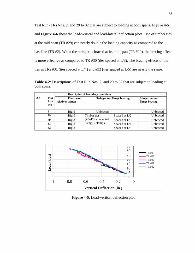
68

Test Run (TR) Nos. 2, and 29 to 32 that are subject to loading at both spans. Figure 4-5

and Figure 4-6 show the load-vertical and load-lateral deflection plots. Use of timber ties

at the mid-span (TR #29) can nearly double the loading capacity as compared to the

baseline (TR #2). When the stringer is braced at its mid-span (TR #29), the bracing effect

is more effective as compared to TR #30 (ties spaced at L/3). The bracing effects of the

ties in TRs #31 (ties spaced at L/4) and #32 (ties spaced at L/5) are nearly the same.

Table 4-2: Descriptions of Test Run Nos. 2, and 29 to 32 that are subject to loading at

both spans

A.1 Test

Run

No.

Description of boundary conditions

Floorbeam

relative stiffness

Stringer top flange bracing Stinger bottom

flange bracing

2 Rigid Unbraced Unbraced

29 Rigid Timber ties

(4”x4”), connected

using C-clamps

Spaced at L/2 Unbraced

30 Rigid Spaced at L/3 Unbraced



0

5

10

15

20

25

30

35

-1 -0.8 -0.6 -0.4 -0.2 0

Load

(k

ips)

Vertical Deflection (in.)

TR #2

TR #29

TR #30

TR #31

TR #32

Figure 4-5: Load-vertical deflection plot

69

The bracing effect of the timber ties is evaluated for a number of test runs

involving either rigid or flexible interior supports, as shown in Figure 4-7 and Figure

4-8. These figures plot the buckling loads versus timber tie spacing. Group III test results

show that the LTB resistance can be increased significantly using minimal lateral

stiffness provided by 4 in. by 4 in. timber ties and C-clamps. For example, buckling load

increased by approximately 70% for all tests when timber ties were provided only at the

mid-span.

Figure 4-7: Bracing effect of timber ties with rigid interior support

0

10

20

30

40

0 0.2 0.4 0.6 0.8 1

Lo

ad

(k

ips)


TR #2

TR #29

TR #30

TR #31

TR #32

Figure 4-6: Load-lateral deflection plot

70

Figure 4-8: Bracing effect of timber ties with flexible interior support

4.1.5 Bracing Effect of Non-composite Concrete Deck

Test Runs #57, 45, 81, and 69 were loaded at Loc. 3 and accounted for various

floorbeam’s relative stiffness and stringer to the floorbeam’s connection conditions as

shown in Table 4-3. Load-vertical deflection and load-lateral deflection at critical

locations were compared for these test runs to an applied load of approximately 80 kips.

These comparisons are conducted to study the effects due to the floorbeam’s relative

stiffness and stringer to the floorbeam’s connection conditions (Figure 4-9 and Figure

4-10). As predicted, the maximum vertical deflections increased substantially with a

flexible floorbeam. Tests where stringers were not bolted to the floorbeam produced

slightly increased maximum vertical deflections when compared to the bolted cases,

irrespective of the floorbeam’s relative stiffness. Figure 4-11 to Figure 4-13 provide the

strain diagrams at interior stringer Locations, 3, 6, and 7 at a load of around 80 kips. It

can be observed that neutral axis’s locations remain constant for the tests. Strains at the

stringer’s top and bottom flanges are not entirely the same, indicating the existence of

small axial strains as a result of possible friction between the stringers and the deck.

71

Table 4-3: Test Run #57, 45, 81, and 69

Test Run No.

Floorbeam relative stiffness

Stringer to floorbeam

connection

57 Rigid

Bolted

45 Unbolted

81 Flexible

Bolted

69 Unbolted

Figure 4-10: Lateral displacement at Loc. 3 in Group IV tests

Note: Lateral deflection of TR #69 at Loc. 3 not recorded after load exceeded 33.4 kips, LVDT slipped.

0102030405060708090

-1.5 -1.25 -1 -0.75 -0.5 -0.25 0 0.25 0.5

Load

(k

ips)

Vertical Deflection (in.)

TR #57 Loc. 3

TR #45 Loc. 3

TR #81 Loc. 3

TR #69 Loc. 3

TR #57 Loc. 10

TR #45 Loc. 10

TR #81 Loc. 10

TR #69 Loc. 10

0102030405060708090

-0.2 -0.15 -0.1 -0.05 0 0.05

Load

(k

ips)


TR #57 Loc. 3

TR #45 Loc. 3

TR #81 Loc. 3

TR #69 Loc. 3

TR #57 Loc. 10

TR #45 Loc. 10

TR #81 Loc. 10

TR #69 Loc. 10

Figure 4-9: Vertical displacement at Loc.3 in Group IV tests

72

Figure 4-11: Strain diagrams at Loc. 3 due to 82 kips

Figure 4-12: Strain diagrams at Loc. 6 due to 82 kips (Load at Loc. 3)

Figure 4-13: Strain diagrams at Loc. 10 due to 82 kips (Load at Loc. 3)

-25

-20

-15

-10

-5

0

-1500 -1000 -500 0 500 1000 1500D

epth

(in

.)

Strain (µε)

Strain Diagram at Loc. 3

TR #57

TR #81

TR #69

-25

-20

-15

-10

-5

0

-1000 -500 0 500 1000

Dep

th (

in.)

Strain (µϵ)


TR #57

TR #45

TR #81

TR #69

-25

-20

-15

-10

-5

0

-1000 -500 0 500 1000

Dep

th (

in.)

Strain (µϵ)


TR #57

TR #45

TR #81

TR #69

73

A diagram of the primary bending moment, Mx, including the deck and spreader

beam weights, is plotted at an applied load of 82 kips in Figure 4-14. The primary

bending moments, Mx, at the interior stringer were determined from measured strains at

critical sections and compared to an elastic analysis from RISA-3D. These comparisons

were performed to study the effect of the floorbeam’s relative stiffness and stringer to the

floorbeam’s connection conditions. Findings indicate that analysis results mostly matched

the measured values:

1. Strains and Mx in Test Run #45 are noticeably larger than Test Run #57.

2. Strains and Mx in Test Run #69 (flexible/unbraced) are slightly larger than Test

Run #81 (flexible/braced) under the same loading.

3. Maximum positive Mx in Test Run #81 (flexible/braced) is larger than Test Run

#57 (rigid/braced) under the same loading. Similarly, maximum negative Mx in

Test Run #81 (flexible/braced) is smaller than Test Run #57 (rigid/braced) under

the same loading.

4. Nearly same Mx is observed in Test Run #81 (flexible/braced) and Test Run #69

(flexible/unbraced).

74

4.1.6 Moment Gradient Factor

One Span Loaded Case

When AASHTO LRFD Bridge Design Specifications (2020) are followed for an

unbraced length of 24 ft. and using a moment gradient factor of 1.0, the flexural

resistance of the stringer is 45.1 kip-ft. Figure 4-15 compares the primary bending

moments, Mx, from the elastic analysis and test data at an applied load of 118.2 kips. Loc.

6 exhibited LTB at 118.2 kips, which resulted in a flexural strength of 122.9 kip-ft. The

ratio of these flexural strengths is 2.73, which corresponds to Cb. From total of three test

runs that was performed for Test Run #45, it was concluded that Cb varies from 2.34 to

2.73 [1].

-100

-50

0

50

100

150

0 6 12 18 24 30 36 42 48

Mo

men

t (K

-ft)

Location (ft)

Test Runs #57, 45, 81, and 69 at Locs. 3, 6, 7, and 10

RISA

Test Run #57

Test Run #45

Test Run #81

Test Run #69

Figure 4-14: Measured and modeled interior stringer Mx diagrams at an applied load of

82 kips

75

Figure 4-15: Measured and modeled interior stringer Mx diagrams at an applied

of 118.2 kips

Two Spans Loaded Case

Figure 4-16 and Figure 4-17 show the strain diagrams at Loc. 3 and 10 subject to

the maximum load of 186.6 kips. Both sections had comparable strain readings and their

strains at the flange top and bottom reached the yield strain.

Figure 4-16: Strain diagrams, Loc. 3, maximum load of 186.6 kips at each span

-150

-100

-50

0

50

100

150

200

250

300

0 6 12 18 24 30 36 42 48M

om

ent

Mx

(K-f

t)

Location (ft)

Test Run #45 Failure 3

RISA

Test Data at Locs. 6,7,10

Test Data at Other Locs.

76

Figure 4-18 presents a Mx diagram based on an elastic analysis of the whole

structure subject to 100 kips at each span. The load of 100 kips was selected for

discussion purpose. It shows that the critical positive moment is about 22% higher than

the moment at Loc. 3. Similarly, the critical negative moment is approximately 18%

higher than the moment at Loc. 6. Also, the critical negative moment is about 20% larger

than the critical positive moment. Figure 4-16 shows that Loc. 3 reached the yield

moment subject to the peak load, indicating that the critical positive moment section

reached plastic moment.

Figure 4-17: Strain diagrams, Loc. 10, maximum load of 186.6 kips at each span

Figure 4-18: Mx diagram, 100 kips at each span

77

Figure 4-19, shows that Loc. 6 has not reached yielding at maximum load of

186.6 kips and indicate a flexural strength of 159.7 kip-ft. Flexural strength at critical

negative moment section is 188.4 kip-ft corresponding to Cb of 4.17.

Figure 4-19: Lab test results - Applied load versus measured longitudinal strains, Test

Run #46

Strain (µϵ)

78

CHAPTER 5

CONCLUSIONS

Finite difference method was used to obtain a theoretical solution for continuous stringers

without any bracings. Finite element models were created and calibrated to match the lab

test results to examine the LTB resistance of a two-span structure. Various types and

locations of bracings were studied on their effects on the LTB resistance, including the

steel diaphragms, timber ties, and non-composite concrete deck. Also, both braced and

unbraced (bolted and unbolted) conditions were investigated at the stringer’s bottom

flange on the floorbeam. In addition, both rigid and flexible floorbeam conditions were

evaluated. The following conclusions are drawn:

1. The concrete deck braces the positive moment section of a stringer; therefore, the non-

composite plastic moment may be used for the stringer’s nominal strength in load rating.

The negative moment section, however, should account for the LTB resistance subject to

either one or two span load case. Comparisons between the measured flexural strength

and predicted strength from the AASHTO LRFD Bridge Design Specifications were

completed to identify the moment gradient factor. The moment gradient factor can be

79

determined using the following equation proposed by Yura and Helwig (2010) and

included in the Commentary C-F1-5 of the AISC (2017):

𝐶𝑏 = 3.0 −2

3(

𝑀1

𝑀0) −

8

3 [

𝑀𝐶𝐿

(𝑀1 + 𝑀0)] Eq. 1-17

The equation above results in comparable moment gradient factors with the lab

testing data and FEA results. The bracing effect of deck is significant in increasing the

LTB resistance of the stringer, which results in a moment gradient factor appreciably

larger than 1.0.

2. In comparison with the test runs using a rigid interior support, the test setups including

a flexible interior support resulted in a larger positive moment and a smaller negative

moment at the critical sections. Therefore, when the floorbeam is flexible, it is

conservative to calculate Cb assuming a rigid interior support.

3. Nearly the same primary bending moment is observed in flexible test runs, irrespective

of stringer to floorbeam connection fixity. Hence, it is recommended to use the full span

length as the unbraced length in both braced and unbraced cases at interior support.

4. Compared to no top bracing test runs, timber bracing increased the flexural strength by

approximately 70% when located at midspan, and non-composite deck increased by

approximately by 300%.

5. Use of the proposed moment gradient factor allows to increasing the load ratings of

continuous stringers substantially. Implementation of the recommended method is

80

demonstrated using one representative bridge, which shows the benefits of using an

increased moment gradient factor (See Appendix A).

81

APPENDIX A

IMPLEMENTATION

One of the representative bridges was taken as an example to show how the

proposed moment gradient factor can be implemented in load rating. A four-span unit of

the bridge superstructure was selected in the analysis and an interior stringer, a W21 x 68,

was load rated for HL-93 (Inventory rating). Floorbeams are spaced at approximately 24

ft. – 8 5/8 in. and the stringers are spaced at 7 ft. – 6 in. A36 steel is used. (See Figure

A-1 and Figure A-2).

Figure A-1: Framing plan, Bridge No. 610065

Figure A-2: Cross section, Bridge No. 610065

82

Cb and Flexural Resistance in Accordance with the AASHTO LRFR

The AASHTO LRFD Specifications Art. A6.3.3 was followed to determine the

flexural strength of the stringers when AASHTOWare BrR [75] was used for load rating.

Excel spreadsheets were developed to perform the rating using the proposed Cb.

Both moment envelope and concurrent moment approaches were examined for

live load analysis. Figure A-3 shows the unfactored moment envelope due to HL-93, in

which a pair of design tandems and a design lane load controlled over other live loads.

The maximum negative moment at the first interior floor stringer is -181.5 Kip-ft. Figure

A-4 plots the concurrent moment under HL-93 matching the maximum negative moment

in Figure A-3. As a result, both moment envelope and concurrent moment approaches

were used to determine moment gradient coefficients and corresponding load rating

factors. Inventory load rating factors under HL-93 are determined using AASHTOWare

BrR and Excel spreadsheets assuming the full stringer span as the unbraced length. Table

A-1 and Table A-2 were created using factored dead load, and live loads. Table A-3

presents Cb calculation for the recommended Yura and Helwig (2010) equation.

Figure A-3: Unfactored moment envelope due to HL-93 (unit in Kip-ft.)

83

Figure A-4: Unfactored concurrent moment due to HL-93 (unit in Kip-ft.)

Table A-1: List of moment from BrR using moment envelope approach

Table A-2: List of moment from RISA using concurrent moment approach

84

Table A-3: Cb calculations using Yura and Helwig (2010)

Table A-4 lists moment gradient factors using moment envelope and concurrent

moment approaches, which follow either the AASHTO LRFD Specifications Art. A6.3.3,

or the proposed approach similar to Yura and Helwig (2010). As shown in, the moment

gradient factor is increased when the proposed Cb is used and the load rating factor is

increased accordingly. Furthermore, the concurrent moment approach allows for an

increased Cb as compared to the moment envelope approach.

Table A-4: Moment gradient and load rating factors

Note: 1.12* and 0.37* from AASHTOWARE BrR software

85

APPENDIX B

THEORETICAL SOLUTION

86

Matrix C =

MatLab Codes

Continuous moment %parameters E = 29000; %modulus elasticity Iw = 739; %warping constant G = 11154; %Shear modulus It = 0.461; %torsional constant Iy = 12.4; %Minor axis inertia L=180; %unbraced length N =100; %dimension of matrix D=L/(N-1); a= 6*E*Iw+ 2*G*It*D^2; b= -4*E*Iw-G*It*D^2; c = E*Iw;

A = zeros(N,N);

for i = 3:N-2 A(i,i) = a; A(i, i+1) = b; A(i, i+2) = c; A(i,i-1) = b; A(i, i-2) = c; end

A(1,1) = 5*E*Iw+ 2*G*It*D^2; A(1,2) = b; A(1,3) =c; A(2,1) = b; A(2,2) = a; A(2,3) = b;

87

A(2,4) =c; A(N-1,N-3) = c; A(N-1,N-2) = b; A(N-1,N-1) = a; A(N-1,N) = b; A(N,N-2) = c; A(N,N-1) = b; A(N,N) = (5*E*Iw+ 2*G*It*D^2);

[Eigen_vec, Eigen_val] = eig(A); [val, idx] = sort(diag(Eigen_val));

i = 1; while i<=length(val) if val(i)> 0 break end i = i+1; end eigval = val(i); Mcr=sqrt(eigval*E*Iy)/(D^2)

plot(Eigen_vec(:,idx(i))) hold on plot(Eigen_vec(:,idx(i+1))) plot(Eigen_vec(:,idx(i+2))) plot(Eigen_vec(:,idx(i+3))) %plot(Eigen_vec(:,idx(i+4))) %eigval = min(eig(A));

%M= sqrt (eigval*E*Iy)/D^2

%Mcr=sqrt(eigval*E*Iy)/(D^2) Mocr=pi/L*sqrt(E*Iy*G*It+(pi*E/L)^2*Iy*Iw)

Simple span- Point loaded E = 29000; %modulus elasticity Iw = 739; %warping constant G = 11154; %Shear modulus It = 0.461; %torsional constant Iy = 12.4; %Minor axis inertia L= 288; %unbraced length N = 100; %dimension of matrix %n= 5; D= L/(N-1); a= 6*E*Iw/D^4+ 2*G*It/D^2; b= -4*E*Iw/D^4-G*It/D^2; c = E*Iw/D^4;

A = zeros(N,N);

for i = 3:N/2 A(i,i) = a/(i*D*13/32)^2; A(i, i+1) = b/(i*D*13/32)^2; A(i, i+2) = c/(i*D*13/32)^2;

88

A(i,i-1) = b/(i*D*13/32)^2; A(i, i-2) = c/(i*D*13/32)^2; end

for i=(N/2)+1:N-2 A(i,i) = a/((13*D*i-16*L)/32)^2; A(i, i+1) = b/((13*D*i-16*L)/32)^2; A(i, i+2) = c/((13*D*i-16*L)/32)^2; A(i,i-1) = b/((13*D*i-16*L)/32)^2; A(i, i-2) = c/((13*D*i-16*L)/32)^2; end A(1,1) = (5*E*Iw/D^4+ 2*G*It/D^2); A(1,2) = b; A(1,3) =c; A(2,1) = b/(2*D*13/32)^2; A(2,2) = a/(2*D*13/32)^2; A(2,3) = b/(2*D*13/32)^2; A(2,4) =c/(2*D*13/32)^2; A(N-1,N-3) = c/((13*D*(N-1)-16*L)/32)^2; A(N-1,N-2) = b/((13*D*(N-1)-16*L)/32)^2; A(N-1,N-1) = a/((13*D*(N-1)-16*L)/32)^2; A(N-1,N) = b/((13*D*(N-1)-16*L)/32)^2; A(N,N-2) = c; A(N,N-1) = b; A(N,N) = (7*E*Iw/D^4+ 2*G*It/D^2);

[Eigen_vec, Eigen_val] = eig(A); [val, idx] = sort(diag(Eigen_val));

i = 1; while i<=length(val) if val(i)> 0 break end i = i+1; end eigval = val(i); Pcr=sqrt(eigval*E*Iy*4)

plot(Eigen_vec(:,idx(i))) hold on plot(Eigen_vec(:,idx(i+1))) plot(Eigen_vec(:,idx(i+2)))

Mocr=pi/L*sqrt(E*Iy*G*It+(pi*E/L)^2*Iy*Iw)

89

APPENDIX C

COMMANDS USED IN ANSYS

Link elements

! Commands inserted into this file will be executed just after material

definitions in /PREP7.

! The material number for this body is equal to the parameter "matid".

! Active UNIT system in Workbench when this object was created: Metric (mm, kg,

N, s, mV, mA)

! NOTE: Any data that requires units (such as mass) is assumed to be in the

consistent solver unit system.

! See Solving Units in the help system for more information.

/com,

/com,

/com,

*get, myarea, SECP, MATID, PROP, Area

ET, MATID, 180

KEYOPT, MATID,2,0

KEYOPT, MATID,3,0

KEYOPT, MATID,12,0

MP,EX,MATID,199947.9615

MP,PRXY,MATID,0.3

TB,BISO,MATID,1,2

TBDATA,,4.2E+2,199.9479615

SECTYPE, MATID, LINK

SECDATA, myarea

/com,

/com,

/com,

Shell elements

!DENS_ = 7850.0

!EX_ = 2.1E5

EX_ = 199947.9615

NUXY_=0.3

!MP,DENS,MAT_ID,DENS_,

MP,EX,MATID,EX_,

MP,NUXY,MATID,NUXY_,

Yield_strength=3.4474E+2

Tangent_modulus=199.9479615

!TB,BKIN,MAT_ID,1,,0

90

TB, BISO, MATID

TBDATA,1,Yield_strength

TBDATA,2,Tangent_modulus

Deck

Solid 185

EX_ = 2E+4

!X_ = 2E+1

NUXY_=0.2

!MP,DENS,MATID,DENS_,

MP,EX,MATID,EX_,


ET,MATID, 185

KEYOPT, MATID,2,0

KEYOPT, MATID,3,0

KEYOPT, MATID,6,0

CPT 215

ET,MATID, 215

KEYOPT, MATID,18,2

Microplane

! Commands inserted into this file will be executed just after material

definitions in /PREP7.

! The material number for this body is equal to the parameter "matid".

! Active UNIT system in Workbench when this object was created: Metric (mm, kg,

N, s, mV, mA)

! NOTE: Any data that requires units (such as mass) is assumed to be in the

consistent solver unit system.

! See Solving Units in the help system for more information.

EX_ = 2E+4

NUXY_=0.2

!MP,DENS,MATID,DENS_,

MP,EX,MATID,EX_,


f_uc = 22.12

f_bc = 25.4384

f_ut = 2.1

r_t = 1

D = 4e4

sigma_c_v = -35

R = 2

gamma_t0 = 0

gamma_c0 = 2e-5

beta_t = 3000

beta_c = 2000

c = 1600

m = 2.5

91

TB, MPLA, MATID,,,DPC

tbdata,1,f_uc

tbdata,2,f_bc

tbdata,3,f_ut

tbdata,4,r_t

tbdata,5,D

tbdata,6,sigma_c_v

tbdata,7,R,gamma_t0,gamma_c0,beta_t,beta_c

TB, MPLA, MATID,,,NLOCAL

tbdata,1,c,m

Rebar- concrete connection

fini

/prep7

!UPGEOM,5,1,1,..\..\buckling2005,rst

!ALLSEL,ALL

CMSEL,S,Deck,ELEM

CMSEL,A,Bar,ELEM

NSLE,S,ALL

CPINTF,ALL,50

ALLSEL,ALL

fini

/solu

Extract solution from Eigenvalue buckling

/copy,file,rst,,..\..\buckling1000,rst

Import solution from Eigenvalue buckling to non-linear analyses

fini

/prep7

upgeom,0.1252,1,1,..\..\buckling326,rst ! Multiplies "factor" by mode 1

displacement

fini

/solu

92

ACRONYMS, ABBREVIATIONS, AND SYMBOLS

Term Description

AASHTO American Association of State Highway and Transportation Officials

ft. foot (feet)

in. inch(es)

LADOTD Louisiana Department of Transportation and Development

LTRC Louisiana Transportation Research Center

LTB Lateral torsional buckling

Cb Moment gradient factor

L Length of span

Lb Unbraced length

RF Rating factor

LRFD Load and resistance factor design

MBE Manual of bridge evaluation

DC Dead load effect due to structural components and attachments

DW Dead load effect due to wearing surface and utilities

LL Live load effect

γDW LRFD load factor for wearing surfaces and utilities

γP LRFD load factor for permanent loads other than dead loads

γLL Evaluation live load factor

Rn Nominal member resistance

LADV Louisiana Design Vehicle Live Load

Fmax Maximum potential compression-flange flexural resistance

Fyr Compression-flange stress at the onset of nominal yielding within the

cross section

Fyc Specified minimum yield strength of a compression flange

Lr Limiting unbraced length to achieve the onset of nominal yielding in

either flange under uniform bending

93

Term Description

Lp Limiting unbraced length to achieve the nominal flexural resistance Mp

under uniform bending

Rb Web load-shedding factor

Rh Hybrid factor

Mmax Maximum potential flexural resistance based on the compression flange

HL-93 LRFD design live load

Fnc Nominal flexural resistance of a member

NRL Notional Rating Load

Fy Specified minimum yield strength of steel

FLB Flange lateral buckling

f1 stress without consideration of lateral bending at the brace point

opposite to the one corresponding to f2, calculated as the intercept of the

most critical assumed linear stress variation passing through f2 and

either fmid or f0, whichever produces the smaller value of Cb

f2 Largest compressive stress without consideration of lateral bending at

either end of the unbraced length of the flange under consideration,

calculated from the critical moment envelope value

f0 Stress due to the factored loads without consideration of flange lateral

bending at a brace point opposite to the one corresponding to f2

MA Absolute value of moment at quarter point of the unbraced segment

MB Absolute value of moment at center of the unbraced segment

MC Absolute value of moment at three-quarter point of the unbraced

segment

Mp Plastic moment

Mu Moment due to the factored loads

Mr Factored flexural resistance

Es Elastic modulus of steel

Ec Elastic modulus of concrete

Iy Moment of inertia about the minor principal axis of the cross section

Ix Moment of inertia about the major principal axis of the cross section

94

REFERENCES

1. AASHTO, 2020. AASHTO LRFD Bridge Design Specifications, Ninth Edition.

Washington, D.C.

2. Ravindra, M.K. and Galambos, T.V., 1978. Load and Resistance Factor Design

for Steel. Journal of the Structural Division, 104(9), pp.1337-1353.

3. Salvadori, M.G., 1955. Lateral Buckling of I-Beams. Transactions of the

American Society of Civil Engineers, 120(1), pp. 1165-1177.

4. AISC, 2017. Steel Construction Manual, Fifteenth Edition. Chicago, IL.

5. Kirby, P.A. and Nethercot, D.A., 1979. Design for Structural Stability. Halsted

Press.

6. CSA Canadian Standards Association, 2014. Canadian Highway Bridge Design

Code S6-14.

7. Standards Australia (SA), 1998. AS4100 Steel Structures. Standards Australia,

Sydney, Australia.

8. British Standards Institution (BSI), 2000. BS5950-1 Structural Use of Steelwork

in Buildings – Part1, Code of Practice for Design Rolled and Welded Sections.

England.

9. López, A., Yong, D.J. and Serna, M.A., 2006. Lateral-Torsional Buckling of Steel

Beams: A General Expression for the Moment Gradient Factor. In Stability and

Ductility of Steel Structures. (pp. 6-8).

10. Subramanian, L. and White, D.W., 2016. Reassessment of the Lateral Torsional

Buckling Resistance of Rolled I-Section Members: Moment Gradient

Tests. Journal of Structural Engineering, 143(4), pp. 04016203.

11. White, D.W., 2008. Unified Flexural Resistance Equations for Stability Design of

Steel I-Section Members: Overview. Journal of Structural Engineering, 134(9),

pp. 1405-1424.

12. White, D.W. and Jung, S.K., 2008. Unified Flexural Resistance Equations for

Stability Design of Steel I-Section Members: Uniform Bending Tests. Journal of

Structural Engineering, 134(9), pp. 1450-1470.

95

13. White, D.W. and Duk Kim, Y., 2008. Unified Flexural Resistance Equations for

Stability Design of Steel I-Section Members: Moment Gradient Tests. Journal of


14. Helwig, T.A., Frank, K.H. and Yura, J.A., 1997. Lateral-Torsional Buckling of

Singly Symmetric I-Beams. Journal of Structural Engineering, 123(9), pp. 1172-

1179.

15. Salvadori, M.G., 1956. Lateral Buckling of Eccentrically Loaded I-Columns.

Transactions of the American Society of Civil Engineers, 121(1), pp. 1163-1178.

16. Wong, E. and Driver, R.G., 2010. Critical Evaluation of Equivalent Moment

Factor Procedures for Laterally Unsupported Beams. Engineering Journal, 47(1),

pp. 1.

17. Yura, J.A., 1995. Bracing for Stability—State-of-the-Art. In Restructuring:

America and Beyond. (pp. 88-103). ASCE.

18. Yura, J.A. and Helwig, T.A., 2010. Buckling of Beams with Inflection Points.

In Proceedings, Annual Stability Conference 2010.

19. Japan Society of Civil Engineers (JSCE), 2007. Standard Specifications for Steel

and Composite Structures. Tokyo: JSCE.

20. Aydin, R., Gunaydin, A. and Kirac, N., 2015. On the Evaluation of Critical

Lateral Buckling Loads of Prismatic Steel Beams. Steel and Composite

Structures, 18(3), pp. 603-621.

21. Cheng, J.J.R., Yura, J.A. and Johnson, C.P., 1998. Lateral Buckling of Coped

Steel Beams. Journal of Structural Engineering, 114(1), pp. 1-15.

22. Da Silva, L.S., Rebelo, C., Nethercot, D., Marques, L., Simões, R. and Real, P.V.,

2009. Statistical Evaluation of the Lateral–Torsional Buckling Resistance of Steel

I-Beams, Part 2: Variability of Steel Properties. Journal of Constructional Steel

Research, 65(4), pp. 832-849.

23. Bui, H.C., 2009. Buckling Analysis of Thin-Walled Sections under General

Loading Conditions. Thin-Walled Structures, 47(6), pp. 730-739.

24. Galambos, T.V., 1993. Inelastic Rating Procedures for Steel Beam and Girder

Bridges, (Vol. 352). Transportation Research Board.

25. Galambos, T.V., 1998. Guide to Stability Design Criteria for Metal Structures.

John Wiley & Sons.

26. Galambos, T.V. and Surovek, A.E., 2008. Structural Stability of Steel: Concepts

and Applications for Structural Engineers (pp. 236-289). New York: John Wiley

& Sons.

96

27. Geng-Shu, T. and Shao-Fan, C., 1988. Buckling of Laterally and Torsionally

Braced Beams. Journal of Constructional Steel Research, 11(1), pp. 41-55.

28. Greiner, R., Ofner, R. and Salzgeber, G., 1999. Lateral Torsional Buckling of

Beam–Columns: Theoretical Background. ECCS-Validation Group, Report 5.

29. Greiner, R. and Lindner, J., 1999. Proposal for Buckling Resistance of Members:

Flexural and Lateral Torsional Buckling. ECCS-Validation Group, Report 6.

30. Gupta, P., Wang, S.T. and Blandford, G.E., 1996. Lateral-Torsional Buckling of

Nonprismatic I-Beams. Journal of Structural Engineering, 122(7), pp. 748-755.

31. Kala, Z., Valeš, J. and Martinásek, J., 2017. Inelastic Finite Element Analysis of

Lateral Buckling for Beam Structures. Procedia Engineering, 172, pp. 481-488.

32. Kitipornchai, S., Wang, C.M. and Trahair, N.S., 1986. Buckling of

Monosymmetric I-Beams under Moment Gradient. Journal of Structural

Engineering, 112(4), pp. 781-799.

33. Kubo, M. and Fukumoto, Y., 1988. Lateral-Torsional Buckling of Thin-Walled I-

Beams. Journal of Structural Engineering, 114(4), pp. 841-855.

34. Kucukler, M., Gardner, L. and Macorini, L., (2015). Lateral–Torsional Buckling

Assessment of Steel Beams through a Stiffness Reduction Method. Journal of

Constructional Steel Research, 109, pp. 87-100.

35. Kucukler, M., Gardner, L. and Macorini, L., 2015. Flexural–Torsional Buckling

Assessment of Steel Beam–Columns through a Stiffness Reduction

Method. Engineering Structures, 101, pp. 662-676.

36. Kurniawan, C.W. and Mahendran, M., 2009. Lateral Buckling Strength of Simply

Supported Litesteel Beams Subject to Moment Gradient Effects. Journal of


37. Larue, B., Khelil, A. and Gueury, M., 2007. Elastic Flexural–Torsional Buckling

of Steel Beams with Rigid and Continuous Lateral Restraints. Journal of

Constructional Steel Research, 63(5), pp. 692-708.

38. Lim, N.H., Park, N.H., Kang, Y.J. and Sung, I.H., 2003. Elastic Buckling of I-

Beams under Linear Moment Gradient. International Journal of Solids and

Structures, 40(21), pp. 5635-5647.

39. Naderian, H.R. and Ronagh, H.R., 2015. Buckling Analysis of Thin-Walled Cold-

Formed Steel Structural Members Using Complex Finite Strip Method. Thin-

Walled Structures, 90, pp. 74-83.

97

40. Nguyen, N.D., Han, S.R., Lee, G.S. and Kang, Y.J., 2011. Moment Modification

Factor of I-Girder with Trapezoidal-Web-Corrugations Considering Concentrated

Load Height Effects. Journal of Constructional Steel Research, 67(11), pp. 1773-

1787.

41. Park, J.S. and Kang, Y.J., 2003. Lateral Buckling of Beams with Top

Bracing. Structural Engineering and Mechanics, 16(5), 2003, pp. 613-625.

42. Park, J.S., Stallings, J.M. and Kang, Y.J., 2004. Lateral–Torsional Buckling of

Prismatic Beams with Continuous Top-Flange Bracing. Journal of Constructional

Steel Research, 60(2), pp. 147-160.

43. Park, N.H., Kang, Y.J., Jo, Y.M. and Lim, N.H., 2007. Modification of C-

Equation in the SSRC Guide for Buckling of Monosymmetric I-Beams under

Transverse Loads. Engineering Structures, 29(12), pp. 3293-3300.

44. Ronagh, H.R. and Bradford, M.A., 1994. Some Notes on Finite Element Buckling

Formulations for Beams. Computers & Structures, 52(6), pp. 1119-1126.

45. Serna, M.A., López, A., Puente, I. and Yong, D.J., 2006. Equivalent Uniform

Moment Factors for Lateral–Torsional Buckling of Steel Members. Journal of

Constructional Steel Research, 62(6), pp. 566-580.

46. Subramanian, L. and White, D.W., 2016. Reassessment of the Lateral Torsional

Buckling Resistance of I-Section Members Uniform-Moment Studies. Journal of

Structural Engineering, 143(3), pp. 04016194.

47. Subramanian, L., Jeong, W.Y., Yellepeddi, R. and White, D.W., 2018.

Assessment of I-Section Member LTB Resistances Considering Experimental

Test Data and Practical Inelastic Buckling Design Calculations. Engineering

Journal-American Institute of Steel Construction, 55(1), pp. 15-44.

48. Suryoatmono, B. and Ho, D., 2002. The Moment–Gradient Factor in Lateral–

Torsional Buckling on Wide Flange Steel Sections. Journal of Constructional

Steel Research, 58(9), pp. 1247-1264.

49. Trahair, N.S., 1996. Laterally Unsupported Beams. Engineering Structures,

18(10), pp. 759-768.

50. Trahair, N.S. and Hancock, G.J., 2004. Steel Member Strength by Inelastic

Lateral Buckling. Journal of Structural Engineering, 130(1), pp. 64-69.

51. White, D.W., Jeong, W.Y. and Toğay, O., 2016. Comprehensive Stability Design

of Planar Steel Members and Framing Systems via Inelastic Buckling Analysis.

International Journal of Steel Structures, 16(4), pp. 1029-1042.

98

52. Yura, J.A. and Widianto, J.A., 2005, April. Lateral buckling and bracing of

beams—A Re-evaluation after the Marcy Bridge Collapse. In Structural Stability

Research Council-2005 Annual Stability Conference, Apr 6-9 2005 (pp. 277-294).

53. Yura, J., Helwig, T., Herman, R. and Zhou, C., 2008. Global Lateral Buckling of

I-Shaped Girder Systems. Journal of Structural Engineering, 134(9), pp. 1487-

1494.

54. Yura, J.A., Phillips, B., Raju, S. and Webb, S., 1992. Bracing of Steel Beams in

Bridges. Interior for Transportation Research. The University of Texas at Austin.

55. Yura, J.A., 2001. Fundamentals of Beam Bracing. Engineering Journal-American

Institute of Steel Construction, 38(1). pp. 11-26.

56. Vegesna, S. and Yura, J.A., 1992. An Ultimate Load Test to Study Bracing Effects

of Bridge Decks. Interior for Transportation Research, University of Texas.

57. Kissane, R.J., 1985. Lateral Restraint of Non-composite Beams. New York State

Department of Transportation, Engineering Research and Development Bureau.

58. Linzell, D., Nevling, D., Kollias, A. and Laman, J., 2002. Experimental and

Numerical Response of a 1915 Riveted Through-Girder Bridge. Transportation

Research Record: Journal of the Transportation Research Board, 1814, pp. 127-

134.

59. Ziemian, R.D., 2010. Guide to Stability Design Criteria for Metal Structures. 6th

Edition. John Wiley & Sons.

60. Timoshenko, S.P. and Gere, J.M., 1961.Theory of Elastic Stability. McGraw Hill,

Newyork.

61. Mottram, J.T., 1992. Lateral-Torsional Buckling of Thin-Walled Composite I-

Beams by the Finite Difference Method. Composites Engineering, 2(2), pp.91-

104.

62. Suryoatmono, B. and Ho, D., 2002. The Moment–Gradient Factor in Lateral–

Torsional Buckling on Wide Flange Steel Sections. Journal of Constructional

Steel Research, 58(9), pp.1247-1264.

63. Chen, W.F. and Lui, E.M., 1987. Structural Stability: Theory and

Implementation. Elscvier Science Publishing Co. Inc, Newyork.

64. Nethercot, D.A., K. C. Rockey K.C., 1971. A Unified Approach to the Elastic

Lateral Buckling of Beams. The Structural Engineer, 49(7).

65. Kamiński, M. and Supeł, Ł., 2016. Elastic Critical Moment for Bisymmetric Steel

Profiles and its Sensitivity by the Finite Difference Method. International Journal

of Applied Mechanics and Engineering, 21(1).

99

66. MatLab R2019a, MathWorks Inc, Las Vegas, NV.

67. Sun C., Linzell D., Puckett J., 2020. Load Rating of Existing Continuous Stringers

on Louisiana’s Bridges. (No. FHWA/LA.19/XXX) United States. Federal

Highway Administration.

68. Khelil, A. and Larue, B., 2008. Simple Solutions for the Flexural-Torsional

Buckling of Laterally Restrained I-Beams. Engineering structures, 30(10),

pp.2923-2934.

69. Durant, N.J., 1944. XCVII. An Application of the Method of Finite Difference

Equations to A Problem of Bending Moments.(Continuous Beam of N Equal

Spans under Uniform Loading.). The London, Edinburgh, And Dublin

Philosophical Magazine and Journal of Science, 35(251), pp.848-850.

70. Wirianto, F., 1979. Finite Difference Analysis of Two-span Continuous Composite

Beams (Doctoral Dissertation). McMaster University.

71. Balázs, I. and Melcher, J., 2015. Stability of Thin-Walled Beams with Lateral

Continuous Restraint. Transactions of the VŠB–Technical University of Ostrava,

Civil Engineering Series., 15(1), pp.1-10.

72. Ansys R19, Ansys Inc, Canonsburg, PA.

73. Ekström, C.M. and Wesley, D., 2017. Lateral-torsional Buckling of Steel Channel

Beams (Master's Thesis). Chalmers University of Technology.

74. Sun C., Linzell D., Puckett J, Rageh, A., Babarinde, T., Kuruppuarachchi, D.,

2021. Experimental Study of Stringer Lateral Torsional Resistance Using A

Grillage System. In SSRC Annual Stability Conference 2021.

75. AASHTOWare Bridge Rating (BrR) 6.8.4.3001, Washington, DC.

https://en.wikipedia.org/wiki/Canonsburg,_Pennsylvania

Documents

Lateral Torsional Buckling Resistance of Continuous Steel