Embed Size (px)
Citation preview

Line-fitting method of model orderreduction for elastic multibody
systems
Dissertation
zur Erlangung des akademischen Grades
Doktoringenieur (Dr.-Ing.)
von Dipl.-Ing. Valery Makhavikou
geb. am 30.05.1986 in Mogilev, Weißrussland
genehmigt durch die Fakultat Maschinenbau
der Otto - von - Guericke - Universitat Magdeburg
Gutachter:
Prof. Dr.-Ing. Roland Kasper
Prof. Dr.-Ing. Andres Kecskemethy
Dr.-Ing. Dmitry Vlasenko
Promotionskolloquium am 24.07.2015

Acknowledgments
I would like to express my special gratitude to Prof. Dr. Roland Kasper, my research
supervisor, for his professional advices, constructive critiques, patient guidance, and will-
ingness to generously invest his time in this research. My grateful thanks are also extended
to Dr. Dmitry Vlasenko for planning and controlling the investigation, for his help in anal-
ysis of results obtained during this study, and for the establishment of joint projects of
the Otto-von-Guericke University and the Schaeffler Technologies AG & Co. KG in the
field of elastic multibody simulation. I wish to acknowledge the Schaeffler company for
the financial support of the research and for finite element models used in this thesis. I
am sincerely grateful to the Otto-von-Guericke University for the financial support and
creation of all necessary conditions for the efficient conduction of scientific work. Finally, I
would like to express my special thanks to my wife and parents for their valuable support
and encouragement throughout this study.
i

Abstract
Computer aided simulation is an important part of development of modern technical
products. Simulation enables optimization of system design and identification of pos-
sible operational problems without manufacturing the product. Many modern technical
systems operate at high speeds and include lightweight components. Such systems can un-
dergo deformation effects that considerably influence system dynamics and, consequently,
must be taken into account in a process of system modeling and simulation.
The subject of this research relates to simulation of elastic multibody systems. The
elastic multibody system is a system of rigid and elastic bodies interconnected by joints
or coupling elements, in which the bodies may undergo large rigid body motion and small
deformations. In this work the modeling of multibody dynamics is made with the help of a
floating frame approach. Dynamics of an elastic body is formulated using a finite element
method, which results in the transformation of partial differential equations of motion
into a set of ordinary differential equations. In order to describe the elastic behavior
accurately, it is necessary to use a fine discretization, which leads to finite element models
having a large number of elastic coordinates. For this reason, efficient simulation of finite
element models of industrial applications often becomes difficult or even infeasible. In
order to enable simulation of multibody systems containing large models of elastic bodies,
elastic coordinates are reduced by means of model order reduction methods. Reduced
order models preserve important dynamic information of original models and make the
simulation of elastic multibody system more efficient from a computational point of view.
Over the last decades a variety of reduction techniques have been developed. The set
of classical reduction methods includes condensation, modal truncation, and component
mode synthesis. The category of modern reduction approaches consists of techniques
based on the singular value decomposition using Gramian matrices and moment matching
via Krylov subspaces.
The main scientific contribution of this thesis is a new method of linear model order
reduction. The proposed method solves the problem of classical reduction approaches: a
lack of possibility to tune a reduced order model for certain transfer functions and certain
frequency ranges. In addition, the new approach satisfies the following requirements: high
accuracy, preservation of stability of reduced order models, small order and stiffness of
reduced order models, and the possibility of application in the context of elastic multibody
systems. The proposed method differs from the modern reduction approaches and has its
ii

own advantages.
The proposed reduction approach relies on the idea of line fitting of model transfer func-
tions. The method is evaluated using several application examples. The reduced order
models are validated in the time and frequency domains and the results are compared
with the results of the classical Craig-Bampton approach. It is shown that the proposed
method generates reduced order models with higher accuracy, smaller order, and smaller
stiffness. The computational cost of a coordinate transformation matrix is higher then in
the Craig-Bampton method, but it remains acceptable for moderately dimensional finite
element models.
iii

Kurzfassung
Die computergestutzte Simulation ist ein wichtiger Bestandteil bei der Entwicklung von
modernen technischen Produkten. Simulationen ermoglichen eine Optimierung des Sys-
temdesigns sowie eine Identifizierung moglicher Betriebsprobleme vor der Herstellung
eines Produkts. Viele moderne technische Systeme arbeiten mit hohen Geschwindigkeiten
und bestehen aus diversen Leichtbauteilen. Solche Systeme konnen Deformationseffekten
unterliegen, die die Systemdynamik deutlich beeinflussen. Deswegen mussen sie bei der
Systemmodellierung und Simulation mit berucksichtigt werden.
Der Fokus dieser wissenschaftlichen Arbeit ist auf die Simulation von elastischen Mehr-
korpersystemen gerichtet. Ein solches System besteht aus starren und elastischen Korpern,
die uber Gelenke bzw. Verbindungselemente miteinander verbunden sind. Weiterhin un-
terliegen diese Korper großen Starrkorperbewegungen sowie kleinen Deformationen. In
dieser Arbeit wird die Modellierung der Mehrkorperdynamik mit Hilfe der Methode des
bewegten Bezugssystems durchgefuhrt. Die Dynamik eines elastischen Korpers wird unter
Verwendung der Finite-Elemente-Methode beschrieben. Diese uberfuhrt die partiellen
Differentialgleichungen mit denen elastische Systeme beschrieben werden in einen Satz von
gewohnlichen Differentialgleichungen. Um das elastische Verhalten genau zu beschreiben,
ist es notwendig eine feine Diskretisierung zu verwenden. Dies resultiert in einer großen
Anzahl von elastischen Koordinaten. Aus diesem Grund wird es oft schwierig oder teil-
weise sogar unmoglich, eine effiziente FEM Simulation durchzufuhren. Um die Simulation
von elastischen Mehrkorpersystemen mit relativ großen Modellen zu ermoglichen, wird
die Anzahl elastischer Koordinaten mit Hilfe eines Ordnungsreduktionsverfahrens stark
verringert. Das reduzierte Modell enthalt die wichtigen dynamischen Informationen des
Originalmodells und ermoglicht eine recheneffiziente Simulation von großen elastischen
Mehrkorpersystemen.
In den letzten Jahrzehnten wurde eine Vielzahl von Ordnungsreduktionsverfahren en-
twickelt. Klassische Reduktionsverfahren umfassen die Kondensation, die Modale Reduk-
tion und die Komponenten-Modus-Synthese. Die modernen Reduktionsansatze setzen
sich aus den Verfahren Gramscher Matrizen und den Krylov-Unterraummethoden zusam-
men.
Der wissenschaftliche Hauptbeitrag dieser Arbeit ist eine neue Methode der linearen Ord-
nungsreduktion. Das vorgeschlagene Verfahren lost das Problem der klassischen Reduk-
tionsansatze. Dazu zahlt die fehlende Moglichkeit zur Abstimmung des reduzierten Mod-
iv
ells fur bestimmte Ubertragungsfunktionen und bestimmte Frequenzbereiche. Daruber
hinaus erfullt der neue Ansatz die folgenden Anforderungen: hohe Genauigkeit, Erhaltung
der Stabilitat, niedrige Ordnung, hohe Steifigkeit und die Moglichkeit der Anwendung im
Rahmen elastischer Mehrkorpersysteme. Das vorgeschlagene Verfahren unterscheidet sich
von den modernen Reduktionsansatzen und besitzt diverse Vorteile.
Das vorgeschlagene Reduktionsverfahren basiert auf der Idee der Kurvenanpassung von
Ubertragungsfunktionen. Die Methode wird anhand mehrerer Anwendungsbeispiele bew-
ertet. Die reduzierten Modelle werden im Zeit- und Frequenzbereich gepruft. Die Ergeb-
nisse werden mit den Ergebnissen des klassischen Craig-Bampton Ansatzes verglichen.
Es wird gezeigt, dass die vorgeschlagene Methode reduzierte Modelle generiert, die eine
hohere Genauigkeit, eine niedrigere Ordnung und kleinere numerische Steifigkeit besitzen.
Der Rechenaufwand einer Koordinatentransformationsmatrix ist hoher als bei der Craig-
Bampton Methode, aber annehmbar fur FE-Modelle mit moderater Dimension.
v

Contents
Acknowledgments i
Abstract iv
Kurzfassung vi
Contents viii
List of Figures ix
List of Tables xi
Notations xiii
1 Introduction 1
1.1 Research area . . . . . . . . . . . . . . . . . . . . . . . . . . . . . . . . . . 1
1.2 State of the art . . . . . . . . . . . . . . . . . . . . . . . . . . . . . . . . . 2
1.2.1 Modeling elastic multibody dynamics . . . . . . . . . . . . . . . . . 2
1.2.2 Model order reduction . . . . . . . . . . . . . . . . . . . . . . . . . 6
1.3 Problem statement and aim of the thesis . . . . . . . . . . . . . . . . . . . 10
1.4 Scopes of the thesis and outline . . . . . . . . . . . . . . . . . . . . . . . . 12
2 Fundamentals of elastic multibody systems 14
2.1 Modeling of elastic body motion . . . . . . . . . . . . . . . . . . . . . . . . 14
2.1.1 Floating frame approach . . . . . . . . . . . . . . . . . . . . . . . . 14
2.1.2 Approximation of displacement field . . . . . . . . . . . . . . . . . 15
2.1.3 Kinematics . . . . . . . . . . . . . . . . . . . . . . . . . . . . . . . 18
2.1.4 Kinetics . . . . . . . . . . . . . . . . . . . . . . . . . . . . . . . . . 21
2.1.5 Equations of motion of free elastic body . . . . . . . . . . . . . . . 28
2.1.6 Definition of body coordinate system . . . . . . . . . . . . . . . . . 30
2.1.7 Approximation of motion integrals by finite element programs . . . 34
2.1.8 Damping definition . . . . . . . . . . . . . . . . . . . . . . . . . . . 39
2.2 Model order reduction of elastic bodies . . . . . . . . . . . . . . . . . . . . 40
2.2.1 Basics of model order reduction . . . . . . . . . . . . . . . . . . . . 41
vi

Contents
2.2.2 Demands on reduction approaches when using for elastic multibody
systems . . . . . . . . . . . . . . . . . . . . . . . . . . . . . . . . . 42
2.3 Model reduction techniques . . . . . . . . . . . . . . . . . . . . . . . . . . 43
2.3.1 Guyan method . . . . . . . . . . . . . . . . . . . . . . . . . . . . . 43
2.3.2 Dynamic condensation method . . . . . . . . . . . . . . . . . . . . 44
2.3.3 Craig-Bampton method . . . . . . . . . . . . . . . . . . . . . . . . 45
2.4 Validation tests for reduced models . . . . . . . . . . . . . . . . . . . . . . 47
2.4.1 Eigenfrequency related test . . . . . . . . . . . . . . . . . . . . . . 48
2.4.2 Eigenvector related test . . . . . . . . . . . . . . . . . . . . . . . . 48
2.4.3 Frequency response analysis . . . . . . . . . . . . . . . . . . . . . . 48
2.5 Modeling elastic multibody systems . . . . . . . . . . . . . . . . . . . . . . 49
2.5.1 Modeling of constraints . . . . . . . . . . . . . . . . . . . . . . . . . 49
2.5.2 Equations of motion of elastic multibody systems . . . . . . . . . . 50
2.5.3 Solution of equations of motion for elastic multibody systems . . . . 51
3 Line-fitting method of model reduction 54
3.1 Elimination of rigid body motion from elastic coordinates . . . . . . . . . . 55
3.2 Approximation of transfer functions . . . . . . . . . . . . . . . . . . . . . . 57
3.2.1 Method description . . . . . . . . . . . . . . . . . . . . . . . . . . . 57
3.2.2 Method initialization . . . . . . . . . . . . . . . . . . . . . . . . . . 60
3.3 Reference frequency points . . . . . . . . . . . . . . . . . . . . . . . . . . . 61
3.3.1 Identification of resonance frequencies . . . . . . . . . . . . . . . . . 61
3.3.2 Identification of antiresonance frequencies . . . . . . . . . . . . . . 61
3.4 Preservation of stability . . . . . . . . . . . . . . . . . . . . . . . . . . . . 62
4 Application examples 63
4.1 Simple model . . . . . . . . . . . . . . . . . . . . . . . . . . . . . . . . . . 64
4.1.1 Model description . . . . . . . . . . . . . . . . . . . . . . . . . . . . 64
4.1.2 Initialization of reduction methods . . . . . . . . . . . . . . . . . . 65
4.1.3 Validation of reduced order models . . . . . . . . . . . . . . . . . . 67
4.1.4 Simulation . . . . . . . . . . . . . . . . . . . . . . . . . . . . . . . . 69
4.1.5 Comparison of reduced order models . . . . . . . . . . . . . . . . . 71
4.2 Complex model . . . . . . . . . . . . . . . . . . . . . . . . . . . . . . . . . 72
4.2.1 Model description . . . . . . . . . . . . . . . . . . . . . . . . . . . . 72
4.2.2 Initialization of reduction methods . . . . . . . . . . . . . . . . . . 75
4.2.3 Validation of reduced order models . . . . . . . . . . . . . . . . . . 77
4.2.4 Simulation . . . . . . . . . . . . . . . . . . . . . . . . . . . . . . . . 81
4.2.5 Comparison of reduced order models . . . . . . . . . . . . . . . . . 83
5 Discussion 84
6 Summary and further work 89
vii

Contents
Appendix 93
Bibliography 93
viii

List of Figures
1.1 Process of elastic multibody simulation. . . . . . . . . . . . . . . . . . . . . 12
2.1 Description of flexible body using the floating frame of reference formulation. 14
2.2 Finite element discretization of deformable body. . . . . . . . . . . . . . . 16
2.3 Deformation of finite element with respect to a global frame. . . . . . . . 17
2.4 Attachment of body coordinate system by three points. . . . . . . . . . . . 31
2.5 Types of projection. . . . . . . . . . . . . . . . . . . . . . . . . . . . . . . . 42
3.1 Elimination of component of rigid body motion from a transfer function. . 57
4.1 Bearing design. . . . . . . . . . . . . . . . . . . . . . . . . . . . . . . . . . 63
4.2 Flexible bar. . . . . . . . . . . . . . . . . . . . . . . . . . . . . . . . . . . . 64
4.3 Operating conditions of the bar. . . . . . . . . . . . . . . . . . . . . . . . . 65
4.4 Input and output coordinates of the bar. . . . . . . . . . . . . . . . . . . . 65
4.5 Interface nodes of the bar for the Craig-Bampton method. . . . . . . . . . 66
4.6 Interface degrees of freedom for the line-fitting reduction method. . . . . . 66
4.7 Choice of reference frequency points for the line-fitting reduction method. . 67
4.8 Relative error of non-zero eigenfrequencies for reduced models. . . . . . . 67
4.9 Validation of deformation modes using MAC test. . . . . . . . . . . . . . . 68
4.10 Input and output coordinates of transfer functions of interest. . . . . . . . 69
4.11 Relative error of frequency response for different reduced models of the bar. 69
4.12 External forces applied to the bar. . . . . . . . . . . . . . . . . . . . . . . . 70
4.13 Simulation results of reduced models. . . . . . . . . . . . . . . . . . . . . . 71
4.14 Flexible cage. . . . . . . . . . . . . . . . . . . . . . . . . . . . . . . . . . . 72
4.15 Input-output coordinate of transfer function used for initialization of beta
coefficient of damping. . . . . . . . . . . . . . . . . . . . . . . . . . . . . . 73
4.16 Bode plots for beta coefficients of damping 10−7 and 10−6. . . . . . . . . . 74
4.17 Set of input coordinates of the cage. . . . . . . . . . . . . . . . . . . . . . 75
4.18 Interface nodes for the Craig-Bampton method. . . . . . . . . . . . . . . . 76
4.19 Relative error of non-zero eigenfrequencies of reduced models. . . . . . . . 77
4.20 Positions of interface nodes and a non-interface node. . . . . . . . . . . . . 78
4.21 Comparison of transfer functions for master input master output coordinates. 79
4.22 Comparison of transfer functions for master input slave output coordinates. 79
4.23 Comparison of transfer functions for slave input slave output coordinates. . 80
ix

List of Figures
4.24 Relative error of transfer functions specified by the interface nodes. . . . . 81
4.25 Stretched spring attached to the cage. . . . . . . . . . . . . . . . . . . . . . 81
4.26 Comparison of spring elongation for the reduced models. . . . . . . . . . . 82
5.1 Decomposition of transfer function into modes contributions. . . . . . . . . 84
5.2 Combined contribution of several modes to a transfer function. . . . . . . . 85
5.3 Approximation of important transfer functions using adjacent transfer func-
tions. . . . . . . . . . . . . . . . . . . . . . . . . . . . . . . . . . . . . . . . 85
A.1 Finite rotation. . . . . . . . . . . . . . . . . . . . . . . . . . . . . . . . . . 91
x

List of Tables
2.1 Components of generalized mass matrix. . . . . . . . . . . . . . . . . . . . 29
2.2 Components of generalized quadratic velocity vector. . . . . . . . . . . . . 29
2.3 Time-invariant components of volume integrals. . . . . . . . . . . . . . . . 35
2.4 Calculation of volume integrals using data imported from finite element tools. 39
4.1 Nonzero eigenfrequencies of free bar. . . . . . . . . . . . . . . . . . . . . . 64
4.2 Comparison of reduced order models of the bar. . . . . . . . . . . . . . . . 72
4.3 Nonzero eigenfrequencies of free cage. . . . . . . . . . . . . . . . . . . . . . 73
4.4 Comparison of reduced order models of the cage. . . . . . . . . . . . . . . . 83
xi

Notation
Roman Symbols
A rotation matrix
I identity matrix
q vector of elastic coordinates
S matrix of space dependent shape functions
x position coordinates for an origin of body frame
zI vector of generalized velocity coordinates of a body
zII vector of generalized acceleration coordinates of a body
z vector of generalized position coordinates of a body
m mass of a body
Greek Symbols
α vector of angular acceleration
ω vector of angular velosity
σ stress vector
θ vector of rotational parameters of body frame
ε strain vector
Abbreviations
CMS Component Mode Synthesis
DoF Degree of Freedom
EMBS Elastic Multibody System
FEM Finite Element Method
xii

Notation
MAC Modal Assurance Criterion
NRED Normalized Relative Eigenfrequency Difference
ODE Ordinary Differential Equation
PDE Partial Differential Equation
ROM Reduced Order Model
SVD Singular Value Decomposition
Mathematical Symbols
ˆ (hat) denotes reduced order coordinates
˜ (tilde) transform a three dimensional vector to a skew-symmetric matrix
xiii

1 Introduction
1.1 Research area
Simulation is an essential part of development of modern technical products because it
enables evaluation of system behavior without its construction. Computer aided analysis
helps to optimize product design and performance, to identify possible operating problems.
In recent decades the interest to light-weight, high-speed and precise mechanical systems
has been greatly increased. Some parts of such products usually undergo deformation
effects, which must be taken into account during a process of system modeling and sim-
ulation.
In this thesis we focus on the simulation of elastic multibody systems (EMBS). The term
EMBS denotes a group of interconnected rigid and elastic bodies that may undergo large
rotational and translational motions. Elastic bodies are solid bodies that return to their
initial shapes after applied stresses are removed. EMBS appear in applications of many
engineering fields: robotics, biomechanics, vehicle and aircraft dynamics.
Modeling of EMBS is based on methods of multibody system dynamics and theory of
elasticity. The most efficient way to describe dynamics of elastic multibody systems
undergoing small deformations is a floating frame formulation. According to this method
the total motion of elastic body is divided into two parts: rigid body motion represented
by the motion of body reference frame and deformations with respect to this frame.
Dynamic formulation of elastic body leads to a set of time- and space-dependent partial
differential equations (PDEs). These equations can be solved analytically only for models
having simple geometries. In other cases, the set of PDEs is approximated by a set of
ordinary differential equations (ODEs) that are obtained by means of spatial discretization
techniques. The most used approach for this purpose is a finite element method (FEM). In
many applications a large number of elastic coordinates have to be employed to properly
describe body deformations. Complex finite element models are usually described by more
than half a million of ODEs. Simulation of such models on standard computers is not
feasible. In the case of small deformations, it is possible to solve the problem using model
order reduction techniques. These methods approximate the large set of ODEs by a small
number of equations that keep important dynamic properties of the original system. The
quality of approximation depends on a choice of model order reduction method.
1

1 Introduction
The main scientific contribution of the thesis is a new linear model order reduction method
for elastic multibody simulation. In the next sections we review previous and current
studies relevant to this topic, formulate demands on model order reduction methods, and
identify a drawback of classical reduction approaches. The method proposed in the thesis
satisfies the stated demands and addresses the problem of classical reduction approaches.
1.2 State of the art
In the past three decades, the interest to elastic multibody applications caused extensive
research of approaches for modeling and simulation of elastic multibody systems. The past
studies can be separated into two large groups: modeling of elastic multibody dynamics
and model order reduction. The information about the modeling and simulation of EMBS
is presented in the textbooks [77, 79] and review articles [78, 89]. Description of basic
model reduction methods can be found in the books [70, 6, 74]. An overview of classical
reduction techniques is presented in [5]. Additional references on the studies relevant to
the thesis topic are given further in the text.
1.2.1 Modeling elastic multibody dynamics
The modeling techniques of EMBS can be divided into two groups: global reference frame
formulation and intermediate reference frames formulation. In the global reference frame
formulation the motion of multibody system is described with respect to an inertial ref-
erence frame. This approach simplifies representation of inertia forces, but calculation
of internal forces (stiffness and damping forces) becomes more complicated. The inertia
forces can be found as a product of mass matrix and a vector of accelerations. It is not
necessary to calculate Coriolis and centrifugal forces because they are already taken into
account in the vector of inertia forces. However, the representation of internal forces is
highly nonlinear in terms of global coordinates. This fact makes impossible using model
order reduction methods together with the global reference frame formulation. The most
suitable applications for this formulation are large deformation problems having a small
order.
In the intermediate reference frame formulation the motion of flexible bodies in a multi-
body system is described using additional reference frames. The intermediate reference
frame is attached to a flexible component and describe its rigid body motion. In this case,
the motion of component relative to the intermediate reference frame is mainly a com-
ponent’s deformation. The approach enables representation of inertial forces as a linear
function of intermediate frame coordinates. The most widely-used intermediate frame is
attached to an entire flexible body and is called a floating reference frame. One of the
important advantages of the floating frame formulation is a possibility to apply model
reduction methods.
2

1 Introduction
The motion of bodies using floating frames can be described by absolute or relative co-
ordinates. These formulations result in different equations of motion. In the absolute
coordinate formulation, the coordinates of body frames are written with respect to the
global reference frame. Joints constrain system degrees of freedom and introduce algebraic
equations to equations of motion. The unknown forces arising in joints are represented
in terms of Lagrangian multipliers. Using absolute coordinate formulation it is simple
to generate equations of motions, but the solution of differential algebraic equations re-
quires a larger computational cost. The formulation suits to modeling of both open and
closed-loop multibody systems [80, 4].
In the relative coordinate approach, the position and orientation of each body in a multi-
body system are defined with respect to a preceding body using degrees of freedom of
joint connecting the bodies [19, 61]. This leads to a minimal set of generalized coordinates
and automatically incorporates joint forces in the equations of motion. Numerical meth-
ods for solving this type of equations are more computationally efficient. However, the
generation of equations of motion is more complicated: the relative coordinate approach
requires additional step to define a tree structure of the system; for closed-loop EMBS it
is necessary to define a location of cut-joint constraint.
Reviews of solution methods for the absolute and relative coordinates formulations can
be found in [75, 27, 38].
Since there exits no unique manner of defining a floating frame it can be attached to a
body in a number of different ways. These approaches can be divided into two categories.
The methods of the first group attach the coordinate system to material points of the
body. The most common procedure to do this is to set six nodal deflections to zero.
These conditions attach a reference frame to the body and eliminate rigid body degrees
of freedom in this coordinate system. As the body frame is allowed to move with respect
to the inertial frame, attaching the moving frame to the body does not exclude any of
the rigid body degrees of freedom in the inertial coordinate system. This formulation is
referred to as fixed axes [80, 1, 68].
The second group of floating frames consists of coordinate systems that follow a body in
an optimal manner. This category includes a frame oriented along the principal axes of
inertia [62], mean-axes frame [60], and a Buckens frame [76, 77, 60]. In contrast to the
fixed axes frames, coordinate systems of this type impose reference conditions on all points
of the body. In the principle axes formulation the moving reference frame is enforced
to coincide with the instantaneous principal axes of the deformable body. This method
provides six conditions based on two basic concepts: the origin of the reference frame must
remain at a instantaneous mass center, and three products of inertia must remain zeros. In
this case, the coupling between flexible and rigid body motion is weaker and equations of
motions become more simple. The mean-axes conditions are six constraints that enforce
a frame to follow a body in such a way that the kinetic energy associated with the
deformation stays at a minimum. The mean axes frame conditions simplify equations of
3

1 Introduction
motion by transforming a generalized mass matrix to a block-diagonal form. The Buckens
coordinate system is a frame relative to which the sum of squares of displacements, with
respect to an observer stationed at the frame, is minimum. This type of moving frames
is identical to a mean-axes frame for the applications where deformations are small. The
choice of the Buckens frame leads to the smallest elastic deformation possible, which is
an important issue for the construction of equations of motion under the assumption of
small deformations. The moving frames eliminate the need to select material points for
attaching the frame, but it is more difficult to determine their location because of specific
frame conditions.
Elastic multibody systems include, in general, two types of bodies: bulky solids that can
be treated as rigid bodies and bodies that are subjected to elastic deformations. The rigid
bodies have a finite number of degrees of freedom, e.g. a rigid body in space has six DoFs
that describe a position and an orientation of the body with respect to a global inertial
frame. In contrast to rigid bodies, elastic components have an infinite number of DoFs
that describe displacements of each point on the body. The dynamic behavior of such
bodies is governed by a set of space and time dependent partial differential equations,
analytical solution of which is only in seldom cases possible. It is especially difficult
to find the analytical solution for bodies with complex body forms, special boundary
conditions, and complicated material properties [43]. In order to solve the problem,
various discretization methods were developed to approximate the solution of PDEs by a
finite number of coordinates, e.g. the Rayleigh–Ritz method, the finite element method
[11, 34, 20], the finite difference method [7], and the boundary element method [13]. All
these methods generate so called shape functions that describe deformation shapes of a
body in the multibody system. The difference between the methods lies in the way, in
which the shape functions are constructed.
The deformation shapes have to satisfy boundary conditions imposed on the body [77, 76].
For bodies with simple geometries and simple boundary conditions the deformation shapes
can be found using the Rayleigh–Ritz method. The analysis of more complex models is
usually carried out by discretization methods as the FEM.
The commonly used discretization approach in elastic multibody dynamics is the FEM.
It provides a systematic way for the construction of shape functions of geometrically
complex models with boundary conditions. The approach has some important advantages
for EMBS in comparison with the finite difference method and the boundary element
method. The general procedure of finite difference approach is to replace derivatives
by finite differences. It follows that the method can use only cubes as discretization
elements; therefore, the approximation of body geometry, especially for curved areas, is
worse. In addition, in the classical finite difference approach a local refinement of mesh is
not possible and it has to be made throughout the entire geometry. This leads to models
with larger number of nodes in comparison to the FEM models and makes difficulties
for the analysis of stresses. One more useful property of FEM is a sparse structure of
4

1 Introduction
matrices that require less memory space. The main advantage of finite difference method
is the simplicity of application.
The difference between the boundary element method and FEM concerns the discretiza-
tion. In the FEM the complete domain must be discretized, while the boundary element
method requires discretization of only surfaces. It follows that the discretization effort is
much smaller and changes in meshing are much easier to perform. Due to no further ap-
proximation is imposed on the solution at interior points, the boundary element method
usually possesses advantages when dealing with stress problems. However, the solution
matrix resulting from the boundary element formulation is non-symmetric and fully pop-
ulated, therefore it is more expensive to store the matrices in the computer memory.
Besides, treatment of thin structure and non-linear problems is difficult. Nowadays, the
boundary element method is under the focus of intensive approach, but the FEM is more
established and developed.
The mass matrix of FE model can be constructed using different formulations. In a lumped
mass formulation, see [46, 67], the total mass of a body is divided between nodes of the
model. This produces a diagonal mass matrix and reduces a numerical cost required to
solve equations of motion. The drawback of the approach is that the inertia properties of
the body are violated [79]. The consistent mass matrix is obtained using space dependent
shape functions of finite elements. This formulation provides better approximation of
body inertia and, as a result, better accuracy for higher frequencies and modes [42].
Equations of motion of elastic bodies require calculation of volume integrals that express
dynamic properties of bodies. Finite element programs provide only a part of integrals
required for the construction of equations motion using the floating frame approach. In
order to obtain a complete set of volume integrals, special preprocessor modules are usually
utilized [84, 69]. The calculation of volume integrals for the consistent mass approach can
be found in [43, 55, 77, 82]. This process for the lumped mass formulation is considered in
[3, 91]. The time-invariant data required for the construction of equations of motion can
be computed in advance and stored in a Standard Input Data format that is proposed in
[88].
The important aspect in modeling of deformations is connected with a choice of suitable
type of analysis. The fundamental principle of linear analysis is the assumption that the
change of stiffness is small enough, so it is possible to use the initial stiffness of the model
throughout the entire process of deformation. The linear analysis provides an acceptable
approximation for the most problems that engineers deal with. If the stiffness of de-
formable component changes significantly under operating conditions, nonlinear analysis
becomes necessary [25]. The cause of nonlinear behavior can be different. A number
of factors influence stiffness of deformable body: body shape, material properties, large
loads, and presence of constraints. If changes of stiffness originate only changes in shape,
nonlinear behavior is defined as geometric nonlinearity. This type includes large deforma-
tions problems, where deformations exceed approximately 10% of the smallest dimension
5

1 Introduction
of body [63]. If changes of stiffness occur due to only changes in material properties under
operating conditions, the problem type belongs to a category of material nonlinearities.
A linear material model assumes stress to be proportional to strain, and once the load
has been removed the model will always return to its original shape. If the loads are high
enough to cause permanent deformations, then a nonlinear material model must be used.
In certain cases, stiffness of a structure can also change due to large applied loads. The
influence of stiffening effect is accounted by a geometric stiffness matrix that is added to
the regular stiffness matrix. The stiffening effects (also called stress stiffening, geometric
stiffening, or incremental stiffening) normally need to be considered for thin structures
for which bending stiffness is very small compared to axial stiffness, such as cables, thin
beams, and shells [63]. A typical example in this field is a rotating beam under the influ-
ence of large centrifugal forces [41, 76]. The geometric stiffness matrix can be generated
using the methods from [71, 76, 10] and the data exported from commercial FE software.
1.2.2 Model order reduction
Finite element models of elastic bodies contain a large number of degrees of freedom,
varying from several thousand to several million depending on a model geometry and
accuracy demands. Due to the high computational cost dynamic analysis of such systems
is practically not feasible. In order to solve the problem, engineers resort to the help
of model order reduction methods, which can greatly reduce the computational cost of
simulation. The main idea of reduction approaches is to approximate the initial FE
model by a model with much smaller number of DoFs so that the reduced model retains
important dynamic characteristics of the initial model. The computational burdens are
also reduced because reduction techniques remove high-frequency components of elastic
body motion enabling the use of a larger integration time step. The possibility to apply
model order reduction methods to elastic bodies is one of the most important advantages
of the floating frame formulation in the context of EMBS [89].
The set of classical reduction approaches applied in elastic multibody dynamics consists
of the methods based on modal truncation, condensation, and component mode synthesis.
The classical approaches are implemented in many simulation software and remain state of
the art techniques for model order reduction. More recently, a few alternative reduction
methods have come from the field of control theory, namely, techniques based on the
singular value decomposition using Gramian matrices and moment matching via Krylov
subspaces. These methods are aimed at the approximation of input-output behavior of
dynamical systems. Each of these reduction procedures has its specific advantages and
disadvantages. The review and comparison of the most popular methods can be found in
[16, 44, 43].
One of the oldest reduction methods is a static condensation. The approach was intro-
duced in [37] and it is called at present as Guyan method. According to this approach,
6

1 Introduction
all DoFs of elastic body are partitioned into the sets of master and slave DoFs. Assum-
ing that there are no forces applied to the slave DoFs, the method expresses the slave
DoFs using the master DoFs and generates a reduced order model depended only on the
master coordinates. The Guyan reduction leads to the exact representation of static de-
formations and to the relative good approximation of low eigenfrequencies and respective
eigenvectors. However, the Guyan approach utilizes only the stiffness matrix of the body
and ignores the influence of mass matrix on a spectrum of the model. Since the influence
of inertia becomes significant for high frequencies, the method results in reduced order
models with an erroneous high frequency spectrum.
The next method of the group of condensation approaches is a dynamic condensation
method [49]. The method is similar to the Guyan procedure, but it utilizes the inertia
information of the body. The dynamic condensation method was originally developed for
reducing the systems that undergo a harmonic or periodical excitation. The accuracy of
the reduced order model is limited to the spectrum defined around the frequency chosen
for the initialization of the method.
The most often used reduction approach is a modal truncation method, which was firstly
presented in the context of EMBS in [80]. The method relies on the eigenvalue decom-
position of the system and employs a limited number of vibration modes of the body
to represent deformation shapes. The high-frequency modes usually carry slight energy
and do not influence significantly the overall motion of the system. Using low-frequency
deformation modes of the body, the modal truncation method builds a low-dimensional
approximation of equations of motion. A linear combination of retained deformation
modes has to capture as accurately as possible the deformation shapes of the body under
operational conditions. The choice of dominant deformation modes is not a trivial task.
The issue is considered in [31, 32, 26], where a few approaches are proposed to determine
relevant deformation modes for input-output behavior of elastic body.
The deformation shapes can be accurately described by a large set of eigenmodes or by a
much smaller set of eigenmodes supplemented with several correction modes. The correc-
tion modes account for effects of truncated eigenmodes and depend on the distribution
of forces acting on the body. Since the spatial distribution of forces is not taken into
account in the modal truncation approach, a relative large number of modes is needed
to sufficiently approximate elastic body deformations [91]. The further studies of modal
reduction were aimed at taking into account the distribution of applied external forces
and computing of necessary correction modes.
The important traditional reduction technique is the component mode synthesis (CMS)
[40, 9, 23]. The method was developed in times of low computational power for practical
finite element analysis. The technique substructures a whole FE model into components,
reduces components accounting boundary conditions, and assembles the parts to form a
reduced model of the whole structure. Nowadays a single elastic body corresponds to a
substructure, therefore the coupling of body components is no longer necessary.
7

1 Introduction
The methods based on CMS approach can be divided into three categories: fixed-interface,
free-interface, and residual-flexible free interface methods. The proper choice of category
is task dependent. The group of fixed-interface methods is recommended for models where
the interest is focused on a low-frequency spectrum of the model. For applications where
it is compulsory to have better approximation of middle and high frequency spectrum,
the free-interface or residual-flexible free interface groups of methods should be exploited
[43, 22]. In this thesis we consider the fixed-interface category of methods in more detail
because the spectrum of interest for majority of EMBS lies in the low-frequency domain.
The most commonly used model reduction technique based on the CMS approach is the
Craig-Bampton method [22]. The method approximates deformation shapes using a com-
bination of fixed interface normal modes and constraint modes. The former set of modes
are dynamic modes that improve the accuracy of reduced model in a low-frequency do-
main, while the constraint modes account for static deformations of the model due to the
influence on the interface coordinates. Unlike the Guyan reduction procedure the Craig-
Bampton method utilizes both stiffness and mass characteristics of the model. Besides,
as opposed to the modal truncation it takes into account distribution of external forces
to compute correction modes for exact modeling of static deformations. The method pro-
vides an accurate approximation for low and medium eigenfrequencies and corresponding
eigenforms. The main drawback of the approach is that the accuracy of reduced model
highly depends on the number and position of interface coordinates. This fact complicates
generation of reduced order models that satisfy specified accuracy demands. In additon,
the number of fixed-interface normal modes required for the acceptable accuracy is diffi-
cult to estimate a priori. Another issue with the computed fixed-interface normal modes is
that they can be nearly orthogonal to the applied loads and, therefore, do not participate
significantly in the solution. It follows that the correct choice of interface coordinates and
fixed-interface modes requires much experience and insight into the specific problem. The
CMS methods can be hardly automated.
The next large group of reduction methods is composed of mathematical methods from
system and control theory. These methods take a frequency response as a characteristic
quantity to describe the original system. According to these approaches, the reduced order
model is defined based on matching certain parameters of reduced and original models
or eliminating less important states of the system. The methods provide more accurate
reduced order models than the modal reduction.
The basic idea of Krylov subspace method is to approximate a transfer function matrix by
matching its values and derivatives at some frequency points. The frequency points are
called expansion points or shifts. For each expansion point the transfer function matrix
is transformed into a power series, coefficients of which are called moments. In order to
match values and derivatives of transfer function matrix, it is necessary to match the mo-
ments of original and reduced models at the expansion points. Due to numerical instability
the explicit calculation of moments is not feasible, but the moment-matching conditions
8

1 Introduction
can be satisfied implicitly by the projection of equations of motion onto Krylov-subspaces.
Initially, the Krylov subspace method was developed for state-space systems [36, 30, 50],
i.e. first order systems. The reduction of second order system can be performed by con-
verting the model into the state-space model and then applying reduction approaches for
first order systems, but in this case, the reduced model will be also of first order type.
Integration of such reduced models into a second order multibody system becomes im-
possible. This makes necessary using reduction techniques that provide models of second
order type. At present, the Krylov subspace method has several adaptations that can be
applied directly to second order systems. The basis of second order Krylov subspace can
be generated with a second order Arnoldi algorithm [8, 73]. The algorithm constructs
iteratively a basis of Krylov subspace using inverse, addition, and multiplication matrix
operations. The total Krylov subspace is defined by concatenating of subspaces obtained
for each expansion point. Due to the iterative nature the approach enables reduction
of large scale models. Besides, the approximation quality of frequency response is high,
particularly around expansion points. Nevertheless, there are also some drawbacks of the
Krylov subspace method. Stability of the reduced model is not guaranteed even if the full
order model is stable [48]. Because of the local nature of the reduction procedure, it is
difficult to develop global error bounds. The method generates reduced systems of large
order when systems with many inputs are under consideration. According to [28, 66],
one of the directions of current research is the reduction of inputs and outputs before the
application of Krylov subspace method.
Another group of reduction methods includes approaches based on SVD or Gramian ma-
trices. The fundamental idea of the methods lies in using energy interpretation of input
output system behavior. The reduction is performed by eliminating those states of the sys-
tem, which require a large amount of energy to be reached and/or produce small amount
of energy to be observed. These states insignificantly contribute to system dynamics and
can be neglected. The basic approach for representing the input and output amount of
energy involves the controllability and observability Gramian matrices. Eigenvalues of
Gramian matrices indicate how strongly the states can be controlled or observed. The
measure of energy for each state of the system is determined by Hankel singular values,
which are calculated as the square roots of the eigenvalues for the product of the control-
lability and observability Gramian matrices. The unimportant states of the systems are
identified by small Hankel singular values.
One of the reduction approaches based on the idea of energy interpretation is a balanced
truncation method. The method was firstly proposed in [58]. The approach in its basic
form can be applied only to first order systems. The advantage of balanced truncation
reduction is an immediately available error bound that is expressed by proper norms of
the difference of transfer function matrices for reduced and original systems [5, 6, 47].
Besides, the method preserves system stability. Using the balanced truncation approach
only the load distribution, the frequency range of interest and a measure for the required
9

1 Introduction
accuracy have to be provided by the user, therefore the method is especially attractive
for optimization problems [65]. However, the calculation of Gramian matrices requires
solution of Lyapunov equations, which is possible only for bodies with a few thousands
degrees of freedom [29]. At present, there are some approaches that adapt the balanced
truncation method to second order systems, see [57, 83], and provide very accurate reduced
order models. However, for second order systems the global error bound is lost and
stability of reduced order system is not guaranteed [66]. A matter of current research
concerning the balanced truncation approach is handling of large scale systems [15, 14].
1.3 Problem statement and aim of the thesis
From the user’s point of view the following aspects of model order reduction are of special
interest:
� accuracy of reduced model,
� possibility to emphasize a certain frequency range of interest,
� computational efficiency of reduction method,
� estimation of error introduced by a reduction process,
� preservation of model stability,
� possibility to automate the reduction process,
� fast simulation of reduced model.
Fidelity of reduced model can be described by the following parameters: an error of
displacement for all nodes of the body, error of displacement for nodes of interest, error of
eigenfrequencies and eigenvectors, and error of transfer function matrices. None of these
parameters provides complete information about the quality of reduced model, therefore
combination of them is usually utilized to validate the reduced model. The fastest way
to assess the reduced model is using of eigenfrequency and eigenvector related tests. The
tests reveal whether these fundamental characteristics are well-approximated. However,
it is impossible to validate the motion of a single point on the body using these tests.
The problem can be solved by analyzing frequency response transfer functions. The
analysis gives comprehensive information about reduced system behavior, but calculation
of reference results is computationally expensive. After these tests showed acceptable
results, the reduced model can be also validated in the time domain.
Since technical products operate in certain frequency ranges, the possibility to tune the
reduced order model for the operating frequencies is of great importance for the user.
The computational efficiency of reduction method is defined by a number of operations
and memory consumption required for generation of coordinate transformation matrix.
10

1 Introduction
The error introduced by reduction can be identified using validation tests described above
or, for some reduction methods, using error estimators that define permissible error
bounds prior to the reduction process.
Preservation of stability is an important property of reduction approach because it ensures
that the reduced model does not cause any type of failure (e.g., instability, excessive
vibrations, large stresses) to the EMBS. Special criteria are used to ascertain whether
this property is preserved.
The fully or partially automated reduction process decreases the user’s involvement and
speeds up producing of reduced order models.
The demand of fast simulation imposes restrictions on the stiffness and number of degrees
of freedom of reduced structure.
The use of model order reduction methods in the context of EMBS imposes on them
additional restrictions:
� reduced models have to preserve a second order structure of equations of motion;
� reduction method has to generate a coordinate transformation matrix that excludes
rigid body motion from equations of motion. The rigid body motion in the floating
frame formulation is accounted by the motion of a coordinate system attached to
the body.
The classical reduction methods are implemented in many simulation software and remain
state of the art techniques for model order reduction. In this thesis we are focused on
the solution of one of the principal problems of classical reduction techniques: a lack
of possibility to tune a reduced model for certain transfer paths (functions) and certain
frequency ranges. Solution of the problem is important because it enables generation of
accurate reduced models having a small order. The goal of the thesis is to fill in this
gap by a new model order reduction approach that, in addition, satisfies the following
requirements: high accuracy of reduced models, preservation of stability, fast simulation of
reduced models, and the possibility of using the method in the context of EMBS. The new
method differs from more recent approaches, namely, the Krylov subspace method and
the balanced truncation, and has its own advantages. The stability of Krylov subspace
method is not guaranteed and reduction of systems with large number of inputs leads
to large reduced order models. The balanced truncation technique preserves stability of
second order systems only in special cases and its application is limited to FE models
with a relative small number of degrees of freedom.
The main idea of new approach is to reduce error of transfer functions in reference fre-
quency points. For this reason, hereinafter the method is referred to as a line-fitting
approach.
11

1 Introduction
Mechanical system
Kinematicaldescription
Kineticaldescription
Principlesof
mechanics
Simulationof
EMBS
Continuumformulation
Finite
ElementMethod
Model order
reduction
modelingmultibodydynamics
modelingflexiblebodies
equations ofmotion of
MBS
data describedreduced models of
flexible bodies
Figure 1.1: Process of elastic multibody simulation.
1.4 Scopes of the thesis and outline
In this thesis we describe a new linear structure preserving model order reduction method
for elastic multibody simulation. The application of the method is limited to mechani-
cal systems that undergo linear elastic deformations. In this contribution we show the
benefits of the developed method in comparison with the classical and widely-used Craig-
Bampton approach. The thorough comparison of line-fitting method with other reduction
techniques falls outside the scope of the thesis.
The thesis has the following structure. We begin with fundamentals of theory for elas-
tic multibody simulation in Chapter 2. The information in this chapter is presented in
accordance with the procedure of simulation of elastic multibody systems, see Fig. 1.1.
The first section of the chapter is devoted to modeling of elastic body motion using a
floating frame formulation. Within this section the following aspects are covered: de-
scription of deformations using the Ritz approach and finite element method, kinematics
and kinetics of a free elastic body for the floating frame of reference formulation and the
Ritz approximation, derivation of equations of motion of a single unconstrained elastic
body by Jourdain’s principle, derivation of motion integrals and their evaluation using FE
preprocessors. In addition, different types of floating frames are considered and some of
possible ways to introduce damping into equations of motion are discussed. The second
section of the theoretical chapter explains the concept of model order reduction based
on projection. We describe the classical reduction techniques, namely, the static and
dynamic condensation, modal truncation, and the Craig-Bampton method. After that
validation tests of reduced models are presented and discussed. The set of tests includes
an eigenfrequency related criterion NRED, eigenvector related criterion MAC, and fre-
quency response analysis. Modeling of constraints, derivation of equations of motion of
whole EMBS, and solution methods are discussed in the final section of the chapter.
12

1 Introduction
The description of line-fitting model order reduction approach is given in the separate
Chapter 3.
Application examples are presented in Chapter 4. There are two models under considera-
tion: a bar and a bearing cage. The former model has a simple form and its finite element
model has a small number of degrees of freedom, while the latter one has a complex shape
and a large number of elastic coordinates. In this chapter we apply the line-fitting method
to the both models, evaluate properties of reduced order models in time and frequency
domains, and compare the results with results of traditional Craig-Bampton approach.
The goal of Chapter 5 is comprehensive evaluation of the line-fitting method. The analysis
is performed based on the theoretical description of the approach in Chapter 3 and the
numerical results presented in Chapter 4.
Finally, Chapter 6 highlights the most important results of this thesis and suggests further
work on the subject.
13

2 Fundamentals of elastic multibody
systems
2.1 Modeling of elastic body motion
2.1.1 Floating frame approach
The floating frame formulation is the most widely used approach for modeling elastic
multibody systems. According to this formulation the motion of deformable body is a
superposition of large nonlinear motion of body frame and small elastic deformations with
respect to the body frame. There are a number of methods to fix a floating frame to a
body. The different types of body frames and associated with them reference conditions
are discussed in detail in Section 2.1.6.
undeformed body
deformed body
P
u
d
x
r0
r
P
Figure 2.1: Description of flexible body using the floating frame of reference formulation.
The motion of a deformable body is represented by the motion of its points. Fig. 2.1
describes motion of an arbitrary point P of the deformable body. The position d(t) of
point P in the global inertial frame is defined as
d (t) = x (t) + r (t) = x (t) + A (t) · r (t) = x (t) + A (t) · (r0 + u (t)), (2.1)
where x denotes a position of origin of body reference frame in the global coordinate
system, the vector r defines a local position of the point P in the global frame, A is a
14

2 Fundamentals of elastic multibody systems
body rotation matrix, the vectors r and r0 correspond to deformed and undeformed local
positions of the point P in the body frame, and the vector u represents a displacement
of P due to deformation. Displacement vectors of all points define a displacement field of
the body.
For the deformable body the vector u is time- and space- dependent. As the body has an
infinite number of points modeling its dynamics requires an infinite set of coordinates. In
order to reduce the number of coordinates to a finite set, approximation approaches such
as Rayleigh-Ritz and the finite element method are used.
2.1.2 Approximation of displacement field
Rayleigh-Ritz method
Separation of variables of the displacement field u in Eq. 2.1 leads to infinite series in the
following form:
u(r0, t) =
u1
u2
u3
=
∞∑k=1
f1k(r0) · q1k(t)∞∑k=1
f2k(r0) · q2k(t)∞∑k=1
f3k(r0) · q3k(t)
(2.2)
The time dependent coefficients q1k, q2k, q3k are called coordinates, and the space de-
pendent functions f1k, f2k, f1k are called base functions. It is necessary that the base
functions satisfy body boundary conditions, the infinite series converge to limit functions
u1, u2, u3, and the limit functions accurately represent the displacement field.
The Rayleigh-Ritz method approximates the displacement field by truncating the infinite
series of Eq. 2.2 and results in the following representation:
u1
u2
u3
≈
l∑k=1
f1k(r0) · q1k(t)m∑k=1
f2k(r0) · q2k(t)n∑k=1
f3k(r0) · q3k(t)
= S · q (2.3)
with S being a shape matrix containing the base functions and q being a vector of time
dependent coordinates. The coordinates q lack a physical meaning. The base functions
in S define predicted deformation shapes for the body.
In order to the approximation of deformations u from Eq. 2.3 converges towards the
solution of partial differential equations, the base functions must be admissible. It means
that they have to form a complete set of functions and satisfy the boundary conditions
15

2 Fundamentals of elastic multibody systems
[76]. Completeness is achieved if the exact displacements, and their derivatives, can be
matched arbitrarily closely if enough coordinates appear in the assumed displacement
field [79].
One of the main problems connected with the Rayleigh–Ritz method is the difficulty to
find the base functions, when deformable bodies have complex geometrical shapes. In
addition, for systems with constrains the set of base functions must be adjusted for the
boundary conditions. The base functions are defined in a body reference frame, therefore
the choice of functions is also affected by the choice of the body frame. These problems
can be eliminated using the finite element method.
Finite element method
The finite element method is a numerical approach for solving partial differential equa-
tions having a set of boundary conditions. Along with the Rayleigh-Ritz approach, the
finite element method reduces the number of coordinates required for the description of
deformations to a finite set.
The idea of the method is to discretize a deformable body into small regions called ele-
ments and to describe the deformation of the whole body by deformations of elements.
The elements are connected at the points called nodes, see Fig. 2.2.
finite elements
nodes global system
element system
Figure 2.2: Finite element discretization of deformable body.
In the finite element method the deformation of elements is defined by interpolation
polynomials and nodal coordinates. The displacement field of the element is described
with respect to an element coordinate system as
ue(re0, t) = Ne(re0) · qe(t), (2.4)
where Ne is a space dependent interpolation matrix, qe is a time dependent vector of
nodal coordinates and the vector re0 defines an undeformed position of a point within the
element in the element reference frame.
16

2 Fundamentals of elastic multibody systems
The displacement field of the whole body can be represented via deformations of elements
as follows. The displacement ue is expressed in the global frame by a rotation matrix Ae
as
ue(re0, t) =Ae · ue(re0, t) = Ae ·Ne(re0) · qe(t). (2.5)
The vector re0 can be also written in another form as
re0 = ATe · (d0 − xe), (2.6)
where d0 and xe are an undeformed position of arbitrary point P within the element and
a position of origin of element system in the global coordinate system, respectively, see
Fig. 2.3.
xe
ue
re0P(t0)
d0
d
P(t)
Figure 2.3: Deformation of finite element with respect to a global frame.
The set of nodal coordinates for the FE model can be represented by a vector
q (t) =
...
qk(t)...
, k = 1, . . . , nnodes (2.7)
of dimension N with qk(t) being a vector of degrees of freedom of k-th node. The element
nodal coordinates qe(t) and the body nodal coordinates q(t) are connected by a matrix
Ce ∈ Rneq×N :
qe(t) = Ce · q(t). (2.8)
Here neq is the number of nodal coordinates of element e. The matrix Ce is calculated as
Ce = Te ·Be. (2.9)
17

2 Fundamentals of elastic multibody systems
The matrix Be ∈ Rneq×N is a Boolean transformation matrix and it serves to express
connectivity of the element e. The matrix Te∈ Rneq×ne
q is a transformation matrix that
consists of elements of matrix AeT and transforms the element nodal coordinates from
the global coordinate system to the local element system. Using Eq. 2.5, Eq. 2.8, Eq. 2.9
and summing over all elements leads the formulation of displacement field of the body in
the global frame:
u(d0,t) =
nE∑e=1
Ae · Ne(d0) ·Te ·Be·q(t) = S(d0) · q(t) (2.10)
In contrast to the Rayleigh-Ritz approach, the finite element method avoids specifying of
base functions for the whole body. The base functions of the body are assembled from
the base functions of elements. There are different types of finite elements that can be
used to represent bodies with complex forms.
Boundary conditions can be imposed direct on the nodal coordinates q.
2.1.3 Kinematics
Position
Using the inertial coordinate system of finite element model as a body coordinate system
and combining Eq. 2.1 with Eq. 2.10 the position of arbitrary point of the elastic body
can be described as follows:
d(r0, t) = x(t) + A(t) · (r0 + u(r0, t)) = (2.11)
x(t) + A(t) · (r0 + S(r0) · q(t)). (2.12)
In three-dimensional analysis, at least six coordinates are required to define configuration
of body frame. One of the methods is to define three coordinates for a position of origin
of the frame and three coordinates for an orientation of the frame with respect to the
inertial coordinate system. The orientation parameters θ can be identified using Euler
angles, Rodrigues parameters, or four dependent Euler parameters. The drawback of the
three-variable representation is singularity at certain orientations of the reference frame
in space. Formulation of rotation matrix A using orientation parameters can be found in
Chapter 6.
The global point position of Eq. 2.11 is written in terms of generalized reference and elastic
coordinates
z =
x
θ
q
. (2.13)
18
2 Fundamentals of elastic multibody systems
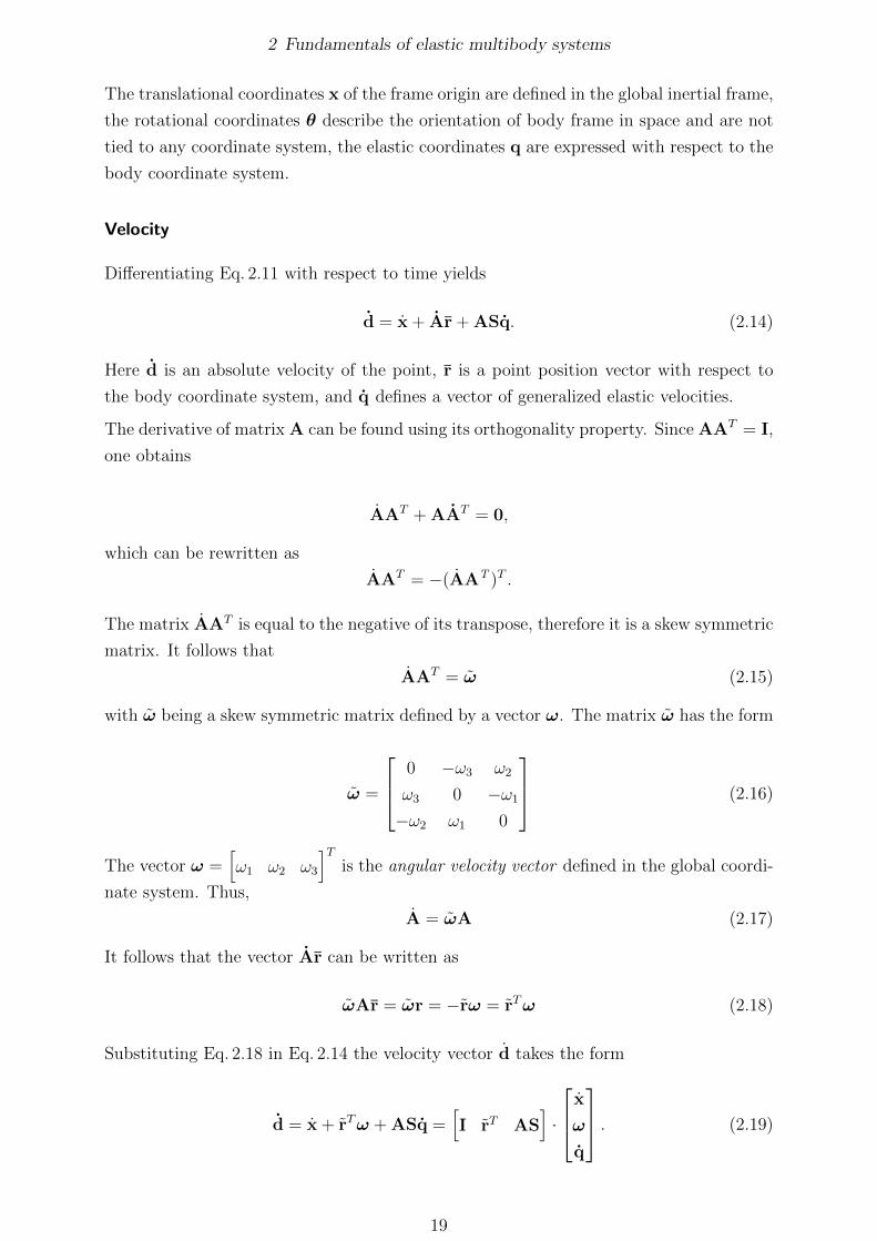
The translational coordinates x of the frame origin are defined in the global inertial frame,
the rotational coordinates θ describe the orientation of body frame in space and are not
tied to any coordinate system, the elastic coordinates q are expressed with respect to the
body coordinate system.
Velocity
Differentiating Eq. 2.11 with respect to time yields
d = x + Ar + ASq. (2.14)
Here d is an absolute velocity of the point, r is a point position vector with respect to
the body coordinate system, and q defines a vector of generalized elastic velocities.
The derivative of matrix A can be found using its orthogonality property. Since AAT = I,
one obtains
AAT + AAT = 0,
which can be rewritten as
AAT = −(AAT )T .
The matrix AAT is equal to the negative of its transpose, therefore it is a skew symmetric
matrix. It follows that
AAT = ω (2.15)
with ω being a skew symmetric matrix defined by a vector ω. The matrix ω has the form
ω =
0 −ω3 ω2
ω3 0 −ω1
−ω2 ω1 0
(2.16)
The vector ω =[ω1 ω2 ω3
]Tis the angular velocity vector defined in the global coordi-
nate system. Thus,
A = ωA (2.17)
It follows that the vector Ar can be written as
ωAr = ωr = −rω = rTω (2.18)
Substituting Eq. 2.18 in Eq. 2.14 the velocity vector d takes the form
d = x + rTω + ASq =[I rT AS
]·
x
ω
q
. (2.19)
19

2 Fundamentals of elastic multibody systems
This can be written in another form as
d =LzI, (2.20)
where
L =[I rT AS
]and zI =
x
ω
q
. (2.21)
The vector zI defines generalized velocity coordinates.
Acceleration
The absolute acceleration of the point can be found by the differentiation of Eq. 2.20 with
respect to time. This results in
d =LzI + LzI. (2.22)
Differentiating of the matrix L yields
L =[0 ˙rT AS
], (2.23)
where the second term can be identified using the relation r = Ar and Eq. 2.17 as
˙rT = − ˙r = −˜r = − ˜(Ar + A˙r) = − ˜(ωAr + ASq), (2.24)
and the third term can be written as AS = ωAS. As a result, the product LzI yields
LzI = ωωAr + 2ωASq. (2.25)
Thus, the acceleration vector takes the following form
d = x+rTα+ ASq + ωωr + 2ωASq, (2.26)
where α is an angular acceleration vector. In this equation the first term represents an
absolute acceleration of the origin of body coordinate system. The second term rTα is
a tangential acceleration of the point. The tangential acceleration is perpendicular to
the vectors r and α. The third component ASq represents an acceleration of the point
due to deformations. The fourth part describes a normal acceleration of the point. This
component is directed along the line connecting the point and the origin of the body
frame. Finally, the latter term represents the Coriolis acceleration. If the body is rigid,
the third and fifth components of Eq. 2.26 vanish.
20

2 Fundamentals of elastic multibody systems
The generalized acceleration coordinates take the form
zII = zI =
x
α
q
. (2.27)
2.1.4 Kinetics
There are a number of methods used to derive equations of motion of elastic body:
D’Alembert’s principle, Hamilton’s principle, Jourdain’s principle, Newton-Euler formal-
ism. All of them lead to the same system of equations. Direct application of Newton’s
second law becomes difficult for large multibody systems. In contrast to Newton’s second
law, the first three approaches are variational principles, which employ scalar quantities
such as kinetic energy, potential energy, virtual work, and virtual power. These methods
make possible finding equations of motion for complex multibody systems. In this work
we utilize Jourdain’s variational principle to derive equations of motion because it is a
straightforward approach for systems where generalized velocity coordinates are not equal
to a derivative of generalized position coordinates.
According to Jourdain’s principle the sum of virtual power of all forces acting on the body
must be zero. It follows that the sum of virtual power of inertial, internal, and external
forces equals zero:
δPinert + δPinter + δPext = 0. (2.28)
Virtual power of inertia forces
The virtual power of inertia forces takes the following form
δPinert =
ˆV
−ρδdT ddV, (2.29)
where d and d are global velocity and acceleration vectors of an arbitrary point of the
body, δd indicates a virtual velocity of the point, ρ defines mass density, and V represents
a volume of the body.
The virtual velocity δd can be expressed in terms of virtual generalized velocity δzI as
δd = LδzI. (2.30)
with L being the matrix from Eq. 2.21. Using the definition of global acceleration vector
d =LzI + LzI from Eq. 2.22, the virtual power of inertia forces can be obtained as follows
δPinert = −(ˆ
V
ρ (δzI)T LTLzIdV +
ˆV
ρ (δzI)T LT LzIdV
). (2.31)
21
2 Fundamentals of elastic multibody systems
Since the vector of generalized velocity coordinates zI depends only on time, one can write
the expression for δPinert as
δPinert = − (δzI)T
([ˆV
ρLTLdV
]zI +
[ˆV
ρLT LzIdV
])= (2.32)
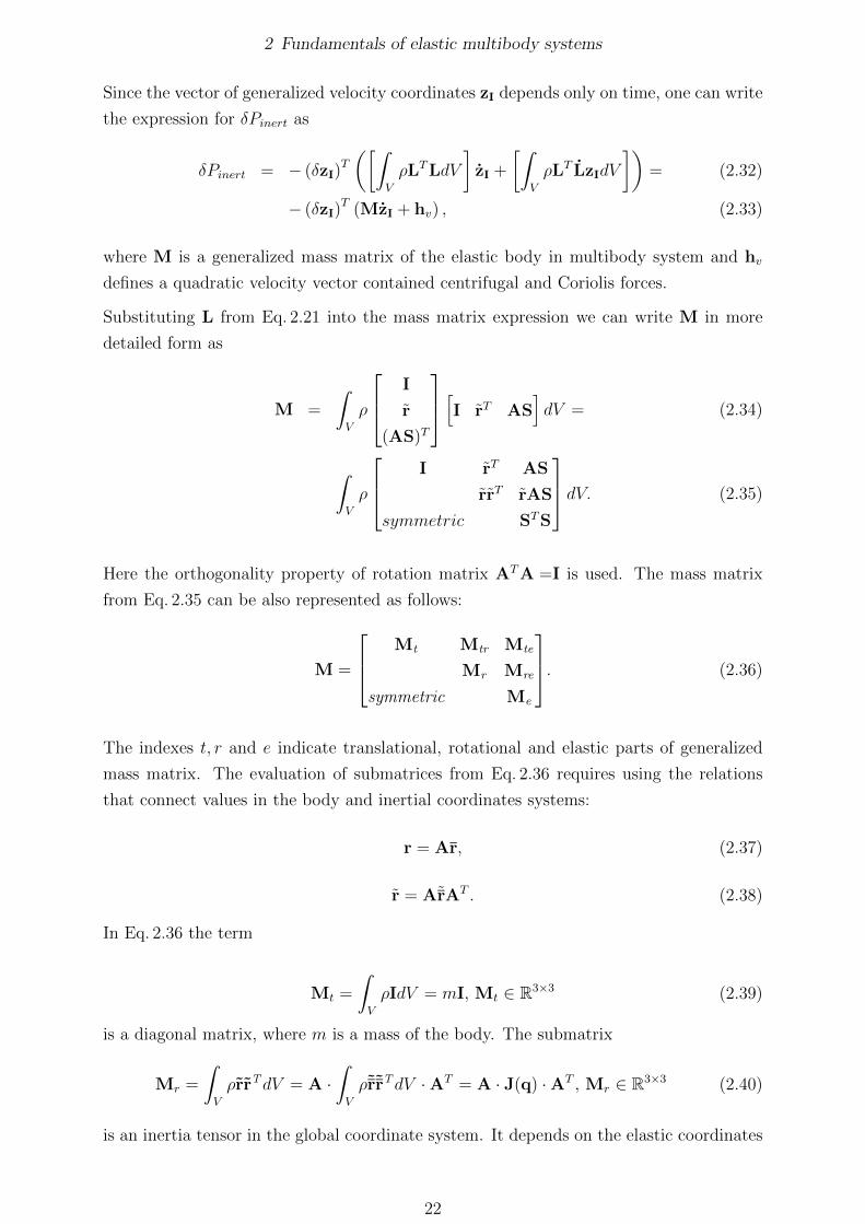
− (δzI)T (MzI + hv) , (2.33)
where M is a generalized mass matrix of the elastic body in multibody system and hv
defines a quadratic velocity vector contained centrifugal and Coriolis forces.
Substituting L from Eq. 2.21 into the mass matrix expression we can write M in more
detailed form as
M =
ˆV
ρ
I
r
(AS)T
[I rT AS]dV = (2.34)
ˆV
ρ
I rT AS
rrT rAS
symmetric STS
dV. (2.35)
Here the orthogonality property of rotation matrix ATA =I is used. The mass matrix
from Eq. 2.35 can be also represented as follows:
M =
Mt Mtr Mte
Mr Mre
symmetric Me
. (2.36)
The indexes t, r and e indicate translational, rotational and elastic parts of generalized
mass matrix. The evaluation of submatrices from Eq. 2.36 requires using the relations
that connect values in the body and inertial coordinates systems:
r = Ar, (2.37)
r = A˜rAT . (2.38)
In Eq. 2.36 the term
Mt =
ˆV
ρIdV = mI, Mt ∈ R3×3 (2.39)
is a diagonal matrix, where m is a mass of the body. The submatrix
Mr =
ˆV
ρrrTdV = A ·ˆV
ρ˜r˜rTdV ·AT = A · J(q) ·AT , Mr ∈ R3×3 (2.40)
is an inertia tensor in the global coordinate system. It depends on the elastic coordinates
22

2 Fundamentals of elastic multibody systems
q. The matrix J denotes an inertia tensor with respect to the body coordinate system.
Next, the term
Me =
ˆV
ρSTSdV, Me ∈ RN×N (2.41)
corresponds to a finite element mass matrix of the body. The component
Mtr =
ˆV
ρrTdV =
ˆV
ρA˜rTATdV = A ·ˆV
ρ˜rTdV ·AT = mA · ˜cT ·AT (2.42)
is 3× 3 matrix with
c = c(q) =1
m
ˆV
ρrdV (2.43)
being a vector of mass center of the body with respect to the body frame. Analogous
to the inertia tensor of the body, the position of mass center also depends on the elastic
coordinates q. Finally, the matrices
Mte =
ˆV
ρASdV = A ·ˆV
ρSdV = A·Ct, Ct ∈ R3×N , (2.44)
Mre =
ˆV
ρrASdV =
ˆV
ρA˜rATASdV = A ·ˆV
ρ˜rSdV = A ·Cr, Cr ∈ R3×N (2.45)
describe coupling terms of rigid body motion and elastic deformations. It is necessary to
note that only the matrices Mt and Me are constant, while other terms of the generalized
mass matrix depend on the generalized coordinates of the body and, as a result, they are
implicit functions of time.
In order to evaluate volume integrals of the quadratic velocity vector hv from Eq. 2.33, we
separate it into translational, rotational, and elastic components hv =[hTvt hTvr hTve
]Tand exploit the expressions for L and LzI from Eq. 2.21 and Eq. 2.25. The translational
part hvt can be obtained as
hvt =
ˆV
ρ (ωωr + 2ωASq) dV = mA˜ω(˜ωc + 2˙c
). (2.46)
The simplification of hvt is accomplished by using the relations
ˆV
ρωωr dV =
ˆV
ρA˜ω ˜ωr dV = A˜ω ˜ωm · 1
m
ˆV
ρr dV = mA˜ω ˜ωc (2.47)
and
ˆV
2ρωASqdV =´V
2ρA˜ωSqdV = 2A˜ωm ˙c (2.48)
where
˙c =1
m
ˆV
ρ ˙rdV (2.49)
23

2 Fundamentals of elastic multibody systems
is a local velocity of mass center in the body frame.
The rotational component of the quadratic velocity vector takes the form
hvr =
ˆV
ρr (ωωr + 2ωASq) dV = A · ˜ωJω + A ·Grω, (2.50)
where Gr is a component of Coriolis forces
Gr = 2
ˆV
ρ˜r˜rTdV (2.51)
and J is the tensor of inertia from Eq. 2.40. The extraction of J in the first term of
Eq. 2.50 is performed using the relation
ˆV
ρrωωrdV = A˜ω
(ˆV
ρ˜r˜rTdV
)ω, (2.52)
where the following operations with skew-symmetric matrices are carried out
rω = ωr + (rω), (2.53)
rωωr = −rωrω = −(ωr + (rω)
)rω =
−ωrrω − (rω)rω =− ωrrω = ωrrTω (2.54)
and the relations r = A˜rAT , ω = A ˜ωAT are used.
The derivation of Gr in Eq. 2.50 is accomplished as follows:
ˆV
2ρrωASqdV = 2
ˆV
ρA˜r˜ω ˙rdV = A · 2ˆV
ρ˜r˜rTdV ω (2.55)
The elastic part hve of the quadratic velocity vector takes the form:
hve =
ˆV
ρ (AS)T (ωωr + 2ωASq) dV =ˆV
ρ (AS)T ωωrdV +
ˆV
ρ (AS)T 2ωASqdV (2.56)
The first summand of Eq. 2.56 is given by
ˆV
ρSTATA˜ωATA˜ωATArdV =
ˆV
ρST ˜ω ˜ωrdV (2.57)
Ordinary matrix operations can not factor the rotational velocity ω out of this integrand,
therefore the combination of matrix and index notation proposed in [77] is used:
ˆV
ρST ˜ω ˜ωrdV =[ωTOekω
], k = 1..N. (2.58)
Here the brackets mean that all components form a vector of length N . The matrix
24

2 Fundamentals of elastic multibody systems
Oek∈ R3×3 is given as
Oek =
ˆV
ρS∗k˜rdV (2.59)
with S∗k being the k-th column of shape matrix S, see [77].
The second summand of Eq. 2.56 can be rewritten as
ˆV
ρ (AS)T 2ωASqdV = 2
ˆV
ρST ˜ωSqdV =
2
ˆV
ρST (Sq)T
ωdV = 2
ˆV
ρST ˙rTdV ω = Geω, (2.60)
where Ge ∈ RN×3 takes the form
Ge = 2
ˆV
ρST ˙rTdV. (2.61)
Summarizing the evaluation of generalized quadratic forces yields
hv =
hvt
hvr
hve
=
Am ˜ω ·(˜ωc + 2˙c
)A ·(˜ωJω + Grω
)[ωTOekω
]+ Geω
. (2.62)
The components c, ˙c, J, Gr, Oek, and Ge are defined in Eq. 2.43, Eq. 2.49, Eq. 2.40,
Eq. 2.51, Eq. 2.59, and Eq. 2.61, respectively.
Virtual power of internal forces
The virtual power due to elastic forces is defined as
δPinter = −ˆV
δεT · σdV, (2.63)
where σ and ε are stress and strain rate vectors, respectively. Further, the relation
between the strain vector ε and the displacement field u is required.
According to the finite element method, the displacement field is approximated by a
shape matrix S and time-depended nodal coordinates q as u(d0, t) = S(d0) · q(t), see
Section 2.1.2. Once the displacement field is given, the strain vector ε(d0, t) is obtained
by applying the differential displacement-strain operator ∇ [79, 51]:
ε(d0, t) = ∇ · u = ∇ · S(d0) · q(t), (2.64)
25

2 Fundamentals of elastic multibody systems
where
∇ =
∂∂x1
0 0
0 ∂∂x2
0
0 0 ∂∂x3
∂∂x2
∂∂x1
0
0 ∂∂x3
∂∂x2
∂∂x3
0 ∂∂x1
. (2.65)
The differentiations in this relation are done with respect to the axes of the body coordi-
nate system that is initially parallel to the global reference frame.
Six elements of strain vector form a symmetric matrix in R3×3. Here the strain is presented
in a vector form
ε =[ε11 ε22 ε33 2ε12 2ε13 2ε23
]T∈ R6. (2.66)
In the elastic multibody dynamics it is generally assumed the linear strain-displacement
relationship, which is described by Eq. 2.64. However, there are some applications that
require taking into account a nonlinear term. Additional non-linear strain is obtained by
a differential operator ∇:
∇(u) =
∂u1∂x1
∂∂x1
∂u2∂x1
∂∂x1
∂u3∂x1
∂∂x1
∂u1∂x2
∂∂x2
∂u2∂x2
∂∂x2
∂u3∂x2
∂∂x2
∂u1∂x3
∂∂x3
∂u2∂x3
∂∂x3
∂u3∂x3
∂∂x3
∂u1∂x1
∂∂x2
+ ∂u1∂x2
∂∂x1
∂u1∂x1
∂∂x2
+ ∂u2∂x2
∂∂x1
∂u1∂x1
∂∂x2
+ ∂u3∂x2
∂∂x1
∂u1∂x2
∂∂x3
+ ∂u1∂x3
∂∂x2
∂u1∂x2
∂∂x3
+ ∂u2∂x3
∂∂x2
∂u1∂x2
∂∂x3
+ ∂u3∂x3
∂∂x2
∂u1∂x3
∂∂x1
+ ∂u1∂x1
∂∂x3
∂u1∂x3
∂∂x1
+ ∂u2∂x1
∂∂x3
∂u1∂x3
∂∂x1
+ ∂u3∂x1
∂∂x3
. (2.67)
The nonlinear strain takes the form
ε = ∇ · u +1
2∇ · u. (2.68)
The strain rate ε can be obtained differentiating Eq. 2.68 as[47]:
ε = ∇ ˙u +1
2
(˙∇u + ∇ ˙u
)= ∇ ˙u + ∇ ˙u. (2.69)
Using the relation ˙u = S · q and Eq. 2.69 the virtual strain rate takes the form
δε =(∇S + ∇S
)δq. (2.70)
According to the generalization of Hooke’s law, the strain and stress vectors are connected
by an elasticity matrix E ∈ R6×6 as
σ = E · ε. (2.71)
26

2 Fundamentals of elastic multibody systems
Substituting Eq. 2.70 and the stress expression of Eq. 2.71 into Eq. 2.63 yields
δPinter = − (δq)T (KeL · q + KeN(q) · q) , (2.72)
where KeL and KeN(q) are linear and nonlinear components of stiffness matrix related
to the elastic coordinates of finite element model and defined as
KeL =
ˆV
(∇S)TE∇SdV (2.73)
KeN =
ˆV
(∇S)TE∇SdV +1
2
ˆV
(∇S)TE∇SdV. (2.74)
It follows that the virtual power of elastic forces is obtained by
δPinter = −δzITKz, (2.75)
where
K =
0 0 0
0 0 0
0 0 KeL + KeN(q)
(2.76)
is a generalized stiffness matrix of the elastic body.
Virtual power of external forces
The virtual power of an external force acting at an arbitrary point of the body can be
defined as
δPext = δdT · f , (2.77)
where f ∈ R3 is an external force expressed in the global coordinate system, the vector d
defines a global velocity of the point where the force is applied. The virtual velocity δd
can be expressed in terms of generalized velocity coordinates zI as
δd = LδzI (2.78)
with L being the matrix from Eq. 2.21. It follows that the virtual power of external forces
is given by
δPext = δzITLT f = δzI
T
I
r
(AS)T
· f . (2.79)
The gravity force can be considered as a concentrated load at the center of gravity or a
27

2 Fundamentals of elastic multibody systems
volume force. The virtual power of a volume force is defined as
δPext =
ˆV
δzIT
I
r
(AS)T
bdV = δzIT
ˆV
I
r
(AS)T
bdV
, (2.80)
where b is a load per unit volume. For the gravity force the relation b = ρ · g can be
used, where g denotes the gravity acceleration.
Moments can be represented using pairs of concentrated forces with the property f1 = −f2.
Similar to the consideration of volume forces, the virtual power of generalized surface
force associated with a surface load p per unit area dD is defined as
δPext = δzIT
ˆD
I
r
(AS)T
pdD. (2.81)
If the body is subjected to several external forces, then their effects must be added. The
generalized external force can be expressed as
hext =
ˆV
I
r
(AS)T
bdV +
I
r
(AS)T
· f +
ˆD
I
r
(AS)T
pdD. (2.82)
The virtual power of external forces takes the form
δPext = δzIT · hext. (2.83)
2.1.5 Equations of motion of free elastic body
Substituting the expressions for the virtual power of inertia forces from Eq. 2.33, internal
forces from Eq. 2.75, and external forces from Eq. 2.83 into Jourdain’s principle of Eq. 2.28
yields
δzIT (MzI + Kz + hv − hext) = 0. (2.84)
Incorporation of damping into the equations of motion is considered in Section 2.1.8.
If components of generalized velocity coordinates zI are independent, then Eq. 2.84 holds
true only upon condition that the term in the parentheses equals zero. It follows the
equations of motion of free elastic body are given as
MzI + Kz + hv − hext = 0. (2.85)
These equations are called generalized Newton-Euler equations of motion [79]. Here M
28
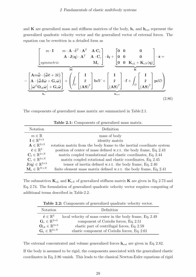
2 Fundamentals of elastic multibody systems
and K are generalized mass and stiffness matrices of the body, hv and hext represent the
generalized quadratic velocity vector and the generalized vector of external forces. The
equation can be rewritten in a detailed form as m · I m ·A · ˜cT ·AT A·Ct
A · J(q) ·AT A ·Cr
symmetric Me
︸ ︷︷ ︸
M
· zI +
0 0 0
0 0 0
0 0 KeL + KeN(q)
︸ ︷︷ ︸
K
· z =
−
Am ˜ω ·(˜ωc + 2˙c
)A ·(˜ωJω + Grω
)[ωTOekω
]+ Geω
︸ ︷︷ ︸
hv
+
ˆV
I
r
(AS)T
bdV +
I
r
(AS)T
· f +
ˆD
I
r
(AS)T
pdD
︸ ︷︷ ︸
hext
(2.86)
The components of generalized mass matrix are summarized in Table 2.1.
Table 2.1: Components of generalized mass matrix.
Notation Definition
m ∈ R mass of bodyI ∈ R3×3 identity matrixA ∈ R3×3 rotation matrix from the body frame to the inertial coordinate system
c ∈ R3 position of center of mass defined w.r.t. the body frame, Eq. 2.43Ct ∈ R3×N matrix coupled translational and elastic coordinates, Eq. 2.44Cr ∈ R3×N matrix coupled rotational and elastic coordinates, Eq. 2.45J(q) ∈ R3×3 tensor of inertia defined w.r.t. the body frame, Eq. 2.40Me ∈ RN×N finite element mass matrix defined w.r.t. the body frame, Eq. 2.41
The submatrices KeL and KeN of generalized stiffness matrix K are given in Eq. 2.73 and
Eq. 2.74. The formulation of generalized quadratic velocity vector requires computing of
additional terms described in Table 2.2.
Table 2.2: Components of generalized quadratic velocity vector.
Notation Definition
˙c ∈ R3 local velocity of mass center in the body frame, Eq. 2.49Gr ∈ R3×3 component of Coriolis forces, Eq. 2.51Oek ∈ R3×3 elastic part of centrifugal forces, Eq. 2.59Ge ∈ R3×N elastic component of Coriolis forces, Eq. 2.61
The external concentrated and volume generalized forces hext are given in Eq. 2.82.
If the body is assumed to be rigid, the components associated with the generalized elastic
coordinates in Eq. 2.86 vanish. This leads to the classical Newton-Euler equations of rigid
29

2 Fundamentals of elastic multibody systems
body motion. In addition, if the motion of the reference frame is constrained to be zero,
Eq. 2.86 is reduced to the classical structural equations.
The generalized mass matrix form Eq. 2.86 has a rank deficiency of six, therefore it is not
solvable until reference conditions are defined.
2.1.6 Definition of body coordinate system
It is assumed in the floating frame formulation that the displacement field u describes
deformation of the body with respect to the body reference frame. The global motion of
body is the superposition of motion of body reference frame and deformations with respect
to the body frame. If the assumed displacement field u contains rigid body modes, they
have to be eliminated to define a displacement field describing only deformations. This
can be done by imposing a set of reference conditions, which are introduced by a set of
linear algebraic equations. As the number of rigid body modes equals six, it is necessary
to impose six reference conditions.
Since there are no unique manner of defining rigid and elastic motions, the floating frame
can be selected in a number of different ways. These methods can be divided into two
categories. The methods of the first group attach a coordinate system to material points
of the body. This formulation is referred to as nodal-fixed axes. The second group of
floating frames consists of coordinate systems that follow a body in an optimal manner.
This category includes a frame oriented along the principal axes of inertia, a mean-axes
(Tisserand) frame, and a Buckens frame. In contrast to nodal-fixed frames, coordinate
systems of this type impose reference conditions on all nodes of the body. The moving
frames eliminate the need to select material points for attaching the floating frame, but it
is more difficult to determine the frame location and orientation because of specific frame
conditions.
Nodal-fixed frames
If points of the body possess rotational degrees of freedom, the body coordinate system
can be attached to one point. In this case, the reference conditions are given asu(rP0 , t
)= 0
ϑ(rP0 , t
)= 0,
(2.87)
where ϑ defines rotational coordinates of the point P and rP0 is an undeformed position
of the point P .
Alternatively, the body coordinate system can be defined by three points P1, P2 and P3.
It is assumed that the origin of the frame is always located at the point P1, the point P2
remains along the x axis, and the point P3 lies on the xy plane, see Fig. 2.4.
30

2 Fundamentals of elastic multibody systems
P2P1
P3
xy
zundeformed body
Figure 2.4: Attachment of body coordinate system by three points.
This yields six reference conditions
u(rP10 , t
)= 0
uy(rP20 , t
)= 0
uz(rP20 , t
)= 0
uz(rP30 , t
)= 0,
(2.88)
where rP10 ,rP2
0 , and rP30 are undeformed positions of points P1,P2, and P3 respectively. If
the body coordinate system differs from the coordinate system of finite element model,
the undeformed locations of body points r0 and shape functions S have to be redefined
with respect to the new body frame.
The reference conditions of Eq. 2.88 can be simplified in the case of fixation of body frame
to nodes of the body. If nodes possess three DoFs, the displacement field u for an arbitrary
node K takes the form
u(rK0 , t
)= qK(t) ∈ R3, (2.89)
where qK is a vector of degrees of freedom for the node K. Then Eq. 2.88 can be rewritten
as
qK1 (t) = 0 ∈ R3
qK2y (t) = 0 ∈ R
qK2z (t) = 0 ∈ R
qK3z (t) = 0 ∈ R
(2.90)
with K1, K2, and K3 being nodes of the body.
The reference conditions of Eq. 2.90 can be automatically taking into account in equa-
tions of motion and there is no need to include them to the system of equations. The
dependency of the vector of unconstrained elastic coordinates qu and the initial vector of
nodal deformations q can be written as
q = B · qu, (2.91)
where B is a linear transformation that arises from imposing the constrains of Eq. 2.90
31

2 Fundamentals of elastic multibody systems
and consists of zeros and ones. The displacement field u can be represented as
u = S ·B · qu = Su · qu , (2.92)
where Su is a shape matrix that satisfies the reference conditions. Substituting Eq. 2.92
into Eq. 2.11 leads to the equations of motion in terms of independent generalized coor-
dinates.
The conditions of Eq. 2.88 attach the reference frame to the body. The rigid-body motion
in this coordinate system is eliminated. Since the body frame is allowed to move with
respect to an inertial frame, attaching the moving frame to the points does not exclude
any of the rigid-body modes in the inertial coordinate system.
Principal axes frame
In this formulation the moving reference frame is enforced to coincide with the instan-
taneous principal axes of a deformable body. This method provides six conditions based
on two requirements: the origin of the reference frame must remain at the instantaneous
mass center, and three products of inertia must remain zeros:
c = 0
Jij = 0, i 6= j , i = 1..3, j = 1..3.(2.93)
Here c is the vector of mass center from Eq. 2.43 and J is the inertia tensor defined in
Eq. 2.40.
In this case, the coupling between flexible and rigid body motion is weaker and equations
of motions become easier: the tensor of inertia J becomes a diagonal matrix, and the
sub-matrices Mtr and Mte of Eq. 2.42 and Eq. 2.44 vanish because the vector of mass
center is equal to zero. Deriving expressions for products of inertia in terms of nodal
coordinates can be found in [77, 62]. In contrast to the nodal fixed frame formulations,
the reference conditions of principal axes frames increase the number of equations to be
solved by six.
Mean-axes frame
The mean-axis conditions are six constraints that enforce the body frame to follow the
motion of nodes in such a way that the following conditions are satisfiedCt · q = 0
Cr(q) · q = 0(2.94)
32

2 Fundamentals of elastic multibody systems
with Ct and Cr being the matrices defined in Eq. 2.44 and Eq. 2.45, respectively. Accord-
ing to [76], if the origin of body frame is located in a mass center of undeformed body,
the first equation from Eq. 2.94 enforces the frame to follow an instantaneous mass center
Ct · q = m · ˙c = 0⇒ c = 0. (2.95)
Similar to the principle axes approach, the first condition of Eq. 2.94 eliminates the terms
Mtr and Mte from the generalized mass matrix of Eq. 2.35. The second equation from
Eq. 2.94 defines orientation of the floating frame and removes the term Mre. It follows
that the generalized mass matrix M takes a block-diagonal form. The inertia tensor
remains a non-diagonal matrix. Due to the conditions of Eq. 2.94 the mean-axes frame
has a property that the kinetic energy associated with the deformation stays at a minimum
[17].
Buckens frame
The Buckens frame is a special case of mean-axes frame. The mean-axes constrains
of Eq. 2.94 are valid even for large deformations of the body. If small deformations are
assumed, the products of elastic coordinates q can be neglected in the equations of motion.
The Taylor expansion of Cr up to the first order terms yields
Cr (q) = Cr0 + Cr1 (q) , (2.96)
where the indexes 0 and 1 define zero and the first order terms of the Taylor expansion,
respectively.
Assuming small deformations, the second condition of mean-axes frame can be simplified
as
Cr (q) · q = Cr0 · q = 0 (2.97)
that leads to Buckens frame conditionsCt · q = 0
Cr0 · q = 0.(2.98)
The term Ct is defined in Eq. 2.44, while Cr0 is given by
Cr0 =
ˆV
ρ˜r0SdV. (2.99)
Similarly to the mean-axes frame constrains, the Buckens frame conditions transform
generalized mass matrix to a block-diagonal form. In addition, according to [87] the
33

2 Fundamentals of elastic multibody systems
Buckens frame ensures that the sum of the squares of elastic displacements with respect
to the body frame is a minimum:
1
2
ˆV
uT · u dm = min. (2.100)
It means that the Buckens coordinate system leads to the smallest elastic displacements
possible. This may be important when the assumption of small deformation for modeling
elastic body motion is used. In the general case the Buckens frame constraints must
be added to equations of motion, but under certain conditions they are automatically
satisfied. One of the approaches to take into account the Buckens frame conditions during
the simulation is proposed in [2]. The other way to satisfy these reference conditions is
connected with using eigenmodes of unconstrained body. The requirements of Buckens
frame can be automatically satisfied, if columns of shape matrix S from Eq. 2.10 are mass
orthogonal to rigid body modes and the position of body frame in the undeformed state
of the body coincides with the mass center, see [77].
2.1.7 Approximation of motion integrals by finite element programs
The dynamic properties of elastic body are defined by the volume integrals introduced
in Section 2.1.4. Most of them depend on generalized elastic coordinates and, therefore,
must be updated at each step of integration. In order to reduce computational costs
during simulation, the volume integrals are expressed by generalized elastic coordinates
and precomputed time-invariant system matrices. These matrices can be found as follows.
Every volume integral Z is expressed as a sum of terms Z0 , Z1, and Z2 that are constant,
linearly, and quadratically depended on the elastic coordinates q, respectively:
Z (q) = Z0 + Z1 (q) + Z2(q). (2.101)
Assuming small deformations, the quadratic component Z2 is negligibly small, therefore
Z (q) = Z0 + Z1 (q) . (2.102)
Using this representation, it is possible to find constant components for all volume in-
tegrals. This process is described in detail in [56, 76]. Table 2.3 contains a set of time-
invariant system matrices required for the calculation of the volume integrals of elastic
body.
The principle of retrieving constant matrices from volume integrals can be illustrated by
processing the inertia tensor. Using the relation r = r0 + S · q of Eq. 2.11, the inertia
34

2 Fundamentals of elastic multibody systems
Table 2.3: Time-invariant components of volume integrals.
Notation Calculation
m · I´VρI dV
m · c0
´Vρr0 dV
J0
´Vρ˜r0 · ˜r
T0 dV
C1´VρS dV
C2´Vρ˜r0 · S dV
C3´VρS · ST dV
C4k´Vρ˜r0 · S∗k dV
C5k´VρS∗k · S dV
C6kl´VρS∗k · S∗l dV
tensor J of Eq. 2.40 takes the form
J (q) =
ˆV
ρ˜r · ˜rTdV =
ˆV
ρ˜r0 · ˜rT0 dV +
ˆV
ρ
(˜r0 · (S · q)
T
+ (S · q) · ˜rT0)dV
+
ˆV
ρ(S · q) · (S · q)T
dV. (2.103)
The first summand of this equation corresponds to the matrix J0 from Table 2.3. The
third part depends quadratically on generalized coordinates q, therefore it vanishes by
small deformations. Using the relation
S · q = S∗1 · q1 + ...+ S∗N · qN (2.104)
the coordinates q can be taken out of the brackets of the second summand of Eq. 2.103
by the transformation
ˆV
ρ
(˜r0 · (S · q)
T
+ (S · q) · ˜rT0)dV =
N∑k=1
ˆV
ρ(˜r0 · ST
∗k + S∗k · ˜rT0)dV qk =
−N∑k=1
ˆV
ρ(˜r0 · S∗k + S∗k · ˜r0
)dV qk. (2.105)
It follows that the inertia tensor J is constructed by the generalized coordinates q and
the time-invariant matrices as
J(q) = J0 −N∑k=1
ˆV
ρ(˜r0 · S∗k + S∗k · ˜r0
)dV qk = J0−
N∑k=1
(C4k + C4Tk
)qk︸ ︷︷ ︸
J1(q)
. (2.106)
Let us consider formulation of other terms of generalized mass matrix in terms of the time-
invariant components. According toTable 2.1, the following terms must be considered:
position of center of mass c, coupling terms Ct and Cr, and the finite element matrix Me.
35

2 Fundamentals of elastic multibody systems
The vector of center of mass can be rewritten as
c = c0 + c1(q) = c0 +1
m·C1 · q. (2.107)
The term of coupling of translational and elastic coordinates takes the form
Ct = C1. (2.108)
The matrix Cr in terms of the time-invariant components is given as
Cr = Cr0 + Cr1(q) = C2 +N∑k=1
C5k · qk. (2.109)
Finally, the finite element mass matrix Me coincides with the component C3.
The terms of generalized quadratic velocity vector from Table 2.2 must be also represented
using constant components of motion integrals. The set of terms to be considered includes
the velocity of mass center ˙c, components of Coriolis force Gr and Ge, and the component
of elastic part of centrifugal force Oek.
Using Eq. 2.49 and ˙r = Sq, the velocity of mass center takes the following form
˙c =1
m·C1 · q. (2.110)
The component Gr from Eq. 2.51 can also be written as
Gr = 2
ˆV
ρ˜rSqTdV. (2.111)
Using the relation ˜r = ˜r0 + Sq and Eq. 2.104, the integrand of the equation takes the form
˜rSqT
= ˜r0 · SqT
+ Sq · SqT
= (2.112)
−N∑k=1
˜r0 · S∗k · qk −N∑k=1
N∑l=1
S∗k · S∗l · qk · ql.
Thus, the component Gr can be expressed in terms of the time invariant matrices as
Gr = −2N∑k=1
C4k · qk − 2N∑k=1
N∑l=1
C6kl · qk · ql. (2.113)
Similarly, the matrix Ge from Eq. 2.61 can be rewritten as
Ge = 2
ˆV
ρST SqTdV = 2
N∑k=1
ˆV
ρST(S∗k
)TdV · qk = 2
N∑k=1
C5Tk · qk.
36

2 Fundamentals of elastic multibody systems
Finally, the terms Oek from Eq. 2.59 are obtained as follows
Oek =
ˆV
ρS∗k˜rdV =
ˆV
ρS∗k˜r0dV +N∑l=1
ˆV
ρS∗kS∗ldV · ql = C4k +N∑l=1
C6kl · ql.
The FE programs can export the component C3. The remaining components must be
computed in special preprocessors. The data needed for the construction of equations
of motion of elastic body can be defined by the finite element stiffness matrix Ke, the
mass matrix Me, information about boundary conditions, and the undeformed positions
of nodes r0. The construction process for consistent mass matrix formulation is presented
in [55, 76, 82]. In this thesis we consider a principle of evaluation of motion integrals by
example of C1 and C4.
If the FE model undergoes only translational rigid body motion, the linear velocity of all
nodes of the model is the same
v(t) = u(r0, t) = S(r0) · q(t). (2.114)
The vector of generalized velocities is composed of velocities of each node
q(t) =
v(t)
...
v(t)
=
I...
I
︸ ︷︷ ︸
St
v(t). (2.115)
Here I is 3× 3 identity matrix. Substituting this equations in the previous one yields the
orthogonality relation
S · St = I. (2.116)
In the case the FE model undergoes rotational rigid body motion, the linear velocity of
each nodes are defined as
u(r0, t) = ωr0 = −˜r0ω = S(r0) · q(t). (2.117)
The vector of generalized velocities takes the form
q(t) =
ωr0
...
ωr0
=
−˜r0
...
−˜r0
︸ ︷︷ ︸Sr
ω. (2.118)
The last two equations result in
− ˜r0 = S · Sr. (2.119)
37

2 Fundamentals of elastic multibody systems
For the construction of volume integrals it is necessary to introduce an auxiliary matrix
Se that is defined as
Se = B (2.120)
with B being a matrix that accounts for boundary conditions imposed on the elastic
coordinates q, see Eq. 2.91. If model reduction methods are applied, the matrix Se is
defined as
Se = B ·V, (2.121)
where V is a coordinate transformation matrix.
The component C1 can be written for the system with boundary conditions and reduced
coordinates as follows:
C1 =
ˆV
ρS · Se dV. (2.122)
Using the relation of Eq. 2.116 this equation can be written in another form
C1 =
ˆV
ρS · Se dV = STt ·[ˆ
V
ρST · S dV]· Se = STt ·Me · Se. (2.123)
The calculation of the term C4k requires using the second relation defined in Eq. 2.119:
C4k =
ˆV
ρ˜r0 · S∗k dV = STr ·ˆρST · S∗k dV. (2.124)
Here the matrix S∗k has to be transformed as
S∗k = −[e1 · S∗k e2S∗k e3S∗k
]= −
[e1 · S · I∗k e2 · S · I∗k e3 · S · I∗k
], (2.125)
where ei ∈ R3×1 are unit vectors and I∗k is the k-th column of identity matrix I ∈ RN×N .
Using the matrix Se, the i-th column of matrix C4k takes the form
[C4k]∗i = −STr ·Xi · [Se]∗k , (2.126)
where Xi =´VρST · ei · S dV .
In order to identify the mass matrix Me in this equation, the matrix ei must be pulled
out of the integral. This can be carried out only for isoparametric finite elements [47].
For the isoparametric elements the locations of material points on the elements, as well as
their displacements are interpolated by the same shape functions. These elements do not
use rotational parameters as nodal coordinates[79]. The pulling out the matrix ei yields
Xi = diag(ei) ·ˆV
ρST · S dV = diag(ei) ·Me. (2.127)
38

2 Fundamentals of elastic multibody systems
The calculation of matrix Xi for nonisoparametric elements is problematic, therefore the
approximation approach proposed in [55] is usually applied:
asym(Xi) :=1
2·(Xi −XT
i
). (2.128)
The final expression for the term C4k is given as
[C4k]∗i = −STr · asym(Xi) · [Se]∗k , i = 1..3. (2.129)
The calculation of volume integrals from Table 2.3 using the finite element data is shown
in Table 2.4.
Table 2.4: Calculation of volume integrals using data imported from finite element tools.
Notation Calculation
m · I STt ·Me · Stm · c0 STr ·Me · St
J0 STr ·Me · SrC1 STt ·Me · SeC2 STr ·Me · SeC3 STe ·Me · Se
[C4k]∗i −STr · asym(diag(ei) ·Me) · [Se]∗k[C5k]i∗ − [Se]∗k
T · asym(diag(ei) ·Me) · Se[C6kl]ij [Se]∗k
T · diag(ei) ·Me · diag(ej) · [Se]∗l
The external forces in Eq. 2.86 can be represented using concentrated nodal forces formu-
lation of which does not require the shape matrix S.
2.1.8 Damping definition
For some applications damping effects must be taken into account. The most simple and
widely used method to incorporate damping forces into equations of motion is to use a
proportional to velocities representation DzI with a constant matrix D. This leads to the
following equations of motion for linearly damped models
MzII + DzI + Kz + hv − hext = 0. (2.130)
Here the damping matrix D takes the form
D =
0 0 0
0 0 0
0 0 De
, D ∈ R(6+N)×(6+N), (2.131)
where De ∈ RN×N defines a finite element damping matrix.
39

2 Fundamentals of elastic multibody systems
In principle, the damping matrix De can be constructed by damping matrices of finite
elements analogous to the mass and stiffness matrices. However, material damping prop-
erties of certain elements are often not defined well enough to employ the same procedure.
The damping matrix can be constructed by Caughey’s series as
De = Me ·r∑
k=0
ak(M−1
e ·KeL
)k, (2.132)
where r defines a quantity of summands in the series, see [18]. In special case r = 1, the
damping matrix is called Rayleigh damping and is defined as
De = a0Me + a1KeL. (2.133)
The damping matrix formulated by Caughey’s series allows the definition of unknown
coefficients ai using a modal damping matrix. According to [21, 11] the coefficients of
modal damping matrix are defined as
φTi Deφj =
0, i 6= j
2ωiξi, i = j,(2.134)
where the pair (φi, ωi) denote the i -th eingenvector and eigenfrequency of the system
and ξi defines a corresponded modal damping factor.
Using the Eq. 2.133 and Eq. 2.134 the modal damping factor ξi can be expressed as shown
in [21] as
ξi =1
2
(a0ωi
+ a1ωi
). (2.135)
Thus, Rayleigh damping can be defined by choosing ξi for two modes and solving for
a0 and a1. The constants a0 and a1 produce specified modal damping factors for two
given modes. The advantage of Rayleigh damping lies in a simple calculation, while the
drawback is that it does not permit to define realistic damping for all modes of interest.
2.2 Model order reduction of elastic bodies
Modern finite element models may have millions degrees of freedom, which significantly
slow down a simulation process. The large number of elastic coordinates qe can be reduced
by model order reduction techniques. The main idea of these methods is to build a low-
dimensional model that preserves important properties of the original model. In this
section we consider model order reduction approaches based on projection, as well as
demands on the methods when using in the context of elastic multibody systems.
40

2 Fundamentals of elastic multibody systems
2.2.1 Basics of model order reduction
Let us consider the elastic part of equations of motion of deformable body
Me · q + De · q + Ke · q = he. (2.136)
Here he denotes a vector of external forces. It is necessary for some reduction methods to
represent the vector he as a product of time dependent load vector u(t) ∈ Rp and a load
distribution matrix Be ∈ RN×p. In addition, the coordinates of interest y(t) ∈ Rr are cut
out from the vector q by a matrix Ce ∈ Rr×N . For these reduction methods the equation
of motion are formulated as
Me · q + De · q + Ke · q = Be · u (2.137)
y = Ce · q.
The reduction techniques based on projection rely on the assumption that a high-dimensional
solution vector q belongs to a subspace V of smaller dimension n� N . Let
V =[
v1, v2, · · · ,vn
]∈ RN×n
define a basis of subspace V , then the elastic coordinates q can be represented as
q ≈ V · q, (2.138)
where the vector q is referred to as reduced coordinates. Substituting this relation into
equations of motion Eq. 2.137 results in an over-determined system and leave a residuum
because an exact solution q may not be an element of subspace V . The residuum can
be eliminated by an orthogonal subspace W represented by a matrix W ∈ RN×n . This
orthogonality condition is called Petrov-Galerkin condition, see [6, 72, 47]. The condition
is introduced in the equations of motion by a premultiplication of Eq. 2.137 by the matrix
WT . Thus, the low-dimensional approximation of original model takes the form
Me · ¨q + De · ˙q + Ke · q = Be · u
y = Ce · q(2.139)
with the reduced matrices Me = WT ·Me ·V, De = WT ·De ·V, Ke = WT ·Ke ·V ∈ Rn×n,
Be = WT ·Be ∈ Rn×p, and Ce = Ce ·V ∈ Rr×n. If the subspaces V and W are identical,
the projection is called orthogonal, otherwise, it is called oblique. The difference of the
projection types is visualized by Fig. 2.5.
The reduced equations of motion of a single elastic body in the multibody system are
41
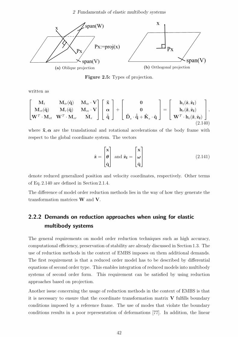
2 Fundamentals of elastic multibody systems
x
Px
span(V)
span(W)
Px:=proj(x)
(a) Oblique projection
x
Px
span(V)(b) Orthogonal projection
Figure 2.5: Types of projection.
written as Mt Mtr(q) Mte ·VMrt(q) Mr(q) Mre ·V
WT ·Met WT ·Mer Me
x
α¨q
+
0
0
De · ˙q + Ke · q
=
ht(z, zI)
hr(z, zI)
WT · he(z, zI)
,(2.140)
where x,α are the translational and rotational accelerations of the body frame with
respect to the global coordinate system. The vectors
z =
x
θ
q
and zI =
x
ω
q
(2.141)
denote reduced generalized position and velocity coordinates, respectively. Other terms
of Eq. 2.140 are defined in Section 2.1.4.
The difference of model order reduction methods lies in the way of how they generate the
transformation matrices W and V.
2.2.2 Demands on reduction approaches when using for elastic
multibody systems
The general requirements on model order reduction techniques such as high accuracy,
computational efficiency, preservation of stability are already discussed in Section 1.3. The
use of reduction methods in the context of EMBS imposes on them additional demands.
The first requirement is that a reduced order model has to be described by differential
equations of second order type. This enables integration of reduced models into multibody
systems of second order form. This requirement can be satisfied by using reduction
approaches based on projection.
Another issue concerning the usage of reduction methods in the context of EMBS is that
it is necessary to ensure that the coordinate transformation matrix V fulfills boundary
conditions imposed by a reference frame. The use of modes that violate the boundary
conditions results in a poor representation of deformations [77]. In addition, the linear
42

2 Fundamentals of elastic multibody systems
combination of columns of V has to be a subspace that does not contain rigid-body modes.
The exclusion of rigid body modes is required by the floating frame formulation. In this
formulation the motion of elastic body is decoupled into the rigid body motion approxi-
mated by the motion of floating frame and deformations with respect to the moving frame.
It follows that the reduction method has to able to produce a coordinate transformation
matrix that excludes rigid body motion from the description of deformations.
In order to satisfy the Buckens frame conditions the coordinate transformation matrix V
has to be modified according the formula
Vmod =(I− V0V
T0 Me
)V, (2.142)
where V0 is a matrix of rigid-body modes normalized by the mass matrix Me, and I is
an identity matrix of size N ×N , see [47, page 135]. This modification does not damage
dynamical properties of reduced model. It only rewrites the modes in V with respect to
the center of mass. In order to obtain rigid body modes, it is not necessary to solve an
eigenvalue problem. The translational and rotational rigid modes can be found as follows:
V0 =[
V0t ,V0r
]=
...
[I]k
...
,
...[−˜r0
]k...
, k = 1, .., N. (2.143)
Here the matrix I is 3× 3 identity matrix, the term [r0]k denotes an undeformed position
of the k-th node of FE model and[˜r0]k
corresponds to an associated with [r0]k skew
symmetric matrix. It is assumed that a finite element node exhibits only three transla-
tional degrees of freedom. The transformation matrix Vmod ensures that the Buckens
frame constraints are automatically satisfied and there is no need to add them to equa-
tions of motion. It is always possible to transform modes so that the conditions of the
Buckens-frame are fulfilled [81].
Linear dependency of columns of Vmod can be removed by the QR decomposition of Vmod
and the exclusion of columns that correspond to zero values on the diagonal of matrix R.
The remaining modes together with the rigid body modes spans the same solution space
as it is spanned by the original modes of V.
2.3 Model reduction techniques
2.3.1 Guyan method
This old reduction approach was proposed by Guyan in [37]. The approach separates
model DoFs into internal and boundary subsets. The b-set of boundary DoFs is defined
43

2 Fundamentals of elastic multibody systems
as a set of coordinates that remain in the system, while an i -set of internal coordinates
includes all DoFs that must be eliminated from the system of equations:
i ∪ b = a, i ∩ b = ∅. (2.144)
Here a defines a set of all DoFs of the system. Let us consider the following undamped
system:
Me · q(t) + Ke · q(t) = he. (2.145)
The partition of the system into internal and boundary coordinates yields[Mii Mib
Mbi Mbb
]e
[qi
qb
]+
[Kii Kib
Kbi Kbb
]e
[qi
qb
]=
[hi
hb
]e
. (2.146)
Due to the static nature of the method the influence of inertia term is not taken into
account. Assuming that there is no force acting on the internal DoFs, i.e. hi = 0, and
solving Eq. 2.146 for qi the following relationship is obtained:
q =
[qi
qb
]=
[−Kii ·Kib
Ib
]· qb, (2.147)
where Ib ∈ RNb×Nb is an identity matrix. According to the Guyan method the low-
dimensional subspace is defined by a transformation matrix V ∈ RN×Nb
V =
[−Kii ·Kib
Ib
]. (2.148)
The Guyan reduction leads to the exact representation of static deformations and to
a relative good approximation of low frequencies and corresponded modes. For higher
frequency modes inertia forces terms become significant that results in inaccurate reduced
order models.
2.3.2 Dynamic condensation method
The dynamic condensation method utilizes the inertia information of FE model. The
method was developed for reducing systems that undergo a harmonic excitation.
The dynamic behavior of FE model in time domain is described by the system of equations
Me · q(t) + Ke · q(t) = he(t). (2.149)
In contrast to Guyan reduction method, the force vector he is time dependent. Assuming
zero initial conditions, the Laplace transformation of Eq. 2.149 leads to the following
44
2 Fundamentals of elastic multibody systems
equations in the frequency domain:
(Me · s2 + Ke) · q(s) = he(s). (2.150)
The vectors q(s) and he(s) denote the Laplace transformation of time dependent dis-
placement and force vectors q(t) and he(t), respectively, i.e.
q(s) = L{qe}(s) =
ˆ ∞0
e−st · q(t) dt (2.151)
he(s) = L{he}(s) =
ˆ ∞0
e−st · he(t) dt. (2.152)
The variable s = i ·ω is a complex number with zero real part. The term ω represents an
angular frequency, which is connected with an excitation frequency f via the relationship
ω=2πf .
Analogously to the Guyan method, the system of Eq. 2.150 is partitioned into the internal
and boundary coordinates as
(−Me · ω2 + Ke)︸ ︷︷ ︸T(ω)
· q(ω) = he(ω) (2.153)
[Tii(ω) Tib(ω)
Tbi(ω) Tbb(ω)
]e
[qi(ω)
qb(ω)
]=
[hi(ω)
hb(ω)
]e
(2.154)
Using the same condition as for the Guyan method, namely, there are no forces applied
to the internal DoFs, and solving the system of equations for qb(ω) the coordinate trans-
formation matrix is obtained as
V =
[−Tii(ω) ·Tib(ω)
Ib
]. (2.155)
The accuracy of models reduced by the dynamic condensation method is limited to the
spectrum defined around the frequency chosen for its initialization.
2.3.3 Craig-Bampton method
According to the Craig-Bampton method, all degrees of freedom are also divided into two
sets: boundary and internal (also called master and slave). The choice of the boundary
set is crucial for the quality of reduced order model. The choice is model dependent and
requires advanced engineering experience. However, there are several common criteria
that specify positions of boundary degrees of freedom [44]:
� points where large deformation is expected,
� such points that all relevant deformations can be described using only the set of
45

2 Fundamentals of elastic multibody systems
boundary nodes,
� equally distributed in the structure,
� positions where forces and boundary constraints are to be defined,
� points with the characteristic of having large concentrated mass and at the same
time small local stiffness .
The boundary degrees of freedom are denoted with an index b and the internal degrees of
freedom with an index i. In this case, the number of all degrees of freedom of FE model
can be written as N = Nb +Ni.
The coordinate transformation matrix V of Craig-Bampton method consists of two parts:
a retained set of fixed interface normal modes Vn and a set of constraint modes Vc.
The following partitioned form of undamped Eq. 2.136 is needed in the derivation of
deformation modes:
[Mii Mib
Mbi Mbb
]e
[qi
qb
]+
[Kii Kib
Kbi Kbb
]e
[qi
qb
]=
[hi
hb
]e
(2.156)
The fixed-interface normal modes are obtained by fixing all boundary DoFs and solving
the following eigenproblem:
(Kii −ΛMii)Vii = 0.
Futher, a subset of low-frequency eigenvectors in Vii is chosen. If Nm is a number of
retained columns of Vii , then the complete set of fixed-interface normal modes Vn is
assembled according to the partitioning in Eq. 2.156 as columns of the modal matrix
Vn ≡
[Vim
0
].
The dimensions of matrix Vim and the null-matrix 0 are Ni × Nm and Nb × Nm, re-
spectively. When normalized with respect to the mass matrix Mii, the modes from Vim
satisfy the conditions as
VTimMiiVim = Imm,V
TimKiiVim = Λmm ,
where Λmm is a diagonal matrix of square angular frequencies.
The quantity of retained modes Nm is usually chosen experimentally: if the quality of
reduced model is insufficient, it is necessary to increase the number of retained normal
modes.
Constraint modes are defined as static deformations of the model when a unit displace-
ment is applied at the boundary coordinates. The remaining coordinates of that set are
46

2 Fundamentals of elastic multibody systems
restrained, and the remaining degrees of freedom of the structure are force-free. The
matrix of constrained modes Vc ∈ RN×Nb is calculated as follows:
Vc =
[−K−1ii Kib
Ibb
].
Thereby, the Craig–Bampton transformation matrix V ∈ RN×(Nb+Nm) takes the following
form:
V =[
Vc Vn
].
The vector of reduced coordinates q from Eq. 2.138 can be written as q =
[qb
η
]. The
vector of modal coordinates η represents the contributions of vibration modes towards
the nodal displacements.
The normal modes improve the accuracy of reduced model in the low-frequency domain,
while the constraint modes describe static deformations of the model due to the influence
on the interface coordinates. Unlike the Guyan reduction procedure the Craig-Bampton
method utilizes the both stiffness and mass characteristics of the model. Besides, as op-
posed to the modal truncation, it takes into account distribution of external forces to
compute correction modes for exact modeling of static deformations. The method pro-
vides an accurate approximation for low and medium eigenfrequencies and corresponded
eigenforms. The main drawback of the approach is that the accuracy of reduced model
highly depends on the number and position of interface coordinates. This fact complicates
generation of reduced order models that satisfy specified accuracy demands. In additon,
the number of fixed-interface normal modes required for the acceptable accuracy is diffi-
cult to estimate a priori. Another issue with the computed fixed-interface normal modes is
that they can be nearly orthogonal to the applied loads and, therefore, do not participate
significantly in the solution. It follows that the correct choice of interface coordinates and
fixed-interface modes requires much experience and insight into the specific problem.
2.4 Validation tests for reduced models
Although in certain cases the theory of the applied reduction approach indicates the qual-
ity of dynamic properties for the reduced model, the application of certain correlation cri-
teria assure that the reduced model’s dynamics sufficiently captures the properties of the
full model [43]. In order to validate the reduced order model we employ the eigenfrequency
related criterion - Normalized Relative Eigenfrequency Difference (NRED), eigenvector re-
lated criterion - Modal Assurance Criterion (MAC), and the frequency response analysis
to evaluate a relative error of transfer functions.
47

2 Fundamentals of elastic multibody systems
2.4.1 Eigenfrequency related test
The NRED creation is defined as follows:
NREDi =
∣∣f ired − f ifull∣∣|f ired|
,
where f ired and f ifull are i-th eigenfrequencies of reduced and full models, respectively. The
lower the value of this criterion is, the better the reduced model captures the dynamic
properties of the original model at the predefined frequency range.
2.4.2 Eigenvector related test
The MAC approach deals with the information regarding the angle of compared eigenvec-
tors, as well as their orthogonal coherence. In order to compare eigenvectors of original
and reduced models, it is necessary to expand the reduced eigenforms Ψred back to the
original dimension. It is can be done using the relationship:
Ψexp = V ·Ψred,
where V is the coordinate transformation matrix from Eq. 2.138 . Denoting Ψfull to be
a matrix of original model eigenvectors, the modal assurance criterion is defined as:
MACi,j =(ΨT
fulli·Ψexpj)
2
(ΨTfulli
.Ψfulli)(ΨTexpj
.Ψexpj). (2.157)
The value MACi,i = 1 corresponds to the absolute correlation. The less this value
becomes, the worse the eigenvector correlation is. If diagonal elements of MAC matrix
have magnitudes larger or equal than 0.8, the correlation is considered satisfactory [43].
It is necessary to point out that if a model has repeated eigenfrequencies, then any linear
combination of the corresponding eigenvectors is also an eigenvector. As the eigenforms
are not uniquely defined, the correlation between the vectors using the MAC might be
low. This implies that the MAC test becomes an unsuitable tool to assess the quality of
reduced order model containing repeated eigenfrequencies.
2.4.3 Frequency response analysis
We perform the frequency response analysis to evaluate a reduction error in the frequency
domain. For a single-input single-output system the quality of reduced order model can
be checked using a Bode plot of transfer function. For multi-input multi-output systems
it is problematically to control all transfer functions separately, therefore the error of
reduction is usually evaluated using the Frobenius norm as
48

2 Fundamentals of elastic multibody systems
ε(ω) =‖H(iω)− H((iω))‖F
‖H(iω)‖F, (2.158)
where H and H are the transfer matrices of original and reduced systems. The error of
transfer functions having small amplitudes has little influence on the value of Eq. 2.158,
therefore the function ε(ω) shows mainly an averaged relative error of transfer functions
with large amplitudes.
2.5 Modeling elastic multibody systems
In the previous sections the derivation of equations of motion was limited to a single
unconstrained elastic body. In this section the model of elastic body is integrated into
a multibody system where the motion of bodies is affected by other system components.
The modeling of constrains, derivation of equations of motion of elastic multibody system,
and solution methods are discussed in the subsequent sections.
2.5.1 Modeling of constraints
The main types of constraints in EMBS are prescribed trajectories, joints, and contacts.
They are introduced to the dynamic formulation of EMBS by algebraic equations
g(z, t) = 0, (2.159)
g(z) = 0, (2.160)
g(z, t) ≥ 0. (2.161)
Here z denotes the vector of system generalized coordinates, t defines time, and g is a
vector of constraints. In this work we consider modeling of prescribed trajectories and
joints. The user interested in modeling of contacts is referred to the review article [92].
The Lagrange multiplier method is currently the most widely used technique for incor-
porating constraints in the floating frame formulation. The method is used with the
absolute coordinate formulation, as well as with the relative coordinate formulation to
describe loop-closure constraints.
For the absolute coordinate formulation the number of Lagrange multipliers is equal to
the number of constraints. The number of system unknown coordinates composed of the
vector of system generalized coordinates and the vector of Lagrange multipliers becomes
maximal. The dynamic formulation of EMBS leads to a system of DAEs. However, the
Lagrange multipliers and associated dependent coordinates can be eliminated prior the
solution, in order to obtain a minimal set of coordinates. The set of dependent coordinates
can be identified using a constraint Jacobian matrix. This coordinate reduction results
49
2 Fundamentals of elastic multibody systems
in a system of ODEs. The solution of the independent differential equations defines the
independent coordinates. The dependent variables are determined by using constraint
equations. The advantage of the Lagrange multiplier method is that the equations of
constraints are satisfied with high accuracy and the equations of motion of various EMBS
can be constructed in a straightforward way. The drawback of the method is that it results
in a system of DAEs with a maximal number of unknown coordinates. The elimination of
dependent DoFs and associated Lagrange multipliers requires additional computational
efforts and usually generates a stiffer system of equations of motion.
The formulation of constraint equations of joints in a three dimensional analysis requires
introducing a joint coordinate system. The joint coordinate systems are attached to so
called pilot nodes with six DoFs. The pilot nodes are defined at the center of interface
surface of the joint. The nodes on the interface surface are connected with the pilot
node by multipoint constraints. The joint contact surface can be modeled as rigid by
rigid multipoint constraints, or as flexible by flexible multipoint constraints. The joint
constraint equations are formulated using two joint coordinate systems in the same way
as it is done in rigid multibody dynamics.
The efficiency of many reduction approaches is limited by the number of interface nodes
in which the elastic body is or can be loaded. The forces in joints may be applied on the
entire joint surface, which leads to an enormous number of interface DoFs. In this case,
interface reduction is required. One of the solutions of the problem is to condense the
nodes of a given interface surface into a single node, which represents the motion of the
interface surface. The interface reduction is considered in [39, 64].
2.5.2 Equations of motion of elastic multibody systems
Using the Lagrange multiplier method and the augmented formulation of equations of
motion, the dynamic behavior of elastic multibody system is defined by the following
system of equations M(z) · zI+D · zI+K · z+GT · λ=w(t, z, zI)
g(t, z) = 0.(2.162)
Here M,D, and K are system mass, damping, and stiffness matrices; z is a vector of
generalized coordinates that is composed of generalized coordinates of each body in the
system; the vector w defines the sum of quadratic velocity and external forces; g denotes
a vector of constraint equations. The constraint forces are introduced to the system of
equations by the Lagrange multipliers λ, and the Jacobian matrix Gz of the vector of
constraints:
G =∂g
∂z·T(z) = Gz ·T(z) (2.163)
50

2 Fundamentals of elastic multibody systems
where the matrix T is from the relation of generalized velocity coordinates and a derivative
of generalized position coordinates:
z = T · zI. (2.164)
Eq. 2.162 is a system of differential equations of motion that can be solved for the vector of
system generalized coordinates z and the vector of Lagrange multipliers λ. This equation
is used as a basis for the development of solution algorithms of multibody dynamics.
2.5.3 Solution of equations of motion for elastic multibody systems
Many techniques are available in the literature for the numerical solution of a mixed set
of differential and algebraic equations. Dynamic equations of multibody systems with
flexible bodies are usually large-dimensional and stiff. This introduces restrictions on the
choice of numerical solution methods. In this section, we outline the most often used
approaches in the context of EMBS simulation.
Eq. 2.162 forms a set of index-3 differential algebraic equations. Solution of equations
written in this form is possible only in rare cases. Solution approaches for DAEs consist of
two groups: transformation of DAEs to ODEs by the elimination of redundant generalized
coordinates and Lagrange multipliers [90, 45, 86]; and index reduction methods that
reduce the system of equations to index-1 DAEs [33, 12].
There is a large number of integration algorithms for the numerical integration of ODE
systems. One-step methods use values of the function and its derivative in a current
interval to determine the next value, while multi-step methods attempt to increase the
accuracy by using values of previous intervals as well. Explicit methods calculate the
next value of the function from the value of the function and its derivative at the current
step, while implicit methods find the next value by solving an equation involving both the
current value and the next one. Due to the high stiffness of dynamic equations of EMBS,
the use of implicit integrators is preferable as they are more stable. Another advantage
of implicit solution procedures over the explicit methods is that the time step can be
larger than the smallest natural period of the system. However, in this case, the modes
with a natural period of the same order or smaller than the chosen time step are not
accurately modeled. For this reason, some experience is needed in choosing a time step
that provides a response within a required accuracy [89]. There exists a critical number
of DoFs above which the explicit procedures are computationally more efficient than the
implicit procedures, because the implicit methods require solution of a system of algebraic
equations at each time step.
The second type of solution methods is index reduction techniques. The index defines
the minimum number of differentiations needed to transform given DAEs into an explicit
system of ODEs for all unknown variables. The index of Eq. 2.162 is determined by two
51

2 Fundamentals of elastic multibody systems
differentiations of constraint equations and one differentiation of Lagrange multipliers.
The DAE system of index-2 takes the form
M(z) · zI + GT · λ=f
G · zI + Gt = 0,(2.165)
where f includes a vector of quadratic velocity force, stiffness and damping forces, and
external forces; Gt defines a derivative of constraint vector g with respect to time.
The second derivative of constraint equations g is given by
g =∂g
∂zz +
∂g
∂zz +
∂g
∂t. (2.166)
Here the first summand takes the form
∂g
∂zz =
∂ (Gz · z + Gt)
∂zz = Gz · z. (2.167)
The term z can be found as
z = T · zI + T · zI. (2.168)
The second summand is obtained as follows:
∂g
∂zz =
∂ (Gz · z + Gt)
∂zz = (Gz · z)z · z + Gtz · z (2.169)
Finally, the last term of Eq. 2.166 yields
∂g
∂t=∂ (Gz · z + Gt)
∂t= Gzt · z + Gtt. (2.170)
Using Eq. 2.164 and Eq. 2.168, the second derivative of constraint vector g is defined as
g = Gz ·(T · zI + T · zI
)+ (Gz · z)z ·T · zI.+ Gtz ·T · zI + Gzt ·T · zI + Gtt. (2.171)
The system of index-1 DAEs can be written as
[M GT
G 0
]·
[zI
λ
]=
[f
γ
](2.172)
with γ = −Gz · T · zI − (Gz · z)z ·T · zI − 2 ·Gzt ·T · zI −Gtt.
If the matrix of left hand side of Eq. 2.172 is invertible in a neighborhood of solution, then
the system has a unique solution for the variables zI and λ. This holds if the Jacobian
matrix G has a full rank, i.e. the constraint equations are linear independent, and the
mass matrix M is symmetric and positive definite.
52

2 Fundamentals of elastic multibody systems
The solution of Eq. 2.172 can be found by the Gaussian elimination and it yieldszI=M−1 ·(f −GT · λ
)λ =
(G ·M−1 ·GT
)−1(G ·M−1 · f − γ) .
(2.173)
Substituting the latter equation into the former leads to an ODE for the variable zI.
The system of equations to be solved is given asz = T · zI
zI=M−1 ·(f −GT
z · λ)
λ =(Gz ·M−1 ·GT
z
)−1(Gz ·M−1 · f − γ) .
(2.174)
Assuming Lipschitz continuity of right hand side of differential equations, the unique
solution for z and zI is guarantied. It follows that the Lagrange multipliers are also
uniquely determined.
It is necessary to point out that the solution of Eq. 2.174 may dissatisfy the position
and velocity constraints. This phenomenon is called a drift effect. Many of the methods
proposed for the solution of index-1 DAEs allow small constraint violations. In order to
alleviate the drift effect stabilization techniques must be used.
In contrast to solution approaches that use minimal set of coordinates, the index reduction
techniques keep sparse structure of equations of motion. The sparsity of system equations
is computationally advantageous because it is usually more efficient to solve a large system
of sparse equations rather than a smaller system of dense equations.
The widely used methods for the solution of Eq. 2.172 are the Newmark, Runge-Kutta,
Gear’s, and generalized alpha methods. Gear’s algorithm is particularly suited to DAEs
because it can be tuned to be stable for stiff equations [89].
53

3 Line-fitting method of model
reduction
The primary goal of model order reduction methods based on projection is to construct
a coordinate transformation matrix V, see Section 2.2.1. For this purpose, the line fit-
ting method exploits transfer functions, which provide complete description of dynamic
behavior of a system. The transfer functions can be found by applying the Laplace trans-
formation to equations of motion of deformable body. In this thesis the equations of
motion are formulated based on the floating frame of reference approach described in
Section 2.1.1. According to this approach the motion of body is separated into the large
rigid body motion approximated by the motion of body coordinate system and small
deformations with respect to the body frame. According to Section 2.2.1, the following
equations describe deformation effects of the body and have to be reduced:
Me · q(t)+De · q(t) + Ke · q(t) = Be · u(t)
y(t) = Ce · q(t).(3.1)
The matrices Me, De, Ke ∈ RN×N denote constant mass, damping, and stiffness matrices,
where N is a total number of DoFs of FE model. The terms u(t) ∈ Rp and y(t) ∈ Rr
define input and output vectors, respectively, with p and r being numbers of input and
output coordinates. The matrices Be ∈ RN×p and Ce ∈ Rr×N are input and output
matrices that distribute loads on respective degrees of freedom of the model and select
coordinates of interests from the vector q, respectively.
The Laplace transformation of a function f(t), t > 0 is defined as
L{f(t)}(s) =
ˆ ∞0
e−st · f(t) dt. (3.2)
The transformation of first and second time derivatives of f(t) yields
L{f(t)}(s) = s · L{f(t)} − f(0) (3.3)
L{f(t)}(s) = s2 · L{f(t)} − s · f(0)− f(0). (3.4)
54

3 Line-fitting method of model reduction
Assuming zero initial conditions, the Laplace transformation of the system of Eq. 3.1 gives
y(s) = H(s) · u(s). (3.5)
The variable s is a complex number, and it takes a physically meaningful value by
s = i · 2πf with f being an excitation frequency. The terms y(s) := L{y(t)}(s) and
u(s) := L{u(t)}(s) define the Laplace transforms of output and input vectors. The
matrix H(s) is a matrix of transfer functions and it is defined as
H(s) = Ce · (s2·Me + s ·De + Ke)−1 ·Be. (3.6)
According to the demands to model order reduction techniques used for EMBS simulation,
see Section 2.2.2, the coordinate transformation matrix V has to capture only deformation
effects. In order to obtain the matrix V without rigid body modes, it is necessary to
exclude the component of rigid body motion from elastic coordinates.
3.1 Elimination of rigid body motion from elastic
coordinates
Slight damping insignificantly influences model eigenvectors and eigenfrequencies. For
this reason, the modal analysis of slightly damped systems can be performed using modal
characteristics of undamped systems. The modal representation of displacement vector
for undamped system takes the form
q = Ψ · η, (3.7)
where the matrix Ψ ∈ RN×Nconsists of modes of the system and η defines modal coor-
dinates. Substituting Eq. 3.7 into Eq. 3.1 and premultiplying by ΨT yield the system of
equations of motion and the transfer function matrix in terms of modal coordinates as
ΨT ·Me ·Ψ · η+ΨT ·De ·Ψ · η + ΨT ·Ke ·Ψ · η = ΨT ·Be · u(t)
y(t) = Ce ·Ψ · η(3.8)
and
H(s) = Ce ·Ψ · (s2 ·ΨT ·Me ·Ψ + s ·ΨT ·De ·Ψ + ΨT ·Ke ·Ψ)−1 ·ΨT ·Be. (3.9)
Partition of modal matrix into rigid and deformation modes yields
55

3 Line-fitting method of model reduction
Ψ =[Ψ0, Ψ1
]. (3.10)
Due to the orthogonality property of eigenvectors, see e.g. [21], the non-diagonal terms
of modal mass and stiffness matrices vanish:
ΨTi ·Me ·Ψj = 0 and ΨT
i ·Ke ·Ψj = 0 for i, j = 0, 1, i 6= j. (3.11)
When using the proportional representation of damping matrix De = α ·Me + β ·Ke ,
the same conditions are satisfied for non-diagonal blocks of modal damping matrix, i.e.:
ΨTi ·De ·Ψj = 0 for i, j = 0, 1, i 6= j. (3.12)
Thus, the transfer function matrix
H(s) = Ce ·[Ψ0, Ψ1
]·
[ΨT
0 ·P ·Ψ0 0
0 ΨT1 ·P ·Ψ1
]−1 [ΨT
0
ΨT1
]·Be
with P = s2 ·Me + s ·De + Ke can be decomposed into two parts
H = H0 + H1, (3.13)
where
Hj = Ce ·Ψj · (ΨTj ·P ·Ψj)
−1 ·ΨTj ·Be, j = 0, 1 (3.14)
The component of transfer function matrix for pure deformations H1 can be calculated
without computing deformation modes as
H1 = H−H0 (3.15)
where the component of rigid body motion H0 can be computed by the matrix of rigid
body modes defined in Eq. 2.143. It follows that the solution of eigenvalue problem is
not necessary for the construction of matrix H1. Graphically the process of eliminating
of the component of rigid body motion from a transfer function can be illustrated by a
magnitude plot shown in Fig. 3.1.
According to [47] the elimination of component of rigid body motion from transfer func-
tions can be also performed by the following transformation of input matrix
Bmod =(I−MeV0V
T0
)Be , (3.16)
where V0 is a matrix of rigid-body modes normalized through the mass matrix Me, and
56

3 Line-fitting method of model reduction
0 200 400 600 800 100010
−8
10−7
10−6
10−5
10−4
10−3
10−2
frequency [Hz]
mag
nit
ude
[m/N
]
deformation + rigid body motion
rigid body motion part
deformation part
Figure 3.1: Elimination of component of rigid body motion from a transfer function.
I is an identity matrix of size N ×N . The reader interested in the physical interpretation
of this transformation is referred to [21, 35].
The goal of the line fitting method is to approximate transfer functions that describe
pure deformations. The eliminated rigid body motion will be taken into account in the
equations of motion by the motion of floating frame.
3.2 Approximation of transfer functions
3.2.1 Method description
Multiplication of the both parts of Eq. 3.13 with the input load vector u yields
H · u = H0 · u + H1 · u (3.17)
that can be written in a more compact form
y = y0 + y1, (3.18)
where y0 and y1 correspond to a rigid body motion component and a deformation compo-
nent of output coordinates y, respectively. Let non-output coordinates be denoted as y⊥.
Similarly to the decomposition of output coordinates y the vector y⊥ can be represented
as
y⊥ = y⊥0 + y⊥1 . (3.19)
Using this notation the vector of nodal displacement coordinates is given as
57

3 Line-fitting method of model reduction
q =
[y
y⊥
]=
[y0
y⊥0
]+
[y1
y⊥1
]= q0 + q1. (3.20)
As it is discussed in Section 2.2.1, the nodal elastic coordinates are approximated using
reduced coordinates q and the coordinate transformation matrix V as
q = V · q. (3.21)
Since we require the matrix V without rigid-body modes, we calculate it using the relation
q1 = V · q. (3.22)
The matrix V obtained from this equation will be used for the reduction of q.
Similarly to the condensation reduction approaches, the degrees of freedom of reduced
order model are chosen to be output coordinates:
q = y1. (3.23)
This choice of q requires a proper initialization of the method, which is discussed in
Section 3.2.2.
Substituting q1 from Eq. 3.20 and Eq. 3.23 into Eq. 3.22 yields
[y1
y⊥1
]= V · y1. (3.24)
The transformation matrix V can be partitioned in the same way as the left hand side of
Eq. 3.24, that is
V =
[I
W
](3.25)
with I ∈ Rr×r and W ∈ R(N−r)×r being an identity matrix and an approximation matrix
for non-output coordinates, respectively. It follows that the non-output coordinates are
approximated using the input coordinates as
y⊥1 = W · y1. (3.26)
The vectors y⊥1 and y1 are connected with the transfer function matrices as
y1(s) = H1(s) · u(s) (3.27)
y⊥1 (s) = H⊥1 (s) · u(s). (3.28)
Analogous to H1 and H⊥1 for the full order model, let H1 and H⊥1 denote transfer function
58

3 Line-fitting method of model reduction
matrices of reduced order model.
The idea is to fit the transfer functions H1 by fitting adjacent to them transfer functions
contained in H⊥1 . The error of adjacent transfer functions is reduced by minimizing an
error of transfer functions from H⊥1 :
∆H⊥1 (s) = H⊥1 (s)−W ·H1(s). (3.29)
This results in the relation
H⊥1 (s) = W ·H1(s). (3.30)
Next, the matrix W is constructed as a compromise between different points sk = i ·2πfk,k = 1..z of the frequency range of interest, where z defines a number of frequency points.
Eq. 3.30 is turned into
[H⊥1 (s1), · · · , H⊥1 (sz)
]= W ·
[H1(s1), · · · , H1(sz)
]. (3.31)
In order to avoid working with complex numbers, Eq. 3.31 is decomposed into real and
imaginary parts as
[<(H⊥1 (s1), · · · , H⊥1 (sz) ), =(H⊥1 (s1), · · · , H⊥1 (sz))
]= (3.32)
W·[<(H1(s1), · · · , H1(sz) ), =(H1(s1), · · · , H1(sz))
]that can be written in more simple form as
Tn = W ·To.
Transposing the last equation we get
TTo ·WT = TT
n . (3.33)
The matrices TTo ∈ R2pz×r and TT
n ∈ R2pz×(N−r), where p, r, and z are the numbers of
input coordinates, output coordinates, and reference frequency points, respectively; N is
the total number of finite element model. The matrix W can be found as a least-squares
solution of Eq. 3.33. After that, the coordinate transformation matrix V is obtained using
Eq. 3.25. The number of reduced coordinates n is equal to the number of outputs r.
The obtained matrix V can be used for the reduction of coordinates in the time domain
59

3 Line-fitting method of model reduction
because V is constant and the inverse Laplace transformation is a linear operator, i.e.
q1(t) = L−1{q1(s)}(t) = L−1{V · q(s)}(t) = (3.34)
V · L−1{q(s)}(t) = V · q(t). (3.35)
Further we discuss under which conditions the described method leads to an accurate
approximation of transfer functions of interest H1.
3.2.2 Method initialization
The accuracy of reduced order model is limited among other factors by a number of
reduced coordinates. There is a certain number of reduced coordinates by which an
accurate approximation of limited frequency range can be gained. In case of the line-fitting
method, the order of reduced model is defined by a number of output DoFs. In order
to improve accuracy of transfer functions of interest, the set of input-output coordinates
for the construction of matrix V can differ from the set of coordinates defined by a user.
The optimal number of reduced coordinates for a certain model is difficult to estimate a
priori. We found that a number of DoFs equal to a double number of eigenfrequencies
contained in the frequency range of interest is usually enough to achieve high accuracy
of important transfer functions. These DoFs have to be distributed thought the model
including the user defined inputs and outputs. Let this set of DoFs be referred to as
interface coordinates. The interface coordinates serve as input and output coordinates
for the method initialization. The important for the user transfer functions are contained
in the set of transfer functions originated by the interface coordinates, therefore tuning
of interface transfer functions leads to the reduction of error of user defined transfer
functions.
The error ∆H⊥1 from Eq. 3.29 can be decreased not only by solving Eq. 3.30 for the matrix
W, but also by including in H1 additional transfer functions that enable more accurate
approximation of H⊥1 . The correction transfer functions can be inserted in H1 by proper
distribution of interface coordinates.
Another issue of the initialization process is related to the choice of reference frequency
points. These points can be defined by analyzing the transfer functions H1. The set of
frequency points is common for all transfer functions in H1, therefore it is sufficient to
assign frequency points only for several of them. The question concerning the proper
choice of reference frequencies is considered in the next section.
60

3 Line-fitting method of model reduction
3.3 Reference frequency points
Resonance and antiresonance frequencies determine important dynamic characteristics
of deformable bodies. For this reason, the reference frequency points that are used for
the initialization of line-fitting method have to include the resonance and antiresonance
points. Besides, the set of reference frequency points can contain additional frequencies
to enhance the quality of reduced models in special ranges of spectrum.
The resonance and antiresonance frequencies can be identified by frequency response
functions or by finite element mass and stiffness matrices.
3.3.1 Identification of resonance frequencies
Resonances correspond to poles of transfer function. They are associated with peaks in
the magnitude of transfer function and with the simultaneous change of phase on −180◦ .
The weak damping has a negligible influence on the resonance frequencies, therefore the
resonances can be determined using an undamped system. The transfer function matrix
of undamped system is obtained as
H =(Ke − ω2 ·Me
)−1=
adj(Ke − ω2 ·Me)
det(Ke − ω2 ·Me). (3.36)
The element clk of adjugate matrix C = adj(A) takes the form
clk = (−1)k+ldet(A[kl]), (3.37)
where A[kl] is obtained from the matrix A by the elimination of k-th row and l-th column.
The poles of transfer functions in the system are defined by the solution of the following
equation
det(Ke − ω2 ·Me) = 0. (3.38)
The resonance frequencies fk are connected with the values ω2k by the relation
fk =
√ω2k
2 · π, k = 1..N. (3.39)
3.3.2 Identification of antiresonance frequencies
Antiresonances correspond to zeros of transfer functions. These frequencies are deter-
mined by dips in the magnitude of transfer function and simultaneous change of phase on
+180◦. The slight damping affects antiresonance frequencies to a small extent [24]. The
antiresonance frequencies are characteristics of transfer functions. The transfer function
with a given input k and output l is defined as an element Hlk of transfer function matrix.
61

3 Line-fitting method of model reduction
The zeros of Hlk are those ω for which the numerator of Hlk vanishes. Using Eq. 3.37 the
zeros of transfer function Hlk are specified by the solution of the eigenvalue problem
det(K[kl] − ω2 ·M[kl]) = 0. (3.40)
The antiresonance frequencies are obtained from the values ω2j as
fj =
√ω2j
2 · π, j = 1..N − 1. (3.41)
3.4 Preservation of stability
The preservation of stability is an important property of reduction approaches because
it ensures that the reduced model does not cause any type of failure (e.g., instability,
excessive vibrations, large stresses) to the EMBS.
In this thesis, the stability concept is considered for a system of linear second order
equations of motion of Eq. 2.139. The stability means that for any limited initial values
q0, ˙q0 there is a limited solution of the system of equations q(t), t > 0, see [6]. The stability
is determined by eigenvalues of the generalized eigenvalue problem. The asymptotic
stability presents if all eigenvalues possess only negative real parts. In [59] a special
criterion is proposed to ascertain whether this property is preserved. The system is
asymptotic stable if and only if the system matrices have the following properties:
Me = MTe > 0, De = DT
e > 0, Ke = KTe > 0. (3.42)
The coordinate transformation matrix of line fitting method possesses no rigid body modes
because the matrix is constructed for the system with suppressed rigid body motion. In
addition, the columns of the coordinate transformation matrix are linear independent
because of identity matrix in V, see Eq. 3.25.
It follows that the reduced system matrices Me, Ke are positive definite. In case of using a
proportional damping matrix, the reduced damping matrix has the same property De > 0.
Besides, considering the symmetric property of original finite element matrices the reduced
system matrices are also symmetric:
MTe =
(VT ·Me ·V
)T= VT ·MT
e · (VT )T = VT ·Me ·V = Me. (3.43)
It follows that the line fitting method preserves model stability.
62

4 Application examples
This chapter is devoted to the comparison of the line fitting reduction approach proposed
in Chapter 3 and the classical Craig-Bampton method described in Section 2.3.3. The
comparison is carried out based on two models: an elastic bar and a bearing cage. The
model of bar was developed for academic purposes to test different order reduction ap-
proaches. It has a simple form and a relative small number of degrees of freedom, which
significantly simplifies its analysis and interpretation of results. The second model is a
part of needle roller bearing (Fig. 4.1) used in rear swinging forks. Due to the complex
geometry and large number of DoFs the model is referred to as a complex model.
Figure 4.1: Bearing design.Source: [85]
The comparison of reduction techniques is performed using the validation methods pre-
sented in Section 2.4: eigenfrequency and eigenvector related tests, frequency response
analysis, as well as validation in the time domain using different simulation setups. The
dynamic properties of finite element non-reduced models developed in Ansys serve as ref-
erence characteristics for the assessment of reduction approaches. Ensuring of compliance
of FE models with real items is a task of FE-engineers, therefore this point is not con-
sidered in the thesis. Section 4.1 covers the comparison of reduction methods based on
the model of elastic bar, while Section 4.2 is devoted to the analysis of more challenging
model - the elastic cage.
63

4 Application examples
4.1 Simple model
4.1.1 Model description
The finite element model of elastic rod is illustrated in Fig. 4.2.
Figure 4.2: Flexible bar.
The bar has the following characteristics:
� Size: 6× 8× 300 mm,
� Mass: 0,1 kg,
� Young’s modulus: 2e+10 Pa,
� Damping factor beta: 10e-5,
� Number of degrees of freedom: 1656.
The modal analysis of free bar yields the eigenfrequencies shown in Table 4.1.
Table 4.1: Nonzero eigenfrequencies of free bar.
Mode 7 8 9 10 11 12 13 ...
Frequency, Hz 133,06 171,78 364,45 469,75 714,94 917,99 1173,7 ...
The bar is subjected to the influence of three external forces applied at the middle point,
left and right ends of the model. The operating conditions of the bar are illustrated in
Fig. 4.3.
We define the interval [0, 1000] Hz as a frequency range of interest. It is necessary to
point out that this interval contains six deformation eigenfrequencies.
64

4 Application examples
Figure 4.3: Operating conditions of the bar.
The set of input coordinates includes 9 DoFs of 3 nodes where external forces are applied,
see Fig. 4.4. The set of output coordinates coincides with the set of input parameters.
Figure 4.4: Input and output coordinates of the bar.
4.1.2 Initialization of reduction methods
Craig-Bampton method
The initialization of Craig-Bampton method is carried out in a standard way. The set
of interface (boundary) nodes consists of the nodes where external forces are applied.
The interface nodes for the Craig-Bampton method are shown in Fig. 4.5. The initial
estimation of sufficient number of dynamic modes is usually made using a rule of thumb
for this method: double number of eigenfrequencies contained in a frequency range of
interest. In order to enhance accuracy of model reduced by the Craig-Bampton method,
we increase the number of retained normal modes to 19, which is more than three times
larger than the number of eigenfrequencies in the frequency rage of interest. It follows
that the number of constrained and dynamic modes is equal to 9 and 19, respectively. In
order to use the obtained modes in the context of elastic multibody simulation, they must
be adapted to demands discussed in Section 2.2.2. Since none of the used modes are mass
orthogonal to a subspace spanned by the rigid body modes, the generated modes have to
be projected onto a subspace of deformation modes. This can be performed using Eq. 2.142
and subsequent elimination of depended modes. As it is discussed in Section 2.2.2 these
operations do not damage dynamic properties of a reduced model. The column dimension
65

4 Application examples
of coordinate transformation matrix V after the execution of described procedure becomes
9 + 19− 6 = 22. It follows that the dimension of reduced order model is 22.
Figure 4.5: Interface nodes of the bar for the Craig-Bampton method.
Line-fitting method
The frequency range of interest and input and output coordinates are considered as a
given information for the initialization of line-fitting method. The task of engineer is to
choose an appropriate order of reduced model, to define interface degrees of freedom, and
to allocate reference frequency points. The order of reduced model depends on a number
of transfer functions that need to be tuned and a number of eigenfrequencies contained
in a frequency range of interest. As it is discussed in Section 3.2.2, the order equal to a
double number of eigenfrequencies in the frequency range of interest is usually enough
to achieve high accuracy of reduced model. In the case of the bar model, we define the
order of reduced model to be 14. After that the same number of interface DoFs must
be determined. Nine interface degrees of freedom are assigned to nine user defined input
and output coordinates, while the remaining five coordinates are distributed thought the
model. The interface coordinates are located as it is shown in Fig. 4.6. The choice of an
optimal order of reduced model and efficient allocation of interface coordinates are the
topics of further research.
Figure 4.6: Interface degrees of freedom for the line-fitting reduction method.
In order to chose reference frequency points, we compute transfer functions specified by the
interface DoFs. As it is considered in Section 3.2.2, the set of reference frequency points
is common for all interface transfer functions, therefore it is possible to obtain a complete
set of frequency points analyzing only several transfer functions. The reference points
are defined at resonance, antiresonance and some intermediate frequencies of the interval
[0,1000] Hz, see Fig. 4.7. For this model 20 frequency points of interest are assigned.
After the coordinate transformation matrices for the Craig-Bampton and line-fitting meth-
ods are generated, we perform the tests aimed at the evaluation of quality of reduced order
models.
66
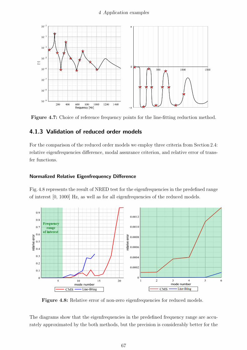
4 Application examples
Figure 4.7: Choice of reference frequency points for the line-fitting reduction method.
4.1.3 Validation of reduced order models
For the comparison of the reduced order models we employ three criteria from Section 2.4:
relative eigenfrequencies difference, modal assurance criterion, and relative error of trans-
fer functions.
Normalized Relative Eigenfrequency Difference
Fig. 4.8 represents the result of NRED test for the eigenfrequencies in the predefined range
of interest [0, 1000] Hz, as well as for all eigenfrequencies of the reduced models.
Figure 4.8: Relative error of non-zero eigenfrequencies for reduced models.
The diagrams show that the eigenfrequencies in the predefined frequency range are accu-
rately approximated by the both methods, but the precision is considerably better for the
67

4 Application examples
line-fitting model. The error of eigenfrequencies outside the interval of interest is more
significant. In the case of line-fitting method, it is explained by the fact that the reference
frequency points are allocated only in the frequency rage of interest. Besides, the dia-
grams show that the number of incorrect values for the line-fitting model is small, which
keeps the order of reduced model close to minimum and eliminates the problems with
an erroneous high-frequency spectrum: ill-conditioned matrices and the need of using a
small integration step.
Modal Assurance Criterion
Fig. 4.9 illustrates the results of MAC test. The diagrams show that MAC values for all
modes in the predefined frequency range are higher than 0.8. This implies a high corre-
lation of deformation forms of the reduced and full models and, as a result, a qualitative
successful approximation.
Figure 4.9: Validation of deformation modes using MAC test.
The quality of reduction can be evaluated more precisely if modes that are active under
operating conditions are known.
Frequency response analysis
The preservation of important dynamic properties in a reduced order model can be exam-
ined using transfer functions of original and reduced models. For multi-input multi-output
systems the error of transfer functions is usually evaluated using Eq. 2.158. The function
ε(ω) can be treated as a total error introduced by a model reduction approach to certain
transfer functions in a certain frequency range.
68

4 Application examples
The transfer functions of interest for the model of bar are specified by the coordinates
shown in Fig. 4.10.
Figure 4.10: Input and output coordinates of transfer functions of interest.
The relative error ε(ω) for the Craig-Bampton and line-fitting reduced order models is
compared in Fig. 4.11.
Figure 4.11: Relative error of frequency response for different reduced models of the bar.
The plot of Fig. 4.11 shows that the line-fitting method approximated the relevant transfer
functions more accurately than the Craig-Bampton approach, especially at the resonance
points. The error of line-fitting model does not exceed 3%. The Craig-Bampton method
provides acceptable results only until 400 Hz. After that the error increases up to 70%.
4.1.4 Simulation
The use of reduced order models in the context of elastic multibody systems implies that
reduction techniques provide a meaningful approximation not only for the elastic part of
69

4 Application examples
equations of motion of Eq. 2.136, but also for the complete set of equations from Eq. 2.140.
In order to verify the complete set of equations of motion, as well as to gain information
about a proper time step of integration and the total time of simulation of reduced order
models, we perform the following simulation test.
The body is subjected to three constant forces as it is shown in Fig. 4.12.
Figure 4.12: External forces applied to the bar.
The value of end-forces is
FCy = FB
y = 5 N,
while the middle-force acts in the opposite direction with a magnitude
FAy = −2FC
y = −10 N.
The resultant force is equal to FAy + FB
y + FCy = 0. The interest is focused on the
displacement of the middle point along the vertical axis Y. The interval of simulation
equals 3 · 10−2 s and covers several periods of bar oscillation. As the body floating frame
is chosen the Buckens coordinate system described in Section 2.1.6. In order to solve the
system of equations, we exploit the implicit Backward-Euler method. The simulation is
performed in Maple.
Fig. 4.13 compares the response of original FE model with the response of models reduced
by the Craig-Bampton and line-fitting methods. The simulation of reduced order models
yields nearly the same results. The accuracy of simulation is high for the both methods,
but the erroneous high-frequency spectrum of Craig-Bampton model significantly de-
creases a suitable step of integration and, consequently, slows down the simulation. The
simulation time of Craig-Bampton model is 3,5 hours, while the simulation of line-fitting
model takes 15 minutes, which is 14 times faster.
70

4 Application examples
Figure 4.13: Simulation results of reduced models.
4.1.5 Comparison of reduced order models
Table 4.2 summarizes the results of analysis of the line-fitting method and compares them
with the corresponding results of the classical Craig-Bampton method based on CMS
approach.
The data show that the method proposed in this thesis constructed the reduced order
model with the lower order, higher accuracy and better condition properties of system
matrices. The cost of coordinate transformation matrix generation is higher as compared
to the Craig-Bampton approach, but it remains acceptable for moderately dimensional
FE models. In addition, the coordinate transformation matrix has to be calculated only
once before the beginning of simulation process.
71

4 Application examples
Table 4.2: Comparison of reduced order models of the bar.
Parameters Craig-Bampton Line-fitting
Order 22 14Highest eigenfrequency, (Hz) 2 · 105 4.5 · 103
Suitable step of integration, (s) 2.5 · 10−7 10−5
Time of simulation, (h) 3.5 0.25Relative error of eigenfrequencies in [0,1000] Hz < 1.4 · 10−3 < 10−4
Correlation of eigenvectors in [0,1000] Hz high very highRelative error of transfer functions in [0,1000] Hz 0.1− 70% 0, 01− 3%
Time of projection matrix generation, (min) 5 10
4.2 Complex model
In this section we reduce a model of bearing cage by the Craig-Bampton method and the
line-fitting method, perform validation tests, and compare the results.
4.2.1 Model description
The model under consideration is shown in Fig. 4.14 and has the following characteristics:
� size: 1.8 Ö 1.8 Ö 2.4 cm,
� mass: 3.3 g,
� Young’s modulus: 2.1·105 MPa,
� number of degrees of freedom: 54000.
Figure 4.14: Flexible cage.
The modal analysis of free system yields the eigenfrequencies illustrated in Table 4.3.
72
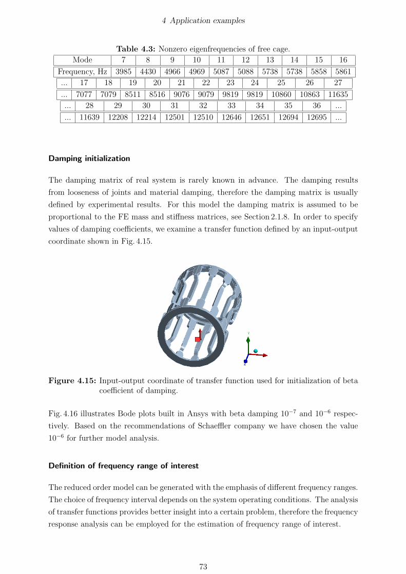
4 Application examples
Table 4.3: Nonzero eigenfrequencies of free cage.
Mode 7 8 9 10 11 12 13 14 15 16
Frequency, Hz 3985 4430 4966 4969 5087 5088 5738 5738 5858 5861
... 17 18 19 20 21 22 23 24 25 26 27
... 7077 7079 8511 8516 9076 9079 9819 9819 10860 10863 11635
... 28 29 30 31 32 33 34 35 36 ...
... 11639 12208 12214 12501 12510 12646 12651 12694 12695 ...
Damping initialization
The damping matrix of real system is rarely known in advance. The damping results
from looseness of joints and material damping, therefore the damping matrix is usually
defined by experimental results. For this model the damping matrix is assumed to be
proportional to the FE mass and stiffness matrices, see Section 2.1.8. In order to specify
values of damping coefficients, we examine a transfer function defined by an input-output
coordinate shown in Fig. 4.15.
Figure 4.15: Input-output coordinate of transfer function used for initialization of betacoefficient of damping.
Fig. 4.16 illustrates Bode plots built in Ansys with beta damping 10−7 and 10−6 respec-
tively. Based on the recommendations of Schaeffler company we have chosen the value
10−6 for further model analysis.
Definition of frequency range of interest
The reduced order model can be generated with the emphasis of different frequency ranges.
The choice of frequency interval depends on the system operating conditions. The analysis
of transfer functions provides better insight into a certain problem, therefore the frequency
response analysis can be employed for the estimation of frequency range of interest.
73

4 Application examples
Figure 4.16: Bode plots for beta coefficients of damping 10−7 and 10−6.
According to the recommendations of Schaeffler’s engineers, we limited the frequency
range of interest by 13000 Hz. There is a gap between the model eigenfrequencies and the
amplitudes of resonance peaks are small. In order to have information about the reduced
model behavior near the boundary of the defined interval, we generate transfer functions
until 15000 Hz.
74

4 Application examples
Figure 4.17: Set of input coordinates of the cage.
Initialization of input and output coordinates
The choice of input and output degrees of freedom is task-dependent. In the case of cage
model, the exact positions of contact forces acting on the body are unknown. However,
the set of possible input coordinates can be defined as it is shown in Fig. 4.17.
In this model we are interested in the response of the same nodes, therefore the set of
output coordinates coincides with the set of input parameters. The goal of model order
reduction is to accurately approximate the dynamic behavior of the defined nodes in the
frequency range of interest.
4.2.2 Initialization of reduction methods
Craig-Bampton method
In order to construct a coordinate transformation matrix of Craig-Bamton method, one
has to define a set of interface nodes and a number of fixed interface dynamic modes.
The choice of interface coordinates is crucial for the quality of the reduced order model.
The choice is model-dependent and requires advanced engineering experience. The com-
mon criteria that specify positions of interface degrees of freedom are discussed in Sec-
tion 2.3.3.
Positions of interface coordinates for the cage model are shown in Fig. 4.18. The number
of interface nodes is 29, which results in 87 interface degrees of freedom.
75

4 Application examples
Figure 4.18: Interface nodes for the Craig-Bampton method.
The quantity of dynamic modes is usually chosen experimentally. We tuned the model
for the given frequency range and determined that 59 dynamic modes result in a very
accurate reduced order model. The size of reduced order model equals 146.
Line-fitting method
The principle of initialization of line-fitting method for the cage model is the same as it is
described in Section 4.1.2 for the elastic bar. We consider the frequency range of interest
and input-output coordinates as a given information for the initialization process. The
next initialization steps include the choice of an appropriate order of reduced model,
definition of interface degrees of freedom, allocation of reference frequency points.
The order of reduced model depends on a number of transfer functions that need to be
tuned and a number of eigenfrequencies contained in a frequency range of interest. As
it is discussed in Section 3.2.2, the order equal to a double number of eigenfrequencies
in the frequency range of interest is usually enough to achieve high accuracy of reduced
model. In case of the cage model, the number of eigenfrequencies in the frequency range
of interest is 30. In order to make the generation of accurate results more difficult for the
line-fitting method, we define the order of reduced model to be 55.
Further, 55 DoFs must be spread throughout the body. The model is stiff in Z direc-
tion (see Fig. 4.14), therefore the interface coordinates are mainly assigned to X and Y
coordinates of the nodes shown in Fig. 4.18.
The main positions of reference frequency points are points of resonances and antireso-
nances of transfer functions specified by the interface DoFs. The total set of frequency
points is the union of sets for the different transfer functions. Usually it is necessary to
allocate reference points for a few transfer functions with highest amplitudes to obtain
accurate approximation of the remaining functions. The frequency rage of the cage is
76

4 Application examples
wide and it includes 30 nonzero eigenfrequencies. For this model we defined 70 reference
frequency points.
4.2.3 Validation of reduced order models
Normalized Relative Eigenfrequency Difference
The frequency interval of interest [0,13000] Hz contains 30 nonzero eigenfrequencies. In
Fig. 4.19 we compare a relative error of eigenfrequencies for the models reduced by the
Craig-Bampton and line-fitting methods.
5 10 15 20 25 30 35 400
1
2
3
4
5
6x 10
−3
eigenfrequency number
NR
ED
[−
]
Craig−Bampton
5 10 15 20 25 30 35 400
1
2
3
4
5
6
7
8x 10
−4
eigenfrequency number
NR
ED
[−
]
Line-fitting
Figure 4.19: Relative error of non-zero eigenfrequencies of reduced models.
The data show that the line-fitting method approximates the model spectrum about ten
times better than the Craig-Bampton procedure. However, the Craig-Bampton model is
still accurate enough, as the relative error of eigenfrequencies does not exceed 0.6 %.
Modal Assurance Criterion
The cage model is symmetric relative to the X and Y axis. This leads to the repetition
of certain eigenfrequencies of the model. In Section 2.4.2 we have pointed out that eigen-
vectors corresponded to repeated eigenfrequencies are not uniquely defined. This makes
the result of MAC test ambiguous and complicated for interpretation, therefore we omit
this test for the model of cage.
Frequency response analysis
In this section we analyze errors of transfer functions specified by different inputs and
outputs. Without loss of generality, we chose three interface nodes shown in Fig. 4.20 in
77

4 Application examples
yellow and a non-interface node marked in green for the analysis of transfer functions. In
scopes of this section the interface and non-interface nodes are referred to as master and
slave nodes, respectively.
Figure 4.20: Positions of interface nodes and a non-interface node.
Further, we consider transfer functions that correspond to master-master, master-slave,
and slave-slave inputs and outputs. Fig. 4.21 presents comparison of Bode plots for the
master-master transfer function. In this case, the input and output are the Y-coordinate
of the node at the middle of the model.
Both methods provide the accurate approximation of transfer function in the given interval
[0,13000] Hz. The increasing error of line-fitting transfer function in the range [13000-
15000] Hz is explained by the absence of reference frequency points in this region. The
Craig-Bampton method captures intervals of antiresonances and the high frequency range
slightly better, but small amplitudes of magnitude in these ranges make the error less
critical. The diagrams demonstrate that the Craig-Bampton method generated the results
comparable with the line-fitting results by the model of three times larger size.
Fig. 4.22 shows the comparison of Bode plots for master input slave output coordinates.
The input coordinate is X degree of freedom at the middle node, while the output is
X coordinate of the slave node. In this case, the responses of reduced models are still
accurate.
78

4 Application examples
0 5000 10000 1500010
−6
10−5
10−4
frequency [Hz]
mag
nitu
de [
m/N
]OriginalCraig−Bampton
Frequency range of interest
13000
0 5000 10000 15000−pi
−pi/2
0
pi/2
pi
frequency [Hz]
phas
e [r
ad]
OriginalCraig−Bampton
13000
0 5000 10000 1500010
−6
10−5
10−4
frequency [Hz]
mag
nitu
de [
m/N
]
OriginalLine-fitting
Frequency range of interest
13000
0 5000 10000 15000−pi
−pi/2
0
pi/2
pi
frequency [Hz]
phas
e [r
ad]
OriginalLine-fitting
13000
Figure 4.21: Comparison of transfer functions for master input master output coordi-nates.
0 5000 10000 1500010
−8
10−7
10−6
10−5
frequency [Hz]
mag
nitu
de [
m/N
]
OriginalCraig−Bampton
13000
0 5000 10000 15000−pi
−pi/2
0
pi/2
pi
frequency [Hz]
phas
e [r
ad]
OriginalCraig−Bampton
13000
0 5000 10000 1500010
−8
10−7
10−6
10−5
frequency [Hz]
mag
nitu
de [
m/N
]
OriginalLine-fitting
13000
0 5000 10000 15000−pi
−pi/2
0
pi/2
pi
frequency [Hz]
phas
e [r
ad]
OriginalLine-fitting
13000
Figure 4.22: Comparison of transfer functions for master input slave output coordinates.
79

4 Application examples
Finally, Fig. 4.23 provides the comparison of results for the slave-slave case, where the
input and output are Y degree of freedom for the slave node. The diagrams show that
the error of slave-slave transfer function is larger as compared with previous tests, but
it remains acceptable because slave DoFs represent unimportant for user coordinates.
Although the line-fitting method tunes only the master-master transfer functions and
reduces the error of master-slave transfer paths, the error of slave-slave transfer function
is turned out to be comparable with the result of Craig-Bampton model.
0 5000 10000 1500010
−7
10−6
10−5
10−4
frequency [Hz]
mag
nitu
de [
m/N
]
OriginalCraig−Bampton
13000
0 5000 10000 15000−pi
−pi/2
0
pi/2
pi
frequency [Hz]
phas
e [r
ad]
OriginalCraig−Bampton
13000
0 5000 10000 1500010
−7
10−6
10−5
10−4
frequency [Hz]
mag
nitu
de [
m/N
]
OriginalLine-fitting
13000
0 5000 10000 15000−pi
−pi/2
0
pi/2
pi
frequency [Hz]
phas
e [r
ad]
OriginalLine-fitting
13000
Figure 4.23: Comparison of transfer functions for slave input slave output coordinates.
Next, we deal with a relative error of transfer functions for all interface nodes shown in
Fig. 4.18. The error is calculated using the formula from Eq. 2.158. Fig. 4.24 compares
the relative error of transfer functions for the both reduced models.
The plot of Fig. 4.24 shows that the low frequency range is accurately approximated by
the both methods. In the interval [3500-6500] Hz the line-fitting model demonstrates
significantly better results than the Craig-Bampton model. In the range [6500-13000]
Hz the errors are comparable and they possess the following peculiarity: the resonance
frequencies are better approximated by the line-fitting method, while the Craig-Bampton
approach captures better amplitudes of antiresonances. Within the frequency range [0-
12000] Hz the error of line-fitting model does not exceed 3%, while the error of Craig-
80

4 Application examples
0 5000 10000 1500010
−4
10−3
10−2
10−1
100
frequency [Hz]
rela
tiv
erro
r [−
]
Line-fittingCraig−Bampton
13000
Figure 4.24: Relative error of transfer functions specified by the interface nodes.
Bampton model reaches 8%.
4.2.4 Simulation
The goal of simulation test described in this section is to validate the equations of motion
of reduced order models in the time domain, as well as to obtain information about the
total time of simulation.
At the initial moment the body is undeformed and it starts to rotate with the angular
velocity ω =[
0, 0, 10]T
. Two longitudinal rods of the cage are connected by a
stretched spring, whose influence can be treated as contact forces. The spring is attached
to the points shown in Fig. 4.25. These points are contained in the sets of interface nodes
for the both reduction techniques. The simulation of original FE model is carried out in
Ansys, while the reduced models are simulated in Maple.
Figure 4.25: Stretched spring attached to the cage.
81

4 Application examples
The interest is focused on the spring elongation. In Ansys the elongation is measured by
a spring probe feature, while in Maple it is calculated using absolute coordinates of the
nodes where the spring is attached. The spring is defined as follows:
� undeformed length: 3.65 mm,
� initial elongation: 0.2 mm,
� stiffness:104 N/m.
The period of simulation is defined to be 10−3s. The system of equations of motion are
solved by the implicit Backward-Euler method. The step of integration is initialized using
a rule of thumb as h = 120·fmax
, where fmax defines the maximal eigenfrequency of reduced
model. This results in the time steps 10−7s and 6 · 10−7s for the Craig-Bampton and
line-fitting models, respectively.
Fig. 4.26 represents the comparison of spring elongation for the both reduced order models.
0 0.2 0.4 0.6 0.8 1
x 10−3
1.75
1.8
1.85
1.9
1.95
2
2.05x 10
−4
time [s]
spri
ng e
long
atio
n [m
]
OriginalCraig−Bampton
0 0.2 0.4 0.6 0.8 1
x 10−3
1.75
1.8
1.85
1.9
1.95
2
2.05x 10
−4
time [s]
spri
ng e
long
atio
n [m
]
OriginalLine−fitting
Figure 4.26: Comparison of spring elongation for the reduced models.
As can be seen, the spring elongation for each reduced order model is in the perfect
agreement with the reference result. This gives reason to assert that equations of motion
are correctly implemented. In addition, the test reveals a significant drawback of the
Craig-Bampton model, namely, the large time of simulation. The problem is caused by
the relative large number of DoFs of the reduced order model and the small time step
of integration. The step is affected by the erroneous high-frequency spectrum of Craig-
Bampton model. These factors considerably slow down the simulation process. The
simulation of Craig-Bampton model takes 8 hours, while for the line-fitting model it is 0.8
hours, which is 10 times faster. The simulation time of the both models can be reduced
by using Matlab, C++ programs, and in some cases by explicit integration schemes.
82

4 Application examples
4.2.5 Comparison of reduced order models
Table 4.4 summarizes the results of analysis of the line-fitting reduction method and com-
pares them with the corresponding results of the classical Craig-Bampton approach.
Table 4.4: Comparison of reduced order models of the cage.
Criteria\Methods Craig-Bampton Line-fitting
Order 140 55Highest eigenfrequency, (Hz) 4·105 8 · 104
Suitable step of integration, (s) 1 · 10−7 6 · 10−7
Time of simulation, (h) 8 0.8Relative error of eigenfrequencies < 6 · 10−3 < 8 · 10−4
Relative error of transfer functions < 8% < 4%Time of projection matrix generation, (h) direct import from FE software 1
The data show that the line-fitting method generated the reduced order model having
the lower order, higher accuracy of eigenfrequencies and important transfer functions,
and better condition properties of system matrices. The advantage of Craig-Bampton
approach lies in the smaller time of coordinate transformation matrix generation. In
addition, there is a possibility to import the Craig-Bampton transformation matrix from
existing FE software, while the generation of line-fitting matrix requires using of additional
preprocessor module.
83
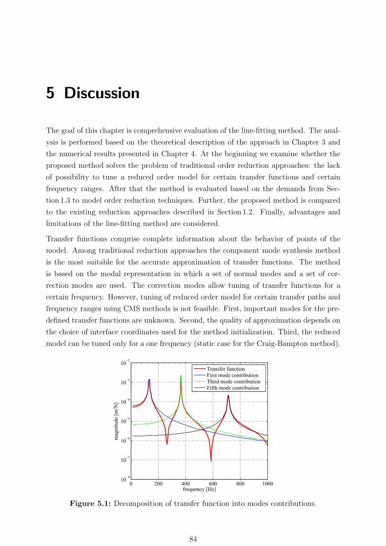
5 Discussion
The goal of this chapter is comprehensive evaluation of the line-fitting method. The anal-
ysis is performed based on the theoretical description of the approach in Chapter 3 and
the numerical results presented in Chapter 4. At the beginning we examine whether the
proposed method solves the problem of traditional order reduction approaches: the lack
of possibility to tune a reduced order model for certain transfer functions and certain
frequency ranges. After that the method is evaluated based on the demands from Sec-
tion 1.3 to model order reduction techniques. Further, the proposed method is compared
to the existing reduction approaches described in Section 1.2. Finally, advantages and
limitations of the line-fitting method are considered.
Transfer functions comprise complete information about the behavior of points of the
model. Among traditional reduction approaches the component mode synthesis method
is the most suitable for the accurate approximation of transfer functions. The method
is based on the modal representation in which a set of normal modes and a set of cor-
rection modes are used. The correction modes allow tuning of transfer functions for a
certain frequency. However, tuning of reduced order model for certain transfer paths and
frequency ranges using CMS methods is not feasible. First, important modes for the pre-
defined transfer functions are unknown. Second, the quality of approximation depends on
the choice of interface coordinates used for the method initialization. Third, the reduced
model can be tuned only for a one frequency (static case for the Craig-Bampton method).
0 200 400 600 800 100010
−8
10−7
10−6
10−5
10−4
10−3
10−2
frequency [Hz]
mag
nitu
de [
m/N
]
Transfer functionFirst mode contributionThird mode contributionFifth mode contribution
Figure 5.1: Decomposition of transfer function into modes contributions.
84

5 Discussion
The contributions of several modes to a transfer function are shown in Fig. 5.1. The
combination of modes leads to the results illustrated in Fig. 5.2.
0 200 400 600 800 100010
−8
10−6
10−4
10−2
frequency [Hz]
mag
nitu
de [
m/N
]
Transfer functionTwo modes contribution
0 200 400 600 800 100010
−8
10−6
10−4
10−2
frequency [Hz]
mag
nitu
de [
m/N
]
Transfer functionThree modes contribution
Figure 5.2: Combined contribution of several modes to a transfer function.
The modal reduction requires using of all modes to obtain exact values of transfer functions
in a limited frequency range. However, the exact values of transfer functions in the limited
frequency range can be obtained using much smaller number of coordinates. This idea
is used in the line-fitting method. In the proposed approach all DoFs of reduced order
model contribute to the improvement of predefined transfer functions in the frequency
interval of interest.
The next idea that stands behind the line-fitting method is connected with the approxima-
tion of predefined transfer functions by minimizing an error of adjacent transfer functions.
In Fig. 5.3 positions of important transfer functions are shown in red, while outputs of
adjacent transfer functions are contained in a blue hemisphere with a small radius. The
curves of adjacent and important functions are almost identical. Since the line fitting
method expresses transfer functions with non-interface outputs through the important
transfer functions, the adjacent transfer functions are accurately approximated. This
forces important transfer functions to be precise as well. The assertion is confirmed by
the results of several numeric examples in Chapter 4. It follows that the line-fitting
method solves the problem of classical reduction approaches.
Figure 5.3: Approximation of important transfer functions using adjacent transfer func-tions.
Further we dwell on the compliance of the line-fitting method with the requirements to
85

5 Discussion
model order reduction techniques. The requirements are formulated in Section 1.3 and
repeated in this section for the discussion:
� accuracy of reduced model,
� computational efficiency of reduction method,
� preservation of model stability,
� estimation of error introduced by the reduction process,
� possibility to automate the reduction process,
� fast simulation of reduced model.
In addition, using of model order reduction methods in the context of EMBS imposes on
them additional restrictions:
� preservation of second order structure of equations of motion,
� coordinate transformation matrix excludes rigid body modes.
The accuracy of line-fitting method is ensured by its ability of tuning important for the
user transfer functions. Local accuracy of transfer functions can be improved by additional
reference frequency points, whereas the quality over a whole frequency range of interest
is enhanced by increasing an order of reduced model.
The main computational burdens of the proposed reduction approach consist in the calcu-
lation of transfer function matrices for several frequency points and the solution of large
least-squares problem. The most of reduction approaches require performing of frequency
response analysis to evaluate accuracy of reduced order model in the frequency domain.
This analysis needs calculating of transfer function matrices for all points in a discrete
frequency range of interest, therefore the calculation of transfer matrices at several points
for the line-fitting method is considered as an uncritical issue. The total computational
cost of the line-fitting method is larger in comparison with the Craig-Bampton approach,
but it remains acceptable for moderately dimensional FE models.
The preservation of stability is an important property of reduction approaches because
it ensures that a reduced model does not cause any type of failure to elastic multibody
systems. It was proven in Section 3.4 that the line-fitting technique meets this essential
requirement.
Along with the classical reduction approaches and the methods based on Krylov subspaces,
the line-fitting reduction method lacks of possibility to specify in advance a permissible
error introduced by the reduction process. In this case, generation of admissible reduced
order model becomes an iterative process where each iteration corrects the quality of
reduced order model.
The current version of the line-fitting reduction method requires user’s involvement in
some steps of the method initialization: the choice of reference frequency points and
86

5 Discussion
distribution of redundant interface coordinates. These steps of the method can be auto-
mated. The complete automation of line-fitting reduction approach is possible, but it is
easier to realize, if a reduction error estimator is available.
Simulation speed in addition to other factors depends on a number of coordinates of
reduced order model and system stiffness. According to the results presented in Chapter
4, the time of simulation of line-fitting models is 10-14 times smaller in comparison with
the Craig-Bampton models under the same conditions. This is achieved due to much
smaller number of DoFs and smaller stiffness of line-fitting models. All coordinates of
line-fitting models are involved in improving the accuracy of reduction, which allows
using of smaller number of DoFs as against the number of coordinates of Craig-Brampton
models. The stiffness is determined by the highest eigenfrequency of the system. The
line-fitting method can influence accuracy of eigenfrequencies contained in the predefined
frequency range, but the spectrum of model beyond this range is uncontrolled. For this
reason, no statements about the limits of the spectrum can be made. However, the both
numeric examples show that the stiffness of line-fitting models remains considerably lower
than the stiffness of Craig-Bampton models.
The systems reduced by the line-fitting method preserve the second order structure of
equations of motion. This enables integration of reduced order models into a multibody
system of second order type.
Since a projection matrix of line-fitting method is calculated based on transfer functions
without a component of rigid body motion, the rigid body modes can not be captured by
this matrix. This property allows the line-fitting method to satisfy the last requirement
in the list above.
The advantages of line-fitting approach in comparison with the classical methods are high
accuracy, low order, and small stiffness of reduced systems. In addition, the proposed
method makes it possible to emphasize certain transfer functions and certain frequency
ranges. The new approach produced significantly more accurate results for systems with
slight damping than the Craig-Bampton method.
The modern reduction methods based on Krylov subspaces are to some extent comparable
to what this thesis proposes and might even outperform it. However, for the Krylov
subspace method stability of reduced model is not guaranteed even if the full order model is
stable. In addition, transfer functions for non-interface DoFs are uncontrolled, which can
lead to artificial and undesired effects in the motion of non-interface nodes of the model.
In contrast, the line-fitting methods ensures that the error of transfer functions having
non-interface outputs is limited. As concerns the modern Balanced truncation method,
high computational burdens make the reduction feasible only for small dimensional FE
models.
Along with a number of advantages, the line-fitting method has several limitations as com-
pared to classical and modern reduction techniques. The main drawback of the method
87

5 Discussion
is computational cost of projection matrix generation. Besides, the modern methods can
excel the line-fitting method in tuning of reduced order models for antiresonance frequen-
cies. Formulation of weighted least squares problem can help to address this issue for the
proposed reduction approach.
The common problem of reduction techniques is processing of a large number of interface
coordinates. Since the set of DoFs of line-fitting model includes interface DoFs, the size
of reduced order model can be redundant. This can result in producing stiff reduced order
systems. One of the solutions of the problem is the interface reduction where the motion
of interface surface is approximated by the motion of several nodes. Another approach is
to omit unnecessary interface DoFs, but this requires much experience and insight into a
specific problem.
88

6 Summary and further work
The main scientific contribution of the thesis is a new linear model order reduction method
for elastic multibody simulation. The set of classical reduction approaches consists of
modal truncation, condensation, and component mode synthesis techniques. The cate-
gory of modern reduction methods includes the techniques based on the singular value
decomposition using Gramian matrices and moment matching via Krylov subspaces. The
proposed method allows solving of problem of classical reduction approaches: the lack
of possibility to tune a reduced order model for certain transfer functions and frequency
ranges. In addition, the new method satisfies the following requirements: high accuracy
of reduced order models, preservation of stability, fast simulation of reduced order models,
and the possibility of using the method in the context of elastic multibody systems. The
new method differs from the modern reduction approaches and it has its own advantages.
The research topic belongs to the area of computational dynamics and relates to such
disciplines as multibody dynamics, finite element analysis, and model order reduction.
Chapter 2 of this work covers fundamentals of elastic multibody system simulation. The
fundamentals include the modeling of multibody dynamics using a floating frame ap-
proach, finite element discretization, model order reduction approaches, validation of
reduced order models, and schemes of numerical solution of equations of motion. Chap-
ter 3 is devoted to the novel reduction technique proposed by the author of the thesis:
line-fitting reduction technique. In Chapter 4 we apply the new method to the bar and
the bearing cage models, perform validation tests of the reduced order models in the time
and frequency domains, and compare the results with results of classical Craig-Bampton
approach. Chapter 5 includes comprehensive evaluation of the line-fitting method and its
comparison with the classical and modern reduction procedures.
The advantages of line-fitting approach in comparison with the classical methods are
higher accuracy, lower order, and usually smaller stiffness of reduced systems. Low or-
der and small stiffness lead to considerable gains in computational speed for practical
EMBS. In addition, the proposed method makes it possible to emphasize certain transfer
functions and certain frequency ranges. It is also necessary to point out that line-fitting
approach produces significantly more accurate results for systems with slight damping
than the Craig-Bampton method. The main drawback of the method is computational
cost of projection matrix generation. However, the computational burdens remain small
for moderately dimensional systems.
89

6 Summary and further work
The line-fitting method can be used as an alternative to modern Krylov subspace based
methods, if the preservation of stability of reduced model is important or it is necessary to
limit an error of non-interface nodes. In addition, the proposed approach is an appropriate
choice for the systems where the application of modern Balanced truncation method is
not feasible due to high computational costs.
The reduction method proposed in this work is developed in scopes of a project “Elastic
bodies in Caba3D” of the Otto von Guericke University and the Schaeffler Technologies
AG & Co. KG. The primary goal of the project was to develop software that can take
into account deformation effects arisen in mechanical systems under operating conditions.
The line-fitting reduction technique is implemented in the commercial simulation software
Caba3D as an alternative to other reduction approaches. Within the project the author
of the thesis et al. published several international articles devoted to the topic of model
order reduction:[53, 54, 52].
Looking ahead, there are a number of points that can improve the current version of
line-fitting reduction. The first issue is the enhancement of computational efficiency. The
solution of this task needs additional investigation. The second aspect relates to the
improvement of accuracy. The unanswered questions remain how to chose an optimal
number of coordinates for a reduced order model and where to allocate interface coordi-
nates to obtain the most accurate approximation. Another issue concerning the accuracy
is better approximation of transfer function in regions with small magnitudes. Next,
the user’s involvement in the initialization of method can be decreased by automating
the choice of reference frequency points and the allocation of interface coordinates. The
range of application of the method can be extended by adopting the line-fitting approach
for models with six degrees of freedom per node. Besides, the correct work of the method
for different types of constraints imposed on the model needs to be confirmed.
90

Appendix
Rotation matrix using Euler parameters
Let’s denote a unit vector of axis of rotation as v and an angle of finite rotation as α, see
Fig. A.1.
α
x
y
z
v
x1
y1z1
Figure A.1: Finite rotation.
A set of Euler parameters is defined asθ0 = cosα2, θ1 = v1 · sinα2 ,
θ2 = v2 · sinα2 , θ3 = v3 · sinα2. (A.1)
From the definition follows that3∑
k=0
(θk)2 = 1.
According to [79], the body rotation matrix A can be expressed in terms of Euler param-
eters as
A(θ) =
1− 2(θ2)2 − 2(θ3)
2 2(θ1θ2 − θ0θ3) 2(θ1θ3 + θ0θ2)
2(θ1θ2 + θ0θ3) 1− 2(θ1)2 − 2(θ3)
2 2(θ2θ3 − θ0θ1)2(θ1θ3 − θ0θ2) 2(θ2θ3 + θ0θ1) 1− 2(θ1)
2 − 2(θ2)2
. (A.2)
The angular velocity vector ω in the global frame and the vector of time derivatives of
Euler parameters are related as
ω = 2 ·Θ(θ) · θ (A.3)
91

where Θ ∈ R3×4 is given by
Θ(θ) =
−θ1 θ0 −θ3 θ2
−θ2 θ3 θ0 −θ1−θ3 −θ2 θ1 θ0
, (A.4)
see, e.g. [79].
92

Bibliography
[1] O. P. Agrawal and A. A. Shabana. Dynamic analysis of multibody systems using
component modes. Computers & Structures, 21(6):1303–1312, 1985.
[2] O. P. Agrawal and A. A. Shabana. Application of deformable-body mean axis to
flexible multibody system dynamics. Computer Methods in Applied Mechanics and
Engineering, 56(2):217–245, 1986.
[3] J. Ambrosio. Dynamics of structures undergoing gross motion and nonlinear defor-
mations: A multibody approach. Computers & Structures, 59(6):1001–1012, 1996.
[4] J. Ambrosio. Efficient kinematic joint descriptions for flexible multibody systems
experiencing linear and non-linear deformations. International Journal for Numerical
Methods in Engineering, 56(12):1771–1793, 2003.
[5] A. Antoulas and D. Sorensen. Approximation of large-scale dynamical systems:
an overview. International Journal of Applied Mathematics and Computer Science,
11(5):1093–1121, 2001.
[6] A. C. Antoulas. Approximation of Large-Scale Dynamical Systems. Society for In-
dustrial and Applied Mathematics, 2005.
[7] K. Atkinson and W. Han. Finite difference method. In W. Han and K. Atkinson,
editors, Theoretical Numerical Analysis, volume 39 of Texts in Applied Mathematics,
pages 253–275. Springer New York, New York, NY, 2009.
[8] Z. Bai and Y. Su. Dimension reduction of large-scale second-order dynamical sys-
tems via a second-order arnoldi method. SIAM Journal on Scientific Computing,
26(5):1692–1709, 2005.
[9] M. Bampton and R. Craig. Coupling of substructures for dynamic analyses. AIAA
Journal, 6(7):1313–1319, 1968.
[10] A. Banerjee and J. M. Dickens. Dynamics of an arbitrary flexible body in large
rotation and translation. Journal of Guidance, Control, and Dynamics, 13(2):221–
227, 1990.
[11] K.-J. Bathe. Finite element procedures. Prentice Hall, Englewood Cliffs, N.J, 1996.
[12] J. W. Baumgarte. A new method of stabilization for holonomic constraints. Journal
of Applied Mechanics, 50(4a):869, 1983.
93

[13] G. Beer, I. Smith, and C. Duenser. The boundary element method with programming:
For engineers and scientists. Springer, Wien and New York, 2008.
[14] P. Benner, P. Kurschner, and J. Saak. An improved numerical method for balanced
truncation for symmetric second-order systems. Mathematical and Computer Mod-
elling of Dynamical Systems, 19(6):593–615, 2013.
[15] P. Benner and J. Saak. Efficient balancing-based mor for large-scale second-order
systems. Mathematical and Computer Modelling of Dynamical Systems, 17(2):123–
143, 2011.
[16] B. Besselink, U. Tabak, A. Lutowska, van de Wouw, N., H. Nijmeijer, D. J. Rixen,
M. E. Hochstenbach, and W.H.A. Schilders. A comparison of model reduction tech-
niques from structural dynamics, numerical mathematics and systems and control.
Journal of Sound and Vibration, 332(19):4403–4422, 2013.
[17] J. R. Canavin and P. W. Likins. Floating reference frames for flexible spacecraft.
Journal of Spacecraft and Rockets, 14(12):724–732, 1977.
[18] T. K. Caughey. Classical normal modes in damped linear dynamic systems. Journal
of Applied Mechanics, 27(2):269, 1960.
[19] K. Changizi and A. A. Shabana. A recursive formulation for the dynamic analysis of
open loop deformable multibody systems. Journal of Applied Mechanics, 55(3):687,
1988.
[20] J. Chaskalovic. Finite element methods for engineering sciences. Springer, New York
and London, 2008.
[21] R. Craig. Structural dynamics: An introduction to computer methods. Wiley, New
York, 1981.
[22] R. Craig. Coupling of substructures for dynamic analyses - an overview. In 41st
Structures, Structural Dynamics, and Materials Conference and Exhibit, April 2000.
[23] R. Craig and A. Kurdila. Fundamentals of structural dynamics. John Wiley, Hoboken,
N.J., 2nd ed. edition, 2006.
[24] W. D’Ambrogio and A. Fregolent. Robust dynamic model updating using point
antiresonances.
[25] Dassault Systemes SolidWorks Corp. Understanding of nonlinear analysis.
http://files.solidworks.com/whitepapers/2010/nonlinear analysis 2010 eng final.pdf.
[26] S. Dietz. Vibration and fatigue analysis of vehicle systems using component
modes: Techn. Univ., Diss–Berlin, volume 401 of Fortschritt-Berichte VDI Reihe
12, Verkehrstechnik/Fahrzeugtechnik. VDI-Verl, Dusseldorf, als ms. gedr edition,
1999.
[27] E. Eich-Soellner and C. Fuhrer. Numerical methods in multibody dynamics. European
Consortium for Mathematics in Industry. Stuttgart, 1998.
94

[28] J. Fehr and P. Eberhard. Simulation process of flexible multibody systems with non-
modal model order reduction techniques. Multibody System Dynamics, 25(3):313–334,
2011.
[29] M. Fischer and P. Eberhard. Linear model reduction of large scale industrial models
in elastic multibody dynamics. Multibody System Dynamics, 31(1):27–46, 2014.
[30] R. W. Freund. Model reduction methods based on krylov subspaces. Acta Numerica,
12:267–319, 2003.
[31] O. Friberg. A method for selecting deformation modes in flexible multibody dynam-
ics. International Journal for Numerical Methods in Engineering, 32(8):1637–1655,
1991.
[32] W. Gawronski. Dynamics and control of structures: A modal approach. Mechanical
engineering series. Springer, New York, 1998.
[33] C. W. Gear. Differential-algebraic equation index transformations. SIAM Journal
on Scientific and Statistical Computing, 9(1):39–47, 1988.
[34] M. Geradin and A. Cardona. Flexible multibody dynamics: A finite element approach.
John Wiley, New York, 2001.
[35] M. Geradin and D. Rixen. Mechanical vibrations: Theory and application to struc-
tural dynamics. John Wiley, Chichester and New York, 2nd ed. edition, 1997.
[36] E. J. Grimme. Krylov Projection Methods For Model Reduction. PhD thesis, Uni-
versity of Illinois at Urbana-Champaign, Urbana-Champaign, 1997.
[37] R. J. Guyan. Reduction of stiffness and mass matrices. AIAA Journal, 3(2):380,
1965.
[38] E. Hairer and G. Wanner. Solving Ordinary Differential Equations II: Stiff and
Differential-Algebraic Problems. Springer Berlin Heidelberg, second revised edition
edition, 1996.
[39] Heirman, G. H. K. and W. Desmet. Interface reduction of flexible bodies for efficient
modeling of body flexibility in multibody dynamics. Multibody System Dynamics,
24(2):219–234, 2010.
[40] W. C. Hurty. Dynamic analysis of structural systems using component modes. AIAA
Journal, 3(4):678–685, 1965.
[41] T. Kane, R. Ryan, and A. Banerjee. Dynamics of a cantilever beam attached to a
moving base. Journal of Guidance, Control, and Dynamics, 10(2):139–151, 1987.
[42] K. Kim. A review of mass matrices for eigenproblems. Computers & Structures,
46(6):1041–1048, 1993.
[43] P. Koutsovasilis. Model order reduction in structural mechanics: Coupling the rigid
and elastic multi body dynamics, volume Nr. 712 of Fortschrittberichte VDI / 12.
VDI-Verl., Dusseldorf, als ms. gedr edition, 2009.
95

[44] P. Koutsovasilis and M. Beitelschmidt. Comparison of model reduction techniques
for large mechanical systems. Multibody System Dynamics, 20(2):111–128, 2008.
[45] A. Kurdila, J. G. Papastavridis, and M. P. Kamat. Role of maggi’s equations in
computational methods for constrained multibody systems. Journal of Guidance,
Control, and Dynamics, 13(1):113–120, 1990.
[46] H. Lai and B. Dopker. Influence of lumped rotary inertia in flexible multibody
dynamics. Mech. Struct. Mach., 18:47–59, 1990.
[47] M. Lehner. Modellreduktion in elastischen Mehrkorpersystemen, volume Bd. 2007,10
of Schriften aus dem Institut fur Technische und Numerische Mechanik der Univer-
sitat Stuttgart. Shaker, Aachen, 2007.
[48] M. Lehner and P. Eberhard. On the use of moment-matching to build reduced order
models in flexible multibody dynamics. Multibody System Dynamics, 16(2):191–211,
2006.
[49] A. Leung. An accurate method of dynamic condensation in structural analysis. In-
ternational Journal for Numerical Methods in Engineering, 12(11):1705–1715, 1978.
[50] B. Lohmann and B. Salimbahrami. Ordnungsreduktion mittels krylov-
unterraummethoden. Automatisierungstechnik 52, pages 30–38, 2004.
[51] A. Love. A treatise on the mathematical theory of elasticity. Cambridge University
Press, Cambridge, 4th ed edition, 2013.
[52] V. Makhavikou and R. Kasper. Choice of a modal reduction method in the context of
modular simulation of flexible multibody dynamics. Selected Works of international
conference on mechanics VI Polyahov’s Readings, pages 27–33, 2012.
[53] V. Makhaviou, R. Kasper, and D. Vlasenko. Method of model reduction for elastic
multibody systems. Proceedings of 11th World Congress on Computational Mechanics
(WCCM XI), 5th European Conference on Computational Mechanics (ECCM V),
July 20-25, pages 475–486, 2014.
[54] V. Makhaviou, D. Vlasenko, and R. Kasper. Alternative method of model reduction
for flexible multibody systems. Effizienz, Praezision, Qualitaet: 11. Magdeburger
Maschinenbau-Tage, page 10, 2013.
[55] D. Mangler. Die Berechnung geometrisch nichtlinearer Probleme der Dynamik
unter Nutzung linearer FEM-Programme. PhD thesis, Otto-von-Guericke Univer-
sity, Magdeburg, 1994.
[56] F. Melzer. Symbolic computations in flexible multibody systems. Nonlinear Dynam-
ics, 9(1-2):147–163, 1996.
[57] D. G. Meyer and S. Srinivasan. Balancing and model reduction for second-order form
linear systems. IEEE Transactions on Automatic Control, 41(11):1632–1644, 1996.
96

[58] B. Moore. Principal component analysis in linear systems: Controllability, observ-
ability, and model reduction. IEEE Transactions on Automatic Control, 26(1):17–32,
1981.
[59] P. C. Muller. Stabilitat und Matrizen: Matrizenverfahren in der Stabilitatstheorie
linearer dynamischer Systeme. Springer-Verlag, Berlin and New York, 1977.
[60] P. Nikravesh. Understanding mean-axis conditions as floating reference frames.
In J. Ambrosio, editor, Advances in Computational Multibody Systems, volume 2
of Computational Methods in Applied Sciences, pages 185–203. Springer-Verlag,
Berlin/Heidelberg, 2005.
[61] P. Nikravesh and J. Ambrosio. Systematic construction of equations of motion for
rigid-flexible multibody systems containing open and closed kinematic loops. Inter-
national Journal for Numerical Methods in Engineering, 32(8):1749–1766, 1991.
[62] P. Nikravesh and Y.-S. Lin. Use of principal axes as the floating reference frame for
a moving deformable body. Multibody System Dynamics, 13(2):211–231, 2005.
[63] N.N. Ansysr academic research, release 14.5, help system, mechanical user guide,
ansys, inc.
[64] C. Nowakowski, J. Fehr, and P. Eberhard. Einfluss von Schnittstellenmodellierun-
gen bei der Reduktion elastischer Mehrkorpersysteme. Automatisierungstechnik,
59(8):512–519, 2011.
[65] C. Nowakowski, J. Fehr, M. Fischer, and P. Eberhard, editors. Model Order Reduction
in Elastic Multibody Systems using the Floating Frame of Reference Formulation,
2012.
[66] C. Nowakowski, P. Kurschner, P. Eberhard, and P. Benner. Model reduction of
an elastic crankshaft for elastic multibody simulations. ZAMM - Journal of Applied
Mathematics and Mechanics / Zeitschrift fur Angewandte Mathematik und Mechanik,
93(4):198–216, 2013.
[67] W. Pan and E. Haug. Flexible multibody dynamic simulation using optimal lumped
inertia matrices. Comput. Methods Appl. Mech., 173:189–200, 1999.
[68] M. S. Pereira and P. Nikravesh. Impact dynamics of multibody systems with fric-
tional contact using joint coordinates and canonical equations of motion. Nonlinear
Dynamics, 9(1-2):53–71, 1996.
[69] J. Pfister. Elastic multibody systems with frictional contacts. Schriften aus dem
Institut fur Technische und Numerische Mechanik der Universitat Stuttgart. Shaker,
Aachen, 2006.
[70] Z.-Q. Qu. Model Order Reduction Techniques: With Applications in Finite Element
Analysis. Springer London, London, 2004.
97

[71] J. Ryu, Sang-S. Kim, and Sung-S. Kim. A general approach to stress stiffening effects
on flexible multibody dynamic systems. Mechanics of Structures and Machines,
22(2):157–180, 1994.
[72] Y. Saad. Iterative methods for sparse linear systems. SIAM, Philadelphia, 2nd ed
edition, 2003.
[73] B. Salimbahrami and B. Lohmann. Order reduction of large scale second-order sys-
tems using krylov subspace methods. Linear Algebra and its Applications, 415(2-
3):385–405, 2006.
[74] W. Schilders, Vorst, H. A. van der, and J. Rommes. Model order reduction: The-
ory, research aspects and applications, volume 13 of Mathematics in industry The
European Consortium for Mathematics in Industry. Springer, Berlin, 2008.
[75] R. von Schwerin. Multibody system simulation: Numerical methods, algorithms,
and software, volume 7 of Lecture notes in computational science and engineering.
Springer-Verlag, Berlin and New York, 1999.
[76] R. Schwertassek and O. Wallrapp. Dynamik flexibler Mehrkoerpersysteme: Metho-
den der Mechanik zum rechnergestutzten Entwurf und zur Analyse mechatronischer
Systeme. Grundlagen und Fortschritte der Ingenieurwissenschaften. Vieweg, Braun-
schweig [u.a.], 1999.
[77] R. Schwertassek, O. Wallrapp, and A. A. Shabana. Flexible multibody simulation
and choice of shape functions. Nonlinear Dynamics, 20(4):361–380, 1999.
[78] A. A. Shabana. Flexible multibody dynamics: Review of past and recent develop-
ments. Multibody System Dynamics, 1(2):189–222, 1997.
[79] A. A. Shabana. Dynamics of multibody systems. Cambridge University Press, Cam-
bridge and New York, 3rd ed edition, 2005.
[80] A. A. Shabana and R. A. Wehage. A coordinate reduction technique for dynamic
analysis of spatial substructures with large angular rotations. Journal of Structural
Mechanics, 11(3):401–431, 1983.
[81] K. Sherif, H. Irschik, and W. Witteveen. Transformation of arbitrary elastic mode
shapes into pseudo-free-surface and rigid body modes for multibody dynamic systems.
Journal of Computational and Nonlinear Dynamics, 7(2):021008, 2012.
[82] P. Sokol. Kinematik und Dynamik von Mehrkorperschleifen mit elastischen Korpern.
PhD thesis, Universitat-Gesamthochschule-Duisburg, 1990.
[83] D. Sorensen and A. Antoulas. Gramians of structured systems and an error bound
for structure-preserving model reduction, 2004.
[84] K. Sorge. Mehrkorpersysteme mit starr-elastischen Subsystemen, volume Nr. 184 of
Fortschrittberichte VDI : Reihe 11, Schwingungstechnik. VDI-Verl, Dusseldorf, als
ms. gedr edition, 1993.
98

[85] The Schaeffler Technologies AG and Co. KG. http://www.schaeffler.de/ con-
tent.schaeffler.de/ en/ branches/ industry/ motorcycles specvehicles/ product/ chas-
sis system/ rear swinging fork/ rear swinging fork.jsp.
[86] F. E. Udwadia and R. E. Kalaba. Explicit equations of motion for mechanical systems
with nonideal constraints. Journal of Applied Mechanics, 68(3):462, 2001.
[87] Veubeke, B. F. de. The dynamics of flexible bodies. International Journal of Engi-
neering Science, 14(10):895–913, 1976.
[88] O. Wallrapp. Standardization of flexible body modeling in multibody system codes,
part i: Definition of standard input data*. Mechanics of Structures and Machines,
22(3):283–304, 1994.
[89] T. M. Wasfy and A. K. Noor. Computational strategies for flexible multibody sys-
tems. Applied Mechanics Reviews, 56(6):553, 2003.
[90] R. A. Wehage and E. J. Haug. Generalized coordinate partitioning for dimension
reduction in analysis of constrained dynamic systems. Journal of Mechanical Design,
104(1):247, 1982.
[91] W. Yoo and E. Haug. Dynamics of articulated structures. part i. theory. Journal of
Structural Mechanics, 14(1):105–126, 1986.
[92] Z.-H. Zhong and J. Mackerle. Contact-impact problems: A review with bibliography.
Applied Mechanics Reviews, 47(2):55, 1994.
99


