Embed Size (px)
Citation preview
Analysis and Optimiza-tion of Medium Voltage-Line Voltage Regulators
Pankaj Raghav Partha Sarathy
MasterofScienceThesis

Analysis and Optimization of MediumVoltage-Line Voltage Regulators
by
Pankaj Raghav Partha Sarathy
in partial fulfillment of the requirements for the degrees ofMSc in Electrical Engineering at Delft University of Technology
&MSc-Technology in Wind Energy at Norwegian University of Science and Technology,
under the European Wind Energy Masters programme (EWEM).To be defended publicly on Friday August 31, 2018 at 02:00 PM.
Student number: 4597524Thesis committee: Dr. ir. Pavol Bauer, TU Delft, supervisor
Dr. Kjell Sand, NTNU Trondheim, supervisorDr. ir. L.M. Ramirez Elizondo, TU Delft
Company supervisors: Frank Cornelius, ABB, GermanyTobias Asshauer, ABB, Germany

Abstract
In recent years, distribution networks have been facing voltage quality issues due to the influx of renewableenergy. Rural areas which are ideal for renewable energy development due to large vacant areas are faced withgrid voltage variations due to long distribution lines. Because of the stringent conditions laid by the Distribu-tion System Operators (DSOs) on voltage variations, voltage regulation is becoming increasingly importantin the distribution grid. A complete grid reinforcement by replacing the conductors can be very expensivefor the DSOs. Active solutions such as shunt and series compensation provides an economical solution toaddress the voltage regulation issues in the distribution grids.
The initial part of this work focuses on quantitatively studying the impact of series and shunt compen-sation on increasing the grid capacity of a Medium Voltage(MV) line compared to a grid reinforcement withconductor upgradation. The analysis was done on a 20 kV, 10 MVA radial line with 5 loads distributed equallyalong the line, and a generator at the end of the line. An algorithm was developed in MATLAB/ Simulink todetermine the allowable grid capacity to stay within the thermal and voltage limits for different voltage reg-ulation strategies. The study indicates that the series voltage regulation with Line Voltage Regulators(LVR) isan effective solution in increasing the grid capacity by actively regulating the voltage in the grid. The MV-LVR product offered by ABB consists of dry-type transformers and mechanical contactors for changing thetap position. However, dry-type transformers are bigger in size and more expensive than oil-type transform-ers. To reduce the cost and the size of the MV-LVR, the study is focused on the feasibility of a MV-LVR withoil-type transformers and On-Load Tap-Changers (OLTCs). The second part of the project work focuses ondeveloping an economical LVR configuration with an oil-type transformer and a mechanical OLTC. ECOTAPVPD III 100 from Maschinenfabrik Reinhausen (MR) was selected as the mechanical OLTC to perform the tapchanging operation in the LVR. ECOTAP OLTC enables low maintenance of transformers due to the use ofvacuum switches for quenching the arc during tap-changes. 7 LVR configurations with single and two activeparts are investigated. All the configurations are finally compared for their cost and range of operation. Thefinal part of the work focuses on a feasibility study of a power electronics based OLTC for LVR applications asmechanical OLTCs require regular maintenance. Anti-parallel thyristors are used as the solid-state switchesfor the LVR application due to its low cost and losses. Commutation instants are defined for the completepower factor range for the thyristor based OLTC to have no/controlled short circuit during tap-changes.
The two active parts LVR configuration constructed with a center tapped feeder transformer and a boostertransformer with the ECOTAP VPD III 100 OLTC is economical for a 20 kV, 10 MVA feeder line. A LVR ratedat 20 kV, 10 MVA with ±6% voltage regulation using the selected configuration was simulated in MATLAB/Simulink. A 400 V, 5 kVA low voltage setup was built with the ECOTAP VPD III 100 OLTC, and the LVR con-figuration was verified with experimental results. The feeder transformer model with two taps was simulatedin MATLAB/Simulink for switching up and switching down operation with a thyristor based OLTC for capac-itive, inductive and resistive power factors. The complete LVR system with thyristor based OLTC placed in aMV distribution line was simulated to verify the control algorithm used for the commutation. The thyristorbased OLTC successfully performs tap-changes for a LVR system with a low voltage stress on the thyristor, andlow short circuit currents between the taps for certain power factor angles during the commutation process.
iii


Acknowledgements
I would like to express my sincere gratitude to my professors Pavol Bauer from TU Delft and Kjell Sand fromNTNU Trondheim for giving me the opportunity to work under their supervision. I am deeply grateful toTobias Asshauer and Frank Cornelius from ABB Brilon for allowing me to be a part of this project at the com-pany and keeping the doors open whenever I ran into trouble during my research. I would like to sincerelythank Gautham Ram from TU Delft for his valuable inputs and motivation which gave me a lot of confidencein moments of doubt. I would like to thank professor Pavol Bauer again for his valuable advice which mademe stay on track in moments of uncertainty.
I would like to take this opportunity to show my appreciation towards European Wind Energy Masters(EWEM) consortium for the generous scholarship to pursue my Erasmus Mundus programme. I would alsolike to thank my friends Andres and Isidora from electrical power systems track and other friends from theEWEM programme for always being together throughout these two years of the Master programme.
Finally, I must express my very deepest gratitude to my parents and to my brother for providing me withunfailing support and encouragement throughout my study. This accomplishment would not have been pos-sible without them. I would like to also thank Niranchana Venkatesh for being the ever supportive companionand helping me see this thesis through to the finish.
Pankaj Raghav Partha SarathyDelft, August 2018
v


The impediment to action advances action.What stands in the way becomes the way.
- Marcus Aurelius
vii


Contents
List of Figures xiList of Tables xv1 Introduction 12 Voltage Variation and Regulation in aMediumVoltage Grid 3
2.1 Introduction . . . . . . . . . . . . . . . . . . . . . . . . . . . . . . . . . . . . . . . . . . . 32.2 Voltage quality standards . . . . . . . . . . . . . . . . . . . . . . . . . . . . . . . . . . . . . 32.3 Medium voltage grid . . . . . . . . . . . . . . . . . . . . . . . . . . . . . . . . . . . . . . . 3
2.3.1 Radial structure . . . . . . . . . . . . . . . . . . . . . . . . . . . . . . . . . . . . . . 42.3.2 Open loop structure . . . . . . . . . . . . . . . . . . . . . . . . . . . . . . . . . . . . 4
2.4 Voltage drop in a conventional distribution grid . . . . . . . . . . . . . . . . . . . . . . . . . 52.5 Voltage rise due to Distributed Generators . . . . . . . . . . . . . . . . . . . . . . . . . . . . 62.6 Impact of line parameters on voltage profile . . . . . . . . . . . . . . . . . . . . . . . . . . . 82.7 Voltage regulation strategies . . . . . . . . . . . . . . . . . . . . . . . . . . . . . . . . . . . 92.8 Series voltage regulation . . . . . . . . . . . . . . . . . . . . . . . . . . . . . . . . . . . . . 9
2.8.1 OLTC in HV/MV substation . . . . . . . . . . . . . . . . . . . . . . . . . . . . . . . . 92.8.2 Line voltage regulators . . . . . . . . . . . . . . . . . . . . . . . . . . . . . . . . . . . 102.8.3 Dynamic voltage regulator . . . . . . . . . . . . . . . . . . . . . . . . . . . . . . . . . 10
2.9 Shunt voltage regulation . . . . . . . . . . . . . . . . . . . . . . . . . . . . . . . . . . . . . 112.9.1 Traditional shunt compensation technologies . . . . . . . . . . . . . . . . . . . . . . . 122.9.2 FACTS based shunt compensation technologies . . . . . . . . . . . . . . . . . . . . . . 12
2.10 Conductor upgradation . . . . . . . . . . . . . . . . . . . . . . . . . . . . . . . . . . . . . . 132.11 Future challenges in the distribution grids . . . . . . . . . . . . . . . . . . . . . . . . . . . . 14
3 Impact of Different Voltage Regulation Strategies on Grid Capacity 153.1 Technical benefit analysis . . . . . . . . . . . . . . . . . . . . . . . . . . . . . . . . . . . . . 153.2 System description . . . . . . . . . . . . . . . . . . . . . . . . . . . . . . . . . . . . . . . . 163.3 Algorithm for evaluation . . . . . . . . . . . . . . . . . . . . . . . . . . . . . . . . . . . . . 163.4 No regulation . . . . . . . . . . . . . . . . . . . . . . . . . . . . . . . . . . . . . . . . . . . 18
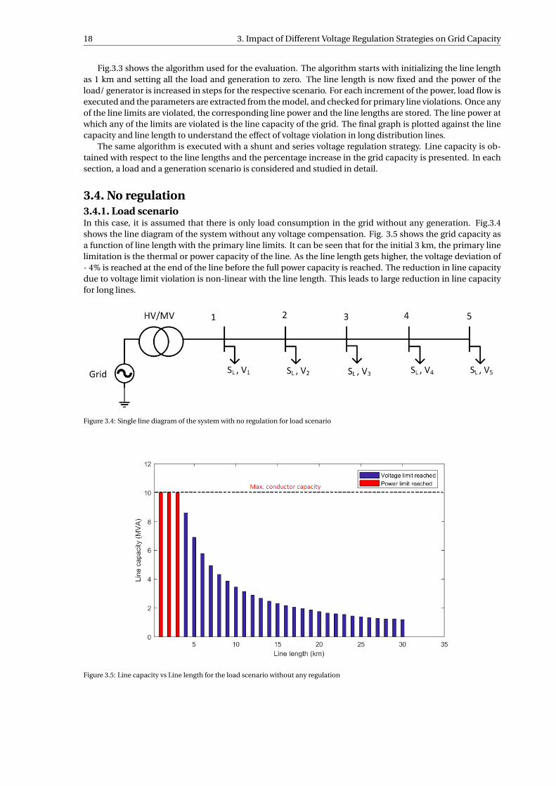
3.4.1 Load scenario . . . . . . . . . . . . . . . . . . . . . . . . . . . . . . . . . . . . . . . 183.4.2 Generation scenario . . . . . . . . . . . . . . . . . . . . . . . . . . . . . . . . . . . . 19
3.5 Shunt voltage regulation . . . . . . . . . . . . . . . . . . . . . . . . . . . . . . . . . . . . . 203.5.1 Load scenario . . . . . . . . . . . . . . . . . . . . . . . . . . . . . . . . . . . . . . . 203.5.2 Generation scenario . . . . . . . . . . . . . . . . . . . . . . . . . . . . . . . . . . . . 21
3.6 Series voltage regulation . . . . . . . . . . . . . . . . . . . . . . . . . . . . . . . . . . . . . 223.6.1 Load scenario . . . . . . . . . . . . . . . . . . . . . . . . . . . . . . . . . . . . . . . 223.6.2 Generation scenario . . . . . . . . . . . . . . . . . . . . . . . . . . . . . . . . . . . . 23
3.7 Conductor upgradation . . . . . . . . . . . . . . . . . . . . . . . . . . . . . . . . . . . . . . 243.7.1 Load scenario . . . . . . . . . . . . . . . . . . . . . . . . . . . . . . . . . . . . . . . 263.7.2 Generation scenario . . . . . . . . . . . . . . . . . . . . . . . . . . . . . . . . . . . . 26
3.8 Voltage regulation impact on grid capacity . . . . . . . . . . . . . . . . . . . . . . . . . . . . 27
4 Analysis of LVR configurations withmechanical OLTCs 294.1 Introduction . . . . . . . . . . . . . . . . . . . . . . . . . . . . . . . . . . . . . . . . . . . 294.2 Transformers . . . . . . . . . . . . . . . . . . . . . . . . . . . . . . . . . . . . . . . . . . . 30
4.2.1 Transformer basics. . . . . . . . . . . . . . . . . . . . . . . . . . . . . . . . . . . . . 304.2.2 Practical transformer and parameters identification . . . . . . . . . . . . . . . . . . . . 314.2.3 Autotransformer . . . . . . . . . . . . . . . . . . . . . . . . . . . . . . . . . . . . . . 32
ix
x Contents
4.3 Modeling of line voltage regulators . . . . . . . . . . . . . . . . . . . . . . . . . . . . . . . . 354.4 Mechanical On-Load Tap-Changer . . . . . . . . . . . . . . . . . . . . . . . . . . . . . . . . 37
4.4.1 On-Load Tap-Changer: switching principle and technology . . . . . . . . . . . . . . . . 374.4.2 Distribution voltage level OLTCs . . . . . . . . . . . . . . . . . . . . . . . . . . . . . . 394.4.3 OLTC selection . . . . . . . . . . . . . . . . . . . . . . . . . . . . . . . . . . . . . . . 40
4.5 One active part LVR configuration . . . . . . . . . . . . . . . . . . . . . . . . . . . . . . . . 414.5.1 OLTC on the primary side of the feeder transformer . . . . . . . . . . . . . . . . . . . . 414.5.2 OLTC on the secondary side of the feeder transformer . . . . . . . . . . . . . . . . . . . 43
4.6 Two active parts LVR configuration . . . . . . . . . . . . . . . . . . . . . . . . . . . . . . . . 474.6.1 LVR with reversing switches on the secondary side of the feeder transformer . . . . . . . 484.6.2 LVR with center tapped transformer . . . . . . . . . . . . . . . . . . . . . . . . . . . . 51
4.7 Comparison of LVR configurations . . . . . . . . . . . . . . . . . . . . . . . . . . . . . . . . 55
5 Simulation & Experimental Results of LVR 595.1 Design of the LVR . . . . . . . . . . . . . . . . . . . . . . . . . . . . . . . . . . . . . . . . . 59
5.1.1 Feeder and booster transformer . . . . . . . . . . . . . . . . . . . . . . . . . . . . . . 605.2 Modeling and Simulation of the system . . . . . . . . . . . . . . . . . . . . . . . . . . . . . . 61
5.2.1 Transformer modeling . . . . . . . . . . . . . . . . . . . . . . . . . . . . . . . . . . . 615.2.2 Line and load modeling . . . . . . . . . . . . . . . . . . . . . . . . . . . . . . . . . . 645.2.3 Positive and negative voltage regulation . . . . . . . . . . . . . . . . . . . . . . . . . . 64
5.3 Experimental results . . . . . . . . . . . . . . . . . . . . . . . . . . . . . . . . . . . . . . . 655.3.1 Positive voltage regulation . . . . . . . . . . . . . . . . . . . . . . . . . . . . . . . . . 675.3.2 Negative voltage regulation . . . . . . . . . . . . . . . . . . . . . . . . . . . . . . . . 68
6 Feasibility of Power Electronics basedOLTCs for LVRs 696.1 LVR configuration . . . . . . . . . . . . . . . . . . . . . . . . . . . . . . . . . . . . . . . . . 696.2 Solid-state switch selection . . . . . . . . . . . . . . . . . . . . . . . . . . . . . . . . . . . . 706.3 Commutation principle for a thyristor based tap-changer . . . . . . . . . . . . . . . . . . . . 71
6.3.1 Equivalent circuit of the tap-changer . . . . . . . . . . . . . . . . . . . . . . . . . . . 736.3.2 Switching down in an inductive power factor region . . . . . . . . . . . . . . . . . . . . 736.3.3 Switching down in unity power factor . . . . . . . . . . . . . . . . . . . . . . . . . . . 756.3.4 Switching down in a capacitive power factor region . . . . . . . . . . . . . . . . . . . . 76
6.4 Determination of firing angle for switching down operation . . . . . . . . . . . . . . . . . . . 786.5 Simulation results of thyristor based tap-changer . . . . . . . . . . . . . . . . . . . . . . . . . 80
6.5.1 Inductive power factor . . . . . . . . . . . . . . . . . . . . . . . . . . . . . . . . . . . 806.5.2 Unity power factor . . . . . . . . . . . . . . . . . . . . . . . . . . . . . . . . . . . . . 806.5.3 Capacitive power factor . . . . . . . . . . . . . . . . . . . . . . . . . . . . . . . . . . 82
6.6 Simulation results of LVR with PE based OLTC . . . . . . . . . . . . . . . . . . . . . . . . . . 846.7 Switching down operation . . . . . . . . . . . . . . . . . . . . . . . . . . . . . . . . . . . . 846.8 Switching up operation . . . . . . . . . . . . . . . . . . . . . . . . . . . . . . . . . . . . . . 866.9 Comparison of PE based OLTC and mechanical OLTCs . . . . . . . . . . . . . . . . . . . . . . 86
7 Conclusion and FutureWork 897.1 Thesis overview . . . . . . . . . . . . . . . . . . . . . . . . . . . . . . . . . . . . . . . . . . 897.2 Results and conclusion . . . . . . . . . . . . . . . . . . . . . . . . . . . . . . . . . . . . . . 897.3 Future Work. . . . . . . . . . . . . . . . . . . . . . . . . . . . . . . . . . . . . . . . . . . . 92
Bibliography 101
List of Figures
1.1 Global renewable energy share and percentage change of installed capacity of different tech-nologies(source: International renewable energy agency, Renewable Capacity Statistics,2016)[7] . . . . . . . . . . . . . . . . . . . . . . . . . . . . . . . . . . . . . . . . . . . . . . . . . . . . . . . . 1
2.1 Radial and open loop layout employed in medium voltage distribution grid [58] . . . . . . . . . . 42.2 (a) A typical two bus distribution system (b) A conventional radial distribution system [40] . . . 52.3 Voltage profile in a radial distribution system . . . . . . . . . . . . . . . . . . . . . . . . . . . . . . 62.4 (a) A typical two bus distribution system with DG connected (b) A radial distribution system
with DG connected [40] . . . . . . . . . . . . . . . . . . . . . . . . . . . . . . . . . . . . . . . . . . . 72.5 (a) Voltage profile when PG = 240 kW (b) Voltage profile when PG = 1 MW [40] . . . . . . . . . . . 82.6 (a) A thevenin equivalent circuit for a wind farm (Bus A) connected to a grid (Bus B) (b) Voltage
variation due to injected power Pn [70] . . . . . . . . . . . . . . . . . . . . . . . . . . . . . . . . . . 92.7 Voltage set-point adjustment by HV/MV transformer OLTC in a distribution line . . . . . . . . . 102.8 Effect of series voltage injection along the line by a LVR in a distribution line . . . . . . . . . . . . 112.9 General structure of a dynamic voltage restorer [69] . . . . . . . . . . . . . . . . . . . . . . . . . . . 112.10 Comparison of PV system voltage at PCC without (left) and with (right) reactive power compensation[45] 122.11 Phasor diagram of the reduction in sending end voltage due to shunt compensation [20] . . . . 132.12 (a) A Typical layout diagram of a SVC (TCR-TSC) [74] (b) A typical layout diagram of a STATCOM
(VSC) [42] . . . . . . . . . . . . . . . . . . . . . . . . . . . . . . . . . . . . . . . . . . . . . . . . . . . 142.13 Typical load profile of residential load with EV charging profile superimposed as dotted lines [33] 14
3.1 Voltage variation limits (%) for the MV and LV grid considered in this study . . . . . . . . . . . . . 153.2 Single line diagram of the 20kV, 10 MVA distribution system under study . . . . . . . . . . . . . . 163.3 Algorithm used to assess the grid capacity with primary line limits . . . . . . . . . . . . . . . . . . 173.4 Single line diagram of the system with no regulation for load scenario . . . . . . . . . . . . . . . . 183.5 Line capacity vs Line length for the load scenario without any regulation . . . . . . . . . . . . . . 183.6 Single line diagram of the system with no regulation for generation scenario . . . . . . . . . . . . 193.7 Line capacity vs Line length for the generation scenario without any regulation . . . . . . . . . . 193.8 Single line diagram of a 20kV, 10 MVA distribution system under study with shunt compensation 203.9 Line capacity vs Line length for the load scenario with shunt compensation . . . . . . . . . . . . 213.10 Percentage increase in the line capacity as a function of line length for the load scenario with
shunt compensation . . . . . . . . . . . . . . . . . . . . . . . . . . . . . . . . . . . . . . . . . . . . . 213.11 Line capacity vs Line length for the generation scenario with individual shunt compensation . . 223.12 Percentage increase in the line capacity as a function of line length for the generation scenario
due to shunt voltage compensation . . . . . . . . . . . . . . . . . . . . . . . . . . . . . . . . . . . . 233.13 Single line diagram of the 20kV, 10 MVA distribution system under study with series voltage
compensation . . . . . . . . . . . . . . . . . . . . . . . . . . . . . . . . . . . . . . . . . . . . . . . . . 233.14 Line capacity vs Line length for the load scenario with a ±10% line voltage regulator . . . . . . . 243.15 Percentage increase in the line capacity as a function of line length due to series compensation
with ±10% line voltage regulator . . . . . . . . . . . . . . . . . . . . . . . . . . . . . . . . . . . . . . 243.16 Line capacity vs Line length for the generator scenario with a ±10% line voltage regulator . . . . 253.17 Percentage increase in the line capacity as a function of line length due to series compensation
with a ±10% line voltage regulator . . . . . . . . . . . . . . . . . . . . . . . . . . . . . . . . . . . . . 253.18 (a) Line capacity (MVA) vs line length (km) for the load scenario with A1_63 conductor (b) Per-
centage increase in the line capacity as a function of line length for the load scenario with A1_63conductor . . . . . . . . . . . . . . . . . . . . . . . . . . . . . . . . . . . . . . . . . . . . . . . . . . . 26
3.19 (a) Line capacity (MVA) vs line length (km) for the load scenario with A1_100 conductor (b)Percentageincrease in the line capacity as a function of line length for the load scenario with A1_100 con-ductor . . . . . . . . . . . . . . . . . . . . . . . . . . . . . . . . . . . . . . . . . . . . . . . . . . . . . . 26
xi
xii List of Figures
3.20 (a) Line capacity (MVA) vs line length (km) for the generation scenario with A1_63 conductor (b)Percentage increase in the line capacity as a function of line length for the generation scenariowith A1_63 conductor . . . . . . . . . . . . . . . . . . . . . . . . . . . . . . . . . . . . . . . . . . . . 27
3.21 (a) Line capacity (MVA) vs line length (km) for the generation scenario with A1_100 conduc-tor (b) Percentage increase in the line capacity as a function of line length for the generationscenario with A1_100 conductor . . . . . . . . . . . . . . . . . . . . . . . . . . . . . . . . . . . . . . 27
4.1 Typical layout of a Line Voltage Regulator system [37] . . . . . . . . . . . . . . . . . . . . . . . . . . 294.2 An ideal two-winding transformer with primary and secondary windings [72] . . . . . . . . . . . 314.3 Equivalent circuit of a practical transformer with non-idealities [72] . . . . . . . . . . . . . . . . . 324.4 (a) Schematic diagram of an autotransformer [72] (b) Physical arrangement of an autotransformer 334.5 A two-winding transformer connected as a autotransformer to boost the voltage (a) Schematic
diagram (b) Physical arrangement . . . . . . . . . . . . . . . . . . . . . . . . . . . . . . . . . . . . . 354.6 (a) Single phase LVR (b) Three phase wye connected LVR . . . . . . . . . . . . . . . . . . . . . . . . 374.7 Tap transition (left to right) without any bridging contact [32] . . . . . . . . . . . . . . . . . . . . . 384.8 Tap transition (left to right) with a bridging contact [32] . . . . . . . . . . . . . . . . . . . . . . . . 384.9 (a) Bridging contact with a resistor (b) Bridging contact with a reactor [32] . . . . . . . . . . . . . 394.10 (a) VR-32 Quick-Drive Tap-Changer[68] (b) MR ECPTAP VPD on-load tap-changer [29] . . . . . 404.11 Single phase LVR configuration with OLTC on the primary side of the feeder transformer . . . . 424.12 Turns ratio Vs Regulation voltage (V2) for OLTC on the primary side of the feeder transformer . . 424.13 Single phase LVR configuration with OLTC on the secondary side of the feeder transformer with
contactors for voltage reversal . . . . . . . . . . . . . . . . . . . . . . . . . . . . . . . . . . . . . . . 444.14 Maximum line power that the LVR configuration 1 can handle for the respective line voltage . . 454.15 Single phase LVR configuration with OLTC on the center-tap secondary side of the feeder trans-
former . . . . . . . . . . . . . . . . . . . . . . . . . . . . . . . . . . . . . . . . . . . . . . . . . . . . . 464.16 Single phase LVR two active parts configuration with OLTC on the secondary side of the feeder
transformer and MV contactors for voltage reversal . . . . . . . . . . . . . . . . . . . . . . . . . . . 494.17 Maximum line power that the LVR configuration 3 & 4 can handle for the respective percentage
of voltage regulation . . . . . . . . . . . . . . . . . . . . . . . . . . . . . . . . . . . . . . . . . . . . . 504.18 Single phase LVR two active parts configuration with OLTC on the secondary side of the feeder
autotransformer . . . . . . . . . . . . . . . . . . . . . . . . . . . . . . . . . . . . . . . . . . . . . . . . 514.19 Single phase LVR two active parts configuration with OLTC on the secondary side of the center
tapped feeder transformer . . . . . . . . . . . . . . . . . . . . . . . . . . . . . . . . . . . . . . . . . . 524.20 Maximum line power that the LVR configuration 5 & 6 can handle for the respective percentage
of voltage regulation . . . . . . . . . . . . . . . . . . . . . . . . . . . . . . . . . . . . . . . . . . . . . 534.21 Single phase LVR two active parts configuration with OLTC on the secondary side of the center
tapped feeder autotransformer . . . . . . . . . . . . . . . . . . . . . . . . . . . . . . . . . . . . . . . 55
5.1 Schematic diagram of a single phase LVR configuration 5 . . . . . . . . . . . . . . . . . . . . . . . 595.2 (a) Internal wiring diagram of the feeder transformer (b) Internal wiring diagram of the booster
transformer . . . . . . . . . . . . . . . . . . . . . . . . . . . . . . . . . . . . . . . . . . . . . . . . . . 615.3 Secondary side of the feeder transformer with tappings . . . . . . . . . . . . . . . . . . . . . . . . 625.4 MATLAB/ Simulink model of a LVR in a MV distribution line . . . . . . . . . . . . . . . . . . . . . 625.5 The feeder and booster transformer with the OLTC in MATLAB/ Simulink . . . . . . . . . . . . . 645.6 Simulation results for 6% positive voltage compensation of phase R . . . . . . . . . . . . . . . . . 655.7 Simulation results for 6% negative voltage compensation of phase R . . . . . . . . . . . . . . . . . 655.8 (a) MR ECOTAP OLTC(left), MR controller(center), DSO (right) (b) Feeder transformer (top),
Booster transformer (bottom) . . . . . . . . . . . . . . . . . . . . . . . . . . . . . . . . . . . . . . . . 665.9 Experimental setup for positive voltage regulation (a) Redistribution of voltage regulation (in
%)(b) Schematic diagram of the experimental setup of LVR for positive voltage regulation . . . . 675.10 Experimental results for positive voltage regulation (a) Per-phase input, output and compensa-
tion voltage waveforms (b) Per-phase RMS input, output and compensation voltage values . . . 675.11 Experimental setup for negative voltage regulation (a) Redistribution of voltage regulation (in
%)(b) Schematic diagram of the LVR . . . . . . . . . . . . . . . . . . . . . . . . . . . . . . . . . . . . 685.12 Experimental results for negative voltage regulation (a) Per-phase input, output and compen-
sation voltage waveforms (b) Per-phase RMS input, output and compensation voltage values . . 68
List of Figures xiii
6.1 Power electronic (PE) switches placement in a LVR with feeder and booster topology . . . . . . . 706.2 (a) Bi-directional IGBT switch in common-emitter configuration (b) Bi-directional thyristor switch
connected in anti-parallel configuration . . . . . . . . . . . . . . . . . . . . . . . . . . . . . . . . . 716.3 Feeder transformer with a thyristor based OLTC on the secondary side of the transformer . . . . 726.4 (a) Switching up and down instants for tap-changes without a short circuit for lagging power
factor (b) Schematic diagram of one tap with thyristor based tap-changer in feeder secondarytransformer . . . . . . . . . . . . . . . . . . . . . . . . . . . . . . . . . . . . . . . . . . . . . . . . . . 72
6.5 (a) Equivalent circuit of two taps with thyristor based tap-changers (b) Voltage and currentwaveforms during switching up operation [75] . . . . . . . . . . . . . . . . . . . . . . . . . . . . . . 74
6.6 Voltage and current waveforms for inductive power factors close to 180 . . . . . . . . . . . . . . 746.7 Voltage and current switching waveforms at unity power factor . . . . . . . . . . . . . . . . . . . . 756.8 Voltage and current commutation waveforms for capacitive power factors without a short circuit 766.9 Voltage and current commutation waveforms for capacitive power factors with a short circuit . 786.10 Firing angle (α) vs Power factor angle (φ) for switching down operation . . . . . . . . . . . . . . . 796.11 MATLAB/ Simulink model of two taps with a thyristor based tap-changer . . . . . . . . . . . . . . 806.12 Simulation results at an inductive power factor angle of 30 for switching down operation (a)
Thyristor voltages VT 1, VT 2 and thyristor current IT 1 (b) Tap output voltage (Vo) . . . . . . . . . . 816.13 Simulation results at an inductive power factor angle of 30 for switching up operation (a)
Thyristor voltages VT 1, VT 2 and thyristor current IT 2 (b) Tap output voltage (Vo) . . . . . . . . . . 816.14 Simulation results at unity power factor for switching down operation (a) Thyristor voltages VT 1,
VT 2 and thyristor current IT 1 (b) Tap output voltage (Vo) . . . . . . . . . . . . . . . . . . . . . . . . 826.15 Simulation results at unity power factor for switching up operation (a) Thyristor voltages VT 1,
VT 2 and thyristor current IT 2 (b) Tap output voltage (Vo) . . . . . . . . . . . . . . . . . . . . . . . . 826.16 Simulation results at capacitive power factor angle of 24.8 (φc ) for switching down operation
(a) Thyristor voltages VT 1, VT 2 and thyristor current IT 1 (b) Tap output voltage (Vo) . . . . . . . . 836.17 Simulation results at capacitive power factor angle of 30 for switching down operation (a)
Thyristor voltages VT 1, VT 2 and thyristor current IT 1 (b) Tap output voltage (Vo) . . . . . . . . . . 836.18 Simulation results at capacitive power factor angle of 30 for switching up operation (a) Thyris-
tor voltages VT 1, VT 2 and thyristor current IT 2 (b) Tap output voltage (Vo) . . . . . . . . . . . . . 846.19 MATLAB/ Simulink model of a LVR with thyristor based OLTC in a MV distribution line . . . . . 846.20 Simulation results of phase R for switching down operation in a LVR (a) Top: Compensation
voltage, Bottom: Thyristor voltages (VT 1, VT 2) and Thyristor current (IT 1, IT 2) (b) LVR input andoutput voltages . . . . . . . . . . . . . . . . . . . . . . . . . . . . . . . . . . . . . . . . . . . . . . . . 85
6.21 Simulation results of phase R for switching up operation in a LVR (a) Top: Compensation volt-age, Bottom: Thyristor voltages (VT 1, VT 2) and Thyristor current (IT 1, IT 2) (b) LVR input andoutput voltages . . . . . . . . . . . . . . . . . . . . . . . . . . . . . . . . . . . . . . . . . . . . . . . . 86
7.1 (a) Line capacity (MVA) vs line length (km) for the load scenario with a ±10% LVR (b) Line ca-pacity (MVA) vs line length (km) for the generation scenario with a ±10% LVR . . . . . . . . . . . 90
7.2 (a)LVR configuration 6 (b) LVR configuration 5 . . . . . . . . . . . . . . . . . . . . . . . . . . . . . . 917.3 Schematic of LVR configuration 5 with thyristor based OLTC . . . . . . . . . . . . . . . . . . . . . 924 MATLAB/Simulink model used for technical benefit analysis . . . . . . . . . . . . . . . . . . . . . 945 MATLAB/ Simulink model of a single phase thyristor based OLTC . . . . . . . . . . . . . . . . . . 976 MATLAB/ Simulink model of thyristor cell subsystem used in fig.5 . . . . . . . . . . . . . . . . . . 977 Extinction angle of T1a for switching down at capacitive power factor angle of 30 . . . . . . . . 988 MATLAB/ Simulink model of two taps with equivalent tap inductance and thyristor based tap-
changer . . . . . . . . . . . . . . . . . . . . . . . . . . . . . . . . . . . . . . . . . . . . . . . . . . . . . 989 Simulation results of VT 1, VT 2 & IT 1 at unity power factor with tap inductance instead of feeder
transformer model . . . . . . . . . . . . . . . . . . . . . . . . . . . . . . . . . . . . . . . . . . . . . . 9910 Simulation results of VT 1, VT 2 & IT 2 at capacitive power factor angle of 24.8 . . . . . . . . . . . 99

List of Tables
2.1 Long duration supply voltage variation statutory limits in different countries . . . . . . . . . . . 3
3.1 Type A1 conductor parameters used for the study taken from IEC 61597 . . . . . . . . . . . . . . 163.2 Type A1 conductor parameters used for the study taken from IEC 61597 . . . . . . . . . . . . . . 253.3 Grid capacity results for load scenario(∗ Conductor A1_40 (60 mm2) was used in the study) . . . 283.4 Grid capacity results for generation scenario(∗ Conductor A1_40 (60 mm2) was used in the study) 28
4.1 Differences between oil-type and vacuum-type OLTCs . . . . . . . . . . . . . . . . . . . . . . . . . 394.2 Comparison of high current carrying (VR) OLTC and low current carrying (DT)OLTC . . . . . . . 414.3 Technical data of ECOTAP VPD III 100 . . . . . . . . . . . . . . . . . . . . . . . . . . . . . . . . . . . 414.4 Technical parameters for LVR configuration 1 . . . . . . . . . . . . . . . . . . . . . . . . . . . . . . 454.5 Technical parameters for LVR configuration 2 . . . . . . . . . . . . . . . . . . . . . . . . . . . . . . 474.6 Technical parameters for LVR configuration 3 (‡ - Contactors are rated for 11.4kV level) . . . . . 504.7 Technical parameters for LVR configuration 4 . . . . . . . . . . . . . . . . . . . . . . . . . . . . . . 514.8 Technical parameters for LVR configuration 5 . . . . . . . . . . . . . . . . . . . . . . . . . . . . . . 544.9 Technical parameters for LVR configuration 6 . . . . . . . . . . . . . . . . . . . . . . . . . . . . . . 544.10 Technical parameters for a 20kV, ±6% LVR configurations (‡ - Contactors are rated for 11.4kV
level, † - Feeder is an autotransformer) . . . . . . . . . . . . . . . . . . . . . . . . . . . . . . . . . . 554.11 Individual cost contribution of each component to the overall cost of the LVR . . . . . . . . . . . 564.12 Individual cost(%) of different components in a LVR . . . . . . . . . . . . . . . . . . . . . . . . . . 564.13 LVR configuration comparison for the maximum line power for different voltage levels and rel-
ative cost percentage . . . . . . . . . . . . . . . . . . . . . . . . . . . . . . . . . . . . . . . . . . . . . 57
5.1 Per-phase ratings of the feeder and booster transformer . . . . . . . . . . . . . . . . . . . . . . . . 615.2 Feeder transformer parameters . . . . . . . . . . . . . . . . . . . . . . . . . . . . . . . . . . . . . . . 635.3 Booster transformer parameters . . . . . . . . . . . . . . . . . . . . . . . . . . . . . . . . . . . . . . 645.4 Type A1 conductor parameters from IEC 61597 . . . . . . . . . . . . . . . . . . . . . . . . . . . . . 645.5 Per-phase ratings of the feeder and booster transformer used in the experimental test setup . . 66
6.1 Thyristor and IGBT parameters used for solid-state switch selection . . . . . . . . . . . . . . . . . 716.2 Power factor angle and firing angle relationship for switching down operation in an inductive
power factor region . . . . . . . . . . . . . . . . . . . . . . . . . . . . . . . . . . . . . . . . . . . . . . 756.3 Transformer, tap, & thyristor parameters used to determine the firing angle . . . . . . . . . . . . 786.4 Technical and cost comparison of ECOTAP VPD III 100 and thyristor based OLTC(∗ Includes
only the cost of thyristor switches) . . . . . . . . . . . . . . . . . . . . . . . . . . . . . . . . . . . . . 87
xv


Nomenclature
abooster Turns ratio of booster transformer
a f eeder Turns ratio of feeder transformer
α Firing angle of the thyristor
δ Extinction angle
δq Thyristor turn-off angle
γ Overlap angle during commutation
ω Angular frequency (rad/s)
φ Power factor angle
CCC Current carrying capacity
DSO Distribution system operator
er Per unit resistance drop
ex Per unit reactance drop
Im Peak value of the current
IT 1 Current in thyristor pair T1
IT 2 Current in thyristor pair T2
Lt ap Per-tap leakage inductance
NB pr i No. of turns on the booster transformer the primary windings
NB sec No. of turns on the booster transformer secondary winding
Npr i No. of tunrs on the the feeder transformer primary windings
Nsec (OLT C ) Effective number of turns for feeder transformer secondary with OLTC
Nt aps No. of taps
PF Power Factor
Sk Short circuit power
Sbooster Power rating of booster transformer
S f eeder Power rating of feeder transformer
SC R Short circuit ratio
tq Thyristor turn-off time
t an(ψ) Network impedance angle
VL Load voltage
Vm Peak value of the voltage
xvii
xviii List of Tables
VS Source voltage
V1T Feeder transformer secondary OLTC voltage
V1 Feeder transformer primary voltage
V2T Booster transformer primary OLTC voltage
V2 Series compensation voltage
Vcomp Compensation Voltage
VGE N Generator voltage
VSnew New voltage set-point
Vstep Step voltage
VT 1 Voltage across thyristor pair T1
VT 2 Voltage across thyristor pair T2
Vt ap Per-tap voltage of the transformer
Reg. range Regulation range of LVR (pu)
RMS Root Mean Square
SCADA Supervisory Control and Data Acquisition technology

1Introduction
There has been a huge push by governments all around the world to move towards renewable energy to re-duce greenhouse gas emissions. Fig. 1.1 shows the installed capacity of global renewable energy from 2006- 2015 and the percentage increase for each technology. The installed capacity of the wind and solar energybased technology are growing at a very rapid rate with a percentage change of 487.7% and 3404.9% respec-tively from 2006-15. With the recent Paris agreement, the share of renewable energy is expected to increaseat a faster rate. Apart from the large wind and solar parks to produce huge amounts of renewable power,integrating renewable energy sources (RES) in to the distribution system has started to become increasinglypopular [9].
Figure 1.1: Global renewable energy share and percentage change of installed capacity of different technologies(source: Internationalrenewable energy agency, Renewable Capacity Statistics,2016) [7]
Increasing the amount of DG penetration into the Medium Voltage (MV) and Low Voltage (LV) grid causesvoltage regulation issues in the distribution network[76]. Injection of active power by the DGs to the distribu-tion network can directly impact the feeder voltage due to high R/X ratio [77]. The voltage variation is morepronounced in rural networks due to long feeders compared to urban networks with shorter lines[19].
Rural areas are ideal for renewable energy development due to their sparse population and large vacantareas [3]. With the growing rural renewable energy development, evacuating the power from rural areas re-quires long overhead lines. The connection cost for a renewable energy project can be reduced by connectingthe generators to a lower voltage level network at the point of common coupling (PCC). The higher the voltage
1
2 1. Introduction
level, the higher the connection cost for the developer [40]. But, active power injection by the DGs to a lowvoltage level network can have a more direct impact on voltage variation than when they are connected to ahigh voltage level network. To bridge the gap, the developers and DSOs should deploy economically activesolutions to maintain the voltage, especially in long rural networks with renewable energy.
The traditional active voltage regulation methods used by the DSOs are as follows [41]:
• Distribution transformer with On-Load Tap-Changers (OLTC)
• Shunt capacitors and reactors
• Series Voltage Regulators (SVRs) or Line Voltage Regulators (LVRs)
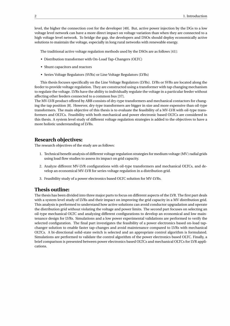
This thesis focuses specifically on the Line Voltage Regulators (LVRs). LVRs or SVRs are located along thefeeder to provide voltage regulation. They are constructed using a transformer with tap changing mechanismto regulate the voltage. LVRs have the ability to individually regulate the voltage in a particular feeder withoutaffecting other feeders connected to a common bus [37].The MV-LVR product offered by ABB consists of dry-type transformers and mechanical contactors for chang-ing the tap position [8]. However, dry-type transformers are bigger in size and more expensive than oil-typetransformers. The main objective of this thesis is to evaluate the feasibility of a MV-LVR with oil-type trans-formers and OLTCs. Feasibility with both mechanical and power electronic based OLTCs are considered inthis thesis. A system level study of different voltage regulation strategies is added to the objectives to have amore holistic understanding of LVRs.
Research objectives:The research objectives of the study are as follows:
1. Technical benefit analysis of different voltage regulation strategies for medium voltage (MV) radial gridsusing load flow studies to assess its impact on grid capacity.
2. Analyze different MV-LVR configurations with oil-type transformers and mechanical OLTCs, and de-velop an economical MV-LVR for series voltage regulation in a distribution grid.
3. Feasibility study of a power electronics based OLTC solution for MV-LVRs.
Thesis outline:The thesis has been divided into three major parts to focus on different aspects of the LVR. The first part dealswith a system level study of LVRs and their impact on improving the grid capacity in a MV distribution grid.This analysis is performed to understand how active solutions can avoid conductor upgradation and operatethe distribution grid without violating the voltage and power limits. The second part focuses on selecting anoil-type mechanical OLTC and analyzing different configurations to develop an economical and low main-tenance design for LVRs. Simulations and a low power experimental validations are performed to verify theselected configuration. The final part investigates the feasibility of a power electronics based on-load tap-changer solution to enable faster tap-changes and avoid maintenance compared to LVRs with mechanicalOLTCs. A bi-directional solid-state switch is selected and an appropriate control algorithm is formulated.Simulations are performed to validate the control algorithm of the power electronics based OLTC. Finally, abrief comparison is presented between power electronics based OLTCs and mechanical OLTCs for LVR appli-cations.
2Voltage Variation and Regulation in a
Medium Voltage Grid
2.1. IntroductionIn a traditional power system, generators are located at a significant distance from the consumers and thepower flow is typically unidirectional. The system is designed so that the consumers connected at the endof a line do not experience voltage violation even during high load conditions. With increase in DistributedGenerators (DGs), distribution networks are challenged by the reverse power flow. Traditionally designed dis-tribution networks are not designed to handle the DG penetration. The increase in distributed generation ischallenging the DSOs to maintain the voltage within the statuatory limits. This chapter elaborates on voltagevariation problems faced in the distribution grids and the methods used to tackle the issue.
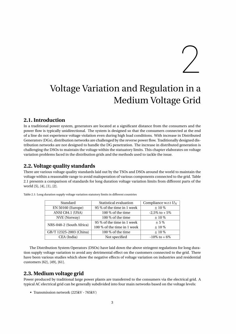
2.2. Voltage quality standardsThere are various voltage quality standards laid out by the TSOs and DSOs around the world to maintain thevoltage within a reasonable range to avoid maloperation of various components connected to the grid. Table2.1 presents a comparison of standards for long duration voltage variation limits from different parts of theworld [5], [4], [1], [2].
Table 2.1: Long duration supply voltage variation statutory limits in different countries
Standard Statistical evaluation Compliance w.r.t UN
EN 50160 (Europe) 95 % of the time in 1 week ± 10 %ANSI C84.1 (USA) 100 % of the time -2,5% to + 5%
NVE (Norway) 100 % of the time ± 10 %
NRS-048-2 (South Africa)95 % of the time in 1 week
100 % of the time in 1 week± 5 %± 10 %
GB/T 12325-2003 (China) 100 % of the time ± 10 %CEA (India) Not specified -10% to + 6%
The Distribution System Operators (DSOs) have laid down the above stringent regulations for long dura-tion supply voltage variation to avoid any detrimental effect on the customers connected to the grid. Therehave been various studies which show the negative effects of voltage variation on industries and residentialcustomers [62], [49], [61].
2.3. Medium voltage gridPower produced by traditional large power plants are transferred to the consumers via the electrical grid. Atypical AC electrical grid can be generally subdivided into four main networks based on the voltage levels:
• Transmission network (225kV - 765kV)
3
4 2. Voltage Variation and Regulation in a Medium Voltage Grid
• Sub-transmission network (25kV - 275 kV)
• Medium voltage network (1kV - 25 kV)
• Low voltage network (up to 1kV )
The most commonly used medium voltage levels in Europe are between 10kV and 20kV due to its optimalpower transfer capability and the cost of components. The most commonly used grid layouts for mediumvoltage are (i) Radial structure (ii) Open loop structure [58]. A brief description of layout is given below:
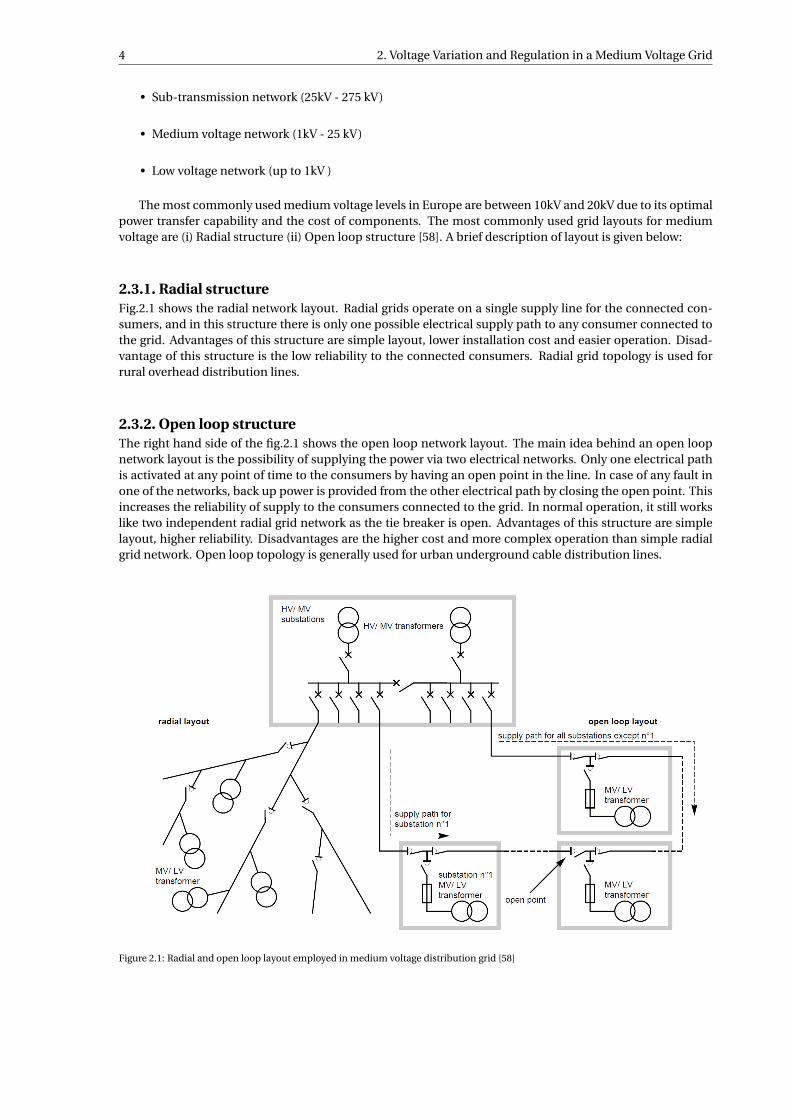
2.3.1. Radial structureFig.2.1 shows the radial network layout. Radial grids operate on a single supply line for the connected con-sumers, and in this structure there is only one possible electrical supply path to any consumer connected tothe grid. Advantages of this structure are simple layout, lower installation cost and easier operation. Disad-vantage of this structure is the low reliability to the connected consumers. Radial grid topology is used forrural overhead distribution lines.
2.3.2. Open loop structureThe right hand side of the fig.2.1 shows the open loop network layout. The main idea behind an open loopnetwork layout is the possibility of supplying the power via two electrical networks. Only one electrical pathis activated at any point of time to the consumers by having an open point in the line. In case of any fault inone of the networks, back up power is provided from the other electrical path by closing the open point. Thisincreases the reliability of supply to the consumers connected to the grid. In normal operation, it still workslike two independent radial grid network as the tie breaker is open. Advantages of this structure are simplelayout, higher reliability. Disadvantages are the higher cost and more complex operation than simple radialgrid network. Open loop topology is generally used for urban underground cable distribution lines.
Figure 2.1: Radial and open loop layout employed in medium voltage distribution grid [58]
2.4. Voltage drop in a conventional distribution grid 5
(a) (b)
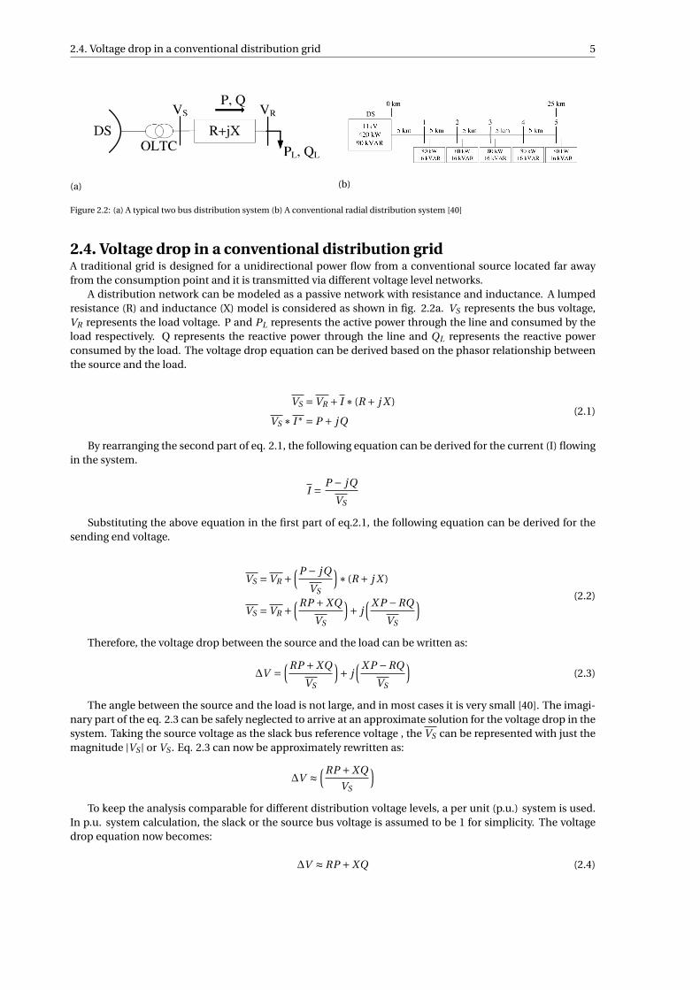
Figure 2.2: (a) A typical two bus distribution system (b) A conventional radial distribution system [40]
2.4. Voltage drop in a conventional distribution gridA traditional grid is designed for a unidirectional power flow from a conventional source located far awayfrom the consumption point and it is transmitted via different voltage level networks.
A distribution network can be modeled as a passive network with resistance and inductance. A lumpedresistance (R) and inductance (X) model is considered as shown in fig. 2.2a. VS represents the bus voltage,VR represents the load voltage. P and PL represents the active power through the line and consumed by theload respectively. Q represents the reactive power through the line and QL represents the reactive powerconsumed by the load. The voltage drop equation can be derived based on the phasor relationship betweenthe source and the load.
VS =VR + I ∗ (R + j X )
VS ∗ I∗ = P + jQ(2.1)
By rearranging the second part of eq. 2.1, the following equation can be derived for the current (I) flowingin the system.
I = P − jQ
VS
Substituting the above equation in the first part of eq.2.1, the following equation can be derived for thesending end voltage.
VS =VR +(P − jQ
VS
)∗ (R + j X )
VS =VR +(RP +XQ
VS
)+ j
( X P −RQ
VS
) (2.2)
Therefore, the voltage drop between the source and the load can be written as:
∆V =(RP +XQ
VS
)+ j
( X P −RQ
VS
)(2.3)
The angle between the source and the load is not large, and in most cases it is very small [40]. The imagi-nary part of the eq. 2.3 can be safely neglected to arrive at an approximate solution for the voltage drop in thesystem. Taking the source voltage as the slack bus reference voltage , the VS can be represented with just themagnitude |VS | or VS . Eq. 2.3 can now be approximately rewritten as:
∆V ≈(RP +XQ
VS
)To keep the analysis comparable for different distribution voltage levels, a per unit (p.u.) system is used.
In p.u. system calculation, the slack or the source bus voltage is assumed to be 1 for simplicity. The voltagedrop equation now becomes:
∆V ≈ RP +XQ (2.4)
6 2. Voltage Variation and Regulation in a Medium Voltage Grid
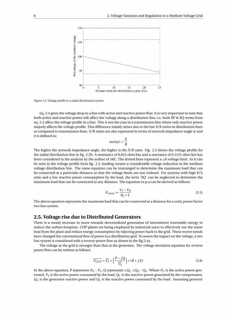
Figure 2.3: Voltage profile in a radial distribution system
Eq. 2.4 gives the voltage drop in a line with active and reactive power flow. It is very important to note thatboth active and reactive power will affect the voltage along a distribution line, i.e, both RP & XQ terms fromeq. 2.4 affect the voltage profile in a line. This is not the case in a transmission line where only reactive powermajorly affects the voltage profile. This difference mainly arises due to the low X/R ratios in distribution linesas compared to transmission lines. X/R ratios are also expressed in terms of network impedance angle ψ andit is defined as:
t an(ψ) = X
R
The higher the network impedance angle, the higher is the X/R ratio. Fig. 2.3 shows the voltage profile forthe radial distribution line in fig. 2.2b. A resistance of 0.625 ohm/km and a reactance of 0.3125 ohm/km hasbeen considered in the analysis by the author of [40]. The dotted lines represent a ±6 voltage limit. As it canbe seen in the voltage profile from fig. 2.3, loading creates a considerable voltage reduction in the mediumvoltage distribution line. The same equation can be rearranged to determine the maximum load that canbe connected at a particular distance so that the voltage limits are not violated. For systems with high R/Xratio and a low reactive power consumption by the load, the term ’XQ’ can be neglected to determine themaximum load that can be connected at any distance. The equation in p.u can be derived as follows:
PLmax ≈ VS −VR
RL ∗L(2.5)
The above equation represents the maximum load that can be connected at a distance for a unity power factortwo bus system.
2.5. Voltage rise due to Distributed GeneratorsThere is a steady increase to move towards decentralized generation of intermittent renewable energy toreduce the carbon footprint. CHP plants are being employed by industrial users to effectively use the wasteheat from the plant and reduce energy consumption by injecting power back to the grid. These recent trendshave changed the conventional flow of power in a distribution grid. To assess the impact on the voltage, a twobus system is considered with a reverse power flow as shown in the fig.2.4a.
The voltage at the grid is stronger than that at the generator. The voltage deviation equation for reversepower flow can be written as follows:
VGE N =VS +(P − jQ
VS
)∗ (R + j X ) (2.6)
In the above equation, P represents PG - PL , Q represents ±QC ±QG - QL . Where PG is the active power gen-erated, PL is the active power consumed by the load, QC is the reactive power generated by the compensator,QG is the generator reactive power and QL is the reactive power consumed by the load. Assuming genertor
2.5. Voltage rise due to Distributed Generators 7
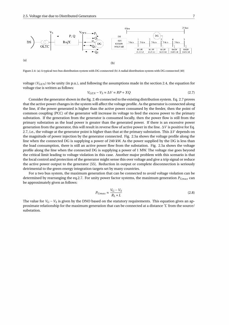
(a)(b)
Figure 2.4: (a) A typical two bus distribution system with DG connected (b) A radial distribution system with DG connected [40]
voltage (VGE N ) to be unity (in p.u.), and following the assumptions made in the section 2.4, the equation forvoltage rise is written as follows:
VGE N −VS ≈∆V ≈ RP +XQ (2.7)
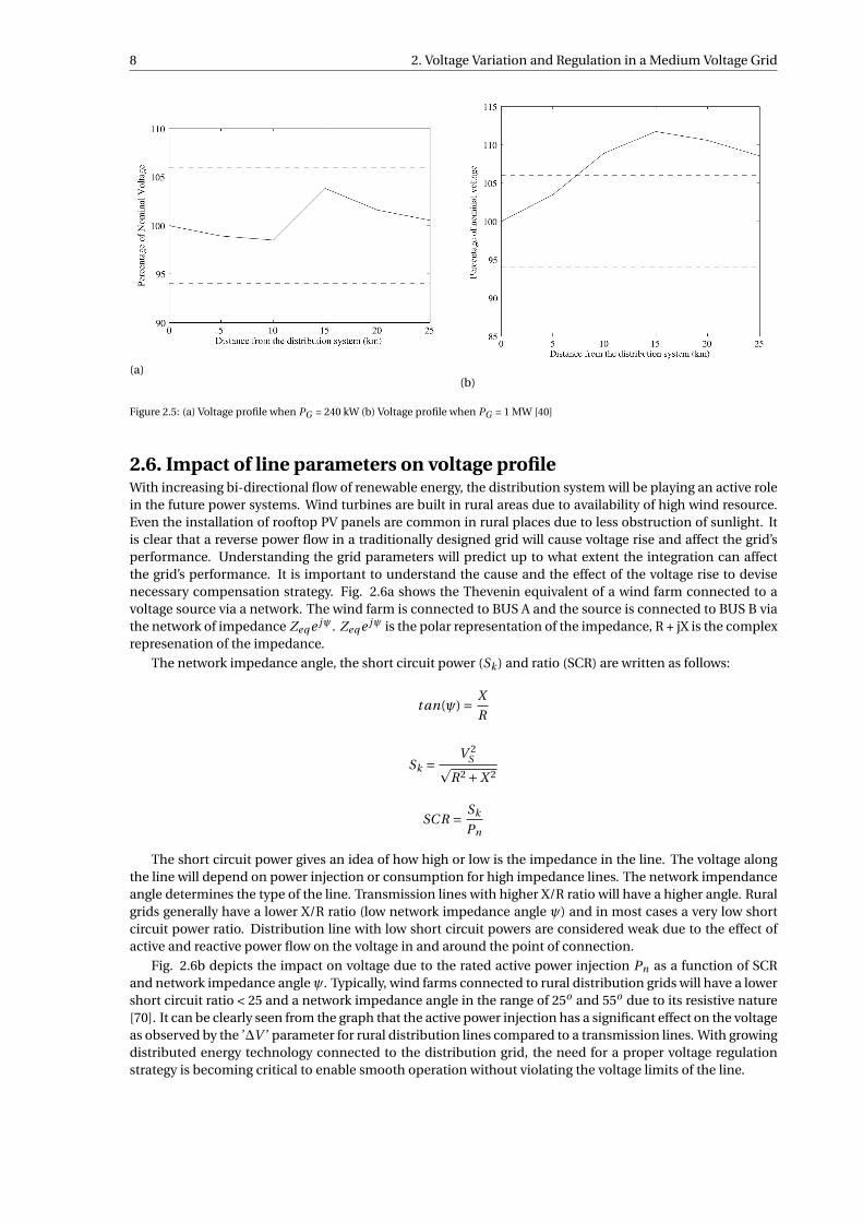
Consider the generator shown in the fig. 2.4b connected to the existing distribution system. Eq. 2.7 provesthat the active power changes in the system will affect the voltage profile. As the generator is connected alongthe line, if the power generated is higher than the active power consumed by the feeder, then the point ofcommon coupling (PCC) of the generator will increase its voltage to feed the excess power to the primarysubstation. If the generation from the generator is consumed locally, then the power flow is still from theprimary substation as the load power is greater than the generated power. If there is an excessive powergeneration from the generator, this will result in reverse flow of active power in the line. ∆V is positive for Eq.2.7, i.e., the voltage at the generator point is higher than that at the primary substation. This ∆V depends onthe magnitude of power injection by the generator connected. Fig. 2.5a shows the voltage profile along theline when the connected DG is supplying a power of 240 kW. As the power supplied by the DG is less thanthe load consumption, there is still an active power flow from the substation. Fig. 2.5a shows the voltageprofile along the line when the connected DG is supplying a power of 1 MW. The voltage rise goes beyondthe critical limit leading to voltage violation in this case. Another major problem with this scenario is thatthe local control and protection of the generator might sense this over voltage and give a trip signal or reducethe active power output to the generator [55]. Reduction in output or complete disconnection is seriouslydetrimental to the green energy integration targets set by many countries.
For a two bus system, the maximum generation that can be connected to avoid voltage violation can bedetermined by rearranging the eq.2.7. For unity power factor systems, the maximum generation PGmax canbe approximately given as follows:
PGmax ≈ VG −VS
RL ∗L(2.8)
The value for VG −VS is given by the DNO based on the statutory requirements. This equation gives an ap-proximate relationship for the maximum generation that can be connected at a distance ’L’ from the source/substation.
8 2. Voltage Variation and Regulation in a Medium Voltage Grid
(a)(b)
Figure 2.5: (a) Voltage profile when PG = 240 kW (b) Voltage profile when PG = 1 MW [40]
2.6. Impact of line parameters on voltage profileWith increasing bi-directional flow of renewable energy, the distribution system will be playing an active rolein the future power systems. Wind turbines are built in rural areas due to availability of high wind resource.Even the installation of rooftop PV panels are common in rural places due to less obstruction of sunlight. Itis clear that a reverse power flow in a traditionally designed grid will cause voltage rise and affect the grid’sperformance. Understanding the grid parameters will predict up to what extent the integration can affectthe grid’s performance. It is important to understand the cause and the effect of the voltage rise to devisenecessary compensation strategy. Fig. 2.6a shows the Thevenin equivalent of a wind farm connected to avoltage source via a network. The wind farm is connected to BUS A and the source is connected to BUS B viathe network of impedance Zeq e jψ. Zeq e jψ is the polar representation of the impedance, R + jX is the complexrepresenation of the impedance.
The network impedance angle, the short circuit power (Sk ) and ratio (SCR) are written as follows:
t an(ψ) = X
R
Sk = V 2Sp
R2 +X 2
SC R = Sk
Pn
The short circuit power gives an idea of how high or low is the impedance in the line. The voltage alongthe line will depend on power injection or consumption for high impedance lines. The network impendanceangle determines the type of the line. Transmission lines with higher X/R ratio will have a higher angle. Ruralgrids generally have a lower X/R ratio (low network impedance angle ψ) and in most cases a very low shortcircuit power ratio. Distribution line with low short circuit powers are considered weak due to the effect ofactive and reactive power flow on the voltage in and around the point of connection.
Fig. 2.6b depicts the impact on voltage due to the rated active power injection Pn as a function of SCRand network impedance angleψ. Typically, wind farms connected to rural distribution grids will have a lowershort circuit ratio < 25 and a network impedance angle in the range of 25o and 55o due to its resistive nature[70]. It can be clearly seen from the graph that the active power injection has a significant effect on the voltageas observed by the ’∆V ’ parameter for rural distribution lines compared to a transmission lines. With growingdistributed energy technology connected to the distribution grid, the need for a proper voltage regulationstrategy is becoming critical to enable smooth operation without violating the voltage limits of the line.
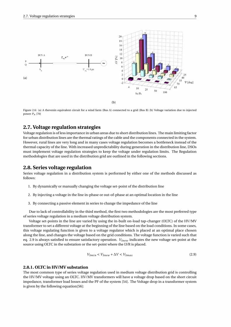
2.7. Voltage regulation strategies 9
(a)
(b)
Figure 2.6: (a) A thevenin equivalent circuit for a wind farm (Bus A) connected to a grid (Bus B) (b) Voltage variation due to injectedpower Pn [70]
2.7. Voltage regulation strategiesVoltage regulation is of less importance in urban areas due to short distribution lines. The main limiting factorfor urban distribution lines are the thermal ratings of the cable and the components connected in the system.However, rural lines are very long and in many cases voltage regulation becomes a bottleneck instead of thethermal capacity of the line. With increased unpredictability during generation in the distribution line, DSOsmust implement voltage regulation strategies to keep the voltage under regulation limits. The Regulationmethodologies that are used in the distribution grid are outlined in the following sections.
2.8. Series voltage regulationSeries voltage regulation in a distribution system is performed by either one of the methods discussed asfollows:
1. By dynamically or manually changing the voltage set-point of the distribution line
2. By injecting a voltage in the line in-phase or out-of-phase at an optimal location in the line
3. By connecting a passive element in series to change the impedance of the line
Due to lack of controllability in the third method, the first two methodologies are the most preferred typeof series voltage regulation in a medium voltage distribution system.
Voltage set-points in the line are varied by using the in-built on-load tap-changer (OLTC) of the HV/MVtransformer to set a different voltage at the beginning of the line based on the load conditions. In some cases,this voltage regulating function is given to a voltage regulator which is placed at an optimal place chosenalong the line, and changes the voltage based on the grid conditions. The voltage function is varied such thateq. 2.9 is always satisfied to ensure satisfactory operation. VSnew indicates the new voltage set-point at thesource using OLTC in the substation or the set-point where the LVR is placed.
VSmi n <VSnew +∆V <VSmax (2.9)
2.8.1. OLTC in HV/MV substationThe most common type of series voltage regulation used in medium voltage distribution grid is controllingthe HV/MV voltage using an OLTC. HV/MV transformers will have a voltage drop based on the short circuitimpedance, transformer load losses and the PF of the system [54]. The Voltage drop in a transformer systemis given by the following equation[56]:
10 2. Voltage Variation and Regulation in a Medium Voltage Grid
∆Vtr ans f or mer = er cos(φ)±ex si n(φ)
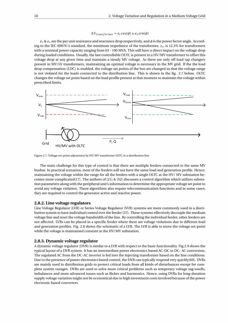
er & ex are the per unit resistance and reactance drop respectively, andφ is the power factor angle. Accord-ing to the IEC 60076-5 standard, the minimum impedance of the transformer, zt , is 12.5% for transformerswith a nominal power capacity ranging from 63 - 100 MVA. This will have a direct impact on the voltage dropduring loaded conditions. Usually, the last controllable OLTC is present in a HV/MV transformer to offset thisvoltage drop at any given time and maintain a steady MV voltage. As there are only off-load tap changerspresent in MV/LV transformers, maintaining an optimal voltage is necessary in the MV grid. If the the loaddrop compensation (LDC) is enabled, the voltage set points of the bus are changed so that the voltage rangeis not violated for the loads connected to the distribution line. This is shown in the fig. 2.7 below. OLTCchanges the voltage set point based on the load profile present at that moment to maintain the voltage withinprescribed limits.
Figure 2.7: Voltage set-point adjustment by HV/MV transformer OLTC in a distribution line
The main challenge for this type of control is that there are multiple feeders connected to the same MVbusbar. In practical scenarios, most of the feeders will not have the same load and generation profile. Hence,maintaining the voltage within the range for all the feeders with a single OLTC at the HV/ MV substation be-comes more complicated[17]. The authors of [21] & [52] discusses a control algorithm which utilizes substa-tion parameters along with the peripheral unit’s information to determine the appropriate voltage set point toavoid any voltage violation. These algorithms also require telecommunication functions and in some cases,they are required to control the generator active and reactive power.
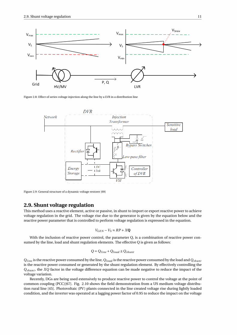
2.8.2. Line voltage regulatorsLine Voltage Regulator (LVR) or Series Voltage Regulator (SVR) systems are more commonly used in a distri-bution system to have individual control over the feeder [37]. These systems effectively decouple the mediumvoltage line and reset the voltage bandwidth of the line. By controlling the individual feeder, other feeders arenot affected. LVRs can be placed in a specific feeder where there are voltage violations due to different loadand generation profiles. Fig. 2.8 shows the schematic of a LVR. The LVR is able to move the voltage set-pointwhile the voltage is maintained constant at the HV/MV substation.
2.8.3. Dynamic voltage regulatorA dynamic voltage regulator (DVR) is similar to a LVR with respect to the basic functionality. Fig.2.9 shows thetypical layout of a DVR system. It has an intermediate power electronics based AC-DC to DC- AC conversion.The regulated AC from the DC-AC inverter is fed into the injecting transformer based on the line conditions.Due to the presence of power electronics based control, the DVR can typically respond very quickly[69]. DVRsare mainly used in distribution grids to protect critical loads from all kinds of disturbances except for com-plete system outages. DVRs are used to solve more critical problems such as temporary voltage sag/swells,imbalances and more advanced issues such as flicker and harmonics. Hence, using DVRs for long-durationsupply voltage variation might not be economical due to high investment costs involved because of the powerelectronic based converters.
2.9. Shunt voltage regulation 11
Figure 2.8: Effect of series voltage injection along the line by a LVR in a distribution line
Figure 2.9: General structure of a dynamic voltage restorer [69]
2.9. Shunt voltage regulationThis method uses a reactive element, active or passive, in shunt to import or export reactive power to achievevoltage regulation in the grid. The voltage rise due to the generator is given by the equation below and thereactive power parameter that is controlled to perform voltage regulation is expressed in the equation.
VGE N −VS ≈ RP +X Q
With the inclusion of reactive power control, the parameter Q, is a combination of reactive power con-sumed by the line, load and shunt regulation elements. The effective Q is given as follows:
Q =Ql i ne +Qload ±Qshunt
Ql i ne is the reactive power consumed by the line, Ql oad is the reactive power consumed by the load and Qshunt
is the reactive power consumed or generated by the shunt regulation element. By effectively controlling theQshunt , the XQ factor in the voltage difference equation can be made negative to reduce the impact of thevoltage variation.
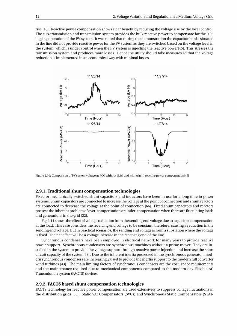
Recently, DGs are being used extensively to produce reactive power to control the voltage at the point ofcommon coupling (PCC)[67]. Fig. 2.10 shows the field demonstration from a US medium voltage distribu-tion rural line [45]. Photovoltaic (PV) plants connected in the line created voltage rise during lightly loadedcondition, and the inverter was operated at a lagging power factor of 0.95 to reduce the impact on the voltage
12 2. Voltage Variation and Regulation in a Medium Voltage Grid
rise [45]. Reactive power compensation shows clear benefit by reducing the voltage rise by the local control.The sub-transmission and transmission system provides the bulk reactive power to compensate for the 0.95lagging operation of the PV system. It was noted that during the demonstration the capacitor banks situatedin the line did not provide reactive power for the PV system as they are switched based on the voltage level inthe system, which is under control when the PV system is injecting the reactive power[45]. This stresses thetransmission system and produces more losses. Hence the utility should take measures so that the voltagereduction is implemented in an economical way with minimal losses.
Figure 2.10: Comparison of PV system voltage at PCC without (left) and with (right) reactive power compensation[45]
2.9.1. Traditional shunt compensation technologiesFixed or mechanically switched shunt capacitors and inductors have been in use for a long time in powersystems. Shunt capacitors are connected to increase the voltage at the point of connection and shunt reactorsare connected to decrease the voltage at the point of connection [66]. Fixed shunt capacitors and reactorspossess the inherent problem of over-compensation or under-compensation when there are fluctuating loadsand generations in the grid [22].
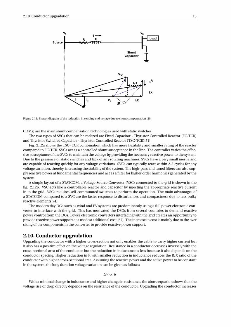
Fig.2.11 shows the effect of voltage reduction from the sending end voltage due to capacitor compensationat the load. This case considers the receiving end voltage to be constant, therefore, causing a reduction in thesending end voltage. But in practical scenarios, the sending end voltage is from a substation where the voltageis fixed. The net effect will be a voltage increase in the receiving end of the line.
Synchronous condensers have been employed in electrical network for many years to provide reactivepower support. Synchronous condensers are synchronous machines without a prime mover. They are in-stalled in the system to provide the voltage support through reactive power injection and increase the shortcircuit capacity of the system[38]. Due to the inherent inertia possessed in the synchronous generator, mod-ern synchronous condensers are increasingly used to provide the inertia support to the modern full converterwind turbines [43]. The main limiting factors of synchronous condensers are the cost, space requirementsand the maintenance required due to mechanical components compared to the modern day Flexible ACTransmission system (FACTS) devices.
2.9.2. FACTS based shunt compensation technologiesFACTS technology for reactive power compensation are used extensively to suppress voltage fluctuations inthe distribution grids [35]. Static VAr Compensators (SVCs) and Synchronous Static Compensators (STAT-
2.10. Conductor upgradation 13
Figure 2.11: Phasor diagram of the reduction in sending end voltage due to shunt compensation [20]
COMs) are the main shunt compensation technologies used with static switches.The two types of SVCs that can be realized are Fixed Capacitor - Thyristor Controlled Reactor (FC-TCR)
and Thyristor Switched Capacitor - Thyristor Controlled Reactor (TSC-TCR)[51].Fig. 2.12a shows the TSC- TCR combination which has more flexibility and smaller rating of the reactor
compared to FC-TCR. SVCs act as a controlled shunt susceptance in the line. The controller varies the effec-tive susceptance of the SVCs to maintain the voltage by providing the necessary reactive power to the system.Due to the presence of static switches and lack of any rotating machines, SVCs have a very small inertia andare capable of reacting quickly for any voltage variations. SVCs can typically react within 2-3 cycles for anyvoltage variation, thereby, increasing the stability of the system. The high-pass and tuned filters can also sup-ply reactive power at fundamental frequencies and act as a filter for higher order harmonics generated by thesystem.
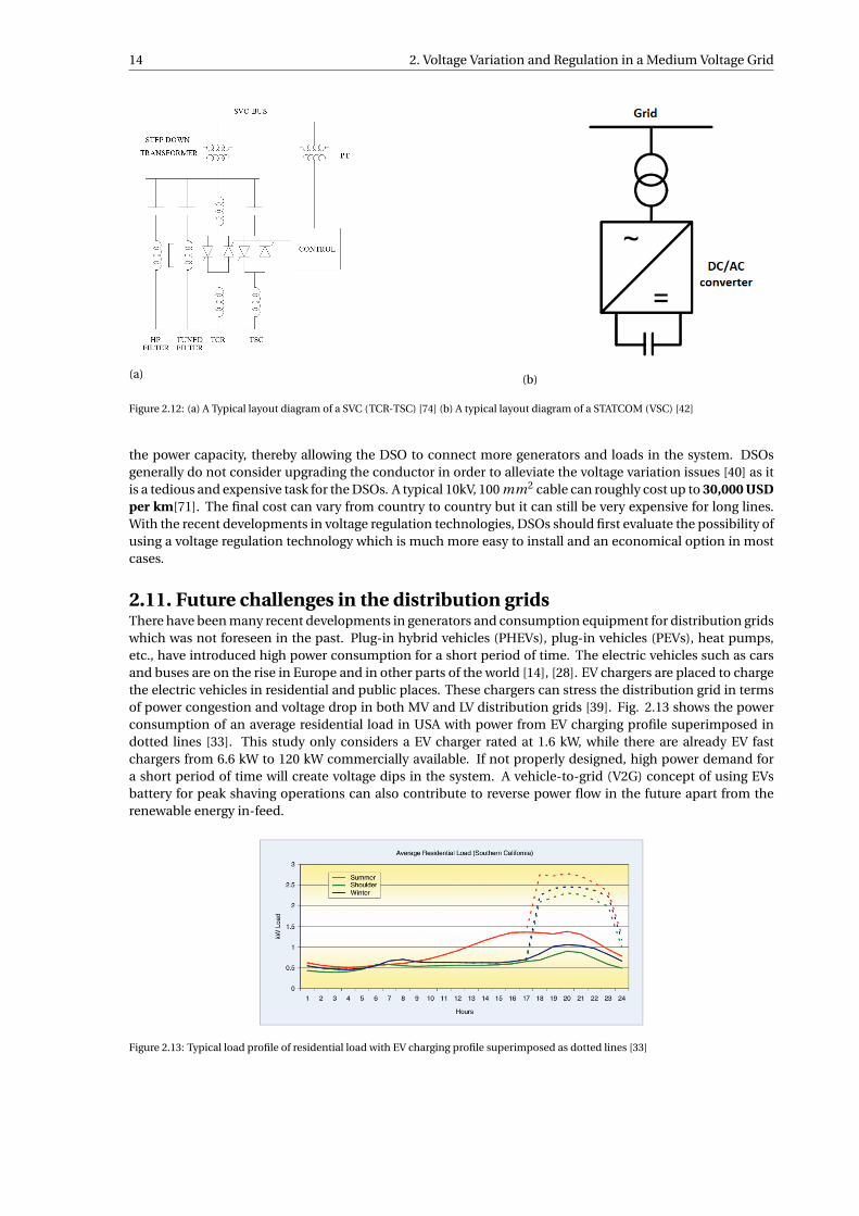
A simple layout of a STATCOM, a Voltage Source Converter (VSC) connected to the grid is shown in thefig. 2.12b. VSC acts like a controllable reactor and capacitor by injecting the appropriate reactive currentin to the grid. VSCs requires self-commutated switches to perform the operation. The main advantages ofa STATCOM compared to a SVC are the faster response to disturbances and compactness due to less bulkyreactive elements[74].
The modern day DGs such as wind and PV systems are predominantly using a full power electronic con-verter to interface with the grid. This has motivated the DSOs from several countries to demand reactivepower control from the DGs. Power electronic converters interfacing with the grid creates an opportunity toprovide reactive power support at a modest additional cost [67]. The increase in cost is mainly due to the oversizing of the components in the converter to provide reactive power support.
2.10. Conductor upgradationUpgrading the conductor with a higher cross-section not only enables the cable to carry higher current butit also has a positive effect on the voltage regulation. Resistance in a conductor decreases inversely with thecross-sectional area of the conductor but the reduction in inductance is less because it also depends on theconductor spacing. Higher reduction in R with smaller reduction in inductance reduces the R/X ratio of theconductor with higher cross-sectional area. Assuming the reactive power and the active power to be constantin the system, the long duration voltage variation can be given as follows:
∆V ∝ R
With a minimal change in inductance and higher change in resistance, the above equation shows that thevoltage rise or drop directly depends on the resistance of the conductor. Upgrading the conductor increases
14 2. Voltage Variation and Regulation in a Medium Voltage Grid
(a) (b)
Figure 2.12: (a) A Typical layout diagram of a SVC (TCR-TSC) [74] (b) A typical layout diagram of a STATCOM (VSC) [42]
the power capacity, thereby allowing the DSO to connect more generators and loads in the system. DSOsgenerally do not consider upgrading the conductor in order to alleviate the voltage variation issues [40] as itis a tedious and expensive task for the DSOs. A typical 10kV, 100 mm2 cable can roughly cost up to 30,000 USDper km[71]. The final cost can vary from country to country but it can still be very expensive for long lines.With the recent developments in voltage regulation technologies, DSOs should first evaluate the possibility ofusing a voltage regulation technology which is much more easy to install and an economical option in mostcases.
2.11. Future challenges in the distribution gridsThere have been many recent developments in generators and consumption equipment for distribution gridswhich was not foreseen in the past. Plug-in hybrid vehicles (PHEVs), plug-in vehicles (PEVs), heat pumps,etc., have introduced high power consumption for a short period of time. The electric vehicles such as carsand buses are on the rise in Europe and in other parts of the world [14], [28]. EV chargers are placed to chargethe electric vehicles in residential and public places. These chargers can stress the distribution grid in termsof power congestion and voltage drop in both MV and LV distribution grids [39]. Fig. 2.13 shows the powerconsumption of an average residential load in USA with power from EV charging profile superimposed indotted lines [33]. This study only considers a EV charger rated at 1.6 kW, while there are already EV fastchargers from 6.6 kW to 120 kW commercially available. If not properly designed, high power demand fora short period of time will create voltage dips in the system. A vehicle-to-grid (V2G) concept of using EVsbattery for peak shaving operations can also contribute to reverse power flow in the future apart from therenewable energy in-feed.
Figure 2.13: Typical load profile of residential load with EV charging profile superimposed as dotted lines [33]
3Impact of Different Voltage Regulation
Strategies on Grid Capacity
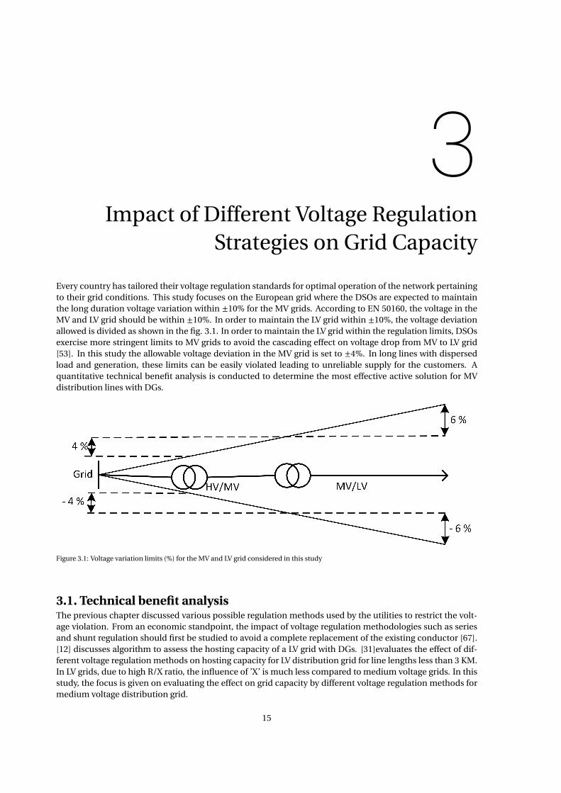
Every country has tailored their voltage regulation standards for optimal operation of the network pertainingto their grid conditions. This study focuses on the European grid where the DSOs are expected to maintainthe long duration voltage variation within ±10% for the MV grids. According to EN 50160, the voltage in theMV and LV grid should be within ±10%. In order to maintain the LV grid within ±10%, the voltage deviationallowed is divided as shown in the fig. 3.1. In order to maintain the LV grid within the regulation limits, DSOsexercise more stringent limits to MV grids to avoid the cascading effect on voltage drop from MV to LV grid[53]. In this study the allowable voltage deviation in the MV grid is set to ±4%. In long lines with dispersedload and generation, these limits can be easily violated leading to unreliable supply for the customers. Aquantitative technical benefit analysis is conducted to determine the most effective active solution for MVdistribution lines with DGs.
Figure 3.1: Voltage variation limits (%) for the MV and LV grid considered in this study
3.1. Technical benefit analysisThe previous chapter discussed various possible regulation methods used by the utilities to restrict the volt-age violation. From an economic standpoint, the impact of voltage regulation methodologies such as seriesand shunt regulation should first be studied to avoid a complete replacement of the existing conductor [67].[12] discusses algorithm to assess the hosting capacity of a LV grid with DGs. [31]evaluates the effect of dif-ferent voltage regulation methods on hosting capacity for LV distribution grid for line lengths less than 3 KM.In LV grids, due to high R/X ratio, the influence of ’X’ is much less compared to medium voltage grids. In thisstudy, the focus is given on evaluating the effect on grid capacity by different voltage regulation methods formedium voltage distribution grid.
15
16 3. Impact of Different Voltage Regulation Strategies on Grid Capacity
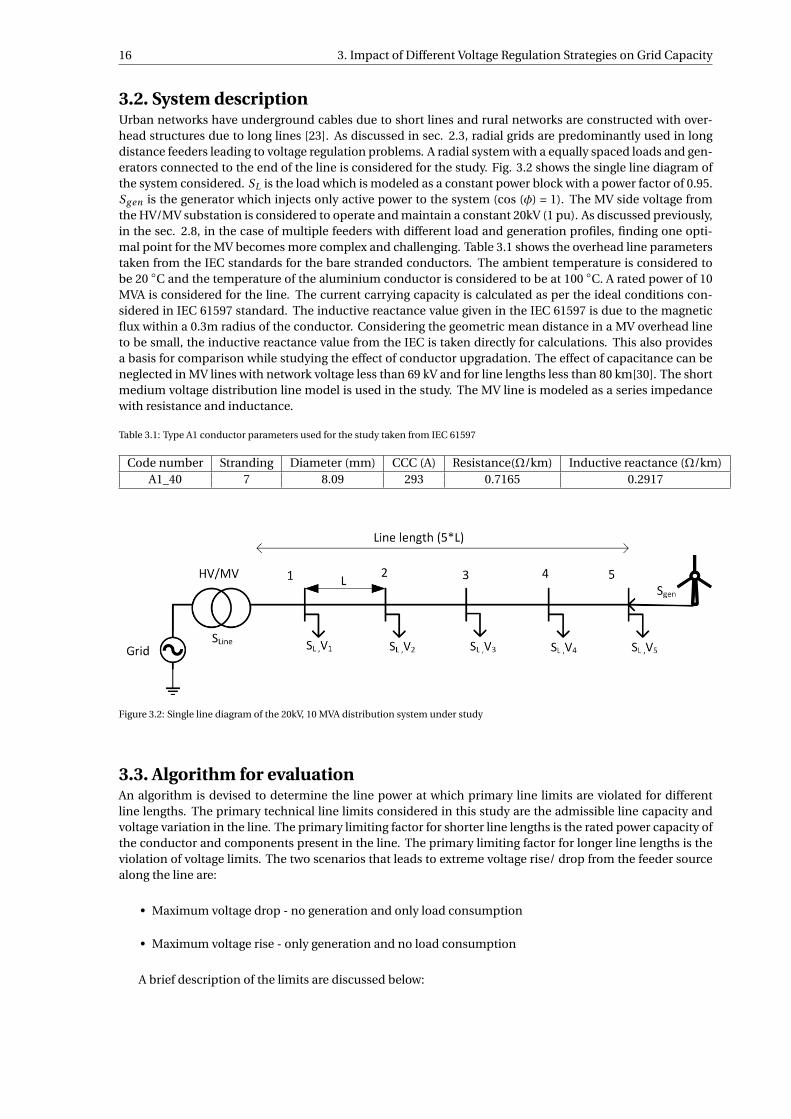
3.2. System descriptionUrban networks have underground cables due to short lines and rural networks are constructed with over-head structures due to long lines [23]. As discussed in sec. 2.3, radial grids are predominantly used in longdistance feeders leading to voltage regulation problems. A radial system with a equally spaced loads and gen-erators connected to the end of the line is considered for the study. Fig. 3.2 shows the single line diagram ofthe system considered. SL is the load which is modeled as a constant power block with a power factor of 0.95.Sg en is the generator which injects only active power to the system (cos (φ) = 1). The MV side voltage fromthe HV/MV substation is considered to operate and maintain a constant 20kV (1 pu). As discussed previously,in the sec. 2.8, in the case of multiple feeders with different load and generation profiles, finding one opti-mal point for the MV becomes more complex and challenging. Table 3.1 shows the overhead line parameterstaken from the IEC standards for the bare stranded conductors. The ambient temperature is considered tobe 20 C and the temperature of the aluminium conductor is considered to be at 100 C. A rated power of 10MVA is considered for the line. The current carrying capacity is calculated as per the ideal conditions con-sidered in IEC 61597 standard. The inductive reactance value given in the IEC 61597 is due to the magneticflux within a 0.3m radius of the conductor. Considering the geometric mean distance in a MV overhead lineto be small, the inductive reactance value from the IEC is taken directly for calculations. This also providesa basis for comparison while studying the effect of conductor upgradation. The effect of capacitance can beneglected in MV lines with network voltage less than 69 kV and for line lengths less than 80 km[30]. The shortmedium voltage distribution line model is used in the study. The MV line is modeled as a series impedancewith resistance and inductance.
Table 3.1: Type A1 conductor parameters used for the study taken from IEC 61597
Code number Stranding Diameter (mm) CCC (A) Resistance(Ω/km) Inductive reactance (Ω/km)A1_40 7 8.09 293 0.7165 0.2917
Figure 3.2: Single line diagram of the 20kV, 10 MVA distribution system under study
3.3. Algorithm for evaluationAn algorithm is devised to determine the line power at which primary line limits are violated for differentline lengths. The primary technical line limits considered in this study are the admissible line capacity andvoltage variation in the line. The primary limiting factor for shorter line lengths is the rated power capacity ofthe conductor and components present in the line. The primary limiting factor for longer line lengths is theviolation of voltage limits. The two scenarios that leads to extreme voltage rise/ drop from the feeder sourcealong the line are:
• Maximum voltage drop - no generation and only load consumption
• Maximum voltage rise - only generation and no load consumption
A brief description of the limits are discussed below:
3.3. Algorithm for evaluation 17
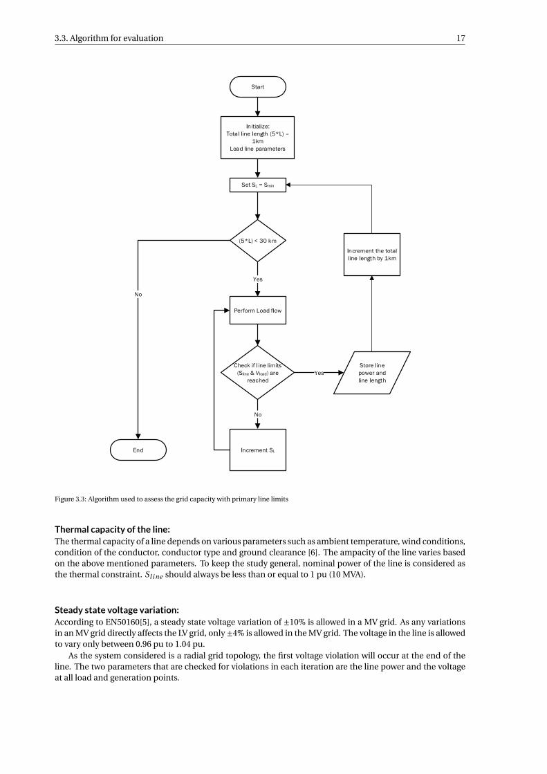
Figure 3.3: Algorithm used to assess the grid capacity with primary line limits
Thermal capacity of the line:The thermal capacity of a line depends on various parameters such as ambient temperature, wind conditions,condition of the conductor, conductor type and ground clearance [6]. The ampacity of the line varies basedon the above mentioned parameters. To keep the study general, nominal power of the line is considered asthe thermal constraint. Sl i ne should always be less than or equal to 1 pu (10 MVA).
Steady state voltage variation:According to EN50160[5], a steady state voltage variation of ±10% is allowed in a MV grid. As any variationsin an MV grid directly affects the LV grid, only ±4% is allowed in the MV grid. The voltage in the line is allowedto vary only between 0.96 pu to 1.04 pu.
As the system considered is a radial grid topology, the first voltage violation will occur at the end of theline. The two parameters that are checked for violations in each iteration are the line power and the voltageat all load and generation points.
18 3. Impact of Different Voltage Regulation Strategies on Grid Capacity
Fig.3.3 shows the algorithm used for the evaluation. The algorithm starts with initializing the line lengthas 1 km and setting all the load and generation to zero. The line length is now fixed and the power of theload/ generator is increased in steps for the respective scenario. For each increment of the power, load flow isexecuted and the parameters are extracted from the model, and checked for primary line violations. Once anyof the line limits are violated, the corresponding line power and the line lengths are stored. The line power atwhich any of the limits are violated is the line capacity of the grid. The final graph is plotted against the linecapacity and line length to understand the effect of voltage violation in long distribution lines.
The same algorithm is executed with a shunt and series voltage regulation strategy. Line capacity is ob-tained with respect to the line lengths and the percentage increase in the grid capacity is presented. In eachsection, a load and a generation scenario is considered and studied in detail.
3.4. No regulation3.4.1. Load scenarioIn this case, it is assumed that there is only load consumption in the grid without any generation. Fig.3.4shows the line diagram of the system without any voltage compensation. Fig. 3.5 shows the grid capacity asa function of line length with the primary line limits. It can be seen that for the initial 3 km, the primary linelimitation is the thermal or power capacity of the line. As the line length gets higher, the voltage deviation of- 4% is reached at the end of the line before the full power capacity is reached. The reduction in line capacitydue to voltage limit violation is non-linear with the line length. This leads to large reduction in line capacityfor long lines.
Figure 3.4: Single line diagram of the system with no regulation for load scenario
Figure 3.5: Line capacity vs Line length for the load scenario without any regulation
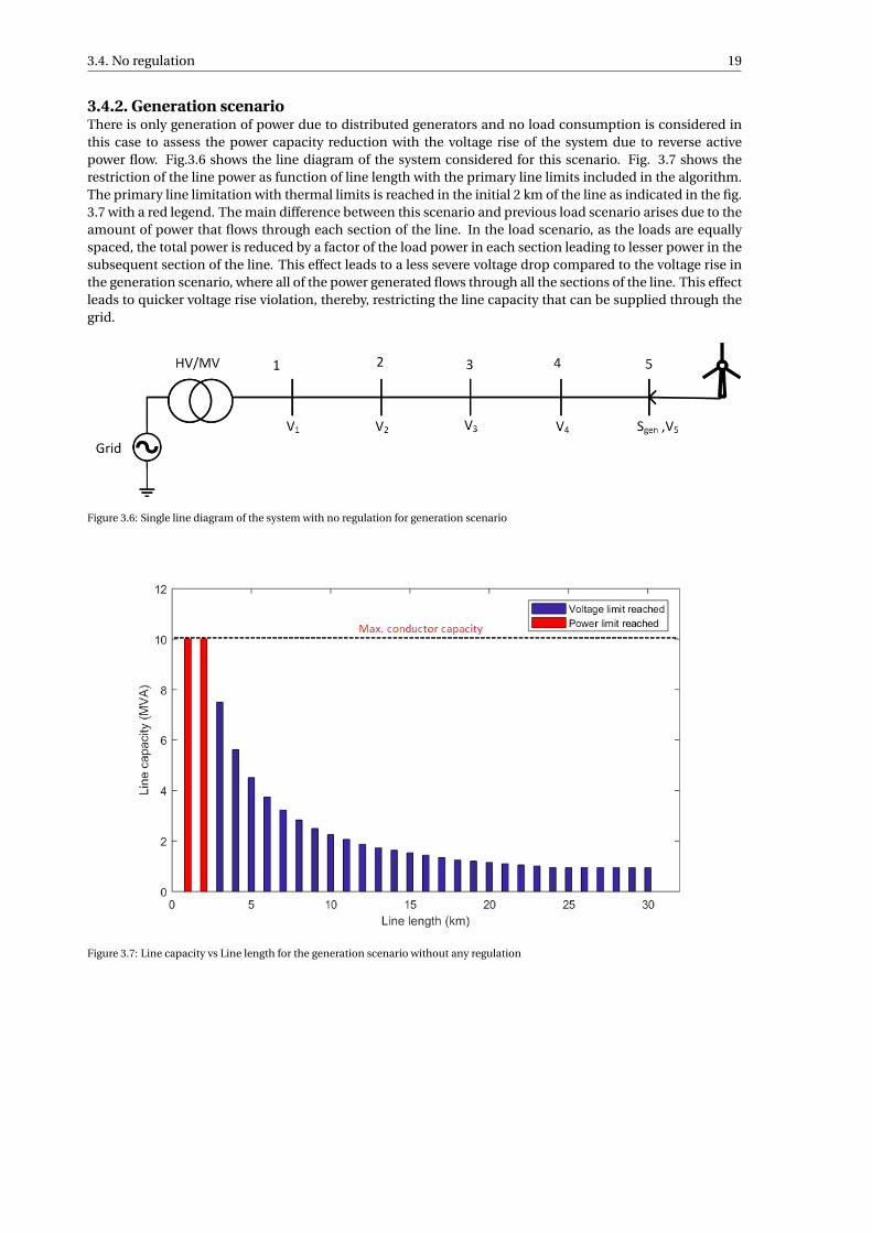
3.4. No regulation 19
3.4.2. Generation scenarioThere is only generation of power due to distributed generators and no load consumption is considered inthis case to assess the power capacity reduction with the voltage rise of the system due to reverse activepower flow. Fig.3.6 shows the line diagram of the system considered for this scenario. Fig. 3.7 shows therestriction of the line power as function of line length with the primary line limits included in the algorithm.The primary line limitation with thermal limits is reached in the initial 2 km of the line as indicated in the fig.3.7 with a red legend. The main difference between this scenario and previous load scenario arises due to theamount of power that flows through each section of the line. In the load scenario, as the loads are equallyspaced, the total power is reduced by a factor of the load power in each section leading to lesser power in thesubsequent section of the line. This effect leads to a less severe voltage drop compared to the voltage rise inthe generation scenario, where all of the power generated flows through all the sections of the line. This effectleads to quicker voltage rise violation, thereby, restricting the line capacity that can be supplied through thegrid.
Figure 3.6: Single line diagram of the system with no regulation for generation scenario
Figure 3.7: Line capacity vs Line length for the generation scenario without any regulation
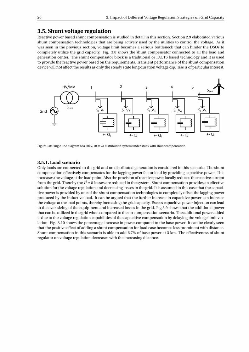
20 3. Impact of Different Voltage Regulation Strategies on Grid Capacity
3.5. Shunt voltage regulationReactive power based shunt compensation is studied in detail in this section. Section 2.9 elaborated variousshunt compensation technologies that are being actively used by the utilities to control the voltage. As itwas seen in the previous section, voltage limit becomes a serious bottleneck that can hinder the DSOs tocompletely utilize the grid capacity. Fig. 3.8 shows the shunt compensator connected to all the load andgeneration center. The shunt compensator block is a traditional or FACTS based technology and it is usedto provide the reactive power based on the requirements. Transient performance of the shunt compensationdevice will not affect the results as only the steady state long duration voltage dip/ rise is of particular interest.
Figure 3.8: Single line diagram of a 20kV, 10 MVA distribution system under study with shunt compensation
3.5.1. Load scenarioOnly loads are connected to the grid and no distributed generation is considered in this scenario. The shuntcompensation effectively compensates for the lagging power factor load by providing capacitive power. Thisincreases the voltage at the load point. Also the provision of reactive power locally reduces the reactive currentfrom the grid. Thereby the I 2 ∗R losses are reduced in the system. Shunt compensation provides an effectivesolution for the voltage regulation and decreasing losses in the grid. It is assumed in this case that the capaci-tive power is provided by one of the shunt compensation technologies to completely offset the lagging powerproduced by the inductive load. It can be argued that the further increase in capacitive power can increasethe voltage at the load points, thereby increasing the grid capacity. Excess capacitive power injection can leadto the over-sizing of the equipment and increased losses in the grid. Fig.3.9 shows that the additional powerthat can be utilized in the grid when compared to the no compensation scenario. The additional power addedis due to the voltage regulation capabilities of the capacitive compensation by delaying the voltage limit vio-lation. Fig. 3.10 shows the percentage increase in power compared to the base power. It can be clearly seenthat the positive effect of adding a shunt compensation for load case becomes less prominent with distance.Shunt compensation in this scenario is able to add 6.7% of base power at 3 km. The effectiveness of shuntregulator on voltage regulation decreases with the increasing distance.
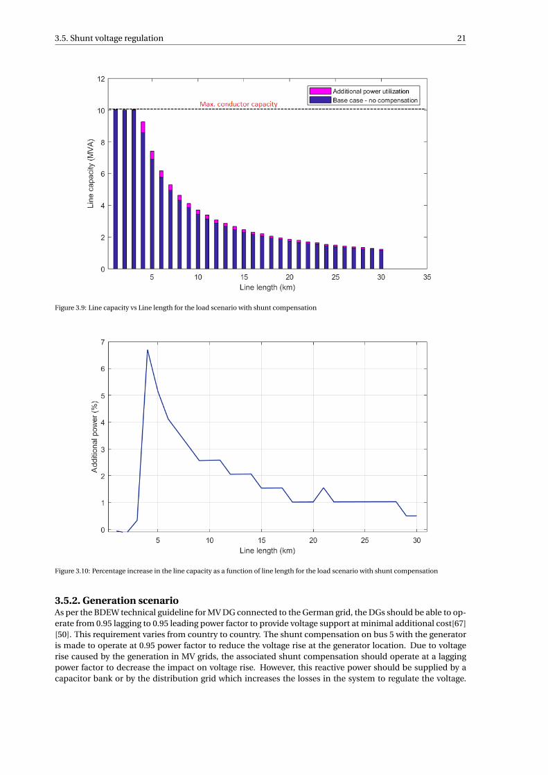
3.5. Shunt voltage regulation 21
Figure 3.9: Line capacity vs Line length for the load scenario with shunt compensation
Figure 3.10: Percentage increase in the line capacity as a function of line length for the load scenario with shunt compensation
3.5.2. Generation scenarioAs per the BDEW technical guideline for MV DG connected to the German grid, the DGs should be able to op-erate from 0.95 lagging to 0.95 leading power factor to provide voltage support at minimal additional cost[67][50]. This requirement varies from country to country. The shunt compensation on bus 5 with the generatoris made to operate at 0.95 power factor to reduce the voltage rise at the generator location. Due to voltagerise caused by the generation in MV grids, the associated shunt compensation should operate at a laggingpower factor to decrease the impact on voltage rise. However, this reactive power should be supplied by acapacitor bank or by the distribution grid which increases the losses in the system to regulate the voltage.
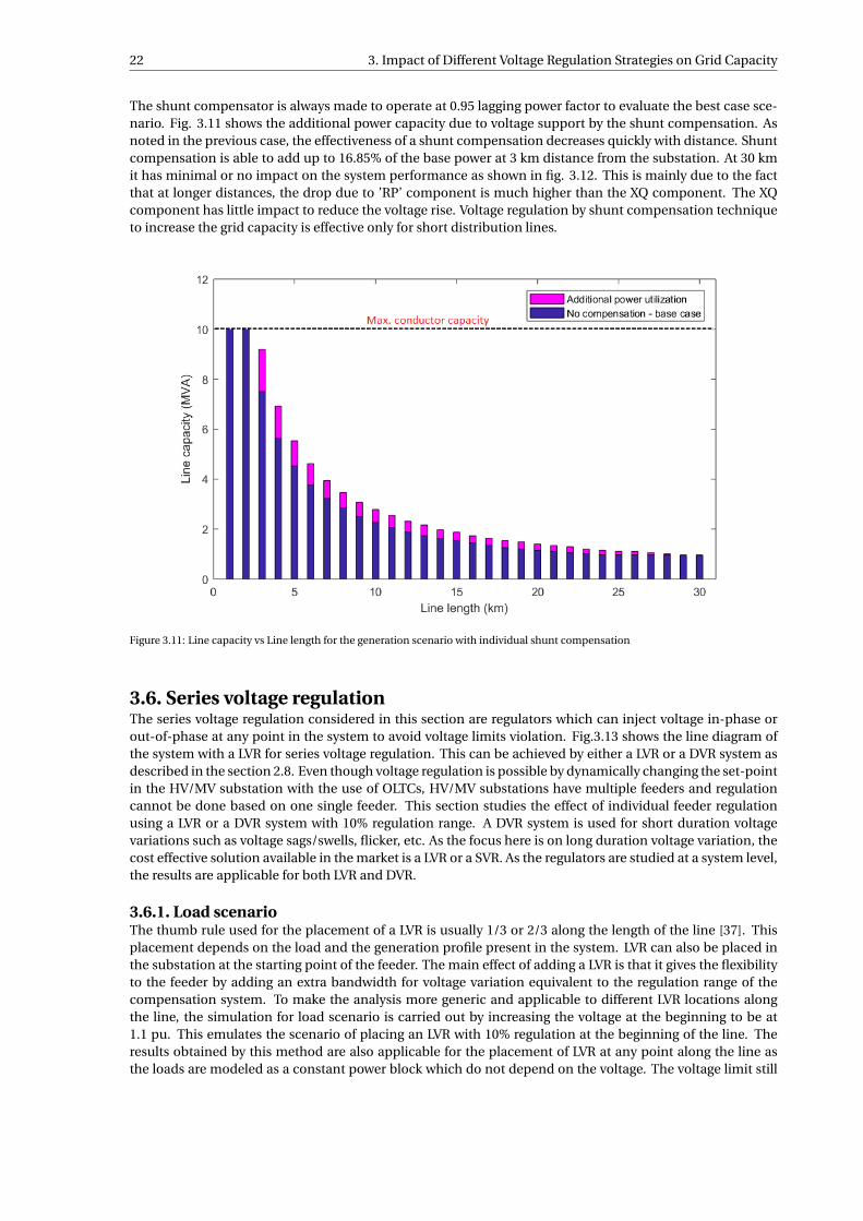
22 3. Impact of Different Voltage Regulation Strategies on Grid Capacity
The shunt compensator is always made to operate at 0.95 lagging power factor to evaluate the best case sce-nario. Fig. 3.11 shows the additional power capacity due to voltage support by the shunt compensation. Asnoted in the previous case, the effectiveness of a shunt compensation decreases quickly with distance. Shuntcompensation is able to add up to 16.85% of the base power at 3 km distance from the substation. At 30 kmit has minimal or no impact on the system performance as shown in fig. 3.12. This is mainly due to the factthat at longer distances, the drop due to ’RP’ component is much higher than the XQ component. The XQcomponent has little impact to reduce the voltage rise. Voltage regulation by shunt compensation techniqueto increase the grid capacity is effective only for short distribution lines.
Figure 3.11: Line capacity vs Line length for the generation scenario with individual shunt compensation
3.6. Series voltage regulationThe series voltage regulation considered in this section are regulators which can inject voltage in-phase orout-of-phase at any point in the system to avoid voltage limits violation. Fig.3.13 shows the line diagram ofthe system with a LVR for series voltage regulation. This can be achieved by either a LVR or a DVR system asdescribed in the section 2.8. Even though voltage regulation is possible by dynamically changing the set-pointin the HV/MV substation with the use of OLTCs, HV/MV substations have multiple feeders and regulationcannot be done based on one single feeder. This section studies the effect of individual feeder regulationusing a LVR or a DVR system with 10% regulation range. A DVR system is used for short duration voltagevariations such as voltage sags/swells, flicker, etc. As the focus here is on long duration voltage variation, thecost effective solution available in the market is a LVR or a SVR. As the regulators are studied at a system level,the results are applicable for both LVR and DVR.
3.6.1. Load scenarioThe thumb rule used for the placement of a LVR is usually 1/3 or 2/3 along the length of the line [37]. Thisplacement depends on the load and the generation profile present in the system. LVR can also be placed inthe substation at the starting point of the feeder. The main effect of adding a LVR is that it gives the flexibilityto the feeder by adding an extra bandwidth for voltage variation equivalent to the regulation range of thecompensation system. To make the analysis more generic and applicable to different LVR locations alongthe line, the simulation for load scenario is carried out by increasing the voltage at the beginning to be at1.1 pu. This emulates the scenario of placing an LVR with 10% regulation at the beginning of the line. Theresults obtained by this method are also applicable for the placement of LVR at any point along the line asthe loads are modeled as a constant power block which do not depend on the voltage. The voltage limit still
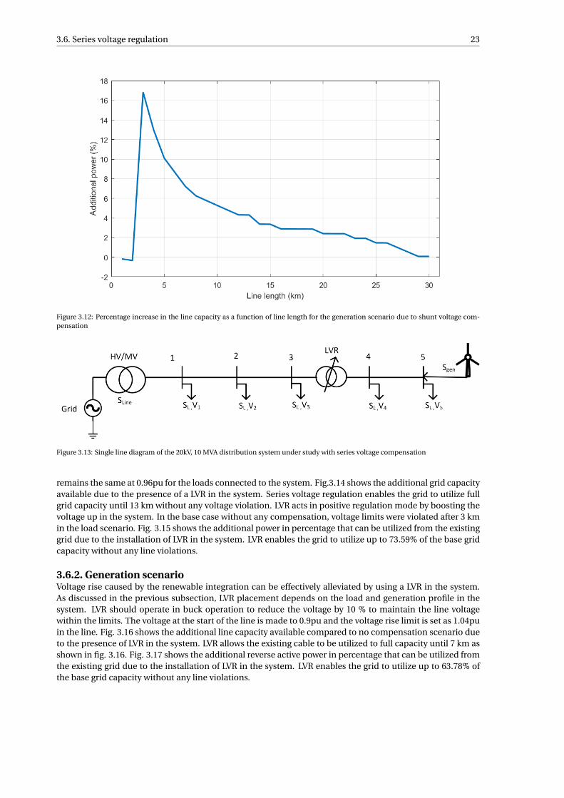
3.6. Series voltage regulation 23
Figure 3.12: Percentage increase in the line capacity as a function of line length for the generation scenario due to shunt voltage com-pensation
Figure 3.13: Single line diagram of the 20kV, 10 MVA distribution system under study with series voltage compensation
remains the same at 0.96pu for the loads connected to the system. Fig.3.14 shows the additional grid capacityavailable due to the presence of a LVR in the system. Series voltage regulation enables the grid to utilize fullgrid capacity until 13 km without any voltage violation. LVR acts in positive regulation mode by boosting thevoltage up in the system. In the base case without any compensation, voltage limits were violated after 3 kmin the load scenario. Fig. 3.15 shows the additional power in percentage that can be utilized from the existinggrid due to the installation of LVR in the system. LVR enables the grid to utilize up to 73.59% of the base gridcapacity without any line violations.
3.6.2. Generation scenarioVoltage rise caused by the renewable integration can be effectively alleviated by using a LVR in the system.As discussed in the previous subsection, LVR placement depends on the load and generation profile in thesystem. LVR should operate in buck operation to reduce the voltage by 10 % to maintain the line voltagewithin the limits. The voltage at the start of the line is made to 0.9pu and the voltage rise limit is set as 1.04puin the line. Fig. 3.16 shows the additional line capacity available compared to no compensation scenario dueto the presence of LVR in the system. LVR allows the existing cable to be utilized to full capacity until 7 km asshown in fig. 3.16. Fig. 3.17 shows the additional reverse active power in percentage that can be utilized fromthe existing grid due to the installation of LVR in the system. LVR enables the grid to utilize up to 63.78% ofthe base grid capacity without any line violations.
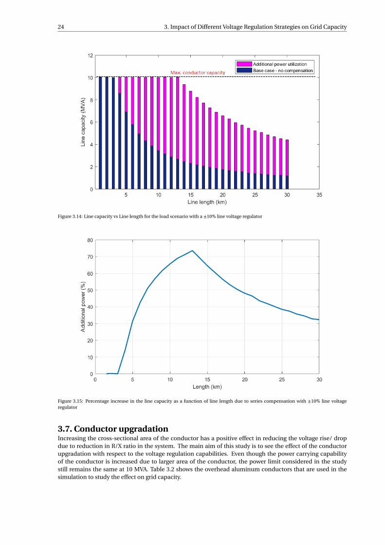
24 3. Impact of Different Voltage Regulation Strategies on Grid Capacity
Figure 3.14: Line capacity vs Line length for the load scenario with a ±10% line voltage regulator
Figure 3.15: Percentage increase in the line capacity as a function of line length due to series compensation with ±10% line voltageregulator
3.7. Conductor upgradationIncreasing the cross-sectional area of the conductor has a positive effect in reducing the voltage rise/ dropdue to reduction in R/X ratio in the system. The main aim of this study is to see the effect of the conductorupgradation with respect to the voltage regulation capabilities. Even though the power carrying capabilityof the conductor is increased due to larger area of the conductor, the power limit considered in the studystill remains the same at 10 MVA. Table 3.2 shows the overhead aluminum conductors that are used in thesimulation to study the effect on grid capacity.
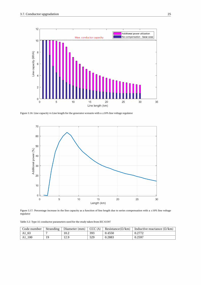
3.7. Conductor upgradation 25
Figure 3.16: Line capacity vs Line length for the generator scenario with a ±10% line voltage regulator
Figure 3.17: Percentage increase in the line capacity as a function of line length due to series compensation with a ±10% line voltageregulator
Table 3.2: Type A1 conductor parameters used for the study taken from IEC 61597
Code number Stranding Diameter (mm) CCC (A) Resistance(Ω/km) Inductive reactance (Ω/km)A1_63 7 10.2 393 0.4550 0.2772A1_100 19 12.9 529 0.2883 0.2597
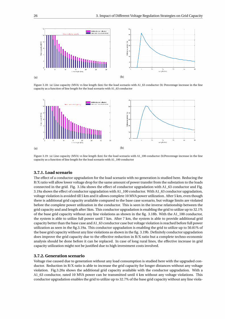
26 3. Impact of Different Voltage Regulation Strategies on Grid Capacity
(a) (b)
Figure 3.18: (a) Line capacity (MVA) vs line length (km) for the load scenario with A1_63 conductor (b) Percentage increase in the linecapacity as a function of line length for the load scenario with A1_63 conductor
(a) (b)
Figure 3.19: (a) Line capacity (MVA) vs line length (km) for the load scenario with A1_100 conductor (b)Percentage increase in the linecapacity as a function of line length for the load scenario with A1_100 conductor
3.7.1. Load scenarioThe effect of a conductor upgradation for the load scenario with no generation is studied here. Reducing theR/X ratio will allow lower voltage drop for the same amount of power transfer from the substation to the loadsconnected in the grid. Fig. 3.18a shows the effect of conductor upgradation with A1_63 conductor and Fig.3.19a shows the effect of conductor upgradation with A1_100 conductor. With A1_63 conductor upgradation,voltage violation is avoided till 5 km and it allows complete 10 MVA power utilization. After 5 km, even thoughthere is additional grid capacity available compared to the base case scenario, but voltage limits are violatedbefore the complete power utilization in the conductor. This is seen in the inverse relationship between thegrid capacity and and length after 5km. This conductor upgradation is enabling the grid to utilize up to 32.1%of the base grid capacity without any line violations as shown in the fig. 3.18b. With the A1_100 conductor,the system is able to utilize full power until 7 km. After 7 km, the system is able to provide additional gridcapacity better than the base case and A1_63 conductor case but voltage violation is reached before full powerutilization as seen in the fig.3.19a. This conductor upgradation is enabling the grid to utilize up to 50.81% ofthe base grid capacity without any line violations as shown in the fig. 3.19b. Definitely conductor upgradationdoes improve the grid capacity due to the effective reduction in R/X ratio but a complete techno-economicanalysis should be done before it can be replaced. In case of long rural lines, the effective increase in gridcapacity utilization might not be justified due to high investment costs involved.
3.7.2. Generation scenarioVoltage rise caused due to generation without any load consumption is studied here with the upgraded con-ductor. Reduction in R/X ratio is able to increase the grid capacity for longer distances without any voltageviolation. Fig.3.20a shows the additional grid capacity available with the conductor upgradation. With aA1_63 conductor, rated 10 MVA power can be transmitted until 4 km without any voltage violations. Thisconductor upgradation enables the grid to utilize up to 32.7% of the base grid capacity without any line viola-
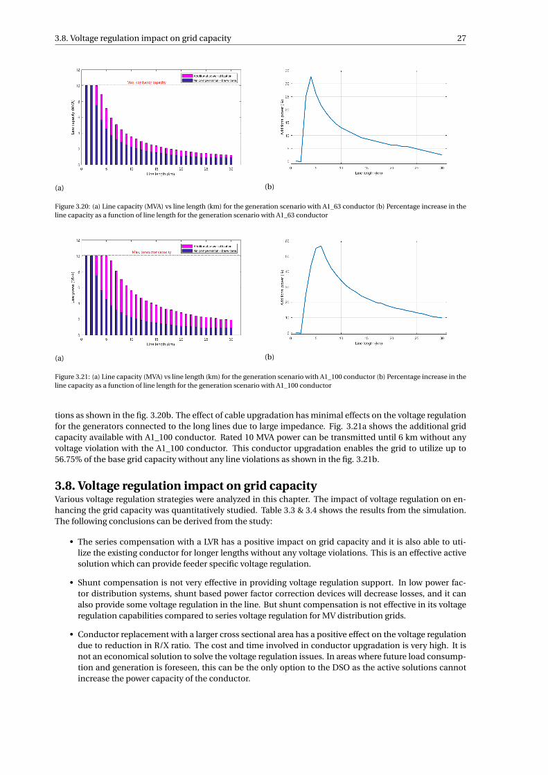
3.8. Voltage regulation impact on grid capacity 27
(a) (b)
Figure 3.20: (a) Line capacity (MVA) vs line length (km) for the generation scenario with A1_63 conductor (b) Percentage increase in theline capacity as a function of line length for the generation scenario with A1_63 conductor
(a) (b)
Figure 3.21: (a) Line capacity (MVA) vs line length (km) for the generation scenario with A1_100 conductor (b) Percentage increase in theline capacity as a function of line length for the generation scenario with A1_100 conductor
tions as shown in the fig. 3.20b. The effect of cable upgradation has minimal effects on the voltage regulationfor the generators connected to the long lines due to large impedance. Fig. 3.21a shows the additional gridcapacity available with A1_100 conductor. Rated 10 MVA power can be transmitted until 6 km without anyvoltage violation with the A1_100 conductor. This conductor upgradation enables the grid to utilize up to56.75% of the base grid capacity without any line violations as shown in the fig. 3.21b.
3.8. Voltage regulation impact on grid capacityVarious voltage regulation strategies were analyzed in this chapter. The impact of voltage regulation on en-hancing the grid capacity was quantitatively studied. Table 3.3 & 3.4 shows the results from the simulation.The following conclusions can be derived from the study:
• The series compensation with a LVR has a positive impact on grid capacity and it is also able to uti-lize the existing conductor for longer lengths without any voltage violations. This is an effective activesolution which can provide feeder specific voltage regulation.
• Shunt compensation is not very effective in providing voltage regulation support. In low power fac-tor distribution systems, shunt based power factor correction devices will decrease losses, and it canalso provide some voltage regulation in the line. But shunt compensation is not effective in its voltageregulation capabilities compared to series voltage regulation for MV distribution grids.
• Conductor replacement with a larger cross sectional area has a positive effect on the voltage regulationdue to reduction in R/X ratio. The cost and time involved in conductor upgradation is very high. It isnot an economical solution to solve the voltage regulation issues. In areas where future load consump-tion and generation is foreseen, this can be the only option to the DSO as the active solutions cannotincrease the power capacity of the conductor.
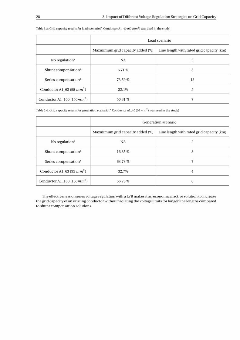
28 3. Impact of Different Voltage Regulation Strategies on Grid Capacity
Table 3.3: Grid capacity results for load scenario(∗ Conductor A1_40 (60 mm2) was used in the study)
Load scenario
Maxmimum grid capacity added (%) Line length with rated grid capacity (km)
No regulation* NA 3
Shunt compensation* 6.71 % 3
Series compensation* 73.59 % 13
Conductor A1_63 (95 mm2) 32.1% 5
Conductor A1_100 (150mm2) 50.81 % 7
Table 3.4: Grid capacity results for generation scenario(∗ Conductor A1_40 (60 mm2) was used in the study)
Generation scenario
Maxmimum grid capacity added (%) Line length with rated grid capacity (km)
No regulation* NA 2
Shunt compensation* 16.85 % 3
Series compensation* 63.78 % 7
Conductor A1_63 (95 mm2) 32.7% 4
Conductor A1_100 (150mm2) 56.75 % 6
The effectiveness of series voltage regulation with a LVR makes it an economical active solution to increasethe grid capacity of an existing conductor without violating the voltage limits for longer line lengths comparedto shunt compensation solutions.
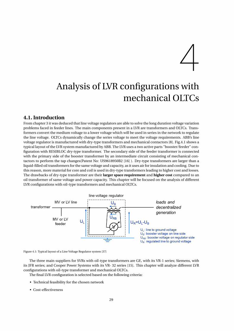
4Analysis of LVR configurations with
mechanical OLTCs
4.1. IntroductionFrom chapter 3 it was deduced that line voltage regulators are able to solve the long duration voltage variationproblems faced in feeder lines. The main components present in a LVR are transformers and OLTCs. Trans-formers convert the medium voltage to a lower voltage which will be used in series in the network to regulatethe line voltage. OLTCs dynamically change the series voltage to meet the voltage requirements. ABB’s linevoltage regulator is manufactured with dry-type transformers and mechanical contactors [8]. Fig.4.1 shows atypical layout of the LVR system manufactured by ABB. The LVR uses a two active parts "booster/feeder" con-figuration with RESIBLOC dry-type transformer. The secondary side of the feeder transformer is connectedwith the primary side of the booster transformer by an intermediate circuit consisting of mechanical con-tactors to perform the tap changes(Patent No: US9618950B2 [16] ). Dry-type transformers are larger than aliquid-filled oil transformers for the same voltage and capacity, as it uses air for insulation and cooling. Due tothis reason, more material for core and coil is used in dry-type transformers leading to higher cost and losses.The drawbacks of dry-type transformer are their larger space requirement and higher cost compared to anoil transformer of same voltage and power capacity. This chapter will be focused on the analysis of differentLVR configurations with oil-type transformers and mechanical OLTCs.
Figure 4.1: Typical layout of a Line Voltage Regulator system [37]
The three main suppliers for SVRs with oil-type transformers are GE, with its VR-1 series; Siemens, withits JFR series; and Cooper Power Systems with its VR- 32 series [15]. This chapter will analyze different LVRconfigurations with oil-type transformer and mechanical OLTCs.
The final LVR configuration is selected based on the following criteria:
• Technical feasibility for the chosen network
• Cost-effectiveness
29
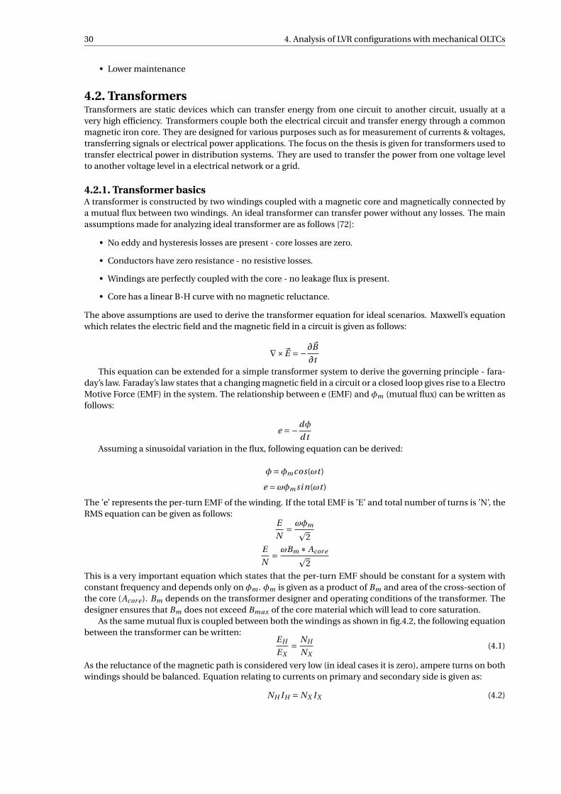
30 4. Analysis of LVR configurations with mechanical OLTCs
• Lower maintenance
4.2. TransformersTransformers are static devices which can transfer energy from one circuit to another circuit, usually at avery high efficiency. Transformers couple both the electrical circuit and transfer energy through a commonmagnetic iron core. They are designed for various purposes such as for measurement of currents & voltages,transferring signals or electrical power applications. The focus on the thesis is given for transformers used totransfer electrical power in distribution systems. They are used to transfer the power from one voltage levelto another voltage level in a electrical network or a grid.
4.2.1. Transformer basicsA transformer is constructed by two windings coupled with a magnetic core and magnetically connected bya mutual flux between two windings. An ideal transformer can transfer power without any losses. The mainassumptions made for analyzing ideal transformer are as follows [72]:
• No eddy and hysteresis losses are present - core losses are zero.
• Conductors have zero resistance - no resistive losses.
• Windings are perfectly coupled with the core - no leakage flux is present.
• Core has a linear B-H curve with no magnetic reluctance.
The above assumptions are used to derive the transformer equation for ideal scenarios. Maxwell’s equationwhich relates the electric field and the magnetic field in a circuit is given as follows:
∇×~E =−∂~B
∂tThis equation can be extended for a simple transformer system to derive the governing principle - fara-
day’s law. Faraday’s law states that a changing magnetic field in a circuit or a closed loop gives rise to a ElectroMotive Force (EMF) in the system. The relationship between e (EMF) and φm (mutual flux) can be written asfollows:
e =−dφ
d tAssuming a sinusoidal variation in the flux, following equation can be derived:
φ=φmcos(ωt )
e =ωφm si n(ωt )
The ’e’ represents the per-turn EMF of the winding. If the total EMF is ’E’ and total number of turns is ’N’, theRMS equation can be given as follows:
E
N= ωφmp
2E
N= ωBm ∗ Acor ep
2
This is a very important equation which states that the per-turn EMF should be constant for a system withconstant frequency and depends only on φm . φm is given as a product of Bm and area of the cross-section ofthe core (Acor e ). Bm depends on the transformer designer and operating conditions of the transformer. Thedesigner ensures that Bm does not exceed Bmax of the core material which will lead to core saturation.
As the same mutual flux is coupled between both the windings as shown in fig.4.2, the following equationbetween the transformer can be written:
EH
EX= NH
NX(4.1)
As the reluctance of the magnetic path is considered very low (in ideal cases it is zero), ampere turns on bothwindings should be balanced. Equation relating to currents on primary and secondary side is given as:
NH IH = NX IX (4.2)
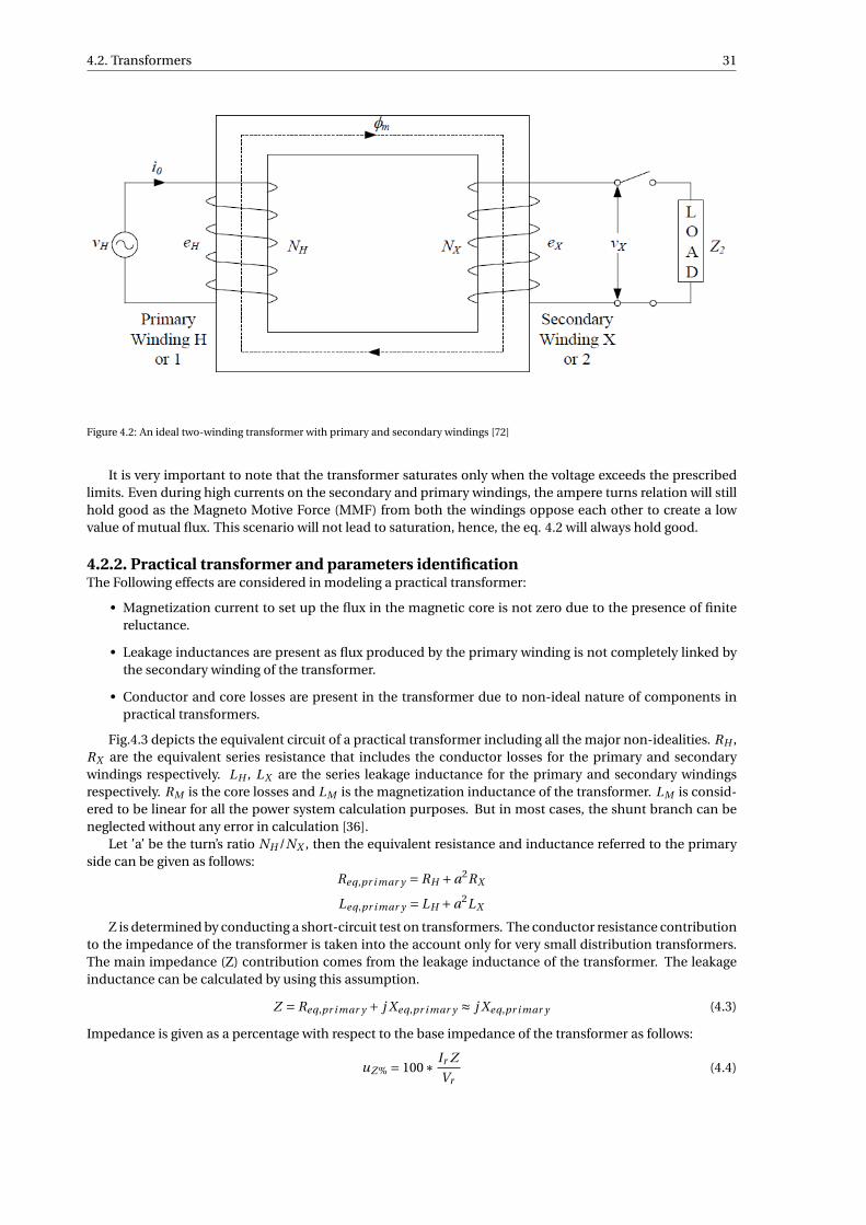
4.2. Transformers 31
Figure 4.2: An ideal two-winding transformer with primary and secondary windings [72]
It is very important to note that the transformer saturates only when the voltage exceeds the prescribedlimits. Even during high currents on the secondary and primary windings, the ampere turns relation will stillhold good as the Magneto Motive Force (MMF) from both the windings oppose each other to create a lowvalue of mutual flux. This scenario will not lead to saturation, hence, the eq. 4.2 will always hold good.
4.2.2. Practical transformer and parameters identificationThe Following effects are considered in modeling a practical transformer:
• Magnetization current to set up the flux in the magnetic core is not zero due to the presence of finitereluctance.
• Leakage inductances are present as flux produced by the primary winding is not completely linked bythe secondary winding of the transformer.
• Conductor and core losses are present in the transformer due to non-ideal nature of components inpractical transformers.
Fig.4.3 depicts the equivalent circuit of a practical transformer including all the major non-idealities. RH ,RX are the equivalent series resistance that includes the conductor losses for the primary and secondarywindings respectively. LH , LX are the series leakage inductance for the primary and secondary windingsrespectively. RM is the core losses and LM is the magnetization inductance of the transformer. LM is consid-ered to be linear for all the power system calculation purposes. But in most cases, the shunt branch can beneglected without any error in calculation [36].
Let ’a’ be the turn’s ratio NH /NX , then the equivalent resistance and inductance referred to the primaryside can be given as follows:
Req,pr i mar y = RH +a2RX
Leq,pr i mar y = LH +a2LX
Z is determined by conducting a short-circuit test on transformers. The conductor resistance contributionto the impedance of the transformer is taken into the account only for very small distribution transformers.The main impedance (Z) contribution comes from the leakage inductance of the transformer. The leakageinductance can be calculated by using this assumption.
Z = Req,pr i mar y + j Xeq,pr i mar y ≈ j Xeq,pr i mar y (4.3)
Impedance is given as a percentage with respect to the base impedance of the transformer as follows:
uZ % = 100∗ Ir Z
Vr(4.4)
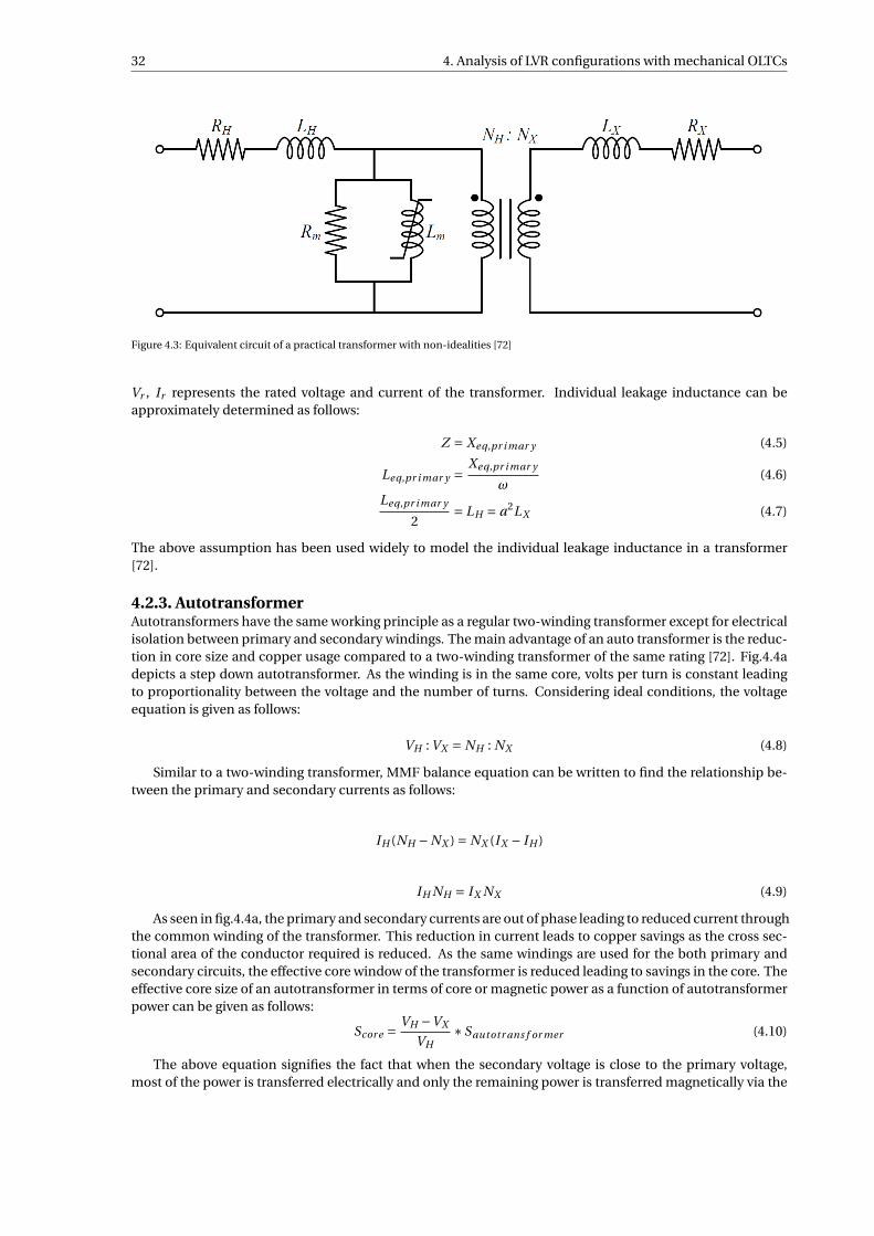
32 4. Analysis of LVR configurations with mechanical OLTCs
Figure 4.3: Equivalent circuit of a practical transformer with non-idealities [72]
Vr , Ir represents the rated voltage and current of the transformer. Individual leakage inductance can beapproximately determined as follows:
Z = Xeq,pr i mar y (4.5)
Leq,pr i mar y =Xeq,pr i mar y
ω(4.6)
Leq,pr i mar y
2= LH = a2LX (4.7)
The above assumption has been used widely to model the individual leakage inductance in a transformer[72].
4.2.3. AutotransformerAutotransformers have the same working principle as a regular two-winding transformer except for electricalisolation between primary and secondary windings. The main advantage of an auto transformer is the reduc-tion in core size and copper usage compared to a two-winding transformer of the same rating [72]. Fig.4.4adepicts a step down autotransformer. As the winding is in the same core, volts per turn is constant leadingto proportionality between the voltage and the number of turns. Considering ideal conditions, the voltageequation is given as follows:
VH : VX = NH : NX (4.8)
Similar to a two-winding transformer, MMF balance equation can be written to find the relationship be-tween the primary and secondary currents as follows:
IH (NH −NX ) = NX (IX − IH )
IH NH = IX NX (4.9)
As seen in fig.4.4a, the primary and secondary currents are out of phase leading to reduced current throughthe common winding of the transformer. This reduction in current leads to copper savings as the cross sec-tional area of the conductor required is reduced. As the same windings are used for the both primary andsecondary circuits, the effective core window of the transformer is reduced leading to savings in the core. Theeffective core size of an autotransformer in terms of core or magnetic power as a function of autotransformerpower can be given as follows:
Scor e = VH −VX
VH∗Sautotr ans f or mer (4.10)
The above equation signifies the fact that when the secondary voltage is close to the primary voltage,most of the power is transferred electrically and only the remaining power is transferred magnetically via the
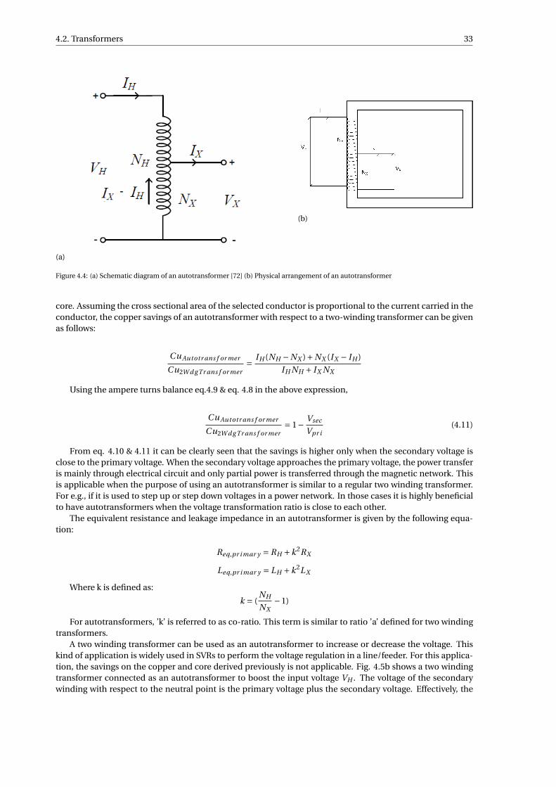
4.2. Transformers 33
(a)
(b)
Figure 4.4: (a) Schematic diagram of an autotransformer [72] (b) Physical arrangement of an autotransformer
core. Assuming the cross sectional area of the selected conductor is proportional to the current carried in theconductor, the copper savings of an autotransformer with respect to a two-winding transformer can be givenas follows:
CuAutotr ans f or mer
Cu2W d g Tr ans f or mer= IH (NH −NX )+NX (IX − IH )
IH NH + IX NX
Using the ampere turns balance eq.4.9 & eq. 4.8 in the above expression,
CuAutotr ans f or mer
Cu2W d g Tr ans f or mer= 1− Vsec
Vpr i(4.11)
From eq. 4.10 & 4.11 it can be clearly seen that the savings is higher only when the secondary voltage isclose to the primary voltage. When the secondary voltage approaches the primary voltage, the power transferis mainly through electrical circuit and only partial power is transferred through the magnetic network. Thisis applicable when the purpose of using an autotransformer is similar to a regular two winding transformer.For e.g., if it is used to step up or step down voltages in a power network. In those cases it is highly beneficialto have autotransformers when the voltage transformation ratio is close to each other.
The equivalent resistance and leakage impedance in an autotransformer is given by the following equa-tion:
Req,pr i mar y = RH +k2RX
Leq,pr i mar y = LH +k2LX
Where k is defined as:
k = (NH
NX−1)
For autotransformers, ’k’ is referred to as co-ratio. This term is similar to ratio ’a’ defined for two windingtransformers.
A two winding transformer can be used as an autotransformer to increase or decrease the voltage. Thiskind of application is widely used in SVRs to perform the voltage regulation in a line/feeder. For this applica-tion, the savings on the copper and core derived previously is not applicable. Fig. 4.5b shows a two windingtransformer connected as an autotransformer to boost the input voltage VH . The voltage of the secondarywinding with respect to the neutral point is the primary voltage plus the secondary voltage. Effectively, the
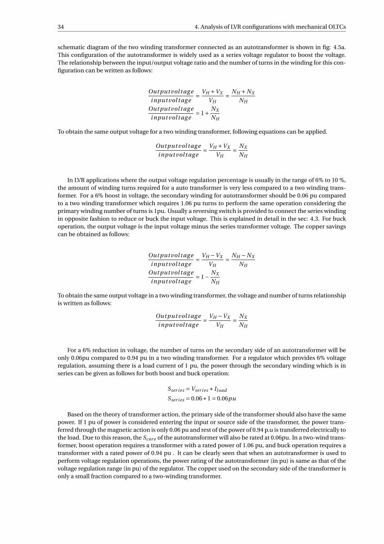
34 4. Analysis of LVR configurations with mechanical OLTCs
schematic diagram of the two winding transformer connected as an autotransformer is shown in fig: 4.5a.This configuration of the autotransformer is widely used as a series voltage regulator to boost the voltage.The relationship between the input/output voltage ratio and the number of turns in the winding for this con-figuration can be written as follows:
Out put vol t ag e
i nput vol t ag e= VH +VX
VH= NH +NX
NH
Out put vol t ag e
i nput vol t ag e= 1+ NX
NH
To obtain the same output voltage for a two winding transformer, following equations can be applied.
Out put vol t ag e
i nput vol t ag e= VH +VX
VH= NX
NH
In LVR applications where the output voltage regulation percentage is usually in the range of 6% to 10 %,the amount of winding turns required for a auto transformer is very less compared to a two winding trans-former. For a 6% boost in voltage, the secondary winding for autotransformer should be 0.06 pu comparedto a two winding transformer which requires 1.06 pu turns to perform the same operation considering theprimary winding number of turns is 1pu. Usually a reversing switch is provided to connect the series windingin opposite fashion to reduce or buck the input voltage. This is explained in detail in the sec: 4.3. For buckoperation, the output voltage is the input voltage minus the series transformer voltage. The copper savingscan be obtained as follows:
Out put vol t ag e
i nput vol t ag e= VH −VX
VH= NH −NX
NH
Out put vol t ag e
i nput vol t ag e= 1− NX
NH
To obtain the same output voltage in a two winding transformer, the voltage and number of turns relationshipis written as follows:
Out put vol t ag e
i nput vol t ag e= VH −VX
VH= NX
NH
For a 6% reduction in voltage, the number of turns on the secondary side of an autotransformer will beonly 0.06pu compared to 0.94 pu in a two winding transformer. For a regulator which provides 6% voltageregulation, assuming there is a load current of 1 pu, the power through the secondary winding which is inseries can be given as follows for both boost and buck operation:
Sser i es =Vser i es ∗ Iload
Sser i es = 0.06∗1 = 0.06pu
Based on the theory of transformer action, the primary side of the transformer should also have the samepower. If 1 pu of power is considered entering the input or source side of the transformer, the power trans-ferred through the magnetic action is only 0.06 pu and rest of the power of 0.94 p.u is transferred electrically tothe load. Due to this reason, the Scor e of the autotransformer will also be rated at 0.06pu. In a two-wind trans-former, boost operation requires a transformer with a rated power of 1.06 pu, and buck operation requires atransformer with a rated power of 0.94 pu . It can be clearly seen that when an autotransformer is used toperform voltage regulation operations, the power rating of the autotransformer (in pu) is same as that of thevoltage regulation range (in pu) of the regulator. The copper used on the secondary side of the transformer isonly a small fraction compared to a two-winding transformer.
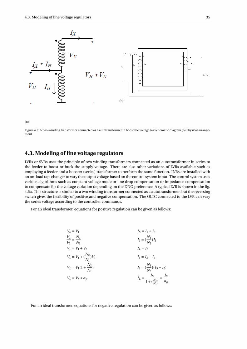
4.3. Modeling of line voltage regulators 35
(a)
(b)
Figure 4.5: A two-winding transformer connected as a autotransformer to boost the voltage (a) Schematic diagram (b) Physical arrange-ment
4.3. Modeling of line voltage regulators
LVRs or SVRs uses the principle of two winding transformers connected as an autotransformer in series tothe feeder to boost or buck the supply voltage. There are also other variations of LVRs available such asemploying a feeder and a booster (series) transformer to perform the same function. LVRs are installed withan on-load tap-changer to vary the output voltage based on the control system input. The control system usesvarious algorithms such as constant voltage mode or line drop compensation or impedance compensationto compensate for the voltage variation depending on the DNO preference. A typical LVR is shown in the fig.4.6a. This structure is similar to a two winding transformer connected as a autotransformer, but the reversingswitch gives the flexibility of positive and negative compensation. The OLTC connected to the LVR can varythe series voltage according to the controller commands.
For an ideal transformer, equations for positive regulation can be given as follows:
VS =V1 IS = I1 + I2
V2
V1= N2
N1I2 = (
N1
N2)I1
VL =V1 +V2 IL = I2
VL =V1 + (N2
N1)V1 I1 = IS − I2
VL =V1(1+ N2
N1) I2 = (
N1
N2)(IS − I2)
VL =VS ∗ap IL = IS
1+ ( N2N1
)= IS
ap
For an ideal transformer, equations for negative regulation can be given as follows:
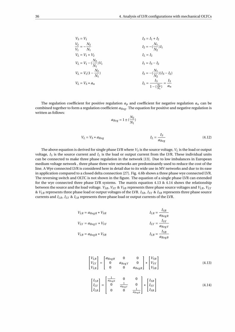
36 4. Analysis of LVR configurations with mechanical OLTCs
VS =V1 IS = I1 + I2
V2
V1=−N2
N1I2 =−(
N1
N2)I1
VL =V1 +V2 IL = I2
VL =V1 − (N2
N1)V1 I1 = IS − I2
VL =V1(1− N2
N1) I2 =−(
N1
N2)(IS − I2)
VL =VS ∗an IL = IS
1− ( N2N1
)= IS
an
The regulation coefficient for positive regulation ap and coefficient for negative regulation an can becombined together to form a regulation coefficient aReg . The equation for positive and negative regulation iswritten as follows:
aReg = 1± (N2
N1)
VL =VS ∗aReg IL = IS
aReg(4.12)
The above equation is derived for single phase LVR where VS is the source voltage, VL is the load or outputvoltage, IS is the source current and IL is the load or output current from the LVR. These individual unitscan be connected to make three phase regulation in the network [13]. Due to low imbalances in Europeanmedium voltage network , three phase three wire networks are predominantly used to reduce the cost of theline. A Wye connected LVR is considered here in detail due to its wide use in MV networks and due to its easein application compared to a closed delta connection [27]. Fig. 4.6b shows a three phase wye connected LVR.The reversing switch and OLTC is not shown in the figure. The equation of a single phase LVR can extendedfor the wye connected three phase LVR systems. The matrix equation 4.13 & 4.14 shows the relationshipbetween the source and the load voltage. VSR , VSY & VSB represents three phase source voltages and VLR , VLY
& VLB represents three phase load or output voltages of the LVR. ISR , ISY & ISB represents three phase sourcecurrents and ILR , ILY & ILB represents three phase load or output currents of the LVR.
VLR = aReg R ∗VSR ILR = ISR
aReg R
VLY = aReg Y ∗VSY ILY = ISY
aReg Y
VLB = aReg B ∗VSB ILB = ISB
aReg B
VLR
VLY
VLB
=aReg R 0 0
0 aReg Y 00 0 aReg B
∗VSR
VSY
VSB
(4.13)
ILR
ILY
ILB
=
1
aReg R0 0
0 1aReg Y
0
0 0 1aReg B
∗ISR
ISY
ISB
(4.14)
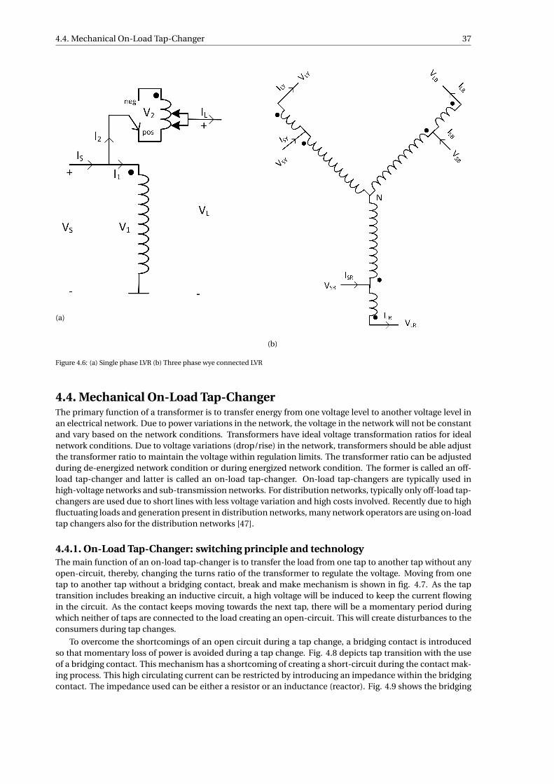
4.4. Mechanical On-Load Tap-Changer 37
(a)
(b)
Figure 4.6: (a) Single phase LVR (b) Three phase wye connected LVR
4.4. Mechanical On-Load Tap-ChangerThe primary function of a transformer is to transfer energy from one voltage level to another voltage level inan electrical network. Due to power variations in the network, the voltage in the network will not be constantand vary based on the network conditions. Transformers have ideal voltage transformation ratios for idealnetwork conditions. Due to voltage variations (drop/rise) in the network, transformers should be able adjustthe transformer ratio to maintain the voltage within regulation limits. The transformer ratio can be adjustedduring de-energized network condition or during energized network condition. The former is called an off-load tap-changer and latter is called an on-load tap-changer. On-load tap-changers are typically used inhigh-voltage networks and sub-transmission networks. For distribution networks, typically only off-load tap-changers are used due to short lines with less voltage variation and high costs involved. Recently due to highfluctuating loads and generation present in distribution networks, many network operators are using on-loadtap changers also for the distribution networks [47].
4.4.1. On-Load Tap-Changer: switching principle and technologyThe main function of an on-load tap-changer is to transfer the load from one tap to another tap without anyopen-circuit, thereby, changing the turns ratio of the transformer to regulate the voltage. Moving from onetap to another tap without a bridging contact, break and make mechanism is shown in fig. 4.7. As the taptransition includes breaking an inductive circuit, a high voltage will be induced to keep the current flowingin the circuit. As the contact keeps moving towards the next tap, there will be a momentary period duringwhich neither of taps are connected to the load creating an open-circuit. This will create disturbances to theconsumers during tap changes.
To overcome the shortcomings of an open circuit during a tap change, a bridging contact is introducedso that momentary loss of power is avoided during a tap change. Fig. 4.8 depicts tap transition with the useof a bridging contact. This mechanism has a shortcoming of creating a short-circuit during the contact mak-ing process. This high circulating current can be restricted by introducing an impedance within the bridgingcontact. The impedance used can be either a resistor or an inductance (reactor). Fig. 4.9 shows the bridging
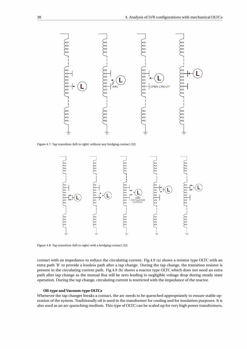
38 4. Analysis of LVR configurations with mechanical OLTCs
Figure 4.7: Tap transition (left to right) without any bridging contact [32]
Figure 4.8: Tap transition (left to right) with a bridging contact [32]
contact with an impedance to reduce the circulating current. Fig.4.9 (a) shows a resistor type OLTC with anextra path ’B’ to provide a lossless path after a tap change. During the tap change, the transition resistor ispresent in the circulating current path. Fig.4.9 (b) shows a reactor type OLTC which does not need an extrapath after tap change as the mutual flux will be zero leading to negligible voltage drop during steady stateoperation. During the tap change, circulating current is restricted with the impedance of the reactor.
Oil-type and Vacuum-type OLTCsWhenever the tap changer breaks a contact, the arc needs to be quenched appropriately to ensure stable op-eration of the system. Traditionally oil is used in the transformer for cooling and for insulation purposes. It isalso used as an arc quenching medium. This type of OLTC can be scaled up for very high power transformers,

4.4. Mechanical On-Load Tap-Changer 39
Figure 4.9: (a) Bridging contact with a resistor (b) Bridging contact with a reactor [32]
and is used widely in the industry. However, there is an increased fire hazard when the arc is quenched inan oil medium. It also degrades the oil whenever there is a tap change which leads to frequent maintenance.Vacuum-type switching technology was introduced to overcome these problems in mechanical OLTCs. Thevacuum interrupter technology is able to provide technical superiority for low and medium voltage trans-formers [57].
Table 4.1: Differences between oil-type and vacuum-type OLTCs
4.4.2. Distribution voltage level OLTCsThere are two types of OLTCs available for distribution networks. They are as follows:
• High current carrying OLTCs used for SVRs
• Low current carrying OLTCs used in Voltage Regulated Distribution Transformers (VRDTs)
High current carrying OLTCsThis type of OLTC has been predominantly used by most of the SVR manufacturers. They all have a simi-lar structure and working mechanism with few differences in minor components. VR-32 Quick-Drive Tap-Changer from Cooper Power Systems [68] is taken into consideration here to understand the basic principleand structure of this type of OLTC. But the details discussed here apply to similar OLTCs produced by othermanufacturers [24], [64]. The VR-32 OLTCs come as a single-phase OLTCs which have a rated current carryingcapacity of up to 668 A. A reversing switch is present to change the polarity of the tapped winding to attainpositive and negative regulation in the SVR. Reactor based bridging contact is employed to reduce the circu-lating current during a tap change operation. Apart from the reactor to restrict circulating current, equalizerwindings are used to improve the contact life for high current applications. An Oil medium is used to quenchthe arc during tap changes due to high currents flowing through the tap-changer. This is one of the maindrawback of this kind of tap changer as it contaminates the oil and requires monitoring of the oil, thereby,increasing the maintenance cost of the system. It uses a traditional geneva gear system with synchronous orinduction motor to move the taps. Fig. 4.10a shows a VR-32 QD5 single phase tap changer.
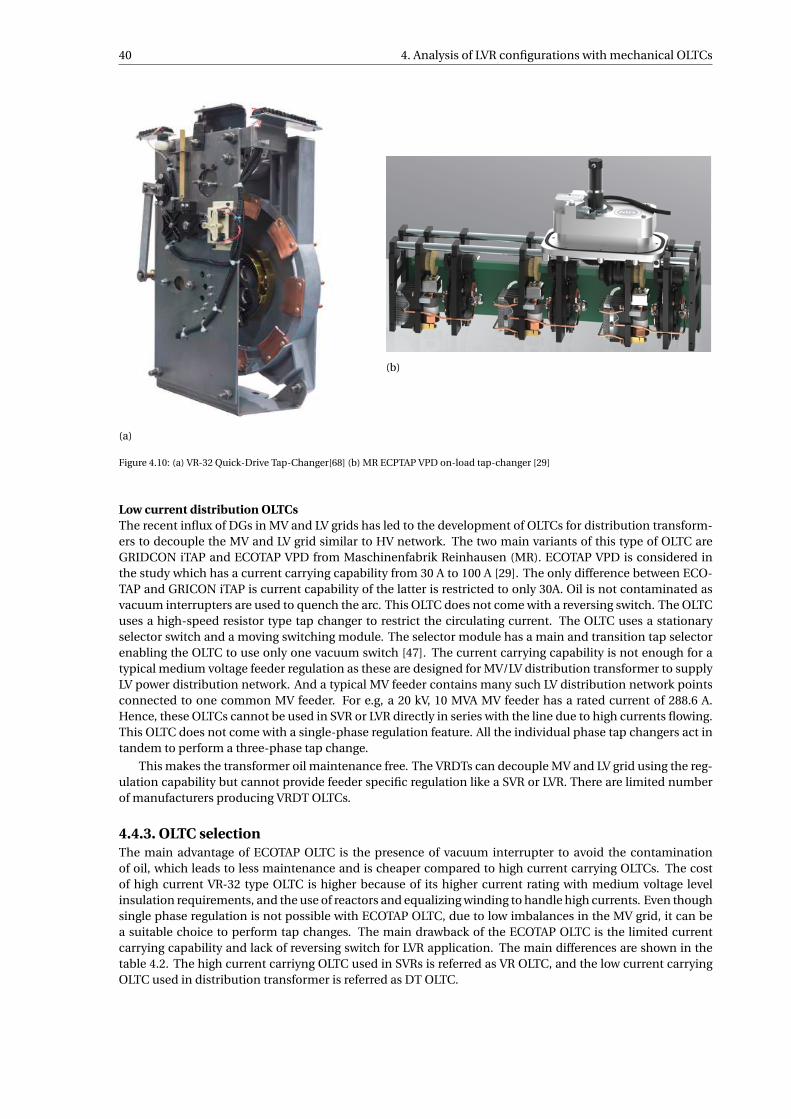
40 4. Analysis of LVR configurations with mechanical OLTCs
(a)
(b)
Figure 4.10: (a) VR-32 Quick-Drive Tap-Changer[68] (b) MR ECPTAP VPD on-load tap-changer [29]
Low current distribution OLTCsThe recent influx of DGs in MV and LV grids has led to the development of OLTCs for distribution transform-ers to decouple the MV and LV grid similar to HV network. The two main variants of this type of OLTC areGRIDCON iTAP and ECOTAP VPD from Maschinenfabrik Reinhausen (MR). ECOTAP VPD is considered inthe study which has a current carrying capability from 30 A to 100 A [29]. The only difference between ECO-TAP and GRICON iTAP is current capability of the latter is restricted to only 30A. Oil is not contaminated asvacuum interrupters are used to quench the arc. This OLTC does not come with a reversing switch. The OLTCuses a high-speed resistor type tap changer to restrict the circulating current. The OLTC uses a stationaryselector switch and a moving switching module. The selector module has a main and transition tap selectorenabling the OLTC to use only one vacuum switch [47]. The current carrying capability is not enough for atypical medium voltage feeder regulation as these are designed for MV/LV distribution transformer to supplyLV power distribution network. And a typical MV feeder contains many such LV distribution network pointsconnected to one common MV feeder. For e.g, a 20 kV, 10 MVA MV feeder has a rated current of 288.6 A.Hence, these OLTCs cannot be used in SVR or LVR directly in series with the line due to high currents flowing.This OLTC does not come with a single-phase regulation feature. All the individual phase tap changers act intandem to perform a three-phase tap change.
This makes the transformer oil maintenance free. The VRDTs can decouple MV and LV grid using the reg-ulation capability but cannot provide feeder specific regulation like a SVR or LVR. There are limited numberof manufacturers producing VRDT OLTCs.
4.4.3. OLTC selectionThe main advantage of ECOTAP OLTC is the presence of vacuum interrupter to avoid the contaminationof oil, which leads to less maintenance and is cheaper compared to high current carrying OLTCs. The costof high current VR-32 type OLTC is higher because of its higher current rating with medium voltage levelinsulation requirements, and the use of reactors and equalizing winding to handle high currents. Even thoughsingle phase regulation is not possible with ECOTAP OLTC, due to low imbalances in the MV grid, it can bea suitable choice to perform tap changes. The main drawback of the ECOTAP OLTC is the limited currentcarrying capability and lack of reversing switch for LVR application. The main differences are shown in thetable 4.2. The high current carriyng OLTC used in SVRs is referred as VR OLTC, and the low current carryingOLTC used in distribution transformer is referred as DT OLTC.
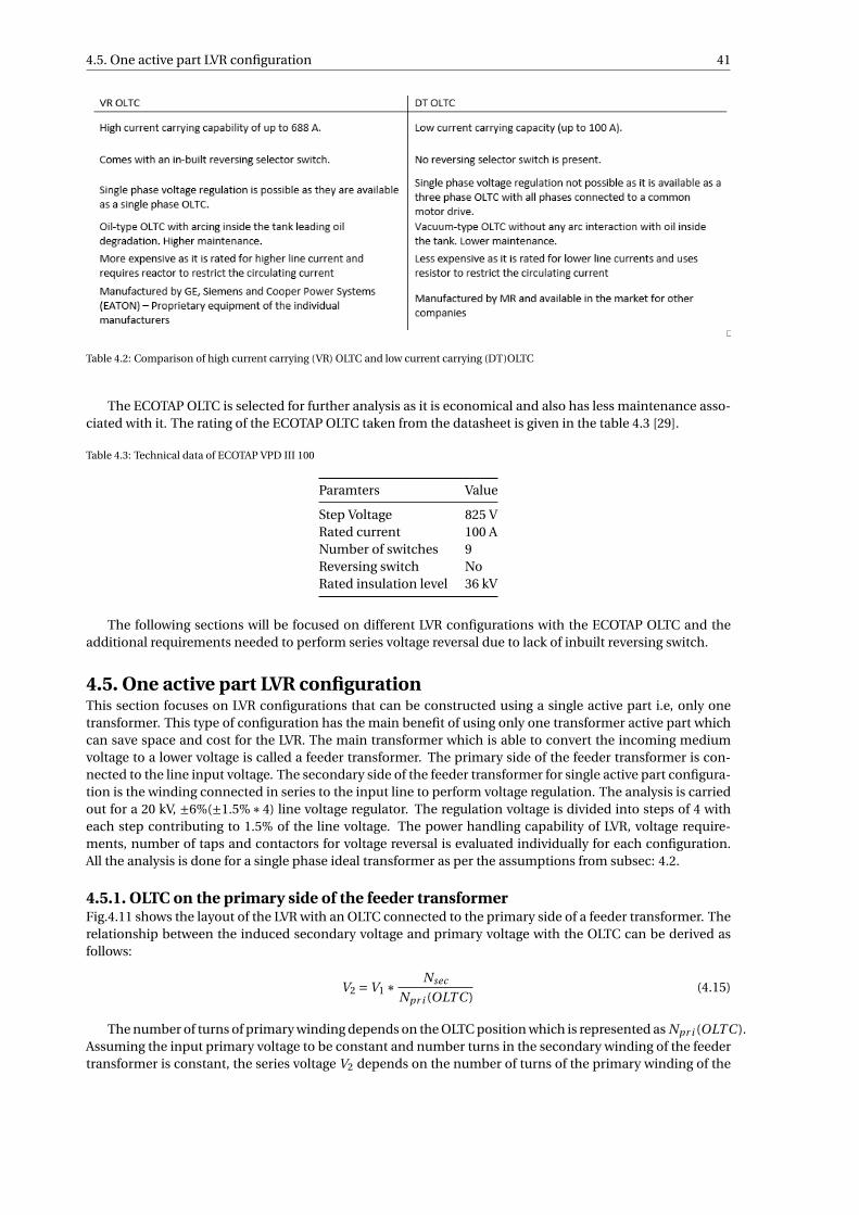
4.5. One active part LVR configuration 41
Table 4.2: Comparison of high current carrying (VR) OLTC and low current carrying (DT)OLTC
The ECOTAP OLTC is selected for further analysis as it is economical and also has less maintenance asso-ciated with it. The rating of the ECOTAP OLTC taken from the datasheet is given in the table 4.3 [29].
Table 4.3: Technical data of ECOTAP VPD III 100
Paramters Value
Step Voltage 825 VRated current 100 ANumber of switches 9Reversing switch NoRated insulation level 36 kV
The following sections will be focused on different LVR configurations with the ECOTAP OLTC and theadditional requirements needed to perform series voltage reversal due to lack of inbuilt reversing switch.
4.5. One active part LVR configurationThis section focuses on LVR configurations that can be constructed using a single active part i.e, only onetransformer. This type of configuration has the main benefit of using only one transformer active part whichcan save space and cost for the LVR. The main transformer which is able to convert the incoming mediumvoltage to a lower voltage is called a feeder transformer. The primary side of the feeder transformer is con-nected to the line input voltage. The secondary side of the feeder transformer for single active part configura-tion is the winding connected in series to the input line to perform voltage regulation. The analysis is carriedout for a 20 kV, ±6%(±1.5%∗4) line voltage regulator. The regulation voltage is divided into steps of 4 witheach step contributing to 1.5% of the line voltage. The power handling capability of LVR, voltage require-ments, number of taps and contactors for voltage reversal is evaluated individually for each configuration.All the analysis is done for a single phase ideal transformer as per the assumptions from subsec: 4.2.
4.5.1. OLTC on the primary side of the feeder transformerFig.4.11 shows the layout of the LVR with an OLTC connected to the primary side of a feeder transformer. Therelationship between the induced secondary voltage and primary voltage with the OLTC can be derived asfollows:
V2 =V1 ∗ Nsec
Npr i (OLT C )(4.15)
The number of turns of primary winding depends on the OLTC position which is represented as Npr i (OLT C ).Assuming the input primary voltage to be constant and number turns in the secondary winding of the feedertransformer is constant, the series voltage V2 depends on the number of turns of the primary winding of the
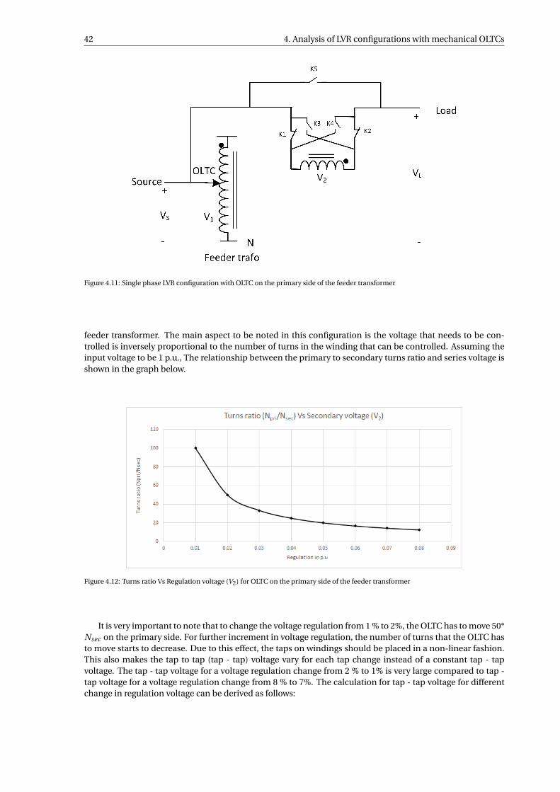
42 4. Analysis of LVR configurations with mechanical OLTCs
Figure 4.11: Single phase LVR configuration with OLTC on the primary side of the feeder transformer
feeder transformer. The main aspect to be noted in this configuration is the voltage that needs to be con-trolled is inversely proportional to the number of turns in the winding that can be controlled. Assuming theinput voltage to be 1 p.u., The relationship between the primary to secondary turns ratio and series voltage isshown in the graph below.
Figure 4.12: Turns ratio Vs Regulation voltage (V2) for OLTC on the primary side of the feeder transformer
It is very important to note that to change the voltage regulation from 1 % to 2%, the OLTC has to move 50*Nsec on the primary side. For further increment in voltage regulation, the number of turns that the OLTC hasto move starts to decrease. Due to this effect, the taps on windings should be placed in a non-linear fashion.This also makes the tap to tap (tap - tap) voltage vary for each tap change instead of a constant tap - tapvoltage. The tap - tap voltage for a voltage regulation change from 2 % to 1% is very large compared to tap -tap voltage for a voltage regulation change from 8 % to 7%. The calculation for tap - tap voltage for differentchange in regulation voltage can be derived as follows:
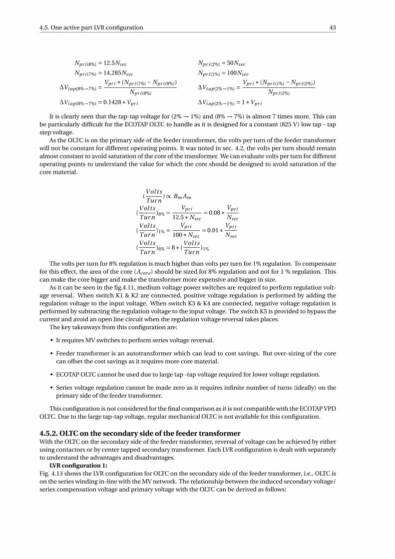
4.5. One active part LVR configuration 43
Npr i (8%) = 12.5Nsec Npr i (2%) = 50Nsec
Npr i (7%) = 14.285Nsec Npr i (1%) = 100Nsec
∆Vt ap(8%→7%) =Vpr i ∗ (Npr i (7%) −Npr i (8%))
Npr i (8%)∆Vt ap(2%→1%) =
Vpr i ∗ (Npr i (1%) −Npr i (2%))
Npr i (2%)
∆Vt ap(8%→7%) = 0.1428∗Vpr i ∆Vt ap(2%→1%) = 1∗Vpr i
It is clearly seen that the tap-tap voltage for (2% → 1%) and (8% → 7%) is almost 7 times more. This canbe particularly difficult for the ECOTAP OLTC to handle as it is designed for a constant (825 V) low tap - tapstep voltage.
As the OLTC is on the primary side of the feeder transformer, the volts per turn of the feeder transformerwill not be constant for different operating points. It was noted in sec. 4.2, the volts per turn should remainalmost constant to avoid saturation of the core of the transformer. We can evaluate volts per turn for differentoperating points to understand the value for which the core should be designed to avoid saturation of thecore material.
(V ol t s
Tur n) ∝ Bm Am
(V ol t s
Tur n)8% = Vpr i
12.5∗Nsec= 0.08∗ Vpr i
Nsec
(V ol t s
Tur n)1% = Vpr i
100∗Nsec= 0.01∗ Vpr i
Nsec
(V ol t s
Tur n)8% = 8∗ (
V ol t s
Tur n)1%
The volts per turn for 8% regulation is much higher than volts per turn for 1% regulation. To compensatefor this effect, the area of the core (Acor e ) should be sized for 8% regulation and not for 1 % regulation. Thiscan make the core bigger and make the transformer more expensive and bigger in size.
As it can be seen in the fig.4.11, medium voltage power switches are required to perform regulation volt-age reversal. When switch K1 & K2 are connected, positive voltage regulation is performed by adding theregulation voltage to the input voltage. When switch K3 & K4 are connected, negative voltage regulation isperformed by subtracting the regulation voltage to the input voltage. The switch K5 is provided to bypass thecurrent and avoid an open line circuit when the regulation voltage reversal takes places.
The key takeaways from this configuration are:
• It requires MV switches to perform series voltage reversal.
• Feeder transformer is an autotransformer which can lead to cost savings. But over-sizing of the corecan offset the cost savings as it requires more core material.
• ECOTAP OLTC cannot be used due to large tap -tap voltage required for lower voltage regulation.
• Series voltage regulation cannot be made zero as it requires infinite number of turns (ideally) on theprimary side of the feeder transformer.
This configuration is not considered for the final comparison as it is not compatible with the ECOTAP VPDOLTC. Due to the large tap-tap voltage, regular mechanical OLTC is not available for this configuration.
4.5.2. OLTC on the secondary side of the feeder transformerWith the OLTC on the secondary side of the feeder transformer, reversal of voltage can be achieved by eitherusing contactors or by center tapped secondary transformer. Each LVR configuration is dealt with separatelyto understand the advantages and disadvantages.
LVR configuration 1:Fig. 4.13 shows the LVR configuration for OLTC on the secondary side of the feeder transformer, i.e., OLTC ison the series winding in-line with the MV network. The relationship between the induced secondary voltage/series compensation voltage and primary voltage with the OLTC can be derived as follows:
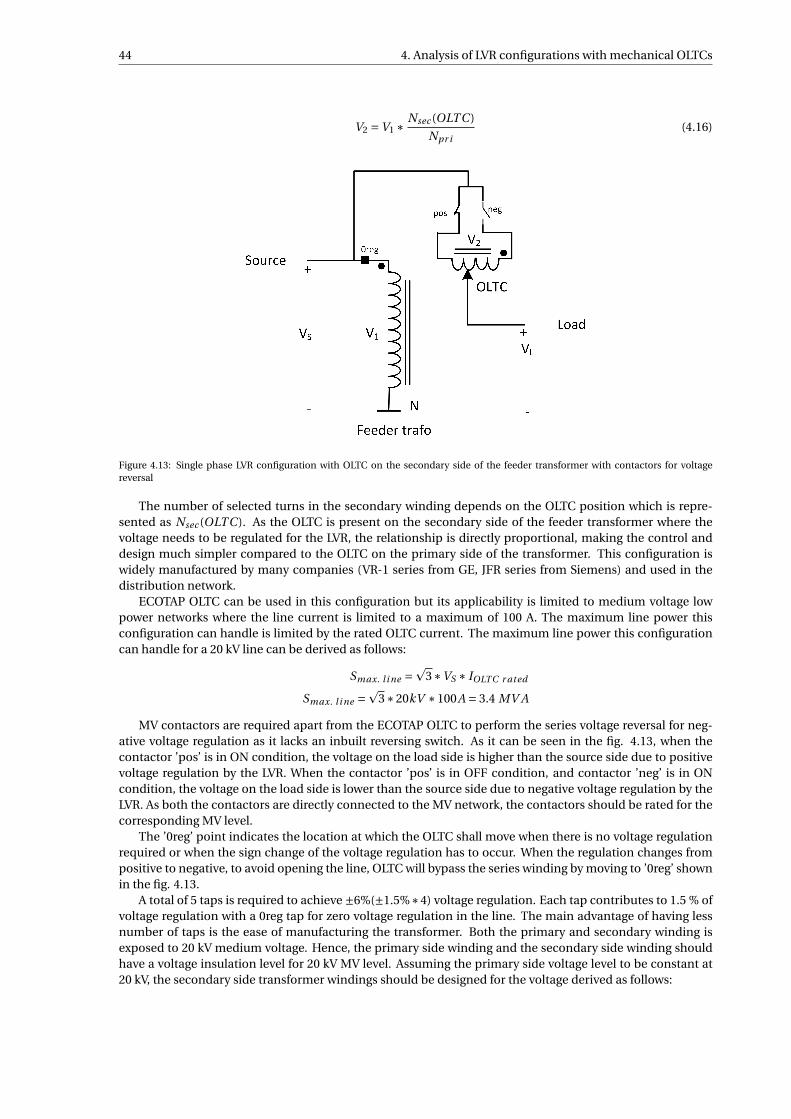
44 4. Analysis of LVR configurations with mechanical OLTCs
V2 =V1 ∗ Nsec (OLT C )
Npr i(4.16)
Figure 4.13: Single phase LVR configuration with OLTC on the secondary side of the feeder transformer with contactors for voltagereversal
The number of selected turns in the secondary winding depends on the OLTC position which is repre-sented as Nsec (OLT C ). As the OLTC is present on the secondary side of the feeder transformer where thevoltage needs to be regulated for the LVR, the relationship is directly proportional, making the control anddesign much simpler compared to the OLTC on the primary side of the transformer. This configuration iswidely manufactured by many companies (VR-1 series from GE, JFR series from Siemens) and used in thedistribution network.
ECOTAP OLTC can be used in this configuration but its applicability is limited to medium voltage lowpower networks where the line current is limited to a maximum of 100 A. The maximum line power thisconfiguration can handle is limited by the rated OLTC current. The maximum line power this configurationcan handle for a 20 kV line can be derived as follows:
Smax. l i ne =p
3∗VS ∗ IOLT C r ated
Smax. l i ne =p
3∗20kV ∗100A = 3.4 MV A
MV contactors are required apart from the ECOTAP OLTC to perform the series voltage reversal for neg-ative voltage regulation as it lacks an inbuilt reversing switch. As it can be seen in the fig. 4.13, when thecontactor ’pos’ is in ON condition, the voltage on the load side is higher than the source side due to positivevoltage regulation by the LVR. When the contactor ’pos’ is in OFF condition, and contactor ’neg’ is in ONcondition, the voltage on the load side is lower than the source side due to negative voltage regulation by theLVR. As both the contactors are directly connected to the MV network, the contactors should be rated for thecorresponding MV level.
The ’0reg’ point indicates the location at which the OLTC shall move when there is no voltage regulationrequired or when the sign change of the voltage regulation has to occur. When the regulation changes frompositive to negative, to avoid opening the line, OLTC will bypass the series winding by moving to ’0reg’ shownin the fig. 4.13.
A total of 5 taps is required to achieve ±6%(±1.5%∗4) voltage regulation. Each tap contributes to 1.5 % ofvoltage regulation with a 0reg tap for zero voltage regulation in the line. The main advantage of having lessnumber of taps is the ease of manufacturing the transformer. Both the primary and secondary winding isexposed to 20 kV medium voltage. Hence, the primary side winding and the secondary side winding shouldhave a voltage insulation level for 20 kV MV level. Assuming the primary side voltage level to be constant at20 kV, the secondary side transformer windings should be designed for the voltage derived as follows:
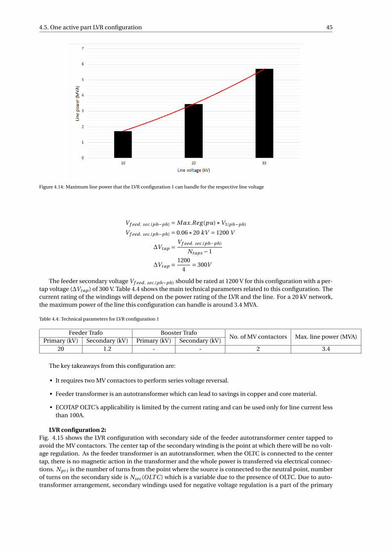
4.5. One active part LVR configuration 45
Figure 4.14: Maximum line power that the LVR configuration 1 can handle for the respective line voltage
V f eed . sec.(ph−ph) = M ax.Reg (pu)∗V1(ph−ph)
V f eed . sec.(ph−ph) = 0.06∗20 kV = 1200 V
∆Vt ap = V f eed . sec.(ph−ph)
Nt aps −1
∆Vt ap = 1200
4= 300V
The feeder secondary voltage V f eed . sec.(ph−ph) should be rated at 1200 V for this configuration with a per-tap voltage (∆Vt ap ) of 300 V. Table 4.4 shows the main technical parameters related to this configuration. Thecurrent rating of the windings will depend on the power rating of the LVR and the line. For a 20 kV network,the maximum power of the line this configuration can handle is around 3.4 MVA.
Table 4.4: Technical parameters for LVR configuration 1
Feeder Trafo Booster TrafoNo. of MV contactors Max. line power (MVA)
Primary (kV) Secondary (kV) Primary (kV) Secondary (kV)20 1.2 - - 2 3.4
The key takeaways from this configuration are:
• It requires two MV contactors to perform series voltage reversal.
• Feeder transformer is an autotransformer which can lead to savings in copper and core material.
• ECOTAP OLTC’s applicability is limited by the current rating and can be used only for line current lessthan 100A.
LVR configuration 2:Fig. 4.15 shows the LVR configuration with secondary side of the feeder autotransformer center tapped toavoid the MV contactors. The center tap of the secondary winding is the point at which there will be no volt-age regulation. As the feeder transformer is an autotransformer, when the OLTC is connected to the centertap, there is no magnetic action in the transformer and the whole power is transferred via electrical connec-tions. Npr i is the number of turns from the point where the source is connected to the neutral point, numberof turns on the secondary side is Nsec (OLT C ) which is a variable due to the presence of OLTC. Due to auto-transformer arrangement, secondary windings used for negative voltage regulation is a part of the primary
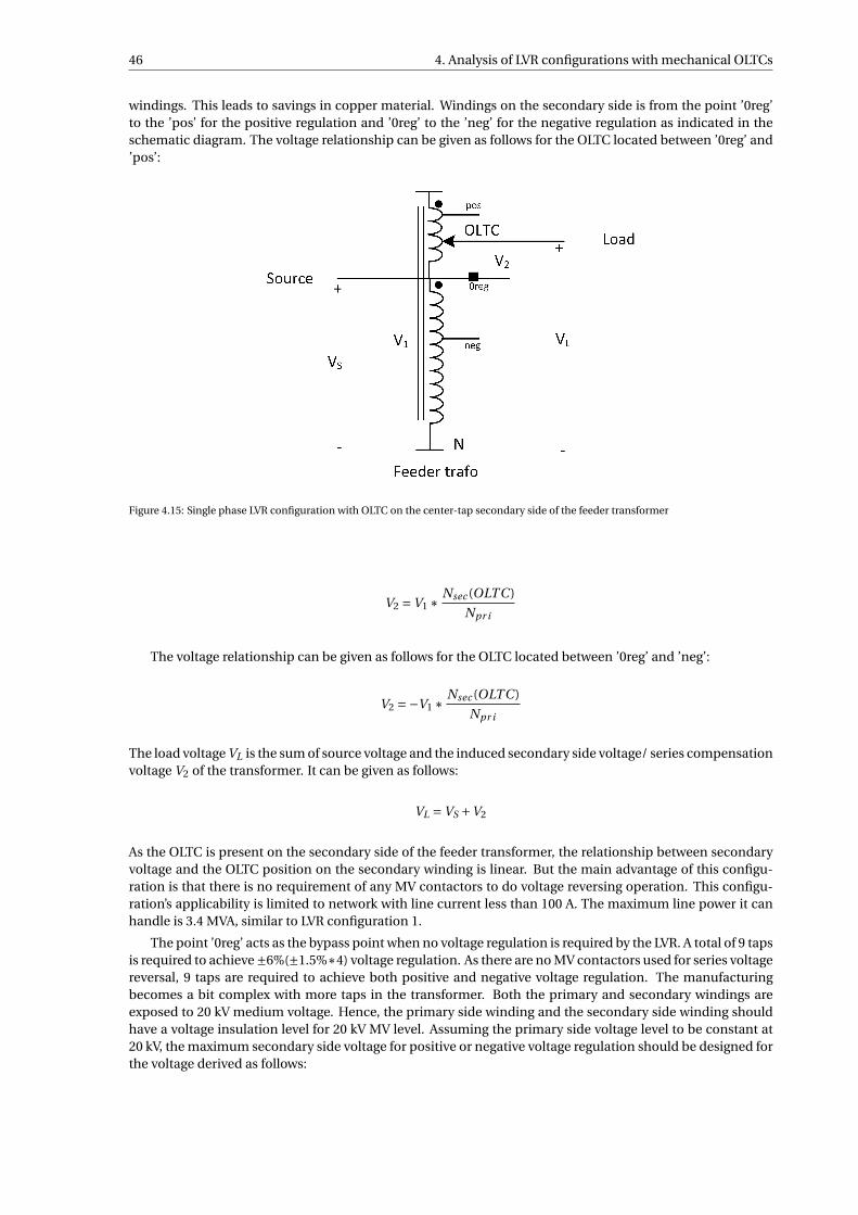
46 4. Analysis of LVR configurations with mechanical OLTCs
windings. This leads to savings in copper material. Windings on the secondary side is from the point ’0reg’to the ’pos’ for the positive regulation and ’0reg’ to the ’neg’ for the negative regulation as indicated in theschematic diagram. The voltage relationship can be given as follows for the OLTC located between ’0reg’ and’pos’:
Figure 4.15: Single phase LVR configuration with OLTC on the center-tap secondary side of the feeder transformer
V2 =V1 ∗ Nsec (OLT C )
Npr i
The voltage relationship can be given as follows for the OLTC located between ’0reg’ and ’neg’:
V2 =−V1 ∗ Nsec (OLT C )
Npr i
The load voltage VL is the sum of source voltage and the induced secondary side voltage/ series compensationvoltage V2 of the transformer. It can be given as follows:
VL =VS +V2
As the OLTC is present on the secondary side of the feeder transformer, the relationship between secondaryvoltage and the OLTC position on the secondary winding is linear. But the main advantage of this configu-ration is that there is no requirement of any MV contactors to do voltage reversing operation. This configu-ration’s applicability is limited to network with line current less than 100 A. The maximum line power it canhandle is 3.4 MVA, similar to LVR configuration 1.
The point ’0reg’ acts as the bypass point when no voltage regulation is required by the LVR. A total of 9 tapsis required to achieve ±6%(±1.5%∗4) voltage regulation. As there are no MV contactors used for series voltagereversal, 9 taps are required to achieve both positive and negative voltage regulation. The manufacturingbecomes a bit complex with more taps in the transformer. Both the primary and secondary windings areexposed to 20 kV medium voltage. Hence, the primary side winding and the secondary side winding shouldhave a voltage insulation level for 20 kV MV level. Assuming the primary side voltage level to be constant at20 kV, the maximum secondary side voltage for positive or negative voltage regulation should be designed forthe voltage derived as follows:
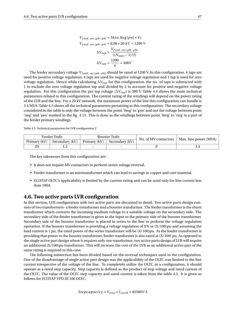
4.6. Two active parts LVR configuration 47
V f eed . sec.(ph−ph) = M ax.Reg (pu)∗VS
V f eed . sec.(ph−ph) = 0.06∗20 kV = 1200 V
∆Vt ap = V f eed . sec.(ph−ph)
((Nt aps −1)/2)
∆Vt ap = 1200
4= 300V
The feeder secondary voltage V f eed . sec.(ph−ph) should be rated at 1200 V. In this configuration, 4 taps areused for positive voltage regulation, 4 taps are used for negative voltage regulation and 1 tap is used for zerovoltage regulation. Hence while calculating ∆Vt ap for this configuration, the no. of taps is subtracted with1 to exclude the zero voltage regulation tap and divided by 2 to account for positive and negative voltageregulation. For this configuration the per-tap voltage (∆Vt ap ) is 300 V. Table 4.4 shows the main technicalparameters related to this configuration. The current rating of the windings will depend on the power ratingof the LVR and the line. For a 20 kV network, the maximum power of the line this configuration can handle is3.4 MVA. Table 4.5 shows all the technical parameters pertaining to this configuration. The secondary voltageconsidered in the table is only the voltage between the point ’0reg’ to ’pos’ and not the voltage between point’neg’ and ’pos’ marked in the fig. 4.15. This is done as the windings between point ’0reg’ to ’neg’ is a part ofthe feeder primary windings.
Table 4.5: Technical parameters for LVR configuration 2
Feeder Trafo Booster TrafoNo. of MV contactors Max. line power (MVA)
Primary (kV) Secondary (kV) Primary (kV) Secondary (kV)20 1.2 - - 0 3.4
The key takeaways from this configuration are:
• It does not require MV contactors to perform series voltage reversal.
• Feeder transformer is an autotransformer which can lead to savings in copper and core material.
• ECOTAP OLTC’s applicability is limited by the current rating and can be used only for line current lessthan 100A.
4.6. Two active parts LVR configurationIn this section, LVR configuration with two active parts are discussed in detail. Two active parts design con-sists of two transformers- a feeder transformer and a booster transformer. The feeder transformer is the shunttransformer which converts the incoming medium voltage to a suitable voltage on the secondary side. Thesecondary side of the feeder transformer is given as the input to the primary side of the booster transformer.Secondary side of the booster transformer is placed in series to the line to perform the voltage regulationoperation. If the booster transformer is providing a voltage regulation of X% or (X/100)pu and assuming theload current is 1 pu, the rated power of the series transformer will be (X/100)pu. As the feeder transformer isproviding that power to the booster transformer, feeder transformer is also rated at (X/100) pu. As opposed tothe single active part design where it requires only one transformer, two active parts design of LVR will requirean additional (X/100)pu transformer. This will increase the cost of the LVR as an additional active part of thesame rating is required in this case.
The following subsection has been divided based on the reversal techniques used in the configuration.One of the disadvantage of single active part design was the applicability of the OLTC was limited to the linecurrent irrespective of the voltage of the line. To completely utilize the OLTC in a configuration, it shouldoperate at a rated step capacity. Step capacity is defined as the product of step voltage and rated current ofthe OLTC. The value of the OLTC step capacity and rated current is taken from the table 4.3. It is given asfollows for ECOTAP VPD III 100 OLTC:
Stepcapaci t y =Vstep ∗ Ir ated = 82500V A
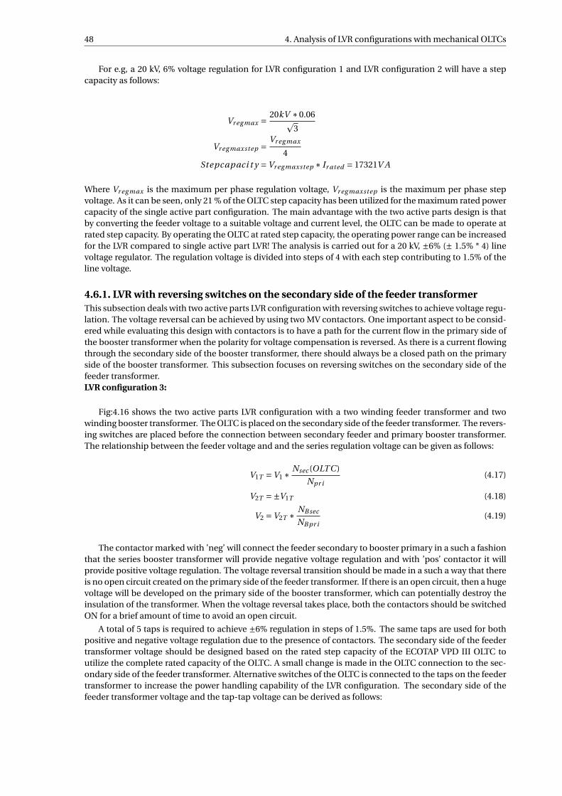
48 4. Analysis of LVR configurations with mechanical OLTCs
For e.g, a 20 kV, 6% voltage regulation for LVR configuration 1 and LVR configuration 2 will have a stepcapacity as follows:
Vr eg max = 20kV ∗0.06p3
Vr eg maxstep = Vr eg max
4Stepcapaci t y =Vr eg maxstep ∗ Ir ated = 17321V A
Where Vr eg max is the maximum per phase regulation voltage, Vr eg maxstep is the maximum per phase stepvoltage. As it can be seen, only 21 % of the OLTC step capacity has been utilized for the maximum rated powercapacity of the single active part configuration. The main advantage with the two active parts design is thatby converting the feeder voltage to a suitable voltage and current level, the OLTC can be made to operate atrated step capacity. By operating the OLTC at rated step capacity, the operating power range can be increasedfor the LVR compared to single active part LVR! The analysis is carried out for a 20 kV, ±6% (± 1.5% * 4) linevoltage regulator. The regulation voltage is divided into steps of 4 with each step contributing to 1.5% of theline voltage.
4.6.1. LVR with reversing switches on the secondary side of the feeder transformerThis subsection deals with two active parts LVR configuration with reversing switches to achieve voltage regu-lation. The voltage reversal can be achieved by using two MV contactors. One important aspect to be consid-ered while evaluating this design with contactors is to have a path for the current flow in the primary side ofthe booster transformer when the polarity for voltage compensation is reversed. As there is a current flowingthrough the secondary side of the booster transformer, there should always be a closed path on the primaryside of the booster transformer. This subsection focuses on reversing switches on the secondary side of thefeeder transformer.LVR configuration 3:
Fig:4.16 shows the two active parts LVR configuration with a two winding feeder transformer and twowinding booster transformer. The OLTC is placed on the secondary side of the feeder transformer. The revers-ing switches are placed before the connection between secondary feeder and primary booster transformer.The relationship between the feeder voltage and and the series regulation voltage can be given as follows:
V1T =V1 ∗ Nsec (OLT C )
Npr i(4.17)
V2T =±V1T (4.18)
V2 =V2T ∗ NB sec
NB pr i(4.19)
The contactor marked with ’neg’ will connect the feeder secondary to booster primary in a such a fashionthat the series booster transformer will provide negative voltage regulation and with ’pos’ contactor it willprovide positive voltage regulation. The voltage reversal transition should be made in a such a way that thereis no open circuit created on the primary side of the feeder transformer. If there is an open circuit, then a hugevoltage will be developed on the primary side of the booster transformer, which can potentially destroy theinsulation of the transformer. When the voltage reversal takes place, both the contactors should be switchedON for a brief amount of time to avoid an open circuit.
A total of 5 taps is required to achieve ±6% regulation in steps of 1.5%. The same taps are used for bothpositive and negative voltage regulation due to the presence of contactors. The secondary side of the feedertransformer voltage should be designed based on the rated step capacity of the ECOTAP VPD III OLTC toutilize the complete rated capacity of the OLTC. A small change is made in the OLTC connection to the sec-ondary side of the feeder transformer. Alternative switches of the OLTC is connected to the taps on the feedertransformer to increase the power handling capability of the LVR configuration. The secondary side of thefeeder transformer voltage and the tap-tap voltage can be derived as follows:
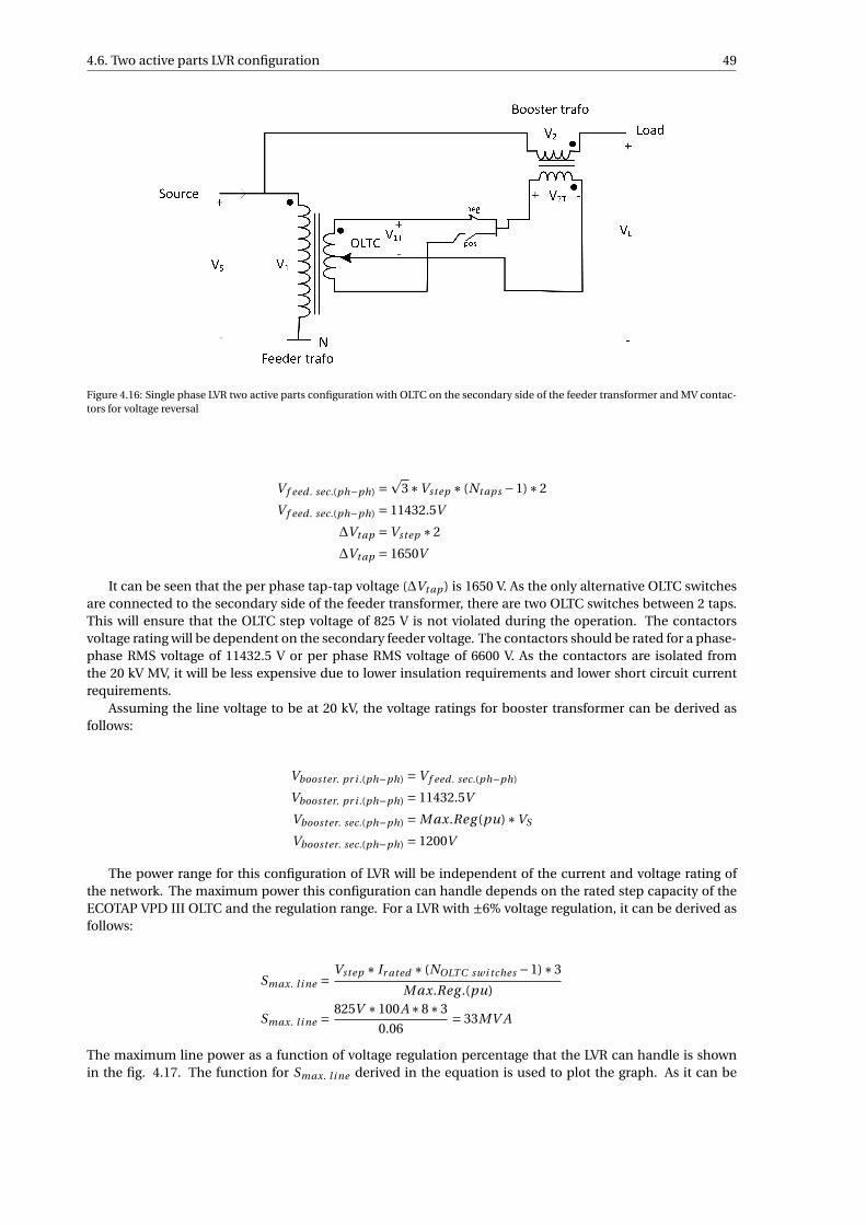
4.6. Two active parts LVR configuration 49
Figure 4.16: Single phase LVR two active parts configuration with OLTC on the secondary side of the feeder transformer and MV contac-tors for voltage reversal
V f eed . sec.(ph−ph) =p
3∗Vstep ∗ (Nt aps −1)∗2
V f eed . sec.(ph−ph) = 11432.5V
∆Vt ap =Vstep ∗2
∆Vt ap = 1650V
It can be seen that the per phase tap-tap voltage (∆Vt ap ) is 1650 V. As the only alternative OLTC switchesare connected to the secondary side of the feeder transformer, there are two OLTC switches between 2 taps.This will ensure that the OLTC step voltage of 825 V is not violated during the operation. The contactorsvoltage rating will be dependent on the secondary feeder voltage. The contactors should be rated for a phase-phase RMS voltage of 11432.5 V or per phase RMS voltage of 6600 V. As the contactors are isolated fromthe 20 kV MV, it will be less expensive due to lower insulation requirements and lower short circuit currentrequirements.
Assuming the line voltage to be at 20 kV, the voltage ratings for booster transformer can be derived asfollows:
Vbooster. pr i .(ph−ph) =V f eed . sec.(ph−ph)
Vbooster. pr i .(ph−ph) = 11432.5V
Vbooster. sec.(ph−ph) = M ax.Reg (pu)∗VS
Vbooster. sec.(ph−ph) = 1200V
The power range for this configuration of LVR will be independent of the current and voltage rating ofthe network. The maximum power this configuration can handle depends on the rated step capacity of theECOTAP VPD III OLTC and the regulation range. For a LVR with ±6% voltage regulation, it can be derived asfollows:
Smax. l i ne =Vstep ∗ Ir ated ∗ (NOLT C swi tches −1)∗3
M ax.Reg .(pu)
Smax. l i ne =825V ∗100A∗8∗3
0.06= 33MV A
The maximum line power as a function of voltage regulation percentage that the LVR can handle is shownin the fig. 4.17. The function for Smax. l i ne derived in the equation is used to plot the graph. As it can be
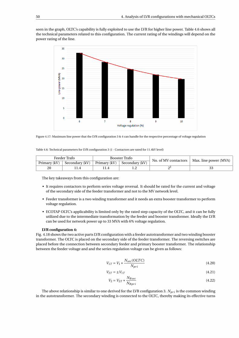
50 4. Analysis of LVR configurations with mechanical OLTCs
seen in the graph, OLTC’s capability is fully exploited to use the LVR for higher line power. Table 4.6 shows allthe technical parameters related to this configuration. The current rating of the windings will depend on thepower rating of the line.
Figure 4.17: Maximum line power that the LVR configuration 3 & 4 can handle for the respective percentage of voltage regulation
Table 4.6: Technical parameters for LVR configuration 3 (‡ - Contactors are rated for 11.4kV level)
Feeder Trafo Booster TrafoNo. of MV contactors Max. line power (MVA)
Primary (kV) Secondary (kV) Primary (kV) Secondary (kV)20 11.4 11.4 1.2 2‡ 33
The key takeaways from this configuration are:
• It requires contactors to perform series voltage reversal. It should be rated for the current and voltageof the secondary side of the feeder transformer and not to the MV network level.
• Feeder transformer is a two winding transformer and it needs an extra booster transformer to performvoltage regulation.
• ECOTAP OLTC’s applicability is limited only by the rated step capacity of the OLTC, and it can be fullyutilized due to the intermediate transformation by the feeder and booster transformer. Ideally the LVRcan be used for network power up to 33 MVA with 6% voltage regulation.
LVR configuration 4:Fig. 4.18 shows the two active parts LVR configuration with a feeder autotransformer and two winding boostertransformer. The OLTC is placed on the secondary side of the feeder transformer. The reversing switches areplaced before the connection between secondary feeder and primary booster transformer. The relationshipbetween the feeder voltage and and the series regulation voltage can be given as follows:
V1T =V1 ∗ Nsec (OLT C )
Npr i(4.20)
V2T =±V1T (4.21)
V2 =V2T ∗ NB sec
NB pr i(4.22)
The above relationship is similar to one derived for the LVR configuration 3. Npr i is the common windingin the autotransformer. The secondary winding is connected to the OLTC, thereby making its effective turns
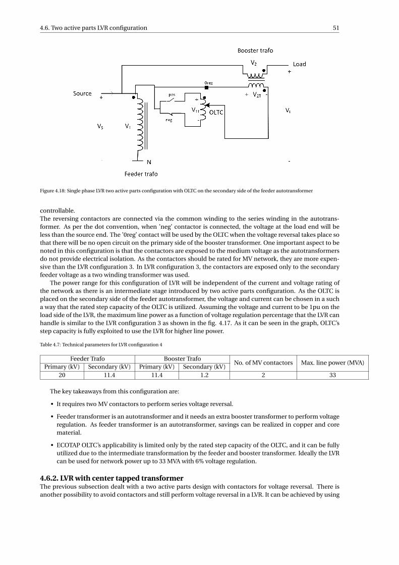
4.6. Two active parts LVR configuration 51
Figure 4.18: Single phase LVR two active parts configuration with OLTC on the secondary side of the feeder autotransformer
controllable.The reversing contactors are connected via the common winding to the series winding in the autotrans-former. As per the dot convention, when ’neg’ contactor is connected, the voltage at the load end will beless than the source end. The ’0reg’ contact will be used by the OLTC when the voltage reversal takes place sothat there will be no open circuit on the primary side of the booster transformer. One important aspect to benoted in this configuration is that the contactors are exposed to the medium voltage as the autotransformersdo not provide electrical isolation. As the contactors should be rated for MV network, they are more expen-sive than the LVR configuration 3. In LVR configuration 3, the contactors are exposed only to the secondaryfeeder voltage as a two winding transformer was used.
The power range for this configuration of LVR will be independent of the current and voltage rating ofthe network as there is an intermediate stage introduced by two active parts configuration. As the OLTC isplaced on the secondary side of the feeder autotransformer, the voltage and current can be chosen in a sucha way that the rated step capacity of the OLTC is utilized. Assuming the voltage and current to be 1pu on theload side of the LVR, the maximum line power as a function of voltage regulation percentage that the LVR canhandle is similar to the LVR configuration 3 as shown in the fig. 4.17. As it can be seen in the graph, OLTC’sstep capacity is fully exploited to use the LVR for higher line power.
Table 4.7: Technical parameters for LVR configuration 4
Feeder Trafo Booster TrafoNo. of MV contactors Max. line power (MVA)
Primary (kV) Secondary (kV) Primary (kV) Secondary (kV)20 11.4 11.4 1.2 2 33
The key takeaways from this configuration are:
• It requires two MV contactors to perform series voltage reversal.
• Feeder transformer is an autotransformer and it needs an extra booster transformer to perform voltageregulation. As feeder transformer is an autotransformer, savings can be realized in copper and corematerial.
• ECOTAP OLTC’s applicability is limited only by the rated step capacity of the OLTC, and it can be fullyutilized due to the intermediate transformation by the feeder and booster transformer. Ideally the LVRcan be used for network power up to 33 MVA with 6% voltage regulation.
4.6.2. LVR with center tapped transformerThe previous subsection dealt with a two active parts design with contactors for voltage reversal. There isanother possibility to avoid contactors and still perform voltage reversal in a LVR. It can be achieved by using
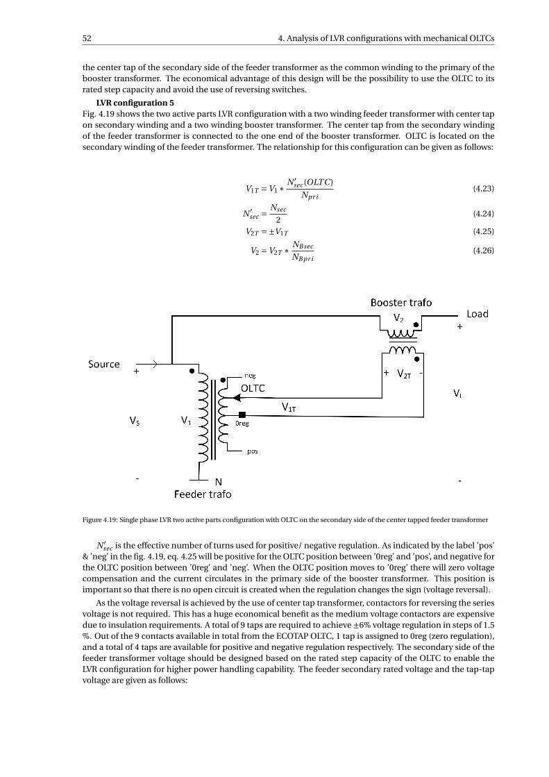
52 4. Analysis of LVR configurations with mechanical OLTCs
the center tap of the secondary side of the feeder transformer as the common winding to the primary of thebooster transformer. The economical advantage of this design will be the possibility to use the OLTC to itsrated step capacity and avoid the use of reversing switches.
LVR configuration 5Fig. 4.19 shows the two active parts LVR configuration with a two winding feeder transformer with center tapon secondary winding and a two winding booster transformer. The center tap from the secondary windingof the feeder transformer is connected to the one end of the booster transformer. OLTC is located on thesecondary winding of the feeder transformer. The relationship for this configuration can be given as follows:
V1T =V1 ∗N ′
sec (OLT C )
Npr i(4.23)
N ′sec =
Nsec
2(4.24)
V2T =±V1T (4.25)
V2 =V2T ∗ NB sec
NB pr i(4.26)
Figure 4.19: Single phase LVR two active parts configuration with OLTC on the secondary side of the center tapped feeder transformer
N ′sec is the effective number of turns used for positive/ negative regulation. As indicated by the label ’pos’
& ’neg’ in the fig. 4.19, eq. 4.25 will be positive for the OLTC position between ’0reg’ and ’pos’, and negative forthe OLTC position between ’0reg’ and ’neg’. When the OLTC position moves to ’0reg’ there will zero voltagecompensation and the current circulates in the primary side of the booster transformer. This position isimportant so that there is no open circuit is created when the regulation changes the sign (voltage reversal).
As the voltage reversal is achieved by the use of center tap transformer, contactors for reversing the seriesvoltage is not required. This has a huge economical benefit as the medium voltage contactors are expensivedue to insulation requirements. A total of 9 taps are required to achieve ±6% voltage regulation in steps of 1.5%. Out of the 9 contacts available in total from the ECOTAP OLTC, 1 tap is assigned to 0reg (zero regulation),and a total of 4 taps are available for positive and negative regulation respectively. The secondary side of thefeeder transformer voltage should be designed based on the rated step capacity of the OLTC to enable theLVR configuration for higher power handling capability. The feeder secondary rated voltage and the tap-tapvoltage are given as follows:
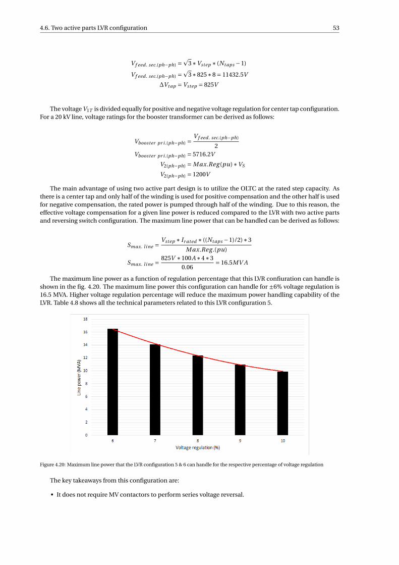
4.6. Two active parts LVR configuration 53
V f eed . sec.(ph−ph) =p
3∗Vstep ∗ (Nt aps −1)
V f eed . sec.(ph−ph) =p
3∗825∗8 = 11432.5V
∆Vt ap =Vstep = 825V
The voltage V1T is divided equally for positive and negative voltage regulation for center tap configuration.For a 20 kV line, voltage ratings for the booster transformer can be derived as follows:
Vbooster pr i .(ph−ph) =V f eed . sec.(ph−ph)
2Vbooster pr i .(ph−ph) = 5716.2V
V2(ph−ph) = M ax.Reg (pu)∗VS
V2(ph−ph) = 1200V
The main advantage of using two active part design is to utilize the OLTC at the rated step capacity. Asthere is a center tap and only half of the winding is used for positive compensation and the other half is usedfor negative compensation, the rated power is pumped through half of the winding. Due to this reason, theeffective voltage compensation for a given line power is reduced compared to the LVR with two active partsand reversing switch configuration. The maximum line power that can be handled can be derived as follows:
Smax. l i ne =Vstep ∗ Ir ated ∗ ((Nt aps −1)/2)∗3
M ax.Reg .(pu)
Smax. l i ne =825V ∗100A∗4∗3
0.06= 16.5MV A
The maximum line power as a function of regulation percentage that this LVR confiuration can handle isshown in the fig. 4.20. The maximum line power this configuration can handle for ±6% voltage regulation is16.5 MVA. Higher voltage regulation percentage will reduce the maximum power handling capability of theLVR. Table 4.8 shows all the technical parameters related to this LVR configuration 5.
Figure 4.20: Maximum line power that the LVR configuration 5 & 6 can handle for the respective percentage of voltage regulation
The key takeaways from this configuration are:
• It does not require MV contactors to perform series voltage reversal.
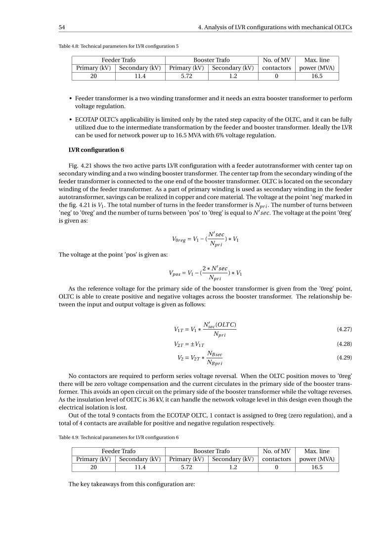
54 4. Analysis of LVR configurations with mechanical OLTCs
Table 4.8: Technical parameters for LVR configuration 5
Feeder Trafo Booster Trafo No. of MVcontactors
Max. linepower (MVA)Primary (kV) Secondary (kV) Primary (kV) Secondary (kV)
20 11.4 5.72 1.2 0 16.5
• Feeder transformer is a two winding transformer and it needs an extra booster transformer to performvoltage regulation.
• ECOTAP OLTC’s applicability is limited only by the rated step capacity of the OLTC, and it can be fullyutilized due to the intermediate transformation by the feeder and booster transformer. Ideally the LVRcan be used for network power up to 16.5 MVA with 6% voltage regulation.
LVR configuration 6
Fig. 4.21 shows the two active parts LVR configuration with a feeder autotransformer with center tap onsecondary winding and a two winding booster transformer. The center tap from the secondary winding of thefeeder transformer is connected to the one end of the booster transformer. OLTC is located on the secondarywinding of the feeder transformer. As a part of primary winding is used as secondary winding in the feederautotransformer, savings can be realized in copper and core material. The voltage at the point ’neg’ marked inthe fig. 4.21 is V1. The total number of turns in the feeder transformer is Npr i . The number of turns between’neg’ to ’0reg’ and the number of turns between ’pos’ to ’0reg’ is equal to N ′sec. The voltage at the point ’0reg’is given as:
V0r eg =V1 − (N ′sec
Npr i)∗V1
The voltage at the point ’pos’ is given as:
Vpos =V1 − (2∗N ′sec
Npr i)∗V1
As the reference voltage for the primary side of the booster transformer is given from the ’0reg’ point,OLTC is able to create positive and negative voltages across the booster transformer. The relationship be-tween the input and output voltage is given as follows:
V1T =V1 ∗N ′
sec (OLT C )
Npr i(4.27)
V2T =±V1T (4.28)
V2 =V2T ∗ NB sec
NB pr i(4.29)
No contactors are required to perform series voltage reversal. When the OLTC position moves to ’0reg’there will be zero voltage compensation and the current circulates in the primary side of the booster trans-former. This avoids an open circuit on the primary side of the booster transformer while the voltage reverses.As the insulation level of OLTC is 36 kV, it can handle the network voltage level in this design even though theelectrical isolation is lost.
Out of the total 9 contacts from the ECOTAP OLTC, 1 contact is assigned to 0reg (zero regulation), and atotal of 4 contacts are available for positive and negative regulation respectively.
Table 4.9: Technical parameters for LVR configuration 6
Feeder Trafo Booster Trafo No. of MVcontactors
Max. linepower (MVA)Primary (kV) Secondary (kV) Primary (kV) Secondary (kV)
20 11.4 5.72 1.2 0 16.5
The key takeaways from this configuration are:
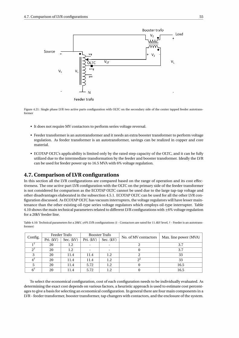
4.7. Comparison of LVR configurations 55
Figure 4.21: Single phase LVR two active parts configuration with OLTC on the secondary side of the center tapped feeder autotrans-former
• It does not require MV contactors to perform series voltage reversal.
• Feeder transformer is an autotransformer and it needs an extra booster transformer to perform voltageregulation. As feeder transformer is an autotransformer, savings can be realized in copper and corematerial.
• ECOTAP OLTC’s applicability is limited only by the rated step capacity of the OLTC, and it can be fullyutilized due to the intermediate transformation by the feeder and booster transformer. Ideally the LVRcan be used for feeder power up to 16.5 MVA with 6% voltage regulation.
4.7. Comparison of LVR configurationsIn this section all the LVR configurations are compared based on the range of operation and its cost effec-tiveness. The one active part LVR configuration with the OLTC on the primary side of the feeder transformeris not considered for comparison as the ECOTAP OLTC cannot be used due to the large tap-tap voltage andother disadvantages elaborated in the subsection 4.5.1. ECOTAP OLTC can be used for all the other LVR con-figuration discussed. As ECOTAP OLTC has vacuum interrupters, the voltage regulators will have lesser main-tenance than the other existing oil-type series voltage regulators which employs oil-type interrupter. Table4.10 shows the main technical parameters related to different LVR configurations with ±6% voltage regulationfor a 20kV feeder line.
Table 4.10: Technical parameters for a 20kV, ±6% LVR configurations (‡ - Contactors are rated for 11.4kV level, † - Feeder is an autotrans-former)
Config.Feeder Trafo Booster Trafo
No. of MV contactors Max. line power (MVA)Pri. (kV) Sec. (kV) Pri. (kV) Sec. (kV)
1† 20 1.2 - - 2 3.72† 20 1.2 - - 0 3.73 20 11.4 11.4 1.2 2 334† 20 11.4 11.4 1.2 2‡ 335 20 11.4 5.72 1.2 0 16.56† 20 11.4 5.72 1.2 0 16.5
To select the economical configuration, cost of each configuration needs to be individually evaluated. Asdetermining the exact cost depends on various factors, a heuristic approach is used to estimate cost percent-ages to give a basis for selecting an economical configuration. In general there are four main components in aLVR - feeder transformer, booster transformer, tap changers with contactors, and the enclosure of the system.
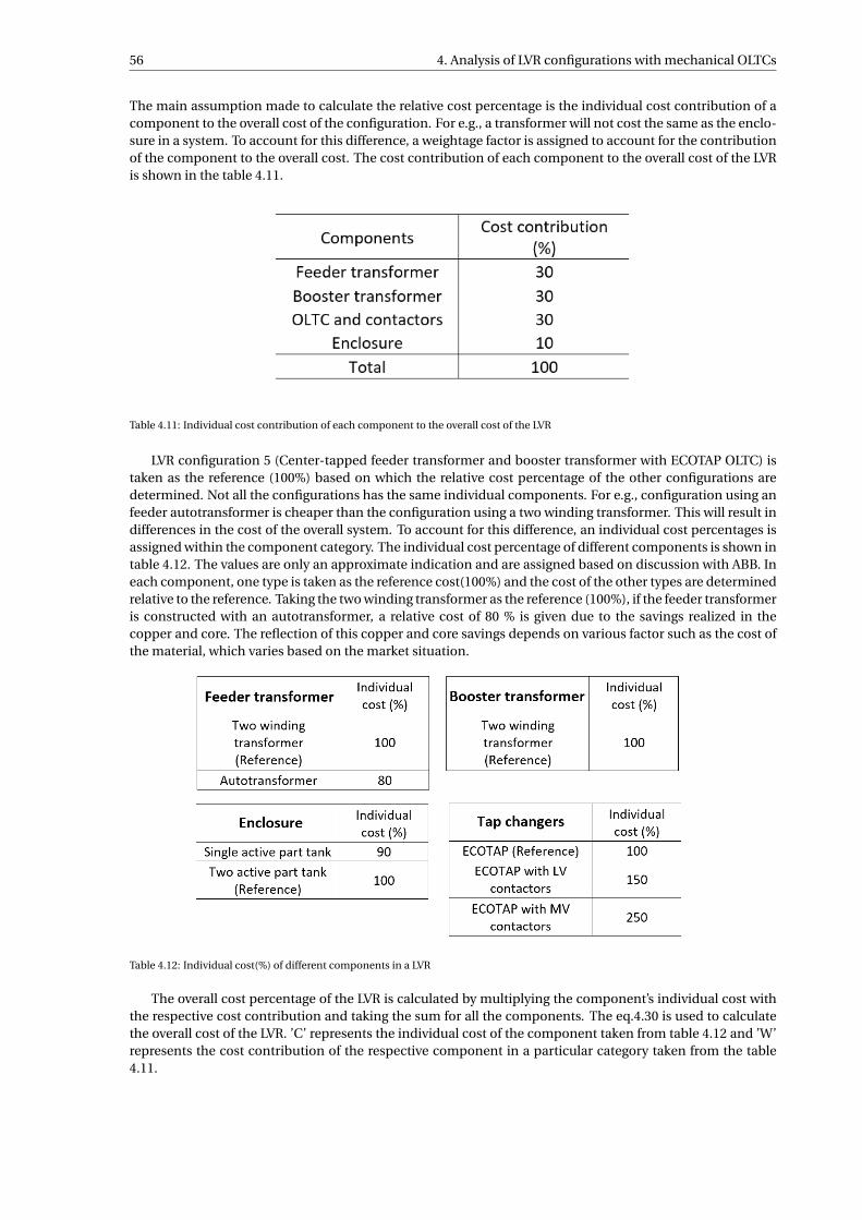
56 4. Analysis of LVR configurations with mechanical OLTCs
The main assumption made to calculate the relative cost percentage is the individual cost contribution of acomponent to the overall cost of the configuration. For e.g., a transformer will not cost the same as the enclo-sure in a system. To account for this difference, a weightage factor is assigned to account for the contributionof the component to the overall cost. The cost contribution of each component to the overall cost of the LVRis shown in the table 4.11.
Table 4.11: Individual cost contribution of each component to the overall cost of the LVR
LVR configuration 5 (Center-tapped feeder transformer and booster transformer with ECOTAP OLTC) istaken as the reference (100%) based on which the relative cost percentage of the other configurations aredetermined. Not all the configurations has the same individual components. For e.g., configuration using anfeeder autotransformer is cheaper than the configuration using a two winding transformer. This will result indifferences in the cost of the overall system. To account for this difference, an individual cost percentages isassigned within the component category. The individual cost percentage of different components is shown intable 4.12. The values are only an approximate indication and are assigned based on discussion with ABB. Ineach component, one type is taken as the reference cost(100%) and the cost of the other types are determinedrelative to the reference. Taking the two winding transformer as the reference (100%), if the feeder transformeris constructed with an autotransformer, a relative cost of 80 % is given due to the savings realized in thecopper and core. The reflection of this copper and core savings depends on various factor such as the cost ofthe material, which varies based on the market situation.
Table 4.12: Individual cost(%) of different components in a LVR
The overall cost percentage of the LVR is calculated by multiplying the component’s individual cost withthe respective cost contribution and taking the sum for all the components. The eq.4.30 is used to calculatethe overall cost of the LVR. ’C’ represents the individual cost of the component taken from table 4.12 and ’W’represents the cost contribution of the respective component in a particular category taken from the table4.11.
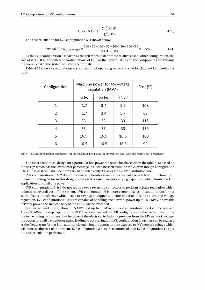
4.7. Comparison of LVR configurations 57
Over al l Cost =∑N
i=1 Ci Wi∑Ni=1 Wi
(4.30)
The cost calculation for LVR configuration 5 is shown below:
Over al l CostLV Rcon f i g 5 =100∗30+100∗30+100∗30+100∗10
30+30+30+10= 100% (4.31)
As the LVR configuration 5 is taken as the reference to determine relative cost of other configuration, thecost of it is 100%. For different configurations of LVR, as the individual cost of the components are varying,the overall cost of the system will vary accordingly.
Table 4.13 shows a comprehensive comparison of operating range and cost for different LVR configura-tions.
Table 4.13: LVR configuration comparison for the maximum line power for different voltage levels and relative cost percentage
The most economical design for a particular line power range can be chosen from the table 4.13 based onthe design which has the lowest cost percentage. As it can be seen from the table, even though configuration2 has the lowest cost, the line power it can handle is only 3.4 MVA for a 20kV distribution line.
LVR configurations 1 & 2 do not require any booster transformer for voltage regulation function. But,the main limiting factor in this design is the OLTC’s rated current carrying capability, which limits the LVRapplication for small line power.
LVR configurations 5 & 6 do not require extra reversing contactors to perform voltage regulation whichreduces the overall cost of the system. LVR configuration 6 is more economical as it uses autotransformeras the feeder transformer which leads to savings in copper and core material. For ±6%(1.5% ∗ 4) voltageregulation, LVR configurations 5 & 6 are capable of handling line network power up to 16.5 MVA. Above thisnetwork power, the step capacity of the OLTC will be exceeded.
For line network power above 16.5 MVA and up to 33 MVA, either configuration 3 or 4 can be utilized.Above 33 MVA, the step capaity of the OLTC will be exceeded. In LVR configuration 3, the feeder transformeris a two winding transformer but because of the electrical isolation it provides from the MV network voltage,the contactors will have a lower rating leading to cost savings. In LVR configuration 4, savings can be realizedas the feeder transformer is an autotransformer, but the contactors are exposed to MV network voltage whichwill increase the cost of the system. LVR configuration 3 is more economical than LVR configuration 4 as perthe cost calculation performed.

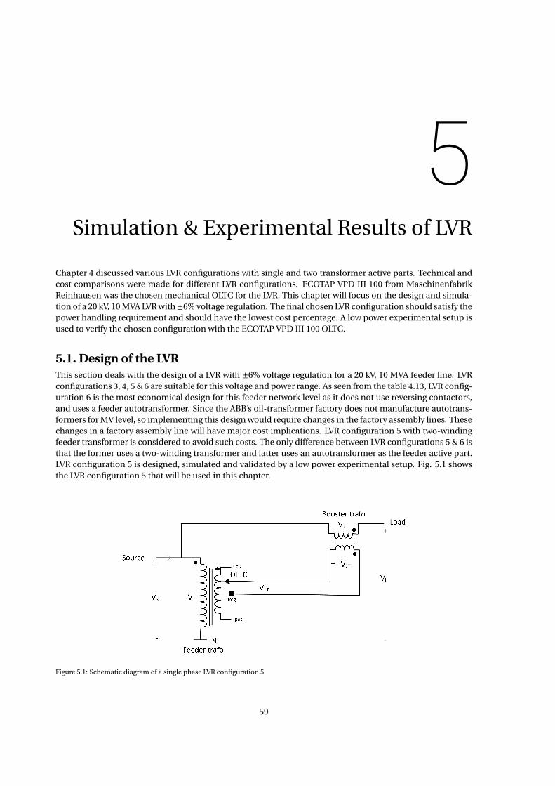
5Simulation & Experimental Results of LVR
Chapter 4 discussed various LVR configurations with single and two transformer active parts. Technical andcost comparisons were made for different LVR configurations. ECOTAP VPD III 100 from MaschinenfabrikReinhausen was the chosen mechanical OLTC for the LVR. This chapter will focus on the design and simula-tion of a 20 kV, 10 MVA LVR with ±6% voltage regulation. The final chosen LVR configuration should satisfy thepower handling requirement and should have the lowest cost percentage. A low power experimental setup isused to verify the chosen configuration with the ECOTAP VPD III 100 OLTC.
5.1. Design of the LVRThis section deals with the design of a LVR with ±6% voltage regulation for a 20 kV, 10 MVA feeder line. LVRconfigurations 3, 4, 5 & 6 are suitable for this voltage and power range. As seen from the table 4.13, LVR config-uration 6 is the most economical design for this feeder network level as it does not use reversing contactors,and uses a feeder autotransformer. Since the ABB’s oil-transformer factory does not manufacture autotrans-formers for MV level, so implementing this design would require changes in the factory assembly lines. Thesechanges in a factory assembly line will have major cost implications. LVR configuration 5 with two-windingfeeder transformer is considered to avoid such costs. The only difference between LVR configurations 5 & 6 isthat the former uses a two-winding transformer and latter uses an autotransformer as the feeder active part.LVR configuration 5 is designed, simulated and validated by a low power experimental setup. Fig. 5.1 showsthe LVR configuration 5 that will be used in this chapter.
Figure 5.1: Schematic diagram of a single phase LVR configuration 5
59
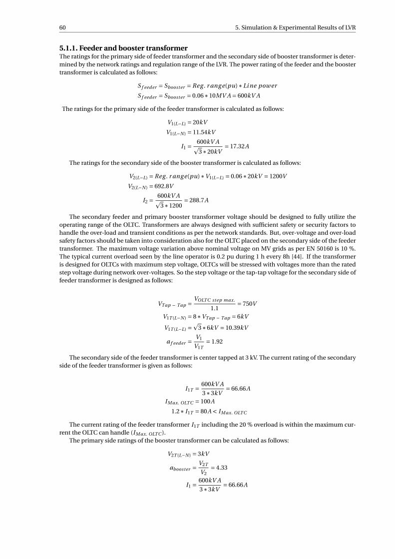
60 5. Simulation & Experimental Results of LVR
5.1.1. Feeder and booster transformerThe ratings for the primary side of feeder transformer and the secondary side of booster transformer is deter-mined by the network ratings and regulation range of the LVR. The power rating of the feeder and the boostertransformer is calculated as follows:
S f eeder = Sbooster = Reg . r ang e(pu)∗Li ne power
S f eeder = Sbooster = 0.06∗10MV A = 600kV A
The ratings for the primary side of the feeder transformer is calculated as follows:
V1(L−L) = 20kV
V1(L−N ) = 11.54kV
I1 = 600kV Ap3∗20kV
= 17.32A
The ratings for the secondary side of the booster transformer is calculated as follows:
V2(L−L) = Reg . r ang e(pu)∗V1(L−L) = 0.06∗20kV = 1200V
V2(L−N ) = 692.8V
I2 = 600kV Ap3∗1200
= 288.7A
The secondary feeder and primary booster transformer voltage should be designed to fully utilize theoperating range of the OLTC. Transformers are always designed with sufficient safety or security factors tohandle the over-load and transient conditions as per the network standards. But, over-voltage and over-loadsafety factors should be taken into consideration also for the OLTC placed on the secondary side of the feedertransformer. The maximum voltage variation above nominal voltage on MV grids as per EN 50160 is 10 %.The typical current overload seen by the line operator is 0.2 pu during 1 h every 8h [44]. If the transformeris designed for OLTCs with maximum step voltage, OLTCs will be stressed with voltages more than the ratedstep voltage during network over-voltages. So the step voltage or the tap-tap voltage for the secondary side offeeder transformer is designed as follows:
VTap − Tap = VOLT C step max.
1.1= 750V
V1T (L−N ) = 8∗VTap − Tap = 6kV
V1T (L−L) =p
3∗6kV = 10.39kV
a f eeder =V1
V1T= 1.92
The secondary side of the feeder transformer is center tapped at 3 kV. The current rating of the secondaryside of the feeder transformer is given as follows:
I1T = 600kV A
3∗3kV= 66.66A
IM ax. OLT C = 100A
1.2∗ I1T = 80A < IM ax. OLT C
The current rating of the feeder transformer I1T including the 20 % overload is within the maximum cur-rent the OLTC can handle (IM ax. OLT C ).
The primary side ratings of the booster transformer can be calculated as follows:
V2T (L−N ) = 3kV
abooster =V2T
V2= 4.33
I1 = 600kV A
3∗3kV= 66.66A
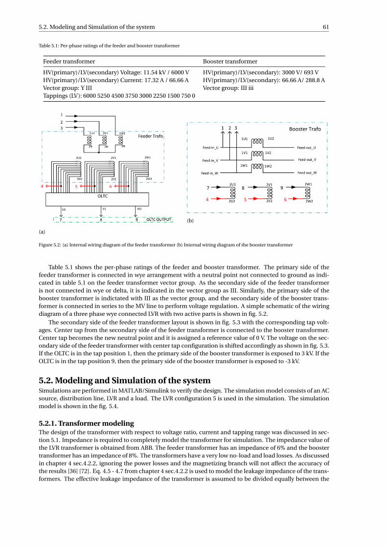
5.2. Modeling and Simulation of the system 61
Table 5.1: Per-phase ratings of the feeder and booster transformer
Feeder transformer Booster transformer
HV(primary)/LV(secondary) Voltage: 11.54 kV / 6000 V HV(primary)/LV(secondary): 3000 V/ 693 VHV(primary)/LV(secondary) Current: 17.32 A / 66.66 A HV(primary)/LV(secondary): 66.66 A/ 288.8 AVector group: Y III Vector group: III iiiTappings (LV): 6000 5250 4500 3750 3000 2250 1500 750 0
(a)
(b)
Figure 5.2: (a) Internal wiring diagram of the feeder transformer (b) Internal wiring diagram of the booster transformer
Table 5.1 shows the per-phase ratings of the feeder and booster transformer. The primary side of thefeeder transformer is connected in wye arrangement with a neutral point not connected to ground as indi-cated in table 5.1 on the feeder transformer vector group. As the secondary side of the feeder transformeris not connected in wye or delta, it is indicated in the vector group as III. Similarly, the primary side of thebooster transformer is indictated with III as the vector group, and the secondary side of the booster trans-former is connected in series to the MV line to perform voltage regulation. A simple schematic of the wiringdiagram of a three phase wye connected LVR with two active parts is shown in fig. 5.2.
The secondary side of the feeder transformer layout is shown in fig. 5.3 with the corresponding tap volt-ages. Center tap from the secondary side of the feeder transformer is connected to the booster transformer.Center tap becomes the new neutral point and it is assigned a reference value of 0 V. The voltage on the sec-ondary side of the feeder transformer with center tap configuration is shifted accordingly as shown in fig. 5.3.If the OLTC is in the tap position 1, then the primary side of the booster transformer is exposed to 3 kV. If theOLTC is in the tap position 9, then the primary side of the booster transformer is exposed to -3 kV.
5.2. Modeling and Simulation of the systemSimulations are performed in MATLAB/Simulink to verify the design. The simulation model consists of an ACsource, distribution line, LVR and a load. The LVR configuration 5 is used in the simulation. The simulationmodel is shown in the fig. 5.4.
5.2.1. Transformer modelingThe design of the transformer with respect to voltage ratio, current and tapping range was discussed in sec-tion 5.1. Impedance is required to completely model the transformer for simulation. The impedance value ofthe LVR transformer is obtained from ABB. The feeder transformer has an impedance of 6% and the boostertransformer has an impedance of 8%. The transformers have a very low no-load and load losses. As discussedin chapter 4 sec.4.2.2, ignoring the power losses and the magnetizing branch will not affect the accuracy ofthe results [36] [72]. Eq. 4.5 - 4.7 from chapter 4 sec.4.2.2 is used to model the leakage impedance of the trans-formers. The effective leakage impedance of the transformer is assumed to be divided equally between the
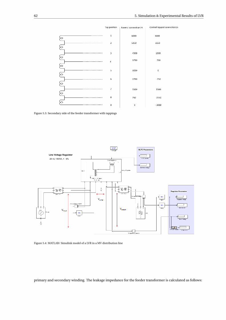
62 5. Simulation & Experimental Results of LVR
Figure 5.3: Secondary side of the feeder transformer with tappings
Figure 5.4: MATLAB/ Simulink model of a LVR in a MV distribution line
primary and secondary winding. The leakage impedance for the feeder transformer is calculated as follows:
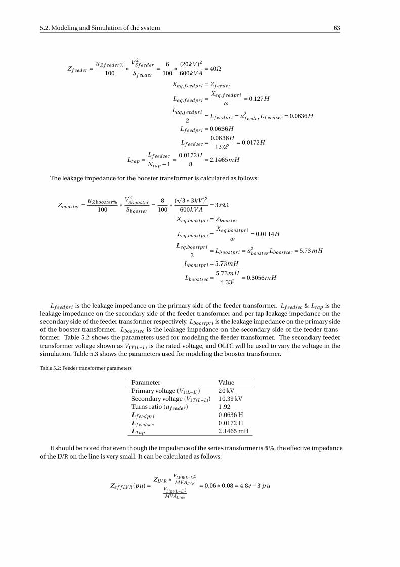
5.2. Modeling and Simulation of the system 63
Z f eeder =uZ f eeder %
100∗
V 2S f eeder
S f eeder= 6
100∗ (20kV )2
600kV A= 40Ω
Xeq, f eed pr i = Z f eeder
Leq, f eed pr i =Xeq, f eed pr i
ω= 0.127H
Leq, f eed pr i
2= L f eed pr i = a2
f eeder L f eed sec = 0.0636H
L f eed pr i = 0.0636H
L f eed sec =0.0636H
1.922 = 0.0172H
Lt ap = L f eed sec
Nt ap −1= 0.0172H
8= 2.1465mH
The leakage impedance for the booster transformer is calculated as follows:
Zbooster =uZ booster %
100∗ V 2
Sbooster
Sbooster= 8
100∗ (
p3∗3kV )2
600kV A= 3.6Ω
Xeq,boost pr i = Zbooster
Leq,boost pr i =Xeq,boost pr i
ω= 0.0114H
Leq,boost pr i
2= Lboost pr i = a2
booster Lboost sec = 5.73mH
Lboost pr i = 5.73mH
Lboost sec =5.73mH
4.332 = 0.3056mH
L f eed pr i is the leakage impedance on the primary side of the feeder transformer. L f eed sec & Lt ap is theleakage impedance on the secondary side of the feeder transformer and per tap leakage impedance on thesecondary side of the feeder transformer respectively. Lboost pr i is the leakage impedance on the primary sideof the booster transformer. Lboost sec is the leakage impedance on the secondary side of the feeder trans-former. Table 5.2 shows the parameters used for modeling the feeder transformer. The secondary feedertransformer voltage shown as V1T (L−L) is the rated voltage, and OLTC will be used to vary the voltage in thesimulation. Table 5.3 shows the parameters used for modeling the booster transformer.
Table 5.2: Feeder transformer parameters
Parameter ValuePrimary voltage (V1(L−L)) 20 kVSecondary voltage (V1T (L−L)) 10.39 kVTurns ratio (a f eeder ) 1.92L f eed pr i 0.0636 HL f eed sec 0.0172 HLTap 2.1465 mH
It should be noted that even though the impedance of the series transformer is 8 %, the effective impedanceof the LVR on the line is very small. It can be calculated as follows:
Ze f f LV R (pu) =ZLV R ∗ VLV R(L−L)2
MV ALV R
VLi ne(L−L)2
MV ALi ne
= 0.06∗0.08 = 4.8e −3 pu
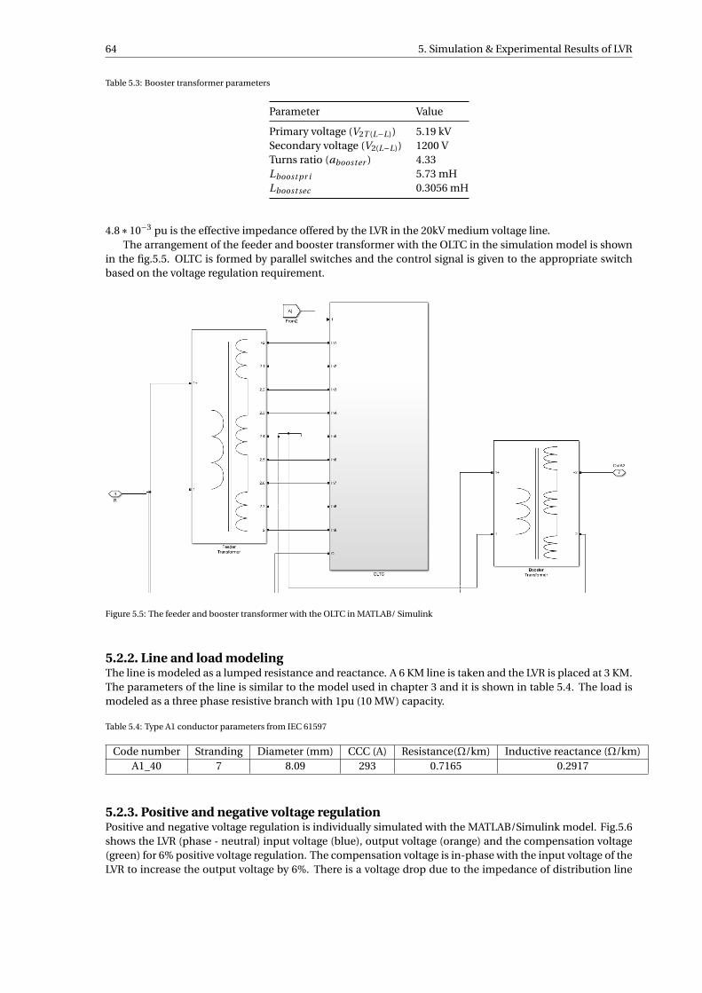
64 5. Simulation & Experimental Results of LVR
Table 5.3: Booster transformer parameters
Parameter Value
Primary voltage (V2T (L−L)) 5.19 kVSecondary voltage (V2(L−L)) 1200 VTurns ratio (abooster ) 4.33Lboost pr i 5.73 mHLboost sec 0.3056 mH
4.8∗10−3 pu is the effective impedance offered by the LVR in the 20kV medium voltage line.The arrangement of the feeder and booster transformer with the OLTC in the simulation model is shown
in the fig.5.5. OLTC is formed by parallel switches and the control signal is given to the appropriate switchbased on the voltage regulation requirement.
Figure 5.5: The feeder and booster transformer with the OLTC in MATLAB/ Simulink
5.2.2. Line and load modelingThe line is modeled as a lumped resistance and reactance. A 6 KM line is taken and the LVR is placed at 3 KM.The parameters of the line is similar to the model used in chapter 3 and it is shown in table 5.4. The load ismodeled as a three phase resistive branch with 1pu (10 MW) capacity.
Table 5.4: Type A1 conductor parameters from IEC 61597
Code number Stranding Diameter (mm) CCC (A) Resistance(Ω/km) Inductive reactance (Ω/km)A1_40 7 8.09 293 0.7165 0.2917
5.2.3. Positive and negative voltage regulationPositive and negative voltage regulation is individually simulated with the MATLAB/Simulink model. Fig.5.6shows the LVR (phase - neutral) input voltage (blue), output voltage (orange) and the compensation voltage(green) for 6% positive voltage regulation. The compensation voltage is in-phase with the input voltage of theLVR to increase the output voltage by 6%. There is a voltage drop due to the impedance of distribution line
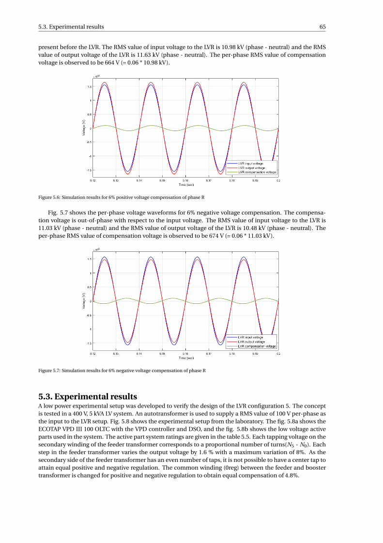
5.3. Experimental results 65
present before the LVR. The RMS value of input voltage to the LVR is 10.98 kV (phase - neutral) and the RMSvalue of output voltage of the LVR is 11.63 kV (phase - neutral). The per-phase RMS value of compensationvoltage is observed to be 664 V (= 0.06 * 10.98 kV).
Figure 5.6: Simulation results for 6% positive voltage compensation of phase R
Fig. 5.7 shows the per-phase voltage waveforms for 6% negative voltage compensation. The compensa-tion voltage is out-of-phase with respect to the input voltage. The RMS value of input voltage to the LVR is11.03 kV (phase - neutral) and the RMS value of output voltage of the LVR is 10.48 kV (phase - neutral). Theper-phase RMS value of compensation voltage is observed to be 674 V (= 0.06 * 11.03 kV).
Figure 5.7: Simulation results for 6% negative voltage compensation of phase R
5.3. Experimental resultsA low power experimental setup was developed to verify the design of the LVR configuration 5. The conceptis tested in a 400 V, 5 kVA LV system. An autotransformer is used to supply a RMS value of 100 V per-phase asthe input to the LVR setup. Fig. 5.8 shows the experimental setup from the laboratory. The fig. 5.8a shows theECOTAP VPD III 100 OLTC with the VPD controller and DSO, and the fig. 5.8b shows the low voltage activeparts used in the system. The active part system ratings are given in the table 5.5. Each tapping voltage on thesecondary winding of the feeder transformer corresponds to a proportional number of turns(N5 - N0). Eachstep in the feeder transformer varies the output voltage by 1.6 % with a maximum variation of 8%. As thesecondary side of the feeder transformer has an even number of taps, it is not possible to have a center tap toattain equal positive and negative regulation. The common winding (0reg) between the feeder and boostertransformer is changed for positive and negative regulation to obtain equal compensation of 4.8%.
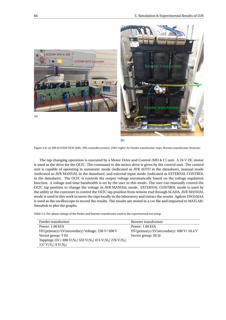
66 5. Simulation & Experimental Results of LVR
(a)
(b)
Figure 5.8: (a) MR ECOTAP OLTC(left), MR controller(center), DSO (right) (b) Feeder transformer (top), Booster transformer (bottom)
The tap changing operation is executed by a Motor Drive and Control (MD & C) unit. A 24 V DC motoris used as the drive for the OLTC. The command to the motor drive is given by the control unit. The controlunit is capable of operating in automatic mode (indicated as AVR AUTO in the datasheet), manual mode(indicated as AVR MANUAL in the datasheet) and external input mode (indicated as EXTERNAL CONTROLin the datasheet). The OLTC is controls the output voltage automatically based on the voltage regulationfunction. A voltage and time bandwidth is set by the user in this mode. The user can manually control theOLTC tap position to change the voltage in AVR MANUAL mode. EXTERNAL CONTROL mode is used bythe utility or the customer to control the OLTC tap position from remote end through SCADA. AVR MANUALmode is used in this work to move the taps locally in the laboratory and extract the results. Agilent DSO1024Ais used as the oscilloscope to record the results. The results are stored in a csv file and imported to MATLAB/Simulink to plot the graphs.
Table 5.5: Per-phase ratings of the feeder and booster transformer used in the experimental test setup
Feeder transformer Booster transformerPower: 1.66 kVA Power: 1.66 kVAHV(primary)/LV(secondary) Voltage: 230 V/ 690 V HV(primary)/LV(secondary): 690 V/ 18.4 VVector group: Y III Vector group: III iiiTappings (LV): 690 V(N5) 553 V(N4) 474 V(N3) 276 V(N2)137 V(N1) 0 V(N0)
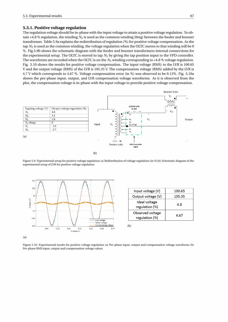
5.3. Experimental results 67
5.3.1. Positive voltage regulationThe regulation voltage should be in-phase with the input voltage to attain a positive voltage regulation. To ob-tain +4.8 % regulation, the winding N2 is used as the common winding (0reg) between the feeder and boostertransformer. Table 5.9a explains the redistribution of regulation (%) for positive voltage compensation. As thetap N2 is used as the common winding, the voltage regulation when the OLTC moves to that winding will be 0%. Fig.5.9b shows the schematic diagram with the feeder and booster transformers internal connections forthe experimental setup. The OLTC is moved to tap N5 by giving the tap position input to the VPD controller.The waveforms are recorded when the OLTC is on the N5 winding corresponding to +4.8 % voltage regulation.Fig. 5.10 shows the results for positive voltage compensation. The input voltage (RMS) to the LVR is 100.65V and the output voltage (RMS) of the LVR is 105.35 V. The compensation voltage (RMS) added by the LVR is4.7 V which corresponds to 4.67 %. Voltage compensation error (in %) was observed to be 0.13%. Fig. 5.10ashows the per-phase input, output, and LVR compensation voltage waveforms. As it is observed from theplot, the compensation voltage is in-phase with the input voltage to provide positive voltage compensation.
(a)
(b)
Figure 5.9: Experimental setup for positive voltage regulation (a) Redistribution of voltage regulation (in %)(b) Schematic diagram of theexperimental setup of LVR for positive voltage regulation
(a)
(b)
Figure 5.10: Experimental results for positive voltage regulation (a) Per-phase input, output and compensation voltage waveforms (b)Per-phase RMS input, output and compensation voltage values
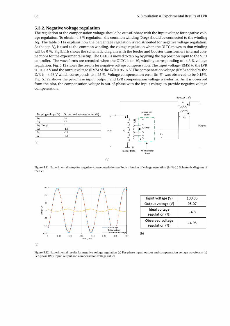
68 5. Simulation & Experimental Results of LVR
5.3.2. Negative voltage regulationThe regulation or the compensation voltage should be out-of-phase with the input voltage for negative volt-age regulation. To obtain -4.8 % regulation, the common winding (0reg) should be connected to the windingN3. The table 5.11a explains how the percentage regulation is redistributed for negative voltage regulation.As the tap N3 is used as the common winding, the voltage regulation when the OLTC moves to that windingwill be 0 %. Fig.5.11b shows the schematic diagram with the feeder and booster transformers internal con-nections for the experimental setup. The OLTC is moved to tap N0 by giving the tap position input to the VPDcontroller. The waveforms are recorded when the OLTC is on N0 winding corresponding to -4.8 % voltageregulation. Fig. 5.12 shows the results for negative voltage compensation. The input voltage (RMS) to the LVRis 100.03 V and the output voltage (RMS) of the LVR is 95.07 V. The compensation voltage (RMS) added by theLVR is - 4.96 V which corresponds to 4.95 %. Voltage compensation error (in %) was observed to be 0.15%.Fig. 5.12a shows the per-phase input, output, and LVR compensation voltage waveforms. As it is observedfrom the plot, the compensation voltage is out-of-phase with the input voltage to provide negative voltagecompensation.
(a)
(b)
Figure 5.11: Experimental setup for negative voltage regulation (a) Redistribution of voltage regulation (in %)(b) Schematic diagram ofthe LVR
(a)
(b)
Figure 5.12: Experimental results for negative voltage regulation (a) Per-phase input, output and compensation voltage waveforms (b)Per-phase RMS input, output and compensation voltage values
6Feasibility of Power Electronics based
OLTCs for LVRs
Mechanical OLTCs have been employed by the transformer manufacturers for a long time due to their robusttap changing capabilities and simple tap changing mechanism using resistors/reactors. However, mechani-cally moving components are prone to wear and tear which leads to regular maintenance. Frequent mainte-nance increases the service cost of mechanical OLTCs. The other drawback is the low speed of tap-changersdue to mechanically moving components and the time required to store the energy for a tap-changing op-eration [26]. With the advent of power electronics technology, researchers have been trying to implementtap-changers using solid state switches to avoid any moving parts in the system so as to increase the speedof tap changing operation and reduce maintenance of the OLTC[10][11]. Mechanical tap-changers assistedby power electronic switches have also been proposed to combine the robustness of a mechanical OLTC andarc free commutation of a power electronics based OLTC [48][34]. The advantages of power electronics basedOLTCs are as follows[26]:
• Low maintenance cost.
• Fast tap changing operation and no delay between two tap changes.
• No upper limit on the number of tap changing operations.
Even though power electronics based OLTCs have many advantages over mechanical OLTCs, there aresome disadvantages associated with them. The initial cost of the solid state switches are high and it has amore complicated control mechanism compared to its mechanical counterpart. It also requires a specialprotection mechanism to protect the switches during voltage and current disturbances. Increase in unpre-dictable generators and loads will require higher duty of OLTCs in a distribution line in the near future [60].Power electronics based OLTCs will be able to perform faster tap changes with lower maintenance for higherduty requirements comapared to mechanical tap-changers. This chapter will focus on the technical andeconomical feasibility study of power electronics based OLTCs for a 20 kV, 10 MVA LVR with ±6% voltageregulation.
6.1. LVR configurationOne of the drawbacks of power electronics based OLTCs is the cost of the solid-state switches. Power elec-tronic switches are expensive for higher voltage and current ratings. Switches are exposed to surge voltagesand short circuit current when directly exposed to a MV line. The power electronic switches should satisfythe short circuit and impulse voltage requirement of the respective medium voltage line if directly exposedto a MV distribution line [18]. Currently there are no electronic switches which can satisfy the requirementsfor a 20kV MV line; hence, power electronic switches should be used in series and parallel for each tap tomeet the requirements. This can drastically increase the cost of the overall system. The switches have to beoverrated when series combination of power electronic switches are used to maintain the reliability in oper-ation. LVR with a feeder and booster configuration can be used to avoid series operation of power electronic
69
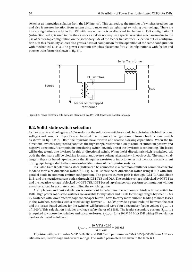
70 6. Feasibility of Power Electronics based OLTCs for LVRs
switches as it provides isolation from the MV line [44]. This can reduce the number of switches used per tapand also it ensures isolation from system disturbances such as lightning/ switching over-voltage. There arefour configurations available for LVR with two active parts as discussed in chapter 4. LVR configuration 5(subsection: 4.6.2) is used in this thesis work as it does not require a special reversing mechanism due to theuse of center-tap configuration on the secondary side of the feeder transformer. Selection of LVR configura-tion 5 in this feasibility studies also gives a basis of comparison for the operation of the same configurationwith mechanical OLTCs. The power electronic switches placement for LVR configuration 5 with feeder andbooster transformer is shown in fig. 6.1.
Figure 6.1: Power electronic (PE) switches placement in a LVR with feeder and booster topology
6.2. Solid-state switch selectionAs the currents and voltages are AC waveforms, the solid-state switches should be able to handle bi-directionalvoltages and currents. Thyrsitors can be used in anti-parallel configuration to form a bi-directional switchas shown in fig. 6.2 (b). Both the thyristors have forward and reverse blocking capabilities. When the bi-directional switch is required to conduct, the thyristor pair is switched-on to conduct current in positive andnegative directions. At any point in time during switch-on, only one of the thyristors is conducting. The losseswill be due to only one thyristor for this bi-directional switch. When the bi-directional switch is switched-off,both the thyristors will be blocking forward and reverse voltage alternatively in each cycle. The main chal-lenge in thyristor based tap-changer is that it requires a resistor or inductor to restrict the short circuit currentduring tap changes due to the semi-controllable nature of the thyristor switches.
Insulated Gate Bipolar Transistors (IGBTs) can be connected in a common-emitter or common-collectormode to form a bi-directional switch[73]. Fig. 6.2 (a) shows the bi-directional switch using IGBTs with anti-parallel diode in common-emitter configuration. The positive current path is through IGBT T1A and diodeD1B, and the negative current path is through IGBT T1B and D1A. The positive voltage is blocked by IGBT T1Aand the negative voltage is blocked by IGBT T1B. IGBT based tap-changer can perform commutation withoutany short circuit by accurately controlling the switching time.
A simple loss and cost calculation is carried out to determine the economical bi-directional switch forLVRs. High power solid-state switches are available for thyristors and IGBTs for voltage ranges between 1 - 6.5kV. Switches with lower rated voltage are cheaper but will have to carry more current, leading to more lossesin the switches. Switches with a rated voltage between 4 - 4.5 kV provide a good trade-off between the costand the losses. Rated voltage for the switches will be around 4250 V for a secondary feeder voltage (V f eed sec )of 1500 V. This calculation includes a voltage safety factor of 2 [65]. The feeder secondary current (I f eed sec )is required to choose the switches and calculate losses. I f eed sec for a 20 kV, 10 MVA LVR with ±6% regulationcan be calculated as follows:
I f eed sec =10 MV A∗0.06
3 ∗ 750= 266.6A
Thyristor with part number 5STP 04D4200 and IGBT with part number 5SNA 0650J450300 from ABB sat-isfies the required voltage and current ratings. The switch parameters are given in the table 6.1.
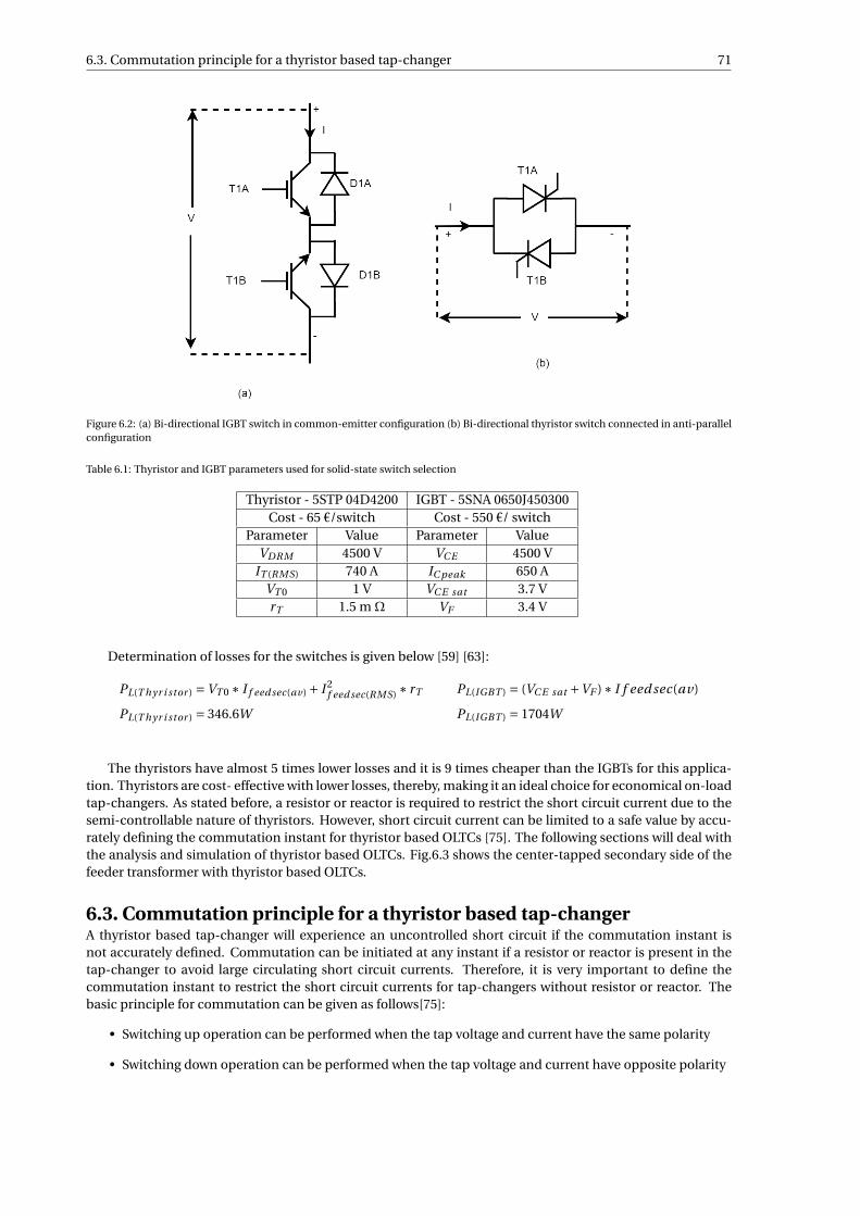
6.3. Commutation principle for a thyristor based tap-changer 71
Figure 6.2: (a) Bi-directional IGBT switch in common-emitter configuration (b) Bi-directional thyristor switch connected in anti-parallelconfiguration
Table 6.1: Thyristor and IGBT parameters used for solid-state switch selection
Thyristor - 5STP 04D4200 IGBT - 5SNA 0650J450300Cost - 65 €/switch Cost - 550 €/ switch
Parameter Value Parameter ValueVDRM 4500 V VC E 4500 V
IT (RMS) 740 A IC peak 650 AVT 0 1 V VC E sat 3.7 VrT 1.5 mΩ VF 3.4 V
Determination of losses for the switches is given below [59] [63]:
PL(T hyr i stor ) =VT 0 ∗ I f eed sec(av) + I 2f eed sec(RMS) ∗ rT PL(IGBT ) = (VC E sat +VF )∗ I f eed sec(av)
PL(T hyr i stor ) = 346.6W PL(IGBT ) = 1704W
The thyristors have almost 5 times lower losses and it is 9 times cheaper than the IGBTs for this applica-tion. Thyristors are cost- effective with lower losses, thereby, making it an ideal choice for economical on-loadtap-changers. As stated before, a resistor or reactor is required to restrict the short circuit current due to thesemi-controllable nature of thyristors. However, short circuit current can be limited to a safe value by accu-rately defining the commutation instant for thyristor based OLTCs [75]. The following sections will deal withthe analysis and simulation of thyristor based OLTCs. Fig.6.3 shows the center-tapped secondary side of thefeeder transformer with thyristor based OLTCs.
6.3. Commutation principle for a thyristor based tap-changerA thyristor based tap-changer will experience an uncontrolled short circuit if the commutation instant isnot accurately defined. Commutation can be initiated at any instant if a resistor or reactor is present in thetap-changer to avoid large circulating short circuit currents. Therefore, it is very important to define thecommutation instant to restrict the short circuit currents for tap-changers without resistor or reactor. Thebasic principle for commutation can be given as follows[75]:
• Switching up operation can be performed when the tap voltage and current have the same polarity
• Switching down operation can be performed when the tap voltage and current have opposite polarity
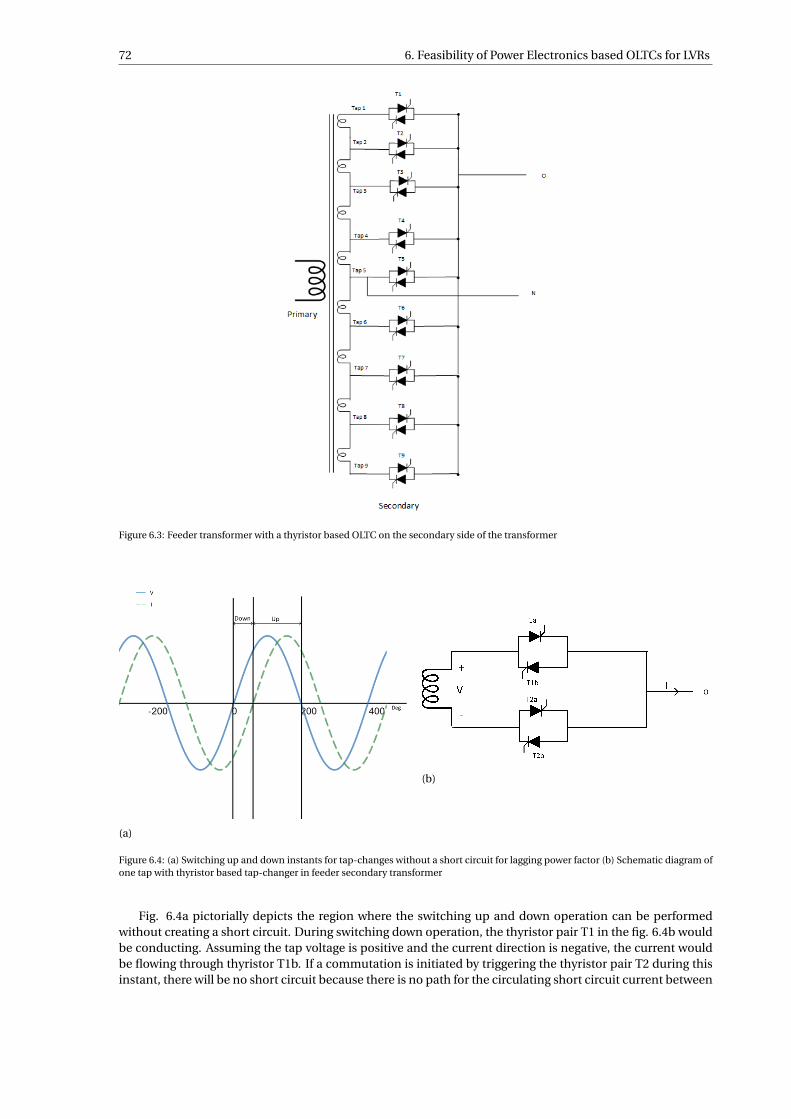
72 6. Feasibility of Power Electronics based OLTCs for LVRs
Figure 6.3: Feeder transformer with a thyristor based OLTC on the secondary side of the transformer
(a)
(b)
Figure 6.4: (a) Switching up and down instants for tap-changes without a short circuit for lagging power factor (b) Schematic diagram ofone tap with thyristor based tap-changer in feeder secondary transformer
Fig. 6.4a pictorially depicts the region where the switching up and down operation can be performedwithout creating a short circuit. During switching down operation, the thyristor pair T1 in the fig. 6.4b wouldbe conducting. Assuming the tap voltage is positive and the current direction is negative, the current wouldbe flowing through thyristor T1b. If a commutation is initiated by triggering the thyristor pair T2 during thisinstant, there will be no short circuit because there is no path for the circulating short circuit current between
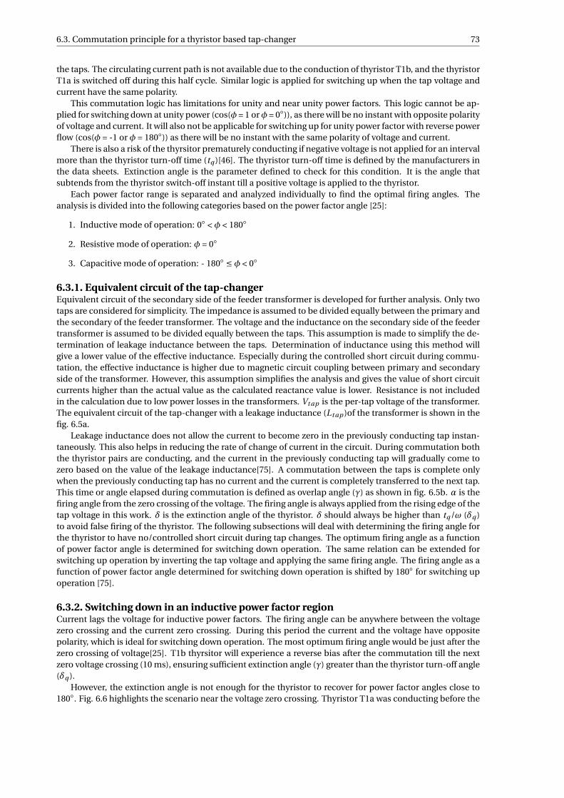
6.3. Commutation principle for a thyristor based tap-changer 73
the taps. The circulating current path is not available due to the conduction of thyristor T1b, and the thyristorT1a is switched off during this half cycle. Similar logic is applied for switching up when the tap voltage andcurrent have the same polarity.
This commutation logic has limitations for unity and near unity power factors. This logic cannot be ap-plied for switching down at unity power (cos(φ = 1 orφ = 0)), as there will be no instant with opposite polarityof voltage and current. It will also not be applicable for switching up for unity power factor with reverse powerflow (cos(φ = -1 or φ = 180)) as there will be no instant with the same polarity of voltage and current.
There is also a risk of the thyrsitor prematurely conducting if negative voltage is not applied for an intervalmore than the thyristor turn-off time (tq )[46]. The thyristor turn-off time is defined by the manufacturers inthe data sheets. Extinction angle is the parameter defined to check for this condition. It is the angle thatsubtends from the thyristor switch-off instant till a positive voltage is applied to the thyristor.
Each power factor range is separated and analyzed individually to find the optimal firing angles. Theanalysis is divided into the following categories based on the power factor angle [25]:
1. Inductive mode of operation: 0 < φ < 180
2. Resistive mode of operation: φ = 0
3. Capacitive mode of operation: - 180 ≤ φ < 0
6.3.1. Equivalent circuit of the tap-changerEquivalent circuit of the secondary side of the feeder transformer is developed for further analysis. Only twotaps are considered for simplicity. The impedance is assumed to be divided equally between the primary andthe secondary of the feeder transformer. The voltage and the inductance on the secondary side of the feedertransformer is assumed to be divided equally between the taps. This assumption is made to simplify the de-termination of leakage inductance between the taps. Determination of inductance using this method willgive a lower value of the effective inductance. Especially during the controlled short circuit during commu-tation, the effective inductance is higher due to magnetic circuit coupling between primary and secondaryside of the transformer. However, this assumption simplifies the analysis and gives the value of short circuitcurrents higher than the actual value as the calculated reactance value is lower. Resistance is not includedin the calculation due to low power losses in the transformers. Vt ap is the per-tap voltage of the transformer.The equivalent circuit of the tap-changer with a leakage inductance (Lt ap )of the transformer is shown in thefig. 6.5a.
Leakage inductance does not allow the current to become zero in the previously conducting tap instan-taneously. This also helps in reducing the rate of change of current in the circuit. During commutation boththe thyristor pairs are conducting, and the current in the previously conducting tap will gradually come tozero based on the value of the leakage inductance[75]. A commutation between the taps is complete onlywhen the previously conducting tap has no current and the current is completely transferred to the next tap.This time or angle elapsed during commutation is defined as overlap angle (γ) as shown in fig. 6.5b. α is thefiring angle from the zero crossing of the voltage. The firing angle is always applied from the rising edge of thetap voltage in this work. δ is the extinction angle of the thyristor. δ should always be higher than tq /ω (δq )to avoid false firing of the thyristor. The following subsections will deal with determining the firing angle forthe thyristor to have no/controlled short circuit during tap changes. The optimum firing angle as a functionof power factor angle is determined for switching down operation. The same relation can be extended forswitching up operation by inverting the tap voltage and applying the same firing angle. The firing angle as afunction of power factor angle determined for switching down operation is shifted by 180 for switching upoperation [75].
6.3.2. Switching down in an inductive power factor regionCurrent lags the voltage for inductive power factors. The firing angle can be anywhere between the voltagezero crossing and the current zero crossing. During this period the current and the voltage have oppositepolarity, which is ideal for switching down operation. The most optimum firing angle would be just after thezero crossing of voltage[25]. T1b thyrsitor will experience a reverse bias after the commutation till the nextzero voltage crossing (10 ms), ensuring sufficient extinction angle (γ) greater than the thyristor turn-off angle(δq ).
However, the extinction angle is not enough for the thyristor to recover for power factor angles close to180. Fig. 6.6 highlights the scenario near the voltage zero crossing. Thyristor T1a was conducting before the
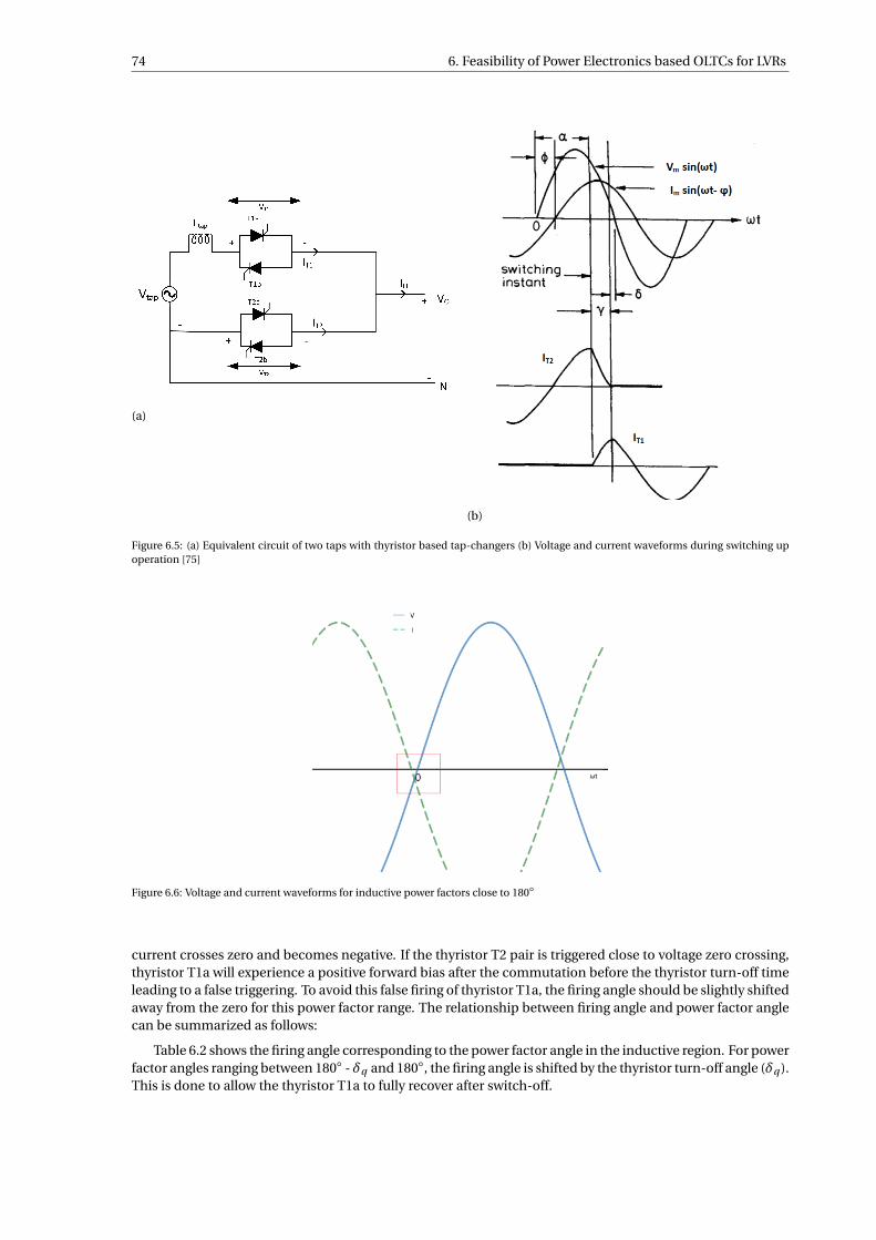
74 6. Feasibility of Power Electronics based OLTCs for LVRs
(a)
(b)
Figure 6.5: (a) Equivalent circuit of two taps with thyristor based tap-changers (b) Voltage and current waveforms during switching upoperation [75]
Figure 6.6: Voltage and current waveforms for inductive power factors close to 180
current crosses zero and becomes negative. If the thyristor T2 pair is triggered close to voltage zero crossing,thyristor T1a will experience a positive forward bias after the commutation before the thyristor turn-off timeleading to a false triggering. To avoid this false firing of thyristor T1a, the firing angle should be slightly shiftedaway from the zero for this power factor range. The relationship between firing angle and power factor anglecan be summarized as follows:
Table 6.2 shows the firing angle corresponding to the power factor angle in the inductive region. For powerfactor angles ranging between 180 - δq and 180, the firing angle is shifted by the thyristor turn-off angle (δq ).This is done to allow the thyristor T1a to fully recover after switch-off.
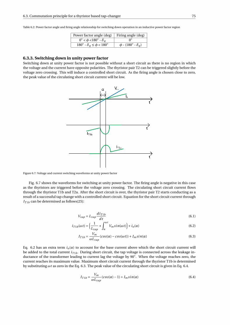
6.3. Commutation principle for a thyristor based tap-changer 75
Table 6.2: Power factor angle and firing angle relationship for switching down operation in an inductive power factor region
Power factor angle (deg) Firing angle (deg)0 < φ <180 - δq 0
180 - δq ≤ φ < 180 φ - (180 - δq )
6.3.3. Switching down in unity power factorSwitching down at unity power factor is not possible without a short circuit as there is no region in whichthe voltage and the current have opposite polarities. The thyristor pair T2 can be triggered slightly before thevoltage zero crossing. This will induce a controlled short circuit. As the firing angle is chosen close to zero,the peak value of the circulating short circuit current will be low.
Figure 6.7: Voltage and current switching waveforms at unity power factor
Fig. 6.7 shows the waveforms for switching at unity power factor. The firing angle is negative in this caseas the thyristors are triggered before the voltage zero crossing. The circulating short circuit current flowsthrough the thyristor T1b and T2a. After the short circuit is over, the thyristor pair T2 starts conducting as aresult of a successful tap change with a controlled short circuit. Equation for the short circuit current throughIT 1b can be determined as follows[25]:
Vt ap = Lt apdiT 1b
d t(6.1)
iT 1b(ωt ) =( 1
Lt ap∗
∫ ωt
αVm si n(ωt )
)+ io(α) (6.2)
IT 1b = Vm
ωLt ap(cos(α)− cos(ωt ))+ Im si n(α) (6.3)
Eq. 6.2 has an extra term io(α) to account for the base current above which the short circuit current willbe added to the total current iT 1b . During short circuit, the tap voltage is connected across the leakage in-ductance of the transformer leading to current lag the voltage by 90. When the voltage reaches zero, thecurrent reaches its maximum value. Maximum short circuit current through the thyristor T1b is determinedby substituting ωt as zero in the Eq. 6.3. The peak value of the circulating short circuit is given in Eq. 6.4.
IT 1b = Vm
ωLt ap(cos(α)−1)+ Im si n(α) (6.4)
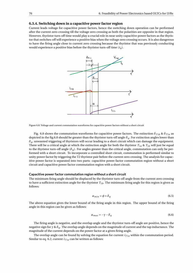
76 6. Feasibility of Power Electronics based OLTCs for LVRs
6.3.4. Switching down in a capacitive power factor regionCurrent leads voltage for capacitive power factors, hence the switching down operation can be performedafter the current zero crossing till the voltage zero crossing as both the polarities are opposite in that region.However, thyristor turn-off time would play a crucial role in near unity capacitive power factors as the thyris-tor that switches-off will experience a positive bias when the voltage zero crossing occurs. It is also dangerousto have the firing angle close to current zero crossing because the thyristor that was previously conductingwould experience a positive bias before the thyristor turn-off time (tq ).
Figure 6.8: Voltage and current commutation waveforms for capacitive power factors without a short circuit
Fig. 6.8 shows the commutation waveforms for capacitive power factors. The extinction δT 1b & δT 1a asdepicted in the fig.6.8 should be greater than the thyristor turn-off angle δq . For extinction angles lower thanδq , unwanted triggering of thyristors will occur leading to a short circuit which can damage the equipment.There will be a critical angle at which the extinction angle for both the thyristor T1a & T1b will just be equalto the thyristor turn-off angle (δq ). For angles greater than the critical angle, commutation can only be per-formed with a short circuit. To incorporate a controlled short circuit, commutation is performed similar tounity power factor by triggering the T2 thyristor pair before the current zero crossing. The analysis for capac-itive power factor is separated into two parts: capacitive power factor commutation region without a shortcircuit and capacitive power factor commutation region with a short circuit.
Capacitive power factor commutation regionwithout a short circuitThe minimum firing angle should be displaced by the thyristor turn-off angle from the current zero crossingto have a sufficient extinction angle for the thyristor T1b . The minimum firing angle for this region is given asfollows:
αmi n =φ+δq (6.5)
The above equation gives the lower bound of the firing angle in this region. The upper bound of the firingangle in this region can be given as follows:
αmax =−γ−δq (6.6)
The firing angle is negative, and the overlap angle and the thyristor turn-off angle are positive, hence thenegative sign for γ& δq . The overlap angle depends on the magnitude of current and the tap inductance. Themagnitude of the current depends on the power factor at a given firing angle.
The overlap angle can be found by solving the equation for current iT 1a within the commutation period.Similar to eq. 6.2, current iT 1a can be written as follows:
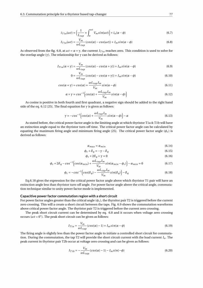
6.3. Commutation principle for a thyristor based tap-changer 77
iT 1a(ωt ) =( 1
Lt ap∗
∫ ωt
αVm si n(ωt )
)+ io(α−φ) (6.7)
IT 1a(ωt ) = Vm
ωLt ap(cos(α)− cos(ωt ))+ Im si n(α−φ) (6.8)
As observed from the fig. 6.8, at ωt =α+γ, the current IT 1a reaches zero. This condition is used to solve forthe overlap angle (γ). The relationship for γ can be derived as follows:
IT 1a(α+γ) = Vm
ωLt ap(cos(α)− cos(α+γ))+ Im si n(α−φ) (6.9)
0 = Vm
ωLt ap(cos(α)− cos(α+γ))+ Im si n(α−φ) (6.10)
cos(α+γ) = cos(α)+ ωLt ap Im
Vmsi n(α−φ) (6.11)
α+γ= cos−1(cos(α)+ ωLt ap Im
Vmsi n(α−φ)
)(6.12)
As cosine is positive in both fourth and first quadrant, a negative sign should be added to the right handside of the eq. 6.12 [25]. The final equation for γ is given as follows:
γ=−cos−1(cos(α)+ ωLt ap Im
Vmsi n(α−φ)
)−α (6.13)
As stated before, the critical power factor angle is the limiting angle at which thyristor T1a & T1b will havean extinction angle equal to the thyristor turn-off time. The critical power factor angle can be calculated byequating the maximum firing angle and minimum firing angle [25]. The critical power factor angle (φc ) isderived as follows:
αmax =αmi n (6.14)
φc +δq =−γ−δq (6.15)
φc +2δq +γ= 0 (6.16)
φc +2δq − cos−1(cos(αmi n)+ ωLt ap Im
Vmsi n(αmi n −φc )
)−αmi n = 0 (6.17)
φc =−cos−1(cos(δq )− ωLt ap Im
Vmsi n(δq )
)−δq (6.18)
Eq.6.18 gives the expression for the critical power factor angle above which thyristor T1 pair will have anextinction angle less than thyristor turn-off angle. For power factor angle above the critical angle, commuta-tion technique similar to unity power factor mode is implemented.
Capacitive power factor commutation regionwith a short circuitFor power factor angles greater than the critical angle (φc ), the thyrsitor pair T2 is triggered before the currentzero crossing. This will a create a short circuit between the taps. Fig. 6.9 shows the commutation waveformsabove critical power factor angle. The thyristor pair T2 is triggered before the current zero crossing.
The peak short circuit current can be determined by eq. 6.8 and it occurs when voltage zero crossingoccurs (ωt = 0). The peak short circuit can be given as follows:
IT 1a = Vm
ωLt ap(cos(α)−1)+ Im si n(α−φ) (6.19)
The firing angle is slightly less than the power factor angle to initiate a controlled short circuit for commuta-tion. During the commutation, the tap T2 will provide the short circuit current with the load current Io . Thepeak current in thyristor pair T2b occur at voltage zero crossing and can be given as follows:
IT 1b =− Vm
ωLt ap(cos(α)−1)− Im si n(−φ) (6.20)
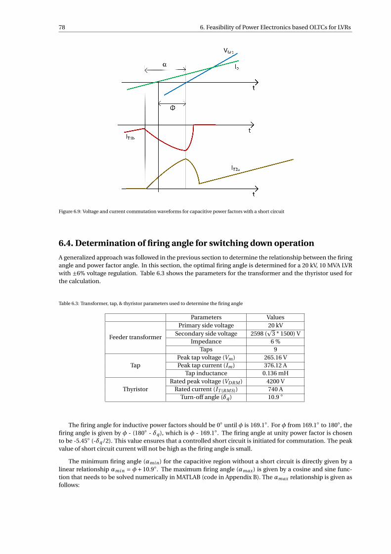
78 6. Feasibility of Power Electronics based OLTCs for LVRs
Figure 6.9: Voltage and current commutation waveforms for capacitive power factors with a short circuit
6.4. Determination of firing angle for switching down operation
A generalized approach was followed in the previous section to determine the relationship between the firingangle and power factor angle. In this section, the optimal firing angle is determined for a 20 kV, 10 MVA LVRwith ±6% voltage regulation. Table 6.3 shows the parameters for the transformer and the thyristor used forthe calculation.
Table 6.3: Transformer, tap, & thyristor parameters used to determine the firing angle
Parameters Values
Feeder transformer
Primary side voltage 20 kVSecondary side voltage 2598 (
p3 * 1500) V
Impedance 6 %Taps 9
TapPeak tap voltage (Vm) 265.16 VPeak tap current (Im) 376.12 A
Tap inductance 0.136 mH
ThyristorRated peak voltage (VDRM ) 4200 V
Rated current (IT (RMS)) 740 ATurn-off angle (δq ) 10.9
The firing angle for inductive power factors should be 0 until φ is 169.1. For φ from 169.1 to 180, thefiring angle is given by φ - (180 - δq ), which is φ - 169.1. The firing angle at unity power factor is chosento be -5.45 (-δq /2). This value ensures that a controlled short circuit is initiated for commutation. The peakvalue of short circuit current will not be high as the firing angle is small.
The minimum firing angle (αmi n) for the capacitive region without a short circuit is directly given by alinear relationship αmi n = φ+ 10.9. The maximum firing angle (αmax ) is given by a cosine and sine func-tion that needs to be solved numerically in MATLAB (code in Appendix B). The αmax relationship is given asfollows:
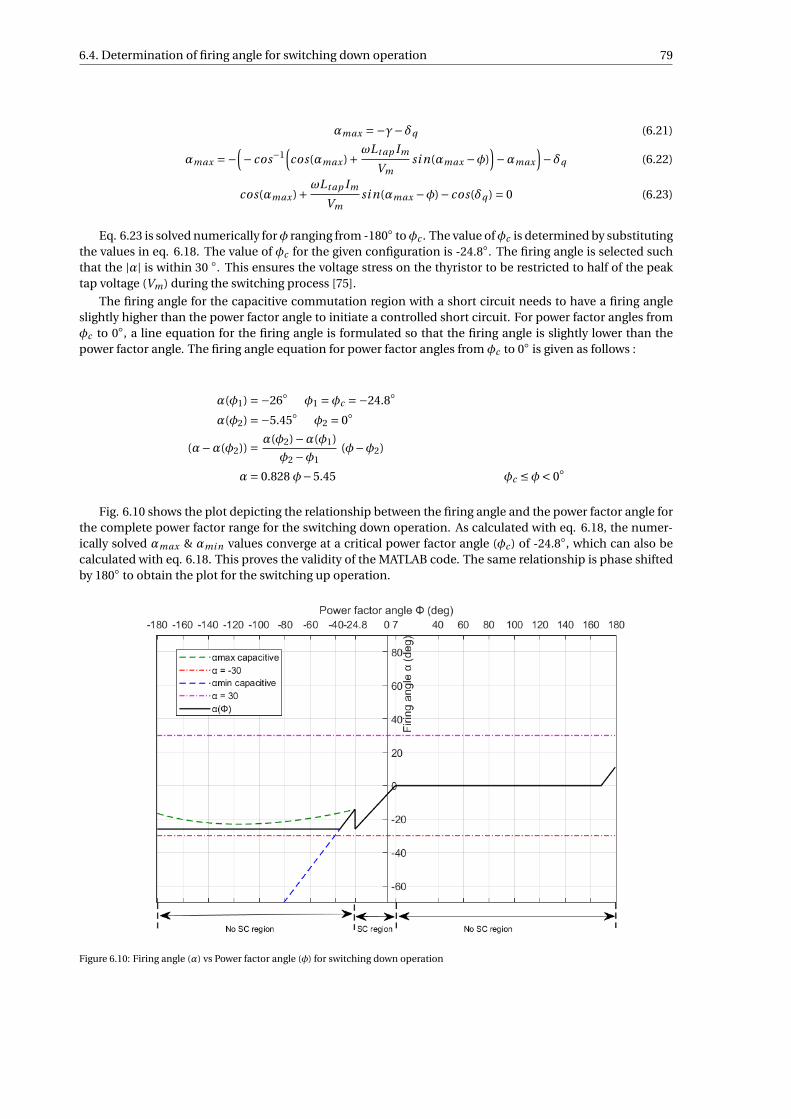
6.4. Determination of firing angle for switching down operation 79
αmax =−γ−δq (6.21)
αmax =−(− cos−1
(cos(αmax )+ ωLt ap Im
Vmsi n(αmax −φ)
)−αmax
)−δq (6.22)
cos(αmax )+ ωLt ap Im
Vmsi n(αmax −φ)− cos(δq ) = 0 (6.23)
Eq. 6.23 is solved numerically forφ ranging from -180 toφc . The value ofφc is determined by substitutingthe values in eq. 6.18. The value of φc for the given configuration is -24.8. The firing angle is selected suchthat the |α| is within 30 . This ensures the voltage stress on the thyristor to be restricted to half of the peaktap voltage (Vm) during the switching process [75].
The firing angle for the capacitive commutation region with a short circuit needs to have a firing angleslightly higher than the power factor angle to initiate a controlled short circuit. For power factor angles fromφc to 0, a line equation for the firing angle is formulated so that the firing angle is slightly lower than thepower factor angle. The firing angle equation for power factor angles from φc to 0 is given as follows :
α(φ1) =−26 φ1 =φc =−24.8
α(φ2) =−5.45 φ2 = 0
(α−α(φ2)) = α(φ2)−α(φ1)
φ2 −φ1(φ−φ2)
α= 0.828 φ−5.45 φc ≤φ< 0
Fig. 6.10 shows the plot depicting the relationship between the firing angle and the power factor angle forthe complete power factor range for the switching down operation. As calculated with eq. 6.18, the numer-ically solved αmax & αmi n values converge at a critical power factor angle (φc ) of -24.8, which can also becalculated with eq. 6.18. This proves the validity of the MATLAB code. The same relationship is phase shiftedby 180 to obtain the plot for the switching up operation.
Figure 6.10: Firing angle (α) vs Power factor angle (φ) for switching down operation
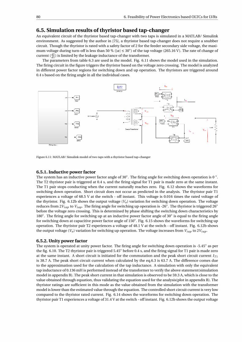
80 6. Feasibility of Power Electronics based OLTCs for LVRs
6.5. Simulation results of thyristor based tap-changerAn equivalent circuit of the thyristor based tap-changer with two taps is simulated in a MATLAB/ Simulinkenvironment. As suggested by the author in [75], a thyristor based tap-changer does not require a snubbercircuit. Though the thyristor is rated with a safety factor of 2 for the feeder secondary side voltage, the maxi-mum voltage during turn-off is less than 50 % (|α| ≤ 30) of the tap voltage (265.16 V). The rate of change ofcurrent ( di
d t ) is limited by the leakage inductance of the transformer.The parameters from table 6.3 are used in the model. Fig. 6.11 shows the model used in the simulation.
The firing circuit in the figure triggers the thyristor based on the voltage zero crossing. The model is analyzedin different power factor regions for switching down and up operation. The thyristors are triggered around0.4 s based on the firing angle in all the individual cases.
Figure 6.11: MATLAB/ Simulink model of two taps with a thyristor based tap-changer
6.5.1. Inductive power factorThe system has an inductive power factor angle of 30. The firing angle for switching down operation is 0 .The T2 thyristor pair is triggered at 0.4 s, and the firing signal for T1 pair is made zero at the same instant.The T1 pair stops conducting when the current naturally reaches zero. Fig. 6.12 shows the waveforms forswitching down operation. Short circuit does not occur as predicted in the analysis. The thyristor pair T1experiences a voltage of 68.5 V at the switch - off instant. This voltage is 0.016 times the rated voltage ofthe thyristor. Fig. 6.12b shows the output voltage (Vo) variation for switching down operation. The voltagereduces from 2Vt ap to Vt ap . The firing angle for switching up operation is -26. The thyristor is triggered 26before the voltage zero crossing. This is determined by phase shifting the switching down characteristics by180. The firing angle for switching up at an inductive power factor angle of 30 is equal to the firing anglefor switching down at capacitive power factor angle of 150. Fig. 6.15 shows the waveforms for switching upoperation. The thyristor pair T2 experiences a voltage of 48.1 V at the switch - off instant. Fig. 6.12b showsthe output voltage (Vo) variation for switching up operation. The voltage increases from Vt ap to 2Vt ap .
6.5.2. Unity power factorThe system is operated at unity power factor. The firing angle for switching down operation is -5.45 as perthe fig. 6.10. The T2 thyristor pair is triggered 5.45 before 0.4 s, and the firing signal for T1 pair is made zeroat the same instant. A short circuit is initiated for the commutation and the peak short circuit current IT 1
is 38.7 A. The peak short circuit current when calculated by the eq.6.3 is 63.7 A. The difference comes dueto the approximation used for the calculation of the tap inductance. A simulation with only the equivalenttap inductance of 0.136 mH is performed instead of the transformer to verify the above statement(simulationmodel in appendix B). The peak short current in that simulation is observed to be 59.3 A, which is close to thevalue obtained through equation, thus validating the equation used for the analysis(plot in appendix B). Thethyristor ratings are sufficient in this mode as the value obtained from the simulation with the transformermodel is lower than the estimated value through the equation. The controlled short circuit current is very lowcompared to the thyristor rated current. Fig. 6.14 shows the waveforms for switching down operation. Thethyristor pair T1 experiences a voltage of 31.4 V at the switch - off instant. Fig. 6.12b shows the output voltage
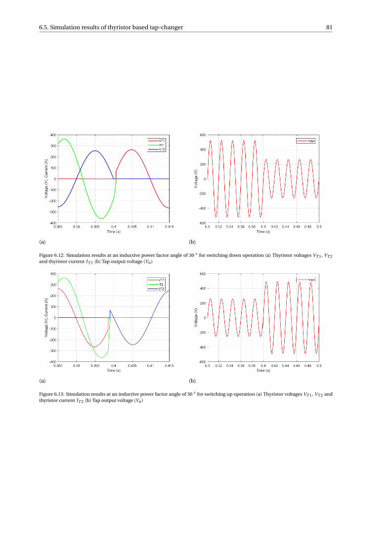
6.5. Simulation results of thyristor based tap-changer 81
(a) (b)
Figure 6.12: Simulation results at an inductive power factor angle of 30 for switching down operation (a) Thyristor voltages VT 1, VT 2and thyristor current IT 1 (b) Tap output voltage (Vo )
(a) (b)
Figure 6.13: Simulation results at an inductive power factor angle of 30 for switching up operation (a) Thyristor voltages VT 1, VT 2 andthyristor current IT 2 (b) Tap output voltage (Vo )
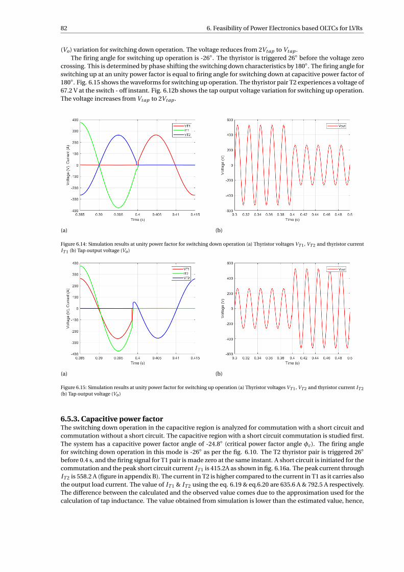
82 6. Feasibility of Power Electronics based OLTCs for LVRs
(Vo) variation for switching down operation. The voltage reduces from 2Vt ap to Vt ap .The firing angle for switching up operation is -26. The thyristor is triggered 26 before the voltage zero
crossing. This is determined by phase shifting the switching down characteristics by 180. The firing angle forswitching up at an unity power factor is equal to firing angle for switching down at capacitive power factor of180. Fig. 6.15 shows the waveforms for switching up operation. The thyristor pair T2 experiences a voltage of67.2 V at the switch - off instant. Fig. 6.12b shows the tap output voltage variation for switching up operation.The voltage increases from Vt ap to 2Vt ap .
(a) (b)
Figure 6.14: Simulation results at unity power factor for switching down operation (a) Thyristor voltages VT 1, VT 2 and thyristor currentIT 1 (b) Tap output voltage (Vo )
(a) (b)
Figure 6.15: Simulation results at unity power factor for switching up operation (a) Thyristor voltages VT 1, VT 2 and thyristor current IT 2(b) Tap output voltage (Vo )
6.5.3. Capacitive power factorThe switching down operation in the capacitive region is analyzed for commutation with a short circuit andcommutation without a short circuit. The capacitive region with a short circuit commutation is studied first.The system has a capacitive power factor angle of -24.8 (critical power factor angle φc ). The firing anglefor switching down operation in this mode is -26 as per the fig. 6.10. The T2 thyristor pair is triggered 26before 0.4 s, and the firing signal for T1 pair is made zero at the same instant. A short circuit is initiated for thecommutation and the peak short circuit current IT 1 is 415.2A as shown in fig. 6.16a. The peak current throughIT 2 is 558.2 A (figure in appendix B). The current in T2 is higher compared to the current in T1 as it carries alsothe output load current. The value of IT 1 & IT 2 using the eq. 6.19 & eq.6.20 are 635.6 A & 792.5 A respectively.The difference between the calculated and the observed value comes due to the approximation used for thecalculation of tap inductance. The value obtained from simulation is lower than the estimated value, hence,
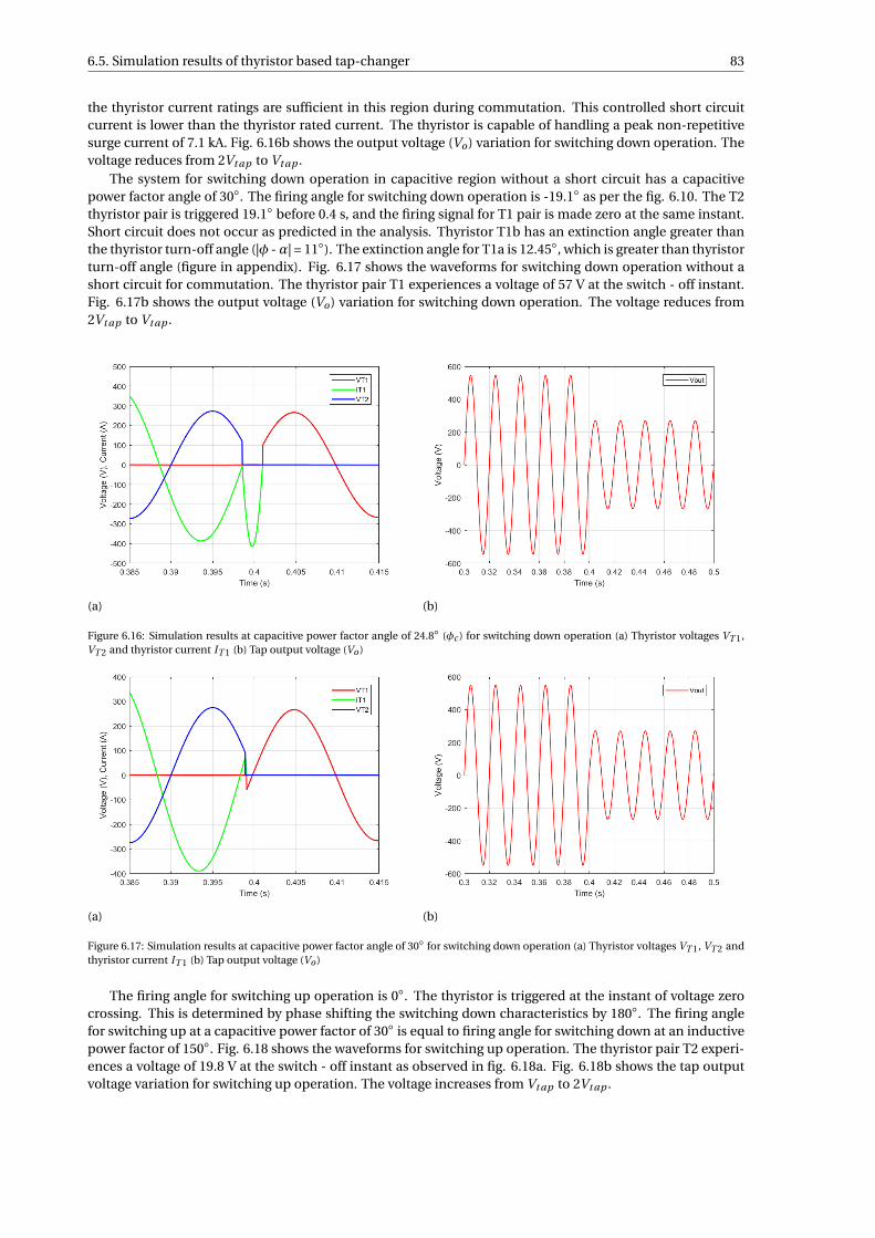
6.5. Simulation results of thyristor based tap-changer 83
the thyristor current ratings are sufficient in this region during commutation. This controlled short circuitcurrent is lower than the thyristor rated current. The thyristor is capable of handling a peak non-repetitivesurge current of 7.1 kA. Fig. 6.16b shows the output voltage (Vo) variation for switching down operation. Thevoltage reduces from 2Vt ap to Vt ap .
The system for switching down operation in capacitive region without a short circuit has a capacitivepower factor angle of 30. The firing angle for switching down operation is -19.1 as per the fig. 6.10. The T2thyristor pair is triggered 19.1 before 0.4 s, and the firing signal for T1 pair is made zero at the same instant.Short circuit does not occur as predicted in the analysis. Thyristor T1b has an extinction angle greater thanthe thyristor turn-off angle (|φ -α| = 11). The extinction angle for T1a is 12.45, which is greater than thyristorturn-off angle (figure in appendix). Fig. 6.17 shows the waveforms for switching down operation without ashort circuit for commutation. The thyristor pair T1 experiences a voltage of 57 V at the switch - off instant.Fig. 6.17b shows the output voltage (Vo) variation for switching down operation. The voltage reduces from2Vt ap to Vt ap .
(a) (b)
Figure 6.16: Simulation results at capacitive power factor angle of 24.8 (φc ) for switching down operation (a) Thyristor voltages VT 1,VT 2 and thyristor current IT 1 (b) Tap output voltage (Vo )
(a) (b)
Figure 6.17: Simulation results at capacitive power factor angle of 30 for switching down operation (a) Thyristor voltages VT 1, VT 2 andthyristor current IT 1 (b) Tap output voltage (Vo )
The firing angle for switching up operation is 0. The thyristor is triggered at the instant of voltage zerocrossing. This is determined by phase shifting the switching down characteristics by 180. The firing anglefor switching up at a capacitive power factor of 30 is equal to firing angle for switching down at an inductivepower factor of 150. Fig. 6.18 shows the waveforms for switching up operation. The thyristor pair T2 experi-ences a voltage of 19.8 V at the switch - off instant as observed in fig. 6.18a. Fig. 6.18b shows the tap outputvoltage variation for switching up operation. The voltage increases from Vt ap to 2Vt ap .
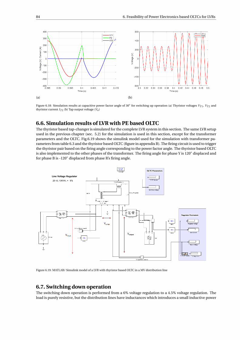
84 6. Feasibility of Power Electronics based OLTCs for LVRs
(a) (b)
Figure 6.18: Simulation results at capacitive power factor angle of 30 for switching up operation (a) Thyristor voltages VT 1, VT 2 andthyristor current IT 2 (b) Tap output voltage (Vo )
6.6. Simulation results of LVR with PE based OLTCThe thyristor based tap-changer is simulated for the complete LVR system in this section. The same LVR setupused in the previous chapter (sec. 5.2) for the simulation is used in this section, except for the transformerparameters and the OLTC. Fig.6.19 shows the simulink model used for the simulation with transformer pa-rameters from table 6.3 and the thyristor based OLTC (figure in appendix B). The firing circuit is used to triggerthe thyristor pair based on the firing angle corresponding to the power factor angle. The thyristor based OLTCis also implemented to the other phases of the transformer. The firing angle for phase Y is 120 displaced andfor phase B is -120 displaced from phase R’s firing angle.
Figure 6.19: MATLAB/ Simulink model of a LVR with thyristor based OLTC in a MV distribution line
6.7. Switching down operationThe switching down operation is performed from a 6% voltage regulation to a 4.5% voltage regulation. Theload is purely resistive, but the distribution lines have inductances which introduces a small inductive power
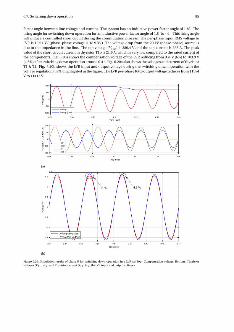
6.7. Switching down operation 85
factor angle between line voltage and current. The system has an inductive power factor angle of 1.8. Thefiring angle for switching down operation for an inductive power factor angle of 1.8 is - 4. This firing anglewill induce a controlled short circuit during the commutation process. The per-phase input RMS voltage toLVR is 10.91 kV (phase-phase voltage is 18.9 kV). The voltage drop from the 20 kV (phase-phase) source isdue to the impedance in the line. The tap voltage (Vt ap ) is 250.4 V and the tap current is 358 A. The peakvalue of the short circuit current in thyristor T1b is 21.6 A, which is very low compared to the rated current ofthe components. Fig. 6.20a shows the compensation voltage of the LVR reducing from 934 V (6%) to 703.9 V(4.5%) after switching down operation around 0.4 s. Fig. 6.20a also shows the voltages and current of thyristorT1 & T2. Fig. 6.20b shows the LVR input and output voltage during the switching down operation with thevoltage regulation (in %) highlighted in the figure. The LVR per-phase RMS output voltage reduces from 11554V to 11412 V.
(a)
(b)
Figure 6.20: Simulation results of phase R for switching down operation in a LVR (a) Top: Compensation voltage, Bottom: Thyristorvoltages (VT 1, VT 2) and Thyristor current (IT 1, IT 2) (b) LVR input and output voltages
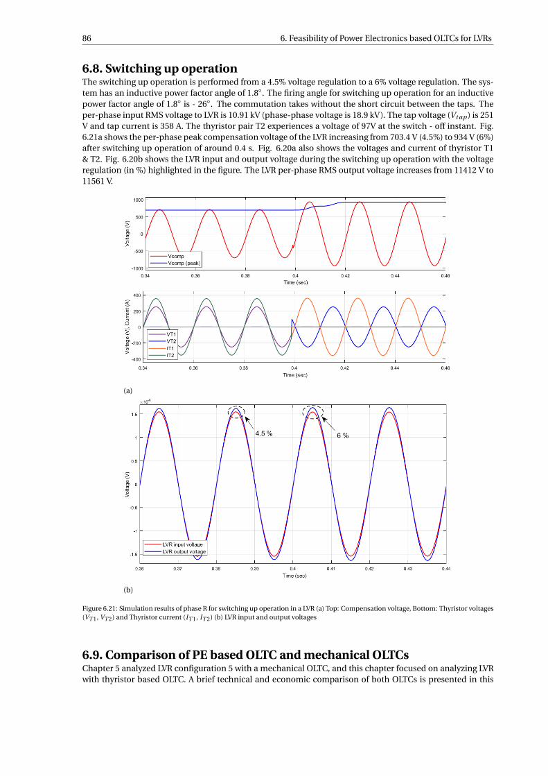
86 6. Feasibility of Power Electronics based OLTCs for LVRs
6.8. Switching up operationThe switching up operation is performed from a 4.5% voltage regulation to a 6% voltage regulation. The sys-tem has an inductive power factor angle of 1.8. The firing angle for switching up operation for an inductivepower factor angle of 1.8 is - 26. The commutation takes without the short circuit between the taps. Theper-phase input RMS voltage to LVR is 10.91 kV (phase-phase voltage is 18.9 kV). The tap voltage (Vt ap ) is 251V and tap current is 358 A. The thyristor pair T2 experiences a voltage of 97V at the switch - off instant. Fig.6.21a shows the per-phase peak compensation voltage of the LVR increasing from 703.4 V (4.5%) to 934 V (6%)after switching up operation of around 0.4 s. Fig. 6.20a also shows the voltages and current of thyristor T1& T2. Fig. 6.20b shows the LVR input and output voltage during the switching up operation with the voltageregulation (in %) highlighted in the figure. The LVR per-phase RMS output voltage increases from 11412 V to11561 V.
(a)
(b)
Figure 6.21: Simulation results of phase R for switching up operation in a LVR (a) Top: Compensation voltage, Bottom: Thyristor voltages(VT 1, VT 2) and Thyristor current (IT 1, IT 2) (b) LVR input and output voltages
6.9. Comparison of PE based OLTC and mechanical OLTCsChapter 5 analyzed LVR configuration 5 with a mechanical OLTC, and this chapter focused on analyzing LVRwith thyristor based OLTC. A brief technical and economic comparison of both OLTCs is presented in this
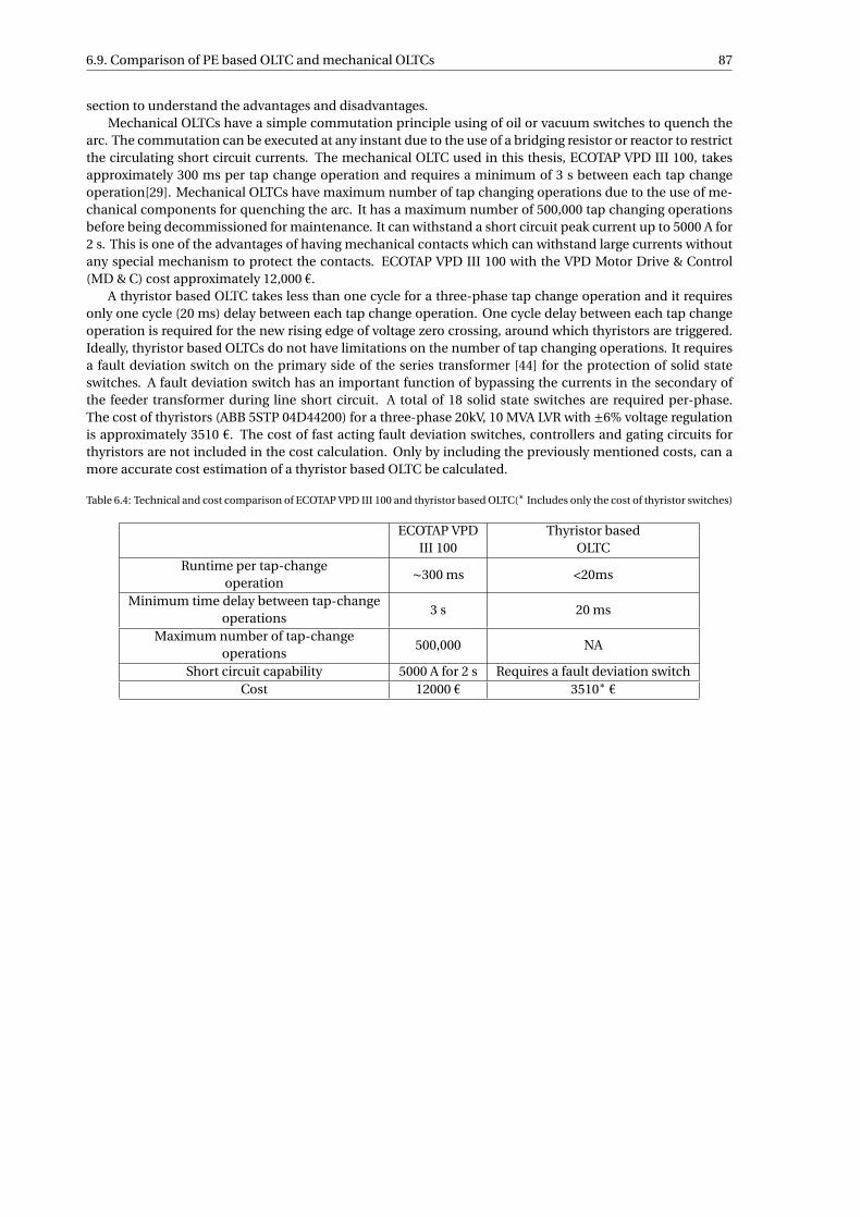
6.9. Comparison of PE based OLTC and mechanical OLTCs 87
section to understand the advantages and disadvantages.Mechanical OLTCs have a simple commutation principle using of oil or vacuum switches to quench the
arc. The commutation can be executed at any instant due to the use of a bridging resistor or reactor to restrictthe circulating short circuit currents. The mechanical OLTC used in this thesis, ECOTAP VPD III 100, takesapproximately 300 ms per tap change operation and requires a minimum of 3 s between each tap changeoperation[29]. Mechanical OLTCs have maximum number of tap changing operations due to the use of me-chanical components for quenching the arc. It has a maximum number of 500,000 tap changing operationsbefore being decommissioned for maintenance. It can withstand a short circuit peak current up to 5000 A for2 s. This is one of the advantages of having mechanical contacts which can withstand large currents withoutany special mechanism to protect the contacts. ECOTAP VPD III 100 with the VPD Motor Drive & Control(MD & C) cost approximately 12,000 €.
A thyristor based OLTC takes less than one cycle for a three-phase tap change operation and it requiresonly one cycle (20 ms) delay between each tap change operation. One cycle delay between each tap changeoperation is required for the new rising edge of voltage zero crossing, around which thyristors are triggered.Ideally, thyristor based OLTCs do not have limitations on the number of tap changing operations. It requiresa fault deviation switch on the primary side of the series transformer [44] for the protection of solid stateswitches. A fault deviation switch has an important function of bypassing the currents in the secondary ofthe feeder transformer during line short circuit. A total of 18 solid state switches are required per-phase.The cost of thyristors (ABB 5STP 04D44200) for a three-phase 20kV, 10 MVA LVR with ±6% voltage regulationis approximately 3510 €. The cost of fast acting fault deviation switches, controllers and gating circuits forthyristors are not included in the cost calculation. Only by including the previously mentioned costs, can amore accurate cost estimation of a thyristor based OLTC be calculated.
Table 6.4: Technical and cost comparison of ECOTAP VPD III 100 and thyristor based OLTC(∗ Includes only the cost of thyristor switches)
ECOTAP VPDIII 100
Thyristor basedOLTC
Runtime per tap-changeoperation
∼300 ms <20ms
Minimum time delay between tap-changeoperations
3 s 20 ms
Maximum number of tap-changeoperations
500,000 NA
Short circuit capability 5000 A for 2 s Requires a fault deviation switchCost 12000 € 3510∗ €

7Conclusion and Future Work
7.1. Thesis overviewThe impact of a shunt voltage compensation, series voltage compensation and conductor upgradation ongrid capacity of a MV radial feeder distribution line was studied. LVR was effective in significantly improvingthe grid capacity without violating the power and voltage limits of the distribution line. Various configura-tions of LVR with single and two active parts were studied. ECOTAP VPD III 100 from Maschinenfabrik Rein-hausen (MR) was chosen as the OLTC for the LVR as it was economical and it required low maintenance forthe oil in the transformer due to vacuum interrupters. LVR with center tapped autotransformer as the feedertransformer and a two winding transformer as the booster transformer was economical for the 20 kV, 10 MVAline. As ABB’s oil-transformer factory does not manufacture autotransformers for MV levels, implementingthis design would require changes in the factory assembly lines, which will lead to major cost implications.Hence, the design and simulation was carried out for the LVR configuration 5 with center tapped two wind-ing transformer as the feeder transformer, and a two winding transformer as the booster transformer. A smallscale experimental setup was built to test the LVR configuration 5 with the ECOTAP VPD III 100 OLTC. Thesimulation and experimental results with LVR configuration 5 were found to be satisfactory. As mechani-cal OLTCs require regular maintenance, a feasibility study of a power electronics based OLTC was conducted.LVR configuration 5 was chosen for this feasibility study as it provides isolation to the solid-state switches andenables the system to use thyristors without a series/parallel connection for the taps. The thyristor switcheswere found to have almost 5 times lower losses and were 9 times cheaper than the IGBT switches for thisapplication. The commutation instants were defined based on the power factor of the system to have con-trolled short circuit currents for certain power factor angles with thyristor based OLTCs. A transformer modelwith two taps was simulated for the complete power factor range. The thyristor based OLTC was also imple-mented to a 20 kV, 10 MVA LVR with ±6% voltage regulation. The switching up and switching down operationwas performed and the simulation results were found to be satisfactory. A brief technical and cost compari-son between mechanical OLTCs and thyristor based OLTCs was also presented.
7.2. Results and conclusionImpact of LVRs on the grid capacityThe main results and conclusions from studying the impact of different voltage regulation strategies on gridcapacity for a 20 kV, 10 MVA radial feeder are as follows:
• Voltage variation limits pose a serious bottleneck to utilize the full grid capacity in a MV distributionnetwork. It was shown that the voltage limits are violated before the thermal or power limits of long MVdistribution lines.
• Shunt compensation using reactive elements or FACTS devices helps to increase the grid capacity onlyby a small percentage. Shunt compensation is not very effective in regulating the voltage in distributionnetworks due to the high R/X ratio.
89
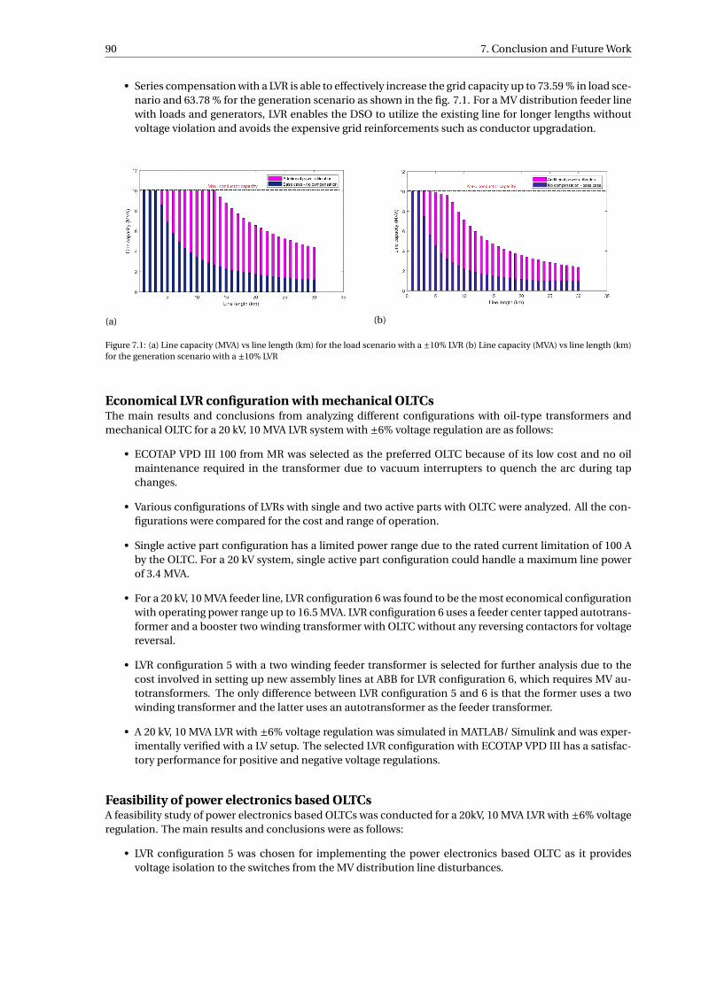
90 7. Conclusion and Future Work
• Series compensation with a LVR is able to effectively increase the grid capacity up to 73.59 % in load sce-nario and 63.78 % for the generation scenario as shown in the fig. 7.1. For a MV distribution feeder linewith loads and generators, LVR enables the DSO to utilize the existing line for longer lengths withoutvoltage violation and avoids the expensive grid reinforcements such as conductor upgradation.
(a) (b)
Figure 7.1: (a) Line capacity (MVA) vs line length (km) for the load scenario with a ±10% LVR (b) Line capacity (MVA) vs line length (km)for the generation scenario with a ±10% LVR
Economical LVR configuration with mechanical OLTCsThe main results and conclusions from analyzing different configurations with oil-type transformers andmechanical OLTC for a 20 kV, 10 MVA LVR system with ±6% voltage regulation are as follows:
• ECOTAP VPD III 100 from MR was selected as the preferred OLTC because of its low cost and no oilmaintenance required in the transformer due to vacuum interrupters to quench the arc during tapchanges.
• Various configurations of LVRs with single and two active parts with OLTC were analyzed. All the con-figurations were compared for the cost and range of operation.
• Single active part configuration has a limited power range due to the rated current limitation of 100 Aby the OLTC. For a 20 kV system, single active part configuration could handle a maximum line powerof 3.4 MVA.
• For a 20 kV, 10 MVA feeder line, LVR configuration 6 was found to be the most economical configurationwith operating power range up to 16.5 MVA. LVR configuration 6 uses a feeder center tapped autotrans-former and a booster two winding transformer with OLTC without any reversing contactors for voltagereversal.
• LVR configuration 5 with a two winding feeder transformer is selected for further analysis due to thecost involved in setting up new assembly lines at ABB for LVR configuration 6, which requires MV au-totransformers. The only difference between LVR configuration 5 and 6 is that the former uses a twowinding transformer and the latter uses an autotransformer as the feeder transformer.
• A 20 kV, 10 MVA LVR with ±6% voltage regulation was simulated in MATLAB/ Simulink and was exper-imentally verified with a LV setup. The selected LVR configuration with ECOTAP VPD III has a satisfac-tory performance for positive and negative voltage regulations.
Feasibility of power electronics based OLTCsA feasibility study of power electronics based OLTCs was conducted for a 20kV, 10 MVA LVR with ±6% voltageregulation. The main results and conclusions were as follows:
• LVR configuration 5 was chosen for implementing the power electronics based OLTC as it providesvoltage isolation to the switches from the MV distribution line disturbances.
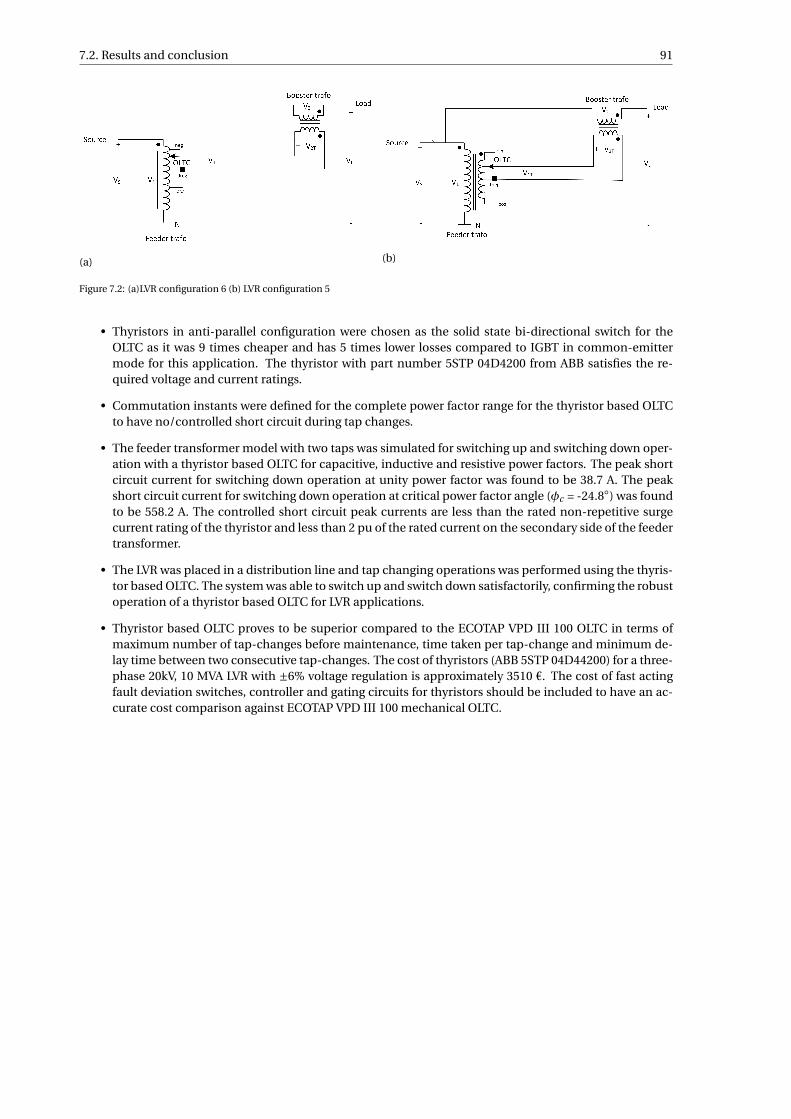
7.2. Results and conclusion 91
(a) (b)
Figure 7.2: (a)LVR configuration 6 (b) LVR configuration 5
• Thyristors in anti-parallel configuration were chosen as the solid state bi-directional switch for theOLTC as it was 9 times cheaper and has 5 times lower losses compared to IGBT in common-emittermode for this application. The thyristor with part number 5STP 04D4200 from ABB satisfies the re-quired voltage and current ratings.
• Commutation instants were defined for the complete power factor range for the thyristor based OLTCto have no/controlled short circuit during tap changes.
• The feeder transformer model with two taps was simulated for switching up and switching down oper-ation with a thyristor based OLTC for capacitive, inductive and resistive power factors. The peak shortcircuit current for switching down operation at unity power factor was found to be 38.7 A. The peakshort circuit current for switching down operation at critical power factor angle (φc = -24.8) was foundto be 558.2 A. The controlled short circuit peak currents are less than the rated non-repetitive surgecurrent rating of the thyristor and less than 2 pu of the rated current on the secondary side of the feedertransformer.
• The LVR was placed in a distribution line and tap changing operations was performed using the thyris-tor based OLTC. The system was able to switch up and switch down satisfactorily, confirming the robustoperation of a thyristor based OLTC for LVR applications.
• Thyristor based OLTC proves to be superior compared to the ECOTAP VPD III 100 OLTC in terms ofmaximum number of tap-changes before maintenance, time taken per tap-change and minimum de-lay time between two consecutive tap-changes. The cost of thyristors (ABB 5STP 04D44200) for a three-phase 20kV, 10 MVA LVR with ±6% voltage regulation is approximately 3510 €. The cost of fast actingfault deviation switches, controller and gating circuits for thyristors should be included to have an ac-curate cost comparison against ECOTAP VPD III 100 mechanical OLTC.
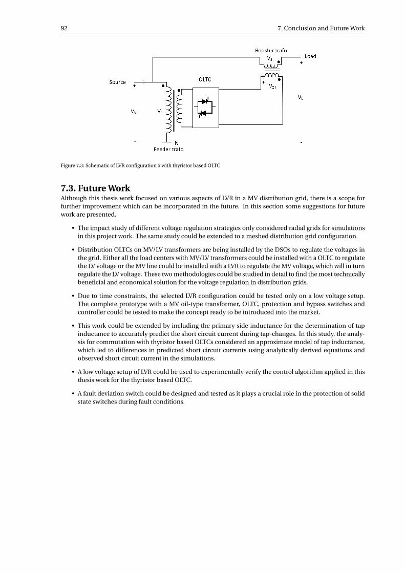
92 7. Conclusion and Future Work
Figure 7.3: Schematic of LVR configuration 5 with thyristor based OLTC
7.3. Future WorkAlthough this thesis work focused on various aspects of LVR in a MV distribution grid, there is a scope forfurther improvement which can be incorporated in the future. In this section some suggestions for futurework are presented.
• The impact study of different voltage regulation strategies only considered radial grids for simulationsin this project work. The same study could be extended to a meshed distribution grid configuration.
• Distribution OLTCs on MV/LV transformers are being installed by the DSOs to regulate the voltages inthe grid. Either all the load centers with MV/LV transformers could be installed with a OLTC to regulatethe LV voltage or the MV line could be installed with a LVR to regulate the MV voltage, which will in turnregulate the LV voltage. These two methodologies could be studied in detail to find the most technicallybeneficial and economical solution for the voltage regulation in distribution grids.
• Due to time constraints, the selected LVR configuration could be tested only on a low voltage setup.The complete prototype with a MV oil-type transformer, OLTC, protection and bypass switches andcontroller could be tested to make the concept ready to be introduced into the market.
• This work could be extended by including the primary side inductance for the determination of tapinductance to accurately predict the short circuit current during tap-changes. In this study, the analy-sis for commutation with thyristor based OLTCs considered an approximate model of tap inductance,which led to differences in predicted short circuit currents using analytically derived equations andobserved short circuit current in the simulations.
• A low voltage setup of LVR could be used to experimentally verify the control algorithm applied in thisthesis work for the thyristor based OLTC.
• A fault deviation switch could be designed and tested as it plays a crucial role in the protection of solidstate switches during fault conditions.

Appendix A
The MATLAB code to run the simulink model for studying the impact of different voltage regulations strate-gies on grid capacity of a distribution line
%% Loading parameters for tech−eco analysisc lear a l l ;c l c ;
%%
N_l = 5 ;Z = zeros ( 3 0 , 1 ) ;s= 1 ;
%% P_s load apparent powerfor L = 0 . 2 : 0.2 : 6
for P_s = 1.1 e6 : 0.05 e6 : 10e6P_a = ( P_s * 1 ) ; %%active powerP_r = sqrt ( P_s^2 − P_a ^ 2 ) ; %% r e a c t i v e power%PC = 0.666 * P_r ;R_line = 0.455* L ;X_line = 0.2772* L ;L_line = ( X_line ) / ( 2 * pi * 5 0 ) ;LF = power_loadflow ( ’−v2 ’ , ’ techecoanalysis5 ’ , ’ solve ’ ) ;bu = LF . bus ;x = s t r u c t 2 t a b l e (bu ) ;V_load = abs ( table2array ( x ( 6 , 1 3 ) ) ) ;P_line = abs ( table2array ( x ( 1 , 1 5 ) ) ) ;
i f P_line >= 0.1 | | V_load <= 0.96break
endend
Z( s ) = P_line ;s=s +1;end%L = 1.4 ; l i n e length in KmLen = 0 . 2 : 0 . 2 : 6 ;Z= Z*100e6 ;plot ( Len*5 ,Z)
93
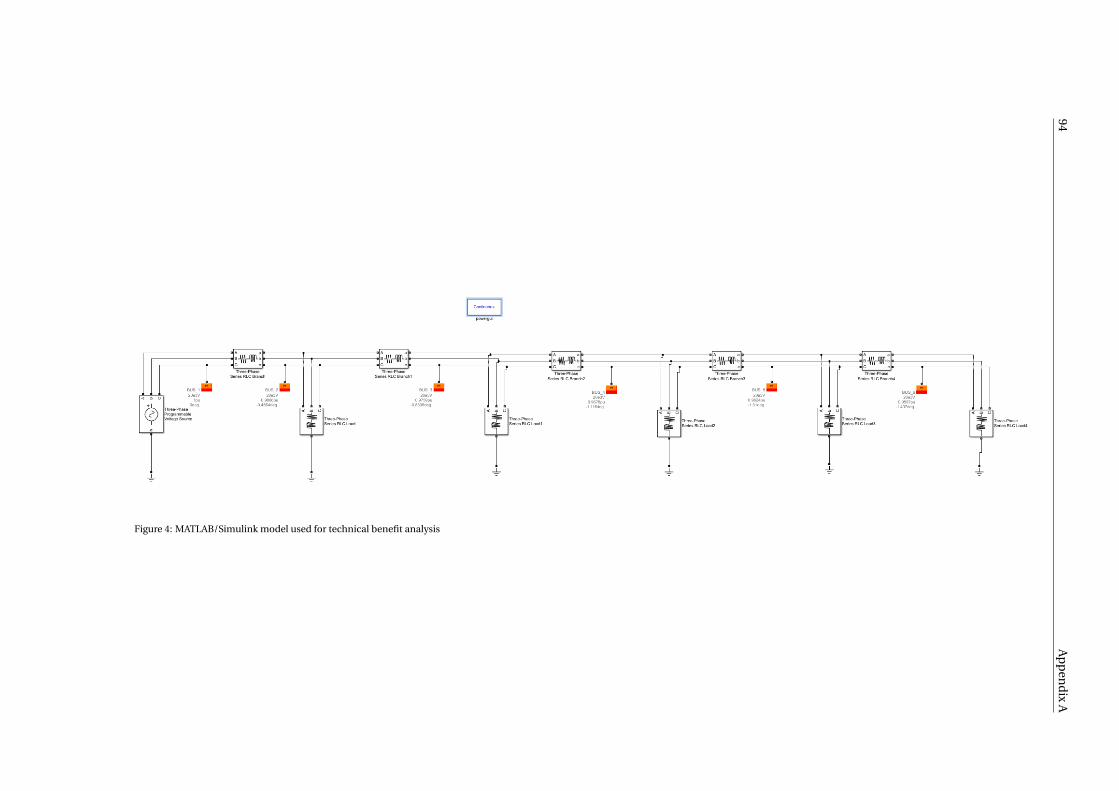
94A
pp
end
ixA
Figure 4: MATLAB/Simulink model used for technical benefit analysis

Appendix B
%% Code for calculat ing alpha maximum for switching down operation in capacit ive power f a c t o r regionclear a l l ;c l c ;
%%
syms x%phi = [30 29 28 27 26 25 24 23 22 2 1 ] ;%f i r i n g _ a n g l e = zeros ( 1 , 1 0 ) ;alpha30 = 30*ones ( 1 , 1 5 6 ) ;phi_sl icap = −1* [24.99 23 22 21 20 19 18 17 16 15 14 13 12 1110 9 8 7 6 5 4 3 2 1 0 −1 −2 −3 −4 −5 −6];alpha_slicap = (0.822* phi_sl icap ) − 5 . 4 5 ;for i = 1 : 156syms xphi ( i ) = 181 − i ;E = cos ( x ) + ( 0 . 0 6 * sin ( x +((181 − i ) * . 0 1 7 ) ) ) + 0 . 9 8 == 0 ;[ x ] = solve (E , x ) ;vpa ( x )alpha = double ( x ) ;alpha = r e a l ( alpha ) ;alpha = rad2deg ( alpha ) ;f i r i n g _ a n g l e ( i ) = 180 − alpha ( 1 ) ;end
plot (−phi , −f i r i n g _ a n g l e )hold onplot (−phi , (−phi +10.9))hold onplot (−phi , −alpha30 )
95
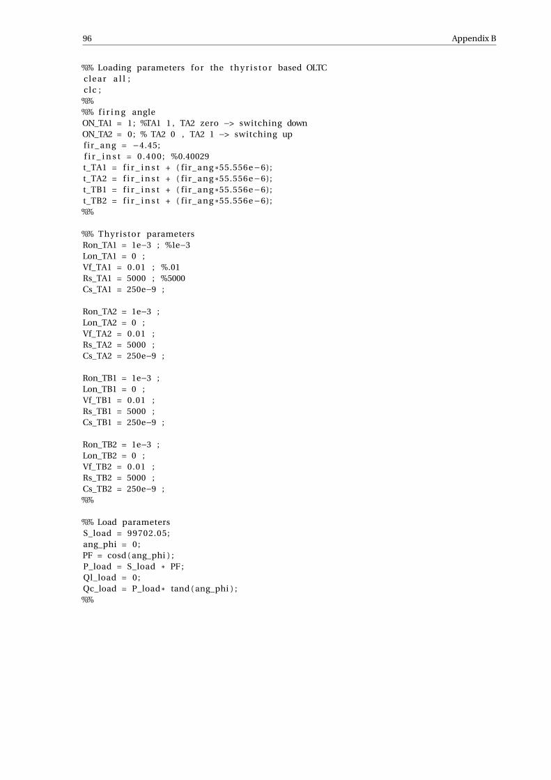
96 Appendix B
%% Loading parameters for the t h y r i s t o r based OLTCclear a l l ;c l c ;
%%%% f i r i n g angleON_TA1 = 1 ; %TA1 1 , TA2 zero −> switching downON_TA2 = 0 ; % TA2 0 , TA2 1 −> switching upfir_ang = −4.45;f i r _ i n s t = 0 . 4 0 0 ; %0.40029t_TA1 = f i r _ i n s t + ( f i r_ang *55.556e−6);t_TA2 = f i r _ i n s t + ( f i r_ang *55.556e−6);t_TB1 = f i r _ i n s t + ( f i r_ang *55.556e−6);t_TB2 = f i r _ i n s t + ( f i r_ang *55.556e−6);%%
%% Thyristor parametersRon_TA1 = 1e−3 ; %1e−3Lon_TA1 = 0 ;Vf_TA1 = 0.01 ; %.01Rs_TA1 = 5000 ; %5000Cs_TA1 = 250e−9 ;
Ron_TA2 = 1e−3 ;Lon_TA2 = 0 ;Vf_TA2 = 0.01 ;Rs_TA2 = 5000 ;Cs_TA2 = 250e−9 ;
Ron_TB1 = 1e−3 ;Lon_TB1 = 0 ;Vf_TB1 = 0.01 ;Rs_TB1 = 5000 ;Cs_TB1 = 250e−9 ;
Ron_TB2 = 1e−3 ;Lon_TB2 = 0 ;Vf_TB2 = 0.01 ;Rs_TB2 = 5000 ;Cs_TB2 = 250e−9 ;%%
%% Load parametersS_load = 99702.05;ang_phi = 0 ;PF = cosd ( ang_phi ) ;P_load = S_load * PF ;Ql_load = 0 ;Qc_load = P_load * tand ( ang_phi ) ;%%
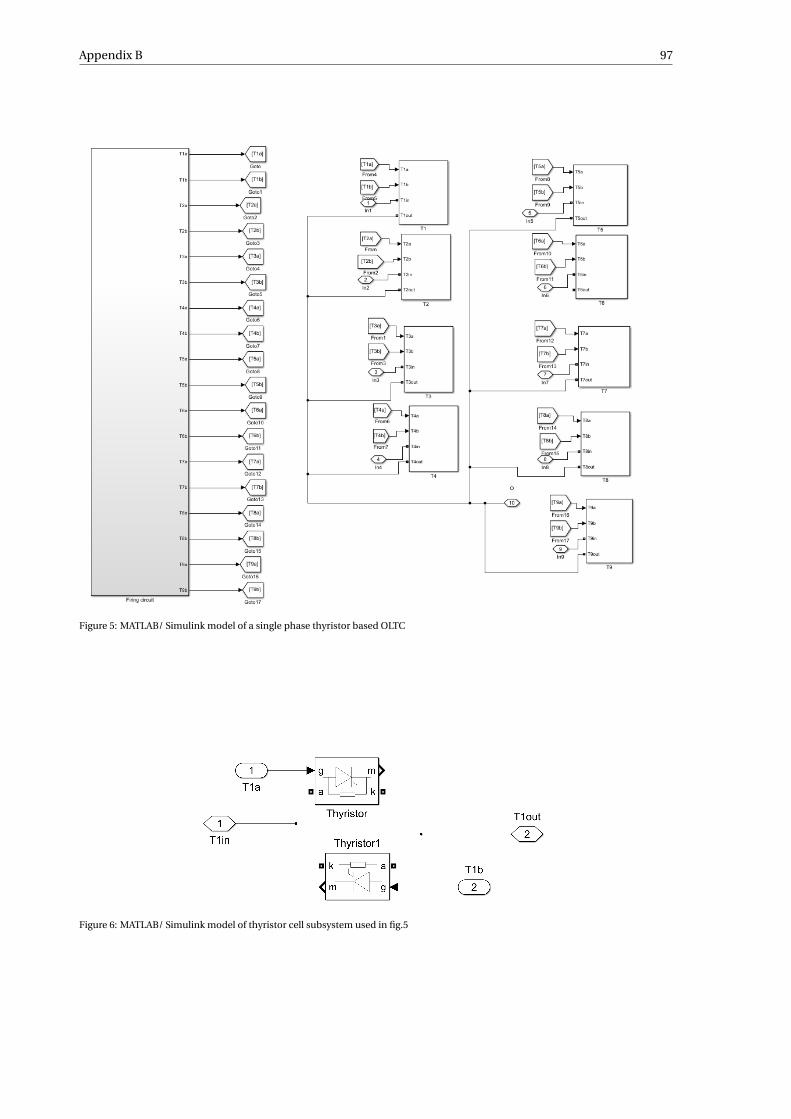
Appendix B 97
Figure 5: MATLAB/ Simulink model of a single phase thyristor based OLTC
Figure 6: MATLAB/ Simulink model of thyristor cell subsystem used in fig.5
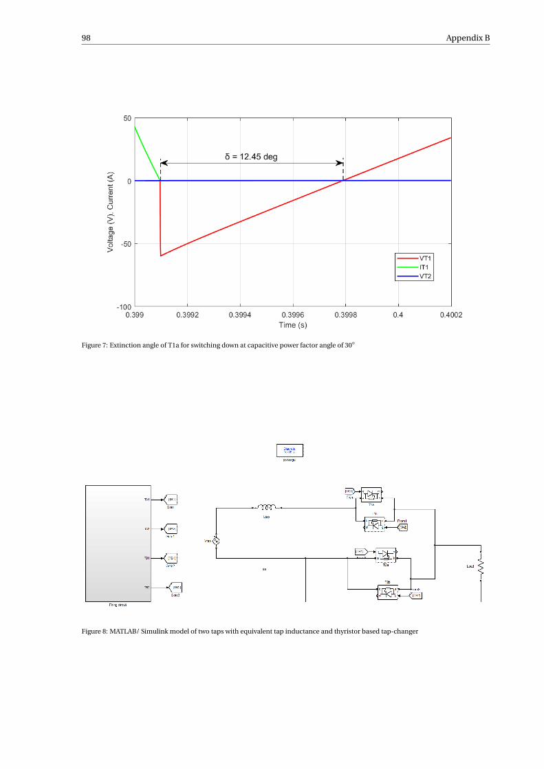
98 Appendix B
Figure 7: Extinction angle of T1a for switching down at capacitive power factor angle of 30
Figure 8: MATLAB/ Simulink model of two taps with equivalent tap inductance and thyristor based tap-changer
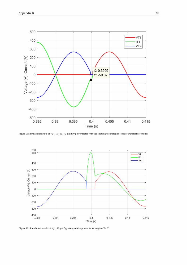
Appendix B 99
Figure 9: Simulation results of VT 1, VT 2 & IT 1 at unity power factor with tap inductance instead of feeder transformer model
Figure 10: Simulation results of VT 1, VT 2 & IT 2 at capacitive power factor angle of 24.8

Bibliography
[1] ANSI C84.1-2011, Voltage ratings for electric power systems and equipment (60 hz).
[2] GB/T 12325-2003, Power quality– Admissible deviation of supply voltage.
[3] Linking Renewable Energy to Rural Development, Executive Summary Brief for Policy Makers.
[4] NRS-048-2, Quality of supply part 2: Voltage characteristics, compatibility levels, limits and assessmentmethods.
[5] EN50160, Voltage characteristics of electricity supplied by public distribution networks.
[6] Transmission line constraints. URL http://nptel.ac.in/courses/108101040/6.
[7] Global trends in renewable energy, Jan 2018. URL https://www.rsm.global/insights/economic-insights/global-trends-renewable-energy.
[8] Line voltage regulator for medium voltage grids with RESIBLOC ® technology Reliable answer to voltagevariations. Tec. Report 2014.
[9] Tao AAXu and PC Taylor. Voltage control techniques for electrical distribution networks including dis-tributed generation. IFAC Proceedings Volumes, 41(2):11967–11971, 2008.
[10] J. Arrillaga and R. M. Duke. A static alternative to the transformer on-load tap-changer. IEEE Transac-tions on Power Apparatus and Systems, PAS-99(1):86–91, 1980. ISSN 00189510. doi: 10.1109/TPAS.1980.319612.
[11] P. Bauer and S. W. H. de Haan. Electronic tap changer for 500 kva/10 kv distribution transformers: design,experimental results and impact in distribution networks. In Conference Record of 1998 IEEE IndustryApplications Conference. Thirty-Third IAS Annual Meeting (Cat. No.98CH36242), volume 2, pages 1530–1537 vol.2, Oct 1998. doi: 10.1109/IAS.1998.730344.
[12] Danilo Bertini, D Falabretti, M Merlo, D Moneta, J SILVA DE ASSIS CARNEIRO, and Andrea Silvestri.Hosting capacity of italian lv distribution networks. In CIRED 2011, pages 1–4, 2011.
[13] M. T. Bishop, J. D. Foster, and D. A. Down. The application of single-phase voltage regulators on three-phase distribution systems. In Proceedings of 1994 IEEE Rural Electric Power Conference, pages C2/1–C2/7, Apr 1994. doi: 10.1109/REPCON.1994.326251.
[14] David Block, John Harrison, Paul Brooker, FS Center, and Ms Denise Dunn. Electric vehicle sales for2014 and future projections. Florida Solar Energy Center, pages 1949–3053, 2015.
[15] Ben O Brewin, Samuel CE Jupe, Marc G Bartlett, Katherine T Jackson, and Clare Hanmer. New technolo-gies for low voltage distribution networks. In Innovative Smart Grid Technologies (ISGT Europe), 20112nd IEEE PES International Conference and Exhibition on, pages 1–8. IEEE, 2011.
[16] Martin Carlen and et al. Voltage control system, Sep 2017.
[17] Martin Carlen, Frank Cornelius, Jens Tepper, Rainer Jakobs, Michael Schneider, Harald Wiesler, AdamSlupinski, and Irma Buschmann. LINE VOLTAGE REGULATOR FOR VOLTAGE ADJUSTMENT IN MV-GRIDS. CIRED, (June):15–18, 2015.
[18] Nan Chen and Lars E. Jonsson. A new Hybrid power electronics on-load tap changer for power trans-former. In Conference Proceedings - IEEE Applied Power Electronics Conference and Exposition - APEC,2015. ISBN 9781479967353. doi: 10.1109/APEC.2015.7104475.
101
102 Bibliography
[19] Carter-brown Clinton. Increasing Network Capacity By Optimising Voltage Regulation on Medium.(May):12–15, 2003. ISSN 1021447X.
[20] California Energy Commission. MODELING AND TESTING OF UNBALANCED LOADING AND VOLTAGEREGULATION. Number March. 2009. ISBN 5002008054.
[21] Stefania Conti and Andrea Maria Greco. Innovative voltage regulation method for distribution networkswith distributed generation. In 19th International Conference on Electricity Distribution, 2007.
[22] Juan Dixon, L. Moran, J. Rodriguez, and Ricardo Domke. Reactive power compensation technolo-gies: State-of-the-art review. Proceedings of the IEEE, 93(12):2144–2164, 2005. ISSN 0018-9219. doi:10.1109/JPROC.2005.859937. URL http://ieeexplore.ieee.org/lpdocs/epic03/wrapper.htm?arnumber=15457685Cnhttp://ieeexplore.ieee.org/xpls/abs_all.jsp?arnumber=1545768.
[23] Edition. Capacity of Distribution Feeders for Hosting DER. 2014.
[24] General Electric Digital Energy. Voltage regulators - robust, maintenance free solutions, 2014.
[25] S. P. Engel and R. W. De Doncker. Control of thyristor-based commutation cells. In 2012 IEEE Energy Con-version Congress and Exposition (ECCE), pages 2030–2037, Sept 2012. doi: 10.1109/ECCE.2012.6342562.
[26] Jawad Faiz and Behzad Siahkolah. Electronic tap-changer for distribution transformers, volume 2.Springer Science & Business Media, 2011.
[27] L. A. Gallego and A. Padilha-Feltrin. Voltage regulator modeling for the three-phase power flow in dis-tribution networks. In 2008 IEEE/PES Transmission and Distribution Conference and Exposition: LatinAmerica, pages 1–6, Aug 2008. doi: 10.1109/TDC-LA.2008.4641843.
[28] Frederik Geth, Koen Willekens, Kristien Clement, Johan Driesen, and Sven De Breucker. Impact-analysisof the charging of plug-in hybrid vehicles on the production park in belgium. In MELECON 2010-201015th IEEE Mediterranean Electrotechnical Conference, pages 425–430. IEEE, 2010.
[29] ECOTAP VPD Maschinenfabrik Reinhausen GmbH. URL https://www.reinhausen.com.
[30] John J. Grainger. Power system analysis. McGraw-Hill, 1994.
[31] Björn Gwisdorf, Thorsten Borchard, Torsten Hammerschmidt, and Christian Rehtanz. Technical andeconomic evaluation of voltage regulation strategies for distribution grids with a high amount of fluc-tuating dispersed generation units. In Innovative Technologies for An Efficient and Reliable ElectricitySupply (CITRES), 2010 IEEE Conference on, pages 8–14. IEEE, 2010.
[32] James H Harlow. Transformer tap changing under load: a review of concepts and standards. In Proc.1993 64th Annual Engineering Conf., pages 305–310, 1993.
[33] Ali Ipakchi and Farrokh Albuyeh. Grid of the future. IEEE power and energy magazine, 7(2):52–62, 2009.
[34] Hao Jiang, Roger Shuttleworth, Bashar A.T. Al Zahawi, Xiaolin Tian, and Andrew Power. Fast responseGTO assisted novel tap changer. IEEE Transactions on Power Delivery, 16(1):111–115, 2001. ISSN08858977. doi: 10.1109/61.905608.
[35] Takehiko Kojima, Hitoshi Isotani, and Makato Yamada. Distribution Static Var Compensators and StaticSynchronous Compensators for Suppressing Voltage Fluctuation. Technical report, Fuji Electric.
[36] SV Kulkarni and SA Khaparde. Transformer engineering design and practice. Indian Institute of Tech-nology, Bombay (Mumbai), 2004.
[37] G Leci and F Cornelius. Increasing grid capacity to connect renewable energies. CIRED, pages 1–9, 2016.
[38] Yang Liu, Shuitao Yang, Shao Zhang, and Fang Zheng Peng. Comparison of synchronous condenser andSTATCOM for inertial response support. 2014 IEEE Energy Conversion Congress and Exposition, ECCE2014, pages 2684–2690, 2014. doi: 10.1109/ECCE.2014.6953761.
[39] JA Peças Lopes, Filipe Joel Soares, and PM Rocha Almeida. Identifying management procedures to dealwith connection of electric vehicles in the grid. In Powertech, 2009 IEEE bucharest, pages 1–8. IEEE, 2009.
Bibliography 103
[40] M.A. Mahmud, M.J. Hossain, and H.R. Pota. Analysis of Voltage Rise Effect on Distribution Networkwith Distributed Generation. IFAC Proceedings Volumes, 44(1):14796–14801, 2011. ISSN 14746670.doi: 10.3182/20110828-6-IT-1002.01305. URL http://linkinghub.elsevier.com/retrieve/pii/S1474667016460064.
[41] Nasif Mahmud and A. Zahedi. Review of control strategies for voltage regulation of the smart distributionnetwork with high penetration of renewable distributed generation. Renewable and Sustainable EnergyReviews, 64:582–595, 2016. ISSN 18790690. doi: 10.1016/j.rser.2016.06.030. URL http://dx.doi.org/10.1016/j.rser.2016.06.030.
[42] Philippe Maibach and System Engineering. STATCOM Technology for Wind Parks to Meet Grid CodeRequirements. pages 1–10.
[43] Paul E. Marken, Arthur C. Depoian, John Skliutas, and Michael Verrier. Modern synchronous condenserperformance considerations. IEEE Power and Energy Society General Meeting, pages 1–5, 2011. ISSN19449925. doi: 10.1109/PES.2011.6039011.
[44] Salvador Martínez García, Juan Carlos Campo Rodríguez, José Antonio Jardini, Joaquin Vaquero López,Alfonso Ibarzábal Segura, and Pedro María Martínez Cid. Feasibility of electronic tap-changing stabiliz-ers for medium voltage lines - Precedents and new configurations. IEEE Transactions on Power Delivery,24(3):1490–1503, 2009. ISSN 08858977. doi: 10.1109/TPWRD.2009.2021032.
[45] Barry Mather and Araya Gebeyehu. Field demonstration of using advanced PV inverter functionality tomitigate the impacts of high-penetration PV grid integration on the distribution system. 2015 IEEE 42ndPhotovoltaic Specialist Conference, PVSC 2015, pages 1–6, 2015. doi: 10.1109/PVSC.2015.7356169.
[46] Undeland Tore M. Robbins Mohan, Ned and William P. Power Electronics - Converters, Applications, andDesign (3rd Edition). John Wiley & Sons, 2003.
[47] S. Mokkapaty, J. Weiss, F. Schalow, and J. Declercq. New generation voltage regulation distribution trans-former with an on load tap changer for power quality improvement in the electrical distribution systems.CIRED - Open Access Proceedings Journal, 2017(1):784–787, 2017. doi: 10.1049/oap-cired.2017.0881.
[48] G. R. Chandra Mouli, P. Bauer, T. Wijekoon, A. Panosyan, and E. Bärthlein. Design of a power-electronic-assisted oltc for grid voltage regulation. IEEE Transactions on Power Delivery, 30(3):1086–1095, June2015. ISSN 0885-8977. doi: 10.1109/TPWRD.2014.2371539.
[49] M. I. Muhamad, N. Mariun, and M. A. M. Radzi. The effects of power quality to the industries. In 20075th Student Conference on Research and Development, pages 1–4, Dec 2007. doi: 10.1109/SCORED.2007.4451410.
[50] A Notholt. Germany’s new code for generation plants connected to medium-voltage networks and itsrepercussion on inverter control.
[51] KR Padiyar. Facts controllers in power transmission and distribution. 2007.
[52] N. Papazacharopoulos, M. Gibescu, and P. Vaessen. Smart voltage control in distribution networks witha large share of distributed renewable generation. In 2015 IEEE Eindhoven PowerTech, pages 1–6, June2015. doi: 10.1109/PTC.2015.7232497.
[53] Nikolaos Papazacharopoulos, Madeleine Gibescu, and Peter Vaessen. Smart voltage control in distribu-tion networks with a large share of distributed renewable generation. PowerTech, 2015.
[54] White Paper and Juan Tobias. Specifying HV / MV Transformers at Large Sites for an Optimized MVElectrical Network.
[55] Robert Passey, Ted Spooner, Iain MacGill, Muriel Watt, and Katerina Syngellakis. The potential im-pacts of grid-connected distributed generation and how to address them: A review of technical andnon-technical factors. Energy Policy, 39(10):6280–6290, 2011.
[56] Prof. P. Sasidhara Rao Prof. Krishna Vasudevan, Prof. G. Sridhara Rao. NPTEL lectures on Voltage Regu-lation. pages 57–64.
104 Bibliography
[57] MR publication. Vacutap® technology new standard for users of regulating transformers.
[58] Christian Puret. Mv public distribution networks throughout the world. E/CT, 155, 1992.
[59] N Rao and D Chamund. Calculating power losses in an igbt module. Application Note, Dynex Semicon-ductor Ltd., 2014.
[60] Daniel J. Rogers and Tim C. Green. An active-shunt diverter for onload tap changers. IEEE Transactionson Power Delivery, 28(2):649–657, 2013. ISSN 08858977. doi: 10.1109/TPWRD.2013.2243171.
[61] M. Schael and C. Sourkounis. Impact of voltage variations on a grid-connected shredder system. InIECON 2014 - 40th Annual Conference of the IEEE Industrial Electronics Society, pages 641–647, Oct 2014.doi: 10.1109/IECON.2014.7048568.
[62] Helge Seljeseth, Thomas Rump, and Krister Haugen. Overvoltage immunity of electrical applianceslaboratory test results from 60 appliances. In Proc. Int. Conf. Electricity Distribution (CIRED), 2011.
[63] ST semiconductors. How to select the right thyristor (scr) for your application. AN4608 Application note,2014.
[64] SIEMENS. Jfr distribution step voltage regulator instructions, 2008.
[65] MD Singh. Power electronics. Tata McGraw-Hill Education, 2008.
[66] S. Sithole, N. Mbuli, and J. H C Pretorius. Voltage regulation in the douglas area using shunt capacitorbanks and controllable shunt reactors. 2013 13th International Conference on Environment and Electri-cal Engineering, EEEIC 2013 - Conference Proceedings, pages 85–90, 2013. doi: 10.1109/EEEIC-2.2013.6737888.
[67] Management Summary, I E A Task, Recommendations Based, and Field Experience Report Iea-pvps. DoIt Locally : Local Voltage Support by Distributed Generation – A Management Summary Do It Locally :Local Voltage Support by Distributed Generation – A Management Summary. (January 2017), 2017.
[68] Cooper Power Systems. Vr-32 voltage regulator with quik-drive™ tap-changer installation, operation,and maintenance instructions, 2017.
[69] Seyed Abbas Taher, Hosein Tahami Fard, and Ehsan Boloor Kashani. New switching approach for DVRusing one cycle control method. Ain Shams Engineering Journal, 2017. doi: 10.1016/j.asej.2017.03.003.
[70] John Olav Tande, Giuseppe Di Marzio, and Kjetil Uhlen. System Requirements for Wind Power Plants.2007.
[71] John Olav Giœver Tande. Exploitation of wind-energy resources in proximity to weak electric grids. InApplied Energy, 2000. doi: 10.1016/S0306-2619(99)00098-7.
[72] LP Teshmont Consultants and Shaarbafi Karim. Transformer modelling guide. aeso, Alberta ElectricSystem Operator, Revision, 2, 2014.
[73] M. Tewolde and S. P. Das. A novel control of bi-directional switches in matrix converter. In 2006International Conference on Power Electronic, Drives and Energy Systems, pages 1–6, Dec 2006. doi:10.1109/PEDES.2006.344404.
[74] I N Power Transmission. Facts Controllers in Power Transmission. 2007. ISBN 9788122425413.
[75] F. Q. Yousef-Zai and D. O’Kelly. Solid-state on-load transformer tap changer. IEE Proceedings - ElectricPower Applications, 143(6):481–491, Nov 1996. ISSN 1350-2352. doi: 10.1049/ip-epa:19960578.
[76] A. Zahedi. A review of drivers, benefits, and challenges in integrating renewable energy sources intoelectricity grid. Renewable and Sustainable Energy Reviews, 15(9):4775–4779, 2011. ISSN 13640321. doi:10.1016/j.rser.2011.07.074. URL http://dx.doi.org/10.1016/j.rser.2011.07.074.
[77] Baosen Zhang, Albert Y. S. Lam, Alejandro Dominguez-Garcia, and David Tse. An Optimal and Dis-tributed Method for Voltage Regulation in Power Distribution Systems. pages 1–13, 2012. ISSN 0885-8950. doi: 10.1109/TPWRS.2014.2347281. URL http://arxiv.org/abs/1204.5226.


