Embed Size (px)
Citation preview

VibroCav
Hydrodynamic Vibration and
Cavitation technology Tom W. Bakker

VibroCav Hydrodynamic Vibration and Cavitation technology
2
VibroCav
Hydrodynamic Vibration and
Cavitation technology
Proefschrift
Ter verkrijging van de graad van doctor
aan de Technische Universiteit Delft,
Op gezag van de Rector Magnificus prof.ir. K.C.A.M. Luyben,
voorzitter van het College voor Promoties
in het openbaar te verdedigen op 8 november 2012 om 15.00 uur
door Thomas Walburgis Bakker
Mijnbouwkundig ingenieur
geboren te Den Haag
VibroCav Hydrodynamic Vibration and Cavitation technology
3
Dit proefschrift is goedgekeurd door de promotor:
Prof. Dr. G.J. Witkamp
Copromotor:
Dr. Ir. H.J.M. Kramer
Samenstelling promotiecommissie:
Rector Magnificus TU Delft, Voorzitter
Prof. Dr. G.J. Witkamp TU Delft, Promotor
Dr. ir. H.J.M. Kramer UHD, TU Delft, Copromotor
Prof. P.K. Currie PhD TU Delft
Prof. Dr. P.L.J. Zitha TU Delft
Prof. Dr. Ir. D.M.J. Smeulders TU Eindhoven
Dr. K.H.A.A. Wolf UHD, TU Delft
Ir. J. Roodenburg CEO Huisman Equipment
Prof. Dr. B.J. Boersma TU Delft, reservelid
Prof.dr.ir G.M. van Rosmalen heeft in belangrijke mate bijgedragen aan de totstandkoming
van het proefschrift.
Dit werk is gedeeltelijk financieel ondersteund via het Noordelijke Industrie Ontwikkeling
Fonds (NIOF), ter beschikking gesteld door het Samenwerkingverband Noord Nederland
(SNN).
Printed by: WÖHRMANN PRINT SERVICE
ISBN: 978‐64‐6203‐207‐1
© 2012 by T.W. Bakker
All rights reserved. No part of the material protected by this copyright notice may be
reproduced or utilized in any form or by any means, electronic or mechanical, including
photocopying, recording or by any information storage and retrieval system, without written
consent of the publisher.
Printed in the Netherlands

VibroCav Hydrodynamic Vibration and Cavitation technology
4
Aan
Nell & Bart
en
Annemarie, Maaike, Tjerk en Ilse

VibroCav Hydrodynamic Vibration and Cavitation technology
5
VibroCav Hydrodynamic Vibration and Cavitation technology
6
Samenvatting
Vibratie en cavitatie kunnen op vele manieren opgewekt worden en vele nuttige doelen
dienen. Deze studie beschrijft fysische aspecten van nuttige vibratie en cavitatie voor een
breed spectrum aan toepassingen bij atmosferische en hogere tegendrukken.
Na een beoordeling van beschikbare apparaten worden de hydrodynamische vibrerend‐
element‐in‐buis instrumenten zoals beschreven in de patenten van Ivannikov geïdentificeerd
als apparaten met een groot toepassingspotentieel. Hun werking is echter nog grotendeels
niet onderzocht. Grote voordelen van deze instrumenten zijn de constructieve eenvoud,
schaalbaarheid, krachtig effect en aantrekkelijk frequentie bereik voor schoonmaakwerk in
diepboringen. Zelfgenerende vibratie waarbij het element botst in de buis met de buiswand
veroorzaakt wisselende stroming rond het element met een actief waterslag effect dat de
vibratie en cavitatie versterkt. Op deze wijze kan cavitatie opgewekt worden bij lagere
stroomsnelheden en hogere tegendrukken dan bij passieve instrumenten zoals
vernauwende openingen. Het ineenstorten van cavitatie bellen bij hoge tegendrukken
veroorzaakt uitzonderlijk sterke effecten, waardoor nieuwe toepassingen ontsloten kunnen
worden. Bij tegendrukken waarbij zelfs actieve cavitatie niet meer mogelijk is blijft zeer
sterke vibratie over, hetgeen kenmerkend is voor omgevingsdrukken die in diepboringen
aangetroffen worden. Dit unieke duale versterkte vibratie en cavitatie gedrag van de
bestudeerde apparaten is de sleutel tot de vibrerend‐element‐in‐buis technologie waarvoor
de nieuwe naam VibroCav bedacht is.
De studie richt zich op VibroCav instrumenten met een bal als trilelement, met uitzondering
van één test serie met een zogenaamd flip‐flop element. Verkennende testen in een 350 bar
test circuit in Assen gaven de aanzet tot de constructie van een gesloten 50 bar laboratorium
test circuit dat in het 3ME lab in Delft werd opgesteld met mogelijkheden om efficiënt te
experimenteren tot 10 bar tegendruk en 40 bar drukval over het apparaat. Er zijn vele
experimenten uitgevoerd in het 50 bar test circuit, aanvankelijk met ballen die aan de
onderzijde gesteund werden en vervolgens met hangende ballen in een buis met een
conische eind waarbij de ruimte tussen de bal en de buiswand van buitenaf ingesteld kon
worden. De invloed van de watersamenstelling, aanwezigheid van gas en materiaal keuze
voor de bal werden getest. Een aantal testen bij zeer hoge tegendruk werden uitgevoerd in
een gesloten 350 bar test circuit in Drachten. In totaal werden er 29 veldtesten op
industriële schaal uitgevoerd voor het schoonmaken van poreuze media rond water en olie
putten en 5 veldtesten om de technologie te onderzoeken voor het verwijderen van
afzettingen in putten.
Met laboratorium experimenten met het 50 bar circuit werden verschillende operationele
toestanden van de VibroCav instrumenten afgebakend als functie van stromingsdebiet en
tegendruk die benoemd kunnen worden als (i) alleen vibratie, (ii) actieve cavitatie uitsluitend
met vibratie, (iii) geen vibratie met passieve cavitatie en (iv) geen vibratie en geen cavitatie.
VibroCav Hydrodynamic Vibration and Cavitation technology
7
Vibratie werd geconstateerd bij de hoogste tegendruk die behaald kon worden en zal
waarschijnlijk mogelijk zijn bij nog hogere tegendruk, echter het vibreren houdt op bij zeer
hoog stromingsdebiet en sterk vernauwde ruimte tussen de bal en de wand door het
verschuiven van het punt waar de stroming loslaat van de bal (zoals voor een bal bij een Re
getal van ongeveer 3 x 10⁵ in een onbegrensd stromingsveld). Net zoals passieve cavitatie
wordt onderdrukt door toenemende tegendruk wordt ook actieve cavitatie onderdrukt; de
hoogste druk waarbij actieve cavitatie is waargenomen is 63 barg. Bij een van onder
gesteunde bal, zoals in het hogedruk circuit gebruikt is, wordt een significant deel van het
stroompad benedenstrooms van de bal aan het zicht onttrokken zodat actieve cavitatie
dichter bij de vernauwing tussen de bal en de wand plaatsgevonden kan hebben. Op grond
hiervan wordt de verwachting uitgesproken dat cavitatie 100 barg tegendruk zou kunnen
overleven.
De invloed van de waterkwaliteit en aanwezigheid van gas bleek niet significant te zijn.
Lichtgewicht ballen die van onder gesteund werden lieten heftige vibratie en sterke actieve
cavitatie zien, maar raakten snel beschadigd door de hoge contact krachten tussen de bal en
de ondersteuning. Hardstalen ballen bedden zich in een ondersteuning van zachter staal in
omdat de krachten de plastische limieten van de ondersteuning te boven gaan. De bal vlakt
af, of breekt, als het materiaal van de bal zachter is dan de ondersteuning.
De veldtesten voor het schoonmaken van poreuze media rond putten, gecombineerd met
een theoretische analyse leveren waardevolle semi‐kwalitatieve kennis op over de invloed
van de trilfrequentie, bron directiviteit, bronenergie, putgeometrie en mate van verstopping
op de werkingsdiepte van schoonmaak apparaten die met trillingen werken. De belangrijkste
golfenergie voor het schoonmaken van een poreus medium komt van de langzame Biot golf
die als een drukgolf door het poriën netwerk loopt. Hoe hoger de maagdelijke permeabiliteit
van het gesteente en hoe lager de golffrequentie hoe groter de werkingsdiepte zal zijn.
Beschadiging van de permeabiliteit door het verstoppen van de poriën nabij de put
vermindert de werkingsdiepte van de schoonmaakbehandeling en bij progressieve
verstopping kan de beschadiging buiten het bereik van de schoonmaakapparaten komen te
liggen.
Een beperkt aantal veldtesten voor het verwijderen van afzettingen in putten lieten een
significant potentieel zien van VibroCav instrumenten vanwege de gecombineerde effecten
van hameren, spuiten, golfenergie en schokgolven van ineenstortende cavitatiebellen.
De studie levert een gedegen basis voor een wetenschappelijk onderbouwde voortzetting
van de ontwikkeling van VibroCav technologie voor vele toepassingsgebieden in meerdere
industriële sectoren en is de voorloper voor een scala van vernieuwende technieken.
VibroCav Hydrodynamic Vibration and Cavitation technology
8
Summary
Vibration and cavitation can be generated in many ways and serve many useful purposes.
This study describes physical aspects of useful vibration and cavitation for a broad spectrum
of applications at atmospheric or elevated pressures.
After a review of available devices, hydrodynamic vibrating‐body‐in‐pipe tools as described
in patents by Ivannikov are identified as having a major potential and being largely
unexplored. Major advantages of these tools are simplicity of construction, scalability,
powerful effects and attractive frequency range for well cleaning applications. Self induced
vibration with a free body colliding with the pipe wall causes alternating flow around the
body with a water hammer effect that enhances the vibration and cavitation. Cavitation can
thus be generated at lower flow rates and at higher backpressures than with passive tools
such as orifices. Cavitational collapse at high backpressure creates exceptionally strong
effects, giving access to novel applications. At backpressures where even water hammer
enhanced cavitation ceases to exist, very strong vibrations persist to pressure levels
encountered in deep wells. This unique dual enhanced vibration and cavitation behaviour of
the tools is the key to vibrating‐body‐in‐pipe technology for which the new name VibroCav
was coined.
The study focuses on VibroCav tools with balls, except for one series of tests with a so‐called
flip‐flop body. Exploratory tests in a 350 bar test circuit in Assen lead to the design of a 50
bar laboratory closed test circuit installed in the 3ME lab in Delft with facilities to apply up to
10 bar backpressure and up to 40 bar pressure differentials over the tools. In the 50 bar test
circuit many experiments were carried out, firstly with bottom supported balls in a straight
pipe and secondly with hanging balls in a pipe with a conical outlet allowing remote
adjustment of the gap between the ball and the pipe wall. The influence of water
composition, gas content and various ball materials was tested. Selected high backpressure
test were carried out with a 350 bar closed test circuit in Drachten. A total of 29 field trials
on an industrial scale were carried out for cleaning the porous media around water and oil
wellbores under widely varying conditions and 5 field trials were done to evaluate the
potential of the technology for the removal of scale deposits in wellbores.
The laboratory experiments with the 50 bar test circuit delineated various operational
modes of the VibroCav tools as function of flow rate and backpressure with regimes
designated as (i) vibration only, (ii) active cavitation always combined with vibration, (iii) no
vibration and passive cavitation and (iv) no vibration and no passive cavitation. The vibration
regime persists to the maximum backpressure that could be reached and probably to much
higher pressures, however at high flow rate conditions and a narrow gap vibration ceases
when the Re value increases beyond the point of drag reduction due to shifting of the
boundary separation point (Re approximately 3 x 10⁵ for unbounded flow). Active cavitation
is just as passive cavitation subdued by increasing backpressure; but in this test circuit it has
VibroCav Hydrodynamic Vibration and Cavitation technology
9
still been observed at a backpressure of 63 barg. With a bottom supported tool as used in
this test circuit a significant path downstream of the ball is obscured and active cavitation
closer to the gap might still exist. This is the basis for the expectation that for this tool active
cavitation may survive up to 100 barg backpressure. Tools with a hanging ball, in which
cavitation is more clearly visible, were not tested at such high backpressures.
The influence of water quality and gas content proved to be insignificant. Lightweight balls
showed in bottom supported tools violent vibration and strong active cavitation but were
easily damaged by the high contact forces between the ball and the support. With hard steel
balls and softer steel supports, bedding‐in is observed due to contact forces beyond the
elastic limit of the support. If the ball is softer than the support, the ball flattens, breaks or is
otherwise damaged by the support.
The field trials for cleaning porous media around wellbores combined with theoretical
analysis provided valuable semi‐quantitative understanding of the influence of frequency,
source directivity, source energy, wellbore geometry and permeability damage on the
penetration depth of sources for vibration based well cleaning. The most significant wave
energy for cleaning porous media is provided by the slow Biot wave, which is a
compressional wave in fluid in the interconnected pore network. The higher the virgin
permeability of the rock and the lower the wave frequency the better is the penetration
depth. Permeability deterioration due to pore fouling reduces the penetration depth of the
cleaning treatment and with progressive fouling the pore damage may get out of reach of
the cleaning tools.
The limited number of scale removal trials showed significant potential of the VibroCav tools
due to the combination of physical hammering, jetting, wave energy and shock waves of
collapsing cavitation bubbles.
The study provides a solid basis for a scientifically founded continuation of the development
of VibroCav technology for many areas of application in several industrial sectors and should
be regarded as the precursor for a range of innovating techniques.
VibroCav Hydrodynamic Vibration and Cavitation technology
10
Index
Samenvatting .............................................................................................................................. 6
Summary .................................................................................................................................... 8
Index ......................................................................................................................................... 10
1.1. Cavitation ...................................................................................................................... 14
1.1.1. Cavitation and its characteristics ........................................................................... 14
1.1.2. Acoustic cavitation ................................................................................................. 16
1.1.3. Hydrodynamic cavitation ....................................................................................... 17
1.1.4. Hydrodynamic cavitation devices .......................................................................... 25
1.1.5. Consequences of cavitational collapse. ................................................................. 27
1.2. Vibration ........................................................................................................................ 31
1.2.1. Vibration sources ................................................................................................... 31
1.2.2. Hydrodynamic vibration ......................................................................................... 31
1.2.3. Consequences of propagating waves ..................................................................... 37
1.2.4. Characterisation of industrially available vibration sources .................................. 42
1.3. Scope of the thesis ........................................................................................................ 48
1.4. Outline of the thesis ...................................................................................................... 49
1.5. References ..................................................................................................................... 51
Chapter 2: Applications of cavitation and vibration ................................................................ 56
2.1. Effects of cavitation ....................................................................................................... 56
2.2. Applications of cavitation .............................................................................................. 58
2.2.1. Mixing ..................................................................................................................... 58
2.2.2. Cell disruption ........................................................................................................ 59
2.2.3. Chemical conversions ............................................................................................. 60
2.2.5. Disintegration ......................................................................................................... 61
2.2.6. Crystallization ......................................................................................................... 62
2.3. Effects of vibration ........................................................................................................ 62
2.4. Applications of vibration ............................................................................................... 63
2.4.1. Cleaning a porous medium around a wellbore ...................................................... 63
VibroCav Hydrodynamic Vibration and Cavitation technology
11
2.4.2. Cleaning the wellbore of scale and deposits .......................................................... 65
2.4.3. Reservoir stimulation ............................................................................................. 65
2.4.4. Friction reduction ................................................................................................... 65
2.4.5. Enhancing the rock destruction process ................................................................ 67
2.4.6. Wellbore measurements ........................................................................................ 68
2.4.7. Densification ........................................................................................................... 68
2.5. Concluding remarks ....................................................................................................... 68
2.6. References ..................................................................................................................... 69
Chapter 3: Design of a 50 bar test circuit ................................................................................. 74
3.1. Design criteria................................................................................................................ 74
3.2. Exploratory high pressure test circuit in Assen ............................................................. 75
3.3. Description of the 50 bar test circuit ............................................................................ 77
3.4. Description of the vibration and cavitation tools ......................................................... 81
3.5. References ..................................................................................................................... 83
Appendix I: Comparison of test conditions .......................................................................... 84
Chapter 4: Cavitation and vibration by flow along a bottom supported ball in a 50 bar test
circuit ........................................................................................................................................ 86
4.1. Introduction ................................................................................................................... 86
4.2. Tool description ............................................................................................................. 89
4.3. Description of experiments ........................................................................................... 90
4.4. Results and discussion ................................................................................................... 92
4.4.1. General behaviour of balls in a flow for a small gap .............................................. 92
4.4.2. Results for small balls ............................................................................................. 93
4.4.3 Results for large balls .............................................................................................. 98
4.4.4. Nylon and Delrin balls .......................................................................................... 101
4.5. Tool wear ..................................................................................................................... 103
4.6. Flip‐flop ........................................................................................................................ 104
4.7. Conclusions .................................................................................................................. 105
4.8. References ................................................................................................................... 106
Chapter 5: Cavitation and vibration by flow along a hanging ball in a conical housing in a 50
bar test circuit ........................................................................................................................ 108
VibroCav Hydrodynamic Vibration and Cavitation technology
12
5.1. Introduction ................................................................................................................. 108
5.2. Tools with a hanging ball in a conical housing ............................................................ 110
5.3. Results and discussion ................................................................................................. 114
5.4. Conclusions .................................................................................................................. 130
Chapter 6: Visualisation and analysis of hydrodynamically induced movement of a ball
hanging in a conical housing .................................................................................................. 132
6.1. Introduction ................................................................................................................. 132
6.2. Equipment ................................................................................................................... 133
6.3. Results and discussion ................................................................................................. 134
6.3.1. Experiment 1 ........................................................................................................ 135
6.3.2. Experiment 2 ........................................................................................................ 137
6.3.3. Experiment 3 ........................................................................................................ 141
6.4. Conclusions .................................................................................................................. 142
Chapter 7: Cavitation and vibration by flow along a bottom supported ball in a 350 bar test
circuit ...................................................................................................................................... 144
7.1. Introduction ................................................................................................................. 144
7.2 . Description of the 350 bar test circuit ....................................................................... 145
7.3. Results and discussion ................................................................................................. 146
7.4. Stress on ball and support ........................................................................................... 152
7.5. Conclusions .................................................................................................................. 158
7.6. References ................................................................................................................... 158
Chapter 8: Industrial trials for cleaning a porous medium around a wellbore ..................... 160
8.1. Fouling of the inflow horizon in wellbores .................................................................. 160
8.2. Effects of hydrodynamic vibration and cavitation ...................................................... 164
8.3. Industrial trials for wellbore cleaning ......................................................................... 165
8.4. Equipment and operating procedure .......................................................................... 165
8.5. Analysis of the treatment ............................................................................................ 168
8.6. Results and discussion ................................................................................................. 169
8.6.1 Trials in oil wells .................................................................................................... 169
8.6.2 Trials in water wells ............................................................................................... 174
8.6.3 Trials for pollution control wells ........................................................................... 179
VibroCav Hydrodynamic Vibration and Cavitation technology
13
8.7. Conclusions .................................................................................................................. 182
8.8. References ................................................................................................................... 183
Chapter 9: Industrial trials for removing scale deposits in wells ........................................... 184
9.1. Scale deposition .......................................................................................................... 184
9.2. Scale removal .............................................................................................................. 184
9.3. Effects of hydrodynamic vibration and cavitation ...................................................... 185
9.4. Industrial trials for scale removal ................................................................................ 185
9.5. Equipment and operating conditions .......................................................................... 186
9.6. Analysis of the treatments .......................................................................................... 189
9.7. Results and discussion ................................................................................................. 189
9.8. Conclusions .................................................................................................................. 191
9.9. References ................................................................................................................... 193
Chapter 10: Outlook ............................................................................................................... 194
10.1. Introduction ............................................................................................................... 194
10.2. Vibration .................................................................................................................... 194
10.3. Mixing ........................................................................................................................ 195
10.4. Cavitation .................................................................................................................. 196
10.5. Way forward .............................................................................................................. 196
Acknowledgements ................................................................................................................ 198
Curriculum Vitae ..................................................................................................................... 200
VibroCav Hydrodynamic Vibration and Cavitation technology
14
Chapter 1: Cavitation and vibration
1.1. Cavitation
1.1.1. Cavitation and its characteristics
What is cavitation? Reference texts on the subject of cavitation [1, 2, 3, 4] generally refrain
from attempting a concise definition of cavitation in a sentence or two, but rather focus on
the general features and characteristics of the fundamental phenomenon. When a liquid is
either heated or its ambient pressure is reduced, a state is eventually reached at which
bubbles, or cavities, become visible and grow. The bubbles may be filled with either the
liquid vapour or a mixture of vapour and ambient or dissolved gas. Slow bubble growth may
arise from the diffusion of dissolved gases into the cavity (sometimes referred to as
‘degassing’), or by the expansion of the gas or vapour content with increasing temperature
or decreasing pressure. More rapid or ‘explosive’ bubble growth will occur under conditions
where large quantities of vapour are released quickly into the cavity. Where this is caused by
temperature rise, we call the condition ‘boiling’. Alternatively, it may be brought about by a
dynamic reduction in pressure at a nominally constant temperature. This is the condition
known as ‘cavitation’.
History describes cavitation as a destructive phenomenon, and until recently most
investigations and scientific studies on the subject have been primarily concerned with its
prevention [1]. As with ship propellers, cavitation along the edge and the tip of the blades
causes slippage and a reduction in propulsion effect, and continuing cavitation may seriously
erode the blade’s metal. Similarly, in the modern use of ultrasound for medical diagnostics,
cavitation of body fluids must be avoided since the creation of gas bubbles in vivo can be
extremely dangerous to health.
An interest in actively exploiting cavitation and its immediate consequences has, however,
become apparent in the last two to three decades, as demonstrated by a marked increase in
scientific publications dedicated to its study. These have covered the ways in which it may be
generated, but have focused principally on understanding its immediate consequences and
the physical phenomena via which these end effects are mediated. Foremost of these is the
phenomenon of cavitational collapse, whereby cavitationally created bubbles become
unstable in an oscillating or otherwise changing pressure field and implode, thereby
releasing highly localized ‘hot spots’ of energy.
Although there are a number of ways of creating cavitation in the laboratory for
experimental purposes, only hydrodynamic and acoustic cavitation can currently produce
intensities that are sufficient and sustained enough for physical and chemical processing
applications [1]. Acoustically generated cavitation has a longer history of use that largely
arises from work in the 1980s and earlier on ‘sonochemistry’ and ‘sonoprocessing’. Initially
at least, these comprised the application of power ultrasound to bring about benefits in
VibroCav Hydrodynamic Vibration and Cavitation technology
15
specific chemical reactions (sonochemistry) and other process applications that generally
involved mixing, dispersion or fragmentation. Ultrasound was also observed to generate
radicals in polar solvents such as water [1].
The application of hydrodynamic cavitation to chemical processing has occurred only very
recently. Furthermore, the applications of hydrodynamic cavitation appear qualitatively
different to those to which acoustic cavitation has been applied. Hydrodynamic cavitation
has for example been applied to enhance the anaerobic digestion of activated sludge [1], for
refining vegetable and animal oils in the production of biodiesel [1], and for breaking up
solid material in the froth flotation of phosphate ores [1]. These are all large‐scale bulk
processing applications, contrasting with the small‐scale fine chemicals applications of
acoustic cavitation. This difference probably reflects the different types of techniques and
different scales of equipment to which the two methods of generation are best adapted,
although large scale acoustic and small scale hydrodynamic applications are emerging.
It is useful at this point to introduce briefly some of the common features of acoustic and
hydrodynamic cavitation, in relation to the general requirements of creating and exploiting
cavitation. Figure 1.1 shows in very simple and general terms how the phenomenon of
cavitation leads to most of its chemical and physical effects. Essentially two things have to
happen:
A void or cavity has to be created, normally by imposing a very low or negative
pressure. The cavity then fills with vapour of the liquid and/or gas dissolved in the
liquid.
The cavity is compressed and reduced in size by a subsequent increase in pressure.
An increase in pressure may render the cavity unstable, in which case it can collapse
releasing energy. It is this localized and intense energy release that directly accounts
for the observed end‐effects.
As will be discussed below, intense concentrations of mechanical energy are created and
dissipated at the highly localized sites at which cavitational collapse occurs, which can give
rise to intense temperature and pressure transients or ‘hot spots’. These conclusions have
been supported by the observation of sonoluminescent photons of energy above 6 eV from
an oscillating acoustic pressure field of average energy density 2.22 J.m‐3, which represents
an energy enhancement of 12 orders of magnitude at an individual site of photon emission
[1].
VibroCav Hydrodynamic Vibration and Cavitation technology
16
Nucleation Growth CollapseNucleation Growth Collapse
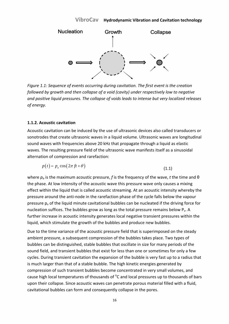
Figure 1.1: Sequence of events occurring during cavitation. The first event is the creation
followed by growth and then collapse of a void (cavity) under respectively low to negative
and positive liquid pressures. The collapse of voids leads to intense but very localized releases
of energy.
1.1.2. Acoustic cavitation
Acoustic cavitation can be induced by the use of ultrasonic devices also called transducers or
sonotrodes that create ultrasonic waves in a liquid volume. Ultrasonic waves are longitudinal
sound waves with frequencies above 20 kHz that propagate through a liquid as elastic
waves. The resulting pressure field of the ultrasonic wave manifests itself as a sinusoidal
alternation of compression and rarefaction:
cos 2ap t p ft (1.1)
where pa is the maximum acoustic pressure, f is the frequency of the wave, t the time and θ
the phase. At low intensity of the acoustic wave this pressure wave only causes a mixing
effect within the liquid that is called acoustic streaming. At an acoustic intensity whereby the
pressure around the anti‐node in the rarefaction phase of the cycle falls below the vapour
pressure pv of the liquid minute cavitational bubbles can be nucleated if the driving force for
nucleation suffices. The bubbles grow as long as the total pressure remains below Pv. A
further increase in acoustic intensity generates local negative transient pressures within the
liquid, which stimulate the growth of the bubbles and produce new bubbles.
Due to the time variance of the acoustic pressure field that is superimposed on the steady
ambient pressure, a subsequent compression of the bubbles takes place. Two types of
bubbles can be distinguished, stable bubbles that oscillate in size for many periods of the
sound field, and transient bubbles that exist for less than one or sometimes for only a few
cycles. During transient cavitation the expansion of the bubble is very fast up to a radius that
is much larger than that of a stable bubble. The high kinetic energies generated by
compression of such transient bubbles become concentrated in very small volumes, and
cause high local temperatures of thousands of oC and local pressures up to thousands of bars
upon their collapse. Since acoustic waves can penetrate porous material filled with a fluid,
cavitational bubbles can form and consequently collapse in the pores.
VibroCav Hydrodynamic Vibration and Cavitation technology
17
Because cavitational collapse is essentially a process that releases energy, its actuation
needs a steady energy input. Inputs can be measured as the power per unit volume of the
working liquid (kW.m‐3). For acoustic cavitation, energy input is often calibrated in terms of
either the ultrasonic tip amplitude or the energy input to the transducer, either of which
may be directly monitored (and adjusted) at the transducer driver unit. Experience with
ultrasonic systems shows that there is a threshold value of intensity or energy input below
which cavitation will not occur. This threshold depends on the physical properties of the
liquid, such as vapour pressure and viscosity, but as a rule‐of‐thumb for atmospheric
ambient pressures energy inputs in excess of 35 kW.m‐3 are usually recommended [1]. At
higher ambient pressures higher power inputs are required to reach pressures around the
anti‐nodes that fall below the vapour pressure of the liquid.
Ultrasonic cavitation devices
Hielsher Ultrasonics [5] is a major supplier of industrial ultrasonic processing equipment for
many applications, such as dispersion, de‐agglomeration, emulsification, wet‐milling, cel
disruption, disinfection and chemical conversion using 18 kHz ‐ 20 kHz industrial vibration
devices with power ratings of 0.5 to 16 kW. A set of four of the largest devices (4 x 16 kW)
processes in flow‐through mode approximately 1 m3/hr for cell extraction for algae
production and up to 50 m3/hr for biodiesel transesterification. Another producer of
ultrasonic equipment is Prosonic [6].
1.1.3. Hydrodynamic cavitation
In hydrodynamic cavitation the flow field is the origin of the pressure fluctuation that brings
about the processes of cavitation and collapse depicted in Figure 1.1. In any flowing system
that is not at a perfect steady state, the liquid flow will be subject to local accelerations and
perturbations of the flow pattern.
Cavitation in streamlined orifices or along streamlined bodies
For a streamlined body, where the disruption to the fluid flow is minimal, the flow
streamlines follow the contours of the surface as far as possible. Pressure variations will be
particularly marked where the liquid accelerates by flowing through a constriction such as a
venturi tube or a streamlined orifice or along a streamlined body confined in a tube. At the
points of high fluid velocity, low static pressures will occur, and here minute air‐ or vapour‐
filled bubbles may form [2], that will then be carried on to a region of higher pressure where
contraction and possibly collapse of the travelling bubbles will occur.
The flow velocity across the constriction or orifice is related to the pressure profile. It thus
depends on pup, pdown and on the geometry of the streamlined constriction.
VibroCav Hydrodynamic Vibration and Cavitation technology
18
For inviscid flow it is best visualized by applying Bernoulli’s equation to the flow upstream
and at location x of the obstruction.
2 21 1
2 2up up x xp v p v C (1.2)
where ν is the liquid velocity at the subscripted point, is the liquid density, and C is a constant value. A pressure below the vapour pressure of the liquid pv is the condition under
which cavities will form in the liquid and expand.
The above analysis enables the definition of a ‘cavitation number’, σ, a dimensionless
parameter that characterizes the propensity of a flow to cavitate [1, 2]. Bernoulli’s equation
(1.2) differentiates the static pressure p from a dynamic pressure term 21
2v which
represents the pressure drop due to the flow of the liquid. If we correct the static pressure
term for the vapour pressure of the liquid pv, then we express the cavitation number as the
ratio of the static and dynamic pressure contributions:
21
2
up vapor
water up
p p
v
(1.3)
The cavitation number basically represents the resistance of the flow to cavitation; the
higher the cavitation number, the less likely cavitation is to occur. Cavitation will appear if
the cavitation number σ falls below minus the pressure coefficient Cp.
21
2
x upp
water up
p pC
v
(1.4)
Cavitation behind bluff bodies protruding from a surface
The antonym of a streamlined body is a ‘bluff body’, which is a generic term for a body
obstructing and disrupting a fluid flow as shown in figure 1.2.
When a flowing liquid becomes detached from its guiding surface, usually because of an
obstruction or a sharp deviation in the duct or flow containment “fixed cavities” are formed.
If we consider the simple case of linear flow past a spherical obstruction of radius r, see
figure 1.2a, there comes with increase in r a point at which the flow lines will detach on the
downstream side. In terms of fluid dynamics [1] flow is driven by pressure, with a higher
pressure on the upstream side of the obstruction than on the downstream side. If we
assume that liquid cannot support a tensile stress (or, more realistically, that tensile stress is
limited to the strength of the liquid), then a point will be reached at which the pressure on
the downstream side of the obstruction falls to zero, and the streamlines will separate from
VibroCav Hydrodynamic Vibration and Cavitation technology
19
the surface. This separation of the boundary layer will create an empty space, or a cavity,
between the liquid flow and the guiding surface, which will eventually fill with vapour. The
subsequent trajectory of the cavity will depend on the pressures in the liquid flow, but at
perfect steady state the cavity will remain static.
In the case of an obstruction with a sharp edge, see figure 1.2.b, radius r becomes effectively
zero beyond the edge and the main flow will separate, leaving a liquid‐filled region possibly
with an eddy downstream (as shown). If the main flow velocity is high enough, the pressure
in the separated region will drop to zero and a vapour‐filled cavity will form. In both cases, as
in figure 1.2a and b, introducing a gas flow into the separated region may also create a gas‐
filled pocket, a condition designated as ventilated flow. The formation of a fixed cavity is
often followed by shedding, whereby small cavities detach from the main fixed cavity and
are carried downstream in the flow.
Cavity p < p vapor
r
Cavity p < p vapor
r
Cavity p < pvapor
Cavity p < pvapor
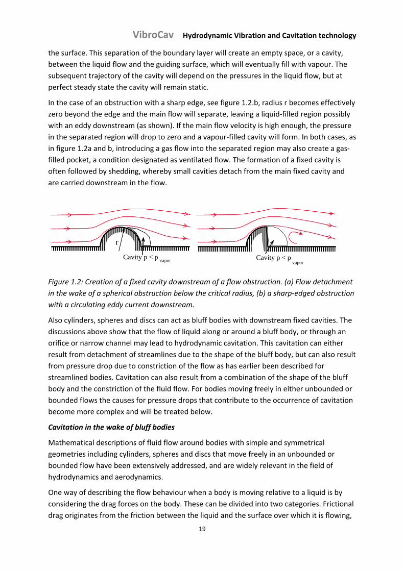
Figure 1.2: Creation of a fixed cavity downstream of a flow obstruction. (a) Flow detachment
in the wake of a spherical obstruction below the critical radius, (b) a sharp‐edged obstruction
with a circulating eddy current downstream.
Also cylinders, spheres and discs can act as bluff bodies with downstream fixed cavities. The
discussions above show that the flow of liquid along or around a bluff body, or through an
orifice or narrow channel may lead to hydrodynamic cavitation. This cavitation can either
result from detachment of streamlines due to the shape of the bluff body, but can also result
from pressure drop due to constriction of the flow as has earlier been described for
streamlined bodies. Cavitation can also result from a combination of the shape of the bluff
body and the constriction of the fluid flow. For bodies moving freely in either unbounded or
bounded flows the causes for pressure drops that contribute to the occurrence of cavitation
become more complex and will be treated below.
Cavitation in the wake of bluff bodies
Mathematical descriptions of fluid flow around bodies with simple and symmetrical
geometries including cylinders, spheres and discs that move freely in an unbounded or
bounded flow have been extensively addressed, and are widely relevant in the field of
hydrodynamics and aerodynamics.
One way of describing the flow behaviour when a body is moving relative to a liquid is by
considering the drag forces on the body. These can be divided into two categories. Frictional
drag originates from the friction between the liquid and the surface over which it is flowing,
VibroCav Hydrodynamic Vibration and Cavitation technology
20
pressure drag from the eddying motions set up in the liquid at the passage of the body.
When the total drag is dominated by the frictional component, the body is said to be
streamlined; where the pressure component dominates the body is bluff. One aspect of the
pressure drag component is boundary layer separation and the formation of a wake
downstream of the bluff body. A wake consists of a train of eddies extending downstream
from an object or obstruction to the point at which fully developed undisturbed flow is re‐
established. The formation of such eddies, vortices and wakes plays a determining role in the
creation of hydrodynamic cavitation. Cylinders and spheres are considered bluff bodies
because their drag is dominated by the pressure losses occurring in the wake. These are
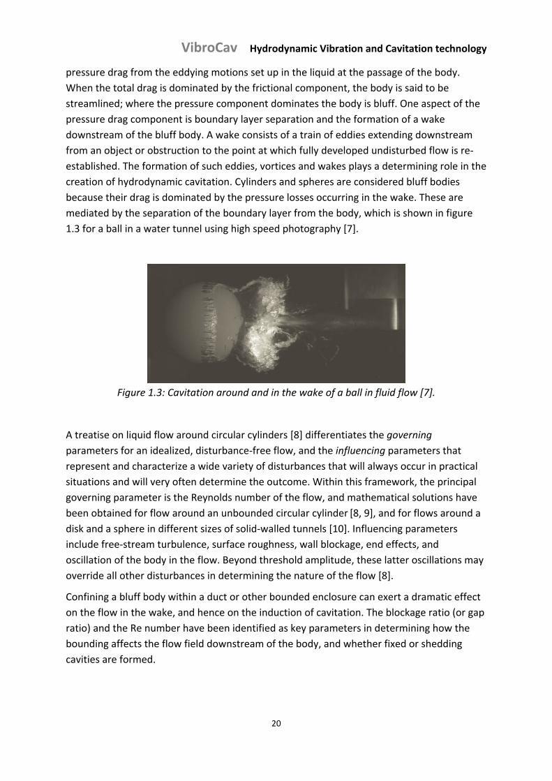
mediated by the separation of the boundary layer from the body, which is shown in figure
1.3 for a ball in a water tunnel using high speed photography [7].
Figure 1.3: Cavitation around and in the wake of a ball in fluid flow [7].
A treatise on liquid flow around circular cylinders [8] differentiates the governing
parameters for an idealized, disturbance‐free flow, and the influencing parameters that
represent and characterize a wide variety of disturbances that will always occur in practical
situations and will very often determine the outcome. Within this framework, the principal
governing parameter is the Reynolds number of the flow, and mathematical solutions have
been obtained for flow around an unbounded circular cylinder [8, 9], and for flows around a
disk and a sphere in different sizes of solid‐walled tunnels [10]. Influencing parameters
include free‐stream turbulence, surface roughness, wall blockage, end effects, and
oscillation of the body in the flow. Beyond threshold amplitude, these latter oscillations may
override all other disturbances in determining the nature of the flow [8].
Confining a bluff body within a duct or other bounded enclosure can exert a dramatic effect
on the flow in the wake, and hence on the induction of cavitation. The blockage ratio (or gap
ratio) and the Re number have been identified as key parameters in determining how the
bounding affects the flow field downstream of the body, and whether fixed or shedding
cavities are formed.
VibroCav Hydrodynamic Vibration and Cavitation technology
21
Supercavitation
In fixed cavities, the length of the cavity increases as cavitation becomes very strong. Vapour
or gas filled “supercavities” can result from the growth of such fixed cavities until their
length is very large compared with the body dimensions. Supercavities can sometimes be
created by ventilating the low pressure zones of a wake [11].
Given that cavitational collapse often gives rise to deleterious effects, supercavitation can
provide a desirable alternative because it gives steadier flow conditions and is less prone to
shedding than a conventional fixed cavity [2]. The phenomenon of supercavitation has been
recognised in the design of propellers [12], supercavitating pumps [13], high‐speed
underwater projectiles [14] and vehicles [15].
Cavitation by water hammer
Another source of cavitation is the water hammer effect that occurs when flow is suddenly
cut off [16, 17, 18, and 19]. The following description is based on Franzini et al. [20], where
the flow of a liquid, generally water, through a pipeline from a reservoir with a constant
liquid level is stopped by complete and instantaneous closure of valve N (see figure 1.4a).
Before closure of the valve the hydraulic grade line HGL in the pipe is sloping because the
static energy reflected by the pressure height at the inlet of the pipe M is lowered by
conversion into kinetic energy of V2/2g per liquid mass due to friction at the pipe wall hL.
Upon closure of the valve the water in front of the valve will be compressed by the upstream
column of liquid that is still flowing towards the valve until it is brought to a rest by the
returning pressure wave built up by the compression.
The compression of the liquid depends on the compressibility of the liquid and on the
elasticity of the stretching pipeline. The velocity of a pressure wave for a liquid such as water
in an elastic pipe is compared to that of a free wave in water reduced by stretching of the
pipe walls and equals:
1combined
pipe
pipe
liquid pipe pipe
E gC
D
E t E
(1.5)
where Epipe is modulus of elasticity of pipe material, Ecombined is bulk modulus of the
combined elasticity of the liquid and pipe, and Dpipe and tpipe are the diameter and wall
thickness of the pipe.
VibroCav Hydrodynamic Vibration and Cavitation technology
22
Time
Time
D
C
B
A
Time
Time
D
C
B
A
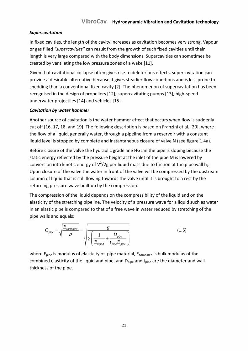
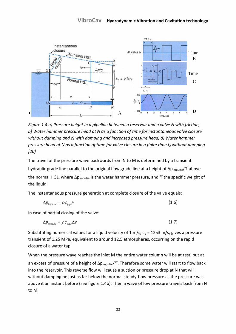
Figure 1.4 a) Pressure height in a pipeline between a reservoir and a valve N with friction,
b) Water hammer pressure head at N as a function of time for instantaneous valve closure
without damping and c) with damping and increased pressure head, d) Water hammer
pressure head at N as a function of time for valve closure in a finite time tc without damping
[20]
The travel of the pressure wave backwards from N to M is determined by a transient
hydraulic grade line parallel to the original flow grade line at a height of Δpimpulse/ϒ above the normal HGL, where Δpimpulse is the water hammer pressure, and ϒ the specific weight of the liquid.
The instantaneous pressure generation at complete closure of the valve equals:
impulse pipep c v (1.6)
In case of partial closing of the valve:
impulse pipep c v (1.7)
Substituting numerical values for a liquid velocity of 1 m/s, cp = 1253 m/s, gives a pressure
transient of 1.25 MPa, equivalent to around 12.5 atmospheres, occurring on the rapid
closure of a water tap.
When the pressure wave reaches the inlet M the entire water column will be at rest, but at
an excess of pressure of a height of Δpimpulse/ϒ. Therefore some water will start to flow back
into the reservoir. This reverse flow will cause a suction or pressure drop at N that will
without damping be just as far below the normal steady‐flow pressure as the pressure was
above it an instant before (see figure 1.4b). Then a wave of low pressure travels back from N
to M.
VibroCav Hydrodynamic Vibration and Cavitation technology
23
The time for a round trip of the pressure wave from N to M and backwards to N is:
2rpipe
LT
c (1.8)
with L as the actual length of the pipe. So the pressure head in N changes in time as
presented in figure 1.4.b.
A slight increase in pressure head over the value of Δp = ρ cp V for total instantaneous
closure was found to exist experimentally. As the wave front moves towards M, point C on
the transient HGL line moves with it and the pressure head at N becomes RS larger (see
figure 1.4.a). So in figure 1.4.c where the pressure head at N is plotted in time taking both
pipe friction and damping into account, the line ab is shown as sloping upwards and the line
ef as sloping downwards.
In a real situation instantaneous closure is not feasible, but for closure times tclose below Tr a
maximum water hammer pressure head of Δp/ϒ is reached between tclose and Tr (see figure 1.4c).
Just as the pressure goes up in front of the valve upon its instantaneous closure, the
pressure drops at the downstream side of the valve, because the liquid continues its flow
pattern, and a low‐pressure transient HLG exists. The pressure head versus time function is
thus opposite for both sides of the valve. As with other hydrodynamic cavitation
phenomena, vapour cavitation occurs due to water hammer effects when the transient
pressure in the liquid falls below the liquid vapour pressure (pv). The chance to produce
cavitation is larger directly behind the valve than in front of the valve if damping is not
neglected. Cavitation can occur as a single, large vapour cavity, which can lead to a column
separation, or as distributed small cavities or clouds of cavities in the liquid flow.
If an object such as a cylinder or a ball rapidly vibrates in a flow, and in particular when this
rapid oscillating behaviour of the object is combined with bouncing against the walls of the
duct, the stream lines of the flow become suddenly and frequently disrupted, and similar
effects are provoked as described above for the sudden closure of a valve. So the oscillating‐
bouncing behaviour contributes to the pressure drop in the liquid that is required to induce
cavitation.
Combined acoustic and hydrodynamic cavitation
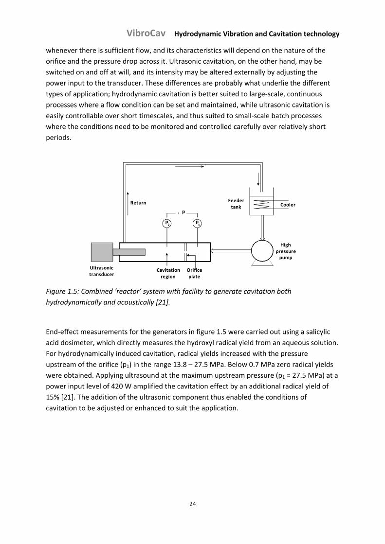
A recent publication [21] describes a single ‘reactor’ system that includes generation of
acoustic and hydrodynamic cavitation as complementary to each other. This is shown
schematically in figure 1.5, and is interesting because it enables a comparison of the drivers
that are required for both generation modes, and also the strengths and weaknesses of each
in operation. Hydrodynamic cavitation is induced by forcing the circulating liquid through an
orifice at high pressure. Cavitation occurs downstream of the orifice in the low pressure
region (p2), and this may be reinforced by acoustically induced cavitation from the ultrasonic
transducer. Figure 1.5 shows that hydrodynamic cavitation will be created continuously
VibroCav Hydrodynamic Vibration and Cavitation technology
24
whenever there is sufficient flow, and its characteristics will depend on the nature of the
orifice and the pressure drop across it. Ultrasonic cavitation, on the other hand, may be
switched on and off at will, and its intensity may be altered externally by adjusting the
power input to the transducer. These differences are probably what underlie the different
types of application; hydrodynamic cavitation is better suited to large‐scale, continuous
processes where a flow condition can be set and maintained, while ultrasonic cavitation is
easily controllable over short timescales, and thus suited to small‐scale batch processes
where the conditions need to be monitored and controlled carefully over relatively short
periods.
Feedertank Cooler
Highpressurepump
Orificeplate
Return
Ultrasonictransducer
Cavitationregion
p2
p1
p
Figure 1.5: Combined ‘reactor’ system with facility to generate cavitation both
hydrodynamically and acoustically [21].
End‐effect measurements for the generators in figure 1.5 were carried out using a salicylic
acid dosimeter, which directly measures the hydroxyl radical yield from an aqueous solution.
For hydrodynamically induced cavitation, radical yields increased with the pressure
upstream of the orifice (p1) in the range 13.8 – 27.5 MPa. Below 0.7 MPa zero radical yields
were obtained. Applying ultrasound at the maximum upstream pressure (p1 = 27.5 MPa) at a
power input level of 420 W amplified the cavitation effect by an additional radical yield of
15% [21]. The addition of the ultrasonic component thus enabled the conditions of
cavitation to be adjusted or enhanced to suit the application.
VibroCav Hydrodynamic Vibration and Cavitation technology
25
1.1.4. Hydrodynamic cavitation devices
Hydrodynamic cavitation can be generated in various ways by creating local high dynamic
energy peaks that lower the static pressure to below the vapour pressure of the fluid. A
selection of available devices is described below:
A high pressure homogenizer in which fluid is forced at a high pressure of 50 to 300
bar through a narrow constriction and projected onto a downstream plate. This
method is energy intensive due to the high feed pressure [22].
A high speed homogenizer where high dynamic energy is created at the tips of a fast
spinning blade in a rotor and stator configuration, also at the expense of a lot of
energy [22],
Flow constrictions in the form of an single or multiple hole orifice plate or a venturi
fed by constant flow, needing less energy than the aforementioned homogenizers,
with orifice plates generally providing more intense cavitational conditions than
venturi devices [22],
The annular space of a static outer housing with a fast spinning (3000 – 3600 rpm)
pock‐marked inner cylinder in a tool marketed by Hydro Dynamic Inc. as the Shock
Wave Powered Reactor or SPR. This method is described as very energy efficient [23],
A liquid whistle tool, whereby a liquid jet created in a shaped nozzle impacts upon a
steel blade that vibrates due to instabilities in the jet stream. The cavitational
performance of such devices can be influenced by adjusting the distance between
the blade and the nozzle outlet [24]. In view of the presence of a nozzle the energy
efficiency is expected to be comparable to that of a nozzle device, and
A rotary pulsed apparatus [25], whereby a closely fitting cylindrical rotor and stator
both provided with axial slots in the outer wall spaced such that the fluid flow is
interrupted if the slots do not coincide, impart strong pulses if fluid is pumped
through the device while rotating the rotor [26]. The energy efficiency is expected to
be comparable to the shock wave reactor device.
Of all available devices, an orifice and a venturi provide a flexible, simple and attractive
method for cavitation generation [22].
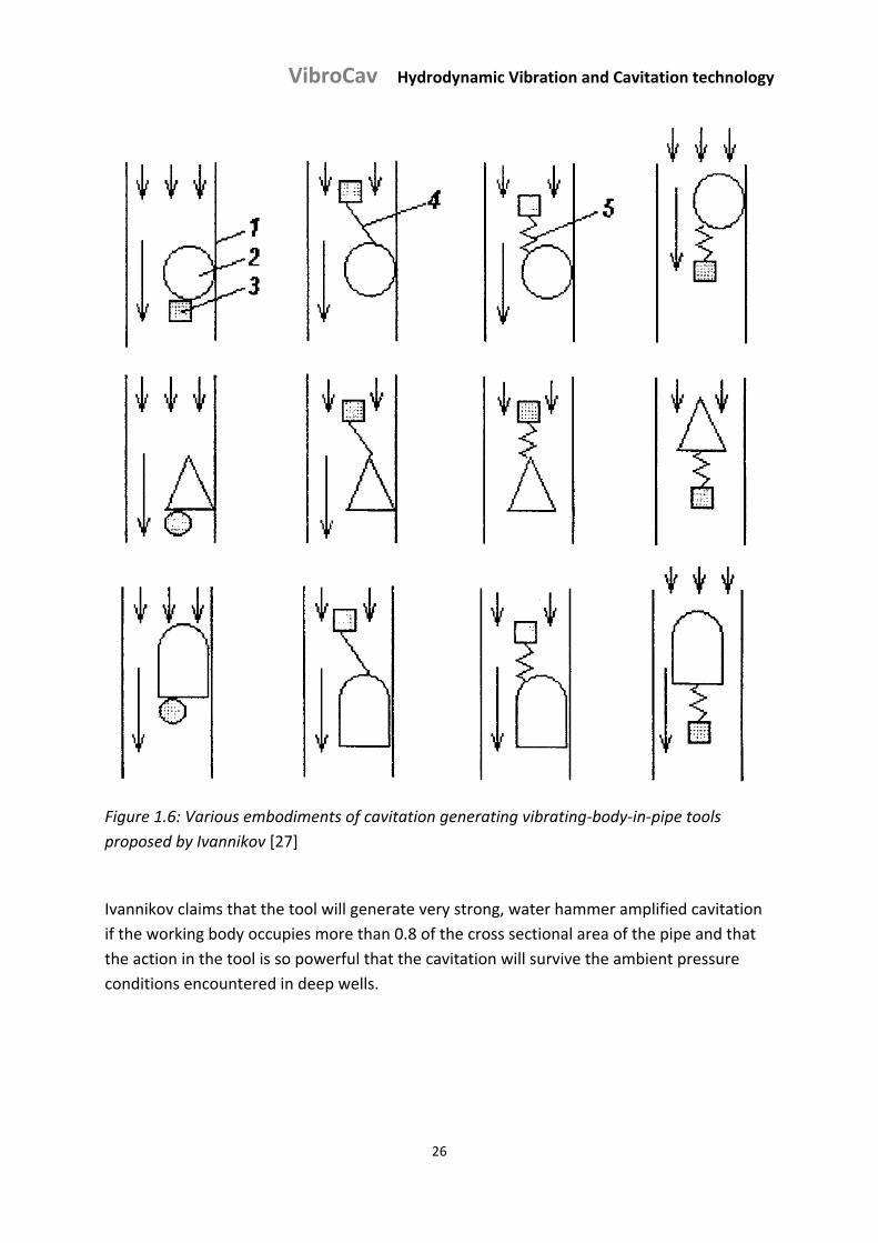
Cavitation can also be generated by the ‘vibrating‐body‐in‐pipe’ tool of Ivannikov [27]
consisting of a tube like housing and a body, mostly a ball, that is restrained in axial
direction, but can freely move transversely as illustrated in Figure 1.6.
VibroCav Hydrodynamic Vibration and Cavitation technology
26
Figure 1.6: Various embodiments of cavitation generating vibrating‐body‐in‐pipe tools
proposed by Ivannikov [27]
Ivannikov claims that the tool will generate very strong, water hammer amplified cavitation
if the working body occupies more than 0.8 of the cross sectional area of the pipe and that
the action in the tool is so powerful that the cavitation will survive the ambient pressure
conditions encountered in deep wells.
VibroCav Hydrodynamic Vibration and Cavitation technology
27
1.1.5. Consequences of cavitational collapse.
For acoustic cavitation a single bubble can be quasi stable or transient. A stable bubble
oscillates in size for many cycles by growing and subsequently shrinking during the
rarefaction and compression phase of the acoustic pressure, while a transient bubble grows
beyond a threshold size in mostly one cycle and collapses during compression. For
hydrodynamic cavitation the travelling cavities grow in size when transported by the flow as
long as the pressure remains below the vapour pressure, and beyond a certain size the
bubble becomes unstable, and collapses at increasing pressure of the flow.
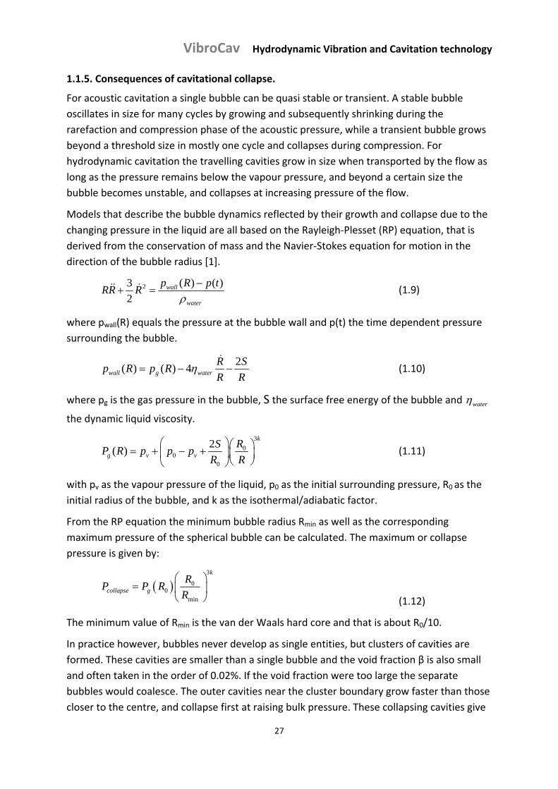
Models that describe the bubble dynamics reflected by their growth and collapse due to the
changing pressure in the liquid are all based on the Rayleigh‐Plesset (RP) equation, that is
derived from the conservation of mass and the Navier‐Stokes equation for motion in the
direction of the bubble radius [1].
2 ( ) ( )3
2wall
water
p R p tRR R
(1.9)
where pwall(R) equals the pressure at the bubble wall and p(t) the time dependent pressure
surrounding the bubble.
2( ) ( ) 4wall g water
R Sp R p R
R R
(1.10)
where pg is the gas pressure in the bubble, S the surface free energy of the bubble and water
the dynamic liquid viscosity.
3
00
0
2( )
k
g v v
RSP R p p p
R R
(1.11)
with pv as the vapour pressure of the liquid, p0 as the initial surrounding pressure, R0 as the
initial radius of the bubble, and k as the isothermal/adiabatic factor.
From the RP equation the minimum bubble radius Rmin as well as the corresponding
maximum pressure of the spherical bubble can be calculated. The maximum or collapse
pressure is given by:
3
00
min
k
collapse g
RP P R
R
(1.12)
The minimum value of Rmin is the van der Waals hard core and that is about R0/10.
In practice however, bubbles never develop as single entities, but clusters of cavities are
formed. These cavities are smaller than a single bubble and the void fraction β is also small
and often taken in the order of 0.02%. If the void fraction were too large the separate
bubbles would coalesce. The outer cavities near the cluster boundary grow faster than those
closer to the centre, and collapse first at raising bulk pressure. These collapsing cavities give
VibroCav Hydrodynamic Vibration and Cavitation technology
28
some part of their potential energy as shock waves to the surrounding liquid, but 25 to 50 %
of this energy is transferred inwards to the surrounding still un‐collapsed cavities. So
towards the centre of the cluster the cavities have stored more energy and their collapse
pressure is higher.
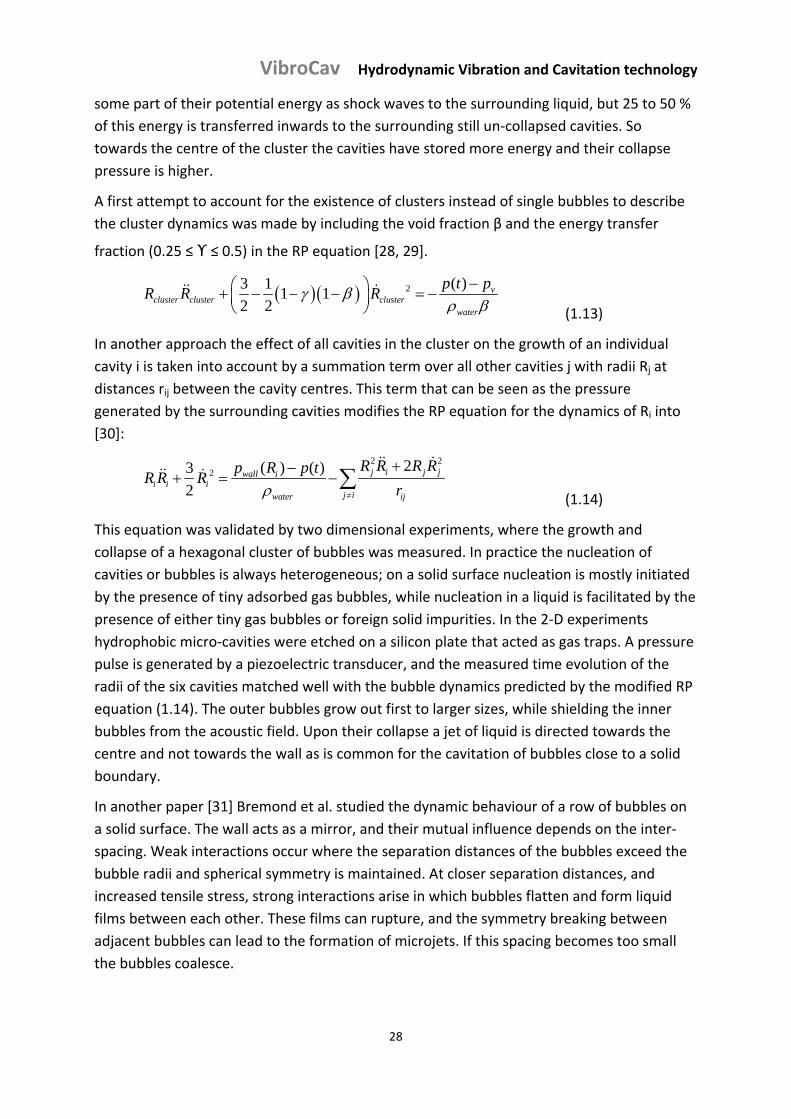
A first attempt to account for the existence of clusters instead of single bubbles to describe
the cluster dynamics was made by including the void fraction β and the energy transfer
fraction (0.25 ≤ ϒ ≤ 0.5) in the RP equation [28, 29].
2 ( )3 11 1
2 2v
cluster cluster clusterwater
p t pR R R
(1.13)
In another approach the effect of all cavities in the cluster on the growth of an individual
cavity i is taken into account by a summation term over all other cavities j with radii Rj at
distances rij between the cavity centres. This term that can be seen as the pressure
generated by the surrounding cavities modifies the RP equation for the dynamics of Ri into
[30]:
2 22 2( ) ( )3
2j i j jwall i
i i ij iwater ij
R R R Rp R p tR R R
r
(1.14)
This equation was validated by two dimensional experiments, where the growth and
collapse of a hexagonal cluster of bubbles was measured. In practice the nucleation of
cavities or bubbles is always heterogeneous; on a solid surface nucleation is mostly initiated
by the presence of tiny adsorbed gas bubbles, while nucleation in a liquid is facilitated by the
presence of either tiny gas bubbles or foreign solid impurities. In the 2‐D experiments
hydrophobic micro‐cavities were etched on a silicon plate that acted as gas traps. A pressure
pulse is generated by a piezoelectric transducer, and the measured time evolution of the
radii of the six cavities matched well with the bubble dynamics predicted by the modified RP
equation (1.14). The outer bubbles grow out first to larger sizes, while shielding the inner
bubbles from the acoustic field. Upon their collapse a jet of liquid is directed towards the
centre and not towards the wall as is common for the cavitation of bubbles close to a solid
boundary.
In another paper [31] Bremond et al. studied the dynamic behaviour of a row of bubbles on
a solid surface. The wall acts as a mirror, and their mutual influence depends on the inter‐
spacing. Weak interactions occur where the separation distances of the bubbles exceed the
bubble radii and spherical symmetry is maintained. At closer separation distances, and
increased tensile stress, strong interactions arise in which bubbles flatten and form liquid
films between each other. These films can rupture, and the symmetry breaking between
adjacent bubbles can lead to the formation of microjets. If this spacing becomes too small
the bubbles coalesce.
VibroCav Hydrodynamic Vibration and Cavitation technology
29
The adapted RP equation where the interaction between the cavities in the cluster is
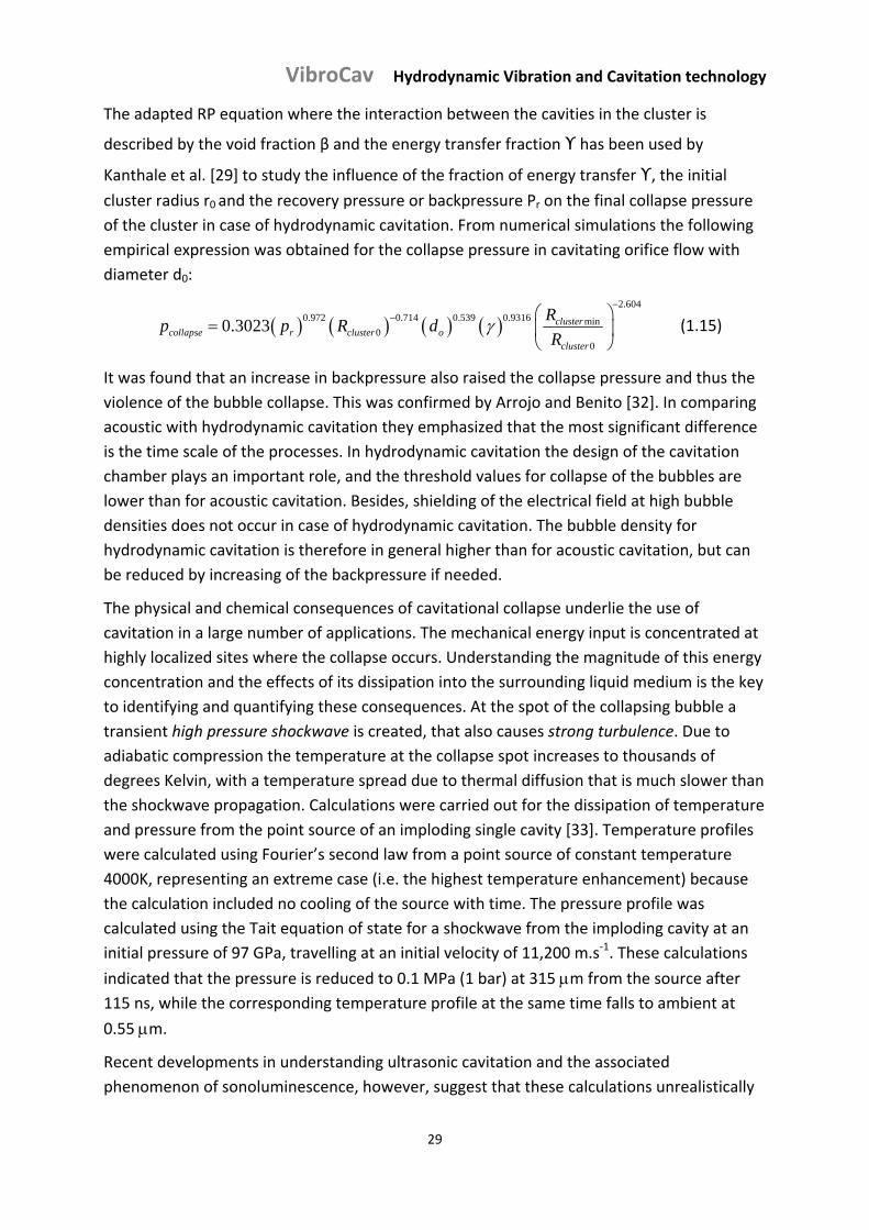
described by the void fraction β and the energy transfer fraction ϒ has been used by Kanthale et al. [29] to study the influence of the fraction of energy transfer ϒ, the initial cluster radius r0 and the recovery pressure or backpressure Pr on the final collapse pressure
of the cluster in case of hydrodynamic cavitation. From numerical simulations the following
empirical expression was obtained for the collapse pressure in cavitating orifice flow with
diameter d0:
2.604
0.972 0.714 0.539 0.9316 min0
0
0.3023 clustercollapse r cluster o
cluster
Rp p R d
R
(1.15)
It was found that an increase in backpressure also raised the collapse pressure and thus the
violence of the bubble collapse. This was confirmed by Arrojo and Benito [32]. In comparing
acoustic with hydrodynamic cavitation they emphasized that the most significant difference
is the time scale of the processes. In hydrodynamic cavitation the design of the cavitation
chamber plays an important role, and the threshold values for collapse of the bubbles are
lower than for acoustic cavitation. Besides, shielding of the electrical field at high bubble
densities does not occur in case of hydrodynamic cavitation. The bubble density for
hydrodynamic cavitation is therefore in general higher than for acoustic cavitation, but can
be reduced by increasing of the backpressure if needed.
The physical and chemical consequences of cavitational collapse underlie the use of
cavitation in a large number of applications. The mechanical energy input is concentrated at
highly localized sites where the collapse occurs. Understanding the magnitude of this energy
concentration and the effects of its dissipation into the surrounding liquid medium is the key
to identifying and quantifying these consequences. At the spot of the collapsing bubble a
transient high pressure shockwave is created, that also causes strong turbulence. Due to
adiabatic compression the temperature at the collapse spot increases to thousands of
degrees Kelvin, with a temperature spread due to thermal diffusion that is much slower than
the shockwave propagation. Calculations were carried out for the dissipation of temperature
and pressure from the point source of an imploding single cavity [33]. Temperature profiles
were calculated using Fourier’s second law from a point source of constant temperature
4000K, representing an extreme case (i.e. the highest temperature enhancement) because
the calculation included no cooling of the source with time. The pressure profile was
calculated using the Tait equation of state for a shockwave from the imploding cavity at an
initial pressure of 97 GPa, travelling at an initial velocity of 11,200 m.s‐1. These calculations
indicated that the pressure is reduced to 0.1 MPa (1 bar) at 315 m from the source after
115 ns, while the corresponding temperature profile at the same time falls to ambient at
0.55 m.
Recent developments in understanding ultrasonic cavitation and the associated
phenomenon of sonoluminescence, however, suggest that these calculations unrealistically

VibroCav Hydrodynamic Vibration and Cavitation technology
30
overestimate the core temperature and pressure at cavitational collapse. Investigations of
single‐bubble sonoluminescence (SBSL) have been extensive; the use of a single bubble
allows observation in detail [34], and also preserves the spherical symmetry of the collapse
such that analysis can be carried out based on the Rayleigh – Plesset equation [35].
Shock waves have been observed experimentally from single bubbles undergoing periodic
cavitational collapse using a Streak camera with high time resolution [36], and their initial
velocity of propagation has been estimated from the images. This initial velocity was 3 times
lower than those calculated with the Tait equation. Other important factors in limiting the
intensity of the collapse response lie in the nature and composition of the liquid and gaseous
phases.
VibroCav Hydrodynamic Vibration and Cavitation technology
31
1.2. Vibration
1.2.1. Vibration sources
Deliberate vibration, as opposed to unwanted vibration, has a multitude of industrial
applications. The most common application is a loudspeaker that produces sound waves in
the air. This study focuses on vibration sources used in a fluid environment at elevated
ambient pressures as encountered in well bores.
As such there is a family of acoustic vibrators or sonotrodes usually based on a piezo‐
electrically activated membrane and a horn to focus the wave energy at frequency levels of
10 kHz up to MHz values; these vibrators require a significant amount of electrical energy
often in excess of what can be supplied in deep well applications and work therefore
sometimes in a pulsed mode in combination with a condenser system to limit the energy
feed to the instrument.
Rather than having to supply high power electrical energy it is easier to supply hydraulic
energy to a vibration instrument in a deep well situation. Among the vibrators that are
driven by the fluid stream itself are nozzle type instruments that use an acoustic reflector
upstream of an organ‐pipe tube as an acoustic chamber creating ring vortices in the exiting
jet stream when the excitation frequency of the fluid jet matches the excitation value of the
nozzle; these tools have no moving parts and can be designed to operate at frequencies of
several hundred Hz to several kHz.
Other instruments use two outflow channels and a short‐circuit bypass to oscillate flow from
one side to the other and thus generate fluid pulses. This mechanism is called fluidic
oscillation. The tools also have no moving parts and operate at typically 250 Hz.
In the low frequency range tools exist that generate powerful pressure pulses by sudden
release of pressure build up between unequally sized tandem pistons that are axially
reciprocated typically operating at 6 Hz and purely mechanically acting impact hammer
tools.
An instrument with an oscillating and bouncing axially restrained ball as described by
Ivannikov [27] is also known to produce strong vibration.
A characterisation of the above vibration sources will be given in section 1.2.4.
1.2.2. Hydrodynamic vibration
Flow induced vibration in unbounded flow
Flow induced vibrations of structures/bodies are generally classified according to the type of
flow (steady flow, unsteady flow and two‐phase flow) and a considerable number of
vibration mechanisms have been identified [37]. Vibrations induced by the periodic shedding
of vortices are the most frequently occurring in practice, and are of interest to many fields of
engineering where a lot of effort is put into avoiding their occurrence that often leads to
disruption of the structure [38]. Detailed reviews on vortex induced vibration (VIV) have
VibroCav Hydrodynamic Vibration and Cavitation technology
32
been written by Williamson & Govardhan [39] and by Sarpkaya [40]. These studies are
primarily concerned with vibrations of elastically mounted bluff bodies such as cylinders
restrained to move only transverse to the flow that can be regarded as unbounded. At Re >
40 two staggered rows of vortices, so‐called von Kármán vortices, develop from either side
of the bluff body into its wake. The periodic force on the bluff body by the shedding of the
vortices has a lift component in the transverse direction with the same frequency as the
vortex‐shedding fvs and a drag component with twice the shedding frequency. The
amplitudes of the cross flow vibrations are larger than those of vibration in the stream‐wise
direction. As the flow rate U increases, a condition is reached where the vortex‐shedding
frequency fvs of the body in motion approaches the body’s natural frequency fN close enough
for the unsteady pressures from the wake vortices to induce the body to respond. This
phenomenon of self‐induced vibration is referred to as resonance or lock‐in. This
synchronisation effect acts to increase the range of flow rates over which vibrations of high
amplitude occur. In the lock‐in range fvs becomes increasingly smaller than the vortex
shedding frequency of a body at rest [41]. This frequency at rest, the so‐called Strouhal
frequency fst is uniquely related to the velocity of the flow and the characteristic size of the
body D through the Strouhal number St = fstD/U, where U is the steady ambient rate of the
uniform flow.
The lock‐in effect is also observed when a cylinder is forced to oscillate sinusoidally in a
uniform stream. This happens when the imposed frequency in the transverse direction
approaches the natural vortex shedding frequency of the cylinder or when the driving
frequency in the stream‐wise direction approaches twice the natural shedding frequency.
The average flow rates in the wake were remarkably similar to those for self‐induced
vibrations.
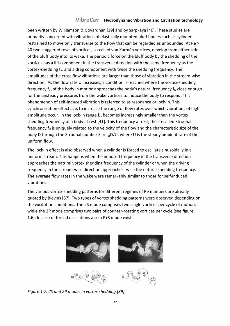
The various vortex‐shedding patterns for different regimes of Re numbers are already
quoted by Blevins [37]. Two types of vortex shedding patterns were observed depending on
the excitation conditions. The 2S mode comprises two single vortices per cycle of motion,
while the 2P mode comprises two pairs of counter‐rotating vortices per cycle (see figure
1.6). In case of forced oscillations also a P+S mode exists.
Figure 1.7: 2S and 2P modes in vortex shedding [39]
VibroCav Hydrodynamic Vibration and Cavitation technology
33
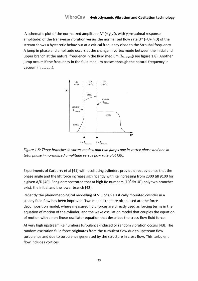
A schematic plot of the normalized amplitude A* (= y0/D, with y0=maximal response
amplitude) of the transverse vibration versus the normalized flow rate U* (=U/(fND) of the
stream shows a hysteretic behaviour at a critical frequency close to the Strouhal frequency.
A jump in phase and amplitude occurs at the change in vortex mode between the initial and
upper branch at the natural frequency in the fluid medium (fN ‐ water)(see figure 1.8). Another
jump occurs if the frequency in the fluid medium passes through the natural frequency in
vacuum (fN ‐ vacuum).
Figure 1.8: Three branches in vortex modes, and two jumps one in vortex phase and one in
total phase in normalized amplitude versus flow rate plot [39].
Experiments of Carberry et al [41] with oscillating cylinders provide direct evidence that the
phase angle and the lift force increase significantly with Re increasing from 2300 till 9100 for
a given A/D [40]. Feng demonstrated that at high Re numbers (104‐5x10⁴) only two branches
exist, the initial and the lower branch [42].
Recently the phenomenological modelling of VIV of an elastically mounted cylinder in a
steady fluid flow has been improved. Two models that are often used are the force‐
decomposition model, where measured fluid forces are directly used as forcing terms in the
equation of motion of the cylinder, and the wake oscillation model that couples the equation
of motion with a non‐linear oscillator equation that describes the cross‐flow fluid force.
At very high upstream Re numbers turbulence‐induced or random vibration occurs [43]. The
random excitation fluid force originates from the turbulent flow due to upstream flow
turbulence and due to turbulence generated by the structure in cross flow. This turbulent
flow includes vortices.
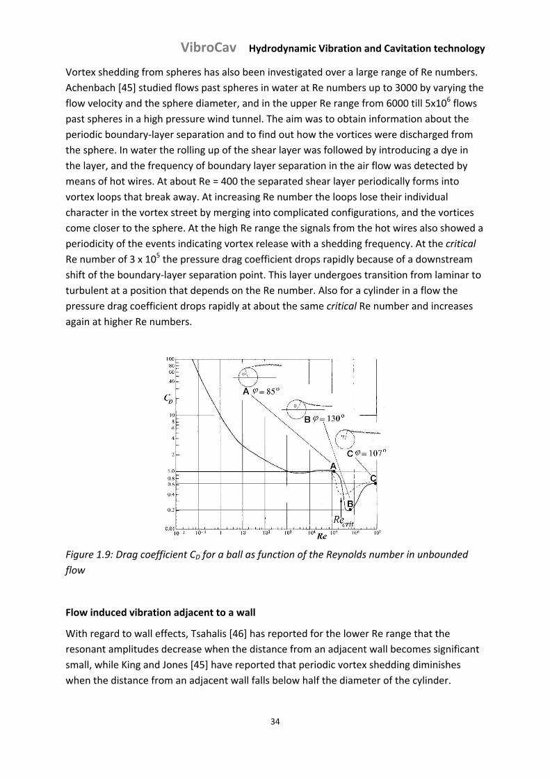
VibroCav Hydrodynamic Vibration and Cavitation technology
34
Vortex shedding from spheres has also been investigated over a large range of Re numbers.
Achenbach [45] studied flows past spheres in water at Re numbers up to 3000 by varying the
flow velocity and the sphere diameter, and in the upper Re range from 6000 till 5x10⁶ flows
past spheres in a high pressure wind tunnel. The aim was to obtain information about the
periodic boundary‐layer separation and to find out how the vortices were discharged from
the sphere. In water the rolling up of the shear layer was followed by introducing a dye in
the layer, and the frequency of boundary layer separation in the air flow was detected by
means of hot wires. At about Re = 400 the separated shear layer periodically forms into
vortex loops that break away. At increasing Re number the loops lose their individual
character in the vortex street by merging into complicated configurations, and the vortices
come closer to the sphere. At the high Re range the signals from the hot wires also showed a
periodicity of the events indicating vortex release with a shedding frequency. At the critical
Re number of 3 x 10⁵ the pressure drag coefficient drops rapidly because of a downstream
shift of the boundary‐layer separation point. This layer undergoes transition from laminar to
turbulent at a position that depends on the Re number. Also for a cylinder in a flow the
pressure drag coefficient drops rapidly at about the same critical Re number and increases
again at higher Re numbers.
Figure 1.9: Drag coefficient CD for a ball as function of the Reynolds number in unbounded
flow
Flow induced vibration adjacent to a wall
With regard to wall effects, Tsahalis [46] has reported for the lower Re range that the
resonant amplitudes decrease when the distance from an adjacent wall becomes significant
small, while King and Jones [45] have reported that periodic vortex shedding diminishes
when the distance from an adjacent wall falls below half the diameter of the cylinder.
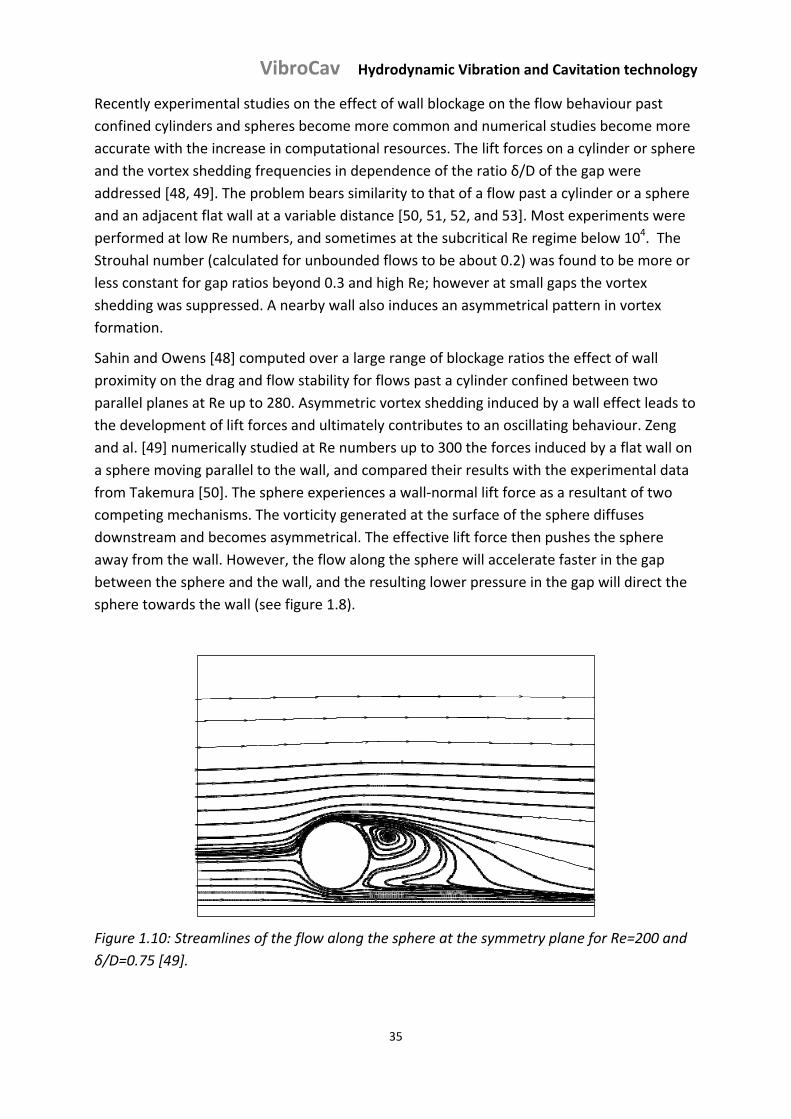
VibroCav Hydrodynamic Vibration and Cavitation technology
35
Recently experimental studies on the effect of wall blockage on the flow behaviour past
confined cylinders and spheres become more common and numerical studies become more
accurate with the increase in computational resources. The lift forces on a cylinder or sphere
and the vortex shedding frequencies in dependence of the ratio δ/D of the gap were
addressed [48, 49]. The problem bears similarity to that of a flow past a cylinder or a sphere
and an adjacent flat wall at a variable distance [50, 51, 52, and 53]. Most experiments were
performed at low Re numbers, and sometimes at the subcritical Re regime below 104. The
Strouhal number (calculated for unbounded flows to be about 0.2) was found to be more or
less constant for gap ratios beyond 0.3 and high Re; however at small gaps the vortex
shedding was suppressed. A nearby wall also induces an asymmetrical pattern in vortex
formation.
Sahin and Owens [48] computed over a large range of blockage ratios the effect of wall
proximity on the drag and flow stability for flows past a cylinder confined between two
parallel planes at Re up to 280. Asymmetric vortex shedding induced by a wall effect leads to
the development of lift forces and ultimately contributes to an oscillating behaviour. Zeng
and al. [49] numerically studied at Re numbers up to 300 the forces induced by a flat wall on
a sphere moving parallel to the wall, and compared their results with the experimental data
from Takemura [50]. The sphere experiences a wall‐normal lift force as a resultant of two
competing mechanisms. The vorticity generated at the surface of the sphere diffuses
downstream and becomes asymmetrical. The effective lift force then pushes the sphere
away from the wall. However, the flow along the sphere will accelerate faster in the gap
between the sphere and the wall, and the resulting lower pressure in the gap will direct the
sphere towards the wall (see figure 1.8).
Figure 1.10: Streamlines of the flow along the sphere at the symmetry plane for Re=200 and
δ/D=0.75 [49].
VibroCav Hydrodynamic Vibration and Cavitation technology
36
A non‐uniform cross‐flow will often lead to a rotation of the sphere that also causes a lift
force. This force is however, small and is often ignored. Yang et al. [51] experimentally
determined the vortex shedding in the wake flow of a cylinder next to a flat plane boundary
up to high Re numbers.
Flow induced vibration for narrow gap sizes with bouncing
Compared to the case of an unbounded flow where the vortex shedding and the excitation
of a cylinder or a ball in the transverse direction are induced by the flow force past the
object, the situation for a ball in a pipe is more complex due to the existence of at least two
above mentioned additional wall normal lift forces. Recently experimental studies were
performed by Karlikov et al. for highly constricted flows, i.e. at gap sizes narrow enough for
bouncing of the vibrating ball against the pipe wall to occur. Since bouncing implies impacts
on the inner pipe wall the normal component of the impact force represents an additional
lift force, while the slip force contributes to the rotation of the ball along an axis near
parallel to the pipe axis.
For bounded flows and a gap ratio S = δ /Dball = (dpipe‐Dball)/ Dball, where Dball = ball diameter
and dpipe = internal pipe diameter, below about 0.35, vibration is more likely to be caused by
low static pressure due to high dynamic pressure in the gap. Karlikov et al. [54, 55 and 56]
studied the acoustic frequency at lateral self‐excited vibration of balls with a narrow gap
ratio between 0.10 and 0.35 for a flow through a cylindrical pipe fixed at the upper end in a
massive support. The Re numbers of the flows in the studies of Karlikov et al. varied from 104
to 105. In a pipe of a variable length balls of various sizes and densities were suspended on a
long filament which permitted free lateral movement of the ball [54, 55]. A water flow was
run through the pipe at increasing flow rates until at a certain flow rate the self‐excited
vibration of the ball started, accompanied by periodic impacts of the ball against the inner
wall of the pipe. When the natural frequency of the vibrations of the ball coincided with that
of the pipe by adjusting the free length of the pipe, a resonance mode commenced, where
the amplitudes of the acoustic waves were sharply amplified and hence easily to measure.
This natural frequency f at a given pipe length was measured to be directly proportional to
the mean flow rate U (= 4Q/πDpipe2 with Q = flow in m3/s). Such measurements were only
extended to flow rates where neither active nor passive cavitation emerged. The frequencies
f were plotted for various lengths of the pipe with diameter d against the flow Q, and
resulted in straight lines through the origin of the plot. The slope of each line depended on
both the gap ratio δ/Dball and the normalized mass of the ball ρball/ρwater.
To relate the self‐excited vibration frequency f with other parameters a dimensionless Sh
number was introduced defined similarly to the Strouhal number as fD
ShV
, although not
coupled with a vortex shedding frequency. From the slopes of the lines in the plot it followed
that:
VibroCav Hydrodynamic Vibration and Cavitation technology
37
1.5 0.2 0.2
1.50.07 0.2 1ball ball
ball water water
Sh BD
(1.16)
with B = blockage ratio. Since the Sh numbers or the frequencies showed no dependence on
Re, the high gradient flow in the gap and the turbulent nature of the flow were mainly held
responsible for the lateral vibration rather than vortex shedding and the formation of a
vortex wake.
In a subsequent paper Karlikov et al. [55] measured the force exerted by the flow on a ball in
a pipe retained by a support. From this force they calculated whether the average hydraulic
resistance coefficient of the pipe in the presence of a ball (= 2 Δp / ρwater v2) and the drag
coefficient of the ball (= 8 F/ ρwater v2 π D2) were affected by the lateral movement of the ball
for small gap sizes. Only for light balls as for plastic, lateral movement of the ball causes a
50% increase in these coefficients.
A set of similar studies was conducted with cylinders of different mass and size oscillating
laterally in a plane channel of rectangular cross‐section with narrow gap ratios between 0.1
and 0.3 at Re numbers from 1.7 x 10⁴ to 7.2 x 10⁴ [54]. The measured Sh number depended
again on the gap ratio ((δ/D)‐1) as well as on the normalized mass of the ball ((ρball/ρwater)‐0.17),
but also marginally on Re. The same counted for the cylinder drag coefficient.
These experimentally observed self‐oscillations of the cylinders were simulated by
Kharlamov [53] by positioning dipoles at the centre of the cylinder with their axis along the
movement of the cylinder.
The idea of a laterally free moving body, mostly but not necessarily a sphere in a cylindrical
or conical housing, constrained either by a rod at the end of the housing or otherwise by
hanging of the body on a rod or string for a blockage ratio of less than 0.80 was patented by
Ivannikov [27]. The action of the tool consisting of the body in a housing was either to induce
pressure waves in the surrounding medium or cavitation or a combination of the two. The
tool was supposed to maintain its vibrational and cavitational action up to high surrounding
pressures, also referred to as backpressures.
1.2.3. Consequences of propagating waves
Waves, regardless if generated by transducers, sonic hammers, pulsators or by bouncing of
balls against a pipe wall as in hydrodynamic vibration tools, propagate from the source into
the surrounding medium, where the waves are used in oil, gas or water wells for seismic
stimulation or cleaning of the formation near the wellbore, the perforation tunnels or the
wellbore itself. In the liquid around the tool only longitudinal pressure or compressional
waves Pl (primary wave in liquid) are transmitted. These waves may have to pass several
steel walls and often a cement layer before they reach the porous medium around the
wellbore. Alternatively they reach the formation via perforation tunnels. The wave energy
that is not lost by reflection at the various interfaces enters the formation, where the waves
VibroCav Hydrodynamic Vibration and Cavitation technology
38
meet a porous medium consisting of a solid matrix with fluid filled pores that are more or
less interconnected.
The behaviour of waves in a porous medium has been described by Biot [57] and confirmed
by Berryman [58], resulting in a widely accepted analysis that the single compressional wave
in the fluid changes at the fluid to rock interface into a fast compressional Pm wave and a fast
shear wave S m with speeds comparable to the velocity of sound in the solid matrix material
both described by Biot as waves of the first kind and a slow compressional Pl wave described
as wave of the second type which is unique to poro‐elastic materials travelling in the fluid of
the porous medium according to Berryman [58] and others at a speed significantly lower
than the speed of sound in water. The shear wave S m is a transversal wave that oscillates
perpendicular to the direction of propagation caused by transverse contraction or ‘Poisson’
effects.
The background to the work of Biot was the drive from Shell Oil Company to better describe
the behaviour of seismic waves in the underground. Biot determined that for the
propagation of fast waves of the first kind in a statistically isotropic porous elastic solid
containing a compressible viscous fluid for wave lengths that are large compared to the size
of the pores and in dynamic conditions with Poiseulle flow in the pores a certain critical
frequency exists at which there is no relative motion between the fluid and the solid; in this
situation of ‘dynamic compatibility’ energy dissipation due to fluid friction will be nil and the
attenuation of the wave will be extremely small and hence the penetration depth very large
as is required for seismic investigation of massive rock volumes.
Low frequency waves of the first kind can meet conditions of dynamic compatibility in the
subsurface and, where they reflect on interfaces of rock layers or other discontinuities, allow
due to velocity and attenuation contrasts seismic characterisation of the underground. By
definition the overall attenuation of these waves is low in order to obtain a satisfactory
depth of investigation and the energy ‘spent’ on the pore fluid and relative motion between
fluid and matrix is low. Nevertheless benign effects such as freeing of stuck oil droplets or
coagulation of oil droplets can be generated in the pores of reservoir rock if the vibration
source is very strong [59]. Some Russian researchers argue that in particular conditions
resonance effects produce signal enhancements that promote effects in the pores [60].
In contrast to this the slow compressional waves ‐ Biot dilatational waves of the second kind
‐ in the pores are highly attenuated due to frictional effects and relative motion of the fluid
and the walls of the pores at frequencies below the critical frequency. While the slow waves
are less interesting for seismic investigations because of their limited depth of penetration,
they play a dominant role in cleaning pores in the vicinity of a wellbore. The loss of energy is
spent mainly on dynamic friction due to relative motion of the fluid and the pores and visco‐
elastic compressional effects, both resulting fluid velocity effects and eventually in heat
generation. In qualitative sense the dissipation of energy occurs closer to the fluid to rock
interface as the frequency increases. A simplified approach to illustrate the influence of
VibroCav Hydrodynamic Vibration and Cavitation technology
39
frequency in relation to the depth of penetration assuming a totally rigid porous frame was
proposed for this study by Smeulders [61]:
The mass balance equation and Darcy’s law are given by:
(1.17)
(1.18)
where w is the fluid velocity within the rigid porous frame, is the porosity and 0k is the
permeability. These equations can be rewritten as:
(1.19)
(1.20)
where the fluid compressibility fK is introduced. For water, fK = 2.25 GPa. Subtracting the
above equations leads to
(1.21)
where is the hydraulic diffusivity. The above equation now has the
form of a standard diffusion equation. For the one‐dimensional case, the penetration depth
L of the wave can be computed. This depth is defined by the half‐amplitude of the wave, so
where exp(‐αL) = ½, with α the attenuation coefficient. The attenuation coefficient of the
slow compressional wave Pl is given by
(1.22)
with f 2 the angular wave frequency of the wave, if f is the frequency of the wave.
Substitution in the expression for the half‐amplitude of the wave allows the penetration
depth L to be expressed as
(1.23)
This simplified analysis provides an impression of the penetration depth defined as the half
amplitude of the slow compressional wave Pl as a function of the wave frequency. It is clear
that low frequency waves penetrate deeper into the porous medium.
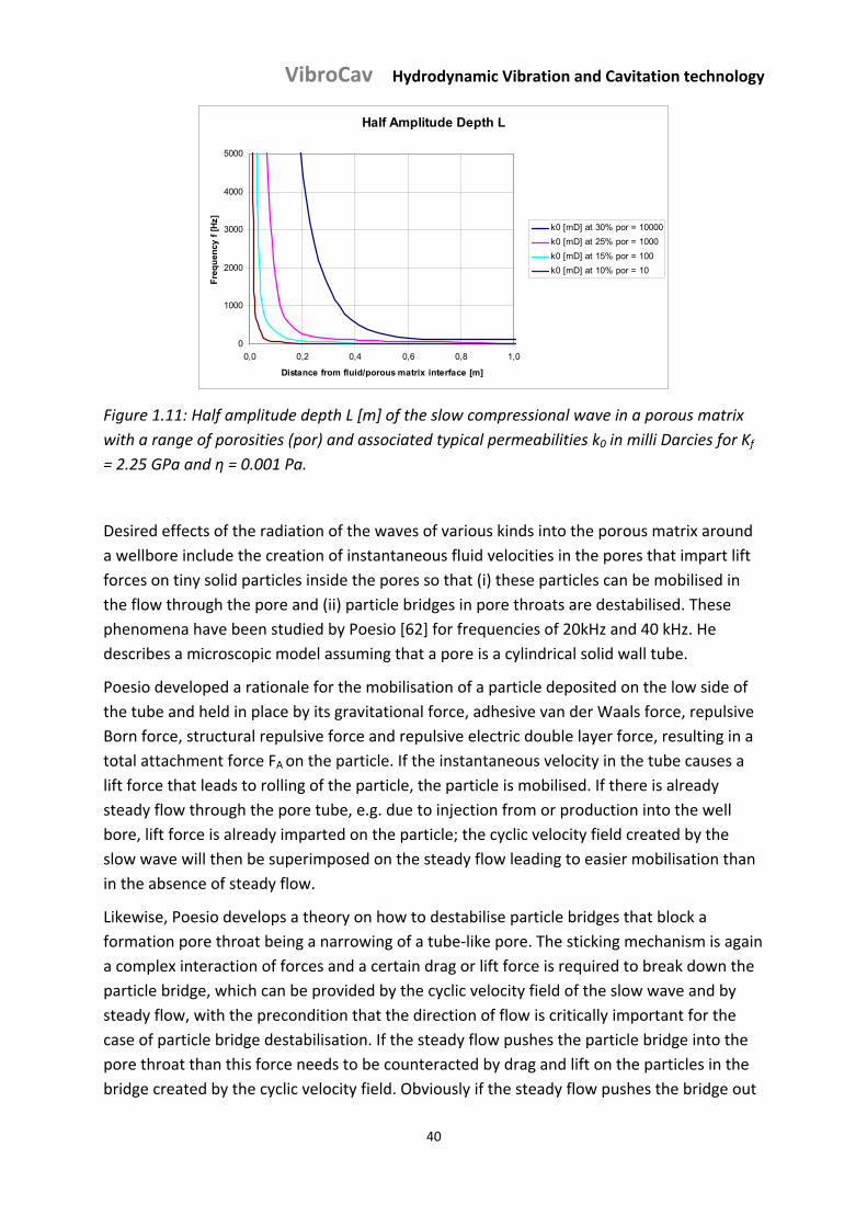
VibroCav Hydrodynamic Vibration and Cavitation technology
40
Half Amplitude Depth L
0
1000
2000
3000
4000
5000
0,0 0,2 0,4 0,6 0,8 1,0
Distance from fluid/porous matrix interface [m]
Fre
qu
ency
f [
Hz]
k0 [mD] at 30% por = 10000
k0 [mD] at 25% por = 1000
k0 [mD] at 15% por = 100
k0 [mD] at 10% por = 10
Figure 1.11: Half amplitude depth L [m] of the slow compressional wave in a porous matrix
with a range of porosities (por) and associated typical permeabilities k0 in milli Darcies for Kf
= 2.25 GPa and η = 0.001 Pa.
Desired effects of the radiation of the waves of various kinds into the porous matrix around
a wellbore include the creation of instantaneous fluid velocities in the pores that impart lift
forces on tiny solid particles inside the pores so that (i) these particles can be mobilised in
the flow through the pore and (ii) particle bridges in pore throats are destabilised. These
phenomena have been studied by Poesio [62] for frequencies of 20kHz and 40 kHz. He
describes a microscopic model assuming that a pore is a cylindrical solid wall tube.
Poesio developed a rationale for the mobilisation of a particle deposited on the low side of
the tube and held in place by its gravitational force, adhesive van der Waals force, repulsive
Born force, structural repulsive force and repulsive electric double layer force, resulting in a
total attachment force FA on the particle. If the instantaneous velocity in the tube causes a
lift force that leads to rolling of the particle, the particle is mobilised. If there is already
steady flow through the pore tube, e.g. due to injection from or production into the well
bore, lift force is already imparted on the particle; the cyclic velocity field created by the
slow wave will then be superimposed on the steady flow leading to easier mobilisation than
in the absence of steady flow.
Likewise, Poesio develops a theory on how to destabilise particle bridges that block a
formation pore throat being a narrowing of a tube‐like pore. The sticking mechanism is again
a complex interaction of forces and a certain drag or lift force is required to break down the
particle bridge, which can be provided by the cyclic velocity field of the slow wave and by
steady flow, with the precondition that the direction of flow is critically important for the
case of particle bridge destabilisation. If the steady flow pushes the particle bridge into the
pore throat than this force needs to be counteracted by drag and lift on the particles in the
bridge created by the cyclic velocity field. Obviously if the steady flow pushes the bridge out
VibroCav Hydrodynamic Vibration and Cavitation technology
41
of the pore, the cyclic velocity field cooperates with destabilising the bridge and if the steady
flow is sufficiently intense no cyclic velocity field will be required. The latter technique is
called back flushing or back surging and is commonly applied in cleaning oil and water wells.
Poesios approach infers that a certain minimum ‘trigger’ velocity is required below which no
particle mobilisation or bridge destabilisation takes place. Shaking or pulsing the formation
and thus the pores itself by the fast compressive Pm and the shear Sm wave action may also
contribute to freeing up and mobilising fines, however these effects were not taken into
account by Poesio.
In order to understand the consequences of various frequencies for the slow wave, it is
important to qualitatively describe the cyclic velocity field generated in the pores as function
of distance from the fluid/porous medium interface. The maximum velocity in the tube‐like
pore is dependent on the power available in the slow wave at the point of the particle or
bridge. Assuming the same power input at the fluid/porous matrix interface and the same
radiation pattern for the high as well as low frequency waves, a high frequency slow wave
will lose its energy much faster than a low frequency slow wave, resulting in a deeper
cleaning action of the low frequency slow wave as illustrated above for the penetration
depth L, defined as the half amplitude value. However the number of ‘velocity hits’ capable
of mobilising a particle or bridge is lower for a low frequency wave and thus longer exposure
will be required for the same number of hits in order to obtain the same cleaning efficiency.
The next factor that merits consideration for the understanding of the effect of vibration
sources as wave generators is the radiation pattern of the waves. In the experiments of
Poesio [62] and Bas [63] an acoustic horn was used radiating a near cylindrical beam of
waves into the core sample, thereby maximising the amount of wave energy radiated into
the sample. Other vibration sources create waves as a point source, resulting in non‐
directional, spherical radiation of the wave energy resulting in a power reduction
proportional to the square root of the distance from the source if attenuation of the signal
due to other means is ignored. Some sources act as bi‐poles or multi‐poles with the result
that the radiated energy is stronger in one direction than another which is a feature called
directivity, described by many scientists, such as Pierce [64] and Zaslavski [65]. The results of
directivity will cause focussing of the energy somewhere between the spherical radiation
and focused directional beaming patterns. Directivity will thus increase the penetration
depth of the wave energy, but again, more exposure time will be required to obtain the
same number of destabilising ‘velocity hits’ in the same volume of rock around a well bore. It
is self‐evident that vibration sources with strong directivity, without the means of rotation
will only treat a rock volume in the beam direction of the source.
The real situation in nature is highly complex. Porosity, permeability, particle bridges,
particle sedimentation in pores, pore and pore throat geometry, vary within short distances
from a wellbore, resulting in huge variances in the consequences of beaming waves into
porous rocks surrounding a well bore. Also a vibration source may not give one frequency
only, but a frequency spectrum including harmonic multiples. In the forgoing qualitative
VibroCav Hydrodynamic Vibration and Cavitation technology
42
discussion some important properties of the vibration source generating the waves have
been mentioned:
Energy of the source
Frequency spectrum of the vibrations
Directivity of the source
The properties of the source will have to be tuned in the best way to the task be it the
removal of near well bore formation damage or deeper damage, in combination with a well
thought‐out treatment process. Taking the variability of the formation into account this will
mean that a suitable source has a high energy output and a wide energy spectrum.
Directivity can improve the treatment depth but the directivity must be compensated by
source rotation and exposure compensation in order to obtain the same treatment results as
in the direction of the beam in a cylindrical rock volume around a well bore.
Commercial documentation often highlights only one ‘dimension’ of the treatment
characteristics of a vibration source, resulting in a biased expectation about the results of a
treatment. In the next section a characterisation will be given of commercially available
vibrations sources.
1.2.4. Characterisation of industrially available vibration sources
Seismic stimulation focuses on releasing oil droplets and promoting flow at distances of
many meters from the wells itself, aiming for low energy effects in a vast volume of reservoir
rock; this type of treatment requires low frequency waves of typically 5 to 100 Hz that
propagate deeply into the reservoir and therefore exhibit low attenuation with a wave
generator in suitably positioned wells or at the surface, Beresnev [66].
For cleaning the formation near the wellbore the treatment is focused on dislodging solid
particles, bridges of solids particles or emulsion droplets in the throats of formation pores
aiming for an effect within several decimetres to several meters away from the wellbore,
combined with flow to remove the dislodged material, attempting to strike a good balance
between the energy radiated into the formation and the depth of propagation. As such there
are low frequency well cleaning tools using typically 100 Hz to 1 kHz to obtain a reasonable
penetration and high energy high frequency tools using typically 10 to 40 kHz with a limited
penetration but with satisfactory effects in perforation tunnels and the first centimetres into
the wellbore wall. Tools that clean the wellbore itself often combine various effects such as
wave energy, shock waves from collapsing cavitation bubbles, jetting and mechanical
hammering; low as well as high frequency tools are used for this purpose.
The Vortech tool is offered commercially in the form of a well cleaning tool and a tool to
assist the drilling process. Its working principle is shown in patent US6029746 [67].
VibroCav Hydrodynamic Vibration and Cavitation technology
43
Figure 1.12: Oscillation chamber for the Vortech tool [67]
Hydraulic oscillation is generated by allowing a high rate fluid flow from a central conduit to
enter into a resonance chamber with a significantly larger diameter. The flow is then forced
into a narrower conduit but is subject to self‐excited oscillating disturbances resulting in a
pulsed flow. For the cleaning tool the flow pulses exit from a single nozzle. The vibration
frequency is 100 to 245 Hz as described in patent US6470980. No information could be
obtained about the vibration energy created in the tool; however the cleaning tools are fairly
small in diameter with flow rates of several hundred l/min and a pressure drop of typically
50 bar. As such the tools can be characterised as omni‐directional low frequency vibration
sources with a relatively high penetration depth.
A tool with a similar working principle is offered by Dynaflow in the form of an organ pipe
‘StratoJet™’ as described by Chanine et al [68]; a tool that generates violent oscillations
combined with cavitation to assist the rock cutting process, being operated at up to 76 l/min
and pressure differentials of several hundred bar. An acoustic chamber in the tool works in
tandem with a self‐exciter at the bottom of the jet and the geometry of the jet, see figure 1.
The operational parameters are selected such that the two oscillations come in resonance.
VibroCav Hydrodynamic Vibration and Cavitation technology
44
Figure 1.13: Working principle of self‐resonating cavitating water jet, after [68]
The vibration source is a downward focused energy beam impacting on formation closely
positioned below the outflow of the nozzle. The effect is claimed to be so violent that at high
backpressure conditions ‘vortex ring cavities’ are created providing a cavitation bubble
collapse assisted vibration crushing of the formation below the jet. The vibration frequency
is 10 kHz to 70 kHz and the pressure spent in the tool several hundred bar. In terms of a
vibration source, the tool is characterised by a focused very high energy beam at a high
frequency. The penetration depth of the resulting waves will be of the order of mm’s to
cm’s, however the rock destruction action is assisted by the collapse of cavitation bubbles.
Laboratory tests report a more than 20 fold increase in cut volume compared to a regular
high pressure jet operating at similar conditions.
Another tool is the Clean Well Tool [69] that works with a hydro‐mechanical oscillator in
combination with a resonance chamber where acoustic energy is created at approximately
260 Hz and emitted from dual pulse ports.
Figure 1.14: Schematic representation of the action of the Clean Well Tool [69]
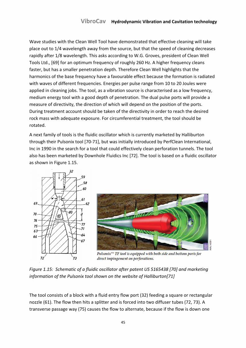
VibroCav Hydrodynamic Vibration and Cavitation technology
45
Wave studies with the Clean Well Tool have demonstrated that effective cleaning will take
place out to 1/4 wavelength away from the source, but that the speed of cleaning decreases
rapidly after 1/8 wavelength. This asks according to W.G. Groves, president of Clean Well
Tools Ltd., [69] for an optimum frequency of roughly 260 Hz. A higher frequency cleans
faster, but has a smaller penetration depth. Therefore Clean Well highlights that the
harmonics of the base frequency have a favourable effect because the formation is radiated
with waves of different frequencies. Energies per pulse range from 10 to 20 Joules were
applied in cleaning jobs. The tool, as a vibration source is characterised as a low frequency,
medium energy tool with a good depth of penetration. The dual pulse ports will provide a
measure of directivity, the direction of which will depend on the position of the ports.
During treatment account should be taken of the directivity in order to reach the desired
rock mass with adequate exposure. For circumferential treatment, the tool should be
rotated.
A next family of tools is the fluidic oscillator which is currently marketed by Halliburton
through their Pulsonix tool [70‐71], but was initially introduced by PerfClean International,
Inc in 1990 in the search for a tool that could effectively clean perforation tunnels. The tool
also has been marketed by Downhole Fluidics Inc [72]. The tool is based on a fluidic oscillator
as shown in Figure 1.15.
Figure 1.15: Schematic of a fluidic oscillator after patent US 5165438 [70] and marketing
information of the Pulsonix tool shown on the website of Halliburton[71]
The tool consists of a block with a fluid entry flow port (32) feeding a square or rectangular
nozzle (61). The flow then hits a splitter and is forced into two diffuser tubes (72, 73). A
transverse passage way (75) causes the flow to alternate, because if the flow is down one
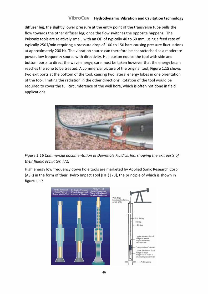
VibroCav Hydrodynamic Vibration and Cavitation technology
46
diffuser leg, the slightly lower pressure at the entry point of the transverse tube pulls the
flow towards the other diffuser leg; once the flow switches the opposite happens. The
Pulsonix tools are relatively small, with an OD of typically 40 to 60 mm, using a feed rate of
typically 250 l/min requiring a pressure drop of 100 to 150 bars causing pressure fluctuations
at approximately 200 Hz. The vibration source can therefore be characterised as a moderate
power, low frequency source with directivity. Halliburton equips the tool with side and
bottom ports to direct the wave energy; care must be taken however that the energy beam
reaches the zone to be treated. A commercial picture of the original tool, Figure 1.15 shows
two exit ports at the bottom of the tool, causing two lateral energy lobes in one orientation
of the tool, limiting the radiation in the other directions. Rotation of the tool would be
required to cover the full circumference of the well bore, which is often not done in field
applications.
Figure 1.16 Commercial documentation of Downhole Fluidics, Inc. showing the exit ports of
their fluidic oscillator, [72]
High energy low frequency down hole tools are marketed by Applied Sonic Research Corp
(ASR) in the form of their Hydro Impact Tool (HIT) [73], the principle of which is shown in
figure 1.17.
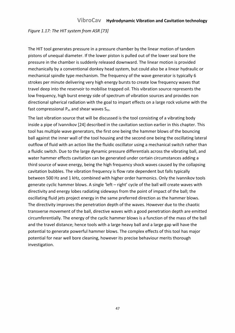
VibroCav Hydrodynamic Vibration and Cavitation technology
47
Figure 1.17: The HIT system from ASR [73]
The HIT tool generates pressure in a pressure chamber by the linear motion of tandem
pistons of unequal diameter. If the lower piston is pulled out of the lower seal bore the
pressure in the chamber is suddenly released downward. The linear motion is provided
mechanically by a conventional donkey head system, but could also be a linear hydraulic or
mechanical spindle type mechanism. The frequency of the wave generator is typically 6
strokes per minute delivering very high energy bursts to create low frequency waves that
travel deep into the reservoir to mobilise trapped oil. This vibration source represents the
low frequency, high burst energy side of spectrum of vibration sources and provides non
directional spherical radiation with the goal to impart effects on a large rock volume with the
fast compressional Pm and shear waves Sm.
The last vibration source that will be discussed is the tool consisting of a vibrating body
inside a pipe of Ivannikov [24] described in the cavitation section earlier in this chapter. This
tool has multiple wave generators, the first one being the hammer blows of the bouncing
ball against the inner wall of the tool housing and the second one being the oscillating lateral
outflow of fluid with an action like the fluidic oscillator using a mechanical switch rather than
a fluidic switch. Due to the large dynamic pressure differentials across the vibrating ball, and
water hammer effects cavitation can be generated under certain circumstances adding a
third source of wave energy, being the high frequency shock waves caused by the collapsing
cavitation bubbles. The vibration frequency is flow rate dependent but falls typically
between 500 Hz and 1 kHz, combined with higher order harmonics. Only the Ivannikov tools
generate cyclic hammer blows. A single ‘left – right’ cycle of the ball will create waves with
directivity and energy lobes radiating sideways from the point of impact of the ball; the
oscillating fluid jets project energy in the same preferred direction as the hammer blows.
The directivity improves the penetration depth of the waves. However due to the chaotic
transverse movement of the ball, directive waves with a good penetration depth are emitted
circumferentially. The energy of the cyclic hammer blows is a function of the mass of the ball
and the travel distance; hence tools with a large heavy ball and a large gap will have the
potential to generate powerful hammer blows. The complex effects of this tool has major
potential for near well bore cleaning, however its precise behaviour merits thorough
investigation.
VibroCav Hydrodynamic Vibration and Cavitation technology
48
1.3. Scope of the thesis
This thesis describes the study into the design, understanding and improvement of a
hydrodynamic tool that produces powerful vibration and cavitation or a combination of the
two, and that is suitable for a large variety of useful applications in a wide range of ambient
pressures from atmospheric to the pressures encountered in wells of several km deep. Tools
selected for the study were based on the patent of Ivannikov [27] where an axially
restrained body, mostly a ball, confined in a housing with a narrow gap can move freely in
random transverse direction in fluid flowing through the housing; referred to as vibrating‐
body‐in‐pipe and VibroCav tools in this study. These tools are relatively simple of
construction, powered by the fluid flow and easily scalable to various applications.
The tool design benefits from the high dynamic pressure created in the narrow gap between
the body and the housing and consequent lowering of the static pressure if fluid is pumped
through the tool. Already at relatively low flow rates the free moving body starts to
oscillate, and at increasing flow rate the self‐induced vibration becomes accompanied by
bouncing of the body against the walls of the housing. Due to this oscillating behaviour the
flow in the pipe is suddenly cut off by the moving body causing a water hammer effect that
enhances the pressure drop across the body and intensifies the bouncing effect.
The static pressure in the core of the vortices created in the wake of the body that are
responsible for this self‐oscillating behaviour of the body may fall below the vapour pressure
of the liquid which gives rise to the generation of cavities. Cavitation also occurs in and
downstream of the gap, where the static pressure falls below the vapour pressure of the
liquid. In addition the bluff geometry of the body causes detachment of the streamlines from
the surface of the body, which contributes to the generation of cavities. The effect of the
water hammer enhanced oscillation is that cavitation is created at much higher static
pressures on the downstream side of the tool than with static orifices or similar flow barriers
and at the same downstream static pressure much stronger cavitation is obtained. At
pressures where cavitation becomes suppressed by high static pressures, very strong
bouncing releases pressure waves with rather low frequencies that propagate deeply into
the surrounding matrix.
Both the cavitational and the vibration behaviour of the tool will be influenced by many
parameters such as the shape and weight of the body of the tool, the flow rate, the fluid
properties, the gap, the roughness of the body and the housing and the surrounding
pressure. So regimes might exist where either of the two modes or a combination of the two
may prevail. Understanding of such regimes is considered the key to optimising the tool for
particular applications. The study also ventures into several tool configurations and sizes and
aspects such as tool wear. The thesis describes field trials for several tool applications in oil,
water and pollution control wells.
VibroCav Hydrodynamic Vibration and Cavitation technology
49
1.4. Outline of the thesis
Chapter 2 focuses on proven and potential applications of cavitation and vibration. First the
mechanisms following from the collapse of cavitational bubbles or the propagation of
acoustic waves created by vibration will be highlighted. In particular hydrodynamic
cavitation and vibration will be addressed. Anticipated advantages and disadvantages of the
VibroCav tools for a particular application will be discussed.
Chapter 3 discusses the experiences with a simple 350 bar exploratory test circuit used in
Assen that have led to the design of a test circuit in Delft for frequent and systematic
laboratory testing of the behaviour of VibroCav tools. The Delft test circuit is then described.
It had a working range up to 10 bar backpressure and operated with a vertical straight tool
and a water column height of about 0.5 m above the vibrating body, mainly a ball, and a
total fluid volume of 0.25 m3. Backpressure was achieved by keeping a closed system that
could be pressurized by an accumulator. Two centrifugal pumps in series provided a
pressure drop of maximally 40 bar over the tool and the high pressure part of the system
had a 50 bar working pressure rating. The test chamber had three viewing windows to
observe the behaviour of the outflow and exit of the tool during operation. The vibrating
body, mostly a ball, made of different materials and at various sizes, in the cylindrical or
conical housing the body was either supported at the bottom by a rod at the end of the
housing or hanging on a string or a rod.
Chapter 4 describes experiments and results with various bodies in a vertical cylindrical
housing in the 50 bar Delft test circuit. The bodies were nearly exclusively balls of different
materials and sizes, supported at the bottom for most of the tests. The nominal gap ratio
δ/Dball was always small and varied for the small housings between 0.028 and 0.110, and for
the large housings between 0.022 and 0.035. For each experiment with a selected ball in a
specific cylindrical housing the flow rate of the liquid along the ball was increased and
subsequently decreased at a constant backpressure. Equally the flow rate was kept constant
and the backpressure was first increased and then decreased. In this way the behaviour of
the ball was studied for different flow and backpressure conditions at a selected gap ratio or
gap. Experiences with tool wear are also discussed in this chapter. A change in the tool
configuration required a significant effort which limited the efficiency of the investigations.
Chapter 5 describes experiments and results with the 50 bar Delft test circuit using tool
housings with conical outflow sections and balls hanging on a rod that could be remotely
adjusted in height with a hydraulic cylinder. This equipment allowed similar tests as
described in Chapter 4, but with remotely adjustable gap ratios and hence permitted
efficient testing of a wide range of parameters. The wealth of data created with these tests
is the input to a thorough analysis of the various regimes encountered when changing flow
rate and backpressure for a wide range of tool characteristics.
Chapter 6 provides results of high speed photography and an analysis of the movement of a
hanging ball in a conically shaped housing during experiments in the Delft test circuit. The
VibroCav Hydrodynamic Vibration and Cavitation technology
50
effect of cavitation on the cyclic motion of the ball is described and discussed. Close‐ups of
the outflow of the VibroCav tool provide visualisation of the cavitation and turbulence
effects created in the fluid and the correlation of these effects with the movement of the
ball.
Chapter 7 describes experiences and results of high backpressure experiments with a 350
bar closed test circuit in Drachten. This circuit was assembled to carry out a limited number
of tests at pressures that are encountered in deep wellbores, without being troubled by the
problems encountered in the open exploratory test circuit used in Assen. In this circuit only
bottom supported balls were tested. Focus of these experiments was to study tool regimes
at very high backpressures, in particular cavitation. The tools were subjected to very high
flow rates and the tests were heavily influenced by tool wear, which is discussed in this
chapter. In particular the process of bedding in of a ball into a bottom support is considered
in detail.
Chapter 8 provides details of 29 industrial trials in oil wells (10), water wells (10) and
pollution control wells (9) for cleaning the porous medium around a wellbore using rotating
and rotated VibroCav tools. This chapter sets out the theoretical background for vibration
based well cleaning, describes in detail the application conditions during the trials and
ventures into semi‐quantified reconciliation of theory with field observation resulting in a
basis for a deeper understanding of the action of vibration based well cleaning tools. This
chapter describes in a novel way the interrelation between tool characteristics, energy,
penetration depth and formation damage characteristics.
Chapter 9 describes 5 industrial trials for the removal of scale in wellbores with a detailed
description of the application conditions. One trial was done to clean a stuck accessory in the
production tubing and four trials were performed to clean scaled perforations in. The
treatment conditions are discussed in detail. The physical effects of the rotating VibroCav
tool for scale removal are discussed, leading to conclusions about the scale cleaning process
and tool requirements.
Chapter 10 is an outlook into the extensive potential of VibroCav technology, reflecting on
the results of the study. This chapter ventures into possible applications in the fields of
useful vibration, mixing and cavitation and forms a basis for further R&D work.
VibroCav Hydrodynamic Vibration and Cavitation technology
51
1.5. References
1. Knapp, R. T.; Daily, J. W.; Hammitt, F. G. ‘Cavitation.’ 1970, McGraw‐Hill Book
Company.
2. Young, F. R. ‘Cavitation.’ 1999, Imperial College Press. First published in 1989,
McGraw‐Hill Book Company (UK).
3. Brennen, Ch. E. ‘Cavitation and Bubble Dynamics’. 1995, Oxford University Press, Inc.,
New York.
4. Lecoffre, Y. ‘Cavitation, Bubble trackers’. 1999 (English translation), Balkema
Publishers, Rotterdam, the Netherlands.
5. Hielscher‐Ultrasound Technology website, www.hielscher.com
6. Prosonic, website
7. Brandner; J Fluid Mech. (2010), vol.656, pp. 147‐176
8. Zdravkovich, M. M. ‘Flow around Circular Cylinders.’ Volume 1, 1997, Oxford
University Press.
9. Williamson, C. H. K. Ann. Rev. Fluid Mech., 1996, 28, 477 ‐ 539.
10. Brennen, C. J. Fluid Mech., 1969, 37(4), 671 – 88.
11. Savchenko, Yu. N. ‘Control of Supercavitation Flow and Stability of Supercavitating
Motion of Bodies. ’ Paper presented at RTO AVT Lecture Series ‘Supercavitating
Flows’, von Karman Institute, Brussels, 12‐16 Febr.2001 Published in RTO EN‐010.
12. Tulin, M. P. p.55 in Davies, R. (Ed.) ‘Cavitation in Real Liquids’ 1964, Elsevier Press.
13. Pearsall, I. S. Proc. Inst. Mech. Engrs. 1973, 187, 649 ‐ 65.
14. Gilbarg, D.; Anderson, R. A. J. Appl. Phys. 1948, 19, 127 ‐ 39.
15. Hargrove, J. ‘Supercavitation and Aerospace Technology in the Development of High‐
Speed Underwater Vehicles.’ Paper AIAA 2004‐130 to 42nd AIAA Aerospace Sciences
Meeting & Exhibit., 5 – 8 Jan. 2004, Reno, Nevada.
16. Batchelor, G. K. ‘An Introduction to Fluid Mechanics.’ 2000, Cambridge University
Press.
17. Song, C. C. S. ‘Fluid Transients.’ Chapter 22 in Saleh, J. (ed.) ‘Fluid Flow Handbook.’
2002, McGraw‐Hill.
18. Tullis, J.P. Chapter 8 in “Hydraulics of Pipelines”. 1989, Wiley
19. Featherstone, R.E.; Chapter 12 in “Civil Engineering Hydraulics”, 4th ed. 2001, Wiley
20. Franzini, J.B.; Finnemore, E.J.; Chapter 12 in “Fluid Mechanics with Engineering
applications”, 9th ed. 1997, McGraw‐Hill
VibroCav Hydrodynamic Vibration and Cavitation technology
52
21. Amin, L. P.; Gogate, P. R.; Burgess, A. E.; Bremner, D. H. Chem. Engg. J. 2010, 156(1),
165 – 9.
22. Gogate, P.R.; Hydrodynamic Cavitation for Food and Water Processing; Food
Bioprocess Technol (2011) 4:996–1011; DOI 10.1007/s11947‐010‐0418‐1
23. Milly, P. J., Toledo, R. T., Kerr, W. L., & Armstead, D. (2008). Hydrodynamic cavitation:
Characterization of a novel design with energy considerations for the inactivation of
Saccharomyces cerevisiae in apple juice. Journal of Food Science, 73(6), M298–M303.
24. Chand R., Bremner D.H, Namkung K.C, Collier P.J, Gogate PR; Water disinfection using
the novel approach of ozone and a liquid whistle reactor; Biochemical Engineering
Journal 35 (2007) 357–364.
25. Chervyakov, V.M. ; Vorob’ev, Yu. V.; Theoretical Foundations of Chemical
Engineering, vol 39, no. 1., pp. 62 – 69.
26. Promtov M.A., Zimin A.I.; Experimental investigation of the emulsification process in
a pulsed‐rotor apparatus; Translated from Khimiko‐Farmatsevticheskii Zhurnal, Vol.
34, No. 10, pp. 38 – 39, October, 2000.
27. Ivannikov, V.I. ; Ivannikov, I.V. ; Patent US 6705396 (2004)
28. Kumar, P.S.; Pandit, A.B.; Chem. Eng. Thechnol. 22, (1999), 12, 1017‐1027
29. Kanthale, P.M.; Gogate, P.R.; Pandit A.B.; Wilhelm, A; Ultrasonic Sonochem. 12
(2005) 441‐452
30. Bremond, N.; Arora, M.; Dammer, S. M.; Lohse, D. Phys. Fluids 2006, 18(12), 121505.
31. Bremond, N.; Arora, M.; Ohl. C‐D.; Lohse, Phys. Rev. Lett. 2006, 96, 224501.
32. Arrojo, S.; Benito, Y.; Ultrasonic Sonochem. 15 (2008) 203‐211
33. Virone, C; Kramer, H.J.M.; van Rosmalen, G.M.; Stoop, A.H.; Bakker, T.W. J. Cryst.
Growth 2006, 294, 9‐15.
34. Gaitan, D. F.; Crum, L. A.; Church, C. C.; Roy, R. A. J. Acoust. Soc. Am. 1992, 91(6),
3166 – 83.
35. Brenner, M. P.; Hilgenfeldt, S.; Lohse, D. Rev. Mod. Phys. 2002, 74(2), 435 – 84.
36. Pecha, R. ; Gompf, B. Phys. Rev. Lett. 2000, 84(6), 1328 – 30 ; Gompf, B.; Pecha, R.
Phys. Rev. E 2000, 61(5), 5253 – 6.
37. R.D. Blevins, Flow‐Induced Vibration, 2nd ed., 1994, Krieger Publ. Co, New York, Eds:
Shigehiko Kaneko et al, Flow‐Induced Vibrations, 2008, UK.
38. P. Anagnostopoulos; ‘Flow‐Induced Vibrations in Engineering Practice’, (Witt press,
2002).
39. Williamson, C.H.K.; Govardhan, R. Annu. Rev. Fluid Mech. 36(2004)413 – 55.
VibroCav Hydrodynamic Vibration and Cavitation technology
53
40. Sarpkaya, T. J. Fluids Struct. 19(2004)389 – 447
41. Carberry, J; Sheridan, J; Rockwell, D, J. Fluids Struct. 15(2001)523 – 32.
42. Feng, C.C. 1968, Master Thesis Univ. BC, Vancouver, Can.
43. R.H.M. Ogink, A.V. Metrikine, J. Sound and Vibration 329(2010)5452 – 73.
44. Ed: Shigehiko Kaneko, Tomomichi Nakamura, Fumio Inada, Minoru Kato, ‘Flow –
Induced Vibrations‘, Classifications and Lessons from Practical Experiences, 2008,
Elsevier, Amsterdam.
45. Achenbach, E. J.Fluid Mech. 62(1974)209 – 21)
46. Tsahalis, D.T. J.Energ.Resour.ASME, 106 (1984) 206‐213.
47. King, R.; Jones R., ‘Practical Experiences with Flow‐Induced vibrations,’ E. Naudacsher
& R. Rockwell (eds), Springer‐Verlag, Berlin, 1980.
48. Sahin, M; Owens,R.G. Phys. Fluids 16(5) (2004)1305 – 20.
49. Zeng, L; Balachandar, S; Fischer, P. J.Fluid Mech. 536 (2005)1 – 25.
50. Takemura, F; Magnaudet, J. J. Fluid Mech. 495 (2003) 235 – 253.
51. Yang, B; Gao, F; Jeng, D‐S; Wu, Y. Acta Mech. Sin. 25 (2009) 51 – 63.
52. Magnaudet, J; Takagi, S; Legendre, D. 476 (2003) 115 – 157.
53. Kharlamov, A.A. Moskow Univ. Mech. Bulletin. 65 (2010) 67 – 69.
54. Karlikov, V.P.; Reznichenko, N.T.; Sholomovich, G.I.; Fluid Dynamics 35 (2000) 268 –
273.
55. Karlikov, V.P.; Reznichenko, N.T.; Sholomovich, G.I.; Fluid Dynamics 36 (2001) 623 –
639.
56. Karlikov, V.P.; Khomyakov, A.N.; Sholomovich, G.I.; Fluid Dynamics 40 (2005) 785 –
789.
57. Biot, M. J. Acoustical Soc. Am. 28 (1956) 168 – 191.
58. Berryman, J.G. ; Appl. Phys. Lett. 37 (1980)
59. Jeong, C.; Kallivokas, L.F.; Huh, C.; Lake, L.W.; SPE 147150 (2011)
60. Kostrov, S.; Wooden, W.; Oil & Gas Jounal, April. 18 (2005)
61. Smeulders, D. private correspondence
62. Poesio, P. and Ooms, G. SPE 100812 (2008)
63. Bas, F. van der; Rouffignac, E. de; Zuiderwijk, P; Wong, S‐W; Batenburg, D. van;
Birchak, B.; Yoo, K; SPE 86492 (2004)

VibroCav Hydrodynamic Vibration and Cavitation technology
54
64. Pierce, A.D.; Acoustics – An introduction to its Physical Principles and Applications;
ISBN: 0‐88318‐612‐8 (1989)
65. Zaslavskii, Yu.M.; Acoustical Physics, Vol. 51, No. 6, pp. 653 – 663 (2005)
66. Beresnev, I.A.; Johnson, P.A.; Geophysics, Vol. 59, No. 6, pp 1000 – 1017 (1994)
67. Patent US 6029746
68. Chahine, G.L.; Kalamuck, K.M.; Frederic, G.S.; 8th Am Water Jet Conference, paper 57
(1995)
69. Clean Well Tools website: www.cleanwelltools.com
70. Patent US 5165438
71. Halliburton website: www.halliburton.com
72. Downhole Fluidics, inc. website: www.dhfluidics.com
73. ASR website: www.appliedseismicresearch.com

VibroCav Hydrodynamic Vibration and Cavitation technology
55
VibroCav Hydrodynamic Vibration and Cavitation technology
56
Chapter 2: Applications of cavitation and vibration
2.1. Effects of cavitation
Cavitation covers the phenomena of formation, growth and subsequent collapse of a swarm
of bubbles. The collapse of a bubble occurs in milliseconds and releases a large amount of
energy which results in local high temperature spots in the range of 1000 to 10000 K and
local high pressures in the range of 100 to 5000 bar. Bubble collapse also creates free
radicals and induces shock waves, and high local turbulence.
Only acoustic and hydrodynamic cavitation are considered to be effective enough to be used
in processing applications in chemical, electrochemical, food and bio‐processing industries,
for environmental waste water treatment as well as for cleaning and for fracture stimulation
applications. Recent overviews can be found in ref. [1‐5].
In acoustic cavitation ultrasound comes from a mostly piezoelectric transducer that transfers
the vibration after amplification to the sonotrode which is in contact with the surrounding
medium. This medium is a liquid or a spray of liquid containing at least 5 to 10% liquid
pockets as in dental cleaning devices.
The low frequency power ultrasound sources of 16 kHz to 100 kHz that are used in most
industrial applications generate large cavitation bubbles needed for high temperatures and
pressures in the cavitation zone. A higher surrounding pressure, referred to as backpressure,
causes a higher cavitation threshold, and thus the number of cavitation bubbles reduces.
The internal pressure of the bubble upon collapse will however, increase, which leads to a
more violent bubble collapse [6].
Acoustic cavitation provokes several striking effects. One of these effects is acoustic
streaming. At lower intensities the ultrasound pressure wave causes compression and
rarefaction of the liquid, and therefore induces motion and mixing in the fluid [7]. The
current of motion increases with the square root of ultrasonic power, and moves away from
the ultrasound source. At higher intensities of the ultrasound wave cavitation bubbles are
formed at the location of the lowest pressures during rarefaction of the fluid which can
violently collapse upon compression due to the wave action. Upon collapse strong shear
waves and turbulence are created.
A standing wave of ultrasound can be formed when the emitted wave reflects against a solid
surface or an air/water interface and the acoustic pressure at the nodes is zero. Bubbles
present in the liquid that are smaller than the resonance size accumulate at the anti‐node,
whereas bubbles with sizes beyond the resonance size accumulate at the node and coalesce.
This mechanism that is responsible for microstreaming in the fluid is used for ultrasonic
degassing.
VibroCav Hydrodynamic Vibration and Cavitation technology
57
When a bubble collapses near to or in direct contact with a solid wall or an interface the
spherical symmetry of the collapse is disturbed, and a liquid microjet is formed. This also
happens when a bubble collapses in a cloud of other bubbles. Such a microjet is a very
strong current pulse with duration of about 0.5 to 1 µs and a volume of about 10‐4 µl.
Microjets play an important role in mixing, cleaning and disinfection, and are the main
reason for an increase in mass transfer by efficiently reducing the diffusion layer.
Upon a violent bubble collapse a high pressure pulse, called a shock wave, can be emanated.
The impact of shock waves on a material surface is one of the causes of its erosion, and plays
together with the microjets a role in cleaning or surface reactivation. It may also play a role
in the promotion of primary nucleation of compounds from solution.
The high temperature and pressure at the centre of the collapsing bubble can create all
kinds of radicals from the water, oxygen and nitrogen vapour molecules that can accelerate
chemical conversions.
Hydrodynamic cavitation generated by a constriction in a flow is referred to in this study as
passive cavitation. The constriction can be a venturi or a choke, an orifice plate or a free ball
moving laterally in a pipe. If the static pressure in the constriction falls below the vapour
pressure of the liquid, bubbles can be formed [8]. If the free movement of a ball in a pipe
contributes, owing to the water hammer effect, to the pressure drop in the constriction
cavitation already occurs at a lower flow rate; this kind of cavitation is referred to in this
study as active cavitation. After the constriction or gap the pressure increases and the
cavitation bubbles collapse. High intensity fluid turbulence is also created behind the gap.
The intensity of turbulence has a major effect on the intensity of cavitation, since the bubble
behaviour under turbulent conditions is more often transient instead of stable or oscillatory
in cases without turbulence. During active cavitation with a laterally vibrating ball, bouncing
of the ball against the pipe wall results in vibration of the system. In the resonance mode
where the natural frequency of the ball coincides with that of the pipe, the vibrations are
sharply amplified. So in this particular case the cavitational effects are accompanied by
pressure waves emitted by the vibrating pipe.
The major difference between acoustic and hydrodynamic cavitation is that for
hydrodynamic cavitation the medium has to flow through a gap, while for acoustic cavitation
the medium can be stagnant. During flow through a gap shear stresses are imposed upon
the fluid or suspension. Of the effects provoked by cavitation, acoustic streaming and micro‐
streaming will not occur in case of hydrodynamic cavitation, but the creation of turbulence,
microjets and shock waves will be similar, just as the creation of radicals in the core of the
imploding cavitational bubbles. Also in their applications differences exist. If cavitational
effects are required in small liquid pockets in a solid matrix as inside cells of vegetables,
acoustic cavitation is the only option. The energy requirement for generating hydrodynamic
cavitation is generally lower than for acoustic cavitation, and can for some applications as
for example for protein release by cell disruption, even be more than two orders of
magnitude lower [ 1, 9, 10]. For large scale applications hydrodynamic cavitation is also more
VibroCav Hydrodynamic Vibration and Cavitation technology
58
suitable, because it can be scaled up relatively easy and the equipment is very robust and
energy saving. Erosion of the cavitation tool below the constriction has long been brought
forward as prohibitive for the use of hydrodynamic cavitation. Erosion can however, be
largely avoided by the use of tools where the cavitation bubbles leave the tool immediately
after their formation, and by using novel hard materials that are extremely wear resistant.
Below some important applications of cavitation will be discussed. These applications are
arranged according to the common use of specific effects of cavitation.
2.2. Applications of cavitation
2.2.1. Mixing
Intensive mixing by collapsing cavitation bubbles is explained by the existence of strong
micro‐vortices formed by cumulative microjets. Cavitation can be used for rapid mixing of
miscible fluids at a molecular scale, while for immiscible fluids very fine, highly stable micro
emulsions can be formed with droplet sizes down to 10‐100 nm with a lower energy input
than for mechanical mixing, and a lower content of emulsifier and stabilizer. Many
theoretical and lately also experimental studies [11‐18] have been devoted to ultrasonic
emulsification of oil in water and water in oil mixtures. The characteristics of three phase
O/W/O emulsions prepared by ultrasound have also been studied [19,20]. Because these
emulsification processes often need a mechanical pre‐emulsification stage, hydrodynamic
cavitation with high shear stresses in the flow is particularly well‐suited for the mixing of
large volumes in continuous operation.
If a liquid is mixed with solid particles finely dispersed suspensions can be achieved by the
use of cavitation. Cavitation bubbles collapsing violently at the solid/liquid interface can
even contribute to the breakage or erosion of the solid particles. Also mixing of gasses into
the liquid as fine stable gas‐bubbles can be reached by use of cavitation.
All these fast mixing processes with minute droplets, particles or gas‐bubbles can be applied
for rapid conversions in physical and chemical processes. An example of a physical process is
the water in diesel fuel application, where a near molecular emulsion of 5 to 10% of water in
oil is used to improve the combustion characteristics of fuels and to reduce the poisonous
components in exhaust gases. Another superior mixing effect is obtained by cavitational
mixing of additives in fuels to improve their reactivity. Mixing of water as minute droplets in
edible fats is another application. Cavitation is also used to obtain fine emulsions of drilling
fluids that remain stable with lower oil/water ratios and a better yield of viscosifiers.
The superior mixing of immiscible fluids or fluids and solids that can be achieved by
cavitation can also be successfully applied to speed up chemical reactions. These
applications are reported under chemical conversions.
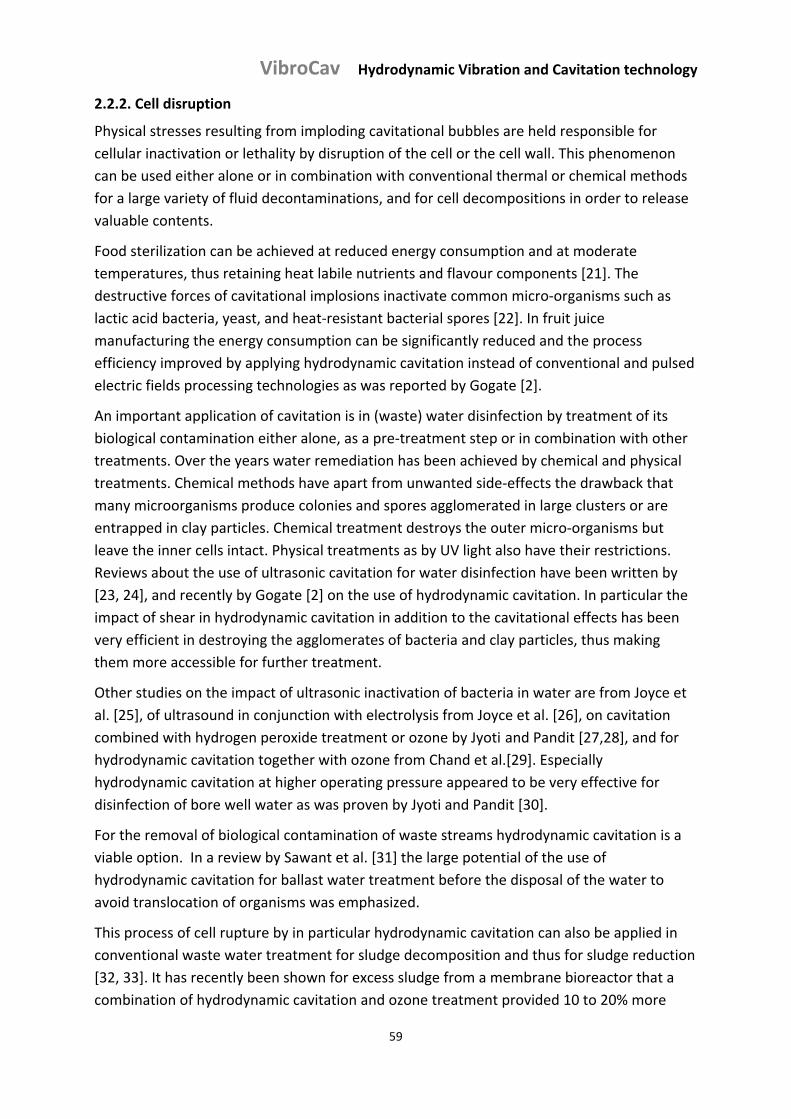
VibroCav Hydrodynamic Vibration and Cavitation technology
59
2.2.2. Cell disruption
Physical stresses resulting from imploding cavitational bubbles are held responsible for
cellular inactivation or lethality by disruption of the cell or the cell wall. This phenomenon
can be used either alone or in combination with conventional thermal or chemical methods
for a large variety of fluid decontaminations, and for cell decompositions in order to release
valuable contents.
Food sterilization can be achieved at reduced energy consumption and at moderate
temperatures, thus retaining heat labile nutrients and flavour components [21]. The
destructive forces of cavitational implosions inactivate common micro‐organisms such as
lactic acid bacteria, yeast, and heat‐resistant bacterial spores [22]. In fruit juice
manufacturing the energy consumption can be significantly reduced and the process
efficiency improved by applying hydrodynamic cavitation instead of conventional and pulsed
electric fields processing technologies as was reported by Gogate [2].
An important application of cavitation is in (waste) water disinfection by treatment of its
biological contamination either alone, as a pre‐treatment step or in combination with other
treatments. Over the years water remediation has been achieved by chemical and physical
treatments. Chemical methods have apart from unwanted side‐effects the drawback that
many microorganisms produce colonies and spores agglomerated in large clusters or are
entrapped in clay particles. Chemical treatment destroys the outer micro‐organisms but
leave the inner cells intact. Physical treatments as by UV light also have their restrictions.
Reviews about the use of ultrasonic cavitation for water disinfection have been written by
[23, 24], and recently by Gogate [2] on the use of hydrodynamic cavitation. In particular the
impact of shear in hydrodynamic cavitation in addition to the cavitational effects has been
very efficient in destroying the agglomerates of bacteria and clay particles, thus making
them more accessible for further treatment.
Other studies on the impact of ultrasonic inactivation of bacteria in water are from Joyce et
al. [25], of ultrasound in conjunction with electrolysis from Joyce et al. [26], on cavitation
combined with hydrogen peroxide treatment or ozone by Jyoti and Pandit [27,28], and for hydrodynamic cavitation together with ozone from Chand et al.[29]. Especially
hydrodynamic cavitation at higher operating pressure appeared to be very effective for
disinfection of bore well water as was proven by Jyoti and Pandit [30].
For the removal of biological contamination of waste streams hydrodynamic cavitation is a
viable option. In a review by Sawant et al. [31] the large potential of the use of
hydrodynamic cavitation for ballast water treatment before the disposal of the water to
avoid translocation of organisms was emphasized.
This process of cell rupture by in particular hydrodynamic cavitation can also be applied in
conventional waste water treatment for sludge decomposition and thus for sludge reduction
[32, 33]. It has recently been shown for excess sludge from a membrane bioreactor that a
combination of hydrodynamic cavitation and ozone treatment provided 10 to 20% more
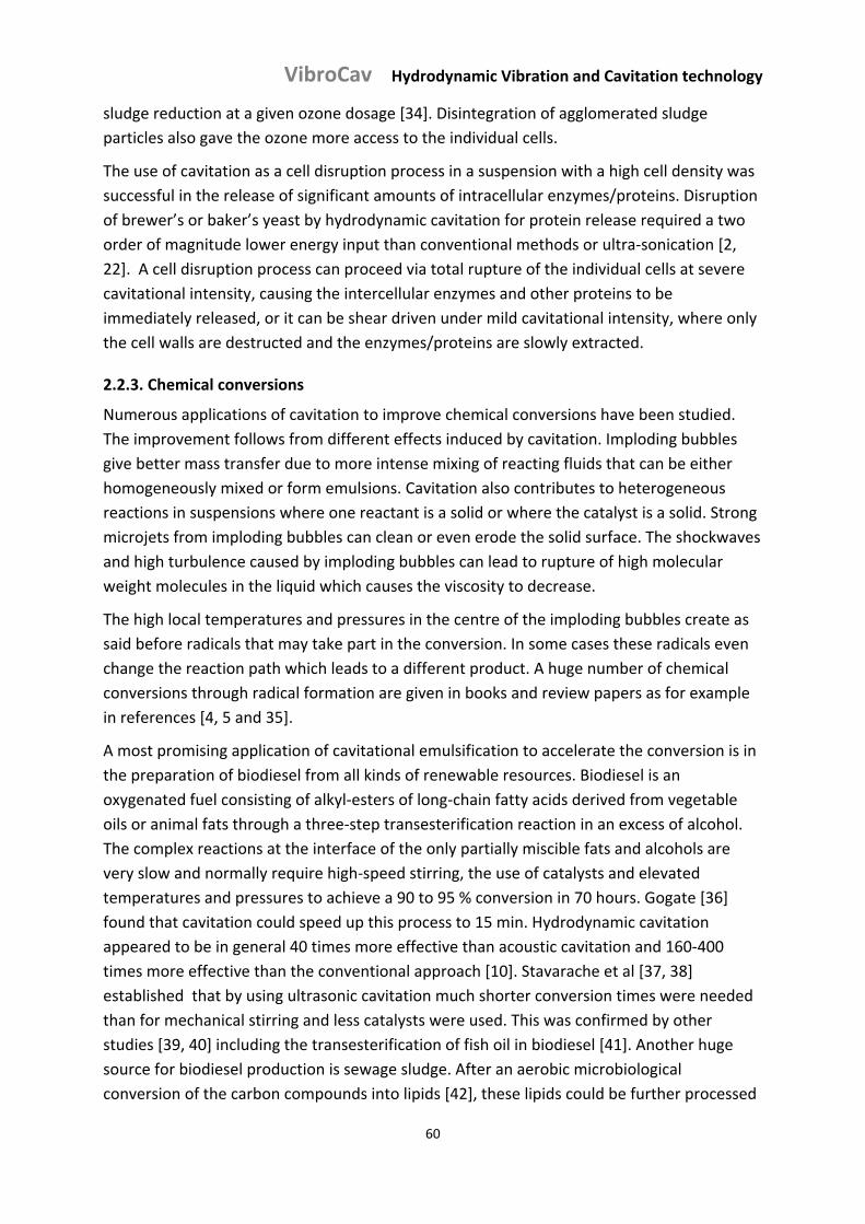
VibroCav Hydrodynamic Vibration and Cavitation technology
60
sludge reduction at a given ozone dosage [34]. Disintegration of agglomerated sludge
particles also gave the ozone more access to the individual cells.
The use of cavitation as a cell disruption process in a suspension with a high cell density was
successful in the release of significant amounts of intracellular enzymes/proteins. Disruption
of brewer’s or baker’s yeast by hydrodynamic cavitation for protein release required a two
order of magnitude lower energy input than conventional methods or ultra‐sonication [2,
22]. A cell disruption process can proceed via total rupture of the individual cells at severe
cavitational intensity, causing the intercellular enzymes and other proteins to be
immediately released, or it can be shear driven under mild cavitational intensity, where only
the cell walls are destructed and the enzymes/proteins are slowly extracted.
2.2.3. Chemical conversions
Numerous applications of cavitation to improve chemical conversions have been studied.
The improvement follows from different effects induced by cavitation. Imploding bubbles
give better mass transfer due to more intense mixing of reacting fluids that can be either
homogeneously mixed or form emulsions. Cavitation also contributes to heterogeneous
reactions in suspensions where one reactant is a solid or where the catalyst is a solid. Strong
microjets from imploding bubbles can clean or even erode the solid surface. The shockwaves
and high turbulence caused by imploding bubbles can lead to rupture of high molecular
weight molecules in the liquid which causes the viscosity to decrease.
The high local temperatures and pressures in the centre of the imploding bubbles create as
said before radicals that may take part in the conversion. In some cases these radicals even
change the reaction path which leads to a different product. A huge number of chemical
conversions through radical formation are given in books and review papers as for example
in references [4, 5 and 35].
A most promising application of cavitational emulsification to accelerate the conversion is in
the preparation of biodiesel from all kinds of renewable resources. Biodiesel is an
oxygenated fuel consisting of alkyl‐esters of long‐chain fatty acids derived from vegetable
oils or animal fats through a three‐step transesterification reaction in an excess of alcohol.
The complex reactions at the interface of the only partially miscible fats and alcohols are
very slow and normally require high‐speed stirring, the use of catalysts and elevated
temperatures and pressures to achieve a 90 to 95 % conversion in 70 hours. Gogate [36]
found that cavitation could speed up this process to 15 min. Hydrodynamic cavitation
appeared to be in general 40 times more effective than acoustic cavitation and 160‐400
times more effective than the conventional approach [10]. Stavarache et al [37, 38]
established that by using ultrasonic cavitation much shorter conversion times were needed
than for mechanical stirring and less catalysts were used. This was confirmed by other
studies [39, 40] including the transesterification of fish oil in biodiesel [41]. Another huge
source for biodiesel production is sewage sludge. After an aerobic microbiological
conversion of the carbon compounds into lipids [42], these lipids could be further processed
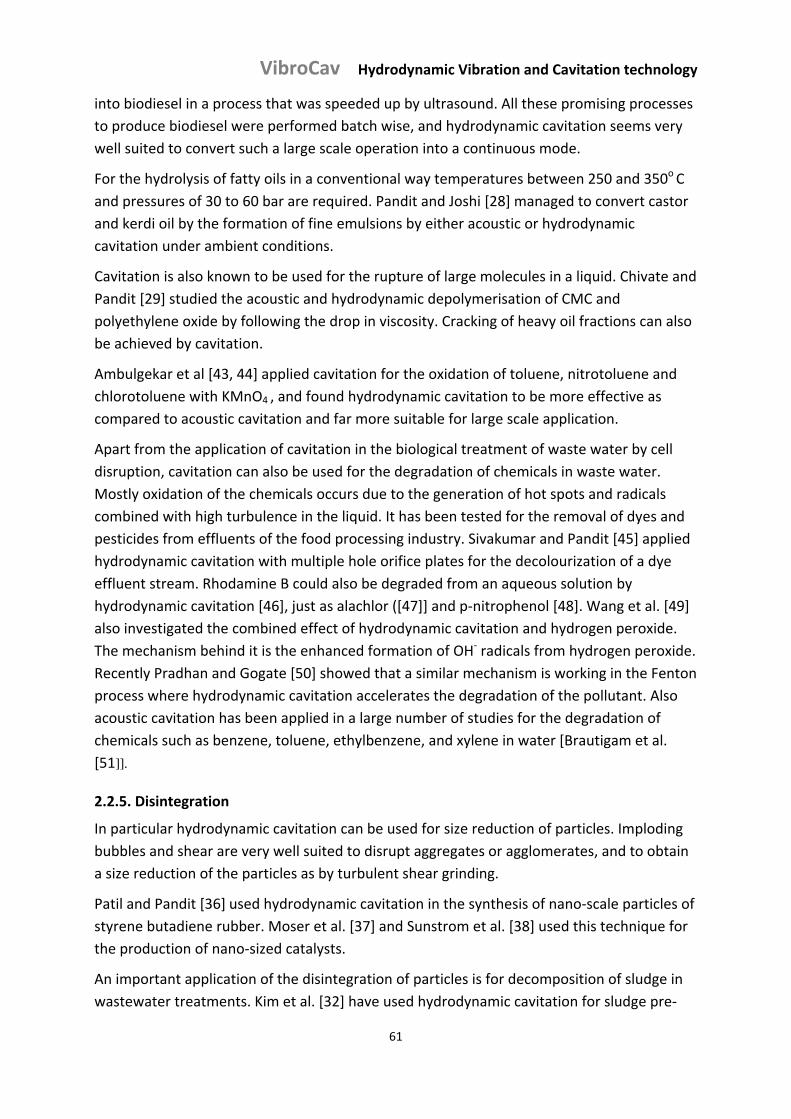
VibroCav Hydrodynamic Vibration and Cavitation technology
61
into biodiesel in a process that was speeded up by ultrasound. All these promising processes
to produce biodiesel were performed batch wise, and hydrodynamic cavitation seems very
well suited to convert such a large scale operation into a continuous mode.
For the hydrolysis of fatty oils in a conventional way temperatures between 250 and 350o C
and pressures of 30 to 60 bar are required. Pandit and Joshi [28] managed to convert castor
and kerdi oil by the formation of fine emulsions by either acoustic or hydrodynamic
cavitation under ambient conditions.
Cavitation is also known to be used for the rupture of large molecules in a liquid. Chivate and
Pandit [29] studied the acoustic and hydrodynamic depolymerisation of CMC and
polyethylene oxide by following the drop in viscosity. Cracking of heavy oil fractions can also
be achieved by cavitation.
Ambulgekar et al [43, 44] applied cavitation for the oxidation of toluene, nitrotoluene and
chlorotoluene with KMnO4 , and found hydrodynamic cavitation to be more effective as
compared to acoustic cavitation and far more suitable for large scale application.
Apart from the application of cavitation in the biological treatment of waste water by cell
disruption, cavitation can also be used for the degradation of chemicals in waste water.
Mostly oxidation of the chemicals occurs due to the generation of hot spots and radicals
combined with high turbulence in the liquid. It has been tested for the removal of dyes and
pesticides from effluents of the food processing industry. Sivakumar and Pandit [45] applied
hydrodynamic cavitation with multiple hole orifice plates for the decolourization of a dye
effluent stream. Rhodamine B could also be degraded from an aqueous solution by
hydrodynamic cavitation [46], just as alachlor ([47]] and p‐nitrophenol [48]. Wang et al. [49]
also investigated the combined effect of hydrodynamic cavitation and hydrogen peroxide.
The mechanism behind it is the enhanced formation of OH‐ radicals from hydrogen peroxide.
Recently Pradhan and Gogate [50] showed that a similar mechanism is working in the Fenton
process where hydrodynamic cavitation accelerates the degradation of the pollutant. Also
acoustic cavitation has been applied in a large number of studies for the degradation of
chemicals such as benzene, toluene, ethylbenzene, and xylene in water [Brautigam et al.
[51]].
2.2.5. Disintegration
In particular hydrodynamic cavitation can be used for size reduction of particles. Imploding
bubbles and shear are very well suited to disrupt aggregates or agglomerates, and to obtain
a size reduction of the particles as by turbulent shear grinding.
Patil and Pandit [36] used hydrodynamic cavitation in the synthesis of nano‐scale particles of
styrene butadiene rubber. Moser et al. [37] and Sunstrom et al. [38] used this technique for
the production of nano‐sized catalysts.
An important application of the disintegration of particles is for decomposition of sludge in
wastewater treatments. Kim et al. [32] have used hydrodynamic cavitation for sludge pre‐
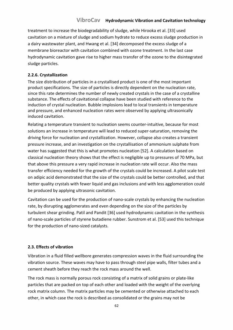
VibroCav Hydrodynamic Vibration and Cavitation technology
62
treatment to increase the biodegradability of sludge, while Hirooka et al. [33] used
cavitation on a mixture of sludge and sodium hydrate to reduce excess sludge production in
a dairy wastewater plant, and Hwang et al. [34] decomposed the excess sludge of a
membrane bioreactor with cavitation combined with ozone treatment. In the last case
hydrodynamic cavitation gave rise to higher mass transfer of the ozone to the disintegrated
sludge particles.
2.2.6. Crystallization
The size distribution of particles in a crystallised product is one of the most important product specifications. The size of particles is directly dependent on the nucleation rate, since this rate determines the number of newly created crystals in the case of a crystalline substance. The effects of cavitational collapse have been studied with reference to the induction of crystal nucleation. Bubble implosions lead to local transients in temperature and pressure, and enhanced nucleation rates were observed by applying ultrasonically induced cavitation.
Relating a temperature transient to nucleation seems counter‐intuitive, because for most
solutions an increase in temperature will lead to reduced super‐saturation, removing the
driving force for nucleation and crystallization. However, collapse also creates a transient
pressure increase, and an investigation on the crystallisation of ammonium sulphate from
water has suggested that this is what promotes nucleation [52]. A calculation based on
classical nucleation theory shows that the effect is negligible up to pressures of 70 MPa, but
that above this pressure a very rapid increase in nucleation rate will occur. Also the mass
transfer efficiency needed for the growth of the crystals could be increased. A pilot scale test
on adipic acid demonstrated that the size of the crystals could be better controlled, and that
better quality crystals with fewer liquid and gas inclusions and with less agglomeration could
be produced by applying ultrasonic cavitation.
Cavitation can be used for the production of nano‐scale crystals by enhancing the nucleation
rate, by disrupting agglomerates and even depending on the size of the particles by
turbulent shear grinding. Patil and Pandit [36] used hydrodynamic cavitation in the synthesis
of nano‐scale particles of styrene butadiene rubber. Sunstrom et al. [53] used this technique
for the production of nano‐sized catalysts.
2.3. Effects of vibration
Vibration in a fluid filled wellbore generates compression waves in the fluid surrounding the
vibration source. These waves may have to pass through steel pipe walls, filter tubes and a
cement sheath before they reach the rock mass around the well.
The rock mass is normally porous rock consisting of a matrix of solid grains or plate‐like
particles that are packed on top of each other and loaded with the weight of the overlying
rock matrix column. The matrix particles may be cemented or otherwise attached to each
other, in which case the rock is described as consolidated or the grains may not be
VibroCav Hydrodynamic Vibration and Cavitation technology
63
interconnected but held in place by grain to grain contact points loaded with the weight of
the overlying rock matrix in which case the rock is unconsolidated.
The pores between the matrix particles are filled with fluids and the combination of matrix,
pores and pore content is described as a porous medium. If a compression wave meets an
interface with a porous medium, the wave energy is divided over 3 wave types, a fast
compression wave Pm and a fast Shear wave Sm in the solid matrix and a slow compression
wave that propagates through the fluid in the pores. The behaviour and effects of these
waves has been qualitatively discussed in Chapter 1 giving rise to a number of useful
applications.
Deliberate mechanical vibrations and hammering can be used in well construction for
applications like friction reduction, improving the cutting process of drilling bits, for the
generation of sound signals for well bore measurements and densification of gravel packs.
2.4. Applications of vibration
2.4.1. Cleaning a porous medium around a wellbore
Already by drilling into the porous rock solids and chemicals ‐long chain polymers in
particular‐ may have caused damage in the near wellbore area. During production the
porous medium in the direct vicinity of the wellbore, typically in the rock cylinder around the
wellbore with a radius of the order of 1 m is particularly sensitive to fouling. This is because
particles liberated in the far field due to flow and pressure effects and carried to the
wellbore by the production flow through the pores converge to the wellbore, while the
velocity in the pores increases leading to conditions where narrower throats between pores
may become bridged. Likewise in the case of injection, particles in the injection stream may
plug the pore throats in the direct vicinity of the wellbore. The near wellbore area can also
become plugged with deposition of asphaltenes, due to release and loss of volatile
components of the crude oil in the pressure drop that is required to create flow towards the
wellbore. Other fouling mechanisms are discussed in Chapter 8.
A well is connected with the porous medium such that production or injection can take place
in a durable way, taking account of the prevailing conditions. The simplest connection is the
open hole as it is drilled without any protection; a low cost method that is used if the porous
formation is fully consolidated. The most common method is to protect the hole with a steel
casing with cement between the casing and porous formation and perforating 20 to 50 holes
per metre of typically 10 mm diameter explosively reaching several decimetres into the
porous medium and thereby bridging the near wellbore area that may have been damaged
by the drilling process. Other methods involve placing filter tubes allowing formation sand to
‘self‐pack’ around the filter and placing ‐in a gravel packing procedure‐ a controlled sand bed
between the filter tube and the porous formation. The actual conditions in the well should
be taken into account when judging the possible effects of a vibration based well cleaning
tool.
VibroCav Hydrodynamic Vibration and Cavitation technology
64
Waves entering the fouled rock mass around the well or perforation tunnels are under
certain conditions capable of mobilising particles in pores and destabilising particle bridges,
as described in Chapter 1. In the cleaning process particle mobilisation and bridge
destabilisation is just the first step in cleaning the near wellbore. The next step is
transporting the fouling particles from the well or placing the particles further into the
formation, allowing them to settle at a place where they will not be re‐mobilised by regular
production or injection activities.
Bakker et al, in 2002 [54] describe successful treatments with the tool that is the subject of
this study. Tambini in 2003 [55] reports of active cavitation and ultrasonic treatment as
emerging technologies, mentioning ultrasonic treatment in the 20kHz to 40 kHz region as a
treatment technology that reaches maximum twice the radius of the wellbore. Some of the
characteristics of this high frequency cleaning process were studied in the laboratory by
Poesio [56] for acoustic tools beaming focused wave energy into core samples. He
established that short bursts of acoustic energy are more efficient for cleaning than long
bursts or continuous beaming. His laboratory observation indicates that at the applied
frequencies cavitation can have a negative effect on the cleaning process. With the
translation of these laboratory results to viable field conditions account should be taken of
the strong directivity of the vibration source in the laboratory experiments which normally is
not achievable in a realistic down hole situation.
The development of an acoustic well cleaning tool based on pulsed 20 kHz radial radiation is
reported by Wong in 2003 [57] and van de Bas in 2004 [58]; the results with the prototype
radial tool did not compare well with the results of previous experiments with a linear
acoustic cell with a focused energy beam. Champion [59] announces in 2004 the
development of a very high power impulse tool generating pressure shocks created by high
voltage electrical discharges that violently vaporise wellbore fluid between two electrodes
with subsequent implosion of the vapour bubble. Many SPE paper report on case studies of
well treatments in the majority with fluidic oscillation tools; with the fluidic oscillator being
the most commonly applied tool for well cleaning at the moment of writing this thesis.
Willemse [60] reports favourable results with the fluidic oscillator in well conditions where
the perforations and reservoir rock to be treated were obstructed by inner tubes and filters,
in a so‐called ‘difficult completion’ situation; this work illustrates that the obstructions cause
only a limited loss of wave energy. Almeida [61] reports favourably about removal of
asphalthene deposits using diesel and butyl glycol pumped through a fluidic oscillator.
Roberts [62] reports good results for ultrasonic removal of organic deposits in laboratory
experiments with focused acoustic waves of 36 kHZ delivering 0.4 W rms radiated through a
horn onto the face of the core sample resulting in effective treatment 12 to 15 cm into the
core; the removal of damage by polymers was less pronounced.
VibroCav Hydrodynamic Vibration and Cavitation technology
65
2.4.2. Cleaning the wellbore of scale and deposits
The wellbore itself, perforation tunnels and the near wellbore can become damaged by the
deposition of scale deposits formed by the crystallisation of various salts deposited from
produced formation water or injection water, the most important being carbonate and
sulphate salts. While carbonate salts can be dissolved rather easily with hydrochloric acid,
sulphate salts are much more difficult to remove and normally have to be broken up and
circulated out of the well. Gohlinezhad [63] provides an overview of various techniques that
can be used to remove insoluble scale, including mechanical removal with a drilling bit or a
mill, high pressure fluid jetting with rotating lateral jet nozzles, cavitation ‐however
described as being severely suppressed by high ambient pressures‐, abrasive jetting typically
using sand in a fluid jet stream, the use of vibratory fluidic oscillation tools and specially
designed explosive charges. Golinezhad is pessimistic about the scale cleaning performance
of vibratory tools alone, however in combination with mechanical destruction and suitable
chemicals satisfactory results can be obtained. A tool with physical hammering capability in
combination with strong vibration would have a good potential for scale removal.
2.4.3. Reservoir stimulation
Reservoir stimulation, also referred to as seismic stimulation or elastic wave based
stimulation is applied as a low cost Enhanced Oil Recovery method that initially caught a lot
of attention in Russia and later was embraced in the USA. The method needs powerful
waves that travel deep into the reservoir rock using vibration sources in wells near to the
reservoir or at the daylight surface. Given the vast volume of rock that needs to be radiated,
only low energy events can be expected, such as releasing oil droplets that are stuck in pores
and need a small trigger to become unstuck or to coalesce with a nearby oil droplets, such
that their larger size will be more mobile in the flow conditions in the reservoir as described
by Kostrov [64]. In Chapter 1 it has been explained that low frequency waves are most
suitable for this task with the fast compression and shear waves being the vehicles to radiate
energy deep into the reservoir, where discontinuities or resonance effects give rise to
reflective effects that generate energy events capable of generating the desired effects on
residual oil. Many papers have been written about reservoir stimulation, often with
considerable speculative expectations. A 2011 study [65] provides an algorithmic approach
to determining optimal signal frequencies for reservoir stimulation treatments, identifying
optimum wave conditions within the frequency band of typically 5 Hz to 50 Hz applied for
reservoir stimulation.
2.4.4. Friction reduction
Many operations in a deep well involve translation and rotation of long pipe strings within
pipes and in contact with newly drilled formation, the so‐called open hole. In all these
operations friction is being experienced that needs to be overcome with axial pipe force or
torque or a combination of the two. The friction forces may become so high that pipe string
may start to buckle sinusoidal or helically, generating so much friction that it cannot be
VibroCav Hydrodynamic Vibration and Cavitation technology
66
lowered to the desired position, or that the mechanical axial strength of the pipe is
insufficient to overcome the axial friction when pulling the pipe out of the hole, or that the
mechanical torque capability of the pipe is insufficient for rotation of the pipe.
The prediction of the behaviour of pipe strings in deep wellbores in wells with complex
trajectories, including extended reach horizontal wells is within the knowledge area of string
mechanics practiced in drilling and completion engineering. The problem of mechanical
friction in a wellbore has a number of common denominators. If the pipe string is not in
motion and the goal is to start moving the pipe string either axially or by rotation, the static
friction has to be overcome. Once the pipe string is in motion, the dynamic friction remains;
often there is a major difference between static and dynamic friction. Axial friction results in
axial force, if the pipe string is rotated axial friction changes into tangential friction that
needs to be overcome by applying torque to the pipe string.
The magnitude of the friction force is related to the normal force between the pipe string
and the wellbore wall. In intervals where the normal forces are high, a lot of friction is
generated. If static friction suddenly changes into dynamic friction elastic energy in the pipe
string applied to overcome the difference between static and dynamic friction sudden
releases, giving rise to a feature called ‘stick – slip’ which may, for example, be extremely
damaging to drilling bits. The stick – slip phenomenon also gives rise to potentially damaging
torque vibrations in the pipe string. Other friction related problems occur when a pipe gets
stuck near the bottom, which may happen in the drilling process for a number of reasons.
The forces that need to be overcome are the force required at the stuck point and the force
required to move or torque up the pipe string in principally static conditions in order to
generate the required force at the stuck point. In a drilling situation special jarring tools are
used to provide axial hammering energy in order to free the pipe at the stuck point.
Vibrations in the pipe body at suitable locations are extremely useful to resolve friction
related problems. Vibration superimposes a cyclic stress field in the pipe string and at
contact points between the pipe string and the wellbore onto the non‐vibrating stress
condition, resulting in miniscule cyclic displacements that affect either the normal forces or
help to break static friction forces and reduce them – ideally ‐ to the level of dynamic
friction. This may assist in countering stick slip problems or getting more force ‘at the stuck
point’. Skyles at al [66] report in 2012 about a friction reducer tool with an oscillating valve
assembly providing pressure pulses at a frequency of 8 to 30 Hz working in tandem with a
Bellville spring vibration tool thus creating axial displacements of several mm. The tool is
being described as very successful for sliding drilling with a mud motor. Hilling et al in 2012
[67] studied various friction reduction tools for coiled tubing operations in extended reach
wells. As coiled tubing is stored on a reel rotation of the pipe string is not possible. Hilling
studied an 8 Hz rotary valve pulse tool, a 12.5 Hz poppet/spring mass tool and a 25 Hz fluidic
flow‐modulating tool all providing axial excitation of the pipe string; the latter outperformed
the other tools.
VibroCav Hydrodynamic Vibration and Cavitation technology
67
2.4.5. Enhancing the rock destruction process
The cutting process of a modern polycrystalline diamond cutter (PDC) drilling bit is alike
cutting steel on a lathe; however, the medium to be cut by the PDC bit is not as
homogeneous as steel and due to frictional effects strong stick – slip related vibration may
occur that negatively interferes with the cutting process and potentially damages the
expensive PDC drilling bit. Deliberate vibrations at a suitable frequency near the drilling bit
may potentially provide beneficial effects. Ali et al 2011 [68] presents field experience with
an axial oscillation generator tool indicating that better rates of penetration can be achieved
at a lower weight‐on‐bit and that less torque at the bit is experienced. Deen et al 2011 [69]
used a torsion impact hammer to improve the drilling with PDC bits, leading to reduced
drilling costs. Babatunde et al 2011 [70] observed in laboratory experiments significant
penetration rate increases with vibration assisted PDC drilling. Li et al [71] conducted
laboratory experiments at 300 and 600 rpm and 60 Hz axial vibration with 0.09, 0.29 and
0.44 mm amplitude and found that the rate of penetration increased proportionally to the
amplitude of the vibration. Bruce et al [72] describe a vibratory drilling method referred to
as sonic drilling using 50 to 150 Hz axial vibration, using a surface exciter and resonance in
the drill string to drill and drive casing into unconsolidated or lightly consolidated formations
at more than twice the speed of conventional drilling operations; the vibrations cause
fluidisation and assist the cutting process; however, the maximum depth that can be
reached is 600 m. Fernandez et al [73] report about a US Department of Energy project for
the development of a down hole mud hammer device generating axial hammer blows
between .25 and 28.5 Hz with flow rates up to 1600 l/min and up to 53.5 bar pressure drop
over the tool; this tool showed substantial improvements in drilling rates in overbalanced,
hard rock formations, and needed at the conclusion of the project still substantial
improvements.
Freeing the formations fragments ‐ also called cuttings ‐ from the bottom of the hole
immediately after cutting, with the objective to avoid crushing the cutting more than once
by the drilling bit is normally achieved by strong fluid jets of drilling fluid directed in such a
way that flushing and cooling of the cutters is optimally achieved. Freshly cut fragments
however may be difficult to move because of ‘chip hold down’ created by the overpressure
in the wellbore and the flush of drilling mud filtrate into the freshly cut rock. A pulsing and
vibrating action of the jet stream will assist freeing freshly cut fragments, hence avoiding re‐
grinding thus improving the drilling speed and the life of the drilling bit. Chahine et al [74]
investigated in 1995 the use of self‐resonating cavitating water jets for rock cutting finding
that a significant improvement in cutting hard rock occurs over normal jet nozzles if the jet
impact pressure is below the rock strength. Vortech developed a pulsating bit sub operating
at 5 bar differential pressure emitting compressional waves claiming a significant increase of
the rate of penetration with coiled tubing drilling; Schneider et al [75] report in 2011
favourable results of the Vortech system.
VibroCav Hydrodynamic Vibration and Cavitation technology
68
2.4.6. Wellbore measurements
Increasing use is made of vibrations at the drilling bit to describe the formation ahead and
around the well using vibration sensors in the drill string at a suitable distance from the bit in
a procedure referred to as seismic while drilling. A roller cone bit used to be a good sound
source because of the teeth impacting onto the bottom of the well during rotation of bit ,
however this not the case with PDC bits that have replaced roller cone bits to a large extent.
Malusa 2003 [76] found that the lateral vibrations of a PDC bit could be a useful sound
source. Anchliya 2006 [77] mentions the introduction of a swept impulse tool generating a
broadband signal at the bit while drilling. Synergistic use of vibration tools that stimulate
rate of penetration and the use of the vibration signals for seismic while drilling purposes
was reported by Fernandez [73].
2.4.7. Densification
In wellbore construction coarse homogeneous sand is sometimes used as a filter in the
annular space between an unconsolidated wellbore and a filter tube; this sand is placed in a
pumping operation in a procedure called gravel packing in the oilfield. The resulting gravel
pack is often formed by loosely settled sand grains and by fluid production from or injection
into the well the stacking of the sand grains may become denser, leading to volume
reduction of the protective sand filter and the exposure of sections of the filter tube that
may then be eroded by particles from the unconsolidated formation resulting in severe
damage to the filter tube. Although no literature references could be found for a technique
of gravel pack densification, vibration techniques are quite common in the field of geo
engineering for ground improvement and reinforcement. Terashi 2000 [78] describes that
vibro‐compaction using vibro‐rod and vibro‐flotation as vibration based techniques to
increase the strength and reduce settlement of loose granular soils.
2.5. Concluding remarks
The above applications for cavitation and vibration form a broad basis for a thorough
evaluation of the VibroCav vibration source selected for this study, because the source has
unique potential to generate very strong cavitation at elevated backpressures and very
strong vibrations. The mechanical hammering caused by the bouncing ball provides unique
features not found in existing applications.
VibroCav Hydrodynamic Vibration and Cavitation technology
69
2.6. References
1. Patist, A.; Bates, D.; Innovative Food Science and Emerging Technologies,
9(2008)147‐154
2. Gogate, P.R.; Food Bioprocess Technol 4(2001)996‐1011
3. Klima, J.; Ultrasonics 51(2011)202‐209
4. Adewuyi, Y.G.; Ind. Eng. Chem. Res. 40 (2001)4681‐4715
5. Theoretical and Experimental Sonochemistry Involving Inorganic Systems, Eds. Pankaj
and Ashokkumar, Springer Science+Business Media B.V. 2011
6. Lorrimer, J.P. ; Mason, T.J. ; Chem. Soci. Reviews 16(1987)239‐274].
7. Leighton, T.G.; The Acoustic Bubble. San Diego: Academic Press. (1994)
8. Gogate; P.R.; Pandit, A.B.; Reviews in Chem. Eng. 17(2001)1‐85
9. Save, S.S.; Pandit A.B.; Joshi, J.B.; Chem.Eng.J. 55(1994)B67‐B72
10. Gogate P.R. ; Pandit, A.B. Chapter 3 in ref.5.
11. Cucheval, C.; Chow, R.C.Y.; Ultrason. Sonochem.15(2008)916–920
12. Abismaïl, B. ; Canselier, J.P.; Wilhelm, A.M.; Delmas, H. ; Gourdon, C. ; Ultrason.
Sonochemistry 6 (1999) 75–83
13. Abismaïl, B. ; Canselier, J.P.; Wilhelm, A.M.; Delmas, H. ; Gourdon, C. ; Ultrason.
Sonochem. 7(2000)187–192
14. Behrend, O. ; Ax, K. ; Schubert, H. ; Ultrason. Sonochem. 7(2000)77–85
15. Behrend, O. ; Schubert, H. ; Ultrason. Sonochem. 8 (2001)271‐276
16. Canselier, J. P. ; Delmas, H. ; Wilhelm, A. M. ; Abismaïl, B. ; J. Dispersion Sci. and
Techn., 23(1‐ 3) (2002), 333‐349
17. Jafari, S.M. ; Assadpoora, E. ; He, Y. ; Bhandari, B. ; Food Hydrocolloids 22(2008)1191–1202
18. Maa, Y. F ; Hsu, C.C.; Pharm. Development and Technology, 4(2) (1999)233–240
19. Cherng‐Yuan Lin; Li‐Wei Chen; Fuel Processing Technology 87(2006)309 – 317
20. Tal‐Figiel, B. ; Trans IChemE, Chem. Eng. Research and Design, 85(A5)(2007)730–734
21. Gogate, P.R. ; Food Bioprocess technol 4(2011)996‐1011
22. Milly, P.J. ; Toledo, R.T.; Kerr, W.L.; Armstead, D. ; J. Food Science 72(9) (2007)
M414‐M422
23. Mason, T.J. ; Joyce, E. ; Phull, S.S. ; Lorimer, J.P. ; Sonochem. 10 (2003) 319 ‐ 323.

VibroCav Hydrodynamic Vibration and Cavitation technology
70
24. Piyasena, P. ; Mohareb, E. ; McKellar R.C.; a review, Int. J. Food Microbiol. 87 (2003)
207 ‐ 216.
25. Joyce, E. ; Phull, S.S. ; Lorimer, J.P. ; Mason, T.J. ; Ultrasonics Sonochemistry 10 (2003)
315–318
26. Joyce, E. ; Mason, T.J. ; Phull, S.S. ; Lorimer, J.P. ; Ultrasonics Sonochemistry
10(2003)231–234
27. Jyoti, K.K. ; Pandit, A.B. ; Biochemical Eng. J. 14(2003)9‐17
28. Jyoti, K.K. ; Pandit, A.B. ; Water Research 38(2004)2248‐2258
29. Chand, R. ; Bremner, D.H. ; Namkung, K.C. ; Collier, P.J. ; Gogate, P.R. ; Biochemical
Eng. J. 35(2007)357‐364
30. Jyoti, K.K. ; Pandit, A.B. ; Biochemical Eng. J. 7(2001)201–212
31. Sawant, S.S. ; Anil, A.C. ; Krishnamurthy, V. ; Gaonkar, C. ; Kolwalkar, J. ;
Khandeparker, L. ; Desai, D. ; Mahulkar, A.V. ; Ranade, V. V. ; Pandit, A.B. ;
Biochemical Eng. J., 42,(2008)320‐328
32. Kim, H.J. ; Nguyen, D.X. ; Bae, J.H. ; Water Science and Technology 57(2008)131‐137
33. Hirooka, K. ; Asano, R. ; Yokoyama, A. ; Okazaki, M. ; akamoto, A. S ; Nakai, Y. ;
Bioresource Technology 100(12)(2009)3161‐3166
34. Hwang, B.K. ; Son, H.S. ; Kim, J.H. ; Ahn, C.H. ; Lee, C.H. ; Song, J.Y. et al.;
J.Ind.Eng.Chem. 16(4)(2010)602‐608
35. Adewuyi, Y.G. ; Environ. Sci. Technol. 39(2005)8557‐8570
36. Gogate, P.R. ; Pandit, A.B. ; Ultrason. Sonochem, 12(2005)21‐27
37. Stavarache, C. ; Vinatoru, M. ; Nishimura, R. ; Maeda, Y. ; Ultrason. Sonochem.
12(2005)367‐372
38. Stavarache, C. ; Vinatoru, M. ; Maeda, Y. ; Bandow, H. ; Ultrason. Sonochem.
14(4)(2007)413‐417
39. Gogate, P.R. ; Chem.Eng.Proc.47(2008)515‐527
40. Gogate, P.R. ; Kabadi, A.M. ; Biochem.Eng.J. 44(2009)60‐72
41. Armenta, R.E. ; Vinatoru, M. ; Burja, A.M. ; Kralovec, J.A. ; Barrow, C.J.J. ; Am. Oil
Chem. Soc. 84(2007)1045‐1052
42. Angerbauer, C. ; Siebenhofer, M. ; Mittelbach, M. ; Guebitz, G.M. ; Bioresour.
Technol. 99(2008)3051‐3056
43. Ambulgekar, G.V. ; Samant, S.D. ; Pandit, A.B. ; Ultrason. Sonochem. 12(2005)85‐90
44. Ambulgekar, G. V. ; Samant, S.D. ; Pandit, A.B. ; Ultrason. Sonochem. 11(2004)191–
196
VibroCav Hydrodynamic Vibration and Cavitation technology
71
45. Sivakumar, M. ; Pandit, A.B. ; Ultrason. Sonochem. 9(2002)123‐131
46. Wang, X. ; Wang, J. ; Guo, P. ; Guo, W. ; Li, G. ; Sonochem. 15(2008)357‐363
47. Wang, X. ; Zhang, Y. ; J. Hazardous Materials, 161 (2009)202‐207
48. Kalamuck, K.M. ; Chahine, G.L. ; J. Fluids Eng. 122(2000)465‐470
49. Wang, X. ; Wang, J. ; Guo, P. ; Guo, W. ; Wang, C. ; J. Hazardous Materials, 169
(2009)486‐491
50. Pradhan, A.A. ; Gogate, P.R. ; Chem. Eng. J. 156(2010)77‐82
51. Brautigam, P. ; Wu, Z‐L., ; Stark, A. ; Ondruschka, B ; Chem Eng Tech 32(2009)745–
753
52. Virone, C. ; Kramer, H. J. M. ; Rosmalen, G. M.van ; Stoop, A. H. ; Bakker, T. W. ; J.
Cryst. Growth 294 (2006)9 – 15
53. Sunstrom, J.E. ; Moser, W.R. ; Marshik‐Guerts, B. ; Chem Mater 8(1996)2061–2067
54. Bakker, T.W. and Ivannikov, V.I. SPE 75352 (2002)
55. Tambini, M. SPE 82573 (2003)
56. Poesio, P. and Ooms, G. SPE 100812 (2008)
57. Wong, S‐W; Bas F. van der; Birchak, B.; Hann, W; Yoo, K; Batenburg, D. van; SPE
84118 (2003)
58. Bas, F. van der; Rouffignac, E. de; Zuiderwijk, P; Wong, S‐W; Batenburg, D. van;
Birchak, B.; Yoo, K;; SPE 86492 (2004)
59. Champion, B; Bas, F. van der; Nitters, G; SPE 82197 (2004)
60. Willemse, M; Mostafa, O.; El‐Ashry, M.; Abdallah, I.; Sattar, A.A.; Waheed, A.; Conrad,
B.; SPE 93987 (2005)
61. Almeida, J.B.N.; Suzart, J.W.P.; Paiva, M.D.M.; Santos, J.A.C.M.; Santos, F.H.M.;
Barbosa, V.P.; SPE 121922 (2009)
62. Roberts, P.M.; Venkitaraman, A.; Sharma, M.M.; SPE 62046 (1999)
63. Gholinezhad, J. ; SPE 99683 (2006)
64. Kostrov, S. ; Wooden, W. ; SPE 114025 (2008)
65. Jeong, C. ; Kallivokas, L.F. ;Hoh, C. ; Lake, L.W.; SPE 147150 (2011)
66. Skyles, L.P. ; Amiraslani, Y.A. ; Wilhoit, J.E. ; IADC/SPE 151221 (2012)
67. Hilling, S. ; Ayling, G. ;SPE 154290 (2012)
68. Ali, A.A ; Barton, S. ; Mohanna, A; SPE 143216 (2011)
69. Deen, A. ; Wedel, R. ; Nayan, A. ; Mathison, S. ; Hightower, G. ; SPE 147193 (2011)
VibroCav Hydrodynamic Vibration and Cavitation technology
72
70. Babatunde, Y. ; Butt, S. ; Molgaard, J. ; Arvani, F. ; Am. Rock. Mech. Ass. 11‐527
(2011)
71. Li, H. ; Butt, S. ; Munaswamy, K. ; Arvani, F. ; Am. Rock. Mech. Ass. 10‐428 (2010)
72. Bruce, D.A. ; Despres, L. ; Sonic Drilling Sytems; Geosystems (ca 2004)
73. Pixton, D. ; Hall, D. ; Advanced Mud Hammer Systems; US DOE research program
(1997 – 2005)
74. Chahine, G.L. ; Kalumuck, K.M. ; Frederick, G.S. ; 8th American Water Jet Conference
1995, paper 57
75. Schneider, C. ; Craig, S. ; Castaneda, J.C. ; Castro, L. ; SPE 147158 (2011)
76. Malusa, M. ; Poletto, F. ; Miranda, F. ; Society of Exploration Geophysicists, Doc. ID
2003‐2223 (2003)
77. Anchliya, A. ; SPE 100352 (2006)
78. Terashi, M. ; Juran, I. ; paper for GeoEng (2000)

VibroCav Hydrodynamic Vibration and Cavitation technology
73
VibroCav Hydrodynamic Vibration and Cavitation technology
74
Chapter 3: Design of a 50 bar test circuit
3.1. Design criteria
The aim of the study is, as mentioned in Chapter 1, the design and optimization of a tool
with a free moving body also referred to as VibroCav tool in order to create powerful
vibration as well as cavitation both at atmospheric and at elevated backpressure. An
important aspect in this context is the investigation of the different tool regimes as function
of process conditions such as feed pressure, backpressure, flow rate and tool geometry.
Active cavitation with a vibrating body can already be induced at a lower flow rate than is
needed to get passive cavitation with a non‐moving body at the same backpressure and
when cavitation occurs in combination with body vibration powerful shockwaves and fluid
jets are generated by the implosion of a swarm of cavitational bubbles.
To create regions of low pressure next to the body the flow velocity of the fluid has to be
high, which requires a large pressure drop over a small gap between the body and the pipe.
Because at small gaps the vibrating body bounces against the pipe wall, mechanical pressure
waves are created like hammer blows, resulting in acoustic shockwaves travelling through
the fluid together with the short range acoustic shockwaves of imploding cavitation bubbles.
In case of passive cavitation with a still body only short range acoustic shockwaves happen.
Although cavitation caused by moving bodies has extensively been mentioned in literature,
and has frequently been encountered in practice mostly as an unwanted phenomenon, tools
that use moving bodies such as balls in pipes with small gaps between the ball and the pipe
wall are rarely described in relation to their vibration and cavitation behaviour. Most
literature on this subject refers to research performed by Karlikov et al. [1‐3] focussing
mainly on vibration effects, and this work together with that of Ivannikov et al. [4] were
taken as starting point for this study. From the patent [4] a straight pipe or tube was
selected, in most cases with a ball as moving body located at the end of the pipe. A straight
pipe was primarily chosen to avoid complicated hydrodynamic conditions upstream of the
ball. The size of the equipment described in the patent was at an industrial scale to be used
for example in cleaning applications for oil and water wells.
Our 50 bar test circuit was built to study the optimal working conditions of the vibration and
cavitation device at a convenient size of the total set‐up, so the circuit was geometrically
scaled down by a factor of 4.5 with respect to the scale in the patent. The scale used by
Karlikov [1‐3] was even smaller than that in the 50 bar test circuit. A parameter that was
kept the same as in the patent was the percentage of the cross‐sectional area of the ball
divided by the cross‐sectional area of the pipe (hereafter called the blockage factor) that
should be at least 80%. A second parameter that was considered essential to be kept similar
was the Reynolds number next to the ball in the gap. This Reynolds number is related to the
flow rate in the pipe and the size of the ball. The third and fourth parameters that put
restrictions on the flow rate were the cavitation number and pressure coefficient (see
Appendix I).
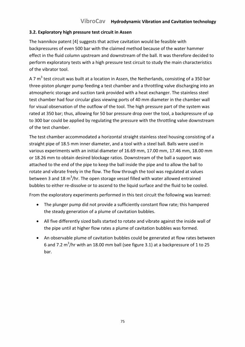
VibroCav Hydrodynamic Vibration and Cavitation technology
75
3.2. Exploratory high pressure test circuit in Assen
The Ivannikov patent [4] suggests that active cavitation would be feasible with
backpressures of even 500 bar with the claimed method because of the water hammer
effect in the fluid column upstream and downstream of the ball. It was therefore decided to
perform exploratory tests with a high pressure test circuit to study the main characteristics
of the vibrator tool.
A 7 m3 test circuit was built at a location in Assen, the Netherlands, consisting of a 350 bar
three‐piston plunger pump feeding a test chamber and a throttling valve discharging into an
atmospheric storage and suction tank provided with a heat exchanger. The stainless steel
test chamber had four circular glass viewing ports of 40 mm diameter in the chamber wall
for visual observation of the outflow of the tool. The high pressure part of the system was
rated at 350 bar; thus, allowing for 50 bar pressure drop over the tool, a backpressure of up
to 300 bar could be applied by regulating the pressure with the throttling valve downstream
of the test chamber.
The test chamber accommodated a horizontal straight stainless steel housing consisting of a
straight pipe of 18.5 mm inner diameter, and a tool with a steel ball. Balls were used in
various experiments with an initial diameter of 16.69 mm, 17.00 mm, 17.46 mm, 18.00 mm
or 18.26 mm to obtain desired blockage ratios. Downstream of the ball a support was
attached to the end of the pipe to keep the ball inside the pipe and to allow the ball to
rotate and vibrate freely in the flow. The flow through the tool was regulated at values
between 3 and 18 m3/hr. The open storage vessel filled with water allowed entrained
bubbles to either re‐dissolve or to ascend to the liquid surface and the fluid to be cooled.
From the exploratory experiments performed in this test circuit the following was learned:
The plunger pump did not provide a sufficiently constant flow rate; this hampered
the steady generation of a plume of cavitation bubbles.
All five differently sized balls started to rotate and vibrate against the inside wall of
the pipe until at higher flow rates a plume of cavitation bubbles was formed.
An observable plume of cavitation bubbles could be generated at flow rates between
6 and 7.2 m3/hr with an 18.00 mm ball (see figure 3.1) at a backpressure of 1 to 25
bar.
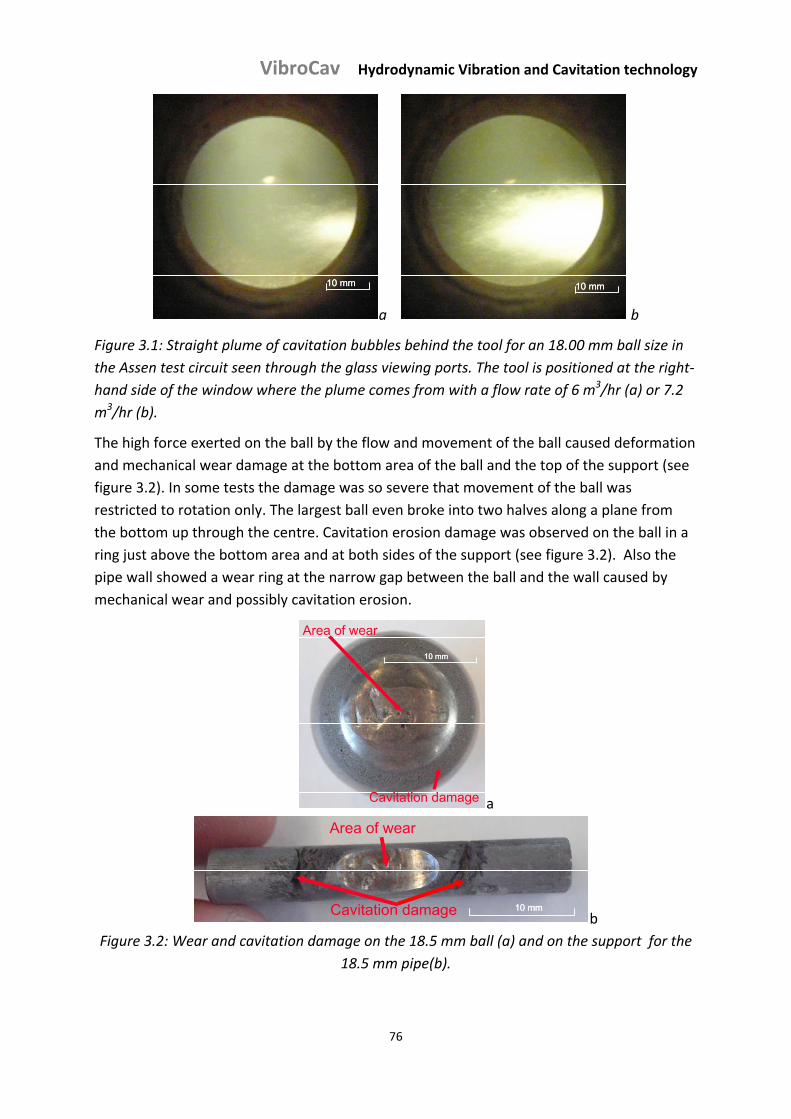
VibroCav Hydrodynamic Vibration and Cavitation technology
76
10 mm10 mm10 mm
a
10 mm10 mm10 mm
b
Figure 3.1: Straight plume of cavitation bubbles behind the tool for an 18.00 mm ball size in
the Assen test circuit seen through the glass viewing ports. The tool is positioned at the right‐
hand side of the window where the plume comes from with a flow rate of 6 m3/hr (a) or 7.2
m3/hr (b).
The high force exerted on the ball by the flow and movement of the ball caused deformation
and mechanical wear damage at the bottom area of the ball and the top of the support (see
figure 3.2). In some tests the damage was so severe that movement of the ball was
restricted to rotation only. The largest ball even broke into two halves along a plane from
the bottom up through the centre. Cavitation erosion damage was observed on the ball in a
ring just above the bottom area and at both sides of the support (see figure 3.2). Also the
pipe wall showed a wear ring at the narrow gap between the ball and the wall caused by
mechanical wear and possibly cavitation erosion.
Cavitation damage
Area of wear
10 mm
Cavitation damage
Area of wear
Cavitation damage
Area of wear
10 mm10 mm
a
Cavitation damage
Area of wear
10 mmCavitation damage
Area of wear
Cavitation damage
Area of wear
10 mm10 mm
b
Figure 3.2: Wear and cavitation damage on the 18.5 mm ball (a) and on the support for the
18.5 mm pipe(b).
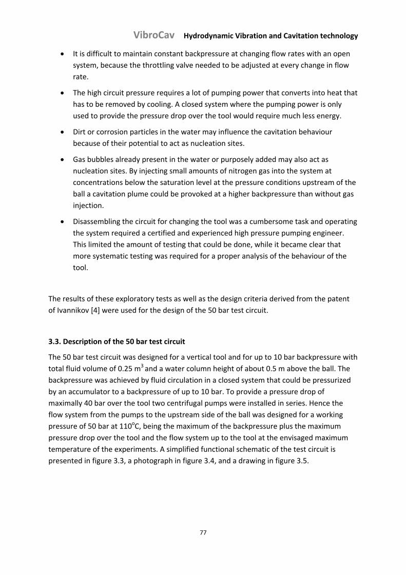
VibroCav Hydrodynamic Vibration and Cavitation technology
77
It is difficult to maintain constant backpressure at changing flow rates with an open
system, because the throttling valve needed to be adjusted at every change in flow
rate.
The high circuit pressure requires a lot of pumping power that converts into heat that
has to be removed by cooling. A closed system where the pumping power is only
used to provide the pressure drop over the tool would require much less energy.
Dirt or corrosion particles in the water may influence the cavitation behaviour
because of their potential to act as nucleation sites.
Gas bubbles already present in the water or purposely added may also act as
nucleation sites. By injecting small amounts of nitrogen gas into the system at
concentrations below the saturation level at the pressure conditions upstream of the
ball a cavitation plume could be provoked at a higher backpressure than without gas
injection.
Disassembling the circuit for changing the tool was a cumbersome task and operating
the system required a certified and experienced high pressure pumping engineer.
This limited the amount of testing that could be done, while it became clear that
more systematic testing was required for a proper analysis of the behaviour of the
tool.
The results of these exploratory tests as well as the design criteria derived from the patent
of Ivannikov [4] were used for the design of the 50 bar test circuit.
3.3. Description of the 50 bar test circuit
The 50 bar test circuit was designed for a vertical tool and for up to 10 bar backpressure with
total fluid volume of 0.25 m3 and a water column height of about 0.5 m above the ball. The
backpressure was achieved by fluid circulation in a closed system that could be pressurized
by an accumulator to a backpressure of up to 10 bar. To provide a pressure drop of
maximally 40 bar over the tool two centrifugal pumps were installed in series. Hence the
flow system from the pumps to the upstream side of the ball was designed for a working
pressure of 50 bar at 110oC, being the maximum of the backpressure plus the maximum
pressure drop over the tool and the flow system up to the tool at the envisaged maximum
temperature of the experiments. A simplified functional schematic of the test circuit is
presented in figure 3.3, a photograph in figure 3.4, and a drawing in figure 3.5.
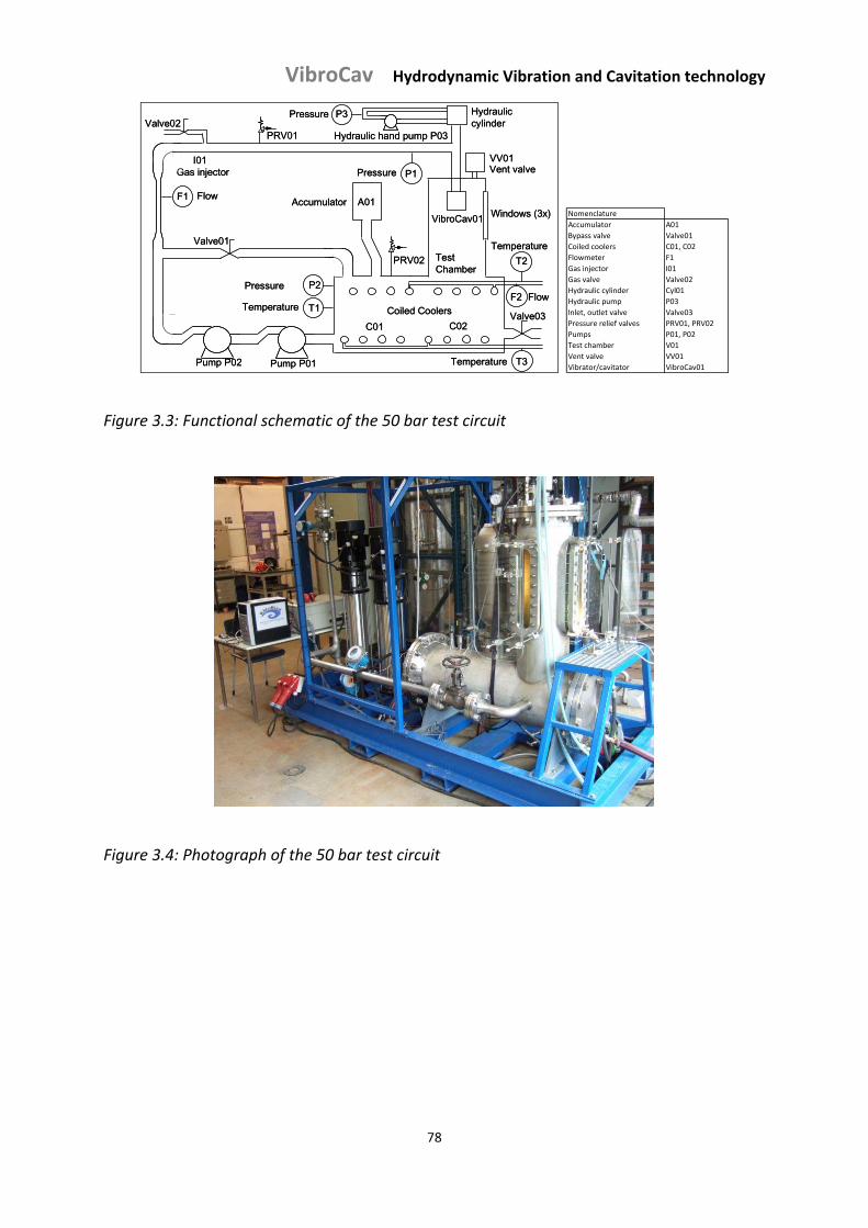
VibroCav Hydrodynamic Vibration and Cavitation technology
78
Valve02
Valve01
I01 Gas injector
Pump P02 Pump P01
F1 Flow
Pressure
Pressure
Pressure
Temperature
Temperature
Temperature
Accumulator
Coiled Coolers
Test Chamber
VibroCav01
Hydraulic cylinder
Hydraulic hand pump P03
Windows (3x)
PRV01
PRV02
VV01Vent valve
P3
P2
P1
T3
T2
T1Valve03
C01 C02
A01
F2 Flow
Nomenclature
Accumulator A01
Bypass valve Valve01
Coiled coolers C01, C02
Flowmeter F1
Gas injector I01
Gas valve Valve02
Hydraulic cylinder Cyl01
Hydraulic pump P03
Inlet, outlet valve Valve03
Pressure relief valves PRV01, PRV02
Pumps P01, P02
Test chamber V01
Vent valve VV01
Vibrator/cavitator VibroCav01
Figure 3.3: Functional schematic of the 50 bar test circuit
Figure 3.4: Photograph of the 50 bar test circuit
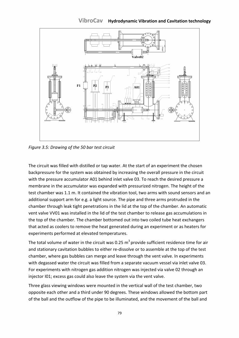
VibroCav Hydrodynamic Vibration and Cavitation technology
79
Valve02
F1 P1P2 A01
Valve02
F1 P1P2 A01
Figure 3.5: Drawing of the 50 bar test circuit
The circuit was filled with distilled or tap water. At the start of an experiment the chosen
backpressure for the system was obtained by increasing the overall pressure in the circuit
with the pressure accumulator A01 behind inlet valve 03. To reach the desired pressure a
membrane in the accumulator was expanded with pressurized nitrogen. The height of the
test chamber was 1.1 m. It contained the vibration tool, two arms with sound sensors and an
additional support arm for e.g. a light source. The pipe and three arms protruded in the
chamber through leak tight penetrations in the lid at the top of the chamber. An automatic
vent valve VV01 was installed in the lid of the test chamber to release gas accumulations in
the top of the chamber. The chamber bottomed out into two coiled tube heat exchangers
that acted as coolers to remove the heat generated during an experiment or as heaters for
experiments performed at elevated temperatures.
The total volume of water in the circuit was 0.25 m3 provide sufficient residence time for air
and stationary cavitation bubbles to either re‐dissolve or to assemble at the top of the test
chamber, where gas bubbles can merge and leave through the vent valve. In experiments
with degassed water the circuit was filled from a separate vacuum vessel via inlet valve 03.
For experiments with nitrogen gas addition nitrogen was injected via valve 02 through an
injector I01; excess gas could also leave the system via the vent valve.
Three glass viewing windows were mounted in the vertical wall of the test chamber, two
opposite each other and a third under 90 degrees. These windows allowed the bottom part
of the ball and the outflow of the pipe to be illuminated, and the movement of the ball and
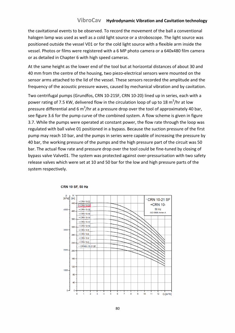
VibroCav Hydrodynamic Vibration and Cavitation technology
80
the cavitational events to be observed. To record the movement of the ball a conventional
halogen lamp was used as well as a cold light source or a stroboscope. The light source was
positioned outside the vessel V01 or for the cold light source with a flexible arm inside the
vessel. Photos or films were registered with a 6 MP photo camera or a 640x480 film camera
or as detailed in Chapter 6 with high speed cameras.
At the same height as the lower end of the tool but at horizontal distances of about 30 and
40 mm from the centre of the housing, two piezo‐electrical sensors were mounted on the
sensor arms attached to the lid of the vessel. These sensors recorded the amplitude and the
frequency of the acoustic pressure waves, caused by mechanical vibration and by cavitation.
Two centrifugal pumps (Grundfos, CRN 10‐21SF, CRN 10‐20) lined up in series, each with a
power rating of 7.5 KW, delivered flow in the circulation loop of up to 18 m3/hr at low
pressure differential and 6 m3/hr at a pressure drop over the tool of approximately 40 bar,
see figure 3.6 for the pump curve of the combined system. A flow scheme is given in figure
3.7. While the pumps were operated at constant power, the flow rate through the loop was
regulated with ball valve 01 positioned in a bypass. Because the suction pressure of the first
pump may reach 10 bar, and the pumps in series were capable of increasing the pressure by
40 bar, the working pressure of the pumps and the high pressure part of the circuit was 50
bar. The actual flow rate and pressure drop over the tool could be fine‐tuned by closing of
bypass valve Valve01. The system was protected against over‐pressurisation with two safety
release valves which were set at 10 and 50 bar for the low and high pressure parts of the
system respectively.
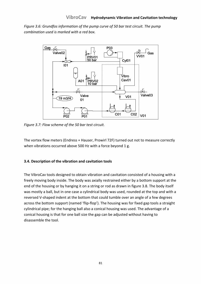
VibroCav Hydrodynamic Vibration and Cavitation technology
81
Figure 3.6: Grundfos information of the pump curve of 50 bar test circuit. The pump
combination used is marked with a red box.
P01P02
Valve01
PRV01
C01 C02
V01
VV01
I01
PRV02
Gas
VibroCav01
Gas
19 m3/H
10 bar
50 bar
V01
P03
Cyl01
A01
Valve02
Valve03
P01P02
Valve01
PRV01
C01 C02
V01
VV01
I01
PRV02
Gas
VibroCav01
Gas
19 m3/H
10 bar
50 bar
V01
P03
Cyl01
A01
Valve02
Valve03
Figure 3.7: Flow scheme of the 50 bar test circuit.
The vortex flow meters (Endress + Hauser, Prowirl 72F) turned out not to measure correctly
when vibrations occurred above 500 Hz with a force beyond 1 g.
3.4. Description of the vibration and cavitation tools
The VibroCav tools designed to obtain vibration and cavitation consisted of a housing with a
freely moving body inside. The body was axially restrained either by a bottom support at the
end of the housing or by hanging it on a string or rod as drawn in figure 3.8. The body itself
was mostly a ball, but in one case a cylindrical body was used, rounded at the top and with a
reversed V‐shaped indent at the bottom that could tumble over an angle of a few degrees
across the bottom support (named ‘flip‐flop’). The housing was for fixed gap tools a straight
cylindrical pipe; for the hanging ball also a conical housing was used. The advantage of a
conical housing is that for one ball size the gap can be adjusted without having to
disassemble the tool.
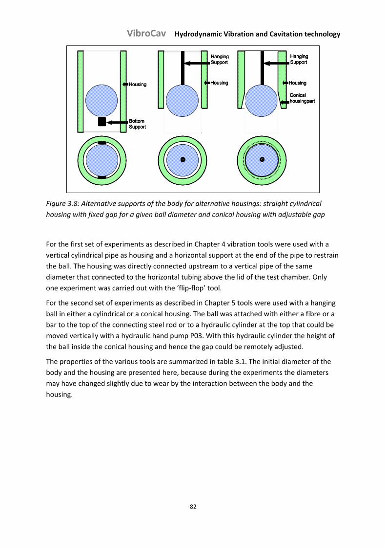
VibroCav Hydrodynamic Vibration and Cavitation technology
82
Hanging Support
Housing
Hanging Support
Conical housingpart
Housing Housing
Bottom Support
Hanging Support
Housing
Hanging Support
Housing
Hanging Support
Conical housingpart
Housing
Hanging Support
Conical housingpart
Housing Housing
Bottom Support
Housing
Bottom Support
Figure 3.8: Alternative supports of the body for alternative housings: straight cylindrical
housing with fixed gap for a given ball diameter and conical housing with adjustable gap
For the first set of experiments as described in Chapter 4 vibration tools were used with a
vertical cylindrical pipe as housing and a horizontal support at the end of the pipe to restrain
the ball. The housing was directly connected upstream to a vertical pipe of the same
diameter that connected to the horizontal tubing above the lid of the test chamber. Only
one experiment was carried out with the ‘flip‐flop’ tool.
For the second set of experiments as described in Chapter 5 tools were used with a hanging
ball in either a cylindrical or a conical housing. The ball was attached with either a fibre or a
bar to the top of the connecting steel rod or to a hydraulic cylinder at the top that could be
moved vertically with a hydraulic hand pump P03. With this hydraulic cylinder the height of
the ball inside the conical housing and hence the gap could be remotely adjusted.
The properties of the various tools are summarized in table 3.1. The initial diameter of the
body and the housing are presented here, because during the experiments the diameters
may have changed slightly due to wear by the interaction between the body and the
housing.
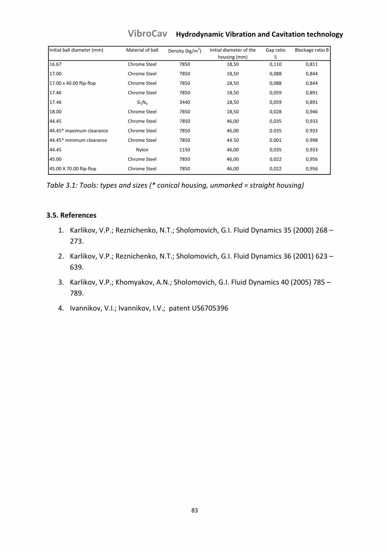
VibroCav Hydrodynamic Vibration and Cavitation technology
83
Initial ball diameter (mm) Material of ball Density (kg/m3) Initial diameter of the
housing (mm)
Gap ratio
S
Blockage ratio B
16.67 Chrome Steel 7850 18,50 0,110 0,811
17.00 Chrome Steel 7850 18,50 0,088 0,844
17.00 x 40.00 flip‐flop Chrome Steel 7850 18,50 0,088 0,844
17.46 Chrome Steel 7850 18,50 0,059 0,891
17.46 Si3N4 3440 18,50 0,059 0,891
18.00 Chrome Steel 7850 18,50 0,028 0,946
44.45 Chrome Steel 7850 46,00 0,035 0,933
44.45* maximum clearance Chrome Steel 7850 46,00 0.035 0.933
44.45* minimum clearance Chrome Steel 7850 44.50 0.001 0.998
44.45 Nylon 1150 46,00 0,035 0,933
45.00 Chrome Steel 7850 46,00 0,022 0,956
45.00 X 70.00 flip‐flop Chrome Steel 7850 46,00 0,022 0,956
Table 3.1: Tools: types and sizes (* conical housing, unmarked = straight housing)
3.5. References
1. Karlikov, V.P.; Reznichenko, N.T.; Sholomovich, G.I. Fluid Dynamics 35 (2000) 268 –
273.
2. Karlikov, V.P.; Reznichenko, N.T.; Sholomovich, G.I. Fluid Dynamics 36 (2001) 623 –
639.
3. Karlikov, V.P.; Khomyakov, A.N.; Sholomovich, G.I. Fluid Dynamics 40 (2005) 785 –
789.
4. Ivannikov, V.I.; Ivannikov, I.V.; patent US6705396
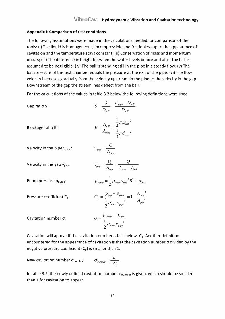
VibroCav Hydrodynamic Vibration and Cavitation technology
84
Appendix I: Comparison of test conditions
The following assumptions were made in the calculations needed for comparison of the
tools: (i) The liquid is homogeneous, incompressible and frictionless up to the appearance of
cavitation and the temperature stays constant; (ii) Conservation of mass and momentum
occurs; (iii) The difference in height between the water levels before and after the ball is
assumed to be negligible; (iv) The ball is standing still in the pipe in a steady flow; (v) The
backpressure of the test chamber equals the pressure at the exit of the pipe; (vi) The flow
velocity increases gradually from the velocity upstream in the pipe to the velocity in the gap.
Downstream of the gap the streamlines deflect from the ball.
For the calculations of the values in table 3.2 below the following definitions were used.
Gap ratio S: pipe ball
ball ball
d DS
D D
Blockage ratio B:
2
2
1414
ballball
pipepipe
DAB
A d
Velocity in the pipe vpipe: pipepipe
Qv
A
Velocity in the gap vgap: gapgap pipe ball
Q Qv
A A A
Pump pressure ppump: 2 21
2pump water gap backp v B p
Pressure coefficient Cp: 2
22
112
gap pump pipep
gapwater pipe
p p AC
Av
Cavitation number σ: 21
2
pump vapor
water pipe
p p
v
Cavitation will appear if the cavitation number σ falls below ‐Cp. Another definition
encountered for the appearance of cavitation is that the cavitation number σ divided by the
negative pressure coefficient (Cp) is smaller than 1.
New cavitation number σnumber: numberpC
In table 3.2. the newly defined cavitation number σnumber is given, which should be smaller
than 1 for cavitation to appear.
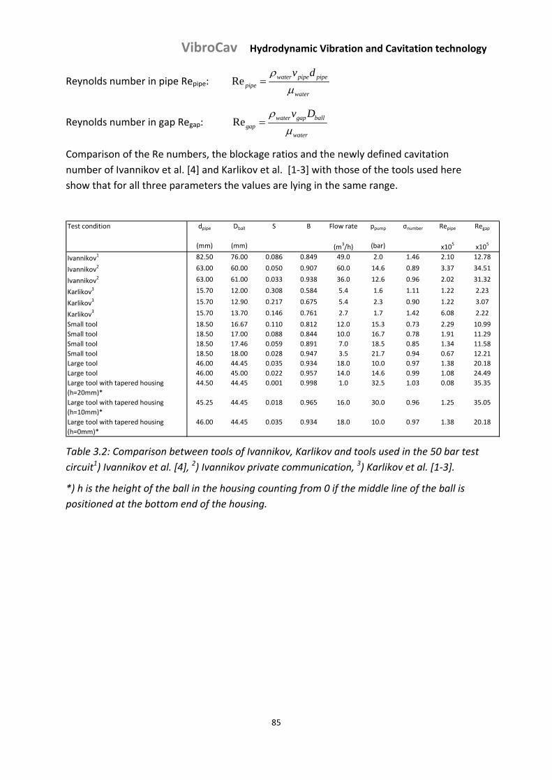
VibroCav Hydrodynamic Vibration and Cavitation technology
85
Reynolds number in pipe Repipe: Re water pipe pipepipe
water
v d
Reynolds number in gap Regap: Re water gap ballgap
water
v D
Comparison of the Re numbers, the blockage ratios and the newly defined cavitation
number of Ivannikov et al. [4] and Karlikov et al. [1‐3] with those of the tools used here
show that for all three parameters the values are lying in the same range.
Test condition dpipe Dball S B Flow rate ppump σnumber Repipe Regap
(mm) (mm) (m3/h) (bar) x105 x105
Ivannikov1 82.50 76.00 0.086 0.849 49.0 2.0 1.46 2.10 12.78
Ivannikov2 63.00 60.00 0.050 0.907 60.0 14.6 0.89 3.37 34.51
Ivannikov2 63.00 61.00 0.033 0.938 36.0 12.6 0.96 2.02 31.32
Karlikov3 15.70 12.00 0.308 0.584 5.4 1.6 1.11 1.22 2.23
Karlikov3 15.70 12.90 0.217 0.675 5.4 2.3 0.90 1.22 3.07
Karlikov3 15.70 13.70 0.146 0.761 2.7 1.7 1.42 6.08 2.22
Small tool 18.50 16.67 0.110 0.812 12.0 15.3 0.73 2.29 10.99
Small tool 18.50 17.00 0.088 0.844 10.0 16.7 0.78 1.91 11.29
Small tool 18.50 17.46 0.059 0.891 7.0 18.5 0.85 1.34 11.58
Small tool 18.50 18.00 0.028 0.947 3.5 21.7 0.94 0.67 12.21
Large tool 46.00 44.45 0.035 0.934 18.0 10.0 0.97 1.38 20.18
Large tool 46.00 45.00 0.022 0.957 14.0 14.6 0.99 1.08 24.49
Large tool with tapered housing
(h=20mm)*
44.50 44.45 0.001 0.998 1.0 32.5 1.03 0.08 35.35
Large tool with tapered housing
(h=10mm)*
45.25 44.45 0.018 0.965 16.0 30.0 0.96 1.25 35.05
Large tool with tapered housing
(h=0mm)*
46.00 44.45 0.035 0.934 18.0 10.0 0.97 1.38 20.18
Table 3.2: Comparison between tools of Ivannikov, Karlikov and tools used in the 50 bar test
circuit1) Ivannikov et al. [4], 2) Ivannikov private communication, 3) Karlikov et al. [1‐3].
*) h is the height of the ball in the housing counting from 0 if the middle line of the ball is
positioned at the bottom end of the housing.
VibroCav Hydrodynamic Vibration and Cavitation technology
86
Chapter 4: Cavitation and vibration by flow along a bottom supported ball in
a 50 bar test circuit
4.1. Introduction
The behaviour of a body that moves laterally in a pipe with a narrow gap by passing flow has
not in depth been studied in spite of its considerable importance for many applications. It is
known that broad ranges of flow rates exist for which self‐excited vibration sets in that can
be accompanied by bouncing of the body against the pipe wall. These ranges shift for
different body and fluid densities and for other variables like the flow rate, the total mass of
the body, the gap, the fluid properties and the surrounding pressure. Bouncing of the body
against the pipe wall mostly causes intense vibrations and strong acoustic waves that
propagate in the surrounding environment.
Based on [1] and own observation in the exploratory Assen test circuit, at low flow rates the
body, mostly a ball, may already start rotating around its axis, caused by viscous drag and if
appropriate by spiralling of non‐rectified flow approaching the ball. At higher flow rates
vibration of the ball is induced primarily by the high dynamic pressure in the passage
between the ball and the wall of the pipe and consequent low static pressure, resulting in a
static pressure differential across the ball. Instabilities in the flow around the ball shift its
position off centre, and once the ball moves it is forced to the side with the highest flow
velocity. Upon its movement the passage opens on the opposite side, reversing the direction
of force; this alternating force results in self‐exited oscillation. A certain minimum flow rate
is required for vibration in conjunction with bouncing of the ball against the pipe wall, the
onset of which is signalled by an increase in acoustic noise, particularly for the larger balls.
For condensed fluids cavitation can be observed in regions of still higher flow rates due to
the increased static pressure drop in the gap, and imploding cavitation bubbles are
transported by the flow along the body. Two types of cavitation can be distinguished; so‐
called active cavitation where the body vibrates and so‐called passive cavitation where the
body stands still. Active as well as passive cavitation is suppressed at increasing pressure
downstream of the tool, the so‐called backpressure. When varying the flow and/or the
backpressure different regimes of tool behaviour and effects like vibration and cavitation
can be observed; such observations are studied in depth in this chapter.
The theoretical flow rate, at which passive cavitation sets in for a given body and pipe
configuration, fluid properties and backpressure can be estimated from the cavitation
number σ and the pressure coefficient cp in the narrow gap between the body and the pipe
as for instance described by Brennen [2]. The theoretical flow rate in case of inviscid flow,
where passive cavitation sets in for a given gap and pressure difference over the ball, can be
estimated from the cavitation number:
VibroCav Hydrodynamic Vibration and Cavitation technology
87
212
pump vapor
water pipe
p p
v
(4.1)
2
22
112
gap pump pipep
gapwater pipe
p p AC
Av
(4.2)
with vpipe = flow rate in the pipe upstream of the ball and pgap = pressure in the gap. If σ < ‐
Cp passive cavitation starts. Cp does not depend on the geometry of the gap in the ideal case
of an inviscid liquid.
Another definition for the onset of passive cavitation is that the cavitation number σ divided
by the negative pressure coefficient (Cp) is smaller than 1.
numberpC
(4.3)
This newly defined cavitation number designated as σnumber is used below. The flow rate for
the actual onset of passive cavitation can differ substantially from the theoretical value for
many reasons, such as viscous effects, surface roughness of the pipe wall and presence of
fine solid particles or dissolved gasses [1]. The flow rate required for the onset of passive
cavitation increases at higher backpressure.
Active cavitation can develop at lower flow rates for a vibrating body, since an additional
dynamic pressure and hence a lower static pressure is created in the gap by the water
hammer effect [3]. This additional static pressure drop results from the lateral movement of
the body which partially shuts off the flow, and causes a local pressure drop of an
approximate magnitude of:
vcP waterrwaterhamme (4.4)
where c = speed of sound, water = density of water and v = instantaneous reduction in flow
rate.
The flow rate range where active cavitation might occur at a given backpressure is a less
explored area. Since unstable behaviour of the surrounding fluid determines the flow
pattern and thus when and how vigorously the body starts vibrating, the flow rate at which
active cavitation starts is prone to fluctuations and its onset can thus vary. The transition
from one regime to another can also show hysteresis meaning that the transition happens at
another value if the regime is entered by increasing or decreasing the flow or the pressure.
Depending on the application, specific regimes where either vibration or cavitation, or a
combination of the two persists can be persecuted with a particular tool.
The oscillating behaviour of a laterally free moving body in an unbounded flow has for long
been subject of detailed study. In unbounded flows shedding of vortices and vortex wake
formation behind a ball are mostly described as the cause for lateral movement, see Chapter
VibroCav Hydrodynamic Vibration and Cavitation technology
88
1. For bounded flows however, and a gap ratio S = δ /Dball = (dpipe ‐ Dball)/ Dball, where Dball =
ball diameter and dpipe = internal pipe diameter, below about 0.35, vibration is more likely to
be caused by the low static pressure due to the high dynamic pressure in the gap. The
behaviour of a body for narrow gaps in flow regimes of increasing velocity seems to be a
poorly explored area both at atmospheric and at higher ambient pressures.
Karlikov et al. [1] studied the acoustic frequency with laterally self‐excited vibration of balls
with a narrow gap ratio between 0.10 and 0.35 for a flow through a cylindrical pipe fixed at
the upper end in a massive support. Intense vibrations of the ball, made from plastic,
duralumin or brass, together with bouncing of the ball on the internal pipe wall were
observed. The bottom of the copper or steel pipe was immersed in an open water tank, so
the backpressure was near‐atmospheric. The ball was hanging on a filament that allowed
lateral movement of the ball. The free length of the pipe was adjusted to obtain resonance
between the vibrations of the ball and the free pipe in order to obtain accurate
measurements of the vibration frequency. A linear relationship between the vibration
frequency of the ball and the flow rate was found for the flow range before the onset of
either active or passive cavitation.
Karlikov et al. presented three pictures of phenomena that were observed in the flow just
below the gap to illustrate what happened close to and beyond the onset of cavitation at
increasingly higher flow rates. The pipe wall was made of transparent plastic, so cavitation
could be visually observed. First vortices were noticed downstream of the narrow gap at
higher flow rates, followed by cavitation plumes emerging alternately on different sides of
the vibrating ball that could be attributed to the generation of active cavitation. The third
picture showed symmetrical and therefore passive cavitation. When passive cavitation
started the vibration stopped. This was ascribed to the stabilizing effect of the symmetrical
wake in case of passive cavitation.
Thus Karlikov et al. showed by observing the movement of the ball during bouncing and by
analysing the pictures that the following regimes existed at increasing flow rates in an open
system, i.e. at atmospheric backpressure: (i) a flow regime without or with vibration of the
ball, but without bouncing against the pipe wall, (ii) a regime with vibration and bouncing
against the pipe wall, (iii) a regime with vibration, bouncing and active cavitation, and (iv) a
regime with no vibration and passive cavitation.
A later patent by Ivannikov et al. [4] focused on the design of tools with a laterally free
moving body in the flow in a pipe to improve active cavitation. A narrower gap ratio of
maximally 0.118 was claimed to be necessary to obtain optimal active cavitation. It was
suggested that cavitation could still be obtained at very high backpressures up to 500 bars
due to free turbulent vortices that should be able to nucleate cavitation.
The study described in this chapter focuses on the identification of the vibration and
cavitation behaviour of bottom supported laterally free moving bodies, mostly balls of
various sizes and densities in an aqueous flow through pipes of various diameters at narrow
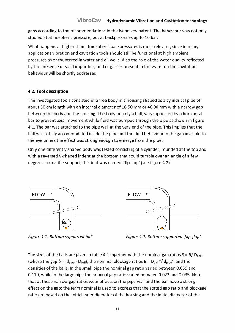
VibroCav Hydrodynamic Vibration and Cavitation technology
89
gaps according to the recommendations in the Ivannikov patent. The behaviour was not only
studied at atmospheric pressure, but at backpressures up to 10 bar.
What happens at higher than atmospheric backpressures is most relevant, since in many
applications vibration and cavitation tools should still be functional at high ambient
pressures as encountered in water and oil wells. Also the role of the water quality reflected
by the presence of solid impurities, and of gasses present in the water on the cavitation
behaviour will be shortly addressed.
4.2. Tool description
The investigated tools consisted of a free body in a housing shaped as a cylindrical pipe of
about 50 cm length with an internal diameter of 18.50 mm or 46.00 mm with a narrow gap
between the body and the housing. The body, mainly a ball, was supported by a horizontal
bar to prevent axial movement while fluid was pumped through the pipe as shown in figure
4.1. The bar was attached to the pipe wall at the very end of the pipe. This implies that the
ball was totally accommodated inside the pipe and the fluid behaviour in the gap invisible to
the eye unless the effect was strong enough to emerge from the pipe.
Only one differently shaped body was tested consisting of a cylinder, rounded at the top and
with a reversed V‐shaped indent at the bottom that could tumble over an angle of a few
degrees across the support; this tool was named ‘flip‐flop’ (see figure 4.2).
FLOW
Ball
FLOW
Ball
FLOWFLOW
Figure 4.1: Bottom supported ball Figure 4.2: Bottom supported ’flip‐flop’
The sizes of the balls are given in table 4.1 together with the nominal gap ratios S = δ/ Dball,
(where the gap δ = dpipe ‐ Dball), the nominal blockage ratios B = Dball 2/ dpipe
2, and the
densities of the balls. In the small pipe the nominal gap ratio varied between 0.059 and
0.110, while in the large pipe the nominal gap ratio varied between 0.022 and 0.035. Note
that at these narrow gap ratios wear effects on the pipe wall and the ball have a strong
effect on the gap; the term nominal is used to express that the stated gap ratio and blockage
ratio are based on the initial inner diameter of the housing and the initial diameter of the
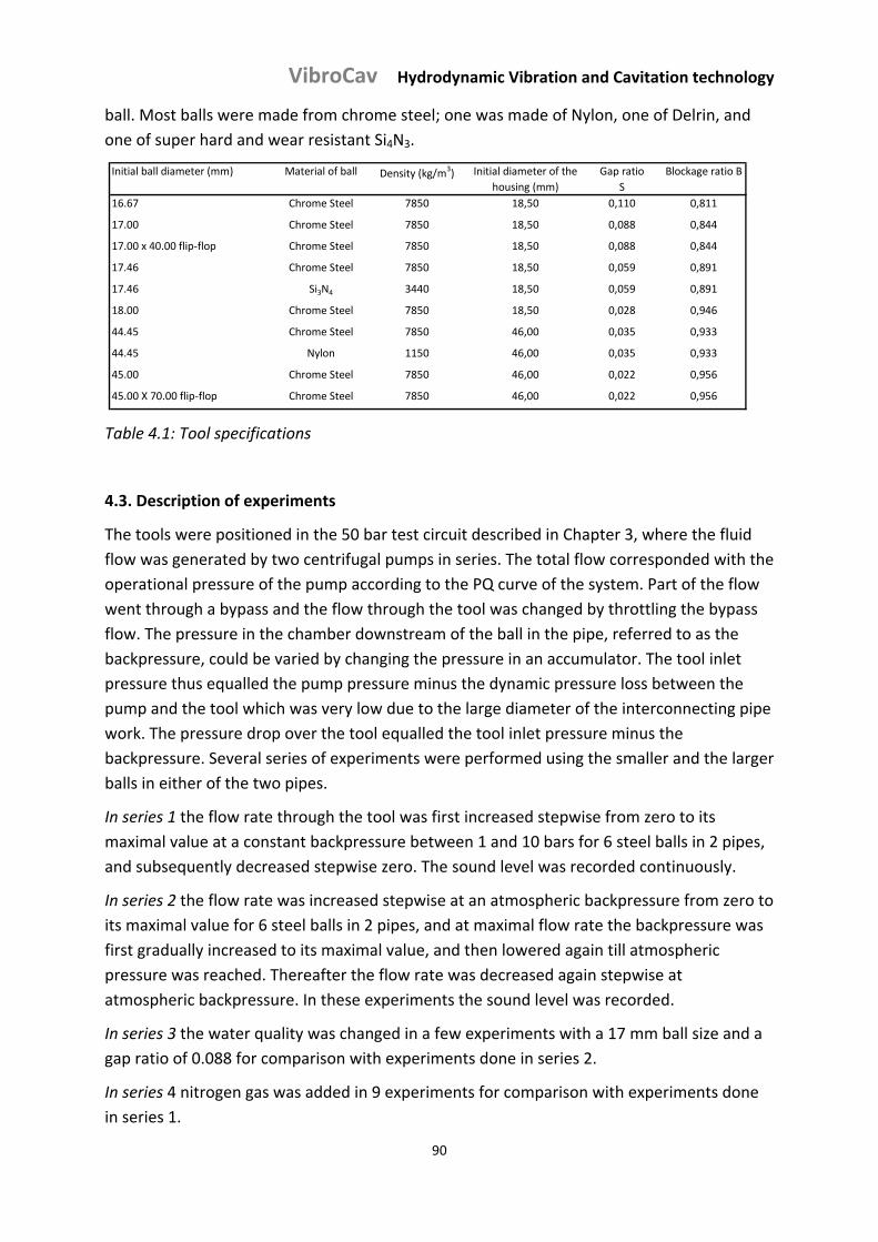
VibroCav Hydrodynamic Vibration and Cavitation technology
90
ball. Most balls were made from chrome steel; one was made of Nylon, one of Delrin, and
one of super hard and wear resistant Si4N3.
Initial ball diameter (mm) Material of ball Density (kg/m3) Initial diameter of the
housing (mm)
Gap ratio
S
Blockage ratio B
16.67 Chrome Steel 7850 18,50 0,110 0,811
17.00 Chrome Steel 7850 18,50 0,088 0,844
17.00 x 40.00 flip‐flop Chrome Steel 7850 18,50 0,088 0,844
17.46 Chrome Steel 7850 18,50 0,059 0,891
17.46 Si3N4 3440 18,50 0,059 0,891
18.00 Chrome Steel 7850 18,50 0,028 0,946
44.45 Chrome Steel 7850 46,00 0,035 0,933
44.45 Nylon 1150 46,00 0,035 0,933
45.00 Chrome Steel 7850 46,00 0,022 0,956
45.00 X 70.00 flip‐flop Chrome Steel 7850 46,00 0,022 0,956
Table 4.1: Tool specifications
4.3. Description of experiments
The tools were positioned in the 50 bar test circuit described in Chapter 3, where the fluid
flow was generated by two centrifugal pumps in series. The total flow corresponded with the
operational pressure of the pump according to the PQ curve of the system. Part of the flow
went through a bypass and the flow through the tool was changed by throttling the bypass
flow. The pressure in the chamber downstream of the ball in the pipe, referred to as the
backpressure, could be varied by changing the pressure in an accumulator. The tool inlet
pressure thus equalled the pump pressure minus the dynamic pressure loss between the
pump and the tool which was very low due to the large diameter of the interconnecting pipe
work. The pressure drop over the tool equalled the tool inlet pressure minus the
backpressure. Several series of experiments were performed using the smaller and the larger
balls in either of the two pipes.
In series 1 the flow rate through the tool was first increased stepwise from zero to its
maximal value at a constant backpressure between 1 and 10 bars for 6 steel balls in 2 pipes,
and subsequently decreased stepwise zero. The sound level was recorded continuously.
In series 2 the flow rate was increased stepwise at an atmospheric backpressure from zero to
its maximal value for 6 steel balls in 2 pipes, and at maximal flow rate the backpressure was
first gradually increased to its maximal value, and then lowered again till atmospheric
pressure was reached. Thereafter the flow rate was decreased again stepwise at
atmospheric backpressure. In these experiments the sound level was recorded.
In series 3 the water quality was changed in a few experiments with a 17 mm ball size and a
gap ratio of 0.088 for comparison with experiments done in series 2.
In series 4 nitrogen gas was added in 9 experiments for comparison with experiments done
in series 1.

VibroCav Hydrodynamic Vibration and Cavitation technology
91
In series 5 a Si4N3 ball in the small pipe and a Nylon and a Delrin ball in the larger pipe were
used to perform experiments equivalent to those in series 2.
In series 6 a differently shaped body designated as ‘flip‐flop’ was used that could only tumble
a few degrees across the horizontal support bar.
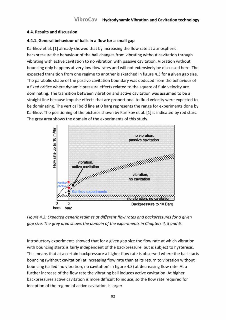
VibroCav Hydrodynamic Vibration and Cavitation technology
92
4.4. Results and discussion
4.4.1. General behaviour of balls in a flow for a small gap
Karlikov et al. [1] already showed that by increasing the flow rate at atmospheric
backpressure the behaviour of the ball changes from vibrating without cavitation through
vibrating with active cavitation to no vibration with passive cavitation. Vibration without
bouncing only happens at very low flow rates and will not extensively be discussed here. The
expected transition from one regime to another is sketched in figure 4.3 for a given gap size.
The parabolic shape of the passive cavitation boundary was deduced from the behaviour of
a fixed orifice where dynamic pressure effects related to the square of fluid velocity are
dominating. The transition between vibration and active cavitation was assumed to be a
straight line because impulse effects that are proportional to fluid velocity were expected to
be dominating. The vertical bold line at 0 barg represents the range for experiments done by
Karlikov. The positioning of the pictures shown by Karlikov et al. [1] is indicated by red stars.
The grey area shows the domain of the experiments of this study.
0 bara
Flow
rate
up
to 1
8 m
3 /hr
0 barg
vibration, no cavitation
vibration, active cavitation
no vibration, passive cavitation
Backpressure to 10 Bargno vibration, no cavitation
Karlikov experiments
Karlikovphotos
0 bara
Flow
rate
up
to 1
8 m
3 /hr
0 barg
vibration, no cavitation
vibration, active cavitation
no vibration, passive cavitation
Backpressure to 10 Bargno vibration, no cavitation
Karlikov experiments
Karlikovphotos
Figure 4.3: Expected generic regimes at different flow rates and backpressures for a given
gap size. The grey area shows the domain of the experiments in Chapters 4, 5 and 6.
Introductory experiments showed that for a given gap size the flow rate at which vibration
with bouncing starts is fairly independent of the backpressure, but is subject to hysteresis.
This means that at a certain backpressure a higher flow rate is observed where the ball starts
bouncing (without cavitation) at increasing flow rate than at its return to vibration without
bouncing (called ‘no vibration, no cavitation’ in figure 4.3) at decreasing flow rate. At a
further increase of the flow rate the vibrating ball induces active cavitation. At higher
backpressures active cavitation is more difficult to induce, so the flow rate required for
inception of the regime of active cavitation is larger.
VibroCav Hydrodynamic Vibration and Cavitation technology
93
The transition between vibration and active cavitation did not show hysteresis during the
introductory experiments. It appeared that under certain conditions active cavitation does
not happen at all, for example when the water hammer effect is too small to contribute
sufficiently to the pressure drop in the gap. In the passive cavitation regime the ball stood
still. The line, where passive cavitation starts at various backpressures, can for a ball standing
still in the centre of the flow be calculated from the cavitation number σnumber for each
ball/pipe combination. The series of experiments discussed below are done to validate and
further explore the regimes of different ball behaviour as sketched in figure 4.3.
4.4.2. Results for small balls
Although the experiments of series 1 were performed for all four small steel balls in the pipe
with an initial diameter of 18.50 mm, only a few representative results will be presented
here to elucidate the generic relevant findings.
Figure 4.4.a presents the flow rate, the pump pressure, the backpressure and the pressure
drop over the ball versus time for a ball of 16.67 mm nominal diameter in an 18.50 mm
nominal pipe, i.e. with a gap ratio of 0.11. The flow rate is first increased in steps, and then
after reaching the maximal value decreased in steps as a function of time at a constant
backpressure of 5 barg. The steps up and down of the flow rate during this experiment are
indicated in figure 4.4.b by vertical arrows. At an increasing flow rate the ball stopped
vibrating at 17 min and at a corresponding flow of 8.4m3/hr passive cavitation set in. For this
ball and gap size no active cavitation bubbles were noticed underneath the pipe during
vibration at a flow rate below 8.4m3/hr. The occurrence of some active cavitation can,
however, not be totally excluded.
At a further increase in flow rate till 11.9 m3/hr more passive cavitation was observed. At
decreasing flow passive cavitation stops after 28 min and the ball resumes vibration at 28
min. The energy needed for vibration causes the pump pressure to rise after a temporary dip
and causes the flow rate to decrease consistently with the PQ curve of the pump. Till 40 min
the ball continues to vibrate, and active cavitation ‐ if there was any ‐ went unnoticed. In
some experiments also a dip in pressure during the increase in flow rate was identified, that
could be related to ceasing vibration of the ball. Disturbance in flow measurements directly
at the start and at the end of the experiment can be attributed to low frequency vibration of
the ball and at the very end with a minimal flow rate to measurement errors.
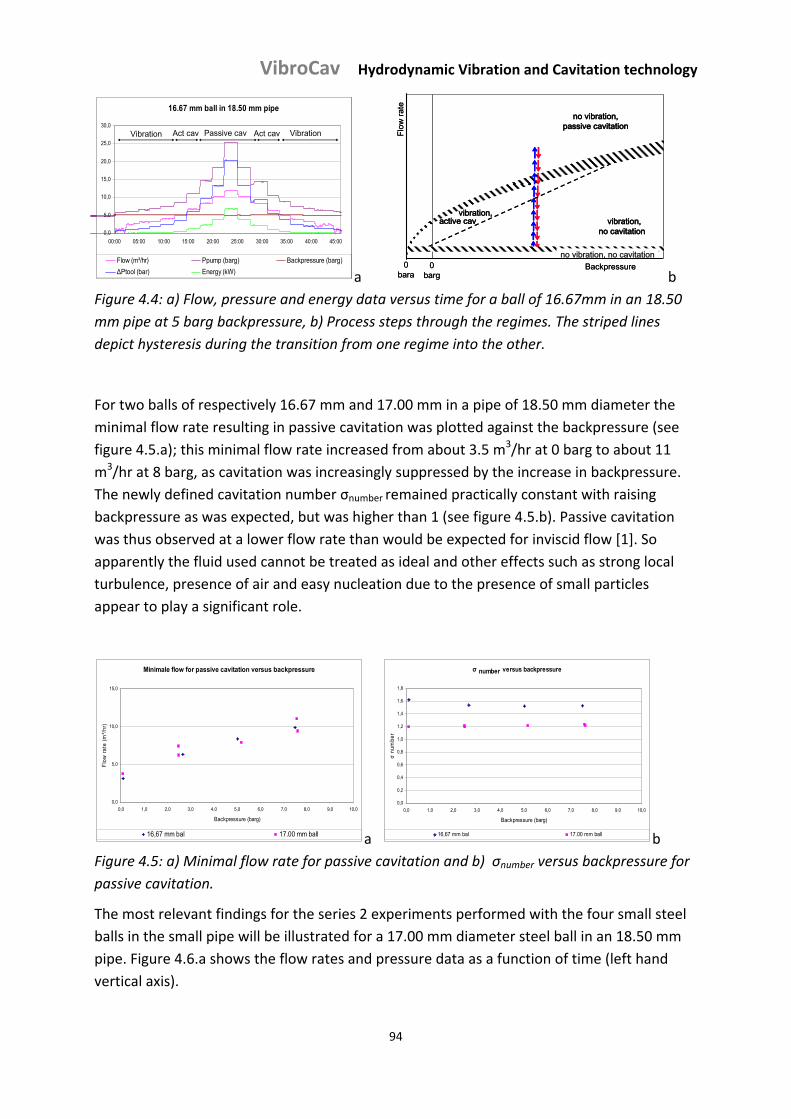
VibroCav Hydrodynamic Vibration and Cavitation technology
94
16.67 mm ball in 18.50 mm pipe
0,0
5,0
10,0
15,0
20,0
25,0
30,0
00:00 05:00 10:00 15:00 20:00 25:00 30:00 35:00 40:00 45:00
Flow (m³/hr) Ppump (barg) Backpressure (barg)
ΔPtool (bar) Energy (kW)
Passive cav VibrationVibration Act cav Act cav
16.67 mm ball in 18.50 mm pipe
0,0
5,0
10,0
15,0
20,0
25,0
30,0
00:00 05:00 10:00 15:00 20:00 25:00 30:00 35:00 40:00 45:00
Flow (m³/hr) Ppump (barg) Backpressure (barg)
ΔPtool (bar) Energy (kW)
Passive cav VibrationVibration Act cav Act cav
a 0
bara
Flow
rate
0 barg
vibration, no cavitation
no vibration, passive cavitation
Backpressureno vibration, no cavitation
vibration, active cav
0 bara
Flow
rate
0 barg
vibration, no cavitation
no vibration, passive cavitation
Backpressureno vibration, no cavitation
vibration, active cav
b
Figure 4.4: a) Flow, pressure and energy data versus time for a ball of 16.67mm in an 18.50
mm pipe at 5 barg backpressure, b) Process steps through the regimes. The striped lines
depict hysteresis during the transition from one regime into the other.
For two balls of respectively 16.67 mm and 17.00 mm in a pipe of 18.50 mm diameter the
minimal flow rate resulting in passive cavitation was plotted against the backpressure (see
figure 4.5.a); this minimal flow rate increased from about 3.5 m3/hr at 0 barg to about 11
m3/hr at 8 barg, as cavitation was increasingly suppressed by the increase in backpressure.
The newly defined cavitation number σnumber remained practically constant with raising
backpressure as was expected, but was higher than 1 (see figure 4.5.b). Passive cavitation
was thus observed at a lower flow rate than would be expected for inviscid flow [1]. So
apparently the fluid used cannot be treated as ideal and other effects such as strong local
turbulence, presence of air and easy nucleation due to the presence of small particles
appear to play a significant role.
Minimale flow for passive cavitation versus backpressure
0,0
5,0
10,0
15,0
0,0 1,0 2,0 3,0 4,0 5,0 6,0 7,0 8,0 9,0 10,0
Backpressure (barg)
Flo
w r
ate
(m³/
hr)
16,67 mm bal 17.00 mm ball a
σ number versus backpressure
0,0
0,2
0,4
0,6
0,8
1,0
1,2
1,4
1,6
1,8
0,0 1,0 2,0 3,0 4,0 5,0 6,0 7,0 8,0 9,0 10,0
Backpressure (barg)
σ n
umbe
r
16,67 mm bal 17.00 mm ball
number
b
Figure 4.5: a) Minimal flow rate for passive cavitation and b) σnumber versus backpressure for
passive cavitation.
The most relevant findings for the series 2 experiments performed with the four small steel
balls in the small pipe will be illustrated for a 17.00 mm diameter steel ball in an 18.50 mm
pipe. Figure 4.6.a shows the flow rates and pressure data as a function of time (left hand
vertical axis).
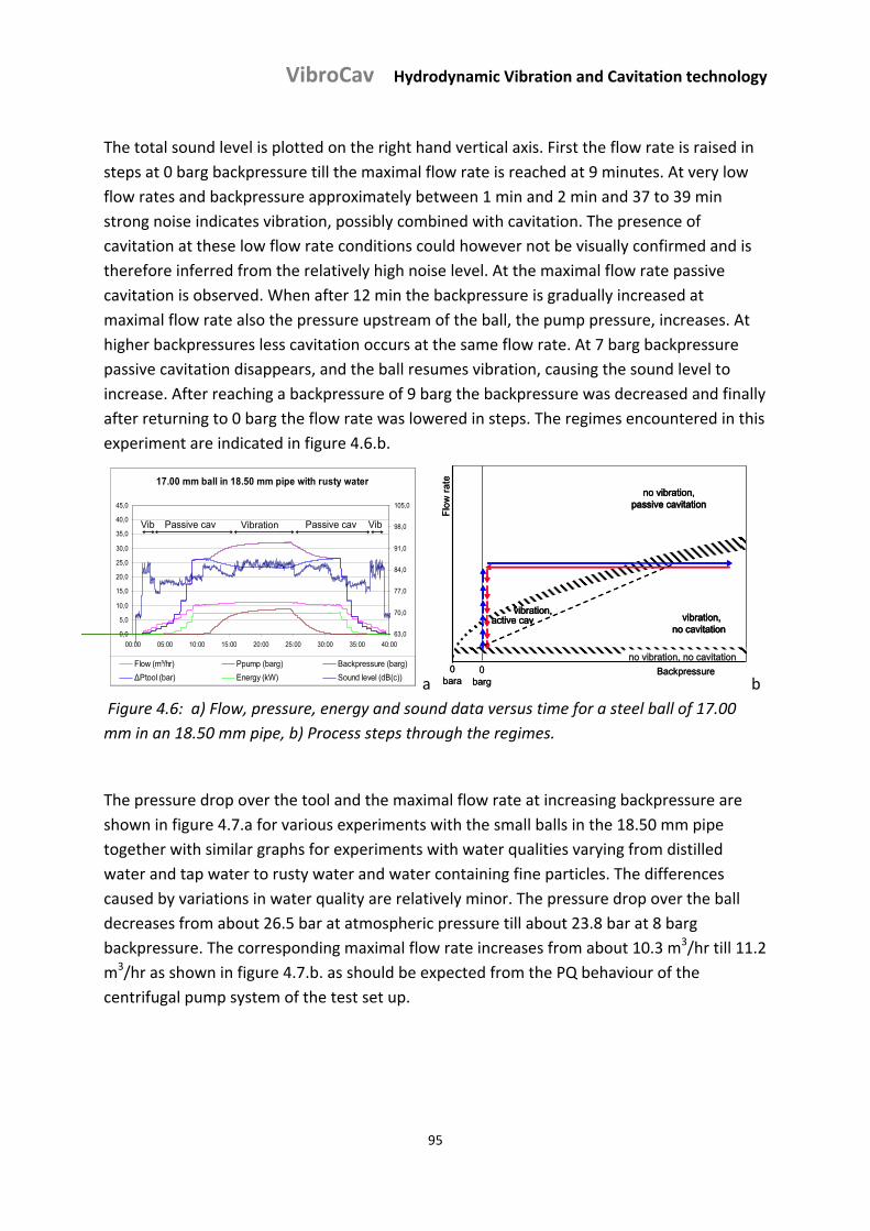
VibroCav Hydrodynamic Vibration and Cavitation technology
95
The total sound level is plotted on the right hand vertical axis. First the flow rate is raised in
steps at 0 barg backpressure till the maximal flow rate is reached at 9 minutes. At very low
flow rates and backpressure approximately between 1 min and 2 min and 37 to 39 min
strong noise indicates vibration, possibly combined with cavitation. The presence of
cavitation at these low flow rate conditions could however not be visually confirmed and is
therefore inferred from the relatively high noise level. At the maximal flow rate passive
cavitation is observed. When after 12 min the backpressure is gradually increased at
maximal flow rate also the pressure upstream of the ball, the pump pressure, increases. At
higher backpressures less cavitation occurs at the same flow rate. At 7 barg backpressure
passive cavitation disappears, and the ball resumes vibration, causing the sound level to
increase. After reaching a backpressure of 9 barg the backpressure was decreased and finally
after returning to 0 barg the flow rate was lowered in steps. The regimes encountered in this
experiment are indicated in figure 4.6.b.
17.00 mm ball in 18.50 mm pipe with rusty water
0,0
5,0
10,0
15,0
20,0
25,0
30,0
35,0
40,0
45,0
00:00 05:00 10:00 15:00 20:00 25:00 30:00 35:00 40:00
63,0
70,0
77,0
84,0
91,0
98,0
105,0
Flow (m³/hr) Ppump (barg) Backpressure (barg)
ΔPtool (bar) Energy (kW) Sound level (dB(c))
Passive cav VibrationVib Passive cav Vib
a 0
bara
Flow
rate
0 barg
vibration, no cavitation
vibration,
no vibration, passive cavitation
Backpressure
active cav
no vibration, no cavitation0
bara
Flow
rate
0 barg
vibration, no cavitation
vibration,
no vibration, passive cavitation
Backpressure
active cav
no vibration, no cavitation
b
Figure 4.6: a) Flow, pressure, energy and sound data versus time for a steel ball of 17.00
mm in an 18.50 mm pipe, b) Process steps through the regimes.
The pressure drop over the tool and the maximal flow rate at increasing backpressure are
shown in figure 4.7.a for various experiments with the small balls in the 18.50 mm pipe
together with similar graphs for experiments with water qualities varying from distilled
water and tap water to rusty water and water containing fine particles. The differences
caused by variations in water quality are relatively minor. The pressure drop over the ball
decreases from about 26.5 bar at atmospheric pressure till about 23.8 bar at 8 barg
backpressure. The corresponding maximal flow rate increases from about 10.3 m3/hr till 11.2
m3/hr as shown in figure 4.7.b. as should be expected from the PQ behaviour of the
centrifugal pump system of the test set up.
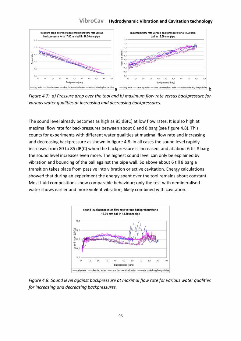
VibroCav Hydrodynamic Vibration and Cavitation technology
96
Pressure drop over the tool at maximum flow rate versus backpressure for a 17.00 mm ball in 18.50 mm pipe
23,0
24,0
25,0
26,0
27,0
28,0
0,0 1,0 2,0 3,0 4,0 5,0 6,0 7,0 8,0 9,0 10,0
Backpressure (barg)
Δp
too
l (b
ar)
rusty water clear tap water clear demineralized water water containing fine particles
Pressure drop over the tool at maximum flow rate versus backpressure for a 17.00 mm ball in 18.50 mm pipe
23,0
24,0
25,0
26,0
27,0
28,0
0,0 1,0 2,0 3,0 4,0 5,0 6,0 7,0 8,0 9,0 10,0
Backpressure (barg)
Δp
too
l (b
ar)
rusty water clear tap water clear demineralized water water containing fine particlesa
maximum flow rate versus backpressure for a 17.00 mm ball in 18.50 mm pipe
9,8
10,0
10,2
10,4
10,6
10,8
11,0
11,2
11,4
11,6
0,0 1,0 2,0 3,0 4,0 5,0 6,0 7,0 8,0 9,0 10,0
backpressure (barg)
Flo
w ra
te (
m³/h
r)
rusty water clear tap water clear demineralized water water containing fine particles b
Figure 4.7: a) Pressure drop over the tool and b) maximum flow rate versus backpressure for
various water qualities at increasing and decreasing backpressures.
The sound level already becomes as high as 85 dB(C) at low flow rates. It is also high at
maximal flow rate for backpressures between about 6 and 8 barg (see figure 4.8). This
counts for experiments with different water qualities at maximal flow rate and increasing
and decreasing backpressure as shown in figure 4.8. In all cases the sound level rapidly
increases from 80 to 85 dB(C) when the backpressure is increased, and at about 6 till 8 barg
the sound level increases even more. The highest sound level can only be explained by
vibration and bouncing of the ball against the pipe wall. So above about 6 till 8 barg a
transition takes place from passive into vibration or active cavitation. Energy calculations
showed that during an experiment the energy spent over the tool remains about constant.
Most fluid compositions show comparable behaviour; only the test with demineralised
water shows earlier and more violent vibration, likely combined with cavitation.
sound level at maximum flow rate versus backpressurefor a 17.00 mm ball in 18.50 mm pipe
75,0
80,0
85,0
90,0
95,0
0,0 1,0 2,0 3,0 4,0 5,0 6,0 7,0 8,0 9,0 10,0
Backpressure (barg)
soun
d le
vel (
db(
c))
rusty water clear tap water clear demineralized water water containing fine particles
Figure 4.8: Sound level against backpressure at maximal flow rate for various water qualities
for increasing and decreasing backpressures.
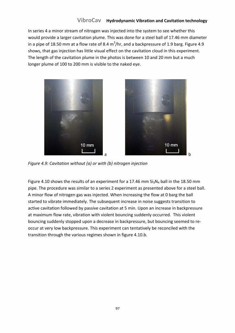
VibroCav Hydrodynamic Vibration and Cavitation technology
97
In series 4 a minor stream of nitrogen was injected into the system to see whether this
would provide a larger cavitation plume. This was done for a steel ball of 17.46 mm diameter
in a pipe of 18.50 mm at a flow rate of 8.4 m3/hr, and a backpressure of 1.9 barg. Figure 4.9
shows, that gas injection has little visual effect on the cavitation cloud in this experiment.
The length of the cavitation plume in the photos is between 10 and 20 mm but a much
longer plume of 100 to 200 mm is visible to the naked eye.
10 mm10 mm10 mm
a
10 mm10 mm10 mm
b
Figure 4.9: Cavitation without (a) or with (b) nitrogen injection
Figure 4.10 shows the results of an experiment for a 17.46 mm Si3N4 ball in the 18.50 mm
pipe. The procedure was similar to a series 2 experiment as presented above for a steel ball.
A minor flow of nitrogen gas was injected. When increasing the flow at 0 barg the ball
started to vibrate immediately. The subsequent increase in noise suggests transition to
active cavitation followed by passive cavitation at 5 min. Upon an increase in backpressure
at maximum flow rate, vibration with violent bouncing suddenly occurred. This violent
bouncing suddenly stopped upon a decrease in backpressure, but bouncing seemed to re‐
occur at very low backpressure. This experiment can tentatively be reconciled with the
transition through the various regimes shown in figure 4.10.b.
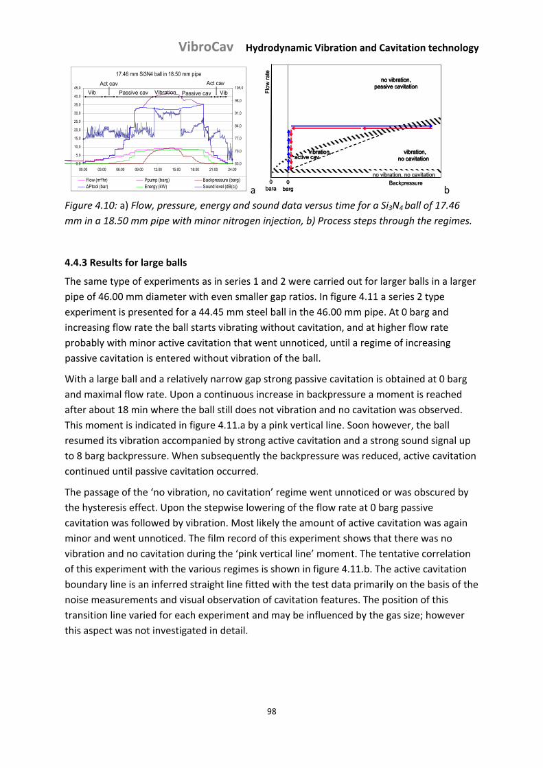
VibroCav Hydrodynamic Vibration and Cavitation technology
98
17.46 mm Si3N4 ball in 18.50 mm pipe
0,0
5,0
10,0
15,0
20,0
25,0
30,0
35,0
40,0
45,0
00:00 03:00 06:00 09:00 12:00 15:00 18:00 21:00 24:00
63,0
70,0
77,0
84,0
91,0
98,0
105,0
Flow (m³/hr) Ppump (barg) Backpressure (barg)ΔPtool (bar) Energy (kW) Sound level (dB(c))
Passive cav VibrationVib Passive cav VibAct cav Act cav
a 0
bara
Flow
rate
0 barg
vibration, no cavitation
no vibration, passive cavitation
Backpressure
vibration, active cav
no vibration, no cavitation0
bara
Flow
rate
0 barg
vibration, no cavitation
no vibration, passive cavitation
Backpressure
vibration, active cav
no vibration, no cavitation
b
Figure 4.10: a) Flow, pressure, energy and sound data versus time for a Si3N4 ball of 17.46
mm in a 18.50 mm pipe with minor nitrogen injection, b) Process steps through the regimes.
4.4.3 Results for large balls
The same type of experiments as in series 1 and 2 were carried out for larger balls in a larger
pipe of 46.00 mm diameter with even smaller gap ratios. In figure 4.11 a series 2 type
experiment is presented for a 44.45 mm steel ball in the 46.00 mm pipe. At 0 barg and
increasing flow rate the ball starts vibrating without cavitation, and at higher flow rate
probably with minor active cavitation that went unnoticed, until a regime of increasing
passive cavitation is entered without vibration of the ball.
With a large ball and a relatively narrow gap strong passive cavitation is obtained at 0 barg
and maximal flow rate. Upon a continuous increase in backpressure a moment is reached
after about 18 min where the ball still does not vibration and no cavitation was observed.
This moment is indicated in figure 4.11.a by a pink vertical line. Soon however, the ball
resumed its vibration accompanied by strong active cavitation and a strong sound signal up
to 8 barg backpressure. When subsequently the backpressure was reduced, active cavitation
continued until passive cavitation occurred.
The passage of the ‘no vibration, no cavitation’ regime went unnoticed or was obscured by
the hysteresis effect. Upon the stepwise lowering of the flow rate at 0 barg passive
cavitation was followed by vibration. Most likely the amount of active cavitation was again
minor and went unnoticed. The film record of this experiment shows that there was no
vibration and no cavitation during the ‘pink vertical line’ moment. The tentative correlation
of this experiment with the various regimes is shown in figure 4.11.b. The active cavitation
boundary line is an inferred straight line fitted with the test data primarily on the basis of the
noise measurements and visual observation of cavitation features. The position of this
transition line varied for each experiment and may be influenced by the gas size; however
this aspect was not investigated in detail.
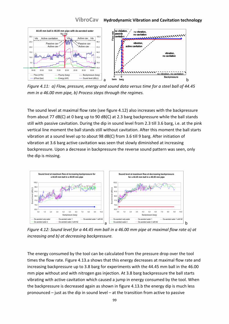
VibroCav Hydrodynamic Vibration and Cavitation technology
99
44.45 mm ball in 46.00 mm pipe with de-aerated water
0,0
5,0
10,0
15,0
20,0
25,0
30,0
00:00 05:00 10:00 15:00 20:00 25:00 30:00 35:00
63,0
70,0
77,0
84,0
91,0
98,0
105,0
Flow (m³/hr) Ppump (barg) Backpressure (barg)
ΔPtool (bar) Energy (kW) Sound level (dB(c))
Passive cav
Active cavVib Vib
No Vib
VibActive cavitation
Passive cavActive cavActive cav
a 0
bara
Flow
rate
0 barg
vibration, no cavitation
active cavitation
Backpressure
vibration,
no vibration, no cavitation
no vibration, passive cavitation
no vibration, no cavitation
0 bara
Flow
rate
0 barg
vibration, no cavitation
active cavitation
Backpressure
vibration,
no vibration, no cavitation
no vibration, passive cavitation
no vibration, no cavitation
b
Figure 4.11: a) Flow, pressure, energy and sound data versus time for a steel ball of 44.45
mm in a 46.00 mm pipe, b) Process steps through the regimes.
The sound level at maximal flow rate (see figure 4.12) also increases with the backpressure
from about 77 dB(C) at 0 barg up to 90 dB(C) at 2.3 barg backpressure while the ball stands
still with passive cavitation. During the dip in sound level from 2.3 till 3.6 barg, i.e. at the pink
vertical line moment the ball stands still without cavitation. After this moment the ball starts
vibration at a sound level up to about 98 dB(C) from 3.6 till 9 barg. After initiation of
vibration at 3.6 barg active cavitation was seen that slowly diminished at increasing
backpressure. Upon a decrease in backpressure the reverse sound pattern was seen, only
the dip is missing.
Sound level at maximum flow at increasing backpressure for a 44.45 mm ball in a 46.00 mm pipe
63,0
70,0
77,0
84,0
91,0
98,0
105,0
0,0 1,0 2,0 3,0 4,0 5,0 6,0 7,0 8,0 9,0 10,0
Backpressure (barg)
Sou
nd
leve
l (dB
(c))
De-aereted rusty water De-aereted water 1 De-aereted water 1 with N2
De-aereted water 2 De-aereted water 2 with N2
Sound level at maximum flow at increasing backpressure for a 44.45 mm ball in a 46.00 mm pipe
63,0
70,0
77,0
84,0
91,0
98,0
105,0
0,0 1,0 2,0 3,0 4,0 5,0 6,0 7,0 8,0 9,0 10,0
Backpressure (barg)
Sou
nd
leve
l (dB
(c))
De-aereted rusty water De-aereted water 1 De-aereted water 1 with N2
De-aereted water 2 De-aereted water 2 with N2 a
Sound level at maximum flow at decreasing backpressure for a 44.45 mm ball in a 46.00 mm pipe
63,0
70,0
77,0
84,0
91,0
98,0
105,0
0,0 1,0 2,0 3,0 4,0 5,0 6,0 7,0 8,0 9,0 10,0
Backpressure (barg)
Sou
nd le
vel (
dB(c
))
De-aereted rusty water De-aereted water 1 De-aereted water 1 with N2
De-aereted water 2 De-aereted water 2 with N2
Sound level at maximum flow at decreasing backpressure for a 44.45 mm ball in a 46.00 mm pipe
63,0
70,0
77,0
84,0
91,0
98,0
105,0
0,0 1,0 2,0 3,0 4,0 5,0 6,0 7,0 8,0 9,0 10,0
Backpressure (barg)
Sou
nd le
vel (
dB(c
))
De-aereted rusty water De-aereted water 1 De-aereted water 1 with N2
De-aereted water 2 De-aereted water 2 with N2 b
Figure 4.12: Sound level for a 44.45 mm ball in a 46.00 mm pipe at maximal flow rate a) at
increasing and b) at decreasing backpressure.
The energy consumed by the tool can be calculated from the pressure drop over the tool
times the flow rate. Figure 4.13.a shows that this energy decreases at maximal flow rate and
increasing backpressure up to 3.8 barg for experiments with the 44.45 mm ball in the 46.00
mm pipe without and with nitrogen gas injection. At 3.8 barg backpressure the ball starts
vibrating with active cavitation which caused a jump in energy consumed by the tool. When
the backpressure is decreased again as shown in figure 4.13.b the energy dip is much less
pronounced – just as the dip in sound level – at the transition from active to passive
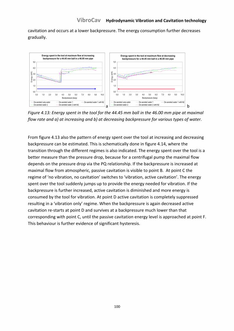
VibroCav Hydrodynamic Vibration and Cavitation technology
100
cavitation and occurs at a lower backpressure. The energy consumption further decreases
gradually.
Energy spent in the tool at maximum flow at increasing backpressure for a 44.45 mm ball in a 46.00 mm pipe
0,0
1,0
2,0
3,0
4,0
5,0
0,0 1,0 2,0 3,0 4,0 5,0 6,0 7,0 8,0 9,0 10,0
Backpressure (barg)
En
erg
y (k
W)
De-aereted rusty water De-aereted water 1 De-aereted water 1 with N2De-aereted water 2 De-aereted water 2 with N2
Energy spent in the tool at maximum flow at increasing backpressure for a 44.45 mm ball in a 46.00 mm pipe
0,0
1,0
2,0
3,0
4,0
5,0
0,0 1,0 2,0 3,0 4,0 5,0 6,0 7,0 8,0 9,0 10,0
Backpressure (barg)
En
erg
y (k
W)
De-aereted rusty water De-aereted water 1 De-aereted water 1 with N2De-aereted water 2 De-aereted water 2 with N2 a
Energy spent in the tool at maximum flow at decreasing backpressure for a 44.45 mm ball in a 46.00 mm pipe
0,0
1,0
2,0
3,0
4,0
5,0
0,0 1,0 2,0 3,0 4,0 5,0 6,0 7,0 8,0 9,0 10,0
Backpressure (barg)
En
erg
y (k
W)
De-aereted rusty water De-aereted water 1 De-aereted water 1 with N2De-aereted water 2 De-aereted water 2 with N2
Energy spent in the tool at maximum flow at decreasing backpressure for a 44.45 mm ball in a 46.00 mm pipe
0,0
1,0
2,0
3,0
4,0
5,0
0,0 1,0 2,0 3,0 4,0 5,0 6,0 7,0 8,0 9,0 10,0
Backpressure (barg)
En
erg
y (k
W)
De-aereted rusty water De-aereted water 1 De-aereted water 1 with N2De-aereted water 2 De-aereted water 2 with N2 b
Figure 4.13: Energy spent in the tool for the 44.45 mm ball in the 46.00 mm pipe at maximal
flow rate and a) at increasing and b) at decreasing backpressure for various types of water.
From figure 4.13 also the pattern of energy spent over the tool at increasing and decreasing
backpressure can be estimated. This is schematically done in figure 4.14, where the
transition through the different regimes is also indicated. The energy spent over the tool is a
better measure than the pressure drop, because for a centrifugal pump the maximal flow
depends on the pressure drop via the PQ relationship. If the backpressure is increased at
maximal flow from atmospheric, passive cavitation is visible to point B. At point C the
regime of ‘no vibration, no cavitation’ switches to ‘vibration, active cavitation’. The energy
spent over the tool suddenly jumps up to provide the energy needed for vibration. If the
backpressure is further increased, active cavitation is diminished and more energy is
consumed by the tool for vibration. At point D active cavitation is completely suppressed
resulting in a ‘vibration only’ regime. When the backpressure is again decreased active
cavitation re‐starts at point D and survives at a backpressure much lower than that
corresponding with point C, until the passive cavitation energy level is approached at point F.
This behaviour is further evidence of significant hysteresis.
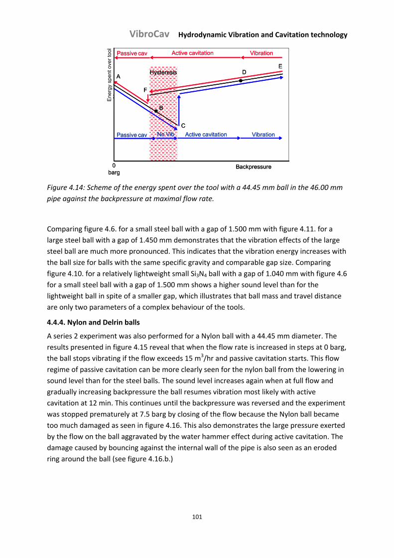
VibroCav Hydrodynamic Vibration and Cavitation technology
101
Ener
gy s
pend
ove
r too
l
0 barg
Backpressure
Hysteresis
No Vib Active cavitationPassive cav Vibration
Active cavitationPassive cav Vibration
B
AD
C
F
E
En
ergy
spe
nt o
ver
tool
Ener
gy s
pend
ove
r too
l
0 barg
Backpressure
Hysteresis
No Vib Active cavitationPassive cav Vibration
Active cavitationPassive cav Vibration
B
AD
C
F
E
En
ergy
spe
nt o
ver
tool
Figure 4.14: Scheme of the energy spent over the tool with a 44.45 mm ball in the 46.00 mm
pipe against the backpressure at maximal flow rate.
Comparing figure 4.6. for a small steel ball with a gap of 1.500 mm with figure 4.11. for a
large steel ball with a gap of 1.450 mm demonstrates that the vibration effects of the large
steel ball are much more pronounced. This indicates that the vibration energy increases with
the ball size for balls with the same specific gravity and comparable gap size. Comparing
figure 4.10. for a relatively lightweight small Si3N4 ball with a gap of 1.040 mm with figure 4.6
for a small steel ball with a gap of 1.500 mm shows a higher sound level than for the
lightweight ball in spite of a smaller gap, which illustrates that ball mass and travel distance
are only two parameters of a complex behaviour of the tools.
4.4.4. Nylon and Delrin balls
A series 2 experiment was also performed for a Nylon ball with a 44.45 mm diameter. The
results presented in figure 4.15 reveal that when the flow rate is increased in steps at 0 barg,
the ball stops vibrating if the flow exceeds 15 m3/hr and passive cavitation starts. This flow
regime of passive cavitation can be more clearly seen for the nylon ball from the lowering in
sound level than for the steel balls. The sound level increases again when at full flow and
gradually increasing backpressure the ball resumes vibration most likely with active
cavitation at 12 min. This continues until the backpressure was reversed and the experiment
was stopped prematurely at 7.5 barg by closing of the flow because the Nylon ball became
too much damaged as seen in figure 4.16. This also demonstrates the large pressure exerted
by the flow on the ball aggravated by the water hammer effect during active cavitation. The
damage caused by bouncing against the internal wall of the pipe is also seen as an eroded
ring around the ball (see figure 4.16.b.)
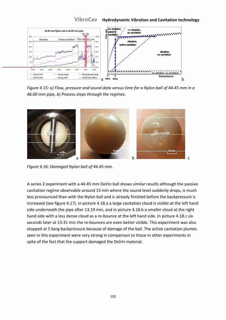
VibroCav Hydrodynamic Vibration and Cavitation technology
102
44.45 mm Nylon bal in 46.00 mm pipe
0,0
5,0
10,0
15,0
20,0
25,0
30,0
00:00 02:00 04:00 06:00 08:00 10:00 12:00 14:00
63,0
70,0
77,0
84,0
91,0
98,0
105,0
Flow (m³/hr) Ppump (barg) Backpressure (barg)
ΔPtool (bar) Energy (kW) Sound level (dB(c))
Act cavVibration Active cavitation
No Vib
Pas cav
44.45 mm Nylon bal in 46.00 mm pipe
0,0
5,0
10,0
15,0
20,0
25,0
30,0
00:00 02:00 04:00 06:00 08:00 10:00 12:00 14:00
63,0
70,0
77,0
84,0
91,0
98,0
105,0
Flow (m³/hr) Ppump (barg) Backpressure (barg)
ΔPtool (bar) Energy (kW) Sound level (dB(c))
Act cavVibration Active cavitation
No Vib
Pas cav
a 0
bara
Flow
rate
0 barg
vibration, no cavitation
active cavitation
Backpressure
vibration,
no vibration, no cavitation
no vibration, passive cavitation
no vibration, no cavitation
0 bara
Flow
rate
0 barg
vibration, no cavitation
active cavitation
Backpressure
vibration,
no vibration, no cavitation
no vibration, passive cavitation
no vibration, no cavitation
b
Figure 4.15: a) Flow, pressure and sound data versus time for a Nylon ball of 44.45 mm in a
46.00 mm pipe, b) Process steps through the regimes.
10 mm10 mm10 mm
a
10 mm10 mm10 mm
b
10 mm10 mm10 mm
c
Figure 4.16: Damaged Nylon ball of 44.45 mm.
A series 2 experiment with a 44.45 mm Delrin ball shows similar results although the passive
cavitation regime observable around 13 min where the sound level suddenly drops, is much
less pronounced than with the Nylon ball and is already finished before the backpressure is
increased (see figure 4.17). In picture 4.18.a a large cavitation cloud is visible at the left hand
side underneath the pipe after 13.19 min, and in picture 4.18.b a smaller cloud at the right
hand side with a less dense cloud as a re‐bounce at the left hand side. In picture 4.18.c six
seconds later at 13:31 min the re‐bounces are even better visible. This experiment was also
stopped at 5 barg backpressure because of damage of the ball. The active cavitation plumes
seen in this experiment were very strong in comparison to those in other experiments in
spite of the fact that the support damaged the Delrin material.
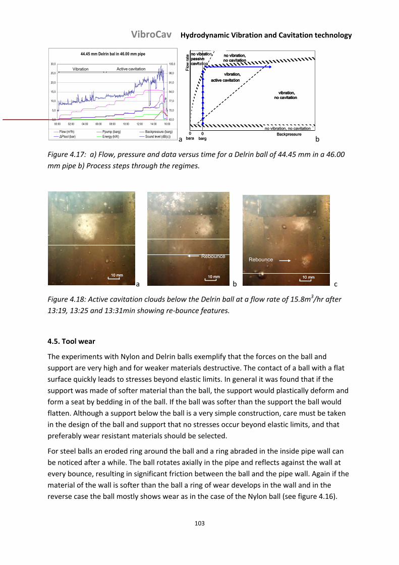
VibroCav Hydrodynamic Vibration and Cavitation technology
103
44.45 mm Delrin bal in 46.00 mm pipe
0,0
5,0
10,0
15,0
20,0
25,0
30,0
00:00 02:00 04:00 06:00 08:00 10:00 12:00 14:00 16:00
63,0
70,0
77,0
84,0
91,0
98,0
105,0
Flow (m³/h) Ppump (barg) Backpressure (barg)ΔPtool (bar) Energy (kW) Sound level (dB(c))
Active cavitationVibration
44.45 mm Delrin bal in 46.00 mm pipe
0,0
5,0
10,0
15,0
20,0
25,0
30,0
00:00 02:00 04:00 06:00 08:00 10:00 12:00 14:00 16:00
63,0
70,0
77,0
84,0
91,0
98,0
105,0
Flow (m³/h) Ppump (barg) Backpressure (barg)ΔPtool (bar) Energy (kW) Sound level (dB(c))
Active cavitationVibration
a 0
bara
Flow
rate
0 barg
vibration, no cavitation
active cavitation
Backpressure
vibration,
no vibration, no cavitation
no vibration, passive cavitation
no vibration, no cavitation
0 bara
Flow
rate
0 barg
vibration, no cavitation
active cavitation
Backpressure
vibration,
no vibration, no cavitation
no vibration, passive cavitation
no vibration, no cavitation
b
Figure 4.17: a) Flow, pressure and data versus time for a Delrin ball of 44.45 mm in a 46.00
mm pipe b) Process steps through the regimes.
10 mm10 mm10 mm
a 10 mm
Rebounce
10 mm10 mm
Rebounce
b 10 mm
Rebounce
10 mm10 mm
Rebounce
c
Figure 4.18: Active cavitation clouds below the Delrin ball at a flow rate of 15.8m3/hr after
13:19, 13:25 and 13:31min showing re‐bounce features.
4.5. Tool wear
The experiments with Nylon and Delrin balls exemplify that the forces on the ball and
support are very high and for weaker materials destructive. The contact of a ball with a flat
surface quickly leads to stresses beyond elastic limits. In general it was found that if the
support was made of softer material than the ball, the support would plastically deform and
form a seat by bedding in of the ball. If the ball was softer than the support the ball would
flatten. Although a support below the ball is a very simple construction, care must be taken
in the design of the ball and support that no stresses occur beyond elastic limits, and that
preferably wear resistant materials should be selected.
For steel balls an eroded ring around the ball and a ring abraded in the inside pipe wall can
be noticed after a while. The ball rotates axially in the pipe and reflects against the wall at
every bounce, resulting in significant friction between the ball and the pipe wall. Again if the
material of the wall is softer than the ball a ring of wear develops in the wall and in the
reverse case the ball mostly shows wear as in the case of the Nylon ball (see figure 4.16).
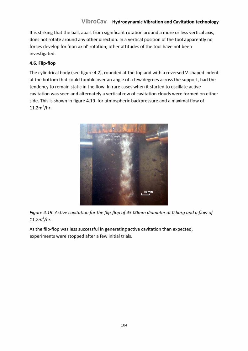
VibroCav Hydrodynamic Vibration and Cavitation technology
104
It is striking that the ball, apart from significant rotation around a more or less vertical axis,
does not rotate around any other direction. In a vertical position of the tool apparently no
forces develop for ‘non axial’ rotation; other attitudes of the tool have not been
investigated.
4.6. Flip‐flop
The cylindrical body (see figure 4.2), rounded at the top and with a reversed V‐shaped indent
at the bottom that could tumble over an angle of a few degrees across the support, had the
tendency to remain static in the flow. In rare cases when it started to oscillate active
cavitation was seen and alternately a vertical row of cavitation clouds were formed on either
side. This is shown in figure 4.19. for atmospheric backpressure and a maximal flow of
11.2m3/hr.
10 mm10 mm10 mm
Figure 4.19: Active cavitation for the flip‐flop of 45.00mm diameter at 0 barg and a flow of
11.2m3/hr.
As the flip‐flop was less successful in generating active cavitation than expected,
experiments were stopped after a few initial trials.
VibroCav Hydrodynamic Vibration and Cavitation technology
105
4.7. Conclusions
In this study the vibration and cavitation behaviour of a supported body freely
moving in lateral directions by the flow in a pipe was studied as a function of the flow
rate and the ambient or backpressure at various narrow gap sizes. The bouncing of
the body, mostly a ball made of steel, Nylon or Delrin, against the internal wall of the
steel pipe induced vibration of the pipe wall. For a given ball size, ball material and
gap ratio the occurrence of vibration with or without cavitation or merely of
cavitation depended on the flow rate and the backpressure.
Cavitation caused clouds of imploding bubbles downstream of the ball. Cavitation
could be either active cavitation if the vibration of the ball contributed through a
water hammer effect to the static pressure drop in the gap, or passive cavitation if
the flow rate in the gap sufficed to lower the static pressure below the vapour
pressure of the liquid. In case of passive cavitation the ball stood still. For active
cavitation clouds of bubbles were formed at either side of the ball, while for passive
cavitation the bubbles developed symmetrically around the ball. Because the ball was
totally accommodated inside the pipe, cavitation could only be observed if the
passing flow transported the bubbles out of the pipe.
At a given backpressure active cavitation could be induced at lower flow rates than
passive cavitation. Both active cavitation and passive cavitation were suppressed at
higher backpressures. Cavitation could however be achieved within the limits of this
50 bar test circuit up to about 10 bar. Vibration of the ball could be achieved up to
the maximal reachable backpressures of 10 bar at relatively low flow rates.
At a given gap size and backpressure various regimes were observed at increasing
flow rates: (i) no vibration and no cavitation at very low flow rates, (ii) vibration with
bouncing but without cavitation at higher flow rates, (iii) vibration with bouncing and
active cavitation and (iv) at still higher flow rates passive cavitation without vibration.
The flow rates needed to achieve active and passive cavitation increase substantially
at higher backpressures. Significant hysteresis is seen at all transitions between
regimes where the ball behaviour changes from no vibration into vibration or visa
versa.
The vibration energy increases with the ball size for balls with the same specific
gravity and comparable gap size. The energy is also larger for heavier balls of the
same size.
Because of the strong force exerted by the flow, the water hammer effect on the ball
and the rotation of the ball around its vertical axis, either the bottom area of the ball
is flattened or the support bar is deformed by stresses beyond the elastic limits of the
material and by wear. Flattening of the ball and/or deformation of the support
hamper free movement of the ball in the flow. For weaker ball materials as Nylon or
VibroCav Hydrodynamic Vibration and Cavitation technology
106
Delrin the bottom of the ball even showed an indent from the support. Bouncing of
the ball against the internal pipe wall during vibration caused a ring of wear either on
the wall or the ball or both.
Supported bodies hamper an early observation of either active or passive cavitation.
A body such as a ball hanging on a filament is therefore better suited, especially
when the bottom end of the ball is hanging just inside or slightly outside of the pipe.
4.8. References
1. Karlikov, V.P ; Rechichenko, N.T. ; Sholomovich, G.I. ; Fluid Dynamics; Vol. 35; No 2
(2000)
2. Brennen, C.E. ; Oxfd Uni Press (1995)
3. Franzini, J.B.; Finnemore, E.J.; Chapter 12 in “Fluid Mechanics with Engineering
applications”, 9th ed. 1997, McGraw‐Hill
4. Ivannikov, V.I. ; Ivannikov, I.V. ; Patent US 6705396 (2004)Patent Ivannikov

VibroCav Hydrodynamic Vibration and Cavitation technology
107
VibroCav Hydrodynamic Vibration and Cavitation technology
108
Chapter 5: Cavitation and vibration by flow along a hanging ball in a conical
housing in a 50 bar test circuit
5.1. Introduction
In Chapter 4 the behaviour of a supported ball that can move laterally by the passing flow in
a straight vertical pipe with a narrow gap between the ball and the pipe wall was studied.
This was done for balls of various sizes and densities at different downstream pressures in
the chamber downstream of the pipe. The study was focused on the identification of
regimes where upon a change in behaviour of the ball different physical phenomena such as
vibration/bouncing of the ball ‐ with or without cavitation ‐ occurred that could support
different applications.
It was observed that a certain minimal flow rate is required to induce vibration of the ball in
conjunction with its bouncing against the pipe wall, the onset of which is signalled by a
strong increase in acoustic sound. The collisions of the ball with the pipe cause vibrations in
the pipe wall. From the tool pressure waves are then emitted into the surrounding liquid.
For condensed fluids cavitation can be observed in regions of higher flow rates due to the
increased pressure drop in the gap next to the ball, and imploding cavitation bubbles are
transported by the flow downstream of the gap. Two types of cavitation can be
distinguished; so‐called active cavitation where the body vibrates in the pipe and so‐called
passive cavitation where the body stands still.
The regimes with active and with passive cavitation are indicated in figure 5.1 that is
composed from observations made in Chapter 4. For passive cavitation the flow rate must
suffice to decrease the static pressure in the gap below the vapour pressure of the liquid.
Cavitation bubbles will then nucleate and grow in the gap during their further transport. For
active cavitation the pressure drop in the gap is partially provided by a water hammer effect
caused by vibration of the body. By bouncing against the wall the body frequently cuts off
part of the flow stream.
From the regime chart in figure 5.1 it can be seen that the transition line for passive
cavitation follows a parabolic relationship as the increase in dynamic pressure required to
lower the static pressure below vapour pressure relates to the square of the fluid velocity,
hence flow rate, as can also be calculated from the pressure coefficient and the cavitation
number. The transition between active cavitation and vibration is expected to be a straight
line because the occurrence of active cavitation is induced by water hammer effects that are
straight proportional to fluid velocity. The vibration regime thus widens up at higher
backpressures.
At high flow rates and backpressures a regime exists without vibration of the ball and
without any cavitation. This probably happens when the turbulence in the wake of the ball
becomes too high (above the critical Re number) to sustain the lift forces needed for
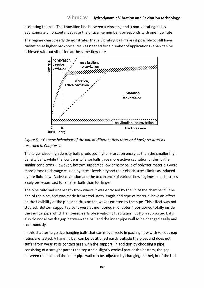
VibroCav Hydrodynamic Vibration and Cavitation technology
109
oscillating the ball. This transition line between a vibrating and a non‐vibrating ball is
approximately horizontal because the critical Re number corresponds with one flow rate.
The regime chart clearly demonstrates that a vibrating ball makes it possible to still have
cavitation at higher backpressures ‐ as needed for a number of applications ‐ than can be
achieved without vibration at the same flow rate.
no vibration, no cavitation0
bara
Flow
rate
0 barg
vibration, no cavitation
Backpressure
vibration, active cavitation
no vibration, passive cavitation
no vibration, no cavitation
no vibration, no cavitation0
bara
Flow
rate
0 barg
vibration, no cavitation
Backpressure
vibration, active cavitation
no vibration, passive cavitation
no vibration, no cavitation
Figure 5.1: Generic behaviour of the ball at different flow rates and backpressures as
recorded in Chapter 4.
The larger sized high density balls produced higher vibration energies than the smaller high
density balls, while the low density large balls gave more active cavitation under further
similar conditions. However, bottom supported low density balls of polymer materials were
more prone to damage caused by stress levels beyond their elastic stress limits as induced
by the fluid flow. Active cavitation and the occurrence of various flow regimes could also less
easily be recognized for smaller balls than for larger.
The pipe only had one length from where it was enclosed by the lid of the chamber till the
end of the pipe, and was made from steel. Both length and type of material have an effect
on the flexibility of the pipe and thus on the waves emitted by the pipe. This effect was not
studied. Bottom supported balls were as mentioned in Chapter 4 positioned totally inside
the vertical pipe which hampered early observation of cavitation. Bottom supported balls
also do not allow the gap between the ball and the inner pipe wall to be changed easily and
continuously.
In this chapter large size hanging balls that can move freely in passing flow with various gap
ratios are tested. A hanging ball can be positioned partly outside the pipe, and does not
suffer from wear at its contact area with the support. In addition by choosing a pipe
consisting of a straight part at the top and a slightly conical part at the bottom, the gap
between the ball and the inner pipe wall can be adjusted by changing the height of the ball
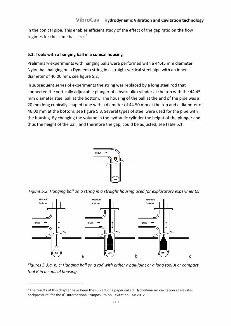
VibroCav Hydrodynamic Vibration and Cavitation technology
110
in the conical pipe. This enables efficient study of the effect of the gap ratio on the flow
regimes for the same ball size. 1
5.2. Tools with a hanging ball in a conical housing
Preliminary experiments with hanging balls were performed with a 44.45 mm diameter
Nylon ball hanging on a Dyneema string in a straight vertical steel pipe with an inner
diameter of 46.00 mm, see figure 5.2.
In subsequent series of experiments the string was replaced by a long steel rod that
connected the vertically adjustable plunger of a hydraulic cylinder at the top with the 44.45
mm diameter steel ball at the bottom. The housing of the ball at the end of the pipe was a
20 mm long conically shaped tube with a diameter of 44.50 mm at the top and a diameter of
46.00 mm at the bottom, see figure 5.3. Several types of steel were used for the pipe with
the housing. By changing the volume in the hydraulic cylinder the height of the plunger and
thus the height of the ball, and therefore the gap, could be adjusted, see table 5.1.
FLOW
Ball
FLOW
Ball
Figure 5.2: Hanging ball on a string in a straight housing used for exploratory experiments.
FLOW
Hydraulic
Cylinder
Ball
FLOW
Hydraulic
Cylinder
Balla
FLOW
Ball
Hydraulic
Cylinder
FLOW
Ball
Hydraulic
Cylinder
b
FLOW
Ball
Hydraulic
Cylinder
FLOW
Ball
Hydraulic
Cylinder
c
Figures 5.3.a, b, c: Hanging ball on a rod with either a ball‐joint or a long tool A or compact
tool B in a conical housing.
1 The results of this chapter have been the subject of a paper called ‘Hydrodynamic cavitation at elevated backpressure’ for the 8th International Symposium on Cavitation CAV 2012
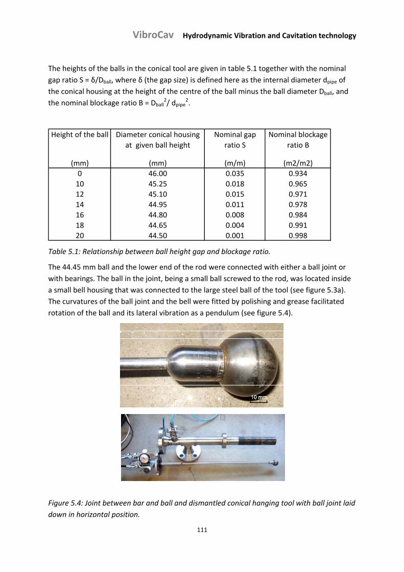
VibroCav Hydrodynamic Vibration and Cavitation technology
111
The heights of the balls in the conical tool are given in table 5.1 together with the nominal
gap ratio S = δ/Dball, where δ (the gap size) is defined here as the internal diameter dpipe of
the conical housing at the height of the centre of the ball minus the ball diameter Dball, and
the nominal blockage ratio B = Dball2/ dpipe
2.
Height of the ball Diameter conical housing
at given ball height
Nominal gap
ratio S
Nominal blockage
ratio B
(mm) (mm) (m/m) (m2/m2)
0 46.00 0.035 0.934
10 45.25 0.018 0.965
12 45.10 0.015 0.971
14 44.95 0.011 0.978
16 44.80 0.008 0.984
18 44.65 0.004 0.991
20 44.50 0.001 0.998
Table 5.1: Relationship between ball height gap and blockage ratio.
The 44.45 mm ball and the lower end of the rod were connected with either a ball joint or
with bearings. The ball in the joint, being a small ball screwed to the rod, was located inside
a small bell housing that was connected to the large steel ball of the tool (see figure 5.3a).
The curvatures of the ball joint and the bell were fitted by polishing and grease facilitated
rotation of the ball and its lateral vibration as a pendulum (see figure 5.4).
10 mm10 mm10 mm
Figure 5.4: Joint between bar and ball and dismantled conical hanging tool with ball joint laid
down in horizontal position.
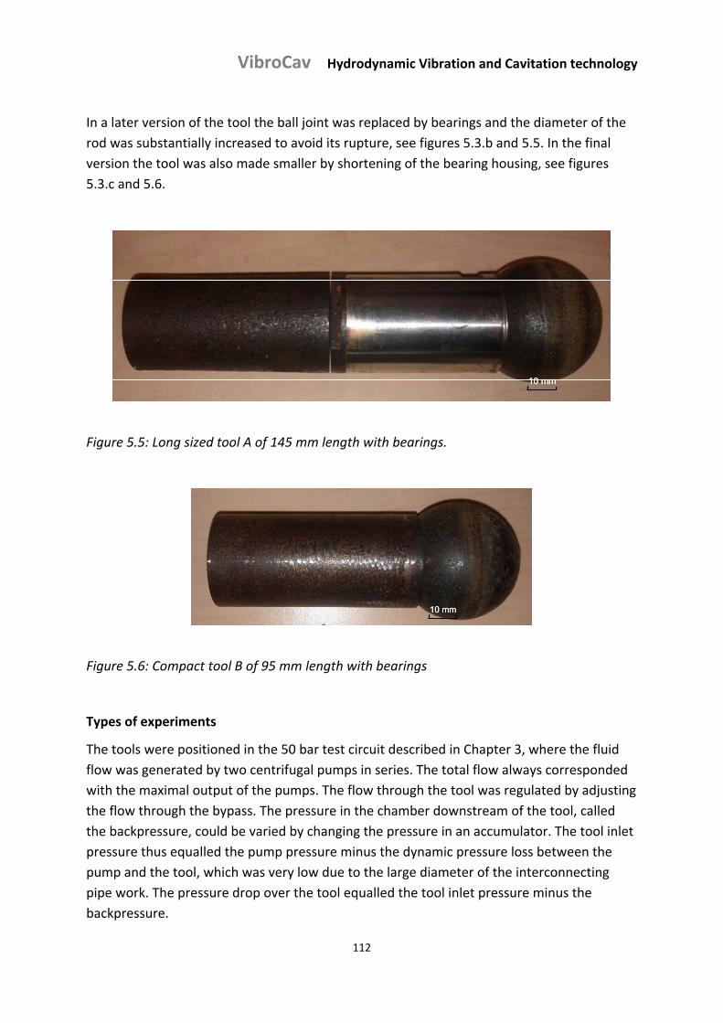
VibroCav Hydrodynamic Vibration and Cavitation technology
112
In a later version of the tool the ball joint was replaced by bearings and the diameter of the
rod was substantially increased to avoid its rupture, see figures 5.3.b and 5.5. In the final
version the tool was also made smaller by shortening of the bearing housing, see figures
5.3.c and 5.6.
10 mm10 mm10 mm
Figure 5.5: Long sized tool A of 145 mm length with bearings.
10 mm10 mm10 mm
Figure 5.6: Compact tool B of 95 mm length with bearings
Types of experiments
The tools were positioned in the 50 bar test circuit described in Chapter 3, where the fluid
flow was generated by two centrifugal pumps in series. The total flow always corresponded
with the maximal output of the pumps. The flow through the tool was regulated by adjusting
the flow through the bypass. The pressure in the chamber downstream of the tool, called
the backpressure, could be varied by changing the pressure in an accumulator. The tool inlet
pressure thus equalled the pump pressure minus the dynamic pressure loss between the
pump and the tool, which was very low due to the large diameter of the interconnecting
pipe work. The pressure drop over the tool equalled the tool inlet pressure minus the
backpressure.
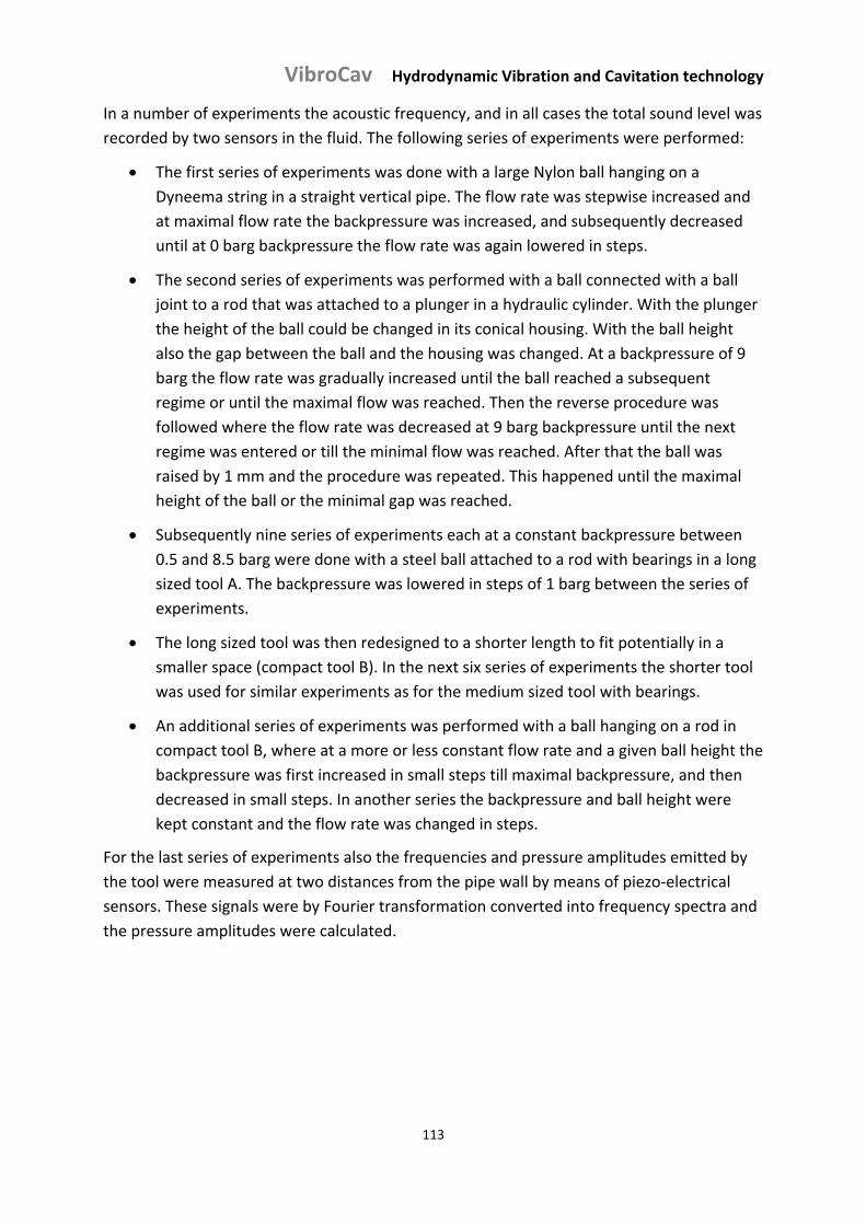
VibroCav Hydrodynamic Vibration and Cavitation technology
113
In a number of experiments the acoustic frequency, and in all cases the total sound level was
recorded by two sensors in the fluid. The following series of experiments were performed:
The first series of experiments was done with a large Nylon ball hanging on a
Dyneema string in a straight vertical pipe. The flow rate was stepwise increased and
at maximal flow rate the backpressure was increased, and subsequently decreased
until at 0 barg backpressure the flow rate was again lowered in steps.
The second series of experiments was performed with a ball connected with a ball
joint to a rod that was attached to a plunger in a hydraulic cylinder. With the plunger
the height of the ball could be changed in its conical housing. With the ball height
also the gap between the ball and the housing was changed. At a backpressure of 9
barg the flow rate was gradually increased until the ball reached a subsequent
regime or until the maximal flow was reached. Then the reverse procedure was
followed where the flow rate was decreased at 9 barg backpressure until the next
regime was entered or till the minimal flow was reached. After that the ball was
raised by 1 mm and the procedure was repeated. This happened until the maximal
height of the ball or the minimal gap was reached.
Subsequently nine series of experiments each at a constant backpressure between
0.5 and 8.5 barg were done with a steel ball attached to a rod with bearings in a long
sized tool A. The backpressure was lowered in steps of 1 barg between the series of
experiments.
The long sized tool was then redesigned to a shorter length to fit potentially in a
smaller space (compact tool B). In the next six series of experiments the shorter tool
was used for similar experiments as for the medium sized tool with bearings.
An additional series of experiments was performed with a ball hanging on a rod in
compact tool B, where at a more or less constant flow rate and a given ball height the
backpressure was first increased in small steps till maximal backpressure, and then
decreased in small steps. In another series the backpressure and ball height were
kept constant and the flow rate was changed in steps.
For the last series of experiments also the frequencies and pressure amplitudes emitted by
the tool were measured at two distances from the pipe wall by means of piezo‐electrical
sensors. These signals were by Fourier transformation converted into frequency spectra and
the pressure amplitudes were calculated.
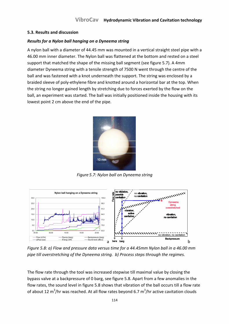
VibroCav Hydrodynamic Vibration and Cavitation technology
114
5.3. Results and discussion
Results for a Nylon ball hanging on a Dyneema string
A nylon ball with a diameter of 44.45 mm was mounted in a vertical straight steel pipe with a
46.00 mm inner diameter. The Nylon ball was flattened at the bottom and rested on a steel
support that matched the shape of the missing ball segment (see figure 5.7). A 4mm
diameter Dyneema string with a tensile strength of 7500 N went through the centre of the
ball and was fastened with a knot underneath the support. The string was enclosed by a
braided sleeve of poly‐ethylene fibre and knotted around a horizontal bar at the top. When
the string no longer gained length by stretching due to forces exerted by the flow on the
ball, an experiment was started. The ball was initially positioned inside the housing with its
lowest point 2 cm above the end of the pipe.
10 mm10 mm10 mm
Figure 5.7: Nylon ball on Dyneema string
63,0
70,0
77,0
84,0
91,0
98,0
105,0
0,0
5,0
10,0
15,0
20,0
25,0
30,0
00:00 05:00 10:00 15:00 20:00
Nylon ball hanging on a Dyneema string
Flow (m³/hr) Ppump (barg) Backpressure (barg)ΔPtool (bar) Energy (kW) Sound level (dB(c))
a 0
bara
Flow
rate
0 barg
vibration, no cavitation
Backpressure
no vibration, passive cavitation
no vibration, no cavitation
vibration, active
cavitation
no vibration, no cavitation
Dyneemastring
overstretched
0 bara
Flow
rate
0 barg
vibration, no cavitation
Backpressure
no vibration, passive cavitation
no vibration, no cavitation
vibration, active
cavitation
no vibration, no cavitation0
bara
Flow
rate
0 barg
vibration, no cavitation
Backpressure
no vibration, passive cavitation
no vibration, no cavitation
vibration, active
cavitation
no vibration, no cavitation
Dyneemastring
overstretched
b
Figure 5.8: a) Flow and pressure data versus time for a 44.45mm Nylon ball in a 46.00 mm
pipe till overstretching of the Dyneema string. b) Process steps through the regimes.
The flow rate through the tool was increased stepwise till maximal value by closing the
bypass valve at a backpressure of 0 barg, see figure 5.8. Apart from a few anomalies in the
flow rates, the sound level in figure 5.8 shows that vibration of the ball occurs till a flow rate
of about 12 m3/hr was reached. At all flow rates beyond 6.7 m3/hr active cavitation clouds
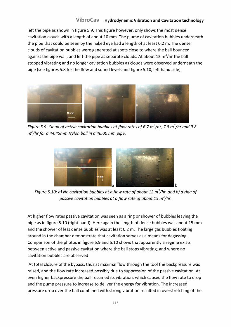
VibroCav Hydrodynamic Vibration and Cavitation technology
115
left the pipe as shown in figure 5.9. This figure however, only shows the most dense
cavitation clouds with a length of about 10 mm. The plume of cavitation bubbles underneath
the pipe that could be seen by the naked eye had a length of at least 0.2 m. The dense
clouds of cavitation bubbles were generated at spots close to where the ball bounced
against the pipe wall, and left the pipe as separate clouds. At about 12 m3/hr the ball
stopped vibrating and no longer cavitation bubbles as clouds were observed underneath the
pipe (see figures 5.8 for the flow and sound levels and figure 5.10, left hand side).
10 mm10 mm10 mm
Figure 5.9: Cloud of active cavitation bubbles at flow rates of 6.7 m3/hr, 7.8 m3/hr and 9.8
m3/hr for a 44.45mm Nylon ball in a 46.00 mm pipe.
10 mm10 mm10 mm
a b
Figure 5.10: a) No cavitation bubbles at a flow rate of about 12 m3/hr and b) a ring of
passive cavitation bubbles at a flow rate of about 15 m3/hr.
At higher flow rates passive cavitation was seen as a ring or shower of bubbles leaving the
pipe as in figure 5.10 (right hand). Here again the length of dense bubbles was about 15 mm
and the shower of less dense bubbles was at least 0.2 m. The large gas bubbles floating
around in the chamber demonstrate that cavitation serves as a means for degassing.
Comparison of the photos in figure 5.9 and 5.10 shows that apparently a regime exists
between active and passive cavitation where the ball stops vibrating, and where no
cavitation bubbles are observed
At total closure of the bypass, thus at maximal flow through the tool the backpressure was
raised, and the flow rate increased possibly due to suppression of the passive cavitation. At
even higher backpressure the ball resumed its vibration, which caused the flow rate to drop
and the pump pressure to increase to deliver the energy for vibration. The increased
pressure drop over the ball combined with strong vibration resulted in overstretching of the
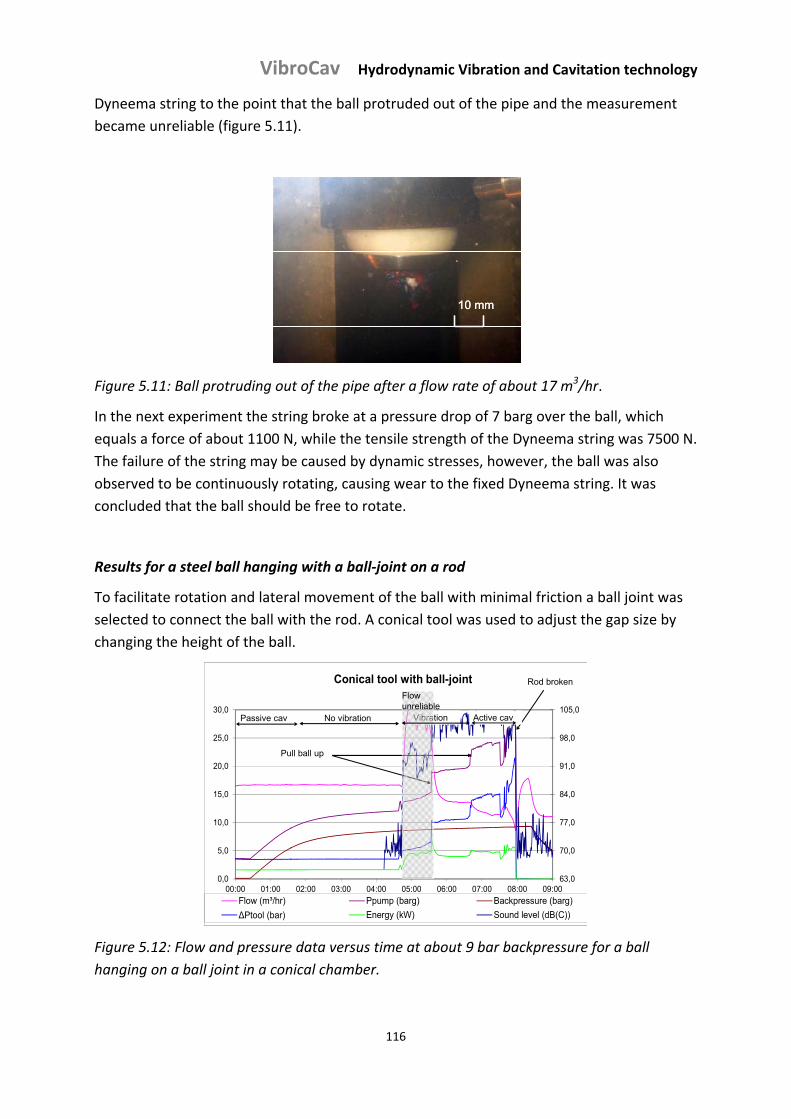
VibroCav Hydrodynamic Vibration and Cavitation technology
116
Dyneema string to the point that the ball protruded out of the pipe and the measurement
became unreliable (figure 5.11).
10 mm10 mm10 mm
Figure 5.11: Ball protruding out of the pipe after a flow rate of about 17 m3/hr.
In the next experiment the string broke at a pressure drop of 7 barg over the ball, which
equals a force of about 1100 N, while the tensile strength of the Dyneema string was 7500 N.
The failure of the string may be caused by dynamic stresses, however, the ball was also
observed to be continuously rotating, causing wear to the fixed Dyneema string. It was
concluded that the ball should be free to rotate.
Results for a steel ball hanging with a ball‐joint on a rod
To facilitate rotation and lateral movement of the ball with minimal friction a ball joint was
selected to connect the ball with the rod. A conical tool was used to adjust the gap size by
changing the height of the ball.
63,0
70,0
77,0
84,0
91,0
98,0
105,0
0,0
5,0
10,0
15,0
20,0
25,0
30,0
00:00 01:00 02:00 03:00 04:00 05:00 06:00 07:00 08:00 09:00
Conical tool with ball-joint
Flow (m³/hr) Ppump (barg) Backpressure (barg)
ΔPtool (bar) Energy (kW) Sound level (dB(C))
Pull ball up
Rod broken
Active cavPassive cav VibrationNo vibration
Flow unreliable
Figure 5.12: Flow and pressure data versus time at about 9 bar backpressure for a ball
hanging on a ball joint in a conical chamber.
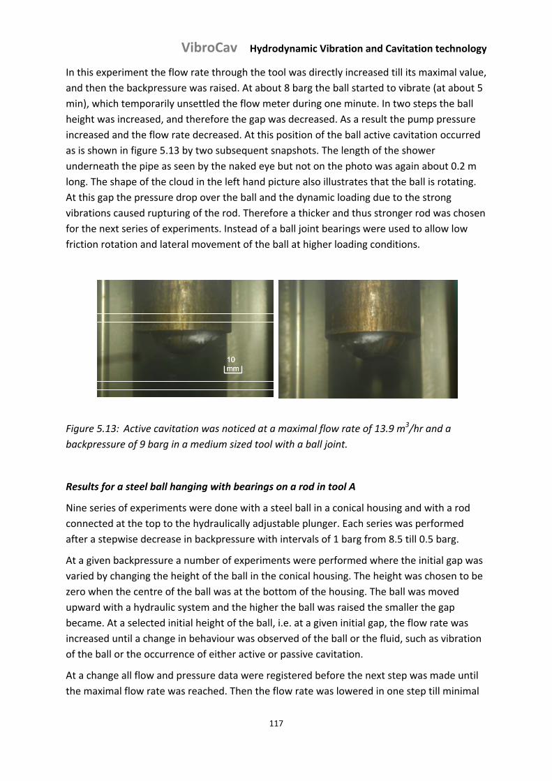
VibroCav Hydrodynamic Vibration and Cavitation technology
117
In this experiment the flow rate through the tool was directly increased till its maximal value,
and then the backpressure was raised. At about 8 barg the ball started to vibrate (at about 5
min), which temporarily unsettled the flow meter during one minute. In two steps the ball
height was increased, and therefore the gap was decreased. As a result the pump pressure
increased and the flow rate decreased. At this position of the ball active cavitation occurred
as is shown in figure 5.13 by two subsequent snapshots. The length of the shower
underneath the pipe as seen by the naked eye but not on the photo was again about 0.2 m
long. The shape of the cloud in the left hand picture also illustrates that the ball is rotating.
At this gap the pressure drop over the ball and the dynamic loading due to the strong
vibrations caused rupturing of the rod. Therefore a thicker and thus stronger rod was chosen
for the next series of experiments. Instead of a ball joint bearings were used to allow low
friction rotation and lateral movement of the ball at higher loading conditions.
10 mm10 mm10 mm
Figure 5.13: Active cavitation was noticed at a maximal flow rate of 13.9 m3/hr and a
backpressure of 9 barg in a medium sized tool with a ball joint.
Results for a steel ball hanging with bearings on a rod in tool A
Nine series of experiments were done with a steel ball in a conical housing and with a rod
connected at the top to the hydraulically adjustable plunger. Each series was performed
after a stepwise decrease in backpressure with intervals of 1 barg from 8.5 till 0.5 barg.
At a given backpressure a number of experiments were performed where the initial gap was
varied by changing the height of the ball in the conical housing. The height was chosen to be
zero when the centre of the ball was at the bottom of the housing. The ball was moved
upward with a hydraulic system and the higher the ball was raised the smaller the gap
became. At a selected initial height of the ball, i.e. at a given initial gap, the flow rate was
increased until a change in behaviour was observed of the ball or the fluid, such as vibration
of the ball or the occurrence of either active or passive cavitation.
At a change all flow and pressure data were registered before the next step was made until
the maximal flow rate was reached. Then the flow rate was lowered in one step till minimal
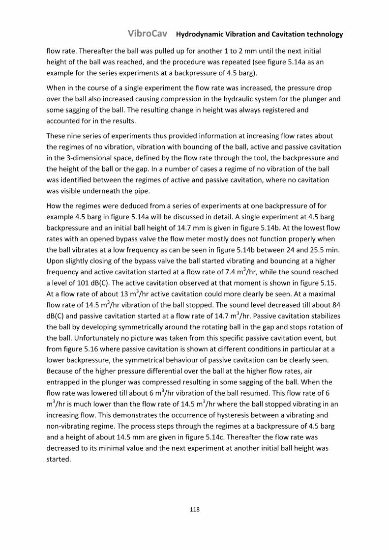
VibroCav Hydrodynamic Vibration and Cavitation technology
118
flow rate. Thereafter the ball was pulled up for another 1 to 2 mm until the next initial
height of the ball was reached, and the procedure was repeated (see figure 5.14a as an
example for the series experiments at a backpressure of 4.5 barg).
When in the course of a single experiment the flow rate was increased, the pressure drop
over the ball also increased causing compression in the hydraulic system for the plunger and
some sagging of the ball. The resulting change in height was always registered and
accounted for in the results.
These nine series of experiments thus provided information at increasing flow rates about
the regimes of no vibration, vibration with bouncing of the ball, active and passive cavitation
in the 3‐dimensional space, defined by the flow rate through the tool, the backpressure and
the height of the ball or the gap. In a number of cases a regime of no vibration of the ball
was identified between the regimes of active and passive cavitation, where no cavitation
was visible underneath the pipe.
How the regimes were deduced from a series of experiments at one backpressure of for
example 4.5 barg in figure 5.14a will be discussed in detail. A single experiment at 4.5 barg
backpressure and an initial ball height of 14.7 mm is given in figure 5.14b. At the lowest flow
rates with an opened bypass valve the flow meter mostly does not function properly when
the ball vibrates at a low frequency as can be seen in figure 5.14b between 24 and 25.5 min.
Upon slightly closing of the bypass valve the ball started vibrating and bouncing at a higher
frequency and active cavitation started at a flow rate of 7.4 m3/hr, while the sound reached
a level of 101 dB(C). The active cavitation observed at that moment is shown in figure 5.15.
At a flow rate of about 13 m3/hr active cavitation could more clearly be seen. At a maximal
flow rate of 14.5 m3/hr vibration of the ball stopped. The sound level decreased till about 84
dB(C) and passive cavitation started at a flow rate of 14.7 m3/hr. Passive cavitation stabilizes
the ball by developing symmetrically around the rotating ball in the gap and stops rotation of
the ball. Unfortunately no picture was taken from this specific passive cavitation event, but
from figure 5.16 where passive cavitation is shown at different conditions in particular at a
lower backpressure, the symmetrical behaviour of passive cavitation can be clearly seen.
Because of the higher pressure differential over the ball at the higher flow rates, air
entrapped in the plunger was compressed resulting in some sagging of the ball. When the
flow rate was lowered till about 6 m3/hr vibration of the ball resumed. This flow rate of 6
m3/hr is much lower than the flow rate of 14.5 m3/hr where the ball stopped vibrating in an
increasing flow. This demonstrates the occurrence of hysteresis between a vibrating and
non‐vibrating regime. The process steps through the regimes at a backpressure of 4.5 barg
and a height of about 14.5 mm are given in figure 5.14c. Thereafter the flow rate was
decreased to its minimal value and the next experiment at another initial ball height was
started.
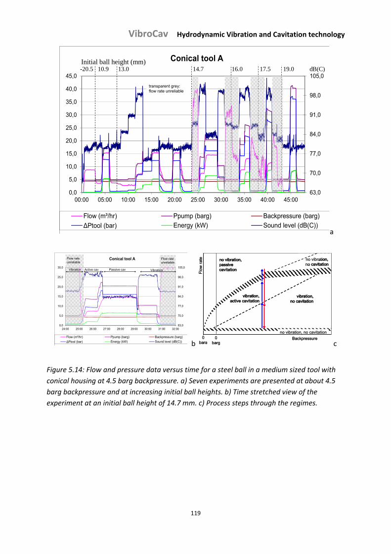
VibroCav Hydrodynamic Vibration and Cavitation technology
119
63,0
70,0
77,0
84,0
91,0
98,0
105,0
0,0
5,0
10,0
15,0
20,0
25,0
30,0
35,0
40,0
45,0
00:00 05:00 10:00 15:00 20:00 25:00 30:00 35:00 40:00 45:00
Conical tool A
Flow (m³/hr) Ppump (barg) Backpressure (barg)
ΔPtool (bar) Energy (kW) Sound level (dB(C))
Initial ball height (mm)-20.5 10.9 13.0 14.7 16.0 17.5 19.0 dB(C)
transparent grey: flow rate unreliable
a
63,0
70,0
77,0
84,0
91,0
98,0
105,0
0,0
5,0
10,0
15,0
20,0
25,0
30,0
24:00 25:00 26:00 27:00 28:00 29:00 30:00 31:00 32:00
Conical tool A
Flow (m³/hr) Ppump (barg) Backpressure (barg)
ΔPtool (bar) Energy (kW) Sound level (dB(C))
Flow rate unreliable
Flow rate unreliable
Active cav Passive cav VibrationVibration
b 0
bara
Flow
rate
0 barg
vibration, no cavitation
vibration,active cavitation
no vibration, passive cavitation
Backpressure
no vibration, no cavitation
no vibration, no cavitation0
bara
Flow
rate
0 barg
vibration, no cavitation
vibration,active cavitation
no vibration, passive cavitation
Backpressure
no vibration, no cavitation
no vibration, no cavitation
c
Figure 5.14: Flow and pressure data versus time for a steel ball in a medium sized tool with
conical housing at 4.5 barg backpressure. a) Seven experiments are presented at about 4.5
barg backpressure and at increasing initial ball heights. b) Time stretched view of the
experiment at an initial ball height of 14.7 mm. c) Process steps through the regimes.
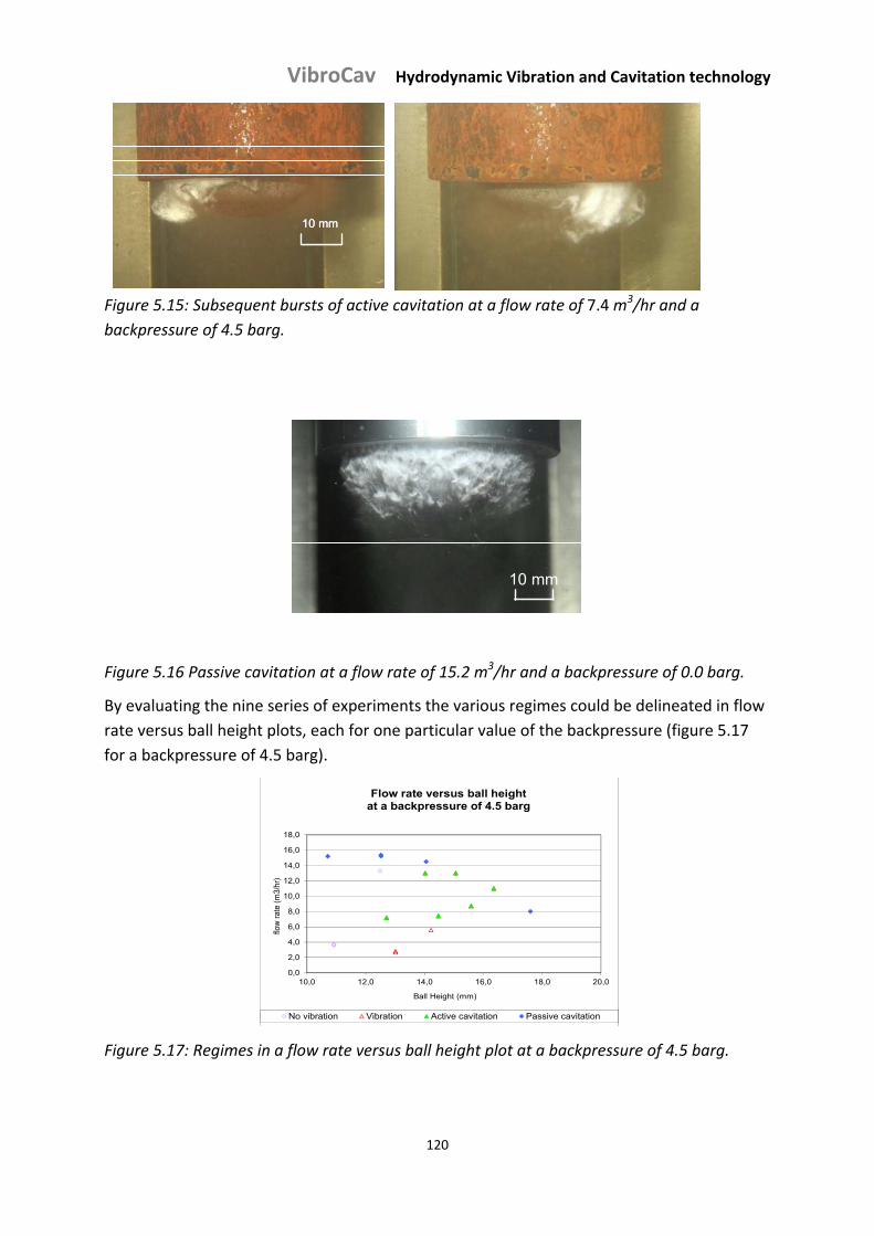
VibroCav Hydrodynamic Vibration and Cavitation technology
120
10 mm10 mm10 mm
Figure 5.15: Subsequent bursts of active cavitation at a flow rate of 7.4 m3/hr and a
backpressure of 4.5 barg.
10 mm10 mm
Figure 5.16 Passive cavitation at a flow rate of 15.2 m3/hr and a backpressure of 0.0 barg.
By evaluating the nine series of experiments the various regimes could be delineated in flow
rate versus ball height plots, each for one particular value of the backpressure (figure 5.17
for a backpressure of 4.5 barg).
0,0
2,0
4,0
6,0
8,0
10,0
12,0
14,0
16,0
18,0
10,0 12,0 14,0 16,0 18,0 20,0
flow
rat
e (m
3/hr
)
Ball Height (mm)
Flow rate versus ball height at a backpressure of 4.5 barg
No vibration Vibration Active cavitation Passive cavitation
Figure 5.17: Regimes in a flow rate versus ball height plot at a backpressure of 4.5 barg.
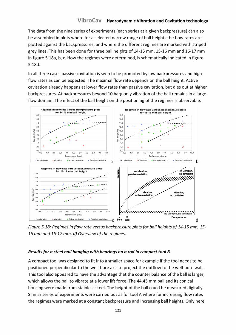
VibroCav Hydrodynamic Vibration and Cavitation technology
121
The data from the nine series of experiments (each series at a given backpressure) can also
be assembled in plots where for a selected narrow range of ball heights the flow rates are
plotted against the backpressures, and where the different regimes are marked with striped
grey lines. This has been done for three ball heights of 14‐15 mm, 15‐16 mm and 16‐17 mm
in figure 5.18a, b, c. How the regimes were determined, is schematically indicated in figure
5.18d.
In all three cases passive cavitation is seen to be promoted by low backpressures and high
flow rates as can be expected. The maximal flow rate depends on the ball height. Active
cavitation already happens at lower flow rates than passive cavitation, but dies out at higher
backpressures. At backpressures beyond 10 barg only vibration of the ball remains in a large
flow domain. The effect of the ball height on the positioning of the regimes is observable.
0,0
2,0
4,0
6,0
8,0
10,0
12,0
14,0
16,0
18,0
0,0 1,0 2,0 3,0 4,0 5,0 6,0 7,0 8,0 9,0 10,0
flow
rat
e (m
3/hr
)
Backpressure (barg)
Regimes in flow rate versus backpressure plots for 14-15 mm ball height
No vibration Vibration Active cavitation Passive cavitation a
0,0
2,0
4,0
6,0
8,0
10,0
12,0
14,0
16,0
18,0
0,0 1,0 2,0 3,0 4,0 5,0 6,0 7,0 8,0 9,0 10,0
flow
rat
e (m
3/hr
)
Backpressure (barg)
Regimes in flow rate versus backpressure plots for 15-16 mm ball height
No vibration Vibration Active cavitation Passive cavitation b
0,0
2,0
4,0
6,0
8,0
10,0
12,0
14,0
16,0
18,0
0,0 1,0 2,0 3,0 4,0 5,0 6,0 7,0 8,0 9,0 10,0
flow
rate
(m3/
hr)
Backpressure (barg)
Regimes in flow rate versus backpressure plots for 16-17 mm ball height
No vibration Vibration Active cavitation Passive cavitation c 0
bara
Flow
rate
0 barg
vibration, no cavitation
vibration,active cavitation
no vibration, passive cavitation
Backpressure
no vibration, no cavitation
no vibration, no cavitation0
bara
Flow
rate
0 barg
vibration, no cavitation
vibration,active cavitation
no vibration, passive cavitation
Backpressure
no vibration, no cavitation
no vibration, no cavitation
d
Figure 5.18: Regimes in flow rate versus backpressure plots for ball heights of 14‐15 mm, 15‐
16 mm and 16‐17 mm. d) Overview of the regimes.
Results for a steel ball hanging with bearings on a rod in compact tool B
A compact tool was designed to fit into a smaller space for example if the tool needs to be
positioned perpendicular to the well‐bore axis to project the outflow to the well‐bore wall.
This tool also appeared to have the advantage that the counter balance of the ball is larger,
which allows the ball to vibrate at a lower lift force. The 44.45 mm ball and its conical
housing were made from stainless steel. The height of the ball could be measured digitally.
Similar series of experiments were carried out as for tool A where for increasing flow rates
the regimes were marked at a constant backpressure and increasing ball heights. Only here
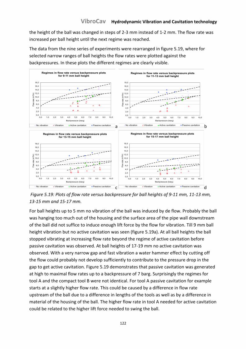
VibroCav Hydrodynamic Vibration and Cavitation technology
122
the height of the ball was changed in steps of 2‐3 mm instead of 1‐2 mm. The flow rate was
increased per ball height until the next regime was reached.
The data from the nine series of experiments were rearranged in figure 5.19, where for
selected narrow ranges of ball heights the flow rates were plotted against the
backpressures. In these plots the different regimes are clearly visible.
0,0
2,0
4,0
6,0
8,0
10,0
12,0
14,0
16,0
18,0
0,0 1,0 2,0 3,0 4,0 5,0 6,0 7,0 8,0 9,0 10,0
Flow
rat
e (m
³/hr)
Backpressure (barg)
Regimes in flow rate versus backpressure plots for 9-11 mm ball height
No vibration Vibration Active cavitation Passive cavitation a
0,0
2,0
4,0
6,0
8,0
10,0
12,0
14,0
16,0
18,0
0,0 1,0 2,0 3,0 4,0 5,0 6,0 7,0 8,0 9,0 10,0
Flo
w r
ate
(m³/h
r)Backpressure (barg)
Regimes in flow rate versus backpressure plots for 11-13 mm ball height
No vibration Vibration Active cavitation Passive cavitation b
0,0
2,0
4,0
6,0
8,0
10,0
12,0
14,0
16,0
18,0
0,0 1,0 2,0 3,0 4,0 5,0 6,0 7,0 8,0 9,0 10,0
Flow
rat
e (m
³/hr)
Backpressure (barg)
Regimes in flow rate versus backpressure plots for 13-15 mm ball height
No vibration Vibration Active cavitation Passive cavitation c
0,0
2,0
4,0
6,0
8,0
10,0
12,0
14,0
16,0
18,0
0,0 1,0 2,0 3,0 4,0 5,0 6,0 7,0 8,0 9,0 10,0
Flo
w r
ate
(m³/
hr)
Backpressure (barg)
Regimes in flow rate versus backpressure plots for 15-17 mm ball height
No vibration Vibration Active cavitation Passive cavitation d
Figure 5.19: Plots of flow rate versus backpressure for ball heights of 9‐11 mm, 11‐13 mm,
13‐15 mm and 15‐17 mm.
For ball heights up to 5 mm no vibration of the ball was induced by de flow. Probably the ball
was hanging too much out of the housing and the surface area of the pipe wall downstream
of the ball did not suffice to induce enough lift force by the flow for vibration. Till 9 mm ball
height vibration but no active cavitation was seen (figure 5.19a). At all ball heights the ball
stopped vibrating at increasing flow rate beyond the regime of active cavitation before
passive cavitation was observed. At ball heights of 17‐19 mm no active cavitation was
observed. With a very narrow gap and fast vibration a water hammer effect by cutting off
the flow could probably not develop sufficiently to contribute to the pressure drop in the
gap to get active cavitation. Figure 5.19 demonstrates that passive cavitation was generated
at high to maximal flow rates up to a backpressure of 7 barg. Surprisingly the regimes for
tool A and the compact tool B were not identical. For tool A passive cavitation for example
starts at a slightly higher flow rate. This could be caused by a difference in flow rate
upstream of the ball due to a difference in lengths of the tools as well as by a difference in
material of the housing of the ball. The higher flow rate in tool A needed for active cavitation
could be related to the higher lift force needed to swing the ball.
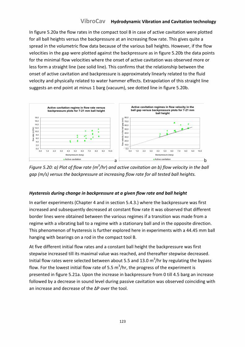
VibroCav Hydrodynamic Vibration and Cavitation technology
123
In figure 5.20a the flow rates in the compact tool B in case of active cavitation were plotted
for all ball heights versus the backpressure at an increasing flow rate. This gives quite a
spread in the volumetric flow data because of the various ball heights. However, if the flow
velocities in the gap were plotted against the backpressure as in figure 5.20b the data points
for the minimal flow velocities where the onset of active cavitation was observed more or
less form a straight line (see solid line). This confirms that the relationship between the
onset of active cavitation and backpressure is approximately linearly related to the fluid
velocity and physically related to water hammer effects. Extrapolation of this straight line
suggests an end point at minus 1 barg (vacuum), see dotted line in figure 5.20b.
0,0
2,0
4,0
6,0
8,0
10,0
12,0
14,0
16,0
18,0
0,0 1,0 2,0 3,0 4,0 5,0 6,0 7,0 8,0 9,0 10,0
flow
rat
e (m
3/hr
)
Backpressure (barg)
Active cavitation regime in flow rate versus backpressure plots for 7-21 mm ball height
Active cavitation a
0,0
10,0
20,0
30,0
40,0
50,0
60,0
70,0
80,0
0,0 1,0 2,0 3,0 4,0 5,0 6,0 7,0 8,0 9,0 10,0
flow
vel
ocity
in th
e ba
ll ga
p (m
/s)
Backpressure (barg)
Active cavitation regimes in flow velocity in the ball gap versus backpressure plots for 7-21 mm
ball height
Active cavitation b
Figure 5.20: a) Plot of flow rate (m3/hr) and active cavitation an b) flow velocity in the ball
gap (m/s) versus the backpressure at increasing flow rate for all tested ball heights.
Hysteresis during change in backpressure at a given flow rate and ball height
In earlier experiments (Chapter 4 and in section 5.4.3.) where the backpressure was first
increased and subsequently decreased at constant flow rate it was observed that different
border lines were obtained between the various regimes if a transition was made from a
regime with a vibrating ball to a regime with a stationary ball and in the opposite direction.
This phenomenon of hysteresis is further explored here in experiments with a 44.45 mm ball
hanging with bearings on a rod in the compact tool B.
At five different initial flow rates and a constant ball height the backpressure was first
stepwise increased till its maximal value was reached, and thereafter stepwise decreased.
Initial flow rates were selected between about 5.5 and 13.0 m3/hr by regulating the bypass
flow. For the lowest initial flow rate of 5.5 m3/hr, the progress of the experiment is
presented in figure 5.21a. Upon the increase in backpressure from 0 till 4.5 barg an increase
followed by a decrease in sound level during passive cavitation was observed coinciding with
an increase and decrease of the ΔP over the tool.
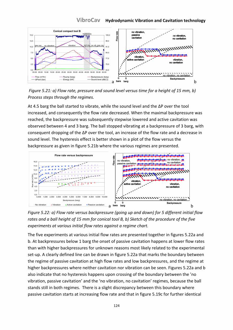
VibroCav Hydrodynamic Vibration and Cavitation technology
124
63,0
70,0
77,0
84,0
91,0
98,0
105,0
0,0
2,5
5,0
7,5
10,0
12,5
15,0
00:00 05:00 10:00 15:00 20:00 25:00 30:00 35:00 40:00 45:00 50:00 55:00 00:00
Conical compact tool B
Flow (m³/hr) Ppump (barg) Backpressure (barg)ΔPtool (bar) Energy (kW) Sound level (dB(C))
hysteresis
pas cavact cavvibrationno vibrationpas cav no vib
a 0
bara
Flow
rate
0 barg
vibration, no cavitation
vibration,active cavitation
no vibration, passive cavitation
Backpressure
no vibration, no cavitation
no vibration, no cavitation0
bara
Flow
rate
0 barg
vibration, no cavitation
vibration,active cavitation
no vibration, passive cavitation
Backpressure
no vibration, no cavitation
no vibration, no cavitation
b
Figure 5.21: a) Flow rate, pressure and sound level versus time for a height of 15 mm, b)
Process steps through the regimes.
At 4.5 barg the ball started to vibrate, while the sound level and the ΔP over the tool
increased, and consequently the flow rate decreased. When the maximal backpressure was
reached, the backpressure was subsequently stepwise lowered and active cavitation was
observed between 4 and 3 barg. The ball stopped vibrating at a backpressure of 3 barg, with
consequent dropping of the ΔP over the tool, an increase of the flow rate and a decrease in
sound level. The hysteresis effect is better shown in a plot of the flow versus the
backpressure as given in figure 5.21b where the various regimes are presented.
0,0
2,0
4,0
6,0
8,0
10,0
12,0
14,0
16,0
0,000 1,000 2,000 3,000 4,000 5,000 6,000 7,000 8,000 9,000 10,000
flow
rat
e (m
3/hr
)
Backpressure (barg)
Flow rate versus backpressure
No vibration Vibration Active cavitation Passive cavitation a 0
bara
Flow
rate
0 barg
vibration, no cavitation
vibration,active cavitation
Backpressure
no vibration, no cavitation
no vibration, passive cavitation
no vibration, no cavitation0
bara
Flow
rate
0 barg
vibration, no cavitation
vibration,active cavitation
Backpressure
no vibration, no cavitation
no vibration, passive cavitation
no vibration, no cavitation
b
Figure 5.22: a) Flow rate versus backpressure (going up and down) for 5 different initial flow
rates and a ball height of 15 mm for conical tool B, b) Sketch of the procedure of the five
experiments at various initial flow rates against a regime chart.
The five experiments at various initial flow rates are presented together in figures 5.22a and
b. At backpressures below 1 barg the onset of passive cavitation happens at lower flow rates
than with higher backpressures for unknown reasons most likely related to the experimental
set‐up. A clearly defined line can be drawn in figure 5.22a that marks the boundary between
the regime of passive cavitation at high flow rates and low backpressures, and the regime at
higher backpressures where neither cavitation nor vibration can be seen. Figures 5.22a and b
also indicate that no hysteresis happens upon crossing of the boundary between the ’no
vibration, passive cavitation’ and the ‘no vibration, no cavitation’ regimes, because the ball
stands still in both regimes. There is a slight discrepancy between this boundary where
passive cavitation starts at increasing flow rate and that in figure 5.19c for further identical
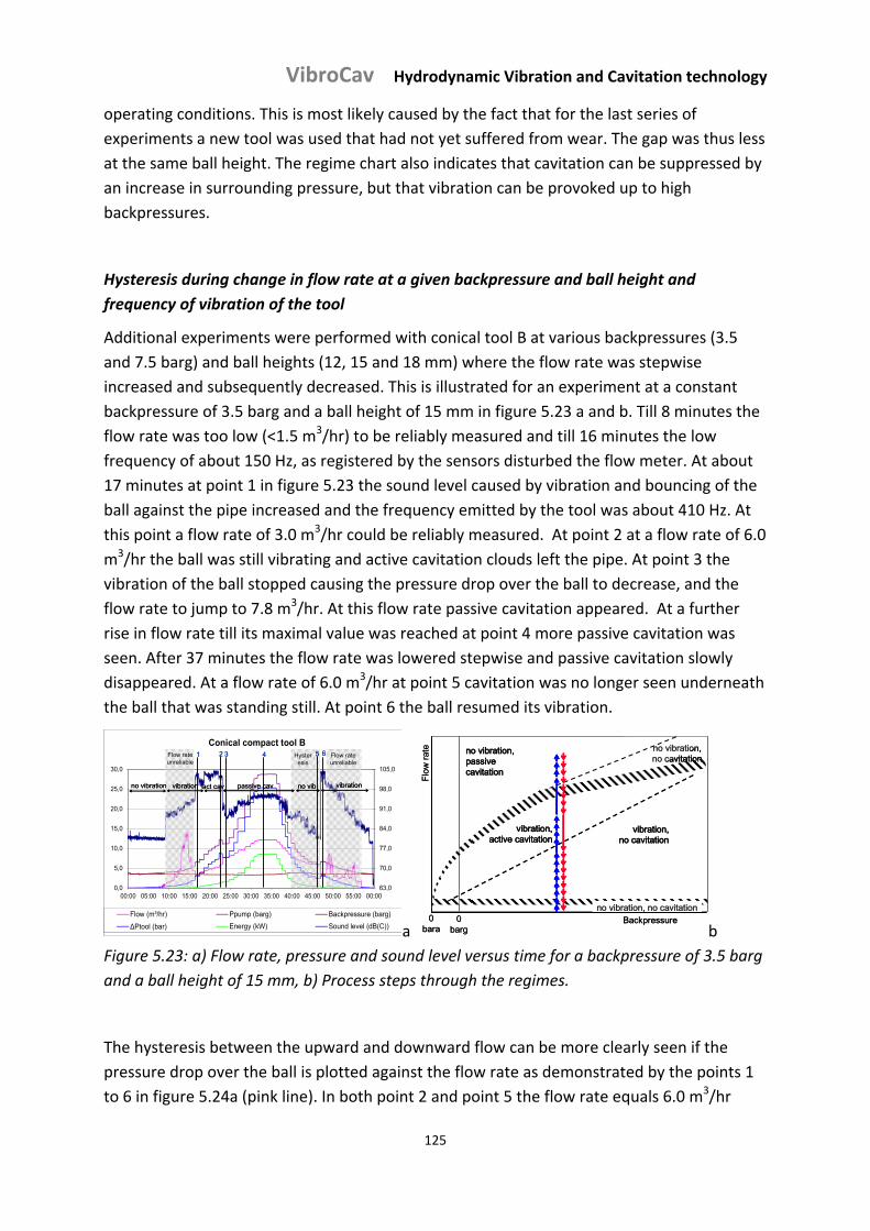
VibroCav Hydrodynamic Vibration and Cavitation technology
125
operating conditions. This is most likely caused by the fact that for the last series of
experiments a new tool was used that had not yet suffered from wear. The gap was thus less
at the same ball height. The regime chart also indicates that cavitation can be suppressed by
an increase in surrounding pressure, but that vibration can be provoked up to high
backpressures.
Hysteresis during change in flow rate at a given backpressure and ball height and
frequency of vibration of the tool
Additional experiments were performed with conical tool B at various backpressures (3.5
and 7.5 barg) and ball heights (12, 15 and 18 mm) where the flow rate was stepwise
increased and subsequently decreased. This is illustrated for an experiment at a constant
backpressure of 3.5 barg and a ball height of 15 mm in figure 5.23 a and b. Till 8 minutes the
flow rate was too low (<1.5 m3/hr) to be reliably measured and till 16 minutes the low
frequency of about 150 Hz, as registered by the sensors disturbed the flow meter. At about
17 minutes at point 1 in figure 5.23 the sound level caused by vibration and bouncing of the
ball against the pipe increased and the frequency emitted by the tool was about 410 Hz. At
this point a flow rate of 3.0 m3/hr could be reliably measured. At point 2 at a flow rate of 6.0
m3/hr the ball was still vibrating and active cavitation clouds left the pipe. At point 3 the
vibration of the ball stopped causing the pressure drop over the ball to decrease, and the
flow rate to jump to 7.8 m3/hr. At this flow rate passive cavitation appeared. At a further
rise in flow rate till its maximal value was reached at point 4 more passive cavitation was
seen. After 37 minutes the flow rate was lowered stepwise and passive cavitation slowly
disappeared. At a flow rate of 6.0 m3/hr at point 5 cavitation was no longer seen underneath
the ball that was standing still. At point 6 the ball resumed its vibration.
63,0
70,0
77,0
84,0
91,0
98,0
105,0
0,0
5,0
10,0
15,0
20,0
25,0
30,0
00:00 05:00 10:00 15:00 20:00 25:00 30:00 35:00 40:00 45:00 50:00 55:00 00:00
Conical compact tool B
Flow (m³/hr) Ppump (barg) Backpressure (barg)
ΔPtool (bar) Energy (kW) Sound level (dB(C))
Hysteresis
1 2 3 4 5 6Flow rate unreliable
Flow rate unreliable
passive cavact cavno vibration no vibvibration vibration
63,0
70,0
77,0
84,0
91,0
98,0
105,0
0,0
5,0
10,0
15,0
20,0
25,0
30,0
00:00 05:00 10:00 15:00 20:00 25:00 30:00 35:00 40:00 45:00 50:00 55:00 00:00
Conical compact tool B
Flow (m³/hr) Ppump (barg) Backpressure (barg)
ΔPtool (bar) Energy (kW) Sound level (dB(C))
Hysteresis
1 2 3 4 5 61 2 3 4 5 6Flow rate unreliable
Flow rate unreliable
passive cavact cavno vibration no vibvibration vibrationpassive cavact cavno vibration no vibvibration vibration
a 0
bara
Flow
rate
0 barg
vibration, no cavitation
vibration,active cavitation
no vibration, passive cavitation
Backpressure
no vibration, no cavitation
no vibration, no cavitation0
bara
Flow
rate
0 barg
vibration, no cavitation
vibration,active cavitation
no vibration, passive cavitation
Backpressure
no vibration, no cavitation
no vibration, no cavitation
b
Figure 5.23: a) Flow rate, pressure and sound level versus time for a backpressure of 3.5 barg
and a ball height of 15 mm, b) Process steps through the regimes.
The hysteresis between the upward and downward flow can be more clearly seen if the
pressure drop over the ball is plotted against the flow rate as demonstrated by the points 1
to 6 in figure 5.24a (pink line). In both point 2 and point 5 the flow rate equals 6.0 m3/hr
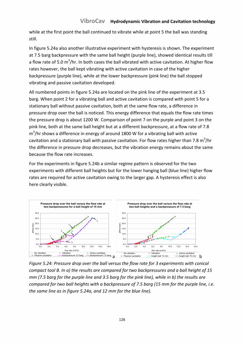
VibroCav Hydrodynamic Vibration and Cavitation technology
126
while at the first point the ball continued to vibrate while at point 5 the ball was standing
still.
In figure 5.24a also another illustrative experiment with hysteresis is shown. The experiment
at 7.5 barg backpressure with the same ball height (purple line), showed identical results till
a flow rate of 5.0 m3/hr. In both cases the ball vibrated with active cavitation. At higher flow
rates however, the ball kept vibrating with active cavitation in case of the higher
backpressure (purple line), while at the lower backpressure (pink line) the ball stopped
vibrating and passive cavitation developed.
All numbered points in figure 5.24a are located on the pink line of the experiment at 3.5
barg. When point 2 for a vibrating ball and active cavitation is compared with point 5 for a
stationary ball without passive cavitation, both at the same flow rate, a difference in
pressure drop over the ball is noticed. This energy difference that equals the flow rate times
the pressure drop is about 1200 W. Comparison of point 7 on the purple and point 3 on the
pink line, both at the same ball height but at a different backpressure, at a flow rate of 7.8
m3/hr shows a difference in energy of around 1800 W for a vibrating ball with active
cavitation and a stationary ball with passive cavitation. For flow rates higher than 7.8 m3/hr
the difference in pressure drop decreases, but the vibration energy remains about the same
because the flow rate increases.
For the experiments in figure 5.24b a similar regime pattern is observed for the two
experiments with different ball heights but for the lower hanging ball (blue line) higher flow
rates are required for active cavitation owing to the larger gap. A hysteresis effect is also
here clearly visible.
0,0
5,0
10,0
15,0
20,0
25,0
30,0
0,0 2,0 4,0 6,0 8,0 10,0 12,0 14,0 16,0
ΔP
tool
(ba
r)
flow rate (m3/hr)
Pressure drop over the ball versus the flow rate at two backpressures for a ball height of 15 mm
No vibration Vibration Active cavitationPassive cavitation backpressure 3,5 barg backpressure 7,5 barg
1
2 3
4
56
7
a
0,0
5,0
10,0
15,0
20,0
25,0
30,0
0,0 2,0 4,0 6,0 8,0 10,0 12,0 14,0 16,0
ΔP
tool
(ba
r)
flow rate (m3/hr)
Pressure drop over the ball versus the flow rate at two ball heights and a backpressure of 7.5 barg
No vibration Vibration Active cavitationPassive cavitation height ball 12 mm height ball 15 mm
0,0
5,0
10,0
15,0
20,0
25,0
30,0
0,0 2,0 4,0 6,0 8,0 10,0 12,0 14,0 16,0
ΔP
tool
(ba
r)
flow rate (m3/hr)
Pressure drop over the ball versus the flow rate at two ball heights and a backpressure of 7.5 barg
No vibration Vibration Active cavitationPassive cavitation height ball 12 mm height ball 15 mm b
Figure 5.24: Pressure drop over the ball versus the flow rate for 3 experiments with conical
compact tool B. In a) the results are compared for two backpressures and a ball height of 15
mm (7.5 barg for the purple line and 3.5 barg for the pink line), while in b) the results are
compared for two ball heights with a backpressure of 7.5 barg (15 mm for the purple line, i.e.
the same line as in figure 5.24a, and 12 mm for the blue line).
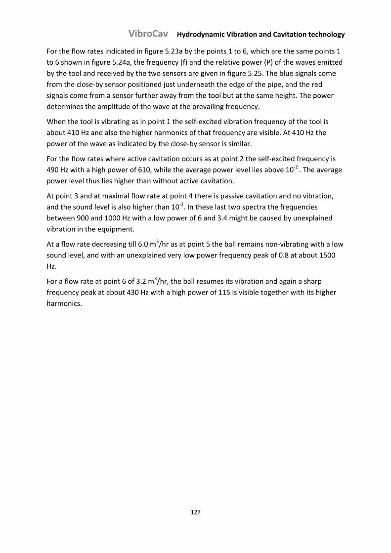
VibroCav Hydrodynamic Vibration and Cavitation technology
127
For the flow rates indicated in figure 5.23a by the points 1 to 6, which are the same points 1
to 6 shown in figure 5.24a, the frequency (f) and the relative power (P) of the waves emitted
by the tool and received by the two sensors are given in figure 5.25. The blue signals come
from the close‐by sensor positioned just underneath the edge of the pipe, and the red
signals come from a sensor further away from the tool but at the same height. The power
determines the amplitude of the wave at the prevailing frequency.
When the tool is vibrating as in point 1 the self‐excited vibration frequency of the tool is
about 410 Hz and also the higher harmonics of that frequency are visible. At 410 Hz the
power of the wave as indicated by the close‐by sensor is similar.
For the flow rates where active cavitation occurs as at point 2 the self‐excited frequency is
490 Hz with a high power of 610, while the average power level lies above 10‐2 . The average
power level thus lies higher than without active cavitation.
At point 3 and at maximal flow rate at point 4 there is passive cavitation and no vibration,
and the sound level is also higher than 10‐2. In these last two spectra the frequencies
between 900 and 1000 Hz with a low power of 6 and 3.4 might be caused by unexplained
vibration in the equipment.
At a flow rate decreasing till 6.0 m3/hr as at point 5 the ball remains non‐vibrating with a low
sound level, and with an unexplained very low power frequency peak of 0.8 at about 1500
Hz.
For a flow rate at point 6 of 3.2 m3/hr, the ball resumes its vibration and again a sharp
frequency peak at about 430 Hz with a high power of 115 is visible together with its higher
harmonics.
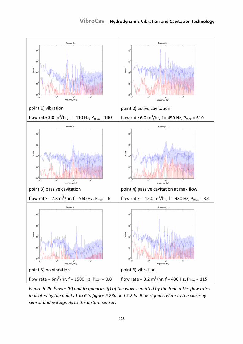
VibroCav Hydrodynamic Vibration and Cavitation technology
128
101
102
103
104
10-6
10-4
10-2
100
102
Fourier plot
frequency (Hz)
Pow
er
point 1) vibration
flow rate 3.0 m3/hr, f = 410 Hz, Pmax = 130
101
102
103
104
10-6
10-4
10-2
100
102
Fourier plot
frequency (Hz)
Pow
er
point 2) active cavitation
flow rate 6.0 m3/hr, f = 490 Hz, Pmax = 610
101
102
103
104
10-6
10-4
10-2
100
102
Fourier plot
frequency (Hz)
Pow
er
point 3) passive cavitation
flow rate = 7.8 m3/hr, f = 960 Hz, Pmax = 6
101
102
103
104
10-6
10-4
10-2
100
102
Fourier plot
frequency (Hz)
Pow
er
point 4) passive cavitation at max flow
flow rate = 12.0 m3/hr, f = 980 Hz, Pmax = 3.4
101
102
103
104
10-6
10-4
10-2
100
102
Fourier plot
frequency (Hz)
Pow
er
point 5) no vibration
flow rate = 6m3/hr, f = 1500 Hz, Pmax = 0.8
101
102
103
104
10-6
10-4
10-2
100
102
Fourier plot
frequency (Hz)
Pow
er
point 6) vibration
flow rate = 3.2 m3/hr, f = 430 Hz, Pmax = 115
Figure 5.25: Power (P) and frequencies (f) of the waves emitted by the tool at the flow rates
indicated by the points 1 to 6 in figure 5.23a and 5.24a. Blue signals relate to the close‐by
sensor and red signals to the distant sensor.
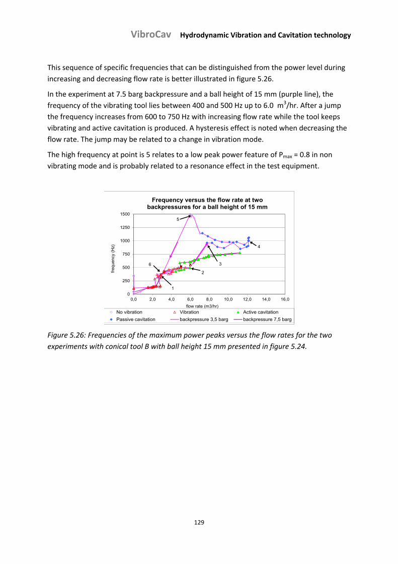
VibroCav Hydrodynamic Vibration and Cavitation technology
129
This sequence of specific frequencies that can be distinguished from the power level during
increasing and decreasing flow rate is better illustrated in figure 5.26.
In the experiment at 7.5 barg backpressure and a ball height of 15 mm (purple line), the
frequency of the vibrating tool lies between 400 and 500 Hz up to 6.0 m3/hr. After a jump
the frequency increases from 600 to 750 Hz with increasing flow rate while the tool keeps
vibrating and active cavitation is produced. A hysteresis effect is noted when decreasing the
flow rate. The jump may be related to a change in vibration mode.
The high frequency at point is 5 relates to a low peak power feature of Pmax = 0.8 in non
vibrating mode and is probably related to a resonance effect in the test equipment.
0
250
500
750
1000
1250
1500
0,0 2,0 4,0 6,0 8,0 10,0 12,0 14,0 16,0
freq
uenc
y (H
z)
flow rate (m3/hr)
Frequency versus the flow rate at two backpressures for a ball height of 15 mm
No vibration Vibration Active cavitation
Passive cavitation backpressure 3,5 barg backpressure 7,5 barg
1
2
3
4
5
6
Figure 5.26: Frequencies of the maximum power peaks versus the flow rates for the two
experiments with conical tool B with ball height 15 mm presented in figure 5.24.
VibroCav Hydrodynamic Vibration and Cavitation technology
130
5.4. Conclusions
From the results the following conclusions could be drawn:
A hanging ball also offers the opportunity to use a conical housing instead of a straight one, where the gap can be adjusted by the positioning of the hanging ball in the housing. Another advantage of a hanging ball is the elimination of wear and damage caused by the bottom support.
Experiments with a hanging ball have provided a much better insight in the behaviour
of the tools because the occurrence of cavitation and of vibration and rotation of the
ball could be better observed. The use of a conical housing and equipment to
remotely adjust the position of the ball in the conical housing, and thereby the gap,
permits a good analysis of the flow and vibration regimes that are encountered
within the physical limitations of the test circuit.
An experiment with a nylon ball hanging on a Dyneema string experienced
premature failure well within the nominal tensional strength of the string due to
torsional wear and possible dynamic overloading resulting from water hammer
effects. It was concluded that friction free rotation of the ball was important for good
vibration action of the tool. The experiments following the ‘Dyneema’ tests were
carried out with vertical tools and a hanging ball that could rotate and laterally move
with minimal friction.
The vibration regime is bounded by a parabolic line and ‐ at higher backpressure and
flow rate ‐ by an almost horizontal line.
The transition between the vibrating and static condition of the ball is subject to
significant hysteresis.
In the vibration regime there is a linear transition line between active cavitation and
vibration only; the transition itself is practically free of hysteresis.
The regimes most importantly demonstrate that with a vibrating ball cavitation is still
possible at high backpressures and at flow rates lower than needed for passive
cavitation without vibration. The regimes also demonstrate that vibration of the ball
is feasible up to high backpressures at moderate flow rates.
Vibration of conical tool B provides a wave energy spectrum with a maximum power
peak at 400 to 750 Hz depending on the flow rate and a series of up to 10 higher
harmonics. Active cavitation increases the average power level compared to the
vibration only regime.
The onset of active cavitation at increasing backpressure relates more or less linearly
with fluid velocity and is therefore related to impulse dominated effects such as
water hammer.

VibroCav Hydrodynamic Vibration and Cavitation technology
131
VibroCav Hydrodynamic Vibration and Cavitation technology
132
Chapter 6: Visualisation and analysis of hydrodynamically induced movement
of a ball hanging in a conical housing
6.1. Introduction
In the former two chapters the vibration and cavitation behaviour of either supported or
hanging balls in a bounded flow through a pipe was reported. The gap ratio S = δ /Dball with δ
= Dpipe ‐ Dball where Dball = ball diameter and Dpipe = internal pipe diameter, was kept at a
small value below about 0.035. The behaviour of the ball was strongly affected by the rate of
the passing flow and by the pressure downstream of the ball, the so‐called backpressure.
Various regimes could be distinguished that were related to the behaviour of the ball. The
transitions between the regimes not only depended on the flow rate and on the
backpressure, but also on ball characteristics such as its size and density, on the gap ratio, as
well as on other tool and fluid parameters.
At higher flow rates self‐excited vibration of the ball is induced by flow instabilities in
conjunction with bouncing of the ball against the internal pipe wall and rotation of the ball
about an axis parallel to the flow direction. The vibration becomes more powerful as the
flow rate increases, and either active cavitation where the ball oscillates, or passive
cavitation where the ball stands still in the centre of the flow may occur. Passive cavitation
starts if the static pressure in the gap decreases below the vapour pressure of the water, and
bubbles are formed. At lower flow rates an additional pressure drop is needed to induce
cavitation which comes from the dynamic pressure drop caused by vibration of the ball in
the fluid. This vibration cuts off the fluid flow and causes the so‐called water hammer effect.
At higher backpressure the flow regimes are shifted in the direction of higher flow rates as
has been illustrated in Chapter 5.
Because in all the experiments the ball was positioned for a major part inside the housing,
being either a straight or conical housing, observations of the behaviour of the ball in
relation to vibration and cavitation events were largely hampered. For this reason the focus
of this study has been the development of techniques to better visualize the movement of
the ball inside its housing, and to relate its oscillating behaviour to the bouncing frequency
against the internal pipe wall as measured acoustically, and when visible with the formation
of clouds of active cavitation bubbles. If feasible also the pattern of the flow that leaves the
pipe would be visualized.
For this purpose the part of the ball protruding from the end of the pipe in the 50 bar test
circuit described in Chapter 3 was illuminated by a sheet of light emitted by a high power
cold light source mounted on an arm just outside a viewing window of the chamber, and
photographic images and films were made with a high speed camera positioned in front of
an opposite viewing window. To follow the rotation of the ball marks were grafted in the
surface of the ball and the ball was illuminated by a diverging cold light beam next to the
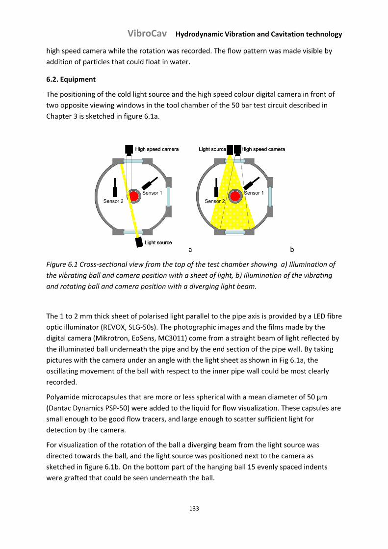
VibroCav Hydrodynamic Vibration and Cavitation technology
133
high speed camera while the rotation was recorded. The flow pattern was made visible by
addition of particles that could float in water.
6.2. Equipment
The positioning of the cold light source and the high speed colour digital camera in front of
two opposite viewing windows in the tool chamber of the 50 bar test circuit described in
Chapter 3 is sketched in figure 6.1a.
Light source
High speed camera
Sensor 1
Sensor 2
Light source
High speed camera
Sensor 1
Sensor 2
a
Light source High speed camera
Sensor 1
Sensor 2
Light source High speed camera
Sensor 1
Sensor 2
b
Figure 6.1 Cross‐sectional view from the top of the test chamber showing a) Illumination of
the vibrating ball and camera position with a sheet of light, b) Illumination of the vibrating
and rotating ball and camera position with a diverging light beam.
The 1 to 2 mm thick sheet of polarised light parallel to the pipe axis is provided by a LED fibre
optic illuminator (REVOX, SLG‐50s). The photographic images and the films made by the
digital camera (Mikrotron, EoSens, MC3011) come from a straight beam of light reflected by
the illuminated ball underneath the pipe and by the end section of the pipe wall. By taking
pictures with the camera under an angle with the light sheet as shown in Fig 6.1a, the
oscillating movement of the ball with respect to the inner pipe wall could be most clearly
recorded.
Polyamide microcapsules that are more or less spherical with a mean diameter of 50 µm
(Dantac Dynamics PSP‐50) were added to the liquid for flow visualization. These capsules are
small enough to be good flow tracers, and large enough to scatter sufficient light for
detection by the camera.
For visualization of the rotation of the ball a diverging beam from the light source was
directed towards the ball, and the light source was positioned next to the camera as
sketched in figure 6.1b. On the bottom part of the hanging ball 15 evenly spaced indents
were grafted that could be seen underneath the ball.
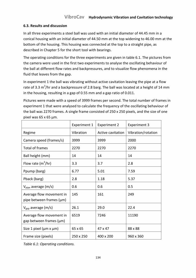
VibroCav Hydrodynamic Vibration and Cavitation technology
134
6.3. Results and discussion
In all three experiments a steel ball was used with an initial diameter of 44.45 mm in a
conical housing with an initial diameter of 44.50 mm at the top widening to 46.00 mm at the
bottom of the housing. This housing was connected at the top to a straight pipe, as
described in Chapter 5 for the short tool with bearings.
The operating conditions for the three experiments are given in table 6.1. The pictures from
the camera were used in the first two experiments to analyse the oscillating behaviour of
the ball at different flow rates and backpressures, and to visualize flow phenomena in the
fluid that leaves from the gap.
In experiment 1 the ball was vibrating without active cavitation leaving the pipe at a flow
rate of 3.3 m3/hr and a backpressure of 2.8 barg. The ball was located at a height of 14 mm
in the housing, resulting in a gap of 0.55 mm and a gap ratio of 0.011.
Pictures were made with a speed of 3999 frames per second. The total number of frames in
experiment 1 that were analysed to calculate the frequency of the oscillating behaviour of
the ball was 2270 frames. A single frame consisted of 250 x 250 pixels, and the size of one
pixel was 65 x 65 µm.
Experiment 1 Experiment 2 Experiment 3
Regime Vibration Active cavitation Vibration/rotation
Camera speed (frames/s) 3999 3999 2000
Total of frames 2270 2270 2270
Ball height (mm) 14 14 14
Flow rate (m3/hr) 3.3 3.7 2.8
Ppump (barg) 6.77 5.01 7.59
Pback (barg) 2.8 1.18 5.37
Vpipe average (m/s) 0.6 0.6 0.5
Average flow movement in
pipe between frames (µm)
145 161 249
Vgap average (m/s) 26.1 29.0 22.4
Average flow movement in
gap between frames (µm)
6519 7246 11190
Size 1 pixel (µm x µm) 65 x 65 47 x 47 88 x 88
Frame size (pixels) 250 x 250 400 x 200 960 x 360
Table 6.1: Operating conditions.
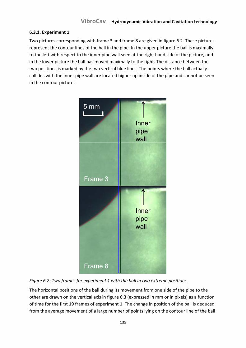
VibroCav Hydrodynamic Vibration and Cavitation technology
135
6.3.1. Experiment 1
Two pictures corresponding with frame 3 and frame 8 are given in figure 6.2. These pictures
represent the contour lines of the ball in the pipe. In the upper picture the ball is maximally
to the left with respect to the inner pipe wall seen at the right hand side of the picture, and
in the lower picture the ball has moved maximally to the right. The distance between the
two positions is marked by the two vertical blue lines. The points where the ball actually
collides with the inner pipe wall are located higher up inside of the pipe and cannot be seen
in the contour pictures.
Frame 3
Frame 8
5 mm
Inner pipe wall
Inner pipe wall
Frame 3
Frame 8
5 mm
Inner pipe wall
Inner pipe wall
Figure 6.2: Two frames for experiment 1 with the ball in two extreme positions.
The horizontal positions of the ball during its movement from one side of the pipe to the
other are drawn on the vertical axis in figure 6.3 (expressed in mm or in pixels) as a function
of time for the first 19 frames of experiment 1. The change in position of the ball is deduced
from the average movement of a large number of points lying on the contour line of the ball
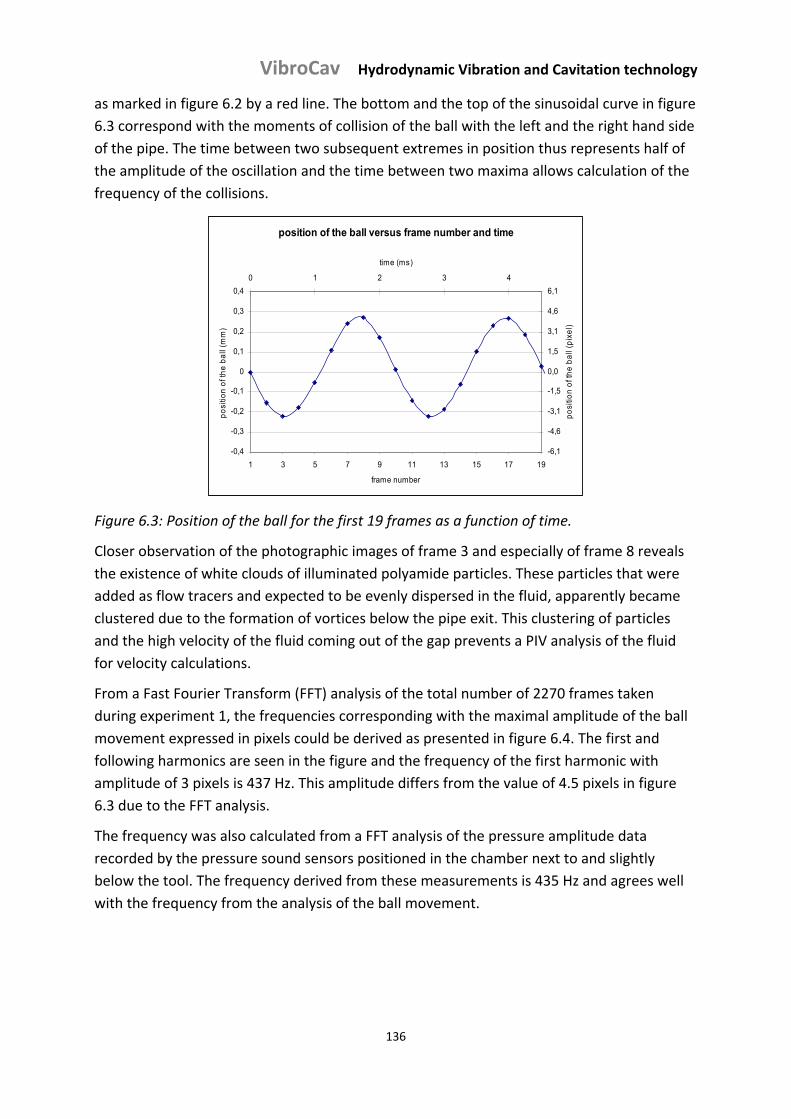
VibroCav Hydrodynamic Vibration and Cavitation technology
136
as marked in figure 6.2 by a red line. The bottom and the top of the sinusoidal curve in figure
6.3 correspond with the moments of collision of the ball with the left and the right hand side
of the pipe. The time between two subsequent extremes in position thus represents half of
the amplitude of the oscillation and the time between two maxima allows calculation of the
frequency of the collisions.
position of the ball versus frame number and time
-0,4
-0,3
-0,2
-0,1
0
0,1
0,2
0,3
0,4
1 3 5 7 9 11 13 15 17 19
frame number
po
sitio
n o
f th
e b
all
(mm
)
-6,1
-4,6
-3,1
-1,5
0,0
1,5
3,1
4,6
6,1
0 1 2 3 4
time (ms)
po
sitio
n o
f th
e b
all
(pix
el)
Figure 6.3: Position of the ball for the first 19 frames as a function of time.
Closer observation of the photographic images of frame 3 and especially of frame 8 reveals
the existence of white clouds of illuminated polyamide particles. These particles that were
added as flow tracers and expected to be evenly dispersed in the fluid, apparently became
clustered due to the formation of vortices below the pipe exit. This clustering of particles
and the high velocity of the fluid coming out of the gap prevents a PIV analysis of the fluid
for velocity calculations.
From a Fast Fourier Transform (FFT) analysis of the total number of 2270 frames taken
during experiment 1, the frequencies corresponding with the maximal amplitude of the ball
movement expressed in pixels could be derived as presented in figure 6.4. The first and
following harmonics are seen in the figure and the frequency of the first harmonic with
amplitude of 3 pixels is 437 Hz. This amplitude differs from the value of 4.5 pixels in figure
6.3 due to the FFT analysis.
The frequency was also calculated from a FFT analysis of the pressure amplitude data
recorded by the pressure sound sensors positioned in the chamber next to and slightly
below the tool. The frequency derived from these measurements is 435 Hz and agrees well
with the frequency from the analysis of the ball movement.
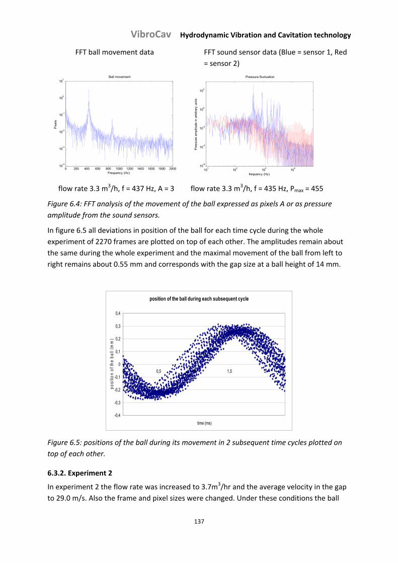
VibroCav Hydrodynamic Vibration and Cavitation technology
137
FFT ball movement data FFT sound sensor data (Blue = sensor 1, Red
= sensor 2)
0 200 400 600 800 1000 1200 1400 1600 1800 200010
-4
10-3
10-2
10-1
100
101
Ball vibration
Frequency (Hz)
Pix
els
Ball movement
0 200 400 600 800 1000 1200 1400 1600 1800 200010
-4
10-3
10-2
10-1
100
101
Ball vibration
Frequency (Hz)
Pix
els
Ball movement
10
110
210
310
410
-6
10-4
10-2
100
102
Fourier plot
frequency (Hz)
Pre
ssur
e am
plitu
de in
arb
itrar
y un
its
Pressure fluctuation
101
102
103
104
10-6
10-4
10-2
100
102
Fourier plot
frequency (Hz)
Pre
ssur
e am
plitu
de in
arb
itrar
y un
its
Pressure fluctuation
flow rate 3.3 m3/h, f = 437 Hz, A = 3 flow rate 3.3 m3/h, f = 435 Hz, Pmax = 455
Figure 6.4: FFT analysis of the movement of the ball expressed as pixels A or as pressure
amplitude from the sound sensors.
In figure 6.5 all deviations in position of the ball for each time cycle during the whole
experiment of 2270 frames are plotted on top of each other. The amplitudes remain about
the same during the whole experiment and the maximal movement of the ball from left to
right remains about 0.55 mm and corresponds with the gap size at a ball height of 14 mm.
position of the ball during each subsequent cycle
-0,4
-0,3
-0,2
-0,1
0
0,1
0,2
0,3
0,4
0 0,5 1 1,5 2
time (ms)
po
sitio
n o
f th
e b
all
(mm
)
Figure 6.5: positions of the ball during its movement in 2 subsequent time cycles plotted on
top of each other.
6.3.2. Experiment 2
In experiment 2 the flow rate was increased to 3.7m3/hr and the average velocity in the gap
to 29.0 m/s. Also the frame and pixel sizes were changed. Under these conditions the ball
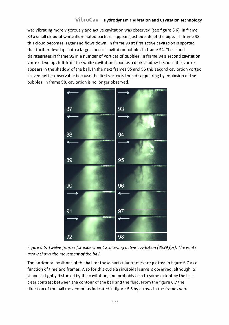
VibroCav Hydrodynamic Vibration and Cavitation technology
138
was vibrating more vigorously and active cavitation was observed (see figure 6.6). In frame
89 a small cloud of white illuminated particles appears just outside of the pipe. Till frame 93
this cloud becomes larger and flows down. In frame 93 at first active cavitation is spotted
that further develops into a large cloud of cavitation bubbles in frame 94. This cloud
disintegrates in frame 95 in a number of vortices of bubbles. In frame 94 a second cavitation
vortex develops left from the white cavitation cloud as a dark shadow because this vortex
appears in the shadow of the ball. In the next frames 95 and 96 this second cavitation vortex
is even better observable because the first vortex is then disappearing by implosion of the
bubbles. In frame 98, cavitation is no longer observed.
87
98
97
96
95
93
94
92
91
90
89
88
Figure 6.6: Twelve frames for experiment 2 showing active cavitation (3999 fps). The white
arrow shows the movement of the ball.
The horizontal positions of the ball for these particular frames are plotted in figure 6.7 as a
function of time and frames. Also for this cycle a sinusoidal curve is observed, although its
shape is slightly distorted by the cavitation, and probably also to some extent by the less
clear contrast between the contour of the ball and the fluid. From the figure 6.7 the
direction of the ball movement as indicated in figure 6.6 by arrows in the frames were
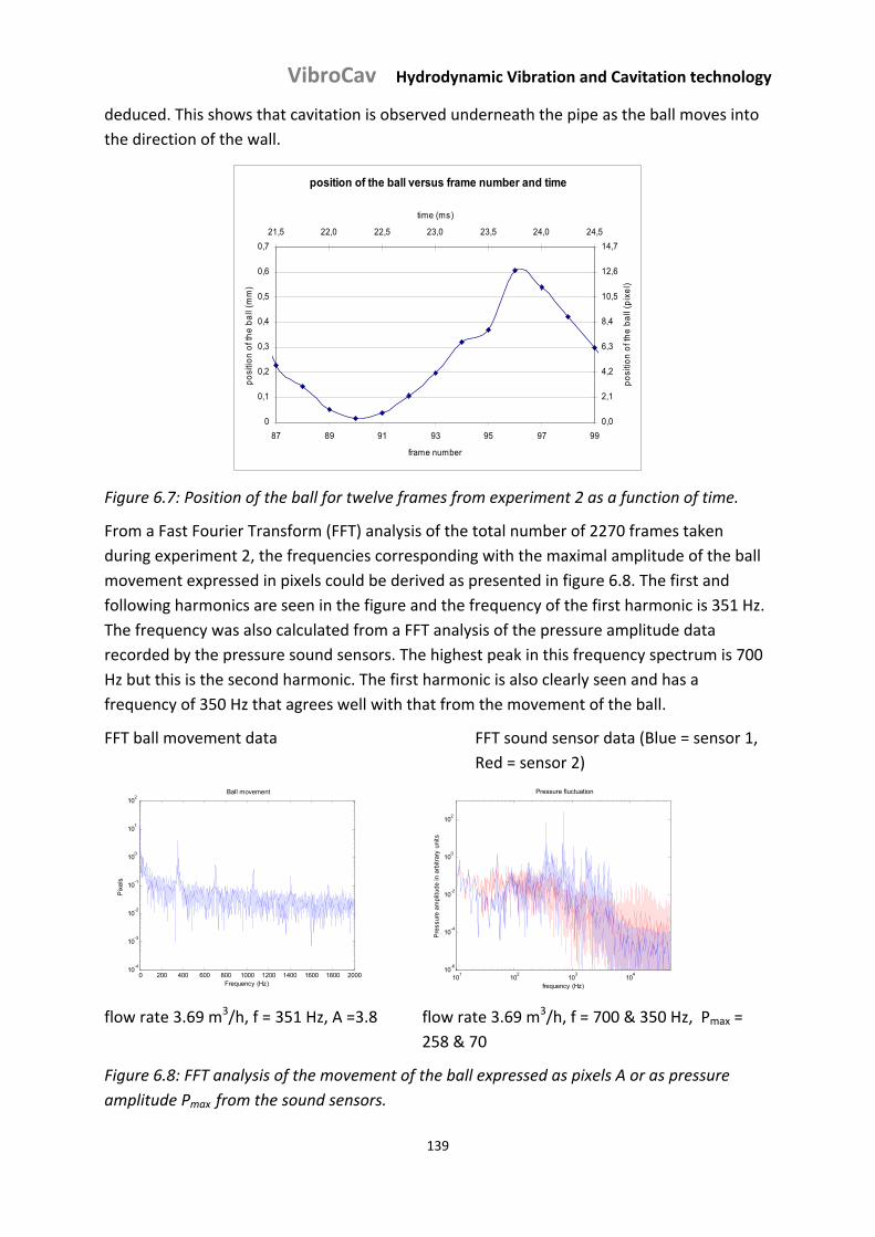
VibroCav Hydrodynamic Vibration and Cavitation technology
139
deduced. This shows that cavitation is observed underneath the pipe as the ball moves into
the direction of the wall.
position of the ball versus frame number and time
0
0,1
0,2
0,3
0,4
0,5
0,6
0,7
87 89 91 93 95 97 99
frame number
po
sitio
n o
f th
e b
all
(mm
)
0,0
2,1
4,2
6,3
8,4
10,5
12,6
14,7
21,5 22,0 22,5 23,0 23,5 24,0 24,5
time (ms)
po
sitio
n o
f th
e b
all
(pix
el)
Figure 6.7: Position of the ball for twelve frames from experiment 2 as a function of time.
From a Fast Fourier Transform (FFT) analysis of the total number of 2270 frames taken
during experiment 2, the frequencies corresponding with the maximal amplitude of the ball
movement expressed in pixels could be derived as presented in figure 6.8. The first and
following harmonics are seen in the figure and the frequency of the first harmonic is 351 Hz.
The frequency was also calculated from a FFT analysis of the pressure amplitude data
recorded by the pressure sound sensors. The highest peak in this frequency spectrum is 700
Hz but this is the second harmonic. The first harmonic is also clearly seen and has a
frequency of 350 Hz that agrees well with that from the movement of the ball.
FFT ball movement data FFT sound sensor data (Blue = sensor 1,
Red = sensor 2)
0 200 400 600 800 1000 1200 1400 1600 1800 200010
-4
10-3
10-2
10-1
100
101
102
Ball vibration
Frequency (Hz)
Pix
els
Ball movement
0 200 400 600 800 1000 1200 1400 1600 1800 200010
-4
10-3
10-2
10-1
100
101
102
Ball vibration
Frequency (Hz)
Pix
els
Ball movement
10
110
210
310
410
-6
10-4
10-2
100
102
Fourier plot
frequency (Hz)
Pre
ssur
e am
plitu
de in
arb
itrar
y un
its
Pressure fluctuation
101
102
103
104
10-6
10-4
10-2
100
102
Fourier plot
frequency (Hz)
Pre
ssur
e am
plitu
de in
arb
itrar
y un
its
Pressure fluctuation
flow rate 3.69 m3/h, f = 351 Hz, A =3.8 flow rate 3.69 m3/h, f = 700 & 350 Hz, Pmax =
258 & 70
Figure 6.8: FFT analysis of the movement of the ball expressed as pixels A or as pressure
amplitude Pmax from the sound sensors.
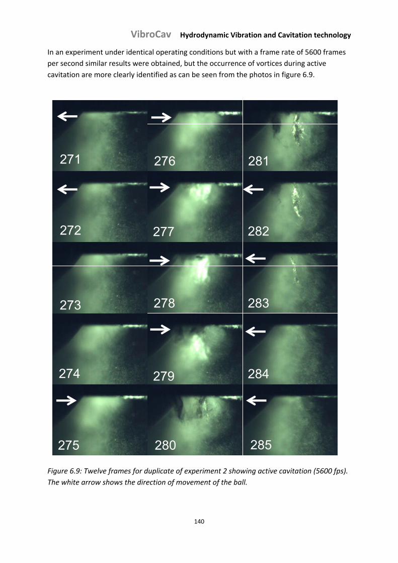
VibroCav Hydrodynamic Vibration and Cavitation technology
140
In an experiment under identical operating conditions but with a frame rate of 5600 frames
per second similar results were obtained, but the occurrence of vortices during active
cavitation are more clearly identified as can be seen from the photos in figure 6.9.
273
275
274
276
278
277
279
280
281
282
283
284
271
272
285
Figure 6.9: Twelve frames for duplicate of experiment 2 showing active cavitation (5600 fps).
The white arrow shows the direction of movement of the ball.
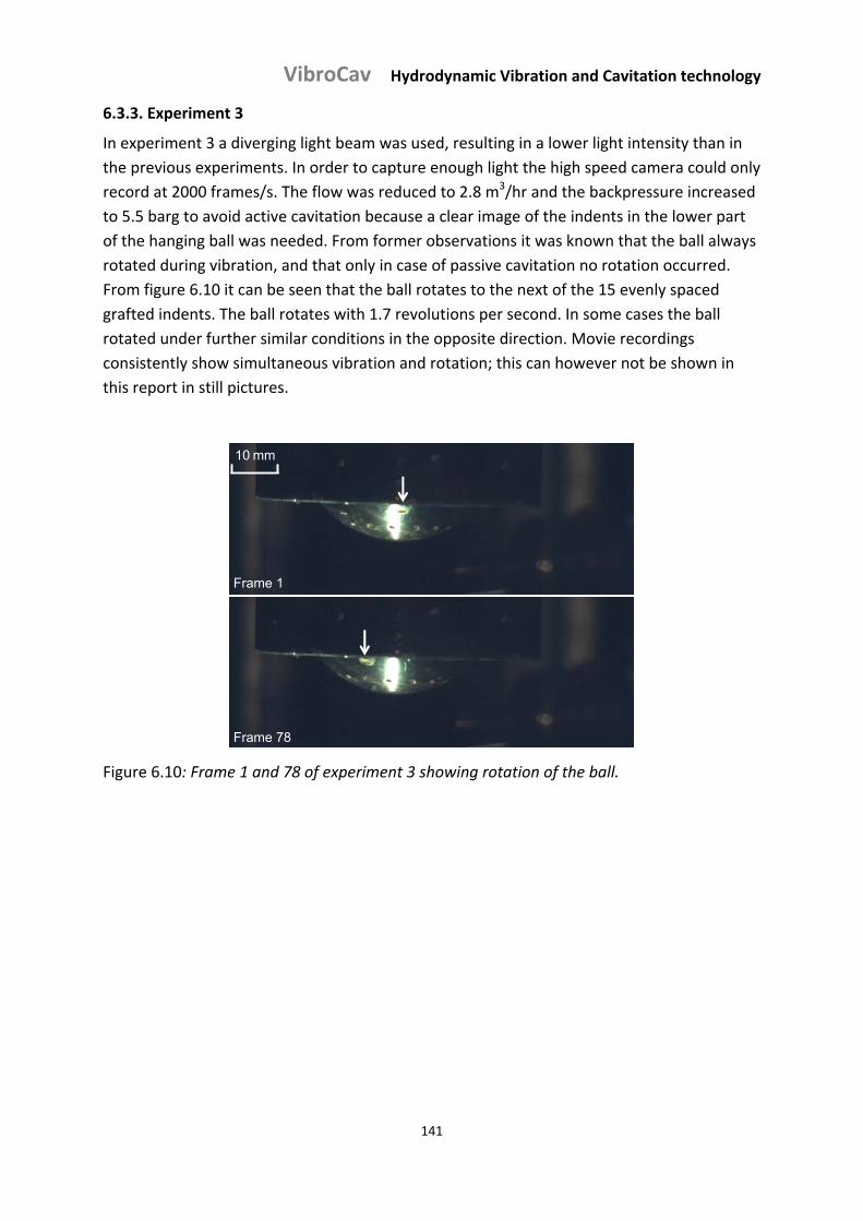
VibroCav Hydrodynamic Vibration and Cavitation technology
141
6.3.3. Experiment 3
In experiment 3 a diverging light beam was used, resulting in a lower light intensity than in
the previous experiments. In order to capture enough light the high speed camera could only
record at 2000 frames/s. The flow was reduced to 2.8 m3/hr and the backpressure increased
to 5.5 barg to avoid active cavitation because a clear image of the indents in the lower part
of the hanging ball was needed. From former observations it was known that the ball always
rotated during vibration, and that only in case of passive cavitation no rotation occurred.
From figure 6.10 it can be seen that the ball rotates to the next of the 15 evenly spaced
grafted indents. The ball rotates with 1.7 revolutions per second. In some cases the ball
rotated under further similar conditions in the opposite direction. Movie recordings
consistently show simultaneous vibration and rotation; this can however not be shown in
this report in still pictures.
Frame 78
Frame 1
10 mm
Frame 78
Frame 1
10 mm
Figure 6.10: Frame 1 and 78 of experiment 3 showing rotation of the ball.

VibroCav Hydrodynamic Vibration and Cavitation technology
142
6.4. Conclusions
During vibration the ball is always rotating either clockwise or counter clockwise around an axis parallel with the direction of flow.
The ball vibrates with a constant amplitude and frequency at a given flow rate and gap size in conditions without observable active cavitation following a sinusoidal displacement versus time relationship.
In case of active cavitation the frequency also remains constant for a constant flow rate; however the displacement versus time relationship shows distortion, probably caused by the cavitation effect.
The frequency of vibration calculated by FFT analysis from the ball movements agrees with those obtained by FFT analysis from pressure data recorded by sound sensors.
The movement of the ball during vibration is consistent with the gap size.
If active cavitation occurs, it is observed to be leaving the pipe when the ball moves towards the pipe wall.

VibroCav Hydrodynamic Vibration and Cavitation technology
143
VibroCav Hydrodynamic Vibration and Cavitation technology
144
Chapter 7: Cavitation and vibration by flow along a bottom supported ball in
a 350 bar test circuit
7.1. Introduction
An important aim of this study is the design of a tool consisting of a free moving body in a
housing, that operates either by vibration of the body, mostly a ball, or by cavitation or by
both actions together in an environment of atmospheric up to high backpressure. Cleaning
of water or oil wells for example to restore the permeability of the porous rock formation in
the inflow horizon or to clean the wellbore itself should be an important application of a
vibration based cleaning tool.
The waves induced by vibration of the ball with frequencies of 100 to 1000 Hz are able to
disrupt assemblies of tiny particles that cause blockage of the pores. The penetration depth
of waves in this frequency range is several decimetres and the power of these vibrations is
not much affected by the backpressure. Cavitation is much more affected by the
backpressure. To induce cavitation at higher surrounding pressures the flow rate has to be
substantially increased.
Shock waves from imploding cavitation bubbles have a lower penetration depth, and their
cleaning action therefore remains limited to surface cleaning of the well bore from fouling or
mineral scale layers and the cleaning of gravel beds behind filter tubes in the immediate
vicinity of the well bore.
In the 50 bar test circuit tests could only be performed up to a maximal backpressure of 10
barg. Both passive and active cavitation died out at backpressures of 8 to 9 barg at the
maximal flow rates that could be achieved with this test circuit. In order to perform
experiments at sufficiently high flow rates and at backpressures as encountered in deep
wells, a new 350 barg test circuit was assembled in Drachten. These experiments allowed
study of the dependence of the regimes where no vibration, vibration combined with
bouncing, active or passive cavitation or a combination of vibration and active cavitation
occurred, on the flow rate at high backpressures behind the ball for different gaps between
the ball and the housing of the tool.
Because a 350 barg test circuit is much more demanding to operate than the 50 barg test
loop, only a limited number of selected tests were done in the 350 barg circuit. This chapter
discusses these experiments with a flow passing along a bottom supported ball in a straight
horizontal tool at high backpressures. Sufficiently high flow rates were generated by a
‘Garden Denver’ triplex plunger pump. Balls of various diameters and types of material were
used in housings of two diameters.
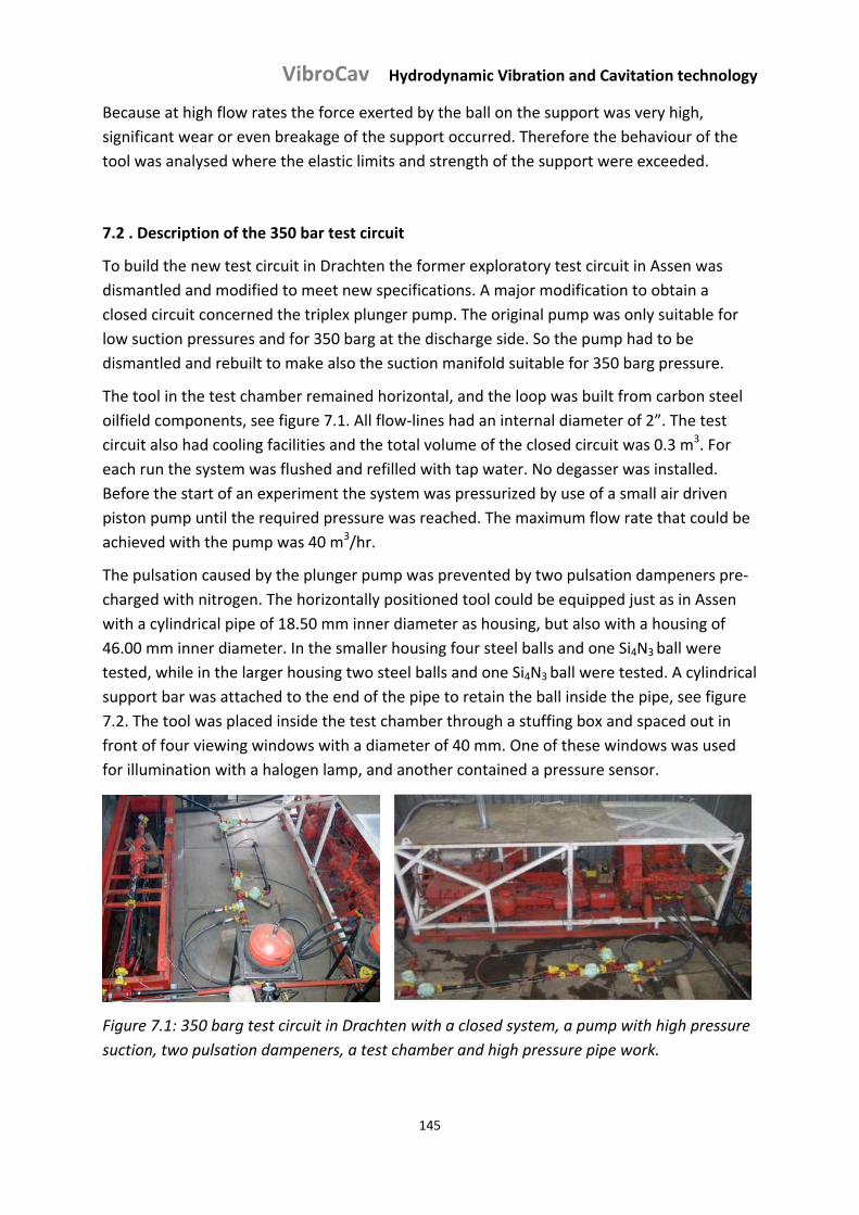
VibroCav Hydrodynamic Vibration and Cavitation technology
145
Because at high flow rates the force exerted by the ball on the support was very high,
significant wear or even breakage of the support occurred. Therefore the behaviour of the
tool was analysed where the elastic limits and strength of the support were exceeded.
7.2 . Description of the 350 bar test circuit
To build the new test circuit in Drachten the former exploratory test circuit in Assen was
dismantled and modified to meet new specifications. A major modification to obtain a
closed circuit concerned the triplex plunger pump. The original pump was only suitable for
low suction pressures and for 350 barg at the discharge side. So the pump had to be
dismantled and rebuilt to make also the suction manifold suitable for 350 barg pressure.
The tool in the test chamber remained horizontal, and the loop was built from carbon steel
oilfield components, see figure 7.1. All flow‐lines had an internal diameter of 2”. The test
circuit also had cooling facilities and the total volume of the closed circuit was 0.3 m3. For
each run the system was flushed and refilled with tap water. No degasser was installed.
Before the start of an experiment the system was pressurized by use of a small air driven
piston pump until the required pressure was reached. The maximum flow rate that could be
achieved with the pump was 40 m3/hr.
The pulsation caused by the plunger pump was prevented by two pulsation dampeners pre‐
charged with nitrogen. The horizontally positioned tool could be equipped just as in Assen
with a cylindrical pipe of 18.50 mm inner diameter as housing, but also with a housing of
46.00 mm inner diameter. In the smaller housing four steel balls and one Si4N3 ball were
tested, while in the larger housing two steel balls and one Si4N3 ball were tested. A cylindrical
support bar was attached to the end of the pipe to retain the ball inside the pipe, see figure
7.2. The tool was placed inside the test chamber through a stuffing box and spaced out in
front of four viewing windows with a diameter of 40 mm. One of these windows was used
for illumination with a halogen lamp, and another contained a pressure sensor.
Figure 7.1: 350 barg test circuit in Drachten with a closed system, a pump with high pressure
suction, two pulsation dampeners, a test chamber and high pressure pipe work.
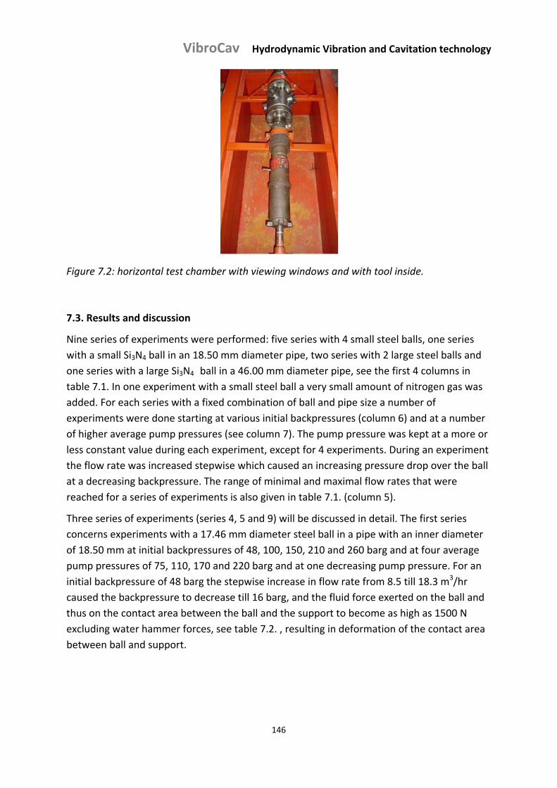
VibroCav Hydrodynamic Vibration and Cavitation technology
146
Figure 7.2: horizontal test chamber with viewing windows and with tool inside.
7.3. Results and discussion
Nine series of experiments were performed: five series with 4 small steel balls, one series
with a small Si3N4 ball in an 18.50 mm diameter pipe, two series with 2 large steel balls and
one series with a large Si3N4 ball in a 46.00 mm diameter pipe, see the first 4 columns in
table 7.1. In one experiment with a small steel ball a very small amount of nitrogen gas was
added. For each series with a fixed combination of ball and pipe size a number of
experiments were done starting at various initial backpressures (column 6) and at a number
of higher average pump pressures (see column 7). The pump pressure was kept at a more or
less constant value during each experiment, except for 4 experiments. During an experiment
the flow rate was increased stepwise which caused an increasing pressure drop over the ball
at a decreasing backpressure. The range of minimal and maximal flow rates that were
reached for a series of experiments is also given in table 7.1. (column 5).
Three series of experiments (series 4, 5 and 9) will be discussed in detail. The first series
concerns experiments with a 17.46 mm diameter steel ball in a pipe with an inner diameter
of 18.50 mm at initial backpressures of 48, 100, 150, 210 and 260 barg and at four average
pump pressures of 75, 110, 170 and 220 barg and at one decreasing pump pressure. For an
initial backpressure of 48 barg the stepwise increase in flow rate from 8.5 till 18.3 m3/hr
caused the backpressure to decrease till 16 barg, and the fluid force exerted on the ball and
thus on the contact area between the ball and the support to become as high as 1500 N
excluding water hammer forces, see table 7.2. , resulting in deformation of the contact area
between ball and support.
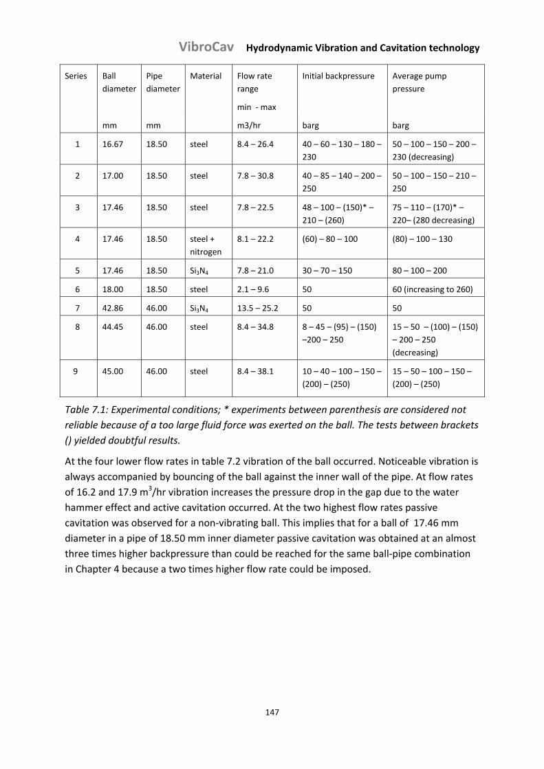
VibroCav Hydrodynamic Vibration and Cavitation technology
147
Series Ball
diameter
Pipe
diameter
Material Flow rate
range
min ‐ max
Initial backpressure Average pump
pressure
mm mm m3/hr barg barg
1 16.67 18.50 steel 8.4 – 26.4 40 – 60 – 130 – 180 –
230
50 – 100 – 150 – 200 –
230 (decreasing)
2 17.00 18.50 steel 7.8 – 30.8 40 – 85 – 140 – 200 –
250
50 – 100 – 150 – 210 –
250
3 17.46 18.50 steel 7.8 – 22.5 48 – 100 – (150)* –
210 – (260)
75 – 110 – (170)* –
220– (280 decreasing)
4 17.46 18.50 steel +
nitrogen
8.1 – 22.2 (60) – 80 – 100 (80) – 100 – 130
5 17.46 18.50 Si3N4 7.8 – 21.0 30 – 70 – 150 80 – 100 – 200
6 18.00 18.50 steel 2.1 – 9.6 50 60 (increasing to 260)
7 42.86 46.00 Si3N4 13.5 – 25.2 50 50
8 44.45 46.00 steel 8.4 – 34.8 8 – 45 – (95) – (150)
–200 – 250
15 – 50 – (100) – (150)
– 200 – 250
(decreasing)
9
45.00 46.00 steel 8.4 – 38.1 10 – 40 – 100 – 150 –
(200) – (250)
15 – 50 – 100 – 150 –
(200) – (250)
Table 7.1: Experimental conditions; * experiments between parenthesis are considered not
reliable because of a too large fluid force was exerted on the ball. The tests between brackets
() yielded doubtful results.
At the four lower flow rates in table 7.2 vibration of the ball occurred. Noticeable vibration is
always accompanied by bouncing of the ball against the inner wall of the pipe. At flow rates
of 16.2 and 17.9 m3/hr vibration increases the pressure drop in the gap due to the water
hammer effect and active cavitation occurred. At the two highest flow rates passive
cavitation was observed for a non‐vibrating ball. This implies that for a ball of 17.46 mm
diameter in a pipe of 18.50 mm inner diameter passive cavitation was obtained at an almost
three times higher backpressure than could be reached for the same ball‐pipe combination
in Chapter 4 because a two times higher flow rate could be imposed.
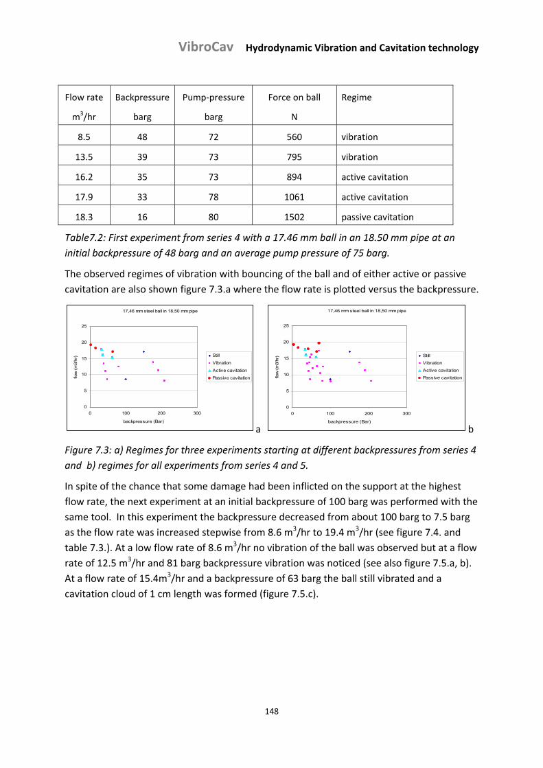
VibroCav Hydrodynamic Vibration and Cavitation technology
148
Flow rate
m3/hr
Backpressure
barg
Pump‐pressure
barg
Force on ball
N
Regime
8.5 48 72 560 vibration
13.5 39 73 795 vibration
16.2 35 73 894 active cavitation
17.9 33 78 1061 active cavitation
18.3 16 80 1502 passive cavitation
Table7.2: First experiment from series 4 with a 17.46 mm ball in an 18.50 mm pipe at an
initial backpressure of 48 barg and an average pump pressure of 75 barg.
The observed regimes of vibration with bouncing of the ball and of either active or passive
cavitation are also shown figure 7.3.a where the flow rate is plotted versus the backpressure.
17,46 mm steel ball in 18,50 mm pipe
0
5
10
15
20
25
0 100 200 300
backpressure (Bar)
flow
(m
3/hr
) Still
Vibration
Active cavitation
Passive cavitation
a
17,46 mm steel ball in 18,50 mm pipe
0
5
10
15
20
25
0 100 200 300
backpressure (Bar)
flow
(m
3/hr
) Still
Vibration
Active cavitation
Passive cavitation
b
Figure 7.3: a) Regimes for three experiments starting at different backpressures from series 4
and b) regimes for all experiments from series 4 and 5.
In spite of the chance that some damage had been inflicted on the support at the highest
flow rate, the next experiment at an initial backpressure of 100 barg was performed with the
same tool. In this experiment the backpressure decreased from about 100 barg to 7.5 barg
as the flow rate was increased stepwise from 8.6 m3/hr to 19.4 m3/hr (see figure 7.4. and
table 7.3.). At a low flow rate of 8.6 m3/hr no vibration of the ball was observed but at a flow
rate of 12.5 m3/hr and 81 barg backpressure vibration was noticed (see also figure 7.5.a, b).
At a flow rate of 15.4m3/hr and a backpressure of 63 barg the ball still vibrated and a
cavitation cloud of 1 cm length was formed (figure 7.5.c).
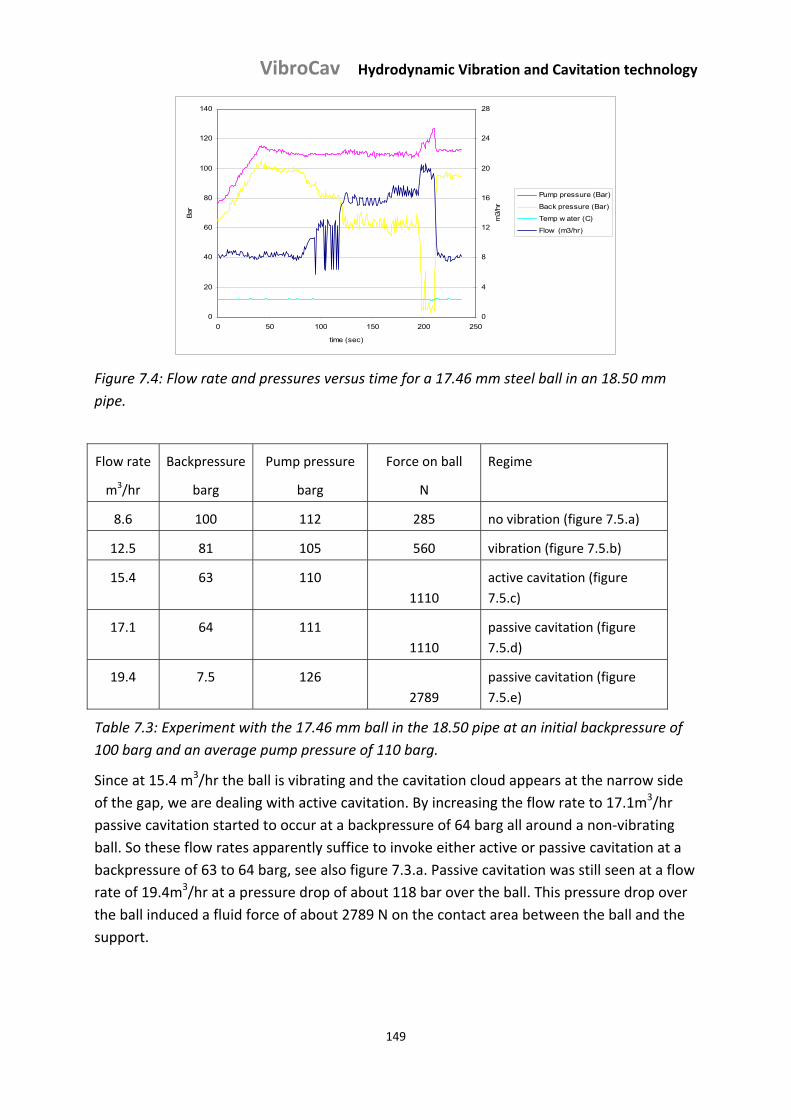
VibroCav Hydrodynamic Vibration and Cavitation technology
149
0
20
40
60
80
100
120
140
0 50 100 150 200 250
time (sec)
Bar
0
4
8
12
16
20
24
28
m3/
hr
Pump pressure (Bar)
Back pressure (Bar)
Temp w ater (C)
Flow (m3/hr)
Figure 7.4: Flow rate and pressures versus time for a 17.46 mm steel ball in an 18.50 mm
pipe.
Flow rate
m3/hr
Backpressure
barg
Pump pressure
barg
Force on ball
N
Regime
8.6 100 112 285 no vibration (figure 7.5.a)
12.5 81 105 560 vibration (figure 7.5.b)
15.4 63 110
1110
active cavitation (figure
7.5.c)
17.1 64 111
1110
passive cavitation (figure
7.5.d)
19.4 7.5 126
2789
passive cavitation (figure
7.5.e)
Table 7.3: Experiment with the 17.46 mm ball in the 18.50 pipe at an initial backpressure of
100 barg and an average pump pressure of 110 barg.
Since at 15.4 m3/hr the ball is vibrating and the cavitation cloud appears at the narrow side
of the gap, we are dealing with active cavitation. By increasing the flow rate to 17.1m3/hr
passive cavitation started to occur at a backpressure of 64 barg all around a non‐vibrating
ball. So these flow rates apparently suffice to invoke either active or passive cavitation at a
backpressure of 63 to 64 barg, see also figure 7.3.a. Passive cavitation was still seen at a flow
rate of 19.4m3/hr at a pressure drop of about 118 bar over the ball. This pressure drop over
the ball induced a fluid force of about 2789 N on the contact area between the ball and the
support.
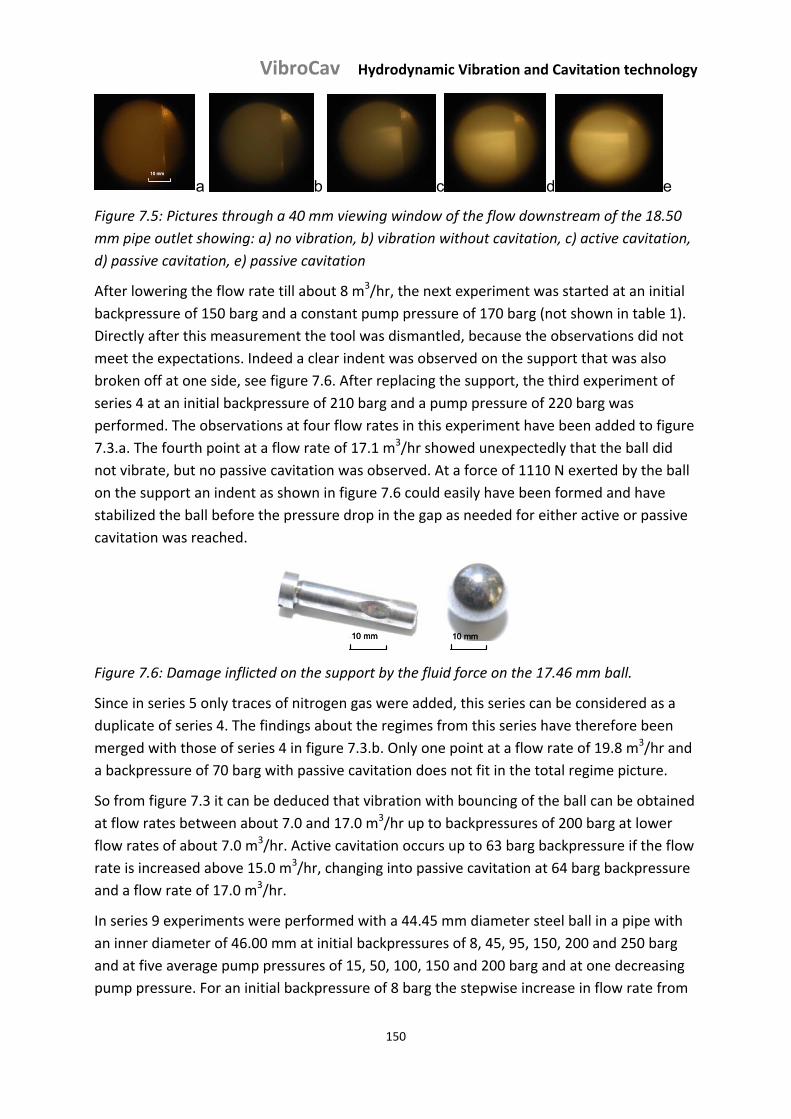
VibroCav Hydrodynamic Vibration and Cavitation technology
150
10 mm10 mm10 mm
a b c d e
Figure 7.5: Pictures through a 40 mm viewing window of the flow downstream of the 18.50
mm pipe outlet showing: a) no vibration, b) vibration without cavitation, c) active cavitation,
d) passive cavitation, e) passive cavitation
After lowering the flow rate till about 8 m3/hr, the next experiment was started at an initial
backpressure of 150 barg and a constant pump pressure of 170 barg (not shown in table 1).
Directly after this measurement the tool was dismantled, because the observations did not
meet the expectations. Indeed a clear indent was observed on the support that was also
broken off at one side, see figure 7.6. After replacing the support, the third experiment of
series 4 at an initial backpressure of 210 barg and a pump pressure of 220 barg was
performed. The observations at four flow rates in this experiment have been added to figure
7.3.a. The fourth point at a flow rate of 17.1 m3/hr showed unexpectedly that the ball did
not vibrate, but no passive cavitation was observed. At a force of 1110 N exerted by the ball
on the support an indent as shown in figure 7.6 could easily have been formed and have
stabilized the ball before the pressure drop in the gap as needed for either active or passive
cavitation was reached.
10 mm10 mm10 mm
10 mm10 mm10 mm
Figure 7.6: Damage inflicted on the support by the fluid force on the 17.46 mm ball.
Since in series 5 only traces of nitrogen gas were added, this series can be considered as a
duplicate of series 4. The findings about the regimes from this series have therefore been
merged with those of series 4 in figure 7.3.b. Only one point at a flow rate of 19.8 m3/hr and
a backpressure of 70 barg with passive cavitation does not fit in the total regime picture.
So from figure 7.3 it can be deduced that vibration with bouncing of the ball can be obtained
at flow rates between about 7.0 and 17.0 m3/hr up to backpressures of 200 barg at lower
flow rates of about 7.0 m3/hr. Active cavitation occurs up to 63 barg backpressure if the flow
rate is increased above 15.0 m3/hr, changing into passive cavitation at 64 barg backpressure
and a flow rate of 17.0 m3/hr.
In series 9 experiments were performed with a 44.45 mm diameter steel ball in a pipe with
an inner diameter of 46.00 mm at initial backpressures of 8, 45, 95, 150, 200 and 250 barg
and at five average pump pressures of 15, 50, 100, 150 and 200 barg and at one decreasing
pump pressure. For an initial backpressure of 8 barg the stepwise increase in flow rate from
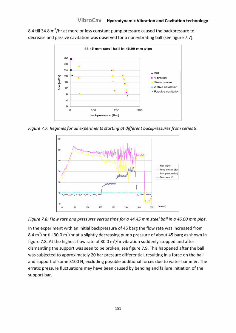
VibroCav Hydrodynamic Vibration and Cavitation technology
151
8.4 till 34.8 m3/hr at more or less constant pump pressure caused the backpressure to
decrease and passive cavitation was observed for a non‐vibrating ball (see figure 7.7).
44,45 mm steel ball in 46,00 mm pipe
0
4
8
12
16
20
24
28
32
0 100 200 300
backpessure (Bar)
flow
(m
3/hr)
Still
Vibration
Strong noise
Active cavitation
Passive cavitation
Figure 7.7: Regimes for all experiments starting at different backpressures from series 9.
0
10
20
30
40
50
60
0 50 100 150 200 250 300 350
Flow (m3/hr)
Pump pressure (Bar)
Back pressure (Bar)
Temp water (C)
time (s)0
10
20
30
40
50
60
0 50 100 150 200 250 300 350
Flow (m3/hr)
Pump pressure (Bar)
Back pressure (Bar)
Temp water (C)
time (s)
Figure 7.8: Flow rate and pressures versus time for a 44.45 mm steel ball in a 46.00 mm pipe.
In the experiment with an initial backpressure of 45 barg the flow rate was increased from
8.4 m3/hr till 30.0 m3/hr at a slightly decreasing pump pressure of about 45 barg as shown in
figure 7.8. At the highest flow rate of 30.0 m3/hr vibration suddenly stopped and after
dismantling the support was seen to be broken, see figure 7.9. This happened after the ball
was subjected to approximately 20 bar pressure differential, resulting in a force on the ball
and support of some 3100 N, excluding possible additional forces due to water hammer. The
erratic pressure fluctuations may have been caused by bending and failure initiation of the
support bar.
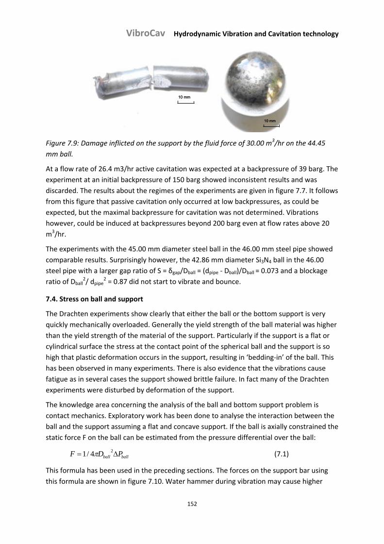
VibroCav Hydrodynamic Vibration and Cavitation technology
152
10 mm10 mm10 mm
10 mm10 mm10 mm
Figure 7.9: Damage inflicted on the support by the fluid force of 30.00 m3/hr on the 44.45
mm ball.
At a flow rate of 26.4 m3/hr active cavitation was expected at a backpressure of 39 barg. The
experiment at an initial backpressure of 150 barg showed inconsistent results and was
discarded. The results about the regimes of the experiments are given in figure 7.7. It follows
from this figure that passive cavitation only occurred at low backpressures, as could be
expected, but the maximal backpressure for cavitation was not determined. Vibrations
however, could be induced at backpressures beyond 200 barg even at flow rates above 20
m3/hr.
The experiments with the 45.00 mm diameter steel ball in the 46.00 mm steel pipe showed
comparable results. Surprisingly however, the 42.86 mm diameter Si3N4 ball in the 46.00
steel pipe with a larger gap ratio of S = δgap/Dball = (dpipe ‐ Dball)/Dball = 0.073 and a blockage
ratio of Dball2/ dpipe
2 = 0.87 did not start to vibrate and bounce.
7.4. Stress on ball and support
The Drachten experiments show clearly that either the ball or the bottom support is very
quickly mechanically overloaded. Generally the yield strength of the ball material was higher
than the yield strength of the material of the support. Particularly if the support is a flat or
cylindrical surface the stress at the contact point of the spherical ball and the support is so
high that plastic deformation occurs in the support, resulting in ‘bedding‐in’ of the ball. This
has been observed in many experiments. There is also evidence that the vibrations cause
fatigue as in several cases the support showed brittle failure. In fact many of the Drachten
experiments were disturbed by deformation of the support.
The knowledge area concerning the analysis of the ball and bottom support problem is
contact mechanics. Exploratory work has been done to analyse the interaction between the
ball and the support assuming a flat and concave support. If the ball is axially constrained the
static force F on the ball can be estimated from the pressure differential over the ball:
ballball PDF 24/1 (7.1)
This formula has been used in the preceding sections. The forces on the support bar using
this formula are shown in figure 7.10. Water hammer during vibration may cause higher
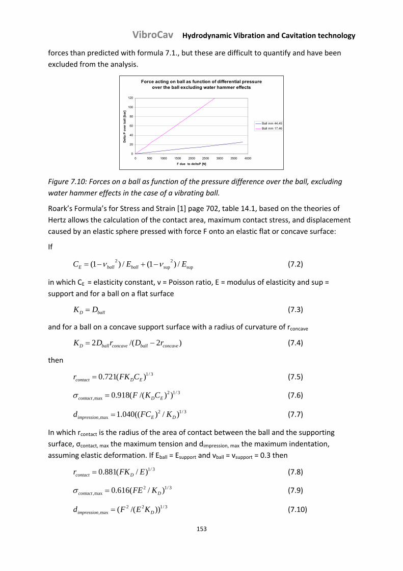
VibroCav Hydrodynamic Vibration and Cavitation technology
153
forces than predicted with formula 7.1., but these are difficult to quantify and have been
excluded from the analysis.
Force acting on ball as function of differential pressure over the ball excluding water hammer effects
0
20
40
60
80
100
120
0 500 1000 1500 2000 2500 3000 3500 4000
F due to deltaP [N]
Del
ta P
ove
r b
all
[bar
]Ball mm 44,45
Ball mm 17,46
Figure 7.10: Forces on a ball as function of the pressure difference over the ball, excluding
water hammer effects in the case of a vibrating ball.
Roark’s Formula’s for Stress and Strain [1] page 702, table 14.1, based on the theories of
Hertz allows the calculation of the contact area, maximum contact stress, and displacement
caused by an elastic sphere pressed with force F onto an elastic flat or concave surface:
If
sup2
sup2 /)1(/)1( EEC ballballE (7.2)
in which CE = elasticity constant, ν = Poisson ratio, E = modulus of elasticity and sup =
support and for a ball on a flat surface
ballD DK (7.3)
and for a ball on a concave support surface with a radius of curvature of rconcave
)2/(2 concaveballconcaveballD rDrDK (7.4)
then
3/1)(721.0 EDcontact CFKr (7.5)
3/12max, ))/((918.0 EDcontact CKF (7.6)
3/12max, )/)((040.1 DEimpression KFCd (7.7)
In which rcontact is the radius of the area of contact between the ball and the supporting
surface, σcontact, max the maximum tension and dimpression, max the maximum indentation,
assuming elastic deformation. If Eball = Esupport and νball = νsupport = 0.3 then
3/1)/(881.0 EFKr Dcontact (7.8)
3/12max, )/(616.0 Dcontact KFE (7.9)
3/122max, ))/(( Dimpression KEFd (7.10)
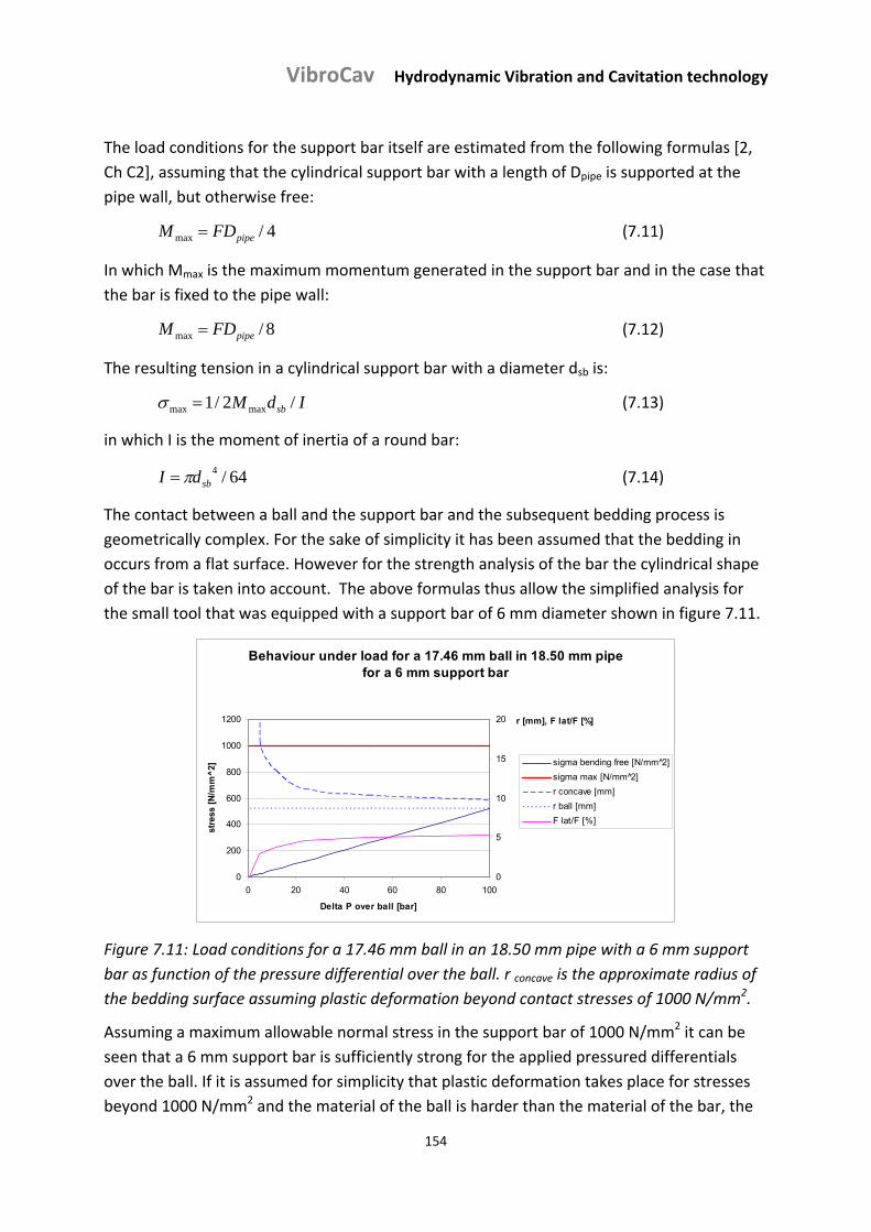
VibroCav Hydrodynamic Vibration and Cavitation technology
154
The load conditions for the support bar itself are estimated from the following formulas [2,
Ch C2], assuming that the cylindrical support bar with a length of Dpipe is supported at the
pipe wall, but otherwise free:
4/max pipeFDM (7.11)
In which Mmax is the maximum momentum generated in the support bar and in the case that
the bar is fixed to the pipe wall:
8/max pipeFDM (7.12)
The resulting tension in a cylindrical support bar with a diameter dsb is:
IdM sb /2/1 maxmax (7.13)
in which I is the moment of inertia of a round bar:
64/4sbdI (7.14)
The contact between a ball and the support bar and the subsequent bedding process is
geometrically complex. For the sake of simplicity it has been assumed that the bedding in
occurs from a flat surface. However for the strength analysis of the bar the cylindrical shape
of the bar is taken into account. The above formulas thus allow the simplified analysis for
the small tool that was equipped with a support bar of 6 mm diameter shown in figure 7.11.
Behaviour under load for a 17.46 mm ball in 18.50 mm pipe for a 6 mm support bar
0
200
400
600
800
1000
1200
0 20 40 60 80 100
Delta P over ball [bar]
stre
ss [
N/m
m^
2]
0
5
10
15
20 r [mm], F lat/F [%]
sigma bending free [N/mm 2̂]
sigma max [N/mm 2̂]
r concave [mm]
r ball [mm]
F lat/F [%]
Figure 7.11: Load conditions for a 17.46 mm ball in an 18.50 mm pipe with a 6 mm support
bar as function of the pressure differential over the ball. r concave is the approximate radius of
the bedding surface assuming plastic deformation beyond contact stresses of 1000 N/mm2.
Assuming a maximum allowable normal stress in the support bar of 1000 N/mm2 it can be
seen that a 6 mm support bar is sufficiently strong for the applied pressured differentials
over the ball. If it is assumed for simplicity that plastic deformation takes place for stresses
beyond 1000 N/mm2 and the material of the ball is harder than the material of the bar, the
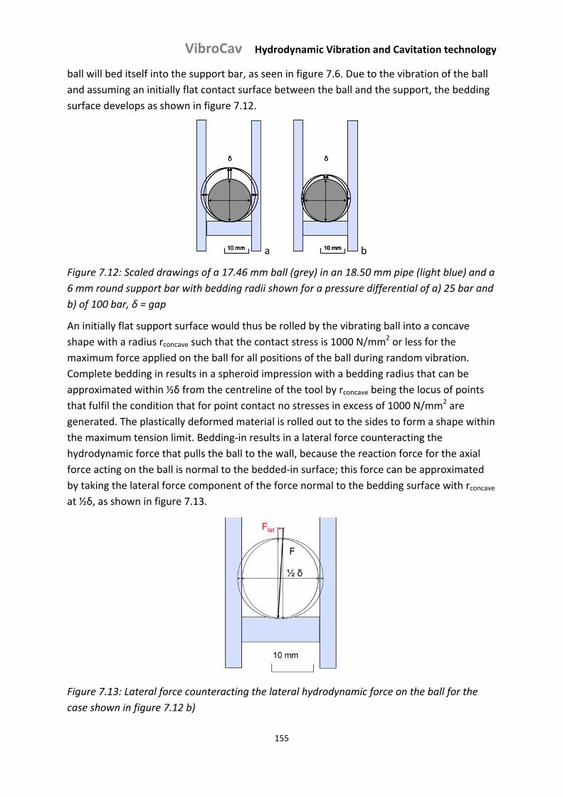
VibroCav Hydrodynamic Vibration and Cavitation technology
155
ball will bed itself into the support bar, as seen in figure 7.6. Due to the vibration of the ball
and assuming an initially flat contact surface between the ball and the support, the bedding
surface develops as shown in figure 7.12.
10 mm
δ
10 mm10 mm
δ
a 10 mm
δ
10 mm10 mm
δ
b
Figure 7.12: Scaled drawings of a 17.46 mm ball (grey) in an 18.50 mm pipe (light blue) and a
6 mm round support bar with bedding radii shown for a pressure differential of a) 25 bar and
b) of 100 bar, δ = gap
An initially flat support surface would thus be rolled by the vibrating ball into a concave
shape with a radius rconcave such that the contact stress is 1000 N/mm2 or less for the
maximum force applied on the ball for all positions of the ball during random vibration.
Complete bedding in results in a spheroid impression with a bedding radius that can be
approximated within ½δ from the centreline of the tool by rconcave being the locus of points
that fulfil the condition that for point contact no stresses in excess of 1000 N/mm2 are
generated. The plastically deformed material is rolled out to the sides to form a shape within
the maximum tension limit. Bedding‐in results in a lateral force counteracting the
hydrodynamic force that pulls the ball to the wall, because the reaction force for the axial
force acting on the ball is normal to the bedded‐in surface; this force can be approximated
by taking the lateral force component of the force normal to the bedding surface with rconcave
at ½δ, as shown in figure 7.13.
Figure 7.13: Lateral force counteracting the lateral hydrodynamic force on the ball for the
case shown in figure 7.12 b)
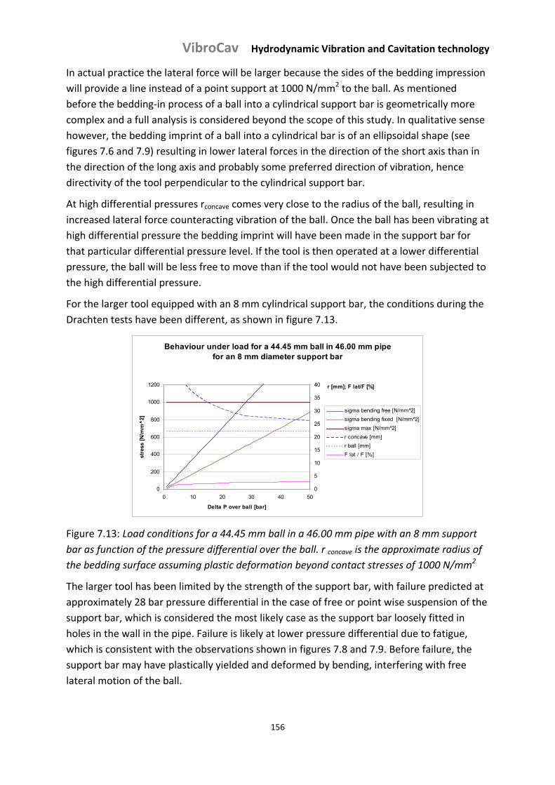
VibroCav Hydrodynamic Vibration and Cavitation technology
156
In actual practice the lateral force will be larger because the sides of the bedding impression
will provide a line instead of a point support at 1000 N/mm2 to the ball. As mentioned
before the bedding‐in process of a ball into a cylindrical support bar is geometrically more
complex and a full analysis is considered beyond the scope of this study. In qualitative sense
however, the bedding imprint of a ball into a cylindrical bar is of an ellipsoidal shape (see
figures 7.6 and 7.9) resulting in lower lateral forces in the direction of the short axis than in
the direction of the long axis and probably some preferred direction of vibration, hence
directivity of the tool perpendicular to the cylindrical support bar.
At high differential pressures rconcave comes very close to the radius of the ball, resulting in
increased lateral force counteracting vibration of the ball. Once the ball has been vibrating at
high differential pressure the bedding imprint will have been made in the support bar for
that particular differential pressure level. If the tool is then operated at a lower differential
pressure, the ball will be less free to move than if the tool would not have been subjected to
the high differential pressure.
For the larger tool equipped with an 8 mm cylindrical support bar, the conditions during the
Drachten tests have been different, as shown in figure 7.13.
Behaviour under load for a 44.45 mm ball in 46.00 mm pipe for an 8 mm diameter support bar
0
200
400
600
800
1000
1200
0 10 20 30 40 50
Delta P over ball [bar]
stre
ss [
N/m
m^
2]
0
5
10
15
20
25
30
35
40 r [mm]; F lat/F [%]
sigma bending free [N/mm 2̂]
sigma bending fixed [N/mm^2]
sigma max [N/mm^2]
r concave [mm]
r ball [mm]
F lat / F [%]
Figure 7.13: Load conditions for a 44.45 mm ball in a 46.00 mm pipe with an 8 mm support
bar as function of the pressure differential over the ball. r concave is the approximate radius of
the bedding surface assuming plastic deformation beyond contact stresses of 1000 N/mm2
The larger tool has been limited by the strength of the support bar, with failure predicted at
approximately 28 bar pressure differential in the case of free or point wise suspension of the
support bar, which is considered the most likely case as the support bar loosely fitted in
holes in the wall in the pipe. Failure is likely at lower pressure differential due to fatigue,
which is consistent with the observations shown in figures 7.8 and 7.9. Before failure, the
support bar may have plastically yielded and deformed by bending, interfering with free
lateral motion of the ball.
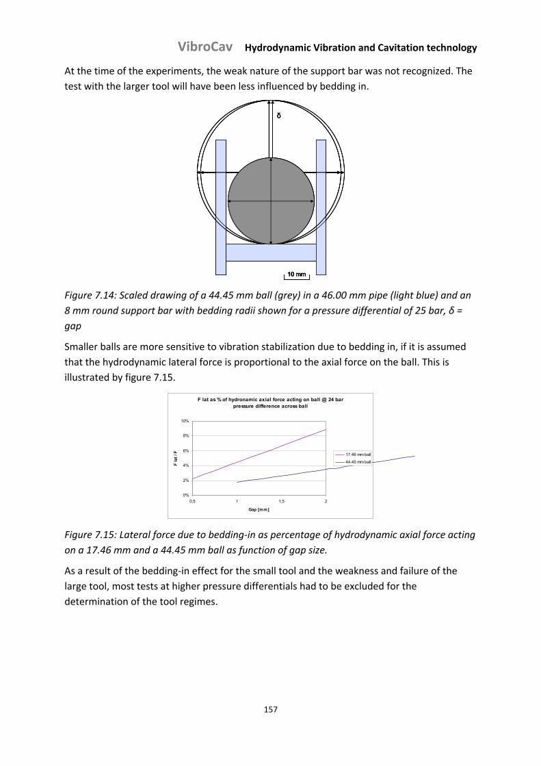
VibroCav Hydrodynamic Vibration and Cavitation technology
157
At the time of the experiments, the weak nature of the support bar was not recognized. The
test with the larger tool will have been less influenced by bedding in.
10 mm
δ
10 mm
δ
10 mm10 mm
δ
Figure 7.14: Scaled drawing of a 44.45 mm ball (grey) in a 46.00 mm pipe (light blue) and an
8 mm round support bar with bedding radii shown for a pressure differential of 25 bar, δ =
gap
Smaller balls are more sensitive to vibration stabilization due to bedding in, if it is assumed
that the hydrodynamic lateral force is proportional to the axial force on the ball. This is
illustrated by figure 7.15.
F lat as % of hydronamic axial force acting on ball @ 24 bar pressure difference across ball
0%
2%
4%
6%
8%
10%
0,5 1 1,5 2
Gap [mm]
F la
t / F 17.46 mm ball
44.45 mm ball
Figure 7.15: Lateral force due to bedding‐in as percentage of hydrodynamic axial force acting
on a 17.46 mm and a 44.45 mm ball as function of gap size.
As a result of the bedding‐in effect for the small tool and the weakness and failure of the
large tool, most tests at higher pressure differentials had to be excluded for the
determination of the tool regimes.
VibroCav Hydrodynamic Vibration and Cavitation technology
158
7.5. Conclusions
The VibroCav tool has been tested in horizontal position for a limited number of
tests, using bottom supported balls in pipes with an internal diameter of 18.50 mm
and 46.00 mm at flow rates of up to 38 m3/hr and backpressures of up to 200 bar.
Active cavitation was visually observed at up to a backpressure of 63 barg. Vibration
was observed at up to 200 barg backpressure. This backpressure was the maximum
operationally achievable and there is no evidence that vibration would cease at even
higher backpressure; however if the flow rate becomes too high the ball may stop
vibrating.
Even at low pressure differentials over the ball the yield strength of the steel ball and
support is easily exceeded due to the small contact area between the ball and a flat
or cylindrical support leading to plastic deformation of the softest component. If the
support is made of softer material, the ball will bed itself in by plastic deformation of
the support, which ultimately leads to a stable situation with stress levels below the
plastic limits.
Bedding‐in interferes with the freedom of the ball to vibrate as it generates a lateral
force counteracting the lateral force that causes the ball to vibrate. Smaller balls are
more sensitive to vibration stabilisation due to bedding in than larger balls at the
same pressure differential of the ball.
At high pressure differentials and larger tools care must be taken for the mechanical
strength of the support itself, taking account of fatigue due to the high cyclic stresses
when vibrating. These aspects are points of attention for the design of the tools.
Bedding‐in influences already at low pressure differentials the free lateral motion of
bottom supported balls. Hanging balls do not suffer from this problem, provided that
the hanging suspension is properly designed with low internal friction characteristics.
7.6. References
1. Young, W.C. ; Budynas, R.G. ; Roarks Formulas for Stress and Strain; McGraw‐Hill
2. Polytechnisch zakboekje, Dutch version, section C2

VibroCav Hydrodynamic Vibration and Cavitation technology
159
VibroCav Hydrodynamic Vibration and Cavitation technology
160
Chapter 8: Industrial trials for cleaning a porous medium around a wellbore
8.1. Fouling of the inflow horizon in wellbores
Oil and water wells are connected with permeable reservoir rock, through which fluids flow
to the well bore. The inflow interval can be several meters long in wells with a low
inclination to hundreds of meters in near horizontal reservoir penetrations. There is a wide
variety of reservoir rock, such as sand stone or carbonate rock and the rock may have
various degrees of consolidation and be undisturbed or naturally fractured. The purpose of
the wells is in the majority to produce or inject fluids. The effective permeability in the
immediate vicinity of the wellbore plays a major role in the production and injection process,
and impaired permeability of the near wellbore interval greatly increases the pressure drop,
because the fluid velocity in the pores is high compared to the velocity further away from
the wellbore.
The characteristics of the inflow interval have been extensively studied and there are many
reasons why the pressure drop required causing fluid flow from the far field in a permeable
porous reservoir is higher than would be expected from a simple radial flow model based on
far field permeability and porosity values. These reasons include deviation of the well bore,
partial completion of the reservoir thickness and limited entry through perforations
however. If these factors are ignored however, the stabilised flow of fluid into the wellbore
of a single well in open communication with a bounded radial reservoir is given by the semi‐
steady state equation:
mw
ei Sr
r
hk
P
QPI
4
3ln
2 0
(8.1)
in which PI = Productivity Index (m3/s.Pa), Q = flow rate (m3/s), ΔPi = Drawdown = Pressure
drop required between the average field pressure and the wellbore (Pa), k0 = ‘far field’
permeability of the reservoir rock (m2), h = vertical formation thickness (m), η= dynamic
viscosity (Pa.s), re = drainage radius of the well (m), rw = radius of the well (m) and Sm =
mechanical skin factor (dim less) [1,2]. If the well is undamaged Sm will be 0 allowing k0 to be
calculated for selected values of re. For the calculations in this study re = 300 m has been
used, a value commonly used in the oil industry. The flow rate at Sm = 0 has been designated
in this study as Qi or initial flow rate.
The decrease in permeability in the near wellbore area, compared to the permeability in the
far field are interrelated through the mechanical skin Sm:
w
d
dm r
r
k
kS ln)1( 0 (8.2)
VibroCav Hydrodynamic Vibration and Cavitation technology
161
in which , kd = permeability of the damaged region and rd = radius of damaged region.
Mathematically Sm is only dependent on the permeability ratio k0/kd and not on the absolute
far field permeability k0, however the damage mechanisms will strongly depend on k0. The
inverse ratio kd/k0 is a measure for the pore damage. For the undamaged well Sm = 0.
The pressure drop associated with mechanical skin Sm only is by definition [2]:
mskin Shk
QP )
2(
0
(8.3)
in which ΔPskin = additional pressure drop due to skin (Pa). ΔPskin can be approximated
through an analysis of flow rates at a known ΔPi using the following formula:
PIQQPP iiskin /)( (8.4)
The relationship between penetration depth L of the Biot slow wave into a porous matrix
defined as the distance from the wall of the porous matrix at which the amplitude of the
slow wave is halved can be approximated by the following formulas:
fDL h /23.1 (8.5)
and,
)/(0 fh KkD (8.6)
in which Dh = the hydraulic diffusivity (m2/s), f = frequency (Hz), Kf = bulk modulus of pore
fluid (Pa), and = porosity (‐), see also Chapter 1, section 1.2.3.
If Sm > 0, the inflow horizon is impaired. Impairment can be caused by many factors, such as
fouling by colloidal solids, polymers or emulsions from the drilling fluid, by crushed
formation due to perforating, by fines of the gravel packing process and by particles
liberated in the reservoir due to fluid flow or matrix crushing or by particles in injection fluids
or a combination of such factors. Restrepo [3] describes a skin factor characterisation
methodology that deepens the understanding of the various factors involved and their
relative importance based on statistical correlation in a number of oilfields.
A well is normally drilled using a drilling fluid with a higher hydrostatic pressure in the
wellbore than the pressure of the pore fluid in the formation, a so‐called overbalance, to
avoid reservoir fluids invading the wellbore and causing safety risks or contamination of the
drilling fluid. The drilling fluid normally contains solids from the drilling process and additives
to control the viscosity and the specific weight and to reduce the fluid loss to the formation.
For weight control, ground barite (BaSO4) is normally used and for fluid loss control polymers
that screen out on the wellbore face and form a seal together with fine solids, referred to in
the drilling industry as mud cake. Before the mud cake is established a certain amount of
mud and filtrate is injected into the near wellbore with pore fouling potential. If drilling fluid
losses are experienced, materials such as ground coconut shells, fibres, and fine carbonate
particles, generically called lost circulation additives, may be used to plug the near wellbore
VibroCav Hydrodynamic Vibration and Cavitation technology
162
area on purpose. Techniques exist to minimise drill‐in permeability damage such as the use
of ground CaCO3 as weighing material for reservoir drill‐ins and for reducing drilling fluid
losses and the use of HCl to remove fine CaCO3 particles by dissolution. In many cases
however, wellbores are left impaired after the drilling process. Barite fines cannot be easily
dissolved. Underbalanced drilling, i.e. allowing the reservoir to flow during the drilling
process and thus avoid reservoir impairment, is gaining popularity as a drill‐in process;
however it is expensive and less safe than the established overbalanced method.
After drilling the reservoir interval is commonly protected by installing a steel casing across
the open hole section and by placing cement between the casing and the formation. The
casing, cement layer and first centimetres or decimetres of formation are then explosively
perforated in under‐ or overbalanced condition. The explosive destruction of steel, cement
and formation creates fines that are blown into the formation surrounding the perforation
tunnels, causing impairment, particularly if the well is overbalanced when firing the
explosives. While underbalanced perforating is preferred to avoid impairment, it is not
always technically feasible.
Another method of securing the inflow horizon is by placing a filter tube across the open
hole in the inflow interval and by filling the annular space between the filter tube and the
formation with a layer of narrow size range well rounded sand, commonly referred to as
gravel. This method is called gravel packing and is discussed in more detail later in this
chapter. Placing the gravel can also lead to impairment by fines that are injected into the
formation in the immediate vicinity of the wellbore. The skin factor is often higher, hence
worse, after a gravel packing operation, compared to before.
Common to the production process is that all fluid from the far field must transit an inflow
area close to the well bore in a predominantly radial fashion. The flow of fluid through pores
and fractures in the reservoir rock mobilizes and entrains sub‐pore sized particles. Pressure
changes due to the production process influence the strain in the rock matrix, which may
result in the generation of fine particles due to rearranging and crushing of the grains and
scraping of the grain surfaces. These fines concentrate in the inflow area, typically
representing the first centimetres to decimetres from the wellbore. Particles that
individually could be entrained through the pores into the wellbore form a bridge of stacked
particles if sufficient particles are forced simultaneously through a pore throat. A swarm
consisting of particles that are significantly smaller than the pore throat diameter is capable
of blocking pore throats. For small particles smaller than typically 10 μm electro‐kinetic
forces come into play in the formation bridges, which dominate below a particle size of 1 μm
[4]. A continued supply of particles results in blocking more and more pore throats in the
flow path to the wellbore with increasingly finer particles becoming trapped in developing
particle bridges. This process results in progressive deterioration of the permeability near
the wellbore, which thus impedes the flow to the wellbore. The described mechanism
pertains typically to porous media such as sand stone. The same plugging mechanism tends
to happen also in flow through fractures in the narrower passages formed by irregularities of
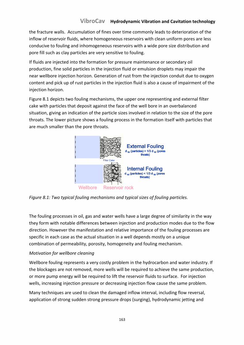
VibroCav Hydrodynamic Vibration and Cavitation technology
163
the fracture walls. Accumulation of fines over time commonly leads to deterioration of the
inflow of reservoir fluids, where homogeneous reservoirs with clean uniform pores are less
conducive to fouling and inhomogeneous reservoirs with a wide pore size distribution and
pore fill such as clay particles are very sensitive to fouling.
If fluids are injected into the formation for pressure maintenance or secondary oil
production, fine solid particles in the injection fluid or emulsion droplets may impair the
near wellbore injection horizon. Generation of rust from the injection conduit due to oxygen
content and pick up of rust particles in the injection fluid is also a cause of impairment of the
injection horizon.
Figure 8.1 depicts two fouling mechanisms, the upper one representing and external filter
cake with particles that deposit against the face of the well bore in an overbalanced
situation, giving an indication of the particle sizes involved in relation to the size of the pore
throats. The lower picture shows a fouling process in the formation itself with particles that
are much smaller than the pore throats.
Wellbore
Filter Cake
External Foulingd 50 (particles) > 1/3 d 50 (pores
thoats)
Internal Foulingd 50 (particles) < 1/3 d 50 (pores
throats)
After: Abrams
Reservoir rockWellbore
Filter Cake
External Foulingd 50 (particles) > 1/3 d 50 (pores
thoats)
Internal Foulingd 50 (particles) < 1/3 d 50 (pores
throats)
After: Abrams
Reservoir rockWellbore
Filter CakeFilter Cake
External Foulingd 50 (particles) > 1/3 d 50 (pores
thoats)
Internal Foulingd 50 (particles) < 1/3 d 50 (pores
throats)
After: Abrams
Reservoir rock
Figure 8.1: Two typical fouling mechanisms and typical sizes of fouling particles.
The fouling processes in oil, gas and water wells have a large degree of similarity in the way
they form with notable differences between injection and production modes due to the flow
direction. However the manifestation and relative importance of the fouling processes are
specific in each case as the actual situation in a well depends mostly on a unique
combination of permeability, porosity, homogeneity and fouling mechanism.
Motivation for wellbore cleaning
Wellbore fouling represents a very costly problem in the hydrocarbon and water industry. If
the blockages are not removed, more wells will be required to achieve the same production,
or more pump energy will be required to lift the reservoir fluids to surface. For injection
wells, increasing injection pressure or decreasing injection flow cause the same problem.
Many techniques are used to clean the damaged inflow interval, including flow reversal,
application of strong sudden strong pressure drops (surging), hydrodynamic jetting and
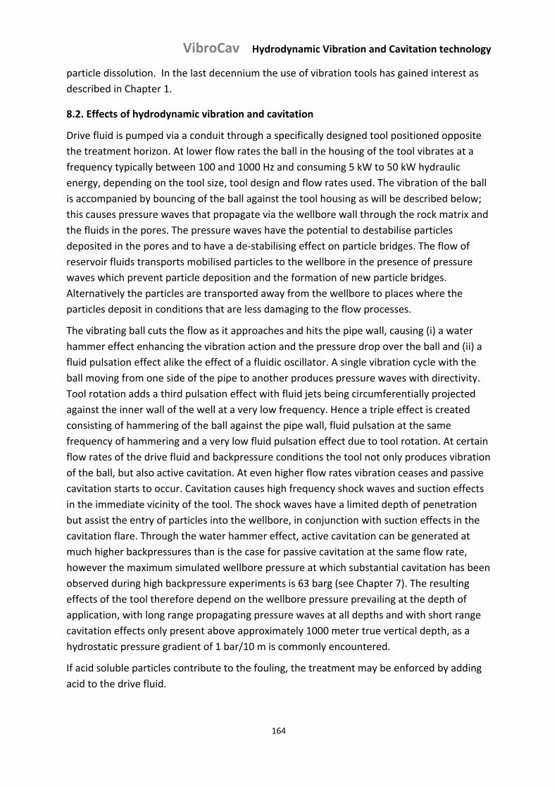
VibroCav Hydrodynamic Vibration and Cavitation technology
164
particle dissolution. In the last decennium the use of vibration tools has gained interest as
described in Chapter 1.
8.2. Effects of hydrodynamic vibration and cavitation
Drive fluid is pumped via a conduit through a specifically designed tool positioned opposite
the treatment horizon. At lower flow rates the ball in the housing of the tool vibrates at a
frequency typically between 100 and 1000 Hz and consuming 5 kW to 50 kW hydraulic
energy, depending on the tool size, tool design and flow rates used. The vibration of the ball
is accompanied by bouncing of the ball against the tool housing as will be described below;
this causes pressure waves that propagate via the wellbore wall through the rock matrix and
the fluids in the pores. The pressure waves have the potential to destabilise particles
deposited in the pores and to have a de‐stabilising effect on particle bridges. The flow of
reservoir fluids transports mobilised particles to the wellbore in the presence of pressure
waves which prevent particle deposition and the formation of new particle bridges.
Alternatively the particles are transported away from the wellbore to places where the
particles deposit in conditions that are less damaging to the flow processes.
The vibrating ball cuts the flow as it approaches and hits the pipe wall, causing (i) a water
hammer effect enhancing the vibration action and the pressure drop over the ball and (ii) a
fluid pulsation effect alike the effect of a fluidic oscillator. A single vibration cycle with the
ball moving from one side of the pipe to another produces pressure waves with directivity.
Tool rotation adds a third pulsation effect with fluid jets being circumferentially projected
against the inner wall of the well at a very low frequency. Hence a triple effect is created
consisting of hammering of the ball against the pipe wall, fluid pulsation at the same
frequency of hammering and a very low fluid pulsation effect due to tool rotation. At certain
flow rates of the drive fluid and backpressure conditions the tool not only produces vibration
of the ball, but also active cavitation. At even higher flow rates vibration ceases and passive
cavitation starts to occur. Cavitation causes high frequency shock waves and suction effects
in the immediate vicinity of the tool. The shock waves have a limited depth of penetration
but assist the entry of particles into the wellbore, in conjunction with suction effects in the
cavitation flare. Through the water hammer effect, active cavitation can be generated at
much higher backpressures than is the case for passive cavitation at the same flow rate,
however the maximum simulated wellbore pressure at which substantial cavitation has been
observed during high backpressure experiments is 63 barg (see Chapter 7). The resulting
effects of the tool therefore depend on the wellbore pressure prevailing at the depth of
application, with long range propagating pressure waves at all depths and with short range
cavitation effects only present above approximately 1000 meter true vertical depth, as a
hydrostatic pressure gradient of 1 bar/10 m is commonly encountered.
If acid soluble particles contribute to the fouling, the treatment may be enforced by adding
acid to the drive fluid.
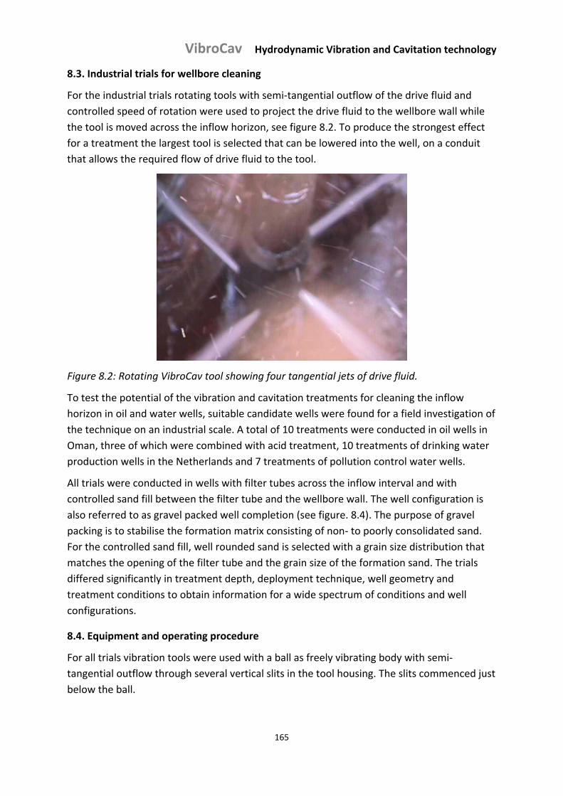
VibroCav Hydrodynamic Vibration and Cavitation technology
165
8.3. Industrial trials for wellbore cleaning
For the industrial trials rotating tools with semi‐tangential outflow of the drive fluid and
controlled speed of rotation were used to project the drive fluid to the wellbore wall while
the tool is moved across the inflow horizon, see figure 8.2. To produce the strongest effect
for a treatment the largest tool is selected that can be lowered into the well, on a conduit
that allows the required flow of drive fluid to the tool.
Figure 8.2: Rotating VibroCav tool showing four tangential jets of drive fluid.
To test the potential of the vibration and cavitation treatments for cleaning the inflow
horizon in oil and water wells, suitable candidate wells were found for a field investigation of
the technique on an industrial scale. A total of 10 treatments were conducted in oil wells in
Oman, three of which were combined with acid treatment, 10 treatments of drinking water
production wells in the Netherlands and 7 treatments of pollution control water wells.
All trials were conducted in wells with filter tubes across the inflow interval and with
controlled sand fill between the filter tube and the wellbore wall. The well configuration is
also referred to as gravel packed well completion (see figure. 8.4). The purpose of gravel
packing is to stabilise the formation matrix consisting of non‐ to poorly consolidated sand.
For the controlled sand fill, well rounded sand is selected with a grain size distribution that
matches the opening of the filter tube and the grain size of the formation sand. The trials
differed significantly in treatment depth, deployment technique, well geometry and
treatment conditions to obtain information for a wide spectrum of conditions and well
configurations.
8.4. Equipment and operating procedure
For all trials vibration tools were used with a ball as freely vibrating body with semi‐
tangential outflow through several vertical slits in the tool housing. The slits commenced just
below the ball.
VibroCav Hydrodynamic Vibration and Cavitation technology
166
For a number of trials (37%, all in Oman) the tool was lowered into the well on a jointed drill
pipe to reach the treatment interval using a well maintenance hoisting installation. During
the treatment the drill pipe was rotated at 40 to 60 rpm.
For the remainder of the trials a drive fluid conduit was used that could not be rotated, such
as continuous steel tube from a reel (coiled tubing) or reinforced plastic pipe from a reel. For
these trials rotating tools were used, referred to as ‘Roto VibroCav’ , mostly with a housing
OD (outer diameter) of 3.2” (81.28 mm), in which the rotation was caused by reaction
forces due to the tangential component in the outflow of the drive fluid, as shown in figure
8.3. A hydrodynamic brake was used to control the speed of rotation in order to maintain
adequate radial impact.
A A’
A A’
Rotating Housing
Free Body
Support
A A’
A A’
Rotating Housing
Free Body
Support
Figure 8.3: Principle sketch of a VibroCav tool that can freely rotate due to a sealing bearing
at the top of the tool (not shown). Rotation of the housing is caused by the tangential
component in the outflow of the tool. (During the industrial scale trials, the tool was
combined with a hydrodynamic brake to avoid free spinning of the tool).
The drive fluid was pumped at rates of 350 to 550 l/min (tools with 2.5” or 3.2” housing), up
to 700 l/min (tool with 4.5” housing), projecting the outflow from the tool against the
wellbore wall. When possible the well was produced at a flow rate significantly higher than
the drive fluid pump rate to ensure net inflow from the formation to entrain dislodged
material into the wellbore and flush this material out of the well with the production flow.
The general approach during a treatment was to start at the bottom in the treatment
interval and move upwards with a speed of typically 1 to 2 m/min. During several treatments
successive passes were made to enhance the cleaning effect.
The ten Oman oil wells with a wellbore diameter of typically 8.5” at a vertical depth below
the surface of 1000 to 1500 m were provided across the inflow horizon with a wire wrapped
filter tube, also called wire wrapped screen, mounted on the outside of a perforated base
pipe as shown in figure 8.4.
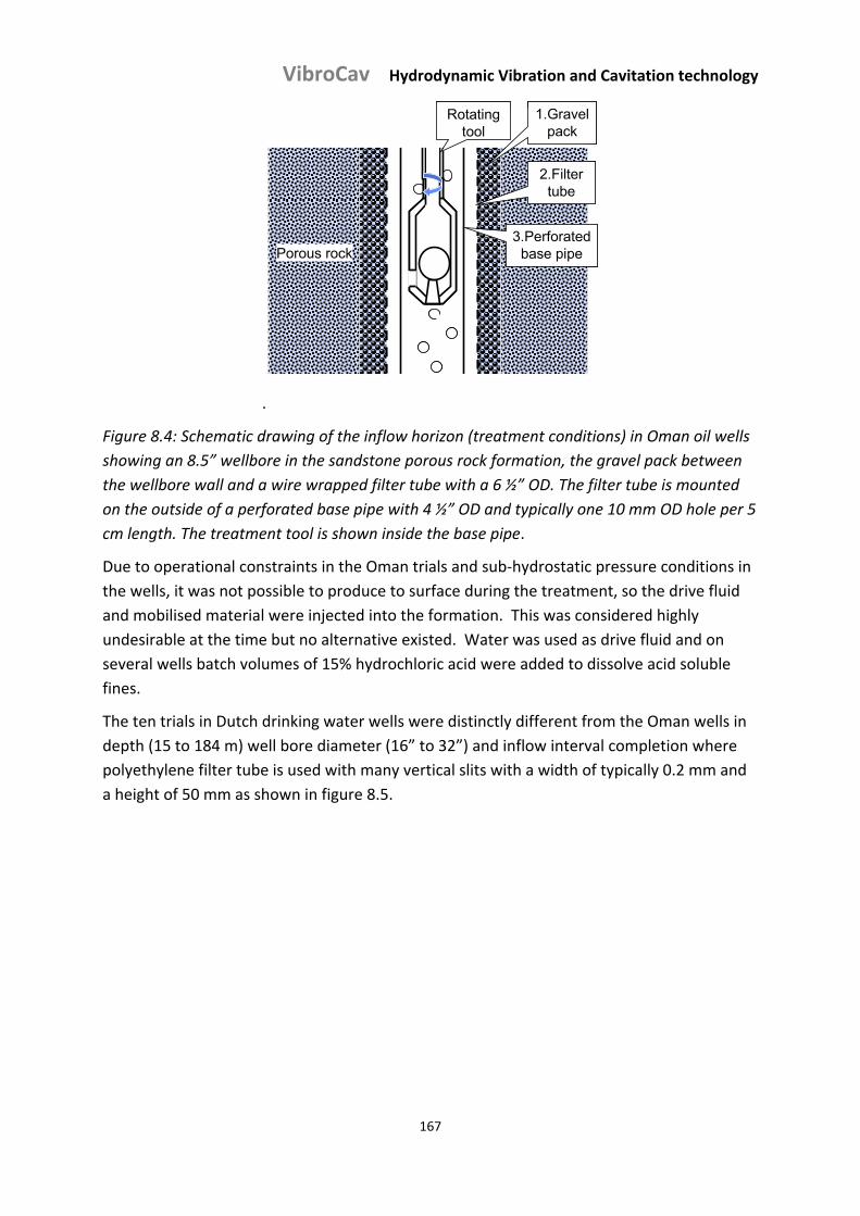
VibroCav Hydrodynamic Vibration and Cavitation technology
167
.
Rotating tool
Porous rock
1.Gravel pack
2.Filter tube
3.Perforated base pipe
Rotating tool
Porous rock
1.Gravel pack
2.Filter tube
3.Perforated base pipe
Figure 8.4: Schematic drawing of the inflow horizon (treatment conditions) in Oman oil wells
showing an 8.5” wellbore in the sandstone porous rock formation, the gravel pack between
the wellbore wall and a wire wrapped filter tube with a 6 ½” OD. The filter tube is mounted
on the outside of a perforated base pipe with 4 ½” OD and typically one 10 mm OD hole per 5
cm length. The treatment tool is shown inside the base pipe.
Due to operational constraints in the Oman trials and sub‐hydrostatic pressure conditions in
the wells, it was not possible to produce to surface during the treatment, so the drive fluid
and mobilised material were injected into the formation. This was considered highly
undesirable at the time but no alternative existed. Water was used as drive fluid and on
several wells batch volumes of 15% hydrochloric acid were added to dissolve acid soluble
fines.
The ten trials in Dutch drinking water wells were distinctly different from the Oman wells in
depth (15 to 184 m) well bore diameter (16” to 32”) and inflow interval completion where
polyethylene filter tube is used with many vertical slits with a width of typically 0.2 mm and
a height of 50 mm as shown in figure 8.5.
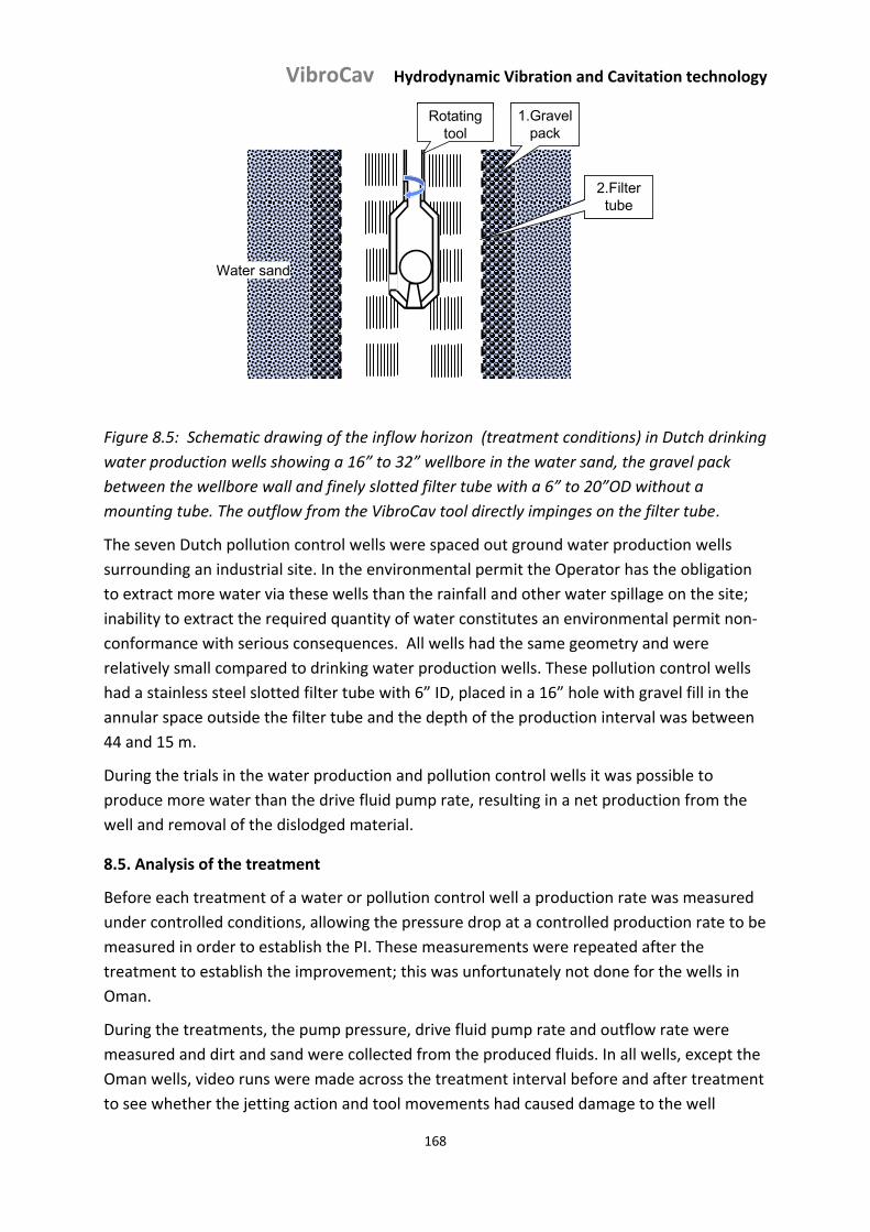
VibroCav Hydrodynamic Vibration and Cavitation technology
168
Rotating tool
Water sand
1.Gravel pack
2.Filter tube
Rotating tool
Water sand
1.Gravel pack
2.Filter tube
Figure 8.5: Schematic drawing of the inflow horizon (treatment conditions) in Dutch drinking
water production wells showing a 16” to 32” wellbore in the water sand, the gravel pack
between the wellbore wall and finely slotted filter tube with a 6” to 20”OD without a
mounting tube. The outflow from the VibroCav tool directly impinges on the filter tube.
The seven Dutch pollution control wells were spaced out ground water production wells
surrounding an industrial site. In the environmental permit the Operator has the obligation
to extract more water via these wells than the rainfall and other water spillage on the site;
inability to extract the required quantity of water constitutes an environmental permit non‐
conformance with serious consequences. All wells had the same geometry and were
relatively small compared to drinking water production wells. These pollution control wells
had a stainless steel slotted filter tube with 6” ID, placed in a 16” hole with gravel fill in the
annular space outside the filter tube and the depth of the production interval was between
44 and 15 m.
During the trials in the water production and pollution control wells it was possible to
produce more water than the drive fluid pump rate, resulting in a net production from the
well and removal of the dislodged material.
8.5. Analysis of the treatment
Before each treatment of a water or pollution control well a production rate was measured
under controlled conditions, allowing the pressure drop at a controlled production rate to be
measured in order to establish the PI. These measurements were repeated after the
treatment to establish the improvement; this was unfortunately not done for the wells in
Oman.
During the treatments, the pump pressure, drive fluid pump rate and outflow rate were
measured and dirt and sand were collected from the produced fluids. In all wells, except the
Oman wells, video runs were made across the treatment interval before and after treatment
to see whether the jetting action and tool movements had caused damage to the well
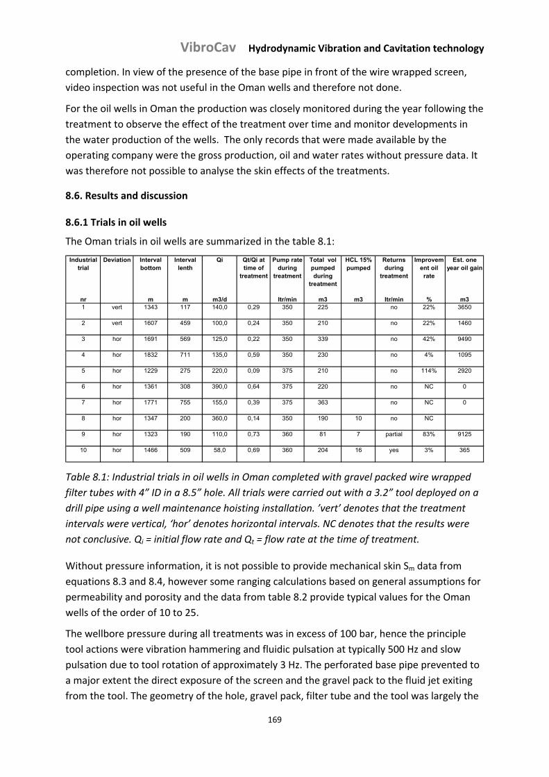
VibroCav Hydrodynamic Vibration and Cavitation technology
169
completion. In view of the presence of the base pipe in front of the wire wrapped screen,
video inspection was not useful in the Oman wells and therefore not done.
For the oil wells in Oman the production was closely monitored during the year following the
treatment to observe the effect of the treatment over time and monitor developments in
the water production of the wells. The only records that were made available by the
operating company were the gross production, oil and water rates without pressure data. It
was therefore not possible to analyse the skin effects of the treatments.
8.6. Results and discussion
8.6.1 Trials in oil wells
The Oman trials in oil wells are summarized in the table 8.1:
Industrial trial
Deviation Interval bottom
Interval lenth
Qi Qt/Qi at time of
treatment
Pump rate during
treatment
Total vol pumped during
treatment
HCL 15% pumped
Returns during
treatment
Improvement oil
rate
Est. one year oil gain
nr m m m3/d ltr/min m3 m3 ltr/min % m31 vert 1343 117 140,0 0,29 350 225 no 22% 3650
2 vert 1607 459 100,0 0,24 350 210 no 22% 1460
3 hor 1691 569 125,0 0,22 350 339 no 42% 9490
4 hor 1832 711 135,0 0,59 350 230 no 4% 1095
5 hor 1229 275 220,0 0,09 375 210 no 114% 2920
6 hor 1361 308 390,0 0,64 375 220 no NC 0
7 hor 1771 755 155,0 0,39 375 363 no NC 0
8 hor 1347 200 360,0 0,14 350 190 10 no NC
9 hor 1323 190 110,0 0,73 360 81 7 partial 83% 9125
10 hor 1466 509 58,0 0,69 360 204 16 yes 3% 365
Table 8.1: Industrial trials in oil wells in Oman completed with gravel packed wire wrapped
filter tubes with 4” ID in a 8.5” hole. All trials were carried out with a 3.2” tool deployed on a
drill pipe using a well maintenance hoisting installation. ’vert’ denotes that the treatment
intervals were vertical, ‘hor’ denotes horizontal intervals. NC denotes that the results were
not conclusive. Qi = initial flow rate and Qt = flow rate at the time of treatment.
Without pressure information, it is not possible to provide mechanical skin Sm data from
equations 8.3 and 8.4, however some ranging calculations based on general assumptions for
permeability and porosity and the data from table 8.2 provide typical values for the Oman
wells of the order of 10 to 25.
The wellbore pressure during all treatments was in excess of 100 bar, hence the principle
tool actions were vibration hammering and fluidic pulsation at typically 500 Hz and slow
pulsation due to tool rotation of approximately 3 Hz. The perforated base pipe prevented to
a major extent the direct exposure of the screen and the gravel pack to the fluid jet exiting
from the tool. The geometry of the hole, gravel pack, filter tube and the tool was largely the
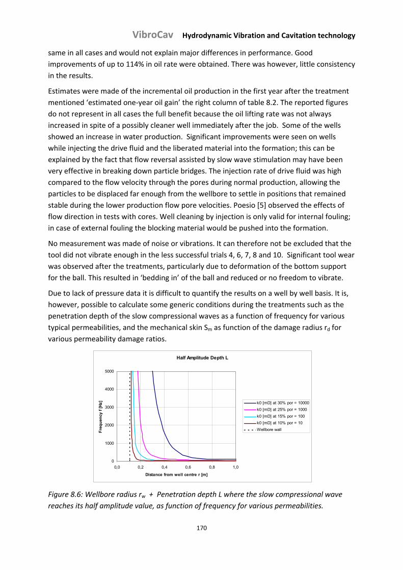
VibroCav Hydrodynamic Vibration and Cavitation technology
170
same in all cases and would not explain major differences in performance. Good
improvements of up to 114% in oil rate were obtained. There was however, little consistency
in the results.
Estimates were made of the incremental oil production in the first year after the treatment
mentioned ‘estimated one‐year oil gain’ the right column of table 8.2. The reported figures
do not represent in all cases the full benefit because the oil lifting rate was not always
increased in spite of a possibly cleaner well immediately after the job. Some of the wells
showed an increase in water production. Significant improvements were seen on wells
while injecting the drive fluid and the liberated material into the formation; this can be
explained by the fact that flow reversal assisted by slow wave stimulation may have been
very effective in breaking down particle bridges. The injection rate of drive fluid was high
compared to the flow velocity through the pores during normal production, allowing the
particles to be displaced far enough from the wellbore to settle in positions that remained
stable during the lower production flow pore velocities. Poesio [5] observed the effects of
flow direction in tests with cores. Well cleaning by injection is only valid for internal fouling;
in case of external fouling the blocking material would be pushed into the formation.
No measurement was made of noise or vibrations. It can therefore not be excluded that the
tool did not vibrate enough in the less successful trials 4, 6, 7, 8 and 10. Significant tool wear
was observed after the treatments, particularly due to deformation of the bottom support
for the ball. This resulted in ‘bedding in’ of the ball and reduced or no freedom to vibrate.
Due to lack of pressure data it is difficult to quantify the results on a well by well basis. It is,
however, possible to calculate some generic conditions during the treatments such as the
penetration depth of the slow compressional waves as a function of frequency for various
typical permeabilities, and the mechanical skin Sm as function of the damage radius rd for
various permeability damage ratios.
Half Amplitude Depth L
0
1000
2000
3000
4000
5000
0,0 0,2 0,4 0,6 0,8 1,0
Distance from well centre r [m]
Fre
qu
ency
f [
Hz] k0 [mD] at 30% por = 10000
k0 [mD] at 25% por = 1000
k0 [mD] at 15% por = 100
k0 [mD] at 10% por = 10
Wellbore wall
Figure 8.6: Wellbore radius rw + Penetration depth L where the slow compressional wave
reaches its half amplitude value, as function of frequency for various permeabilities.
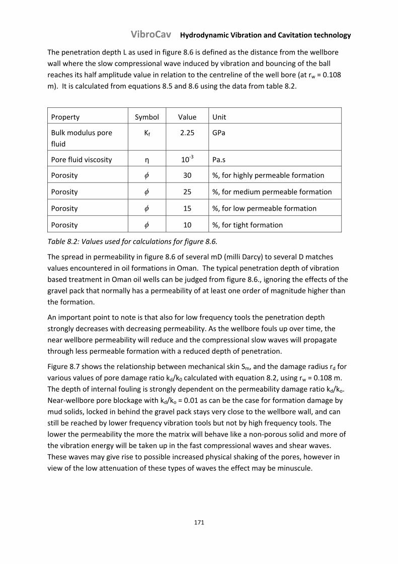
VibroCav Hydrodynamic Vibration and Cavitation technology
171
The penetration depth L as used in figure 8.6 is defined as the distance from the wellbore
wall where the slow compressional wave induced by vibration and bouncing of the ball
reaches its half amplitude value in relation to the centreline of the well bore (at rw = 0.108
m). It is calculated from equations 8.5 and 8.6 using the data from table 8.2.
Property Symbol Value Unit
Bulk modulus pore
fluid
Kf 2.25 GPa
Pore fluid viscosity η 10‐3 Pa.s
Porosity 30 %, for highly permeable formation
Porosity 25 %, for medium permeable formation
Porosity 15 %, for low permeable formation
Porosity 10 %, for tight formation
Table 8.2: Values used for calculations for figure 8.6.
The spread in permeability in figure 8.6 of several mD (milli Darcy) to several D matches
values encountered in oil formations in Oman. The typical penetration depth of vibration
based treatment in Oman oil wells can be judged from figure 8.6., ignoring the effects of the
gravel pack that normally has a permeability of at least one order of magnitude higher than
the formation.
An important point to note is that also for low frequency tools the penetration depth
strongly decreases with decreasing permeability. As the wellbore fouls up over time, the
near wellbore permeability will reduce and the compressional slow waves will propagate
through less permeable formation with a reduced depth of penetration.
Figure 8.7 shows the relationship between mechanical skin Sm, and the damage radius rd for
various values of pore damage ratio kd/k0 calculated with equation 8.2, using rw = 0.108 m.
The depth of internal fouling is strongly dependent on the permeability damage ratio kd/ko.
Near‐wellbore pore blockage with kd/ko = 0.01 as can be the case for formation damage by
mud solids, locked in behind the gravel pack stays very close to the wellbore wall, and can
still be reached by lower frequency vibration tools but not by high frequency tools. The
lower the permeability the more the matrix will behave like a non‐porous solid and more of
the vibration energy will be taken up in the fast compressional waves and shear waves.
These waves may give rise to possible increased physical shaking of the pores, however in
view of the low attenuation of these types of waves the effect may be minuscule.
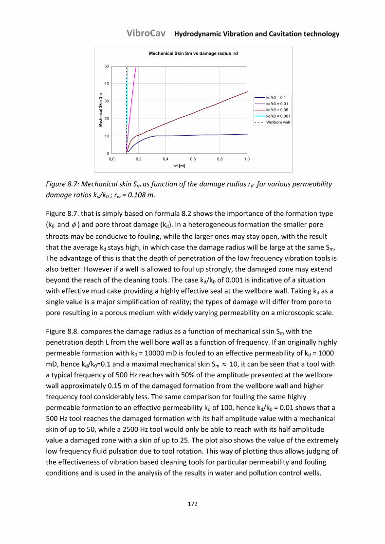
VibroCav Hydrodynamic Vibration and Cavitation technology
172
Mechanical Skin Sm vs damage radius rd
0
10
20
30
40
50
0,0 0,2 0,4 0,6 0,8 1,0
rd [m]
Mec
hn
ical
Ski
n S
mkd/k0 = 0,1
kd/k0 = 0,01
kd/k0 = 0,05
kd/k0 = 0,001
Wellbore wall
Figure 8.7: Mechanical skin Sm as function of the damage radius rd for various permeability
damage ratios kd/k0 ; rw = 0.108 m.
Figure 8.7. that is simply based on formula 8.2 shows the importance of the formation type
(k0 and ) and pore throat damage (kd). In a heterogeneous formation the smaller pore
throats may be conducive to fouling, while the larger ones may stay open, with the result
that the average kd stays high, in which case the damage radius will be large at the same Sm.
The advantage of this is that the depth of penetration of the low frequency vibration tools is
also better. However if a well is allowed to foul up strongly, the damaged zone may extend
beyond the reach of the cleaning tools. The case kd/k0 of 0.001 is indicative of a situation
with effective mud cake providing a highly effective seal at the wellbore wall. Taking kd as a
single value is a major simplification of reality; the types of damage will differ from pore to
pore resulting in a porous medium with widely varying permeability on a microscopic scale.
Figure 8.8. compares the damage radius as a function of mechanical skin Sm with the
penetration depth L from the well bore wall as a function of frequency. If an originally highly
permeable formation with k0 = 10000 mD is fouled to an effective permeability of kd = 1000
mD, hence kd/k0=0.1 and a maximal mechanical skin Sm 10, it can be seen that a tool with a typical frequency of 500 Hz reaches with 50% of the amplitude presented at the wellbore
wall approximately 0.15 m of the damaged formation from the wellbore wall and higher
frequency tool considerably less. The same comparison for fouling the same highly
permeable formation to an effective permeability kd of 100, hence kd/k0 = 0.01 shows that a
500 Hz tool reaches the damaged formation with its half amplitude value with a mechanical
skin of up to 50, while a 2500 Hz tool would only be able to reach with its half amplitude
value a damaged zone with a skin of up to 25. The plot also shows the value of the extremely
low frequency fluid pulsation due to tool rotation. This way of plotting thus allows judging of
the effectiveness of vibration based cleaning tools for particular permeability and fouling
conditions and is used in the analysis of the results in water and pollution control wells.
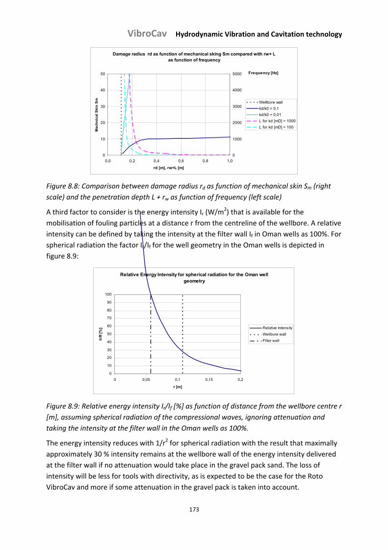
VibroCav Hydrodynamic Vibration and Cavitation technology
173
Damage radius rd as function of mechanical sking Sm compared with rw+ L as function of frequency
0
10
20
30
40
50
0,0 0,2 0,4 0,6 0,8 1,0
rd [m], rw+L [m]
Mec
hn
ical
Ski
n S
m
0
1000
2000
3000
4000
5000 Frequency [Hz]
Wellbore wall
kd/k0 = 0,1
kd/k0 = 0,01
L for kd [mD] = 1000
L for kd [mD] = 100
Figure 8.8: Comparison between damage radius rd as function of mechanical skin Sm (right
scale) and the penetration depth L + rw as function of frequency (left scale)
A third factor to consider is the energy intensity Ir (W/m2) that is available for the
mobilisation of fouling particles at a distance r from the centreline of the wellbore. A relative
intensity can be defined by taking the intensity at the filter wall If in Oman wells as 100%. For
spherical radiation the factor Ir/If for the well geometry in the Oman wells is depicted in
figure 8.9:
Relative Energy Intensity for spherical radiation for the Oman well geometry
0
10
20
30
40
50
60
70
80
90
100
0 0,05 0,1 0,15 0,2
r [m]
Ir/If
[%
] Relative Intensity
Wellbore wall
Filter wall
Figure 8.9: Relative energy intensity Ir/If [%] as function of distance from the wellbore centre r
[m], assuming spherical radiation of the compressional waves, ignoring attenuation and
taking the intensity at the filter wall in the Oman wells as 100%.
The energy intensity reduces with 1/r2 for spherical radiation with the result that maximally
approximately 30 % intensity remains at the wellbore wall of the energy intensity delivered
at the filter wall if no attenuation would take place in the gravel pack sand. The loss of
intensity will be less for tools with directivity, as is expected to be the case for the Roto
VibroCav and more if some attenuation in the gravel pack is taken into account.
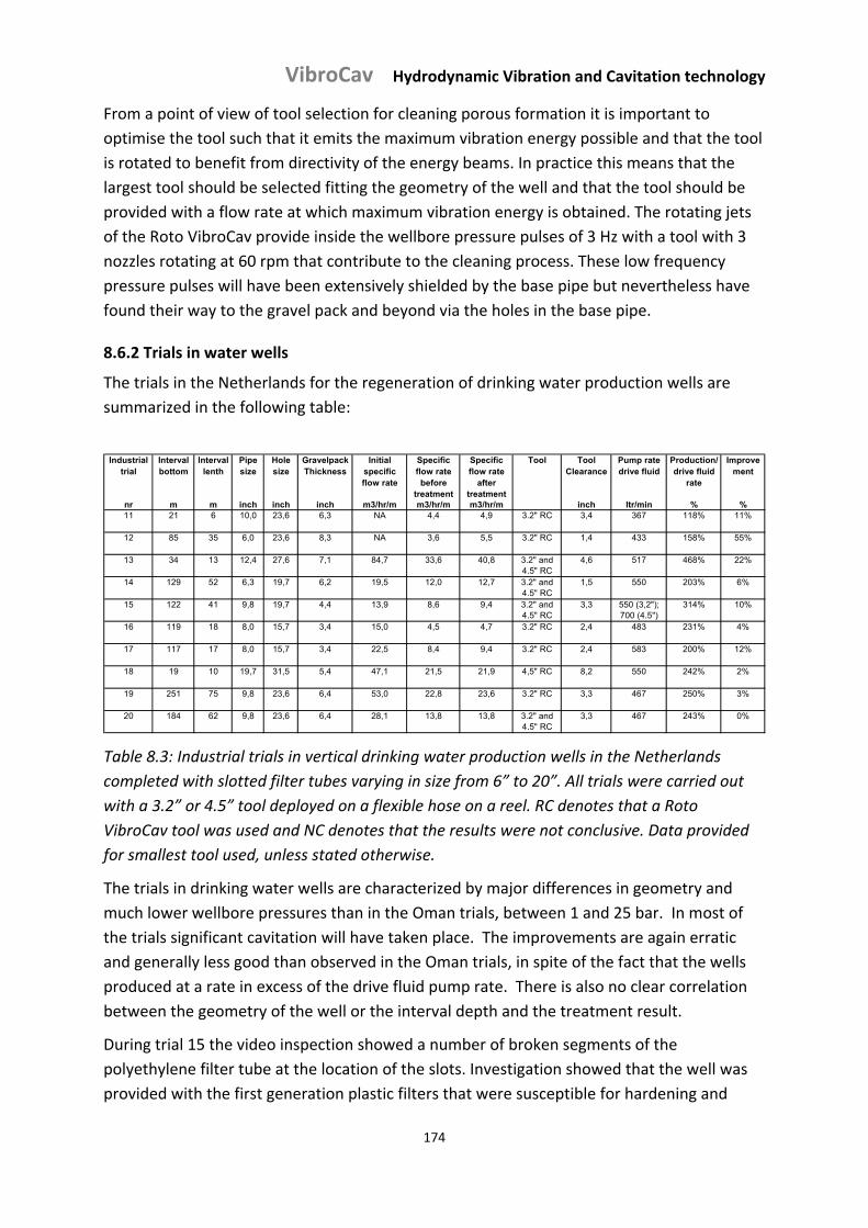
VibroCav Hydrodynamic Vibration and Cavitation technology
174
From a point of view of tool selection for cleaning porous formation it is important to
optimise the tool such that it emits the maximum vibration energy possible and that the tool
is rotated to benefit from directivity of the energy beams. In practice this means that the
largest tool should be selected fitting the geometry of the well and that the tool should be
provided with a flow rate at which maximum vibration energy is obtained. The rotating jets
of the Roto VibroCav provide inside the wellbore pressure pulses of 3 Hz with a tool with 3
nozzles rotating at 60 rpm that contribute to the cleaning process. These low frequency
pressure pulses will have been extensively shielded by the base pipe but nevertheless have
found their way to the gravel pack and beyond via the holes in the base pipe.
8.6.2 Trials in water wells
The trials in the Netherlands for the regeneration of drinking water production wells are
summarized in the following table:
Industrial
trialInterval bottom
Interval lenth
Pipe size
Hole size
Gravelpack Thickness
Initial specific flow rate
Specific flow rate before
treatment
Specific flow rate
after treatment
Tool Tool Clearance
Pump rate drive fluid
Production/drive fluid
rate
Improvement
nr m m inch inch inch m3/hr/m m3/hr/m m3/hr/m inch ltr/min % %11 21 6 10,0 23,6 6,3 NA 4,4 4,9 3.2" RC 3,4 367 118% 11%
12 85 35 6,0 23,6 8,3 NA 3,6 5,5 3.2" RC 1,4 433 158% 55%
13 34 13 12,4 27,6 7,1 84,7 33,6 40,8 3.2" and 4.5" RC
4,6 517 468% 22%
14 129 52 6,3 19,7 6,2 19,5 12,0 12,7 3.2" and 4.5" RC
1,5 550 203% 6%
15 122 41 9,8 19,7 4,4 13,9 8,6 9,4 3.2" and 4.5" RC
3,3 550 (3,2"); 700 (4.5")
314% 10%
16 119 18 8,0 15,7 3,4 15,0 4,5 4,7 3.2" RC 2,4 483 231% 4%
17 117 17 8,0 15,7 3,4 22,5 8,4 9,4 3.2" RC 2,4 583 200% 12%
18 19 10 19,7 31,5 5,4 47,1 21,5 21,9 4,5" RC 8,2 550 242% 2%
19 251 75 9,8 23,6 6,4 53,0 22,8 23,6 3.2" RC 3,3 467 250% 3%
20 184 62 9,8 23,6 6,4 28,1 13,8 13,8 3.2" and 4.5" RC
3,3 467 243% 0%
Table 8.3: Industrial trials in vertical drinking water production wells in the Netherlands
completed with slotted filter tubes varying in size from 6” to 20”. All trials were carried out
with a 3.2” or 4.5” tool deployed on a flexible hose on a reel. RC denotes that a Roto
VibroCav tool was used and NC denotes that the results were not conclusive. Data provided
for smallest tool used, unless stated otherwise.
The trials in drinking water wells are characterized by major differences in geometry and
much lower wellbore pressures than in the Oman trials, between 1 and 25 bar. In most of
the trials significant cavitation will have taken place. The improvements are again erratic
and generally less good than observed in the Oman trials, in spite of the fact that the wells
produced at a rate in excess of the drive fluid pump rate. There is also no clear correlation
between the geometry of the well or the interval depth and the treatment result.
During trial 15 the video inspection showed a number of broken segments of the
polyethylene filter tube at the location of the slots. Investigation showed that the well was
provided with the first generation plastic filters that were susceptible for hardening and
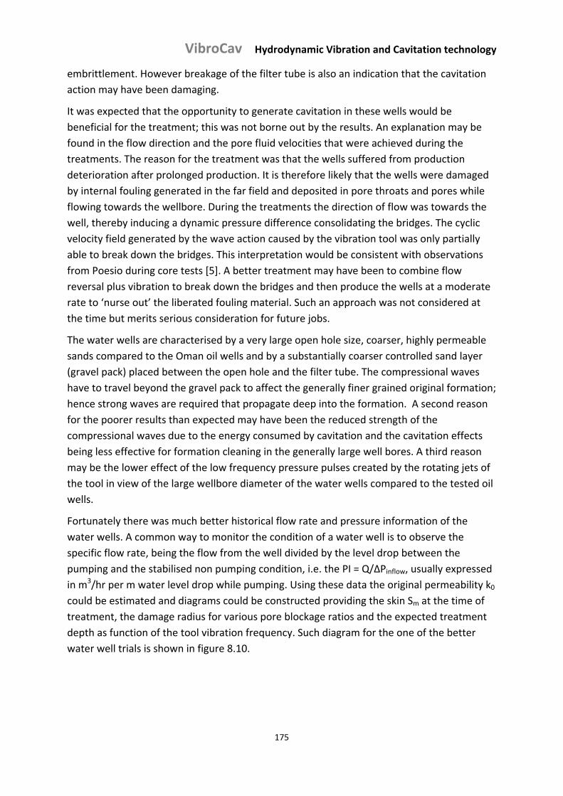
VibroCav Hydrodynamic Vibration and Cavitation technology
175
embrittlement. However breakage of the filter tube is also an indication that the cavitation
action may have been damaging.
It was expected that the opportunity to generate cavitation in these wells would be
beneficial for the treatment; this was not borne out by the results. An explanation may be
found in the flow direction and the pore fluid velocities that were achieved during the
treatments. The reason for the treatment was that the wells suffered from production
deterioration after prolonged production. It is therefore likely that the wells were damaged
by internal fouling generated in the far field and deposited in pore throats and pores while
flowing towards the wellbore. During the treatments the direction of flow was towards the
well, thereby inducing a dynamic pressure difference consolidating the bridges. The cyclic
velocity field generated by the wave action caused by the vibration tool was only partially
able to break down the bridges. This interpretation would be consistent with observations
from Poesio during core tests [5]. A better treatment may have been to combine flow
reversal plus vibration to break down the bridges and then produce the wells at a moderate
rate to ‘nurse out’ the liberated fouling material. Such an approach was not considered at
the time but merits serious consideration for future jobs.
The water wells are characterised by a very large open hole size, coarser, highly permeable
sands compared to the Oman oil wells and by a substantially coarser controlled sand layer
(gravel pack) placed between the open hole and the filter tube. The compressional waves
have to travel beyond the gravel pack to affect the generally finer grained original formation;
hence strong waves are required that propagate deep into the formation. A second reason
for the poorer results than expected may have been the reduced strength of the
compressional waves due to the energy consumed by cavitation and the cavitation effects
being less effective for formation cleaning in the generally large well bores. A third reason
may be the lower effect of the low frequency pressure pulses created by the rotating jets of
the tool in view of the large wellbore diameter of the water wells compared to the tested oil
wells.
Fortunately there was much better historical flow rate and pressure information of the
water wells. A common way to monitor the condition of a water well is to observe the
specific flow rate, being the flow from the well divided by the level drop between the
pumping and the stabilised non pumping condition, i.e. the PI = Q/ΔPinflow, usually expressed
in m3/hr per m water level drop while pumping. Using these data the original permeability k0
could be estimated and diagrams could be constructed providing the skin Sm at the time of
treatment, the damage radius for various pore blockage ratios and the expected treatment
depth as function of the tool vibration frequency. Such diagram for the one of the better
water well trials is shown in figure 8.10.
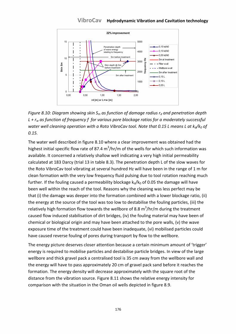
VibroCav Hydrodynamic Vibration and Cavitation technology
176
22% improvement
0
5
10
15
0,00 0,50 1,00 1,50 2,00
rd [m] or L+rw [m]
Ski
n S
m
0
1000
2000
3000
4000
5000
freq
uen
cy H
z
0,15 kd/k0
0,10 kd/k0
0,05 kd/k0
Sm at treatment
Filter w all
Wellbore w all
Sm after treatment
0,15 L
0,10 L
0,05 L
Penetration depthof wave energy relating to frequency
Skin depth @ Smbefore treatment
Sm before treatment
Sm after treatment
Figure 8.10: Diagram showing skin Sm as function of damage radius rd and penetration depth
L + rw as function of frequency f for various pore blockage ratios for a moderately successful
water well cleaning operation with a Roto VibroCav tool. Note that 0.15 L means L at kd/k0 of
0.15.
The water well described in figure 8.10 where a clear improvement was obtained had the
highest initial specific flow rate of 87.4 m3/hr/m of the wells for which such information was
available. It concerned a relatively shallow well indicating a very high initial permeability
calculated at 183 Darcy (trial 13 in table 8.3). The penetration depth L of the slow waves for
the Roto VibroCav tool vibrating at several hundred Hz will have been in the range of 1 m for
clean formation with the very low frequency fluid pulsing due to tool rotation reaching much
further. If the fouling caused a permeability blockage kd/k0 of 0.05 the damage will have
been well within the reach of the tool. Reasons why the cleaning was less perfect may be
that (i) the damage was deeper into the formation combined with a lower blockage ratio, (ii)
the energy at the source of the tool was too low to destabilise the fouling particles, (iii) the
relatively high formation flow towards the wellbore of 8.8 m3/hr/m during the treatment
caused flow induced stabilisation of dirt bridges, (iv) the fouling material may have been of
chemical or biological origin and may have been attached to the pore walls, (v) the wave
exposure time of the treatment could have been inadequate, (vi) mobilised particles could
have caused reverse fouling of pores during transport by flow to the wellbore.
The energy picture deserves closer attention because a certain minimum amount of ‘trigger’
energy is required to mobilise particles and destabilise particle bridges. In view of the large
wellbore and thick gravel pack a centralised tool is 35 cm away from the wellbore wall and
the energy will have to pass approximately 20 cm of gravel pack sand before it reaches the
formation. The energy density will decrease approximately with the square root of the
distance from the vibration source. Figure 8.11 shows the relative energy intensity for
comparison with the situation in the Oman oil wells depicted in figure 8.9.
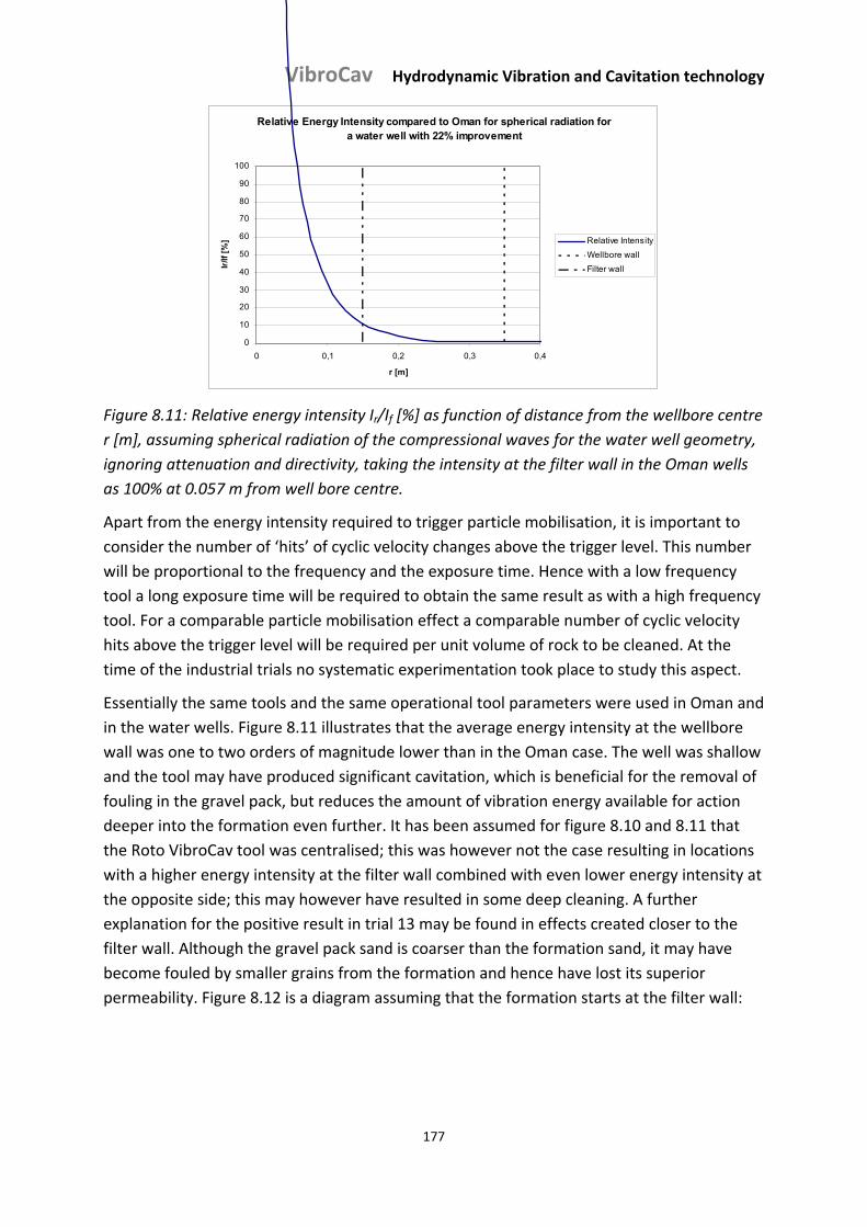
VibroCav Hydrodynamic Vibration and Cavitation technology
177
Relative Energy Intensity compared to Oman for spherical radiation for a water well with 22% improvement
0
10
20
30
40
50
60
70
80
90
100
0 0,1 0,2 0,3 0,4
r [m]
Ir/If
[%
] Relative Intensity
Wellbore wall
Filter wall
Figure 8.11: Relative energy intensity Ir/If [%] as function of distance from the wellbore centre
r [m], assuming spherical radiation of the compressional waves for the water well geometry,
ignoring attenuation and directivity, taking the intensity at the filter wall in the Oman wells
as 100% at 0.057 m from well bore centre.
Apart from the energy intensity required to trigger particle mobilisation, it is important to
consider the number of ‘hits’ of cyclic velocity changes above the trigger level. This number
will be proportional to the frequency and the exposure time. Hence with a low frequency
tool a long exposure time will be required to obtain the same result as with a high frequency
tool. For a comparable particle mobilisation effect a comparable number of cyclic velocity
hits above the trigger level will be required per unit volume of rock to be cleaned. At the
time of the industrial trials no systematic experimentation took place to study this aspect.
Essentially the same tools and the same operational tool parameters were used in Oman and
in the water wells. Figure 8.11 illustrates that the average energy intensity at the wellbore
wall was one to two orders of magnitude lower than in the Oman case. The well was shallow
and the tool may have produced significant cavitation, which is beneficial for the removal of
fouling in the gravel pack, but reduces the amount of vibration energy available for action
deeper into the formation even further. It has been assumed for figure 8.10 and 8.11 that
the Roto VibroCav tool was centralised; this was however not the case resulting in locations
with a higher energy intensity at the filter wall combined with even lower energy intensity at
the opposite side; this may however have resulted in some deep cleaning. A further
explanation for the positive result in trial 13 may be found in effects created closer to the
filter wall. Although the gravel pack sand is coarser than the formation sand, it may have
become fouled by smaller grains from the formation and hence have lost its superior
permeability. Figure 8.12 is a diagram assuming that the formation starts at the filter wall:
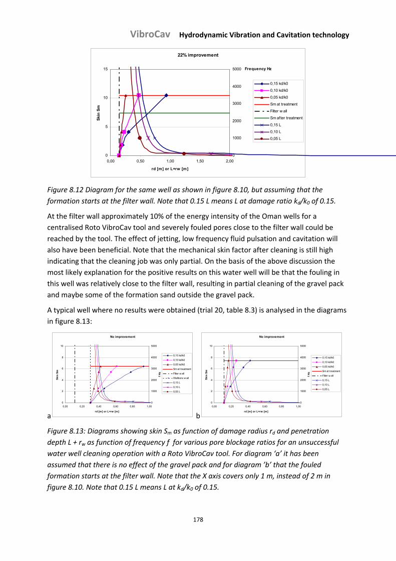
VibroCav Hydrodynamic Vibration and Cavitation technology
178
22% improvement
0
5
10
15
0,00 0,50 1,00 1,50 2,00
rd [m] or L+rw [m]
Ski
n S
m
0
1000
2000
3000
4000
5000 Frequency Hz
0,15 kd/k0
0,10 kd/k0
0,05 kd/k0
Sm at treatment
Filter w all
Sm after treatment
0,15 L
0,10 L
0,05 L
Figure 8.12 Diagram for the same well as shown in figure 8.10, but assuming that the
formation starts at the filter wall. Note that 0.15 L means L at damage ratio kd/k0 of 0.15.
At the filter wall approximately 10% of the energy intensity of the Oman wells for a
centralised Roto VibroCav tool and severely fouled pores close to the filter wall could be
reached by the tool. The effect of jetting, low frequency fluid pulsation and cavitation will
also have been beneficial. Note that the mechanical skin factor after cleaning is still high
indicating that the cleaning job was only partial. On the basis of the above discussion the
most likely explanation for the positive results on this water well will be that the fouling in
this well was relatively close to the filter wall, resulting in partial cleaning of the gravel pack
and maybe some of the formation sand outside the gravel pack.
A typical well where no results were obtained (trial 20, table 8.3) is analysed in the diagrams
in figure 8.13:
a
No improvement
0
2
4
6
8
10
0,00 0,20 0,40 0,60 0,80 1,00
rd [m] or L+rw [m]
Ski
n S
m
0
1000
2000
3000
4000
5000
f H
z
0,15 kd/k0
0,10 kd/k0
0,05 kd/k0
Sm at treatment
Filter w all
Wellbore w all
0,15 L
0,10 L
0,05 L
b
No improvement
0
2
4
6
8
10
0,00 0,20 0,40 0,60 0,80 1,00
rd [m] or L+rw [m]
Ski
n S
m
0
1000
2000
3000
4000
5000
f H
z
0,15 kd/k0
0,10 kd/k0
0,05 kd/k0
Sm at treatment
Filter w all
0,15 L
0,10 L
0,05 L
Figure 8.13: Diagrams showing skin Sm as function of damage radius rd and penetration
depth L + rw as function of frequency f for various pore blockage ratios for an unsuccessful
water well cleaning operation with a Roto VibroCav tool. For diagram ‘a’ it has been
assumed that there is no effect of the gravel pack and for diagram ’b’ that the fouled
formation starts at the filter wall. Note that the X axis covers only 1 m, instead of 2 m in
figure 8.10. Note that 0.15 L means L at kd/k0 of 0.15.
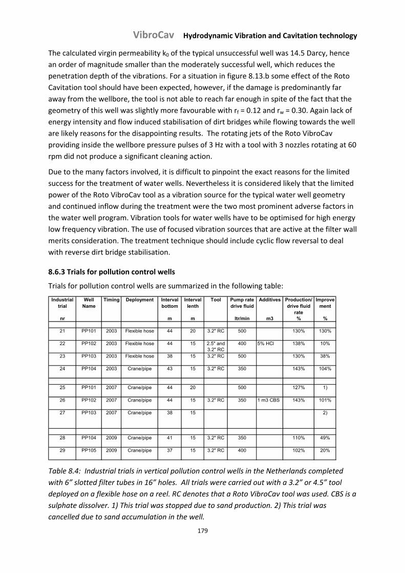
VibroCav Hydrodynamic Vibration and Cavitation technology
179
The calculated virgin permeability k0 of the typical unsuccessful well was 14.5 Darcy, hence
an order of magnitude smaller than the moderately successful well, which reduces the
penetration depth of the vibrations. For a situation in figure 8.13.b some effect of the Roto
Cavitation tool should have been expected, however, if the damage is predominantly far
away from the wellbore, the tool is not able to reach far enough in spite of the fact that the
geometry of this well was slightly more favourable with rf = 0.12 and rw = 0.30. Again lack of
energy intensity and flow induced stabilisation of dirt bridges while flowing towards the well
are likely reasons for the disappointing results. The rotating jets of the Roto VibroCav
providing inside the wellbore pressure pulses of 3 Hz with a tool with 3 nozzles rotating at 60
rpm did not produce a significant cleaning action.
Due to the many factors involved, it is difficult to pinpoint the exact reasons for the limited
success for the treatment of water wells. Nevertheless it is considered likely that the limited
power of the Roto VibroCav tool as a vibration source for the typical water well geometry
and continued inflow during the treatment were the two most prominent adverse factors in
the water well program. Vibration tools for water wells have to be optimised for high energy
low frequency vibration. The use of focused vibration sources that are active at the filter wall
merits consideration. The treatment technique should include cyclic flow reversal to deal
with reverse dirt bridge stabilisation.
8.6.3 Trials for pollution control wells
Trials for pollution control wells are summarized in the following table:
Industrial trial
Well Name
Timing Deployment Interval bottom
Interval lenth
Tool Pump rate drive fluid
Additives Production/drive fluid
rate
Improvement
nr m m ltr/min m3 % %
21 PP101 2003 Flexible hose 44 20 3.2" RC 500 130% 130%
22 PP102 2003 Flexible hose 44 15 2.5" and 3.2" RC
400 5% HCl 138% 10%
23 PP103 2003 Flexible hose 38 15 3.2" RC 500 130% 38%
24 PP104 2003 Crane/pipe 43 15 3.2" RC 350 143% 104%
25 PP101 2007 Crane/pipe 44 20 500 127% 1)
26 PP102 2007 Crane/pipe 44 15 3.2" RC 350 1 m3 CBS 143% 101%
27 PP103 2007 Crane/pipe 38 15 2)
28 PP104 2009 Crane/pipe 41 15 3.2" RC 350 110% 49%
29 PP105 2009 Crane/pipe 37 15 3.2" RC 400 102% 20%
Table 8.4: Industrial trials in vertical pollution control wells in the Netherlands completed
with 6” slotted filter tubes in 16” holes. All trials were carried out with a 3.2” or 4.5” tool
deployed on a flexible hose on a reel. RC denotes that a Roto VibroCav tool was used. CBS is a
sulphate dissolver. 1) This trial was stopped due to sand production. 2) This trial was
cancelled due to sand accumulation in the well.
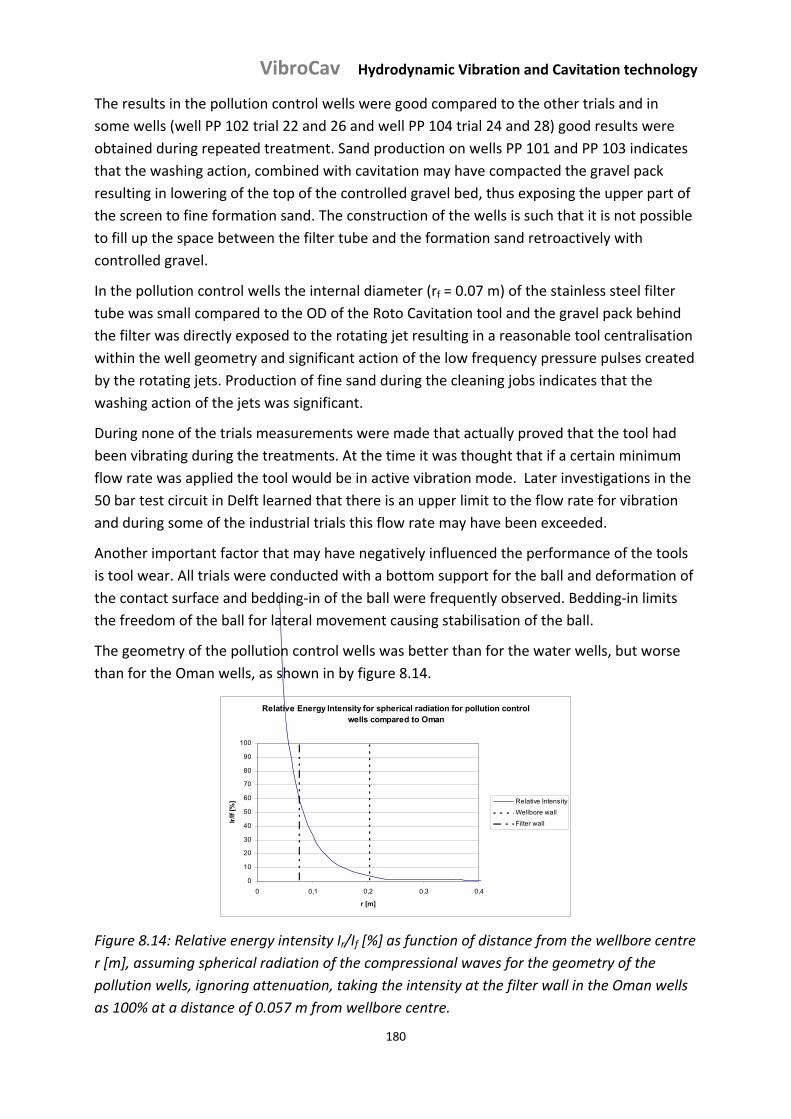
VibroCav Hydrodynamic Vibration and Cavitation technology
180
The results in the pollution control wells were good compared to the other trials and in
some wells (well PP 102 trial 22 and 26 and well PP 104 trial 24 and 28) good results were
obtained during repeated treatment. Sand production on wells PP 101 and PP 103 indicates
that the washing action, combined with cavitation may have compacted the gravel pack
resulting in lowering of the top of the controlled gravel bed, thus exposing the upper part of
the screen to fine formation sand. The construction of the wells is such that it is not possible
to fill up the space between the filter tube and the formation sand retroactively with
controlled gravel.
In the pollution control wells the internal diameter (rf = 0.07 m) of the stainless steel filter
tube was small compared to the OD of the Roto Cavitation tool and the gravel pack behind
the filter was directly exposed to the rotating jet resulting in a reasonable tool centralisation
within the well geometry and significant action of the low frequency pressure pulses created
by the rotating jets. Production of fine sand during the cleaning jobs indicates that the
washing action of the jets was significant.
During none of the trials measurements were made that actually proved that the tool had
been vibrating during the treatments. At the time it was thought that if a certain minimum
flow rate was applied the tool would be in active vibration mode. Later investigations in the
50 bar test circuit in Delft learned that there is an upper limit to the flow rate for vibration
and during some of the industrial trials this flow rate may have been exceeded.
Another important factor that may have negatively influenced the performance of the tools
is tool wear. All trials were conducted with a bottom support for the ball and deformation of
the contact surface and bedding‐in of the ball were frequently observed. Bedding‐in limits
the freedom of the ball for lateral movement causing stabilisation of the ball.
The geometry of the pollution control wells was better than for the water wells, but worse
than for the Oman wells, as shown in by figure 8.14.
Relative Energy Intensity for spherical radiation for pollution control wells compared to Oman
0
10
20
30
40
50
60
70
80
90
100
0 0,1 0,2 0,3 0,4
r [m]
Ir/If
[%
] Relative Intensity
Wellbore wall
Filter wall
Figure 8.14: Relative energy intensity Ir/If [%] as function of distance from the wellbore centre
r [m], assuming spherical radiation of the compressional waves for the geometry of the
pollution wells, ignoring attenuation, taking the intensity at the filter wall in the Oman wells
as 100% at a distance of 0.057 m from wellbore centre.
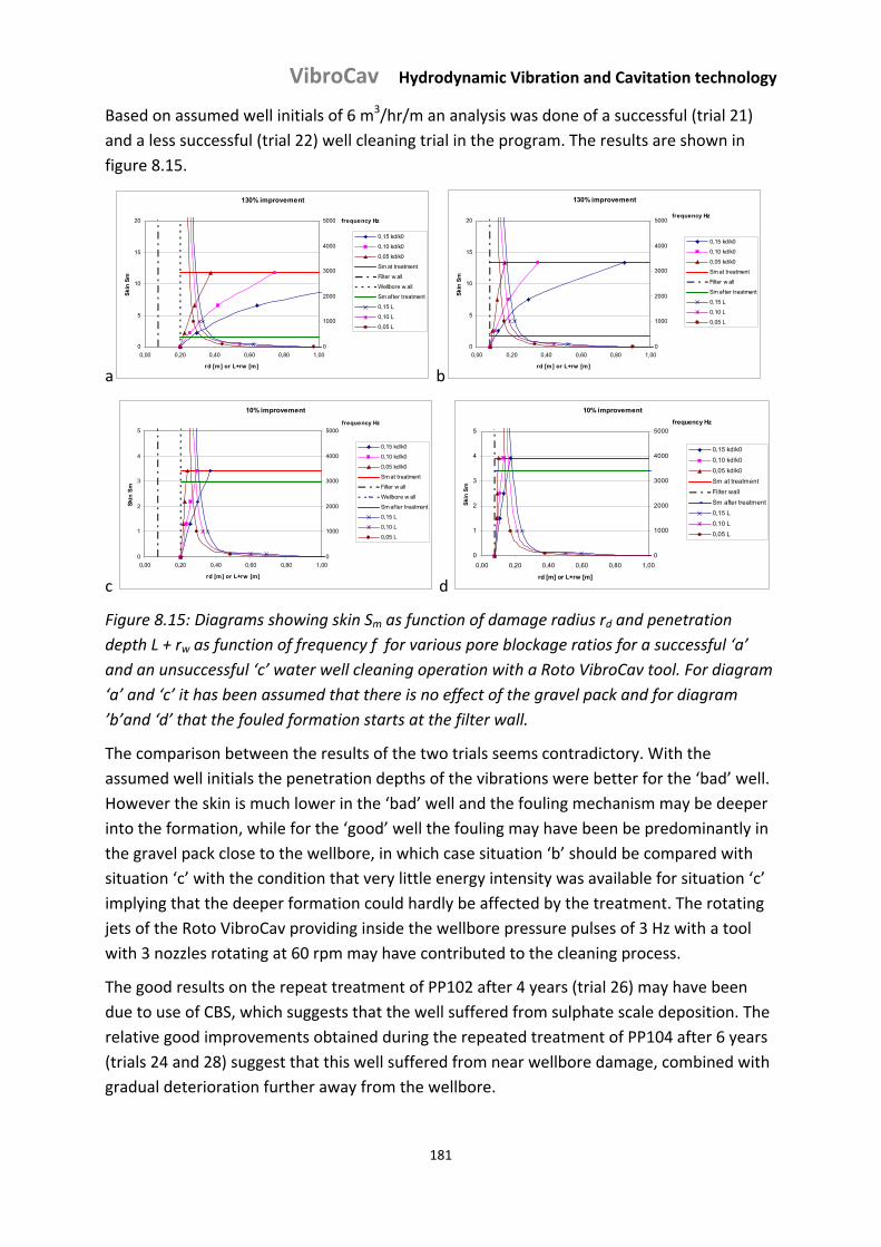
VibroCav Hydrodynamic Vibration and Cavitation technology
181
Based on assumed well initials of 6 m3/hr/m an analysis was done of a successful (trial 21)
and a less successful (trial 22) well cleaning trial in the program. The results are shown in
figure 8.15.
a
130% improvement
0
5
10
15
20
0,00 0,20 0,40 0,60 0,80 1,00
rd [m] or L+rw [m]
Ski
n S
m
0
1000
2000
3000
4000
5000 frequency Hz
0,15 kd/k0
0,10 kd/k0
0,05 kd/k0
Sm at treatment
Filter w all
Wellbore w all
Sm after treatment
0,15 L
0,10 L
0,05 L
b
130% improvement
0
5
10
15
20
0,00 0,20 0,40 0,60 0,80 1,00
rd [m] or L+rw [m]
Ski
n S
m
0
1000
2000
3000
4000
5000frequency Hz
0,15 kd/k0
0,10 kd/k0
0,05 kd/k0
Sm at treatment
Filter w all
Sm after treatment
0,15 L
0,10 L
0,05 L
c
10% improvement
0
1
2
3
4
5
0,00 0,20 0,40 0,60 0,80 1,00
rd [m] or L+rw [m]
Ski
n S
m
0
1000
2000
3000
4000
5000frequency Hz
0,15 kd/k0
0,10 kd/k0
0,05 kd/k0
Sm at treatment
Filter w all
Wellbore w all
Sm after treatment
0,15 L
0,10 L
0,05 L
d
10% improvement
0
1
2
3
4
5
0,00 0,20 0,40 0,60 0,80 1,00
rd [m] or L+rw [m]
Ski
n S
m
0
1000
2000
3000
4000
5000
frequency Hz
0,15 kd/k0
0,10 kd/k0
0,05 kd/k0
Sm at treatment
Filter wall
Sm after treatment
0,15 L
0,10 L
0,05 L
Figure 8.15: Diagrams showing skin Sm as function of damage radius rd and penetration
depth L + rw as function of frequency f for various pore blockage ratios for a successful ‘a’
and an unsuccessful ‘c’ water well cleaning operation with a Roto VibroCav tool. For diagram
‘a’ and ‘c’ it has been assumed that there is no effect of the gravel pack and for diagram
’b’and ‘d’ that the fouled formation starts at the filter wall.
The comparison between the results of the two trials seems contradictory. With the
assumed well initials the penetration depths of the vibrations were better for the ‘bad’ well.
However the skin is much lower in the ‘bad’ well and the fouling mechanism may be deeper
into the formation, while for the ‘good’ well the fouling may have been be predominantly in
the gravel pack close to the wellbore, in which case situation ‘b’ should be compared with
situation ‘c’ with the condition that very little energy intensity was available for situation ‘c’
implying that the deeper formation could hardly be affected by the treatment. The rotating
jets of the Roto VibroCav providing inside the wellbore pressure pulses of 3 Hz with a tool
with 3 nozzles rotating at 60 rpm may have contributed to the cleaning process.
The good results on the repeat treatment of PP102 after 4 years (trial 26) may have been
due to use of CBS, which suggests that the well suffered from sulphate scale deposition. The
relative good improvements obtained during the repeated treatment of PP104 after 6 years
(trials 24 and 28) suggest that this well suffered from near wellbore damage, combined with
gradual deterioration further away from the wellbore.
VibroCav Hydrodynamic Vibration and Cavitation technology
182
8.7. Conclusions
The industrial trials have provided further insight into major parameters controlling
the characteristics of vibration based well cleaning tools, being (i) the mechanical
skin and effective permeability around the wellbore, (ii) the relationship between the
effective permeability and the penetration depth as function of the vibration
frequency and (iii) the energy intensity as function of geometry and tool directivity
and (iv) the number of cyclic velocity ‘hits’ above the trigger level for particle
mobilisation per unit rock volume to be cleaned and (v) the effect of continuous pore
flow on the stabilisation or destabilisation of fouling particles.
The best moment of cleaning a well after the drilling process is immediately after
drilling, because the damage is likely to be close to the wellbore and hence relatively
easy to remove. If fouling is allowed to take place over prolonged periods of time, the
pore damage may be outside of the reach of vibration based well cleaning tools.
The penetration depth of any vibration based well cleaning tool is dependent on the
effective permeability around the wellbore. If a well progressively fouls up due to
plugging by particles entrained with the flow from the ‘far field’, a situation may arise
in which the vibration based cleaning tools can no longer reach the damaged zone.
There may be a small benefit of ‘pore shaking’ if the vibration energy is not used for
slow wave energy dissipation; this effect was however not evaluated in this study.
The Oman trials indicate that flow reversal is beneficial for the vibration based
cleaning process. Less energy intensity will be required to destabilise bridges and
mobilise fouling particles. Cyclic flow reversal is an important technique to consider
for vibration based cleaning operations.
The Oman trials indicate that chasing mobilised fouling particles into the ‘far field’ at
a higher injection rate than the production rate can create a condition of sustained
production improvement. The fouling particles settle in pores where insufficient
production pore flow velocity is created to re‐mobilise the particles towards the
wellbore.
The wellbore geometry must play an important role in the design of a vibration based
cleaning operation. The trials in water wells indicate that insufficient energy intensity
was available for significant cleaning work. Focused vibration tools delivering the
vibration energy at the filter wall merit serious consideration.
The rotating jets in the Roto VibroCav tool provide very low frequency pressure
pulses that are likely to contribute to the cleaning process if the tool is sufficiently
close to the wellbore wall. The Oman and pollution control wells trials indicate that
this may be the case.
VibroCav Hydrodynamic Vibration and Cavitation technology
183
Vibration based wellbore cleaning may be seen as (i) producing cyclic velocity ‘hits’ in
the formation pores to trigger the mobilisation of fouling particles and (ii) a
considered process to remove the mobilised particles from the well or place them
deep into the formation in positions where the particles are harmless to the
production. High frequency tools (kHz range) suffer from a very shallow penetration
depth but benefit from a high ‘hit rate’ and are therefore considered suitable for
near wellbore cleaning with relatively short exposure times. Low frequency tool
(several Hz to 1 kHz) reach deeper at comparable energy emission at source but need
longer exposure time to obtain a useful density of hits.
Tool wear may have interfered with the trials to such an extent that no or severely
compromised vibration took place during some of the unsuccessful treatments.
Acoustic measurements must be made for future treatments to prove that the tool is
producing vibrations.
8.8. References
1. Pucknell, J.K. ; Clifford, P.J. ; SPE 23100 (1991)
2. Dake, L.P. ; Fundamentals of reservoir engineering; Elsevier 1978
3. Restrepo, A ; Duarte, J. ; SPE 107674 (2007)
4. Zwart de A.H. ; Investigation of Clogging processes in Unconsolidated Aquifers near Water
Supply Wells; Thesis TU Delft 2007
5. Poesio, P. ; Ultrasonic flow stimulation and particles removal in a porous material; Thesis
TU Delft 2004
VibroCav Hydrodynamic Vibration and Cavitation technology
184
Chapter 9: Industrial trials for removing scale deposits in wells
9.1. Scale deposition
Scale deposition in the pores of the reservoir and on pipes in well bores is quite commonly
observed. The presence of Ca2+, Sr2+, Ba2+ in formation water with CO32‐ and SO4
2‐ ions at
saturation level from either formation or injection water is often the cause of deposition of
CaCO3, CaSO4, SrSO4 and BaSO4 scale in a well as the aqueous streams get mixed and the
temperature and pressure change or water evaporates (gas wells) when the fluids flow to
surface. Calcium carbonate scale can be dissolved with acids like diluted HCl; however
sulphate scale cannot be readily dissolved and the use of strong acids may be unwanted
because this may be destructive for the well materials. Scale may decrease the well bore
diameter so much that the flow from the well is significantly reduced. Scale may also plug
perforation tunnels and formation pores or obstruct accessories like sliding side doors or
side pockets so their functionality is affected. If a scale layer breaks off, it may cause
obstructions elsewhere.
9.2. Scale removal
Scale represents a very costly problem in the gas, oil and water production industry, not only
inside the well bore but also in the porous medium around the inflow area of the well. Scale
can be removed chemically, mechanically or physically. With chemical methods the scale is
converted into soluble substance and produced out of the well. By proper placement the
well bore itself and the surrounding porous medium can be reached, however placement of
the chemical treatment fluids in low permeable zones, often the zones most affected by
scale, may be difficult. Moreover the use of chemical substances may be unwanted.
Mechanical methods by crushing the scale in direct contact with a rotating drilling or milling
bit and flushing the liberated debris from the well are relatively rough, may leave a thin layer
of scale behind and hold a risk exists of damaging the pipe wall. A physical method such as
crushing scale using hydrodynamically generated vibrations and cavitation bubble collapse
or strong vortices has the potential to remove scale from the well bore and the surrounding
formation, including the less permeable zones.
Physical scale removal techniques include hydrodynamic jetting and hydrodynamic vibration
and cavitation. In the last decennium the use of fluidic oscillation has gained interest, using
frequencies of 120 to 200 Hz to obtain acoustic waves in the fluids and successful field
applications have been reported [1]. The use of 20 to 60 Hz vibration for impact drilling and
milling of scale provides successes in the field [2]. Ultrasonic devices have also been
considered for the task of scale removal [3].
This study ventures into the area of low frequency vibration and the tools that have been
investigated produce apart from strong vibration also strong cavitation if the well bore
pressure is typically lower than 100 bar. As cavitation is suppressed by higher wellbore
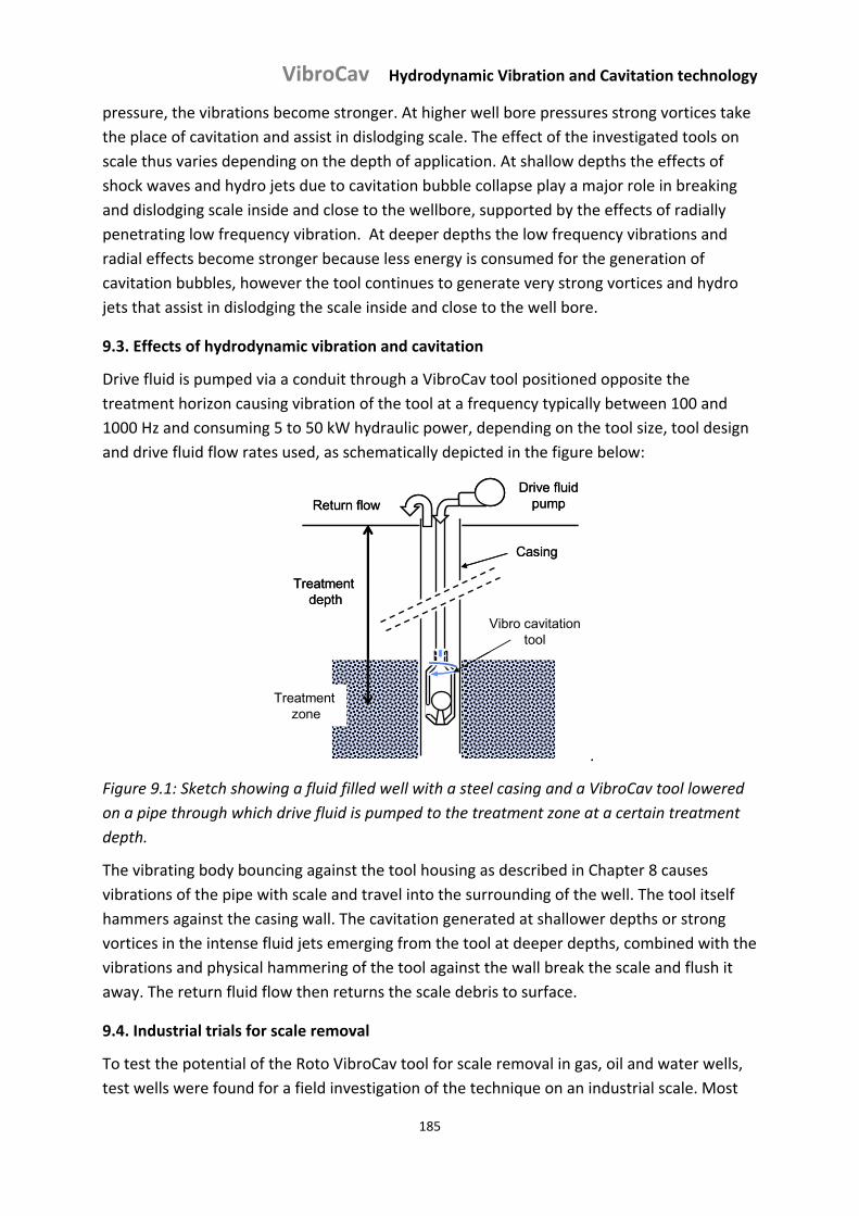
VibroCav Hydrodynamic Vibration and Cavitation technology
185
pressure, the vibrations become stronger. At higher well bore pressures strong vortices take
the place of cavitation and assist in dislodging scale. The effect of the investigated tools on
scale thus varies depending on the depth of application. At shallow depths the effects of
shock waves and hydro jets due to cavitation bubble collapse play a major role in breaking
and dislodging scale inside and close to the wellbore, supported by the effects of radially
penetrating low frequency vibration. At deeper depths the low frequency vibrations and
radial effects become stronger because less energy is consumed for the generation of
cavitation bubbles, however the tool continues to generate very strong vortices and hydro
jets that assist in dislodging the scale inside and close to the well bore.
9.3. Effects of hydrodynamic vibration and cavitation
Drive fluid is pumped via a conduit through a VibroCav tool positioned opposite the
treatment horizon causing vibration of the tool at a frequency typically between 100 and
1000 Hz and consuming 5 to 50 kW hydraulic power, depending on the tool size, tool design
and drive fluid flow rates used, as schematically depicted in the figure below:
Drive fluidpump
Treatment zone
Return flow
Treatment depth
Vibro cavitationtool
Casing
Drive fluidpump
Treatment zone
Return flow
Treatment depth
Vibro cavitationtool
Casing
.
Figure 9.1: Sketch showing a fluid filled well with a steel casing and a VibroCav tool lowered
on a pipe through which drive fluid is pumped to the treatment zone at a certain treatment
depth.
The vibrating body bouncing against the tool housing as described in Chapter 8 causes
vibrations of the pipe with scale and travel into the surrounding of the well. The tool itself
hammers against the casing wall. The cavitation generated at shallower depths or strong
vortices in the intense fluid jets emerging from the tool at deeper depths, combined with the
vibrations and physical hammering of the tool against the wall break the scale and flush it
away. The return fluid flow then returns the scale debris to surface.
9.4. Industrial trials for scale removal
To test the potential of the Roto VibroCav tool for scale removal in gas, oil and water wells,
test wells were found for a field investigation of the technique on an industrial scale. Most
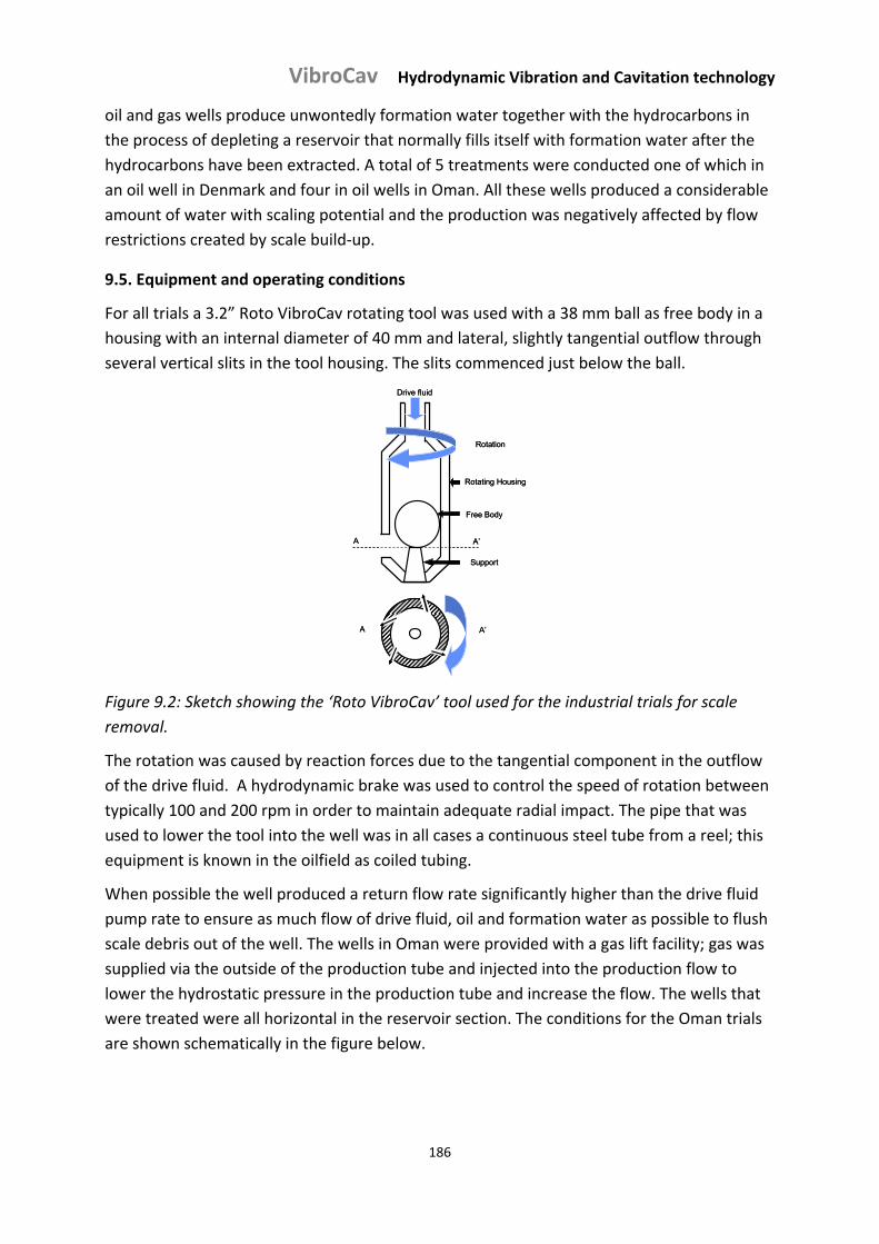
VibroCav Hydrodynamic Vibration and Cavitation technology
186
oil and gas wells produce unwontedly formation water together with the hydrocarbons in
the process of depleting a reservoir that normally fills itself with formation water after the
hydrocarbons have been extracted. A total of 5 treatments were conducted one of which in
an oil well in Denmark and four in oil wells in Oman. All these wells produced a considerable
amount of water with scaling potential and the production was negatively affected by flow
restrictions created by scale build‐up.
9.5. Equipment and operating conditions
For all trials a 3.2” Roto VibroCav rotating tool was used with a 38 mm ball as free body in a
housing with an internal diameter of 40 mm and lateral, slightly tangential outflow through
several vertical slits in the tool housing. The slits commenced just below the ball.
A A’
A A’
Rotating Housing
Free Body
Support
Drive fluid
Rotation
A A’
A A’
Rotating Housing
Free Body
Support
Drive fluid
Rotation
Figure 9.2: Sketch showing the ‘Roto VibroCav’ tool used for the industrial trials for scale
removal.
The rotation was caused by reaction forces due to the tangential component in the outflow
of the drive fluid. A hydrodynamic brake was used to control the speed of rotation between
typically 100 and 200 rpm in order to maintain adequate radial impact. The pipe that was
used to lower the tool into the well was in all cases a continuous steel tube from a reel; this
equipment is known in the oilfield as coiled tubing.
When possible the well produced a return flow rate significantly higher than the drive fluid
pump rate to ensure as much flow of drive fluid, oil and formation water as possible to flush
scale debris out of the well. The wells in Oman were provided with a gas lift facility; gas was
supplied via the outside of the production tube and injected into the production flow to
lower the hydrostatic pressure in the production tube and increase the flow. The wells that
were treated were all horizontal in the reservoir section. The conditions for the Oman trials
are shown schematically in the figure below.
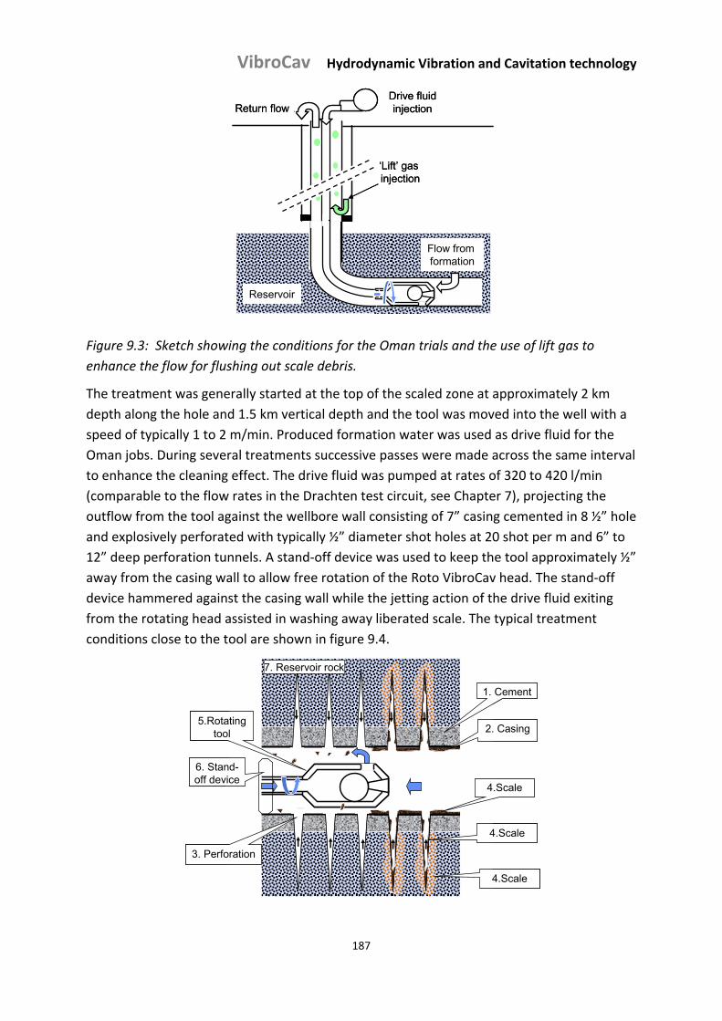
VibroCav Hydrodynamic Vibration and Cavitation technology
187
Drive fluidinjectionReturn flow
‘Lift’ gas injection
Flow from formation
Reservoir
Drive fluidinjectionReturn flow
‘Lift’ gas injection
Flow from formation
Reservoir
Figure 9.3: Sketch showing the conditions for the Oman trials and the use of lift gas to
enhance the flow for flushing out scale debris.
The treatment was generally started at the top of the scaled zone at approximately 2 km
depth along the hole and 1.5 km vertical depth and the tool was moved into the well with a
speed of typically 1 to 2 m/min. Produced formation water was used as drive fluid for the
Oman jobs. During several treatments successive passes were made across the same interval
to enhance the cleaning effect. The drive fluid was pumped at rates of 320 to 420 l/min
(comparable to the flow rates in the Drachten test circuit, see Chapter 7), projecting the
outflow from the tool against the wellbore wall consisting of 7” casing cemented in 8 ½” hole
and explosively perforated with typically ½” diameter shot holes at 20 shot per m and 6” to
12” deep perforation tunnels. A stand‐off device was used to keep the tool approximately ½”
away from the casing wall to allow free rotation of the Roto VibroCav head. The stand‐off
device hammered against the casing wall while the jetting action of the drive fluid exiting
from the rotating head assisted in washing away liberated scale. The typical treatment
conditions close to the tool are shown in figure 9.4.
5.Rotating tool
7. Reservoir rock
1. Cement
2. Casing
3. Perforation
4.Scale
6. Stand-off device
4.Scale
4.Scale
5.Rotating tool
7. Reservoir rock
1. Cement
2. Casing
3. Perforation
4.Scale
6. Stand-off device
4.Scale
4.Scale
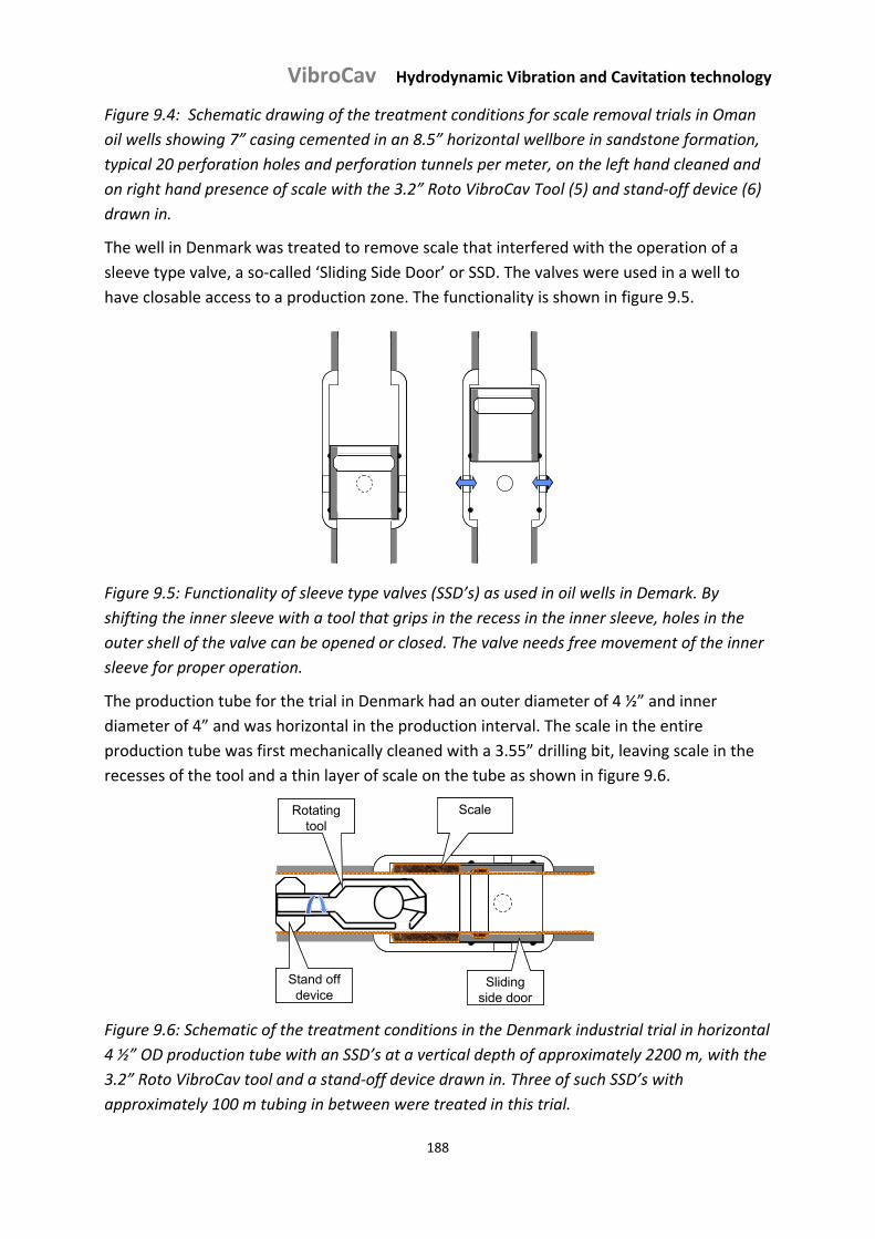
VibroCav Hydrodynamic Vibration and Cavitation technology
188
Figure 9.4: Schematic drawing of the treatment conditions for scale removal trials in Oman
oil wells showing 7” casing cemented in an 8.5” horizontal wellbore in sandstone formation,
typical 20 perforation holes and perforation tunnels per meter, on the left hand cleaned and
on right hand presence of scale with the 3.2” Roto VibroCav Tool (5) and stand‐off device (6)
drawn in.
The well in Denmark was treated to remove scale that interfered with the operation of a
sleeve type valve, a so‐called ‘Sliding Side Door’ or SSD. The valves were used in a well to
have closable access to a production zone. The functionality is shown in figure 9.5.
Figure 9.5: Functionality of sleeve type valves (SSD’s) as used in oil wells in Demark. By
shifting the inner sleeve with a tool that grips in the recess in the inner sleeve, holes in the
outer shell of the valve can be opened or closed. The valve needs free movement of the inner
sleeve for proper operation.
The production tube for the trial in Denmark had an outer diameter of 4 ½” and inner
diameter of 4” and was horizontal in the production interval. The scale in the entire
production tube was first mechanically cleaned with a 3.55” drilling bit, leaving scale in the
recesses of the tool and a thin layer of scale on the tube as shown in figure 9.6.
ScaleRotating tool
Stand off device
Sliding side door
ScaleRotating tool
Stand off device
Sliding side door
Figure 9.6: Schematic of the treatment conditions in the Denmark industrial trial in horizontal
4 ½” OD production tube with an SSD’s at a vertical depth of approximately 2200 m, with the
3.2” Roto VibroCav tool and a stand‐off device drawn in. Three of such SSD’s with
approximately 100 m tubing in between were treated in this trial.
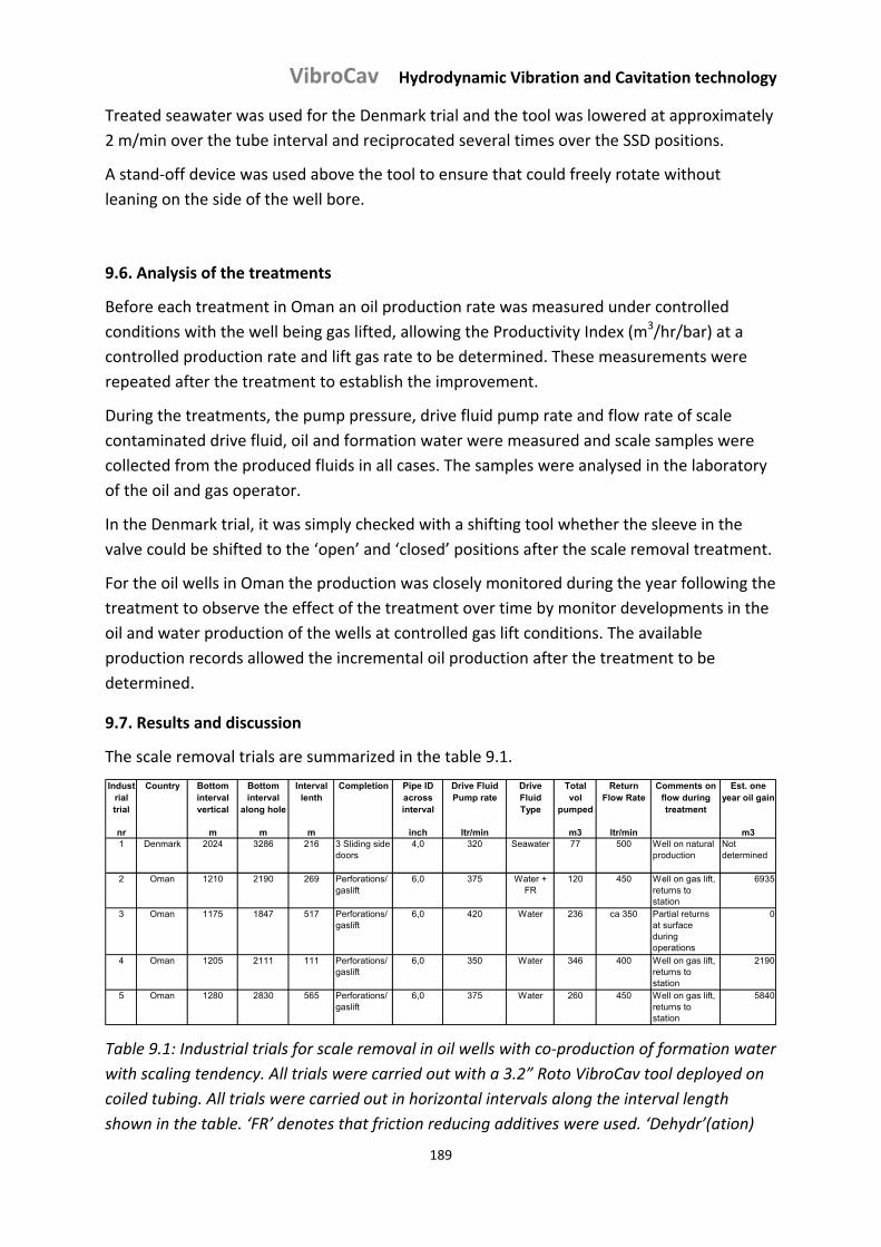
VibroCav Hydrodynamic Vibration and Cavitation technology
189
Treated seawater was used for the Denmark trial and the tool was lowered at approximately
2 m/min over the tube interval and reciprocated several times over the SSD positions.
A stand‐off device was used above the tool to ensure that could freely rotate without
leaning on the side of the well bore.
9.6. Analysis of the treatments
Before each treatment in Oman an oil production rate was measured under controlled
conditions with the well being gas lifted, allowing the Productivity Index (m3/hr/bar) at a
controlled production rate and lift gas rate to be determined. These measurements were
repeated after the treatment to establish the improvement.
During the treatments, the pump pressure, drive fluid pump rate and flow rate of scale
contaminated drive fluid, oil and formation water were measured and scale samples were
collected from the produced fluids in all cases. The samples were analysed in the laboratory
of the oil and gas operator.
In the Denmark trial, it was simply checked with a shifting tool whether the sleeve in the
valve could be shifted to the ‘open’ and ‘closed’ positions after the scale removal treatment.
For the oil wells in Oman the production was closely monitored during the year following the
treatment to observe the effect of the treatment over time by monitor developments in the
oil and water production of the wells at controlled gas lift conditions. The available
production records allowed the incremental oil production after the treatment to be
determined.
9.7. Results and discussion
The scale removal trials are summarized in the table 9.1.
Industrial trial
Country Bottom interval vertical
Bottom interval
along hole
Interval lenth
Completion Pipe ID across interval
Drive Fluid Pump rate
Drive Fluid Type
Total vol
pumped
Return Flow Rate
Comments on flow during treatment
Est. one year oil gain
nr m m m inch ltr/min m3 ltr/min m31 Denmark 2024 3286 216 3 Sliding side
doors4,0 320 Seawater 77 500 Well on natural
productionNot determined
2 Oman 1210 2190 269 Perforations/gaslift
6,0 375 Water + FR
120 450 Well on gas lift, returns to station
6935
3 Oman 1175 1847 517 Perforations/gaslift
6,0 420 Water 236 ca 350 Partial returns at surface during operations
0
4 Oman 1205 2111 111 Perforations/gaslift
6,0 350 Water 346 400 Well on gas lift, returns to station
2190
5 Oman 1280 2830 565 Perforations/gaslift
6,0 375 Water 260 450 Well on gas lift, returns to station
5840
Table 9.1: Industrial trials for scale removal in oil wells with co‐production of formation water
with scaling tendency. All trials were carried out with a 3.2” Roto VibroCav tool deployed on
coiled tubing. All trials were carried out in horizontal intervals along the interval length
shown in the table. ‘FR’ denotes that friction reducing additives were used. ‘Dehydr’(ation)
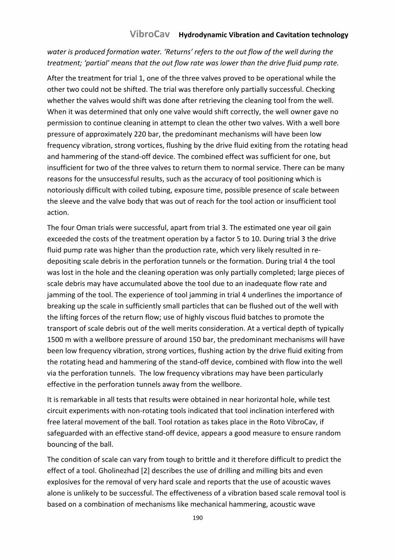
VibroCav Hydrodynamic Vibration and Cavitation technology
190
water is produced formation water. ‘Returns’ refers to the out flow of the well during the
treatment; ‘partial’ means that the out flow rate was lower than the drive fluid pump rate.
After the treatment for trial 1, one of the three valves proved to be operational while the
other two could not be shifted. The trial was therefore only partially successful. Checking
whether the valves would shift was done after retrieving the cleaning tool from the well.
When it was determined that only one valve would shift correctly, the well owner gave no
permission to continue cleaning in attempt to clean the other two valves. With a well bore
pressure of approximately 220 bar, the predominant mechanisms will have been low
frequency vibration, strong vortices, flushing by the drive fluid exiting from the rotating head
and hammering of the stand‐off device. The combined effect was sufficient for one, but
insufficient for two of the three valves to return them to normal service. There can be many
reasons for the unsuccessful results, such as the accuracy of tool positioning which is
notoriously difficult with coiled tubing, exposure time, possible presence of scale between
the sleeve and the valve body that was out of reach for the tool action or insufficient tool
action.
The four Oman trials were successful, apart from trial 3. The estimated one year oil gain
exceeded the costs of the treatment operation by a factor 5 to 10. During trial 3 the drive
fluid pump rate was higher than the production rate, which very likely resulted in re‐
depositing scale debris in the perforation tunnels or the formation. During trial 4 the tool
was lost in the hole and the cleaning operation was only partially completed; large pieces of
scale debris may have accumulated above the tool due to an inadequate flow rate and
jamming of the tool. The experience of tool jamming in trial 4 underlines the importance of
breaking up the scale in sufficiently small particles that can be flushed out of the well with
the lifting forces of the return flow; use of highly viscous fluid batches to promote the
transport of scale debris out of the well merits consideration. At a vertical depth of typically
1500 m with a wellbore pressure of around 150 bar, the predominant mechanisms will have
been low frequency vibration, strong vortices, flushing action by the drive fluid exiting from
the rotating head and hammering of the stand‐off device, combined with flow into the well
via the perforation tunnels. The low frequency vibrations may have been particularly
effective in the perforation tunnels away from the wellbore.
It is remarkable in all tests that results were obtained in near horizontal hole, while test
circuit experiments with non‐rotating tools indicated that tool inclination interfered with
free lateral movement of the ball. Tool rotation as takes place in the Roto VibroCav, if
safeguarded with an effective stand‐off device, appears a good measure to ensure random
bouncing of the ball.
The condition of scale can vary from tough to brittle and it therefore difficult to predict the
effect of a tool. Gholinezhad [2] describes the use of drilling and milling bits and even
explosives for the removal of very hard scale and reports that the use of acoustic waves
alone is unlikely to be successful. The effectiveness of a vibration based scale removal tool is
based on a combination of mechanisms like mechanical hammering, acoustic wave
VibroCav Hydrodynamic Vibration and Cavitation technology
191
impingement, imploding cavitation bubbles or very strong vortices in a fluid stream jetted
onto the scaled up wellbore, and washing action; in fact all the effects generated by the Roto
Cavitation tool. For successful scale removal physical tool vibration and hammering is
considered of high relative importance; hence the tool should be optimised for these effects.
In general this will mean that the largest tool fitting the well geometry provided with the
largest possible ball with maximum mass would be selected with a fairly wide gap, operated
at a flow rate to optimise the vibration and bouncing strength. The stand‐off device should
be designed to optimise lateral hammering against the pipe wall aiming for circumferential
coverage. Deliberate rotation of the vibration head using a mud motor or string rotation and
the application of mechanical cutting structure in the vibration and jetting head would
combine mechanical destruction and liberation of scale with vibration and jetting based
scale removal.
In view of the strong decrease of energy intensity with the distance from the tool, it is
essential that the tool action is emitted as close as possible to the target.
9.8. Conclusions
Mechanical hammering, low frequency vibrations, strong vortices and flushing action
have likely been the contributing scale cleaning mechanisms at the depth of the
trials. The strong vortices generated by the vibrating ball and jetted in the drive fluid
stream against the pipe wall by the rotating tool housing provide a strong washing
action. Mechanical hammering of the tool against the pipe wall and transfer of the
vibrations to the production tube or casing assist in disintegration of the scale.
Further away from the wellbore, such as in perforation tunnels and the surrounding
porous matrix, a positive effect of the low frequency vibrations can be expected. The
relatively large scale debris must be produced out of the well, as re‐deposition will
very likely result in near wellbore plugging.
During scale treatment it is possible that liberated scale particles are too large to be
flushed out of the hole effectively. Large scale particles are a threat for the tool
becoming stuck, because they may accumulate above the tool and bridge when
pulling up the tool. The use of viscous fluid batches to promote the transport scale
debris merits consideration.
The 3.2” Roto VibroCav was not yet optimised for the vibration action. The outside
dimensions of the tool allow the installation of a larger and heavier ball. Also the ball
and chamber gap can be optimised to realise maximum effects from mechanical
hammering by the tool.
Tool wear may have interfered to such an extent that no or severely compromised
vibration took place during some of the unsuccessful treatments. It is considered
important that down hole and surface measurements are made to ascertain that the
tool is vibrating properly.
VibroCav Hydrodynamic Vibration and Cavitation technology
192
For scale removal from completions accessories like SSD’s it is critical that the tool is
precisely positioned opposite the accessory and that the exposure to the tool effects
is sufficiently long.
Tools for scale cleaning should be optimised for vibration action. This means that
tools should be chosen with a heavy ball as large as possible within the given
geometry and a ball to chamber clearance selected to achieve the strongest
vibrations at the available drive fluid flow. Means of actively tuning the clearance to
achieve the strongest vibration effect would be beneficial. Maximum advantage must
be taken of the mechanical hammering of the stand‐off device and the tool must
have primary or secondary functionality to break up scale particles to hydraulically
transportable dimensions without allowing the existence of oversized particles. Use
of batches of viscous fluid to promote the transportation of scale debris from the
well merits consideration. Down hole filtration of the scale debris in situations where
the debris cannot be circulated to surface may also be considered.
Apart from ‘self’ generated rotation by tangential outflow, tools can be externally
rotated by means of rotating the pipe on which the tool is lowered into the well from
surface or by means of a down hole motor activated by the drive fluid or a
combination of the two. The advantage of an externally rotated tool is that the
outflow ports can be purely radial resulting in improved projection of the outflow
onto the well bore wall. Externally driven tools can also be better combined with a
cutting structure at the bottom and top of the tool to enhance the mechanical scale
destruction capability of the tool.
For scale removal from accessories like SSD’s it is recommended to combine a shifter
tool with the cleaning tool to check whether the SSD will operate after cleaning and
immediately resume cleaning if necessary. The shifter tool will also aid in accurate
depth positioning. The use of an optimised rotated tool with cutting structures at the
top and bottom of the tool may also be considered; the combination with shifter
functionality may then be less realistic.
In future scale cleaning applications vibration must be measured with down hole
and/or surface microphones to ascertain the tool is working optimally. During a
treatment sound can be used to find the optimum operating conditions of the tool
and immediate action can be taken if the tool stops vibration.

VibroCav Hydrodynamic Vibration and Cavitation technology
193
9.9. References
1. Gholinezhad, J. ; SPE 99683 (2006)
2. Joppe, L. ; Mackenzie, G. ; McGurk, M. ; SPE 99415 (2006)
3. Champion, B. ; Bas, van der F. ; Nitters, G. ; SPE 82197 (2004)
VibroCav Hydrodynamic Vibration and Cavitation technology
194
Chapter 10: Outlook
10.1. Introduction
The study has revealed enormous potential and also limits of vibrating‐body‐in‐pipe tools for
the hydrodynamic generation of cavitation at elevated backpressures and useful vibrations.
For cavitation applications the strong points of the tools are the simple construction,
cavitation generation at elevated backpressure, low energy consumption compared to other
cavitation generating tools and scalability for processing large flows. Disadvantages include
the high noise emission, and tool wear leaving metal traces in the treated fluids, however
these points can largely be overcome with sound abatement methods and good tool
engineering.
For vibration based wellbore cleaning applications, the tools are unique in the aspect of
mechanically hammering of the body against the inside of the tool, combined with a
vibrating outflow of the tool providing some directivity and a wide energy spectrum. If the
tool produces cavitation, shockwaves of bubble collapse enhance short range cleaning.
The work to date has given an in depth insight into the physical phenomena involved in the
tools and their effects, but has just lifted the tip of the vale of the potential of VibroCav
technology. The technology development deserves scaling up and investment. In the
following sections envisaged application potential is discussed.
10.2. Vibration
This study has demonstrated that the intensity of tool vibration is a function of tool size, tool
geometry, mass of moving parts, flow rate through the tool, condition of the drive fluid and
the downstream pressure. Depending on the conditions, the vibration intensity may vary
from insignificant to very strong.
It has also been observed that strong tool vibration does not necessarily match with the
strongest cavitation effects; hence it is anticipated that tools can be optimised specifically
for vibration effects at minimum expense of energy. For applications in deep wells it is
generally attractive to aim for the maximum effect at the lowest possible flow rate. If
vibration is the purpose of the application it may not be desired from the perspective of tool
wear that cavitation occurs.
Induced vibrations in the upstream pipe work of the test loops have been observed.
However it is not clear whether these vibrations are tool vibrations propagated through the
pipe wall or through cyclic water hammer effects in the drive fluid. These two types of
induced vibration are very difficult to distinguish from each other with the instrumentation
used to date. Hence the knowledge about induced vibration is currently still limited with
respect to the importance of water hammer in tools with partial flow shut off.
VibroCav Hydrodynamic Vibration and Cavitation technology
195
If continued R&D would indicate that it would not be possible to generate strong cyclic
water hammer effects with partial shut off tools, it could be envisaged to pursue the
development of stop‐flow vibrating tools. It is anticipated that it will be a major challenge to
build durable stop‐flow tools, however industrial ceramics and poly crystalline diamond
materials may provide satisfactory solutions.
Some promising applications based on vibration include:
Cleaning of porous media around deep wellbores
Removing scale in deep wellbores, combined with mechanical disintegration
Friction reduction in wells
Increasing drill rates with vibrating bit action
Freeing of stuck drill strings
Improve gravel packing of filter tubes
Improve sand slurry flow for suction dredging
10.3. Mixing
In these applications the tool and system parameters are tuned to optimise the generation
of fluid shear and reduce the amount of energy required to achieve the desired effect.
Generally a high volume rate capability and low noise emission will be favourable features.
In mixing applications the amount and nature of cavitation is subservient to the mixing effect
and in some applications for mixing one may want to avoid that cavitation occurs e.g. in
order to avoid chemical change. The general purpose of the mixing application will be to
achieve a high degree of homogeneity and stability at the minimum expense of energy and
stabilising substances while treating high volume rates.
For emulsions the application would aim for a higher degree of dispersion of the immiscible
fractions than possible with other methods: micro‐emulsions trending to ‘near molecular’
emulsions where the droplets of the immiscible phase become so small that the highest
degree of stability is obtained with the minimum amount of emulsifying chemicals.
A particularly interesting application for a ‘near molecular’ emulsion is the water in fuel
application where a fraction of up to 10% water is used to improve the combustion
characteristics of fuels and improve the quality of exhaust gasses. One can visualise that
‘water mixing kits’ are built as car components with full integration with the fuel injection
and exhaust quality management systems. It could be a retrofit solution for clean diesel cars.
Prototype ‘mixing tools’ have been used already with good results for mixing of drilling fluid.
VibroCav Hydrodynamic Vibration and Cavitation technology
196
Some promising applications for mixing include:
Mixing of water based drilling fluids
Emulsification of oil emulsion drilling fluids
‘Near molecular’ homogenisation and emulsification
‘Near catalyst free’ esterification for biodiesel
Stable water in fuel emulsions
10.4. Cavitation
The tools for these applications would be optimised specifically to produce the desired the
cavitation effect, ranging from maximum implosion energy ‐ e.g. to force chemical change ‐
to maximum flare length and suction effects – e.g. for well cleaning applications. The project
was started for the development of well cleaning technology. Several tools have been
successfully applied in industrial field trials and with the knowledge gained more effective
treatments are considered feasible. Particularly geothermal wells appear good candidates.
Some promising applications include:
Cleaning of shallow porous media around wellbores
Removing scale in wellbores, combined with mechanical disintegration
Cell disruption for drinking and sewage water decontamination
Destruction of viruses
Sewage sludge digestion
Stimulation of phase transitions in fluids
Low temperature ‘pasteurisation’
10.5. Way forward
VibroCav technology should be seen as a useful addition to the existing inventory of
processing and well intervention tools. The potential is so extensive that structured R&D
work and investment is considered warranted. It is hoped that this study has paved the way
to further development of VibroCav technology.

VibroCav Hydrodynamic Vibration and Cavitation technology
197
VibroCav Hydrodynamic Vibration and Cavitation technology
198
Acknowledgements
This study would never have taken place if Professor Vladimir Ivannikov and Alexander
Poroykov would not have crossed my tracks in 1998. As Russian scientists they were looking
for opportunities in the West for some exotic technologies, including active cavitation for
cleaning of wells. Me being me, I was carried away by the prospects of their cavitation
technology the moment their first email arrived on my screen. I will never forget the remark
of Professor Ivannikov at the start of our relationship that ‘there are more secrets to a
vibrating ball than you can imagine’. He proved to be correct and I am extremely grateful for
planting the ideas and for all advice received.
I immediately became thrilled by the simplicity of the proposed tools and their envisaged
effects. We had pragmatic prototypes made and easily found launching customers for field
tests. It was my nephew Taco Wever starting with us in Vries as beginning Delft mining
engineer to market the tools and support field tests in the early days who coined the Dutch
name ‘klopstofzuiger’ or in good English ‘knocking vacuum cleaner’ for our tools. Sadly Taco
died in a micro‐light plane crash only months after the start of his working life.
After initial trials it became clear that more scientific investigation was required to
understand the behaviour and effects of the tools. Albert Stoop became involved at this
point. The innovative nature of the technology gave access to subsidies mainly through SNN
(Samenwerkingsverband Noord Nederland) for which I am extremely grateful. It was
required for the project to involve universities in development work. This brought me to the
TU Delft department of 3ME, section API (in Dutch: ‘Apparatenbouw voor de Proces
Industry’ or in English ‘Construction of Devices for the Process Industry’) where Albert and
the project found a hospitable home and guidance from Professor Geertjan Witkamp and
Herman Kramer for several years, for which I am extremely grateful.
For the design of the 50 bar test circuit, the house style of Whirlwind International BV our
operating company and test support, I thank my son Tjerk who was graduating in Delft for
Mechanical Engineering at the time. Yolanda Kolenberg, Bertjan Koers, Chris Schepers, Erwin
Hamminga and Bastiaan v.d. Veen must be mentioned and thanked for their excellent input
and support via Whirlwind.
Without the unwavering support of emeritus Professor Gerda van Rosmalen I would have
lost the way long ago and her stimulating influence has lifted the project to a level that I
would hardly have considered possible. Her apparently innocent questions often forced me
to dig deeper than I would have done otherwise. Especially while processing the wealth of
data for this thesis it became clear how complete, accurate and consistent Albert had done
the experiments and recorded his observations. Gerda, Albert and I spent many hours
sparring over the underlying concepts forcing me regularly to reconsider rather
preconceived standpoints. I feel deeply indebted to them.

VibroCav Hydrodynamic Vibration and Cavitation technology
199
An important driver for wanting this promotion is the positive stimulation I have received
from my parents during my entire life. My father who left us much too early would have
read this thesis over and over again and my 94 year old mother will tell the entire service flat
how proud she is.
Last but not least I am deeply grateful to my dear wife Annemarie in particular and my direct
family in general for loving and accepting me diving into this demanding project and stealing
many hours that we could have spent together socially.
Tom Bakker
October 2012
VibroCav Hydrodynamic Vibration and Cavitation technology
200
Curriculum Vitae
Personal Information________________________________________________________________
Name : Thomas (Tom) Walburgis Bakker
Date of birth : 27th of October 1948
Nationality : Dutch
Education________________________________________________________________________
1968 ‐ 1974 Technical University Delft, Mining Engineering Msc (Honours),
Dutch Ir title
Professional Experience_____________________________________________________________
2000 – now Director of Whirlwind International BV
Q4 ‘96 ‐ now Director of Well Engineering Partners (WEP) BV, Hoogeveen, The
Netherlands.
Currently working with 30 staff engineers and extensive network of specialist
consultants.
Q2 ‘96 ‐ Q4 ’96 Shell, Rijswijk
Well Engineering Manager in the Research and Technology Support Group
1992 ‐ Q2 ‘96 Netherlands Aardolie Maatschappij (NAM), Assen
Head Well Engineering, NE Netherlands as Shell seconded staff.
1988 ‐ 1992 Shell Expro, Aberdeen, UK
Head Well Technology
1983 ‐ 1988 Shell, stationed in Miri, Sarawak
Head Drilling Operations Engineering
1979 ‐ 1983 Shell, Copenhagen, Denmark
Senior Drilling Operations Engineer with Maersk/Danbor as second Shell Staff
1976 ‐ 1979 Shell
Introduction programme for Petroleum Engineers in Shell The Hague.
Drilling Operations Engineer with Shell Company Qatar.
1974 – 1976 National Service
Platoon commander with the armoured engineers

VibroCav Hydrodynamic Vibration and Cavitation technology
201

VibroCav Hydrodynamic Vibration and Cavitation technology
202

VibroCav Hydrodynamic Vibration and Cavitation technology
203


