Embed Size (px)
Citation preview
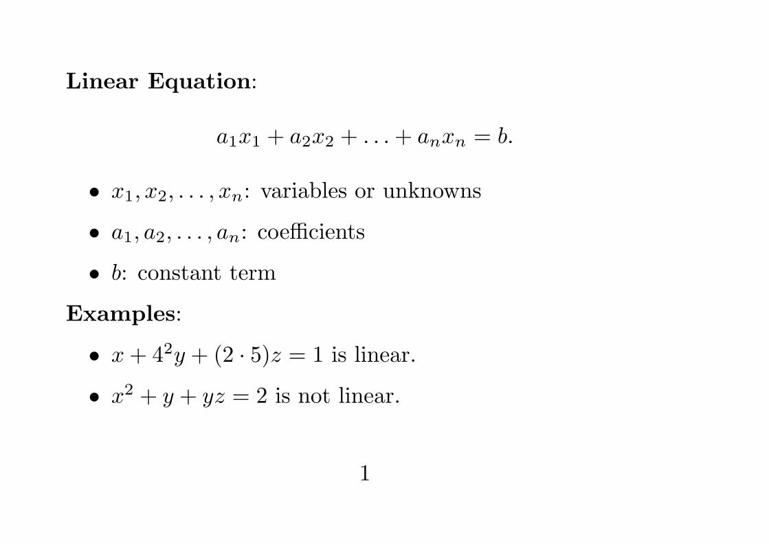
Linear Equation:
a1x1 + a2x2 + . . .+ anxn = b.
• x1, x2, . . . , xn: variables or unknowns
• a1, a2, . . . , an: coefficients
• b: constant term
Examples:
• x+ 42y + (2 · 5)z = 1 is linear.
• x2 + y + yz = 2 is not linear.
1
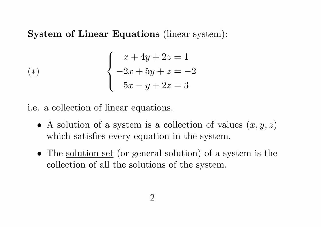
System of Linear Equations (linear system):
(∗)
x+ 4y + 2z = 1
−2x+ 5y + z = −25x− y + 2z = 3
i.e. a collection of linear equations.
• A solution of a system is a collection of values (x, y, z)which satisfies every equation in the system.
• The solution set (or general solution) of a system is thecollection of all the solutions of the system.
2
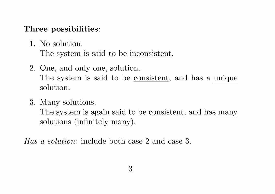
Three possibilities:
1. No solution.The system is said to be inconsistent.
2. One, and only one, solution.The system is said to be consistent, and has a uniquesolution.
3. Many solutions.The system is again said to be consistent, and has manysolutions (infinitely many).
Has a solution: include both case 2 and case 3.
3
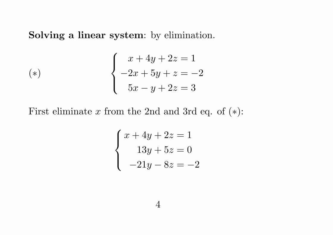
Solving a linear system: by elimination.
(∗)
x+ 4y + 2z = 1
−2x+ 5y + z = −25x− y + 2z = 3
First eliminate x from the 2nd and 3rd eq. of (∗):x+ 4y + 2z = 1
13y + 5z = 0
−21y − 8z = −2
4
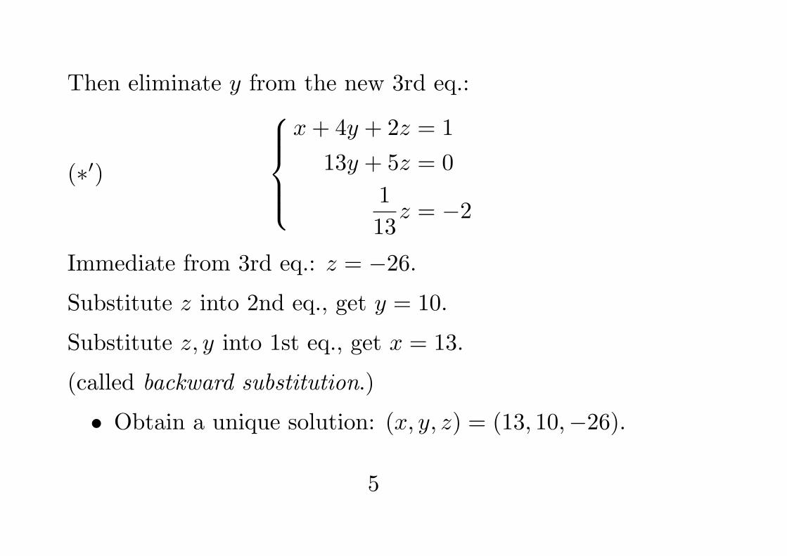
Then eliminate y from the new 3rd eq.:
(∗′)
x+ 4y + 2z = 1
13y + 5z = 0
1
13z = −2
Immediate from 3rd eq.: z = −26.Substitute z into 2nd eq., get y = 10.
Substitute z, y into 1st eq., get x = 13.
(called backward substitution.)
• Obtain a unique solution: (x, y, z) = (13, 10,−26).
5
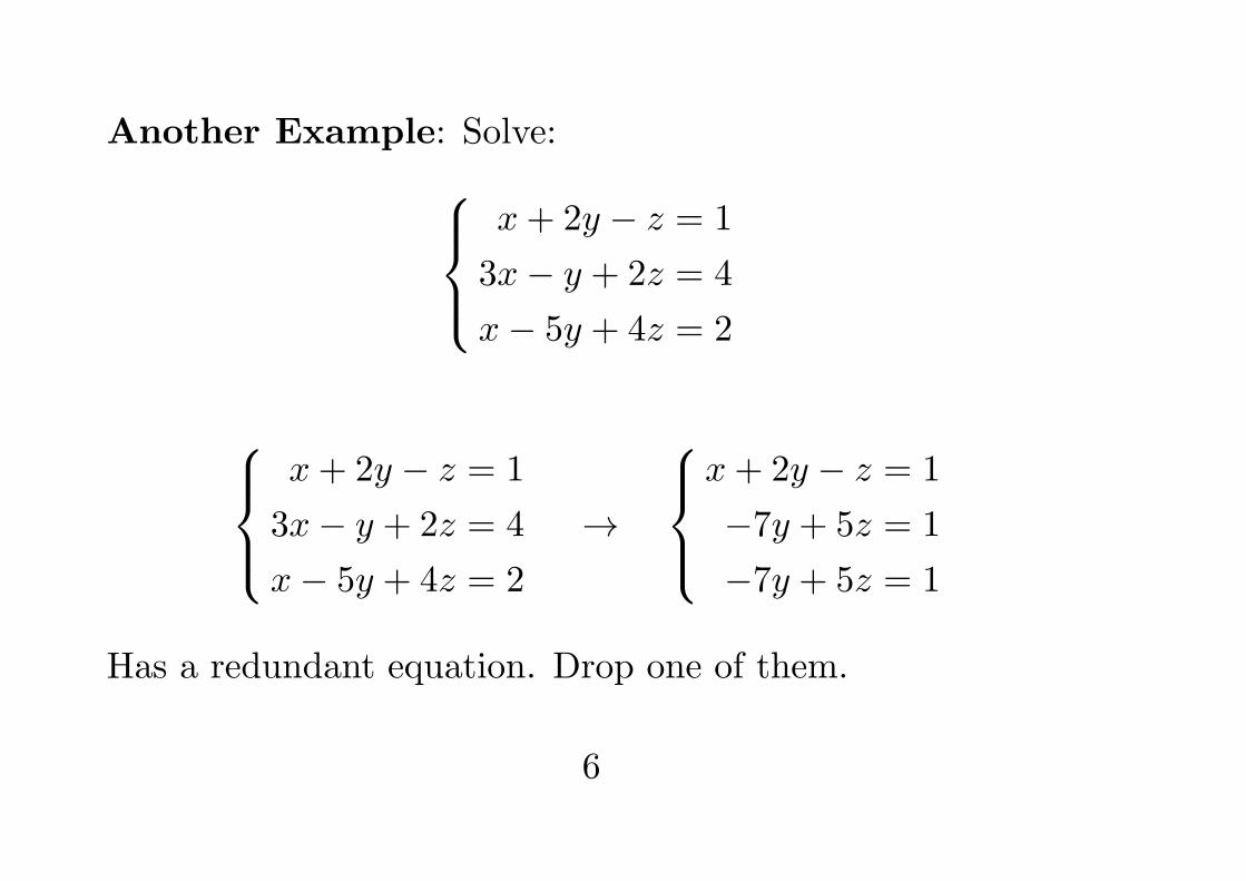
Another Example: Solve:x+ 2y − z = 1
3x− y + 2z = 4
x− 5y + 4z = 2
x+ 2y − z = 1
3x− y + 2z = 4
x− 5y + 4z = 2
→
x+ 2y − z = 1
−7y + 5z = 1
−7y + 5z = 1
Has a redundant equation. Drop one of them.
6
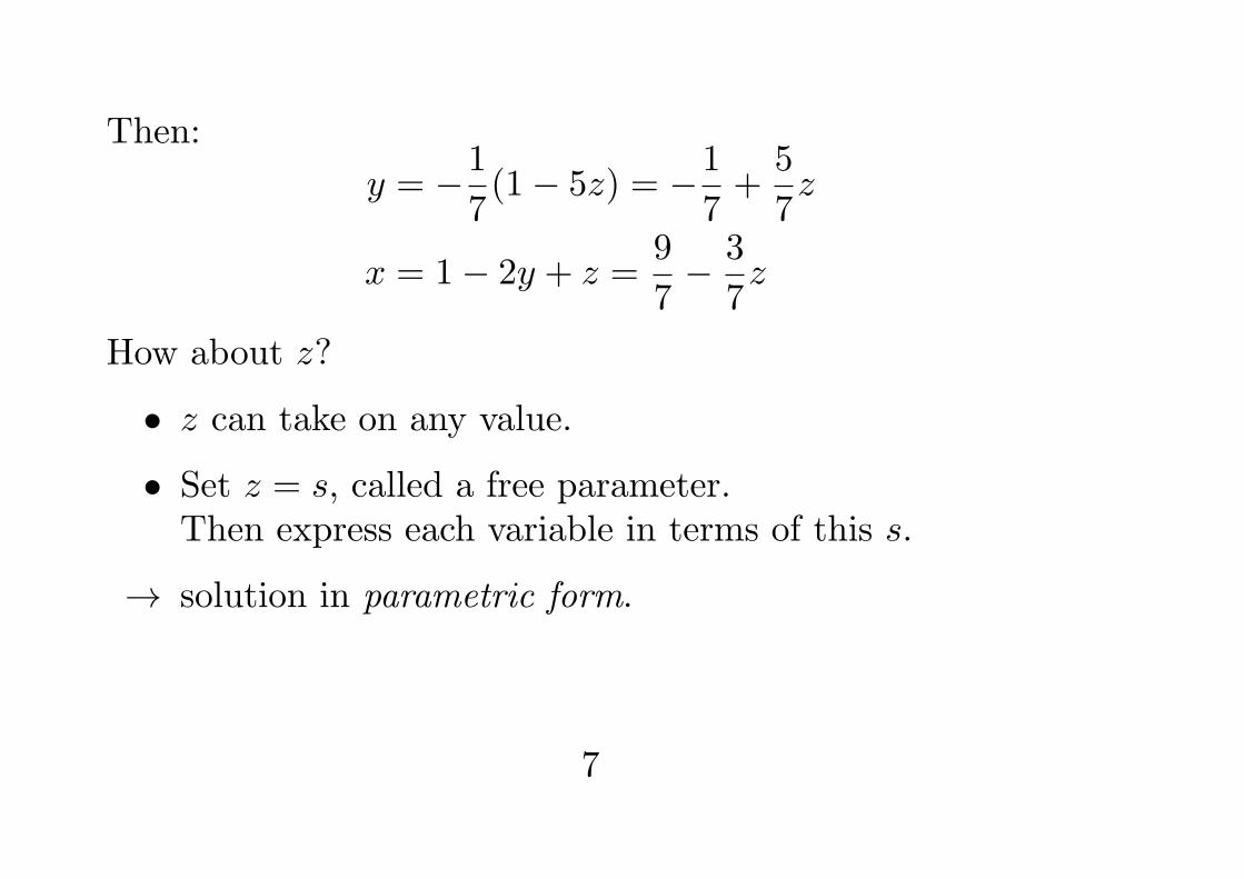
Then:
y = −1
7(1− 5z) = −1
7+
5
7z
x = 1− 2y + z =9
7− 3
7z
How about z?
• z can take on any value.
• Set z = s, called a free parameter.Then express each variable in terms of this s.
→ solution in parametric form.
7
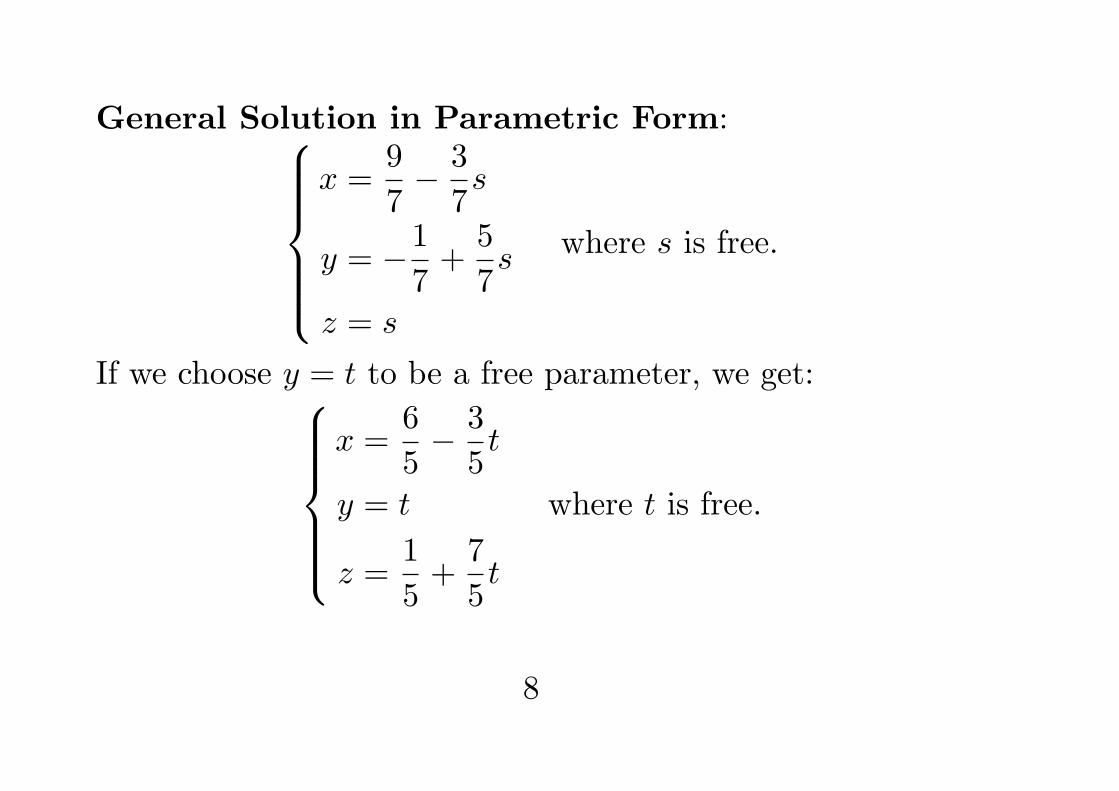
General Solution in Parametric Form:x =
9
7− 3
7s
y = −1
7+
5
7s
z = s
where s is free.
If we choose y = t to be a free parameter, we get:x =
6
5− 3
5t
y = t
z =1
5+
7
5t
where t is free.
8
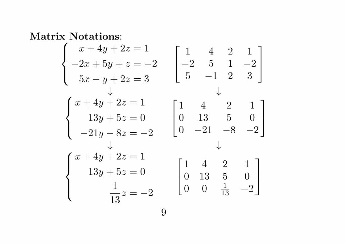
Matrix Notations:x+ 4y + 2z = 1
−2x+ 5y + z = −25x− y + 2z = 3
1 4 2 1−2 5 1 −25 −1 2 3
↓ ↓
x+ 4y + 2z = 1
13y + 5z = 0
−21y − 8z = −2
1 4 2 10 13 5 00 −21 −8 −2
↓ ↓
x+ 4y + 2z = 1
13y + 5z = 0
1
13z = −2
1 4 2 10 13 5 00 0 1
13 −2
9
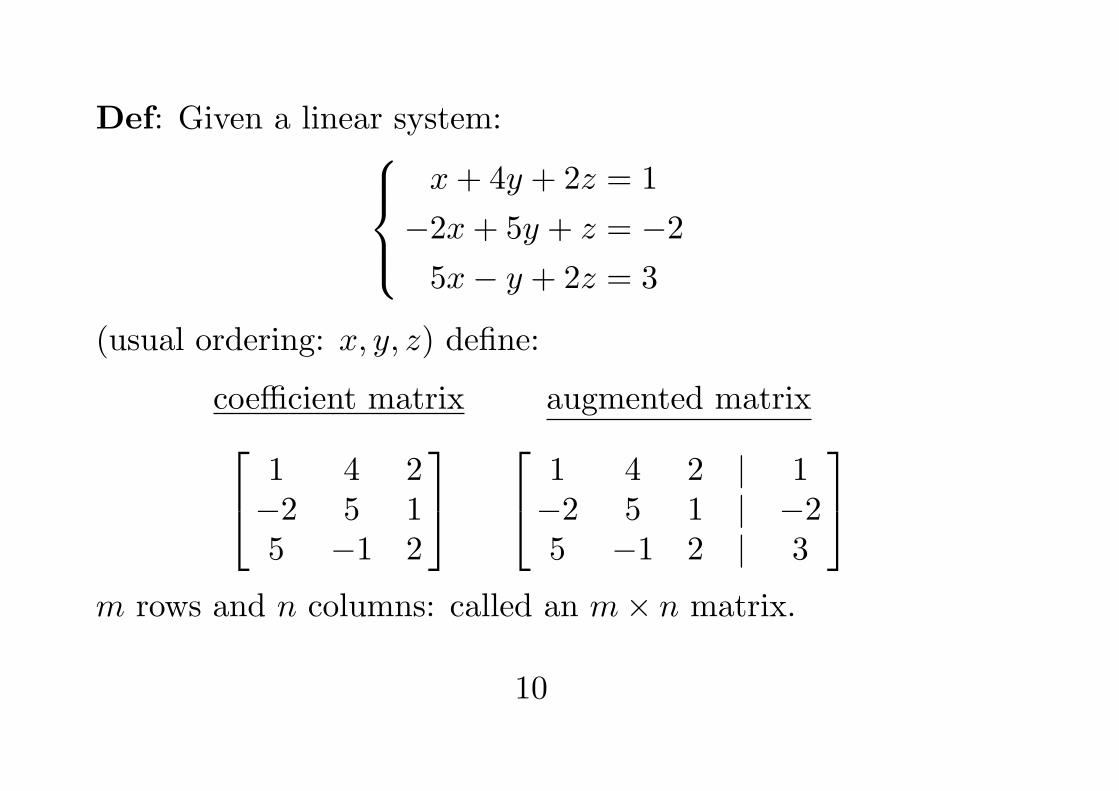
Def: Given a linear system:x+ 4y + 2z = 1
−2x+ 5y + z = −25x− y + 2z = 3
(usual ordering: x, y, z) define:
coefficient matrix 1 4 2−2 5 15 −1 2
augmented matrix 1 4 2 | 1−2 5 1 | −25 −1 2 | 3
m rows and n columns: called an m× n matrix.
10
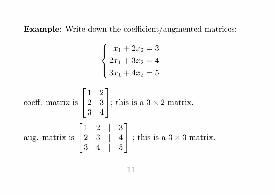
Example: Write down the coefficient/augmented matrices:x1 + 2x2 = 3
2x1 + 3x2 = 4
3x1 + 4x2 = 5
coeff. matrix is
1 22 33 4
; this is a 3× 2 matrix.
aug. matrix is
1 2 | 32 3 | 43 4 | 5
; this is a 3× 3 matrix.
11
Example: Write down the augmented matrix:x1 + 2x3 = 1
x2 + x4 = 2
x3 − x4 = 3
***
12
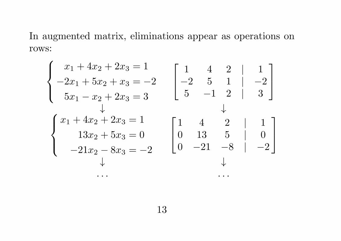
In augmented matrix, eliminations appear as operations onrows:
x1 + 4x2 + 2x3 = 1
−2x1 + 5x2 + x3 = −25x1 − x2 + 2x3 = 3
1 4 2 | 1−2 5 1 | −25 −1 2 | 3
↓ ↓
x1 + 4x2 + 2x3 = 1
13x2 + 5x3 = 0
−21x2 − 8x3 = −2
1 4 2 | 10 13 5 | 00 −21 −8 | −2
↓ ↓. . . . . .
13
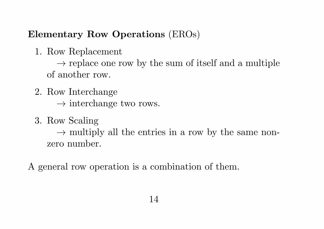
Elementary Row Operations (EROs)
1. Row Replacement→ replace one row by the sum of itself and a multiple
of another row.
2. Row Interchange→ interchange two rows.
3. Row Scaling→ multiply all the entries in a row by the same non-
zero number.
A general row operation is a combination of them.
14
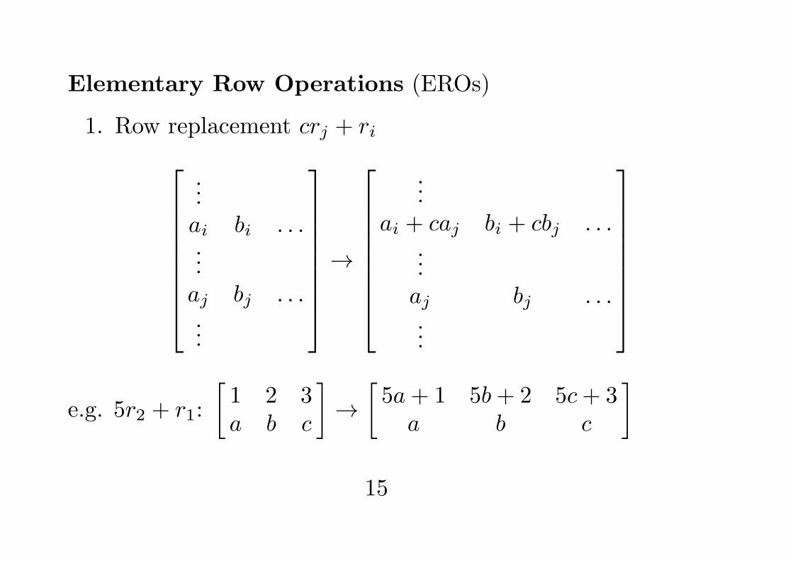
Elementary Row Operations (EROs)
1. Row replacement crj + ri
...ai bi . . ....aj bj . . ....
→
...ai + caj bi + cbj . . .
...aj bj . . ....
e.g. 5r2 + r1:
[1 2 3a b c
]→
[5a+ 1 5b+ 2 5c+ 3
a b c
]
15
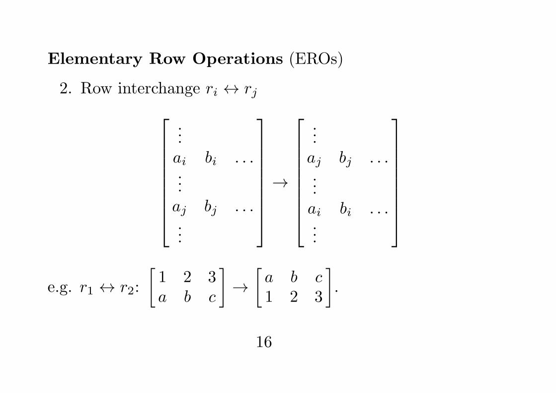
Elementary Row Operations (EROs)
2. Row interchange ri ↔ rj
...ai bi . . ....aj bj . . ....
→
...aj bj . . ....ai bi . . ....
e.g. r1 ↔ r2:
[1 2 3a b c
]→
[a b c1 2 3
].
16
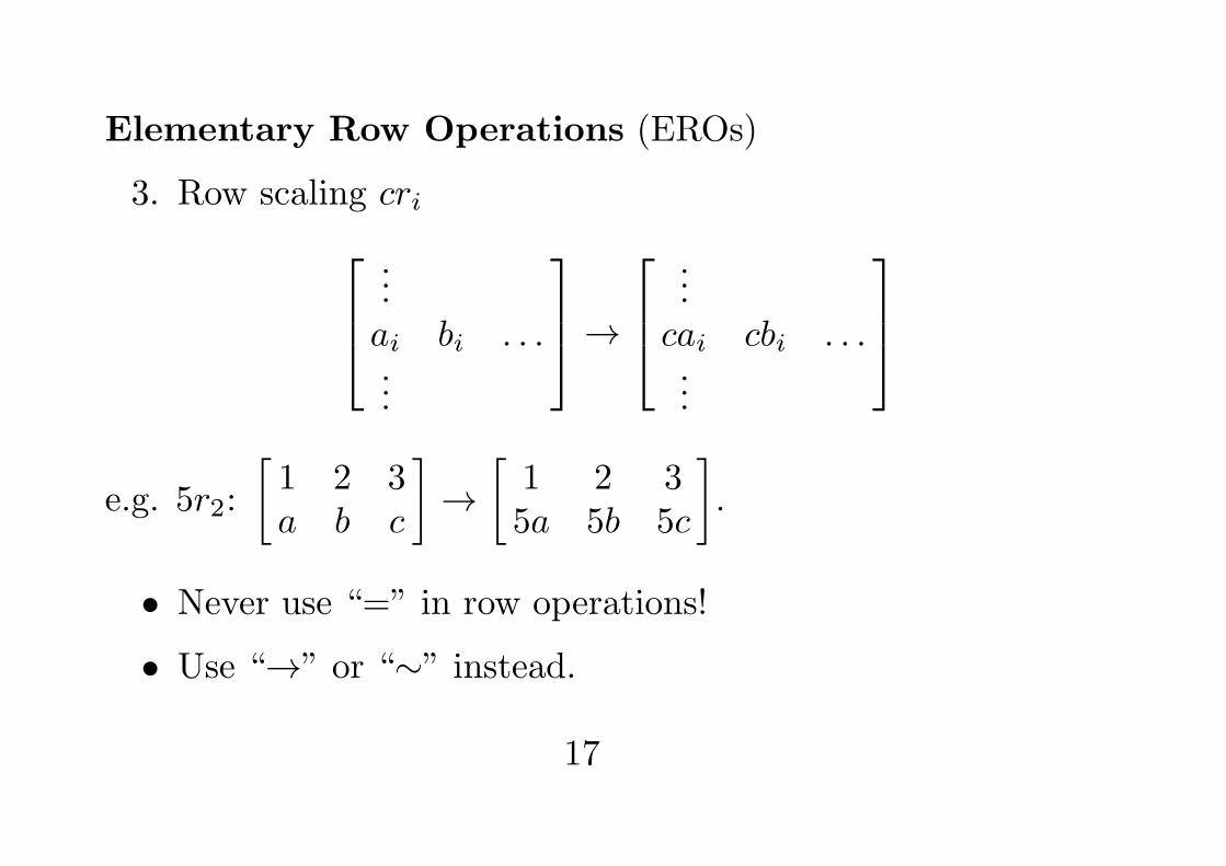
Elementary Row Operations (EROs)
3. Row scaling cri...ai bi . . ....
→
...cai cbi . . ....
e.g. 5r2:
[1 2 3a b c
]→
[1 2 35a 5b 5c
].
• Never use “=” in row operations!
• Use “→” or “∼” instead.
17
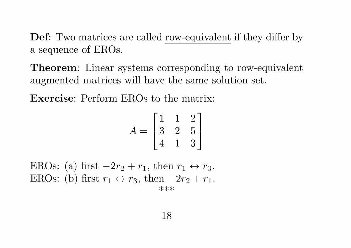
Def: Two matrices are called row-equivalent if they differ bya sequence of EROs.
Theorem: Linear systems corresponding to row-equivalentaugmented matrices will have the same solution set.
Exercise: Perform EROs to the matrix:
A =
1 1 23 2 54 1 3
EROs: (a) first −2r2 + r1, then r1 ↔ r3.EROs: (b) first r1 ↔ r3, then −2r2 + r1.
***
18
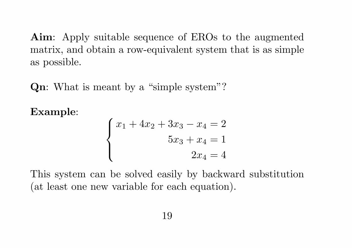
Aim: Apply suitable sequence of EROs to the augmentedmatrix, and obtain a row-equivalent system that is as simpleas possible.
Qn: What is meant by a “simple system”?
Example: x1 + 4x2 + 3x3 − x4 = 2
5x3 + x4 = 1
2x4 = 4
This system can be solved easily by backward substitution(at least one new variable for each equation).
19
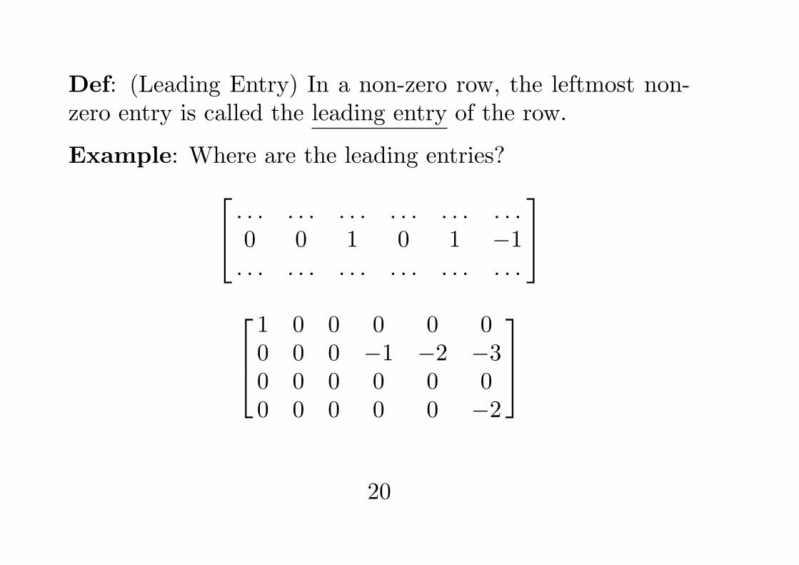
Def: (Leading Entry) In a non-zero row, the leftmost non-zero entry is called the leading entry of the row.
Example: Where are the leading entries? . . . . . . . . . . . . . . . . . .0 0 1 0 1 −1. . . . . . . . . . . . . . . . . .
1 0 0 0 0 00 0 0 −1 −2 −30 0 0 0 0 00 0 0 0 0 −2
20
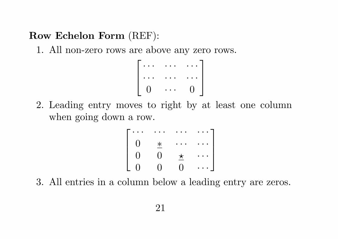
Row Echelon Form (REF):
1. All non-zero rows are above any zero rows. · · · · · · · · ·· · · · · · · · ·0 · · · 0
2. Leading entry moves to right by at least one column
when going down a row.· · · · · · · · · · · ·0 ∗ · · · · · ·0 0 ⋆ · · ·0 0 0 · · ·
3. All entries in a column below a leading entry are zeros.
21
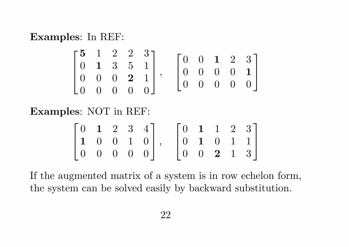
Examples: In REF:5 1 2 2 30 1 3 5 10 0 0 2 10 0 0 0 0
,
0 0 1 2 30 0 0 0 10 0 0 0 0
Examples: NOT in REF: 0 1 2 3 4
1 0 0 1 00 0 0 0 0
,
0 1 1 2 30 1 0 1 10 0 2 1 3
If the augmented matrix of a system is in row echelon form,the system can be solved easily by backward substitution.
22
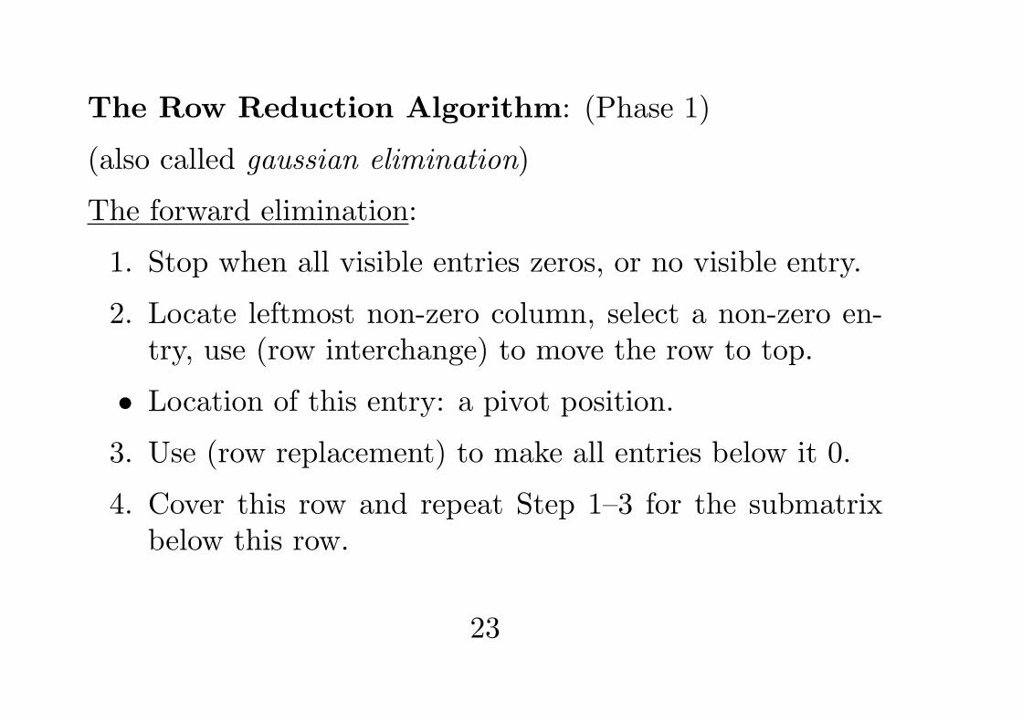
The Row Reduction Algorithm: (Phase 1)
(also called gaussian elimination)
The forward elimination:
1. Stop when all visible entries zeros, or no visible entry.
2. Locate leftmost non-zero column, select a non-zero en-try, use (row interchange) to move the row to top.
• Location of this entry: a pivot position.
3. Use (row replacement) to make all entries below it 0.
4. Cover this row and repeat Step 1–3 for the submatrixbelow this row.
23
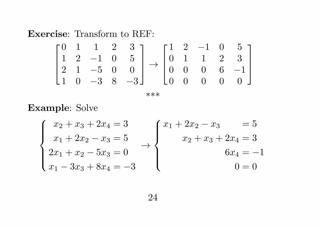
Exercise: Transform to REF:0 1 1 2 31 2 −1 0 52 1 −5 0 01 0 −3 8 −3
→1 2 −1 0 50 1 1 2 30 0 0 6 −10 0 0 0 0
***
Example: Solvex2 + x3 + 2x4 = 3
x1 + 2x2 − x3 = 5
2x1 + x2 − 5x3 = 0
x1 − 3x3 + 8x4 = −3
→
x1 + 2x2 − x3 = 5
x2 + x3 + 2x4 = 3
6x4 = −10 = 0
24
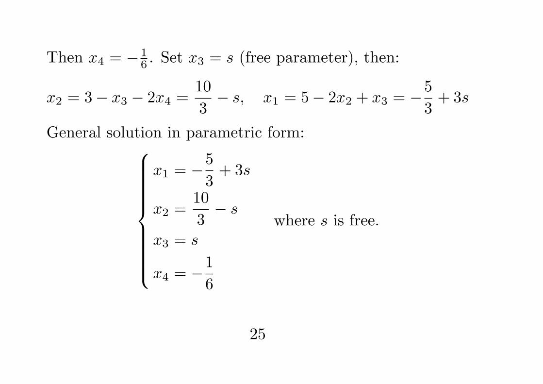
Then x4 = −16 . Set x3 = s (free parameter), then:
x2 = 3− x3 − 2x4 =10
3− s, x1 = 5− 2x2 + x3 = −5
3+ 3s
General solution in parametric form:
x1 = −5
3+ 3s
x2 =10
3− s
x3 = s
x4 = −1
6
where s is free.
25
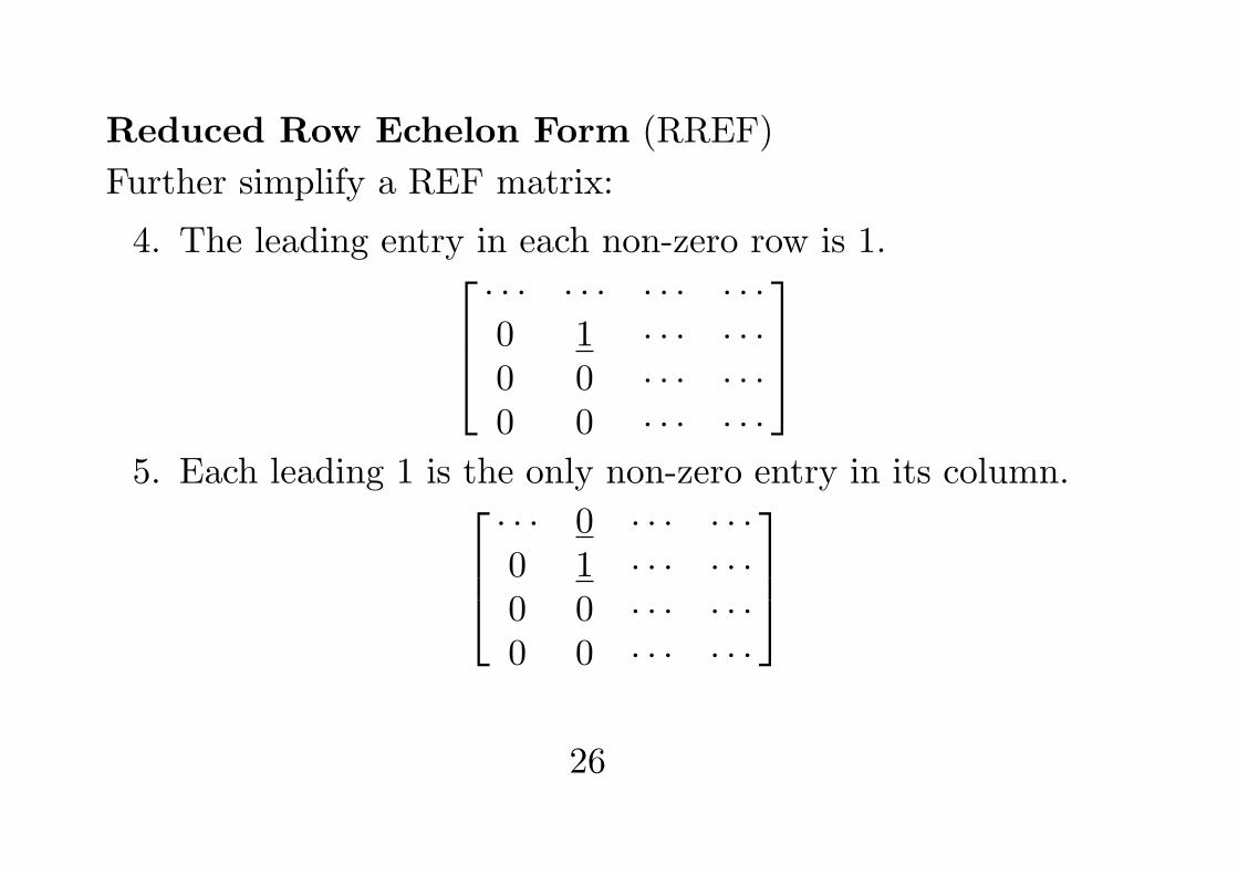
Reduced Row Echelon Form (RREF)
Further simplify a REF matrix:
4. The leading entry in each non-zero row is 1.· · · · · · · · · · · ·0 1 · · · · · ·0 0 · · · · · ·0 0 · · · · · ·
5. Each leading 1 is the only non-zero entry in its column.
· · · 0 · · · · · ·0 1 · · · · · ·0 0 · · · · · ·0 0 · · · · · ·
26
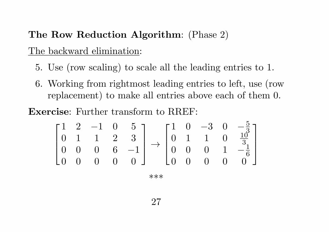
The Row Reduction Algorithm: (Phase 2)
The backward elimination:
5. Use (row scaling) to scale all the leading entries to 1.
6. Working from rightmost leading entries to left, use (rowreplacement) to make all entries above each of them 0.
Exercise: Further transform to RREF:1 2 −1 0 50 1 1 2 30 0 0 6 −10 0 0 0 0
→1 0 −3 0 − 5
30 1 1 0 10
30 0 0 1 − 1
60 0 0 0 0
***
27
Importance of RREF: uniqueness.
Thm 1 (P.13): Each matrix is row-equivalent to one andonly one reduced row echelon matrix.
Because of the above uniqueness property, the concept ofpivot position is well defined:
Def: A pivot position in a matrix A is a location in A thatcorresponds to a leading 1 in the RREF of A.
Def: A pivot column is a column of A that contains a pivotposition.
Note that we cannot have two pivot positions sitting in thesame row or in the same column.
28
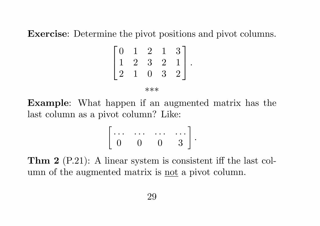
Exercise: Determine the pivot positions and pivot columns. 0 1 2 1 31 2 3 2 12 1 0 3 2
.
***Example: What happen if an augmented matrix has thelast column as a pivot column? Like:[
. . . . . . . . . . . .0 0 0 3
].
Thm 2 (P.21): A linear system is consistent iff the last col-umn of the augmented matrix is not a pivot column.
29
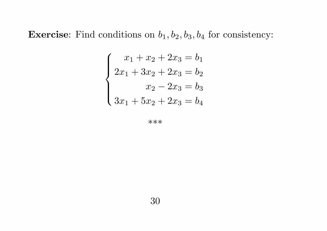
Exercise: Find conditions on b1, b2, b3, b4 for consistency:x1 + x2 + 2x3 = b1
2x1 + 3x2 + 2x3 = b2
x2 − 2x3 = b3
3x1 + 5x2 + 2x3 = b4
***
30
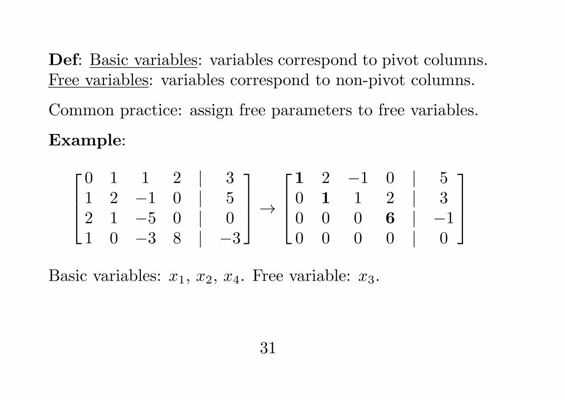
Def: Basic variables: variables correspond to pivot columns.Free variables: variables correspond to non-pivot columns.
Common practice: assign free parameters to free variables.
Example:0 1 1 2 | 31 2 −1 0 | 52 1 −5 0 | 01 0 −3 8 | −3
→1 2 −1 0 | 50 1 1 2 | 30 0 0 6 | −10 0 0 0 | 0
Basic variables: x1, x2, x4. Free variable: x3.
31
Rank of a matrix
Def: rankA = no. of pivot positions in A.
For a system to be consistent, the last column of its aug-mented matrix cannot be a pivot column, so:
Theorem: A linear system [ A | b ] is consistent iff
rankA = rank [ A | b ].
Theorem: Let [ A | b ] represent a consistent system withn variables. Then: no. of free parameters = n− rankA.
32
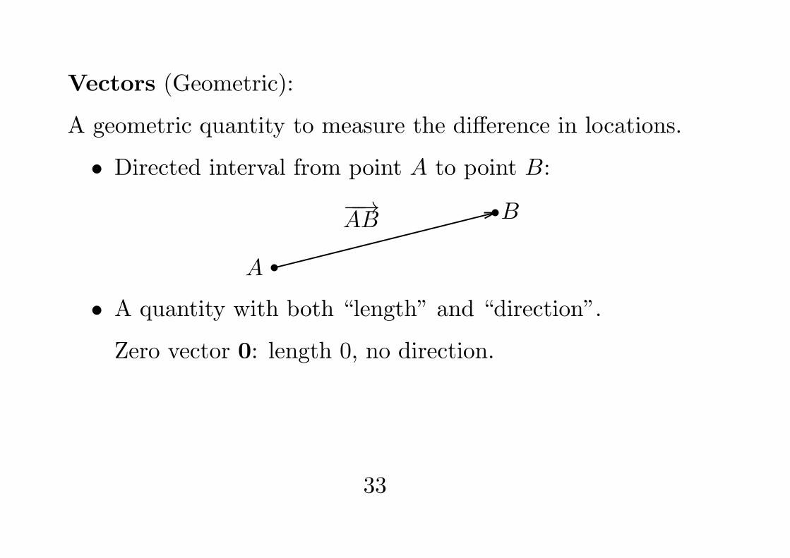
Vectors (Geometric):
A geometric quantity to measure the difference in locations.
• Directed interval from point A to point B:
A
B−−→AB
• A quantity with both “length” and “direction”.
Zero vector 0: length 0, no direction.
33
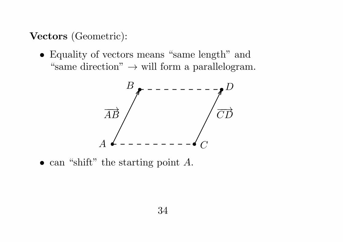
Vectors (Geometric):
• Equality of vectors means “same length” and“same direction” → will form a parallelogram.
A
B
−−→AB
C
D
−−→CD
• can “shift” the starting point A.
34
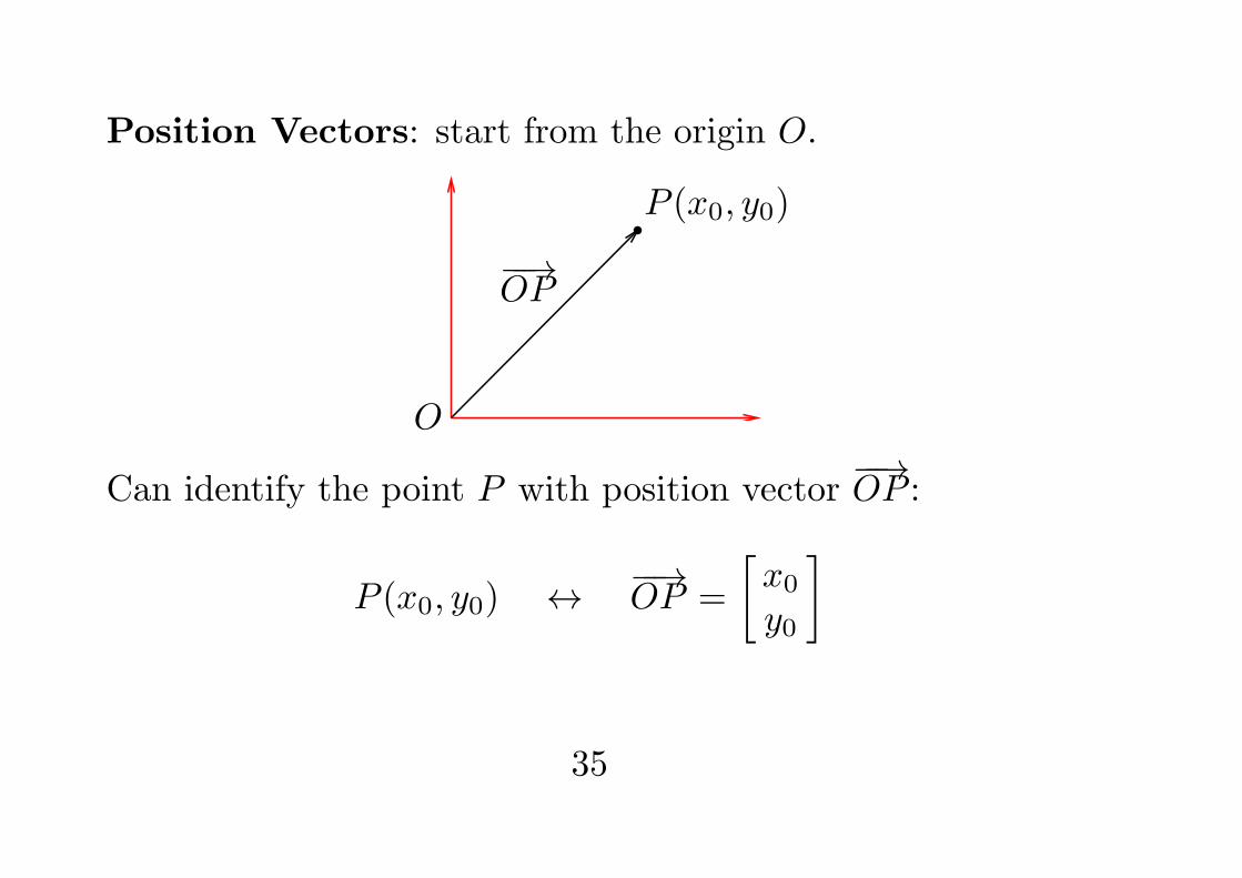
Position Vectors: start from the origin O.
O
P (x0, y0)
−−→OP
Can identify the point P with position vector−−→OP :
P (x0, y0) ↔ −−→OP =
[x0
y0
]
35
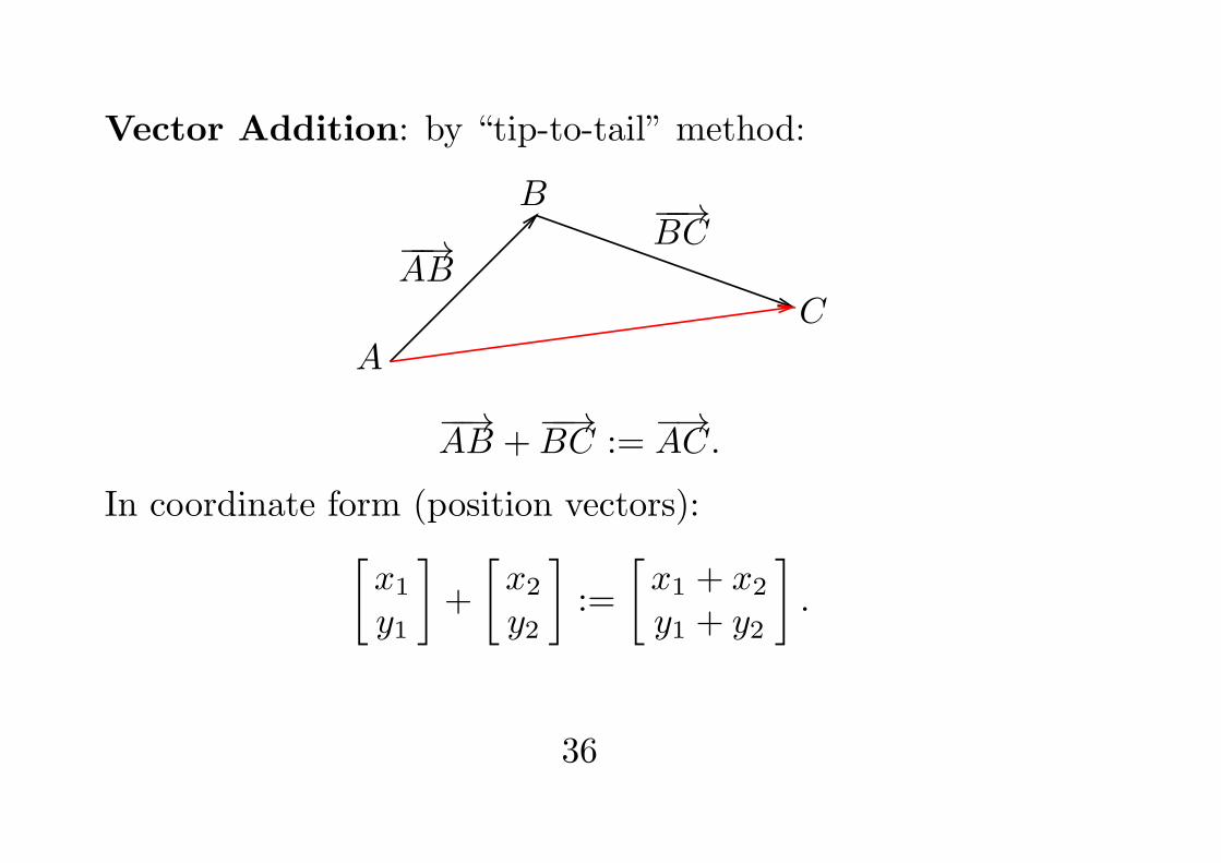
Vector Addition: by “tip-to-tail” method:
A
B
−−→AB
C
−−→BC
−−→AB +
−−→BC :=
−→AC.
In coordinate form (position vectors):[x1
y1
]+
[x2
y2
]:=
[x1 + x2
y1 + y2
].
36
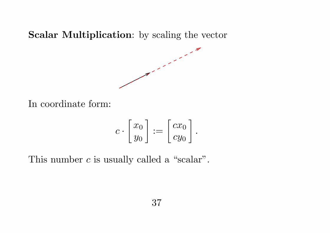
Scalar Multiplication: by scaling the vector
In coordinate form:
c ·[x0
y0
]:=
[cx0
cy0
].
This number c is usually called a “scalar”.
37
Vectors (Algebraic):
1. A vector is a collection of no. arranged in column form.
u =
[12
], v =
22−1
, 0 =
[00
].
2. The size of a vector is the no. of entries in the vector.
u is a 2-vector, v is a 3-vector, 0 ... depends.
3. Usually denoted by bold face letters like u,v,w.
38
Equality of Vectors: same size, same corr. entries 123
= [12
], and
123
=
abc
only when a = 1, b = 2, c = 3.
Notation: The collection of all (real) vectors of size n:
Rn =
{ a1...an
: a1, . . . , an ∈ R
}.
39
Operations: Vector addition and Scalar multiplication
1. Vectors of the same size can be added together:[ab
]+
[pq
]:=
[a+ pb+ q
].
Vectors of different sizes cannot be added together.
2. Scalar multiplication of a vector by a number c:
c
[pq
]:=
[cpcq
].
This number c is usually called a “scalar”.
40
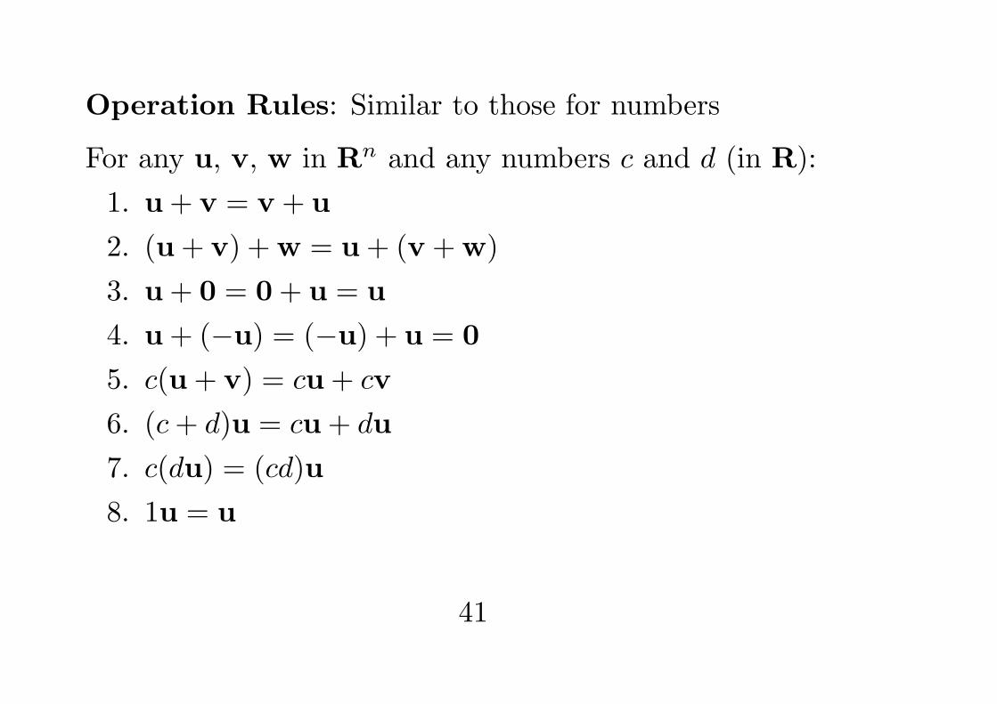
Operation Rules: Similar to those for numbers
For any u, v, w in Rn and any numbers c and d (in R):
1. u+ v = v + u
2. (u+ v) +w = u+ (v +w)
3. u+ 0 = 0+ u = u
4. u+ (−u) = (−u) + u = 0
5. c(u+ v) = cu+ cv
6. (c+ d)u = cu+ du
7. c(du) = (cd)u
8. 1u = u
41
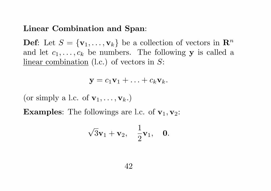
Linear Combination and Span:
Def: Let S = {v1, . . . ,vk} be a collection of vectors in Rn
and let c1, . . . , ck be numbers. The following y is called alinear combination (l.c.) of vectors in S:
y = c1v1 + . . .+ ckvk.
(or simply a l.c. of v1, . . . ,vk.)
Examples: The followings are l.c. of v1,v2:
√3v1 + v2,
1
2v1, 0.
42
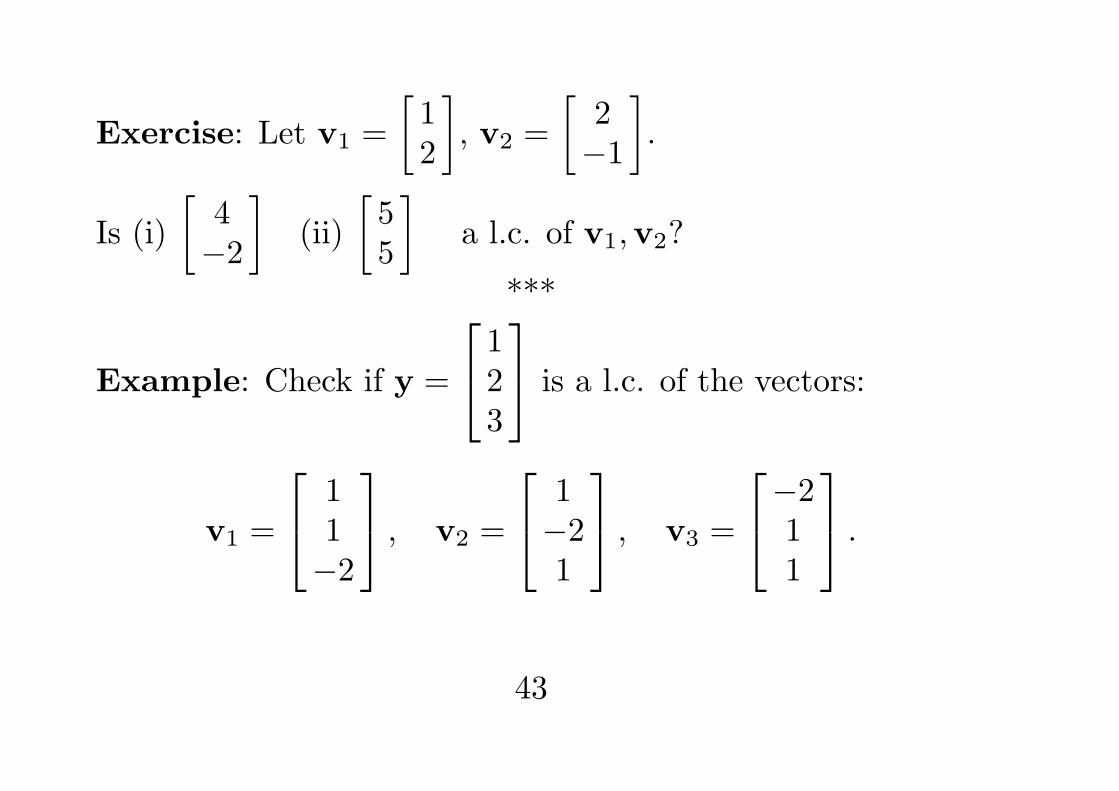
Exercise: Let v1 =
[12
], v2 =
[2−1
].
Is (i)
[4−2
](ii)
[55
]a l.c. of v1,v2?
***
Example: Check if y =
123
is a l.c. of the vectors:
v1 =
11−2
, v2 =
1−21
, v3 =
−211
.
43
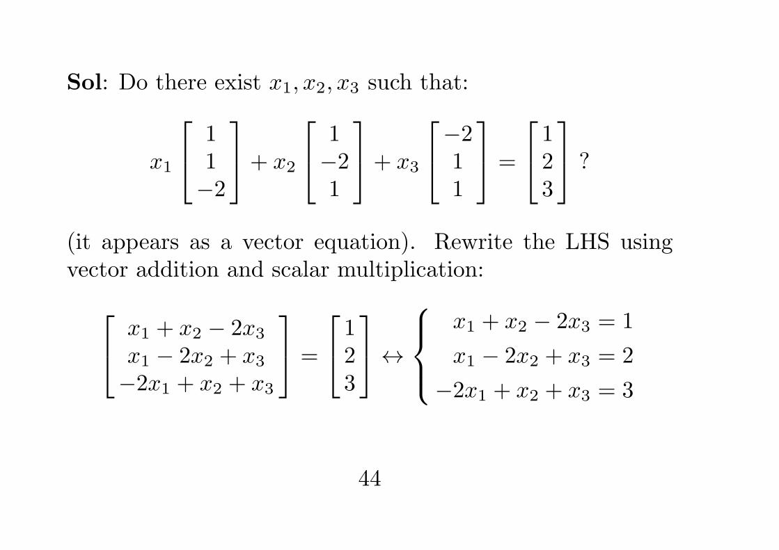
Sol: Do there exist x1, x2, x3 such that:
x1
11−2
+ x2
1−21
+ x3
−211
=
123
?
(it appears as a vector equation). Rewrite the LHS usingvector addition and scalar multiplication: x1 + x2 − 2x3
x1 − 2x2 + x3
−2x1 + x2 + x3
=
123
↔
x1 + x2 − 2x3 = 1
x1 − 2x2 + x3 = 2
−2x1 + x2 + x3 = 3
44
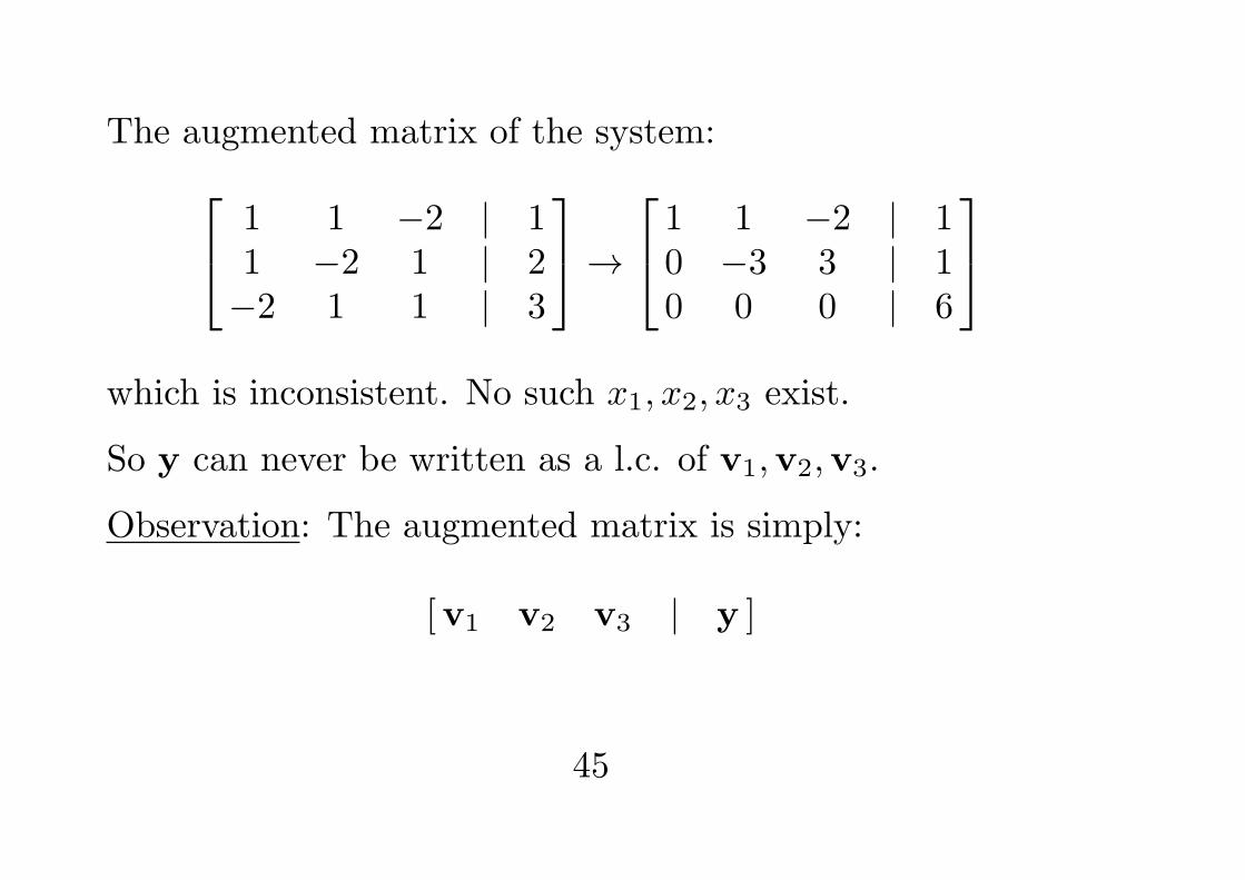
The augmented matrix of the system: 1 1 −2 | 11 −2 1 | 2−2 1 1 | 3
→ 1 1 −2 | 10 −3 3 | 10 0 0 | 6
which is inconsistent. No such x1, x2, x3 exist.
So y can never be written as a l.c. of v1,v2,v3.
Observation: The augmented matrix is simply:
[v1 v2 v3 | y ]
45
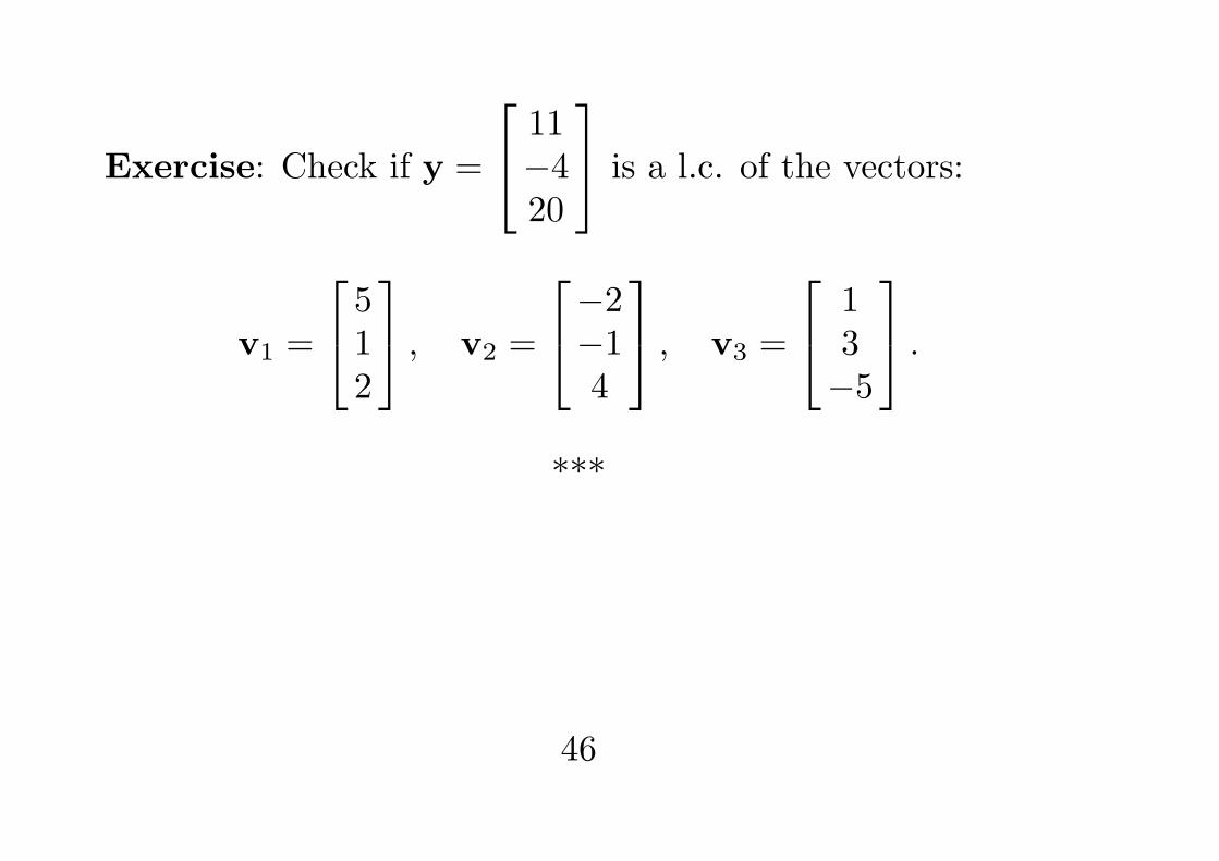
Exercise: Check if y =
11−420
is a l.c. of the vectors:
v1 =
512
, v2 =
−2−14
, v3 =
13−5
.
***
46
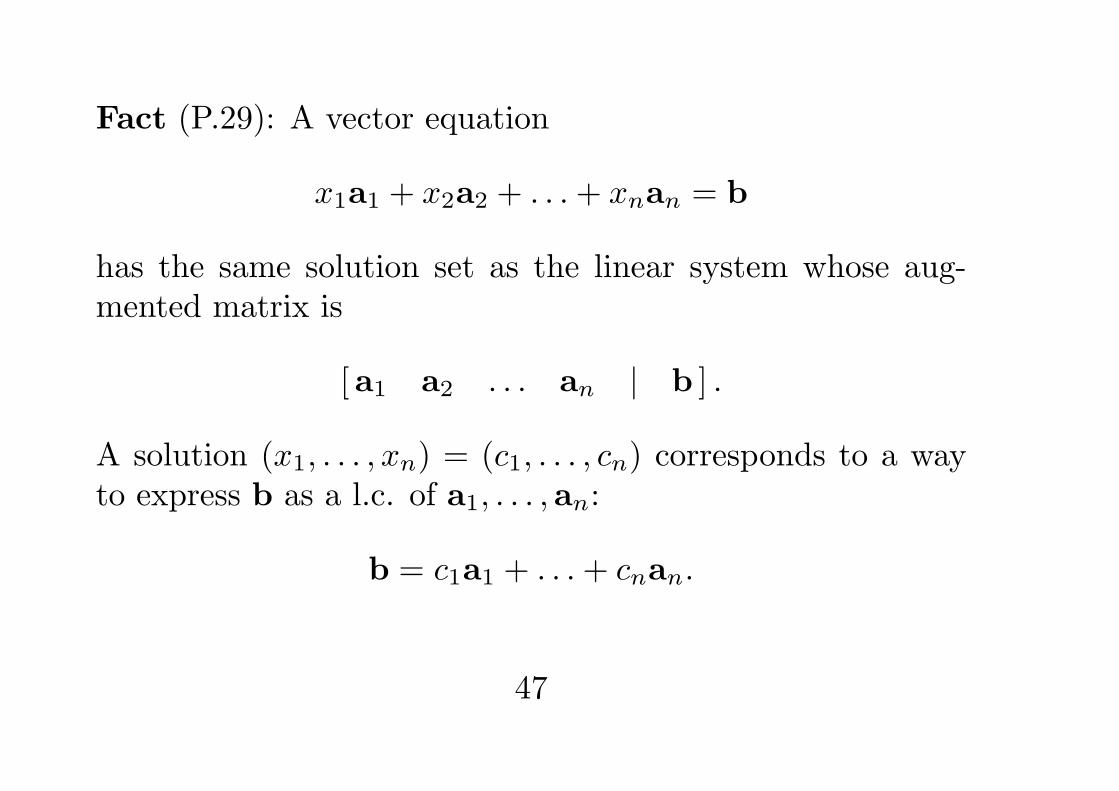
Fact (P.29): A vector equation
x1a1 + x2a2 + . . .+ xnan = b
has the same solution set as the linear system whose aug-mented matrix is
[a1 a2 . . . an | b ] .
A solution (x1, . . . , xn) = (c1, . . . , cn) corresponds to a wayto express b as a l.c. of a1, . . . ,an:
b = c1a1 + . . .+ cnan.
47
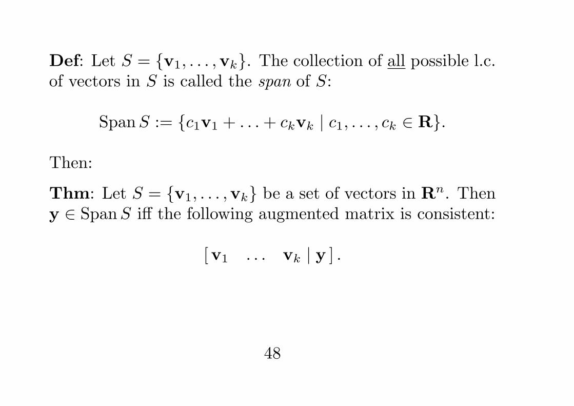
Def: Let S = {v1, . . . ,vk}. The collection of all possible l.c.of vectors in S is called the span of S:
SpanS := {c1v1 + . . .+ ckvk | c1, . . . , ck ∈ R}.
Then:
Thm: Let S = {v1, . . . ,vk} be a set of vectors in Rn. Theny ∈ SpanS iff the following augmented matrix is consistent:
[v1 . . . vk | y ] .
48
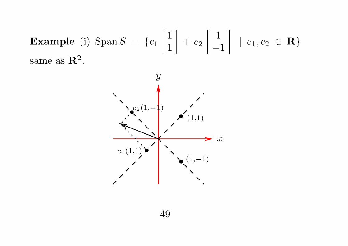
Example (i) SpanS = {c1[11
]+ c2
[1−1
]| c1, c2 ∈ R}
same as R2.
x
y
(1,1)
(1,−1)c1(1,1)
c2(1,−1)
49
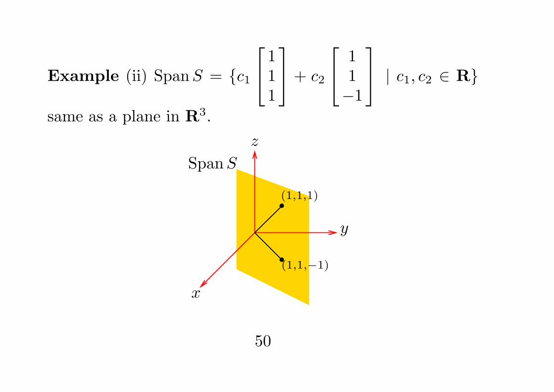
Example (ii) SpanS = {c1
111
+ c2
11−1
| c1, c2 ∈ R}
same as a plane in R3.
x
y
z
(1,1,1)
(1,1,−1)
SpanS
50
Recall: a vector equation like:
x1
512
+ x2
−2−14
+ x3
13−5
=
11−420
is just another way to express the following system:
5x1 − 2x2 + x3 = 11
x1 − x2 + 3x3 = −42x1 + 4x2 − 5x3 = 20
They have the same solution set in (x1, x2, x3).
51
Matrix representation of the system:
A =
5 −2 11 −1 32 4 −5
, x =
x1
x2
x3
, b =
11−420
.
By defining Ax to be:
Ax := x1
512
+ x2
−2−14
+ x3
13−5
Then the linear system can be written as Ax = b, called amatrix equation.
52
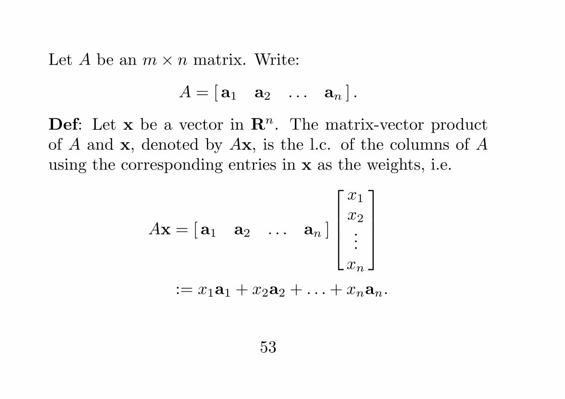
Let A be an m× n matrix. Write:
A = [a1 a2 . . . an ] .
Def: Let x be a vector in Rn. The matrix-vector productof A and x, denoted by Ax, is the l.c. of the columns of Ausing the corresponding entries in x as the weights, i.e.
Ax = [a1 a2 . . . an ]
x1
x2...xn
:= x1a1 + x2a2 + . . .+ xnan.
53
Remark: Ax is defined only when:
no. of columns in A = no. of entries in x.
Properties of matrix-vector product Ax:
Thm 5 (P.39): Let A be an m×n matrix, u,v ∈ Rn, c ∈ R.Then:
a. A(u+ v) = Au+Av
b. A(cu) = cA(u)
Note: The above properties are called the “linear” proper-ties of matrix-vector product (see §1.8).
54
Example: Compute Ax where A =
1 23 5−1 1
.Sol: To form Ax correctly, x must be a 2-vector.
Set: x =
[x1
x2
]. Then
Ax =
1 23 5−1 1
[x1
x2
]= x1
13−1
+ x2
251
=
1 · x1 + 2 · x2
3 · x1 + 5 · x2
−1 · x1 + 1 · x2
55
Example: Rewrite the following into a matrix equation:[13
]−[22
]+ 2
[−15
]− 3
[12
]=
[−65
]Sol: LHS is a l.c. of the following 4 vectors:[
13
],
[22
],
[−15
],
[12
].
We form a matrix A using these vectors:
A =
[1 2 −1 13 2 5 2
]56
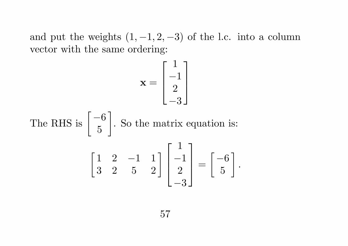
and put the weights (1,−1, 2,−3) of the l.c. into a columnvector with the same ordering:
x =
1−12−3
The RHS is
[−65
]. So the matrix equation is:
[1 2 −1 13 2 5 2
]1−12−3
=
[−65
].
57
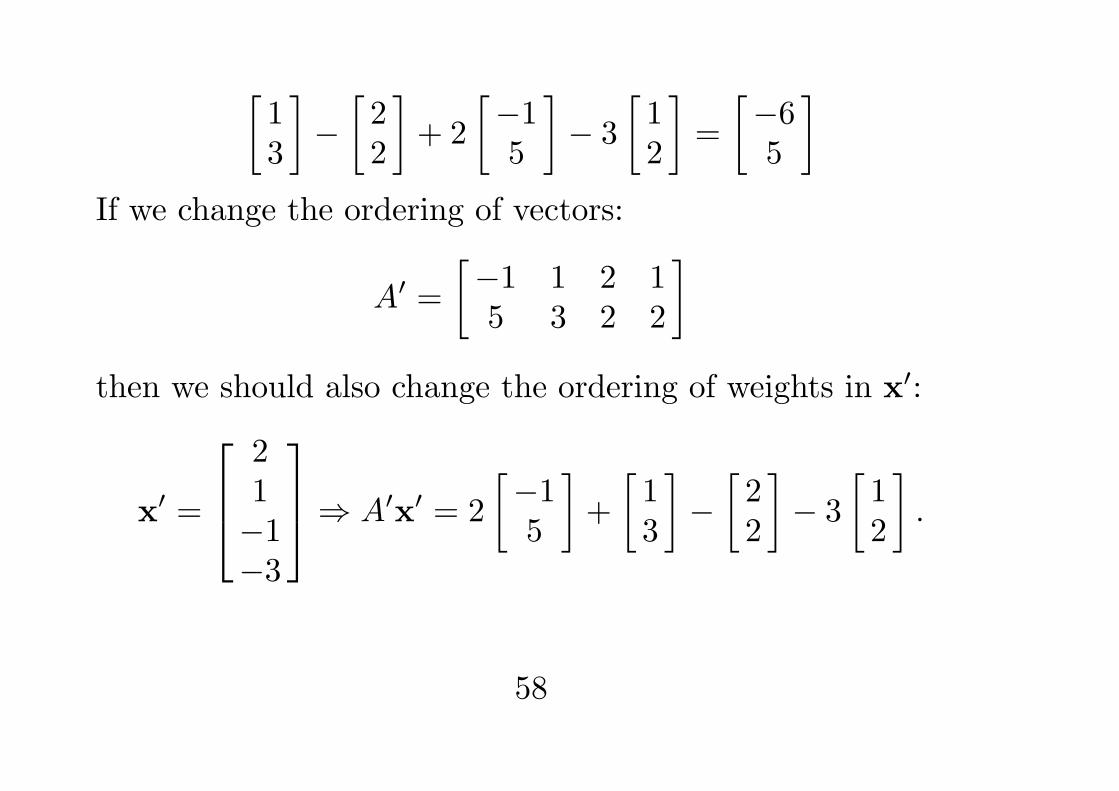
[13
]−[22
]+ 2
[−15
]− 3
[12
]=
[−65
]If we change the ordering of vectors:
A′ =
[−1 1 2 15 3 2 2
]then we should also change the ordering of weights in x′:
x′ =
21−1−3
⇒ A′x′ = 2
[−15
]+
[13
]−[22
]− 3
[12
].
58
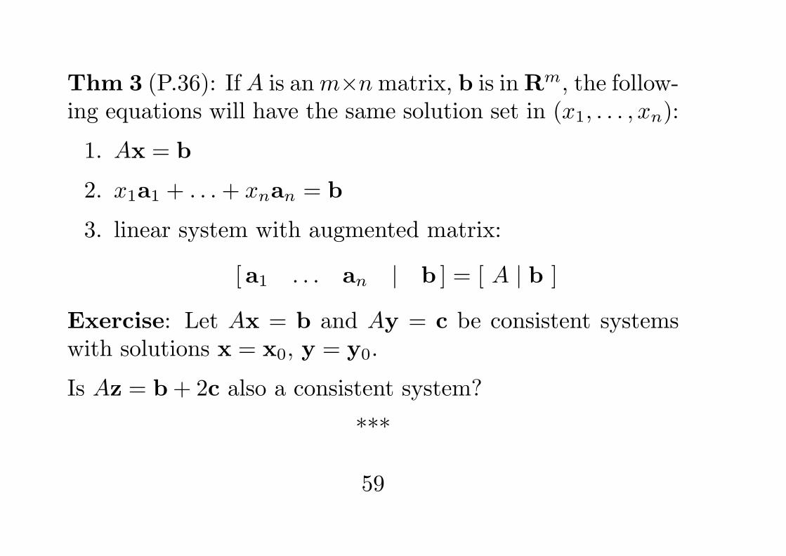
Thm 3 (P.36): If A is anm×nmatrix, b is inRm, the follow-ing equations will have the same solution set in (x1, . . . , xn):
1. Ax = b
2. x1a1 + . . .+ xnan = b
3. linear system with augmented matrix:
[a1 . . . an | b ] = [ A | b ]
Exercise: Let Ax = b and Ay = c be consistent systemswith solutions x = x0, y = y0.
Is Az = b+ 2c also a consistent system?
***
59
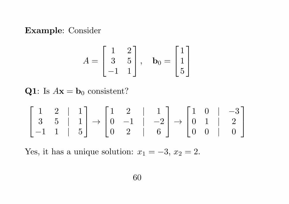
Example: Consider
A =
1 23 5−1 1
, b0 =
115
Q1: Is Ax = b0 consistent? 1 2 | 1
3 5 | 1−1 1 | 5
→ 1 2 | 10 −1 | −20 2 | 6
→ 1 0 | −30 1 | 20 0 | 0
Yes, it has a unique solution: x1 = −3, x2 = 2.
60
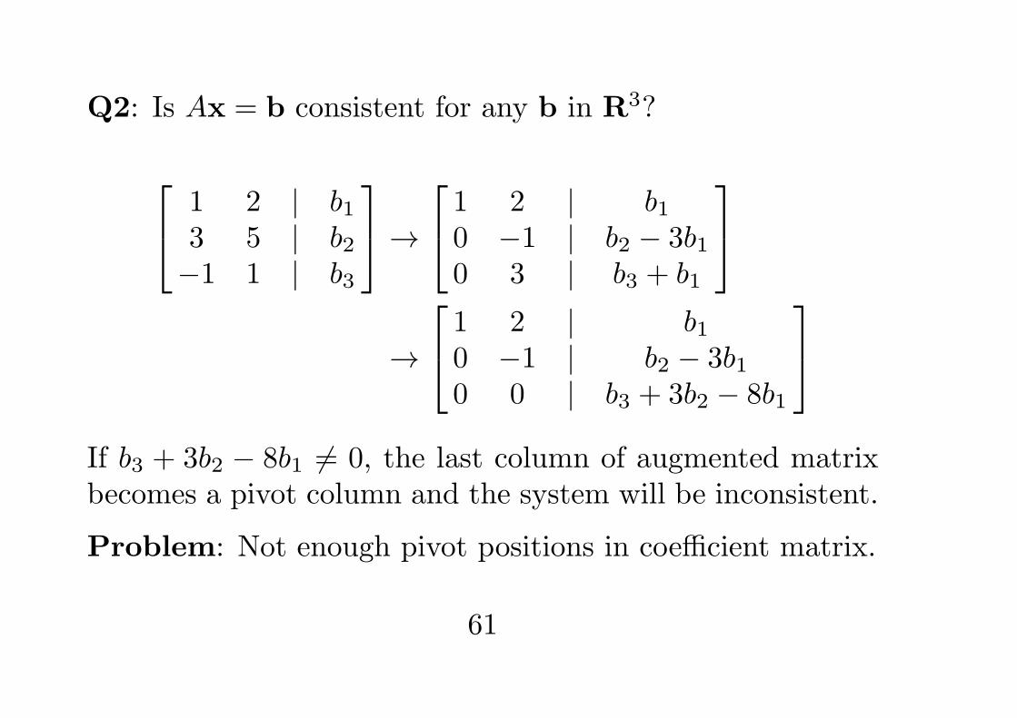
Q2: Is Ax = b consistent for any b in R3?
1 2 | b13 5 | b2−1 1 | b3
→ 1 2 | b10 −1 | b2 − 3b10 3 | b3 + b1
→
1 2 | b10 −1 | b2 − 3b10 0 | b3 + 3b2 − 8b1
If b3 + 3b2 − 8b1 = 0, the last column of augmented matrixbecomes a pivot column and the system will be inconsistent.
Problem: Not enough pivot positions in coefficient matrix.
61
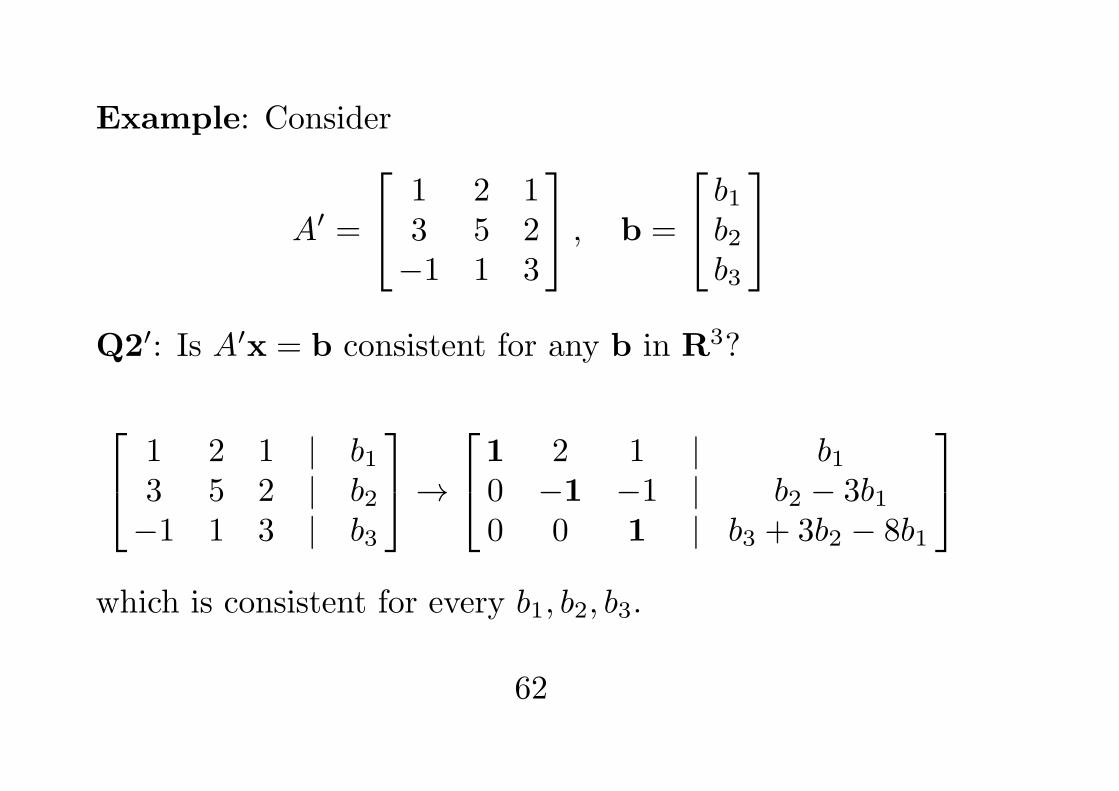
Example: Consider
A′ =
1 2 13 5 2−1 1 3
, b =
b1b2b3
Q2′: Is A′x = b consistent for any b in R3?
1 2 1 | b13 5 2 | b2−1 1 3 | b3
→1 2 1 | b10 −1 −1 | b2 − 3b10 0 1 | b3 + 3b2 − 8b1
which is consistent for every b1, b2, b3.
62
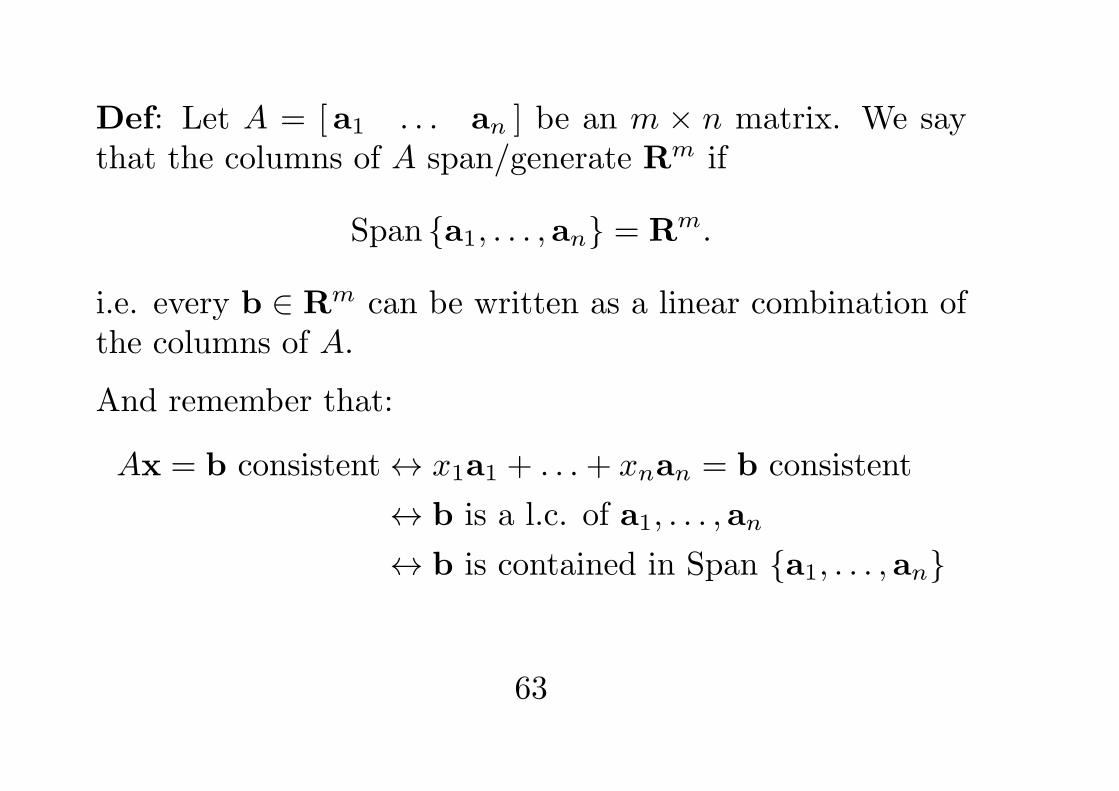
Def: Let A = [a1 . . . an ] be an m × n matrix. We saythat the columns of A span/generate Rm if
Span {a1, . . . ,an} = Rm.
i.e. every b ∈ Rm can be written as a linear combination ofthe columns of A.
And remember that:
Ax = b consistent↔ x1a1 + . . .+ xnan = b consistent
↔ b is a l.c. of a1, . . . ,an
↔ b is contained in Span {a1, . . . ,an}
63
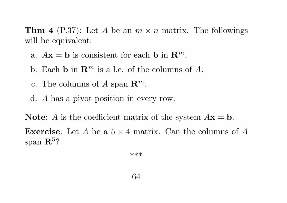
Thm 4 (P.37): Let A be an m × n matrix. The followingswill be equivalent:
a. Ax = b is consistent for each b in Rm.
b. Each b in Rm is a l.c. of the columns of A.
c. The columns of A span Rm.
d. A has a pivot position in every row.
Note: A is the coefficient matrix of the system Ax = b.
Exercise: Let A be a 5 × 4 matrix. Can the columns of Aspan R5?
***
64
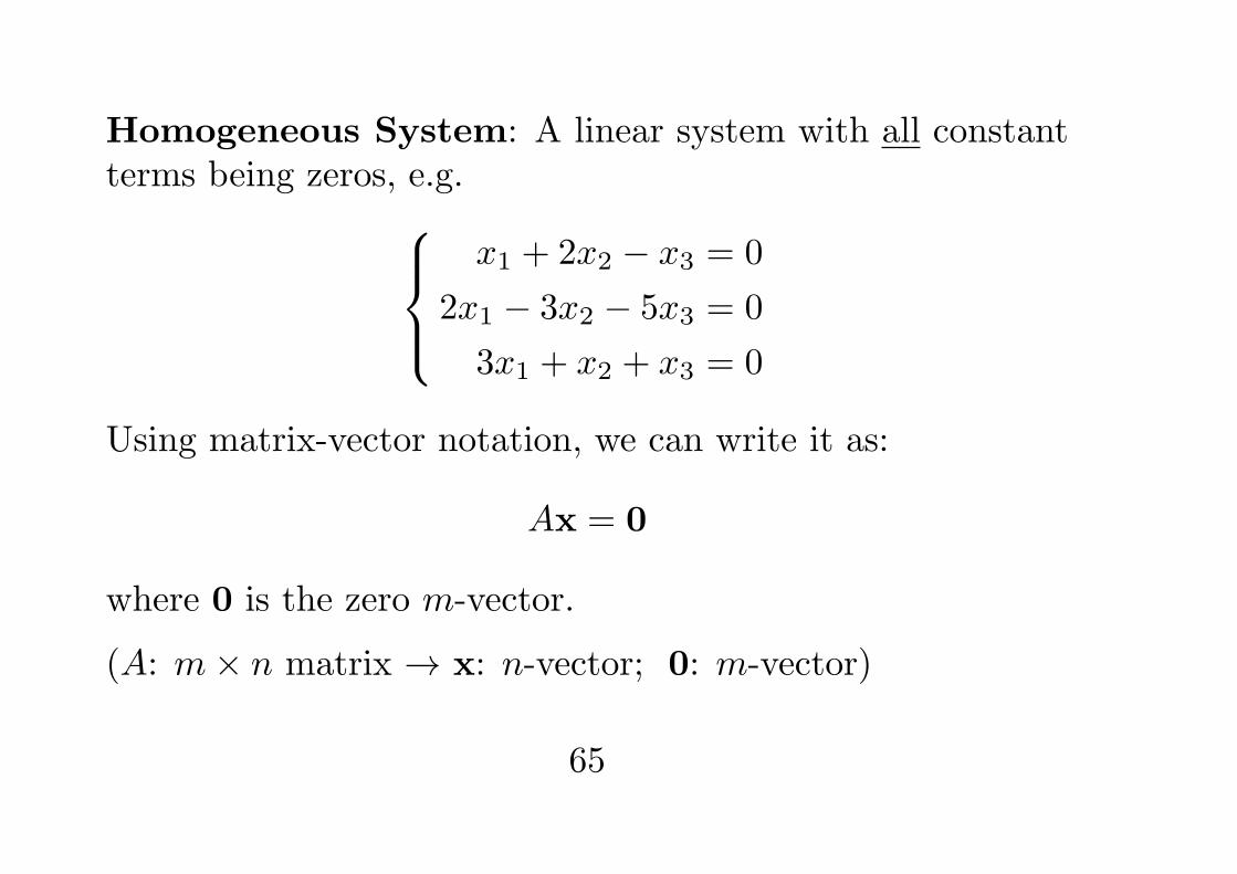
Homogeneous System: A linear system with all constantterms being zeros, e.g.
x1 + 2x2 − x3 = 0
2x1 − 3x2 − 5x3 = 0
3x1 + x2 + x3 = 0
Using matrix-vector notation, we can write it as:
Ax = 0
where 0 is the zero m-vector.
(A: m× n matrix → x: n-vector; 0: m-vector)
65
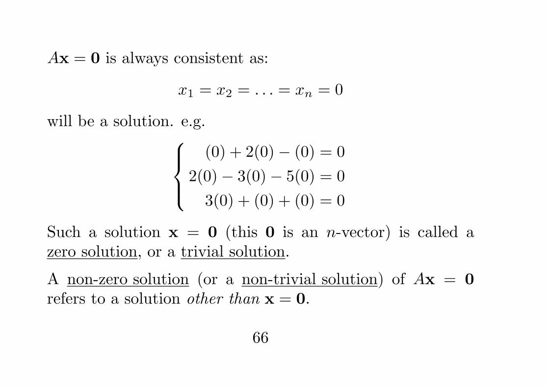
Ax = 0 is always consistent as:
x1 = x2 = . . . = xn = 0
will be a solution. e.g.(0) + 2(0)− (0) = 0
2(0)− 3(0)− 5(0) = 0
3(0) + (0) + (0) = 0
Such a solution x = 0 (this 0 is an n-vector) is called azero solution, or a trivial solution.
A non-zero solution (or a non-trivial solution) of Ax = 0refers to a solution other than x = 0.
66
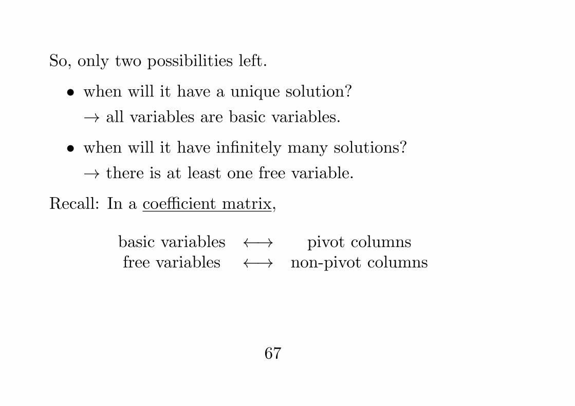
So, only two possibilities left.
• when will it have a unique solution?
→ all variables are basic variables.
• when will it have infinitely many solutions?
→ there is at least one free variable.
Recall: In a coefficient matrix,
basic variables ←→ pivot columnsfree variables ←→ non-pivot columns
67
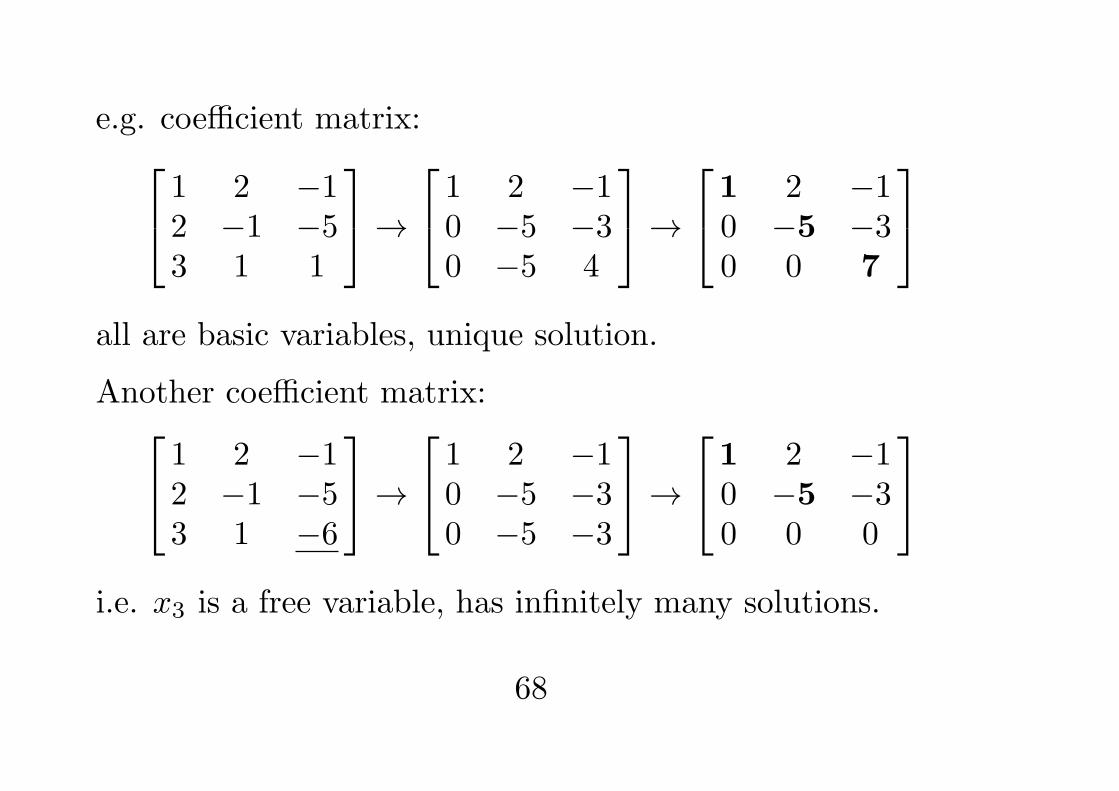
e.g. coefficient matrix: 1 2 −12 −1 −53 1 1
→ 1 2 −10 −5 −30 −5 4
→1 2 −10 −5 −30 0 7
all are basic variables, unique solution.
Another coefficient matrix: 1 2 −12 −1 −53 1 −6
→ 1 2 −10 −5 −30 −5 −3
→1 2 −10 −5 −30 0 0
i.e. x3 is a free variable, has infinitely many solutions.
68
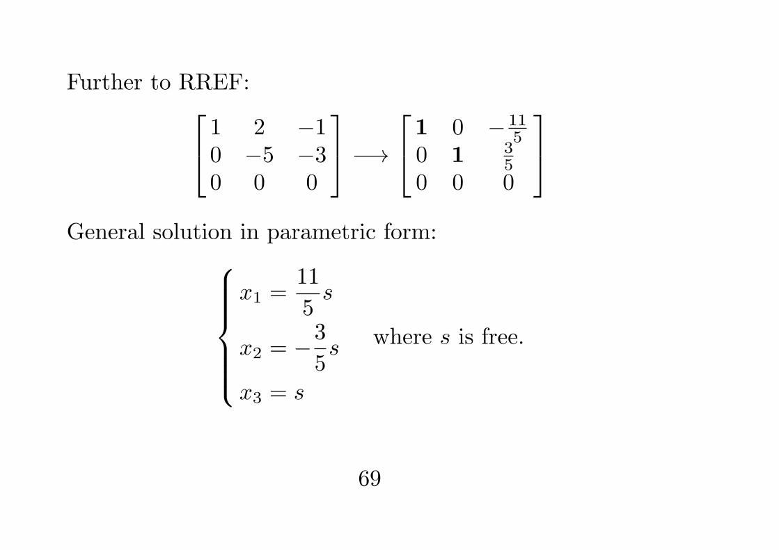
Further to RREF: 1 2 −10 −5 −30 0 0
−→1 0 −11
50 1 3
50 0 0
General solution in parametric form:
x1 =11
5s
x2 = −3
5s
x3 = s
where s is free.
69
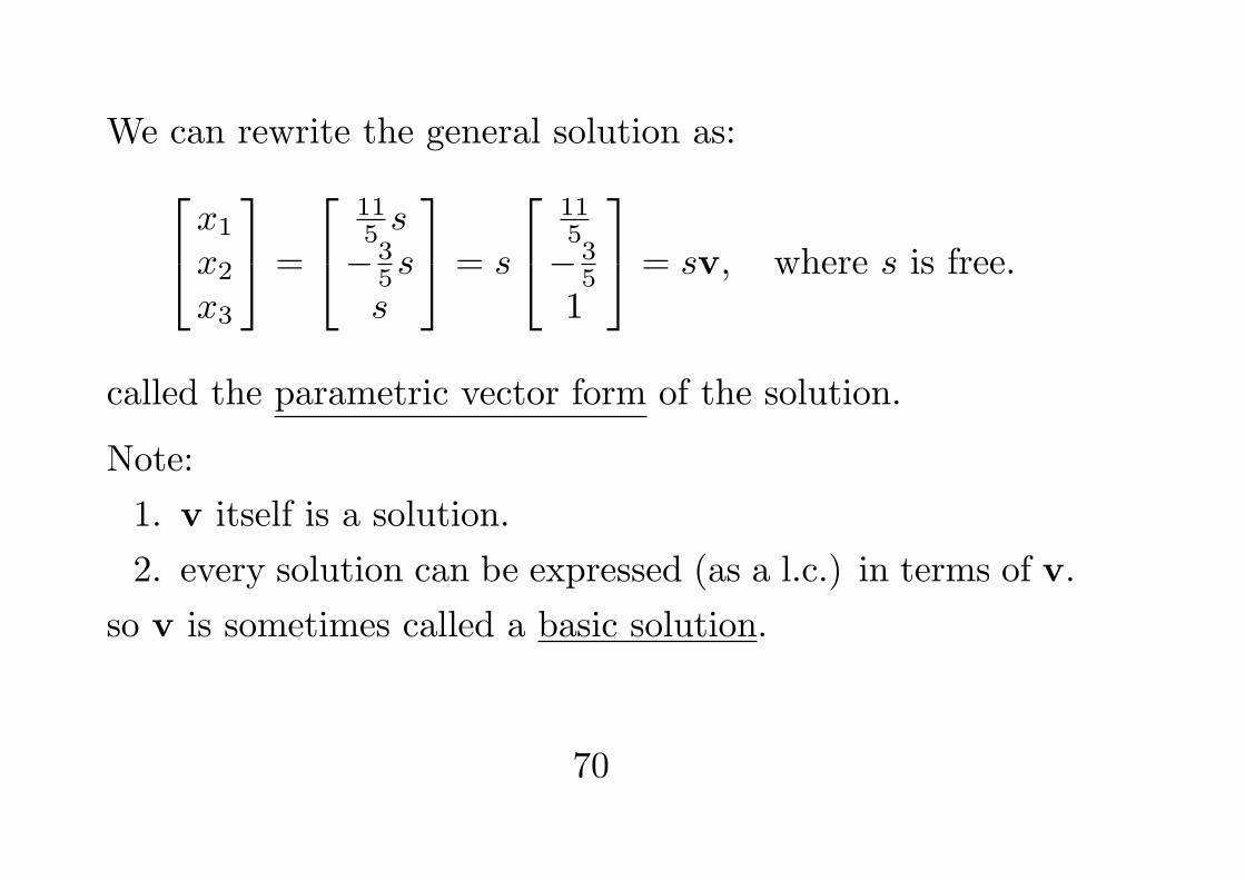
We can rewrite the general solution as:x1
x2
x3
=
115 s−3
5ss
= s
115−3
51
= sv, where s is free.
called the parametric vector form of the solution.
Note:
1. v itself is a solution.
2. every solution can be expressed (as a l.c.) in terms of v.
so v is sometimes called a basic solution.
70
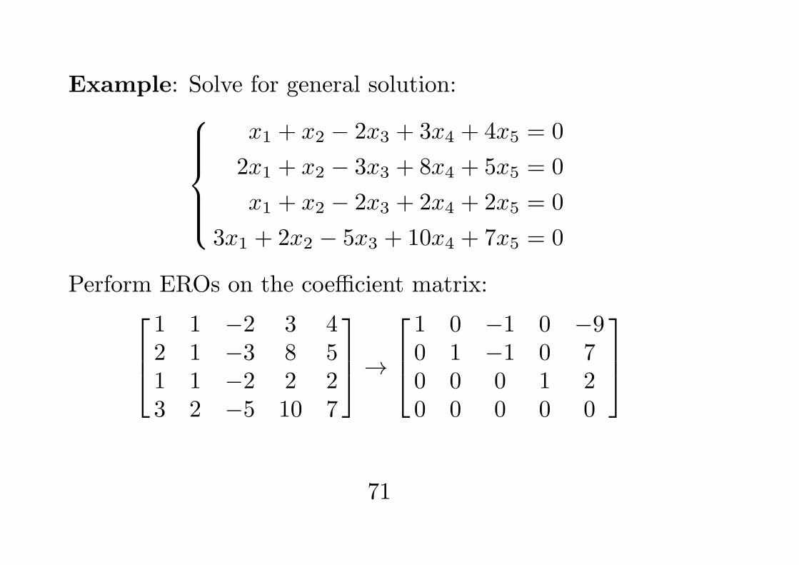
Example: Solve for general solution:x1 + x2 − 2x3 + 3x4 + 4x5 = 0
2x1 + x2 − 3x3 + 8x4 + 5x5 = 0
x1 + x2 − 2x3 + 2x4 + 2x5 = 0
3x1 + 2x2 − 5x3 + 10x4 + 7x5 = 0
Perform EROs on the coefficient matrix:1 1 −2 3 42 1 −3 8 51 1 −2 2 23 2 −5 10 7
→1 0 −1 0 −90 1 −1 0 70 0 0 1 20 0 0 0 0
71
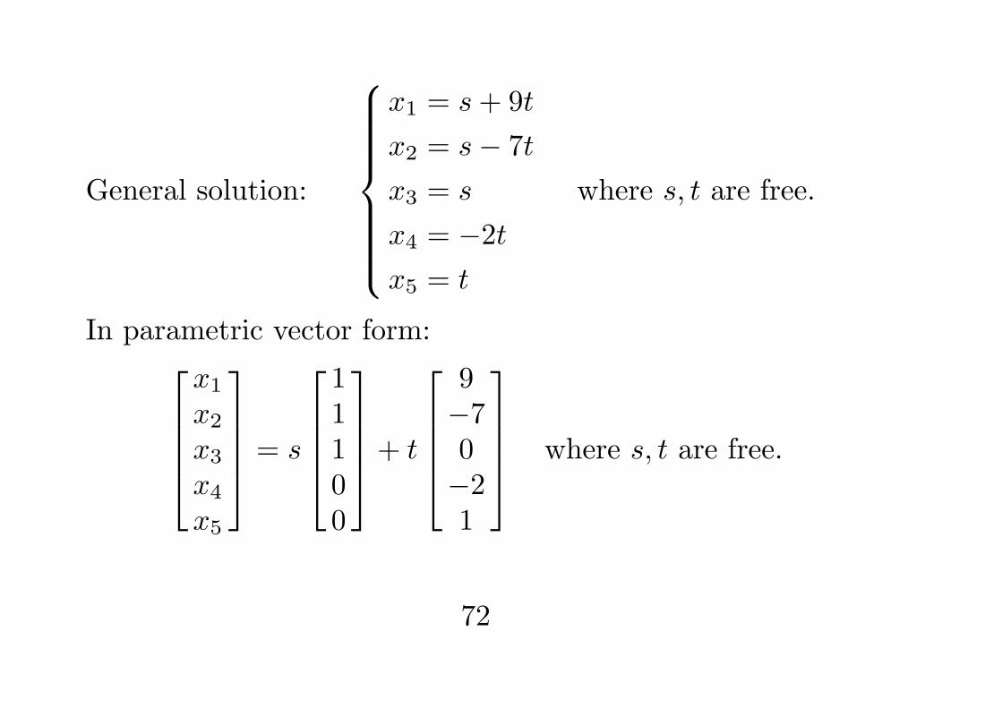
General solution:
x1 = s+ 9t
x2 = s− 7t
x3 = s
x4 = −2tx5 = t
where s, t are free.
In parametric vector form:x1
x2
x3
x4
x5
= s
11100
+ t
9−70−21
where s, t are free.
72
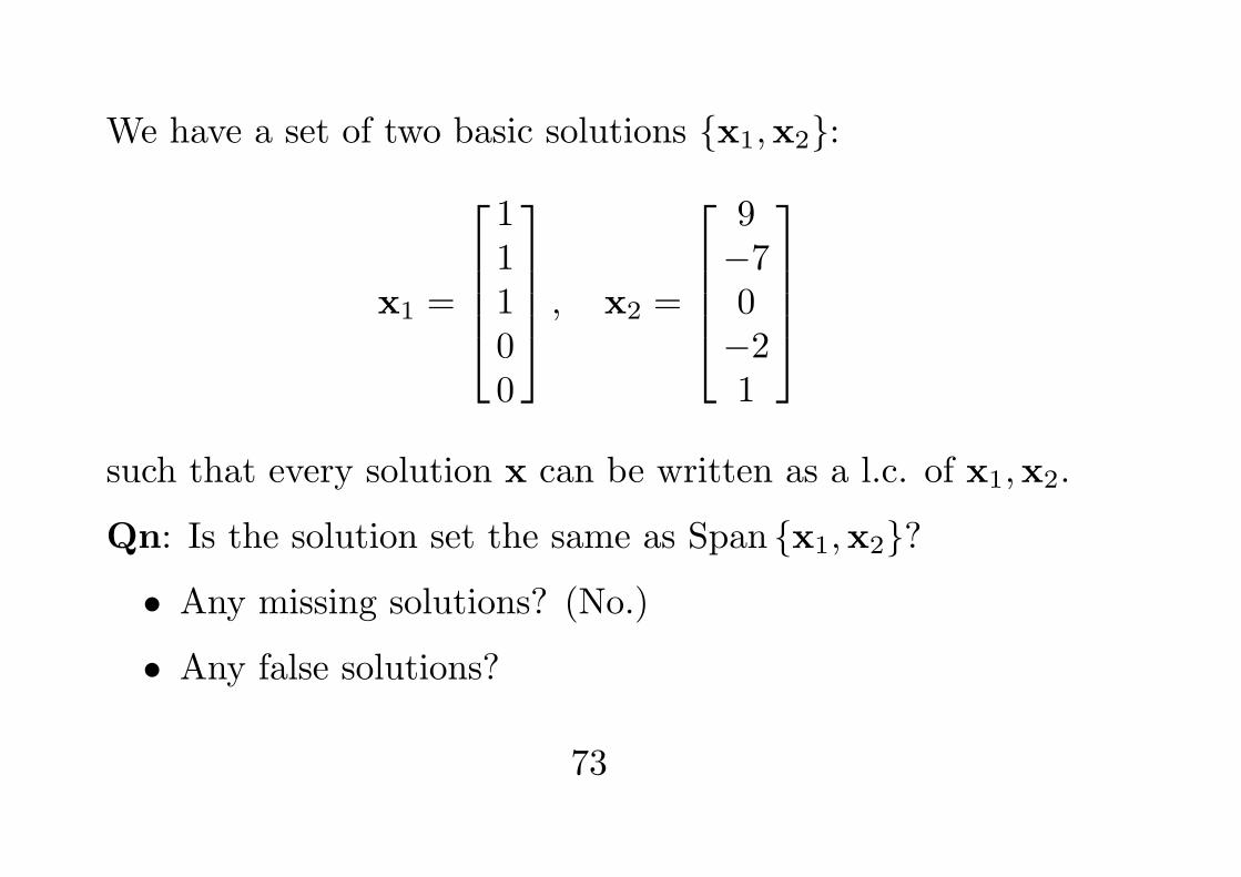
We have a set of two basic solutions {x1,x2}:
x1 =
11100
, x2 =
9−70−21
such that every solution x can be written as a l.c. of x1,x2.
Qn: Is the solution set the same as Span {x1,x2}?
• Any missing solutions? (No.)
• Any false solutions?
73
Let v1, v2 be two solutions of Ax = 0.
i.e. Av1 = 0, Av2 = 0
• is 5v1 a solution? (Yes.)
• is v1 + v2 a solution? (Yes.)
• is any l.c. of v1, v2 a solution? (Yes.)
If v1, v2, . . ., vn are solutions of Ax = 0, then any vector inSpan {v1, . . . ,vn} will also be a solution of Ax = 0.
So no false solution will be introduced.
74
Theorem: Let Ax = 0 have k free variables. Then thegeneral solution can be written as:
x = s1x1 + . . .+ skxk,
where {x1, . . . ,xk} is a set of basic solutions for the sys-tem and s1, . . . , sk are independent free parameters. In otherwords, the solution set of the homogeneous system is:
Span {x1, . . . ,xk}.
Remark: When Ax = 0 has unique trivial solution, there isno basic solution. And the solution set is just {0}.
75
Non-homogeneous system:
Ax = b with b = 0
(i.e. there are some non-zero entries in b.)
e.g.
1 2 −12 −1 −53 1 −6
x =
100
Let u1, u2 be two solutions of a non-homogeneous system.
• is 3u1 a solution? (No.)
• is u1 + u2 a solution? (No.)
• is u1 − u2 a solution? (No.)
76
Def: Given a non-homogeneous system Ax = b, the sys-tem Ax = 0, obtained by replacing b with 0, is called theassociated homogeneous system.
• Thus, if u1, u2 are solutions of Ax = b, then (u1 − u2)will be a solution of Ax = 0.
Suppose: one solution u0 of Ax = b is found.
• If u is any other solution of Ax = b, we know thatA(u− u0) = 0.
• (u− u0) = w is a solution of Ax = 0.
• Then u = u0 +w.
77
i.e. Any solution u of Ax = b will look like
u = u0 +w, where Aw = 0
→ We know how to determine the general form of w→ obtain the general solution of Ax = b!
Thm 6 (P.46): Let Ax = b be a consistent system with aparticular solution u0. Then the solution set of Ax = b isthe set of all vectors of the form u = u0 + w, where w isthe general solution of the associated homogeneous systemAx = 0.
78
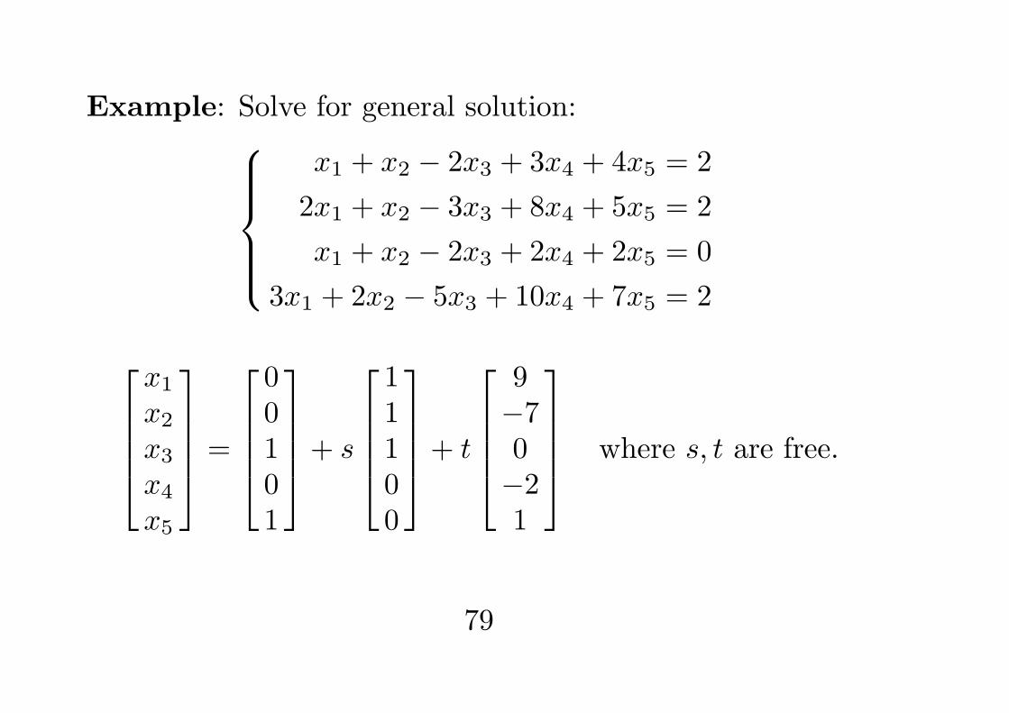
Example: Solve for general solution:x1 + x2 − 2x3 + 3x4 + 4x5 = 2
2x1 + x2 − 3x3 + 8x4 + 5x5 = 2
x1 + x2 − 2x3 + 2x4 + 2x5 = 0
3x1 + 2x2 − 5x3 + 10x4 + 7x5 = 2
x1
x2
x3
x4
x5
=
00101
+ s
11100
+ t
9−70−21
where s, t are free.
79
Linearly Independent Sets
Def: An indexed set of vectors {v1, . . . ,vp} is called linearlyindependent (l.i.) if the vector equation:
c1v1 + . . .+ cpvp = 0
has the unique (zero) solution:
c1 = . . . = cp = 0.
Remark: The zero solution is always there. The key pointis its uniqueness.
80
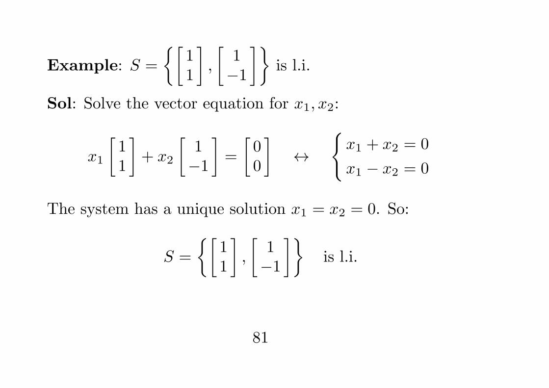
Example: S =
{[11
],
[1−1
]}is l.i.
Sol: Solve the vector equation for x1, x2:
x1
[11
]+ x2
[1−1
]=
[00
]↔
{x1 + x2 = 0
x1 − x2 = 0
The system has a unique solution x1 = x2 = 0. So:
S =
{[11
],
[1−1
]}is l.i.
81
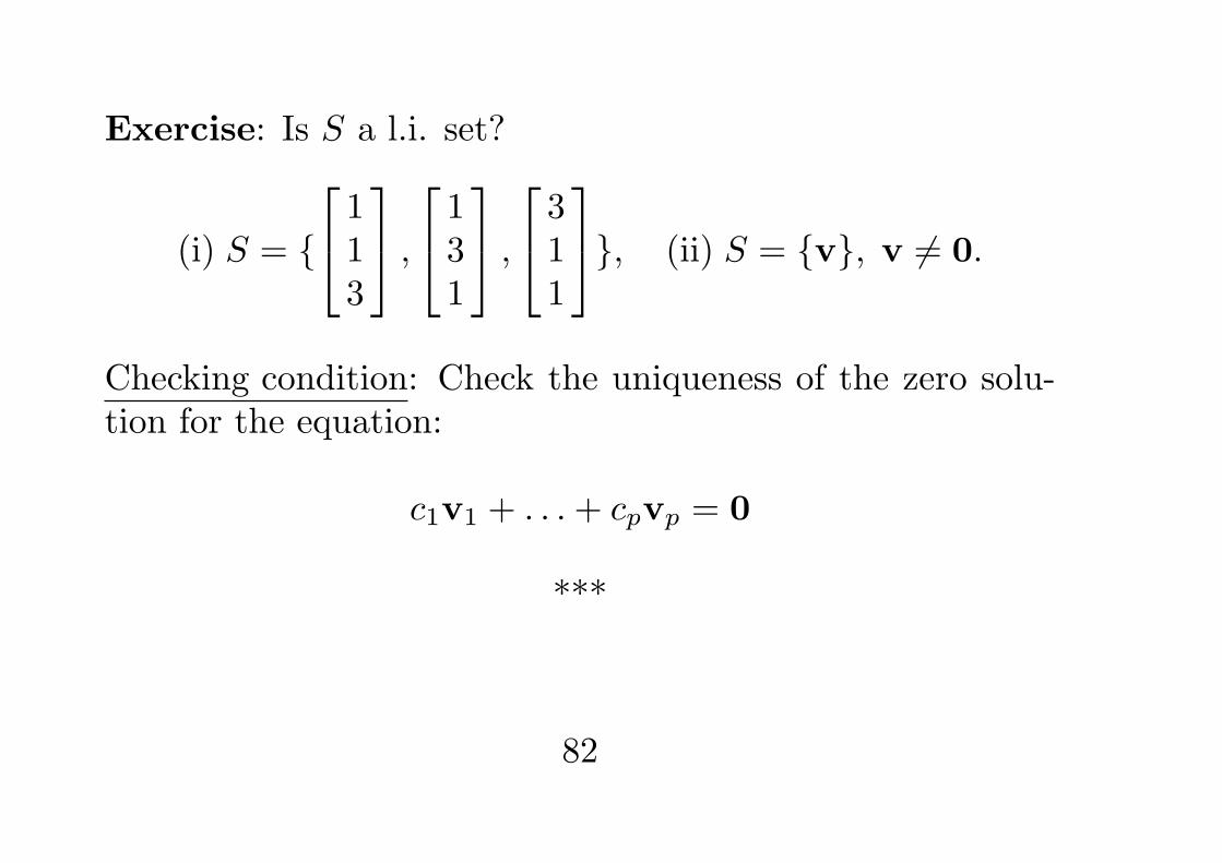
Exercise: Is S a l.i. set?
(i) S = {
113
,
131
,
311
}, (ii) S = {v}, v = 0.
Checking condition: Check the uniqueness of the zero solu-tion for the equation:
c1v1 + . . .+ cpvp = 0
***
82
A set of vectors is called linearly dependent if it is NOTlinearly independent.
Linearly Dependent Sets
Def: A set of vectors {v1, . . . ,vp} is called linearly depen-dent (l.d.) if there are numbers c1, . . . , cp, not all zeros, s.t.
c1v1 + . . .+ cpvp = 0. (∗)
i.e. The vector eq. has a non-zero solution in c1, . . . , cp.
Remark: A non-trivial combination in (∗) is sometimescalled “a dependence relation among the vectors”.
83
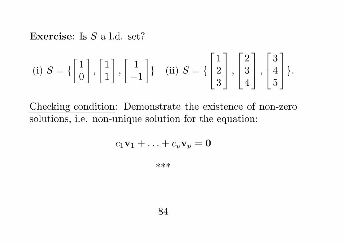
Exercise: Is S a l.d. set?
(i) S = {[10
],
[11
],
[1−1
]} (ii) S = {
123
,
234
,
345
}.Checking condition: Demonstrate the existence of non-zerosolutions, i.e. non-unique solution for the equation:
c1v1 + . . .+ cpvp = 0
***
84
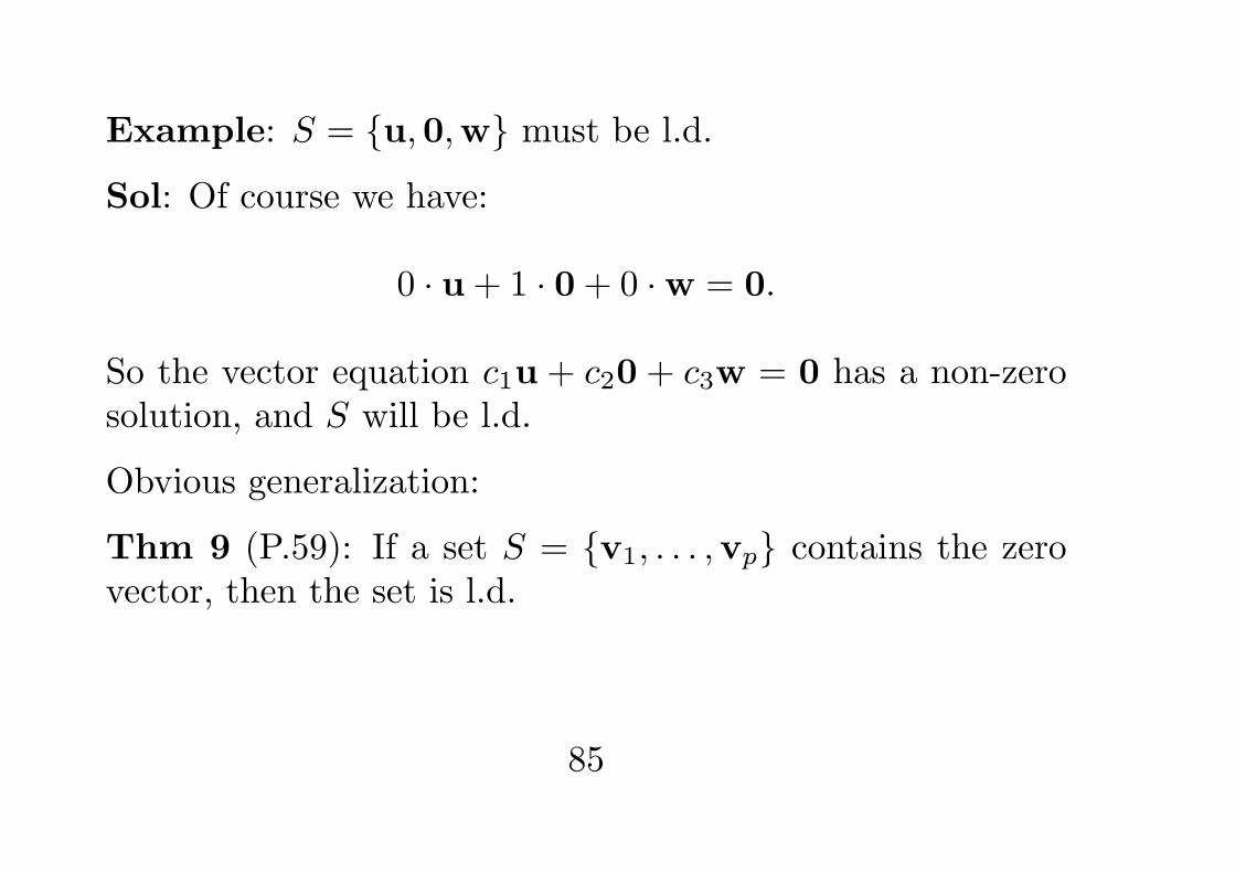
Example: S = {u,0,w} must be l.d.
Sol: Of course we have:
0 · u+ 1 · 0+ 0 ·w = 0.
So the vector equation c1u + c20 + c3w = 0 has a non-zerosolution, and S will be l.d.
Obvious generalization:
Thm 9 (P.59): If a set S = {v1, . . . ,vp} contains the zerovector, then the set is l.d.
85
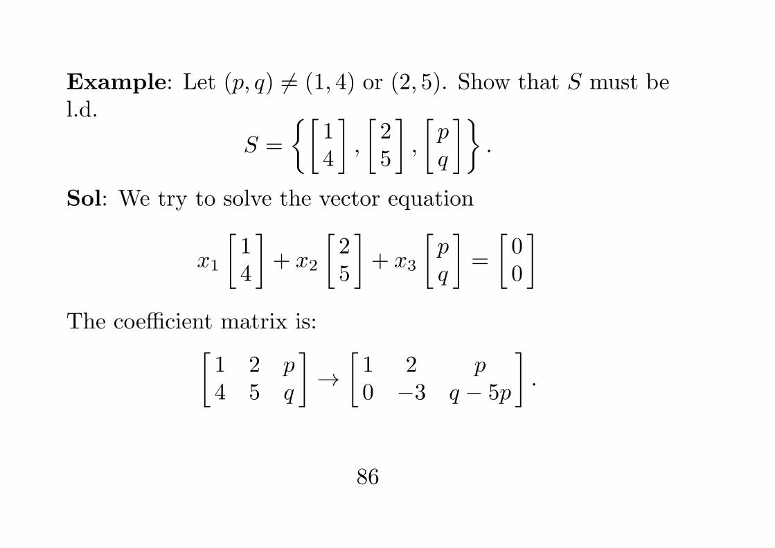
Example: Let (p, q) = (1, 4) or (2, 5). Show that S must bel.d.
S =
{[14
],
[25
],
[pq
]}.
Sol: We try to solve the vector equation
x1
[14
]+ x2
[25
]+ x3
[pq
]=
[00
]The coefficient matrix is:[
1 2 p4 5 q
]→
[1 2 p0 −3 q − 5p
].
86
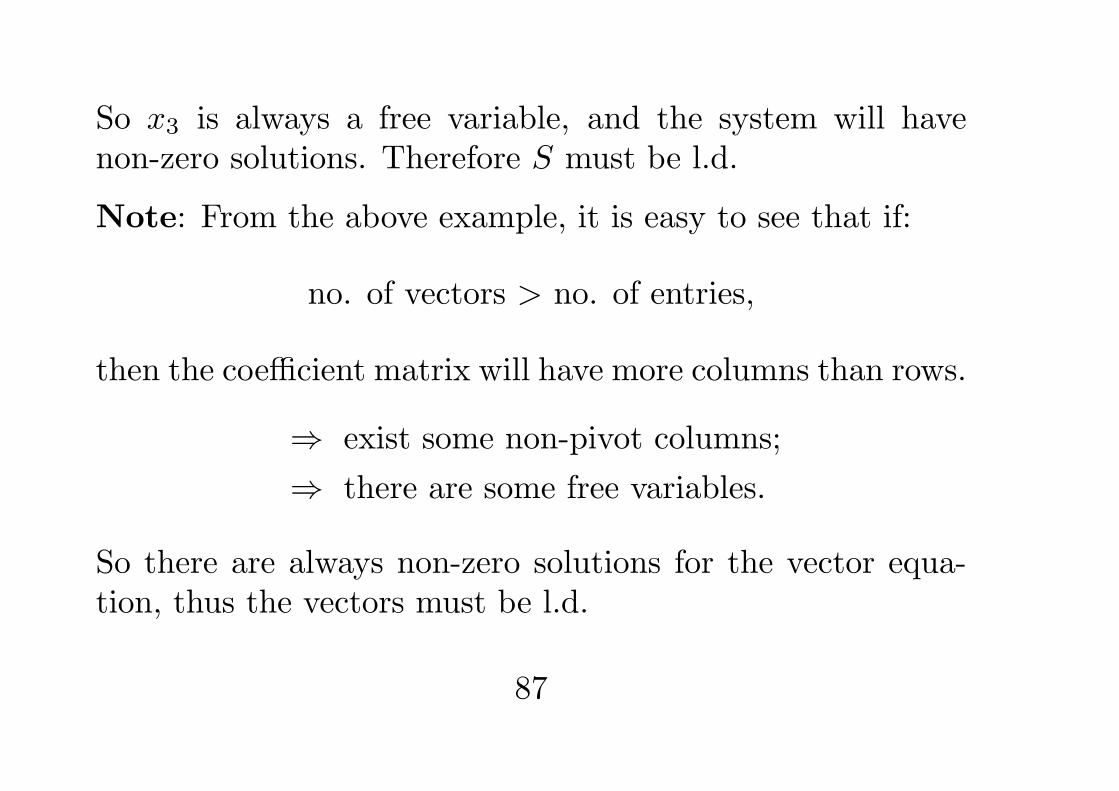
So x3 is always a free variable, and the system will havenon-zero solutions. Therefore S must be l.d.
Note: From the above example, it is easy to see that if:
no. of vectors > no. of entries,
then the coefficient matrix will have more columns than rows.
⇒ exist some non-pivot columns;
⇒ there are some free variables.
So there are always non-zero solutions for the vector equa-tion, thus the vectors must be l.d.
87
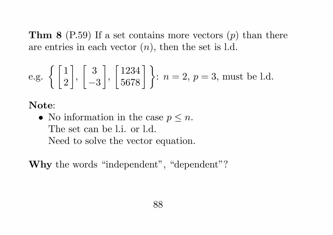
Thm 8 (P.59) If a set contains more vectors (p) than thereare entries in each vector (n), then the set is l.d.
e.g.
{[12
],
[3−3
],
[12345678
]}: n = 2, p = 3, must be l.d.
Note:• No information in the case p ≤ n.
The set can be l.i. or l.d.Need to solve the vector equation.
Why the words “independent”, “dependent”?
88
Suppose that {v1,v2,v3} is l.d., i.e. there are some numbersc1, c2, c3, not all zeros, such that:
c1v1 + c2v2 + c3v3 = 0.
(1) When c1 = 0, we have v1 = − 1c1(c2v2 + c3v3);
(2) When c2 = 0, we have v2 = − 1c2(c1v1 + c3v3);
(3) When c3 = 0, we have v3 = − 1c3(c1v1 + c2v2).
i.e. at least one of them can be written as a l.c. of the others.
• So the word: dependent.
89
• What if none of the vectors depends on the others?(i.e. they are essentially different vectors.)
The equation:
c1v1 + c2v2 + c3v3 = 0
cannot have a solution with c1 = 0 or c2 = 0 or c3 = 0, i.e.can only have the unique zero solution.
• So the word: independent.
Thm 7 (P.58): Let v1 = 0 and p ≥ 2: {v1, . . . ,vp} is l.d.
⇔ some vj (j ≥ 2) is a l.c. of {v1, . . . ,vj−1}.
90
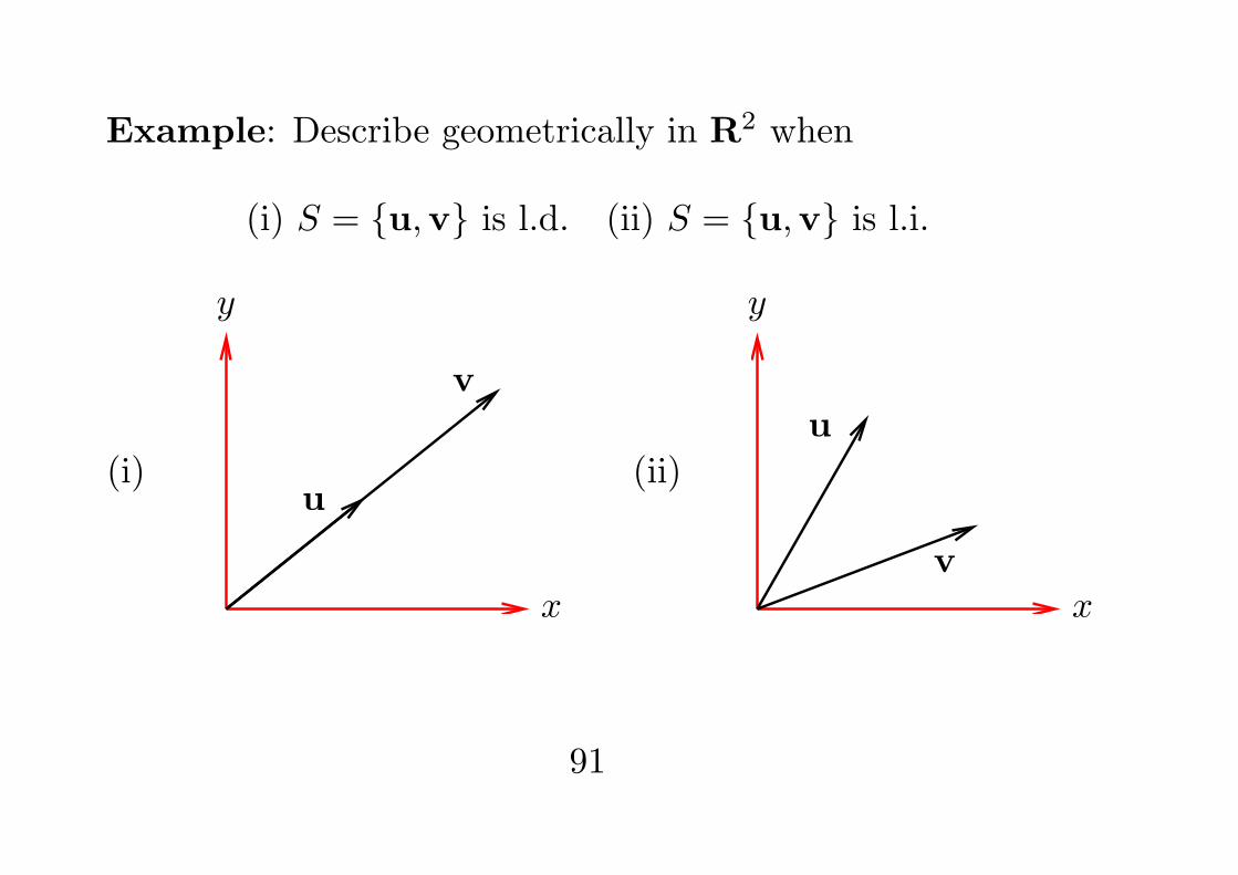
Example: Describe geometrically in R2 when
(i) S = {u,v} is l.d. (ii) S = {u,v} is l.i.
x
y
u
v
(i)
x
y
u
v
(ii)
91
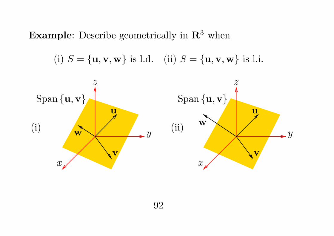
Example: Describe geometrically in R3 when
(i) S = {u,v,w} is l.d. (ii) S = {u,v,w} is l.i.
x
y
z
u
v
w
Span {u,v}
(i)
x
y
z
u
v
w
Span {u,v}
(ii)
92
Matrix Transformations:
Let A be an m× n matrix.
Consider a linear system Ax = b.
Old viewpoint: equation solving viewpoint
b is given, and find x that satisfies Ax = b.
New viewpoint: transformation viewpoint
study x 7→ Ax, see which x “lands” on b
93
Example: Suppose that the following solutions are known
Ax1 =
[10
], Ax2 =
[01
].
How about the solution of Ax =
[3−2
]?
[3−2
]= 3
[10
]− 2
[01
]= 3Ax1 − 2Ax2
= A(3x1 − 2x2)
At least has a solution x = 3x1 − 2x2.
94
Notations and Terminologies:
We will denote a matrix transformation by
T : Rn → Rm
T : x 7→ Ax
• domain: Rn, x: an object
• codomain: Rm
• T (x): the image of x under T , i.e. Ax
• range: collection of all possible T (x)
Note: Though T (x) = Ax for every x, T is NOT a matrix.
What is the range of T?
95
Range of a matrix transformation:
• range of T collects all possible T (x).
• T (x) = Ax = x1a1+ . . .+xnan is a l.c. of columns of A
• i.e. range of T collects all possible l.c. of columns of A
• Span {a1, . . . ,an} collects all possible l.c. of {a1, . . . ,an}
So, we have:
range of T = Span {a1, . . . ,an}
96
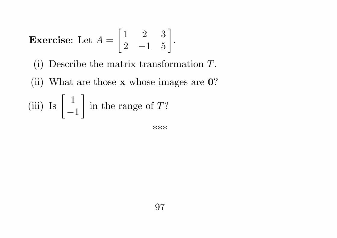
Exercise: Let A =
[1 2 32 −1 5
].
(i) Describe the matrix transformation T .
(ii) What are those x whose images are 0?
(iii) Is
[1−1
]in the range of T?
***
97
Linear Transformations in general:
A transformation T : Rn → Rm is called linear if
(a) T (u+ v) = T (u) + T (v)
(b) T (cu) = cT (u)
for any choices of u, v in Rn and any choice of number c.
We can combine the two conditions together and check if
T (k1v1 + k2v2) = k1T (v1) + k2T (v2)
is true for any vectors v1,v2 ∈ Rn and any numbers k1, k2.
98
As matrix-vector multiplication satisfies
1. A(u+ v) = Au+Av
2. A(ku) = k(Au)
Each matrix transformation is also a linear transformation.
• The converse is also true. See next section.
A linear transformation will automatically satisfy:
• T (0) = 0;
• T (c1v1 + . . .+ cpvp) = c1T (v1) + . . .+ cpT (vp).
Can write T (u) as Tu, if no confusion arises.
99
Examples: Linear transformations?
1. T
[x1
x2
]=
[|x1|x2
](No.) It does not satisfy conditions (a), (b).
Counter example: Take
x =
[11
], −x =
[−1−1
]Then, by the defining formula:
T (−x) =[| − 1|−1
]=
[1−1
], but − T (x) =
[−1−1
]
100
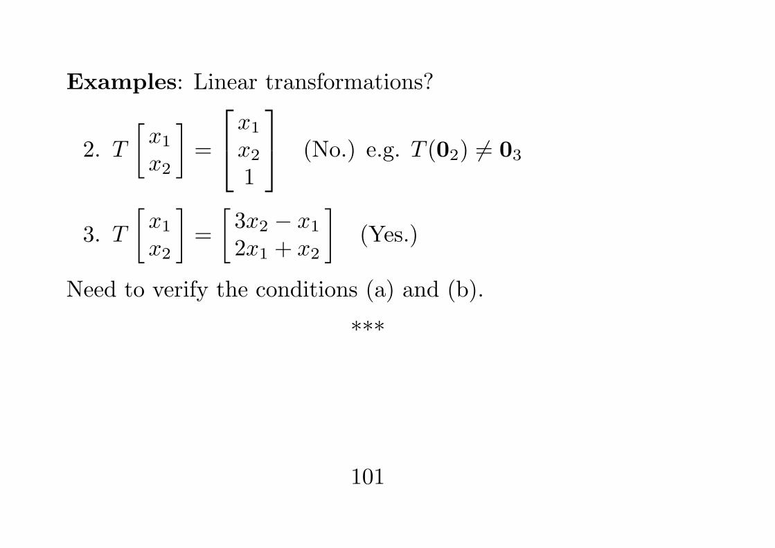
Examples: Linear transformations?
2. T
[x1
x2
]=
x1
x2
1
(No.) e.g. T (02) = 03
3. T
[x1
x2
]=
[3x2 − x1
2x1 + x2
](Yes.)
Need to verify the conditions (a) and (b).
***
101
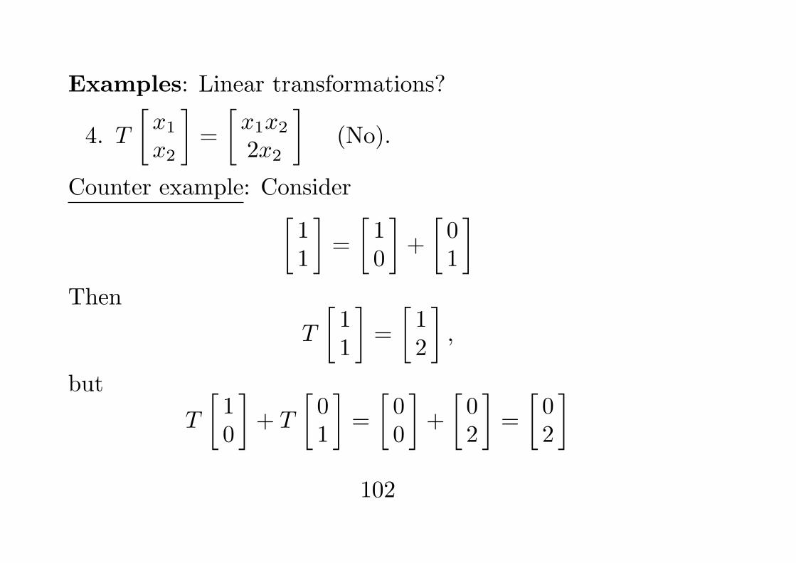
Examples: Linear transformations?
4. T
[x1
x2
]=
[x1x2
2x2
](No).
Counter example: Consider[11
]=
[10
]+
[01
]Then
T
[11
]=
[12
],
but
T
[10
]+ T
[01
]=
[00
]+
[02
]=
[02
]102
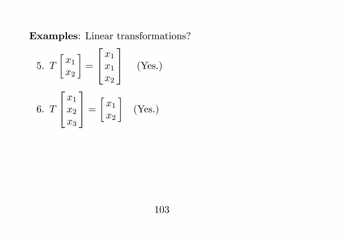
Examples: Linear transformations?
5. T
[x1
x2
]=
x1
x1
x2
(Yes.)
6. T
x1
x2
x3
=
[x1
x2
](Yes.)
103
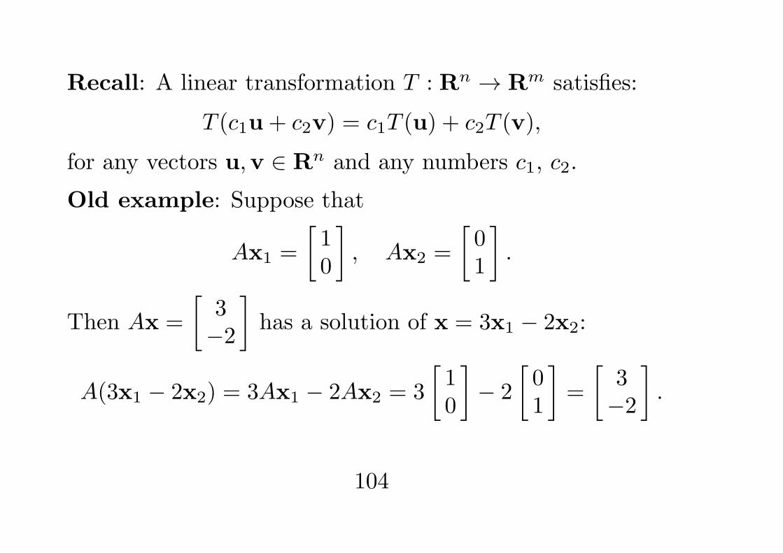
Recall: A linear transformation T : Rn → Rm satisfies:
T (c1u+ c2v) = c1T (u) + c2T (v),
for any vectors u,v ∈ Rn and any numbers c1, c2.
Old example: Suppose that
Ax1 =
[10
], Ax2 =
[01
].
Then Ax =
[3−2
]has a solution of x = 3x1 − 2x2:
A(3x1 − 2x2) = 3Ax1 − 2Ax2 = 3
[10
]− 2
[01
]=
[3−2
].
104
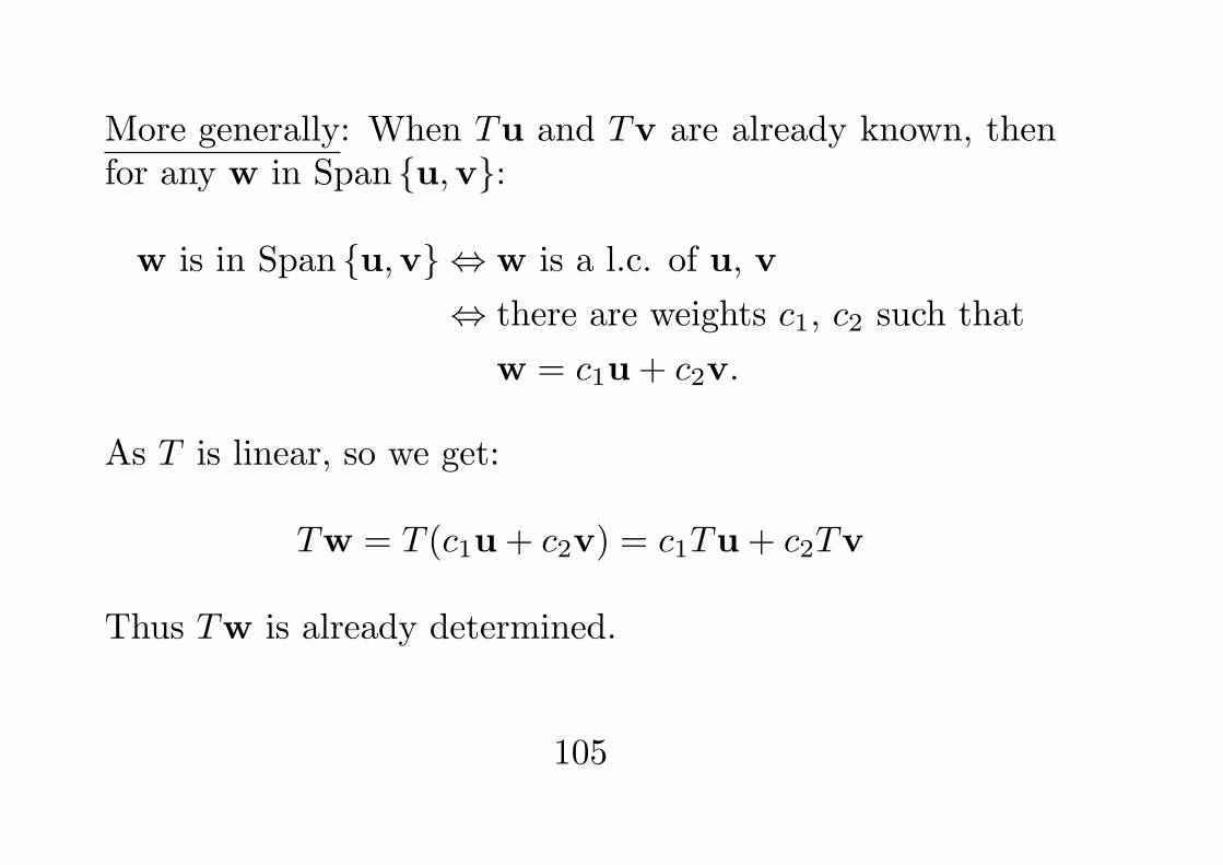
More generally: When Tu and Tv are already known, thenfor any w in Span {u,v}:
w is in Span {u,v} ⇔ w is a l.c. of u, v
⇔ there are weights c1, c2 such that
w = c1u+ c2v.
As T is linear, so we get:
Tw = T (c1u+ c2v) = c1Tu+ c2Tv
Thus Tw is already determined.
105
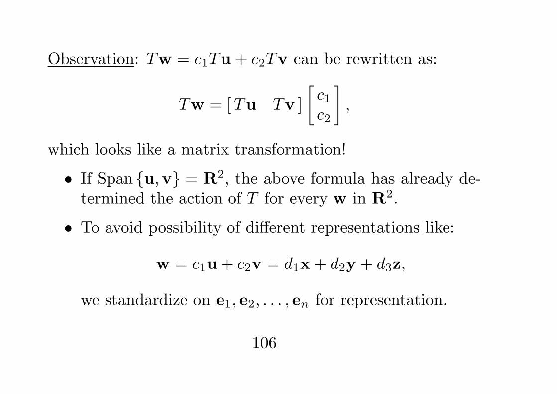
Observation: Tw = c1Tu+ c2Tv can be rewritten as:
Tw = [Tu Tv ]
[c1c2
],
which looks like a matrix transformation!
• If Span {u,v} = R2, the above formula has already de-termined the action of T for every w in R2.
• To avoid possibility of different representations like:
w = c1u+ c2v = d1x+ d2y + d3z,
we standardize on e1, e2, . . . , en for representation.
106
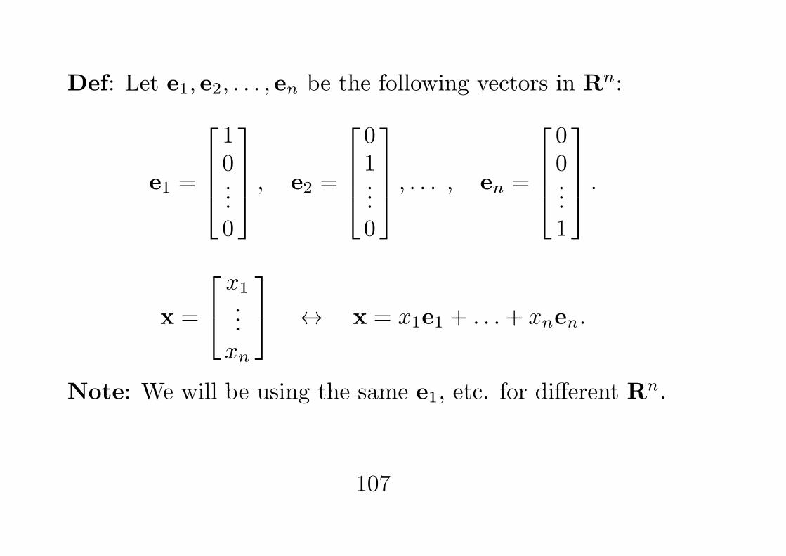
Def: Let e1, e2, . . . , en be the following vectors in Rn:
e1 =
10...0
, e2 =
01...0
, . . . , en =
00...1
.
x =
x1...xn
↔ x = x1e1 + . . .+ xnen.
Note: We will be using the same e1, etc. for different Rn.
107
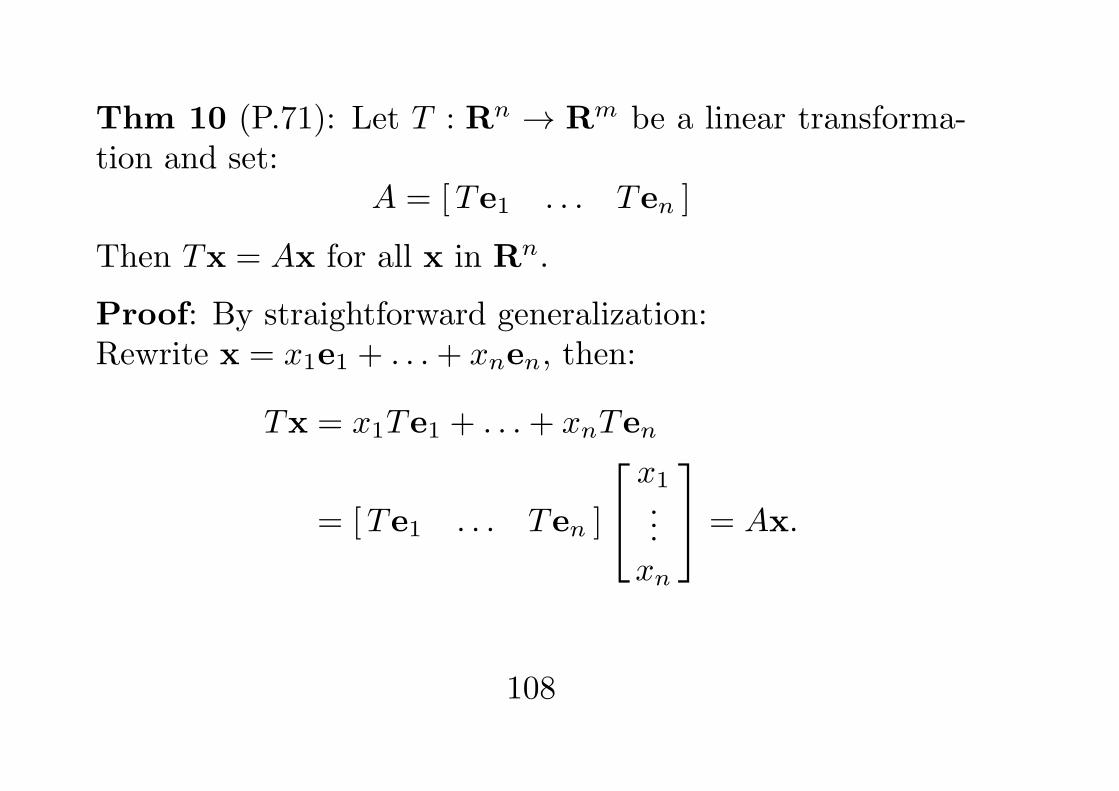
Thm 10 (P.71): Let T : Rn → Rm be a linear transforma-tion and set:
A = [Te1 . . . Ten ]
Then Tx = Ax for all x in Rn.
Proof: By straightforward generalization:Rewrite x = x1e1 + . . .+ xnen, then:
Tx = x1Te1 + . . .+ xnTen
= [Te1 . . . Ten ]
x1...xn
= Ax.
108
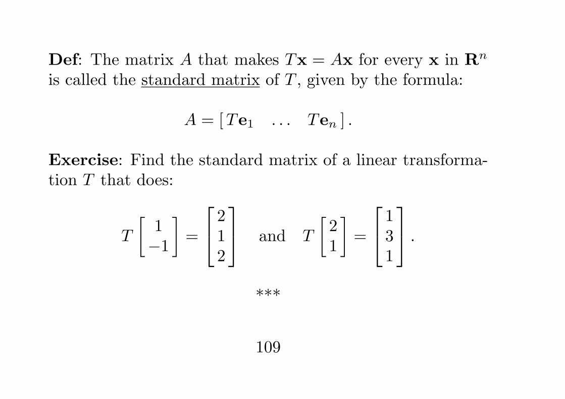
Def: The matrix A that makes Tx = Ax for every x in Rn
is called the standard matrix of T , given by the formula:
A = [Te1 . . . Ten ] .
Exercise: Find the standard matrix of a linear transforma-tion T that does:
T
[1−1
]=
212
and T
[21
]=
131
.
***
109
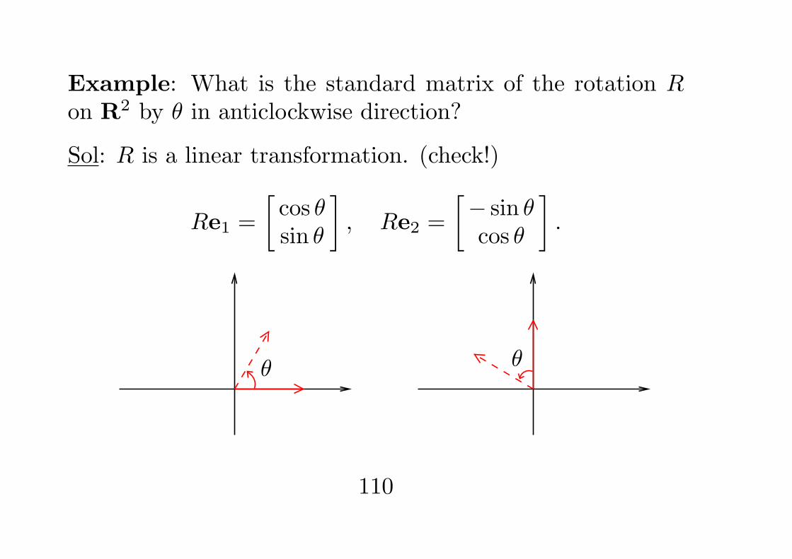
Example: What is the standard matrix of the rotation Ron R2 by θ in anticlockwise direction?
Sol: R is a linear transformation. (check!)
Re1 =
[cos θsin θ
], Re2 =
[− sin θcos θ
].
θ θ
110
So, the standard matrix of R should be:[cos θ − sin θsin θ cos θ
].
This gives the transformation formulas:{x′ = x cos θ − y sin θ
y′ = x sin θ + y cos θ
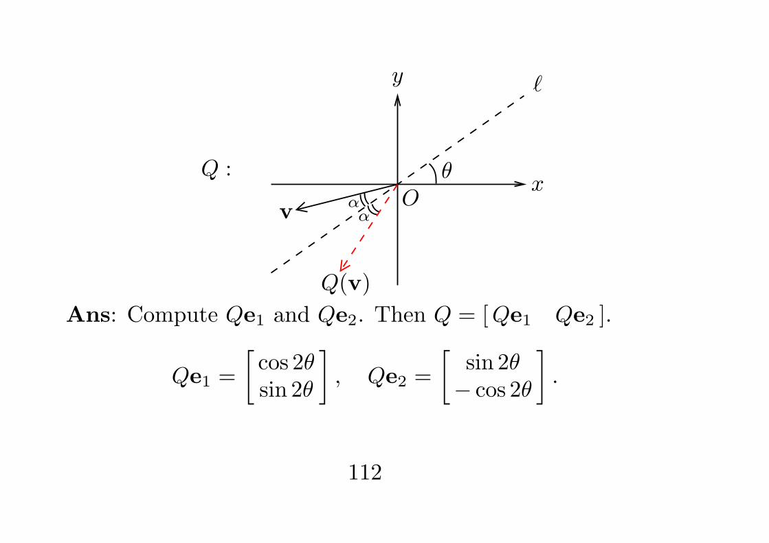
Example: What is the standard matrix of the reflection Qon R2 about a line ℓ passing through O and making angle θwith the positive x-axis?
111
Q :
y
xO
ℓ
θ
ααv
Q(v)
Ans: Compute Qe1 and Qe2. Then Q = [Qe1 Qe2 ].
Qe1 =
[cos 2θsin 2θ
], Qe2 =
[sin 2θ− cos 2θ
].
112
One-to-One and Onto properties:
One-to-one: If Tx1 = b = Tx2, is it necessary that x1 = x2?
Let A be the standard matrix. Then we ask:
If x1,x2 both satisfy Ax = b, must we have x1 = x2?
i.e. about uniqueness of solution.
As T is linear, Tx1 = Tx2 means:
0 = Tx1 − Tx2 = T (x1 − x2).
If the homogeneous system Ax = 0 has only the zero solu-tion, then x1 − x2 must be 0 and hence x1 = x2.
113
Thm 11 (P.76): Let T : Rn → Rm be a linear transforma-tion. Then T is one-to-one iff Tx = 0 has only the trivialsolution.
When will Ax = 0 have only the trivial solution?
• all variables are basic;
• all columns of A are pivot columns;
Note that Ax = 0 is in fact the following vector equation:
x1a1 + . . .+ xnan = 0.
It has only the trivial solution if and only if• the vectors a1, . . ., an are linearly independent.
114
One-to-One and Onto properties:
Onto: Given any b ∈ Rm, is it always possible to find x ∈ Rn
such that T (x) = b?
i.e. Ax = b is consistent for every b;
or Range of T = Rm.
Note that the range of a matrix transformation is:
Span {a1, . . . ,an}.
So T is onto if and only if the columns of A spans Rm.
115
When will the columns of A span Rm?
• Every b is a l.c. of columns of A;
• Ax = b is consistent for every b;
• every row of A has a pivot position.
Thm 12 (P.77): Let A be the standard matrix of a lineartransformation T : Rn → Rm.
1. T is onto ⇔ columns of A span Rm;
2. T is one-to-one ⇔ columns of A are l.i.
116
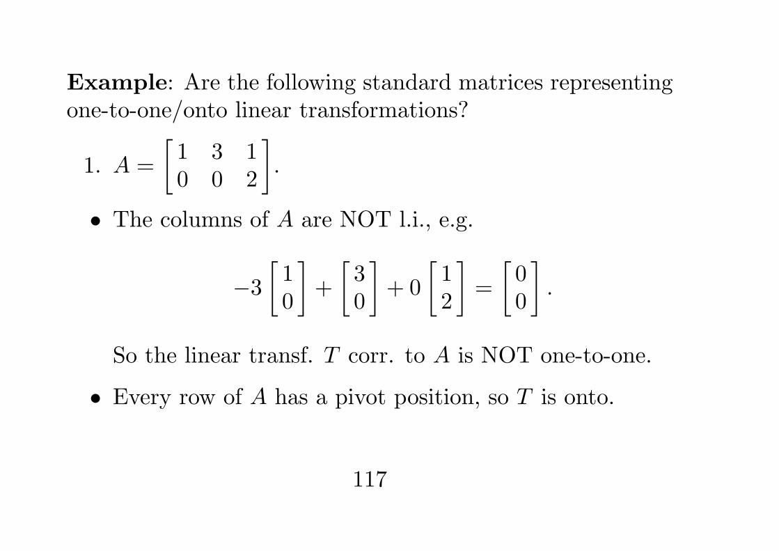
Example: Are the following standard matrices representingone-to-one/onto linear transformations?
1. A =
[1 3 10 0 2
].
• The columns of A are NOT l.i., e.g.
−3[10
]+
[30
]+ 0
[12
]=
[00
].
So the linear transf. T corr. to A is NOT one-to-one.
• Every row of A has a pivot position, so T is onto.
117
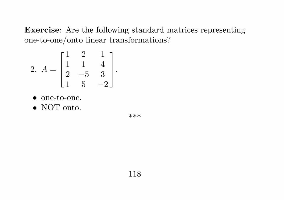
Exercise: Are the following standard matrices representingone-to-one/onto linear transformations?
2. A =
1 2 11 1 42 −5 31 5 −2
.• one-to-one.• NOT onto.
***
118
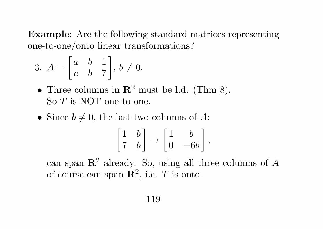
Example: Are the following standard matrices representingone-to-one/onto linear transformations?
3. A =
[a b 1c b 7
], b = 0.
• Three columns in R2 must be l.d. (Thm 8).So T is NOT one-to-one.
• Since b = 0, the last two columns of A:[1 b7 b
]→
[1 b0 −6b
],
can span R2 already. So, using all three columns of Aof course can span R2, i.e. T is onto.
119
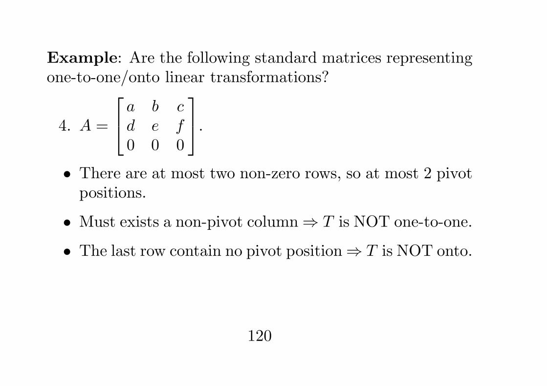
Example: Are the following standard matrices representingone-to-one/onto linear transformations?
4. A =
a b cd e f0 0 0
.• There are at most two non-zero rows, so at most 2 pivot
positions.
• Must exists a non-pivot column⇒ T is NOT one-to-one.
• The last row contain no pivot position⇒ T is NOT onto.
120
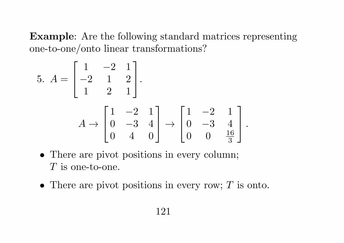
Example: Are the following standard matrices representingone-to-one/onto linear transformations?
5. A =
1 −2 1−2 1 21 2 1
.A→
1 −2 10 −3 40 4 0
→ 1 −2 10 −3 40 0 16
3
.
• There are pivot positions in every column;T is one-to-one.
• There are pivot positions in every row; T is onto.
121


![Id‚v A^-tbgvkv h{P-Pq-_nen hnti-jm¬ ]Xn∏vc - Kerala PSC](https://img.pdfslide.net/doc/110x75/631c87277051d371800f845f/idv-a-tbgvkv-hp-pq-nen-hnti-jm-xnvc-kerala-psc.jpg)


