Smooth transition autoregressions, neural networks, and linear

models in forecasting macroeconomic time series: A

re-examination

Timo Terasvirta∗

Department of Economic Statistics

Stockholm School of Economics

Dick van Dijk†

Econometric Institute

Erasmus University Rotterdam

Marcelo C. Medeiros‡

Department of Economics

Pontifical Catholic University of Rio de Janeiro

PRELIMINARY AND INCOMPLETE

December 5, 2003

Abstract

In this paper we examine the forecast accuracy of four univariate time series models for47 macroeconomic variables of the G7 economies. The models considered are the linearautoregressive model, the smooth transition autoregressive model, and two neural networkmodels. The two neural network models are different because they are specified using twodifferent techniques. Forecast accuracy is assessed in a number of ways, comprising evaluationof point, interval and density forecasts. The results indicate that the linear autoregressiveand the smooth transition autoregressive model have the best overall performance. Positiveresults for the nonlinear smooth transition autoregressive model may be largely due to thefact that linearity is tested before building any nonlinear model. This implies that a nonlinearmodel is employed only when there is a need for it, which makes the risk of fitting unidentifiedmodels to the data relatively low.

Keywords: nonlinear modeling, point forecast, interval forecast, density forecast, forecastcombination, forecast evaluation.JEL Classification Codes: C22, C53

∗Department of Economic Statistics, Stockholm School of Economics, Box 6501, SE-113 83 Stockholm, Sweden,email: Timo.Terasvirta@hhs.se (corresponding author)

†Econometric Institute, Erasmus University Rotterdam, P.O. Box 1738, NL-3000 DR Rotterdam, The Nether-lands, email: djvandijk@few.eur.nl

‡Department of Economics, Pontifical Catholic University of Rio de Janeiro (PUC-Rio), Rua Marques de SaoVicente, 225 - Gavea, 22453-900 Rio de Janeiro, RJ, Brazil, email: mcm@econ.puc-rio.br

1 Introduction

In recent years, forecast competitions between linear and nonlinear models for macroeconomic

time series have received plenty of attention. Comparisons based on a large number of variables

have been carried out, and the results on forecast accuracy have generally not been favourable

to nonlinear models.

In a paper with an impressive depth and a wealth of results, Stock and Watson (1999),

henceforth SW, addressed the following four issues, among many others. First, do nonlinear time

series models produce forecasts that improve upon linear models in real time? Second, if they do,

are the benefits greatest for relatively tightly parameterized models or for more nonparametric

approaches? Third, if forecasts from different models are combined, does the combined forecast

outperform its components? Finally, are the gains from using nonlinear models and combined

forecasts over simple linear autoregressive models large enough to justify their use?1

In this paper, we re-examine these four issues. The reason for this, and the motivation for

this paper, is the following. SW used two nonlinear models to generate their forecasts: a “tightly

parameterized” model and a “more nonparametric” one. The former model was the (logistic)

smooth transition autoregressive ((L)STAR) model, see Bacon and Watts (1971), Chan and

Tong (1986) and Terasvirta (1994), and the latter the autoregressive single-hidden layer neural

network (AR-NN) model. For a general overview of neural network models, see Fine (1999).

Neural network models typically contain a large number of parameters. SW applied these models

to 215 monthly US macroeconomic time series. They considered three different forecast horizons,

one, six and 12 months ahead, and constructed a different model for each horizon. Furthermore,

as they were interested in real-time forecasting, the models were re-estimated each time another

observation was added to the information set. Repeating this procedure some 300 times (as the

longest possible forecasting period was January 1972 to December 1996) amounted to estimating

a remarkably large number of both linear and nonlinear models.

Carrying out these computations obviously required some streamlining of procedures. Thus,

SW chose to employ a large number of different specifications of STAR and AR-NN models,

keeping these specifications fixed over time and only re-estimating the parameters each period.

1Among the other issues addressed by SW was the effect of the pre-test based choice of levels versus differenceson forecast accuracy, but that question will not be taken up in the present work.

1

This simplification was necessary in view of the large number of time series and forecasts. But

then, it can be argued that building nonlinear models requires a large amount of care. As an

example, consider the STAR model. First, it is essential to test linearity. The reason is that,

when the data-generating process is a linear AR model, some of the parameters of the STAR

model are not identified. This results in inconsistent parameter estimates, in which case the

STAR model is bound to lose any forecast comparison against an appropriate linear AR model.

Another problem is that the transition variable of the STAR model is typically not known and

has to be determined from data. Fixing it in advance may lead to a badly specified model and,

again, to forecasts inferior to those from a simple linear model.

Similar arguments can be made for the AR-NN model. The ones SW used contained a linear

part, that is, they nested a linear autoregressive model. This is reasonable when NN models are

fitted to macroeconomic time series because the linear component can in that case be expected

to explain a large share of the variation in the series. But then, if the data-generating process

is linear, the nonlinear “hidden units” of the AR-NN model are redundant, and the model will

most likely lose forecast comparisons against a linear AR model. Testing linearity is therefore

important in this case as well. Furthermore, if the number of hidden units is too large in the

sense that some of the units do not contribute to the explanation, convergence problems and

implausible parameter estimates may occur. This calls for a modelling strategy also for AR-NN

models.

In contrast to examining the forecast performance of multiple but fixed specifications of

STAR and AR-NN models, in this paper we consider a single but dynamic specification. An

important part of our re-examination thus comprises careful specification of STAR as well as

AR-NN models. This is done “manually”as follows. Linearity is tested for every series and a

STAR or AR-NN model is considered only if linearity is rejected. The nonlinear models are

then specified using available data-based techniques that will be described in some detail below.

This would be a remarkable effort if it were done sequentially every time another observation

is added to the in-sample period. In order to keep the computational burden manageable, the

models are respecified and re-estimated only once every 12 months. Besides, we shall consider

fewer time series than SW did. Even with these restrictions, the human effort involved is still

quite considerable. Scarce resources have also forced us to ignore an important part of model

2

building, namely detailed in-sample evaluation of estimated models. This may have an adverse

effect on some of our results.

As noted before, SW defined a different model for each forecast horizon. In the case of

nonlinear models such as STAR and AR-NN models, it may be difficult to find a useful model

if in modelling yt, only lags yt−j , j ≥ 12, say, are allowed. A part of our re-examination consists

of asking what happens if we specify only a nonlinear model for one month ahead forecasts

and obtain the forecasts for longer horizons numerically, by simulation or bootstrap. Can such

forecasts compete with ones from a linear AR model?

An advantage of this approach is that forecast densities are obtained simply as a by-product.

These densities can be used for constructing interval forecasts that in turn can be compared

with each other. It is sometimes argued that the strength of nonlinear models in macroeconomic

forecasting lies in interval and density forecasts; see for example Siliverstovs and van Dijk (2003)

and Lundbergh and Terasvirta (2002). This claim will be investigated in this study.

Finally, following SW we shall also consider combinations of forecasts. The difference between

our study and SW is that the number of forecasts to be combined here will be considerably

smaller. This is due to the fact that we generate fewer forecasts for the same variable and time

horizon than SW do. On the other hand, generating interval and density forecasts also opens up

an opportunity to combine them and see what the effects of this are. Could they be sufficiently

positive to make combining interval forecasts and density forecasts worthwhile? The details of

this will be discussed below.

The plan of the paper is as follows. In Section (2) we review some previous studies on

forecasting with neural network and STAR models. These two models are presented in Section

3 with a brief discussion of how to specify them. The issues involved in forecasting with nonlinear

models are discussed in Section 4. The recursive procedure to specify and estimate the models

and compute the forecasts is presented in Section 5. Section 6 deals with forecast combination.

The data set used in the paper is described in Section 7. The results are presented and analyzed

in Section 8, including point, interval and density forecasts. Finally, conclusions can be found in

Section 9. The forecast evaluation statistics applied in Section 8 are discussed in the Appendix.

3

2 Previous studies

There exists a vast literature on comparing forecasts from neural network and linear models.

Zhang, Patuwo, and Hu (1998) provide a survey. Many applications are to other than macroe-

conomic series, and the results are variable. In addition to SW, recent articles which examine

macroeconomic forecasting with linear and AR-NN models include Swanson and White (1995),

Swanson and White (1997b), Swanson and White (1997a), Tkacz (2001), Marcellino (2002),

Rech (2002) and Heravi, Osborn, and Birchenhall (in press). In the articles by Swanson and

White, the idea was to select either a linear or an AR-NN model and choose the size of the NN

model using a model selection criterion such as BIC; see Rissanen (1978) and Schwarz (1978).

Rech (2002) compared forecasts obtained from several neural network models that were specified

and estimated using different methods and algorithms.

The general conclusion from the papers cited above appears to be that in general, there is

not much to gain from using an AR-NN model instead of the simple linear autoregressive model

as far as point forecasts are concerned. Marcellino (2002) is to some extent an exception to this

rule. The data set in this study consisted of 480 monthly macroeconomic series from the 11

countries that originally formed the European Monetary Union. While a linear AR model was

the best overall choice as far as point forecast accuracy was concerned, there was a reasonable

amount of time series that were predicted most accurately by AR-NN models when the criterion

for comparisons was the root mean square forecast error.

Terasvirta and Anderson (1992) considered forecasting the volume of industrial production

with STAR models. Even here, the results were mixed when the root mean square prediction

error was used as a criterion for comparison with linear models. Sarantis (1999) forecast real

exchange rates using linear and STAR models and found that there was not much to choose

between them. STAR models did, however, produce more accurate point forecasts than Markov-

switching models. Similarly, Boero and Marrocu (2002) found that STAR models did not per-

form better than linear AR models in forecasting nominal exchange rates, although Kilian and

Taylor (2003) did find considerable improvements in forecast accuracy from using STAR models

for such series, in particular for longer horizons. The results in SW did not suggest that fore-

casts from LSTAR models are more accurate than forecasts from linear models. The findings

4

of Marcellino (2002) were similar to his findings concerning AR-NN models: a relatively large

fraction of the series were most accurately forecast by LSTAR models, but then for many other

series this model clearly underperformed.

It should be mentioned that while there is not much literature on comparing forecasting

performance of STAR with other linear or nonlinear models, several comparisons include a

threshold autoregressive (TAR) model that in its simplest form (one threshold) is nested in the

logistic STAR model; see, for example, Siliverstovs and van Dijk (2003), Clements and Krolzig

(1998) and Clements and Smith (1999).

Less work has been done on comparing interval and density forecasts of different models.

Clements and Smith (2000) argued, based on a study of bivariate linear and nonlinear vector

autoregressive models, that density forecasts from the nonlinear model better corresponded

to the density of future values of the process than the corresponding forecasts from a linear

model. On the other hand, comparing the MSFE of the point forecasts did not suggest any

superiority of linear models over nonlinear ones. Recently, Clements, Franses, Smith, and van

Dijk (2003) investigated the accuracy of interval and density forecasts from TAR models and

compared it with the accuracy of corresponding forecasts from linear autoregressive models.

Their conclusion, based on a simulation study, was that interval and density forecast evaluation

methods are not likely to be very useful in the context of macroeconomic time series. By this

the authors meant that it is difficult to discriminate between TAR and linear AR models for

the sample sizes typically available for macroeconomic time series. If the true model is a TAR

model, then, according to the available evaluation criteria, interval forecasts from the linear

model are not less accurate than the corresponding forecasts from the TAR model. This may

make it difficult to investigate the claims on the usefulness of nonlinear models in generating

interval and density forecasts that was our stated goal in the Introduction.

3 The models

In this section we briefly present the LSTAR and the AR-NN models and the modelling tech-

niques used in this study. Throughout, we denote by yt,h the h-month (percent) change between

t − h and t of the macroeconomic time series of interest, and define yt ≡ yt.

5

3.1 The smooth transition autoregressive model

3.1.1 Definition

The autoregressive smooth transition (STAR) model is defined as follows:

yt = φ′wt + θ′wtG(y∗t−d; γ, c) + εt, t = 1, . . . , T (1)

where wt = (1, yt−1, . . . , yt−p)′ consists of an intercept and p lags of yt, φ = (φ0, φ1, . . . , φp)

′ and

θ = (θ0, θ1, . . . , θp)′ are parameter vectors, and εt ∼ IID(0, σ2). Note that the model (1) can be

rewritten as

yt ={φ + θG(y∗t−d; γ, c)

}′wt + εt,

indicating that the model can be interpreted as a linear model with stochastic time-varying

coefficients φ + θG(y∗t−d; γ, c).

In general, the transition function G(y∗t−d; γ, c

)is a bounded function of y∗t−d, continuous

everywhere in the parameter space for any value of y∗t−d. In the present study we employ the

logistic transition function, which has the general form

G(y∗t−d; γ, c) =

(1 + exp

{−γ

K∏

k=1

(y∗t−d − ck

)})−1

, γ > 0, c1 ≤ . . . ≤ cK , (2)

with d ≥ 1, and where the restrictions on the slope parameter γ and on the location parameters

c = (c1, . . . , cK)′ are identifying restrictions. Equations (1) and (2) jointly define the LSTAR

model. For more discussion see Terasvirta (1994).

The most common choices of K in the logistic transition function (2) are K = 1 and K = 2.

For K = 1, the parameters φ + θG(y∗t−d; γ, c) change monotonically as a function of y∗

t−d from

φ to φ + θ. When K = 1 and γ → ∞, the LSTAR model becomes a two-regime TAR model

with c1 as the threshold value. SW chose K = 1 for the LSTAR model in their study, and we

restrict ourselves to this case as well.

For K = 2, the parameters in (1) change symmetrically around the mid-point (c1 + c2)/2

where this logistic function attains its minimum value. The minimum lies between zero and 1/2.

It reaches zero when γ → ∞ and equals 1/2 when c1 = c2 and γ < ∞. Parameter γ controls

6

the slope and c1 and c2 the location of the transition function. LSTAR models are capable of

generating asymmetric realizations, which makes them interesting in modelling macroeconomic

series. They can also generate limit cycles, see Tong (1990), Chapter 2, but this property may

not be very important in economic applications.

Finally, in our application, the transition variable y∗t−d is taken to be a lagged annual dif-

ference, y∗t−d = yt−d,12. This is a consequence of the fact that in this work we are interested

in modelling nonlinearities that are related to the business cycle component of the variables in

question. A lagged first difference would be too volatile a transition variable for that purpose.

A similar choice is made in Skalin and Terasvirta (2002) who modelled asymmetries in quarterly

unemployment rate series.

3.1.2 Building STAR models

In building STAR models we shall follow the modelling strategy presented in Terasvirta (1998),

see also van Dijk, Terasvirta, and Franses (2002) and Lundbergh and Terasvirta (2002). As al-

ready indicated, the building of STAR models has to be initiated by testing linearity. Equation

(1) shows that the LSTAR model nests a linear AR model. Testing the linearity hypothesis is

not straightforward, however, due to the presence of unidentified nuisance parameters that in-

validates the standard asymptotic inference. In the STAR context it is customary to circumvent

this problem using the idea of approximating the alternative model as discussed in Luukkonen,

Saikkonen, and Terasvirta (1988). Linearity is tested separately for a number of potential tran-

sition variables y∗t−d, d ∈ D = {1, 2, . . . , dmax} where we set dmax = 6, and the results are at the

same time used to select the delay d as discussed, for example, in Terasvirta (1994) or Terasvirta

(1998). As we assume K = 1, the data-based choice between K = 1 and K = 2, which normally

is part of the specification procedure, is not needed.

The lag structure of the model can in principle be specified by estimating models and remov-

ing redundant lags, that is, (sequentially) imposing zero restrictions on parameters. Preliminary

experiments have indicated, however, that doing so often impairs forecasts, and as a result this

reduction is not used in this paper. Hence, we restrict ourselves to “full” models containing all

lags up to a certain order p, where p is determined using BIC.

The estimated models are evaluated by misspecification tests as discussed in Terasvirta

7

(1998). As a whole, the modelling strategy requires a substantial amount of human resources

and consequently, as mentioned in the Introduction, the STAR model is respecified only once

every year. However, we do re-estimate the parameters every month.

3.2 The autoregressive artificial neural network model

3.2.1 Definition

The autoregressive single hidden-layer feedforward neural network model used in our work has

the following form

yt = β′0wt +

q∑

j=1

βjG(γ ′jwt) + εt (3)

where wt = (1, yt−1, ..., yt−p)′ as before and βj , j = 1, . . . , q, are parameters, called “connection

strengths” in the neural network literature. Furthermore, function G(·) is a bounded function

called a “hidden unit” or “squashing function” and γj , j = 1, . . . , q, are parameter vectors. Our

squashing function is the logistic function as in (2) with K = 1. The errors εt are assumed

IID(0, σ2

). We include the “linear unit” β′

0wt in (3) despite the fact that many users assume

β0 = 0. A theoretical argument used to motivate the use of AR-NN models is that they are

universal approximators. Suppose that yt = H(wt), that is, there exists a functional relationship

between yt and the variables in vector wt. Then, under mild regularity conditions for H, there

exists a positive integer q ≤ q0 < ∞ such that for arbitrary δ > 0,∣∣∣H(wt) −

∑qj=1 βjG(γ′

jwt)∣∣∣ <

δ for all wt. This is an important result because q is finite, so that any unknown function

H can be approximated arbitrarily accurately by a linear combination of squashing functions

G(γ′jwt). This universal approximator property of (3) has been discussed in several papers

including Cybenko (1989), Funahashi (1989), Hornik, Stinchombe, and White (1989), and White

(1990). In principle, equation (3) offers a very flexible parametrization for describing the dynamic

structure of yt. Building AR-NN models will be discussed next.

3.2.2 Building AR-NN models using statistical inference

Building AR-NN models involves two choices. First, one has to select the input variables for the

model. In the univariate case this is equivalent to selecting the relevant lags from a set of lags

determined a priori. Second, one has to choose the number of hidden units, q, to be included

8

in the model. Broadly speaking, there exist two alternative ways of building AR-NN models.

On the one hand, one may begin with a small model and gradually increase its size. This is

sometimes called a “bottom-up” approach or “growing the network” and is applied, for example,

in Swanson and White (1995, 1997a,b). On the other hand it, is also possible to have a large

model as a starting-point and prune it, which means removing hidden units and variables. In

this paper we apply both approaches and shall first describe a bottom-up approach based on

the use of statistical inference, originally suggested in Medeiros, Terasvirta, and Rech (2002).

The first step of the bottom-up inference-based strategy is to select the variables. This is done

by applying another universal approximator, a general polynomial. For example, approximating

the right-hand side of (3) by a general third-order polynomial yields

yt = µ0 +

p∑

i=1

αiyt−i +

p∑

i=1

p∑

i=j

αijyt−iyt−j +

p∑

i=1

p∑

i=j

p∑

k=1

αijkyt−iyt−jyt−k + ε∗t . (4)

An appropriate model selection criterion such as BIC is used to sort out the redundant com-

binations of variables and thus select the lags as described in Rech, Terasvirta, and Tschernig

(2001). The automated selection technique by Krolzig and Hendry (2001) may also be used for

this purpose.

The second step consists of selecting the number of hidden units. As in the STAR case,

linearity is tested first. An identification problem similar to the one encountered in STAR

models is present here as well. It is circumvented by using (4) and the neural network linearity

test of Terasvirta, Lin, and Granger (1993). If linearity is rejected, a model with a single hidden

unit (q = 1 in (3)) is estimated. The next stage is to test this model against an AR-NN model

with q ≥ 2 hidden units as described in Medeiros, Terasvirta, and Rech (2002) and, if rejected,

estimate an AR-NN model with two hidden units. The sequence is continued until the first

acceptance of the null hypothesis. We favour parsimonious models and follow the suggestion of

Medeiros, Terasvirta, and Rech (2002) to allow the significance levels of the tests in the sequence

to form a decreasing sequence of positive real numbers. More specifically, the significance level

is halved at each stage. In this work, the significance level of the first (linearity) test equals 0.05.

Even here, in order to avoid very irregular forecasts, no reduction of the model is attempted

after the number of hidden units has been determined. The parameters are estimated by con-

9

ditional maximum likelihood and the resulting model evaluated by misspecification tests. For a

detailed discussion of this modelling strategy, see Medeiros, Terasvirta, and Rech (2002).

3.2.3 Building AR-NN models using Bayesian regularization

There exist many methods of pruning a network, see for example Fine (1999, Chapter 6) for an

informative account. In this paper we apply a technique called Bayesian regularization described

in MacKay (1992a). The aim of Bayesian regularization is twofold. First, it is intended to

facilitate maximum likelihood estimation by penalizing the log-likelihood. Second, the method

is used to find a parsimonious model within a possibly very large model. In order to describe the

former aim, suppose that the estimation problem is “ill-posed” in the sense that the likelihood

function is very flat in several directions of the parameter space. This is not uncommon in

large neural network models, and it makes maximization of the likelihood numerically difficult.

Besides, the maximum value may be strongly dependent on a small number of data points. An

appropriate prior distribution on the parameters acts as a regularizer that imposes smoothness

and makes estimation easier. For example, a prior distribution may be defined such that it

shrinks the parameters or some linear combinations of them towards zero. Information in the

time series is used to find “optimal shrinkage”. Furthermore, by defining a set of submodels

within the largest one it is possible to choose one of them and thus reduce the model in size

compared to the original one. This requires determining prior probabilities for the models in

the set and finding the one with the highest posterior probability.

Bayesian regularization can be applied to feedforward neural networks of type (3). This

is discussed in MacKay (1992b). In this context, the set of eligible AR-NN models does not

usually contain models with a linear unit, and we adhere to that practice here. In our case, the

largest model has nine hidden units (q = 9 in (3)), and the maximum lag equals six. We apply

the Levenberg-Marquardt optimization algorithm in conjunction of Bayesian regularization as

proposed in Foresee and Hagan (1997).

As already mentioned, in the approach based on statistical inference discussed in Section

3.2.2 parsimony is achieved by starting from a small model and growing the network by applying

successively tightening selection criteria. Bayesian regularization also has parsimony as a guiding

principle, but it is achieved from the opposite direction by pruning a large network. In what

10

follows and in all tables, a neural network model obtained this way is called the NN model,

whereas a neural network model built as explained in Section 3.2.2 is called the AR-NN model.

4 Forecasting with STAR and neural network models

As pointed out in the Introduction, we obtain forecasts for different horizons for a given variable

from the same one-step ahead model. This means that the forecasts from nonlinear models have

to be generated numerically as discussed in Granger and Terasvirta (1993). Let

yt+1 = f(wt+1; θ) + εt (5)

where wt+1 = (1, yt, ..., yt−p+1)′, θ is the parameter vector, and εt ∼ IID

(0, σ2

), be a nonlin-

ear model with an additive error term. The STAR model (1)-(2) and the AR-NN model (3)

considered here are special cases of (5). The one-step ahead point forecast for yt+1 equals

yt+1|t = f(wt+1; θ).

For the two-step ahead forecast of yt+2 one obtains

yt+2|t =

∫ ∞

−∞f(yt+1|t + εt+1, yt, . . . , yt−p+2; θ)dεt+1. (6)

For longer horizons, obtaining the point forecast would even require a multidimensional numeri-

cal integration. Numerical integration in (6) can be avoided either by approximating the integral

by simulation or by bootstrapping the residuals. The latter alternative requires the assumption

that the errors of model (5) be independent.

In this paper we adopt the bootstrap approach, see Lundbergh and Terasvirta (2002) for

another application of this method in the context of STAR models. In particular, we simulate

N paths for yt+1, yt+2, . . . , yt+hmax , where we set N = 500 and hmax = 12, and obtain the

h-period ahead point forecast as the average of these paths. For example, the two-step ahead

11

point forecast is computed as

yt+2|t =1

N

N∑

i=1

yt+2|t(i) =1

N

N∑

i=1

f(yt+1|t + εi, yt, . . . , yt−p+2; θ),

where εi are resampled residuals from the model estimated using observations up to time period

t. We set N = 500 and hmax = 12. To be even more precise, we do not consider h-step

ahead forecasts of the 1-month growth rate yt+h|t, but instead focus on forecasts of the h-month

growth rate, denoted as yt+h,h|t, which can be obtained from the bootstrap forecasts by using

yt+h,h|t(i) =∑h

j=1 yt+j|t(i). Results are reported only for forecast horizons h=1, 6 and 12

months, as these are of most relevance for practical purposes. Detailed results for other forecast

horizons are available upon request.

Note that neither SW nor Marcellino (2002) need numerical forecast generation because they

build a separate model for each forecast horizon. Their point forecasts for the h-month growth

rate are of the form

yt+h,h|t = fh(wt+1; θh), h ≥ 1,

where fh(wt+1; θh) is the estimated conditional mean of yt+h at time t according to the model

constructed for forecasting h periods ahead.

A useful by-product of the bootstrap method is that the N replications yt+h,h|t(i) can be

considered as a random sample from the predictive density of yt+h,h|t and thus directly render a

density forecast, denoted as pt+h,h|t(x), see Tay and Wallis (2002) for a recent survey. Interval

forecasts are obtained from these density forecasts by selecting the interval such that the tail

probabilities outside the interval are equal. Another possibility is to use highest density regions,

see Hyndman (1996). The choice between the two depends on the loss function of the forecaster.

A general reference to constructing interval forecasts is Chatfield (2001) who calls these forecasts

prediction intervals.

5 Recursive specification, estimation, and forecasting

Specification, estimation, and forecasting are carried out recursively using an expanding window

of observations. For most of the series considered in this paper the first window starts in January

12

1960 and ends in December 1980, whereas the last window also starts in January 1960 but ends

in December 1999. However, for a few series the starting-date for the windows and the ending

date for the last window is slightly different. The general rule is that all windows begin from

the first observation and the last window is closed 12 months before the last observation. The

maximum lag allowed in all models equals 12. As already mentioned, each model is respecified

only once every year, but parameters are re-estimated every month. For every window we model

Mi to compute point, interval, and density forecasts{

y(i)t+h,h|t

}R+P

t=Rof the h-month growth rate

yt+h,h of all variables, where h = 1, . . . , 12, R is the point where the first forecast is made, and

P is the number of windows. This procedure gives us P forecasts for all horizons; for most series

in our data set P = 228.

The neural network models have a tendency to overfit in the sense that the specification

procedure may lead to a large number of hidden units and poor out-of-sample performance. For

this reason we impose an “insanity filter” on the forecasts; see also Swanson and White (1995).

If a forecast deviates more than plus/minus two standard deviations from the average of the

observed h-month differences ∆hyt|t−h, it is replaced by the arithmetic mean of ∆hyt|t−h, com-

puted with the available observations up until t−h. “Insanity” is thus replaced by “ignorance”.

Another possibility would be to apply a ”linear insanity filter”, where the outlying forecast is

replaced by a forecast from a linear AR model, but that has not been done in the present work.

6 Combining forecasts

We also consider combining forecasts from different models, where we focus on combinations of

the following model pairs: forecasts from AR and STAR models, AR and AR-NN models, and

AR-NN and STAR models. Following Granger and Bates (1969), the composite point forecast

based on models Mi and Mj is given by

y(i,j)t+h,h|t = (1 − λt)y

(i)t+h,h|t + λty

(j)t+h,h|t (7)

where λt, 0 ≤ λt ≤ 1, is the weight of the h -month forecast y(j)t+h,h|t from model Mj . The weights

can be time-varying and based on previous forecast performance of Mi and Mj , but they may

also be fixed. In fact, a general conclusion from the literature on forecast combinations appears

13

to be that equal weighting, that is λt ≡ 1/2, does an adequate job in the sense that more refined

weighting schemes generally do not lead to further improvements in forecast accuracy. This

conclusion was also reached by SW.

It is also possible to combine interval forecasts. Suppose yt+h,h is forecast at time period

t using two models Mi and Mj . Assume that the number of “correct” predictions out of the

previous w forecasts using model Mi given the coverage probability of the interval equals nt,i.

Then the weights could be set such that

λt =nt,j/w

nt,i/w + nt,j/w=

nt,j

nt,i + nt,j

.

Now, each of the N pairs of simulated paths from the two models is weighted using weights

λt for model Mj) and 1 − λt for model Mi. Note that these pairs should be obtained using

the same resampled (or simulated) residuals for both forecasts. The empirical distribution of

the N weighted forecasts is the combined density forecast. Even here, it may be assumed that

λt ≡ 1/2. Another possibility would be to pool the forecast densities p(i)t+h,h|t(x) and p

(j)t+h,h|t(x)

such that the combined forecast density equals

p(i,j)t+h,h|t(x) = (1 − λt)p

(i)t+h|t(x) + λtp

(j)t+h,h|t(x). (8)

A drawback of (8) is, however, that the connection between the simulated forecasts based on

the same random numbers is lost. For this reason we prefer the former approach to (8).

Note that in the present applications, these weighting schemes favour the linear model. In

both STAR and NN approaches, forecasts are obtained from a linear model when linearity is

not rejected. The implicit weight of the linear model in combined forecasts is thus greater than

the weight indicated by λT .

7 Data

We consider the following monthly macroeconomic variables for each of the G7 countries: volume

of industrial production (IP), consumption price index (CPI), narrow money (M1), short-term

interest rate (STIR), volume of exports (VEX), volume of imports (VIMP), and unemployment

14

rate (UR). The unemployment rates for France and Italy are missing from the data set because

sufficiently long monthly series have not been available, meaning that the data set consists of 47

monthly time series. Most series start in January 1960 and are available up to December 2000.

The series are seasonally adjusted with the exception of the CPI and the short-term interest rate.

For all series except the unemployment rate and interest rate, models are specified for monthly

growth rates yt, obtained by first differencing the logarithm of the levels. For unemployment

rates and interest rates, models are specified for the levels of the series, which is effectively done

by including a lagged level term as additional variable in the model for the one-month change.

Most series have been adjusted to remove the influence of outliers. Details, including the data

sources data and the types of adjustments made before using the series, are shown in Table 1.

Complete details of the data adjustment can be obtained from the authors upon request.

8 Results

Before we turn to the empirical results of the forecasting exercise, we briefly discuss the results

of the linearity tests. These are summarized in Table 2, showing the fraction of times linearity

is rejected with tests performed once a year when the models are re-specified.

The results for the two models (or linearity tests) are not identical, the differences being

most pronounced for the IP series. There are at least three reasons for this. First, the linear

models that form the null hypothesis are not the same for the STAR and AR-NN alternatives.

In the STAR case the linear models contain all lags up to the highest one selected by BIC. In

the AR-NN case, the variables to be included in the AR-NN model are selected first applying

the technique described in Rech, Terasvirta, and Tschernig (2001) using BIC, and a linear

combination of them is the basis of the model under test. Second, the alternative against which

linearity is tested is not the same either. The LSTAR model is the more restrictive alternative

of the two. In the latter case, the test we apply is the test described in Terasvirta, Lin, and

Granger (1993). The significance levels of the tests equal 0.05 for both alternatives. Finally,

a “rejection” against the STAR model is a result of carrying out the test against a number of

alternatives in which the transition variable of the model is different; see Terasvirta (1994) or

Terasvirta (1998) for details.

15

Linearity is rejected somewhat more frequently against LSTAR than against AR-NN. The

interest rate series, the CPI and the unemployment rate appear to be most systematically

nonlinear when linearity is tested against STAR. There are some country/series combinations

for which linearity is never rejected. Their number is larger when linearity is tested against

the AR-NN alternative. In that case, the interest rate and volume of imports variables are the

“most nonlinear” ones.

Note that the fact that linearity is always rejected does not mean stability of the AR-NN

specification over time. As an example, the AR-NN model for German unemployment rate first

contains two hidden units. This number first drops to one for a period of time, then fluctuates

between two and four before it drops to one again towards the end of the observation period.

There are other examples, however, such as the Canadian VIMP, in which the number of hidden

units remains unchanged, in this case one, over the whole period.

8.1 Evaluation of point forecasts

The point forecasts are evaluated by using the root mean square forecast error (RMSFE) and

mean absolute forecast error (MAFE). Furthermore, pairwise comparisons between models are

also carried out using the Diebold-Mariano test in its modified form, see Harvey, Leybourne, and

Newbold (1997), and the pairwise forecast encompassing test developed in Harvey, Leybourne,

and Newbold (1998). A generalization to more than two forecasts can be found in Harvey and

Newbold (2000). Details of these tests are given in the Appendix.

The monthly time series used in this study can be divided into two categories as far as results

of forecast accuracy are concerned. The IP, CPI, M1, VEX and VIMP series containing a clear

trend form one category, whereas the short-term interest rate (STIR) and the unemployment

rate form (UR) another. We discuss the results for these two categories under separate headings

and begin with trending series.

8.1.1 Forecasting trending series

Table 3 reports the ratios of the RMSFE for a given horizon, h = 1, 6, 12 months, relative

to the RMSFE of the linear AR model, which is our benchmark model. It appears that in

terms of RMSFE gains from nonlinear models are generally small for trending series. CPI is an

16

exception to this rule in the sense that in some cases the LSTAR model yields distinctly more

accurate forecasts than the linear AR model and is ranked best for all three forecast horizons.

On the other hand, both neural network models fail for CPI, in particular when forecasting one

month ahead. Why this happens is not clear. The differences become less pronounced at longer

forecast horizons, as may be expected. In fact, the pruned NN model, specified using Bayesian

regularization, does reasonably well for the 12 month horizon.

The best example of the potential gains in forecast accuracy from nonlinear models is the

Italian M1 series, which is being forecast more accurately by any of the three nonlinear models

than the linear AR model. But then, nonlinear models can also be quite unreliable, and this is

not only true for forecasts of CPI. The AR-NN model in particular has this adverse property.

It is the one that most often generates the least precise forecasts for any variable and horizon.

This can be seen from Table 3 that also contains the ranks of each model for every variable

across the three forecast horizons. Without the insanity filter the results would be even worse.

The weakness of the AR-NN approach appears to be that sometimes the modelling strategy

leads to a heavily overparameterized model. A “bad spiral” may occur: The specification tests

suggest adding one hidden unit after another to patch up the previous specification. It seems

that building AR-NN models would require even more care than is provided in this experiment.

An estimated model may well be found deficient at the evaluation stage when it is subjected

to tests. For example, the errors of a misspecified model are typically autocorrelated. No

misspecification tests have been carried out in this work, however, as that would have put even

more strain on computational and human resources. This omission has no doubt had an adverse

effect on the results.

On the other hand, the LSTAR model emerges as a useful forecasting tool. An important

reason is that specification of the model begins by testing linearity. If linearity is not rejected,

the forecasts are identical from the ones from the linear AR model. There are several occasions

in which linearity is never rejected. For example, in modelling the VIMP series this occurs for

three countries out of seven: Canada, France and Japan. Consequently, the LSTAR model rarely

fails badly. Note, however, that no in-sample evaluation of LSTAR models by misspecification

tests is carried out either, but the quality of forecasts suggests that serious specification failures

have been rare.

17

The pruned NN model also performs reasonably well, CPI forecasts excepted. There are

three occasions in which its forecasting performance is ranked the last for all forecast horizons

(the LSTAR model does not have any), but it also ranks first three times, compared to three as

well for the AR and seven times for the LSTAR model (three of them for CPI).

The differences in performance between the models are also illustrated by Tables 4–5. They

contain results of pairwise model comparisons in terms of MSFE across series and models, using

the Diebold-Mariano test. The entries in the tables represent the number of times the forecasts

from the model indicated by row have smaller MSFE than forecasts from the model indicated

by column. Choosing the significance level 0.05 as our criterion, the AR model is rarely found

worse than any other. M1 and CPI are the only exceptions: in the former case the AR model

loses a pairwise comparison in 10 cases out of 63, whereas the same figure is 13 out of 63 for

the latter. Eight of the 10 cases for M1 concern one- and six-month horizons. According to the

Diebold-Mariano test, the LSTAR model is the best choice overall, followed by the AR and the

NN model. The AR-NN model is clearly the worst performer. The corresponding results when

MAFE is used as a criterion for comparisons are similar to the ones based on RMSFE and are

not reproduced here.

We also conduct pairwise forecast encompassing evaluation based on equation (A.3) and

the modified Diebold-Mariano statistic. The results in Tables 6–7 indicate that the AR and

the LSTAR models are the ones that forecast encompass the other models most often (the null

hypothesis is not rejected at significance level 0.05). At the other end of the scale, the AR-NN

model is least likely to forecast encompass other models.

The CPI series constitute an interesting exception to the general tendency. At the one-month

horizon, almost no model ever encompasses another for any of the seven countries. These series

thus seem to form a good case for combining forecasts. In forecasting 12-month CPI growth

rates, both the AR and the STAR models encompass the three others two times out of seven.

8.1.2 Forecasting non-trending series

Two of the series, STIR and UR do not generally have a clear trend and are in fact bounded

between zero and unity. They were originally modelled without transforming them to first

differences, but neural network models based on levels generated remarkably bad forecasts. The

18

NN and AR-NN models for STIR are therefore based on first differences, which improved their

quality. The results of forecasting STIR in Table 3 reveal that the LSTAR model now fails on

several occasions; see, for example, the results for Canada, Japan and the US. They probably

mostly reflect the difference between models based on differenced observations on the one hand

and levels on the other. The ranks in Table 3 show that there is no clear winner. The linear AR

model is only slightly better than the two NN models.

Pairwise model comparisons by the Diebold-Mariano test in Tables 4–5 confirm the previous

impression. The LSTAR model is the one that is most often found to have a larger MSFE

than the model it is compared with, in particular for the 12-month forecast horizon. For the

one-month horizon, this honour goes to the AR-NN model. Tables 6–7 show that in forecasting

one month ahead, the neural network models rarely forecast encompass any other model. The

LSTAR model has the same property, the only exception being that it encompasses the others

in the case of Italy (the AR-NN model does the same).

The unemployment rates are best forecast by a linear model; see Table 3, with the LSTAR

model a close second. The NN models, which are based on levels of the series as are the other

models, performs remarkably badly. The NN model obtained by pruning is now inferior to

the AR-NN model as well. As far as the performance of the AR-NN model is concerned, the

problem is that many of the estimated models are explosive, which leads to inferior forecasts.

Model evaluation, ignored in this study, appears necessary before these models can be put into

use. The NN models do not contain a linear component, but it seems that characterizing a

slowly flucuating level series with a NN model in which lagged levels appear in the squashing

function is difficult.

The ranks in Table 3 complete this picture as do the results of pairwise comparisons by the

Diebold-Mariano test in Tables 4–5. When equality of the MSFE is tested such that either the

AR or the LSTAR model is involved and improvement by any of the other models constitutes

the alternative, the null hypothesis is not rejected a single time. From Tables 6–7 it is seen that,

conversely, the NN model generally does not forecast encompass other models for the one-month

horizon, whereas the AR-NN model encompasses the NN model in three cases out of five but

never an AR or an LSTAR model.

The single most important reason for inaccurate forecasts for UR series from the neural

19

network models is that the unemployment rate series are nearly nonstationary or “locally non-

stationary” (they cannot be nonstationary as the observations are bounded between zero and

one). The linear unit of the AR-NN model, when estimated, sometimes makes the whole model

explosive, which in turn makes the forecasts unreliable, in particular at longer horizons. The

pruned NN models do not contain a linear unit, but it appears that it is difficult to adequately

describe a nearly nonstationary series using its own past when the past values just appear in the

exponent of the squashing function. Differencing the unemployment rate and fitting neural net-

work models to first differences may be the only possible remedy to the situation. Consequences

of making the decision of differencing on the basis of unit root tests is discussed in Diebold

and Kilian (2000). They also draw attention to the problem of obtaining explosive roots when

estimating (linear) level models that contain a unit root or a near-unit root.

Our results are not fully comparable with the results in SW and Marcellino (2002). These

authors built a separate model for each forecast horizon, whereas in this study the same model

has been used for generating forecasts for all three horizons. Whether or not this is an important

difference has to be investigated, but it is not done here. At any rate, our results indicate that

building nonlinear models with care has a positive effect on forecast accuracy. This is true for

LSTAR models and it should also be true for neural network models. It appears, however, that

the modelling technique presented in Medeiros, Terasvirta, and Rech (2002) for AR-NN models

needs improvements before the AR-NN model becomes a serious competitor to the linear model.

It is obvious that building AR-NN models requires even more individual care than what has been

possible to exercise in this simulation experiment. For example, in-sample model evaluation has

not been carried out. Building NN models by pruning works somewhat better in our experiment

but flaws of that approach become evident in forecasting unemployment rates. Differencing the

UR series first may yield better results.

8.1.3 Combining point forecasts

As indicated in Section 6, our aim is also to consider the accuracy of forecasts that are a results

of combining point forecasts. We consider the three possible combinations of pairs involving

a linear AR model and two combinations that only involve nonlinear models. The latter ones

are NN+STAR and AR-NN+STAR. Following SW, equal weights are used in combining the

20

forecasts.

Table 11 contains results for RMSFE comparisons. The benchmark is again the linear AR

model, which means that the entries in the table are ratios of the RMSFE of the combined

forecast and the corresponding RMSFE of the linear AR model. A general conclusion is that

combining forecasts often improves the accuracy compared to the benchmark, unless the pair

contains a model that generates strongly inferior forecasts. In that case, the forecasts are more

accurate than the ones from the inferior model but still less accurate than the benchmark. In

this study, the inferior model is most often the AR-NN model.

Sometimes the combination of two nonlinear models produces very good results. A case

in point is the Canadian CPI. Combining forecasts from the NN and LSTAR model leads to

remarkably good forecasts, even though the forecasts from the NN model are not particularly

accurate, see Table 3. Combinations in which the linear AR model is one of the components are

conservative in the sense that they further emphasize the linear model. For example, combining

the linear and the LSTAR model often lead to forecasts that are slightly more accurate than the

forecasts from the linear model. This is due to the fact that some of the STAR forecasts may

be “linear” in the sense that they arise from a linear model. This happens when linearity is not

rejected against STAR, so that the model actually used for forecasting is the linear AR model.

8.2 Evaluation of interval forecasts

Christoffersen (1998) argues that a good interval forecast should possess two essential properties.

First, its empirical coverage should be close to the nominal coverage probability. Second, in the

presence of (conditional) heteroskedasticity, the interval should be narrow in tranquil periods

and wide in volatile periods. In other words, the observations falling outside the interval should

be divided randomly over the sample and not form clusters. To assess these two properties for

the interval forecasts obtained from various models, we follow Siliverstovs and van Dijk (2003)

and apply the Pearson-type χ2 tests developed in Wallis (2003). While these are asymptotically

equivalent to the likelihood ratio tests developed in Christoffersen (1998), the advantage of the

Pearson-type tests is that they allow calculation of exact p-values when the number of forecasts

is limited. A brief description of these tests can be found in the Appendix.

Tables 8 and 9 contain the results of the three tests that have been applied to three interval

21

forecasts with nominal coverage probability equal to 0.5, 0.75 and 0.9, using a significance level

of 0.05. The results are aggregated over the three forecast horizons and seven countries (Table 8)

or seven variables (Table (9). The entries in the tables are numbers of times the null hypothesis

is rejected, so that the largest figure possible in the tables is 21 (15 for UR). Consider first the

test of correct unconditional coverage defined by (A.7). It appears that the linear AR and the

LSTAR model are somewhat more successful in covering the true value with correct probability

than the neural network models. The differences are small, however, except for UR. For this

variable, the AR-NN and NN models perform clearly worse than the linear AR and the LSTAR

models. This reflects the fact, already known from the analysis of point forecasts, that level

models for the unemployment rate have problems in forecasting changes in this variable.

The check whether or not observations falling outside the interval form clusters with the

test of independence does not discriminate between the models. The number of accepted null

hypotheses is about the same for all models. The only variable for which some differences appear

is again UR. There the neural network models perform less satisfactorily in that the number of

acceptances is lower than it is for the other variables. This is the case in particular when the

nominal coverage probability equals 0.9.

The test of correct conditional coverage indicates that the LSTAR model may perform best

in this respect, followed by the linear AR model. The neural network models are inferior, in

particular when it comes to predicting the two nontrending variables STIR and UR.

As mentioned in Section 2, Clements, Franses, Smith, and van Dijk (2003) argued that it

may be difficult to discriminate between linear and nonlinear models on the basis of their interval

and density forecast accuracy. Their conclusion was based on a simulation study involving two-

regime TAR models. Our tests suggest that the LSTAR model, which nests the TAR model as

a special case, and the linear AR model have similar performance, but in this case we of course

do not know the underlying models. Forecasts of the unemployment rate make it possible to

discriminate between the models. The results on the accuracy of point forecasts in Section 8.1.2

combined with the results of this section suggest that only sufficiently large differences in the

accuracy of the point forecasts are reflected as discernible differences in the accuracy of the

interval forecasts.

22

8.3 Evaluation of density forecasts

A density forecast is an estimate of the probability distribution of the observation to be forecast.

Density forecasts thus provide a complete description of the uncertainty associated with the

forecasts and may be considered a natural extension of interval forecasts. In this paper we follow

the approach developed in Diebold, Gunther, and Tay (1998) to evaluate density forecasts using

the probability integral transform [PIT] of the realization with respect to the density forecast.

The details of this approach are described in the Appendix.

When the density forecasts are evaluated by the Kolmogorov-Smirnov test, there are no

appreciable differences between the models but large differences across variables. The results

can be found in Table 10. The null hypothesis of the PITs being independent and uniformly

distributed is rarely rejected for UR but relatively often for CPI. These results say something

about the shape of the forecast density but do not seem very useful in assessing forecast accuracy.

We also followed the suggestion of Berkowitz (2001), see the Appendix, and transformed the

PIT-transformed forecasts to be standard normal. Perhaps surprisingly, results of the normality

test by Doornik and Hansen (1994) were completely uninformative: normality was very rarely

rejected at significance level 0.05 for any model or variable. The detailed results are therefore

not reported here.

9 Conclusions

In this paper we consider forecast accuracy of a linear AR model and three different nonlinear

models, the LSTAR model and two neural network models. A result that emerges is that in

order to obtain acceptable results with nonlinear models, modelling has to be carried out with

care. Testing linearity is essential in improving the performance of LSTAR models and getting

it to a level where these models possibly generate more accurate point forecasts than linear

AR models. When it comes to neural network models, there is a considerable risk of obtaining

completely erroneous forecasts, and controls have to be applied to weed them out and replace

them by simple but less unreasonable rule-of-thumb forecasts.

The results of interval forecasting show smaller differences in performance between the mod-

els. Nevertheless, in the few cases where differences can be observed, the linear AR model and

23

the LSTAR model appear to have better probability coverage than the neural network mod-

els. The higher the nominal coverage probability, the more accentuated are the differences.

Evaluation of forecast densities does not appear to produce much useful information as far as

comparison of different models is concerned. What is considered is in fact the shape of the

forecast density, and forecast accuracy is not emphasized by the criteria available for evaluation.

It appears that evaluation of interval forecasts is in this respect more useful than evaluation of

forecast densities using tests of the form of the distribution.

The answer to the first of the questions posed in the Introduction is thus mixed. It appears

that LSTAR models generate forecasts that to some extent are more accurate than forecasts

from linear models. But then, that is not true for the neural network models we have considered

here. The answer to the second question thus appears to be that tightly parameterized models,

here represented by the LSTAR family, have an edge over more nonparametric approaches such

as neural network models.

Furthermore, it appears that combining forecasts improves the accuracy of point forecasts.

This answer to the third question in the Introduction is not without reservations, but by and

large the results of this paper seem favourable to the idea. There is no unique answer to the

final question. Whether or not the gains in forecast accuracy appear worthwhile depends on

how large the cost of careful nonlinear model specification is estimated to be compared to the

gains achieved by these models.

The results in this work are based on the assumption that all models have constant pa-

rameters during the estimation period. Evaluation of models should contain testing parameter

constancy. This requirement is difficult to satisfy in a simulation study with a large number of

models, and no evaluation tests have been carried out, although such tests exist. In practice it

may therefore be possible to build better models than the ones used for forecasting in this study.

But then, if the number of series to be predicted is large, it may be that the forecaster cannot

devote extensive resources for building all the forecasting models he needs. The results of this

study at least indicate that when one considers choosing a forecasting model from a large family

of models, careful specification (selecting a member of this family) may improve the precision of

forecasts.

24

References

Bacon, D. W., and D. G. Watts (1971): “Estimating the Transition Between Two Inter-

secting Straight Lines,” Biometrika, 58, 525–534.

Berkowitz, J. (2001): “Testing Density Forecasts with Applications to Risk Management,”

Journal of Business and Economic Statistics, 19, 465–474.

Boero, G., and E. Marrocu (2002): “The Performance of Non-Linear Exchange Rate Models:

A Forecast Comparison,” Journal of Forecasting, 21, 513–542.

Chan, K. S., and H. Tong (1986): “On Estimating Thresholds in Autoregressive Models,”

Journal of Time Series Analysis, 7, 178–190.

Chatfield, C. (2001): “Prediction Intervals for Time Series,” in Principles of Forecasting: A

Handbook for Researchers and Practitioners, ed. by J. S. Armstrong, pp. 475–494, Amsterdam.

Kluwer Academic.

Christoffersen, P. F. (1998): “Evaluating Interval Forecasts,” International Economic Re-

view, 39, 841–862.

Clements, M. P., P. H. Franses, J. Smith, and D. van Dijk (2003): “On SETAR Non-

Linearity and Forecasting,” Journal of Forecasting, 22, 359–375.

Clements, M. P., and H.-M. Krolzig (1998): “A Comparison of the Forecast Performance of

Markov-Switching and Threshold Autoregressive Models of US GNP,” Econometrics Journal,

1, C47–C75.

Clements, M. P., and J. Smith (1999): “A Monte Carlo Study of the Forecasting Performance

of Empirical SETAR Models,” Journal of Applied Econometrics, 14, 123–141.

(2000): “Evaluating the Forecast Densities of Linear and Non-Linear Models: Appli-

cations to Output Growth and Unemployment,” Journal of Forecasting, 19, 255–276.

Cybenko, G. (1989): “Approximation by Superposition of Sigmoidal Functions,” Mathematics

of Control, Signals, and Systems, 2, 303–314.

25

Diebold, F. X., T. A. Gunther, and A. S. Tay (1998): “Evaluating density forecasts with

applications to financial risk management,” International Economic Review, 39, 863–883.

Diebold, F. X., and L. Kilian (2000): “Unit-Root Tests are Useful for Selecting Forecasting

Models,” Journal of Business and Economic Statistics, 18, 265–273.

Diebold, F. X., and R. S. Mariano (1995): “Comparing Predictive Accuracy,” Journal of

Business and Economic Statistics, 13, 253–263.

Doornik, J., and H. Hansen (1994): “A Practical Test for Univariate and Multivariate

Normality,” Discussion paper, Nuffield College, Oxford.

Fine, T. L. (1999): Feedforward Neural Network Methodology. Springer-Verlag, Berlin.

Foresee, F. D., and M. . T. Hagan (1997): “Gauss-Newton Approximation to Bayesian

Regularization,” in IEEE International Conference on Neural Networks (Vol. 3), pp. 1930–

1935, New York. IEEE.

Funahashi, K. (1989): “On the Approximate Realization of Continuous Mappings by Neural

Networks,” Neural Networks, 2, 183–192.

Granger, C. W. J., and J. Bates (1969): “The Combination of Forecasts,” Operations

Research Quarterly, 20, 451–468.

Granger, C. W. J., and T. Terasvirta (1993): Modelling Nonlinear Economic Relation-

ships. Oxford University Press, Oxford.

Harvey, D., S. Leybourne, and P. Newbold (1997): “Testing the Equality of Prediction

Mean Squared Errors,” International Journal of Forecasting, 13, 281–291.

(1998): “Tests for Forecast Encompassing,” Journal of Business and Economic Statis-

tics, 16, 254–259.

Harvey, D., and P. Newbold (2000): “Tests for Multiple Forecast Encompassing,” Journal

of Applied Econometrics, 15, 471–482.

26

Heravi, S., D. R. Osborn, and C. R. Birchenhall (in press): “Linear versus Neural Net-

work Forecasts for European Industrial Production Series,” International Journal of Forecast-

ing.

Hornik, K., M. Stinchombe, and H. White (1989): “Multi-Layer Feedforward Networks

are Universal Approximators,” Neural Networks, 2, 359–366.

Hyndman, R. J. (1996): “Computing and Graphing Highest Density Regions,” The American

Statistician, 50, 120–126.

Kilian, L., and M. Taylor (2003): “Why is it so Difficult to Beat the Random Walk Forecast

of Echange Rates?,” Journal of International Economics, 60, 85–107.

Krolzig, H.-M., and D. F. Hendry (2001): “Computer Automation of General-to-Specific

Model Selection Procedures,” Journal of Economic Dynamics and Control, 25, 831–866.

Lundbergh, S., and T. Terasvirta (2002): “Forecasting with Smooth Transition Autore-

gressive Models,” in A Companion to Economic Forecasting, ed. by M. P. Clements, and D. F.

Hendry, pp. 485–509, Oxford. Blackwell.

Luukkonen, R., P. Saikkonen, and T. Terasvirta (1988): “Testing Linearity Against

Smooth Transition Autoregressive Models,” Biometrika, 75, 491–499.

MacKay, D. J. C. (1992a): “Bayesian Interpolation,” Neural Computation, 4, 415–447.

(1992b): “A Practical Bayesian Framework for Backpropagation Networks,” Neural

Computation, 4, 448–472.

Marcellino, M. (2002): “Instability and Non-Linearity in the EMU,” Discussion Paper No.

3312, Centre for Economic Policy Research.

Medeiros, M. C., T. Terasvirta, and G. Rech (2002): “Building Neural Network Models

for Time Series: A Statistical Approach,” SSE/EFI Working Paper Series in Economics and

Finance 508, Stockholm School of Economics.

Miller, L. H. (1956): “Table of Percentage Points of Kolmogorov Statistics,” Journal of the

American Statistical Association, 51, 111–121.

27

Rech, G. (2002): “Forecasting with Artificial Neural Network Models,” Working Paper Series

in Economics and Finance 491, Stockholm School of Economics.

Rech, G., T. Terasvirta, and R. Tschernig (2001): “A Simple Variable Selection Tech-

nique for Nonlinear Models,” Communications in Statistics, Theory and Methods, 30, 1227–

1241.

Rissanen, J. (1978): “Modeling by Shortest Data Description,” Automatica, 14, 465–471.

Sarantis, N. (1999): “Modelling Non-Linearities in Real Effective Exchange Rates,” Journal

of International Money and Finance, 18, 27–45.

Schwarz, G. (1978): “Estimating the Dimension of a Model,” Annals of Statistics, 4, 461–464.

Siliverstovs, B., and D. van Dijk (2003): “Forecasting Industrial Production with Lin-

ear, Nonlinear, and Structural Change Models,” Econometric Institute Report EI 2003-16,

Erasmus University Rotterdam.

Skalin, J., and T. Terasvirta (2002): “Modeling Asymmetries and Moving Equilibria in

Unemployment Rates,” Macroeconomic Dynamics, 6, 202–241.

Stock, J. H., and M. W. Watson (1999): “A Comparison of Linear and Nonlinear Univariate

Models for Forecasting Macroeconomic Time Series,” in Cointegration, Causality and Fore-

casting. A Festschrift in Honour of Clive W.J. Granger, ed. by R. F. Engle, and H. White,

pp. 1–44, Oxford. Oxford University Press.

Swanson, N. R., and H. White (1995): “A Model-Selection Approach to Assessing the

Information in the Term Structure Using Linear Models and Artificial Neural Networks,”

Journal of Business and Economic Statistics, 13, 265–275.

(1997a): “Forecasting Economic Time Series Using Flexible Versus Fixed Specification

and Linear Versus Nonlinear Econometric Models,” International Journal of Forecasting, 13,

439–461.

(1997b): “A Model Selection Approach to Real-Time Macroeconomic Forecasting Using

Linear Models and Artificial Neural Networks,” Review of Economics and Statistics, 79, 540–

550.

28

Tay, A. S., and K. F. Wallis (2002): “Density Forecasting: A Survey,” in A Companion to

Economic Forecasting, ed. by M. P. Clements, and D. F. Hendry, pp. 45–68, Oxford. Blackwell.

Terasvirta, T. (1994): “Specification, Estimation, and Evaluation of Smooth Transition Au-

toregressive Models,” Journal of the American Statistical Association, 89, 208–218.

(1998): “Modeling Economic Relationships with Smooth Transition Regressions,” in

Handbook of Applied Economic Statistics, ed. by A. Ullah, and D. E. Giles, pp. 507–552, New

York. Dekker.

Terasvirta, T., and H. M. Anderson (1992): “Characterizing Nonlinearities in Business

Cycles Using Smooth Transition Autoregressive Models,” Journal of Applied Econometrics,

7, S119–S136.

Terasvirta, T., C.-F. Lin, and C. W. J. Granger (1993): “Power of the Neural Network

Linearity Test,” Journal of Time Series Analysis, 14, 309–323.

Tkacz, G. (2001): “Neural Network Forecasting of Canadian GDP Growth,” International

Journal of Forecasting, 17, 57–69.

Tong, H. (1990): Non-Linear Time Series. A Dynamical System Approach. Oxford University

Press, Oxford.

van Dijk, D., T. Terasvirta, and P. H. Franses (2002): “Smooth Transition Autoregres-

sive Models - A Survey of Recent Developments,” Econometric Reviews, 21, 1–47.

Wallis, K. F. (2003): “Chi-squared Tests of Interval and Density Forecasts, and the Bank of

England’s Fan Charts,” International Journal of Forecasting, 19, 165–175.

White, H. (1990): “Connectionist Nonparametric Regression: Multilayer Feedforward Net-

works Can Learn Arbitrary Mappings,” Neural Networks, 3, 535–550.

Zhang, G., B. E. Patuwo, and M. Y. Hu (1998): “Forecasting with Artificial Neural Net-

works: The State of the Art,” International Journal of Forecasting, 14, 35–62.

29

Appendix A Statistics and tests for evaluating forecasts

In this Appendix we discuss the various forecast evaluation methods employed, for point, interval and

density forecasts.

A.1 Evaluating point forecasts

Define{

y(i)t+h,h|t

}R+P

t=Ras the sequence of point forecasts of the h-month growth rate yt+h,h of length

P , obtained from model Mi. The corresponding forecast error equals e(i)t+h,h|t = yt+h,h − y

(i)t|t−h

. The

Mean Squared Forecast Error (MSFE) is defined as MSFEi = 1P

∑R+P

t=R

(e(i)t+h,h|t

)2

and we use its

square root (RMSFE) in this work. Similarly, the Mean Absolute Forecast Error (MAFE) is defined as

MAFEi = 1P

∑R+P

t=R |e(i)t+h,h|t|.

In order to assess the statistical significance of differences in MSFE or MAFE for two competing

models Mi and Mj , we use the test of equal forecast accuracy developed by Diebold and Mariano (1995).

Let g(e(i)t+h,h|t

)denote the loss associated with the forecast of the h-month growth rate yt+h,h from Mi.

The null hypothesis of equal forecast accuracy for models Mi and Mj is given by H0 : E

(g(e(i)t+h,h|t

))=

E

(g(e(j)t+h,h|t

)). Defining the loss differential as dt+h,h = g

(e(i)t+h,h|t

)− g

(e(j)t+h,h|t

), equal forecast

accuracy implies E (dt+h,h) = 0. Given a covariance-stationary sequence of loss differentials {dt+h,h}R+P

t=R

of length P , the Diebold-Mariano (DM) statistic for testing the null hypothesis of equal forecast accuracy

is given by

DM =d√

V(d)

D→ N(0, 1), (A.1)

where d = P−1∑R+P

t=R dt+h,h is the sample mean of the loss differential and V(d)

a consistent estimator

of the asymptotic variance of d as P → ∞. The variance is usually computed as an unweighted sum of

sample autocovariances up to order h − 1, that is,

V(d)

= P−1

(γ0 + 2

h−1∑

k=1

γk

),

where γk = P−1∑R+P

t=R+k

(dt+h,h − d

) (dt+h−k,h − d

).

We apply the modifications suggested by Harvey, Leybourne, and Newbold (1997) to size-correct

the DM statistic and to account for the possibility that forecast errors are fat-tailed. This means that

statistic (A.1) is multiplied by the following correction factor

CF =P + 1 − 2h + h(h − 1)/P

P. (A.2)

30

Under the null hypothesis E (dt+h,h) = 0, the resulting statistic MDM = CF × DM is asymptotically

distributed as a Student’s t with (P − 1) degrees of freedom. Further details can be found in Harvey,

Leybourne, and Newbold (1997).

Point forecasts from different models can also be compared by forecast encompassing tests. Model

Mi is said to forecast encompass a competitor Mj if the forecasts from Mj contain no useful information

beyond that contained in the forecasts from Mi. Essentially, a test for forecast encompassing can be

based on the composite forecast y(c)t+h,h|t, constructed as a linear combination of the forecasts from the

individual models,

y(c)t+h,h|t = αy

(j)t+h,h|t + (1 − α)y

(i)t+h|t, (A.3)

where the coefficient α denotes the optimal weight attached to the forecast from Mj . In this context, Mi

forecast encompasses Mj if α = 0. We use the test proposed by Harvey, Leybourne, and Newbold (1998).

These authors showed that a test for forecast encompassing can be carried out by applying statistic

MDM but defining dt+h,h = e(i)t+h,h|t

(e(i)t+h,h|t − e

(j)t+h,h|t

).

Finally, we mention the forecast encompassing test for K ≥ 2 competing forecasts developed in

Harvey and Newbold (2000). Let

y(c)t+h,h|t = α1y

(1)t+h,h|t + α2y

(2)t+h,h|t + · · · + αK−1y

(K−1)t+h,h|t + (1 − α1 − · · · − αK−1)y

(K)t+h,h|t. (A.4)

The null hypothesis is that model MK forecast encompasses all other K − 1 models, which is tanta-

mount to H0 : α1 = · · · = αK−1 = 0 in (A.4). Defining the (K − 1 × 1) vector dt+h,h with elements

e(K)t+h,h|t

(e(K)t+h,h|t − e

(j)t+h,h|t

)for j = 1, . . . ,K − 1, the statistic for testing zero mean of this vector is

MS =dV−1d

(K − 1)(P − 2)(P − K + 1), (A.5)

where d = P−1∑R+P

t=R dt+h,h. Furthermore, V is the sample covariance matrix constructed using the

Newey-West estimator with Bartlett kernel in order to account for possible serial dependence in the

forecast errors. We follow the suggestion of Harvey and Newbold (2000) to multiply MS by the correction

factor CF given in (A.2) and obtain critical values from the FK−1,P−K+1 distribution.

A.2 Evaluating interval forecasts

Consider first the evaluation of one-period-ahead interval forecasts. Let Lt+1|t(q) and Ut+1|t(q) denote the

lower and the upper limits of the interval forecasts of yt+1 made at time t, for a given nominal coverage

probability q. Define the sequence of indicator functions{It+1|t

}R+P

t=R+1of length P , where It+1|t takes

31

value one when the realization yt+1 lies inside the forecast interval and zero otherwise. Wallis (2003)

presents three Pearson-type χ2 tests: a test of correct unconditional coverage, a test of independence,

and a test of correct conditional coverage, building upon Christoffersen (1998). The three statistics have

the common form

X2 =∑

i

(Oi − Ei)2

Ei

(A.6)

and they measure the discrepancy between the observed outcome (Oi) and the expected outcome (Ei)

under the appropriate null hypothesis.

The test of correct unconditional coverage compares the sample proportion of times when the interval

forecast includes the realization yt+1 with the nominal coverage probability q. This empirical coverage

probability is estimated by π = n1/P where n1 =∑R+P

t=R It+1|t. Under the null hypothesis of correct

unconditional coverage, the expected frequencies of observing the actual value yt+1 inside and outside

the interval forecast are equal to m1 = qP and m0 = (1 − q)P , respectively. The test statistic for

unconditional coverage is given by

X2 =

1∑

i=0

(ni − mi)2

mi

=P (π − q)

2

q(1 − q)(A.7)

where n0 = P − n1.

In the test of correct unconditional coverage only the overall number of interval “hits” matters.

The test does not account for potential temporal dependencies in{It+1|t

}R+P

t=R. In order to detect such

dynamic behaviour, one can carry out a test for independence based on the number of transitions nij of

It+1|t from “state” i to “state” j, for i, j = 0, 1. The observed contingency matrix is written as

Π0 =

n00 n01

n10 n11

. (A.8)

In this case, the expected frequencies mij = P(

ni+

P

) (n+j

P

), with row sums ni+ = ni0 + ni1 and column

sums n+j = n0j + n1j , i, j = 0, 1. The resulting test statistic equals

X2 =

1∑

i=0

2∑

j=1

(nij − mij)2

mij

. (A.9)

Finally, the conditional coverage test combines the tests of correct unconditional coverage and of

independence. The test statistic is computed as in (A.9), where the observed transition counts are taken

32

from (A.8). The expected frequencies mij are now obtained from

ΠEcc =

(1 − q)n0+ qn0+

(1 − q)n1+ qn1+

. (A.10)

Under the null hypothesis, the statistic for testing unconditional coverage and the statistic for testing

independence both have an asymptotic χ2 distribution with one degree of freedom, whereas the statistic

for testing conditional coverage follows an asymptotic χ2(2) distribution. In small samples the use of

exact p-values might be desirable, as discussed in Wallis (2003).

Extending these tests to the evaluation of interval forecasts for the h-month growth rate with h > 1

is not straightforward, as the corresponding sequence{It+h,h|t

}R+P

t=Ris expected to exhibit serial depen-

dence up to order (h − 1) under the null. We adopt the approach advocated by Diebold, Gunther, and

Tay (1998) in the context of evaluation of density forecasts. This requires partitioning{It+h,h|t

}R+P

t=Rinto

h subsets of independent observations (IR+h,h|R, IR+2h,h|R+h, . . .), (IR+1+h,h|R+1, IR+1+2h,h|R+1+h, . . .),

. . ., (IR+(h−1)+h,h|R+(h−1), IR+(h−1)+2h,h|R+(h−1)+h, . . .). The interval forecast evaluation tests are car-

ried out for each of these subsets at significance level α/h, and the null hypothesis of correct calibration

of the interval forecasts rejected if the null hypothesis is rejected for at least one of these h tests. This

procedure ensures that the overall size of the test is bounded from above by α. Note that the number of

forecasts in the subsets quickly becomes small as h increases. For the longest time series in our data set,

it drops from 114 for h = 2 to 24 for h = 12, which underlines the relevance of the Pearson-type tests

discussed here.

A.3 Evaluating density forecasts

Suppose we want to evaluate density forecasts of the one-month growth rate yt. Let pt+1|t(·) denote the

density forecast generated at time t from a particular model and ft+1(·) be the true predictive density of

yt+1. Diebold, Gunther, and Tay (1998) suggest a comparison of pt+1|t(·) with ft+1(·) via the probability

integral transform (PIT) zt+1|t of the actual realization of yt+1 with respect to the density forecast

pt=1|t(·). The PIT is defined as follows:

zt+1|t =

∫ ∆yt+1

−∞

pt+1|t(u)du. (A.11)

Under the null hypothesis of equivalence of density forecasts and the predictive density, i.e., pt+1|t(·) =

ft+1(·), the elements of the sequence of PITs{zt+1|t

}R+P

t=Rare independent and uniformly (0,1) distributed:

zt+1|t ∼ UID(0, 1). The null hypothesis is tested using the Kolmogorov-Smirnov (KS) statistic that is

based on the maximum deviation of the empirical cumulative density function from the theoretical one.

33

The appropriate critical values are obtained using an analytical formula in Miller (1956).

The KS-test requires independence of the observations. While this may not be an unreasonable as-

sumption in case of density forecasts for the one-month growth rate, it is likely to fail when h-month

growth rate forecasts are considered for h > 1. Again, we follow the suggestion of Diebold, Gun-

ther, and Tay (1998) and partition the sequence{zt+h,h|t

}R+P

t=Rinto h sub-groups of independent ob-

servations(zR+h,h|R, zR+2h,h|R+h, . . .

),(zR+1+h,h|R+1, zR+1+2h,h|R+1+h, . . .

), . . ., (zR+(h−1)+h,h|R+(h−1),

zR+(h−1)+2h,h|R+(h−1)+h, . . .), for which the assumption of independence can be maintained. We perform

a KS-test at significance level α/h on each of the partitioned groups and reject the null hypothesis of

correct calibration of the density forecasts if the null hypothesis is rejected at least once for the h tests

performed.

The maintained assumption of independence can be checked by testing for autocorrelation in the

partitioned sequences of{zt+h,h|t

}R+P

t=Rusing the Ljung-Box test with the significance level α/h with h =

1, . . . , 12, for power transformations of the demeaned sequences{(

zt+h|t − zt+h,h|t

)k}R+P

t=R, k = 1, . . . , 4.

Berkowitz (2001) applies the inverse normal cumulative density function transformation of the se-

quence{zt+1|t

}R+P

t=R+1. Under the assumption that the elements of the sequence

{zt+1|t

}R+P

t=R+1are

UID(0, 1) under the null hypothesis, the elements of the sequence of transformed PIT’s{

z∗t+1|t

}R+P

t=R

are NID(0, 1). Berkowitz (2001) suggests that tests of normality of{

z∗t+1|t

}R+P

t=Rmay be more powerful

than the KS-test. In this paper we test normality of{

z∗t+1|t

}R+P

t=Rusing the test statistic proposed in

Doornik and Hansen (1994) (DH). For several-steps-ahead density forecasts, we test the normality as-

sumption after partitioning the corresponding sequences into subgroups as discussed in Diebold, Gunther,

and Tay (1998).

34

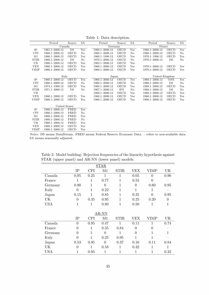
Table 1: Data description.

Period Source SA Period Source SA Period Source SACanada Germany France

IP 1961.1–2000.12 DS Yes 1960.1–2000.12 OECD Yes 1960.1–2000.12 OECD YesCPI 1960.1–2000.12 OECD No 1960.1–2000.12 OECD No 1960.1–2000.12 OECD NoM1 1960.1–2000.12 OECD Yes 1960.1–1998.12 OECD Yes 1970.1–1998.12 OECD Yes

STIR 1960.1–2000.12 DS No 1970.1–2000.12 OECD No 1970.1–2000.12 DS NoUR 1960.1–2000.12 OECD Yes 1962.1–2000.12 OECD Yes –

VEX 1960.1–2000.12 OECD Yes 1960.1–2000.12 OECD Yes 1970.1–2000.12 OECD YesVIMP 1960.1–2000.12 OECD Yes 1960.1–2000.12 OECD Yes 1970.1–2000.12 OECD Yes

Italy Japan United KingdomIP 1960.1–2000.12 OECD Yes 1960.1–2000.12 OECD Yes 1960.1–2000.12 ONS Yes

CPI 1960.1–2000.12 OECD No 1960.1–2000.12 OECD No 1960.1–2000.12 DS NoM1 1974.1–1998.12 OECD Yes 1960.1–2000.12 OECD Yes 1969.1–2000.12 OECD Yes

STIR 1971.1–2000.12 DS No 1967.1–2000.12 IFS No 1960.1–2000.12 DS NoUR – – – 1960.1–2000.12 OECD Yes 1960.1–2000.12 OECD Yes

VEX 1960.1–2000.12 OECD Yes 1960.1–2000.12 OECD Yes 1960.1–2000.12 OECD YesVIMP 1960.1–2000.12 OECD Yes 1960.1–2000.12 OECD Yes 1960.1–2000.12 OECD Yes

United StatesIP 1960.1–2000.12 FRED Yes

CPI 1960.1–2000.12 FRED NoM1 1960.1–2000.12 FRED Yes

STIR 1960.1–2000.12 FRED NoUR 1960.1–2000.12 FRED Yes

VEX 1960.1–2000.12 OECD YesVIMP 1960.1–2000.12 OECD Yes

Notes: DS means DataStream. FRED means Federal Reserve Economic Data. – refers to non-available data.SA means seasonally adjusted.

Table 2: Model building: Rejection frequencies of the linearity hypothesis againstSTAR (upper panel) and AR-NN (lower panel) models.

STARIP CPI M1 STIR VEX VIMP UR

Canada 0.95 0.25 1 1 0.05 0 0.90France 1 1 0.77 1 0.55 0 –Germany 0.90 1 0 1 0 0.60 0.95Italy 0 1 0.22 1 1 1 –Japan 0.15 1 0.85 1 0.35 0 0.95UK 0 0.35 0.95 1 0.25 0.20 0USA 1 1 0.80 1 0.50 1 1

AR-NNIP CPI M1 STIR VEX VIMP UR

Canada 0 0.95 0.47 1 0.11 1 0.74France 0 1 0.35 0.84 0 0 –Germany 0 1 0 1 0 1 1Italy 0 1 0.25 0.95 1 1 –Japan 0.53 0.95 0 0.37 0.16 0.11 0.84UK 0 1 0.58 1 0.32 1 1USA 1 0.95 1 1 1 1 0.32

35

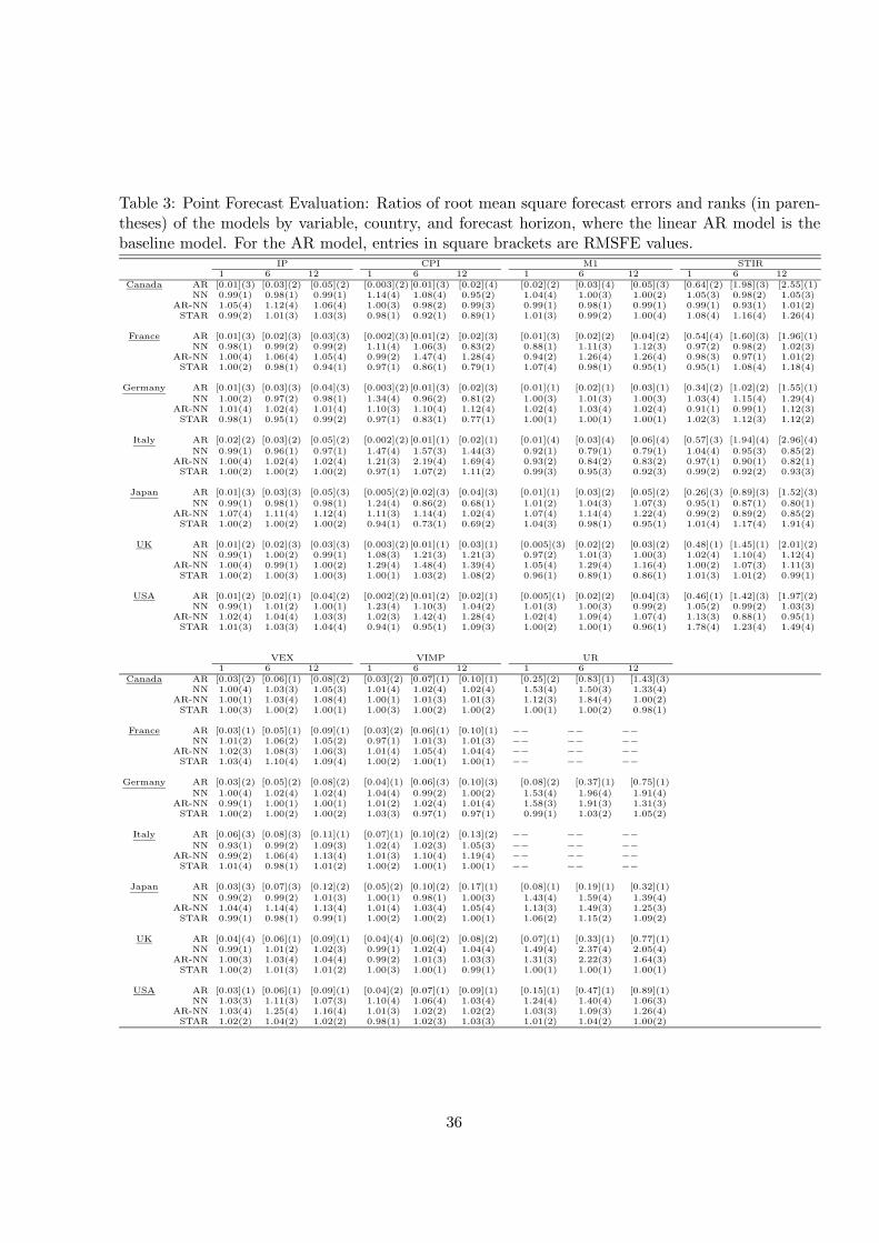
Table 3: Point Forecast Evaluation: Ratios of root mean square forecast errors and ranks (in paren-theses) of the models by variable, country, and forecast horizon, where the linear AR model is thebaseline model. For the AR model, entries in square brackets are RMSFE values.

IP CPI M1 STIR1 6 12 1 6 12 1 6 12 1 6 12

Canada AR [0.01](3) [0.03](2) [0.05](2) [0.003](2)[0.01](3) [0.02](4) [0.02](2) [0.03](4) [0.05](3) [0.64](2) [1.98](3) [2.55](1)NN 0.99(1) 0.98(1) 0.99(1) 1.14(4) 1.08(4) 0.95(2) 1.04(4) 1.00(3) 1.00(2) 1.05(3) 0.98(2) 1.05(3)

AR-NN 1.05(4) 1.12(4) 1.06(4) 1.00(3) 0.98(2) 0.99(3) 0.99(1) 0.98(1) 0.99(1) 0.99(1) 0.93(1) 1.01(2)STAR 0.99(2) 1.01(3) 1.03(3) 0.98(1) 0.92(1) 0.89(1) 1.01(3) 0.99(2) 1.00(4) 1.08(4) 1.16(4) 1.26(4)

France AR [0.01](3) [0.02](3) [0.03](3) [0.002](3)[0.01](2) [0.02](3) [0.01](3) [0.02](2) [0.04](2) [0.54](4) [1.60](3) [1.96](1)NN 0.98(1) 0.99(2) 0.99(2) 1.11(4) 1.06(3) 0.83(2) 0.88(1) 1.11(3) 1.12(3) 0.97(2) 0.98(2) 1.02(3)

AR-NN 1.00(4) 1.06(4) 1.05(4) 0.99(2) 1.47(4) 1.28(4) 0.94(2) 1.26(4) 1.26(4) 0.98(3) 0.97(1) 1.01(2)STAR 1.00(2) 0.98(1) 0.94(1) 0.97(1) 0.86(1) 0.79(1) 1.07(4) 0.98(1) 0.95(1) 0.95(1) 1.08(4) 1.18(4)

Germany AR [0.01](3) [0.03](3) [0.04](3) [0.003](2)[0.01](3) [0.02](3) [0.01](1) [0.02](1) [0.03](1) [0.34](2) [1.02](2) [1.55](1)

NN 1.00(2) 0.97(2) 0.98(1) 1.34(4) 0.96(2) 0.81(2) 1.00(3) 1.01(3) 1.00(3) 1.03(4) 1.15(4) 1.29(4)AR-NN 1.01(4) 1.02(4) 1.01(4) 1.10(3) 1.10(4) 1.12(4) 1.02(4) 1.03(4) 1.02(4) 0.91(1) 0.99(1) 1.12(3)STAR 0.98(1) 0.95(1) 0.99(2) 0.97(1) 0.83(1) 0.77(1) 1.00(1) 1.00(1) 1.00(1) 1.02(3) 1.12(3) 1.12(2)

Italy AR [0.02](2) [0.03](2) [0.05](2) [0.002](2)[0.01](1) [0.02](1) [0.01](4) [0.03](4) [0.06](4) [0.57](3) [1.94](4) [2.96](4)

NN 0.99(1) 0.96(1) 0.97(1) 1.47(4) 1.57(3) 1.44(3) 0.92(1) 0.79(1) 0.79(1) 1.04(4) 0.95(3) 0.85(2)AR-NN 1.00(4) 1.02(4) 1.02(4) 1.21(3) 2.19(4) 1.69(4) 0.93(2) 0.84(2) 0.83(2) 0.97(1) 0.90(1) 0.82(1)STAR 1.00(2) 1.00(2) 1.00(2) 0.97(1) 1.07(2) 1.11(2) 0.99(3) 0.95(3) 0.92(3) 0.99(2) 0.92(2) 0.93(3)

Japan AR [0.01](3) [0.03](3) [0.05](3) [0.005](2)[0.02](3) [0.04](3) [0.01](1) [0.03](2) [0.05](2) [0.26](3) [0.89](3) [1.52](3)

NN 0.99(1) 0.98(1) 0.98(1) 1.24(4) 0.86(2) 0.68(1) 1.01(2) 1.04(3) 1.07(3) 0.95(1) 0.87(1) 0.80(1)AR-NN 1.07(4) 1.11(4) 1.12(4) 1.11(3) 1.14(4) 1.02(4) 1.07(4) 1.14(4) 1.22(4) 0.99(2) 0.89(2) 0.85(2)STAR 1.00(2) 1.00(2) 1.00(2) 0.94(1) 0.73(1) 0.69(2) 1.04(3) 0.98(1) 0.95(1) 1.01(4) 1.17(4) 1.91(4)

UK AR [0.01](2) [0.02](3) [0.03](3) [0.003](2)[0.01](1) [0.03](1) [0.005](3) [0.02](2) [0.03](2) [0.48](1) [1.45](1) [2.01](2)NN 0.99(1) 1.00(2) 0.99(1) 1.08(3) 1.21(3) 1.21(3) 0.97(2) 1.01(3) 1.00(3) 1.02(4) 1.10(4) 1.12(4)

AR-NN 1.00(4) 0.99(1) 1.00(2) 1.29(4) 1.48(4) 1.39(4) 1.05(4) 1.29(4) 1.16(4) 1.00(2) 1.07(3) 1.11(3)STAR 1.00(2) 1.00(3) 1.00(3) 1.00(1) 1.03(2) 1.08(2) 0.96(1) 0.89(1) 0.86(1) 1.01(3) 1.01(2) 0.99(1)

USA AR [0.01](2) [0.02](1) [0.04](2) [0.002](2)[0.01](2) [0.02](1) [0.005](1) [0.02](2) [0.04](3) [0.46](1) [1.42](3) [1.97](2)NN 0.99(1) 1.01(2) 1.00(1) 1.23(4) 1.10(3) 1.04(2) 1.01(3) 1.00(3) 0.99(2) 1.05(2) 0.99(2) 1.03(3)

AR-NN 1.02(4) 1.04(4) 1.03(3) 1.02(3) 1.42(4) 1.28(4) 1.02(4) 1.09(4) 1.07(4) 1.13(3) 0.88(1) 0.95(1)STAR 1.01(3) 1.03(3) 1.04(4) 0.94(1) 0.95(1) 1.09(3) 1.00(2) 1.00(1) 0.96(1) 1.78(4) 1.23(4) 1.49(4)

VEX VIMP UR1 6 12 1 6 12 1 6 12

Canada AR [0.03](2) [0.06](1) [0.08](2) [0.03](2) [0.07](1) [0.10](1) [0.25](2) [0.83](1) [1.43](3)NN 1.00(4) 1.03(3) 1.05(3) 1.01(4) 1.02(4) 1.02(4) 1.53(4) 1.50(3) 1.33(4)

AR-NN 1.00(1) 1.03(4) 1.08(4) 1.00(1) 1.01(3) 1.01(3) 1.12(3) 1.84(4) 1.00(2)STAR 1.00(3) 1.00(2) 1.00(1) 1.00(3) 1.00(2) 1.00(2) 1.00(1) 1.00(2) 0.98(1)

France AR [0.03](1) [0.05](1) [0.09](1) [0.03](2) [0.06](1) [0.10](1) −− −− −−

NN 1.01(2) 1.06(2) 1.05(2) 0.97(1) 1.01(3) 1.01(3) −− −− −−

AR-NN 1.02(3) 1.08(3) 1.06(3) 1.01(4) 1.05(4) 1.04(4) −− −− −−

STAR 1.03(4) 1.10(4) 1.09(4) 1.00(2) 1.00(1) 1.00(1) −− −− −−

Germany AR [0.03](2) [0.05](2) [0.08](2) [0.04](1) [0.06](3) [0.10](3) [0.08](2) [0.37](1) [0.75](1)

NN 1.00(4) 1.02(4) 1.02(4) 1.04(4) 0.99(2) 1.00(2) 1.53(4) 1.96(4) 1.91(4)AR-NN 0.99(1) 1.00(1) 1.00(1) 1.01(2) 1.02(4) 1.01(4) 1.58(3) 1.91(3) 1.31(3)STAR 1.00(2) 1.00(2) 1.00(2) 1.03(3) 0.97(1) 0.97(1) 0.99(1) 1.03(2) 1.05(2)

Italy AR [0.06](3) [0.08](3) [0.11](1) [0.07](1) [0.10](2) [0.13](2) −− −− −−

NN 0.93(1) 0.99(2) 1.09(3) 1.02(4) 1.02(3) 1.05(3) −− −− −−

AR-NN 0.99(2) 1.06(4) 1.13(4) 1.01(3) 1.10(4) 1.19(4) −− −− −−

STAR 1.01(4) 0.98(1) 1.01(2) 1.00(2) 1.00(1) 1.00(1) −− −− −−

Japan AR [0.03](3) [0.07](3) [0.12](2) [0.05](2) [0.10](2) [0.17](1) [0.08](1) [0.19](1) [0.32](1)

NN 0.99(2) 0.99(2) 1.01(3) 1.00(1) 0.98(1) 1.00(3) 1.43(4) 1.59(4) 1.39(4)AR-NN 1.04(4) 1.14(4) 1.13(4) 1.01(4) 1.03(4) 1.05(4) 1.13(3) 1.49(3) 1.25(3)STAR 0.99(1) 0.98(1) 0.99(1) 1.00(2) 1.00(2) 1.00(1) 1.06(2) 1.15(2) 1.09(2)

UK AR [0.04](4) [0.06](1) [0.09](1) [0.04](4) [0.06](2) [0.08](2) [0.07](1) [0.33](1) [0.77](1)NN 0.99(1) 1.01(2) 1.02(3) 0.99(1) 1.02(4) 1.04(4) 1.49(4) 2.37(4) 2.05(4)

AR-NN 1.00(3) 1.03(4) 1.04(4) 0.99(2) 1.01(3) 1.03(3) 1.31(3) 2.22(3) 1.64(3)STAR 1.00(2) 1.01(3) 1.01(2) 1.00(3) 1.00(1) 0.99(1) 1.00(1) 1.00(1) 1.00(1)

USA AR [0.03](1) [0.06](1) [0.09](1) [0.04](2) [0.07](1) [0.09](1) [0.15](1) [0.47](1) [0.89](1)NN 1.03(3) 1.11(3) 1.07(3) 1.10(4) 1.06(4) 1.03(4) 1.24(4) 1.40(4) 1.06(3)

AR-NN 1.03(4) 1.25(4) 1.16(4) 1.01(3) 1.02(2) 1.02(2) 1.03(3) 1.09(3) 1.26(4)STAR 1.02(2) 1.04(2) 1.02(2) 0.98(1) 1.02(3) 1.03(3) 1.01(2) 1.04(2) 1.00(2)

36

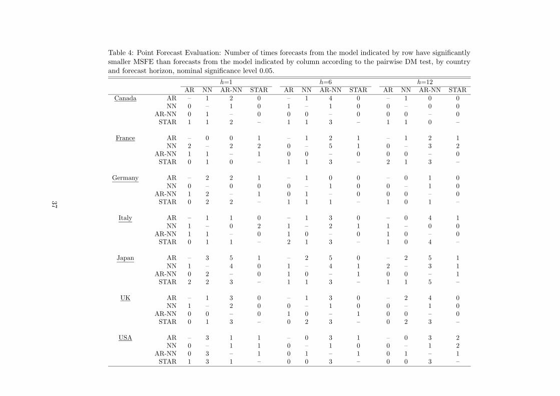
Table 4: Point Forecast Evaluation: Number of times forecasts from the model indicated by row have significantlysmaller MSFE than forecasts from the model indicated by column according to the pairwise DM test, by countryand forecast horizon, nominal significance level 0.05.

h=1 h=6 h=12AR NN AR-NN STAR AR NN AR-NN STAR AR NN AR-NN STAR

Canada AR – 1 2 0 – 1 4 0 – 1 0 0NN 0 – 1 0 1 – 1 0 0 – 0 0

AR-NN 0 1 – 0 0 0 – 0 0 0 – 0STAR 1 1 2 – 1 1 3 – 1 1 0 –

France AR – 0 0 1 – 1 2 1 – 1 2 1NN 2 – 2 2 0 – 5 1 0 – 3 2

AR-NN 1 1 – 1 0 0 – 0 0 0 – 0STAR 0 1 0 – 1 1 3 – 2 1 3 –

Germany AR – 2 2 1 – 1 0 0 – 0 1 0NN 0 – 0 0 0 – 1 0 0 – 1 0

AR-NN 1 2 – 1 0 1 – 0 0 0 – 0STAR 0 2 2 – 1 1 1 – 1 0 1 –

Italy AR – 1 1 0 – 1 3 0 – 0 4 1NN 1 – 0 2 1 – 2 1 1 – 0 0

AR-NN 1 1 – 0 1 0 – 0 1 0 – 0STAR 0 1 1 – 2 1 3 – 1 0 4 –

Japan AR – 3 5 1 – 2 5 0 – 2 5 1NN 1 – 4 0 1 – 4 1 2 – 3 1

AR-NN 0 2 – 0 1 0 – 1 0 0 – 1STAR 2 2 3 – 1 1 3 – 1 1 5 –

UK AR – 1 3 0 – 1 3 0 – 2 4 0NN 1 – 2 0 0 – 1 0 0 – 1 0

AR-NN 0 0 – 0 1 0 – 1 0 0 – 0STAR 0 1 3 – 0 2 3 – 0 2 3 –

USA AR – 3 1 1 – 0 3 1 – 0 3 2NN 0 – 1 1 0 – 1 0 0 – 1 2

AR-NN 0 3 – 1 0 1 – 1 0 1 – 1STAR 1 3 1 – 0 0 3 – 0 0 3 –

37

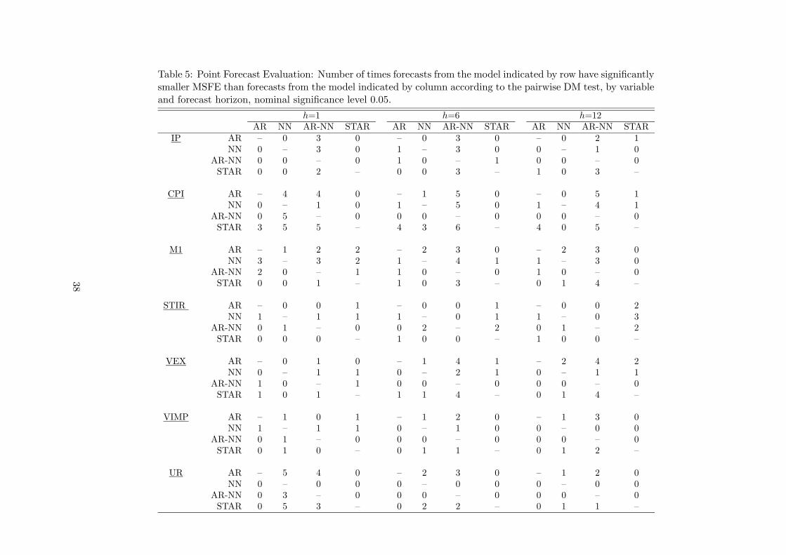
Table 5: Point Forecast Evaluation: Number of times forecasts from the model indicated by row have significantlysmaller MSFE than forecasts from the model indicated by column according to the pairwise DM test, by variableand forecast horizon, nominal significance level 0.05.

h=1 h=6 h=12AR NN AR-NN STAR AR NN AR-NN STAR AR NN AR-NN STAR

IP AR – 0 3 0 – 0 3 0 – 0 2 1NN 0 – 3 0 1 – 3 0 0 – 1 0

AR-NN 0 0 – 0 1 0 – 1 0 0 – 0STAR 0 0 2 – 0 0 3 – 1 0 3 –

CPI AR – 4 4 0 – 1 5 0 – 0 5 1NN 0 – 1 0 1 – 5 0 1 – 4 1

AR-NN 0 5 – 0 0 0 – 0 0 0 – 0STAR 3 5 5 – 4 3 6 – 4 0 5 –

M1 AR – 1 2 2 – 2 3 0 – 2 3 0NN 3 – 3 2 1 – 4 1 1 – 3 0

AR-NN 2 0 – 1 1 0 – 0 1 0 – 0STAR 0 0 1 – 1 0 3 – 0 1 4 –

STIR AR – 0 0 1 – 0 0 1 – 0 0 2NN 1 – 1 1 1 – 0 1 1 – 0 3

AR-NN 0 1 – 0 0 2 – 2 0 1 – 2STAR 0 0 0 – 1 0 0 – 1 0 0 –

VEX AR – 0 1 0 – 1 4 1 – 2 4 2NN 0 – 1 1 0 – 2 1 0 – 1 1

AR-NN 1 0 – 1 0 0 – 0 0 0 – 0STAR 1 0 1 – 1 1 4 – 0 1 4 –

VIMP AR – 1 0 1 – 1 2 0 – 1 3 0NN 1 – 1 1 0 – 1 0 0 – 0 0

AR-NN 0 1 – 0 0 0 – 0 0 0 – 0STAR 0 1 0 – 0 1 1 – 0 1 2 –

UR AR – 5 4 0 – 2 3 0 – 1 2 0NN 0 – 0 0 0 – 0 0 0 – 0 0

AR-NN 0 3 – 0 0 0 – 0 0 0 – 0STAR 0 5 3 – 0 2 2 – 0 1 1 –

38

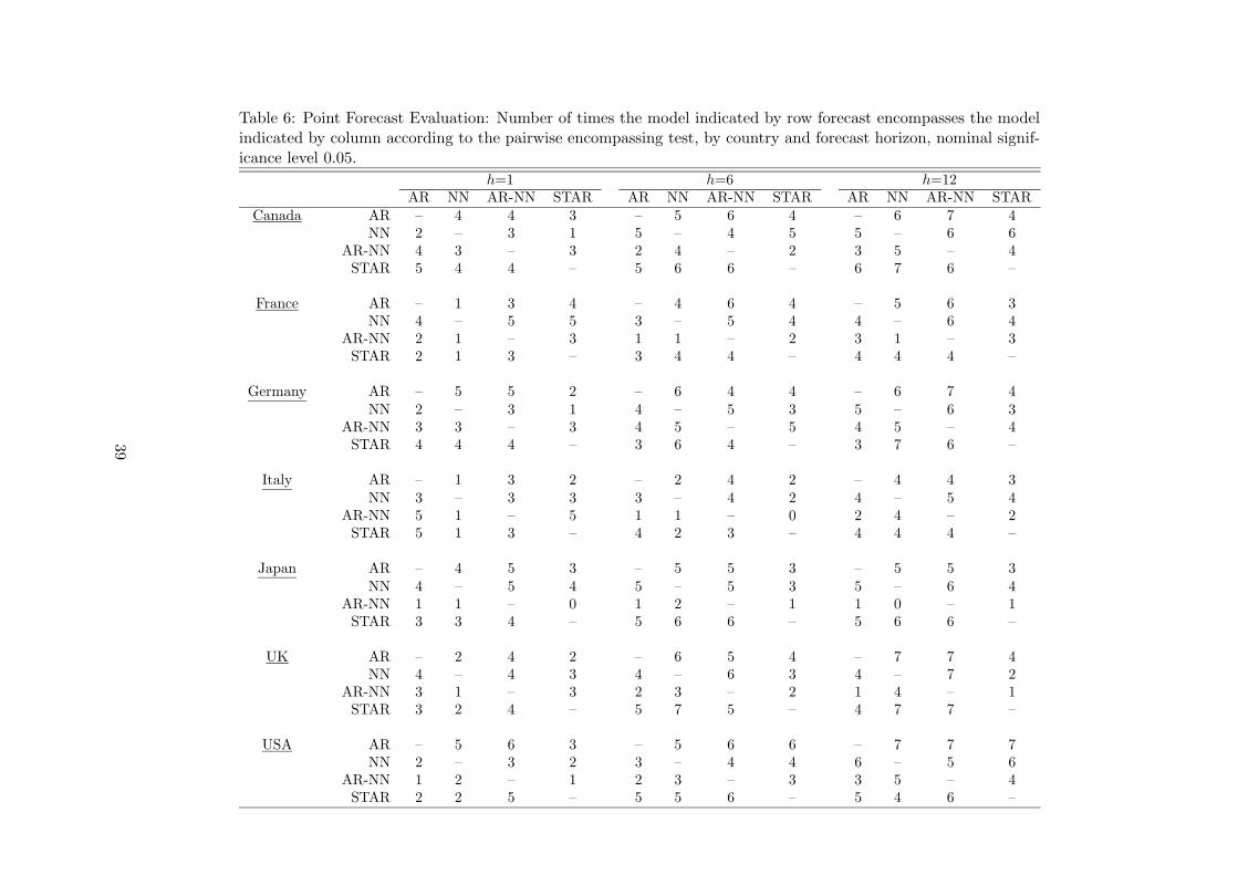
Table 6: Point Forecast Evaluation: Number of times the model indicated by row forecast encompasses the modelindicated by column according to the pairwise encompassing test, by country and forecast horizon, nominal signif-icance level 0.05.

h=1 h=6 h=12AR NN AR-NN STAR AR NN AR-NN STAR AR NN AR-NN STAR

Canada AR – 4 4 3 – 5 6 4 – 6 7 4NN 2 – 3 1 5 – 4 5 5 – 6 6

AR-NN 4 3 – 3 2 4 – 2 3 5 – 4STAR 5 4 4 – 5 6 6 – 6 7 6 –

France AR – 1 3 4 – 4 6 4 – 5 6 3NN 4 – 5 5 3 – 5 4 4 – 6 4

AR-NN 2 1 – 3 1 1 – 2 3 1 – 3STAR 2 1 3 – 3 4 4 – 4 4 4 –

Germany AR – 5 5 2 – 6 4 4 – 6 7 4NN 2 – 3 1 4 – 5 3 5 – 6 3

AR-NN 3 3 – 3 4 5 – 5 4 5 – 4STAR 4 4 4 – 3 6 4 – 3 7 6 –

Italy AR – 1 3 2 – 2 4 2 – 4 4 3NN 3 – 3 3 3 – 4 2 4 – 5 4

AR-NN 5 1 – 5 1 1 – 0 2 4 – 2STAR 5 1 3 – 4 2 3 – 4 4 4 –

Japan AR – 4 5 3 – 5 5 3 – 5 5 3NN 4 – 5 4 5 – 5 3 5 – 6 4

AR-NN 1 1 – 0 1 2 – 1 1 0 – 1STAR 3 3 4 – 5 6 6 – 5 6 6 –

UK AR – 2 4 2 – 6 5 4 – 7 7 4NN 4 – 4 3 4 – 6 3 4 – 7 2

AR-NN 3 1 – 3 2 3 – 2 1 4 – 1STAR 3 2 4 – 5 7 5 – 4 7 7 –

USA AR – 5 6 3 – 5 6 6 – 7 7 7NN 2 – 3 2 3 – 4 4 6 – 5 6

AR-NN 1 2 – 1 2 3 – 3 3 5 – 4STAR 2 2 5 – 5 5 6 – 5 4 6 –

39

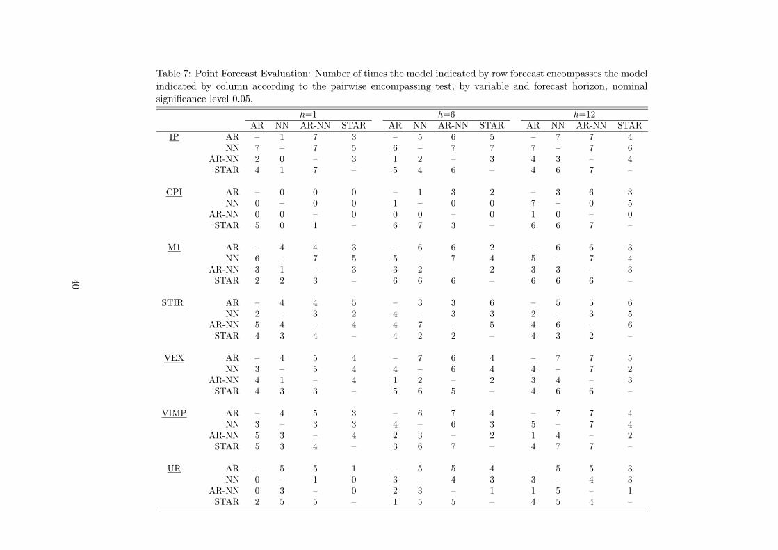
Table 7: Point Forecast Evaluation: Number of times the model indicated by row forecast encompasses the modelindicated by column according to the pairwise encompassing test, by variable and forecast horizon, nominalsignificance level 0.05.

h=1 h=6 h=12AR NN AR-NN STAR AR NN AR-NN STAR AR NN AR-NN STAR

IP AR – 1 7 3 – 5 6 5 – 7 7 4NN 7 – 7 5 6 – 7 7 7 – 7 6

AR-NN 2 0 – 3 1 2 – 3 4 3 – 4STAR 4 1 7 – 5 4 6 – 4 6 7 –

CPI AR – 0 0 0 – 1 3 2 – 3 6 3NN 0 – 0 0 1 – 0 0 7 – 0 5

AR-NN 0 0 – 0 0 0 – 0 1 0 – 0STAR 5 0 1 – 6 7 3 – 6 6 7 –

M1 AR – 4 4 3 – 6 6 2 – 6 6 3NN 6 – 7 5 5 – 7 4 5 – 7 4

AR-NN 3 1 – 3 3 2 – 2 3 3 – 3STAR 2 2 3 – 6 6 6 – 6 6 6 –

STIR AR – 4 4 5 – 3 3 6 – 5 5 6NN 2 – 3 2 4 – 3 3 2 – 3 5

AR-NN 5 4 – 4 4 7 – 5 4 6 – 6STAR 4 3 4 – 4 2 2 – 4 3 2 –

VEX AR – 4 5 4 – 7 6 4 – 7 7 5NN 3 – 5 4 4 – 6 4 4 – 7 2

AR-NN 4 1 – 4 1 2 – 2 3 4 – 3STAR 4 3 3 – 5 6 5 – 4 6 6 –

VIMP AR – 4 5 3 – 6 7 4 – 7 7 4NN 3 – 3 3 4 – 6 3 5 – 7 4

AR-NN 5 3 – 4 2 3 – 2 1 4 – 2STAR 5 3 4 – 3 6 7 – 4 7 7 –

UR AR – 5 5 1 – 5 5 4 – 5 5 3NN 0 – 1 0 3 – 4 3 3 – 4 3

AR-NN 0 3 – 0 2 3 – 1 1 5 – 1STAR 2 5 5 – 1 5 5 – 4 5 4 –

40

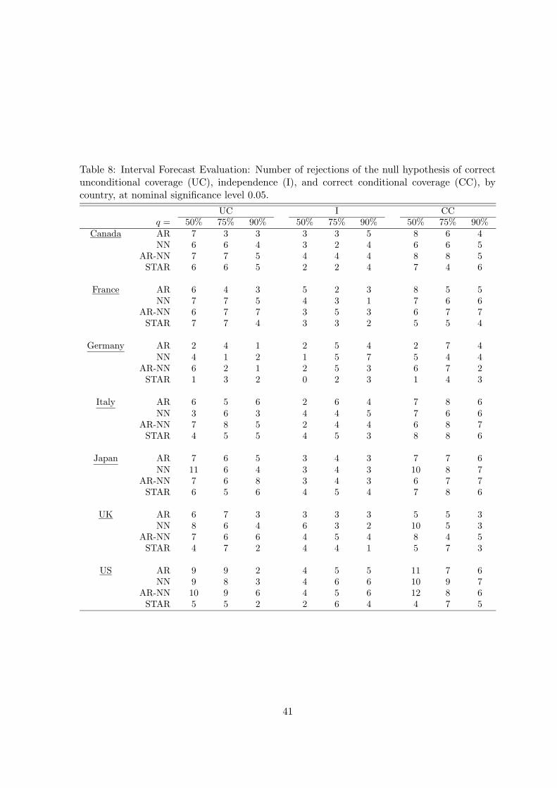
Table 8: Interval Forecast Evaluation: Number of rejections of the null hypothesis of correctunconditional coverage (UC), independence (I), and correct conditional coverage (CC), bycountry, at nominal significance level 0.05.

UC I CCq = 50% 75% 90% 50% 75% 90% 50% 75% 90%

Canada AR 7 3 3 3 3 5 8 6 4NN 6 6 4 3 2 4 6 6 5

AR-NN 7 7 5 4 4 4 8 8 5STAR 6 6 5 2 2 4 7 4 6

France AR 6 4 3 5 2 3 8 5 5NN 7 7 5 4 3 1 7 6 6

AR-NN 6 7 7 3 5 3 6 7 7STAR 7 7 4 3 3 2 5 5 4

Germany AR 2 4 1 2 5 4 2 7 4NN 4 1 2 1 5 7 5 4 4

AR-NN 6 2 1 2 5 3 6 7 2STAR 1 3 2 0 2 3 1 4 3

Italy AR 6 5 6 2 6 4 7 8 6NN 3 6 3 4 4 5 7 6 6

AR-NN 7 8 5 2 4 4 6 8 7STAR 4 5 5 4 5 3 8 8 6

Japan AR 7 6 5 3 4 3 7 7 6NN 11 6 4 3 4 3 10 8 7

AR-NN 7 6 8 3 4 3 6 7 7STAR 6 5 6 4 5 4 7 8 6

UK AR 6 7 3 3 3 3 5 5 3NN 8 6 4 6 3 2 10 5 3

AR-NN 7 6 6 4 5 4 8 4 5STAR 4 7 2 4 4 1 5 7 3

US AR 9 9 2 4 5 5 11 7 6NN 9 8 3 4 6 6 10 9 7

AR-NN 10 9 6 4 5 6 12 8 6STAR 5 5 2 2 6 4 4 7 5

41

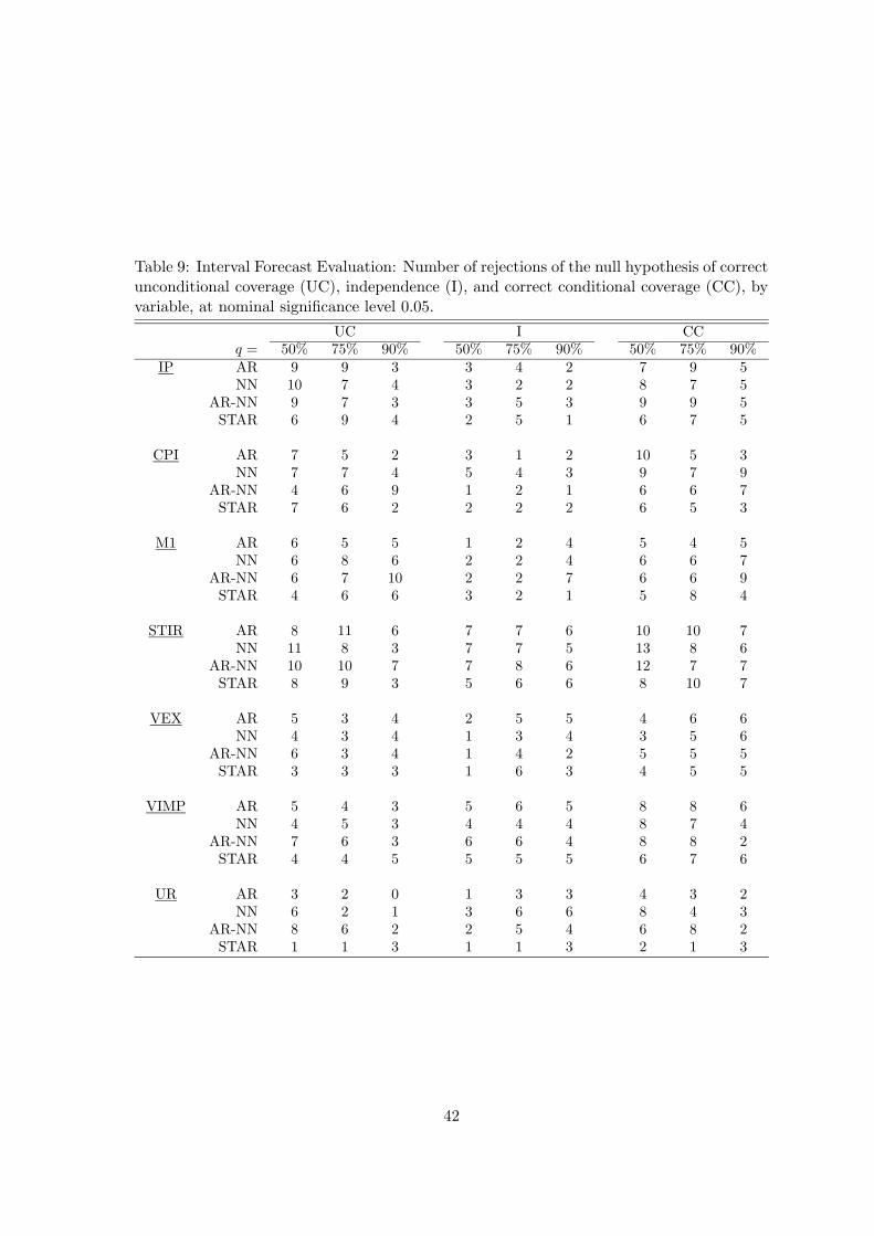
Table 9: Interval Forecast Evaluation: Number of rejections of the null hypothesis of correctunconditional coverage (UC), independence (I), and correct conditional coverage (CC), byvariable, at nominal significance level 0.05.

UC I CCq = 50% 75% 90% 50% 75% 90% 50% 75% 90%

IP AR 9 9 3 3 4 2 7 9 5NN 10 7 4 3 2 2 8 7 5

AR-NN 9 7 3 3 5 3 9 9 5STAR 6 9 4 2 5 1 6 7 5

CPI AR 7 5 2 3 1 2 10 5 3NN 7 7 4 5 4 3 9 7 9

AR-NN 4 6 9 1 2 1 6 6 7STAR 7 6 2 2 2 2 6 5 3

M1 AR 6 5 5 1 2 4 5 4 5NN 6 8 6 2 2 4 6 6 7

AR-NN 6 7 10 2 2 7 6 6 9STAR 4 6 6 3 2 1 5 8 4

STIR AR 8 11 6 7 7 6 10 10 7NN 11 8 3 7 7 5 13 8 6

AR-NN 10 10 7 7 8 6 12 7 7STAR 8 9 3 5 6 6 8 10 7

VEX AR 5 3 4 2 5 5 4 6 6NN 4 3 4 1 3 4 3 5 6

AR-NN 6 3 4 1 4 2 5 5 5STAR 3 3 3 1 6 3 4 5 5

VIMP AR 5 4 3 5 6 5 8 8 6NN 4 5 3 4 4 4 8 7 4

AR-NN 7 6 3 6 6 4 8 8 2STAR 4 4 5 5 5 5 6 7 6

UR AR 3 2 0 1 3 3 4 3 2NN 6 2 1 3 6 6 8 4 3

AR-NN 8 6 2 2 5 4 6 8 2STAR 1 1 3 1 1 3 2 1 3

42

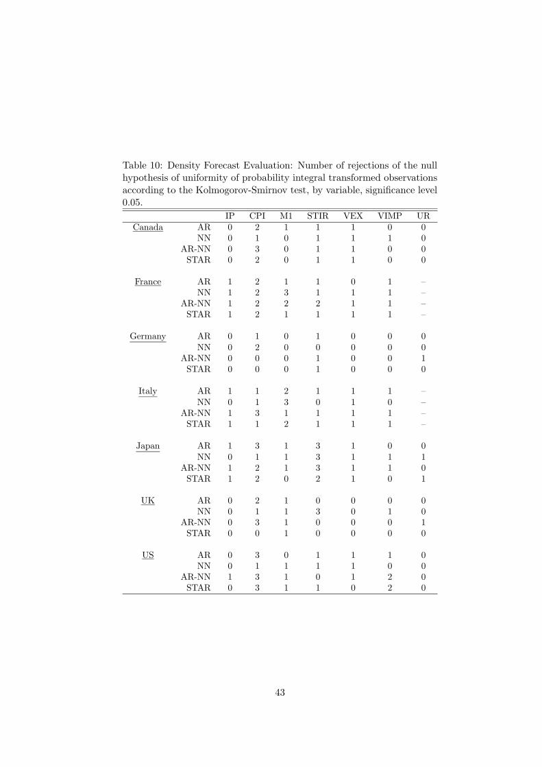
Table 10: Density Forecast Evaluation: Number of rejections of the nullhypothesis of uniformity of probability integral transformed observationsaccording to the Kolmogorov-Smirnov test, by variable, significance level0.05.

IP CPI M1 STIR VEX VIMP URCanada AR 0 2 1 1 1 0 0

NN 0 1 0 1 1 1 0AR-NN 0 3 0 1 1 0 0STAR 0 2 0 1 1 0 0

France AR 1 2 1 1 0 1 –NN 1 2 3 1 1 1 –

AR-NN 1 2 2 2 1 1 –STAR 1 2 1 1 1 1 –

Germany AR 0 1 0 1 0 0 0NN 0 2 0 0 0 0 0

AR-NN 0 0 0 1 0 0 1STAR 0 0 0 1 0 0 0

Italy AR 1 1 2 1 1 1 –NN 0 1 3 0 1 0 –

AR-NN 1 3 1 1 1 1 –STAR 1 1 2 1 1 1 –

Japan AR 1 3 1 3 1 0 0NN 0 1 1 3 1 1 1

AR-NN 1 2 1 3 1 1 0STAR 1 2 0 2 1 0 1

UK AR 0 2 1 0 0 0 0NN 0 1 1 3 0 1 0

AR-NN 0 3 1 0 0 0 1STAR 0 0 1 0 0 0 0

US AR 0 3 0 1 1 1 0NN 0 1 1 1 1 0 0

AR-NN 1 3 1 0 1 2 0STAR 0 3 1 1 0 2 0

43

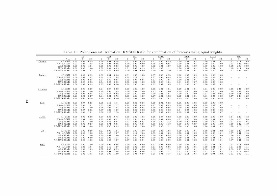
Table 11: Point Forecast Evaluation: RMSFE Ratio for combination of forecasts using equal weights.IP CPI M1 STIR VEX VIMP UR

h = 1 6 12 1 6 12 1 6 12 1 6 12 1 6 12 1 6 12 1 6 12Canada AR+NN 0.99 0.99 0.99 0.96 0.94 0.94 1.01 0.99 0.99 0.97 0.96 0.99 1.00 1.01 1.02 1.00 1.01 1.01 1.17 1.11 1.03

AR+AR-NN 1.01 1.05 1.02 0.96 0.93 0.96 0.99 0.99 0.99 0.98 0.95 0.98 1.00 1.01 1.03 0.99 1.00 1.00 1.03 1.26 0.98AR+STAR 0.99 0.99 1.01 0.99 0.95 0.93 1.00 0.99 1.00 1.02 1.04 1.09 1.00 1.00 1.00 1.00 1.00 1.00 0.99 0.99 0.98NN+STAR 0.98 0.98 1.00 0.95 0.91 0.89 1.01 0.99 0.99 0.99 1.02 1.11 1.00 1.01 1.02 1.00 1.01 1.01 1.15 1.11 1.03

AR-NN+STAR 1.00 1.04 1.02 0.95 0.89 0.89 1.00 0.98 0.99 1.00 1.01 1.10 1.00 1.01 1.03 0.99 1.00 1.00 1.02 1.26 0.97

France AR+NN 0.99 0.99 0.99 0.92 0.94 0.86 0.91 1.05 1.06 0.97 0.96 0.95 1.00 1.02 1.02 0.98 1.00 1.00 – – –AR+AR-NN 1.00 1.02 1.02 0.94 1.11 1.08 0.95 1.11 1.11 0.97 0.95 0.95 0.99 1.02 1.02 1.00 1.02 1.02 – – –AR+STAR 0.99 0.99 0.97 0.97 0.89 0.85 1.02 0.97 0.95 0.91 0.99 1.05 1.00 1.04 1.04 1.00 1.00 1.00 – – –NN+STAR 0.98 0.98 0.96 0.94 0.93 0.80 0.93 1.02 1.00 0.90 0.98 1.04 1.01 1.08 1.07 0.98 1.00 1.00 – – –

AR-NN+STAR 1.00 1.02 0.99 0.92 0.99 0.90 0.98 1.06 1.04 0.92 0.98 1.05 1.01 1.09 1.07 1.00 1.02 1.02 – – –

Germany AR+NN 1.00 0.98 0.99 1.04 0.87 0.82 1.00 1.00 1.00 0.98 1.01 1.04 0.99 1.01 1.01 1.01 0.98 0.99 1.18 1.34 1.29

NN+AR-NN 1.00 1.01 1.00 0.99 0.99 1.05 1.00 1.01 1.00 0.93 0.95 1.00 0.99 1.00 1.00 1.00 1.00 1.00 1.18 1.32 1.08AR+STAR 0.98 0.96 0.98 0.97 0.87 0.82 1.00 1.00 1.00 1.00 1.01 1.01 1.00 1.00 1.00 1.01 0.98 0.98 0.99 1.01 1.02NN+STAR 0.98 0.95 0.97 1.04 0.84 0.78 1.00 1.00 1.00 0.97 1.01 1.08 0.99 1.01 1.01 1.01 0.97 0.98 1.17 1.33 1.28

AR-NN+STAR 0.98 0.97 0.98 0.96 0.85 0.86 1.00 1.01 1.00 0.93 0.96 1.02 0.99 1.00 1.00 1.00 0.98 0.98 1.17 1.33 1.08

Italy AR+NN 0.98 0.97 0.98 1.06 1.13 1.11 0.93 0.85 0.86 0.99 0.91 0.83 0.93 0.98 1.03 0.98 0.98 1.00 – – –

AR+AR-NN 1.00 1.01 1.01 1.02 1.32 1.17 0.94 0.87 0.88 0.97 0.89 0.83 0.98 1.02 1.05 0.99 1.02 1.07 – – –AR+STAR 1.00 1.00 1.00 0.96 1.01 1.04 0.99 0.97 0.95 0.99 0.95 0.96 1.00 0.98 0.99 1.00 1.00 1.00 – – –NN+STAR 0.98 0.97 0.98 1.07 1.21 1.20 0.93 0.82 0.82 0.98 0.89 0.82 0.94 0.97 1.03 0.98 0.98 1.00 – – –

AR-NN+STAR 1.00 1.01 1.01 1.00 1.27 1.18 0.93 0.85 0.84 0.97 0.87 0.82 0.99 1.01 1.05 0.99 1.02 1.07 – – –

Japan AR+NN 0.99 0.99 0.99 0.97 0.85 0.78 1.00 1.02 1.03 0.96 0.87 0.82 1.00 1.00 1.00 0.99 0.98 1.00 1.14 1.23 1.13

AR+AR-NN 1.02 1.04 1.05 0.95 0.98 0.97 1.02 1.05 1.09 0.99 0.91 0.88 1.01 1.06 1.06 1.00 1.01 1.02 1.04 1.20 1.08AR+STAR 1.00 1.00 1.00 0.96 0.86 0.84 1.01 0.95 0.93 0.98 1.00 1.32 0.99 0.99 0.99 1.00 1.00 1.00 1.01 1.06 1.04NN+STAR 0.99 0.99 0.98 0.95 0.74 0.65 1.01 0.96 0.95 0.95 0.88 1.10 0.99 0.98 0.99 0.99 0.98 1.00 1.16 1.32 1.19

AR-NN+STAR 1.02 1.04 1.04 0.92 0.86 0.82 1.02 0.99 1.00 0.97 0.88 1.11 1.00 1.05 1.06 1.00 1.01 1.02 1.05 1.25 1.12

UK AR+NN 0.99 1.00 0.99 0.91 0.99 1.04 0.98 1.00 1.00 1.00 1.03 1.03 0.99 1.00 1.01 0.99 1.01 1.02 1.13 1.42 1.30AR+AR-NN 1.00 0.99 1.00 1.04 1.05 1.07 1.01 1.11 1.06 0.99 1.01 1.02 1.00 1.01 1.02 0.99 1.00 1.01 1.07 1.41 1.18AR+STAR 1.00 1.00 1.00 0.99 0.98 1.00 0.96 0.89 0.85 1.00 0.99 0.98 1.00 1.00 1.00 1.00 1.00 1.00 1.00 1.00 1.00NN+STAR 0.99 1.00 0.99 0.92 1.05 1.13 0.94 0.89 0.86 1.00 1.03 1.00 0.99 1.01 1.01 0.99 1.01 1.01 1.13 1.42 1.30

AR-NN+STAR 1.00 0.99 1.00 1.02 1.03 1.07 0.97 1.00 0.91 0.99 1.00 0.99 0.99 1.01 1.02 0.99 1.00 1.01 1.07 1.41 1.18

USA AR+NN 0.99 1.00 1.00 1.00 0.96 0.96 1.00 1.00 0.99 0.97 0.94 0.99 1.00 1.04 1.03 1.02 1.01 1.01 1.07 1.11 0.99AR+AR-NN 1.01 1.01 1.01 0.99 1.10 1.07 1.00 1.02 1.02 1.01 0.90 0.96 1.00 1.08 1.05 1.00 1.01 1.01 1.01 1.04 1.11AR+STAR 1.00 1.01 1.02 0.95 0.93 0.99 0.99 0.98 0.96 1.23 1.02 1.12 1.01 1.02 1.01 0.98 1.00 1.01 0.99 1.00 0.99NN+STAR 0.99 1.01 1.01 0.99 0.98 1.06 0.99 0.99 0.96 1.23 0.99 1.17 1.01 1.06 1.04 1.02 1.02 1.02 1.07 1.13 0.98

AR-NN+STAR 1.01 1.02 1.03 0.96 1.06 1.09 1.00 1.01 0.98 1.25 0.94 1.13 1.01 1.11 1.07 0.99 1.01 1.02 1.01 1.05 1.11

44