linking oceanic emissions and troposph - ACP - Recent

A multi-model intercomparison of halogenated veryshort-lived substances (TransCom-VSLS): linkingoceanic emissions and tropospheric transport for areconciled estimate of the stratospheric source gasinjection of bromineR. Hossaini1,a, P. K. Patra2, A. A Leeson1,b, G. Krysztofiak3,c, N. L. Abraham4,5, S.J. Andrews6, A. T. Archibald4, J. Aschmann7, E. L. Atlas8, D. A. Belikov9,10,11, H.Bönisch12, R. Butler13, L. J. Carpenter6, S. Dhomse1, M. Dorf14, A. Engel12, L.Feng13, W. Feng1,4, S. Fuhlbrügge15, P. T. Griffiths5, N. R. P. Harris5, R. Hommel7,T. Keber12, K. Krüger15,16, S. T. Lennartz15, S. Maksyutov9, H. Mantle1, G. P.Mills 17, B. Miller18, S. A. Montzka18, F. Moore18, M. A. Navarro8, D. E. Oram17, P.I. Palmer13, K. Pfeilsticker19, J. A. Pyle4,5, B. Quack15, A. D. Robinson5, E.Saikawa20,21, A. Saiz-Lopez22, S. Sala12, B.-M Sinnhuber3, S. Taguchi23, S.Tegtmeier15, R. T. Lidster6, C. Wilson1,24, and F. Ziska15

1School of Earth and Environment, University of Leeds, Leeds, UK.2Research Institute for Global Change, JAMSTEC, Yokohama, Japan.3Institute for Meteorology and Climate Research, KarlsruheInstitute of Technology, Karlsruhe,Germany.4National Centre for Atmospheric Science, UK.5Department of Chemistry, University of Cambridge, Cambridge, UK.6Department of Chemistry, University of York, Heslington, York, UK.7Institute of Environmental Physics, University of Bremen,Bremen, Germany.8Rosenstiel School of Marine and Atmospheric Science, University of Miami, USA.9Center for Global Environmental Research, National Institute for Environmental Studies,Tsukuba, Japan.10National Institute of Polar Research, Tokyo, Japan.11Tomsk State University, Tomsk, Russia.12Institute for Atmospheric and Environmental Sciences, Universität Frankfurt/Main, Germany.13School of GeoSciences, The University of Edinburgh, Edinburgh, UK.14Max-Planck-Institute for Chemistry, Mainz, Germany.15GEOMAR Helmholtz Centre for Ocean Research Kiel, Kiel, Germany.16University of Oslo, Department of Geosciences, Oslo, Norway.17School of Environmental Sciences, University of East Anglia, Norwich, UK.18National Oceanic and Atmospheric Administration, Boulder, USA.19Institute for Environmental Physics, University of Heidelberg, Heidelberg, Germany.20Department of Environmental Sciences, Emory University, Atlanta, USA.21Department of Environmental Health, Rollins School of Public Health, Emory University,Atlanta, USA.22Atmospheric Chemistry and Climate Group, Institute of Physical Chemistry Rocasolano, CSIC,Madrid, Spain.23National Institute of Advanced Industrial Science and Technology, Japan.24National Centre for Earth Observation, Leeds, UK.

1

Atmos. Chem. Phys. Discuss., doi:10.5194/acp-2015-822, 2016Manuscript under review for journal Atmos. Chem. Phys.Published: 18 January 2016c© Author(s) 2016. CC-BY 3.0 License.

anow at: Department of Chemistry, University of Cambridge, Cambridge, UK.bnow at: Lancaster Environment Centre, University of Lancaster, Lancaster, UK.cnow at: Laboratoire de Physique et Chimie de l’Environnement et de l’Espace, CNRS-Universitéd’Orléans, Orléans, France.

Correspondence to: Ryan Hossaini([email protected])

2


Abstract. The first concerted multi-model intercomparison of halogenated very short-lived sub-

stances (VSLS) has been performed, within the framework of the ongoing Atmospheric Tracer

Transport Model Intercomparison Project (TransCom). Eleven global models or model variants par-

ticipated, simulating the major natural bromine VSLS, bromoform (CHBr3) and dibromomethane

(CH2Br2), over a 20-year period (1993-2012). The overarching goal of TransCom-VSLS was to5

provide a reconciled model estimate of the stratospheric source gas injection (SGI) of bromine from

these gases, to constrain the current measurement-derivedrange, and to investigate inter-model dif-

ferences due to emissions and transport processes. Models ran with standardised idealised chemistry,

to isolate differences due to transport, and we investigated the sensitivity of results to a range of

VSLS emission inventories. Models were tested in their ability to reproduce the observed seasonal10

and spatial distribution of VSLS at the surface, using measurements from NOAA’s long-term global

monitoring network, and in the tropical troposphere, usingrecent aircraft measurements - including

high altitude observations from the NASA Global Hawk platform.

The models generally capture the seasonal cycle of surface CHBr3 and CH2Br2 well, with a strong

model-measurement correlation (r≥0.7) and a low sensitivity to the choice of emission inventory,15

at most sites. In a given model, the absolute model-measurement agreement is highly sensitive to

the choice of emissions and inter-model differences are also apparent, even when using the same

inventory, highlighting the challenges faced in evaluating such inventories at the global scale. Across

the ensemble, most consistency is found within the tropics where most of the models (8 out of

11) achieve optimal agreement to surface CHBr3 observations using the lowest of the three CHBr320

emission inventories tested (similarly, 8 out of 11 models for CH2Br2). In general, the models are

able to reproduce well observations of CHBr3 and CH2Br2 obtained in the tropical tropopause layer

(TTL) at various locations throughout the Pacific. Zonal variability in VSLS loading in the TTL is

generally consistent among models, with CHBr3 (and to a lesser extent CH2Br2) most elevated over

the tropical West Pacific during boreal winter. The models also indicate the Asian Monsoon during25

boreal summer to be an important pathway for VSLS reaching the stratosphere, though the strength

of this signal varies considerably among models.

We derive an ensemble climatological mean estimate of the stratospheric bromine SGI from

CHBr3 and CH2Br2 of 2.0 (1.2-2.5) ppt,∼57% larger than the best estimate from the most re-

cent World Meteorological Organization (WMO) Ozone Assessment Report. We find no evidence30

for a long-term, transport-driven trend in the stratospheric SGI of bromine over the simulation pe-

riod. However, transport-driven inter-annual variability in the annual mean bromine SGI is of the

order of a±5%, with SGI exhibiting a strong positive correlation with ENSO in the East Pacific.

3


1 Introduction

Halogenated very short-lived substances (VSLS) are gases with atmospheric lifetimes shorter than,35

or comparable to, tropospheric transport timescales (∼6 months or less at the surface). Naturally-

emitted VSLS, such as bromoform (CHBr3), have marine sources and are produced by phytoplank-

ton (e.g. Quack and Wallace, 2003) and various species of seaweed (e.g. Carpenter and Liss, 2000)

- a number of which are farmed for commercial application (Leedham et al., 2013). Once in the at-

mosphere, VSLS (and their degradation products) may ascendto the lower stratosphere (LS), where40

they contribute to the inorganic bromine (Bry) budget (e.g. Pfeilsticker et al., 2000; Sturges et al.,

2000) and thereby enhance halogen-driven ozone (O3) loss (Salawitch et al., 2005; Feng et al., 2007;

Sinnhuber et al., 2009; Hossaini et al., 2015a; Sinnhuber and Meul, 2015). On a per molecule ba-

sis, O3 perturbations near the tropopause exert the largest radiative effect (e.g. Lacis et al., 1990;

Forster and Shine, 1997; Riese et al., 2012) and recent work has highlighted the climate relevance45

of VSLS-driven O3 loss in this region (Hossaini et al., 2015a).

Quantifying the contribution of VSLS to stratospheric Bry (BrV SLSy ) has been a major objective of

numerous recent observational studies (e.g. Dorf et al., 2008; Laube et al., 2008; Brinckmann et al.,

2012; Sala et al., 2014; Wisher et al., 2014) and modelling efforts (e.g. Warwick et al., 2006; Hossaini et al.,

2010; Liang et al., 2010; Aschmann et al., 2011; Tegtmeier etal., 2012; Hossaini et al., 2012b, 2013;50

Aschmann and Sinnhuber, 2013; Fernandez et al., 2014) in recent years. However, despite a wealth

of research, BrV SLSy remains poorly constrained, with a current best-estimate range, reported in

the most recent World Meteorological Organization (WMO) Ozone Assessment Report, of 2-8 ppt

(Carpenter and Reimann, 2014). Between 15% and 76% of this supply comes from the stratospheric

source gas injection (SGI) of VSLS; i.e. the transport of a source gas (e.g. CHBr3) across the55

tropopause, followed by its breakdown and in-situ release of BrV SLSy in the LS. The remainder

comes from the troposphere-to-stratosphere transport of both organic and inorganic product gases,

formed following the breakdown of VSLS below the tropopause; termedproduct gas injection (PGI).

Due to their short tropospheric lifetimes, combined with significant spatial and temporal inhomo-

geneity in their emissions (e.g. Carpenter et al., 2005; Archer et al., 2007; Orlikowska and Schulz-Bull,60

2009; Ziska et al., 2013; Stemmler et al., 2015), the atmospheric abundance of VSLS can exhibit

sharp tropospheric gradients. The stratospheric SGI of VSLS is expected to be most efficient in

regions where strong uplift, such as convectively active regions, coincide with regions of elevated

surface mixing ratios (e.g. Tegtmeier et al., 2012, 2013; Liang et al., 2014), driven by strong lo-

calised emissions or “hot spots”. Both the magnitude and distribution of emissions, with respect to65

transport processes, could be, therefore, an important determining factor for SGI. However, current

global-scale emission inventories of CHBr3 and CH2Br2 are poorly constrained, owing to a paucity

of observations used to derive their surface fluxes (Ashfoldet al., 2014), contributing significant

uncertainty to model estimates of BrV SLSy (Hossaini et al., 2013). Given the uncertainties outlined

4


above, it is unclear how well preferential transport pathways of VSLS to the LS are represented in70

global scale models.

Strong convective source regions, such as the tropical WestPacific during boreal winter, are

likely important for the troposphere-to-stratosphere transport of VSLS (e.g. Levine et al., 2007;

Aschmann et al., 2009; Pisso et al., 2010; Hossaini et al., 2012b; Liang et al., 2014). The Asian Mon-

soon also represents an effective pathway for boundary layer air to be rapidly transported to the LS75

(e.g. Randel et al., 2010; Vogel et al., 2014; Orbe et al., 2015; Tissier et al., 2015), though its impor-

tance for the troposphere-to-stratosphere transport of VSLS is largely unknown, owing to a lack of

observations in the region. While global models generally simulate broad and similar features in the

spatial distribution of convection, large inter-model differences in the amount of tracers transported

to the tropopause have been reported by Hoyle et al. (2011), who performed a model intercompar-80

ison of idealised (“VSLS-like”) tracers (with a uniform surface distribution). In order for a robust

estimate of the stratospheric SGI of bromine, it is necessary to consider spatial variations in VSLS

emissions, and how such variations couple with transport processes. However, a concerted model

evaluation of this type has yet to be performed.

Over a series of two papers, we present results from TransCom-VSLS, the first VSLS multi-85

model intercomparison project. The TransCom initiative was setup in the 1990s to examine the

performance of chemical transport models. Previous TransCom studies have examined non-reactive

tropospheric species, such as sulphur hexafluoride (SF6) (Denning et al., 1999) and carbon diox-

ide (CO2) (Law et al., 1996, 2008). Most recently, TransCom projectshave examined the influ-

ence of emissions, transport and chemical loss on atmospheric CH4 (Patra et al., 2011) and N2O90

(Thompson et al., 2014), though the initiative has yet to examine shorter-lived ozone-depleting com-

pounds, such as VSLS. The overarching goal of TransCom-VSLSwas to constrain estimates of

BrV SLSy , towards closure of the stratospheric bromine budget, by (i) providing a reconciled cli-

matological model estimate of bromine SGI, to reduce uncertainty on the measurement-derived

range (0.7-3.4 ppt Br), currently uncertain by a factor of∼5 (Carpenter and Reimann, 2014) and95

(ii) quantify the influence of emissions and transport processes on inter-model differences in SGI.

Specific objectives were to (a) evaluate models against measurements from the surface to the trop-

ical tropopause layer (TTL), (b) examine zonal and seasonalvariations in VSLS loading in TTL,

(c) examine trends and inter-annual variability in the stratospheric loading of VSLS and (d) inves-

tigate how these relate to climate modes. Section 2 gives a description of the experimental design100

and an overview of participating models. Model-measurement comparisons are given in Sections 3.1

to 3.3. Section 3.4 examines zonal/seasonal variations in the troposphere-stratosphere transport of

VSLS and Section 3.5 provides our reconciled estimate of bromine SGI and discusses inter-annual

variability.

5


2 Methods, Models and Observations105

Eleven models, or their variants, took part in TransCom-VSLS. Each model simulated the major

bromine VSLS, bromoform (CHBr3) and dibromomethane (CH2Br2), which together account for

77-86% of the total bromine SGI from VSLS reaching the stratosphere (Carpenter and Reimann,

2014). Participating models also simulated the major iodine VSLS, methyl iodide (CH3I), though

results from the iodine simulations will feature in a forthcoming, stand-alone paper (Hossaini et al.110

2016, in prep). Each model ran with multiple CHBr3 and CH2Br2 emission inventories (see Section

2.1) in order to (i) investigate the performance of each inventory, in a given model, against observa-

tions and (ii) identify potential inter-model differenceswhilst using the same inventory. Analogous

to previous TransCom experiments (e.g. Patra et al., 2011),a standardised treatment of tropospheric

chemistry was employed, through use of prescribed oxidantsand photolysis rates (see Section 2.2).115

This approach (i) ensured a consistent chemical sink of VSLSamong models, minimising the in-

fluence of inter-model differences in tropospheric chemistry on the results, and thereby (ii) isolated

differences due to transport processes. Long-term simulations, over a 20 year period (1993-2012),

were performed by each model in order to examine trends and transport-driven inter-annual vari-

ability in the stratospheric SGI of CHBr3 and CH2Br2. Global monthly mean model output over the120

full simulation period, along with output at a higher temporal resolution (typically hourly) over mea-

surement campaign periods, was requested from each group. Abrief description of the participating

models is given in Section 2.3 and a description of the observational data used in this work is given

in Section 2.4. Figure 1 summarises the approach of TransCom-VSLS and its broad objectives.

2.1 Tracers and oceanic emission fluxes125

Owing to significant differences in the magnitude and spatial distribution of VSLS emission fluxes,

among previously published inventories (Hossaini et al., 2013), all participating models ran with

multiple CHBr3 and CH2Br2 tracers. Each of these tracers used a different set of prescribed sur-

face emissions. Tracers named “CHBr3_L”, “CHBr 3_O” and “CHBr3_Z” used the inventories of

Liang et al. (2010), Ordóñez et al. (2012) and Ziska et al. (2013), respectively. These three studies130

also reported emission fluxes for CH2Br2, and thus the same (L/O/Z) notation applies to the model

CH2Br2 tracers, as summarised in Table 1. As these inventories wererecently described and com-

pared by Hossaini et al. (2013), only a brief description of each is given below.

The Liang et al. (2010) inventory is a top-down estimate of VSLS emissions based on aircraft

observations, mostly concentrated around the Pacific and North America between 1996 and 2008.135

Measurements of CHBr3 and CH2Br2 from the following National Aeronautics and Space Admin-

istration (NASA) aircraft campaigns were used to derive theocean fluxes: PEM-Tropics, TRACE-P,

INTEX, TC4, ARCTAS, STRAT, Pre-AVE and AVE. This inventory is aseasonal and assumes the

same spatial distribution of emissions for CHBr3 and CH2Br2. The Ordóñez et al. (2012) inventory

6


is also a top-down estimate based on the same set of aircraft measurements with the addition of the140

NASA POLARIS and SOLVE campaigns. This inventory weights tropical (±20◦ latitude) CHBr3

and CH2Br2 emissions according to a monthly-varying satellite climatology of chlorophyll a (chl

a), a proxy for oceanic bio-productivity, providing some seasonality to the emission fluxes. The

Ziska et al. (2013) inventory is bottom-up estimate of VSLS emissions, based on a compilation of

seawater and ambient air measurements of CHBr3 and CH2Br2. Climatological, aseasonal emission145

maps of these VSLS were calculated using the derived sea-airconcentration gradients and a com-

monly used sea-to-air flux parameterisation; considering wind speed, sea surface temperature and

salinity (Nightingale et al., 2000).

2.2 Tropospheric chemistry

Participating models considered chemical loss of CHBr3 and CH2Br2 through oxidation by the hy-150

droxyl radical (OH) and by photolysis. These loss processesare comparable for CHBr3, with pho-

tolysis contributing∼60% of the CHBr3 chemical sink at the surface (Hossaini et al., 2010). For

CH2Br2, photolysis is a minor tropospheric sink, with its loss dominated by OH-initiated oxidation.

The overall local lifetimes of CHBr3 and CH2Br2 in the tropical marine boundary layer have recently

been evaluated to be 15 (13-17) and 94 (84-114) days, respectively (Carpenter and Reimann, 2014).155

These values are calculated based on [OH] = 1×106 molecules cm−3, T = 275 K and with a global

annual mean photolysis rate. For completeness, participating models also considered loss of CHBr3

and CH2Br2 by reaction with atomic oxygen (O(1D)) and chlorine (Cl) radicals. However, these

are generally very minor loss pathways owing to the far larger relative abundance of tropospheric

OH and the respective rate constants for these reactions; taken from the most recent Jet Propulsion160

Laboratory (JPL) data evaluation (Sander et al., 2011) (seeTable 1). Note, the focus and design of

TransCom-VSLS was to constrain the stratospheric SGI of VSLS, thus product gases - formed fol-

lowing the breakdown of CHBr3 and CH2Br2 in the TTL (Werner et al. 2015, in prep) - and the

stratospheric PGI of bromine was not considered.

Participating models ran with the same global monthly-meanoxidant fields. For OH, O(1D)165

and Cl, these fields were the same as those used in the previousTransCom-CH4 model inter-

comparison (Patra et al., 2011). Within the TransCom framework, these fields have been exten-

sively used and evaluated and shown to give a realistic simulation of the tropospheric burden and

lifetime of methane and also methyl chloroform. Models alsoran with the same monthly-mean

CHBr3 and CH2Br2 photolysis rates, calculated offline from the TOMCAT chemical transport model170

(Chipperfield, 2006). TOMCAT has been used extensively to study the tropospheric chemistry of

VSLS (e.g. Hossaini et al., 2010, 2012b, 2015b) and photolysis rates from the model were used to

evaluate the lifetime of VSLS for the recent WMO Ozone Assessment Report (Carpenter and Reimann,

2014).

7


2.3 Participating models and output175

Eight global models (ACTM, B3DCTM, EMAC, MOZART, NIES-TM, STAG, TOMCAT and UKCA)

and 3 of their variants (see Table 2) participated in TransCom-VSLS. All the models are offline

chemical transport models (CTMs), forced with analysed meteorology (e.g. winds and temperature

fields), with the exception of EMAC and UKCA which are free-running chemistry-climate mod-

els (CCMs), calculating winds and temperature online. The horizontal resolution of participating180

models ranged from∼1◦×1◦ (longitude× latitude) to 3.75◦×2.5◦. In the vertical, the number of

levels varied from 32 to 85, with various coordinate systems. A summary of the participating models

and their salient features is given in Table 2. Note, these features do not necessarily link to model

performance as evaluated in this work.

Three groups, the Karlsruhe Institute of Technology (KIT),the University of Leeds (UoL) and185

the University of Cambridge (UoC), submitted output from anadditional set of simulations using

variants of their models. KIT ran the EMAC model twice, as a free running model (here termed

“EMAC_F”) and also innudged mode (EMAC_N). The UoL performed two TOMCAT simulations,

the first of which diagnosed convection using the model’sstandard parameterisation, based on the

mass flux scheme of Tiedtke (1989). The second TOMCAT simulation (“TOMCAT_conv”) used190

archived convective mass fluxes, taken from the ECMWF ERA-Interim reanalysis. A description

and evaluation of these TOMCAT variants is given in Feng et al. (2011). In order to investigate the

influence of resolution, the UoC ran two UKCA model simulations with different horizontal/vertical

resolutions. The horizontal resolution in the “UKCA_high”simulation was a factor of 4 (2 in 2

dimensions) greater than that of thestandard UKCA run (Table 2).195

All participating models simulated the 6 CHBr3 and CH2Br2 tracers (see Section 2.1) over a 20

year period; 01/01/1993 to 31/12/2012. This period was chosen as it (i) encompasses a range of field

campaigns during which VSLS measurements were taken and (ii) allows the strong El Niño event of

1997/1998 to be investigated in the analysis of SGI trends. The monthly mean volume mixing ratio

(vmr) of each tracer was archived by each model on the same 17 pressure levels, extending from200

the surface to 10 hPa over the full simulation period. The models were also sampled hourly at 15

surface sites over the full simulation period and during periods of recent ship/aircraft measurement

campaigns, described in Section 2.4 below. Note, the first two years of simulation were treated as

spin up and output was analysed post 1995.

2.4 Observational data and processing205

2.4.1 Surface

Model output was compared to and evaluated against a range ofobservational data. At the surface,

VSLS measurements at 15 sites were considered (Table 3). Allsites except one form part of the on-

going global monitoring program (see http://www.esrl.noaa.gov/gmd) of the National Oceanic and

8


Atmospheric Administration’s Earth System Research Laboratory (NOAA/ESRL). Further details210

related to the sampling network are given in Montzka et al. (2011) (see also Hossaini et al. (2013)).

Briefly, NOAA/ESRL measurements of CHBr3 and CH2Br2 are obtained from whole air samples,

collected approximately weekly into paired steel or glass flasks, prior to being analysed using gas

chromatography/mass spectrometry (GC/MS) in their central Boulder laboratory. Here, the climato-

logical monthly mean mole fractions of these VSLS were calculated at each site based on monthly215

mean surface measurements over the 01/01/98 to 31/12/2012 period (except SUM, THD and SPO

which are shorter records). Similar climatological fields of CHBr3, CH2Br2 were calculated from

each model’s hourly output sampled at each location.

Surface measurements of CHBr3 and CH2Br2, obtained by the University of Cambridge in Malaysian

Borneo (Tawau, site “TAW”, Table 3), were also considered. A description of these data is given in220

Robinson et al. (2014). Briefly, in-situ measurements were made using theµ-Dirac gas chromato-

graph instrument with electron capture detection (GC-ECD)(e.g. Pyle et al., 2011). Measurements

at TAW are for a single year (2009) only, making the observed record at this site far shorter than that

at NOAA/ESRL stations discussed above.

A subset of participating models also provided hourly output over the period of the TransBrom225

and SHIVA (Stratospheric Ozone: Halogen Impacts in a Varying Atmosphere) ship cruises. During

both campaigns, surface CHBr3 and CH2Br2 measurements were obtained on-board the Research

Vessel (R/V)Sonne. TransBrom sampled along a meridional transect of the West Pacific, from Japan

to Australia, during October 2009 (Krüger and Quack, 2013).SHIVA was a European Union (EU)-

funded project to investigate the emissions, chemistry andtransport of VSLS (http://shiva.iup.uni-230

heidelberg.de/). Ship-borne measurements of surface CHBr3 and CH2Br2 were obtained in Novem-

ber 2011, with sampling extending from Singapore to the Philippines, within the South China Sea

and along the northern coast of Borneo (Fuhlbrügge et al., 2015). The ship track is shown in Figure

2.

2.4.2 Aircraft235

Observations of CHBr3 and CH2Br2 from a range of aircraft campaigns were also used (Figure 2).

As (i) the troposphere-to-stratosphere transport of air (and VSLS) primarily occurs in the tropics,

and (ii) because VSLS emitted in the extratropics have a negligible impact on stratospheric ozone

(Tegtmeier et al., 2015), TransCom-VSLS focused on aircraft measurements obtained in the latitude

range 30◦N to 30◦S. Hourly model output was interpolated to the relevant aircraft sampling location,240

allowing for point-by-point model-measurement comparisons. A brief description of the aircraft

campaigns follows.

The HIAPER Pole-to-Pole Observations (HIPPO) project (http://www.eol.ucar.edu/projects/hippo)

comprised a series of aircraft campaigns between 2009 and 2011 (Wofsy et al., 2011), supported by

the National Science Foundation (NSF). Five campaigns wereconducted; HIPPO-1 (January 2009),245

9


HIPPO-2 (November 2009), HIPPO-3 (March/April 2010), HIPPO-4 (June 2011) and HIPPO-5 (Au-

gust/September 2011). Sampling spanned a range of latitudes, from near the North Pole to coastal

Antarctica, on board the NSF Gulfstream V aircraft, and fromthe surface to∼14 km over the Pacific

Basin. Whole air samples, collected in stainless steel and glass flasks, were analysed by two differ-

ent laboratories using GC/MS; NOAA/ESRL and the Universityof Miami. HIPPO results from both250

laboratories are provided on a scale consistent with NOAA/ESRL.

The SHIVA aircraft campaign, based in Miri (Malaysian Borneo), was conducted during November—

December 2011. Measurements of CHBr3 and CH2Br2 were obtained during 14 flights of the DLR

Falcon aircraft, with sampling over much of the northern coast of Borneo, within the South China

and Sulu seas, up to an altitude of∼12 km (Sala et al., 2014; Fuhlbrügge et al., 2015). VSLS mea-255

surements were obtained by two groups; the University of Frankfurt (UoF) and the University of East

Anglia (UEA). UoF measurements were made using an in-situ GC/MS system (Sala et al., 2014),

while UEA analysed collected whole air samples, using GC/MS.

CAST (Coordinated Airborne Studies in the Tropics) is an ongoing research project funded by the

UK Natural Environment Research Council (NERC) and is a collaborative initiative with the NASA260

ATTREX programme (see below). The CAST aircraft campaign, based in Guam, was conducted

in January-February 2014 with VSLS measurements made by theUniversity of York on-board the

FAAM (Facility for Airborne Atmospheric Measurements) BAe-146 aircraft, up to an altitude of

∼8 km. These observations were made by GC/MS collected from whole air samples as described in

Andrews et al. (2016).265

Observations of CHBr3 and CH2Br2 within the TTL and lower stratosphere (up to∼20 km) were

obtained during the NASA (i) Pre-Aura Validation Experiment (Pre-AVE), (ii) Costa Rica Aura

Validation Experiment (CR-AVE) and (iii) Airborne Tropical TRopopause EXperiment (ATTREX)

missions. The Pre-AVE mission was conducted in 2004 (January-February), with measurements

obtained over the equatorial eastern Pacific during 8 flightsof the high altitude WB-57 aircraft.270

The CR-AVE mission took place in 2006 (January-February) and sampled a similar region around

Costa Rica (Figure 2), also with the WB-57 aircraft (15 flights). The ATTREX mission consists of

an ongoing series of aircraft campaigns using the unmanned Global Hawk aircraft. Here, CHBr3

and CH2Br2 measurements from 10 flights of the Global Hawk, over two ATTREX campaigns,

were used. The first campaign (February-March, 2013) sampled large stretches of the north east and275

central Pacific ocean, while the second campaign (January-March, 2014) sampled predominantly the

West Pacific, around Guam. During Pre-AVE, CR-AVE and ATTREX, VSLS measurements were

obtained by the University of Miami following GC/MS analysis of collected whole air samples.

10


3 Results and Discussion

3.1 Model-observation comparisons: surface280

In this section, we evaluate the models in terms of (i) their ability to capture the observed seasonal

cycle of CHBr3 and CH2Br2 at the surface and (ii) the absolute agreement to the observations. We

focus on investigating the relative performance of each of the tested emission inventories, within a

given model, and the performance of the inventories across the ensemble.

3.1.1 Seasonality285

We first consider the seasonal cycle of CHBr3 and CH2Br2 at the locations given in Table 3. Fig-

ure 3 compares observed and simulated (CHBr3_L tracer) monthly mean anomalies, calculated by

subtracting the climatological monthly mean CHBr3 surface mole fraction from the climatological

annual mean (to focus on the seasonal variability). Based onphotochemistry alone, in the north-

ern hemisphere (NH) one would expect a CHBr3 winter (Dec-Feb) maximum owing to a reduced290

chemical sink (e.g. slower photolysis rates and lower [OH])and thereby a relatively longer CHBr3

lifetime. This seasonality, apparent at most NH sites shownin Figure 3, is particularly pronounced

at high-latitudes (>60◦N, e.g. ALT, BRW and SUM), where the amplitude of the observedseasonal

cycle is greatest. A number of features are apparent from these comparisons. First, in general most

models reproduce the observed phase of the CHBr3 seasonal cycle well, even with emissions that295

do not vary seasonally, suggesting that seasonal variations in the CHBr3 chemical sink are generally

well represented. For example, model-measurement correlation coefficients (r), summarised in Table

4, are>0.7 for at least 80% of the models at 7 of 11 NH sites. Second, atsome sites, notably MHD,

THD, CGO and PSA, the observed seasonal cycle of CHBr3 is not captured by virtually all of the

models (see discussion below). Third, at most sites the amplitude of the seasonal cycle is generally300

consistent across the models (within a few percent, excluding clear outliers). With respect to the

observations, the amplitude of the seasonal cycle is eitherunder- (e.g. BRW) or over-estimated (e.g.

KUM) at some locations, by all models. This possibly reflectsa systematic bias in the prescribed

CHBr3 loss rate and/or relates to emissions, though this effect isgenerally small and localised.

A similar analysis has been performed to examine the seasonal cycle of surface CH2Br2. Observed305

and simulated monthly mean anomalies, calculated in the same fashion as those for CHBr3 above,

are shown in Figure 4 and correlation coefficients are given in Table 5. The dominant chemical sink

of CH2Br2 is through OH-initiated oxidation and thus its seasonal cycle at most stations reflects

seasonal variation in [OH] and temperature. At most sites, this gives rise to a minimum in the sur-

face mole fraction of CH2Br2 during summer months, owing to greater [OH] and temperature, and310

thereby a faster chemical sink. Relative to CHBr3, CH2Br2 is considerably longer-lived (and thus

well mixed) near the surface, meaning the amplitude of the seasonal cycle is far smaller. At most

sites, most models capture the observed phase and amplitudeof the CH2Br2 seasonal cycle well,

11


though as was the case for CHBr3, agreement in the southern hemisphere (e.g. SMO, CGO, PSA)

seems poorest. For example, at SMO and CGO only 40% of the models are positively correlated to315

the observations with r>0.5 (Table 5).

At two sites (MHD and THD) virtually all of the models do not reproduce the observed CHBr3

seasonal cycle, exhibiting an anti-correlation with the observed cycle (see bold entries in Table 4).

At MHD, seasonality in the local emission flux is suggested tobe the dominant factor controlling

the seasonal cycle of surface CHBr3 (Carpenter et al., 2005). This leads to the observed summer320

maximum (as shown in Figure 3) and is not represented in the models’ CHBr3_L tracer which, at

the surface, is driven by the aseasonal emission inventory of Liang et al. (2010). A similar summer

maximum seasonal cycle is observed for CH2Br2, also not captured by the models’ CH2Br2_L tracer.

To investigate the sensitivity of the model-measurement correlation to the prescribed surface fluxes,

multi-model mean (MMM) surface CHBr3 and CH2Br2 fields were calculated for each tracer (i.e.325

for each emission inventory considered) and each site. Figure 5 shows calculated MMM r values

at each site for CHBr3 and CH2Br2. For CHBr3, r generally has a low sensitivity to the choice of

emission fluxes at most sites (e.g. ALT, SUM, BRW, LEF, NWR, KUM, MLO, SPO), though notably

at MHD, use of the Ziska et al. (2013) inventory (which is aseasonal) reverses the sign of r to give

a strong positive correlation against the observations. For CHBr3, this highlights the importance of330

the emission distribution with respect to transport processes serving this location. At other sites,

such as TAW, no clear seasonality is apparent in the observedbackground mixing ratios of CHBr3

and CH2Br2 (Robinson et al., 2014). Here, the models exhibit little or no significant correlation to

measured values and are unlikely to capture small-scale features in the emission distribution (e.g the

contribution from local aquaculture) that conceivably contribute to observed levels of CHBr3 and335

CH2Br2 in this region (Robinson et al., 2014).

3.1.2 Absolute agreement

To compare the absolute agreement between a model (M) and an observation (O) value, for each

monthly mean surface model-measurement comparison, the mean absolute percentage error (MAPE,

equation 1) was calculated (for each model tracer). Figure 6shows the CHBr3 and CH2Br2 tracer340

that provides the lowest MAPE (i.e. best agreement) for eachmodel (indicated by the fill colour of

cells). The numbers within the cells give the MAPE value itself, and therefore correspond to the

“best agreement” that can be obtained from the various tracers with the emission inventories that

were tested.

MAPE =100n

n∑

t=1

| Mt−Ot

Ot| (1)345

For both CHBr3 and CH2Br2, within any given model, no single emission inventory is able to

provide the best agreement at all surface locations (i.e. from the columns in Figure 6). This was pre-

12


viously noted by Hossaini et al. (2013) using the TOMCAT model, and to some degree likely reflects

the geographical coverage of the observations used to create the emission inventories. Hossaini et al.

(2013) also noted significant differences between simulated and observed CHBr3 and CH2Br2, using350

the same inventory; i.e. a low CHBr3 MAPE (good agreement), at a given location using a partic-

ular inventory, does not necessarily mean a corresponding low CH2Br2 MAPE can be achieved

using the same inventory, at that location. A key finding of this study is that significant inter-model

differences are also apparent (i.e. see rows in Figure 6 grid). For example, for CHBr3, no single

inventory performs best across the full range of models at any given surface site. This analysis im-355

plies that, on a global scale, the “performance” of emissioninventories is somewhat model-specific

and highlights the challenges of evaluating such inventories. Previous conclusions as to thebest per-

forming VSLS inventories, based on single model simulations (Hossaini et al., 2013), must therefore

be treated with caution. When one considers that previous modelling studies (Warwick et al., 2006;

Liang et al., 2010; Ordóñez et al., 2012), each having derived different VSLS emissions based on360

aircraft observations, report generally good agreement between their respective model and obser-

vations, our findings are perhaps not unexpected. However, we note also that few VSLS modelling

studies have used long-term surface observations to evaluate their models, as performed here.

As the chemical sink of VSLS was consistent across all models, the inter-model differences dis-

cussed above are attributed primarily to differences in transport processes, including (i) convection365

and (ii) boundary layer mixing, both of which can significantly influence the near-surface abun-

dance of VSLS in the real (Fuhlbrügge et al., 2013, 2015) and model (Zhang et al., 2008; Feng et al.,

2011; Hoyle et al., 2011) atmospheres. Large-scale vertical advection, the native grid of a model and

its horizontal/vertical resolution may also be contributing factors, though quantifying their relative

influence was beyond the scope of TransCom-VSLS. At some sites, differences among emission370

inventory performance are even apparent between model variants that, besides transport, are other-

wise identical; for example, see EMAC_F and EMAC_N model entries, and also the TOMCAT and

TOMCAT_CONV entries of Figure 6.

Despite the inter-model differences in the performance of emission inventories, some generally

consistent features are apparent across the ensemble. First, for CHBr3 the tropical MAPE (see Figure375

7), based on the model-measurement comparisons in the latitude range±20◦, is lowest when using

the emission inventory of Ziska et al. (2013), for most (8 outof 11, ∼70%) of the participating

models. This is significant as troposphere-to-stratosphere transport primarily occurs in the tropics

and the Ziska et al. (2013) inventory has the lowest CHBr3 emission flux in this region (and globally,

Table 1). Second, for CH2Br2, the tropical MAPE is lowest for most (also∼70%) of the models380

when using the Liang et al. (2010) inventory, which also has the lowest global flux of the three

inventories tested. For a number of models, a similar agreement is also obtained with Ordóñez et al.

(2012) inventory, as the two are broadly similar in magnitude/distribution (Hossaini et al., 2013). For

CH2Br2, the Ziska et al. (2013) inventory performs poorest across the ensemble (models generally

13


overestimate CH2Br2 with this inventory). Overall, the tropical MAPE for a givenmodel is more385

sensitive to choice of emission inventory for CHBr3 than CH2Br2 (Figure 7). Based on each model’s

preferred inventory (i.e. from Figure 7), the tropical MAPE is generally ∼40% for CHBr3 and<20%

for CH2Br2 (in most models). One model (STAG) exhibited a MAPE of>50% for both species,

regardless of the choice of emission inventory, and was therefore omitted from the subsequent model-

measurement comparisons to aircraft data and also from the multi-model mean SGI estimate derived390

in Section 3.5.

For the subset of models that submitted hourly output over the period of the SHIVA (2011) and

TransBrom (2009) ship cruises, Figures 8 and 9 compare the multi-model mean (MMM) CHBr3

and CH2Br2 mixing ratio (and the model spread) to the observed values. Note, the MMM was cal-

culated based on each model’s preferred tracer (i.e. preferred emissions inventory). Generally, the395

models reproduce the observed mixing ratios from SHIVA well, with a MMM campaign MAPE of

25% or less for both VSLS. This is encouraging as SHIVA sampled in the tropical West Pacific re-

gion, where rapid troposphere-to-stratosphere transportof VSLS likely occurs (e.g. Aschmann et al.,

2009; Liang et al., 2014) and where VSLS emissions, weightedby their ozone depletion potential,

are largest (Tegtmeier et al., 2015). Model-measurement comparisons during TransBrom are varied400

with models generally underestimating observed CHBr3 and CH2Br2 during significant portions of

the cruise. The underestimate is most pronounced close to the start and end of the cruise during

which observed mixing ratios were more likely influenced by coastal emissions, potentially under-

estimated in global-scale models. Note, TransBrom also sampled sub-tropical latitudes (see Figure

2).405

Overall, our results show that most participating models capture the observed seasonal cycle and

the magnitude of surface CHBr3 and CH2Br2 reasonably well, using a combination of emission

inventories. Generally, this leads to a realistic surface distribution at most locations, and thereby

provides good agreement between models and aircraft observations above the boundary layer; see

Section 3.2 below.410

3.2 Model-observation comparisons: free troposphere

We now evaluate modelled profiles of CHBr3 and CH2Br2 using observations from a range of recent

aircraft campaigns (see Section 2.4). Note, for these comparisons, and from herein unless noted,

all analysis is performed using each modelspreferred CHBr3 and CH2Br2 tracer (i.e. preferred

emissions inventory), as was diagnosed in the previous discussion (i.e. from Figure 7, see Section415

3.1.2 also). This approach ensures consistent model estimates of stratospheric bromine SGI, based on

simulations with optimal model-measurement agreement at the surface. The objective here is to show

that the participating models produce a realistic simulation of CHBr3 and CH2Br2 in the tropical free

troposphere and thus intricacies of individual model-measurement comparison are not discussed.

Rather, Figure 10 compares MMM profiles (and the model spread) of CHBr3 and CH2Br2 mixing420

14


ratio to observed campaign means within the tropics (±20◦ latitude). Generally model-measurement

agreement, diagnosed by both the campaign-averaged MAPE and the correlation coefficient (r) is

excellent during most campaigns. For all of the 7 campaigns considered, the modelled MAPE for

CHBr3 is ≤35% (≤20% for CH2Br2). The models also capture much of the observed variability

throughout the observed profiles, including, for example, the signature “c-shape” of convection in425

the measured CHBr3 profile from SHIVA. Correlation coefficients between modelled and observed

CHBr3 are≥0.8 for 5 of the 7 campaigns and for CH2Br2 are generally>0.5.

It is unclear why model-measurement agreement (particularly the CHBr3 MAPE) is poorest for

the HIPPO-4 and HIPPO-5 campaigns. However, we note that at most levels MMM CHBr3 and

CH2Br2 falls within±1 standard deviation (σ) of the observed mean. Note, an underestimate of sur-430

face CHBr3 does not generally translate to a consistent underestimateof measured CHBr3 at higher

altitude. Critically, for the most part, the models are ableto reproduce observed values of both gases

well at ∼12-14 km, within the lower TTL. Recall that the TTL is here defined as the layer be-

tween the level of main convective outflow (∼200 hPa,∼12 km) and the tropical tropopause (∼100

hPa,∼17 km) (Gettelman and Forster, 2002). Use of the non-preferred tracers (i.e. with different435

CHBr3/CH2Br2 emission inventories, not shown), generally leads to worsemodel-measurement

agreement in the TTL. Overall, given the large spatial/temporal variability in observed VSLS mixing

ratios, in part due to the influence of transport processes, global-scale models driven by aseasonal

emissions and using parameterised transport schemes face challenges in reproducing VSLS observa-

tions in the tropical atmosphere. Yet despite this, we find that the TransCom-VSLS models generally440

provide a very good simulation of the tropospheric abundance of CHBr3 and CH2Br2, particularly

in the important tropical West Pacific region (e.g. SHIVA comparisons).

3.3 Model-observation comparisons: TTL and lower stratosphere

Figure 11 compares model profiles of CHBr3 and CH2Br2 with high altitude measurements obtained

in the TTL, extending into the tropical lower stratosphere.Across the ensemble, model-measurement445

agreement is varied but generally the models capture observed CHBr3 from the Pre-AVE and CR-

AVE campaigns, in the Eastern Pacific, well. It should be noted that the number of observations

varies significantly between these two campaigns; CR-AVE had almost twice the number of flights

than Pre-AVE and this is reflected in the larger variability in the observed profile, particularly in the

lower TTL. For both campaigns, the models capture the observed gradients in CHBr3 and variability450

throughout the profiles; model-measurement correlation coefficients (r) for all of the models are

>0.93 and>0.88 for Pre-AVE and CR-AVE, respectively. In terms of absolute agreement, 100% of

the models fall within±1σ of the observed CHBr3 mean at the tropopause during Pre-AVE (and

±2σ for CR-AVE). For both campaigns, virtually all models are within the measured (min-max)

range (not shown) around the tropopause.455

15


During both ATTREX campaigns, larger CHBr3 mixing ratios were observed in the TTL (panels

c and d of Figure 11). This possibly reflects the location of the ATTREX campaigns compared to

Pre-AVE and CR-AVE; over the tropical West Pacific, the levelof main convective outflow extends

deeper into the TTL compared to the East Pacific (Gettelman and Forster, 2002), allowing a larger

portion of the surface CHBr3 mixing ratio to detrain at higher altitudes. Overall, model-measurement460

agreement of CHBr3 in the TTL is poorer during the ATTREX campaigns, with most models ex-

hibiting a low bias between 14-16 km altitude. MOZART and UKCA simulations (which prefer

the Liang CHBr3 inventory) exhibit larger mixing ratios in the TTL, though are generally consis-

tent with other models around the tropopause. Most (≥70%) of the models reproduce CHBr3 at the

tropopause to within±1σ of the observed mean and all the models are within the measured range465

(not shown) during both ATTREX campaigns. Model-measurement CHBr3 correlation is>0.8 for

each ATTREX campaign, showing that again much of the observed variability throughout the CHBr3

profiles is captured. The same is true for CH2Br2, with r >0.84 for all but one of the models during

Pre-AVE and r>0.88 for all of the models in each of the other campaigns.

Overall, mean CHBr3 and CH2Br2 mixing ratios around the tropopause, observed during the470

2013/2014 ATTREX missions, are larger than the mean mixing ratios (from previous aircraft cam-

paigns) reported in the latest WMO Ozone Assessment Report (Table 1-7 of Carpenter and Reimann

(2014)). As noted, this likely reflects the location at whichthe measurements were made; ATTREX

2013/2014 sampled in the tropical West and Central Pacific, whereas the WMO estimate is based on

a compilation of measurements with a paucity in that region.From Figure 11, observed CHBr3 and475

CH2Br2 at the tropopause was (on average)∼0.35 ppt and∼0.8 ppt, respectively, during ATTREX

2013/2014, compared to the 0.08 (0.00—0.31) ppt CHBr3 and 0.52 (0.3-–0.86) ppt CH2Br2 ranges

reported by Carpenter and Reimann (2014).

3.4 Seasonal and zonal variations in the troposphere-to-stratosphere transport of VSLS

In this section we examine seasonal and zonal variability inthe loading of CHBr3 and CH2Br2480

in the TTL and lower stratosphere, indicative of transport processes. In the tropics, a number of

previous studies have shown a marked seasonality in convective outflow around the tropopause,

owing to seasonal variations in convective cloud top heights (e.g. Folkins et al., 2006; Hosking et al.,

2010; Bergman et al., 2012). Such variations influence the near-tropopause abundance of short-lived

tracers, such as CO (Folkins et al., 2006) and also brominated VSLS (Hoyle et al., 2011; Liang et al.,485

2014). Figures 12 and 13 show the simulated seasonal cycle ofCHBr3 and CH2Br2, respectively, at

the base of the TTL and the cold point tropopause (CPT). CHBr3 exhibits a pronounced seasonal

cycle at the CPT, with virtually all models showing the same phase; with respect to the annual mean

and integrated over the tropics, CHBr3 is most elevated during boreal winter (DJF). The amplitude

of the cycle varies considerably between models, with departures from the annual mean ranging490

from around±10% to±40%, in a given month (panel b of Figure 12). Owing to its relatively

16


long tropospheric lifetime, particularly in the TTL (Hossaini et al., 2010), CH2Br2 exhibits a weak

seasonal cycle at the CPT as it is less influenced by seasonal variations in transport.

Panels (c) and (d) of Figures 12 and 13, also show the modelledabsolute mixing ratios of CHBr3

and CH2Br2 at the TTL base and CPT. Annually averaged, for CHBr3, the model spread results in a495

factor of∼3 difference in simulated CHBr3 at both levels (similarly, for CH2Br2 a factor of 1.5). The

modelled mixing ratios fall within the measurement-derived range reported by Carpenter and Reimann

(2014). The MMM CHBr3 mixing ratio at the TTL base is 0.51 ppt, within the 0.2-1.1 ppt measurement-

derived range. At the CPT, the MMM CHBr3 mixing ratio is 0.20 ppt, also within the measured

range of 0.0-0.31 ppt. On average, the models suggest a∼60% gradient in CHBr3 between the TTL500

base and tropopause. Similarly, the annual MMM CH2Br2 mixing ratio is 0.82 ppt at the TTL base,

within the measured range of 0.6-1.2 ppt, and at the CPT is 0.73 ppt, within the measured range of

0.3-0.86 ppt. On average, the models show a CH2Br2 gradient of 10% between the two levels. These

model absolute values are annual means over the whole tropical domain. However, zonal variability

in VSLS loading within the TTL is expected to be large (e.g. Aschmann et al., 2009; Liang et al.,505

2014), owing to inhomogeneity in the spatial distribution of convection and oceanic emissions. The

Indian Ocean, the Maritime Continent (incorporating Malaysia, Indonesia, and the surrounding is-

lands and ocean), central America, and central Africa are all convectively-active regions, shown to

experience particularly deep convective events with the potential, therefore, to rapidly loft VSLS

from the surface into the TTL (e.g. Gettelman et al., 2002, 2009; Hosking et al., 2010). As previ-510

ously noted, the absolute values can vary, though generallythe TransCom-VSLS models agree on

the locations with the highest VSLS mixing ratios, as seen from the zonal CHBr3 anomalies at the

CPT shown in Figure 14. These regions are consistent with theconvective source regions discussed

above. The largest CHBr3 mixing ratios at the CPT are predicted over the tropical WestPacific

(20◦S-20◦N, 100◦E-180◦E), particularly during DJF. Integrated over the tropical domain, this signal515

exerts the largest influence on the CHBr3 seasonal cycle at the CPT. This result is consistent with

the model intercomparison of Hoyle et al. (2011), who examined the seasonal cycle of idealised

VSLS-like tracers around the tropopause, and reported a similar seasonality.

While meridionally, the width of elevated CHBr3 mixing ratios during DJF is similar across the

models, differences during boreal summer (JJA) are apparent, particularly in the vicinity of the Asian520

Monsoon (5◦N-35◦N, 60◦E-120◦E). Note, the CHBr3 anomalies shown in Figure 14 correspond to

departures from the mean calculated in the latitude range of±30◦, and therefore encompass most

of the Monsoon region. A number of studies have highlighted (i) the role of the Monsoon in trans-

porting pollution from east Asia into the stratosphere (e.g. Randel et al., 2010) and (ii) its potential

role in the troposphere-to-stratosphere transport of aerosol precursors, such as volcanic SO2 (e.g.525

Bourassa et al., 2012; Fromm et al., 2014). For VSLS, and other short-lived tracers, the Monsoon

may also represent a significant pathway for transport to thestratosphere (e.g. Orbe et al., 2015).

Here, a number of models show elevated CHBr3 in the lower stratosphere over the Monsoon region,

17


though the importance of the Monsoon with respect to the tropics as a whole varies substantially be-

tween the models. For example, from Figure 14, models such asACTM and UKCA show far greater530

enhancement in CHBr3 associated with the Monsoon during JJA, compared to others (e.g. MOZART,

TOMCAT). A comparison of CHBr3 anomalies at 100 hPa but confined to the Monsoon region, as

shown in Figure 15, reveals a Monsoon signal in most of the models, but as noted above the strength

of this signal varies considerably. Examining the difference between UKCA_HI and UKCA_LO

reveals that horizontal resolution is a significant factor.The UKCA_HI simulation shows a greater535

role of the Monsoon region, likely due to a more faithful representation of convection (including its

occurrence related to surface emissions) in higher resolution model simulations (Russo et al., 2015).

Overall, aircraft VSLS observations within this poorly sampled region are required in order to elu-

cidate further the role of the Monsoon in the troposphere-to-stratosphere transport of brominated

VSLS.540

3.5 Stratospheric source gas injection of bromine and trends

In this section we quantify the climatological SGI of bromine from CHBr3 and CH2Br2 to the

tropical LS and examine inter-annual variability. The current measurement-derived range of bromine

SGI ([3×CHBr3] + [2×CH2Br2] at the tropical tropopause) from these two VSLS is 1.28 (0.6-2.65)

ppt Br, i.e. uncertain by a factor of∼4.5 (Carpenter and Reimann, 2014). This uncertainty dominates545

the overall uncertainty on thetotal stratospheric bromine SGI range (0.7-3.4 ppt Br), which includes

relatively minor contributions from other VSLS (e.g. CHBr2Cl, CH2BrCl and CHBrCl2). Given

that SGI may account for up to 76% of stratospheric BrV SLSy (Carpenter and Reimann, 2014) (note,

BrV SLSy also includes the contribution of product gas injection), constraining the contribution from

CHBr3 and CH2Br2 is, therefore, desirable.550

The TransCom-VSLS climatological MMM estimate of Br SGI is 2.0 (1.2-2.5) ppt Br, with the

reported uncertainty from the model spread. CH2Br2 accounts for∼72% of this total, in good agree-

ment with the∼80% reported by Carpenter and Reimann (2014). The model spread encompasses the

best estimate reported by Carpenter and Reimann (2014), though our best estimate is 0.72 ppt (57%)

larger. The spread in the TransCom-VSLS models is also 37% lower than the Carpenter and Reimann555

(2014) range, suggesting that their measurement-derived range in bromine SGI is possibly too con-

servative, particularly at the lower limit (Figure 16), andfrom a climatological perspective. We

note that (i) the TransCom-VSLS estimate is based on models,shown here, to simulate the sur-

face to tropopause abundance of CHBr3 and CH2Br2 well and (ii) represents a climatological esti-

mate over the simulation period, 1995-2012. The measurement-derived best estimate and range, at560

present, does not include the high altitude observations over the tropical West Pacific obtained dur-

ing the most recent NASA ATTREX missions. As noted in Section3.3, mean CHBr3 and CH2Br2

measured around the tropopause during ATTREX (2013/2014 missions), is at the upper end of the

compilation of observed values given in the recent WMO Ozone Assessment Report (Table 1-7 of

18


Carpenter and Reimann (2014)). Inclusion of these data would bring the WMO SGI estimate from565

CHBr3 and CH2Br2 closer to the TransCom-VSLS estimate reported here.

Our uncertainty estimate on simulated bromine SGI (from themodel spread) reflects inter-model

variability, primarily due to differences in transport, but does not account for uncertainty on the

chemical factors influencing the loss rate and lifetime of VSLS (e.g. tropospheric [OH]) - as all of

the models used the same prescribed oxidants. However, Aschmann and Sinnhuber (2013) found570

that the stratospheric SGI of Br exhibited a low sensitivityto large perturbations to the chemical loss

rate of CHBr3 and CH2Br2; a±50% perturbation to the loss rate changed bromine SGI by 2% at

most in their model sensitivity experiments. Furthermore,our SGI range is compatible with recent

model SGI estimates that used different [OH] fields; for example, Fernandez et al. (2014) simulated

a stratospheric SGI of 1.7 ppt Br from CHBr3 and CH2Br2.575

We found no clear long-term transport-driven trend in the stratospheric SGI of bromine. However,

in terms of inter-annual variability the simulated annual mean bromine SGI varied by±5% around

the climatological mean (panel (b) of Figure 16) over the simulation period. Naturally, this encom-

passes inter-annual variability of both CHBr3 and CH2Br2 reaching the tropical LS. The latter of

which is far smaller and given that CH2Br2 is the larger contributor to SGI, dampens the overall580

inter-annual variability. Note, inter-annual changes in emissions, [OH] or photolysis rates were not

quantified here (only transport). On a monthly basis, the amount of CHBr3 reaching the tropical

LS can clearly exhibit larger variability. CHBr3 anomalies (calculated as monthly departures from

the climatological monthly mean mixing ratio) at the tropical tropopause are shown in Figure 17.

Also shown in Figure 17 is the Multivariate El Niño Southern Oscillation (ENSO) Index (MEI) -585

a time-series which characterises ENSO intensity based on arange of meteorological and oceano-

graphic components (Wolter and Timlin, 1998). See also: http://www.esrl.noaa.gov/psd/enso/mei/.

The transport of CHBr3 (and CH2Br2, not shown) to the tropical LS is strongly correlated (r values

ranging from 0.6 to 0.75 across the ensemble) to ENSO activity over the Eastern Pacific (owing to the

influence of sea surface temperature on convection). For example, a clear signal of the very strong590

El Niño event of 1997/1998 is apparent in the models (i.e. with enhanced CHBr3 at the tropopause),

for that region, generally supporting the notion that bromine SGI is sensitive to such climate modes

(Aschmann et al., 2011). However, integrated over the tropics no strong correlation between VSLS

loading in the LS and the MEI (or just sea surface temperature) trends was found across the ensem-

ble.595

4 Summary and Conclusions

Understanding the chemical and dynamical processes which influence the atmospheric loading of

VSLS in the present, and how these may change in the future, isimportant to understand the role

of VSLS in a range of issues. In the context of the stratosphere, it is important to (i) determine the

19


relevance of VSLS for assessments of O3 layer recovery timescales (Yang et al., 2014), (ii) assess600

the full impact of proposed stratospheric geoengineering strategies (Tilmes et al., 2012) and (iii) ac-

curately quantify the ozone-driven radiative forcing (RF)of climate (Hossaini et al., 2015a). Here

we performed the first concerted multi-model intercomparison of halogenated VSLS. The overarch-

ing objective of TransCom-VSLS was to provide a reconciled model estimate of the SGI of bromine

from CHBr3 and CH2Br2 to the lower stratosphere and to investigate inter-model variability due605

to emissions and transport processes. Participating models performed simulations over a 20-year

period, using a standardised chemistry setup (prescribed oxidants/photolysis rates) to isolate, pre-

dominantly, transport-driven variability between models. We examined the sensitivity of results to

the choice of CHBr3/CH2Br2 emission inventory within individual models, and also quantified the

performance of emission inventories across the ensemble. The main findings of TransCom-VSLS610

are summarised below.

– The TransCom-VSLS models are able to reproduce the observedsurface abundance, distribution and

seasonal cycle of CHBr3 and CH2Br2, at most locations where long-term measurements are avail-

able, reasonably well. At most sites, the simulated seasonal cycle of these VSLS is not particularly

sensitive to the choice of emission inventory, though a notable exception is at Mace Head (Ireland).615

Within a given model, absolute model-measurement agreement at the surface is highly dependent on

the choice of VSLS emission inventory, particularly for CHBr3 for which the global emission dis-

tribution and magnitude is somewhat poorly constrained. Wefind that at a number of locations, no

consensus among participating models as to which emission inventory performs best can be reached.

This is due to differences in the representation of transport processes between models which can620

significantly influence the boundary layer abundance of short-lived tracers. This effect was even ob-

served between model variants which, other than tropospheric transport schemes, are identical. A

major implication of this finding is that care must be taken when assessing the performance of emis-

sion inventories in order to constrain global VSLS emissions, based on single model studies alone.

However, we also find that within the tropics - where the troposphere-to-stratosphere transport of625

VSLS takes place - most participating models (∼70%) achieve optimal agreement with measured

surface CHBr3 when using a bottom-up derived inventory, with the lowest CHBr3 emission flux

(Ziska et al., 2013). Similarly for CH2Br2 most (also∼70%) of the models achieve optimal agree-

ment using the CH2Br2 inventory with the lowest emission flux in the tropics (Lianget al., 2010),

though agreement is generally less sensitive to the choice of emission inventory. Recent studies have630

questioned the effectiveness of using aircraft observations and global-scale models (i.e. the top-down

approach) in order to constrain regional VSLS emissions (Russo et al., 2015). For this reason and

given growing interest as to possible climate-driven changes in VSLS emissions (e.g. Hughes et al.,

2012), online calculations (e.g. Lennartz et al., 2015) which produce seasonally-resolved sea-to-air

fluxes may prove a more insightful approach, over use of prescribed emission climatologies, in future635

modelling work.

20


– The TransCom-VSLS models generally agree on the locations where CHBr3 and CH2Br2 are most

elevated around the tropopause. These locations are consistent with known convectively active re-

gions and include the Indian Ocean, the Maritime Continent and wider tropical West Pacific and the

tropical Eastern Pacific, in agreement with of a number of previous VSLS-focused modelling stud-640

ies (e.g. Aschmann et al., 2009; Pisso et al., 2010; Hossainiet al., 2012b; Liang et al., 2014). Owing

to significant inter-model differences in transport processes, both the absolute tracer amount trans-

ported to the stratosphere and the amplitude of the seasonalcycle varies among models. However,

of the above regions, the tropical West Pacific is the most important in all of the models (regardless

of the emission inventory), due to rapid vertical ascent of VSLS simulated during boreal winter.645

In the free troposphere, the models were able to reproduce observed CHBr3 and CH2Br2 from the

recent SHIVA and CAST campaigns in this region to within≤16% and≤32%, respectively. How-

ever, at higher altitudes in the TTL the models generally underestimated CHBr3 between 14-16 km

observed during the 2014 NASA ATTREX mission in this region.Generally good agreement was

obtained to high altitude aircraft measurements of VSLS around the tropopause in the Eastern Pa-650

cific. During boreal summer, most models show elevated CHBr3 around the tropopause above the

Asian Monsoon region. However, the strength of this signal varies considerably among the mod-

els with a spread that encompasses virtually no CHBr3 enhancement over the Monsoon region to

strong (85%) CHBr3 enhancements at the tropopause, with respect to the zonal average. Measure-

ments of VSLS in the poorly sampled Monsoon region from the upcoming StratoClim campaign655

(http://www.stratoclim.org/) will prove useful in determining the importance of this region for the

troposphere-to-stratosphere transport of VSLS.

– Climatologically, we estimate that CHBr3 and CH2Br2 contribute 2.0 (1.2-2.5) ppt Br to the lower

stratosphere through SGI, with the reported uncertainty due to the model spread. The TransCom-

VSLS best estimate of 2.0 ppt Br is (i)∼57% larger than the measurement-derived best estimate of660

1.28 ppt Br reported by Carpenter and Reimann (2014), and (ii) the TransCom-VSLS range (1.2-2.5

ppt Br) is∼37% smaller than the 0.6-2.65 ppt Br range reported by Carpenter and Reimann (2014).

From this we suggest that, climatologically, the measurement-derived SGI range, based on a limited

number of aircraft observations (with a particular paucityin the tropical West Pacific), is potentially

too conservative at the lower limit. Although we acknowledge that (i) our uncertainty estimate (the665

model spread) accounts for uncertainty within the constraints of the TransCom experimental design

and therefore (ii) does not account for a number of intrinsicuncertainties within global models, for

example, tropospheric [OH] (as the participating models used the same set of prescribed oxidants).

No significant transport-driven trend in stratospheric bromine SGI was found over the simulation

period, though inter-annual variability was of the order of±5%. Loading of both CHBr3 and CH2Br2670

around the tropopause over the East Pacific is strongly coupled to ENSO activity but no strong

correlation to ENSO or sea surface temperature was found across the wider tropical domain.

21


Overall, results from the TransCom-VSLS model intercomparison support the large body of ev-

idence that natural VSLS contribute significantly to stratospheric bromine. Given suggestions that

VSLS emissions from the growing aquaculture sector will likely increase in the future (WMO, 2014;675

Phang et al., 2015) and that climate-driven changes to oceanemissions (Tegtmeier et al., 2015), tro-

pospheric transport and/or oxidising capacity (Dessens etal., 2009; Hossaini et al., 2012a) could

lead to an increased stratospheric loading of VSLS, it is paramount to constrain the present day

BrV SLSy contribution to allow any possible future trends to be distinguished. In addition to SGI,

this will require constraint on the stratospheric product gas injection of bromine which conceptually680

presents a number of challenges for global models given its inherent complexity.

Acknowledgements. RH thanks M. Chipperfield for comments and the Natural Environment Research Coun-

cil (NERC) for funding through the TropHAL project (NE/J02449X/1).PKP was supported by JSPS/MEXT

KAKENHI-A (grant 22241008). GK, B-MS and PK acknowledge funding by the Deutsche Forschungsgemein-

schaft (DFG) through the Research Unit SHARP (SI 1400/1-2 and PF 384/9-1 and in addition through grant685

PF 384/12-1) and by the Helmholtz Association through the Research Programme ATMO. NRPH and JAP ac-

knowledge support of this work through the ERC ACCI project (projectno. 267760), and by NERC through

grant nos. NE/J006246/1 and NE/F1016012/1. NRPH was supported bya NERC Advanced Research Fellow-

ship (NE/G014655/1). PTG was also support through ERC ACCI. Contribution of JA and R Hommel has been

funded in part by the DFG Research Unit 1095 SHARP, and by the German Ministry of Education and Research690

(BMBF) within the project ROMIC-ROSA (grant 01LG1212A).

22


References

Andrews, S. J., et al.: A comparison of very short-lived halocarbon (VSLS) aircraft measurements in the West

Tropical Pacific from CAST, ATTREX and CONTRAST, paper in preparation for Atmos. Chem. Phys.

Discuss.695

Archer, S. D., Goldson, L. E., Liddicoat, M. I., Cummings, D. G., and Nightingale, P. D.: Marked seasonality

in the concentrations and sea-to-air flux of volatile iodocarbon compounds in the western English Channel,

J. Geophys. Res., 112, C08009, doi:10.1029/2006JC003963, 2007.

Aschmann, J. and Sinnhuber, B.-M.: Contribution of very short-lived substances to stratospheric bromine load-

ing: uncertainties and constraints, Atmos. Chem. Phys., 13, 1203–1219, doi:10.5194/acp-13-1203-2013,700

2013.

Aschmann, J., Sinnhuber, B.-M., Atlas, E. L., and Schauffler, S.M.: Modeling the transport of very short-lived

substances into the tropical upper troposphere and lower stratosphere, Atmos. Chem. Phys., 9, 9237–9247,

2009.

Aschmann, J., Sinnhuber, B.-M., Chipperfield, M. P., and Hossaini, R.: Impact of deep convection and de-705

hydration on bromine loading in the upper troposphere and lower stratosphere, Atmos. Chem. Phys., 11,

2671–2687, doi:10.5194/acp-11-2671-2011, 2011.

Aschmann, J., Burrows, J. P., Gebhardt, C., Rozanov, A., Hommel, R., Weber, M., and Thompson, A. M.: On

the hiatus in the acceleration of tropical upwelling since the beginning of the 21st century, Atmos. Chem.

Phys., 14, 12803–12814, doi:10.5194/acp-14-12803-2014, 2014.710

Ashfold, M. J., Harris, N. R. P., Manning, A. J., Robinson, A. D., Warwick, N. J., and Pyle, J. A.: Es-

timates of tropical bromoform emissions using an inversion method, Atmos. Chem. Phys., 14, 979–994,

doi:10.5194/acp-14-979-2014, 2014.

Belikov, D., Maksyutov, S., Miyasaka, T., Saeki, T., Zhuravlev, R., and Kiryushov, B.: Mass-conserving tracer

transport modelling on a reduced latitude-longitude grid with NIES-TM, Geosci. Model Dev., 4, 207–222,715

doi:10.5194/gmd-4-207-2011, 2011.

Belikov, D. A., Maksyutov, S., Sherlock, V., Aoki, S., Deutscher, N. M., Dohe, S., Griffith, D., Kyro, E., Morino,

I., Nakazawa, T., Notholt, J., Rettinger, M., Schneider, M., Sussmann, R., Toon, G. C., Wennberg, P. O.,

and Wunch, D.: Simulations of column-averaged CO2 and CH4 using the NIES TM with a hybrid sigma-

isentropic (σ–θ) vertical coordinate, Atmos. Chem. Phys., 13, 1713–1732, doi:10.5194/acp-13-1713-2013,720

2013.

Bergman, J. W., Jensen, E. J., Pfister, L., and Yang, Q.: Seasonal differences of vertical-transport efficiency in

the tropical tropopause layer: On the interplay between tropical deep convection, large-scale vertical ascent,

and horizontal circulations, J. Geophys. Res., 117, D05302, doi:10.1029/2011JD016992, 2012.

Bourassa, A. E., Robock, A., Randel, W. J., Deshler, T., Rieger,L. A., Lloyd, N. D., Llewellyn, E. J. T., and725

Degenstein, D. A.: Large volcanic aerosol load in the stratosphere linked to asian monsoon transport, Science,

337, 78–81, doi:10.1126/science.1219371, 2012.

Brinckmann, S., Engel, A., Bönisch, H., Quack, B., and Atlas, E.: Short-lived brominated hydrocarbons –

observations in the source regions and the tropical tropopause layer, Atmos. Chem. Phys., 12, 1213–1228,

doi:10.5194/acp-12-1213-2012, 2012.730

23


Carpenter, L. and Liss, P.: On temperate sources of bromoform andother reactive organic bromine gases, J.

Geophys. Res., 105, 20 539–20 547, doi:10.1029/2000JD900242,2000.

Carpenter, L., Wevill, D., O’Doherty, S., Spain, G., and Simmonds, P.: Atmospheric bromoform at Mace Head,

Ireland: seasonality and evidence for a peatland source, Atmos. Chem. Phys., 5, 2927–2934, 2005.

Carpenter, L. J, Reimann, S, Burkholder, J. B., Clerbaux, C., Hall,B. D., Hossaini, R., Laube, J. C., and Yvon-735

Lewis, S. A.: Ozone-Depleting Substances (ODSs) and Other Gases ofInterest to the Montreal Protocol, in:

Scientific Assessment of Ozone Depletion: 2014, Global Ozone Research and Monitoring Project, Report

No. 55, Chapt. 1, World Meteorological Organization, Geneva , 2014.

Chipperfield, M. P.: New version of the TOMCAT/SLIMCAT off-line chemical transport model: intercompar-

ison of stratospheric tracer experiments, Q. J. Roy. Meteor. Soc., 132, 1179–1203, doi:10.1256/qj.05.51,740

2006.

Chipperfield, M.: Nitrous oxide delays ozone recovery, Nat. Geosci.,2, 742–743, doi:10.1038/ngeo678, 2009.

Denning, A. S., Holzer, M., Gurney, K. R., Heimann, M., Law, R. M., Rayner, P. J., Fung, I. Y., Fan, S.-M.,

Taguchi, S., Freidlingstein, P., Balkanski, Y., Taylor, J., Maiss, M.,and Levin, I.: Three-dimensional transport

and concentration of SF6: A model intercomparison study (TransCom 2), Tellus, 51B, 266–297, 1999.745

Dessens, O., Zeng, G., Warwick, N., and Pyle, J.: Short-lived bromine compounds in the lower stratosphere;

impact of climate change on ozone, Atmos. Sci. Lett., 10, 201–206, doi:10.1002/asl.236, 2009.

Dorf, M., Butz, A., Camy-Peyret, C., Chipperfield, M. P., Kritten, L., and Pfeilsticker, K.: Bromine in the

tropical troposphere and stratosphere as derived from balloon-borne BrO observations, Atmos. Chem. Phys.,

8, 7265–7271, 2008.750

Emmons, L. K., Walters, S., Hess, P. G., Lamarque, J.-F., Pfister, G. G., Fillmore, D., Granier, C., Guenther, A.,

Kinnison, D., Laepple, T., Orlando, J., Tie, X., Tyndall, G., Wiedinmyer, C., Baughcum, S. L., and Kloster,

S.: Description and evaluation of the Model for Ozone and Related chemical Tracers, version 4 (MOZART-

4), Geosci. Model Dev., 3, 43–67, doi:10.5194/gmd-3-43-2010, 2010.

Feng, W., Chipperfield, M. P., Dorf, M., Pfeilsticker, K., and Ricaud, P.: Mid-latitude ozone changes: studies755

with a 3-D CTM forced by ERA-40 analyses, Atmos. Chem. Phys., 7, 2357–2369, 2007.

Feng, W., Chipperfield, M. P., Dhomse, S., Monge-Sanz, B. M., Yang, X., Zhang, K., and Ramonet, M.: Evalua-

tion of cloud convection and tracer transport in a three-dimensional chemical transport model, Atmos. Chem.

Phys., 11, 5783–5803, doi:10.5194/acp-11-5783-2011, 2011.

Fernandez, R. P., Salawitch, R. J., Kinnison, D. E., Lamarque, J.-F., and Saiz-Lopez, A.: Bromine partitioning760

in the tropical tropopause layer: implications for stratospheric injection, Atmos. Chem. Phys., 14, 13 391–

13 410, doi:10.5194/acp-14-13391-2014, 2014.

Folkins, I., Bernath, P., Boone, C., Lesins, G., Livesey, N., Thompson, A. M., Walker, K., and Witte, J. C.:

Seasonal cycles of O3, CO, and convective outflow at the tropical tropopause, Geophys. Res. Lett., 33,

doi:10.1029/2006GL026602, 2006.765

Forster, P. M. and Shine, K. P.: Radiative forcing and temperature trends from stratospheric ozone changes, J.

Geophys. Res., 102, 10841-10855, doi:10.1029/96JD03510, 1997.

Fromm, M., Kablick, G., Nedoluha, G., Carboni, E., Grainger, R., Campbell, J., and Lewis, J.: Correcting the

record of volcanic stratospheric aerosol impact: Nabro and Sarychev Peak, J. Geophys. Res., 119, 10,343—

10,364, doi:10.1002/2014JD021507, 2014.770

24


Fuhlbrügge, S., Krüger, K., Quack, B., Atlas, E., Hepach, H., and Ziska, F.: Impact of the marine atmospheric

boundary layer conditions on VSLS abundances in the eastern tropical and subtropical North Atlantic Ocean,

Atmos. Chem. Phys., 13, 6345–6357, doi:10.5194/acp-13-6345-2013, 2013.

Fuhlbrügge, S., Quack, B., Tegtmeier, S., Atlas, E., Hepach, H., Shi, Q., Raimund, S., and Krüger, K.: The

contribution of oceanic halocarbons to marine and free troposphere airover the tropical West Pacific, Atmos.775

Chem. Phys. Discuss., 15, 17 887–17 943, doi:10.5194/acpd-15-17887-2015, 2015.

Gettelman, A. and Forster, P. M.: A Climatology of the Tropical Tropopause Layer, J. Meteor. Soc. Japan., 80,

911–924, 2002.

Gettelman, A., Seidel, D. J., Wheeler, M. C., and Ross, R. J.: Multidecadal trends in tropical convective available

potential energy, J. Geophys. Res., 107, 4606, doi:10.1029/2001JD001082, 2002.780

Gettelman, A., Lauritzen, P. H., Park, M., and Kay, J. E.: Processes regulating short-lived species in the tropical

tropopause layer, J. Geophys. Res., 114, doi:10.1029/2009JD011785, 2009.

Hosking, J. S., Russo, M. R., Braesicke, P., and Pyle, J. A.: Modelling deep convection and its impacts on the

tropical tropopause layer, Atmos. Chem. Phys., 10, 11 175–11 188,doi:10.5194/acp-10-11175-2010, 2010.

Hossaini, R., Chipperfield, M. P., Monge-Sanz, B. M., Richards, N.A. D., Atlas, E., and Blake, D. R.: Bro-785

moform and dibromomethane in the tropics: a 3-D model study of chemistry and transport, Atmos. Chem.

Phys., 10, 719–735, doi:10.5194/acp-10-719-2010, 2010.

Hossaini, R., Chipperfield, M. P., Dhomse, S., Ordonez, C., Saiz-Lopez, A., Abraham, N. L., Archibald,

A., Braesicke, P., Telford, P., Warwick, N., Yang, X., and Pyle, J.: Modelling future changes to

the stratospheric source gas injection of biogenic bromocarbons, Geophys. Res. Let., 39, L20813,790

doi:10.1029/2012GL053401, 2012a.

Hossaini, R., Chipperfield, M. P., Feng, W., Breider, T. J., Atlas, E., Montzka, S. A., Miller, B. R., Moore, F., and

Elkins, J.: The contribution of natural and anthropogenic very short-lived species to stratospheric bromine,

Atmos. Chem. Phys., 12, 371–380, doi:10.5194/acp-12-371-2012, 2012b.

Hossaini, R., Mantle, H., Chipperfield, M. P., Montzka, S. A., Hamer,P., Ziska, F., Quack, B., Krüger, K.,795

Tegtmeier, S., Atlas, E., Sala, S., Engel, A., Bönisch, H., Keber, T., Oram, D., Mills, G., Ordóñez, C., Saiz-

Lopez, A., Warwick, N., Liang, Q., Feng, W., Moore, F., Miller, B. R., Marécal, V., Richards, N. A. D., Dorf,

M., and Pfeilsticker, K.: Evaluating global emission inventories of biogenic bromocarbons, Atmos. Chem.

Phys., 13, 11 819–11 838, doi:10.5194/acp-13-11819-2013, 2013.

Hossaini, R., Chipperfield, M. P., Montzka, S. A., Rap, A., Dhomse,S., and Feng, W.: Efficiency of short-800

lived halogens at influencing climate through depletion of stratospheric ozone, Nat. Geosci., 8, 186–190,

doi:10.1038/ngeo2363, 2015.a.

Hossaini, R., Chipperfield, M. P., Saiz-Lopez, A., Harrison, J. J.,von Glasow, R., Sommariva, R., Atlas, E.,

Navarro, M., Montzka, S. A., Feng, W., Dhomse, S., Harth, C., Mühle, J., Lunder, C., O’Doherty, S., Young,

D., Reimann, S., Vollmer, M. K., Krummel, P. B., and Bernath, P. F.:Growth in stratospheric chlorine805

from short-lived chemicals not controlled by the Montreal Protocol, Geophys. Res. Lett., 42, 4573—4580,

doi:10.1002/2015GL063783, 2015.b.

Hoyle, C. R., Marecal, V., Russo, M. R., Allen, G., Arteta, J., Chemel, C., Chipperfield, M. P., D’Amato, F.,

Dessens, O., Feng, W., Hamilton, J. F., Harris, N. R. P., Hosking, J. S., Lewis, A. C., Morgenstern, O., Peter,

T., Pyle, J. A., Reddmann, T., Richards, N. A. D., Telford, P. J.,Tian, W., Viciani, S., Volz-Thomas, A.,810

25


Wild, O., Yang, X., and Zeng, G.: Representation of tropical deep convection in atmospheric models - Part

2: Tracer transport, Atmos. Chem. Phys., 11, 8103–8131, doi:10.5194/acp-11-8103-2011, 2011.

Hughes, C., Johnson, M., von Glasow, R., Chance, R., Atkinson, H., Souster, T., Lee, G. A., Clarke, A.,

Meredith, M., Venables, H. J., Turner, S. M., Malin, G., and Liss, P.S.: Climate-induced change in bio-

genic bromine emissions from the Antarctic marine biosphere, Global Biogeochem. Cycles, 26, GB3019,815

doi:10.1029/2012GB004295, 2012.

Jöckel, P., Tost, H., Pozzer, A., Brühl, C., Buchholz, J., Ganzeveld, L., Hoor, P., Kerkweg, A., Lawrence, M. G.,

Sander, R., Steil, B., Stiller, G., Tanarhte, M., Taraborrelli, D., van Aardenne, J., and Lelieveld, J.: The

atmospheric chemistry general circulation model ECHAM5/MESSy1: consistent simulation of ozone from

the surface to the mesosphere, Atmos. Chem. Phys., 6, 5067–5104,doi:10.5194/acp-6-5067-2006, 2006.820

Jöckel, P., Kerkweg, A., Pozzer, A., Sander, R., Tost, H., Riede, H., Baumgaertner, A., Gromov, S., and Kern, B.:

Development cycle 2 of the Modular Earth Submodel System (MESSy2),Geosci. Model Dev., 3, 717–752,

doi:10.5194/gmd-3-717-2010, 2010.

Krüger, K. and Quack, B.: Introduction to special issue: the TransBrom Sonne expedition in the tropical West

Pacific, Atmos. Chem. Phys., 13, 9439–9446, doi:10.5194/acp-13-9439-2013, 2013.825

Lacis, A. A., Wuebbles, D. J., and Logan, J. A.: Radiative forcing of climate by changes in the vertical distri-

bution of ozone, J. Geophys. Res., 95, 9971-9981, doi:10.1029/JD095iD07p09971, 1990.

Laube, J. C., Engel, A., Boenisch, H., Moebius, T., Worton, D. R.,Sturges, W. T., Grunow, K., and Schmidt,

U.: Contribution of very short-lived organic substances to stratospheric chlorine and bromine in the tropics -

a case study, Atmos. Chem. Phys., 8, 7325–7334, 2008.830

Law, R. M., Rayner, P. J., Denning, A. S., Erickson, D., Fung, I.Y., Heimann, M., Piper, S. C., Ramonet,

M., Taguchi, S., Taylor, J. A., Trudinger, C. M., and Watterson, I.G.: Variations in modelled atmospheric

transport of carbon dioxide and the consequences for CO2 inversions, Global Biogeochem. Cy., 10, 783–796,

1996.

Law, R. M., Peters, W., Rödenbeck, C., Aulagnier, C., Baker, I.,Bergmann, D. J., Bousquet, P., Brandt, J., Bruh-835

wiler, L., Cameron-Smith, P. J., Christensen, J. H., Delage, F., Denning, A. S., Fan, S., Geels, C., Houweling,

S., Imasu, R., Karstens, U., Kawa, S. R., Kleist, J., Krol, M. C., Lin, S. J., Lokupitiya, R., Maki, T., Maksyu-

tov, S., Niwa, Y., Onishi, R., Parazoo, N., Patra, P. K., Pieterse, G., Rivier, L., Satoh, M., Serrar, S., Taguchi,

S., Takigawa, M., Vautard, R., Vermeulen, A. T., and Zhu, Z.: TransCom model simulations of hourly at-

mospheric CO2: Experimental overview and diurnal cycle results for 2002, Global Biogeochem. Cy., 22,840

GB3009, doi:10.1029/2007gb003050, 2008.

Leedham, E. C., Hughes, C., Keng, F. S. L., Phang, S.-M., Malin,G., and Sturges, W. T.: Emission of atmo-

spherically significant halocarbons by naturally occurring and farmedtropical macroalgae, Biogeosciences,

10, 3615–3633, doi:10.5194/bg-10-3615-2013, 2013.

Lennartz, S. T., Krysztofiak-Tong, G., Marandino, C. A., Sinnhuber, B.-M., Tegtmeier, S., Ziska, F., Hos-845

saini, R., Krüger, K., Montzka, S. A., Atlas, E., Oram, D., Keber, T., Bönisch, H., and Quack, B.: Mod-

elling marine emissions and atmospheric distributions of halocarbons and DMS: the influence of pre-

scribed water concentration vs. prescribed emissions, Atmos. Chem. Phys. Discuss., 15, 17 553–17 598,

doi:10.5194/acpd-15-17553-2015, 2015

26


Levine, J. G., Braesicke, P., Harris, N. R. P., Savage, N. H., andPyle, J. A.: Pathways and timescales for850

troposphere-to-stratosphere transport via the tropical tropopause layer and their relevance for very short

lived substances, J. Geophys. Res., 112, doi:10.1029/2005JD006940, 2007.

Liang, Q., Atlas, E., Blake, D., Dorf, M., Pfeilsticker, K., and Schauffler, S.: Convective trans-

port of very short lived bromocarbons to the stratosphere, Atmos. Chem. Phys., 14, 5781–5792,

doi:10.5194/acp-14-5781-2014, 2014.855

Liang, Q., Stolarski, R. S., Kawa, S. R., Nielsen, J. E., Douglass, A.R., Rodriguez, J. M., Blake, D. R., Atlas,

E. L., and Ott, L. E.: Finding the missing stratospheric Bry: a global modeling study of CHBr3 and CH2Br2,

Atmos. Chem. Phys., 10, 2269–2286, 2010.

Montzka, S. A., Krol, M., Dlugokencky, E., Hall, B., Jöckel, P., andLelieveld, J.: Small Interannual Variability

of Global Atmospheric Hydroxyl, Science, 331, 67–69, doi:10.1126/science.1197640, 2011.860

Morgenstern, O., Braesicke, P., O’Connor, F. M., Bushell, A. C.,Johnson, C. E., Osprey, S. M., and Pyle, J. A.:

Evaluation of the new UKCA climate-composition model - Part 1: The stratosphere, Geosci. Model Dev., 2,

43–57, doi:10.5194/gmd-2-43-2009, 2009.

Nightingale, P. D., Malin, G., Law, C. S., Watson, A. J., Liss, P. S., Liddicoat, M. I., Boutin, J., and Upstill-

Goddard, R. C.: In situ evaluation of air-sea gas exchange parameterizations using novel conservative and865

volatile tracers, Glob. Biogeochem. Cy., 14, 373—387, 2000.

Orbe, C., Waugh, D. W., and Newman, P. A.: Air-mass origin in the tropical lower stratosphere: The influence

of Asian boundary layer air, Geophys. Res. Lett., 42, 4240–4248, doi:10.1002/2015GL063937, 2015.

Ordóñez, C., Lamarque, J.-F., Tilmes, S., Kinnison, D. E., Atlas, E. L., Blake, D. R., Santos, G. S.,

Brasseur, G., and Saiz-Lopez, A.: Bromine and iodine chemistry in a global chemistry-climate model:870

description and evaluation of very short-lived oceanic sources, Atmos. Chem. Phys., 12, 1423–1447,

doi:10.5194/acp-12-1423-2012, 2012.

Orlikowska, A. and Schulz-Bull, D.: Seasonal variations of volatile organic compounds in the coastal Baltic

Sea, Envir. Chem., 6, doi:10.1071/EN09107, 2009.

Patra, P. K., Takigawa, M., Dutton, G. S., Uhse, K., Ishijima, K., Lintner, B. R., Miyazaki, K., and Elkins, J. W.:875

Transport mechanisms for synoptic, seasonal and interannual SF6 variations and "age" of air in troposphere,

Atmos. Chem. Phys., 9, 1209–1225, doi:10.5194/acp-9-1209-2009, 2009.

Patra, P. K., Houweling, S., Krol, M., Bousquet, P., Belikov, D., Bergmann, D., Bian, H., Cameron-Smith, P.,

Chipperfield, M. P., Corbin, K., Fortems-Cheiney, A., Fraser, A.,Gloor, E., Hess, P., Ito, A., Kawa, S. R.,

Law, R. M., Loh, Z., Maksyutov, S., Meng, L., Palmer, P. I., Prinn, R. G., Rigby, M., Saito, R., and Wilson,880

C.: TransCom model simulations of CH4 and related species: linking transport, surface flux and chemical

loss with CH4 variability in the troposphere and lower stratosphere, Atmos. Chem. Phys., 11, 12 813–12 837,

doi:10.5194/acp-11-12813-2011, 2011.

Phang, S-M., Keng, FS-L., Paramjeet-Kaur, M. S., Lim, Y-K., Rahman, N. A., Leedham, E. C., Robinson,

A. D., Harris, N. R. P., Pyle, J. A., and Sturges, W. T.: Can seaweed farming in the tropics contribute to885

climate change through emissions of short-lived halocarbons, Malaysian Journal of Science, 34, 8–19, 2015.

Pfeilsticker, K., Sturges, W. T., Bösch, H., Camy-Peyret, C., Chipperfield, M. P., Engel, A., Fitzenberger, R.,

Müller, M., Payan, S., and Sinnhuber, B.-M.: Lower stratospheric organic and inorganic bromine budget for

the Artic winter 1998/99, Geophys. Res. Lett., 27, 20, 3305-3308, 2000.

27


Pisso, I., Haynes, P. H., and Law, K. S.: Emission location dependent ozone depletion potentials for very short-890

lived halogenated species, Atmos. Chem. Phys., 10, 12 025–12 036,doi:10.5194/acp-10-12025-2010, 2010.

Pyle, J. A., Ashfold, M. J., Harris, N. R. P., Robinson, A. D., Warwick, N. J., Carver, G. D., Gostlow, B.,

O’Brien, L. M., Manning, A. J., Phang, S. M., Yong, S. E., Leong,K. P., Ung, E. H., and Ong, S.: Bromoform

in the tropical boundary layer of the Maritime Continent during OP3, Atmos.Chem. Phys., 11, 529–542,

doi:10.5194/acp-11-529-2011, 2011.895

Quack, B. and Wallace, D.: Air-sea flux of bromoform: Controls, rates, and implications, Global Biogeochem.

Cycles, 17, doi:10.1029/2002GB001890, 2003.

Randel, W. J., Park, M., Emmons, L., Kinnison, D., Bernath, P., Walker, K. A., Boone, C., and

Pumphrey, H.: Asian Monsoon Transport of Pollution to the Stratosphere, Science, 328, 611–613,

doi:10.1126/science.1182274, 2010.900

Riese, M., Ploeger, F., Rap, A., Vogel, B., Konopka, P., Dameris,M., and Forster, P.: Impact of uncertainties

in atmospheric mixing on simulated UTLS composition and related radiative effects, J. Geophys. Res., 117,

D16305, doi:10.1029/2012JD017751, 2012.

Robinson, A. D., Harris, N. R. P., Ashfold, M. J., Gostlow, B., Warwick, N. J., O’Brien, L. M., Beardmore, E. J.,

Nadzir, M. S. M., Phang, S. M., Samah, A. A., Ong, S., Ung, H. E.,Peng, L. K., Yong, S. E., Mohamad, M.,905

and Pyle, J. A.: Long-term halocarbon observations from a coastal and an inland site in Sabah, Malaysian

Borneo, Atmospheric Chemistry and Physics, 14, 8369–8388, doi:10.5194/acp-14-8369-2014, 2014.

Roeckner, E., Brokopf, R., Esch, M., Giorgetta, M., Hagemann, S., Kornblueh, L., Manzini, E., Schlese, U.,

and Schulzweida, U.: Sensitivity of simulated climate to horizontal and vertical resolution in the ECHAM5

atmosphere model, J. Climate, 19, 3771–3791, doi:10.1175/JCLI3824.1, 2006.910

Russo, M. R., Ashfold, M. J., Harris, N. R. P., and Pyle, J. A.: On the emissions and transport of bromo-

form: sensitivity to model resolution and emission location, Atmos. Chem. Phys. Discuss., 15, 20655–20678,

doi:10.5194/acpd-15-20655-2015, 2015.

Sala, S., Bönisch, H., Keber, T., Oram, D. E., Mills, G., and Engel, A.: Deriving an atmospheric budget of

total organic bromine using airborne in situ measurements from the western Pacific area during SHIVA,915

Atmospheric Chemistry and Physics, 14, 6903–6923, doi:10.5194/acp-14-6903-2014, 2014.

Salawitch, R., Weisenstein, D., Kovalenko, L., Sioris, C., Wennberg,P., Chance, K., Ko, M., and McLin-

den, C.: Sensitivity of ozone to bromine in the lower stratosphere, Geophys. Res. Lett., 32, L05811,

doi:10.1029/2004GL021504, 2005.

Sander, S., Friedl, R., Barker, J., Golden, D., Kurylo, M., Wine, P., Abbatt, J., Burkholder, J., Kolb, C., Moortgat,920

G., Huie, R., and Orkin, V.: Chemical Kinetics and Photochemical Data for Use in Atmospheric Studies,

Evaluation Number 17, JPL Publication 10-6, Jet Propulsion Laboratory, 2011.

Sinnhuber, B.-M. and Meul, S.: Simulating the impact of emissions of brominated very short lived substances

on past stratospheric ozone trends, Geophys. Res. Lett., 42, 2449–2456, doi:10.1002/2014GL062975, 2015.

Sinnhuber, B.-M., Sheode, N., Sinnhuber, M., Chipperfield, M. P., and Feng, W.: The contribution of anthro-925

pogenic bromine emissions to past stratospheric ozone trends: a modelling study, Atmos. Chem. Phys., 9,

2863–2871, 2009.

Stemmler, I., Hense, I., and Quack, B.: Marine sources of bromoform in the global open ocean – global patterns

and emissions, Biogeosciences, 12, 1967–1981, doi:10.5194/bg-12-1967-2015, 2015.

28


Sturges, W., Oram, D., Carpenter, L., Penkett, S., and Engel, A.: Bromoform as a source of stratospheric930

bromine, Geophys. Res. Lett., 27, 2081–2084, doi:10.1029/2000GL011444, 2000.

Taguchi, S.: A three-dimensional model of atmospheric CO2 transport based on analyzed winds: Model descrip-

tion and simulation results for TRANSCOM, J. Geophys Res., 101, 15099–15109, doi:10.1029/96JD00504,

1996.

Taguchi, S., Tasaka, S., Matsubara, M., Osada, K., Yokoi, T., and Yamanouchi, T.: Air-sea gas transfer rate for935

the Southern Ocean inferred from 222Rn concentrations in maritime air and a global atmospheric transport

model, J. Geophys. Res., 118, 7606–7616, doi:10.1002/jgrd.50594, 2013.

Tegtmeier, S., Krüger, K., Quack, B., Atlas, E. L., Pisso, I., Stohl,A., and Yang, X.: Emission and transport of

bromocarbons: from the West Pacific ocean into the stratosphere, Atmos. Chem. Phys, 12, 10 633–10 648,

doi:10.5194/acp-12-10633-2012, 2012.940

Tegtmeier, S., Krüger, K., Quack, B., Atlas, E., Blake, D. R., Boenisch, H., Engel, A., Hepach, H., Hossaini,

R., Navarro, M. A., Raimund, S., Sala, S., Shi, Q., and Ziska, F.: The contribution of oceanic methyl iodide

to stratospheric iodine, Atmos. Chem. Phys., 13, 11869–11886, doi:10.5194/acp-13-11869-2013, 2013.

Tegtmeier, S., Ziska, F., Pisso, I., Quack, B., Velders, G. J. M., Yang, X., and Krüger, K.: Oceanic bromine

emissions weighted by their ozone depletion potential, Atmos. Chem. Phys. Discuss., 15, 14643–14684,945

doi:10.5194/acpd-15-14643-2015, 2015.

Tiedtke, M.: A comprehensive mass flux scheme for cumulus parameterization in large-scale models, Mon.

Weather Rev., 117, 1779–1800, doi:10.1175/1520-0493, 1989.

Tilmes, S., Kinnison, D. E., Garcia, R. R., Salawitch, R., Canty, T., Lee-Taylor, J., Madronich, S., and Chance,

K.: Impact of very short-lived halogens on stratospheric ozone abundance and UV radiation in a geo-950

engineered atmosphere, Atmos. Chem. Phys., 12, 10 945–10 955, doi:10.5194/acp-12-10945-2012, 2012.

Tissier, A.-S. and Legras, B.: Transport across the tropical tropopause layer and convection, Atmos. Chem.

Phys. Discuss., 15, 26231–26271, doi:10.5194/acpd-15-26231-2015, 2015.

Thompson, R. L., Patra, P. K., Ishijima, K., Saikawa, E., Corazza,M., Karstens, U., Wilson, C., Bergamaschi,

P., Dlugokencky, E., Sweeney, C., Prinn, R. G., Weiss, R. F., O’Doherty, S., Fraser, P. J., Steele, L. P.,955

Krummel, P. B., Saunois, M., Chipperfield, M., and Bousquet, P.: TransCom N2O model inter-comparison

– Part 1: Assessing the influence of transport and surface fluxes ontropospheric N2O variability, Atmos.

Chem. Phys., 14, 4349-4368, doi:10.5194/acp-14-4349-2014, 2014.

Vogel, B., Günther, G., Müller, R., Grooß, J.-U., Hoor, P., Krämer, M., Müller, S., Zahn, A., and Riese, M.:

Fast transport from Southeast Asia boundary layer sources to northern Europe: rapid uplift in typhoons960

and eastward eddy shedding of the Asian monsoon anticyclone, Atmos. Chem. Phys., 14, 12745—12762,

doi:10.5194/acp-14-12745-2014, 2014.

Warwick, N. J., Pyle, J. A., Carver, G. D., Yang, X., Savage, N. H., O’Connor, F. M., and Cox, R. A.: Global

modeling of biogenic bromocarbons, J. Geophys. Res., 111, doi:10.1029/2006JD007264, 2006.

Werner, B., Atlas, E., Cheung, R., Chipperfield, M. P., Colosimo, F., Daube, B., Deutschmann, T., Elkins, J. W.,965

Fahey, D. W., Feng, W., Festa, J., Gao, R-S., Hintsa, E. J., Hossaini, R., Moore, F. L., Navarro, M. A., Pittman,

J., Raecke, R., Scalone, L., Spolaor, M., Stutz, J., Thornberry,T. D., Tsai, C., Wofsy, S., and Pfeilsticker,

K.: Probing the subtropical lowermost stratosphere, tropical upper troposphere, and tropopause layer for

inorganic bromine, paper in preparation for Atmos. Chem. Phys. Discuss.

29


Wisher, A., Oram, D. E., Laube, J. C., Mills, G. P., van Velthoven, P., Zahn, A., and Brenninkmeijer,970

C. A. M.: Very short-lived bromomethanes measured by the CARIBICobservatory over the North At-

lantic, Africa and Southeast Asia during 2009–2013, Atmospheric Chemistry and Physics, 14, 3557–3570,

doi:10.5194/acp-14-3557-2014, 2014.

WMO: Scientific Assessment of Ozone Depletion: 2014, Global Ozone Research and Monitoring Project, Re-

port No. 55, World Meteorological Organization, Geneva, Switzerland., 2014.975

Wofsy, S. C., Team, H. S., Team, C. M., and Team, S.: HIAPER Pole-to-Pole Observations (HIPPO): fine-

grained, global-scale measurements of climatically important atmosphericgases and aerosols, Phil. Trans.,

369, 2073–2086, doi:10.1098/rsta.2010.0313, 2011.

Wolter, K. and Timlin, M. S.: Measuring the strength of ENSO events: How does 1997/98 rank?, Weather, 53,

315–324, doi:10.1002/j.1477-8696.1998.tb06408.x, 1998.980

Yang, X., Abraham, N. L., Archibald, A. T., Braesicke, P., Keeble, J., Telford, P. J., Warwick, N. J., and Pyle,

J. A.: How sensitive is the recovery of stratospheric ozone to changesin concentrations of very short-lived

bromocarbons?, Atmos. Chem. Phys., 14, 10 431–10 438, doi:10.5194/acp-14-10431-2014, 2014.

Zhang, K., Wan, H., Zhang, M., and Wang, B.: Evaluation of the atmospheric transport in a GCM using radon

measurements: sensitivity to cumulus convection parameterization, Atmos. Chem. Phys., 8, 2811–2832,985

doi:10.5194/acp-8-2811-2008, 2008.

Ziska, F., Quack, B., Abrahamsson, K., Archer, S. D., Atlas, E.,Bell, T., Butler, J. H., Carpenter, L. J., Jones,

C. E., Harris, N. R. P., Hepach, H., Heumann, K. G., Hughes, C.,Kuss, J., Krüger, K., Liss, P., Moore, R. M.,

Orlikowska, A., Raimund, S., Reeves, C. E., Reifenhäuser, W., Robinson, A. D., Schall, C., Tanhua, T.,

Tegtmeier, S., Turner, S., Wang, L., Wallace, D., Williams, J., Yamamoto, H., Yvon-Lewis, S., and Yokouchi,990

Y.: Global sea-to-air flux climatology for bromoform, dibromomethaneand methyl iodide, Atmos. Chem.

Phys., 13, 8915–8934, doi:10.5194/acp-13-8915-2013, 2013.

30


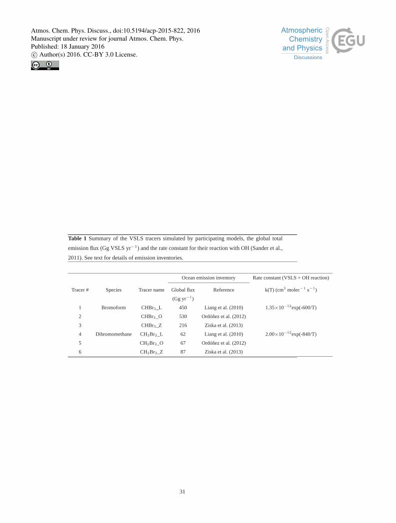
Table 1 Summary of the VSLS tracers simulated by participating models, the global total

emission flux (Gg VSLS yr−1) and the rate constant for their reaction with OH (Sander et al.,

2011). See text for details of emission inventories.

Ocean emission inventory Rate constant (VSLS + OH reaction)

Tracer # Species Tracer name Global flux Reference k(T) (cm3 molec−1 s−1)

(Gg yr−1)

1 Bromoform CHBr3_L 450 Liang et al. (2010) 1.35×10−12exp(-600/T)

2 CHBr3_O 530 Ordóñez et al. (2012)

3 CHBr3_Z 216 Ziska et al. (2013)

4 Dibromomethane CH2Br2_L 62 Liang et al. (2010) 2.00×10−12exp(-840/T)

5 CH2Br2_O 67 Ordóñez et al. (2012)

6 CH2Br2_Z 87 Ziska et al. (2013)

31


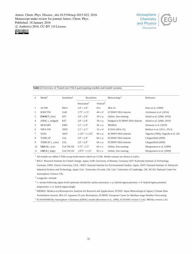
Table 2Overview of TransCom-VSLS participating models and model variants.

# Model1 Institution2 Resolution Meteorology5 Reference

Horizontal3 Vertical4

1 ACTM RIGC 2.8◦×2.8◦ 67σ JRA-25 Patra et al. (2009)

2 B3DCTM UoB 3.75◦×2.5◦ 40σ-θ ECMWF ERA-Interim Aschmann et al. (2014)

3 EMAC 6(_free) KIT 2.8◦×2.8◦ 39σ-p Online, free-running Jöckel et al. (2006, 2010)

4 EMAC (_nudged) KIT 2.8◦×2.8◦ 39σ-p Nudged to ECMWF ERA-Interim Jöckel et al. (2006, 2010)

5 MOZART EMU 2.5◦×1.9◦ 56σ-p MERRA Emmons et al. (2010)

6 NIES-TM NIES 2.5◦×2.5◦ 32σ-θ JCDAS (JRA-25) Belikov et al. (2011, 2013)

7 STAG AIST 1.125◦×1.125◦ 60σ-p ECMWF ERA-Interim Taguchi (1996); Taguchi et al. (2013)

8 TOMCAT UoL 2.8◦×2.8◦ 60σ-p ECMWF ERA-Interim Chipperfield (2009)

9 TOMCAT (_conv) UoL 2.8◦×2.8◦ 60σ-p ECMWF ERA-Interim Chipperfield (2009)

10 UKCA (_low) UoC/NCAS 3.75◦×2.5◦ 60σ-z Online, free-running Morgenstern et al. (2009)

11 UKCA (_high) UoC/NCAS 1.875◦×1.25◦ 85σ-z Online, free-running Morgenstern et al. (2009)

1 All models are offline CTMs except bold entries which are CCMs. Model variants are shown in italics.2 RIGC: Research Institute for Global Change, Japan; UoB: Universityof Bremen, Germany; KIT: Karlsruhe Institute of Technology,

Germany; EMU: Emory University, USA ; NIES: National Institute for Environmental Studies, Japan; AIST: National Institute of Advanced

Industrial Science and Technology, Japan; UoL: University of Leeds, UK; UoC: University of Cambridge, UK; NCAS: National Centre for

Atmospheric Science, UK.3 Longitude×latitude4 σ: terrain-following sigma levels (pressure divided by surface pressure);σ-p: hybrid sigma-pressure;σ-θ: hybrid sigma-potential

temperature;σ-z: hybrid sigma-height.5 MERRA: Modern-era Retrospective Analysis for Research and Applications; JCDAS: Japan Meteorological Agency Climate Data

Assimilation System; JRA-25: Japanese 25-year ReAnalysis; ECMWF: European Center for Medium range Weather Forecasting.6 ECHAM/MESSy Atmospheric Chemistry (EMAC) model (Roeckner et al.,2006). ECHAM5 version 5.3.02. MESSy version 2.42.

32


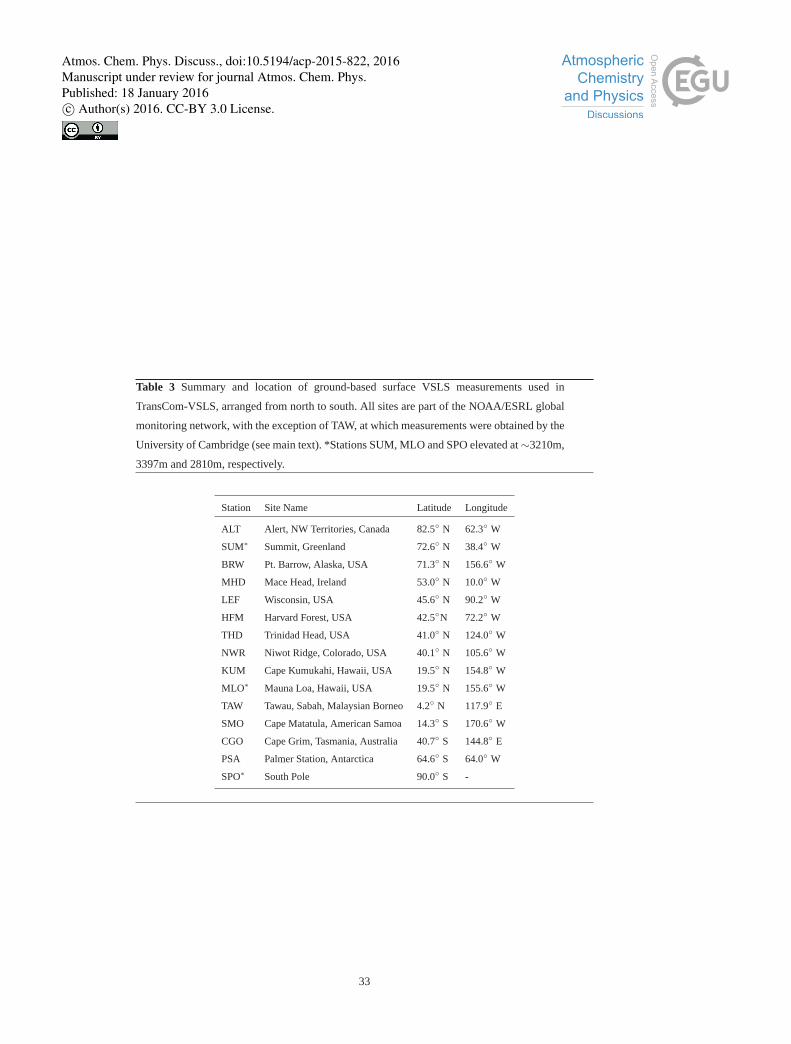
Table 3 Summary and location of ground-based surface VSLS measurements used in

TransCom-VSLS, arranged from north to south. All sites are part of the NOAA/ESRL global

monitoring network, with the exception of TAW, at which measurements were obtained by the

University of Cambridge (see main text). *Stations SUM, MLOand SPO elevated at∼3210m,

3397m and 2810m, respectively.

Station Site Name Latitude Longitude

ALT Alert, NW Territories, Canada 82.5◦ N 62.3◦ W

SUM∗ Summit, Greenland 72.6◦ N 38.4◦ W

BRW Pt. Barrow, Alaska, USA 71.3◦ N 156.6◦ W

MHD Mace Head, Ireland 53.0◦ N 10.0◦ W

LEF Wisconsin, USA 45.6◦ N 90.2◦ W

HFM Harvard Forest, USA 42.5◦N 72.2◦ W

THD Trinidad Head, USA 41.0◦ N 124.0◦ W

NWR Niwot Ridge, Colorado, USA 40.1◦ N 105.6◦ W

KUM Cape Kumukahi, Hawaii, USA 19.5◦ N 154.8◦ W

MLO∗ Mauna Loa, Hawaii, USA 19.5◦ N 155.6◦ W

TAW Tawau, Sabah, Malaysian Borneo 4.2◦ N 117.9◦ E

SMO Cape Matatula, American Samoa 14.3◦ S 170.6◦ W

CGO Cape Grim, Tasmania, Australia 40.7◦ S 144.8◦ E

PSA Palmer Station, Antarctica 64.6◦ S 64.0◦ W

SPO∗ South Pole 90.0◦ S -

33


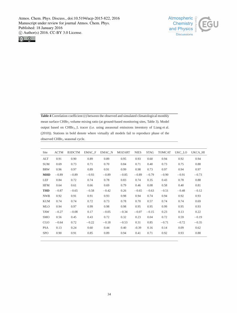
Table 4Correlation coefficient (r) between the observed and simulated climatological monthly

mean surface CHBr3 volume mixing ratio (at ground-based monitoring sites, Table 3). Model

output based on CHBr3_L tracer (i.e. using aseasonal emissions inventory of Liang et al.

(2010)). Stations in bold denote where virtually all modelsfail to reproduce phase of the

observed CHBr3 seasonal cycle.

Site ACTM B3DCTM EMAC_F EMAC_N MOZART NIES STAG TOMCAT UKC_LO UKCA_HI

ALT 0.91 0.90 0.89 0.89 0.95 0.93 0.60 0.94 0.92 0.94

SUM 0.69 0.73 0.71 0.70 0.84 0.71 0.40 0.73 0.75 0.88

BRW 0.96 0.97 0.89 0.91 0.99 0.98 0.73 0.97 0.94 0.97

MHD −0.89 −0.89 −0.93 −0.89 −0.85 −0.89 −0.79 −0.90 −0.91 −0.73

LEF 0.84 0.72 0.74 0.78 0.83 0.74 0.35 0.43 0.78 0.88

HFM 0.64 0.61 0.66 0.69 0.79 0.46 0.08 0.58 0.40 0.81

THD −0.87 −0.65 −0.58 −0.42 0.26 −0.65 −0.63 −0.51 −0.48 −0.12

NWR 0.92 0.91 0.91 0.93 0.98 0.94 0.74 0.94 0.92 0.93

KUM 0.74 0.74 0.72 0.73 0.78 0.70 0.57 0.74 0.74 0.69

MLO 0.94 0.97 0.99 0.98 0.98 0.95 0.95 0.99 0.95 0.93

TAW −0.27 −0.08 0.17 −0.05 −0.34 −0.07 −0.15 0.23 0.13 0.22

SMO 0.56 0.45 0.43 0.72 0.32 0.23 0.04 0.72 0.59 −0.19

CGO −0.64 0.72 −0.22 −0.18 −0.53 0.31 0.85 −0.71 −0.72 −0.35

PSA 0.13 0.24 0.60 0.44 0.40 -0.39 0.16 0.14 0.09 0.62

SPO 0.90 0.91 0.85 0.89 0.94 0.41 0.71 0.92 0.93 0.88

34


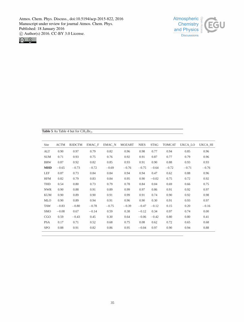
Table 5As Table 4 but for CH2Br2.

Site ACTM B3DCTM EMAC_F EMAC_N MOZART NIES STAG TOMCAT UKCA_LO UKCA_HI

ALT 0.90 0.97 0.79 0.82 0.96 0.98 0.77 0.94 0.85 0.96

SUM 0.71 0.93 0.75 0.76 0.92 0.91 0.87 0.77 0.79 0.96

BRW 0.87 0.92 0.82 0.85 0.93 0.91 0.90 0.88 0.93 0.93

MHD −0.65 −0.73 −0.72 −0.69 −0.76 −0.75 −0.64 −0.72 −0.71 −0.76

LEF 0.87 0.73 0.84 0.84 0.94 0.94 0.47 0.62 0.88 0.96

HFM 0.82 0.79 0.83 0.84 0.95 0.90 −0.02 0.75 0.72 0.92

THD 0.54 0.80 0.73 0.79 0.78 0.84 0.04 0.69 0.66 0.75

NWR 0.90 0.88 0.91 0.89 0.99 0.97 0.86 0.91 0.92 0.97

KUM 0.90 0.89 0.90 0.91 0.99 0.91 0.74 0.90 0.92 0.98

MLO 0.90 0.89 0.94 0.91 0.96 0.90 0.30 0.91 0.93 0.97

TAW −0.83 −0.80 −0.78 −0.75 −0.39 −0.47 −0.12 0.15 0.20 −0.16

SMO −0.08 0.67 −0.14 0.59 0.38 −0.12 0.34 0.97 0.74 0.00

CGO 0.59 −0.43 0.45 0.30 0.64 −0.06 −0.42 0.80 0.80 0.41

PSA 0.17 0.71 0.52 0.68 0.75 0.08 0.62 0.72 0.65 0.68

SPO 0.88 0.91 0.82 0.86 0.95 −0.04 0.97 0.90 0.94 0.88

35


TransCom-VSLS

EmissionInventories

Top-down Bottom-up

3x CHBr3

3x CH2Br2

2x CH3I

VSLS

Global Models& their variants

StandardisedChemistry

Photolysis

rates

Prescribed

oxidants

ObservationsGround-based,

ship, aircraft

Model

evaluation

8 Tracers

VSLS Distribution

& Trends(altitude, latitude,

season, year)

Troposphere to

Stratosphere

Transport(preferred pathways)

Reconciled

estimate of

bromine SGI

Stratospheric Br

Source Gas

Injection (SGI)(inter-model variability)

Isolate

transport-driven

inter-model

variability

Figure 1. Schematic of the the TransCom-VSLS project approach.

-90 090 180

-30

30

90

90 180 -90

90 180 -90

-30

30

-3030

Surface ATTREX 13 ATTERX 14 CAST HIPPO-1 HIPPO-2 HIPPO-3

HIPPO-4 HIPPO-5 Pre-Ave CR-AVE SHIVA (ship) TransBrom (ship)

Figure 2. Summary of ground-based and campaign data used in TransCom-VSLS. See main text for details.

36


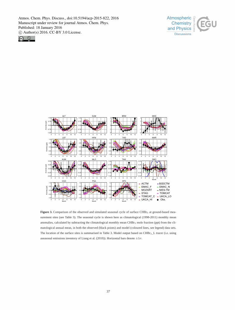
ALT

0 2 4 6 8 10 12

-1.50

-0.75

0.00

0.75

1.50

An

om

aly

[p

pt]

SUM

0 2 4 6 8 10 12

-1.50

-0.75

0.00

0.75

1.50BRW

0 2 4 6 8 10 12

-2

-1

0

1

2MHD

0 2 4 6 8 10 12

-2

-1

0

1

2

LEF

0 2 4 6 8 10 12

-1.0

-0.5

0.0

0.5

1.0

An

om

aly

[p

pt]

HFM

0 2 4 6 8 10 12

-1.0

-0.5

0.0

0.5

1.0THD

0 2 4 6 8 10 12

-1.0

-0.5

0.0

0.5

1.0NWR

0 2 4 6 8 10 12

-1.0

-0.5

0.0

0.5

1.0

KUM

0 2 4 6 8 10 12

-0.50

-0.25

0.00

0.25

0.50

An

om

aly

[p

pt]

MLO

0 2 4 6 8 10 12

-0.50

-0.25

0.00

0.25

0.50TAW

0 2 4 6 8 10 12

-1.50

-0.75

0.00

0.75

1.50SMO

0 2 4 6 8 10 12Month

-0.50

-0.25

0.00

0.25

0.50

CGO

0 2 4 6 8 10 12Month

-1.0

-0.5

0.0

0.5

1.0

An

om

aly

[p

pt]

PSA

0 2 4 6 8 10 12Month

-1.0

-0.5

0.0

0.5

1.0SPO

0 2 4 6 8 10 12Month

-1.0

-0.5

0.0

0.5

1.0ACTM B3DCTM

EMAC_F EMAC_N

MOZART NIES-TM

STAG TOMCAT

TOMCAT_C UKCA_LO

UKCA_HI Obs.

Figure 3. Comparison of the observed and simulated seasonal cycle of surfaceCHBr3 at ground-based mea-

surement sites (see Table 3). The seasonal cycle is shown here as climatological (1998-2011) monthly mean

anomalies, calculated by subtracting the climatological monthly mean CHBr3 mole fraction (ppt) from the cli-

matological annual mean, in both the observed (black points) and model(coloured lines, see legend) data sets.

The location of the surface sites is summarised in Table 3. Model output based on CHBr3_L tracer (i.e. using

aseasonal emissions inventory of Liang et al. (2010)). Horizontal bars denote±1σ.

37


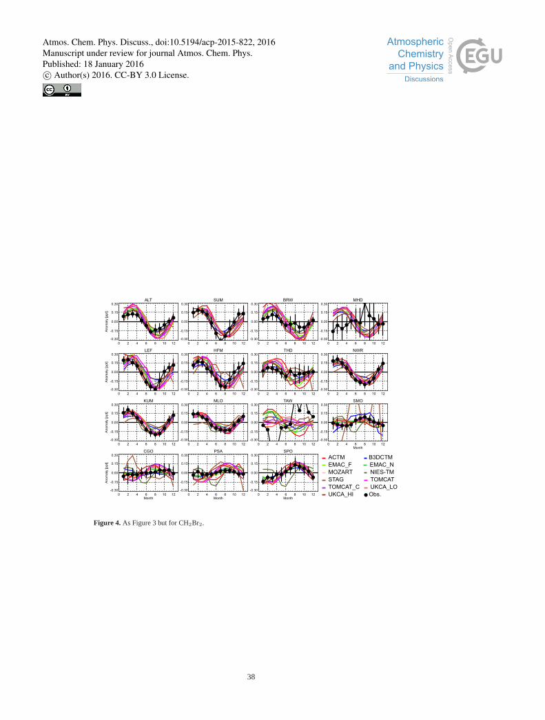
ALT

0 2 4 6 8 10 12

-0.30

-0.15

0.00

0.15

0.30

An

om

aly

[p

pt]

SUM

0 2 4 6 8 10 12

-0.30

-0.15

0.00

0.15

0.30BRW

0 2 4 6 8 10 12

-0.30

-0.15

0.00

0.15

0.30MHD

0 2 4 6 8 10 12

-0.30

-0.15

0.00

0.15

0.30

LEF

0 2 4 6 8 10 12

-0.30

-0.15

0.00

0.15

0.30

An

om

aly

[p

pt]

HFM

0 2 4 6 8 10 12

-0.30

-0.15

0.00

0.15

0.30THD

0 2 4 6 8 10 12

-0.30

-0.15

0.00

0.15

0.30NWR

0 2 4 6 8 10 12

-0.30

-0.15

0.00

0.15

0.30

KUM

0 2 4 6 8 10 12

-0.30

-0.15

0.00

0.15

0.30

An

om

aly

[p

pt]

MLO

0 2 4 6 8 10 12

-0.30

-0.15

0.00

0.15

0.30TAW

0 2 4 6 8 10 12

-0.30

-0.15

0.00

0.15

0.30SMO

0 2 4 6 8 10 12Month

-0.30

-0.15

0.00

0.15

0.30

CGO

0 2 4 6 8 10 12Month

-0.30

-0.15

0.00

0.15

0.30

An

om

aly

[p

pt]

PSA

0 2 4 6 8 10 12Month

-0.30

-0.15

0.00

0.15

0.30SPO

0 2 4 6 8 10 12Month

-0.30

-0.15

0.00

0.15

0.30ACTM B3DCTM

EMAC_F EMAC_N

MOZART NIES-TM

STAG TOMCAT

TOMCAT_C UKCA_LO

UKCA_HI Obs.

Figure 4. As Figure 3 but for CH2Br2.

38


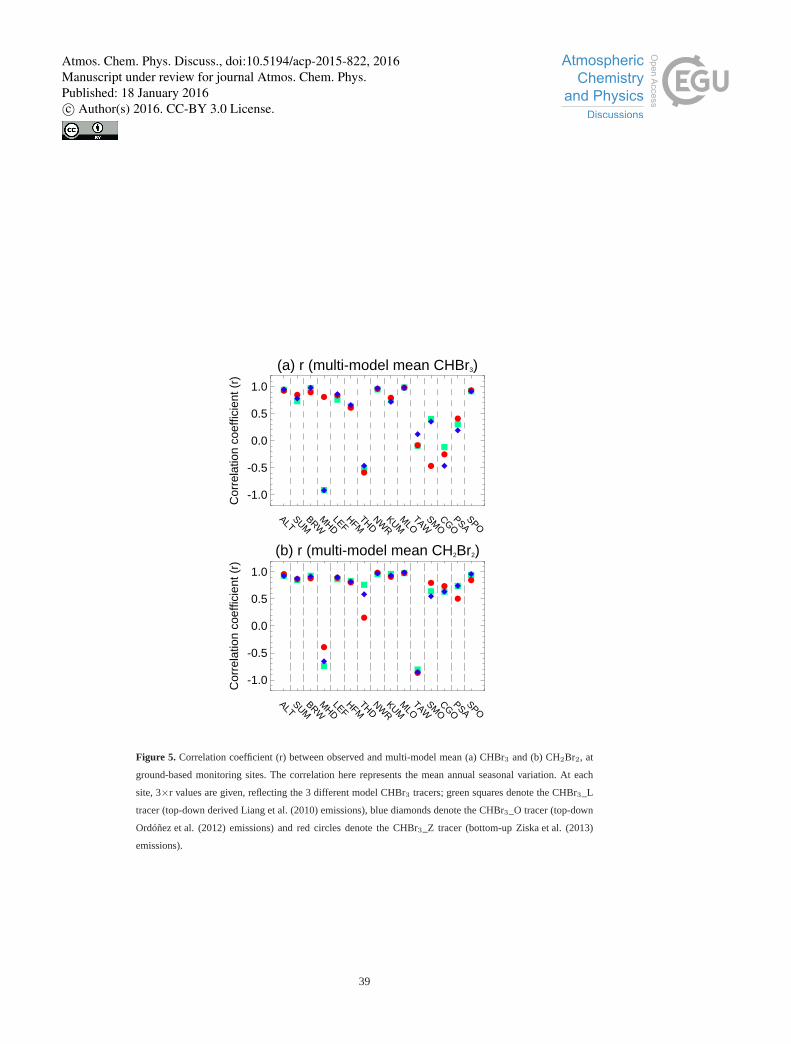
(a) r (multi-model mean CHBr3)

-1.0

-0.5

0.0

0.5

1.0

Cor

rela

tion

coef

ficie

nt (

r)

ALTSUM

BRWM

HDLEF

HFMTHD

NWRKUM

MLO

TAWSM

OCGO

PSASPO

(b) r (multi-model mean CH2Br2)

-1.0

-0.5

0.0

0.5

1.0

Cor

rela

tion

coef

ficie

nt (

r)

ALTSUM

BRWM

HDLEF

HFMTHD

NWRKUM

MLO

TAWSM

OCGO

PSASPO

Figure 5. Correlation coefficient (r) between observed and multi-model mean (a) CHBr3 and (b) CH2Br2, at

ground-based monitoring sites. The correlation here represents the mean annual seasonal variation. At each

site, 3×r values are given, reflecting the 3 different model CHBr3 tracers; green squares denote the CHBr3_L

tracer (top-down derived Liang et al. (2010) emissions), blue diamonds denote the CHBr3_O tracer (top-down

Ordóñez et al. (2012) emissions) and red circles denote the CHBr3_Z tracer (bottom-up Ziska et al. (2013)

emissions).

39


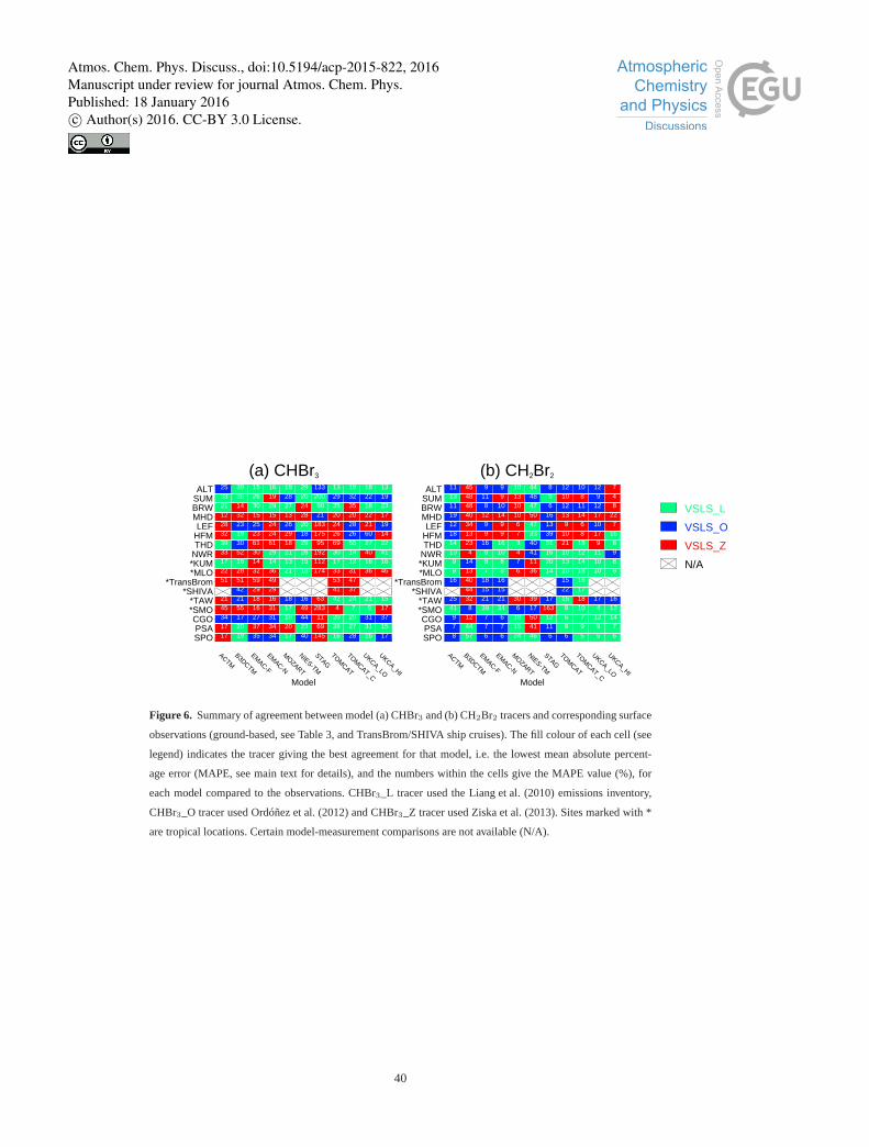
Model

SPO PSA CGO *SMO *TAW *SHIVA

*TransBrom *MLO *KUM NWR THD HFM LEF MHD BRW SUM ALT

ACTM B3DCTM

EMAC-F

EMAC-N

MOZART

NIES-TM

STAG TOM

CAT

TOMCAT_C

UKCA_LO

UKCA_HI

17 17 34 45 21*** 51 22 17 33 39 32 28 12 21 33 25

19 20 17 55 21 42 51 28 16 52 30 19 23 32 14 35 39

35 37 27 16 18 29 59 32 14 30 61 23 25 15 30 26 15

34 34 31 31 16 29 49 36 14 29 61 24 24 15 29 19 16

17 20 18 17 18****** 21 13 21 18 29 26 13 27 28 18

40 23 44 49 16****** 18 15 28 29 18 20 28 24 20 29

145 69 11283 63******174112192 95175183 21 90200133

16 28 20 4 42 41 53 33 17 30 69 26 24 20 35 29 13

28 27 20 7 24 37 47 31 12 14 55 26 28 20 35 32 18

16 31 31 9 21****** 36 16 40 27 60 21 22 18 22 18

17 15 37 17 15****** 46 16 41 22 14 19 17 23 19 13

(a) CHBr3 (b) CH2Br2

Model

SPO PSA CGO *SMO *TAW *SHIVA

*TransBrom *MLO *KUM NWR THD HFM LEF MHD BRW SUM ALT

ACTM B3DCTM

EMAC-F

EMAC-N

MOZART

NIES-TM

STAG TOM

CAT

TOMCAT_C

UKCA_LO

UKCA_HI

8 7 9 41 25*** 16 9 9 13 14 18 12 19 11 13 11

57 44 12 8 32 44 40 13 14 4 23 13 34 40 48 48 45

6 7 7 39 21 15 18 7 8 8 16 9 9 12 8 11 9

6 7 6 34 21 15 16 8 8 10 16 9 9 14 10 9 9

24 15 18 6 30****** 6 7 4 3 7 6 10 10 13 10

46 41 50 17 39****** 36 11 41 40 33 47 50 47 48 44

6 11 12163 17****** 14 20 16 31 39 13 16 6 9 8

6 9 6 8 16 22 15 10 13 10 21 10 9 13 12 10 12

5 9 7 10 18 17 16 18 14 12 18 8 6 14 11 8 10

5 9 12 4 17****** 10 10 11 9 17 10 17 12 9 12

6 7 14 12 16****** 9 8 9 8 16 7 22 8 4 7

VSLS_L

VSLS_O

VSLS_Z

N/A

Figure 6. Summary of agreement between model (a) CHBr3 and (b) CH2Br2 tracers and corresponding surface

observations (ground-based, see Table 3, and TransBrom/SHIVA ship cruises). The fill colour of each cell (see

legend) indicates the tracer giving the best agreement for that model, i.e. the lowest mean absolute percent-

age error (MAPE, see main text for details), and the numbers within the cells give the MAPE value (%), for

each model compared to the observations. CHBr3_L tracer used the Liang et al. (2010) emissions inventory,

CHBr3_O tracer used Ordóñez et al. (2012) and CHBr3_Z tracer used Ziska et al. (2013). Sites marked with *

are tropical locations. Certain model-measurement comparisons are not available (N/A).

40


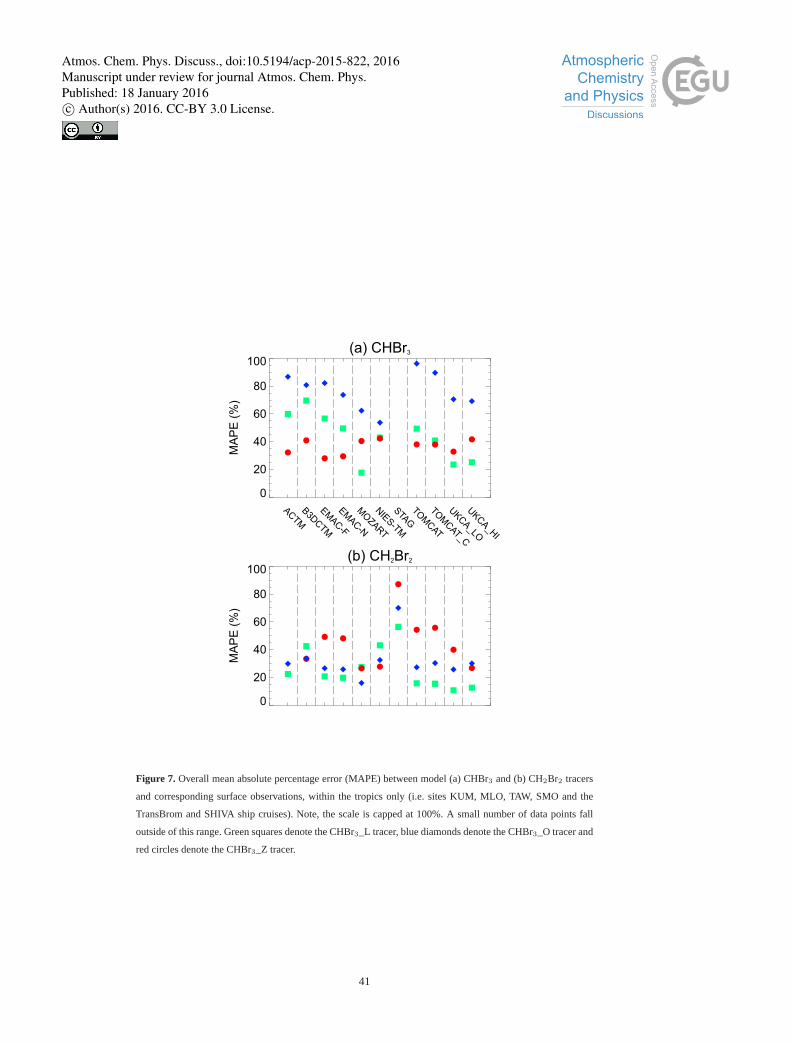
(a) CHBr3

0

20

40

60

80

100

MA

PE

(%

)

ACTM

B3D

CTM

EM

AC-F

EM

AC-N

MOZA

RT

NIE

S-TM

STA

G

TOM

CAT

TOM

CAT_C

UKCA_LO

UKCA_H

I

(b) CH2Br2

0

20

40

60

80

100

MA

PE

(%

)

Figure 7. Overall mean absolute percentage error (MAPE) between model (a) CHBr3 and (b) CH2Br2 tracers

and corresponding surface observations, within the tropics only (i.e. sites KUM, MLO, TAW, SMO and the

TransBrom and SHIVA ship cruises). Note, the scale is capped at 100%. A small number of data points fall

outside of this range. Green squares denote the CHBr3_L tracer, blue diamonds denote the CHBr3_O tracer and

red circles denote the CHBr3_Z tracer.

41


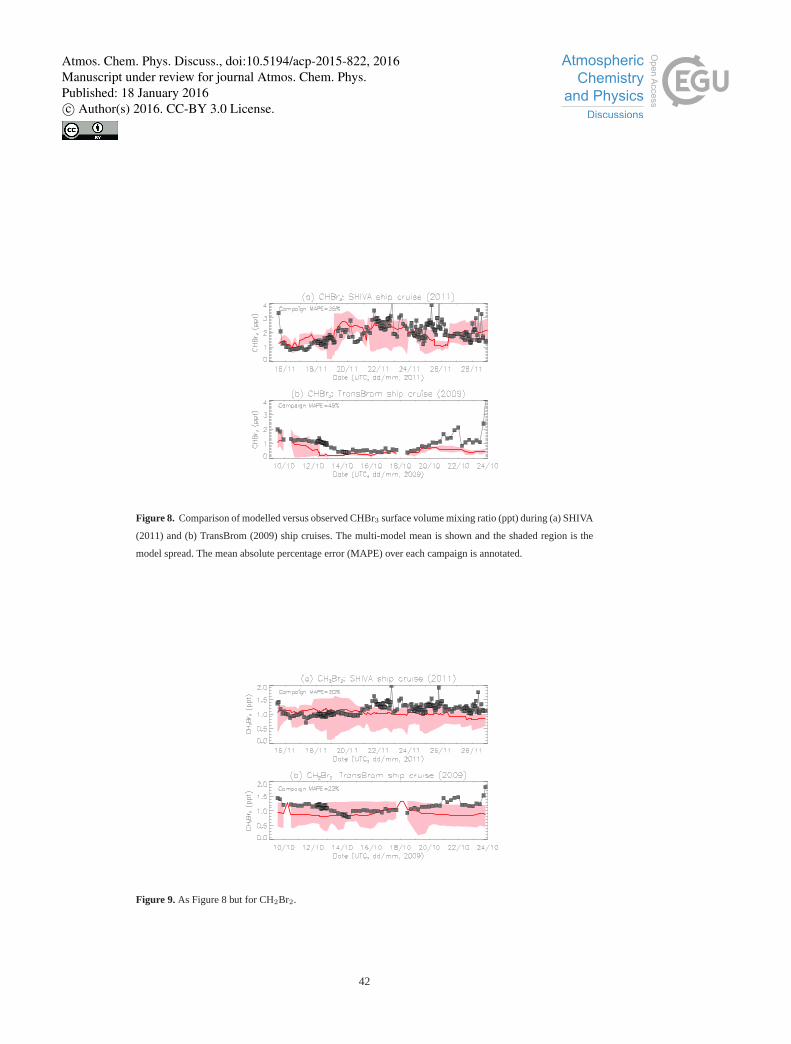
Figure 8. Comparison of modelled versus observed CHBr3 surface volume mixing ratio (ppt) during (a) SHIVA

(2011) and (b) TransBrom (2009) ship cruises. The multi-model mean is shown and the shaded region is the

model spread. The mean absolute percentage error (MAPE) over each campaign is annotated.


42


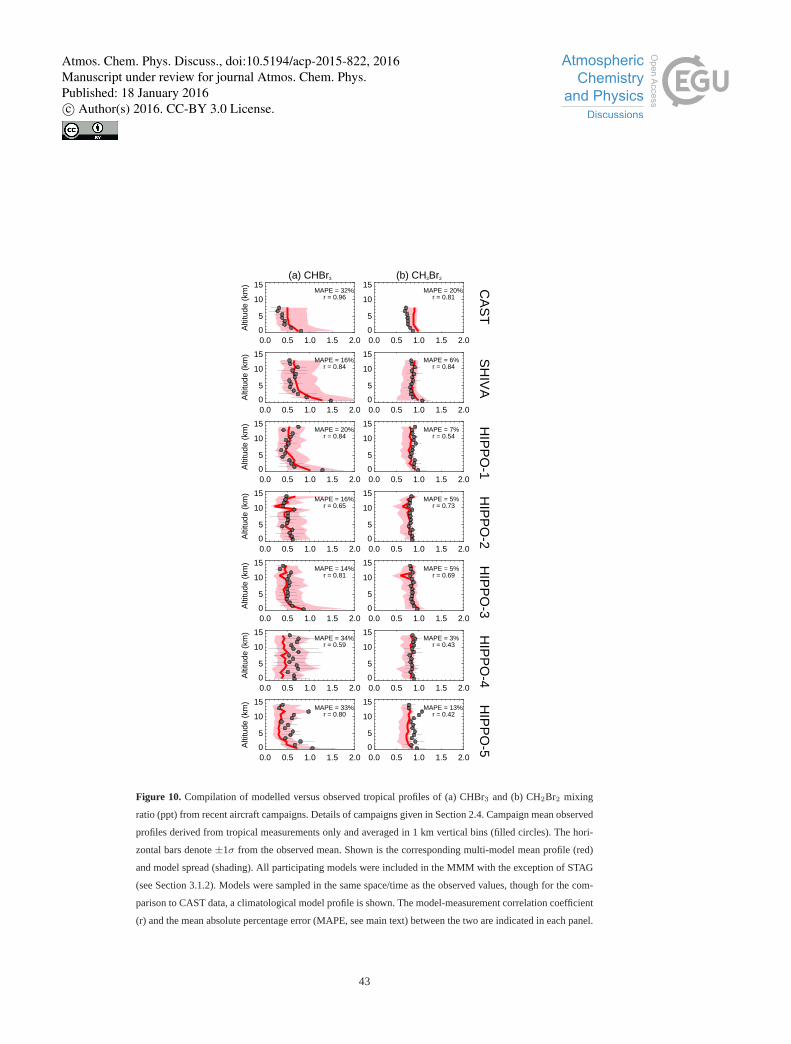
(a) CHBr3

0.0 0.5 1.0 1.5 2.00

5

10

15

Alti

tude

(km

) CA

ST

r = 0.96MAPE = 32%

(b) CH2Br2

0.0 0.5 1.0 1.5 2.00

5

10

15

r = 0.81MAPE = 20%

0.0 0.5 1.0 1.5 2.00

5

10

15

Alti

tude

(km

) SH

IVA

r = 0.84MAPE = 16%

0.0 0.5 1.0 1.5 2.00

5

10

15

r = 0.84MAPE = 6%

0.0 0.5 1.0 1.5 2.00

5

10

15

Alti

tude

(km

) HIP

PO

-1

r = 0.84MAPE = 20%

0.0 0.5 1.0 1.5 2.00

5

10

15

r = 0.54MAPE = 7%

0.0 0.5 1.0 1.5 2.00

5

10

15

Alti

tude

(km

) HIP

PO

-2

r = 0.65MAPE = 16%

0.0 0.5 1.0 1.5 2.00

5

10

15

r = 0.73MAPE = 5%

0.0 0.5 1.0 1.5 2.00

5

10

15

Alti

tude

(km

) HIP

PO

-3

r = 0.81MAPE = 14%

0.0 0.5 1.0 1.5 2.00

5

10

15

r = 0.69MAPE = 5%

0.0 0.5 1.0 1.5 2.00

5

10

15

Alti

tude

(km

) HIP

PO

-4

r = 0.59MAPE = 34%

0.0 0.5 1.0 1.5 2.00

5

10

15

r = 0.43MAPE = 3%

0.0 0.5 1.0 1.5 2.00

5

10

15

Alti

tude

(km

) HIP

PO

-5

r = 0.80MAPE = 33%

0.0 0.5 1.0 1.5 2.00

5

10

15

r = 0.42MAPE = 13%

Figure 10. Compilation of modelled versus observed tropical profiles of (a) CHBr3 and (b) CH2Br2 mixing

ratio (ppt) from recent aircraft campaigns. Details of campaigns given in Section 2.4. Campaign mean observed

profiles derived from tropical measurements only and averaged in 1 km vertical bins (filled circles). The hori-

zontal bars denote±1σ from the observed mean. Shown is the corresponding multi-model meanprofile (red)

and model spread (shading). All participating models were included in theMMM with the exception of STAG

(see Section 3.1.2). Models were sampled in the same space/time as the observed values, though for the com-

parison to CAST data, a climatological model profile is shown. The model-measurement correlation coefficient

(r) and the mean absolute percentage error (MAPE, see main text) between the two are indicated in each panel.

43


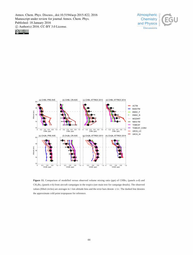
0 0.2 0.4 0.6 0.8 1.0

12

14

16

18

20(a) CHBr3 PRE-AVE

0 0.2 0.4 0.6 0.8 1.0CHBr3 (ppt)

12

14

16

18

20

Altitude (

km

)

(b) CHBr3 CR-AVE

0 0.2 0.4 0.6 0.8 1.0CHBr3 (ppt)

(c) CHBr3 ATTREX 2013

0 0.2 0.4 0.6 0.8 1.0CHBr3 (ppt)

(d) CHBr3 ATTREX 2014

0 0.2 0.4 0.6 0.8 1.0CHBr3 (ppt)

(e) CH2Br2 PRE-AVE

0 0.3 0.6 0.9 1.2CH2Br2 (ppt)

12

14

16

18

20

Altitude (

km

)

(f) CH2Br2 CR-AVE

0 0.3 0.6 0.9 1.2CH2Br2 (ppt)

(g) CH2Br2 ATTREX 2013

0 0.3 0.6 0.9 1.2CH2Br2 (ppt)

(h) CH2Br2 ATTREX 2014

0 0.3 0.6 0.9 1.2CH2Br2 (ppt)

ACTM

B3DCTM

EMAC_F

EMAC_N

MOZART

NIES-TM

TOMCAT

TOMCAT_CONV

UKCA_LO

UKCA_HI

Figure 11. Comparison of modelled versus observed volume mixing ratio (ppt) of CHBr3 (panels a-d) and

CH2Br2 (panels e-h) from aircraft campaigns in the tropics (see main text for campaign details). The observed

values (filled circles) are averages in 1 km altitude bins and the error barsdenote±1σ. The dashed line denotes

the approximate cold point tropopause for reference.

44


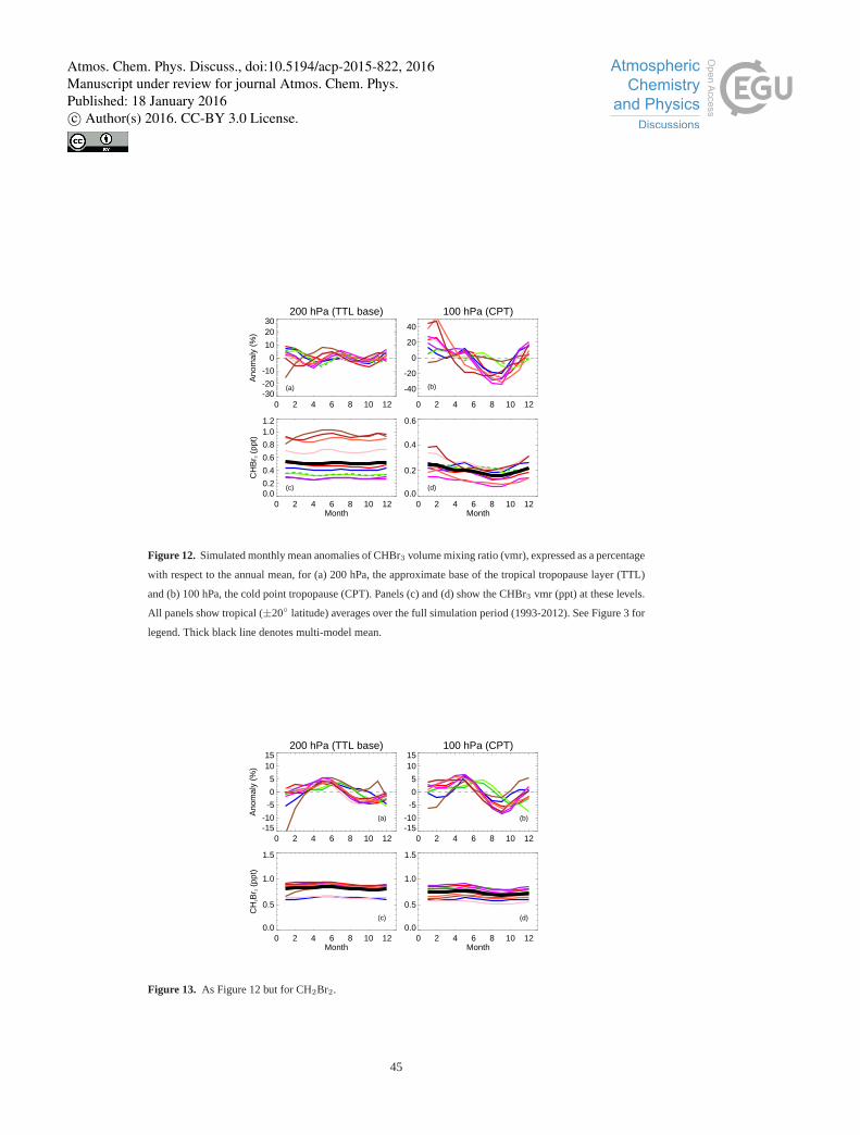
200 hPa (TTL base)

0 2 4 6 8 10 12-30-20

-10

0

10

2030

Ano

mal

y (%

)

(a)

100 hPa (CPT)

0 2 4 6 8 10 12

-40

-20

0

20

40

(b)

0 2 4 6 8 10 12Month

0.00.2

0.4

0.6

0.8

1.01.2

CH

Br 3

(ppt

)

(c)

0 2 4 6 8 10 12Month

0.0

0.2

0.4

0.6

(d)

Figure 12. Simulated monthly mean anomalies of CHBr3 volume mixing ratio (vmr), expressed as a percentage

with respect to the annual mean, for (a) 200 hPa, the approximate baseof the tropical tropopause layer (TTL)

and (b) 100 hPa, the cold point tropopause (CPT). Panels (c) and (d)show the CHBr3 vmr (ppt) at these levels.

All panels show tropical (±20◦ latitude) averages over the full simulation period (1993-2012). See Figure 3 for

legend. Thick black line denotes multi-model mean.

200 hPa (TTL base)

0 2 4 6 8 10 12-15-10

-5

0

5

1015

Ano

mal

y (%

)

(a)

100 hPa (CPT)

0 2 4 6 8 10 12-15-10

-5

0

5

1015

(b)

0 2 4 6 8 10 12Month

0.0

0.5

1.0

1.5

CH

2Br 2

(ppt

)

(c)

0 2 4 6 8 10 12Month

0.0

0.5

1.0

1.5

(d)


45


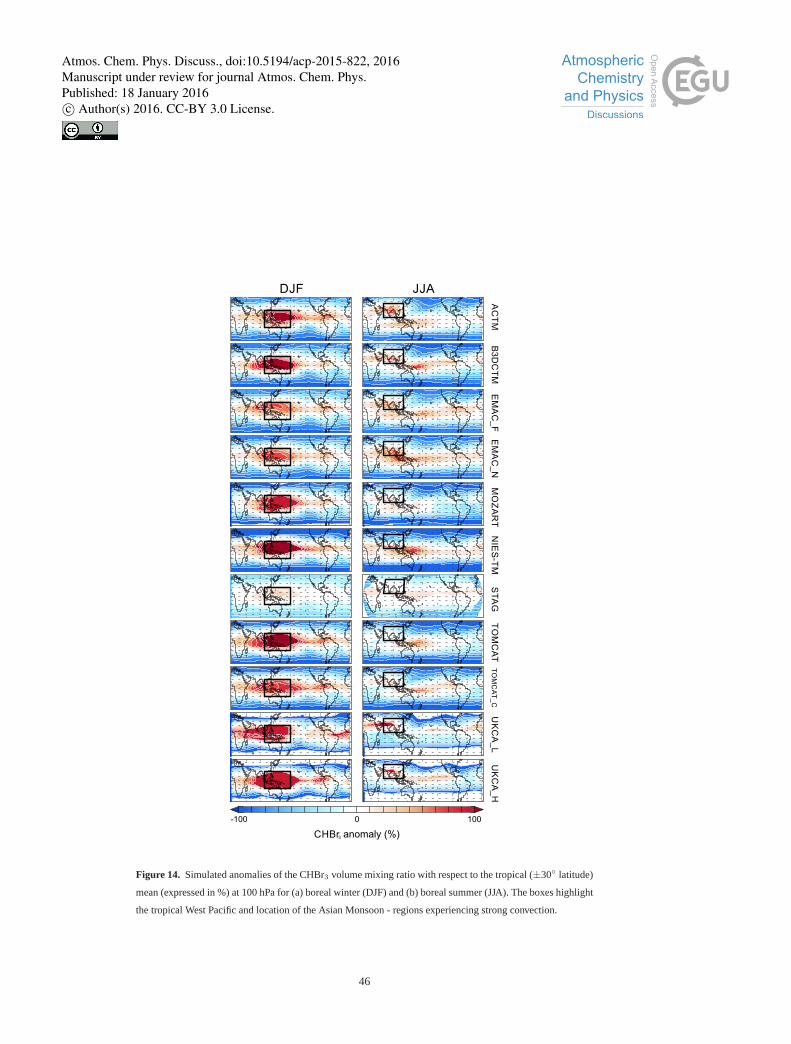
DJF JJAA

CT

MB

3D

CT

ME

MA

C_F

EM

AC

_N

MO

ZA

RT

NIE

S-T

MS

TA

GT

OM

CA

TT

OM

CA

T_

CU

KC

A_L

UK

CA

_H

-100 0 100

CHBr3 anom ly (%)a

Figure 14. Simulated anomalies of the CHBr3 volume mixing ratio with respect to the tropical (±30◦ latitude)

mean (expressed in %) at 100 hPa for (a) boreal winter (DJF) and (b) boreal summer (JJA). The boxes highlight

the tropical West Pacific and location of the Asian Monsoon - regions experiencing strong convection.

46


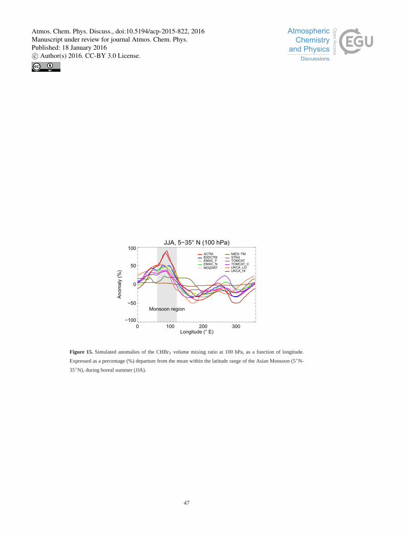
JJA, 5−35° N (100 hPa)

0 100 200 300Longitude (° E)

−100

−50

0

50

100

Anom

aly

(%

)

Monsoon region

ACTMB3DCTMEMAC_FEMAC_NMOZART

NIES−TMSTAGTOMCATTOMCAT_CUKCA_LOUKCA_HI

Figure 15. Simulated anomalies of the CHBr3 volume mixing ratio at 100 hPa, as a function of longitude.

Expressed as a percentage (%) departure from the mean within the latituderange of the Asian Monsoon (5◦N-

35◦N), during boreal summer (JJA).

47


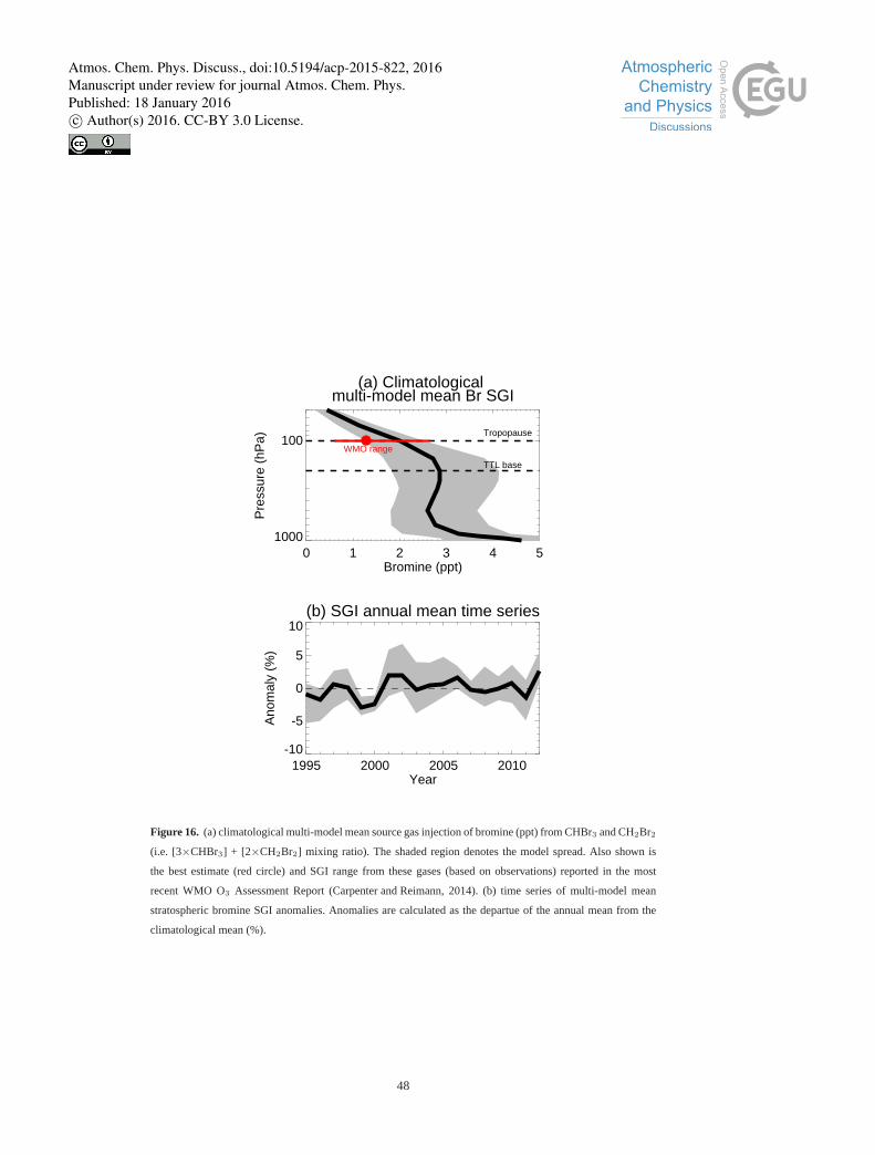
(a) Climatological multi-model mean Br SGI

0 1 2 3 4 5Bromine (ppt)

1000

100

Pre

ssur

e (h

Pa)

TTL base

Tropopause

WMO range

(b) SGI annual mean time series

1995 2000 2005 2010Year

-10

-5

0

5

10

Ano

mal

y (%

)

Figure 16. (a) climatological multi-model mean source gas injection of bromine (ppt) from CHBr3 and CH2Br2

(i.e. [3×CHBr3] + [2×CH2Br2] mixing ratio). The shaded region denotes the model spread. Also shown is

the best estimate (red circle) and SGI range from these gases (based on observations) reported in the most

recent WMO O3 Assessment Report (Carpenter and Reimann, 2014). (b) time seriesof multi-model mean

stratospheric bromine SGI anomalies. Anomalies are calculated as the departue of the annual mean from the

climatological mean (%).

48


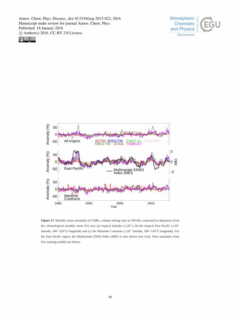
-50

0

50

Ano

mal

y (%

)

All tropics ACTM B3DCTM EMAC-N MOZARTNIES-TM STAG TOMCAT

-50

0

50

Ano

mal

y (%

)

East Pacific Multivariate ENSO Index (MEI) -3

0

3

ME

I

-50

0

50

Ano

mal

y (%

)

Maritime Continent

1995 2000 2005 2010Year

Figure 17.Monthly mean anomalies of CHBr3 volume mixing ratio at 100 hPa, expressed as departures from

the climatological monthly mean (%) over (a) tropical latitudes (±20◦), (b) the tropical East Pacific (±20◦

latitude, 180◦-250◦E longitude) and (c) the Maritime Continent (±20◦ latitude, 100◦-150◦E longitude). For

the East Pacific region, the Multivariate ENSO Index (MEI) is also shown (see text). Note anomalies from

free-running models not shown.

49


Documents

linking oceanic emissions and troposph - ACP - Recent