Embed Size (px)
Citation preview
Tectonophysics 474 (2009) 322–336
Contents lists available at ScienceDirect
Tectonophysics
j ourna l homepage: www.e lsev ie r.com/ locate / tecto
Lithospheric gravitational instability beneath the Southeast Carpathians
P. Lorinczi ⁎, G.A. HousemanEarth Sciences, School of Earth and Environment, University of Leeds, Leeds, LS2 9JT, UK
⁎ Corresponding author. Tel.: +44 113 3436620; fax:E-mail address: [email protected] (P. Lorincz
0040-1951/$ – see front matter © 2008 Elsevier B.V. Adoi:10.1016/j.tecto.2008.05.024
A B S T R A C T
A R T I C L E I N F OArticle history:
The Southeast corner of the Received 10 January 2008Received in revised form 24 April 2008Accepted 22 May 2008Available online 3 July 2008Keywords:Gravitational instabilitySeismicityStrain-rate tensorFinite-element methodViscous flowMantle downwelling
Carpathians, known as the Vrancea region, is characterised by a cluster of strongseismicity to depths of about 200 km. The peculiar features of this seismicity make it a region of highgeophysical interest. In this study we calculate the seismic strain-rate tensors for the period 1967–2007, anddescribe the variation of strain-rate with depth. The observed results are compared with strain-ratespredicted by numerical experiments. We explore a new dynamical model for this region based on the idea ofviscous flow of the lithospheric mantle permitting the development of local continental mantle downwellingbeneath Vrancea, due to a Rayleigh–Taylor instability that has developed since the cessation of subduction at11 Ma. The model simulations use a Lagrangean frame 3D finite-element algorithm solving the equations ofconservation of mass and momentum for a spatially varying viscous creeping flow. The finite deformationcalculations of the gravitational instability of the continental lithosphere demonstrate that the Rayleigh–Taylor mechanism can explain the present distribution of deformation within the downwelling lithosphere,both in terms of stress localisation and amplitude of strain-rates. The spatial extent of the high stress zonethat corresponds to the seismically active zone is realistically represented when we assume that viscositydecreases by at least an order of magnitude across the lithosphere. The mantle downwelling is balanced bylithospheric thinning in an adjacent area which would correspond to the Transylvanian Basin. Crustalthickening is predicted above the downwelling structure and thinning beneath the basin.
© 2008 Elsevier B.V. All rights reserved.
1. Introduction
The Carpathians are a major mountain system of Central andEastern Europe, linked to the Alpine and Dinaric systems, andsurround the Pannonian and Transylvanian Basins. Located in thesoutheast corner of the Carpathians, in Romania, the Vrancea region isbounded to the north and north-east by the Eastern Europeanplatform, to the west by the Transylvanian and Pannonian Basins, tothe south by the Moesian Platform, to the south-east by the DobrogeaOrogen and to the east by the Scythian platform.
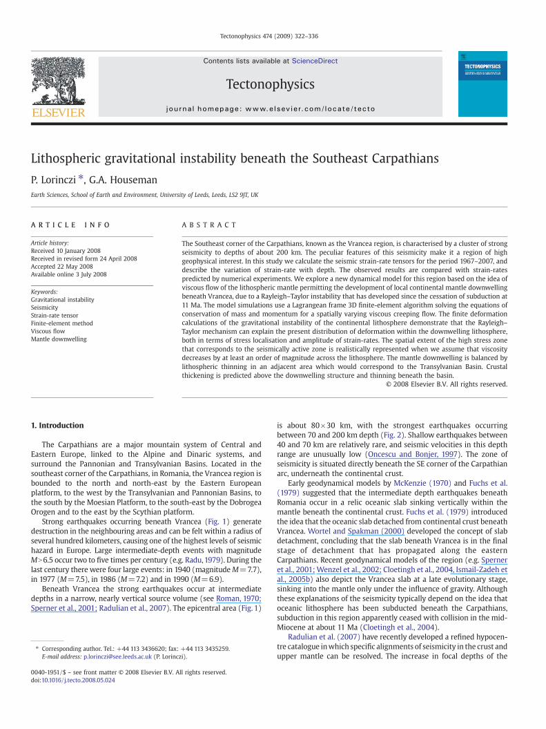
Strong earthquakes occurring beneath Vrancea (Fig. 1) generatedestruction in the neighbouring areas and can be felt within a radius ofseveral hundred kilometers, causing one of the highest levels of seismichazard in Europe. Large intermediate-depth events with magnitudeMN6.5 occur two to five times per century (e.g. Radu,1979). During thelast century there were four large events: in 1940 (magnitudeM=7.7),in 1977 (M=7.5), in 1986 (M=7.2) and in 1990 (M=6.9).
Beneath Vrancea the strong earthquakes occur at intermediatedepths in a narrow, nearly vertical source volume (see Roman, 1970;Sperner et al., 2001; Radulian et al., 2007). The epicentral area (Fig. 1)
+44 113 3435259.i).
ll rights reserved.
is about 80×30 km, with the strongest earthquakes occurringbetween 70 and 200 km depth (Fig. 2). Shallow earthquakes between40 and 70 km are relatively rare, and seismic velocities in this depthrange are unusually low (Oncescu and Bonjer, 1997). The zone ofseismicity is situated directly beneath the SE corner of the Carpathianarc, underneath the continental crust.
Early geodynamical models by McKenzie (1970) and Fuchs et al.(1979) suggested that the intermediate depth earthquakes beneathRomania occur in a relic oceanic slab sinking vertically within themantle beneath the continental crust. Fuchs et al. (1979) introducedthe idea that the oceanic slab detached from continental crust beneathVrancea. Wortel and Spakman (2000) developed the concept of slabdetachment, concluding that the slab beneath Vrancea is in the finalstage of detachment that has propagated along the easternCarpathians. Recent geodynamical models of the region (e.g. Sperneret al., 2001;Wenzel et al., 2002; Cloetingh et al., 2004, Ismail-Zadeh etal., 2005b) also depict the Vrancea slab at a late evolutionary stage,sinking into the mantle only under the influence of gravity. Althoughthese explanations of the seismicity typically depend on the idea thatoceanic lithosphere has been subducted beneath the Carpathians,subduction in this region apparently ceased with collision in the mid-Miocene at about 11 Ma (Cloetingh et al., 2004).
Radulian et al. (2007) have recently developed a refined hypocen-tre catalogue inwhich specific alignments of seismicity in the crust andupper mantle can be resolved. The increase in focal depths of the
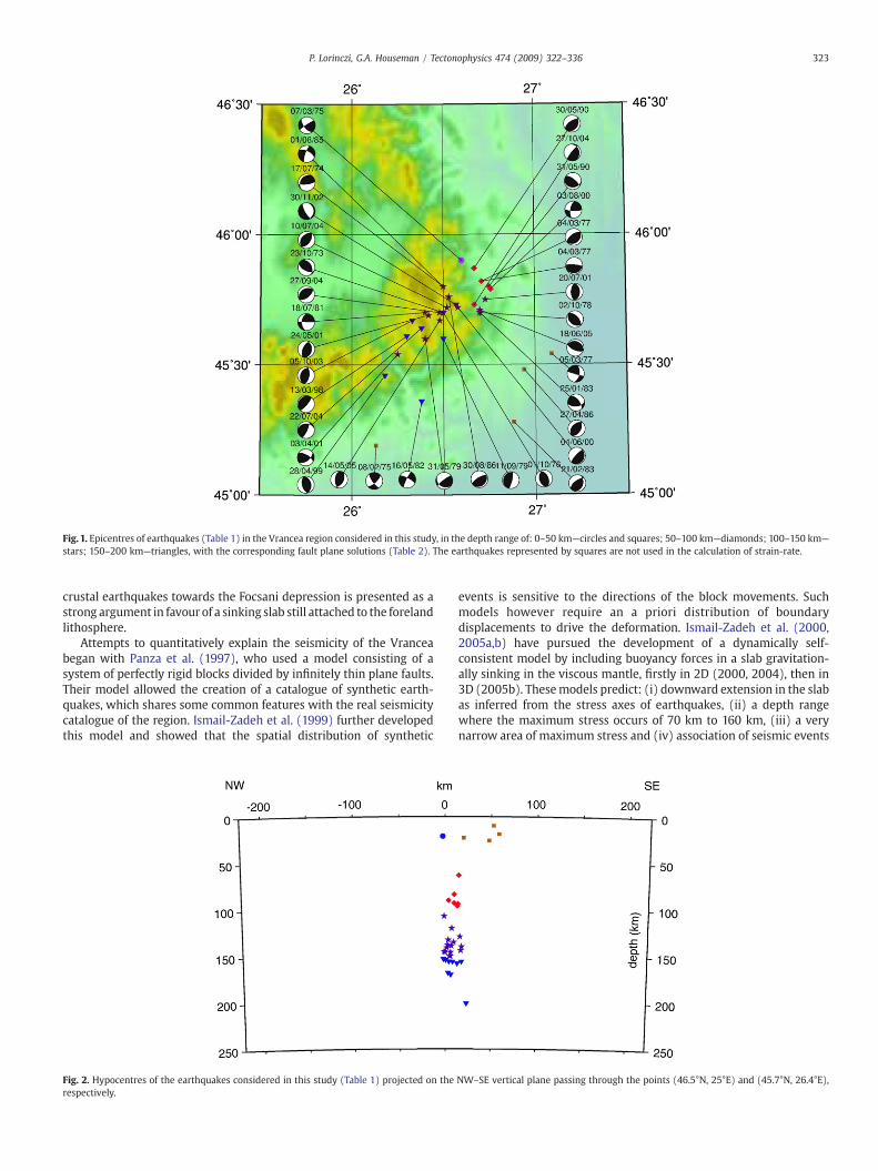
Fig. 1. Epicentres of earthquakes (Table 1) in the Vrancea region considered in this study, in the depth range of: 0–50 km—circles and squares; 50–100 km—diamonds; 100–150 km—
stars; 150–200 km—triangles, with the corresponding fault plane solutions (Table 2). The earthquakes represented by squares are not used in the calculation of strain-rate.
323P. Lorinczi, G.A. Houseman / Tectonophysics 474 (2009) 322–336
crustal earthquakes towards the Focsani depression is presented as astrong argument in favour of a sinking slab still attached to the forelandlithosphere.
Attempts to quantitatively explain the seismicity of the Vranceabegan with Panza et al. (1997), who used a model consisting of asystem of perfectly rigid blocks divided by infinitely thin plane faults.Their model allowed the creation of a catalogue of synthetic earth-quakes, which shares some common features with the real seismicitycatalogue of the region. Ismail-Zadeh et al. (1999) further developedthis model and showed that the spatial distribution of synthetic
Fig. 2. Hypocentres of the earthquakes considered in this study (Table 1) projected on therespectively.
events is sensitive to the directions of the block movements. Suchmodels however require an a priori distribution of boundarydisplacements to drive the deformation. Ismail-Zadeh et al. (2000,2005a,b) have pursued the development of a dynamically self-consistent model by including buoyancy forces in a slab gravitation-ally sinking in the viscous mantle, firstly in 2D (2000, 2004), then in3D (2005b). Thesemodels predict: (i) downward extension in the slabas inferred from the stress axes of earthquakes, (ii) a depth rangewhere the maximum stress occurs of 70 km to 160 km, (iii) a verynarrow area of maximum stress and (iv) association of seismic events
NW–SE vertical plane passing through the points (46.5°N, 25°E) and (45.7°N, 26.4°E),
324 P. Lorinczi, G.A. Houseman / Tectonophysics 474 (2009) 322–336
at intermediate depths with zones of maximum shear stresslocalisation. Ismail-Zadeh et al. (2000) hypothesized that dehydra-tion-induced faulting can contribute to stress localisation in theVrancea region at intermediate depths.
The models targeting the Vrancea zone are diverse. Royden (1993)and Horvath (1993) suggest slab retreat; the roll back of thesubducting plate is associated with a deep foreland basin. Quaternaryfolding is proposed as amodel for the SE Carpathians, byMatenco et al.(2007), based on the coexistence of apparently contrasting styles ofdeformation and associated vertical movements in this area. Girbaceaand Frisch (1998) proposed amodel inwhich the Vrancea slab appearsas a segment of delaminated lower lithospheric mantle that isseismically active due to the ongoing pull of the eclogitized oceaniccrust. Gvirtzman (2002) distinguished lithospheric tearing associatedwith release of seismic energy below the Vrancea zone, slow sinking ofthe detaching root in the Brasov area, and complete detachment, fromthe Brasov area toward the Transylvanian basin. Knapp et al. (2005)proposed an alternativemodel for Vrancea, inwhich active continentallithospheric delamination occurs, following the Miocene closure of anintra-continental basin and attendant lithospheric thickening. Thedistribution and the peculiar features of the Vrancea earthquakes donot necessarily determine whether the seismically active volume is ofcontinental or oceanic origin. Heidbach et al. (2007) describe stressorientations for Romania, and infer that the slab beneathVrancea is notstrongly coupled to the crust, since the crustal stress observations donot indicate a large regional signal associated with Vrancea.
Kinematic reconstruction of vertical movements provides animportant constraint on dynamical models of Vrancea (Bertotti etal., 2003). The collision at 11Ma is followed by generalized subsidenceuntil the beginning of the Quaternary, followed by shorteningassociated with uplift in the core of the orogen and subsidence inthe foreland. The present-day Focsani Depression is believed to befilled with about 13 km of Badenian–Quaternary sediments (Tar-apoanca et al. 2003). Matenco et al. (2007) attributed a generalizedsubsidence during Miocene–Pliocene times to the effect of slab-pulland intraplate folding caused by Quaternary inversion.
Sperner et al. (2004) used the subsidence history of the Focsanibasin to develop a notional sequence of oceanic subduction,continental collision, slab steepening, delamination, and break-off.Their model is consistent with the present-day position and dip angleof the slab as seen in seismicity and seismic tomography, and with thegravity data. They explained the evolution of the Transylvanian basinin terms of slab steepening and delamination. Tarapoanca et al. (2004)modelled the tectonic processes controlling subsidence in the FocsaniDepression. They inferred a uniform crust–mantle lithosphericthinning of at most 1.1 in order to produce more than 100 m post-rift subsidence after Middle Miocene (Badenian).
Russo et al. (2005) show that seismic attenuation is low at stationseast and north of the Vrancea zone, while attenuation at stations inand near Vrancea and the Transylvanian Basin is high, believed to bedue to the presence of hot asthenosphere at shallow depths belowthese areas. The high attenuation zones are consistent with thethinning or removal of continental mantle lithosphere above and tothe NW of a steepening slab.
The evolution of the Transylvanian basin and its relation to theCarpathian fold belt and its foreland are described by Krezsek and Bally(2006). The major basin subsidence is coeval with the 160–220 km ofMiocene shortening in the Carpathians (Roure et al., 1993; Royden,1993).The onset of the major subsidence is Middle Badenian (~16–15 Ma), thebasin recording gradually increasing inversion towards the end of theSarmatian, being completely exhumed at roughly present-day elevationstowards the end of the Pannonian (~9 Ma), after Carpathian collision at11 Ma (Krezsek and Filipescu, 2005).
The Transylvanian lithospheric structure has been a subject of debate.Horvath (1993) estimates a lithospheric thickness of about 80–120 km forthe Transylvania Basin,while lithospheric thickness estimates obtained by
Dererova et al. (2006) (based on gravity modelling) are about 100 to130 km. Our models predict a thinning of the mantle lithosphere belowTransylvaniawhich is consistentwith theestimates ofHorvath (1993), butthe degree of thinning depends on the key model parameters: the initialcrust to lithosphere thickness ratio and the viscosity structure of thelithosphere.
The purpose of this study is to provide a quantitative explanation forthepresent distributionof theVrancea earthquakes and thegeodynamicevolution of the structures in which they occur. We first estimate thedistribution of strain-rates implied by the seismic activity within theVrancea ‘slab’. Although the accepted models for Vrancea are based onsubduction of the oceanic lithosphere, we develop here the idea that thepresent seismicity is the result of an instability of continental mantlelithosphere rather than an indication of the continuing presence ofsubducted oceanic lithosphere. The idea that we explore is based on thedownwelling of the continental lithosphere due to the Rayleigh–Taylorinstability. We use a dynamically self-consistent 3D finite-elementalgorithm which enables a general 3D flow field to be computed forarbitrary distribution of density and stress-dependent viscous strength.Our models simulate mantle downwelling that can explain the strainand stress localisationwhichultimately is the cause of the intermediate-depth seismicity beneath Vrancea.
Although there is clear evidence of lateral variation in the strengthof the lithosphere and thickness of crust and lithosphere in this region(Zoetemeijer et al., 1999; Cloetingh et al., 2004; Tarapoanca et al.,2004; Andreescu and Demetrescu, 2001), we assume for simplicitythat lithosphere in these model calculations is initially laterallyhomogeneous. The mantle downwelling in this model must beaccompanied by thinning of the mantle lithosphere in an adjacentregion. This localised thinning is most likely to have occurredunderneath the Transylvanian Basin.
Our experiments include both Newtonian and non-Newtonianlithospheric viscosity, and a range of mantle:crust viscosity ratios.Computed strain-rates from our simulations are broadly consistentwith rates determined from the seismic moment tensor data, from40 years of Vrancea earthquakes.
1.1. Strain-rate from seismicity
The average strain-rate tensor within a volume V can be obtainedby summing the moment tensors of earthquakes that occur in thatvolume within a specified time interval t (Kostrov, 1974):
:ei j =
12μV t
XNk=1
M kð Þi j ð1Þ
where N is the total number of events (earthquakes), µ is the shearmodulus, V is the volume, t is the time interval andMi j
(k) is the seismicmoment tensor of the event k. This method of estimating strain-rateswithin a sub-vertical zone of seismicity was used by Holt (1995), whoinvestigated the strain-rate within the plane of the Tonga slab.Previous moment tensor calculations for the Vrancea region byOncescu and Bonjer (1997), using four of themajor earthquakes of the20th century, estimated a strain-rate on the order of 10−13 s−1, withvertical extension balancing SE–NW convergence.
The calculations in this study were done using the moment tensordata for 31 earthquakes that occurred in the period 1967–2007 (Tables1 and 2, Figs. 1 and 2). The moment tensor data were obtained from:the Harvard University Centroid Moment Tensor (CMT) Catalog(http://www.globalcmt.org/CMTsearch.html), the database of Earth-quake Mechanisms of European Area (EMMA) (http://ibogfs.df.unibo.it/user2/paolo/www/EMMA/) and the Swiss SeismologicalService (http://www.seismo.ethz.ch/).
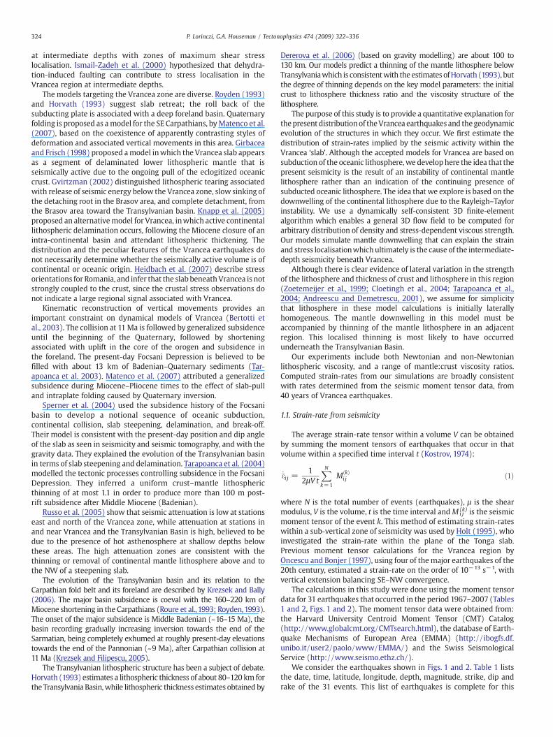
We consider the earthquakes shown in Figs. 1 and 2. Table 1 liststhe date, time, latitude, longitude, depth, magnitude, strike, dip andrake of the 31 events. This list of earthquakes is complete for this
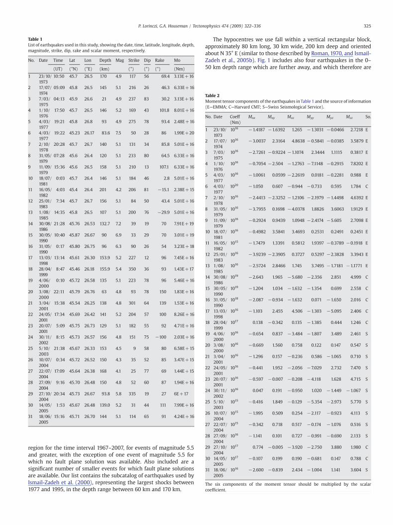
Table 1List of earthquakes used in this study, showing the date, time, latitude, longitude, depth,magnitude, strike, dip, rake and scalar moment, respectively.
No. Date Time Lat Lon Depth Mag Strike Dip Rake Mo
(UT) (°N) (°E) (km) (°) (°) (°) (Nm)
1 23/10/1973
10:50 45.7 26.5 170 4.9 117 56 69.4 3.13E+16
2 17/07/1974
05:09 45.8 26.5 145 5.1 216 26 46.3 6.33E+16
3 7/03/1975
04:13 45.9 26.6 21 4.9 237 83 30.2 3.13E+16
4 1/10/1976
17:50 45.7 26.5 146 5.2 169 43 101.8 8.01E+16
5 4/03/1977
19:21 45.8 26.8 93 4.9 275 78 93.4 2.48E+16
6 4/03/1977
19:22 45.23 26.17 83.6 7.5 50 28 86 1.99E+20
7 2/10/1978
20:28 45.7 26.7 140 5.1 131 34 85.8 5.01E+16
8 31/05/1979
07:28 45.6 26.4 120 5.1 233 80 64.5 6.33E+16
9 11/09/1979
15:36 45.6 26.5 158 5.1 210 13 107.1 6.33E+16
10 18/07/1981
0:03 45.7 26.4 146 5.1 184 46 2.8 5.01E+16
11 16/05/1982
4:03 45.4 26.4 201 4.2 206 81 −15.1 2.38E+15
12 25/01/1983
7:34 45.7 26.7 156 5.1 84 50 43.4 5.01E+16
13 1/08/1985
14:35 45.8 26.5 107 5.1 200 76 −29.9 5.01E+16
14 30/08/1986
21:28 45.76 26.53 132.7 7.2 39 19 70 7.91E+19
15 30/05/1990
10:40 45.87 26.67 90 6.9 33 29 70 3.01E+19
16 31/05/1990
0:17 45.80 26.75 96 6.3 90 26 54 3.23E+18
17 13/03/1998
13:14 45.61 26.30 153.9 5.2 227 12 96 7.45E+16
18 28/04/1999
8:47 45.46 26.18 155.9 5.4 350 36 93 1.43E+17
19 4/06/2000
0:10 45.72 26.58 135 5.1 223 78 96 5.46E+16
20 3/08/2000
22:11 45.79 26.76 63 4.8 93 78 150 1.83E+16
21 3/04/2001
15:38 45.54 26.25 138 4.8 301 64 139 1.53E+16
22 24/05/2001
17:34 45.69 26.42 141 5.2 204 57 100 8.26E+16
23 20/07/2001
5:09 45.75 26.73 129 5.1 182 55 92 4.71E+16
24 30/11/2002
8:15 45.73 26.57 156 4.8 151 75 −100 2.03E+16
25 5/10/2003
21:38 45.67 26.33 153 4.5 9 58 80 6.58E+15
26 10/07/2004
0:34 45.72 26.52 150 4.3 35 52 85 3.47E+15
27 22/07/2004
17:09 45.64 26.38 168 4.1 25 77 69 1.44E+15
28 27/09/2004
9:16 45.70 26.48 150 4.8 52 60 87 1.94E+16
29 27/10/2004
20:34 45.73 26.67 93.8 5.8 335 19 27 6E+17
30 14/05/2005
1:53 45.67 26.48 139.0 5.2 31 44 111 7.99E+16
31 18/06/2005
15:16 45.71 26.70 144 5.1 114 65 91 4.24E+16
Table 2Moment tensor components of the earthquakes in Table 1 and the source of information(E—EMMA; C—Harvard CMT; S—Swiss Seismological Service).
No. Date Coeff(Nm)
Mxx Mxy Mxz Myy Myz Mzz So.
1 23/10/1973
1016 −1.4187 −1.6392 1.265 −1.3031 −0.0466 2.7218 E
2 17/07/1974
1016 −3.0037 2.3164 4.8638 −0.5841 −0.0385 3.5879 E
3 7/03/1975
1016 −2.7261 −0.9224 −1.1074 2.3444 1.1115 0.3817 E
4 1/10/1976
1016 −0.7054 −2.504 −1.2763 −7.1148 −0.2915 7.8202 E
5 4/03/1977
1016 −1.0061 0.0599 −2.2619 0.0181 −0.2281 0.988 E
6 4/03/1977
1020 −1.050 0.607 −0.944 −0.733 0.595 1.784 C
7 2/10/1978
1016 −2.4413 −2.3252 −1.2106 −2.1979 −1.4498 4.6392 E
8 31/05/1979
1016 −3.7955 0.1698 −4.0378 1.8826 3.6063 1.9129 E
9 11/09/1979
1016 −0.2924 0.9439 1.0948 −2.4174 −5.605 2.7098 E
10 18/07/1981
1016 −0.4982 3.5841 3.4693 0.2531 0.2491 0.2451 E
11 16/05/1982
1015 −1.7479 1.3391 0.5812 1.9397 −0.3789 −0.1918 E
12 25/01/1983
1016 −3.9239 −2.3905 0.3727 0.5297 −2.3828 3.3943 E
13 1/08/1985
1016 −2.5724 2.8466 1.745 3.7495 −1.7181 −1.1771 E
14 30/08/1986
1019 −2.643 1.965 −5.680 −2.356 2.851 4.999 C
15 30/05/1990
1019 −1.204 1.034 −1.632 −1.354 0.699 2.558 C
16 31/05/1990
1018 −2.087 −0.934 −1.632 0.071 −1.650 2.016 C
17 13/03/1998
1016 −1.103 2.455 4.506 −1.303 −5.095 2.406 C
18 28/04/1999
1017 0.138 −0.342 0.135 −1.385 0.444 1.246 C
19 4/06/2000
1016 −0.654 0.837 −3.484 −1.807 3.489 2.461 S
20 3/08/2000
1016 −0.669 1.560 0.758 0.122 0.147 0.547 S
21 3/04/2001
1016 −1.296 0.157 −0.236 0.586 −1.065 0.710 S
22 24/05/2001
1016 −0.441 1.952 −2.056 −7.029 2.732 7.470 S
23 20/07/2001
1016 −0.597 −0.007 −0.208 −4.118 1.628 4.715 S
24 30/11/2002
1016 0.047 0.191 −0.950 1.020 −1.449 −1.067 S
25 5/10/2003
1015 −0.416 1.849 −0.129 −5.354 −2.973 5.770 S
26 10/07/2004
1015 −1.995 0.509 0.254 −2.117 −0.923 4.113 S
27 22/07/2004
1015 −0.342 0.718 0.517 −0.174 −1.076 0.516 S
28 27/09/2004
1016 −1.141 0.101 0.727 −0.991 −0.690 2.133 S
29 27/10/2004
1017 0.774 −0.005 −3.920 −2.750 3.880 1.980 C
30 14/05/2005
1017 −0.107 0.199 0.190 −0.681 0.147 0.788 C
31 18/06/2005
1016 −2.600 −0.839 2.434 −1.004 1.141 3.604 S
The six components of the moment tensor should be multiplied by the scalarcoefficient.
325P. Lorinczi, G.A. Houseman / Tectonophysics 474 (2009) 322–336
region for the time interval 1967–2007, for events of magnitude 5.5and greater, with the exception of one event of magnitude 5.5 forwhich no fault plane solution was available. Also included are asignificant number of smaller events for which fault plane solutionsare available. Our list contains the subcatalog of earthquakes used byIsmail-Zadeh et al. (2000), representing the largest shocks between1977 and 1995, in the depth range between 60 km and 170 km.
The hypocentres we use fall within a vertical rectangular block,approximately 80 km long, 30 km wide, 200 km deep and orientedabout N 35° E (similar to those described by Roman, 1970, and Ismail-Zadeh et al., 2005b). Fig. 1 includes also four earthquakes in the 0–50 km depth range which are further away, and which therefore are
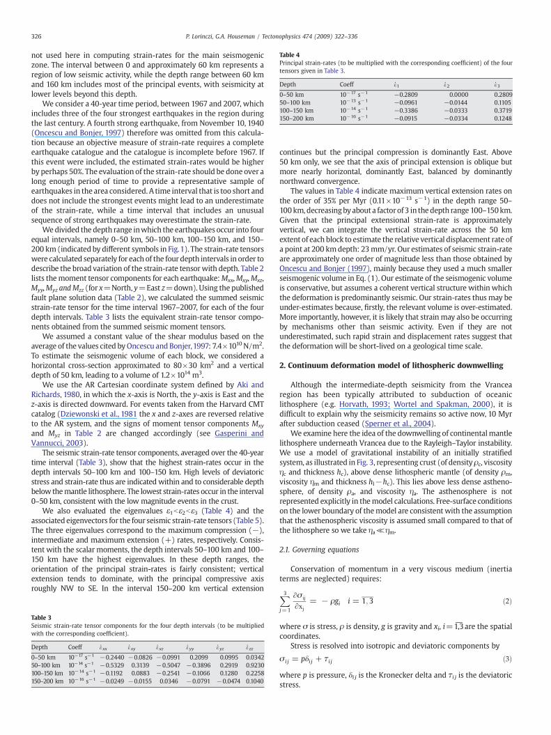
Table 4Principal strain-rates (to be multiplied with the corresponding coefficient) of the fourtensors given in Table 3.
Depth Coeff e.1 e
.2 e
.3
0–50 km 10−17 s−1 −0.2809 0.0000 0.280950–100 km 10−13 s−1 −0.0961 −0.0144 0.1105100–150 km 10−14 s−1 −0.3386 −0.0333 0.3719150–200 km 10−16 s−1 −0.0915 −0.0334 0.1248
326 P. Lorinczi, G.A. Houseman / Tectonophysics 474 (2009) 322–336
not used here in computing strain-rates for the main seismogeniczone. The interval between 0 and approximately 60 km represents aregion of low seismic activity, while the depth range between 60 kmand 160 km includes most of the principal events, with seismicity atlower levels beyond this depth.
We consider a 40-year time period, between 1967 and 2007, whichincludes three of the four strongest earthquakes in the region duringthe last century. A fourth strong earthquake, from November 10, 1940(Oncescu and Bonjer, 1997) therefore was omitted from this calcula-tion because an objective measure of strain-rate requires a completeearthquake catalogue and the catalogue is incomplete before 1967. Ifthis event were included, the estimated strain-rates would be higherby perhaps 50%. The evaluation of the strain-rate should be done over along enough period of time to provide a representative sample ofearthquakes in the area considered. A time interval that is too short anddoes not include the strongest events might lead to an underestimateof the strain-rate, while a time interval that includes an unusualsequence of strong earthquakes may overestimate the strain-rate.
We divided the depth range inwhich the earthquakes occur into fourequal intervals, namely 0–50 km, 50–100 km, 100–150 km, and 150–200 km(indicated by different symbols in Fig.1). The strain-rate tensorswere calculated separately for each of the four depth intervals in order todescribe the broad variation of the strain-rate tensorwith depth. Table 2lists themoment tensor components for each earthquake:Mxx,Mxy,Mxz,Myy,Myz andMzz (for x=North, y=East z=down). Using the publishedfault plane solution data (Table 2), we calculated the summed seismicstrain-rate tensor for the time interval 1967–2007, for each of the fourdepth intervals. Table 3 lists the equivalent strain-rate tensor compo-nents obtained from the summed seismic moment tensors.
We assumed a constant value of the shear modulus based on theaverage of the values cited byOncescu andBonjer,1997: 7.4×10¹⁰N/m2.To estimate the seismogenic volume of each block, we considered ahorizontal cross-section approximated to 80×30 km2 and a verticaldepth of 50 km, leading to a volume of 1.2×10¹⁴ m3.
We use the AR Cartesian coordinate system defined by Aki andRichards, 1980, in which the x-axis is North, the y-axis is East and thez-axis is directed downward. For events taken from the Harvard CMTcatalog (Dziewonski et al., 1981 the x and z-axes are reversed relativeto the AR system, and the signs of moment tensor components Mxy
and Myz in Table 2 are changed accordingly (see Gasperini andVannucci, 2003).
The seismic strain-rate tensor components, averaged over the 40-yeartime interval (Table 3), show that the highest strain-rates occur in thedepth intervals 50–100 km and 100–150 km. High levels of deviatoricstress and strain-rate thus are indicated within and to considerable depthbelow themantle lithosphere. The lowest strain-rates occur in the interval0–50 km, consistent with the low magnitude events in the crust.
We also evaluated the eigenvalues ε1bε2bε3 (Table 4) and theassociated eigenvectors for the four seismic strain-rate tensors (Table 5).The three eigenvalues correspond to the maximum compression (−),intermediate and maximum extension (+) rates, respectively. Consis-tent with the scalar moments, the depth intervals 50–100 km and 100–150 km have the highest eigenvalues. In these depth ranges, theorientation of the principal strain-rates is fairly consistent; verticalextension tends to dominate, with the principal compressive axisroughly NW to SE. In the interval 150–200 km vertical extension
Table 3Seismic strain-rate tensor components for the four depth intervals (to be multipliedwith the corresponding coefficient).
Depth Coeff e.xx e
.xy e
.xz e
.yy e
.yz e
.zz
0–50 km 10−17 s−1 −0.2440 −0.0826 −0.0991 0.2099 0.0995 0.034250–100 km 10−14 s−1 −0.5329 0.3139 −0.5047 −0.3896 0.2919 0.9230100–150 km 10−14 s−1 −0.1192 0.0883 −0.2541 −0.1066 0.1280 0.2258150–200 km 10−16 s−1 −0.0249 −0.0155 0.0346 −0.0791 −0.0474 0.1040
continues but the principal compression is dominantly East. Above50 km only, we see that the axis of principal extension is oblique butmore nearly horizontal, dominantly East, balanced by dominantlynorthward convergence.
The values in Table 4 indicate maximum vertical extension rates onthe order of 35% per Myr (0.11×10⁻¹³ s−1) in the depth range 50–100km, decreasingbyabout a factorof 3 in thedepth range 100–150km.Given that the principal extensional strain-rate is approximatelyvertical, we can integrate the vertical strain-rate across the 50 kmextent of each block to estimate the relative vertical displacement rate ofa point at 200 kmdepth: 23mm/yr. Our estimates of seismic strain-rateare approximately one order of magnitude less than those obtained byOncescu and Bonjer (1997), mainly because they used a much smallerseismogenic volume in Eq. (1). Our estimate of the seismogenic volumeis conservative, but assumes a coherent vertical structure within whichthe deformation is predominantly seismic. Our strain-rates thus may beunder-estimates because, firstly, the relevant volume is over-estimated.More importantly, however, it is likely that strain may also be occurringby mechanisms other than seismic activity. Even if they are notunderestimated, such rapid strain and displacement rates suggest thatthe deformation will be short-lived on a geological time scale.
2. Continuum deformation model of lithospheric downwelling
Although the intermediate-depth seismicity from the Vrancearegion has been typically attributed to subduction of oceaniclithosphere (e.g. Horvath, 1993; Wortel and Spakman, 2000), it isdifficult to explain why the seismicity remains so active now, 10 Myrafter subduction ceased (Sperner et al., 2004).
We examine here the idea of the downwelling of continentalmantlelithosphere underneath Vrancea due to the Rayleigh–Taylor instability.We use a model of gravitational instability of an initially stratifiedsystem, as illustrated in Fig. 3, representing crust (of density ρc, viscosityηc and thickness hc), above dense lithospheric mantle (of density ρm,viscosity ηm and thickness hl−hc). This lies above less dense astheno-sphere, of density ρa, and viscosity ηa. The asthenosphere is notrepresented explicitly in themodel calculations. Free-surface conditionson the lower boundary of themodel are consistent with the assumptionthat the asthenospheric viscosity is assumed small compared to that ofthe lithosphere so we take ηa≪ηm.
2.1. Governing equations
Conservation of momentum in a very viscous medium (inertiaterms are neglected) requires:
X3j=1
∂σ ij
∂xj= − ρgi i = 1;3 ð2Þ
where σ is stress, ρ is density, g is gravity and xi, i=1,3―
are the spatialcoordinates.
Stress is resolved into isotropic and deviatoric components by
σ i j = pδi j + τi j ð3Þ
where p is pressure, δi j is the Kronecker delta and τi j is the deviatoricstress.
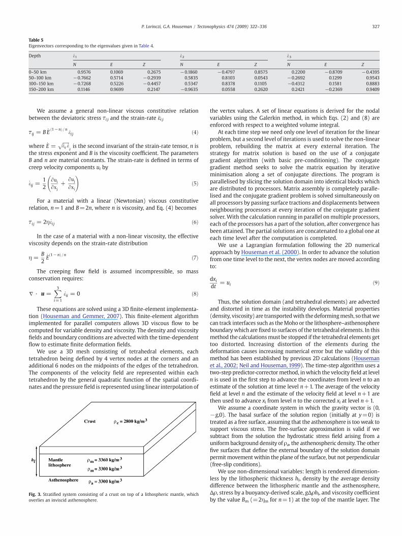
Table 5Eigenvectors corresponding to the eigenvalues given in Table 4.
Depth e.1 e
.2 e
.3
N E Z N E Z N E Z
0–50 km 0.9576 0.1069 0.2675 −0.1860 −0.4797 0.8575 0.2200 −0.8709 −0.439550–100 km −0.7662 0.5714 −0.2939 0.5835 0.8103 0.0543 −0.2692 0.1299 0.9543100–150 km −0.7268 0.5226 −0.4457 0.5347 0.8378 0.1105 −0.4312 0.1581 0.8883150–200 km 0.1146 0.9699 0.2147 −0.9635 0.0558 0.2620 0.2421 −0.2369 0.9409
327P. Lorinczi, G.A. Houseman / Tectonophysics 474 (2009) 322–336
We assume a general non-linear viscous constitutive relationbetween the deviatoric stress τi j and the strain-rate εi j
τij = B:E
1−nð Þ=n :ei j ð4Þ
where:E =
ffiffiffiffiffiffi:eij:e
pijis the second invariant of the strain-rate tensor, n is
the stress exponent and B is the viscosity coefficient. The parametersB and n are material constants. The strain-rate is defined in terms ofcreep velocity components ui by
:eij =
12
∂ui∂xj
+∂uj∂xi
!ð5Þ
For a material with a linear (Newtonian) viscous constitutiverelation, n=1 and B=2n, where n is viscosity, and Eq. (4) becomes
τi j = 2η:ei j ð6Þ
In the case of a material with a non-linear viscosity, the effectiveviscosity depends on the strain-rate distribution
η =B2
:E
1−nð Þ=n ð7Þ
The creeping flow field is assumed incompressible, so massconservation requires:
j · u =X3i=1
:eii = 0 ð8Þ
These equations are solved using a 3D finite-element implementa-tion (Houseman and Gemmer, 2007). This finite-element algorithmimplemented for parallel computers allows 3D viscous flow to becomputed for variable density and viscosity. The density and viscosityfields and boundary conditions are advectedwith the time-dependentflow to estimate finite deformation fields.
We use a 3D mesh consisting of tetrahedral elements, eachtetrahedron being defined by 4 vertex nodes at the corners and anadditional 6 nodes on the midpoints of the edges of the tetrahedron.The components of the velocity field are represented within eachtetrahedron by the general quadratic function of the spatial coordi-nates and the pressure field is represented using linear interpolation of
Fig. 3. Stratified system consisting of a crust on top of a lithospheric mantle, whichoverlies an inviscid asthenosphere.
the vertex values. A set of linear equations is derived for the nodalvariables using the Galerkin method, in which Eqs. (2) and (8) areenforced with respect to a weighted volume integral.
At each time step we need only one level of iteration for the linearproblem, but a second level of iterations is used to solve the non-linearproblem, rebuilding the matrix at every external iteration. Thestrategy for matrix solution is based on the use of a conjugategradient algorithm (with basic pre-conditioning). The conjugategradient method seeks to solve the matrix equation by iterativeminimisation along a set of conjugate directions. The program isparallelised by slicing the solution domain into identical blocks whichare distributed to processors. Matrix assembly is completely paralle-lised and the conjugate gradient problem is solved simultaneously onall processors by passing surface tractions and displacements betweenneighbouring processors at every iteration of the conjugate gradientsolver. With the calculation running in parallel onmultiple processors,each of the processors has a part of the solution, after convergence hasbeen attained. The partial solutions are concatenated to a global one ateach time level after the computation is completed.
We use a Lagrangian formulation following the 2D numericalapproach by Houseman et al. (2000). In order to advance the solutionfrom one time level to the next, the vertex nodes are moved accordingto:
dxidt
= ui ð9Þ
Thus, the solution domain (and tetrahedral elements) are advectedand distorted in time as the instability develops. Material properties(density, viscosity) are transportedwith thedeformingmesh, so thatwecan track interfaces such as theMoho or the lithosphere–asthenosphereboundarywhich are fixed to surfaces of the tetrahedral elements. In thismethod the calculationsmust be stopped if the tetrahedral elements gettoo distorted. Increasing distortion of the elements during thedeformation causes increasing numerical error but the validity of thismethod has been established by previous 2D calculations (Housemanet al., 2002; Neil and Houseman, 1999). The time-step algorithm uses atwo-step predictor-correctormethod, inwhich the velocity field at leveln is used in the first step to advance the coordinates from level n to anestimate of the solution at time level n+1. The average of the velocityfield at level n and the estimate of the velocity field at level n+1 arethen used to advance xi from level n to the corrected xi at level n+1.
We assume a coordinate system in which the gravity vector is (0,−g,0). The basal surface of the solution region (initially at y=0) istreated as a free surface, assuming that the asthenosphere is tooweak tosupport viscous stress. The free-surface approximation is valid if wesubtract from the solution the hydrostatic stress field arising from auniform background density of ρa, the asthenospheric density. The otherfive surfaces that define the external boundary of the solution domainpermitmovement within the plane of the surface, but not perpendicular(free-slip conditions).
We use non-dimensional variables: length is rendered dimension-less by the lithospheric thickness hl, density by the average densitydifference between the lithospheric mantle and the asthenosphere,Δρ, stress by a buoyancy-derived scale, gΔρhl, and viscosity coefficientby the value Bm (=2ηm for n=1) at the top of the mantle layer. The
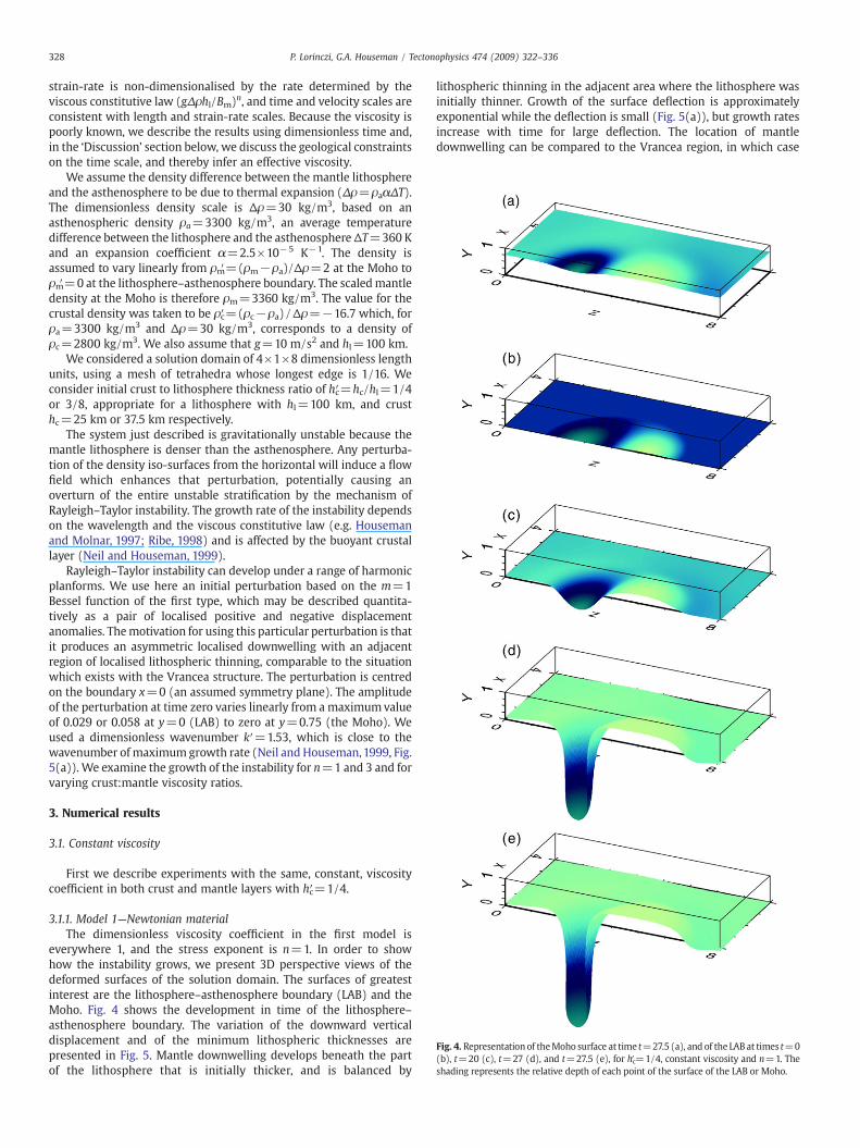
Fig. 4. Representation of theMoho surface at time t=27.5 (a), and of the LAB at times t=0(b), t=20 (c), t=27 (d), and t=27.5 (e), for hc′=1/4, constant viscosity and n=1. Theshading represents the relative depth of each point of the surface of the LAB or Moho.
328 P. Lorinczi, G.A. Houseman / Tectonophysics 474 (2009) 322–336
strain-rate is non-dimensionalised by the rate determined by theviscous constitutive law (gΔρhl/Bm)n, and time and velocity scales areconsistent with length and strain-rate scales. Because the viscosity ispoorly known, we describe the results using dimensionless time and,in the ‘Discussion’ section below, we discuss the geological constraintson the time scale, and thereby infer an effective viscosity.
We assume the density difference between the mantle lithosphereand the asthenosphere to be due to thermal expansion (Δρ=ρaαΔT).The dimensionless density scale is Δρ=30 kg/m3, based on anasthenospheric density ρa=3300 kg/m3, an average temperaturedifference between the lithosphere and the asthenosphere ΔT=360 Kand an expansion coefficient α=2.5×10⁻⁵ K−1. The density isassumed to vary linearly from ρm′=(ρm−ρa)/Δρ=2 at the Moho toρm′=0 at the lithosphere–asthenosphere boundary. The scaledmantledensity at the Moho is therefore ρm=3360 kg/m3. The value for thecrustal density was taken to be ρc′=(ρc−ρa)/Δρ=−16.7 which, forρa=3300 kg/m3 and Δρ=30 kg/m3, corresponds to a density ofρc=2800 kg/m3. We also assume that g=10 m/s2 and hl=100 km.
We considered a solution domain of 4×1×8 dimensionless lengthunits, using a mesh of tetrahedra whose longest edge is 1/16. Weconsider initial crust to lithosphere thickness ratio of hc′=hc/hl=1/4or 3/8, appropriate for a lithosphere with hl=100 km, and crusthc=25 km or 37.5 km respectively.
The system just described is gravitationally unstable because themantle lithosphere is denser than the asthenosphere. Any perturba-tion of the density iso-surfaces from the horizontal will induce a flowfield which enhances that perturbation, potentially causing anoverturn of the entire unstable stratification by the mechanism ofRayleigh–Taylor instability. The growth rate of the instability dependson the wavelength and the viscous constitutive law (e.g. Housemanand Molnar, 1997; Ribe, 1998) and is affected by the buoyant crustallayer (Neil and Houseman, 1999).
Rayleigh–Taylor instability can develop under a range of harmonicplanforms. We use here an initial perturbation based on the m=1Bessel function of the first type, which may be described quantita-tively as a pair of localised positive and negative displacementanomalies. Themotivation for using this particular perturbation is thatit produces an asymmetric localised downwelling with an adjacentregion of localised lithospheric thinning, comparable to the situationwhich exists with the Vrancea structure. The perturbation is centredon the boundary x=0 (an assumed symmetry plane). The amplitudeof the perturbation at time zero varies linearly from a maximumvalueof 0.029 or 0.058 at y=0 (LAB) to zero at y=0.75 (the Moho). Weused a dimensionless wavenumber k′=1.53, which is close to thewavenumber of maximum growth rate (Neil and Houseman,1999, Fig.5(a)). We examine the growth of the instability for n=1 and 3 and forvarying crust:mantle viscosity ratios.
3. Numerical results
3.1. Constant viscosity
First we describe experiments with the same, constant, viscositycoefficient in both crust and mantle layers with hc′=1/4.
3.1.1. Model 1—Newtonian materialThe dimensionless viscosity coefficient in the first model is
everywhere 1, and the stress exponent is n=1. In order to showhow the instability grows, we present 3D perspective views of thedeformed surfaces of the solution domain. The surfaces of greatestinterest are the lithosphere–asthenosphere boundary (LAB) and theMoho. Fig. 4 shows the development in time of the lithosphere–asthenosphere boundary. The variation of the downward verticaldisplacement and of the minimum lithospheric thicknesses arepresented in Fig. 5. Mantle downwelling develops beneath the partof the lithosphere that is initially thicker, and is balanced by
lithospheric thinning in the adjacent area where the lithosphere wasinitially thinner. Growth of the surface deflection is approximatelyexponential while the deflection is small (Fig. 5(a)), but growth ratesincrease with time for large deflection. The location of mantledownwelling can be compared to the Vrancea region, in which case
329P. Lorinczi, G.A. Houseman / Tectonophysics 474 (2009) 322–336
the adjacent region of thinned mantle lithosphere would correspondto the Transylvanian basin.
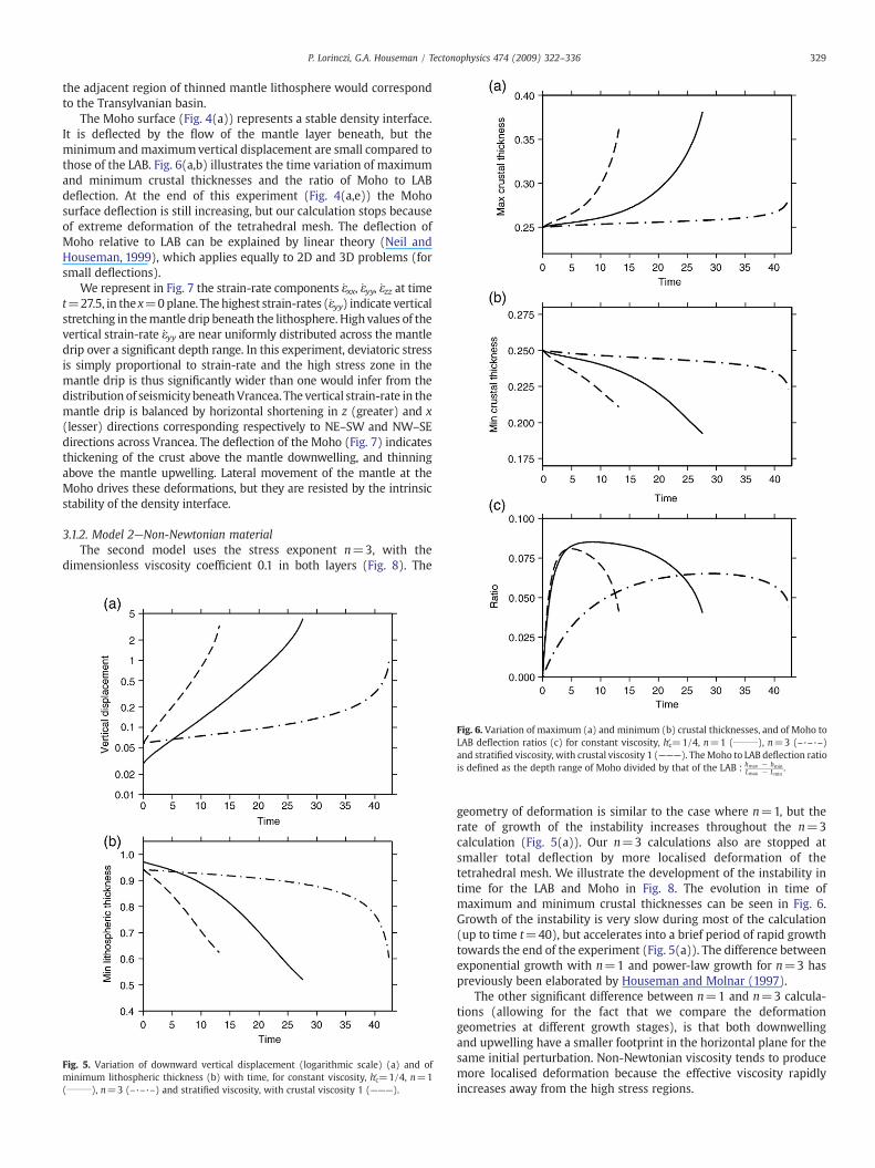
The Moho surface (Fig. 4(a)) represents a stable density interface.It is deflected by the flow of the mantle layer beneath, but theminimum andmaximumvertical displacement are small compared tothose of the LAB. Fig. 6(a,b) illustrates the time variation of maximumand minimum crustal thicknesses and the ratio of Moho to LABdeflection. At the end of this experiment (Fig. 4(a,e)) the Mohosurface deflection is still increasing, but our calculation stops becauseof extreme deformation of the tetrahedral mesh. The deflection ofMoho relative to LAB can be explained by linear theory (Neil andHouseman, 1999), which applies equally to 2D and 3D problems (forsmall deflections).
We represent in Fig. 7 the strain-rate components εxx, εyy, εzz at timet=27.5, in the x=0plane. The highest strain-rates (εyy) indicate verticalstretching in themantle drip beneath the lithosphere. High values of thevertical strain-rate εyy are near uniformly distributed across the mantledrip over a significant depth range. In this experiment, deviatoric stressis simply proportional to strain-rate and the high stress zone in themantle drip is thus significantly wider than one would infer from thedistribution of seismicity beneathVrancea. The vertical strain-rate in themantle drip is balanced by horizontal shortening in z (greater) and x(lesser) directions corresponding respectively to NE–SW and NW–SEdirections across Vrancea. The deflection of the Moho (Fig. 7) indicatesthickening of the crust above the mantle downwelling, and thinningabove the mantle upwelling. Lateral movement of the mantle at theMoho drives these deformations, but they are resisted by the intrinsicstability of the density interface.
3.1.2. Model 2—Non-Newtonian materialThe second model uses the stress exponent n=3, with the
dimensionless viscosity coefficient 0.1 in both layers (Fig. 8). The
Fig. 5. Variation of downward vertical displacement (logarithmic scale) (a) and ofminimum lithospheric thickness (b) with time, for constant viscosity, hc′=1/4, n=1(_______), n=3 (–·–·–) and stratified viscosity, with crustal viscosity 1 (———).
Fig. 6. Variation of maximum (a) and minimum (b) crustal thicknesses, and of Moho toLAB deflection ratios (c) for constant viscosity, hc′=1/4, n=1 (_______), n=3 (–·–·–)and stratified viscosity, with crustal viscosity 1 (———). TheMoho to LAB deflection ratiois defined as the depth range of Moho divided by that of the LAB : hmax − hmin
Lmax − Lmin.
geometry of deformation is similar to the case where n=1, but therate of growth of the instability increases throughout the n=3calculation (Fig. 5(a)). Our n=3 calculations also are stopped atsmaller total deflection by more localised deformation of thetetrahedral mesh. We illustrate the development of the instability intime for the LAB and Moho in Fig. 8. The evolution in time ofmaximum and minimum crustal thicknesses can be seen in Fig. 6.Growth of the instability is very slow during most of the calculation(up to time t=40), but accelerates into a brief period of rapid growthtowards the end of the experiment (Fig. 5(a)). The difference betweenexponential growth with n=1 and power-law growth for n=3 haspreviously been elaborated by Houseman and Molnar (1997).
The other significant difference between n=1 and n=3 calcula-tions (allowing for the fact that we compare the deformationgeometries at different growth stages), is that both downwellingand upwelling have a smaller footprint in the horizontal plane for thesame initial perturbation. Non-Newtonian viscosity tends to producemore localised deformation because the effective viscosity rapidlyincreases away from the high stress regions.
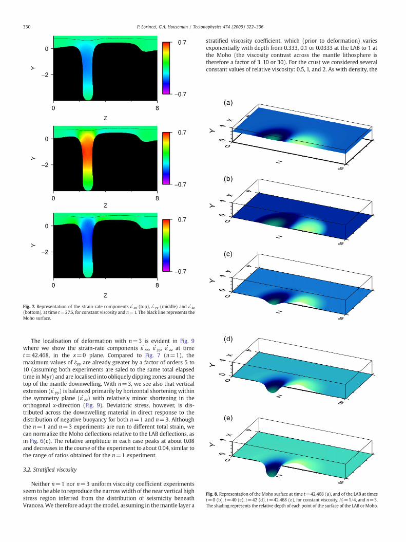
Fig. 7. Representation of the strain-rate components ε·xx (top), ε·yy (middle) and ε·zz(bottom), at time t=27.5, for constant viscosity and n=1. The black line represents theMoho surface.
Fig. 8. Representation of the Moho surface at time t=42.468 (a), and of the LAB at timest=0 (b), t=40 (c), t=42 (d), t=42.468 (e), for constant viscosity, hc′=1/4, and n=3.The shading represents the relative depth of each point of the surface of the LAB orMoho.
330 P. Lorinczi, G.A. Houseman / Tectonophysics 474 (2009) 322–336
The localisation of deformation with n=3 is evident in Fig. 9where we show the strain-rate components ε·xx, ε
·yy, ε
·zz at time
t=42.468, in the x=0 plane. Compared to Fig. 7 (n=1), themaximum values of ε yy are already greater by a factor of orders 5 to10 (assuming both experiments are saled to the same total elapsedtime inMyr) and are localised into obliquely dipping zones around thetop of the mantle downwelling. With n=3, we see also that verticalextension (ε·yy) is balanced primarily by horizontal shortening withinthe symmetry plane (ε·zz) with relatively minor shortening in theorthogonal x-direction (Fig. 9). Deviatoric stress, however, is dis-tributed across the downwelling material in direct response to thedistribution of negative buoyancy for both n=1 and n=3. Althoughthe n=1 and n=3 experiments are run to different total strain, wecan normalize the Moho deflections relative to the LAB deflections, asin Fig. 6(c). The relative amplitude in each case peaks at about 0.08and decreases in the course of the experiment to about 0.04, similar tothe range of ratios obtained for the n=1 experiment.
3.2. Stratified viscosity
Neither n=1 nor n=3 uniform viscosity coefficient experimentsseem to be able to reproduce the narrowwidth of the near vertical highstress region inferred from the distribution of seismicity beneathVrancea.We therefore adapt themodel, assuming in themantle layer a
stratified viscosity coefficient, which (prior to deformation) variesexponentially with depth from 0.333, 0.1 or 0.0333 at the LAB to 1 atthe Moho (the viscosity contrast across the mantle lithosphere istherefore a factor of 3, 10 or 30). For the crust we considered severalconstant values of relative viscosity: 0.5, 1, and 2. As with density, the
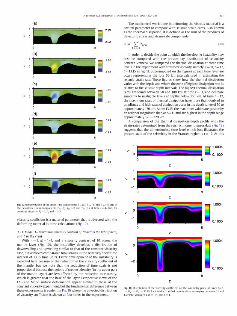
Fig. 9. Representation of the strain-rate components ε·xx (a), ε·yy (b) and ε·yy (c), and of
the deviatoric stress components τxx (d), τyy (e) and τzz (f ) at time t=42.468, forconstant viscosity, hc′=1/4, and n=3.
Fig. 10. Distribution of the viscosity coefficient on the symmetry plane at times t=5,t=11, t=12, t=13.15, for initially stratified mantle viscosity varying between 0.1 and1, crustal viscosity 1, hc′=1/4, and n=1.
331P. Lorinczi, G.A. Houseman / Tectonophysics 474 (2009) 322–336
viscosity coefficient is a material parameter that is advected with thedeforming material in these calculations (Fig. 10).
3.2.1. Model 3—Newtonian viscosity contrast of 10 across the lithosphere,and 1 in the crust
With n=1, hc′=1/4, and a viscosity contrast of 10 across themantle layer (Fig. 10), the instability develops a distribution ofdownwelling and upwelling similar to that of the constant viscositycase, but achieves comparable total strains in the relatively short timeinterval of 13.15 time units. Faster development of the instability isexpected here because of the reduction in the viscosity coefficient ofthe mantle, but we note that the reduction of time scale is notproportional because the regions of greatest density (in the upper partof the mantle layer) are less affected by the reduction in viscosity,which is greater near the base of the layer. Perspective views of theLAB and Moho surface deformation appear similar to those of theconstant viscosity experiment, but the fundamental difference betweenthese experiments is evident in Fig. 10 where the advected distributionof viscosity coefficient is shown at four times in the experiment.
The mechanical work done in deforming the viscous material is anatural parameter to compare with seismic strain-rates. Also knownas the thermal dissipation, it is defined as the sum of the products ofdeviatoric stress and strain-rate components:
Φ =X
1Vi;jV3
τi jei j ð10Þ
In order to decide the point at which the developing instability maybest be compared with the present-day distribution of seismicitybeneath Vrancea, we compared the thermal dissipation at three timelevels in the experiment with stratified viscosity, namely: t=11, t=12,t=13.15 in Fig. 11. Superimposed on the figures at each time level areboxes representing the four 50 km intervals used in estimating theseismic strain-rate. These figures show how the thermal dissipationvaries with the depth, and where the zone of highest dissipation rate is,relative to the seismic depth intervals. The highest thermal dissipationrates are found between 50 and 100 km at time t=11, and decreasesmoothly to negligible levels at depths below 150 km. At time t=12,the maximum rates of thermal dissipation have more than doubled inamplitude and high rates of dissipation occur in the depth range of 50 toapproximately 170 km. At t=13.15, the maximumvalues are greater byan order of magnitude than at t=11 and are highest in the depth rangeapproximately 120−220 km.
A comparison of the thermal dissipation depth profile with thestrain-rates determined from the seismic moment tensor data (Fig. 12)suggests that the dimensionless time level which best illustrates thepresent state of the seismicity in the Vrancea region is t=12. At this
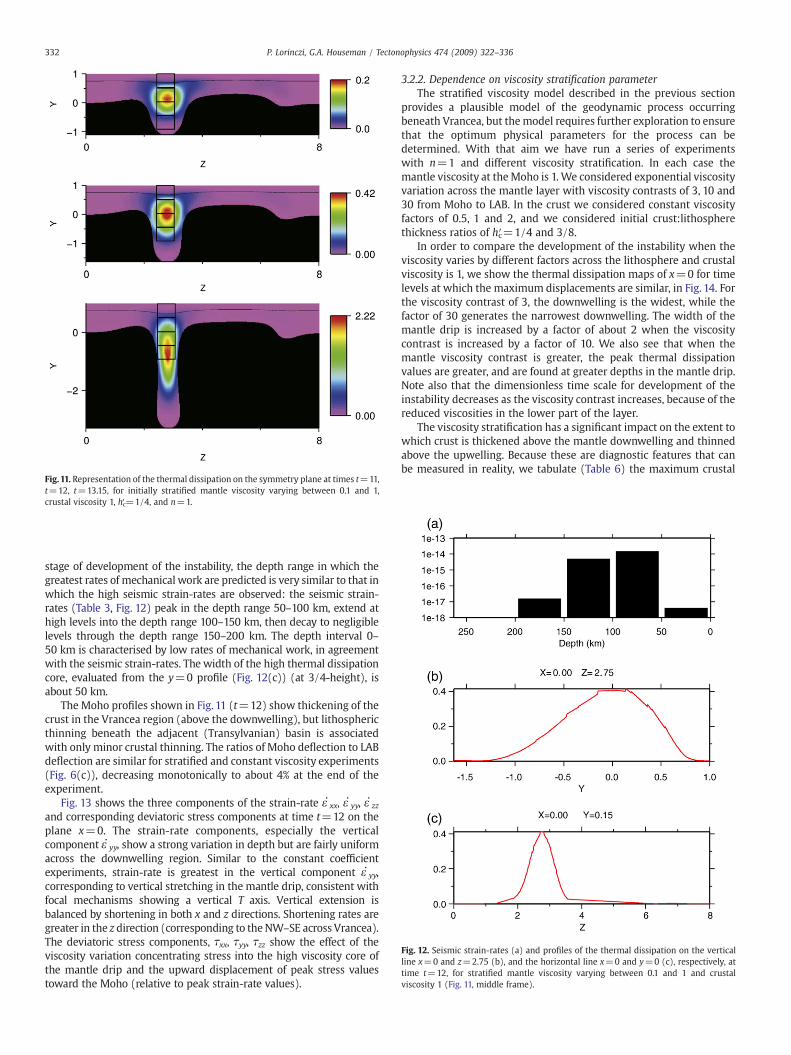
Fig.11. Representation of the thermal dissipation on the symmetry plane at times t=11,t=12, t=13.15, for initially stratified mantle viscosity varying between 0.1 and 1,crustal viscosity 1, hc′=1/4, and n=1.
Fig. 12. Seismic strain-rates (a) and profiles of the thermal dissipation on the verticalline x=0 and z=2.75 (b), and the horizontal line x=0 and y=0 (c), respectively, attime t=12, for stratified mantle viscosity varying between 0.1 and 1 and crustalviscosity 1 (Fig. 11, middle frame).
332 P. Lorinczi, G.A. Houseman / Tectonophysics 474 (2009) 322–336
stage of development of the instability, the depth range in which thegreatest rates of mechanical work are predicted is very similar to that inwhich the high seismic strain-rates are observed: the seismic strain-rates (Table 3, Fig. 12) peak in the depth range 50–100 km, extend athigh levels into the depth range 100–150 km, then decay to negligiblelevels through the depth range 150–200 km. The depth interval 0–50 km is characterised by low rates of mechanical work, in agreementwith the seismic strain-rates. The width of the high thermal dissipationcore, evaluated from the y=0 profile (Fig. 12(c)) (at 3/4-height), isabout 50 km.
The Moho profiles shown in Fig. 11 (t=12) show thickening of thecrust in the Vrancea region (above the downwelling), but lithosphericthinning beneath the adjacent (Transylvanian) basin is associatedwith only minor crustal thinning. The ratios of Moho deflection to LABdeflection are similar for stratified and constant viscosity experiments(Fig. 6(c)), decreasing monotonically to about 4% at the end of theexperiment.
Fig. 13 shows the three components of the strain-rate ε·xx, ε·yy, ε
·zz
and corresponding deviatoric stress components at time t=12 on theplane x=0. The strain-rate components, especially the verticalcomponent ε·yy, show a strong variation in depth but are fairly uniformacross the downwelling region. Similar to the constant coefficientexperiments, strain-rate is greatest in the vertical component ε·yy,corresponding to vertical stretching in the mantle drip, consistent withfocal mechanisms showing a vertical T axis. Vertical extension isbalanced by shortening in both x and z directions. Shortening rates aregreater in the z direction (corresponding to theNW–SE across Vrancea).The deviatoric stress components, τxx, τyy, τzz show the effect of theviscosity variation concentrating stress into the high viscosity core ofthe mantle drip and the upward displacement of peak stress valuestoward the Moho (relative to peak strain-rate values).
3.2.2. Dependence on viscosity stratification parameterThe stratified viscosity model described in the previous section
provides a plausible model of the geodynamic process occurringbeneath Vrancea, but themodel requires further exploration to ensurethat the optimum physical parameters for the process can bedetermined. With that aim we have run a series of experimentswith n=1 and different viscosity stratification. In each case themantle viscosity at theMoho is 1. We considered exponential viscosityvariation across the mantle layer with viscosity contrasts of 3, 10 and30 from Moho to LAB. In the crust we considered constant viscosityfactors of 0.5, 1 and 2, and we considered initial crust:lithospherethickness ratios of hc′=1/4 and 3/8.
In order to compare the development of the instability when theviscosity varies by different factors across the lithosphere and crustalviscosity is 1, we show the thermal dissipation maps of x=0 for timelevels at which the maximum displacements are similar, in Fig. 14. Forthe viscosity contrast of 3, the downwelling is the widest, while thefactor of 30 generates the narrowest downwelling. The width of themantle drip is increased by a factor of about 2 when the viscositycontrast is increased by a factor of 10. We also see that when themantle viscosity contrast is greater, the peak thermal dissipationvalues are greater, and are found at greater depths in the mantle drip.Note also that the dimensionless time scale for development of theinstability decreases as the viscosity contrast increases, because of thereduced viscosities in the lower part of the layer.
The viscosity stratification has a significant impact on the extent towhich crust is thickened above the mantle downwelling and thinnedabove the upwelling. Because these are diagnostic features that canbe measured in reality, we tabulate (Table 6) the maximum crustal
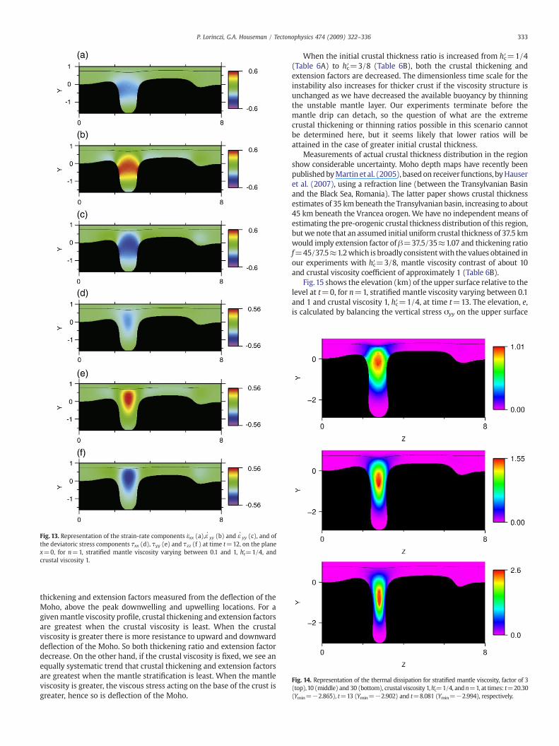
Fig. 13. Representation of the strain-rate components εxx (a),ε·yy (b) and ε·yy (c), and of
the deviatoric stress components τxx (d), τyy (e) and τzz (f ) at time t=12, on the planex=0, for n=1, stratified mantle viscosity varying between 0.1 and 1, hc′=1/4, andcrustal viscosity 1.
Fig. 14. Representation of the thermal dissipation for stratified mantle viscosity, factor of 3(top),10 (middle) and 30 (bottom), crustal viscosity 1,hc′=1/4, andn=1, at times: t=20.30(Ymin=−2.865), t=13 (Ymin=−2.902) and t=8.081 (Ymin=−2.994), respectively.
333P. Lorinczi, G.A. Houseman / Tectonophysics 474 (2009) 322–336
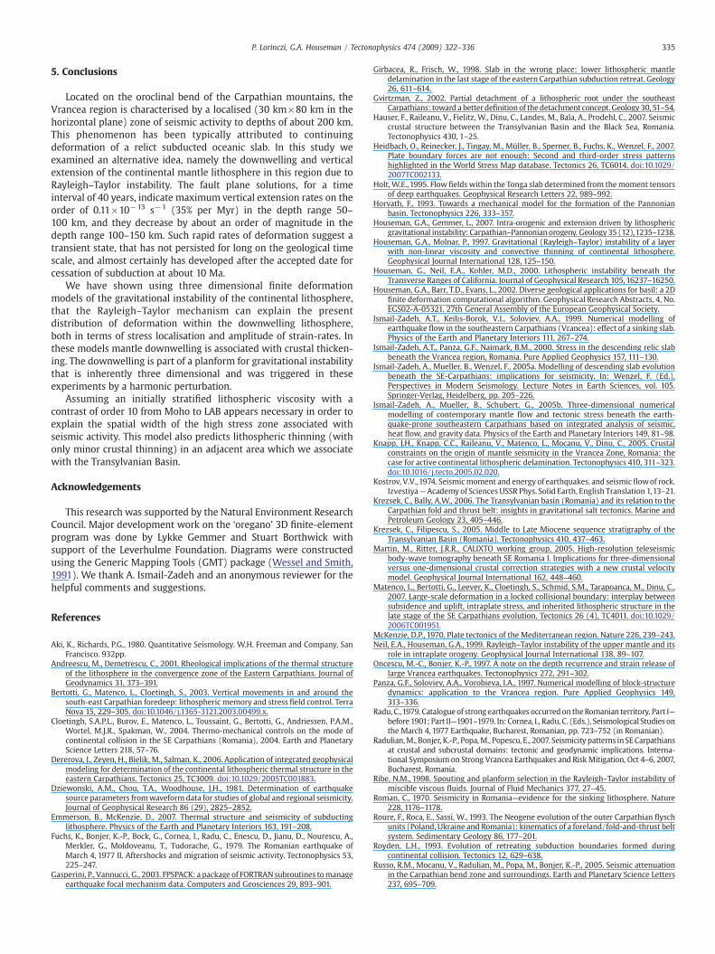
thickening and extension factors measured from the deflection of theMoho, above the peak downwelling and upwelling locations. For agivenmantle viscosity profile, crustal thickening and extension factorsare greatest when the crustal viscosity is least. When the crustalviscosity is greater there is more resistance to upward and downwarddeflection of the Moho. So both thickening ratio and extension factordecrease. On the other hand, if the crustal viscosity is fixed, we see anequally systematic trend that crustal thickening and extension factorsare greatest when the mantle stratification is least. When the mantleviscosity is greater, the viscous stress acting on the base of the crust isgreater, hence so is deflection of the Moho.
When the initial crustal thickness ratio is increased from hc′=1/4(Table 6A) to hc′=3/8 (Table 6B), both the crustal thickening andextension factors are decreased. The dimensionless time scale for theinstability also increases for thicker crust if the viscosity structure isunchanged as we have decreased the available buoyancy by thinningthe unstable mantle layer. Our experiments terminate before themantle drip can detach, so the question of what are the extremecrustal thickening or thinning ratios possible in this scenario cannotbe determined here, but it seems likely that lower ratios will beattained in the case of greater initial crustal thickness.
Measurements of actual crustal thickness distribution in the regionshow considerable uncertainty. Moho depth maps have recently beenpublishedbyMartin et al. (2005), based on receiver functions, byHauseret al. (2007), using a refraction line (between the Transylvanian Basinand the Black Sea, Romania). The latter paper shows crustal thicknessestimates of 35 kmbeneath the Transylvanian basin, increasing to about45 km beneath the Vrancea orogen. We have no independent means ofestimating the pre-orogenic crustal thickness distribution of this region,but we note that an assumed initial uniform crustal thickness of 37.5 kmwould imply extension factor of β=37.5/35≈1.07 and thickening ratiof=45/37.5≈1.2which is broadly consistentwith the values obtained inour experiments with hc′=3/8, mantle viscosity contrast of about 10and crustal viscosity coefficient of approximately 1 (Table 6B).
Fig.15 shows the elevation (km) of the upper surface relative to thelevel at t=0, for n=1, stratified mantle viscosity varying between 0.1and 1 and crustal viscosity 1, hc′=1/4, at time t=13. The elevation, e,is calculated by balancing the vertical stress σyy on the upper surface
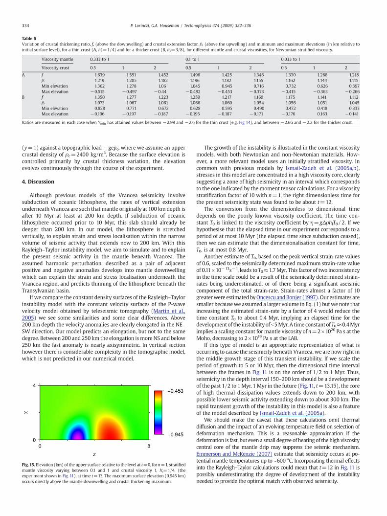
Table 6Variation of crustal thickening ratio, f, (above the downwelling) and crustal extension factor, β, (above the upwelling) and minimum and maximum elevations (in km relative toinitial surface level), for a thin crust (A, hc′=1/4) and for a thicker crust (B, hc′=3/8), for different mantle and crustal viscosities, for Newtonian stratified viscosity.
Viscosity mantle 0.333 to 1 0.1 to 1 0.033 to 1
Viscosity crust 0.5 1 2 0.5 1 2 0.5 1 2
A f 1.639 1.551 1.452 1.496 1.425 1.346 1.330 1.288 1.218β 1.219 1.205 1.182 1.196 1.182 1.155 1.162 1.144 1.115Min elevation 1.362 1.278 1.06 1.045 0.945 0.716 0.732 0.626 0.397Max elevation −0.515 −0.497 −0.44 −0.492 −0.453 −0.373 −0.415 −0.363 −0.266
B f 1.350 1.277 1.223 1.259 1.217 1.169 1.175 1.141 1.112β 1.073 1.067 1.061 1.066 1.060 1.054 1.056 1.051 1.045Min elevation 0.828 0.771 0.672 0.628 0.595 0.490 0.472 0.418 0.333Max elevation −0.196 −0.197 −0.187 −0.195 −0.187 −0.171 −0.176 0.163 −0.141
Ratios are measured in each case when Ymin has attained values between −2.99 and −2.6 for the thin crust (e.g. Fig 14), and between −2.66 and −2.2 for the thicker crust.
334 P. Lorinczi, G.A. Houseman / Tectonophysics 474 (2009) 322–336
(y=1) against a topographic load−gepc, where we assume an uppercrustal density of ρc=2400 kg/m3. Because the surface elevation iscontrolled primarily by crustal thickness variation, the elevationevolves continuously through the course of the experiment.
4. Discussion
Although previous models of the Vrancea seismicity involvesubduction of oceanic lithosphere, the rates of vertical extensionunderneath Vrancea are such thatmantle originally at 100 km depth isafter 10 Myr at least at 200 km depth. If subduction of oceaniclithosphere occurred prior to 10 Myr, this slab should already bedeeper than 200 km. In our model, the lithosphere is stretchedvertically, to explain strain and stress localisation within the narrowvolume of seismic activity that extends now to 200 km. With thisRayleigh–Taylor instability model, we aim to simulate and to explainthe present seismic activity in the mantle beneath Vrancea. Theassumed harmonic perturbation, described as a pair of adjacentpositive and negative anomalies develops into mantle downwellingwhich can explain the strain and stress localisation underneath theVrancea region, and predicts thinning of the lithosphere beneath theTransylvanian basin.
If we compare the constant density surfaces of the Rayleigh–Taylorinstability model with the constant velocity surfaces of the P-wavevelocity model obtained by teleseismic tomography (Martin et al.,2005) we see some similarities and some clear differences. Above200 km depth the velocity anomalies are clearly elongated in the NE–SW direction. Our model predicts an elongation, but not to the samedegree. Between 200 and 250 km the elongation is more NS and below250 km the fast anomaly is nearly axisymmetric. In vertical sectionhowever there is considerable complexity in the tomographic model,which is not predicted in our numerical model.
Fig.15. Elevation (km) of the upper surface relative to the level at t=0, for n=1, stratifiedmantle viscosity varying between 0.1 and 1 and crustal viscosity 1, hc′=1/4, (theexperiment shown in Fig. 11), at time t=13. The maximum surface elevation (0.945 km)occurs directly above the mantle downwelling and crustal thickening maximum.
The growth of the instability is illustrated in the constant viscositymodels, with both Newtonian and non-Newtonian materials. How-ever, a more relevant model uses an initially stratified viscosity. Incommon with previous models by Ismail-Zadeh et al. (2005a,b),stresses in this model are concentrated in a high viscosity core, clearlysuggesting a zone of high seismicity in an interval which correspondsto the one indicated by the moment tensor calculations. For a viscositystratification factor of 10 with n=1, the right dimensionless time forthe present seismicity state was found to be about t=12.
The conversion from the dimensionless to dimensional timedepends on the poorly known viscosity coefficient. The time con-stant T0 is linked to the viscosity coefficient by η=gΔρhlT0/2. If wehypothesise that the elapsed time in our experiment corresponds to aperiod of at most 10 Myr (the elapsed time since subduction ceased),then we can estimate that the dimensionalisation constant for time,T0, is at most 0.8 Myr.
Another estimate of T0, based on the peak vertical strain-rate valuesof 0.6, scaled to the seismically determined maximum strain-rate valueof 0.11×10⁻¹³s−1, leads to T0≈1.7Myr. This factor of two inconsistencyin the time scale could be a result of the seismically determined strain-rates being underestimated, or of there being a significant aseismiccomponent of the total strain-rate. Strain-rates almost a factor of 10greaterwere estimatedbyOncescu andBonjer (1997). Our estimates aresmaller becausewe assumed a larger volume in Eq. (1) butwe note thatincreasing the estimated strain-rate by a factor of 4 would reduce thetime constant T0 to about 0.4 Myr, implying an elapsed time for thedevelopmentof the instability of b5Myr. A time constantof T0≈0.4Myrimplies a scaling constant for mantle viscosity of n=2×10²⁰ Pa s at theMoho, decreasing to 2×10¹⁹ Pa s at the LAB.
If this type of model is an appropriate representation of what isoccurring to cause the seismicity beneath Vrancea, we are now right inthe middle growth stage of this transient instability. If we scale theperiod of growth to 5 or 10 Myr, then the dimensional time intervalbetween the frames in Fig. 11 is on the order of 1/2 to 1 Myr. Thus,seismicity in the depth interval 150–200 km should be a developmentof the past 1/2 to 1Myr.1 Myr in the future (Fig.11, t=13.15), the coreof high thermal dissipation values extends down to 200 km, withpossible lower seismic activity extending down to about 300 km. Therapid transient growth of the instability in this model is also a featureof the model described by Ismail-Zadeh et al. (2005a).
We should make the caveat that these calculations omit thermaldiffusion and the impact of an evolving temperature field on selection ofdeformation mechanism. This is a reasonable approximation if thedeformation is fast, but even a small degree of heating of the high viscositycentral core of the mantle drip may suppress the seismic mechanism.Emmerson and McKenzie (2007) estimate that seismicity occurs at po-tential mantle temperatures up to ~600 °C. Incorporating thermal effectsinto the Rayleigh–Taylor calculations could mean that t=12 in Fig. 11 ispossibly underestimating the degree of development of the instabilityneeded to provide the optimal match with observed seismicity.
335P. Lorinczi, G.A. Houseman / Tectonophysics 474 (2009) 322–336
5. Conclusions
Located on the oroclinal bend of the Carpathian mountains, theVrancea region is characterised by a localised (30 km×80 km in thehorizontal plane) zone of seismic activity to depths of about 200 km.This phenomenon has been typically attributed to continuingdeformation of a relict subducted oceanic slab. In this study weexamined an alternative idea, namely the downwelling and verticalextension of the continental mantle lithosphere in this region due toRayleigh–Taylor instability. The fault plane solutions, for a timeinterval of 40 years, indicate maximum vertical extension rates on theorder of 0.11×10⁻¹³ s−1 (35% per Myr) in the depth range 50–100 km, and they decrease by about an order of magnitude in thedepth range 100–150 km. Such rapid rates of deformation suggest atransient state, that has not persisted for long on the geological timescale, and almost certainly has developed after the accepted date forcessation of subduction at about 10 Ma.
We have shown using three dimensional finite deformationmodels of the gravitational instability of the continental lithosphere,that the Rayleigh–Taylor mechanism can explain the presentdistribution of deformation within the downwelling lithosphere,both in terms of stress localisation and amplitude of strain-rates. Inthese models mantle downwelling is associated with crustal thicken-ing. The downwelling is part of a planform for gravitational instabilitythat is inherently three dimensional and was triggered in theseexperiments by a harmonic perturbation.
Assuming an initially stratified lithospheric viscosity with acontrast of order 10 from Moho to LAB appears necessary in order toexplain the spatial width of the high stress zone associated withseismic activity. This model also predicts lithospheric thinning (withonly minor crustal thinning) in an adjacent area which we associatewith the Transylvanian Basin.
Acknowledgements
This research was supported by the Natural Environment ResearchCouncil. Major development work on the ‘oregano’ 3D finite-elementprogram was done by Lykke Gemmer and Stuart Borthwick withsupport of the Leverhulme Foundation. Diagrams were constructedusing the Generic Mapping Tools (GMT) package (Wessel and Smith,1991). We thank A. Ismail-Zadeh and an anonymous reviewer for thehelpful comments and suggestions.
References
Aki, K., Richards, P.G., 1980. Quantitative Seismology. W.H. Freeman and Company, SanFrancisco. 932pp.
Andreescu, M., Demetrescu, C., 2001. Rheological implications of the thermal structureof the lithosphere in the convergence zone of the Eastern Carpathians. Journal ofGeodynamics 31, 373–391.
Bertotti, G., Matenco, L., Cloetingh, S., 2003. Vertical movements in and around thesouth-east Carpathian foredeep: lithospheric memory and stress field control. TerraNova 15, 229–305. doi:10.1046/j.1365-3121.2003.00499.x.
Cloetingh, S.A.P.L., Burov, E., Matenco, L., Toussaint, G., Bertotti, G., Andriessen, P.A.M.,Wortel, M.J.R., Spakman, W., 2004. Thermo-mechanical controls on the mode ofcontinental collision in the SE Carpathians (Romania), 2004. Earth and PlanetaryScience Letters 218, 57–76.
Dererova, J., Zeyen, H., Bielik, M., Salman, K., 2006. Application of integrated geophysicalmodeling for determination of the continental lithospheric thermal structure in theeastern Carpathians. Tectonics 25, TC3009. doi:10.1029/2005TC001883.
Dziewonski, A.M., Chou, T.A., Woodhouse, J.H., 1981. Determination of earthquakesource parameters fromwaveform data for studies of global and regional seismicity.Journal of Geophysical Research 86 (29), 2825–2852.
Emmerson, B., McKenzie, D., 2007. Thermal structure and seismicity of subductinglithosphere. Physics of the Earth and Planetary Interiors 163, 191–208.
Fuchs, K., Bonjer, K.-P., Bock, G., Cornea, I., Radu, C., Enescu, D., Jianu, D., Nourescu, A.,Merkler, G., Moldoveanu, T., Tudorache, G., 1979. The Romanian earthquake ofMarch 4, 1977 II. Aftershocks and migration of seismic activity. Tectonophysics 53,225–247.
Gasperini, P., Vannucci, G., 2003. FPSPACK: a package of FORTRAN subroutines tomanageearthquake focal mechanism data. Computers and Geosciences 29, 893–901.
Girbacea, R., Frisch, W., 1998. Slab in the wrong place; lower lithospheric mantledelamination in the last stage of the eastern Carpathian subduction retreat. Geology26, 611–614.
Gvirtzman, Z., 2002. Partial detachment of a lithospheric root under the southeastCarpathians: toward a betterdefinitionof thedetachment concept.Geology 30, 51–54.
Hauser, F., Raileanu, V., Fielitz, W., Dinu, C., Landes, M., Bala, A., Prodehl, C., 2007. Seismiccrustal structure between the Transylvanian Basin and the Black Sea, Romania.Tectonophysics 430, 1–25.
Heidbach, O., Reinecker, J., Tingay, M., Müller, B., Sperner, B., Fuchs, K., Wenzel, F., 2007.Plate boundary forces are not enough: Second and third-order stress patternshighlighted in the World Stress Map database. Tectonics 26, TC6014. doi:10.1029/2007TC002133.
Holt, W.E.,1995. Flow fields within the Tonga slab determined from themoment tensorsof deep earthquakes. Geophysical Research Letters 22, 989–992.
Horvath, F., 1993. Towards a mechanical model for the formation of the Pannonianbasin. Tectonophysics 226, 333–357.
Houseman, G.A., Gemmer, L., 2007. Intra-orogenic and extension driven by lithosphericgravitational instability: Carpathian–Pannonianorogeny. Geology35 (12),1235–1238.
Houseman, G.A., Molnar, P., 1997. Gravitational (Rayleigh–Taylor) instability of a layerwith non-linear viscosity and convective thinning of continental lithosphere.Geophysical Journal International 128, 125–150.
Houseman, G., Neil, E.A., Kohler, M.D., 2000. Lithospheric instability beneath theTransverse Ranges of California. Journal of Geophysical Research 105, 16237–16250.
Houseman, G.A., Barr, T.D., Evans, L., 2002. Diverse geological applications for basil: a 2Dfinite deformation computational algorithm. Geophysical Research Abstracts, 4, No.EGS02-A-05321. 27th General Assembly of the European Geophysical Society.
Ismail-Zadeh, A.T., Keilis-Borok, V.I., Soloviev, A.A., 1999. Numerical modelling ofearthquake flow in the southeastern Carpathians (Vrancea): effect of a sinking slab.Physics of the Earth and Planetary Interiors 111, 267–274.
Ismail-Zadeh, A.T., Panza, G.F., Naimark, B.M., 2000. Stress in the descending relic slabbeneath the Vrancea region, Romania. Pure Applied Geophysics 157, 111–130.
Ismail-Zadeh, A., Mueller, B., Wenzel, F., 2005a. Modelling of descending slab evolutionbeneath the SE-Carpathians: implications for seismicity. In: Wenzel, F. (Ed.),Perspectives in Modern Seismology. Lecture Notes in Earth Sciences, vol. 105.Springer-Verlag, Heidelberg, pp. 205–226.
Ismail-Zadeh, A., Mueller, B., Schubert, G., 2005b. Three-dimensional numericalmodelling of contemporary mantle flow and tectonic stress beneath the earth-quake-prone southeastern Carpathians based on integrated analysis of seismic,heat flow, and gravity data. Physics of the Earth and Planetary Interiors 149, 81–98.
Knapp, J.H., Knapp, C.C., Raileanu, V., Matenco, L., Mocanu, V., Dinu, C., 2005. Crustalconstraints on the origin of mantle seismicity in the Vrancea Zone, Romania: thecase for active continental lithospheric delamination. Tectonophysics 410, 311–323.doi:10.1016/j.tecto.2005.02.020.
Kostrov, V.V.,1974. Seismicmoment and energy of earthquakes, and seismic flowof rock.Izvestiya—Academyof SciencesUSSR Phys. Solid Earth, English Translation 1,13–21.
Krezsek, C., Bally, A.W., 2006. The Transylvanian basin (Romania) and its relation to theCarpathian fold and thrust belt: insights in gravitational salt tectonics. Marine andPetroleum Geology 23, 405–446.
Krezsek, C., Filipescu, S., 2005. Middle to Late Miocene sequence stratigraphy of theTransylvanian Basin (Romania). Tectonophysics 410, 437–463.
Martin, M., Ritter, J.R.R., CALIXTO working group, 2005. High-resolution teleseismicbody-wave tomography beneath SE Romania I. Implications for three-dimensionalversus one-dimensional crustal correction strategies with a new crustal velocitymodel. Geophysical Journal International 162, 448–460.
Matenco, L., Bertotti, G., Leever, K., Cloetingh, S., Schmid, S.M., Tarapoanca, M., Dinu, C.,2007. Large-scale deformation in a locked collisional boundary: interplay betweensubsidence and uplift, intraplate stress, and inherited lithospheric structure in thelate stage of the SE Carpathians evolution. Tectonics 26 (4), TC4011. doi:10.1029/2006TC001951.
McKenzie, D.P., 1970. Plate tectonics of the Mediterranean region. Nature 226, 239–243.Neil, E.A., Houseman, G.A., 1999. Rayleigh–Taylor instability of the upper mantle and its
role in intraplate orogeny. Geophysical Journal International 138, 89–107.Oncescu, M.-C., Bonjer, K.-P., 1997. A note on the depth recurrence and strain release of
large Vrancea earthquakes. Tectonophysics 272, 291–302.Panza, G.F., Soloviev, A.A., Vorobieva, I.A., 1997. Numerical modelling of block-structure
dynamics: application to the Vrancea region. Pure Applied Geophysics 149,313–336.
Radu, C.,1979. Catalogueof strong earthquakes occurredon theRomanian territory. Part I—before 1901; Part II—1901–1979. In: Cornea, I., Radu, C. (Eds.), Seismological Studies onthe March 4, 1977 Earthquake, Bucharest, Romanian, pp. 723–752 (in Romanian).
Radulian,M., Bonjer, K.-P., Popa,M., Popescu, E., 2007. Seismicity patterns in SECarpathiansat crustal and subcrustal domains: tectonic and geodynamic implications. Interna-tional Symposium on Strong Vrancea Earthquakes and RiskMitigation, Oct 4–6, 2007,Bucharest, Romania.
Ribe, N.M., 1998. Spouting and planform selection in the Rayleigh–Taylor instability ofmiscible viscous fluids. Journal of Fluid Mechanics 377, 27–45.
Roman, C., 1970. Seismicity in Romania—evidence for the sinking lithosphere. Nature228, 1176–1178.
Roure, F., Roca, E., Sassi, W., 1993. The Neogene evolution of the outer Carpathian flyschunits (Poland, Ukraine and Romania): kinematics of a foreland/fold-and-thrust beltsystem. Sedimentary Geology 86, 177–201.
Royden, L.H., 1993. Evolution of retreating subduction boundaries formed duringcontinental collision. Tectonics 12, 629–638.
Russo, R.M., Mocanu, V., Radulian, M., Popa, M., Bonjer, K.-P., 2005. Seismic attenuationin the Carpathian bend zone and surroundings. Earth and Planetary Science Letters237, 695–709.

336 P. Lorinczi, G.A. Houseman / Tectonophysics 474 (2009) 322–336
Sperner, B., Lorenz, F., Bonjer, K., Hettel, S., Muller, B., Wenzel, F., 2001. Slab break-off—abrupt cut or gradual detachment? New insights from the Vrancea region (SECarpathians, Romania). Terra Nova 13 (3), 172–179.
Sperner, B., Ioane, D., Lillie, R.J., 2004. Slab behaviour and its surface expression:new insights from gravity modelling in the SE Carpathians. Tectonophysics 382,51–84.
Tarapoanca, M., Bertotti, G., Matenco, L., Dinu, C., Cloetingh, S.A.P.L., 2003. Architectureof the Focani Depression: a 13 km deep basin in the Carpathians bend zone(Romania). Tectonics 22 (6), 1074. doi:10.1029/2002TC001486.
Tarapoanca, M., Garcia-Castellanos, D., Bertotti, G., Matenco, L., Cloetingh, S.A.P.L., Dinu,C., 2004. Role of the 3-D distributions of load and lithospheric strength in orogenic
arcs: polystage subsidence in the Carpathians foredeep. Physics of the Earth andPlanetary Interiors 221, 163–180.
Wenzel, F., Sperner, B., Lorenz, F., Mocanu, V., 2002. Geodynamics, tomographic imagesand seismicity of the Vrancea region (ES-Carpathians, Romania). EGU StephanMueller Special Publications Series 3, 95–104.
Wessel, P., Smith, W.H.F., 1991. Free Software helps Map and Display Data. EOS Trans.AGU 72 (441), 445–446.
Wortel, M.J.R., Spakman, W., 2000. Subduction and slab detachment in theMediterranean–Carpathian Region. Science 290, 1910–1917.
Zoetemeijer, R., Tomek, Č., Cloetingh, S., 1999. Flexural expression of European conti-nental lithosphere under the western outer Carpathians. Tectonics 18 (5), 843–861.


