arX

iv:m

ath-

ph/0

3060

28v1

10

Jun

2003

SUNYB/03-04, IOP-BBSR/03-12

Local Identities Involving Jacobi Elliptic Functions

Avinash Khare

Institute of Physics, Sachivalaya Marg, Bhubaneswar 751005, India

Arul Lakshminarayan

Physical Research Laboratory, Navrangpura, Ahmedabad 380009, India

Uday Sukhatme

Department of Physics, State University of New York at Buffalo, Buffalo, NY 14260, U.S.A.

Abstract: We derive a number of local identities of arbitrary rank involving Jacobi elliptic functions and

use them to obtain several new results. First, we present an alternative, simpler derivation of the cyclic

identities discovered by us recently, along with an extension to several new cyclic identities of arbitrary

rank. Second, we obtain a generalization to cyclic identities in which successive terms have a multiplicative

phase factor exp(2iπ/s), where s is any integer. Third, we systematize the local identities by deriving four

local “master identities” analogous to the master identities for the cyclic sums discussed by us previously.

Fourth, we point out that many of the local identities can be thought of as exact discretizations of standard

nonlinear differential equations satisfied by the Jacobian elliptic functions. Finally, we obtain explicit

answers for a number of definite integrals and simpler forms for several indefinite integrals involving Jacobi

elliptic functions.

1

1 Introduction

In a recent paper [1], (henceforth referred to as I), we have given many new mathematical identities involving

the Jacobi elliptic functions sn (x,m ), cn (x,m ), dn (x,m ), where m is the elliptic modulus parameter

(0 ≤ m ≤ 1). The functions sn (x,m ), cn (x,m ), dn (x,m ) are doubly periodic functions with periods

(4K(m ), i2K ′(m )), (4K(m ), i4K ′(m )), (2K(m ), i4K ′(m )), respectively [2, 3]. Here, K(m ) ≡∫ π/20 dθ[1−

m sin2 θ]−1/2 denotes the complete elliptic integral of the first kind, and K ′(m ) ≡ K(1 − m ). The m = 0

limit gives K(0) = π/2 and trigonometric functions: sn(x, 0) = sinx, cn(x, 0) = cos x, dn(x, 0) = 1. The

m → 1 limit gives K(1) → ∞ and hyperbolic functions: sn(x, 1) → tanh x, cn(x, 1) → sech x, dn(x, 1) →

sech x. For simplicity, from now on we will not explicitly display the modulus parameter m as an argument

of the Jacobi elliptic functions.

The identities discussed in ref. I are all cyclic with the arguments of the Jacobi functions in successive

terms separated by either 2K(m )/p or 4K(m )/p, where p is an integer. Each p-point identity of rank R

involves on its left hand side a cyclic homogeneous polynomial in Jacobi elliptic functions of degree R with

p equally spaced arguments. The separation is 2K(m )/p or 4K(m )/p depending on whether the period

of any term on the left hand side is 2K(m ) or 4K(m ). In another recent publication [4] (referred to as

II), we presented rigorous mathematical proofs valid for arbitrary p and R even though, for simplicity, we

only presented identities of low rank. In ref. II, we classified the identities into four types, each with its

own “master identity” which we proved using a combination of the Poisson summation formula and the

special properties of elliptic functions [4, 5]. We also provided a rigorous derivation of cyclic identities with

successive terms having alternating signs.

In this paper, we provide several generalizations of the results discussed in refs. I and II. Here, our

approach is different and involves the use of “local” identities which focus on just any one term in a

cyclic identity. This term involves a product of Jacobi elliptic functions and is expressed via the local

identity as the sum of many terms of lower rank. The purpose of this paper is to derive and make use of a

number of local identities for Jacobi elliptic functions. These local identities form the building blocks for

cyclic as well as much more general identities. For instance, adding p local identities with equally spaced

arguments permits us to re-derive cyclic identities. More generally, taking p local identities with a phase

2

(−1)(j−1) = e(j−1)iπ and summing over the index j gives previously derived identities in which successive

terms have alternative signs. Finally, as discussed below, the generalization to taking p local identities with

an even more general phase exp(2i(j − 1)π/s), where s is any integer and summing over the index j yields

interesting new identities in which successive terms have different weights. Also, while in principle we were

able to prove the general form for identities of arbitrary rank in refs. I and II, in practice it was very

difficult to obtain the explicit coefficients in these identities. The use of local identities permits evaluation

of these coefficients. As a byproduct, a number of definite integrals involving Jacobi elliptic functions can

be explicitly evaluated and a number of indefinite integrals can be expressed in simpler form. Finally,

we show that some special linear combinations of various identities mentioned above have a particularly

simple right hand side, and we give several illustrative examples.

To clarify the above ideas about the approach used in this paper, consider as an example, one specific

basic local identity derived here:

dn2(y)dn(y + a) = −cs2(a)dn(y + a) + ds(a)ns(a)dn(y) − m cs(a)cn(y)sn(y) . (1)

Choosing y = x + (j − 1)2K(m )/p with j = 1, 2, ..., p actually corresponds to p identities, one for each

value of the integer j. Taking a = r2K(m )/p, where r is an integer which is less than p and coprime to it,

and summing over j yields the cyclic identity

p∑

j=1

d2jdj+r =

p∑

j=1

[

A

2dj − m cs(a)sjcj

]

, (2)

where the coefficient A is given by A = 2[ds(a)ns(a) − cs2(a)] and we have used the notation

dj ≡ dn(x+(j−1)2K(m )/p,m), sj ≡ sn(x+(j−1)2K(m )/p,m), cj ≡ cn(x+(j−1)2K(m )/p,m) . (3)

Similar manipulations using a = −r2K(m )/p yield cyclic identities for expressions like∑p

j=1 d2j [dj+r±dj−r].

The result with the negative sign is new and will be discussed later in this paper. The result with the

positive sign isp∑

j=1

d2j [dj+r + dj−r] = A

p∑

j=1

dj , (4)

and is one of the cyclic identities derived in ref. II by more complicated techniques.

3

Further, while it was clear from refs. I and II that the identities of arbitrary (odd) rank which are

generalizations of eq. (4) must have the structure

p∑

j=1

d2nj [dj+r + dj−r] = A1

p∑

j=1

d2n−1j + ... + An

p∑

j=1

dj , (5)

we were unable to obtain the coefficients A1, ..., An. Here, we will obtain explicit expressions for the

coefficients. In ref. II, we were able to obtain the analogue of identity (4) with alternating signs given by

p∑

j=1

(−1)j−1d2j [dj+r + dj−r] = A

p∑

j=1

(−1)j−1dj , A = 2[

ds(a)ns(a) + cs2(a)]

, a =r2K

p. (6)

Here, we will obtain identities with more general weights like

p∑

j=1

ωj−1d2j [dj+r + dj−r] , ω = exp(

2iπ

s) , (7)

where ω is the sth root of unity, with s being any integer (< p) and p being 0 mod s. Finally, in ref. II we

had obtained MI-II (class II master identity, also see Sec. 4 below) identities like

p∑

j=1

d2jd

2j+r = −2cs2(a)

p∑

j=1

d2j +

p

2K

(

∫ 2K

0dn2(t)dn2(t + a)dt + 4Ecs2(a)

)

, a =r2K

p, (8)

where E is the complete elliptic integral of second kind [3]. The approach in this paper will permit an

evaluation of the definite integral on the right hand side.

The plan of this paper is as follows. In Sec. 2, we state several local identities and indicate how they

are derived. It may be noted here that each identity has an integer label R indicating the rank of the

identity, i.e. the left hand side of the identity is a homogeneous polynomial of degree R. We also show here

that linear combinations of cyclic identities often yield simpler results. In Sec. 3, we use the local identities

of rank 2, 3, 4 recursively to obtain local identities of arbitrary odd and even rank, using which one can

immediately obtain the corresponding cyclic identities with weight factors ω. In Sec. 4, we provide a unified

framework for the local identities by deriving four master local identities, from which all the identities can

be derived in an alternative manner without using addition formulas. In Sec. 5, we concentrate on those

identities of ref. II in which one of the terms on the right hand side is a definite integral (which we were

previously unable to evaluate). Using our local identities, we show that one can obtain cyclic identities

where all the terms on the right hand side are now explicitly known. In fact, we show that by starting

4

from any given local identity, the indefinite integral of the left hand side of this identity can be analytically

obtained in terms of well known integrals of Jacobi elliptic functions and indefinite elliptic integrals of

the first, second and third kind [3, 6]. We would like to re-emphasize that most of these integrals do

not seem to be known in the literature. In Sec. 6, we discuss continuum limits of the local and cyclic

identities, showing that these degenerate to standard differential equations or integral formulas. Sec. 7

contains conclusions and a discussion of some open problems. All local identities of ranks 2, 3 and 4 are

presented in Appendices A, B and C respectively. A few local identities of rank 5 and arbitrary rank are

presented in Appendices D and E respectively. Several simple results obtained by taking suitable linear

combinations of cyclic identities are given in Appendix F. Many new definite and indefinite integrals are

given in Appendices G and H respectively.

2 The Basic Local Identities

In this section we shall obtain several basic local identities. These identities are easily derived using the

well-known addition formulas for the sn, cn, dn functions [2, 3]:

dn(a + b) =dn(a)dn(b) − m cn(a)cn(b)sn(a)sn(b)

1 − m sn2(a)sn2(b), (9)

cn(a + b) =cn(a)cn(b) − dn(a)sn(a)dn(b)sn(b)

1 − m sn2(a)sn2(b), (10)

sn(a + b) =sn(a)cn(b)dn(b) + cn(a)dn(a)sn(b)

1 − m sn2(a)sn2(b). (11)

We shall also use the addition formula for the Jacobi zeta function given by

Z(a + b) = Z(a) + Z(b) − m sn(a)sn(b)sn(a + b) . (12)

One of the simplest, local, rank two identities is

dn(x)dn(x + a) = dn(a) + cs(a)[Z(x + a) − Z(x) − Z(a)] , (13)

which is easily proved by algebraic simplification after using the addition formulas (9) to (12). The power

of this local identity can be appreciated by the fact that we can immediately derive the cyclic identity

p∑

j=1

djdj+1 = p

[

dn(2K

p) − cs(

2K

p)Z(

2K

p)

]

, (14)

5

which was obtained in ref. II. This is done by writing local identities like (13) with x being replaced by

x + a, x + 2a, . . . , x + (p − 1)a and choosing a = 2K/p. On adding these identities and noting that

dn(x) has a period 2K, we then immediately obtain the cyclic identity (14). Here p denotes the number of

subdivisions of the period at which Jacobi elliptic functions dn(x) are evaluated. A generalization of this

identity to rth neighbours is immediate, i.e. on choosing a = r2K/p (where r is coprime to and less than

p), we obtain the more general identity

p∑

j=1

djdj+r = p[dn(a) − cs(a)Z(a)] , a =r2K

p, (15)

which was also obtained in ref. II.

We can immediately obtain a local identity for dn(x)dn(x − a) by changing a to −a and recognizing

the fact that while cn(a),dn(a) are even functions of a, the functions sn(a),Z(a) are odd:

dn(x)dn(x − a) = dn(a) − cs(a)[Z(x − a) − Z(x) + Z(a)] . (16)

Adding and subtracting eqs. (13) and (16) yields alternative simple expressions:

dn(x)[dn(x + a) + dn(x − a)] = 2dn(a) + cs(a)[Z(x + a) − Z(x − a) − 2Z(a)] , (17)

and

dn(x)[dn(x + a) − dn(x − a)] = cs(a)[Z(x + a) + Z(x − a) − 2Z(x)] . (18)

If we now consider the local identities analogous to (13) with x being replaced by x + a, x + 2a,...,x +

(p − 1)a, multiply them in turn by ω, ω2,..., ωp−2, ωp−1 respectively and add to the local identity (13),

then we obtain the remarkable identity

p∑

j=1

ωj−1djdj+r = p[dn(a) − cs(a)Z(a)]δs1 −(

1 − 1

ω

)

cs(a)p∑

j=1

ωj−1Zj , (19)

where a = r2K/p. The phase ω is as given by eq. (7) with s < p and p being 0 mod s. For the special case

s = 1 we recover the cyclic identity (15) with all terms on the left hand side having positive signs. For

s = 2, eq. (19) gives the cyclic identity with terms having alternating signs as obtained in ref. II. Thus

the local identities are very basic in the sense that once they are known, then the corresponding cyclic

6

identities with and without arbitrary weight ω are immediately obtainable. It is worth emphasizing here

that the cyclic identities with arbitrary weight are new.

Proceeding in the same way, we have derived all possible local identities of rank two, three and four.

They are given in Appendices A, B and C respectively. Some examples of local identities of rank 5 are

given in Appendix D. By following the procedure explained above, in each case it is easy to obtain the

corresponding cyclic identities with weights ω.

One advantage of the local identities approach is that for the MI-II type of cyclic identities, the right

hand side is explicitly known. In this context, it is worth mentioning that in ref. II (also see [5]) we

had obtained several MI-II cyclic identities in which one of the terms on the right hand side is a definite

integral. For example, one of the cyclic MI-II identities obtained in ref. II is given by eq. (8). However,

if we take the local identity (166) given in Appendix C, and use the procedure described above, we find a

simpler, more elegant form for this cyclic identity

p∑

j=1

d2jd

2j+r = −2cs2(a)

p∑

j=1

d2j + p[cs2(a) + ds2(a) − 2cs(a)ds(a)ns(a)Z(a)] , a =

r2K

p. (20)

Proceeding in this way and using various local identities obtained in this paper, the corresponding MI-II

cyclic identities are easily written where the constant on the right hand side is now explicitly known and

is not just formally expressed as an unevaluated definite integral.

Let us now consider the following cyclic identity of rank two

m cn(x)[sn(x + a) − sn(x − a)] = 2ns(a)dn(x) − ds(a)[dn(x + a) + dn(x − a)] , (21)

which is easily derived by using eqs. (9) to (12). ¿From here we easily obtain the following cyclic identity

with weighted terms

p∑

j=1

m ωj−1cj [sj+r − sj−r] = 2

[

ns(a) − cos(2π

s)ds(a)

] p∑

j=1

ωj−1dj , (22)

where a = r2K/p. Some examples of new cyclic identities (with weighted terms) of rank 3 and 4 are:

mp∑

j=1

ωj−1dj [cj+rsj+r − cj−rsj−r] = 2p[cs(a) − ds(a)ns(a)Z(a)]δs1

−2i sin(2π

s)ds(a)ns(a)

p∑

j=1

ωj−1Zj − 2 cos(2π

s)cs(a)

p∑

j=1

ωj−1d2j , (23)

7

p∑

j=1

ωj−1dj[cj+rdj+r − cj−rdj−r] = 2cs(b) cos(2π

s)

p∑

j=1

ωj−1sjdj − 2i sin(2π

s)ds(b)ns(b)

p∑

j=1

ωj−1cj , (24)

mp∑

j=1

ωj−1cj [cj+rsj+rdj+r − cj−rsj−rdj−r] = −2i sin(2π

s)cs(b)ns(b)

p∑

j=1

ωj−1sjdj

−2m cos(2π

s)ds(b)

p∑

j=1

ωj−1c3j + 2ds(b)

[

(m + cs2(b)) cos(2π

s) − cs(b)ns(b)

] p∑

j=1

ωj−1cj , b =r4K

p.(25)

It may be noted that the identities (24) and (25) are of type MI-IV and hence cj ≡ cn(x+(j−1)4K/p,m).

Proceeding in the same way, corresponding to most of the cyclic identities discussed in I and II, we can

obtain the corresponding cyclic identities with weighted terms. For illustration purposes, a few such cyclic

identities are presented in Appendix F.

3 Local Identities of Arbitrary Rank

Now that we have obtained local and hence cyclic identities of low rank, the obvious question to ask is

whether one can generalize and obtain corresponding local (and hence also cyclic) identities of arbitrary

rank. In this section, we show that this is indeed possible. In particular, we show that corresponding to

each local low rank identity, we can obtain a local identity of arbitrary rank in which all the coefficients

are explicitly known.

As an illustration, let us start from the local identity

dn2(x)[dn(x + a) + dn(x − a)] = Adn(x) + B[dn(x + a) + dn(x − a)] , (26)

where A,B are constants

A = 2ds(a)ns(a) , B = −cs2(a) . (27)

This identity can be easily derived using the addition formula (9). On repeatedly multiplying both sides

of identity (26) by dn2(x) and using eq. (26) we obtain the following local identity of arbitrary odd rank

dn2n(x)[dn(x + a) + dn(x − a)] = An∑

k=1

Bk−1dn2(n−k)+1(x) + Bn[dn(x + a) + dn(x − a)] , (28)

8

where the constants A,B are as given by eq. (27). Using the procedure described in Sec. 2, the corre-

sponding cyclic identities with and without arbitrary weight ω are immediately obtained:

p∑

j=1

d2nj [dj+r + dj−r] = A

p∑

j=1

n∑

k=1

Bk−1d2(n−k)+1j + 2Bn

p∑

j=1

dj , (29)

p∑

j=1

ωj−1d2nj [dj+r + dj−r] = A

p∑

j=1

n∑

k=1

ωj−1Bk−1d2(n−k)+1j + 2Bn cos(

2π

s)

p∑

j=1

ωj−1dj , (30)

where A,B and ω are as given by eqs. (27) and (7) respectively while a = 2rK/p and p = 0 mod s. Note

that the identity without any weight (i.e. (29)) is obtained from (30) in the limit s = 1 while for s = 2

we obtain the identity with alternate sign. It is worth emphasizing that in the identities (28) to (30) of

arbitrary odd rank, all the coefficients are explicitly known.

In order to obtain the corresponding local identity of arbitrary even rank, we start from the identity

(28) and multiply both sides of it by dn(x) and use the local identity (17) to obtain

dn2n+1(x)[dn(x+a)+dn(x−a)] = An∑

k=1

Bk−1dn2(n−k+1)(x)+2Bndn(a)+Bncs(a)[Z(x+a)−Z(x−a)−2Z(a)].

(31)

The corresponding cyclic identities with and without arbitrary weight are then immediately obtained by

following the steps as above.

Proceeding in the same way, but starting from the identity

dn2(x)[dn(x + a) − dn(x − a)] = Dcn(x)sn(x) + B[dn(x + a) − dn(x − a)] , D = −2m cs(a) , (32)

multiplying recursively by dn2(x) and using the identity (32), we obtain the following identities of arbitrary

odd and even rank

dn2n(x)[dn(x + a) − dn(x − a)] = Dn∑

k=1

Bk−1cn(x)sn(x)dn2(n−k)(x) + Bn[dn(x + a) − dn(x − a)] , (33)

dn2n+1(x)[dn(x+a)−dn(x−a)] = Dn∑

k=1

Bk−1cn(x)sn(x)dn2(n−k)+1(x)+Bncs(a)[Z(x+a)+Z(x−a)−2Z(x)],

(34)

where B = −cs2(a) and D = −2m cs(a). The corresponding cyclic identities are then immediately written

down. Further, by adding the two identities (28) and (33), we obtain the basic local cyclic identity of any

9

odd rank:

dn2n(x)dn(x + a) =D

2

n∑

k=1

Bk−1cn(x)sn(x)dn2(n−k)(x) + Bndn(x + a) +A

2

n∑

k=1

Bk−1dn2(n−k)+1(x) , (35)

where A,B,D are given by eqs. (27) and (32). It is worth pointing out that using this identity, we can

immediately write down the local identity for the combination dn(x)dn2n(x+a). This is done by replacing

x by x − a followed by changing a to −a in eq. (35). In this way we obtain

dn(x)dn2n(x+a) =A

2

n∑

k=1

Bk−1dn2(n−k)+1(x+a)−D

2

n∑

k=1

Bk−1cn(x+a)sn(x+a)dn2(n−k)(x+a)+Bndn(x). (36)

Now dn(x)dn2n(x − a) can be immediately obtained from here by replacing a by −a. We find that

p∑

j=1

d2nj [dj+r ± dj−r] = ±

p∑

j=1

dj

[

d2nj+r ± d2n

j−r

]

, (37)

p∑

j=1

(−1)j−1d2nj [dj+r ± dj−r] = ∓

p∑

j=1

(−1)j−1dj

[

d2nj+r ± d2n

j−r

]

. (38)

In the next section we shall see that similar relations are in fact true in general for any such combinations

of Jacobi elliptic functions.

Proceeding in the same way, by starting from each of the lower rank identities given in Appendices A,

B, C we can write down the corresponding identities of arbitrary even as well as odd rank. Some illustrative

examples with arbitrary even as well as odd powers of dn(x) (or sn(x) or cn(x)) are given in Appendix E.

4 Master Local Identities

In ref. II, we derived four master identities from which all the cyclic identities could be derived as special

cases. In this section we show how a similar procedure works at the level of the local identities, thereby

systematizing the identities and providing a unified framework for them. Besides, rather than using the

addition formulas for Jacobi elliptic functions, the master identities (MI) provide an alternative way to

derive the local, and hence also cyclic, identities. We may note here the differences that arise in the two

approaches: addition formulas do not lead to unevaluated constants in the form of integrals on the right

hand side, while the MI, in particular one of the four classes of MI do; on the other hand MI reduces the

right hand side maximally to standard forms, while the addition formulas approach needs considerable

10

algebraic manipulation to attain the simplest final form. In any case, the two approaches are of course

compatible and either of them may be used. In this section and in Sec. 6, we will use z instead of x as the

variable to emphasize that there is no restriction to the real numbers.

The classification in ref. I and in the above sections has been in terms of the polynomial order of the

elliptic functions appearing in the left hand side, called the rank of the identities. In contrast, the master

identities first use symmetries to identify four classes. Within each class, the identities are characterized

by a number which is the highest order of the singularities in the fundamental domain of the left hand side.

Thus, the analytic structure of the functions appearing on the left hand side of any identity determines

the constants and the form of the functions that appear on the right hand side. It is then quite easy to

write symbolic manipulation programs that turn any given form of the left hand side into an appropriate

local identity.

We first recall essential details of the analytic properties of the Jacobi elliptic functions [6]. The function

dn(z) is an even elliptic function of order two; there are two simple poles inside the period parallelogram

(0, 2K, 2K+4iK ′ , 4iK ′) situated at iK ′ and 3iK ′ with residues of −i and i respectively. The function sn(z)

is an odd elliptic function of order two; with two simple poles situated at iK ′ and iK ′ + 2K, with residues

1/√

m and −1/√

m , inside the fundamental period parallelogram (0, 4K, 4K + 2iK ′, 2iK ′). The function

cn(z) is an even elliptic function of order two; with two simple poles situated at iK ′ and 2K + iK ′, with

residues −i/√

m and i/√

m , inside the fundamental parallelogram (−2K, 2K, 4K + 2iK ′, 2iK ′). We note

that the lattice of the poles in the complex plane is identical for all these three functions. However these

functions have the following important distinguishing properties that we will use below: dn(z + 2iK ′) =

−dn(z), sn(z + 2iK ′) = sn(z), cn(z + 2iK ′) = −cn(z), dn(z + 2K) = dn(z), sn(z + 2K) = −sn(z),

cn(z + 2K) = −cn(z).

The symmetry and periodicity properties put together allow us to concentrate on the region (0, 2K, 2K+

2iK ′, 2iK ′) uniformly for all the functions, and consider only one simple pole at iK ′. We supplement these

possible symmetries with one additional one, for which we describe the properties of the elliptic function

dn2(z). Equivalently one may choose cn2(z) or sn2(z). The function dn2(z) has the fundamental domain

(0, 2K, 2K + 2iK ′, 2iK ′) and consequently is completely periodic with respect to translations of 2K and

11

2iK ′. It is also of order two, with one double pole at iK ′, with a residue of 0. Thus we classify functions

f(z) constructed from the Jacobian elliptic functions into four symmetry classes. We define the quantities

P,Q by:

f(z + 2iK ′) = (−1)P f(z), f(z + 2K) = (−1)Qf(z), P,Q = 0, 1 . (39)

We denote the four possibilities by (−,+), (+,+), (+,−) and (−,−), where the first sign refers to

the sign of (−1)P and the second to that of (−1)Q. We note that as far as periodicity is concerned these

functions are identical to dn(z), dn2(z), sn(z) and cn(z) respectively. We also note that repeated differ-

entiation does not change the symmetry class to which the functions belong, while this creates functions

with arbitrarily high order of poles. This then allows us to tailor suitable combinations of derivatives of

these four functions such that not only the periodicity, but also the singular parts match with the given

function f(z). Thus the difference between the function f(z) and the tailored combination is an elliptic

function with no poles anywhere including at infinity. We then use Liouville’s theorem that states that

if an analytic function has no pole anywhere including at infinity then it must be a constant, and then

explicitly show that the constant is zero in all cases except the second, where it can be evaluated as a

definite integral.

4.1 Master Identities of Types I, III and IV

Let f(z) be an elliptic function with the symmetry properties corresponding to P = 1, Q = 0, (type I) and

having np poles at positions ar (r = 1, . . . , np) within the region (0, 2K, 2K + 2iK ′, 2iK ′) which we will

call ABCD. Let the principal part around the pole ar be

Lr∑

lr=1

α(r)lr

(z − ar)lr(40)

We note that the principal part of dn(z) around the pole iK ′ is

−i

(z − iK ′). (41)

Therefore if we consider the function g(z):

g(z) =

np∑

r=1

Lr∑

lr=1

i(−1)lr−1

(lr − 1)!α

(r)lr

dlr−1 dn(z)

dzlr−1|z−ar+iK ′ (42)

12

this has identical poles as f(z) and at these poles also has identical principal parts. Due to the symmetry

requirements, the functions f(z) and g(z) also have identical periods and hence they by Liouville’s theorem

they can differ utmost by a constant that is independent of z. However integrating both these functions

from 0 to 4iK ′, we see from the antisymmetry that these must vanish, implying that the constant is zero;

and hence f(z) = g(z). This is our “master” local identity of type I; often the evaluated function g(z) is

of a simpler form than f(z).

Consider as an illustration the identity that results when f(z) = dn2(z)[dn(z + a) + dn(z − a)]. This

function has three poles, within ABCD at a1 = iK ′, a2 = −a + iK ′, and a3 = a + iK ′. This function has

P = 1, Q = 0, and hence is of type I. At a1 ≡ iK ′ the principal part is

−2 ids(a)ns(a)/(z − iK ′).

We note that although dn2(z) has a double pole at iK ′ it gets “softened” by one, because dn(z+a)+dn(z−a)

has a zero at iK ′ for all a. This is the reason why we expect that the RHS of such identities are simpler

than the LHS. Thus α(1)1 = −2ids(a)ns(a) and L1 = 1. Similarly we get: α

(2)1 = i cs2(a), L2 = 1 and

α(3)1 = i cs2(a), L3 = 1. Hence this master identity yields the already stated result in Eq. (26), which was

alternatively derived using addition formulas.

We note that in the case of cyclic identities further simplification occurs and the α at the various poles

can be summed up, while in the case of local identities they are left as they are. We note that the structure

of the LHS yielded to simplification because roughly a zero cancelled a pole. We can look at the “parts”

of this identity where this does not happen fully. Thus when we take f(z) = dn2(z)dn(z − a) we get the

identity:

dn2(z)dn(z − a) = ds(a)ns(a) dn(z) + m cs(a) cn(z)sn(z) − cs2(a)dn(z − a). (43)

We note that the rank of the RHS is one less than that of the LHS, and further reduction by one occurs

when a is changed to −a and the two identities for dn2(z)dn(z + a) and dn2(z)dn(z − a) are added which

results in the already quoted identity of Eq. (26).

Similarly we derive the master identity for functions belonging to type III (P = 0, Q = 1):

f(z) =

np∑

r=1

Lr∑

lr=1

√m(−1)lr−1

(lr − 1)!α

(r)lr

dlr−1 sn(z)

dzlr−1|z−ar+iK ′ , (44)

13

and type IV (P = 1, Q = 1):

f(z) =

np∑

r=1

Lr∑

lr=1

i√

m(−1)lr−1

(lr − 1)!α

(r)lr

dlr−1 cn(z)

dzlr−1|z−ar+iK ′. (45)

That the constant is zero in the case of type III and type IV identities can be seen by integrating both

sides from 0 to 4K. It may be noted that symbolic manipulation packages that calculate series expansions

can be effectively used to generate these identities.

4.2 Master Identity of Type II

This last type of identity deserves special mention; firstly the function archetype is dn2(z) which has a

double pole at iK ′, secondly it leads to identities with non-zero constants, and lastly the Jacobian zeta

function appears in an essential way. A function belonging to this type is periodic with periods 2K and

2iK ′ (hence P = 0, Q = 0). Its principal part around iK ′ is

−1/(z − iK ′)2.

Thus we write the master identity in this case as

f(z) = C +

np∑

r=1

Lr∑

lr=1

(−1)lr−1

(lr − 1)!α

(r)lr

dlr−2 dn2(z)

dzlr−2|z−ar+iK ′, (46)

where C is a constant. Note that the derivative order starts from −1, which should be interpreted as

an integral. Functions of this type can have also simple poles and therefore the function dn2(z) and its

derivatives are not sufficient to construct these. If we include its integral the master identity is complete,

therefore we note the standard result [6] which can be taken to be the definition of the Jacobian zeta

function Z(z):

Z(z) =

∫ z

0

[

dn2(u) − E

K

]

du = E(z) − E

Kz, (47)

where E(z) is the incomplete elliptic integral of the second kind and E and K are the complete elliptic

integrals of the second and first kinds respectively. Thus Z(z) is closely related to the incomplete elliptic

integral of the second kind, and is periodic with a period of 2K, but is not elliptic. It is however almost

elliptic due to the identity [6]: Z(z + 2iK ′) = Z(z) − iπ/K. If we write the lr = 1 part of this master

14

equation, which has the only part with the Jacobian zeta function, it is

np∑

r=1

α(r)1 Z(z − ar + iK ′). (48)

We note that this is an elliptic function with the correct periods of 2K and 2iK ′, due to the fact that:

np∑

r=1

α(r)1 = 0. (49)

This is the sum of the residues of the function at all the poles in ABCD. Making use of the double

periodicity of f(z) we find the integral around ABCD vanishes, hence from Cauchy’s theorem it follows

that the sum of the residues must also vanish, hence proving the above. Thus we are justified in using the

zeta function in this type of master identity even if it is not elliptic: it will always appear in combinations

that are elliptic functions.

Integrating both sides of the master identity from 0 to 2K we get to evaluate the constant C:

C =1

2K

∫ 2K

0f(z) dz +

γ2E

K, (50)

where γ2 =∑np

r=1 α(r)2 . We can therefore evaluate the identity at some convenient z where there is no

singularity (for instance perhaps z = 0) and then make use of the above to evaluate definite integrals.

Assuming for instance that there is no pole at z = 0 we may write:

1

2K

∫ 2K

0f(z) dz = f(0) − γ2

E

K−

np∑

r=1

Lr∑

lr=1

(−1)lr−1

(lr − 1)!α

(r)lr

dlr−2 dn2(z)

dzlr−2|iK ′−ar

(51)

We note that this integral cannot be evaluated by a direct application of Cauchy’s theorem due to the

vanishing of both the contour integral around ABCD and its residue. This is an useful way of integrating

many functions.

We also point out here something that is of relevance to the cyclic identities:

p∑

j=1

g(zj)[h(zj+1) ± h(zj−1)] = ±p∑

j=1

h(zj)[g(zj+1) ± g(zj−1)], (52)

p∑

j=1

(−1)jg(zj)[h(zj+1) ± h(zj−1)] = ∓p∑

j=1

(−1)jh(zj)[g(zj+1) ± g(zj−1)], (53)

where h(z) and g(z) are combinations of Jacobian elliptic functions as above. These relate ordinary and

alternating sums under an interchange of h and g and follow from quite general considerations related

15

only to the periodicity of h and g. The RHS amounts to a rewriting of the LHS if we recall that either

h(zp+1) = h(z1) and g(zp+1) = g(z1) or h(zp+1) = −h(z1) and g(zp+1) = −g(z1) as the whole function

g(z)[h(z + T/p) + h(z − T/p)] is periodic with period T .

5 Evaluation of Several Elliptic Integrals

In ref. II, we obtained several cyclic identities of type MI-II in which the right hand side contained a definite

integral involving products of Jacobi elliptic functions. These integrals are not available in standard tables

of integrals [3, 6]. We now show that using local identities we can explicitly evaluate many such definite

integrals.

As an illustration, we start from local identity (166). On integrating both sides with respect to x over

an interval [0, 2K] yields the definite integral

∫ 2K

0dn2(x)dn2(x + a) dx = −4Ecs2(a) + 2K[cs2(a) + ds2(a) − 2cs(a)ds(a)ns(a)Z(a)] . (54)

It may be noted that a is here any non-zero constant. Using this value of the integral in the MI-II cyclic

identity (8) that we obtained in ref. II and choosing a = 2rKp , immediately yields the cyclic identity (20)

which we had directly obtained from the local identity.

The other definite integrals which we are now able to evaluate are related to cyclic identities containing

an even number of dn or sn or cn. For example, in ref. II, we simply stated the identity

1

p

p∑

j=1

djdj+rdj+sdj+t ≡ A =1

2K

∫ 2K

0dn(x)dn(x + a)dn(x + a′)dn(x + a′′) dx , (55)

but were unable to evaluate the integral and hence find A. Here, a = 2rKp , a′ = 2sK

p , a′′ = 2tKp . We now

show that using the local identities, we can in fact evaluate this definite integral even for arbitrary but

unequal a, a′, a′′. To this purpose, we start from the local identity (115). Integrating both sides over the

interval [0, 2K] yields

1

2K

∫ 2K

0dn(x)dn(x + a)dn(x + a′)dn(x + a′′) dx = dn(a)dn(a′)dn(a′′) + cs(a)cs(a′ − a)cs(a′′ − a)Z(a)

− cs(a′)cs(a′ − a)cs(a′′ − a′)Z(a′) + cs(a′′)cs(a′′ − a)cs(a′′ − a′)Z(a′′), (56)

which is eq. (301). Note that the special case a = 2rKp , a′ = 2sK

p , a′′ = 2tKp yields the cyclic identity (55).

16

Finally, there are some MI-II cyclic identities and hence definite integrals which were not even discussed

in ref. II. For example, consider the local identity (102) from which by following the method explained in

Sec. 2 we can deduce the cyclic identity

1

p

p∑

j=1

m djsj+rcj+s =1

2K

∫ 2K

0m dn(x)sn(x + a)cn(x + a′) dx, (57)

where a = 2rKp , a′ = 2sK

p . By using the local identity (102), we can in fact obtain this integral for arbitrary

but unequal values of a, a′. In particular, on integrating both sides of eq. (102) over the interval [0, 2K]

yields

1

2K

∫ 2K

0m dn(x)sn(x+a)cn(x+a′) dx = −ds(a−a′)[dn(a)−cs(a)Z(a)]+ns(a−a′)[dn(a′)−cs(a′)Z(a′)]. (58)

In the special case when a = 2rKp , a′ = 2sK

p , one recovers the cyclic identity (57).

Proceeding in the same way, we have been able to obtain expressions for all the definite integrals which

appear in the cyclic identities of the type MI-II (and which to the best of our knowledge are not known

in the literature). The answers for some of these definite integrals involving Jacobi elliptic functions are

given in Appendix G.

Actually, we can even simplify several indefinite integrals. In fact, by starting from any local identity

we can obtain the indefinite integral of its left hand side in terms of the well known integrals [3, 6] of

snn(x),dnn(x), cnn(x). The only exceptions are those MI-II local identities in which the right hand side

has a term proportional either to [Z(x + a) + Z(x− a)− 2Z(x)] or to [Z(x + a)−Z(x− a)]. We show below

that in that case the indefinite integral of the left hand side also has terms containing indefinite elliptic

integrals of the first, second and third kind [3, 6].

We start from the local identity

dn2(x)dn(x + a) = Bdn(x + a) + ds(a)ns(a)dn(x) − m cs(a)sn(x)cn(x) , B ≡ −cs2(a) , (59)

which is obtained by adding the identities (26) and (32). On integrating both sides with respect to x and

using the known integral of dn(x) [3] we then obtain

∫

dn2(x)dn(x + a) dx = Bam(x + a) + ds(a)ns(a)am(x) + cs(a)dn(x) , (60)

17

where∫

dn(x) dx = am(x) = sin−1(sn(x)) = i ln [cn(x) − isn(x)]. On multiplying both sides of eq. (59) by

dn2(x) and using eq. (60) we then find that

∫

dn4(x)dn(x + a) dx = B2am(x + a)

+ds(a)ns(a)

[

1 + B − m

2

]

am(x) + Bcs(a)dn(x) +cs(a)

3dn3(x) +

m ds(a)ns(a)

2sn(x)cn(x) . (61)

Proceeding in this way, one can find the indefinite integral of dn2n(x)dn(x + a). One can also derive a

recursion relation relating the various integrals. In particular, using eq. (35) one can show that

dn2n(x)dn(x + a) = Bdn2n−2(x)dn(x + a) + ds(a)ns(a)dn2n−1(x) − m cs(a)sn(x)cn(x)dn2n−2(x) . (62)

On integrating both sides with respect to x, we find a recursion relation relating various integrals:

In = BIn−1 +cs(a)

(2n − 1)dn2n−1(x) + ds(a)ns(a)

∫

dn2n−1(x) dx ; Ik ≡∫

dn2k(x)dn(x + a) dx. (63)

Note that the integral of any power of dn(x) (as well as sn(x), cn(x)) is known in principle [3]. We might

also add that once the integral of say dn2n(x)dn(x + a) is known then the integral of dn(x)dn2n(x + a) is

obtained from it by simply replacing x by x − a followed by a → −a.

Using the above procedure one can obtain indefinite integrals of the left hand sides of all the local

identities given in this paper except for those MI-II local identities where the combination [Z(x+a)−Z(x−a)]

or [Z(x+a)+Z(x−a)− 2Z(x)] also occurs on the right hand side. Let us now explain how to handle these

integrals.

We start from the local identity (17). On using eq. (9) it is easily shown that

dn(x)[dn(x + a) + dn(x − a)] =2dn(a)[1 − m sn2(x)]

1 − m sn2(a)sn2(x). (64)

On integrating both sides of eq. (17) over x, using eq. (64) and well known integrals (see integrals 336.01

and 337.01 of ([6])) we finally find that

∫

dn(x)[dn(x + a) + dn(x − a)] dx = 2[dn(a) − cs(a)Z(a)]x + cs(a)

∫

[Z(x + a) − Z(x − a)] dx

= 2ds(a)ns(a)F (am x, k) − 2dn(a)cs2(a)Π(am x, k2sn2(a), k) , (65)

18

where k2 = m . Here F (am x, k) and Π(am x, k2sn2(a), k) are indefinite elliptic integrals of first and third

kind respectively. Similarly, on using eqs. (9) and (18) it is easy to show that

∫

dn(x)[dn(x+a)−dn(x−a)] dx = cs(a)

∫

[Z(x+a)+Z(x−a)−2Z(x)] dx = cs(a) ln[1−m sn2(a)sn2(x)], (66)

and hence

∫

dn(x)dn(x + a) dx = [dn(a) − cs(a)Z(a)]x − cs(a)

∫

[Z(x + a) − Z(x)] dx

= ds(a)ns(a)F (am x, k) − dn(a)cs2(a)Π(am x, k2sn2(a), k) + (1/2)cs(a) ln[1 − m sn2(a)sn2(x)]. (67)

We now show that using eq. (67) one can obtain the indefinite integral of the left hand side of any

local MI-II identity. As an illustration, consider the local identity (208). It is easy to show from here that

dn2n(x)dn2(x + a) = Bdn2n−2(x)[dn2(x) + dn2(x + a)] − (1−m )dn2n−2(x) + 2Bn−1ds(a)ns(a)dn(x + a)dn(x)

+2ds(a)ns(a) [ds(a)ns(a)dn(x) − m cs(a)sn(x)cn(x)]n−1∑

k=1

Bk−1[dn(x)]2(n−k)−1 , (68)

where B ≡ −cs2(a) and n ≥ 2. On integrating both sides of this equation, we get the recursion relation

In = BIn−1 +

∫

Bdn2n(x) dx − (1 − m )

∫

dn2n−2(x) dx + 2Bn−1ds(a)ns(a)

∫

dn(x + a)dn(x) dx

+cs(a)ds(a)ns(a)n−1∑

k=1

Bk−1dn2n−2k(x)

n − k+ 2ds2(a)ns2(a)

n−1∑

k=1

∫

Bk−1dn2(n−k)(x) dx , (69)

where I1 is easily obtained by using the integral (67) and the local identity (166). We find

I1≡∫

dn2(x)dn2(x+a)dx =−cs2(a)[E(am x, k)+E(am(x+a), k)]−(1−m )x+2ds(a)ns(a)

∫

dn(x+a)dn(x)dx,

(70)

where E(am x, k) is the indefinite elliptic integral of the second kind.

Recursion relations for several indefinite elliptic integrals are given in Appendix H, where the right

hand side is in terms of Jacobi elliptic functions, their integrals, and indefinite elliptic integrals of the first,

second and third kind.

6 Continuum Limit of Local and Cyclic Identities

We now study what happens to the local identities as a → 0. Although the identities are not valid at a = 0,

this limit leads to well known nonlinear ordinary differential equations satisfied by the Jacobian elliptic

19

functions. Thus we will see that the local identities may be viewed as exact discretization of these differential

equations. This provides our justification for calling these identities “local”. This is to be contrasted with

the cyclic identities that are exact discretization of integral identities. Just as the differential equation can

be integrated, the local identities are simply summed to produce the cyclic identities.

Take the simple type I identity:

dn2(z)[dn(z + a) + dn(z − a)] = 2ds(a)ns(a)dn(z) − cs2(a)[dn(z + a) + dn(z − a)] . (71)

Since cs2(a) has a pole of order two at a = 0, we expand to second order in a:

dn(z + a) + dn(z − a) = 2dn(z) + a2 d2

dz2dn(z) + O(a3) . (72)

Using

lima→0

[ds(a)ns(a) − cs2(a)] = 1 − m

2, (73)

then leads to the limiting differential equation:

(2 − m )y − d2y

dz2= 2y3 , (74)

with y = dn(z) . Of the many applications of such differential equations, the most straightforward one

would be the interpretation of this as Newton’s equation of motion for a particle in a one-dimensional

double well potential, with z taking the role of time.

It is well known that finite difference versions of such nonlinear one-dimensional problems tend to

exhibit chaos, and therefore the difference equation does not have analytical solutions in terms of the

Jacobi elliptic functions. However we precisely achieve this when converting this differential equation into

a finite difference equation in the following manner:

(2 − m)y(z) − [y(z + ∆) + y(z − ∆) − 2y(z)]

∆2= y2(z)[y(z + ∆) + y(z − ∆)] . (75)

Of course depending on the smallness of ∆, the above discrete equation will only be an approximation to

the actual solution dn(z). However, replacing 2−m in the difference scheme with 2[ds(∆)ns(∆)− cs2(∆)]

and the 1/∆2 factor multiplying the second difference with cs2(∆) leads to an exact difference scheme:

2[ds(∆)ns(∆) − cs2(∆)]yn − cs2(∆)[yn+1 + yn−1 − 2yn] = y2n[yn+1 + yn−1] , (76)

20

where y(n) ≡ y(z + n∆), which is identical to the local identity in eq. (71) when we put ∆ ≡ a. This is of

course just the reverse of the small a limit.

The local identity implies that yn = dn(a n) is a solution of this difference equation with the initial

condition y0 = 1, y1 = dn(a). The modulus parameter is m in all the elliptic functions involved. This is

analogous to the differential equation eq. (74) whose solution is y(z) = dn(z), when the initial conditions

are y(0) = 1, y′(0) = 0, where the prime denotes differentiation. It may be noted that the local identity

in eq. (43) also has the same continuum limit as the above, and that the difference equation is therefore

genuinely second order rather than first. All of the two-point local identities limit to well known differential

equations, or to those that can be derived from these.

The cyclic identities limit to definite integrals, but we may, with little effort, also generalize to indefinite

integrals. By way of illustration again consider the type I local identity in eq. (71). Let zi = z0+A (i−1)/p,

with i = 1, . . . , p. Here A is arbitrary and p is an integer, zi are the sample points between z0 and z ≡ z0+A.

Chaining the local identities at these sample points together we get:

p∑

i=1

dn2(zi)[dn(zi+1) + dn(zi−1)] = [2ds(a)ns(a) − cs2(a)]p∑

i=1

dn(zi)

−cs2(a)[dn(zp+1) − dn(z1) + dn(z0) − dn(zp)] , (77)

with a = A/p. This becomes a cyclic identity when A = 2K in which case the “end correction” that is the

last term in the above equation vanishes due to the periodicity of dn(z). Multiply both sides by A/p and

then take the a → 0 (or equivalently p → ∞) limit. The end corrections are rewritten and evaluated as

follows:

− A

pcs2(a)[dn(zp+1) − dn(z1) + dn(z0) − dn(zp)] → − p

A[dn(zp+1) − dn(zp) + dn(z0) − dn(z1)] (78)

→ m sn(z)cn(z) − m sn(z0)cn(z0) .

Here we have used that the derivative of dn(z) is −m sn(z)cn(z). Thus the entire identity in eq. (77) limits

effectively to the indefinite integral:

∫

dn3(z) dz =1

2(2 − m )

∫

dn(z) dz +m

2sn(z)cn(z) , (79)

which is a standard identity, for instance eq. (314.03) of Byrd and Friedman [6]. Thus the cyclic identities

21

are exact Riemann sums of integral identities while local identities are exact discretization of differential

equations.

In the case of three-point local identities (those which have the elliptic functions evaluated at three

points, z, z + a and z + a′) there are more than one limiting cases. The case a′ → a or a′ → 0 leads to

two-point local identities involving z and z + a. For instance starting from the local identity in eq. (93)

and taking the a → a′ limit or the a′ → 0 limit leads essentially to the local two-point identity in eq. (43).

7 Comments and Discussion

In this paper, we have proved a wide class of local identities, using which we have obtained corresponding

cyclic identities with arbitrary weights. These results are easily extended in several directions. For example,

we could evaluate these identities at points separated by gaps of T/p with imaginary or complex period

T thereby obtaining corresponding local identities for pure imaginary as well as complex shifts. Secondly,

we can also obtain similar identities for all 9 auxiliary Jacobi functions like ns(x,m ) as well as 6 ratios of

Jacobi functions like cn(x)dn(x)/sn(x). Further, by following the procedure in ref. II, we can readily write

down the corresponding local as well as cyclic identities for Weierstrass functions, as well as for the ratio

of any two of the four Jacobi theta functions.

Many of these identities have nontrivial m = 0, 1 limits. For example, a cyclic identity derived in ref.

II, which is valid for any odd integer p, and l < p, is

p∑

j=1

djdj+r...dj+(l−1)r =

[ (l−1)/2∏

k=1

cs2(ka) + 2(−1)(l−1)/2(l−1)/2∑

k=1

l∏

n=1,n 6=k

cs([n − k]a)

] p∑

j=1

dj , (80)

while for l = p, we have the simpler identity

p∏

j=1

dj =

(p−1)/2∏

n=1

cs2(2Kn

p)

p∑

j=1

dj , (81)

where a = r2K/p. At m = 0, these identities reduce to interesting trigonometric identities

1 =

(l−1)/2∏

k=1

cot2(rkπ

p) + 2(−1)(l−1)/2

(l−1)/2∑

k=1

l∏

n=1,n 6=k

cot([n − k]rπ

p) , (82)

1

p=

(p−1)/2∏

n=1

cot2(nπ

p) . (83)

22

Actually, identity (82) is also valid for even p and r = 1, provided l < (p + 2)/2.

For the special case of l = 3, one can write down cyclic identities for products of three dn’s at arbitrary

separation (in units of 2K/p) for both even and odd p. In particular, using the local identity (93), one can

immediately write down cyclic identities for combinations like∑p

j=1 djdj+rdj+s with r and s being unequal

but arbitrary otherwise. In the limit m = 0, summing of all such independent cyclic identities yields the

following remarkable trigonometric identities:

(p − 1)(p − 2)

3=

p−1∑

j=1

cot2(jπ

p) . (84)

Similarly, many of the other local identities we have derived in this paper also reduce to interesting

trigonometric identities in the limit m = 0.

Finally, note that even though our local identities have been derived assuming that a is an arbitrary

constant, the identities are also valid when a is any function of x. For example, on calling x + a = b, the

local identities (90) and (91) give generalized addition theorems

dn(a − b)sn(a)sn(b) + cn(a)cn(b) = cn(a − b) , (85)

dn(a − b)sn(a)cn(b) − cn(a)sn(b) = −dn(a)sn(a − b) , (86)

which in the limit m = 0 reduce to the well known addition theorems for the trigonometric functions.

AK and US gratefully acknowledge support from the U.S. Department of Energy.

23

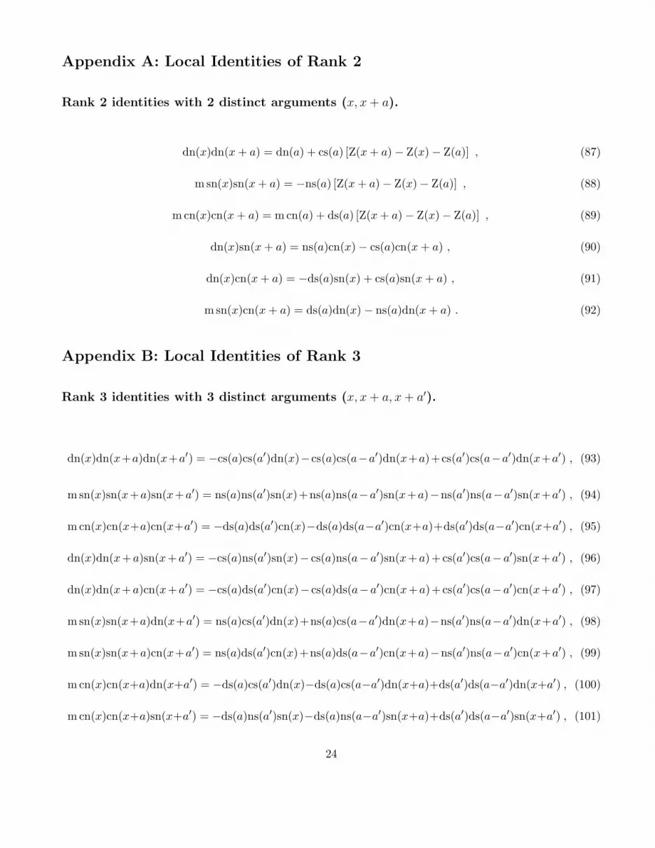
Appendix A: Local Identities of Rank 2

Rank 2 identities with 2 distinct arguments (x, x + a).

dn(x)dn(x + a) = dn(a) + cs(a) [Z(x + a) − Z(x) − Z(a)] , (87)

m sn(x)sn(x + a) = −ns(a) [Z(x + a) − Z(x) − Z(a)] , (88)

m cn(x)cn(x + a) = m cn(a) + ds(a) [Z(x + a) − Z(x) − Z(a)] , (89)

dn(x)sn(x + a) = ns(a)cn(x) − cs(a)cn(x + a) , (90)

dn(x)cn(x + a) = −ds(a)sn(x) + cs(a)sn(x + a) , (91)

m sn(x)cn(x + a) = ds(a)dn(x) − ns(a)dn(x + a) . (92)

Appendix B: Local Identities of Rank 3

Rank 3 identities with 3 distinct arguments (x, x + a, x + a′).

dn(x)dn(x+a)dn(x+a′) = −cs(a)cs(a′)dn(x)−cs(a)cs(a−a′)dn(x+a)+cs(a′)cs(a−a′)dn(x+a′) , (93)

m sn(x)sn(x+a)sn(x+a′) = ns(a)ns(a′)sn(x)+ns(a)ns(a−a′)sn(x+a)−ns(a′)ns(a−a′)sn(x+a′) , (94)

m cn(x)cn(x+a)cn(x+a′) = −ds(a)ds(a′)cn(x)−ds(a)ds(a−a′)cn(x+a)+ds(a′)ds(a−a′)cn(x+a′) , (95)

dn(x)dn(x+a)sn(x+a′) = −cs(a)ns(a′)sn(x)− cs(a)ns(a−a′)sn(x+a)+ cs(a′)cs(a−a′)sn(x+a′) , (96)

dn(x)dn(x+a)cn(x+a′) = −cs(a)ds(a′)cn(x)− cs(a)ds(a−a′)cn(x+a)+cs(a′)cs(a−a′)cn(x+a′) , (97)

m sn(x)sn(x+a)dn(x+a′) = ns(a)cs(a′)dn(x)+ns(a)cs(a−a′)dn(x+a)−ns(a′)ns(a−a′)dn(x+a′) , (98)

m sn(x)sn(x+a)cn(x+a′) = ns(a)ds(a′)cn(x)+ns(a)ds(a−a′)cn(x+a)−ns(a′)ns(a−a′)cn(x+a′) , (99)

m cn(x)cn(x+a)dn(x+a′) = −ds(a)cs(a′)dn(x)−ds(a)cs(a−a′)dn(x+a)+ds(a′)ds(a−a′)dn(x+a′) , (100)

m cn(x)cn(x+a)sn(x+a′) = −ds(a)ns(a′)sn(x)−ds(a)ns(a−a′)sn(x+a)+ds(a′)ds(a−a′)sn(x+a′) , (101)

24

m dn(x)sn(x + a)cn(x + a′) = −ds(a − a′){dn(a) + cs(a) [Z(x + a) − Z(x) − Z(a)]}

+ns(a − a′){dn(a′) + cs(a′)[

Z(x + a′) − Z(x) − Z(a′)]

} . (102)

Rank 3 identities with 2 distinct arguments (x, x + a).

As explained in the text, local identities for say m cn(x)sn(x + a)dn(x + a) and m sn(x)dn(x)cn(x + a)

are related to each other by x → x − a followed by a → −a and hence only one of these identities is given

below.

dn2(x)dn(x + a) = −cs2(a)dn(x + a) + ds(a)ns(a)dn(x) − m cs(a)cn(x)sn(x) , (103)

m sn2(x)sn(x + a) = ns2(a)sn(x + a) − cs(a)ds(a)sn(x) − ns(a)cn(x)dn(x) , (104)

m cn2(x)cn(x + a) = −ds2(a)cn(x + a) + cs(a)ns(a)cn(x) − ds(a)sn(x)dn(x) , (105)

dn(x)sn(x)dn(x + a) = −cs(a)ns(a)sn(x + a) + ds(a)ns(a)sn(x) + cs(a)cn(x)dn(x) , (106)

dn(x)cn(x)dn(x + a) = −cs(a)ds(a)cn(x + a) + ds(a)ns(a)cn(x) − cs(a)sn(x)dn(x) , (107)

m dn(x)sn(x)sn(x + a) = cs(a)ns(a)dn(x + a) − cs(a)ds(a)dn(x) + m ns(a)cn(x)sn(x) , (108)

m sn(x)cn(x)sn(x + a) = ds(a)ns(a)cn(x + a) − cs(a)ds(a)cn(x) + ns(a)sn(x)dn(x) , (109)

m dn(x)cn(x)cn(x + a) = −cs(a)ds(a)dn(x + a) + cs(a)ns(a)dn(x) − m ds(a)cn(x)sn(x) , (110)

m sn(x)cn(x)cn(x + a) = −ds(a)ns(a)sn(x + a) + cs(a)ns(a)sn(x) + ds(a)cn(x)dn(x) , (111)

m dn(x)sn(x)cn(x + a) = −ds(a) − cs(a)ns(a) [Z(x + a) − Z(x) − Z(a)] + ds(a)dn2(x) , (112)

m cn(x)dn(x)sn(x + a) = −ds(a)dn(a) − cs(a)ds(a) [Z(x + a) − Z(x) − Z(a)] + ns(a)dn2(x) , (113)

m sn(x)cn(x)dn(x + a) = −cs(a) − ds(a)ns(a) [Z(x + a) − Z(x) − Z(a)] + cs(a)dn2(x) . (114)

Appendix C: Local Identities of Rank 4

25

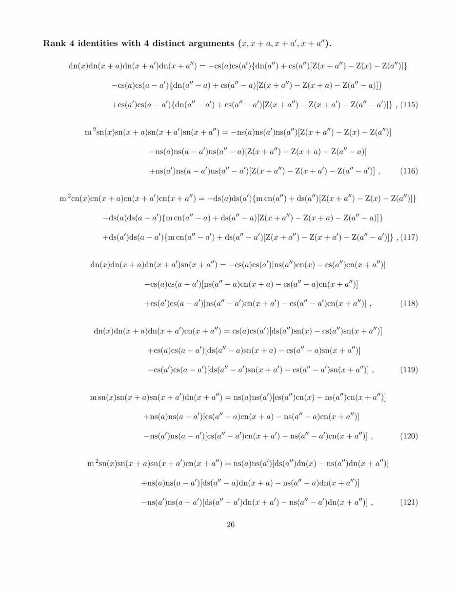
Rank 4 identities with 4 distinct arguments (x, x + a, x + a′, x + a

′′).

dn(x)dn(x + a)dn(x + a′)dn(x + a′′) = −cs(a)cs(a′){dn(a′′) + cs(a′′)[Z(x + a′′) − Z(x) − Z(a′′)]}

−cs(a)cs(a − a′){dn(a′′ − a) + cs(a′′ − a)[Z(x + a′′) − Z(x + a) − Z(a′′ − a)]}

+cs(a′)cs(a − a′){dn(a′′ − a′) + cs(a′′ − a′)[Z(x + a′′) − Z(x + a′) − Z(a′′ − a′)]} , (115)

m 2sn(x)sn(x + a)sn(x + a′)sn(x + a′′) = −ns(a)ns(a′)ns(a′′)[Z(x + a′′) − Z(x) − Z(a′′)]

−ns(a)ns(a − a′)ns(a′′ − a)[Z(x + a′′) − Z(x + a) − Z(a′′ − a)]

+ns(a′)ns(a − a′)ns(a′′ − a′)[Z(x + a′′) − Z(x + a′) − Z(a′′ − a′)] , (116)

m 2cn(x)cn(x + a)cn(x + a′)cn(x + a′′) = −ds(a)ds(a′){m cn(a′′) + ds(a′′)[Z(x + a′′) − Z(x) − Z(a′′)]}

−ds(a)ds(a − a′){m cn(a′′ − a) + ds(a′′ − a)[Z(x + a′′) − Z(x + a) − Z(a′′ − a)]}

+ds(a′)ds(a − a′){m cn(a′′ − a′) + ds(a′′ − a′)[Z(x + a′′) − Z(x + a′) − Z(a′′ − a′)]} , (117)

dn(x)dn(x + a)dn(x + a′)sn(x + a′′) = −cs(a)cs(a′)[ns(a′′)cn(x) − cs(a′′)cn(x + a′′)]

−cs(a)cs(a − a′)[ns(a′′ − a)cn(x + a) − cs(a′′ − a)cn(x + a′′)]

+cs(a′)cs(a − a′)[ns(a′′ − a′)cn(x + a′) − cs(a′′ − a′)cn(x + a′′)] , (118)

dn(x)dn(x + a)dn(x + a′)cn(x + a′′) = cs(a)cs(a′)[ds(a′′)sn(x) − cs(a′′)sn(x + a′′)]

+cs(a)cs(a − a′)[ds(a′′ − a)sn(x + a) − cs(a′′ − a)sn(x + a′′)]

−cs(a′)cs(a − a′)[ds(a′′ − a′)sn(x + a′) − cs(a′′ − a′)sn(x + a′′)] , (119)

m sn(x)sn(x + a)sn(x + a′)dn(x + a′′) = ns(a)ns(a′)[cs(a′′)cn(x) − ns(a′′)cn(x + a′′)]

+ns(a)ns(a − a′)[cs(a′′ − a)cn(x + a) − ns(a′′ − a)cn(x + a′′)]

−ns(a′)ns(a − a′)[cs(a′′ − a′)cn(x + a′) − ns(a′′ − a′)cn(x + a′′)] , (120)

m 2sn(x)sn(x + a)sn(x + a′)cn(x + a′′) = ns(a)ns(a′)[ds(a′′)dn(x) − ns(a′′)dn(x + a′′)]

+ns(a)ns(a − a′)[ds(a′′ − a)dn(x + a) − ns(a′′ − a)dn(x + a′′)]

−ns(a′)ns(a − a′)[ds(a′′ − a′)dn(x + a′) − ns(a′′ − a′)dn(x + a′′)] , (121)

26

m cn(x)cn(x + a)cn(x + a′)dn(x + a′′) = ds(a)ds(a′)[cs(a′′)sn(x) − ds(a′′)sn(x + a′′)]

+ds(a)ds(a − a′)[cs(a′′ − a)sn(x + a) − ds(a′′ − a)sn(x + a′′)]

−ds(a′)ds(a − a′)[cs(a′′ − a′)sn(x + a′) − ds(a′′ − a′)sn(x + a′′)] , (122)

m 2cn(x)cn(x + a)cn(x + a′)sn(x + a′′) = −ds(a)ds(a′)[ns(a′′)dn(x) − ds(a′′)dn(x + a′′)]

−ds(a)ds(a − a′)[ns(a′′ − a)dn(x + a) − ds(a′′ − a)dn(x + a′′)]

+ds(a′)ds(a − a′)[ns(a′′ − a′)dn(x + a′) − ds(a′′ − a′)dn(x + a′′)] , (123)

m sn(x)dn(x + a)sn(x + a′)dn(x + a′′) = cs(a)ns(a′){dn(a′′) + cs(a′′)[Z(x + a′′) − Z(x) − Z(a′′)]}

+ns(a)ns(a − a′){dn(a′′ − a) + cs(a′′ − a)[Z(x + a′′) − Z(x + a) − Z(a′′ − a)]}

−ns(a′)cs(a − a′){dn(a′′ − a′) + cs(a′′ − a′)[Z(x + a′′) − Z(x + a′) − Z(a′′ − a′)]} , (124)

m cn(x)dn(x + a)cn(x + a′)dn(x + a′′) = −cs(a)ds(a′){dn(a′′) + cs(a′′)[Z(x + a′′) − Z(x) − Z(a′′)]}

−ds(a)ds(a − a′){dn(a′′ − a) + cs(a′′ − a)[Z(x + a′′) − Z(x + a) − Z(a′′ − a)]}

+ds(a′)cs(a − a′){dn(a′′ − a′) + cs(a′′ − a′)[Z(x + a′′) − Z(x + a′) − Z(a′′ − a′)]} , (125)

m 2sn(x)cn(x + a)cn(x + a′)sn(x + a′′) = ds(a)ds(a′)ns(a′′)[Z(x + a′′) − Z(x) − Z(a′′)]

+ns(a)ds(a − a′)ns(a′′ − a)[Z(x + a′′) − Z(x + a) − Z(a′′ − a)]

−ns(a′)ds(a − a′)ns(a′′ − a′)[Z(x + a′′) − Z(x + a′) − Z(a′′ − a′)] , (126)

m cn(x)dn(x + a)dn(x + a′)sn(x + a′′) = −cs(a)cs(a′)[ns(a′′)dn(x) − ds(a′′)dn(x + a′′)]

−ds(a)cs(a − a′)[ns(a′′ − a)dn(x + a) − ds(a′′ − a)dn(x + a′′)]

+ds(a′)cs(a − a′)[ns(a′′ − a′)dn(x + a′) − ds(a′′ − a′)dn(x + a′′)] , (127)

m sn(x)dn(x + a)sn(x + a′)cn(x + a′′) = −cs(a)ns(a′)[ds(a′′)sn(x) − cs(a′′)sn(x + a′′)]

−ns(a)ns(a − a′)[ds(a′′ − a)sn(x + a) − cs(a′′ − a)sn(x + a′′)]

+ns(a′)cs(a − a′)[ds(a′′ − a′)sn(x + a′) − cs(a′′ − a′)sn(x + a′′)] , (128)

27

m cn(x)dn(x + a)cn(x + a′)sn(x + a′′) = −cs(a)ds(a′)[ns(a′′)cn(x) − cs(a′′)cn(x + a′′)]

−ds(a)ds(a − a′)[ns(a′′ − a)cn(x + a) − cs(a′′ − a)cn(x + a′′)]

+ds(a′)cs(a − a′)[ns(a′′ − a′)cn(x + a′) − cs(a′′ − a′)cn(x + a′′)] . (129)

Rank 4 identities with 3 distinct arguments (x, x + a, x + a′).

dn2(x)dn(x + a)dn(x + a′) = −cs(a)cs(a − a′){dn(a) + cs(a)[Z(x + a) − Z(x) − Z(a)]}

+cs(a′)cs(a − a′){dn(a′) + cs(a′)[Z(x + a′) − Z(x) − Z(a′)]} − cs(a)cs(a′)dn2(x) ,(130)

m 2sn2(x)sn(x + a)sn(x + a′) = −ns2(a)ns(a − a′)[Z(x + a) − Z(x) − Z(a)]

+ns2(a′)ns(a − a′)[Z(x + a′) − Z(x) − Z(a′)] + m ns(a)ns(a′)sn2(x) , (131)

m 2cn2(x)cn(x + a)cn(x + a′) = −ds(a)ds(a − a′){m cn(a) + ds(a)[Z(x + a) − Z(x) − Z(a)]}

+ds(a′)ds(a − a′){m cn(a′) + ds(a′)[Z(x + a′) − Z(x) − Z(a′)]} − m ds(a)ds(a′)cn2(x) ,(132)

m dn(x)sn(x)dn(x + a)sn(x + a′) = cs(a)ns(a)ns(a − a′)[Z(x + a) − Z(x) − Z(a)]

−cs(a′)ns(a′)cs(a − a′)[Z(x + a′) − Z(x) − Z(a′)] − m cs(a)ns(a′)sn2(x) , (133)

m dn(x)cn(x)dn(x + a)cn(x + a′) = −cs(a)ds(a − a′){m cn(a) + ds(a)[Z(x + a) − Z(x) − Z(a)]}

+cs(a′)cs(a − a′){m cn(a′) + ds(a′)[Z(x + a′) − Z(x) − Z(a′)]} − m cs(a)ds(a′)cn2(x) , (134)

m 2sn(x)cn(x)sn(x + a)cn(x + a′) = ds(a)ns(a)ds(a − a′)[Z(x + a) − Z(x) − Z(a)]

−ds(a′)ns(a′)ns(a − a′)[Z(x + a′) − Z(x) − Z(a′)] − m ns(a)ds(a′)sn2(x) , (135)

dn(x)2dn(x + a)sn(x + a′) = −cs(a)ns(a − a′)[ns(a)cn(x) − cs(a)cn(x + a)]

+cs(a′)cs(a − a′)[ns(a′)cn(x) − cs(a′)cn(x + a′)] − cs(a)ns(a′)sn(x)dn(x) , (136)

28

dn(x)2dn(x + a)cn(x + a′) = cs(a)ds(a − a′)[ds(a)sn(x) − cs(a)sn(x + a)]

−cs(a′)cs(a − a′)[ds(a′)sn(x) − cs(a′)sn(x + a′)] − cs(a)ds(a′)cn(x)dn(x) , (137)

m 2cn(x)2sn(x + a)cn(x + a′) = −ds(a)ds(a − a′)[ns(a)dn(x) − ds(a)dn(x + a)]

+ds(a′)ns(a − a′)[ns(a′)dn(x) − ds(a′)dn(x + a′)] − m ns(a)ds(a′)cn(x)sn(x) , (138)

m dn(x)sn(x)sn(x + a)cn(x + a′) = −ns(a)ds(a − a′)[ds(a)sn(x) − cs(a)sn(x + a)]

+ns(a′)ns(a − a′)[ds(a′)sn(x) − cs(a′)sn(x + a′)] + ns(a)ds(a′)cn(x)dn(x) , (139)

m dn(x)sn(x)dn(x + a)cn(x + a′) = −cs(a)ds(a − a′)[ds(a)dn(x) − ns(a)dn(x + a)]

+cs(a′)cs(a − a′)[ds(a′)dn(x) − ns(a′)dn(x + a′)] − m cs(a)ds(a′)cn(x)sn(x) , (140)

dn(x)sn(x)dn(x + a)dn(x + a′) = −cs(a)cs(a − a′)[cs(a)cn(x) − ns(a)cn(x + a)]

+cs(a′)cs(a − a′)[cs(a′)cn(x) − ns(a′)cn(x + a′)] − cs(a)cs(a′)sn(x)dn(x) , (141)

m dn(x)sn(x)sn(x + a)sn(x + a′) = ns(a)ns(a − a′)[ns(a)cn(x) − cs(a)cn(x + a)]

−ns(a′)ns(a − a′)[ns(a′)cn(x) − cs(a′)cn(x + a′)] + ns(a)ns(a′)sn(x)dn(x) , (142)

m dn(x)sn(x)cn(x + a)cn(x + a′) = −ns(a)ds(a − a′)[ns(a)cn(x) − cs(a)cn(x + a)]

+ns(a′)ds(a − a′)[ns(a′)cn(x) − cs(a′)cn(x + a′)] − ds(a)ds(a′)sn(x)dn(x) , (143)

m dn(x)cn(x)sn(x + a)cn(x + a′) = −ds(a)ds(a − a′)[ns(a)cn(x) − cs(a)cn(x + a)]

+ds(a′)ns(a − a′)[ns(a′)cn(x) − cs(a′)cn(x + a′)] − ns(a)ds(a′)sn(x)dn(x) , (144)

m dn(x)cn(x)dn(x + a)sn(x + a′) = −cs(a)ns(a − a′)[ns(a)dn(x) − ds(a)dn(x + a)]

+cs(a′)cs(a − a′)[ns(a′)dn(x) − ds(a′)dn(x + a′)] − m cs(a)ns(a′)cn(x)sn(x) , (145)

29

dn(x)cn(x)dn(x + a)dn(x + a′) = cs(a)cs(a − a′)[cs(a)sn(x) − ds(a)sn(x + a)]

−cs(a′)cs(a − a′)[cs(a′)sn(x) − ds(a′)sn(x + a′)] − cs(a)cs(a′)cn(x)dn(x) , (146)

m dn(x)cn(x)sn(x + a)sn(x + a′) = −ds(a)ns(a − a′)[ds(a)sn(x) − cs(a)sn(x + a)]

+ds(a′)ns(a − a′)[ds(a′)sn(x) − cs(a′)sn(x + a′)] + ns(a)ns(a′)cn(x)dn(x) , (147)

m dn(x)cn(x)cn(x + a)cn(x + a′) = ds(a)ds(a − a′)[ds(a)sn(x) − cs(a)sn(x + a)]

−ds(a′)ds(a − a′)[ds(a′)sn(x) − cs(a′)sn(x + a′)] − ds(a)ds(a′)cn(x)dn(x) , (148)

m 2sn(x)cn(x)sn(x + a)sn(x + a′) = ds(a)ns(a − a′)[ds(a)dn(x) − ns(a)dn(x + a)]

−ds(a′)ns(a − a′)[ds(a′)dn(x) − ns(a′)dn(x + a′)] + m ns(a)ns(a′)sn(x)cn(x) , (149)

m sn(x)cn(x)dn(x + a)dn(x + a′) = −ns(a)cs(a − a′)[ns(a)dn(x) − ds(a)dn(x + a)]

+ns(a′)cs(a − a′)[ns(a′)dn(x) − ds(a′)dn(x + a′)] − m cs(a)cs(a′)cn(x)sn(x) , (150)

m 2sn(x)cn(x)cn(x + a)cn(x + a′) = −ns(a)ds(a − a′)[ns(a)dn(x) − ds(a)dn(x + a)]

+ns(a′)ds(a − a′)[ns(a′)dn(x) − ds(a′)dn(x + a′)] − m ds(a)ds(a′)cn(x)sn(x) , (151)

m sn(x)cn(x)dn(x + a)sn(x + a′) = −ns(a)ns(a − a′)[cs(a)sn(x) − ds(a)sn(x + a)]

+ns(a′)cs(a − a′)[cs(a′)sn(x) − ds(a′)sn(x + a′)] + cs(a)ns(a′)cn(x)dn(x) , (152)

m sn(x)cn(x)dn(x + a)cn(x + a′) = −ds(a)ds(a − a′)[cs(a)cn(x) − ns(a)cn(x + a)]

+ds(a′)cs(a − a′)[cs(a′)cn(x) − ns(a′)cn(x + a′)] − cs(a)ds(a′)sn(x)dn(x) . (153)

Rank 4 identities with 2 distinct arguments (x, x + a).

m dn(x)sn(x)cn(x)dn(x + a) = −cs(a)[ds2(a) + 1]dn(x) + cs(a)ds(a)ns(a)dn(x + a)

+ cs(a)dn3(x) + m ds(a)ns(a)cn(x)sn(x) , (154)

30

m dn(x)sn(x)cn(x)sn(x + a) = −ns(a)[ds2(a) − 1]sn(x) + cs(a)ds(a)ns(a)sn(x + a)

−m ns(a)sn3(x) − cs(a)ds(a)cn(x)dn(x) , (155)

m dn(x)sn(x)cn(x)cn(x + a) = −ds(a)[m + cs2(a)]cn(x) + cs(a)ds(a)ns(a)cn(x + a)

+m ds(a)cn3(x) + cs(a)ns(a)sn(x)dn(x) , (156)

dn3(x)dn(x + a) = −m cs(a)sn(x)cn(x)dn(x) + ds(a)ns(a)dn2(x)

−cs2(a)dn(a) − cs3(a) [Z(x + a) − Z(x) − Z(a)] , (157)

dn3(x)sn(x + a) = cs3(a)cn(x + a) − ns(a)(

2cs2(a) − ds2(a))

cn(x)

+ cs(a)ds(a)sn(x)dn(x) + m ns(a)cn3(x) , (158)

dn3(x)cn(x + a) = −cs3(a)sn(x + a) − ds(a)(

2 − ns2(a))

sn(x)

+ cs(a)ns(a)cn(x)dn(x) + m ds(a)sn3(x) , (159)

msn3(x)dn(x + a) = −ns3(a)cn(x + a) +(

m + ns2(a))

cs(a)cn(x)

− ds(a)ns(a)sn(x)dn(x) − m cs(a)cn3(x) , (160)

m 2sn3(x)sn(x + a) = −m ns(a)sn(x)cn(x)dn(x) + cs(a)ds(a)dn2(x)

−cs(a)ds(a) − ns3(a) [Z(x + a) − Z(x) − Z(a)] , (161)

m 2sn3(x)cn(x + a) =(

1 + ns2(a))

ds(a)dn(x) − ns3(a)dn(x + a)

−m cs(a)ns(a)sn(x)cn(x) − ds(a)dn3(x) , (162)

m cn3(x)dn(x + a) = −ds3(a)sn(x + a) +(

2ds2(a) − ns2(a))

cs(a)sn(x)

+ ds(a)ns(a)cn(x)dn(x) + m cs(a)sn3(x) , (163)

31

m 2cn3(x)sn(x + a) = ds3(a)dn(x + a) −(

2ds2(a) − cs2(a))

ns(a)dn(x)

+ m cs(a)ds(a)sn(x)cn(x) + ns(a)dn3(x) , (164)

m 2cn3(x)cn(x + a) = −m ds(a)sn(x)cn(x)dn(x) + cs(a)ns(a)dn2(x)

−cs(a)ns(a)[1 − m + m dn2(a)] − ds3(a) [Z(x + a) − Z(x) − Z(a)] , (165)

dn2(x)dn2(x + a) = −cs2(a)[dn2(x) + dn2(x + a)] + [ds2(a) + cs2(a)]

+2cs(a)ds(a)ns(a) [Z(x + a) − Z(x) − Z(a)] , (166)

m dn2(x)sn(x + a)cn(x + a) = cs(a)[ds2(a) + ns2(a)]dn(x) − 2cs(a)ds(a)ns(a)dn(x + a)

−m cs2(a)sn(x + a)cn(x + a) − m ds(a)ns(a)cn(x)sn(x) , (167)

m sn2(x)dn(x + a)cn(x + a) = ns(a)[cs2(a) + ds2(a)]sn(x) − 2cs(a)ds(a)ns(a)sn(x + a)

+ ns2(a)cn(x + a)dn(x + a) + cs(a)ds(a)cn(x)dn(x) , (168)

m cn2(x)dn(x + a)sn(x + a) = ds(a)[cs2(a) + ns2(a)]cn(x) − 2cs(a)ds(a)ns(a)cn(x + a)

− ds2(a)sn(x + a)dn(x + a) − cs(a)ns(a)sn(x)dn(x) , (169)

m 2sn(x)cn(x)sn(x + a)cn(x + a) = ds(a)ns(a)[

dn2(x) + dn2(x + a)]

−[

ds2(a) + ns2(a)]

{dn(a) + cs(a) [Z(x + a) − Z(x) − Z(a)]} , (170)

m dn(x)sn(x)dn(x + a)sn(x + a) = −cs(a)ns(a)[1 + dn2(a)] + cs(a)ns(a)[

dn2(x) + dn2(x + a)]

−ds(a)[cs2(a) + ns2(a)] [Z(x + a) − Z(x) − Z(a)] , (171)

m dn(x)cn(x)dn(x + a)cn(x + a) = 2cs(a)ds(a) − cs(a)ds(a)[

dn2(x) + dn2(x + a)]

+ns(a)[ds2(a) + cs2(a)] [Z(x + a) − Z(x) − Z(a)] , (172)

32

m dn(x)cn(x)dn(x + a)sn(x + a) = ds(a)[cs2(a) + ns2(a)]dn(x) − ns(a)[cs2(a) + ds2(a)]dn(x + a)

−m cs(a)ds(a)sn(x + a)cn(x + a) − m cs(a)ns(a)cn(x)sn(x) , (173)

m dn(x)cn(x)sn(x + a)cn(x + a) = cs(a)[ds2(a) + ns2(a)]cn(x) − ns(a)[cs2(a) + ds2(a)]cn(x + a)

− cs(a)ds(a)sn(x + a)dn(x + a) − ds(a)ns(a)sn(x)dn(x) , (174)

m sn(x)cn(x)dn(x + a)sn(x + a) = ds(a)[cs2(a) + ns2(a)]sn(x) − cs(a)[ds2(a) + ns2(a)]sn(x + a)

+ ds(a)ns(a)cn(x + a)dn(x + a) + cs(a)ns(a)cn(x)dn(x) . (175)

Appendix D: Some Examples of Local Identities of Rank 5

m dn(x)sn(x)cn(x)dn(x + a)sn(x + a) = −cs(a)ns(a)[cs2(a) + ds2(a) + ns2(a)]cn(x)

+[

ns2(a)(ds2(a) + cs2(a)) + cs2(a)ds2(a)]

cn(x + a) + cs(a)ds(a)ns(a)sn(x + a)dn(x + a)

+ds(a)[cs2(a) + ns2(a)]sn(x)dn(x) + m cs(a)ns(a)cn3(x) , (176)

m dn(x)sn(x)cn(x)dn(x + a)cn(x + a) = cs(a)ds(a)[cs2(a) + ds2(a) + ns2(a)]sn(x)

−[

ns2(a)(ds2(a) + cs2(a)) + cs2(a)ds2(a)]

sn(x + a) + cs(a)ds(a)ns(a)cn(x + a)dn(x + a)

+ns(a)[cs2(a) + ds2(a)]cn(x)dn(x) + m cs(a)ds(a)sn3(x) , (177)

m 2dn(x)sn(x)cn(x)sn(x + a)cn(x + a) = −ds(a)ns(a)[cs2(a) + ds2(a) + ns2(a)]dn(x)

+[

ns2(a)(ds2(a) + cs2(a)) + cs2(a)ds2(a)]

dn(x + a) + m cs(a)ds(a)ns(a)cn(x + a)sn(x + a)

+m cs(a)[ds2(a) + ns2(a)]cn(x)sn(x) + ds(a)ns(a)dn3(x) , (178)

m dn(x)sn(x)cn(x)dn2(x + a) = cs(a)ds(a)ns(a)[dn2(x + a) + 2dn2(x) − dn2(a) − 2]

−m cs2(a)dn(x)sn(x)cn(x) + [ns2(a)(

ds2(a) + cs2(a))

+ cs2(a)ds2(a)] [Z(x + a) − Z(x) − Z(a)] .(179)

Appendix E: Local Identities of Arbitrary Rank

33

In the following identities, B ≡ −cs2(a), B1 ≡ ns2(a), B2 ≡ −ds2(a).

dn2n(x)dn(x + a) = Bndn(x + a) + [ds(a)ns(a)dn(x) − m cs(a)cn(x)sn(x)]n∑

k=1

Bk−1[dn(x)]2(n−k) , (180)

dn2n+1(x)dn(x + a) = Bn(dn(a) + cs(a)[Z(x + a) − Z(x) − Z(a)])

+ [ds(a)ns(a)dn(x) − m cs(a)cn(x)sn(x)]n∑

k=1

Bk−1[dn(x)]2(n−k)+1 , (181)

m nsn2n(x)sn(x + a) = Bn1 sn(x + a) − [cs(a)ds(a)sn(x) + ns(a)cn(x)dn(x)]

n∑

k=1

m n−kBk−11 [sn(x)]2(n−k) ,

(182)

m n+1sn2n+1(x)sn(x + a) = −Bn1 ns(a) [Z(x + a) − Z(x) − Z(a)]

− [cs(a)ds(a)sn(x) + ns(a)cn(x)dn(x)]n∑

k=1

m n−kBk−11 [sn(x)]2(n−k)+1 , (183)

m ncn2n(x)cn(x + a) = Bn2 cn(x + a)

+ [cs(a)ns(a)cn(x) − ds(a)sn(x)dn(x)]n∑

k=1

m n−kBk−12 [cn(x)]2(n−k) , (184)

m n+1cn2n+1(x)cn(x + a) = Bn2 {m cn(a) + ds(a) [Z(x + a) − Z(x) − Z(a)]}

+ [cs(a)ns(a)cn(x) − ds(a)sn(x)dn(x)]n∑

k=1

m n−kBk−12 [cn(x)]2(n−k)+1 , (185)

m ncn2n(x)sn(x)dn(x + a) = −Bn2 ns(a)cn(x + a) + cs(a)m ncn2n+1(x)

−ns(a) [cs(a)ns(a)cn(x) − ds(a)sn(x)dn(x)]n∑

k=1

m n−kBk−12 [cn(x)]2(n−k) , (186)

m nsn2n(x)cn(x)dn(x + a) = Bn1 ds(a)sn(x + a) − cs(a)m nsn2n+1(x)

−ds(a) [cs(a)ds(a)sn(x) + ns(a)cn(x)dn(x)]n∑

k=1

m n−kBk−11 [sn(x)]2(n−k) , (187)

m dn2n(x)cn(x)sn(x + a) = −Bnds(a)dn(x + a) + ns(a)dn2n+1(x)

−ds(a) [ds(a)ns(a)dn(x) − m cs(a)cn(x)sn(x)]n∑

k=1

Bk−1[dn(x)]2(n−k) , (188)

34

m dn2n(x)sn(x + a)cn(x + a) = m Bnsn(x + a)cn(x + a) − 2nBn−1ds(a)cs(a)ns(a)dn(x + a)

+n∑

k=1

Bk−1[

(m + 2ds2(a))cs(a) + 2(k − 1)ds2(a)nc(a)ns(a)]

[dn(x)]2(n−k)+1

−mds(a)ns(a)n∑

k=1

(2k − 1)Bk−1cn(x)sn(x)[dn(x)]2(n−k) , (189)

m dn2n+1(x)sn(x + a)cn(x + a) = −mds(a)ns(a)n∑

k=1

(2k − 1)Bk−1cn(x)sn(x)[dn(x)]2(n−k)+1

+Bn−1cs(a)

[

(1 − m) − (2n + 1)ds(a)ns(a)(dn(a) + cs(a)[Z(x + a) − Z(x) − Z(a)])

]

+n∑

k=1

Bk−1[(m + 2ds2(a))cs(a) + 2(k − 1)ds2(a)nc(a)ns(a)][dn(x)]2(n−k+1)−Bncs(a)dn2(x + a) ,(190)

dn2n(x)sn(x + a)dn(x + a) = Bnsn(x + a)dn(x + a) − 2nBn−1ds(a)cs(a)ns(a)cn(x + a)

−n∑

k=1

Bk−1[

cs(a)ns(a) + 2(k − 1)ds2(a)nc(a)]

sn(x)[dn(x)]2(n−k)+1

+ds(a)n∑

k=1

Bk−1[cs2(a) + (2k − 1)ns2(a)]cn(x)[dn(x)]2(n−k) , (191)

dn2n+1(x)sn(x + a)dn(x + a) = −Bncs(a)cn(x + a)dn(x + a) + Bn−1cs(a)ns(a)[cs2(a) + 2nds2(a)]sn(x)

−n∑

k=1

Bk−1[cs(a)ns(a) + 2(k − 1)ds2(a)nc(a)]sn(x)[dn(x)]2(n−k+1) + (2n + 1)Bnds(a)ns(a)sn(x + a)

+ds(a)n∑

k=1

Bk−1[cs2(a) + (2k − 1)ns2(a)]cn(x)[dn(x)]2(n−k)+1 , (192)

dn2n(x)cn(x + a)dn(x + a) = Bncn(x + a)dn(x + a) + 2nBn−1ds(a)cs(a)ns(a)sn(x + a)

−n∑

k=1

Bk−1 [cs(a)ds(a) + 2(k − 1)ds(a)nc(a)ns(a)] cn(x)[dn(x)]2(n−k)+1

−ns(a)n∑

k=1

Bk−1[cs2(a) + (2k − 1)ds2(a)]sn(x)[dn(x)]2(n−k) , (193)

dn2n+1(x)cn(x + a)dn(x + a) = Bncs(a)sn(x + a)dn(x + a) + Bn−1cs(a)ds(a)[cs2(a) + 2nns2(a)]cn(x)

−n∑

k=1

Bk−1[cs(a)ds(a) + 2(k − 1)ds(a)nc(a)ns(a)]cn(x)[dn(x)]2(n−k+1)+ (2n + 1)Bnds(a)ns(a)cn(x + a)

−ns(a)n∑

k=1

Bk−1[cs2(a) + (2k − 1)ds2(a)]sn(x)[dn(x)]2(n−k)+1 , (194)

35

dn2n(x)dn2(x + a) = 2nBn−1ds(a)ns(a)[dn(a) + cs(a)(Z(x + a) − Z(x) − Z(a))]

−(1 − m)Bn−1 +n−1∑

k=1

Bk−1[B2 − (1 − m) + 2kds2(a)ns2(a)][dn(x)]2(n−k)

+Bndn2(x + a) + Bdn2n − 2mcs(a)ds(a)ns(a)sn(x)cn(x)n−1∑

k=1

kBk−1[dn(x)]2(n−k)−1 , (195)

dn2n+1(x)dn2(x + a) = Bdn2n+1(x) + Bnm cs(a)cn(x + a)sn(x + a)

+n∑

k=1

Bk−1[B2 − (1 − m) + 2kds2(a)ns2(a)][dn(x)]2(n−k)+1

−2mcs(a)ds(a)ns(a)sn(x)cn(x)n∑

k=1

kBk−1[dn(x)]2(n−k) + (2n + 1)Bnds(a)ns(a)dn(x + a) , (196)

Appendix F: Examples of Identities with Weighted Terms and Their

Linear Combinations

In this appendix a = 2rKp , a′ = 2sK

p , b = 4rKp .

F1: MI-I Identities

mp∑

j=1

cj [sj+r − sj−r] = 2[ns(a) − ds(a)]p∑

j=1

dj , (197)

p∑

j=1

d2j [dj+r − dj−r] = −2m cs(a)

p∑

j=1

cjsj , (198)

p∑

j=1

cj [cj+rdj+r − cj−rdj−r] = 2ds(a)p∑

j=1

cjsj , (199)

p∑

j=1

sj[sj+rdj+r − sj−rdj−r] = −2ns(a)p∑

j=1

cjsj , (200)

p∑

j=1

cj [dj+rcj+s − dj−rcj−s] = 0 , (201)

p∑

j=1

sj[dj+rsj+s − dj−rsj−s] = 0 , (202)

p∑

j=1

dj [dj+rdj+s − dj−rdj−s] = 0 , (203)

36

p∑

j=1

dj [cj+rcj+s − cj−rcj−s] = 0 , (204)

p∑

j=1

dj[sj+rsj+s − sj−rsj−s] = 0 , (205)

mp∑

j=1

d2j [cj+rsj+r − cj−rsj−r] = 2cs(a)[ns2(a) + ds2(a) − 2ns(a)ds(a)]

p∑

j=1

dj , (206)

mp∑

j=1

cjdj [dj+rsj+r − dj−rsj−r] = −2[ns(a)(cs2(a) + ds2(a)) − ds(a)(cs2(a) + ns2(a))]p∑

j=1

dj , (207)

p∑

j=1

d3j [d

2j+r − d2

j−r] = −2m cs(a)[cs2(a) + 2ds(a)ns(a)]p∑

j=1

cjsj , (208)

mp∑

j=1

cjsjdj [cj+rsj+r − cj−rsj−r] = 2cs(a)[(ds2(a) + ns2(a)) + ds(a)ns(a)]p∑

j=1

cjsj , (209)

mp∑

j=1

cjsjdj [dj+r − dj−r] = 2cs(a)p∑

j=1

d3j

−2cs(a)[ds2(a) + 1 − ds(a)ns(a)]p∑

j=1

dj , (210)

mp∑

j=1

cjsjdj [d3j+r − d3

j−r] = 2cs(a)[ds(a)ns(a) − cs2(a)]p∑

j=1

d3j + 2cs(a)

[

2cs2(a)ds2(a)

+2ns2(a)(ds2(a) + cs2(a)) − cs4(a) − ds(a)ns(a)(ds2(a) + cs2(a) + ns2(a))

] p∑

j=1

dj , (211)

mp∑

j=1

cjdj[dj+rsj+s−dj−rsj−s] = 2[ns(a−a′)cs(a)(ds(a)−ns(a))− cs(a−a′)cs(a′)(ds(a′)−ns(a′))]p∑

j=1

dj ,

(212)

mp∑

j=1

sjdj [dj+rcj+s−dj−rcj−s] = −2[ds(a−a′)cs(a)(ds(a)−ns(a))−cs(a−a′)cs(a′)(ds(a′)−ns(a′))]p∑

j=1

dj ,

(213)

mp∑

j=1

cjsj[dj+rdj+s − dj−rdj−s] = 2cs(a− a′)[ns(a)(ds(a)− ns(a))− ns(a′)(ds(a′)− ns(a′))]p∑

j=1

dj , (214)

m 2p∑

j=1

cjsj[sj+rsj+s−sj−rsj−s] = −2ns(a−a′)[ns(a)(ds(a)−ns(a))−ns(a′)(ds(a′)−ns(a′))]p∑

j=1

dj , (215)

m 2p∑

j=1

cjsj[cj+rcj+s − cj−rcj−s] = 2ds(a− a′)[ns(a)(ds(a)− ns(a))− ns(a′)(ds(a′)− ns(a′))]p∑

j=1

dj , (216)

37

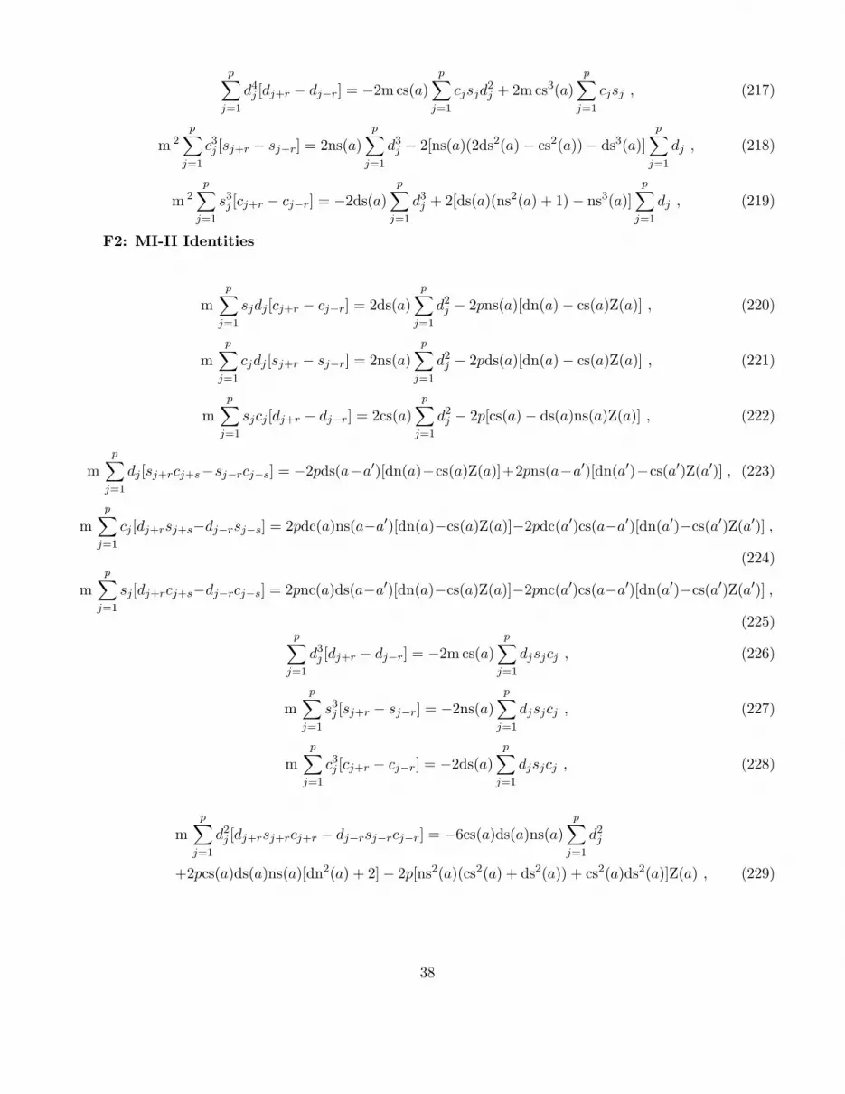
p∑

j=1

d4j [dj+r − dj−r] = −2m cs(a)

p∑

j=1

cjsjd2j + 2m cs3(a)

p∑

j=1

cjsj , (217)

m 2p∑

j=1

c3j [sj+r − sj−r] = 2ns(a)

p∑

j=1

d3j − 2[ns(a)(2ds2(a) − cs2(a)) − ds3(a)]

p∑

j=1

dj , (218)

m 2p∑

j=1

s3j [cj+r − cj−r] = −2ds(a)

p∑

j=1

d3j + 2[ds(a)(ns2(a) + 1) − ns3(a)]

p∑

j=1

dj , (219)

F2: MI-II Identities

mp∑

j=1

sjdj [cj+r − cj−r] = 2ds(a)p∑

j=1

d2j − 2pns(a)[dn(a) − cs(a)Z(a)] , (220)

mp∑

j=1

cjdj [sj+r − sj−r] = 2ns(a)p∑

j=1

d2j − 2pds(a)[dn(a) − cs(a)Z(a)] , (221)

mp∑

j=1

sjcj [dj+r − dj−r] = 2cs(a)p∑

j=1

d2j − 2p[cs(a) − ds(a)ns(a)Z(a)] , (222)

mp∑

j=1

dj [sj+rcj+s−sj−rcj−s] = −2pds(a−a′)[dn(a)−cs(a)Z(a)]+2pns(a−a′)[dn(a′)−cs(a′)Z(a′)] , (223)

mp∑

j=1

cj [dj+rsj+s−dj−rsj−s] = 2pdc(a)ns(a−a′)[dn(a)−cs(a)Z(a)]−2pdc(a′)cs(a−a′)[dn(a′)−cs(a′)Z(a′)] ,

(224)

mp∑

j=1

sj[dj+rcj+s−dj−rcj−s] = 2pnc(a)ds(a−a′)[dn(a)−cs(a)Z(a)]−2pnc(a′)cs(a−a′)[dn(a′)−cs(a′)Z(a′)] ,

(225)p∑

j=1

d3j [dj+r − dj−r] = −2m cs(a)

p∑

j=1

djsjcj , (226)

mp∑

j=1

s3j [sj+r − sj−r] = −2ns(a)

p∑

j=1

djsjcj , (227)

mp∑

j=1

c3j [cj+r − cj−r] = −2ds(a)

p∑

j=1

djsjcj , (228)

mp∑

j=1

d2j [dj+rsj+rcj+r − dj−rsj−rcj−r] = −6cs(a)ds(a)ns(a)

p∑

j=1

d2j

+2pcs(a)ds(a)ns(a)[dn2(a) + 2] − 2p[ns2(a)(cs2(a) + ds2(a)) + cs2(a)ds2(a)]Z(a) , (229)

38

mp∑

j=1

sjcj [d3j+r − d3

j−r] = −2cs(a)[ds2(a) + ns2(a) + cs2(a)]p∑

j=1

d2j

−2pcs(a)[1 − m − 3ds2(a) + 3cs(a)ds(a)ns(a)Z(a)] , (230)

m 2p∑

j=1

djcj [s3j+r − s3

j−r] = 2ns(a)[ds2(a) + ns2(a) + cs2(a)]p∑

j=1

d2j

+2pns(a)[1 − m − 3ds2(a) + 3cs(a)ds(a)ns(a)Z(a)] , (231)

m 2p∑

j=1

djsj [c3j+r − c3

j−r] = −2ds(a)[ds2(a) + ns2(a) + cs2(a)]p∑

j=1

d2j

−2pds(a)[1 − m − 3ds2(a) + 3cs(a)ds(a)ns(a)Z(a)] , (232)

F3: MI-III Identities

p∑

j=1

dj[cj+r − cj−r] = 2[cs(b) − ds(b)]p∑

j=1

sj , (233)

p∑

j=1

m s2j [sj+r − sj−r] = −2ns(b)

p∑

j=1

cjdj , (234)

p∑

j=1

cj [sj+rcj+s − sj−rcj−s] = 0 , (235)

p∑

j=1

dj [dj+rsj+s − dj−rsj−s] = 0 , (236)

p∑

j=1

sj [dj+rdj+s − dj−rdj−s] = 0 , (237)

p∑

j=1

sj [cj+rcj+s − cj−rcj−s] = 0 , (238)

p∑

j=1

sj[sj+rsj+s − sj−rsj−s] = 0 , (239)

p∑

j=1

d2j [cj+rdj+r − cj−rdj−r] = −2ns(b)[cs2(b) + ds2(b) − 2cs(b)ds(b)]

p∑

j=1

sj , (240)

mp∑

j=1

sjdj [cj+rsj+r − cj−rsj−r] = −2[ds(b)(cs2(b) + ns2(b)) − cs(b)(ds2(b) + ns2(b))]p∑

j=1

sj , (241)

m 2p∑

j=1

s3j [s

2j+r − s2

j−r] = 2ns(b)[ns2(b) + 2ds(b)cs(b)]p∑

j=1

cjdj , (242)

39

mp∑

j=1

cjsjdj [cj+rdj+r − cj−rdj−r] = 2ns(b)[(ds2(b) + cs2(b)) + ds(b)cs(b)]p∑

j=1

cjdj , (243)

mp∑

j=1

cjsjdj [sj+r − sj−r] = −2m ns(b)p∑

j=1

s3j

−2ns(b)[(−ds2(b) + 1)) + ds(b)ns(b)]p∑

j=1

sj , (244)

m 2p∑

j=1

cjsjdj [s3j+r − s3

j−r] = 2m ns(b)[ds(b)cs(b) − ns2(b)]p∑

j=1

s3j − 2ns(b)

[

3cs2(b)ds2(b)

+ns2(b)(2ds2(b) + cs2(b)) − 2ds(b)cs(b)(ds2(b) + cs2(b) + ns2(b))

] p∑

j=1

sj , (245)

mp∑

j=1

cjsj [dj+rsj+s − dj−rsj−s] = 2[ns(b − b′)ns(b)(ds(b) − cs(b)) − cs(b − b′)ns(b′)(ds(b′) − cs(b′))]p∑

j=1

sj ,

(246)

mp∑

j=1

sjdj [sj+rcj+s − sj−rcj−s] = −2[ds(b− b′)ns(b)(ds(b)− cs(b))− ns(b− b′)ns(b′)(ds(b′)− cs(b′))]p∑

j=1

sj ,

(247)p∑

j=1

cjdj [dj+rdj+s − dj−rdj−s] = −2cs(b − b′)[cs(b)(ds(b) − cs(b)) − cs(b′)(ds(b′) − cs(b′))]p∑

j=1

sj , (248)

mp∑

j=1

cjdj[sj+rsj+s − sj−rsj−s] = −2ns(b − b′)[ds(b)(ds(b) − cs(b)) − ds(b′)(ds(b′) − cs(b′))]p∑

j=1

sj , (249)

mp∑

j=1

cjdj [cj+rcj+s − cj−rcj−s] = 2ds(b − b′)[ds(b)(ds(b) − cs(b)) − ds(b′)(ds(b′) − cs(b′))]p∑

j=1

sj , (250)

m 2p∑

j=1

s4j [sj+r − sj−r] = 2ns(b)

p∑

j=1

cjd3j − 2ns(b)[ns2(b) + 1]

p∑

j=1

cjdj , (251)

p∑

j=1

d3j [cj+r − cj−r] = 2m ds(b)

p∑

j=1

s3j − 2[cs3(b) − ds(b)(ns2(b) − 2]

p∑

j=1

sj , (252)

mp∑

j=1

c3j [dj+r − dj−r] = 2m cs(b)

p∑

j=1

s3j − 2[ds3(b) − cs(b)(2ds2(b) − 1]

p∑

j=1

sj , (253)

F4: MI-IV Identities

p∑

j=1

dj [sj+r − sj−r] = 2[ns(b) − cs(b)]p∑

j=1

cj , (254)

40

p∑

j=1

m c2j [cj+r − cj−r] = −2ds(b)

p∑

j=1

sjdj , (255)

p∑

j=1

sj[sj+rcj+s − sj−rcj−s] = 0 , (256)

p∑

j=1

dj [dj+rcj+s − dj−rcj−s] = 0 , (257)

p∑

j=1

cj [dj+rdj+s − dj−rdj−s] = 0 , (258)

p∑

j=1

cj [cj+rcj+s − cj−rcj−s] = 0 , (259)

p∑

j=1

cj[sj+rsj+s − sj−rsj−s] = 0 , (260)

p∑

j=1

d2j [sj+rdj+r − sj−rdj−r] = 2ds(b)[cs2(b) + ns2(b) − 2cs(b)ns(b)]

p∑

j=1

cj , (261)

mp∑

j=1

cjdj [cj+rsj+r − cj−rsj−r] = 2[cs(b)(ds2(b) + ns2(b)) − ns(b)(ds2(b) + cs2(b))]p∑

j=1

cj , (262)

m 2p∑

j=1

c3j [c

2j+r − c2

j−r] = −2ds(b)[ds2(b) + 2ns(b)cs(b)]p∑

j=1

sjdj , (263)

mp∑

j=1

cjsjdj [sj+rdj+r − sj−rdj−r] = 2ds(b)[(ns2(b) + cs2(b)) + ns(b)cs(b)]p∑

j=1

sjdj , (264)

mp∑

j=1

cjsjdj [cj+r − cj−r] = 2m ds(b)p∑

j=1

c3j

−2ds(b)[(cs2(b) + m)) − cs(b)ns(b)]p∑

j=1

cj , (265)

m 2p∑

j=1

cjsjdj [c3j+r − c3

j−r] = 2m ds(b)[ns(b)cs(b) − ds2(b)]p∑

j=1

c3j − 2ds(b)

[

2cs(b)ns(b)(ds2(b) + cs2(b)

+ns2(b)) − ((2ds2(b) + 3cs2(b))ns2(b) + ds2(b)(2cs2(b) − ds2(b))

] p∑

j=1

cj , (266)

mp∑

j=1

cjsj[dj+rcj+s − dj−rcj−s] = 2[ds(b − b′)ds(b)(ns(b) − cs(b)) − cs(b − b′)ds(b′)(ns(b′) − cs(b′))]p∑

j=1

cj ,

(267)

41

mp∑

j=1

cjdj[sj+rcj+s − sj−rcj−s] = −2[ds(b− b′)ds(b)(ns(b)− cs(b))− ns(b− b′)ds(b′)(ns(b′)− cs(b′))]p∑

j=1

cj ,

(268)p∑

j=1

djsj[dj+rdj+s − dj−rdj−s] = 2cs(b − b′)[cs(b)(ns(b) − cs(b)) − cs(b′)(ns(b′) − cs(b′))]p∑

j=1

cj , (269)

mp∑

j=1

djsj[sj+rsj+s − sj−rsj−s] = 2ns(b − b′)[ns(b)(ns(b) − cs(b)) − ns(b′)(ns(b′) − cs(b′))]p∑

j=1

cj , (270)

mp∑

j=1

djsj[cj+rcj+s − cj−rcj−s] = −2ds(b − b′)[ns(b)(ns(b) − cs(b)) − ns(b′)(ns(b′) − cs(b′))]p∑

j=1

cj , (271)

m 2p∑

j=1

c4j [cj+r − cj−r] = −2ds(b)

p∑

j=1

sjd3j + 2ds(b)[2ds2(b) − cs2(b)]

p∑

j=1

sjdj , (272)

p∑

j=1

d3j [sj+r − sj−r] = 2m ns(b)

p∑

j=1

c3j + 2[cs3(b) + ns(b)(ds2(b) − 2cs2(b)]

p∑

j=1

cj , (273)

mp∑

j=1

s3j [dj+r − dj−r] = −2m cs(b)

p∑

j=1

c3j − 2[ns3(b) − cs(b)(ns2(b) + m]

p∑

j=1

cj , (274)

F5: MI-I Identities With Alternating Signs

Note in this and the next subsection, p is even and r is necessarily an odd integr.

mp∑

j=1

(−1)j−1sj[cj+r − cj−r] = 2(ds(a) + ns(a))p∑

j=1

(−1)j−1dj , (275)

p∑

j=1

(−1)j−1d2j [dj+r − dj−r] = −2m cs(a)

p∑

j=1

(−1)j−1cjsj , (276)

p∑

j=1

(−1)j−1cjdj[cj+r − cj−r] = −2ds(a)p∑

j=1

(−1)j−1cjsj , (277)

p∑

j=1

(−1)j−1sjdj [sj+r − sj−r] = 2ns(a)p∑

j=1

(−1)j−1cjsj , (278)

p∑

j=1

(−1)j−1d2j [cj+rsj+r − cj−rsj−r] = 2cs(a)[ds2(a) + ns2(a) + 2ds(a)ns(a)]

p∑

j=1

(−1)j−1dj , (279)

p∑

j=1

(−1)j−1sjdj [cj+rdj+r − cj−rdj−r] = 2[ns(a)(cs2(a) + ds2(a) − ds(a)(cs2(a) + ns2(a)]p∑

j=1

(−1)j−1cjsj ,

(280)

F6: MI-II Identities with Alternating Signs

42

mp∑

j=1

(−1)j−1cjsj[dj+r − dj−r] = 2cs(a)p∑

j=1

(−1)j−1d2j , (281)

mp∑

j=1

(−1)j−1djsj[cj+r − cj−r] = 2ds(a)p∑

j=1

(−1)j−1d2j , (282)

mp∑

j=1

(−1)j−1cjdj [sj+r − sj−r] = 2ns(a)p∑

j=1

(−1)j−1d2j , (283)

mp∑

j=1

(−1)j−1cjsj[d3j+r − d3

j−r] = 2cs(a)(ds2(a) + 1)p∑

j=1

(−1)j−1d2j , (284)

m 2p∑

j=1

(−1)j−1djsj [c3j+r − c3

j−r] = 2ds(a)(cs2(a) + m)p∑

j=1

(−1)j−1d2j , (285)

mp∑

j=1

(−1)j−1cjdj [s3j+r − s3

j−r] = 2ns(a)(1 − ds2(a))p∑

j=1

(−1)j−1d2j , (286)

p∑

j=1

(−1)j−1d3j [dj+r − dj−r] = −2mcs(a)

p∑

j=1

(−1)j−1djsjcj + 4cs3(a)p∑

j=1

(−1)j−1Zj , (287)

m 2p∑

j=1

(−1)j−1s3j [sj+r − sj−r] = −2mns(a)

p∑

j=1

(−1)j−1djsjcj + 4ns3(a)p∑

j=1

(−1)j−1Zj , (288)

m 2p∑

j=1

(−1)j−1c3j [cj+r − cj−r] = −2mds(a)

p∑

j=1

(−1)j−1djsjcj + 4ds3(a)p∑

j=1

(−1)j−1Zj , (289)

p∑

j=1

(−1)j−1d3j [d

3j+r − d3

j−r] = 4mcs3(a)p∑

j=1

(−1)j−1djsjcj

−4cs(a)[ns2(a)(cs2(a) + 3ds2(a)) + cs2(a)(cs2(a) + ds2(a))]p∑

j=1

(−1)j−1Zj , (290)

m 3p∑

j=1

(−1)j−1s3j [s

3j+r − s3

j−r] = −4mns3(a)p∑

j=1

(−1)j−1djsjcj

+4ns(a)[ns2(a)(cs2(a) + ds2(a) + ns2(a)) + 3cs2(a)ds2(a)]p∑

j=1

(−1)j−1Zj , (291)

m 3p∑

j=1

(−1)j−1c3j [c

3j+r − c3

j−r] = 4mds3(a)p∑

j=1

(−1)j−1djsjcj

−4ds(a)[ns2(a)(3cs2(a) + ds2(a)) + cs2(a)(cs2(a) + ds2(a))]p∑

j=1

(−1)j−1Zj , (292)

43

m 2p∑

j=1

(−1)j−1djsjcj [dj+rsj+rcj+r − dj−rsj−rcj−r] = −4mds(a)cs(a)ns(a)p∑

j=1

(−1)j−1djsjcj

+8ds(a)cs(a)ns(a)[ns2(a) + cs2(a) + ds2(a)]p∑

j=1

(−1)j−1Zj , (293)

m 2p∑

j=1

(−1)j−1djs2jcj [sj+r − sj−r] = −2ns(a)

p∑

j=1

(−1)j−1d4j + 2ns(a)[ds2(a) + 1]

p∑

j=1

(−1)j−1d2j , (294)

Appendix G: Some Definite Integrals

Here K,E correspond to the complete elliptic integrals of the first and second kind respectively.

∫ 2K

0

dn3(x)dn(x + a) dx = 2ds(a)ns(a)E − 2Kcs2(a)[dn(a) − cs(a)Z(a)], (295)

∫ 2K

0

m 2sn3(x)sn(x + a) dx = 2cs(a)ds(a)E − 2K[cs(a)ds(a) − ns3(a)Z(a)], (296)

∫ 2K

0

m 2cn3(x)cn(x + a) dx = 2cs(a)ns(a)E + 2K[m 2cn(a) − cs(a)ns(a) + ds3(a)Z(a)], (297)

∫ 2K

0

mdn(x)sn(x)dn(x + a)sn(x + a) dx = 4cs(a)ns(a)E − 2Kns(a)[cs(a)(1 + dn2(a)) − (1 + cn2(a))ds(a)ns(a)Z(a)],

(298)∫ 2K

0

mdn(x)cn(x)dn(x + a)cn(x + a) dx = −4cs(a)ds(a)E + 2K[2cs(a)ds(a) − (cs2(a) + ds2(a))ns(a)Z(a)], (299)

∫ 2K

0

m 2sn(x)cn(x)sn(x + a)cn(x + a) dx = 4ds(a)ns(a)E + 2Kns(a)(1 + dn2(a))[cs(a)ns(a)Z(a) − ds(a)], (300)

1

2K

∫ 2K

0

dn(x)dn(x + a)dn(x + a′)dn(x + a′′) dx = dn(a)dn(a′)dn(a′′) + cs(a)cs(a′ − a)cs(a′′ − a)Z(a)

− cs(a′)cs(a′ − a)cs(a′′ − a′)Z(a′) + cs(a′′)cs(a′′ − a)cs(a′′ − a′)Z(a′′), (301)

1

2K

∫ 2K

0

m 2sn(x)sn(x + a)sn(x + a′)sn(x + a′′) dx = ns(a)ns(a′ − a)ns(a′′ − a)Z(a)

− ns(a′)ns(a′ − a)ns(a′′ − a′)Z(a′) + ns(a′′)ns(a′′ − a)ns(a′′ − a′)Z(a′′), (302)

1

2K

∫ 2K

0

m 2cn(x)cn(x + a)cn(x + a′)cn(x + a′′) dx = m 2cn(a)cn(a′)cn(a′′) + ds(a)ds(a′ − a)ds(a′′ − a)Z(a)

− ds(a′)ds(a′ − a)ds(a′′ − a′)Z(a′) + ds(a′′)ds(a′′ − a)ds(a′′ − a′)Z(a′′), (303)

1

2K

∫ 2K

0

m 2cn(x)sn(x + a)cn(x + a′)sn(x + a′′) dx = m 2sn(a)cn(a′)sn(a′′) − ds(a)ds(a′ − a)ns(a′′ − a)Z(a)

+ ds(a′)ns(a′ − a)ns(a′′ − a′)Z(a′) − ds(a′′)ns(a′′ − a)ds(a′′ − a′)Z(a′′), (304)

44

1

2K

∫ 2K

0

msn(x)dn(x + a)sn(x + a′)dn(x + a′′) dx = −ns(a)ns(a′ − a)cs(a′′ − a)Z(a)

+ ns(a′)cs(a′ − a)cs(a′′ − a′)Z(a′) − ns(a′′)cs(a′′ − a)ns(a′′ − a′)Z(a′′), (305)

1

2K

∫ 2K

0

mcn(x)dn(x + a)cn(x + a′)dn(x + a′′) dx = mdn(a)cn(a′)dn(a′′) + ds(a)ds(a′ − a)cs(a′′ − a)Z(a)

− ds(a′)cs(a′ − a)cs(a′′ − a′)Z(a′) + ds(a′′)cs(a′′ − a)ds(a′′ − a′)Z(a′′). (306)

Appendix H: Some Indefinite Integrals

We give below recursion relations expressing certain arbitrary order integrals in terms of lower order

integrals, well known integrals of snn(x), dnn(x), cnn(x) [3], and incomplete elliptic integrals of the first,

second and third kind, which essentially occur due to the integral (67). It should be noted that in view

of the identities (88) and (89), the integrals for m sn(x + a)sn(x) and m cn(x + a)cn(x) are related to the

integral (67). In this appendix, n ≥ 1.

In = ns2(a)In−1 −m n−1ns(a)

(2n − 1)sn2n−1(x) − cs(a)ds(a)m n−1

∫

sn2n−1(x) dx, (307)

where, Ik ≡∫

m ksn2k(x)sn(x + a) dx.

In = −ds2(a)In−1 +m n−1ds(a)

(2n − 1)cn2n−1(x) + cs(a)ns(a)m n−1

∫

cn2n−1(x) dx, (308)

where, Ik ≡∫

m kcn2k(x)cn(x + a) dx.

In = ns2(a)In−1 −m n−1ds(a)ns(a)

(2n − 1)sn2n−1(x) + cs(a)m n

∫

sn2n−1(x)cn2(x) dx, (309)

where, Ik ≡∫

m ksn2k(x)cn(x)dn(x + a) dx, I0 ≡ ds(a)∫

sn(x + a) dx − cs(a)∫

sn(x) dx.

In = −ds2(a)In−1 −m n−1ds(a)ns(a)

(2n − 1)cn2n−1(x) − cs(a)m n

∫

cn2n−1(x)sn2(x) dx, (310)

where, Ik ≡∫

m kcn2k(x)sn(x)dn(x + a) dx, I0 ≡ −ns(a)∫

cn(x + a) dx + cs(a)∫

cn(x) dx.

In = −cs2(a)In−1 −cs(a)ds(a)

(2n − 1)dn2n−1(x) + mns(a)

∫

dn2n−1(x)cn2(x) dx, (311)

45

where, Ik ≡∫

mdn2k(x)cn(x)sn(x + a) dx , I0 ≡ −ds(a)∫

dn(x + a) dx + ns(a)∫

dn(x) dx.

In = BIn−1 +ds(a)ns(a)

(2n − 1)dn2n−1(x) + 2ds(a)ns(a)

n−1∑

k=1

Bk[dn(x)]2(n−k)−1

2(n − k) − 1− 2cs(a)ds(a)ns(a)

∫

dn(x + a) dx

+ cs(a)[m + 2ds2(a)]

∫

dn2n−1(x) dx − 2cs(a)ds2(a)ns2(a)

n−1∑

k=1

Bk−1

∫

[dn(x)]2(n−k)−1 dx, (312)

where, Ik ≡∫

mdn2k(x)cn(x + a)sn(x + a) dx, B ≡ −cs2(a) , I0 = −dn(x + a).

In = −cs2(a)In−1 +cs(a)

(2n)dn2n(x) + ds(a)ns(a)

∫

dn2n(x) dx , (313)

where, Ik ≡∫

mdn2k+1(x)dn(x + a) dx , I0 ≡∫

dn(x + a)dn(x) dx .

In = ns2(a)In−1 −m n−1ns(a)

(2n)sn2n(x) − m n−1cs(a)ds(a)

∫

sn2n(x) dx , (314)

where, Ik ≡∫

m k+1sn2k+1(x)sn(x + a) dx , I0 ≡∫

msn(x + a)sn(x) dx = +dc(a)x − nc(a)∫

dn(x + a)dn(x) dx.

In = −ds2(a)In−1 +m n−1ds(a)

(2n)cn2n(x) + m n−1cs(a)ns(a)

∫

cn2n(x) dx , (315)

where, Ik ≡∫

m k+1cn2k+1(x)cn(x+a) dx , I0 ≡∫

mcn(x+a)cn(x) dx = −(1−m)nc(a)x+ds(a)∫

dn(x+a)dn(x) dx.

In = BIn−1 +ds(a)ns(a)

(2n)dn2n(x) + ds(a)ns(a)

n−1∑

k=1

Bk[dn(x)]2(n−k)

(n − k)− 2cs(a)ds2(a)ns2(a)

n−1∑

k=1

Bk−1

∫

[dn(x)]2(n−k) dx

+cs(a)[m + 2ds2(a)]

∫

dn2n(x) dx − 2cs(a)ds(a)ns(a)Bn−1

∫

dn(x + a)dn(x) dx , (316)

where, Ik ≡∫

mdn2k+1(x)sn(x + a)cn(x + a) dx , B ≡ −cs2(a) ,

I0 ≡∫

mdn(x)sn(x + a)cn(x + a)dx = −(1 − m)cs(a)x + cs(a)E(am x, k) + ds(a)nc(a)

∫

dn(x + a)dn(x)dx.

46

References

[1] A. Khare and U. Sukhatme, Cyclic Identities Involving Jacobi Elliptic Functions, Jour. Math. Phys.

43, 3798 (2002), arXiv: math-ph/0201004.

[2] For the properties of Jacobi elliptic functions, see, for example, M. Abramowitz and I. Stegun, Hand-

book of Mathematical Functions (Dover, 1964).

[3] I. S. Gradshteyn and I. M. Ryzhik, Table of Integrals, Series and Products (Academic Press, 1980).

[4] A. Khare, A. Lakshminarayan and U. Sukhatme, Cyclic Identities for Jacobi Elliptic and Related

Functions, Jour. Math. Phys. 44, 1822 (2003).

[5] A. Khare, A. Lakshminarayan and U. Sukhatme, Cyclic Identities Involving Jacobi Elliptic Functions

II, arXiv: math-ph/0207019 (2002).

[6] P. F. Byrd and M. D. Friedman, Handbook of Elliptic Integrals for Engineers and Physicists (Springer

Verlag, 1954).

47