arX

iv:g

r-qc

/020

3073

v2 2

8 Ju

n 20

02

The Generalized Jacobi Equation

C. Chicone

Department of MathematicsUniversity of Missouri-Columbia

Columbia, Missouri 65211, USA

B. Mashhoon∗

Department of Physics and Astronomy

University of Missouri-ColumbiaColumbia, Missouri 65211, USA

February 7, 2008

Abstract

The Jacobi equation in pseudo-Riemannian geometry determinesthe linearized geodesic flow. The linearization ignores the relativevelocity of the geodesics. The generalized Jacobi equation takes therelative velocity into account; that is, when the geodesics are neighbor-ing but their relative velocity is arbitrary the corresponding geodesicdeviation equation is the generalized Jacobi equation. The Hamilto-nian structure of this nonlinear equation is analyzed in this paper.The tidal accelerations for test particles in the field of a plane gravita-tional wave and the exterior field of a rotating mass are investigated.In the latter case, the existence of an attractor of uniform relative ra-dial motion with speed 2−1/2

c ≈ 0.7c is pointed out. The astrophysicalimplication of this result for the terminal speed of a relativistic jet isbriefly explored.

PACS numbers: 04.20.Cv, 98.58.Fd; Keywords: general relativity, Jacobiequation, jets

∗Corresponding author. E-mail: mashhoonb@missouri.edu (B. Mashhoon).

1

1 Introduction

The analysis of observations in Einstein’s general relativity theory is a rathercomplicated issue in contrast with the elegant simplicity of the geometricstructure of the theory [1]. Take, for instance, the excess perihelion preces-sion of Mercury that was explained by Einstein in 1915 and provided the firstmajor success of general relativity. This standard theoretical result followsfrom the solution of the geodesic equation in the post-Newtonian approxi-mation. However, the relevant observational results are usually obtained bymonitoring the motion of Mercury from the Earth via electromagnetic ra-diation that is reflected by Mercury and reaches astronomical telescopes onthe Earth. In effect, one has to deal with the relative motion of one geodesic(“Mercury”) with respect to the other (“Earth”) [2]. Ideally, the observerfollowing the reference geodesic sets up in its neighborhood a laboratory,where the measuring devices are assumed to work as in inertial spacetime.This local inertial frame of the observer is represented by the Fermi coordi-nate system. To construct such a coordinate patch, an orthonormal set ofideal gyroscopes would be required to define the local spatial frame of theobserver, while an ideal standard clock would measure the observer’s propertime. The reduced equation of geodesic motion of a nearby particle in such asystem is the generalized Jacobi equation that will be studied in this paper.The results may be applied to high energy astrophysical phenomena as wellas precision measurements in space involving the tidal field of the Earth oran incident gravitational wave.

In a congruence of timelike geodesics, neighboring curves have rates ofseparation that are usually negligible compared to the speed of light in vac-uum c. In this case the geodesic deviation equation is the standard Jacobiequation [3]. There are physical circumstances, however, where the worldlinesof adjacent geodesics diverge rapidly. Consider, for instance, a congruenceof test particles with a common initial velocity falling toward a black holesuch that depending on their impact parameters, some particles would becaptured by the black hole, while others would escape its gravitational pull.Though the geodesics are neighboring as they approach the black hole, therate of separation between the particles that fall in and those that are merelydeflected would no longer be small compared to c. This example makes itclear that the relevant equation of relative motion, i.e. the generalized Ja-cobi equation, has a limited domain of applicability, since rapidly diverginggeodesics would no longer be adjacent after a period of time that is char-

2

acteristic of the spacetime curvature—that is, /c, where is the radius ofcurvature.

The investigation of the relative motion of neighboring observers follow-ing arbitrary timelike curves leads to the general deviation equation. Therelativistic theory of tides is based on the general geodesic deviation equa-tion. This is rather complicated when the rate of separation of geodesicscould be close to the speed of light; therefore, we confine our detailed discus-sion here to a limited form of this equation that is valid to first order in therelative separation (i.e. the generalized Jacobi equation). On the other hand,in the (“nonrelativistic”) case where a smooth geodesic congruence is given,a general treatment of the geodesic deviation equation is available; in fact,a new derivation can be found in the recent work of Kerner, van Holten andColistete [4] who also give a novel application: they use the geodesic devia-tion equation together with Poincare’s perturbation method to approximatebounded (eccentric) geodesics in the Schwarzschild metric that are close tocircular geodesics.

The generalized Jacobi equation is discussed in detail in Section 2; inparticular, we are interested in the dynamical system represented by thisnonlinear equation, where the nonlinearity is due to the existence of velocity-dependent terms in the system. Therefore, we present a detailed analysis ofits Hamiltonian structure.

To illustrate certain general dynamical features of the generalized Jacobiequation, we consider the relative motion of neighboring test particles in thefield of a plane gravitational wave in Section 3 and in the exterior field of agravitating source in Section 4. We note that many compact astrophysicalsystems emit powerful oppositely-directed jets that are highly collimated.No basic theory of astrophysical jets is available at present, though many—especially magnetohydrodynamic—models have been proposed. In particu-lar, the physical processes that determine the asymptotic speed of the bulkflow are not clear at this time. Of particular interest in this connection isthe relevance of the relative radial motion described in Section 4 to the “ter-minal” bulk motion of a relativistic jet once such an outflow is beyond theactive region around the source and the bulk motion is subject only to thegravitational attraction of the source. Taking only the relativistic tidal forcesinto account, we demonstrate in this case the presence of an “attractor” at aLorentz factor Γ =

√2, corresponding to V = c/

√2 ≈ 0.7c, for the terminal

bulk motion of a jet relative to the ambient medium.Finally, Section 5 contains a discussion of our results. In the following

3

sections, we use units such that c = 1.

2 Generalized Jacobi equation

The generalized Jacobi equation in Fermi coordinates can be simply obtainedby writing an alternative form of the geodesic equation, i.e. the reduced

geodesic equation (2.5) below, in Fermi coordinates. However, to clarify theHamiltonian and Lagrangian aspects of this equation, it is useful to proceedas in the following subsections.

2.1 Hamiltonian and Lagrangian formalisms

As is well-known, the geodesic equation in local coordinates xµ on a pseudo-Riemannian manifold with metric

ds2 = gµν(x)dxµdxν

is equivalent to the Euler-Lagrange equation for the Lagrangian

L(xµ, uν) =1

2gµν(x)uµuν ,

where

uµ :=dxµ

dλ,

the canonical momentum is given by

pµ =∂L∂uµ

= gµν(x)uν ,

and λ is an arbitrary parameter (see [5]). In fact, the Euler-Lagrange equa-tion for this system is equivalent to

d2xµ

dλ2+ Γµ

αβ

dxα

dλ

dxβ

dλ= 0,

where

Γµαβ =

1

2gµγ(gγα,β + gγβ,α − gαβ,γ)

4

are the Christoffel symbols. The corresponding Hamiltonian is

H(xµ, pν) = pµuµ − L(xµ, uν) =

1

2gµν(x)pµpν ,

which is independent of the parameter λ; thus, H is constant on geodesics.It follows that along a geodesic λ is a linear function of s.

2.2 Isoenergetic reduction

Let us specialize to a four-dimensional Lorentzian manifold where we takean admissible coordinate chart and the sign convention (−, +, +, +) for theLorentzian metric. We will also use the Einstein summation rules; Greek in-dices run from zero to three and Latin indices run from one to three. More-over, round brackets around indices denote symmetrization, while squarebrackets denote antisymmetrization.

The timelike geodesics ((ds/dλ)2 < 0) with energy H = −1/2 have λ = τ ,where τ is the proper time along the geodesic such that (ds/dτ)2 = −1.We will determine the isoenergetic reduction for the Hamiltonian systemrestricted to this manifold.

The Hamiltonian equations of motion (where we have assumed for sim-plicity that pµ = uµ; that is, the mass of the free test particle is normalizedto unity) are given by

dxµ

dτ=

∂H∂pµ

= gµνpν = pµ,

dpµ

dτ= − ∂H

∂xµ= −1

2gαβ

,µ pαpβ. (2.1)

Reduction is accomplished by first separating the pairs of canonically con-jugate variables (xµ, pν) into time and space variables; that is, we take(xµ, pν) = (t, p0; x

i, pj) so that points in spacetime with energy −1/2 sat-isfy the equation

H(t, p0; xi, pj) =

1

2g00p2

0 + g0ip0pi +1

2gijpipj = −1

2. (2.2)

Because the flow of time does not stop along the worldline of an observer,we have dt/dτ 6= 0. Hence, by Hamilton’s equations, the partial derivative

5

∂H/∂p0 does not vanish. By the implicit function theorem, there is a functionα such that

H(t, α(t, xi, pj), xi, pj) = −1

2. (2.3)

That is, the energy surface is (locally) the graph of α. Of course, we can alsosolve explicitly for α. Indeed, because g00 6= 0 in an admissible chart we cancomplete the square with respect to p0 in equation (2.2) to obtain

(

p0 +g0ipi

g00

)2= −1 + gijpipj

g00,

where

gij := gij − g0ig0j

g00.

Hence,

α(t, xi, pj) = − g0i

g00pi ±

(1 + gijpipj

(−g00)

)1/2

.

We note that (gij) is the inverse of the spatial metric (gij); that is, gikgkj = δij .

On the energy surface, the equation

dp0

dτ= −∂H

∂t(t, α(t, xi, pj), x

i, pj)

decouples from the system (2.1). By computing the partial derivatives withrespect to xi and pi on both sides of equation (2.3), we obtain the identities

∂H∂p0

∂α

∂xi+

∂H∂xi

= 0,

∂H∂p0

∂α

∂pi+

∂H∂pi

= 0.

Using these relations, the Hamiltonian system (2.1) for the spatial variablescan be expressed as

dxi

dτ=

∂H∂pi

= −∂H∂p0

∂α

∂pi,

dpi

dτ= −∂H

∂xi=

∂H∂p0

∂α

∂xi,

6

where ∂H/∂p0 = dt/dτ 6= 0 since t is the timelike variable. Hence, theremaining “spatial” equations in the Hamiltonian system (2.1) can be recastinto the time-dependent Hamiltonian system (“the isoenergetic reduction”)

dxi

dt= − ∂α

∂pi(t, xj , pk),

dpi

dt=

∂α

∂xi(t, xj , pk), (2.4)

with Hamiltonian −α.The Hamiltonian isoenergetic reduction procedure is equivalent to a La-

grangian procedure. In fact, let us define the Lagrangian [2]

L(t, xi, vj) = −[

− (g00(t, x) + 2g0i(t, x)vi + gij(t, x)vivj)]1/2

,

where vi := dxi/dt, the minus sign under the square root ensures that L isreal and the other minus sign is to conform with the sign convention used inthe Hamiltonian system (2.4). We now have

pi :=∂L

∂vi= (g0i + gijv

j)[

− (g00 + 2g0ivi + gijv

ivj)]−1/2

and the corresponding time-dependent Hamiltonian

H = H(t, xi, pj) := pivi − L(t, xi, vj)

is given by

H = −(g00 + g0idxi

dt)dt

dτ= −(g00p

0 + g0ipi) = −g0αpα = −p0,

where we have used the fact that the proper time τ along the geodesic world-line is such that L = −dτ/dt. Hence H = −α in system (2.4).

This reduced system is equivalent to the second-order differential equation

d2xi

dt2− (Γ0

αβ

dxα

dt

dxβ

dt)dxi

dt+ Γi

αβ

dxα

dt

dxβ

dt= 0, (2.5)

which is the reduced geodesic equation. To prove this fact, note that theHamiltonian or Lagrangian equations of motion are equivalent to the Euler-Lagrange equation

d

dt

[

(g0i + gijvj)[−(g00 + 2g0iv

i + gijvivj)]−1/2

]

=1

2(g00,i + 2g0j,iv

j + gkl,ivkvℓ)[−(g00 + 2g0iv

i + gijvivj)]−1/2. (2.6)

7

Let us use the proper time τ to recast equation (2.6) in the form

d

dτ(giαuα) =

1

2gαβ,iu

αuβ,

where uµ = dxµ/dτ . After computation of the derivative by the product rule,the equation can be rearranged to the equivalent form

giαduα

dτ+

1

2(giα,β + giβ,α − gαβ,i)u

αuβ = 0.

We multiply both sides of the last equation by gµi and use the identitygµigiα + gµ0g0α = δµ

α to show that

(δµα − gµ0g0α)

duα

dτ+

1

2gµi(giα,β + giβ,α − gαβ,i)u

αuβ = 0.

Also, using the identity

Γµαβ =

1

2gµi(giα,β + giβ,α − gαβ,i) +

1

2gµ0(g0α,β + g0β,α − gαβ,0),

we have the equation

duµ

dτ+ Γµ

αβuαuβ − gµ0g0αduα

dτ− 1

2gµ0(g0α,β + g0β,α − gαβ,0)u

αuβ = 0. (2.7)

We claim that

uµ(duµ

dτ+ Γµ

αβuαuβ) = 0. (2.8)

To prove this identity, we replace Γµαβ by its defined value, multiply through

by uµ and then use the antisymmetry of the last two terms in the resultingexpression to conclude that

uµ(duµ

dτ+ Γµ

αβuαuβ) = uµduµ

dτ+

1

2uρgρα,βuαuβ.

A calculation shows that the right-hand side of this last equation is equal to

1

2

d

dτ(gµνu

µuν),

and therefore it is equal to zero, since (ds/dτ)2 = gµνuµuν = −1.

8

After multiplying equation (2.7) by uµ, we use equation (2.8) to see that

g0αduα

dτ+

1

2(g0α,β + g0β,α − gαβ,0)u

αuβ = 0,

since uµgµ0 = u0 = dt/dτ 6= 0. By inserting this equality into equation (2.7),

it follows that

duµ

dτ+ Γµ

αβuαuβ = 0.

In particular, if µ = 0, then

d2t

dτ 2+ Γ0

αβuαuβ = 0; (2.9)

and if µ = i, then

d2xi

dτ 2+ Γi

αβuαuβ = 0. (2.10)

Using the chain rule, we have that

d2xi

dτ 2=

( dt

dτ

)2 d2xi

dt2+

d2t

dτ 2

dxi

dt.

By inserting this identity into equation (2.10) and by replacing dxρ/dτ with(dxρ/dt)(dt/dτ), we obtain equation (2.5) with its left-hand side multiplied

by the nonzero factor(

dt/dτ)2

. This proves the desired result.

2.3 Generalized Jacobi equation

The generalized Jacobi equation is the linearization of the reduced geodesicequation (2.5) in Fermi coordinates with respect to the space variables, butnot their velocities. We will obtain the explicit expression for this equation inFermi coordinates valid in a cylindrical spacetime region along the worldlineof a reference observer, which is at rest at the spatial origin of the Fermicoordinates (see Appendix A). This is perhaps the most useful form of thegeneralized Jacobi equation.

For an arbitrary spacetime, when a reference observer (that follows ageodesic) in a coordinate chart (t, xi) is specified, we can always find a Fermi

9

coordinate system (T, X i) in a neighborhood of the worldline of the fiducialobserver so that the metric tensor is given by

g00 = −1 − FR0i0j(T )X iXj + · · · ,

g0i = −2

3FR0jik(T )XjXk + · · · ,

gij = δij −1

3FRikjℓ(T )XkXℓ + · · · , (2.11)

where

FRαβγδ = Rµνρσλµ(α)λ

ν(β)λ

ρ(γ)λ

σ(δ),

are the components of the Riemann tensor projected onto the orthonor-mal tetrad frame λµ

(α)(T ) that is parallel propagated along the worldline

of the reference observer at rest at the spatial origin of the Fermi chart (cf.Appendix A). By expanding the coefficients of the reduced geodesic equa-tion (2.5) for the metric expressed in the Fermi coordinates and retainingonly the first-order terms in the spatial directions, we obtain the generalizedJacobi equation

d2X i

dT 2+ FR0i0jX

j + 2 FRikj0VkXj

+(2 FR0kj0ViV k +

2

3FRikjℓV

kV ℓ +2

3FR0kjℓV

iV kV ℓ)Xj = 0, (2.12)

where V i := dX i/dT . Alternatively, we could start from the Hamiltonianequations (2.4) and substitute in the Hamiltonian for g00, g0i and gij expan-sions corresponding to equations (2.11) and recover equation (2.12) directlyfrom Hamilton’s equations (2.4); this is done in Appendix B. The generalizedJacobi equation in arbitrary spacetime coordinates is given in Appendix C.

It is interesting to note a special scaling property of equation (2.12). Tothis end, we let denote the radius of curvature; it is defined here so that1/2 is the supremum of the absolute magnitudes of the components of theRiemann tensor over the coordinate patch where the Fermi coordinates aredefined. We will use the natural rescaling of the generalized Jacobi equationgiven by

X i = xi, T = t. (2.13)

10

In fact, under this rescaling the generalized Jacobi equation maintains itsform except that each component of the Riemann tensor is multiplied by 2.The scaled equation is valid for |xi| ≪ 1 and for arbitrary velocities whosemagnitudes do not exceed the speed of light c = 1. The requirement that|x| ≪ 1 would naturally imply that in most cases the generalized Jacobiequation would hold for a limited interval of time t − t0 starting from someinitial state at t = t0 such that |t − t0| . 1.

The Hamiltonian dynamics of the generalized Jacobi equation will beexplored in the following section for relative motion in the field of a planegravitational wave. The dimensionless Fermi coordinates (t, x) introducedin equation (2.13) will only be employed in the latter part of Section 3 andshould not be confused with the usual local coordinates that are used toexpress the spacetime metric of the plane wave below.

3 Generalized Jacobi equation for a plane grav-

itational wave

In this section we will determine the generalized Jacobi equation for a plane

gravitational wave given by the metric

ds2 = −dt2 + dx2 + U2(e2hdy2 + e−2hdz2),

where U and h are functions of retarded time u = t − x. This metric is asolution of Einstein’s field equations in vacuum (Rµν = 0) provided that

U,uu + (h,u)2U = 0. (3.14)

Under this assumption, the gravitational field is of Petrov type N (see [6])and represents a plane wave propagating along the positive x-axis.

When |h| ≪ 1 and U = 1, the metric reduces to a linear plane gravita-tional wave in the T -T gauge that is linearly polarized (“⊕”).

Any observer that remains at rest at spatial coordinates (x, y, z) followsa geodesic of this spacetime. This is a consequence of a more general resultdiscussed in Appendix D.

Let us consider the reference observer at rest at the spatial origin. Weclaim that the orthonormal tetrad frame of this observer

λµ(0) = (1, 0, 0, 0), λµ

(1) = (0, 1, 0, 0),

λµ(2) = (0, 0, U−1e−h, 0), λµ

(3) = (0, 0, 0, U−1eh) (3.15)

11

is parallel propagated along its worldline; that is,

dλµ(α)

dt+ Γµ

ρσλρ(0)λ

σ(α) = 0.

It follows from Appendix D that the worldline of this observer lies on ageodesic (that is, the last equation holds for α = 0), so it suffices to showthat the equation holds for α = i. In fact, because the nonzero componentsof Γi

0α are

Γ202 =

1

2

g22,0

g22, Γ3

03 =1

2

g33,0

g33,

it is easy to see that λµ(1) satisfies the equation. The desired result for λµ

(2) and

λµ(3) follows from the fact that U−1 exp(−h) and U−1 exp(h) in equation (3.15)

are respectively equal to (g22)−1/2 and (g33)

−1/2 up to a sign factor.To obtain the generalized Jacobi equation for the reference observer, we

must compute the Fermi components of curvature along its worldline. Sincethe observer is at rest at the origin (x = y = z = 0), these components willbe functions of its proper time t = T only. In fact, for

K(u) := h,uu + 2h,uU,u

U

we have that

FR1212 = FR1220 = FR2020 = −K(T ),FR1313 = FR1330 = FR3030 = K(T )

are the only nonzero components except for the symmetries of the Riemanntensor. In the Fermi system, the spatial coordinates X are characterizedinvariantly with respect to the tetrad system as described in Appendix A.

By inserting the curvature components into the generalized Jacobi equa-tion (2.12) with X i = dX i/dT , we have the following system of second-order

12

differential equations:

X = −2

3K(T )(X − 1)[X(Y 2 − Z2) − Y Y (X − 3)

+ ZZ(X − 3)],

Y = −1

3K(T )2XY (X + Y 2 − Z2) − Y [3 + 2Y 2(X − 3) − 6X + 2X2]

+ 2ZY Z(X − 3),

Z =1

3K(T )2XZ(X − Y 2 + Z2) + 2Y Y Z(X − 3)

− Z[3 + 2Z2(X − 3) − 6X + 2X2]. (3.16)

We note that this system is invariant under the transformation X 7→ X,Y 7→ Z, Z 7→ Y and K 7→ −K. The generalized Jacobi system (3.16) with itsvelocity-dependent nonlinearities may conceivably have practical applicationsin the future for the case of space-based gravitational wave detectors such asLISA [7].

3.1 Dynamics

System (3.16) has a seven-dimensional extended state space such that thefive-dimensional submanifolds

MY := (X, Y, Z, X, Y , Z, T ) : Y = Y = 0,MZ := (X, Y, Z, X, Y , Z, T ) : Z = Z = 0

are invariant. The extended state space is simply the space of positions,velocities and time. On the three-dimensional invariant intersection of thesemanifolds, the flow is given by X = 0 and T = 1. That is, equations (3.16)permit the uniform motion of a particle along the direction of wave propaga-tion relative to the fiducial particle. This is due to the transverse characterof the gravitational wave. Since the corresponding two-parameter familyof solutions is X(T ) = X(0)T + X(0), the relative motion is always un-stable. That is, most members of this two-parameter family of geodesicsdiverge from the reference geodesic, which is the member of this family withX(0) = X(0) = 0.

In the small-h approximation for a monochromatic wave with U = 1,the curvature is given by K = h,uu; hence, the assumption that h(u) =

13

−ǫ cos(φ+Ωu) results in the curvature K(T ) = ǫΩ2 cos(φ+ΩT ), where ǫ ≪ 1,Ω is the wave frequency and φ is a constant phase. In this case, the radius ofcurvature is = 1/(Ω

√ǫ) and, using the scaled variables (2.13), system (3.16)

maintains its form except that K(T ) is replaced by k(t) := cos(φ + t/µ),where µ :=

√ǫ. It is convenient therefore to define a new temporal variable

S := t/µ and consider the equivalent first-order system with

x′ = µξ, y′ = µη, z′ = µζ,

where a prime denotes differentiation with respect to the new “fast” time S.Each component of the vector field corresponding to the resulting first-ordersystem has order µ and is 2π-periodic. This system is therefore in the correctform for averaging with respect to the temporal variable.

By averaging to second-order in the small parameter µ, we transformsystem (3.16) (by a near-identity nonautonomous change of variables) to asystem that is autonomous to second-order in µ. In fact, the second-orderapproximation of the averaged system is given by

x′ = µξ,

ξ′ = 0,

y′ = µη − µ2y sin φ,

η′ = µ2η sin φ,

z′ = µζ + µ2z sin φ,

ζ ′ = −µ2ζ sin φ. (3.17)

This second-order approximation is not affected by the nonlinear terms inthe generalized Jacobi equation; that is, the result would be the same for thecorresponding Jacobi equation. The effect of the nonlinearities first appearsin the third-order averaged system, i.e. at order ǫ3/2.

Let us note that taking into account the first-order approximation inµ only, the approximation procedure suggests that on average X, Y andZ are not affected by the presence of the wave; that is, to first order inµ, X(T ) = X(0) + X(0)T . In case sin φ 6= 0, the first correction to thisapproximation—necessary only for Y (T ) and Z(T )—is obtained from thesecond-order approximation of the averaged system (3.17); in fact, we have

14

that

Y (T ) = Y (0)e−ǫΩT sinφ +Y (0)

ǫΩ sin φsinh(ǫΩT sin φ)

= Y (0) + Y (0)T − ǫY (0)ΩT sin φ + O(ǫ2),

Z(T ) = Z(0)eǫΩT sinφ +Z(0)

ǫΩ sin φsinh(ǫΩT sin φ)

= Z(0) + Z(0)T + ǫZ(0)ΩT sin φ + O(ǫ2). (3.18)

It follows from these results that for sin φ = 0, the motion is on averageunaffected by the presence of the wave to first order in ǫ, as expected fromthe form of equation (3.17). Moreover, equations (3.18) ignore nonlinearitiesin the system (3.16) and are therefore valid for the Jacobi equation averagedto order ǫ. It should be noted that for the Jacobi equation the motions in Yand Z are stable as follows from an analysis of the corresponding Mathieuequations. This is not in conflict with equations (3.18) since to see thisstability one has to average to higher orders than µ2 = ǫ.

3.2 Hamiltonian Chaos

The dynamical behavior of the generalized Jacobi system (3.16) is compli-cated by its high dimensionality and the velocity-dependent nonlinear terms.On the other hand, the system is Hamiltonian and if K is periodic, we ex-pect some dynamical effects associated with Hamiltonian chaos: resonancephenomena, stochastic regions and diffusion. While an investigation of thesephenomena is beyond the scope of this paper, we illustrate the existence ofHamiltonian chaos in generalized Jacobi equations for the simpler systemwith 1 + 1/2 degrees of freedom given by

d2X

dT 2= K(T )(1 − 2V 2)X, (3.19)

where V := dX/dT and K is a periodic function. This equation of rel-ative motion is obtained from the generalized Jacobi equation by limitingattention to a two-dimensional world, i.e. a surface (T, X), where K is theGaussian curvature of the surface (cf. Section 4). According to the resultsof Appendix B, equation (3.19) can be obtained from a Hamiltonian

H(T, X, p) = ∓(1 + p2)1/2[1 +1

2K(T )X2],

15

once only terms linear in X are retained in the equation of relative motion.It is interesting to remark that the equivalent first-order system

X = V, V = K(T )(1 − 2V 2)X, (3.20)

is Hamiltonian with respect to the symplectic form

-0.75 -0.5 -0.25 0 0.25 0.5 0.75 1

-0.75

-0.5

-0.25

0

0.25

0.5

0.75

1

Figure 1: The plot of V versus X at T = 2nπ for n = 0, 1, 2, . . . , 600 isdepicted for several orbits of the Poincare map for the system (3.19) withK(T ) = 0.5 cos(T ).

ω = (1 − 2V 2)−1/2dX ∧ dV,

in the region of the state space where V 2 6= 1/2. Also, we note that thechange of coordinates

x = X, v =1

2√

2ln

(1 +√

2V

1 −√

2V

)

,

for V 2 6= 1/2, transforms system (3.20) to

x =1√2

(exp(2√

2 v) − 1

exp(2√

2 v) + 1

)

, v = −K(T )x,

a system that is Hamiltonian with respect to the usual symplectic structure.

16

A few typical orbits with |V | < (1/2)1/2 are illustrated in Figure 1for a stroboscopic Poincare map obtained by numerical integration of sys-tem (3.20) with K(T ) = 0.5 cos(T ); that is, we plot V versus X at times2nπ for nonnegative integer values of n. We note the presence of stochas-tic layers, resonant island chains and invariant closed curves. The proof ofthe existence of chaotic invariant sets even in this two-dimensional case isnot simple since a straightforward application of the Melnikov method runsinto standard difficulties; in particular, one has to deal with the problem ofexponentially small splittings of homoclinic loops.

4 Generalized Jacobi equation for radial mo-

tion in black hole spacetimes

Imagine the relative motion of nearby free test particles along the axis of ro-tational symmetry of a Kerr source. For the reference geodesic, the equationof motion, using the standard Boyer-Lindquist radial coordinate r, is [2]

(dr

dτ

)2= γ2 − 1 +

2GMr

r2 + a2, (4.21)

where G is Newton’s gravitational constant, M is the mass of the Kerr sourceand aM is its angular momentum. Here γ is a positive constant of integrationand γ > 1 has the interpretation of the Lorentz factor for the particle atinfinity (r → ∞).

For a neighboring geodesic, the generalized Jacobi equation describingmotion along the axis relative to the fiducial observer is

d2R

dT 2+ k(T )

[

1 − 2(dR

dT

)2]R = 0, (4.22)

where X = (R, 0, 0), R is the relative radial distance along the axis, T = τalong the reference geodesic and k(T ) is obtained [2] from the solution ofequation (4.21) and

k = −2GMr(r2 − 3a2)

(r2 + a2)3. (4.23)

It is interesting to note that in this form k is independent of boosts along theaxis. This is a consequence of the fact that the Kerr solution is of Petrov type

17

D and hence the Kerr symmetry axis provides two special tidal directions foringoing and outgoing trajectories [8, 3]. For a = 0, the problem reduces topurely radial relative motion in the exterior Schwarzschild spacetime.

More generally, starting from the generalized Jacobi equation and limitingour attention to a two-dimensional world as in Section 3.2, let us considerthe equation of relative motion in the form

d2X

dT 2+ κ(1 − 2V 2)X = 0, (4.24)

where κ(T ), κ = FR0101, is the Gaussian curvature of the surface (X, T ) andV = dX/dT .

XX+X

V

Figure 2: Phase diagram of equation (4.24) for negative constant curvature.The bold horizontal lines correspond to X±.

To investigate the main consequences of equation (4.24) beyond the origi-nal Jacobi equation for arbitrary curvature, we assume that |V |, −1 < V < 1,is not negligibly small compared to unity. In particular, let us note that equa-tion (4.24) has constant velocity solutions with V 2 = 1/2 regardless of the

18

XXV X+

Figure 3: Phase diagram of equation (4.24) for positive constant curvature.The bold horizontal lines correspond to X±.

curvature of the surface, i.e. X± = X0 ± (1/2)1/2(T − T0), where T0 is a con-stant initial time and X0 = X(T0). It is therefore interesting to investigatethe general behavior of solutions of equation (4.24) near these constant ve-locity solutions. The asymptotic behavior of nearby solutions is determinedby the curvature. Figures 2 and 3 depict the phase portraits of system (4.24)for constant curvature cases κ < 0 and κ > 0, respectively. We note that forconstant κ, equation (4.24) is completely integrable. It would be interestingto investigate the behavior of the solutions of equation (4.24) near X± forarbitrary κ(T ). In the rest of this section we limit our attention to κ(T ) < 0,since it follows from equation (4.23) that this is the relevant case for motionaway from a Kerr source (r2 > 3a2).

For the negative curvature case we consider the asymptotic stability ofthe invariant sets X± := (X, V, T ) : V = ±(1/2)1/2 in the extended statespace for equation (4.24). For example, we call X+ asymptotically stable if forevery solution (X(T ), V (T ), T ) in the extended state space of equation (4.24)

19

that starts near X+, its distance to X+ along the velocity direction decreasesto zero as T increases to infinity. It can be shown that asymptotic stability isessentially determined by the linearized first-order system along X+, i.e. thesystem involving the linear approximation W of X−X+ and Q of V −(1/2)1/2

that is given by

dW

dT= Q,

dQ

dT= 2κ(T )[

√2X0 + (T − T0)]Q. (4.25)

By integration of system (4.25), we find that the invariant set X+ of theequation (4.24) is positively asymptotically stable if for each real number C0

we have∫

∞

T0

κ(T )(T + C0) dT = −∞. (4.26)

This result has a useful corollary: if κ(T ) is asymptotic to a negative constantmultiple of T−p with p ≤ 2 as T → ∞, then X+ is asymptotically stable.

Let us note that if γ < 1 in the differential equation (4.21), then thereis a real solution only if the right-hand side of the differential equation ispositive. In this case the real solutions with r > 0 remain bounded betweenthe two positive roots of the right-hand side. Under the additional assump-tion that the square of the smaller positive root exceeds 3a2, the curvatureobtained from equation (4.23) is bounded below zero; therefore, the integralcondition (4.26) is satisfied and X+ is positively asymptotically stable. Forγ = 1, by using an asymptotic analysis of equation (4.21) we find that r(T )is asymptotic to a constant multiple of T 2/3 as T → ∞ and κ(T ) is thereforeasymptotic to a negative constant multiple of T−2. Thus, for γ = 1 theinvariant set X+ is again asymptotically stable; the rate of attraction, how-ever, is slower than any exponential rate. For γ > 1, the set X+ is no longerasymptotically stable. Although nearby solutions in this case move closerto X+ as T → ∞, they are bounded away from this manifold. Let us notethat the results of this analysis also apply to the behavior of solutions nearX−, since in this case the linearized system is identical with equation (4.25)except for X0 7→ −X0.

The κ < 0 case is particularly interesting in connection with the problemof “superluminal” jets in astrophysics [9]. In fact, the Galactic “superlumi-nal” jet sources GRS 1915+105 and GRO J1655−40 have speeds that maybe near (1/2)1/2 ≈ 0.7.

20

5 Discussion

The main dynamical features of the generalized Jacobi equation have beenpresented in this paper. In contrast to the standard Jacobi equation, thegeneralized Jacobi equation is nonlinear and therefore exhibits Hamiltonianchaos under certain circumstances. Two specific applications have been con-sidered: relative test particle motion in the field of a plane gravitational waveand in the field of a rotating mass. The results may be relevant respectivelyto future space-based gravitational wave detectors and high-energy astro-physical phenomena associated with jets.

The bulk speed of Galactic “superluminal” jets appears to be constantand estimated to be around 90% of the speed of light, though many uncer-tainties are associated with this estimate [9]. Jet motion is detected via thetemporal evolution of the radiation intensity contours relative to the back-ground, which would indicate the motion of blobs (electron clouds) in the jetrelative to the ambient medium. This motion, under the influence of gravi-tation alone, is described by the generalized Jacobi equation as discussed indetail in the previous section. In this case, the generalized Jacobi equationexhibits an attractor with constant speed 2−1/2, approximately equal to 70%of the speed of light.

Assuming that far from the source gravitational tidal forces are domi-nant, it follows from our results that the jet speed should approach 2−1/2

from above and below over a certain characteristic timescale. This timescalecan be calculated from the solution of equation (4.25) for Q. More explicitly,let us consider the jet along the axis of a Kerr black hole of mass M andangular momentum J ≤ M2 at a distance r0 ≫ 2GM ; then, the charac-teristic timescale is ρ0, where ρ0 is the radius of curvature at r0 given byρ0 ≈ (r3

0/2GM)1/2. Simple estimates suggest that further refinements of theobservational techniques [9] are required before it may be possible to test thisprediction of the elementary theory of the asymptotic jet speed presented inthis paper.

A Fermi coordinate systems

Consider a reference observer following a curve C in spacetime. Let τ be theproper time along C and uµ = dxµ/dτ be its tangent vector. The fiducialobserver carries a triad λµ

(i) representing three ideal gyroscope directions so

21

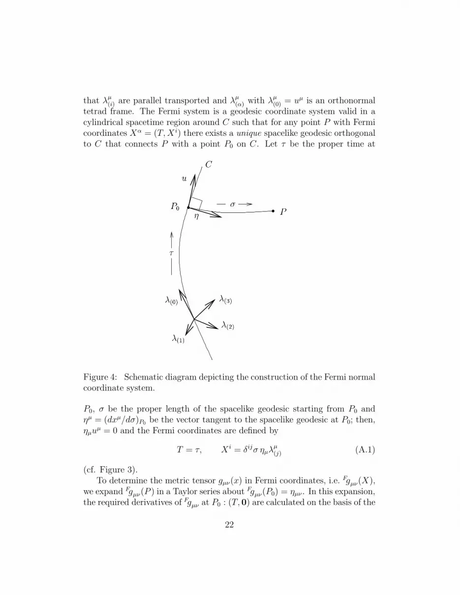
that λµ(i) are parallel transported and λµ

(α) with λµ(0) = uµ is an orthonormal

tetrad frame. The Fermi system is a geodesic coordinate system valid in acylindrical spacetime region around C such that for any point P with Fermicoordinates Xα = (T, X i) there exists a unique spacelike geodesic orthogonalto C that connects P with a point P0 on C. Let τ be the proper time at

(2)

CuP0 P

(1)(0) (3)Figure 4: Schematic diagram depicting the construction of the Fermi normalcoordinate system.

P0, σ be the proper length of the spacelike geodesic starting from P0 andηµ = (dxµ/dσ)P0

be the vector tangent to the spacelike geodesic at P0; then,ηµuµ = 0 and the Fermi coordinates are defined by

T = τ, X i = δijσ ηµλµ(j) (A.1)

(cf. Figure 3).To determine the metric tensor gµν(x) in Fermi coordinates, i.e. Fgµν(X),

we expand Fgµν(P ) in a Taylor series about Fgµν(P0) = ηµν . In this expansion,the required derivatives of Fgµν at P0 : (T, 0) are calculated on the basis of the

22

following considerations: The equations of motion of the tetrad frame carriedby the observer along the fiducial geodesic C in Fermi coordinates reduces toFΓ

µ00(T, 0) = 0 and FΓ

µ0i(T, 0) = 0. Moreover, the spacelike curve connecting

P0 to P satisfies the geodesic equation, which in Fermi coordinates (A.1)reduces to F Γ

µij(T,X)X iXj = 0. Expanding FΓ

µij in a Taylor series about

P0 : (T, 0), we find that

FΓµ

ij(T, 0) = 0, F Γµ

(ij,k)(T, 0) = 0, FΓµ

(ij,kℓ)(T, 0) = 0, · · · . (A.2)

Using all these relations regarding the connection coefficients at P0, the re-quired derivatives of the metric tensor at P0 can be calculated. The resultscan be expressed as

Fg00 = −1 − FRi0j0XiXj − 2

3FRi0j0kX

iXjXk + · · · , (A.3)

Fg0i = −2

3FR0jikX

jXk +1

2FR0jkiℓX

jXkXℓ + · · · , (A.4)

Fgij = δij −1

3FRikjℓX

kXℓ +1

3FRiℓrjkX

kXℓXr + · · · , (A.5)

where Rµνρσω is given in terms of covariant derivatives of the Riemann tensorby

Rµνρσω =1

2(Rµνρσ;ω + Rµρων;σ). (A.6)

It is simple to show that the tensor Rµνρσω satisfies the following relations

Rµνρσω = −Rµρνωσ , Rµνρσω −Rµρωνσ = Rρσµ(ν;ω). (A.7)

The first covariant derivatives of the Riemann tensor are not completelyspecified by the tensor Rµνρσω . Moreover, the next terms in equations (A.3)–(A.5) contain, among other terms, the tensor

Tµνρσωπ =1

3Rµνρσω;π +

2

3Rξ

ρωνRµξπσ, (A.8)

etc. It follows from these results that the reduced geodesic equation (2.5) inFermi coordinates becomes the tidal equation

d2X i

dT 2+ Ki

jXj +

1

2!Ki

jkXjXk +

1

3!Ki

jkℓXjXkXℓ + · · · = 0, (A.9)

23

where the quantities Kij, Kijk, etc., characterize, respectively, the tidal ac-celeration terms of the first order, second order, etc. We find from equa-tions (A.3)–(A.5) that

Kij = FR0i0j − 2FR0jikXk − 2(FR0j0kX

i − 1

3FRiℓjkX

ℓ)Xk

− 2

3FR0ℓkjX

iXℓXk,

as in the generalized Jacobi equation and Kijk = 2K ′

i(jk), where

K ′

ijk = FRi0j0k + 2[FR0jℓik −1

3(FRijℓk0 + FR0ijkℓ)]X

ℓ − FR0j0k0Xi

+ (FRjℓikr +5

6FRkriℓj)X

ℓXr +2

3(2FR0jℓ0k − FRj0k0ℓ)X

iXℓ

+1

6(FRkℓ0jr − 5FRℓk0rj)X

iXℓXr.

The Jacobi equation in spaces of arbitrary dimensions was first discussedby Levi-Civita [10] and Synge [11, 12, 1]. These references contain a detailedand explicit exposition of the theorem of Fermi [13] involving the possibilityof choosing a system of coordinates in a cylindrical region along an arbitraryopen curve in spacetime such that all the connection coefficients vanish andgµν = ηµν on the curve.

The generalized Jacobi equation was first discussed in [14, 15, 16] anddeveloped further in [17]. Later, this generalization was independently redis-covered by Ciufolini [18, 19]. Further discussions of the Jacobi equation canbe found, e.g., in [20, 21, 22, 4].

B Hamiltonian equations of motion

Consider a coordinate system Xα = (T, X i) in the region of interest in space-time such that the metric tensor takes the form gµν = ηµν + hµν , where hµν

is a small perturbation on the Minkowski background. In particular, we areinterested in Fermi normal coordinates (2.11). The isoenergetically reducedHamiltonian system is given in these coordinates by

dX i

dT=

∂H

∂pi

,dpi

dT= − ∂H

∂X i, (B.1)

24

where

H =g0i

g00pi ∓

(1 + gijpipj

−g00

)1/2

. (B.2)

To first order in hµν , the Hamiltonian can be expressed as

H = ∓√

1 + p2(1 − 1

2h00 −

1

2

hijpipj

1 + p2) + h0ipi, (B.3)

where p2 = δijpipj and H is a quadratic form in spatial Fermi coordinatesX. Using (B.3), the system of equations (B.1) can be written as

dX i

dT= ∓ pj

√

1 + p2[(1 − 1

2h00 +

1

2

hkℓpkpℓ

1 + p2)δij − hij ] + h0i, (B.4)

dpi

dT= ∓1

2

√

1 + p2 (h00,i +hkℓ

,i pkpℓ

1 + p2) − h0j

,i pj . (B.5)

Letting ∓pi → pi and defining

Pi :=pi

√

1 + p2(B.6)

and P i := δijPj , we find that (1 + p2)(1 − P 2) = 1 and pi = Pi/√

1 − P 2. Interms of P, the Hamiltonian equations of motion (B.4)–(B.5) take the form

dX i

dT= P i(1 − 1

2h00 +

1

2hkℓPkPℓ) + h0i (B.7)

− hijPj +1

2hkℓPkPℓP

i,

√1 − P 2

d

dT

( Pi√1 − P 2

)

=1

2h00,i − h0j

,i Pj +1

2hkℓ

,i PkPℓ . (B.8)

We are interested in the behavior of X i = X i(T ) to first order in δ =|X|/. To this end, we note from equation (B.7) that P i = V i + O(hµν),where V i = dX i/dT . Thus equation (B.7) can be written to first order inhµν as

Pi := (1 +1

2h00 −

1

2hkℓV

kV ℓ)Vi + h0i + hijVj . (B.9)

25

Similarly, equation (B.8) can be written as

dP i

dT+

1

1 − P 2(P · dP

dT)P i =

1

2h00,i + h0j,iV

j +1

2hkℓ,iV

kV ℓ. (B.10)

This relation, after multiplying by Pi and summing over i, takes the form

1

1 − P 2(P · dP

dT) =

1

2h00,iV

i + h0j,iViV j +

1

2hkℓ,iV

kV ℓV i. (B.11)

Substituting equations (B.11) and (B.9) in equation (B.10) and noting that

dV i/dT = O(δ), hµν,0 = O(δ2),

we finally obtain the desired equation of motion

dV i

dT+ (h00,jV

j + h0j,kVjV k)V i − 1

2h00,i

+(h0i,j − h0j,i)Vj + (hij,k −

1

2hjk,i)V

jV k = 0. (B.12)

Taking due account of the approximations under consideration here, wenote that

−Γ0αβ

dXα

dT

dXβ

dT= h00,jV

j + h0j,kVjV k

and

Γiαβ

dXα

dT

dXβ

dT= Γi

00 + 2Γi0jV

j + ΓijkV

jV k

= −1

2h00,i + (h0i,j − h0j,i)V

j + (hij,k −1

2hjk,i)V

jV k

in agreement with equation (2.5). Moreover, to first order in δ

h00,i = −2R0i0jXj,

h0i,j = −2

3(R0jik + R0kij)X

k,

hℓm,i = −1

3(Rℓimk + Rmiℓk)X

k,

in the Fermi system. Substituting these relations in equation (B.12) andusing the symmetries of the Riemann tensor, such as R0[ijk] = 0, we obtainequation (2.12). This is the generalized Jacobi equation in Fermi coordinates;for arbitrary coordinates see Appendix C.

26

C Generalized Jacobi equation in arbitrary

coordinates

Consider a reference timelike geodesic C as in Appendix A representing theworldline of an observer with proper time τ . Let ξµ = σηµ; then, to firstorder in σ/, the generalized Jacobi equation [14, 15] takes the form

D2ξµ

Dτ 2+ Rµ

ρνσuρξνuσ + (uµ +Dξµ

Dτ)(2Rζρνσu

ζ Dξρ

Dτξνuσ

+2

3Rζρνσuζ Dξρ

Dτξν Dξσ

Dτ) + 2Rµ

ρνσ

Dξρ

Dτξνuσ +

2

3Rµ

ρνσ

Dξρ

Dτξν Dξσ

Dτ= 0.

Here

Dξµ

Dτ= ξµ

;ν

dxν

dτ= ξµ

;νuν

is the covariant derivative of ξµ along the reference worldline. If we now useFermi coordinates and set

ξµ = X iλµ(i),

Dξµ

Dτ=

dX i

dTλµ

(i),D2ξµ

Dτ 2=

d2X i

dT 2λµ

(i), . . . ,

we recover equation (2.12). Here we have used the relation Dλµ(α)/Dτ = 0;

i.e. the tetrad is parallel transported along C.

D Worldlines of observers at rest

Consider a spacetime metric of the form

ds2 = −dt2 + gij(t, xk)dxidxj .

If a particle is a rest at a point in the corresponding space, then its worldlinefollows a geodesic. Indeed, the four-velocity of the particle uµ = dxµ/dτ isgiven by u0 = 1 and ui = 0. We must show that

duµ

dτ+ Γµ

αβuαuβ = 0.

27

For µ = 0, it suffices to prove that Γ000 = 0. Because of the block form of the

metric, we have g00 = −1 and g0i = 0; therefore,

Γ000 = −1

2g00,0 = 0.

For µ = i, it suffices to show that Γi00 = 0. In this case we have g0j = 0 and

g00 = −1. Hence,

Γi00 =

1

2gij(2gj0,0 − g00,j) = 0,

as required.

References

[1] J. L. Synge, Relativity: The General Theory (North-Holland, Ams-terdam, 1960).

[2] B. Mashhoon, Proc. Second Marcel Grossmann Meeting on GeneralRelativity, edited by R. Ruffini (North-Holland, New York, 1982) pp.647–672; N.B. section IV.

[3] J. K. Beem, P. E. Ehrlich and K. L. Easley, Global Lorentzian Ge-ometry, 2nd ed. (Dekker, New York, 1996) ch. 2.

[4] R. Kerner, J. W. van Holten and R. Colistete, Jr., Class. QuantumGrav. 18 (2001) 4725.

[5] R. Abraham and J. Marsden, Foundations of Mechanics, 2nd Edition(Perseus Books, Reading, 1985) pp. 223–225.

[6] H. Bondi, F. A. E. Pirani, and I. Robinson, Proc. Roy. Soc. A 251(1959) 519.

[7] The LISA mission is described in http://lisa.jpl.nasa.gov/ andhttp://www.estec.esa.nl/spdwww/future/html/lisa.htm.

[8] B. Mashhoon and J. C. McClune, Mon. Not. R. Astron. Soc. 262(1993) 881.

[9] R. Fender, astro-ph/0109502.

28

[10] T. Levi-Civita, Math. Ann. 97 (1926) 291.

[11] J. L. Synge, Phil. Trans. Roy. Soc. London A 226 (1926) 31.

[12] J. L. Synge, Duke Math. J. 1 (1935) 527.

[13] E. Fermi, Atti Accad. Naz. Lincei Rend. Cl. Sci. Fis. Mat. Nat. 31(1992) 21, 51.

[14] D. E. Hodgkinson, Gen. Rel. Grav. 3 (1972) 351.

[15] B. Mashhoon, Astrophys. J. 197 (1975) 705.

[16] B. Mashhoon, Astrophys. J. 216 (1977) 591.

[17] W.-Q. Li and W.-T. Ni, J. Math. Phys. 20 (1979) 1473, 1925.

[18] I. Ciufolini, Phys. Rev. D 34 (1986) 1014.

[19] I. Ciufolini and M. Demianski, Phys. Rev. D 34 (1986) 1018.

[20] S. L. Bazanski, Ann. Inst. Henri Poincare 27 (1977) 115, 145.

[21] A. N. Alexandrov and K. A. Piragas, Theoret. Math. Phys. 38 (1979)48.

[22] S. Manoff, Int. J. Mod. Phys. A 16 (2001) 1109.

29