Deep-Sea Research II 91 (2013) 71–83

Contents lists available at SciVerse ScienceDirect

Deep-Sea Research II

0967-06

http://d

n Corr

Oceano

United

E-m

journal homepage: www.elsevier.com/locate/dsr2

Local oceanic response to atmospheric forcing in the Gulf Stream region

Xujing Jia Davis n, Robert A. Weller, Sebastien Bigorre, Albert J. Plueddemann

Physical Oceanography Department, Woods Hole Oceanographic Institution, Woods Hole, MA 02543, United States

a r t i c l e i n f o

Available online 26 February 2013

Keywords:

Air-sea interaction

Gulf Stream

Atmospheric forcing

Ocean heat budget

Surface mooring

45/$ - see front matter & 2013 Elsevier Ltd. A

x.doi.org/10.1016/j.dsr2.2013.02.028

espondence to: Physical Oceanography Depa

graphic Institution, Clark 344b, MS#21, Wood

States. Tel.: þ1 508 289 2404; fax: þ1 508 45

ail address: xdavis@whoi.edu (X.J. Davis).

a b s t r a c t

The dominance of shifts in the location of the Gulf Stream (GS) in the local heat balance was observed in

an hourly 15-month record of unprecedented surface mooring measurements at a site in the western

North Atlantic occupied from November 2005 to January 2007. Instrumentation on the buoy provided a

high quality record of air-sea exchanges of momentum, heat, and freshwater flux; and oceanographic

sensors recorded ocean variability in the upper 640 m. The mooring was at times in the GS and at other

times north of the GS. Our intent was to isolate the local oceanic response to the atmosphere from the

influence of the GS shifts. A one-dimensional heat budget analysis indicated that the advective

contribution from the GS shifts dwarfed the heat contribution by atmospheric forcing and therefore

played the dominant role for upper oceanic thermal variability during the whole time record. A GS case

study (i.e., when the surface mooring was in the GS), isolated the upper oceanic response to the

atmospheric forcing in the GS and supported the critical role of GS shifts in total oceanic heat content.

Through both an Empirical Orthogonal Function (EOF) analysis and by referencing temperatures to that

observed at 200 m, the impact of GS shifts and atmospheric forcing were decomposed, allowing the

local oceanic thermal response to be isolated. This local oceanic response was particularly prominent

during the period of sustained heating during summer. A case study of summer conditions revealed a

near surface flow consistent with Ekman dynamics within a shallow, warm ocean mixed layer.

& 2013 Elsevier Ltd. All rights reserved.

1. Introduction

The Gulf Stream (GS) is the Western Boundary Current (WBC)in the North Atlantic, and a focus of complex air-sea dynamicscritical to global climate processes (Kelly et al., 2010). Ocean-atmosphere exchange above the GS is particularly prominentduring winter months when this warm, fast traveling currentencounters the cold continental air from the subpolar region andlarge air-sea temperature differences induce intense local air–seainteraction. The wintertime heat loss in the GS region is conse-quently among the highest observed in any ocean basin (Yu andWeller, 2007) and this intense exchange is marked by the spatialpatterns and temporal frequencies of the GS. On climatic scales,Joyce et al. (2000) showed that the GS variability has been highlycorrelated with the North Atlantic Oscillation (NAO). Over shorterdaily and seasonal time scales, heat loss associated with the GShas been found to be responsible for other key processes. Theseinclude the intensification and track of synoptic weather events(Joyce et al., 2009) and Eighteen Degree Water (EDW) formation, asignificant water mass in the North Atlantic region (Davis et al.,

ll rights reserved.

rtment, Woods Hole

s Hole, MA 02543,

7 2181.

2013). Hence, local air–sea interaction in the GS region plays aprominent role in weather and climate (Minobe et al., 2008).Much of this local air-sea exchange is made possible by theintense coupling between surface wind and the SST front asso-ciated with the GS (Chelton et al., 2006). However, the influencesof fine scale dynamics upon this coupling have proven difficult tofully characterize (Chelton et al., 2006), in large part due to thephysical challenges of obtaining accurate in-situ air-sea measure-ments within the GS itself. In the following presented work,an investigation of local air–sea interaction in the GS region ispursued using a recent and unprecedented dataset describedbelow. Particular attention is devoted to the upper oceanicresponse to the atmospheric forcing in the GS region.

The data and observations of this study are part of the ClimateVariability and Predictability Mode Water Dynamics Experiment(CLIMODE), a comprehensive field campaign in the North Atlanticbetween 2005 and 2007. A central motivation in this campaignwas a marked discrepancy between formation rates of EDWestimated by theoretical studies based on air-sea flux and subsur-face float observations (CLIMODE Group, 2009). In conjunctionwith this experiment, one surface mooring was deployed in thevicinity of the GS (latitude: 38.31N, longitude 64.81W, location Fin Fig. 1). This mooring site was chosen not only because thisis the location where ocean lost the most heat to the atmo-sphere based on climatology but also due to its proximity to the

Fig. 1. Location of the surface mooring F is labeled with white square with plus sign inside, the color contours are monthly mean satellite OISST (1C). The OISST contours

are plotted in 0.5 1C intervals, the thick black and green lines stand for 17 1C and 19 1C isotherms respectively. In the bottom left corner, DTGS ¼ 15 1C�T200 m, is the

monthly mean difference between 15 1C and mooring temperature at 200 m (the monthly values from December 2005 to December 2006 are �3.1, �0.7, 2.8, 1.7, 1.7, 1.3,

2.3, �0.4, �0.3, �0.9, 1.0, �4.3, �4.1, �3.1 1C respectively). (For interpretation of the references to color in this figure legend, the reader is referred to the web version of

this article.)

X.J. Davis et al. / Deep-Sea Research II 91 (2013) 71–8372

TOPEX/Poseidon satellite track. During the 15 months of observa-tion, the GS meandered frequently, so the surface mooring was in,north of and south of the sharp SST front during different timeperiods (Fig. 1). The extent of the observational record at such alocation is remarkable, given the challenge of functioning for �15months in such proximity to the GS, and enduring the harsh winterconditions and the intense currents (Weller et al., 2012). This surfacemooring measurement in fact is the first successful deployment of asurface mooring in the GS region over such a long duration.

Measurements from this surface mooring provided a �15months record of subsurface measurements as well as local air-

sea fluxes and meteorological conditions within the marineatmospheric boundary layer above. At the surface, the meteor-ological data were measured every minute (SST, wind, air humid-ity and temperature, short and long wave radiation, precipitationand barometric pressure). The turbulent fluxes were calculatedusing the COARE 3.0 algorithm and some direct covariancemeasurements as well. More detailed description and analysisof the surface meteorological and heat fluxes data can be found inWeller et al. (2012) and Bigorre et al. (in press).

This study focuses on the analysis of the subsurface mea-surements and investigates the local oceanic response to the

Table 1Subsurface oceanographic instrumentation under Climode F surface mooring.

Sensor Variables Depth (m) Recordinterval (min)

SBE37 (2) T, C 0.89 1

SBE37 T, C 5 5

Nortek Aquadopp U, V, W, T, P 10 15

SBE39 T 15 5

Nortek Aquadopp U, V, W, T, P 20 15

SBE39 T 40 5

SBE39 T 80 5

SBE39 T 120 5

SBE39 T 160 5

SBE39 T 200 5

SBE39 T 240 5

SBE39 T 280 5

SBE37 C, T 341 5

SBE39 T 360 5

SBE39 T 400 5

SBE39 T 440 5

SBE39 T 480 5

SBE39 T 520 5

SBE39 T 560 5

X.J. Davis et al. / Deep-Sea Research II 91 (2013) 71–83 73

atmospheric forcing in the GS region. The central questionsexplored include: (1) How sensitive is local air–sea interactionto the position of the GS? (2) How do the roles of oceanicadvection differ based on the relative locations of the mooringto the GS path? (3) Since the GS shift is dominant in local oceanicvariability, which analysis methods are effective in isolating localoceanic responses to atmospheric forcing? In pursuit of thesequestions, this investigation proceeds in the following order:Section 2 presents a detailed description of the subsurfaceobservational data used. In order to examine quantitatively therole played by the GS shift in the upper ocean variability, weintroduce an index for the mooring’s relative location to the GS inSection 3. Significant aspects of variability of the upper oceandiscerned from the data, including a 1-D heat budget analysisover the whole time record and during the time when the surfacemooring was in the GS, are described in Section 4. Determinationof the local oceanic response to the atmosphere is made in Section5. In Section 6, a case study of the summer period reveals both anEkman response in the near-surface current and a local thermalresponse in a thin surface layer. A summary and further discus-sion of key findings is presented in Section 7.

SBE39 T 600 5

SBE37 C, T, P 662 5

2. Data description

The primary data used in this work are the subsurfacetemperature data and horizontal current velocity, measured fromthe surface mooring F during the CLIMODE campaign. The recordprovided �15 months of temperature in the upper�660 m,surface salinity and current at 10 m and 20 m (Weller et al.,2012).

This dataset consists of in-situ temperatures averaged to hourlyvalues during the period November 14 2005–January 31 2007,with a data gap between November 19 and 21 2006 when the firstyear mooring was recovered and replaced with a new mooring.Fifteen Seabird SBE 39 temperature recorders, five Seabird SBE 37temperature and conductivity recorders were deployed. Two of theSBE37 were attached next to each other beneath the buoy hull(approximately 1.5 m depth) and their temperature record wasused as the sea surface temperature (SST) estimate. Finally, twoNortek Aquadopp current meters measured U, V, W, temperatureand pressure. Note that temperature accuracy typically is 0.002 1Cand 0.1 1C for the Seabird and Nortek respectively, according tomanufacturers. In practice, the mooring line was tilted by environ-mental forces, the depth of the temperature sensors is not knownexactly (Bigorre et al., in press), which degrades the temperatureaccuracy to 0.01 1C for the Seabird sensors located near strongvertical temperature gradients, such as the mixed layer base. Therewas no apparent bias in the temperature data from the Aquadopps,despite the lower accuracy.

The Seabird sensors recorded data every 5 min whereas theAquadopps recorded every 15 min. Table 1 shows the configura-tion of the oceanographic instruments under the CLIMODE Fsurface mooring. Note the vertical resolution is between 5 and10 m in the upper 20 m and 40 m below 40 m depth. Thesedepths are nominal depths based on sensor positions on mooringline. Because the mooring line was not always vertical, the actualdepths of each of the subsurface instruments tended to beshallower than their nominal depths. Indeed, the measuredpressure range for the lowermost sensor was 570–670 dbars.We therefore applied a depth correction in the following manner.Using the pressure measurements from the lowermost sensor, wecomputed first its depth in meters (zbottom) and then the ratio toits nominal depth R¼zbottom/662. Assuming the mooring line inthe upper 660 m was taut (a reasonable assumption due to theweight on the mooring line), we applied a linear depth correction

to all instruments above by multiplying their nominal depth withR at each data point. For more details, see Bigorre et al. (in press).

During the first year deployment, a ship hit the buoy onJanuary 19 2006. After this date, data from the SBE 37 sensor at5 m depth were unavailable and we did not include data from thissensor. The SBE 39 at 15 m depth was lost upon recovery of thesecond deployment so there were no temperature data at thisdepth from November 2006 until the end of deployment. The SBE37 at 341 m nominal depth had periods with suspicious jumps intemperature. These periods were November 13 2005–January 212006, March 20–23 2006, July 27–August 3 2006, August 23–272006, September 4–8 2006 and November 12–19 2006. Theseperiods amount to 25% of the data record from this instrumentand were replaced with interpolated data from the two sensorsimmediately above and below it. When the intermediate leveldata were available, the interpolation scheme was compared toactual data and the estimates were very close. For other periodswhen data were not suspicious, the standard deviation with theinterpolation was 0.14 1C.

Most sensors had a clock drift of less than 1 min, with twoinstruments with close to two minutes drift after 12 months ofdeployment. The data were first interpolated to 1-min sampling,then timestamps were synchronized using a linear drift correc-tion. Finally, the temperature data were hourly averaged. The datawere then gridded into vertical coordinates using linear inter-polation for each hour. Because of the lower vertical resolutionbelow 40 m in the raw dataset, we chose to interpolate to 1 mgrid points above 40 m, then 5 m down to 150 m depth, 10 mdown to 440 m depth and finally 20 m down to 660 m depth.Finally, the data gap (�2 days from November 19 and 21, 2006)between CLIMODE1 F and CLIMODE2 F was filled with linearinterpolation in time at each depth.

3. The index for mooring’s relative location to GS

During the �15 months of observation, the position of the GSfluctuated to the south and the north of the mooring position dueto seasonal shifts in its path and stochastic meandering. The shiftof the GS from north during winter and spring to south duringsummer and fall is a typical seasonal pattern of the GS and hasalso been documented in numerous studies such as in (Kelly and

X.J. Davis et al. / Deep-Sea Research II 91 (2013) 71–8374

Gille, 1990; Frankignoul et al., 2001). Though the satellite SSTmeasurements were a good reference for the GS location (Fig. 1),their resolution in both time and space was not sufficient toresolve the sharp frontal features observed in the surface mooringdata. Therefore, temperature observations at the mooring wereemployed to define the mooring’s location relative to the GS.In previous studies such as Joyce and Zhang (2010), the GSnorth wall (GS_NW) was defined as the location of the 15 1Cisotherm at 200 m. Though the surface mooring measurement

Fig. 2. Temperature at 200 m at the mooring site. Temperatures were above 15 1C (red

below 15 1C (blue line) when the mooring was north of the GS north wall, which occurre

the reader is referred to the web version of this article.).

Fig. 3. Observed (a) net air-sea heat flux (Qnet), (b) Wind, (c) SST and (d) difference be

mean. The red and blue colors in (a), (c) and (d) correspond to the time periods when mo

1 summer seasons are defined as shown in (a) and (b). Note that wind vectors represen

in this figure legend, the reader is referred to the web version of this article.).

was at a single site and cannot solely be used to identify the GSlocation, the relative position between the mooring and GS can beinferred qualitatively by comparing the temperature measured at200 m (T200 m, red and blue line in Fig. 2) and the 15 1C (black linein Fig. 2). To be specific, the mooring was defined to be to thenorth (south) of the GS_NW if T200 m was cooler (warmer) than15 1C. Based on this, the mooring was to the north (south) of theGS_NW �55% (45%) of the time during the �15 months record(Fig. 2). The monthly mean of the difference between 15 1C and

line) when the mooring was south of the GS north wall (GS_NW, i.e., GS front) and

d 55% of the time (For interpretation of the references to color in this figure legend,

tween the air temperature (Tair) and SST. All the above values are 5 days running

oring was to the south and north of the GS north wall. Based on Qnet, 2 winters and

t flow towards the indicated direction (For interpretation of the references to color

Fig. 4. Observed upper oceanic variability at the surface mooring site. (A) The hourly temperature record in upper 640 m, where the red line stands for the 15 1C isotherm.

(B) 1-D heat budget terms. Where the HCOcean (black line) is the HC in upper 600 m, the 3�AFAtm (green line) is the cumulative heat input from Qnet (multiplied by 3 to

see more clearly). The residual is plotted in red and blue lines, where red and blue marks the time periods when mooring site was south and north of GS respectively.

(C) EDW layer (red and blue shading) based on the definition that EDW is between 17 and 19 1C and with its dT/dzo¼0.006 1C/m, similar to (B), the red and blue color

correspond to the time period when mooring was south and north of GS north wall. (D) Vertical temperature gradient (dT/dz, 1C/m) and (E) The velocity difference at

10m and 20 m (m/s). The black solid lines in (A), (C) and (D) are the daily mean MLD (m). (For interpretation of the references to color in this figure legend, the reader is

referred to the web version of this article.)

X.J. Davis et al. / Deep-Sea Research II 91 (2013) 71–83 75

T200 m was also calculated (noted in bottom left corner and captionin Fig. 1). Comparing to the satellite SST pattern, the abovementioned index for mooring’s location relative to the GS_NWwas in good agreement with the surface SST image. Note that whenthe mooring was south of the GS_NW, it could be sometimes in thecore of the GS and near the south wall of the GS other times (Thesouth wall of GS is seasonally dependent and hard to define.).

4. Overview of the �15 months record of observation

In this section, we present the �15 month record of theobserved features in the air-sea surface (Fig. 3) and in the upperocean (Fig. 4). The variability of these characteristics demon-strated that both seasonality and GS shifts dominated fluctuationswere apparent.

X.J. Davis et al. / Deep-Sea Research II 91 (2013) 71–8376

4.1. Seasonality in the air-sea surface

The net heat flux (Qnet, Fig. 3a) used in this study was the sumof the net short and net long wave radiation, turbulent fluxesand flux due to precipitation: Qnet¼QBþQH þQlþQrþQs, whereQB, QH, Ql, Qs and Qr are sensible, latent, net long wave, net shortwave heat flux and the heat flux resulted from rain, respectively.These fluxes were computed through the COARE 3.0 formulae(Weller et al., 2012). Using error propagation in the bulkformulae and comparison with direct covariance fluxes availableon the buoy, Bigorre et al. (in press) estimated the relative errorsof the air-sea fluxes to be less than 20%. The negative values ofQnet represented the heat loss from the ocean (Fig. 3a). The heatloss from the ocean occurred in winter months during November2005–April 2006 and September 2006–February 2007 especiallyin conjunction with the flow of cold, dry air from the land duringthe passage of low pressure atmospheric systems. The oceangained heat in the summer months during May–August 2006when air came from the ocean. These are typical seasonalpatterns in the subtropical region. Hereafter, we divide thewhole record into three different seasons: winter 2005/2006(beginning of the record, November 14th 2005–April 30th 2006),summer 2006 (May 1st–August 31st 2006) and winter 2006/2007 (September 1st to end of the record, January 31, 2007).In these three different seasons, i.e., in winter 2005/2006, insummer 2006 and winter 2006/2007, the mean heat exchangesare �214.5, 93.1 and �295.5 W/m2, respectively. The oceanlost a large amount of heat to the atmosphere during winter,especially when the mooring was south of the GS, due to thelarge air-sea temperature difference. The calculated monthlymean of Qnet suggests the maximum heat loss for the two winterseasons occurred in December 2005 (489.3 W/m2) and January2007 (437.3 W/m2), when the mooring was to the south of theGS mostly. The hourly maximum heat loss (gain) was deter-mined to be as much as 1380.0 (859.5) W/m2, as observed at07:30 on January 21 2007 (15:30 on June 4th 2006). The winterof 2007 in the GS region was found to be colder than the meanwinter condition during the previous 19 years (Joyce et al.,2013).

The seasonal cycle in the wind forcing is also evident despitethe high frequency variations (Fig. 3b). During both winters,strong northwesterlies and southwesterlies associated withsynoptic low pressure systems prevailed. In contrast, a weakerwind regime characterized the summer and the wind waspredominantly southerly. The mean value of the hourly windspeeds are 7.9 m/s, 5.7 m/s and 8.7 m/s during winter 2005/2006, summer 2006 and winter 2006/2007, respectively.

Though seasonality was dominant, the sensitivity of Qnet to theGS location was also detected. One good example is during thewinter of 2005/2006, when the maximum heat loss was detectedin December in our mooring record, whereas during recent yearsthe maximum heat loss from ocean to atmosphere generallyoccurred in March (Davis et al., 2013; Joyce et al., 2013).In the GS region, the large heat loss occurred during the flow of‘‘cold’’ winter air over ‘‘warm’’ SST. There is a high correlationcoefficient (0.94) between Qnet (Fig. 3a) and air-sea temperaturedifference (Fig. 3d) in our record. During winter 2005/2006, theGS’s path shifted from north to south of the mooring in mid-January 2006, the SST decreased sharply (Fig. 3c), and thedifference of the ‘‘cold’’ air temperature and ‘‘less warm’’ SSTbecame smaller (Fig. 3d). As a result, the ocean lost less heat tothe atmosphere after mid-January and even gained heat duringpart of March and April when the mooring was north of the GS.Therefore, it was the change in SST due to the GS shift thatresulted in the maximum Qnet in December 2005 instead ofMarch 2006.

4.2. Upper ocean thermal variability

In this section, we discuss the upper 640 m ocean temperaturevariability (Fig. 4A) and explore its response to the seasonal atmo-spheric forcing. A 1-D heat budget calculation quantified the role ofthe GS shift in the upper oceanic thermal variability (Fig. 4B). TheEDW water layer (Fig.4C) and the vertical gradient of temperature(Fig. 4D) were also mapped and calculated based on temperaturerecord to elucidate the upper oceanic thermal variability.

As an intense meandering current, the GS has a warm and salinecore (Talley et al., 2011), which distinguishes itself from surround-ing waters. Consequently, the upper ocean temperature changeddramatically at the mooring site due to the position shifts of the GS(Fig. 4A). The dominance of the GS shift in the upper ocean thermalvariability was manifested in the significant vertical displacementof the isothermal surfaces such as the15 1C isotherm surfaces (redline in Fig. 4A). Meanwhile, the deepening of the mixed layer (ML,black line in Fig. 4A, C and D) in winter and shoaling in summerindicated the seasonal variation. Here the ML is defined as thedepth where temperature is 0.1 1C cooler than SST. To evaluate therelative importance of the variability associated with the GS shiftand seasonality of atmospheric forcing in the upper ocean varia-bility, we next carried out a 1-D heat budget analysis.

4.2.1. Evaluation of the role of the GS shift in upper ocean thermal

variability based on a 1-D heat budget analysis

4.2.1.1. During the whole 15-month time record when mooring was

in/out of GS. The heat content (HC) in the upper ocean (fromsurface to the base of the ML) is balanced by the net air-sea heat fluxinput, heat flux advected by ocean currents, vertical entrainment ofheat at the base of the ML, and heat flux associated with oceanicdiffusive processes, which include both horizontal and verticaldiffusion and are defined as kr2T , where k¼ ðkx,ky,kzÞ is theeddy diffusivity coefficient. Here we assume the vertical entrain-ment at the base of the ML and the diffusive terms are small, andthat the HC will be mainly determined by the air-sea heat flux andoceanic advection. In our observational record, the mixed layerdepth (MLD) was consistently shallower than 600 m, so we calculatethe upper ocean HC in upper 600 m, and compare results with thecumulative net heat input from the atmosphere.

The heat content was calculated as HCOcean ¼ rCp

R 600 m0 TðzÞdz

(black line in Fig. 4B) where T(z) is the temperature at depth z asmeasured from mooring, Cp ¼ 4016 J=kg K is the specific heatcapacity at constant pressure, r the density of the sea waterand calculated from the measured temperature assuming a meansalinity of 36, as subsurface salinity data was not available at thevertical resolution of the temperature data and we assume thatthe density is mainly dependent on the temperature. The heatinput from atmospheric forcing was represented by the timeintegral of the net heat flux between ocean and atmosphereHFAtm ¼

R tt0

Qnet dt (green line in Fig. 4B, note that the plottedgreen line shown is three times of the actual HFAtm value todemonstrate its variability more clearly), where t0 is the starttime of the record, i.e., 00:30:00 on November 14th 2005. Toeliminate a constant offset between the values, the HCOcean attime t (black line in Fig. 4B) is defined as the anomaly withrespect to HCOcean at time t0, whose value is 3.16�1010 J/m2. Theresidual, or difference between the HCOcean and the HFAtm (red/blue lines in Fig. 4B correspond to mooring’s location south/northof the GS_NW), has a high correlation (r¼0.96) with the index formooring’s relative location to GS, i.e., T200 m, which indicate theclose tie of GS shifts to the residual term (or oceanic advectionbased on our assumption) at the mooring location. The residualterm (red and blue lines in Fig. 4B) was also very similar to the

Fig. 5. (A) 1-D heat budget terms calculated the same way as that in Fig. 4B during the time period from December 13th 2005 to January 11th 2006 when surface mooring

was in the GS and mooring’s relative position to GS_NW was stable relatively. (B) The observed hourly net heat flux Qnet and (C) The observed 15 min ocean current

components U (the black line) and V (the blue line) at 20 m. positive values of U/V indicated eastward/northward directions of the current. (For interpretation of the

references to color in this figure legend, the reader is referred to the web version of this article.)

X.J. Davis et al. / Deep-Sea Research II 91 (2013) 71–83 77

oceanic thermal variability HCOcean and suggested the dominance ofthe GS shift in HCOcean. When the mooring was south of the GS_NW(red line in Fig. 4B), the large amount of heat from the warm waterin the GS dwarfed the heat by air-sea heat flux HFAtm. When themooring was to the north of the GS_NW (blue line in Fig. 4B), theresidual term mainly reflected the oceanic advection outside of GS,which carries both warm and cold anomalies to the mooringlocation at different times but of much smaller magnitude.

The HFAtm showed a clear seasonal pattern (green line inFig. 4B), with cumulative heat loss increasing from November2005 to end of the April, followed by heat gain from May throughlate August, then switching back to be heat loss again. Thisseasonality was in agreement with what we discussed inSection 4.1. Over the 15 months of the record, the ocean lost6.02�109 J/m2 heat to the atmosphere. This is not surprisingsince there were two winters and one summer in this record. Still,in the 1 year cycle observed (November 2005–November 2006),the heat flux exchange was not balanced. The upper oceanthermal variability HCOcean (black line in Fig. 4B) was dominatedby high frequency variability and these fluctuations were muchdifferent from the HFAtm. The standard deviation of HCOcean was8.55�109 J/m2, one order larger than that of HFAtm, which was1.13�109 J/m2. Over the course of the record, heat contentdeclined by 9.4% or 2.97�109 J/m2 (black line in Fig. 4B).

4.2.1.2. GS jet case study: when mooring was in the GS. As shown inSection 4.2.1.1, the upper oceanic thermal variability was mainlymodulated by the GS shift, especially when GS_NW passed acrossthe mooring. To examine how the upper ocean responded to theatmospheric forcing when mooring was in the GS, here we repeatthe above 1-D heat budget analysis but focus on the time periodfrom December 13th 2005 to January 11th 2006. During this time,not only did the mooring remain to the south of the GS_NW, butalso the relative location of the mooring to the GS_NW wasrelatively stable based on T200m (Fig. 2).

During this time span, the ocean lost heat to the atmospherepredominantly through several cold air outbreaks with periods of�6 days (Fig. 5B), which resulted in the large air-sea temperaturedifference (Fig. 3d). Thus the cumulative heat content throughair-sea exchanges HFAtm decreased continuously (green lines inFig. 5A). However, the upper oceanic heat content (HCOcean)exhibited different variability with higher frequency fluctuationsand increased generally. From December 13th 2005 to January11th 2006, HCOcean increased 1.7�109 J/m2 (black line in Fig. 5A),compared to the cumulative heat loss of �1.1�109 J/m2 to theatmosphere (green line in Fig. 5A). The residual, or oceanicadvection term approximately converged 2.8�109 J/m2 of heatto the mooring location (red line in Fig. 5A). The 15-min mooringmeasured current at 10 m during this time showed strong east-ward movement (Fig. 5C), suggesting this advection was from thewest. In the monthly mean satellite SST image (Fig.1), warmer SSTwas observed southwest of the surface mooring in the GS inDecember 2005 and January 2006, which supported the advectionof warm water to the mooring location from upstream.

Therefore, during this time period, the significant atmosphericforcing (synoptic cold air outbreaks) was accomplished by east-ward (downstream) advection of GS warmer water from the west.This oceanic advected heat in the GS was on the same order as buthad larger magnitude than the heat loss due to atmosphericforcing, the HCOcean increased as a result.

Comparing to the whole observed time record when GS_NWcrossed the mooring site multiple times (Fig. 4B), the HCOcean

change in the GS here was one order smaller (or relatively stayedconstant), so was the residual (or oceanic advective term). Thisalso supports the significant influence of the GS shift on the upperoceanic thermal variability.

4.2.2. Sensitivity of the EDW to the GS location

One notable characteristic corresponding to the presence ofthe GS was the EDW observed during the mooring record (red and

X.J. Davis et al. / Deep-Sea Research II 91 (2013) 71–8378

blue shading in Fig. 4C). Here, the EDW was defined as a homo-genous water mass whose temperature ranged between 17 1C and19 1C and its vertical gradient (dT/dz, Fig. 4D) was less than orequal to 0.006 1C/m (Kwon and Riser, 2004). This EDW was notobserved throughout the whole record but was present 91% of thetime while the mooring was to the south of the GS_NW. Majorbodies of EDW were also observed below the ML from December2005 to January 2006 and from November 2006 to January 2007,with both time spans occurring prior to the EDW formationseason (Fig. 4C). During the typical formation season of EDW,i.e., from late January to early May (Davis et al., 2013), ourmooring was to the north of the GS_NW, and no substantialvolume of EDW was found within or below the mixed layer.

Therefore, our findings suggest that EDW was not formedlocally north of the GS_NW. This result is consistent with previousliterature establishing that EDW is commonly formed inside andto the south of the GS (Joyce et al., 2013). This large body of EDWalso contributed significantly to the upper ocean thermal varia-bility as discussed earlier.

4.2.3. Seasonal pattern in the MLD dominated by wind and heat

forcing

Though the GS shift was dominant in the upper ocean thermalvariability at this location, a seasonal cycle was observed in theMLD, primarily in response to the seasonal buoyancy (mainly heatflux) and wind forcing (Fig. 3a and b).

In winter 2005/2006, ocean heat loss to the atmosphere and theseasonal intensification of westerlies contributed to ML deepeningfrom 34 m on November 15th 2005 to 357 m on March 26th 2006(black line in Fig. 4A). During the early part of April, as wind stressweakened and the ocean gained heat from the atmosphere, surfacerestratification forced shoaling of the ML to a depth of �27 m. Insummer 2006, the ocean gained heat and surface wind stressweakened. This provided for the maintenance of a summertimeMLD of less than 40 m, and a corresponding seasonal mean MLD of

Fig. 6. (A) Mean temperature averaged over the whole time record, as a function of d

months of study, where the black, blue, red and green lines are vertical structures of th

variance is also noted in the legend. (For interpretation of the references to color in th

17 m. In the late summer of 2006, the SST was warmer than thesurface air temperature (Fig. 3d) and the heat flux reversed sign inthe later part of August. As the ocean entered winter season again,MLD deepened correspondingly. By the end of our record, the dailyMLD increased to be 182 m (on January 27th 2007).

4.2.4. Seasonality in temperature gradient below MLD and vertical

velocity shear

Comparing the two winters and one summer in the mooringrecord, two further differences observed were the upper oceanthermal stratification (Fig. 4D) and the difference of the horizontalvelocity between 10 and 20 m (Fig. 4E). In spite of the stronginfluence of the GS shift, the summer heating was able to shoalthe ML and create near surface stratification. Conversely, duringwinter, the higher wind speed and enormous heat loss facilitatedthe formation of a much deeper ML. The presence of this summerstratification (Fig. 4D) supported a larger velocity differencebetween 10 m and 20 m (Fig. 4E). During summer, though thewind stress was much weaker, the velocity different at twodepths was larger compared to winter. The summer stratificationand its potential isolating effect, suggested the possible season-ality of the local oceanic response to the atmosphere. We willexplore this scenario in detail in Sections 5 and 6.

5. Oceanic local response to the atmospheric forcing

When the mooring was south of the GS_NW, the warm waterin the GS dominated the thermal variability and therefore(Fig. 4B) the seasonal signal was masked by the shift of the GS.Away from the GS, such as further south in the interior of thesubtropical gyre (Davis et al., 2013), seasonality was much morepronounced. Hence, we will isolate the influence of the GS shift inoceanic thermal variability and elucidate the oceanic responseforced primarily by local seasonal atmospheric forcing.

epth. (B) The 1st 4 EOF vertical modes of the 640 m temperature during the �15

e 1st, 2nd, 3rd and 4th modes respectively. The individual contribution to the total

is figure legend, the reader is referred to the web version of this article.)

X.J. Davis et al. / Deep-Sea Research II 91 (2013) 71–83 79

5.1. Local oceanic thermal response to atmospheric forcing during

the whole record: EOF analysis and result from the T200 m method

In order to isolate the dominant signal of GS shifts in upperoceanic thermal variability, we performed an Empirical Orthogo-nal Function (EOF) analysis of the upper ocean temperature timeseries. The 1st and 2nd EOF modes together contributed morethan 97% of the total variance, therefore we only focused on thesefirst two modes. The 1st EOF mode explained 86.1% of the totalvariance and showed a nearly uniform vertical structure in theupper 640 m (black line in Fig. 6B), indicating the nearly uniformshift of the GS vertically. Note that the nearly depth-independentmovement of the GS represented by the 1st EOF verticalmode does not mean the temperature of the GS does not vary.Instead, the time mean temperature about which the EOF modesfluctuated, varied significantly with depth (Fig. 6A), with warmertemperature near the surface and cooler temperature at 640m(�13 1C difference). The corresponding time coefficient (Fig. 7A)

Fig. 7. In (A) and (B), the time coefficients for the 1st and 2nd modes of EOF are plotted.

mode, where the black and white lines stand for the 17 1C and 19 1C isotherms. In (D)

reconstruction and T200 m method as described in the text. The correlations are r¼0.60

upper 200 m HCOcean from the 2nd EOF mode (T200 m method) and the cumulative hea

figure legend, the reader is referred to the web version of this article.)

of the 1st EOF mode resembled the variability of T200 m (Fig. 2),i.e., the index for mooring’s relative location to GS. This wasfurther reflected by a high correlation of 0.98 between the 1st EOFtime coefficient and the T200 m. The vertical mode of the 2ndEOF (blue line in Fig. 6B) changed sign at 200 m, with largestmagnitude near the surface. This 2nd mode explained 11.2% of thetotal variance. The time coefficient of the 2nd mode (Fig. 7B)exhibited a clear seasonal pattern. Similarly, seasonality can beseen in the temperature record reconstructed based on the 2ndEOF mode and the time mean temperature field (Fig. 7C). And inthis temperature field represented by 2nd EOF, the outcrop ofEDW was present in both winters (white and black lines inFig. 7C), indicating the formation of EDW at this location withoutthe influence of the GS shifts, which masked the seasonalityinduced by observed atmospheric forcing (Fig. 3a, b and black linein Fig. 7D). The HCOcean calculated from this reconstructed tem-perature record showed a close correlation with the HFAtm (r¼0.6within 95% level of confidence between the blue and black lines in

In (C), a new subsurface temperature record is reconstructed based on the 2nd EOF

, the blue and red lines are the upper 200 m HCOcean calculated from the 2nd EOF

(r¼0.57) between the low pass filtered (removed the periods shorter than 24 h)

t input from the atmosphere. (For interpretation of the references to color in this

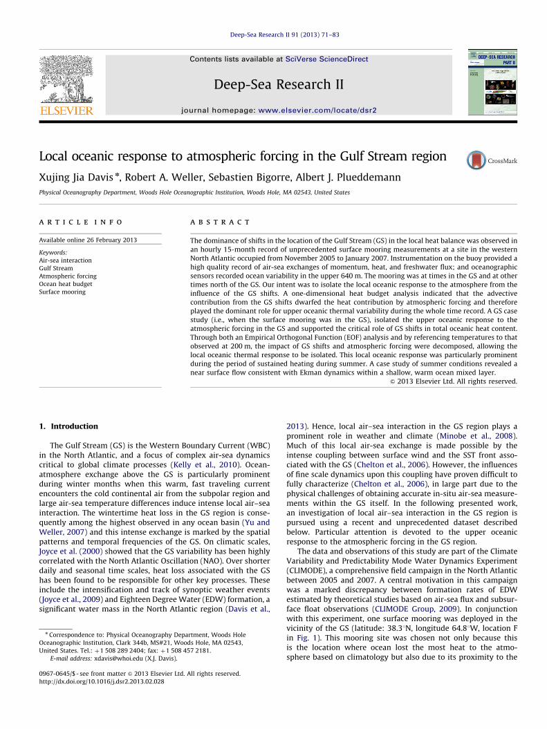
Fig. 8. As in Fig. 7d but in (A) winter 2005/2006, (B) summer 2006 and (C) winter 2006/2007.

X.J. Davis et al. / Deep-Sea Research II 91 (2013) 71–8380

Fig. 7D), suggesting that local oceanic response to the atmo-spheric forcing was captured in the 2nd EOF mode. Specifically, inFig. 7D we noted cooling and decreasing HC in the two winters aswell as warming and HC increase in the summer. Here weexamined the upper 200 m since this 2nd EOF mode capturedthe near-surface features and has zero crossing at 200 m.

Note that this correlation was high, but there are still differ-ences between the HFAtm and the HCOcean from the 2nd EOF modereconstruction. There were higher frequency signals in the upperocean related to the cooling and warming (Fig. 7C and blue line inFig. 7D), which did not agree with the relatively slow variation ofthe HFAtm (black line in Fig. 7D). One of the possible causes forthese high frequency signals could have been geostrophic advec-tion not related to the GS position. However, estimates ofthe geostrophic advection based on satellite SSH and SST, i.e.,uSSH��!�rTSST did not match the discrepancy between HFAtm and

the HCOcean from the 2nd EOF mode, where the uSSH��!

is thegeostrophic velocity calculated from satellite SSH and TSST is thesatellite SST. Other possible sources of this difference may havebeen derived from (1) advection caused by ageostrophic current;(2) the limited resolution of the available satellite data and itsinability to capture the sharp gradient near the GS front at surfaceand subsurface; (3) these high frequency fluctuations representthe residual from GS advection, which was not completelyexplained by the 1st EOF mode and (4) different dynamics wereinvolved in the variability captured in the 2nd EOF mode.

The EOF decomposition result was in agreement with the heatbudget analysis, in the sense that it also demonstrated the

dominant role of the GS shift in upper oceanic thermal variabilityand offered a quantitative evaluation of its variability to the totalvariance but from a different perspective. More importantly, thisEOF method revealed the local upper oceanic thermal response tothe atmospheric forcing even in the vicinity of the GS.

The correlation between the time coefficient of the 1st EOF andT200 m (index for mooring’s relative location to GS) was as high as0.98. Both this close correlation and the 2nd EOF mode (verticalmode has zero crossing at 200 m) suggested the uniqueness andimportance of T200 m. Thus we employed an alternative method toremove the role of the GS shift in upper ocean variability by usingT200 m as a reference. Specifically, a new temperature recordT0(t,z)¼T(t,z)�T(t, 200 m) was constructed by removing T200 m

at each time step and at each depth, then the HC in the upper200 m of T0(t,z) was calculated and compared to the HC from the2nd EOF mode. For convenience, this method is referred to as theT200 m method. During the whole time record, the T200 m methodalso revealed the local oceanic response to the atmosphericforcing, HCT200 m (red line in Fig. 7D) was correlated with HFAtm

(black line in Fig. 7D) with a correlation of 0.57, comparable tothat based on the 2nd EOF (r¼0.60).

5.2. The evaluation of the EOF and T200 m methods in isolating the

local oceanic response

As reviewed in Section 4.1, the seasonality was detected in theobservational record and there were distinct differences betweenwinter and summer, and even between two winters in different

X.J. Davis et al. / Deep-Sea Research II 91 (2013) 71–83 81

years. We are interested in the evaluation of the above mentionedmethods for isolating the local oceanic response in differentocean/GS conditions. Therefore, we applied the same methodsto three seasons (winter 2005/2006, summer 2006 and winter2006/2007) individually to test their effectiveness. During allthree seasons, the local oceanic response to the atmosphericforcing was detected through both the EOF and T200 m methods(Fig. 8).

Comparing the three seasons, the isolation of the local oceanicresponse, using these two methods, was better during winter2006/2007 than the other two seasons. During winter 2005/2006and summer 2006, the GS moved south and north of mooring sitemultiple times (Fig. 2). However, the GS and the mooring’srelative positions only changed twice during winter 2006/2007.This may be one of the reasons that the GS influence was betterremoved by EOF and T200 m during winter 2006/2007. Anothernoticeable feature was that during winter 2006/2007, the MLD(Fig. 4A) was shallower but closer to 200 m compared to the othertwo seasons. During winter 2005, the MLD was sometimes muchdeeper than 200 m and during summer 2006, the MLD was muchshallower than 200 m. Since both EOF and T200 m methods areclosely tied to the variability at 200 m depth, the two methodsmay better represent the time period when MLD was justshallower than 200 m as during winter 2006/2007.

6. Case study of the upper oceanic response to atmosphericforcing: summer 2006

As noted in Sections 4.2.3 and 4.2.4, the summer of 2006 had amuch shallower mixed layer (Fig. 4A), with a temperaturegradient (Fig. 4D) that supported larger velocity differencebetween 10 m and 20 m (Fig.4E) than that during the two wintersobserved. Here we focus on the near surface layer in the summerand examine in more detail the oceanic response to the atmo-spheric forcing.

The progressive vector plot of the velocity difference between10 m and 20 m is plotted (blue line in Fig. 9), together with the

Fig. 9. Progressive vector plot of the vertical shear of the horizontal current at 10 m and

(For interpretation of the references to color in this figure legend, the reader is referre

wind stress vector at noon time on each day (red line with arrowin Fig. 9). The wind-current relationship (Fig. 9) suggests thepresence of the Ekman dynamics in the upper ocean boundarylayer: the summer winds were southwesterly while the surfaceflow was to the southeast. During summer 2006, the verticalshear of the current between 10 m and 20 m was to the right ofthe wind stress almost throughout the summer season. Theformulae for Ekman layer thickness, DE ¼

ffiffiffiffiffiffiffiffiffiffiffiffiffi2Av=f

p, where DE is

the Ekman layer thickness, Av is the a constant eddy viscosity,yields 33 m if we take Av¼0.05 m2/s, a reasonable value withinthe observed range (Talley et al., 2011). Though this estimate isnot accurate since Av is not constant in the real ocean, theestimated depth favors the idea that the current measurementsat 10 m and 20 m were within the Ekman layer.

Next we calculate the mean Ekman velocity based on a slabmodel (McNally and White, 1985; Rudnick, 2003; McGrath et al.,2010): VE ¼ t=rf H, where VE is the mean Ekman velocity in theslab layer, t the wind stress, H the thickness of the ML. Thedirection of the VE is to the right of the wind stress (northernhemisphere). The estimated magnitude for VE over the �15months record indicated that the Ekman velocity was strongerin summer than that during the winter (Fig. 10). The southeastEkman transport was most significant from late May to earlyAugust and late October. Although the wind forcing was moreintense in winter than in summer (Fig. 3b), the MLD was alsomuch deeper in winter. Therefore, the ratio of wind stress to MLDin the slab model was generally larger in summer than that inwinter.

The presence of Ekman dynamics motivated a more thoroughlook at the thermal response in the summer time, but focused onthe depth just below the ML. The 1-D heat budget calculation wasrepeated here but in the upper 40 m since the MLD was mostlyshallower than 40 m in the summer (Fig. 11). It was found thatthe local oceanic thermal response was predominant (with acorrelation coefficient of 0.82 between the upper 40 m HC andheat input from air-sea flux, red and black lines in Fig. 11) in thisthin layer without removing the GS signal by any means. Thisresult indicated that the GS influence was not strong enough to

20 m (blue line). The red vector represents the wind stress at noon time each day

d to the web version of this article.).

Fig. 10. Mean Ekman velocity averaged in the mixed layer based on a slab model.

Fig. 11. Heat budget terms during summer in upper 40 m. Where the black line is the accumulated heat input from the air-sea flux (HFAtm), red line is the heat content in

upper 40 m of the ocean (HCOcean). The correlation between the two time series is 0.82. (For interpretation of the references to color in this figure legend, the reader is

referred to the web version of this article.)

X.J. Davis et al. / Deep-Sea Research II 91 (2013) 71–8382

mask the local oceanic thermal response to the atmosphericforcing in this thin near-surface layer during summer. As theocean gained heat mostly during the whole summer (black line inFig. 11), the HC in the upper 40 m of the ocean (red line in Fig. 11)decreased some times and increased some other times, whichindicate the local oceanic advection brought both cold and warmwaters to the mooring location.

7. Summary and discussion

In the 15 months long observations of surface meteorologyand subsurface ocean variability at the CLIMODE surface mooringsite F (latitude: 38.31N, longitude 64.81W), the GS shifted tothe north and south of mooring location numerous times. Thisprovided a unique opportunity to study the upper oceanic vari-ability near the GS.

Through a 1-D heat budget analysis and under the assumptionthat the vertical entrainment at the base of the ML and diffusiveterms were small, the oceanic advective heat flux associated withthe GS shift was found to be dominant and to dwarf the impactof seasonal atmospheric forcing on the upper oceanic thermalvariability. While in the GS, the ocean advected heat was on thesame order as that induced by the atmospheric forcing. Awayfrom the GS to the south in the interior of the subtropical gyre, theheat from oceanic advection and atmospheric forcing was alsofound to share the same order (Davis et al., 2013). All the aboveresults suggest that the GS shift across the mooring site was themain cause for the dramatic change of the upper oceanic thermalvariability observed at the mooring location.

The contribution of the GS shift to the total variance in oceanicthermal variability was as much as 86.1% and its influencepenetrated from surface to at least the deepest depth of ourobservation (�640 m). This dominance of the GS shift was clearlyshown in the upper ocean thermal structure and the existenceof the EDW. The air-sea heat exchange was also found to be

sensitive to the presence of the GS via its SST signature, forexample, that the maximum heat loss in winter 2005/2006occurred in December instead of March. However, this dominantrole of the GS shift was not strong enough to counteract theseasonality as seen not only in the heat flux and wind stressrecord, but also in the seasonal signal in the upper ocean asreflected in the evolution of the MLD.

We were able to capture most of the upper oceanic thermalvariability in the first two EOF modes, which explain 97% of thetotal variance. The 1st EOF mode (86.1%) was a good representa-tion of the GS shift in the sense that its time coefficient was highlycorrelated with T200 m (the index for mooring’s relative location toGS). The 2nd EOF mode (11.2%) was found to be highly correlatedwith the time integral of the atmospheric thermal forcing, and tocapture the local oceanic thermal response to the atmosphere.This response was further supported by an alternative method(T200 m method) of computing HC, by removing the GS contribu-tion represented by temperature at 200 m, based on the impor-tance of T200 m indicated by both the GS index (defined by T200 m)and the vertical structure of the 2nd EOF (zero crossing at 200 m).Tests of the EOF and T200 m methods in different oceanic/GSconditions showed that both methods were more effective duringthe time period when the GS position was relatively stable(during winter 2006/2007 in our record) and the MLD was closerto 200 m.

The sustained heating, and weaker wind during summercreated a warm, stable and thin ML, separated from the lowercold layer by a relatively thick, strong vertical thermal shear rightbelow the ML. A closer examination of the summertime observa-tions established that Ekman dynamics were evident within theML and the local oceanic thermal response to the atmosphericforcing was also prominent, even without removing the influenceof the GS.

These findings have implications for other ongoing climateresearch. First of all, we found that the GS location (north orsouth) influenced both the air–sea interaction and oceanic

X.J. Davis et al. / Deep-Sea Research II 91 (2013) 71–83 83

thermal variability. We also provided quantitative analysis of itsrole in heat budget and variance contribution. Secondly, ourrecord showed that although the position shifts of the GSdominated upper ocean thermal variability, the GS did notsuppress a local, wind and buoyancy-driven response. We intro-duced two methods to decompose the influence of GS and atmo-spheric forcing and were able to reveal the local oceanic thermalresponse disguised by the GS shift. These results may be mean-ingful to the climate modeling community, since it is a challengeto accurately reproduce the sharp frontal features due to thecoarse model resolution and error in the air-sea boundary condi-tions (Yasuda and Kitamura, 2003). Our decomposition of the GSsignal may offer some insight into the characterization of themodel parameterization and improvement of the modeling result.

Acknowledgments

This work was funded by the National Science Foundation,Grant OCE04-24536 as part of the CLIVAR Mode Water DynamicsExperiment (CLIMODE). We would like to acknowledge the UpperOcean Processes Group at WHOI for the design, calibration,deployment of the surface mooring and collection of the data.We also wish to acknowledge Terry Joyce for helpful discussions.Three anonymous reviewers have offered invaluable insights andhelped improve our manuscript; we appreciate their time andexpertise.

References

Bigorre, S., Weller, R.A., Edson, J.B., Ware, J.D. A surface mooring for air–sea interactionresearch in the Gulf Stream. Part 2: Analysis of the observations and theaccuracies, J. Atmos. Oceanic Technol., doi: 10.1175/JTECH-D-12-00078.1, inpress.

Chelton, D.B., Freilich, M.H., Sienkiewicz, J.M., Von Ahn, J.M., 2006. On the use ofQuikSCAT scatterometer measurements of surface winds for marine weatherprediction. Mon. Weather Rev. 134, 2055–2071.

Davis, X.J., Straneo, F., Kwon, Y., Kelly, K.A., Toole, J.M., 2013. Evolution andformation of North Atlantic Eighteen Degree Water in the Sargasso Sea frommoored data. Deep-Sea Res. II 91, 11–24.

Frankignoul, C., de Coetlogon, G., Joyce, T.M., Dong, S.F., 2001. Gulf Streamvariability and ocean-atmosphere interactions. J. Phys. Oceanogr. 31,3516–3529.

Joyce, T.M., Deser, C., Spall, M.A., 2000. On the relation between decadal variabilityof Subtropical Mode Water and the North Atlantic Oscillation. J. Clim. 13,2550–2569.

Joyce, T.M., Kwon, Y.-O., Yu, L., 2009. On the relationship between synopticwintertime atmospheric variability and path shifts in the Gulf Stream andthe Kuroshio Extension. J. Clim. 22, 3177–3192.

Joyce, T.M., Zhang, R., 2010. On the Path of the Gulf Stream and the AtlanticMeridional Overturning Circulation. J. Clim. 23, 3146–3154.

Joyce, T.M., Thomas, L.N., Dewar, W.K., Girton, J.B., 2013. Eighteen Degree Waterformation within the Gulf Stream during CLIMODE. Deep-Sea Res. II 91, 1–10.

Kelly, K.A., Small, R.J., Samelson, R.M., Qiu, B., Joyce, T.M., Kwon, Y.-O., Cronin, M.F.,2010. Western boundary currents and frontal air sea interaction: Gulf Streamand Kuroshio Extension. J. Clim. 23, 5644–5667.

Kelly, K.A., Gille, S.T., 1990. Gulf Stream surface transport and statistics at 691Wfrom the Geosat altimeter. J. Geophys. Res. 95, 3149–3161.

Kwon, Y.-O., Riser, S.C., 2004. North Atlantic subtropical mode water: a historyof ocean-atmosphere interaction 1961–2000. Geophys. Res. Lett. 31, L19307,http://dx.doi.org/10.1029/2004GL021116.

McGrath, G.G., Rossby, T., Merrill, J.T., 2010. Drifters in the Gulf Stream. J. Mar. Res.68, 699–721.

McNally, G.J., White, W.B., 1985. Wind driven flow in the mixed layer observed bydrifting buoys during the autumn-winter in the mid-latitude North Pacific.J. Phys. Oceanogr. 15, 684–694.

Minobe, S., Kuwano-Yoshida, A., Komori, N., Xie, S.-P., Small, R.J., 2008. Influence ofthe Gulf Stream on the troposphere. Nature 452, 206–209.

Rudnick, D.L., 2003. Observations of momentum transfer in the upper ocean: DidEkman get it right? In: Proceedings of the 13th Aha Huliko’a Hawaiian WinterWorkshop, Honolulu, HI, pp. 163–170.

Talley, L.D., Pickard, G.L., Emery, W.J., Swift, J.H., 2011. Descriptive PhysicalOceanography: An Introduction, Sixth Edition Elsevier, Boston 560 pp.

The CLIMODE Group, 2009. Observing the cycle of convection and restratificationover the Gulf Stream system and the subtropical gyre of the North Atlanticocean: preliminary results from the CLIMODE field campaign. Bull. Am.Meteorol. Soc., 90, 1337–1350.

Weller, R.A., S. Bigorre, J., Lord, J.D., Ware, J.B., Edson, 2012. A surface mooring forair-sea interaction research in the Gulf Stream. Part 1: mooring design andinstrumentation. J. Atmos. Oceanic Technol. 29 (9), 1363–1376.

Yasuda, T., Kitamura, Y., 2003. Long-term variability of the North Pacific sub-tropical mode water in response to the spin-up of the subtropical gyre.J. Oceanogr. 9, 279–290.

Yu, L., Weller, R.A., 2007. Objectively analyzed air sea heat fluxes for the global icefree oceans (1991–2005). Bull. Am. Meteorol. Soc. 88 (527), 539.