arX

iv:1

108.

1799

v1 [

hep-

ph]

8 A

ug 2

011

Lorentz- and CPT-violating models for neutrino oscillations

Jorge S. Dıaz and V. Alan KosteleckyPhysics Department, Indiana University, Bloomington, IN 47405, U.S.A.

(Dated: IUHET 561, August 2011)

A class of calculable global models for neutrino oscillations based on Lorentz and CPT violationis presented. One simple example matches established neutrino data from accelerator, atmospheric,reactor, and solar experiments, using only two degrees of freedom instead of the usual five. A thirddegree of freedom appears in the model, and it naturally generates the MiniBooNE low-energyanomalies. More involved models in this class can also accommodate the LSND anomaly andneutrino-antineutrino differences of the MINOS type. The models predict some striking signals invarious ongoing and future experiments.

I. INTRODUCTION

The minimal Standard Model (SM) of particle physicscontains three flavors of massless left-handed neutrinos.However, experiments with solar, reactor, accelerator,and atmospheric neutrinos have convincingly demon-strated the existence of neutrino flavor oscillations. Thiseffect cannot be accommodated within the SM and sorepresents forceful evidence for new physics.

A popular hypothesis attributes neutrino oscillationsto the existence of a tiny neutrino mass matrix with off-diagonal components. Extending the SM to incorporatethis notion produces a model with three flavors of massiveneutrinos (3νSM), in which oscillations are controlled bya 3×3 matrix involving six parameters: two mass-squareddifferences ∆m2

⊙, ∆m2atm, three angles θ12, θ23, θ13, and

a phase δ controlling CP violation. The first four of theseparameters must be nonzero to match established experi-mental data, while recent results provide indications thatthe angle θ13 must also be nonzero [1, 2].

In this work, we explore an alternative hypothesisattributing part of the observed neutrino oscillationsto tiny Lorentz and CPT violation, which might arisein a Planck-scale theory unifying gravity and quantumphysics such as string theory [3]. One motivation forstudying alternative hypotheses for neutrino oscillationsis based on existing data. Several neutrino experimentshave reported potential evidence for anomalous neutrinooscillations that is incompatible with the 3νSM. This in-cludes the LSND signal [4], the MiniBooNE low-energyexcess [5], and neutrino-antineutrino differences in theMiniBooNE [6] and MINOS [7] experiments. Anothermotivation is philosophical: having more than one viablehypothesis is known to be of great value in guiding ex-perimental and theoretical investigations of new physics.Lorentz and CPT violation is interesting in this contextbecause it naturally generates neutrino oscillations andmoreover leads to simple global models describing all es-tablished and anomalous neutrino data [8, 9].

An appropriate theoretical framework for studying re-alistic signals of Lorentz violation is effective field the-ory [10]. In this context, CPT violation is necessarilyaccompanied by Lorentz violation [11], and the com-prehensive description for Lorentz and CPT violation

containing the SM and General Relativity is given bythe Standard-Model Extension (SME) [12, 13]. In theSME action, each Lorentz-violating term is a coordinate-independent quantity constructed from the product of aLorentz-violating operator and a controlling coefficient.The combination of observer coordinate invariance andLorentz violation implies particles in the SME follow tra-jectories in a pseudo-Riemann-Finsler geometry [14].Over the last decade or so, many experimental analyses

using a broad variety of techniques have been performedto seek nonzero SME coefficients for Lorentz and CPTviolation [15]. The interferometric nature of particleoscillations suggests that sensitive neutrino or neutral-meson experiments might well yield the first detectablesignals of tiny Lorentz violation. In the neutrino sector,recent SME-based phenomenological studies [8, 9, 16–33] and methodologies for experimental analysis [34, 35]have spurred searches for Lorentz and CPT violation bythe LSND [36], Super-Kamiokande (SK) [37], MINOS[38, 39], MiniBooNE [40], and IceCube collaborations[41]. Searches have also been performed with neutralmesons [42, 43], and recent D0 results suggest some evi-dence for anomalous CP violation [44] that could be at-tributed to Lorentz and CPT violation [45].Here, we focus on a special class of ‘puma’ models in

which the 3×3 effective hamiltonian hνeff governing oscil-

lations of three flavors of active left-handed neutrinos ischaracterized by two simple properties: isotropic Lorentzviolation, and a zero eigenvalue [9]. The isotropic Lorentzviolation implies boost invariance is broken while leavingrotations unaffected, so hν

eff is independent of the direc-tion of the neutrino momentum but must contain uncon-ventional dependence on the neutrino energy E. Thisleads to unconventional energy dependences even in vac-uum oscillations, producing a broad range of unique neu-trino behavior. The zero eigenvalue can be attributed toa discrete symmetry of hν

eff . It ensures quadratic calcula-bility of the mixing matrix and of oscillation probabilitiesfor all models, even when matter effects are included.These two features differ qualitatively from the 3νSM,in which the Lorentz-invariant mass terms force a 1/Eenergy dependence of all terms in hν

eff and the lack ofsymmetry results in calculational complexity.The unconventional energy dependence in hν

eff gener-ically takes the form of polynomials in E arising from

2

Lorentz-violating operators of arbitrary dimension in theSME Lagrange density [46]. The polynomial coefficientsare therefore determined in terms of SME coefficients forLorentz violation. For much of this work we make theplausible assumption that a few terms of comparativelylow mass dimension dominate the neutrino behavior, ei-ther by chance or due to the presently unknown structureof the underlying theory, and hence that only a few co-efficients are needed to reproduce the bulk of existingneutrino data. Indeed, the basic puma models consid-ered below have only three degrees of freedom, whichincludes one mass and two Lorentz-violating coefficients.Remarkably, two of these degrees of freedom suffice toreproduce all established neutrino behavior, a frugal re-sult compared to the five degrees of freedom required bythe 3νSM. Moreover, the third degree of freedom nat-urally reproduces the anomalous results found by Mini-BooNE [5, 6] without introducing new particles or forces.Comparatively minor modifications of these simple pumamodels that preserve the discrete symmetry of hν

eff canalso accommodate the LSND signal [4] and anomalies ofthe MINOS type [7].

The structure of this paper is as follows. The basicproperties of the general puma models are presented inSec. II. Applications to existing experiments are dis-cussed in Sec. III. A specific model involving one massparameter and two Lorentz-violating operators, one ofwhich is CPT odd, is used for illustrative purposes. Pre-dictions for future experiments are presented in Sec. IV.Some of these are strikingly different from models basedon the 3νSM. Variant puma models using three differ-ent degrees of freedom or more than three parametersare considered in Sec. V. Finally, Sec. VI contains somecomments on the general nature of the models.

The notation adopted here is that of Refs. [8, 9]. Amass parameter is denoted m, a coefficient for isotropicCPT-odd Lorentz violation is denoted a(d), and a coeffi-cient for isotropic CPT-even Lorentz violation is denotedc(d), where d is the dimension of the corresponding opera-tor. To identify the various specific puma models accord-ing to their coefficient content, we introduce a convenientnomenclature listing coefficients in descending order ofoperator mass dimension. For example, a model withthree degrees of freedom including a mass term m andcoefficients a(5) and c(8) for Lorentz violation is called ac8a5m model.

II. GENERAL MODEL

In the general puma model, the effective 3 × 3 hamil-tonian hν

eff describing the oscillation of three active neu-trino flavors e, µ, τ takes the form [9]

hνeff = A

1 1 11 1 11 1 1

+B

1 1 11 0 01 0 0

+ C

1 0 00 0 00 0 0

, (1)

where A(E), B(E), and C(E) are real functions of theneutrino energy E. In this work, the function A is cho-sen to be A = m2/2E, where m is the unique neutrinomass parameter in the theory. The functions B and Chave nonstandard energy dependence, which here is takento arise from Lorentz-violating terms in the SME, someof which may lie in the nonrenormalizable sector. Thetreatment of possible contributions to hν

eff from Lorentz-invariant operators lies outside our present scope and willbe given elsewhere. We assume all SME coefficients con-tributing to hν

eff are spacetime constants, so the model (1)incorporates translation invariance and conserves energyand momentum. In the context of spontaneous Lorentzviolation, where the SME coefficients can be interpretedin terms of expectation values in an underlying theory,this assumption implies soliton solutions, massive modes,and Nambu-Goldstone modes [47] are disregarded. Thelatter may play the role of the graviton [48], the photon inEinstein-Maxwell theory [49], or various new forces [50].For simplicity in most specific models considered here, Band C are taken to be monomials in E, although morecomplicated polynomials or nonpolynomial functions canalso be of interest.

The function A decreases inversely with energy, whileB and C typically increase. At low energies, the effectivehamiltonian hν

eff is therefore well approximated by the Aterm alone. This term has a ‘democratic’ form, exhibit-ing symmetry under the permutation group S3 actingon the three neutrino flavors e, µ, τ . In contrast, thenonstandard energy dependences in the B and C termsdominate at high energies. The flavor-space structure ofthese terms breaks the S3 symmetry to its S2 subgroupin the µ-τ sector.

For antineutrinos, oscillations are governed by theCPT image hν

eff of the effective hamiltonian hνeff . The

effect of the CPT transformation on hνeff is to change the

signs of any coefficients for Lorentz violation that areassociated with CPT-odd operators in the SME. Sincemass terms are invariant under CPT [11], the A term inhνeff is unaffected by the transformation. At low ener-

gies, the full permutation symmetry of the puma modelis therefore S3 ×S3, where S3 is the symmetry acting onantineutrino flavors. At high energies, the S3×S3 invari-ance breaks to S2 × S2. If any coefficients for CPT-oddLorentz violation are present, differences between neutri-nos and antineutrinos can become manifest.

An elegant feature of the puma model is the existenceof a zero eigenvalue for the effective hamiltonian, whichis a consequence of the permutation symmetry of the tex-ture (1). This implies considerable calculational simplifi-cation compared to the 3νSM and typical other neutrino-oscillation models. Many results can be obtained exactlyby hand even when all three neutrino flavors mix. A shortcalculation reveals that the eigenvalues λa′ , a′ = 1, 2, 3,

3

of the effective hamiltonian hνeff take the exact form

λ1 = 12

[

3A+B + C −√

(A−B − C)2 + 8(A+B)2]

,

λ2 = 12

[

3A+B + C +√

(A−B − C)2 + 8(A+B)2]

,

λ3 = 0. (2)

The mixing matrix Ua′a that diagonalizes hνeff can also

be expressed exactly as

Ua′a =

λ1 − 2A

N1

A+B

N1

A+B

N1

λ2 − 2A

N2

A+B

N2

A+B

N2

0 − 1√2

1√2

. (3)

In this equation, the index a ranges over a = e, µ, τ andthe normalization factors are

N1 =√

(λ1 − 2A)2 + 2(A+B)2,

N2 =√

(λ2 − 2A)2 + 2(A+B)2. (4)

The eigenvalues λa′ , the mixing matrix Ua′a, and thenormalization factors N1, N2 for the antineutrino effec-tive hamiltonian hν

eff are obtained by CPT conjugationof B and C.In the low-energy limit, the mixing matrix (3) reduces

to the tribimaximal form originally postulated on phe-nomenological grounds by Harrison, Perkins, and Scott[51]. The democratic structure of the A term in hν

efftherefore ensures tribimaximal mixing of the three neu-trino flavors at low energies. Combined with the choiceA = m2/2E > 0, this mixing guarantees agreement ofthe puma model with low-energy solar neutrinos [52] andwith the mixing observed in KamLAND [53]. For a suit-able choice of mass parameterm, as discussed in the nextsection, the A term can also correctly describe the L/Eoscillation signature observed by KamLAND [54].Another defining feature of the puma model is a

Lorentz-violating seesaw [8] that mimics a mass term athigh energies, without invoking mass. This differs fromthe usual seesaw mechanism [55, 56], which is based onmass terms in the action. Suppose B and C are mono-mials of the form

B(E) = k(p)Ep−3, C(E) = c(q)Eq−3, (5)

where p and q are the dimensions of the operators asso-

ciated with the coefficients k(p) and c(q). In this work,we take c(q) > 0 for definiteness but consider both sign

options for k(p). Reversing the sign of c(q) produces phe-nomenology closely related to reversing instead the sign

of k(p), as can be seen by inspecting Eqs. (2) and (3). Ifq > p then C grows faster than B, so at high energies

λ1 ≈ −2B2

C= −2(k(p))2E2p−q−3

c(q). (6)

For the choice q = 2(p− 1), the eigenvalue λ1 is propor-tional to 1/E and therefore plays the role of an effectivemass term, even though no mass parameter is present athigh energies. Note that imposing this choice requiresthe dominant coefficient in C to be CPT even. The nullentries in the µ-τ block of hν

eff and the fast-growing eeelement guarantee maximal νµ ↔ ντ mixing at high en-ergies, consistent with observations of atmospheric neu-trinos [57–59]. For a suitable choice of the ratio B2/C,as discussed in the next section, the seesaw mechanismalso reproduces the L/E oscillation signature in the SKexperiment [60].Since the elements of hν

eff are real, the probabilityPνb→νa of oscillation from νb to νa can be written in thesimple form

Pνb→νa = δab − 4∑

a′>b′

Ua′aUa′bUb′aUb′b sin2(∆a′b′L/2),

(7)where the quantities ∆a′b′ = λa′ − λb′ are the eigen-value differences and L is the baseline. For each flavorpair a, b, the above sum contains three terms labeledby the values of a′, b′ < a′. Each term is the prod-uct of an amplitude −4UUUU with a sinusoidal phase.The antineutrino-oscillation probabilities Pνb→νa

are ob-tained by CPT conjugation. Since A, B, and C are real,all processes are T invariant. As a result, CP violationoccurs if and only if CPT violation does. Notice thatCP-violating effects can appear even though no analogueof the phase δ in the 3νSM exists in the puma model.All the above properties are insensitive to the ee com-

ponent of the B term in hνeff . As a result, a modified

texture h′νeff can be constructed in which the ee entry

in the B term vanishes. We have verified that most ofthe properties discussed in the remainder of this workremain unchanged for this modified texture. One excep-tion is the renormalizable model presented in Sec. VA,for which we use a zero ee entry in the B term becausethe nonzero value produces a tension between the de-scriptions of long-baseline reactor and of solar neutrinos.

III. EXPERIMENTS

Next, we study the implications of the general model(1) for different experiments. Many characteristics of themodel are generic. For definiteness, in this section weillustrate the discussion with a specific c8a5m model [9].Some comments on variant models are provided in Sec.IV.The numerical values of the three parameters in the

c8a5m model are

m2 = 2.6× 10−23 GeV2,

a(5) = −2.5× 10−19 GeV−1,

c(8) = 1.0× 10−16 GeV−4, (8)

The nonzero value of a(5) implies this model containsCPT violation. The value for m2 is consistent with limits

4

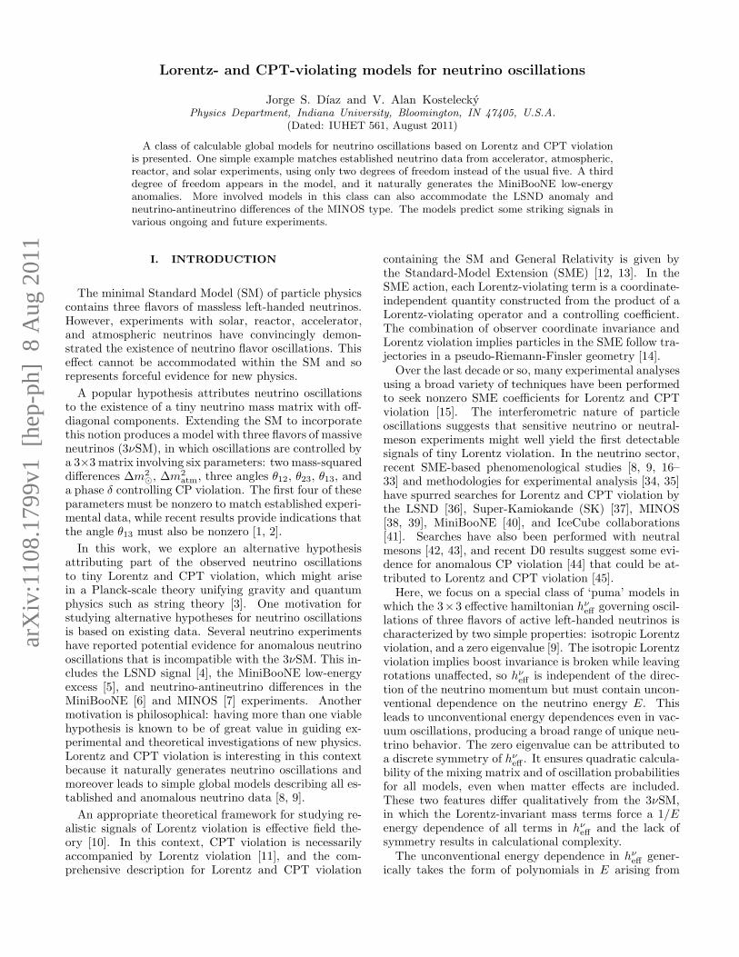
FIG. 1: Energy dependences of the oscillation lengths for neu-trinos (top) and antineutrinos (bottom). The disappearancelengths for the puma model are L31 (top, solid line), L21

(top, dashed line), L31 (bottom, solid line), and L21 (bottom,dashed line), displayed for the values (8). The dotted lines arethe disappearance lengths L⊙ (solar) and Latm (atmospheric)in the 3νSM.

from direct mass measurements and cosmological bounds[1].

By construction, a(5) and c(8) are the only nonzeroSME coefficients defined in an isotropic frame I. In somescenarios, it is reasonable to identify I with a universalinertial frame U such as that defined by the cosmic mi-crowave background (CMB), but other possibilities exist.Whatever the choice for I, the experiment frame E isboosted in it by some combination of the Earth’s motionrelative to the CMB, the Earth’s revolution about theSun, and the Earth’s rotation. The coefficients a(5) andc(8) therefore induce anisotropic effects via the net boostin I. These could, for example, be detected by searchesfor sidereal or annual variations in E [42]. Experimentalconstraints and signals must be reported in a specifiedframe, but the frame E itself is inappropriate becauseit is noninertial and experiment specific. By convention,the canonical inertial frame used to report results is aSun-centered frame S [15, 61]. Inspection reveals thatthe size of the effects in S induced by the values (8) alllie below the sensitivity levels achieved in experimentsto date [36, 38–41]. Future experiments might offer im-proved sensitivity and thereby provide a distinct avenuefor testing the model.

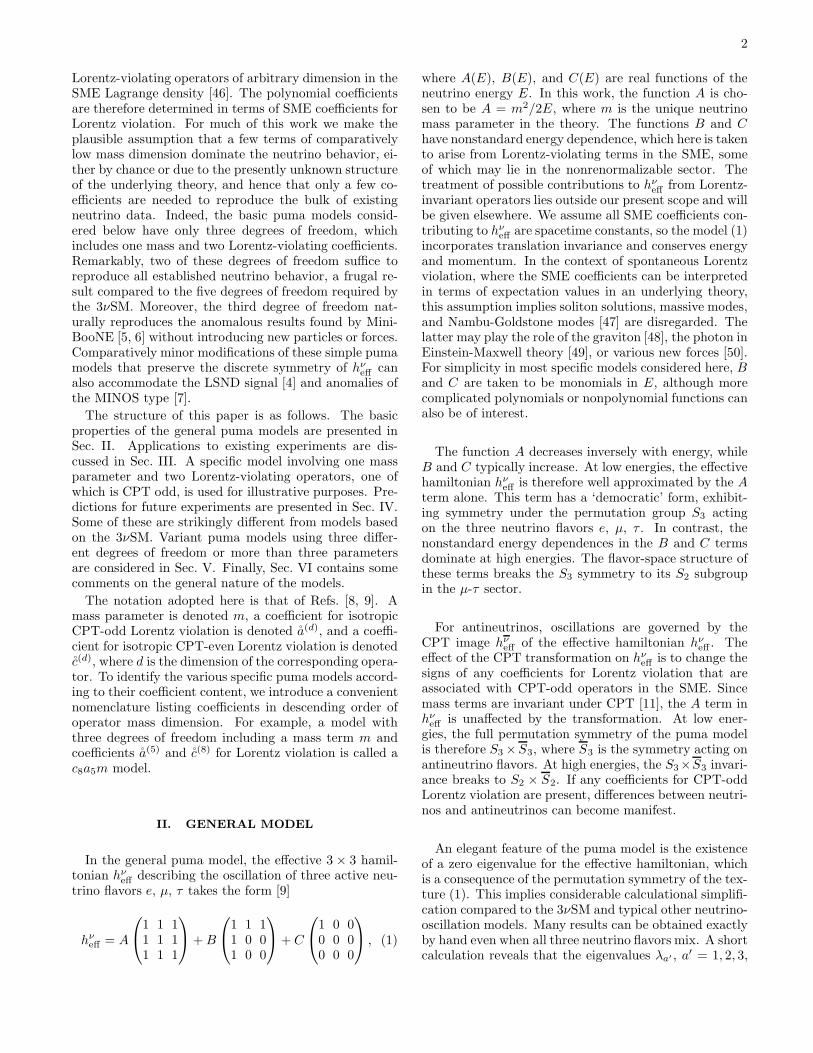
FIG. 2: Flavor content of the three neutrino eigenstates ofhν

eff (left) and the three antineutrino eigenstates of hν

eff (right)as a function of energy. For the puma model, the left-handpanel shows the energy dependences of |Ua′e|

2 (white), |Ua′µ|2

(light grey), and |Ua′τ |2 (dark grey) for each neutrino mass

eigenstate νa′ , a′ = 1, 2, 3, while the right-hand panel dis-plays the analogous energy dependences for antineutrinos.For the 3νSM, the corresponding quantities |Ua′e|

2 (regionsabove dashed lines), |Ua′µ|

2 (regions between dashed and solidlines), and |Ua′τ |

2 (regions below solid lines) for neutrinos andthose for antineutrinos are energy independent. The modelscoincide at all energies for the eigenstates ν3, ν3, but ν1, ν1

match ν2, ν2 only at low energies.

A. General features

The predictions of any model for neutrino and antineu-trino oscillations can be visualized using a certain plot inE-L space [8]. Experiments are represented on the plotas regions determined by their baseline and energy cover-age, while a given theory is represented by its characteris-tic oscillation wavelengths La′b′ = 2π/|∆a′b′ | associatedwith the eigenvalue differences ∆a′b′(E). The absolutevalue is used because the oscillation phase is insensitiveto the sign of ∆a′b′ . Each curve La′b′ = La′b′(E) indi-cates the first maximum of a kinematic phase in the oscil-lation probability, thereby establishing the minimal dis-tance from the neutrino source required for appearanceor disappearance signals in a specific oscillation channel.Substantial signals appear in the region above each curvebut are suppressed below it.

Figure 1 shows this plot for the puma model withvalues (8) and the 3νSM. The 3νSM has two indepen-dent oscillation lengths, L⊙ = 4πE/∆m2

⊙ and Latm =4πE/∆m2

atm, both of which grow linearly with the en-ergy and are therefore represented by straight lines inthe plot. In the puma model, however, the unconven-tional energy dependences from B(E) and C(E) producemore general curves instead. These curves partially dif-fer for neutrinos and antineutrinos, a consequence of theCPT violation implied by the values (8).

5

The figure shows that the puma curves merge withthe 3νSM lines L⊙ and Latm at low and high energies,respectively, suggesting consistency of the puma modelwith results in KamLAND, solar, and atmospheric ex-periments. This agreement is confirmed in the subsec-tions below. However, the two models are qualitativelydifferent at intermediate energies.

Novel effects arise from the unconventional energy de-pendence of hν

eff , which generates energy-dependent mix-ing. The flavor content of the three eigenstates of hν

efftherefore changes with energy. Figure 2 shows this energydependence for the values (8). At low energies, the flavorcontent approaches the tribimaximal limit. However, athigh energies the eigenstate ν2 becomes completely popu-lated by νe. This implies the mixing νµ ↔ ντ is maximaland controlled by ∆31. The onset of this feature coincideswith the onset of the Lorentz-violating seesaw. Indeed,as the mass term A becomes negligible in hν

eff , the frac-tion of νe in ν2 grows with the separation between thelines L21 and L31 in Fig. 1.

Notice that the mixing angles in the 3νSM are en-ergy independent parameters that can freely be chosento match data. In contrast, the mixing angles in thepuma model at low and high energies are determined bythe texture of hν

eff and therefore are fixed features of themodel that cannot be adjusted according to experiment.This reduced freedom is one reason why the puma modeloffers a more economical description of confirmed neu-trino data than the 3νSM.

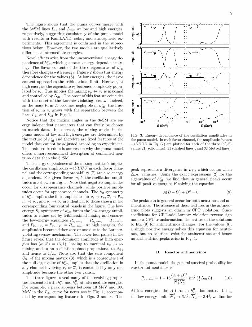
The energy dependence of the mixing matrix U impliesthe oscillation amplitudes −4UUUU in each flavor chan-nel and the corresponding probability (7) are also energydependent. For given flavors a, b, the oscillation ampli-tudes are shown in Fig. 3. Note that negative amplitudesoccur for disappearance channels, while positive ampli-tudes occur for appearance channels. The S2 symmetryof hν

eff implies the four amplitudes for νe → ντ , νe → ντ ,ντ → ντ , and ντ → ντ are identical to those shown in thecorresponding four central panels in the figure. The low-energy S3 symmetry of hν

eff forces the low-energy ampli-tudes to values set by tribimaximal mixing and ensuresthe low-energy equalities Pνe→νe = Pνµ→νµ = Pντ→ντ

and Pνe→νe= Pνµ→νµ

= Pντ→ντ. At high energies, the

amplitudes become either zero or one due to the Lorentz-violating seesaw mechanism. The lower four panels in thefigure reveal that the dominant amplitude at high ener-gies has (a′, b′) = (3, 1), leading to maximal νµ ↔ ντmixing and to an oscillation phase proportional to ∆31

and hence to 1/E. Note also that the zero componentU3e of the mixing matrix (3), which is a consequence ofthe null eigenvalue of hν

eff , implies that the oscillation inany channel involving νe or νe is controlled by only oneamplitude because the other two vanish.

The three figures reveal many of the evolving proper-ties associated with hν

eff and hνeff at intermediate energies.

For example, a peak appears between 10 MeV and 100MeV in the L31 curve for neutrinos in Fig. 1, accompa-nied by corresponding features in Figs. 2 and 3. The

FIG. 3: Energy dependence of the oscillation amplitudes inthe puma model. In each flavor channel, the amplitude factors−4UUUU in Eq. (7) are plotted for each of the three (a′, b′)values 21 (solid lines), 31 (dashed lines), and 32 (dotted lines).

peak represents a divergence in L31, which occurs when∆a′b′ vanishes. Using the exact expressions (2) for theeigenvalues of hν

eff , we find that in general peaks occurfor all positive energies E solving the equation

A(B − C) +B2 = 0. (9)

The peaks can in general occur for both neutrinos and an-tineutrinos. The absence of these features in the antineu-trino plots suggests an origin in CPT violation. Sincecoefficients for CPT-odd Lorentz violation reverse signunder a CPT transformation, the nature of the solutionsto Eq. (9) for antineutrinos changes. For the values (8),a single positive energy solves this equation for neutri-nos, but no solutions exist for antineutrinos and henceno antineutrino peaks arise in Fig. 1.

B. Reactor antineutrinos

In the puma model, the general survival probability forreactor antineutrinos is

Pνe→νe= 1− 16

(A+B)4

N2

1N2

2

sin2(

12∆21L

)

. (10)

At low energies, the A term in hνeff dominates. Using

the low-energy limits N2

1 → 6A2, N2

2 → 3A2, we find for

6

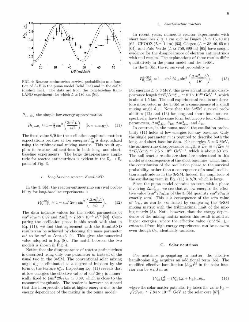
FIG. 4: Reactor-antineutrino survival probabilities as a func-tion of L/E in the puma model (solid line) and in the 3νSM(dashed line). The data are from the long-baseline Kam-LAND experiment, for which L ≃ 180 km [54].

Pνe→νethe simple low-energy approximation

Pνe→νe≈ 1− 8

9 sin2

(

3m2L

4E

)

(low energy). (11)

The fixed value 8/9 for the oscillation amplitude matchesexpectations because at low energies hν

eff is diagonalizedusing the tribimaximal mixing matrix. This result ap-plies to reactor antineutrinos in both long- and short-baseline experiments. The large disappearance ampli-tude for reactor antineutrinos is evident in the νe → νe

panel of Fig. 3.

1. Long-baseline reactor: KamLAND

In the 3νSM, the reactor-antineutrino survival proba-bility for long-baseline experiments is

P 3νSMνe→νe

≈ 1− sin2 2θ12 sin2

(

∆m2⊙L

4E

)

. (12)

The data indicate values for the 3νSM parameters ofsin2 2θ12 ≃ 0.92 and ∆m2

⊙ ≃ 7.58× 10−5 eV2 [53]. Com-paring the oscillation phase in this result with that inEq. (11), we find that agreement with the KamLANDresults can be achieved by choosing the mass parameterm2 to be m2 = ∆m2

⊙/3 [9]. This gives the numericalvalue adopted in Eq. (8). The match between the twomodels is shown in Fig. 4.Notice that the disappearance of reactor antineutrinos

is described using only one parameter m instead of theusual two in the 3νSM. The conventional solar mixingangle θ12 is eliminated as a degree of freedom by theform of the texture hν

eff . Inspecting Eq. (11) reveals that

at low energies the effective value of sin2 2θ12 is numer-ically fixed to (sin2 2θ12)eff ≃ 0.89, which is close to themeasured magnitude. The reader is however cautionedthat this interpretation fails at higher energies due to theenergy dependence of the mixing in the puma model.

2. Short-baseline reactors

In recent years, numerous reactor experiments withshort baselines L ∼< 1 km such as Bugey (L ≃ 15, 40 m)[62], CHOOZ (L ≃ 1 km) [63], Gosgen (L ≃ 38, 46, 65 m)[64], and Palo Verde (L ≃ 750, 890 m) [65] have soughtevidence for the disappearance of electron antineutrinoswith null results. The explanations of these results differqualitatively in the puma model and the 3νSM.In the 3νSM, the νe survival probability is

P 3νSMνe→νe

≈ 1− sin2 2θ13 sin2

(

∆m2atmL

4E

)

. (13)

For energiesE ≃ 3 MeV, this gives an antineutrino disap-pearance length 2πE/∆m2

atm ≃ 8.1×1018 GeV−1, whichis about 1.5 km. The null experimental results are there-fore interpreted in the 3νSM as a consequence of a smallmixing angle θ13. Note that the 3νSM survival prob-abilities (12) and (13) for long and short baselines, re-spectively, have the same form but involve four differentparameters, ∆m2

solar, θ12, ∆m2atm, and θ13.

In contrast, in the puma model the oscillation proba-bility (11) holds at low energies for any baseline. Onlythe single parameter m is required to describe both thelong- and short-baseline data. For energies E ≃ 3 MeV,the antineutrino disappearance length is L21 ≡ π/∆21 ≈2πE/∆m2

⊙ ≃ 2.5 × 1020 GeV−1, which is about 50 km.The null reactor results are therefore understood in thismodel as a consequence of the short baselines, which limitthe contribution of the oscillation phase to the survivalprobability, rather than a consequence of a small oscilla-tion amplitude as in the 3νSM. Indeed, the amplitude ofthe oscillating term in Eq. (11) is 8/9, which is large.Since the puma model contains no term with a phase

involving ∆m2atm, we see that at low energies the effec-

tive value (sin2 2θ13)eff of the 3νSM quantity sin2 2θ13 isexactly zero. This is a consequence of the zero valueof U3e, as can be confirmed by comparing the 3νSMmixing matrix with the tribimaximal limit of the mix-ing matrix (3). Note, however, that the energy depen-dence of the mixing matrix makes this result invalid athigher energies, where the effective value (sin2 2θ13)effextracted from high-energy experiments can be nonzeroeven though U3e identically vanishes.

C. Solar neutrinos

For neutrinos propagating in matter, the effectivehamiltonian hν

eff acquires an additional term [66]. Themodified effective hamiltonian (hν

eff)M in the solar inte-

rior can be written as

(hνeff)

Mab = (hν

eff)ab + V⊙δaeδbe, (14)

where the solar matter potential V⊙ takes the value V⊙ =√2GFne ≃ 7.84× 10−21 GeV at the solar core [67].

7

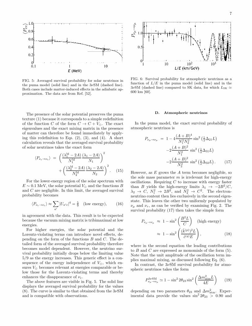
FIG. 5: Averaged survival probability for solar neutrinos inthe puma model (solid line) and in the 3νSM (dashed line).Both cases include matter-induced effects in the adiabatic ap-proximation. The data are from Ref. [52].

The presence of the solar potential preserves the pumatexture (1) because it corresponds to a simple redefinitionof the function C of the form C → C + V⊙. The exacteigenvalues and the exact mixing matrix in the presenceof matter can therefore be found immediately by apply-ing this redefinition to Eqs. (2), (3), and (4). A shortcalculation reveals that the averaged survival probabilityof solar neutrinos takes the exact form

〈Pνe→νe〉 =

(

(λM1 − 2A)

NM1

(λ1 − 2A)

N1

)2

+

(

(λM2 − 2A)

NM2

(λ2 − 2A)

N2

)2

. (15)

For the lower-energy region of the solar spectrum withE ∼ 0.1 MeV, the solar potential V⊙ and the functions Band C are negligible. In this limit, the averaged survivalprobability becomes

〈Pνe→νe〉 ≈∑

a′

|Ua′e|4 = 59 (low energy), (16)

in agreement with the data. This result is to be expectedbecause the vacuum mixing matrix is tribimaximal at lowenergies.For higher energies, the solar potential and the

Lorentz-violating terms can introduce novel effects, de-pending on the form of the functions B and C. The de-tailed form of the averaged survival probability thereforebecomes model dependent. However, the neutrino sur-vival probability initially drops below the limiting value5/9 as the energy increases. This generic effect is a con-sequence of the energy independence of V⊙, which en-sures V⊙ becomes relevant at energies comparable or be-low those for the Lorentz-violating terms and therebyenhances the disappearance of νe.The above features are visible in Fig. 5. The solid line

displays the averaged survival probability for the values(8). The curve is similar to that obtained from the 3νSMand is compatible with observations.

FIG. 6: Survival probability for atmospheric neutrinos as afunction of L/E in the puma model (solid line) and in the3νSM (dashed line) compared to SK data, for which LSK ≃600 km [60].

D. Atmospheric neutrinos

In the puma model, the exact survival probability ofatmospheric neutrinos is

Pνµ→νµ = 1− 4(A+B)4

N21N

22

sin2(

12∆21L

)

−2(A+B)2

N21

sin2(

12∆31L

)

−2(A+B)2

N22

sin2(

12∆32L

)

. (17)

However, as E grows the A term becomes negligible, sothe sole mass parameter m is irrelevant for high-energyoscillations. Requiring C to increase with energy fasterthan B yields the high-energy limits λ1 → −2B2/C,λ2 → C, N2

1 → 2B2, and N22 → C2. The electron-

neutrino content then lies exclusively in the second eigen-state. This leaves the other two uniformly populated byνµ and ντ , as can be verified by examining Fig. 2. Thesurvival probability (17) then takes the simple form

Pνµ→νµ ≈ 1− sin2(

B2L

C

)

(high energy)

≈ 1− sin2

(

(k(p))2L

c(q)E

)

, (18)

where in the second equation the leading contributionsto B and C are expressed as monomials of the form (5).Note that the unit amplitude of the oscillation term im-plies maximal mixing, as discussed following Eq. (6).In contrast, the 3νSM survival probability for atmo-

spheric neutrinos takes the form

P 3νSMνµ→νµ

≃ 1− sin2 2θ23 sin2

(

∆m2atmL

4E

)

(19)

depending on two parameters θ23 and ∆m2atm. Exper-

imental data provide the values sin2 2θ23 > 0.90 and

8

|∆m2atm| ≃ 2.32 × 10−3 eV2 [57]. Comparison of Eqs.

(18) and (19) suggests agreement with atmospheric data

can be obtained when the ratio of (k(p))2 and c(q) satisfies

(k(p))2

c(q)= 1

4∆m2atm. (20)

This condition has been used to constrain the coefficientsa(5) and c(8) in Eq. (8) [9]. The resulting match betweenthe two models is shown in Fig. 6 along with SK data.Note that the ratio (20) represents only one degree of

freedom. Nonetheless, it suffices to reproduce the datafor atmospheric neutrinos via Eq. (18). The other degree

of freedom in the two coefficients k(p), c(q) determinesthe onset of the Lorentz-violating seesaw. Increasing c(q)

while holding fixed the ratio (20) causes the seesaw totrigger at lower energies.

E. Short-baseline accelerator neutrinos

At high energies E ∼> 1 GeV, a variety of short-baselineexperiments have reported null results. BNL-E776 (L =1 km) searched for νµ → νe and νµ → νe at 1 GeV[68]. CCFR (L ≃ 1 km) searched for νµ → νe, νµ →νe, νe → ντ , and νe → ντ at 140 GeV [69]. CDHS(L ≃ 130 m) searched for νµ disappearance at 1 GeV[70]. CHORUS (L ≃ 600 m) searched for νµ → ντ at 27GeV [71]. NOMAD (L ≃ 600 m) searched for νµ → ντand νe → ντ at 45 GeV [72]. NuTeV (L ≃ 1 km) searchedfor νµ → νe and νµ → νe at 150 GeV [73].The puma model is consistent with all these null re-

sults. For energies above the seesaw scale ∼ 1 GeV,νµ ↔ ντ mixing becomes maximal by construction, asdescribed following Eq. (6). This feature implies vanish-ing high-energy mixing and hence no oscillations in thechannels νµ → νe, νµ → νe, νe → ντ , and νe → ντ . Thebehavior can be seen directly from Fig. 3, which displaysthe energy dependence of the oscillation amplitudes.In the νµ → ντ channel, the oscillation amplitude

is maximal at high energies. However, the oscillationphase is controlled by ∆21, which generates an appear-ance length L21 of several hundred kilometers at 1 GeV.The lack of a signal in this channel in the CHORUS orNOMAD data is therefore understood here as a conse-quence of their short baselines.

F. MiniBooNE anomalies

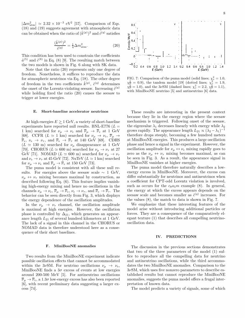
Two results from the MiniBooNE experiment indicatepossible oscillation effects that cannot be accommodatedwithin the 3νSM. For neutrino oscillations νµ → νe,MiniBooNE finds a 3σ excess of events at low energiesaround 200-500 MeV [5]. For antineutrino oscillationsνµ → νe, a 1.3σ low-energy excess has also been reported[6], with recent preliminary data suggesting a larger ex-cess [74].

FIG. 7: Comparison of the puma model (solid lines; χ2ν = 1.0,

χ2

ν = 0.9), the tandem model [19] (dotted lines; χ2ν = 1.9,

χ2

ν = 1.0), and the 3νSM (dashed lines; χ2ν = 2.2, χ2

ν = 1.1),with MiniBooNE neutrino [5] and antineutrino [6] data.

These results are interesting in the present contextbecause they lie in the energy region where the seesawmechanism is triggered. Following onset of the seesaw,the eigenvalue λ1 decreases linearly with energy while λ2

grows rapidly. The appearance length L21 ∝ (λ2−λ1)−1

therefore drops steeply, becoming a few hundred metersat MiniBooNE energies. This produces a large oscillationphase and hence a signal in the experiment. However, theoscillation amplitude for νµ ↔ νe mixing rapidly goes tozero as the νµ ↔ ντ mixing becomes maximal, as canbe seen in Fig. 3. As a result, the appearance signal inMiniBooNE vanishes at higher energies.The puma model therefore naturally describes a low-

energy excess in MiniBooNE. Moreover, the excess candiffer substantially for neutrinos and antineutrinos whena coefficient for CPT-odd Lorentz violation is involved,such as occurs for the c8a5m example (8). In general,the energy at which the excess appears depends on theseesaw scale and becomes smaller as c(q) increases. Forthe values (8), the match to data is shown in Fig. 7.We emphasize that these interesting features of the

model arise without introducing additional particles orforces. They are a consequence of the comparatively el-egant texture (1) that describes all compelling neutrino-oscillation data.

IV. PREDICTIONS

The discussion in the previous sections demonstratesthat two of the three parameters of the model (1) suf-fice to reproduce all the compelling data for neutrinoand antineutrino oscillations, while the third accommo-dates the two MiniBooNE anomalies. Comparison to the3νSM, which uses five nonzero parameters to describe es-tablished results but cannot reproduce the MiniBooNEanomalies, suggests the puma model offers a frugal inter-pretation of known data.The model predicts a variety of signals, some of which

9

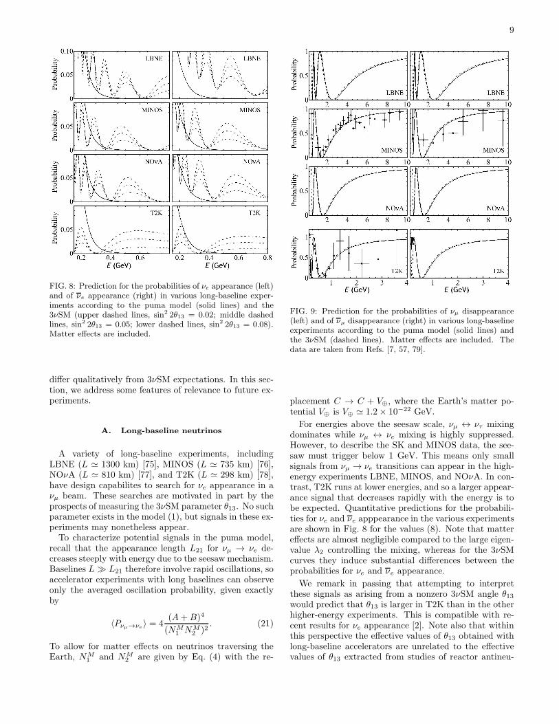
FIG. 8: Prediction for the probabilities of νe appearance (left)and of νe appearance (right) in various long-baseline exper-iments according to the puma model (solid lines) and the3νSM (upper dashed lines, sin2 2θ13 = 0.02; middle dashedlines, sin2 2θ13 = 0.05; lower dashed lines, sin2 2θ13 = 0.08).Matter effects are included.

differ qualitatively from 3νSM expectations. In this sec-tion, we address some features of relevance to future ex-periments.

A. Long-baseline neutrinos

A variety of long-baseline experiments, includingLBNE (L ≃ 1300 km) [75], MINOS (L ≃ 735 km) [76],NOνA (L ≃ 810 km) [77], and T2K (L ≃ 298 km) [78],have design capabilites to search for νe appearance in aνµ beam. These searches are motivated in part by theprospects of measuring the 3νSM parameter θ13. No suchparameter exists in the model (1), but signals in these ex-periments may nonetheless appear.To characterize potential signals in the puma model,

recall that the appearance length L21 for νµ → νe de-creases steeply with energy due to the seesaw mechanism.Baselines L ≫ L21 therefore involve rapid oscillations, soaccelerator experiments with long baselines can observeonly the averaged oscillation probability, given exactlyby

〈Pνµ→νe〉 = 4(A+B)4

(NM1 NM

2 )2. (21)

To allow for matter effects on neutrinos traversing theEarth, NM

1 and NM2 are given by Eq. (4) with the re-

FIG. 9: Prediction for the probabilities of νµ disappearance(left) and of νµ disappearance (right) in various long-baselineexperiments according to the puma model (solid lines) andthe 3νSM (dashed lines). Matter effects are included. Thedata are taken from Refs. [7, 57, 79].

placement C → C + V⊕, where the Earth’s matter po-tential V⊕ is V⊕ ≃ 1.2× 10−22 GeV.

For energies above the seesaw scale, νµ ↔ ντ mixingdominates while νµ ↔ νe mixing is highly suppressed.However, to describe the SK and MINOS data, the see-saw must trigger below 1 GeV. This means only smallsignals from νµ → νe transitions can appear in the high-energy experiments LBNE, MINOS, and NOνA. In con-trast, T2K runs at lower energies, and so a larger appear-ance signal that decreases rapidly with the energy is tobe expected. Quantitative predictions for the probabili-ties for νe and νe apppearance in the various experimentsare shown in Fig. 8 for the values (8). Note that mattereffects are almost negligible compared to the large eigen-value λ2 controlling the mixing, whereas for the 3νSMcurves they induce substantial differences between theprobabilities for νe and νe appearance.

We remark in passing that attempting to interpretthese signals as arising from a nonzero 3νSM angle θ13would predict that θ13 is larger in T2K than in the otherhigher-energy experiments. This is compatible with re-cent results for νe appearance [2]. Note also that withinthis perspective the effective values of θ13 obtained withlong-baseline accelerators are unrelated to the effectivevalues of θ13 extracted from studies of reactor antineu-

10

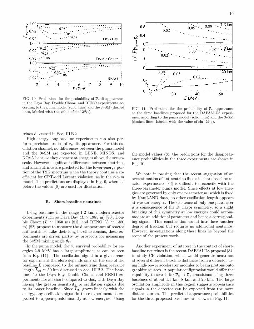
FIG. 10: Predictions for the probability of νe disappearancein the Daya Bay, Double Chooz, and RENO experiments ac-cording to the puma model (solid lines) and the 3νSM (dashedlines, labeled with the value of sin2 2θ13).

trinos discussed in Sec. III B 2.High-energy long-baseline experiments can also per-

form precision studies of νµ disappearance. For this os-cillation channel, no differences between the puma modeland the 3νSM are expected in LBNE, MINOS, andNOνA because they operate at energies above the seesawscale. However, significant differences between neutrinosand antineutrinos are predicted for the lower-energy por-tion of the T2K spectrum when the theory contains a co-efficient for CPT-odd Lorentz violation, as in the c8a5mmodel. The predictions are displayed in Fig. 9, where asbefore the values (8) are used for illustration.

B. Short-baseline neutrinos

Using baselines in the range 1-2 km, modern reactorexperiments such as Daya Bay (L ≃ 1985 m) [80], Dou-ble Chooz (L ≃ 1050 m) [81], and RENO (L ≃ 1380m) [82] propose to measure the disappearance of reactorantineutrinos. Like their long-baseline cousins, these ex-periments are driven partly by prospects for measuringthe 3νSM mixing angle θ13.In the puma model, the νe survival probability for en-

ergies 2-9 MeV has a large amplitude, as can be seenfrom Eq. (11). The oscillation signal in a given reac-tor experiment therefore depends only on the size of thebaseline L compared to the antineutrino disappearancelength L21 ≃ 50 km discussed in Sec. III B 2. The base-lines for the Daya Bay, Double Chooz, and RENO ex-periments are all short compared to this, with Daya Bayhaving the greater sensitivity to oscillation signals dueto its longer baseline. Since L21 grows linearly with theenergy, any oscillation signal in these experiments is ex-pected to appear predominantly at low energies. Using

FIG. 11: Predictions for the probability of νe appearanceat the three baselines proposed for the DAEδALUS experi-ment according to the puma model (solid lines) and the 3νSM(dashed lines, labeled with the value of sin2 2θ13).

the model values (8), the predictions for the disappear-ance probabilities in the three experiments are shown inFig. 10.

We note in passing that the recent suggestion of anoverestimation of antineutrino fluxes in short-baseline re-actor experiments [83] is difficult to reconcile with thethree-parameter puma model. Since effects at low ener-gies are governed by only one parameterm, which is fixedby KamLAND data, no other oscillation length appearsat reactor energies. The existence of only one parameteris a consequence of the S3 flavor symmetry, so a slightbreaking of this symmetry at low energies could accom-modate an additional parameter and hence a correspond-ing signal. This construction would introduce anotherdegree of freedom but requires no additional neutrinos.However, investigations along these lines lie beyond thescope of the present work.

Another experiment of interest in the context of short-baseline neutrinos is the recent DAEδALUS proposal [84]to study CP violation, which would generate neutrinosat several different baseline distances from a detector us-ing high-power accelerator modules to beam protons ontographite sources. A popular configuration would offer thecapability to search for νµ → νe transitions using threebaselines of about 1.5 km, 8 km, and 20 km. The largeoscillation amplitude in this region suggests appearancesignals in the detector can be expected from the moredistant sources. The predicted appearance probabilitiesfor the three proposed baselines are shown in Fig. 11.

11

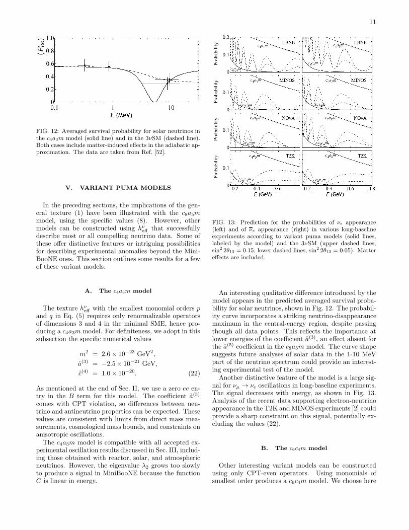
FIG. 12: Averaged survival probability for solar neutrinos inthe c4a3m model (solid line) and in the 3νSM (dashed line).Both cases include matter-induced effects in the adiabatic ap-proximation. The data are taken from Ref. [52].

V. VARIANT PUMA MODELS

In the preceding sections, the implications of the gen-eral texture (1) have been illustrated with the c8a5mmodel, using the specific values (8). However, othermodels can be constructed using hν

eff that successfullydescribe most or all compelling neutrino data. Some ofthese offer distinctive features or intriguing possibilitiesfor describing experimental anomalies beyond the Mini-BooNE ones. This section outlines some results for a fewof these variant models.

A. The c4a3m model

The texture hνeff with the smallest monomial orders p

and q in Eq. (5) requires only renormalizable operatorsof dimensions 3 and 4 in the minimal SME, hence pro-ducing a c4a3m model. For definiteness, we adopt in thissubsection the specific numerical values

m2 = 2.6× 10−23 GeV2,

a(3) = −2.5× 10−21 GeV,

c(4) = 1.0× 10−20. (22)

As mentioned at the end of Sec. II, we use a zero ee en-try in the B term for this model. The coefficient a(3)

comes with CPT violation, so differences between neu-trino and antineutrino properties can be expected. Thesevalues are consistent with limits from direct mass mea-surements, cosmological mass bounds, and constraints onanisotropic oscillations.The c4a3m model is compatible with all accepted ex-

perimental oscillation results discussed in Sec. III, includ-ing those obtained with reactor, solar, and atmosphericneutrinos. However, the eigenvalue λ2 grows too slowlyto produce a signal in MiniBooNE because the functionC is linear in energy.

FIG. 13: Prediction for the probabilities of νe appearance(left) and of νe appearance (right) in various long-baselineexperiments according to variant puma models (solid lines,labeled by the model) and the 3νSM (upper dashed lines,sin2 2θ13 = 0.15; lower dashed lines, sin2 2θ13 = 0.05). Mattereffects are included.

An interesting qualitative difference introduced by themodel appears in the predicted averaged survival proba-bility for solar neutrinos, shown in Fig. 12. The probabil-ity curve incorporates a striking neutrino-disappearancemaximum in the central-energy region, despite passingthough all data points. This reflects the importance atlower energies of the coefficient a(3), an effect absent forthe a(5) coefficient in the c8a5m model. The curve shapesuggests future analyses of solar data in the 1-10 MeVpart of the neutrino spectrum could provide an interest-ing experimental test of the model.Another distinctive feature of the model is a large sig-

nal for νµ → νe oscillations in long-baseline experiments.The signal decreases with energy, as shown in Fig. 13.Analysis of the recent data supporting electron-neutrinoappearance in the T2K and MINOS experiments [2] couldprovide a sharp constraint on this signal, potentially ex-cluding the values (22).

B. The c6c4m model

Other interesting variant models can be constructedusing only CPT-even operators. Using monomials ofsmallest order produces a c6c4m model. We choose here

12

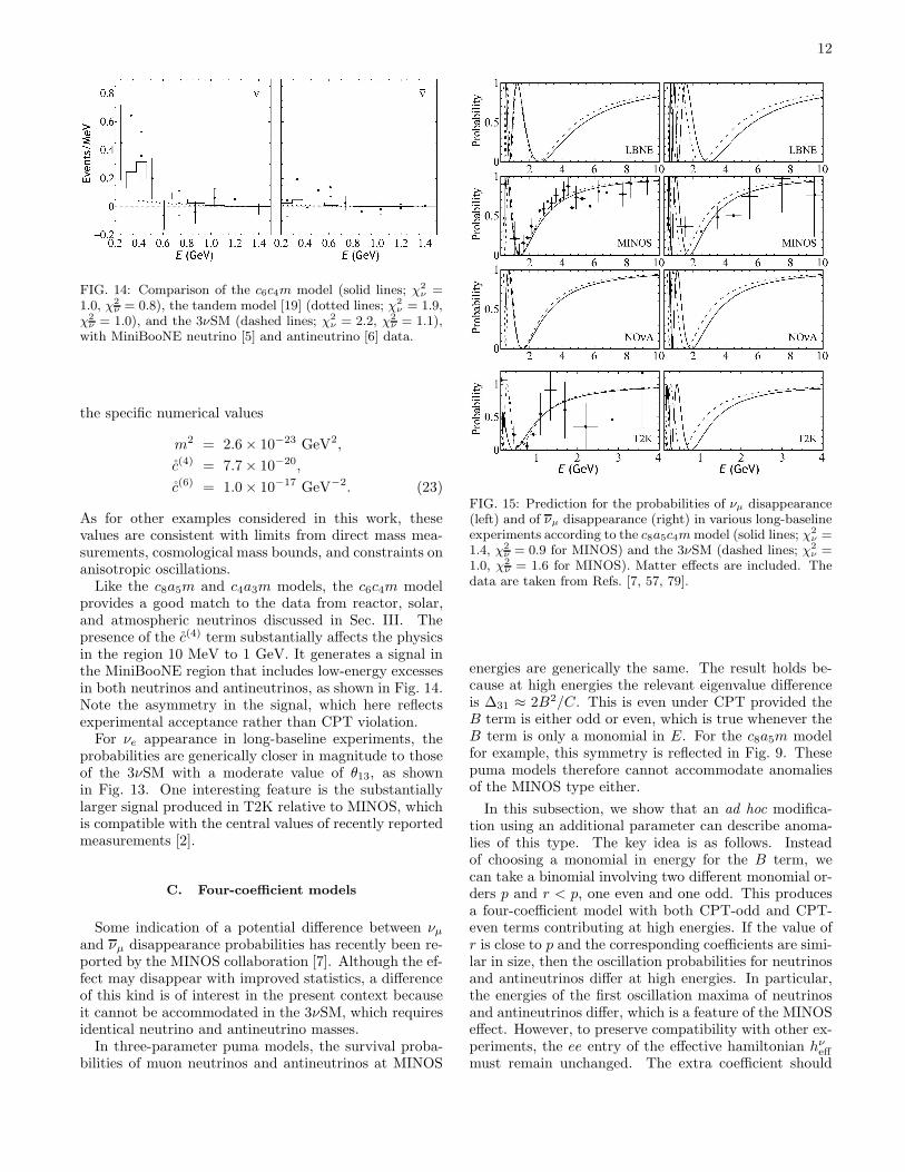
FIG. 14: Comparison of the c6c4m model (solid lines; χ2ν =

1.0, χ2

ν = 0.8), the tandem model [19] (dotted lines; χ2ν = 1.9,

χ2

ν = 1.0), and the 3νSM (dashed lines; χ2ν = 2.2, χ2

ν = 1.1),with MiniBooNE neutrino [5] and antineutrino [6] data.

the specific numerical values

m2 = 2.6× 10−23 GeV2,

c(4) = 7.7× 10−20,

c(6) = 1.0× 10−17 GeV−2. (23)

As for other examples considered in this work, thesevalues are consistent with limits from direct mass mea-surements, cosmological mass bounds, and constraints onanisotropic oscillations.Like the c8a5m and c4a3m models, the c6c4m model

provides a good match to the data from reactor, solar,and atmospheric neutrinos discussed in Sec. III. Thepresence of the c(4) term substantially affects the physicsin the region 10 MeV to 1 GeV. It generates a signal inthe MiniBooNE region that includes low-energy excessesin both neutrinos and antineutrinos, as shown in Fig. 14.Note the asymmetry in the signal, which here reflectsexperimental acceptance rather than CPT violation.For νe appearance in long-baseline experiments, the

probabilities are generically closer in magnitude to thoseof the 3νSM with a moderate value of θ13, as shownin Fig. 13. One interesting feature is the substantiallylarger signal produced in T2K relative to MINOS, whichis compatible with the central values of recently reportedmeasurements [2].

C. Four-coefficient models

Some indication of a potential difference between νµand νµ disappearance probabilities has recently been re-ported by the MINOS collaboration [7]. Although the ef-fect may disappear with improved statistics, a differenceof this kind is of interest in the present context becauseit cannot be accommodated in the 3νSM, which requiresidentical neutrino and antineutrino masses.In three-parameter puma models, the survival proba-

bilities of muon neutrinos and antineutrinos at MINOS

FIG. 15: Prediction for the probabilities of νµ disappearance(left) and of νµ disappearance (right) in various long-baselineexperiments according to the c8a5c4mmodel (solid lines; χ2

ν =1.4, χ2

ν = 0.9 for MINOS) and the 3νSM (dashed lines; χ2ν =

1.0, χ2

ν = 1.6 for MINOS). Matter effects are included. Thedata are taken from Refs. [7, 57, 79].

energies are generically the same. The result holds be-cause at high energies the relevant eigenvalue differenceis ∆31 ≈ 2B2/C. This is even under CPT provided theB term is either odd or even, which is true whenever theB term is only a monomial in E. For the c8a5m modelfor example, this symmetry is reflected in Fig. 9. Thesepuma models therefore cannot accommodate anomaliesof the MINOS type either.

In this subsection, we show that an ad hoc modifica-tion using an additional parameter can describe anoma-lies of this type. The key idea is as follows. Insteadof choosing a monomial in energy for the B term, wecan take a binomial involving two different monomial or-ders p and r < p, one even and one odd. This producesa four-coefficient model with both CPT-odd and CPT-even terms contributing at high energies. If the value ofr is close to p and the corresponding coefficients are simi-lar in size, then the oscillation probabilities for neutrinosand antineutrinos differ at high energies. In particular,the energies of the first oscillation maxima of neutrinosand antineutrinos differ, which is a feature of the MINOSeffect. However, to preserve compatibility with other ex-periments, the ee entry of the effective hamiltonian hν

effmust remain unchanged. The extra coefficient should

13

therefore appear only in the eµ and eτ entries of hνeff .

One way to achieve this is to choose a binomial for theC term as well, compensating for the modification of theee entry arising from the change to B.As an example, we can add a fourth coefficient to the

c8a5m model while leaving unchanged its main features.Choosing r = 4, which satisfies the requirement r < p =5 with r near p, the fourth coefficient can be denotedc(4). To generate a neutrino-antineutrino difference athigh energies, it suffices to redefine the B and C termsas B → B + c(4)E, C → C − c(4)E. For definiteness, wecan take the numerical values

m2 = 2.6× 10−23 GeV2,

c(4) = 2.0× 10−20,

a(5) = −2.6× 10−19 GeV−1,

c(8) = 1.0× 10−16 GeV−4, (24)

which as before are consistent with limits from directmass measurements, cosmological mass bounds, and con-straints on anisotropic oscillations. These choices pre-serve the attractive features of the simpler c8a5m model.The introduction of the fourth coefficient primarily af-

fects the probabilities of νµ and νµ disappearance in long-baseline experiments, as shown in Fig. 15 for the values(24). In particular, the MINOS data in Ref. [7] are rea-sonably described by the model. The location of the pri-mary minimum for antineutrino oscillations is at a higherenergy than that for neutrinos, in agreement with the re-ported effect. We emphasize that this result is achievedwith a single additional parameter, without any masses,in a global model of neutrino oscillations. Note also thatthis c8a5c4m model predicts a large difference betweenthe probabilities of νµ and νµ disappearance in the T2Kexperiment. However, the νe appearance probabilities inlong-baseline experiments are essentially unchanged fromthose for the c8a5m model shown in Fig. 8.

D. Enhanced models

In a search for appearance of electron antineutrinosin a beam of muon antineutrinos, the LSND experimentfound evidence for a small probability Pνµ→νe

≃ 0.26 ±0.08% of νµ → νe oscillations at baseline L = 30 m andenergies in the range 20-60 MeV [4]. This signal cannotbe accommodated within the 3νSM because the requiredmass-squared difference ∆m2

LSND ≃ 1 eV2 is orders ofmagnitude larger than ∆m2

⊙ and ∆m2atm.

In the general puma model, the oscillation νµ → νe isgiven exactly by

Pνµ→νe= 8

(A+B)4

N2

1N2

2

sin2(

∆21L

2

)

, (25)

which is governed by the same eigenvalues that controlreactor antineutrinos. The energies in the LSND experi-ment are greater than those of reactor antineutrinos, but

FIG. 16: Energy dependences of the oscillation lengths forantineutrinos in the doubly enhanced puma model. The cor-responding plot for neutrinos in the top panel of Fig. 1 re-mains unaffected. The disappearance lengths for the modelare L31 (solid line) and L21 (dashed line), displayed for thevalues given by Eqs. (24), (27), and (28). The dotted lines arethe disappearance lengths L⊙ (solar) and Latm (atmospheric)in the 3νSM.

FIG. 17: Comparison of enhanced puma model (solid line,χ2 = 1.6) and the 3νSM (dashed line, χ2 = 2.6) with LSNDantineutrino data [5].

the appearance length is smaller by about two orders ofmagnitude. Achieving this with a monomial energy de-pendence in hν

eff while preserving consistency with otherexperiments is challenging, as it requires a large power ofthe energy and a seesaw triggered around 10 MeV.An interesting option generating the required steep fall

and rise in L21(E) is to introduce a smooth nonpolyno-mial function with a peak. A function of this type couldact as an enhancement of hν

eff arising from a series of co-efficients in the SME. It can be approximated genericallyusing at least three parameters, one to position it, oneto fix its height, and one to specify its width. A simpleexample is a gaussian enhancement of the form

δh = α exp[−β(E − ε)2]. (26)

To preserve the S2 symmetry of hνeff , the enhancement

can be limited to the eµ and eτ entries of hνeff via the

14

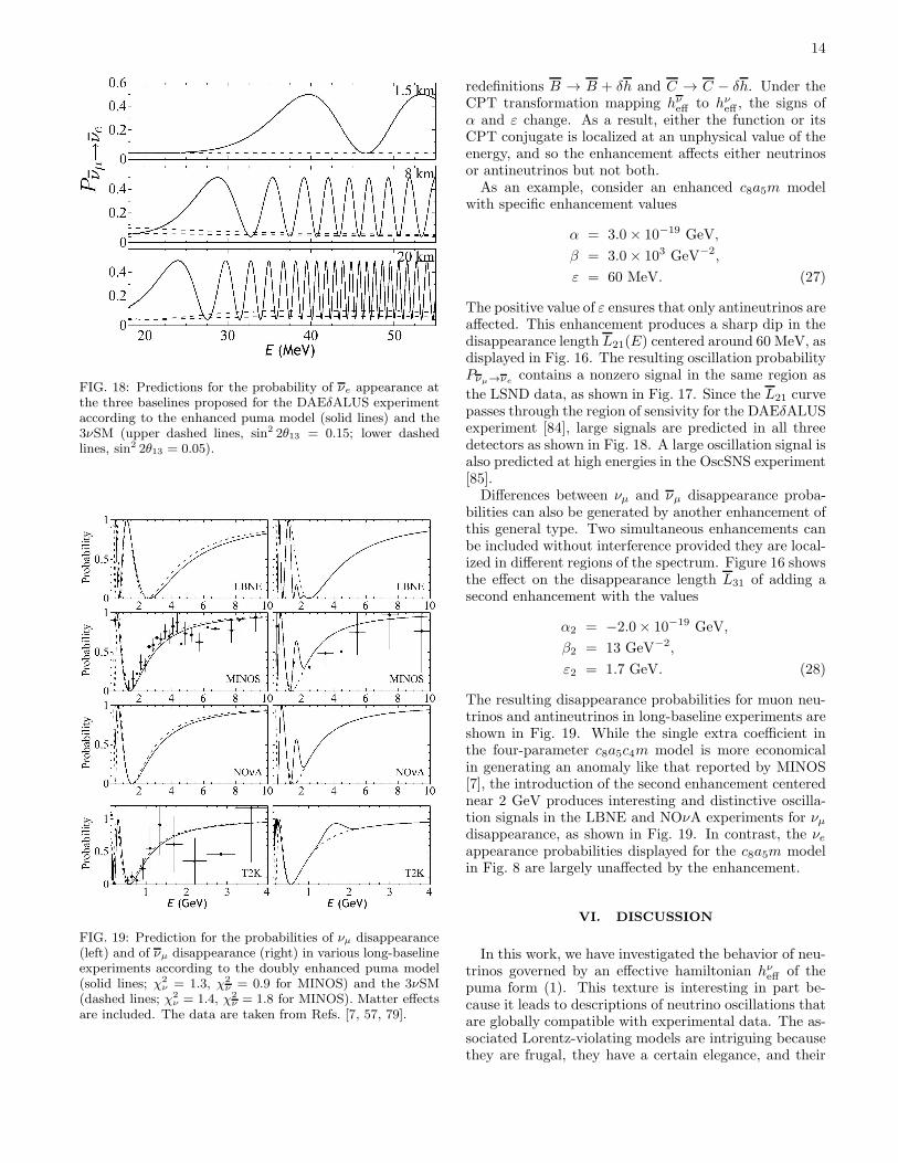
FIG. 18: Predictions for the probability of νe appearance atthe three baselines proposed for the DAEδALUS experimentaccording to the enhanced puma model (solid lines) and the3νSM (upper dashed lines, sin2 2θ13 = 0.15; lower dashedlines, sin2 2θ13 = 0.05).

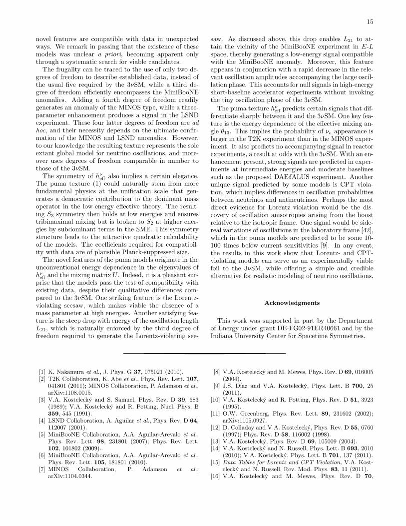
FIG. 19: Prediction for the probabilities of νµ disappearance(left) and of νµ disappearance (right) in various long-baselineexperiments according to the doubly enhanced puma model(solid lines; χ2

ν = 1.3, χ2

ν = 0.9 for MINOS) and the 3νSM(dashed lines; χ2

ν = 1.4, χ2

ν = 1.8 for MINOS). Matter effectsare included. The data are taken from Refs. [7, 57, 79].

redefinitions B → B + δh and C → C − δh. Under theCPT transformation mapping hν

eff to hνeff , the signs of

α and ε change. As a result, either the function or itsCPT conjugate is localized at an unphysical value of theenergy, and so the enhancement affects either neutrinosor antineutrinos but not both.As an example, consider an enhanced c8a5m model

with specific enhancement values

α = 3.0× 10−19 GeV,

β = 3.0× 103 GeV−2,

ε = 60 MeV. (27)

The positive value of ε ensures that only antineutrinos areaffected. This enhancement produces a sharp dip in thedisappearance length L21(E) centered around 60 MeV, asdisplayed in Fig. 16. The resulting oscillation probabilityPνµ→νe

contains a nonzero signal in the same region as

the LSND data, as shown in Fig. 17. Since the L21 curvepasses through the region of sensivity for the DAEδALUSexperiment [84], large signals are predicted in all threedetectors as shown in Fig. 18. A large oscillation signal isalso predicted at high energies in the OscSNS experiment[85].Differences between νµ and νµ disappearance proba-

bilities can also be generated by another enhancement ofthis general type. Two simultaneous enhancements canbe included without interference provided they are local-ized in different regions of the spectrum. Figure 16 showsthe effect on the disappearance length L31 of adding asecond enhancement with the values

α2 = −2.0× 10−19 GeV,

β2 = 13 GeV−2,

ε2 = 1.7 GeV. (28)

The resulting disappearance probabilities for muon neu-trinos and antineutrinos in long-baseline experiments areshown in Fig. 19. While the single extra coefficient inthe four-parameter c8a5c4m model is more economicalin generating an anomaly like that reported by MINOS[7], the introduction of the second enhancement centerednear 2 GeV produces interesting and distinctive oscilla-tion signals in the LBNE and NOνA experiments for νµdisappearance, as shown in Fig. 19. In contrast, the νeappearance probabilities displayed for the c8a5m modelin Fig. 8 are largely unaffected by the enhancement.

VI. DISCUSSION

In this work, we have investigated the behavior of neu-trinos governed by an effective hamiltonian hν

eff of thepuma form (1). This texture is interesting in part be-cause it leads to descriptions of neutrino oscillations thatare globally compatible with experimental data. The as-sociated Lorentz-violating models are intriguing becausethey are frugal, they have a certain elegance, and their

15

novel features are compatible with data in unexpectedways. We remark in passing that the existence of thesemodels was unclear a priori, becoming apparent onlythrough a systematic search for viable candidates.The frugality can be traced to the use of only two de-

grees of freedom to describe established data, instead ofthe usual five required by the 3νSM, while a third de-gree of freedom efficiently encompasses the MiniBooNEanomalies. Adding a fourth degree of freedom readilygenerates an anomaly of the MINOS type, while a three-parameter enhancement produces a signal in the LSNDexperiment. These four latter degrees of freedom are ad

hoc, and their necessity depends on the ultimate confir-mation of the MINOS and LSND anomalies. However,to our knowledge the resulting texture represents the soleextant global model for neutrino oscillations, and more-over uses degrees of freedom comparable in number tothose of the 3νSM.The symmetry of hν

eff also implies a certain elegance.The puma texture (1) could naturally stem from morefundamental physics at the unification scale that gen-erates a democratic contribution to the dominant massoperator in the low-energy effective theory. The result-ing S3 symmetry then holds at low energies and ensurestribimaximal mixing but is broken to S2 at higher ener-gies by subdominant terms in the SME. This symmetrystructure leads to the attractive quadratic calculabilityof the models. The coefficients required for compatibil-ity with data are of plausible Planck-suppressed size.The novel features of the puma models originate in the

unconventional energy dependence in the eigenvalues ofhνeff and the mixing matrix U . Indeed, it is a pleasant sur-

prise that the models pass the test of compatibility withexisting data, despite their qualitative differences com-pared to the 3νSM. One striking feature is the Lorentz-violating seesaw, which makes viable the absence of amass parameter at high energies. Another satisfying fea-ture is the steep drop with energy of the oscillation lengthL21, which is naturally enforced by the third degree offreedom required to generate the Lorentz-violating see-

saw. As discussed above, this drop enables L21 to at-tain the vicinity of the MiniBooNE experiment in E-Lspace, thereby generating a low-energy signal compatiblewith the MiniBooNE anomaly. Moreover, this featureappears in conjunction with a rapid decrease in the rele-vant oscillation amplitudes accompanying the large oscil-lation phase. This accounts for null signals in high-energyshort-baseline accelerator experiments without invokingthe tiny oscillation phase of the 3νSM.

The puma texture hνeff predicts certain signals that dif-

ferentiate sharply between it and the 3νSM. One key fea-ture is the energy dependence of the effective mixing an-gle θ13. This implies the probability of νe appearance islarger in the T2K experiment than in the MINOS exper-iment. It also predicts no accompanying signal in reactorexperiments, a result at odds with the 3νSM. With an en-hancement present, strong signals are predicted in exper-iments at intermediate energies and moderate baselinessuch as the proposed DAEδALUS experiment. Anotherunique signal predicted by some models is CPT viola-tion, which implies differences in oscillation probabilitiesbetween neutrinos and antineutrinos. Perhaps the mostdirect evidence for Lorentz violation would be the dis-covery of oscillation anisotropies arising from the boostrelative to the isotropic frame. One signal would be side-real variations of oscillations in the laboratory frame [42],which in the puma models are predicted to be some 10-100 times below current sensitivities [9]. In any event,the results in this work show that Lorentz- and CPT-violating models can serve as an experimentally viablefoil to the 3νSM, while offering a simple and crediblealternative for realistic modeling of neutrino oscillations.

Acknowledgments

This work was supported in part by the Departmentof Energy under grant DE-FG02-91ER40661 and by theIndiana University Center for Spacetime Symmetries.

[1] K. Nakamura et al., J. Phys. G 37, 075021 (2010).[2] T2K Collaboration, K. Abe et al., Phys. Rev. Lett. 107,

041801 (2011); MINOS Collaboration, P. Adamson et al.,arXiv:1108.0015.

[3] V.A. Kostelecky and S. Samuel, Phys. Rev. D 39, 683(1989); V.A. Kostelecky and R. Potting, Nucl. Phys. B359, 545 (1991).

[4] LSND Collaboration, A. Aguilar et al., Phys. Rev. D 64,112007 (2001).

[5] MiniBooNE Collaboration, A.A. Aguilar-Arevalo et al.,Phys. Rev. Lett. 98, 231801 (2007); Phys. Rev. Lett.102, 101802 (2009).

[6] MiniBooNE Collaboration, A.A. Aguilar-Arevalo et al.,Phys. Rev. Lett. 105, 181801 (2010).

[7] MINOS Collaboration, P. Adamson et al.,arXiv:1104.0344.

[8] V.A. Kostelecky and M. Mewes, Phys. Rev. D 69, 016005(2004).

[9] J.S. Dıaz and V.A. Kostelecky, Phys. Lett. B 700, 25(2011).

[10] V.A. Kostelecky and R. Potting, Phys. Rev. D 51, 3923(1995).

[11] O.W. Greenberg, Phys. Rev. Lett. 89, 231602 (2002);arXiv:1105.0927.

[12] D. Colladay and V.A. Kostelecky, Phys. Rev. D 55, 6760(1997); Phys. Rev. D 58, 116002 (1998).

[13] V.A. Kostelecky, Phys. Rev. D 69, 105009 (2004).[14] V.A. Kostelecky and N. Russell, Phys. Lett. B 693, 2010

(2010); V.A. Kostelecky, Phys. Lett. B 701, 137 (2011).[15] Data Tables for Lorentz and CPT Violation, V.A. Kost-

elecky and N. Russell, Rev. Mod. Phys. 83, 11 (2011).[16] V.A. Kostelecky and M. Mewes, Phys. Rev. D 70,

16

031902(R) (2004).[17] S. Choubey and S.F. King, Phys. Lett. B 586, 353 (2004).[18] G. Lambiase, Phys. Rev. D 71, 065005 (2005).[19] T. Katori et al., Phys. Rev. D 74, 105009 (2006).[20] V. Barger, D. Marfatia, and K. Whisnant, Phys. Lett. B

653, 267 (2007).[21] N. Cipriano Ribeiro et al., Phys. Rev. D 77, 073007

(2008).[22] A.E. Bernardini and O. Bertolami, Phys. Rev. D 77,

085032 (2008).[23] B. Altschul, J. Phys. Conf. Ser. 173 012003 (2009).[24] S. Hollenberg, O. Micu, and H. Pas, Phys. Rev. D 80,

053010 (2009).[25] S. Ando, M. Kamionkowski, and I. Mocioiu, Phys. Rev.

D 80, 123522 (2009).[26] M. Bustamante, A.M. Gago, and C. Pena-Garay, J. Phys.

Conf. Ser. 171, 012048 (2009).[27] S. Yang and B.-Q. Ma, Int. J. Mod. Phys. A 24, 5861

(2009).[28] P. Arias and J. Gamboa, Int. J. Mod. Phys. A 25, 277

(2010).[29] D.M. Mattingly et al., JCAP 1002, 007 (2010).[30] A. Bhattacharya et al., JCAP 1009, 009 (2010).[31] C.M. Ho, arXiv:1012.1053.[32] C. Liu, J.-t. Tian, and Z.-h. Zhao, Phys. Lett. B 702,

154 (2011).[33] V. Barger, J. Liao, D. Marfatia, and K. Whisnant,

arXiv:1106.6023.[34] V.A. Kostelecky and M. Mewes, Phys. Rev. D 70, 076002

(2004).[35] J.S. Dıaz et al., Phys. Rev. D 80, 076007 (2009).[36] LSND Collaboration, L.B. Auerbach et al., Phys. Rev. D

72, 076004 (2005).[37] M.D. Messier, in CPT and Lorentz Symmetry III, V.A.

Kostelecky, ed., World Scientific, Singapore, 2005.[38] MINOS Collaboration, P. Adamson et al., Phys. Rev.

Lett. 101, 151601 (2008).[39] MINOS Collaboration, P. Adamson et al., Phys. Rev.

Lett. 105, 151601 (2010).[40] T. Katori, arXiv:1008.0906.[41] IceCube Collaboration, R. Abbasi et al., Phys. Rev. D

82, 112003 (2010).[42] V.A. Kostelecky, Phys. Rev. Lett. 80, 1818 (1998).[43] KLOE Collaboration, A. Di Domenico, J. Phys. Conf.

Ser. 171, 012008 (2009); BaBar Collaboration, B. Aubertet al., Phys. Rev. Lett. 100, 131802 (2008); FOCUS Col-laboration, J.M. Link et al., Phys. Lett. B 556, 7 (2003);KTeV Collaboration, H. Nguyen, hep-ex/0112046; V.A.Kostelecky, Phys. Rev. D 64, 076001 (2001); Phys. Rev.D 61, 016002 (2000).

[44] D0 Collaboration, V.M. Abazov et al., Phys. Rev. D 82,032001 (2010).

[45] V.A. Kostelecky and R. Van Kooten, Phys. Rev. D 82,101702(R) (2010).

[46] V.A. Kostelecky and M. Mewes, Phys. Rev. D 80, 015020(2009); in preparation.

[47] Y. Nambu, Phys. Rev. Lett. 4, 380 (1960); J. Goldstone,Nuov. Cim. 19, 154 (1961); J. Goldstone, A. Salam, andS. Weinberg, Phys. Rev. 127, 965 (1962).

[48] V.A. Kostelecky and R. Potting, Gen. Rel. Grav. 37,1675 (2005); Phys. Rev. D 79, 065018 (2009); S.M. Car-roll, H. Tam, and I.K. Wehus, Phys. Rev. D 80, 025020(2009); J.L. Chkareuli, C.D. Froggatt, and H.B. Nielsen,Nucl. Phys. B 848, 498 (2011).

[49] V.A. Kostelecky and S. Samuel, Phys. Rev. D 40, 1886(1989); Phys. Rev. Lett. 63, 224 (1989); R. Bluhm andV.A. Kostelecky, Phys. Rev. D 71, 065008 (2005); R.Bluhm et al., Phys. Rev. D 77, 065020 (2008); O. Berto-lami and J. Paramos, Phys. Rev. D 72, 044001 (2005);M.D. Seifert, Phys. Rev. D 79, 124012 (2009); Phys. Rev.D 81, 065010 (2010); J. Alfaro and L.F. Urrutia, Phys.Rev. D 81, 025007 (2010).

[50] N. Arkani-Hamed, H.-C. Cheng, M. Luty, and J. Thaler,JHEP 0507, 029 (2005); V.A. Kostelecky and J.D. Tas-son, Phys. Rev. Lett. 102, 010402 (2009); Phys. Rev. D83, 016013 (2011); B. Altschul et al., Phys. Rev. D 81,065028 (2010).

[51] P.F. Harrison, D.H. Perkins, and W.G. Scott, Phys. Lett.B 530, 167 (2002).

[52] Borexino Collaboration, G. Bellini et al., Phys. Rev. D82, 033006 (2010).

[53] KamLAND Collaboration, K. Eguchi et al., Phys. Rev.Lett. 90, 021802 (2003).

[54] KamLAND Collaboration, T. Araki et al., Phys. Rev.Lett. 94, 081801 (2005); S. Abe et al., Phys. Rev. Lett.100, 221803 (2008).

[55] M. Gell-Mann, P. Ramond, and R. Slansky, in P. vanNieuwenhuizen and D.Z. Freedman, ed., Supergravity,

North Holland, Amsterdam, 1979; T. Yanagida, in O.Sawada and A. Sugamoto, eds., Workshop on Unified

Theory and the Baryon Number of the Universe, KEK,Japan, 1979; R. Mohapatra and G. Senjanovic, Phys.Rev. Lett. 44, 912 (1980).

[56] For a review see, for example, P. Langacker, Int. J. Mod.Phys. A18, 4015 (2003).

[57] MINOS Collaboration, P. Adamson et al., Phys. Rev.Lett. 106, 181801 (2011).

[58] Super-Kamiokande Collaboration, Y. Ashie et al., Phys.Rev. D 71, 112005 (2005); Y. Fukuda et al., Phys. Rev.Lett. 81, 1562 (1998).

[59] K2K Collaboration, M. H. Ahn et al., Phys. Rev. Lett.90, 041801 (2003).

[60] Super-Kamiokande Collaboration, Y. Ashie et al., Phys.Rev. Lett. 93, 101801 (2004).

[61] R. Bluhm et al., Phys. Rev. D 68, 125008 (2003); Phys.Rev. Lett. 88, 090801 (2002); V.A. Kostelecky and M.Mewes, Phys. Rev. D 66, 056005 (2002).

[62] Y. Declais et al., Nucl. Phys. B 434, 503 (1995).[63] M. Apollonio et al., Eur. Phys. J. C 27, 331 (2003).[64] G. Zacek et al., Phys. Rev. D 34, 2621 (1986).[65] F. Boehm et al., Phys. Rev. D 64, 112001 (2001).[66] L. Wolfenstein, Phys. Rev. D 17, 2369 (1978); S. Mikheev

and A. Smirnov, Sov. J. Nucl. Phys. 42, 913 (1986); Sov.Phys. JETP 64, 4 (1986); Nuovo Cimento 9C, 17 (1986).

[67] J.N. Bahcall, A.M. Serenelli, and S. Basu, Astrophys. J.Suppl. 165, 400 (2006).

[68] L. Borodovsky et al., Phys. Rev. Lett. 68, 274 (1992).[69] A. Romosan et al., Phys. Rev. Lett. 78, 2912 (1997); D.

Naples et al., Phys. Rev. D 59 031101 (1999).[70] F. Dydak et al., Phys. Lett. B 134, 281 (1984).[71] CHORUS Collaboration, E. Eskut et al., Phys. Lett. B

497, 8 (2001).[72] NOMAD Collaboration, P. Astier et al., Nucl. Phys. B

611, 3 (2001).[73] NuTeV Collaboration, S. Avvakumov et al., Phys. Rev.

Lett. 89, 011804 (2002).[74] MiniBooNE Collaboration, E.D. Zimmerman, talk at the

19th Particles and Nuclei International Conference, MIT,

17

Cambridge, Massachusetts, July 25, 2011.[75] V. Barger et al., arXiv:0705.4396.[76] MINOS Collaboration, P. Adamson et al., Phys. Rev.

Lett. 103, 261802 (2009); Phys. Rev. D 82, 051102(2010).

[77] NOνA Collaboration, D.S. Ayres et al., arXiv:hep-ex/0503053.

[78] T2K Collaboration, Y. Itow et al., arXiv:hep-ex/0106019.

[79] T2K Collaboration, C. Giganti, talk at the 2011 Interna-tional Europhysics Conference on High Energy Physics,

Grenoble, France, July 21, 2011.[80] Daya Bay Collaboration, X. Guo et al., arXiv: hep-

ex/0701029.[81] Double Chooz Collaboration, F. Ardellier et al., arXiv:

hep-ex/0606025.[82] RENO Collaboration, J.K. Ahn et al., arXiv:1003.1391.[83] G. Mention et al., Phys. Rev. D 83, 073006 (2011).[84] J. Alonso et al., arXiv:1006.0260.[85] OscSNS Collaboration, G.T. Garvey et al., Phys. Rev. D

72, 092001 (2005).