arX

iv:0

704.

1848

v2 [

hep-

th]

19

Jul 2

007

UV stable, Lorentz-violating dark energy with transient phantom era

Maxim Libanov and Valery RubakovInstitute for Nuclear Research of the Russian Academy of Sciences,

60th October Anniversary Prospect, 7a, Moscow, 117312, Russia

Eleftherios PapantonopoulosDepartment of Physics, National Technical University of Athens,

Zografou Campus GR 157 73, Athens, Greece

M. SamiCentre for Theoretical Physics, Jamia Millia, New Delhi-110025, India

Shinji TsujikawaDepartment of Physics, Gunma National College of Technology, Gunma 371-8530, Japan

Phantom fields with negative kinetic energy are often plagued by the vacuum quantum instabilityin the ultraviolet region. We present a Lorentz-violating dark energy model free from this problemand show that the crossing of the cosmological constant boundary w = −1 to the phantom equationof state is realized before reaching a de Sitter attractor. Another interesting feature is a peculiar time-dependence of the effective Newton’s constant; the magnitude of this effect is naturally small but maybe close to experimental limits. We also derive momentum scales of instabilities at which tachyonsor ghosts appear in the infrared region around the present Hubble scale and clarify the conditionsunder which tachyonic instabilities do not spoil homogeneity of the present/future Universe.

I. INTRODUCTION

The compilations of various observational data show that the Universe has entered the stage of an acceleratedexpansion around the redshift z ∼ 1 [1, 2, 3, 4, 5, 6]. The equation of state (EOS) parameter w of Dark Energy (DE)responsible for the acceleration of the Universe has been constrained to be close to w = −1. However, the phantomEOS (w < −1) is still allowed by observations and even favored by some analyses of the data [7]. It is also possiblethat the EOS of DE crossed the cosmological constant boundary (w = −1) in relatively near past [8].

The presence of the phantom corresponds to the violation of weak energy condition, the property which is generallydifficult to accommodate within the framework of field theory. The simplest model which realizes the phantom EOS isprovided by a minimally coupled scalar field with a negative kinetic term [9, 10] (see also Refs. [11, 12]). The negativekinetic energy is generally problematic because it leads to a quantum instability of the vacuum in the ultraviolet(UV) region [10, 13, 14, 15, 16, 17]: the vacuum is unstable against the catastrophic particle production of ghosts andnormal (positive energy) fields.

There have been a number of attempts to realize the phantom EOS without having the pathological behaviour inthe UV region. One example is scalar-tensor gravity in which a scalar field φ with a positive kinetic term is coupled toRicci scalar R [18, 19]. This coupling leads to the modification of gravitational constant, but it was shown in Ref. [20]that there are some parameter regions in which a phantom effective EOS is achieved without violating local gravityconstraints in the present Universe.

Another example is provided by the so-called modified gravity, including f(R) gravity models [21] and the Gauss-Bonnet (GB) models [22]. In f(R) models it is possible to obtain a strongly phantom effective EOS, but in that casethe preceding matter epoch is practically absent [23]. For GB DE models it was shown in Ref. [24] that the crossing ofthe cosmological constant boundary, w = −1, is possible, but local gravity experiments place rather strong constraintson the effective GB energy fraction [25]. In addition, tensor perturbations are typically plagued by instabilities inthe UV region if the GB term is responsible for the accelerated expansion of the Universe [26]. Thus, it is generallynot so easy to construct viable modified gravity models that realize the phantom effective EOS without violatingcosmological and local gravity constraints.

The third example is the Dvali-Gabadadze-Porrati (DGP) braneworld model [27] and its extension [28] with a GBterm in the bulk, which allow for the possibility to have w < −1 [29, 30]. However, it was shown in Ref. [31] that theDGP model contains a ghost mode, which casts doubts on the viability of the self-accelerating solution.

While the above models more or less correspond to the modification of gravity, it was recently shown that in theEinstein gravity in a Lorentz-violating background the phantom EOS can be achieved without any inconsistency inthe UV region [32, 33]. In particular, in the model of Ref. [33] Lorentz invariance is broken in the presence of a vectorfield Bµ which has two-derivative kinetic terms similar to those given in Ref. [34]. The effect of the Lorentz violation

2

is quantified by a parameter Ξ ≡ BµBµ/M2, where M is an UV cut-off scale. In analogy to Ref. [35] the vector fieldalso has one-derivative coupling ǫ∂µΦBµ with a scalar field Φ, where ǫ is a small parameter that characterizes an IRscale. In the UV region, where the spatial momentum p is much larger than ǫ, ghosts, tachyons and super-luminalmodes are not present. Meanwhile tachyons or ghosts can appear in the IR region p <∼ ǫ. This is not problematicprovided that ǫ is close to the present Hubble scale.

In this paper we apply this Lorentz-violating model to dark energy and study the cosmological dynamics in detailin the presence of mass terms in the potential, V = 1

2m2Φ2 − 12M2X2 (where X2 = BµBµ). We show that the

model has a de Sitter attractor responsible for the late-time acceleration. At early times DE naturally has normalEOS with w > −1, while the phantom EOS can be realized between the matter-dominated era and the final de Sitterepoch. We clarify the conditions under which the cosmological constant boundary crossing to the phantom regionoccurs. Interestingly, in a range of parameters this crossing takes place at the epoch when Ωm ∼ ΩDE thus makingthe crossing potentially observable.

Another interesting feature of our model is the time-dependence of the effective Newton’s constant. It is naturallyweak, but may well be comparable with current experimental limits. Moreover, the effective Newton’s constant G∗(t)has a peculiar behaviour correlated with the deviation of w from −1.

We also derive momentum scales of instabilities of perturbations, first in Minkowski spacetime. This is the extensionof the work [33] that mainly focused on the case of massless scalar (m = 0). We show that in the UV region (p ≫ ǫ)the model does not have any unhealthy states such as ghosts, tachyons or super-luminal modes. In the IR region(p <∼ ǫ) tachyons or ghosts appear, depending on the momentum. Finally, we study the evolution of perturbationsin the cosmological background and estimate the amplitude of perturbations amplified by the tachyonic instabilityaround the scale of the present Hubble radius. The perturbations remain to be smaller than the background fieldsunder certain restriction on the model parameters.

This paper is organized as follows. In Sec. II we present our Lorentz-violating model and derive basic equationsdescribing spatially flat Friedmann–Robertson–Walker cosmology in the presence of DE, radiation and non-relativisticmatter. In Sec. III the cosmological dynamics is discussed in detail analytically and numerically with an emphasison the occurrence of a phantom phase before reaching a de Sitter attractor. The time-dependence of the effectivegravitational constant is also considered. In Sec. IV we study the Minkowski spectrum of field perturbations andclarify the properties of tachyons and ghosts in the IR region. We then discuss the tachyonic amplification of fieldperturbations around the present Hubble scale in the cosmological background. We summarize our results in Sec. V.Appendix A contains the derivation of the effective “Newtonian gravitational constant” in our model. In AppendixB we derive the fixed points of the system by rewriting the equations in autonomous form. We analyse the stabilityof the fixed points and show analytically that the cosmological evolution proceeds from radiation-dominated stagethrough matter-dominated stage to the final de Sitter regime.

II. LORENTZ-VIOLATING MODEL

We study a 4-dimensional Lorentz-violating model whose Lagrangian density includes a vector field Bµ and a scalarfield Φ:

L = −1

2α(Ξ)gνλDµBνDµBλ +

1

2β(Ξ)DµBνDµBλ

BνBλ

M2+

1

2∂µΦ∂µΦ + ǫ∂µΦBµ − V (B, Φ) , (1)

where Ξ = BµBµ/M2 with M being an UV cut-off scale of the effective theory. The dimensionless parameters αand β are the functions of Ξ, and ǫ is a free positive parameter that characterizes an IR scale. The first two termsin (1) are familiar in two-derivative theory [34], whereas the one-derivative term ǫ∂µΦBµ is introduced following theapproach of Ref. [35].

We study dynamics of flat Friedmann-Robertson-Walker (FRW) Universe

ds2 = N 2(t)dt2 − a2(t)dx2 , (2)

where N (t) is a Lapse function and a(t) is a scale factor. In the case of spatially homogeneous fields with Bi = 0(i = 1, 2, 3), the Lagrangian (1) reads

√−gL =γ

2

a3

N X2 − 3α

2

a2a

N X2 +1

2

a3

N φ2 + ǫa3φX − a3NV (X, φ) , (3)

where X = B0/N , φ is the homogeneous part of the field Φ and

γ(X) =X2

M2β(X) − α(X) . (4)

3

Hereafter we study the case in which the following condition holds

α > γ > 0 .

This is required to avoid a superluminal propagation in Minkowski spacetime [33], as we will see later. Throughoutthis paper we assume that α and γ are of order unity.

For fixed X , the second term in the Lagrangian (3) has precisely the form of the Einstein–Hilbert action specifiedto the flat FRW metric. Hence, it leads to the change of the “cosmological” effective Planck mass [33]

m2pl,cosm = m2

pl + 4παX2 . (5)

Another effective Planck mass mpl,Newton determines the strength of gravitational interactions at distances muchshorter than the cosmological scale; in general, these two effective Planck masses are different [19, 35, 36]. We showin Appendix A that the “Newtonian” Planck mass in our model is given by

m2pl,Newton = m2

pl − 4παX2 . (6)

Both effective Planck masses depend on time via X = X(t). Since the time-dependent terms in (5) and (6) differ bysign only, it will be sufficient to study one of these effective masses. In what follows we concentrate on the “Newtonian”mass (6) for definiteness.

In this paper we focus on the case in which the potential V takes a separable form:

V = W (φ) + U(X) . (7)

We take into account the contributions of non-relativistic matter and radiation whose energy densities ρm and ρr,respectively, satisfy

ρm + 3Hρm = 0 , (8)

ρr + 4Hρr = 0 . (9)

The energy density of the fields is derived by taking the derivative with respect to N of the action S =∫

d4x√−gL:

ρ = − 1

a3

[

δS

δN

]

N=1

=γ

2X2 − 3α

2H2X2 +

1

2φ2 + V . (10)

We set N = 1 for the rest of this paper.The Friedmann equation is given by

H2 ≡(

a

a

)2

=κ2

3

[

1

2γX2 − 3α

2H2X2 +

1

2φ2 + W (φ) + U(X) + ρm + ρr

]

, (11)

where κ2 = 8π/m2pl. The equations of motion for the homogeneous fields φ and χ are

− γ(

X + 3HX)

− 1

2γ,XX2 − 3

2α,XH2X2 − 3αH2X + ǫφ = U,X , (12)

−(φ + 3Hφ) − ǫ(X + 3HX) = W,φ , (13)

where γ,X = dγ/dX , etc. Taking the time-derivative of Eq. (11) and using Eqs. (12) and (13), we obtain

H = −κ2

2

(

ρ + p + ρm +4

3ρr

)

,

where

ρ + p = ǫφX + αHX2 + 2αHXX + γX2 + φ2 + α,XHX2X . (14)

In what follows we assume for simplicity that α and γ are constants, i.e., α,X = γ,X = 0.Following Ref. [33] we consider the simplest potential for the fields,

W (φ) =1

2m2φ2 , U(X) = −1

2M2X2 , (15)

which allows for a possibility to realize a phantom phase.

4

III. DYNAMICS OF DARK ENERGY

One way to analyse the cosmological dynamics in our model is to make use of the autonomous equations, thetechniques widely used in the context of dark energy studies [6, 38, 39]. This approach is presented in Appendix B,where we analytically confirm that our model can lead to the sequence of radiation, matter and accelerated epochs.Also, in Appendix B we derive the conditions under which the de Sitter solution given below is an attractor. Here wefirst present a simpler analysis based on the slow-roll approximation. Then we give numerical solutions to eqs. (8),(9), (11), (12), (13), exhibiting transient phantom behaviour, and study their dependence on various parameters ofour model, including the initial values of the fields.

A. Final and initial stages

One immediate point to note is that in the absence of radiation and matter, the system of equations (11), (12),(13) has a de Sitter solution, H = const, for which φ and X are also independent of time, provided that

ǫ

m>

√

2α

3. (16)

Indeed, for constant H, φ and X eqs. (11), (12), (13) reduce to a simple algebraic system

H2 =κ2

3

[

−3α

2H2X2 − M2

2X2 +

m2

2φ2

]

,

3αH2 = M2 ,

−3ǫHX = m2φ . (17)

Once the inequality (16) is satisfied, this system has a solution

HA =M√3α

,

φA =

√

3

4π

Mmplǫ√αm2

1√

3ǫ2/m2 − 2α,

XA = − mpl√4π

1√

3ǫ2/m2 − 2α. (18)

We will see in what follows, and elaborate in Appendix B, that in a range of parameters this solution is an attractorwhich corresponds to the de Sitter phase in asymptotic future (hence the notation). In order to use this for darkenergy we require that the mass scale M is of the order of the present Hubble parameter H0. Then the Newtonianeffective Planck mass, Eq. (6), is given by

m2pl,Newton = m2

pl

(

1 − α

3ǫ2/m2 − 2α

)

. (19)

In order that the change of the Planck mass be small, we impose the condition

ǫ ≫ √αm . (20)

It is worth noting that under this condition, the contribution of the field φ in the energy density dominates in thede Sitter regime,

m2

2φ2

A ≫ M2

2X2

A =3αH2

2X2

A . (21)

Thus, as the system approaches the de Sitter attractor, the total energy density in the Universe becomes determinedby the scalar field energy density.

Another point to note is that at early times (at the radiation-dominated epoch already), when the Hubble parameteris large enough, the term (−3αH2X) in Eq. (12) drives the field X to zero, the relevant time being of the order of

5

the Hubble time. Soon after that the field φ obeys the usual scalar field equation in the expanding Universe, so theHubble friction freezes this field out. Thus, the initial data for the interesting part of the DE evolution are

Xi = 0 ,

φi = const . (22)

The value of φi is a free parameter of the cosmological evolution in our model. Since at early times the field X isclose to zero, its effect on the evolution of the field φ is negligible. The field φ slowly rolls down its potential, and itsenergy density dominates over that of X . Therefore, EOS for DE at early times is normal, w > −1, with w beingclose to −1. We refer to this regime as quintessence stage. As we will see below, in a range of parameters, the systemeventually crosses the cosmological constant boundary w = −1 and passes through a transient phantom phase beforereaching the de Sitter asymptotics (18).

B. Slow roll phantom regime

The approach to the de Sitter solution (18) occurs in the slow roll regime. To see how this happens, we truncateEqs. (12) and (13) to

ǫφ − 3αH2X = U,X , (23)

−3ǫHX = W,φ . (24)

This truncation is legitimate provided that in addition to the usual slow-roll conditions φ ≪ Hφ and X ≪ HX, thefollowing conditions are satisfied:

φ ≪ ǫX , (25)

ǫφX ≪ V , (26)

X ≪ HX . (27)

[When writing inequalities, we always mean the absolute values of the quantities.] Note that we do not impose the

condition ǫφ ≫ 3αH2X unlike in Ref. [33], since the term 3αH2X is not necessarily negligible relative to the termU,X in Eq. (23).

From Eq. (23) we obtain

X = − ǫφ

ξM2, (28)

where

ξ ≡ 1 − 3αH2

M2. (29)

Note that ξ may be considered as a measure of the deviation from the de Sitter regime (18).Substituting Eq. (28) into Eq. (24) we get the following equation

3Hφ = ξW,φ , (30)

where

W (φ) ≡ m2M2

2ǫ2φ2 .

Equation (30) shows that the field φ rolls up the potential W (φ) for ξ > 0, i.e., for

H <M√3α

. (31)

This is the region in which the phantom equation of state (w < −1) is realized; indeed, Eq. (14) gives ρ + p ≈ ǫφX =ξXU,X ≡ −ξM2X2. Another way to understand the phantom behaviour is to notice that when the system approaches

6

the de Sitter regime, the field φ dominates the energy density, see Eq. (21), so the energy density increases as thefield φ rolls up.

Let us find out whether the slow roll conditions (25), (26) and (27) are indeed satisfied. Making use of Eq. (28) weobtain that the condition (25) is equivalent to

ǫ2 ≫ ξM2 , (32)

while using Eqs. (28) and (30) we rewrite the condition (26) as

ǫ2 ≫ ξm2M2

H2. (33)

The second inequality ensures also the validity of the relation (27); this can be seen by taking the time derivativeof Eq. (24). The latter two inequalities are automatically valid at small ξ, that is near the de Sitter solution (18).We conclude that the approach to the de Sitter solution indeed occurs in the slow roll regime, and that the phantomphase is indeed realised provided that the relation (31) holds. Our analysis implies also that the de Sitter solution(18) is an attractor: the Hubble parameter slowly increases towards its de Sitter value, ξ decreases, and the dynamicsgets frozen as ξ → 0.

Since the field φ dominates the energy density at the phantom slow roll stage, the condition (31) takes a simpleform

φ < φA =MmPl√4παm

, (34)

where we made use of (20). The latter relation translates into the range of initial conditions which eventually lead tothe transient phantom behaviour,

φi<∼ φA . (35)

Indeed, during the radiation- and matter-dominated stages the field φ remains almost constant, and at the quintessencestage it also does not roll down much.

Recalling again that φ dominates the energy density, we rewrite the inequality (33) as εs ≪ 1, where

εs =2α

3

m2

ǫ2

(

φA

φ

)2

ξ . (36)

The parameter εs may be viewed as the slow roll parameter for the field φ. Indeed, one observes that

φ2

ξW= εs , (37)

which, together with Eq. (30), justifies this interpretation.From Eqs. (10), (14), (28) and (30) it follows that during the slow roll phantom stage, the EOM parameter of DE

is given by

w = −1 − εs . (38)

Hence, the appreciable deviation from w = −1 occurs when εs is not much smaller than unity, i.e., when φi isappreciably smaller than φA.

In the next section we confirm these expectations by numerical analysis, and also show explicitly that in a range ofparameters, the cosmological evolution proceeds from radiation-dominated to matter-dominated epoch, and then tothe slow roll phantom stage, before finally ending up in the de Sitter regime (18).

C. Numerical solutions

In our numerical analysis we choose initial conditions X = φ = X = 0 with nonzero values of φ, ρm and ρr. Thischoice corresponds to the initial data (22). We have also tried many other initial conditions and found that the results

are not sensitive to the initial values of X , X and φ, in accord with the discussion in the end of Sec. III A.

7

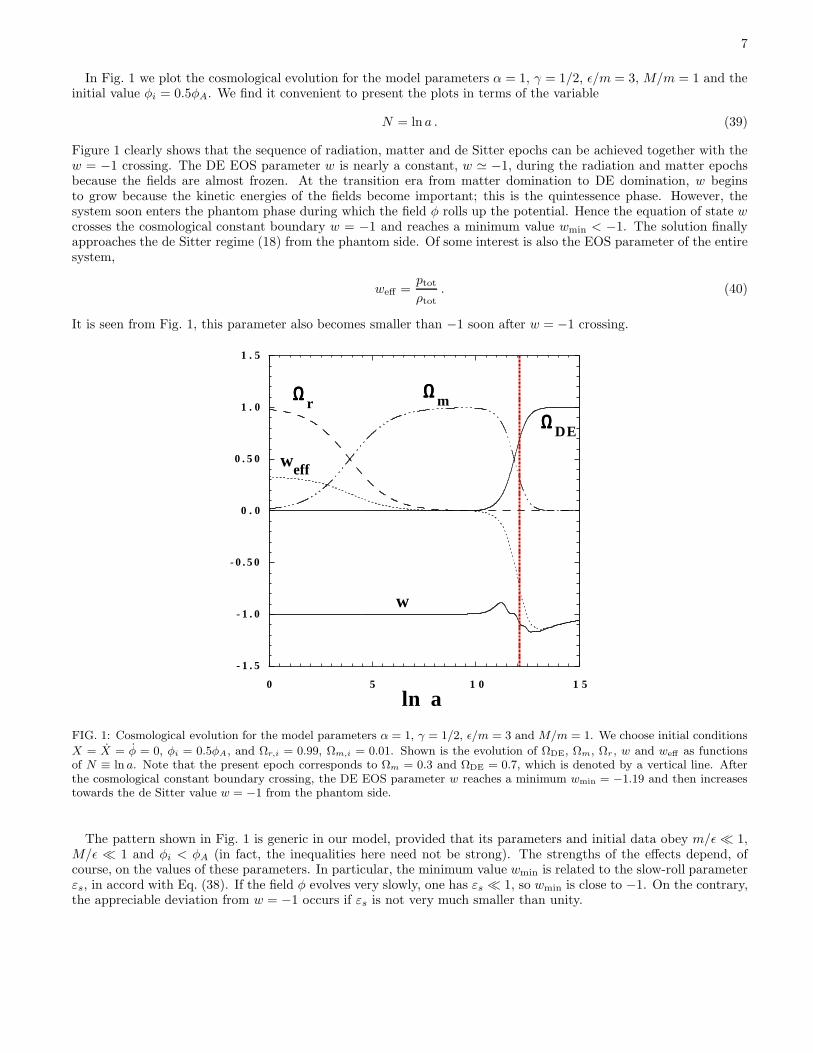
In Fig. 1 we plot the cosmological evolution for the model parameters α = 1, γ = 1/2, ǫ/m = 3, M/m = 1 and theinitial value φi = 0.5φA. We find it convenient to present the plots in terms of the variable

N = ln a . (39)

Figure 1 clearly shows that the sequence of radiation, matter and de Sitter epochs can be achieved together with thew = −1 crossing. The DE EOS parameter w is nearly a constant, w ≃ −1, during the radiation and matter epochsbecause the fields are almost frozen. At the transition era from matter domination to DE domination, w beginsto grow because the kinetic energies of the fields become important; this is the quintessence phase. However, thesystem soon enters the phantom phase during which the field φ rolls up the potential. Hence the equation of state wcrosses the cosmological constant boundary w = −1 and reaches a minimum value wmin < −1. The solution finallyapproaches the de Sitter regime (18) from the phantom side. Of some interest is also the EOS parameter of the entiresystem,

weff =ptot

ρtot. (40)

It is seen from Fig. 1, this parameter also becomes smaller than −1 soon after w = −1 crossing.

- 1 . 5

- 1 . 0

- 0 . 5 0

0 . 0

0 . 5 0

1 . 0

1 . 5

0 5 1 0 1 5

ln a

WDE

WrWm

weff

w

FIG. 1: Cosmological evolution for the model parameters α = 1, γ = 1/2, ǫ/m = 3 and M/m = 1. We choose initial conditions

X = X = φ = 0, φi = 0.5φA, and Ωr,i = 0.99, Ωm,i = 0.01. Shown is the evolution of ΩDE, Ωm, Ωr , w and weff as functionsof N ≡ ln a. Note that the present epoch corresponds to Ωm = 0.3 and ΩDE = 0.7, which is denoted by a vertical line. Afterthe cosmological constant boundary crossing, the DE EOS parameter w reaches a minimum wmin = −1.19 and then increasestowards the de Sitter value w = −1 from the phantom side.

The pattern shown in Fig. 1 is generic in our model, provided that its parameters and initial data obey m/ǫ ≪ 1,M/ǫ ≪ 1 and φi < φA (in fact, the inequalities here need not be strong). The strengths of the effects depend, ofcourse, on the values of these parameters. In particular, the minimum value wmin is related to the slow-roll parameterεs, in accord with Eq. (38). If the field φ evolves very slowly, one has εs ≪ 1, so wmin is close to −1. On the contrary,the appreciable deviation from w = −1 occurs if εs is not very much smaller than unity.

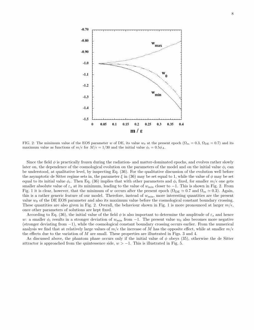
8

FIG. 2: The minimum value of the EOS parameter w of DE, its value w0 at the present epoch (Ωm = 0.3, ΩDE = 0.7) and itsmaximum value as functions of m/ǫ for M/ǫ = 1/30 and the initial value φi = 0.5φA.

Since the field φ is practically frozen during the radiation- and matter-dominated epochs, and evolves rather slowlylater on, the dependence of the cosmological evolution on the parameters of the model and on the initial value φi canbe understood, at qualitative level, by inspecting Eq. (36). For the qualitative discussion of the evolution well beforethe asymptotic de Sitter regime sets in, the parameter ξ in (36) may be set equal to 1, while the value of φ may be setequal to its initial value φi. Then Eq. (36) implies that with other parameters and φi fixed, for smaller m/ǫ one getssmaller absolute value of εs at its minimum, leading to the value of wmin closer to −1. This is shown in Fig. 2. FromFig. 1 it is clear, however, that the minimum of w occurs after the present epoch (ΩDE ≃ 0.7 and Ωm ≃ 0.3). Again,this is a rather generic feature of our model. Therefore, instead of wmin, more interesting quantities are the presentvalue w0 of the DE EOS parameter and also its maximum value before the cosmological constant boundary crossing.These quantities are also given in Fig. 2. Overall, the behaviour shown in Fig. 1 is more pronounced at larger m/ǫ,once other parameters of solutions are kept fixed.

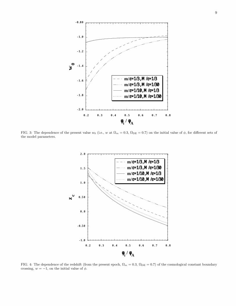
According to Eq. (36), the initial value of the field φ is also important to determine the amplitude of εs and hencew: a smaller φi results in a stronger deviation of wmin from −1. The present value w0 also becomes more negative(stronger deviating from −1), while the cosmological constant boundary crossing occurs earlier. From the numericalanalysis we find that at relatively large values of m/ǫ the increase of M has the opposite effect, while at smaller m/ǫthe effects due to the variation of M are small. These properties are illustrated in Figs. 3 and 4.

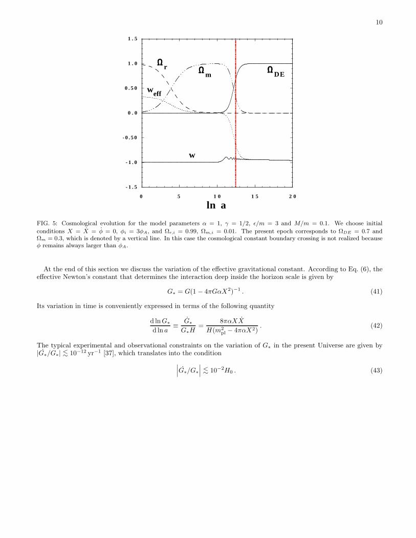
As discussed above, the phantom phase occurs only if the initial value of φ obeys (35), otherwise the de Sitterattractor is approached from the quintessence side, w > −1. This is illustrated in Fig. 5.

9

- 2 . 0

- 1 . 8

- 1 . 6

- 1 . 4

- 1 . 2

- 1 . 0

- 0 . 8 0

0 . 2 0 . 3 0 . 4 0 . 5 0 . 6 0 . 7 0 . 8

m/e=1/3, M/e=1/3

m/e=1/3, M/e=1/30

m/e=1/10, M/e=1/3

m/e=1/10, M/e=1/30

w0

fi / fA

FIG. 3: The dependence of the present value w0 (i.e., w at Ωm = 0.3, ΩDE = 0.7) on the initial value of φ, for different sets ofthe model parameters.

- 1 . 0

- 0 . 5 0

0 . 0

0 . 5 0

1 . 0

1 . 5

2 . 0

0 . 2 0 . 3 0 . 4 0 . 5 0 . 6 0 . 7 0 . 8

m/e=1/3, M/e=1/3

m/e=1/3, M/e=1/30

m/e=1/10, M/e=1/3

m/e=1/10, M/e=1/30

z c

fi / fA

FIG. 4: The dependence of the redshift (from the present epoch, Ωm = 0.3, ΩDE = 0.7) of the cosmological constant boundarycrossing, w = −1, on the initial value of φ.

10

- 1 . 5

- 1 . 0

- 0 . 5 0

0 . 0

0 . 5 0

1 . 0

1 . 5

0 5 1 0 1 5 2 0

ln a

WDEWm

Wr

weff

w

FIG. 5: Cosmological evolution for the model parameters α = 1, γ = 1/2, ǫ/m = 3 and M/m = 0.1. We choose initial

conditions X = X = φ = 0, φi = 3φA, and Ωr,i = 0.99, Ωm,i = 0.01. The present epoch corresponds to ΩDE = 0.7 andΩm = 0.3, which is denoted by a vertical line. In this case the cosmological constant boundary crossing is not realized becauseφ remains always larger than φA.

At the end of this section we discuss the variation of the effective gravitational constant. According to Eq. (6), theeffective Newton’s constant that determines the interaction deep inside the horizon scale is given by

G∗ = G(1 − 4πGαX2)−1 . (41)

Its variation in time is conveniently expressed in terms of the following quantity

d lnG∗

d ln a≡ G∗

G∗H=

8παXX

H(m2pl − 4παX2)

. (42)

The typical experimental and observational constraints on the variation of G∗ in the present Universe are given by|G∗/G∗| <∼ 10−12 yr−1 [37], which translates into the condition

∣

∣

∣G∗/G∗

∣

∣

∣

<∼ 10−2H0 . (43)

11

- 0 . 0 1 0

0 . 0

0 . 0 1 0

0 . 0 2 0

0 . 0 3 0

0 . 0 4 0

0 5 1 0 1 5 2 0

( a )( b )

ln a

.

.

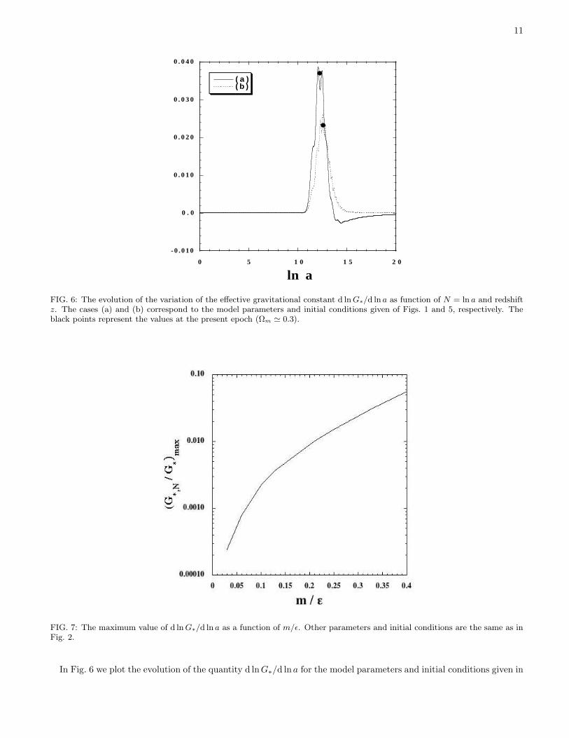
FIG. 6: The evolution of the variation of the effective gravitational constant d ln G∗/d ln a as function of N = ln a and redshiftz. The cases (a) and (b) correspond to the model parameters and initial conditions given of Figs. 1 and 5, respectively. Theblack points represent the values at the present epoch (Ωm ≃ 0.3).

FIG. 7: The maximum value of d ln G∗/d ln a as a function of m/ǫ. Other parameters and initial conditions are the same as inFig. 2.

In Fig. 6 we plot the evolution of the quantity d lnG∗/d lna for the model parameters and initial conditions given in

12

Figs. 1 and 5. At the present epoch (Ωm ≃ 0.3) we obtain the values G∗/G∗ = 3.5× 10−2H−10 and 2.4× 10−2H−1

0 forthese two cases, respectively. Comparing Fig. 6 with Figs. 1 and 5 one observes that the variation of the gravitationalconstant is correlated in time with the deviation of w from −1. This is clear from Eq. (41) too: the gravitationalconstant varies when the field X changes in time, while the latter occurs during the transition from the matterdominated stage to the final de Sitter attractor. It is precisely at this transition stage that w substantially deviatesfrom −1.

Figure 7 shows the maximum value of d lnG∗/d lna as a function of m/ǫ. Again, the variation of the effectiveNewton’s constant is more pronounced at larger m/ǫ. This means that it is correlated with the amplitude of thedeviation of w from −1. The dependence of d lnG∗/d lna on M and on the initial value of φ is rather weak.

It is worth pointing out that as long as the deviation of the EOS from w = −1 is not so significant, the modelssatisfy the constraint (43), and also that our model suggests that the variation of G∗ is close to the present upper

bound on G∗/G∗.

IV. MOMENTUM SCALES OF INSTABILITIES

In this section the momentum scales of instabilities are present in our model. We first study dispersion relations inthe Minkowski space-time and then proceed to those in the FRW space-time. We wish to clarify the conditions underwhich a tachyon or a superluminal mode appears by considering dispersion relations. We also evaluate the energy ofthe modes to find out a ghost state.

A. Minkowski spectrum

Let us consider the perturbations for the fields,

B0 = X + b0 , Bi = bi , Φ = φ + ϕ . (44)

The quadratic Lagrangian for perturbations, following from the general expression (1), is

Lb0,bi,ϕ =γ

2∂µb0∂

µb0 +α

2∂µbi∂

µbi +1

2∂µϕ∂µϕ + ǫ∂0ϕb0 − ǫ∂iϕbi

−1

2m2

0b20 −

1

2m2

1b2i −

1

2m2

ϕϕ2 , (45)

where

m20 = U,XX , m2

1 = −U,X

X, m2

ϕ = W,φφ . (46)

For our model (15) one has −m20 = m2

1 = M2 and m2ϕ = m2. In what follows we concentrate on this case, and assume

the following relations, see (20) and (32),

ǫ ≫ √αm ,

ǫ ≫ M . (47)

Varying the Lagrangian (45) with respect to bi, b0 and ϕ, we obtain the equations for the field perturbations. In

order to find the spectrum of the system we write the solutions in the form b0 = b0eipµx

µ

= b0ei(ωt−p·r), bi = bie

ipµxµ

and ϕ = ϕeipµxµ

. The transverse mode of the vector field Bi has the dispersion relation

ω20 = p2 +

M2

α. (48)

The three scalar modes bi = (pi/p)bL, b0 and ϕ satisfy the following equations

(

ω2 − p2 − M2

α

)

bL + iǫ

αpϕ = 0 , (49)

(

ω2 − p2 +M2

γ

)

b0 − iǫ

γωϕ = 0 , (50)

(

ω2 − p2 − m2)

ϕ − iǫωb0 − iǫpbL = 0 . (51)

13

Expressing bL and b0 in terms of ϕ from Eqs. (49), (50) and plugging them into Eq. (51), we find that the eigenfre-quencies corresponding to three mixed states satisfy

(z − m2)

(

z +M2

γ

) (

z − M2

α

)

− ǫ2z

(

z

γ+

p2

γ+

p2

α− M2

γα

)

= 0 , (52)

where

z ≡ ω2 − p2 . (53)

The spectrum in the case m = 0 was studied in Ref. [33]. Our purpose here is to extend the analysis to the case ofnon-zero m. Denoting the solutions of Eq. (52) as z1, z2 and z3, we obtain the relation

z1z2z3 = −m2M4

αγ. (54)

Once the conditions (47) are satisfied, then one can show that if the relation

z1 < z2 < z3 (55)

holds at some momentum, then the inequality (55) is satisfied for all momenta.In the limits p → ∞ and p → 0, we obtain the following dispersion relations, respectively.

• (A) UV limit (p → ∞)

ω1 = p − ǫ

2

√

1

γ+

1

α+

ǫ2

8p

(

2m2

ǫ2+

1

γ− 1

α

)

+ O(M2/p) , (56)

ω2 = p +m2M4

2p3ǫ2(α + γ)+ O(1/p5) ,

ω3 = p +ǫ

2

√

1

γ+

1

α+

ǫ2

8p

(

2m2

ǫ2+

1

γ− 1

α

)

+ O(M2/p) .

We see that ω1 < ω2 < ω3 and z1 < 0, z2,3 > 0. In all three cases the group velocities ∂ωi/∂p are less than 1,so neither mode is superluminal at high three-momenta, provided that α > γ. The two-derivative terms in theLagrangian (45) dominate in the UV limit, so there are neither ghosts nor tachyons in this limit.

• (B) IR limit (p → 0)

ω1 = −m2M2

ǫ2[

1 + O(m2/ǫ2, M2/ǫ2)]

, (57)

ω2 =M2

α,

ω3 =ǫ2

γ+ m2 + O(M2) .

We see again that ω1 < ω2 < ω3 and z1 < 0, z2,3 > 0. This means that using the property (55) we can identifythe modes: the first one has the behaviour (56) and (57), and so on.

It follows from Eq. (54) that zi never vanish. In fact the coefficients in Eq. (52) are regular at all momenta, so zi

are regular as well. Therefore, zi never change signs and hence z1 < 0, z2,3 > 0 for all momenta. This means, inparticular, that the second and third modes never become tachyonic.

Let us discuss the dangerous mode with the dispersion relation ω = ω1(p) in some detail. The expression for thefields in each mode is

bL,i = −iǫp(

γzi + M2)

· Ci ,

b0,i = iǫω(αzi − M2) · Ci ,

ϕi = (γzi + M2)(αzi − M2) · Ci , (58)

14

where Ci are the normalization factors. Setting ω2 = 0 in Eq. (52), we obtain three critical momenta

p21,2 =

1

2

ǫ2 − M2

α− m2 ±

√

(

ǫ2 − M2

α− m2

)2

− 4m2M2

α

, (59)

p23 =

M2

γ. (60)

Under the conditions (47), the critical momenta p21,2 are approximately given by

p21 ≃ ǫ2 − M2

α− m2 , p2

2 ≃ m2M2

ǫ2, (61)

so that p21 > p2

3 > p22 > 0. The tachyonic mode (ω2

1 < 0) is present for 0 < p2 < p22 and p2

3 < p2 < p21.

In order to find whether there are ghosts we calculate the energy of the modes (58),

Ei(p) = 2ω2|Ci|2[

αǫ2p2(γzi + M2)2 + ǫ2(γp2 − M2)(αzi − M2)2 + (γzi + M2)2(αzi − M2)2]

. (62)

For the modes with ω2,3 we have E2,3(p) > 0. For the mode with ω1 the energy is equal to zero at p = p3 = M/√

γ.

While ω21 > 0 for p2 < p2

3 ≡ M2/γ, the energy E1(p) changes its sign at this momentum. Thus the mode with ω1 is aghost for p2 < M2/γ.

We summarize the properties of the dangerous mode as follows:

• (i) p2 > (ǫ2 − M2)/α − m2: healthy

• (ii) M2/γ < p2 < (ǫ2 − M2)/α − m2: tachyon

• (iii) m2M2/ǫ2 < p2 < M2/γ: ghost, but not tachyon

• (iv) 0 < p2 < m2M2/ǫ2: tachyon.

Unlike the case m = 0 [33] the tachyon is present in the deep IR region (iv).To end up the discussion of the modes in Minkowski space-time, we give the expressions for the minimum values of

ω2 in the tachyonic regions,

• (ii):

ω2min = − γǫ2

4α(α + γ)at p2 =

ǫ2

4α

γ + 2α

γ + α. (63)

• (iv):

ω2min = −m2M2

ǫ2at p2 = 0 .

Note that |ω2min| is relatively large in the region (ii), so this region is the most problematic.

B. Evolution of perturbations in cosmological background

Finally we discuss the evolution of field perturbations in the FRW background (2). In the cosmological contextthe physical momentum p is related to the comoving momentum k as p = k/a. Once the parameters of the modeland initial data are such that the cosmological boundary crossing occurs, the present epoch (ΩDE ≃ 0.7) typicallycorresponds to the phantom region. From Fig. 1 one can see that the Hubble parameter does not change much duringthe transition from the phantom epoch to the final de Sitter era. Hence the present value of the Hubble parameter (H0)

is of the same order as the value H = M/√

3α in the de Sitter asymptotics. This means that the value p3 = M/√

γis of the same order as H0 provided that γ and α are of order unity.

The tachyon appears when the momentum p = k/a of the dangerous mode becomes smaller than√

(ǫ2 − M2)/α − m2 and temporally disappears when the mode crosses the value M/√

γ. Hence this instability

is present for the modes which are inside the Hubble radius and satisfy M/√

γ < p <√

(ǫ2 − M2)/α − m2, but it

15

is absent for the modes deep inside the Hubble radius, satisfying p >√

(ǫ2 − M2)/α − m2. After the Hubble radiuscrossing (k = aH), the tachyonic instability disappears in the momentum region m2M2/ǫ2 < p2 < M2/γ, but thetachyon appears again for p2 < m2M2/ǫ2. Note that the ghost existing at m2M2/ǫ2 < p2 < M2/γ is a not a problembecause of its low energy [13, 40].

In what follows we discuss the evolution of field perturbations in the two tachyonic regimes. Before doing that it isinstructive to study the high-momentum regime that sets the initial data for the tachyonic evolution.

1. p2≫ (ǫ2 − M2)/α − m2

We denote the overall amplitude of the dangerous mode as ϕ. Since the modes are deep inside the Hubble radius(k/a ≫ H) in the regime we discuss here, the field perturbation χ approximately satisfies

d2

dη2χ + k2χ ≃ 0 , (64)

where χ = aϕ and η is conformal time defined by η =∫

a−1dt. Taking the asymptotic Minkowski vacuum state,

χ = e−ikη/√

2k, the squared amplitude of the field perturbation ϕ is given by [41]

Pϕ =4πk3

(2π)3|ϕ|2 =

(

k

2πa

)2

. (65)

Since the maximum momentum at which the tachyon appears is k/a ≃ ǫ/√

α, one has the following estimate for theamplitude of the field perturbation at the beginning of the tachyonic instability,

ϕi ≃ǫ

2π√

α. (66)

As usual, this amplitude characterizes the contribution of a logarithmic interval of momenta into 〈ϕ2(x)〉.

2. M2/γ < p2 < (ǫ2 − M2)/α − m2

This interval of momenta is dangerous, as the perturbations undergo the tachyonic amplification. Since the modesare still inside the Hubble radius, one can neglect the gravitational effects on the “frequency” ω when estimating thegrowth of field perturbations. By the time the tachyonic amplification ends up, the amplitude of field perturbationsis estimated as

ϕ ≃ ϕi exp

(∫ tf

ti

|ω1|dt

)

= ϕi exp

(∫ p3

p1

|ω1|H

dp

p

)

. (67)

Recall that p1 ≃ ǫ/√

α and p3 = M/√

γ. The largest value of |ω21 | is approximately given by (63). Substituting this

value into Eq. (67) and recalling that the background changes slowly (H ≃ const), one finds that the amplitude ofthe field perturbation after exit from the tachyonic regime is of order

ϕ ≃ ǫ

2π√

αexp

[

1

2

√

γ

α(γ + α)

ǫ

Hlog

(√

γ

α

ǫ

M

)]

, (68)

where we used Eq. (66).

Recall now that H is of the same order as M/√

3α during the phantom phase. Hence the large ratio ǫ/M leads toa strong amplification of field perturbations. From (18), the homogeneous field φ at the phantom and de Sitter phase

is estimated as φ ≃√

34π

Hmpl

m . The requirement that the perturbation ϕ is smaller than the background field φ leads

to the constraint

exp

[

1

2

√

γ

α(γ + α)

ǫ

Hlog

(√

γ

α

ǫ

M

)]

<√

3απHmpl

ǫm. (69)

As an example, in the case m = H0 = 10−42 GeV, M =√

3αH0, α = 1 and γ = 1/2, we obtain the constraintǫ/M <∼ 70. As long as α and γ are of order one, the ratio ǫ/M should not be too much larger than unity.

16

3. 0 < p2 < m2M2/ǫ2

After the Hubble radius crossing, the effect of the cosmic expansion can no longer be neglected when estimatingthe “frequencies” of the field perturbations. Since there are no tachyonic instabilities for m2M2/ǫ2 < p2 < M2/γ,we consider the evolution of perturbations in the region 0 < p2 < m2M2/ǫ2. In Ref. [33] the equations for the fieldperturbations were derived in the slow-rolling background under the condition p2 ≪ M2, m2. The equation for theperturbation χ = aϕ is approximately given by

d2

dη2χ +

(

k2 − 1

a

d2a

dη2− a2 m2M2

ǫ2

)

χ = 0 . (70)

Here we neglected the contribution of metric perturbations on the r.h.s. of this equation. Note that metric pertur-bations works as a back reaction effect after the field perturbation is sufficiently amplified. The growth rate of theperturbation χ is mainly determined by the terms in the parenthesis of Eq. (70) rather than the backreaction of metricperturbations.

The last term corresponds to the tachyonic mass term, which already appeared in Minkowski spacetime [see Eq. (57)].Since the term (d2a/dη2)/a is of order a2H2, one can estimate the ratio of the tachyonic mass relative to thisgravitational term:

δ ≡ a2m2M2/ǫ2

(d2a/dη2)/a≃ m2M2

ǫ2H2. (71)

If we use the de Sitter value H = M/√

3α, this ratio is estimated as δ = 3αm2/ǫ2 ≪ 1. Hence the gravitational term(d2a/dη2)/a dominates over the tachyonic mass.

In the de Sitter background with a = −1/(Hη) the approximate solutions to Eq. (70) can be obtained by setting

χ = −(C/H)η−1+δ. One finds that δ = −m2M2/(3H2ǫ2) for the growing solution, thereby giving

ϕ = Cη−m2M2

3H2ǫ2 ∝ aδ/3 . (72)

In Ref. [33] it was shown that the physical temporal component of the vector field perturbations evolves as b0/a ∝ aδ/3,whereas the physical spatial component of the vector field decreases as Bi/a ∝ a−1+δ/3. The growth rate of ϕ andb0/a is small due to the condition δ ≪ 1. So, the second tachyonic instability is harmless for the past and presentcosmological evolution. However, we notice that since the de Sitter solution is a late-time attractor, the perturbationsϕ and b0/a become larger than the homogeneous background fields in the distant future. At this stage we expect thatthe contribution of metric perturbations can be also important.

V. CONCLUSIONS

In this paper we have studied the dynamics of dark energy in a Lorentz-violating model with the action given in(1). The model involves a vector field Bµ and a scalar field Φ with mass terms M and m, respectively. The presenceof the one-derivative term ǫ∂µΦBµ leads to an interesting dynamics at the IR scales larger than ǫ−1. The phantomequation of state can be realized without having ghosts, tachyons or superluminal modes in the UV region.

We have taken into account the contributions of radiation and non-relativistic matter and studied the cosmologicalevolution of the system. Interestingly, there exists a de Sitter attractor solution that can be used for the late-timeacceleration. The phantom regime is not an attractor, but we have found that in a range of parameters, the phantomstage occurs during the transition from the matter epoch to the final de Sitter attractor. As is seen, e.g., in Fig. 1the equation of state parameter w of dark energy crosses the cosmological constant boundary towards the phantomregion. We clarified the conditions under which the w = −1 crossing is realized together with the existence of thestable de Sitter solution.

In the model studied in this paper, the effective Newton’s constant is time-dependent. We have found, however,that this dependence is typically mild, though for interesting values of parameters it is close to the experimentalbounds.

We have also considered the field perturbations in Minkowski spacetime and obtained the momentum scales ofinstabilities present in the IR region (p <∼ ǫ). We have found that either tachyons or ghosts appear for the spatial

momenta p smaller than√

(ǫ2 − M2)/α − m2, while in the UV region there are no unhealthy modes. In the cosmo-logical context the presence of tachyons at the IR scales leads to the amplification of large-scale field perturbationswhose wavelengths are roughly comparable to the present Hubble radius. There are two tachyonic regions of spatial

17

momenta in this model: (a) one is sub-horizon and its momenta are characterized by M2/γ < p2 < (ǫ2−M2)/α−m2;(b) another is super-horizon and has 0 < p2 < m2M2/ǫ2. In the region (a) we derived the condition under which theperturbations always remain smaller than the homogenous fields, see Eq. (69). While the existence of the phantomphase requires that ǫ > M , the condition (69) shows that ǫ cannot be very much larger than M . Thus the allowedrange of ǫ is constrained to be relatively narrow. In the tachyonic region (b) the growth of the perturbations is

estimated as ϕ ∝ aαm2/ǫ2 . Since the growth rate is suppressed by the factor m2/ǫ2, this effect is negligible in the pastand at present, though the inhomogeneities can start to dominate over the homogenous fields in the distant future.

There are several issues yet to be understood. The presence of the tachyonic instability on sub-horizon scales maylead to the variation of the gravitational potential, which can be an additional source of the late-time integratedSaches-Wolfe effect on the CMB power spectrum. Another property of this model is the peculiar time-dependence ofthe effective Newton’s constant, which may result in interesting phenomenology.

The model studied in this paper is likely to belong to a wider class of Lorentz-violating theories exhibiting thephantom behaviour (see Refs. [42] for a number of Lorentz-violating models). It would be interesting to understandhow generic are the features we found in our particular model — late-time de Sitter attractor, transient phantom stage,time-dependent Newton’s constant, sub-horizon tachyons, super-horizon ghosts, etc. One more direction is to modifyour model in such a way that it would be capable of describing inflationary epoch rather than the late-time acceleration.Since it is known that the spectra of scalar and tensor perturbations produced during the phantom inflationary phaseare typically blue-tilted [43], this model may give rise to some distinct features in the CMB spectrum.

ACKNOWLEDGEMENTS

This work is supported by RFBR grant (M. L. and V. R., 05-02-17363-a), grant of the President of Russian Federation(M. L. and V. R., NS-7293.2006.2), INTAS grant (M. L., YSF 04-83-3015), grant of Dynasty Foundation awarded bythe Scientific Board of ICFPM (M. L.), the European Union through the Marie Curie Research and Training NetworkUniverseNet (E. P., MRTN-CT-2006-035863) and JSPS (S. T., No. 30318802).

Appendix A

We are going to find the effective Newton’s constant that determines the strength of gravitational interactions atdistances shorter than all scales present in our model, including ǫ−1, M−1, m−1 as well as the Hubble distance. Tothis end, we neglect the last two terms in the action (1), and also neglect the time dependence of the background fieldsφ and X . We also neglect the space-time curvature of the Universe, and therefore consider our model in Minkowskispace-time.

Let us impose the gauge h0i = 0, where hµν is the metric perturbation about the Minkowski background. Then thequadratic Lagrangian for perturbations of metric, vector and scalar fields is readily calculated,

L =1

2α

[

(

bi +1

2X∂ih00

)2

−(

∂ibj −1

2Xhij

)2]

+1

2γ

[

(

b0 +1

2Xh00

)2

−(

∂ib0 +1

2Xh00

)2]

+1

2

[

ϕ2 − (∂iϕ)2]

. (73)

where X2 = B20 is the background value. Clearly the scalar field ϕ decouples in our approximation, so we will not

consider it in what follows.By varying the quadratic action with respect to h00 and hij , one obtains (00)- and (ij)-components of the linearized

energy-momentum tensor for perturbations (note that T µν = −2δS/δhµν). Specifying further to scalar perturbationswith bi = ∂ibL and choosing conformal Newtonian gauge, h00 = 2Φ, hij = −2Ψδij, one obtains (we keep the standardnotation for the Newtonian potential, even though the same notation was used for the original scalar field in the maintext)

T 00 = αX(X∆Φ − ∆bL) + γX (b0 + XΦ) ,

T ij = αX∂i∂j bL − δijαX2Ψ , (74)

18

where ∆ = ∂i∂i and = ∂20 − ∆. The field equations for b0 and bL in the absence of sources for these fields read

(b0 + XΦ) = 0 ,

− bL + X(Φ − Ψ) = 0 . (75)

Now, the longitudinal (proportional to ∂i∂j) part of the (ij)-component of the Einstein equations, in the absence ofexternal anisotropic stresses, gives

Φ + Ψ = 8πGαXbL , (76)

while the trace part and (00)-component are

Ψ +1

2∆(Φ + Ψ) = −4πGαX2Ψ − 4πGpext , (77)

−∆Ψ = 4πG(αX2∆Φ − αX∆ ˙bL) + 4πGρext , (78)

where ρext and pext are energy density and pressure of an external source.For time-independent, pressureless source it is consistent to take all perturbations independent of time and set

bL = 0. Then one finds, as usual, Ψ = −Φ and obtains the following equation for the Newtonian potential,

(1 − 4πGαX2)∆Φ = 4πGρext . (79)

Thus, the effective Newton’s constant in the background field X is

G∗ = G(1 − 4πGαX2)−1 . (80)

This means that the effective Planck mass entering the Newton’s law is given by (6).

Appendix B

A. Autonomous equations

Let us define the following dimensionless variables which are convenient for studying the dynamical system [6, 38]:

x1 =κ√

γX√6H

, x2 =κφ√6H

, x3 =κmφ√

6H, x4 =

√

4π

3

X

mpl, x5 =

M

H, x6 =

κ√

ρr√3H

. (81)

Then we obtain the following autonomous equations

x′1 = −3x1 −

3α√γ

x4 +ǫ

M

1√γ

x2x5 +1√γ

x4x25 − x1

H ′

H, (82)

x′2 = −3x2 −

ǫ

M

1√γ

x1x5 − 3ǫ

Mx4x5 −

m

Mx3x5 − x2

H ′

H, (83)

x′3 =

m

Mx2x5 − x3

H ′

H, (84)

x′4 =

1√γ

x1 , (85)

x′5 = −x5

H ′

H, (86)

x′6 = −2x6 − x6

H ′

H, (87)

and

H ′

H= −3

2

1 + x21 + x2

2 − x23 + x2

4(3α + x25) + x2

6/3 + 2(ǫ/M)x2x4x5 + 4(α/√

γ)x1x4

1 + 3αx24

,

19

where prime denotes the derivative with respect to

N ≡ ln(a) .

Equation (11) gives the constraint

Ωm ≡ κ2ρm

3H2= 1 − x2

1 − x22 − x2

3 + x24

(

3α + x25

)

− x26 . (88)

Note that the above equations are invariant under the simultaneous change of the signs of φ and X . Hence it is notrestrictive to study the case of positive φ. Note also that we study the case of an expanding Universe with H > 0.

B. Fixed points

By setting x′i = 0 one formally finds the following six fixed points:

• (A) de Sitter (i): (x1, x2, x3, x4, x5, x6) =

(

0, 0, ǫm

√

33ǫ2/m2−2α ,− 1√

3(3ǫ2/m2−2α),√

3α, 0

)

,

• (B) de Sitter (ii): (x1, x2, x3, x4, x5, x6) = (0, 0, const, 0, 0, 0) ,

• (C) matter: (x1, x2, x3, x4, x5, x6) = (0, 0, 0, 0, 0, 0) ,

• (D) radiation: (x1, x2, x3, x4, x5, x6) = (0, 0, 0, 0, 0, 1) ,

• (E1) kinetic point (i): (x1, x2, x3, x4, x5, x6) = (0, 1, 0, 0, 0, 0) ,

• (E2) kinetic point (ii): (x1, x2, x3, x4, x5, x6) = (0,−1, 0, 0, 0, 0) .

The fixed point (A) is precisely the de Sitter solution (18) that we discussed in Sec. III A. We will comment on itsstability shortly.

The point (B) is also in some sense a de Sitter point. It exists even in the absence of the field X and satisfiesthe relation 3H2 = κ2W (φ). To reach the solution (B), the Hubble parameter needs to increase towards infinity(M/H → 0), and the field φ needs to diverge as well.

The point (C) corresponds to matter-dominated era satisfying Ωm = 1 and weff = 0, whereas the point (D) describesradiation-dominated epoch with Ωr = 1 and weff = 1/3.

The points (E1) and (E2) are kinetic solutions satisfying ΩDE = 1 and weff = 1. These solutions are used neitherfor dark energy nor for radiation/matter dominated epochs.

A cosmologically viable trajectory starts from the radiation point (D), connects to the matter solution (C) andfinally approaches the de Sitter point (A). [Note that the initial data (22) indeed correspond to x1, x2, x3, x4, x5 → 0as t → 0.] To see that this sequence of events is indeed possible, let us study the stability of the fixed points againstperturbations.

Let us consider linear perturbations δxi. By perturbing Eqs. (82)-(86) we obtain

δx′1 =

(

−3 − H ′

H− c1x1

)

δx1 +

(

ǫ

M

1√γ

x5 − c2x1

)

δx2 − c3x1δx3

+

(

1√γ

x25 −

3α√γ− c4x1

)

δx4 +

(

ǫ

M

1√γ

x2 +2√γ

x4x5 − c5x1

)

δx5 − c6x1δx6 , (89)

δx′2 = −

(

ǫ

M

1√γ

x5 + c1x2

)

δx1 −(

3 + c2x2 +H ′

H

)

δx2 −( m

Mx5 + c3x2

)

δx3

−(

3ǫ

Mx5 + c4x2

)

δx4 −(

ǫ

M

1√γ

x1 + 3ǫ

Mx4 +

m

Mx3 + c5x2

)

δx5 − c6x2δx6 , (90)

δx′3 = −c1x3δx1 +

( m

Mx5 − c2x3

)

δx2 − c3x3δx3 − c4x3δx4 +( m

Mx2 − c5x3

)

δx5 − c6x3δx6 , (91)

δx′4 =

1√γ

δx1 , (92)

δx′5 = −c1x5δx1 − c2x5δx2 − c3x5δx3 − c4x5δx4 −

(

H ′

H+ c5x5

)

δx5 − c6x5δx6 , (93)

δx′6 = −c1x6δx1 − c2x6δx2 − c3x6δx3 − c4x6δx4 − c5x6δx5 −

(

2 +H ′

H+ c6x6

)

δx6 , (94)

20

where δ(H ′/H) =∑6

i=1 ciδxi with

c1 = −3x1 + 6(α/√

γ)x4

1 + 3αx24

x4 , c2 = −3x2 + 3(ǫ/M)x4x5

1 + 3αx24

, c3 =3x3

1 + 3αx24

,

c4 = −3x4(3α + x25) + 3(ǫ/M)x2x5 + 6(α/

√γ)x1

1 + 3αx24

− 6αx4

1 + 3αx24

H ′

H,

c5 = −3x24x5 + 3(ǫ/M)x2x4

1 + 3αx24

, c6 = − x6

1 + 3αx24

. (95)

The stability of fixed points can be analyzed by considering eigenvalues of the 6 × 6 matrix M for perturbationsalong the lines of Ref. [6, 38].

The stability of the de Sitter point (A) is important for having the late-time accelerated epoch. This depends uponthe two ratios ǫ/m and M/m once the parameters α and γ are fixed. When α = 1 and γ = 1/2, for example, theparameter range of ǫ/m is determined by the ratio M/m. We find that the point (A) is a stable attractor if thefollowing conditions hold:

• (i) When M/m = 0.1, ǫ/m > 0.817,

• (ii) When M/m = 1, ǫ/m > 1.35,

• (iii) When M/m = 10, ǫ/m > 3.52,

When ǫ ≫ m, the stability of the point (A) is ensured automatically unless the ratio M/m is too much larger thanunity. In view of (20) the case ǫ ≫ m is of particular interest.

For another de Sitter point (B), the eigenvalues are

− 3,−3,−3

2± 1

2

√

9 − 12α

γ, 0,−1/2 , (96)

This means that this point is marginally stable. The zero eigenvalue comes from the perturbation equation for δx5.If H continues to increase toward the solution (B), this eigenvalue actually obtains a small negative value, as can beseen from Eq. (93). Thus in such a case the point (B) is stable. However, we know that the phantom phase is realizedonly for finite field values bounded by φA, see Eq. (34). Hence it is not possible that the actual solutions approachthe point (B) with infinite H and φ.

The matter point (C) has the eigenvalues

3/2,−3/2,−4

3±

√

9 − 48α

γ, 0,−1/2 , (97)

which shows that the matter era corresponds to a saddle point with one positive eigenvalue. Hence the solutionseventually repel away from this fixed point even if they temporarily approach it.

The radiation point (D) has the eigenvalues

− 1

2± 1

2

√

1 − 12α

γ,−1, 0, 2, 1 . (98)

One finds that the radiation epoch corresponds to a saddle point with two positive eigenvalues.The kinetic points (E1) and (E2) have the eigenvalues

3, 3, 1, 0,

√

3α

γi,−

√

3α

γi , (99)

which shows that they are unstable.The above stability analysis shows that the sequence of radiation, matter and de Sitter epochs can indeed be

realized.

[1] A. G. Riess et al., Astron. J. 116, 1009 (1998); Astron. J. 117, 707 (1999); S. Perlmutter et al., Astrophys. J. 517, 565(1999); P. Astier et al., Astron. Astrophys. 447, 31 (2006); W. M. Wood-Vasey et al., arXiv:astro-ph/0701041.

21

[2] D. N. Spergel et al. [WMAP Collaboration], Astrophys. J. Suppl. 148, 175 (2003); D. N. Spergel et al.,arXiv:astro-ph/0603449.

[3] U. Seljak et al. [SDSS Collaboration], Phys. Rev. D 71, 103515 (2005); M. Tegmark et al., Phys. Rev. D 74, 123507 (2006).[4] D. J. Eisenstein et al. [SDSS Collaboration], Astrophys. J. 633, 560 (2005).[5] V. Sahni and A. A. Starobinsky, Int. J. Mod. Phys. D 9, 373 (2000); V. Sahni, Lect. Notes Phys. 653, 141 (2004)

[arXiv:astro-ph/0403324]; S. M. Carroll, Living Rev. Rel. 4, 1 (2001); T. Padmanabhan, Phys. Rept. 380, 235 (2003);P. J. E. Peebles and B. Ratra, Rev. Mod. Phys. 75, 559 (2003); V. Sahni and A. Starobinsky, Int. J. Mod. Phys. D 15

2105 (2006); S. Nojiri and S. D. Odintsov, Int. J. Geom. Meth. Mod. Phys. 4, 115 (2007).[6] E. J. Copeland, M. Sami and S. Tsujikawa, Int. J. Mod. Phys. D 15, 1753 (2006).[7] A. Melchiorri, L. Mersini-Houghton, C. J. Odman and M. Trodden, Phys. Rev. D 68, 043509 (2003); J. Weller and

A. M. Lewis, Mon. Not. Roy. Astron. Soc. 346, 987 (2003); B. A. Bassett, P. S. Corasaniti and M. Kunz, Astrophys. J.617, L1 (2004); U. Seljak, A. Slosar and P. McDonald, JCAP 0610, 014 (2006).

[8] U. Alam, V. Sahni, T. D. Saini and A. A. Starobinsky, Mon. Not. Roy. Astron. Soc. 354, 275 (2004); R. Lazkoz, S. Nesserisand L. Perivolaropoulos, JCAP 0511, 010 (2005); J. Q. Xia, G. B. Zhao, B. Feng, H. Li and X. Zhang, Phys. Rev. D 73,063521 (2006); S. Nesseris and L. Perivolaropoulos, JCAP 0701, 018 (2007); U. Alam, V. Sahni and A. A. Starobinsky,JCAP 0702, 011 (2007); G. B. Zhao, J. Q. Xia, B. Feng and X. Zhang, arXiv:astro-ph/0603621.

[9] R. R. Caldwell, Phys. Lett. B 545, 23 (2002); R. R. Caldwell, M. Kamionkowski and N. N. Weinberg, Phys. Rev. Lett.91, 071301 (2003).

[10] S. M. Carroll, M. Hoffman and M. Trodden, Phys. Rev. D 68, 023509 (2003).[11] P. Singh, M. Sami and N. Dadhich, Phys. Rev. D 68 023522 (2003); S. Nojiri and S. D. Odintsov, Phys. Lett. B 562,

147 (2003); Phys. Lett. B 565, 1 (2003); J. G. Hao and X. Z. Li, Phys. Rev. D 67, 107303 (2003); P. F. Gonzalez-Diaz,Phys. Rev. D 68, 021303 (2003); L. P. Chimento and R. Lazkoz, Phys. Rev. Lett. 91, 211301 (2003); M. P. Dabrowski,T. Stachowiak and M. Szydlowski, Phys. Rev. D 68, 103519 (2003); L. P. Chimento and R. Lazkoz, Phys. Rev. Lett.91, 211301 (2003); S. Tsujikawa, Class. Quant. Grav. 20, 1991 (2003); M. Sami and A. Toporensky, Mod. Phys. Lett.A 19, 1509 (2004); E. Elizalde, S. Nojiri and S. D. Odintsov, Phys. Rev. D 70, 043539 (2004); H. Stefancic, Phys. Lett.B 586, 5 (2004); V. B. Johri, Phys. Rev. D 70, 041303 (2004); Z. K. Guo, Y. S. Piao and Y. Z. Zhang, Phys. Lett.B 594, 247 (2004); J. M. Aguirregabiria, L. P. Chimento and R. Lazkoz, Phys. Rev. D 70, 023509 (2004); S. Nojiri,S. D. Odintsov and S. Tsujikawa, Phys. Rev. D 71, 063004 (2005); S. Nojiri and S. D. Odintsov, Phys. Rev. D 72, 023003(2005); L. Perivolaropoulos, Phys. Rev. D 71, 063503 (2005); T. Chiba, JCAP 0503, 008 (2005); M. Bouhmadi-Lopez andJ. A. Jimenez Madrid, JCAP 0505, 005 (2005); V. Faraoni, Class. Quant. Grav. 22, 3235 (2005); L. P. Chimento, Phys.Lett. B 633, 9 (2006); L. P. Chimento and D. Pavon, Phys. Rev. D 73, 063511 (2006); O. Hrycyna and M. Szydlowski,arXiv:0704.1651 [hep-th].

[12] A. Vikman, Phys. Rev. D 71, 023515 (2005); Z. K. Guo, Y. S. Piao, X. M. Zhang and Y. Z. Zhang, Phys. Lett. B 608, 177(2005); W. Hu, Phys. Rev. D 71, 047301 (2005); R. R. Caldwell and M. Doran, Phys. Rev. D 72, 043527 (2005); H. Wei,R. G. Cai and D. F. Zeng, Class. Quant. Grav. 22, 3189 (2005); G. B. Zhao, J. Q. Xia, M. Li, B. Feng and X. Zhang, Phys.Rev. D 72, 123515 (2005); S. Tsujikawa, Phys. Rev. D 72, 083512 (2005); I. Y. Aref’eva, A. S. Koshelev and S. Y. Vernov,Phys. Rev. D 72, 064017 (2005); B. McInnes, Nucl. Phys. B 718, 55 (2005); L. P. Chimento, R. Lazkoz, R. Maartensand I. Quiros, JCAP 0609, 004 (2006); R. Lazkoz and G. Leon, Phys. Lett. B 638, 303 (2006); X. F. Zhang and T. Qiu,Phys. Lett. B 642, 187 (2006); W. Zhao, Phys. Rev. D 73, 123509 (2006); H. Mohseni Sadjadi and M. Alimohammadi,Phys. Rev. D 74, 043506 (2006); Z. K. Guo, Y. S. Piao, X. Zhang and Y. Z. Zhang, Phys. Rev. D 74, 127304 (2006);I. Y. Aref’eva and A. S. Koshelev, JHEP 0702, 041 (2007); Y. f. Cai, M. z. Li, J. X. Lu, Y. S. Piao, T. t. Qiu andX. m. Zhang, arXiv:hep-th/0701016; Y. F. Cai, T. Qiu, Y. S. Piao, M. Li and X. Zhang, arXiv:0704.1090 [gr-qc].

[13] J. M. Cline, S. Jeon and G. D. Moore, Phys. Rev. D 70, 043543 (2004).[14] N. Arkani-Hamed, H. C. Cheng, M. A. Luty and S. Mukohyama, JHEP 0405, 074 (2004).[15] F. Piazza and S. Tsujikawa, JCAP 0407, 004 (2004).[16] R. V. Buniy and S. D. H. Hsu, Phys. Lett. B 632, 543 (2006).[17] S. Dubovsky, T. Gregoire, A. Nicolis and R. Rattazzi, JHEP 0603, 025 (2006).[18] J. P. Uzan, Phys. Rev. D 59, 123510 (1999); L. Amendola, Phys. Rev. D 60, 043501 (1999); T. Chiba, Phys. Rev. D 60,

083508 (1999); N. Bartolo and M. Pietroni, Phys. Rev. D 61, 023518 (2000); F. Perrotta, C. Baccigalupi and S. Matarrese,Phys. Rev. D 61, 023507 (2000); A. Riazuelo and J. P. Uzan, Phys. Rev. D 66, 023525 (2002); D. F. Torres, Phys. Rev.D 66, 043522 (2002); L. Perivolaropoulos, JCAP 0510, 001 (2005); M. X. Luo and Q. P. Su, Phys. Lett. B 626, 7 (2005);J. Martin, C. Schimd and J. P. Uzan, Phys. Rev. Lett. 96, 061303 (2006).

[19] B. Boisseau, G. Esposito-Farese, D. Polarski and A. A. Starobinsky, Phys. Rev. Lett. 85, 2236 (2000).[20] R. Gannouji, D. Polarski, A. Ranquet and A. A. Starobinsky, JCAP 0609, 016 (2006).[21] S. Capozziello, V. F. Cardone, S. Carloni and A. Troisi, Int. J. Mod. Phys. D 12, 1969 (2003); S. M. Carroll, V. Duvvuri,

M. Trodden and M. S. Turner, Phys. Rev. D 70, 043528 (2004).[22] S. Nojiri, S. D. Odintsov and M. Sasaki, Phys. Rev. D 71, 123509 (2005); M. Sami, A. Toporensky, P. V. Tretjakov and

S. Tsujikawa, Phys. Lett. B 619, 193 (2005); G. Calcagni, S. Tsujikawa and M. Sami, Class. Quant. Grav. 22, 3977 (2005);B. M. N. Carter and I. P. Neupane, JCAP 0606, 004 (2006).

[23] L. Amendola, R. Gannouji, D. Polarski and S. Tsujikawa, Phys. Rev. D 75, 083504 (2007). See also L. Amendola, D. Polarskiand S. Tsujikawa, Phys. Rev. Lett. 98, 131302 (2007); arXiv:astro-ph/0605384.

[24] T. Koivisto and D. F. Mota, Phys. Lett. B 644, 104 (2007); S. Tsujikawa and M. Sami, JCAP 0701, 006 (2007); T. Koivistoand D. F. Mota, Phys. Rev. D 75, 023518 (2007); B. M. Leith and I. P. Neupane, arXiv:hep-th/0702002.

[25] L. Amendola, C. Charmousis and S. C. Davis, JCAP 0612, 020 (2006).

22

[26] A. De Felice, M. Hindmarsh and M. Trodden, JCAP 0608, 005 (2006); G. Calcagni, B. de Carlos and A. De Felice, Nucl.Phys. B 752, 404 (2006); Z. K. Guo, N. Ohta and S. Tsujikawa, Phys. Rev. D 75, 023520 (2007).

[27] G. R. Dvali, G. Gabadadze and M. Porrati, Phys. Lett. B 485, 208 (2000).[28] G. Kofinas, R. Maartens and E. Papantonopoulos, JHEP 0310 (2003) 066 [arXiv:hep-th/0307138].[29] V. Sahni and Y. Shtanov, JCAP 0311, 014 (2003).[30] A. Lue and G. D. Starkman, Phys. Rev. D 70, 101501 (2004).[31] D. Gorbunov, K. Koyama and S. Sibiryakov, Phys. Rev. D 73, 044016 (2006).[32] L. Senatore, Phys. Rev. D 71, 043512 (2005); P. Creminelli, M. A. Luty, A. Nicolis and L. Senatore, JHEP 0612, 080

(2006).[33] V. A. Rubakov, Theor. Math. Phys. 149, 1651 (2006) [arXiv:hep-th/0604153].[34] B. M. Gripaios, JHEP 0410, 069 (2004).[35] M. V. Libanov and V. A. Rubakov, JHEP 0508, 001 (2005).[36] S. M. Carroll and E. A. Lim, Phys. Rev. D 70, 123525 (2004).[37] J. P. Uzan, Rev. Mod. Phys. 75, 403 (2003).[38] E. J. Copeland, A. R. Liddle and D. Wands, Phys. Rev. D 57, 4686 (1998).[39] B. Gumjudpai, T. Naskar, M. Sami and S. Tsujikawa, JCAP 0506, 007 (2005).[40] S. L. Dubovsky, JHEP 0410, 076 (2004).[41] B. A. Bassett, S. Tsujikawa and D. Wands, Rev. Mod. Phys. 78, 537 (2006).[42] J. M. Cline and L. Valcarcel, JHEP 0403, 032 (2004); N. Arkani-Hamed, H. C. Cheng, M. Luty and J. Thaler, JHEP 0507,

029 (2005); M. V. Libanov and V. A. Rubakov, JCAP 0509, 005 (2005); Phys. Rev. D 72, 123503 (2005); S. M. Carrolland J. Shu, Phys. Rev. D 73, 103515 (2006); H. C. Cheng, M. A. Luty, S. Mukohyama and J. Thaler, JHEP 0605, 076(2006); S. Kanno and J. Soda, Phys. Rev. D 74, 063505 (2006); P. G. Ferreira, B. M. Gripaios, R. Saffari and T. G. Zlosnik,Phys. Rev. D 75, 044014 (2007).

[43] M. Baldi, F. Finelli and S. Matarrese, Phys. Rev. D 72, 083504 (2005).