LOW-LEVEL ATMOSPHERIC JETS AND INVERSIONS OVER THEWESTERN WEDDELL SEA ?

EDGAR L ANDREAS1, KERRY J. CLAFFEY1 and ALEKSANDR P. MAKSHTAS21U.S. Army Cold Regions Research and Engineering Laboratory, 72 Lyme Road, Hanover, New

Hampshire 03755-1290, U.S.A.;2International Arctic Research Center, 930 Koyukuk Drive,Fairbanks, Alaska 99775-7335, U.S.A.

(Received in final form 26 April 2000)

Abstract. For four months in the fall and early winter of 1992, as Ice Station Weddell (ISW)drifted northward through the ice-covered western Weddell Sea, ice station personnel profiled theatmospheric boundary layer (ABL) with radiosondes. These showed that the ABL was virtuallyalways stably stratified during this season: 96% of the soundings found a near-surface inversionlayer. Forty-four percent of these inversions were surface-based. Eighty percent of the soundings thatyielded unambiguous wind profiles showed an atmospheric jet with speeds as high as 14 m s−1 in acore below an altitude of 425 m. This paper documents the features of these inversions and low-leveljets. Because the inversion statistics, in particular, are like those reported in and around the ArcticOcean, similar local processes seem to control the ABL over sea ice regions in both hemispheres.A simple two-layer model, in which an elevated layer becomes frictionally decoupled from thesurface, does well in explaining the ISW jet statistics. This model also implies a new geostrophicdrag parameterization for sea-ice regions that depends on the magnitude of the geostrophic wind, the10-m drag coefficient CDN10, and the ABL height, but not explicitly on any stratification parameter.

Keywords: Geostrophic drag relation, Inertial oscillations, Inversions, Low-level jet, Stable bound-ary layer, Weddell Sea.

1. Introduction

The theme that the polar regions are ideal ‘laboratories’ for studying atmosphericprocesses is a recurring one in the meteorological literature (e.g., Lettau, 1971;Smith et al., 1983; Andreas and Cash, 1999). We reiterate that theme here anddemonstrate it with a study of the stable atmospheric boundary layer (ABL) at IceStation Weddell (ISW).

Our understanding of the stable boundary layer (SBL) lags that of the convectiveboundary layer (CBL) because, in temperate latitudes, the SBL is generally onlya nighttime phenomenon. Since the SBL takes longer to develop than the CBL(Nieuwstadt and Duynkerke, 1996), it frequently does not reach steady state bysunrise in mid-latitudes; its characteristics are, thus, difficult to quantify. In the po-lar regions, on the other hand, the low sun angle, the highly reflective and emissive

? The U.S. government right to retain a non-exclusive royalty-free license in and to any copyrightis acknowledged.

Boundary-Layer Meteorology97: 459–486, 2000.© 2000Kluwer Academic Publishers. Printed in the Netherlands.

460 EDGAR L ANDREAS ET AL.

snow surface, and the long polar nights combine to produce frequent and long-lasting SBLs. During our 4-month deployment on ISW, for example, virtually allof our radiosoundings showed a stably stratified ABL. In other words, we foundnearly ideal conditions for an SBL experiment.

Here we report on two features of the SBL over sea-ice that our radiosound-ing program on Ice Station Weddell revealed: low-level atmospheric jets andinversions. Over 96% of our 164 radiosoundings on ISW showed a low-level tem-perature inversion with its top below 600 m. And 80% of the soundings for whichwe measured the wind vector as well as temperature showed an atmospheric jetwith its core below 425 m. Andreas et al. (1993, 1995), Claffey et al. (1994), andMakshtas et al. (1998) made preliminary reports on these jets and inversions. Herewe document details of both the inversions and jets and describe a simple modelof inertial oscillations in a layer decoupled from the surface by stable stratificationthat explains the jet observations. This model also implies a new formulation forthe geostrophic drag relation over sea-ice.

2. Measurements

Ice Station Weddell drifted through the western Weddell Sea for four months inthe austral fall and winter of 1992 (Figure 1), basically following the course ofthe legendaryEndurance(Anonymous, 1992; ISW Group, 1993). The RussianicebreakerAkademik Fedorovdeployed the ice camp in early February near 51◦ W,71◦ S; theFedorovand the U.S. icebreakerNathaniel B. Palmerretrieved the campin early June near 53◦ W, 66◦ S.

On ISW we launched radiosondes twice a day, at 0000 UT and 1200 UT, toinvestigate the structure of the ABL. Claffey et al. (1994) reported the details ofour radiosounding program. That report includes a list of all the ISW soundingsand also the soundings made on theFedorov in late May and early June as itapproached the camp from the northeast, tabulates some of the statistics we reporthere, and plots all the ISW andFedorovsoundings. In addition, electronic files ofthese soundings are available from us and from the CRREL library.

We used two types of radiosondes on ISW: tethersondes and airsondes (bothmade by Atmospheric Instrumentation Research, Boulder, Colorado). The tether-sonde was our preferred sounding system because, besides pressure, temperature,and humidity, it also measured wind speed with a cup anemometer and wind dir-ection using the aerodynamically shaped balloon as a vane. But for surface windsabove 5–7 m s−1, it was hazardous to launch the tethersonde. In these cases, wemade the scheduled sounding with a disposable airsonde, which measured onlypressure, temperature, and humidity.

The tethersonde was tethered to a winch. We raised the balloon and sonde ata rate of 1–2 m s−1. The tethersonde had a 10-s sampling interval and, thus, gaveus excellent vertical resolution of 10–20 m. The airsondes generally ascended at

LOW-LEVEL ATMOSPHERIC JETS AND INVERSIONS 461

Figure 1.The drift track of Ice Station Weddell, showing station highlights and the duration of ourradiosounding program. The numbers indicate the Julian day in 1992.

462 EDGAR L ANDREAS ET AL.

about 5 m s−1. Because this system had a sampling rate of 5 s, it also provided arespectable vertical resolution of 20–25 m.

TheFedorovused a Vaisala MicroCORA for 40 6-hourly soundings in late Mayand early June that were coordinated with soundings at the ice camp. This systemmeasured pressure, temperature, and humidity as well as wind speed and directionusing the Omega navigational aid signals (e.g., Andreas and Richter, 1982). TheMicroCORA had a 10-s sampling interval, and the balloon typically ascendedat 5 m s−1; thus, pressure, temperature, and humidity have a resolution of about50 m. But the system needed several Omega fixes on the radiosonde to computewind speed and direction. Consequently, the MicroCORA profiles have a verticalresolution that is generally no better than 100 m for wind data.

Because of this coarser resolution of the MicroCORA data, we could not com-pare ice camp andFedorovsoundings in detail. Claffey et al. (1994) and Makshtaset al. (1998) described our attempts at such comparisons and showed that grossdetails, such as the frequency of inversions, the temperature of the inversion base,and the temperature difference through the inversion, were comparable at theFe-dorov and at the ice camp, despite separations up to several hundred kilometres.We infer from these comparisons that the bulk thermal structure of the ABL overthe ice-covered Weddell Sea did not have large horizontal variations. But the Mi-croCORA simply did not have the vertical resolution to provide the details of thejets and inversions that we see in the ice camp soundings. Hence, we will discusstheFedorovsoundings no further.

On ISW we made 164 soundings between 21 February and 4 June 1992; 129were made with the tethersonde and, thus, include profiles of wind speed anddirection as well as pressure, temperature, and humidity. Because we tended tolaunch an airsonde rather than the tethersonde when the surface wind was above5–7 m s−1, the statistics we report for the low-level jets might be somewhat biased.According to the definition that we will present shortly, jets are more probablewhen the surface wind is light. Thus, since about 80% (= 129/164) of our soundingswere made with the tethersonde, our statistics could be biased by 20%. High winds,however, did not necessitate all of the 35 airsonde ascents (i.e., 164 – 129). Thetethersonde experienced some losses and equipment failures that grounded it whenwind conditions were otherwise acceptable for launching; Claffey et al. (1994)described these equipment problems.

To further investigate any possible sampling bias, from the standard meteorolo-gical observations on ISW (e.g., Andreas and Claffey, 1995), we (Makshtas et al.,1998) created a subset of wind speed observations made at 0000 UT and 1200 UTfor the duration of the drift. From this set, we created another subset of the 0000-UT and 1200-UT wind speeds measured only during tethersonde launches. Bothwind speed sets followed a Rayleigh distribution with standard deviations of 3.88and 3.27 m s−1, respectively. Using Pearson’sχ2 test, we found that the two subsetscame from the same population with 95% probability or better. Consequently, at

LOW-LEVEL ATMOSPHERIC JETS AND INVERSIONS 463

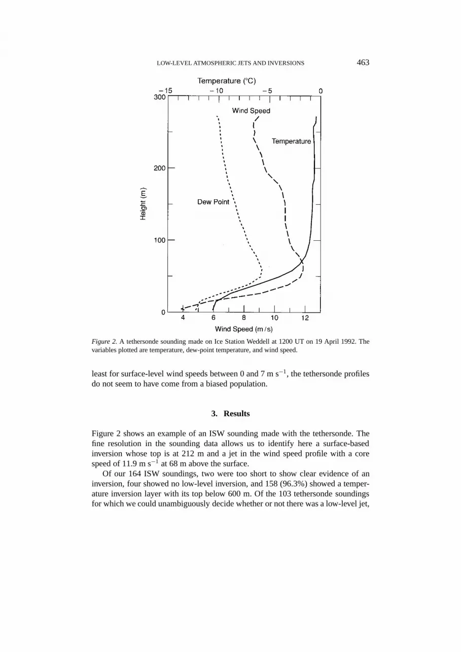
Figure 2.A tethersonde sounding made on Ice Station Weddell at 1200 UT on 19 April 1992. Thevariables plotted are temperature, dew-point temperature, and wind speed.

least for surface-level wind speeds between 0 and 7 m s−1, the tethersonde profilesdo not seem to have come from a biased population.

3. Results

Figure 2 shows an example of an ISW sounding made with the tethersonde. Thefine resolution in the sounding data allows us to identify here a surface-basedinversion whose top is at 212 m and a jet in the wind speed profile with a corespeed of 11.9 m s−1 at 68 m above the surface.

Of our 164 ISW soundings, two were too short to show clear evidence of aninversion, four showed no low-level inversion, and 158 (96.3%) showed a temper-ature inversion layer with its top below 600 m. Of the 103 tethersonde soundingsfor which we could unambiguously decide whether or not there was a low-level jet,

464 EDGAR L ANDREAS ET AL.

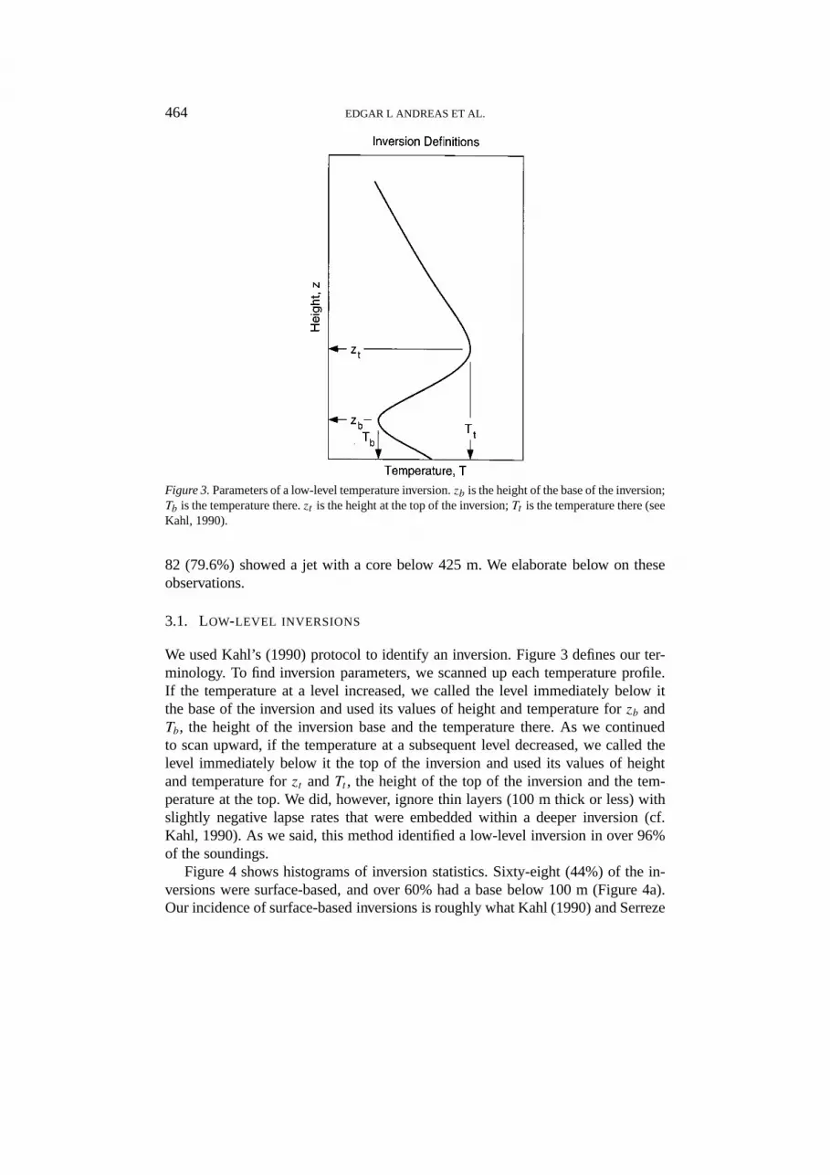
Figure 3.Parameters of a low-level temperature inversion.zb is the height of the base of the inversion;Tb is the temperature there.zt is the height at the top of the inversion;Tt is the temperature there (seeKahl, 1990).

82 (79.6%) showed a jet with a core below 425 m. We elaborate below on theseobservations.

3.1. LOW-LEVEL INVERSIONS

We used Kahl’s (1990) protocol to identify an inversion. Figure 3 defines our ter-minology. To find inversion parameters, we scanned up each temperature profile.If the temperature at a level increased, we called the level immediately below itthe base of the inversion and used its values of height and temperature forzb andTb, the height of the inversion base and the temperature there. As we continuedto scan upward, if the temperature at a subsequent level decreased, we called thelevel immediately below it the top of the inversion and used its values of heightand temperature forzt andTt , the height of the top of the inversion and the tem-perature at the top. We did, however, ignore thin layers (100 m thick or less) withslightly negative lapse rates that were embedded within a deeper inversion (cf.Kahl, 1990). As we said, this method identified a low-level inversion in over 96%of the soundings.

Figure 4 shows histograms of inversion statistics. Sixty-eight (44%) of the in-versions were surface-based, and over 60% had a base below 100 m (Figure 4a).Our incidence of surface-based inversions is roughly what Kahl (1990) and Serreze

LOW-LEVEL ATMOSPHERIC JETS AND INVERSIONS 465

et al. (1992) reported for coastal and sea-ice sites in the Arctic Ocean. Since ourobservations were in autumn and early winter, the temperature at the inversion basewas always less than 0◦C (Figure 4b).

Figures 4c and 4d show the depth of the inversion,zt − zb, and the temperaturechange through the inversion,Tt − Tb. Although we could identify an inversionand, thus, the inversion base in 158 soundings, many of our soundings did notreach high enough to show the top of the inversion. As a result, Figures 4c and 4ddo not contain 158 observations.

Figure 4c shows that the inversions were fairly thin; most were thinner than550 m. Kahl (1990) and Serreze et al. (1992) reported thicker inversion layers infall and winter over Arctic sea-ice and at Arctic coastal sites. Because of the finervertical resolution of our sondes, we put more faith in the ISW inversion statistics.The radiosoundings on which Kahl and Serreze et al. based their analyses hadcoarser vertical resolution because of sensor response time, balloon ascent rate,and sampling interval, as discussed by Skony et al. (1994), Walden et al. (1996),and Mahesh et al. (1997).

The temperature change through the inversion (Figure 4d) can be quite dra-matic, up to 20◦C. Usually, though, that temperature change is more modest, 5 to10 ◦C. Figure 4d agrees fairly well with Kahl’s (1990) analysis based on autumnand winter observations at Barrow and Barter Island, Alaska. The analysis by Ser-reze et al. (1992), based on radiosoundings at Russian coastal and island stations,suggests more modest temperature changes through the inversion layer; their me-dian values generally range from 2 to 6◦C. Again, though, these differences in theRussian data used by Serreze et al. could be due to differences in sensor responsetime and sampling protocol, as explained above.

In summary, our ISW radiosounding program established that low-level tem-perature inversions are common in autumn and early winter over compact sea-icein the western Weddell Sea. Despite differences in sounding technology, the ISWinversion statistics do not seem to be markedly different from similar inversionstatistics observed at Arctic coastal and sea-ice sites during the same seasons. Wethus suggest that the atmospheric boundary layer over Arctic and Antarctic sea-iceregions tends to be locally controlled in the autumn and winter. In other words,the sea-ice surface, the ABL, the clouds, and the sky in both the Arctic and theAntarctic are in quasi-equilibrium because the equilibration time scale is shorterthan the time scale of advective events. Makshtas et al. (1999) made the samepoint, at least about winter, for the two regions.

3.2. LOW-LEVEL JETS

Figure 5 defines parameters of the low-level jets. If the wind speed profile showsa local maximum that is 2 m s−1 higher than speeds both above and below it,we call the feature a jet. Notice, with this definition, the jet must be elevated andcannot occur at the surface. This definition is similar to Stull’s (1988, p. 521),

466E

DG

AR

LA

ND

RE

AS

ET

AL

.

Figure 4.Histograms of inversion statistics as observed on Ice Station Weddell. Panel a shows the height of the inversion base (zb); panel b, the temperatureat the inversion base (Tb); panel c, the depth of the inversion (zt − zb); and panel d, the temperature change through the inversion (Tt − Tb).

LOW-LEVEL ATMOSPHERIC JETS AND INVERSIONS 467

Figure 5.Parameters of a low-level atmospheric jet.zj is the height of the jet core;Uj is the windspeed in the core.

except he does not require the jets to be elevated. Almost 80% of the tethersondesoundings that went high enough to yield an unambiguous profile showed a jet withthe characteristics depicted in Figure 5.

Figure 6 shows statistics of the jets observed on ISW. In 103 available sound-ings, the jet core was always below 425 m; two-thirds of the jets occurred between25 and 175 m (Figure 6a). Speeds in the core of the jet ranged between 3.0 and13.6 m s−1, with a majority of the speeds being between 4 and 10 m s−1 (Figure 6b).

Figure 7 demonstrates that the jet is truly low-level and could be considered aboundary-layer phenomenon (cf. Beyrich and Klose, 1988). For only seven of the82 observed jets was the core of the jet above the top of the temperature inversionlayer. In other words, the jets were usually embedded in the inversion layer. Whilethe inversion heightzt is often taken as the nominal height of the ABL, we willexplain shortly that, for SBLs,zt usually overestimates the boundary-layer height.

Low-level jets are commonly found in nocturnal boundary layers at lowerlatitudes (e.g., Blackadar, 1957; Bonner, 1968; Stull, 1988, p. 520 ff.; Kurzeja etal., 1991; Singh et al., 1993; Mahrt, 1999). Zemba and Friehe (1987), Smedmanet al. (1997), and Källstrand (1998) also observed jets during daytime in stablystratified ABLs over water. In a setting similar to ours, Walter and Overland (1991)found low-level jets over sea-ice in the central Arctic during two days of aircraftobservations.

Several processes are known to cause low-level jets; Stull (1988, p. 521 ff.)listed most of these. For example, Bonner (1968) suggested that the low-level jet

468 EDGAR L ANDREAS ET AL.

Figure 6.Histograms of low-level jet statistics as observed on Ice Station Weddell. Panel a shows theheight of the jet core (zj ), while panel b shows the wind speed in the core (Uj ).

frequently seen over the U.S. Great Plains results from baroclinicity induced, eitherthermally or dynamically, by the Rocky Mountains. Zemba and Friehe (1987) alsoshowed that the jet they observed off the California coast resulted from the baro-clinicity caused by the land-sea surface temperature difference. Frequently, jets arepresumed to be manifestations of inertial oscillations in a layer decoupled from thesurface by frictional damping (e.g., Blackadar, 1957; Thorpe and Guymer, 1977;

LOW-LEVEL ATMOSPHERIC JETS AND INVERSIONS 469

Figure 7.A comparison of the height of the jet core,zj , with the height of the top of the low-leveltemperature inversion,zt . The 1 : 1 line shows where the two heights are equal.

Smedman et al., 1993; Källstrand, 1998; Mahrt, 1999). In the Antarctic specifically,jets have been associated with katabatic winds (King and Turner, 1997, p. 296 ff.)and with the barrier winds blowing northward on the east side of the AntarcticPeninsula (Parish, 1983; Schwerdtfeger, 1984, p. 78 ff.; King and Turner, 1997, p.281 ff.).

As we have mentioned, our site was ideal for an SBL experiment. ISW wasalways at least 200 km from the nearest topography; there was no surface slope;and the surface was covered in sea-ice (with, perhaps, 5% lead coverage) and,thus, was fairly homogeneous for several hundred kilometres in all directions. Asa result, we can discard some of the explanations in Stull’s (1988, p. 521 ff.) list ofcauses for low-level jets as not relevant to our setting. The data that we collectedon ISW also argue against some of the explanations.

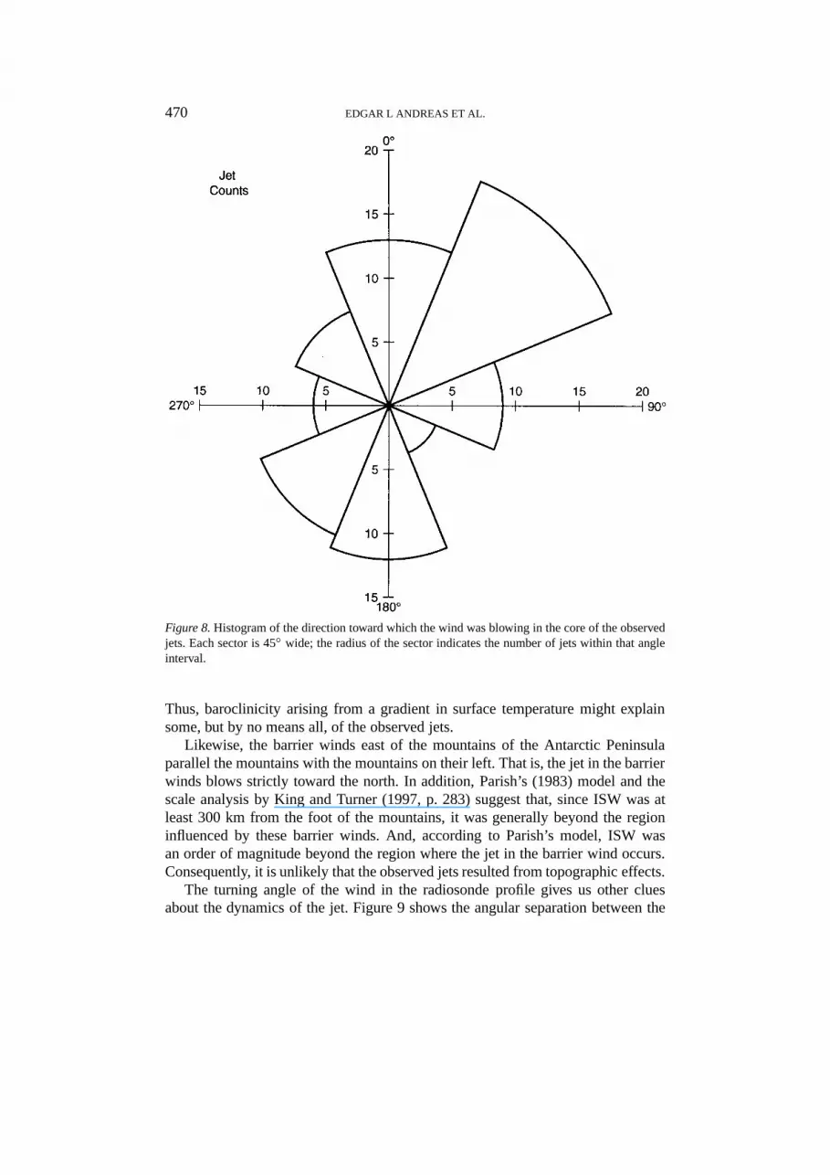
For example, Figure 8 shows the direction toward which the wind was blowingin the core of the observed jets. The ISW jets blew in all directions, with northand northeast and south and southwest orientations represented most. The wideangular distribution of these jet directions argues against topographic or surfacecontrol of the jets. If baroclinicity resulting from the surface temperature contrastbetween the ice-covered Weddell Sea and the open ocean to the north and eastcaused the jets, their preferred direction would be southeasterly (e.g., Andreas,1998) since the nearest ice edge generally runs north-south or northwest-southeastin February, March, April, and May (Zwally et al., 1983; Gloersen et al., 1992).

470 EDGAR L ANDREAS ET AL.

Figure 8.Histogram of the direction toward which the wind was blowing in the core of the observedjets. Each sector is 45◦ wide; the radius of the sector indicates the number of jets within that angleinterval.

Thus, baroclinicity arising from a gradient in surface temperature might explainsome, but by no means all, of the observed jets.

Likewise, the barrier winds east of the mountains of the Antarctic Peninsulaparallel the mountains with the mountains on their left. That is, the jet in the barrierwinds blows strictly toward the north. In addition, Parish’s (1983) model and thescale analysis by King and Turner (1997, p. 283) suggest that, since ISW was atleast 300 km from the foot of the mountains, it was generally beyond the regioninfluenced by these barrier winds. And, according to Parish’s model, ISW wasan order of magnitude beyond the region where the jet in the barrier wind occurs.Consequently, it is unlikely that the observed jets resulted from topographic effects.

The turning angle of the wind in the radiosonde profile gives us other cluesabout the dynamics of the jet. Figure 9 shows the angular separation between the

LOW-LEVEL ATMOSPHERIC JETS AND INVERSIONS 471

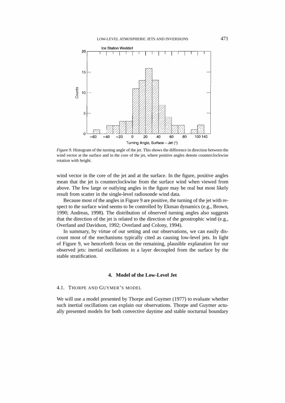
Figure 9.Histogram of the turning angle of the jet. This shows the difference in direction between thewind vector at the surface and in the core of the jet, where positive angles denote counterclockwiserotation with height.

wind vector in the core of the jet and at the surface. In the figure, positive anglesmean that the jet is counterclockwise from the surface wind when viewed fromabove. The few large or outlying angles in the figure may be real but most likelyresult from scatter in the single-level radiosonde wind data.

Because most of the angles in Figure 9 are positive, the turning of the jet with re-spect to the surface wind seems to be controlled by Ekman dynamics (e.g., Brown,1990; Andreas, 1998). The distribution of observed turning angles also suggeststhat the direction of the jet is related to the direction of the geostrophic wind (e.g.,Overland and Davidson, 1992; Overland and Colony, 1994).

In summary, by virtue of our setting and our observations, we can easily dis-count most of the mechanisms typically cited as causing low-level jets. In lightof Figure 9, we henceforth focus on the remaining, plausible explanation for ourobserved jets: inertial oscillations in a layer decoupled from the surface by thestable stratification.

4. Model of the Low-Level Jet

4.1. THORPE ANDGUYMER’ S MODEL

We will use a model presented by Thorpe and Guymer (1977) to evaluate whethersuch inertial oscillations can explain our observations. Thorpe and Guymer actu-ally presented models for both convective daytime and stable nocturnal boundary

472 EDGAR L ANDREAS ET AL.

layers. Because we saw predominantly stable stratification and no convection,however, we use only their model of the nocturnal boundary layer. This buildson Blackadar’s (1957) model in which an elevated layer becomes frictionally de-coupled from a lower layer because the stable stratification has eliminated turbulentexchange between the layers. When this decoupling occurs, the upper layer beginsinertial oscillations that lead to frequent supergeostrophic speeds in the layer. Mal-cher and Kraus (1983) and Beyrich and Klose (1988) also based models of thelow-level jet on Thorpe and Guymer’s work.

Thorpe and Guymer’s (1977) nocturnal boundary-layer model has two layers.The lower layer, which has thickness h, is frictionally coupled to the surface byturbulent momentum exchange. It is basically an Ekman layer in which the layer-averaged easterly (U ) and northerly (V ) velocity components obey

dU

dt− f V = 1

ρ

dτxdz, (1a)

dV

dt+ f (U − Ug) = 1

ρ

dτydz. (1b)

Here,t is time,z is height,f is the Coriolis parameter,Ug is the easterly componentof the geostrophic wind (the northerly component,Vg, is taken as zero),ρ is the(constant) air density, andτx andτy are the easterly and northerly components ofthe horizontal stress.

The stable stratification has damped out the turbulence above heighth. Con-sequently, in the upper layer, we find only inertial oscillations governed by

dU

dt− f V = 0, (2a)

dV

dt+ f (U − Ug) = 0. (2b)

Thorpe and Guymer (1977) included only two layers in their model of the noc-turnal boundary layer: the lower turbulent layer, which reaches heighth, and theupper nonturbulent layer that extends up to heighthu, which is associated with thetop of the inversion layerzt . Mahrt et al. (1979), however, explained that the regionimmediately above the jet is intermittently turbulent because of the wind shear.This turbulence extracts energy from the mean wind and, thus, accentuates the jetprofile. In other words, this intermittently turbulent layer is crucial for producinga jet with the features depicted in Figure 5 (cf. Makshtas et al., 1998). Above thisintermittently turbulent layer, we assume geostrophic balance.

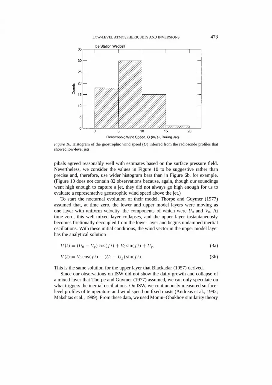
Figure 10 is a histogram of inferred values of the geostrophic wind speedG

[= (U2g + V 2

g )1/2] associated with our jet profiles. Plotted values are simply the

tethersonde measurements of wind speed in the region above the jet. Källstrand(1998) found that similar estimates of the geostrophic wind speed obtained from

LOW-LEVEL ATMOSPHERIC JETS AND INVERSIONS 473

Figure 10.Histogram of the geostrophic wind speed (G) inferred from the radiosonde profiles thatshowed low-level jets.

pibals agreed reasonably well with estimates based on the surface pressure field.Nevertheless, we consider the values in Figure 10 to be suggestive rather thanprecise and, therefore, use wider histogram bars than in Figure 6b, for example.(Figure 10 does not contain 82 observations because, again, though our soundingswent high enough to capture a jet, they did not always go high enough for us toevaluate a representative geostrophic wind speed above the jet.)

To start the nocturnal evolution of their model, Thorpe and Guymer (1977)assumed that, at time zero, the lower and upper model layers were moving asone layer with uniform velocity, the components of which wereU0 andV0. Attime zero, this well-mixed layer collapses, and the upper layer instantaneouslybecomes frictionally decoupled from the lower layer and begins undamped inertialoscillations. With these initial conditions, the wind vector in the upper model layerhas the analytical solution

U(t) = (U0− Ug) cos(f t)+ V0 sin(f t)+ Ug, (3a)

V (t) = V0 cos(f t)− (U0− Ug) sin(f t). (3b)

This is the same solution for the upper layer that Blackadar (1957) derived.Since our observations on ISW did not show the daily growth and collapse of

a mixed layer that Thorpe and Guymer (1977) assumed, we can only speculate onwhat triggers the inertial oscillations. On ISW, we continuously measured surface-level profiles of temperature and wind speed on fixed masts (Andreas et al., 1992;Makshtas et al., 1999). From these data, we used Monin–Obukhov similarity theory

474 EDGAR L ANDREAS ET AL.

to compute hourly averages of the surface fluxes of momentum and sensible heatand the Obukhov length L, which characterizes the stability of the atmosphericsurface layer (ASL). Although the ABL was virtually always stably stratified, theASL was occasionally unstably stratified according to these calculations. Using Las the criterion, we found that, between March 1 and June 4 on ISW, there wereeight episodes of unstable or near-neutral stratification in the ASL that lasted atleast one day and four episodes that lasted at least three days. Of the 18 tethersondesoundings between March 1 and June 4 that revealed no low-level jet, eight weremade during or shortly after these periods of unstable stratification in the ASL.

In summary, we presume, as did Thorpe and Guymer (1977), that the onsetof stable stratification in the ABL triggers the low-level jets. Day-long periods ofunstable stratification in the atmospheric surface layer, probably associated withadvective events, can foster sufficient mixing within the ABL to erode the jet. Anobvious, related conclusion is that, when once triggered, the inertial oscillationsare long lasting since we saw them in 80% of the soundings.

To treat the evolution of the lower layer, Thorpe and Guymer (1977) assumedthat the stress profile in Equation (1) is linear. That is,

τx = τxs(1− z

h

), (4a)

τy = τys(1− z

h

), (4b)

whereτxs andτys are surface values of the respective stress components. Overland(1985) corroborated this assumption by showing several stress profiles measuredover Arctic sea-ice that were approximately linear with height. Nicholls (1985) alsoreported an approximately linear stress profile in a well-mixed boundary layer overwater. The stress data that Caughey et al. (1979) obtained under stable stratificationduring the Minnesota experiment also are compatible with a linear decrease instress with height. As a counterpoint, though, Smedman’s (1991) observations inSBLs seem to follow

τ = τs(1− z

h

)7/4, (5)

whereτ = (τ 2x + τ 2

y )1/2 andτs = (τ 2

xs + τ 2ys)

1/2.Although this issue about the form of the stress profile is, thus, still unresolved,

we assume that the stress profile is linear because this form greatly simplifies theanalysis. With Equation (4) substituted into Equation (1),

dU

dt− f V = −τxs

ρh, (6a)

dV

dt+ f (U − Ug) = −τys

ρh. (6b)

LOW-LEVEL ATMOSPHERIC JETS AND INVERSIONS 475

Thorpe and Guymer (1977) offered two solutions to this set of equations: thefirst uses a parameterization for the surface stress that is linear in wind speed; thesecond uses a parameterization that is quadratic in wind speed. We discuss only thequadratic parameterization since no known observations support the validity of ashear stress parameterization that depends linearly on wind speed.

4.2. QUADRATIC STRESS RELATION

Thorpe and Guymer’s (1977) model of the wind vector in the lower layer based ona quadratic stress relation parameterizes the surface stress as

τxs = ρCD(U2+ V 2)1/2U, (7a)

τys = ρCD(U2+ V 2)1/2V, (7b)

whereCD is the drag coefficient. Substituting Equation (7) into Equation (6) yieldsequations for the velocity components in the lower layer:

dU

dt= f V − CD(U2+ V 2)U/h, (8a)

dV

dt= −f (U − Ug)− CD(U2+ V 2)1/2V/h. (8b)

We solved these equations for the velocity components in the lower layer usingthe fourth-order Runge–Kutta formula (e.g., Press et al., 1994, p. 702 ff.). For CD,we used the average value for the 10-m, neutral-stability drag coefficient,CDN10,that Andreas and Claffey (1995) measured on ISW, 1.9× 10−3. Equation (3) givesthe solution in the upper layer.

Figure 11 shows wind hodographs in the lower and upper model layers, com-puted with Equation (8) and Equation (3), respectively, for typical ISW values oflatitude, jet height h (Figure 7), and geostrophic wind speedG (Figure 10). Attime zero, when the upper layer becomes frictionally decoupled from the surface,it begins undamped inertial oscillations about the geostrophic wind vector. The ve-locity vector in the lower layer rapidly decays and turns clockwise (in the SouthernHemisphere), reaching steady state in about five hours.

Let us look more closely at the steady-state behaviour of the wind vectors inthe upper and lower layers. Equation (3) represents a vector from the origin thatterminates on a circle of radius

R = [(U0−G)2+ V 20 ]1/2, (9)

centered on the geostrophic wind vector. The tip of the wind vector in the upperlayer makes one complete cycle around this circle for each inertial period startingat time zero. As a result, the angular deviation between the wind vector in the upper

476 EDGAR L ANDREAS ET AL.

Figure 11.Solution of the jet model for conditions typical of Ice Station Weddell. The drag coeffi-cientCD in the stress relation (7) is taken to be the average 10-m, neutral-stability value from ISW,1.9× 10−3 (Andreas and Claffey, 1995). The numbers near the filled circles show the time in hourssince the lower and upper layers decoupled.

layer (i.e., the jet layer) and the geostrophic wind vector ranges between−β and+β, where

β = arcsin(R/G). (10)

In the lower layer in Figure 11, the wind vector immediately begins decayingafter time zero and rotates clockwise. In the steady-state limit, the wind vector hereobeys

fV = CD(U2+ V 2)1/2U/h, (11a)

−f (U − Ug) = CD(U2+ V 2)1/2V/h. (11b)

These yield

U(t →∞) = G

1+ C2DS

2Q

f 2h2

, (12a)

V (t →∞) = CDSQ

f h

G

1+ C2DS

2Q

f 2h2

, (12b)

LOW-LEVEL ATMOSPHERIC JETS AND INVERSIONS 477

whereSQ is the magnitude of the steady-state wind vector in the lower layer,

S2Q = U2(t →∞)+ V 2(t →∞) = f 2h2

2C2D

[(1+ 4GC2

D

f 2h2

)1/2

− 1

]. (13)

The subscriptQ reminds us that this result derives from Thorpe and Guymer’s(1977) quadratic stress parameterization.

The angular separation between the geostrophic wind vector and the steady-state wind vector in the lower layer is

αQ = −arctan

(CDSQ

f h

)

= −arctan

signf

[1

2

(1+ 4GC2

D

f 2h2

)1/2

− 1

2

]1/2 . (14)

Here signf represents the sign of the Coriolis parameter, and the minus sign infront of the right two terms transforms our Cartesian model coordinates into ameteorological coordinate system in which angles increase clockwise. Thus, pos-itive αQ means that the steady-state wind in the lower layer is clockwise fromthe geostrophic wind when viewed from above. (Remember,f is negative in theSouthern Hemisphere.)

From Equation (10) and Equation (14), we deduce that, in steady state, theangular deviation between the wind vector in the jet and in the lower layer isbounded by|αQ ± β|. For the example in Figure 11,αQ = 57◦ andβ = 24◦.Consequently, for the typical ISW conditions depicted in Figure 11, we wouldexpect to see turning angles between the jet and the surface wind ranging from33◦ to 81◦. Figure 9 shows that this prediction agrees fairly well with our ISWobservations.

It is also easy to determine geometrically from Figure 11 how frequently jetsshould be observed if our model is accurate. The steady-state wind vector in thelower layer has magnitudeSQ of 5.45 m s−1. Thus, we simply inscribe an arc withradiusSQ + 2 m s−1 (= 7.45 m s−1) around the origin in Figure 11. Any segment ofthe wind hodograph in the upper layer that is inside this circle would not producea jet profile according to our definition. Segments of the hodograph outside thiscircle, on the other hand, have a wind speed that is at least 2 m s−1 higher thanthe speed in the lower layer and would produce a jet profile. Approximately 10/13= 77% of the upper-level hodograph is outside this circle of radius 7.45 m s−1.This percentage agrees remarkably well with our ISW result that 80% of availabletethersonde profiles showed a low-level jet.

Lastly, according to Figure 11, the range of speeds in the modelled jet is 7.4to 14 m s−1. Our observations (Figure 6b) yielded some jets with core speeds lessthan 6 m s−1, but most speeds were between 6 and 14 m s−1, as Figure 11 predicts.

478 EDGAR L ANDREAS ET AL.

Ultimately, this range of speeds depends mostly on the speed of the geostrophicwind.

In summary, the Thorpe and Guymer (1977) model of low-level jets, based onundamped inertial oscillations in an elevated layer that is frictionally decoupledfrom the surface, does well in explaining the range of observations we made inlow-level jets on ISW. In particular, model calculations predict both the correctpercentage of jet occurrences and the range of angular deviations between thesurface wind vector and the wind vector in the jet core. Our modelling, of course,does not rule out other causes of the jets but suggests that the modelled scenario isthe dominant one in the western Weddell Sea in autumn and early winter.

5. Discussion

5.1. BOUNDARY-LAYER HEIGHT

For the model calculations in the last section, we took the heighth to be the heightof the jet core. For a convective boundary layer, the height of the inversionzt iscommonly used as the ABL height (e.g., Kaimal et al., 1976). For the SBL, how-ever, this height is not as meaningful. Mahrt (1981) and Zilitinkevich and Mironov(1996), for example, explained that, in stable stratification, the ABL should bedefined as the region that is at least intermittently turbulent. We infer that the SBLis thus the region between the surface and the core of the low-level jet. Figure 7emphasizes that, with this definition, the height of the SBL is usually much lessthanzt .

The Richardson number helps us decide where turbulence is present. Mahrt(1981) and Heinemann and Rose (1990) defined a bulk Richardson number fromradiosounding data as

Ri(z) = gz

2(z)

2(z)−2s

S2(z). (15)

Here,g is the acceleration of gravity;z, the height of a radiosounding observation;2(z) andS(z), the potential temperature and wind speed at z; and2s, the potentialtemperature at the surface (which we computed from the temperature at the lowestradiosounding level, about 2 m).

As we scan up a radiosounding profile, computing Ri(z) at each reporting heightz, we compare Ri(z) with the critical Richardson number Ricr , where Ricr = 0.4,a value midway between Mahrt’s (1981) 0.5 and Heinemann and Rose’s (1990)0.33. If Ri(z) < Ricr , we assume that the layer between the surface and heightz isturbulent and, thus, that levelz is still within the boundary layer. The lowest levelfor which Ri(z) ≥ Ricr is denotedzRi and is assumed to be the top of the turbulentregion. That is,zRi estimates the height of the SBL.

LOW-LEVEL ATMOSPHERIC JETS AND INVERSIONS 479

Figure 12 shows time series of our observations ofzt andzj and our computedzRi values. Although thezj andzRi points in panel b do not track perfectly,zj ismuch more closely related tozRi than it is tozt . On average,zj andzRi agree verywell. The average of thezj values in Figure 12 is 151 m; the average of thezRi

values is 143 m. Hence, as Mahrt (1981) concluded, the height of the low-level jetis an indicator of the height of the SBL. Therefore, we can approximate the heighth of the lower layer in the model described in the last section with eitherzj or zRi,whichever is more readily available.

Makshtas et al. (1998) attributed the ranges ofzj andzRi in Figures 7 and 12to the influence of the surface radiation balance on boundary layer turbulence.Figure 12 also shows the time series of daily averaged net radiation,Rn, that wemeasured on ISW with individual radiometers that monitored incoming and outgo-ing longwave and shortwave radiation (Andreas et al., 1992; Makshtas et al., 1999).Our convention is thatRn is positive when the surface is gaining energy radiatively.A negative net radiation means that the surface is losing energy radiatively; thiswould lead to stable stratification.

Although the correlation betweenRn and any of the heights plotted in Figure 12,zt , zj , orzRi, is not high, the plot is suggestive. WhenRn is positive or near zero,zt ,zj , andzRi all tend to be larger than whenRn is more negative. When the radiativelosses become large, i.e., when the hourly values are about−40 W m−2, internalgravity waves begin breaking within the boundary layer and create new turbulence(Makshtas et al., 1998). Thus, the height of the SBL reaches a quasi-minimum of50–100 m with strong radiative forcing.

5.2. GEOSTROPHIC DRAG COEFFICIENT

In large-scale sea-ice and ocean models, it is common to estimate the surface stressτ with a geostrophic drag relation

τ = ρC2gG

2, (16)

whereCg is the geostrophic drag coefficient, andG is again the geostrophic windspeed (e.g., Parkinson and Washington, 1979; Brown and Liu, 1982; Hibler, 1985;Overland and Davidson, 1992; Brown and Foster, 1994). OftenCg is taken asa constant; but, in general, it depends on boundary-layer characteristics such asstability, surface roughness, or ABL height (e.g., Overland and Davidson, 1992;Overland and Colony, 1994; Brown and Foster, 1994; Andreas, 1998).

The turning angleα between the geostrophic wind vector and the surface windvector is the second piece of information needed to specify surface stress from thegeostrophic wind. Again, some assume thatα is constant; but, in general, it alsodepends on ABL characteristics.

The jet model we described in Section 4 implies a new geostrophic drag relationappropriate when low-level jets are present. Although Thorpe and Guymer (1977)

480 EDGAR L ANDREAS ET AL.

Figure 12. Ice Station Weddell observations of inversion height (zt ; panel a) and height of the jetcore (zj ; panel b) based on radiosounding data. Panel b also shows the height of the stable boundarylayer (zRi) estimated from a critical Richardson number criterion. Panel c shows the daily averagednet radiation (Rn) on ISW.

developed this jet model, they did not discuss the geostrophic drag relation impliedby it.

The quadratic stress relation, Equation (7), gives

τ = ρCD(U2+ V 2), (17)

which at steady-state is

τ = ρCDS2Q. (18)

LOW-LEVEL ATMOSPHERIC JETS AND INVERSIONS 481

Combining this with Equation (16) yields

Cg = C1/2D SQ

G. (19)

In turn, substituting (13) here gives

Cg = |f |h√2C1/2

D G

[(1+ 4G2C2

D

f 2h2

)1/2

− 1

]1/2

, (20)

while Equation (14) gives the turning angleα between the geostrophic wind andthe surface stress vector. In a meteorological coordinate system, we simply addα

to the direction of the geostrophic wind to find the direction of the surface stress.Note that, because our model treats only the SBL when jets are present, neither

Equation (20) nor the expression for the turning angle (14) contains any explicit sta-bility dependence. Such stability dependence is usual in expressions that model thegeostrophic drag coefficient for general conditions (e.g., Brown, 1990; Overlandand Colony, 1994; Andreas, 1998).

Figure 13 showsCg andα for conditions typical of ISW, as predicted by Equa-tions (14) and (20). Despite the absence of any stability dependence in our model,for values ofG, h, andCDN10 that we observed on ISW, the predictedGg andαvalues still span the range of values obtained from observations over Arctic sea-ice(e.g., Brown, 1981; Overland, 1985; Overland and Davidson, 1992; Overland andColony, 1994). That is, variations inG, h, andCDN10 provide enough degrees offreedom for our jet model to produce all observed values ofCg andα without theneed for an additional, independent stratification parameter. Overland and David-son (1992) and Overland and Colony (1994), in contrast, predictedCg andα on thebasis of stratification alone and included no explicit dependence onG, h, orCDN10.We infer that a stratification parameter and the parameter set{G,h,CDN10} provideredundant information for the ABL over polar sea-ice.

We can summarize Figure 13 by noting thatCg is smaller and the absolutevalue ofα is larger when the boundary-layer heighth is smaller. Conversely, ashincreases,Cg becomes larger and|α| becomes smaller. Clearly, when viewed fromabove, the surface wind (and surface stress) is clockwise from the geostrophic windin the Southern Hemisphere and counterclockwise in the Northern Hemisphere.

Our model for the geostrophic drag relation, represented by Equation (14) forα and (20) forCg, is more complex than some currently in use, for example, thosethat use constant values for bothCg andα. But it is also less complex than somethat require detailed atmospheric temperature data for computing a stratificationparameter. Our model is simpler than these because it applies only over sea-ice,where the stratification is usually stable and the height of the SBL is, thus, generallyconstrained between 50 and 300 m.

482 EDGAR L ANDREAS ET AL.

Figure 13.The geostrophic drag relation derived from the jet model. Panels a and b, respectively,show the geostrophic drag coefficientCg (see Equation (20)) and the turning angleα (see Equation(14)) between the geostrophic wind vector and the surface stress in the Southern Hemisphere asfunctions of the geostrophic wind speed.h is the height of the stable boundary layer. Positiveαvalues mean that the surface stress is clockwise from the geostrophic wind vector when viewed fromabove. Calculations assumeCD = CDN10= 1.9× 10−3 and that the latitude is 68◦S.

LOW-LEVEL ATMOSPHERIC JETS AND INVERSIONS 483

6. Conclusions

We have presented here the first long-term, detailed observations of the structureof the atmospheric boundary layer over Antarctic sea-ice. Over sea-ice, the ABL,defined as the near-surface layer that is, at least, intermittently turbulent, is oftenstably stratified. During four months of radiosonde observations on Ice StationWeddell in the austral autumn and early winter, we found a low-level inversionlayer 96% of the time. Because statistics of these ISW inversions are grossly similarto the statistics of inversions observed in and around the Arctic Ocean, we presumethat ABL characteristics over sea-ice regions in both hemispheres are largely lo-cally controlled by the interplay among the sea-ice surface, the free atmosphere,and the clouds.

The stable stratification of ISW frequently produced low-level atmospheric jets.Eighty percent of our soundings that yielded unambiguous wind speed profilesshowed a jet with its core below 425 m. A simple two-layer model, in which an el-evated layer is frictionally decoupled from a near-surface layer and thus undergoesundamped inertial oscillations, can explain most of the features of the low-leveljets that we have documented.

This two-layer model also implies a geostrophic drag parameterization thatrelates the geostrophic drag coefficient and the turning angle to latitude, ABLheight, geostrophic wind speed, and the 10-m drag coefficient. Because this para-meterization presupposes stable stratification and a decoupled elevated layer, it ismore limited than some geostrophic drag relations; but it can consequently also besimpler. Our parameterization does not explicitly depend on a stratification para-meter, as other more complex parameterizations do, and the independent variablesare either readily available or have only limited domains. Because stable stratifica-tion is very common over sea-ice, this geostrophic drag parameterization may thusbe widely applicable despite its simplicity.

Acknowledgements

We dedicate this manuscript to the memory of William T. Bates, who draftedmost of the figures in it. His passing left an enormous hole in CRREL’s technicalpublishing group. We thank Larry Mahrt, John Weatherly, and two anonymousreviewers for comments on the manuscript. The U.S. National Science Foundationsupported this work with grants OPP-90-24544, OPP-93-12642, OPP-97-02025,and OPP-98-14024; the U.S. Department of the Army supported it through project4A161102AT24.

484 EDGAR L ANDREAS ET AL.

References

Andreas, E. L.: 1998, ‘The Atmospheric Boundary Layer over Polar Marine Surfaces’, in M.Leppäranta (ed.),Physics of Ice-Covered Seas, Vol. 2, Helsinki University Press, pp. 715–773.

Andreas, E. L. and Cash, B. A.: 1999, ‘Convective Heat Transfer over Wintertime Leads andPolynyas’,J. Geophys. Res.104(C11), 25,721–25,734.

Andreas, E. L. and Claffey, K. J.: 1995, ‘Air-Sea Drag Coefficients in the Western Weddell Sea: 1.Values Deduced from Profile Measurements’,J. Geophys. Res.100(C3), 4821–4831.

Andreas, E. L. and Richter, W. A.: 1982, ‘An Evaluation of Vaisala’s MicroCORA AutomaticSounding System’, CRREL Rept. 82-28, U.S. Army Cold Regions Research and EngineeringLaboratory, Hanover, NH, 17 pp. [NTIS: AD-B070011.]

Andreas, E. L., Claffey, K. J., Makshtas, A. P., and Ivanov, B. V.: 1992, ‘Atmospheric Sciences onIce Station Weddell’,Antarct. J. U.S.27(5), 115–117.

Andreas, E. L., Claffey, K. J., and Makshtas, A. P.: 1993, ‘Low-Level Atmospheric Jets andInversions on Ice Station Weddell 1’,Antarct. J. U.S.28(5), 274–276.

Andreas, E. L., Claffey, K. J., and Makshtas, A. P.: 1995, ‘Low-Level Atmospheric Jets overthe Western Weddell Sea’, in Preprint Volume, Fourth Conference on Polar Meteorology andOceanography, 15–20 January 1995, Dallas, TX, American Meteorological Society, Boston, pp.252–257.

Anonymous: 1992, ‘U.S. and Russian Scientists Complete Historic Weddell Sea Investigation’,Antarct. J. U.S.27(4), 8–11.

Beyrich, F. and Klose, B.: 1988, ‘Some Aspects of Modelling Low-Level Jets’,Boundary-LayerMeteorol.43, 1–14.

Blackadar, A. K.: 1957, ‘Boundary Layer Wind Maxima and their Significance for the Growth ofNocturnal Inversions’,Bull. Amer. Meteorol. Soc.38, 283–290.

Bonner, W. D.: 1968, ‘Climatology of the Low Level Jet’,Mon. Wea. Rev.96, 833–850.Brown, R. A.: 1981, ‘Modeling the Geostrophic Drag Coefficient for AIDJEX’.J. Geophys. Res.

86(C3), 1989–1994.Brown, R. A.: 1990, ‘Meteorology’, in W. O. Smith, Jr. (ed.),Polar Oceanography, Part A. Physical

Science, Academic Press, San Diego, pp. 1–46.Brown, R. A. and Foster, R. C.: 1994, ‘On PBL Models for General Circulation Models’,Global

Atmos. Ocean System2, 163–183.Brown, R. A. and Liu, W. T.: 1982, ‘An Operational Large-Scale Marine Planetary Boundary Layer

Model’, J. Appl. Meteorol.21, 261–269.Caughey, S. J., Wyngaard, J. C., and Kaimal, J. C.: 1979, ‘Turbulence in the Evolving Stable

Boundary Layer’,J. Atmos. Sci.36, 1041–1052.Claffey, K. J., Andreas, E. L., and Makshtas, A. P.: 1994, ‘Upper-Air Data Collected on Ice Station

Weddell’, Special Rept. 94-25, U.S. Army Cold Regions Research and Engineering Laboratory,Hanover, NH, 61 pp. [NTIS: AD-289707.]

Gloersen, P., Campbell, W. J., Cavalieri, D. J., Comiso, J. C., Parkison, C. L., and Zwally, H. J.:1992,Arctic and Antarctic Sea Ice, 1978–1987: Satellite Passive-Microwave Observations andAnalysis, NASA SP-511, National Aeronautics and Space Administration, Washington, D.C.,290 pp.

Heinemann, G. and Rose, L.: 1990, ‘Surface Energy Balance, Parameterizations of Boundary-LayerHeights and the Application of Resistance Laws near an Antarctic Ice Shelf Front’,Boundary-Layer Meteorol.51, 123–158.

Hibler, W. D., III: 1985, ‘Modeling Sea-Ice Dynamics’,Adv. Geophys.28A, 549–579.ISW Group: 1993, ‘Weddell Sea Exploration from Ice Station’,Eos, Trans. Amer. Geophys. Union

74, 121–126.Kahl, J. D.: 1990, ‘Characteristics of the Low-Level Temperature Inversion along the Alaskan Arctic

Coast’,Int. J. Climatol.10, 537–548.

LOW-LEVEL ATMOSPHERIC JETS AND INVERSIONS 485

Kaimal, J. C., Wyngaard, J. C., Haugen, D. A., Coté, O. R., Izumi, Y., Caughey, S. J., and Readings,C. J.: 1976, ‘Turbulence Structure in the Convective Boundary Layer’,J. Atmos. Sci.33, 2152–2169.

Källstrand, B.: 1998, ‘Low Level Jets in a Marine Boundary Layer during Spring’,Contr. Atmos.Phys.71, 359–373.

King, J. C. and Turner, J.: 1997,Antarctic Meteorology and Climatology, Cambridge UniversityPress, Cambridge, U.K., 409 pp.

Kurzeja, R. J., Berman, S., and Weber, A. H.: 1991, ‘A Climatological Study of the NocturnalPlanetary Boundary Layer’,Boundary-Layer Meteorol.54, 105–128.

Lettau, H.: 1971, ‘Antarctic Atmosphere as a Test Tube for Meteorological Theories’, in L. O. Quam(ed.), Research in the Antarctic, Pub. No. 93, American Association for the Advancement ofScience, Washington, D.C., pp. 443–475.

Mahesh, A., Walden, V. P., and Warren, S. G.: 1997, ‘Radiosonde Temperature Measurements inStrong Inversions: Correction for Thermal Lag Based on an Experiment at the South Pole’,J.Atmos. Oceanic Technol.14, 45–53.

Mahrt, L.: 1981, ‘Modelling the Depth of the Stable Boundary-Layer’,Boundary-Layer Meteorol.21, 3–19.

Mahrt, L.: 1999, ‘Stratified Atmospheric Boundary Layers’,Boundary-Layer Meteorol.90, 375–396.Mahrt, L., Heald, R. C., Lenschow, D. H., Stankov, B. B., and Troen, I.: 1979, ‘An Observational

Study of the Structure of the Nocturnal Boundary Layer’,Boundary-Layer Meteorol.17, 247–264.

Makshtas, A. P., Andreas, E. L., Svyashchennikov, P. N., and Timachev, V. F.: 1999, ‘Accounting forClouds in Sea Ice Models’,Atmos. Res.52, 77–113.

Makshtas, A. P., Timachev, V. F., and Andreas, E. L.: 1998, ‘Structure of the Lower AtmosphericLayer over Ice Cover of the Weddell Sea’,Russian Meteorol. Hydrol.10, 68–75.

Malcher, J. and Kraus, H.: 1983, ‘Low-Level Jet Phenomena Described by an Integrated DynamicalPBL Model’, Boundary-Layer Meteorol.27, 327–343.

Nicholls, S.: 1985, ‘Aircraft Observations of the Ekman Layer during the Joint Air-Sea InteractionExperiment’,Quart. J. Roy. Meteorol. Soc.111, 391–426.

Nieuwstadt, F. T. M. and Duynkerke, P. G.: 1996, ‘Turbulence in the Atmospheric Boundary Layer’,Atmos. Res.40, 111–142.

Overland, J. E.: 1985, ‘Atmospheric Boundary Layer Structure and Drag Coefficients over Sea Ice’,J. Geophys. Res.90(C5), 9029–9049.

Overland, J. E. and Colony, R. L.: 1994, ‘Geostrophic Drag Coefficients for the Central ArcticDerived from Soviet Drifting Station Data’,Tellus46A, 75–85.

Overland, J. E. and Davidson, K. L.: 1992, ‘Geostrophic Drag Coefficients over Sea Ice’,Tellus44A,54–66.

Parish, T. R.: 1983: ‘The Influence of the Antarctic Peninsula on the Wind Field over the WesternWeddell Sea’,J. Geophys. Res.88(C4), 2684–2692.

Parkinson, C. L. and Washington, W. M.: 1979, ‘A Large-Scale Numerical Model of Sea Ice’,J.Geophys. Res.84(C1), 311–337.

Press, W. H., Teukolsky, S. A., Vetterling, W. T., and Flannery, B. P.: 1994,Numerical Recipesin FORTRAN: The Art of Scientific Computing, Second Edition, Cambridge University Press,Cambridge, U.K., 963 pp.

Schwerdtfeger, W.: 1984,Weather and Climate of the Antarctic, Elsevier, Amsterdam, 261 pp.Serreze, M. C., Kahl, J. D., and Schnell, R. C.: 1992, ‘Low-Level Temperature Inversions of the

Eurasian Arctic and Comparisons with Soviet Drifting Station Data’,J. Climate5, 615–629.Singh, M. P., McNider, R. T., and Lin, J. T.: 1993, ‘An Analytical Study of Diurnal Wind-Structure

Variations in the Boundary Layer and the Low-Level Nocturnal Jet’,Boundary-Layer Meteorol.63, 397–423.

486 EDGAR L ANDREAS ET AL.

Skony, S. M., Kahl, J. D. W., and Zaitseva, N. A.: 1994, ‘Differences between Radiosonde andDropsonde Temperature Profiles over the Arctic Ocean’,J. Atmos. Oceanic Technol.11, 1400–1408.

Smedman, A.-S.: 1991, ‘Some Turbulence Characteristics in Stable Atmospheric Boundary LayerFlow’, J. Atmos. Sci.48, 856–868.

Smedman, A.-S., Högström, U., and Bergström, H.: 1997, ‘The Turbulence Regime of a Very StableMarine Airflow with Quasi-frictional Decoupling’,J. Geophys. Res.102(C9), 21,049–21,059.

Smedman, A.-S., Tjernström, M., and Högström, U.: 1993, ‘Analysis of the Turbulence Structure ofa Marine Low-Level Jet’,Boundary-Layer Meteorol.66, 105–126.

Smith, S. D., Anderson, R. J., den Hartog, G., Topham, D. R., and Perkin, R. G.: 1983, ‘An Inves-tigation of a Polynya in the Canadian Archipelago, 2, Structure of Turbulence and Sensible HeatFlux’, J. Geophys. Res.88(C5), 2900–2910.

Stull, R. B.: 1988,An Introduction to Boundary Layer Meteorology, Kluwer Academic Publishers,Dordrecht, 666 pp.

Thorpe, A. J. and Guymer, T. H.: 1977, ‘The Nocturnal Jet’,Quart. J. Roy. Meteorol. Soc.103,633–653.

Walden, V. P., Mahesh, A., and Warren, S. G.: 1996, ‘Comment on “Recent Changes in the NorthAmerican Arctic Boundary Layer in Winter” by R. S. Bradley et al.’,J. Geophys. Res.101(D3),7127–7134.

Walter, B. and Overland, J. E.: 1991, ‘Aircraft Observations of the Mean and Turbulent Structure ofthe Atmospheric Boundary Layer during Spring in the Central Arctic’,J. Geophys. Res.96(C3),4663–4673.

Zemba, J. and Friehe, C. A.: 1987, ‘The Marine Atmospheric Boundary Layer Jet in the CoastalOcean Dynamics Experiment’,J. Geophys. Res.92(C2), 1489–1496.

Zilitinkevich, S. and Mironov, D. V.: 1996, ‘A Multi-limit Formulation for the Equilibrium Depth ofa Stably Stratified Boundary Layer’,Boundary-Layer Meteorol.81, 325–351.

Zwally, H. J., Comiso, J. C., Parkinson, C. L., Campbell, W. J., Carsey, F. D., and Gloersen, P.:1983,Antarctic Sea Ice, 1973–1976: Satellite Passive-Microwave Observations, NASA SP-459,National Aeronautics and Space Administration, Washington, D.C., 206 pp.