Low-Resolution Modeling of Dense Drainage Networks in Conﬁning Layers

Low-Resolution Modeling of Dense DrainageNetworks in Confining Layersby P.S. Pauw1,2, S.E.A.T.M. Van der Zee1, A. Leijnse1, J.R. Delsman3, P.G.B. De Louw3, W.J. De Lange3, andG.H.P. Oude Essink3

AbstractGroundwater-surface water (GW-SW) interaction in numerical groundwater flow models is generally simulated using a Cauchy

boundary condition, which relates the flow between the surface water and the groundwater to the product of the head differencebetween the node and the surface water level, and a coefficient, often referred to as the ‘‘conductance.’’ Previous studies haveshown that in models with a low grid resolution, the resistance to GW-SW interaction below the surface water bed should oftenbe accounted for in the parameterization of the conductance, in addition to the resistance across the surface water bed. Threeconductance expressions that take this resistance into account were investigated: two that were presented by Mehl and Hill (2010)and the one that was presented by De Lange (1999). Their accuracy in low-resolution models regarding salt and water fluxes to adense drainage network in a confined aquifer system was determined. For a wide range of hydrogeological conditions, the influenceof (1) variable groundwater density; (2) vertical grid discretization; and (3) simulation of both ditches and tile drains in a singlemodel cell was investigated. The results indicate that the conductance expression of De Lange (1999) should be used in similarhydrogeological conditions as considered in this paper, as it is better taking into account the resistance to flow below the surfacewater bed. For the cases that were considered, the influence of variable groundwater density and vertical grid discretization on theaccuracy of the conductance expression of De Lange (1999) is small.

IntroductionFresh groundwater reserves in coastal areas are

jeopardized by future stresses such as sea level rise,climate change, and land subsidence (Custodio andBruggeman 1987; Overeem and Syvitski 2009). Theseeffects are often quantified using numerical models(Oude Essink et al. 2010; Cobaner et al. 2012; FanecaSanchez et al. 2012; Langevin and Zygnerski 2013).When investigating large-scale (more than 100 km2)problems, a low grid resolution is inevitable in viewof the computational demand. A low grid resolutionrequires the upscaling of hydraulic parameters (Bierkens1994; Renard and DeMarsily 1997; Dagan et al. 2013)and boundary conditions. Vermeulen et al. (2006) showedthat in case of a dense drainage network, the upscalingof hydraulic parameters is less important than theparameterization of the boundary condition that describes

1Department of Soil Physics and Land Management,Wageningen University, Wageningen, The Netherlands.

2Corresponding author: Department of Soil and Ground-water, Deltares, Utrecht, The Netherlands; +31623786887;[email protected]

3Department of Soil and Groundwater, Deltares, Utrecht, TheNetherlands.

Received March 2014, accepted August 2014.© 2014, National Ground Water Association.doi: 10.1111/gwat.12273

the groundwater-surface water (GW-SW) interaction.Appropriate simulation of GW-SW interaction in coastalareas with a dense drainage network is important for thequantification of advection in the aquifer (e.g., salt waterintrusion), salt and nutrient loads to the surface water andfor providing information for downscaled models that areused to describe local scale systems.

GW-SW interaction is generally simulated using aCauchy boundary condition, which is in the form of:

Q = (hsw − hn) C (1)

where Q is the volumetric flow rate between the surfacewater and the aquifer [L3/T], hsw is the surface water level[L], hn is the hydraulic head of the node where the Cauchyboundary condition is applied [L], and C is the coefficient[L2/T], often referred to as “conductance.” McDonaldand Harbaugh (1988) described how the conductancecan be determined from the dimensions of the surfacewater bed (i.e., its length, width, and thickness) and itshydraulic resistance (i.e., the thickness of the bed dividedby its vertical hydraulic conductivity). This approach isoften adopted in groundwater flow models. However,McDonald and Harbaugh (1988) also described that thisapproach should only be used if the majority of the totalhead loss due to GW-SW interaction occurs across thesurface water bed and that the head loss in the aquifer can

NGWA.org Groundwater 1

be neglected. This has also been shown in later studies (DeLange 1998; Hunt et al. 2003; Anderson 2005; Rushton2007; Mehl and Hill 2010).

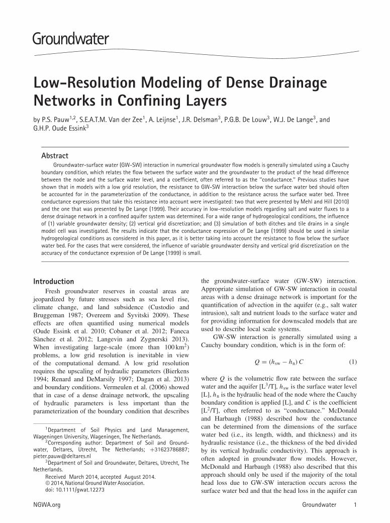
For the purpose of illustration, an example is givenhere to emphasize that in case of simulating a densesurface water network in a confining layer using a lowmodel resolution, neglecting the resistance to GW-SWinteraction in the confining layer leads to erroneousmodel results. Only the main features of this exampleare discussed, as similar details will be presented furtherin this paper. Figure 1a shows the result of a density-dependent groundwater flow and coupled salt transportmodel of a confined aquifer system in vertical crosssection, using a high grid resolution (i.e., 0.1 m, both forthe width of the columns and the thickness of the layers).The drainage system consists of tile drains and shallowditches, which are simulated using the conductanceexpression of McDonald and Harbaugh (1988). In thiscase, the conductance can be based on the resistanceacross the surface water bed only, as the additionalresistance in the confining layer is accounted for by thehigh-resolution grid. The streamlines show a regional flowof saline groundwater in the aquifer from the left to theright, and part of the water flows up through the 4-m thickconfining layer. The fresh groundwater recharge results inshallow rainwater lenses between the tile drains. Figure 1bshows the result of a corresponding model with the samemodel layer thickness but with a column width of 100 m.Again, the conductance expression of McDonald andHarbaugh (1988) is used by summing the widths of theindividual tile drains and ditches in the cell, so that onlythe resistance to flow across the streambed is accountedfor. The streamlines indicate that all saline groundwaterthat enters the model on the left boundary flows to theupper boundary, and that there is also inflow from theright boundary. This illustrates that the resistance to GW-SW interaction is greatly underestimated. In this case, thetotal flux toward the surface water is overestimated by afactor of 6. Such significant errors can also be expectedin similar hydrogeological conditions.

Despite its importance, expressions for the conduc-tance that take into account the resistance to GW-SWinteraction below the surface water bed are relativelyscarce in the international literature. In this paper, the per-formance of three existing conductance expressions thateach take into account the resistance below the surfacewater bed in a different way are evaluated. These are thetwo conductance expressions that were presented by Mehland Hill (2010) and the conductance expression of DeLange (1999). Morel-Seytoux (2009) and Morel-Seytouxet al. (2014) presented a method to account for the resis-tance below the surface water bed, which relies on com-bining an analytical expression that accounts for all theresistance due to GW-SW interaction, with the numericalsolution at a “far” distance. However, this method can-not be directly applied as a Cauchy boundary condition incases where multiple surface water have to be accountedfor in a single model cell or the aquifer is discretized in thevertical direction. Because the latter is crucial for the work

(a)

(b)

Figure 1. Illustrative example on simulating GW-SW inter-action using a high grid resolution (a) and low grid resolution(b), where the conductance is only based on the dimensionsand hydraulic resistance of the surface water bed (i.e., theconductance expression of McDonald and Harbaugh [1988]).The colors indicate concentrations, and the white lines indi-cate streamlines. The unit of the horizontal and verticalextent indications is meter.

of the present paper, the methods presented in Morel-Seytoux (2009) and Morel-Seytoux et al. (2014) are notconsidered.

The objective of this paper is to assess the accuracy ofthe two conductance expressions of Mehl and Hill (2010),and the conductance expression of De Lange (1996) whenapplied in simulations with a low grid resolution. Theinfluence of (1) variable groundwater density; (2) verticalgrid discretization; and (3) simulation of ditches andtile drains in a single model cell, on the accuracy ofquantifying water fluxes and salt loads to ditches and tiledrains is considered for a wide range of hydrogeologicalconditions, and the differences between the methods arediscussed.

Materials and Methods

Conductance ExpressionsMehl and Hill (2010) presented two expressions for

the conductance that, besides the resistance across thesurface water bed, also account for the resistance belowit. For convenience, “surface water” refers to both ditchesand tile drains in this paper, and “surface water bed”refers to the hydraulically resistive unit directly belowthe surface water (e.g., a streambed). The first expressionfor the conductance (Equation 3 of Mehl and Hill 2010)is denoted here with C MH3:

CMH3 =(

c0

BlB+ 0.5�z

kvA

)−1

(2)

c0 is the entry resistance of the surface water bed[T]. c0 is defined here as the thickness of the surfacewater bed divided by its vertical hydraulic conductivity.

2 P.S. Pauw et al. Groundwater NGWA.org

Furthermore, B l is the length of the surface water in thegrid cell [L], B is the width of the surface water in thegrid cell [L], A is the area of the grid cell [L2], �z isthe thickness of the model layer in which the boundarycondition is applied [L], and kv is the vertical hydraulicconductivity of the hydrogeological unit below the surfacewater bed [L/T]. Note that the numerator in the secondterm of Equation 2 is different than the expression byMehl and Hill (2010), because it is assumed here that thesurface water does not penetrate (deep) into the confininglayer. Moreover, it is assumed that the thickness of thesurface water bed can then be neglected relative to thethickness of the confining layer and that the bottom ofthe surface water bed is located close to the top of thesaturated thickness of the confining layer.

The first term on the right-hand side of Equation 2 isequal to the “river” conductance expression of McDonaldand Harbaugh (1988). Note that in case of multiple ditchesor tile drains in one grid cell, their total length (B l) andtotal width (B ) are summed. Here, only cases where thetile drains or ditches have equal properties are considered,such as c0 and B . The second term on the right-handside of Equation 2 is a correction for the vertical flowresistance below the surface water bed. In this correction,it is assumed that the total cell area contributes to theflow between the surface water bed and the node wherethe boundary condition is applied.

The second expression for the conductance presentedby Mehl and Hill (2010) (Equation 4 in their work) isdenoted here with C MH4 and is defined as

CMH4 =(

c0

BlB+ 0.5�z

kvBlB

)−1

(3)

The difference with Equation 2 is related to thecorrection for the vertical flow resistance below thesurface water bed; in Equation 3, it is assumed thatonly the area below the surface water bed contributes tothe flow between the bottom of the surface water bed(i.e., the top of the saturated thickness of the confininglayer) and the node where the boundary conditionis applied, whereas in Equation 2, this is the totalcell area.

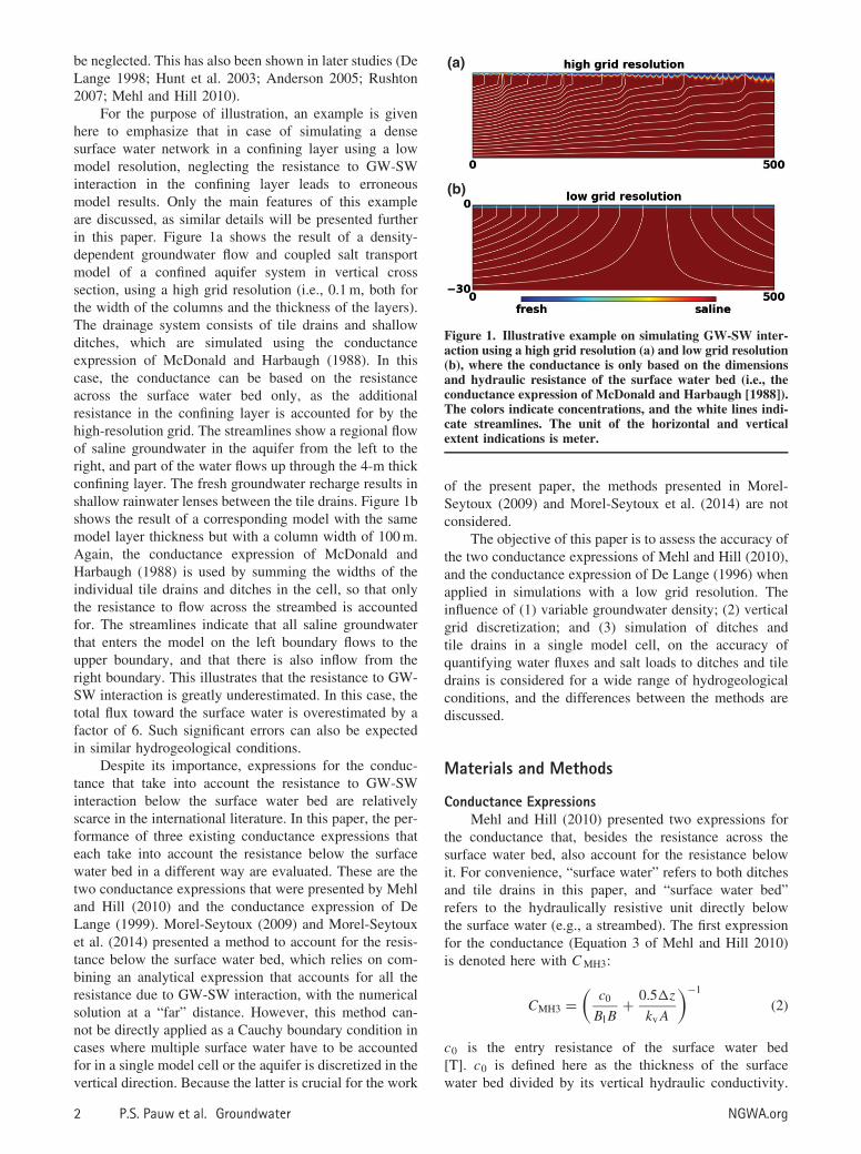
De Lange (1996, 1999) presented an expression forthe conductance based on an analytical solution of arepresentative local flow system; the interaction betweena regional aquifer, a relatively thin upper aquifer (in ourcase, a confining layer), and surface water (Figure 2). Forthis system, De Lange (1999) derived an expression forthe resistance to flow toward or from the surface water,based on the parameters B , c0, c1 (vertical resistance ofthe layer below the confining layer [T]), H (thicknessof the confining layer [L]), kh (horizontal hydraulicconductivity in the confining layer [L/T]), kv (verticalhydraulic conductivity in the confining layer), and L (thedistance between the surface water [L]). Based uponhis work, the expression for the resistance to GW-SWinteraction used in this paper (cPL; the phreatic leakage

semi-confining layer

regional aquifer

0.5 B

H

0.5 L

C0

C1

kh, kv

N

no fl

ow

no fl

ow

GW-SWinteraction

aquifers interaction

surface water

Figure 2. Concept that De Lange (1999) used to derive cPL(Equation 4).

resistance) is

cPL = 1ω

c∗B(c

∗L+crad)

+ (1−ω)

(c∗L+crad) 1

E

− c′1 (4)

ω is the areal percentage of the surface water in the gridcell. In two-dimensional (2D) cross section, ω is equal toB /(L + B ). E is a correction if L is larger than the widthof the grid cells. In this paper, L is always smaller than orequal to the width of the grid cells, and E equals 1. Theremaining expressions are

c∗B =

(c0 + c

′1

)c∗

L − c0L

B

c∗L =

(c0 + c

′1

)FL +

(c0L

B

)FB

Fi = i

2λi

cotanh

(i

2λi

), (i = B,L)

λB =√

kHc0c′1

c0 + c′1

c′1 = c1 + H

kv

crad = L

π√

khkvln

(4H

πB

√kh

kv

)(5)

c′1 and crad account for the vertical flow resistance and

radial flow resistance (i.e., resistance to flow due toconvergence of flow lines) within the confining layer,respectively. These terms are corrections for the Dupuitassumption. De Lange (1999) implemented these termsempirically using the superposition principle. The resultsof the solution with these empirical corrections havebeen verified with the results of a 2D analytical solutionby Bruggeman (1972), which does exactly account forthe resistance to vertical and radial flow. Note that crad

accounts for anisotropy by multiplication of the isotropichydraulic conductivity k by

√(khkv) and multiplication of

H by√

(kh/kv). Similar transformation procedures werepresented by Bear and Dagan (1965).

The conductance for a given type of surface water(e.g., with a comparable width and drainage level) using

NGWA.org P.S. Pauw et al. Groundwater 3

the method of De Lange (1999) is equal to the planar areaof the grid cell divided by cPL and is denoted in this paperwith C DL. In three-dimensional (3D) models, L is equal tothe planar area of the grid cell divided by the total lengthof that surface water in the grid cell. Further details onthe use C DL in 3D models can be found in De Lange(1996) and De Lange (1999). Note that although C DL isan overlooked conductance expression in the literature,it is successfully applied in the national hydrologicalinstrument of the Netherlands (De Lange et al. 2014).

Besides that C DL is based on an analytical solutionof a flow problem (Figure 2), it differs from C MH3 andC MH4 by two main aspects. First, C DL takes into account,in addition to the vertical flow resistance, the resistance tohorizontal flow and radial flow. Second, the correction forthe vertical flow resistance is not related to the distancebetween the node where the boundary condition is appliedand the bottom of the surface water bed, but on ananalytical expression for the concept shown in Figure 2.

Grid Resolution ComparisonsSEAWAT (Langevin et al. 2007) was used for the

numerical simulations. How the influence of variablegroundwater density, vertical grid discretization, and thesimulation of both ditches and drains in a single modelcell on the accuracy of C DL, C MH3, and C MH4 regardingwater and salt fluxes was analyzed is explained in the nextsections. The groundwater flow equation in SEAWAT wassolved using the PCG package (Hill 1990) with a headconvergence criterion of 10−6 m and the dispersion andsink and source terms of solute transport equation weresolved using the GCG package (Zheng and Wang 1999)with a convergence criterion of 10−6. Advection wassimulated using the MOC method with a Courant numberof 0.75 and a minimum number of 9 and a maximumnumber of 27 particles per grid cell.

Base ComparisonIn a “base comparison,” the model concept shown in

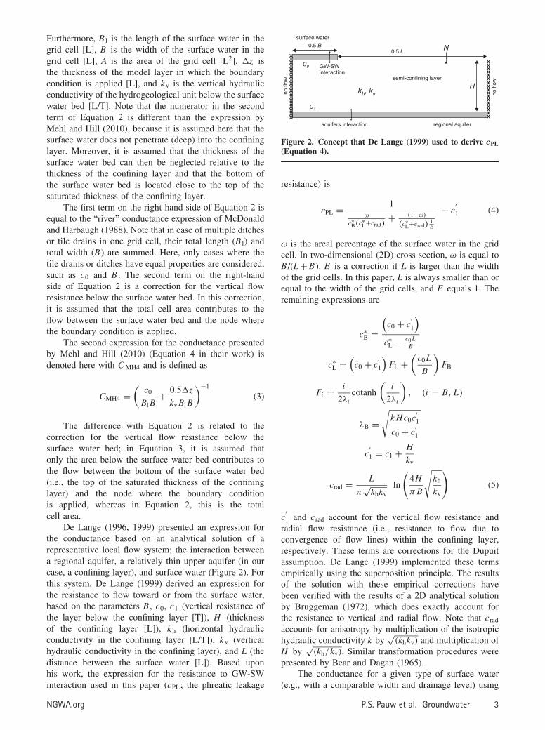
Figure 3 was used. It represents a section halfway betweenthe two tile drains in a confining layer that overlies aregional aquifer. The left and right boundaries are no-flow boundaries. The lower boundary is a constant-headboundary condition with hydraulic head φ [L], which ishigher than the drainage level. This results in an upwardflow from the bottom of the model. Related studies onshallow rainwater lenses (e.g., Eeman et al. 2011; DeLouw et al. 2013) have also used a similar boundarycondition at depth to simulate the upward flow of salinegroundwater. A tile drain is present in the region 0.5Bdr.In the region 0.5Ldr, there is fresh groundwater rechargewith a rate N [L/T].

A high (reference) grid resolution and a low gridresolution were used for this model. In the reference gridresolution, the columns have a width (�x ) of 0.05 m and alayer thickness (�z ) of 0.1 m in the confining layer. In theunderlying aquifer, �z increases steadily with depth. Forthe conductance of the tile drain, the method of McDonaldand Harbaugh (1988) was used. A comparison with a

H

0.5 Ldrdr

N0.5 B

0 m

-20 m


regional aquifer

drain

Figure 3. Model setup for the base comparison and forinvestigating the influence of vertical discretization andvariable groundwater density on the accuracy of C DL, C MH3,and CMH4.

higher grid resolution with a �x of 0.01 m indicateda relative difference in fluxes of less than 1%, whichindicates that a sufficiently fine grid for the referenceresolution was used.

For the low grid resolution, the same layer thicknessas in the reference grid resolution was used, but thecolumn width (�x ) is equal to 0.5(Ldr + Bdr). For theconductance, C MH3, C MH4, and C DLwere used. In whatfollows, C MH3, C MH4, and C DL will refer to the low gridresolution.

The two grid resolutions were compared by analyzinga relative error in the flux toward the tile drain ε for C DL,C MH3, and C MH4:

ε = Qlow − Qref

Qref× 100 (6)

Q ref is the volumetric flux toward the tile drain using thereference grid resolution and Q low is the volumetric fluxtoward the tile drain using the low grid resolution.

In the base comparison, variable density groundwaterflow and dispersive salt transport take place in anisotropic regional confined aquifer system. The aquiferhas a hydraulic conductivity of 20 m/d. The longitudinaldispersivity in the system is 0.1 m, and the horizontaland vertical transversal dispersivity is 0.01 m. Salt contentis expressed as chloride concentration. The chlorideconcentration (Cl) varies between 0 (fresh water) and18.63 g/L (salt water), corresponding to a groundwaterdensity of 1000 and 1025 kg/m3, respectively. Cl varieslinearly with groundwater density. The initial Cl in themodel domain is 18.63 g/L. Fresh groundwater rechargewith a rate of 0.001 m/d takes place in the upper modellayer. The hydraulic head φ in the bottom layer is 0.5 m,and the drainage level in the top layer is 0 m. The tile drainwas implemented using the DRAIN package of SEAWAT.The thickness of the tile drain envelope divided by thehydraulic conductivity of the drain envelope (this ratio isreferred to as the entry resistance) was assumed to be 1d, and the tile drain has a perimeter of 0.3 m. The modelswere analyzed at steady state regarding the total mass inthe model domain.

A wide range of hydrogeological conditions repre-sentative for confined systems in deltaic coastal areas wasconsidered, using a sensitivity analysis based on variationof the parameters H, Ldr (the distance between the tile


drains), and homogeneous k (i.e., for the confining layer).These parameters were related based on the Hooghoudtrelationship (Hooghoudt 1940), which is common in thedrainage design, avoids unrealistic parameter combina-tions, and reduces the parameters space in the sensitivityanalysis:

N = 8kd�h + 4k (�h)2

L2dr

(7)

where N is the recharge rate, �h is the difference inmaximum hydraulic head between the tile drains, andd is the effective depth of groundwater flow. d can becalculated using the equation of Moody (1966):

d = H

1 + 8HπLdr

ln HBdr

(8)

Because d also depends on Ldr, Equations 7 and 8 shouldbe solved iteratively to calculate Ldr for a given N , �h ,k, Bdr, and H . In this relationship between H , Ldr andk , N and �h were assumed to be 0.007 m/d and 0.5 m,respectively (common values in the tile drainage design[ILRI 1973]), and Bdr was held constant at 0.3 m. H variesbetween 2, 4, and 6 m, and k ranges from 0.05 to 0.5 m/d.

Influence of Variable Groundwater DensityThe influence of variable groundwater density was

investigated by comparing all simulations of the basecomparison with the corresponding constant groundwaterdensity simulations. In addition, the influence of a lowerhydraulic head (0.1 m) at the bottom of the model wasinvestigated. The rationale of investigating the influenceof a lower hydraulic head is that it influences the variablegroundwater density flow, because a system of mixedconvection was considered. Amongst others, the differenthydraulic head at the bottom of the model affects thethickness of the shallow fresh water lens that formsbetween tile drains (Figure 1).

Influence of Vertical DiscretizationFor the influence of vertical discretization, the same

approach as in the base comparison was used, butwith a layer thickness �z of 2 m in the low gridresolution. An influence of vertical discretization can beexpected as C MH3 and C MH4 depend on �z , and C DL

was derived for situations where the confining layer isnot discretized vertically. Note that in density-dependentgroundwater flow and solute transport models, more layersare generally used compared to constant density models(Langevin 2003).

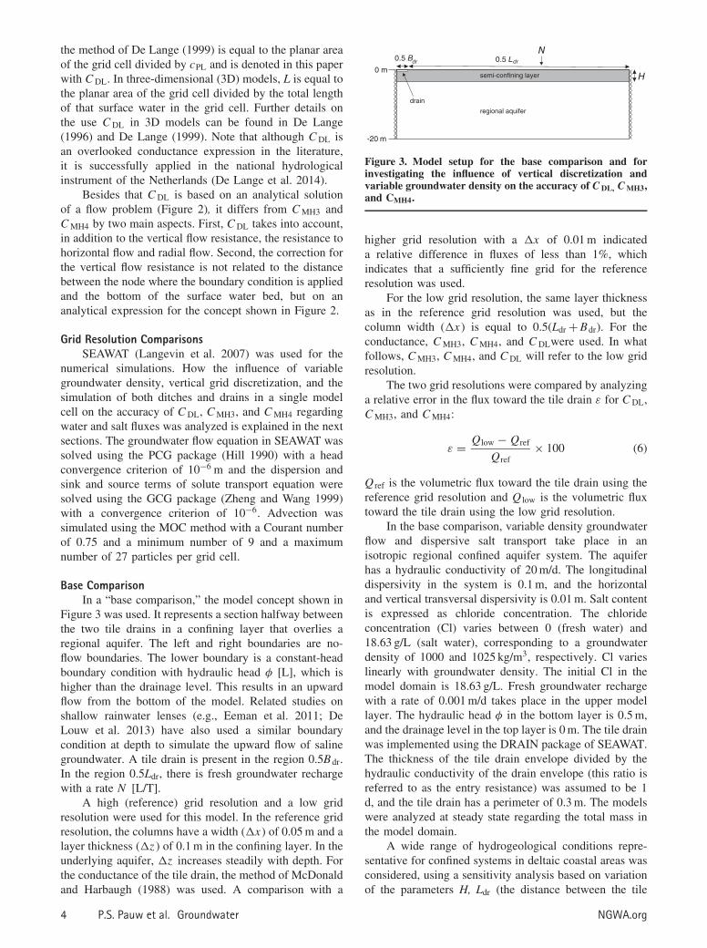
Simulation of Ditches and Tile DrainsThe rationale of investigating the influence of simu-

lating both ditches and tile drains in a single model cell onthe accuracy C MH3, C MH4, and C DL was twofold. First,ditches may have different dimensions and properties thantile drains in the model cell. These different properties

H

0.5Ldt

N0.5 Bdt

0 m

-20 m


regional aquifer

ditch drain

Ldr

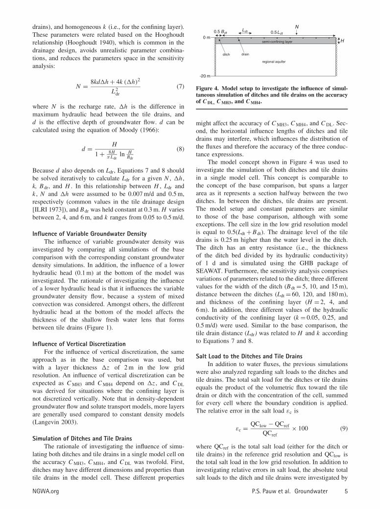
Figure 4. Model setup to investigate the influence of simul-taneous simulation of ditches and tile drains on the accuracyof C DL, C MH3, and C MH4.

might affect the accuracy of C MH3, C MH4, and C DL. Sec-ond, the horizontal influence lengths of ditches and tiledrains may interfere, which influences the distribution ofthe fluxes and therefore the accuracy of the three conduc-tance expressions.

The model concept shown in Figure 4 was used toinvestigate the simulation of both ditches and tile drainsin a single model cell. This concept is comparable tothe concept of the base comparison, but spans a largerarea as it represents a section halfway between the twoditches. In between the ditches, tile drains are present.The model setup and constant parameters are similarto those of the base comparison, although with someexceptions. The cell size in the low grid resolution modelis equal to 0.5(Ldt + Bdt). The drainage level of the tiledrains is 0.25 m higher than the water level in the ditch.The ditch has an entry resistance (i.e., the thicknessof the ditch bed divided by its hydraulic conductivity)of 1 d and is simulated using the GHB package ofSEAWAT. Furthermore, the sensitivity analysis comprisesvariations of parameters related to the ditch; three differentvalues for the width of the ditch (Bdt = 5, 10, and 15 m),distance between the ditches (Ldt = 60, 120, and 180 m),and thickness of the confining layer (H = 2, 4, and6 m). In addition, three different values of the hydraulicconductivity of the confining layer (k = 0.05, 0.25, and0.5 m/d) were used. Similar to the base comparison, thetile drain distance (Ldr) was related to H and k accordingto Equations 7 and 8.

Salt Load to the Ditches and Tile DrainsIn addition to water fluxes, the previous simulations

were also analyzed regarding salt loads to the ditches andtile drains. The total salt load for the ditches or tile drainsequals the product of the volumetric flux toward the tiledrain or ditch with the concentration of the cell, summedfor every cell where the boundary condition is applied.The relative error in the salt load εc is

εc = QClow − QCref

QCref× 100 (9)

where QCref is the total salt load (either for the ditch ortile drains) in the reference grid resolution and QClow isthe total salt load in the low grid resolution. In addition toinvestigating relative errors in salt load, the absolute totalsalt loads to the ditch and tile drains were investigated by


analyzing the simulations on the difference in total saltload between the low grid resolution and reference gridresolution, per unit area (�QC):

�QC = QCcrs

Acrs− QCref

Acrs(10)

where Acrs is the area of the cell in the low grid resolutionmodel.

ResultsFor convenience, the discussion of the results regard-

ing C MH3, C MH4, and C DL is based on resistances.

Base ComparisonFigure 5 shows ε for all the parameter combina-

tions in the base comparison, where the reference gridresolution was compared with a low grid resolution (inwhich �x was equal to 0.5(Ldr + Bdr)). The most impor-tant observation from Figure 5 is the difference betweenC MH3, C MH4, and C DL; C DL performs much better thanC MH3 and C MH4. This is also indicated in Table 1, wherethe average absolute value of ε among all parameter com-binations (|εav|) is given.

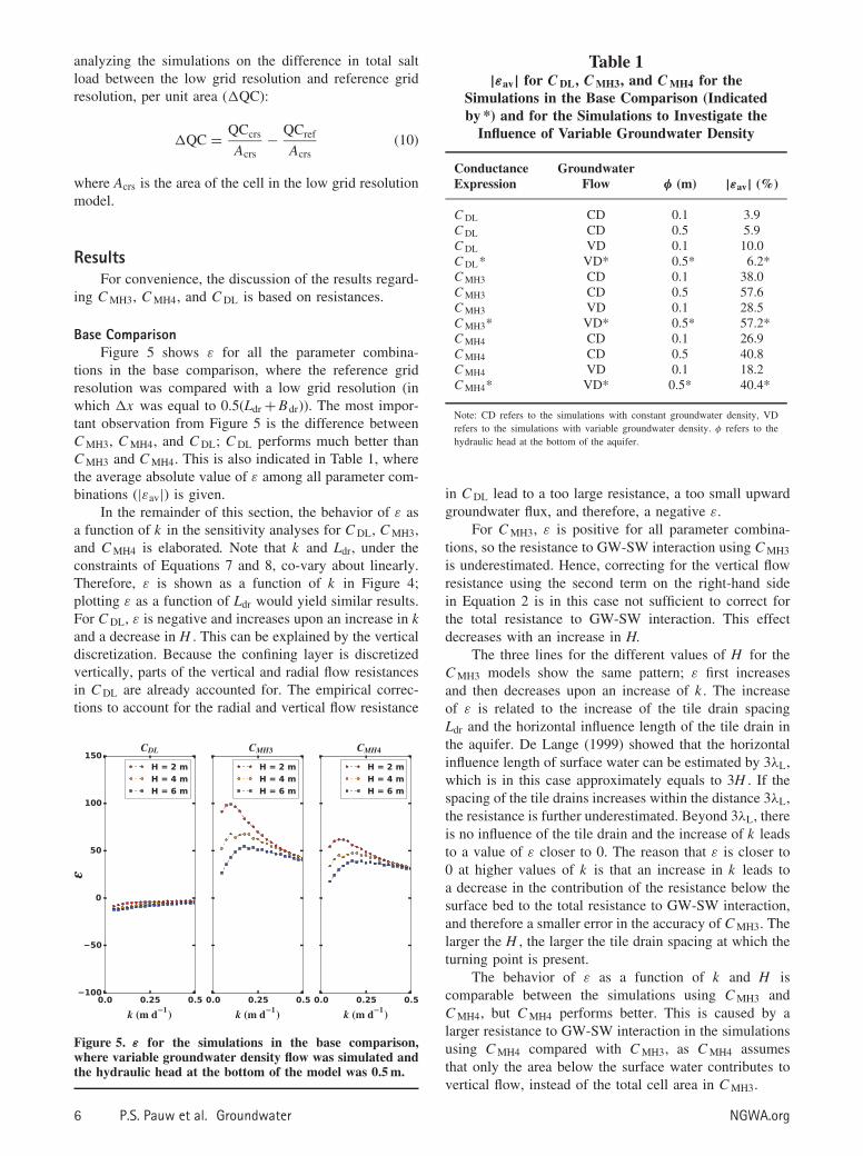
In the remainder of this section, the behavior of ε asa function of k in the sensitivity analyses for C DL, C MH3,and C MH4 is elaborated. Note that k and Ldr, under theconstraints of Equations 7 and 8, co-vary about linearly.Therefore, ε is shown as a function of k in Figure 4;plotting ε as a function of Ldr would yield similar results.For C DL, ε is negative and increases upon an increase in kand a decrease in H . This can be explained by the verticaldiscretization. Because the confining layer is discretizedvertically, parts of the vertical and radial flow resistancesin C DL are already accounted for. The empirical correc-tions to account for the radial and vertical flow resistance

Figure 5. ε for the simulations in the base comparison,where variable groundwater density flow was simulated andthe hydraulic head at the bottom of the model was 0.5 m.

Table 1|εav| for C DL, C MH3, and C MH4 for the

Simulations in the Base Comparison (Indicatedby *) and for the Simulations to Investigate the

Influence of Variable Groundwater Density

ConductanceExpression

GroundwaterFlow φ (m) |εav| (%)

C DL CD 0.1 3.9C DL CD 0.5 5.9C DL VD 0.1 10.0C DL* VD* 0.5* 6.2*C MH3 CD 0.1 38.0C MH3 CD 0.5 57.6C MH3 VD 0.1 28.5C MH3* VD* 0.5* 57.2*C MH4 CD 0.1 26.9C MH4 CD 0.5 40.8C MH4 VD 0.1 18.2C MH4* VD* 0.5* 40.4*

Note: CD refers to the simulations with constant groundwater density, VDrefers to the simulations with variable groundwater density. φ refers to thehydraulic head at the bottom of the aquifer.

in C DL lead to a too large resistance, a too small upwardgroundwater flux, and therefore, a negative ε.

For C MH3, ε is positive for all parameter combina-tions, so the resistance to GW-SW interaction using C MH3

is underestimated. Hence, correcting for the vertical flowresistance using the second term on the right-hand sidein Equation 2 is in this case not sufficient to correct forthe total resistance to GW-SW interaction. This effectdecreases with an increase in H.

The three lines for the different values of H for theC MH3 models show the same pattern; ε first increasesand then decreases upon an increase of k . The increaseof ε is related to the increase of the tile drain spacingLdr and the horizontal influence length of the tile drain inthe aquifer. De Lange (1999) showed that the horizontalinfluence length of surface water can be estimated by 3λL,which is in this case approximately equals to 3H . If thespacing of the tile drains increases within the distance 3λL,the resistance is further underestimated. Beyond 3λL, thereis no influence of the tile drain and the increase of k leadsto a value of ε closer to 0. The reason that ε is closer to0 at higher values of k is that an increase in k leads toa decrease in the contribution of the resistance below thesurface bed to the total resistance to GW-SW interaction,and therefore a smaller error in the accuracy of C MH3. Thelarger the H , the larger the tile drain spacing at which theturning point is present.

The behavior of ε as a function of k and H iscomparable between the simulations using C MH3 andC MH4, but C MH4 performs better. This is caused by alarger resistance to GW-SW interaction in the simulationsusing C MH4 compared with C MH3, as C MH4 assumesthat only the area below the surface water contributes tovertical flow, instead of the total cell area in C MH3.


Variable Groundwater DensityFor the simulations to investigate the influence of

variable groundwater density, the relative behavior of ε

as a function of k is comparable to the results of thebase comparison. For brevity, the corresponding figuresare given in the Supporting Information in the onlineversion of this article. The absolute errors, however, showdifferences. Table 1 shows the average of the absolute ε

of the simulations (|εav|). The most important observationfrom Table 1 is the difference in |εav| between C MH3,C MH4, and C DL; C DL performs much better than C MH3

and C MH4 for the different values of φ, independent ofwhether variable density groundwater flow is simulatedor not.

The influence of variable groundwater density onC MH3, C MH4, and C DL is small in case of φ = 0.5 m.For φ = 0.1 m, variable groundwater density leads toan increase of |εav| using C DL, but a decrease usingeither C MH3 or C MH4. The higher influence of variablegroundwater density at lower values of φ could beexpected, as the influence of variable groundwater densityin this forced convection setting increases with decreasingvalues of φ. The influence of a higher hydraulic head atthe bottom of the aquifer on |εav| is moderate for C DL

relative to C MH3 and C MH4.

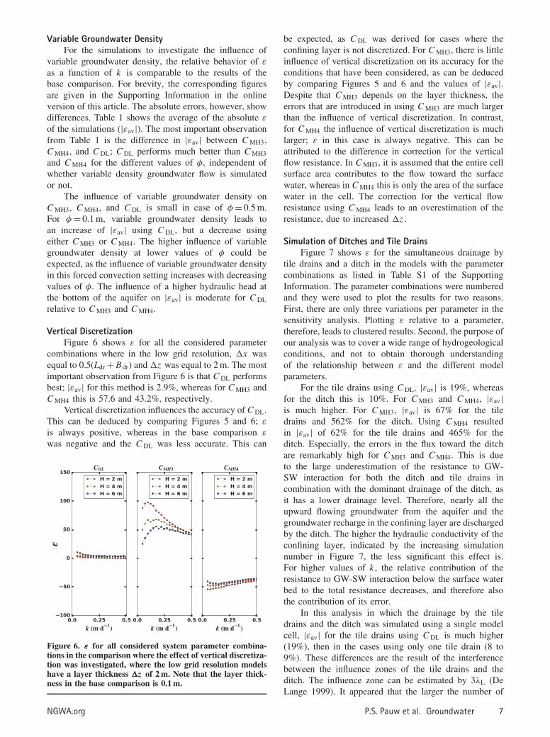
Vertical DiscretizationFigure 6 shows ε for all the considered parameter

combinations where in the low grid resolution, �x wasequal to 0.5(Ldr + Bdr) and �z was equal to 2 m. The mostimportant observation from Figure 6 is that C DL performsbest; |εav| for this method is 2.9%, whereas for C MH3 andC MH4 this is 57.6 and 43.2%, respectively.

Vertical discretization influences the accuracy of C DL.This can be deduced by comparing Figures 5 and 6; ε

is always positive, whereas in the base comparison ε

was negative and the C DL was less accurate. This can

Figure 6. ε for all considered system parameter combina-tions in the comparison where the effect of vertical discretiza-tion was investigated, where the low grid resolution modelshave a layer thickness �z of 2 m. Note that the layer thick-ness in the base comparison is 0.1 m.

be expected, as C DL was derived for cases where theconfining layer is not discretized. For C MH3, there is littleinfluence of vertical discretization on its accuracy for theconditions that have been considered, as can be deducedby comparing Figures 5 and 6 and the values of |εav|.Despite that C MH3 depends on the layer thickness, theerrors that are introduced in using C MH3 are much largerthan the influence of vertical discretization. In contrast,for C MH4 the influence of vertical discretization is muchlarger; ε in this case is always negative. This can beattributed to the difference in correction for the verticalflow resistance. In C MH3, it is assumed that the entire cellsurface area contributes to the flow toward the surfacewater, whereas in C MH4 this is only the area of the surfacewater in the cell. The correction for the vertical flowresistance using C MH4 leads to an overestimation of theresistance, due to increased �z .

Simulation of Ditches and Tile DrainsFigure 7 shows ε for the simultaneous drainage by

tile drains and a ditch in the models with the parametercombinations as listed in Table S1 of the SupportingInformation. The parameter combinations were numberedand they were used to plot the results for two reasons.First, there are only three variations per parameter in thesensitivity analysis. Plotting ε relative to a parameter,therefore, leads to clustered results. Second, the purpose ofour analysis was to cover a wide range of hydrogeologicalconditions, and not to obtain thorough understandingof the relationship between ε and the different modelparameters.

For the tile drains using C DL, |εav| is 19%, whereasfor the ditch this is 10%. For C MH3 and C MH4, |εav|is much higher. For C MH3, |εav| is 67% for the tiledrains and 562% for the ditch. Using C MH4 resultedin |εav| of 62% for the tile drains and 465% for theditch. Especially, the errors in the flux toward the ditchare remarkably high for C MH3 and C MH4. This is dueto the large underestimation of the resistance to GW-SW interaction for both the ditch and tile drains incombination with the dominant drainage of the ditch, asit has a lower drainage level. Therefore, nearly all theupward flowing groundwater from the aquifer and thegroundwater recharge in the confining layer are dischargedby the ditch. The higher the hydraulic conductivity of theconfining layer, indicated by the increasing simulationnumber in Figure 7, the less significant this effect is.For higher values of k , the relative contribution of theresistance to GW-SW interaction below the surface waterbed to the total resistance decreases, and therefore alsothe contribution of its error.

In this analysis in which the drainage by the tiledrains and the ditch was simulated using a single modelcell, |εav| for the tile drains using C DL is much higher(19%), then in the cases using only one tile drain (8 to9%). These differences are the result of the interferencebetween the influence zones of the tile drains and theditch. The influence zone can be estimated by 3λL (DeLange 1999). It appeared that the larger the number of


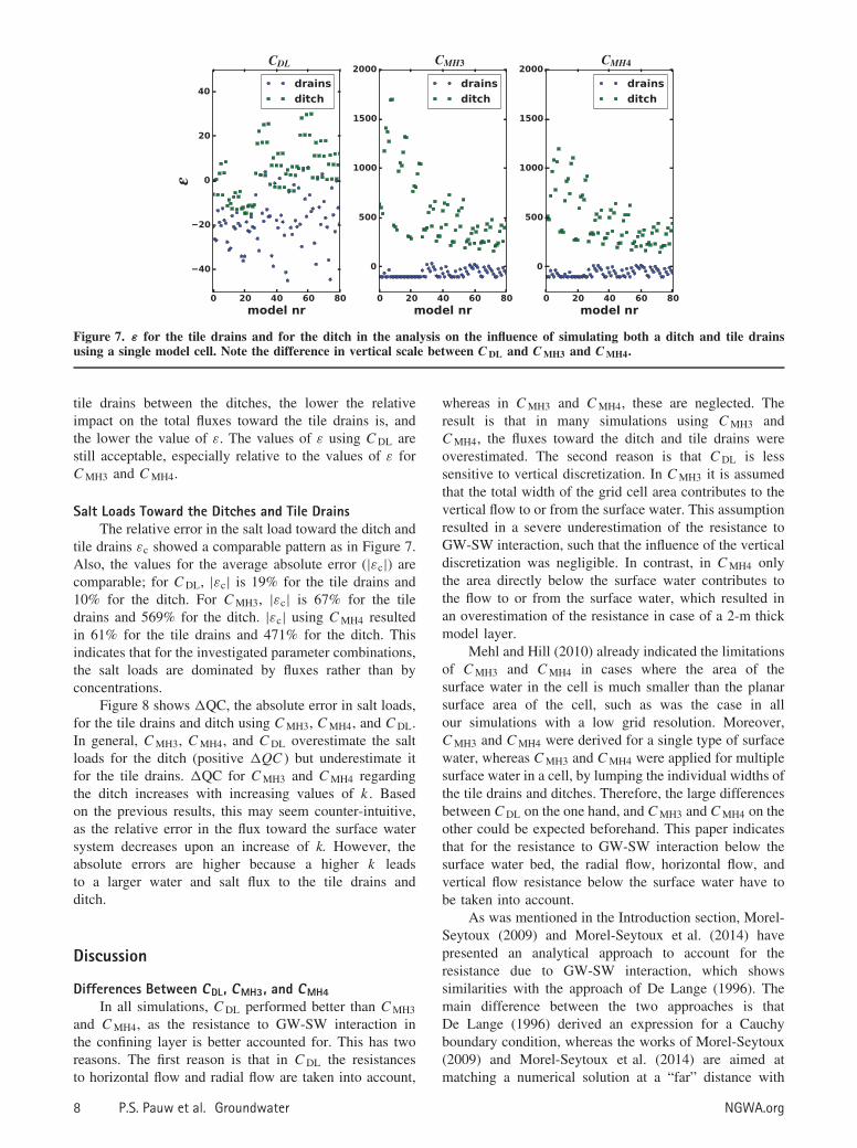
Figure 7. ε for the tile drains and for the ditch in the analysis on the influence of simulating both a ditch and tile drainsusing a single model cell. Note the difference in vertical scale between C DL and C MH3 and C MH4.

tile drains between the ditches, the lower the relativeimpact on the total fluxes toward the tile drains is, andthe lower the value of ε. The values of ε using C DL arestill acceptable, especially relative to the values of ε forC MH3 and C MH4.

Salt Loads Toward the Ditches and Tile DrainsThe relative error in the salt load toward the ditch and

tile drains εc showed a comparable pattern as in Figure 7.Also, the values for the average absolute error (|εc|) arecomparable; for C DL, |εc| is 19% for the tile drains and10% for the ditch. For C MH3, |εc| is 67% for the tiledrains and 569% for the ditch. |εc| using C MH4 resultedin 61% for the tile drains and 471% for the ditch. Thisindicates that for the investigated parameter combinations,the salt loads are dominated by fluxes rather than byconcentrations.

Figure 8 shows �QC, the absolute error in salt loads,for the tile drains and ditch using C MH3, C MH4, and C DL.In general, C MH3, C MH4, and C DL overestimate the saltloads for the ditch (positive �QC ) but underestimate itfor the tile drains. �QC for C MH3 and C MH4 regardingthe ditch increases with increasing values of k . Basedon the previous results, this may seem counter-intuitive,as the relative error in the flux toward the surface watersystem decreases upon an increase of k. However, theabsolute errors are higher because a higher k leadsto a larger water and salt flux to the tile drains andditch.

Discussion

Differences Between CDL, CMH3, and CMH4In all simulations, C DL performed better than C MH3

and C MH4, as the resistance to GW-SW interaction inthe confining layer is better accounted for. This has tworeasons. The first reason is that in C DL the resistancesto horizontal flow and radial flow are taken into account,

whereas in C MH3 and C MH4, these are neglected. Theresult is that in many simulations using C MH3 andC MH4, the fluxes toward the ditch and tile drains wereoverestimated. The second reason is that C DL is lesssensitive to vertical discretization. In C MH3 it is assumedthat the total width of the grid cell area contributes to thevertical flow to or from the surface water. This assumptionresulted in a severe underestimation of the resistance toGW-SW interaction, such that the influence of the verticaldiscretization was negligible. In contrast, in C MH4 onlythe area directly below the surface water contributes tothe flow to or from the surface water, which resulted inan overestimation of the resistance in case of a 2-m thickmodel layer.

Mehl and Hill (2010) already indicated the limitationsof C MH3 and C MH4 in cases where the area of thesurface water in the cell is much smaller than the planarsurface area of the cell, such as was the case in allour simulations with a low grid resolution. Moreover,C MH3 and C MH4 were derived for a single type of surfacewater, whereas C MH3 and C MH4 were applied for multiplesurface water in a cell, by lumping the individual widths ofthe tile drains and ditches. Therefore, the large differencesbetween C DL on the one hand, and C MH3 and C MH4 on theother could be expected beforehand. This paper indicatesthat for the resistance to GW-SW interaction below thesurface water bed, the radial flow, horizontal flow, andvertical flow resistance below the surface water have tobe taken into account.

As was mentioned in the Introduction section, Morel-Seytoux (2009) and Morel-Seytoux et al. (2014) havepresented an analytical approach to account for theresistance due to GW-SW interaction, which showssimilarities with the approach of De Lange (1996). Themain difference between the two approaches is thatDe Lange (1996) derived an expression for a Cauchyboundary condition, whereas the works of Morel-Seytoux(2009) and Morel-Seytoux et al. (2014) are aimed atmatching a numerical solution at a “far” distance with


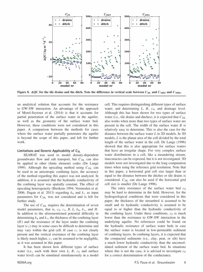
Figure 8. �QC for the tile drains and the ditch. Note the difference in vertical scale between C DL and C MH3 and C MH4.

an analytical solution that accounts for the resistanceto GW-SW interaction. An advantage of the approachof Morel-Seytoux et al. (2014) is that it accounts forpartial penetration of the surface water in the aquifer,as well as the geometry of the surface water bed.However, these conditions were not considered in thispaper. A comparison between the methods for caseswhere the surface water partially penetrates the aquiferis beyond the scope of this paper, and left for furtherwork.

Limitations and Generic Applicability of CDLSEAWAT was used to model density-dependent

groundwater flow and salt transport, but C DL can alsobe applied in other (finite element) codes (De Lange1999). Although the upscaling method using C DL canbe used in an anisotropic confining layer, the accuracyof the method regarding this aspect was not analyzed. Inaddition, it is assumed that the hydraulic conductivity ofthe confining layer was spatially constant. The effect ofupscaling heterogeneity (Bierkens 1994; Vermeulen et al.2006; Dagan et al. 2013) regarding kh and kv as inputparameters for C DL was not considered and is left forfurther study.

The use of C DL requires the determination of sevenmodel parameters, that is, c0, c1, B, L, kh, kv, and H .In addition to the aforementioned potential difficulty indetermining kh and kv, the thickness of the confining layer(H ) and the resistance of the layer under the confininglayer (c1) may in some cases be difficult to determine andmay vary within the grid cell. If case c1 is not clearlypresent and the vertical resistance of the confining layeris likely much higher, c1 can be assumed to be negligible,as it was assumed in this paper.

It has been shown how different types of surfacewater (i.e., each with their own L, B , c0 and surfacewater level) can be simulated simultaneously in a model

cell. This requires distinguishing different types of surfacewater, and determining L, B , c0, and drainage level.Although this has been shown for two types of surfacewater (i.e., tile drains and ditches), it is expected that C DL

also works when more than two types of surface water arepresent in the cell. The width of the surface water B isrelatively easy to determine. This is also the case for thedistance between the surface water L in 2D models. In 3Dmodels, L is the planar area of the cell divided by the totallength of the surface water in the cell. De Lange (1996)showed that this is also appropriate for surface watersthat have an irregular shape. For very complex surfacewater distributions in a cell, like a meandering stream,inaccuracies can be expected, but it is not investigated. 3Dmodels were not investigated due to the long computationtimes when using the reference grid resolution. Note thatin this paper, a horizontal grid cell size larger than orequal to the distance between the ditches or tile drains isconsidered. C DL can also be used if the horizontal gridcell size is smaller (De Lange 1996).

The entry resistance of the surface water bed c0

may be hard to determine in the field. However, for thehydrogeological conditions that were considered in thispaper, the thickness of the streambed is assumed to besmall and its hydraulic conductivity is assumed to beequal to or higher than the hydraulic conductivity ofthe confining layer. Under these conditions, c0 is muchlower than the resistance to GW-SW interaction in theunderlying aquifer. No references could be found onthe hydraulic resistance of surface water beds in casethe surface water is located in low-permeable sedimentof confining layers. In confining layers, it is expected thatthe compacted sediments (i.e., clay, peat, or silt) havea much lower hydraulic conductivity than the unconsol-idated sediment of the surface water bed. In situationswhere this is not the case, it is advised to investigate c0

for a correct determination of the conductance.


ConclusionsIn numerical groundwater flow models of confined

aquifers using a low grid resolution, the resistance toGW-SW interaction below the surface water bed is impor-tant to take into account for determining the conductance.For the different aspects and hydrogeological conditionsthat were considered in this work, the conductance expres-sion C DL performed better than the expressions C MH3

and C MH4 as it better accounts for the horizontal, verti-cal, and radial flow resistance to GW-SW interaction inthe confining layer. The influence of variable groundwaterdensity and vertical grid discretization on the accuracy ofquantifying water and salt fluxes using C DL was small.

AcknowledgmentsThe authors thank Steffen Mehl and an anony-

mous reviewer for their comments, which significantlyimproved this paper. They also thank Jacco Hoogewoudfor his comments and discussions about the results inthis paper. This work was carried out within the Dutch“Knowledge for Climate” program.

Supporting InformationAdditional Supporting Information may be found in theonline version of this article:

Table S1. Parameter combinations for the investigationof the influence of the simultaneous simulation of ditchesand tile drains, per model number.Figure S1. This figure shows ε for all considered systemparameter combinations in the simulations with constantgroundwater density flow and a constant head at thebottom of the aquifer of 0.5 m.Figure S2. This figure shows ε for all considered systemparameter combinations in the simulations with variablegroundwater density flow and a constant head at thebottom of the aquifer of 0.1 m.Figure S3. This figure shows ε for all considered systemparameter combinations in the simulations with constantgroundwater density flow and a constant head at thebottom of the aquifer of 0.1 m.

ReferencesAnderson, E.I. 2005. Modeling groundwater–surface water

interactions using the Dupuit approximation. Advances inWater Resources 28, no. 4: 315–327.

Bear, J., and G. Dagan. 1965. The relationship between solutionsof flow problems in isotropic and anisotropic soils. Journalof Hydrology 3, no. 2: 88–96.

Bierkens, M.F.P. 1994. Complex confining layers: A stochasticanalysis of hydraulic properties at various scales. Ph.D.thesis, Utrecht University, Utrecht, The Netherlands.

Bruggeman, G.A. 1972. Twee-Dimensional Stroming in Semi-spanningwater (Two-Dimensional Flow in a Semi-confinedAquifer) Appendix to Report De Groeve. Leidschendam,The Netherlands: National Institute for Water Supply.

Cobaner, M., R. Yurtal, A. Dogan, and L.H. Motz. 2012. Threedimensional simulation of seawater intrusion in coastal

aquifers: A case study in the Goksu Deltaic Plain. Journalof Hydrology 464–465: 262–280.

Custodio, E., and G.A. Bruggeman. 1987. Groundwater Prob-lems in Coastal Areas, Studies and Reports in Hydrol-ogy (International Hydrological Programme). Paris, France:UNESCO.

Dagan, G., A. Fiori, and I. Jankovic. 2013. Upscaling of flowin heterogeneous porous formations: Critical examinationand issues of principle. Advances in Water Resources 51:67–85.

De Lange, W.J., G.F. Prinsen, J.C. Hoogewoud, A. Veldhuizen,J. Verkaik, G.H.P. Oude Essink, P.E.V. van Walsum, J.R.Delsman, J.C. Hunink, H.T.L. Massop, and T. Kroon.2014. An operational, multi-scale, multi-model systemfor consensus-based, integrated water management andpolicy analysis: The Netherlands Hydrological Instrument.Environmental Modelling & Software 59: 98–108.

De Lange, W.J. 1999. A Cauchy boundary condition for thelumped interaction between an arbitrary number of surfacewaters and a regional aquifer. Journal of Hydrology 226:250–261.

De Lange, W.J. 1998. On the errors involved with the parame-terization of the MODFLOW river and drainage packages.In MODFLOW’98 Proceedings of the 3rd InternationalConference of the International Ground Water Modeling ,Vol. 1, ed. E. Poeter, Z. Zheng, and M. Hill, 249–256.Golden, Colorado.

De Lange, W.J. 1996. Groundwater modelling of large domainswith analytic elements. Ph.D. thesis, Delft University ofTechnology, Delft, The Netherlands.

De Louw, P.G.B., S. Eeman, G.H.P. Oude Essink, E. Vermue,and V.E.A. Post. 2013. Rainwater lens dynamics andmixing between infiltrating rainwater and upward salinegroundwater seepage beneath a tile-drained agriculturalfield. Journal of Hydrology 501: 133–145.

Eeman, S., A. Leijnse, P.A.C. Raats, and S.E.A.T.M. van derZee. 2011. Analysis of the thickness of a fresh waterlens and of the transition zone between this lens andupwelling saline water. Advances in Water Resources 34,no. 2: 291–302.

Faneca Sanchez, M., J.L. Gunnink, E.S. van Baaren, G.H.P.Oude Essink, B. Siemon, E. Auken, and W. Elderhorst.2012. Modelling climate change effects on a Dutchcoastal groundwater system using airborne electromagneticmeasurements. Hydrology and Earth System Sciences 16:4499–4516.

Hill, M.C. 1990. Preconditioned conjugate-gradient 2 (PCG), acomputer program for solving ground-water flow equations.Water-Resources Investigations Report 90-4048. Reston,Virginia: U.S. Geological Survey.

Hooghoudt, S.B. 1940. General consideration of the problem offield drainage by parallel drains, ditches, watercourses, andchannels. In Contribution to the Knowledge of Some Phys-ical Parameters of the Soil , Publ. No. 7 (titles translatedfrom Dutch). Groningen, The Netherlands: BodemkundigInstituut.

Hunt, R.J., H.M. Haitjema, J.T. Krohelski, and D.T. Fein-stein. 2003. Simulating ground water–lake interactions:Approaches and insight. Ground Water 41, no. 2: 227–237.

ILRI. 1973. Drainage Principles and Applications . Wageningen,The Netherlands: International Institute for Land Reclama-tion and Improvement.

Langevin, C.D., and M. Zygnerski. 2013. Effect of sea-levelrise on salt water intrusion near a coastal well field inSoutheastern Florida. Groundwater 51, no. 5: 781–803.

Langevin, C.D., D.T. Thorne Jr., A.M. Dausman, M.C. Sukop,and W. Guo. 2007. SEAWAT Version 4: A ComputerProgram for Simulation of Multi-Species Solute and HeatTransport: U.S. Geological Survey Techniques and MethodsBook 6, Chapter A22. Reston, Virginia: U.S. GeologicalSurvey.


Langevin, C.D. 2003. Simulation of submarine ground waterdischarge to a marine estuary: Biscayne Bay, Florida.Ground Water 41, no. 6: 758–771.

McDonald, M.G., and A.W. Harbaugh. 1988. A Modular Three-Dimensional Finite-Difference Ground-Water Flow Model.US Geological Survey Techniques of Water-ResourcesInvestigations, Book 6 . Reston, Virginia: U.S. GeologicalSurvey.

Mehl, S., and M.C. Hill. 2010. Grid-size dependence of Cauchyboundary conditions used to simulate stream–aquiferinteractions. Advances in Water Resources 33: 430–442.

Moody, W.T. 1966. Nonlinear differential equation of drainspacing. Journal of Irrigation and Drainage Engineering92, no. 2: 1–10.

Morel-Seytoux, H.J., S. Mehl, and K. Morgado. 2014. Factorsinfluencing the stream-aquifer flow exchange coefficient.Groundwater 52: 775–781.

Morel-Seytoux, H.J. 2009. The turning factor in the estimationof stream–aquifer seepage. Ground Water 47: 205–212.

Oude Essink, G.H.P., E.S. van Baaren, and P.G.B. de Louw.2010. Effects of climate change on coastal groundwater

systems: A modeling study in the Netherlands. WaterResources Research 46, no. 10: 1–16.

Overeem, I., and J.P.M. Syvitski (Eds). 2009. Dynamics andVulnerability of Delta Systems, LOICZ Reports and StudiesNo 35. Geesthacht, Germany: GKSS Research Center.

Renard, P., and G. DeMarsily. 1997. Calculating equivalentpermeability: A review. Advances in Water Resources 20,no. 5/6: 253–278.

Rushton, K. 2007. Representation in regional models of saturatedriver–aquifer interaction for gaining/losing rivers. Journalof Hydrology 334: 262–281.

Vermeulen, P.T.M., C.B.M. te Stroet, and W. Heemink. 2006.Limitations to upscaling of groundwater flow modelsdominated by surface water interaction. Water ResourcesResearch 42, no. 10: 1–12.

Zheng, C., and P.P. Wang. 1999. MT3DMS: A Modular Three-Dimensional Multispecies Transport Model for Simulationof Advection, Dispersion and Chemical Reactions of Con-taminants in Groundwater Systems, Documentation andUser’s Guide. Tuscaloosa, Alabama: Alabama University.


Documents

Low-Resolution Modeling of Dense Drainage Networks in Conﬁning Layers