Embed Size (px)
Citation preview
University of Wollongong Thesis Collections
University of Wollongong Thesis Collection
University of Wollongong Year
Low-velocity pneumatic transportation of
bulk solids
Bo MiUniversity of Wollongong
Mi, Bo, Low-velocity pneumatic transportation of bulk solids, PhD thesis, Department ofMechanical Engineering, University of Wollongong, 1994. http://ro.uow.edu.au/theses/830
This paper is posted at Research Online.
http://ro.uow.edu.au/theses/830

DECLARATION
This is to certify that the work presented in this thesis was carried out by the author in the
Department of Mechanical Engineering at the University of WoUongong and has not been
submitted for a degree to any other university or institution.

Low-Velocity Pneumatic Transportation of Bulk Solids
ACKNOWLEDGMENTS
I would Uke to thank my supervisor, Dr P. W. Wypych, Senior Lecturer in the
Department of Mechanical Engineering at the University of Wollongong, for his
supervision, generous assistance and encouragement during the period of this study. I am
indebted to Professor P. C. Arnold, Dr A. Mclean, Mr O. Kennedy, Dr Z. Gu and Dr R.
Pan, the staff of the Bulk Materials Handling group, for their constructive suggestions in
the development of tiie theory.
I gratefuUy acknowledge the financial support of the University of Wollongong under the
Postgraduate Research Award scheme and the financial contribution by the Bulk
Materials Handling and Physical Processing research program.
Acknowledgment also is made of the assistance given by other staff of the department,
especially that of Mrs R. Hamlet and Mrs B. Butler, who completed many of the
administrative tasks associated with this project. My thanks are extended to the technical
staff in the Workshop and Bulk Solids Handling Laboratory with whose help and
expertise the experimental apparatus was constructed. In particular, I would like to
express my gratitude to Mr D. Cook, Mr I. Frew, Mrs W. Halford, Mr L McColm and
Mr S. Dunster.
Finally, special acknowledgment is made to my dear wife Yao Feng and my parents for
their unfailing help and encouragement.
Low-Velocity Pneumatic Transportation of Bulk Solids U
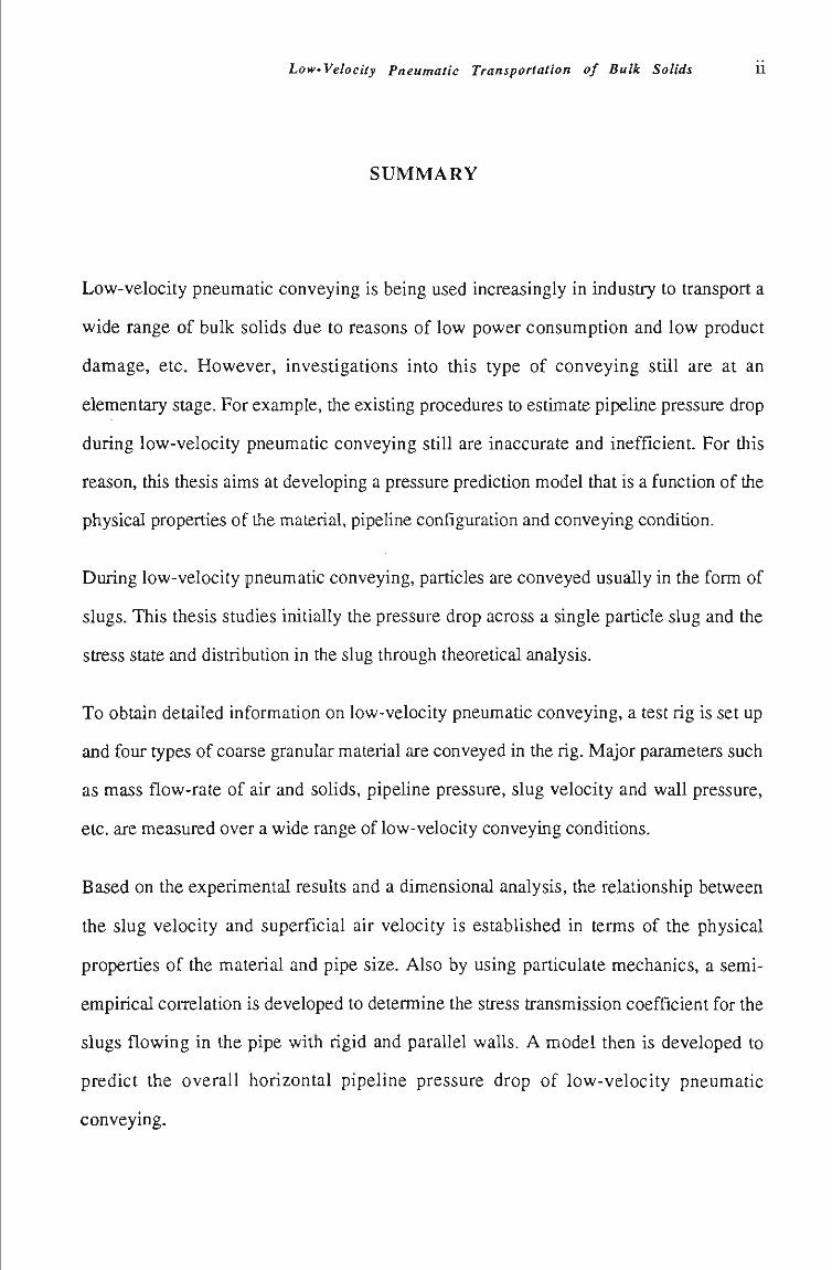
SUMMARY
Low-velocity pneumatic conveying is being used increasingly in industry to transport a
wide range of bulk soHds due to reasons of low power consumption and low product
damage, etc. However, investigations into this type of conveying still are at an
elementary stage. For example, the existing procedures to estimate pipeline pressure drop
during low-velocity pneumatic conveying stiH are inaccurate and inefficient. For this
reason, this thesis aims at developing a pressure prediction model that is a function of the
physical properties of the material, pipeline configuration and conveying condition.
During low-velocity pneumatic conveying, particles are conveyed usually in the form of
slugs. This thesis studies initially the pressure drop across a single particle slug and the
stress state and distribution in the slug through theoretical analysis.
To obtain detailed information on low-velocity pneumatic conveying, a test rig is set up
and four types of coarse granular material are conveyed in the rig. Major parameters such
as mass flow-rate of air and solids, pipeHne pressure, slug velocity and wall pressure,
etc. are measured over a wide range of low-velocity conveying conditions.
Based on the experimental results and a dimensional analysis, the relationship between
the slug velocity and superficial air velocity is established in terms of the physical
properties of the material and pipe size. Also by using particulate mechanics, a semi-
empirical correlation is developed to determine the stress transmission coefficient for the
slugs flowing in the pipe with rigid and parallel waUs. A model then is developed to
predict the overaH horizontal pipeHne pressure drop of low-velocity pneumatic
conveying.
Low-Velocity Pneumatic Transportation of Bulk Solids i u
This model is used to predict the pneumatic conveying characteristics and static air
pressure distributíon for different test rig pipeHnes and materials. Good agreement is
obtained between the predicted and experimental results. Based on the developed model,
a method for determining the economical operatíng point in low-velocity pneumatic
conveying is presented.
Additional experimental results from the conveying of semoHna show that the
performance of fine powders is quite different in low velocity. Based on these
experimental results, an appropriate modificadon to the model is made so that it can be
appHed to the prediction of pressure drop in low-velocity pneumatic conveying of fme
powders.
Low-Velocity Pneumatic Transportation of Bulk Solids ÍV
TABLE OF CONTENTS
ACKNOWLEDGMENTS i
SUMMARY ii
TABLEOFCONTENTS iv
LIST OF FIGURES ix
LISTOFTABLES xvii
NOMENCLATURE xix
CHAPTER
1 INTRODUCnON 1
2 LITERATURE SURVEY 7
2.1 Introduction 8
2.2 Suitability of B ulk Material 8
2.3 Performance of Low-Velocity Pneumatic Conveying 15
2.3.1 FlowPattern 15
2.3.2 Pipehne Pressure Drop 17
2.3.2.1 Pressure Drop in Horizontal Flow 17
2.3.2.2 Pressure Drop in Vertical Flow 24
2.3.2.3 Pressure Drop Around Bends 26
2.4 Design of Low-Velocity Conveying System 27
3 THEORYONLOW-VELOCITYPNEUMATICCONVEYING 32
3.1 Introduction 33
3.2 Flow Pattem and Formatíon of Particle Slugs 33
3.3 StateofParticleSlug 35 •
3.4 Pressure Gradient of Horizontal Slug 39
3.4.1 Stresses Acting on Moving Slug 40
3.4.2 ForceBalanceandPressureGradientofHorizontalSlug 44
Low-Velocity Pneumatic Transportation of Bulk Solids
3.5 Axial Stress and Transmission Radial Stress 46
3.5.1 Distributíon of Axial Stress 46
3.5.2 Average Axial Stress 48
3.6 Stress on Front and Back Surface of Slug 49
TEST F ACILITY AND PROCEDURES 51
4.1 Introduction 52
4.2 General Arrangement of Main Test Rig 52
4.2.1 Material Feeders 52
4.2.1.1 High Pressure Rotary Valve 55
4.2.1.2 BlowTank 58
4.2.2 Feed Hopper and Receiving Silo 59
4.2.3 Conveying Pipeline 59
4.3 Air Supply and Control 62
4.3.1 AirSupply 62
4.3.2 Air Row Control 62
4.4 Experimental Instrumentatíon and Technique 64
4.4.1 Mass Flow-Rate of Solids 65
4.4.2 Mass FIow-Rate of Air 65
4.4.3 Static Air Pressure 66
4.4.4 WaH Pressure 66
4.4.5 Stationary Bed Thickness 68
4.4.6 SlugVelocity 68
4.5 Data Acquisition and Processing Systems 69
4.5.1 Hewlett Packard 3044A System 69
4.5.2 PC B ased Quick Data Acquisition System 70
4.5.3 Data Processing 71
4.6 Test Procedures 74
4.6.1 SystemCheck 74
Low-Velocity Pneumatic Transportation of Bulk Solids VÍ
4.6.2 Calibration 75
4.6.2.1 Load CeU Calibration 76
4.6.2.2 Pressure Transducer CaUbration 77
4.6.3 TestPrograms 79
TEST MATERIAL AND PROPERTIES 82
5.1 Introduction 83
5.2 Particle Size and Distribution 84
5.3 Density Analysis and Measurement 87
5.3.1 Particle Density 87
5.3.2 BulkDensity 89
5.3.3 BulkVoidage 90
5.4 FIow Properties of Bulk Material 91
5.4.1 Intemal and Effectíve Friction Angle 91
5.4.2 Wall Friction Angle 95
5.5 TestMaterial 99
VELOCITY OF PARTICLE SLUG 101
6.1 InU-oduction 102
6.2 Defmitions of Velocity 104
6.2.1 Velocities for Fluid Medium 104
6.2.2 Velocitíes for Particulate Medium 105
6.3 Experimental Determination of Slug Velocity 107
6.3.1 Principle and Method of Slug Velocity Measurement 107
6.3.2 Calculation of Cross Correlation Function 111
6.3.3 ResoIutionofVelocity 114
6.4 Experimental Results of Slug Velocity 117
6.4.1 Presentation of Results vs Mass Flow-Rate of Air 118
6.4.2 Presentation of Results vs Mass FIow-Rate of Solids 122
6.4.3 Presentation of Results vs Superficial Air Velocity 124
Low-Velocity Pneumatic Transportation of Bulk Solids VU
6.5 Empirical Correlation for Slug Velocity 127
6.5.1 Linear Model of Slug Velocity 127
6.5.2 Regression Slope for Linear Model 128
6.5.3 Dimensional Analysis 130
6.5.4 Minimum Air Velocity 131
WALL PRESSURE AND STRESS TRANSMISSION COEFFICIENT 136
7.1 Introduction 137
7.2 Wall Pressure Measurement 139
7.2.1 Method of Wall Pressure Measurement 139
7.2.2 Installation of Transducers 140
7.2.3 Test Procedures and Special Requirements 142
7.2.3.1 Re-calibration of Transducers 142
7.2.3.2 CheckTest 142
7.2.3.3 Improvement of Phase Difference of Signals 145
7.2.4 Data Processing 147
7.3 Experimental Results 147
7.4 Strength of Paiticulate Medium 155
7.5 Stress Transmission Coefficient 159
7.5.1 Stress Transmission Coefficient in Pipe 159
7.5.2 Discussion on Stress Transmission Coefficient 162
7.6 Correlation of Static Intemal Friction Angle 166
TOTAL HORIZONTAL PIPELINE PRESSURE DROP 171
8.1 Introduction 172
8.2 Geometrical Parameters of Low-Velocity Pneumatic Conveying 173
8.2.1 AirGapLength 174
8.2.2 SlugLength 186
8.2.3 Stationary Bed Thickness 189
8.2.3.1 Measurement of Stationary Bed Thickness 190
Low-Velocity Pneumatic Transportation of Bulk Solids VUÍ
8.2.3.2 Results of Stationary Bed Thickness 192
8.3 Pneumatic Conveying Characteristics 195
8.4 Effect of Bends on Pressure Drop 201
8.5 Correlatíon of Horizontal PipeUne Pressure Drop 206
8.6 Comparison of Experimental and Predicted Results 208
9 PRACnCALAPPLICATIONS 213
9.1 Introduction 214
9.2 Predictionof PneumaticConveyingCharacteristics 214
9.2.1 TestMaterials 215
9.2.2 TestRigs 216
9.2.3 TestResuIts 219
9.2.4 Predicted Pneumatic Conveying Characteristics 220
9.3 Prediction of Pipeline Pressure Distribution 227
9.4 Determination of Economical Operatíng Point 231
9.5 AppUcation of Model to Fine Powders 235
9.5.1 Test Material and Properties 236
9.5.2 TestResuIts 237
9.5.3 Modification of Model and Predicted Results 239
10 CONCLUSIONS AND SUGGESTIONS FOR FURTHER WORK 241
10.1 Conclusions 242
10.2 Suggestions for Further Work 245
11 REFERENCES 247
APPENDICES 262
A EXPERIMENTALDATAOFMAINTESTS 263
B LOCATIONS OF PRESSURE TRANSDUCERS 276
C COMPUTERPROGRAMMEFORPRESSUREDROPPREDICTION 277
D WALLPRESSUREDISTRIBUTIONINVERTICALSLUG-FLOW 279
E PUBLICATIONS WHILE PHD CANDIDATE 280
Low-Velocity Pneumatic Transportation of Bulk Solids ÍX
LIST OF FIGURES
Figure Title Page
1.1 Phase diagram of pneumatic conveying 2
1.2 Flow pattems of pneumatic conveying in horizontal pipe 3
2.1 Dixon's slugging diagram for a 100 mm diameter pipe [28] 10
2.2 Pressure gradient vs permeability factor [78] 13
2.3 Pressure gradient vs term accounting for de-aeration factor and
partícle density [78] 14
2.4 Schematíc graph of measuring pipe from Legel and Schwedes [71] 23
2.5 Dissipated energy versus air flow-rate from Daoud et al. [23] 30
3.1 Flow pattem of horizontal low-velocity pneumatic conveying 33
3.2 Paiticle in air sti'eam 34
3.3 Formatíon process of slug 35
3.4 Fluidisation rig and schematíc iUustratíon of aggregatíve
fluidisatíon 36
3.5 Pressure gradient of bed versus superficial air velocity 37
3.6 Forces and stresses acting on a horizontal particle slug 41
3.7 Total waU pressure and its components 42
3.8 Cross section of a slug 43
3.9 Pressure to maintain movement of a particle slug in a pipe [17] 45
3.10 Distributíon curve of axial stress of a moving slug 47
3.11 Stresses actíng on the frontal surface of a slug 50
4.1 Schematíc layout of low-velocity pneumatic conveying test rig 53
4.2 Feed devices and receiving silo 54
4.3 ZGR-250 high pressure rotary valve 55
4.4 Air leakage curves of ZGR-250 rotary valve 57
Low-Velocity Pneumatic Transportation of Bulk Solids
4.5 Configuration of 0.9 m^ low-velocity blow tank feeder 58
4.6 DetaUs of 96 m x 105 mm ID test rig pipeline 61
4.7 General arrangement of compressed air supply 63
4.8 Sonicnozzles 64
4.9 Orifice plate device 66
4.10 Exploded view of typical air pressure tapping location 67
4.11 Wall pressure measuring assembly 68
4.12 Data acquisition systems 70
4.13 Typical graphic outputs from "HPPLT" 73
4.14 Linear relationship between physical phenomena and
electrical signal 76
4.15 Calibration of load cells 77
4.16 Calibration line of a pressure transducer 78
4.17 Range of low-velocity pneumatic conveying for a given ms 79
5.1 Regular and irregular shaped particles 84
5.2 Particle size distribution 86
5.3 Schematic of stereo pycnometer 88
5.4 Different arrangement of particles [120] 90
5.5 Jenike shearing test [121] 91
5.6 Mohr circle and yield locus of cohesive material 92
5.7 Jenike direct shear tester 93
5.8 Typical measured yield locus 95
5.9 Arrangement for waU yield locus test 96
5.10 WaU yield locus 96
5.11 Wall yield locus for polystyrene chips 98
6.1 Slug flowing in a horízontal pipe 106
6.2 Time history records 108
6.3 Typical cross-coirelation plot 108
Low'Velocity Pneumatic Transportation of Bulk Solids XI
6.4 Correlated signals taken by two neighbouring sensors 110
6.5 Discrete sequences sampled from continuous time signals 111
6.6 Discrete cross con-elation function 114
6.7 Discrete cross cortelation function with the peak value not at
sampling point 115
6.8 Graph of an actual cross coiTelation function, obtained from
the experiment where mf =0.0498 kgs"^ and m^ = 0.840 kgs-^ 118
6.9 Slug velocity vs mass flow-rate of air for white plastic pellets 119
6.10 Slug velocity vs mass flow-rate of air for black plastic pellets 119
6.11 Slug velocity vs mass flow-rate of air for wheat 120
6.12 Slug velocity vs mass flow-rate of air for barley 120
6.13 Slug velocity vs mass flow-rate of solids for white plastic
pellets, cairied out in the 105 mm ID mild steel pipeline 122
6.14 Slug velocity vs mass flow-rate of solids for black plastic
pellets, carried out in the 105 mm ID mUd steel pipeline 123
6.15 Slug velocity vs mass flow-rate of soUds for wheat,
carried out in the 105 mm ID mUd steel pipeline 123
6.16 Slug velocity vs mass flow-rate of soUds for barley,
carried out in the 105 mm ID mUd steel pipeline 124
6.17 Slug velocity vs supeificial air velocity for white plastic
pellets, canied out in the 105 mm ID mUd steel pipeline 125
6.18 Slug velocity vs superficial air velocity for black plastic
pellets, carried out in the 105 mm ID mUd steel pipeline 125
6.19 Slug velocity vs supei-ficial air velocity for wheat,
carried out in the 105 mm ID mUd steel pipeline 126
6.20 Slug velocity vs superficial air velocity for barley,
carried out in the 105 mm ID mUd steel pipeline 126
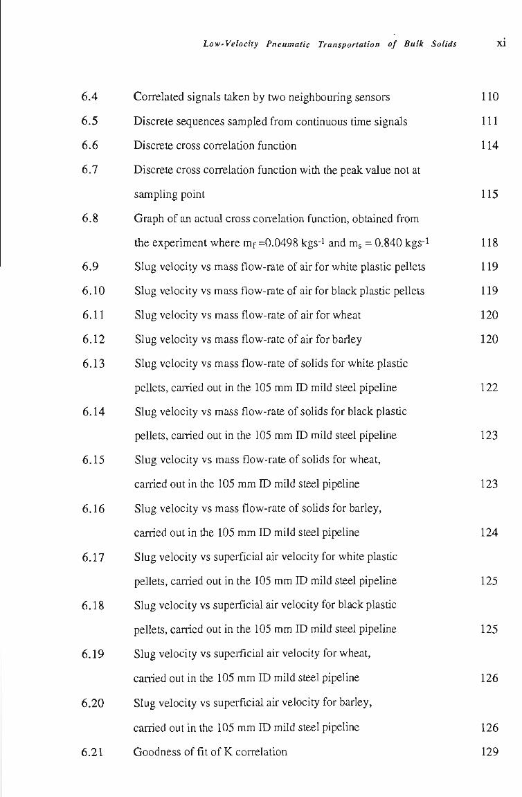
6.21 Goodness of fit of K correlation 129
Low-Velocity Pneumatic Transportation of Bulk Solids XU
6.22 Idealised slug with acting forces at initial motion 132
7.1 Pressures acting on the sensitive surfaces of transducers 139
7.2 Location requirement of pressure transducers 141
7.3 Type-B transducer installed flush with pipe wall 141
7.4 Typical graphs of the pressures and processed results from
check tests 144
7.5 Phase difference of signals 145
7.6 Plots of waU pressure and air pressure for black plastic
pellets, mf = 0.0643 kgs-i, m = 0.849 kgs-i 148
7.7 Plots of waU pressure and air pressure for black plastic
pellets, mf = 0.0498 kgs-i, m = 0.840 kgs-i 149
7.8 WaU pressure versus mass flow-rate of air for white plastic pellets 150
7.9 Wall pressure versus mass flow-rate of air for black plastic pellets 151
7.10 WaU pressure versus mass flow-rate of air for wheat 151
7.11 WaU pressure versus mass flow-rate of air for barley 152
7.12 Stresses acting on a particle slug 152
7.13 Stresses on element P in particulate medium and Mohr circle
representation 156
7.14 Possible state of stress at element P represented by a series of
Mohrcircles 157
7.15 Possible states of stress at element P in passive stress state 158
7.16 Particles flowing in a vertical pipe 159
7.17 Diagram of sU-ength 160
7.18 Particles moving in a sUo 164
7.19 Variation trend of stress iransmission coefficient in active case 165
7.20 Possible Mohr circles representing the stress state of
apartícleslug 167
7.21 Goodness of fit 170
Low-Velocity Pneumatic Transportation of Bulk Soîids XÍU
8.1 Geometrical parameters of slug-flo w 174
8.2 Various positíons of slugs during low-velocity pneumatic
conveying 176
8.3 Time history records of static air and wall pressures 177
8.4 Plot of air gap length versus mass flow-rate of air for
white plastic pellets 182
8.5 Plot of air gap length versus mass flow-rate of solids for
white plastic pellets 182
8.6 Plot of air gap length versus mass flow-rate of air for
black plastic pellets 183
8.7 Plot of air gap length versus mass flow-rate of solids for
black plastic pellets 183
8.8 Plot of air gap length versus mass flow-rate of air for wheat 184
8.9 Plot of air gap length versus mass flow-rate of soUds for wheat 184
8.10 Plotof air gap length versus mass flow-rateof airfor barley 185
8.11 Plot of air gap length versus mass flow-rate of solids for barley 185
8.12 Cross section of stationary bed 190
8.13 Measurement of stationary bed thickness with a camera 191
8.14 A typical photograph of the statíonary bed of barley for the
experiment of m^ = 1.32 kgs-^ mf = 0.088 kgs-^ conducted
in the 96 m long pipeline 192
8.15 Cross-sectíonal area ratío of statíonary bed to pipe versus slug
velocity for white plastíc pellets 193
8.16 Cross-sectional area ratio of statíonary bed to pipe versus slug
velocity for black plastíc peUets 193
8.17 Cross-sectíonal area ratío of statíonary bed to pipe versus slug
velocity for wheat 194
Low-Velocity Pneumatic Transportation of Bulk Solids XÍV
8.18 Cross-sectional area ratío of statíonary bed to pipe versus slug
velocity for barley 194
8.19 General form of steady state pneumatíc conveying characteristícs
for a given material and pipeUne 196
8.20 Experimental conveying characteristícs of black plastíc peUets
conveyed in the 52 m long pipeUne 197
8.21 Experimental conveying characteristícs of wheat con veyed in
the 52 m long pipeUne 198
8.22 Pressure distribution along a horizontal pipe for white plastíc
peUets 199
8.23 Pressure distiibutíon along a horizontal pipe for black plastíc
pellets 199
8.24 Pressure distribution along a horizontal pipe for wheat 200
8.25 Pressure distribution along a horizontal pipe for barley 200
8.26 Arrangement of transducers for the investígatíon into bend effect 201
8.27 Comparison of pressure gradient for black plastic pellets 203
8.28 Comparison of pressure gradient for white plastic pellets 203
8.29 Slug flowing through pipeUne with a bend and the
corresponding idealised pressure wave form 204
8.30 Predicted conveying characteristícs of white plastic pellets in the
horizontal pipe Lth = 36 m and D = 0.105 m, showing the
curves of constant m^ 209
8.31 Predicted conveying characteristics of white plastic pellets in the
horizontal pipe Lth = 78 m and D = 0.105 m, showing the
curves of constant m^ 209
8.32 Predicted conveying characteristícs of black plastic peUets in the
horizontal pipe Lth = 36 m and D = 0.105 m, showing the
curves of constant m 210
Low-Velocity Pneumatic Transportation of Bulk Solids XV
8.33 Predicted conveying characteristícs of black plastic peUets in the
horizontal pipe Lth = 78 m and D = 0.105 m, showing the
curves of constant ms 210
8.34 Predicted conveying characteristícs of wheat in the horizontal
pipe Lth = 36 m and D = 0.105 m, showing the curves of
constantms 211
8.35 Predicted conveying characteristics of wheat in the horizontal
pipe Lth = 78 m and D = 0.105 m, showing the curves of
constantms 211
8.36 Predicted conveying characteristics of barley in the horizontal
pipe Lth = 36 m and D = 0.105 m, showing the curves of
constantms 212
8.37 Predicted conveying characteristícs of barley in the horizontal
pipe Lth = 78 m and D = 0.105 m, showing the curves of
constantms 212
9.1 Pneumatíc conveying test rig with 80.5 mm ID pipeline 218
9.2 Procedure for determining pneumatíc conveying characteristícs 221
9.3 Relationship between slug velocity and superficial air velocity 222
9.4 Predicted PCC of the horizontal pipeline of Rig 1 for conveying
polystyrene chips, Lth = 78 m, D = 105 mm 223
9.5 Predicted PCC of the horizontal pipeUne of Rigs 2 and 3 for
conveying polystyrene chips, Lth = 40 m, D = 156 mm 224
9.6 Predicted PCC of the horizontal pipeline of Rig 4 for conveying
black plastic pellets, Lth = 116 m, D = 80.5 mm 224
9.7 Predicted pressure drop compared with experimental pressure
drop obtained on Rig 1 for polystyrene chips 225
9.8 Predicted pressure drop compared with experimental pressure
drop obtained on Rigs 2 and 3 for polystyrene chips 226
Low-Velociíy Pneumatic Transportation of Bulk Solids XVÍ
9.9 Predicted pressure drop compared with experimental pressure
drop obtained on Rig 4 for black plastic pellets 226
9.10 PipeUne pressure distribution for white plastic pellets
and D = 105 mm 228
9.11 PipeUne pressure distributíon for black plastíc peUets
and D = 105 mm 228
9.12 Pipeline pressure distributíon for wheat and D = 105 mm 229
9.13 Pipeline pressure distiibution for barley and D = 105 mm 229
9.14 Variatíon of pressure gradient 230
9.15 Economical operatíng curve of white plastíc pellets shown
on PCC graph for 36 m horizontal pipeline 233
9.16 Economical operatíng curve of black plastíc pellets shown
on PCC graph for 36 m horizontal pipeUne 233
9.17 Economical operating cuive of wheat shown on PCC
graph for 78 m horizontal pipeline 234
9.18 Economical operating curve of barley shown on PCC
graph for 36 m horizontal pipeline 234
9.19 Partícle size distributíon of semoUna 236
9.20 Semolina shown in Dixon's slugging diagram 237
9.21 Low-velocity pneumatic conveying characteristics of
105 mm ID, 52 m mUd steel pipeline for semolina 238
9.22 Plot of slug velocity versus superficial air velocity for semoUna 239
9.23 Predicted pneumatic conveying characteristícs of semolina and
36 m horizontal pipeline by using modifîed model 240
B. 1 Schematíc layout of 96 m long pipeline and transducer locatíons 276
D. 1 A particle slug in a vertical pipe 279
Low-Velocity Pneumatic Transportation of Bulk Solids XVU
LIST OF TABLES
Table Title Page
5.1 Physical properties of test material 100
6.1 K, Uamin nd 7^ for Hnes of various test materials 127
6.2 Optimal coefficient 129
7.1 Experimental wall pressure and stress transmission
coefficient for wheat 154
7.2 Stress transmission coefficient ?t for different test materials 155
7.3 Static intemal friction angles for test materials 168
7.4 Coefficientofbestfit 169
9.1 Conveying pipelines 217
9.2 Steady-state dense-phase results for black plastic pellets 219
9.3 Steady-state dense-phase results for polystyrene chips 220
9.4 Economical superficial air velocity 232
A. 1 Experimental values of major parameters for conveying
white plastíc pellets in 52 m long pipeline 264
A.2 Experimental values of major parameters for conveying
white plastic pellets in 96 m long pipeline 265
A.3 Experimental values of major parameters for conveying
black plastic pellets in 96 m long pipeUne 266
A.4 Experimental values of major parameters for conveying
black plastic peUets in 52 m long pipeUne 267
A.5 Experimental values of major parameters for conveying
wheat in 52 m long pipeline 268
A.6 Experimental values of major parameters for conveying
wheat in 96 m long pipeline 269
Low-Velocity Pneumatic Transportation of Bulk Solids XVUl
A.7 Experimental values of major parameters for conveying
barley in 96 m long pipeline 270
A.8 Experimental values of major parameters for conveying
barley in 52 m long pipeline 271
A.9 Experimental values of pressure along 96 m long pipeline
for white plastic peUets 272
A.IO Experimental values of pressure along 96 m long pipeline
for black plastic pellets 273
A. 11 Experimental values of pressure along 96 m long pipeline
for wheat 274
A. 12 Experimental values of pressure along 96 m long pipeline
for barley 275
B. 1 Pressure transducer locatíons (distance from end of pipeUne) 276
Low-Velocity Pneumatic Transportation of Bulk Solids XIX
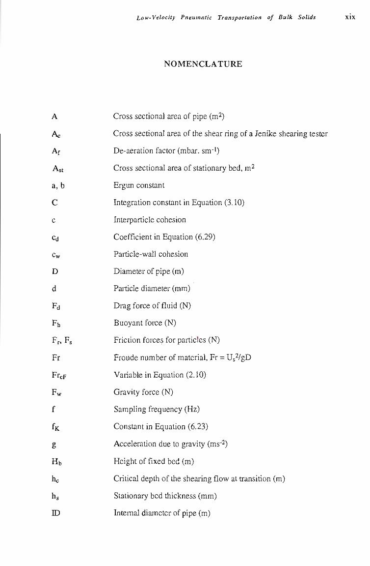
NOMENCLATURE
A Cross sectional area of pipe (m^)
Ac Cross sectional area of the shear ring of a Jenike shearing tester
Af De-aeration factor (mbar. sm-i)
Ast Cross sectional area of statíonary bed, m^
a, b Ergun constant
C Integratíon constant in Equatíon (3.10)
c Interpartícle cohesion
Cd Coefficient in Equat íon (6.29)
Cw PaiticIe-waU cohesion
D Diameter of p ipe (m)
d Pait icle d iameter (mm)
Fd Dragforceoffluid(N)
Fh Buoyant force (N)
Ff, Fs Frictíon forces for particles (N)
Fr Froude number of material, Fr = Us^/gD
FrcF Variable in Equatíon (2.10)
Fw Gravity force (N)
f Sampling frequency (Hz)
f Constant in Equatíon (6.23)
g Acceleratíon due to gravity (ms-^)
Hb Height of fixed bed (m)
hc Critícal depth of the shearing flow at transitíon (m)
hg Stationary bed thickness (mm)
ID Intemal diameter of pipe (m)
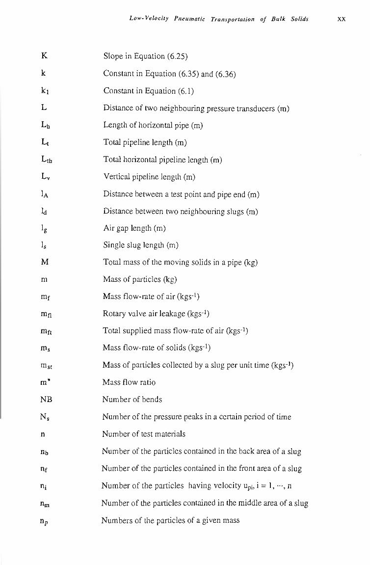
Low-Velocity Pneumatic Transportation of Bulk Solids XX
K Slope in Equatíon (6.25)
k Constant in Equatíon (6.35) and (6.36)
ki Constant in Equatíon (6.1)
L Distance of two neighbouring pressure transducers (m)
Lh Length of horizontal pipe (m)
Lt Total pipeUne length (m)
Lth Total horizontal pipeline length (m)
Lv Vertical pipeline length (m)
U Distance between a test point and pipe end (m)
Id Distance between two neighbouring slugs (m)
Ig Air gap length (m)
Is Single slug length (m)
M Total mass of the moving soUds in a pipe (kg)
m Mass of paiticles (kg)
mf Mass flow-rate of air (kgs-i)
mfl Rotary valve air leakage (kgs-^)
mft Total supplied mass flow-rate of air (kgs-^)
ms Mass flow-rate of solids (kgs-i)
mst Mass of particles collected by a slug per unit time (kgs-^
m* Mass flow ratío
NB Number of bends
Ns Number of the pressure peaks in a certain period of time
n Number of test materials
nb Number of the particles contained in the back area of a slug
nf Number of the paiticles contained in the front area of a slug
ni Number of the partícles having velocity Upi, i = 1, —, n
Hni Number of the particles contained in the middle area of a slug
np Numbers of the partícles of a given mass
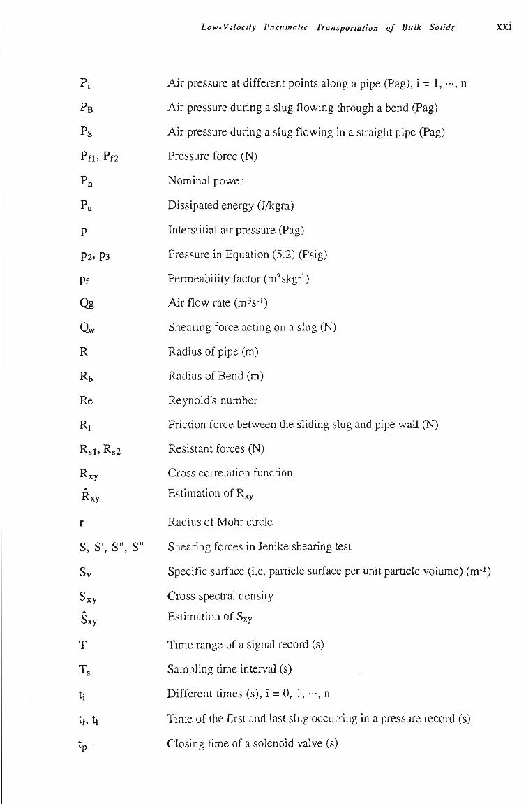
Low-Velocity Pneumatic Transportation of Bulk Solids XXÍ
Pi Air pressure at different points along a pipe (Pag), i = 1, •-, n
PB Air pressure during a slug flowing through a bend (Pag)
Ps Air pressure during a slug flowing in a straight pipe (Pag)
Pfi' Pf2 Pressure force (N)
Pn Nominal power
Pu Dissipated energy (J/kgm)
p Interstitial air pressure (Pag)
P2, P3 Pressure in Equatíon (5.2) (Psig)
Pf Permeability factor (m^skg-i)
Qg Air flow rate (m^s'O
Qw Shearing force acting on a slug (N)
R Radius of pipe (m)
Rb Radius of Bend (m)
Re Reynold's number
Rf Friction force between the sliding slug and pipe waU (N)
Rsi, Rs2 Resistant forces (N)
Rxy Cross correlatíon functíon
R Estimation of R y
r Radius of Mohr circle
S, S', S", S'" Shearing forces in Jenike shearing test
Sv Specific suiface (i.e. particle surface per unit partícle volume) (m-i)
Sxy Cross spectral density
§ Estimatíon of Sxy
T Time range of a signal record (s)
Ts Sampling tíme intei-val (s)
tj Different tímes (s), i = 0, 1, •••, n
tf, ti Time of the first and iast slug occuning in a pressure record (s)
tp Closing tíme of a solenoid valve (s)
Low-Velocity Pneumatic Transportation of Bulk Solids XXÍÍ
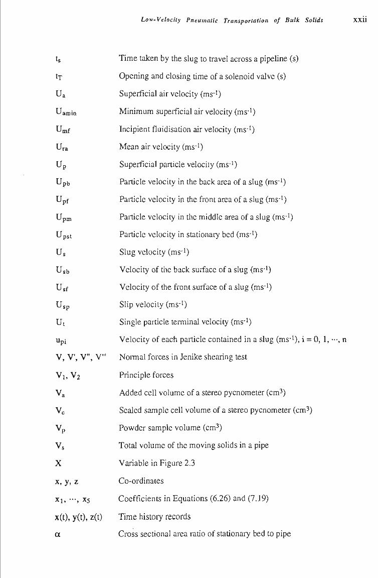
ts Time taken by the slug to travel across a pipeUne (s)
tx Opening and closing tíme of a solenoid valve (s)
Ua Superficial air velocity (ms'O
Uamin Minimum supei-ficial air velocity (ms-^)
Umf Incipient fluidisatíon air velocity (ms-^)
Ura Mean air velocity (ms-^)
Up Superficial particle velocity (ms-^
Upb Particle velocity in the back area of a slug (ms" )
Upf Particle velocity in the front area of a slug (ms-^)
Upm Particle velocity in the middle area of a slug (ms'i)
Upst Particle velocity in stationary bed (ms'^)
Us Slug velocity (ms'O
Usb Velocity of the back surface of a slug (ms-^)
Usf Velocity of the front surface of a slug (ms-0
Usp Slip velocity (ms-^
Ut Single particle tenninal velocity (ms-^
Upi Velocity of each particle contained in a slug (ms-^), i = 0, 1, —, n
V, V', V", V'" Normal forces in Jenike shearing test
Vi, V2 Principle forces
Va Added ceU volume of a stereo pycnometer (cm^)
Vc Sealed sample cell volume of a stereo pycnometer (cm^)
Vp Powder sample volume (cm^)
Vs Total volume of the moving soUds in a pipe
X Variable in Figure 2.3
X, y, z Co-ordinates
xi , •••, X5 Coeffícients in Equatíons (6.26) and (7.19)
x(t), y(t), z(t) Time histoiy records
a Cross sectíonal area ratío of statíonary bed to pipe
Low-Velocity Pneumatic Transportation of Bulk Solids XXUl
ttb
P
Pb
Pf
6
Ae=øi-e2
Ap
Api
Apt
Apth
At
e
<!>
<î>s
(t>w
7
7b
Ys
Tl
XA
^min, ^max
A,o
^omin» ^omax
A,p
^w
0
Incline angle of bend with respect to the horizontal (°)
Coefficient in Equatíon (6.36)
Incline angle of the back surface of a slug (°)
IncUne angle of the front surface of a slug (°)
Effectíve intemal frictíon angle (°)
Radian of bend in Equatíon (2.15) (°)
Pressure drop across a single slug (Pa)
Pipeline pressure drops at different locatíons (Pa), i = 1, —, n
Total pipeline pressure drop (Pa)
Total horizontal pipeline pressure drop (Pa)
Interval time (s)
Bulk voidage
Intemal frictíon angle (°)
Statíc intemal frictíon angle (°)
WaU friction angle (°)
Coefficient of coiTelation
Bulk specific weight with respect to water at 4 °C
Particle specific weight with respect to water at 4 C
Dynamic viscosity of fluid, Nsm-^
Stress transmission coefficient
Stress transmission coefficient at active faUure
Minimum and maximum stress transmission coefficient
Static stress transmission coefficient
Minimum and maximum static stress transmission coefficient
Stress transmission coefficient at passive faUure
Coefficient of intemal frictíon
Coefficient of wall frictíon
Angle in Figure (3.8) (°)
Low-Velocity Pneumatic Transportation of Bulk Solids XXÍV
Øs Angle in Figure (8.12) («)
Pa Air density (kgm-3)
Pb Bulk density (kgm-^)
Pbst Bulk density of stationary bed (kgm-3)
ps Particle density (kgm-3)
<5 Normal stress (Pa)
C\,<32 Principle stresses (Pa)
(Tb Stress on the back face of a slug (Pa)
Gf Stress on the front face of a slug (Pa)
Cx Radial stress (Pa)
Gg Gravity pressure (Pa)
Gn Normal stress coordinate
Otw Total wall pressure (Pa)
Gw Wall pressure (Pa)
Gwm Average wall pressure (Pa)
<^x, CTy, <7z Normal stresses in x, y, z direction (Pa)
Gxm Average stress in x directíon
X Shearing stress (Pa)
Td Time delay between two signals (s)
Tp Specific tíme delay for the peak value of cross-correlation function (s)
tn Shearing stress coordinate
ttw Total shear stress at a wall (Pa)
Txy, Xxz> 'Cyz Shcar stresses at the planes perpendicular to x, y, z coordinates
Cû Angle defined in Figure 7.17 (°)

CHAPTER 1
INTRODUCTION
Chapter 1: Introduction 2
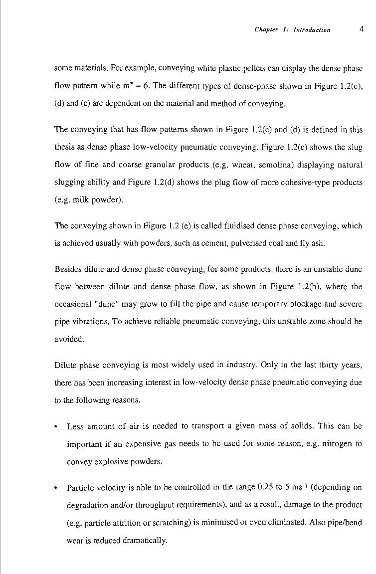
Pneumatic conveying is being used increasingly in industry to transport a wide range of
bulk soUds. Numerous efforts have been made to advance the research and applicatíon of
this method of transport. Experience has demonstrated that pneumatíc conveying exhibits
different performances and flow pattems for different air mass flow rates (mf). There are
many ways of describing the different flow pattems. Among them, the concept of the
phase diagram originaUy proposed by Zenz [118] is most well known by pneumatic
conveying researchers. It is usually a graph of pressure gradient versus superficial air
velocity, on which lines of constant mass flow-rate of solids m are shown. A log-log
scale generally is used so that a wide range of values can be included, as shown in Figure
1.1.
Dû O
Fixed Bed
Dilute-Phase or Suspension Flow
Log (Ua) U al
Figure 1.1 Phase diagram of pneumatíc conveying.
By using the phase diagram, the flow pattems can be determined within a pipeHne for a
given set of conveying conditíons. According to the different flow pattems, pneumatíc
conveying is classified primarUy as dilute phase or dense phase.
Chapter 1: Introduction 3
Dilute phase conveying in general employs large volumes of air at high velocity so that
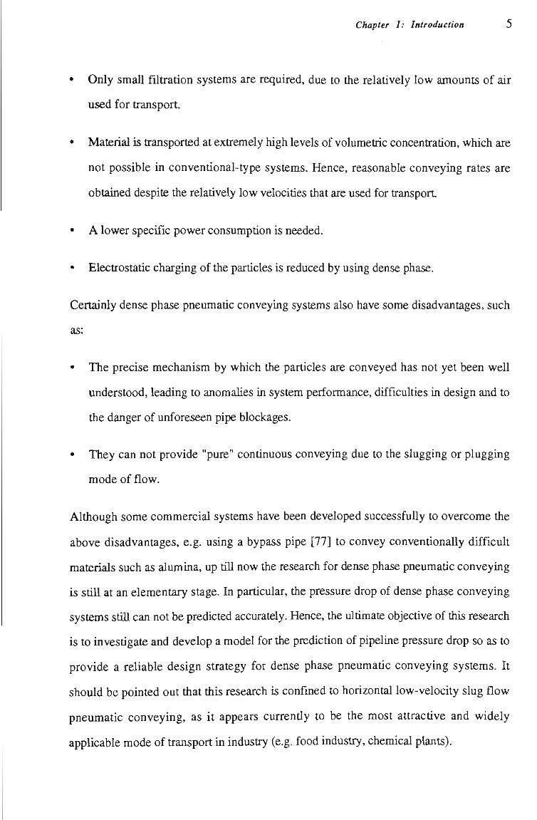
the individual particles are conveyed as a fuUy suspended flow, as shown in Figure
1.2(a). If the mass flow ratio (m*), which is a ratio of the soHds mass flow rate (m ) to
the conveying air mass flow rate (mf), is in the range 0 <m*< 15, then the mode of flow
usually is regarded as dilute phase conveying [17].
(a)
• • • • • • _ • ••-v"S*S*%* . • . • • • . • S * ' ^ * S " S * . • • • • • ••%•%• _• . • • a^S^V'S^ • • • > . - I . . ^ . ^ . ^ . . . . J . - . - . — - . • ^ — . - > . - . . - . . - . . J — — - . - • • • • • - . • • . . - . . - . • ^ • • • • _ . . . . . J . J - . . . P . • . • J l . j
(b)
'mmm^ l ' !• !• I ' l ' !• I ' ' l ' 1 . . . • . • • ^ . ^ • , . . • • . . • • . . • ,
'^•^•^•^•^•^•^•^•\^ ..^•v.s.s^s^v^v^s^v^v^. . í s í s í A í s í W s í s í i í s .
^ • • ^ • ^ . . ^ . . ^ . . ^ • ^ • ^ • • • • • • • • • • • • • • • • • . • . • . • • • / • • ^ • • ^ • • ^ • ^ • ^ • • ^ • ^ • • ^ • • • • • • • • • • • • • • ^ • ^ • • ^ • • ^ • ^ • • . • • • ^ • • ^ • • ^ • ^ • ^ • ^
(c)
" ^ - ^ - ^ - ^ • ^ - J - ^ ' ^ - '
(d)
J. •••! I" ! • 1 . - . ' | . I^ l^ I J 1« I" I" !• 1» ! • I • • • V ^ V . i •^•^•^•. •^; .^..••.•••••^' ^•^•^•.••i > ^•^•."•,
/ • s - s s ' - • . . s -s î sVsiSis .-s's'S^s^s.S' • I s . s . s . s . s . .ÎSÍS.S"'.
,a&M*Ml • • • • • • • • •kMfc^&Mfl « • • • mM.m» mm mM,^^i.mM • • • • • • • • • • • • • • i l • • • • • • ak afl • • • • • • aSmmA^
(e)
Figure 1.2 Flow pattems of pneumatíc conveying in horizontal pipe.
Dense phase conveying is defined by Konrad et al.[68, 69] as the conveying of particles
by air along a pipe that is filled with particles at one or more cross-sections, as shown in
Figure 1.2(c), (d) and (e). The flow pattem and behaviour of dense phase conveying are
much more complex than those of dilute phase conveying so that there is, as yet, no
universally accepted definitíon for dense phase conveying. Some researchers [70, 74]
define dense phase conveying when m* > 15. This defînitíon seems inappropriate for
Chapter I: Introduction 4
some materials. For example, conveying white plastic pellets can display the dense phase
flow pattem while m* = 6. The different types of dense-phase shown in Figure 1.2(c),
(d) and (e) are dependent on the material and method of conveying.
The conveying that has flow pattems shown in Figure 1.2(c) and (d) is defined in this
thesis as dense phase low-velocity pneumatíc conveying. Figure 1.2(c) shows the slug
flow of fine and coarse granular products (e.g. wheat, semolina) displaying natural
slugging ability and Figure 1.2(d) shows the plug flow of more cohesive-type products
(e.g. miUc powder),
The conveying shown in Figure 1.2 (e) is called fluidised dense phase conveying, which
is achieved usually with powders, such as cement, pulverised coal and fly ash.
Besides dilute and dense phase conveying, for some products, there is an unstable dune
flow between dilute and dense phase flow, as shown in Figure 1.2(b), where the
occasional "dune" may grow to flll the pipe and cause temporary blockage and severe
pipe vibrations. To achieve reliable pneumatic conveying, this unstable zone should be
avoided.
DUute phase conveying is most widely used in industry. Only in the last thirty years,
there has been increasing interest in low-velocity dense phase pneumatic conveying due
to the following reasons.
• Less amount of air is needed to transport a given mass of solids. This can be
important if an expensive gas needs to be used for some reason, e.g. nitrogen to
convey explosive powders.
• Partícle velocity is able to be controUed in the range 0.25 to 5 ms-i (depending on
degradatíon and/or throughput requirements), and as a result, damage to the product
(e.g. particle attritíon or scratching) is minimised or even eliminated. Also pipe/bend
wear is reduced dramaticaUy.
Chapter 1: Introduction 5
• Only small filtratíon systems are required, due to the relatively low amounts of air
used for transport.
• Material is transported at extremely high levels of volumetric concentratíon, which are
not possible in conventíonal-type systems. Hence, reasonable conveying rates are
obtained despite the relatívely low velocitíes that are used for transport
• A lower specific power consumption is needed.
• Electrostatic charging of the particles is reduced by using dense phase.
Certainly dense phase pneumatic conveying systems also have some disadvantages, such
as:
• The precise mechanism by which the particles are conveyed has not yet been well
understood, leading to anomaUes in system performance, difficulties in design and to
tíie danger of unforeseen pipe blockages.
• They can not provide "pure" continuous conveying due to the slugging or plugging
mode of flow.
Although some commercial systems have been developed successfully to overcome the
above disadvantages, e.g. using a bypass pipe [77] to convey conventionally difficult
materials such as alumina, up tiU now the research for dense phase pneumatic conveying
is stiU at an elementary stage. In particular, the pressure drop of dense phase conveying
systems stiU can not be predicted accurately. Hence, the ultimate objective of this research
is to investígate and develop a model for the prediction of pipeline pressure drop so as to
provide a reliable design strategy for dense phase pneumatic conveying systems. It
should be pointed out that this research is confined to horizontal low-velocity slug flow
pneumatic conveying, as it appears currentiy to be the most attractíve and widely
applicable mode of transport in industry (e.g. food industry, chemical plants).
Chapter 1: Introduction 6
To achieve the ultimate goal of this research, the work is concentrated on the foUowing
aspects:
(i) Reviewing published literature to assess the current state of the knowledge of
low-velocity pneumatic conveying (Chapter 2),
(u) Introducing and further studying the behaviour of a single particle slug (Chapter
3),
(iu) Organising low-velocity pneumatic conveying experiments and finalising the
main test program (Chapters 4 and 5),
(iv) Establishing an empirical correlation of slug velocity in terms of superficial air
velocity, pipe size and the physical propertíes of the material (Chapter 6),
(v) Measuring the pipe wall pressures exerted by moving slugs and establishing a
semi-empirical relationship between the radial and axial stress in partícle slug
flow (Chapter 7),
(vi) Exploring a broad range of conveying conditíons so that the performance of
low-velocity pneumatic conveying can be evaluated and finally developing a
model for the predictíon of total horizontal pipeHne pressure drop which is a
function of the physical properties of the material, conveying conditions and
pipeUne configuratíon (Chapter 8),
(vu) Dlustrating appUcatíons of the developed model into different conveying systems
and providing guidelines for the optimal design of low-velocity pneumatic
conveying systems (Chapter 9).
FinaUy, concluding remarks based on the investígations and suggestíons for further work
are given in Chapter 10.
CHAPTER 2
LITERATURE SURVEY
Chapter 2: Literature Survey 8
2.1 Introduction
This chapter reviews published literature to present the current state of knowledge on
dense phase pneumatíc conveying. The reviewing is very necessary for there stíU exists a
lot of confusion even though dense phase pneumatíc conveying has been in use for over
thirty years. These problems focus on the foUowing aspects:
• The definition of dense-phase conveying is stUl a matter of some debate.
• The precise mechanism by which the particles are conveyed has never been weU
understood, resulting in difficulties to predict conveying performance.
• Different flow pattems exist for dtfferent conveying methods and materials.
• Conflicting experimental work causes numerous controversies and there is a lack of a
coherent theory to explain the discrepancies.
As a large amount of Hterature has been published Ín the field of dense phase conveying,
this reviewing is confined only to dense phase low-velocity pneumatic conveying and
encompasses the foUowing three aspects:
• SuitabUity of buUc material for low-veiocity pneumatic conveying.
• Performance of low-velocity pneumatic conveymg.
• Design considerations of conveying systems.
2.2 Suitability of Bulk Material
Experience has demonstrated that tíie range of materials that can be conveyed successfuUy
in a dense phase mode of flow is more limited than that of dUute phase. An appropriate
procedure for assessing tiie suitabiUty of material for conveying in dense phase pneumatic
conveying is necessary for design and industrial appUcations.
Chapter 2: Literature Survey 9
Geldart [39] firstly classified buUc materials into four groups according to the mean
particle size and density difference for the purpose of predicting fluidisatíon behaviour,
Group A materials retain aeratíon and if fluidised, generaUy expand before bubbling.
Group B materials do not retain aeratíon and bubble immediately after fluidisatíon. Group
C materials are cohesive and generaUy difficult to be fluidised. The materials in Group D
have simUar behaviour to the materials in Group B but require much larger air flows to
maintain fluidisatíon. Geldart's classification was proposed by some researchers (e.g.
Marcus [124]) as a method to indicate the potential of conveying material in dense phase (
i.e. as this mode of flow was analogous to the mechanism to fluidisation). Unfortunately,
Geldart's classificatíon does not appear [78] to give a reliable predictíon for pneumatíc
conveying.
Dixon [28] conveyed ten different materials ranging from fme powder to coarse peUets in
dense phase systems of different pipe diameter and also recognised that the fluidisatíon
propertíes of a product have significant influences on its suitability to dense phase
conveying. He suggested that some materials have a natural tendency to slug in dense
phase conveying systems whereas others tend towards dune-flow. Fine powders form
neither slugs nor dunes but flow naturally as a well-mixed 'fluidised' column. Based on
Geldart's classifîcation of fluidisatíon, Dixon [28] generated the slugging diagram for
assessing the suitability of material for conveying in dense phase pneumatíc conveying.
He further produced tíieoretícal criteria for classifying materials into groups based on the
argument that an air slug wUl be destroyed by particle entrainment if the relative slug
velocity exceeds the single particle terminal velocity. As example of a Dixon [28]
slugging diagram for a 100 mm diameter pipe is presented in Figure 2.1. The Group AB
boundary is defîned by Equation (2.1):
Ut=0.35 (2gD)«-5 (2.1)
where Utis the single particle terminal velocity, and
Chapter 2: Literature Survey 10
U t = (Ps-Pa)gd' _ ^r s r a
18ri
U t = _0.152gQ'^^^d^-^'^(Ps-Pa)''^'
^0.428p0.285
Re < 2.0
2.0 < Re < 500
Figure 2 1 Dixon's slugging diagram for a 100 mm diameter pipe [28].
The Group BD boundary is defîned by Equatíon (2.2):
Umf=0.35(gD) 05 (2.2)
where Umf is the minimum fluidisatíon velocity, and determined by the following
equation with e = 0.45,
^(l-e)TlUmf . 1 ^ c P a U m f , .
de-150^"^:'r""+L75^^:3^=Psg
d^e^
Please see print copy for image
Chapter 2: Literature Survey 11
The boundary between Group A and C is an empirical relatíonship, and is not as weU
defined (e.g. Dixon [28] simply reproduced this boundary from the Geldart [39]
diagram)^
Dixon [28] then concluded that the materials in Groups A and D can be conveyed in
dense phase. The materials in Group D have strong namral slugging tendency and are the
best candidates for low-velocity pneumatic conveying, witii slugs moving slower than the
air in dense phase. The materials in Group A have no slugging tendency but can be
conveyed at very high m* values. They can be made to slug by commercial techniques.
The materials in Group B have weak natural slugging tendency and can be troublesome in
dense phase conveying.
Dixon [29] undertook further work to modify slightly his slugging diagram, as he found
that it was more appropriate to replace the equatíons for calculating Ut and Umf by
Ut= (Ps-Pa)gd^ _ ' • r s ra,/
18TI Re < 0.4
and
Ut= 2„2'
4 (Ps-Pa) g 225 p,Tl
Umf= _(Ps-Pa)gd^
1650T1
0.4 < Re < 500
Re<20
Umf= (Ps-Pa)gd
24.5P, Re>1000
To date Dixon's slugging diagram [28, 29] has been used most commonly for assessing
the suitabiUty of material for conveying in dense phase pneumatíc conveying. However,
Dixon's work is stíll imprecise as tiie behaviour of soUds are extremely complex.
Jodlowski [57] successfully conveyed some materials, which are classifîed as "difficult"
products for dense phase conveying in Dixon's classification, by using tíie dense phase
3 0009 03100 9587
Chapter 2: Liíerature Survey 12
systems with careful selectíon of the mass flow ratío, conveying velocity, pipe diameter
and the distribution of air flow along the conveying length. Hence, Jodlowski [57]
beUeved that tiie Geldart and Dixon classifications based on mean particle size and density
difference is insufficient. Other parameters of material properties must be taken into
account, such as particle size range, partícle shape, hardness, compressibUity, cohesion,
product behaviour after subjection to fluidisatíon and frictíon coefficient, etc. Jodlowski
[57] further stressed that the design of conveying systems also has equal importance for
successful dense phase conveying.
Ginestet et al. [41] attempted to use the results of the air-solids, soHds-solids and solids-
wall interactíon factors to predict the suitability of material for dense phase conveying.
Unfortunately, Ginestet's work had not been completed entirely by the time he published
his paper. Therefore no valuable conclusions were given.
Jones et al. [58] carried out conveying experiments to determine the conveying
characteristics for five products. Based on the detailed information provided by these
conveying characteristícs, Jones et al. [58] studied the potentíal of the product to be
conveyed in dense phase and pointed out that the two properties which are identífied as
most useful for the determining conveyabiUty are the permeabUity of a product to air and
the ability of a product to retain air. Jones et al. [58] found that products that exhibit good
air retention properties are the most Hkely candidates for dense phase conveying and
products that exhibit relatívely poor air permeability characteristics are also good
candidates for dense phase conveying. Jones et al. [58] did not establish criteria for
identifying the good air retentíon properties and poor air permeabUity characteristícs.
However, they believed tiie air retentíon and air permeability properties of a product can
be determined by analysing a smaU sample of tiie product so that the conveyabUity of tiie
product can be predicted.

Chapter 2: Literature Survey 13
Mainwaring and Reed [78] recognised the unreliability of the Geldart and Dixon
classifîcatíons. They agreed that the air retention properties and air permeability
characteristícs influence the conveyability of the material. Hence tiiey proposed an
approach based on the measured permeabiHty and de-aeration characteristícs of the
materials in their research. The approach is reviewed below.
Figure 2.2 Pressure gradient vs permeability factor [78].
Mainwaring and Reed [78] fîrstíy generated a diagram for the potentíal of dense phase
conveying according to the permeabUity of material, as shown m Figure 2.2. They found
that tiie materials exhibitíng high values of permeability factor (pf) generaUy can be
Please see print copy for image
Chapter 2: Literature Survey 14
conveyed in a plug type mode of dense phase conveying, whUe the otiier materials are
conveyed eitíier in dense phase moving bed type flow or not at aU in dense phase. The
line of constant superficial air velocity drawn on the diagram represents the boundary
between these two modes of flow and is defîned by the equatíon Umf = pf(Ap/Hb) = 50
mms -1
Figure 2.3 Pressure gradient vs term accountíng for de-aeratíon factor
and particle density [78].
Mainwaring and Reed [78] also found that materials that have high values of de-aeratíon
factor divided by partícle density can be conveyed in a moving bed type of flow while
Please see print copy for image
Chapter 2: Literature Survey 15
others are conveyed either in the slug type flow or cannot be conveyed in dense phase at
aU. Hence they produced another graph for dense phase potentíal according to the de-
aeration characteristícs of materials, as shown in Figure 2.3. The boundary line is
represented by the equatíon (Ap/Hb)X = Af/ps with the constant X = O.CX lm skg-i,
Mainwaring and Reed [78] claimed that this approach enables the potentíal for dense
phase conveying to be established with more certainty tiian the Dixon's method.
2.3 Performance of Low-Velocity Pneumatic Conveying
2.3.1 FIow Pattern
The earliest research into dense phase pneumatic conveying probably was carried out by
Albright el at [1], where pulverized coal was conveyed through horizontal pipes at mass
flow ratíos up to = 200. As the pipes used for conveying were made of copper, the flow
pattem could not be observed.
Wen and Simons [109] were the first to outUne the flow pattem of dense phase pneumatic
conveying based on visual observation. Since the conveyed materials appear to belong to
the Dixon [28] Group B, more descriptions were given to the dune-flow pattem in their
paper.
Konrad et al. [69] photographed low-velocity pneumatic conveying and to date provided
one of the most comprehensive descriptions for this flow pattem. A brief summary is
given below.
For horizontal conveying, the solids flow in discrete slugs. Between the slugs, tiie upper
part of the pipe contains moving air with some dispersed particles whUe the lower part of
the pipe is fUled with stationary particles. Each slug sweeps up the stationary particles in
front and leaves behind a stationary layer of approximately tiie same tiiickness.
Chapter 2: Literaíure Survey 16
For vertical flow, the flow pattem resembles that of square-nosed slugging in a fluidized
bed. The solids move up as plug of partícles that occupy the entíre cross-section of the
pipe. Partícles are seen to rain down from the back of one plug and then to be coUected
by the front of the next plug.
Similar descriptions also were given by several other researchers [16, 48, 71, 105]. Hitt
[48] defîned this type of slug flow as full bore flow and further pointed out that at low
pipeline pressure gradients, horizontal conveying takes the form of shearing flow, i.e. a
series of plugs shearing across a statíonary layer of partícles. Hitt [48] also developed a
model for predictíng the critícal depth of the shearing flow at the transitíon to fuU bore
flow. For cohesionless material, Hitt's model is given by Equatíon (2.3):
^ = - ^ (2.3) R H
Tsuji et al. [105] introduced a new concept to assist in the research of low-velocity
pneumatic conveying. They used simulation technology to study iow-velocity flow from
a microscopic point of view, since they believed that although the flow stmcture is
complicated, the most basic mechanism of particle-to-particle interaction is fundamental
and simple to model. That is, for single particles in a conveying system, the state and
position of the particles are determined only by the contacting force and fluid drag force.
The contacting force can be calculated by simplifying the particle by a spring model with
dashpot and slider. The fluid force acting on the particles can be evaluated by applying
Ergun's equation [32]. Therefore the simulation of low-velocity pneumatic conveying can
be conducted by using a computer. The results were presented in the form of graphical
output showing the flow pattem involved.
According to the simulated graphs, Tsuji et al. [105] gave a very similar description for
the flow pattem to that given by Konrad et al. [69] and other researchers [16, 48, 71]
through actual observations. They also deduced that there exists a critical value of the
quantíty of particles per unit length of pipe to form slug flow.
Chapter 2: Liíerature Survey 17
With the simulation, the motion of individual particles, especiaUy the particles marked
with different colours near the middle and rear end of a slug, can be observed easily and
clearly. Theoretically, the flow pattem can be defined numerically by using this
technology. That is, the geometrical sizes reflecting the namre of the flow pattem, such as
the particle slug length, air gap length and the shape of the air-partícle interface between
two slugs, can be predicted, although Tsuji et al. [105] did not mention this in their
paper. It is extremely difficult to determine such parameters through visual observatíons
and photograph records. With the simulation technology, slug velocity and the normal
pressure exerted on the wall by the particles also were obtained by Tsuji et al. [105].
Simulation is a very promising method for the smdy of pneumatíc conveying.
2.3.2 Pipeline Pressure Drop
One of the most important aspects of pneumatic conveying research is to investigate
pipeline pressure drop and the influence of conveying conditions and other factors.
Numerous studies of course have been undertaken for low-velocity pneumatic
conveying, as described in the foUowing sections.
2.3.2.1 Pressure Drop in Horizontal FIow
Albright et al. [1] are believed to have undertaken the first research into dense phase
pneumatíc conveying. They conveyed puiverized coal through horizontal pipes with
different pipe diameters in dense phase and measured the pipeline pressure drop. Two
empirical equatíons were presented for predictíng the pressure drop of the dense phase
flow based on the measured results. As the flow pattem could not be observed from the
experiments (the flow pattem used by Albright et al. was most Hkely fluidized dense-
phase as Dixon [28] Group A materials were conveyed), it is diffîcult to evaluate whether
the equatíons of Albright et al. [1] are suitable for low-velocity pneumatíc conveying (viz.
slug flow). That is, tíie flow pattem defines the mechanisms that have to be investígated
in order to predict the pressure drop.
Chapter 2: Literature Survey 18
Wen and Simons [109] studied the flow characteristics of dense phase horizontal
conveying of glass beads and coal powders of various sizes (0.071 to 0.754 mm). Based
on their experimental finding that the average interstitíal air velocity is about twice as large
as the average partícle velocity, they presented an empirical correlatíon for the pipeline
pressure gradient in terms of the pipe and particle propertíes and conveying conditíons.
The correlatíon by Konrad [68] converted to SI units is
^ = 41.82msA-«-^<^ Lt VD
vO.25/ > -0.55 mf ms
V^Pa Psy (2.4)
Wen and Simons [109] observed four types of flow pattem that occurred in their dense
phase conveying experiments, but they did not indicate clearly the one that their model
represented. According to the type of materials they conveyed, i.e. materials in Dixon
[28] Group B, the conveying is believed most likely to be dune-flow. Hence their model
is most likely suitable to dune-flow. In additíon, the experimental work of Wen and
Simons [109] was only for a test section of approximately 3 m length. Hence any effects
due to changing air density might not be large enough to be correlated reliably. Therefore,
the correlation is probably only valid at air pressures close to ambient.
Dickson et al. [27] carried out a set of experiments to investígate the pressure drop
required to sustain the movement of a single partícle plug in a horizontal pipe. In these
experiments, the plugs were confined loosely at their ends by porous fibre slugs. The
discs were connected to each other by a length of string passing through the plug. The
test materials, glass beads and bentonite, were conveyed tiirough perspex and galvanised
iron pipes. To investígate the difference between pneumatic propulsion of the plug and
mechanical propulsion, the propelling force required to move the slug by mechanical
means also was determined. They found that the pressure required to move a plug of
granular material by pneumatic propulsion is proportional to the length of the plug, i.e.
the pressure gradient in the plug is constant. However, in mechanical propulsion the
force to sustain the continuous movement of the plug is proportíonal to exponent of the
Chapter 2: Literature Survey 19
length of the plug. Their work was preliminary since no correlations for pressure drop in
terms of partícle propertíes and conveying conditions were presented. Despite títís, the
method and conclusions of their work are stiU very meaningful to tiie present research on
low-velocity conveying.
Butters [16] presented a calculatíon method for the total pipeHne pressure drop of low-
velocity pneumatic conveying by equating the air pressure force to the frictíon force
caused by the slug weight. The research of this thesis has found that the frictíon force
caused by the slug weight only takes up a minor part of the pressure drop, hence this
method may not be reUable for predicting the pipeUne pressure.
According to the conclusion of Dickson et al. [27] that the pressure required to move a
plug of granular material by pneumatic propulsion is proportional to the length of the
plug, Konrad et al. [69] firstíy derived a theoretical equatíon to predict the pressure drop
required to move a single particle slug in a horizontal pipe by using the method of
Janssen (1895). That is, for cohesionless material:
42 = %^a, + 2p,gn. (2.5) Is '^
The significance of Equatíon (2.5) is that it has laid a foundation for the research of low-
velocity pneumatic conveying. It also indicates tiiat the pressure loss across a single slug
is composed of two parts, i.e. the pressure loss caused by the slug coUectíng statíonary
partícles and the pressure loss caused by the friction force due to partícle weight.
A low-velocity pneumatíc conveying system usuaUy includes several partícle slugs
flowing in the pipeline. In order to predict the total pipeHne pressure drop, the
relationship between the single slug pressure drop and the total pipeline pressure drop
must be estabUshed. For tíiis purpose, Konrad et al. [69] treated aU the slugs moving at
an average slug velocity (Ug) (i.e. tiie average particle velocity designated by Konrad et
al. [69]) in tiie horizontal sectíon of tiie pipeline as one slug.
Chapter 2: LUerature Survey 2 0
As Konrad et al. [69] believed that the particle slugs can be considered as a packed bed
model, they applied Ergun's equation [32] to the bed resulting in:
Ap_150Ti(l-£)^(U, + Up-Us) 1.75p,(l-e)(Ua+Up-Usf Is d^e^ de^
Obviously combinatíon of Equation (2.6) with Equation (2.5) can determine the slug
velocity (Us).
A correlatíon for Ls in terms of the mass flow rate of soHds (m ), the bulk density of the
slugs (pb), the total length of the horizontal pipeline (Lt) and slug velocity (Ug) was given
by Konrad et al. [69] as
Ls = T ^ (2.7)
By replacing the single slug pressure drop (Ap) and length (Ig) with the total pipeline
pressure drop (Apt) and total slug length (Ls), Konrad et al. [69] at last gave a model for
predicting the total horizontal pipeline pressure drop of low-velocity pneumatic
conveying:
Apt^2.168^t^XVgUsL ms_ Ls Vfe [ ApbUs-msj
+ 2pbg tw (2.8)
Compared with their experimental results, Konrad et al. [69] claimed that the model gave
good predictions with the passive failure selectíon of the value of the stress transmission
coefficient X in Equatíon (2.8). These results were for the conveying of 4 mm diameter
polyethylene granules through a 47.3 mm diameter horizontal pipelines, 6.36 m in
length.
The models of Konrad et al. [69], particularly the model for the pressure gradient of a
single slug, i.e. Equation (2.5), are introduced and cited most extensively by the
researchers of low-velocity pneumatíc conveying. However, comparisons between the
predictíons of Konrad's model and practical experimental pressure drops of fuU-scale
Chapter 2: Literature Survey 21
conveying systems are rarely found. In the research of this thesis, the comparisons
between the predicled results and the author's experimental data show that Equation (2.8)
always overpredicts the total horizontal pipeline pressure drop, in some cases by a factor
of 2.5. The experimental results obtained in this research were for the conveying of 3.76
mm diameter black plastic pellets through 105 mm diameter mild steel horizontal
pipeHnes, 36 m and 78 m in length. There are two possible reasons to cause this over
prediction.
One reason is that the determination of the stress transmission coefficient X in passive
faUure case may be inappropriate. Konrad et al. [69] derived formulae for evaluating two
extremes of X, known as the passive and active failure solutions according to particle
mechanics. That is.
for active faUure:
for passive faUure:
. . sin<t) where smco = -.
l+sin<l)cos(cû-(t) )
l+sin(î)cos(cû+(t) ) Ap =
l-sin(|)cos(û)+(t) )
sin(t)
Konrad et al. [69] pointed out that in theory, X should occur between these two extreme
solutions. Borzone and Klinzing [10] also indicated this fact. However, as it is difficult
to determine exactiy the real value of X between these two extremes, Konrad et al. [69]
further recommended using Xf for slug-flow pneumatic conveying according to their
experimental results. In fact, the range of the two extremes of X for some materials is
quite large. For example, Xp^ = 0.178 and ^p = 3.566 for white plastic pellets. Hence,
using Xp instead of the real value of X may cause large deviations in predicted values. For
example, if the real value of X for white plastic pellets is taken as the average of the two
extremes, i.e. X = 1.8, then Xp/X = 2.0, tiien tíie predicted pressure gradient in a single
slug when using X,p may be twice as large as tiie real pressure gradient.
Chapter 2: Literature Survey 2 2
Another reason probably is that applying Ergun's equation [32] to the particle slugs in
slug flow is not applicable as the particle slugs are found to be fluidized in this research,
refer to Chapter 3.
Hence Equation (2.8) for the prediction of the total pipeline pressure drop does not
appear to be reliable.
Legel and Schwedes [71] derived an equation similar to Equation (2.5) from a force
balance for determining the pressure drop required to move a single slug.
f = <^<-M^. (2.9)
The difference is that the second term in the right hand Equation (2.9), which represents
the frictíon force due to the weight of the slug, is half the corresponding term in Equation
(2.5). Legel and Schwedes [71] believed that the weight of slug only exerts pressure on
the lower half of the pipe wall. However, this consideration appears incorrect. For
example, if the upper half of the pipe was removed, obviously the partícles in the slug in
the upper half part of the pipe wUl flow outwards without the restriction of the pipe wall.
This indicates that the weight of the slug generates the stress exerted on the upper half of
the pipe wall, resulting in the friction force. For the stress transmission coefficient, Legel
and Schwedes [71] considered that its value can be set equal to the coefficient of earth
pressure at static state, i.e. X « 1 - sin ({>. For most cases, X ~ 0.5. This consideration
[71] conflicts witii that of Konrad et al. [69].
Legel and Schwedes [71] generated slugs in their experiments by means of pulses of
pressured air that were introduced periodically into the particle column by a solenoid
valve. Hence the length of each slug was able to be controlled and adjusted by the
operating frequency of the solenoid valve, and from the operating frequency of the
solenoid valve, the total length of slugs was calculated. Based on this work, Legel and
Chapter 2: Liíerature Survey 23
Schwedes [71] gave a semi-empirical model for predicting the total horizontal pipeHne
pressure drop:
tx (2.10)
where FT2Í?^ = f
cF ras Yrt
Ap v^Pby
1
txj Dg
The model given by Equation (2.10) may not be suitable for natural slugging pneumatic
conveying systems since the model was developed based on the experiments that slugs
were not generated naturally.
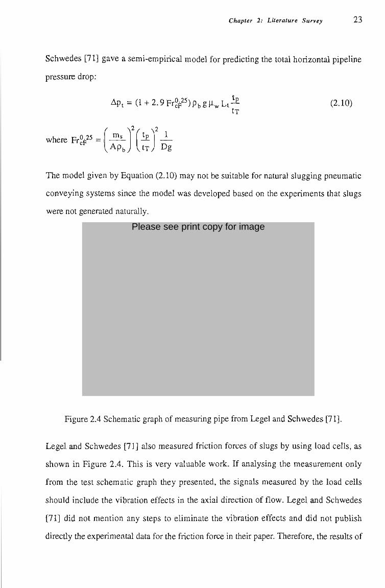
Figure 2.4 Schematic graph of measuring pipe from Legel and Schwedes [71].
Legel and Schwedes [71] also measured friction forces of slugs by using load cells, as
shown in Figure 2.4. This is very valuable work. If analysing the measurement only
from the test schematic graph they presented, the signals measured by the load cells
should include the vibration effects in the axial direction of flow. Legel and Schwedes
[71] did not mention any steps to eliminate the vibration effects and did not publish
directiy the experimental data for tíie frictíon force in their paper. Therefore, the results of
Please see print copy for image
Chapter 2: LUerature Survey 2 4
this work cannot be evaluated and used for further research. Also test results for the
wedge number [71] obtained from the measurement of the frictíon force are considered
with some sceptícism.
2.3.2.2 Pressure Drop in Vertical Flow
Studies into dense phase vertícal conveying commenced in the 1960's. However, the
earUer work seldom dealt with "typical" or "conventional" low-velocity pneumatíc
conveying. For example, Lippert's study [77] was related to the bypass system, Sandy
[95] researched the moving bed system and tiie flow pattem in the study of Tomita et al.
[101] for dense phase vertical flow was unclear. This unfortunately hinders the use of
their findings in the current world on low-velocity pneumatic conveying. Also, as the
earlier smdies of vertical flow have been reviewed extensively by Leung [72] and Konrad
[68], the review of this section will concentrate on the more recent developments of
vertical slug flow.
Konrad et al. [69] developed an equation for estimating the pressure drop required to Hft
a single slug in a vertical pipe when they did similar work for horizontal flow. The
foUowing equatíon was given for cohesiorúess materials:
Ap 4 | i A, /o 11A - ^ = — ^ G f + Pbg (2.11) Is '-^
The pressure loss across a vertícal slug is also composed of two parts, one represented
slug weight, the other represented by the frontal stress (Gf) of the slug. The partícles
raining down from the back of one slug cause this frontal stress.
In Equatíon (2.11), the stress transmission coefficient (X) and frontal stress (Gf) are
parameters to be determined further. Konrad [66] presented an equatíon for calculatíng
tiie frontal stress in 1987 from a momenmm balance and contínuity of flow, tiiat is
_egps(l-£)(up-ug) 2
^ f = 1 c \ (2.12) (1-e-eg)
Chapter 2: Literature Survey 2 5
Konrad and Totah [64] undertook further experimental work to measure the pressure
drops across single slugs moving through the vertical section of a 50.8 mm diameter
circulating unit. The length of slug, velocity of the partícles within the slug and velocity
of the front of the slug also were measured by using a high speed camera. The material
conveyed by Konrad and Totah [64] was a mixture of black and white polyethylene with
a particle diameter of 3 mm. The black polyethylene took up 5 % of the volume of the
mixture. From the experimental results of the pressure gradient, Konrad and Totah [64]
concluded that for a given frontal stress, the pressure drop across a moving slug of
cohesionless soUd is directíy proportional to its length, and Equatíon (2.11) gave a good
predictíon if the stress transmission coeffîcient X was selected between the actíve and
passive failure solutions.
An immediate problem of the work of Konrad et al. [64, 66, 69] is that the model is not
applicable for multi-slug vertical flow systems. Another problem is that the value of X,
was stiU uncertain.
Borzone and Klinzing [10] derived models from the force balance for predictíng the
pressure drop to Uft a single slug of cohesive soUds in a vertical pipe.
„ . Ap ^ . 4c^t^(Xp + l)cos(î)cos(cû+(Í)J , 4cw .^ .^. For passive case: —^ = Pbg+ ^ " rT (2.13)
Is U D
„ . Ap ^ ^ 4c^i^(U + l)cos(|)cos(co-(t)J 4cw .^ ... For active case: —^ = Pbg fj ^~f~ (2.14)
Borzone and Klinzing [10] then conducted experiments by conveying coal powders of
various sizes (9.8 to 38.0 |im) tíirough a 25.4 mm diameter vertical pipe, 3.05 m in
length in low-velocity pneumatic conveying. Gu and Klinzing [42] continued the
experiments with different diameters of vertícal pipe (50 mm and 100 mm). The pressure
drop across a single slug, slug length and slug velocity were measured. From the
experimental results, Borzone, Gu and Klinzing [10, 42] achieved the same conclusion
as tfiat of Konrad and Totah [64] for tíie relationship between the pressure drop and slug
Chapter 2: Literature Survey 2 6
length, i.e. constant pressure gradient in the slug, Compared with the experimental
results, the models of Borzone, Gu and Klinzing [10, 42] provided estimates of the
pressure drop across a single slug of cohesive material. They also found that the slug
velocity is independent of the slug length and depends mainly on the air velocity. In their
experiments, tíie slug velocity appears to be 90 % of the superficial air velocity.
According to the work of Borzone, Gu and Klinzing [10, 42], using the passive case or
actíve case models to predict pressure drop of a single slug of cohesive material seems
not important as the predictíons made by the two models were very close. However the
relatíonship between the total pipeline pressure drop and single slug pressure drop was
not established in their work making it difficult to apply their model directíy to multí-slug
vertical flow systems.
Hikita et al. [47] conveyed coke particles of 0.21 mm diameter in vertical acrylic resin
pipes of 50 and 150 mm diameter, 4 m in length. The partícles were observed to rise in
the pipe with an altemate pattem of particle and air slug, accompanied by a coUapse of the
particle slug. Experimental data for pressure drop across the transport pipe were
presented by plotting against the solid static head. No models for the pressure drop were
given by HUdta et al. [47].
2.3.2.3 Pressure Drop Around Bends
Investigations into the pressure drop caused by bends in low-velocity pneumatic
conveying have not received much attention, except for the recent work by Aziz and
Klinzing [5]. One possible reason is that the slug flow around bends has more complex
mechanisms than the slug flow through straight pipes. Another reason is that
experimental work of Hitt [48] displayed that the bends had no signifîcant effect on the
conveying characteristícs since the particles moved at rather low velocity during flow.
Hence in tíiis sectíon, only the work of Aziz and KUnzing [5] is reviewed.
Chapter 2: Literature Survey 27
Aziz and Klinzing [5] found that tíie pressure loss around bends is dependent on the
material properties and the parameters of the bends. By analysing the behaviour of the
slugs flowing around bends witíi a packed bed model and using a force balance on a
differentíal length of the slug contained in a bend, they derived the foUowing model for
predictíng tiie pressure drop across the slug.
^ = 4^^PbgAe[l + ? .F r (^ - l ) ] + 2pbgsinab[cos(^)-cos(^)] (2.15) Rb Ua 2 2
This model is a function of the physical propertíes of the material, bend parameters and
slug and air velocity.
Aziz and Klinzing [5] also conveyed pulverised coal in slug-flow pattem in the 25.4 mm
and 50.8 mm clear PVC pipes which included bends of different radu. The bends were
inclined at 0, 45 and 90 degrees witii respect to the horizontal. They claimed that both
bend model predictions and the experimental pressure drop data showed a linear variation
between bend pressure drop and slug length. Also the pressure drop increases with
increasing air velocity but decreases with increasing pipe diameter and bend ra(Uus. They
noted that a minimum bend radius is necessary to allow a given length of slug to flow
easUy tlirough the bend.
2 .4 Design of Low-Velocity Conveying System
Although the precise mechanism of low-velocity pneumatic conveying has not been weU
understood, leadmg to diffîculties in system design, researchers continue to make efforts
to estabUsh a standardised and universally agreed technique for the proper design of low-
velocity pneumatíc conveying systems.
Wypych and Hauser [116] proposed basic principles for the design of low-velocity
pneumatic conveying systems after summarising tíie progress in research and technology.
They indicated that the design consideratíons must include the following three aspects:
Chapter 2: Literature Survey 28
(i) Selecting a most suitable pattem of conveying for the given material by
analysing the material characteristics and using the existing methods of
material/conveying phase classificatíon,
(u) Selecting the most suitable conveying system to confum flow pattem and avoid
pipeline blockages,
(iu) Establishing reliable and economical operating conditions according to
conveying characteristícs.
Wypych and Hauser [116] further recommended using the classifîcatíon work of Geldart
[39], Dixon [28, 29], Jones et al. [58], Mainwaring and Reed [78] to assist the selectíon
of flow pattem.
The unclear mechanism of the flow also led to the danger of unforeseen pipe blockages.
Hence a great amount of work [34, 35, 36, 37, 77] was carried out to assist in the
development of various conveying systems to ensure proper flow pattern and the
reliabiUty of conveying. Wypych and Hauser [116] mentioned some of these conveying
systems (e.g. blow tanks and its method of air injection, by-pass systems and pipe-
boosters systems) and set up some principles for the selection of these systems.
Since the classificatíons of material have been reviewed in Section 2.2 of tiiis chapter and
the different conveying systems have been reviewed extensively by Klintworth and
Marcus [61] yielding quaUtatíve diagrams for selecting the appropriate conveying system,
this sectíon mainly reviews the work on establishing reliable and economical operatíng
conditíons.
Daoud et al. [23] conveyed polyethylene pellets of 3.09 mm diameter in pipelines of 50
mm diameter. The pipelines were 25 to 70 m in length and made of stainless steel except
for the first 10 m. The pipe of tíie first 10 m was made of Plexiglas to aUow a visual
study of the flow pattem. During tíie experiments, slug flow pattems were observed. The
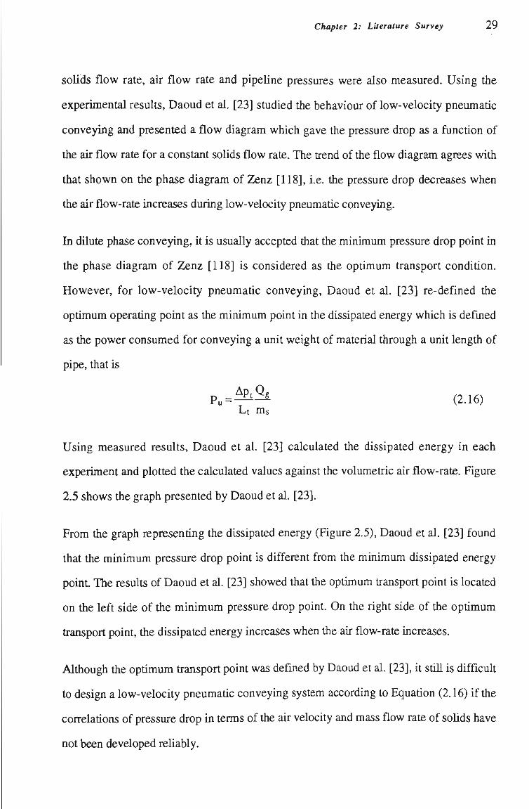
Chapter 2: Literature Survey 2 9
soHds flow rate, air flow rate and pipeline pressures were also measured. Using the
experimental results, Daoud et al. [23] studied the behaviour of low-velocity pneumatic
conveying and presented a flow diagram which gave the pressure drop as a function of
tiie air flow rate for a constant solids flow rate. The trend of the flow diagram agrees witii
that shown on the phase diagram of Zenz [118], i.e. the pressure drop decreases when
the air flow-rate increases during low-velocity pneumatic conveying.
In dilute phase conveying, it is usually accepted that the minimum pressure drop point in
the phase diagram of Zenz [118] is considered as the optimum transport conditíon.
However, for low-velocity pneumatic conveying, Daoud et al. [23] re-defined the
optímum operatíng point as the mirúmum point in the dissipated energy which is defîned
as the power consumed for conveying a unit weight of material through a unit length of
pipe, that is
Pu = - ^ ^ (2.16) Lt ms
Using measured results, Daoud et al. [23] calculated the dissipated energy in each
experiment and plotted the calculated values against the volumetric air flow-rate. Figure
2.5 shows the graph presented by Daoud et al. [23].
From the graph representíng the dissipated energy (Figure 2.5), Daoud et al. [23] found
that the minimum pressure drop point is different from the minimum dissipated energy
point The results of Daoud et al. [23] showed that tiie optimum transport point is located
on the left side of the minimum pressure drop point. On the right side of the optímum
transport point, the dissipated energy increases when the air flow-rate increases.
Although the optímum transport point was defined by Daoud et al. [23], it stíU is difficult
to design a low-velocity pneumatíc conveying system according to Equatíon (2.16) if the
correlatíons of pressure drop in terms of the air velocity and mass flow rate of soUds have
not been developed reliably.
Chapter 2: Literature Survey 30
Figure 2.5 Dissipated energy versus air flow-rate from Daoud et al. [23].
Rao and Ramakrishnan [89] undertook an experimental smdy to investígate the influence
of conveying air and system pressure drop to arrive at the optímum pressure drop and
corresponding minimum energy consumed. For this purpose, data for air flow rate,
solids flow rate, solid-air mass flow ratío and specific power consumptíon were collected
from the experiments. These experiments were for conveying four types of material (i.e.
cement, flyash, pulverized coal and rawmeal) in dense phase. A turbuflow system was
employed in the experiments to ensure dense phase conveying since some of the test
materials were classifîed as conventíonaUy diffîcult dense phase products.
Rao and Ramakrishnan [89] estabUshed an experimental program to identify tíie optimum
point of conveying performance. They firstiy presented the coUected data by plottíng the
specific power consumption against the air mass flow rate with constant solid-air mass
flow ratios for a test material. Then according to the plot the minimum specific power
consumption was evaluated and the corresponding operation point was considered as the
optímum for conveying. Rao and Ramakrishnan [89] also presented another plot
Please see print copy for image
Chapter 2: Literature Survey 3 1
showing a group of curves for the conveying pressure versus air mass flow rate with
constant soHd-air mass flow ratios. From this plot, Rao and Ramakrishnan [89] finaUy
identified the optimum conveying pressure corresponding to the maximum solid-air mass
flow ratío according to the determined optímum air mass flow rate.
Rao and Ramakrishnan [89] also found from the plots of conveying pressure that the
conveying of pulverised coal used low power consumption compared with other
materials. Hence they concluded that from the point of view of saving power, the
pulverised coal appeared to be the best for dense phase conveying.
Although this work did not contribute to the ultímate aim of accurate pressure drop
predictíon, it stíll is helpful for the optimal design of low-velocity pneumatíc conveying
systems. It should be noted that as the conveying system employed by Rao and
Ramakrishnan [89] was the turbuflow system, the data they coUected may not be
applicable to dense phase conveying in general.
32
CHAPTER 3
THEORY ON LOW-VELOCITY PNEUMATIC CONVEYING
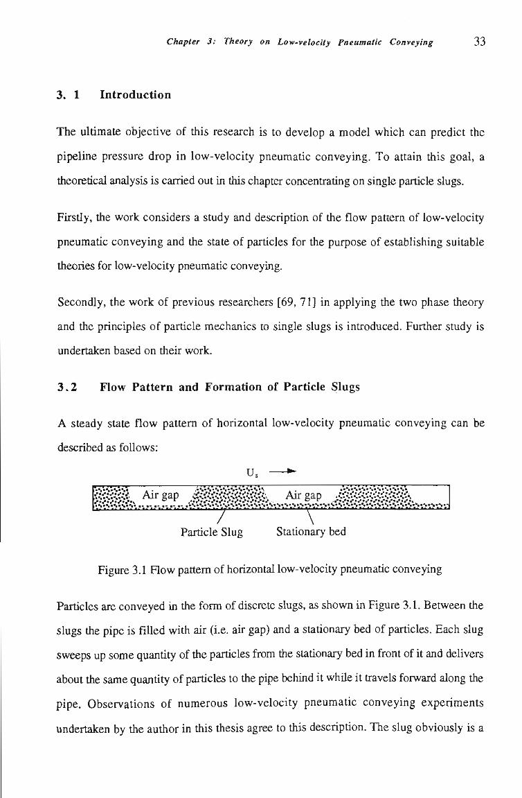
Chapíer 3: Theory on Low-velocity Pneumatic Conveying 3 3
3. 1 Introduction
The ultímate objectíve of this research is to develop a model which can predict the
pipeline pressure drop in low-velocity pneumatic conveying. To attain this goal, a
theoretícal analysis is carried out in this chapter concentrating on single particle slugs.
Firstiy, the work considers a study and descriptíon of the flow pattem of low-velocity
pneumatíc conveying and the state of partícles for the purpose of establishing suitable
theories for iow-velocity pneumatic conveying.
Secondly, the work of previous researchers [69, 71] in applying the two phase theory
and the principles of particle mechanics to single slugs is introduced. Further study is
undertaken based on their work.
3.2 FIow Pattern and Formation of Particle Slugs
A steady state flow pattem of horizontal low-velocity pneumatic conveying can be
described as foUows:
' s
•V-S»V'S-S'S"S'S».^ . . . • S - S » S ' S - S ' S - S . S " íSSSS. Airgap .ággggígggí^ Airgap Jgggggggg^ .
/ \ Partícle Slug Statíonary bed
Figure 3.1 How pattem of horizontal low-velocity pneumatic conveying
Partícles are conveyed in the form of discrete slugs, as shown in Figure 3.1. Between the
slugs the pipe is fiUed with air (i.e. air gap) and a statíonary bed of particles. Each slug
sweeps up some quantíty of the partícles from Úie statíonary bed in front of it and delivers
about the same quantíty of partícles to the pipe behind it whUe it travels forward along tíie
pipe. Observatíons of numerous low-velocity pneumatíc conveying experiraents
undertaken by the author in this thesis agree to this descriptíon. The slug obviously is a
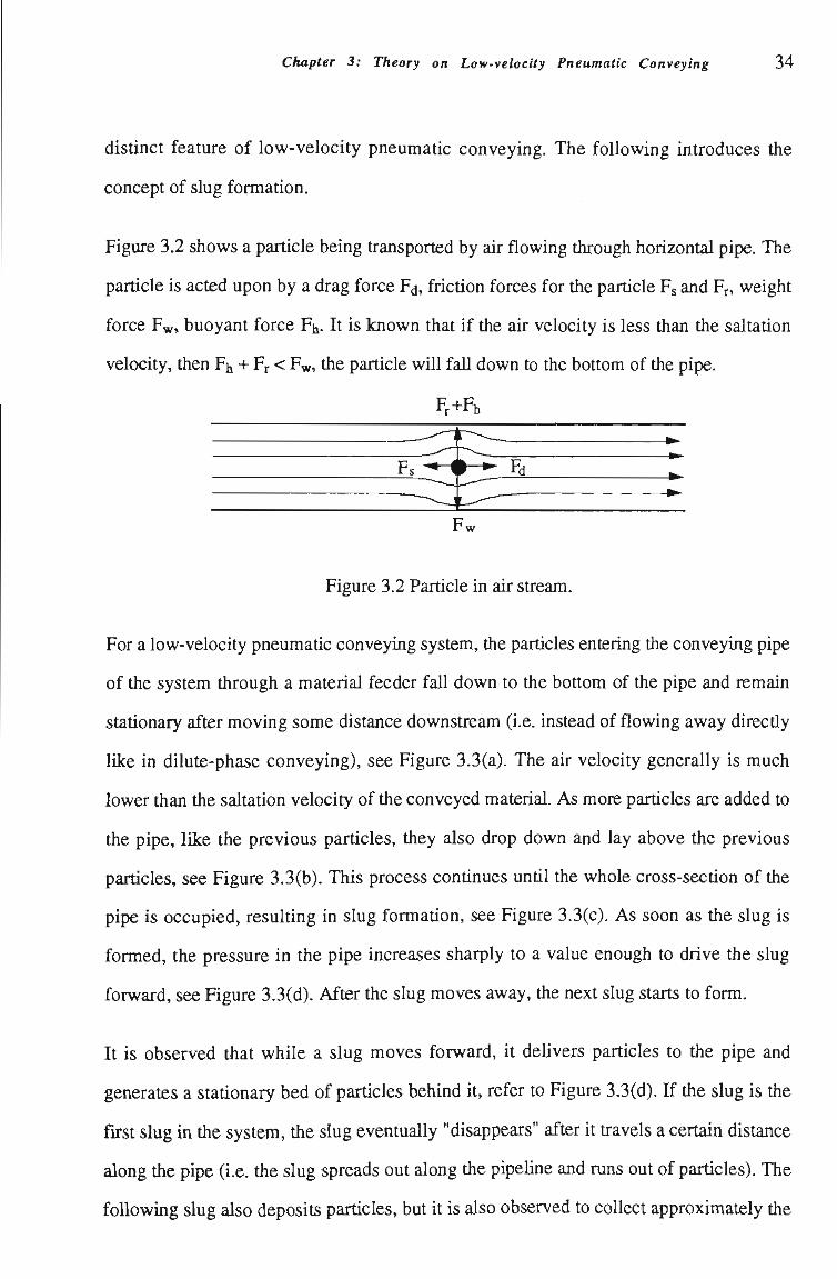
Chapter 3: Theory on Low-velocity Pneumatic Conveying 3 4
distínct feature of low-velocity pneumatic conveying. The following introduces the
concept of slug formation.
Figure 3.2 shows a partícle being transported by air flowing through horizontal pipe. The
partícle is acted upon by a drag force Fd, frictíon forces for the partícle Fs and Fr, weight
force Fw, buoyant force Fh. It is known that if the air velocity is less than the saltatíon
vel(x;ity, then Fh + Fr < F^, the particle wiU faU down to the bottom of the pipe.
Fr+Fh
'w
Figure 3.2 Particle in air stream.
For a low-velocity pneumatic conveying system, tíie particles entering the conveying pipe
of tíie system through a material feeder fall down to the bottom of the pipe and remain
statíonary after moving some distance downstream (i.e. instead of flowing away directíy
like in dilute-phase conveying), see Figure 3.3(a). The air velocity generally is much
lower than the saltatíon velocity of tiie conveyed material. As more particles are added to
the pipe, lUce the previous particles, they also drop down and lay above the previous
partícles, see Figure 3.3(b). This process contínues untíl the whole cross-sectíon of the
pipe is occupied, resuUing in slug formatíon, see Figure 3.3(c). As soon as the slug is
formed, the pressure in the pipe increases sharply to a value enough to drive the slug
forward, see Figure 3.3(d). After the slug moves away, the next slug starts to form.
It is observed that while a slug moves forward, it deUvers particles to tíie pipe and
generates a statíonary bed of particles behind it, refer to Figure 3.3(d). If the slug is the
furst slug in tíie system, tiie slug eventually "disappears" after it travels a certain distance
along tíie pipe (i.e. Ûie. slug spreads out along tiie pipeUne and mns out of particles). The
foUowing slug also deposits partícles, but it is also observed to collect approximately the
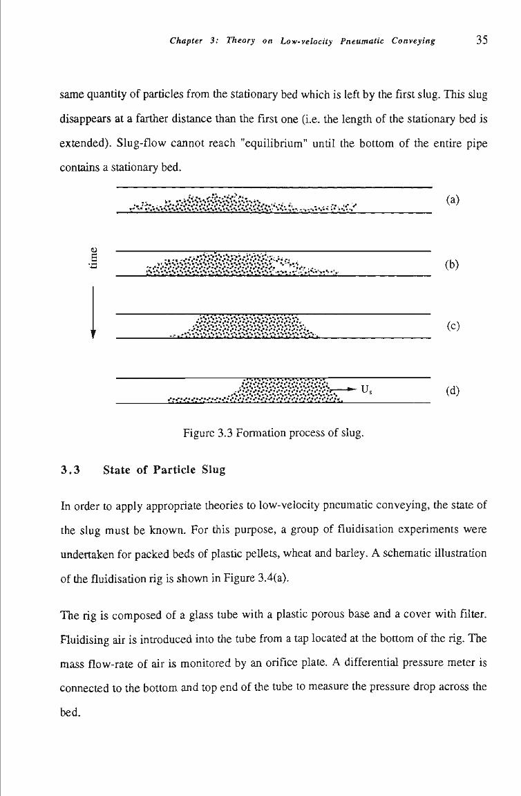
Chapter 3: Theory on Low-velocity Pneumatic Conveying 3 5
same quantíty of partícles from the statíonary bed which is left by the first slug. This slug
disappears at a farther distance than the first one (i.e. the length of the stationary bed is
extended). Slug-flow cannot reach "equilibrium" until the bottom of the entire pipe
contains a statíonary bed.
m- b" •".•S-S-S.S-S-S-S-S-%-S \d.)
>• ^* .*-.S.S.S.-S.-S.S»S.S..S.S.S..S.-S.S.-S._' .S-.-.-_n ._-i.%-S- . . .Sf.-.
(U ?—e-C _.i..s".%Xs.s.>"" • .'.Xs*.
•^ii^i^^ii^^ií^^ír-í^^ .. ( b ) iS,s,s,s-s,sr>^s,s^,s^,s,s,s-s.i:,^sr.,.^.,s.vN-.
• - • - Y - • - • - • - • - • - • - • - • - • - • - • - • - • - • - * - •
(c)
.•SISIMMMSlS'S'S'Si; iS ,S ,S ..S 'S ,S ,S '.S -.s ..s -.s , -
.-••.••-".•'•".•^.•"".•.•A'V."V.'V."Víy."'-'."*T~"^" U j ( d ) . .•S-S-S-S>S"S-S,S,S-S«S>S,S,S • • . • ^ . • ^ • • ^ . • ^ • • • ( • . • ^ . • ^ • • - • . " • " . " • " • • ^ . • ^ " . " ^ . " ^ - • ^ . • ^ • • ^ . • ^ - • ^ • • ".";".";,
Figure 3.3 Formation process of slug.
3.3 State of Particle Slug
In order to apply appropriate theories to low-velocity pneumatíc conveying, the state of
the slug must be known, For this purpose, a group of fluidisation experiments were
undertaken for packed beds of plastic peUets, wheat and barley. A schematic Ulustratíon
of tíie fluidisatíon rig is shown in Figure 3.4(a).
The rig is composed of a glass tube with a plastic porous base and a cover with filter.
Fluidising air is introduced into the tube from a tap located at the bottom of tíie rig. The
mass flow-rate of air is monitored by an orifice plate. A differentíal pressure meter is
connected to the bottom and top end of the tube to measure the pressure drop across the
bed.
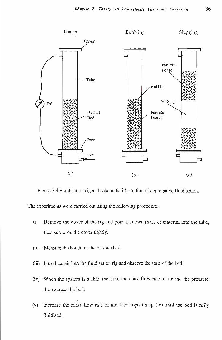
Chapter 3: Theory on Low-velocity Pneumatic Conveying 36
Dense BubbUng Slugging
".^i^".^;^ • .^ • •^ • .^" .^ •• . • • • , • • • , • •"• .
• • , • • • , • . • • . • , •1 :^'.^'.^'.^ • • • . • ; . " , » ^ " . • ^ • ^ • ^ • • ^ • • • • , • • . • . • • • • , ••"•••"••.^•-•^ •^j • - • • ' • • • ! ; • •S^S^-V*^^ ÍAÍCÍ^s ísísísís • - • ' - • ' - • ' . • '
"-".•-•- • .^ • •^ • •^ • . • ' • • • • • , • • • , • . • • ,
• •^"•^" .^• .^ • • • • • • ^ ••• , • , .•S'.S-.S'S^ • • • , . • , • . • • . . . , . •. •. •. . ' • ^ • • • • ^ • , • .s;S^sVs
• • ' • " " • "<
Cover
C l
Tube
Packed Bed
Base ' • • • • • • & • • ,
s^s-íls. , , . • • • • • . . • !
Air
Particle Dense
Bubble
Air Slug
Particle Dense
, ' S - S ' S - S . • • • • • ^ j j ' * ,-s.s-s-s • • • . • • ^ . • ^ . 1 ,-s»s-s-s • • • • • • ^ • ^ * í s ís ís ís ,«S»S-S"S .-•. . .•..•., ,.s.,s.,s.,s ^ •••,•.•,•.••, , ' S - S ' S - S ^:^:^:^:< ' S ' S ' S ' S • • - • • - ^ • - • '
. lS-S>S;S • • • • • • , • - . • -, . S -S>S .S • • • • • . • . • . - • • , • , , S ' S « S ' S • • • • • • ^ • ^ . , .S;S«S.,S - • , • - • • . • • • • , • , ,;S-S>S>S ^:^:^:^: ,s,s>s,s
(a) (b) (c)
Figure 3.4 Fluidisation rig and schematic iUustration of aggregative fluidisation.
The experiments were carried out using the following procedure:
(i) Remove the cover of the rig and pour a known mass of material into the tube,
then screw on the cover tightiy.
(U) Measure the height of the particle bed.
(ÍU) Introduce air into the fluidisation rig and observe tfie state of tiie bed.
(iv) When the system is stable, measure the mass flow-rate of air and the pressure
drop across the bed.
(v) Increase the mass flow-rate of air, then repeat step (iv) untU the bed is fuliy
fluidised.
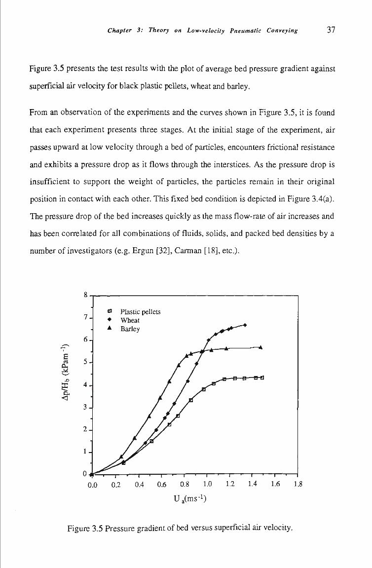
Chapter 3: Theory on Low-velocity Pneumatic Conveying 37
Figure 3.5 presents the test results witii the plot of average bed pressure gradient against
superficial air velocity for black plastic peUets, wheat and barley.
From an observatíon of the experiments and the curves shown in Figure 3.5, it is found
that each experiment presents three stages. At the initíal stage of the experiment, air
passes upward at low velocity through a bed of partícles, encounters frictíonal resistance
and exhibits a pressure drop as it flows through the interstíces. As the pressure drop is
insufficient to support the weight of partícles, the partícles remain in their original
positíon in contact with each other. This fixed bed conditíon is depicted in Figure 3.4(a).
The pressure drop of the bed increases quickly as the mass flow-rate of air increases and
has been correlated for all combinatíons of fluids, solids, and packed bed densitíes by a
number of investigators (e.g. Ergun [32], Carman [18], etc).
6
<
8
7
6
5
4
3.
2,
^ Plastic pellets • Wheat ^ Barley
e—B—H~H
0.0 0.2 0.4 0.6 0.8 1.0 1.2 1.4 1.6 1.8
Ua(ms-l)
Figure 3.5 Pressure gradient of bed versus superficial air velocity.
Chapter 3: Theory on Low-velocity Pneumatic Conveying 38
As the air velocity is increased to the point at which the pressure drop caused by the air
passing up through the bed of partícles is just equal to the weight of the partícle bed, the
weight of each partícle tiieoretically is balanced by the pressure drop across the partícle.
Hence, the inter particle stress disappears, although the partícles stUl are in contact with
each other. There is no motíon of particles (i.e. partícles keep fixed relatíve to each
other). The pressure drop of the bed arrives at its maximum theoretical value. The partícle
state at this stage is called incipient fluidisation. The flow rate of the air corresponding to
tíiis point is termed as the incipient fluidisation rate.
If velocities above the incipient fluidisation rate, for some materials, the bed expands in
volume, the particles in the bed move further apart and open up the interstices to allow
easy passage of the air, thus the bulk density decreases (i.e. the buUc voidage increases),
and all the particles are no longer touching each other. The bed is in the so-called "fluid"
state. This system is said to exhibit particulate fluidisation. On the other hand, for some
other materials such as the materials used in this investigatíon, any excessive air passes
up tíirough the bed in the form of bubbles, as shown in Figure 3.4(b). This system is
said to exhibit aggregative fluidisation. If the flow rate of air is increased further, more
bubbles occur in the bed, and coalesce to form larger bubbles. During aggregative
fluidisation, the bed is divided into two phases: particle dense phase, in which the
particles are believed to exhibit fîxed bed configuration and the volume of the air passes
through the phase just at the incipient fluidisation rate; and particle dilute phase, i.e.
bubbles, which are formed by the excessive air and small numbers of particles "free-fall"
in the bubbles. In theory, the pressure drop across the bed no longer increases after the
bed is fluidised. In practice, the pressure drop stiU increases slightly with the fluid flow
rate increasing, see Figure 3.5. From these figures, a transition area between the fixed
bed and fluidised bed regions can be observed.
If the flow rate of air provided for fluidisation is sufficientiy high to achieve an
aggregative fluidisatíon bed, the volume of some bubbles increases untíl the diameter is
Chapter 3: Theory on Low-velocity Pneumatic Conveying 3 9
equal to the diameter of the bed, see Figure 3.4(c). At this tíme the partícle dense phase is
lifted and slug-flow appears. According to the flow pattem of low-velocity pneumatíc
conveying and the fluidisation experiments, the foUowing conclusions can be obtained
for low-velocity pneumatíc conveying:
1 Low-velocity pneumatic conveying can be represented by an aggregatíve fluidised
bed model.
2 Two partícle phases exist in low-velocity pneumatíc conveying. One is the partícle
dense phase (i.e. the partícle slugs), the other is the particle dilute-phase (i.e. the air
gaps). These constitute the discontinuous flow pattem of low-velocity pneumatíc
conveying.
3 The particle slugs are a special case of dense phase (i.e. incipient fluidisatíon), in
which the air flow-rate is equal to that required just to fluidise the material. The air
gaps are formed by using air in excess of that needed to fluidise the material.
Therefore, for a low-velocity pneumatic conveying system and a given mass flow-
rate of solids, increasing the mass flow-rate of air in theory does not change the
pressure gradient of the slugs and only increases the length of the air gaps or forms
new air gaps. The air gaps are axisymmetric for vertícal slug flow and asymmetric
for horizontal slug flow which results in tíie existence of a statíonary bed.
4 From the definitíon of incipient fluidisatíon it is known that the particle slugs have a
conventíonal fixed-bed configuratíon (i.e. tiie partícles in the slugs are just in contact
and are fixed relatíve to each other), with a buUc density simUar to tíie loose-poured
bulk density.
3.4 Pressure Gradient of Horizontal Slug
The foUowing sectíon introduces tíie theoretícal analysis for the pressure gradient of a
single slug, as conducted by K. Konrad [69] based on the Janssen's method for
Chapter 3: Theory on Low-velocity Pneumatic Conveying 4 0
analysing hopper flow problems. Further studies then are given by the author for the
stress state of a single slug. For this purpose, the foUowing assumptíons are made:
• AU the air flows through a slug in the axial direction of the slug (i.e. tíiere is no
motíon of the air in a directíon perpendicular to the axis of the slug).
• When low-velocity pneumatic conveying reaches steady state, the acceleratíon of
tiie slug is not significant, so that tíie motion of slug can be regarded as uniform.
• The axial stress and transmission radial stress in a slug are functíons of the length
of slug only, i.e. their values are constant at a particular cross sectíon of slug.
• The ratío of the axial stress to the transmission radial stress is constant, although
the stresses themselves are functíons of the length of slug.
• The length of slug is much greater than its diameter, i.e. Ij » D.
• The partícle slug is cohesionless and obeys the Coulomb faUure criterion.
3.4.1 Stresses Acting on Moving Slug
Figure 3.6 shows a moving particle slug in a horizontal pipe. The average length of the
slug is Is and the inner pipe diameter (i.e. the diameter of the slug) is D. During
conveying, the slug is subjected to the pressure forces Pi and P^, collecting and
delivering resistant forces Rsi and Rs2, as weU as the friction force Rf between the sliding
siug and pipe waU, as shown in Figure 3.6(a).
The extemal forces acting on the slug generate various stresses. The stresses acting on an
element of the slug are shown in Fig 3.6(b). The notatíons in the fîgure are explained
below.
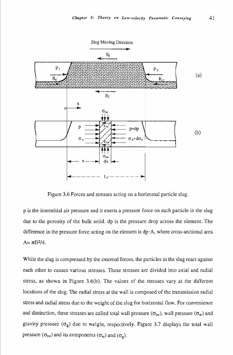
Chapter 3: Theory on Low-velocity Pneumatic Conveying 41
Slug Moving Direction
Rf
. > i ' . ^ . ' ^ ; > • : . • • ^;••.• ^:••.• ••.• :•• .• ;^;••.• -".• ;^;•• • ^ - • • • • • • •• • > • ^ - • • • • • . • • •• * ! > • • • • • •
S-s,s^s,s,s,s.s..v.s,s.s.s,s^s.s,s,s^s,s,s,s,s,s,s,s,s,s^s^s,s * i ^ B M ^
Rf
tw
iii / t t w
<Jtw
dx
p+dp \
(a) ^•K.Ki
^ (b)
Figure 3.6 Forces and stresses actíng on a horizontal partícle slug.
p is the interstítíal air pressure and it exerts a pressure force on each particle in the slug
due to the porosity of the bulk solid. dp is the pressure drop across the element. The
difference in the pressure force actíng on the element is dp^ A, where cross-sectional area
A= KD2/4.
While the slug is compressed by the extemal forces, the particles in the slug react against
each other to causes various stresses. These stresses are divided into axial and radial
stress, as shown in Figure 3.6(b). The values of the stresses vary at the different
locatíons of the slug. The radial stress at the wall is composed of the transmission radial
stress and radial stress due to the weight of the slug for horizontal flow. For convenience
and distinctíon, these stresses are caUed total wall pressure (Otw), wall pressure (0^) and
gravity pressure (Gg) due to weight, respectively. Figure 3.7 displays the total wall
pressure (atw) and its components (a^) and (ag).
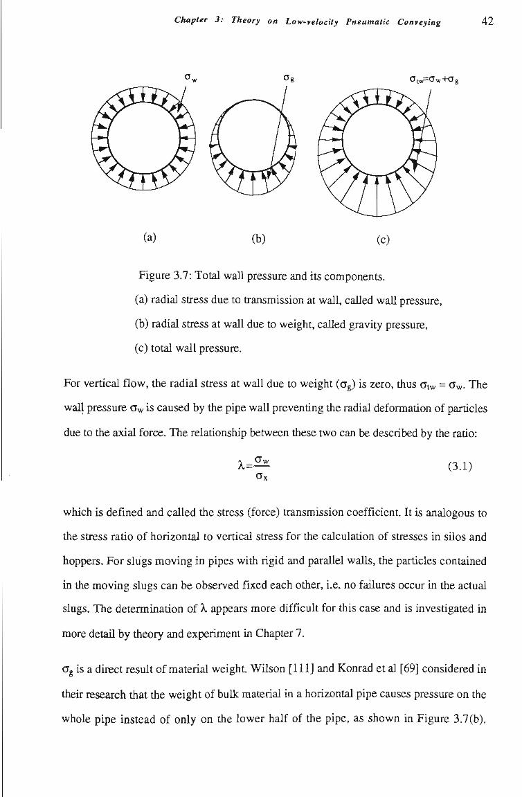
Chapter 3: Theory on Low-velocity Pneumatic Conveying 42
^tW ^W T ^ g
(a) (b) (c)
Figure 3.7: Total waU pressure and its components.
(a) radial stress due to transmission at wall, caUed waU pressure,
(b) radial stress at wall due to weight, caUed gravity pressure,
(c) total wall pressure.
For vertícal flow, the radial stress at wall due to weight (Og) is zero, thus atw = a^. The
wall pressure a^ is caused by the pipe wall preventíng tiie radial deformatíon of partícles
due to the axial force. The relationship between these two can be described by the ratío:
X = ^ (3.1)
which is defined and called the stress (force) transmission coefficient. It is analogous to
the stress ratío of horizontal to vertical stress for the calculation of stresses in sUos and
hoppers. For slugs moving in pipes with rigid and parallel walls, the partícles contained
in the moving slugs can be observed fixed each other, i.e. no failures occur in the actual
slugs. The determinatíon of X appears more difficult for this case and is investigated in
more detaU by theory and experiment in Chapter 7.
Og is a direct result of material weight. Wilson [111] and Konrad et al [69] considered in
their research that the weight of bulk material in a horizontal pipe causes pressure on the
whole pipe instead of only on the lower half of the pipe, as shown in Figure 3.7(b).
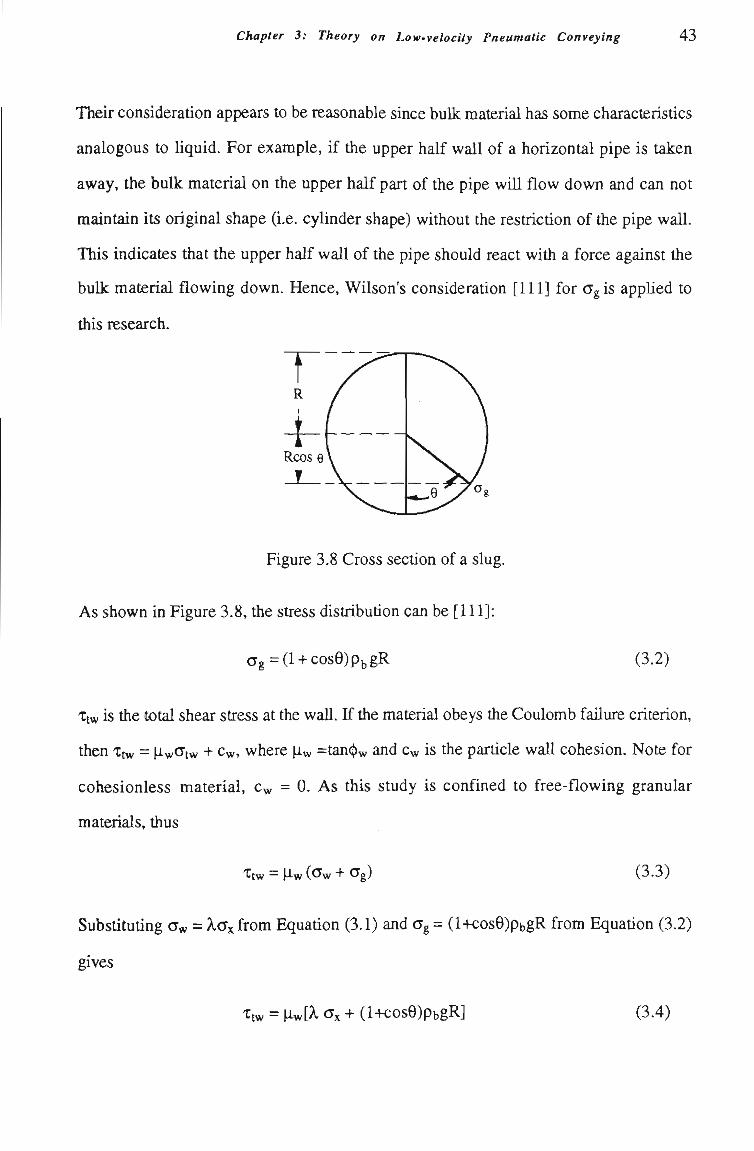
Chapter 3: Theory on Low-velocity Pneumatic Conveying 43
Their consideration appears to be reasonable since buUc material has some characteristícs
analogous to liquid. For example, if the upper half wall of a horizontal pipe is taken
away, the bulk material on the upper half part of the pipe wUl flow down and can not
maintain its original shape (i.e. cylinder shape) without the restrictíon of the pipe wall.
This indicates that the upper half wall of the pipe should react with a force against tíie
bulk material flowing down. Hence, Wilson's consideratíon [111] for a^is appHed to
this research.
Figure 3.8 Cross section of a slug.
As shown in Figure 3.8, the stress distributíon can be [111]:
ag = (l + cosØ)PbgR (3.2)
Ttw is tíie total shear stress at the waU. If tfie material obeys tíie Coulomb faUure criterion,
then Xtw = M-wíJtw + Cw, where iw =tan(t)w and Cw is the particle wall cohesion. Note for
cohesionless material, Cw = 0. As this study is confined to free-flowing granular
materials, thus
t tw = M-w (c^w + CTg) (3.3)
Substítuting aw = >.axfrom Equation (3.1) and ag= (l+cose)pbgR from Equation (3.2)
gives
ttw = iwí Ox + (l+cose)pbgR] (3.4)
Chapter 3: Theory on Low-velocîty Pneumatic Conveying 4 4
3.4.2 Force Balance and Pressure Gradient of Horizontal Slug
Because the motion of a slug is regarded as uniform, there exists an equUibrium of the
forces acting on tiie element of length dx, so that:
^ + ^ + % = 0 (3.5) dx dx A
where Qw in Equation (3.5) is the total shear stress acting on the waU around the pipe,
therefore:
Qw= fxtwRdB (3.6)
From Equation (3.4),
Qw= Jjl^[Xax + (l + cosØ)PbgR] RdØ (3.7)
Integrating the right hand side of Equation (3.7) gives
Qw = 27cR|iw[ ax + pbgR] (3.8)
If a deaerated particle slug is forced to move by a mechanical piston, the motíve pressure
usually is expected to be proportional to the exponential of the slug length, as shown in
Figure 3.9. However, some researchers [17, 27] pointed out that the pressure to
maintain the movement of a slug by using air is much smaller, as the slug may allow air
to permeate through the partícles and aerate the soUds resultíng in a reduced material to
waU frictíon force. The pressure is expected to be proportional to the slug length raised to
a power (n) as shown in Figure 3.9. The value of the exponent (n) depends on the
propertíes of the material such as permeabiUty, etc. and is in tiie range 1 < n < 2 [17].
Chapter 3: Theory on Low-velocity Pneumatic Conveying 45
Figure 3.9 Pressure to maintain movement of a particle slug in a pipe [17].
Tltís research is concentrated on the low-velocity pneumatic conveying of coarse granular
material. This type of material has natural slugging behaviour and good permeabiUty. It
can form rather short slugs naturaUy while stíU being conveyed at low velocity. Hence,
the conveying air can aerate the particles completely. It is assumed that the value of the
exponent (n) approaches 1 and the pressure is proportional to the slug length (i.e. the
pressure gradient in the coarse granular material slug is constant). Therefore, — = — - , dx Is
where Ig is the length of a single slug.
Substímtíng Equatíon (3.8) into Equatíon (3.5), and replacing A with T R^, resitíts in:
^ . l l i ^ < , , . ^ , 2 ^ : „ p , g = 0 (3.9) dx D Is
where R has been replaced by D/2. The solutíon to Equatíon (3.9) is,
r. ^^ r^ Ap, D Ox = C e " - ^ ^ + (-2pbg iw + -r> Is 4 i X
(3.10)
where C is the integration constant and can be determined by the following boundary
conditíons where the stresses on the front and back surface of a slug are af and ab,
respectívely.
Please see print copy for image
Chapter 3: Theory on Low-velocity Pneumatic Conveying 46
ax = af, at X = l ,
ax = ab, at X = 0.
Applying the above conditíons to Equatíon (3.10) yields
4^w^, An D af = C e—5-1' + (-2p,gn, + T^^TiTT ^^.ll)
Is '+Kw^
ab = C + (-2Pbg iw + — ) T \ (3.12) Is 4^t^?.
Eliminating constant C yields
4HW^. 4|i^>., An n cTf-abe~5-i' = (1- e-—i^)(-2p,g^i, + ^ ) - ^ (3.13)
Is ^ l^w^
Actual observatíons of low-velocity pneumatic conveying found that the statíonary bed
thickness on the two sides of a slug is very similar. It is mentioned by Konrad et al. [69]
that the value of a^ is approximately equal to the value of af if the cross sectional area
ratio of statíonary bed to pipe is similar on average both in front of and behind a slug.
Hence assume that af « ab, as well as \ » D, which is reasonable for a natural slug-
flow system, an equation for the pressure gradient of a single horizontal slug is
determined:
^ = l l i ^ , , , . IMV^^ (3.14) Is tJ
3.5 Axial Stress and Transmission Radial Stress
3.5.1 Distribution of Axial Stress
Rearranging Equatíon (3.14):
<,, = (-2p,g,„ . ^ ) ^ (3.15)
Replacing (-^p^g^i^ + — ) in Equatíons (3.10) and (3.12) with af gives Is 4^ A
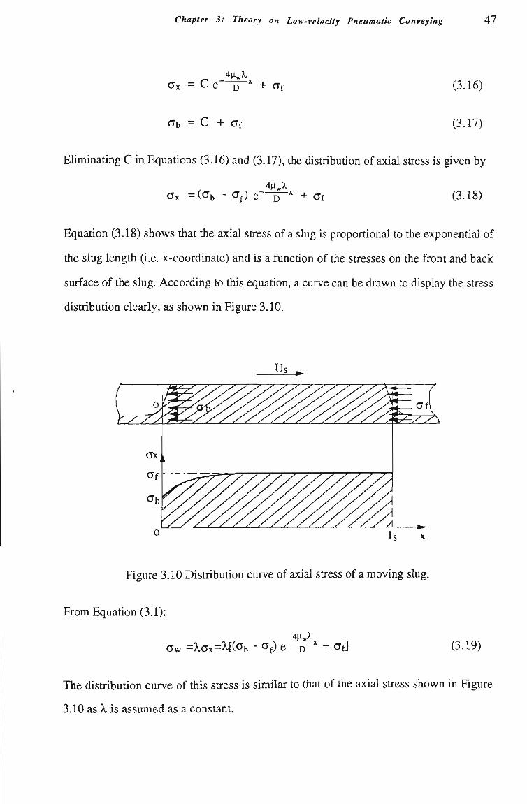
Chapter 3: Theory on Low-velocity Pneumatic Conveying 47
_4n„X. Cx = C e D ^ + CTf
ab = C + af
(3.16)
(3.17)
EUminatíng C in Equatíons (3.16) and (3.17), tíie distributíon of axial stress is given by
(3.18) ax = (cTb - ^f) e ~B~^ + af
Equatíon (3.18) shows that the axial stress of a slug is proportional to the exponentíal of
tíie slug lengtíi (i.e. x-coordinate) and is a functíon of the stresses on tíie front and back
surface of the slug. According to this equatíon, a curve can be drawn to display tiíie stress
distribution clearly, as shown in Figure 3.10.
Us
Figure 3.10 Distribution curve of axial stress of a moving slug.
From Equatíon (3.1):
4|i„X. aw =XGx=H(<^b - CJf) e D ^ + t fl (3.19)
The distributíon curve of this stress is similar to that of the axial stress shown in Figure
3.10 as X, is assumed as a constant.
Chapter 3: Theory on Low-velocity Pneumatic Conveying 4 8
3.5.2 Average Axial Stress
From Equation (3.18), tíie total axial stress of a slug can be obtained easUy by integratíng
tíie axial stress along the slug lengtíi (i.e. calculating tiie shaded area in Figure 3.10). The
average axial stress is the total stress divided by the slug length.
axm = - jQaxdx = -JJ'[(cib-af) e ~ i - ^ + af]dx (3.20)
which results in:
^ ^ = <f [ 1 - 7 7 7 ^ ( 1 - — ) ( l - e - ^ ^ ) ] (3.21) 4HwAls af
D a h '*i w'
As af = ab and U » D, therefore — (1 - — )(1 - e 5" ') = 0, so tiiat: 4|iw^ls af
Oxm = Of (3.22)
This result can be observed clearly from Figure 3.10 where most of the axial stress is
close to the value of the frontal stress of the slug.
If the average wall pressure of the slug is awm, as ^ is assumed as a constant in a slug,
fromEquation(3.1):
^^ow^awm (323)
C x CTxm
Substituting axm ~ C7f into Equatíon (3.23):
X = - ^ (3.24) CTf
Equation (3.24) shows that the stress transmission coefficient of a slug can be
approximated by the ratío of the average wall pressure to the frontal stress of the slug.
This result is useful for determining X by experiment, since it is difficult to measure the
axial stress inside a slug and its corresponding transmission stress.
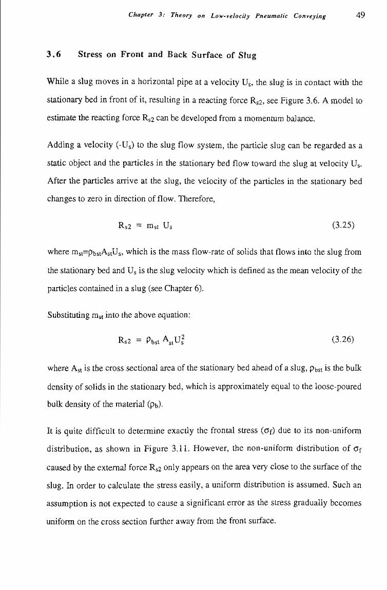
Chapter 3: Theory on Low-velocity Pneumatic Conveying 4 9
3.6 Stress on Front and Back Surface of Slug
While a slug moves in a horizontal pipe at a velocity Us, tíie slug is in contact witíi tíie
statíonary bed in front of it, resultíng in a reactíng force Rs2, see Figure 3.6. A model to
estimate the reactíng force Rs2 can be developed from a momenmm balance.
Adding a velocity (-Us) to the slug flow system, the particle slug can be regarded as a
statíc object and the partícles in the statíonary bed flow toward the slug at velocity Us.
After the particles arrive at the slug, the velocity of the particles in the statíonary bed
changes to zero in direction of flow. Therefore,
Rs2 = mst Us (3.25)
where mst=PbstAstUs, which is the mass flow-rate of solids that flows into the slug from
the statíonary bed and Ug is the slug velocity which is defined as the mean velocity of the
partícles contained in a slug (see Chapter 6).
Substímtíng mst into the above equation:
Rs2 = Pbst A,tU? (3.26)
where Ast is the cross sectíonal area of the statíonary bed ahead of a slug, pbst is the buUc
density of solids in the statíonary bed, which is approximately equal to the loose-poured
bulk density of the material (pb).
It is quite difficult to determine exactíy the frontal stress (af) due to its non-uniform
distributíon, as shown in Figure 3.11. However, the non-uniform distribution of af
caused by the extemal force Rs2 only appears on the area very close to the surface of the
slug. In order to calculate the stress easily, a uniform distributíon is assumed. Such an
assumptíon is not expected to cause a significant error as the stress graduaUy becomes
uniform on tiie cross sectíon further away from tíie front surface.
Chapter 3: Theory on Low-velocity Pneumatic Conveying 50
Hence,
Of = aPbU^ (3.27)
where a is the cross sectíonal area ratío of statíonary bed to pipe.
U
-.sísísísísísísísísísísísísí-[í^íWWsísísísísísísW
. ^ . ^ . ^ . ^ . ^ . . • . / . / • . . . . ^
i»«i " '.S• S,S,S..SrS-.S"S,S-S••• ••,•.•íjt'S
Relative Moving Direction of Particles toSlug
Figure 3.11 Stresses acting on the frontal surface of a slug.
While the moving slug deposits particles to the stationary bed behind the slug, the
deposited particles impact the stationary bed, also resulting in a force Rsi. A similar
method can be employed to estímate the stress on the back face of a slug, so that:
Ob = aPbU^ (3.28)
51
CHAPTER 4
TEST FACILITY AND PROCEDURES
Chapter 4: Test Facility and Procedures 5 2
4.1 Introduction
To understand tíie performance of low-velocity pneumatic conveying and determine some
parameters which are difficult to predict theoretically, such as slug velocity and stress
transmission coefficient X, experimental investigations are necessary. Based on the
experimental data, empirical correlatíons are established to demonstrate tiie influence and
relatíonship of the major parameters of low-velocity pneumatíc conveying. Substítutíng
these empirical correlations into the theoretical models developed in Chapter 3 results in
tíie fînal solution. More tests are carried out witfi different materials and pipeUnes and tíie
data are used to verify the validity of the prediction model. The equipment described in
this chapter is designed specifically for this purpose. The test rig allows product, air
flow-rates and conveying distances to be of simUar scale to indusúial applications.
4.2 General Arrangement of Main Test Rig
The main low-velocity pneumatic conveying test rig consists primarily of material feeders
(either a blow tank or high pressure rotary valve), a feed hopper, conveying pipelines,
receiving silo mounted above the blow tank and rotary valve feed hopper and some
instmmentatíon. A schematíc layout of the low-velocity pneumatíc conveying test rig is
shown in Figure 4.1. If the conveying pressure of the system is no more than 350 kPag,
the rotary valve is chosen as the feed device, otherwise, the blow tank is employed to
allow tests to be carried out at higher pressures.
4.2.1 Material Feeders
There are many types of devices which have been used as material feeders successfully in
pneumatíc conveying. In tíiis thesis, a high pressure rotary valve and blow tank feeder
are available for dense-phase granular conveying in the low-velocity pneumatic
conveying test rig, see Figure 4.2.
Chapter 4: Test Facility and Procedures 53
1 Feed Hopper 2 ZGR-250 Rotary Valve 3 BlowTank 4 Vertical Lift, 6.5 m 5 Transport Line 105 mm E),
One Loop 52 m, Two Loops 96m
6 52 m Loop Connector 7 Back Pressure Valve 8 Reverse-jet Filter 9 Receiving Silo lOBlowTankFiUing
11 Rotary Valve Filling 12 Conveying Air Inlet P Static Air PressuieTapping SG SightGlass WP Wall Pressure Fittings
Figure 4.1 Schematíc layout of low-velocity pneumatíc conveying test rig.
Chapter 4: Test Facility and Procedures 54
1 Filter 4 SiloValve 7 ZGR-250RotaryValve 10 VentValve 2 Receiving Silo 5 FeedHopper 8 BlowTankVentPipe 11 BIowTank 3 Pulse Valve 6 Hopper Valve 9 BIow Tank FiII Valve LC - Load Cell
Figure 4.2 Feed devices and receiving silo.
Chapter 4: Test Facility and Procedures 55
4.2.1.1 High Pressure Rotary Valve
The principle requUement of a feeder is Úiat it should be capable of feedmg the soUds at a
reliable rate from the supply hopper at one pressure to the conveying line at another
pressure. For this reason rotary valves are an ideal selection for pneumatic conveying
systems. Since rotary valves are used for feeding products from a low pressure area into
a higher pressure area, air leakage automatically occurs between rotor and housing due to
the existence of clearance between them. Conventional rotary valves (up to pressures of
100 kPag) are most commonly applied to dilute-phase systems. Feeding into high
pressure systems almost always involves the use of a blow tank, which usually is
capable of working at the pressures up to about 600 kPag. One disadvantage of the blow
tank is that the feed rate cannot be controUed easily.
Material Inlet
Conveying Airlnlet • ^
Feeding Shoe
Air & Material Outlet
Figure 4.3 ZGR-250 high pressure rotary valve.
Thanks to the furtiier systematíc development of rotary valve technology, the appUcatíon
for rotary valves has been extended into dense-phase pneumatíc conveying systems. The
Chapter 4: Test Facility and Procedures 5 6
ZGR-250 rotary valve shown in Figure 4.3 is a high performance rotary valve designed
and manufactured specially for dense-phase pneumatíc conveying by Waeschle
Maschinenfabrick GmbH (Germany).
Designers of the company found new ways to seal off the rotor at the side by extemal,
self-adjustíng axial rotatíng mechanical seals to reduce air leakage under high pressure. A
rotor shaft sealmg ring also can be used to minimise air leakage further. The applicatíon
of these new developments aUows the ZGR-250 rotary valve to handle fme and coarse
materials up to the conveying pressures of 350 kPag and reduce the air leakage by up to
60% compared to conventíonal rotary valves.
Although the air leakage of the ZGR-250 rotary valve is quite low (compared with
conventional rotary valves), it stiU may be quite significant in low-velocity pneumatíc
conveying. That is, the effect of air leakage on systems cannot be ignored. In order to
determine air leakage of the ZGR-250 rotary valve under different conveying pressures,
experiments are undertaken as follows.
(i) Block the air and material outlet of the ZGR-250 rotary with a steel plate, refer to
Figure 4.3.
(U) Load a certain mass of material (e.g. plastic pellets) into the feed hopper and
operate the rotary valve at a given rotor speed (e.g 20 rpm).
(iU) Blow air from the conveying air inlet, see Figure 4.3, into the rotary valve. As the
air and material outiet of the rotary valve is blocked, all the air escapes out of the
rotary valve tíirough the clearance between the rotor and housing.
(iv) Measure the mass flow-rate of the blowing air by an orifice plate and the pressure
in the feeding shoe of the rotary valve.
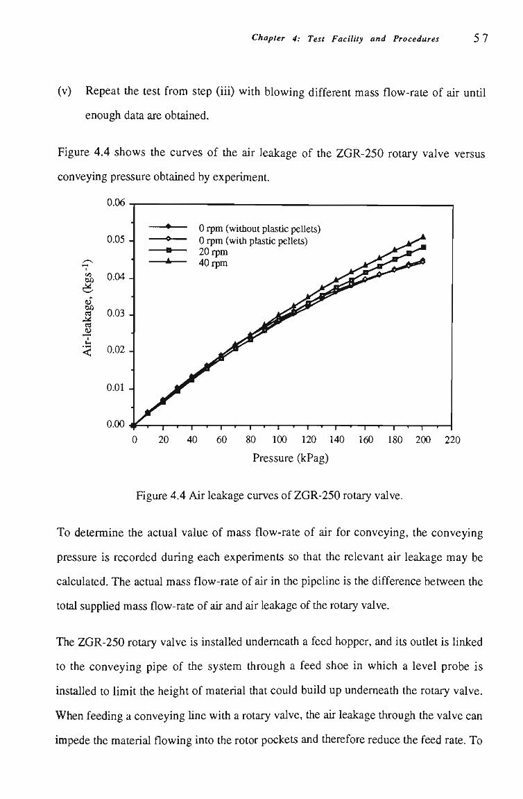
Chapter 4: Test Facility and Procedures 57
(v) Repeat the test from step (iii) with blowing different mass flow-rate of air untíl
enough data are obtained.
Figure 4.4 shows tíie curves of tíie air leakage of tíie ZGR-250 rotary valve versus
conveying pressure obtained by experiment.
0.06
0.05 -
a 0.04
Bû S 0.03 0)
0.02
0.01 -
0.00
• 0 rpm (without plastic pellets) * 0 rpm (with plastic pellets)
20rpm 40rpm
T — • — I —
120 140 160 180 200 220
Pressure (kPag)
Figure 4.4 Air leakage curves of ZGR-250 rotary valve.
To determine the actual value of mass flow-rate of air for conveying, the conveying
pressure is recorded during each experiments so that the relevant air leakage may be
calculated. The actual mass flow-rate of air in the pipeline is the difference between the
total suppUed mass flow-rate of air and air leakage of the rotary valve.
The ZGR-250 rotary valve is installed undemeath a feed hopper, and its outlet is linked
to the conveying pipe of the system through a feed shoe in which a level probe is
installed to limit the height of material that could build up undemeath the rotary valve.
When feeding a conveying Une with a rotary valve, the air leakage through tiie valve can
impede the material flowing into the rotor pockets and therefore reduce the feed rate. To
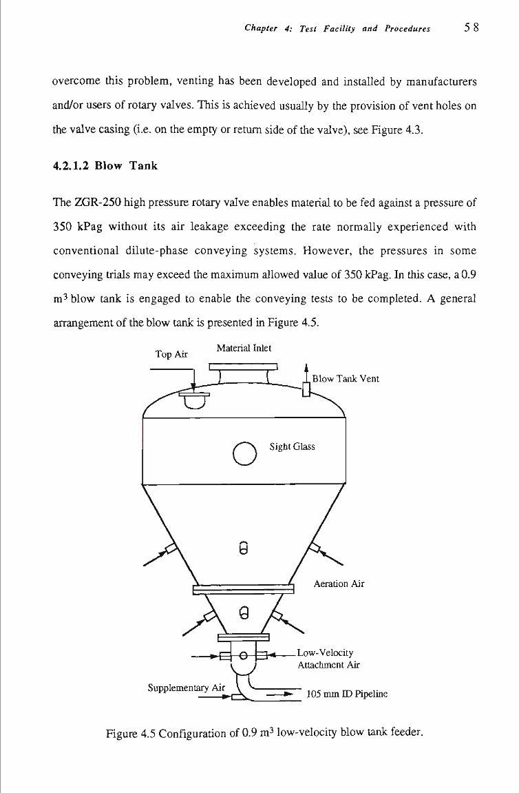
Chapter 4: Test Facility and Procedures 58
overcome tiiis problem, venting has been developed and instaUed by manufacmrers
and/or users of rotary valves. This is achieved usuaUy by the provision of vent holes on
the valve casing (i.e. on the empty or retum side of the valve), see Figure 4.3.
4.2.L2 Blow Tank
The ZGR-250 high pressure rotary valve enables material to be fed against a pressure of
350 kPag without its air leakage exceeding the rate normally experienced with
conventional dilute-phase conveying systems. However, the pressures in some
conveying trials may exceed tíie maximum allowed value of 350 kPag. In this case, a 0.9
m^ blow tank is engaged to enable the conveying tests to be completed. A general
arrangement of the blow tank is presented in Figure 4.5.
Material Inlet TopAir
Blow Tank Veni
Aeration Air
» M O r~l'* Low-Velocity Attachment Air
Supplementary Air uy Air V V-105 nmi ID Pipeline
Figure 4.5 Configuratíon of 0.9 m^ low-velocity blow tank feeder.
Chapter 4: Test Facility and Procedures 5 9
This blow tank was developed jointíy by the University of WoUongong and NEI John
Thompson (Australia) to allow friable and/or granular products to be conveyed with
extremely low levels of product degradatíon or damage (e.g. solids conveying velocitíes
usually occur in the range 0.25 to 2 ms-i). The blow tank is supported on load ceUs
which are fixed on a supporting stmcture. The mass of product discharged from or
loaded into the blow tank can be measured by the load cells.
4.2.2 Feed Hopper and Receiving Silo
A 0.9 m^ feed hopper providing material for the rotary valve is supported witíiin a
framework by load ceUs, see Figure 4.2. The mass of material discharged from or loaded
into the hopper can be measured by the load cells. The hopper is connected to the rotary
valve via a flexible mbe to avoid tíie influence of vibratíon of the working rotary valve on
the output of the load cells.
The receiving silo is designed to be slightly larger in capacity than the blow tank or feed
hopper to allow for the loss of volumetric capacity by uneven distributíon of the received
material within the silo. The mass of the received material can be measured by the load
cells which support the receiving silo. A filter is instaUed on top of the silo to separate the
air from the conveyed solids. Four pulse valves, see Figure 4.2, are mounted on the
coiúcal hopper of the silo to assist in the complete discharge of material from the sUo.
4.2.3 Conveying Pipeline
The low-velocity pneumatíc conveying test rig consists of a mild steel closed loop
pipeHne, see Figure 4.1, either 96 m or 52 m in lengtíi (105 mm ID), fitted with flanges
connected properly to provide continuous unintermpted flow. The main sectíon of the
pipeline is constracted horizontally above the roof of the Bulk Solids Handling
Laboratory, A 6.5 m vertícal lift required to send material up to this horizontal sectíon is
located at the beginning of the conveying line. The total pipeUne comprises various
Chapter 4: Test Facility and Procedures 6 0
lengths of pipe and the length of each pipe is shown in Figure 4.6. Ten 90° 1.2 m radius
bends are installed along the pipeline with a back pressure valve and a 45° 1.2 m radius
bend at the end of the Une.
Two sight glasses (each 1.0 m in length), see Figure 4.1, can be fitted to the test pipeline
for the visual study of slug-flow. The effect of the sight glasses, in partícular due to the
different frictíonal characteristics between the steel and glass with the conveyed products,
is unknown. However, the length of each sight glass is very small compared to the total
length of the pipeUne and the effect on flow performance is assimied negligible.
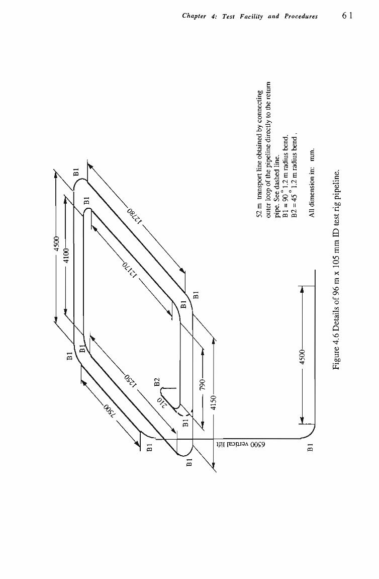
Chapter 4: Test Facility and Procedures 61
«0 3 c p
.... u. O « c ^ c o o *-
S c
íl c o. e 5 a
W1 O
<1) c
T5 <U
^ •o ii <u
V2
ã
•o c <u C/1 3
"2 2 S
( S »-H
0
s II
D .a
"O c ^ «1 3
"2 2 B cs 1.H
3
II
CQ
O « • • Cli o o
c .2 't/î c <u S
s •t
JJTI IB0pJ3A 0059 m
o c
"«3 o.
•c •4-t
B
B B e «o o X
S
o </)
<u Q
Chapter 4: Test Facility and Procedures 6 2
4.3 Air Supply and Control
4.3.1 Air Supply
The major consideratíon in the selection of an air supply plant for a test rig is that
sufficient air is available for aU experiments. In tíie BuUc Solids HandUng Laboratory, ak
at a maximum pressure head of 800 kPag is suppHed from tiie foUowing rotary screw
compressors:
• Atias Copco electric-powered Model GA-308, 3.1 m^ min- free air deUvery.
• IngersoU Rand diesel-powered Model P374-WP, 10.6 m^ min-i free air deUvery.
• Ingersoll Rand diesel-powered Model P840-WGM, 24.1 m^ min-^ free air
delivery.
To handle a wide range of bulk solids through numerous sizes of pipeline (e.g. 50 to 150
mm), any combination of the above compressors can be employed for the test rig. The
compressors are connected to an after-cooler, two refrigerated air dryers and two air
receivers (1.74 and 6.0 m^ volumetric capacity). Various filters and separators are
installed in series with these compressors to ensure a dry and oil-free air supply. Figure
4.7 shows a general arrangement of the air supply system.
4.3.2 Air FIow Control
Cooled, dried and oU-free air is introduced into the conveying pipeUne through an orifice
plate or annubar where the air flow-rate is measured, as shown in Figure 4.7. It is a
general requirement that the mass flow-rate of air is as constant as possible during a
conveying trial. Due to the fluctoatíons in the air supply pressure, the mass flow-rate of
air entering the pipeline normally will vary (i.e. without using mass flow-rate control
device). For this reason, sonic nozzles are installed before the entrance of the pipeUne of
the low-velocity pneumatíc conveying test rig, as shown in Figure 4.8.
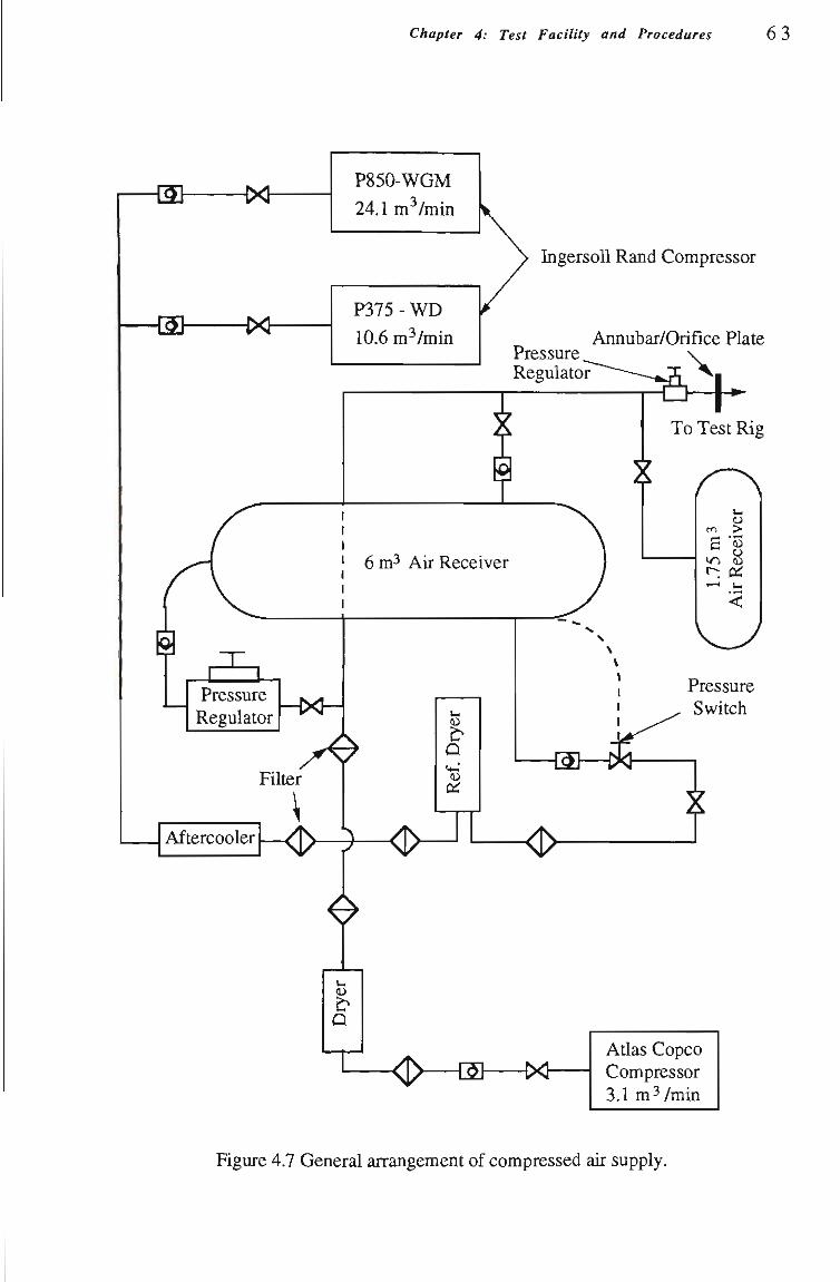
Chapter 4: Test Facility and Procedures 63
m
•Sh
-ix
• ^
Pressure Regulator
P850-WGM 24.1 m^/min
P375 - WD 10.6 m^/min
IngersoU Rand Compressor
Pressure Regulator
Annubar/Orifice Plate
\ .
X
6m3 AirReceiver
To Test Rig
HXl-
FUter A
Aftercooler
(U
û
<u
o >n <u
W Pressure Switch
< ^
4 <u
o
<>—ca—X-Atías Copco Compressor 3.1 m^/min
Figure 4.7 General arrangement of compressed air supply.
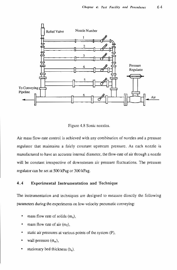
Chapter 4: Test Facility and Procedures 64
To Conveying Pipeline
Nozzle Number
Figure 4.8 Sonic nozzles.
Air mass flow-rate control is achieved with any combinatíon of nozzles and a pressure
regulator that maintains a fairly constant upstream pressure. As each nozzle is
manufacmred to have an accurate intemal diameter, the flow-rate of air through a nozzle
wiU be constant irrespective of downstream air pressure fluctuatíons. The pressure
regulator can be set at 500 kPag or 300 kPag.
4.4 Experimental Instrumentation and Technique
The instrumentation and techniques are designed to measure directly the foUowing
parameters during the experiments on low-velocity pneumatíc conveying:
mass flow rate of solids (m ),
mass flow rate of air (mf),
statíc air pressures at various points of the system (P),
wall pressure (Ow),
statíonary bed thickness (hj).
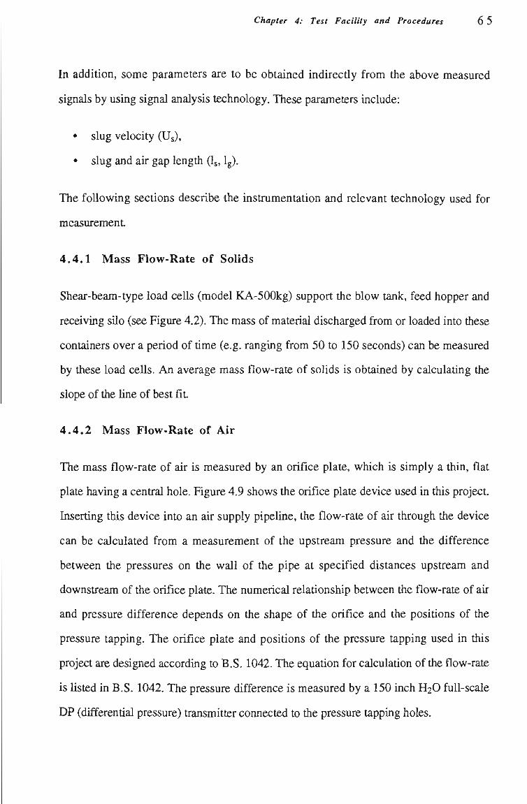
Chapter 4: Test Facility and Procedures 6 5
In additíon, some parameters are to be obtained indirectíy from the above measured
signals by using signal analysis technology. These parameters include:
• slug velocity (Us),
• slug and air gap length (Ig, Ig).
The foUowing sections describe the instrumentation and relevant technology used for
measuremenL
4.4.1 Mass Flow-Rate of Solids
Shear-beam-type load ceUs (model KA-500kg) support the blow taiUc, feed hopper and
receiving sUo (see Figure 4.2). The mass of material discharged from or loaded into these
containers over a period of time (e.g. ranging from 50 to 150 seconds) can be measured
by these load cells. An average mass flow-rate of solids is obtained by calculating the
slope of the Une of best fit.
4.4.2 Mass FIow-Rate of Air
The mass flow-rate of air is measured by an orifice plate, which is simply a thin, flat
plate having a central hole. Figure 4.9 shows the orifice plate device used in this project.
Insertíng this device into an air supply pipeline, the flow-rate of air through the device
can be calculated from a measurement of the upstream pressure and the difference
between the pressures on the wall of the pipe at specified distances upstream and
downstream of the orifice plate. The numerical relationship between the flow-rate of air
and pressure difference depends on the shape of the orifice and the positions of the
pressure tapping. The orifice plate and positions of the pressure tapping used in this
project are designed according to B.S. 1042. The equation for calculation of the flow-rate
is listed in B.S. 1042. The pressure difference is measured by a 150 inch H^O fuU-scale
DP (differential pressure) transmitter connected to the pressure tapping holes.
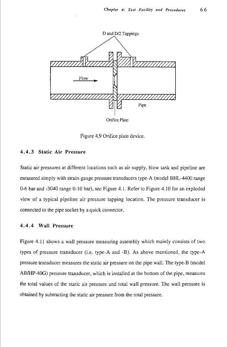
Chapter 4: Test Facility and Procedures 66
D and D/2 Tappings
'A \-////////////A
V/////////////77777. \ (/////////////////\ Pipe
Orifice Plate
Figure 4.9 Orifice plate device.
4.4 .3 Static Air Pressure
Static air pressures at different locations such as air supply, blow tank and pipeline are
measured simply with strain-gauge pressure transducers type-A (model BHL-4400 range
0-6 bar and -3040 range 0-10 bar), see Figure 4.1. Refer to Figure 4.10 for an exploded
view of a typical pipeline air pressure tapping location. The pressure transducer is
connected to the pipe socket by a quick connector.
4.4 .4 Wall Pressure
Figure 4.11 shows a wall pressure measuring assembly which mainly consists of two
types of pressure transducer (i.e. type-A and -B). As above mentioned, the type-A
pressure transducer measures the static air pressure on the pipe wall. The type-B (model
AB/HP-40G) pressure transducer, which is installed at the bottom of the pipe, measures
the total values of the static air pressure and total wall pressure. The wall pressure is
obtained by subtracting the static air pressure from the total pressure.
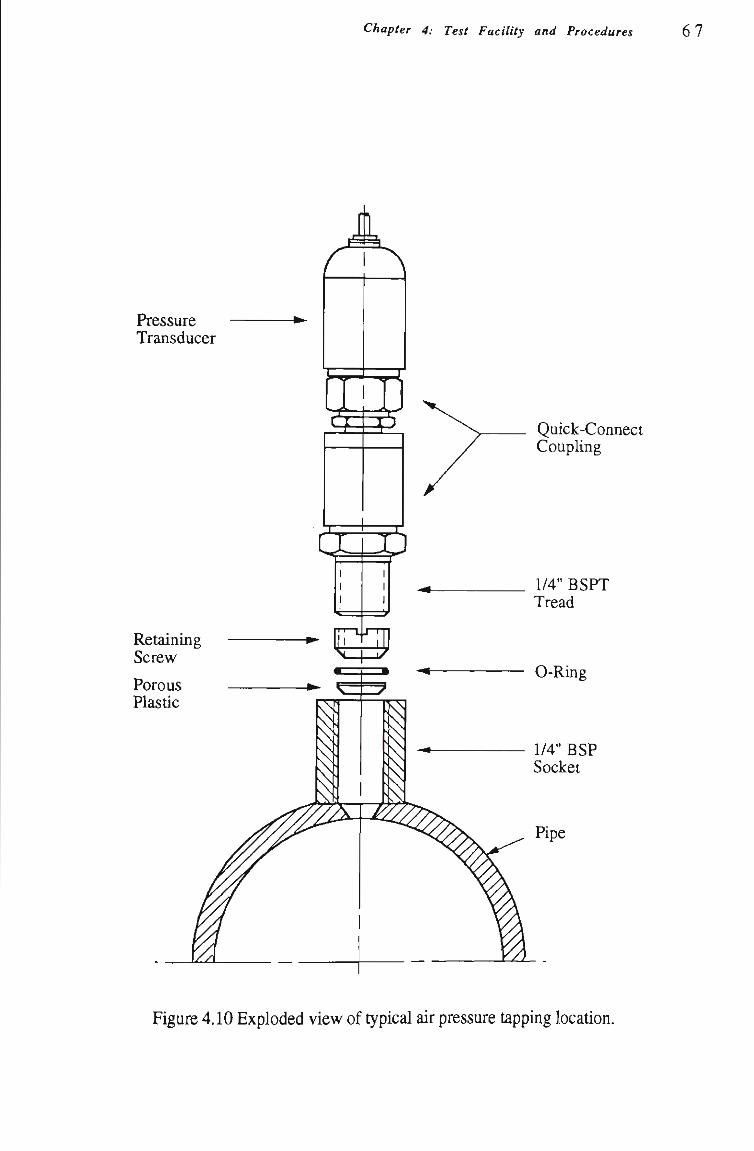
Chapter 4: Test Facility and Procedures 67
Pressure Transducer
Retaining Screw
Porous Plastic
; V ' y ! .
a
f^S^
Quick-Connect Coupling
1/4" BSPT Tread
0-Ring
1/4" BSP Socket
Figure 4.10 Exploded view of typical air pressure tapping location.
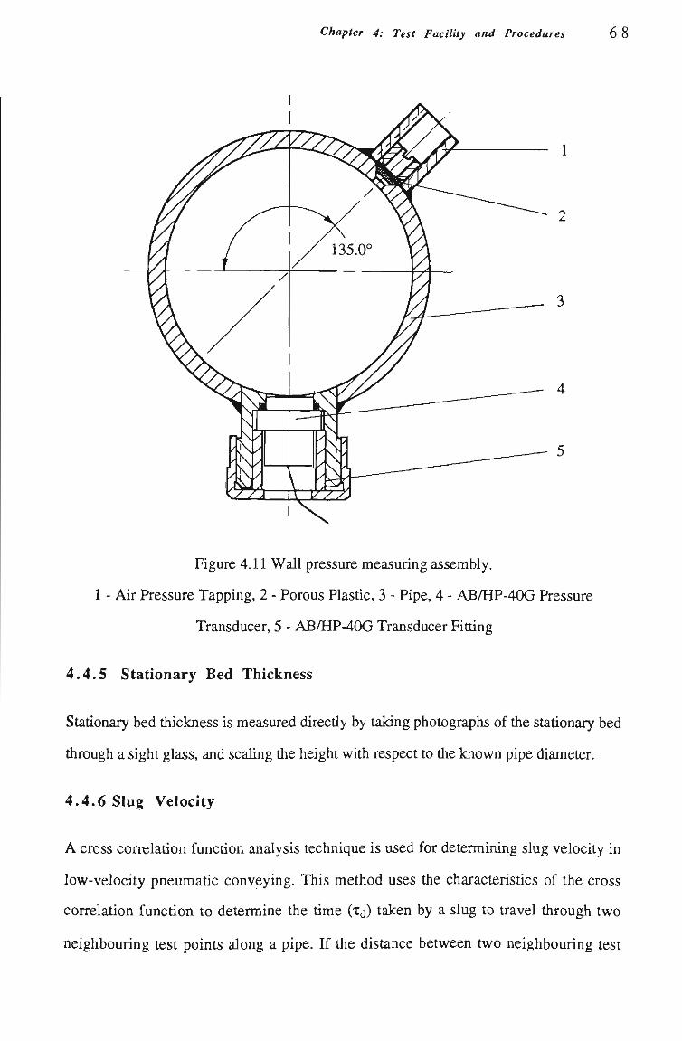
Chapter 4: Test Facility and Procedures 68
Figure 4.11 Wall pressure measuring assembly.
1 - Air Pressure Tapping, 2 - Porous Plastic, 3 - Pipe, 4 - AB/HP-40G Pressure
Transducer, 5 - AB/HP-40G Transducer Fittíng
4.4.5 Stationary Bed Thickness
Statíonary bed thickness is measured directiy by taking photographs of the stationary bed
through a sight glass, and scaUng the height with respect to tiie known pipe diameter.
4.4.6 Slug Velocity
A cross correlation function analysis technique is used for determining slug velocity in
low-velocity pneumatíc conveying. This method uses the characteristícs of the cross
correlation functíon to determine the time (Td) taken by a slug to travel through two
neighbouring test points along a pipe. If the distance between two neighbouring test
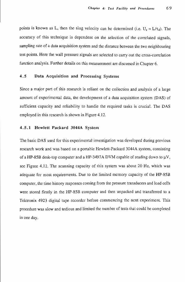
Chapter 4: Test Facility and Procedures 6 9
points is known as L, then the slug velocity can be determmed (i.e. Us = L/Xd). The
accuracy of this technique is dependent on the selectíon of the correlated signals,
sampling rate of a data acquisitíon system and the distance between tíie two neighbouring
test points. Here the wall pressure signals are selected to carry out the cross-correlatíon
functíon analysis. Further detaUs on this measurement are discussed in Chapter 6.
4.5 Data Acquisition and Processing Systems
Since a major part of this research is reliant on the coUectíon and analysis of a large
amount of experimental data, the development of a data acquisitíon system (DAS) of
sufficient capacity and reliability to handle the required tasks is crucial. The DAS
employed in this research is shown in Figure 4.12.
4.5.1 Hewlett Packard 3044A System
The basic DAS used for this experimental investigation was developed during previous
research work and was based on a portable Hewlett-Packard 3044A system, consisting
of a HP-85B desk-top computer and a HP-3497A DVM capable of reading down to |iV,
see Figure 4.12. The scanning capacity of this system was about 20 Hz, which was
adequate for most requirements. Due to the limited memory capacity of the HP-85B
computer, the time history responses coming from the pressure transducers and load cells
were stored firstly in the HP-85B computer and then unpacked and transferred to a
Tektronix 4923 digital tape recorder before commencing the next experiment. This
procedure was slow and tedious and limited the number of tests tíiat could be completed
in one day.
Chapter 4: Test Facility and Procedures 70
Pipeline Flow Direction
PTl
U
o
ê e
s I
ftí
I w .e •s
á
PT2 PTn
Transducer Signal Conditioning Unit
HP-3497 Scanning Control Unit
HP-85B Desk-Top Computer
Tektronix 4923 Digital Tape Recorder
Noise Filter Unit
PC-Computer with AX 5621 Board (Data are stored directly onto computer hard disk or floppy diskette)
l I I I c S
i «5 «3
ê" B
.4J
Quick Data Acquisition System
Data Acquisition System
Figure 4.12 Data acquisitíon systems.
4.5 .2 PC Based Quick Data Acquisition System
Due to the quite low sampling rate of the Hewlett-Packard 3044A system, it was not
adequate for some requirements of measuremenL For example, tiie determinatíon of slug
velocity by using cross correlatíon functíon technique required a high sampHng rate to
ensure good accuracy of results. Another reason for needing a high speed data
acquisitíon system was that tíie pressure fluctuatíon in low-velocity pneumatic conveying
is much more evident compared with dUute-phase conveying. A low speed data
acquisitíon system may lose some frequency components and result in incorrect
Chapter 4: Test Facility and Procedures 1 1
informatíon. Hence a new PC based "quick" data acquisitíon system was developed for
tiiis study on low-velocity pneumatic conveying, see Figure 4.12.
A compatible IBM-PC/XT or AT computer was selected. An AX5621 board, which is a
high-speed, high-resolutíon analog-digital converter, was plugged into an expansion slot
of tiie computer. Signal scanning was carried out by the board. A software package was
written to control tfie operation of the board and arrange the coUection and storage of the
data in a useful format. A software package called "logger" was designed for tiiis
purpose. This new system was able to scan a maximum of 1000 scans for eight channels
at a scaiming rate of 160 Hz.
4.5.3 Data Processing
A data processing software package "HPPLT" was developed by previous researchers of
the Bulk SoHds Handling Research group and modified by the author with FORTRAN
77 language based on a compatible IBM-PC/XT or AT computer. The software
supporting this processing was DOS and PLOTPACKAGE, which was developed by the
University of WoIIongong. AU time history signals sampled by either the DAS or quick
DAS were stored finally onto floppy diskettes as data fîles. A data processing computer
can read the data files directiy from the diskettes, then display tfie signals as required or
carry out further calculations on the signals. The functions of "HPPLT" are Hsted below:
1 Print caUbrated transducer responses with respect to cycle time
2 Plot pipeUne air pressures at a particular cycle tmie
3 Plot multiple pipeUne transducer responses
4 Calculate and plot mass flow-rate of air with respect to cycle time
5 Calculate flow characteristics
Chapter 4: Test Facility and Procedures 1 2
6 Plot conveying parameter relationships
7 Change the data (in Engmeering Units)
8 Plot multíple pipeline transducer responses and mass flow-rate of air onto one
screen
9 Finish
In these functíons, Functíons 3, 4, 5 and 8 are most commonly used. Functíons 3 and 8
are similar, but Functíon 3 only displays one type of transducer response (e.g. air
pressure), whereas Function 8 allows several types of transducer responses (e.g. air
pressure, mass flow-rate of air etc.) to be shown simultaneously for ease of comparison.
Typical graphic outputs generated by Functíon 8 are repeated in Figure 4.13, where the
channels 0 and 1 are the wall pressure and static air pressure signals, respectívely, the
channels 8 and 9 represent the mass of material loaded into the silo and discharged from
the feed hopper. Functíon 4 is used to calculate the mass flow-rate of air according to the
orifice plate/annubar equation using the values of differentíal pressure and upstream
pressure of the orifice plate/annubar. These calculated results can also be presented by
Functíon 8, see Figure 4.13.
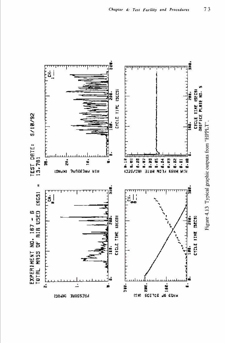
Chapter 4: Test Facility and Procedures 7 3
cn
(D
\U
lU (H
11 11 I I 11 1 I I 11 I I I I f I 111 I I 111 I
• 11 i l • I ' ' ' ' I I i l I I 11I I I 11 11 I I
ui i | i i i i | i i i i [ i i i i | i i i i | i i i i [r i i i | i i i i | i i i i | i iM
•
illlllllllllll l l l l i l l l l l lmilMii l i iMlnii lni
BB U D B UJ K
bU
UJ
W IV ^ e g [ n B i r * i u i < « 7 1 ( V ' ^ a
• riíaaBBBiBivaisaia
(33S/ 3HI 3IUU NOIJ BSUH UtU
cn
LiJ I ÍO
z o «— lO z tn lO cc z x:
u j n : û_ I -X o
I I I I I I I I I I I I I I I I I I I
Ml r11 I [ I 11 I I I 11 I [1 I I i j I I I I ; I 11 I
• • • I ' ' • I L. ..1 1 1 1 1
t-3
0* X
o < 4 - l
3 4..*
o o Ci,
2
o .^ Q, >> H
2Í 3
I " • I ' • ' < i ' ' " I • " ' I ' • " I ' " '
IVI
OUd>ll 3UnS53ti(! r» Bu rt
[3M] sQnas jo ecuM
Chapter 4: Test Facility and Procedures 7 4
Function 5 is used for the statístícal calculatíon of some major parameters, including the
average value of the mass flow-rate of air in a specific time range, average air pressure
and wall pressure, blow tank or rotary valve feed rate, etc.
If an experiment includes measurement of wall pressure, the waU pressure responses also
can be subtracted from the total pressure by using the HPPLT software package.
Note that the slug velocity calculation based on cross correlatíon functíon analysis
technique is not included in this software package.
4.6 Test Procedures
After aU the instruments are installed as required, they are then connected to the relevant
data acquisition system via a zero box. Experiments are carried out in the test rig using
the foUowing procedures.
4.6.1 System Check
To ensure the rig and experiments run smoothly and correctíy, a system check is
necessary. This work mainly includes double checking the instaUation of the pipeline
system and various instruments, which can be verified easily via direct observatíon, and
checking for air leakage at each pressure tapping poinL For the low-velocity pneumatic
conveying test rig, tiie air leakage check is carried out as the foUows:
(i) Block one end of tiie pipeline witíi a thin steel plate and close the back pressure
valve, open the air supply valve to allow air into the pipeUne.
(U) When the air pressure in the pipeline reaches a designated va ue (e.g. 100
kPag), close the air supply valve.
(iu) Drop soapy water onto each tapping point and observe whether soapy bubbles
appear.
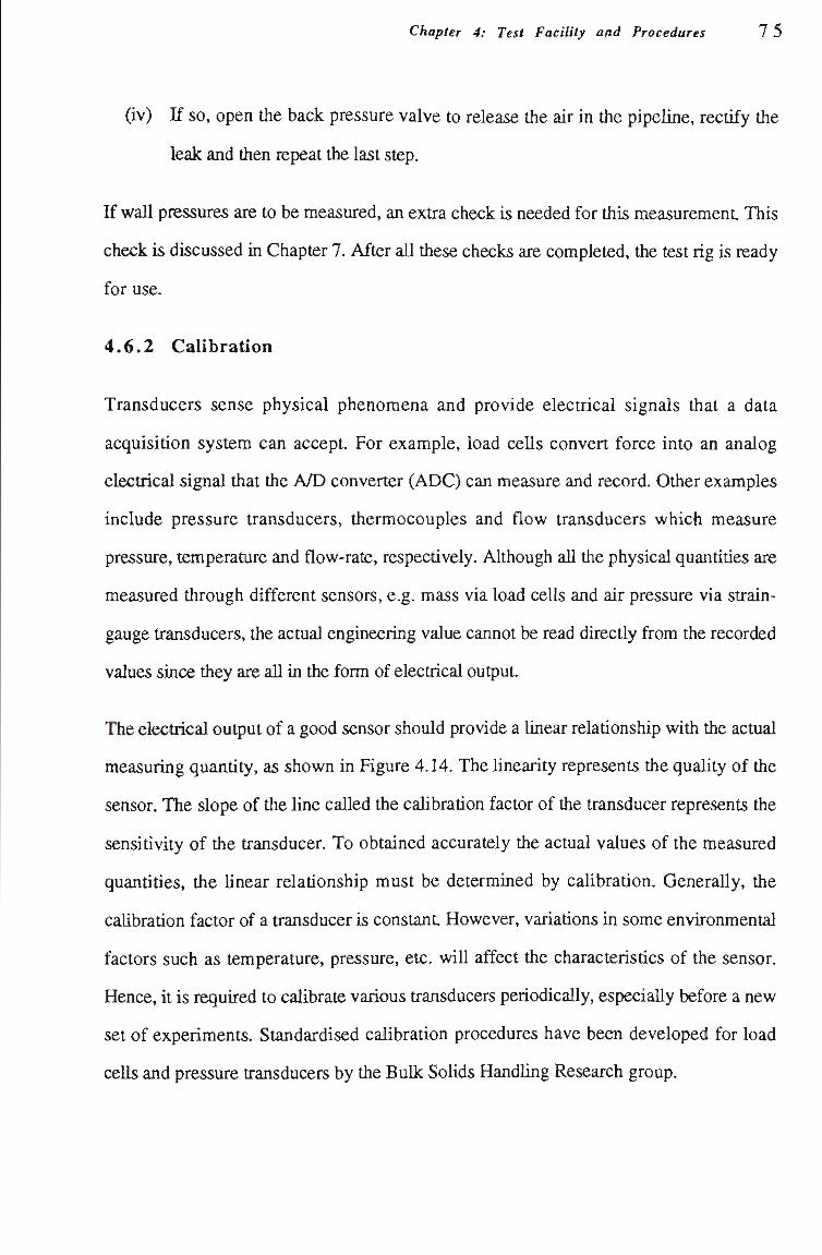
Chapter 4: Test Facility and Procedures 7 5
(iv) If so, open tíie back pressure valve to release the air in tíie pipeUne, rectífy tíie
leak and then repeat the last step.
If wall pressures are to be measured, an extra check is needed for this measurement. This
check is discussed in Chapter 7. After all tiiese checks are completed, the test rig is ready
for use.
4.6.2 Calibration
Transducers sense physical phenomena and provide electrical signals that a data
acquisitíon system can accept. For example, load cells convert force into an analog
electrical signal that the A/D converter (ADC) can measure and record. Other examples
include pressure transducers, thermocouples and flow transducers which measure
pressure, temperature and flow-rate, respectively. Although all the physical quantitíes are
measured through different sensors, e.g. mass via load cells and air pressure via strain-
gauge transducers, the actual engineering value cannot be read directly from the recorded
values since they are aU in the form of electrical output.
The electrical output of a good sensor should provide a linear relationship with tiie actual
measuring quantíty, as shown in Figure 4.14. The linearity represents the quality of the
sensor. The slope of the line called the calibratíon factor of tiie transducer represents the
sensitívity of the transducer. To obtained accurately the actual values of the measured
quantíties, the linear relationship must be determined by caUbration. GeneraUy, the
calibration factor of a transducer is constant However, variations in some environmental
factors such as temperature, pressure, etc. wiU affect the characteristícs of the sensor.
Hence, it is required to calibrate various transducers periodically, especiaUy before a new
set of experiments. Standardised calibration procedures have been developed for load
cells and pressure transducers by the BuUc Solids Handling Research group.
Chapter 4: Test Facility and Procedures 76
3
> 13 o .»-• «3 >>
Electrical output
Figure 4.14 Linear relationship between physical phenomena and electrical signal.
4.6.2.1 Load Cell Calibration
Load cells which are used to support the rotary valve feed hopper, blow tank and product
receiving silo, monitor the mass of material loaded in or discharged from these
containers. Calibration of load cells is carried out by fiIUng a given mass of product into
the feed hopper. The detaUed steps are:
(i) Remove any previously conveyed material from the pneumatic conveying test
ríg and purge the rig with a high flow-rate of air untíl the pipeline and rig are
beUeved clean. Record the voltage output of all load ceUs.
(U) Load a given mass of a product (say 40 kg) into the feed hopper or blow tartíc.
Record the voltage output of the load ceUs.
(iu) Transport this material to the receiving silo (using a high flow-rate of air to
ensure no product is left in the pipeline) and record the voltage output from the
load ceUs of the receiving sUo.
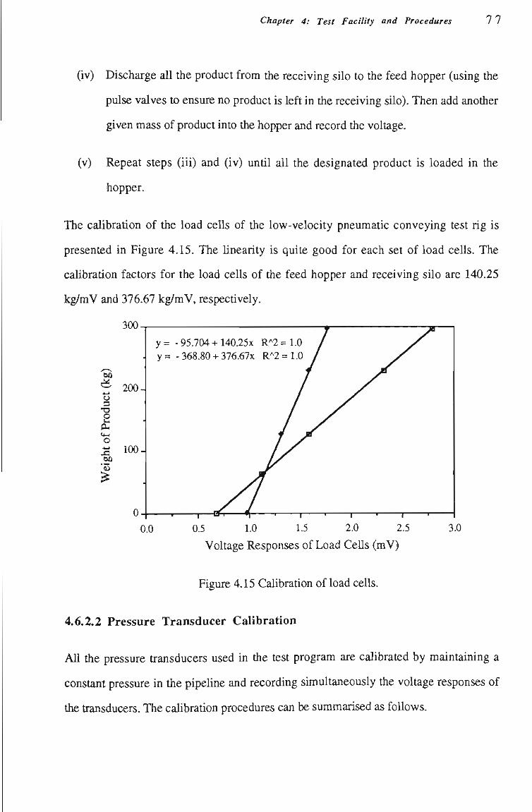
Chapter 4: Test Facility and Procedures 11
(iv) Discharge all the product from the receiving silo to the feed hopper (usmg tíie
pulse valves to ensure no product is left in tíie receiving silo). Then add anotiier
given mass of product into the hopper and record the voltage.
(v) Repeat steps (iu) and (iv) untíl all the designated product is loaded in tíie
hopper.
The calibration of the ioad cells of the low-velocity pneumatic conveying test rig is
presented in Figure 4.15. The linearity is quite good for each set of load cells. The
calibratíon factors for the load cells of the feed hopper and receiving silo are 140.25
kg/mV and 376.67 kg/mV, respectívely.
300.
y = - 95.704 + 140.25x R^2 = 1.0 . y = - 368.80 + 376.67x R^2 = 1.0
200-Oû
o 3 o
^ 100-
u ^
0.0 0.5 1.0 1.5 2.0 2.5
Voltage Responses of Load CeUs (mV) 3.0
Figure 4.15 CaUbration of load cells.
4.6.2.2 Pressure Transducer Calibration
AU the pressure transducers used in the test program are calibrated by maintaining a
constant pressure in the pipeUne and recording simultaneously the voltage responses of
the transducers. The calibration procedures can be summarised as foUows.
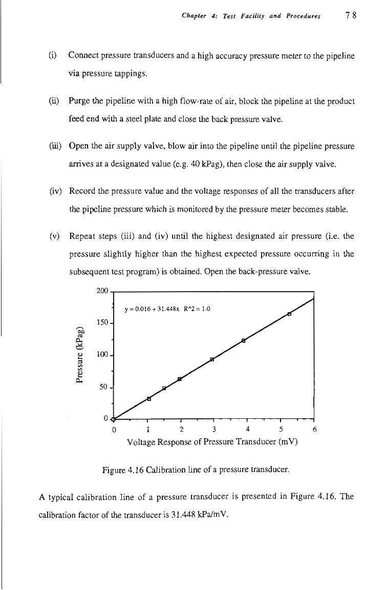
Chapter 4: Test Facility and Procedures 78
(i) Connect pressure transducers and a high accuracy pressure meter to tíie pipeUne
via pressure tappings.
(U) Purge the pipeline with a high flow-rate of air, block the pipeUne at tíie product
feed end with a steel plate and close the back pressure valve.
(iu) Open the air supply valve, blow air into the pipeUne untíl tíie pipeline pressure
arrives at a designated value (e.g. 40 kPag), then close tiie air supply valve.
(iv) Record the pressure value and the voltage responses of all tiie transducers after
the pipeline pressure which is monitored by the pressure meter becomes stable.
(v) Repeat steps (iii) and (iv) until the highest designated air pressure (i.e. the
pressure slightly higher than the highest expected pressure occurring in the
subsequent test program) is obtained. Open the back-pressure valve.
200.
150. DO 03
2 3 Cfl
04
y = 0.016+ 31.448X ^^^2=1.0
T ' r T ' 1 ' 1 ^
0 1 2 3 4 5 6
Voltage Response of Pressure Transducer (mV)
Figure 4.16 Calibration line of a pressure transducer.
A typical caUbratíon line of a pressure transducer is presented in Figure 4.16. The
calibration factor of the transducer is 31.448 kPa/mV.
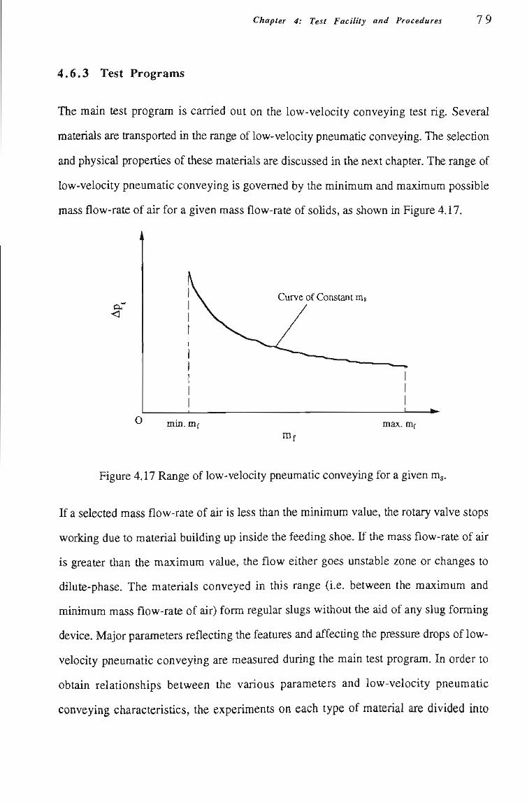
Chapter 4: Test Facility and Procedures 79
4.6.3 Test Programs
The main test program is carried out on the low-velocity conveying test rig. Several
materials are transported in the range of low-velocity pneumatíc conveying. The selectíon
and physical propertíes of these materíals are discussed in the next chapter. The range of
low-velocity pneumatic conveying is govemed by the minimum and maximum possible
mass flow-rate of air for a given mass flow-rate of soUds, as shown in Figure 4.17.
<
min. mf
Curve of Constant ms
max. mf m,
Figure 4.17 Range of low-velocity pneumatic conveying for a given mg.
If a selected mass flow-rate of air is less tiian the minimum value, tfie rotary valve stops
working due to materíal building up inside the feeding shoe. If tíie mass flow-rate of air
is greater than the maximum value, the flow either goes unstable zone or changes to
dilute-phase. The materials conveyed in this range (i.e. between the maximum and
minimum mass flow-rate of air) form regular slugs without tíie aid of any slug forming
device. Major parameters reflecting tíie features and affectíng the pressure drops of low-
velocity pneumatíc conveying are measured during the main test program. In order to
obtain relatíonships between the various parameters and low-velocity pneumatic
conveying characteristics, the experiraents on each type of material are divided into
Chapter 4: Test Facility and Procedures 8 0
several groups according to their mass flow-rate of solids to fulfil. The test program is
designed as foUows:
(i) Adjust the rotary valve to a designated rotor speed (i.e. f x tíie mass flow-rate of
solids), operate the first test with the minimum possible mass flow-rate of air.
(u) StíU using the same rotor speed, conduct more experiments with increased
values of mf untU the maximum mass flow-rate of air for low-velocity pneumatíc
conveying has been reached (i.e. for the given m ).
(ui) Alter the rotor speed, repeat steps (i) and (ii).
The operating procedures of each test are summarised below for the rig using the rotary
valve feeder:
(i) Open the silo valve and load sufficient material into the feed hopper, see Figure
4.2, then close thé valve after loading.
(u) Adjust the rotor speed of the rotary valve to obtain a suitable mass flow-rate of
solids.
(iiO Predetermine a mass flow-rate of air by selection of the relevant critical flow
nozzles, see Figure 4.8.
(iv) Set the data acquisitíon system to scan the required channels at a suitable
sampUng rate.
(v) Start the data acquisitíon system.
(vi) After about 10 seconds, open the conveying air valve to introduce air into the
pipeline.
Chapter 4: Test Facility and Procedures 8 1
(vu) Operate the rotary valve and open the hopper valve to feed tíie material in tíie
conveying pipeline.
(viS) After all the material in tiie hopper has been conveyed into the silo, tum off tíie
rotary valve.
(ix) Keep the air blowing untíl aU the material left in the rig and pipeline retums to
the silo, then close the air supply valve.
In ensure good accuracy results, each test is repeated at least two times. In additíon, each
repeated experiment is scanned at different sampling rates to rationalise the memory
limitatíon problem of the DAS. That is, at least one repeated experiment is scanned at a
low sampling rate to make the total scanning tíme of the DAS cover the entire range of
the test, and another repeated experiment is scanned at the maximum possible sampling
rate of the DAS for measuring slug velocity.
In additíon to the main experiments, other experiments were conducted on other test rigs
with different configuratíons of pipeline (i.e. to confirm the validity of model predictíons
for different materials and pipe sizes). These experiments and relevant facUitíes are
discussed in Chapter 9.

82
CHAPTER 5
TEST MATERIAL AND PROPERTIES
Chapter 5: Test Material and Properties 8 3
5.1 Introduction
Pneumatic conveying performance can vary considerably for different buUc materials.
Some materials can be conveyed over a wide range of the flow conditíons, from high-
velocity, dilute-phase to low-velocity, dense-phase. Other materials, however, are
restricted to dilute-phase only in conventíonal pneumatíc conveying systems (i.e. using
standard pipelines). Some cannot be conveyed pneumatícally (e.g. 3 |im lead fume). In
additíon, materials which are capable of being conveyed pneumatícally can exhibit for
given conditions quite different levels of performance in terms of flow pattem, material
throughput, etc, partícularly at low velocity. It is believed that all these quite different
performances are dependent on the properties of the materials to be conveyed. Hence for
a pneumatíc conveying system to be designed or upgraded to ensure satisfactory and
efficient operatíon or the total pipeline pressure drop of an existíng system to be predicted
accurately, the influence of tíie properties of the materials must be considered properly.
However, due to the complicated nature of two phase flow, it is quite difficult to
determine how the propertíes of the materials exactíy affect pneumatíc conveying
performance and behaviour.
A relatively reliable method for design and/or pressure predictíon of a pneumatíc
conveying system accepted by most researchers and engmeers is to undertake a serious of
experiments with a representatíve sample of the material in a pUot plant, then obtain the
fuU scale plant data from tíie test rig results by using appropriate scale-up procedures.
Obviously tíie pilot plant experimental results include the mfluence of the propertíes of the
material, and this information is transferred to the fuU scale plant data by the scale-up
procedures. A major disadvantage of tíiis strategy is tíiat U may be tíme consuming and
costíy. Therefore tíie ultímate aim of pneumatíc conveying research is to design and/or
predict pressure drop for a pneumatic conveying system without tíie need to carry out
small or fuU scale conveying tests (i.e. to establish relatíonships between pneumatic
conveying performance and tiie physical propertíes of tíie material).
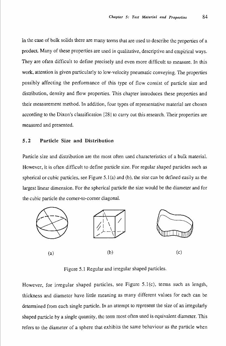
Chapter 5: Test Material and Properties 84
In the case of buUc solids tiiere are many terms that are used to describe tíie propertíes of a
product Many of these propertíes are used in qualitative, descriptíve and empirical ways.
They are often difficult to define precisely and even more difficult to measure. In tíiis
work, attention is given partícularly to low-velocity pneumatíc conveying. The propertíes
possibly affecting the performance of this type of flow consist of particle size and
distributíon, density and flow propertíes. This chapter introduces these propertíes and
their measurement method. In additíon, four types of representative material are chosen
according to the Dixon's classtfication [28] to carry out this research. Their propertíes are
measured and presented.
5.2 Particle Size and Distributíon
Partícle size and distributíon are the most often used characteristícs of a bulk material.
However, it is often difficult to define partícle size. For regular shaped partícles such as
spherical or cubic partícles, see Figure 5.1(a) and (b), the size can be defined easUy as the
largest Unear dimension. For the spherical partícle the size would be the diameter and for
the cubic partícle the comer-to-comer diagonal.
(a) (b) (c)
Figure 5.1 Regular and irregular shaped particles.
However, for irregular shaped particles, see Figure 5.1(c), terms such as length,
thickness and diameter have Uttíe meaning as many different values for each can be
determined from each single partícle. In an attempt to represent tiie size of an irregularly
shaped particle by a single quantíty, tíie term most often used is equivalent diameter. This
refers to tíie diameter of a sphere tíiat exhibits the same behaviour as tíie partícle when
Chapter 5: Test Material and Properties 85
subjected to the same sizing technique, e.g. tiie sphere that has the same projected area or
mass or that just passes through a mesh aperture. Thus the measurement of the size
(equivalent diameter) of particles is dependent on the method used to determine that
parameter.
The partícle size mentíoned above actually indicates single partícle size. The size and
shape of partícles that randomly make up a real buUc solid usually vary quite widely. In
this case, a mean particle size is needed to represent the size namre of the bulk soUd. Only
after knowing the single particle size and distributíon of a bulk solid, the mean particle
size (equivalent diameter) of the bulk solid may be calculated by an appropriate method,
such as the methods of arithmetic mean, geometric mean and log geometric mean, etc.
Hence the size range (distribution) of the bulk solids also is an important parameter that
defines the size nature of the bulk solid. There are many methods that can be used for
determining the size distributíon of partículate materials. These include:
Mechanical sieving,
SedUnentation,
Microscopy,
Electron microscopy,
Scanning electron microscopy,
Advanced optícal methods (e.g. laser diffractíon).
Mechanical sieving is tíie most widely used metíiod for determining the size distributíon
of a buUc soUd and is a process weU known to most researchers and engineers, as it
covers tíie range of partícle sizes that are of considerable industrial importance. With ûiis
method, a bulk solid sample is placed on a nest of screens with precisely defined
apertures. These sieves are either manuaUy or mechanicaUy shaken for a designated
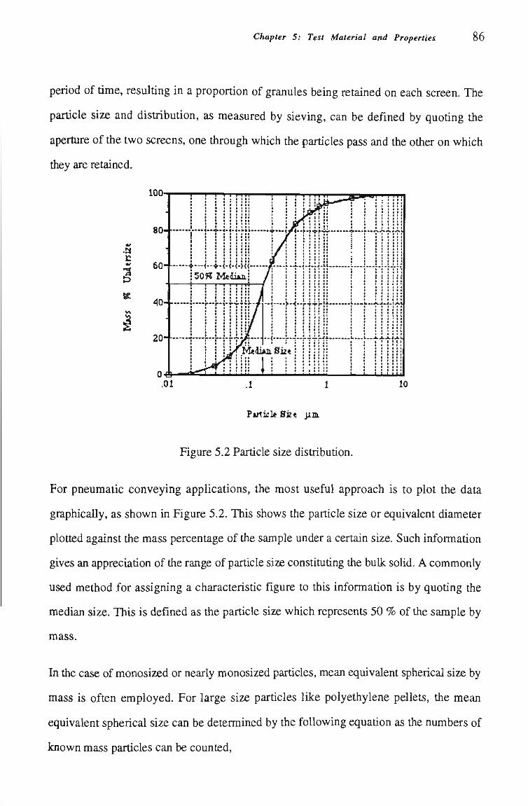
Chapter 5: Test Material and Properties 86
period of time, resulting in a proportion of granules being retained on each screen. The
particle size and distribution, as measured by sieving, can be defined by quoting the
aperture of tíie two screens, one tíirough which the partícles pass and the otíier on which
they are retained.
P»nicIeSÊ« ixjsi
Figure 5.2 Particle size distributíon.
For pneumatic conveying appUcations, the most useful approach is to plot the data
graphically, as shown in Figure 5.2. This shows the particle size or equivalent diameter
plotted against the mass percentage of the sample under a certain size. Such information
gives an appreciatíon of the range of partícle size constítotíng the bulk solid. A commonly
used method for assigning a characteristíc figure to this informatíon is by quotíng the
median size. This is defined as the particle size which represents 50 % of the sample by
mass.
In the case of monosized or nearly monosized partícles, mean equivalent spherical size by
mass is often employed. For large size partícles like polyethylene pellets, the mean
equivalent spherical size can be determined by the foUowing equatíon as the numbers of
known mass partícles can be counted.

Chapter 5: Test Material and Properties 87
d = ,|-Ai2_ (5.1)
where d is the mean equivalent particle diameter, m is the mass of particles, Up is the
number of the partícles of the known mass, ps is the particle density.
5.3 Density Analysis and Measurement
A buUc solid consists of many randomly grouped partícles. This bulk material has an
apparent bulk density, i.e. the mass of the bulk divided by the volume of the particles and
voids contained in the buUc Besides the buUc density, each partícle tiiat makes up the bulk
solid has particle density. GeneraUy speaking, the partícle density is constant the bulk
density is not unique for a buUc material. It is dependent on the particle density, partícle
shape and how the particles are packed or positíoned with respect to one another. The
bulk density and partícle density are both parameters of primary importance in the
investígatíon of pneumatíc conveying.
It is well known that specific weight is often used in fluid research instead of density.
Since buUc materials have some simUar features to fluid, specific buUc and particle weight
of the bulk materials are defined as tfie bulk and particle density relatíve to tiie density of
water at 4 °C.
5.3.1 Particle Density
Partícle density can often be measured using an air comparison pycnometer or stereo
pycnometer. In this study, a stereo pycnometer is used for most measurements of particle
density. It employs Archimedes principle of fluid dispiacement to determine the volume
of tfie solid objects. The displaced fluid is a gas which can penetrate the finest pores to
assure maxmium accuracy. A diagram displaying the principle of tiie stereo pycnometer is
presented in Figure 5.3.
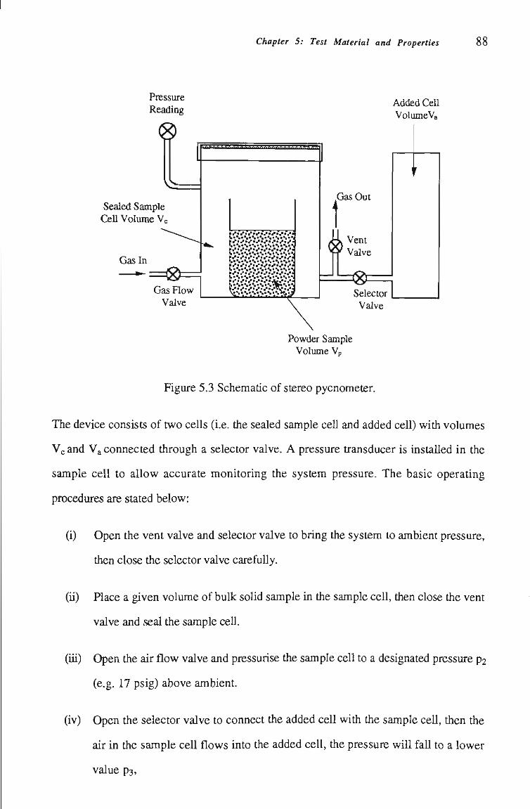
Chapter 5: Test Material and Properties 88
Pressure Reading
< ^
Sealed Sample CeU Volume Vc
Gasln
AddedCell VolumeVa
=0=1 GasFlow
Valve
w • s . s « s • s • % • s • s . 1 • ^ • ^ • ^ • • " • ^ • ^ • ^ • ^ i
^i^;'^;'»;^í^i"' ^V • ^ • ^ • ^ • ^ • ^ . ^ • ^ . ^ f
ii.''y-y'V-i''V'V'V' ^ • - • - • - • - . - . '
GasOut
Selector Valve
Powder Sample Volume Vp
Figure 5.3 Schematíc of stereo pycnometer.
The device consists of two cells (i.e. the sealed sample ceU and added cell) with volumes
Vc and Va connected through a selector valve. A pressure transducer is instaUed in the
sample cell to allow accurate monitoring the system pressure. The basic operating
procedures are stated below:
(i) Open the vent valve and selector valve to bring the system to ambient pressure,
then close the selector valve carefuUy.
(u) Place a given volume of bulk solid sample in the sample cell, then close the vent
valve and seal the sample ceU.
(iu) Open the air flow valve and pressurise the sample cell to a designated pressure p^
(e.g. 17 psig) above ambient.
(iv) Open the selector valve to connect the added cell with the sample ceU, then the
air in the sample cell flows into the added cell, the pressure will fall to a lower
value p3.
Chapter 5: Test Material and Properties 89
(v) Calculate tíie partícle volume according to the foUowmg equatíon:
Vp = Ve + T - ^ V (5-2) 1 - P2/P3
It should be noted that either the comparison- or stereo- pycnometer only measures the
average particle density of a buUc solid. The densitíes of different constíment partícles in a
blended product can be determined by measuring them before mixing. AIso, the
pycnometer yields the apparent particle density which is the mass of product divided by
the occupied volume including closed pores but excluding open pores.
5.3.2 Bulk Density
BuUc density does not have an unique value for a particular bulk solid and it varies with
the condition of the bulk solid. For example, a bulk solid that has been conveyed
pneumatícally may be aerated and have a lower bulk density than if it had been aUowed to
de-aerate. It is not always easy to determine tíie bulk density of a product under changing
consoUdatíon conditíons. Since it has been concluded in Chapter 3 that partícle slugs have
approximately a loose-poured bulk density in low-velocity pneumatíc conveying, only the
loose-poured buUc density is discussed here.
Loose-poured bulk density usuaUy can be obtained by tiie foUowing steps:
(i) Pour carefully and gently a certain volume of bulk solid into a measuring
cylinder. Note that the measuring cylinder must be held at an angle of 45° to the
horizontal when pouring to avoid compaction.
(u) Bring the cyUnder upright and note the volume occupied by the bulk solid.
(iu) Weigh the cyUnder and bulk soUd and deduce the mass of the bulk soUd.
(iv) Determine the loose-poured buUc density by knowing the mass and the poured
volume of the bulk soUd.
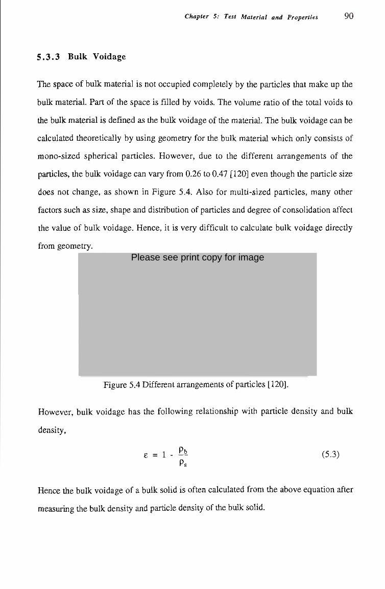
Chapter 5: Test Material and Properties 90
5.3.3 Bulk Voidage
The space of bulk material is not occupied completely by the partícles that make up tíie
bulk material. Part of the space is fiUed by voids. The volume ratío of the total voids to
the bulk material is defined as the bulk voidage of the material. The buUc voidage can be
calculated theoretícally by using geometry for the bulk material which only consists of
mono-sized spherical particles. However, due to the different arrangements of the
partícles, the buHc voidage can vary from 0.26 to 0.47 [120] even though the partícle size
does not change, as shown in Figure 5.4. Also for multi-sized particles, many other
factors such as size, shape and distribution of particles and degree of consolidatíon affect
the value of bulk voidage. Hence, it is very difficult to calculate buUc voidage directíy
from geometry.
Figure 5.4 Different arrangements of particles [120].
However, bulk voidage has the following relatíonship with partícle density and bulk
density,
Pb e = 1 (5.3)
Hence the bulk voidage of a bulk solid is often calculated from the above equation after
measuring tíie bulk density and partícle density of the buUc solid.
Please see print copy for image
Chapter 5: Test Material and Properties 91
5.4 Flow Properties of Bulk Material
The flow propertíes of buUc material mainly include intemal and effectíve frictíon angle
and waU frictíon angle, which are of special interest to pneumatíc conveying.
5.4 .1 Internal and Effective Friction Angle
Figure 5.5 shows a JenUce shearing test [121]. The shear ceU, see Figure 5.5, is
composed of a base which is located on a frame, a shearing ring which rests on the top of
the base, and a cover which has a loading bracket attached to it. The test apparatos
permits failure to develop only along the shear plane.
Figure 5.5 Jenike shearing test [121].
A buUc soUd is placed in the shear cell and loaded by a normal force V. After applying a
shearing force S through the shearing ring, the normal stress a (= V/A^) and shearing
stress 1 (=S/Ac) occur along the shear plane, where Ag is the cross-sectíonal area of the
shear cell. If S is less than the maximum possible shearing force corresponding to a
given normal force V, then no continuous deformation occurs. However slip takes place
along the shear plane as soon as S reaches its maximum value. If a an-Xn coordinate
system is introduced to generate a shear-compressive stress diagram, the stresses on the
shear plane at shearing can be expressed by a circle C, as shown in Figure 5.6.
Please see print copy for image
Chapter 5: Test Material and Properties 92
*-an
Figure 5.6 Mohr circle and yield locus of cohesive material.
This circle is called the Mohr circle. Note <5\ and a^ are major and minor normal stress.
If repeating the direct shear test for the sample with the same initial void ratío (i.e. same
consoUdatíng pressures) but with a range of constant V values, a yield locus (YL for
short), which is called the Mohr failure envelope, can be obtained, see Figure 5.6. For
the values of the normal stress and shearing stress (a, x) lying below that line, the soUd
can be considered to behave rigidly (or elastically), for the values lying on the line,
faUure or yield occurs. The locus (envelope) usuaUy can be represented approximately by
a straight line. If the slope and intercept of the line are designated as (j) and c,
respectively, then the locus in Figure 5.6 may be written as
x = atan(l)+c (5.4)
The form of Equation (5.4) was firstíy given by Coulomb in 1776 and hence, is called
tíie Coulomb faUure criterion. (j) and c in Equatíon (5.4) are called intemal frictíon angle
and cohesion of the buUc solid.
As shown in Figure 5.6, tíie tangent to tíie Mohr circle C and passmg tiirough tíie origin
of tíie an-Xn coordinate system is called the effectíve yield locus (EYL for short). The
angle Ô between the effectíve yield locus and an-coordinate in Figure 5.6 is called tíie
Chapter 5: Test Material and Properties 93
effectíve frictíon angle. Using angle 5, the foUowing relationship between major stress
and minor stress can be given [121],
ai l+sin8 <52 1-sinÔ
(5.5)
For cohesionless solids, such as dry sand and plastic peUets, the yield locus passes
through the origin of the normal stress and shearing stress axes. This yield locus
coincides with the effectíve yield locus (EYL). The intemal frictíon angle (|) is equal to the
effectíve intemal frictíon angle ô. The discussion hereafter for flow propertíes of bulk
materials is limited to this situatíon, since all the materials selected in this thesis for the
conveying triais are cohesionless bulk solids.
Intemal and effectíve friction angle can be measured by a Jentke direct shear tester as
shown in Figure 5.7. The tester includes a shear ceU of circular shape, a gravity vertícal
loading system which appUes a normal force on the top of the shear ceU, a driven loading
stem which moves horizontally and generates the shearing action. The shear force is
measured by a load ceU and recorded by a chart recorder.
Shear CeU
Chart Recorder Motor and Loading Load Cell Stem
• / / / / / / /
I Vertical Load
Figure 5.7 Jenike direct shear tester.
Chapter 5: Test Material and Properties 9 4
The test procedure is summarised below:
(i) Turn on the Jenike shear tester and chart recorder, then calibrate the chart
recorder.
(u) Undertake preconsolidatíon of the sample, i.e.
• Put the shear ceU rings with a mould ring on the frame of tiie tester and fiU with
the sample (do not press down on the sample).
• Place the twistíng top on tiie mould ring, apply weight W on the twistíng top by
a weight hanger and then twist tiie top for a given number of tímes.
• Take the hanger with weight and mould ring off, scrape off the excess sample
flush with the rings.
(Ui) Undertake consoUdatíon of the sample (running a test), i.e.
• Place the cover of the shear cell on the top ring, add shear weight V by the
hanger and then tum on the force actuator.
• Check the chart recprded results, tum off the force actuator after mn úie test fuU
tíme.
• Repeat from step (ii) onwards adjustíng preconsolidation weights and twists
untU the correct result is obtained, i.e. chart flattens out.
• Tum off the force actuator, take off the shear weight and put on shearing weight
V', V" and V'", respectively.
• Write down the first height, i.e. where it flattens out, S and corresponding
second height, i.e. where the top of the peak is in the chart recorder, S', S" and
S'".
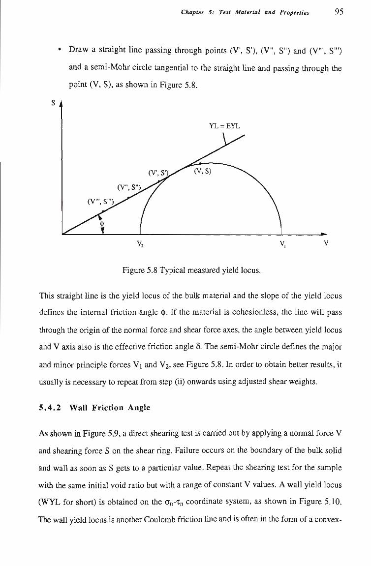
Chapter 5: Test Material and Properties 9 5
Draw a straight line passing through points (V', S'), (V", S") and (V'", S'")
and a semi-Mohr circle tangentíal to the straight line and passing tíirough the
point (V, S), as shown in Figure 5.8.
YL = EYL
V
Figure 5.8 Typical measured yield locus.
This straight line is the yield locus of the bulk material and the slope of the yield locus
defines the intemal friction angle ^. If the material is cohesionless, the line wiU pass
through the origin of the normal force and shear force axes, the angle between yield locus
and V axis also is the effectíve frictíon angle 5. The semi-Mohr circle defines the major
and minor principle forces Vi and V , see Figure 5.8. In order to obtain better results, it
usually is necessary to repeat from step (ii) onwards using adjusted shear weights.
5.4.2 Wall Friction Angle
As shown in Figure 5.9, a direct shearing test is carried out by applying a normal force V
and shearing force S on the shear ring. Failure occurs on the boundary of the buUc soUd
and wall as soon as S gets to a particular value. Repeat the shearing test for the sample
witii tiie same initíal void ratío but witíi a range of constant V values. A waU yield locus
(WYL for short) is obtained on tíie a -Xn coordinate system, as shown in Figure 5.10.
The wall yield locus is anoúier Coulomb frictíon line and is often in the form of a convex-
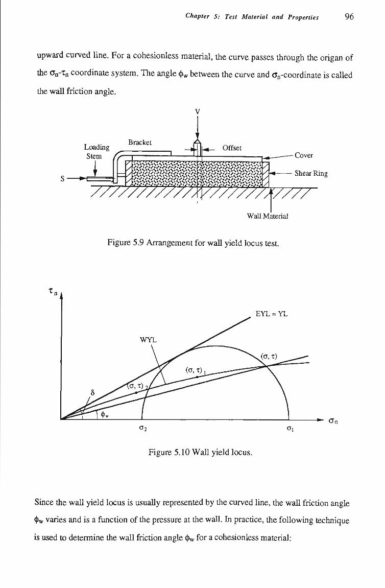
Chapter 5: Test Material and Properties 96
upward curved line. For a cohesionless material, the curve passes tíirough tíie origan of
tíie an-Xn coordinate system. The angle (^^ between the curve and an-coordinate is caUed
the waU frictíon angle.
Cover Loading Stem /p
Shear Ring
Wall Material
Figure 5.9 Arrangement for waU yield locus test.
EYL = YL
an 0 2 <Ji
Figure 5.10 Wall yield locus.
Since the waU yield locus is usuaUy represented by the curved line, the waU frictíon angle
^vf varies and is a functíon of the pressure at the wall. In practíce, the foUowing technique
is used to determine the wall frictíon angle (^ for a cohesionless material:
Chapter S: Test Material and Properties 9 7
firstiy, determine the value of the effectíve frictíon angle 5 of the buUc material and tíie
value of tiie major compressive stress ai under a certain preconsolidatíon. Draw tíie EYL
and tangential to the semi-Mohr circle passing through ai, see Figure 5.10. Then draw a
straight Une from the origin to tiie point (a, x) which is the intersectíon of tiie semi-Mohr
circle with the WYL. Finally, fmd tiie angle between the straight Une and an-coordinate.
The Coulomb failure criterion can be written as follows for the boundary of buUc material
and waU:
x = atan())w (5.6)
where (()w is the waU friction angle.
The wall friction angle can also be measured by the Jenike direct shear tester. The
arrangement for the wall friction angle test is referred to in Figure 5.9. The test of the
waU frictíon angle is much easier to be carried out than that of the intemal frictíon angle.
The measurement steps can be summarised as follows.
(i) Tum on the Jenike shear tester and chart recorder, then calibrate the chart
recorder.
(U) Set a material plate (i.e. wall) correctíy and place the shear ring with a mould
ring on it, then load the sample.
(iu) Preconsolidate the sample with a given weight on a hanger (e.g. 18 Ib including
the hanger weight).
(iv) Remove the weight hanger and mould ring, scrape off the excess sample so that
it is flush with the shear ring.
(v) Place the cover of the shear ceU on the shear ring, then put the hanger on the
cover, add 8 X 2 Ib weights (normal forces V) on the hanger.
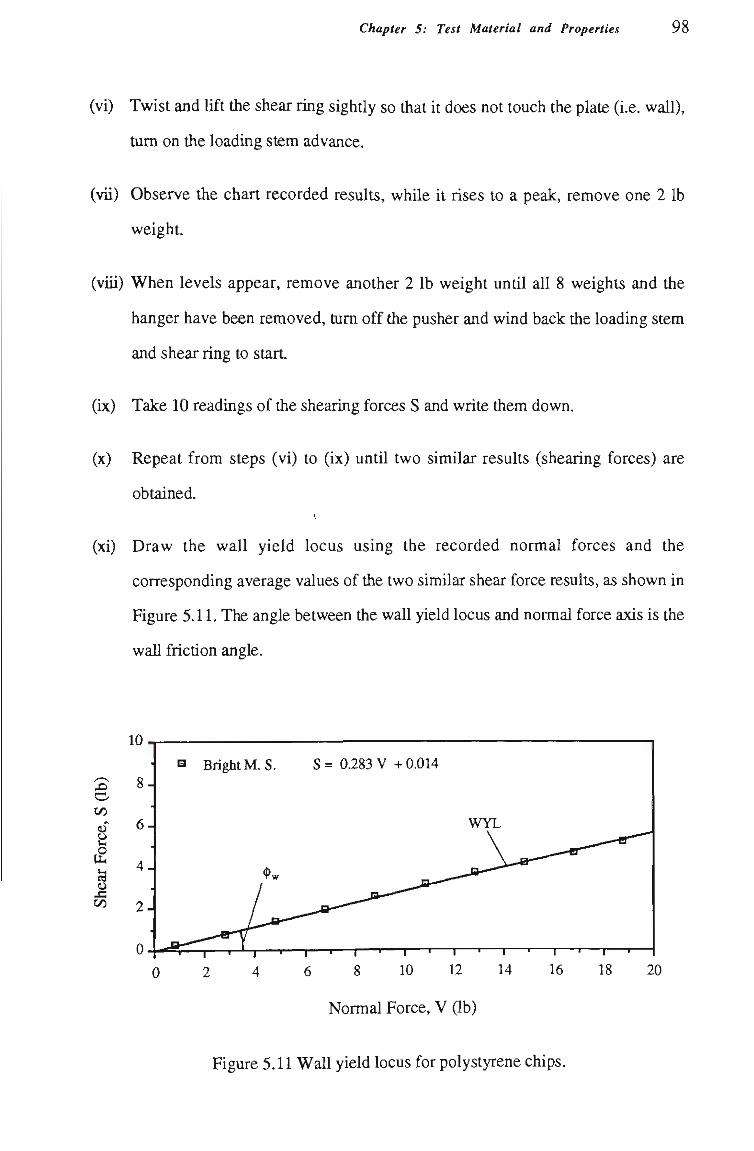
Chapter 5: Test Material and Properties 98
(vi) Twist and lift the shear ring sightíy so tíiat it does not touch tíie plate (i.e. waU),
tum on the loading stem advance.
(vu) Observe the chart recorded results, while it rises to a peak, remove one 2 Ib
weight.
(viu) When levels appear, remove another 2 Ib weight untU aU 8 weights and the
hanger have been removed, tum off the pusher and wind back the loading stem
and shear ring to start.
(ix) Take 10 readings of the shearing forces S and write them down.
(x) Repeat from steps (vi) to (ix) until two similar results (shearing forces) are
obtained.
(xi) Draw the wall yield locus using the recorded normal forces and the
corresponding average values of the two similar shear force results, as shown in
Figure 5.11. The angle between the wall yield locus and normal force axis is the
waU frictíon angle.
C/5
•c C/3
10
8
6
4
2.
H Bright M. S. S = 0.283 V + 0.014
WYL
18 20
Normal Force, V (Ib)
Figure 5.11 Wall yield locus for polystyrene chips.
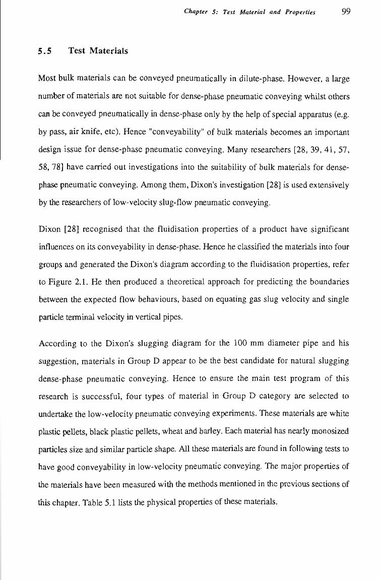
Chapter 5: Test Material and Properties 9 9
5.5 Test Materials
Most buUc materíals can be conveyed pneumatícally in dilute-phase. However, a large
number of materials are not suitable for dense-phase pneumatic conveying witílst others
can be conveyed pneumatically in dense-phase only by the help of special apparams (e.g.
by pass, air knife, etc). Hence "conveyabiUty" of buUc materials becomes an important
design issue for dense-phase pneumatic conveying. Many researchers [28, 39, 41, 57,
58, 78] have carried out investígatíons into the suitabiUty of bulk materials for dense-
phase pneumatic conveying. Among them, Dixon's investígatíon [28] is used extensively
by tiie researchers of low-velocity slug-flow pneumatíc conveying.
Dixon [28] recognised that the fluidisation properties of a product have significant
influences on its conveyability in dense-phase. Hence he classifîed the materials into four
groups and generated the Dixon's diagram according to the fluidisation propertíes, refer
to Figure 2.1. He then produced a theoretical approach for predicting the boundaries
between the expected flow behaviours, based on equatíng gas slug velocity and single
partícle terminal velocity in vertícal pipes.
According to the Dixon's slugging diagram for the 100 mm diameter pipe and his
suggestion, materials in Group D appear to be the best candidate for natural slugging
dense-phase pneumatíc conveying. Hence to ensure the main test program of this
research is successful, four types of material in Group D category are selected to
undertake the low-velocity pneumatíc conveying experiments. These materials are white
plastíc peUets, black plastíc pellets, wheat and barley. Each material has nearly monosized
partícles size and similar partícle shape. All these materials are found in foUowing tests to
have good conveyability in low-velocity pneumatíc conveying. The major properties of
the materials have been measured witii tiie metiiods mentioned in the previous sections of
tiiis chapter. Table 5.1 lists tiie physical propertíes of tíiese materials.
Chapter 5: Test Material and Properties 100
Table 5.1: Physical Properties of Test Material
BuUc
SoUd White Plastíc PeUets Black Plastíc PeUets
Wheat
Barley
d
(mm)
3.12
3.76
3.47
3.91
Ps (kgm-3)
865.1
834.1
1449.0
1350.0
Pb (kgm-3)
493.7
458.0
811.5
721.7
Ys
0.865
0.834
1.449
1.350
Yb
0.494
0.458
0.812
0.722
e
0.430
0.451
0.440
0.465
(t>w*
(°)
15.15
12.95
16.01
14.20
ít)
(°)
44.70
43.76
43.73
31.07
'' Wall material is bright mUd steel.
101
CHAPTER 6
VELOCITY OF PARTICLE SLUG
Chapter 6: Velocity of Particle Slug 102
6.1 Introduction
In pneumatíc conveying systems, partícles and conveying air are both moving entítíes. In
order to describe and research flow pattem, velocities are used for the partícles and
conveying air. Both are very important parameters in the investígatíon of pneumatic
conveying projects. They determine not only whether a bulk solid can be conveyed
successfuUy in a pneumatic conveying system under given conditíons (e.g. suspension,
duning or plug/slug flow), but also whether the conveying system is operatíng efficientíy
and satísfactorily. There are many other reasons to carry out investígations into these
velocitíes:
• Air velocity determines the conveying performance and total power consumptíon of
a pneumatic conveying system.
• Transfer of energy from the air-stream to the partícles takes place as a result of the
drag force arising from relatíve or slip velocity (difference between the air velocity
and partícle velocity).
• Particle velocity determines the material output of pneumatic conveying. For low-
velocity slug-flow pneumatic conveying, it also determines the total length of the
pipe which is completely occupied by particles. Total pipeline pressure drop is
dependent on this length.
• Partícle velocity affects the inner stress state and distribution of partícle slug during
low-velocity pneumatíc conveying.
• Partícle velocity affects partícle damage/attritíon and pipeUne wear, etc.
In pneumatíc conveying, the air velocity is relatívely srniple to determine compared with
the partícle velocity. Hence, partícle velocity has received much attentions in research. In
the past years, many investigatíons [2, 38, 69, 71, 84, 85, 113] into particle velocity
Chapter 6: Velocity of Particle Slug 103
have been completed and most of these have dealt witii dilute-phase conveying. For low-
velocity pneumatic conveying, only a few workers [69, 71, 84, 85] have investígated
slug velocity, which reflects more the moving nature of tíie particles since the particles
travel in the form of slugs. For example, Nicklin et al. [84] gave rise to the foUowing
form of correlatíon for vertícal air-water system.
Us = ki(Ua-Umf)-^0.35(gD)>^ (6.1)
where ki is a constant and is generally about 1.0 when the slugs have reached a stable
size, Ua is the superficial air velocity, Umf is the incipient flmdisatíon air velocity, g is the
acceleration due to gravity and D is the pipe diameter.
As the behaviour of low-velocity pneumatic conveying is analogous to the behaviour of a
gas-Uquid system, it is accepted by most researchers that much of the theory for the latter
can be appUed to slug flow.
Legel and Schwedes [71] only measured the slug velocity of various materials and pipes
and presented the measured results. No further work was undertaken for exploring the
relatíonship between the slug velocity and its influentíal factors.
Konrad et al. [69] developed a third order equation model of slug velocity for horizontal
slug-flow by using two phase theory. However, there exists some weaknesses in the
model. Firstly, the model is too complex to be solved easily. Secondly, many
assumptíons are involved in the development of tiie model, such as the packed bed model
of slug are doubtful. Thirdly, the model was found by the author's experiments in this
research to be inaccurate.
For this reason, the work in this chapter deals with measuring various slug velocities by
using the cross correlatíon function analysis technique while materials flow through a
horizontal pipe. Then further work is carried out to develop a simple empirical model for
predicting slug velocity based on the measured results.
Chapter 6: Velocity of Particle Slug 1 0 4
6 .2 Definitions of Velocity
Before undertaking tiie velocity investígatíon, velocitíes for describing different terms are
firsúy defmed to avoid confusion.
6.2.1 Velocities for Fluid Medium
The fluid medium in pneumatic conveying is air. Air velocity and superfîcial air velocity
are frequently used to describe the speed of the air. The air velocity is the actual velocity
of conveying air in a pipe. Due to the variation of the air velocity at a cross sectíon of
pipe, mean air velocity is often employed to represent the air velocity. If there is only air
flowing at a given flow-rate through a pipe, the mean air velocity at a cross sectíon of tiie
pipe can be determined easUy from:
Ura = ^ (6.2) PaA
where Ura is tiie air velocity, mf is the mass flow-rate of air, Pa is the air density, A is the
cross sectíonal area of tíie pipe.
However during pneumatíc conveying, part of the space of the pipe is occupied by
conveyed partícles. If the voidage is known as e (i.e. tíie volume ratío of the air to pipe in
a certain length) in the conveying pipe, the actual mean air velocity is found to be
Ura = ^ (6.3) Pa^A
Due to the variatíon of e along the pipeUne, the determinatíon of the acmal air velocity is
compUcated and extremely difficult. For this reason, superficial air velocity is introduced
to the research of pneumatíc conveying to represent the motíon of air. The superficial air
velocity is defined by the foUowing equatíon,
Ua = -21L (6.4) PaA
Chapter 6: Velocity of Particle Slug 105
From this definition, it is found that the superficial air velocity is analogous to air velocity
witiiout particles flowing in tiie pipe for tiie same flow-rate of air.
6.2.2 Velocities for Particulate Medium
Particle velocity is often used to describing the motion of the particulate medium in
pneumatic conveying. Strictly speaking, particle velocity indicates the actual moving
speed of a particle. However, the motíon of each particle is very complex and random in
pneumatic conveying. Even in dilute-phase conveying, determining the motion and
velocity of the partícle at the time becomes almost impossible. In order to simplify the
research into partícle velocity, mean partícle velocity generally is accepted by researchers.
Many factors affect particle velocity (e.g. superficial air velocity, air and particle
propertíes, etc), hence the research into partícle velocity is rather difficult, partícularly on
a theoretícal basis.
When conveyed in the form of slugs during low-velocity pneumatíc conveying, particles
appear to be bound togetiier. Obviously, slug velocity mainly reflects the particle motion
in low-velocity pneumatíc conveying. Hence it is reasonable to select slug velocity to
describe the motíon characteristics for the particulate medium in low-velocity pneumatíc
conveying. Since the velocities of the partícles contained in a slug are not completely
same, the slug velocity is defined in this study as the mean velocity of all the particles
contained in the slug, that is
niupi -H n2 Up2 -H • • • + nkUpk n i - I - n 2 + •••••• Uk
where Upi, Up2, - , Upk are the velocitíes of tíie partícles in different parts of tíie slug and
ni, n , —, n^ are tíie numbers of the particles which have the particle velocities of Upi,
Up2»—,Upk.
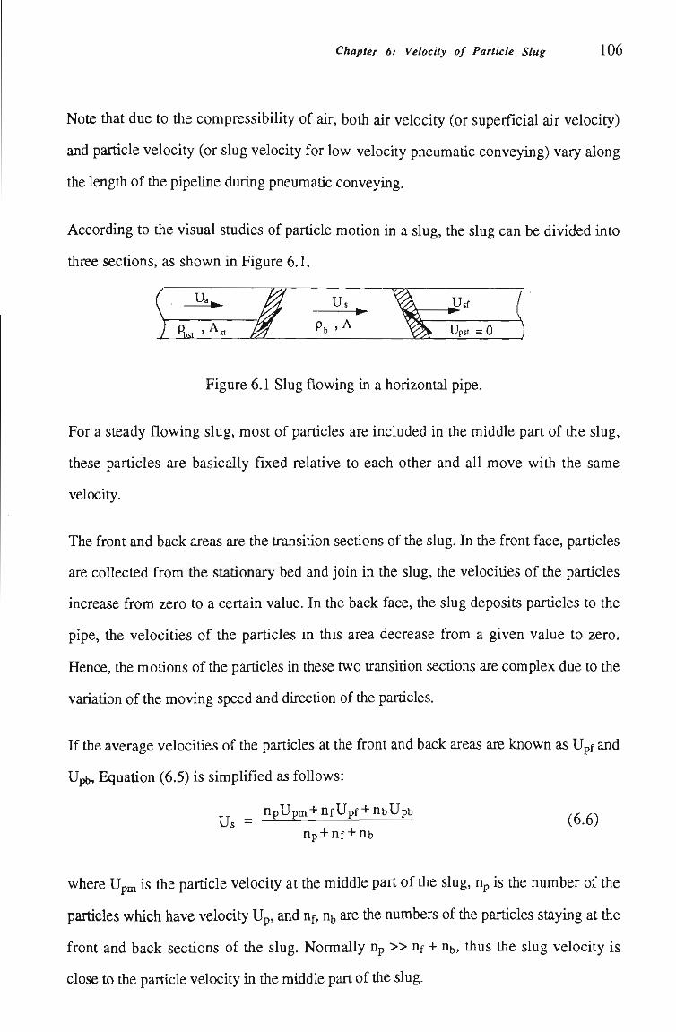
Chapter 6: Velocity of Particle Slug 106
Note that due to the compressibility of air, both air velocity (or superficial air velocity)
and particle velocity (or slug velocity for low-velocity pneumatic conveying) vary along
the length of the pipeline during pneumatic conveying.
According to the visual studies of particle motion in a slug, the slug can be divided into
three sectíons, as shown in Figure 6.1.
i ^ > ^ Us ^ JJsf 1^
Pb* ' ^»t ^ Pb ' A ^ Upst=0
Figure 6.1 Slug flowing in a horizontal pipe.
For a steady flowing slug, most of particles are included in the middle part of the slug,
these particles are basically fixed relatíve to each other and all move with the same
velocity.
The front and back areas are the transitíon sectíons of tiie slug. In the front face, partícles
are coUected from the statíonary bed and join in the slug, the velocitíes of the partícles
increase from zero to a certain value. In the back face, the slug deposits partícles to the
pipe, tíie velocities of the particles in this area decrease from a given value to zero.
Hence, the motíons of the particles in these two transitíon sectíons are complex due to the
variatíon of tiie moving speed and directíon of the particles.
If the average velocities of the particles at the front and back areas are known as Upf and
Upb, Equatíon (6.5) is simpUfied as foUows:
npUpm- nf Upf + nbUpb ,^ ^.
Up + nf + nb
where Upm is the partícle velocity at the middle part of the slug, Up is tíie number of tíie
partícies which have velocity Up, and nf, nb are tíie numbers of tiie particles staying at Úie
front and back sectíons of tíie slug. Normally Up » Uf -i- n , thus the slug velocity is
close to the partícle velocity in the middle part of tiie slug.
Chapter 6: Velocity of Particle Slug 107
While a particle slug is moving forward, particles wUl join into the slug from tíie
statíonary bed. The front surface of the slug grows contínuously and the front surface
appears to move at a higher velocity tíian tiie average partícle velocity. SimUarly, tiie back
surface of the slug obtains a higher back surface velocity due to the partícles leaving tíie
slug contínuously . If tíie slug and statíonary bed have tíie same buUc density of pb, and
if tiie same quantíty of partícles are coUected from and deposited to Ûie statíonary bed, tiie
relatíonship between the surface velocity and slug velocity can be derived from a mass
balance as:
Usf = Usb = Us 1 1 - ^ 1 (6.7) Ast
Some researchers, such as Konrad et. al. [69], defined the slug velocity as tíie surface
velocity in their investígations.
6.3 Experimental Determination of Slug Velocity
In order to obtain some practícal knowledge about slug velocity, experiments have been
conducted under various conveying conditions. The actual velocitíes of slugs have been
measured from the experiments.
There are several ways for measuring particle velocity in pneumatíc conveying. Among
these, the cross correlation function analysis technique is often selected by many
investígators. This method does not need extra apparatus and instmments and can obtain
high accuracy of measurement. The measurement of slug velocity for low-velocity
pneumatíc conveying by using the cross correlation function analysis technique is
discussed in the following sectíon.
6.3.1 Principle and Method of Slug Velocity Measurement
Figure 6.2 shows two contínuous-time waveforms, say x(t) and y(t). In order to describe
the general dependence of one on the otiier, the cross correlatíon functíon is defined:
Chapter 6: Velocity of Particle Slug 108
Rxy(i:d)= lim -J^x(t)y(t+Xd)dt T->oo 1
(6.8)
Figure 6.2 Time history records.
A typical plot of the cross cortelatíon function versus tíme displacement for a pair of time
history records is illustrated in Figure 6.3. When Rxy(t) = 0, x(t) and y(t) are said to be
uncorrelated. The plot will sometimes display peaks which indicate the existence of
correlatíon between x(t) and y(t) for a specific time delay (Xp), see Figure 6.3.
Peak Value
td
Figure 6.3 Typical cross-correlation pIoL
According to this, if two correlated signals are obtained, the time delay between the
signals can be established by notíng the tíme displacement associated with an observed
peak in the cross-correlation functíon graph. It is this principle that is applied to
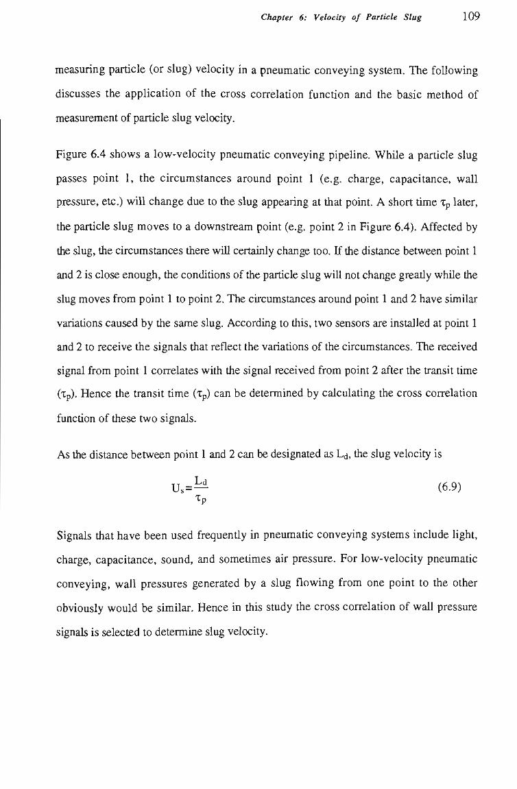
Chapter 6: Velocity of Particle Slug 109
measuring partícle (or slug) velocity in a pneumatic conveying system. The foUowing
discusses the application of the cross correlatíon function and the basic method of
measurement of particle slug velocity.
Figure 6.4 shows a low-velocity pneumatíc conveying pipeline. While a partícle slug
passes point 1, the circumstances around point 1 (e.g. charge, capacitance, wall
pressure, etc.) wiU change due to the slug appearing at that point. A short tUne Xp later,
the particle slug moves to a downstream point (e.g. point 2 in Figure 6.4). Affected by
the slug, the circumstances there wiU certainly change too. If the distance between point 1
and 2 is close enough, the conditíons of the partícle slug wiU not change greatíy whUe the
slug moves from point 1 to point 2. The circumstances around point 1 and 2 have similar
variatíons caused by the same slug. According to this, two sensors are installed at point 1
and 2 to receive the signals that reflect the variations of the circumstances. The received
signal from point 1 correlates with the signal received from point 2 after the transit time
(Xp). Hence the transit tíme (Xp) can be determined by calculating the cross correlatíon
functíon of these two signals.
As the distance between point 1 and 2 can be designated as L , tiie slug velocity is
Us=— (6.9) Xp
Signals that have been used frequentíy in pneumatíc conveying systems include light,
charge, capacitance, sound, and sometímes air pressure. For low-velocity pneumatic
conveying, waU pressures generated by a slug flowing from one point to the other
obviously would be similar, Hence in this study the cross correlatíon of wall pressure
signals is selected to determine slug velocity.
Chapter 6: Velocity of Particle Slug 110
Flow Velocity
zrjrff'j': ^: ^: H • .•. . • í^ . j-jj-i^ij'.j-.j-lj-ij-ífT ' • ' » • * ' • ' * •* K^s\sVs'.s-.s\s\s.s\s\sVs\sVs:s\s:sVsVsVsV^^^
X(t)
n Position 1 y(t) Position 2
• ^ t - • t
Adjustable Time Delay
Figure 6.4 Cortelated signals taken by two neighbouring sensors.
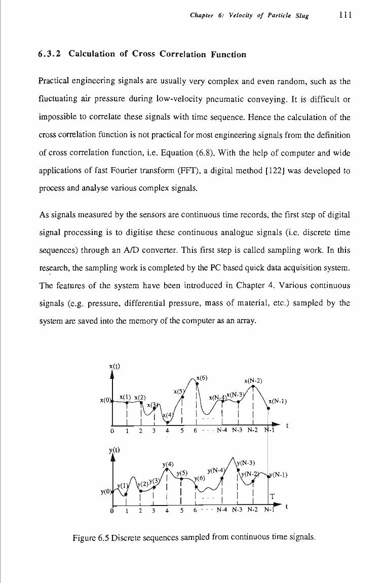
Chapter 6: Velocity of Particle Slug 111
6.3.2 Calculation of Cross Correlation Function
Practícal engineering signals are usually very complex and even random, such as the
fluctíiatíng air pressure during low-velocity pneumatic conveying. It is difficult or
impossible to correlate these signals with tíme sequence. Hence the calculation of the
cross correlatíon functíon is not practícal for most engineering signals from the defmitíon
of cross correlation functíon, i.e. Equatíon (6.8). With the help of computer and wide
applicatíons of fast Fourier transform (FFT), a digital method [122] was developed to
process and analyse various complex signals.
As signals measured by the sensors are contínuous tíme records, the first step of digital
signal processing is to digitise these contínuous analogue signals (i.e. discrete time
sequences) through an A/D converter. This first step is called sampling work. In this
research, the sampling work is completed by the PC based quick data acquisition system.
The features of the system have been introduced in Chapter 4. Various continuous
signals (e.g. pressure, differentíal pressure, mass of material, etc.) sampled by the
system are saved into the memory of the computer as an array.
x(04- (i>J^) x(N-l)
0 1 2 3 4 5 6 • • • N-4 N-3 N-2 > -1 • - t
0 1 2 3 4 5 6 N-4 N-3 N-2 N-1 ^
Figure 6.5 Discrete sequences sampled from contínuous tíme signals.
Chapter 6: Velocity of Particle Slug 112
As shown in Figure 6.5, the contínuous signals x(t) and y(t) are sampled to discrete
sequences {x(n)} and {y(n)} by an A/D converter,
{x(n)} ={x(0), x(l), x(2), - , x(N-l)}
and {y(n)} = {y(0), y(l), y(2), - , y(N-l)}.
where x(n), y(n) are the samples of x(t) and y(t) at t = nTg, n = 0, 1, 2, —, N-1, l/Tg is
the sampUng rate (frequency). Note it is better if N = 2^ where r is an integer.
After the first step, various methods of digital processing and analysis can be then
undertaken by a computer according to a given program, e.g. correlatíon analysis, power
spectíal density analysis, etc.
There are two algorithms for cross correlatíon functíon. One is a direct method which
calculates the cross correlatíon function from the definition. As N (N = l^) values have
been sampled respectívely from the continuous signals x(t) and y(t), the estímate of the
cross correlation functíon at time delay Xd (= nTg) can be obtained by the following
equatíon,
N-n-l
Rxy(ll) = R x y ( n T s ) = X ^ W y ( Í + " ) (6.10)
n = 1, 2, 3, • • • •, m (m < N)
where n is the number of the tíme delay, m is the maximum number of the tíme delay,
R (n) is tíie estmiate of Rxy('Cd) at tiie tíme delay Xd (= nTs), smce tiiere is a limit to the
number of sampled data. More samples obtained from the x(t) and y(t) give a more
accurate estimate of the cross correlatíon functíon.
Anotíier way is an indirect method based on carrying out a reverse Fourier u-ansform to
tíie cross spectral density, as the cross spectral density and cross correlatíon functíon are
a Fourier transform pair, that is
Chapter 6: Velocity of Particle Slug 113
Sxy(f) = ílRxy(Xd)e-J2^f^dXd
Rxy(Xd) = JISxy(f)e-Í2'^f^''df ^^'^^^
Equation (6.11) is usually called the "Wiener-Khinchine theorem" [122]. For discrete
signals, it can be obtamed in place of Equatíon (6.11),
Sxy( f ) = Ts XRxy(n)e-J2'^"fTs n=-oo
' y^") = l Í Sxy(f)eJ2-fTsdf
>xy'
(6.12)
Further, the cross spectral density can be obtained by calculatmg the followmg equatíon.
2 T N - 7 ^ X k * Y k , k = 0, 1, 2, ..., '-^ N 2
Sxy(fk) = ^ X k * Y k , k = 0, 1, 2, ..., - - 1 (6.13)
Xxífv) YTÍflr) where Xk= and Yk= > Xjífk) and Yj^fk) are the limited Fourier
Ts Ts transforms of the discrete signals {x(n)} and {y(n)}. They are defined as
XT(f k)=Ts x(n)e--'2'"f''T, (6 14) n=0
YT(f k)=Ts^ y(n)e-J2'«'f^T. (6.15) n=0
Because Xj fk) and YT(fk) can be obtained easUy and quickly from the sequences {x(n)}
and {y(n)} by FFT, this method is more efficient and quicker for calculating cross
correlation function, particularly if a large number of data are recorded. Hence this
indirect algorithm is applied to this research. The procedures can be summed up as
follows.
(i) Change tíie original sequences{x(n)} and {y(n)}, n = 0, 1, 2, - , N-1, to the
sequences {x'(n)} and {y'(n)}, n = 0, 1, 2, - , 2N-1, by adding N zeroes into
the original sequences, which is matiiematically requUed for calculatíng tiie cross
spectral density.
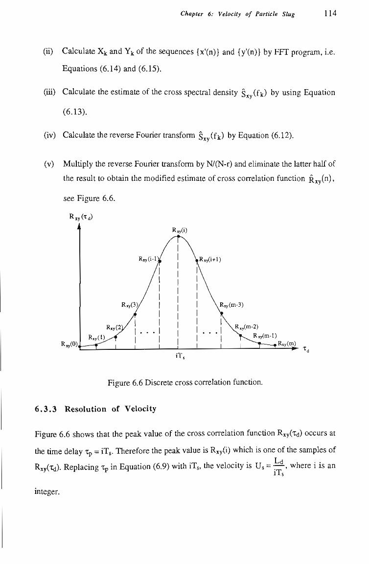
Chapter 6: Velocity of Particle Slug 114
(U) Calculate Xk and Y^ of the sequences {x'(n)} and {y'(n)} by FFT program, i.e.
Equatíons (6.14) and (6.15).
(Ui) Calculate tíie estimate of the cross spectral density Sxv(f k) by using Equatíon
(6.13).
>xy*
(iv) Calculate tíie reverse Fourier transform ^ (f ) by Equatíon (6.12) xy'
(v) Multíply tíie reverse Fourier transfomi by N/(N-r) and elimmate tíie latter half of
the result to obtain the modified estímate of cross correlatíon functíon R (n),
see Figure 6.6.
Rxy(O) Rxy(m)
Figure 6.6 Discrete cross correlation functíon.
6.3.3 Resolution of Velocity
Figure 6.6 shows that the peak value of the cross correlation functíon Rxy(Xd) occurs at
the tíme delay Xp = iTg. Therefore the peak value is Rxy(i) which is one of the samples of
Rxy(Xd). Replacing Xp in Equatíon (6.9) with iTs, the velocity is Us = — , where i is an iTs
integer.
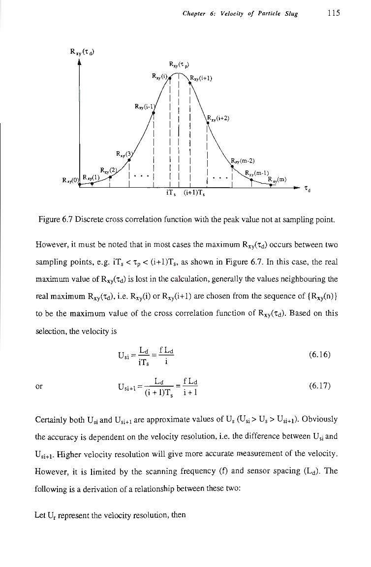
Chapter 6: Velocity of Particle Slug 115
Rxy(Td)
Rxy(-Cp)
R.y(0).
ÍT, (i+l)T3 - x^
Figure 6.7 Discrete cross correlatíon function with the peak value not at sampUng point.
However, it must be noted that in most cases the maximum Rxy(Xd) occurs between two
sampling points, e.g. iTs < Xp < (i-i-I)Ts, as shown in Figure 6.7. In this case, the real
maximum value of Rxy(Xd) is lost in the calculatíon, generally the values neighbouring the
real maximum Rxy(td), i.e. Rxy(i) or Rxy(i-i-l) are chosen from the sequence of {Rxy(n)}
to be the maximum value of the cross correlatíon functíon of Rxy(Xd). Based on this
selectíon, the velocity is
TT _ Ld _ f Ld Usi — ~ iTs
or Usi+i -Ld
(i + l)Ts
fLd i-Hl
(6.16)
(6.17)
Certainly both Usi and Usi+i are approximate values of Us (Usi > Us > Usi+i). Obviously
tiie accuracy is dependent on the velocity resolutíon, i.e. the difference between Uji and
Usi+i. Higher velocity resolutíon wiU give more accurate raeasurement of the velocity.
However, it is limited by the scanning frequency (f) and sensor spacing (L^). The
foUowing is a derivation of a relatíonship between these two:
Let Ur represent the velocity resolutíon, then
Chapter 6: Velocity of Particle Slug 116
Ur=Usi-Usi+i (6.18)
Replacing Usi and Usi+i m Equatíon (6.18) with Equations (6.16) and (6.17), tíien
1 1 + 1 1 1 + 1
or fLd = i(i + l)Ur (6.19)
f L As i = — , tiie Equatíon (6.19) can be written as
Usi
f L d = ^ ( ^ + l)Ur (6.20) Usi Usi
Dividing by (fLd) and rearranging Equation (6.20),
Ur = ^"^"^^ (6.21) fLd
If the value of Ur is small enough compared with the real velocity Uj, the product
Usi-Usi+i is approximately equal to U^, thus Equation (6.21) can be simplified as:
U^ Ur» - ^ (6.22)
f Ld
From Equatíon (6.22) it can be found that tiie velocity resolutíon is inversely proportional
to the sampling frequency of a data acquisitíon system and the distance between two
sensors. If the accuracy of the velocity measurement needs to be improved (i.e. high
velocity resolutíon is required), the sampling frequency f or distance Ld or both must be
increased. However, it is a general requirement that the two points for installing the
sensors in a pipe should be put as ciose as possible to ensure signal similarity. Therefore,
tiie data acquisitíon system is expected to have a high samplmg rate in tiie tests of velocity
measurement. For example, assume that the sampling rate of a data acquisitíon system is
fixed at 40 Hz (for four channels) which is the maximum scanning speed of the quick
data system used in this research, the velocity of a moving object is 5 ms-^ which is a
typical partícle slug velocity and the required resolutíon is 5% of the velocity to be
Chapter 6: Velocity of Particle Slug 117
measured, i.e. U = 0.25 ms-i, then according to Equatíon (6.22), the mimmum distance
between the two transducers is
U^ 52 Ld = — = : r r ^ r ^ = 2.5(m)
fUr 40x0.25 '
In otíier words, if the distance for installing the transducers is less than 2.5 m, tíie error
in measurement wiU exceed 5%.
If tíie scanning speed is increased to 100 Hz, the two transducers can be put closer
togetiien
U^ 52 Ld = — = = 1.0(m)
fUr 100x0.25
6.4 Experimental Results of Slug Velocity
Numerous experiments are conducted on the low-velocity pneumatic conveying test rig.
Two wall pressure transducers, from which the signals are used to carry out the analysis
of cross correlation function, are instaUed 2.49 m apart. The scanning speed of the quick
data acquisition system is selected as high as possible. Hence the accuracy of
measurement is sufficient for the low-velocity pneumatic conveying tests as most of the
slug velocities measured in this project are less than 6 ms-^. The experiments are
undertaken in several groups. Each group relates to a constant mass flow rate of solids,
but different mass flow-rates of air. Different groups have different mass flow-rates of
solids so that the experiments can cover a wide range of conveying conditíons. Refer to
Chapter 4 for the details of the test program and procedures.
According to the calculatíon method introduced in Sectíon 6.3.2, various slug velocitíes
are obtained, see Appendix A, by calculating the cross correlation functions of the
correlated waU pressure signals taken from the experiments which include various
materials and conveying conditíons. Figure 6.8 shows the plot of an actual cross
correlatíon functíon calculated according to tiie experimental signals.
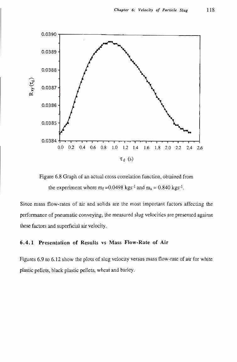
Chapter 6: Velocity of Particle Slug 118
ftá
U . U 0 3 U -
0.0389 -
0.0388 -
0.0387 -
0.0386 •
0.0385 •
0.0384 - — 1 — 1 — • — r — I — 1 — • — i ; — 1 — 1 — 1 — 1 — 1 — 1 — • — I — I — 1 — 1 — 1 — 1 — I — r ~ T — 1 —
0.0 0.2 0.4 0.6 0.8 1.0 1.2 1.4 1.6 1.8 2.0 2.2 2.4 2.6
Xd (s)
Figure 6.8 Graph of an acmal cross correlation function, obtained from
the experiment where mf =0.0498 kgs- and m = 0.840 kgs-^
Since mass flow-rates of air and soUds are the most important factors affectíng the
performance of pneumatic conveying, the measured slug velocitíes are presented against
these factors and superficial air velocity.
6.4.1 Presentation of Results vs Mass FIow-Rate of Air
Figures 6.9 to 6.12 show the plots of slug velocity versus mass flow-rate of air for white
plastíc peUets, black plastíc pellets, wheat and barley.
Chapter 6: Velocity of Particle Slug 119
B &
D
o 'o >
55
7
6-
5-
4-
3
2J
• measured values
• Eqn. (6.23) [69]
0.04
B ig
* * *
— I — 0.05
•
V4^
0.06 0.07 0.08 0.09
Mass FIow-Rate of Air, m f, (kgs - )
•S.
0.10
Figure 6.9 Slug velocity vs mass flow-rate of air for white plastic pellets.
c/3
1
r—\ 1
Cfl
E >«. . •
! ^
s •t-t
o o u > ti) 3
6-
5-
4 -
3 -
• 4
measured values
Eqn. (6.23) [69]
lS> EI
a
EISB
*
^ '
1 1 1 T T 1 1 1 " 1 • 1 .
0.03 0.04 0.05 0.06 0.07 0.08 0.09 0.10
Mass Flow-Rate of Air, m f, O^gs -i)
Figure 6.10 Slug velocity vs mass flow-rate of air for black plastíc peUets.
Chapter 6: Velocity of Particle Slug 120
«5
Ê
o
I s
I—< C/3
5-
4 -
3 -
2 .
1 -
H measured values
* Eqn. (6.23) [69]
E)
< r — ' • — r •
å"
t
—' — r
d^ D
*
1
%
* * *
s D
D
* *
* *
0.04 0.05 0.06 0.07 0.08 0.09 0.10
Mass FIow-Rate of Air, m f, (kgs-i)
Figure 6.11 Slug velocity vs mass flow-rate of air for wheat.
5-
4 -tfl
D
W)
^ 24
Q measured values
« Eqn. (6.23) [69]
0.04
njfi
DIB
•
— I —
0.05
D D D
0«^
I
0.08 0.06 0.07 0.08 0.09
Mass Flow-Rate of Air, mf, (kgs-i)
0.10
Figure 6.12 Slug velocity vs mass flow-rate of air for barley.
Chapter 6: Velocity of Particle Slug 121
Konrad et al. [69] presented the foUowing tiiird order equatíon of Us for horizontal slug-
flow:
U?+U2 ^"'^^-2(Ua+Up) " ^ bPa PbA
s
ms(a+2f ) . ms
PbAbpa PbA 2(Ua+Up) m
+U
f
a(Ua+Up),,,, ^ , , ,2 2gPb^,
V -+(Ua+Up)' ^
bPa bp.
^ 5 ^ + ( U a + U p ) ^ ^-^^^ '
(6.23)
PbAl bp bp =0
a y
where f = -- ^r-^ is a constant. Equation (6.23) includes the parameters of
the conveying conditions, physical properties of the conveyed material and pipeline
diameter. Therefore, if these conditíons are given, the slug velocity can be predicted by
solving Equation (6.23). It should be noted that Equation (6.23) has three roots. The
only root that is vaUd lies in the range (Ua+Uf) > Us > 2ms/(pbA).
Using Equation (6.23), the values of slug velocity are calculated for given experimental
conditíons and superimposed onto the above graphs for comparison. The results show
that the slug velocities predicted by Equatíon (6.23) are always much lower than the
measured values. For example, wheat was conveyed through the 52 m long pipeline in
the low-velocity pneumatíc conveying test rig. When mf = 0.0742 kgs"^ and m^ = 1.439
kgs-^, the slug velocity was measured as 3.58 ms-^ at the point 15.85 m from the end of
the pipeline, refer to Figure 6.11, whereas the slug velocity at the corresponding point
was predicted as 2.13 ms-^ by Equatíon (6.23). Two possible reasons are listed below:
1. Care must be taken by investígators to apply Ergun's equatíon [32] to the partícle
slugs m low-velocity pneumatic conveying, as tiie equation can only calculate the
pressure drop in fixed beds with a relatívely narrow range of bulk voidages. Since
tíie partícle slugs are in the fluidised state during slug-flow, refer to Chapter 3, the
applicatíon of Ergun's equation to tí s type of flow is not suitable.
2. Determinatíon of tíie stíess transmission coefficient X in Equatíon (6.23) may be
another problem. Konrad et al. [69] developed prediction equatíons for X based on
Chapter 6: Velocity of Particle Slug 122
tíie premise that stress failures occur at both the pipe wall and mside tíie buUc
material, simUar to the case of solids flowing in silos and hoppers. However, this
premise is found in Chapter 7 to be incon-ect for the slugs flowing m a pipe witíi
rigid and paraUel waUs.
6.4.2 Presentation of Results vs Mass FIow-Rate of Solids
Figures 6.13 to 6.16 display the plots of slug velocity against mass flow-rate of soUds
for different test materials. It can been seen easily that the slug velocity is relatively
independent of the mass flow-rate of solids. That is, the slug velocity is not affected
significantíy by the mass flow-rate of solids (i.e. for a given superficial air velocity). The
variation of the flow-rate of solids only changes the number of the slugs contained in a
certain length of a pipe at a specific tíme whUe the superficial air velocity maintains a
constant.
e
D
'o o
8
7
6-
5-
4-
3-
D •
Ua=4.10 (ms-1) Ua=5.56 (ms-i) Ua=6.10 (ms-i) Ua=8.00 (ms-i)
0.4
-a- -tr
— I 1 r ' 1 ' 1 —
0.6 0.8 1.0 1.2
Mass Flow-Rate of Solids, m^, (kgs-i)
1.4
Figure 6.13 Slug velocity vs mass flow-rate of soUds for white plastic peUets,
carried out in tíie 105 mm ID mUd steel pipeline.
Chapter 6: Velocity of Particle Slug 123
B
D
o o^ >
5o
8-
7-
6.
0.4
D •
Ua=4.30 (ms-') Ua=5.60 (ms-i) Ua=6.20 (ms-i) Ua=7.00 (ms-i)
n- -cr
—\— 1.0 0.6 0.8 1.0 1.2
Mass Flow-Rate of SoUds, ms, (kgs-i) 1.4
Figure 6.14 Slug velocity vs mass flow-rate of soUds for black plastíc peUets,
carried out in the 105 mm ID mUd steel pipeline.
«3
E
*o o
l 5o
D •
Ua=5.20(ms-i) Ua =5.70 (ms-i) Ua=6.50 (ms-i) Ua=6.80 (ms-i)
Mass Flow-Rate of SoUds, ms, (kgs-^)
Figure 6.15 Slug velocity vs mass flow-rate of solids for wheat,
carried out in the 105 mm ID mUd steel pipeline.
Chapter 6: Velocity of Particle Slug 124
. •
>
2 4-1
60 S
t—I
<^ 34
H U»=5.50 (ms-i) • Ua=6.00 (ms-i) O Ua=6.80 (ms-i) O Ua=7.20 (ms-i)
24-1.0 1.2
—r-1.4
"T— 1.6
I
1.8 — I —
2.0
Mass FIow-Rate of Solids, m^, (kgs-i)
Figure 6.16 Slug velocity vs mass flow-rate of soUds for barley,
carried out in tiie 105 mm ID mUd steel pipeline.
2.2
6.4.3 Presentation of Results vs Superfîcial Air Velocity
Figures 6.17 to 6.20 present the plots of slug velocity versus superficial air velocity for
each different test material. The slug velocity depends strongly on tiie superficial air
velocity. In tiie range of experimental superficial air velocity, the slug velocity appears to
vary Unearly. It should be noted tiiat for each test material, the line does not pass through
tíie origin given in Figures 6.17 to 6.20. This indicates tíie minimum air velocity tíiat is
necessary to initíate the motíon of a particle slug in a horizontal pipe. This feature also
was described by Legel and Schwedes [71] in tíieir investigatíon.
Chapter 6: Velocity of Particle Slug 125
B
D
o o
I 60
55
6-
5-
4-
3-
2-
1-
a 0
y = 0.873X- 0.893
R' ^ = 0.967
3 4 5 6 7
Superficial Air Velocity, Ua, (m s-i)
10
Figure 6.17 Slug velocity vs superficial air velocity for white plastic peUets,
carried out in the 105 mm ID mUd steel pipeUne.
Cfl
B
>> 'o o
l 60 3
OTJ
7.
6-
5-
4-
3-
2-
1-
0. 0
y=1.059x-1.659
R' ^ = 0.991
-* T -
9 10
Superficial Air Velocity, Ua, ( m s - )
Figure 6.18 Slug velocity vs superficial air velocity for black plastic peUets,
carried out in tíie 105 mm ID mUd steel pipeUne.
Chapter 6: Velocity of Particle Slug 126
C/3
B
lA
o o > 60
5o
6
5-
4-
3-
1-
y=1.013x-2.217 ^^^2 = 0.991
Superficial Air Velocity, Ua, (m s - )
Figure 6.19 Slug velocity vs superficial air velocity for wheat,
carried out in the 105 mm ID mUd steel pipeline.
o
> 60
C^
6
5-
4-
3-
2-
1.
0
y = 1.359x-3.764
R' ^ = 0.990
1 2 3 4 5 6
Superficial Air Velocity, Ua, (m s - )
T -7
Figure 6.20 Slug velocity vs superficial air velocity for barley,
carried out in tiie 105 mm ID mUd steel pipeline.
Chapter 6: Velocity of Particle Slug 127
6.5 Empirical Correlation for Slug Velocity
Since the prediction of slug velocity is not satísfactory according to Konrad's equatíon
(i.e. Equatíon (6.23)), it is necessary to develop an empirical correlatíon of slug velocity
based on the measured slug velocitíes and the relevant data at present. The foUowing
work is undertaken for this purpose.
6.5.1 Linear Model of Slug Velocity
It has been known that in the range of experimental superficial air velocity, the data for
each material can be represented by an approximate linear correlation, hence a linear
model of the slug velocity with superficial air velocity can be assumed firstiy as:
Us = KUa + constant (6.24)
where K is the slope of the line.
Due to the existence of a minimum air velocity, the linear model can be modified further
as foUowing,
Us = K(Ua-Uamin) (6.25)
The lines of best fit are obtained by least-squares and shown in Figures 6.17 to 20. Table
6.1 lists the experimental values of the slope (K) and minimum air velocity (Uamin)- The
square of the correlatíon coefficient of each line is also listed in the table to show the
goodness of fit.
Table 6.1: K, Uamin and y^ for lines of various test materials Item
K
Uamin(niS-l)
y'
Plastíc PeUets
(White)
0.873
1.023
0.966
Plastíc PeUets
(Black)
1.059
1.566
0.991
Wheat
1.013
2.189
0.991
Barley
1.359
2.770
0.990
Chapter 6: Velocity of Particle Slug 128
Obviously, for tíie experiments conducted in a 105 mm ID mild steel pipeline, different
materials have different Unear equations (i.e. different K and Uamin) to express tíie
relatíonship between tíie slug velocity and superficial air velocity. This indicates tíiat K
and Uamin in the linear model of Equatíon (6.25) must be functíons of material propertíes.
Smce material flow occurs in a pipe, the waU frictíonal force is certainly a major factor
that affects slug velocity, i.e. the waU frictíon angle (øw) should be included in tíie
functíons. Therefore, K = f (e, d, ps, (1), (|)w) and Uamin = f (e, d, ps, ({), øw). It should be
noted that the buUc density of material is excluded from tíie functíons. The reason is that
Pb = (1 - e)ps. The mass flow-rate of soUds (m ) is also excluded from the model of slug
velocity since it was found to have little effect on slug velocity.
6.5.2 Regression Slope for Linear Model
An expression for K in Equation (6.25) is assumed initíally as foUows,
Ki = ef'dpTs^tan(î),f'tan(!)p , i= l ,2 , - , n (6.26)
where e is the bulk voidage of slug, d is the partícle diameter and 7s is the partícle specific
weight which is applied to Equatíon (6.26) to represent tíie effect of the partícle density
(Ps). The purpose of using Ys instead of ps is to obtain smaller difference between every
two factors in Equatíon (6.26) so that a better regression can be achieved. ())w is the wall
frictíon angle, (j) is the intemal friction angle, xi, x , X3, X4 and X5 are coefficients, which
are obtained by the method of least squares, n is the number of the test materials.
Therefore, a deviation function is generated as foUows:
n 2 F(x) = X(ef'dpys^tan(})„rtan(t)f .Ki) (6.27)
i=l
The optímal coefficients xi, x , X3, X4 and X5 are obtained by minimizing the above
functíon. Table 6.2 Usts tíie coefficients calculated by using the optimization program
"MDOD" [123].
Chapter 6: Velocity of Particle Slug 129
Table 6.2: Optímal coefficients
xi
1.
X2
1.
X3
0.0013
X4
0.333
X5
-0.333
From tíiis table, it is found that the effect of the particle specific weight term is not
significant since the index X3 is very smaU (near to zero). To sUnplify tiie model, tíie term
of tíie partícle specific weight is taken out from Equatíon (6.26), and the expression of
the slope K is simplified as follows:
K=ed(tan(t) /tan(t))3 (6.28)
The goodness of fit of the regression model is shown in Figure 6.21.
__o
U
• T — r
0.8 0.9 1.0
Observed Slope K
Figure 6.21 Goodness of fit of K correlatíon.
It should be noted that while undertaking the regression calculatíon, tíie unit of miUimetre
is selected for the particle diameter. Hence the unit of millimetre for particle diameter
should be used in Equations (6.28).
Chapter 6: Velocity of Particle Slug 1 3 0
6.5.3 Dimensional Analysis
An expression for the slope K of the linear relatíonship between slug velocity and
superficial air velocity which is a functíon of bulk voidage (e), particle diameter (d),
intemal frictíonal angle ((})) and wall frictíonal angle {<Sf^) has been developed by usmg tiie
least square method based on the experimental data. However, it should be pointed out
that aU the data are based on the experiments carried out in the 105 mm ID mild steel
horizontal pipeline. Hence, the data cannot provide information on the effect of pipe
diameter on the slope K. Further investígatíons should be undertaken for different pipe
diameters. However, limited by finance, time and measurement technique, etc, it seems
impossible to construct a large number of pneumatic conveying test rigs with different
diameter pipelines. To explore the influence of pipe diameter on slope K, dimensional
analysis is employed in this investigation.
Since K is the slope of a linear model, it should be a parameter without unit. However,
tiie present expression of K, see Equation (6.28), has the unit of length since the partícle
diameter exists in this equation. To taken into account the influence of pipe diameter, (i.e.
pipe diameter is included in the expression of K), the following expression of K is
proposed
1
(6.29) K=c.-^
where Cd is a dimensionless coefficient.
edTtan t) ^ w
tan(t)
3
Obviously the coefficient Cd can be determined by insertíng the known slope K, physical
propertíes of material and pipe diameter into Equatíon (6.29). For example, for the white
plastíc pellets flowing through the 105 mm ID mUd steel pipeline in dense phase, the
following values can be given:
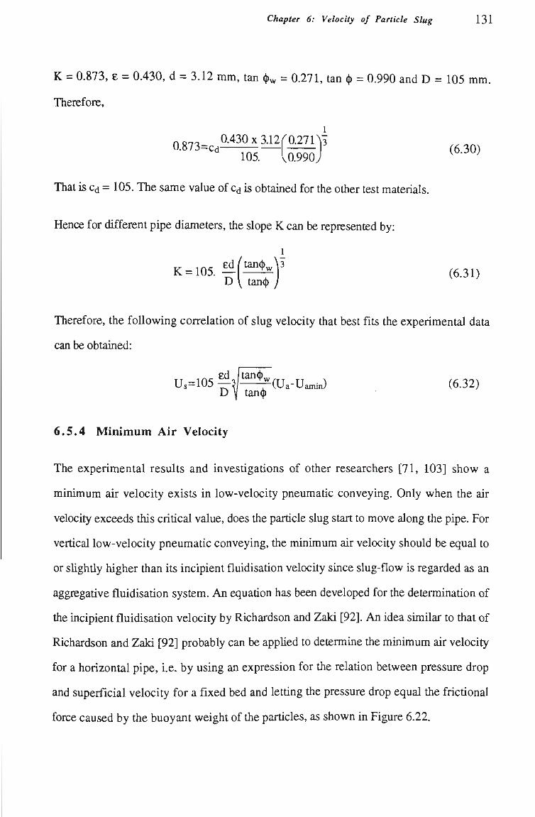
Chapter 6: Velocity of Particle Slug 131
K = 0.873, e = 0.430, d = 3.12 mm, tan isf^ = 0.271, tan () = 0.990 and D = 105 mm.
Therefore,
0_g,3 0430x112^0271^^
105. ^0990. (6.30)
That is Cd = 105. The same value of c is obtamed for the otiier test materials.
Hence for different pipe diameters, tiie slope K can be represented by:
Therefore, the following correlatíon of slug velocity that best fits the experimental data
can be obtained:
Us=105 ^ ? - ^ ( U a - U a m i n ) (6.32) D y tan(t)
6.5.4 Minimum Air Velocity
The experimental results and investigations of other researchers [71, 103] show a
minimum air velocity exists in low-velocity pneumatíc conveying. Only when the air
velocity exceeds this critícal value, does the partícle slug start to move along the pipe. For
vertícal low-velocity pneumatic conveying, the minimum air velocity should be equal to
or sUghtíy higher than its incipient fluidisatíon velocity since slug-flow is regarded as an
aggregatíve fluidisatíon system. An equatíon has been developed for the determinatíon of
the incipient fluidisatíon velocity by Richardson and Zaki [92]. An idea sUnilar to that of
Richardson and Zaki [92] probably can be appUed to determine the minimum air velocity
for a horizontal pipe, i.e. by using an expression for the relatíon between pressure drop
and superfîcial velocity for a fixed bed and lettíng the pressure drop equal the frictíonal
force caused by the buoyant weight of the particles, as shown in Figure 6.22.
Chapter 6: Velocity of Particle Slug 132
g
Thus,
Figure 6.22 IdeaUsed slug with acting forces at mitial motíon.
Ap AIs—Rs
Is
Neglecting the buoyancy of air, Equatíon (6.33) becomes
Ap
Is •=2Pbgtan(t) w
(6.33)
(6.34)
The correct selection of a suitable expression for the relation between the pressure drop
and superficial velocity for a fixed bed wiU have a great influence on tíie predicted results
of the minimum velocity. For example, for fluid flow at low Reynold's number (which is
referred to as viscous flow), Carman [18] developed the following equation for the
pressure gradient in a fîxed bed:
Ap_k36(l-e)^r|Ua Hb~ e^d^
(6.35)
where, k = constant = 5. According to other experiments [22], the value of k was found
to be dependent on partícle diameter and contained in the range 4.65 to 5.34.
Chapter 6: Velocity of Particle Slug 1 3 3
However, for turbulent flow through granular beds (i.e. at high Reynold's number),
over a relatively narrow range of fixed bed voidages, Ergun [31, 32] carried out
extensive research and suggested that during turbulent flow, the pressure loss across tíie
bed is due to not only viscous energy loss but also kinetic energy loss. Based on tíie
work of Carman [18], accounting for kinetic effects, Ergun [31, 32] developed ti^e
foUowing initíal equation for mrbulent flow,
Ap_^k36(l-e) TlUa , ÍXl- e)p,SvU^ Hb e d^ 8e3
where P is a dimensionless coeffîcient and can be determined experimentaUy.
The first term of Equation (6.36) is the pressure loss due to viscous effects (viz.
Equation (6.39)) and the second term defines the kinetic energy loss. Ergun [31] pointed
out that the relative importance of the viscosity and kinetíc terms is dependent on the
range of Reynold's number. For example, for Re = 0.1, viscous forces account for
99.8% of the pressure and the second term is approximately zero, whereas for complete
turbulent flow, Re = 3000 for instance, kinetic effects become more important and
account for 96%. For turbulent flow, Equatíon (6.36) is in tíie following form,
Ap 150Ti(l-e)^Ua , 1.75p,(l-e)U^ — = r i — • * • n ( o . j / j Hb d^e^ de^
Between tíiese two values, flow is transitíonary and both terms are significant. For these
reasons, the flow type must be taken into account while selectíng an expression for the
relatíon between the pressure drop and superficial velocity for a frxed bed.
Assuming tíiat the flow is a complete turbulent flow, predictíon of the minimum air
velocity can be obtained by substímtíng ApAs from Equatíon (6.34) into Equatíon (6.37),
thatis
150Tl(l-e)^Uamin , l - 7 5 P a ( l - e ) U L i n _ , p ^ g , , . ^ ^ (6.38)
d^e^ de^
Chapter 6: Velocity of Particle Slug 1 3 4
For tiie test materials white plastíc peUets, black plastíc peUets, wheat and barley, tiie
calculated minimum velocities from Equatíon (6.38) are 0.616 ms-i, 0.684 ms-^ 0.953
ms-i and 1.015 ms-i, respectively. These values are much lower tíian the ones obtained
from tiie Unear regression of experimental data, see Table 6.1.
Assuming tiiat the flow is viscous, substítutíng Ap/ls from Equatíon (6.34) into Equatíon
(6.35), tíien
2, k36(l-e)^ lU ^ H - ^ = 2Pbgtan(t), (6.39) d e
If k = 5.0, the minknum air velocities are found to be 1.902 ms-^ 2.609 ms'^ 4.554 ms-
^ and 5.860 ms" for white plastic pellets, black plastic pellets, wheat and barley,
respectively. These values are higher than the corresponding values listed in Table 6.1.
One interesting fact is that all the calculated values are approximately twice the values
listedinTable6.1.
According to the assumption of complete turbulent flow or laminar flow, the calculatíon
cannot obtain satisfactory results. This indicates that the air flow is neither complete
viscous flow nor complete turbulent flow in the slug at initíal motíon. That is, the type of
flow must be transitionary.
In a vertical fîxed bed, the air flows through the material uniformly across the cross
sectíon of the bed (i.e. due to an even distributíon of voids). However, in a horizontal
partícle slug, as shown in Figure 6.22, affected by partícle weight, the buUc voidage of
the bed at the upper part of the pipe wUI be greater than that at the lower part. Hence it is
easier for the air to pass through the upper part of the pipe and results in a variatíon of
flow-rate across the cross sectíon of the pipe. Sometímes channelling may occur at the
top part of the pipe due to low wall frictíon, resulting in a high proportion of the air
flowing tíirough channels, so that only a small amount of air flows through the partícle
bed. Hence the different types of flow (i.e. laminar and turbulent flow) may exist
Chapter 6: Velocity of Particle Slug 1 3 5
simultaneously at a cross sectíon of tíie pipe. In additíon, from tíie experimental values of
minmium air velocity listed in Table 6.1, tíie air flow is also found to be m tíie transitíon
from viscosity to turbulent flow. For example, at initíal motíon of a slug of white plastíc
peUets, the minimum air velocity is about 1 ms-i and Re = 220. Hence it is more
reasonable to assume that the total pressure loss is composed of both laminar flow and
turbulent flow pressure losses. It is difficuU to estímate accurately the actual proportíon
of viscous and turbulent flow in the slug. However it should be noted that tíie values
predicted by Equation (6.39) are approximately twice the values listed in Table 6.2.
Hence, it may be assumed that the two terms in Equatíon (6.36) have the same effect on
pressure loss. That is, the pressure loss across the slug is assumed approximately twice
the viscous or kinetic effect. That is,
Ap k36(l-e)^r|Ua . Pd- e)p,SvU^ , k36(l-e)^r|Ua , . .^, = T—::, 1 —-^ = ^ 5"^; ( 0 . 4 U ;
Is e d^ 8e3 e d
Combining Equations (6.34) and (6.40) results in the following expression for the
minimum superfîcial air velocity.
. ^Psgtan(t)^e3d^ ^"™" 36k(l-e)Ti ^ ^
If k = 5.0, then according to Equation (6.41), the minimum superficial air velocitíes for
white plastíc pellets, black plastíc pellets, wheat and barley are calculated as 0.951 ms- ,
1.355 ms-i, 2.266 ms- and 2.935 ms- , respectívely. Compared witíi tíie corresponding
values Usted in Table 6.1, agreement generally is quite good. Considering the possible
variatíon in the value of k mentíoned earUer (i.e. between 4.7 and 5.3), better agreements
are possible.
136
CHAPTER 7
WALL PRESSURE AND STRESS
TRANSMISSION COEFFICIENT
Chapter 7: Wall Pressure & Stress Transmission Coeffîcient 137
7,1 Introduction
The pressure which is exerted on the waU of a silo by a buUc material (i.e. the waU
pressure) has been studied by numerous investígators [7, 8, 9, 43, 55, 56, 106, 107,
108]. The term "silo" wiU be used here to describe all types of containing strucmres, e.g.
bins, hoppers, conveying pipes, bunkers and chutes etc. There are many reasons to
further this area of study. For example, whether the bulk material contained in a silo
flows or not, the bulk material exerts pressure on various parts of the silo wall and the
values of waU pressure are a major design parameter to determine the strength of tiie waU.
Another example is that during low-velocity pneumatíc conveying, tiíie wall pressure
generates the major resistance force to particle slugs.
Within the vertical part of a silo with a circular cross section, wall pressure is well
represented by the Janssen formula:
p, D 4X+l„ aw=-7^ ( l - e—' ) (7.1)
The case of a bulk material flowing in the form of slugs through a conveying pipe
(partícularly a vertícal pipe) is very simUar to the case of a bulk material flowing in the
vertícal part of the silo. Therefore, based on Janssen's metíiod, a formula for the wall
pressure is derived for vertícal slug-flow pneumatic conveying, refer to Appendix D:
aw = > ^ a f ( l - e - ^ M (7.2)
Equatíon (7.2) obviously is similar to Equatíon (7.1). A formula of the wall pressure was
developed for horizontal slug-flow in Chapter 3, see Equatíon (3.18). For ease of
reference, it is quoted here again:
CTw=M(<^b - ^f) e-~5~'' + CTf] (7.3)
In Equations (7.2) and (7.3), CTWÍS the waU pressure. CTf is the pressure on the front
surface of a slug, which is generated by the slug collectíng the particles and CT^ is tíie
Chapter 7: Wall Pressure & Stress Transmission Coeffîcient 138
pressure on tíie back surface of the slug, which is caused by the slug depositing partícles.
X is the sti-ess tiransmission coefficient which has been defined in Chapter 3 (refer to
Sectíon 3.4.1).
Although the general relatíonships between wall pressure and surface stress have been
demonstrated by Equatíons (7.2) and (7.3), it must be noted that waU pressure cannot be
predicted for low-velocity slug-flow pneumatíc conveying from these equatíons, since the
front and back stress CTf, CT^, as well as the stress transmission coefficient X in these
equatíons, are stiU unknown. Another reason is that many factors cannot be taken into
account properly whUe developing these equations. For example, bulk materials may arch
randomly, with the result that wall pressure increases sharply in the arched area. Also the
material may collapse or deform in some area of a slug so that the wall pressure is
rearranged. Hence further experimental work is needed to assist in the investígatíon of the
wall pressure of slug flow pneumatic conveying. For this purpose, wall pressure
measurement techniques and corresponding instrumentatíon have been developed and
instaUed in specific points in the pipeline system of tiie low velocity pneumatíc conveying
test rig. As soon as the particle slug flows through these measuring points, wall
pressures exerted by the slug can be obtained directíy by measurement. To fuUy
understand the effect of conveying conditíons and particle properties on wall pressure,
experiments are conducted with various conveying conditíons and materials. The test
results are presented later in this chapter.
From Equatíons (7.2) and (7.3), it can be seen that the stress transmission coefficient X,
which is defined as the ratio of radial stress to axial stress in Chapter 3, plays an
important role in tíie analysis of wall pressure. It was applied firstíy by Janssen to "sUo"
research about one hundred years ago. However, even up tíU now, many "sUo"
investígators stíU feel confused about its values. For low-velocity pneumatic conveying,
less informatíon about tíie stress transmission coefficient is presented. After measuring
waU pressures in tíiis research, some data for X in tíie low-velocity pneumatic conveying
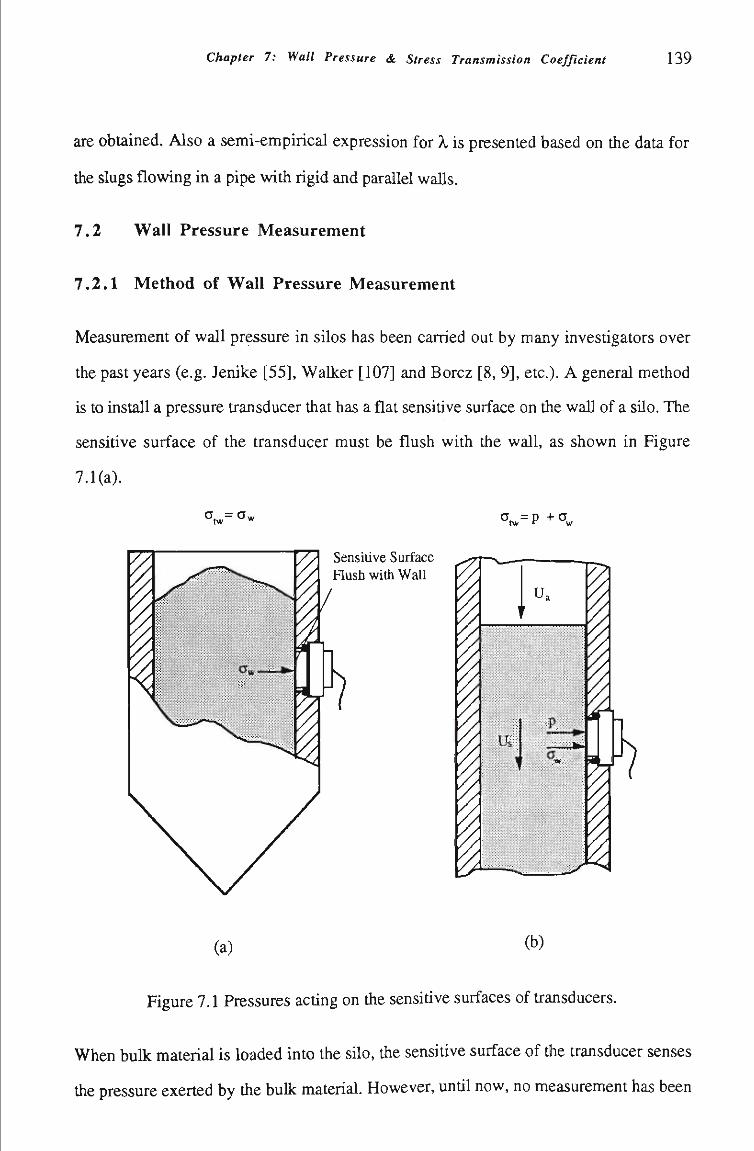
Chapter 7: Wall Pressure & Stress Transmission Coeffîcient 139
are obtained. Also a semi-empirical expression for X is presented based on tíie data for
the slugs flowing in a pipe with rigid and parallel waUs.
7.2 Wall Pressure Measurement
7.2.1 Method of Wall Pressure Measurement
Measurement of wall pressure in silos has been carried out by many investígators over
the past years (e.g. Jenike [55], WaUcer [107] and Borcz [8, 9], etc). A general method
is to install a pressure transducer that has a flat sensitive surface on the waU of a sUo. The
sensitive surface of the transducer must be flush with the wall, as shown in Figure
7.1(a).
tw *
Sensitive Surface Rush with Wall
tw * w
Élillliá * h
(a) (b)
Figure 7.1 Pressures actíng on the sensitíve surfaces of transducers.
When buUc material is loaded into the silo, the sensitíve surface of the transducer senses
tiie pressure exerted by tíie buUc material. However, untíl now, no measurement has been
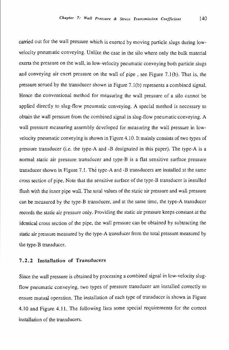
Chapter 7: Wall Pressure & Stress Transmission Coeffîcient 1 4 0
carried out for the waU pressure which is exerted by moving particle slugs during low-
velocity pneumatíc conveying. UnlUce the case in the silo where only the buLk material
exerts the pressure on the wall, in low-velocity pneumatic conveying botii partícle slugs
and conveying air exert pressure on the waU of pipe , see Figure 7.1(b). That is, the
pressure sensed by the transducer shown in Figure 7.1(b) represents a combined signal.
Hence the conventional method for measuring the wall pressure of a silo cannot be
applied directly to slug-flow pneumatic conveying. A special method is necessary to
obtain the wall pressure from the combined signal in slug-flow pneumatic conveying. A
wall pressure measuring assembly developed for measuring the wall pressure in low-
velocity pneumatic conveying is shown in Figure 4.10. It mainly consists of two types of
pressure transducer (i.e. the type-A and -B designated in this paper). The type-A is a
normal static air pressure transducer and type-B is a flat sensitive surface pressure
transducer shown in Figure 7.1. Thé type-A and -B transducers are installed at the same
cross section of pipe. Note that the sensitive surface of the type-B transducer is installed
flush with the inner pipe waU. The total values of tiie statíc air pressure and waU pressure
can be measured by the type-B transducer, and at the same tíme, the type-A transducer
records the statíc air pressure only. Providing the statíc air pressure keeps constant at the
identícal cross sectíon of the pipe, the wall pressure can be obtained by subtractíng the
static air pressure measured by tiie type-A transducer from the total pressure measured by
the type-B transducer.
7.2.2 Installation of Transducers
Since tíie waU pressure is obtained by processing a combined signal in low-velocity slug-
flow pneumatic conveying, two types of pressure transducer are installed correctly to
ensure mutual operatíon. The installatíon of each type of transducer is shown in Figure
4.10 and Figure 4.11. The following lists some special requirements for the correct
installatíon of tiie transducers.
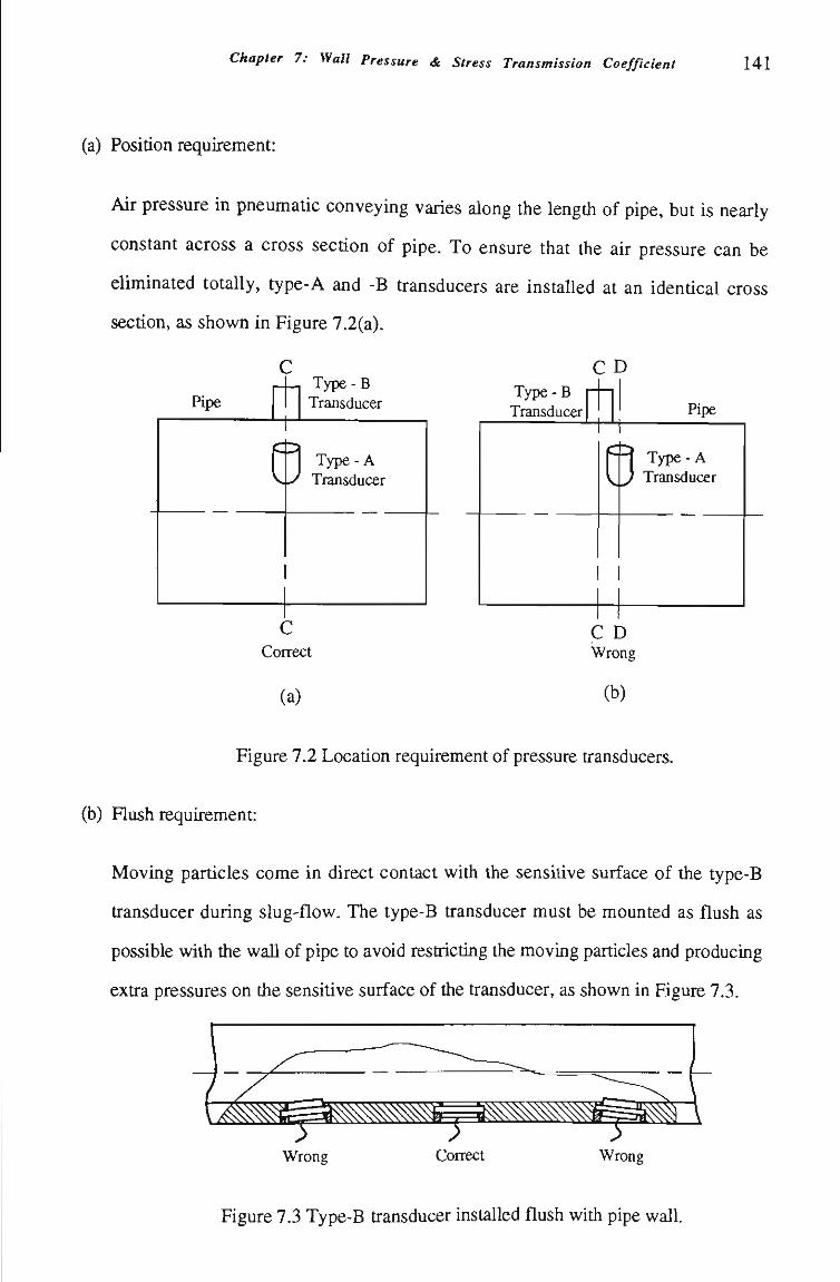
Chapter 7: Wall Pressure & Stress Transmission Coeffîcient 141
(a) Positíon requirement:
Air pressure in pneumatic conveying varies along the length of pipe, but is nearly
constant across a cross section of pipe. To ensure that the air pressure can be
eliminated totaUy, type-A and -B transducers are installed at an identical cross
section, as shown in Figure 7.2(a).
Pipe Type-B Transducer
í Type-A Transducer
C Correct
(a)
C D Type-B Transducer Pipe
8 Type-A Transducer
C D Wrong
(b)
Figure 7.2 Locatíon requirement of pressure transducers.
(b) Flush requirement:
Moving partícles come in direct contact with the sensitive surface of the type-B
transducer during slug-flow. The type-B transducer must be mounted as flush as
possible with tiie waU of pipe to avoid restricting tiie moving particles and producing
extra pressures on the sensitíve surface of the transducer, as shown in Figure 7.3.
Wrong Correct Wrong
Figure 7.3 Type-B transducer installed flush witíi pipe wall.
Chapter 7: Wall Pressure & Stress Transmission Coeffîcient 142
7.2.3 Test Procedures and Special Requirements
Wall pressure measurements are taken during various low-velocity pneumatíc conveying
experiments. The experiments are completed according to the procedure described in
Chapter 4, refer to Sectíon 4.6 for details. As the wall pressure measurement is based on
the mutual operation of two pressure transducers, further special procedures are required
for the experiments and subsequent data processing.
7.2.3.1 Re-calibration of Transducers
It is known generally that each transducer must be calibrated to obtained a calibration
factor, The calibration factor should not change over a short period of time, so that the
calibration work is not necessary for each experiment. Normally, the calibration work is
undertaken periodically (e.g. every 2 or 3 days depending on the frequency of work) and
also before commencing the project. However, both type-A and -B pressure transducers
should be calibrated frequently to obtain tiieir calibration factors as accurately as possible
(i.e. due to changes in environmental conditíons). For example, the calibratíon factor of
the type-B transducer wUI drift due to the sensitíve surface being heated by direct contact
of the slugs, whereas the calibratíon factor of the type-A transducer will be affected less
by temperature. Hence it is recommended that type-A and -B transducers be calibrated
before startíng each group of tests. This work is designated as re-caUbratíon of
transducer. Calibration methods and steps for different types of transducers were
described previously in Chapter 4, refer to Section 4.6.2 for details.
7.2.3.2 Check Test
In order to confirm that air pressure is eliminated totaUy during wall pressure
measurement, a check test is conducted after tíie re-calibratíon of transducers. The steps
of tiie check test are listed below:
Chapter 7: Wall Pressure & Stress Transmission Coeffîcient 143
(i) Remove all material from the pipeline of the low-velocity pneumatíc conveymg
test rig, then block the pipeline at the feed end by using a steel plate and close
the back pressure valve (refer to Figure 4.1).
(U) Open the air supply valve, blow air into the pipeUne untíl a designated pressure
(e.g. 50 kPag) is reached, then close the air supply valve.
(Ui) Maintain the pressure for a certain length of tíme.
(iv) Open the air supply valve and blow more air into the pipeline to get a higher
level of pressure (e.g. 100 kPag).
(v) Repeat steps (iii) and (iv) untíl the highest possible experimental pressure (e.g.
300 kPag) is reached.
(vi) By actuating the back pressure valve, decrease the pressure step by step to zero.
(vU) Record and process all the data by computer (i.e subtract the pressure measured
by type-A transducer from the pressure measured by the type-B transducer).
Chapter 7: Wall Pressure & Stress Transmission Coeffîcient 144
(\J tn
cs • — 1
•v
•• Ul 1— BC a y- • in 1 UJ (—
.—•
1
•
o
LU £ 1 — •
L L I
0->c I x l U J B
1 B
1 1 •
•
.L;_^
-. "— •
-
-•
—
^ -: ~
" •
m
_ -" 1 1
• B B V
_ l 1
~ • 1 '^ ^^
-'——
• I 1
1 •
1 T - l - I T - T I T
' 1
J
r~, J
1 • • ' • 1 1 1 1
8 H
- T i T - r i
1
1
;
; j * '1 1
• 1 1 1 1
•
> V
1 1 1 1 •
J
—^ J J -1 1 t 1
Ol <w
• Bl r^ m n U
iLl m
1 l ^
" M - ^ gy ^ «_ ,
l y
y ^ EJ
(9 EB
•
BO
•
• r
[í]klJ>l] lUdEESUd U I U
1 1 1 1 1 r 1
/
^
1 1 1 1 1 I 1
B
1 1 1 1 1
J
• ;
. . 1 . 1
•
I I r r_
_ •
. -
~
'__
LÍ -—
m
hr •
U i
• •a •a M — c
U l i n
m *^ 'M
U _ J • J
>-• U
B r.4
•
B t
1 1 1 1 1 I T
: i | •
. ». ' "
•
'
—»
_ • ;
~ •
• 1
• -' 1 1 1 1 1 1
•
VJ
aHJifí
i i n j i i i T | i n i | i i
- • 1
• ^
:*'«'
'-
-
—
T i > i l . . i i l l l l l l i . g o i B i i ^ •• B B BB
- r r-i—r ri—r' i i i i j 1 ' ;
'
^ i i
_ - j , ^
•
1
t 1 1 1 1 1 1 1 1 1 1 1 ~
Bi
<
•
•B in
g
• 90 IB
k
B
• r
—• B
gyucB^ud uiu
irpiii|iiTi|riiipiiipn |TnT
WÊ
(n in •« ^ (M ^ fl (fe O l « H B H B
S
a >•
^ a IB 91
•
1» I B
•
s 1
« m U lU n
u
1 -
• J u ^ ( J
u U l
U I X . !-•
U l - J
0
, co
5Í M 0 4)
6 2 <iz 2
3 U l
-o 1) 1/1 C f l
0 0 u
C
W3
<u V . !
3 «5 e« <U U i
O. (U *->
« * H
0
0 -U i Ot)
'S,
3 ao
E
M m «a lokijxi ainBfi3Ud yiu [au.jHi ^uuBBjy^ uiu
Chapter 7: Wall Pressure & Stress Transmission Coeffîcient 145
Typical plots from the check tests are presented in Figure 7.4. Figures 7.4(a) and 7.4(b)
display the graphs of the air pressure measured by type-B and -A transducers
respectively in one check test. Figures 7.4(c) and 7.4(d) demonstrate the processed
results, i.e. the pressure differences. Figure 7.4(c) shows tiiat tiie pressure difference is
equal to or near zero over the fuU range of pressures. This indicates that the test system is
accurate and the air pressure can be eliminated successfully from the total pressure.
Therefore wall pressure measurement can progress. It is believed that the average
processed pressure difference should be less than ten percent of the estimate of wall
pressure for using this measurement technique. Figure 7.4(d) shows the case that the
pressure difference is too large and test system cannot ensure that the air pressure can be
eliminated satisfactorily from the total pressure. Therefore the waU pressure measurement
must be stopped (e.g. re-checking or re-instalUng the relevant transducers and seals, re-
caUbrating the transducers, etc).
7.2.3.3 Improvement of Phase Difference of Signals
For two time-variable signals, even though the two signals have the same amplitude, the
difference of the two signals will not be zero due to the existence of phase difference, as
shown in Figure 7.5.
Figure 7.5 Phase difference of signals.
Theoretically, the pressure signals measured respectively by type-A and -B transducers
(Signal-A and -B for short in the following) should have same tiie phase but different
Chapter 7: Wall Pressure ã Stress Transmission Coeffîcient 146
ampUtudes if tiie transducers are instaUed correctiy at an identical cross section of a pipe.
However, due to the resistance of the porous plastic, which is fitted in tíie static air
pressure tapping to prevent particles penetrating/blocking the transducer, refer to Figure
4.10, the pressure signal taken after the porous plastic (i.e. Signal-A) wiU be delayed by
a short time after tiie real time signal (i.e. Signal-B). That is, a small phase difference
exists between Signal-A and -B, as shown in Figure 7.5. Thereafter, measurement error
wiU be caused by this phase difference in the wall pressure measurement. To reduce tiie
error, the phase difference must be decreased. Practícal experience shows that the
permeabiUty of tiie porous plastic has a signifîcant influence on the phase difference.
During a pneumatíc conveying test, the fine particles in the pipe will enter the porous
plastic and reduce its permeability or sometímes even block the porous plastícs totally
(i.e. after several runs). To ensure good permeability of the porous plastíc, it is
recommended that new porous plastics be used for each waU pressure measurement test.
In addition, the signals are scanned sequentially by a data acquisitíon system in this
research. This also generates a phase difference of signals. For example, if the sampling
rate of the data acquisitíon system is set to 1 Hz for 4 channels, then the tíme interval of
the scan is 0.25 seconds. Providing that type-B transducer Ís connected to the channel 1
of the data acquisition system and the type-A transducer is connected to the channel 2,
then the pressure signal sampled by the type-A transducer wUI be sampled 0.25 seconds
after the pressure signal is scanned by the type-B transducer. If the type-A transducer is
connected to channel 3, Signal-A wiU be delayed by 0.5 seconds after Signal-B. For this
reason, it is required that the signals coming from tiie type-A and -B transducers should
be connected to the neighbouring channels of the data acquisition system. Obviously,
enhancing the sampling rate of the data acquisitíon system is another way to reduce the
phase difference.
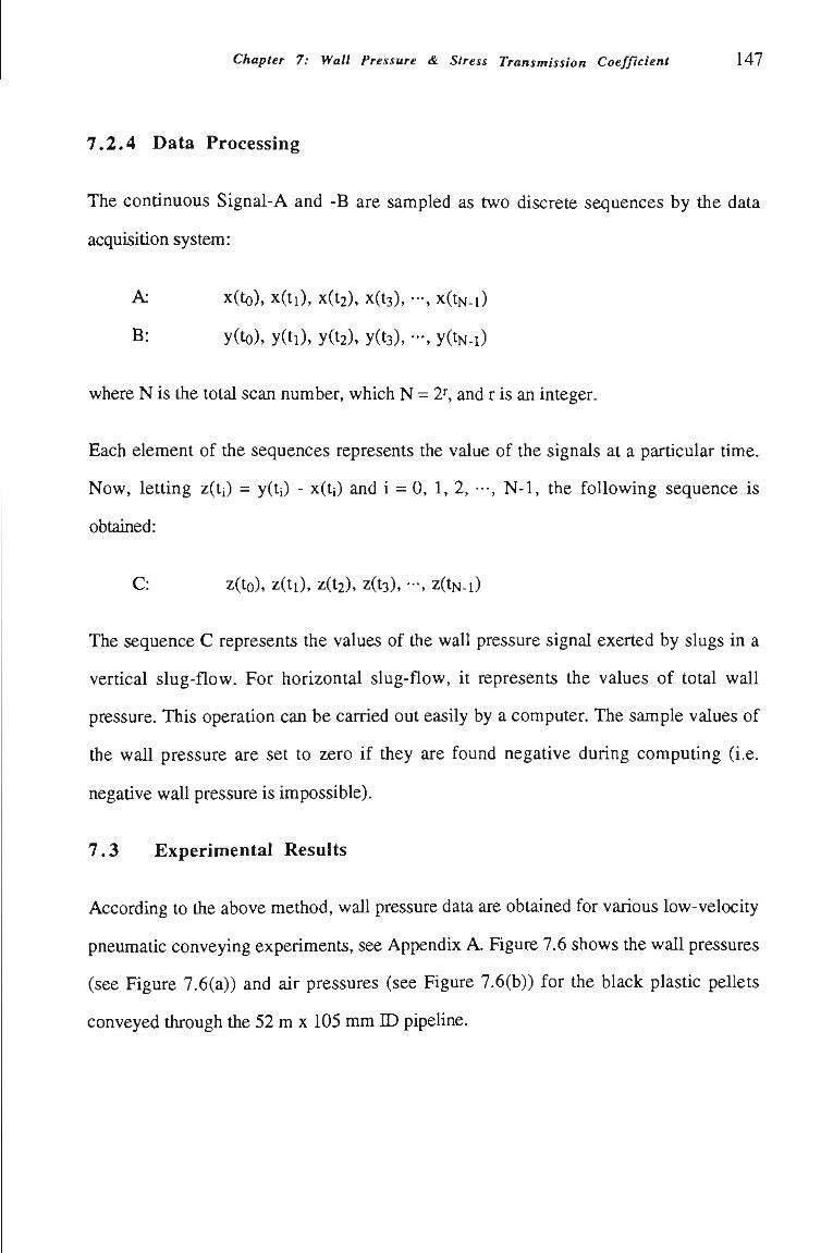
Chapter 7: Wall Pressure & Stress Transmission Coeffîcient 147
7 .2 .4 Data Processing
The continuous Signal-A and -B are sampled as two discrete sequences by the data
acquisitíon system:
A: x(to), X(ti), X(t2), X(t3), - , x(tN-l)
B: y(to), y(ti), y(t2), yds), - , y(tN.i)
where N is the total scan number, which N = 2^ and r is an integer.
Each element of the sequences represents the value of the signals at a partícular tíme.
Now, letting z(ti) = y(ti) - x(ti) and i = 0, 1, 2, • ••, N-1, the following sequence is
obtained:
C: z(to), z(ti), Z(t2), z(t3), - , z(tN.i)
The sequence C represents the values of the wall pressure signal exerted by slugs in a
vertícal slug-flow. For horizontal slug-flow, it represents the values of total wall
pressure. This operation can be carried out easily by a computer. The sample values of
the wall pressure are set to zero if they are found negative during computing (i.e.
negatíve wall pressure is impossible).
7.3 Experimental Results
According to the above method, wall pressure data are obtained for various low-velocity
pneumatic conveying experiments, see Appendix A. Figure 7.6 shows the wall pressures
(see Figure 7.6(a)) and air pressures (see Figure 7.6(b)) for the black plastic pellets
conveyed through the 52 m x 105 mm ID pipeline.
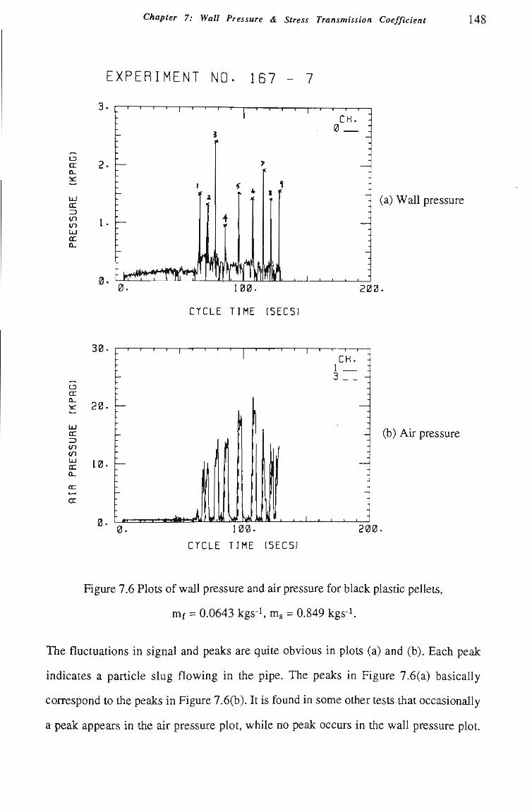
Chapter 7: Wall Pressure & Stress Transmission Coeffîcient 148
L3 d
tn UJ cc D_
EXPERIMENT NO. 167 - 7
100.
CrCLE TIME (SECS)
- (a) Wall pressure
200.
cn tn UJ cc Q-
oc
cc
30.
L3
Í 20.
l i j cc
10.
0.
-1 î 1 r-
,....iNii.4ii.>Jii y bá
I I — 1 1 — 1 — i -
CH. -I 1 3 - - H
_i I I i__j i_
100.
CrCLE TIME (SECSJ
- (b) Air pressure
200.
Figure 7.6 Plots of wall pressure and air pressure for black plastic pellets,
mf = 0.0643 kgs-i, m = 0.849 kgs-i.
The fluctuations in signal and peaks are quite obvious in plots (a) and (b). Each peak
indicates a particle slug flowing in the pipe. The peaks in Figure 7.6(a) basicaUy
correspond to tiie peaks in Figure 7.6(b). It is found in some other tests that occasionally
a peak appears in the air pressure plot, while no peak occurs in the wall pressure plot.
Chapter 7: Wall Pressure & Stress Transmission Coeffîcient 149
This indicates that a slug forms at a downstream point of the test point of tiie wall
pressure, as shown in Figure 7.7
EXPERIMENT NQ. 167 - 6
LD cn Q_ 5c:
tn
cc Q_
1. —
n I , 1. .ujulmit.
0.
20.
LD (X Q_ îc:
UJ oc tn in UJ oc Q-
10. —
CTCLE TIME (SECSl
(a) Wall pressure
200.
(b) Air pressure
200.
CrCLE TIME (SECSl
Figure 7.7 Plots of wall pressure and air pressures for black plastic pellets,
mf = 0.0498 kgs-i, m = 0.840 kgs-i.
Figures 7.6 and 7.7 also show tiiat tiie location of each peak is same in tiie two plots, but
the pressure decay rate after each peak is slower in plot (b) than plot (a). The reason is
that the peak of wall pressure only appears when the slug passes through the test point.
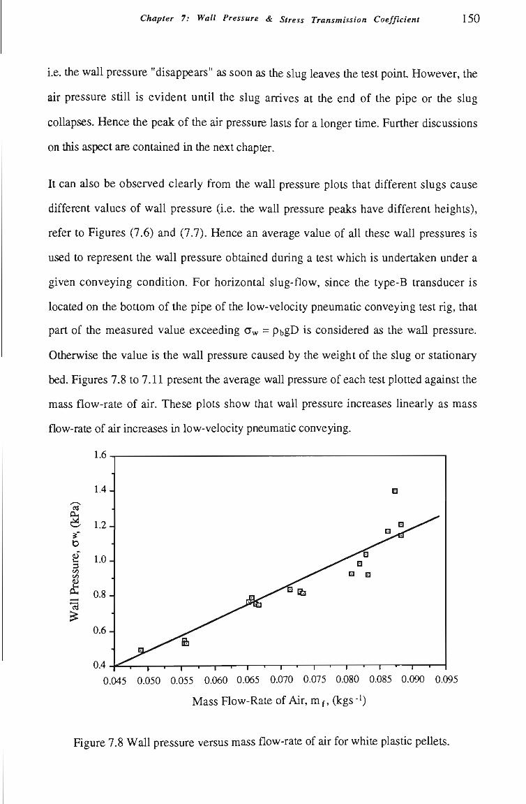
Chapter 7: Wall Pressure & Stress Transmission Coeffîcient 150
i.e. tiie wall pressure "disappears" as soon as the slug leaves the test pomt However, the
air pressure stíU is evident untU the slug arrives at tiie end of the pipe or tiie slug
coUapses. Hence the peak of the air pressure lasts for a longer tíme. Further discussions
on this aspect are contained in the next chapter.
It can also be observed clearly from the wall pressure plots that different slugs cause
different values of wall pressure (i.e. the wall pressure peaks have different heights),
refer to Figures (7.6) and (7.7). Hence an average value of aU these wall pressures is
used to represent the wall pressure obtained during a test which is undertaken under a
given conveying condition. For horizontal slug-flow, since the type-B transducer is
located on the bottom of the pipe of the low-velocity pneumatíc conveying test rig, that
part of the measured value exceeding a^ = PbgD is considered as the wall pressure.
Otherwise the value is the wall pressure caused by the weight of the slug or stationary
bed. Figures 7.8 to 7.11 present the average wall pressure of each test plotted against the
mass flow-rate of air. These plots show that wall pressure increases linearly as mass
flow-rate of air increases in low-velocity pneumatic conveying.
1.6
- 1 — I — I — I — I — 1 — • — I — • — r — ' — I — ' — I — ' — I — ' — r
0.045 0.050 0.055 0.060 0.065 0.070 0.075 0.080 0.085 0.090 0.095
Mass FIow-Rate of Air, m f, (kgs - )
Figure 7.8 Wall pressure versus mass flow-rate of air for white plastíc peUets.
Chapter 7: Wall Pressure & Stress Transmission Coeffîcient 151
1 1 1 1 1 1 1 1 1 1 1 1 1 1 1 1 1-
0.040 0.045 0.050 0.055 0.060 0.065 0.070 0.075 0.080 0.085 0.090
Mass Flow-Rate of Air, m f, (kgs "0
Figure 7.9 Wall pressure versus mass flow-rate of air for black plastic peUets.
1.1
^
ê •s
t-l
00 Cfl
^ ^ 1 - H
-ã ^
1.0
0.9
0.8
0.7
0.6
0.5
0.4.
0.3 1 • T 1 r ' 1 ' 1 ' 1 ' 1 f~
0.050 0.055 0.060 0.065 0.070 0.075 0.080 0.085 0.090
Mass Flow-Rate of Air, m f, (kgs '^)
Figure 7.10 WaU pressure versus mass flow-rate of air for wheat.
Chapter 7: Wall Pressure & Stress Transmission Coeffîcient 152
a fe o b
B s C/3
rcs
ØH ^ (H ^
1.4-
1.2.
1.0-
0.8-
0 6 H
0.4-
0 7 - — ^ —r —^ 1— ' r—' r—
^y^^ Q
> X ^
r 1 -r "T- 1 r
^ ^ i ^ ^
X ^ B Ø
1 t '
0.045 0.050 0.055 0.060 0.065 0.070 0.075 0.080 0.085 0.090
Mass FIow-Rate of Air, m f, (kgs -i)
Figure 7.11 Wall pressure yersus mass flow-rate of air for barley.
The stress transmission coefficient (K) is a parameter relevant to waU pressure. Since the
stress transmission coefficient in a slug is approximately equal to the ratío of the average
wall pressure to the frontal stress of the slug in low-velocity pneumatíc conveying, i.e.
^--Jî™^ seg Sectíon 3.5.2, it is possible to obtain the approximate values of X after the CTf
wall pressure data have been measured.
Us
Figure 7.12 Stresses actíng on a particle slug.
Besides the wall pressure, the slug velocity (Us) and statíonary bed thickness (hs) as
shown in Figure 7.12, are also needed to determine X, since CTf=apbUj. In fact, Us and
Chapter 7: Wall Pressure & Stress Transmission Coeffîcient 153
hs have been measured already in this research for different conveying tests. The results
of the slug velocitíes have been shown in Chapter 6. The results of the statíonary bed
thickness and corresponding a are presented in Chapter 8. Hence X can be calculated.
For example, when wheat (pb = 811.5 kgm-^) is conveyed under the conveying
conditions of mf = 0.0495 kgs- and m = 0.967 kgs-i, the average wall pressure, slug
velocity, cross sectional area ratio of stationary bed to pipe are measured as: CTwm = 0.334
kPa, Us = 1.747 ms-i and a = 0.256, therefore,
CTf = aPbU2 = 0.256x811.5xl.7472 = 634.0 Pa = 0.634 kPa
and x^^^ = ^ ^ = Q.521 CTf 0.634
Table 7.1 lists the values of the stress transmission coefficient and corresponding
operating conditíons for wheat.
Chapter 7: Wall Pressure & Stress Transmission Coeffîcient 154
Table 7.1: Experimental wall pressure
Exp. No.
1
2
3
4
5
6
7
8
9
10
11
12
13
14
15
16
17
18
19
20
and stress transmission coefficient for wheaL
52 m pipeUne mf
(kgs-i)
0.0495
0.0663
0.0733
0.0828
0.0882
0.0495
0.0665
0.0742
0.0836
0.0885
0.0545
0.0676
0.0747
0.0796
0.0868
0.0543
0.0657
0.0747
0.0838
0.0885
ms (kgs-i)
0.967
0.959
0.957
0.961
0.962
1.450
1.439
1.439
1.439
1.461
1.945
1.986
1.977
1.997
1.996
2.300
2.383
2.403
2.388
2.415
(kPa)
0.334
0.671
0.726
0.896
0.978
0.341
0.639
0.785
0.892
0.997
0.442
0.711
0.746
0.814
0.909
0.403
0.663
0.780
0.952
1.028
CTf
OcPa)
0.634
1.158
1.346
1.656
1.729
0.622
1.101
1.333
1.604
1.762
0.760
1.234
1.300
1.423
1.597
0.773
1.130
1.364
1.688
1.747
X
0.527
0.579
0.539
0.541
0.566
0.548
0.580
0.589
0.556
0.566
0.582
0.576
0.573
0.572
0.569
0.521
0.587
0.572
0.564
0.588
96 m pipeline mf
(kgs-i)
0.0557
0.0676
0.0749
0.0838
0.0870
0.0559
0.0678
0.0754
0.0833
0.0869
0.0560
0.0678
0.0739
0.0838
0.0878
0.0556
0.0677
0.0744
0.0835
0.0873
m^ (kgs-i)
1.159
1.157
1.161
1.168
1.162
1.494
1.494
1.496
1.497
1.493
1.960
1.957
1.968
1.969
1.964
2.387
2.402
2.374
2.373
2.375
(kPa)
0.420
0.702
0.706
0.926
0.969
0.423
0.737
0.796
0.882
1.007
0.423
0.707
0.788
0.948
1.008
0.423
0.673
0.781
0.928
0.996
CTf
(kPa)
0.768
1.193
1.310
1.688
1.712
0.762
1.223
1.364
1.529
1.623
0.728
1.191
1.346
1.524
1.703
0.828
1.190
1.357
1.535
1.709
X
0.547
0.588
0.539
0.601
0.587
0.555
0.603
0.584
0.577
0.622
0.515
0.594
0.585
0.622
0.592
0.511
0.566
0.576
0.605
0.583
From tiie values of X Usted m Table 7.1, it can be seen that for a given granular material,
the stress transmission coefficient is approximately constant and for wheat obtains an
average value of 0.572, despite tiie different conveying conditíons and pipe lengths. This
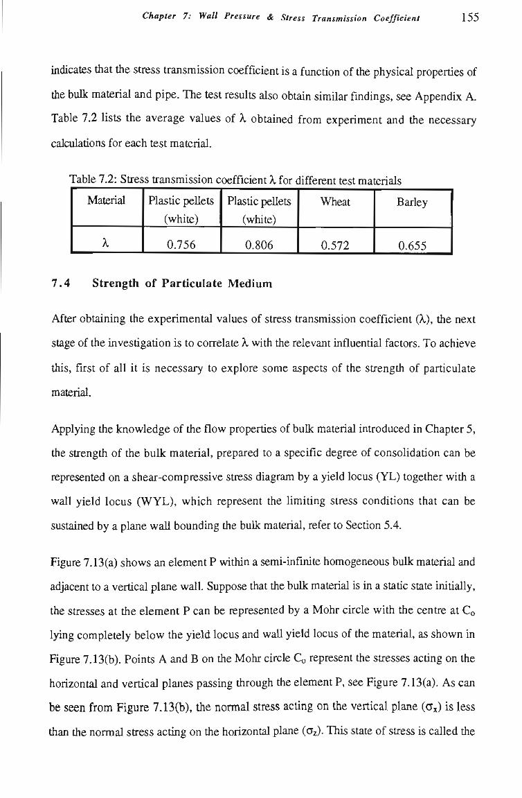
Chapter 7: Wall Pressure & Stress Transmission Coeffîcient 155
indicates that the stress transmission coefficient is a function of the physical propertíes of
tiie buUc raaterial and pipe. The test results also obtain similar fmdings, see Appendix A.
Table 7.2 lists the average values of X obtained from experiment and the necessary
calculations for each test material.
Table 7.2: Stress transmission coefficient X for different test materials
Material
X
Plastíc peUets
(white)
0.756
Plastíc peUets
(white)
0.806
Wheat
0.572
Barley
0.655
7.4 Strength of Particulate Medium
After obtaining the experimental values of stress transmission coefficient (X), the next
stage of the investigation is to correlate X with the relevant influentíal factors. To achieve
this, first of all it is necessary to explore some aspects of the strength of partículate
material.
Applying the knowledge of the flow properties of bulk material introduced in Chapter 5,
the strengtii of the buUc material, prepared to a specific degree of consolidatíon can be
represented on a shear-compressive stress diagram by a yield locus (YL) together with a
wall yield locus (WYL), which represent the Umitíng stress conditíons that can be
sustained by a plane waU boundmg tiie bulk material, refer to Sectíon 5.4.
Figure 7.13(a) shows an element P within a semi-mfinite homogeneous buUc material and
adjacent to a vertícal plane wall. Suppose tiiat tiie buUc material is in a statíc state initially,
the stresses at tíie element P can be represented by a Mohr circle with the centre at Co
lying completely below the yield locus and wall yield locus of the material, as shown in
Figure 7.13(b). Points A and B on the Mohr circle CQ represent the stresses acting on the
horizontal and vertícal planes passing through the element P, see Figure 7.13(a). As can
be seen from Figure 7.13(b), tiie normal stress acting cn the vertical plane (CT ) is less
tiian the normal stress actmg on tiie horizontal plane (CTz). This state of stress is called tiie
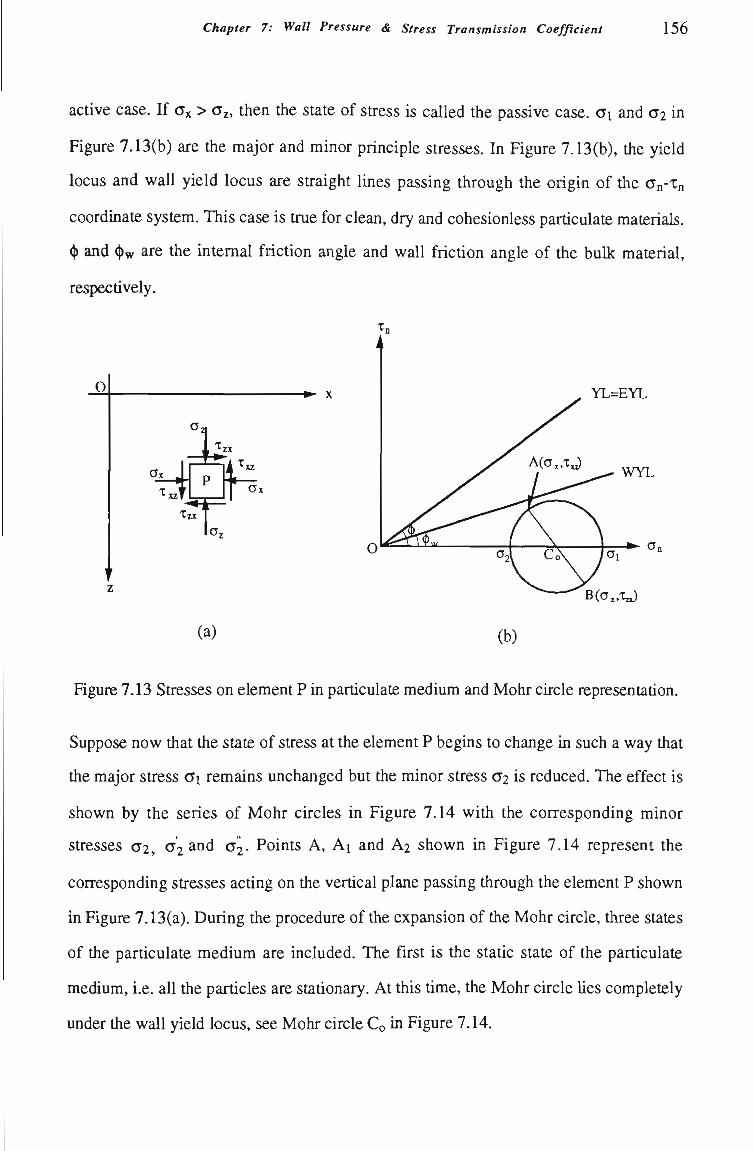
Chapter 7: Wall Pressure & Stress Transmission Coeffîcient 156
actíve case. If CTX > CTZ, then the state of stress is called the passive case. CTI and Oi in
Figure 7.13(b) are the major and minor principle stresses. In Figure 7.13(b), tiie yield
locus and wall yield locus are straight lines passing through the origin of the CTn-Xn
coordinate system. This case is true for clean, dry and cohesionless particulate materials.
(j) and (j)w are the intemal frictíon ang e and waU frictíon angle of the buUc material,
respectívely.
O
Ox
txzf
— l i , ^
Xtx
(a)
- • X YL=EYL
WYL
* • o„
B(o„xJ
(b)
Figure 7.13 Stresses on element P in particulate medium and Mohr circle representation.
Suppose now that the state of stress at the element P begins to change in such a way that
the major stress CTI remains unchanged but the minor stress CT^ is reduced. The effect is
shown by the series of Mohr circles in Figure 7.14 with the corresponding minor
stresses CT2, CT^ and CT^. Points A, Ai and A^ shown in Figure 7.14 represent the
corresponding stresses acting on the vertical plane passing through the element P shown
in Figure 7.13(a). During the procedure of the expansion of the Mohr circle, three states
of the particulate medium are included. The fîrst is the static state of the particulate
medium, i.e. all the partícles are stationary. At this tíme, the Mohr circle Ues completely
under the wall yield locus, see Mohr circle Co in Figure 7.14.
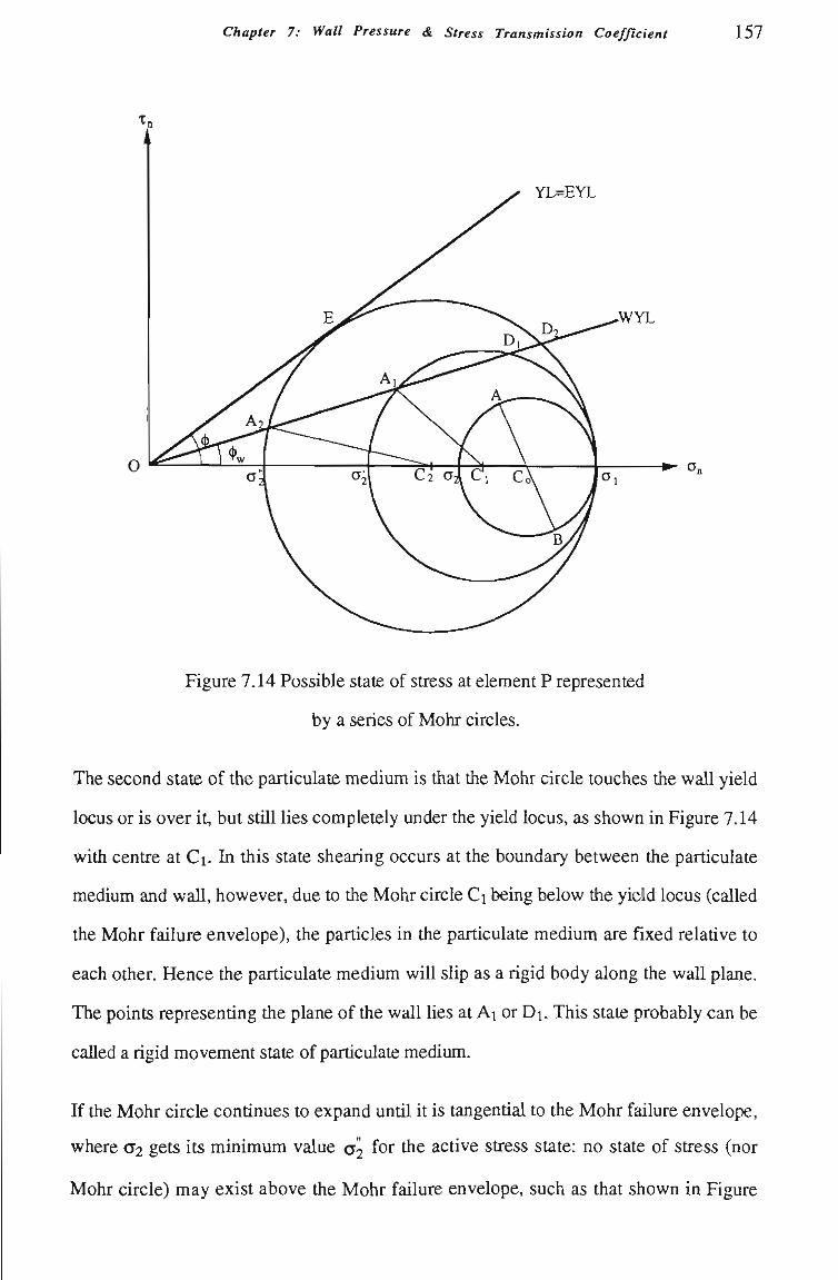
Chapter 7: Wall Pressure & Stress Transmission Coeffîcient 157
YL=EYL
•WYL
Figure 7.14 Possible state of stress at element P represented
by a series of Mohr circles.
The second state of the particulate medium is that tiie Mohr circle touches the wall yield
locus or is over it, but stUI lies completely under the yield locus, as shown in Figure 7.14
with centre at Ci. In this state shearing occurs at the boundary between the particulate
medium and waU, however, due to the Mohr circle Ci being below tiie yield locus (called
the Mohr failure envelope), the particles in the particulate medium are fixed relatíve to
each other. Hence the particulate medium will slip as a rigid body along the wall plane.
The points representíng the plane of the wall lies at Ai or Di. This state probably can be
caUed a rigid movement state of partículate medium.
If the Mohr circle contínues to expand untíl it is tangentíal to the Mohr failure envelope,
where CT^ gets its minimum value a^ for the active stress state: no state of stress (nor
Mohr circle) may exist above the Mohr failure envelope, such as that shown in Figure
Chapter 7: Wall Pressure & Stress Transmission Coeffîcient 158
7.14 with centre at C^. This is the third state of the particulate medium. In tíûs state, tiie
faUure (flowing) of the material occurs, i.e. relatíve movement exists between tiie
partícles. The failure occurring at the actíve stress state is called actíve faUure. The
particles adjacent to the wall plane also sUp along the wall and A^ or D^ represent tiie
plane of tíie wall. The state of stress actmg at tiie point E in Figure 7.14 is tiie tiieoretical
Umiting state of stress on tiie faUure plane at faUure.
x„
YL=EYL
WYL
Figure 7.15 Possible states of stress at element P in passive stress state.
The above discussion involves the actíve stress case. If still maintaining the major stress
CTi, the stress state now is changed by increasing the major stress CT^. The circles
representing possible states of stress at element P are shown in Figure 7.15. With CT2
increasing, the circle passes through the element circle CT2 = CTi to the limiting case where
the failure of the partículate medium occurs with CT^ and CT^, as shown in Figure 7.15
with the centre at C^. CT^ is the maximum value in passive case. This failure is called
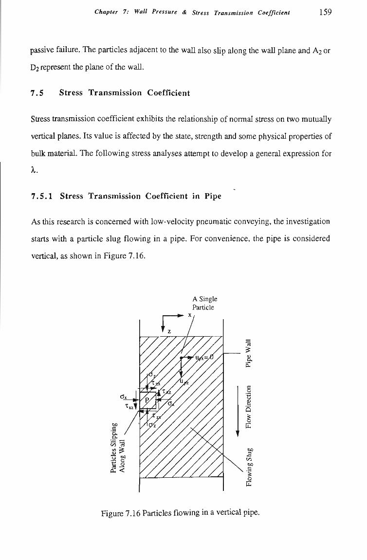
Chapter 7: Wall Pressure & Stress Transmission Coeffîcient 159
passive failure, The particles adjacent to tiie waU also sUp along the waU plane and A2 or
D2 represent the plane of the waU.
7.5 Stress Transmission Coeffícient
Sti"ess transmission coefficient exhibits the relatíonship of normal stress on two mutually
vertícal planes. Its value is affected by the state, strength and some physical propertíes of
buUc material. The foUowing stress analyses attempt to develop a general expression for
X.
7.5.1 Stress Transmission Coeffícient in Pipe
As this research is concemed with low-velocity pneumatic conveying, the investígatíon
starts with a particle slug flowing in a pipe. For convenience, the pipe is considered
vertical, as shown in Figure 7.16.
A Single Particle
Figure 7.16 Particles flowing in a vertical pipe.
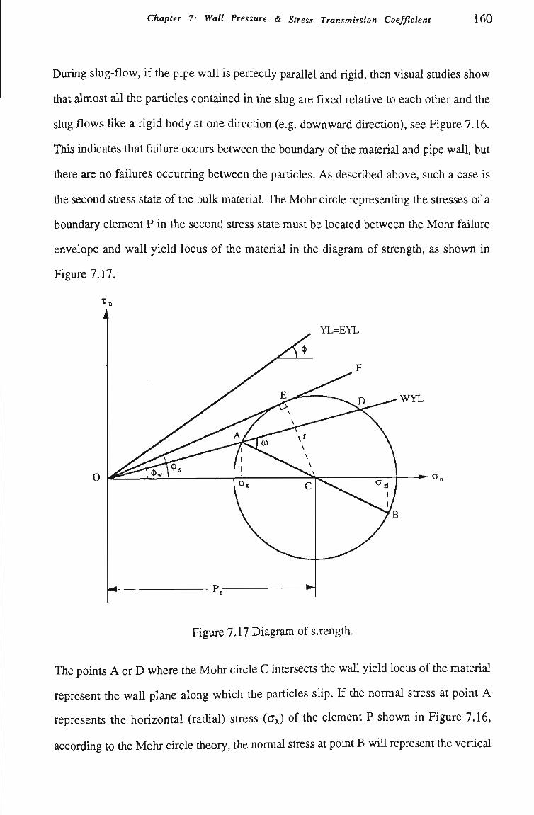
Chapter 7: Wall Pressure & Stress Transmission Coeffîcient 160
During slug-flow, if tiie pipe wall is perfectíy parallel and rigid, tiien visual studies show
tiiat almost aU tiie partícles contained in the slug are fixed relatíve to each otiier and tiie
slug flows lUce a rigid body at one direction (e.g. downward directíon), see Figure 7.16.
This indicates that faUure occurs between the boundary of tiie material and pipe wall, but
there are no failures occurring between the particles. As described above, such a case is
the second stress state of the buUc material. The Mohr circle representing the stresses of a
boundary element P in the second stress state must be located between the Mohr faUure
envelope and wall yield locus of the material in the diagram of strength, as shown in
Figure 7.17.
YL=EYL
WYL
• • o .
Figure 7.17 Diagram of strengtfi.
The points A or D where the Mohr circle C intersects tiie wall yield locus of the material
represent the wall plane along which the partícles slip. If the normal stress at point A
represents the horizontal (radial) stress (CT ) of the element P shown in Figure 7.16,
accordmg to tiie Mohr circle tiieory, the normal strcss at point B wiU represent the vertical
Chapter 7: Wall Pressure & Stress Transmission Coeffîcient 161
(axial) stress (CTZ) of the element P. Hence, the stress transmission coefficient in tiie
vertícal pipe wUl be CT^/CTZ. AS CT^ < CTZ, the stress state of the element P is tiie active case.
The stress transmission coefficient at actíve case is written as XA which can be
determined from the principles of geometry.
Draw a tangent line OF to the Mohr circle C and let it pass through the origin of CTn-Xn
coordinate system, see Figure 7.17. The angle between the straight line OF and CTn-
coordinate is (j)s defined here as the static intemal friction angle since any particle in the
slug remains stationary relatíve to the adjacent particles at this stage. As the bulk material
sUps along the pipe waU, (t) < (t) < (j).
Applying the sine mle to triangle OAC in Figure 7.17:
CTx = Ps - rcos(Cû-(l)J (7.4)
CTz = Ps -H rcos(æ-(l)J (7.5)
(7.6) sin(7i-û)) siníj)
From tiie triangle OEC:
sm^Pj Ps = - ^ (7.7)
Substituting Ps m Equations (7.4) and (7.5) with Equation (7.7), and eliminating r,
CTx l-sin(|),cos(co-(})J CTz l-i-sm( 3C0s(cû-(t) )
Also substímtmg Ps in Equatíon (7.6) with Equatíon (7.7) and eliminatíng r,
sinû) = sin(t)w/sin(t)s (7.9)
Chapter 7: Wall Pressure & Stress Transmission Coeffîciení 162
Note that aU the above equatíons apply to the actíve case of stress state. For tiie passive
case of stress state, the stress transmission coefficient Xp is obtained simUarly, provided
CTx and CTz are interchanged in Figure 7.17. The final result is
;i^^-gx^l-HSÍn(t),COS(0)-Kl)J
CTz l-sin(|)5Cos((û + (t) )
From Equatíons (7.8) and (7.10), it can be found that for a given bulk material, the stress
transmission coefficient is determined only by its static intemal friction angle and wall
friction angle whUe the material flows in the pipe with rigid and parallel wall. Obviously
Ap > XA,.
Note that although Equations (7.8), (7.9) and (7.10) are developed for the stress
transmission coefficient in a vertical pipe, no special nature of the vertícal pipe has been
used during the development of the equatíons. Hence it is reasonable to assume that the
equations are also suitable for the stress transmission coefficient in a horizontal pipe.
Certainly for the horizontal pipe, the pressure due to weight must be excluded from this
coefficient.
7 .5 .2 Discussion on Stress Transmission Coeffícient
From Equations (7.8), (7.9) and (7.10), it can be seen clearly that stress transmission
coefficient (X) is a functíon of statíc intemal frictíon angle ((^s) and wall frictíon angle
((t)w). As the wall frictíon angle is normally a constant for a given bulk material and pipe,
the following discussion is focused on the variatíon of X with different ^^-
Díscussion 1: Wall frictíon angle (t)w = 0.
This case occurs at the statíc state of the buUc material supported by a plane. Looking at
Figure 7.16, if the pipe has a bottom, the material wiU be supported by the bottom and
has no trend of slipping along the wall. Therefore, the wall frictíon angle is equal to zero.
The buUc material contained in a sUo or hopper with the outlet gate closed is analogous to
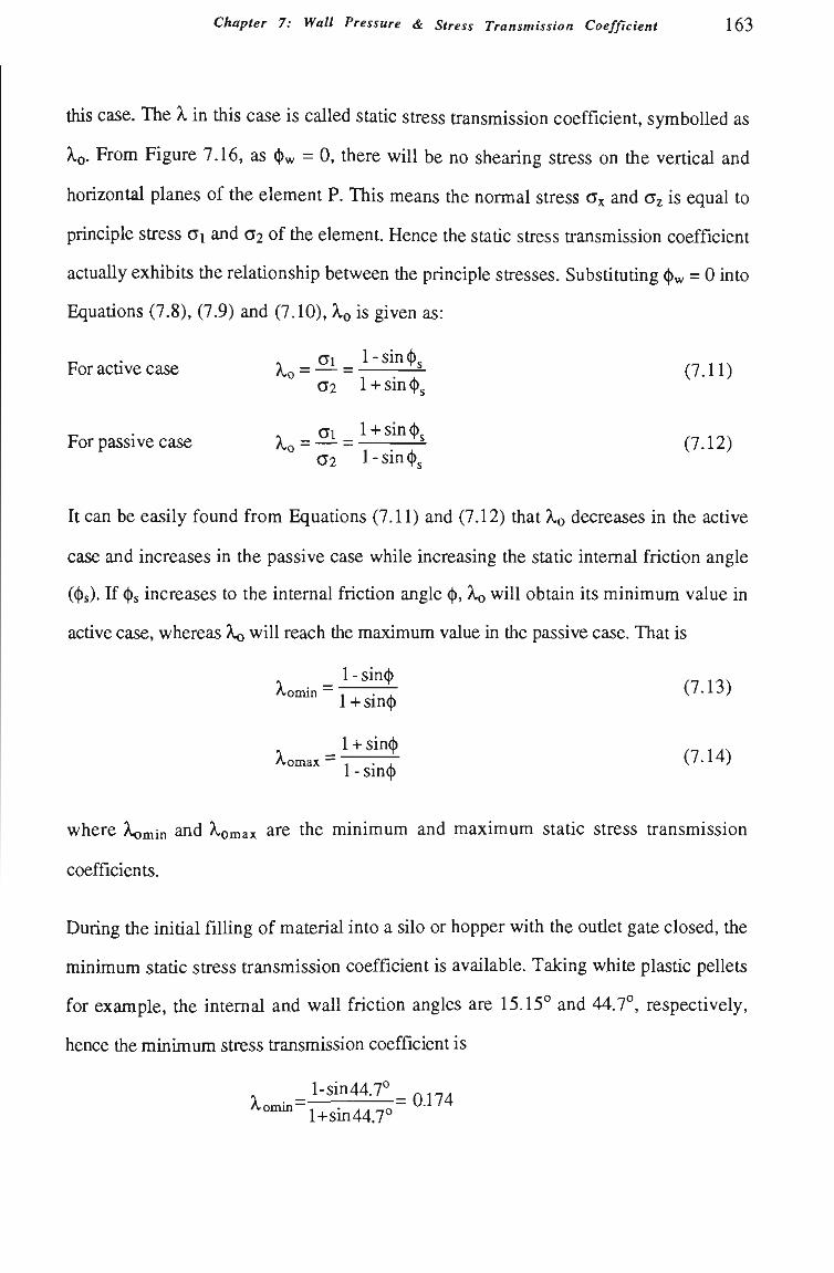
Chapter 7: Wall Pressure & Stress Transmission Coeffîcient 163
tíiis case. The X in tiiis case is called statíc stress transmission coefficient, symboUed as
XQ. From Figure 7.16, as (t)w = 0, there wUI be no shearing stress on tíie vertícal and
horizontal planes of the element P. This means the normal stress CTX and CTZ is equal to
principle stress CTI and CT^ of tiie element. Hence the static stress transmission coefficient
actually exhibits the relatíonship between the principle stresses. Substítutíng (t)w = 0 into
Equatíons (7.8), (7.9) and (7.10), X,o is given as:
For actíve case x,o = — = — (7.11) CT2 l + sin t)
For passive case Xo = — = — ^ ^ ^ (7.12) 02 l-sm t)
It can be easily found from Equations (7.11) and (7.12) that XQ decreases in the active
case and increases in the passive case while increasing the static intemal frictíon angle
((t)s). If (t)s increases to the intemal friction angle ^, XQ will obtain its minimum value in
actíve case, whereas Xo wUI reach the maximum value in the passive case. That is
l-sin(t) A,oinin 1 • . y-'^-J)
1 + sm(t)
X J l ^ (7 14) A,omax 1 . , V'. A^/
1 - sm(t)
where Xomin and Xomax are the minimum and maximum static stress transmission
coefficients.
During the initíal filUng of material into a sUo or hopper with the outíet gate closed, the
minimum statíc stress transmission coefficient is available. Taking white plastic pellets
for example, the intemal and waU frictíon angles are 15.15° and 44.7°, respectively,
hence the minimum stress transmission coefficient is
_l -s in44.7°^ ^ ™ l+sm^^.?"
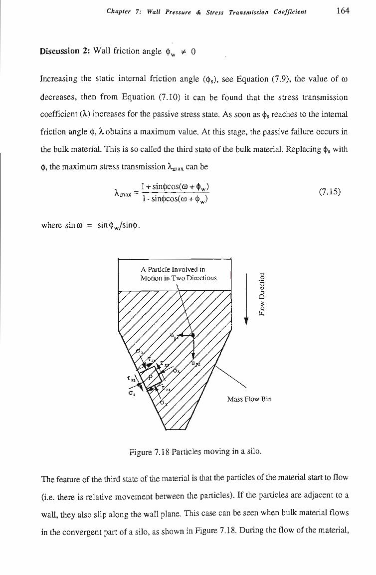
Chapter 7: Wall Pressure & Stress Transmission Coeffîcient 164
Discussion 2: WaU frictíon angle ^^ :^ 0
Increasing the static intemal frictíon angle ((t)s), see Equation (7.9), the value of O)
decreases, then from Equatíon (7.10) it can be found that the stress transmission
coefficient (X) increases for the passive stress state. As soon as s reaches to tiie intemal
friction angle ^, X obtains a maximum value. At this stage, the passive failure occurs in
the buUc material. This is so called the third state of the bulk material. Replacing ^^ with
(}), the maximum stress transmission Xmax can be
1 + sin(t)Cos(û) + (t) ) i-max 1 - SÍn(î)COS(CÛ + (j)^)
(7.15)
where sino) = sin(j) /sin(î).
A Particle Involved in Motion in Two Directions c
ts
Q
o E
Mass Flow Bin
Figure 7.18 Particles moving in a silo.
The feature of tiie tíiird state of tiie material is tiiat tiie particles of tiie material start to flow
(i.e. tiiere is relatíve movement between the particles). If the partícles are adjacent to a
waU, they also sUp along the waU plane. This case can be seen when buUc material flows
in tiie convergent part of a silo, as shown in Figure 7.18. During tiie flow of the material.
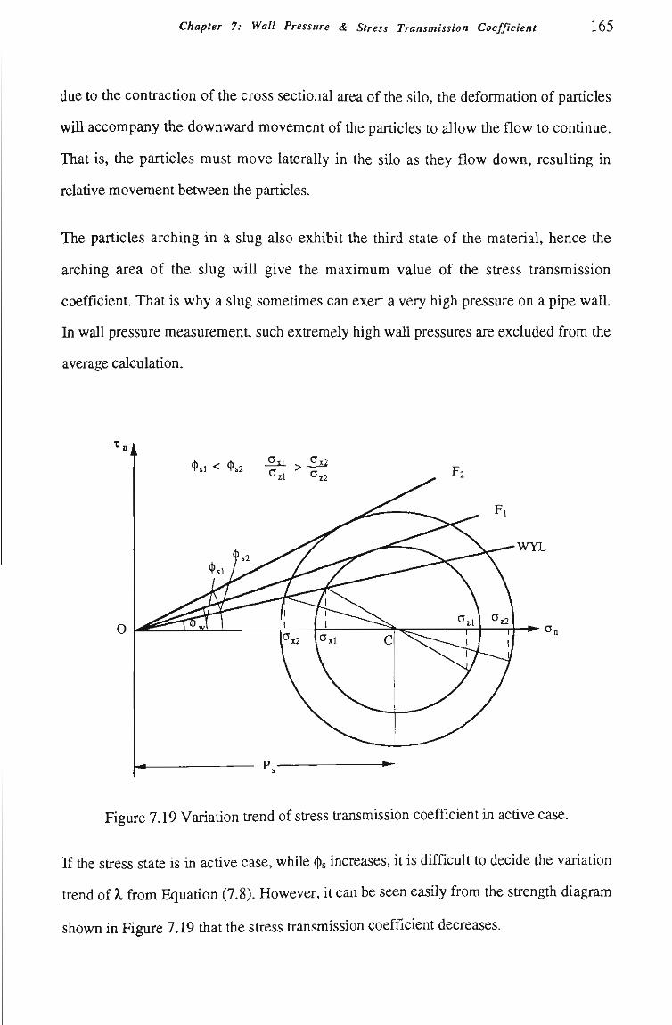
Chapter 7: Wall Pressure & Stress Transmission Coeffîcient 165
due to the contractíon of the cross sectíonal area of the sUo, the deformatíon of partícles
wiU accompany the downward movement of the particles to allow the flow to contínue.
That is, the particles must move laterally in the silo as they flow down, resulting in
relatíve movement between the particles.
The particles arching in a slug also exhibU the third state of the material, hence tiie
arching area of the slug will give the maximum value of the stress transmission
coefficient. That is why a slug sometimes can exert a very high pressure on a pipe wall.
In wall pressure measurement, such extremely high waU pressures are excluded from the
average calculation.
WYL
^ a.
Figure 7.19 Variatíon trend of stress transmission coefficient in actíve case.
If tíie stress state is in active case, while (t)s increases, it is difficult to decide the variation
ti-end of X from Equatíon (7.8). However, it can be seen easUy from the strength diagram
shown in Figure 7.19 tíiat tíie stress transmission coefficient decreases.
Chapter 7: Wall Pressure & Stress Transmission Coeffîcient 166
Similarly, the active failure occurs while ^ rises to (j), the stress transmission coefficient
X reaches its minimum value. Replacing (^^ in Equation (7.8) with ^, the minimum X can
be
_ l-sin(t)cos(ú)-(t)J Amin - 1 . • -, 7 - T ( / - l o )
1 + sm(t)cos(û) - (j) )
where sino) = sin^^/sin(t).
This case can be found in the particles flowing in the expansion part of a silo.
From the discussion, it is known that the X at active failure and passive failure are the
extreme values which are determined by intemal and wall friction angles. Generally
speaking, the intemal friction angle ^ or wall friction angle (^^ are constant for a given
material and wall, hence X at active failure and passive failure (i.e. Xn n and Xmax) are
determined uniquely. For exaraple, O) is calculated as 21.82° for white plastíc pellets, so
tíiat Xmin and Xmax are
^ l-sin44.7°cos(21.82° - 15.15°) ^^ . g '" '"~l + sin44.7°cos(21.82°- 15.15°)
1+sin44.7°cos(21.82° +15.15°) ^ ... AmaTt = = • J - - > 0 0
°'^'' 1 - sin44.7°cos(21.82° +15.15°)
That is, all possible stress transmission coefficients are contained in the range of
0.178 < X < 3.566 for tiie white plastic pellets.
7.6 Correlation of Static Internal Friction Angle
Equations have been developed and discussed in the previous section for the stress
transmission coefficient X. However, the value of X is dependent on the static intemal
frictíon angle ((t)s) as given in Equatíons (7.8), (7.9) and (7.10). Hence, a relatíonship
between ^^ and its influentíal factors also needs to be investigated.
Chapter 7: Wall Pressure & Stress Transmission Coeffîciení 167
WYL
Figure 7.20 Possible Mohr circles representing the stress state of a partícle slug.
As shown in Figure 7.20, while a bulk material flows in the form of slugs in a pipe,
there are an infinite number of possible Mohr circles representing the stress state of the
slug located between the YL and WYL of the material. For example, the stress states
represented by the Mohr circles Ci and C2 satísfy the criteria of the slug flowing in the
pipe, i.e. the particles of the slug slip along the pipe wall, but there is no relative
movement between the partícles. By drawing tangent Une OFi to the Mohr circle Ci and
tangent line OF2 to the Mohr circle C2 through the origin of the coordinate system, two
different statíc intemal frictíon angles are obtained as (f si and ^si- It appears difficult to
know exactíy the actual statíc intemal frictíon angle. However, there always exists a
unique Mohr circle which represents the actual stress state of the slug. Due to the
uncertainty of the actual "locatíon" of Mohr circle of tíie slug, it seems impossible to
predict tíie intemal statíc frictíon angle from theory. Hence, an empirical correlatíon is
sought.
Chapter 7: Wall Pressure & Stress Transmission Coeffîcient 168
From tíie results of X listed in Table 7.2, statíc intemal frictíon angles can be calculated
by using Equations (7.8) and (7.9) or (7.10) for the test material. U is also noted tiiat all
tíie stí-ess transmission coefficients for tfie materials are less than 1. This means tíiat tiie
stress state of slugs should be in the active stress case during slug-flow. Hence Equatíon
(7.10) wiU not be useful for this calculation.
For example, the experimental X of white plastíc pellets is 0.756. Substítutíng tíiis value
and the data of the intemal and wall friction angle of the white plastic peUets into
Equatíons (7.8) and (7.9) gives
sinû) = sinl5.15%in(t)s
l-sin(t)3COs(G)-15.15°)
l+sin(t)sCos(û)-15.15°) =0756
(7.17)
(7.18)
Solving Equatíons (7.17) and (7.18), the value of the static intemal frictíon angle ^s is
15.75° for the white plastíc pellets when they flow in the form of slugs in a pipe.
Table 7.3 Usts the calculated static intemal friction angles of each test material.
Table 7.3: Static intemal friction angles for test materials Material
^s
Plastic peUets (white)
15.75°
Plastic peUets (white)
13.40°
Wheat
20.08°
Barley
16.81°
Based on the data listed in Table 7.3, an expression for static intemal frictíon angle can
be regressed. SimUar to the intemal friction angle, the static intemal friction angle also is
one of the flow properties of material. Therefore, its value is only relevant to the material
and should have nothing to do with the size of the material and the extemal factors such
as the size and shape of a pipe, conveying conditions, etc. Also, as the expression of ^
is to be regressed for the material in the second state, i.e. the particles of the material sUp
along the waU but keep fixed relatíve to each other, ^s wUI be relevant to the flow
property of the wall frictíon angle instead of the intemal frictíon angle. Hence ^s should
Chapter 7: Wall Pressure & Stress Transmission Coeffîcient 169
be a functíon of the buUc voidage, density (or specific weight), and waU frictíon angle of
material, tiiat is (t)s = f (e, YS, <t>w). The buUc density of the material is not included into tiie
functíon as it is govemed by e and YS- An appropriate model for regression is assumed as
foUows,
<l)si = xi(l-ei)^^Y,^^(t),f\ i= l ,2 , - , n (7.19)
where xi, x , X3, and X4 are the coefficients to be determined, n is the number of tíie test
materials.
Applying the method of least squares with the limit of (l)s < (!>, the coefficients are
obtained and listed in Table 7.4.
'able 7.4: Coefficient of best fit.
Xl
1.33
X2
0.33
X3
0.33
X4
1.00
Therefore, (t)s is best fitted by the foUowing functíon:
1 = T<l>w[(l-e)Ys]^ (7.20)
As Yb = (1 - e) Ys' Equatíon (7.20) can be written as
<t>s = -^ n (7.21)
where Yb is the bulk specific weight with respect to water at 4 °C.
The goodness of fit is show in Figure 7.21.
Chapter 7: Wall Pressure & Stress Transmission Coeffîcient 170
-e-B
u
Observed (t> s
Figure 7.21 Goodness of fit.
171
CHAPTER 8
TOTAL HORIZONTAL PIPELINE PRESSURE DROP
Chapter 8: Total Horizontal Pipeline Pressure Drop 172
8.1 Introduction
The accurate prediction of total pipeline pressure drop is one of the most important
aspects of research in pneumatíc conveying systems. For example, if a pneumatíc
conveying system is to be designed or upgraded to ensure satísfactory and efficient
operatíon, accurate informatíon on conveying performance (i.e. the relatíonship between
total pipeUne pressure drop and its influentíal factors) must be obtained. Generally, the
factors affecting the total pipeline pressure drop mainly include the physical propertíes of
the material, pipeUne confíguratíons and conveying conditions. Hence the development of
a model which is a function of the physical properties, pipeline configuratíons and
conveying conditions for the total pipeline pressure drop becomes the ultimate aim of
many researchers of pneumatic conveying. Numerous predictíng models have been
developed for various pneumatic conveying systems. Most of these are confined to
dilute-phase conveying. Unfortunately, only a few were developed for dense-phase
conveying, and these models are stíll far from reliable due to the complexity and
variabiUty of the dense-phase conveying. For this reason, developing a more accurate and
efficient model for low-velocity pneumatic conveying is the main ultimate goal of this
research. As the pressure gradient across a single slug and the relevant factors affecting
the pressure gradient such as slug velocity, wall pressure and stress transmission
coefficient, etc. have been studied in previous chapters, the work in this chapter
correlates the total pipeline pressure drop with the single slug pressure drop and otíier
relevant factors to lead to tíie final model. The model should be a function of the physical
properties of the material to be handled, conveying condirions and pipeline
configuratíons. In order to complete the correlatíon work successfully and to achieve tíie
ultímate goal of this research, the following extra investígatíons also are carried ouL
A low-velocity pneumatíc conveying system normally includes several slugs and air gaps
flowing along tíie pipeline. Each slug length constítutes the total slug lengtíi that affects
tíie total pipeline pressure drop. In additíon, some other geometrical parameters such as
Chapter 8: Total Horizontal Pipeline Pressure Drop 173
statíonary bed thickness also influence the pressure drop. Therefore, tíie relatíonship
between the geometrical parameters reflectíng the nature of the flow pattern and
conveying conditions is studied firstíy based on numerous experiments and analyses of
the experimental signals. As a result of this study, the flow pattern also can be
understood more clearly and quantítatívely.
The effects of pipeline confîguration (i.e. the diameter and length of pipe, type and
locatíon of bends, etc.) on the total pipeline pressure drop tiien are investigated.
After these investigations, the model for predicting the total horizontal pipeline pressure
drop is developed. Based on this model, a prediction procedure is recommended based
on computer iteration.
Finally, comparisons are made between the predicted results and experimental results to
examine the accuracy of the developed model.
8.2 Geometrical Parameters of Low-Velocity Pneumatic Conveying
Visual studies of slug flow geometry have been made by many researchers [16, 48, 69,
71, 105] for low-velocity pneumatíc conveying. For example, a detailed descriptíon of
the flow pattem was presented by Konrad et al. [69], see Sectíon 3.2 in Chapter 3. In
this research, the observatíons made during tíie numerous experiments of low-velocity
pneumatíc conveying of various types of granular material agree to tíiis descriptíon.
However, quantítatíve studies and analyses are rarely found for the flow pattem and its
relations with the pipeline pressure drop and conveying conditíons. The work in tíiis
sectíon wUl provide some assistance for tíUs purpose by presentíng experimental data and
analyses.
In order to describe flow pattem quantítatively, it is expected to know which geometrical
parameters basically reflect tíie main aspects of tiie flow. It is beUeved that tiie parameters
should at least include the slug length Os) and air gap length (Ig), slug diameter which is
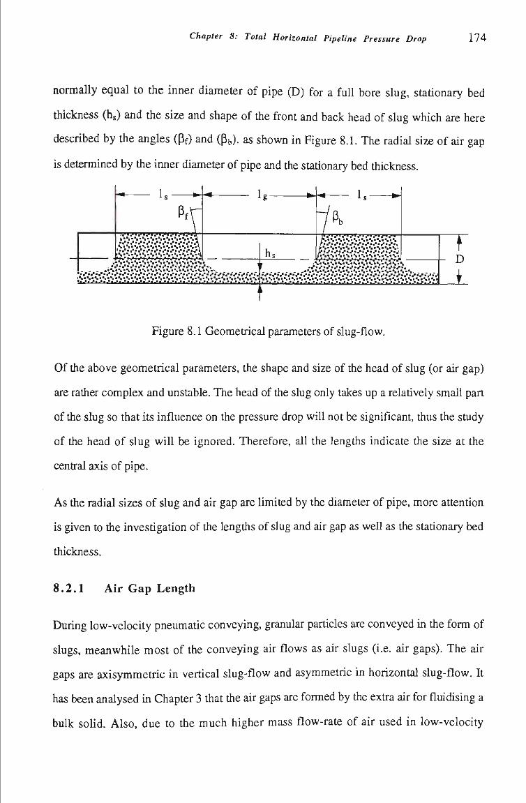
Chapter 8: Total Horizontal Pipeline Pressure Drop 1 7 4
normally equal to the inner diameter of pipe (D) for a fuU bore slug, statíonary bed
thickness (hs) and the size and shape of tíie front and back head of slug which are here
described by the angles (pf) and (pb). as shown in Figure 8.1. The radial size of air gap
is determined by tíie inner diameter of pipe and the statíonary bed tiiickness.
^-M-
P,i
• •? . * . • «• .• . * • . • » .*.• . * • . » • • • • . • • . • J
- * - • • -
Pb
f íViVivSKvSvSv v
JiiiívSiíîíiívív v-Vi . ' .• . • • H - .•.• •• • . • • H . H • •• • . * » > ^^•^•^•^•^•^•f.f'f.^'^'f... W -J'^yí^ifi/i^f.J^J'.J^J^^.
. . . .•S"S^%"V»S"V»S"V^s.S"\^%i.v... T •sVsiSísVsísísVn.VsVOsísís.s is • s j s • s • s • s ".s • s ; s • s • s •s^s^s.s^s^s^s^s-s^s^s^ s Js • sV sV sVsV sVsVsVsVsVsVsVsVOsVsVsVsVsVsVsVsVs'
T D
i_
Figure 8.1 Geometrical parameters of slug-flow.
Of the above geometrical parameters, the shape and size of the head of slug (or air gap)
are rather complex and unstable. The head of the slug only takes up a relatively smaU part
of the slug so that its influence on the pressure drop wiU not be significant, thus the study
of the head of slug will be ignored. Therefore, all the lengths indicate the size at the
central axis of pipe.
As the radial sizes of slug and air gap are limited by the diameter of pipe, more attentíon
is given to the investígation of the lengths of slug and air gap as weU as the statíonary bed
thickness.
8.2.1 Air Gap Length
During low-velocity pneumatíc conveying, granular particles are conveyed in the form of
slugs, meanwhile most of the conveying air flows as air slugs (i.e. air gaps). The air
gaps are axisymmetric in vertical slug-flow and asymmetric in horizontal slug-flow. It
has been analysed m Chapter 3 that tiie air gaps are formed by the extra air for fluidising a
bulk soUd. AIso, due to the much higher mass flow-rate of air used in low-velocity
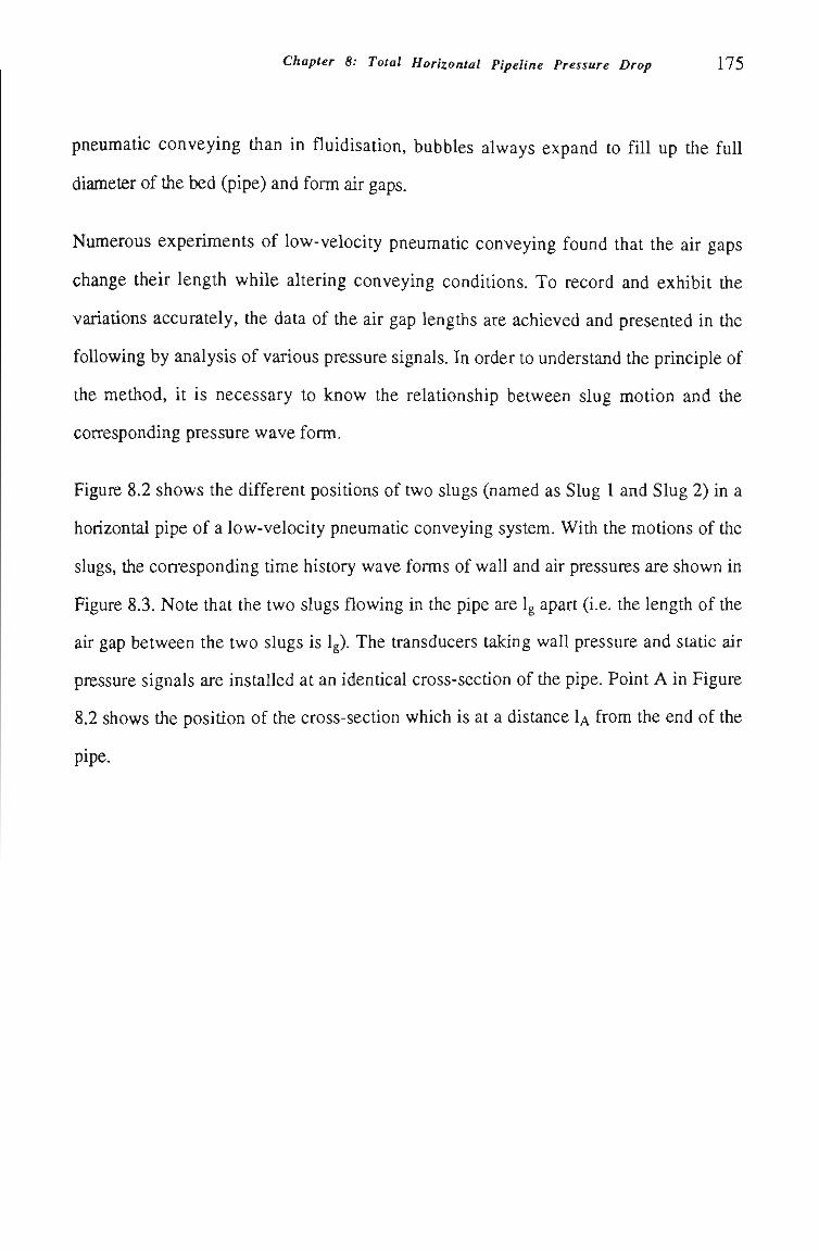
Chapter 8: Total Horizontal Pipeline Pressure Drop 175
pneumatic conveying than in fluidisatíon, bubbles always expand to fiU up tíie fuU
diameter of tiie bed (pipe) and form air gaps.
Numerous experiments of low-velocity pneumatic conveying found that the air gaps
change their length whUe altering conveying conditíons. To record and exhibit tiie
variatíons accurately, the data of the air gap lengths are achieved and presented in the
foUowing by analysis of various pressure signals. In order to understand the principle of
the method, it is necessary to know the relationship between slug motion and the
corresponding pressure wave form.
Figure 8.2 shows the different positions of two slugs (named as Slug 1 and Slug 2) in a
horizontal pipe of a low-velocity pneumatíc conveying system. With the motíons of the
slugs, the cortesponding time history wave forms of wall and air pressures are shown in
Figure 8.3. Note that the two slugs flowing in the pipe are Ig apart (i.e. the length of tíie
air gap between the two slugs is Ig). The transducers taking wall pressure and statíc air
pressure signals are instaUed at an identical cross-sectíon of the pipe. Point A in Figure
8.2 shows the positíon of the cross-sectíon which is at a distance U from the end of the
pipe.
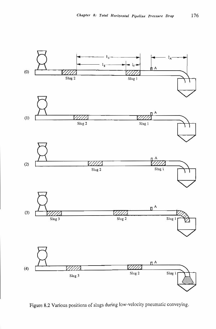
Chapter 8: Total Horizontal Pipeline Pressure Drop 1 7 6
(0) ^ ^ Slug2
• * I s - * -
m^ <« L
Slug 1 ^ ^
(1) [
(2)
T7m Slug2
•^^7/77^ Slug2
-ym Slugl
(3) I l^///A T ^ ^ Slug3 Slug2
N;^
i Slug l
^
^ ^
Slug l
X7
(4) C i//m wm n
Slug3 Slug 2 Slug 1
^ ^
Figure 8.2 Various positíons of slugs during low-velocity pneumatic conveying.
Chapter 8: Total Horizontal Pipeline Pressure Drop 111
3 00 c/5 (U
<
O to
Slugl Slug2
i, t, - • t
3 </3 CO (U t -
o
Slugl
(a)
Slug 2
t2
Atf
At
t6
(b)
Figure 8.3 Time history records of statíc air and wall pressures.
Figure 8.2(0) shows the initíal positíons of tiie slugs. Because the transducers are located
at the downstream of Slug 1 at this stage, neither the statíc air pressure nor wall pressure
is sensed by the transducers if the pressure drop caused by the air alone is low enough to
be neglected. Hence both the air and wall pressures are zero at this initial stage, see the
time period from to to ti in Figure 8.3(a) (i.e. the plot of the time history wave form of
the statíc air pressure) and Figure 8.3(b) (i.e. the plot of the time history wave form of
the wall pressure).
Figure 8.2(1) displays the positíons of tiie slugs while Slug 1 just arrives at point A. The
time at which Slug 1 arrives at the point is indicated as ti in Figure 8.3(a) and (b). From
this tíme ti, the transducers begin to sense the static air and wall pressure signals. Then
Slug 1 moves further forward, for example, untU its end just leaves point A, as shown in
Chapter 8: Total Horizontal Pipeline Pressure Drop 178
Figure 8.2(2). t^is used to indicate the "departure" time of Slug 1. During tíiis process,
both wall and air transducers can always receive time-variable signals with the variation
of the positíons of the slugs. From time ti to ti, the air pressure increases its value from
zero to maximum as the air pressure is proportional to the length of the slug, however,
the wall pressure gets a value which is equal to the transmission frontal stress (Xaf)
immediately at tíme ti instead of zero and then varies exponentíally according to the waU
pressure distribution, refer to Chapter 3. When the whole Slug 1 has left point A, the
waU pressure disappears, but the air pressure stUI maintains its maximum value if Slug 1
has not reached the end of the pipe.
Figure 8.2(3) and 8.2(4) show the positíons of the slugs respectívely when the head and
end of Slug 1 have just arrived at tiie end of tiie pipe. Assuming Ig > 1A + Is, then Slug 2
has not arrived yet at the test point A. During this period of time, i.e. from t to t shown
in Figure 8.3(a) and (b), the air pressure reduces its value from the maximum to zero.
Witíi Slug 1 moving towards the end of the pipe, Slug 2 approaches point A.
After tíme t , both the wall and air pressures are zero untíl Slug 2 reaches point A. As
soon as Slug 2 arrives at the point, the pressure signals start to vary again and exhibit a
simUar tíme history wave form to the last one, as shown in Figure 8.3(a) and (b).
From Figures 8.3(a) and 8.3(b), it can be found that each peak of the wave forais
corresponds to a slug passing through the test point, if Ig > U + Is- The starting points of
tíie peaks indicate the tíme that the slug just arrives at the test point. The end point of the
peak of the waU pressure indicates the tíme that the slug leaves the test point, whereas tiie
end point of tiie peak of ûie air pressure represents tiie time tiiat the slug completely exits
the pipe. This is why the peak of the air pressure lasts longer than the wall pressure does
in the tíme coordinates of the plots. As the tíme that Slug 1 and Slug 2 arrive at the test
point can be found from the plots of the air pressure or waU pressure to be ti and 15,
respectívely, the length of air gap can be calculated from:
Chapter 8: Total Horizontal Pipeline Pressure Drop 179
lg = UsAt-ls (8.1)
where At = (ts - ti).
If I s « I g (which is tme for most of the tests carried out in this thesis), then
lg = UsAt (8.2)
As the slug velocity has been measured and the interval tíme At can be obtained by
checking the data files of pressure signals, the length of air gap can be determined
approximately by Equatíon (8.2). This is tíie principle of the metiiod for tiie determination
of air gap length.
If an accurate value of the length of air gap is needed, the time history of Slug 1 leaving
and Slug 2 reaching tiie test point can be examined only from the plot of the wall pressure
to obtain t and t . The product of the slug velocity U^ and the interval time Atg (= ts -1^)
wUI be the accurate length of air gap. That is
Ig = Us Atg (8.3)
Refer to Figure 7.6 for actual time history records of the static air and wall pressure for
conveying black plastíc pellets. The conveying is conducted in the low-velocity test rig
with the 52 m pipeline. The conveying condition is given as mj = 0.849 kgs'K mf =
0.0643 kgs"^. The sampling rate of the data acquisitíon system is selected as 4 Hz (i.e. 4
scans/second) for eight channels. From this figure, it can be seen that the time interval
between neighbouring peaks is similar. This indicates that the distances between pairs of
neighbouring slugs approximately equal for a given conveying conditíon, that is, the air
gaps maintain an approximate length. However, it can also be seen that slight differences
occur in some of these interval tímes. For example, tfie interval time between tiie pealcs 4
and 5 is obviously larger than that between the peaks 1 and 2. This indicates that the air
gap between slugs 4 and 5 is longer than that between slugs 1 and 2. If using tíie symbol
Chapter 8: Toíal Horizontal Pipeline Pressure Drop 1 8 0
Nsti to represent the scan number corresponding with peak i, then it can be found that
Nsti = 278, Nst2 = 299, Nst4 = 346 and Nsts = 388 from the recorded experimental data
file. Therefore, the interval time
Ati2 = (Nst2 - Nsti)/f = (299 - 278)/4 = 5.25 (s)
At45 = (Nst5- Nst4)/f = (388 - 346)/4 = 10.5 (s)
As tiie average slug velocity has been measured under this conveying condition as 4.032
ms'^ then:
Igi2 = 4.032 X 5.25 = 21.168 (m)
Ig45 = 4.032 X 10.5 = 42.336 (m)
This means that an average value is necessary to express the air gap length for a given
conveying condition. There are two ways to obtain the average length of air gap, one is to
determine the starting and ending time of each pressure peak, calculate the length of each
air gap by using Eqiiatíon (8.3) and then find the average value. Another way is to
establish the starting times of the first and last slugs tf, ti, count the total number of the
slugs Ns and then calculate the average interval time from:
Atm = ^ r ^ (8.4) N s - 1
The first metiiod wiU be quite tedious, especiaUy for a system including a large number of
slugs. However, if an accurate value of average air gap length is required, this method is
necessary. The second method can only calculate the average distance between the slugs
but not the real air gap length.
In practíce, the wall pressure wave form is employed to determine the length of air gap
instead of the air pressure wave form. The reason is that the wall pressure wave form
reflects more clearly a slug reaching and leaving tíie test point. Another reason is that if Ig
Chapter 8: Total Horizontal Pipeline Pressure Drop 181
< 1A + Is, refer to Figure 8.2(0), the peaks of the air pressure wUI join together and
exhibU a contínuous tíme history record so that the starting tímes of two neighbouring
peaks can not be distinguished. For example, refer to the peaks 1 and 2 of the air
pressure signal shown in Figure 7.6(b). AIso sometímes although no slug passes tíirough
the test point, a peak of air pressure stiU appears on the plot when a slug forms
downstream of the test point.
Figures 8.4 to 8.11 present results of average distances between neighbouring slugs
which were determined by using Equation (8.4). For example, when black plastic pellets
are conveyed through the 52 m long pipeline with mf = 0.0643 kgs'^ m = 0.849 kgs-^
the average slug velocity are measured as 4.032 ms-^ There are 9 wall pressure peaks in
the full range of the test, refer to Figure 7.6(a). The startíng times of the first and last
peak (i.e. tf and tj) are at 69.5 s and 127 s, respectively. Hence, the average distance
between the slugs is calculated as:
n . . 1 ^ Us(ti-tf) 4.032(127-69.5) .Qorn.^ (IB + Is) = = = 29.0 (m).
^ Ns-1 9-1
Due to Ig » I s in these tests, the distances are regarded as the approximate average length
of air gap. The results are plotted against tiie mass flow-rate of solids and air.
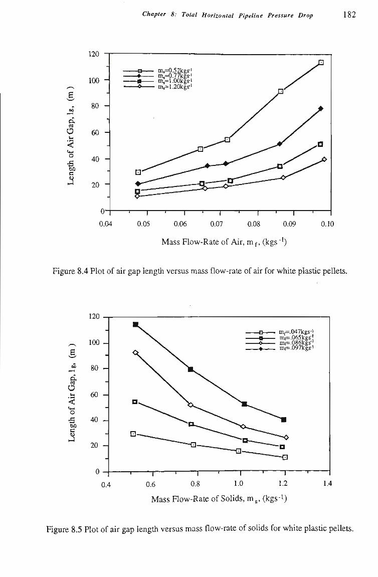
Chapter 8: Total Horizontal Pipeline Pressure Drop 182
120
ei
«4-1
o
C
100 -
80 -
O 60 -
40 -
20 -
iiu=0.52kgs-' •4 m,=0.77kgs-' - • m^=1.00kgs-i
» m,=1.20kgs-'
0.04 0.05
— I — 1 — I 1 1 — i — r 0.06 0.07 0.08 0.09 0.10
Mass FIow-Rate of Air, m f, (kgs '^)
Figure 8.4 Plot of air gap lengtii versus mass flow-rate of air for white plastic pellets.
120
100 -
^ 80 -
O 60 -
o •S Oû B (D
S 40 -
20 -
0.4 —r 0.6 0.8
r 1.0
m[= mf= mf=
047kgs-i .065kgs-' .086kgs-' .097kgs-i
—r 1.2 1.4
Mass FIow-Rate of Solids, m^, (kgs-^)
Figure 8.5 Plot of air gap lengtii versus mass flow-rate of solids for white plastic pellets.
Chapter 8: Total Horizontal Pipeline Pressure Drop 183
B
B8
O
c
0.04 0.05 0.06 0.07
Mass Flow-Rate of Air, m f, (kgs " )
0.09
Figure 8.6 Plot of air gap length versus mass flow-rate of air for black plastic peUets.
O
< <4-( o
CJQ
C
0.4 r
0.6 0.8 1.0 1.2 Mass FIow-Rate of Solids, m^, (kgs-^)
1.4
Figure 8.7 Plot of air gap length versus mass flow-rate of solids for black plastic pellets.
Chapter 8: Total Horizontal Pipeline Pressure Drop 184
100
B^
o < o
X5 • t -> 00 c
80 -
60 _
40 _
20 -
-O ms=0.96kgs-' - • ms=1.45kgs-' -« ms=1.98kgs-' -0 ms=2.38kgs-'
1 1 « 1 1 1—
0.04 0.05 0.06 0.07
Mass Flow-Rate of Air, m f, (kgs )
—I ^ 0.08 0.09
l >
Figure 8.8 Plot of air gap lenglh versus mass flow-rate of air for wheat.
100
80 _
60 -00
cJ O
"^ 40 _ J3 6Û C (U
20 _
0.6
C mf=.067kgs-i • mf=.074kgsr' O mf=.082kgs-J
1 1 ' 1 ' r 1.0 1.4 1.8
mf=.088kgs-'
Mass FIow-Rate of SoUds, m^, (kgs-^)
"T ' \ 2.2 2.6
Figure 8.9 Plot of air gap length versus mass flow-rate of solids for wheat.
Chapter 8: Total Horizontal Pipelîne Pressure Drop 185
120
100
BO
c a
O
< (4-1
o • ^
euQ
c
80 _
60 -
40 -
20 -
0.04
-B- ms=1.04kgs-' m;=1.31kgs-'
-B ms=1.74kgs-' » ms=2.06kgs-'
-1 j 1 r
0.05 0.06 0.07 1
0.08
Mass Flow-Rate of Air, m f, (kgs " )
0.09
Figure 8.10 Plot of air gap length versus mass flow-rate of air for barley.
ao
O «-i
o -B Dû C
mf=.066kgs'' mf=.073kgs-i
„ mf=.082kgs-i J ^ m,=.088kgs:'
Mass Flow-Rate of SoUds, m s, (kgs-^)
Figure 8.U Plot of air gap length versus mass flow-rate of solids for barley.
Chapter 8: Total Horizontal Pipeline Pressure Drop 1 8 6
From Figures 8.4 to 8.11, it can be seen for a given mass flow-rate of solids, tiie lengtíi
of air gap increases with the mass flow-rate of air. The reason is that air gaps are formed
by the extra air for "aerating" the material. For slug-flow conveying which has been
aerated already, increasing the mass flow-rate of air simply increases the volume of tíie
exû-a air for aeratíng the material m a given period of tíme. Since tiie diameter of aU gap is
limited by tiie pipe, the length of air gap must be increased. On the otiier hand, for a
given mass flow-rate of air, increasing the mass flow-rate of solids decreases the length
of air gap. In Chapter 6, it has been found that mass flow-rate of solids has littíe
influence on slug velocity, refer to Sectíon 6.5.2. In other words, the slug velocity
remains approximately constant for a given mass flow-rate of air no matter how the mass
flow-rate of solids changes. Hence if increasing the mass flow-rate of solids, but still
keeping the mass flow-rate of air (i.e. slug velocity) constant, the number of the slugs
included in a certain length of pipe obviously must increase to maintain the higher mass
flow-rate of solids.
It can also be found from Figures. 8.4 to 8.11 that under some conveying conditíons, air
gaps are longer than the length of pipe. For example, whUe black plastic pellets are
conveyed through the 52 m long pipeUne with m = 0.57 kgs-i, mf = 0.082 kgs-^ the
average air gap length is 71.15 m. This indicates that for certain periods of tíme there is
no slug in the pipeline and the pressure drop approaches the air-only condition. In this
case, the tíme history record of air pressure wiU display an discontinuous curve, refer to
Figures 7.6(b)
8.2.2 Slug Length
Slug length is another major geometrical feature of the slug-flow pattem. Slug-flow
pneumatíc conveying normaUy includes several slugs flowing along the pipeline. AU
these slugs are observed to have approximately the same length, which is affected by the
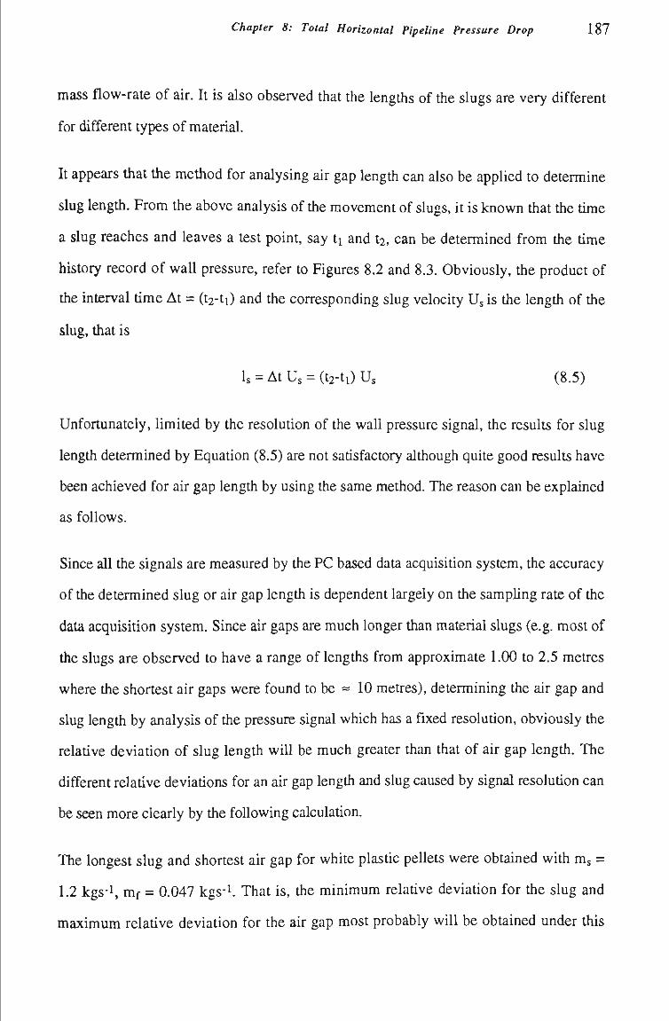
Chapter 8: Total Horizontal Pipeline Pressure Drop 187
mass flow-rate of air. It is also observed that the lengths of the slugs are very different
for different types of material.
It appears tíiat the method for analysing air gap length can also be applied to determine
slug lengtíi. From the above analysis of the movement of slugs, it is known tíiat the time
a slug reaches and leaves a test point, say ti and t , can be determined from tíie tíme
history record of waU pressure, refer to Figures 8.2 and 8.3. Obviously, tíie product of
the interval tíme At = (t^-ti) and the corresponding slug velocity Us is tíie length of the
slug, that is
Is = At Us = (t2-ti) Us (8.5)
Unfortunately, limited by the resolution of the wall pressure signal, the results for slug
length determined by Equatíon (8.5) are not satísfactory although quite good results have
been achieved for air gap length by using the same method. The reason can be explained
as follows.
Since all the signals are measured by the PC based data acquisition system, the accuracy
of the determined slug or air gap lengtii is dependent largely on the sampUng rate of the
data acquisition system. Since air gaps are much longer than material slugs (e.g. most of
the slugs are observed to have a range of lengths from approximate 1.00 to 2.5 metres
where the shortest air gaps were found to be = 10 metres), determining the air gap and
slug length by analysis of the pressure signal which has a fixed resolution, obviously the
relatíve deviatíon of slug length wiU be much greater than that of air gap length. The
different relatíve deviatíons for an air gap lengtfi and slug caused by signal resolution can
be seen more clearly by Ûie foUowing calculatíon.
The longest slug and shortest air gap for white plastic peUets were obtained with m =
1.2 kgs-i, mf = 0.047 kgs-^. That is, the minimum relative deviation for the slug and
maximum relatíve deviation for the air gap most probably wUI be obtained under this
Chapter 8: Total Horizontal Pipeline Pressure Drop 188
conveying conditíon. The slug velocity was measured as 2.632 ms-i. The air gap lengtíi
was calculated as 10.6 metres and the slug length was observed about 1.5 metres. Even
tíiough tíie wall pressure signals were sampled at the rate of 10 Hz, which is tiie highest
possible sampling rate for obtaining a sufficient long time history record due to tíie
memory limitatíons of the computer, the relatíve deviation for the slug is stUI too large to
be accepted. That is, the maximum possible deviation of the length of air gap and slug
can be 0.26 m (i.e. 2.632 ms- x 0.1 s). Therefore, the relative deviations wiU be 2.4 %
for the air gap and 17 % for tiie slug.
Besides tiie lengtii of single slug, the total slug lengtii contained in tiie conveying pipeline
is also an important parameter for the particle slug since slug-flow usually includes
several slugs. In fact, it is the total slug length that determines the total pipeline pressure
drop if the pressure gradient has been determined. Note that the total slug length used
here indicates an average value, since low-velocity pneumatic conveying is a
discontinuous flow of slugs. Although the data of each single slug length have not been
obtained, it still is possible to calculate the total slug length for a given conveying
condition. For example, the slug velocity (Us) can be found according to the
investigations in Chapter 6 when the mass flow-rate of air (mf) is given. If the total
length of pipeUne is Lt, the time taken by a slug to travel across tiie pipeUne wUl be
ts= ^ (8.6) Us
In additíon, if the mass flow-rate of solids is known, the mass of partícles entering the
pipeUne can be calculated matfîematícally during a certain period of tíme, i.e. it foUows
that the mass of the moving solids M = (mass flow rate of solids) x (tíme). The number
of partícles moving in the pipeline is equal to that amount of the particles entering the
pipeUne during the tíme taken for tiie slug to travel across the pipeline, that is
M=ms t s = ^ (8.7) Us
Chapter 8: Total Horizontal Pipeline Pressure Drop 189
As almost all the partícles flow in the form of slugs and as these slugs have been
assumed to have a loose-poured buUc density for granular material, therefore, tiie mass of
partícles also is
M=PbVs (8.8)
where V is tíie volume of tiie particles moving in the pipeUne and Vs = A(l-a)Ls m slug-
flow pneumatic conveying if tfie total slug length is L .
Combining Equation (8.7) and Equatíon (8.8) and replacing V in Equation (8.8) witíi
A(l-a)Ls, tíien an equatíon for calculatíng tiie total lengtii of slugs can be obtained:
Ls = — ^ ^ ^ (8.9) A(l-a)Pi,Us
8.2.3 Stationary Bed Thickness
A stationary bed occurs only in the horizontal pipes of low-velocity pneumatíc
conveying. The formatíon of the statíonary bed is due to the particle slugs delivering
some quantíties of partícles to the horizontal pipe behind it while the particle slugs move
forward. Hence, during the initial stages of low-velocity pneumatíc conveying, the
partícle slugs formed at tiie entrance of the conveying pipeline often disappear before they
arrive at the end of the pipeline. Only at the stable or equilibrium stage of conveying (i.e.
statíonary bed has covered the entíre length of the pipeline), can the slugs move through
the entíre pipeline with an approximately constant volume. As the bottom of the pipe is
occupied by the particles of the stationary bed, air gaps can not fUI up the whole pipe area
between two slugs and therefore display asymmetric bubbles in horizontal slug-flow.
Through sight glass observations, stationary bed thickness is observed to vary for
different conveying conditions and different materials.
It was found eariier that the existence of the statíonary bed affects the movement and
inner stress of the slug. While a slug picks up particles from the statíonary bed in front of
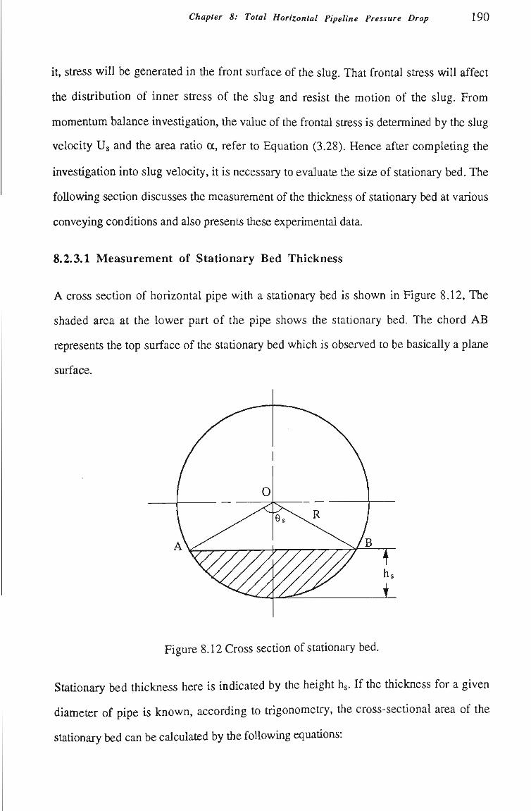
Chapter 8: Total Horizontal Pipeline Pressure Drop 190
it, sti-ess will be generated in the front surface of the slug. That frontal stress will affect
the distí-ibutíon of inner stress of the slug and resist tíie motion of the slug. From
momentum balance investigatíon, the value of the frontal stress is determmed by the slug
velocity Us and the area ratio a, refer to Equatíon (3.28). Hence after completíng the
investígatíon into slug velocity, it is necessary to evaluate the size of stationary bed, The
foUowing section discusses the measurement of the thickness of statíonary bed at various
conveying conditions and also presents these experimental data.
8.2.3.1 Measurement of Stationary Bed Thickness
A cross section of horizontal pipe with a stationary bed is shown in Figure 8.12, The
shaded area at the lower part of the pipe shows the statíonary bed. The chord AB
represents the top surface of the statíonary bed which is observed to be basically a plane
surface.
Figure 8.12 Cross sectíon of stationary bed.
Statíonary bed thickness here is indicated by the height h . If the thickness for a given
diameter of pipe is known, according to trigonometry, the cross-sectíonal area of the
statíonary bed can be calculated by tíie foUowing equations:
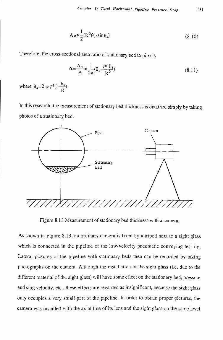
Chapter 8: Total Horizontal Pipeline Pressure Drop 191
Ast=-(R^es-sines) (8.10)
Thercfore, tiie cross-sectíonal area ratio of stationary bed to pipe is
A 2% R2 (8.11)
where es=2cos-Hl-—). R
In tiiis research, the measurement of stationary bed thickness is obtained simply by taking
photos of a stationary bed.
Camera
' / / / / / / / / / / / / / / / / / / / / / / / / / / / / / / /
Figure 8.13 Measurement of statíonary bed thickness with a camera.
As shown in Figure 8.13, an ordinary camera is fixed by a tripod next to a sight glass
which is connected in the pipeline of the low-velocity pneumatic conveying test rig.
Lateral pictures of the pipeline with statíonary beds then can be recorded by taking
photographs on the camera. Although the installatíon of the sight glass (i.e. due to the
different material of tiie sight glass) will have some effect on the statíonary bed, pressure
and slug velocity, etc, tfiese effects are regarded as insignificant, because tfie sight glass
only occupies a very small part of the pipeUne. In order to obtain proper pictures, the
camera was installed with the axial line of its lens and the sight glass on the same level
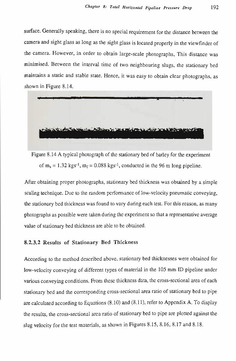
Chapter 8: Total Horizontal Pipeline Pressure Drop 192
surface. Generally speakmg, there is no special requirement for tíie distance between tíie
camera and sight glass as long as the sight glass is located properiy in tíie viewfmder of
the camera. However, in order to obtain large-scale photographs, This distance was
minimised. Between the interval tíme of two neighbouring slugs, the statíonary bed
maintains a static and stable state. Hence, it was easy to obtain clear photographs, as
shown in Figure 8.14.
Figure 8.14 A typical photograph of the statíonary bed of barley for the experiment
of ms = 1.32 kgs'i, mf = 0.088 kgs-^ conducted in the 96 m long pipeline.
After obtaining proper photographs, stationary bed thickness was obtained by a simple
scaUng technique. Due to the randora performance of low-velocity pneumatíc conveying,
the stationary bed thickness was found to vary during each test. For this reason, as many
photographs as possible were taken during the experiment so that a representative average
value of statíonary bed thickness are able to be obtained.
8.2.3.2 Results of Stationary Bed Thickness
According to the method described above, stationary bed thicknesses were obtained for
low-velocity conveying of different types of material in the 105 mm ID pipeline under
various conveying conditions. From these thickness data, the cross-sectíonal area of each
stationary bed and the corresponding cross-sectíonal area ratío of statíonary bed to pipe
are calculated according to Equatíons (8.10) and (8.11), refer to Appendix A. To display
tíie results, the cross-sectíonal area ratío of stationary bed to pipe are plotted against the
slug velocity for the test materials, as shown in Figures 8.15, 8.16, 8.17 and 8.18.
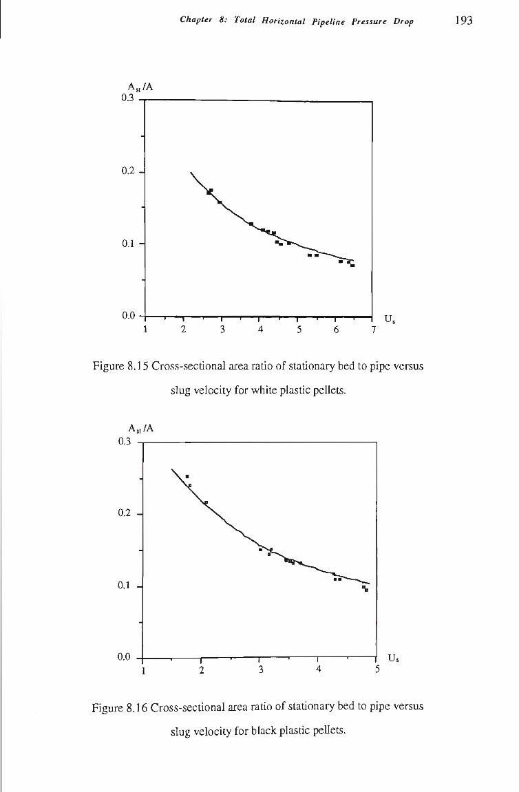
Chapter 8: Total Horizontal Pipeline Pressure Drop 193
Figure 8.15 Cross-sectíonal area ratío of statíonary bed to pipe versus
slug velocity for white plastíc peUets.
A.,/A 0.3
0.2 -
0.1 -
0.0 f Us
Figure 8.16 Cross-sectional area ratio of statíonary bed to pipe versus
slug velocity for black plastíc peUets.
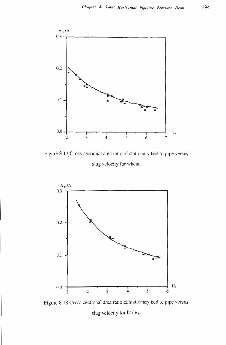
Chapter 8: Total Horizontal Pipeline Pressure Drop 194
A,t/A
Figure 8.17 Cross-sectional area ratio of statíonary bed to pipe versus
slug velocity for wheat.
Us 2 3 4 5 6
Figure 8.18 Cross-sectional area ratio of statíonary bed to pipe versus
slug velocity for barley.
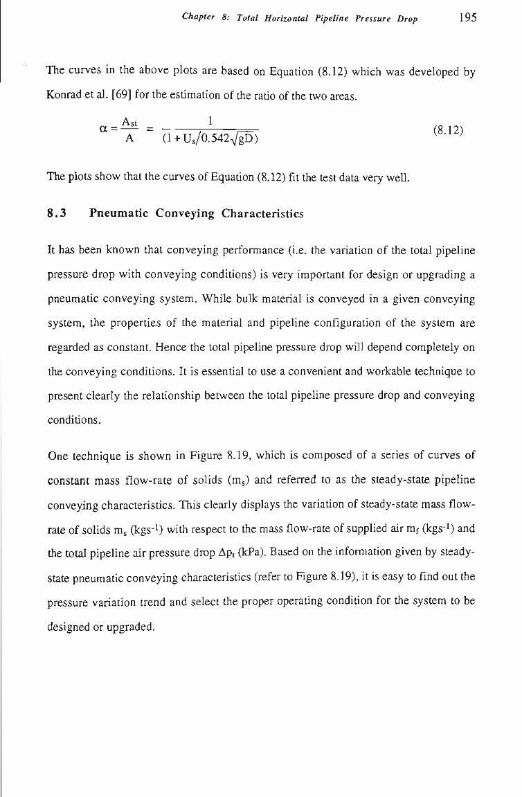
Chapter 8: Total Horizontal Pipeline Pressure Drop 195
The curves in the above plots are based on Equatíon (8.12) which was developed by
Konrad et al. [69] for the estímatíon of the ratío of the two areas.
a = — = -A r— (8 12) A (1 + Us/0.542VÍD) ^''•'^^
The plots show that the curves of Equatíon (8.12) fit the test data very weU.
8.3 Pneumatic Conveying Characteristics
It has been known that conveying performance (i.e. the variation of tíie total pipeline
pressure drop with conveying conditíons) is very important for design or upgrading a
pneumatic conveying system. While bulk material is conveyed in a given conveying
system, the properties of the material and pipeline configuration of the system are
regarded as constant. Hence the total pipeline pressure drop will depend completely on
the conveying conditions. It is essential to use a convenient and workable technique to
present clearly the relatíonship between the total pipeline pressure drop and conveying
conditíons.
One technique is shown in Figure 8.19, which is composed of a series of curves of
constant mass flow-rate of solids (m ) and referred to as the steady-state pipeline
conveying characteristícs. This clearly displays the variatíon of steady-state mass flow-
rate of solids m G gs' ) with respect to the mass flow-rate of supplied air m (kgs-^) and
tíie total pipeline air pressure drop Apt (kPa). Based on the informatíon given by steady-
state pneumatíc conveying characteristícs (refer to Figure 8.19), it is easy to find out the
pressure variation trend and select the proper operatíng conditíon for the system to be
designed or upgraded.
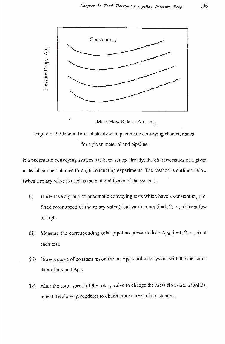
Chapter 8: Total Horizontal Pipeline Pressure Drop 196
CU <
cx, o
Û
3
Mass FIow Rate of Air, m f
Figure 8.19 General form of steady state pneumatic conveying characteristics
for a given material and pipeline.
If a pneumatic conveying system has been set up already, the characteristícs of a given
material can be obtained through conducting experiments. The method is outUned below
(when a rotary valve is used as the material feeder of tiie system):
(i) Undertake a group of pneumatic conveying tests which have a constant mg (i.e.
fixed rotor speed of the rotary valve), but various mfi (i =1, 2, —, n) from low
to high.
(U) Measure the corresponding total pipeUne pressure drop Apti (i =1, 2, —, n) of
each test.
(iU) Draw a curve of constant m on the mf-Apt coordinate system with the measured
data of mfi and Apti.
(iv) Alter the rotor speed of the rotary valve to change the mass flow-rate of soUds,
repeat tiie above procedures to obtain more curves of constant m .
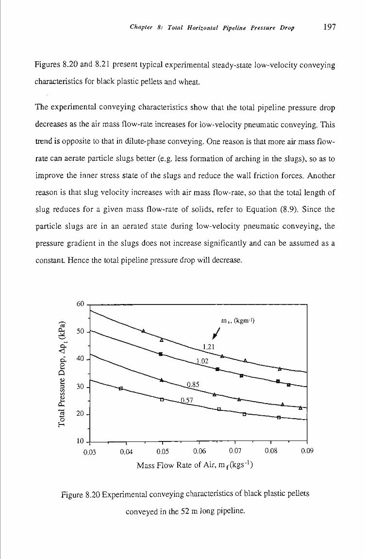
Chapter 8: Total Horizontal Pipeline Pressure Drop 197
Figures 8.20 and 8.21 present typical experimental steady-state low-velocity conveying
characteristics for black plastic peUets and wheat.
The experimental conveying characteristícs show that the total pipeline pressure drop
decreases as the air mass flow-rate increases for low-velocity pneumatic conveying. This
trend is opposite to that in dilute-phase conveying. One reason is tíiat more air mass flow-
rate can aerate particle slugs better (e.g. less formatíon of arching in the slugs), so as to
improve the inner stress state of the slugs and reduce the wall frictíon forces. Another
reason is that slug velocity increases with air mass flow-rate, so that the total length of
slug reduces for a given mass flow-rate of solids, refer to Equation (8.9). Since the
particle slugs are in an aerated state during low-velocity pneumatic conveying, the
pressure gradient in the slugs does not increase significantly and can be assumed as a
constant. Hence the total pipeline pressure drop wUI decrease.
0.03 0.04 0.05 0.06 0.07 0.08 Mass FIow Rate of Air, mf(kgs-^)
0.09
Figure 8.20 Experimental conveying characteristics of black plastic peUets
conveyed in the 52 m long pipeline.
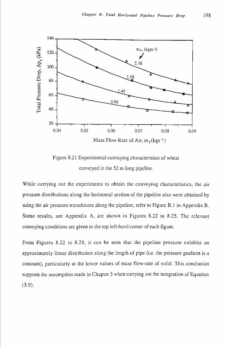
Chapter 8: Total Horizontal Pipeline Pressure Drop 198
<
O Ui
û 3 V3
Cu
4-> o H
0.06 0.07 0.08 0.09
Mass FIow Rate of Air, m f (kgs" )
Figure 8.21 Experimentalconveyingcharacteristícs of wheat
conveyed in the 52 m long pipeline.
While carrying out the experiments to obtain the conveying characteristics, the air
pressure distributions along the horizontal section of the pipeline also were obtained by
using the air pressure transducers along the pipeline, refer to Figure B.l in Appendix B.
Some results, see Appendix A, are shown in Figures 8.22 to 8.25. The relevant
conveying conditions are given in the top left-hand comer of each figure.
From Figures 8.22 to 8.25, it can be seen that the pipeline pressure exhibits an
approximately linear distributíon along the length of pipe (i.e. the pressure gradient is a
constant), particularly at the lower values of mass flow-rate of solid. This conclusion
supports the assumption made in Chapter 3 when carrying out the integration of Equation
(3.9).
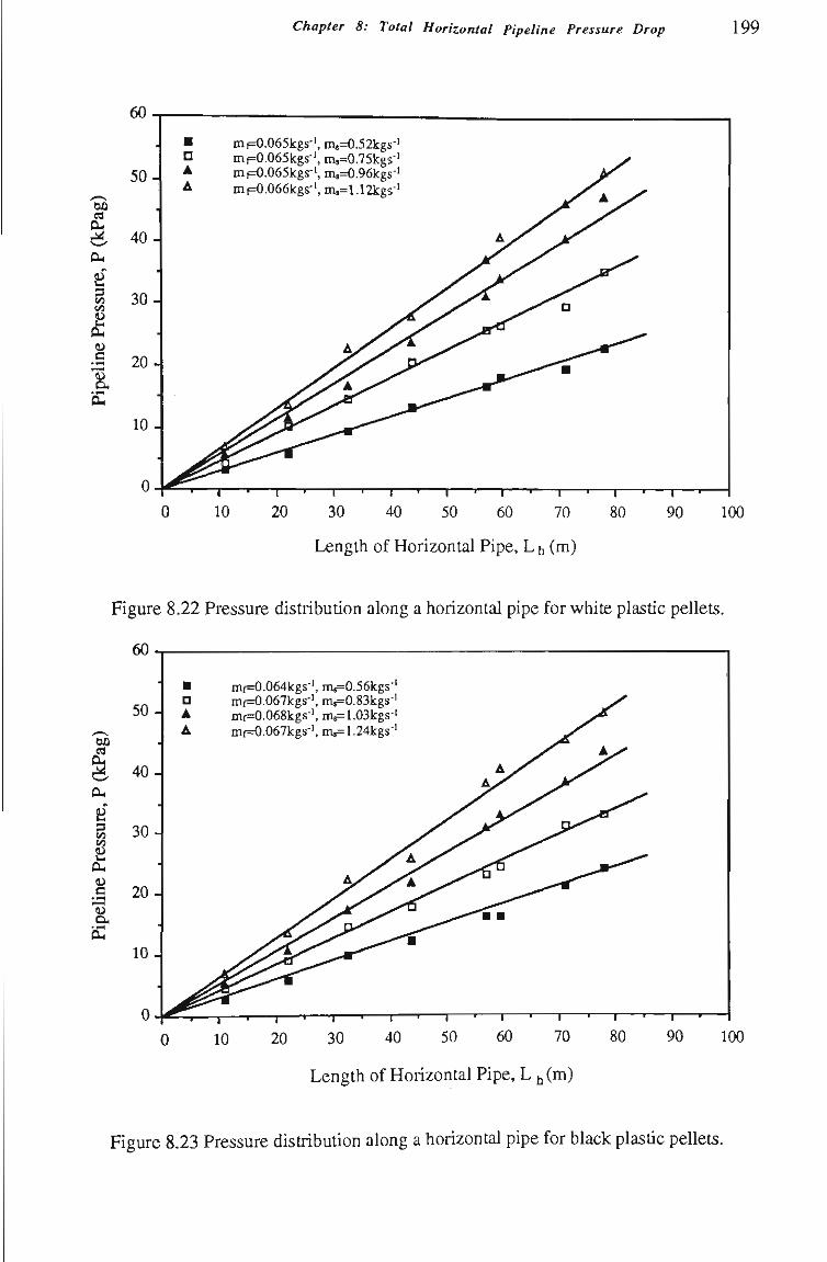
Chapter 8: Total Horizontal Pipeline Pressure Drop 199
CLH
Ú s
_c
20 30 40 50 60 70
Length of Horizontal Pipe, L h (m)
Figure 8.22 Pressure distribution along a horizontal pipe for white plastíc pellets.
60
I5Û
s co C3
<u c D
0 10 20 30 40 50 60 70
Length of Horizontal Pipe, L ^(m)
Figure 8.23 Pressure distributíon along a horizontal pipe for black plastíc peUets.
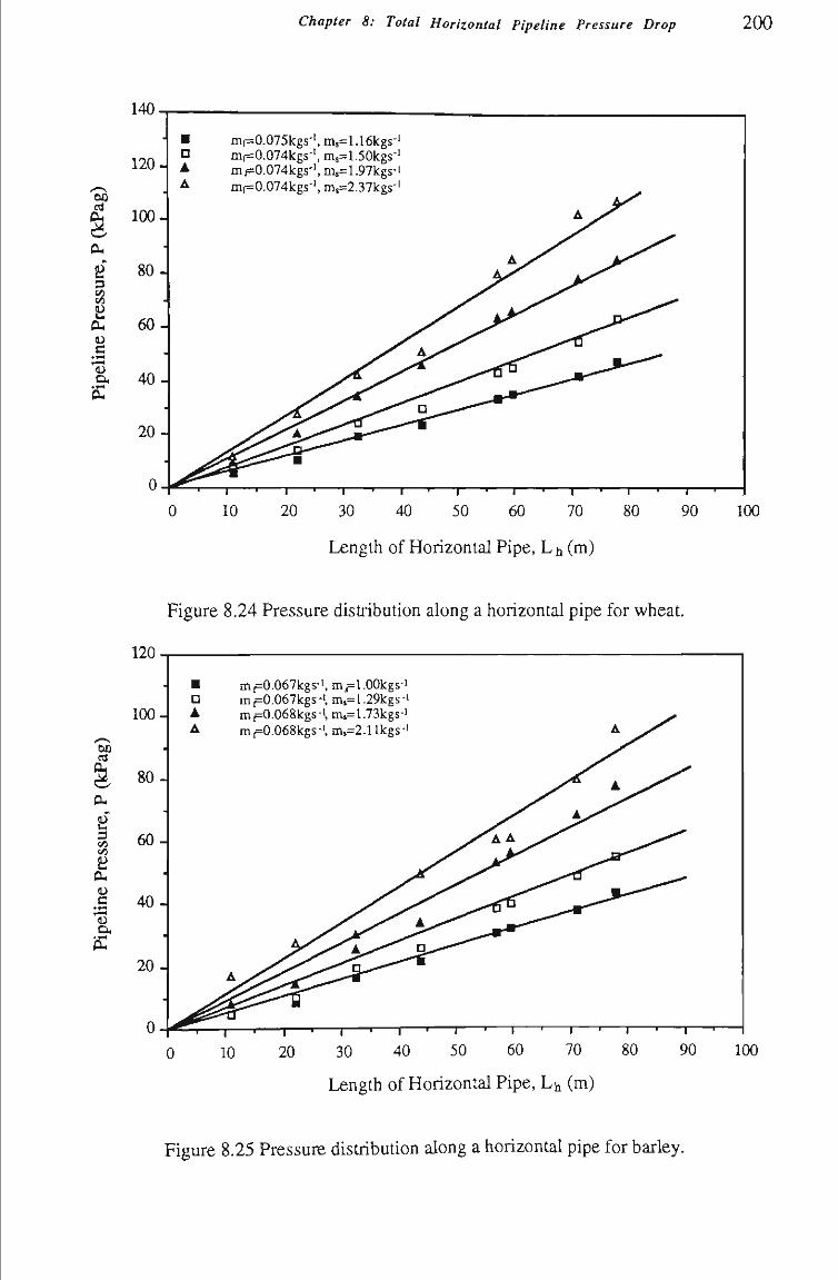
Chapter 8: Total Horizontal Pipeline Pressure Drop 200
C4
p
CL,
C • 1 - 4 1—1
120-
100-
80-
60-
4 0 -
2 0 -
-
0 -
• • •
mf=0.075kgs-', m,=1.16kgs-' mf=0.074kgs-', ms=1.50kgs-' mf=0.074kgs-', ms=1.97kgs-' mf=0.074kgs-', m,=2.37kgs-'
y^^^"'"''''^^^—"^^ ^ ^ ^ ^ ^ ^ " • ^
— I ' — I — ' 1 '—r
A X ^
• „ .^
-1- - p
Ly/^
- ^ 1 '
^ y ^
— i — 1 — 1 — 1 — - 1 — 1 —
10 20 30 40 50 60 70 80
Length of Horizontal Pipe, L h (m)
90 100
Figure 8.24 Pressure disuibutíon along a horizontal pipe for wheat.
6Û
2Í 3 </) (/)
<u C
120.
100-• • Á
mf=0.067kgs-', mi=1.00kgs-' mp0.067kgs-', m,=1.29kgs-' mp0.068kgs-', m»=1.73kgs-' mp0.068kgs-i, ms=2.11kgs-'
30 40 50 60 70
Length of Horizontal Pipe, Lh (m)
T 80 100
Figure 8.25 Pressure distributíon along a horizontal pipe for barley.
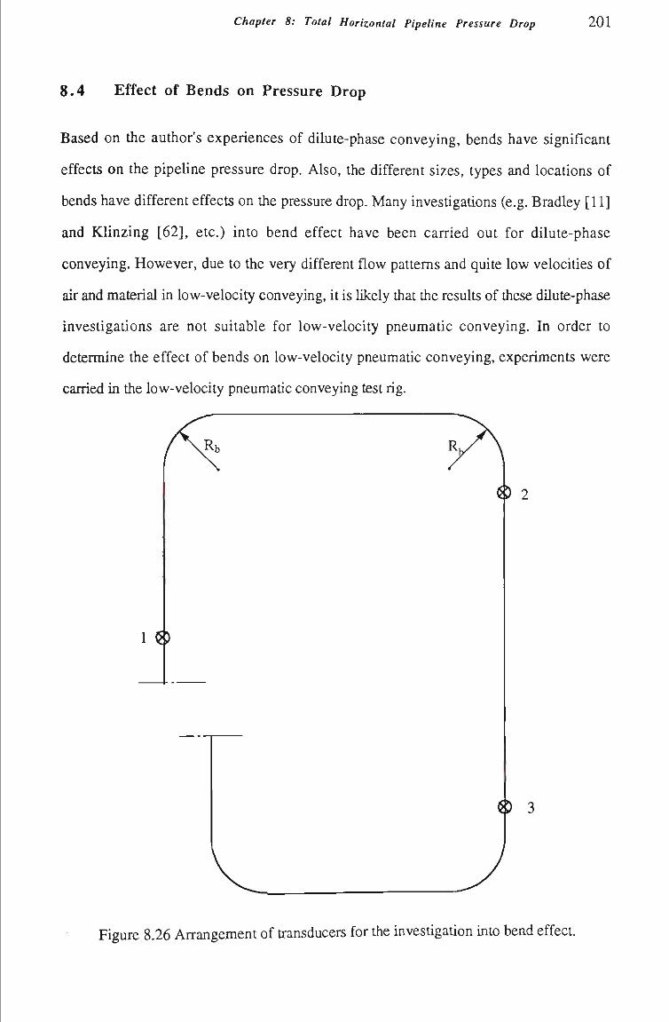
Chapter 8: Total Horizontal Pipeline Pressure Drop 201
8.4 Effect of Bends on Pressure Drop
Based on the author's experiences of dilute-phase conveying, bends have significant
effects on the pipeline pressure drop. AIso, the different sizes, types and locatíons of
bends have different effects on tiie pressure drop. Many investigatíons (e.g. Bradley [11]
and Klinzing [62], etc.) into bend effect have been carried out for dilute-phase
conveying. However, due to the very different flow pattems and quite low velocitíes of
air and material in low-velocity conveying, it is likely that the results of these dUute-phase
investigations are not suitable for low-velocity pneumatic conveying. In order to
determine the effect of bends on low-velocity pneumatic conveying, experiments were
carried in the low-velocity pneumatic conveying test rig.
1 <5)
R,
O 2
O 3
Figure 8.26 Arrangement of transducers for the investígatíon into bend effect.
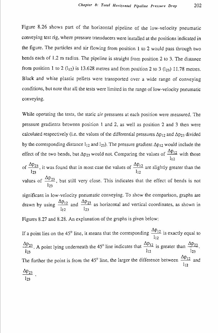
Chapter 8: Total Horizontal Pipeline Pressure Drop 2 0 2
Figure 8.26 shows part of the horizontal pipeline of the low-velocity pneumatíc
conveying test rig, where pressure transducers were instaUed at the positions indicated m
the figure. The particles and air flowing from positíon 1 to 2 would pass through two
bends each of 1.2 m radius. The pipeline is straight from position 2 to 3. The distance
from positíon 1 to 2 (I12) is 13.628 metres and from position 2 to 3 G23) 11.78 metres.
Black and white plastic pellets were transported over a wide range of conveying
conditíons, but note that all the tests were limited in the range of low-velocity pneumatíc
conveying.
While operating the tests, the static air pressures at each positíon were measured. The
pressure gradients between position 1 and 2, as well as positíon 2 and 3 then were
calculated respectively (i.e. the values of the differential pressures Api2 and Ap23 divided
by the corresponding distance I12 and I23). The pressure gradient Api2 would include the
effect of the two bends, but Ap23 would not. Comparing the values of —£-12. vvith those I12
Apon ^VA') of ——, it was found that in most case the values of —— are slightly greater than the
I23 I12 values of —£-21, but stiU very close. This indicates that the effect of bends is not
I23
significant in low-velocity pneumatic conveying. To show the comparison, graphs are
drawn by using ^^ and —— as horizontal and vertical coordinates, as shown in I12 I23
Figures 8.27 and 8.28. An explanation of tiie graphs is given below:
Ap,., If a point lies on the 45° line, it means that the correspondmg —— is exactly equal to
I12
- ^ . A point lying underneath the 45° line indicates that — ^ is greater than —21 I23 I12 I23
The further the point is from the 45° line, tiie larger the difference between — ^ and I12
Ap23
I23
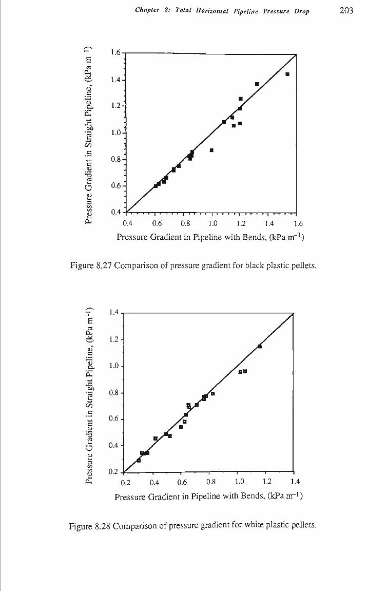
Chapter 8: Total Horizontal Pipeline Pressure Drop 203
1.6.
CL,
_c 13 • cu W)
'êS
C/0
.S w C
O aí V3
a,
1.4-
1.2-
1.0-
0.8-
0.6-
0.4-<-r-,- I ' • ' ' I I ' ' ' ' I
0.4 0.6 0.8 1.0 1.2 1.4 1.6
Pressure Gradient in PipeUne with Bends, (kPa m" )
Figure 8.27 Comparison of pressure gradient for black plastic peUets.
a
c 13
J3 Oû 'ã
l - i -4—»
on c
c JJ
'5 ed b.1
o 3 W3 00
<u Ui
cu
1.2-
1.0-
0.8-
0.6-
0.4-
0 2-
> * • y ^ B
' — ' 1 — ' 1
^u
/nn
— 1 ' 1 '
0.2 0.4 0.6 0.8 1.0 1.2 1.4
Pressure Gradient in Pipeline with Bends, O Pa nri)
Figure 8.28 Comparison of pressure gradient for white plastic peUets.
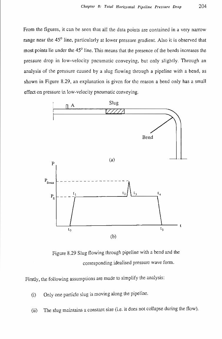
Chapter 8: Total Horizontal Pipeline Pressure Drop 204
From the fígures, it can be seen that all the data points are contained in a very narrow
range near the 45° line, particularly at lower pressure gradient. AIso it is observed that
most points lie under tiie 45° line. This means that the presence of the bends increases tfie
pressure drop in low-velocity pneumatic conveying, but only slightly. Through an
analysis of the pressure caused by a slug flowing through a pipeline with a bend, as
shown in Figure 8.29, an explanation is given for the reason a bend only has a small
effect on pressure in low-velocity pneumatíc conveying.
Slug JlA
Bend
(a)
Bmax
to
(b)
Figure 8.29 Slug flowing through pipeline with a bend and tiie
corresponding idealised pressure wave form.
Firstiy, tíie following assumptíons are made to simpUfy the analysis:
(i) Only one particle slug is moving along tfie pipeUne.
(U) The slug maintains a constant size (i.e. U does not coUapse during tiie flow).
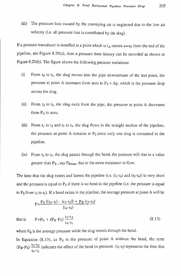
Chapter 8: Total Horizontal Pipeline Pressure Drop 205
(ui) The pressure loss caused by the conveying air is neglected due to the low air
velocity (i.e. all pressure loss is contributed by the slug).
If a pressure transducer is installed at a point which is U metres away from the end of tfie
pipeline, see Figure 8.29(a), then a pressure time history can be recorded as shown in
Figure 8.29(b). The figure shows the following pressure variations:
(i) From to to ti, the slug moves into the pipe downstream of the test point, the
pressure at point A increases from zero to Ps = Ap, which is the pressure drop
across the slug.
(U) From t to ts, the slug exits from the pipe, the pressure at point A decreases
from Ps to zero.
(iU) From ti to t and ts to t , the slug flows in the straight section of the pipeline,
the pressure at point A remains at Ps since only one slug is contained in the
pipeline.
(iv) From t to t , the slug passes through the bend, the pressure will rise to a value
greater than Ps , say PBmax' due to the extra resistance to flow.
The time that the slug enters and leaves the pipeline (i.e. (ti-to) and (t^-t^)) is very short
and the pressure is equal to Ps if tiiere is no bend in the pipeline (i.e. the pressure is equal
to Ps from t2 to t^). If a bend exists in the pipeline, the average pressure at point A will be
p_^Ps [(t4-ti) - (t3-t2)] + P B (t3-t2)
(t4-tl)
tíiatis P=Ps + (PB-PS) — (8-13)
t4-tl
where PB is tiie average pressure while the slug travels through tfie bend.
In Equatíon (8.13), as Ps is the pressure of point A without the bend, the term (PB-PS) ^ ^ ^ indicates the effect of the bend on pressure. (t^-t^) represents the tíme tíiat
t4-ti
Chapter 8: Total Horizontal Pipeline Pressure Drop 2 0 6
tiie slug passes tfirough the bend, and (t^-ti) represents the approximate tíme tfiat the slug
flows tiirough the total pipeline. In most pneumatic conveying systems, the total pipeline
lengtfi is always much greater than tfie total lengtfi of bends mcluded in tiie pipeline, tiius
(t4-ti) » (t3-t2), therefore the bends do not have a great effect on Apt even tiiough PB
could be much greater tiian Ps.
8.5 Correlation of Horizontal Pipeline Pressure Drop
For a single horizontal slug of cohesionless material, Equatíon (3.14) was developed for
the prediction of the pressure gradient of the slug. However, an actual low-velocity
pneumatic conveying system normally has several slugs flowing along the pipeline.
Since each slug undergoes the same variation in velocity while it flows from the high
pressure end to the low pressure end, it is reasonable to assume that every slug flows
through the pipeline with one average velocity. Hence all the moving particles in the
pipeUne can be treated as one long slug with a length Ls, which represents the sum of tiie
length of aU the individual slugs. The relatíonship between Ls and Lt is expressed by
Equatíon (8.9).
If a system is totally composed of horizontal pipes and bends and neglecting the pressure
loss caused by conveying air and bends, then the pressure gradient in the total length of
slug can be obtained by replacing Ap and Is in Equatíon (3.14) with the total horizontal
pipeUne pressure drop Apt and total length of slug Ls, respectívely. That is
AP. = ^ ^ , ^ 2p,gH„ (8.14) Ls •'-'
Substítuting Equatíon (8.9) and Equatíon (3.27) into Equatíon (8.14), then the total
pressure drop in the horizontal pipeUne is given by
^' 1-a gD 1-a AUs
Chapter 8: Total Horizontal Pipeline Pressure Drop 2 0 7
Replacing a in Equatíon (8.15) witii Equation (8.12) and letting Fr = —-, then
Apt = (l-Hl.084XFrQ-^-H0.542Fr-Q-^)^^^^"'^^' (8.16) AUs
where Fr is called the Froude number for the material.
Equation (8.16) shows that the total pipeUne pressure drop is a function of the properties
of the material, conveying condition and pipeline configuratíon. Although mf and some
parameters reflecting the particle propertíes are not in the equatíon, the slug velocity Us
and stress transmission coefficient X in the equatíon are functíons of mf and particle
properties. It must be pointed out that Equation (8.16) is developed under the assumption
that a system is totally composed of horizontal pipes. If a system contains some vertical
sections, then Equatíon (8.16) is only suitable for predictíng the overall pressure drop of
the horizontal sectíon of pipeline. To avoid confusion and possible error, Apt and Lt in
Equatíon (8.16) are replaced witfi Apth and Lth, respectívely, that is
APt,=(l+L084;^Fr0-5-fO542Fr-0^)2^^^f^^ (8.17) AUs
where Apth is the overaU horizontal pipeline pressure drop, Lth is the total length of
horizontal pipeline.
Although the model can be used only to predict the pressure drops for horizontal
pipelines, the predicted results stíU have great significance since most pipeline systems
contain a significant proportion of horizontal piping.
By assuming a preUminary pipeline pressure drop for a low-velocity pneumatic
conveying system, the mean slug velocity (Us) and Froude number (Fr) in Equation
(8.17) can be estimated for a given mass flow rate of air (mf) and pipeline diameter (D).
The determinatíon of tíie value of the stress transmission coefficient (X) was discussed
earlier in Chapter 7, see Equations (7.8), (7.9) and (7.21). Therefore, for low-velocity
Chapter 8: Total Horizontal Pipeline Pressure Drop 2 0 8
pneumatíc conveying with a given mass flow-rate of solids (mj), the pressure drop
across the horizontal pipe of length (Lt) can be predicted by using computer iteratíon,
refer to Appendix C for computer programme. The calculatíon procedure is listed as
foUows:
(i) Calculate the stress transmission coefficient (X,), according to Equatíons (7.8),
(7.9) and (7.21) in Chapter 7.
(U) Assume an initial value for tfie pipeUne pressure drop (Apti).
(iU) Calculate the mean air density (pa) and the mean superficial air velocity (Ua).
(iv) Estimate the mean slug velocity (Us) from Equations (6.32) and (6.41) in
Chapter 6, and determine the Froude number of the conveyed material (Fr).
(v) Substitute these values of Uj, Fr, and X into Equation (8.17) to calculate the
pressure drop.
(vi) Revise the estímate of the pipeline pressure drop in (ii), and repeat from (iii)
untíl convergence is obtained.
8.6 Comparison of Experimental and Predicted Results
To examine tfie accuracy of the developed model, pneumatic conveymg characteristícs of
horizontal pipelines are predicted by using Equatíon (8.17) for conveying the various
materials in the low-velocity pneumatíc conveying test rig, as shown in Figures 8.30 to
8.37. The experimental results are superimposed onto each figure for comparison. The
comparison shows that the agreement is very good, so that the predictíon model is
considered accurate and reUable.
Chapter 8: Total Horizontal Pipeline Pressure Drop 209
35
30-
5 25
<
2 Q
3 «3
20-
15-
10 .
1.20
1.01
0.77
0.52
m5=0.52kgs-' m=0,77kgs-' iH=1.01kgs-' mi=1.20kgs-'
— I 1 1 1 1 1 1 1 1 1 1 1 1 1 1 —
0.03 0.04 0.05 0.06 0.07 0.08 0.09 0.10 0.11
Mass Flow-Rate of Air, m (kgs-^)
Figure 8,30 Predicted conveying characteristícs of white plastíc pellets in the horizontal
pipe Lth = 36 m and D = 0.105 m, showing the curves of constant m .
70
•3
<
á. o <-i
Û
3 V3
60-
50-
40 -
30-
20-
10
m, (kgs-') m,=0.52kgs-' m,=0.75kgs-' m,=0.97kgs-' n>,=1.12kgs-'
T -I 1 1 — r T ' 1 ' r
Mass FIow-Rate of Air, m^ (kgs-^
— 1 — I — 1 — I
0.03 0.04 0.05 0.06 0.07 0.08 0.09 0.10 0.11 0.12 0.13
Figure 8.31 Predicted conveying characteristics of white plastic peilets in the horizontal
pipe Lth = 78 m and D = 0.105 m, showing the curves of constant m .
Chapter 8: Total Horizontal Pipeline Pressure Drop 210
35
es
•3
<
p
c cfl
30-
2 5 -
20
15
10
0.85
0.57
0.02 I
0.03
m, (kgs-')
—I ' \— 0.06 0.07
m,=0.57kgs-' in,=0.85kgs-' m^l.07kgs-i
23kgs-'
0.04 0.05 0.06 0.07 0.08
Mass FIow-Rate of Air, mf (kgs'i)
— I ' 1 —
0.09 0.10 0.11
Figure 8.32 Predicted conveying characteristics of black plastic pellets in the horizontal
pipe Lth = 36 m and D = 0.105 m, showing the curves of constant m .
rt
% •B
<
2 Q
3 c« «5
2
0.03 0.04 0.05
Mass FIow-Rate of Air, m^(kgs-^)
0.11
Figure 8.33 Predicted conveying characteristics of black plastic pellets in tiie horizontal
pipe Lth = 78 m and D = 0.105 m, showing the curves of constant m .
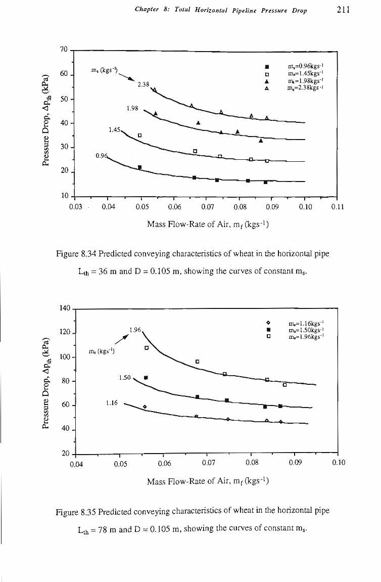
Chapter 8: Total Horizontal Pipeline Pressure Drop 211
70
%
-B
< Cu O
2 s C/3
2
60-
50-
40-
30-
2 0 .
10
ni,(kgs-')
0.03 0.04 — I ' 1 ' 1 —
0.05 0.06 0.07
m,=0.96kgs-' m,=1.45kgs-' nk=1.98kgs-'
2.38kgs-i
0.08 0.09
Mass Flow-Rate of Air, m^ (kgs-^)
— I ' 1
0.10 0.11
Figure 8.34 Predicted conveying characteristics of wheat in tíie horizontal pipe
Lth = 36 m and D = 0.105 m, showing the curves of constant m .
140
rt
•B
< d. o
Q 2 s 2
120-
100-
80-
60
4 0 ,
20
1.96
ms (kgs*')
0.04
1.16
— I — 0.07
ms=1.16kgs-' ms=1.50kgs-'
96kgs-'
A * —
I 0.08 0.05 0.06 0.07 0.08 0.09
Mass FIow-Rate of Air, m^ O^gs-i)
0.10
Figure 8.35 Predicted conveying characteristics of wheat in tiie horizontal pipe
Lth = 78 m and D = 0.105 m, showing the curves of constant m .
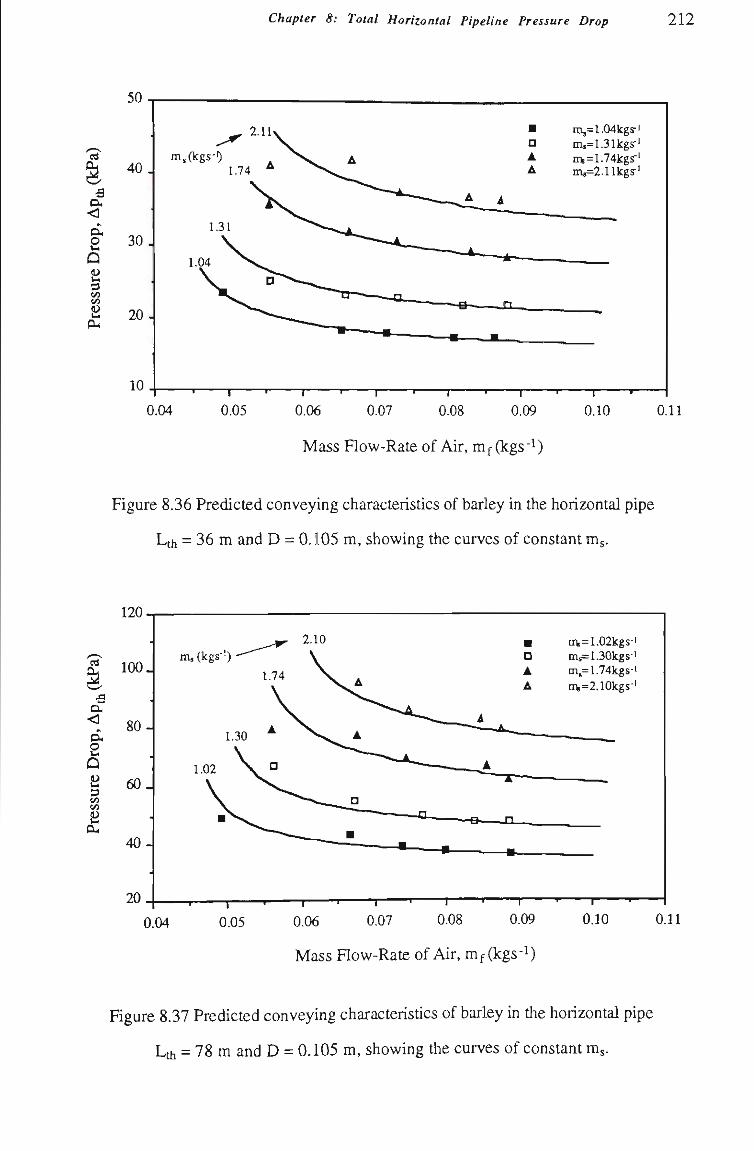
Chapter 8: Total Horizontal Pipeline Pressure Drop 212
50
ei
•B
< o. o w.
Û 2 3 C/3 C/3
9>
4 0 .
30 .
20-
10
2.11
m,(kgs-')
T ' 1
0.04 0.05 0.06 0.07 0.08
Mass FIow-Rate of Air, m^ (kgs"i)
m,=1.04kgs-' 31kgs-' ,74kgs-' llkgs-'
—\ ' \ ' 0.09 0.10 0.11
Figure 8.36 Predicted conveying characteristics of barley in the horizontal pipe
Lth = 36 m and D = 0.105 m, showing the curves of constant m .
cd
J3 Cí*
< cx 2 Û 2 3 V) 00
2
0.04 T ' r 0.05 0.06 0.09 0.10
Mass Row-Rate of Air, m^ (kgs-^)
0.11
Figure 8.37 Predicted conveying characteristics of barley in tfie horizontal pipe
Lth = 78 m and D = 0.105 m, showing the curves of constant m .
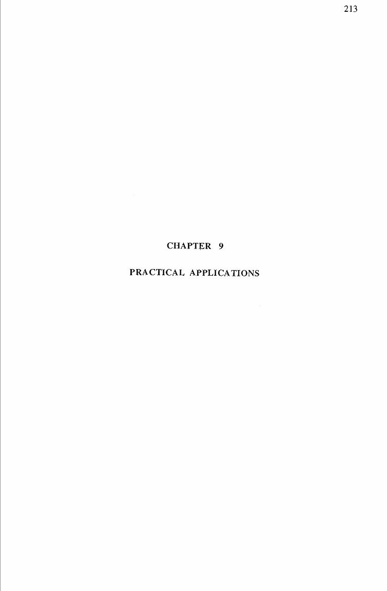
213
CHAPTER 9
PRACTICAL APPLICATIONS
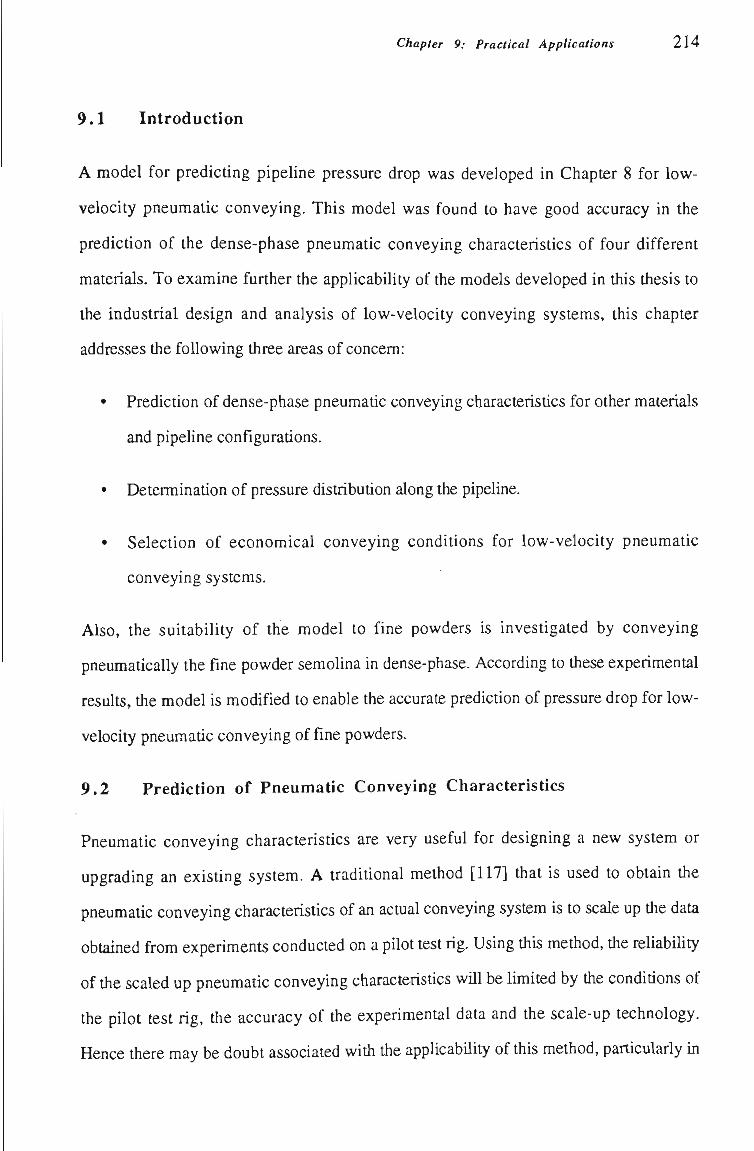
Chapter 9: Practical Applications 2 1 4
9.1 Introduction
A model for predicting pipeline pressure drop was developed in Chapter 8 for low-
velocity pneumatic conveying. This model was found to have good accuracy in the
predictíon of the dense-phase pneumatic conveying characteristics of four different
materials. To examine further the applicability of the models developed in this thesis to
the industrial design and analysis of low-velocity conveying systems, this chapter
addresses the foUowing tíiree areas of concem:
• Predictíon of dense-phase pneumatic conveying characteristics for other materials
and pipeUne configurations.
• Determination of pressure distribution along the pipeline.
• Selection of economical conveying conditions for low-velocity pneumatic
conveying systems.
Also, the suitability of the model to fine powders is investigated by conveying
pneumatically the fine powder semolina in dense-phase. According to these experimental
results, the model is modified to enable the accurate prediction of pressure drop for low-
velocity pneumatic conveying of fine powders.
9.2 Prediction of Pneumatic Conveying Characteristics
Pneumatic conveying characteristícs are very useful for designing a new system or
upgrading an existíng system. A traditíonal method [117] that is used to obtain the
pneumatic conveying characteristics of an actual conveying system is to scale up the data
obtained from experiments conducted on a pilot test rig. Using tfiis method, tfie reliabiUty
of the scaled up pneumatíc conveying characteristics wUI be Umited by tiie conditions of
the pilot test rig, the accuracy of the experimental data and the scale-up technology.
Hence there may be doubt associated witii the applicabUity of this method, particularly in
Chapter 9: Practical Applications 2 1 5
dense-phase conveying as the scale-up technology has not been proven yet for tiiis type
of conveying.
As tiie model developed in Chapter 8 is a functíon of material propertíes, pipeline
configuratíon and conveying conditíon, it is possible that pneumatic conveying
characteristícs can be determined directly from the model for low-velocity pneumatíc
conveying (i.e. instead of conductíng pilot plant experiments) if the conditíons of the
material and pipeline are known. The following sectíons provide examples of tíiis
applicatíon. It should be noted tiiat all tfie work is conducted on tiie basis of tiie horizontal
section of pipeline.
9.2.1 Test Materials
Polystyrene chips and black plastic pellets are very useful materials which have been
applied to many fields of industries. These materials are also good candidates for
pneumatic conveying. They have been transported successfully in dilute- and dense-
phase by various pneumatíc conveying systems in the Bulk Solids Handling Laboratory
at the University of WoUongong. Based on the developed model, low-velocity pneumatíc
conveying characteristícs of these materials are predicted for those conveying systems.
Note that the pneumatic conveying characteristics of black plastic pellets were obtained
previously by experiment and the model here wUI predict and compare the characteristícs
of black plastíc pellets in a different test rig.
Representative properties of bulk material are often the particle diameter, particle and
buUc density, intemal and wall frictíon angle in pneumatic conveying. The definitíons and
measurement methods of these terms were introduced in Chapter 5. Using these
methods, the following values are obtained for polystyrene chips:
Mean particle diameter, d 2.98 mm
Particle density, Ps 1039 kgm-3
Chapter 9: Practical Applications 2 1 6
BuUc density (loosed), pb 637 kgm-^
Bulk voidage, e 0.387
Intemal friction angle, <j) 44.6 o
Wall friction angle (with respect to mUd steel), øw 15.8 °
The propertíes of black plastíc pellets were measured and listed previously in Table 5.1.
9 .2 .2 Test Rigs
Three different test rigs (called Rigs 1, 2 and 3) are employed to convey polystyrene
chips and one rig (called Rig 4) for black plastic pellets. DetaUs of the rigs are given
below.
Rig 1 is the low-velocity pneumatic conveying test rig employed to conduct most of the
experiments of this research, refer to Figure 4.1 for details. The low-velocity pneumatíc
conveying test rig has two arrangements for its pipeline system, in this application only
the 96 m long pipeline arrangement is used for conveying polystyrene chips.
Rigs 2 and 3 employ an identícal 156 mm ID mild steel pipeline system. The only
difference between these rigs is that Rig 3 uses a ZGR-250 rotary valve feeder, whereas
Rig 2 uses a 0.9 m^ blow tank. The main purpose of applying different material feeders
to tiie one pipeUne is to investígate the suitabUity of both feeders to polystyrene chips and
also to achieve higher pressures and capacities in Rig 2. The use of different material
feeders has little influence on pipeline conveying characteristics (i.e. as long as rotary
valve air leakage is allowed for in the air flow calculations in Rig 1).
The pipeline layout of Rigs 2 and 3 is very similar to the low-velocity pneumatic
conveying test rig with the 52 m long pipeUne arrangement, refer to Figure 4.6. Hence,
Rigs 2 and 3 have tiie same pipeline length and artangement of bends as the low-velocity
pneumatic conveying test rig with the 52 m pipeline arrangement. That is, Rigs 2 and 3
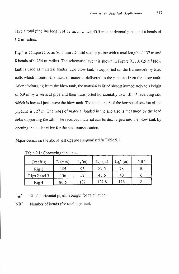
Chapter 9: Practical Applications 217
have a total pipeline length of 52 m, in which 45.5 m is horizontal pipe, and 6 bends of
1.2 m radius.
Rig 4 is composed of an 80.5 mm ID mUd steel pipeUne witii a total lengtfi of 137 m and
8 bends of 0.254 m radius. The schematic layout is shown in Figure 9.1. A 0.9 m^ blow
tank is used as material feeder. The blow tank is supported on the framework by load
ceUs which monitor the mass of material delivered to the pipeline from tfie blow tank.
After discharging from the blow tank, the material is lifted almost immediately to a height
of 5.9 m by a vertical pipe and then transported horizontally to a 1.0 m^ receiving sUo
which is located just above tfie blow tank. The total length of tfie horizontal section of tiie
pipeline is 127 m. The mass of material loaded in the silo also is measured by the load
cells supportíng the silo. The received material can be discharged into the blow tank by
opening the outíet valve for the next transportatíon.
Major detaUs on the above test rigs are summarised in Table 9.1.
Table 9.1: Conveying pipelir
Test Rig
Rigl
Rigs 2 and 3
Rig4
D(mm)
105
156
80.5
les.
Lt(m)
96
52
137
Lth (m)
89.5
45.5
127.8
Lth* (m)
78
40
116
NB*
10
6
8
Lth* Total horizontal pipeline lengtii for calculation.
NB * Number of bends (for total pipeline).
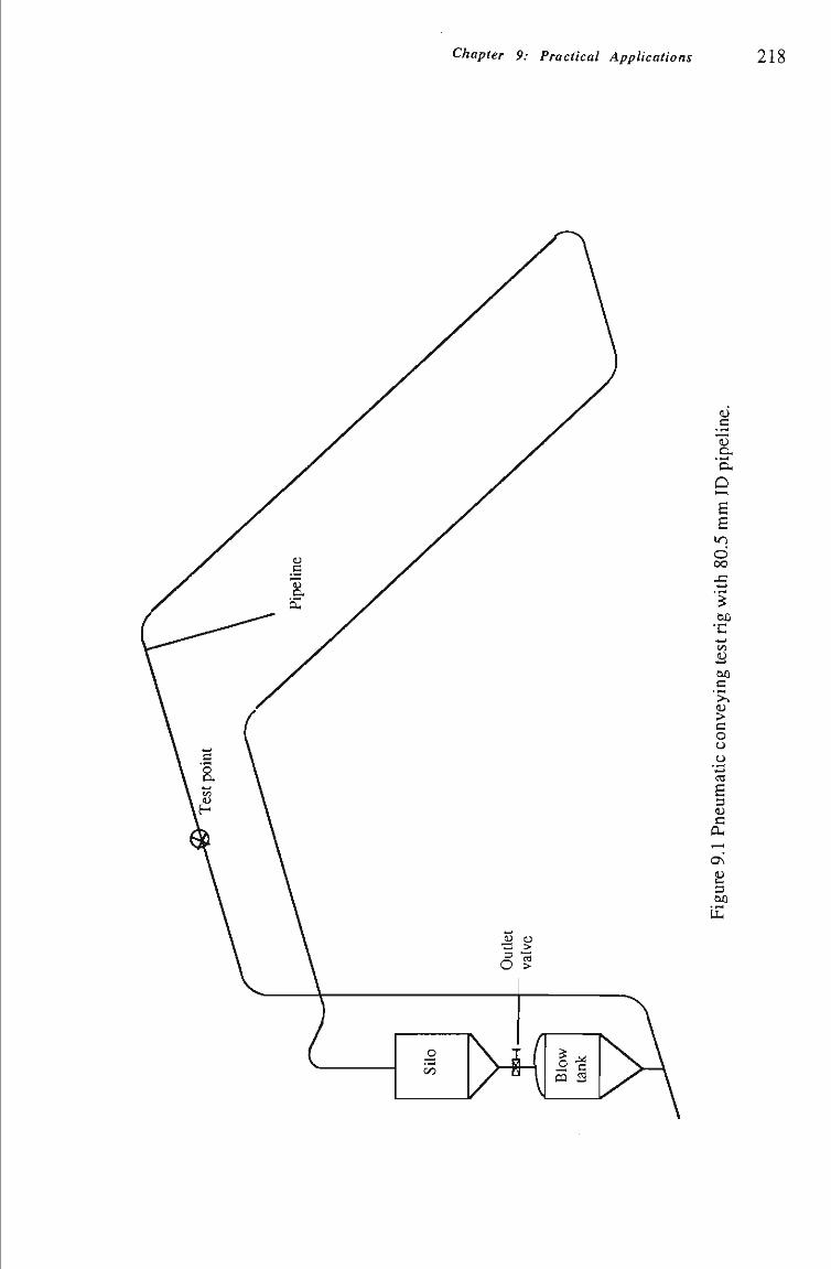
Chapter 9: Practical Applications 218
c
o.
Q l-H
6 B
d oo
•c w
<D
Oû
c > c o o
B 3 C
CL, .—I
0\
2 3 6Û
Chapter 9: Practical AppUcations 219
9.2.3 Test Results
Polystyrene chips and black plastíc pellets are conveyed pneumatícally in tfie above test
rigs. A wide range of conveying conditions are selected for these tests, i.e. for a given
mass flow-rate of solids, the air mass flow-rate is selected to convey the materials from
dense-phase to dilute-phase. A large number of results are obtained. Tables 9.2 and 9.3
list the horizontal pipeline pressures and relevant parameters during dense-phase
conveying.
Table 9.2: Stea
Test
Ri?
4
Exp.
No.
1
2
8
9
15
16
22
23
29
30
dy-state dense-phase results for black plastíc
Speed*
(rpm)
-
-
-
-
-
-
-
-
-
-
mft
(kgs-i)
.0293
.0422
.0319
.0450
.0344
.0465
.0350
.0470
.0352
.0469
mfl
(kgs-i)
-
-
-
-
-
-
-
-
-
-
mf
(kgs-i)
.0293
.0422
.0319
.0450
.0344
.0465
.0350
.0470
.0352
.0469
pellets.
ms
(kgs-i)
.304
.332
.378
.415
.454
.497
.470
.515
.474
.535
Apth
(kPa)
40.12.
40.08.
54.23.
47.81
59.01
54.50.
61.21
55.14
61.61
54.00
Rotary valve speed.
Note tíiat:
• Speed = rotary valve speed (applicable to Rigs 1 and 3 only),
• mft = total supplied mass flow rate of air,
• mfi = rotary valve air leakage,
• mf = actual mass flow rate of air in pipeline,
• ms = mass flow rate of solids,
• Apth = total horizontal pipeline pressure drop.
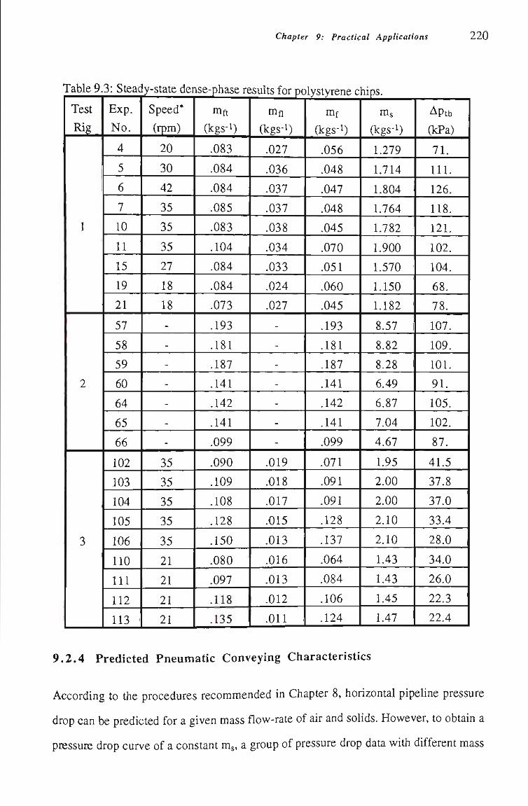
Chapter 9: Practical Applications 220
Table 9.3: Steady-state dense-phase results for polystvrene chips.
Test
Rig
1
2
3
Exp.
No.
4
5
6
7
10
11
15
19
21
57
58
59
60
64
65
66
102
103
104
105
106
110
111
112
113
Speed*
(rpm)
20
30
42
35
35
35
27
18
18
-
-
-
-
-
-
-
35
35
35
35
35
21
21
21
21
mft
(kgs-i)
.083
.084
.084
.085
.083
.104
.084
.084
.073
.193
.181
.187
.141
.142
.141
.099
.090
.109
.108
.128
.150
.080
.097
.118
.135
mfl
(kgs-i)
.027
.036
.037
.037
.038
.034
.033
.024
.027
-
-
-
-
-
-
-
.019
.018
.017
.015
.013
.016
.013
.012
.011
mf
(kgs-i)
.056
.048
.047
.048
.045
.070
.051
.060
.045
.193
.181
.187
.141
.142
.141
.099
.071
.091
.091
.128
.137
.064
.084
.106
.124
ms
(kgs-i)
1.279
1.714
1.804
1.764
1.782
1.900
1.570
1.150
1.182
8.57
8.82
8.28
6.49
6.87
7.04
4.67
1.95
2.00
2.00
2.10
2.10
1.43
1.43
1.45
1.47
Apth
OcPa)
71.
111.
126.
118.
121.
102.
104.
68.
78.
107.
109.
101.
91.
105.
102.
87.
41.5
37.8
37.0
33.4
28.0
34.0
26.0
22.3
22.4
9.2.4 Predicted Pneumatic Conveying Characteristics
According to the procedures recommended in Chapter 8, horizontal pipeUne pressure
drop can be predicted for a given mass flow-rate of air and soUds. However, to obtain a
pressure drop curve of a constant m , a group of pressure drop data with different mass
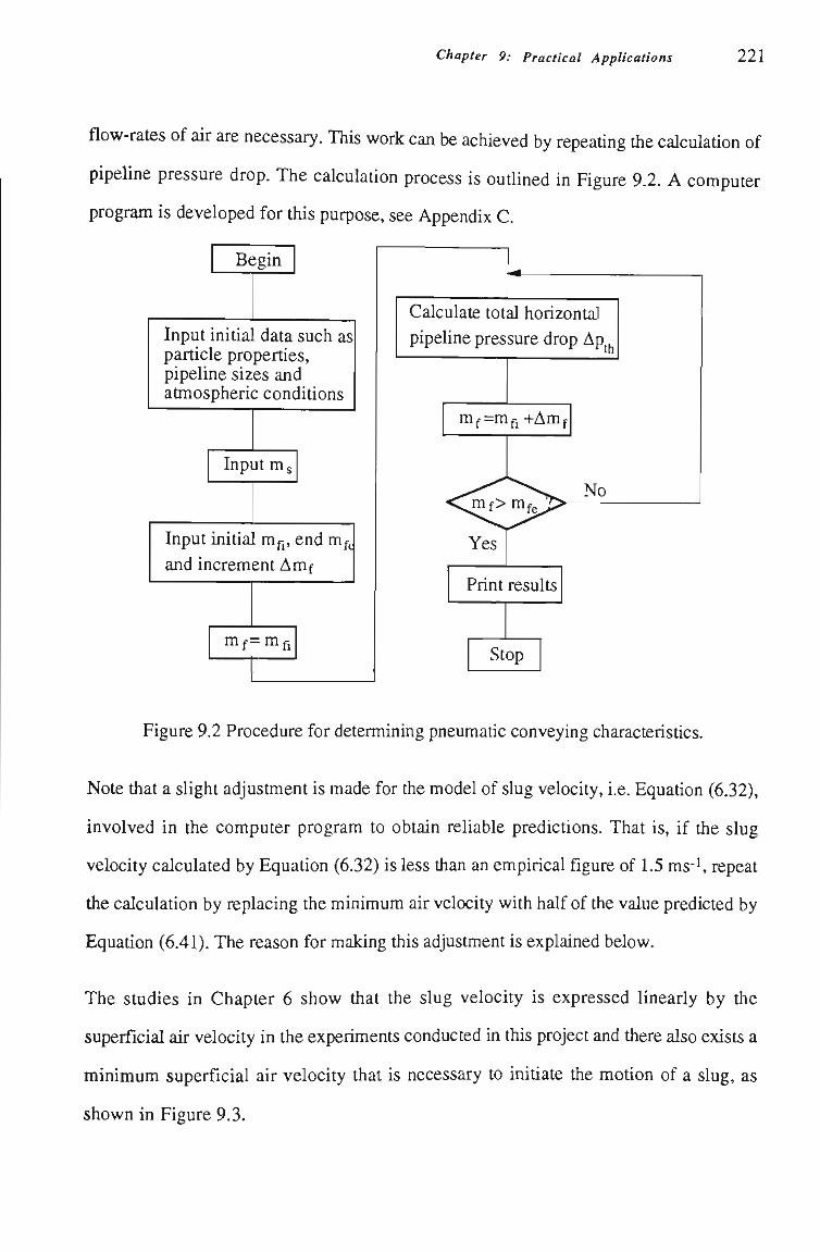
Chapter 9: Practical Applications 221
flow-rates of air are necessary. This work can be achieved by repeatíng the calculatíon of
pipeUne pressure drop. The calculatíon process is outíined in Figure 9.2. A computer
program is developed for this purpose, see Appendix C.
Begin
Input initíal data such as particle properties, pipeline sizes and atmospheric conditions
Input m s
Input initial m^, end m^ and increment Amf
m f = m fl
Calculate total horizontal pipeline pressure drop Ap
mf=mfl-t-Amf
^ > mfe
Yes
No
Print results
Stop
Figure 9.2 Procedure for determining pneumatíc conveying characteristícs.
Note tfiat a slight adjustment is made for the model of slug velocity, i.e. Equation (6.32),
involved in the computer program to obtain reliable predictíons. That is, if the slug
velocity calculated by Equatíon (6.32) is less tfian an empirical figure of 1.5 ms-^ repeat
the calculation by replacing the minimum air velocity with half of the value predicted by
Equatíon (6.41). The reason for making this adjustment is explained below.
The studies in Chapter 6 show that the slug velocity is expressed linearly by the
superficial air velocity in the experiments conducted in this project and there also exists a
minimum superficial air velocity that is necessary to initíate the motíon of a slug, as
shown in Figure 9.3.
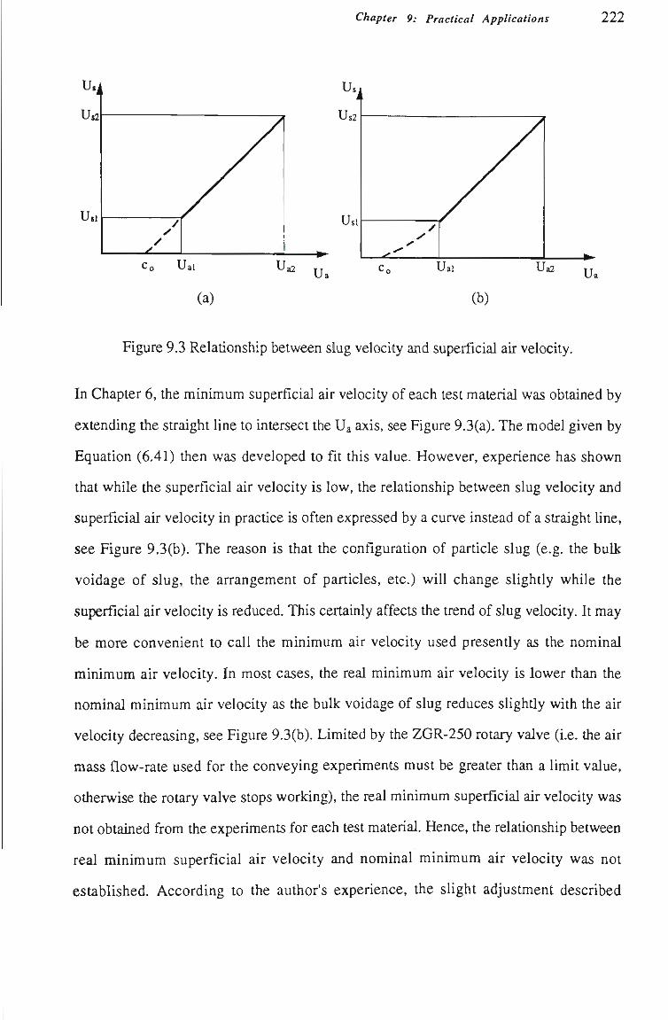
Chapter 9: Practical Applications 222
(a) (b)
Figure 9.3 Relationship between slug velocity and superficial air velocity.
In Chapter 6, the minimum superficial air velocity of each test material was obtained by
extending the straight line to intersect the Ua axis, see Figure 9.3(a). The model given by
Equation (6,41) then was developed to fit this value. However, experience has shown
that while the superficial air velocity is low, the relationship between slug velocity and
superficial air velocity in practice is often expressed by a curve instead of a straight line,
see Figure 9.3(b). The reason is that the configuratíon of particle slug (e.g. the buUc
voidage of slug, the arrangement of particles, etc.) will change slightly while the
superficial air velocity is reduced. This certainly affects the trend of slug velocity. It may
be more convenient to call the minimum air velocity used presently as the nominal
minimum air velocity. In most cases, the real minimum air velocity is lower than the
nominal minimum air velocity as the bulk voidage of slug reduces sUghtly with the air
velocity decreasing, see Figure 9.3(b). Limited by the ZGR-250 rotary valve (i.e. the air
mass flow-rate used for the conveying experiments must be greater than a limit value,
otherwise the rotary valve stops working), the real minimum superficial air velocity was
not obtained from the experiments for each test material. Hence, the relatíonship between
real minimum superficial air velocity and nominal minimum air velocity was not
established. According to the author's experience, the slight adjustment described
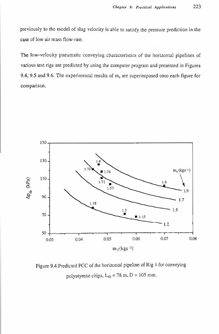
Chapter 9: Practical Applicaíions 223
previously to the model of slug velocity is able to satísfy the pressure predictíon in tíie
case of low air mass flow-rate.
The low-velocity pneumatic conveying characteristícs of the horizontal pipeUnes of
various test rigs are predicted by using the computer program and presented in Figures
9.4, 9.5 and 9.6. The experimental results of m are superimposed onto each figure for
comparison.
ca
<
0.03 0.04 0.05 0.06
mf(kgs-i)
0.07 0.08
Figure 9.4 Predicted PCC of tfie horizontal pipeUne of Rig 1 for conveying
polystyrene chips, Lth = 78 m, D = 105 mm.
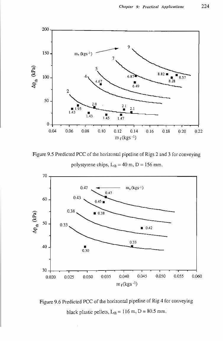
Chapter 9: Practical Applications 224
200
150.
ca
<
100-
50-
ms(kgs-i)
1.43 1.45 1.47
T ' 1 ' 1 ' 1 ' T I I I I I
0.04 0.06 0.08 0.10 0.12 0.14 0.16 0.18 0.20 0.22 mf(kgs-l)
Figure 9.5 Predicted PCC of the horizontal pipeline of Rigs 2 and 3 for conveying
polystyrene chips, Lth = 40 m, D = 156 mm.
70
O i <
-' 1 ' r 0.020 0.025 0.030 0.035 0.040 0.045
1 • 1 •-
0.050 0.055 0.060
mf(kgs-l)
Figure 9.6 Predicted PCC of tíie horizontal pipeUne of Rig 4 for conveying
black plastic pellets, Lth = 116 m, D = 80.5 mm.
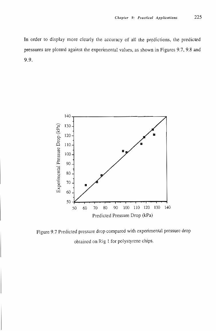
Chapter 9: Practical Applications 225
In order to display more cleariy the accuracy of all the predictíons, the predicted
pressures are plotted against the experimental values, as shown in Figures 9.7, 9.8 and
9.9.
cu
o
2 3 t/3 c/3 2 cu 13 c 6
•d Cu X
m
130-
120-
110-
100-
90-
80-
70-
60-
50-
B y/^
B p /
^ B
^ B
50 60 70 80 90 100 110 120 130 140
Predicted Pressure Drop (kPa)
Figure 9.7 Predicted pressure drop compared with experimental pressure drop
obtained on Rig 1 for polystyrene chips.
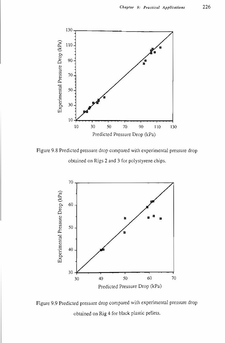
Chapter 9: Practical Applications 226
Cu ^ O-o t.1
Û <u v 3
ess
V.I OH
^^ CS 4 - *
c D
e •c <D O-î^
Ltí
•
I IO^
90-
70 :
50-
30-
10-
y a
- / ^ B yJB
• fl
1 • • • • 1 • • - • 1 • • • •
10 30 50 70 90 110 130
Predicted Pressure Drop (kPa)
Figure 9.8 Predicted pressure drop compared with experimental pressure drop
obtained on Rigs 2 and 3 for polystyrene chips.
C3 D H
o-o
Q <D V-i 3 c« C/3 CU l - i
OH
"cS • 4 - " c <u 6
. . .H l - l (U o-X
PJ
30 40 50 60
Predicted Pressure Drop QcPa)
Figure 9.9 Predicted pressure drop compared with experimental pressure drop
obtained on Rig 4 for black plastíc pellets.
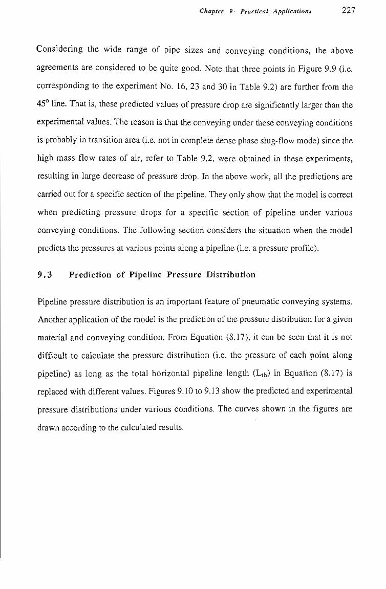
Chapter 9: Practical Applications 2 2 7
Considering the wide range of pipe sizes and conveying conditions, the above
agreements are considered to be quite good. Note that three points in Figure 9.9 (i.e.
corresponding to the experiment No. 16, 23 and 30 in Table 9.2) are further from tíie
45° Ime. That is, these predicted values of pressure drop are signUicantíy larger tíian tíie
experimental values. The reason is that the conveying under these conveying conditíons
is probably in transitíon area (i.e. not in complete dense phase slug-flow mode) since the
high mass flow rates of air, refer to Table 9.2, were obtained in these experiments,
resultíng in large decrease of pressure drop. In the above work, all tíie predictíons are
carried out for a specific sectíon of the pipelme. They only show that the model is correct
when predicting pressure drops for a specific section of pipeline under various
conveying conditíons. The following sectíon considers the situatíon when the model
predicts the pressures at various points along a pipeline (i.e. a pressure profile).
9 .3 Prediction of Pipeline Pressure Distribution
Pipeline pressure distributíon is an important feature of pneumatic conveying systems.
Another applicatíon of the model is the predictíon of the pressure distributíon for a given
material and conveying conditíon. From Equatíon (8.17), it can be seen that it is not
difficult to calculate ihe pressure distribution (i.e. the pressure of each point along
pipeline) as long as the total horizontal pipeline length (Lth) in Equation (8.17) is
replaced with different values. Figures 9.10 to 9.13 show the predicted and experimental
pressure distributíons under various conditíons. The curves shown in the figures are
drawn according to the calculated results.
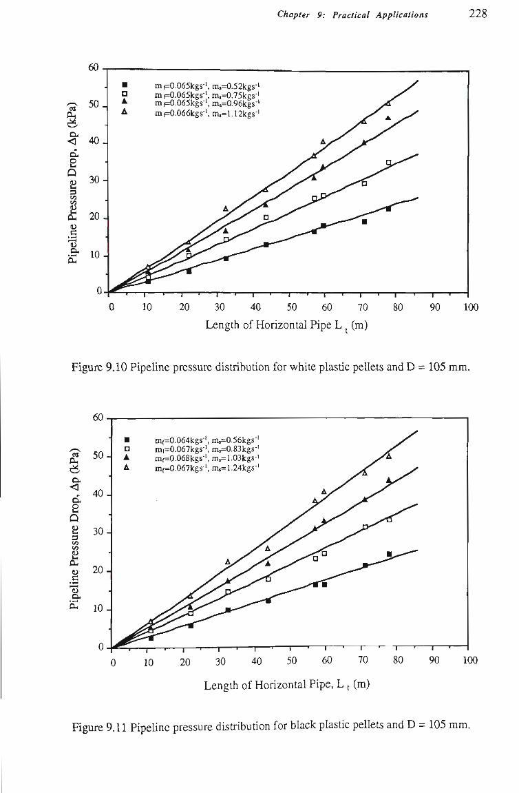
Chapter 9: Practical Applications 228
60
mf=0.065kgs-', m,=0.52kgs-' mf=0.065kgs-', m5=0.75kgs-' mf=0.065kgs-', ms=0.96kgs-' mf=0.066kgs-', ms=1.12kgs-'
20 30 40 50 60 70
Length of Horizontal Pipe L ^ (m)
80 - i —
90 100
Figure 9.10 Pipeline pressure distribution for white plastic peUets and D = 105 mm.
«1 50-
<
S Q
3 C<3
(Xi 4) C
'«3 o.
20 30 40 50 60 70
Length of Horizontal Pipe, L ^ (m)
Figure 9.11 PipeUne pressure distribution for black plastic pellets and D = 105 mm.
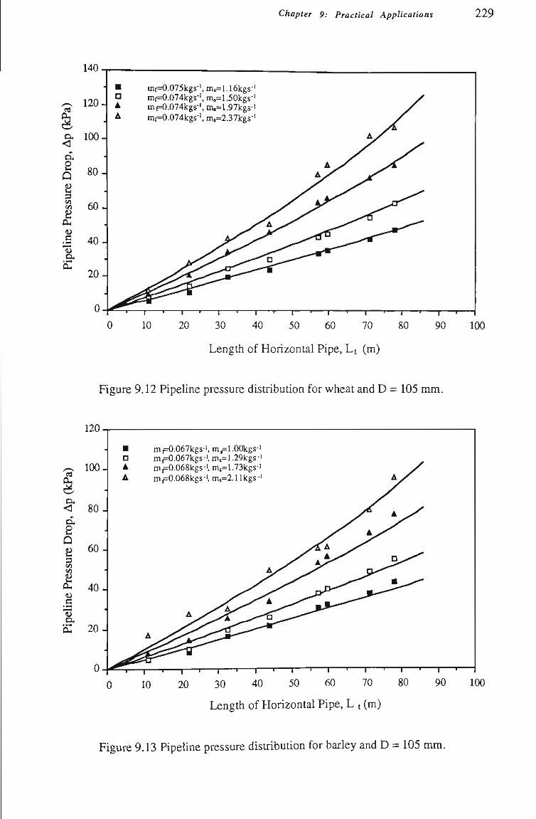
Chapter 9: Practical Applications 229
20 30 40 50 60 70
Length of Horizontal Pipe, Lt (m)
Figure 9.12 Pipeline pressure distribution for wheat and D = 105 mm.
120
ta 100-
O i
< 80 Ôi
s Q S 3 c«
ÛH
<û
c
o.
D A A
mp0.067kgs-', m^l.OOkgs-" mp0.067kgs-', ms=1.29kgs-' mp0.068kgs-i, ms=1.73kgs-i mf=0.068kgs-', ms=2.11kgs-'
30 40 50
Length of Horizontal Pipe, L t (m)
Figure 9.13 PipeUne pressure distributíon for barley and D = 105 mm.
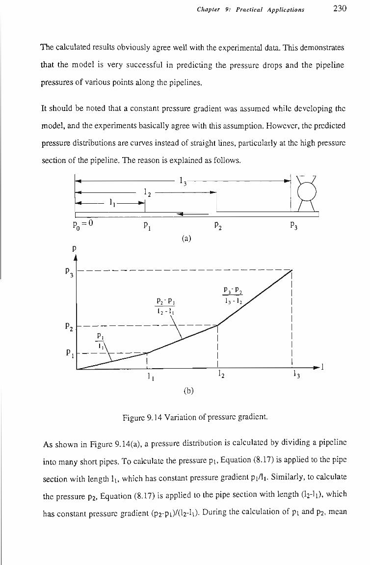
Chapter 9: Practical Applications 230
The calculated results obviously agree weU with the experimental data. This demonstrates
that the model is very successful in predicting the pressure drops and the pipeline
pressures of various points along the pipeUnes.
It should be noted that a constant pressure gradient was assumed while developing the
model, and the experiments basically agree with this assumption. However, tiie predicted
pressure distributions are curves instead of straight Unes, particularly at the high pressure
section of the pipeline. The reason is explained as foUows.
I. L
p =0
• • I
(b)
Figure 9.14 Variation of pressure gradient.
As shown in Figure 9.14(a), a pressure distribution is calculated by dividing a pipeline
into many short pipes. To calculate the pressure pi, Equation (8.17) is appUed to the pipe
sectíon with lengtii h, which has constant pressure gradient pi/Ii. SimUarly, to calculate
the pressure p2, Equation (8.17) is applied to the pipe section with length (I2-I1), which
has constant pressure gradient (p2-pi)/(l2-li)- During the calculatíon of pi and p2, mean
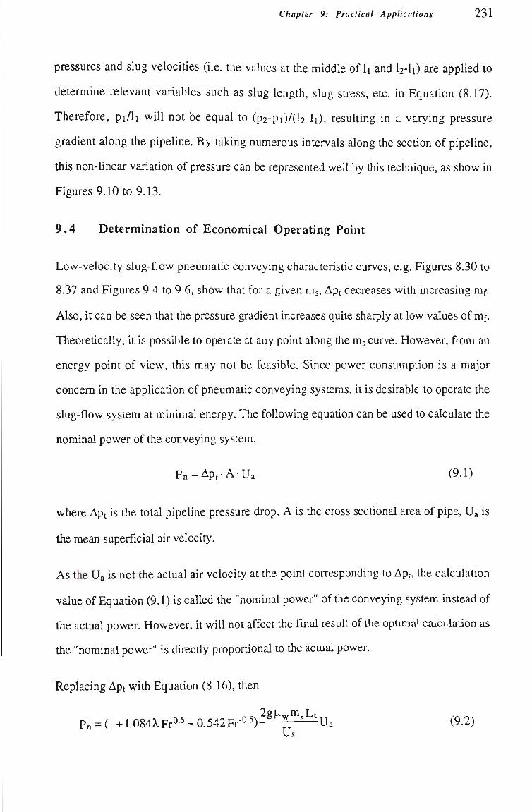
Chapter 9: Practical Applications 2 3 1
pressures and slug velocitíes (i.e. the values at the middle of h and I2-I1) are applied to
determine relevant variables such as slug length, slug stress, etc. in Equatíon (8.17).
Therefore, pi/h wiU not be equal to (p2-pi)/(l2-li), resultíng in a varying pressure
gradient along the pipeUne. By taking numerous intervals along the sectíon of pipeUne,
tíiis non-linear variatíon of pressure can be represented weU by tiiis technique, as show in
Figures 9.10 to 9.13.
9.4 Determination of Economical Operating Point
Low-velocity slug-flow pneumatic conveying characteristic curves, e.g. Figures 8.30 to
8.37 and Figures 9.4 to 9.6, show that for a given m , Apt decreases with increasing mf.
Also, it can be seen that the pressure gradient increases quite sharply at low values of mf.
Theoretically, it is possible to operale at any point along the m^ curve. However, from an
energy point of view, this may not be feasible. Since power consumption is a major
concem in the application of pneumatic conveying systems, it is desirable to operate the
slug-flow system at minimal energy. The foUowing equation can be used to calculate the
nominal power of the conveying system.
Pn = Apt-A-Ua (9.1)
where Apt is the total pipeline pressure drop, A is the cross sectional area of pipe, Ua is
the mean superficial air velocity.
As the Ua is not the actual air velocity at the point corresponding to Apt, the calculation
value of Equation (9.1) is called the "nominal power" of the conveying system instead of
the actual power. However, it will not affect the final result of the optimal calculation as
tíie "nominal power" is directíy proportional to the actual power.
Replacing Apt with Equatíon (8.16), then
P„ = (1 + 1.084A.FrO-5 + 0.542Fr-Q-^)^^^;^"'^^'Ua (9.2) Us
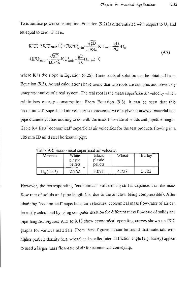
Chapter 9: Practical Applications 232
To minimise power consumption, Equation (9.2) is differentiated with respect to Ua and
let equal to zero. That is.
K^UÍ-3K^UaminU^a+(3K^U gD^ 'amm , ,-,0/i'^'^'-'amin-^. .)Ua 1.084X
g D , (9.3)
-(K^U'aniin-^j^^^K:U^in-t-Tr-Uamin)=0
where K is the slope in Equation (6.25). Three roots of solution can be obtained from
Equatíon (9.3). Actual calculatíons have found that two roots are complex and obviously
unrepresentatíve of a real system. The real root is the mean superficial air velocity which
minimises energy consumptíon. From Equatíon (9.3), it can be seen that this
"economical" superficial air velocity is representatíve of a given conveyed material and
pipe diameter, it has nothing to do with the mass flow-rate of solids and pipeUne length.
Table 9.4 lists "economical" superficial air velocitíes for the test products flowing in a
105 mm ID mUd steel horizontal pipe.
Table 9.4: Economical superí Materiai
Ua(ms-i)
White plastíc pellets
2.762
îcial air velocity. Black plastic pellets
3.071
Wheat
4.738
Barley
5.102
However, the corresponding "economical" value of mf still is dependent on the mass
flow rate of solids and pipe length (i.e. due to the air flow being compressible). After
obtaining "economical" superficial air velocities, economical mass flow-rates of air can
be easily calculated by using computer iteration for different mass flow rate of solids and
pipe lengths. Figures 9.15 to 9.18 show economical operatíng curves shown on PCC
graphs for various materials. From these figures, it can be found that materials with
higher partícle density (e.g. wheat) and smaller intemal frictíon angle (e.g. barley) appear
to need a larger mass flow-rate of air for economical conveying.
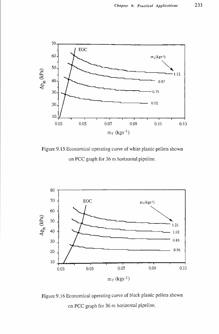
Chapter 9: Practical Applications 233
a
B o. <
0.07 0.09
mf (kgs'^)
0.13
Figure 9.15 Economical operatíng curve of white plastic pellets shown
on PCC graph for 36 m horizontal pipeline.
CU M,
ja
or <
80
70 -J
60
50
40
30
20 J
10
0.03 0.05
EOC
^ ^ 1
1
ms(kgs-')
1.21
- ^ 1,02
U.83
0.07
mf (kgs-1)
0.09 0.11
Figure 9.16 Economical operating curve of black plastic pellets shown
on PCC graph for 36 m horizontal pipeline.
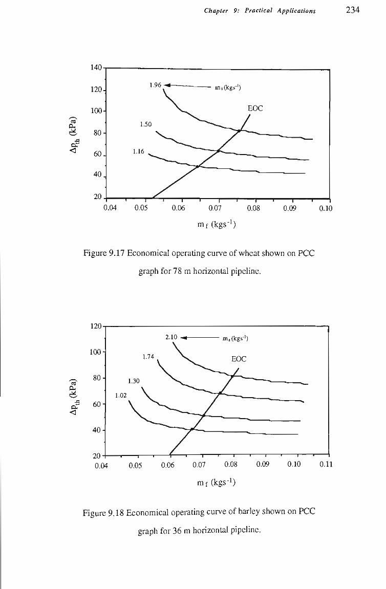
Chapter 9: Practîcal Applications 234
CL,
é <
I I 0.04 0.05
mf (kgs-1)
Figure 9.17 Economical operating curve of wheat shown on PCC
graph for 78 m horizontal pipeline.
0.10
120
cu
o, <
100-
80-
60
40-
2.10
1.02
20 0.04 0.05 0.06 0.07 0.08 0.09 0.10
mf (kgs-1)
0.11
Figure 9.18 Economical operating curve of barley shown on PCC
graph for 36 m horizontal pipeline.
Chapter 9: Practical Applications 2 3 5
A general procedure for the reliable design of low-velocity pneumatic conveymg syetems
with economical power consumption is summarised below:
(i) Measure the physical properties of the bulk material to be conveyed
pneumatically, refer to Chapter 5.
(U) Determine the pipeline configuration, including the pipeline diameter, pipeline
lengtii, size, type and locations of bends, according to the provided conditíons.
(iU) Calculate the economical superficial air velocity by using Equatíon (9.3) for
low-velocity pneumatic conveying.
(iv) Determine the economical mass flow-rate of air for a given mass flow-rate of
solids and the pipeline length by using computer iteration.
(v) Use the pressure prediction procedure recommended in Chapter 8 to predict the
total pipeline pressure drop according to the measured particle properties, the
pipeline configuration and tiie calculated economical conveying conditions.
(vi) Choose a suitable compressor for the system according to the predicted total
pipeline pressure drop and required intake volume.
9.5 Application of Model to Fine Powders
The previously presented pressure prediction model was based on low-velocity
experimental data obtained on various coarse granular materials. Hence, this model
should be used only for the coarse granular materials at tiiis stage. It would be premamre
to apply the model directíy to fine powders, as these materials may have very different
effects on some aspects of the performance of low-velocity pneumatic conveying.
However, low-velocity pneumatic conveying of buUc materials, regardless of fine
powders or coarse granules, always has a simUar flow pattem and mechanism. Hence it
should be possible to apply the model to fine powders (although some modificatíons to
Chapter 9: Practical AppUcations 236
some fundamental aspects such as slug velocity may be needed). To investígate tíiese
issue, some low-velocity pneumatic conveying experiments are carried out on a fine
powder.
9.5.1 Test Material and Properties
Semolina is considered as a fine powder. According to the measurement methods
introduced in Chapter 5, the physical propertíes of semolina are measured and listed
below:
Median partícle diameter, d
Partícle density, ps
BuUc density (loose), pb
Bulk voidage, e
Intemal frictíon angle, ^
Wall friction angle (with respect to mUd steel), (jw
390
1459
736
0.496
30.8
27.5
|im
kgm-3
kgm-3
0
0
c o
• d 3
J=> 'C
• 4 — *
c«
>
3
6 3
u
Particle Size (|im)
Figure 9.19 Partícle size distribution of semolina.
Chapter 9: Practical Applications 237
Note that for fine powders, the particle size used here is the median partícle diameter
which is defined as the particle size which represents 50 % of the sample by mass.
Mechanical sieving is employed to detemine the size distributíon. The measurement of
the particle size is repeated two times to obtain an average value. One of the results is
shown in Figure 9.19.
10.
c
Û
s u Û
1.0
0.1
l l
ll 1 1
1 \
1 >l
1 \
-^ vv s-
X
c
• '
l \
N'
N"*
\ , A
^ \ ' \
/ .
»^
^ S \ i
• s
N \
\ S \
\ >
\
Bs
\
\
\ \
\
4
1
\
L _ _
\ i
\ )li ia ^
s - t -
k
\
D
10 100 1000 10000
Mean Particle Síze Qjjn)
Figure 9.20 SemoUna shown in Dixon's slugging diagram.
According to the measured properties of semolina, it belongs to Dixon [28] Group B, but
is close to Group D, as shown in Figure 9.20. Hence U may be possible to convey
semoUna under low-velocity slug-flow conditíons (to be confirmed by expermient).
9.5.2 Test Results
During the conveying tests, the semolina was found to be a good candidate for low-
velocity pneumatic conveying. That is, whUe conveying semoUna with an appropriate
mass flow-rate of air, regular slugs formed naturally and reliably without the aid of any
slug forming device. Compared with the conveying of the Group D granular materials
Chapter 9: Practical Applications 238
(e.g. plastíc pellets, wheat, etc), the semolina did appear more sensitíve witíi regard to
pipeUne blockage. That is, there existed a minimum mass flow-rate of air for a given
mass flow-rate of soUds, at which pipeline blockage was easy to obtain.
From the experimental data, the low-velocity pneumatíc conveying characteristícs over 52
m are presented in Figure 9.21.
140.
0.02 0.05 0.06
mf(kgs-i)
0.09
Figure 9.21 Low-velocity pneumatíc conveying characteristícs of
105 mm ID, 52 m mild steel pipeline for semoUna.
Velocitíes also are measured for the semolina. As previous investigatíons (see Chapter 6)
into low-velocity pneumatíc conveying indicated that the mass flow-rate of solids only
had littíe influence on particle velocity, the velocities of the semolina are measured only
witíi different mass flow-rates of air. Note that the velocities determined by using the
cross correlation functíon analysis technique relate to particle slugs rather than to
individual partícles. Figure 9.22 shows the plot of the slug velocity versus superficial air
velocity.
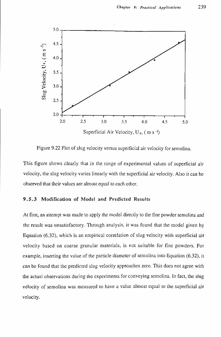
Chapter 9: Practical Applications 239
- 1
c«
6 VI
iloci
ty.
^
Slug
4.5-
4 .0-
3.5-
3.0-
2.5-
2.0-
^ ^ ^ B
1 • 1 • 1 1 1 1 1 1
2.0 2.5 3.0 3.5 4.0
Superficial Air Velocity, Ua, ( m s - )
4.5 5.0
Figure 9.22 Plot of slug velocity versus superficial air velocity for semoUna.
This figure shows clearly that in the range of experimental values of superficial air
velocity, the slug velocity varies linearly with the superficial air velocity. Also it can be
observed that their values are almost equal to each other.
9 .5 .3 Modifícation of Model and Predicted Results
At first, an attempt was made to apply the model directíy to tfie fine powder semolina and
the result was unsatisfactory. Through analysis, it was found that the model given by
Equatíon (6.32), which is an empirical correlation of slug velocity with superficial air
velocity based on coarse granular materials, is not suitable for fine powders. For
example, inserting the value of the partícle diameter of semolina into Equation (6.32), it
can be found that the predicted slug velocity approaches zero. This does not agree with
the actual observatíons during the experiments for conveying semolina. In fact, the slug
velocity of semolina was measured to have a value almost equal to the superficial air
velocity.
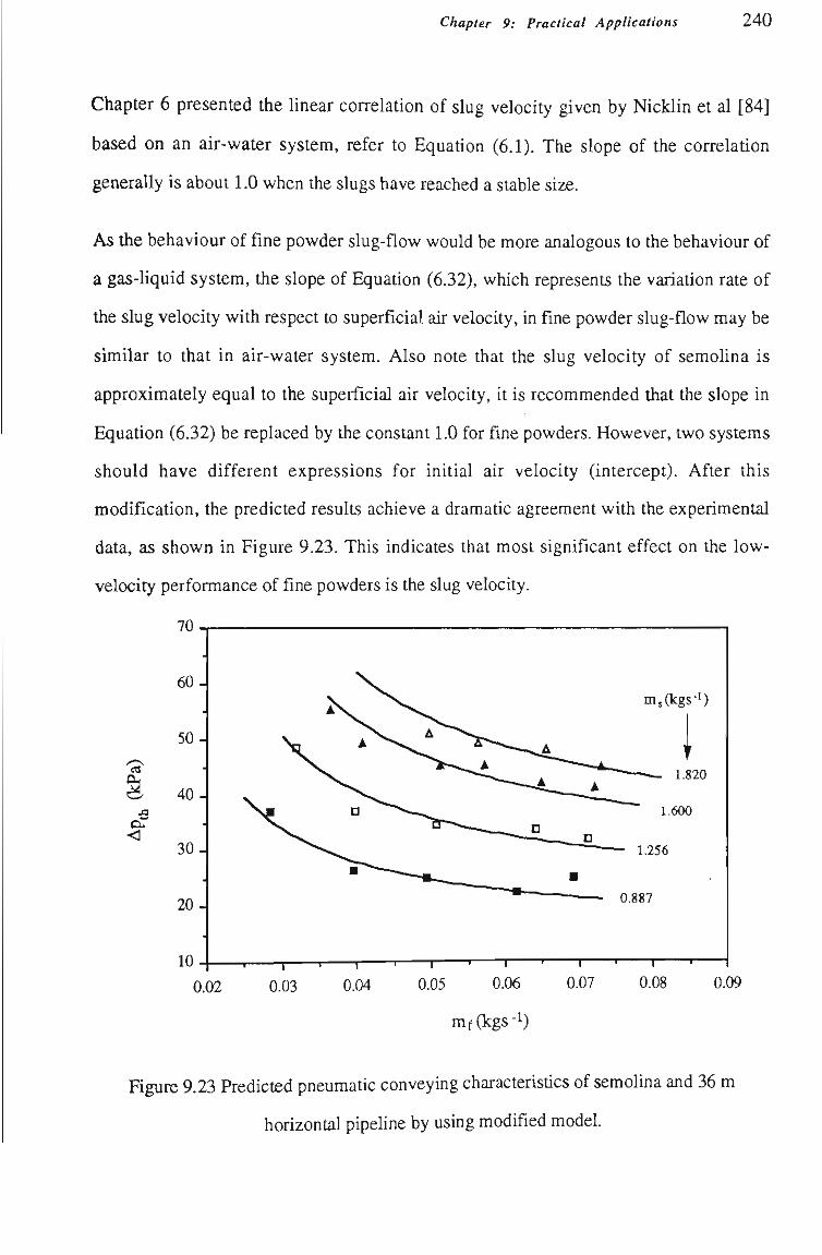
Chapter 9: Practical Applications 240
Chapter 6 presented the linear correlatíon of slug velocity given by Nicklin et al [84]
based on an air-water system, refer to Equatíon (6.1). The slope of the correlatíon
generally is about 1,0 when the slugs have reached a stable size.
As the behaviour of fine powder slug-flow would be more analogous to tíie behaviour of
a gas-liquid system, the slope of Equatíon (6.32), which represents tíie variatíon rate of
the slug velocity with respect to superficial air velocity, in fine powder slug-flow may be
similar to that in air-water system. AIso note that the slug velocity of semoUna is
approximately equal to the superficial air velocity, it is recommended that the slope in
Equation (6.32) be replaced by the constant 1.0 for fine powders. However, two systems
should have different expressions for initial air velocity (intercept). After this
modification, the predicted results achieve a dramatic agreement with the experimental
data, as shown in Figure 9.23. This indicates that most significant effect on the low-
velocity performance of fine powders is the slug velocity.
70
J3
o. <
0.02 0.03 0.09
mf(kgs-i)
Figure 9.23 Predicted pneumatíc conveying characteristícs of semolina and 36 m
horizontal pipeUne by using modU ed model.
241
CHAPTER 10
CONCLUSIONS AND SUGGESTIONS FOR FURTHER WORK
Chapter 10: Conclusions & Suggestions for Further Work 2 4 2
10 .1 Conclusions
This thesis was aimed at developing a model for predictíng the total horizontal pipeUne
pressure drop for low-velocity pneumatíc conveying. For this purpose, a tíieoretícal
analysis was carried out for the pressure gradient and stress state in a single slug, then
numerous experiments were undertaken to investígate the slug velocity, waU pressure,
stress transmission coefficient, etc. to establish empirical or semi-empirical cortelatíons
for these parameters. The relatíonship between the pressure drop across a single slug and
the total pipeline pressure drop also was established. The following conclusions are
based on the investígatíons and fmdings of thesis.
1 Flow pattern
• During low-velocity horizontal pneumatíc conveying, particles are conveyed in the
form of discrete slugs. Between each pair of slugs, the pipe usually is filled with an
air gap and a stationary bed of particles. Each slug sweeps up the partícles from the
stationary bed in front of it and delivers about same the quantíty of partícles to the
pipe behind it whUe travelling forward along the pipeline.
• Low-velocity pneumatíc conveying is analogous to an aggregative fluidised bed
model, Two partícle phases exist in low-velocity pneumatic conveying. One is
partícle dense phase i.e. partícle slugs, and the other is partícle dUute-phase i.e. air
gaps. These constítute the discontinuous flow pattern of low-velocity pneumatic
conveying.
• The particle slugs are a special case of dense phase i.e. mcipient fluidisatíon, in which
the air flow-rate is at least equal to that required just to fluidise tfie material. The air
gaps are formed by the excess air for fluidising the material. Therefore, for the low-
velocity pneumatic conveying system of a given mass flow-rate of solids, increasing
the mass flow-rate of air does not change the pressure gradient through the slugs in
Chapter 10: Conclusions & Suggestions for Further Work 2 4 3
theory and only increases tfie length of air gaps or forms a new air gap. The aU gaps
are axisymmetric for vertical slug-flow and asymmetric for horizontal slug-flow due
to tiie presence of stationary bed.
• From the definition of incipient fluidisatíon it is known that the particle slugs have a
conventíonal fixed-bed configuratíon (i.e. tfie particles in the slugs are fixed relative to
each other) and a bulk density simUar to the loose-poured conditíon.
• For a given mass flow-rate of solids, increasing the mass flow-rate of air increases
the length of air gap, whereas for a given mass flow-rale of air, increasing the mass
flow-rate of solids decreases tiie length of air gap.
• The experimental results on the cross sectional area ratio of stationary bed to pipe
agree well with the predictíons of Konrad et al. [69].
2 Stress in Slug
• Inter-partícle normal stress in a moving slug varies as a exponentíal function along its
length and is confined by the stress on the front and back surface of the slug, see
Equation (3.18).
• The stress on the front and back surface of a slug is a functíon of the slug velocity
and statíonary bed thickness, see Equatíons (3.27) and (3.28). The stress on the front
surface is nearly equal to the stress on the back surface of the slug since the average
statíonary bed thickness is approximately the same both in front of and behind the
slug.
• The average axial normal stress in a slug is approximately equal to its frontal stress.
Thus the stress transmission coefficient of a slug can be approximated by the ratío of
the average radial stress to the frontal stress.
Chapter 10: Conclusions & Suggestions for Further Work 2 4 4
• The normal stress in a horizontal moving slug is in actíve state so that tíie value of
stress transmission coefficient is determined by Equatíons (7.8), (7.9) and (7.21).
3 Slug Velocity
• Slug velocity appears to be independent of mass flow rate of solids, but varies
Unearly witíi superficial air velocity. A minimum air velocity exists for each material
to initiate the motíon of particle slug.
• The linear model of slug velocity for coarse granular materials can be expressed by
Equatíon (6.32). For fine powders, the slope of the linear model of Equatíon (6.32)
appears to be 1.0.
• Carman's equatíon [18] for fluid flowing through a fixed granular fixed bed and the
suggestíons of Ergun [31, 32] are combined to produce Equatíon (6.41) which
provides a good estímate of the minimum air velocity.
4 Total Horizontal Pipeline Pressure Drop
• Pipeline pressure exhibits approximately a linear distributíon along the length of pipe,
partícularly at low mass flow-rate of solids.
• Total pipeline pressure drop decreases as mass flow-rate of air increases for dense-
phase conveying. This trend is opposite to that in dilute-phase conveying.
• The presence of bends increases the pipeline pressure drop, but the effect is not
significant for low-velocity pneumatic conveying.
• For low-velocity pneumatíc conveying, the minimum pressure drop point is not the
minimum power consumptíon point. "Economical" superficial air velocity is
representative of a given conveyed material and pipe diameter and has nothing to do
with the mass flow-rate of solids and pipeUne length.
Chapter 10: Conclusions & Suggestions for Further Work 2 4 5
10.2 Suggestions for Further Work
1 Pressure Drop in Vertical Pipe
The work completed in this thesis is concerned with developing a pressure prediction
model for horizontal low-velocity pneumatic conveying since horizontal pipes are used
extensively in all test rigs. However, the experiments in this thesis show that the pressure
gradient in vertical slug-flow is much greater than that in horizontal slug-flow, so tiiat the
pressure drop in the vertical pipe often cannot be ignored. For example, the pressure drop
over the 52 m long pipeline which contains a 6.5 m vertical Uft was nearly twice as large
as the pressure drop over the 36 m long horizontal section of the pipeline when
conveying black plastic pellets, see Figures 8.20 and 8.32. Hence, investigations into
slug-flow in vertical pipe are necessary so that a reliable prediction model is established
for the vertical pipeline pressure drop.
2 Fine and Mixed Size Material
The work in this thesis concentrates on the investigation into low-velocity pneumatic
conveying of coarse monosized granular materials. Fine and mixed size materials wiU
exhibit different behaviour and performance in some aspects during pneumatic
conveying. Although the model developed based on coarse granular material has been
modified to suit the application for fíne powders, only one type of fine powder semolina
was tested. Experiments of conveying more fine powders in low-velocity are necessary.
It also is necessary to clarify and define the concept of "fine powder" and "coarse
granule" to establish the appropriate slope in Equation (6.32). The effect of mixed size
materials on the pressure predictíon model and the suitability of using a representing
partícle diameter also requires further investígatíon.
Chapter 10: Conclusions & Suggestions for Further Work 2 4 6
3 Boundaries of Low-Velocity Pneumatic Conveying
Pneumatíc conveying characteristícs show that there are two boundaries for low-velocity
pneumatíc conveying. The lower boundary represents the minimum air velocity required
just to initiate the motion of particle slug. The higher boundary represents the transitíon
from stable steady slug-flow to unstable flow. The estimation of each boundary is
essential for the reliable design of low-velocity pneumatíc conveying systems, In
addition, further studies of the lower boundary (i.e. the minimum air velocity) will be
helpful for the modification of the slug velocity model given by Equation (6.32), so as to
predict more accurately the pressure drop at low mass flow-rates of air, refer to Section
9.2.4,
4 Flow Pattern
For dense phase pneumatíc conveying, flow pattems define the problem that has to be
solved in order to predict the pressure drop and the conveyability of the product. More
contributíons are necessary to describe numerically the flow pattern of low-velocity
pneumatíc conveying, e.g. develop models for defining the length of single slug and air
gap and the shape of the air-particle interface between two slugs. FIow pattems of other
types of dense phase conveying (e.g. fluidised dense phase, moving bed flow and dense
phase plug-flow of cohesive products) also need to be investigated further.
247
CHAPTER 11
REFERENCES
Chapter 11: References 2 4 8
1. Albright, C. W„ Holden, J, H„ Simons, H, H, and Schmigt, L. D., Pressure
Drop in FIow of Dense Coal-Air Mixtures, Industrial and Engineering Chemistry,
Vol. 43, No. 8, Aug. 1951, pp 1837 -1840.
2. Anthony, S., The Determination of Solids Velocity by Cross- Correlation of
Pressure Signals in a Pneumatíc Conveying Pipeline, BE Thesis, Dept. of
Mechanical Engineering, University of WoIIongong, 1991.
3. Amold, P. C. and Wypych, P. W., The Development of Pneumatíc Conveying in
AustraUa, Bulk SoUds Handling, Vol. 11, No. 1, 1991, pp 85 - 91.
4. Amold, P. C, Reed, A. R. and Wypych, P. W., Advances in the Design of
Pneumatic Transport Systems, Internatíonal Symposium on Reliable Flow of
Particulate Solids II, Aug. 23 - 25, 1993, Oslo, Norway, pp 453 - 475.
5. Aziz, Z, B. and KUnzing, G. E., Dense Phase Transfer: Plug Flow Around Bends,
Pneumatech 4, Fourth Internatíonal Conference on Pneumatic Conveying
Technology, Mar. 1987, pp 1 - 18.
6. Barker, C. G. J. and Geldart, D., An Invesfigatíon into the Slugging
Characteristícs of Large Particles, Powder Technology, Vol. 19, 1978, pp 177 -
187.
7. Blair-fish, P. M. and Bransby, P. L., FIow Pattems and Wall Stresses in a Mass-
FIow Bunker, Journal of Engineering for Industry, Transactíon of ASME, Series
B, Vol. 95,No. 1, 1973, pp 17-26.
8. Borcz, A. and Rahim, H. A., A New Method to Measure Pressure and
Temperature in Silos, Powder Handling and Processing, Vol. 1, No. 4, 1989, pp
349 - 352.
Chapter 11: References 2 4 9
9. Borcz, A. and Rahim, H. A., Pressure Measurements on Cement Silos, Powder
HandUng and Processing, Vol. 2, No. 3, 1990, pp 239 - 246.
10. Borzone, L. A. and Klinzing, G. E., Dense-Phase Transport: Vertícal Plug Flow,
Powder Technology, 53, 1987, pp 273 - 283.
11. Bradley, M. S. A. and MUls, D., Approaches to DeaUng with the Problems of
Energy Loss Due to Bends, 13th Annual Powder and Bulk Solids Conference,
M a y 9 - 12, 1988, pp 705 - 715.
12. Bradley, M. S. A. and Reed, A. R., Advances in the Design of Pneumatic
Conveying Systems, Bulk SoUd HandUng, Vol. 11, No. 1, Mar. 1991, pp 93 -
97.
13. Bradley, M. S. A., An Improved Method of Predictíng Pressure Drop Along
Pneumatíc Conveying Pipelines, Third Intematíonal Conference on Bulk Materials,
Storage, Handling and Transportation, Jun. 1989, pp 282 - 288.
14. Briks, A. H., A Bulk SoUd Classificatíon System Based on Failure Property
Mechanisms, 14th Annual Powder and Bulk Solids Conference, 1989, pp 3 -10,
15. Brown, R. W., Dense Phase Conveying, Pneumotransport 3, Third Intemational
Conference on the Pneumatic Transport of Solids in Pipes, Apr. 7 - 9, 1976,
England, A 4 - 33.
16. Butters, G„ Plastíc Pneumatic Conveying and Bulk Storage, Applied Science,
London, 1981.
17. Chambers, A, J„ Introduction to Pneumatic Conveying, ITC Bulk Materials
HandUng, Design and Operatíon of Pneumatíc Conveying Systems, Short Course
Notes, 3 - 5 July 1989, Dept, of Mechanical Engineering, University of
WoIIongong.
Chapter 11: References 2 5 0
18, Carman, P, C„ Fluid FIow Through Granular Beds, Transactions of tiie Institutíon
of Chemical Engineers, Vol. 15,1937, pp 150 - 166.
19, Chari, S. S., Pressure Drop in Horizontal Dense Phase Conveying of Air-SoUd
Mixtures, AIChE Symposium Series, Vol. 67, No. 116, 1971, pp 77 - 84.
20, Chen, T, Y„ Walkwender, W, P, and Fan, L, T„ Moving Bed SoUds Flow
Between Two Fluidised Beds, Powder Technology, 22, 1979, pp 89 -96,
21, Cheng, K, Q, and Chen, H. X., An Approach to Determining Moving Parameters
of Pulse Plug FIow Type Pneumatic Conveying, Pneumatech 4, Fourth
Intematíonal Conference on Pneumatic Conveying Technology, Mar. 1987, pp 235
-252.
22, Coulson, The Streamline Flow of Liquids Through Beds Composed of Spherical
Particles, PhD thesis, University of London, 1935.
23, Daoud, K,, Ginestet, A., Large, J., F. and Guigon, P., Performances of Dense
Phase Plug FIow Pneumatíc Conveyor and Characterisatíon on FIow Regime,
Intematíonal Symposium on Reliable Flow of Particulate Solids II, Aug. 23 - 25,
1993, Oslo, Norway, pp 677 - 684.
24, Davidson, J, F, and Harrison, D., Fluidisation, Academic Press, London and New
York, 1971.
25, Dayam, J. and Levenspiel, O., The Residence-Time Distribution for Flow Models
with Cross FIow between Plug-FIow Regions, AIChE Chemical Engineering
Progress Symposium Series, No. 101, Vol. 66, pp 28 - 36.
26, Decamps, F., Dumont, G. and Goossens, W., Vertícal Pneumatic Conveyer with a
Fluidised Bed as Mixing Zone, Powder Technology, 5, 1971/1972, pp 299 - 306.
Chapter 11: References 2 5 1
27. Dickson, A. J., Skews, B. W. and Marcus, R. D., Plug Phase Conveying,
Pneumotransport 4, Fourth Intemational Conference on tiie Pneumatíc Transport of
SoUds in Pipes, Jun. 26 - 28, 1978, Califomia, USA, D 6 - 73.
28. Dixon, G. The Impact of Powder Properties on Dense Phase FIow, Proceedings of
Intematíonal Conference on Pneumatíc Conveying, Jan. 1979, London, UK.
29. Dixon, G., Fluidisatíon Theory Throws Light on Dense Phase Conveying Particle,
Pneumatech 4, Fourth Internatíonal Conference on Pneumatic Conveying
Technology, March, 1987, pp 27 - 37.
30. Dixon, G., How do Different Powders Behave, Bulk Storage Movement Control,
May/June, 1979, pp 81 - 88.
31. Ergun, S. and Orning, A. A., Fluid FIow Through Randomly Packed Columns
and Fluidised Beds, Industrial and Engineering Chemistry, Vol. 41, No. 6, pp
1179-1184.
32. Ergun, S., Fluid Row Through Packed Columns, Chemical Engineering Progress,
Vol. 48, 1952, pp 89 - 94.
33. Esmailzadeh, E. K., Horizontal Pneumatic Transport at High Solids Loadings,
Pneumotransport 3, Third Intematíonal Conference on the Pneumatíc Transport of
SoUds in Pipes, Apr. 7 - 9, 1976, England, D 3 - 33.
34. Flatt, W. and Blumer, P., Low Velocity Conveying, Pneumatech 1, First
Intematíonal Conference on Pneumatíc Conveying Technology, May 3 - 5, 1982,
Stratford-Upon-Avon, UK, pp 1 - 4.
35. Flatt, W., Latest Developments and AppUcatíons of High Density Pneumatíc
Conveying Systems, Pneumotransport 3, Third Intematíonal Conference on the
Pneumatíc Transport of Solids in Pipes, Apr. 7 - 9, 1976, England, A 3 - 21.
Chapter 11: References 2 5 2
36. Flatt, W., Low Velocity Pneumatic Conveying of Granulated and Pulverised
Products, Criteria for Selecting the Optimal Pneumatic Conveying System,
Pneumotransport 5, Fifth Intemational Conference on the Pneumatic Transport of
SoUds in Pipes, Apr. 16 - 18, 1980, London, UK, pp 409 - 418.
37. Flatt, W,, Today's Possibilities for Low Velocity Conveying of Carbon Black and
Pigments with New Conveying Technology, International Conference on
Pneumatic Conveying Technology, Sep. 4 - 6, 1984, Canterbury, UK, pp 1 - 18.
38. Francisco, J. and Cabrejos, I. M., Incipient Motíon of Solid Particles in Pneumatic
Conveying, M. Sc. Dissertatíon, University of Pittsburgh, 1991
39. Geldart, D„ Types of Gas Fluidisatíon, Powder Technology, 7, 1973, pp 285 -
292,
40. Gerchow, F. J., Rotary Valve Selectíon for Pneumatic Conveying Systems, BuUs:
Solids Handling, Vol. 1, No. 1, Feb. 1981, pp 171 - 174.
41. Ginestet, A., Daoud, K., Largr, J. F., Guigon, P. and Jodlowski, C , SuitabiUty
of Bulk Products for Dense Phase Pneumatic Conveying, Pneumatech 4, Fourth
Internatíonal Conference on Pneumatic Conveying Technology, Mar. 1987, pp 27
-37 .
42. Gu, H. and Klinzing, G. E., Vertícal Plug FIow of Cohesive Coal in 2- and 4-
Inch Pipes, Powder Technology, 57, 1989, pp 59 -67.
43. Hancock, A. W. and Nedderman, R. M., Predictíon of Stresses on Vertical
Bunker Walls, Transactíons of the Instímtíon of Chemical Engineers, Vol. 52, No.
2, Apr. 1974, pp 170 -179.
44. Happel, J., Pressure Drop Due to Vapour Flow through Moving Beds, Industrial
and Engineering Chemistry, Vol. 41, No. 6, pp 1161 - 1174.
Chapter 11: References 2 5 3
45, Hariu, O, H, and Molstad, M, C, Pressure Drop in Vertical Tubes in Transport of
Solids by Gases, Industrial and Engineering Chemistry, Vol, 41, No. 6, Jun.
1949, pp 1148- 1160.
46, Hauser, G. and Sommer, K., Plug FIow Pneumatic Transport in DUute and Dense
Phase, Bulk Solids Handling, Vol. 2, No. 2, Jun. 1982, pp 9 - 15.
47, Hikita, T., Ikeda, M. and Asano, H., Upward Transportation of Particles in Dense
Phase, Fourth Internatíonal Conference on Fluidisatíon, 1983, KasUcojima, Japan,
pp 219 - 232
48, Hitt, R. J., An Investígatíon into the Low Velocity Pneumatíc Conveying of Bulk
Solids, PhD dissertatíon, School of Mechanical Engineering, Thames Polytechnic,
Jan. 1985.
49, Hitt, R. J., An Investígatíon into the Low Velocity Pneumatíc Conveying of Bulk
Solids, Pneumatech 1, First Internatíonal Conference on Pneumatic Conveying
Technology, May 3 - 5, 1982, Stratford-Upon-Avon, UK, pp 1 - 26
50, Hong, J. and Shen, Y., Characteristics in Horizontal Pneumatic Conveying at
High Solids Loading and Low Gas Velocity, Intematíonal Symposium on ReUable
FIow of Partículate Solids H, Aug. 23 - 25, 1993, Oslo, Norway, pp 677 - 711.
51, Hongky, J. N., Design and Scale-Up Low Velocity Pneumatic Conveying
Systems, BE Thesis, Dept. of Mechanical Engineering, University of WoUongong,
1990.
52, Hoppe, H., Heep, D. and Storf, R., Modem Rotary Valve Technology for Various
Pneumatíc Conveying Systems, Bulk Solids Handling, Vol. 5, No. 4, Aug. 1985,
pp 161 - 165.
Chapter 11: References 2 5 4
53. Hoppe, H., Modem, Economical Pneumatic Conveying Technologies for In-plant
Quality Assurance, Pneumatech 4, Fourth Intematíonal Conference on Pneumatic
Conveying Technology, Mar. 1987, pp 253 - 266.
54. Huggett, M. R., Low Velocity - The Ultímate Dense Phase Conveyor, Powder
Handling and Processing, Vol. 2, No. 3, 1990, pp 207 - 210.
55. Jenike, A. W. and Johanson, J. R., Bin Loads, Joumal of the Stmcture Division,
ASCE, Vol. 95, No. ST4, 1968, pp 1011 - 1041
56. Jenike, A. W. and Johanson, J. R., On the Theory of Bin Loads, Journal of
Engineering for Industry, Transactíons of ASME, Series B, Vol. 91, No. 2, May
1969, pp 339 - 344.
57. Jodlowski, C, Considerations on Two Phase Gas/Solid Flow at Low Velocitíes,
Pneumatech 2, International Conference on Pneuraatic Conveying Technology,
Sep. 4 - 6, 1984, Canterbury, UK, pp 19 - 39.
58. Jones, M. G., Mills, D. and Mason, J. S., Pneumatic Conveying of High Bulk
Density Products, Pneumatech 4, Fourth Intematíonal Conference on Pneumatic
Conveying Technology, Mar. 1987, pp 371 - 396.
59. Kadlec, R, H,, The Behaviour of Slugging Gas-FIuidised SoUd, PhD Dissertatíon,
University of Michigan, 1961,
60. Kessel, S. R., Reed, A. R. and Mason, J. S., An Investígatíon into the FIow
Behaviour in the Entrainment Section of a Rotary Valve Fed Pneumatic Conveying
System, Pneumatech 1, First Intematíonal Conference on Pneumatic Conveying
Technology, May 3 - 5, 1982, Stratford-Upon-Avon, UK, pp 1 - 23.
Chapter 11: References 2 5 5
61 . Klintworth, J, and Marcus, R. D., A Review of Low-Velocity Pneumatic
Conveying Systems, Bulk SoUds HandUng, Vol. 5, No. 4, Aug. 1985, pp 25 -
31.
62. KUnzing, G. E., A Comparison Pressure Losses in Bends Between Recent Data
and Models for Gas-SoUd Flow, Canadian Joumal of Chemical Engineering, Vol.
58, 1980, pp 670 - 672.
63. Klinzing, G, E„ Artificial InteUigence Approaches to Pneumatíc Conveying
Operatíons, Internatíonal Symposium on Reliable FIow of Partículate Solids II,
Aug, 23 - 25, 1993, Oslo, Norway, pp 481 - 499,
64. Konrad, K. and Totah, T. S., Vertícal Pneumatic Conveying of Particle Plugs,
Canadian Journal of Chemical Engineering, Vol. 67, Apr. 1989, pp 245 - 250.
65. Konrad, K., Dense-Phase Pneumatíc Conveying through Long Pipelines: Effect of
Significantly Compressible Air FIow on Pressure Drop, Powder Technology, 48
(1986), pp 193 - 203.
66. Konrad, K., An Exploratory Analysis of Dense Phase Pneumatic Conveying
through Vertical PipeUne, Joumal of Pipelines 6,1987, pp 99 -104.
67. Konrad, K., Dense Phase Pneumatíc Conveying of Particles, PhD dissertation,
Trinity CoUege, University of Cambridge, 1980.
68. Konrad, K., Dense Phase Pneumatic Conveying: A Review, Powder Technology,
49, 1986, pp 1 - 35.
69. Konrad, K., Harrison, D., Nedderman, R. M. and Davidson, J. F., Predictíon of
the Pressure Drop for Horizontal Dense Phase Pneumatic Conveying of Particles,
Pneumotransport 5, Fifth Internatíonal Conference on the Pneumatic Transport of
Solids in Pipes, Apr. 16-18, 1980, London, UK, pp 225 - 244.
Chapter 11: References 2 5 6
70. Kunii, D, and Levenspid, O,, Fluidisation Engineering, Wiley, New York,
London, Sydney and Toronto, 1969.
71 . Legel, D. and Schwedes, J., Investígation of Pneumatíc Conveying of Plug of
Cohesionless BuUc Solids in Horizontal Pipes, BuUc SoUds Handling, Vol. 4, No.
2, Jun. 1984, pp 399 - 405.
72. Leung, L. S., Vertícal Pneumatic Conveying: A FIow Regime Diagram and a
Review of Choking Versus Non-Choking Systems, Powder Technology, Vol. 25,
1980, pp 185 - 190.
73. Leva, M., Fluid Flow through Packed Beds, Chemical Engineering, 56, May
1949, pp 115- 117.
74. Leva, M., Fluidisatíon, MacGraw-HiU, New York, 1959.
75. Lewis, W. K. and GiIUIand, E. R. and Baner, W. C , Characteristics of Fluidised
Particles, Industrial and Engineering Chemistry, Vol. 41, No. 6, pp 1104 - 1117.
76. Li, H., The Fluid-Particle FIow Phase Diagram and Ideal Sealing State for a
Vertícal Moving Bed, Powder Technology, 67, 1991, pp 37 - 42.
77. Lippert, A., Pneumatíc Conveyence at High Solids Concentratíons, Chemie-Ing-
Techn. 38, No. 3, pp 350 - 355.
78. Mainwaring, N, J, and Reed, A, R., An Appraisal of Dixon's Slugging Diagram
for Assessing the Dense Phase Conveying Potentíal of Bulk Solid Materials,
Pneumatech 4, Fourth International Conference on Pneumatic Conveying
Technology, Mar. 1987, pp 221 - 234.
Chapter 11: References 2 5 7
79. Mason, D. J., Cross, M., Patel, M. K. and Reed, A. R., Numerical Modelling of
" Dense Phase" Pneumatic Conveying of Bulk Partículate Materials, 14tíi Annual
Powder and Bulk Solids Conference, 1989, pp 449 - 460.
80. Matsen, J. M„ A Phase Diagram for Gas-Partícle Flow, Fluidisatíon IV, Fourth
Intematíonal Conference on Fluidisatíon, 1983, KasUcojima, Japan, pp 225 - 233.
81. Morikawa, Y. and Sakamoto, S., Flow Characteristícs of Mixed Size Particles in
Horizontal Pneumatic Conveying, Bulk Solids Handling, Vol. 5, No. 3, Jun.
1985, pp 61 - 65.
82. Morse, R. D., Fluidisatíon of Granular Solids (Fluid Mechanics and Quality),
Industrial and Engineering Chemistry, Vol. 41, No. 6, pp 1117 - 1124.
83. Myler, C A., Zaltash, A., Dhodapkar, S. and KUnzing, G. E., Phase Equilibrium
in Horizontal Pneumatic Transport, Powder Technology, 57,1989, pp 51 - 57.
84. Nicklin, D. J., Wilkes, J. O. and Davidson, J. F., Two-Phase FIow in Vertícal
Tubes, Transactíons of the Instítutíon of Chemical Engineers, Vol. 40, 1962, pp
61 - 68.
85. Oi-miston, R. M., Mitchell, F. R. G. and Davidson, J. F., The Velocity of Slugs in
Fluidised Beds, Transactions of the Institutíon of Chemical Engineers, Vol. 43,
1965, pp 209-216.
86. Owen, P. R., Pneumatic transport, Joumal of Fluid Mechanics, Vol. 39, Part 2,
1969, pp 407 - 432.
87. Partridge, B. A. and Rowe, P. N., Analysis of Gas FIow in a BubbUng Fluidised
Bed When Cloud Formation Occurs, Transactíons of the Instítutíon of Chemical
Engineers, Vol. 44, 1966, T 349 - 358.
Chapter 11: References 2 5 8
88. Perloff, W, H. and Baron, W., SoU Mechanics, Principles and Applications,
1976, Wiley, New York.
89. Rao, K. R. and Ramakrishnan, T., Investigations into Dense Phase Pneumatíc
Conveying, Intemational Symposium on Reliable FIow of Particulate Solids 11,
Aug. 23 - 25, 1993, Oslo, Norway, pp 539 - 547.
90. Rao, M. M., Ramakrishnan, T. and David, P., Numerical Study of PIug-Type
Pneumatic Conveying, Powder HandUng and Processing, Vol. 3, No. 1, 1991, pp
57 - 60.
91. Richardson, J, F. and Mcleman, M., Pneumatíc Conveying - Part II, Solids
Velocities and Pressure Gradients in One-Inch Horizontal Pipe, Transactions of tíie
Institution of Chemical Engineers, Vol. 38, 1960, pp 257 - 266.
92. Richardson, J. F. and Zaki, W. N., Sedimentatíon and Fluidisation: Part I,
Transactíons of the Instítution of Chemical Engineers, Vol. 32, 1954, pp 35 - 53.
93. Rizk, F„ A Comparison Between Horizontal and Vertical Pneumatic Conveying
Systems Considering the Optímal Operatíng Conditions, Joumal of Powder and
Bulk Solids Technology 7, pp 5 - 11.
94. Sadler, A. M., Gas-Solids Fluidising for Transport, Chemical Engineering, 56,
May 1949, pp 110- 111.
95. Sandy, C W., Daubert, T. E. and Jones, J. H., Vertical Dense Phase Gas-Solid
Transport, AIChE Chemical Engineering Progress Symposium Series, No. 105,
pp 133 - 142.
96. Saunders, J. H., Chao, B. T. and Soo, S. L., Real Time Mass FIux Measurements
of Gas-Solid Suspensions at Low Velocitíes, Joumal of Powder and BuUc SoUds
Technology, 6, Part 3, 1982, pp 17 - 21.
Chapter 11: References 2 5 9
97, Shepherd, N, G, and Dickson, A. J., Dense Phase Conveying Wool Pulp,
Pneumotransport 4, Fourth Intemational Conference on tfie Pneumatic Transport of
SoUds in Pipes, Jun. 24 - 28, 1978, Califomia, USA, D 5 - 61.
98, Stadler, H., Dense Phase Pneumatíc Conveying, South African Mechanical
Engineer, Vol. 26, Part 4, 1976, pp 168 - 173.
99, Streat, M, and Wilson, K. C , Comments on Moving-Bed Solids Flow Between
Two Fluidised Beds, Powder Technology, Vol. 24, 1979, pp 271 - 272.
100, Tanaka, T., Yonemura, S. and Tsuji, Y., Discrete Partícle Simulatíon of Dispersed
Particulate FIows, Intematíonal Symposium on Reliable FIow of Particulate Solids
II, Aug. 23 - 25, 1993, Oslo, Norway, pp 373 - 383.
101, Tomita, Y., Yutani, S. and Jotaki, T., Pressure Drop in Vertical Pneumatic
Transport Lines of Powdery Material at High Solids Loading, Powder
Technolûgy, 25, 1978, pp 101 -107.
102, Trees, J., A Practical Investígation of the FIow of Particulate Solids through
Sloping Pipes, Instítutíon of Chemical Engineering Transactíon, Vol, 40, 1962, pp
286 - 296,
103, Tsuji, Y,, Morikawa, Y. and Honda, H., A Study on Blowing off A Stationary
Plug of Coarse Partícles in a Horizontal Pipe, Joumal of Powder and Bulk SoUds
Technology, 3, Part 4, 1979, pp 30 - 35.
104, Tsuji, Y., Recent Studies of Pneumatic Conveying in Japan, Bulk SoUds
HandUng, Vol. 3, No. 3, Sept. 1983, pp 147 - 153
105, Tsuji, Y., Tanaka, T. and Ishida, T., Graphic Simulation of Plug Conveying,
Pneumatech 4, Fourth Internatíonal Conference on Pneumatíc Conveying
Technology, Mar. 1987, pp 39 - 50.
Chapter 11: References 2 6 0
106. Walker, D. M., An Approximate Theory for Pressures and Arching in Hoppers,
Chemical Engineering Science, Vol. 21,1966, pp 975 - 997.
107. Walker, D. M. and Blanchard, M. H., Pressures in Experimental Coal Hoppers,
Chemical Engineering Science, Vol. 22, 1967, pp 1713 -1745.
108. Walters, J. K., A Theoretícal Analysis of Stresses in Silos with Vertical Walls,
Chemical Engineermg Science, Vol. 28, 1973, pp 13 - 21.
109. Wen, C Y. and Simons, H. P., FIow Characteristics in Horizontal Fluidised
Solids Transport, AIChE Joumal, Vol. 5, No. 2, 1959, pp 263 - 267.
110. Wemer, D,, Influence of Partícle Size Distributíon During Pneumatíc Dense Phase
Conveying in Vertical and Horizontal Pipes, Bulk Solids HandUng, Vol. 3, No. 2,
Jun. 1983, pp 43-51.
111. Wilson, K. C and Judge, D. G., New Techniques for the Scale-Up of PUot-PIant
Results to Coal Slurry Pipelines, Joumal of Powder and Bulk Solids Technology,
4, Part 1, 1980, pp 15-22.
112. Wilson, K. C, Analysis of Slip of a Particulate Mass in a Horizontal Pipe, BuUc
SoUds Handling, Vol. 1, No. 2, May 1981, pp 67-71.
113. Wirth, K. E. and Molerus, O., Critícal SoUds Transport Velocity with Horizontal
Pneumatíc Conveying, Journal of Powder and Bulk SoUds Technology, 9, Part 1,
1985, pp 17 - 24.
114. Wuertele, F. S., Dense Phase Pneumatic Conveying, Classification and Industry
Standards, Bulk Solids HandUng, Vol. 12, No. 1, Feb. 1992, pp 57 - 59.
115. Wypych, P. W. and Arnold, P. C, A Standardised-Test Procedure for Pneumatic
Conveying Design, Bulk Solids HandUng, Vol. 5, No. 4, Aug. 1985, pp 33 - 41.
•L
Chapter 11: References 2 6 1
116. Wypych, P. W. and Hauser, G., Design Consideratíons for Low-velocity
Conveying Systems and Pipelines, Pneumatech 4, Fourth Intemational Conference
on Pneumatic Conveying Technology, Jun. 26-28, 1990, Glasgow, Scotíand.
117. Wypych, P. W., On improving Scale-up Procedures for Pneumatíc Conveying
Design, Powder Technology, 50, 1987, pp 281 - 294.
118. Zenz, F. A. and Othmer, D. F., Fluidisatíon and Fluid-Particle Systems, Reinhold,
New York, 1960.
119. Zheng, L., Zhang, Y. and Pan, X., Analysis of the Pressure Drop for Horizontal
Plug Pneumatíc Conveying of Particles, Bulk Solids HandUng, Vol. 7, No. 6,
Dec. 1987, pp 859 - 864.
120. Beijing University of Iron and Steel Technology, Pneumatic Conveying
Equipment, Renming Jiaotong Press, Beijing, Dec. 1974.
121. Arnold, P. C and Mclean, A. G., Seminar for Bulk SoUds Storage and Flow -
Some Recent Development, Powder Europa, 22 - 24 Jan. 1980, Rhein - Main -
Halle, Wiesbaden.
122. Elliott, D. F., Handbook of Digital Signal Processing, Engineering Applications,
Academic Press, 1987.
123. Pan, R., Private Communicatíon, University of WoIIongong, WoUongong,
Australia.
124 Marcus, R. D., Pneumatíc Conveying of BuUc SoUds, Notes for a Short Course,
The University of Newcastle, Newcastle, Australia, September 1983.
262
APPENDICES
Appendices 2 6 3
A Experimental Data of Main Tests
Appendices 264
g pi
pelin
e.
, pla
stíc
pel
lets
in
52 m
lon
enta
l va
lues
of m
ajor
par
amet
ers
for c
onve
ying
whi
te
Al:
Ex
per
im
Tab
le
tí
<<
Ê ed
^M
-S ca
^ 2 3
0 < n j <M
B ^
c"^
No.
0.17
1 0.
749
0.44
2 2.
643
4.12
0
, — ( l-H
23.5
0.
512
0.04
76
, — (
0.12
2 0.
758
0.
767
4.
095
5.48
0 10
.8
22.8
0.
524
0.06
44
C4
0.10
3 0.
775
0.79
7 4.
495
6.14
2 10
.2
22.5
0.
519
0.07
16
cn
0,10
1 0.
840
0.94
3 4.
743
7.22
6 10
.2
19.2
0.
521
0.08
63
-^
0.07
2 0.
749
1.11
4 6.
468
8.03
0 9.
6 15
.7
0.52
0 0.
0973
>o
0.17
4 0.
723
0.45
2 2.
697
4.17
2 16
.3
31.5
0.
780
0.04
76
VO
0.11
8 0.
719
0.74
1 4.
206
5.65
3 15
.6
26.0
0.
773
0.06
64
r-
0.10
1 0.
742
0.80
2 4.
423
6.02
7 14
.2
25.3
0.
768
0.07
13
oo
0.08
6 0.
772
0.92
0
5.29
4 7.
213
14.4
23
.0
0.77
3
0.08
59
o\
0.07
6 0.
772
1.13
5 6.
256
8.01
7 14
.9
25.5
0.
773
0.09
70
o
0.15
8 0.
742
0.49
1 2.
912
4.05
4 21
.9
44.8
0.
986
0.04
74
^
0.12
9 0.
824
0.75
0 3.
778
5.52
1 19
.9
37.4
1.
004
0.06
47
CN
0.11
5 0.
734
0.80
4 4.
392
6.17
0 19
.5
32.0
1.
014
0.07
23
cn
0.08
5 0.
762
0.97
1 5.
509
7.31
4 17
.5
25.9
,—1 q
0.08
59
r t
0.07
6 0.
731
1.08
6 6.
291
7.97
5 18
.1
26.0
1.
012
0.09
68
»o
1
0.71
3 0.
417
2.63
2 4.
025
26.8
53
.0
1.20
0 0.
0473
VD
1
0.77
2 0.
731
4.01
3 5.
594
23,6
43
,3
1-H
o CN
0,06
58
t ^
'
0,79
6 0,
792
4,18
5 6,
003
23,7
38
.7
oo
0.07
13
oo
1
0.71
2 0.
884
5.14
5 7,
225
23,7
37
,5
1,20
4 0,
0871
o\
1
0.73
4 1.
123
6.20
9 7.
974
22.9
34
.9
1.19
5 0.
0980
o CN
Appendices 265
ai .S "03 o-'o. Oû c o
r ^
B VO
o\ c
etsi
*—)
<u o.
astíc
"o. u •4—)
'Æ ^
c
br c
onve
yi
^i-i
£2
ete
lara
m
p.
o
)fm
aj
uesc
va
l en
tal
perim
X
í2 CN
< Ji
s ca H
a
<<
S c«
t)TÍ^
^
5cd
^ 2 a
•" c«
<S2
«05
S M M
E oû
d iz;
CN 00 ,—H
d
r-)0 r--d
VO
o\ •<í-
d
CM O r-ci
r-VO q • "
^
vd CN
0C3
OCJ cn
o\
>o d
cn oo Tt O o'
T—(
o CN ,-H
d
-^ Tt r-d
o vo r-d
o >o ,—(
Tt'
>o o ^_ >o
r-; CN <N
CM
vd cn
o\ r-H
>o d
o >o vo o d
CN
lO ,—( .—(
o'
oo >o r-d
,—(
cn oo d
CN
o\ cn ^'
rt r~ ,—1
vd
^, CM' CM
CM
Tt' cn
Tt
>o d
CN r-. o d
cn
oo o r—t
o'
• *
vo r-d
r--,—(
o d
cn rt r-rt'
r—(
,-H
OJ
r
• *
ri CN
o d cn
o CM >o o'
r-VO oo O
d
• ^
T—(
oo O
d
• ^
OS VO
d
,—1
vo ,—(
^
oo vo '^
vd
r->o r-r-~"
VO
d CN
t-; vd CN
O CN >o o'
cn t--o\ o d
>o
>o o CN d
CM
r-r-d
VO ''t >o d
cn o vo CM'
Tt VO ON
cn
>o o\ cn
"ît od >o
)0 vo r-d
o r-•<:t
o d
vo
^
cn *—'
d
cn CM oo d
r-oo r-d
o o •0C3
cn
oo CN cn >o
cn ocí cn
r-; ,-H
>o
vo Tt r--d
oo • ^
vo o d
r-
CM l—i
'—'
d
o >o r-d
Cí ,—(
oo d
cn Cí •rt •<í'
r-cn o\ ui
q o6 cn
.-H
o\ ^
,-H
>o r-d
Cs
r-o d
oo
cn o\ o d
o vo r-d
OS
r-0\
d
^*
o CN
>o'
CN t-H
cn r-
oo >o cn
r-^' • *
o >o r-d
oo >o 00
o d
o\
,-H
oo o d
,-H
vo r-d
vo o Cl ,—1
T—1
o\ C4
vd
• ^
CN CM
ocj
>o cn cn
• ^ ,
CM' ^*
r->o r-d
oo vo o\ o d
o
cn Os ,-H
d
o c r-d
vo CN >o d
o cn vq CM'
r-vo oo cn"
cn CM
>o
C4
cn r-
o vo o\ o"
Cl
r-•rt o d
^
cn CM ,-H
d
r-vo r-d
^
>o r-d
cn ^H
o Tt'
CN lO >o >o'
CN
r Tt
cn Tt' VO
oo lO o\ d
cn >o vo O
d
CN
O
o'
r-r-r-d
00 .-H
oo d
vo 0\ >o • ^ '
,-H
T-H
cn vd
vo • ^ '
Tt
vO
d VO
ON
vo o\ d
• ^
cn r-o d
cn
rt 00
o d
cn CM r-d
o ON
d
o .-H
«o >o'
CN o ^^ r-
cn CN ^
cn vd >o
<7V vo o\ d
r->o oo O
d
• ^
c— t--
o d
vo VO r-d
—H ^
,—(
VO >o CM
vd
Cl • ^
0\
r-'
lO CN' • ^
'sT
*' lO
• ^
r-o\ d
OO VO 0\ o d
>o
r-o CN d
oo cn r-d
r-CN >o d
^ ,-H
VO CM'
CN r-o\ cn'
a\ r >o
f—i
o\ r-
>o '-H
\o r-•* o d
vO
r-o
d
o cn r-d
VO • ^
r-d
cn y—t
o • ^ '
cn o • ^ ^
>o
cn ^'
>o
VO
d r-
r-,-H
vo >o VO O
d
r-
r-o ,-H
d
Tt «o r-d
>o o 00 d
CN ON ^ -*'
T-H
0\ cn vd
T-H
T-
>o
cn r VO
0\ ,-H
r-Cí
r-o d
oo
Ov o\ o d
cn CN r-d
o\ CN
q ,-H
• ^
Ov cn >o'
t^ 1-H
• * _
r-"
oo o\ • ^
•«t
cn VO
• ^
,-H
CM VO oo O d
o\
o VO
o d
VO cn r-d
VO O^ cn i—t
CN
o q oo"
,—(
oo r-; ON
,—(
cn • ^
r-; >o >o
VO ,-H
>o o ,—( >—'
d
o CN
Appendices 266
ai ,S o-'o. 00 c
6 VD
C
lets
i
(U Oi
astíc
"0, .ik^
å 3
br c
onve
ying
M-(
nete
rs
O
ues
of m
aj
'a >
enta
l pe
rim
X tí cn' < •
ble
E-H
e
<<
6 cd
^ h-íi«
^S
^
Di
3 c
tSa
.f ed
<2a
^ «1 c/5
S oû TM
^ B 00
d 'Z
VO
>o ,-H
d
• *
cn oo
d
d o\ •^
d
cn r-oo CN
CM CN O •<í-'
>o >o Cl
,-H
cn' ^
oo VO >o d
>o o\ •<í
o d
r—<
>o 1-H
1—H
o'
i—t
• ^
oo d
\o ON
r-d
00
cn CN Tt'
r-r-lO iri
o\ cn CJ
r-; r-' cn
»o >o *o o'
>o cn VO o d
Cí
o\ o\ o d
OO
o ÛO
d
vo oo •oo
d
Cl T-H
o\ • ^
r-o ^ vo'
cn CM' CM
o cn cn
o vo lO
d
r—l
•rt-r-o d
cn 1
CN oo o d
T-H
oo r-d
r-cn T-H
,-H
>o CN Cj vd
,-H
,-H
^ r-'
cn r—t
C4
o d cn
o >o vo
d
oo CN oo o d
"t
T—(
r-o d
cn >o r-d
>o o CN ,—1
•'t ,-H
q r-
o r—(
CN oo'
r-
o\ ^ CM
rt VO lO
d
cn oo oo o d
>o
r-,-H d
•t ,-H oo
d
r^ >o • ^
d
o VO VO ci
"* r-o • ^ '
o> vd cn
r-'ît'
»o
oo CN oo d
oo oo 'ít o d
vo
o ,-H
'—'
d
C4 r-i
oo d
»o oo r-d
CM oo cn ^'
— H
o oo >o'
q cn cn
r-d >o
0\ CN oo
d
o\ VO VO o d
r-
r—l
o • — '
d
o cn oo d
o\ oo O
d
Cl ,-H
oo • *
»o cn a\ >o
Cj CM" cn
Tt
r-' -*
»o C) oo
d
CM '^ r-o d
00
1
00 oo o d
o oo d
cn o q
cn r->o >o
CN r-VO vd
cn 1—1
cn
oo cn' ^*
^ • ^
oo
d
o r-r-o d
o
CN
r-o d
r-oo r-d
vo cn CN
o o o\ vd
T-H
o q od
vo —H
cn
vo ci ^
o cn oo
d
r-H
r-oo o d
o
o VO —H
d
d c r-d
_ i
C4 >o o"
r-0\ o\ CN
rt Tt cn Tt"
VO
>o Tt
C4
V vo
d —H
q
>o o\ •t
o d
—H
oo O '—1
o"
oo cn oo
d
>o O
d
cn cn Tt •t"
vo oo ^. vd
rt
cn • ^
r-_ oo" »o
o cn q
lO r-VO o d
CM
0\ 0\ o d
Tt cn oo
d
VO
o\ d
o Cl o\ ^
o CN cn vd
>o r H
'st
VO 0\ »o
Tt CN q
lO ^ r-o d
cn
oo r-o d
>o VO r-d
\c CM
—H
00 T—1
^, vd
t--o ^_ r-"
Cj
o\ cn
cn r-»o
cn Cl q
CN '^ oo O
d
• ^
CN r-o d
00 0\ r-d
CN C) CM
VO r—l
oo vd
cn ,-H
(3\ r-"
_ o\ cn
vq cn »o
Tt CM q
oo oo OO o d
>o
o r-—H d
• ^
r-r-d
o OO cn
d
CN r—(
>o CN
cn o o\ cn
0\
vd >o
cn d oo
oo O CN
o\ ^ •t
o d
vo
o r-H ,-H
d
>o o r-d
>o r-r-
d
o o Tt • ^
vo d CN vd
vq o\ '^
(X3 — H
c--
r—<
• ^
CN
• *
r-VO o d
r-"
o\ 0\ o d
CM
oo
d
•rt oo oo
d
o O 0\ •"^t'
^ H
r-CN vd
vq vd •«t
*. vd vo
oo o\ ,-H
Tt •"t
r-o d
00
cn oo o d
a\ CN oo d
Ov cn ,-H
CM T-H
q vd
cn oo 0\ VO'
Tt cn • ^
,-H
o' VO
cn O cs
t cn oo o d
o\
VO r-o d
r-cn oo
d
,-H
•ít CM 1—1
cn CJ >o vd
oo cn vq r-'
OC3 • ^ '
• *
VO «o' VO
>o o CN
o oo oo o d
o CN
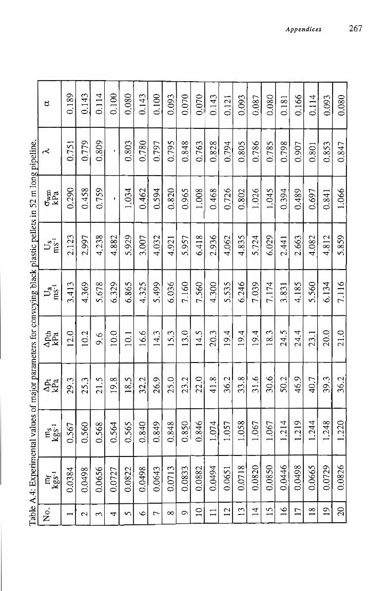
Appendices 267 pe
line.
o. 60 C o E
d lO c
llet
si
astíc
pe
" 0 .
t
or c
onve
ying
bl
nete
rs f
of m
ajor
par
ai
valu
es
enta
l 4:
Exp
erim
<
Tab
le
B
c<
Ê cd ^<2-(
^B
^l
•3 d 0 , 0 1
0 , 0 . <M
S oû M
C 60
No
.
C3V 00
0
r - ( >o r-0
.290
0
cn d r-H
d
3.41
3
0 d
cn o\ d
567
0
0.03
84
, - H
cn •^* , -H
0
.779
0
.458
0
.997
d
4.36
9
d 0
cn >o d
560
0
0.04
98
d
' î t , -H r H
0
.809
0
.759
0
.238
T t
5.67
8
vo
>o ,-H
d
568
0
0.06
56
cn
0 0 r—(
0
t
1
.882
• *
6.32
9
0
0
0 0
o ,—H
564
0
0.07
27
' t
.080
0
.803
0
.034
, - H
.929
>o
6.86
5
0
>o 00 —H
565
0
0.08
22
>o
cn • ^ ,-H
0
.780
0
462
0
.007
cn
4.32
5
vo VO
d d cn
840
0
0.04
98
VO
0 0
0
.797
0
594
0
032
^*
5.49
9
cn ' í t
0\ vo d
849
0
0.06
43
r-
093
0
795
0
820
0
T-H
d 0\ T t
6.03
6
cn >o
0
>o d
848
0
0.07
13
00
070
0
848
0
965
0
957
>o
7.16
0
0
cn
d cn d
850
0
0.08
33
0\
070
0
763
0
008
^ 41
8
VO
7.56
0
10
r t
0
d d
846
0
0.08
82
0
cn r—(
0
828
0
468
0 93
6
d
4.30
0
cn 0
00
T t
.074
0.
0494
^
T-H d
0
794
0
726
0
062
Tt
5.53
5
Tt 0\
d VO cn
.057
0.
0651
d
093
0
805
0
802
0
835
T t
6.24
6
r t o\
00
cn cn
.058
0.
0718
cn
087
0
786
0
026
-^
724
>o 7.
039
r t 0\
VO
cn
.067
0.
0820
T t
080
0
785
0
045
«-H
029
vo
7.17
4
c^ 00
VO
0 cn
.067
0.
0850
>o
0 0
0
798
0
394
0
T t d
3.83
1
>o • t d
d 0 »0
.214
0.
0446
vo
166
0
907
0
489
0
663
d
4.18
5
" t •rt d
0\
vo
.219
0.
0498
t--
"*
0
r—( 0 00 0
697
0
082
• t
5.56
0 23
.
r-0 • ^
.244
0.
0665
0 0
093
d
853
0
841
0
812
• ^
6.13
4 0
20.
cn 0\ cn
248
0.07
29
0\
080
d
847
0
066
, - H
859
>o
7,11
6 0
d
d vd cn
220
0.08
26
0 d
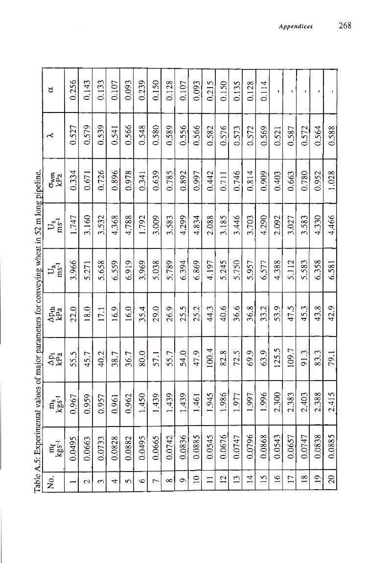
Appendices 268
<u" c
ipel
i
o. 60 C O^
S d >o c
• r ^ •4—t cd (U -G ^
60 _C 'SL
nve^
o o Ui
t2 <4-H
i2
a (U
^ o. IH
o
ofm
aj
ues
val
tal
c <u
E D. X U >o < ^
Z E2
s
r<
S ed
,
„
D"|
5 cd O.0H
<\M
Jt cd
<M
^ "»CO
6 "=* M
^
S 60 M
6 Z
VO
>o d
d
r~ d >o d
Tt cn cn d
r-•<í-
r-;
VO VO o\ cn
q d" d
>o »o >o
r-VO ON
o'
>o 0\ rt o d
T—(
cn • ^
,-H
o'
o r->o d
,-H
r-vo d
o VO T—1
cn
1—1
r-d >o
q oo' ,-H
r-; >o •st
o\ >o ON
d
cn VO VO
o d
d
cn cn r—(
d
0\
cn »o d
vo d r-d
d
cn >o cn
oo lO vq iri
r—(
r- ,-H
Cj
d • ^
r->o ON
o'
cn cn r-o d
cn
r-o ,-H
o'
,-H
• ^
>o d
VO
o oo d
oo vo cn Tt'
o\ >o lO
vd
<0\
vd ,—1
r-; oo' cn
r—(
VO o\ d
oo d oo o d
• ^
cn ON
o o'
VO VO >o d
oo r-<a\ d
oo oo r-•"^ '
o\ — H
0\
vd
o vd ,—(
r-; vd cn
d VO O
d
d oo oo o d
»o
ON
cn d
o"
oo • ^
>o d
,-H
^* cn d
d
<rv r-; ,-H
0\ vo ON
cn
• ^ ,
>o" cn
q d OO
o >o • ^ _
»o o\ •5t
o d
VO
O >o r-H
o"
o oo lO
d
o\ cn vo d
0\ o q cn
oo cn q >o"
q 0\ d
,-H
r-' >o
o\ cn • ^ _
»o vo VO o d
r-1
oo d ,—(
d
<Jv oo lO
d
»o oo r-d
cn oo »o cn
o\ oo r-; »in
o\ vd d
r-; >o >o
o\ cn Tt
d Tt r-o d
'OO
r-o r—(
d
VO >o >o d
d 0\ oo d
ON CTN d • ^ '
Tt o\ cn vd
>o >o" d
o ^* lO
o\ cn •<t
vo cn oo o d
Ov
cn o\ o d
vo vo >o d
r-0\ 0\
d
rt cn oo rt'
o\ vo c» vd
d
>o' d
o\ r-^
,-H
vo • *
»o oo oo o d
o
>o d
d
d oo >o d
d ^ Tt
d
00 oo q d'
r-o\ ^ ^
cn rt' ^
• ^
o' O
>o Tt o\
>o Tt >o o d
1
o >o
d
vo r->o d
r-(
r-d
m oo ,-H
cn
>o Tt d
>o'
VO
d '^
oo ci oo
VO oo o\
VO
r-VO o d
d
>o cn
d
cn r->o d
vO Tt r-d
vo • ^
Tf cn
o »o r->o
vq vd cn
>o d' r-
r-r-0\
r-• ^
r-o d
cn
oo d
d
d r->o d
• ^
,-H
oo d
cn o r-; cn
ir->o <y\
>o'
C<3
vd cn
Ov o< vo
r-0\ 0\
vO 0\ r-o d
• ^
rj
r H
o'
0\ vo >o d
ON o ON d
o <3V d
^'
r-r->o vd
d
cn' cn
<0\ cn VO
vo o\ 0\
oo vo oo o d
>o
1
d >o d
cn o • ^
d
d <J\ q d'
oo oo cn ' '
ON
cn lO
>o >o d
o o cn d*
m Tt >o o d
vo
1
t--oo >o d
m vo VO
d
r-d
q cn
d ,-H
^.
>o
»o r> • *
t-; Ov'
o —H
m oo m d'
t^ >o vo o d
t--
1
d 1—->o d
o oo r-d
m oo »o cn
m oo >o >o'
cn )0 -«t
cn r—1
o\
m o •ít
d'
r-• *
r-o d
00
1
Tt VO >o d
d >o o\ d
o m m •ít
oo »o m_ vo'
oo m' • *
cn cn 00
oo oo cn d'
oo m oo O o'
O^
1
oo oo >o d
oo d
q —H
vo VO • ^
• ^
^ H
oo >o vd
Os d' • *
,-H
ON r-
>o —H
• * _
d'
»o oo oo o d
o d
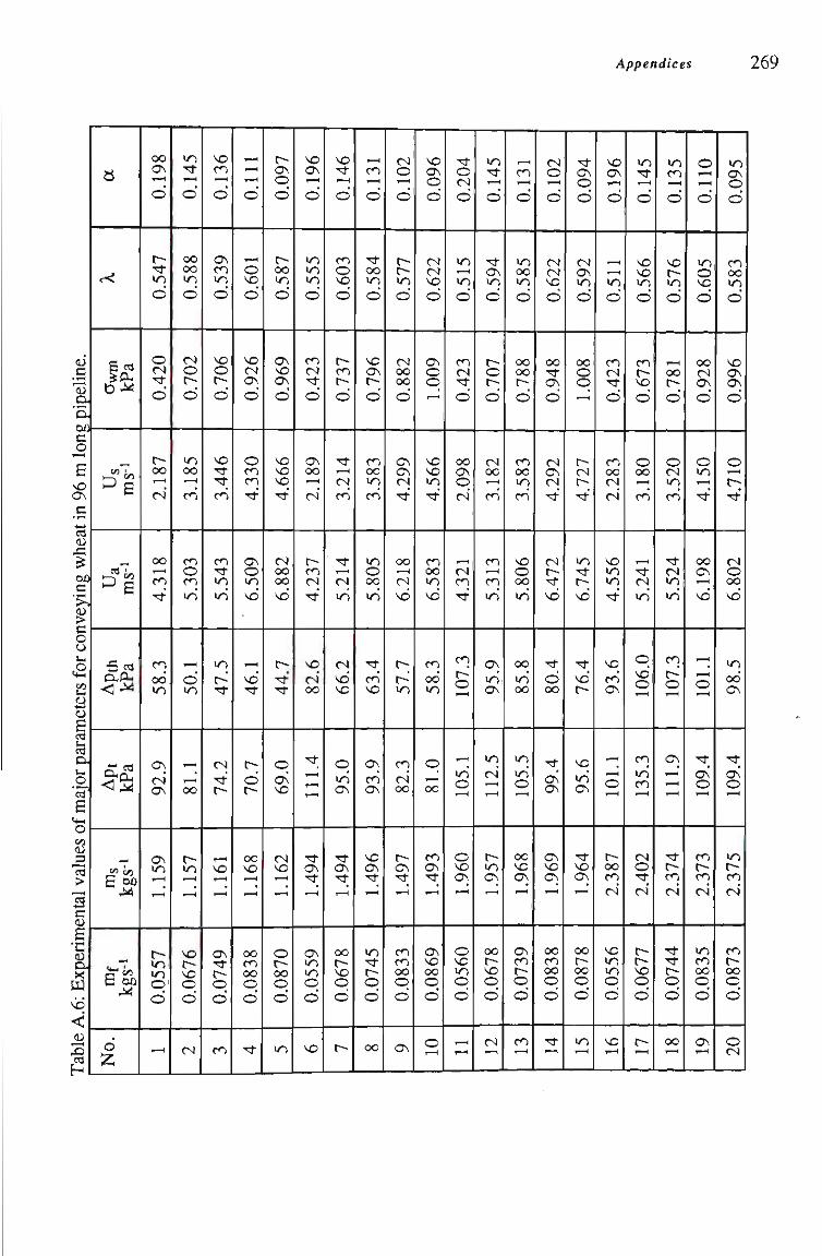
Appendices 269
<u c
o. D-no c O
6 vn
c . r N • ,H cd <U
JC
00
c
conv
eyi
(^
eter
í
c
o.
ues
of m
ajor
cd
>
enta
l pe
rim
X
u vd <
ble
cd H
S
c ^
S cd
- 's
r ^
^ C O
^f=
•3 cd
t22
- f cd 0.£2 < S
««5 E 'M)
M
C' "5 E 60 TÍ-Í
d :z;
oo o^ O
r-• ^
>o o
o d • ^
o
r-oo 7—1
d
oo 7—1
m • ^ '
m oo' »o
0\ d 0\
0\ »o r-H
r-»o l O o o
, - H
«o •^
o
oo oo >o o
d
o r-o
»o oo r H
m
m o m >o
, - H
o >o
^
oo
r->o
VO t ^ VO o o
d
\o m
o
<0\
m >o d
vo o i - -
o
vo • ^
• ^
m
m • ^
>o >o
>o r-• *
d
T t r -
r H
vo r H
<7\ •ct r-o o
m
'~~*
o
—H
<-<) \o o
VO d <T\ O
O m m • ^
o\ o >o vd
r H
VO • ^
r-o r -
oo VO , - H
0 0 m <» o o
^*
r-<j\ o o
r-oo «o o
o\ VO C3N O
vo VO vo T f
d oo oo vo
r-• *
• ^
o 0\ vo
d vo , - H
o r-<50 o o
>o
\ 0 CA T - H
o
l O
>o >o o
m d • t
O
o\ oo T - H
CM
r-m d x t
VO
d oo
T t
s
• *
C7\ xt
f7\ >o >o o d
VO
vo •<í
'—' o
m o vo o
r-m r-o
^* , - H
d
m
T t ^ H
d
>o
d
vo VO
O >o ON
•<t <7\ ^
oo r-VO o o
r-
—H
m r H
O
• ^
oo >o o
VO <^ r-o
m oo >o m
>o o oo
>o
^ m vo
0 \
m <7\
vo C7\ ^
>o • ^
r-o o
(X>
d O r H
O
r-r-l O
o
d oo oo O
o\ 0\ d
' î t
oo 7—1
d
vo
r-r->o
m d oo
r-<7\ ^
m m 00 O o
<J\
vo <0\ o o
d d VO
o
0 \ o o , - H
vo VO >o '(t
m oo >o vo
m oo >o
o 7—1
oo
m <7\ ^
C7\ VO OO O O
O
"(t O d
o
>o , - H
>o o
m d •<t
o
oo 0\ o d
d m r t
m_ r-' o r H
- : >o o r H
O VD o\
O VD >o O O
H H
>o ^* 7—1
o
"<t CT\ >o o
r-O r-o
d oo T - H
m
m 7—1
m »o
0\ >o OV
>o d ,-H
r->o C3\
oo r-VO O o
d
m T - H
o
>o oo >o o
oo oo r-o
m oo l O
m
vo O oo m
oo >o oo
>o >o" o , - H
oo vo <y\
<j\ m r-o o
m
d o
o
d d vo O
oo • ^ ON
d
d C7V d
^
d r-T t
vo
'^ d oo
T t
o o\
o\ vo o\
0 0
m oo o O
^*
Tt-CT\ O
O
d i7 \ >o o
oo o o - H
r-d r-^
>o ^ r-vo
'^ VO r-
VO
»o C \
T t vo <7\
oo r-oo O o
>o
vO o\ , - H
o
, - H
,—( >o o
m d r t o
m oo d d
VO »o >o r t
vo m o\
- .
o r H
r-oo m d
VO
>o >o o o
vo
>o r t
O
vn vn >o o
m r-VO
o
o oo —H
m
^* d
>o
o vd o , - H
m >o m ,-H
d o • t d
r-r-VO o o
r-
>o m
o
vo r->o o
, - H
oo r-d
o d >o m
•<;t d >o >o
cn r- o
o\
, -H r H
•<t r-m d
• t r t t ^ o o
oo
o , - H , - H
o
>o o VO
o
oo d <3\
o
O >o
• ^
oo OS T - H
VO
, - H
r H
o
• r t
0 \ o r H
m r-m d
>o m oo O O
ON
>o (^ o o
m oo >o o
VO o\ OS
o
o
r-• ^
d o oo vo
>o oo (3\
T t
o\ O ,-H
«o r-m d
m t ^ oo o o
o d
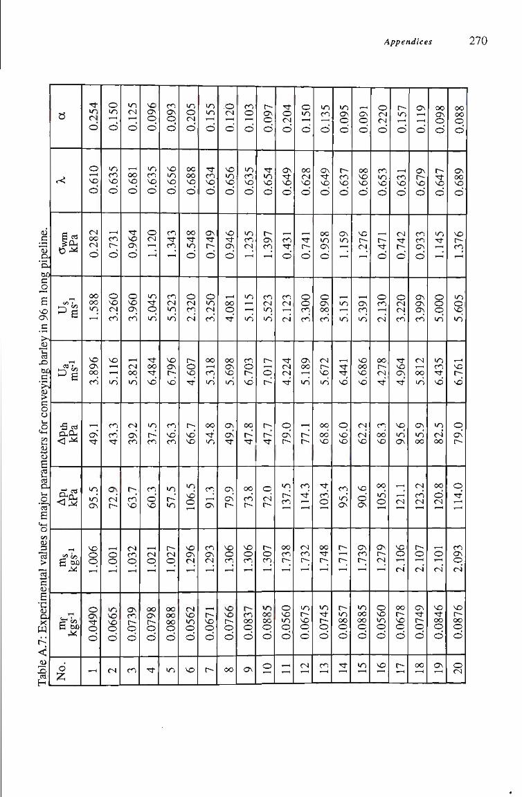
Appendices 270 g
pipe
Une
. y
in 9
6 m
lon
enta
l va
lues
of
maj
or p
aram
eter
s fo
r con
veyi
ng b
arle
A
,7:
Exp
erim
T
able
S
<<
E cd h
^ S
6 cd C O H <:\M
r^ <^
<22
S <iû M
E 60 TÍ«Í
No.
0.25
4
0,61
0 0.
282
1.58
8 3.
896
49.1
95
.5
1.00
6 0,
0490
-
0.15
0 0.
635
0.73
1 3.
260
5.11
6 43
.3
72.9
, -H o o
0.06
65
d
0.12
5 0.
681
0.96
4 3.
960
5.82
1 39
.2
63.7
1.
032
0.07
39
m
0.09
6
0.63
5 1.
120
5.04
5 6.
484
37.5
60
.3
7—1
d o
0.07
98
• *
0.09
3
0.65
6 1.
343
5.52
3 6.
796
36.3
57
.5
1.02
7 0.
0888
>o
0.20
5
0.68
8 0.
548
2.32
0 4.
607
66.7
10
6.5
1.29
6 0.
0562
VO
0.15
5 0.
634
0.74
9 3.
250
5.31
8 54
.8
91.3
1.
293
0.06
71
r-
0.12
0 0.
656
0.94
6 4.
081
5.69
8 49
.9
79.9
1.
306
0.07
66
oo
0.10
3 0.
635
1.23
5 5.
115
6.70
3 47
.8
73.8
1.
306
0.08
37
<7\
0.09
7 0.
654
1.39
7 5.
523
7.01
7 47
.7
72.0
1.
307
0.08
85
o
0.20
4 0.
649
0.43
1 2.
123
4.22
4 79
.0
137.
5 1.
738
0.05
60
-^
0.15
0 0.
628
0.74
1 3.
300
5.18
9 77
.1
114.
3 1.
732
0.06
75
d
0.13
5 0.
649
0.95
8 3.
890
5.67
2 68
.8
103.
4 1.
748
0.07
45
m
0.09
5 0.
637
1.15
9 5.
151
6.44
1
0*99
95.3
I.
7I7
0.
0857
• ^
0.09
1 0.
668
1.27
6 5.
391
6.68
6 62
.2
90.6
1.
739
0.08
85
vo
0.22
0 0.
653
0.47
1 2.
130
4.27
8 68
.3
105.
8 1.
279
0.05
60
vo
0.15
7 0.
631
0.74
2 3.
220
4.96
4
9*56
121.
1 2.
106
0.06
78
r-
0,11
9 0.
679
0.93
3
3.99
9
5.81
2 85
.9
123.
2 2,
107
0,07
49
oo
0,09
8 0,
647
1.14
5 5.
000
6.
435
82.5
12
0,8
2.10
1 0.
0846
a\
0.08
8
0.68
9 1.
376
5.60
5 6.
761
79.0
11
4.0
2.09
3 0.
0876
o d
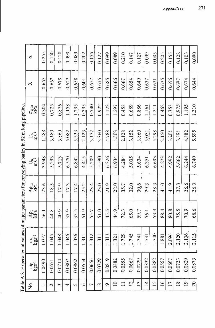
Appendices 271
di c
•
• o .
y in
52
m lo
n en
tal
valu
es o
f m
ajor
par
amet
ers
for c
onve
ying
bar
le
A.8
: E
xper
ím
Tab
le
a
cs;
g ed ^ O H
^M
^B
^ E
•a cd O - O H
c ^ <M
J«C<3 E t>û
c ' ^ E 60
T Í ^
No.
1 0.
255
0.65
5
0.30
4 1.
588
3.94
8 23
.6
56,1
r-
o
0,04
90
-
0,15
0 0,
662
0,72
5 3,
180
5.29
3 18
.5
44.8
1.
045
0.06
51
d
0.12
0 0.
679
0.87
6 3.
860
5.71
3 17
.9
40.9
1.
048
0.07
14
m
0.09
9
0.62
7 1,
158
5,08
2 6,
570
17,3
37
.9
1.04
6 0.
0807
T t
0.08
9 0.
658
1.29
5 5.
533
6.84
2 17
.4
35.5
1.
036
0.08
62
>o
0.20
2 0.
601
0.39
5
2.12
3 4.
415
25.2
61
.9
T-H
m
0.05
54
vo
0.15
5 0.
657
0.74
0
3.17
2 5.
209
23.4
55
.7
1.31
2 0.
0656
r-
0.12
7 0.
675
0.92
2 3.
860
5.59
0 23
.0
51.0
m
0.07
29
oo
0.09
9 0.
685
1.12
3 4.
788
6.32
6 21
.9
45.5
m ,-H
m
0.08
19
<y\
0.08
9 0.
666
1.
297
5.50
3 6.
934
22.0
44
.9
d m
0.08
82
o
0.21
0 0.
667
0.45
8 2.
128
4.28
4 35
.7
72.3
1.
729
0.05
55
^
0.14
7 0.
654
0.68
9 3.
152
5.03
5 32
.0
65.0
1,
745
0,06
62
d
0.12
7 0.
649
0.88
6 3.
860
5.63
4 30
.6
59.7
7—1
•^ r-
0.07
29
m
0.09
9 0.
637
1.16
1 5.
051
6.35
1 29
.3
56.1
,-H m r-
0.08
32
' t
0.08
5 0.
671
1.21
1 5.
298
6.69
3 28
.3
53.3
1.
740
0.08
82
>o
0.20
5 0.
675
0.46
2 2.
150
4.27
3 41
.0
88.4
—H oo oo
0.05
57
vo
0.15
5 0.
656
0.75
3 3.
201
4.99
2 41
.9
80.8
2,
096
0,06
67
r-
0,12
8 0.
697
0.97
5
3.89
1 5.
662
37.3
75
.5
2,12
0 0,
0733
oo
0.10
3 0.
674
1.19
5 4.
882
6.24
4 36
.6
70.9
2.
106
0,08
29
<3\
0,09
0
0,64
4 1.
310
5,
595
6,74
0 36
.3
9*89
2.11
5 0.
0873
o d
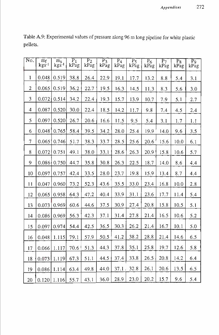
Appendices 272
Table A.9: Experimental values of pressure along 96 m long pipeline for white plastíc pellets.
No.
1
2
3
4
5
6
7
8
9
10
11
12
13
14
15
16
17
18
19
20
mf kgs-i
0.048
0.065
0.072
0.087
0.097
0.048
0.065
0.072
0.086
0.097
0.047
0.065
0.073
0.086
0.097
0.048
0.066
0.073
0.086
0.120
m^ kgs-i
0.519
0.519
0.514
0.520
0.520
0.765
0.746
0.751
0.750
0.757
0.960
0.958
0.969
0.969
0.974
1.115
1.117
1.119
1.114
1.116
Pl kPag
38.8
36.2
34.2
30.0
26.7
58.4
51.7
49.1
44.7
42.4
73.2
64.3
60.6
56.3
54.4
79.1
70.6
67.3
63.4
55.7
P2 kPag
26.4
22.7
22.4
22.4
20.6
39.5
38.3
38.0
35.8
33.5
52.3
47.2
44.6
42.3
42.5
57.9
51.3
51.1
49.8
43.1
P3 kPag
22.9
19.5
19.3
18.5
16.6
34.2
33.7
33.1
30.8
28.0
43.6
40.4
37.5
37.1
36.5
50.5
44.3
44.5
44.0
36.0
P4 kPag
19.1
16.3
15.7
14.2
11.5
28.0
28.5
28.6
26.3
23.7
35.5
33.9
30.9
31.4
30.3
41.2
37.8
37.4
37.1
28.9
Ps kPag
17.7
14.5
13.9
11.7
9.5
25.4
25.6
26.3
22.5
19.8
33.0
31.1
27.4
27.8
26.2
38.2
35.1
33.8
32.8
23.0
P6 kPag
13.2
11.3
10.7
9.8
5.4
19.9
20.6
20.9
18.7
15.9
23.4
23.6
20.8
21.4
21.4
28.8
25.8
26.5
26.1
20.2
P? kPag
8.8
8.3
7.9
7.4
3.1
14.0
15.6
15.8
14.0
13.4
16.8
17.7
15.8
16.5
16.7
21.4
19.7
20.8
20.6
15.7
Pg kPag
5.4
5.6
5.1
4.5
1.7
9.6
10.0
10.6
8.6
8.7
10.0
11.4
10.5
10.6
10.1
14.6
12.6
14.2
13.5
9.6
P9 kPag
3.1
3.0
2.7
2.4
1.1
3.5
6.1
5.7
4.4
4.4
2.8
5.4
5.1
5.2
5.0
6.5
5.8
6.4
6.5
5.4
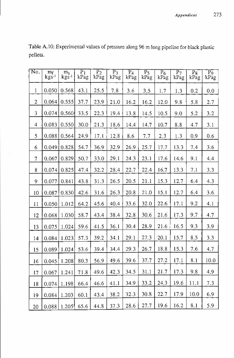
Appendices 273
Table A.IO: Experimental values of pressure along 96 m long pipeline for black plastíc pellets.
No.
1
2
3
4
5
6
7
8
9
10
11
12
13
14
15
16
17
18
19
20
mf kgs-i
0,050
0,064
0,074
0.083
0.088
0.049
0.067
0.074
0.077
0.087
0.050
0.068
0.075
0.084
0.089
0.045
0.067
0.074
0.084
0.088
ms kgs-i
0.568
0.555
0.560
0.550
0.564
0.828
0.829
0.825
0.841
0.830
1.012
1.030
1.024
1.023
1.024
1.208
1.241
1.198
1.203
1.205
Pl kPag
43.1
37.7
33.5
30.0
24.9
54.7
50.7
47.4
43.8
42.6
64.2
58.7
59.6
57.3
53.6
80.3
71.8
66.4
60.1
65.6
P2 kPag
25.5
23.9
22.3
21.3
17.1
36.9
33.0
32.2
31.3
31.6
45.6
43.4
41.5
39.2
39.4
56.9
49.6
46.6
43.4
44.8
Ps kPag
7.8
21.0
19.4
18.6
12.8
32.9
29.1
28.4
26.5
26.3
40.4
38.4
36.1
34.1
34.4
49.6
42.3
41.1
38.2
37.3
P4 kPag
3.6
16.2
13.8
14.4
8.6
26.9
24.3
22.7
20.5
20.8
33.6
32.8
30.4
29.1
29.3
39.6
34.5
34.9
32.3
28.6
P5 kPag
3.5
16.2
14.5
14.7
7.7
25.7
23.1
22.4
21.1
21.0
32.0
30.6
28.9
27.3
26.7
37.7
31.1
33.2
30.8
27.7
Pô kPag
1.7
12.0
10.5
10.7
2.3
17.7
17.6
16.7
15.3
15.1
22.6
21.6
21.6
20.1
18.8
27.2
21.7
24.3
22.7
19.6
P? kPag
1.3
9.8
9.0
8.8
1.3
13.3
14.6
13.3
12.7
12.7
17.1
17.3
16.5
15.7
15.3
17.1
17.3
19.6
17.9
16.2
Pg kPag
0.2
5.8
5.2
4.7
0.9
7.4
9.1
7.1
6.4
6.4
9.2
9.7
9.3
8.5
7.6
8.1
9.8
11.1
10.0
8.1
P9 kPag
0.0
2.7
3.2
3.1
0.6
3.6
4.4
3.3
4.3
3.6
4.1
4.7
3.9
3.3
4.7
10.0
4.9
7.3
6.9
5.9
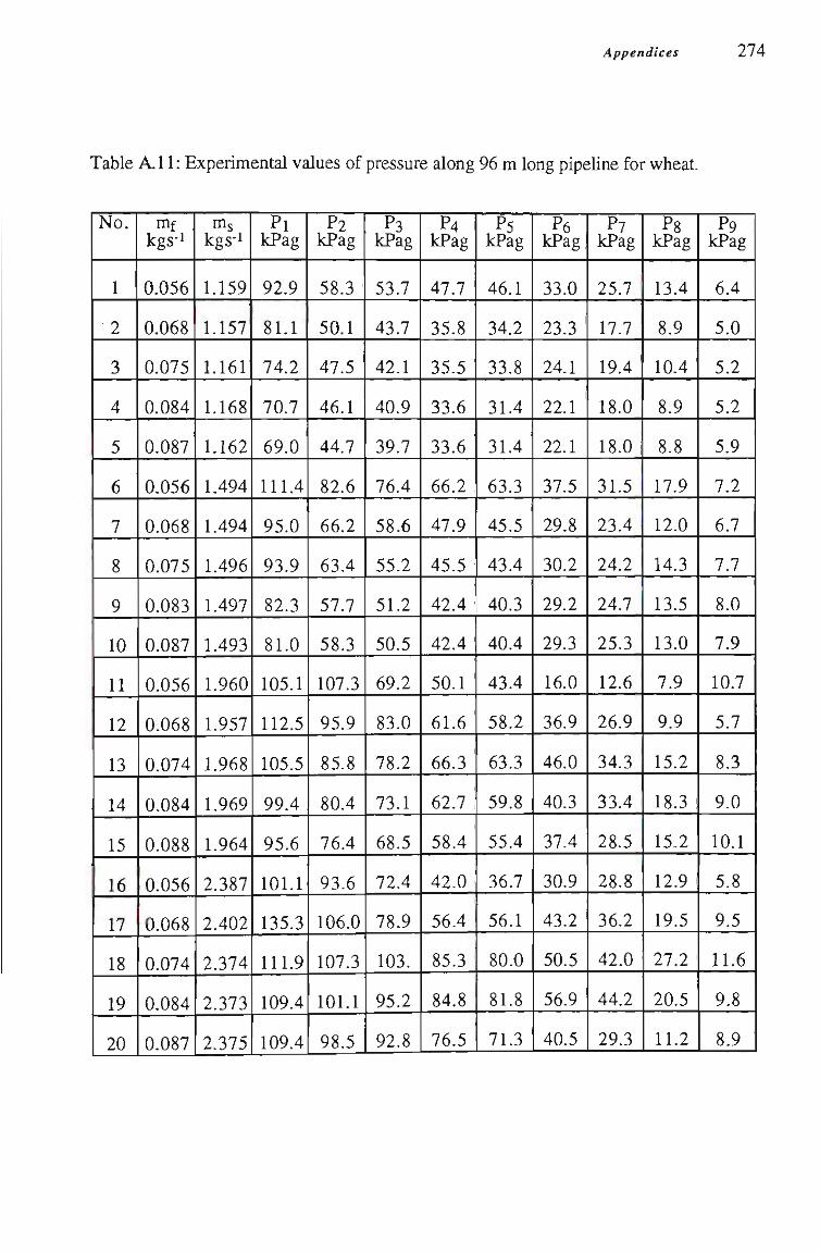
Appendices 274
Table A.11: Experimental values of pressure along 96 m long pipeUne for wheat.
No.
1
2
3
4
5
6
7
8
9
10
11
12
13
14
15
16
17
18
19
20
mf kgs-i
0.056
0.068
0,075
0,084
0,087
0.056
0.068
0.075
0.083
0.087
0.056
0.068
0.074
0.084
0.088
0.056
0.068
0.074
0.084
0.087
ms kgs-i
1.159
1.157
1.161
1.168
1.162
1.494
1.494
1.496
1.497
1.493
1.960
1.957
1.968
1.969
1.964
2.387
2.402
2.374
2.373
2.375
Pl kPag
92.9
81.1
74.2
70.7
69.0
111.4
95.0
93.9
82.3
81.0
105.1
112.5
105.5
99.4
95.6
101.1
135.3
111.9
109.4
109.4
P2 kPag
58.3
50.1
47.5
46.1
44.7
82.6
66.2
63.4
57.7
58.3
107.3
95.9
85.8
80.4
76.4
93.6
106.0
107.3
101.1
98.5
P3 kPag
53.7
43.7
42.1
40.9
39.7
76.4
58.6
55.2
51.2
50.5
69.2
83.0
78.2
73.1
68.5
72.4
78.9
103.
95.2
92.8
P4 kPag
47.7
35.8
35.5
33.6
33.6
66.2
47.9
45.5
42.4
42.4
50.1
61.6
66.3
62.7
58.4
42.0
56.4
85.3
84.8
76.5
P5 kPag
46.1
34.2
33.8
31.4
31.4
63.3
45.5
43.4
40.3
40.4
43.4
58.2
63.3
59.8
55.4
36.7
56.1
80.0
81.8
71.3
Pô kPag
33.0
23.3
24.1
22.1
22.1
37.5
29.8
30.2
29.2
29.3
16.0
36.9
46.0
40.3
37.4
30.9
43.2
50.5
56.9
40.5
P? kPag
25.7
17.7
19.4
18.0
18.0
31.5
23.4
24.2
24.7
25.3
12.6
26.9
34.3
33.4
28.5
28.8
36.2
42.0
44.2
29.3
Pg kPag
13.4
8.9
10.4
8.9
8.8
17.9
12.0
14.3
13.5
13.0
7.9
9.9
15.2
18.3
15.2
12.9
19.5
27.2
20.5
11.2
P9 kPag
6.4
5.0
5.2
5.2
5.9
7.2
6.7
7.7
8.0
7.9
10.7
5.7
8.3
9.0
10.1
5.8
9.5
11.6
9.8
8.9
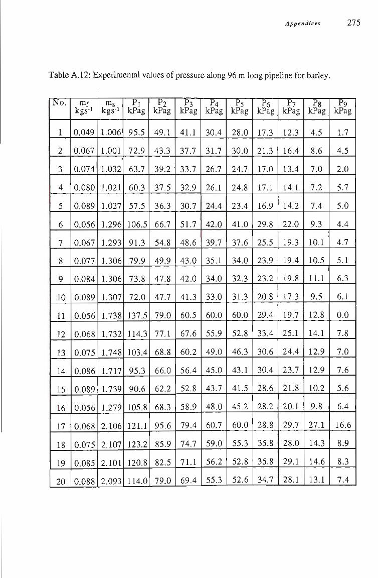
Appendices 275
Table A.12: Experimental values of pressure along 96 m long pipeUne for barley.
No.
1
2
3
4
5
6
7
8
9
10
11
12
13
14
15
16
17
18
19
20
mf kgs-i
0,049
0,067
0,074
0,080
0,089
0,056
0.067
0.077
0.084
0.089
0.056
0.068
0.075
0.086
0.089
0.056
0.068
0.075
0.085
0.088
m^ kgs-i
1.006
1.001
1.032
1.021
1.027
1.296
1.293
1.306
1.306
1.307
1.738
1.732
1.748
1.717
1.739
1.279
2.106
2.107
2.101
2.093
Pl kPag
95.5
72.9
63.7
60.3
57.5
106.5
91.3
79.9
73.8
72.0
137.5
114.3
103.4
95.3
90.6
105.8
121.1
123.2
120.8
114.0
P2 kPag
49.1
43.3
39.2
37.5
36.3
66.7
54.8
49.9
47.8
47.7
79.0
77.1
68.8
66.0
62.2
68.3
95.6
85.9
82.5
79.0
P3 kPag
41.1
37.7
33.7
32.9
30.7
51.7
48.6
43.0
42.0
41.3
60.5
67.6
60.2
56.4
52.8
58.9
79.4
74.7
71.1
69.4
P4 kPag
30.4
31.7
26.7
26.1
24.4
42.0
39.7
35.1
34.0
33.0
60.0
55.9
49.0
45.0
43.7
48.0
60.7
59.0
56.2
55.3
Ps kPag
28.0
30.0
24.7
24.8
23.4
41.0
37.6
34.0
32.3
31.3
60.0
52.8
46.3
43.1
41.5
45.2
60.0
55.3
52.8
52.6
Pô kPag
17.3
21.3
17.0
17.1
16.9
29.8
25.5
23.9
23.2
20.8
29.4
33.4
30.6
30.4
28.6
28.2
28.8
35.8
35.8
34.7
P? kPag
12.3
16.4
13.4
14.1
14.2
22.0
19.3
19.4
19.8
17.3
19.7
25.1
24.4
23.7
21.8
20.1
29.7
28.0
29.1
28.1
Pg kPag
4.5
8.6
7.0
7.2
7.4
9.3
10.1
10.5
11.1
9.5
12.8
14.1
12.9
12.9
10.2
9.8
27.1
14.3
14.6
13.1
P9 kPag
1.7
4.5
2.0
5.7
5.0
4.4
4.7
5.1
6.3
6.1
0.0
7.8
7.0
7.6
5.6
6.4
16.6
8.9
8.3
7.4
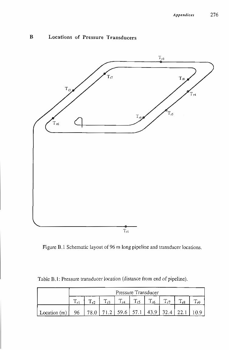
B Locations of Pressure Transducers
Appendices 2 7 6
Trl
Figure B.l Schematic layout of 96 m long pipeline and transducer locatíons.
Table B.l: Pressure transducer location (distance from end of pipeline).
Locatíon (m)
Pressure Transducer
Trl
96
Tr2
78.0
Tr3
71.2
Tr4
59.6
Tr5
57.1
Tr6
43.9
Tr7
32.4
Tr8
22.1
T^
10.9
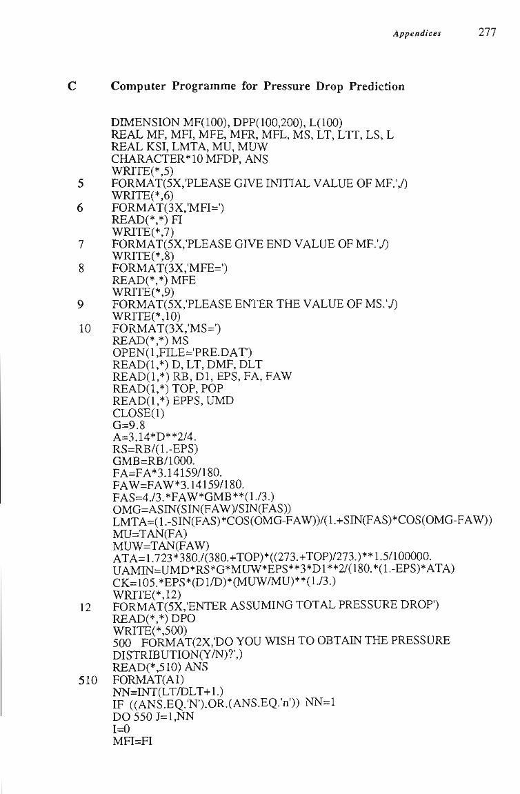
Appendices 2 7 7
Computer Programme for Pressure Drop Prediction
DIMENSION MF(IOO), DPP(100,200), L(IOO) REAL MF, MFI, MFE, MFR, MFL, MS, LT, LTT, LS, L REAL KSI, LMTA, MU, MUW CHARACTER*10 MFDP, ANS WRITE(*,5)
5 F0RMAT(5X,'PLEASE GIVEINITIAL VALUE OF MF.',/) WRITE(*,6)
6 F0RMAT(3X,'MFI=') READ(*,*) m WRITE(*,7)
7 F0RMAT(5X,'PLEASE GIVE END VALUE OF MF.',/) WRITE(*,8)
8 F0RMAT(3X,'MFE=') READ(*,*) MFE WRITE(*,9)
9 F0RMAT(5X,'PLEASE ENTER THE VALUE OF MS.'^) WRITE(*,10)
10 F0RMAT(3X,'MS=') READ(*,*) MS OPEN( 1 ,FILE='PRE.D AT') READ(1,*) D, LT, DMF, DLT READ(1,*) RB, Dl, EPS, FA, FAW READ(1,*) TOP, POP READ(1,*)EPPS,UMD CLOSE(l) G=9.8 A=3.14*D**2/4. RS=RB/(1.-EPS) GMB=RB/1000. FA=FA*3.14159/180. FAW=FAW*3.14159/180. FAS=4./3.*FAW*GMB**(l./3.) OMG=ASIN(SIN(FAW)/SIN(FAS)) LMTA=(1.-SIN(FAS)*C0S(0MG-FAW))/(1.+SIN(FAS)*C0S(0MG-FAW)) MU=TAN(FA) MUW=TAN(FAW) ATA=1.723*380./(380.+TOP)*((273.+TOP)/273.)**1.5/100000. UAMIN=UMD*RS*G*MUW*EPS**3*D1**2/(180.*(1.-EPS)*ATA) CK=105.*EPS*a01/D)*(MUW/MU)**(l./3.) WRITE(*,12)
12 F0RMAT(5X,'ENTER ASSUMING TOTAL PRESSURE DROP') READ(*,*) DPO WRITE(*,500) 500 F0RMAT(2X,'D0 YOU WISH TO OBTAIN THE PRESSURE DISTRIBUTION(Y/N)?',) READ(*,510)ANS
510 FORIvlAT(Al) NN=INT(LT/DLT+1.) IF ((ANS.EQ.'N').OR.(ANS.EQ.'n')) NN=1 DO550J=l,NN 1=0 MFI=FI
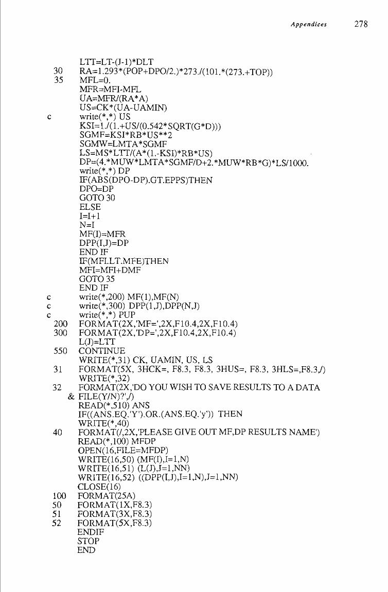
Appendices 278
LTr=LT-(J-l)*DLT 30 RA=1.293*(POP+DPO/2.)*273./(101.*(273.+TOP)) 35 MFL=0.
MFR=MFI-MFL UA=MFR/(RA*A) US=CK*(UA-UAMIN)
c write(*,*) US KSI= 1./(1 .+US/(0.542* SQRT(G*D))) SGMF=KSI*RB*US**2 SGMW=LMTA*SGMF LS=MS*LTT/(A*(1.-KSI)*RB*US) DP=(4.*MUW*LMTA*SGMF/D+2.*MUW*RB*G)*LS/1000. write(*,*) DP IF(ABS(DPO-DP).GT.EPPS)THEN DPO=DP GOTO 30 ELSE 1=1+1 N=I MF(I)=MFR DPP(I,J)=DP ENDIF IF(MFLLT.MFE)THEN MFI=MFI+DMF GOTO 35 ENDIF
c write(*,200) MF(1),MF(N) c write(*,300) DPP(1,J),DPP(N,J) c write(*,*) PUP
200 FORMAT(2X,'MF=',2X,F10.4,2X,F10.4) 300 FORMAT(2X,'DP=',2X,F10.4,2X,F10.4)
L(J)=LTT 550 CONTINUE
WRITE(*,31) CK, UAMIN, US, LS 31 F0RMAT(5X, 3HCK=, F8.3, F8.3, 3HUS=, F8.3, 3HLS=,F8.3y)
WRITE(*,32) 32 F0RMAT(2X,'D0 YOU WISH TO SAVE RESULTS TO A DATA
& FILE(Y/N)?',/) READ(*,510)ANS IF((ANS.EQ.'Y').OR.(ANS.EQ.'y')) THEN WRITE(*,40)
40 F0RMAT(/,2X,'PLEASE GIVE OUT MF,DP RESULTS NAME') READ(*,100)MFDP OPEN( 16,FILE=MFDP) WRITE( 16,50) (MF(I),I=1,N) WRITE( 16,51) (L(J),J=1,NN) WRITE(16,52) ((DPP(I,J),I=1,N),J=1,NN) CL0SE(16)
100 FORMAT(25A) 50 F0RMAT(1X,F8.3) 51 FORMAT(3X,F8.3) 52 FORMAT(5X,F8.3)
ENDIF STOP END
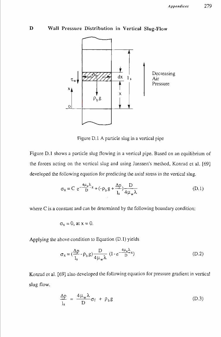
Appendices 279
D Wall Pressure Distribution in Vertical Slug-Flow
\ mm
0
Phê
JL dx 1
Decreasing Air Pressure
Figure D. 1 A particle slug in a vertícal pipe
Figure D.l shows a partícle slug flowing in a vertical pipe. Based on an equilibrium of
the forces acting on the vertical slug and using Janssen's method, Konrad et al. [69]
developed the following equatíon for predicting the axial stress in the vertícal slug.
c7x = C e D + ( - P b g + V ^ T ; - T (D.l)
where C is a constant and can be determined by the following boundary condition:
Ox = 0, at X = 0.
Applying the above conditíon to Equatíon (D.l) yields
ax = ( - ^ - P b g ) 7 - T ( l - e D ^) (D.2)
Konrad et al. [69] also developed the foUowing equatíon for pressure gradient in vertícal
slug flow.
Ap _ 4lt^X = fTf +
Is D CTf + Pbg (D.3)
Appendices 2 8 0
where CTf is the stress on the front surface of tíie slug.
Substítutíng Equatíon (D.3) into Equatíon (D.2) and replacing a^ witfi cJX:
aw = X.af(l-e ~~S~^) (D.4)
E Publications While PhD Candidate
1 Mi, B. and Wypych, P.W., Partícle Slug Velocities in Horizontal Slug-Flow
Pneumatic Conveying, Powder Handling & Processing, Vol. 5, No. 3, Sep. 1993,
pp 227 - 233.
2 Mi, B. and Wypych, P.W., Predictíon of Pressure Drop and Determinatíon of
Optimal Operating Point in Low-Velocity Pneumatic Conveying, to be published in
Powder Technology.
3 Pan, R., Mi, B. and Wypych, P., Design of Pneumatíc Conveying System for
Granular Materials, International Conference on Advanced Technology and
Equipment of Materials HandUng, Shanghai, China, Oct. 25-27, 1994.
4 Pan, R., Mi, B. and Wypych, P.W., Pneumatíc Conveying Characteristícs of Fine
and Granular Bulk SoUds, to be published in Kona, No. 12, 1994.


