QuantumMechanics

L.v. Tarasov, BasicConceptsof

Although quantum mechanicsdeals with microparticles, itssignificance is by no meanslimited to microphenomena.In our endless questfor undersfanding and per­fe ing our knowledge ofthe laws of nature quantummechanics represents animportant qualitative leap.

•

-MlR-Pubiishers Moscow

~r-;'-:':---"-_-~-"""",,,,",qi------ --r-

7hi-s bOOK be/O,?-~5 to EX U 13 R I5 '.

Amit- J)haKulk01i{ ])t IB/J./J2K\

II

~ .

, I

I )

•

1

d

11. B. TapaCOB

OCHOBblKBAHTOBO~ MEXAH~K~';bA9.Ta llbCTBO

«BblCWafi WKOJla»

MOCKBa

-.1T" ...

, \.,L.V. Tarasov Basic Concepts of .

Quantum Mechanics

Translated from the Russianby Ram S. Wadhwa

MIR Publishers· Moscow

First published 1980Revised from the 1978 Russian edition

© H3AaTeJIbCTBo «BblCmaJi mKOJIa&, 197R© English translation. Mir Publishers, 1980

.,

Contents

Preface 1

Prelude. Can the System of Classical Physics Con-cepts Be Considered Logically Perfect? 12

Chapter I.

Chapter II.

Chapter Ill.

Physics of the Microparticles

Physical Foundations of Quantum Mechanics

Linear Operators in Quantum Mechanics

17

67

161

On the History of Origin and Growth of QuantumMechanics (A Brief Historical Survey) 239

Appendices 249

References 258

Subject Index 262

.,

Preface

Research in physics, conducted at the end of the 19th Some Preliminary Remarks

century and in the first half of the 20th century, revealedexceptionally peculiar nature of the laws governing thebehaviour of microparticles-atoms, electrons, and so on.On the basis of this research a new physical theory calledquantum mechanics was founded.The growth of quantum mechanics turned out to be quitecomplicated' and prolonged. The mathematical part ofthe theory, and the rules linking the theory with experi­ment, were constructed relatively quickly (by the begin­ning of the thirties). However, the understanding of thephysical and philosophical substance of the mathematicalsymbols used in the theory was unresolved for decades.In Fock's words [il, The mathematical apparatus of non­relativistic quantum mechanics worked well and was freeof contradictions; but in spite of many successful applica­tions to different problems of atomic physics the physicalrepresentation of the mathematical scheme still remaineda problem to be solved.Many difficulties are involved in a mathematical inter­pretation of the quantum-mechanical apparatus. Theseare associated with the dialectics of the new laws, theradical revision of the very nature of the questions whicha physicist "is entitled to put to nature", the reinterpreta­tion of the role of the observer vis a vis his surroundings,the new approach to the question of the relation betweenchance and necessity in physical phenomena, and therejection of many accepted notions and concepts. Quan­tum mechanics was born in an atmosphere of discussionsand heated clashes between contradictory arguments.The names of many leading scientists are linked withits development, including N. Bohr, A. Einstein,M. Planck, E. Schrodinger, M. Born, W. Pauli, A. Som­merfeld, L. de Broglie, P. Ehrenfest, E. Fermi, W. Hei­senberg, P. Dirac, R. Feynman, and others.It is also not surprising that even today anyone whostarts studying quantum mechanics encounters somesort of psychological barrier. This is not because of themathematical complexity. The difficulty arises fromthe fact that it is difficult to break away from acceptedconcepts and to reorganize one's l'attern of thinkingwhich are based on everyday experience.

Preface 7

;•••••••••••••••••••••••••••••••OI·C7Tiillill-IIIiIE"lIln__..-..·k.J&:"~••

Before starting a study of quantum mechanics, it isworthwhile getting an idea about its place and role inphysics. We shall consider (naturally in the most generalterms) the following three questions: What is quantummechanics? What is the relation between classical physicsand quantum mechanics? What specialists need quantummechanics? So, what is quantum mechanics?The question can be answered in different ways. Firstand foremost, quantum mechanics is a theory describingthe properties of matter at the level of microphenomena­it considers the laws of motion of microparticles. Micro­particles (molecules, atoms, elementary particles) arethe main "characters" in the drama of quantum me­chanics.From a broader point of view quantum mechanics shouldbe treated as the theoretical foundation of the moderntheory of the structure and properties of matter. In com­parison with classical physics, quantum mechanics consi­ders the properties of matter on a deeper and more funda­mental level. It provides answers to many questions whichremained unsolved in classical physics. For example,why is diamond hard? Why does the electrical conductivi­ty of a semiconductor increase with temperature? Whydoes a magnet lose its properties upon heating? Unableto get answers from classical physics to these questions,we turn to quantum mechanics. Finally, it must be em­phasized that quantum mechanics allows one to calculatemany physical parameters of substances. Answering thequestion "What is quantum mechanics?", Lamb [2] re­marked: The only easy one (answer) is that quantum mecha­nics is a discipline that provides a wonderful set of rulesfor calculating physical properties of matter.What is the relation of quantum mechanics to classicalphysics? First of all quantum mechanics includes classicalmechanics as a limiting (extreme) case. Upon a transitionfrom microparticles to macroscopic bodies, quantum­mechanical laws are converted into the laws of classicalmechanics. Because of this it is often stated, though notvery accurately, that quantum mechanics "works" in themicroworld and the classical mechanics, in the macro­world. This statement assumes the existence of an isolated"microworld" and an isolated "macroworld". In actualpractice We can only speak" of microparticles (micro­phenomena) and macroscopic bodies (macrophenomena).It is also significant that microphenomena form the basisof macrophenomena and that macroscopic bodies aremade up of micI'oparticles. Consequently, the transitionfrom classical physics to quantum mechanics is a transi-

8

tion not from one "world" to another, but from a shallowerto a deeper level of studying matter. This means thatin studying the behaviour of microparticles, quantummechanics considers in fact the same macroparticles,but on a more fundamental level. Besides, it must beremembered that the boundary between micro- and macro­phenomena in general is quite conditional and flexible.Classical concepts are frequently found useful when consid­ering microphenomena, while quantum-mechanical ideashelp in the understanding of macrophenomena. There iseven a special term "quantum macrophysics" which isapplied, in particular, to quantum electronics, to thephenomena of superfluidity and superconductivity andto a number of other cases.In answering the question as to what specialists needquantum mechanics, we mention beforehand that wehave in mind specialists training in engineering colleges.There are at least three branches of engineering for whicha study of quantum mechanics is absolutely essential.Firstly, there is the field of nuclear power and the appli­cation of radioactive isotopes to industry. Secondly, thefield of materials sciences (improvement of propertiesof materials, preparation of new materials with preas­signed properties). Thirdly, the field of electronics andfirst of all the field of semiconductors and laser technology.If we consider that today almost any branch of industryuses new materials as well as electronics on a large scale,it will become clear that a comprehensive training inengineering is impossible without a serious study ofquantum mechanics.

The aim of this book is to acquaint the reader with The Structure of the Bookthe concepts and ideas of quantum mechanics and thephysical properties of matter; to reveal the logic of itsnew ideas, to show how these ideas are embodied in themathematical apparatus of linear operators and to de-monstrate the working of this apparatus using a numberof examples and problems of interest to engineeringstudents.

~ The book consists of three chapters. By way of an intro­duction to quantum mechanics, the first chapter includes

I a study of the physics of microparticles. Special attentionI has been paid to the fundamental ideas of quantization

and duality as well as to the uncertainty relations. Thefirst chapter aims at "introducing" the main "character",

s Le. the microparticle, and at showing the necessity of~ rejecting a number of concepts of classical physics.1 The second chapter deals with the physical concepts of

quantum mechanics. The chapter starts with an analysis

Preface 9

1!

10

of a set of basic experiments which form a foundationfor a system of quantum-mechanical ideas. This systemis based on the concept of the amplitude of transitionprobability. The rules for working with amplitudes aredemonstrated on the basis of a number of examples, theinterference of amplitudes being the most important.The principle of superposition and the measurementprocess are considered. This concludes the first stage inthe discussion of the physical foundation of the theory.In the second stage an analysis is given based on ampli­tude concepts of the problems of causality in quantummechanics. The Hamiltonian matrix is introduced whileconsidering causality and its role is illustrated usingexamples involving microparticles with two basic states,with emphasis on the example~ofan electron in a magnet­ic field. The chapter concludes with a section of a generalphysical and philosophical nature.The third chapter deals with the application of linearoperators in the apparatus of quantum mechanics. At thebeginning of the chapter the required mathematicalconcepts from the theory of Hermitian and unitary linearoperators are introduced. It is then shown how the physi­cal ideas can be "knitted" to the mathematical symbols,thus changing the apparatus of operator theory into theapparatus of quantum theory. The main features of thisapparatus are further considered in a concrete form in theframework of the coordinate representation. The transi­tion from the coordinate to the momentum representationis illustrated. Three ways of describing the evolution ofmicrosystems in time, corresponding to the Schrodinger,Heisenberg and Dirac representation, have been discussed.A number of typical problems are considered to demon­strate the working of the apparatus; particular attentionis paid to the problems of the motion of an electronin a periodic field and to the calculation of the probabilityof a quantum transition. "The book contains a number of interludes. These aredialogues in which the author has allowed himself freeand easy style of considering ~ certain questions. Theauthor was motivated to include interludes in the bookby the view that one need not take too serious an attitudewhen studying serious subjects. And yet the readershould take the interludes fairly seriously. They areintended not so much for mental relaxation, as for help­ing the reader with fairly delicate questions, which canbe understood best through a flexible dialogue treatment.Finally, the book contains many quotations. The authoris sure that the "original words" of the founders of quan-

tum mechanics will offer the reader useful additionalinformation.

The author wishes to express his deep gratitude to Personal RemarksProf. I.I. Gurevich, Corresponding Member of the USSRAcademy of Sciences, for the stimulating discussionswhich formed the basis of this book. Prof. Gurevichdiscussed the plan of the book and its preliminary drafts,and was kind enough to go through the manuscript. Hisadvice not only helped mould the structure of the book,but also helped in the nature of exposition of the material.The subsection "The Essence of Quantum Mechanics"in Sec. 16 is a direct consequence of Prof. Gurevich'sideas. .The author would like to record the deep impressionleft on him by the works on quantum mechanics by theleading American physicist R. Feynman [3-51. Whilereading the sections in this book dealing with the appli­cations of the idea of probability amplitude, superposi­tion principle, microparticles with two basic states, thereader can easily detect a definite similarity in approachwith the corresponding parts in Feynman's "Lectures inPhysics". The author was also considerably influencedby N. Bohr (in particular by his wonderful essays AtomicPhysics and Human Knowledge [6]), V. A. Fock [1, 7],W. Pauli [8], P. Dirac [9], and also by the comprehensiveworks of L. D. Landau and E. M. Lifshitz [10], D. I. Blo­khintsev [11], E. Fermi [12], L. Schiff [131.The author is especially indebted to Prof. M. I. Podgo­retsky, D.Sc., for a thorough and extremely usefulanalysis of the manuscript. He is also grateful to Prof.Yu. A. Vdovin, Prof. E. E. Lovetsky, Prof. G. F. Druka­rev, Prof. V. A. Dyakov, Prof. Yu. N. Pchelnikov, andDr. A. M. Polyakov, all of whom took the trouble ofgoing through the manuscript and made a number ofvaluable comments. Lastly, the author is indebted tohis wife Aldina Tarasova for her constant interest in thewriting of the book and her help in the preparation ofthe manuscript. But for her efforts, it would have beenimpossible to bring the book to its present form.

Prelude. Can the Systemof Classical PhysicsConcepts Be ConsideredLogically Perfect?

Participants: the Author and theClassical Physicist (Physicist ofthe older generation, whoseviews have been formed on thebasis of classical physics alone).

Author:

Classical Physicist:

Author:Classical Physicist:

Author:

Classical Physicist:

12

He who would study organic existence,First drives out the soul with rigidpersistence,Then the parts in his hands he mayhold and classBut the spiritual link is lost, alas!Goethe (Faust)

It is well known that the basic contents of a physical theoryare formed by a system of concepts which reflect the objectivalaws of nature within the framework of the given theory. Let ustake the system of concepts lying at the root of classical physics.Can this system be considered logically perfect?

It is quite perfect. The concepts of classical physics were formedon the basis of prolonged human experience; they have stood thetest of time.

What are the main concepts of classical physics?I would indicate three main points: (a) continuous variation

of physical quantities; (b) the principle of classical determinism;(c) the analytical method of studying objects and phenomena.While talking about continuity, let us remember that the state ofan object at every instant of time is completely determined bydescribing its coordinates and velocities, which are continuous func­tions of time. This is what forms the basis of the concept of motionof objects along trajectories. The change in the state of an objectmay in principle be made as small as possible by reducing the timeof observation.Classical determinism assumes that if the state of an object aswell as all the forces applied to it are known at some instant oftime, we can precisely predict the state of the object at any sub­sequent instant. Thus, if we know the position and velocity ofa freely falling stone at a certain instant, we can precisely tell itsposition and velocity at any other instant, for example, at theinstant when it hits the ground.

In other words, classical physics assumes an unambiguous andinflexible link between present and future, in the same way asbetween past and present.

The possibility of such a link is in close agreement with thecontinuous nature of the change of physical quantities: for everyinstant of time we always have an answer to two questions: "Whatare the coordinates of an object"? and, "How fast do they change?"Finally, let us discuss the analytical method of studying objectsand phenomena. Here we come to a very important point in thesystem of concepts of classical physics. The latter treats matteras made up of different parts which, although they interact withone another, may be investigated individually. This means that

Prelude

Author:

Classical Physicist:

Author:

Classical Physicist:

Author:

Classical Physicist:

Author:

Classical Physicist:Author:

firstly, the object may be isolated from its environments and treatedas an independent entity, and secondly, the object may be brokenup, if necessary, into its constituents whose analysis could leadto an understanding of the nature of the object.

I t means that classical physics reduces the question "whatis an object like?" to "what is it made of?"

Yes, indeed. In order to understand any apparatus we must"dismantle" it, at least in one's imagination, into its constituents.By the way, everyone tries to do this in his childhood. The sameis applicable to phenomena: in order to understand the idea behindsome phenomenon, we have to express it as a function of time,Le. to find out what follows what.

But surely such a step will destroy the notion of the objector phenomenon as a single unit.

To some extent. However, the extent of this "destruction"can be evaluated each time by taking into account the interactionsbetween different parts and relation between the time stages ofa phenomenon. It may so happen that the initially isolated object(a part of it) may considerably change with time as a result of itsinteraction with the surroundings (or interaction between partsof the object). However, since these changes are continuous, theindividuality of the isolated object can always be returned overany period of time. It is worthwhile to stress here the internallogical connections among the three fundamental notions of clas­sical physics.

I would like to add that one special consequence of the "prin­ciple of analysis" is the notion, characteristic of classical physics,of the mutual independence of the object of observation and themeasuring instrument (or observer). We have an instrument andan object of measurement. They can and should be consideredseparately. independently from one another.

Not quite independently. The inclusion of an ammeter inan electric circuit naturally changes the magnitude of the currentto be measured. However, this change can always be calculatedif we know the resistance of the ammeter.

When speaking of the independence of the instrument and theobject of measurement, I just meant that their interaction may besimply "ignored".

In that case I fully agree with you.Born has considered this point in [14]. Characterizing the philos­

ophy of science which influenced "people of older generation", hereferred to the tendency to consider that the object of investiga­tion and the investigator are completely isolated from each other,that one can study physical phenomena without interfering withtheir passage. Born called such style of thinking "Newtonian",since he felt that this was I"Jflected in "Newton's celestial me­chanics."

13

[I,I,I

I; :, I

14

Classical Physicist: Yes, these are the notions of classical physics in general terms.They are based on everyday commonplace experience and it maybe confidently stated that they are acceptable to our common sense,Le. are taken as quite natural. I rather believe that the "principleof analysis" is not only a natural but the only effective method ofstudying matter. It is incomprehensible how one can gain a deeperinsight into any object or phenomenon without studying its com­ponents. As regards the principle of classical determinism, it re­flects the causality of phenomena in nature and is in full accordancewith the idea of physics as an exact science.

A uthor: And yet there are grounds to doubt the "flawlessness" of clas-sical concepts even from very general considerations.Let us try to extend the principle of classical determinism to theuniverse as a whole. We must conclude that the positions andvelocities of all "atoms" in the universe at any instant are preciselydetermined by the positions and velocities of these "atoms" at thepreceding instant. Thus everything that takes place in the worldis predetermined beforehand, all the events can be fatalisticallypredicted. According to Laplace, we could imagine some "super­being" completely aware of the future and the past. In his Theorieanalytique des probabilites, published in 1820, Laplace wrote [15]:A n intelligence knowing at a given instant of time all forces actingin nature as well as the momentary positions of all things of whichthe universe consists, would be able to comprehend the motions of thelargest bodies of the world and those of the lightest atoms in one singleformula, provided his intellect were sufficiently powerful to subjectall data to analysis, to him nothing would be uncertain, both pastand future would be present to his eyes. It can be seen that an imagi­nary attempt to extend the principle of classical determinism tonature in its entity leads to the emergence of the idea of fatalism,which obviously cannot be accepted by common sense.Next, let us try to apply the "principle of analysis" to an investi­gation of the structure of matter. We shall, in an imaginary way,break the object into smaller and smaller fractions, thus arrivingfinally at the molecules constituting the object. i\J further "breaking­up" leads us to the conclusion that molecules are made up of atoms.We then find out that atoms are made up of a nucleus and electrons.Accustomed to the tendency of splitting, we would like to knowwhat an electron is made of. Even if we were able to get an answerto this question, we would have obviously asked next: What arethe constituents, which form an electron, made of? And so on.We tend to accept the fact that such a "chain" of questions is end­less. The same common sense will revolt against such a chaineven though it is a direct consequence of classical thinking. .Attempts were made at different times to solve the problem ofthis chain. We shall give two examples here. The first one is basedon Plato's views on the structure of matter. He assumed thatmatter is made up of four "elements"-earth, water, air and fire.

'"I

Preluoe

Each of these elements is in turn made of atoms having definitegeometrical forms. The atoms of earth are cubic, those of waterare icosahedral" while the atoms of air and fire are octahedral andtetrahedral, respectively. Finally, each atom was reduced to tri­angles. To Plato, a triangle appeared as the simplest and most per­fect mathematical form, hence it cannot be made up of any con­stituents. In this way, Plato reduced the chain to the purely mathe­matical concept of a triangle and terminated it at this point.The other example is characteristic for the beginning of the 20thcentury. It makes use of the external similarity of form betweenthe planetary model of the atom and the solar system. It is assumedthat our solar system is nothing but an isolated atom of someother, gigantic world, and an ordinary atom is a sort of "solarsystem" for some third dwarfish world for which "our electron"is like a planet. In this case we admit the existence of an infiniterow of more and more dwarfish worlds, just like more and moregigantic worlds. In such a system the structure of matter is de­scribed in accordance with the primitive "chinese box" principle.The "chinese box" principle of hollow tubes, according to whichnature has a more or less similar structure, was not accepted byall the physicists of older generations. However, this principleis quite characteristic of classical physics, it conforms to classicalconcepts, and follows directly from the classical principle of anal­ysis. In this connection, criticizing Pascal's views that the smallestand the largest objects have the same structure, Langevin pointedout that this would lead to the same aspects of reality being revealedat all levels. The universe should then be reflected in an absolutelyidentical fashion in all objects, though on a much smaller scale.Fortunately, reality turns out to be much more diverse and in­teresting.Thus, we are convinced that a successive application of the prin­ciples of classical physics may, in some cases, lead to results whichappear doubtful. This indicates the existence of situations forwhich classical principles are not applicable. Thus it is to beexpected that for a sufficiently strong "breaking-up" of matter, theprinciple of analysis must become redundant (thus the idea of theindependence of the object of measurement from the measuringinstrument must also become obsolete). In this context the question"what is an electron made of?" would simply appear to have lostits meaning.If this is so, we must accept the relatiVity of the classical conceptswhich are so convenient and dear to us, and replace them with somequalitatively new ideas on the motion of matter. The classicalattempts to obtain an endless detailization of objects and phenom­ena mean that the desire inculcated in us over centuries "to studyorganic existence" leads at a certain stage to a "driving out of thesoul" and a situation arises, where, according to Goethe, "the spiri­tual link is lost".

15

I'I; I

Section 1.

Section 2.

Section 3.

Section 4.

Section 5.

Section 6.

Certain Characteristics and Properties of Micro-particles 18

Two Fundamental Ideas of Quantum Mechanics 25

Uncertainty Relations 34

Some Results Ensuing from the Uncertainty Relations 42

Impossibility of Classical Representation of a Micro-particle 49

Rejection of Ideas of Classical Physics 55

Interlude. Is a "Physically Intuitive" Model of aMicroparticle Possible? 63

-- fI

Chapter 1 Physicsof the Microparticles

9

5

3

rl

Section I

I', :!

Microparticles

Spin of a Microparticle

18

Certain Characteristics andProperties of Microparticles

Molecules, atoms, atomic nuclei and elementary particlesbelong to the category of microparticles. The list ofelementary particles is at present fairly extensive andincludes quanta of electromagnetic field (photons) as wellas two groups of particles, the hadrons and the leptons.Hadrons are characterized by a strong (nuclear) inter­action, while leptons never take part in strong interac­tions. The electron t the muon and the two neutrinos (theelectronic and muonic) are leptons. The group of hadronsis numerically much larger. It includes nucleons (pro­ton and neutron), mesons (a group of particles lighterthan the proton) and hyperons (a group of particlesheavier than the neutron). With the exception of pho­tons and some neutral mesons, all elementary particleshave corresponding anti-particles.,Among properties of microparticles, let us first mentionthe rest mass and electric charge. As an example, we notethat the mass m of an electron is equal to 9.1 X 10-28 g;a proton has mass equal to 1836m, a neutron, 1839mand a muon, 207m. Pions (n-mesons) have a mass ofabout 270m and kaons (K-mesons) , about 970m. Therest mass of a photon and of both neutrinos is assumedto be equal to zero.The mass of a molecule, atom or atomic nucleus is equalto the sum of the masses of the particles constituting thegiven microparticle, less a certain amount known as themass defect. The mass defect is equal to the ratio of theenergy that must be expended to break up the micropar­ticle into its constituent particles (this energy is usuallycalled the binding energy) to the square of velocity oflight. The stronger the binding between particles, thegreater is the mass defect. Nucleons in atomic nucleihave the strongest binding-the rnas~ defect for onenucleon exceeds 10m.The magnitude of the electric charge of a microparticleis a multiple of the magnitude of the charge of an elec­tron, which is equal to 1.6 X 10-19 C (4.8 X 10-10 CGSEunits). Apart from charged microparticles, there alsoexist neutral microparticles (for example, photon, neutri­no, neutron). The electric charge of a complex micro­particle is equal to the algebraic sum of the charges ofits constituent particles.

Spin is one of the most important specific character­istics of a microparticle. It may be interpreted as theangular momentum of the microparticle not related to

its motion as a whole (it is frequently known as theinternal angular momentum of the microparticle). Thesquare of this angular momentum is equal to ;,,zs (s + 1),where -s for the given microparticle is a definite integralor semi-integral number (it is this number which isusually referred to as the spin), Ii is a universal physicalconstant which plays an exceptionally important rolein quantum mechanics. It is called Planck's constantand is equal to 1.05 X 10-34 J.s Spin s of a photon isequal to 1, that of an electron (or any other lepton) is

equal, to .~ , while pions and kaons don't have any

spin. * Spin is a specific property of a microparticle. Itdoes not have a classical analogue and certainly pointsto the complex internal structure of the microparticle.True, it is sometimes attempted to explain the conceptof spin on the 'model of an object rotating around itsaxis (the very word "spin" means "rotate"). Such a modeis descriptive but not true. In any case, it cannot beliterally accepted. The term "rotating microparticle"that one comes across in the literature does not by anymeans indicate the rotation of the microparticle, butmerely the existence of a specific internal angular mo­mentum in it. In order that this momentum be trans­formed into "classical" angular momentum (and the objectthereby actually rotate) it is necessary to satisfy theconditions s ~ 1. Such a condition, however, is usuallynot satisfied.The peculiarity of the angular momentum of a micro-

.. particle is manifested, in particular, in the fact that itsprojection in any fixed direction assumes discrete valueslis, Ii (s -1), ... , -lis, thus in total 2s + 1 values.It means that the microparticle may exist in 28 + 1 spinstates. Consequently, the existence of spin in a micro­particle leads to the appearance of additional (internal)degrees of freedom.

If we know the spin of a microparticle, we can predict Bosons and Fermionsits behaviour in the collective of microparticles similarto it (in other words, to predict the statistical propertiesof the microparticle). It turns out that all the micropar-ticles in nature can be divided into two groups, according

• The definition of spin of a microparticle assumes that spin isindependent of external conditions. This is true for elementaryparticles. However, the spin of an atom, for example, may changewith a change in the state of the latter. In other words, the spinof an atom may change as a result of influences on the atom whichlead to a change in its state.

Sec. 1 19

I'I\,

II

t

<'

Instability of Microparticles

20

to their statistical properties: a group with integral valuesof spin or with zero spin, and another with half-integralspin.Microparticles of the first group are capable of populatingone and the same state in unlimited numbers. * Moreover,the more populated is a given state, the higher is theprobability that a microparticle appears in this state.Such microparticles are known to obey the Bose-Einsteinstatistics, in short they are simply called bosons. Micro­particles of the second group may inhabit the states onlyone at a time, if the state under consideration is alreadyoccupied, no other microparticle of the given type canbe accommodated there. Such microparticles obey Fermi­Dirac statistics and are called fermions.Among elementary particles, photons and mesons arebosons while the leptons (in particular, electrons), nu­cleons and hyperons are fermions. The fact that electronsare fermions is reflected in the well-known Pauli exclusionprinciple.

All elementary particles except the photon, the elec­tron, the proton and both neutrinos are unstable. Thismeans that they decay spontaneously, without any exter­nal influence, and are transformed into other particles.For example, a neutron spontaneously decays into a pro­ton, an electron and an electronic antineutrino (n -+ p ++ e- + v e ). It is impossible to predict precisely at whattime a particular neutron will decay since each individ­ual act of disintegration occurs randomly. However, byfollowing a large number of acts, we find a regularityin decay. Suppose there are No neutrons (N 0 ~ 1) attime t = O. Then at the moment t we are left withN (t) = No exp (-tiT:) neutrons, where T is a certainconstant characteristic of neutrons. It is called the life­time of a neutron and is equal to 103 s. The quantityexp (-tIT) determines the probability that a givenneutron will not decay in time t.Every unstable elementary particle is characterized byits lifetime. The smaller the lifetime of a particle, thegreater the probability that it will decay. For example,the lifetime of a muon is 2.2 X 10-6 s, that of a positivelycharged Jt-meson is 2.6 X 10-8 s, while for a neutralJt-meson the lifetime is 10-16 s and for hyperons, 10-10 s.In recent years, a large number of particles (about 100)have been observed to have an anomalously small lifetimeof about 10-22-10-23 s. These are called resonances.

* The concept of the state of a microparticle is discussed in Sec. 3below.

~

~1

e

S

"l

s

,-

t

~

~

tl

n

yn

ye,"

Y1

I)e

3

It is worthnoting that hyperons and mesons may decayin different ways. For example, the positively chargedn-meson may decay into a muon and a muonic neutrino

It (n + -+ f.-t + + "It), into a positron (antielectron) and elec-tronic neutrino (:n: + -+ e+ + "e), into a neutral :n:-meson,positron and electronic neutrino (n + --+ :n:o + e+ + "e).For any particular :n:-meson, it is impossible to predictnot only the time of its decay, but also the mode of decayit might "choose". Instability is inherent not only inelementary particles, but also in other microparticles.The phenomenon of radioactivity (spontaneous conver­sion of isotopes of one chemical element into isotopes ofanother, accompanied by emission of particles) showsthat the atomic nuclei can also be unstable. Atoms andmolecules in excited states are also unstable; they spon­taneously returp to their ground state or to a less excitedstate.Instability determined hy the probability laws is, apartfrom spin, the second special specific property inherentin microparticles. This may also be considered as anindication of a certain "internal complexity" in themicroparticles.In conclusion, we may note that instability is a specific,but by no means essential, property of microparticles.Apart from the unstable ones, there are many stablemicroparticles: the photon, the electron, the proton,the neutrino, the stable atomic nuclei, as well as atomsand molecules in their ground states.

Looking at the decay scheme of a neutron (n -+ p + Interconversion of Microparticles

+ e- + v:,), an inexperienced reader might presumethat a neutron is made up of mutually bound proton,electron and electronic antineutrino. Such an assumptionis wrong. The decay of elementary particles is by nomeans a disintegration in the literal sense of the word;it is just an act of conversion of the original particleinto a certain aggregate of new particles; the originalparticle is annihilated while new particles are created.The unfoundedness of the literal interpretation of theterm "decay of particles" becomes apparent when oneconsiders that many particles can decay in several dif-ferent ways.The interconversion of elementary particles turns outto be much more diverse and complicated if we considerparticles not only in a free,' but also in a bound state.A free proton is stable, and a free neutron decays accord­ing to the equation mentioned above. If, however, theneutron and the proton are not free but bound in anatomic nucleus, the situation radically changes. Now

Sec. 1 21

.,

22

the following equations of interconversion are operative:n.- p + ~C, P -+- n + n+ (here, n- is a negativelycharged n-meson, the antiparticle of the n +-meson).These equations very well illustrate that an attempt tofind out whether the proton is a "constituent" of theneutron, or vice versa is pointless.Everyday experience teaches us that to break up anobject into parts means to reveal its structure. The ideaof analysis (or splitting) reflects the characteristic featureof classical methods. When we go over to the micropar­ticles, this idea still holds to a certain extent: the mole­cules are made up of atoms, the atoms consist of nucleiand electrons, the nuclei are made up of protons andneutrons. However, the idea exhausts itself at this point:for example, "splitting up" of a neutron or a proton doesnot reveal the structure of these particles. As regardselementary particles, when we say that a particle decaysinto parts, it does not mean that these particles constitutethe given particle. This condition itself might serve asa definition of an elementary particle.Decay of elementary particles is not the only kind ofinterconversion of particles. Equally important is thecase of interconversion of particles when they collidewith one another. As an example, we shall consider someequations of interconversion during collision of photons(V) with protons and neutrons:

V+ p.-n+n+, l'+n.-p+n-,1'+ p.- p+no, ,\,+n.-n+no,'\' +p.- p + n+ + n-,

l'+n .-n+ nO+ nO,

1'+ p.- p+ p+ PCD-denotes an antiproton)

It should be mentioned here that in ,all the above equa­tions, the sum of the rest masses of the end particles isgreater than the rest mass of the initial ones. In otherwords, the energy of the colliding particles is convertedinto mass (according to the well-known relation E = mc2).

These equations demonstrate, in particular, the fruitless­ness of efforts to break up elementary particles (in thiscase, nucleons) by "bombarding" them with other par­ticles (in this case, photons): in fact, it does not lead toa breaking-up of the particles being bombarded at, butto the creation of new particles, to some extent at theexpense of the energy of the colliding particles.A study of the interconversion of elementary particlespermits us to determine certain regularities. These regu-

II·

S

l'

IiI.

i-

.s-0

ItIe

)s1-

T:.es .are exp,?,~ed in the form of law, of con,erva'i?n

I', of certalll quantities which play the role of some defimte; characteristics of certain particles. As a simple example,~. we take the electric charge of a particle. For any inter-i conversion of particles, the algebraic sum of electric

charges of the initial and end particles remains the same.The law of conservation of the electric charge refers toa definite regularity in the interconversion of particles:it permits one to summarily reject equations where thetotal electric charge is not conserved.

As a more complicated example, we mention the so-called barioniccharge of a particle. It has been observed that the number of nu-leons during an interconversion of particles is conserved. With the

discovery of antinucleons, it was observed that additional nu­cleons may be created, but they must be created in pairs withthese antinucleons. So a new characteristic of particles, the barion­ic charge, was introduced. It is equal to zero for photons, leptonsand mesons, +1 for nucleons, and -1 for antinucleons. This per­mits us to consider the above-mentioned regularity as a law ofconservation of the total barionic charge of the particles. The lawwas also confirmed by the discoveries that followed: the hyperonswere assigned a barionic charge equal to 1 (as for nucleons) and theantihyperons were given a barionic charge equal to -1 (as forantinucleons).

While going over from macroparticles to microparticles, Universal Dynamic Variablesone would expect qualitatively di fferent answers toquestions like: Which dynamic variables should be usedto describe the state of the object? How should its motionbe depicted? Answers to these questions reveal to a con-siderable extent the specific nature of microparticles.In classical physics, we make use of the laws of conserva­

-tion of energy, momentum and angular momentum. It iswoll known that these laws are consequences of certainproperties of the symmetry of space and time. Thus, thelaw of conservation of energy is a consequence of homoge­neity oj time (independence of the course of a physicalprocess of the moment chosen as the starting point ofthe process); the law of conservation of momentum isa consequence of the unijormity of space (all points inspace are physically equivalent); the law of conservationof angular momentum is a consequence of the_ isotropyof space (all directions in space are physically equivalent).To elucidate the properties of symmetry of space andtime, we note, for example, that thanks to these pro­perties, Kepler's laws describing the motion of the plan­ets around the sun are independent of the position ofthe sun in the galaxy, of the orientation in space of the

I

Sec. 1 23

rl

plane of motion of the planets and also of the century inwhich these laws were discovered. The connection betweenthe properties of symmetry of space and time and thecorresponding conservation laws means that the energy,momentum and angular momentum can be consideredas integrals of motion, whose conservation is a consequenceof the corresponding homogeneity of time and the homo­geneity and isotropy of space.The absence of any experimental evidence indicatingviolation of the above-mentioned properties of symmetryof space and time for microphenomena reveals that suchdynamic parameters as energy, momentum and angularmomentum should retain their meaning when appliedto microparticles. In other words, the connection of thesedynamic variables with the fundamental properties ofsymmetry in space and time makes them universalvariables, Le. variables which are "used" while consider­ing the kind of phenomena occurring in different branchesof physics.When transferring the concepts of energy, momentumand angular momentum from classical physics to quan­tum mechanics, however, the specific nature of the micro­particles must be taken into account. In this connectionwe recall the well-known expressions for energy (E),

momentum (p) and angular momentum (M) of a classical

object, having mass m, coordinate -;, velocity ;;

I,I,

,!

mv2 -* -+ ---+ -+ -+-+

E= -2-+U (r),p=mv, M =m(r X V). (1.1)

Eliminating the velocity, we get from here the relationsconnecting energy, momentum and angular momentllmof a classical ohject:

If we turn to a microparticle, we can go a bit farther,(see Sec. 3) and conclude that relations (1.2) and (1.3)are no longer valid. In other words, the classical connec­tions between the integrals of motion become useless aswe go over to microparticles (as regards relations (1.1),they cannot be mentioned at all since the very concept ofthe velocity of a microparticle, as we shall see below, ismeaningless). This is the first qualitatively new cir­cumstance.

(1.2)

(1.3)

p2 -+

E=2:m+ U (r),

24

In order to consider the other qualitatively new circum­stances, we must turn to the fundamental ideas of quan­tum mechanics, i. e. the idea of quantization of physicalquantities and the idea of wave-particle duality.

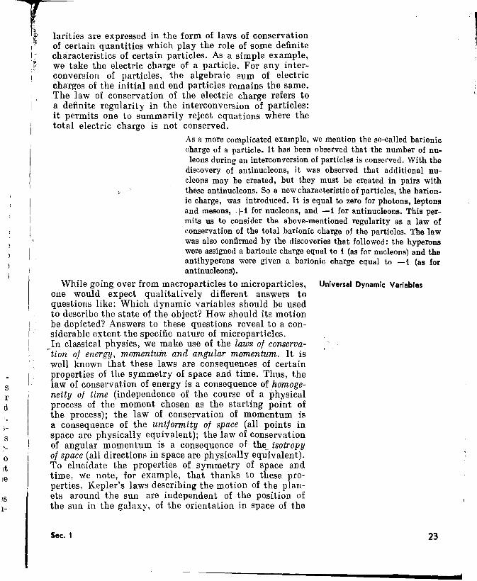
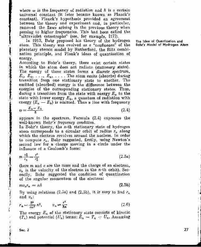
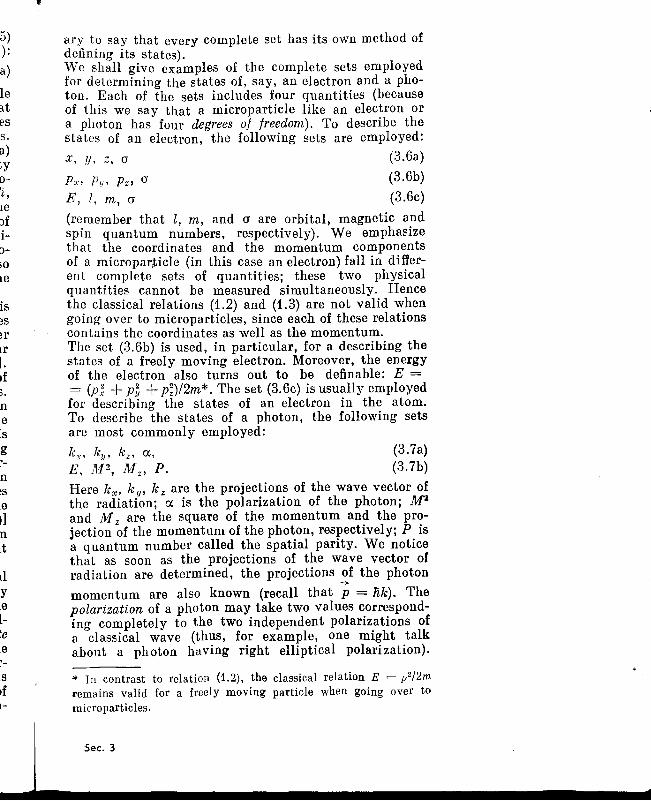
The essence of the idea of quantization lies in thefact that certain physical quantities related to the micro­particles may assume, under relevant circumstances,only certain discrete values. These quantities are saidto be quantized.Thus the energy of any microparticle in a bound state,like that of an ~lectron in an atom, is quantized. Theenergy of a freely moving microparticle, however isnot quantized.Let us consider the energy of an electron in an atom.The system of so-ealled energy levels corresponds to adiscrete set of values of electron energy. We considertwo energy levels E 1 and E 2 as shown in Fig. 2.1 (thevalues of electron energy are plotted along the verticalaxis). The electron may possess energy E 1 or E 2 andcannot possess any intermediate energy-all values ofenergy E satisfying the condition E 1 < E < E 2 areforbidden for it*. It should be noted that the discretenessof energy does not mean in any case that the electron is"doomed" to remain forever in the initial energy state (forexample on level E1). The electron may go over to anotherenergy state (level E 2 or any other) by acquiring orreleasing the corresponding amount of energy. Sucha transition is called a quantum transition.The quantum-mechanical idea of discreteness has a fairlylong history. By the end of 19th century, it was establishedthat the radiation spectra of free atoms are line spectra(i.e. they consist of sets of lines) and contain, for everyelement, definite lines which form ordered groups (series).In 1885, it was discovered that atomic hydrogen emitsradiation of frequencies (iln (henceforth we use the cyclicfrequencies (il, related to the normal frequencies v throughthe equation (il = 2nv) which may be described by theformula

(iln = 2ncR ( 1- :2 ), (2.1)

The Idea of Quantization(Discreteness)

Section 2 Two Fundamental Ideas ofQuantum Mechanics

Fig. 2.1

£

E., e

'i * A specific situation in quantum mechanics is possible in whichone must assume that an electron occupies level £1 as well as level£2 (see Sec. 10).

Sec. 2 25

t

)

26

where n are integral numbers 3, 4, 5, ... , c is thevelocity of light, R is the so-called Rydberg constant(R = 1.097 X 107 m-1). Formula (2.1) was derived byBalmer, hence the set of frequencies described by thisformula is called the Balmer series. The frequencies ofthe Balmer series fall in the visible region of spectrum.Later (in the beginning of 20th century), additional seriesof radiation from atomic hydrogen falling in the ultra­violet and infrared regions were discovered. The regulari­ties in the structure of these spectra were identical to theregularities in the structure of the Balmer series, whichenabled a generalization of formula (2.1) in the followingform:

CJ)n = 2ncR ( ;. - n~ ) . (2.2)

The number k fixes the series (in each series n > k);k = 2 gives the Balmer series, k = 1, the Lyman series(ultraviolet frequencies), k = 3, the Paschen series (infra­red frequencies), and so on.Regularity in the structure of series was observed notonly in the spectrum of atomic hydrogen, but also in thespectra of other atoms. It definitely indicated the possibil­ity of some generalizations. One such generalizationwas proposed by Ritz in 1908 in his combination principle,which states that if the formulae of series are given andthe constants occurring in them are known, any newlydiscovered line in the spectrum may be obtained fromthe lines already known by means of combinations in theform of sums and differences. This principle may beapplied to hydrogen in the following way: we write theso-called spectral terms for different numbers n:

T(n) = 2ncRln2 •

Then each frequency observed in the hrdrogen spectrummay be expressed as a combination of two spectral terms.By combining the spectral terms, it is possible to predictdifferent frequencies.It is remarkable that at about the same time, the ideaof discreteness arose in another direction (not relatedto atomic spectroscopy). This is the case of radiationwithin a closed volume or, in other words, black bodyradiation. After analyzing the experimental data, Planckin 1900 proposed his famous hypothesis. He suggestedthat the energy of electromagnetic radiation is emittedby the walls of a cavity not continuously, but in portions(quanta), the energy of a quantum being equal to

E = nw (2.3)

I

I

where ro is the frequency of radiation and n is a certainuniversal constant (it later became known as Planck'sconstant). Planck's hypothesis provided an agreementbetween the theory and experiment and, in particular,removed the flaws arising in the previous theory whenpassing to higher frequencies. This had been called the"ultraviolet catastrophe" (see, for example, [17]).

In 1913, Bohr proposed his theory of the hydrogenatom. This theory was evolved as a "confluence" of theplanetary atomic model by Rutherford, the Ritz combi­nation principle, and Plank's ideas of quantization ofenergy.According to Bohr's theory, there exist certain statesin which the atom does not radiate (stationary states).The energy of these states forms a discrete spectrum,E I , E 2 , ••• , En' .... The atom emits (absorbs) duringtransition frow. one stationary state to another. Theemitted (absorbed) energy is the difference between theenergies of the corresponding stationary states. Thus,during a transition from the state with energy En to thestate with lower energy Ell' a quantum of radiation withenergy (En - Ell) is emitted. Thus a line with frequency

E n - Ell (2.4)ro = Ii

appears in the spectrum. Formula (2.4) expresses thewell-known Bohr's frequency condition.In Bohr's theory, the n-th stationary state of hydrogenatom corresponds to a circular orbit of radius rn alongwhich the electron revolves around the nucleus. In orderto compute rn , Bohr suggested, firstly, using Newton'ssecond law for a charge moving in a circle under theinfluence of a Coulomb's force:

The Idea of Quantization andBohr's Model of Hydrogen Atom

(here m and e are the mass and the charge of an electron,Vn is the velocity of the electron in the n-th orbit). Sec­ondly, Bohr suggested the condition of quantizationof the angular momentum of the electron:

mvnrn = nn (2.5b)

By using relations (2.5a) and (2.5b), it is easy to find rn

and Vn:

1i2 e2

rn=-2 n2 , v =- (2.6)me n lin

The energy En of the stationary state consists of kinetic(Tn) and potential (Un) terms: En = Tn + Un. Assuming

(2.5a)

Sec. 2 27

that Tn = mv~/2, Un = -e2/r" and using (2.6), we findthat

The negative sign of the energy means that the electronis in a bound state (energy of a free electron is taken tobe equal to zero).Substituting the result (2.7) into the frequency relation(2.4), and comparing the expression thus obtained withformula (2.2), we may, following Bohr, find an expressionfor Rydberg's constant:

me4

E ----n - 2fz2n2 (2.7)

(2.8)

On Quantization of AngularMomentum

28

Bohr's theory (or the old quantum theory, as it is nowcalled) suffered from internal contradictions; in orderto determine the radius of the orbit, one had to makeuse of relations of different kinds-the classical relation(2.5a), and the quantum relation (2.5b). In spite of this,the theory was of great significance as a first step towardsthe creation of a consistent quantum theory. Moreover,the nature of the spectral terms, and, consequently,the Ritz combination principle, was revealed for thefirst time and the calculated value of Rydberg's constantwas in excellent agreement with its empirical value. Thesuccess of the theory proved testimony to the usefulnessof the idea of quantization. Having acquainted himselfwith Bohr's calculations, Sommerfeld wrote Bohr a letter,in which he said:I thank you very much for sending me your extremely interest­ing work.... The problem of expressing the Rydberg-Ritzconstant by Planck's has been for some time in my thoughts...A lthough I am for the present still rather sceptical aboutatom models in general, nevertheless the calculation of theconstant is indisputably a great achievement.

We must note that in contrast to energy, the angularmomentum of a microparticle is always quantized. Thus,the observed values of the square of angular momentumof a microparticle are expressed by the formula

M2 = fizl (l + 1), (2.9a)

where l is an integer 0, 1, 2, .... If we consider theangular momentum of an electron in the atom in then-th stationary state, the number l assumes values from 0to n - 1.In the literature, it is customary to refer to the angularmomentum as simply momentum. Henceforth, we shallfollow this practice.

The projection of the momentum of a microparticle ina certain direction (let us denote it as z-direction) assumesthe values

M z = nm (2.9b)

where m = --l, -l + 1, ... , 1-1, l. For a given valueof the number l, the number m can assume 2l + 1 discretevalues. We emphasize here that different projections ofthe momentum of a microparticle in a given directiondiffer from one another by values which are multiplesof Planck's constant.It was mentioned above that spin is a distinctive "inter­nal" momentum of a microparticle having a definitevalue for a given microparticle. To distinguish it fromthe spin momentum, ordinary momentum is calledorbital momentum. Kinematically the spin momentumis analogous" to the orbital momentum. Naturally, inorder to find the possible projections of the spin momen­tum we must use a formula of the type (2.9b) (as in thecase of orbital momentum, the projections of the spinmomentum differ from one another by integral multiplesof Planck's constant). If s is the spin of a microparticle(this number was introduced in Sec. 1), then the pro­jection of the spin momentum assumes values na, wherea = -s, -s + 1, ... , s - 1, s. Thus, the projection

of the spin of an electron assumes values - ~ and + ~ .The numbers n, l, m, a considered here determine thedifferent discrete values of the quantized dynamic vari­ables (in this case, energy and momentum), and arecalled quantum numbers; n is called the principal quantumnumber; l, the orbital quantum number; m, the magneticquantum number and a, the spin quantum number. Therealso exist other quantum numbers.

In spite of the resounding success of Bohr's theory, theidea of quantization engendered serious doubts in thebeginning. It was notfC8d thittbTs idea was full of inter­nal contradictions. Thus in his letter to Bohr, Rutherford[19] wrote in 1913:...Your ideas as to the mode of origin of the spectrum ofhydrogen are very ingenious and seem to work out well;but the mixture of Planck's ideas with the old mechanicsmakes it very difficult to form a physical idea of what isthe basis of it. There appears to me one grave difficulty inyour hypothesis which I have no doubt you fUlly realisenamely, how does an electron decide what frequency it isgoing to vibrate at when it passes from one stationary stateto the other? It seems to me that you would have to assume

Sec. 2

nJJS'I!;- )rl\L (jr

A;' r," ,L' "~oj

Anomalies of Quantum Transitions

29

that the electron knows beforehand where it is going tostop*...We shall explain the difficulties noticed by Rutherford:Let an electron occupy level E1 (Fig. 2.1). In order to goover to the level E2 , the electron must absorb a quantumof radiation (i.e. a photon) with a definite energy equalto (E2 - E1)· Absorption of a photon with any otherenergy will not result in the indicated transition and istherefore not possible (for simplicity, we shall consideronly two levels). The question now arises: In what waydoes an electron perform a "selection" of the "required"photon out of the photon flux of different energies fallingon it? In order to "select" the "required" photon, theelectron must be "preViously aware" of the second level,i.e. as if it had already visited it. However, in order tovisit the second level, the electron must have first absorbedthe "required" photon. This gives rise to a vicious circle.

Further contradictions are observed while considering the jumpof an electron from one orbit in the atom to another. Whateverthe speed at which the transition of the electron from the orbitof one radius to that of another takes place, it has to last for somefinite period of time (otherwise it would be a violation of the basicrequirements of the theory of relativity). But then it is hard tounderstand what the energy of the electron should be during thisintermediate period-the electron no longer occupies the orbitcorresponding to energy E1 and has not yet arrived at the orbitcorresponding to energy E 2 •

Idea of Wave-Particle Duality

It is thus not surprising that at one time efforts were madeto obain an explanation of experimental results withoutresorting to the idea of quantization. In this respect,the famous remarks by Schrodinger about "these damnedquantum jump~", which, of course, were made .in theheat of· the moment, are worth noting.

However, experience inevitably point~d to the useful­ness of quantization and no place was left for analternative.In this case, there is just one way out: new ideas mustbe introduced, which form a non-contradictory pictureof the whole including the ideas of discreteness. Theidea of wave-particle duality was just such a new physicalconcept.

Classical physics acquaints us with two types of motion:corpuscular and wave motion. The first type is characterized

* The reader should not be confused by the remarks about theoscillations of electron: uniform motion in a eircle is a super­position of two harmonic oscillations in mutually perpendiculardirections.

Ii 30f

by a localization of the object in space and the existenceof a definite trajectory of its motion. The second type,on the contrary, is characterized by delocalization inspace. No localized object corresponds to the motion ofa wave, it is the motion of a medium. In the world ofmacrophenomena, the corpuscular and wave motions areclearly distinguished. The motion of a stone thrownupward is something entirely different from the motionof a wave breaking a beach.These usual concepts, however, cannot be transferredto quantum mechanics. In the world of microparticles,the above-mentioned strict demarcation between the twotypes of motion is considerably obliterated. The motionof a microparticle is characterized simultaneously bywave and corpuscular properties. If we schematicallyconsider the classical particles and classical waves as twoextreme cases •.of the motion of matter, microparticlesmust occupy in this scheme a place somewhere in be­tween. They are not "purely" (in the classical sense) cor­puscular, and at the same time they are not "purely"wavelike; they are something qualitatively different.It may be said that a microparticle to some extent isakin to a corpuscle, and in some respect it is like a wave.Moreover, the extent depends, in particular, on theconditions under which the microparticle is considered.While in classical physics a corpuscle and a wave aretwo mutually exclusive extremities (either particle, orwave), these extremities, at the level of microphenomena,combine dialectically within the framework of a singlemicroparticle. This is known as wave-particle duality.The idea of duality was first applied to electromagneticradiation. As early as 1917, Einstein suggested thatquanta of radiation, introduced by Planck, should beconsidered as particles possessing not only a definiteenergy, but also a definite momentum:

, I

E = !iffi,Jiw

P=-c-' (2.10)

Later (from 1923), these particles became known asphotons.

The corpuscular properties of radiation were very clearly demon­strated in the Compton effect (1923). Suppose a beam of X-raysis scattered by atoms of matter. According to dassical concepts,the scattered rays should have the same wavelength as the incidentrays. However, experiment shows that the wavelength of scatteredwaves was greater than the initial wavelength of the rays. More­over, the difference between the wavelengths depends on the angle

!:J

j

Sec. 2 31

of scattering. The Compton effect was explained by assuming thatthe X-ray beam behaves like a flux of photons which undergo elas­tic collisions with the electrons of the atoms, in conformity withthe laws of conservation of energy and momentum for collidingparticles. This led not only to a qualitative but also to a quanti­tative agreement with experiment (see [17]).

In 1924, de Broglie suggested that the idea of dualityshould be extended not only to radiation but also to allmicroparticles. He proposed to associate with everymicroparticle corpuscular characteristics (energy E andmomentum p) on the one hand and wave characteristics(frequency ffi and wavelength 'A) on the other hand. Themutual dependence between the characteristics of differ­ent kinds was accomplished, according to de Broglie,through the Planck's constant n in the following way:

2nnE=nffi, P=-",- (2.11)

(the second relation is known as de Broglie's equation).For photons, relation (2.11) is automatically satisfiedif we substitute ffi = 2nclt,. in (2.10). The boldness ofde Broglie's hypothesis lays in that relation (2.11) wasassumed to be satisfied not only for photons, but gen­erally for all microparticles, and in particular, for thosewhich have a rest mass and which were hitherto associatedwith corpuscles.De Broglie's ideas received confirmation in 1927, withthe discovery of electron diffraction. While studying thepassage of electrons through thin foils, Davisson andGermer (as well as Tartakovsky) observed characteristicdiffraction rings on the detector screen. For "electronwaves" the crystal lattice of the target served as a diffrac­tion grating. Measurement of distances between diffractionrings for electrons of a given energy confirmed de Broglie'sformula. ;,In 1949, Fabrikant and coworkers set up an interestingexperiment. They passed an extremely weak electronbeam through the diffraction apparatus. The intervalbetween successive acts of passage (between two electrons)was more than 104 times longer than the time requiredfor the passage of an electron through the apparatus.This ensured that other electrons of the beam do notinfluence the behaviour of an electron. The experimentshowed that for a prolonged exposure, permitting reg­istration of a large number of electrons on the detectorscreen, the same diffraction pattern was observed as inthe case of regular electron beams. It was thus concludedthat the wave nature of the electrons cannot be explained

32

Here k is the wave vector; its direction coincides withthe direction of propagation of the wave, and its magni-

as an effect of the electron aggregate; every single electronpossesses wave properties.

The idea of quantization introduces discreteness, anddiscreteness requires a unit of measure. Planck's constantplays the role of such a measure. It may be said that thisconstant determines the "boundary" between microphe­nomena and macrophenomena. By using Planck's con­stant, as well as mass and charge of an electron, we mayform the following simple composition having dimensionsof length:

n2

r j =-2=0.53 X 10-8 em (2.12)me

(note that r1 is the radius of the first Bohr orbit). Accord­ing to (2.12), a magnitude of about 10-8 em may be consid­ered as the spatial "boundary" of microphenomena.This is just abol\~ the linear dimensions of an atom.If the Planck constant 'Ii were, say, 100 times larger,then (other conditions being equal) the "limit" of micro­phenomena would, according to (2.12), have been of theorder of 10-4 em. This would mean that the microphenom­ena would become much closer to us, to our scale, andthe atoms would have been much bigger. In other words,matter in this case would have appeared much "coarser",and classical concepts would have to be revised on a muchlarger scale.As was indicated above, the projections of the momentumof a microparticle differ from one another by multiplesof 'Ii [see (2.9b)]' Consequently, Planck's constant appearshere as a unit of quantization. If the orbital momentumis much greater than 'Ii, its quantization may be neglected.We get in this case the classical angular momentum.In contrast to the orbital momentum, spin momentumcannot be very large. It is clear, that it is impossible toneglect its quantization in principle; hence the spinmomentum does not have a classical analogue (this cir­cumstance was already indicated in Sec. 1).Planck's constant is inseparably linked not only withthe idea of quantization, but also with the idea of duality.From (2.11) it is evident that this constant plays a fairlyimportant role-it supplies a "link" between the corpuscu­lar and wave properties of a microparticle. This becomesquite clear if we rewrite (2.11) in a form permitting usto take account of the vector nature of momentum:

Ifs

eI

1

eIc1

::I

S

gtl

J;)d,.Itt I

,-II.

,r

,Indd

E = nro i;=nk. (2.13)

The Role of Planck's Constant

Sec. 2 33 ,, .

tude is expressed through the wavelength in the followingway: k = 2n/A. The left-hand sides of equations (2.13)describe corpuscular properties of a microparticle, andthe right-hand sides wave properties. We note, by theway, that the form of relations (2.13) indicates the rela­tivistic invariance of the idea of duality.Thus, Planck's constant plays two fundamental roles inquantum mechanics-it serves as a measure of discrete­ness, and it combines the corpuscular and wave aspectsof the motion of matter. The fact that the same constantplays both these roles is an indirect indication of theinternal unity of the two fundamental ideas of quantummechanics.In conclusion, we remark that the presence of Planck'sconstant in any expression indicates the "quantum-mecha­nical nature" of this expression. *

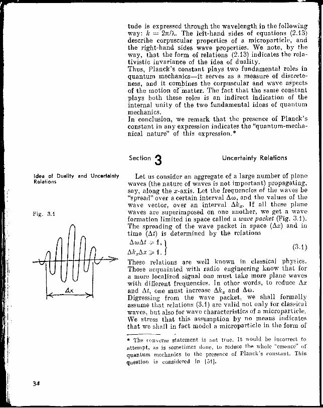
Section 3 Uncertainty Relations

Idea 01 Duality and UncertaintyRelations

Fig. 3.1'j

(:1I

, ,r

i (i n1\

Ir,i ' -ji

v UIV-,...

V'I

J,I V

IiJ Ax ~

I "" -7[;i!

!Ii

Let us consider an aggregate of a large number of planewaves (the nature of waves is not important) propagating,say, along the x-axis. Let the frequencies of the waves be"spread" over a certain interval ~ffi, and the values of thewave vector, over an interval ~kx. If all these planewaves are superimposed on one another, we get a waveformation limited in space called a wave packet (Fig. 3.1).The spreading of the wave packet in space (~x) and intime (M) is determined by the relations

~ffi~t ••f.1,} (3.1)~kx~x do 1.These relations are well known in classical physics.Those acquainted with radio engineering know that fora more localized signal one must take more plane waveswith different frequencies. In other words, to reduce ~x

and ~t, one must increase ~kx and ~ffi.

Digressing from the wave packet, we shall formallyassume that relations (3.1) are valid not only for classicalwaves, but also for wave characteristics of a microparticle.We stress that this assumption by no means indicatesthat we shall in fact model a microparticle in the form of

* The converse statement is not true. It would be incorrect toattempt, as is sometimes done, to reduce the whole '·csscnce" ofquantum mechanics to the presence of Planck's constant. Thisquestion is considered in [51].

'I

I~

~34

a wave packet. By considering U) and k x in (3.1) as wavecharacteristics of a microparticle and making use ofrelations (2.13), it is easy to go over to an analogousexpression for the corpuscular characteristics of a micro­particle (for its energy and momentum):

~EM ~ ti, (>\.2)

~Px~x ~ n. (.3.;3)

~. These relations were first introduced by Heisenbefg in1927 and are called uncertainty relations.Relations (3.2) and (3.3) should be supplemented by thefollowing uncertainty relation:

~ ~Mx~CPx dt n, (3.4)

where ~CPx is the uncertainty in the angular coordinatesof the microparticle (we consider rotation around thex-axis) and ~Mx is the uncertainty in the projection ofthe momentum on the x-axis. *By analogy with (3.3) and (3.4), one may write downrelations for other projections of momentum and angular

(J momentum:

e­oe­o'.

)

;.

:sX

YII

!1P y !1y ~ n, ~Pz~z ~ ti, (3.:3<1)

~My~cpy dt ti, ~Mz~CPz ~ n. (3.4a)

Let us consider relation (3.3). Here ~x is the uncertainty The Meaning of the Uncertaintyin the x-coordinate of the microparticle and ~Px, the Relationsuncertainty in the x-projection of its momentum. Thesmaller ~x is, the greater ~Px is, and vice versa. If themicroparticle is localized at a certain definite point x,then the x-projection of its momentum must have arbi-trarily large uncertainty. If, on the contrary, the micro-particle is in a state with a definite value of Px' then itcannot be localized exactly on the x-axis.Sometimes the uncertainty relation (3.3) is interpretedin the following way: it is impossible to measure simulta­neously the coordinate and momentum of a microparticlewith an arbitrarily high precision; the more accurately,ve measure the coordinate, the less accurately can themomentum be determined. Such an interpretation is notvery good since it might lead to the erroneous conclusionthat the essense of the uncertainty relation (3.3) is respon­sible for limitations associated with the process of measurr-

* Notice that relations (3.4) and (3.4a) are valid only for smallvalues of the uncertainty in angular coordinate (~cp ~ 2n) or, inothpr words, for large values of uncertainty in the projection ofthe momentum.

I1..

Sec. 3 35

t

36

ment. One might be led to assume that a microparticleitself possesses a definite coordinate as well as a definitemomentum, but the uncertainty relation does not permitus to measure them simultaneously.Actually the situation is quite different. The microparticleitself simply cannot have simultaneously a definite coor­dinate and a corresponding definite projection of themomentum. If, for example, it is in a state with a moredefinite value of the coordinate, then in this state thecorresponding projection of its momentum is less definite.From this the actual impossibility of simultaneous mea­surements of coordinates and momenta of a microparticlefollows naturally. This is a result of the specific characterof the microparticle and is by no means a whim of naturewhich makes it impossible for us to perceive all thatexists. Consequently, the sense ot relation (3.3) is notthat it creates certain obstacles to the understanding ofmicrophenomena, but that itreflects certain peculiaritiesof the objective properties ofallicroparticle. The lastremark is, of course, of a general nature: it refers not onlyto relation (3.3), but also to other uncertainty relations.Now let us look at relation (3.2). Let us consider twodifferent, though mutually supporting interpretations,of this relation. Suppose that the microparticle is unstableand that M is its lifetime in the state under consideration.The energy of the microparticle in this state must havean uncertainty I1E which is related to the lifetime I1tthrough inequality (3.2). In particular, if the state isstationary (M is arbitrarily large), the energy of themicroparticle will be precisely determined (I1E = 0).The other interpretation of relation (3.2) is connectedwith the measurements carried out to ascertain whetherthe microparticle is located at the level E1 or E z. Sucha measurement requires a finite time T which depends onthe distance between the levels (EZ'I- E]):(E 2 - E 1) T ~ Ii. (3.2a)

It is not difficult to see the connection between thesetwo interpretations. In order to distinguish the levels E 1and E 2 , it is necessary that the uncertainty I1E in theenergy of the microparticle should not be greater thanthe distance between the levels: I1E ~ (E z - E]). Atthe same time the duration of measurement T shouldobviously not exceed the lifetime M of the microparticlein the given state: T ~ M. Consequently, the limitingconditions, under which measurement is still possible,are given by

I1E ~ E 2 - Ej1 T ~ I1t.

'If,

Ieleit

Ier-lere1ee.a-leerre'ltotofesstIys.ms,Ien.ve~t

islie

~d

er3hm

a)

se"fE1liem'\tldIe19e,

By using (3.2), we can arrive at (3.2a) from these rela­tions.The uncertainty relations (3.2)-(3.4) show how the con­cepts of energy, momentum and angular momentumshould be applied in the case of microparticles. Here,a very important peculiarity of the physics of micro­particles is revealed: the energy, momentum and theangular momentum of a microparticle have meaningonly within the limitations imposed by the uncertaintyrelations. Heisenberg [20] writes that we cannot inter­pret processes on an atomic scale in the same way asprocesses on a large scale. If we make use of the usualconcepts, their applicability is limited by the uncertaintyrelations.It should, however, be pointed out that the uncertaintyrelations do not in any way lead to the above-mentionedrestrictions OD the applicability of classical concepts ofcoordinates, momentum, energy, etc. for microparticles.It would be unfair not to mention the considerable "posi­tive aspects" of uncertainty relations after having talkedabout their "negative aspects". They serve as a workinginstrument of the quantum theory. By reflecting the spe­cific character of the physics of microparticles, the uncer­tainty relations allow us to obtain fairly important resultsthrough fairly simple means. Some examples are givenin Sec. 4 below.

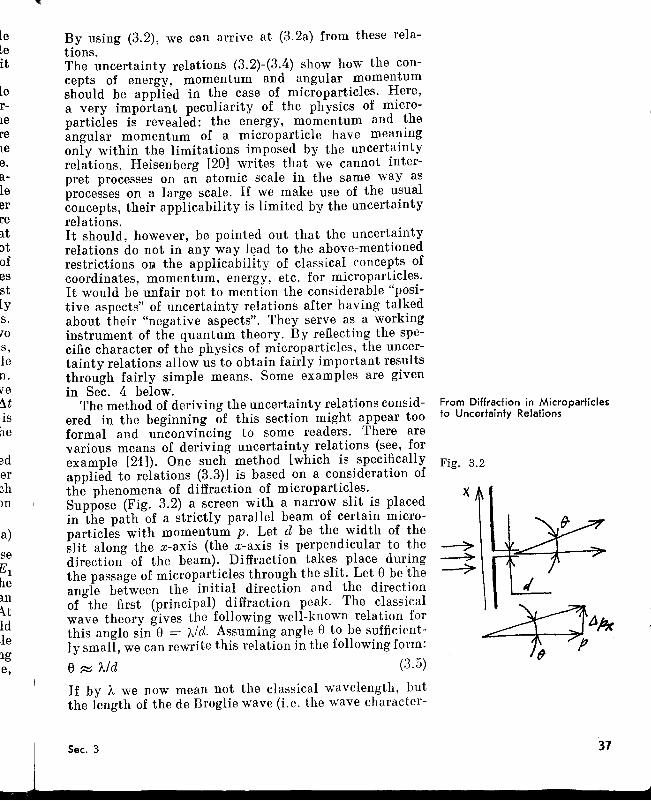
The method of deriving the uncertainty relations consid­ered in the beginning of this section might appear tooformal and unconvincing to some readers. There arevarious means of deriving uncertainty relations (see, forexample [21]). One such method [which is specificallyapplied to relations (3.3)] is based on a consideration ofthe phenomena of diffraction of microparticles.Suppose (Fig. 3.2) a screen with a narrow slit is placedin the path of a strictly parallel beam of certain micro­particles with momentum p. Let d be the width of theslit along the x-axis (the x-axis is perpendicular to thedirection of the beam). Diffraction takes place duringthe passage of microparticles through the slit. Let ebe theangle between the initial direction and the directionof the first (principal) diffraction peak. The classicalwave theory gives the following well-known relation forthis angle sin e = 'f.ld. Assuming angle e to be sufficient­ly small, we can rewrite this relation in the following form:

e~ 'A/d (3.5)

If by A we now mean not the classical wavelength, butthe length of the de Broglie wave (i.e. the wave character-

From Diffraction in Microparticlesto Uncertainty Relations

Fig. 3.2

_J_.s.ec..3 •

37

__

1

Uncertainty Relations and theState of Microparticles.The Concept of a Complete Setof Physical Quantities

38

istic of the microparticle), we may rewrite relation (3.5)in "corpuscular language" by using the expression (2.11):

8 ~ nlpd. (3.5a)

But how we are to understand the existence of the angle8 in "corpuscular language"? Obviously, it means thatwhile passing through the slit, the microparticle acquiresa certain momentum !1p", in the direction of the x-axis.It is easy to see that I1px ~ p8. Substituting (3.5a)into this, we get I1px ~ Md. By considering the quantityd as the uncertainty !1x in the x-coordinate of the micro­particle passing through the slit, we get !1px!1x ~ 11"

i.e. we arrive at the uncertainty relation (3.3). Thus theattempt to determine in some way the coordinate ofa microparticle in a direction perpendicular to the di­rection of its motion leads to an uncertainty in the mo­mentum of the microparticle in that direction, which alsoexplains the phenomenon of diffraction observed in theexperiment.

In order to describe the state of a classical object it isnecessary to give a definite set of numbers-the coordinatesand the velocity components. In doing this otherquantities, in particular, energy, momentum and angularmomentum of the object will also be determined [see (1.1)1.The uncertainty relations show that this method ofdefining a state is not applicable to microparticles.Thus, for example, the existence of a definite projectionof momentum in a given direction for a microparticlemeans that the position of the microparticle in thisdirection cannot be determined unambiguously: accordingto (3.3), the corresponding spatial coordinate is character­ized by an infinitely large uncertainty. The electronin an atom has a definite energy; moreover its coordinatesare characterized by an uncertainty of t,he order of thelinear dimensions of the atom. This [according to (3.3)]leads to an uncertainty in the projection of the momentumof the elect.ron equal to the ratio of Planck's constantto the linear dimension of the atom.We now indicate the following situations, fundamentalin quantum mechanics, which arise from the uncertaintyrelation: (a) various dynamic variables of a microparticleare combined in sets of lJimultaneoulJly determined (simul­taneously measurable) quantities, the so-called completesets of quantities; (b) various states of a microparticleare combined in groups of states corresponding to differ­ent complete sets of quantities. Each group containsthe states of the microparticle in which the values ofthe corresponding complete sets are known (it is custom-

1!

5)):a)

Ieitess.a);y0-

~,

le

:>fi-:>-;0

Le

is3S

lrtrI.If5.

nelsg~-

n~s

e~1n.t

11Y.el-~e

.e'-

.sIft-

J

ary to say that every complete set has its own method ofdefining its states).We shall give examples of the complete sets employedfor determining the states of, say, an electron and a pho­ton. Each of the sets includes four quantities (becauseof this we say that a microparticle like an electron ora photon has four degrees of freedom). To describe thestates of an electron, the following sets are employed:

x, y, Z, (J (3.6a)

p~., PIi' pz> (J (3.6b)E, 7, m, (J (3.6c)

(remember that l, m, and (J are orbital, magnetic andspin quantum numbers, respectively). We emphasizethat the coordinates and the momentum componentsof a microparUcle (in this case an electron) fall in differ­ent complete sets of quantities; these two physicalquantities cannot be measured simultaneously. Hencethe classical relations (1.2) and (1.3) are not valid whengoing over to microparticles, since each of these relationscontains the coordinates as well as the momentum.The set (3.6b) is used, in particular, for a describing thestates of a freely moving electron. Moreover, the energyof the electron also turns out to be definable: E == (p~ + p~ + p;)/2m*. The set (3.6c) is usually employedfor describing the states of an electron in the atom.To describe the states of a photon, the following setsare most commonly employed:

k" "y, kz> ex, (3.7a)E, 211 2 , Mz> P. (3.7b)

Here "x, kif' k z are the projections of the wave vector ofthe radiation; ex is the polarization of the photon; M2and M z are the square of the momentum and the pro­jection of the momentum of the photon, respectively; P isa quantum number called the spatial parity. We noticethat as soon as the projections of the wave vector ofradiation are determined, the projections of the photon

momentum are also known (recall that p = nk). Thepolarization of a photon may take two values correspond­ing completely to the two independent polarizations ofa classical wave (thus, for example, one might talkabout a photon having right elliptical polarization).

... In contrast to relation (1.2), the classical relation E = p2/2mremains valid for a freely moving particle when going over tomicroparticles.

Sec. 3

d

Uncertainty Relations andQuantum Transitions

40

The spatial parity is a characteristic property of a micro­particle; it may be considered as an integral of motionwhose conservation is a result of symmetry with respectto the operation of reflection by a mirror. At a later stage(see Sec. 20) we shall discuss it in greater detail. Here.we only mention that parity can assume one of the twovalues: +1 and -1.The set (3.7a) is used for describing the states of photonscorresponding to plane classical waves, in this case theenergy of the photon is also defined (recall that E = nw == nck). The states described by the set (3.7a) are calledkcx-statos. The set (3.7b) is employed for describingthe states of photons belonging to spherical classicalwaves. We note that just as a spherical wave may berepresented as a superposition of plane waves, the statesof a photon described by the set (3.7b) may be representedas a "superposition" of states described by the set (3.7a).The converse statement regarding the representation ofplane waves as a superposition of spherical waves is alsotrue. Here we have touched upon (for the present justtouched upon) one of the most important and delicateaspects of the quantum-mechanical description of mat­ter-the specific character of the "interrelations" betweenstates of a microparticle described by different completesets. This specific character is reflected in the mostconstructive principle of quantum mechanics-the prin­ciple of superposition of states. The superposition of stateswill be considered in detail in the second chapter; herewe shall just restrict ourselves to the above-mentionedremarks.

The main contradiction regarding quantum transitionsindicated in Sec. 2 is essentially overcome by makinguse of the idea of duality or, more precisely, the uncer­tainty relation (3.2). Let us consider transition of anelectron in an atom from level E 1 to level E 2 by absorbinga photon of energy nw = E 2 - E 1 • We recall that thecontradiction in transition was connected with thequestion whether the absorption of the photon precedesthe transition of the electron or vice versa. It is easyto see that this question simply loses its meaning now.In fact, if we have a bound electron with energies E}and E 2 before and after interaction with radiation, respec­tively, then during the interaction we have one quantum­mechanical system including both the electron and theradiation. This system exists for a definite time (whilethe interaction with the radiation takes place) and, accord­ing to (3.2), cannot have any definite energy. Henceit is meaningless to find out precisely what takes place

ro- in such a system. Strictly speaking, during the interac-on tion of the electron with the photon there is no electronlct and no photon, but a single entity which must be treated,ge as such, without going into details. This example showsret that in quantum mechanics a physical process cannot beVilO infinitely detailed in time. The question ''what follows

what"? cannot always be posed in the case of microphe-us nomena.*he

The uncertainty relation (3.2) allows us to introduce and employed a very important concept in quantum theory, the so-called virtualng transitions, for explaining quantum transitions. \Ve shall give:al here a simplified treatment of virtual transitions, but we shallbe give a detailed explanation later in Sec. 6. According to relation,es (3.2), an electron may go over from level E l to E 2 without gettinged any energy from outside; what is important is that it should quick-I). ly return to its initial level E l • Such a "journey" (E l -+ E 2 -+ E l )

of is possible if its duration /:,t is such that the inequality nI /:,t >so > (E

2- E l ) is satisfied, because in this case the uncertainty in

st the energy of the electron is greater than the difference in the ener-te gies of the levels under consideration. Hence it is clear that thet- statement "the electron occupies level Et may be understood quiteln specifically-as incessant "transition" of the electron from thete given state to others with an inevitable return every time to thest starting level E l . Such transitions cannot be observed experimen-n- tally, and are called virtual transitions in contrast to the normales (real) transitions. During interaction of an electron undergoingre virtual transitions with radiation, the electron is liable to change-~d its "residence". For example, it might now occupy level E 2 and will

in future perform virtual transitions not from level El , but from1S level E 2' If such a thing happens, the electron is said to have ab-19 sorbed a photon of energy fw) = E 2 - El , and undergone a tran-r- sition from level E l to E 2• Virtual transitions don't require any.n expenditure of energy from outside while a real transition cannot19 occur without expenditure of energy-the energy of the photons-Le absorbed (or emitted) by electrons during interaction with radia-le tion.lS To explain the difference between real and virtual transitions, we-y note that a real transition from a level E l to another level E 2

r. and back may be broken up into two successive events in time''1 (in between, the electron may be experimentally registered in the-

intermediate state E 2 ). However, the virtual transition from level:- E

lto E 2 and back cannot be broken up into two events in time-

e both parts of the transition must be considered as a single, indi-e visible process in time.

e * The anomaly of quantum transition is completely removed bye considering the principle of superposition of states (see Sec. 10).

Sec. 3 4t

_ •• 1

Section 4

l1

"Ii,

II

i'il"

Ii

Uncertainty Relation "Number ofPhotons-Phase"

Evaluation of Energy of GroundState of Hydrogen Atom

42

The uncertainty relations used in quantum theory areby no means exhausted by relations (3.2)-(3.4). As anexample of one more such relation we consider the uncer­tainty relations for the number of photons and the phaseof the wave.Let there be a monochromatic radiation of frequency ffi.On one hand, it may be considered as a collective ofphotons each having energy nffi; on the other hand, wemight treat it as a classical electromagnetic wave. Let Nbe the number of photons in the volume under considera­tion and let cI> = ffit be the phase of the classical wave.The corpuscular characteristic of the radiation (numberof photons N) and its wave characteristic (phase cI»cannot have definite values simultaneously; there existsthe uncertainty relationdNdcI> d- 1. (3.8)In order to arrive at relation (3.8), we start from theuncertainty relation for energy and time. We recallthat for measuring the energy of a quantum object withan accuracy dE we must spend time M ~ tildE. If wetake the collective of photons as the quantum object,we getdE = nffidN,

where dN is the uncertainty in the number of photons.During the time dt necessary for measurement of theenergy of the object with an accuracy nffidN, the phase cI>changes by dcI> = ffiM. Substituting into this the rela­tion dt d- tilnffidN, we find dcI> d- 11dN, Q.E.D.Relation (3.8) reflects the dialectically contradictoryunity of corpuscular and wave properties of radiation.The uncertainty dcI> is small when the wave propertiesof radiation are clearly exhibited; in this case the densityof photons is high (N is large) and sq, is the uncertaintydN. On the other hand, the uncertainty dN is smallwhen there are a few photons in the aggregate. In thiscase the corpuscular properties of radiation are clearlyexhibited and therefore the uncertainty dcI> is large.

Some Results Ensuing fromthe Uncertainty Relations

The uncertainty relations serve as very useful workingtools of quantum theory since they permit one to obtainimportant results, by fairly simple means.As an example, we consider the hydrogen atom in itsground state. We make use of the well-known classical

'Ij'

~e

nr­;e

€xpression for energy of a charged particle moving in<I Coulomb field:

(4.1 )

(4.4)

(4.3)

(4.2)

I' from (4.1) by using (4.2),

The values given by (4.4) fully coincide with the resultsof the rigorous theory*. Of course such a complete coinci­dence must be considered to some extent as an accidentalsuccess. Only the order of the quantities should be takenseriously here. We emphasize that this order can beevaluated quite simply as follows: it is sufficient firstto simply replace the precise values of the dynamic vari­ables in expression (4.1) by quantities which characterizethe degree of "blurring" of these variables, Le. by theiruncertainties, and then use the quantum-mechanicalrelations connecting the said uncertainties.

where m and e are the mass and charge of the electron,respectively. In order to use the classical expression (4.1)in the quantum theory, we consider the quantities pand I' occurring in it as uncertainties in momentum andcoordinates of the electron, respectively. According torelation (3.3), these quantities are connected with eachother. We assume pI' ~ Ii, or, simply,

pI' = h.

Eliminating the quantitywe get

[12 t'e 2 pE(p)=---.

2m h

It is easy to see that the function E (p) has a minimumfor a certain value P = Pl' We denote it as El . The quan­tity E l may be considered as the energy of the ground

state of the hydrogen atom while the quantity 1'1 = !!...P1

is the estimate of the linear dimensions of the atom(in Bohr's theory this is the radius of the first orbit).

By equating the derivative dd E (p) to zero, we findz P

Pl - m~ • This at once gives the required evaluations

Icf. (2.6) and (2.7)]:

m

~y

11.

es;y;y11is.ye.

s.1ert>a-

1e11;hv-et,

3)

).

)fre7V1­

e.er»)ts

ts11

<I< In the rigorous theory the quantity r1 is a characteristic forthe ground state of the hydrogen atom and denotes the distancefrom the nucleus at which an electron is most likely to be observed(see expression (5.4)].

Sec. 4 43

__• 1

Estimate of the Energy ofZero-point Oscillations of anOscillator

We shall proceed exactly in the same way as in thepreceding example. The energy of a classical one-dimen­sional harmonic oscillator is given by the expression

(4.5)

Treating Px and x as uncertainties in the momentum andcoordinate of the oscillating microparticle and using theequality Px'X = Ii as the uncertainty relation, we getfrom (4.5)

(4.6)

Evaluation of the "Blurring" ofthe Optical Absorption BandEdge in the Franz-Keldysh Effect

44

By equating the derivative 3:..- E (PJ to zero we finddpx

the value of Po = + V mliffi for which the function E (Px)assumes its minimum value. It is easy to see that thisvalue is

(4.7)

This result is quite interesting. It shows that in quantummechanics the energy of an oscillator cannot vanish;its minimum value is of the order of liffi. This is theenergy of what is called the zero-point oscillation. Wenote that the estimate (4.7) differs from the exact expres­sion for the energy of the zero-point oscillation just by

1a factor of 1/2 (exact value Eo = 2" liffi).

By taking the zero-point oscillations into account, onemay arrive at the following interesting conclusion: theenergy of the oscillatory motion of atoms in a crystaldoes not vanish even at absolute zero.The zero-point oscillations illustrate a basically generalcircumstance: it is impossible to find a microparticle atthe "bottom of the potential well", or, in other words"a microparticle cannot fall to the bottom of the poten­tial well". This conclusion does not depend on the formof the potential well, since it is a direct consequence ofthe uncertainty relation: "falling to the bottom of thewell" is connected with the vanishing of momentum andhence the uncertainty in the momentum of the micro­particle. In this case, the uncertainty in the coordinatebecomes so large that there is a direct contradiction withthe very fact that the microparticle is in a potential well.

The essence of the effect, investigated in 1958 by Kel­dysh, and independently by Franz, lies in the following:in a uniform external electric field, the minimum of theelectron energy in the Conduction band of semiconduc--

(4.9)

'I

I

el-

n

I)

deit

I)

d

,)is

')

nl;

ee;-

y

IeeII

11ts

11IfedI-eII

e

I

J

tors shifts downwards on the energy scale, leading toa "blurring" of the edge of the fundamental optical absorp­tion band (as a result the absorption of the photons withenergies lower than the forbidden band width becomespossible) [22]. The value of the shift of electronic statescharacterizing the indicated "blurring" may be obtainedin the same way as the preceding evaluations were made.We make use of the classical expression for the energyof a charged particle in the electric field of intensity G :

(4.8)

Here m is the effective mass of the electron in the conduc­tion band. Treating Px and x as uncertainties in themomentum and coordinate of the electron and usingthe equality px·x = n as the uncertainty relation, weget from (4.8)

E ( ) = pi _ ~enPx 2m Px'

Next, as usual we equate the derivative -f- E (Px)Px

to zero and obtain the value Po = - (Y'0enm for whichthe function E (Px) assumes its minimum value:

(4.10)

Expression (4.10) gives an estimate of the extent of the"blurring" of the edge of the fundamental optical absorp­tion band in the Franz-Keldysh effect.

While postulating the stationary states, Bohr's theory Why does not the Electron Falldid not explain why, after all, the electron, moving into the Nucleus?

under acceleration, does not radiate and fall into thenucleus as a result of this. Relation (3.3) explains thisfact. The falling of an electron into a nucleus wouldobviously mean a considerable reduction in the uncer-tainty of its coordinate. Before the hypothetical fallinginto the nucleus, the electron is localized within thelimits of the atom, i.e. in a region of space with lineardimensions n2/me2 ~ 10-8 em [see (4.4)], whereas afterfalling into the nucleus it would be localized in a regionwith linear dimensions less than 10-12 em. Accordingto (3.3) a stronger localization of a microparticle in spaceis linked with a "blurring" of its momentum. Hence uponfalling into the nucleus, the mean value of the momentumof the electron must increase, which requires an expendi-ture of energy. Thus it turns out that effort has to bemade not to "hold" the electron from falling into the

Sec. 4 45

d

nucleus, but on the contrary to "force" the electron to belocalized within the nucleus.In the example of the zero-point oscillations it waspointed out that the microparticle in a potential wellalways possesses a non-zero minimum energy Eo. Themagnitude of Eo depends, in particular, on the spatialdimensions of the well (or on its width a, which determinesthe extent of localization of the microparticle inspace). By taking into account the uncertainty relation,it is easy to see that

(4.11)

On the "Trajecfory" ofMicroparticles

46

If a decreases, Eo increases. For sufficiently small a, theenergy Eo may become greater than the depth of thepotential well. It is obvious that such a well will nothold the microparticle at all.The falling of an electron into the nucleus corresponds toa decrease in the width of the potential well from 10-8 cmto 10-12 cm (and even lower). According to (4.11) theminimum energy Eo should increase in this case from10 to 109 eV (and higher). As a result the minimum energyof the electron turns out to be a few orders higher thanthe binding energy of a nucleon in the atomic nucleus(the latter being not greater than 107 eV). This meansthat the electron cannot ever be present in the nuclearpotential well and hence it can by any means be compelledto be localized within the nucleus, not even by force.This not only eliminates the problem of "an electrollfalling into the nucleus" but also solves another funda­mental question: the electron is not one of the constituentsof the atomic nucleus.

In order to draw the trajectory of a particle, it is neces­sary, strictly speaking, to know the coordinate and mo­mentum of the particle at every moment of time (in fact,in order to depict the dependence x (t), it is necessary to

know, for every t, the values x and ~~), Since, according

to the uncertainty relation (3.3), a microparticle canllotsimultaneously possess a defmite coordinate and a definiteprojection of the momentum, one can draw the conclusionthat the concept of trajectory in case of microparticle,strictly speaking, is not applicable.The rejection of the trajectory concept is connected withthe existence of wave properties in microparticles, whichdo not permit one to consider microparticles as classicalcorpUScles. The movement of a microparticle along thex-axis cannot be associated with the differentiable func-

47

~ tion x (t) which is so widely used when consideringthe mechanics of classical objects. From a known value

, of x of the microparticle at a certain time t, it is impossibleto predict the value of its coordinate at the time t ++ dt.As applied to Bohr's theory, this means a rejection ofthe very concept of "the orbit of an electron in an atom".One may speak about the localization of the electronwithin the atom as a whole; the orbit requires a muchgreater spatial localization. Turning to the problem of"the electron falling into the nucleus" discussed above,we can understand the consequence to which such a local­ization leads. The planetary model of the atom thusturns out to be just an intermediate step in developmentof our concept of the atom. Much later, in the fifties,Bohr himself amusingly recalled how after one of hislectures a student came up and asked him "Were therereally idiots who thought that the electron revolvesin an orbit?"

We note that with the rejection of the idea of orbits of the electronin an atom the contradiction regarding the problems of the in­stantaneous jump of the electron from one orbit into another, dis-­cussed in Sec. 2, is automatically eliminated.

There are situations, however, in which one can makeuse of the idea of "the trajectory of a microparticle". As anexample we consider the motion of electrons in the kine­scope of a television set. The momentum of the electronalong the axis of the tube is p = V2meU, where U isthe accelerating voltage. The formation of the electronbeam means a definite localization of the coordinate inthe transverse direction. The degree of this localizationis characterized by the diameter d of the beam. Accordingto (3.3), there must be an uncertainty in the electronmomentum in a direction perpendicular to the axis ofthe beam: !'J.p ~ Md. As a result of this uncertainty, theelectron may deviate from the axis of the beam withinan angle !'J.8 ~ !'J.p/p ~ h/pd. Let L be the path lengthof the electron in the kinescope. Then the uncertaintyin the position of the point of impingement of an electronon the screen will be characterized by the quantity!'J.x ~ L!'J.8 ~ Lli/pd. Assuming U = 20 kV, d = 10-3 em,L = 102 em, we get !'J.x ~ 10-5 cm. In this way, theblurring of the point of impingement due to the uncertain­ty relation is considerably less than the diameter of thebeam. It is clear that in such cases the motion of theelectron may be treated classically.

I Sec. 4

i lI I..J, ...."

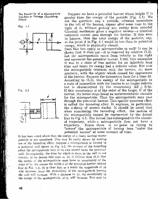
The Possibility of a MicroparticieSub-Barrier Passage (TunnelingEffect)

48

II

III

: I

1......1--

Fig. 4.1

Suppose we have a potential barrier whose height U isgreater than the energy of the particle (Fig. 4.1). Weask the question: can a particle, situated somewhereto the left of the barrier, appear after some time to theright of it, without getting any energy from outside?Classical mechanics gives a negative answer-a classicalcorpuscle cannot pass through the barrier. If this wereto happen, then the total energy of the particle, say,at the point A in Fig. 4.1 would be less than its potentialenergy, which is physically absurd.Does this ban apply to microparticles as well? It can beshown that it does not-it is removed by relation (3.2).Let the microparticle move from infinity to the rightand encounter the potential barrier. Until this encounterit was in a state of free motion for an infinitely longtime and hence its energy had a definite value. But nowthe microparticle interacts with the barrier, or, moreprecisely, with the objects which caused the appearanceof the barrier. Suppose the interaction lasts for a time M.According to (3.2), the energy of the microparticle ina state of interaction with the barrier is no longer definitebut is characterized by the uncertainty i1E:p Ii/ M.If this uncertainty is of the order of the height U of thebarrier, the latter stops being an unsurmountable obstaclefor the microparticle. Thus the microparticle may passthrough the potential barrier. This specific quantum effectis called the tunneling effect. It explains, in particular,the a-decay of atomic nuclei. It should be noted thatwhen considering the tunneling effect, the motion ofthe microparticle cannot be represented by the dottedline in Fig. 4.1. The dotted line corresponds to the classic­al trajectory, while a microparticle does not have atrajectory. Hence there is no point in trying to"accuse" the microparticle of having been "under thepotential barrier" at some moment of time.

It has been noted above that the energy of a freely moving micro­particle is not quantized. This may be easily shown by makinguse of the tunneling effect. Suppose a micro particle is located ina potential well shown in Fig. 4.2. On account of the tunneling,effect the microparticle may of its own accord leave the potentialwell. Consequently, the time for which it stays in the well is notinfinite. If we denote this time as !':.t, it follows from (3.2) thatthe energy of the microparticle must have an uncertainty of the-order tz/ ""t. We reduce the width b of the potential barrier (dottedline in Fig. 4.2). It is clear that as a result the magnitude of f':..twill decrease, since the probability of the microparticle leavingthe well will increase. With a decrease in f'>.t, the uncertainty inthe energy of the microparticle, tz/!':.t, will increase. This may be

:Fig. 4.2

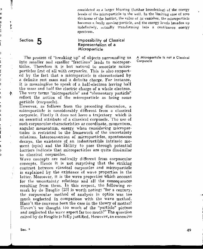
seee?I

,,

considered as a larger blurring (further broadening) of the energylevels of the microparticle in the well. In the limiting case of zerothickness of the barrier, the value of f.,t vanishes, the microparticlebecomes a freely moving particle, and the energy levels broaden upindefinitely, actually transforming into a continuous energyspectrum.

Section 5

r

Impossibility of ClassicalRepresentation of aMicroparticle

The process of "breaking up" of objects surrounding usinto smaller and smaller "fractions" leads to micropar­ticles. Therefore it is but natural to associate micro­particles first of all with corpuscles. This is also support­ed by the fact that a microparticle is characterized bya definite rest mass and a definite charge. For instance,it is meaningless to speak of a half-electron having halfthe mass and half the electric charge of a whole electron.The very terms "microparticle" and "elementary particle"reflect the notion of the microparticle as being someparticle (corpuscle).However, as follows from the preceding discussion, amicroparticle is considerably different from a classicalcorpuscle. Firstly it does not have a trajectory which isan essential attribute of a classical corpuscle. The use ofsuch corpuscular characteristics as coordinate, momentum,angular momentum, energy when considering micropar­ticles is restricted to the framework of the uncertaintyrelations. Interconversion of microparticles, spontaneousdecays, the existence of an indestructible intrinsic mo­ment (spin) and the ability to pass through potentialbarriers indicate that microparticles are quite dissimilarto classical corpuscles.Wave concepts are radically different from corpuscularconcepts. Hence it is not surprising that the strikingcontrast between classical corpuscles and microparticleis explained by the existence of wave properties in thelatter. Moreover, it is the wave properties which accountfor the uncertainty relations and all the consequencesresulting from them. In this respect, the following re­mark by de Broglie [23] is worth noting: "for a century,the corpuscular method of analysis in optics was toomuch neglected in comparison with the wave method.Hasn't the converse been the case in the theory of matter?Haven't we thought too much of the "particle" pictureand neglected the wave aspect far too much?" The questionraised by de Broglie is fully justified. However, an excessive

Sec. .;

A Microparticle Is not a ClassicalCorpuscle

49

I

~---------------------_-..I'

A Microparticle Is not IIClassical Wave

Example 1

Example 2

exaggeration of the wave aspect while consideringmicroparticles should be avoided. We must rememberthat while on one hand a microparticle is not a classicalcorpuscle, it is similarly, on the other hand, not a classi­cal wave.

The analysis of one mistake which is committed quiteoften even these days when considering a simplifiedaccount of quantum mechanics is quite instructive.We shall demonstrate this mistake through two examples.

It is contended that the wave properties of an electronpermit one to derive the conditions for the quantizationof momentum which are postulated in Bohr's theory.The "derivation" is done in the following way. Let 2:n:rnbe the perimeter of the n-th Bohr's orbit. In this orbit,an electron moves with de Broglie's wavelength An == 2:n:1i/Pn' The basic assumption lies in the fact thatthe perimeter of the orbit should contain n wavelengthsAn of the electron. Consequently, 2:n:rn = nAn' Thisat once gives the desired condition for quantizationof momentum:

(5.1)

It is stated that the wave properties of an electronpermit a very simple derivation of the formula for theenergy levels in a potential well, if we assume that adefinite number of de Broglie half-waves are confinedin the potential well (in analogy with the number ofhalf-waves contained in the length of a string fixed atboth ends) corresponding to different stationary states.Designating the width of the one-dimensional poten­tial well by a, we write a = nAnl2, from which we getthe desired result:

(5.2)

50

Both these final results [(5.1) as well as (5.2)] arecorrect; they are the same as the result deduced fromstrict theory. However, the "derivation" of these formulasmust be considered to be unsound. In both cases infact the same fundamental mistake has been committed:they are based on the wrong assumption that the electronin a potential well has a definite de Broglie wavelength,or, in other words, a definite momentum. However,according to (3.3), the momentum of a microparticlein a bound state is characterized by the uncertainty!1p ;:r Ma. Since in the above examples p ~ li/').. ~ Ma,it follows that the momentum is of the same order ofmagnitude as the uncertainty in momentum given by

AHempts to Represent aMicroparlicle as a Symbiosis of aCorpuscle and a Wave

I'I relation (3.3). It is clear that in such cases one cannot

speak about any value of the electron momentum (andcorrespondingly of its de Broglie wavelength) even ap­proximately.* These examples demonstrate an obviousexaggeration of the wave aspect. The identification ofan electron in a potential well with a classical waveinside a "resonator" is incorrect. The picture of an electronwave in a "resonator" is the same kind of simplificationas the picture of an electron-ball moving in a classicalorbit. We shall return again to the question of wavesin quantum mechanics; however, it is useful to emphasizeat this stage that by the term "de Broglie wave" wedo not conceal any sort of classical wave. It is just areflection in our imagination of the fact that microparti­cles possess wave properties.

If a microparticle is neither a corpuscle nor a wave,then may be it is some kind of a symbiosis of a corpuscleand a wave? Several attempts were made to model sucha symbiosis and thus also to visually demonstrate thewave-particle duality. One such attempt represents amicroparticle as a formation, limited in space and intime. This may be the wave packet mentioned in Sec 3.This may also be just a "scarp" of a wave, often calleda wave train. Another attempt uses a model of a pilot-wave, according to which a microparticle is some sortof a "compound" of a corpuscular "core" with a certainwave which controls the motion of the core.

One of the versions of the pilot wave model is considered byD. Baum in his book [25]: We first postulate that connected witheach of the "fundamental" particles of physics (e.g. an electron) is a bodyexisting in a small region of space.... in most applications at theatomic level the body can be approximated as a mathematical point..The next step is to assume that associated with this body there is awave without which the body is never found. This wave will be assumedto be an oscillation in a new kind of field, which is represented mathe­matically by the ,p-field of Schrodinger ... somewhat like the gravita­tional and the electromagnetic, but having some new characteristicsof its own....We now assume that the ,p-field and the "body" are interconnected inthe sense that the ,p-jield exerts a new kind of "quantum-mechanical"force on the body, ... the force is such as to produce a tendency to pullthe body into regions where I ,p I is largest.If the above tendency were all that were present, the body would even­tually find itself at the place where the ,p-field had the highest intensity.We now further assume that this tendency is resisted by random motions

... This question is considered in greater detail in Sec. 23 of thisbook. See also [24].

i!i

i':'

Sec. 5 51

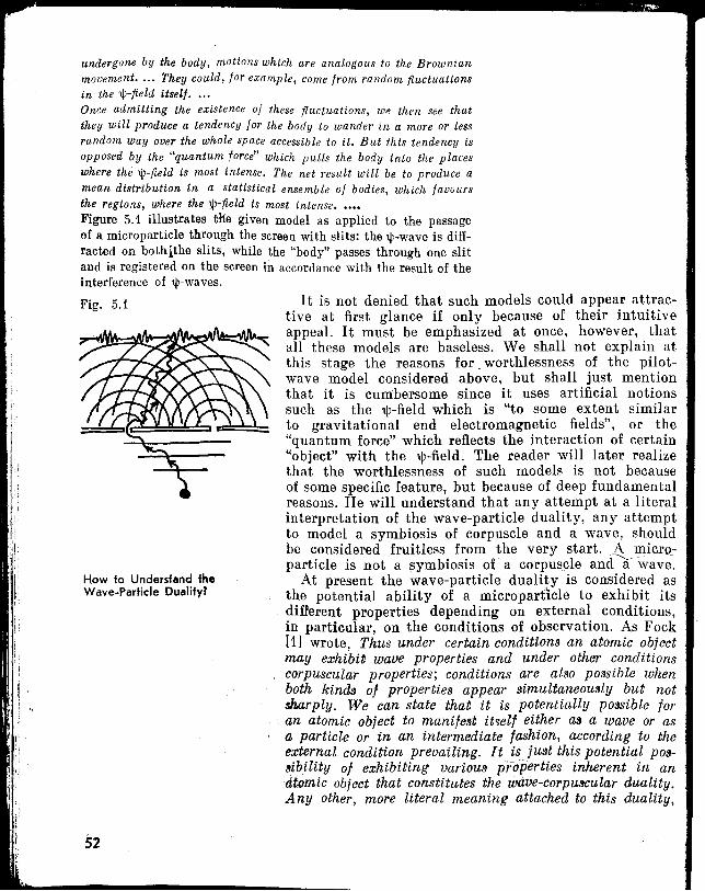
undergone by the body, motions which are analogous to the Brownianmovement• ... They could, for example, come from random fluctuationsin the ~-field itself. .. ,Once admitting the existence of these fluctuations, we then see thatthey will produce a tendency for the body to wander in a more or lessrandom way over the whole space accessible to it. But this tendency isopposed by the "quantum force" which pulls the body into the placeswhere the ~-field is most intense. The net result will be to produce amean distribution in a statistical ensemble of bodies, which favoursthe regions, where the 1,jJ-field is most intense• ....Figure 5.1 illustrates We given model as applied to the passageof a microparticle through the screen with slits: the ~-wave is diff­racted on bothithe slits, while the "body" passes through one slitand is registered on the screen in accordance with the result of theinterference of ~-waves.

l:It

Fig. 5.1

How to Understand theWave-Particle DUlIlityl

It is not denied that such models could appear attrac­tive at first glance if only because of their intuitiveappeal. It must be emphasized at once, however, thatall these models are baseless. We shall not explain atthis stage the reasons for. worthlessness of the pilot­wave model considered above, but shall just mentionthat it is cumbersome since it uses artificial notionssuch as the 'llJ-field which is "to some extent similarto gravitational end electromagnetic fields", or the"quantum force" which reflects the interaction of certain"object" with the 'IjJ-field. The reader will later realizethat the worthlessness of such models is not becauseof some specific feature, but because of deep fundamentalreasons. He will understand that any attempt at a literalinterpretation of the wave-particle duality, any attemptto model a symbiosis of corpuscle and a wave, shouldbe considered fruitless from the very start. A micrQ~

particle is not a symbiosis of a corpuscle anda-wave.At present the wave-particle duality is considered as

the potential ability of a microparilcle to exhibit itsdifferent properties depending on external conditions,in particular, on the conditions of observation. As Fock[1] wrote, Thus under certain condition~ an atomic objectmay exhibit wave properties and under other conditionscorpuscular properties; conditions are al~o po~sible whenboth kinds of propertie~ appear simultaneou~ly but notsharply. We can state that it is potentially po~sible foran atomic object to manife~t it~elf either ail a wave or as

.a particle or in an intermediate fashion, according to theexternal condition prevailing. It is ju~t this potential po~­

il.i~ility of exhibiting various properties inherent in andtomic object that constitutes the wave-corpuilcular duality.Any other, more literal meaning attached to this duality,

ac­lvelatat

ot­:onmslar;helinizeIsetalrallptlIdro­ve.asitsns,lckect~ns

zennotforas

the'08­

anty.ty,

'T

Isuch as a wave-particle model of any kind, is incorrect.Let us consider a simple example. Let a beam of electronspass through a screen with slits and then hit a detectorscreen. While passing through the slits, the electronsrealize their wave properties which leads to a distributionfor electrons beyond the slit characteristic of interference.When impinging on the detector screen, the electronsexhibit their corpuscular properties-each of them isregistered at a certain point on the screen. It m.ay besaid that the electron passes through the slit as a "wave",and is registered on the detector screen as a "particle".In this connection, it is sometimes said that a micro­particle is a wave under some circumstances, and a micro­particle is a particle under other circumstances. Sucha treatment of wave-particle duality is incorrect.0Vhat­ever the conditions, a microparticle is neither a wave,nor a particle, "not even a symbiosis of a wave and aparticle. It is a quite specific object, capable of exhibitingcorpuscular or wave properties to some extent or otherdepending on the circumstances. The understanding ofwave-particle duality as the potential capability of themicroparticle to exhibit different properties in differentexternal conditions is the only correct one. Hence, inparticular, follows an important conclusion: it is impos­sible to give a definite visual model of a microparticle.

The absence of a visual model of a microparticle doesnot in any way prevent us from using tentative modelsquite suitable for representing a microparticle underdifferent conditions. As an example, let us consider anelectron in an atom.We recall that the state of an electron in anatom is described by a set of quantum numbersn, l, m, cr. A given state is characterized by a definiteenergy, while in the particular case of the hydrogenatom, it depends only on the number n [see (2.7)), andin a more general case on the numbers nand l. An electronin an atom isdelocalized in space-its coordinates havean uncertainty of the order of the size of the atom. Usual­ly, when considering an electron in an atom, it is custom­ary to introduce the concept of an electron cloud whichmay be interpreted in this case as a tentative imageof the electron. The form and the effective size of anelectron cloud depend on the quantum numbers n, l,m and, consequently, vary from one state of the electronin the atom to another.In order to describe the dimensions and the form ofthe electron cloud, we introduce a certain functionun1m (r, 8, Ip) = Unl (r) Zlm (8, Ip), (5.3)

Electron in an Atom

,I

''fI

:j

J.se.c,.5 5

•

3

....

1

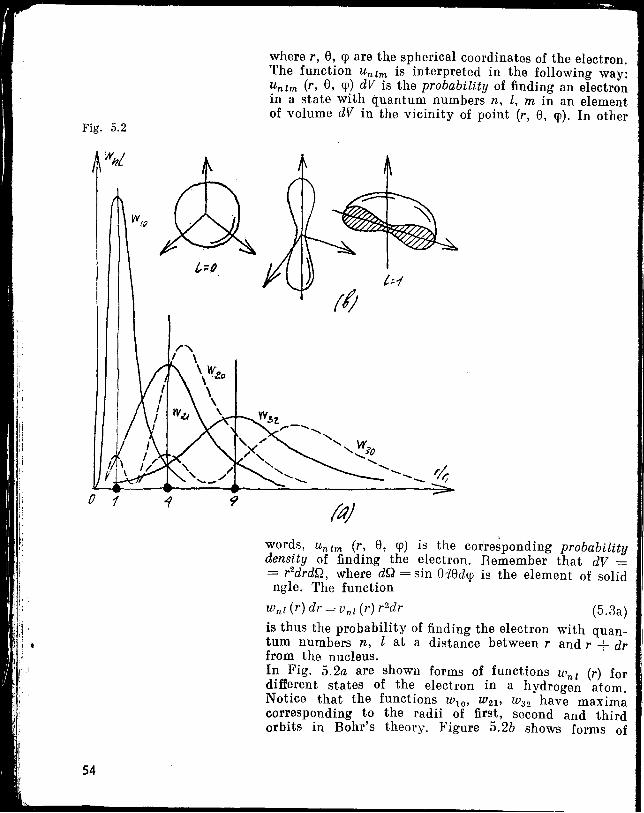
(I;

Fig. 5.2

where r, e, cp are the spherical coordinates of the electron.The function Unlm is interpreted in the following way:Unl m (r, e, cp) dV is the probability of finding an electronin a state with quantum numbers n, l, m in an elementof volume dV in the vicinity of point (r, e, cp). In other

••

f) 1

54

/"""I \

\lV~o\\

\

words, Un 1m (r, e, cp) is the corre;ponding probabilitydensity of finding the electron. Remember that dV == r 2drdQ, where dQ = sin ededcp is the element of solidngle. The function

Wnl (r) dr = Unl (r) r2dr (5.3a)

is thus the probability of finding the electron with quan­tum numbers n, l at a distance between rand r + drfrom the nucleus.In Fig. 5.2a are shown forms of functions Wnl (r) fordifferent states of the electron in a hydrogen atom.Notice that the functions WIO, W21' W 32 have maximacorresponding to the radii of first, second and thirdorbits in Bohr's theory. Figure 5.2b shows forms of

Section 6

m.ly:'onmtler

:ity

lid

3a)

an­dr

for1m.mairdof

, function Zim fo, some states of the electron. Fo' I .~ 0., (for the so-called s-electron) we have a spherical electron

cloud. For l = 1 (for p-electron) the electron cloudhas a form of either a spindle or a toroid depending onthe quantum number m. Thus in order to imagine anelectron in atom, one may use conventional forms likethe models of a sphere, spindle, toroid, etc. ,The ground state of the hydrogen atom is characterizedby a spherical electron cloud. Theory shows (see, forexample, [11]) that in this case

wnl(r)=4r:exp(_~). (5.4)r 1 r 1

The parameter r 1 characterizing the effective radiusof the cloud is determined by relation (4.4); in Bohr'stheory it occurs as the radius of the first orbit.In conclusion w/iJ note that during quantum transitions in anatom, there occurs not only a change in energy, butalso a "redistribution" of electron clouds-a change oftheir shape and size.

Rejection of Ideas ofClassical Physics

As has been asserted, a transition from macrophenom­ena to microphenomena presupposes a rejection of thebasic ideas of classical physics. The notion of a strictcontinuity in the spectrum of values of physical quanti­ties is no longer valid, the classical concept of a tra­jectory is rejected, the principle of classical determinismis in question. At the root of this viewpoint lie ideas ofquantization (discreteness) and wave-particle dualitywhich are alien to classical physics.On the basis of a number of examples that we have consid­ered, we could see the need to reject the classical principleof unlimited detailing of objects in space, and of phenom­ena in time. Thus the question of the internal structure ofelementary particles turns out to be groundless. Like­wise the efforts towards a detailed development in timeof the process of the quantum jump (quantum transition)have no meaning.The concepts of energy. momentum, angular momentumwhich are widely used in classical physics are carried overto quantum mechanics as well. However, these concepts arenow seen differently with a reconsideration of the previousinterconnections, taking into account the possibility of quan­tization, and the limitations imposed by the uncertainty

Sec. 6

General Remarks

55

,J

relations. In particular, there arises the question, unknownto classical physics, of the simultaneous measurement ofphysical quantities, and questions about the state and themethods of describing a state are put in a new light.In conclusion we stress the impossibility of the classicalinterpretation of a microparticle, and the loss of theclarity of classical physics.

Identity of Microparticles The rejection of the classical individualization of anobject is quite fundamental. In classical mechanics ob­jects are known to have individuality since it is alwayspossible in principle to enumerate them and observethe behaviour of anyone of them. In this case, how­ever alike two classical objects may be, they are neveridentical and can always be distinguished. But in quantummechanics two microparticles of the same type shouldbe treated as absolutely identical. Thus, all electronsare identical and so are all unexcited hydrogen atoms,helium nuclei, etc.

Suppose we have several electrons, one of which is "assigned" thenumber 1 at the moment of time t = O. Can this electron be identi­fied after a certain time t? Such an identification could have beeneasily done if we could put some "label" on this isolated object.We could get by without "labelling" this electron if we could sim­ply keep a watch over the isolated object, i.e. if we could "mentally"follow it (in our imagination) along its trajectory. This is preciselywhat we would have done in the case of isolated classical objects.However, none of this holds in the case of an electron; it is inprinciple impossible to "label" it. Strictly speaking, it has notrajectory. The electron "isolated" by us at the instant t = 0, cannotbe isolated in actual practice: it does not have the individualitywhich would allow it to be identified in the assembly of electronsafter a certain time t. Two electrons are much more "like eachother" than the proverbial "two peas in a poll"; sinctl the latterare classical objects, they could differ in size or in chemic'll com­position in some way.

Chance and Necessity in theBehaviour of a Microparticle

56

It is understood that the identity of microparticles doesnot exclude the possibility of their differentiation onthe basis of different states in which these particlesmay be found. Two electrons belonging to two differentatoms are, of course, identical but at the same timedistinguishable. The affiliation of an electron to oneatom or another permits its "isolation". However, nothingchanges physically if the electrons interchange places.It is clear that if such an exchange is possible, for example,by combining the atoms under consideration into amolecule, the distinguishability of the electrons vanishes.

LaplaCian determinism excludes the element of chancefrom the behaviour of an isolated object; in classical

lS

nlS

Iteeg;,."

Ja;.

eI

n)­

is'er-lrndIS

3,

mechanics, necessity completely dominates. Because ofthis, the laws of classical mechanics are dynamic andnot statistical. The element of chance (and, consequently,statistical laws also) appear in classical physics onlywhen considering aggregates of objects or assemblies ofparticles.From this point of view, it is important to stress thatin quantum mechanics we are dealing with a qualita­tively different situation concerning the behaviour ofindividual microparticles: here, elements of necessity,as well as chance, are present. An excited atom spon­taneously returns to the ground state without any ex­ternal influence. This is associated with the spontaneoustransitions of electrons in the atom from one set of energylevels to another. It is impossible in principle to indicateprecisely when a particular excited atom will returnto its ground state; such a return is a random act.Precisely in the same way, it is impossihle to predict exactlywhen a given elementary particle, for example, a neutron,will decay spontaneously. In this case also an element

I ~ 0If chance is present.1,',1,. n addition to elements of chance, there are also pres-t ent the elements of necessity in the behaviour of ai( microparticle. As has already been indicated in Sec. 1,

if we have No neutrons at the instant t = 0, No:?> 1,we can confidently state that at the time t we will beleft with only No exp (-th:) neutrons, • being a constantcalled the lifetime of the neutron. Here, the necessityis obvious. In the case of an individual neutron thisnecessity is replaced by a definite probability of keepingthe neutron intact until time t, once it has managedto survive to time t = O. This probability is equalto exp (-tl.). It should be noted that this probabilityis independent of the time for which the given neutronhas survived up to the time t = O. Necessity is alsomanifested in the conservation laws which govern decayprocesses as well as the processes of interconversion ofmicroparticles in general. We may also mention the factthat there are definite modes of decay; for example,a free neutron may decay into a proton, an electron andan electronic neutrino.The existence of chance as well as necessity in the be­haviour of an individual microparticle has very im­portant consequences. It leads to the fact that quantummechanics turns out to be in principle a statistical theorywith probability as one of its basic attributes. As Fock[1] has remarked, in quantum physics the concept of prob­ability is a primary concept and plays a fundamental

J.s.ec.'.6 .57__

1,1

~

frI,

t

Virtual Transitions and VirtualMicroparticles

'S8

role. It could be said that the behaviour of an individualmicroparticle is random, but the probability of thisbehaviour is necessary*. The electronic cloud consideredin Sec. 5 may serve as a good example of this. The oc­currence of an electron at some point near the nucleusis a random event, but the probability of its being foundat a given point (r, e, <p) is definite-it is described bya function of the type (5.3) or, in other words, is deter­mined by the shape and size of the corresponding electroncloud.In the end, we note that the element of chance in thebehaviour of an individual microparticle is due to theuncertainty relations. In Sec. 4, we concluded on thebasis of relation (3.3) that it is impossible to "aim amicroparticle to hit a given point". In other words, theregistration of a particular electron at some point ofa detector screen is random; we can only speak of theprobability of such a fact. In Sec. 3, we introducedon the basis of relation (3.2) the concept of the virtualtransitions of a microparticle. It is easy to see that suchtransitions also point, towards the existence of randomnessin the behaviour of a microparticle. When discussingthe specific nature of the physics of microparticles, itis necessary to discuss in greater detail the idea of virtualtransitions and of virtual microparticles associated withthem.

Perhaps there is nothing more alien to classical physicsthan the idea of virtual transitions and virtual micro­particles. The virtual transition of an electron from levelE 2 to level E 1 and back (the transition E 2 -+ E 1 + E

2)

may be considered as a process in which the electronemits and absorbs a photon of energy (E2 - E1). Sucha photon is called virtual. In contrast to the photonsparticipating in real transitions, virtual photons cannotbe observed experimentally. The creatioh of a virtualphoton is not connected with an absorption of energyfrom outside, and its annihilation is not connected witha release of energy. The law of conservation of energyis not violated since a virtual photon exists for a veryshort time I'J.t and, according to uncertainty relation(3.2), the energy of an electron emitting the virtualphoton is characterized by the uncertainty I'J.E > iiI I'J.t,which may be of the order of, or greater than, the energyof the photon (E 2 - E t ). The· emission or absorptionby an electron of virtual photons corresponds, from a

* Here, it is quite appropriate to recall the words of F. Engels:Necessity emerges from within the framework of randomness.

1

t.....:.• [1~.

~~-

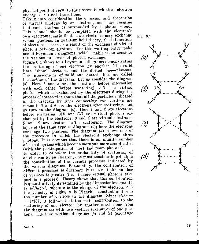
M1------<Fig. 6.1

I".

z.1

rei)

((;

physical point of view, to the process in which an electronundergoes virtual transitions.Taking into consideration the emission and absorptionof virtual photons by an electron, one may imaginethat each electron is surrounded by a photon cloud.This "cloud" should be compared with the electron'sown electromagnetic field. Two electrons may exchangevirtual photons. In quantum field theory, the interactionof electrons is seen as a result of the exchange of virtualphotons between electrons. For this we frequently makeuse of Feynman's diagrams, which enable us to considerthe various processes of photon exchange.Figure 6.1 shows four Feynman's diagrams demonstratingthe scattering of one electron by another. The solidlines "show" electrons and the dotted one-photons.The intersections of solid and dotted lines are calledthe vertices Qf the diagram. Let us consider the diagram(a). Here 1 and 2 are the electrons before interactionwith each other (before scattering), AB is a virtualphoton which is exchanged by the electrons during theprocess of interaction (note that all the particles indicatedin the diagram by lines connecting two vertices arevirtual); 3 and 4 are the electrons after scattering. Letus turn to the diagram (b). Here 1 and 2 are electronsbefore scattering, AB and CD are virtual photons ex­changed by the electrons, 3 and 4 are virtual electrons,5 and 6 are electrons after scattering. The diagram(c) is of the same type as diagram (b); here the electronsexchange two photons. The diagram (d) shows one ofthe processes in which the electrons exchange threephotons. It is obvious that there is an infinite numberof such diagrams which become more and more complicated(with the participation of more and more photons).In order to calculate the probability of scattering ofan electron by an electron, one must consider in principlethe contribution of the various processes indicated bythe various diagrams. Fortunately, the contribution ofdifferent processes is different: it is less if the numberof vertices is greater (Le. if more virtual photons takepart in a process). Theory shows that this contributionis quantitatively determined by the dimensionless quanti­ty (e2/tw)n/ 2 , where e is the charge of the electron, c isthe velocity of light, Ii is Planck's constant and n isthe number of vertices in the diagram. Since e2/nc == 1/137, it followS that the main contribution to thescattering of one electron by another must come fromthe diagram (a) with two vertices (exchange of one pho­ton). The four vertices diagrams (b) and (c) (exchange

Ii)'

I'I

,I't

"

II

Sec. 6 S9

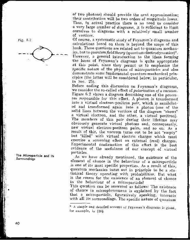
Fig. 6.2

----o-~--

The Microparticle and ItsSurroundings

60

of two photons) should provide the next approximation;their contribution will be two orders of magnitude lower.Thus, in actual practice there is no need to considera very large number of diagrams, it is sufficient to limitourselves to diagrams with a relatively small numberof vertices.Of course, a systematic study of Feynman's diagrams andcalculations based on them is beyond the scope of thisbook. These questions are related not to quantum mechan­ics, but to quantum field theory (quantum electrodynamics)*.However, a general introduction to the ideas formingthe bases of Feynman's diagrams is quite appropriateat this point, since they permit us to emphasize thespecific nature of the physics of microparticles and alsodemonstrate some fundamental quantum-mechanical prin­ciples (the latter will be considered below, in particular,in Sec. 25).Before ending this discussion on Feynman's diagrams,we consider the so-called effect of polarization of a vacuum.Figure 6.2 shows a diagram describing one of the proces­ses responsible for this effect. A photon is transformedinto a virtual electron-positron pair, which is annihilat­ed and transformed again into a photon (one of thesolid lines between the vertices of the diagram "shows"a virtual electron, and the other, a virtual positron).The members of this pair during their lifetime mayobviously generate virtual photons and, consequently,new virtual electron-positron pairs, and so on. As aresult of this, the vaeuum turns out to be not "empty"but "fIlled" with virtual electric charges which mustexercise a screening effect on external (real) charges.Experimental confirmation of this effect is the bestevidence of the usefulness of our concept of virtualparticles.

As we have already mentioned, the existence of theelement of chance in the behaviour of a microparticleis one of its most specific properties. As a result of this,quantum mechanics turns out in principle to be a sta­tistical theory operating with probabilities. But whatis the reason for the existence of an element of chancein the behaviour of a microparticle?This question can be answered as follows: The existenceof chance in microphenomena is explained by the factthat a microparticle, figuratively speaking, interactswith all its surroundings. The specific nature of quantum

* A simple and detailed account of Feynman's diagrams is given,for example, in [26].

mechanics is such that, strictly speaking, not a singleobject in it can be considered to be fully isolated, com­pletely independent of its surroundings. It has beenremarked [27] that the cause of the statistical natureof quantum mechanics is the same as in classical statis­tical mechanics, i.e. the existence of a large numberof bonds affecting the motion of the object. A particletreated as free in quantum mechanics is in fact freeonly from influences of a dynamic nature. But it remainsunder the influence of random forces which cause quantumfluctuations in its behaviour, as reflected by the uncertain­ty relation.What is the nature of the random influences on a micro­particle? In quantum fIeld theory, it manifests itselfin an explicit form as the interaction of a microparticlewith a vacuum (recall that a vacuum is not "empty";it is "filled" ,with virtual charges). It may be said thata microparticle interacts with its surroundings throughvirtual microparticles.The reader should now find it quite natural to inter­pret wave-particle duality as the potential ability ofa microparticle to exhibit one kind of property or another,depending on the external conditions, i.e. on the micro­particle's surroundings. This envisages a close connectionbetween the microparticle and its surroundings-in fact,the very nature of a microparticle is displayed in oneform or another depending on specific conditions andcircumstances.The impossibility of an unlimited detailization of ob­jects and phenomena being displayed in quantum me­chanics should also be explained by the interactionof a microparticle with its surroundings. This meansthat after a certain stage of investigation, physicalobjects cannot be considered as being isolated. Hereit is appropriate to recall the statement given in Sec. 3regarding the discussion on quantum transition: "Duringthe interaction of an electron with photons there is,strictly speaking, no electron and no photon but a singleentity which must be considered as such without goinginto details."Quantum mechanics re-establishes the idea acquiredthrough everyday experience regarding the unity of theuniverse and general connections among phenomena.This idea received a setback in the classical theory.The sharp boundaries that existed between waves andparticles, particles and fields, object under investigationand the medium are all obliterated and the conceptof the interconversion of matter is introduced. We fwd

Sec. 6 61

I!

\ II!

ourselves in full agreement with the following appro­priate remark made by Bohm [281: It seems necessaryto give up the idea that the world can correctly be analysedinto distinct parts, and to replace it with the assumptionthat the entire universe is basically a single, indivisibleunit. Only in the classical limit can the description interms of component parts be correctly applied withoutreservations. Wherever quantum phenomena play a signifi­cant role, we shall find that the apparent parts can changein a fundamental way with the passage of time, becauseof the underlying indivisible connections between them.Thus, we are led to picture the world as an indivisible,but flexible and everchanging, unit.

Interlude. Is a "PhysicallyIntuitive" Model of aMicroparticle Possible?

Participants: (same as inPrelude).

It may well be that these electronsAre worlds just like our very own,With kings and scholars, arts and armies,A nd memories of ages flown.And atoms-cosmic systems, spinningAround a central spinning sphere.Where things are just like ours, but smaller,Or nothing like what we have here.Bryusov (The World of the Electron)

Interlude

A uthor: The impossibility of the classical interpretation of a micro-particle predetermines a negative answer to the question "Is itpossible to have a "physically intuitive" model for a microparticle?"

Classical Physicist: It is still not clear why a "physically intuitive" model[ of aparticle explaining its various properties including spin, insta­bility, wave properties, etc. cannot be created. Such a model mayturn out to be complicated. Or, it may be possible that we stilldo not know enough about a microparticle to create such a model.But why can't we believe in the very possibility of~ this model?

A uthor: There are very sound reasons for this. I shall indicate justtwo of them. Firstly, any modelling envisages in the long run adetailization irrespective of whether it is a model of an objector a process. However, the impossibility of an unlimited detailiza­tion is characteristic of microparticles and microphenomena, aswe have already mentioned. This important situation was persis­tently stressed by Bohr. He wrote, in particular (see his articleQuantum Physics and Philosophy-[6]): A new epoch in physicalscience was inaugurated, however, by Planck's discovery of the ele­mentary quantum of action, which revealed a feature of wholenessinherent in atomic divisibility of mdtter. Indeed, it became clear thatthe pictorial description of classical physical theories represents anidealization valid only for phenomena in the analysis of which allactions involved are sufficiently large to permit the neglect of thequantum.... It is appropriate to mention here that this featureof wholeness indicated by Bohr is closely linked with the identityof a microparticle. Secondly, as we have already indicated, a char­acteristic property of microparticles is their inavoidable inter­action with surroundings leading, in particular, to a dependenceof some of the properties of microparticle on definite externalcircumstances. These properties should be treated as certain pos­sibilities which can be realized depending on the external circum­stances. One may ask, in what way can these possibilities be re­flected in the framework of a definite "physically intuitive" model?

Classical Physicist: It must be admitted that these ideas serve as strong argumentsagainst a "physically intuitive" model of a microparticle. However,I don't like the very spirit of quantum mechanics which rejectsgraphic representations. In my view it introduces subjectivenessin describing real world. Take, for example, the statement: "The

63

,III'

64

electron may present itself as a wave or as a particle, dependingon circumstances". Now, everything depends on circumstances,especially on the circumstances of observation. Involuntarily, onegets the idea that the electron is not something objective, butrather something subjective depending on how we "look" at it.

A uthor: Of course, this is not true. First of all, you overlook the factthat the electron has quite definite characteristics like rest mass,electric charge, spin, etc. It is stable and is a fermion. As regardsa "physically intuitive" model of an electron, well, it simply doesnot exist. However, in rejecting a "physically intuitive" modelof a microparticle, quantum mechanics in no way sacrifices objec­tivity in favour of subjectivity. It is just that the electron is avery complicated physical object, and depending on the externalcircumstances, including circumstances of observation, it exhibitsits different aspects, which objectively existed in potential form(I stress this) even before the observer was born. A sober assessmentof this complex situation is that a "physically intuitive" modelof the electron is not possible.

Classical Physicist: Can one seriously speak about an object without having anidea of what it looks like? Isn't it strange that we study, for example,the behaviour of an electron in a crystal while we don't even knowwhat an electron actually is?

Author: I don't agree that we don't even know what an electron is.I have just indicated a number of precisely determined characteris­tics and properties of an electron. More detailed properties of micro­particles in general and electrons in particular were considered inthe preceding sections of the book (and will be considered in thefollowing sections). In fact, we know quite a lot about the electronand know, in particular, about its behaviour in a crystal. This isevidenced by the large number of semiconducting devices fabricatedand used by us in practice. As you will see, the absence of a "physi­cally intuitive" model of the electron has in no way turned outto be a serious obstacle. We may even go a step further and statethat an understanding of natural phenomena in which Planck'sconstant plays an important role is possible ~nly through a signif­icant rejection of a graphic description. By the way, this ideawas given by Heisenberg, in whose works much attention was givento questions of the use of physically intuitive methods.

Classical Physicist: But by rejecting models, isn't quantum mechanics runningthe risk of losing its material basis? Won't we be finally leftwith only equations and abstract mathematical symbols?

A uthor: I can understand your doubts. For you, apparently, only theextremes matter: either graphic models, or mathematical abstrac­tion. To you, either a model should reflect everything or almosteverything, otherwise it is quite useless. The doubts arising inyour mind' are a consequence of precisely this type of viewpoint.However, the quantum-mechanical approach to such questions ismOTe flexible, or rather, dialectical.

19s,le

lt

cts,jseselc-a

altsmrltel

III

e,IW

s.s-o-inilemis

Old;i-utte

it: s[f-ea

,Ien

rlg IIlft

IIilec-,stinIt.is

Classical Physicist:Author:

Classical Physicist:Author:

Classical Physicist:Author:

Classical Physicist:Author:

I don't understand what exactly you mean by that.I want to stress two points. Firstly, although there is no "phys­

ically intuitive" model for a microparticle, this does not standin the way of the "model representations" in quantum mechanics.

That means I was right after all?This is something different. Quantum mechanics believes that

even the most refined model cannot reflect the specific characteris­tics of a microparticle. Hence quantum mechanics makes use oftentative models (tentative images)-sometimes one, sometimesanother, admitting the relativity of every model. The only thingthat is important is that each of the models employed should reflectsome side of the nature of the object or phenomenon. Thus, whenconsidering electronic transitions through the forbidden bandin a semiconductor, we unhesitatingly imagine electrons as somekind of corpuscles, which "jump" on the energy scale. When con­sidering the propagation of electrons through an ideal crystallattice we use wave concepts. It is convenient to study the scatteringof electron waves by the elastic waves of a crystal in a "corpuscularlanguage", using the picture of collisions of corpuscles of twotypes-electrons and phonons. Similarly, the image of the electroncloud used for describing electrons in an atom also serves as agood example of ~tentative modelling. As you see, modelling inquantum mechanics is used quite extensively and flexibly. More­over, all models are not interpreted literally but tentatively.

All right. And what is your second point?The second point is as follows: Quantum mechanics makes use

of both tentative models and mathematical abstractions on anequal footing. Just on equal footing I At this point modern physicsbreaks off quite radically from classical concepts. Stressing thegreat heuristic (and leading) significance acquired by mathematicsin the new physics, which was not the case earlier in the epoch ofthe domination of "physically intuitive" concepts, Vavilov [29]writes: we don't have enough accepted ideas and concepts for a physi­cally intuitive model interpretation, but logic with its immense per­spectives represented in mathematical form continues to be valid,thereby creating order in the new, unexplored world and opening pos­sibilities for physical predictions.

As a matter of fact, there is nothing definite in all this.;'To be more precise, there is nothing predetermined beforehand.

The new physics turns to a study of theT objective world, if onemay say so, "without classical prejudices". It flexibly makes useof different media: models and mathematical abstractions. Figu­ratively speaking, it is not "alien to anything that is human".Summing up, we may say that firstly, when studying microphe­nomena, we do make use of visual models quite extensively. Se­condly, models are by no means taken literally in quantummechanics; their relativeness and arbitrariness are considered.Thirdly, getting acquainted with microphenomena is based onthe dialectic unity of model conceptI and TTUlthemattcal abstractions.

'.

II.,.

~ "'1

Section 7.

Section 8.

Section 9.

Section 10.

Section 11.

Some Basic Experiments

Amplitudes of Transition Probabilities (Formulationof Basic Principles)

Amplitudes of Transition Probabilities (Demonstra­tion of Basic Principles)

Superposition of States

Measurement in Quantum Mechanics

! I

68 I

79 I

84

96

106

Interlude. Are These the Same Waves? Or, Againon Waves in Quantum Mechanics 115

Section 12.

Section 13.

Section 14.

Section 15.

Section 16.

Causality in Quantum Mechanics

Microparticles with Two Basic States

The Electron in a Magnetic Field

The Wave Function

Quantum Mechanics as a Qualitative Leap in Man'sKnowledge of the Laws of Nature

Interlude. Do Quantum-Mechanical Concepts Con­tradict Our Common Sense?

117

123

131

138

J:i1

143 .~

I'f'

156 r Ii

~ Ohapter 2

68

Physical Foundationsof Quantum Mechanics

.~79 \

84

96

106

115

117

123

131 I'\

138

143 I

156

Section 7 Some Basic Experiments

,.

Actual Experiments and theSystem of Basic Experiments

~8

The concepts of quantum mechanics are based ona vast collection of experimental data gathered overa period of more than fifty years at the end of the 19thcentury and in the first half of the 20th century. Amongthe large number of experiments, a few stand out asbeing definite "milestones" and can hence be called deci­sive. They include the experiments of Lummer andPringsheim on black body radiation coupled with Planck'stheoretical works (1900), the experiments of Frank andHertz (1914) on inelastic collision of electrons withatoms, Millikan's experiments (1914) on the photoelectriceffect, confirming the laws predicted ealier by Einstein,the experiments conducted by Stern and Gerlach (1921)on the splitting of atomic beams in non-uniform mag­netic fields, the measurements of wavelengths of X-raysscattered by matter carried out by Compton (1923),and the experiments of Davisson and Germer, and Tarta­kovsky (1927) on electron diffraction*. These experiments(and many others which did not become so famous)constitute the foundation on which, over a number ofdecades, quantum theory was built, perfected, freedfrom various paradoxes, and finally brought to itspresent harmonious structure.Looking now from the position of the existing quantumtheory at the experimental quest which led to it, itis worth generalizing the actual experimental pictureby omitting the details that do not play a significantrole and trying to conceive the simplest system of basicexperiments which describe the fundamental aspects ofthe quantum-mechanical viewpoint. In this section anattempt has been made to consider such a system ofexperiments. This system is built on ,the basis of actualexperiments but one should not look for a one-to-onecorrespondence between the basic experiments and actualexperiments conducted at a certain time in a certainlaboratory. Basic experiments must be seen as a sortof generalization of several actual experiments. Hence,the experimental details concerning a certain apparatusor various details of a historical nature do not playa significant role here.In our view, resorting to the system of basic experimentsis motivated by two circumstances. Firstly, being free

* A description of these experiments may he found, for example.in [30].

,

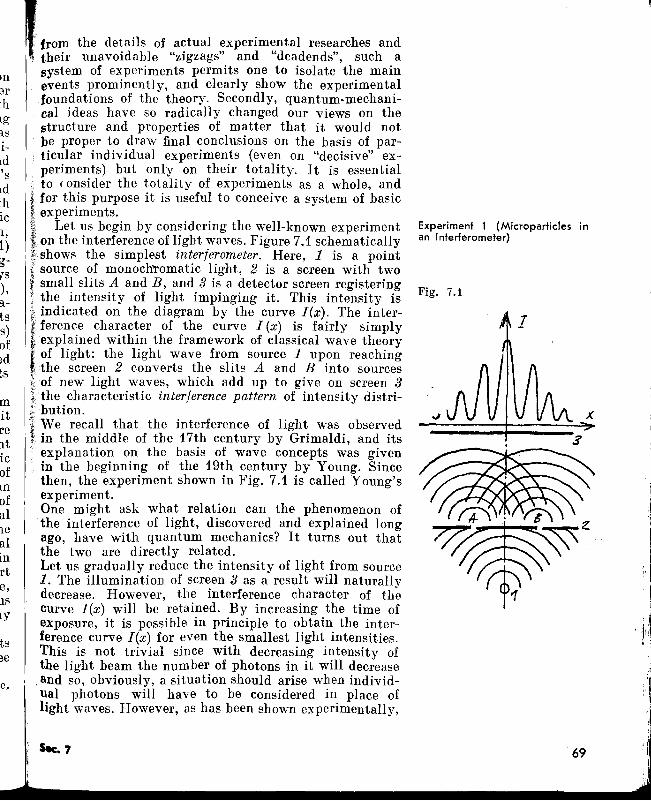
'f

Fig. 7.1

Experiment 1 (Microparticles inan Interferometer)

t.· .: from the detail, of actual experimental re,earche' and.• their unavoidable "zigzags" and "deadends", such a

system of experiments permits one to isolate the mainevents prominently, and clearly show the experimentalfoundations of the theory. Secondly, quantum-mechani­cal ideas have so radically changed our views on thestructure and properties of matter that it would notbe proper to draw final conclusions on the basis of par-ticular individual experiments (even on "decisive" ex­periments) but only on their totality. It is essentialto (onsider the totality of experiments as a whole, andfor this purpose it is useful to conceive a system of basicexperiments.

Let us begin by considering the well-known experimenton the interference of light waves. Figure 7.1 schematically

the simplest interferometer. Here, 1 is a pointsource of monochromatic light, 2 is a screen with twosmall slits A and B, and 3 is a detector screen registeringthe intensity of light impinging it. This intensity isindicated on the diagram by the curve I(x). The inter­ference character of the curve I (x) is fairly simplyexplained within the framework of classical wave theoryof light: the light wave from source 1 upon reachingthe screen 2 converts the slits A and B into sourcesof new light waves, which add up to give on screen 3

characteristic interference pattern of intensity distri­bution.We recall that the interference of light was observed

the middle of the 17th century by Grimaldi, and itsexplanation on the basis of wave concepts was givenin the beginning of the 19th century by Young. Sincethen, the experiment shown in Fig. 7.1 is called Young'sexperiment.One might ask what relation can the phenomenon ofthe interference of light, discovered and explained longago, have with quantum mechanics? It turns out thatthe two are directly related.Let us gradually reduce the intensity of light from source1. The illumination of screen 3 as a result will naturallydecrease. However, the interference character of thecurve I(x) will be retained. By increasing the time ofexposure, it is possible in principle to obtain the inter­ference curve I(x) for even the smallest light intensities.This is not trivial since with decreasing intensity ofthe light beam the number of photons in it will decrease

I ,and so, obviously, a situation should arise when individ­ual photons will have to be considered in place oflight waves. However, as has been shown experimentally,

e,ISly

mitreIticofLll

ofal1ealInrt

yS),a­tss)ofldGS

0'­:>

;hLglS1­

ld'sld;hic1,

1)

srIn

e.

69 -(I

p

I·

70

2

the natu'" 01 the interlerenee eueve lex) obvion'ly re-'lI:mains unchanged no matter how much the light inten- ~! of 1sity is decreased. The distribution of the individual screphotons falling on the detector screen gives the same' distinterference pattern on the screen as is produced by bylight waves. slitMoreover, the interference is observed even if at point 1 By(Fig. 7.1) we place a source of monochromatic electrons but(all having the same energy). In this case also the in- thetensity of the electron beam may be reduced indefinitely. wasWe can even perform an experiment in which the electrons abllpass through the interferometer one by one. By studying anythe distribution of the electrons falling on the detector dis1screen over a sufficiently long exposul'e time we get inin this case also the characteristic interference pattern doe[curve I(x)l. Experiments repeated with other micro- slitparticles (protons, neutrons, etc.) lead to similar results. thuFrom an observation of the behaviour of microparticles mu:in the interferometer it should be concluded that, first- byly, the phenomenon of interference is inherent in all pasmicroparticles and, secondly, it should be explained I1(Jby the properties not of en5embles of microparticles thebut of individual microparticles. regWe shall try to "follow" the motion of an individual ingmicroparticle (say, electron) in the interferometer shown to ;in Fig. 7.1. The electron emerges from point 1, passes witthrough the slits in screen 2 and is finally registered sagat a certain point x on screen 3. By repeating the ex- theperiment for a large number of single electrons we notice Hotwo fairly interesting facts. sin~

The first fact is the impossibility of predicting pre- cancisely at what point x a particular electron will be regis- weteredo The experimental conditions are the same for each oneelectron (remember that the electrons pass through the I all(interferometer one by one) and yet each electron "behaves ofin its own way"; moreover, one cannot predict the way assin which it will behave. This remark applies to every (desingle electron. However, by following a large number slitof electrons, we observe a pattern in the distribution onof their incidence on the screen 3, shown by a kind of (WI

the interference curve I(x). Moreover it is immaterial "hEwhether we observe the distribution of the incidences thEof a large number of single electrons or the distribution thIof the incidences of electrons from a beam. Thus, the ob'unpredictability concerning the behaviour of an indiv- Thidual microparticle is associated with the predictability "hlconcerning the behaviour of a large number of micro- owobjects. otl

5e

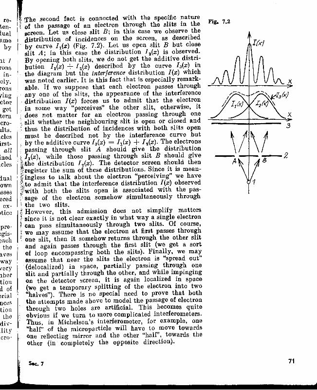
re­ten­iualarne

by

rJ.t 1ronsin­

ely.ronsyingctorget

terncro­Ilts.deslrst-

alllnedcles

iualownlsseseredex­

ltice

pre­19is­~ach

theaveswayvery[lbertiond oflrialficeStionthe

div­ilitycro-

'The second lact is connected with the specilic nat",e.~. of the passage of an electron through the slits in the

screen. Let us close slit B; in this case we observe thedistribution of incidences on the screen, as describedby curve /l(X) (Fig. 7.2). Let us open slit B but closeslit A; in this case the distribution /2(X) is observed.By opening both slits, we do not get the additive distri­bution /l(X) + /2(X) described by the curve /3(X) inthe diagram but the interference distribution /(x) whichwas noted earlier. It is this fact that is especially remark­able. If we suppose that each electron passes throughanyone of the slits, the appearance of the interferencedistribution /(x) forces us to admit that the electronin some way "perceives" the other slit, otherwise, itdoes not matter for an electron passing through oneslit whether the neighbouring slit is open or closed andthus the distribution of incidences with both slits openmust be described not by the interference curve butby the additive curve /3(X) = /l(X) + /2(X). The electronspassing through slit A should give the distribution

~ 11(x), while those passing through slit B should give~,the distribution 12(x). The detector screen should thenif~register the sum of these distributions. Since it is mean-

'Iingless to talk about the electron "perceiving" we havei~to admit that the interference distribution /(x) observed~'with both the slits open is associated with the pas­; sage of the electron somehow simultaneously throughf the two slits.ti However, this admission does not simplify mattersil since it is not clear exactly in what way a single electron~. can pass simultaneously through two slits. Of course,xwe may assume that the electron at first passes through~ one slit, then it somehow returns through the other slit

and again passes through the first slit (we get a sortof loop encompassing both the slits). Finally, we mayassume that near the slits the electron is "spread out"(delocalized) in space, partially passing through oneslit and partially through the other, and while impingingon the detector screen, it is again localized in space(we get a temporary splitting of the electron into two"halves"). There is no special need to prove that boththe attempts made above to model the passage of electronthrough two holes are artificial. This becomes quiteobvious if we turn to more complicated interferometers.Thus, in Michelson's interferometer, for example, one"half" of the microparticle will have to move towardsone reflecting mirror and the other "half", towards theother (in completely the opposite direction).

Sec. 7

Fig. 7.2

[(xl

\1\/- --2,4 13

71

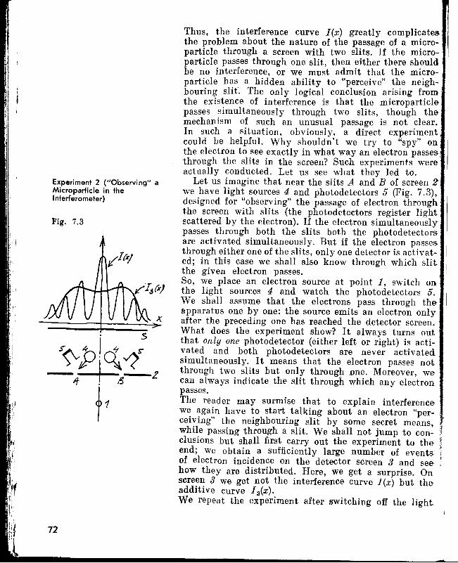
Experiment 2 ("Observing" aMicroparticle in theInterferometer)

Fig. 7.3

11,f"

, ,

\:1 72Hf

Thus, the interference curve lex) greatly complicatesthe problem about the nature of the passage of a micro­particle through a screen with two slits. If the micro­particle passes through one slit, then either there shouldbe no interference, or we must admit that the micro­particle has a hidden ability to "perceive" the neigh­bouring slit. The only logical conclusion arising fromthe existence of interference is that the microparticlepasses simultaneously through two slits, though themechanism of such an unusual passage is not clear.In such a situation, obviously, a direct experimentcould be helpful. Why shouldn't we try to "spy" onthe electron to see exactly in what wayan electron passesthrough the slits in the screen? Such experiments wereactually conducted. Let us see what they led to.

Let us imagine that near the slits A and B of screen 2we have light sources 4 and photodetectors 5 (Fig. 7.3),designed for "observing" the passage of electron throughthe screen with slits (the photodetectors register lightscattered by the electron). If the electron simultaneouslypasses through both the slits both the photodetectorsare activated simultaneously. But if the electron passesthrough either one of the slits, only one detector is activat­ed; in this case we shall also know through which slit I

the given electron passes. 'So, we place an electron source at point 1, switch onthe light sources 4 and watch the photodetectors 5.We shall assume that the electrons pass through theapparatus one by one: the source emits an electron onlyafter the preceding one has reached the detector screen.What does the experiment show? It always turns outthat only one photodetector (either left or right) is acti­vated and both photodetectors are never activatedsimultaneously. It means that the electron passes notthrough two slits but only through .one. Moreover, wecan always indicate the slit through which any electronpasses.The reader may surmise that to explain interferencewe again have to start talking about an electron "per­ceiving" the neighbouring slit by some secret means,while passing through a slit. We shall not jump to con­clusions but shall first carry out the experiment to theend; we obtain a sufficiently large number of eventsof electron incidence on the detector screen 3 and seehow they are distributed. Here, we get a surprise. Onscreen 3 we get not the interference curve lex) but theadditive curve I sex).We repeat the experiment after switching off the light

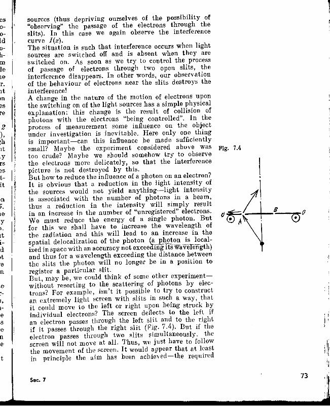
,es0-

O-ld0-

b.-ill

IIe-le-

I,r.Itm fes k,

•re- l

2),~hItlyrs~s

t-it

ill

) .le-y1.

Itl-

d.t'e-n

:er-l,

l-e'.se-ne-

t

sources (thus depriving ourselves of the possibility of"observing" the passage of the electrons through theslits). In this case we again observe the interferencecurve I(x).The situation is such that interference occurs when lightsources are switched off and is absent when they areswitched on. As soon as we try to control the processof passage of electrons through two open slits, theinterference disappears. In other words, our observationof the behaviour of electrons near the slits destroys theinterference!A change in the nature of the motion of electrons uponthe switching on of the light sources has a simple physicalexplanation: this change is the result of collision ofphotons with the electrons "being controlled". In theprocess of measurement some influence on the objectunder investigation is inevitable. Here only one thingis important-can this influence be made sufficientlysmall? Maybe the experiment considered above wastoo crude? Maybe we should somehow try to observethe electrons more delicately, so that the interferencepicture is not destroyed by this.But how to reduce the influence of a photon on an electron?It is obvious that a reduction in the light intensity ofthe sources would not yield anything-light intensityis associated with the number of photons in a beam,thus a reduction in the intensity will simply resultin an increase in the number of "unregistered" electrons.We must reduce the energy of a single photon. Butfor this we shall have to increase the wavelength ofthe radiation and this will lead to an increase in thespatial delocalization of the photon (a photon is local­ized in space with an accuracy not exceedingffiwaveIength)and thus for a wavelength exceeding the distance betweenthe slits the photon will no longer be in a position toregister a particular slit.But, may be, we could think of some other experiment­without resorting to the scattering of photons by elec­trons? For example, isn't it possible to try to constructan extremely light screen with slits in such away, thatit could move to the left or right upon being struck byindividual electrons? The screen deflects to the left ifan electron passes through the left slit and to the rightif it passes through the right slit (Fig. 7.4). But if theelectron passes through two slits simultaneously, thescreen will not move at all. Thus, we just have to followthe movement of the screen. It would appear that at leastin principle the aim has been achieved-the required

Sec. 7

Fig. 7.4

I,\

73

1

II

. I, I

,1,1.II ~

'\

I.I

delicate experiment has been conceived. But it is mean­ingless to set up such an experiment. To make sure thatthis is so, we recall the uncertainty relation for momen­tum and coordinate. It follows from this relation thatif the experimental conditions really permit us to register­the momentum of the screen due to a recoil from the elec­tron impingement, the same condition must lead to an "­uncertainty in the position of the screen on the line 00 ~

(Fig. 7.4). Consequently, the shift in such a screen doesnot permit one to draw any conclusion on the nature ofpassage of an electron through the slits. If, on the otherhand, we fix the position of the screen on the line 00,then it is easy to see that a measurement of the momen­tum of its recoil will become impossible.Several attempts were made to devise such an experimentin which the passage of electrons through a screen withslits could be "controlled" without seriously influencingthe electrons themselves (so that the interference is notdestroyed). But all these attempts proved futile. As aresult, we must admit that the above conclusion regardingthe destruction of interference caused by observing thebehaviour of electrons near the slit, is of a fundamentalnature. In other words, the effect of observation (measure­ment) destroying interference cannot be eliminated inprinciple.

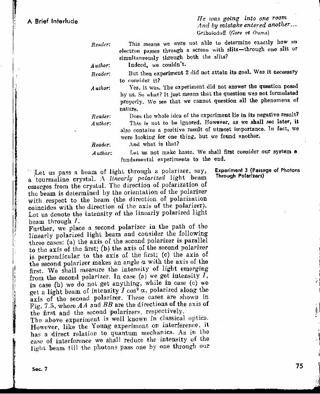
Author:

Reader:

Reader:

Reader:Author:

Author:

Author:

Reader:

He was going into one roomAnd by mistake entered another...Griboiedoff (Gore ot Ouma)

This means we were not able to determine exactly how anelectron passes through a screen with slits-through one slit orsimultaneously through both the slits?

Indeed, we couldn't.But then experiment 2 did not attain its goal. Was it necessary

to consider it?Yes, it was. The experiment did not answer the question posed

by us. So what? It just means that the question was not formulatedproperly. We see that we cannot question all the phenomena ofnature.

Does the whole idea of the experiment lie in its negative result?This is not to be ignored. However, as we shall see later, it

also contains a positive result of utmost importance. In fact, wewere looking for one thing, but we found another.

And what is that?Let us not make haste. We shall first consider our system 8

fundamental experiments to the end.

'jLet us pass a beam of light through a polarizer, say, Experiment 3 (Passage of Photonsa tourmaline crystal. A linearly polarized light beam Through Polarizers)

emerges from the crystal. The direction of polarization ofthe beam is determined by the orientation of the polarizerwith respect to the beam (the direction of polarizationcoincides with the direction of the axis of the polarizer).Let us denote the intensity of the linearly polarized lightbeam through f.Further, we place a second polarizer in the path of thelinearly polarized light beam and consider the followingthree cases: (a) the axis of the second polarizer is parallelto the axis of the first; (b) the axis of the second polarizeris perpendicular to the axis of the first; (c) the axis ofthe second polarizer makes an angle a with the axis of thefirst. We shall measure the intensity of light emergingfrom the second polarizer. In case (a) we get intensity f,in case (b) we do not get anything, while in case (c) weget a light beam of intensity f cos2 a, polarized along theaxis of the second polarizer. These cases are shown inFig. 7.5, where AA and BB are the directions of the axis ofthe first and the second polarizers, respectively.The above experiment is well known in classical optics.However, like the Young experiment on interference, ithas a direct relation to quantum mechanics. As in thecase of interference we shall reduce the intensity of thelight beam till the photons pass one by one through our

A Brief Interlude

I,Sec. 7 7S

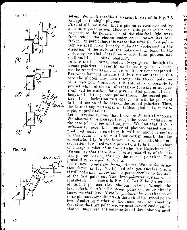
Fig. 7.5

fa)

(I;

Fig. 7.6

~i 76

~1

set-up. We shall consider the cases illustrated in Pig. 7.5as applied to single photons.First of all, we recall that a photon is characterized bya definite polarization. Moreover, this polarization cor­responds to the polarization of the classical light wavefrom which the photon under consideration has been"taken". In particular, this means that after the first polar­izer we shall have linearly polarized (polarized in thedirection of the axis of the polarizer) photons. In thefollowing we shall "deal" only with these photons andshall call them "initial photons".In case (a) the initial photon always passes through thesecond polarizer; in case:(b), on the contrary, it never pas­ses the second polarizer. These results are not unexpected.But what happens in case (c)? It turns out that in thiscase the photon may pass through the second polarizeror it may not. Moreover, it is absolutely impossible topredict which of the two alternatives (passing or not pas­sing) will be realized for a given initial photon. If it sohappens that the photon passes through the second polar­izer, its polarization will change-it will be polarizedin the direction of the axis of the second polarizer. Thus,the fate of any particular individual photon is, in prin­ciple, unpredictable!Let us assume further that there are N initial photons.We observe their passage through the second polarizer inthe case (c) and see what happens. We find that if N issufficiently large, the number of photons passed can bepredicted fairly accurately; it will be about N cos 2 ex.In this connection, we recall our earlier remark that theunpredictability in the behaviour of an individual mi­croparticle is related to the predictability in the behaviourof a large number of microparticles (see Experiment 1).We can say that there is a definite prohaboility of the ini­tial photon passing through the second polarizer. Thisprobability is equal to cos 2 ex.Let us now complicate the experiment. We use the situa­tion shown in Fig. 7.5 (c) and add yet another (i.e. athird) polarizer, whose axis is perpendicular to the axisof the first polarizer. The three-polarizer system underconsideration is shown in Fig. 7.6. Let N be the numberof initial photons (i.e. photons passing through thefirst polarizer). After the second polarizer, as we alreadyknow, we shall have N cos 2 ex photons, the polarization ofthese photons coinciding with the axis of the second polar­izer. Analysing further in the same way, we concludethat after the third polarizer, we must have N cos2 ex sin2 exphotons; moreover, the polarization of these photons must

coP€Tlise:lillttCf

W

faa]PifiIf"1tiFna

u1rIfIIt~

I

Itt1

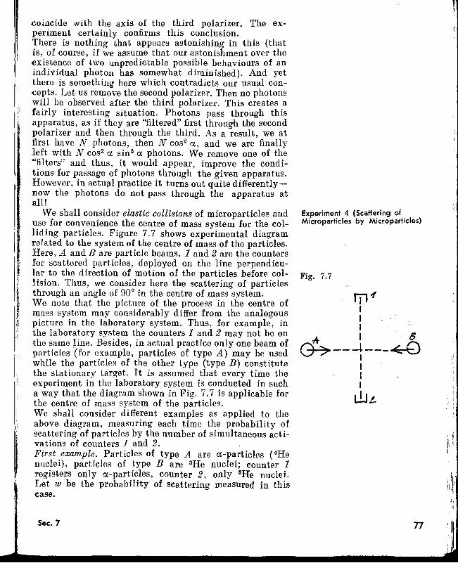
It

coincide with the axis of the third polarizer. The ex­periment certainly confirms this conclusion.There is nothing that appears astonishing in this (thatis, of course, if we assume that our astonishment over theexistence of two unpredictable possible behaviours of anindividual photon has somewhat diminished). And yetthere is something here which contradicts our usual con­cepts. Let us remove the second polarizer. Then no photonswill be observed after the third polarizer. This creates afairly interesting situation. Photons pass through thisapparatus, as if they are "filtered" first through the secondpolarizer and then through the third. As a result, we atfirst have N photons, then N cos2 a, and we are finallyleft with N cos2 a sin2 a photons. We remove one of the«filters" and thus, it would appear, improve the condi­tions for passage of photons through the given apparatus.However, in actufll practice it turns out quite differently­now the photons do not pass through the apparatus atall!

We shall consider elastic collisions of microparticles anduse for convenience the centre of mass system for the col­liding particles. Figure 7.7 shows experimental diagramrelated to the system of the centre of mass of the particles.Here, A and B are particle beams, 1 and 2 are the countersfor scattered particles, deployed on the line perpendicu­lar to the direction of motion of the particles before col­lision. Thus, we consider here the scattering of particlesthrough an angle of 90° in the centre of mass system.We note that the picture of the process in the centre ofmass system may considerably differ from the analogouspicture in the laboratory system. Thus, for example, inthe laboratory system the counters 1 and 2 may not be onthe same line. Besides, in actual practice only one beam ofparticles (for example, particles of type A) may be usedwhile the particles of the other type (type B) constitutethe stationary target. It is assumed that every time theexperiment in the laboratory system is conducted in sucha way that the diagram shown in Fig. 7.7 is applicable forthe centre of mass system of the particles.We shall consider different examples as applied to theabove diagram, measuring each time the probability ofscattering of particles by the number of simultaneous acti­vations of counters 1 and 2.First example. Particles of type A are a-particles (4Henuclei), particles of type Bare 3He nuclei; counter 1registers only a-particles, counter 2, only 3He nuclei.Let 1IJ be the probability of scattering measured in thiscase.

Sec. 7

Experiment 4 (Scattering ofMicroparticles by Microparticles)

Fig. 7.7

1j1"(

II

,+. I '. /3

~--~---~IIII

L!.Jt.

77

:11'"II.'"~'I

',.1·1'

Ii

,I;

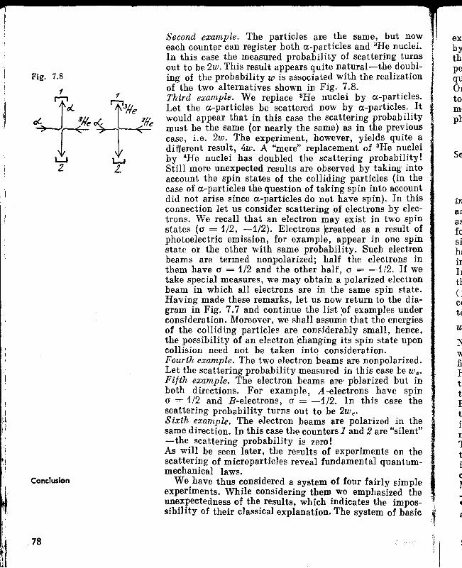
Conclusion

78

Second example. The particles are the same, but noweach counter can register both a-particles and 3He nuclei.In this case the measured probability of scattering turnsout to be 2w. This result appears quite natural-the doubl­ing of the probability w is associated with the realizationof the two alternatives shown in Fig. 7.8.Third example. We replace 3He nuclei by a-particles.Let the a-particles be scattered now by a-particles. Itwould appear that in this case the scattering probabilitymust be the same (or nearly the same) as in the previouscase, i.e. 2w. The experiment, however, yields quite adifferent result, 4w. A "mere" replacement of 3He nucleiby 4He nuclei has doubled the scattering probability!Still more unexpected results are observed by taking intoaccount the spin states of the colliding particles (in thecase of a-particles the question of taking spin into accountdid not arise since a-particles do not have spin). In thisconnection let us consider scattering of electrons by elec­trons. We recall that an electron may exist in two spinstates (a = 1/2, -1/2). Electrons Jcreated as a result ofphotoelectric emission, for example, appear in one spinstate or the other with same probability. Such electronbeams are termed nonpolarized; half the electrons inthem have a = 1/2 and the other half, a = -1/2. If wetake special measures, we may obtain a polarized electronbeam in which all electrons are in the same spin state.Having made these remarks, let us now return to the dia­gram in Fig. 7.7 and continue the list bf examples underconsideration. Moreover, we shall assume that the energiesof the colliding particles are considerably small, hence,the possibility of an electron ~hanging its spin state uponcollision need not be taken into consideration.Fourth example. The two electron beams are nonpolarized.Let the scattering probability measured in this case be We.

Fifth example. The electron beams are pblarized but inboth directions. For example, A-electrons have spina = 1/2 and B-electrons, a = -1/2. In this case thescattering probability turns out to be 2we •

Sixth example. The electron beams are polarized in thesame direction. In this case the counters 1 and 2 are "silent"-the scattering probability is zero!As will be seen later, the results of experiments on thescattering of microparticles reveal fundamental quantum­mechanical laws.

We have thus considered a system of four fairly simpleexperiments. While considering them we emphasized theunexpectedness of the results, which indicates the impos­sibility of their classical explanation. The system of basic

exbythpequ01tomlph

Se

inaraEfosihIirIItl( j

c<t<w

1\

"fiFt:t:Eti,n1tic~, 4

~

j

I

I

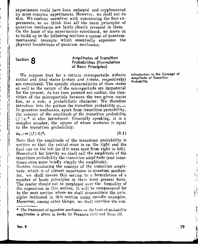
Section 8

experiments could have been enlarged and supplementedby more complex experiments. However, we shall not dothis. We content ourselves with considering the four ex­periments, as we think that all the basic principles ofquantum mechanics are fairly :clearly revealed in them.On the basis of the experiments considered, we move onto build up in the following sections a system of quantum­mechanical concepts which essentially expresses thephysical foundations of quantum mechanics.

Amplitudes of TransitionProbabilities (Formulationof Basic Principles)

We suppose that for a certain microparticle definiteinitial and fina~ states (s-state and I-state, respectively)are considered. The specific characteristics of these statesas well as the nature of the microparticle are immaterialfor the present. As has been pointed out earlier, the tran­sition of the microparticle between the two given stateshas, as a rule, a probabilistic character. We thereforeintroduce into the picture the transition probability Ws-f'

In quantum mechanics, apart from transition probability,the concept of the amplitude 01 the transition probability(I Is) * is also introduced. Generally speaking, it is acomplex number, the square of whose modulus is equalto the transition probability:

W,_f= 1<1 I s)1 2• (8.1)

Note that the amplitude of the transition probability iswritten so that the initial state is on the right and thefinal one on the left (as if it were read from right to left).Henceforth for brevity we shall call the amplitude of thetransition probability the transition amplitude (and some­times even more briefly simply the amplitude).Besides introducing the concept of the transition ampli­tude, which is of utmost importance to quantum mechan­ics, we shall devote this section to a formulation of anumber of basic principles in their most general form.The reader should not be perplexed over the formality ofthe exposition in this section. It will be compensated forin the next section where we shall demonstrate the prin­ciples indicated in this section using specific examples.Moreover, among other things, we shall consider the con-

• The treatment of quantum mechanics on the basis of probabilityamplitudes is given in books by Feynman [3-5] and'birac [9].

Sec. 8

Introduction to the Concept ofAmplitude of TransitionProbability

79

;, i, ,I

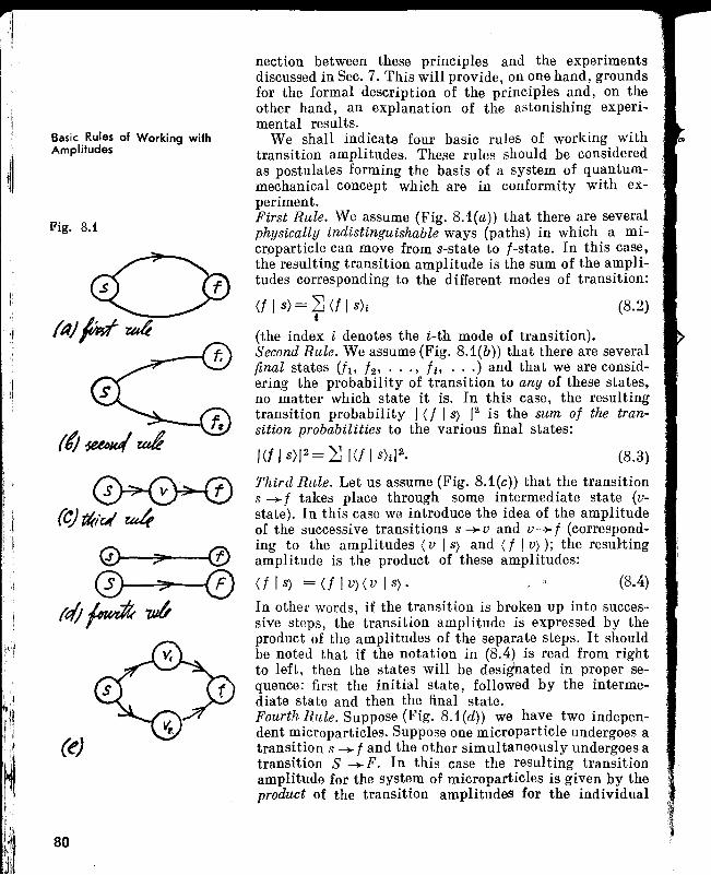
1'14,'

illI I

~I,

1.•...1.'1..~ .

~II

Basic Rules of Working withAmplitudes

Fig. 8.1

~{q)tI<i~ u4

o ;>- (0

~ftl;fJt tJb

(e)

80

nection between these principles and the experimentsdiscussed in Sec. 7. This will provide, on one hand, groundsfor the formal description of the principles and, on theother hand, an explanation of the astonishing experi­mental results.

We shall indicate four basic rules of working withtransition amplitudes. These rules should be consideredas postulates forming the basis of a system of quantum­mechanical concept which are in conformity with ex­periment.First Rule. We assume (Fig. 8.1(a)) that there are severalphysicaUy indistingUishable ways (paths) in which a mi­croparticle can move from s-state to I-state. In this case,the resulting transition amplitude is the sum of the ampli­tudes corresponding to the different modes of transition:

(f I s) = ~ <I I S)i (8.2)t

(the index i denotes the i-th mode of transition).Second Rule. We assume (Fig. 8.1(b)) that there are severalfinal states (f1' 12' ... , Ii' ... ) and that we are consid­ering the probability of transition to any of these states,no matter which state it is. In this case, the resultingtransition probability I <I I S) /2 is the sum 01 the tran­sition probabilities to the various final states:

/</ I S)/2= Lj /<1 I s)i1 2• (8.3)

Third Rule. Let us assume (Fig. 8.1(c)) that the transitions -+ I takes place through some intermediate state (v­state). In this case we introduce the idea of the amplitudeof the successive transitions s -+ v and v-+ I (correspond­ing to the amplitudes <v I s) and <I I v»); the resultingamplitude is the product of these amplitudes:

<t I s) = <t I V) <v I s) • (8.4)

In other words, if the transition is broken up into succes­sive steps, the transition amplitude is expressed by theproduct of the amplitudes of the separate steps. It shouldbe noted that if the notation in (8.4) is read from rightto left, then the states will be designated in proper se­quence: first the initial state, followed by the interme­diate state and then the final state.Fourth Rule. Suppose (Fig. 8.1(d)) we have two indepen­dent microparticles. Suppose one microparticle undergoes atransition s -+ I and the other simultaneously undergoes atransition S -+ F. In this case the resulting transitionamplitude for the system of microparticles is given by theproduct of the transition amplitudes for the individual

'"

_-jJ;*~ In.icroparticles:~k <IF IsS) = (f I s) (F I S> . (8.5)

We can see that the second, third and fourth rules ap­pear quite natural since, together with (8.1), they repre­sent well-known theorems, i.e. the theorem of addition ofprobabilities (second rule) and the theorem of multipli­cation of probabilities of independent events (third andfourth rules). Only the first rule, which may be called therule 01 addition at amplitudes, appears unusual. In a cer­tain sense, the entire system of quantum-mechanical con­cepts is based on the rule of the addition of amplitudes.

Suppose that the transition of a microparticle from theinitial to the final state (s ~ I transition) always takesplace through one of the intermediate states (VI' V 2, •••

• • . , Vi' ... ) (Fig. 8.1(e)). In this case, one or the othermode of transition s ~ I (one alternative or the other)is determined by the "participation" of the correspondingintermediate state in the transition.We take two different cases. Suppose in the first case theintermediate state through which a given t'ransition takes

- place is known. This is the case of physically distinguishablealternatives. To describe this we must combine the secondand the third rules. The transition probability that weobtain as a result will be of the form

Distinguishable andIndistinguishable Alternatives.Interference of Amplitudes

yI

(8.6)

One might ask: where does the second rule come in if itonly involves the various final states? As a matter of fact,if we know the intermediate state at which the micropar­ticle arrives, it may be treated as the final state of thefirst step of the transition. We fix the microparticle in thisstate and temporarily stop the experiment here. One micro­particle will be fixed in one state, the others in variousother states, so, a situation with different final statesactually arises. We stress here that distinguishability ofalternatives is connected with the actual existence of differ­ent final states (even if in the given experiment theyplay the role of intermediate states).In the second case, we don't know the intermediate statethrough which a particular transition takes place. This isthe case of physically indistinguishable alternatives.To describe this case we should combine the first and thethird rules. The resulting transition probability will beof the form

<I I s) = ~ (f I Vi) (Vi Is).i

Sec. 8

(8.7)

81

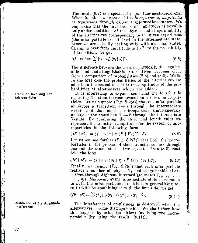
j.11I

Transition Involving TwoMicroparticles

Destruc:tion of the AmplitudeIntenerenc:e

82

The result (8.7) is a specifically quantum-mechanical one.When it holds, we speak of the interference of amplitudes·of transitions through different intermediate states. Weemphasize that the interference of amplitudes is possibleonly under conditions of the physical indistinguishabilityof the alternatives corresponding to the given experiment(the microparticle is not fixed in the intermediate state,hence we are actually dealing only with one final state).Changing over from amplitude in (8.7) to the probabilityof transition, we get

/<fls)/2=2,]I<flvi}(Vils)12. (8.8),The difference between the cases of physically distinguish­able and indistinguishable alternatives becomes clearfrom a comparison of probabilities (8.6) and (8.8). Whilein the first case the probabilities of the alternatives areadded, in the second case it is the amplitudes of the pro­babilities of alternatives which are added.

It is interesting to expand somewhat the fourth ruleregarding the simultaneous transition of two micropar­ticles. Let us suppose (Fig. 8.2(a» that one microparticleun lergoes a transition s --+ f through the intermediatev-state and that another microparticle simultaneouslyundergoes the transition S --+ F through the intermediateV-state. By combining the third and fourth rules werepresent the transition amplitude for the system of mic­roparticles in the following form:

(fF IsS) = <t I V) (v I s) (F I V) ( V I S) • (8.9)

Let us assume further (Fig. 8.2(b) that both the micro­particles in the process of their transitions ass throughone and the same intermediate vI-state. Then (8.9) musttake the form

(IF IsS) = (I I VI) (VI I s) (F I VI) (VI .. IS) • (8.10)

Finally, we assume (Fig. 8.2(c) that each microparticlerealizes a number of physically indistinguishable alter­natives through different intermediate states (VI, V 2 , •••

. . •, Vi)' Moreover, every intermediate state is commonto both the microparticles. In this case generalizing re­sult (8.10) by combining it with the first rule, we get

<IF I 5S) = 1(f I VI) (VI Is) (F IVi) (VI IS). (8.11)

The interference of amplitudes is destroyed when thealternatives become distinguishable. We shall show howthis happens by using transitions involvi19 two micro­particles [by using the result (8.11) l.

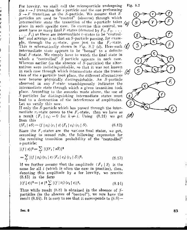
t'

(8.14)

(8.13)

For brevity, we shall call the microparticle undergoing Fig. 8.2

the s -+ f tra?~ition the s-particl: and the one perform.ing 1':"\ ~J:"\ -..t:nS -+F transItIOn as the S-partIcle. We assume that S- ~ '!:!particles are used to "control" (observe) through which~intermediate state the transition of the s-particle takes fa/) S v Fplace in each specific case. To exercise this control, wemust have as many final F -states (denoted by F l' F 2' ...

... , F;) as there are intermediate v-states to be "control­led" and arrange it so that an S-particle passing, for exam-ple, through the Vi-state, goes just to the Fi-state.This is schematically shown in Fig. 8.2 (d). Here each ft;intermediate state appears to be "bound" to a definite'final F-state. We simply have to watch the final state inwhich a "controlled" S-particle appears in each case.Whereas earlier (in the absence of S -particles) the alter­natives were indistinguishable, so that it was not knownin each case through which intermediate state the transi- (e)tion of the s-particle took place, the different alternativesnow become physically distinguishable. An S-particleobserved in any F-state unambiguously indicates theintermediate state through which a given transition tookplace. According to the remarks made above, the use ofS-particles for distinguishing intermediate states mustlead to a destruction of the interference of amplitudes.Let us verify this now.If only the S-particle which has passed through the inter­mediate vcstate comes to the Fi-state, then we have as /.J')a result (F i 1 Vii) =0 for k=/=i. Using (8.11) we get {C'lJ

from this(fFi IsS) = <I I Vi) (Vi Is) (Fi I Vi) (Vi IS). (8.12)

Since the Fi-states are the various final states, we get,according to second rule, the following expression forthe resulting transition probability of the "controlled"s-particle:

IU / s)1 2 = LJ IUFi I sS)1 2

i

= LJ 1<1/ Vi) (Vi 1S) (Pi IVi) (Vi I S)1 2•i

If we further assume that the amplitude (F i I S) is thesame for all i (which is often the case in practice), then,denoting this amplitude by a for brevity, we rewrite(8.13) in the form

IU I s)1 2 = I a /2 LJ IU IVi) (Vi I s)I 2•i

{

see'Yt

Thus while result (8.8) is obtained in the absence of S­particles (in the absence of "control"), we now have theresult (8.14). It is easy to see that it corresponds to (8.6)-

Sec. 8 83

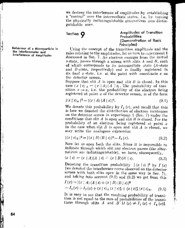
;1\I

I':

Behaviour of a Microparticle inthe Interferometer andInterference of Amplitudes

84

we destroy the interference of amplitudes by establishinga "control" over the intermediate states, i.e. by turningthe physically indistinguishable alternatives into distin­guishable ones.

S . 9 Amplitudes of Transitionectlon Probabilities

(Demonstration of BasicPrinciples)

Using the concept of the transition amplitude and therules relating to the amplitudes, let us turn to experiment 1discussed in Sec. 7. An electron emerges from the initials-state, passes through a screen with slits A and B, eachof which corresponds to its intermediate state (A -stateand B-state, respectively) and is finally registered inits final x-state, i.e. at the point with coordinate x onthe detector screen.Suppose that slit A is open and slit B is closed. In thiscase (x I S) A = (x IA) (A Is). The probability of tran­sition s -x, i.e. the probability of the electron beingregistered at point x of the detector screen, is of the form

I(x I S)A /2= I(x I A) (A I S)/2. (9.1)

We denote this probability by II (x), and recall that thisis how we denoted the distribution of electron incidenceson the detector screen in experiment 1 (Sec. 7) under theconditions that slit A is open and slit B is closed. For theprobability of an electron being registered at point xin the case when slit B is open and slit A is closed, wemay write the analogous expression

(9.2)

Now let us open both the slits. Since it is impossible toindicate through which slit any electron passes (the alter­natives are indistinguishable), we have,; consequently,

(x I s) = (x I A )(A I s) + (x I B)(B , s). (9.3)

Denoting the transition probability I (x I s) 12 by I (x)(we denoted the interference curve observed on the detectorscreen with both slits open in the same way in Sec. 7),and taking into account (9.1) and (9.2) we get from this

I(x)= /(x I A) (A / s)+(x I B) (B I s)/%

= Ii (x) +12 (x) + (x I S)A (x I s)1 + (x I s)l (x Ish. (9.4)

It is easy to see that the resulting probability of transi­tion is not equal to the sum of probabilities of the transi­tions through slits A and B [I (x) =1= II (x) + 1

2(x)l.

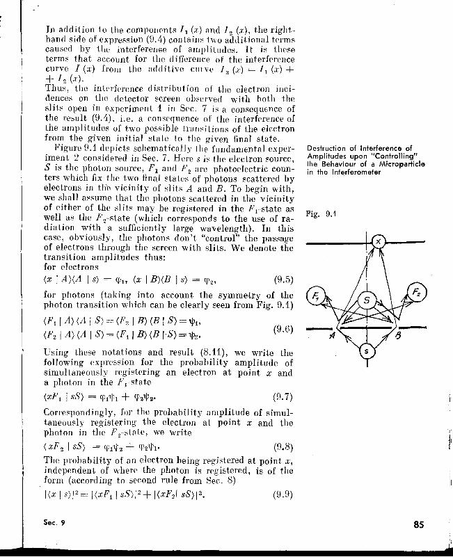
(9.6)

In addition to the components I I (x) and 1 2 (x), the right­hand side of expression (9.4) contains two additional termscaused by the interferen~ of amplitudes. It is theseterms that account for the difference of the interferencecurve I (x) from the add itive cmve 1 3 (x) = I I (x) ++ 12 (x).Thus, the interference distribution of the electron inci­dences on the detector screen observed with both theslits open in experiment 1 in Sec. 7 is a consequence ofthe result (9.4), i.e. a consequence of the interference ofthe amplitudes of two possible transitions of the electronfrom the given initial state to the given final state.

Figure 9.1 depicts schematically the fundamental exper­iment 2 considered in Sec. 7. Here s is the electron source,S is the photon source, PI and P 2 are photoelectric coun­ters which fix the two final states of photons scattered byelectrons in th'e vicinity of slits A and B. To begin with,we shall assume that the photons scattered in the vicinityof either of the slits may be registered in the Fl-state aswell as the P 2-state (which corresponds to the use of ra­diation with a sufficiently large wavelength). In thiscase, obviously, the photons don't "control" the passageof electrons through the screen with slits. We denote thetransition amplitudes thus:for electrons(x I A)(A Is) = CPI, (x I B)(B Is) = CP2' (9.5)

for photons (taking into account the symmetry of thephoton transition which can be clearly seen from Fig. 9.1)

(Fi I A) (A I S) = (F2 I B) (B I S) = "'1'(F21 A)(A 1 S)=(F i / B)(B /,S)="'2'

Using these notations and result (8.11), we write thefollowing expression for the probability amplitude ofsimultaneously registering an electron at point x anda photon in the Fl-state

(xFI IsS> = CPlll\ + CP21\J2' (9.7)

Correspondingly, for the probability amplitude of simul­taneously registering the electron at point x and thephoton in the P 2-st3te, we write

(xF2 1 sS) = CPIlP2 + CP2lP!. (9.8)The probability of an electron being registered at point x,independent of where the photon is registered, is of theform (according to second rule from Sec. 8)

I(x I s)1 2 = l(xF1 1sS))2+ l(xF2 / sS)1 2 • (9.9)

Sec. 9

Destruction of Interference ofAmplitudes upon "Controlling"the Behaviour of a Microparticlein the Interferometer

Fig. 9.1

"jiI

:1II

, !8S I

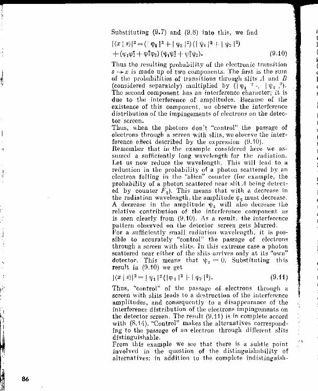
Thus the resulting probability of the electronic transitions --+ x is made up of two components. The first is the sumof the probabilities of transitions through slits A and B(considered separately) multiplied by (I 'ljJ1 [2 + ['ljJ2 1

2).The second component has an interference character; it isdue to the interference of amplitudes. Because of theexistence of this component, we observe the interferencedistribution of the impingements of electrons on the detec­tor screen.Thus, when the photons don't "control" the passage ofelectrons through a screen with slits, we observe the inter­ference effect described by the expression (9.10).Remember that in the example considered here we as­sumed a sufficiently long wavelength for the radiation.Let us now reduce the wavelength. This will lead to areduction in the probability of a photon scattered by anelectron falling in the "alien" counter (for example, theprobability of a photon scattered near slit A being detect­ed by counter F 2 ). This means that with a decrease inthe radiation wavelength, the amplitude 1/12 must decrease.A decrease in the amplitude 1/12 will also decrease therelative contribution of the interference component asis seen clearly from (9.10). As a result, the interferencepattern observed on the detector screen gets blurred.For a sufficiently small radiation wavelength, it is pos­sible to accurately "control" the passage of electronsthrough a screen with slits. In this extreme case a photonscattered near either of the slits arrives only at its "own"detector. This means that 1P2 = O. Substituting thisresult in (9.10) we get

I(x I s)1 2= /1VtI 2(lcpt 12+ I CP21 2). (9.11)

Thus, "control" of the passage of electrons through ascreen with slits leads to a destruction of the interferenceamplitudes, and consequently to a disappearance of theinterference distribution of the electrons impingements onthe detector screen. The result (9.11) is in complete accordwith (8.14). "Control" makes the alternatives correspond­ing to the passage of an electron through different slitsdistingUishable.From this example we see that there is a subtle pointinvolved in the question of the distinguishability ofalternatives: in addition to the complete indistinguish-

86

Substituting (9.7) and (9.8) into this, we find

I(x I s)1 2=(/ qJ11 2+ I qJ21 2) (I 'ljJt/ 2 + I 'ljJ21 2)

+ (qJtqJ~ + qJlqJ2) (1Pt'ljJ~ + ~)N2). (9.10)

"

3

t1(g(

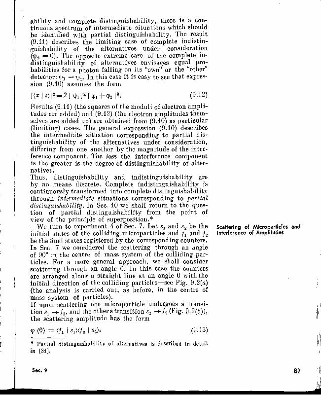
ability and complete distinguishability, there is a con­tinuous spectrum of intermediate situations which shouldbe identified with partial distinguishability. The result(9.11) describes the limiting case of complete indistin­guishability of the alternatives under considerationN2 = 0). The opposite extreme case of the complete in­distinguishability of alternatives envisages equal pro­babilities for a photon falling on its "own" or the "other"detector: 1J'1 = 1J'2' In this case it is easy to see that expres­sion (9.10) assumes the form

I(x I s)1 2=21 'lJJ1/ 21cr1 + cr2 12• (9.12)

Results (9.11) (the squares of the moduli of electron ampli­tudes are added) and (9.12) (the electron amplitudes them­selves are added up) are obtained from (9.10) as particular(limiting) cas~s. The general expression (9.10) describesthe intermediate situation corresponding to partial dis­tinguishability of the alternatives under consideration,differing from one another by the magnitude of the inter­ference component. The less the interference componentis the greater is the degree of distinguishability of alter­native3.Thus, distinguishability and indistinguishability areby no means discrete. Complete indistinguishability iscontinuously transformed into complete distinguishabilitythrough intermediate situations corresponding to partialdistinguishability. In Sec. 10 we shall return to the ques­tion of partial distinguishability from the point ofview of the principle of superposition.*

We turn to experiment 4 of Sec. 7. Let Sl and 8 2 be theinitial states of the colliding microparticles and 11 and 12be the final states registered by the corresponding counters.In Sec. 7 we considered the scattering through an angleof 90° in the centre of mass system of the colliding par­ticles. For a more general approach, we shall considerscattering through an angle e. In this case the countersare arranged along a straight line at an angle e with theinitial direction of the colliding particles-see Fig. 9.2(a)(the analysis is carried out, as before, in the centre ofmass system of particles).If upon scattering one microparticle undergoes a transi­tions1 -11' and theotheratransitions2 -/2 (Fig. 9.2(b)),the scattering amplitude has the form

Scatfering of Microparticles andInterference of Amplitudes

~. i, 'i

(9.13)

* Partial distinguishability of alternatives is described in detailin [31].

Sec. 9 87

;~.

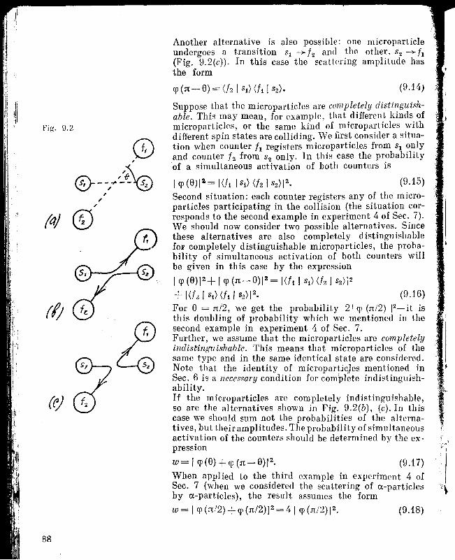
(9.14 )

Suppose that the microparticles are completely distinguish­able. This may mean, for example, that different kinds ofmicroparticles, or the same kind of microparticles withdifferent spin states are colliding. We fIrst consider a situa­tion when counter 11 registers microparticles from SI onlyand counter 12 from S2 only. In this case the probabilityof a simultaneous activation of both counters is

Another alternative is also possible: one microparticleundergoes a transition SI -+ 12 and the other, S2 -+ 11(Fig. 9.2(c». In this case the scattering amplitude hasthe form

1q> (8)1 2 = W1 181) (/21 S2)/2. (9.15)Second situation: each counter registers any of the micro­particles participating in the collision (the situation cor­responds to the second example in experiment 4 of Sec. 7).We should now consider two possible alternatives. Sincethese alternatives are also completely distinguishablefOF completely distinguishable microparticles, the proba­bility of simultaneous activation of both counters willbe given in this case by the expression

I q> (8)1 2 + I q> (n-8)1 2 = 1<11 181) (121 52)1 2

+ 1(14181) (/1182)12. (9.16)For 8 = n/2, we get the probability 21 q> (:rr/2) 1

2-it isthis doubling of probability which we mentioned in thesecond example in experiment 4 of Sec. 7.Further, we assume that the microparticles are completelyindistinguishablJe. This means that microparticles of thesame type and in the same identical state are considered.Note that the identity of micropartiq]es mentioned inSec. 6 is a necessary condition for complete indistinguish­ability.If the microparticles are completely indistinguishable,so are the alternatives shown in Fig. 9.2(b), (c). In thiscase we should sum not the probabilities of the alterna­tives, but their amplitudes. The probability of simultaneousactivation of the counters should be determined by the ex­pression

W= / rp (8) + cp (n- 8)/2. (9.17)

When applied to the third example in experiment 4 ofSec. 7 (when we considered the scattering of a-particles 'i~

by a-particles), the result assumes the form

W= / cp(:rr/2)+cp(:rr/2)1 2 =41 cp(:rr/2)/2. (9.18)

(I;

(f)

CD,

,~ -.®---,+'-"-l(0,,,

(tI) CD

Fig. 9.2

88

,. ..

~~

It is this four-fold increase in the probability I cp (:11/2) 12

which was observed in the experiment.Interference of scattering amplitudes is just one of theconsequences of the complete indistinguishability of mic­roparticles. Another consequence is that the probabilityof the simultaneous activation of counters should notchange if we interchange Sl and S2' or, in other words, ifwe interchange the scattering amplitudes cp (8) andcp (n - 8). If we proceed from these consequences, theprobability may be formally written in the form

W = I cp (8) + qJ (n - 8)12. (9.19)

The alternative with the "+" sign (interfering amplitudeshave the same sign) is already familiar to us-it is theexpression (9.17). The other alternative, when the ampli­tude with opposite signs interfere, is alE:O formally pos­sible. It is remarkable that nature "employs" this alter­native as well; this can be verified by studying the resultsof experiments on scattering of electrons by electrons.Thus, we assume that amplitudes with opposite signs in­terfere:

W e = I qJ (8)-cp (:n-8)1 2 (9.20)

\

and turn to the results of the indicated experiments. For8 = :n/2, the probability (9.20) vanishes. This corres­ponds to the sixth example in experiment 4 of Sec. 7.We recall that th is example concerned the collision ofelectrons in the same spin state. It is in this case that wehave two completely indistinguishable alternatives forthe electrons*.If the colliding electrons are in different spin states (thefifth example in experiment 4), the alternatives are distin­guishable. In this case the probability of the activationof the counters is given (as for distinguishable particles)by expression (~l.17), which for 8 = :n/2 leads to the famil­iar result 2 I (P (:n/2) 1

2 • In the case of non-polarizedelectron beams (the fourth example in experiment 4),it should be remembered that the probability of collisionbetween two electrons in similar spin states is 1/2. Fromthis, taking (9.20) and (9.16) into account, we get thefollowing expression for the probability of activation of

* We shall henceforth omit the word "completely", but shall ahaysmean it while speaking of distinguishable and indistinguishablealternatives. Partial distinguishability will be specially mentioned.

Sec. 9

~ I

I

ile

!

89:1..

the counters1

We =2 1 cp (8)-cp (n-8)1:>.

+ ~ [j cp(8)12+ I cp(n-8)1 21. (9.21)

,II,H,'It,j

II,~

,~j

Interference of Amplitudes andDivision of Microparticles intoBosons and Fermions

90

Result (9.21) includes the summing of amplitudes (forcases characterized by indistinguishable alternatives)as well as the summing of probabilities (for cases charac­terized by distinguishable alternatives). For 8 = n/2,(9.21) gives the probability We = I cp (n/2) /2. This ishalf the "classical probability" (i.e. the probability takingplace in the case of indistinguishable alternatives) incomplete agreement with the results of the experimentsconsidered in Sec. 7.

Thus, we have found that the experiments on the scat­tering of microparticlesdescribed in Sec. 7 provide a goodexperimental background for the concept of the interfer­ence of amplitudes. Moreover, these experiments indi­cate the necessity for using not one but two different lawsof interference, (9.17) and (9.20). We shall discuss themeaning of these two laws, assuming that 8 = n/2.According to (9.17), we have for a-particles

W = 4 I cp (n/2) 12, (9.22)

and from (9.20) we have for the electrons in the same spinstate

we = O. (9.23) '*The use of angle 8 = n/2 makes the scattering diagramsymmetrical. If in addition we also take into accountthat the electrons are in similar spin states (a-particlesdo not have spin), we may conclude that expressions (9.22) ,and (9.23) describe the probabilities of a~particle pairs ~',.r,and electron pairs, respectively, appearing in the same 1state. Comparing this expression with the "classical pro- (bability" 2 Icp (nIQ) 12 , we can come to the conclusion thatone kind of microparticles (a-particles in this case) exhib-its a tendency to "populate" a given state densely, whileother microparticles (electrons in this case), on the con-trary, may "populate" states only one at a time.The fact that all microparticles in nature are divided,according to their behaviour in assemblies of similarparticles, into two groups-bosons (with a tendency todensely "populate" the same state) and fermions ("popu­lating" the states only one at a time) has already beenmentioned in Sec. 1. Now we see that this fundamentalfact is associated with the existence of two different laws

"

for the interference of amplitudes. In the case of bosons,the amplitudes with like signs interfere; in the case offermions, it is the amplitudes with opposite signs thatinterfere.

Let us consider an example: there are three atoms emit­ting photons (81, 82, 83) and three photon counters (f1'

f2' 13)' The amplitude of probability that three transitions81 -~.j1' 8 2 -+/2' 83 -+/3 take place simultaneously is<11 181) (f2 182) (f3 183), We assume that the photonsare registered in the same state. We then have 3! = 6indistinguishable alternatives. Besides the one indicatedabove, the remaining fivp amplitudes are given by

<t1 1 82) <12 I 81) <t31 83),</1 I 81) <t31 82) <12 1 83),

<fa I 81) (f21 82) <11 1 8a),

</1 I 82) (/2 I 83) (f3/ 81),</1 I 83) (/21 81) <t31 82 ),

Assuming that the amplitude of each transition 8i -+ Ikis the same (we denote it by a), and taking into account theindistinguishability of alternatives, we get, for the ampli­tude of a transition with the emission of three photons,the expression 3 !aa, and for the probability of the tran­sition (3! )21 a3 12. If the alternatives were distinguishable(if distinguishable microparticles were emitted), theprobability would be expressed by 3! I a3

12

• Generalizingthese results for the case of n microparticles, we get foremission probabilities the expressions (n!)21 an 1

2 andn! 1 an 1

2, respectively.

Let w" be the probability of the emission of n bosons (pho­tons in this case) in the same state, and W n the probabil­ity of the emission of n distinguishable microparticlesin the same state. It is easy to see that

W n = nl W", (9.24)

Consequently, the probability of the combined detectionof n bosons is nl times greater than the probability of thecombined detection of n distinguishable microparticles.We rewrite the result (9.24), replacing n by n + 1:

wn+1=(n+1)!Wn+t. (9.25)

Dividing (9.25) by (9.24) we get

wn+1Iwn=(n+l) Wn+iIWn' (9.26)

This means that the probability of getting one more bosonin a state where there are already n bosons is (n + 1) times

Bosonic Nature of Photons andProcesses of Spontaneous andInduced Emission of Light

II' I

'I'I,

Sec. ., 91 I II

~----_ ...._--------~

Here we consider a particular state, and (1 I 0) is theamplitude of the transition:(unoccupied state) --+ (state with one boson), (n + 1 In>is the amplitude of the transition:(state with n bosons) --+ (state with n + 1 bosons). Whenapplied to amplitudes and not probabilities, result (9.27)means

greater than the probability of getting one more distinguish­able microparticle in a state where there are already n.such microparticles. We note further t bat for d istinguish­able microparticles the degree of prior "population"of the state is not important. When applied to hOSOIlS, itis analogous to the situation when a boson appears ina state which was not occupied earlier. Hence result (9.26)may also be interpreted in a different way. The probabilityof getting another boson in a state having n bosons isn + 1 times greater than the probability of a boson appear­ing in a state which was hitherto unoccupied. In accord­ance with this interpretation we can rewrite result(9.26) in the form

1(n + 1 In) 12 = (n + 1) 1(1 10) 12• (9.27)

Let us analyse the result (9.27) by considering photonemission (emission of light). It is easy to see that theprobability of emission is split into two components:

The component (9.29) describes the probability of spon­taneous emission of light and the compol).eut (9.30) thatof induced emission of light. In the case of sp'ontaneous emis­sion, the transitions in a substance (to be more precise,in the radiating atoms) are spontaneous. They are mutu­ally unrelated and are independent of external rad iation.In contrast to spontaneous emission, induced emissiondepends on the existence of photons near the rad iatingatom-the more photons there are, the greater is the pro­bability of induced emission. It turns out that on accountof their hosonic nature, the photons "extract", as it were,new photons from the substance. To be more prccise,they stimulate transitions in a substance which lead tothe emission of new photons. We stress that a "stimulated"photon is created in the same state in which the "stimulat­ing" photon was.

,

(I

,I

:I!i ~ !

:1

~

~92

(n + 1 / n) = V n + 1 (1 / 0).

/(n+1/ s)I~= /(1/ 0)/2,

l(n+11 n)I~= n/(11 0)1 2 •

(9.28)

(9.29)

(9.30) ~1""",',

,,:\

<1t~

c1qa~

aodistsSI'

C

t(

\h

"

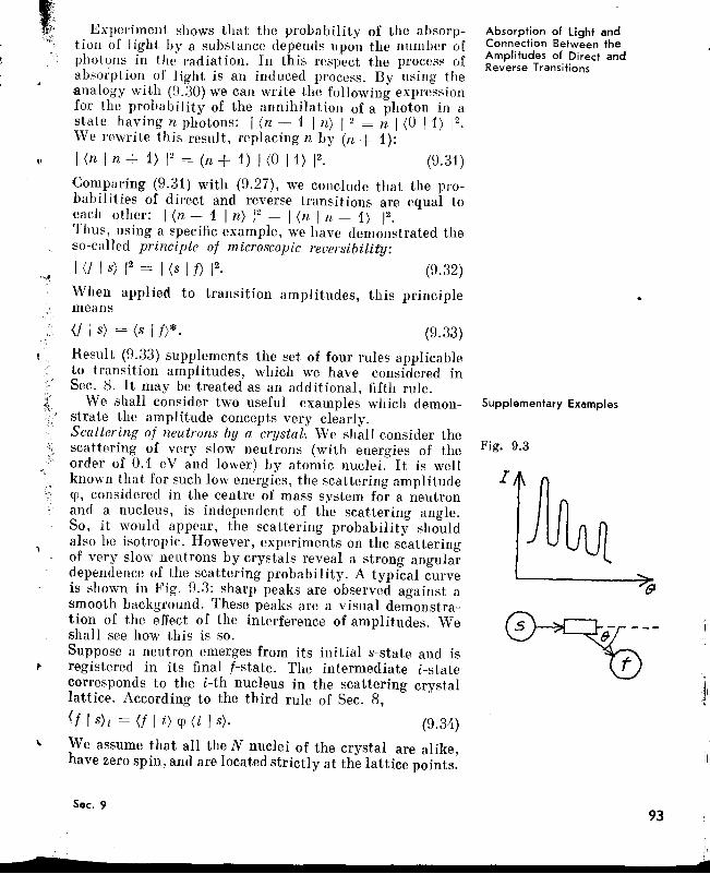
Experiment shows that the probability of the absorp­tion of light by a substance depends upon the number ofphotons in tlie radiation. In this respect the process ofabsorption of light is an induced process. By using theanalogy with (\3.30) we can write the following expressionfor the probability of the annihilation of a photon in astate having n photons: I (n - 1 I n) I 2 = n 1(0 11) 12 •

We rewrite this result, replacing n by (n + 1):

I (n I n + 1) 12 = (n + 1) 1(0 11) 12 • (9.31)

Comparing (9.31) with (9.27), we conclude that the pro­babilities of direct and reverse transitions are equal toBach other: I (n + 1 In) 12 = I (n 1n + 1) 12 •

Thus, using a specifiC example, we have demonstrated theso-called principle of microscopic reversibility:

I (f 1 s) 12 = I (s I f) 12• (9.32)

When applied to transition amplitudes, this principlemeans

Absorption of Light andConnection Between theAmplitudes of Direct andReverse Transitions

Fig. 9.3

Supplementary Examples

I

<f I s) = (s I f)*. (9.33)

Result (9.33) supplements the set of four rules applicableto transition amplitudes, which we have considered inSec. 8. It may be treated as an additional, fifth rule.

We shall consider two useful examples which demon­strate the amplitude concepts very clearly.Scattering of neutrons by a crystal. We shall consider thescattering of very slow neutrons (with energies of theorder of 0.1 eV and lower) by atomic nuclei. It is wellknown that for such low energies, the scattering amplitude{fl, considered in the centre of mass system for a neutronand a nucleus, is independent of the scattering angle.So, it would appear, the scattering probability shouldalso be isotropic. However, experiments on the scatteringof very slow neutrons by crystals reveal a strong angulardependence of the scattering probability. A typical curveis shown in Fig. D.3: sharp peaks are observed against asmooth background. These peaks are a visual demonstra­tion of the effect of the interference of amplitudes. Weshall see how this is so.Suppose a neutron emerges from its initial s-state and isregistered in its final f-state. The intermediate i-statecorresponds to the i-th nucleus in the scattering crystallattice. According to the third rule of Sec. 8,

<f I S)i = (f 1i) cp (i Is). (9.34)

We assume that all the N nuclei of the crystal are alike,have zero spin, and are located strictly at the lattice points.

Sec. 993 Ii

I_.?_------------------_....~

Taking (9.35) into account, the probability of scatteringof the neutron has the form

N

1<1 I s)1 2 = I qJ 12 12J <t I i) (i I s)1 2 • (9.36)i

In this case it is impossible in principle to indicate pre­cisely which nucleus causes the scattering of the neutron­the alternatives corresponding to the scattering by differ­ently "numbered" nuclei are indistinguishable. Hence,we must take into account the interference of the ampli­tudes:

(9.35)

(9.37)

The first term on the right-hand side of (9.37) accountsfor the characteristic interference peaks in Fig. 9.3,while the second term is responsible for the smooth back­ground. It is customary to say that the first term de­scribes the probability of the coherent scattering, and thesecond that of the incoherent scattering of neutrons.

On account of the addition of the amplitudes of the scat­tering at the nuclei, which are distributed in space in adefinite order, a mutual "cancelling" of amplitudes ispossible in some directions and a mutual "enhancement"in some others; this interference effect is manifested inthe form of sharp peaks for definite scattering angles.We further assume that nuclei in the crystal have a spin(let it be equal to 1/2, as for neutrons). In this case weshould distinguish between the amplitude of scatteringby the nucleus with spin inversion (in accordance withthe law of conservation of momentum, the neutron spinmust also be inverted in this case), and without spin inver­sion of the nucleus (and the neutron), Le. between Xand qJ,respectively. If the scattering of the colliding micropar­ticles is accompanied by spin inversion, the correspondingalternative is distinguishable-it is clear that in suchan act of scattering only that nucleus participates whosespin has been inverted. Now the probabilities and notthe amplitudes should be summed.Taking account of the amplitudes qJ and X we can repre­sent the scattering probability of neutrons from s-stateto f-state in the following form:

N

I (f I s)2 = 1 qJ 12 12J <f I i) (i I s) 12f

N

+ I X/2 2J I (f 1i) (i I s) 12

•i

N N

(f I S)= 2J (f I S)i= 2J (f I i) qJ(i Is).i i

94

ilII'~I(

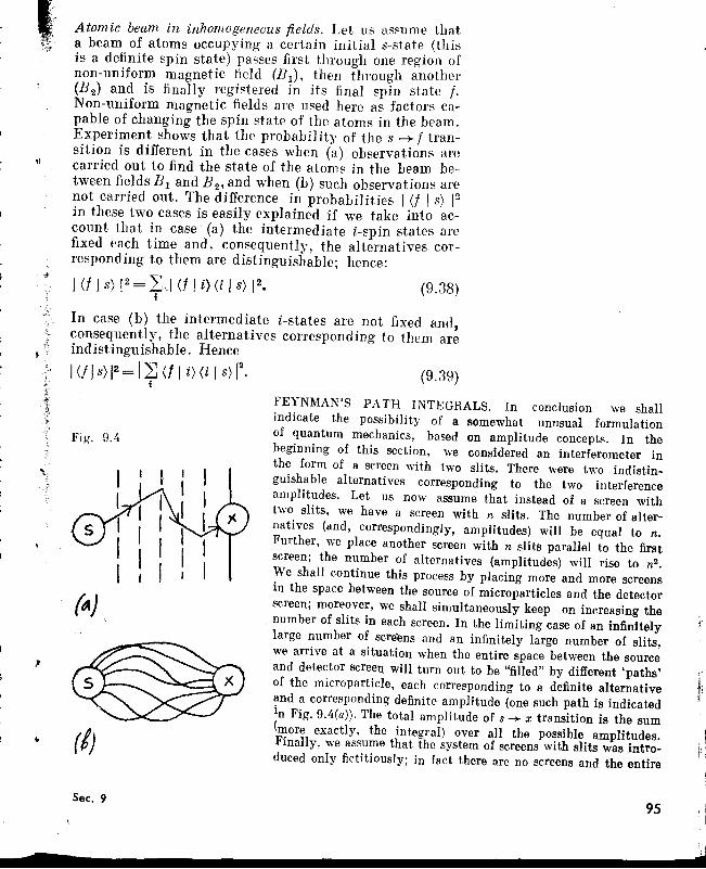
Atomic beam in inhomogeneous fields. Let us assume thata beam of atoms occupying a certain initial s-state (thisis a definite spin state) passes first through one region ofnon-uniform magnetic field (B 1 ), then through another(B 2 ) and is fmally registered in its final spin state j.Non-uniform magnetic fields are used here as factors ca­pable of changing the spin state of the atoms in the beam.Experiment shows that the probability of the s -+ j tran­sition is different in the cases when (a) observations arecarried out to find the state of the atoms in the beam be­tween fields B} and B 2 , and when (b) such observations arenot carried out. The difference in probabilities I <t I s) 12

in these two cases is easily explained if we take into ac­count that in case (a) the intermediate i-spin states arefixed each time and, consequently, the alternatives cor­responding to them are distinguishable; hence:

I (f I s) 12 = 2J,,1 (f I i}(i I s) 12• (9.38)i

In case (b) the intermediate i-states are not fixed and,consequently, the alternatives corresponding to them areindistinguishable. Hence

I (f J s) 12 = 12J (/ I i) (i I s) r (9.39)i

'I

Fig. 9.4

(~)

(I)

FEYNMAN'S PATH INTEGRALS. In conclusion we shallindicate the possibility of a somewhat unusual formulationof quantum mechanics, based on amplitude concepts. In thebeginning of this section, we considered an interferometer inthe form of a screen with two slits. There were two indistin­guishable alternatives corresponding to the two interferenceamplitudes. Let us now assume that instead of a screen withtwo slits, we have a screen with n slits. The number of alter­natives (and, correspondingly, amplitudes) will be equal to n.Further, we place another screen with n slits parallel to the firstscreen; the number of alternatives (amplitudes) will rise to n2.We shall continue this process by placing more and more screensin the space between the source of microparticles and the detectorscreen; moreover, we shall simultaneously keep on increasing thenumber of slits in each screen. In the limiting case of an infinitelylarge number of screens and an infinitely large number of slits,we arrive at a situation when the entire space between the sourceand detector screen will turn out to be "filled" by different 'paths'of the microparticle, each corresponding to a definite alternativeand a corresponding definite amplitude (one such path is indicatedin Fig. 9.4(a»). The total amplitude of s ...... x transition is the sum(more exactly, the integral) over all the possible amplitudes.Finally, we assume that the system of screens with slits was intro­duced only fictitiously; in fact there are no screens and the entire

ji1

95Sec. 9

Iif

I

sM....._-------------

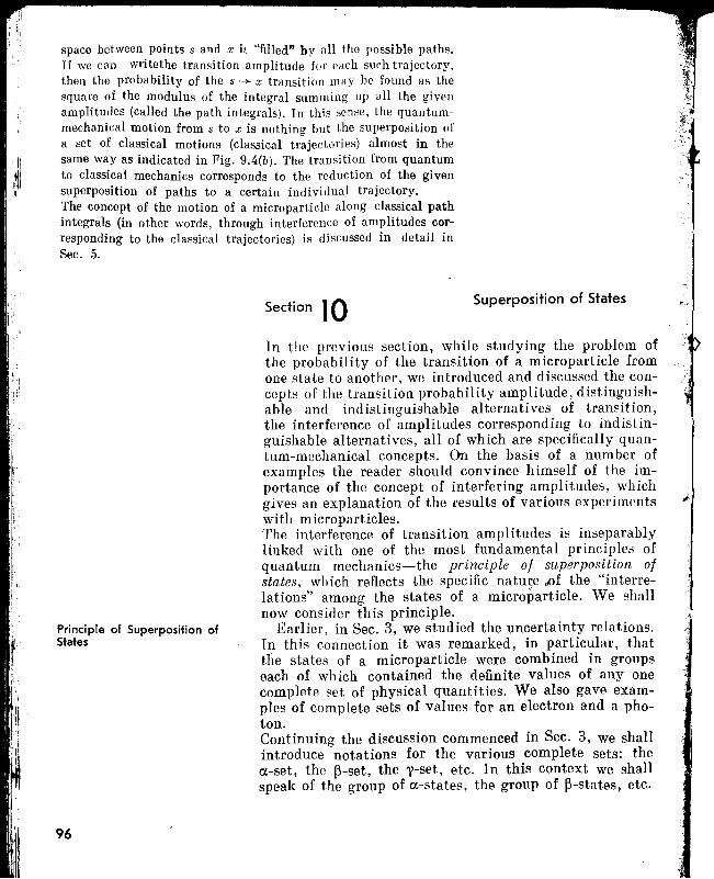
Superposition of States

In the previous section, while studying the problem ofthe probability of the transition of a microparticle fromone state to another, we introduced and discussed the con­cepts of the transition probability amplitude, distinguish­able and indistinguishable alternatives of transition,the interference of amplitudes corresponding to indistin­guishable alternatives, all of which are specifically quan­tum-mechanical concepts. on the basis of a number ofexamples the reader should convince himself of the im­portance of the concept of interfering amplitudes, whichgives an explanation of the results of various experimentswith microparticles.The interference of transition amplitudes is inseparablylinked with one of the most fundamental principles ofquantum mechanics-the principle of superposition ofstates, which reflects the specific nature ;.of the "interre­lations" among the states of a microparticle. We shallnow consider this principle.

Earlier, in Sec. 3, we studied the uncertainty relations.In this connection it was remarked, in particular, thatthe states of a microparticle were combined in groupseach of which contained the definite values of anyonecomplete set of physical quantities. We also gave exam­ples of complete sets of values for an electron and a pho­ton.Continuing the discussion commenced in Sec. 3, we shallintroduce notations for the various complete sets: thea-set, the ~-set, the y-set, etc. In this context we shallspeak of the group of a-states, the group of ~-states, etc.

Section 10

Principle of Superposition ofStates

96

space between points s and x il "filled" by all the possible paths.If we can writethe transition amplitude for each such trajectory,then the probability of the s -+ x transition may be found as thesquare of the modulus of the integral summing up all the givenamplitudes (called the path integrals), In this sense, the quantum­mechanical motion from s to x is nothing but the superposition ofa set of classical motions (classical trajectories) almost in the

ii same way as indicated in Fig, 9.4(b). The transition from quantumi~l to classi~al mechanics corresponds to the reduction of the givenIi superposItion of paths to a certain individual trajectory.

The concept of the motion of a microparticle along classical pathintegrals (in other words, through interference of amplitudes cor­responding to the classical trajectories) is discussed in detail inSec. 5.

We suppose that the microparticle is in one of the a­states. It means that the quantities in the a-set havedefinite values. But what can we say about the values ofthe quantities in any other complete set, for example, the~-set? According to the uncertainty relations, the quan­tities in the 13-set do not have definite values in the stateunder consideration. The reader is justified in taking thisas a negative fact. But, fortunately, this is fully "com­pensated" by a positive circumstance-the principle ofthe superposition of states.According to the principle of 5uperposition, there existsa link between the states of the microparticle, corre­sponding to different complete sets: any state from one setmay be represented in the form of a superposition of statesfrom another set. Thus, for example, a given a-state maybe represented in the form of a superposition of ~-states.If we arbitrar,,ily adopt the symbol ( I to indicate thestate of a microparticle, the principle of superposition maybe written in the form

(al=2J<Da/3(~I. (10.1)II

The expression (10.1) appears as an "expansion" of thegiven state (a I into the sum of ~-states, the numbers cDa /3playing the role of coefficients in the expansion. Moreconcretely, the number <Da/3 is the amplitude of the prob­ability that we shall obtain values corresponding tothe state (P I while measuring the quantities from thep-set in the state (a I. In other words, it is the amplitudeof the probability that a microparticle in state (a I mayalso be found in the state (P I. If we denote this amplitudeby the usual symbol (a I ~>, expression (10.1) assumesthe following form:

(a I= LJ (a I P> (~ I· (10.2)13

In the preceding sections we considered the amplitudes ofthe transition probability (in short, transition ampli­tudes). At first glance, the principle of superposition "bringsinto play" a new type of amplitudes of probability. Ac­tually, the above-mentioned expression "(a IP> is theamplitude of the probability that a microparticle instate (a I may also be found in state (P I" allows anotherobvious interpretation: "(a I P> is the amplitude of theprobability of a microparticle arriving in state (P I,if it is known that the give~ particle actually exists instate (a I". In short, the latter statement means that(a I ~> is the amplitude of the probability with whichany ~-state is "represented" in a given a-state. This pro-

'1,i:t Sec. 10

jp--------------

Pb

(J

MIemOJ

pIti01

iust

w

ciqlsi

mp<Ti

WI

MtbmorIth

Ir.!

T:duces the impression that the amplitudes (a I ~) don't .•·.1 orhave anything to do with any transitions or processes. .'. : to,Considering this impression, we introduce a new term (rlfor (a I ~)-the amplitude of probability of state (in brief, prthe amplitude of state). heThe reader must be warned at once that the above impres- Itsion is erroneous. However, in order to be convinced of ththis, we must analyse the process of measurement. Mea- nGsurement in quantum mechanics will be discussed in bJjSec. 11. This discussion will necessitate some correction I inin the above definition of the amplitudes (a I ~ > and ". SIwill enable us to actually reduce the amplitudes of states silto the already familiar amplitudes of transitions. tv!But everything has its own time, and so, for the time being, hfwe shall operate with the concept of "amplitude of state" pcas an independent concept, without ascertaining the thpractical meaning of, say, the phrase "a particle in state ~-(a I can also be found in state (~ I". ofAs has been noted earlier, the principle of superposition • of"supplements", as it were, the uncertainty relations; its :,. (cpositive content "compensates" the well-known negativeaspect of these relations. Figuratively speaking, the uncer­tainty relations indicate the "old" concept which mustbe rejected while we go over from macrophenomena tomicrophenomena. In particular, they require a rejectionof the simultaneous meai'lurability of all physical quan­tities characterizing a given object. At the same time,the principle of superposition indicates the "new" con­cept which is applicable when considering microparticles;superposition (10.2) means that if a microparticle is ina state in which the quantities of the a-set are measurable,then the value of the quantities in the ~-set may be pre­dicted with a probability equal to I (a I P>/2.

In classical physics one comes across superposition quitefrequently, the foremost example being ihe well-knownsuperposition of classical waves. From a mathematicalpoint of view, the classical superposition and superpo­sition in quantum mechanics are analogous. This circum­stance greatly stimulated the development of quantumtheory. At the same time, it certainly complicated theinterpretation of the physical content of theoreticallyobtained results since it tempted one to draw erroneousanalogies with classical waves. In the words of Dirac [9]the assumption of superposition relationships between thestates leads to a mathematical theory in which the equationsthat define a state are linear in the unknowns. In conse­quence of this, people have tried to establish analogies withsystems in classical mechanics, such as Vibrating strings

Superposition in Classical Physicsand Quantum Mechanics

f

s.

t

n

;-

,f

[l

n:ls

,"ee

1

S

e

t)

1

or membranes, which are governed by linear equations anafor which, therefore, a superposition principle holds....(remember the criticism in Sec. 5 of the attempts to re­present the motion of a bound microparticle with thehelp of classical waves in a resonator-author's remarks).It is important to remember, however, that the superpositionthat occurs in quantum mechanics is of an essentially differentnature from any occurring in the classical theory, as is shownby the fact that the quantum superposition principle demandsindeterminacy in the results of observations.Speaking of the difference between quantum and clas­sical superpositions, remember that a superposition oftwo classical waves leads to the generation of a new wavehaving, of course, new characteristics. However, a super­position of two states (~l I and (~2 I, characterized bythe values ~l and ~2' respectively, of quantities in the~-set, by no means leads to a state having any new valueof ~. As an example, let us consider a certain superpositionof states

(a I ~l )(~l I + (a I ~2) (~2 I.We shall measure the ~-quantity in this state. As a result,we get every time one of the earlier values, ~l or ~2'

Moreover, it is impossible to accurately predict which ofthe two states will be obtained in any particular measure­ment. We can only indicate the probability of getting ~l

or ~2' These probabilities are equal to I (a I ~l) 12 and

I (al ~2) 12, respectively. It is this specific uncertainty inthe results of measurements that determines the funda­mental difference between quantum and classical super­positions.Taking into consideration the quantum-mechanical prin­ciple of superposition, let us return to the question ofquantum transitions discussed in Sec. 2. Suppose we con­sider, as before, two energy levels E 1 and E 2 of the micro­particle. We denote the corresponding states of the par­ticle in which it has energy E 1 or E 2 (i.e. is on the firstor second level) through (1 I and (21 respectively. Accord­ing to the principle of superposition, in addition tostates (1 I and (2 I we can also get the state

(fl=(fI1)(11+(/12}(21. (10.3)

Measurement of energy of the microparticle in this stateleads either to the result E 1 or to the result E 2 (as if themicroparticle were on the level E 1 and simultaneouslyOn the level E 2). The first result is obtained with theprobability I (f 11) 12 , and the second, with the proba­bility I (f I 2) 12• The possibility of the existence of such

I1:1"I

Sec. 10III

,,'...rz :~

t,(10.4)

a specific quantum-mechanical situation immediatelyremoves the basic contradiction of the quantum transi­tion, mentioned in Section 2. It is sufficient to assumethat an interaction of a microparticle with radiation leadsto a superposition state of the type (10.3). Then the prob­ability of finding a particle on one energy level or anoth­er (on its earlier level or on a new one) will be describedsimply by the square of the modulus of the correspondingamplitude of state.

In order to finally convince ourselves that the quantum­mechanical principle of superposition has in fact nothingin common with the classical superposition we turn toexpression (10.2) and see how it changes upon the tran­sition to classical physics. Since in classical physics allthe quantities can be simultaneously measured, they formtogether one "complete set". Considering that the superposi- .1..·.•.tion bonds described by relation (10.2) operate between .different complete sets, we arrive at the conclusion thatin the classical case such bonds simply do not exist and, .~consequently, all formally composed amplitudes of statesfmust be taken as being equal to zero:

(ex I ~) = o.In quantum mechanics condition (10.4) also exists, butonly "within the limits" of the given complete set (forstates belonging to the same set). Thus, for example,

(exi I exj) = 0, if i =1= j. (10.5)

The amplitude of a state is equal to zero if and only ifthe two corresponding states are mutually independent(if an object is in one of these states, it cannot be foundin the other). Such states are called mutually orthogonal.In this respect all the states of a classical particle aremutually orthogonal, while in quantum ,mechanics onlythe states belonging to the same complete set are orthog­onal and the states belonging to different sets are non­orthogonal. This last fact is reflected in the principle ofsuperposition of states.The idea of mutually orthogonal states permits us todefine more precisely the concept of complete and partialdistinguishability. For this purpose it is convenient tomake use of the above-mentioned example of the scatter­ing of microparticles of one type by one another. Sincesuch particles are identical, their distinguishability isdetermined by the distinguishability of states (states{"1 I and (82 I; see Sec. 9). We recall that in Sec. 9 we dis­cussed, in particular, microparticles of the same kindbut in different spin states, as examples of completely

Mutually Orthogonal States;Total and Partial Distinguishability<If States

.1

.,flIi.1

" 100

I

1

1

t

distinguishable microparticles. We thus tacitly assumedthat different spin states are completely distinguishable.We can now clearly indicate the criterion of complete andpartial distinguishability of states: if (Sl I S2) = 0, thestates (Sl I and (S2 \ are completely distinguishable;there are no superposition bonds between them. But if(Sl I S2) =1= 0, the states under consideration are partiallydistinguishable. In other words, orthogonality of statesis the criterion of their complete distinguishability.Suppose we are considering scattering of two bosons ofthe same type. The result (9.16) will hold good if theinitial states are mutually orthogonal (let these statesbe (al I and (a

2I). The result (9.17) will be valid if the

initial states are similar (say, (al I and (al I). Both theseresults are just two extreme cases corresponding to com­plete distinguishability and complete indistinguishabilityof microparticles, respectively. However, different inter­mediate situations corresponding to partial distinguish­ability are possible, when the initial states of microparti­cles are a superposition of several mutually orthogonalstates:

(S1 I = (S1 I(1) (a1 \ + (S1 1(2) (a2 I,(S2 1= (S2 I (1)(a1 I+ (S2 I (2) (a2 I. (10.6)

It can be shown (see [31]) that in this case the probabilityof simultaneous activation of detectors is determined bythe expression

I!V= I cp(El) 12 + I cp(n-El) 12

+ I (S1\ S2) 12 [cp(El)cp*(n-El),+cp*(El)cp(n-El)]. (10.7)

For I (Sl I S2) 12 + 0, the result (10.7) turns into (9.16)(we come to the limiting case of complete distinguish­ability). For I (Sl I S2) 12 + 1, the result (10.7) turns into(9.17) (we come to the limiting case of complete indistin-guishability) .Thus, we find that the question of the complete and par-tial distinguishability of alternatives in quantum mechan­ics is closely linked with the quantum-mechanical prin­ciple of superposition, more precisely, with the mutualorthogonality or non-orthogonality of states.

The different states corresponding to the same complete Basic Statesset of quantities are called basic states (eigenstates).The amplitudes of elementary states satisfy the condition

(ai I aj) = {jij, (10.8)

where {jij is the so-called Kronecker delta symbol; it isequal to zero for i =I=- j and unity for i = j. The expres-

Sec. 10101

II

il!

sion (10.8) is called the condition of orthonormalization ofbasic states. It is obtained by taking into consideration{1O.5) and the fact that the probability of getting thevalue at in the state (at I is obviously equal to unity.The important property of the system of basic states isits completeness: any state may be expanded in a system-of elementary states.Basic states may be selected in different ways depending-on the complete set under consideration. Thus, differentsystems of basic states may be used: {(at J}, {(~t I},etc. It is said that different representations are possible.For a more general approach, the principle of superposi­tion of states signifies the fact that any state (f I of amicroparticle may be expanded in any system of basicstates:

(f I = ~ (f I at) (ai I,i

(10.9)...........<I I = ~ (f I ~i) <~i I,

i

The principle of superposition permits an explanation-of the results of experiment 3 in Sec. 7. Using this prin­ciple, we shall consider the passage of individual photonsthrough the system of three polarizers shown in Fig. 7.6.We denote the state of polarization of a photon after thefirst polarization by (s I. According to the principle ofsuperposition, the state (s I may be considered as a super­position of the basic states (1 , and (2 I, correspondingto two independent polarizations of the photon-alongand perpendicular to the axis of the second polarizer,respectively:

(ql = (311)(1/ + (s/ 2)(2/ (10.10)"{note that in this example, the system of basic states con-

tains only two states). The amplitudes of the states maybe written in this case in the form (3 I 1 ) = cos a and(3 I 2> = sin a. Thus,

(3 I = cos a (1 [ + sin a (2 I. (10.11)

The second polarizer lets through photons from the state(1 I only. Since according to 00.11) the state (1 I is

"represented" in state (s I with a probability cos 2 a,out of N photons only N cos2 a photons will pass throughthe second polarizer. Moreover, all the photons that passwill appear in the state (1 I (i.e. they will be polarizedalong the axis of the second polarizer). Thus, in front ofthe second polarizer, the photon exists as if partially in

Superposition of States andPassage of Photons ThroughPolarizers

102

'Wi~1

IIfne

s0-

'J'~

t

the state (1 I and partially in the state (2 I. At the instantwhen the photon passes through the polarizer, this "dual­ity" vanishes. In some cases a photon exists in the state(2 I and so cannot pass through the polarizer, while insome other cases it is in the state (1 I and can thus passthrough the polarizer. Further, for any individual photonit is impossible to predict in which state it will appear(hence it is impossible to predict whether a given photonwill pass through the polarizer or not).While studying the passage of photons through the thirdpolarizer, we proceed in a similar way. The state (1 I isexpanded into a system of basic states (1' I and (2' Icorresponding to a polarization of photon along or perpen­dicular to the axis of the third polarizer:

(1 I = sin a (1' [ + cos a (2' I. (10.12)

The third poll'!,rizer lets through photons in the state (1' Ionly. This state is "represented" in the state (1 I with aprobability sin2 a. Hence out of N cos2 a photons onlyN cos2 a sin2 a photons will pass through the third po­larizer, all these photons being in the state (1' [.If we now remove the second polarizer, then in place of(10.11) and (10.12) we get

(81= (.9\1')(1' 1+ (8\2')(2' l, (10.13)

where, as can be easily seen, (.9 11') = 0 and (3 I 2' > = 1,so that (3 I = (2' I. Naturally, in this case, at the outletof the system of polarizers no photons are observed at all.

Let the transition from state (.'lIto state (f \ take placethrough certain intermediate v-states. We suppose thatthe microparticle is not fixed in the intermediate state sothat a case of physically indistinguishable alternativetakes place. In this case, as \Ve know, the transition ampli­tude (f I 8) is given by the expression

(f I s) = ~ (f IVi) (Vi Is), (10.14)i

where (f I Vi) and (Vi I 3> are the amplitudes of the re­spective transitions. The intermediate v-states must becompletely distinguishable, since otherwise there is nopoint in introducing the concept of distinguishable orindistinguishable alternatives, since the very concept ofalternatives loses its meaning. Consequently, the v-statesmust form a system of mutually orthogonal basic states.Taking this into consideration, we make use of the prin­ciple of superposition and express the state (f I in the form

(f I = ~ (f 1Vi) (Vi I, (10.15)i

Sec. 10

Principle of Superposition ofStates and Interference ofTransition Amplitudes

103

\1

IIi:;

I~,jj;

"Mechanics of QuantumMechanics"

where the amplitudes (/ I Vi) are essentially the ampli­tudes of the states (the bar is used to distinguish the ampli­tude of the state from the transition amplitude (/ I Vi ».If superposition (10.15) exists, there is actually no need toperform a transition from (8 'to (/ I. Since the state (/ Iis a superposition of states (Vi I, it is sufficient to simplyaccomplish transitions from the state (8 I to each of thestates (Vi I· This means that the transition amplitude(/ 1 8) is a superposition of the transition amplitudes(Vi I 8):

(f I s) = L (f I Vi) (Vi Is). (10.16)f

Comparing (10.16) and (10.14) we conclude that

(f IVi)=(j I Vi). (10.17)

This means that at the level of mathematical apparatus,we have accomplished a reduction of the amplitudes ofthe states to transition of amplitudes. In other words, theamplitudes of the states in fact play the same role in theapparatus of quantum mechanics as the transition ampli­tudes. Incidentally, we have also established that rela­tions (10.14) and (10.15) are closely related to each otherand hence the effect of the interference of transition ampli­tudes and the principle of the superposition of states aredirectly interrelated.In conclusion, we mention an important method whichis widely applied in quantum mechanics. It is easy tosee that if we delete the sign of the initial and final statesin the expression for the interference of amplitudes, weautomatically obtain the superposition expression forthe undeleted state. Thus, if in (10.14) we delete [8)on the left- and right-hand sides of the equation, we obtainthe superposition expression (10.11) for the state (/ I(note that in addition to the symbol ( /' the symbol I )is used for denoting a state).

We shall demonstrate the basic methods reflecting, inFeynman's words, the "mechanics of quantum mechan­ics". Let us delete the state (/ I from the left- and right­hand sides of equation (10.14). This gives

VIt(

Ft}

(v

(twpI

(f

Sl

(f

Slthfo.fo:

Let us further assume that some apparatus convertsstate 18 ) into some other state 18'). We express this inthe general form as

104

A 18) = /s').

(10.18)

(10.19)

Fi]an,thlwo

Sec

1II' We shall say that the operator A has acted on the state

1.9 >giving rise to state Is'). We shall apply the operator Ato both sides of equation (10.18). Using (10.19), we get

Is') = 2: A I Vi) (Vi I s) (10.20)i

Further, in place of the state (1 Ideleted earlier, we restorethe state (vi I belonging to the system of basic states:

(10.21)

(the notation (Vi I A I Vi) should be taken as (v, I vi ),where I vi) = A I Vi ». Finally, we rewrite (10.14), re­placing 1.9) by 1.9'):

<f Is') = ~ (f IVj) (Vj I Sf) (10.22)i

Substituting (10.21) into (10.22) we get

(f I A I s) = .LJ .LJ <f I vi) (Vi I A I Vi)(vi Is).j i (10.23)

Summarizing the methods demonstrated above, we writethe equations obtained so far and leave it to the reader tofollow the logic and appreciate the beauty of the trans­formations:

(f I s) = (/ Is),

<f I s) = .LJ <f I vi) (Vi Is),i

I s) = .LJ I Vi) (Vi Is),i

A I s) = 2J A I Vi) (Vi Is),i

(Vi I A I s) = ~ (Vi I A I Vi) (Vi Is),t

~ (/ I Vj) (Vi I A I s)j

= ~ 2J <f I vi) (Vi I A I Vi) (Vi Is),j i

(f I A I s) = ~ 2j (f IVj) (Vi I A I Vi) (Vi Is).j i

!Ii:1

105 It

~

Finally, we assume that operator A acts on the state I .9),and is followed by operator B. If the reader has masteredthe logic of the "mechanics of quantum mechanics" (itWould have been more accurate to call it the "algebra of

Sec. 10

~-----------------

quantum mechanics"), he will at once surmise that

<t I BA Is)= ~ ~ ~ (f I v,,) (v" I B I Vj) (Vj I A IVi) (Vi I s) (10.24)

" j i

(the notation (/ I BA I 8) should be taken as (/ I 8"),where I 8") = B Is') and 18') = A 18».This formal structure of the mathematical "manipula­tions" is characteristic for quantum mechanics. In whatfollows, this structure will assume a definite meaning onthe basis of definite examples. Here it has been given inits most general form, which also allows us to follow itsinternal logic. We emphasize that the basis of this struc­ture is the idea of quantum-mechanical interference (super­position) and the use of a certain system of basic states interms of which the expansions are carried out.

Section II Measurement in QuantumMechanics

The Origin of the Superpositionof States and the Meaning of theAmplitudes of States

The question of carrying out measurements in quantum­mechanical systems and an interpretation of the resultsso obtained is rightly considered to be very complicated,requiring even today further research. We shall not givea detailed analysis of the problem of quantum-mechani­cal measurements, but shall try to describe a number offundamental statements which have been explainedclearly, and demonstrate them using some examples*.

Suppose that a microparticle is in a certain state (ex I·According to the principle of superposition, the state(ex I may be expanded in terms of any system of basicstates, for example, in the {(~i 1} system:.

'\1(ex I = ~ (ex I ~i) (~i I·

i

(11.1)

106

The numbers (ex I ~i) in the superposition (11.1) areessentially the amplitudes of the states (~i lor, moreaccurately, the amplitudes of the probabilities withwhich the various basic states (~i I are "represented" inthe state (ex [.The reader who has read the previous section is alreadyfamiliar with all this. It is appropriate now to makethings more precise.

* The problem of measurement in quantum mechanics has beendealt with, in particular, in [2, 28, 32].

i€

s

eehn

y:e

m

Firstly, we shall note that any definite superposition ofstates in a microparticle arises as a result of its inter­action with the surroundings. The latter may be somemacroscopic body (which is either produced artificiallyor is a part of the natural external conditions). This macro­scopic body is referred to as the analyzer. The expression(11.1) should be interpreted in the following way: asa result of the interaction with a particular analyzer (inthis case, we may speak of a ~-analyzer), a microparticlelying in state (ex I is transformed into the superposition

state >-J (ex I ~i) (~i I. Taking into account the quantum-i

mechanical nature of the superposition state, it may be saidthat by interacting with the ~-analyzer, the microparticlein some sense is "transformed" at once into all the states(~i I· Here, the amplitude (ex I ~i) should be treated asthe amplitude caused by the indicated interaction of thetransition (ex I + (~i [. The quantity I (ex I ~i) 12 is theprobability of finding the microparticle finally in justthe (~i I state.One can anticipate at least three questions from the reader.First question: What do we really mean by the expression"the microparticle is at once transformed into all the(~i I states"? The answer to this question will be givenbelow in the subsection "Potentialities and their realiza­tion in the measuring process". Here, we just remarkthat although the microparticle is "simultaneously trans­formed into all the (~i I states" as a result of its interac­tion with the ~-analyzer, it can be found in principle eachtime in only one ~-state. Hence it may be said that noconfusion arises. By the way, the reader has already comeacross a similar situation when considering experiments 1and 2 in Sec. 7. Here we once again remind the readerthat quantum-mechanical logic does not always havea corresponding graphic model.Second question: If the amplitude of state is really thetransition amplitude, what about the definitions of am­plitudes of states given in Sec. 10? Answering this qu.estionwe recall the following definition given in Sec. 10:"(ex I B) is the probability amplitude of a microparticleexisting in state (ex I being also registered in state (B I".In this definition the word "existing" should be replacedby a more accurate word "existed", since after interactionwith the analyzer the microparticle no longer exists inthe state (ex I. Now the word "also" becomes redundant.The definition then assumes the following form: "(ex I B)is the amplitude of probability of a microparticle thatexisted in state (ex I being registered in state (~I". Reg-

Sec. 11107

III

IIil

p

(11.3)

Examples of Analyzers

108

istering is a kind of measuring process and (a i P> playsthe role of the amplitude of the transition (a I + (P Iwhich takes place in this process. Here we remark thatin the above-mentioned interaction of the microparticlewith the analyzer is just one part of the measuring process.A more detailed treatment of the measuring process willbe given at a later stage.Third question: It was agreed earlier (see Sec. 8) to readthe transition amplitudes from right to left. If (a I Pi>is also transition amplitude, it should also be read in thereverse direction (from left to right). Isn't it confusing?Actually, if we strictly follow the condition of writingthe preceding states to the right of the ones that follow,then (11.1) should be written as

'lL..J I Pi) (Pi Ia) = I a). (iLia)i

However, such a notation, as a rule, is not used. Hencewe decided to allow some inconsistency, and in order toavoid possible confusion in this connection we shall infuture retain the term amplitude of state along with theterm transition amplitude. When using both these termsthe reader must remember that from the point of viewof physical meaning, the amplitude of state is nothingbut the transition amplitude (this has already been shownfrom a mathematical point of view in the previous section).

The reader has in fact already come across analyzerseach time the interference of transition amplitudes wasconsidered. We shall give a few examples.First example: [see (9.3)l-the analyzer is a screen withtwo slits. It gives rise to the superposition

(8 I = (8 I A)(A I + (8 I B >(B I. (11.2)

Second example: [see (9.35)l-the analyzer is a crystallattice consisting of nuclei of the same type with zerospin. It generates the superposition

]V

(8 I = ~ (8 I i) cp (i /.i

Third example: [see (9.39)l-the analyzer is a nonuniformmagnetic field B1• It gives rise to the superposition

(81 = 2.j (8 I i) (i I. (11.4)i

It may be said that an analyzer, generating a certainsuperposition of states, in fact ensures the emergence ofindistinguishable alternatives. Moreover, the number ofalternatives is equal to the number of basic states in thegiven st'perposition. In the first example this number is

jiiI

B

cv

~

IJ

V

IJ

iIsutIIIl

<It1i1ssIlveatsar,ovsPttiC

cas:

s

1just equal to two (i.e. to the number of slits in the screen);in the second example, it is equal to the number of nucleiin the crystal, while in the third example it is equal to thenumber of spin states (Le. to 2s + 1, if s is the spin of theatom).

The process of measurement in quantum mechanicsconsists of three successive stages: (1) a preparatory stagewhen the microparticle is "prepared" in a certain state(ex I, considered below as the initial state; (2) a working

!tage in which the "prepared" microparticle interactswith a certain analyzer and goes over to the superposition!tate, and (3) a registering stage in which the microparticleis registered in one of the basic states forming the super­position. In this stage the microparticle interacts withsome macroscopic body, capable of changing its stateunder the influence of the microparticle. This macroscopicbody is called the detector.If for the sake of simplicity we do not consider the pre­paratory stage, the abstract "scheme" of the measurementprocess may be written in the following way:

1 " l 2{sl ~L;<S!~i)<~tl~<~i" (11.5)

i

The Essence of MeasuringProcess

r)

3

3

1

)

Io

a

)

Here the arrow 1 corresponds to the working stage, andthe arrow 2 to the registering stage.The basic elements of the measuring instrument (measur­ing apparatus) are thus the analyzer and the detector.The role of the analyzer has already been explained. Weshall now consider the role of the detector. Figurativelyspeaking, its role boils down to "spying" on how the micro­particle "behaves itself" in the superposition state whichwas created by the analyzer. If we make use of the aboveexamples of analyzers, this "spying" could provide ananswer to the question: Which slit did a particular elec­tron pass through? Which nucleus of the crystal latticescattered a particular neutron? What is the spin state ofa particular atom? The reader who is familiar with theresults of similar "spying" (in particular, with the resultsof the experiment 2 in Sec. 7) may foresee that an "inter­vention" by the detector leads to the destruction of thesuperposition of states. The detector registers the micro­particle each time in one of the states which constitutethe superposition. This is done at the expense of the destruc­tion of superposition. From the point of view of the ideasConsidered in Sees. 8 and 9, this means that the detectorconverts indistinguishable alternatives into distinguish­able ones and thus destroys the interference of the tran­sition amplitudes.

109s.c. 11

II« ~-'n ~

Some Peculiarities of theQuantum-Mechanical MeasuringProcess

110

We separate from the "scheme" (11.5) the registeringstage corresponding to the interaction of the micropar­ticle with the detector:

(11.6)

It is often said that a "scheme" of the type (11.6) de­scribes a "construction" of the superposition ~ (.'I I ~i ) (~i I

ito the state (~i I. This process is also known as "reductionof the wave packet".Thus, while the analyzer creates a definite superpositionof states, the detector destroys it by confining this super­position of states to one of the states constituting it.It is obvious that if the "scheme" (11.5) is tried on asingle microparticle, it is difficult to say anything aboutgetting any u"leful information. It is necessary to repeatthe measuring process for a sufficiently large number ofmicroparticles. In this case the observer may find out,firstly, the values of the quantities of the ~ -set encoun­tered in practice, and, secondly, the frequency with whichthe microparticle is found in one ~-state or another.This allows us to experimentally determine, firstly, thespectrum of the values of the quantities in a ~ -set and,secondly, the probabilities I (8 I ~i > 12•

In the first place we note that the process of measure­ment has a radical influence on a microparticle. It isenough to point out that a change in the initial state ofthe microparticle in the measuring process is a circum­stance of fundamental importance. It is well knownthat while carrying out measurements with macroscopicbodies it is possible to isolate the object to a certainextent from the means of measurement. In quantummechanics this is in principle impossible ,to do so. Inother words, it is impossible to neglect" the interactionof the microparticle with its surroundings.The "scheme" of the measuring process, and more concrete­ly that part which is described by expression (11.6),is a demonstration of the existence of the element ofchance in the behaviour of a microparticle. Indeed, it isimpossible to predict unambiguously in which ~ -statea certain microparticle will be finally found.The impossibility of a graphic representation of thefirst stage of the process (when the analyzer creates. asuperposition of states) or the final stage (when the de­tector "confines" this superposition to a single state) is.also a specific feature of the quantum-mechanical measur­ing process. Thus, obviously, in the first stage ot the

prla ]ofthlwesib(aswhitsltrerislintnala 'mathiindpalsiventpalres'sta-in 1

eacat ~

reflthadis:vatsecitiOIparis 2Pertatjsic~

tiOIthestalrevithelyzithethamilHo'eno

Sec.

t

I

'IIii,II

111 II~

process of measurement it must not be assumed thata microparticle is literally "spread" over various statesof superposition (for example, that it passes partiallythrough one slit and partially through the other in thewell-known two-slit experiment). Similarly, it is impos­sible to assume that as soon as a detector is activated(as soon as the act of registering occurs) the microparticlewhich is spread over various states suddenly assemblesitself in one of these states. It should be noted that thetreatment of final stage of the measuring process gaverise to many arguments. Supporters of a model (classical)interpretation of microparticles and microphenomenanaturally were at a loss when they tried to visualizea "reduction of wave packets". Inasmuch as the statesmaking up a superposition may be spread in space, inthis case the "reduction of a wave packet" should actuallyindicate a mo:rp.entary spatial localization of the micro­particle. In particular, the following example was exten­sively used. A wave packet interacts with a semitranspar­ent mirror (the mirror plays the role of analyzer), ispartially reflected and partially transmitted (which cor­responds to a spreading of the microparticle into the twostates comprising the superposition). Detectors are placedin the path of each of the wave packets. It is known thateach time only one detector is activated. Suppose thatat a certain instant the detector placed in the path of thereflected part of the wave packet is activated. This meansthat the other part of the wave packet momentarilydisappears from that part of the space where the unacti­vated detector is placed, and reappears in front of thesecond detector the moment before the act of registra­tion. The absurdity of such "behaviour" of the micro­particle, which, by the way, "cannot know" which detectoris activated in a given case, is quite obvious.Persisting in the efforts to retain the classical interpre­tation, attempts are sometimes made to turn to the clas­sical interpretation of superposition. Such an interpreta­tion assumes that the microparticle after interaction withthe analyzer, will actually appear in one of the basicstates. The role of the detector is simply reduced torevealing the accomplished fact, i.e. in which basic statethe microparticle appears upon interaction with the ana­lyzer. Now everything appears very easy: activation ofthe detector in the example cited above reveals the factthat the given wave packet upon interaction with themirror was reflected and not transmitted.However, such a course has already been precluded. It isenough to remind the reader of the argument put for-

Sec. 11

1

ea

I,If.se

ncn0.

nn

s,f

1-

e

1

1

ttf

e'-:s.l-

~------------------

pIisidab<tiTJcathbilaOtissiisTlarethIIJt)larelinmti,bEtacoItbEpITJcoct.tushpI(1bEsub~thmleiisirl

Se

.1

Comments on Detectors

Ii

I 1\2

ii"I:,.

r-----------------Tward in the discussion of experiment 1 in Sec. 7. If itwere possible to assume that a microparticle passesthrough one slit in the screen in some cases and throughthe other in some other cases, then, as has been remarkedearlier, we would not have observed the interferencepattern on the detector screen. In other words, the classi­cal concept of superposition of states is equivalent toa destruction of superposition. It must be admitted thatuntil the detector registers the micropa:rticle, the latterexists in the supposition state 2J (8 IBi ) (B i I and notin any of the states (~i I. As to the question of how thiscan be visu,.Uy represented, we simply have to give uplooking for an answer. It may be said that a discussionof quantum-mechanical measuring process (especiallythe problem of "reduction of a wave packet") gives aspecially convincing proof of fundamental impossibilityof a classical interpretation of the microparticle.

A detector in a quantum-mechanical measuring instru-ment is, as a rule, a macroscopic system in a state whichis so unstable that a microscopic influence, or the influ­ence of the microparticle, is enough1to change it. In orderto be "seen" by an observer, the- microparticle causesa complete "catastrophe", an "explosion" on the scaleof microphenomena.Examples of such "catastrophes" include events like theformation of a droplet in Wilson's cloud chamber, ora bubble in a bubble chamber, chemical processes involv­ing photoemulsion grains, avalanche processes of genera­tion of secondary electIons in a photomultiplier, etc.The "observable" microparticle might perish in the"catastrophe" caused by it (as, for example, in the caseof the registration of a photon in a photomultiplier or ofan electron on a detector screen). However, an evenmore interesting situation is possible when. a microparticle"entrusts" the task of causing the catastrophe to othermicroparticles. Thus, for example, in Wilson's chamber,the electron "under observation" creates various ions inits wake each of which in turn serves as a centre for thecondensation of the supersaturated vapour filling thechamber. It is these ions that cause the "catastrophes"which the observer sees as mist droplets. A multitude ofsuch droplets forms the track which is left by the electron"under observation". We emphasize that an electrontrack is nothing but a multitude of successively occurringmicroscopic events, a totality of "catastrophes" on thelevel of microphenomena.

eef[1

er

nee

Ifnnge

, When disCussing the idea of quantum-mechanical~ principle of superposition we come to a situation which

is analogous to the one encountered when discussing theidea of wave-particle duality (see Sec. 5). In both cases,a visual (classical) interpretation is not possible. In

I·; both cases we come to a problem connected with poten­;, tialities and with their realization.

I The possibility and the actuality are the well-knowncategories of materialistic dialectics. The contradictionthat exists between them disappears every time a possi-bility is realized in one way or the other. Every particu­lar situation is characterized by a set of possibilitiesout of which only one is realized. The realization processis irreversible; as soon as it is accomplished, the initialsituation qualitatively changes (one of the possibilitiesis realized at the expense of all the other possibilities).The possibility that has been realized corresponds toa new situation 'with new possibilities. The process ofresolving the contradictions between the possible andthe actual thus turns out to be endless.In classical mechanics (as also in all theories of dynamictype) the problem of distinguishing between the possible

) and the actual does not arise because of the absence of thei J elements of chance in such theories. This problem arisesi in theories of statistical type. The basically statistical, nature of quantum mechanics (where, as has been men­; tioned earlier, an element of chance is present in thei

.~ behaviour of an individual object) indicates the impor-t tance of the problem of the possible and the actual when1 considering microparticles and microphenomena.

It is from this point of view of resolution of contradiction~ between the possible and the actual that the measuringI' process in quantum mechanics should be considered.

The presence of a microparticle in the superposition statecorresponds to a situation where the microparticle ischaracterized by a definite set of possibilities. The quan­tum-mechanical principle of superposition of statesshould be interpreted in this way only. In the interactionprocess of a microparticle with the detector [in the process(11.6)], the above-mentioned resolution of distinctionbetween the possible and the actual takes place, thesuperposition of probabilities is destroyed and is replacedby one of the alternatives realized. It may be said thatthe "formula" of measuring process [formula (11.6)] is the

. mathematical expression for the process in which the dia­lectical contradiction between the possible and the actualis resolved. The nature of this resolution is that of antn-eversible and uncontrollable jump.

Sec. 11

Potentialities and TheirRealization in the MeasuringProcess

113

Iii'I

:\III'i

114

Before concluding this section, it should be stre"ed tharthe problems of the interference of amplitudes, the super- I Saposition of states and of measurement are not isolated I onfrom one another, but form a single entity. Taking this M,into consideration, we recommend that the reader shouldpause a little, go back and read through Secs. 7-11 once Par

again, in order to get a general idea about the physical Rei

foundations of quantum mechanics.

1tr­idis.d

Interlude. Are These theSame Waves?, Or, Againon Waves in QuantumMechanics

Participants: the Author and theReader.

Call it then, what thou wilt­Call it bliss! Hearl! Love! God!I have no name to give it!Feeling is all in all:The Name is sound and smoke,Obscuring Heaven's clear glow.Goethe (Faust)

Reader:

Author:

Reader:

Author:

Reader:

Author:Reader:

Author:Reader:

Author:

I would like to return to the question of classical superposition.Sometimes I get a seditious idea: what is wrong with such a super­position? In any case it explains the interference effect more clearlythan the superposition of amplitudes. I have due regard for thestructure of quantum-mechanical concepts based on working withprobability amplitudes, but still this idea keeps on haunting mefrom time to time.

Classical superposition certainly does explain interference.But what about the result of the experiment involving "spying"on the behaviour of a microparticle in the interferometer (forexample, in the case of a screen with slits)? The experiment indi­cates a destruction of interference. Classical interference does notexplain this destruction.

But suppose it were possible to give a classical interpretatioBof the destruction of the interference pattern?

No, such an interpretation is impossible in principle. Thisinference can be drawn from a consideration of the problem of the"reduction of a wave packet". A classical interpretation of themicroparticle is impossible, and hence a classical interpretation ofthe interference observed in experiments with microparticles isalso excluded.

This means that the de Broglie waves have nothing in commonwith classical waves?

At least they are not classical waves.Consequently, the diffraction of electrons is also not associated

with classical wave processes?Of course, it is not.In that case it is quite surprising that one so often comes acrosS

the term "wave" in quantum mechanics: "wave-particle duality","de Broglie waves", "wave function", "wave equation", etc. Evenquantum mechanics itself is sometimes called wave mechanics.

Terminology is created under definite historical circumstances;it is not always quite correct. It is possible that the term "wave"is used too often and even without justification when consideringmicrophenomena. We have become accustomed to treating inter­ference as a specific wave phenomenon. Hence it is not surprisingthat when in 1927 experimenters observed interference patterns inexperiments involving electrons, they immediately started usingthe term "electron waves". Actually electron interferenfle has a more"subtle" origin;:'it arises because, generally speaking, the proba-

I'Ii

I11 S

~ .d

116

Reader:

Author:

Reader:

Author:

Reader:

Author:

Reader:

Author:

Reader:

\

bility laws of nature don't follow the law of addition of proba­bilities, but require the summing of probability amplitudes. Atfirst, of course, this was not known. And meanwhile the rathererroneous terminology took root in the literature.

And what about wave quantities such as the electron wavevector or its wavelength? They also appear in mathematical expres­

sions.They are wave characteristics of a microparticle, but are by

no means parameters of any classical wave.But we also have the classical light waves, or, in other words,

photon waves. Aren't the wave vector and the wavelength theparameters of a wave in this case also?

Here we have a qualitatively different situation. You haveraised quite an important question. We recall that photons arebosons and hence have a tendency to densely "populate" states.Suppose we are considering a photon state characterized by the

quantities k, w, ex (ex is the photon polarization). This state is calledthe kex-state. Suppose there is only one photon in this state. Wedon't have any classical wave yet. But suppose this state is "popu­lated" by more and more photons. In the limiting case of a sufficient­ly large number of photons, we shall get a classical light wavewhose parameters coincide with the characteristics of the photonstate. We can now speak of the parameters of the classical wave,

Le. of the wave vector k, frequency w, polarization ex. A peculiar"transformation" of the wave characteristics of a photon into theparameters of a wave has taken place. It must be emphasized thatthis is the result of an accumulation of photons in one state. Theclassical wave has been generated as a collective effect.In the case of electrons, however, such a collective effect is inprinciple impossible. Electrons are fermions and hence can only"populate" states one at a time. Consequently, classical electronic(and in general fermionic) waves simply can not exist.

I think now I understand the position of waves in quantum me­chanics. But if I am not mistaken, classical int'erference (classicalsuperposition) may take place in boson ensembles.

You are right. By the way, that is the reason why the inter­ference of light was discovered long before the interference ofelectrons.

It turns out that there are two kinds of interference phenomenain nature: classical interference resulting from a summation ofwaves, and quantum-mechanical interference where the proba-bility amplitudes are summed. ~

In normal conditions, the classical interference (if we are talking ..l..·../f•.'.•...•of an ensemble of bosons) "masks" the quantum-mechanical inter- •••ference. But in the case of electrons, for example, this "masking"does not take placll. In this respect we have a "pure" situation.

Since any mention of waves in quantum mechanics is valid

Causality in QuantumMechanics

The impossibility of predicting exactly how a certainmicroparticle will behave in the measuring process at onetime gave rise to talk of "indeterminacy" in quantummechanics. In particular, it was suggested that causalityis absent in microphenomena and in its place the uncon­trollable event reigns. In time these ideas were replacedby a deeper understanding of the specific nature of timedevelopment of processes involving microparticles. Thecomplaints about the indeterminacy of quantum mechanicsproved grou~dless. It was realized that causality inmicrophenomena certainly is present although it is consid­erably different from the classical determinism whiehis characteristic for "old physics".

In quantum mechanics the principle of causality refersto the possibilities of the realization of events (proper­ties). In other words, in quantum mechanics it is notindividually realized events that are causally related,

'e,-y

5,

Le

Ieres.1e

~d

IelI­

t­,eIII

e,

if

1eit1e

Inlyic

e­al

r­of

1a

ofa-

g"

id

I Section 12

only for bosons and that too only when they "populate" the statesfairly densely, don't you think it would be worthwhile to waterdown the "wave terminology" a bit?

A uthor: I would prefer not to uproot the established terminology. Firstof all, it is not the terminology itself that is important but ratherthe meaning concealed behind it. However, if there is a choice, thenone must certainly choose the most appropriate term. That is whywe are using here the term "probability amplitude" instead of"wave function". The former is more appropriate, though the latteris used more frequently.

Reader: I have already pointed out that so far, you have said nothingabout the wave function, although it is widely used in all bookson quantum mechanics.

A uthor: For the same reason we shall also introduce the wave functionat a later stage. In fact we have already introduced it since the"wave function" and "probability amplitude" are terms describingthe same thing. However, when speaking of the physical founda­tions of quantum mechanics, it is better to use the term "probabil­ity amplitude". We can go over to the wave function when weconsider the mathematical apparatus of the theory.In conclusion I would like to stress that it is not the terms thatare important, but the way they are used. We can use the term"wave" for a microparticle, but we must not forget its specificnature. Here it is worthwhile recalling the remark made in Sec. 5about the impropriety of using the model of a classical wave ina resonator for a bound electron.

The Specific Nature of theQuantum-Mechanical Concept ofCausality

117Sec. 12 II

~ .... "b

The Manifestation of Causality inMicrophenomena

but only the possibilities of the realization of theseevents. This is the essence of the quantum-mechanicalmeaning of causality. As Pauli stated in his Nobellecture, ., .the statements of quantum mechanics are dealingonly with p033ibilitie3, not with actualities. They havethe form, 'This i3 not possible', or 'Either this or that ispossible', but they can never 3ay, ';that will actually happenthen and there.Considering the specific nature of the quantum-mechanicalmeaning of causality, we stress the difference betweenpossible and realized events in quantum mechanics. Wealso emphasize the objective nature of possibilities deter­mined by the properties of the microparticles and theexternal conditions.Since possible and actually realized events are identicalin classical mechanics, it is clear that upon a transitionfrom the quantum to the classical description of theworld, the causal relation between the possible eventsmnst be converted into causal relation between realizedevents. In this sense the quantum-mechanical principleof causality is a generalization of the principle of classicaldeterminism-it turns into the latter when going overfrom microphenomena to macrophenomena.

One may ask: If in quantum mechanics it is not therealized events but rather the possibilities of their real­ization that are causally related, then how can the observermake use of such a causality? In an experiment one alwayshas to deal with events that have been realized.The answer to this question is as follows: the observermust repeat a set of similar acts of measurements (forthis he must have a sufficiently large number of similarmicroparticles, ensuring each time the same externalconditions for each of them). In each act of measurementa random value of the quantity being., measured willbe realized. However, a set of these random values willallow us to find the law of distribution and the mean valueof the quantity, which can be predicted a priori. Theexistence of a causal relationship between possible eventsis expressed through the possibility of such predictions.We shall consider an example. Let the quantities of thep-set be measured in the (ex I state. By carrying out a largenumber of identical measurements, the observer getsa whole set of values ~ 17 P2' ~3' •••• Having got Nvalues, the mean value may be determined:

Stt:

"vbotd()

1\htt

'C

rr0(

i(

I,~

I,(

i

118

N1 "V

(~) = N L.J Pi. (12.1 )

(12.3)

(12.2)

For computing (~> we must use the relation

Suppose that the observer decides to repeat his observa­tions the next day (or the next year). He will get a cer­tain set of values ~~,~;, ~;, .... The new set of valueswill be different from the old set, yet the new meanvalue determined by a formula of the type (12.1) willbe close to the mean value <~ >obtained earlier (provided,{)f course, that N is sufficiently large). This means thatthere was no need for the observer to toil on the secondday. The mean value could be predicted on the basis{)f the previous day's measurements.Moreover, the value (~> could have been computed before­hand without carrying out any measurement. True, forthis the observer would have to have known the ampli­tudes (ex. I ~i > in the superposition

We assume that the reader has already understood the·crux of the problem. This lies in the fact that the causalrelationship among possible events signifies a causalrelationship among the probabilities of the realization{)f these events. In short, prediction in quantum mechan­ics has a probability character! In order to predict the·quantity (~> in the state <ex. I, we must know the proba­bility I <ex. I ~i > 12 of the realization of values ~i in the.given state. But if these probabilities are not knownbeforehand one must collect the corresponding statistics{)f the measurements of ~-quantities which allow us tofind the required probability.

Summing up the remarks made above, we quote Fock'swords: The probability of a given behaviour of an object.in given external conditions is determined by the internalproperties of the individual object and by the nature ofthese external conditions. It is a number characterizing

tl :the potential possibilities of this or that behaViour of the{)bject. This possibility manifests itself in the frequency{)f occurrence of the given behaViour of the object; the relativefrequency is its numerical measure. The probability thusbelongs to the individual object and characterizes its poten­:tial possibilities; at the same time, to determine its numeT i­cal value from experiment one must have the statistics of

) . l'ealization of these possibilities, so that many repetitionsO1f the experiment are necessary.

eI1ge '~;

8 I~

I1

e

tl

1

tl

S

1tl

Ir

tl

r

rrrItII~

Sec. 12 119

...._------------------

Causality in Statistical Theories

Statistical Nature of QuantumMechanics

120

It has already been remarked in Sec. 6 when discussingthe problem of necessity and chance in microphenomena.that quantum mechanics is a statistical theory. Hence,the question of causality in quantum mechanics may beseen first of all from the point of view of the manifesta­tion of causality in general in statistical theories (asstatistical mechanics, physical kinetics, microscopicelectrodynamics).In any statistical theory necessity and chance appear asdialectical categories. The relationship between them isthat of unity and conflict of opposites. The velocitiesof molecules in a gas are random (any instantaneousvelocity distribution of molecules is random) but theaverage velocity of a molecule can always be determined.The incidence of any electron passing through a screenwith slits at any particular point of the detector screenis random, but the resulting interference pattern canalways be determined. Necessity, like chance, is present.in every statistical theory. It expresses causal relation- .ships. Consequently, causality in statistical theories leadsto necessity in these theories.While in dynamic theories necessity dominates, thusmaking exact predictions of the values of physical quanti­ties possible, it appears in statistical theories throughdistribution laws which give only the probabilities ofvarious values of physical quantities.As an additional (quite important) manifestation ofnecessity in statistical theories, we mention the conserva­tion laws. It is well known that conservation laws maybe seen as exclusion principles. From this point of view,the role of conservation laws in statistical theories isfairly obvious: they serve as conditions which reducethe probability of definite processes to zero.

When treating quantum mechanics .as a statisticaltheory, one must remember that it occupies a specialplace among these theories. Within the framework ofclassical physics the laws describing the behaviour oflarge number of objects are of statistical nature, whilethe laws relating to the behaviour of an individual objectare dynamic. By considei'ing the element of chance in thebehaviour of a single object, quantum mechanics placesitself in a special position-that of a statistical theory of anindividual object. That is why we earlier called quantummechanics a statistical theory in principle.This circumstance predetermines the specific nature ofstatistical ensembles in quantum mechanics.

According to Fock [1], the elements of statistical collectivesconsidered in quantum mechanics, are not the microobjects

Ig 1la,e, ~be •

'~~

a· H

as lic

'.

asises1SIed.mmLll

It,l-Is

ISi-'h)f

)fz-yr,is,e

II:l,f i

,fetes~

1

f

~

~

'hemselves, but the results of experimen's with them, a defini­te experimental arrangement corresponding to a definitecollective.Previously We considered an example in which measure­ments of quantities in the ~-set were carried out ona microparticle in the state <CG I. A large number ofrepeated measurements gives a certain set of numbers ~1'

~2' ~3' • • • • This set of numbers is an example of sta­tistical ensemble in quantum mechanics. Looking at theexpression (12.3) we may conclude that 1 (CG I ~i) 12 playsthe role of a distribution function for the given statisticalensemble. By changing the experiment (for example, bygoing over to the measurement of quantities in the '\'-set)the observer will be dealing with another statistical en­semble '\'1' '\'2' '\'3' .... It follows from this that it isin fact possible to have several statistical ensemblescorresponding to a single microparticle.Classical and quantum-mechanical ensembles, as can beeasily seen, are different in nature. In classical physicsa statistical ensemble is made up of a set of many objects,while in quantum mechanics, it is the set of the manypossible ways of realizing properties of a microparticle,that forms an ensemble. Any change in the conditionswill lead to a new ensemble. In particular, this differencemanifests itself in that in classical physics averaging isperformed over different states of the system, whereasin quantum mechanics we speak of mean values in agiven state in the system (thus, in the example citedabove, we spoke about the mean value (~) in the <CG 1­state).Naturally, in quantum theory we also have to carry outaveraging over different states and consider statisticalensembles formed by a set of microparticles. Such pro­blems, however, are beyond the scope of quantum mecha­nics itself and form a separate discipline called quantumstatistics. Quantum statistics deals with two types ofstatistical ensembles and in this sense it is a doubly sta­tistical theory.

Consider the following amplitude of state:

Cj (t) = (s (t) I j). (12.4)

This is the probability amplitude of finding a micropar­ticle in its basic j-state while it is located in the s-stateat time t (at time t the detector is activated and thusthe microparticle is observed in some particular state).The causal relationship among the probabilities of realiz­ing events, which is a characteristic property of quantummechanics, must be manifested in the existence of a mu-

Sec. 12

Quantum-Mechanical Equatiol?Expressing the Principle ofCausality

121

"

....._-------------- .,

tual relationship between amplitudes considered at themoments of time t and t + 11t. Taking into account theprinciple of superposition we express the relationshipbetween amplitudes as a linear equation

(On the right-hand side the sum is taken over all thebasic states.) The expansion coefficients Vij (t, i1t) fo1'small values of i1l will be represented in the form

iV ij (t, /l.t) = 6ij +Jj H ij (t) M. (12.6)

1

'Iij

o(It

d

(12.5)Cdt+i1t)=~Vij(t, M)Cj(t)t

This representation is justified by the fact that for i1l +- 0the coefficient V ij will obviously be transformed into6ij (6ij is the Kronecker delta symbol).Substituting (12.6) into (12.5), we get

- in Ci (t-'-- ~~-Cdt) = ~ Hij (t) Cj (t). (12.7).; ,

In the limit as I1t + 0 we find the equation

- in :r Cdt) = ~ H ij (t) Cj (t).j

(12.8)

aa:

fIFdnR

01

Hamiltonian Matrix

122

This is the fundamental quantum-mechanical equationrepresenting the principle of causality. Here Hij arecertain matrix elements describing the physics of theproblem under consideration.

The matrix Hij is called the Hamiltonian matrix.We make the following remarks concerning the Hamilto­nian matrix:1. The time dependence of the Hamiltonian matrixreflects the dependence of physical conditions on time(for example, a microparticle situated "in a magneticfield which varies with time). If the conditions do notchange, the matrix does not depend on time.2. If the Hamiltonian matrix is diagonalized (only itsdiagonal elements are non-zero) then in this case theelements of the matrix have a simple physical meaning:they are the possible values of the energy of the micro­particle*. Because of this the Hamiltonian matrix mayalso be called the energy matrix.3. The elements of the Hamiltonian matrix satisfy therelation

(12.9)

* This remark will be explained later (see Sec. 13).

iJe<wIT

iJIT

110"

tlric;0:Il

gpe:t]

I This relation is associated with the fact that the probab­ility of the presence of a microparticle in at least oneof the basic states obviously cannot change with time(the probabilities Lj CiCt). In order to prove this rela­tion, we shall proceed from the equation

d~ ~ CiGt=O. (12.10)

Taking into account that

d ~ C C* ~ de i C* ~ C dqdtLJ i i=LJdt i+LJ iat,iii

and using expression (12.8), we find that equation (12.10)assumes the form

~ Lj (Hij - Hit) CjGt = 0, (12.11)i .i

from which the result (12.9) follows directly.Finally, we note that from (12.9) one can deduce that thediagonal elements of the Hamiltonian matrix are realnumbers. This circumstance is in conformity with theabove-mentioned role of the diagonal elements as valuesof the energy of a microparticle.

The answer to this question may be given by consider­ing expression (12.8) for the basic quantum-mechanicalequation. The gist of the answer is as follows. Firstly,we must choose a set of basic states {(i I}; secondly, wemust find the form of the Hamiltonian matrix consideredin the system of chosen basic states. After this we canmake definite predictions by using equation (12.8).It is ospecially simple to consider cases when the numberof basic states is equal to two. We can further simplifythese by assuming that the Hamiltonian matrix is inva­riant with time. In Sees. 13 and 14 we shall consider suchcases. The use of equation (12.8) which forms the basisof a causal description of microphenomena will be de­monstrated by particular examples.

What Are the Requirements for aCausal Description of Phenomenain Quantum Theory?

Section 13 Microparticles with TwoBasic States

The number of basic states of a microparticle is usually Examples of Microparticles withgreater than two. However, there are situations when it is Two Basic States

possible to consider only two basic states. Taking anexample already familiar to the reader we shall considerthe passage of a photon through a polarizer. The photon

Sec. 13 123

..... d

III)------------------~

(13.1)

The Role of Non-DiagonalElements in the HamiltonianMatrix

124

is in a state ",ith definite momentum nk (and definite

energy like). In this case we shall only consider the pos­sible changes in the polarization of the photon. Hence, onemay speak of just two basic states of the photon, havingin mind its polarization states.So, every time when we talk about a microparticle withtwo basic states, it is assumed that we only considerthe possible changes in some particular "parameter"of the microparticle (for example, its polarization). Allthe other "parameters" are assumed to be known. We shallnow cite some examples where one can speak of a micro­particle with two basic states. These states are denotedby (1 I and (2 I, respectively.The ammonia molecule consists of one nitrogen atom andthree hydrogen atoms. The nitrogen atom does not lie inthe plane passing through the hydrogen atoms (for brevi­ty, we shall call this plane the H-plane). The state (1 Icorresponds to the nitrogen atom being on one side of theH-plane, and the state (2 I corresponds to this atom beingon the other side of the H-plane.The hydrogen molecule is made up of two protons and twoelectrons, the spin states of the latter being different.Suppose we single out one of these spin states. Then the·basic state (1 I may be defined as the state of the mole­cule in which the electron with the singled out spinis localized near one proton, and the state (2 I as thestate with the localization of this electron near the otherproton. Moreover, the second electron is localized eachtime near the corresponding "vacant" proton (the possibi­lity of the localization of both electrons near one protonneed not be considered in view of the strong Coulomb­repulsion between electrons).

We represent an arbitrary state (.'I I of a microparticlein the form of a superposition of basic "states (1 I and(2 I:

(s I = (s I 1) (1 I + (s I2 ) (2 I,or, taking into account relation (12.4),

{s I = Cd1 I + C2 (2 [.

According to (12.8), the amplitudes C1 and C2 satisfythe system of equations

-in ~ Cl=HuCl+H12C2, }(13.2)

-in d~ C2=H21Cl+H22C2'

i

V\FecIIir

11pa]

Ccl

Snfl

II

{tiI:J0:

Vbntj

hvabata

e 1e~

"b.

Jr,"111-

d

dn[-

leg

'0

t.le

e-in1ee1':hli-mIb

IeId

We shall cOiisider two cases:First case. The non-diagonal elements H 12 and H 21 areequal to zero (the Hamiltonian matrix is diagonalized).In this case the system of equations (13.2) splits into twoindependent equations

-in ~ Ct =H11Ct , -in ~ C2 =H22C2 • (13.3)

It follows from (13.3) that if at a certain time the micro­particle is, for example, in the state (1 \, it will neverappear in the state (2 \. Here, the basic states (1 \ and(2 I are in fact the stationary states of the microparticle

characterized by the energy values H ll and H 22 respecti­vely.Second case. The non-diagonal elements H 12 and H 21 arenon-zero. In this case, we have a system of two mutuallyrelated equations [system (13.2)]. Hence if at a givenmoment the microparticle is, for example, in the state(1 \, it may appear in the state (2 I at another instant oftime. The presence of non-diagonal elements in theHamiltonian matrix means the existence of transitionsof the microparticle within various basic states.While considering examples of microparticles with twobasic states, we note that in the ammonia molecule, thenitrogen atom undergoes transitions changing its posi­tion with respect to the H-plane. The protons in thehydrogen molecule "exchange" electrons. Note that thisvery "exchange" of the electron pair forms the basis ofa chemical bond. It may be said that a valency bondbetween two atoms arises as a result of each of theseatoms "contributing for common use" one electron. It isthese "shared" electrons that are responsible for theappearance of a bond between the atoms.

1)

fy

2)

.-Iz ....

, ,

'I!

A Brief Interlude

Reader:

Author:

Reader:Author:

~You understand, and ate acquainted with Latin, withoutdoubtJ

-Yes; but act as if I were not acquainted with it.

Molier (The Cit Turned Gentleman)

Earlier, in Sec. 10, it was stated that "if an object IS III onebasic state, it cannot be found in another basic state". Isn't thisin contradiction with the possibility just mentioned of transitions.between basic states?

In Sec. 10, we were talking about the principle of superpositionof states. During the course of the discussion we did not take intoaccount the possibility of the development in time of transitionbetween the states giving rise to the superposition.

Please clarify this.First of all, let us expand (13.1) in the following form:

(s (t) I = C1 (t) (1 I + C 2 (t) (2 I. (13.1a)

't'",

126

We have the microparticle in the superposition state (s (t) /. Ifthe detector is activated at time t, the microparticle will be foundin the state (1 1 or (2 I, the probability of these events beingI CI (t) 12 and I C 2 (t) 12, respectively. It is significant that one­event excludes the other-this is what we mean by the statementyou quoted.

Reader: I understand the crux of the matter. If the microparticle isfound, for example, in the state (1 I at time t, this excludes thepossibility of its being found in the state (2 I at the same time.However, the microparticle may be found in the state (2 I atanother instant of time.

A uthor: It is important that the non-diagonal elements of the Hamil-tonian matrix should be non-zero in this case. Otherwise, if youfind the microparticle in the state (1 I, you will never find it inthe state (2 I.

Reader: I understand that the superposition states and transitionsbetween basic states are different "subjects".

A uthor: That is true but don't forget that when considering transitionswe should take into acount not only the nondiagonality of theHamiltonian matrix, but also the superposition relation (13.1a).In this case, everything depends on the nature of the time depen­dence of the amplitudes C1 and C 2• In one case it so happens thatI Cl l2 and 1 C2 12 do not vary with time; in this case there are nC}transitions between the basic states. In the other case I C1 12 andI C2 1

2 vary with time and then we do have transitions. In short,the question of the nature of the time dependence of the amplitudes­C1 and C2 requires a more detailed consideration.

1

(13.4)

Itr?

lit

isis-

non

)

fd.!ra-t

sa

t

1I:,;

We shall consider two cases exhibiting the time depen­dence of the amplitudes C1 and C2 •

First case. The non-diagonal elements of the Hamilto­nian matrix are equal to zero. By solving equation (13.3),we find

C1 (t) = Ct (0) exp (iH utln),

C2 (t) = C2 (0) oxp (iH22 tln).

This is the nature of the dependence on time of the ampli­tudes describing stationary states.From (13.4) it can be seen that the probability of findingthe microparticle in any basic state is invariant in time:

(13.5)

If at time t = 0 the microparticle is in the state (1 I,then I C1 (t) I~, = 1 and I C2 (t) 12 = O. As expected, thelifetime of a microparticle in a stationary state turns outto be indefinitely long.Second case: The non-diagonal elements of the Hamilto­nian matrix are different from zero. We assume that wecan put*

H u =H22 =Eo• (13.6)

Besides, if we assume that non-diagonal elements of theHamiltonian matrix are real and take (12.9) into account,we can denote

Change of Amplitudes of Statein Time

(13.7)

(13.8)

I By u,ing (13.6) and (13.7) we 'ew,i'e (13.2) in 'he fo1'Irl

:1' -in ~ Ct =EoCt -AC2 , }

- in~ C2 = EoC2 -ACttdt

This system of equations is equivalent to the followingsystem:

- in ~ (Ct +C2 ) = (Eo-A) (C t +C2 ), }

-iii ~ (Ct- C2)=(Eo+A) (Ct -C2 ) •

... This can be done if the problem under consideration is characterized by a certain symmetry; thus in the example with the ammoniamolecule, the states (1 I and (2 I correspond to positions of thenitrQgen atom which are symmetrical with respect to the H-plane.

Sec. 13127

~ ....s

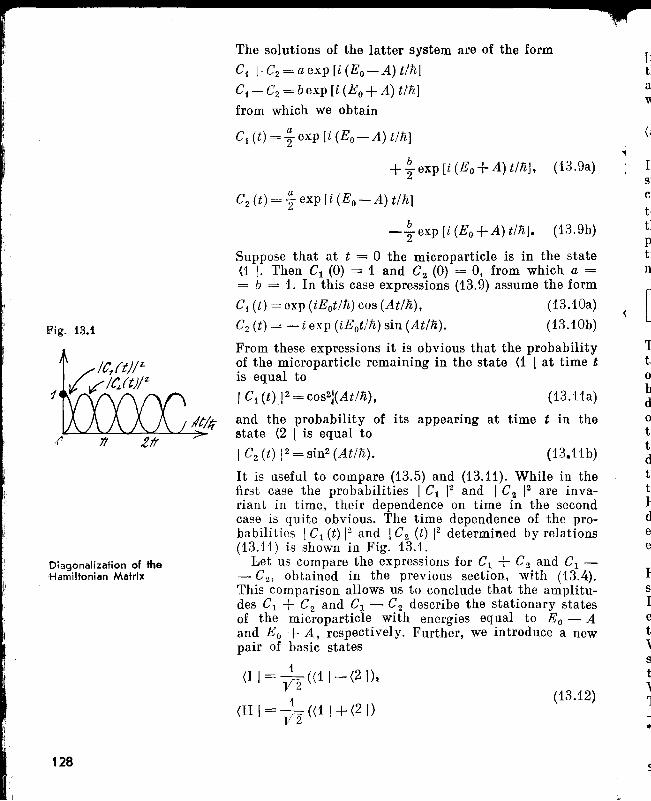
(13.12)

I·

Fig. 13.t

Oiagonalization of the:Hamiltonian Matrix

128

tlt/~

The solutions of the latter system are of the form

C j +C2 = a exp [i (Eo-A) trn]

C j - C2 = bexp [i (Eo + A) tlli]

from which we obtain

Cdt) = ~ exp [i (Eo-A) tlli]

+ ~exp [i (Eo+A) tlli] , (1a.9a)

C2 (t) = 1- exp [i (Eo - A) tlli]

- ~ exp [i (Eo +A) tlli]. (13.9b)

Suppose that at t = 0 the microparticle is in the state(1 I. Then C1 (0) = 1 and C2 (0) = 0, from which a == b = 1. In this case expressions (13.9) assume the form

C j (t) = exp (iEot/li) cos (Atlli) , (13.10a)

C2 (t) = - i exp (iEot/li) sin (Atm). (1a.1 Ob)

From these expressions it is obvious that the probabilityof the microparticle remaining in the state (1 I at time tis equal to

I C1 (t) 12 = cos2i(At/li) , (13.ita)

and the probability of its appearing at time t in thestate (2 [ is equal to

1 C2 (t) 12 ----,- sin2 (Atlli). (13.11b)

It is useful to compare (13.5) and (13.11). While in thefirst case the probabilities 1 C1 12 and I C2 [2 are inva­riant in time, their dependence on time in the secondcase is quite obvious. The time dependence of the pro­babilities 1 C1 (t) /2 and I C2 (t) 12 determiaed by relations(13.11) is shown in Fig. 13.1.

Let us compare the expressions for C1 + Cz and C1 ­

- C2 , obtained in the previous section, with (13.4).This comparison allows us to conclude that the amplitu­des C1 + C2 and C1 - C2 describe the stationary statesof the microparticle with energies equal to Eo - Aand Eo + A, respectively. Further, we introduce a newpair of basic states

1(I 1= VZ «11-(2[),

(111= ~z«1I+(21)

[it]

a

"(I

~

IslC,

tlt]ptJn

[Tti0

bd0

tt,dtt,I-dee

I-sIet"\st\1

•

s

[it is easy to see that if the states (1 I and (2 I satisfythe orthonormalization condition (10.8), the states (I Iand (II I also satisfy this conditionl. By using (13.12),we rewrite (13.1) in the form

(13.13)

e

n

l)

I)

Yt

l)

) )

Le1­

d)-

lS

).1-

lS

4w

l)

It can be seen from here that a transition from the basicstates (1 I and (2 I to the basic states (I I and (II Icorresponds to a transition from amplitudes C1 and C2

to amplitudes (C1 - C2)IV2 and (C1 + C2)IV2. Since

the latter describe the stationary states of the micro­particle, it follows that the transition under considera­tion is associated with a diagonalization of the Hamilto­nian matrix.

Thus, suppose we have a certain microparticle under cer­tain external conditions. Let us choose a certain systemof basic states. The attempt is usually made to choosebasic states which have a clear physical meaning (as wedid, for example, in the case of the ammonia moleculeor the hydrogen molecule). The basic states chosen onthe basis of such considerations lead, in the general case,to a Hamiltonian matrix whose non-diagonal elements aredifferent from zero (the microparticle undergoes transi­tions between the basic states). Further, it is possibleto go over to a new system of basic states for which theHamiltonian matrix is diagonal. The new basic statesdescribe the stationary states of the microparticle; theelements of the diagonalized Hamiltonian matrix areessentially the values of the energy in these states.

In the general case the non-diagonal elements of the General CaseHamiltonian matrix are different from zero and so thesimplifying conditions (13.6) and (13.7) are not applicable.In this case one must solve not the simplified system ofequations (13.8), but the more general system of equa-tions (13.2) for a microparticle with two basic states.We suggest that the reader, if he so desires, solves thesystem (13.2) himself, assuming for the sake of simplicitythat the Hamiltonian matrix is invariant in time*.We shall limit ourselves here giVing some results.The energy of the stationary states of a microparticle is

• Such a solution is given, for example, in [3].

Sec. 13 129

... 5

determined by the expression--,,.,,--=------,,-----

E - Jf ll +H 22 + -. /( H ll -H 22 )2+ H H1, II - 2 - V 2 i2 2i' (13.14)

i:d

1

(13.15)

(t::U6)

",

'Ij

·1 Example of the AmmoniaMolecule

130

The basic states (I I and (II I corresponding to theseenergy values are expressed in terms of the elementarystates (1 1 and (2 I describing the equation system (13.2)in the following manner:

(I 1= ad1 1+ bi (2 I, }(II I = a2 (1 I+ b2 (2 I,where

I a i 12 + I bi 1

2 = 1 a2 12 + I b2 1

2 = 1, }ai/bi = H i2/(EI - H u ),

a2/b2= H 2i/(En - H 22 ).

It can be easily seen that if Hll = H 22 = Eo and H 12 == H 21 = - A, the result (13.14) gives E r ,I1 = Eo ++ A, the superpositions (13.15) turn into (13.12). Inother words, we arrive at the simplified case of the non­diagonal Hamiltonian matrix discussed above in detail.But if H 12 = H 21 = 0, the result (13.14) gives E r = HUtEll = H 22-we arrive at the case of the diagonal Hamil­tonian matrix (I I = (1 I, (II 1= (2 I).

,We recall that the basic states (1 I and (2 1 of theammonia molecule were chosen using graphic physicalconsiderations: they correspond respectively to the posi­tion of the nitrogen atom on one side of the H~plane

and on the other. Since these positions are symmetrical,we may take JIll = JI22 - Eo. Assuming further thatthe elements H 12 and JI 21 are real (JI12 = H 21 - -A),which, as it turns out, does not involve the loss of gene­rality in this case, we arrive at the situation to whichthe simplified system of equation" (13.8) corresponds.It follows from this that the energy levels of a moleculeare essentially Eo + A and Eo - A. We emphasizethat if no transitions took place between the states (1 Iand (2 I, there would have been only one level Eo inplace of the levels Eo + A and Eo - A. It would havebeen doubly degenerate since there would be two statescorresponding to it. It may be said that transitions be­tween the states (1 I and (2 I (associated with "pushing"of the nitrogen atom through the H-plane) correspondto a removal of degeneracy, Le. to a splitting of thelevel Eo into two levels Eo + A and Eo - A.Further, let us assume that the ammonia molecule isplaced in a static electric field with intensity ~ which

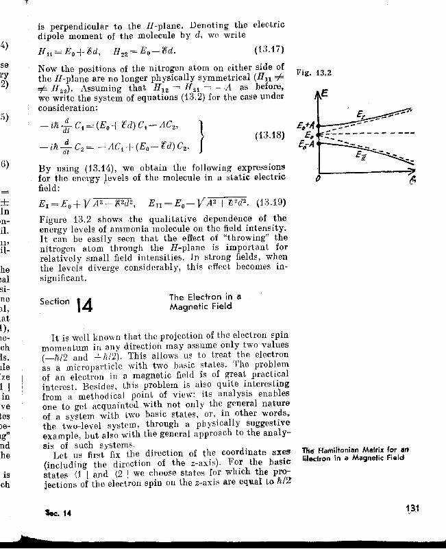
By using (13.14), we obtain the following expressionsfor the energy Jevels of the molecule in a static electricfield:

E1=Eo+ VA2+~2d2, En=Eo- -VA2+e2d2. (13.19)

Figure 13.2 shows the qualitative dependence of theenergy levels of ammonia molecule on the field intensity.It can be easily seen that the effect of "throwing" thenitrogen atom through the H-plane is important forrelatively small fleld intensities. In strong fields, whenthe levels diverge considerably, this effect becomes in­signiflcant.

---"-.------- ------

The Hamiltonian Matrix for anElectron in a Magnetic Field

(13.18)

The Electron in aMagnetic Field

It is well known that the projection of the electron spinmomentum in any direction may assume only two values(-1iI2 and +1iI2). This allows us to treat the electronas a microparticle with two basic states. The problemof an electron in a magnetic field is of great practicalinterest. Besides, this problem is also quite interestingfrom a methodical point of view: its analysis enablesone to get acquainted with not only the general natureof a system with two basic states, or, in other words,the two-level system, through a physically suggestiveexample, but also with the general approach to the analy­sis of such systems.

Let us first fix the direction of the coordinate axes(including the direction of the z-axis). For the basicstates (1 I and (2 I we choose states for which the pro­jections of the electron spin on the z-axis are equal to nlZ

Section 14

is perpendicular to the H-plane. Denoting the electricdipole moment of the molecule by d, we write

Hl1=Eo+~d, H22=Eo-~d. (1;-U7)

Now the positions of the nitrogen atom on either side ofthe H-plane are no longer physically symmetrical (Hu =F Fig. 13.2;:/= H 22). Assuming that H 12 = H 21 = -A as before,we write the system of equations (13.2) for the case under Econsideration:

-;I,:, C,~(E,-I td)C,~AC" }

-in d~ c 2 = -AC 1 +(Eo-ed)C2 •

4)

isch

he~al

si­ne11,atl ),le­chIs.lIelze1 Iinve~es

Je­19"ndhe

u,il-

In-il.

+In

6)

5)

sery2)

lee. 14 1}1

...._---------------

and -fi/2, respectively. We switch on a static magneticfield (we denote the value of the magnetic inductionby B) and consider the following two cases.First case: the magnetic field is directed along the z-axis{B x = By = 0). In this case the basic states (1 I and(2 I are stationary; the state (1 I has energy -f-tB z andthe state (2 I has energy f-tB z (f-t denotes the magneticmoment of the electron). The amplitudes C1 and C'I.satisfy two independent equations of the type (13.3):

I-nCEt:

The Hamiltonian matrix of the electron is of the form

"Ji del B C-l -=-11 1dt r z , (14.1)

(14.2)

Ivi\

,Second case: the magnetic field is in an arbitrary direction.In the first place, we note that irrespective of the direc­tion of the field (in other words, irrespective of the choice-of the direction of the coordinate axes) the energy levels·of the electron are determined by the expressions -f-tBand f-tB; while in the previous case we had to take B == B z, in this case we must have B = (B~ + B~ ++ BD1/ 2• Thus

E1 = -f-t VB~+B~+b'~, En=f-t VB~+B~+1:f;.(14.3)

Note that

E1=-Eu · (14.4)

:Further we make use of relation (13.14). By taking (14.4):into account, we may assume that H ll +·H22 = O. As.a result, by combining (14.3) and (12.9', we get

(14.5)

(14.6)

We shall assume a linear relationship between the ele­ments of the Hamiltonian matrix and the field. It turns.out that this fairly natural assumption allows us toderive the following relations from (14.5): H ll = -f-tB z'H 22 = f-tB z' H21 = Hi2 = -f-t (Bx + iB y). Thus, theHamiltonian matrix of an electron in a magnetic field

"has the following general form:

. ',. [ -f-tBz -f-t(Bx-iBII)l.un = (B +'B ) B J .:" , -f-t x l iJ f-t z

~

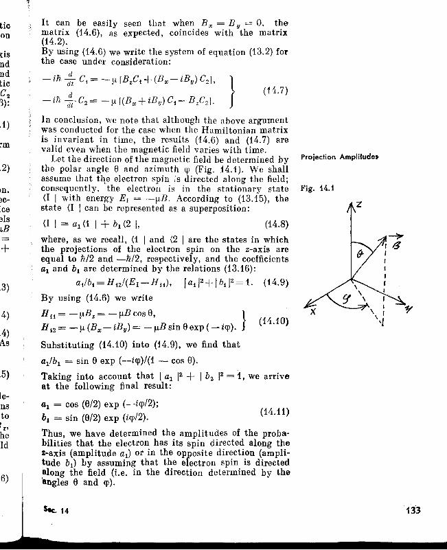
18III,II,I

\ I

''1

zFig. 14.1

Projection Amplitudes-

(14.8)

(14.7)

(14.11)

}

It can be easily seen that when B x = By = 0, thematrix (14.6), as expected, coincides with the matrix(14.2).By using (14.6) we write the system of equation (13.2) forthe case under consideration:

- i'n tt C t = _. ,.![BzCt + (Bx - iBy ) C2 ],

-in :r C2 = -",,[(Bx+iBy)Ct-·BzC21.

a l = cos (8/2) exp (-ilp/2);

bi = sin (8/2) exp (ilp/2).

Thus, we have determined the amplitudes of the proba­bilities that the electron has its spin directed along theZ-axis (amplitude aI) or in the opposite direction (ampli­tUde bI ) by assuming that the electron spin is directedalong the field (Le. in the direction determined by the'angles 8 and lp).

where, as we recall, (1 I and (2 I are the states in whichthe projections of the electron spin on the z-axis areequal to nl2 and -nl2, respectively, and the coefficientsal and bi are determined by the relations (13.16):

at/bt = H t2 /(E 1-H11 ), /a t I2 +/btl2 =1. (14.9)

By using (14.6) we write

H 11 = -""Bz = -""Bcose, }H

t2= -I-t (Bx - iBy ) = -""B sin eexp (- ilp). (14.10)

Substituting (14.10) into (14.9), we find that

ai/bi = sin e exp (--ilp)/(1 - cos e).Taking into account that I al 12 + 1 bz 12 = 1, we arriveat the following final result:

In conclusion, we note that although the above argumentwas conducted for the case when the Hamiltonian matrixis invariant in time, the results (14.6) and (14.7) arevalid even when the magnetic field varies with time.

Let the direction of the magnetic field be determined bythe polar angle e and azimuth lp (Fig. 14.1). We shallassume that t~e electron spin is directed along the field;consequently, the electron is in the stationary state(I I with energy E1 = -""B. According to (13.15), thestate (I I can be represented as a superposition:

6)

le­nsto•, %'

held

,5)

,4)

,4)As

"ticon

dsndndticCz3):

.1)

rm

.2)

m.~c-

icealstB

+

,3)

Stc. 14 133

(14.13)

(14.15)

(14.14)

I;1.;j

~

p,

Note that (14.11) does not contain the magnetic induc~

tion B. It is obvious that the result (14.11) must be validin the limiting case B -+ O. In other words: we may exclu­de the field from consideration and interpret (14.11) inthe following way. It is clear that the direction of theelectron spin is determined by the angles 8 and cp. Inthis case the amplitude of the probability that the electronspin is along the z-axis is al and the amplitude of theprobability that the electron spin is in the oppositedirection is b1 • Expression (14.8) should be treated in thiscase as an expansion of the spin state (8, cp I in termsof the spin states (z I and (-z I:{8, cp I= cos (8/2) exp ( - icp/2) (z I

+sin(8/2)exp(icp/2)(-zl. (14.12)

The amplitudes of the states occurring in (14.12)

(8, cp Iz) = cos (8/2) exp (-iqJ/2);

(8, (pi - z) = sin (8/2) exp (icp/2)

are called projection amplitudes.By using projection amplitudes, we may predict theresult of the following experiment. Let an electron beam,polarized in a direction given by the angles 8 and cp,pass through some "filter" which only allows throughelectrons whose spin is along the z-axis. In this case theamplitude of probability of an electron passing throughthe apparatus (through the "filter") is (8, cp I z). Theprojection amplitude here plays the role of the amplitudeof the electron transition from the state (8, cp I to thestate (z I.

Precession of the Electron Spin Let the direction of the electron spin be given by theangles 8 and cp (the electron is in the state (8, cp I). Thisstate can be represented in the form" of superposition(14.12) of the states (z I and (-z l Suppose that attime t = 0 we switch on a magnetic field B which isdirected along the z-axis. Now the states (z I and (-z Ibecome stationary states. Using this, we write [see (13.4)]

(8, cplz)=CdO)exp(-i/-tBzt/n), }'<8, cpl-z)=C2(0)exp(i/-tBzt/n).Comparing (14.14) with (14.13), we conclude thatC t (0) = cos (8/2) exp ( - icp/2);

C~ (0) = sin (8/2) exp (icp/2).,It follows from this that in time t after the magnetic fieldhas been switched on the projection amplitUdes assume

tl

(I

(I

1zlJ

tf

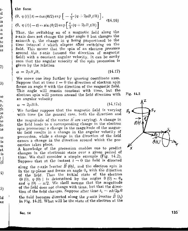
c­ld11­

In1enIII

1eteisas

2)

3)

1eismatis, I~)l

4)

5)

ldne

1::~ :~:~,) ~ "" (612) cxp [ - -H~ 12~B ,tin)J'(14.16)

; <e, CP(t)l-z)=sin(8/2)exp[~ (cp+2~tBzt/n)J

I.,i,'.. Thus, the switching on of a magnetic fIeld along the, z-axis does not change the polar angle 8 but changes the

azimuth cp, the change in cp being proportional to the

i'.,"", time interval t which elapses after switching on the, field. This means that the spin of an electron precesses, around the z-axis (around the direction of magneticI field) with a constant angular velocity. It can be easilyI seen that the angular velocity of the spin precession isi given by the relation

I ill = 2~Bz/n. (14.17)!

We move one step further by ignoring coordinate axes.Suppose that at time t = 0 the direction of electron spinforms an angle 8 with the direction of the magnetic field.This angle will remain constant with time, but theelectron spin will precess around the field direction withan angular velocity

(i) = 2~lB/!1. (14.17a)

We further suppose that the magnetic field is varyingwith time (in the general case, both the direction and

the magnitude of the vector B-'> are varying). A change inthe field leads to a corresponding change in the electronspin precession: a change in the magnitude of the magne­tic field results in a change in the angular velocity ofprecession, while a change in the direction of the fieldcauses a change in the direction around which the pre­cession takes place.A knowledge of the precession enables one to predictchanges in the electronic state over a given period oftime. We shall consider a simple example (Fig. 14.2).Suppose that at the instant t = 0 the field is directed-along the z-axis [vector B (0)1, and the elect~onspin isin the zy-plane and forms an angle 80 with the directionof the field. Thus the initial state of the electron<8 (0), cp (0) I is determined by the angles 8 (0) = 80

and cp (0) = n/2. We shall assume that the magnitudeof the field does not change with time, but that the direc­tion of the field changes. Suppose after time h = nn/2ItB

the field becomes directed along the y-axis [vector B (t1)

.in Fig. 14:21. What will be the state of the electron at the

Sec. 14

Fig. 14.2

z.

135'

Generalization of the Problem ofan Electron in a Magnetic Fieldto an Arbitrary Two-Level System

time t1? It is clear that if the field direction had remainedunchanged, the end point of the electron spin vector,while precessing around the z-axis, would have describeda semicircle during the time nnl2ltB, thus shifting frompoint SI to point S2. If we take into account the variationin field direction, we shall find that it has shifted notto the point S2 but to the point S3. Consequently, therequired state of the electron (8 (tl), cP (tl) I would bedetermined by the angles 8 (tl) = n/2 - 80 and cP (tl) == n/2.

According to Feynman [3], it is interesting that themathematical ideas we have just gone over for the spinningelectron in a magnetic field can be applied to any two­state system. That means that by making a mathematicalanalogy to the spinning electron, any problem about two­state systems can be solved by pure geometry .... If we cansolve the electron problem in general, we have solved alltwo-state problems. Let us clarify these remarks.We shall consider some two-level system with the basicstates {1 I and (2 I. We assign some vector to each stateof the microparticle. A choice of the basic states {1 Iand {2 I in this case is equivalent to a choice of thez-axis (as if these two states correspond to the two z­projections of the electron spin). Suppose that the micro­particle is in the state {s (0) I at the initial momentof time. We assign to this state a vector whose directionis determined by the angles 8 (0) and cP (0):

{s (0) I +-+ (8 (0), cP (0) I. (14.18)

In order to find the angles 8 (0) and cP (O)~we must Expandthe state (s (0) I in terms of the basic states {1 I and{2 I and use for the coefficients of expansion expression(14.13) for the projection amplitudes. This expansionis of the form

{8 (0)1 = cos [8 (0)/2J expl[ _ iCPJ(0)/2j!{11 "

+sin [8 (0)/2J exp [icp (O)/2J!{2/. (14.19)

Further, let us turn to the Hamiltonian matrix of themicroparticle. First of all we shift the zero point of theenergy in such a way that it is located precisely half-waybetween the two energy levels or, in other words, sothat the condition (14.4) is satisfied. In this case

8 11 +822 =0. (H.~O)->-

We now formally introduce a vector ItB (it is in no wayassociated with any magnetic field!) such that its projec­tions on the coordinate axes (remember that the axesare determined by the choice of the basic states) satisfy

d.,dnntee

eg

~

l

j

it

IIt

the conditions

H 11 = -lJBz, H 12 = -f-l(Bx-iBy). (14.21)

By using (14.21) we determine

ro=2f-l(B:+B~+B~)1IZ/Jz. (14.22)

In order to solve this two-level problem, Le. in orderto determine the change in the (s I-state during certaintime t, we must consider the precession of the vector

~

(8, cp I around the direction B with an angular velocity ro.lf the Hami~tonian matrix is time dependent, both the

direction of B and the magnitude of the angular velocityof precession will change accordingly. After a time t,the microparticle will be in the state (s (t) I, defined bythe angles 8 (t) and cp (t), which may be determined if weknow the initial values 8 (0) and cp (0) and the precession(in exactly th'e same way as was done in the examplegiven at the end of the preceding subsection). The transi­tion from the angles 8 (t) and cp (t) to the required finalstate (s (t) I is accomplished by using the familiar super­position:

(8 (t) I= cos [8 (t)/2] exp [ - icp (t)/2] (11

+sin [8 (t)/2] exp [icp (t)/2] (21. (14.23)

Applying these remarks to the example of the ammoniamolecule considered in Sec. 13, we must shift the zeropoint of the energy by an amount Eo, and go over (forthe sake of convenience) from the basic states (1 I and(2 I to the basic states (I I and (II I. As a result, we getin place of (13.18) the following system of equations:

- ih :t CI = ACI +edC II, }

d • (14.24)- ih(F Cn = edC l -ACn .

This system is convenient for drawing the analogy withthe electron in a magnetic field. Comparing (14.24)and (14.7), we find that the quantity A corresponds to-f-lB z and the quantity ed to -/.-lBx· Consequently,we have to consider the precession of the vector describingthe state (s I of the molecule in the "magnetic field" whichis made up of two components: a constant componentalong the z-axis, associated with the effect of the "throw­ing" of a nitrogen atom through the H-plane, and a com­ponent along the x-axis, associated with the electricfield. The latter component may, obviously, vary withtime.

Sec. 14 137

~.. ...t

p.,---------------------a:::p-I

PAULI SPIN MATRICES. In conclusion, we shall mention thePauli spin matrices which are wirlely used in the quantum me­chanics of two-level systems. These matrices are of the form

By using these matrices, we can rewrite the expression for theelements of Hamiltonian matrix of all electron in a magnetic fICld(14.6) in the fOllowing form:

[01Jax = 1 ° ; [

1a Z~ .0 UJ-1 . (14.25)

(14.26)

t(~

tI

1

By considering ax, aY, OX as components of some matrix vector ;,we can rewrite (14.26) in a form which is independent of the choice(If the coordinate axes:

--> -->Hij= -!L0ijB. (14.27)

Pauli spin matrices are useful because any second-order matrix(in particular, the Hamiltonian matrix of any microparticle withtwo basic states) may be represented as a superposition of thesematrices. The Pauli spin matrices introduced for an electron ina magnetic field have proved to be convenient for considering awide range of two-level problems. This is not surprising when we-consider the possibility, discussed above, of generalizing the pro­blem of an electron in a magnetic field to arbitrary two-level sys­tems.

Section 15 The Wave Function

At the very outset, let us make it clear that this sectionhardly adds anything new to the physical foundationsof quantum mechanics considered in this chapter. Infact, we are already able to summarize the physicalaspects of the theory and go over to its mathematical side,based on the use of linear operators. However, beforedoing so, it is worthwhile to introduce the concept ofthe wave junction. Wave functions are widely used inthe existing literature on quantum mechanics; henceit is important that the reader should be aware of the"position" of the wave function in the above descriptionof amplitUde concepts. Until now, the wave function,being essentially the amplitude of state, existed in thispicture in an implicit form; we shall now make it explicit.Besides, one must remember that while changing overto the mathematical apparatus of quantum mechanics,it is more convenient to use the wave function ratherthan the amplitude of state.

138

Let (x I be the state of a microparticle corresponding The Wave Function as theto its localization at a point in space with the coordinate x Amplitude of State

(for simplicity we consider the one-dimensional case).Then (s I x> may be considered as the probability ampli-tude that a microparticle in the state (s I has the coordi-nate x.However, we must make this a little more precise. Whenconsidering the probability of any spatial localization ofa microparticle, we must take into account the continuityin the variation of a spatial coordinate. Hence, insteadof the probability of finding a microparticle preciselyat the point x, we must consider the probability of find­ing it on the interval from x to x + dx. Denoting thisprobability by dws (x), we have

dws (x) = I (s I x) 12 dx. (15.1)

Consequently" the quantity (s I x> is, strictly speaking,not the amplitude of probability, but the amplitude ojprobability density.In literature, the quantity (s 1 x> is referred to as thewave junction and is expressed, for example, by 'ljJs (x).Thus,

\jJs (x) = (s I x>. (15.2)

Using (15.2) we can rewrite (15.1) as

dws (x) = l1\1s (x) J2 dx. (15.3)

It follows from (15.3) that 11\1. (x) 12 is the probabilitydensity of finding a microparticle with the state (s\at the point x.From a mathematical point of view, the wave function in\jJ. (x) is a parametric function, the parameters being thequantities which are precisely defined in the state (s \.Taking into account the earlier remarks on the structureof amplitudes of states, we may state that the quantitiesof one complete set serve as the argument for the wavefunction, its parameter being the quantities of another set.It is often said that the wave function 'IjJ. (x) is an eigen­junction of the quantities of the s-set, given in the repre­sentation determined by the quantities of the x-set (orsimply, in the x-representation).

Wave functions are frequently used in practice in the Generalization of the Concept ofx-representation (coordinate representation). However, the Wave Function

apart from the x-representation, other representations areobviously also possible. In this connection, the conceptof the wave function must be generalized:

3

f1

e1

s

r

r'ljJa (~) = (ex I~).

Sec. 15

(15.4)

~ 1

.,--------------------..,..-The function tPa (~) is the eigenfunction of the quantitiesof the a-set, given in the ~-representation. If the valuesof the ~-set change discretely, 'Pa. (~) is the amplitude ofthe probability that the state (~ I is represented in thestate (a I. In the case of continuously changing valuesof the ~ -set, ~la (~) is the amplitude of the given probabi­lity density.By giving the wave function tPa (~) we give the exactvalues of the quantities in the a-set and probable valuesof the quantities in the ~-set. Correspondingly, by givingthe function CPa (y) we give the exact values of the a-setand probable for the values of the y-set. It could be saidthat the function tPa. (~) describes the state (a I in the~-representation, while the function CPa. (y) describes thesame state, but in the y-representation. The fact thatdifferent functions tP ... (~) and cp:'(y) are used for describingthe same state (a I indicates that there must be someconnection between them. This connection is expressedthrough the principle of superposition of states. Assumingthat y-values change discretely, we can write

1

~

1';

I

C';

,

(15.5)

It can be easily seen that (15.5) is the expression for thesuperposition of amplitudes of states:

(15.5a)

If the y-values vary continuously, we get in place of (15.5)

(15.6)

Let us consider the eigenfunction of the quantities of acertain set given in the representation ()Lthe quantitiesof the same set. If these quantities change discretely, wehave, according to (10.8),

(15.7)

140

If, however, the quantities vary continuously, we get inplace of (15.7)

'Y.~(a)=(')(a-a'). (15.8)

where (') (a - a') is the so-called Dirac delta junction,which is a generalization of the Kronecker's symbol forthe case of continuously varying quantities.*• The delta function is discussed in detail, for example. in [t3}.

I

i

The delta function is determined in the following way:

Strictly speaking, it is impossible to plot the function6 (a - a') because it would involve drawing an infinite­ly narrow and infinitely high peak at the point a = a'with a finite "area" under it equal to unity. One of themost important properties of the delta function, whichcan be easily derived from its definition (15.9), can bewritten as follows:

where f (a) is a bounded function, continuous at thepoint a = a';

Assuming that the a-values are discrete and the ~-va- Condition of Orthonormalizatiolllues vary continuously we rewrite (15.6) in the form of Eigenfunctions

'I'c<;(aj)= 51pa,(~)<1>Il(aj)d~. (15.11)

By using (9.33). we can write

<1>f:l (aj) = 1p~. (~). (15.12)]

From (15.12) and (15.7), we obtain from (15.11) thecondition for the orthonormalization of the eigenfunction8"'I%i (~):

51pa; (~) 1pcij (~) d~ = 6i /. (15.13)

If the a-quantities vary continuously. we must use (15.8)instead of (15.7). In this case the condition of orthonor­malization of the eigenfunctions assumes the form

s 1s It

fes

ts'J~

t}

eet'J~

eI'J~

)

)

o(a-a')==O at a*a';

00

i f (a) 6 (a-a') da = f (a'),-00

00

r ' I'J 6 (a - a ) da = 1. (15.9)

;(15.10)

51pa (~) 1P~ (~) d~ = 6 (a-a'). (15.14)

As an example, we consider the case of a freely moving The Wave Function of a Freelymicroparticle. For simplicity, we assume that it has Moving Microparticle

zero spin. The wave function in coordinate (three-dimen-sional) representation has the form*

.... ........ -3/2 ........1p-+ (r) = (Po Ir) = (2nli) exp (iporlli)1 (15.15)

Po

where Po is the momentum of the microparticle and -; is

its spatial coordinate. The function 1p-.. (;:) is an eigen-Po

... We shall derive this result later (see Sec. 20).

Sec. 15 141

I '~ .t

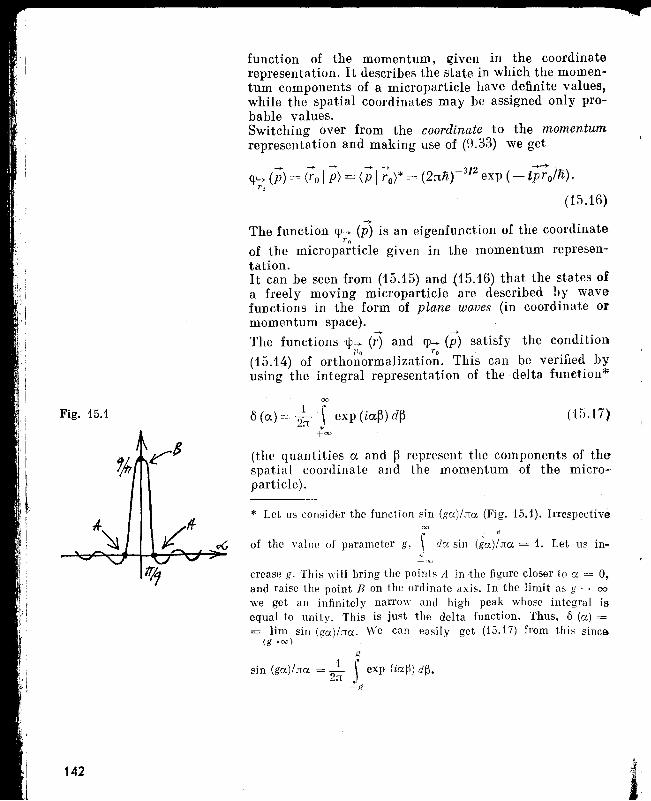
142

(15.17)1 •

6(~)=2JT J exp(i~~)d~+00

crease g. This will bring the points A in the figure closer to a = 0,and raise the point B on the ordinate axis. In the limit as g --+ 00

we get an infinitely narrow and high peak whose integral isequal to unity. This is just the delta function. Thus, 0 (a) == lim sin (ga)/na. We can easily get (15.17) from this since

(g~oo) .

f{

sin (ga)/na = _1_ r exp (ia~) d~.2n J

-f{

~ --+ -+ -)0 -+ 3/2 ~-+

{fJ-. (p) = (roIp) = (p I ro)* = (2:n:nF exp (- tpro;n)·To

(15.16)

(the quantities ~ and ~ represent the components of the­spatial coordinate and the momentum of the micro­particle).

The function CP-+ (P) is an eigenfunction of the coordinateTo

of the microparticle given in the momentum represen-tation.It can be seen from (15.15) and (15.16) that the states ofa freely moving microparticle are described by wavefunctions in the form of plane waves (in coordinate ormomentum space).

The functions '¢-+ (;:) and Cp-+ (p) satisfy the condition])0 . To '

(15.14) of orthonormalization. This can be verified byusing the integral representation of the delta function*

function of the momentum, given in the coordinaterepresentation. It describes the state in which the momen­tum components of a microparticle have definite values,while the spatial coordinates may be assigned only pro­bable values.Switching over from the coordinate to the momentumrepresentation and making use of (9.33) we get

Fig. 15.1

* Let us consider the function sin (ga)/ITa (Fig. 15.1). Irrespective00

_~P~+-1-~~~~~~ of the value of parameter g, j do. sin (ga)/na = 1. Let us in--00

Section 16 Quantum Mechanics as aQualitative Leap in Man'sKnowledge of the Laws ofNature

)

Of course it IS impossible to distinguish sharply betweennatural philosophy and human culture. The physicalsciences are, in fact, an integral part of our civilization,not only because our ever-increasing mastery of the forcesof nature has so completely changed the material conditionsof life, but also because the study (If these sciences has con­tributed so much to clarify the background of our ownexistence.

N. Bohr

Although quantum mechanics deals with microparticles,its significance is by no means limited to microphenome­na. In our endless quest for understanding and perfectingour knowledge of the laws of nature, quantum mechanicsrepresents an important qualitative leap. Without a com­prehension of the importance, and radical (we could evensay revolutionary) nature of this leap, it is impossibleto understand the modern physical picture of the world.In this section, an attempt has been made to look atquantum mechanics from this point of view. This mayserve as a logical conclusion to the chapter, which hasbeen devoted to the physical foundations of this astonish­ing theory.

The expression "crazy theory" as one which is "crazy "Crazy Ideas"enough to be true" was once coined by Bohr. This expres-sion reflects the stunning impression produced on Bohr'scontemporaries by the astonishing physical discoveriesmade at the beginning of the 20th century, discoverieswhich could not be confined within the framework ofclassical concepts. It became obvious that an explanationof these discoveries required radically new ideas and a newapproach.In Sec. 2 we considered two fundamental ideas of quantummechanics-the idea of discreteness and the idea of duality.Returning, in our imagination, to the beginning of thecentury, we could call the first idea "incomprehensible"and the second, "not properly understood". The intro­duction of discreteness to the physical picture of theworld led to incomprehensible and, apparently, logicallycontroversial quantum "jumps". The idea of duality,which asserts the specific nature of microparticles, elimi­nated the contradiction of quantum "jumps" by suggest­ing a "manoeuvring" between the "particle" and the"wave" concepts. But the meaning of the wave conceptintroduced here remained in fact unclear for a very longtime. These two "absurd" ideas led to the emergence of

Sec:. 16 143

~ lIIIIiIIIt

).r

The Essence of QuantumMechanics

144

the extravagant "uncertainty relations" which resultedin a different outlook on even such fundamental con­cepts as "energy", "momentum" and "angular momen­tum".Quantum mechanics was born under circumstances ofa significant breaking up of physical traditions. It calledfor a rejection of many usual and accepted notions suchas the strict continuity of the spectra of values of physicalquantities, the trajectory as an essential attribute of themotion of an object, Laplace determinism as the basicform of expression of the principle of causality, the possi­bility of an infinite detailization of the structure of anobject or of a phenomenon with respect to time, thepossibility of distinguishing between two objects, howeversimilar to each other, under any circumstances, the beliefthat it is always possible, at least in principle, to disre­gard the measuring instrument when conducting anymeasurements, etc. (all these questions have been analys­ed in detail in the preceding sections).It is difficult to recall any other period in the historyof physics when such a serious and large-scale revisionof physical concepts was carried out. According to Bohr,... the new lesson which has been impressed upon physicistsstresses the caution with which all usual conventions must beapplied as soon as we are not concerned with everyday expe­rience... In the study of atomic phenomena we haverepeatedly been taught that questions which were believedto have received long ago their final answers had most unex­pected surprises in store for us.

The revision of the concepts and the rejection of manyaccepted notions could well be considered as a "negativeaspect" of quantum mechanics. Let us now consider its"positive aspect".If we try to summarize the main positiv~ knowledge im­parted by quantum mechanics to man: in his search forlearning about his surroundings, the following two impor­tant points stand out:First: quantum mechanics showed that the basic laws ofnature are not dynamic but are statistical, and that theprobabilistic form of causality is the fundamental formwhile the classical determinism is just its limiting (degene­rate) case.Second: quantum mechanics revealed that probability innature should not be dealt with as in classical statisticaltheories. It was found that in certain cases it is not theprobabilities of events that should be summed, but ratherthe amplitudes of these probabilities. This leads to theinterference of probability amplitudes.

I

I

f1

dl­

l-

.fdhIIec

1-

y

ytl.,:se

'ed:-

yeS

r'-

~

lEl

rEl

flo Thus we empha,;'. firstly the probabili3tte eharacter ojI, '.~. the laws of nature (the pre-eminence of statistical laws)I r and, secondly, the special relations among the probabilities,

which assume not only the summation of the latter, butalso the specific interference effects. In our view, it is inthis that the main importance of the information one getsfrom quantum mechanics is to be found.As Born pointed out in [14], the statistical methods foundwider applicability with the development of physics.As regards modern physics, it is completely based on sta­tistical foundations. In Born's view, it is the quantumtheory that established the closest links between statisticsand the basic aspects of physics. This should be consideredas an important event in the history of human knowledge,with consequences reaching far beyond the limits of science.It is sometimes said that the fundamental difference be­tween quantum mechanics and classical mechanics isdetermined by \ the statistical nature of the former anddynamic nature of the latter. Upon careful consideration,this apparently bland and irrefutable statement turnsout to be incorrect. While revealing the pre-eminence ofstatistical laws in physics, quantum mechanics showsat the same time that dynamic laws with their uniquepredictions are, as a matter of fact, a special (degenerate)case of probability laws. In this respect not only quantummechanics, but classical mechanics as well, must be,strictly speaking, formulated in the language of probabil­ities*. The qualitative difference between quantum me­chanics and classical mechanics (or classical physics ingeneral) depends on how the relations among probabilitiesare considered. It has been mentioned in [27] that themain difference between quantum mechanics and classicalmechanics does not lie in the statistical nature of theformer. It lies in the fact that it is not the probabilitybut its amplitude, the wave function, that is of primaryimportance in quantum mechanics. This leads to theinterference of probabilities, an effect which does nothave an analogy in classical mechanics.Developing the above ideas, let us single out the follow­ing points: (a) the special interrelations among quantum­mechanical states and the resulting specific nature ofquantum-mechanical description of phenomena; (b) the

* This point of view is systematically analysed in [27], where itis stated, in particular, that Feynman's concepts of path integralsin fact converts the principle of least action into the principle ofmaximum probability, i.e. it proves that the fundamental dynamicPrinciple is essentially statistical in nature.

Sec. 16145

..6rr..~ '1

·I!:"

Ii

The Specific Nature ofQuantum-Mechanical Descriptionof Phenomena

146

specific nature of the application of probabilities inquantum mechanics; (c) the special role of interferencein quantum mechanics; (d) the complementarity principleas a logical foundation of quantum mechanics, and (e) thedialectical nature of quantum mechanics. We shall con­sider these questions one by one.

According to Feynman, one of the most outstandingachievements of quantum mechanics lies in the fact thatit allows so much to be extracted from so little.The reader has already found out how much can beachieved from the phenomenon of interference of ampli­tudes (see Sec. 9), on the basis of the principle of super­position of states (see Sec. 10), and from a considerationof the simplest quantum-mechanical systems, Le. micro­particles with two basic states (see Secs. 13, 14). Therelative formal simplicity of the description of microphe­nomena is connected with the specific nature of thisdescription. Remember that for a quantum-mechanicaldescription we must know firstly the basic states and,secondly, the Hamiltonian matrix, which reflects thephysics of the phenomena under consideration. A simplifi­cation in the description can be achieved because of thefollowing two circumstances.Firstly, it is important that the number of basic states,and consequently the number of elements of the Hamilto­nian matrix required for describing a definite phenome­non, should not be large. Thus, in the examples givenin Secs. 13 and 14, this number was equal to two. Herethe contradiction regarding the diversity in the possiblestates of the microparticle does not arise, since accordingto the principle of superposition either of them may berepresented in the form of some superposition of basicstates. The principle of superposition itself is the decidingfactor, which permits us to manage usually with a smallnumber of states selected as the basic "states. As Diracwrote [9], ... in departing from the determinacy of the classi­cal theory a great complication is introduced into the descrip­tion of Nature, which is a highly undesirable feature. Thiscomplication is undeniable, but it is offset by a greatsimplification prOVided by the general principle of superpo­sition of states....It has been noted earlier (see Sec. 10) that in classicalphysics all states of a particle should be considered asmutually orthogonal, or, in other words, as basic states.Because of this, the above-mentioned simplifying situa­tion is impossible here in principle.Secondly, the relative simplicity of superposition relationsallows us to draw analogies among microparticles having

l,[l

eee1-

g.t

el-'-

nI-

.el-

is11

1,Lei-Le

s,)-

e-mre1eLgleic19111C

i-el-

is'It0-

alass.a-

llS

19

the same number of basic states and reduce all the realproblems in practice to a consideration of the two-levelproblem, three-level problem, etc. It has been shownin Sec. 14 how an arbitrary problem with two basic statescan be reduced formally to the problem of an electronin a magnetic field.Of course, it cannot be deduced from all this that ingeneral "quantum mechanics is simpler than classicalmechanics". Certainly it is simpler in the above-mentionedsense. However, it has sufficient problems of its own,especially problems connected with a rational choice ofthe system of basic states and with finding the form of theHamiltonian matrix. It is hardly necessary to recountall the difficulties which invariably result from thenecessity of departing from graphic representations ofaccustomed concepts. That is the way things are. Henceit wouldn't be wise to say that "quantum mechanics issimple!". And 'yet one must remember that the peculiarrelations that exist among different states of a micropar­ticle and appear in the specific principle of superpositionof states considerably simplify the quantum-mechanicaldescription of phenomena.

Quantum mechanics forces us to take a fresh look atthe well-known theorem of addition of probabilities forincompatible events. We have to consider not only theincompatibility but also the distinguishability of theevents. This is where the novelty of the approach lies.It is well known that in the probability theory used inclassical physics, as well as in engineering, it is alwaysimplied that events are distinguishable.In order to demonstrate the specific nature of the applica­tion of probability in quantum mechanics, we make useof the example considered in Secs. 9 and 10 of the scatter­ing of bosons of the same type by each other. We recallthe notations introduced in these sections: lp (8) == </1 1 81} </2 I 8 2 }-the probability amplitude of one event(one transition), lp (n - 8) = </2 I Sl} <Ii 1 S2 }-the proba­bility amplitude of the other event, w - the probabilityof simultaneous activation of both detectors. Sincemicroparticles of the same type are scattered by eachother, the question of their distinguishability leads tothe distinguishability of the initial states <81 I and (S2 I.In this connection three cases may be isolated:First case. The events are completely indistinguishable.This means that the initial states are the same, and

(16.1)

Probability in QuantumMechanics

"

See. 16147

I,I

iI. j

148

In this case, we get [see (9.17)]

w=lep(8)+ep(n-8)12. (16.2)Second case. The events are partially distinguishable. Thismeans that the amplitude (SI I S2) satisfies the condition

0< I (SI I S2) 1<1. (16.3)

In this case, we get [see (10.7)]

w = I ep (8) 12+ I ep (n - 8) 12

+ I (s{ I S2) 12[ep (8) ep* (n - 8) + ep* (8) ep (n - 8)]. (16.4)

Third case. The events are completely distinguishable.This means that the amplitude (.'11 I S2) satisfies thecondition

(SI I S2) = O. (16.5)

This gives us [see (9.16)]

IV = I ep (8) 12+ I ep (n -- 8) 12• (16.6)

Thus we find that the theorem of the addition of proba­bilities "holds" only in the third of the above-mentionedcases, i.e. in the case of completely distinguishableevents. From (16.5) it follows that the states (.~1 I and(S2 I must be mutually orthogonal* in this case. In theremaining cases the theorem of the addition of probabili- Ities does not hold. If the events are completely indistin- \guishable, the amplitudes of the probabilities should besummed. But if the events are partially distinguishable, ..we must use the more complicated relation (16.4). Whenderiving this relation, both the law of the addition ofamplitudes and the theorem of the addition of probabili­ties have been used in the same way as in Sec. 9 whenderiving (9.10).It can be easily seen that the result (16.4) based on theaddition of probabilities as well as the addition of ampli­tudes is the most general one. When the condition (16.5)is satisfied, it at once leads to the "purely" classical caseof addition of probabilities while condition (16.1) isfulfilled "purely" in the case of addition of amplitudesof probabilities.It should be emphasized that the very possibility of theexistence of the general result (16.4) is caused by thepresence of superposition bonds between the states (S1 I

* It is worthwhile mentioning here that the mutual orthogonalityof all states of a classical object stipulates a complete distinguish­ability of events and, as a result, leads to the theorem of ·additionof probabilities.

2)tis)n

3)

4)

~e.

he

5)

6)

>a-ed.leadheli­n­beIe,enofli­en

heli­.5)lseis

les

hehe11 I

itysh­ion

and ("2 I [see (10.6) in this connection]. Thus we trackthe active connection between the quantum-mechanicalprinciple of superposition of states and the specific natureof the application of probability in quantum mechanics.The superposition relations among states and the inter­ference of probability amplitudes have the same physicalnature.

We draw the reader's attention to the following fact.In order to explain the interference results in experimentswith microparticles (for example, the interference patternon the detector-screen in Experiment 1 of Sec. 7), we canformally proceed in two different ways. One way corres­ponds to the "conservation" in quantum mechanics ofthe theorem of the addition of probabilities for any incom­patible events. This way, however, requires a comparisonof the microparticle with some classical wave. The otherway corresponds to the addition of probability amplitudes.In this case an explanation of interference results nolonger requires the introduction of any visual wavemodel.The specific nature of microparticles, which has beendiscussed in detail in the preceding sections, precludesthe first way and so puts the question of interference andwave processes in a new light. Before the appearance ofquantum mechanics, interference was always consideredas an example of a typical wave effect. If a characteristicinterference pattern was observed in any experiment,it was considered sufficient evidence to draw conclusionson the presence of waves. In this sense, wave" were consid­ered as being "primary", and interference as being se­condary. Quantum mechanics shows that the reverse orderof emphasis is more correct.In revealing that the probability laws of nature involvethe addition of probability amplitudes and not of theprobabilities themselves, quantum mechanics revealedthe fundamental role of interference in physical phenome­na. Simultaneously, it showed that classical wave proces­ses need not essentially be at the root of an interferencepattern. In the general case, interference is a specificallyquantum-mechanical effect associated with the additionof probability amplitudes.Traditions, however, die hard. This explains attempts to"translate" the interference of probability amplitudesinto the graphic language of classical waves, whichinevitably leads to a definite misuse of wave terminology(see the above interlude "Are these the same waves?").In a number of cases the "translation" into wave languageis not justified even from a formal point of view. For

Sec:. 16

Quantum Mechanics andInterference

149

I. i'

:i'

150

example, the division of microparticles into fermions and ­bosons, which is such an important consequence of theinterference of amplitudes, is fairly difficult to explainon the basis of wave processes. The analysis of the processof the destruction of interference of amplitudes in themeasuring process ("the reduction of the wave packet")directly indicates the impropriety of using classical waveconcepts when considering microphenomena. All thisindicates that an explanation of interference obviouslydoes not come within the framework of the traditionalwave model.By the way, the last fact may be taken as the startingpoint for a generalization of the very concept of "waveprocess". Such a generalization assumes a transition fromvisual classical waves with real amplitudes to some sortof generalized waves with complex amplitudes. The classi­cal waves must appear as an extreme (degenerate) case ofsuch generalized waves. In other words, quantum-mechan­ical interference may be used for an extension of theframework of the accepted wave picture (which, incident­ally, is invariably accompanied by rejection of a graphicrepresentation) and for creating a theory for the general­ized wave processes which would reflect not only theprobability nature of physical laws but also the specialrelations among probabilities in nature.By demonstrating the fundamental nature of the pheno­menon of interference, quantum mechanics naturallyarises an interest in the study of this phenomenon indifferent branches of physics. In our view, it raises definitehopes that modern physics, stimulated by the effect ofinterference, will develop in future into a study of theinterference of effects in the fields of both microphenomenaand macrophenomena.The idea of "addition" (summation, accumulation) ofdifferent phenomena is familiar to u8.1n a way, this canbe compared with the "addition of probabilities". It islikely that quantum mechanics tells us (indicates in itsown way) that such a picture is the result of a certain"averaging", approximation or simplification of a finerand better pictne in which we "add up" not the effectsthemselves, but something different (corresponding toprobability amplitudes in the language of quantummechanics), thereby arriving at the phenomenon of inter­ference of effects.

.dLen,SLe")'eis.y11

19reIII

rti­)fl­

iet­icl­ieII

)­

lyinteofrrela

ofmistsinertstomr-

A Brief Interlude

11lIerlude

Fairy tales, though oft untrue,Teach good lads a thing or two.

Pushkin

Reader: It is not clear what you wanted to say in the last sentenceswhich, though quite eloquent, are tentative. Please explain them,if possible.

A uthor: Gladly. Let us take a definite example. It is well known thatif a substance is placed in a condenser, its optical properties willchange under the influence of the external electric field. Such effectsare called electro-optical effects. If the substance is subjected toa light field of sufficient intensity (generated, say, by a high-powerlaser), the optical properties change in this case also. These effectsare called nonlinear optical effects. It so happens that if a condenserfield and an intense light field are simultaneously switched on, thenin addition to the familiar electro-optical and nonlinear opticaleffects we observe qualitatively different effects which may beexplained only as a unique interference of electro-optics and non­linear optics. This is an example of the interference of effects.

Reader: But can one perceive in this example any tendency towards thedevelopment of modern physics?

A uthor: Let us take another example, that of a laser. We shall not dis-cuss the principle of its working here; it is just sufficient to mentionthat it is based on some nonlinear effect, called the saturation effect.Let us take another instrument, the second-harmonic generator(that is what a transformer of coherent light which doubles thefrequency is called in quantum mechanics). We shall simply statethat this instrument also is based on the principle of nonlinearoptical effect called the generation of second harmonics. Thus, thelaser produces coherent light of a definite frequency, while thesecond-harmonic generator partially transforms the frequency ofthis light. We can say that we first use the saturation effect andthen the effect of second-harmonic generation. Such is a general situa­tion corresponding to a simple "summing" of these effects. Now,suppose that both these effects are used simultaneously. In orderto do so, we must place a special crystal, which causes a transformation of the frequency of light passing through it, inside thela~er (or, more precisely, inside the resonator of the laser). Here,we are speaking of a qualitatively different situation correspondingto the interference of two nonlinear optical effects. It is quite signifi­cant that this and other similar situations have been increasinglydrawing the attention of specialists engaged in the field of quan­tum electronics. Intraresonator generation of second harmonicis already being put into practice; it has been proved that it canensure a more effective transformation of optical frequency.

Reader: This really sounds interesting. It is possible that some tendencyis indicated here. But what has:this got to do with quantum me­chanics?

151

< ,

Author: When studying reality on a fundamental level, quantum mechan-ics highlighted some important points. It showed that the questionof interference is deeper than it was considered, and that this ques­tion can be posed independently of wave questions; and finally,that interference is an example of qualitatively new interrelations,Le. relations which obviously have more prospects than the tra­ditional interrelations corresponding to a simple summing, adding,or accumulation.

I,

I\

:~:11

I:

f

~Ii,

I

dl

Complementary Principle

152

The dialectical nature of quantum mechanics is reflectedin its very initial principles. In this connection theprinciple of complementarity, put forth by Bohr, is ofspecial interest. This principle forms in fact the logicalfoundation of the entire system of quantum-mechanicalideas.The essence of the principle of complementarity lies inthe following: it is stated that in any experiment withmicroparticles, the observer gets information not aboutthe "properties of the particles themselves" but aboutthe properties of the particles associated with some par­ticular situation including, among other things, the meas­uring instruments. The information about the objectobtained under some definite conditions should be consid­ered as complementary to the information obtained underdifferent conditions. Essentially, the information obtainedunder different circumstances cannot be added, accumu­lated or combined into a single picture; it reflects varioussides (complementing one another) of a single reality,to wit the object under investigation. The principle ofcomplementarity finds a direct expression, in particular,in the idea of wave-particle duality and in the uncertaintyrelations.According to Bohr, the term 'complementarity' is usedin order to stress that in the contrasting phenomena we haveto do with equally essential aspects of all; well-defined know­ledge about the object (N. Bohr, "On the Notions of Causal­ity and Complementarity") ... .In atomic physics the word 'complementarity'is used tocharacterize the relationship between experiences obtainedby different experimental arrangements and visualizableonly by mutually exclusive ideas... (N. Bohr, "NaturalPhilosophy and Human Cultures") ... .Evidence obtained under different experimental conditionscannot be comprehended within a single picture, but mustbe regarded as complementary... (N. Bohr, "Discussionwith Einstein on Epistemological Problems in AtomicPhysics").

In quantum physios, however, evidence about atomicobjects obtained by different experimental arrangementsexhibits a novel kind of complementary relationship. Indeed,it must be recognized that such evidence which appears con­tradictory when eombination into a single picture is attempt­ed, exhausts all conceivable knowledge about the object(N. Bohr, "Quantum Physics and Philosophy").We advise the reader to carefully read the words of Bohronce again. Thus, data about a microparticle may be"graphically interpreted" only on the basis of "ideas mutu­ally excluding one another". In this sense they cannotbe added in a simple way, and "cannot be contained ina single picture". Various data have "peculiar" (the readermust not let this epithet go unnoticed) relations with oneanother, hence the term "complementarity". The peculi­arity of the "complementarity" relations lies in the factthat data "complementary" to one another may be ob­tained only "under different experimental conditions".

The specific nature of quantum-mechanical ideas,emphasized frequently in the foregoing, and their somewhatunusual logic rests to a considerable extent on the prin­ciple of complementarity. A microparticle is neither a cor­puscle, nor a wave, but still we employ both these images,which mutually exclude each other, for describing a micro­particle. Just imagine the situation: the corpuscle andwave pictures are used for describing an object which isneither a corpuscle, nor a wave, nor even a symbiosis ofthem! Naturally, this could give rise to a ticklishquestion: Doesn't this mean an alienation of the imagefrom the object, which is fraught with a transition to theposition of subjectivism? A negative answer to this ques­tion is given by the principle of complementarity itself.From the position of this principle, pictures mutuallyexcluding one another are used as mutually complementarypictures, adequately representing various sides of theobjective reality called the microparticle. According toBohr, this point is of great logical consequence, sin'ce it isonly the circumstance that we are presented with a choiceof either tracing the path of a particle or obserVing inter­ference effects, which allows us to escape from the paradox­ical necessity of concluding that the behaviour of an electronor a proton should depend on the presence of a slit in thediaphragm through which it could be proved not to pass.

It is true that dialectical nature is inherent in everyphysical science to some extent. Still it may be stated thatclassical physics, because of the very style of its philo­sophy (unambiguous predictions in theories of dynamictype, the approach to any object as a "combination" of

The Dialectical Nature ofQuantum Mechanics

153

certain "details", and to any phenomenon as a successionof certain elementary events, etc.) is drawn towardsmetaphysics. In this sense the significance of quantummechanics cannot be overestimated. It has convincinglyshown that a higher level of knowledge of the laws ofnature is inevitably linked with a deeper and more seriousknowledge and application of the methods of materialisticdialectics.In considering the cases in which the dialectical characterof quantum mechanics is especially manifested, we singleout two points which appear most important to us.These are the statement of relations of dialectical typeand the application of the categories of dialectics.Statement of Relations of Dialectical Type. Simple accu­mulation, or summation of data, properties and conceptsare characteristic (we shall say that summation relationsare characteristic) of a metaphysical method. These rela­tions to a considerable extent form the logical foundationsof classical physics. Quantum mechanics lays emphasis onrelations of a qualitatively different, dialectical type,like the relations of complementarity and relations of inter­ference. Thus, it shows that data about an object, strictlyspeaking, do not simply add up but complement one ano­ther, that the probabilities of different events, strictlyspeaking, are not summed, but interfere with one another.We have discussed these specific relations above whenconsidering the principle of complementarity and the spe-cific nature of the application of probability in quantummechanics. When evaluating complementarity and inter- >~.'ference as new relations, or new interrelations correspond- fI, ,ing to a higher level of knowledge of the laws of nature,"

'/:it can't be denied that quantum mechanics really deter-mines the direction for the development of modern physics.Application of the Categories ot Materialistic Dialectics.In classical theories of dynamic typ(j' the concepts ofnecessity and chance, possibility and actuality do notappear as dialectical categories. Necessity here is abso­lutely (metaphysically) the opposite of chance. The latteris simply banished from the theory, which immediatelyleads to an identification of the concepts of the possibilityand actuality. As dialectical categories, relations amongwhich is unity and struggle of opposites, these con­cepts appear in statistical theories, primarily in quan­tum mechanics. It is essential that in quantum mechanicsthe dialectical categories of necessity and chance, possib­ility and actuality are applied not only to the ensemblesof objects but also to an individual microparticle. Theapplication ,of dialectical categories in quantum mechanics

I:1I'II

till

154

1 ~S

1

Yfsc

re

e

ss

s11

y

Y

11

11

has been considered throughout this book when discuss­ing certain questions. We remind the reader that ananalysis of the problem of causality in quantum mechanicscould be accomplished only on the basis of the dialecticalcategories of necessity and chance. An explanation of thequantum-mechanical superposition of states and itsdestruction in the process of measurement was made pos­sible only by using the dialectical categories of possibilityand actuality.In conclusion, we: note that quantum mechanics has clearlydemonstrated the dialectical struggle between form andcontent. In Bohr's words, the lesson we have hereby receivedwould seem to have brought us a decisive step further in theneverending struggle for harmony between content and form,and taught us once again that no content can be graspedwithout a formal frame and that any form, however usefulit has hitherto ,proved, may be found to be too narrow to com­prehend new experience.

,ft

ryyg

s

ses

t: .....

~...------------------_...

Interlude. Do Quantum­Mechanical ConceptsContradict Our CommonSense?

In this unusual discussion theauthor is joined by twophysicists (Bohr and Cooper) andtwo Iiterateurs (Dobrolyubov andPerrault).Excerpts from the followingworks have been used in thediscussion: N. Bohr, "Naturalphilosophy and human cultures"in "Atomic Physics and HumanKnowledge", 1958; N. Bohr,"The Unity of Knowledge",1955; N. A. Dobrolyubov, "WhatIs Oblomovshchina?" 1948;L. N. Cooper, "An Introductionin the Meaning and Structure ofPhysics", 1968; C. Perrault, "TheSunshine Book" 1946.

Common sense is that layer of prejudice we ac­quire before we are 16.A. EinsteinIn the balance between seriousness and humour,characteristic of all truly artistic achievements, weare reminded of complementary aspects conspicuousin children's play and no less appreciated in ma­ture life.N. Bohr

f I

I

d

Cooper: There have been bitter complaints from some of our contem-poraries, that physics in the twentieth century has become tooabstract, has lost touch with those things ordinary people canunderstand, has lost contact with common sense and substitutedinstead constructs so abstract that the ordinary mind can neverattain them.

Author: That is why I want to talk about quantum mechanics and"common sense". I have many times heard the complaint thatquantum mechanics is hard to follow because its concepts are in"contradiction to common sense". Unfortunately nobody knowsprecisely the meaning of "common sense". If I am not mistaken,you are of the view that "common sense" is a relative concept, andthat its meaning changes significantly with the development inscience. .; "

Cooper: Yes, it is a cliche that the commonsense of the new generationis formed from concepts laboriously constructed by their elders,that what is avant-garde for one generation is common sense andprosaic for the next. It seems dubious that the Newtonian concep­tion of the world would have been common sense to the Greeksin the time of Aristotle, for that matter to the scholastic scholars·It was not even so for many of his contemporaries. And those soenamored of common sense (at present Newton's world) are oftenjust those who complain that the mechanical Newtonian viewdestroyed the magical medieval world.

Author: It is difficult to counter such a point of view. By the way, itimmediately solves the question posed by us at the very beginning.Isn't it?

II 156i'II

I •

Interlude

Cooper:

Author:

Bohr:

Author:

Bohr:

Author:

Bohr:

Author:Bohr:

I think so, for the present generation of physicists it is quantumphysics that is common sense. It is the structure of the quantumtheory that is closest to them, relations of the quantum theorythat have an immediacy and an intuitive correctness....

However, without denying the justification of the point ofview mentioned above, let us try to solve the question of commonsense and look at this question from a more open position. More­over, we would like to speak of the commonsense not of physicists,but of "ordinary people", those who "bitterly complain" that the"ordinary mind can never attain" the ideas of modern physics.An approach from a more open position to the "common sense"in quantum mechanics was strongly advocated by one of our ho­noured participants. It would be nice to hear in this connectionhis remarks on the complementarity principle, for example.

Using the word "complementarity" much as it is used in atomicphysics, to characterise the relationship between experiences ob­tained by different experimental arrangements, and visualizableonly by mutually exclusive ideas, we may truly say that differenthuman cultures are complementary to each other. Indeed, eachsuch culture represents a harmonious balance of traditional con­ventions by means of which latent potentialities of human lifecan unfold themselves in a way which reveals to us new aspectsof its unlimited richness and variety.

What is there that an ordinary person cannot comprehend?And yet the complementarity principle finally boils down to un­certainty relations as well as wave-particle duality of micropar­ticles. Meanwhile, all these incomprehensible ideas find theirdue place not only in questions linked with human cultures buteven in quite common questions, for example questions linkedwith psychology.

We all know the old saying that, if we try to analyse our ownemotions, we hardly possess them any longer, and in that sensewe recognise between physical experiences, for the descriptionsof which words such as "thoughts" and "feelings" are adequatelyused, a complementary relationship similar to that between theexperiences regarding the behaviour of atoms obtained underdifferent experimental arrangements.

But can't we go one step further, and try to draw some anal­ogies between modern ideas in physics and ideas contained infamous literary works? It would be quite interesting to comparepoetical truth and scientific truth.

In other words, is there a poetical or spiritual or cultural truthdistinct from scientific truth?

Precisely.We are indeed directly confronted with the relationship of

science and art. The enrichment which art can give us originatesin its power to remind us of harmonies beyond the grasp of sys­tematic analysis.

157

fI

iI

IiI

:1

158

Author:

Dobrolyubov:

Author:

Dobroluybov:

Author:Bohr:

Author:

Perrault:

Author:

I am extremely grateful to you. You have helped dispel someof my doubts. I would now turn to particular examples, the firstexample being Oblomov, a novel by 1. A. Goncharov. Let us recallwhat one of our distinguished participants has written about theimage of Oblomov.

Well, take for example this: Oblomov's wishes always assumethe form "how good it would be if this were done", but how thiscan be done he does not know. That is why he is so fond of dreamingand dreads the moment when his dreams may come in contactwith reality.

I remember that you drew analogy between Oblomov and suchliterary heroes as Onegin, Pechorin, Rudin.

Yes, indeed. But the point is that they all have one commonfeature-a fruitless striving for activity, the consciousness thatthey could do a great deal but will do nothing.

(to Bohr): And what would you say to this?I would say that the relation between the experience of a feeling

of volition and conscious pondering on motives for action is es­pecially instructive.';.

I should state that the ideas expressed by my learned friendspertain to different situations and were profounded at differenttimes. And yet they do have something in common. To a certainextent the personal tragedy of Oblomov lies in his inability toovercome the dialectical contradiction between the possible andthe actual. Potentially, much is vested in Oblomov; this is anevidence of the considerable superposition of possibilities. Butthe "act of measurement", which would allow Oblomov to realizesome aspect of his nature at the cost of this superposition is miss­ing. This actl does not occur, the superposition is not destroyedand everything remains as it was.Let us now consider the second literary example, the famous fairy­tale "Cinderella" by Charles Perrault. Will you please narrate thescene in which the fairy godmother sees Cinderellaroff[to~th I laIlat King's palace.

Here you are: The fairy godmother then' said to Cinderella,"Her(is a coach fit for the ball, and coachman and footmen" .... AsCinderella stepped into the carriage, her fairy godmother said,"Remember, you must not stay a minute after twelve, for if youdo, your coach will become a pumpkin again, the horses will turnback into mice; the footmen will become lizards, and the coachmanwill become a rat; and your dress will turn to rags."

Thank you. I wanted to draw your attention to the fact thatthe omnipotent fairy godmother gave the coach and the dress toCinderella only for a while, until midnight. And why not for good?It is clear that she could have done that but it would be agailllstthe inherent logic and the central idea of the tale. It would, soto say, take away the "charm". If it is for a while, well and good;but if it is for ever, there is no charm. Doesn't it remind us of a

model of virtual transitions? The conservation laws are violated,treasures are created out of "nothing" with the help of a magic wand,but all this is allowed only for a finite interval of time-"untilmidnight". After this, Cinderella must return to her previous state,and without the beautiful dress. Just compare: a quantum systemvisits a new level without any expenditure of energy from outside,only for a limited interval of time after which the system mustreturn to its previous level. In the same way, Cinderella performsl'virtual transitions" between her house and the royal palace, enjoysand dances but is careful not to overstep the agreed time limit.Then a messenger with the crystal slipper appears on the scene.Please narrate what happened after this.

Perrault: The messenger, who had been sent with the slipper, said thateveryone was to try it. He looked at Cinderella and saw that shewas beautiful. He ordered her to sit dOwn and put the slipper onIt fitted her perfectly... Just then the fairy godmother appearedand touched Cinderella with her wand and her rags became a dressmore beautiful than any she had yet worn.

Author: And so, it came true. The fairy godmother gave Cinderellathe dress to keep for ever. The virtual transition led to a real tran­sition by Cinderella to "a new level". The prince, the slipper, themessenger-all played the role of the photon which, by interactingwith the system undergoing virtual transitions, has led to a realtransition. Of course, the Cinderella story should not be seriouslytaken as an illustration of the idea of virtual transitions, as anexplanation of quantum jumps. In the same way the novel Oblomovshould not be seriously taken as an illustration of the principle ofsuperposition of states or as an explanation of the problem ofdestruction of superposition in the act of measurement. However,it is easy to see the general internal logic in the comparison drawnabove.

Bohr: It may not be irreverent to remark that even at the climall'of his work the artist relies on this common human foundationon which'twe stand.

Author: With this interesting discussion we come to the end of ourconsideration of the basic concepts of quantum mechanics. Ofcourse, quantum-mechanical ideas are quite unusual and peculiar.And yet they did not appear from nothing but rather arose on thebasis of a solid foundation of concepts and ideas which are a resultof the entire human experience. Hence the analogies between phys­ical models and[ literary images are not incidental, but tratherinevitable.

~----------------~

.--------~------..---'J:~

!~

Section 17.

Section 18.

Section 19.j

Section 20.

Section 21.

Section 22.

Section 23.

Section 24.

Section 25.

Section 26.

A Brief Look at the Theory of Linear Operators 163

From Hamiltonian Matrix to Energy Operator 171

Linear Operators in Quantum Mechanics 177

The Quantum-Mechanical Apparatus in CoordinateRepresentation 184

Applications of the Schrodinger Equation 195

The Hamiltonian in Some Specific Problems 208

Transition to the Momentum Representation 215

An Electron in a Periodic Field 220

The Probability of Quantum Transitions 228

Ways of Describing Evolution of Micr0sYs(ems with

Time 233

i

t.··;~·ii i

.~

[;Chapter 31) Linear Operators

in Quantum Mechanics}~ '.. ,

3,')

I-~ ,

,!

7

t •

i I.

iIi

1\i

lip-----------------------c:rSome General Remarlcs

162

Every physical theory is a synthesis of certain physicalideas (advanced on the basis of experiment) and a certainmathematical apparatus. The building-up of a theory isa complicated and controversial process developing accord­ing to successive approximations. However, in this contro­versial process, at least in its initial stage, a completelydefinite logical structure is envisaged, including threelogically successive stages: (1) a stage in which the basicideas are formulated and interpreted, and the physicalfoundation of the theory is built; (2) a stage in whichan adequate mathematical aparatus for the physical ideasis found and the physical ideas and the mathematicalapparatus are linked together, Le. it is postulated exactlywhat physical meaning corresponds to the various mathe.matical symbols (as a result, the mathematical relationsacquire the meaning of physical laws), and (3) a stagein which the "physicized" mathematical apparatus is "setto work". The new results thus obtained are checked exper­imentally where this is possible. This leads to a furtherunderstanding of the physical content of theory an&toa further development of its apparatus.At the time of creation of a theory the mathematicalapparatus adequate for the description of physical ideasmayor may not be available. When Newton created hismechanics, he also had to work out the correspondingmathematical apparatus-the method of fluxions whichlater developed into differential and integral calculus.But when quantum mechanics was created, the appro­priate mathematical apparatus was already available inthe form of theory of linear operators.In Quantum Physics and Philosophy [6], Bohr writes... in quantal formalism, the quantities by u"hich the stateof a physical system is ordinarily defined are replaced bysymbolic operators subjected to a non-commutative algorisminvolVing Planck's constant. This procedure'prevents a fixa­tion of such quantities to the extent which would be reqUiredfor the deterministic description of classical physics, butallows us to determine their spectral distribution as revealedby evidence about atomic processes. In conform ity with thenon-pictorial character of the formalism, its physical inter­pretation finds expression in laws, of an essentially statisti­cal type ...Turning to the mathematical aspect of quantum theory,we shall consider below how quantum-mecbanical ideas"are introduced into" the apparatus of linear operators. Weshall demonstrate the working of this apparatus by a num­ber of specially selEcted examples and problems.

1I

linear Operators (BasicDefinitions)

17-Section A Brief Look at the Theoryof Linear Operators

This section is essentially mathEmatical in nature. Itincludes different questions on the theory of linear opera­tors. In other words, it describes the fundamentals of themathematical apparatus which proved to be suitable forthe creation of quantum theory. We emphasize that inthis section none of the mathematical symbols is "loaded"with any physical meaning.

An operator, when applied to some function, transfmmsit into a new function. The notation

L1p (x) = cp (x) (17.1)

means that the operator denotEd by the symbol L actson the function 1p (x), as a result of which we get functioncp (x). •

The operator L is called linear if it satisfies the condi­tions

L (1pi + '!'2) = L'!'i +1'!'2; 1 (a'!') = aL,!,~ (17.2)

where a is some number. We shall be using only linearoperators below.The effect of an operator acting on a function ma~ berepresented as a definite or an improper integral:

f1p (x) = fL~I(x,~y)()lp (y) dy. (17.3)

The quantity L (x, y) is called the kernel of the operator.If the variable is discrete, we will have instead of (17.3)

L'!'n = LJ L~m'!'m' (17.4)m

The totality of coefficients Lnm forms the matrix of theoperator [, and we speak of the matrix representationof the operator. A matri:x representation is alwayspos~

sible because the kernel L (x, y) in (17.3) may obviouslybe treated as a continuous matrix.Suppose .L1p = cp; the operator L* is called the complexconjugate of the operator L, if by the action of this opera­tor on the function 1p* we get the function cp*:

L*,!,*(x)=cp* (x). (17.5)

The operator I is said to be the transpose of the operatorL if the following condition is satisfiEd:

r'l'(x)I.L,!,(xrdx = J,!,(x)L'l'(X)dx., (17.6~

Sec. 17

The kernel of the transposed operator satisfies the condi­tion

L (x, y) = L (y, x).

while the matrix satisfies the condition

(17.7)

(17.8)

If

Let us consider some linear operator £. Let us find itscomplex conjugate operator L*. We then find the transpo-

sed operator L* for the operator L*. This operator isdenoted by £+ and is said to be conjugate to the operator t.By using the concept of the conjugate operator, two impor­tant types of linear operators are defined: Hermitianoperators and unitary operators. If

L=L+, (17.9)

the operator L is called Hermitian (self-adjoint). If

LL+=£~L=1, (17.10)

the operator L is said to be a unitary operator. Note thatunitary operators are usually denoted by the symbol (j.The matrix of a unitary operator satisfies the condition

(17.11)

Note an important property of unitary operators. Sup­pose ~ Unm'!'m = lpn' It can be easily seen that

m

(17.12)

164

The basic equation of the theory of linea,lO operators has theform'

£'!'=A'!'. (17.13)

The numbers A for which the equation (17.13) has finitesolutions, form the spectrum of eigenvalues of the operator [The spectrum of eigenvalues of an operator may be con­tinuous, discrete or mixed. The solutions,!, (x) of equa­tion (17.13) are called the eigenfunctions of the opera-tor i. One or more ei~enfunctions may correspond toa given eigenvalue. If s linearly independent eigenfunc­tions correspond to a certain value AI, it is said that the~igenvalue Al is s-fold degenerate.

We shall state three theorems concerning the basic Properties of Hermitian Operators

properties of Hermitian operators. (The proofs of thefirst two theorems are given in Appendix A.)

First Theorem

An operator has real eigenvalues if and only if it is Hermi­tian.

Second Theorem

The eigenfunctions of a Hermitian operator, correspond­ing to different eigenvalues, are mutually orthogonal.Let .L'ljJn = Anti-ln. The theorem states that for An =t= Am,

~ 'IjJ~ (x) 'ljJn (x) dx = O. (17.14)

Since (17.13) is "hbmogeneous, the eigenfunctions aredetermined upto an arbitrary constant multiplier. Wechoose this multiplier so that the normalization condi­tion is satisfied:

J'IjJ~(x)'ljJn(x)dx=1. (17.15)

By combining (17.14) and (17.15), we get the conditionof orthonormalization of the eigenfunctions of a Hermi­tian operator:

j 'IjJ~(x)'ljJn(x)dx=6mn. (17.16)

If the spectrum of the operator is continuous, we getinstead of (17.16)

.\ 'IjJ~,(x)'ljJdx)dx=6(A-A'). (17.17)

Let us consider the case of the s-fold degeneracy of aneigenvalue. The eigenfunctions corresponding to thiseigenvalue are, generally speaking, not orthonormalized.However, we can form s linear combinations of thegiven functions which satisfy the condition of orthonor,mal ization.

Third Theorem

Any bounded function may be expanded in a series(integral) of eigenfunctions of a Hermitian operator.In other words, the system of eigenfunctions of a Hermi­tian operator is a closed (complete) one.Using the last theorem, we represent any particularfunction dl(x) in the form of a series of eigenfunction~

'ljJn (x): dl = ~cntjJn' In order to find Cn, we multiplyn

Sec. 17 165

(17.19)

(17.20)

Representations

166

this equation by ,,~ (x) and int.gmt. with ,"speet to x:r) 'P;';. (x) <I> (x) dx = ~ :cn f 'P;';. (x) 'Pn (x) dx.

n

Using (17.16), we get from this

5'P~n(x)<I>(x)dx= 2: cn6mn =cm·n

Thus,

<I> (x) = ~ Cn'Pn (x), } ~where (17.18) .~

~'n ~ J'i>~ (x) <l> (x) dx. IIn the case of a continuous spectrum, we must use the Jcondition (17.17). As a result, we get instead of (17.18) t,<D (x) = ) C(A) 'PI. (x) dA, }

where

C(A)= ~ 'P~(x)<I>(x)dx..

We shall mention one of the results which is a direct con­sequence of the completeness of the system of eigen-functions of a Hermitian !operator. Suppose <I> (x) = I= ) C (A) 'PI. (x) dA and 'I' (x) = ) b (A') 'PI.' (x) dA'. Byusing (17.17), it can be easily seen that

J'1'* (x) <I>(x)dx= ) b*(A)C(A) dA.

Suppose that the Hermitian operator M transforms thefunction ~ (x) into the function qr (x):, I

:e~X~s eX::d(:~e functions <I> and 'I' in terms of (:;~~:~l·functions 'PI. (x) of another Hermitian operator (the ope- ~

atH L). AS3uming- that the spectrum of the operator l "is continuous, we have ~

<D (x) = ) C (A) IJ'I. (x) dA; 'I' (x) = f b,(A) 'PI. (x) dA f(17.22)

'The transformation (17.21) will then have some correspond­ing tran.sformation of the function c (A.) to the functionb (A). We write this transformation in the form

b (A) = M ,(A) J: (A.). (17.23)

(17.25)

It is said that (17.21) and (17.23) are two different repre­sentations of the same transformation. The nature ofthe representation is determined by the variables on whichthe initial and final functions depend. Hence we speakof x-representation in the case of (17.21) and of A-repre-sentation (representation of the operator L) in the caseof (17.23). Correspondingly, the operator Ai in (17.21)is the operator of the given transformation, defined inthe x-representation [for convenience, we shall henceforthwrite it as it (x)], while the operator Ai (A) occurringin (17.23) is the operator of the given transformation,defined in A-representation.Let us see what the Hermitian operator looks like ineigen representation. Let (flit (x) he the eigenfunctionsof the operator Ai. In this case, we can write (17.22)in the following form:

<11 (x) = JC(/l) (flit (x) d/l; 'I'(x) = Jb(/l)CPIL(x)d/l.

(17.24)

Applying the operator M (x) to the function <11 (x), we get

M (x) <I> (x) = .i C(11,) M(x) (fl1L (x) d/l = J /lC (Il) (fl1L (x) dll·

Comparing this result with the second equality in (17.24),we have

b (Il) = IlC (Il),

whence we get

Ai (~l) = /l. (17.26)Thus in its eigen representation, the Hermitian operatorcoincides with its eigenvalues.We shall now consider a more general situation: the ope-rator "W(x) is known; it is required to find out the formof this operator in the A-representation. Using (17.21)and (17.22) we write

'I' (x) = 111 (x) <1> (x) = fC(ATM (x) 'PA' (x) dA'

= Jb (A') 'PA' (x) dA'.

, Multiplying both sides of the last of these equalities by'IjJ~ (x) and integrating with respect to x, we get

~ C (A') r) 'P~ (x) if (x) 'PA' (x) dX] dA'

= Jb (A') [J 'IjJ~ (x) 'IjJ).,;(x) dX] dA'.

Sec. 1; 167

i"

r

(17.27) ;:

(17.29)

finally get

By using (17.17), we find that

b (A) = J[J "'~ (x) M(x) 1/11.' (x) dx ] C (A') dA'.

Lastly, by taking (17.23) into account, wethe result [compare with (17.3)]:

if/I (A) C (A) = JM (A, A') C (A') dA',

where

M (A, A') = ~ '\J~ (x) 1ft (x) 1/11.' (x) dx.r,~

Thus, if the form of the operator is known, say, in the i~

x-representation, we can find the matrix of this operator ~.

in the A-representation by using the eigenfunctions of, ~.

the operator 1~ given in the x-representation, by (17.27).rIn conclusion, we mention a situation where the eigen­

functions of one Hermitian operator are given in the ;.•..representation of another operator. In thi~ case, the fol- ilowing relation is valid: I t

"'df.L)=cp~(A)·1 (17.28)1···.•,•.•..A transition from the A-representation to the x-represen- .

tation is determined with the help of (17.22). In operatorform, these relations can be written as 'F

;t<1> (x) = U (x, A) C (A); 1I' (x) = 0 (x, A) b (Ie).

Next, we put

J '¥* (x) <1> (x) dx = J '¥* (x) (j (x, A) C (A) dx

= JC (A) [V+ (A, x) '¥ (:)1,* dA.

Using (17.20), we get

b (A) = [r (A, x) '¥ (x).

Transition from OneRepresentation to Another asUnitary Transformation

Two important results follow from the last formula.Firstly,

'I' (x) = U (x, A) b (A) = (j (x, A) UT (A, x) 1I' (x)

and, consequently,

V~(x, A) 0+ (A, x) = 1. (17.30)

This means that the transition from one representationto another is accomplished with the help of a unitarytransformati6n. Secondly, if

168

(17.31)

(17.32)

'¥ (x) = M (x) <D (x), then U (x, A.) b (A.) = M(x) U(x, 'A) c (A.)

and, according to (17.30),

b (Ie) = (;+ (A., x) M(x) (; (x, 'A) c ('A).

Comparing (17.31) and (17.23), we get

if (Ie) = {;+ (Ie, x) Sf (x) () (x, Ie).

It should be explained here that a product of operatorsmeans the successive action of the operators on the func­tions to their right. In the present case we should firstapply the operator U (x, A.) to the function c (A.), thusgetting the function <D (x). Operator M (x) then actson the function 4>t(x) , resulting in the function l' (x).Finally, the function 'I' (x) is acted on by the operatorU+ (A., x).Thus, the relations (17.29) describe the transition fromone representation of functions to another carried out withthe help of a unitary operator. Relation (17.32) describesthe same transition for operators.

Quantities and properties which do not cbange withunitary transformations and are, consequently, indepen- Unitary Invariant~

dent of the choice of representation are called unitaryim;ariants. Unitary invariants include: (a) the Hermitianproperty of an operator (if an operator is Hermitian inone representation, it will be Hermitian in any otherrepresentation); (b) the spectrum of eigenvaluEs of a Her-mitian operator; (c) the condition of orthonormalizationof eigenfunctions [this is immediatelyse€n from (17.12»);

(d) integrals of the type J'1'* (x) (IJ (x) dx [this directly

foll~ws from (17.20»); (e) integrals of the type J'1'* (x) X

X M (x) <D (x) dx and of the more general type

J'1'* (x) iJn (x) <D (x) dx, where n is a positive integer.

Note that unitary invariance ,of these integrp Js meansthat the following relations hofd:"

) '¥·~(x) M (x)~<D(x) dx= J~b·(A)M (A.)~ (A.) d'A, (17.33)

J~ '¥*i(x) ijn (x) <1J (x);.ax = Jb* (~ Mn (11.)0 (A.)' d'A. (17.34)

As! an example we shall prove (17.33). Using (17.29)and (17.32), we successively transform the left-hand side

Sec. 17 t69

----------------y--

Commutation of Operators andthe System of CommonEigenfunctions

170

of (17.33):

J[(;*b* ('A)] [;ft-I ('A) (j+UC(A) dx

= J[[;*b* (A)) OM (A) C (A) dx

= Jb* (A) [;+[;if (A) C (A) dA = J b* (A) if (A) C (A) d A.

Thus, as a result, we get the right-hand side of (17.33),Q.E.D.

Two operators L and if are called commutative if forany bounded function <1> (x) they satisfy the followingcondition:

ML<1> (x) = LM<1> (x). (17.35)

If there is even one function for which (17.35) does nothold, the operators L and £I are called non-commutative.The notation [M, L] = £IL - L£I is called the com­mutator operator of Land M. If the operators commute,this fact is often expressed thus: [M, L], = O.The following theorem holds: If the operators Land Mhave common eigenfunctions forming a closed system,the operators commute. We shall prove this theo­rem.We denote the eigenfunctions of the operators Land Mby 'PAJ.l (x). (The double subscript AfA- indicates the factthat these functions are common). Obviously,

ML'PAlt = Mf'¢Alt = AfA-'PAJ.ll

LM'ljJAJ.l = fA-.L'¢;\J.l = fA-A'P}.J.l.I t follows from this that

(~IL-1M)'PAJ.l = 0,

and since the functions 'P;,J.l (x) are known to form a closedsystem, for any function <1> (x) we can write

(ML-.LM) <1> (x) = ~ c}.J.l (ML-LM) '¢AIl (x) = 0,

Q.E.D.We stress the importance of the fact that common eigen­functions must fo'rm a closed system. It may so happenthat two operators have only one common eigenfunction.In this case it is impossible to draw any conclusion aboutthe commutativity of the operators.The above theorem means that commutativity of opera­tors is a necessary property of the commonness of the

t '-~

II

system of eigenfunctions of these operators. But is thisproperty a sufficient condition also? The answer to thisquestion is in the affirmative in the case when there isno degeneracy in the eigenvalues of the operators. Inthe more general case, taking into account the possibilityof degeneracy, the following theorem is valid. If the oper­ators Land Af commute, we can find their common eigen­functions. For example, suppose the eigenvalue Al iss-fold degenerate. From the 8 solutions of the equationL't/J = AI't/J, we can choose 8 linear combinations whichare also the eigenfunctions of the operator M. In thiscase, Al will in general correspond to 8 different eigen­values of the operator M.With this we conc~ude our degression in the field of "pure"mathematics. The information contained here is sufficientfor further use of the apparatus of linear operators withoutreferring to special literature.

i••

The Influence of the Choice ofBasic States

(18.1 )

(18.2)

Section 18 From Hamiltonian Matrix toEnergy Operator

We turn to equation (12.8) discussed in Sec. 12. Therewe chose a certain system of basic states of microparticle{( i I}. An arbitrary state (8 (t) I of this microparticleat time t was represented as a superposition of thesebasic states:

<s (t) I = ~ (8(t) I i) (i I.i

The notation C i (t) was employed for the amplitudes<8 (t) I i). It was shown that the amplitudes C i (t) satisfythe equation

- in .!!-. Ci (t) = ~ H ij (t) Cj (t),dt LJ

j

Sec. 181

which permits one to find, from a knowledge of the ampli­tudes C i (t) and the Hamiltonian matrix H ij (t) at time t,the amplitudes Ci at any subsequent moments oftime.The expression (18.1) clearly shows that the set of ampli­tudes {C i (t)} depends on the choice of the system of basicstates {( i I}. Suppose we have to go over to a new systemof basic states {( m I}. In order to accomplish this transi­tion, we represent the earlier basic states in the form ofsuperposition of new basic states:

(i I = L] (i I m) (m I (18.3)m

17t:

.~i

----------------.,..Substituting this superposition in (18.1), we get

(s(t)1 =~2]Cdt)(ilm)(m!,i m

or

(s (t) I = Cm (t) (m I,where

Cm (t) = ", Ci (t) (i 1m).i

(18.4)

(18.5)

The new amplitudes Cm (t), corresponding to the system ofbasic states {( m I}, satisfy an equation of the type(18.2) but obviously with a new Hamiltonian matrixH mn (t):

- in :t Cm (t) = ~ H mn (t) C n (t). (18.6)n

We shall show how the old Hamiltonian matrix can beexpressed in terms of the new one. Substituting (18.5)in (18.6), we find

- in ~ ~ Cj • (t) (tim) = ~ ~ H mn (t) Cj (t) (jln).j' n j

Multiplying both sides of the last equation by (m Ii)and summing with respect to m, we get'

-iii :t ~ Cj' (t) [~(tlm)(mli)]j' m

= ~ [~ ~ H mn (t) Uln) (mli) ] Cj (t).j n m

Taking into account that ~ (j' 1m) (m I i} F (j' I i) =m

= 6r i' we can simplify the left-hand side of the lastequation. As a result, we get

- iii ~ Ci:(t) = ~ Hi} (t) Cj (t),j

where

Hi/(t) - 2J 2J H mn (t) (j In) (m Ii).n m

(18.7)

Thus the choice of any system of basic states of a micro­particle influences both the form of the amplitudes ofstates satisfying (12.8) as well as the form of the Hamil­tonian matrix.

172

Taking the complex-conjugate of the equation and con­sidering (9.33) and (12.9), we get

Note that while going over from (18.9) to (18.10) or from(18.11) to (18.12), we have made use of the rules givenin Sec. 10 under the heading "The Mechanics of QuantumMechanics". The final equation (18.12) is analogous toequation (18.2), but unlike the latter, it is independentof the choice of basic states.

.'The operator Ii (t), acting on the basic state < i I, givesrise to a new state <'" (t) I = Ii (t) I i), which is notbasic. The element of the Hamiltonian matrix H

ij(t)

here plays the role of the amplitude <j I'" (t», I.e. ofthe amplitude probability that a microparticle in thebasic state (j I may be found in the state <'" (t) I.Substituting (18.8) :in (18.2), we get

~.'\I(,I.!I

.~

1'1

j~

Transformatioll of an EquationExpressing Causality Into a f'ormIndependent of the Choice ofBasic States

(18.8)

(18.9)

(18.10)

(18.11)

(18.12)

Hij';(t) = (II H!(t) Ii).

iii ~ (ils(t)=(illi(t)ls(t)

d ~

iii dt Is (t) = H (t) Is (t).

1t was mentioned in Sec. 13 that the system of basic.states is usually chosen in such a way that these statescould have a direct physical meaning. However, for thesake of greater convenience when considering equation(12.8), we go over to new, specially selected basic statesin a number of cases. Thus, in Sec. 13, the transitionfrom the basic states (1 I and (2 I to the basic states<I I and (II I was motivated by a desire to diagonalizethe Hamiltonian matrix, while in Sec. 14 it was donein order to express the Hamiltonian matrix in a formeonvenient for drawing an ,analogy with an electron inmagnetic field.

Let us consider operator Ii (t) satisfying the followingrelation:

-iii :t (s(t)li)= ~ (s(t)lj)(jIH(t)li)

or

or

-iii ~ (s(t)li)=<s(t)IH(t)/i).

Sec. 18173

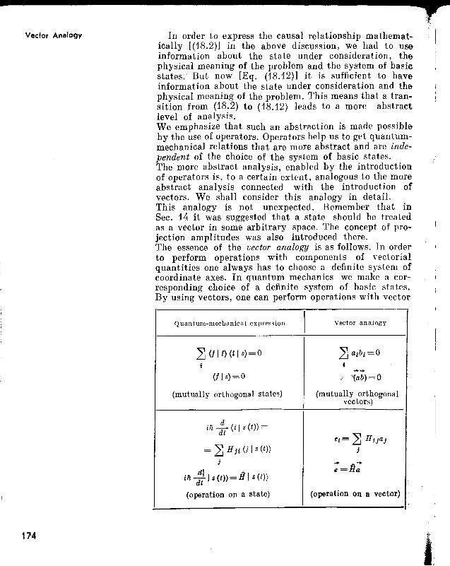
a

Vector Analogy

114

In order to express the causal relationship mathemat­ically [(18.2)] in the above discussion, we had to useinformation about the state under consideration, thephysical meaning of the problem and the system of basicstates. But now [Eq. (18.12)] it is sufficient to haveinformation about the state under consideration and thephysical meaning of the problem. This means that a tran­sition from (18.2) to (18.12) leads to a more abstractlevel of analysis.We emphasize that such an abstraction is made possibleby the use of operators. Operators help us to get quantum­mechanical relations that are more abstract and are inde­pendent of the choice of the system of basic states.The more abstract analysis, enabled by the introductionof operators is, to a certain extent, analogous to the moreabstract analysis connected with the introduction ofvectors. We shall consider this analogy in detail.This analogy is not unexpected. Remember that inSec. 14 it was suggested that a state should be treatedas a vector in some arbitrary space. The concept of pro­jection amplitudes was also introduced there.The essence of the vector analogy is as follows. In orderto perform operations with components of vectorialquantities one always has to choose a definite system ofcoordinate axes. In quantum mechanics we make a cor­responding choice of a definite system of basic states.By using vectors, one can perform operations with vector

Quanturn-mechanical expression I Vector analogy

~ (f I i) (i I s) = 0 ~ aibi=O

i f->->

(f J s)=O '(ab)=O

(mutually orthogonal states) (mutually orthogonalvectors)

in~ (i I s (t) =dt

ei= ~ Hijaj= ~ H ji (j I s (t» j

j -> ~->

dJ ~ e=Hai!i-ls(t»=HI s(t»

dt

(operation on a state) (operation on a vector)

crI

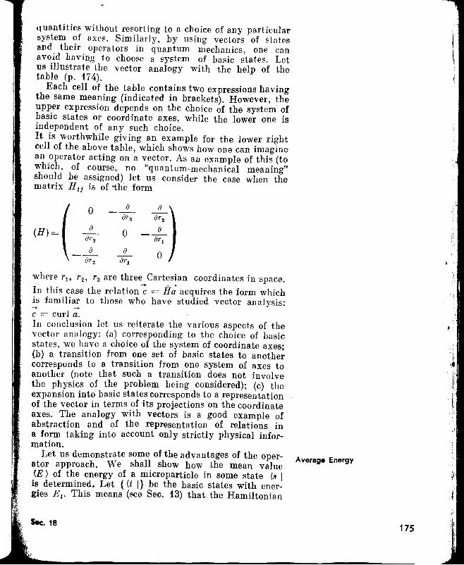
quantities without resorting to a choice of any particularsystem of axes. Similarly, by using vectors of statesand their operators in quantum mechanics, one canavoid having to choose a system of basic states. Letus illustrate the vector analogy with the help of thetable (p. 174).

Each cell of the table contains two expressions havingthe same meaning (indicated in brackets). However, theupper expression depends on the choice of the system ofbasic states or coordinate axes, while the lower one isindependent of any such choice.It is worthwhile giving an example for the lower rightcell of the above table, which shows how one can imaginean operator acting on a vector. As an example of this (towhich, of course, no "quantum-mechanical meaning"should be assigned) let us consider the case when thematrix Hij is of'tne form

(H)~( ~f)

,:,)f)r a

0 f)

f)r a - f)r1

f) f)0f)r 2 f)r1

I'

••

Average Energy

where r1 , r2 , r3 are three Cartesian coordinates in space.

In this case the relation ~ = iI; acquires the form whichis familiar to those who have studied vector analysis:...,. ...,.c = curl a.In conclusion let us reiterate the various aspects of thevector analogy: (a) corresponding to the choice of basicstates, we have a choice of the system of coordinate axes;(b) a transition from one set of basic states to a.nothercorresponds to a transition from one system of axes toanother (note that such a transition does not involvethe physics of the problem being considered); (c) theexpansion into basic states corresponds to a representationof the vector in terms of its projections on the coordinateaxes. The analogy with vectors is a good example ofabstraction and of the representation of relations ina form taking into account only strictly physical infor­mation.

Let us demonstrate some of the advantages of the oper­ator approach. We shall show how the mean value(E) of the energy of a microparticle in some state (3 Iis determined. Let {(i I} be the basic states with ener­gies E j • This means (see Sec. 13) that the Hamiltonian

175

p------------------.,..matrix is diagonal. Hence,

(j 1Ii Ii) = {jiJEft

or(jIHli) = (jli) E i • (18.13)

We expand the state (s I in terms of the system of basicstates {(i I~ : (s I = LJ (s Ii> (i I, and try to find the mean

value of tHe energy <1? > with the help of a formula ofthe type (12.3):

(E) = ~ I(sli) 12 E i • (18.14)i

By taking (9.33) into account, we rewrite (18.14) in theform(E) = 2}(sli}E i (i!s}=(slcp}, (18.15)

i

where

"

!cp) = ~ Ii} E i (ils).i

From (18.13) it follows that

H!i) = Ii) E i •

Substituting (18.17) in (18.16), we get

!cp) = ~ Hli}(ils}=Hls},i

(18.16)

(18.17)

after which we get the required result from (18.15):

(E> = (3 I iI I 3 >. (18.18)

Energy Operator (Hamiltonian)

176

It can be seen from (18.18) that mean value of the energyof a microparticle in the state (s I is expressed only throughthe operator iI. Basic states do not enter this relation.The convenience of the relation (18.18) is due to its inde­pendence from the choice of basic states, which allowsone to use freely any system of basic states when carryingout calculations. For example, suppose it is convenientto use the basic states {(m I}. In this case the operatorrelation (18.18) immediately acquire the correspondingform

(E) = 2] 2] (slm) (mIHln) (nls). (18.19)m n

It has been mentioned above that the Hamiltonianmatrix could be called the energy matrix (rememberthat the elements of the diagonalized Hamiltonian matrix

(18.21)

(18.12)

(18.18)

(18.20)

i

'.

Using (18.21) and taking into account that (il s) = ct,we can rewrite (18.2) in a form which, as can be easilyseen, is completely analogous in form to (18.12):

in ~ (i Is (t) = Ii (i Is (t». (18.22)

Correspondingly, (18.20) may be written in the form

H (i I f) = E (i I f). (18.23)

are essentially the possible values of the energy of theroicroparticle). The connection between the operator Iiand the Hamiltonian matrix as well as relation (18.18),expressing the average energy ofIa microparticle in termsof the operator H, justify the name energy operator givento it. In the literature the operator H is also called theHamiltonian.We write expressions derived above in which the Hamil­tonian of a microparticle is present (we emphasize theexceptional importance of these expressions):

in~ Is (t) = His (t),dt

(E) = (sIHls),HI!) = If) E..

In expression (18.20), (f I denotes some stationary stateand E is the energy in this state.Finally, we note that the Hamiltonian (as well as anyother operator) may act not only on the state Is), butalso en its amplitude (i Is), since we always have therepresentation [see (17.4)1

HCi(t) = 2J HiJC j (t).j

We now come to the main problem of this chapter, Le.that of imparting physical meaning to the mathematicalapparatus of linear operators in order to convert it intothe apparatus of quantum mechanics. In this sense theprevious section should be considered as a preliminarystep towards solving this problem.

The following two points must be noted when consider­ing the role of linear operators in quantum mechanics.Firstly, in quantum mechanics to every dynamic variable(spatial coordinate, energy, momentum, angular momen-

Section 19 Linear Operators inQuantum Mechanics

Role of Operators in QuantumMechanics

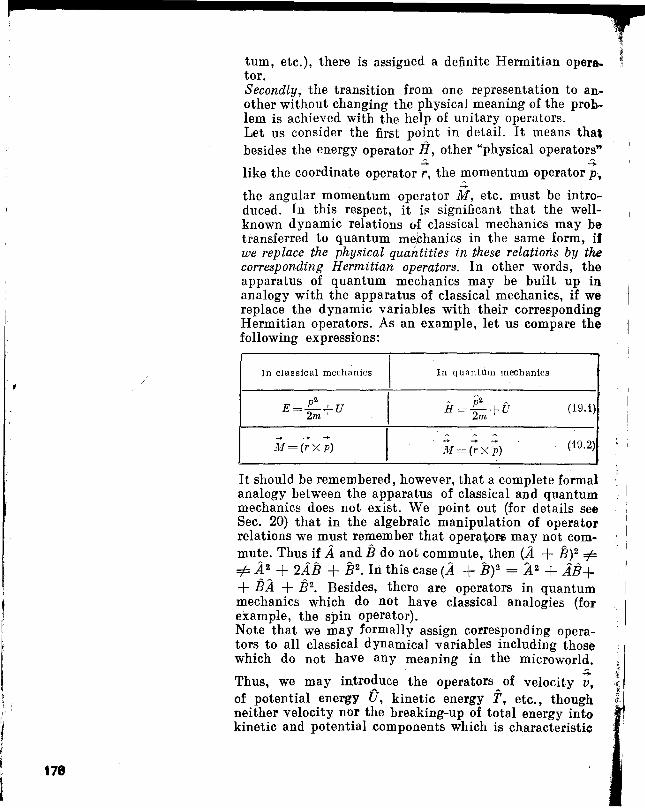
p---------------,-~

tum, etc.), there is assigned a definite Hermitian opera- .~

tor.Secondly, the transition from one representation to an.,.other without changing the physical meaning of the prolr­lem is achieved with the help of unitary operators.Let us consider the first point in detail. It means thatbesides the energy operator fl, other "physical operators"

like the coordinate operator;-' the ~omentum operator ~,the angular momentum operator if, etc. must be intro~duced. In this respect, it if' significant that the well­known dynamic relations vf classical mechanics may betransferred to quantum me.t.hanics in the same form, ifwe replace the physical quantities in these relations by thecorresponding Hermitian operators. In other words, theapparatus of quantum mechanics may be built up inanalogy with the apparatus of classical mechanics, if wereplace the dynamic variables with their correspondingHermitian operators. As an example, let us compare thefollowing expressions:

In classical mechanics I In quantum mechanics

p2

I~ p2 ~

(19.1)E= 2m+U H= 2m+U

- - - I~ ~ ~- - -M=(rx p) M=(rX p) (19.2)

It should be remembered, however, that a complete formalanalogy between the apparatus of classical and quantummechanics does not exist. We point out (for details seeSec. 20) that in the algebraic manipulation of operatorrelations we must remember that operators may not com-mute. Thus if ..4 and B do not commute, then (..4 + B)'1. =1==1=..4'1. + 2AB + jJ'1.. In this case (A + B)'1. = A2 + AB++ BA + B'1.. Besides, there are operators in quantummechanics which do not have classical analogies (forexample, the spin operator).Note that we may formally assign corresponding opera­tors to all classical dynamical variables including thosewhich do not have any meaning in the microworld.

Thus, we may introduce the operators of velocity;,of potential energy 0, kinetic energy T, etc., thoughneither velocity nQr the breaking-up of total energy intokinetic and potential components which is characteristic

178

for classical mechanics, have any meaning for micropar­ticles.

Let us consider the question: In exactly what way canwe compare a physical quantity with a Hermitian opera­tor? In other words, what is the meaning of the word"compare" here? The following two basic postulates pro­vide an answer to this question.Postulate 1. If the operator L is compared with aphys­ical quantity l, it means that the eigenvalues A of theoperator are identified with the values of the physicalquantity under consideration obtained by measurement.Postulate 2. If operator L is compared Fith a physicalquantity l, it means that the eigenfunctions 'Iv,. (a) ofthe operator are identified with the eigenfunctions of thequantities from theA-set, expressed in a-representation.By the remarks nul.de in Sec. 15, this means that theeigenfunctions '¢1. (a) of the operator are identified withthe amplitudes of states {Ala >, often called the wavefunctions. ' . .Thus a study of the fundamental equation of the theoryof linear operators [see (17.13)]' '

..... j I

L (a){Ala) = A(Ala) (19.3)includes physical problems such as finding the spectrumof possible values A of a physical quantity l, and findingthe amplitudes of states {A I a> in which the correspond­ing values of A occur.When applied to the energy operator, (19.3) takes theform of (18.23). A study of equation (18.23) permits usto find the possible values of the energy.of a microparticleand the corresponding amplitUde values O'f the stationarystates.

The postulates formulated above "knit together" the-physical and mathematical aspects; they "load" the mathe­matical symbols and inferences with a definite physicalmeaning. We shall demonstrate this with a _number ofobservations.1. The eigenvalues of a Hermitian operator are real.From a physical point of view this means that the valuesof quantities obtained during measurements are real.2. The spectrum of the eigenvalues of a Hermitian opera­tor may be discrete or continuous. This corresponds toquantization or a continuous variation of the physicalquantities characterizing a microparticle.3. The eigenfunctions of a Hermitian operator satisfythe condition of orthonormalization. This mathematical'lact becomes the condition of orthonormalization of eigen­1unctions of physical quantities and, in particular, the

Basic Postulates

Mathematical Results and TheirPhysical Meaning I'

·t

p

t80

condition 01 orthogonality 01 basic states 01 a micro-Tparticle. In other words, the mathematical result' (17.16) !

is converted into physical relations (15.13) and (10.8),while the mathematical result (17.17) is converted intothe physical relation (15.14).4. The system of eigenfunctions of a Hermitian operatoris a closed (complete) one. From a physical point ofview, this means that it is possible to expand any ampli­tude in terms of amplitudes which are eigenfunctions ofa physical quantity, Le. in terms of basic amplitudes. Inother words, the completeness of a system of eigenfunc­tions of a Hermitian operator is converted into the phys­ical principle of superposition of states.5. The eigenvalues of a Hermitian operator may be degen­erate. Physically this means that one value of a quan­tity may correspond to several different states.6. The mather¥tical result (17.28) for the eigenfunctionsof operators corresponds to the physical result (9.33)for amplitudes of states.7. Unitary transformations corresponding to the transi­tion from one representation to another, physically cor­respond to a transition from one complete set of quanti­ties to another and, in particular, from one system ofbasic states of a. microparticle to another.8. ,The existence of a common complete system of eigen­functions means that the operators commute. This mathe­matical fact corresponds to the possibility of 8imulta­noous measurement of the corresponding physical values.Note ,that the impossibility of the simultaneous measure­~nt of such physical quantities as the coordinate andmomentum of a microparticle means that the operators ofcoordinate and momentum do not commute.9,. The mathematical fact of commutativity of the Hamil-tonian it and the operator £ meanstl¥lt. physically thequantity l corresponding to the operat~r L is an integralof'motion. In other words, the condition

IH, L] = 0

from the physical point of view is the law of conservationof the quantity 1.The last remark will be rigorously proved below. Here,we shall just mention Some ideas of a qualitative naturefor this purpose. If operators iI and L commute, thequantities E and 1 can be simultaneously measured sincethere are states in which both these quantities have defi­nite values. A state in which energy has a definite value;is stationary, Le. has an infinitely long "life" time. But

II........•.'.·.·.~-5;'

t ..

this means that the quantity 1 must also be conservedfor an infinitely long time, just like any other physicalquantity for which the given state is an eigenfunction.

If the quantity 1 is measured in a state describedby the amplitude (AI ex), then, according to basic postu­lates, the measured value will be A. We assume now thatthe quantity 1 is measured not in its eigenstate, but insome "other" state, for example, in the state describedby the amplitude <1>s (ex) = (3 I ex). In this case the resultof a single measurement cannot be predicted unambiguous­ly; probabilistic predictions enter into the picture now,thus permitting an estimation of the mean value (A)from a relatively large number of measurements (in thisconnection see Sec. 12). We shall show how to computethe mean value (A) in the state (s I, if we know the Hermi-tian operator L corresponding to the quantity l. Notethat in the particular case when energy is used in placeof the quantity l, this problem was considered in Sec. 18,where the following result was obtained:

Mean Value of a Quantity

(we assume for definiteness in this case that the variable exwhich characterizes the representation varies contin­uously). Let us prove this.We expand the amplitudes <1>s (ex) and <1>:(ex) in termsof eigenfunctions '¢n (ex) = (An I ex) of the operator £ (weassume that the spectrum of the operator L is discrete):

<E) = (3 I Ii Is).

In the general case, (18.18) takes the form

(A) = J<1>: (ex) L (ex) <1>s (ex) dex

(18.18)

(19.4)

<1>s (ex) = 2l (siAn) '¢n (ex),n

<D: (ex) = ~ (sIAm)* '¢~ (ex).m

Substituting these superpositions in (19.4) and using(19.3) and (17.16), we get

J<1>: (ex) L (ex) <Ds (ex) dex

= ~ ~ (sIAn)(SIAm)* J'!'~ (ex) L (ex) 'iJn (ex) dexn m

. ~ ~ (sIAn)(sIAm)* An J'¢~ (ex) '!'n (ex) dexn m

Sec. 19 181

i'

'.

n m n

By (12.3), the last sum is equal to {A >, Q.E.D.The result (19.4) is very important. In fact this one resultis sufficient to demonstrate the usefulness of the applica­tion of operators in quantum mechanics.In analogy with (18.18), the result (19.4) can be writtenin a more abstract form which avoids a choice of repre­sentation:

<A> = {s I £ Is>. (19.5)

The Variation of the Mean Value Using (19.5) and assuming at the outset that the op-of a Quantity with Time erator L is independent of time, let us write

d d ~

dt (P.) = dt (s (t) IL Is (t»

=( :t (s(t)I) lils(t»+<s(t)ILI (:t Is(t»). (19.6)

Further, we turn to (18.12) and transform it into the formd A- in at (s (t) I = (s (t) IH+,

or, taking into account the hermiticity of the Hamil­tonian,

d ~- in_ tlk (s (t) I = (s (t) ,H. (19.7)

Substituting (18.12) and (19.7) into (19.6), we getd i A~ ~ ~

dt (A) = h (s (t)IHL -LHls (t),

ord i ~ ~

;:rt(A)=n(sl[H, L]18). (19.8)

If the quantity 1 is an integral of motion, ft(A) = O.

It follows from (19.8) that the above-mentioned condi­tion [Ii, L1 = 0 is a condition for the conservation ofhe quantity l. ~

We introduce a new operator i, defining it by the relation~ d

(s ILl s) = dt (A). (19.9)

Comparing (19.9) with (19.8), we conclude that in the

case when L is independent of time, the operator L

182

l~~f :1>9 _f",~*., L =-;:; [H, L].

If L varies with time, we get instead of (19.10)

(19.Hl)

(19.11)

The physical meaning of any result is obviously inde- Unitary Invariance of Physicalpendent of the choice of a representation. In other words, Resultsthe physical meaning of a result should not change upona transition from one representation to another. Sincethese transitions are accomplished by means of unitarytransformations, it means that physical results must enterthe mathematical apparatus as unitary invariants.Thus, the requirement of unitary invariance of corre­sponding results may serve as an additional criterion of thecorrectness of the basic postulates formulated above andthe consequences that follow from them. In this connec­tion, we first mention the fact of unitary invariance ofthe property of hermiticity of an operator mentionedin Sec. 17, and also the unitary invariance of the spectrum()f eigenvalues of a Hermitian operator. I t is easy to seethat the commutator [fI, Ll is also a unitary invariantand, consequently, the condition of conservation of anyphysical quantity is, as expected, independent of thechoice of a representation. We mention further that uni-

tary invariance of the relation J'IJ'~'IJ'm dx now indicatesthe i Ildependence from the choice of representation of the-condition of orthonormalization of eigenfunctions of aphysical quantity. Finally, unitary invariance of the

-expression ) <D* r(x) L (x) <D (x) dx indicates the inde­

pendence from the choice of representation of the meanvalues of physical quantities.

Note that the result (19.4) could have been obtained unambiguous­ly from the requirement of the unitary invariance of the quantity<1..) using the expression (18.18) obtained for a special case. Indeed,from the requirement of unitary invariance it follows that (I..)must be represented by an expression of the type

) <Xl. (x) in (x) <D (X) dx,

and a comparison with the particular result (i8.i8) indicates thatin this case n must be put equal te t.

Sec. 19 183

Section 20

rf

Operators of Coordinate andMomentum

18A

The Quantum-MechanicalApparatus in CoordinateRepresentation

A further treatment of the apparatus of quantum mechan­ics requires a knowledge of the definite form of the oper­ators of various physical quantities. For this it is essen­tial to choose a definite representation. Let us choose thecoordinate representation for this purpose.Note the importance of finding the form of the two basic"physical operators", the coordinate and the momentumof a microparticle. Knowing these operators, we mayobtain the energy operator [see (19.1)] and the angularmomentum operator [see (19.2)1.

For simplicity we shall consider one-dimensional motionalong the xi-axis (the result so obtained can be easily gen­eralized to a. three-dimensional case). Taking into accountthe remarks made in Sec. 17 about the form of Hermitianoperator in its eigen representation [see (17.26)], we con­clude that the operator of a coordinate in the coordinaterepresentation is the coordinate itself:x (x) = x. (20.1}

This result can be generalized to any coordinate function:

V (x) = lZ{x). (20.2)Let us now try to find the form of the momentum opera­tor. First we shall prove the following theorem. Supposean operator {j somehow transforms a coordinate. If the·Hamiltonian Ii remains invariant under this transfor­mation, the operators lJ and H commute. Proof: LetOx = x'; we act on H (x) 1J' (aJ) with the operator {)to • get on (x) 1J' (:») = Ii (x') 1J' (x') = iJ. (x) 1J' (x') == H (x) VIp (x), which proves the theo,rem.Suppose the operator 0 is the operator of infinitesimaltranslation along the x-axis: 61J' (x) = 'I\J (x + dx). Mak­ing use of the smallness of the translation, we write

¢ (X+dX)=[1+dX ~J ¢(x)

Thus~ d0= 1+dxa;-

Proceeding from the properties of homogeneity of space.we conclude that an operation by {) must leave the Hamil­tonian of a microparticle invariant. Hence, accordingto the theorem proved above, we obtain [6, H] = 0

1..... >.'....•. '.,

or L~, h] = O. Bm it was shown above in Sec. 19 thata commutation with the Hamiltonian expresses the lawof conservation of a physical quantity. This means thatdld:JJ is the operator of Some physical quantity which isconserved. We know that momentum is a quantity whoseconservation is a consequence of the homogeneity ofspace (see Sec. 1). Consequently, the operator dldx mustcoincide with the momentum operator of a microparticleup to some constant factor:II ...

(fX= 'VPx' (20.3)

The factor y is determined from a consideration of the lim­iting transition from quantum" mechanics to classicalmechanics (see Appendix B). It can be shown that y == i/n. Thus the operator of the x-component of a micro­particle momentuih in the coordinate representation hasthe form

A • dPx = - ~h dZ' (20.4)

The results (20.1) and (20.4) can be easily generalizedto a three-dimensional case:

r== r, (20.5)~

p== -in'V. (20.6)

Using (20.4), we can write an equation for the eigen- Eigenfunctions of Momentumfunctions of the x-component of the momentum:

-in :x ljJpx (x) = PX'¢Px (x). (20.7)

It can be easily seen that (20.7) can be solved for anyvalues of the parameter P.t. Consequently, the momentumof a micro particle is not quantized (the spectrum of theeigenvalues of the momentum is continuous).From equation (20.7) it follows that the eigenfunctionsof operator Px have the form of plane waves:

\lJPIll (x) = A exp (iP xx/1i); (20.8)

To determine the factor A, we make use of the conditionof orthonormalization (17.17):

JljJ* p; (x) '¢Px (x) dx = <') (Px- p;).

SUbstituting (20. 8) into this equation, we find

4'12.Jexp [- ix (p:- Px)/1i} dx = <') (Px- p~).

'.f ,1

"l,

·f',

185

Schrodinger Equation

Further, taking into account (15.17), we obtain

i exp fix (Px- p;)/n] dx = 2:rtM (Px- p;).

Comparing the last two equations, we get A2 == (2nnt1.Consequently,

'/Jp (x) = (2nn)-1/2 exp(ipxxlh). (20.9)x

A generalization for the three-dimensional case gives

'/J-p (;:) = (2nn):o:3/2 exp (ipr!1i). ;(20.10)

Note that the eigenfunction of the momentum (20.10)coincides with the wave function (15.15) derived inSec. 15 tor a freely moving microparticle.

Let us consider the equation (18.23) for eigenfunctionsof a ,Hamiltonian:. /'

Hrp (x)=Erp (x). ( ~20.11)~E E

Using (19.1) for the Hamiltonian of a micro particlemoving in an external field with potential U (:Il), andtaking into aC(jount (20.2) and (20.4), we get~. h2 d2

HI(X) = - 2m dx2 +U (x). (20.12)

Substituting (20.12) into (20. 11), we get

h2 d2 e- 2m dx2 rpg (X) + [U (X) -; 1rpE (X) = O. (20.13)

This is the one-di mensional SchriJdinger equ,ation. Gener­alizing it for the three-dimensional case, we write

(20.14)

Knowing the functions cp g (:Il), we may write the expres­sions for amplitudes of stationary states 'YE (:Il, t), sincethe time dependence in this case has the universal formdiscussed in Sec. 13. Using (13.4) and taking into accountthe fact that!

'Yg (x, t)= (E I X, t}=(x, t I E}·=C~ (t), (20.15)

1'86

we get

'Yg (x, t)=rpB (x) exp (-iEt/1i). (20.16)

I t can be easily seen that the functions 'Y~ (:Il, t) arethe solutions of equation (18.22), where the Hamiltonian

(20.12) has been used in place of fl. In this case, the equa­tion has the form

(20.17)

The operator of the square of angular momentum is givenby the expression

It is also called the Schrodinger equation More precisely,equation (20.13) is called the time-independent Schrodingerequation and the equation (20.17) is called the time­dependent Schrodinger equation.Schrodinger's contribution was that he guessed (yes,guessed!) how to write the Hamiltonian of a micro particlein the form (20.12). It is true that in our discussions (20.12)does not appear unexpectedly, it appears here as a conse­quence of results (19.1), (20.2) and (20.4). It should,however, be l'emembered that (19.1) has not been derivedhere, in fact it was.postulated (more precisely, an analogybetween classical and quantum-mechanical relations waspostulated). When Schrodinger proposed his famousequation, this analogy was not yet apparent. Moreover,the result (20.12) itself, as we shall see below, servedas the basis for this analogy. (For establishing the rela­tion (20.17), we may make use of the transition fromquantum to classical mechanics-see Appendix B.), By using (19.2) and (20.4) we can easily get the expres­~ions for the operators of projections of the angular mo­mentum:~ . a a) 'IM = -in(y --Z-. I

x 'Uz dy' I~ (d a )M = - in z - - x - ~

• Y ax az' I

M' (a a) J= - ili x - - y - .z ay ax

M'=M~+M~+M~.

(20.18)

(20.19)

Operators of the AngularMomentum Projections and theSquare of Angular Momentum

'.

While considering the angular momentum operators, it isconvenient to use spherical coordinates r, a, <p insteadof Cartesian coordinates x, y, z: '

:t= r sin acos <p, }Y.= r sin asin <p,

Z = rcos a.(20.20)

187

(20.21)

,Using (20.20), we represent the derivative a~ '¢ informa iJl/J ax al/J all al/J az

acp 'IjJ = ax aqJ +ay aqJ +az aqJ

alp . e . al/J. e= -a;; rsm smtp+ayrsm costp

=(x3-- y 3-).h.ay "ax 'f'

From this, with the help of (20.18), we get

iII = -in3-z aqJ •

In a similar way from the derivative a .1, we findae 'f'

(20.22)

Commutation Relations

M M~ n +" (a e a )x + i y = e- 1(j) + as+ i cot acp

from which, with the h«t!If of (20.19), we get~ L'· 1 a2 1 a (. a )-1

M2 = - n2 sin2e acp2 + sin e as sm eas J. (20.23)

These relations form the commutation rules for theoperators of coordinate, momentum and angular momen­tum of a microparticle. Denoting the Cartesian compo­nents of these operators by subscripts i, j, k, we canwrite these commutation rules (it will be shown lateron how they may be derived):

(20.24)

(20.25)

(20.26)

(20.27)

(20.28)

(20.29)

(20.30)

[ril rj] =0.A A

[Pi,Pj]=O,

LPil rj] = - i'h6ij ,A ,.. ~ a ".,~

[Pi> t (r)] = - in -a t (r),rt

[.111 il ;j] = in ~ eijk;k,II.

[M i , Pj] = in ~ eijkPk,II.

~ ~ '\.' ~

[Mil MJl = in L.J eij.kMk·II.

Here etJk is a unit antisymmetric tensor of the 3rd rank,e123 = e 231 = e312 = 1, e132 = e321 = e213 = -1, and theremaining 21 components of thi s tensor are equal to zero(in these components at least twolsubscripts have thesame value). It can be easily seen; that in summationswith respect to k not more than one term is present.

188'

ln the coordinate representation ri = ri; therefore, the..esult (20.24) is obvious. It means that all three coordi­nates of a microparticle can be measured simultaneously{as was mentioned in Sec. 3, they OCcur in the same com­iplete set of quantities).Prom (20.4), we write

[p~. p.].1._ -n2 (_82 82_).1.II J '" - 8ri 8rj 8rj 8ri "'.

Since the value of the mixed derivative is independent of1;he order in which the differentiation is carried out, itfollows that [Pi> Pi] = O. This result means that all the1;hree components of momentum can be measured simul­otaneously (they belong to the same complete set of quan­otities)."The result (20.2&) IS derived in the following way:

:{Pi, ij] '\jJ= -in {8~i (rj'\jJ)-r j 8~i '\jJ}

.f, 8rj .1. 'f,~= - Ut 8ri '" = - lnUij'\jJ.

It means that components of momentum and coordinatewhich have different subscripts can be simultaneouslymeasured, while components with like subscripts areunmeasurable, in complete accord with the uncertainty,relations for coordinate and momentum of a micropar­ticle described in Sec. 3. The result (20.26) also indicatesthat the three components of coordinate and the threeeomponents of momentum enter in different completesets of quantities.The result (20.27) is a generalization of (20.26). In fact,

~ ~ 'n { 8 (/.1,) / 8 .I'} 'n 8/ .1.[Pi' f] '\jJ= -l ar; '" - 8ri '" = -l 8r; "'.

Results (20.28)-(20.30) can be obtained from (19.2) byusing the preceding commutation relations (see Ap­pendix C).Results (20.28) and (20.29) mean that components of theangular momentum and coordinate (angular momentumand momentum) with like subscripts can be measuredsimultaneously, while those with different subscriptscannot be measured simultaneously. These results alsomean that projections of the angular momentum cannotbelong to complete sets which include coordinates or themomentum components.

. The result (20.30) means that different components of an­I· gular momentum don't have a common closed system ofI~. eigenfunctions and cannot appear in the same complete set

I.~··..!:_~._2_0_ 189

.'

'.

$ r" I

of quantities. Considering the examples discussed earlier,we can conclude that different components of angularmomentum cannot be measured simultaneously. Thisconclusion is correct, but it should be slightly improvedon the basis of the example of the components of angularmomentum. As a matter of fact, there is one case whenall the three components of angular momentum can besimultaneously measured-this is the particular case whenall of them are equal to zero. This case, however, does notessentially change anything since, as has been remarkedin Sec. 17, the presence of one common eigenfunction isin no way connected with the commutation of operators.By using relations (20.19) and (20.30), we can establishone more rule for commutation (see Appendix D):

[M2, Mi ] = 0 (20.31)

This means that we must include the square of the angu­lar momentum and anyone of the projections of the angu­lar momentum in the same complete set of quantities.

Note that the simultaneous measurability of all the componentsof momentum and the impossibility of similar measurement forthe angular momentum components have a very simple explana­tion. The fact is that the parallel translations associated with themomentum operator are commutative, while the rotations asso­ciated with the angular momentum operator are noncommutative.It is immaterial whether we move first along the x-axis and thenalong the y-axis, or in the reverse order.However, the sequence of rotations is certainly not immaterial.Take, for example, a point on the I-axis and make two successiverotations through 90o-in one case first around the x-axis and thenaround the z-axis, in the other case first around the z-axis andthen around the x-axis. It can be easily seen that the final positionsof the point are different in these two cases.

The Inversion Operator; Parity

190

The inversion operator P is defined in the following:way:

P'ljJ (;, t) = P'ljJ ( - -;,t), (20.32)

where P is a constant. By applying the i"ersion operatortwice, we obviously return to the initial function 'ljJ (;, t).It follows from this that p2 = 1, Le. .

P = ±1. (20.33)'

The quantity P is called the spatial parity. If P = 1,_

and consequently, P'ljJ (;, t) = 'tV (-;, t), the micropar~ticle is said to possess even parity. If, however, P = -1'

191

* It must be noted that in some processes involving elementaryparticles, the symmetry of "usual wOJ;'ld" and "mirror world" isViolated. It was shown by Wu in 1957 that in experiments on thefl-decay of nuclei, spatial parity is not conserved. This resultwas predicted in 1956 by Lee and Yang.

and, consequently, P'IjJ~, t) = -'IjJ (--;., t), the micro­particle is said to pos'>ess odd parity.Suppose [P, ill = O. In this case, according to (19.10),the parity is a conservahle quantity. If at the initialmoment of time the microparticle was, for example, ina state with even parity, it must have the same parityat subsequent moments of time (which, of course, imposescertain restrictions on the possible changes in the stateof the microparticle).It was mentioned in Sec. 1 that the laws of conservationof energy, momentum and angular momentum are theresults of definite propertills of the symmetry of space andtime. The law of conservation of parity is no exception tothis. It is a consequence of the symmetry with respectto inversion operation, which, as can be easily seen,reduces to a combipation of the operation of rotation andreflection fin fact, the operation (x, y, z) -+ (-x, _y,-z) consists of rotation through 180°, say, arround thez-axis, and reflection in the plane perpendicular to thez-axisJ. Taking into account that the conservation ofangular momentum is linked with rotational symmetry,we conclude: the conservation of spatial parity is asso­ciated with the fact that physical processes take placeidentically in the "usual world" and the "mirror world".*

Let us write the equation for the eigenfunctions of the Eigenvalues and Eigenfuncfionsoperator if z' defined by (20.21): of the Operators Mz and M2

-iho~'IjJ=Mz'IjJ. (20.34)

The solutions of this equation are of the form ..

..p (cp) = A exp (iM zcp/n)~ ". (20.35)-The function .p is periodic: 'IjJ (cp + 2n) = 'IjJ (cp). Consequently, '.M z = Jim, m = 0, ±1, +2, . . . . (20.36)The reader is already familiar with this results: the pro­jection of angular momentum is quantized; it assumesvalues differing by multiples of Planck's constant (seeSec. 2). The factor A in (20.35) is determin.ed from the

2n

, normalization condition ~ 'ljJi:.'ljJmdcp = 1. It is easy too

TWe now turn to the operator M2. Using (20.23), we write

>

see that A = (2n)-1/2. Thus

'i'm (cp) = (2n)-1/2 exp (imcp).

1.2 [ 1 82

'IjJ + 1 a ( . e 8'IjJ ) ] _ M2'h- n sin2 e 8<p2 sin e as sm as - 'Y'

(20.37)

(20.38)

? i

'\

This equation is known in mathematics as the equationfor spherical junctions. It has bounded solutions underthe condition that

M2 = lZ 2l (l + 1), l = 0, 1, 2, .... (20.39)

(20.40)

Assuming that the condition (20.39) is satisfied, we writethe solutions of (20.38) in the form of spherical harmonics:

'11 = .. /" (l-I mJ)! (2l+1) pi m I (cos 8) eimQJ-1m V (l+lm/)14n I ,

where m = 0, ±1, •.. , ±l. Taking (20.31) into consid­eration, we conclude that the eigenfunctions of Mt

and M2 are common. Hence, m should be treated as a mag­netic quantum number corresponding to the projectionof the angular momentum of the z-axis. It assumes 2l + 1values (from -l to l). The functions p!ml(cos 8) appear­ing in (20.40) are essentially the associated Legendrefunctions. We remind the reader that

m dmPI (x) = (1- x2)m/2 dxm PI (x)

where PI (x) are Legendre polynomials*: I

1 dl /PI(x)= 2111 dx l [(x2 -1)1].

(20.41)

(20.42)

(20.43)

192

The spherical functions '\JIm (8, cp) are orthonormalized:

2lt It

Jj '\Jim (8, cp) '\JI'm' (8, cp) sin 8 d8 dcp = 611'~~"o 0

If the result (20.36) is known, we can derive the result(20.39) by assuming that

M2 = 3 (M;) = 3/is (m2).

• Legendre polynomials and associated functions are consideredin Appendix D.

I\

The Relations of ClassicalMechanics in Operator Form

I:tIf

I

The mean value (m2 ) is determined by the expressionI 1

"" m2

"" m2

1(m2)= .L.J 21+1 =2 .L.J 21+1 =3 1(1+1).

m=-I m=O

This leads directly to (20.39).It follows from (20.18) that the inversion operators Parity and Angular Momentum

commute with operators of any projection of the angularmomentum. Moreover, the inversion operators and theoperators of the square of the angular momentum com-mute:

[P,Mi]=O, [P,M2]=0. (20.44).

This mean that the operators P and Mi have a commoncomplete system of eigenfunctions. The same applies tothe operators P and,M2. From this it follows in particu­lar that a state with a definite orbital quantum number 1must also be characterized by a definite spatial parity.In spherical coordinates the inversion is of the formr--+r, 8--+n-8, cp--+ljJ+n. (20.45)

Using (20.40)-(20.42) we find that for such a transforma­tion the function 'ljJ/m (8, cp) is multiplied by (_1)1:

I "'\JIm --+ (-1) 'ljJ/m' (20.46)

It follows hence that states with even 1have an even paritywhile the states with odd 1 have an odd parity.It is appropriate here to recall that the example given inSec. 3 for the complete set of quantities describing thestate of a photon includes M2, M z and P [see (3.7b)1.Note that the parity and the angular momentum occurin the same complete set of quantities. Formally, this isa consequence of relations (20.44). However, one canstart from considerations based on direct physical intui­tion. In fact, the obvious "affinity" between the parityand the angular momentum is connected with the above­mentioned fact that the inversion operation includes rota­tion in addition to reflection. The order in which theseoperations are carried out is immaterial; rotation canfollow reflection or, the other way round, it can precedereflection.

So far, we have several times used the fact that theapparatus of quantum mechanics is based on the well­known equations of classical mechanics written, however,in operator form. This fact is so important that it is ap-propriate to return to it once again.We have mentioned above the brilliant guess by Schrodin­gel', who proposed the expression (20.12) for the Hamilto-

'.

s.c. 20

-.

193

194

nian of a microparticle. If we use this guess and the funda';"mental result (19.10), we can easily see that the equations;.of classical mechanics can be actually transferred to quan- .ttum mechanics by replacing the physical quantities by the'corresponding Hermitian operators. Substituting the oper­ator L = x in (19.10), and using the expression (20.12)for the operator iI, we get

;; = Px1m. (20.47)

This is the well-known classical result: the velocity isequal to momentum divided by mass. In quantum-mechan­ical interpretation this result means that the velocityoperator is equal to the momentum operator divided bythe mass. Further, we substitute the operator L = p~

in (19.10). Using the expression (20.12) for ii as before,we get:' dP:r.= -lh" U (x). (20.48)

It can be easily seen that this is just Newton's second lawof motion, written in operator form. ~ ,. .Remember, that the operators of the type x and Px areintroduced in accordance with the definition (19.9). Hence,it follows that the results (20.47) and (20.48) indicatethe validity of the classical relations for the mean valuesof physical quantities:d ~

7ft (x) = (s IP~ I s)1 m, (20.47a)

d ddt (Px) = - dx U (x). (20.48a)

Ehrenfest was the first to point out this and hence rela­tions of the type (20.47a) or (20.48a) a~lled Ehren/esttheorems. In short, Ehrenfest's theorems lstate that clas­sical relations for physical quantities al.re transformedin quantum mechanics into relations for mean values ofphysical quantities.It was noted in Sec. 19 that the mathematical analogybetween classical mechanics and quantum mechanics con­sidered here requires a certain amount of caution sinceoperators don't always commute with each other. Thisleads to the conclusion that the information containedin the classical relations is insufficient for building up thequantum-mechanical apparatus. It is necessary to haveadditional information about the properties of commuta­tion of the operators under consideration. In other words,

the classical relations must be supplemented by the com­mutation relations of the type (20.26)-(20.30).Thus, it is the commutation relations which carry thespecific information essential to the apparatus of quantummechanics. In this connection, we note that the right­hand sides of the commutation relations contain the speci­fically quantum-mechanical constant, i.e. the Planck'sconstant.

Section21 Applications of theSchrodinger Equation

I

We shall mention three types of problems involving thesolution of the Schrodinger equation.First type of problems. We consider the motion of a micro­particle in a limiJ;·ed region of space or, in other words,in a potential well (for example, the motion of an electronin an atom). Such a motion is called finite and the micro­particle is said to be in a bound state. In this case thetime-independent Schrodinger equation is used [see (20.13)or (20.14)1. By solving the Schrodinger equation undercertain boundary conditions imposed on the wave func­tion and its first derivative*, the spectrum of the valuesof the energy of the microparticles and the wave functionsof the stationary states can be found.Second type of problems. The infinite motion (motion un­bounded in space) of a microparticle in an external fieldis considered. For example, the microparticle passesthrough a potential barrier (we recall the tunnelingeffect mentioned in Sec. 4) or is scattered by some energycentre. Since the motion is infinite, the energy spectrumof the microparticle is continuous. By solving the time­independent Schrodinger equation, we can find the formof the wave fun-etions of the microparticle far from thescattering centre (or barrier) from which, for example, theprobability of scattering at a certain angle (or the prob­ability of tunneling through the barrier as well as of reflec­tion from it) can be calculated.Third type of problems. In the two types of problems indi­cated above, we spoke of the stationary states of a micro­particle. For those the time-independent Schrodingerequation was used. The third type of problems involvesa change in the state of a microparticle with time, and forthis the time-dependent Schrodinger equation is used [see

* The boundary conditions are considered below during a dis­cussion on specific problems.

Sec. 21

Some Characteristic Problems iBQuantum Mechanics

195

••

A Particle in a One-DimensionalPotential Well with Infinitely Hign"Walls"

(20.17)1. By solving this problem we can fmd the prob­ability of any quantum transition taking place underthe influence of a given external force.Examples of problems of first two types are given in thissection and in Sec. 24. The third type of problems can befound in Sec. 25. Naturally, we shall limit ourselves tojust a few typical examples. But it should be mentionedhere that the applied aspects of quantum mechanics are,reflected quite comprehensively in the existing literature '(in this connection, we recommend [34, 35] which givespecially selected quantum-mechanical problems).

Such a well is described by a potential U of the form

{

OO' x<O,U (x) = 0, O-<x-<a, (21.1)

00, x>a.

The parameter a is the width of the well. The energy ismeasured from the bottom of the well. Within the limitsof the well (0 -< x -< a), the Schrodinger equation (20.13)is of the form

At the boundaries of the well (for x = 0 and x = a)the continuous wave function cp vanishes, since the infi­nitely high "walls" make it impossible for the particle to befound beyond the limits of the well*. Thus in this casethe boundary conditions are of the form

where

k~ = 2mEln2.

cp (0) = cp (a) = O.

We can write the general solutiontion (21.2) as follows:

cp (x) = A sin (kx) + B cos (kx).

Since cp (0) = 0, it follows that

cp (x) = A sin (kx).

(21.2)

(21.3)

(21.4)

ofl.rential equa-

(21.5)

B = O. Thus,

(21.6)

From the condition cp (a) = 0, we conclude that

ka = nn, where n is ail integer. (21.7)

196

* In the case of "walls" having a finite height, this possibility,as will be shown helow, is not excluded.

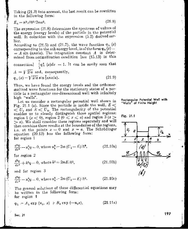
Taking (2'1.3) into account, the last result can be rewrittenin the following form:

En = n2J[,2/t2 /2ma2. (21.8)

The expression (21.8) determines the spectrum of values ofthe energy (energy levels) of the particle in the potentialwell. It coincides with the expression (5.2) derived ear­lier.According to (21.5) and (21.7), the wave function CPn (x)corresponding to the nth energy level, is of the form CPn (x) == A sin (Jtnx/a). The integration constant A is deter­mined from normalization condition [see (15.13) in this

a

connection] ScP~ (x)dx = 1. It can be easily seen thato

A = V2/a and, consequently,

CPn (x) = V2/a sin (Jt~x/a). (21.9)

Thus, we have found the energy levels and the orthonor­malized wave functions for the stationary states of a par­ticle in a rectangular one-dimensional well with infinitelyhigh "walls".

Let us consider a rectangular potential well shown inFig. 21.1 (a). Since the particle is inside the well, E << VI and E < V 2' The rectangularity of the potentialenables us to clearly distinguish three spatial regions:region 1 (x < 0), region 2 (0 <. x <. a) and region 3 (x >> a). We shall consider these regions separately and willthen combine these results at the boundaries of the regions,Le. at the points x = ° and x = a. The Schrodingerequation (20.13) has the following form:for region 1

~:; - x~CP = 0, where x~ = 2m (V 1 - E)/ltl,

for region 2d2rpdx

2+k2cp=0, where k2=2mE/1t2,

and for region 3

d2rpdx

2-x~<p=O, wherex~=2m(V2-E)/1t2.

(21.10a)

(21.10b)

(21.10c)

Rectangular Potential Well with"Walls" of Finite Height

Fig. 21.1

V, E tJ~X

1 t' 2- a~

~ (

ftl)x

R{q,e,(I;

••

, ~,

The general solutions of these differential equations maybe written in the following form:for region 1

CPI = Al exp (Xl' x) + B I exp (-XiX), (21.11a)

Sec. 21 191

198

for region 2<P2 = A 2 exp (ikx) + B 2 exp (-ik:JJ), (21. 11 b)

for region 3

<P3 = A 3 exp (x 2x) + B3 exp (-x 2x). (21. 11c)

[Note that the solution of equation (21.10b) may bewritten in the form (21.11b) or (21.5).] The boundednessof the wave function requires that B t and A 3 be putequal to zero. Thus,

<Pi (x) = Ai exp (Xi x),

<P2 (x) = .12 exp (ikx) +B2 exp (- ikx), (21.12)

<Pa (x) = Baexp (- x2x).

The qualitative form of the functions CPt, CP3 and Re {CP2}is shown in Fig. 21.1 (b). The reader should pay attentionto the fact that in the case of a potential well with "walls"of finite height, there always exists a probability offinding the particle beyond the limits of the well; thisprobability decreases exponentially with the distancefrom the boundaries of the well.In order to find the four coeffIcients (AI, A 2 , B 2 , B 3 ),

we make use of the fact that both the function and its firstderivative must be continuous at the boundaries. Thecontinuity of the wave function is obvious, while the con­tinuity of the derivative can be easily shown. In orderto do so, let us integrate Schrodinger's equation (20.13)over a certain interval (a - ~, a + M containing thepotential jump. We get

a+1\.dcp A dcp 2m rdx (a +Ll) - a:; (a - M= fi2 J [U (x) - E] cP dx.

a-I\.

Since the functions under the integral sign are bounded,in the limit of ~ -+ 0 this integral vanishes. As a result

~ ~ /we get di (a + 0) = dx (a - 0), which w,.J)e proved.

Returning to our problem, we write the 1I0~dary condi­tions (conditions of 'piecing' together the solutions at theboundaries of the region):cpdO) = cpdO) , ICP2 (a) = CPa (a), Idrpl (0) = drp2 (0) ~ (21.13)dx dx' Idd~2 (a) = dd~3 (a).)

Substituting the expressions (21.12) in these equations, we

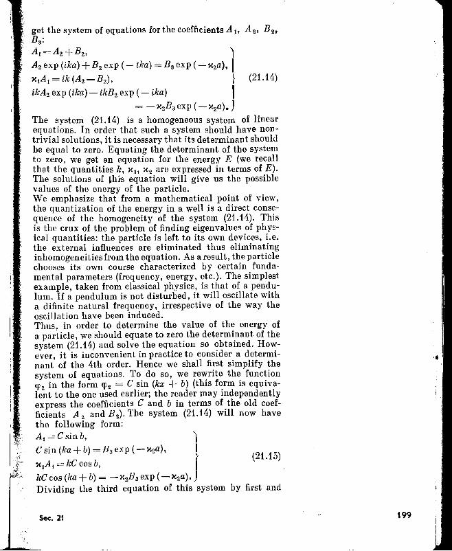
get the system of equations ior the coefficients A l' A 2' B 2J

B3 :

At =A2+B2, IA2exp (ika) +B 2exp ( - ika) = B 3 exp ( - X2a ), IXtA t =ik(A2-B2), ~ (21.14)

ikA2exp (ika) - ikB2exp ( - ika) I= - X2 B 3 exp ( - x2a). J

The system (21.14) is a homogeneous system of linearequations. In order that such a system should have non­trivial solutions, it is necessary that its determinant shouldbe equal to zero. Equating the determinant of the systemto zero, we get an equation for the energy E (we recallthat the quantities k, Xl' X 2 are expressed in terms of E).The solutions of this equation will give us the possiblevalues of the energy of the particle.We emphasize that from a mathematical point of view,the quantization of the energy in a well is a direct conse­quence of the homogeneity of the system (21.14). Thisis the crux of the problem of finding eigenvalues of phys­ical quantities: the particle is left to its own devices, Le.the external influences are eliminated thus eliminatinginhomogeneities from the equation. As a result, the particlechooses its own course characterized by certain funda­mental parameters (frequency, energy, etc.). The simplestexample, taken from classical physics, is that of a pendu­lum. If a pendulum is not disturbed, it will oscillate witha difinite natural frequency, irrespective of the way theoscillation have been induced.Thus, in order to determine the value of the energy ofa particle, we should equate to zero the determinant of thesystem (21.14) and solve the equation so obtained. How­ever, it is inconvenient in practice to consider a determi­nant of the 4th order. Hence we shall first simplify thesystem of equations. To do so, we rewrite the function(jJ2 in the form lp2 = C sin (kx + b) (this form is equiva­lent to the one used earlier; the reader may independentlyexpress the coefficients C and b in terms of the old coef­ficients A 2 and B 2)' The system (21.14) will now havethe following form:At = C sin b, ICsin(ka+b)=B3 exp(-x2a), Ir (21.15)xtA t = kC cos b, JkCcos (ka+b) = -x2B3 exp (-X2a).Dividing the third equation of this system by first and

Sec. 21 199

'.

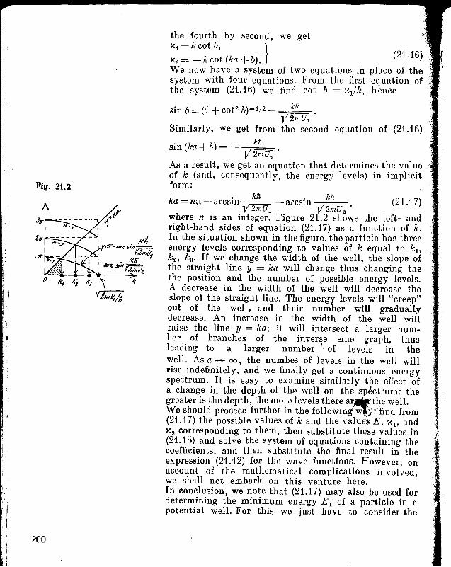
Fig. 21.2

200

the fourth by second, we getXl = kcot b, }

X2=-= -kcot(ka+b).We now have a system of two equations in place of thesystem with four equations. From the first equation ofthe system (21.16) we fwd cot b = xl/k, hence

kftsin b = (1 +cot2 b)-1/2 = --;-==-Y2mU l

Similarly, we get from the second equation of (21.16)

sin (ka+b) = -"IIkft •v 2mU2

As a result, we get an equation that determines the valueof k (and, consequently, the energy levels) in implicitform:

k . kft . kft (21 17)a = n:rr - arCSIn ,I - arcsIn ,1' .v 2mUl v 2mU2

where n is an integer. Figure 21.2 shows the left- andright-hand sides of equation (21.17) as a function of k.In the situation shown in the figure, the particle has threeenergy levels corresponding to values of k equal to kI ,

k 2 , k3 • If we change the width of the well, the slope ofthe straight line y = ka will change thus changing thethe position and the number of possible energy levels,A decrease in the width of the well will decrease theslope of the straight line. The energy levels will "creep"out of the well, and their number will graduallydecrease. An increase in the width of the well willraise the line y = ka; it will intersect a larger num­ber of branches of the inverse sine graph, thusleading to a larger number' of levels in thewell. As a -+ 00, the numbes of levels in the well willrise indefinitely, and we finally get a continuous energyspectrum. It is easy to examine similarly the effect ofa change in the depth of th~ well on the s~ctrum: thegreater is the depth, the mOlel levels therea~'t.he well.We should proceed further in the followin w y. find from(21.17) the possible values of k and the valu sE, Xl' andX2 corresponding to them, then substitute these values in(21.15) and solve the system of equations containing thecoefficients, and then substitute the final result in theexpression (21.12) for the wave functions. However, onaccount of the mathematical complications involved,we shall not embark on this venture here.In conclusion, we note that (21.17) may also be used fordetermining the minimum energy E I of a particle in apotential well. For this we just have to consider the

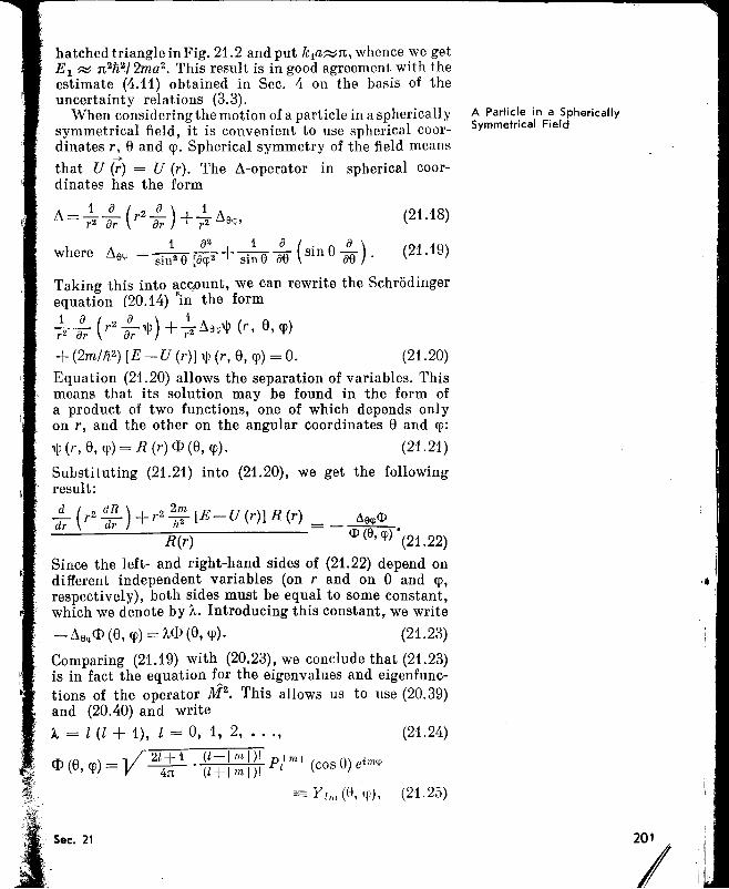
hatched triangle in Fig. 21.2 and put k1a;:::::,rr" whence we getE 1 ;:::::, rr,2fi2J 2ma2• This result is in good agreement. with theestimate (4.11) obtained in Sec. 4 on the basis of theuncertainty relations (3.3).

When considering the motion of a particle in a spherically A Particle in a Sphericallysymmetrical field, it is convenient to use spherical coor- Symmetrical Field

dinates r, 8 and cpo Spherical symmetry of the field means

that U (--;) = U (r). The ~-operator in spherical coor-dinates has the form

1 a ( a) 1~=-- r2 - -L_~s (21.18)r 2 iJr ar I r 2 q;,

1 iJ2 1 a (_ a)where ~S'l' = sin28 [acp2 + sin 8 as sm 8 as' (21.19)

Taking this into ~cc,ount, we can rewrite the Schrodingerequation (20.14) in the form

1 iJ ( a ) 172a; r 2 a;'IjJ +72~9q;'IjJ (r, 8, cp)

+ (2m/1i2) [E - U (r)] 'IjJ (r, 8, cp) = O. (21.20)

Equation (21.20) allows the separation of variables. Thismeans that its solution may be found in the form ofa product of two functions, one of which depends onlyon r, and the other on the angular coordinates 8 and cp:

'IjJ (r, 8, cp) = R (r) ll> (8, cp). (21.21)

Substituting (21.21) into (21.20), we get the followingresult:

d ( dR) 2m(Ii" r 2 a;:- +r2 [;2[E-U(r)]R(r) =_ dSq><D

R(r) <D (8, cp) •(21.22)

Since the left- and right-hand sides of (21.22) depend ondifferent independent variables (on r and on 8 and cp, -.respectively), both sides must be equal to some constant,which we denote by A. Introducing this constant, we write

- ~eq;ll> (8, cp) = All> (8, cp). (21.23)

Comparing (21.19) with (20.23), we conclude that (21.23)is in fact the equation for the eigenvalues and eigenfunc-tions of the operator JVj2. This allows us to use (20.39)and (20.40) and write

A = 1 (1 + 1), 1 = 0, 1, 2, ••. , (21.24)

rh 8 .. / 2l + 1 (l-I m I )! pi m I 0) imlpw(,cp)=V ~'(l+lml)! l (cosue

= Y lm (0, lp), (21.25)

Sec. 21

I'"

It should be noted that (21.27) may be reduced to theone-dimensional Schrodinger equation with a specialboundary condition at r = O. For this we must use thesubstitution

(21.28)

(21.27)

(21.26c)

where we have introduced the notation

r-Y 9 +2 = 1/ ~ sin2 8e±2irp

~, - 32n .

cp (r) = rR (r) .. (21.29)

and in view of the boundedness of the 1\4\~n R (r),require that the condition q> (0) = 0 be satisfied. It canbe easily seen that the substitution (21.29) in fact con­verts (21.27) into the one-dimensional Schrodinger equa­tion

d2cp 2m ) rrJ 0)

dr 2 +fi2 [E - Udr hI (r) = O. (21.3

In this case the boundary condition q> (0) = 0 correspondsto the one-dimensional potential well having an infinitelyhigh vertical wall on the left (at r = 0).

We emphasize that the "angular part" of the wave functionis independent of the particular form of the potentialU (r); this is a direct and important consequence of thespherical symmetry of the potential.'Ve now turn to the "radial part" of the wave function,i.e. to the function R(r). According to (21.22) and (21.24),this must be a solution of the equation

1 d ( dR) 2m-- r 2 - +-[E-U[(r)]R(r)=Or 2 dr dr fj2 ,

U ( ) = U ( ) _I- !l2l (l+ 1)[ r r I 2mr2 •

where m = 0, +1, ... , +l. The functions Y 'm (8, q»are spherical harmonics (they were introduced in Sec. 20).It will be useful to write down the expressi ons for thefirst few spherical harmonics:

1Y oo = f - , (21.26a)

1 4n

/3 .. /-YIO=ll 4n cos8; Y1,±1= V 8~ sin8e±irp, (21.26b)

202

where T= P; is the vector of the density of flow of theliquid.Equation (21.31) is independent of the choice of the vol­ume V. Using this fact, we can decrease the volume Vto some particular point. In the limit as V -+ 0, (21.31)

Thus,a i" .t --..-+at j p dV + Ypv dS = 0.

v s

By replacing the integral over the closed surface by avolume integral, we can rewrite the last equation in thefollowing form:

'It

203

The Continuity Equation and theSchrodinger Equation

(21.31)J(~~ +divT) dV=O,v

Further study of (21.30) obviously requires a considera­.. tion of the particular form of the potential U(r).It should be noted that among the problems on the motionof a particle in a spherically symmetrical field are theproblems of an electron in an atom and the scatteringof particles by spherically symmetrical centres.

We shall establish a formal analogy between the time­dependent Schrodinger equation and the continuity equa­tion, which is widely used in classical physics, especiallyin hydrodynamics. We assume that there is a certainmedium (for example, a liquid) described by the functions

p (;) and -;~) [p(;) is the density of the medium and

-; ~.) is the velocity of the particles of the medium at--..

the poin t r; naturally, these functions may also dependon time!. Let u~ imagine a certain volume V in themedium to be isolated. The change in the quantity of

liquid in this volume per unit time is equal to .!!.. r pdV.atJv

Let us isolate a certain element of surface area dS onthe area S bounding the volume V, and associate with

-+it a vector dS equal to dS in magnitude and directed alongthe outward normal to the surface. The amount of liquidpassing per unit time from the volume V through an

-* -+ ---*element of surface area dS is equal to pv dS. The amountof liquid passing through the entire surface per unit

~ --..-+time is equal to ;y pv dS. The law of conservation of

s af ~--..-+matte·r requires that --aJ p dV and ;y pv dS be equal.

tv S

(21.33)

(21.32)

, I

i

204

becomes a differential equation at this point:

ap +d' ":'" 0- IVJ=.atThis is the classical continuity equation.Let us turn to the time-dependent Schr6dinger equation.We shall generalize the one-dimensional equation (20.17)for the three-dimensional case:

a -r !i2 -r -r-->-

in- 'P' (r, t) = --2- ~ lV (r, t) +U (r) 'P' (r, t).(}t m

We introduce purely formally a certain "medium" anddefine the density of this "medium" as 'P''P'*. This densitymay be called the "probability density". In other words,the probability of finding a particle will be greater atthose points of space, where the density of the "medium"is higher.This "probability density" may be given a fairly simplephysical meaning if we imagine that the space is filledwith a large number of particles (the interaction of parti­cles is to be neglected in this case). Obviously, the numberof particles in some volume ~V is proportional to theprobability of finding a particle in this volume. Withthis approach, W'P'* may be considered simply as thedensity of the number of particles.As in the classical case, we start by considering a certainfinite volume V:

~ r dV = ~ r If'P'* dV = r (W* a'l' + 'P' a'l'* ) dVat J P at J J at at .

v v v

Substituting into this :t Wand :t If* from the Schr6d­

inger equation (21.33), and from the complex conjugateof equation (21.33), we get

~ rIf'F* dV =~ r ('P'*~ 'P' - If~ qr*) dVat J 2m JV V

= ~: j div ('P'*Y'lf - WY'W*)d~ .

V ~The last result can be written in the form

r [.!...- (W'P'*) - div {.!:.!!- (If*Y'"lfJ Ot 2rnv

- lfY'lf*) }JdV = 0, (21.34)

or, after decreasing the volume V to a point,

:t (lflf*) - div [ ~~n (If*Y'lI' - lfY'W*)J= O. (21.:35)

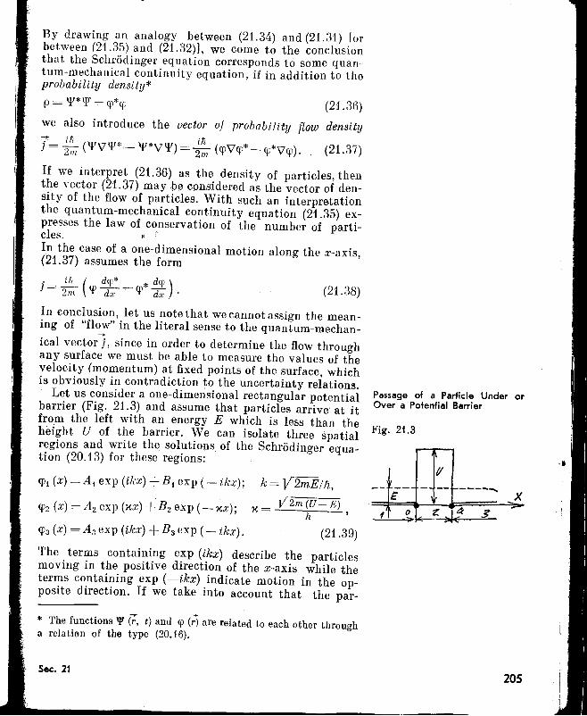
Sec. 21

'I< The functions 'P' C;, t) and qJ (;:'j are related to each other througha relation of the type (20.16).

x

205

----"-'

o~

E

Passage of a Particle Under orOver a Potential Barrier

Fig. 21.3

(21.38)

(21.39)

k=V2mE/tz,Y2m(U-E)

x= Ii

. _. iii ( dqJ * * dqJ )I-2m cp~-cp a:; .

By drawing an analogy between (21.34) and (21.31) [orbetween (21.35) and (21.32)], we come to the conclusionthat the Schrodinger equation corresponds to some quan­tum-mechanical continuity equation, if in addition to theprobability density*

p = 1¥*1Jf = cP*cP (21.36)

we also introduce the vector of probability flow den8ity-:" in . ill] = 2m (1Jf'V1Jf*- 1Jf*'V1Jf) ="2,;"i" (cp\7cp* -. CP*'Vcp). (21.37)

If we interpret (21.36) as the density of particles, thenthe vector (21.37) may be considered as the vector of den­sity of the flow of particles. With such an interpretationthe quantum-mechanical continuity equation (21.35) ex­presses the law of conservation of the number of parti-cles. ,,'In the case of a one-dimensional motion along the .:r-axis,(21.37) assumes the form

CPt (x) = At exp (ikx) +B t exp (- ikx);

CP2 (x) = A 2 exp (xx) +B 2 exp (- xx);

CPa (x) = Aa exp (ikx) +Ba exp ( - ikx).

In conclusion, let us note that we cannot assign the mean­ing of "flow" in the literal sense to the quantum-mechan-

ical vectorj, since in order to determine the flow throughany surface we must be able to measure the values of thevelocity (momentum) at fixed points of the surface, whichis obviously in contradiction to the uncertainty relations.

Let us consider a one-dimensional rectangular potentialbarrier (Fig. 21.3) and assume that particles arrive at itfrom the left with an energy E which is less than theheight U of the barrier. We can isolate three spatialregions and write the solutions of the Schrodinger equa­tion (20.13) for these regions:

The terms containing exp (ikx) describe the particlesmoving in the positive direction of the x-axis while theterms containing exp (-ikx) indicate motion in the op­posite direction. If we take into account that the par-

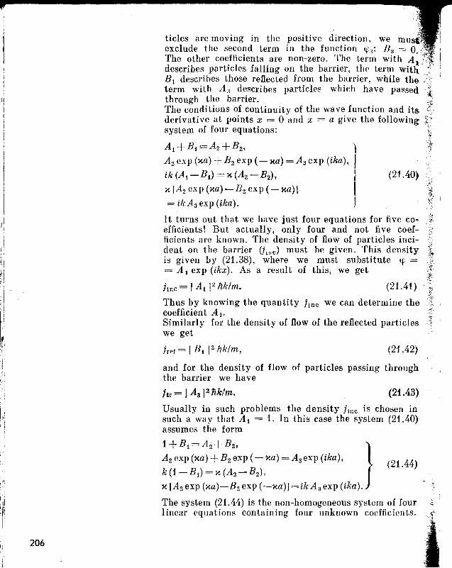
(21.40)

ticles are moving in the positive direction, we muexclude the second term in the function 4l:l: B 3 = O.The other coefficients are non-zero. The term with Atdescribes particles falling on the barrier, the term withB1 describes those reflected from the barrier, while theterm with A., describes particles which have passedthrough the barrier.The conditions of continuity of the wave function and itsderivative at points x = 0 and x = a give the followingsystem of four equations:

At+Bt=Az+Bz, ')

Az exp (xa) +Bz exp (- xa) = A 3 exp (ika), Iik(A t -Bt )=x(Az-B2), (

x [A z exp (xa)-Bz exp (-xa)J I=ikA3 exp(ika). J

It turns out that we have just four equations for five co­efficients! But actually, only four and not five coef­ficients are known. The density of flow of particles inci­dent on the barrier Ulnc) must be given. This densityis given by (21.38), where we must substitute qJ == A 1 exp (ikx). As a result of this, we get

jlnc = I At 12 ftk/m. (21.41)

Thus by knowing the quantity jlnc we can determine thecoefficient AI'Similarly for the density of flow of the reflected particleswe get

(21.42)

and for the density of flow of particles passing throughthe barrier we have

hr = I A3 12 nk/m. (21.43)

I' 206

Usually in such problems the density jlnc is chosen insuch a way that Al = 1. In this case the system (21.40)assumes the form

1+Bt =A2+B2 , }

A 2 exp (xa) +Bzexp (- xa) = A3 exp (ika), (21.44)

k (1-Bt ) = X (A z- B2 ),

x [A z exp (xa)-Bz exp (-xa)] = ik A 3 exp (ika).

The system (21.44) is the non-homogeneous system of fourlinear equations containing four unknown coefficients.

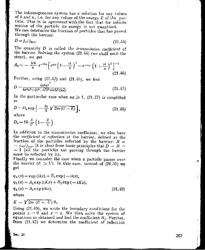
The inhomogeneous system has a solution for any valuesof k and x, i.e. for any values of the energy E of the par­ticle. This is in agreement with the fact that for infinitemotion of the particle its energy is not quantized.We can determine the fraction of particles that has passedthrough the barrier:

D=itr/itnc. (21.45)

The quantity D is called the transmission coefficient ofthe barrier. Solving the system (21.44) (w~ shall omit thesteps), we get

Aa=- :k e-ika[exa(t_ i: r- e- xa (1+ i: )2J-1.(21.46)

Further, using (21.49) and (21.45),~' '"

D = 4k2x 2

4k2x 2+(k2+X2)2 sinh2 (xa) .

In the particular case when xa ~ 1,as

f· 2a ]D=Doexp. --7': V2m(U--E) •

where

Do=16 Z(1- ~).

we find

(21.47)

(21.47) is simplified

(21.48)

(21.49)

In addition to the transmission coefficient, we also havethe coefficient of reflection at the barrier, defined as thefraction of the particles reflected by the barrier: R == jrer/hnc. It is clear from basic principles that D + R == 1 (all the particles not passing through the barriermust be reflected by it).Finally we consider the case when a particle passes overthe barrier (E > U). In this case, instead of (21.39) weget

CPt (x) = exp (ikx) +B t exp (- ikx),

cpz (x) = Azexp (iKx) +Bzexp (- iKx),

CPa (x) = Aaexp (ikx),

where

K = V2m (E - U)/Ii.

Using (21.49), we write the boundary conditions for thepoints x = 0 and x = a. We then solve the system ofequations so obtained and find the coefficient B 1• Further,from (21.42) we determine the coefficient of reflection

207

'.

Fig. 21.4

t>1

III ~,

~IIIII--------------R--j-re-t-/j-ln-c-.-I-t--tu-r-n-s-o-u-t-tO-b-e-e-q-U-a-l-t·o------rI _ (k2_K2)2 sin2 (Ka) ,j, R - 4k2KLt--(k2-K2)2 sin2 (Ka) • (21.50)

Using (21.47) and (2(50) we can fwd the dependence ofthe transmission coefficient D on the ratio E/U. Thisdependence is shown graphically in Fig. 21.4. The samefigure shows the dependence D (E /U) for a classical par­ticle (dotted line). A comparison of the solid curve withthe dotted line indicates the quantum-mechanical na­ture of microparticles. Note that for E < U in classicalmechanics all particles are reflected from the barrier andnot a single particle passes through. In quantum mechan­ics, however, a part of the particl~s is reflected anda part passes through the barrier. For E > U, in classicalmechanics all particles pass through and not a singleparticle is reflected, while in quantum mechanics a partof the particles passes through, and another is reflected.Both sub-barrier transmission and above-barrier reflectionof microparticles are specifically quantum effects.

(22.1)

(22.4 a)

(22.4 b)

(22.4c)

The Hamiltonian in SomeSpecific Problems

The Hamiltonian is of the form~ ft2 d2 m(i)2,y2

H= - 2m dx2 +-2-'

Section 22

It is obtained from (4.5) by taking (19.1) and (20.4) intoaccount. The eigenvalues are

En=ft(fJ (n+ ~); n=O, 1, 2, ... (22.2)

[for n = 0 we get from (22.2) the energy of zero-pointoscillations, which was determined in Sec. 4 on the basisof the uncertainty relations]. The eigenfunctions are

'Pn (x) = y m(fJ!1i exp (- £2/2) H n (£), (22.3)

where £ = x y m(fJ!1i, and H n (£) are called Hermite poly­nomials. Let us write down the expressions for the firstfew functions 'Pn (x):'Po (x) = (xoVn)-t/2 exp (- x2/2x:) ,

'Pt (x) = (2xo Vn)-t/2 exp (-x2/2x:) 2x/xo,

'P2(X) = (SxoVn)-t/2exp(-x2/2x:)(4 :; -2)

(where X o = Y1ilm(fJ).

208

Linear Harmonic Oscillator·

hi

!'Iir

/Ii

i~ Id,I,I

(22.6)

Sec. 22 209

The Hydrogen Atom

Note. Hermite polynomials, generalized Laguerre polyno­mials (mentioned below), harmonic functions and Legen­dre polynomials (introduced in Sec. 20) are called spe­cial functions. A considerable amount of mathematicalliterature has been devoted to special functions and theirapplications; for reference we mention l36, 37]. A basicaccount of polynomials and associated Legendre functions,special functions and Hermitian polynomials is given inAppendix E.

The problem of the hydrogen atom is a well-known exam­ple of the motion of an electron in a spherically symmetric.al Coulomb field. The Hamiltonian has the form~ 1i2 e2

HI=--~--2m r (22.5)

[it is obtained from (4.1) by using (19.1) and (20.6)].The eigenvalues 'If (this Hamiltonian are given by thefollowing familiar expression [see (2.5)]:

En = -me"-/21i2n2 ; n = 1, 2, 3, ....

The eigenfunctions of the Hamiltonian (22.5) may beexpressed in the form

1J'nlm = R nl (r) Ylm~(8,j cp); 1=0, 1, •.. , n-1;(22.7)

m=O, ±1, "', ± l.

Here y 1m (8, cp) are spherical functions. They define the"angular part" of the wave function irrespective of theparticular form of the spherically symmetrical potential;Rnl (r) is the "radial part" of the wave function, it isdefined by (21.30) with the Coulomb potential [U (r) == - e2/r]. The form of the function Rnl (r) is describedby the expression

Rnl:(r) = const exp (r/rin)I(2r/rin)1 L~I:,t~(2rlrin), (22.8)

where r1 = 1i2/me2 (this quantity is already known to thereader as the radius of Bohr's first orbit) and L~~/ arethe so-called generalized Laguerre functions (see, forexample, [36]).Expressions for some of the first harmonic functions havebeen given in Sec. 21 [see (21.26)]. We shall now give theexpressions for the first few functions R nl (r):

RiO = 2r1 3/ 2 exp (- rlrl), (22.9a)

R 20 = (2rD-l/2 exp (- r/2rl) (t - 2~1 ) , (22.9b)

R 2i = (2 -V 6rn- i exp (- r/2rl) r/r1• (22.9c)

I '

I

I'1

On Degeneracy of Energy Levels

In Sec. 5, when discussing the concept of an electron clou ",we introduced the functions Un I and Z 1m' Figure 5.2 (a)~showed the form of some of the functions W n I (r) =.= r2un z (r), while Fig. 5.2 (b) showed some of the func­tions Z Zm- Returning to the functions considered in thissection, we note)hat unz=R;tz (r) and!Zzm= I Y lm (e,q» I'.In particular, we note that (5.4) is in agreementwith (22.9a).By using (22.9) and (21.26), we can write the first feweigenfunctions of the Hamiltonian (22.5):

\jJ160 = (nrD- 1/2 exp (- r/r1)' (22.10a)

\jJ200=(SnrD- 1/ 2 exp(-r/2r1) (1- 2~1)' (22.10b)

\jJ211 = (sVnr; t 1exp ( - r/2r1) sin eet(j)r/r1' (22.10c)

'¢210 = (4 V2nr~ti exp ( - r/2r1) cos er/ri' (22.10d)

The function (22.10a) describes the ground state of thehydrogen atom, while the functions (22.10b)-(22.10d)describe the excited states corresponding to the first ex- /cited energy level (n = 2).

It follows from (22.6) that the energy of an electron inthe hydrogen atom is determined only by the quantumnumber n, whil e the states (the functions ~)n Zm) are de­termined by three quantum numbers n, land m. Besides,when considering electronic states we must take intoaccount the quantum number (J which does not occur inthese expressions.Since for a given value of the principalquantum number n the orbital quantum number l assumesintegral values from 0 to n - 1, and for every l themagnetic quantum number acquires 2l + 1 values, thefollowing gn states must correspond to an energy level En:

n-l

gn = 2 ')1. (2l +1) = 2n2 (22.11)z=o

(the factor 2 takes account of the two spin states of theelectron). This means that the eigenvalue En of the Ha­miltonian (22.5) (in other words, the nth energy level) .'is 2n2-fold degenerate. lDegeneracy of energy levels, as a rule, is associated with isymmetry in the atomic system. Thus, for example, owingto the spherical symmetry of intra-atomic fields, there is idegeneracy of the quantum numbers mand a-the energyis independent of the orientation of the orbital momentumand the spin momentum of the electron. The degeneracy

,of the quantum number l is .associated with the specificnature of the Coulomb potential; in non-Coulomb fields

the energy of the electron depends not only on n but alsoon 1.Various fields, external as well as internal, may lowerthe degree of symmetryofthe system. Thus, for example,"switching on" an external electric field leads to the ap­pearance of a physically distinguished direction. As aresult, the spherical symmetry disappears and is replacedby cylindric< I symmetry. A decrease in symmetry lEadsto a removal of degeneracy (partial or total). This isexhibited in a splitting of energy levels, i.e. in their con­version into sets of Jl( w, less degenerate levels. Splittingof energy levels in an external electric field is known asStark's effect, while the splitting in an external magneticfield is known as Zeeman's effect.

The Hamiltonian of a crystal consisting of N nuclei andZN electrons can be ~ written in the form

N .' ZN~ 1"'1~ 1~~

H = 2M LJPf+ 2m LJ p~i A

., -t-- .....

+Ud{rk}) +Uz ({R i }) +Us ({rk}' {R i }), (22.12)

where M is the mass of the nucleus, Pi is the momentumoperator for the ith nucleus, m is the mass of the electron,

Pk is the momentum operator for the kth electron, {;k}is the set of coordinates of the electrons, {R i} is the setof coordinates of the nuclei. The function U 1 desclibes theinteraction of electrons. It is of the form

Ut = ~ ~ ~e2/rk/' (22.13)kcf:-l

where rR/ is the distance between the kth and Ith electrons.The function U 2 describes the mutual interaction of thenuclei, while the function U 3 describes the interactionof the nuclei with the electrons.*Since M ~ m, the nuclei move much more slowly thanthe electrons. This permits us to consider the motions ofnuclei and electrons separately: when considering themotion of electrons, we assume that the nuclei are sta­tionary, while when considering the motion of the nuclei,we assume that the electrons colIectively create an aver­age field which is independent of the coordinate of indi­vidual electrons. In this case the waye function of the

• The functionsUi. U2 , Ua, describing the various interactionpotentids, in .fact correspond to operators in the coordinate repre~

se~tation. .

Sec. 22

Crystal; the AdiabaticApproximation

I';

,It

il;

crystal may be represented in the form of a product Of'"nuclear" and "electronic" functions:

~ -+ -+--+-

'IjJ ({rk}, {R1}) = 'I' ({R1}) CPe ({rk}). (22.14)

We also represent the Hamiltonian (22.12) as a sum of the"nuclear" Hamiltonian HI and the "electronic" Hamilton­ian iI2:

(22.15)

(22.17)

(22.16)~ 1 ~ ~ 1 ~ e2 .....

H2 = 2m LJP~+2 LJ ~ r;-+U3 ({rk }).

k k4=1 I

The function U 3 describes the potential energy of theelectrons in the field of the nuclei which are located at thelattice sites in the crystal.Thus, instead of solving an extremely complicated Schro­dinger equation for the entire crystal

" ~ -+ ~-+

H'IjJ ({rk}, {R i }) = Ecr\jJ({rk}, {R i})

it is enough to solve two much simpler equations:(a) for nuclei (for crystal lattice)

jj1'I'({Ri }) =Elat'I'~({Rtl),(b) for electrons~..... .....

H 2CPe ({rk}) = Eecpe ({rk}),

(22.18)

(22.19)

One-Electron Approximation

where Ecr = Elat + Ee. This approximation is calledadiabatic.In conclusion, we make a fairly important clarification.When using the adiabatic approximation we consider,strictly speaking, not the bare nuclei, but nuclei togetherwith those electrons which are tightly bound to them.Consequently, when we speak about a separate treatment-of the electrons ensemble, we mean not all the electrons,but only those which have been "collectivized" by thecrystal (in other words, the electrons moving over thecrystal lattice, for example, the conduction electrons).

In accordance with the adiabatic approximation, weshall consider, without going into the dynamics of thecrystal lattice, the motion of electrons which have been"collectivized" by the crystal. We use the expression

(22.16) and consider that the function U3 ({;k}) may berepresented as a summation over the "collectivized"

(22.21)

f electrons (,ince each electron interacts with the lattice~ field independently from other electrons): U3 ({;k}) =

= L} U~ (;k). In this case the "electronic" Hamiltoniank

(22.16) assumes the form

~ 1 ~~! 1 ~ ~ e! ~ -+H= 2m LJPk+2: LJLJ rkl + LJUdrk)' (22.20)

k k~l k

Further simplification is based on the assumption that

the term ~ LjL} e2/rkl in (22.20) may be approximated byk I

a summation over the electrons:1 ~ ~ e2 -+2: LJ LJ '7kl ~ ~ U5 (rk)'

k~l k ..In other words, when considering electron-electron in­teraction, it is assumed that each electron moves in acertain field which is common for the whole ensemble(it is called the self-consistent field). As a result, the Ha­miltonian of the electron ensemble can be represented asa sum of "one-electron" Hamiltonian. This allows us torepresent the wave function of the ensemble in the form ofa product of "one-electron" functions [we denote them by...<p (rk)], after which the Schrodinger equation for the elec­tron ensemble turns into set of "om-electron" equationsof the form

(22.22)

iI ~

.+ •Here p and r are the momentum operator and the coor-dinate of one of the "collectivized" electrons, E being theenergy of the electron.Thus, by using (22.21) we can go over from a considera­tion of the electron ensemble to consideration of a singleelectron moving in the field:

-+ -+ -+

U(r)=U.(r)+U~(r). (22.23)This transition is called the one-electron approximation.

The potential U (-;) is a periodic function with the periodof the crystal lattice. It will be shown in Sec. 24 that theenergy of an electron moving in a periodic field is brokenup into alternate bands of allowed and forbidden values,Le. has a band structure. An electron bound to an atom hasenergy levels, while a free electron is characterized by acontinuous energy spectrum. An electron "collectivized"

Sec. 22 213

by the crystal occupies an "intermediate" position to a,certain extent-it is "free", but only within the limits ofthe crystal. The band structure of the energy states ofsuch an electron is obvious and is "intermediate" betweenthe structure of discrete levels and that of a continuousspectrum.The relative freedom of movement of a "collectivized"eleotron is reflected, in particular, in its wave function~

which is represented in the form of what are called Blochfunctions:

(22.24)

The Hamiltonian of theInteraction of an Electron withElectromagnetic Radiation

This is the wave function (15.15) of a free electron, modu­

lated by the function u (---;), which has the period of the

potential U (~ (for more about Bloch functions, seeSec. 24).

We shall consider the system of a bound electron plusradiation. In the absence of interaction between the elec~

tron and the radiation, the system is described by the"unperturbed" Hamiltonian:

_;;9 ~

H O=2m-+ U +Hv, (22.25)

where p2/2m + U is the Hamiltonian of the electron, andHv is the Hamiltonian of the radiation. In the case ofinteraction between the electron and the radiation, thesystem is described by a "perturbed" Hamiltonian

11 = (~- : 1)212m +U +Iiv (22.26)

I~.

wIleI'cl A is tile oparator of the vector potential of tile ra­diation field [we recall that in the coordinate'representa-

-+-+ -+-+ .

tionA (r) = A (r)l*. Note that the field potentials herehave beem chosen in such a way that the well-known cal-

ibration conditions div ;; = 0 and <p = 0 (<p is the scalarpotential of the field) are satisfied. Next, we represent theHamiltonian in the following form:

(22.27)

214

* It is shown in classical field theory [381 that the interaction ofa charge with an electromagnetic field may be considered by replac-

~ -+- e-+ing p by p - -; A. We use this classical result here, replacing

the dynamic variables with the corresponding operators.

i

2t5

Momentum and CoordinateOperators in the MomentumRepresentation

(23.1)

Transition to the MomentumRepresentationSection 23

We shall show how to go over from the coordinate tothe momentum representation and shall give some re­sults in the momentum representation.

Obviously, the momentum operator in the momentumrepresentation is the momentum itself:

,... e ~ -+ e2

Ht= -2me(pA) + 2meZ A2. (22.29)

It should be noted here that the Hamiltonian (22.29) isresponsible for all processes of absorption and emission(spontaneous as w¥ll, as induced) of photons by an elec­tron.

where fi' is the interaction Hamiltonian, which playsthe role of the perturbation. Comparing (22.25), (22.26)and (22.27), we find that

"., e ~-+ -+~ e2

H t = - -2-[pA) + (Ap)] -+ -2zA2. (22.28): me meThis expression can be somewhat simplified if we put,in

..:+-+ -+ -+ -+-.:;: -+0-+

accordance with (20.27), pA (r) -A(r) p=-ilidivA(r).

Using the fact that div 1= 0, we get

Px=Px; P=p·

We shall, therefore, go over directly to a considerationof the x-coordinate.Suppose that the amplitude of a state is given in the coor­dinate representation by the function cp (x), and in themomentum representation by the function <1> (Px)' Byusing (17.33), we can write

. ) cp* (x) X(x) cp (x) dx= ) <1>* (Px) x(Px) <1> (Px) dpxo (23.2)

The relation between the functions cp (x) and <1> (Px),according to (15.6), is of the form

q> (x) = J<1> (Px) '¢px (x) dpx' (23.3)

where '¢px (x) are the eigenfunctions of the operator Pxin the coordinate representation. By using (20.9) we can-rewrite the expression (23.3) in the following form:

q> (x) = (2nli)-1/2 ~ <1> (Px) exp (iPxx/li) dpx' (23.4)

(23.8}

00

- in Jd;x [<1>exp (iPxxlh)) dpx-00

By substituting (23.4) in the left-hand side of the equal­ity (23.2), we get

Jlp* (x) xlp (x) dx

= 2~nJ JJ<1>* (p~) e-iP~x/nx<1>(px)/pxx/ndp~dpxdx. (23.5)

The factor x <1>(px) exp (iPxxltt) under the integral signin (23.5) may be expressed in the following form:

x<1>(px) exp (ipxxln) = - in dd [<1>exp (ipxx/n))Px

+iti dd<D exp (ipxx/n). (23.6)Px

We substitute (23.6) into (23.5) and consider the integralwith respect to Px' In so doing, we take into account that

=- in <1> (Px) exp (ipxx/n) 1:'00

= 0

[since it is physically impossible to attain an infinitelylarge momentum, we get <1> (00) = 0 and <1> (-00) = 0).Thus in the integral with respect to Px, only the second

term on the right-hand side of (23.6), indd<D exp (ipxx/n)Px

should remain. As a result, (23.5) assumes the form

Jlp* (x) xlp(x) dx

= 2~nJ JJ<1>* (p~) in exp [i(Px-p~)xltt) d~~:x) dp~dpxdx.

(23.7)

Integration with respect to x on the right-hand side ofthis equation gives, according to (15.17),

(2nnt 1 Jexp[i(px-p~)x/n)dx=c5(px-p~)·

Further, using the property of the delta function, we per­form an integration with respect to p~:

J<1>* (P~) c5 (Px- p~) dp~ = <1>* (Px)'

As a result, we are left with only the integral with respectto Px' and (23.7) assumes the form

216

I

JiI!

:1,\

'I

,."

Comparing the right-hand sides of (23.8) and (23.2), wefind the expression for the x-coordinate operator in themomentum representation:~ . dx (Px) = In -d-. (23.9)

Px

A generalization to the three-dimensional case gives..+-->-r (p) = itt V-->-' (23.10)

p

where V-->- is the gradient in the momentum space.p

By using (23.1) and (23.9) it is easy to see that the com­mutators of the operators of the coordinate and momen­tum components will be exactly the same in the momen­tum representation, as in the coordinate representation[we are speaking of the expressions (20.24)-(20.26)]. Thisconclusion may abo be extended to the expressions(20.27)-(20.30). (n other words, the commutation rela­tions are independent of the choice of a representation,i.e. are unitary invariants. This is quite natural, if werecall that the mathematical fact of commutation ofoperators has a definite physical meaning which, obvious­ly, cannot change while going over from one representa­tion to another.

Going over to the momentum representation, we canwrite (20.11) in the fOlllll

Ii (Px) TEl (Px)=ETF(Px). (23.11)where T E (Px) are the eigenfunctions of the Hamiltonianin the momentum representation. Note that the quanti­ties E in (23.11) are exactly the same as in (20.11), sincethe spectrum of eigenvalues of a Hermitian operator isa unitary invariant. Since in the momentum representa-

tionpx = Px and x= in -dd, the Hamiltonian (20.12)Px

will now have the form

iJ (Px) = f~ +U (in d;x). (23.12)

As a result, we get the following equation in place of(20.13) :

(:~ - E) TE (Px) +U(in ~;=) = O. (23.13)

This is the time-independent Schrodinger equation in themomentum representation.As an example, let us write out the Hamiltonian of alinear ha,rmonic oscillator:~ pi mw2Jj2 d2

H (Px) = 2m --2- dpi. (23.14)

Sec. 23

Unitary Invariance of theCommutation Relations

Schrodinger Equation in theMomentum Representation

217

Compare this expression with (22.1), which describes thesame Hamiltonian in the coordinate representation.The momentum representation allows us to obtain fairlyeasily one result with which the reader is already famil­iar. If a microparticle moves freely, equation (23.13)is obviously simplified:

( :~ - E) 1:E (Px) = 0, (23.15)

from which it immediately follows that

E = p~/2m. (23.16)

The result (23.16) has been already mentioned in Sec. 1.It means that a freely moving particle simultaneouslypossesses a definite energy and a definite momentum;moreover, these quantities are related to each other bythe classical relation (23.16). In the case of a freely mov­ing microparticle, the stationary state is also an eigen­function of the momentum operator. We emphasize thatthis can in no way be extended to bound microparticles(see the following example).

In Sec. 21 we considered the problem of the motion ofa particle in a one-dimensional rectangular potentialwell with infinitely high walls in the coordinate repre­sentation. The energy levels (21.8) and the orthonorma­lized amplitudes of stationary states (21. 9) were deter­mined.When going over to the momentum representation, theresult (21.8) obviously does not change, while the result(21. 9) changes. By finding the amplitude of stationarystates in the momentum representation, we can also findthe probability of values of momentum of a particle inthe n-th energy state. We denote these amplitudes byTn (Px); the required probability will then be l1:n (Px)1 2•

The amplitude 1:n (Px) are related to the amplitude ofstationary states in the coordinate representation [tothe amplitudes qJn (x)] by superposition relations of thesame type as (23.3):

1:n (Px) = JqJn (x) 'i'~ (Px) dx, (23.17)A

where 'i'~ (Px) are the eigenfunctions of the operator xin the momentum representation. By using the fact that'tjJ~ (Px) = 1/lp~ (x), and (20.9), we can rewrite (23.17) inthe following form:

Probability of Momentum Value~

for a Particle in a RectangularWell with Infinitely High Walls

218

a

1:n (Px) = (2nn)-1/2 JqJn (x) exp ,( - iPxxl1i) dx.o

(23.18)

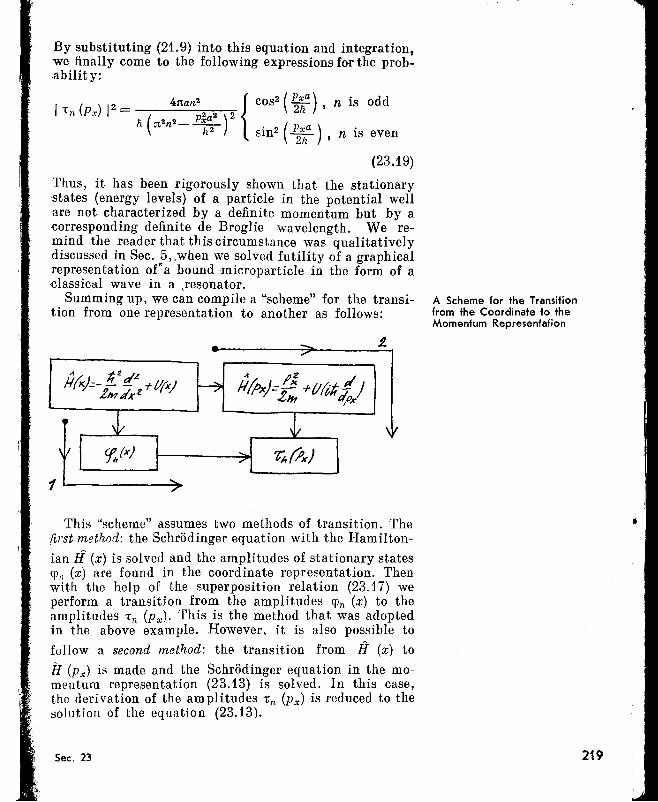
By substituting (21.9) into this equation and integration,we finally come to the following expressions for the prob­,ability:

I T ( ) 12 = 4nan2{ cos2( ~~a) , n is odd

n Px ( p2a2 ) 2Ii n

2n

2_ :-2 . 2(_Pxa ) n l'S

n sIn 2ft' even

(23.19)

Thus, it has been rigorously shown that the stationarystates (energy levels) of a particle in the potential wellare not characterized by a definite momentum but by a-corresponding definite de Broglie wavelength. We re­mind the reader that this circumstance was qualitativelydiscussed in Sec. 5"when we solved futility of a graphicalrepresentation oCa bound microparticle in the form of a-classical wave in a ,resonator.

Summing up, we can compile a "scheme" for the transi­tion from one representation to another as follows:

1L------~

This "scheme" assumes two methods of transition. Thefirst method: the Schr5dinger equation with the Hamilton-

ian Ii (x) is solved and the amplitudes of stationary statesq)n (x) are found in the coordinate representation. Thenwith the help of the superposition relation (23.17) weperform a transition from the amplitudes CPn (x) to theamplitudes Tn (Px)' This is the method that was adoptedin the above example. However, it is also possible to

follow a second method: the transition from H (x) to

if (Px) is made and the Schr5dinger equation in the mo­mentum representation (23.13) is solved. In this case,the derivation of the amplitudes Tn (Px) is reduced to thesolution of the equation (23.13).

Sec. 23

------~-~- -------.,.

A Scheme for the Transitionfrom the Coordinate to theMomentum Representation

219

The quantum-mechanical problem of an electron in aperiodic field plays an important role in the solid-statetheory. We turn to this problem, using the one-electronapproximation discussed in Sec. 22.

Let us consider a one-dimensional periodic potentialU (x) satisfying the condition

U (x + p) = U (x). (24.1)

Following the second method in the scheme given at theend of the preceding section, we change over to themomentum representation. This means that the poten­tial U(x) should be expressed as an operator in the mo-

mentum representation, tJ (P:x;). (In order to simplifythe notation we shall write P for Px here.)We expand the periodic function (24.1) in a Fourier series:

The Band Structure of theEnergy Spectrum. Brillouin Zones

;··----··-·----s-e-c-ti-o-n-2-4--------~-i~-ld-E-re-c -tr-o-n-j-n-a-p-e-r,·rO·d·rc·.-"

~

00

U (x) = ~ U n~exp (- i2nnx/a):::I n=-oo

and, changing to the momentum representation, we write

U(p)=00

~U (2:rtnh d)exp ----n a dp •

n=-oo

(24.2)

We shall now show that the operator exp (PI d~) isa displacement operator with a finite displacement inp-space by the amount P = Pl' This is so, as

dT 1 2 d2't-r (p + Pi) = -r (p) + Pi dp (p) + 21 Pi dp2 (p) + ...

= [1+Pi d~ + ;, P: :;2 + ... ] -r (p) = exp (Pi ~; ) •Thus

exp (Pi ~; ) = -r (p +Pi)' (24.3)

From (24.2) and (24.3) it follows that00

~ ( 2:rth)U(p)-r (p)= ~ Un-r p+-a-n • (24.4)n=-oo

By using (24.4) we can write the Schrodinger equation(23.13) in the following form:

'I·:'"

Ir

i220

00

(::-E)-r(p)+ ~ Un-r (p+2

:rtahn) =0.n=-oo

(24.5)J I

j"". '.

In fact, (24.S) isa homogeneous system of linear equationscontaining the functions 't (P), 't (p - 2'JTJi/a), 1: (p ++ 2nfila), etc. Generally speaking, this system consistsof an infinite number of equations:

................................................................ 0 ..

[ (p+;:n/a)2 EJ 't (p + 2:n )

+ ~ UnT: (p+2nn (:+1) ) = 0,

n00

[:: -EJ1:(p)+ ~ U n1: (p+2n:n )=0,} (24.6)

n=-oo

[(p-;:n/a)2 EJ't(p_2~n)

+v2 Un't (p+2nn

(:-1) ) = O.

.....................................~ ,Nonzero solutions of this homogeneous system are possibleonly if its determinant is equal to zero. We denote thisdeterminant by D (E, p) and symbolically write

D (E, p) = O. (24.7)

We fix P (let, say, P = PI) and write the roots of equation(24.7) as E I (PI)' E 2 (PI)' E 3 (PI), .... For a differentvalue of P (say P = P2) we get new roots: E I (P2)' E 2 (P2)'E 3 (P2)' .... By choosing different values of P, wefinally get a set of functions defined by equation (24.7):

E 1 (p), E 2 (p), E a (p), ... , E j (P), ••• (24.8)

For every index j, the energy is a continuous function ofthe momentum. By assuming that these functions arebounded we write for the index j

E min /" E .( ) <" E max (24 . 9)j """" j P "'" j •

The inequalities (24.9) include the energy values for themicroparticle which constitute the jth energy band. IfEf-af < Emr, we get a region of unattainable energyvalues between the (j - 1)th and jth energy bands. Thisregion is llsually called the forbidden band.Thus, the energy spectrum of an electron in a periodicfield must consist of a number of energy bands, some ofwhich may be separated by forbidden bands. Within everyenergy band the energy varies continuously; it is describedby some contil1luous function Ej (p).

Sec. 2.. ~-21

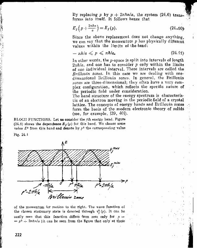
(24.11)·

...---------------------..II ro;.:::pl:;~nft:.lrlr tll~~:nh~~::~;::tem (24.6) transJ,:I~ Ej (p+2n:

n)=Ej (p). (24.10}I.'

1:1 Since the above replacement does not change anything,I' we can say that the momentum p has physically differentr:i values within the limits of the band:

Ii' . - nti/a -< p -< nfi/a.

r

Ii'"

i.'

In other words, the p-space is split into intervals of length2nfi/a, and one has to consider p only within the limitsof one individual interval. These intervals are called theBrillouin zones. In this case we are dealing with one­dimensional Brillouin zones. In general, the Brillouinzones are three-dimensional; they often have a very com­plex configuration, which reflects the specific nature ofthe periodic field under consideration.The band structure of the energy spectrum is characteris­tic of an electron moving in the periodic field of a crystallattice. The concepts of energy bands and Brillouin zonesform the basis of the modern electronic theory of solids(see, for example, [39, 40]).

BLOCH FUNCTIONS. Let us consider the jth energy band. Figure(24.1) shows the dependence EJ (p) for this band. We choose somevalue EO from this band and denote by pO the corresponding value

Fig. 24.1

of the momentum for motion to the right. The wave function ofthe chosen stationary state is denoted through ..~ (p). It can be

easily seen that this function differs from zero only forp == pO + 2Jtnn/a [it can be seen from the figure that only at th~se

222

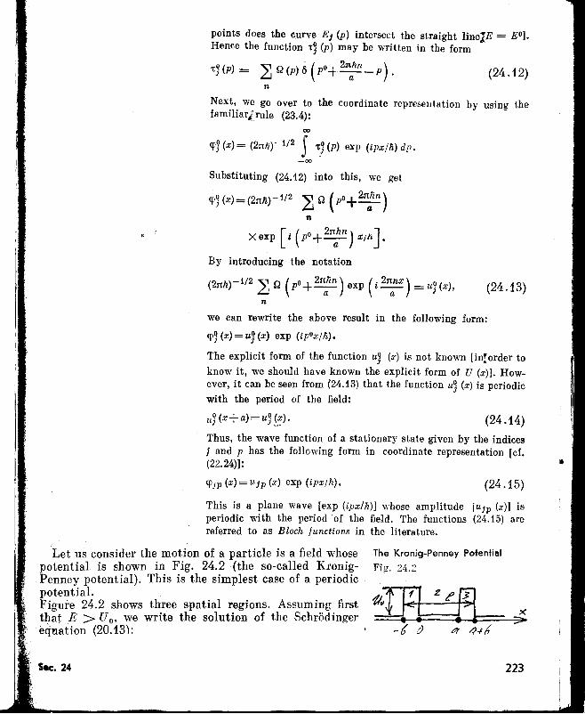
points does the curve Ej (P) intersect the straight linelE = EO].Hence the function -r~ (p) may be written in the form

-rJ(p)= ~Q(P)6(po+2nann_p). (24.12)n

Next, we go over to the coordinate representation by using thefamiliar; rule (23.4):

co

(fJ (x) = (2nn)-1/2 J-rJ (p) exp (ipx/h) dp.

-co

we can rewrite the above result in the following form:

(fJ (x) = uJ (x) exp (ipox/h).

The explicit form of the function uJ (x) is not known [in~order to

know it, we should have known the explicit form of U (x)]. How­ever, it can be seen from (24.13) that the function u~ (x) is periodicwith the period of the field:

uJ(x+a)=uH;:)· (24.14)

Thus, the wave function of a stationary state given by the indicesj and p has the following form in coordinate representation [ef.(22.24)]:

y.. '

Substituting (24.12) into this, we get

(f~(x)=(2nli)-1/2 ~ g (po+2nalin)

n

X exp [t (po+ 2n:ln) XIii].By introducing the notation

(2nli)-1/2 ~ Q (po+ 2n:n) exp (i 2nanx) = uJ (x),

n

(24.13)

This is a plane wave [exp (ipx/Ii)] whose amplitude [Ujp (x)] isperiodic with the period of the field. The functions (24.15) arereferred to as Bloch functions in the literature.

223

(24.15)

The Kronig-Penney Potential

Fig. 24.2

(fjp (x)=Ujp (x) exp (ipx/h).

tet us consider the motion of a particle is a field whosepotential is shown in Fig. 24.2 (the so-called Kronig­Penney potential). This is the simplest case of a periodicpotential.Figure 24.2 shows three spatial regions. Assuming firstthat E > U 0' we write the solution of the Schrodingereqnation (20.13):

Sec. 24

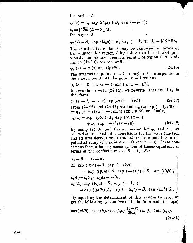
, ,..for region 1

qJdx)=Ai exp (ikix)+Bi exp (-ikix);

ki = V2m (E-Uo)//i;for region 2

qJ2(x)=A2 exp (ik2x)+B2 exp (-ik2x); k2=V2mE//i.

The solution for region 3 may be expressed in terms ofthe solution for region 1 by using results obtained pre­viously. Let us take a certain point x of region 3. Accord­ing to (24.15), we can write

qJa (x) = u (x) exp (ipx//i). (24.16)

The symmetric point x - 1 in region 1 corresponds tothe chosen point. At the point x - 1 we have

qJl (x - 1) = u (x - l) exp lip (x - l)//i].

In accordance with (24.14), we rewrite this equality inthe formqJl (x - l) = u (x) exp lip (x - l)//il. (24.17)

From (24.16) and (24.17) we find qJa (x) exp (- ipx//i) == qJl (x - l) exp (- ipx//i) exp (ipl//i) or, finally,

qJa (x) = exp (ipl//i){A i exp [ikdx-l)]

+B i exp [-ik.(x-l)]} (24.18)

By using (24.18) and the expression for qJl and qJ2' wecan write the continuity conditions for the wave functionand its first derivative at the points corresponding to thepotential jump (the points x = 0 and x = a). These con­ditions form a homogeneous system of linear equations interms of the coefficients AI' B l , A 2 , B 2 :

Ai +Bi =A2 +B2

Ai exp (ik2a) +Bi exp (-ik2a)

= exp (ipll/i)[A i exp (- ikib) +B i exp (ikib)],

kiAi-kiBi = k2A2-k2B 2,

k2[A2 exp (ik2a)-B2 exp (-ik2a)]

=exp (ipll/i)[A i exp (-ikib)-Bi exp (ikib)]kio

By equating the determinant of this system to zero, weget the following system (we omit the intermediate steps):

.cos (pll/i) = cos (~a) cos (kib) kJ;;;k:i sin (k2a) sin (kib).

(24.19)

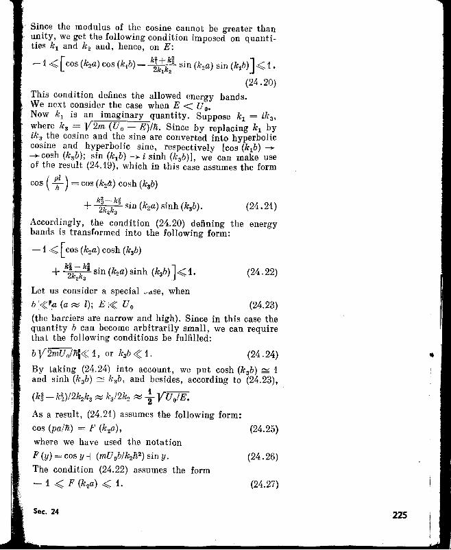
Since the modulus of the cosine cannot be greater thanunity, we get the following condition imposed on quanti­ties k1 and k 2 and, hence, on E:

-1-<: [cos (kza) cos (k1b)- kJ::~~ sin (k2a) sin (k1b)]<;: 1.

(24.20)This condition defines the allowed energy bands.We nex t consider the case when E < U o.Now k1 is an imaginary quantity. Suppose k1 = ik 3 ,

where k 3 = V2m (Uo - E)/li. Since by replacing k1 byik3 the cosine and the sine are converted into hyperboliccosine and hyperbolic sine, respectively [cos (k1b) -+-+cosh (k 3b); sin (k1b) -+ i sinh (k 3b)1, we can make useof the result (24.19), which in this case assumes the form

cos ( ~ ) = cos (k2tl) cosh (k3b)

+ ~k---;":~ sin (k2a) sinh (k3b). (24.21)

Accordingly, the condition (24.20) defining the energybands is transformed into the following form:

-1 -<: [cos (kza) cosh (k3b)

+ k;k~k:i sin (kza) sinh (k3b) ] -<: 1. (24.22)

Let us consider a special ~dse, when

b '~rr (a ~ l); E!~ Uo (24.23)(the barriers are narrow and high). Since in this case thequantity b can become arbitrarily small, we can requirethat the following conditions be fulfilled:

bV2mUolli;~ 1, or k3b~ 1. (24.24)

By taking (24.24) into account, we put cosh (k 3b) /'OV 1and sinh (k 3 b) /'OV k 3b, and besides, according to (24.23),

(k~-k~)/2k2k3 ~ k3 /2k2~ ~ YUo/E.

As a result, (24.21) assumes the following form:

cos (pa/li) = F (k 2a), (24.25)

where we have used the notation

F (y) = cos y + (mUoblk2li2 ) sin y.

The condition (24.22) assumes the form

- 1 -<: F (k 2a) -<: 1.

Sec. 24

(24.26)

(24.27)

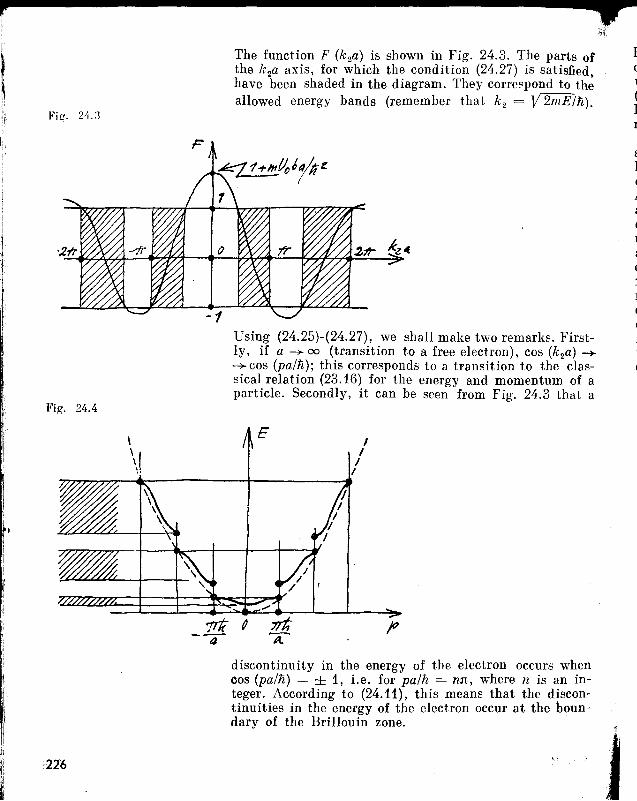
p------------------zrFig. 24.:3

The function F (k 2a) is shown in Fig. 24.3. The parts ofthe k 2a axis, for which the condition (24.27) is satisfied,have been shaded in the diagram. They correspond to theallowed energy bands (remember that k 2 = y!2mEln).

I(

1

(II

Fig. 24.4

\

\1\.

Using (24.25)-(24.27), we shall make two remarks. First­ly, if a ~ 00 (transition to a free electron), cos (k 2a) ~~ cos (pain); this corresponds to a transition to the clas­sical relation (23.16) for the energy and momentum of aparticle. Secondly, it can be seen from Fig. 24.3 that a

II

II

I:1'IIi

I

discontinuity in the energy of the electron occurs whencos (pain) = + 1, i.e. for pain = nn, where n is an in­teger. According to (24.11), this means that the discon­tinuities in the energy of the electron occur at the boun-dary of the Brillouin zone. '

Figure (24.4) shows the dependence of the electron energyon momentum as determined by (24.25). The discontin­uities in the energy mentioned above are clearly seen(the energy bands are shown on the left side by hatching).For comparison the classical dependence of energy onmomentum is shown for a free electron: E = p2/2m.

The conversion of energy levels of an electron in theatom into energy bands of an electron "collectivized"by the crystal may be seen as an effect of the removal ofcommutation degeneracy.As was mentioned in Sec. 22, the electron energy in anatom in the general case of a non-Coulomb potential isdetermined by the quantum numbers nand l. This givesrise to a 2 (2l + 1)-fold degeneracy of this energy. Byassuming that the atom is a part of some perfectly orderedensemble of N similar atoms and that it remains isolatedfrom its neighbours', the degeneracy in the electron energymust be taken as 2N (2l + i)-fold. The factor N is asso­ciated with the so-called commutation degeneracy: in anordered ensemble, there are no physically isolated atoms,hence the energy of an electron cannot depend on any ofthe N atoms near which it is localized. However, in a realensemble (i.e. a crystal), the atoms are not isolated­they interact with one another. This interaction leads toa "collectivization" of the electron and a partial removalof degeneracy of its levels. The level with a 2N (2l + 1)­fold degeneracy is split up into a system consisting ofN (2l + 1) sublevels, each of which remains doubly de­generate (according to the spin quantum number 0').

: Thus a "collectivization" of the electron by the crystalleads to a removal of commutation degeneracy and de­generacy with respect to the quantum number m.It is significant that a system of N (2l + 1) sublevels isin reality not discrete, but forms a band of allowed val­ues of the electron energy. Indeed, let !1.E be the widthof this system of sublevels, and !1.e be the distance be­tween the neighbouring sublevels: !1.e = !1.E/N (2l + 1).For the system of sublevels to be discrete, it is essentialthat !1.e > hh, where't is the lifetime of an electron ina crystal. In other words, the distance between sublevelsmust be greater than the uncertainty jn the energy of theSublevel described by the relation (3.2). This means thatthe condition

Formation of Energy Bands as anEffect of the Removal ofCommutation Degeneracy

h (2l + 1) N/!1.E < 't (24.28)

must be satisfied. Assuming that N (2l + 1) ~ 1023 ,

'dE ~ 1 eV, we find that't should be more than 108 s,Le. more than 10 years. Since the real lifetime of a "col-

p--------------------"..lectivized" electron in the crystal may only be less thanthis, the relation (24.28) is obviously not satisfied. Thisenables us to consider the system of N (2l + 1) sublevelsas an energy band. Naturally the number of electron statesin the band remains finite-the band may "accommodate"up to 2N (2l + 1) electrons. In this connection we speakof the degree of filling in of a band, of completely filledbands, etc.

Section 25 The Probability of QuantumTransitions

Quantum Transitions and thePrinciple of Superposition ofStates

We assume that a microparticle undergoes a transitionfrom one stationary state to another under the action ofsome external factor. How to find the probability of sucha transition?The initial and the final states of the microparticle aredescribed by functions of the type (20.16). For example,let the initial state be given by 'l'n (x, t)= ern (Xl exp (- iEnt/fi). For simplicity, the set of spatialcoordinates is denoted by x. The functions 'J!n satisfythe Schr6dinger equation (20.17): .

(25.1)

(we shall call it the "unperturbed" equation). The phys­ical nature of external factor, which causes the quantumtransition of the microparticle, is arbitrary. In particular,it may be the interaction of the microparticle with electro­magnetic radiation. In the quantum theory apparatussuch a factor appears in the form of an interaction poten­tial which must be added to the "unperturbed" Hamilto-nian fl. In Sec. 22 in the example of the interaction of anelectron with radiation, this "addition" to the Hamilto­nian was interpreted as some perturbation and was denotedby it'. We shall use the same notation here. By takinginto account the perturbation iI', we can rewrite theSchr6dinger equation in the form

(25.2)

228

This equation is called the "perturbed" equation. Itssolutions CDn are no longer stationary states. Hence theindex n here does not fix the energy level, but merelyindicates the past history: the given "perturbed" statehas "emerged" from nth "unperturbed" state.

Essentially, the state <Pn is a superposition state:

(25.3)n

If at a certain time t we "switch on" the correspondingdetector, the superposition (25.3) is destroyed and themicroparticle will be observed in one of the stationarystates, for example, in the state '¥m' This means that themicroparticle has undergone a quantum transition fromthe state 1fn to the state 1fm' It is well known that theprobability of such a transition is 1 Xnm 0) 12 •

The reader is in fact familiar with all this. The remarksmade above are in agreement with those made in Sec. 10,regarding the relation (10.3), which is essentiallyequivalent to the.relation (25.3).Thus, the transition probability is, as expected, the squareof the modulus of the corresponding transition ampli­tude:

W nm =IXnm(t)12. (25.4)

This amplitude is one of the coefficients in the superposi­tion (25.3), which is just an expansion of the "perturbed"state <Pn in terms of "unperturbed" states.

In order to find the probability Wnm , we should firstsolve equation (25.2) and then find the expansion coef­ficients of the solutions obtained for states of the type(20.16). As can be easily seen, such an approach corre­sponds to the first method in the "scheme" of transitionfrom one representation to another, considered in Sec. 23.The other approach corresponding to the second methodin this scheme, however, is more rational. We shall followthe second method here.According to (15.5), the coefficients Xnk of the superposi­tion (25.3) may be treated as a wave function describingthe "perturbed" state, though not in the coordinate re­presentation (in the coordinate representation this is doneby the function <pn ), but in the representation of a set ofthose physical quantities with respect to which the funo­tions 1fk are eigenfunctions. Since the functions 1f k areeigenfunctions of the Hamiltonian, we call this repre­sentation the energy representation. Thus, following thesecond method in the "scheme" in Sec. 23, we must "trans­late" the "perturbed" equation (25.2) given in the coor­dinate representation into the energy representation. Thiswill give us a new equation-the "perturbed" Schrodingerequation in the energy representation. The solutions

. of this equation will be the required transition ampli-

Sec. 25

Transition to the EnergyRepresentation

229

(25.5)

p-----------------crtudes. Performing the operations indicated above, we sub­stitute (25.3) into (25.2), and take into account (25.1).We get

.~ ", dXnk nr - ~ H' , (t) urlft LJ ---cit" Tli - LJ Xnk Tk·

k k

Premultiplying both sides of (25.5) by 1f~ and in­tegrating with respect to the spatial coordinates, we obtain

(25.6)

i

'[

in L; d~~k I 1f~qrkdx= ~ Xnk I '¥~fI' (t) lJ.'kdx.k k

Taking into account the orthonormalization of stationarystates, we can rewrite the last expression in the follow·ing form:

'f;, dXnm ~ r lrr* H- 'ur d~" -cit = LJ Xnk J T m T k X.

1\

Next, we introduce the expression

Jqr~H'1f"dx=exp (iWmk t ) Jtp:aH'cp"dx

= exp (iwm"t) ( m Iii' Ik), (25.7)

Application of the Method ofPerturbations to Computation ofthe Transition Probabilities

230

where

wmk=(Em-Ek)/n. (25.8)

Taking into account (25.7) we may rewrite (25.6) in thefollowing final form:

d i"'V ~dt Xnm = - T LJ Xnk <m IH' (t) Ik) exp (iWmk t ).

k

(25.9)Thus, we have obtained the "perturbed" Schrodingerequation in the energy representation. In fact (25.9) isnot one equation, but a system of equations. We emphasizethat the system (25.9) is more convenient than (25.2),since by solving this system we can at once determine thetransition amplitudes Xnm' It is also quite significantthat when solving the system (25.9), the perturbationmethod can usually be applied.

The perturbation is usually very small, which enablesus to obtain an approximate solution of the system (25.9)by using the method of perturbations. A small perturbationmeans that the function cI>n may be represented in thefurm ':<Dn="'¥n+An, (25.10)

(25.13)

(25.14)

(25.15)

where An is a small addition to the unperturbed function'Yn' In accordance with (25.10), we can write

Xnk = 6nk + X~h + xi{~ + Xit3~ +- . . . . (25.11)

It can be easily seen that A = L lxh1i + xi:l. + X~~ +It

+ ... J 1J'k' According to (25.11), the small addition Ais in turn split into additions differing in the order ofsmallness: the functions X<Jk are of the same order as theperturbation, X~2h are of the order of the square of per­turbation, etc. Substituting (25.11) into (25.9), we get

d !II + d (2) + d \1,dt Xnm dt Xnm dt Xnm + ...- i ~ (~ -L (1) + (2) + ) H~' Ik )- -Ii: LJ Unk I Xnk Xnk ••. (m I )exp (iwmk t .

k

(25.12)

We rewrite (25.12), retaining terms of only first order inthe perturbation:

d <1, i ( 1 H~' I (.)(JtXnm= -Ii m n) exp ~wnmt.

This is the approximate expression for the amplitudesXnm, obtained in the first-order approximation in themethod of perturbations.If it turns out that (m I iI' In) = 0, we must use theapproximate expression for the amplitudes in the second­order approximation in the method of perturbations. Itis obtained from (25.12) by retaining terms of the secondorder in the perturbation:

d (2) i'V (1)( IH~'lk) (. t)dt Xnm = - Ii LJ Xnk m exp lWmk •k

Similar!y, for the third-order approximation in the methodof perturbations we get

d (3) i ~ (2) ( IH~ , Ik) (. t)- Xnm = ---,;- LJ Xnk m exp ~Wmkdt "

k

etC.Knowing the transition amplitudes for any order in themethod of perturbations, we may obtain the transitionprobabilities in the corresponding approximation. Inthe first approximation, we get, from (25.13),

w;;~ = I X;;~ (t) 12

t

= ;21) (mIH'(t)ln) exp (iW mnt)dt\2. (25.1G)_00

Sec. 25 231

...,-----------------.....For the second-order approximation in the method ofperturbations we get, from (25.14),

t

w~~ = n\ I~ j X~l~ (t)( m,H' (t) Ik)k -00

(25.17)

Feynman's Diagrams and theCalculation of TransitionProbabilities

232

. /2X exp (lffimkt) dt ,

etc.Note that the result (25.17) describes the interference ofamplitudes. The resulting transition amplitude here isthe sum of the transition amplitudes through various in­termediate states. The impossibility of finding the micro­particle in any intermediate state leads to the indistin­guishability of alternatives and permits us to speak ofintermediate states as virtual states.The further course of action envisages a substitution of...definite operators H' in expressions of the type (25.16)and (25.17). In quantum electronics, for example, theoperator (22.29) is used. A detailed consideration of suchquestions is beyond the scope of this book. The reader isadvised to refer, for example, to [12, 411, in this connec­tion.

In conclusion, we return to the Feynman's diagramsconsidered in Sec. 6 (see the diagrams 6.1, relating to thescattering of one electron by another). Note that all thediagrams shown in Fig. 6.1 are associated with the samequantum transition-the transition of two electrons fromparticular initial states to particular final states. Strictlyspeaking, each particular transition must be described byan infinite number of diagrams, with an ever increasingnumber of vertices. In this connection, we recall the re­mark expressed in Sec. 6: "In order to caloulate the prob­ability of scattering of an electron by an electron, itis necessary, in principle, to take into account the Con­tribution (to this transition) of various processes de­scribed by different diagrams."Returning to Feynman's diagrams, we can now clarifythe meaning of the remark quoted above. We can nowexplain the meaning of "taking into account" of the con­tribution from different diagrams. What happens is thatto each diagram there corresponds a definite transitionamplitude. The resulting amplitude is the sum of theseamplitudes. Consequently, in order to compute the prob­ability of a particular quantum transition, it is necessaryfirstly to form all the possible Feynman's diagrams of thetransition and write the amplitudes corresponding to the

t

233

(26.1 )

To conclude the book, let us discuss in very general termstbe very important problem of the methods of describingthe evolution of microsystems with time. The quantum­mechanical apparatus so far developed uses three differentmethods. Three different forms of the equations of motionin quantum mechanics correspond to these methods.We shall discuss these methods below. Usually we referto them as three different representations: the Schrodingerrepresentation, the Heisenberg representation and theinteraction representation (Dirac representation). The term"representation" is used here in a different, wider sensethan in the previous sections. We may also speak ofSchrodinger's coordinate representation or Schrodinger'smomentum representation. In the previous sections werestricted ourselves to the Schrodinger representation butconsidered various representations, understood in a morerestricted sense-the coordinate, the momentum and theenergy representations. We shall now consider Schrodin­ger, Heisenberg and Dirac representations, restrictingourselves to the coordinate representation.

Here, the evolution of a microsystem with time is de- Schrodinger Representationscribed as an evolution of the amplitudes of states of the givenmicrosystem:

Sec. 26

various diagrams, and, secondly, sum all these ampli­tudes and find the square of the modulus of the sum.

In Sec. 6 we had the sentence: "Fortunately, the con­tribution of different processes (different diagrams) isdifferent." This means that in practice the method of per­turbations is used, which allows us to restrict the summa­tion of amplitudes to just the first few terms. The dimen­sionless quantity (e2/lic)n j 2, mentioned in Sec. 6, is thefactor which in the above-mentioned sum of amplitudescontains the amplitudes corresponding to the diagramswith n vertices. The smallness of this quantity explainsthe applicability of the method of perturbations in quan­tum electrodynamics.It may be said that the quantum-mechanical idea of in­terference of transition amplitudes along with the methodof perturbations ft>rtns, from a most general point of view,the foundation of quantum electrodynamics as a quantumtheory.

Section 26 Ways of DescribingEvolution of Microsystemswith Time

~----------------..

(26.7)

Heisenberg Representation

The operator U (t, to) satisfies the conditions

{J (to, to) = 1, (26.2)

(;rJ+ = frO = 1. (26.3)

The condition (26.2) is obvious. The condition (26.3) ofunitarity is a direct consequence of the independence ofthe normalization of amplitudes of state from the choiceof the instant of time:

J'tlJ* (x, t) 'tlJ (x, t) dx = .\. 'tlJ* (x, to) \jJ (x, to) dx.

The quantum-mechanical equation of motion in theSchrodinger representation (corresponding to Schrodin­ger's equation) is of the form

a ~

in at 'tlJ (x, t) = H (x) \jJ (x, t), (26.4)

where the operator Ii does not depend on time. By using(26.4) and (26.2), we can easily find the form of theoperator rJ (t, to):

fj (t, to) = exp [ - ~ (t - to) H (x) J. (26.5)

The exponent should be treated here as an expansion intoa power series.

'fhe evolution of a microsystem with time is describedas an evolution of Hermitian operators describing a givenmicrosystem. The amplitudes of states are treated astime-independent:

<p (x, t) = cp (x, to)' (26.6)

The transition from amplitudes in the Schrodinger repre­sentation to amplitudes in the Heisenberg representationis carried out, as can be seen from (26.1), with the helpof the operator 0+ (t, to):

cp (x, t) = {J+ (t, to) 'tlJ (x, to).

For, substituting (26.1) into (26.7), we get

cp (x, t) = O+U'tlJ (x, to) = 'tlJ (x, to)

= {; (to, to) cp (x, to) = cp (x, to)

Let L (x) be the operator of some physical quantity inSchrodinger's representation. According to (17.32) and(26.7), this operator in the Heisenberg representationwill have the form :',

234

L (x, t) = 0+ (t, to) i (x) rJ (t, to).' (26.8)

Substituting (26.5) into (26.8), we find

1 (x, i) =exp [~ (i-io) H (x)] [(x)

X exp [ - ~ (i-io) H (x) J. (26.9)

Differentiating (26.9) with respect to time, we get

in :t L (x, i) = exp [+(i- to) H (x) ] L (x)H (x)

xexp[ - ~ (i-to)H(x) J-exp[ ~ (t-to) If (x)]

X if (x) L (x) exp [ - +(t - to)l! (x) l (26.10)

This may be written in the forma~ ~~ ~ • ~~ ~ •

in 7ft L (x, i) =U+L (x) H (x) U -U+H (x) L (x) U (26.11)

or, by taking into account (26.3), in the form

in :t L (x, i) = [rL (x) O{riT (x) (; - (rIf (x) [JOt i (x) O.

(26.12)

Using (26.8) with respect to the operator £ (x) as well asthe operator if (x), we get the quantum-mechanical equa­tion of motion in the Heisenberg representation [ef.(19.10)]:. lJ- ~ ~

lit 7ft L (x, i) = [L (x, i), H (x, t)]. (26.13)

We note that at the time to we have cp (x, to) = 'I1J (x, to) Comparison of Schri:idinger and

and L (x, to) = L (x), i.e. both the amplitudes of states Heisenberg Representations

and the operators coincide in these two representations.However, at subsequent moments of time, we encountertwo different situations. In the Schrodinger representation

\ the amplitude of state changes, while the operator re­mains the same as it was at the moment to; in the Heisen­berg representation, on the contrary, the operator changes,while the amplitude of state remains the same as itwas at the moment to' It could be said that in the Schro­dinger representation the dependence on time is shiftedto the amplitudes of states, and in the Heisenberg repre­sentation, to the operators.For practical calculations, it is usually more convenientto use the Schrodinger representation. However, the Hei­senberg representation has the advantage that it permitsus to draw a mathematical analogy between quantum

Sec. 26 235

Pili;-----------------------....

Interaction Representation (DiracRepresentation)

mechanics and classical mechanics. In Heisenberg'srepresentation the quantum-mechanical relations havethe form of classical relations, in which the physicalquantities are replaced by operators (in this connection,we recall the last item of Sec. 20).Schrodinger, when he introduced in 1926 the representa­tion now named after him, considered the time-dependentamplitudes of states as the amplitudes of certain waves,and thus gave birth to the subject of "wave mechanics".A year earlier, Heisenberg proposed his method of de­scribing the evolution of microsystems with time, thusintroducing for the first time equation (26.13) in matrixform. This gave rise to the subject of "matrix mechanics".The difference between both these subjects is reduced tothe above-mentioned difference between the Schrodingerand the Heisenberg representations, Le. it is of a strictlyformal, mathematical nature.

Suppose that the Hamiltonian of a microsystem can bebroken into two components, one of which (if0) representsthe Hamiltonian of the microsystem itself, and the other(if1) describes the interaction of the initial microsystemwith external fields or other systems (in other words, is"responsible" for the effect of perturbation of the initialmicrosystem) :

(26.14)

In this case, it is convenient to use the interaction repre­sentation introduced by Dirac.The amplitude of state '¥ (x, t) in the interaction repre­sentation is expressed through the amplitude of state'I\J (x, t) in the Schrodinger representation in the followingway:

'¥ (x, t) = exp [~ Ho (x) (t- to)] 'I\J (x, t). (26.15)

(26.16)

236

In accordance with (17.32) we find from here the form 01the operator £B (x, t) in the interaction representation:

LB (x, t) = exp [~ (t - to)lfo (x)] L (x)

xexp[ - ~- (t-to)Ho(x)].

We emphasize that in (26.15) and (26.16) we have usednot the entire Hamiltonian, but just its "unperturbed"component iI 0 (x). Differentiating (26.15) with respect

to time, we get

iii :t 'I' (x, t) = -flo (x) 'I' (x, t)

+ iii exp [+(t- to) i/o (x)] :t '" (x, t).

Since

iii :t ",(x, t)=[Ho(x)+HtCx , t)J'" (x, t),

the last result can be written in the following form:

iii :t 'I'(x, t)=exp[ ~ (t-to)Ho(x) ]lItCx, t) '" (x, t)

=exp[+(t-to) H o(x)] Ht exp[ - ~ (t-to)llo(x) JX 1f (x, t) = flf (x, t) 'I' (x, t). (26.17)

Combining the results obtained above, we write the quan­tum-mechanical equations of motion in the interactionrepresentation as. a ~ ~ ~

(Ii 7ft L B (x, t) = [L B (x, t), H o(x, t)J,

fn :t 'I' (x, t) = iff (x, t) 'I' (x, t)

(26.18)

(26.19)

[note that (26.18) is obtained as a result of differentia­tion of (26.16) with respect to timeJ.Thus, in the interaction representation, the dependenceof the amplitude of state on time is determined by theinteraction (perturbation) Hamiltonian iff, while thetime dependence of the operator is determined by the"unperturbed" Hamiltonian lio. In this sense the inter­action representation lies in between the Schrodinger andthe Heisenberg representations.

The vector analogy enables us to compare quite clearly On the Vector Analogy Againall the three representations considered above. We cor-relate the system of basic states of the microparticle withthe system of mutually orthogonal basic vectors in somearbitrary space. We shall consider all operators in matrixform defined by the system of basic vectors. The statesof the microparticle are described by vectors consideredin the coordinate system defined by the basic vectors.Thus we have a system of basic vectors and a set of vectorstates to be considered relative to this system.We now turn to various representations. In Schrodinger'srepresentation the evolution of a microparticle with timeassumes a rotation of the vector state relative to the sta-

II'---------------------~

, '

I

One Additional Remark

238

tionary system of basic vectors. In the Heisenberg repre­sentation the evolution of a microparticle with time as­sumes, on the contrary, a rotation of the system of basic vec­tors relative to the stationary vector state. Finally, inthe interaction representation we assume a rotation ofboth the system of basic vectors and the vector state.Moreover, the rotation of the vector state is caused ex­elusively by the interaction of the microparticle with theexternal fields (perturbation) and is therefore dynamicin nature. The rotation of its system of basic vectors,however, is not related to the external factors, and iskinematic in nature.

The methods of describing the evolution of microsys­tems with time considered above are based on the use ofthe quantum-mechanical equations of motion. They assumea continuous evolution in time of either amplitudesof states or of certain Hermitian operators, or simulta­neously of the amplitudes of states and the operatorsboth. However, there are other qualitatively differentprocesses. Thus, it is well known that a destruction ofthe superposition of states caused by the detector in theact of measurement leads to an abrupt change in the am­plitude of state. It is obvious that this change in the am­plitude does not follow any equation of motion and obeysonly probabilistic predictions.In this connection two types of process are distinguishedin quantum mechanics: processes associated with a con­tinuous change in the amplitude of state in accordancewith the equation of motion, and those connected withabrupt, unpredictable, unambiguous changes in the am­plitude of state in the act of measurement. In the exist­ing quantum-mechanical apparatus processes of the firstkind are mainly involved. A considerable increase inrecent times in the interest in quantum-mechanical prob­lems of measurement indicates the starting point of se­rious research into processes of the second type (in thisconnection see the remarks about the problem of measure­ment in quantum mechanics in [42]).It is often believed that the probabilistic interpretationof quantum mechanics is limited by the introduction ofprobability amplitudes, since the latter can be predictedunambiguously from a solution of the Schrodinger equa­tion. Such a belief, as can be easily seen, is associated witha fact that the above-mentioned processes of the secondtype are not taken into account. Undoubtedly, theseprocesses intensify and complicate the probability aspectof quantum mechanics since they point to the necessityof considering a sort of "secondary probability"-the

probability of the realization of the amplitude ofprobability.It must be admitted that the theory of quantum-mechani­cal measurement is still far from complete; processes ofthe second type have not been sufficiently incorporatedinto the apparatus of quantum mechanics. This meansthat modern quantum mechanics, in spite of its strictnessand indisputable mathematical beauty, "conceals" un­solved problems, which predetermine its further develop­ment as a physical theory.

On the History of Originand Growth of QuantumMechanics(A Brief Historical Survey)

"The Crisis in Phy!ics". 19th century was an era of rapidgrowth in physics. It is enough to mention just a few areas:the achievements in electricity and magnetism which ledto Maxwell's electromagnetic field theory and permittedthe inclusion of optics into the framework of electromag­netic phenomena; the significant progress in the develop­ment of classical mechanics which came close to perfec­tion as the result of a number of brilliant mathematicalworks; the enunciation of many universal principles inphysics, of prime importance among them being the lawof conservation and transformation of energy. It is notastonishing that towards the end of the 19th century itwas generally believed that the description of the laws ofnature was in a final stage. In this respect the famous re­marks of Planck are worth noting. After defending hisPh.D. thesis, Planck wrote to his teacher and mentorPhilip J oIly asking his advice as to whether he shouldseek a career in theoretical physics. Young man, repliedJolly, Why do you want to ruin your life? The theoreticalphysics is practically finished, the differential equations haveall been solved. A II that is left now is to consider individualspecial cases involving variations of initial boundary con­ditions. Is it worthwhile taking up a job which does nothold any prospects for the future?In the August of 1900, the celebrated mathematician Hil­bert presented his famous 23 problems before the SecondInternational Congress of Mathematicians. One of theseproblems (the sixth one) pertained to axiomation inphysics. Hilbert proposed that a finite number of initialaxioms should be formulated so that all the results neededfor a complete description of the physical picture of theworld could be obtained from them by purely logicalmeans. The very fact "that such a problem was stated

A Brief Historical Survey 239

p-------------------,...speaks in most convincing manner of the belief held byscientists at the time that a final description of physicalphenomena was at hand.Events which followed dispelled such illusions very soon.At the turn of the 20th century a number of fundamentaldiscoveries which could not be contained within the frame~

work of the existing theories in physics were reported.The list of these discoveries was quite imposing: X-rays,the dependence of the mass of an electron on its velocity,the incomprehensible laws of the photoelectric effect,radioactivity, etc. It appeared that nature had decidedto "laugh" at the self-confidence of people who thoughtthey had uncovered all its secrets.Such an unexpected turn of events forced many physicistsand philosophers to speak of a Gollapse of the earlier foun­dations, of the impossibility of knowing everything aboutmatter, of the absence of objective laws of nature, of the"disappearance of mass", etc. The earlier unanimity wasreplaced by sharp differences of opinion about fundamen­tal ideas.In his book "Materialism and Empiriocriticism" publishedin 1908, V. I. Lenin called this period in the developmentof physics a period of "crisis in physics": The essence ofthe crisis in modern physics consists in the break-down ofthe old laws and basic principles, in the rejection of an objec­tive reality existing outside the mind, that is, in the replace­ment of materialism by idealism and agnosticism. '111atterhas disappeared' -one may thus express the fundamental andcharacteristic difficulty in relation to many particular ques­tions which has created this crisis.Analysing the causes that led to this crisis, Lenin wrote:I t is mainly because the physicists did not know dialecticsthat the new physics strayed into idealism.Defending the dialectical point of view, Lenin emphasizedthat 'Matter disappears' means that the limit within whichwe have hitherto known matter disappears and that our know­ledge is penetrating deeper ....Lenin pointed out that the period of crisis will culminatein a new leap in the development of physics and that itsfurther development will occur on the lines of materialis­tic dialectics. He wrote: j'IJodern physics is in travail; itis giving birth to dialectical materialism. The process ofehild-birth is painful.Looking back, we can now say that this "travail" led alsoto the birth of quantum mechanics. As Lenin envisaged,the overcoming of this "crisis in physics" resulted in adeepening of our knowledge of matter, and demanded adecisive turn from metaphysical to dialectical ideas. This

240

was reflected most clearly in the quantum-mechanicalconcepts. We have every reason to associate quantummechanics with a qualitative leap in our knowledge aboutnature (see Sec. 16).Considering the history of the initial period of quantummechanics, we can isolate three distinct stages. Thefirst stage: end of 19th century-1912 (first experiments andfirst attempts to explain them). The second stage: 1913­1922 (Bohr's quantum theory). The third stage: 1923­1927 (establishment of quantum mechanics). We shallnow proceed to study these three stages in detail.First Experiments and First A ttempts to Explain Them(end of 19th century-1912). The foundations of quantummechanics were laid by experiments conducted at theend of the 19th century and the beginning of th.e 20thcentury in variou~,branchesof physics which at that timewere not connected with one another, e.g. atomic spectro­scopy, study of black body radiation and the photoelectriceffect, solid state physics, study of the structure of atom.By the end of the 19th century a lot of experimentalma­terial on the radiation spectra of atoms was accumulated.I t turned out that atomic spectra are ordered sets of dis­crete lines (series). In 1885, Balmer discovered a seriesof lines of atomic hydrogen, later named after him,thatcould be described by a simple formula. In 1889, Rydbergfound a series of lines for thallium and mercury. Exten­sive studies of the spectra of different atoms were conduct­ed ,during this period by Kaiser and Runge who used pho­tographic methods. In 1904, Lyman discovered a seriesof hydrogen lines falling in the ultraviolet region of thespectrum and in 1909, Paschen found a hydrogen seriesin the infrared region of the spectrum. Remarkably, theLyman and Paschen series could be described by a for~

mula which was very close to the one established earlierby Balmer. Noticing the regularities among various se­ries of an atom, Ritz in 1908 formulated his famous com­bination principle (see Sec. 2). However, right until1913, this formula could not be explained, the nature ofthe spectral lines remained unclear.Wien in 1896, studying black body radiation, derived aformula which accounted for the experimental resultsobtained for high radiation frequencies quite accurately(Wien's law). This formula, however, was not applicablefor lower frequencies. In 1900, Rayleigh proposed a for­mula which agreed fairly well with experiments for lowfrequencies (the Rayleigh-Jeans law) but led to absurdresults for higher frequencies (this situation was known as'ultraviolet catastrophe'). In the same year Lummer and

A Brief Historical Survey 241

III'----------------_z:p-Pringsheim conducted detailed experimental studiesover a wide frequency range. In order to explain the re­sults obtained by Lummer and Pringsheim, Planck pro­posed his famous empirical formula which transformedinto Wien's and Rayleigh's formulae in the correspondinglimiting cases.The formula proposed by Planck contained a certainconstant, which he called an elementary quantum of action(Le., the Planck's constant Ii). According to Planck (see(44]), Either the quantum of action was a fictitious quantity,in which case all the deductions from the radiation theorywere largely illusory and were nothing more than mathemati­cal juggling. Or the radiation theory is founded on actualphysical ideas, and then the quantum of action must playa fundamental role in physics, and proclaim itself as some­thing quite-new and hitherto unheard of, forcing us to recastnllr physical ideas, which, since the foundation of the infini­tesimal calculus by Leibniz and Newton, were built on theassumption of continuity of all causal relations.After a careful consideration of his formula, Planckarrived at a brilliant conclusion: it must be assumed thatevery radiating atom in a solid emits energy only dis­cretely, in quanta, the energy of an individual quantumbeing equal to liw. This resulted in the historic paper byPlanck Theory of the Law ofDistribution of Energy in a N or­mal Spectrum, which he presented before the Berlin Acade­my of Sciences on 14th December, 1900. This day may, infact, be considered as the birthday of quantum mechan­ics.Planck's discovery was in sharp contradiction with theclassical theory. It must be admitted that this was atfirst disturbing for Planck himself. In an attempt toreconcile his discovery with classical concepts, Planckproposed in 1911 a hybrid conception. According to thisconception, only the emission process in radiation isdiscrete while the processes of propagation and absorp­tion of radiation are continuous ones.Planck's hybrid hypothesis got no recognition. Earlier,in 1905, Einstein gave a brilliant explanation of all thelaws of the photoelectric effect known at that time by assum­ing that light is emitted as well as absorbed discretely.Later, in 1917, Einstein came to the conclusion that alight quantum possesses not only a definite energy butalso a definite momentum equal to liw/c.In 1907, Einstein successfully applied the idea of quanti­zation to solve an important problem in solid-state phys­ics which had baffled scientists for many years. Physicists

242

in the 19th century had faced a violation of the classicallaw by Dulong and Petit. It was observed that the spe­cific heat of solids is not constant but decreases upon aconsiderable lowering of temperature. As an example,let us consider the experiments conducted by Weber in1875. He discovered a temperature dependence of thespecific heat of boron, carbon and silicon. The fact thatspecific heats of solids depend on temperature could notbe explained within the framework of classical theoryuntil the appearance in 1907 of Einstein's paper Correlat­ing Planck's Radiation Theory and the Specific Heat Theory.Applying Planck's idea of quantization of energy toatomic vibrations in crystals, Einstein deduced a for­mula which, in agreement with experiment, describedthe temperature dependence of the specific heat of solids.Einstein's work laid the foundation of the modern theoryof the specific hea"t of solids. .Finally, we must mention studies of the atomic structurewhose origin can be tracted to the year 1904 when Thom­son proposed a model for the hydrogen atom in the formof a uniformly positively charged sphere with one electronat~ the centre. Later, Thomson came to the conclusionthat the number of electrons in an atom must! be propor~

tional to the atomic weight and that the stability ofthe atom is impossible without the motion of the elec­trons. In 1908 Geiger and Marsden began studies on the scat­tering of a-particles passing through thin foils of differentmetals. They discovered that most of the a-particles passthrough the foil without being scattered while some a­particles, roughly one in ten thousand, are stronglydeflected (by an angle greater than 90°). In 1911, Ruther­ford came to the conclusion that the strong deflection ofan a-particle occurs not as a result of many collisions,but in a single act of collision with an atom and, conse­quently, there must be a small positively charged nucleusat the centre of the atom, containing almost the entiremass of the atom. This was a decisive step towards thecreation of the planetary model of the atom which Ruther­ford finally formulated in 1913.Thus, from the end of the 19th century to the year 1913a large number of experimental facts, which could not beexplained on the basis of existing theory, were accumulat­ed: the discovery of ordered series in atomic spectra, thediscovery of the quantization of energy in black bodyradiation, the photoelectric effect, and the specific heatof solids; also the planetary model of the atom was creat­ed. However, until 1913, all these discoveries were con­isdered separately. It was Bohr's genius that understood

A Brief Historical Survey 243

III'-------------------zp-the common character of these facts and created a fairlyharmonious quantum theory on the atom based on thesefacts.Bohr's Quantum Theory (1913-1922). Bohr's famous paperOn the Constitution of A toms and Molecules appeared in1913. It considered the theory of the planetary model ofthe hydrogen atom based Oil the idea of quantization(the energy and the angular momentum of an electron inan atom were quantized). Resolutely departing from ac­cepted concepts, Behr's theory ruled out a direct linkbetween the frequency of the radiation emitted by anatom and the frequency of the rotation of the electron inthe atom. Having acquainted himself with Bohr's theory,Einstein remarked: Then the frequency of light does notdepend at all on the frequency of the electron.... This is anenormous achievement! In fact, Bohr's frequency rule pro­vided a convincing explanation for Ritz' combinationprinciple and permitted calculations of the Rydberg con­stant. Later, in 1945, referring to Bohr's theory, Einsteinwrote: This insecure and contradic-tory f07Jnd(ltionsufficient to enable a man of Bohr's unique instinct andtact to discover the major laws of spectral lines and of theelectron-shells of the atoms together with their significancefor chemistry appeared to me like a miracle and appears tome as a miracle even today. This is the highest form of musi­cality in the sphere of thought.Experiments conducted in 1914 gave direct experimentalevidence for the fact that an atom may change its energyonly discretely. These were the famous experiments byFranck and Hertz on the measurement of the electronenergy spent on exciting mercury atoms.In 1915-1916, Sommerfeld developed Bohr's theory. Inparticular, he generalized. the method of quantization forthe case of systems having more than one degree of free­dom,by changing from circular orbit~ to elliptical ones,and studied the precession of an elliptical orbit in its ownplane. In 1916 Debye and Sommerfeld came to the con­clusion that the angular momentum components in thedirection of a magnetic field are quantized, thus introduc­ing the concept of quantization in space. This receivedexcellent confirmation later in the experiments of Sten1and Gerlach (1921 )on the splitting of atomic beams innonuniform magnetic fields.Continuing his researches in the field of quantum theoryof atoms, Bohr in 1918 introduced the famous correspond­ence principle (in his article On the Quantum Theon! ofLine Spectra) which he had been using in fact since 1913.AccQrding to this principle, the laws of quantum physics

244

1

mllst turn into the laws of classical physics for large val­ues of quantum numbers of a systeul, i.e. if the relativevalues of the ~uantum of action are negligibly small.It follows from this that classical physics is of greatimportance in the discovery of laws of quantum me­chanics. The period from 1913 to the early twenties call beconsidered as the period of the creation aI~d development ofBohr's quantmn theory. The achievements of this theoryare beyond a shadow of doubt. It served as the most im­portant step towards the creation of quantum mechanics.However, in the course of the development of Boln"stheory, its internal contrad ictions associated to a consid­erable extent with contradictions in the very idea ofquantization and of "quantum jumps" (see Sec. 2) becamemore and more apparent. The theory clearly betrayed astage of crisis. A~further development of quantum me­chanics demanded an overcoming of this crisis and theintroduction of new ideas. As was mentioned in Sec. 2,these contradictions were overcome by introducing theidea of wave-particle duality. By eliminating the contra­dictions of the "old quantum theory" the idea of dualitymarked the beginning of a new stage in the establish­ment of quantum mechanics as a genuine theory in phys­ics, culminating in the creation of its apparatus, and,consequently, in the solution of a number of problems ofatomic and nuclear physics.The Growth of Quantum Mechanics (1923-1927). In 192~l,

Compton discovered the effect, later named after him, ofa decrease in the wavelength of X-rays upon scatteringhv matter. This effect clearly indicated the existence of;ave as well as corpuscular p'roperties of radiation. Lightquanta were introduced into physics as elementary par­ticles once and for all under the name of photons.In 1923-1924, de Broglie suggested in his doctoral thesisthat the idea of wave-particle duality should be extendedto all microparticles, associating both wave and corpus­cular characteristics with every particle (see Sec. 2).Later (in 1927), the idea of duality received a convincingconfirmation by experiments on 'electron diffraction con­ducted simultaneously in several different laboratories.Jn 1925 de Broglie introduced the concept of "matterwaves" described by the 'so-called wave function.The combination of the idea of quantization with theidea of wave-particle duality proved to be very fruitfulfor the development of quantum mechanics. The wholeapparatus of quantum mechanics was, in fact, built in1925-1926. Heisenberg in 1925 took ,the first step in thisdirection. He suggested that every quantized dynamic

A Brief Historical Survey 245

variable should be represented in the form of some ma­trix whose diagonal elements are essentially the experi­mentally observed values of the variable (the reader isfamiliar with this approach for the case of the Hamilton­ian, or energy, matrix which has been discussed in detailin the book). Using the correspondence principle, Hei­senberg converted the matrix relations into classicalrelations for corresponding variables. In doing so, how­ever, Heisenberg took into account the possibility of thecommutativity of the product of the matrices involved.In 1926, Schrodinger in his paper On Quantization as anEigenvalue Problem used the wave concepts to introducehis well-known differential equation for a wave function(this equation is now termed the Schrodinger equation).The problem of calculating the energy levels of a boundmicroparticle was reduced by Schrodinger to the problemof finding eigenvalues.After the appearance ofSchrodinger's work, it was atfirst believed that we now had two independent theories,Schrodinger's wave mechanics and Heisenberg's matrixmechanics. However, already in 1926, Schrodinger showedthat both these theories are, in fact, equivalent andare just two different ways of looking at the sameproblem. It should be mentioned that the wave'formalism ofSchrodinger's theory was very well received, since 'it "en­abled a solution of quantum-mechanical problem with thehelp of established methods ofmathematical physics. Planck '51

opinion [46] of Schrodinger equation is worth noting.According to him, the fundamental importance of thisdifferential equation lies not only in the way it has beenderived, but also in its physical interpretation, whosedetails are still not clear. But most important is thefact that owing to the introduction of the quantum lawinto the well-known system of usual differential equations,we get an entirely new method which, with the help ofmathematics, can solve the complicated quantum-me­chanical problem. This is the first case when a quantum ofaction, which thus far was impervious to all attempts tolook at it from the point of view of classical physics, canbe included in a differential equation.While the formalism of Schrodinger's theory was readilyaccepted, the problem of the interpretation of wave me­chanics and the physical description of the concept ofthe "wave function" remained the subject of heated dis-cussion for a long time. In 1926, Born proposed a proba- Ibility interpretation of the wave function; "matter waves"were replaced by "probability waves". The impossibility Iof interpreting the wave function as the amplitude of a

~46 A

l

certain material field (like the electromagnetic or thegravitational Helds) was recognized even at that time.Planck in 1928, commenting on the nature of the wavefunction, wrote (see [46]) that the impossibility of a phys­ically intuitive representation of this quantity, whichonly has an indirect symbolic meaning, is a direct Con­sequence of the fact that the wave motion takes place notin the ordinary three-dimensional space, but in the 80­

called configurational space, where the dimensionalityis determined by the number of degrees of freedom of thesystem being considered.This meant that de Broglie waves could not be interpretedas classical waves of some sort.The next important step towards the development ofquantum mechanics, which revealed its physical andphilosophical aspoc,ts, was made in 1927 by Heisenbergwho introduced his famous uncertainty relation. Throughthese relations Heisenberg showed how the concepts ofenergy, momentum, coordinate, etc. should be appliedto the case of microparticles (see Sec. 3). The appearanceof the uncertainty relations marked a final break of quan­tum mechanics from classical determinism, thus establish­ing quantum mechanics as a statistical theory. Startingfrom the uncertainty relations, Bohr formulated in thesame year one of the leading discoveries of 20th century,i.e. the complementarity principle (see Sec. 16).The twenties was undoubtedly a period of most intensivedevelopment of quantum mechanics. It is impossible todescribe here all the important researches conductedrluring this period. We shall simply mention a few pointsbelow to supplement the above picture.In 1924, Pauli proposed that an electron could be assign­

ed an additional (fourth) degree of freedomwhich can have two values. Uhlenbeck andGoudsmit, using Pauli's idea, introduced in1925 the concept of a "spinning electron" (inother words, the spin concept).

In 1924, Bose carried out fundamental studies, whichwere extended by Einstein in the form of astatistical theory for photons which came to heknown as Bose-Einstein statistics. In the frame­work of this theory, Planck's formula for black­body radiation at last found a complete ex­planation.

In 1925, Pauli formulated his famous exclusion principlefor electrons.

In 1925, Born and Jordan formulated Heisenberg's theo­ry in matrix form.

A Brief Historical Survey 247

In 1925, Dirac developed the relativistic theory of elec­tron and hydrogen-like atoms.

In 1926, Fermi and Dirac carried out fundamental stud-'\ies on the statistical theory of electrons, latercalled the Ferrni-D irac statistics.

NaturallY, the history of the development of quantummechan ics did not terminate in 1927. In the followingyears, quantum mechanics was enriched by many newmethods, applications, and most importantly by furtherstudies of its physical and philosophical aspects. Someproblems of quantum mechanics (above all, the problemof measurement) are still being investigated. However,we shall end our brief historical discussion with the year,1927, assuming that further developments in quantum"mechanics form the subject of a special study. IHeaders who want to go further into details concerningthe origin and development of quantum mechanics areadvised to refer to [47-501.

Tip;

OJ

T·

']

I

r

i:

r

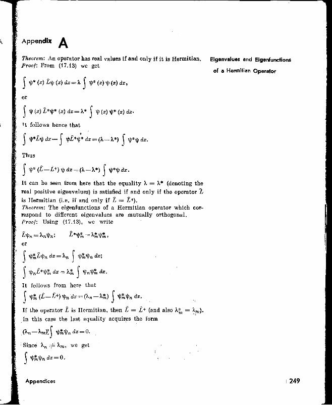
Appendix ATheorem: An operator has real values if and only if it is Hermitian.Proof: From (17.13) we get

JW* (x) LW (x) dx= I.. JW* (x) W(x) dx,

or

J'IjJ (x) L*W* (x) dx= 1..* JW(x) w* (x) dx.

! t follows hence that

Thus

JW*(L-£+)Wdx=(I..-I..*) JW*'ljJdx.

It can be seen from here that the equality')." = 1..* (denoting the

real positive eigenvalues) is satisfied if and only if the operator '1is Hermitian (Le. if and only if L = Lt).Theorem: The eigenfunctions of a Hermitian operator which cor­respond to different eigenvalues are mutually orthogonal.Proof: Using (17.13), we write

Eigenvalues and Eigenfundions

of a Hennitian Operator

, or

JW;LWn dx = I..n JW;Wn dx;

r ~ * * r *dJ WnL*Wm dx= I..m J WnWm x.

It follows from here that

JW; (L-L+) 'ljJndx = (I..n -I..;) JW;'ljJn dx.

If the operator L is Hermitian, then L = Lt (and also I..~ = I..m).

In this case the last equality acquires the form

(I..n-l..m}l)W~'ljJn dx=O.

'Since I..n 0#- I..m , we get

JW;Wn dx=O.

Appendices : 249

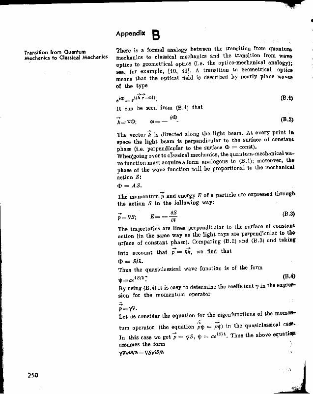
Transition from QuantumMechanics to Clll5sical Mechanics

•Appendix BThere is a formal analogy between the transition from quantummechanics to classical mechanics and the transition from waveoptics to geometrical optics (Le. the optico-mechanical analogy);see, for example, [10, 11]. A transition to geometrical opticsmeans that the optical field is described by nearly plane wavtBof the type

~

eie:tl = ei(k r-lilf).

It can be seen from (B .1) that

- a<Dk=V<D; 00=-

(B.t)

(B.2)

The vector k is directed along the light beam. At every point inspace the light beam is perpendicular to the surface of constantphase (Le. perpendicuYar to the surface <D = const).When:going over to classical mechanics, the quantum-mechanical wa­ve function must acquire a form analogous to (B.1); moreover, thephase of the wave function will be proportional to the mechanical

action S:

<D = AS.

The momentum -; and energy E of a particle are expressed throughthe action S in the following way:

;=VS;as

E=-­at(B.3)

250

The trajectories are lines perpendicular to the surface of constan\action (in the same way as the light rays are perpendicular to theurface of constant phase). Comparing (B.2) and (B.3) and taking- -into account that p = ftk, we find that

<D = SIn.Thus the quasiclassical wave function is of tlle form

'i'= aeiS/h~ (B••)

By using (B.4) it is easy to determine the coefficient y in the flxpree­sion for the momentum operator.;;.p=yV.Let us consider the equation for the eigenfunctions of the mome"

..; -tum operator (the equation P'i' = p'¢) in the quasiclassical caSll.

In this case we get -; = VS, 'i' = aeis/II. Thus the above equatiOP

assumes the formyVeiB/7a = VSlliS/'A

g

te Appendix C

251

(C.1)

~ ~

== (; X p) may he written in the form3 3

Ml= ~ ~ t'lm;:kPn,k_ln_l

Appendices

where e'kn is a unit antis~-mmetric tensor of tbe 3rd rank (e123 === e2S1 = eSl~ R: f, e132 = e321 = eU3 == -1, all the flther com­ponents of the tensor are equal to zero).

Let us consider the commutator [Mi' ;:j]' By using (C.1), we tanwnte thI!! commutator in the following form:

Mj, ~j]=M;;'j-~jMi== ~ ~ e'kn (~kPn~j-~J~llPn).11 n

We shall show how the commutation relations (20.28)-(20.30) can Commutation Relation~

he derived. To start with we remark that the equahty M=

It can be easily seen that iy/1i = 1, and, consequently, '\' = -in.The quasiclassical case may he used to substantiate the Schrodingerequation. It can be easily seen that the well-known classical Ha­milton-Iacobi equation

~+-!.- (VS)2+U=0at 2m

s a limiting case of the Schrodinger equation (20.17). By putting'I' = eiS/,.. we get in this case

tl! .!.... 'I'=_~ is/~.at at e ,

_ 21!2 A'I'= - 21!2 V,(V'I')=_~m m 2m

XV (.!:.... VS.eiS/,.) = -i2- AS.eiS/~+~(VS)! eiS/h.I! 2m 2m~

Substituting these results intEl (20.17) and neglecting terms con­taiDlng Planck's constant in thu expression for A'I', we get theequatiEln

_~ eiS/,.,;;;-!.- (VS)! eiS/~+UeiS/,..at 2m

By cancelling out the factor eiS/,.. this equation becomes the Ha­milton-Iacohi equation.

.,yeiS/f,VS .!...=VS.eiS/~.

n

)

)

eI

}

t

•Taking into account that ;ik = ~rj, we get

[Mi, ;/]= L} L} eiknrk lPn' r/l.k n

According to (20.26), [Pn' rjl = -iMn/• This leads to the requiredrelation (20.28):

[Mi, ;j]= -iii L} eiklrk=ili L} eijk;k.k k

This relation means that

[M l' r2]= i1i;3'

1M2' ;31 = ilir1 ,

1M3' ;1] = ilir2 ,

[M 1 , ;11 = [M 2 , ~I = [M 3 , r~] =0.

Next let us consider the commutator [Mi , .oj]' By using (C. i), oNecan write it in the form

{Mi, Pj]= L} L} eikn(;kPnPJ-PI;kPn).k n

Taking into account that PnPj = i/Pn' we get

[Mi' Pj] = L} L} eikn [;k, PI] Pn.k n

According to (20.26), Irk' pj] = iMkj. As a result, we get therequired relation (20.29):

[Mi' .0/]= iii L} eijnPn.n

Thus

[M l' .02] = iliP3'

[M2, p3]=iliPi'

1M3' P1] = iliP2'[M1, pd=[M2, p2]=[M3, .03]=0.Going over to the commutator [Mi , Mj ], we shall restrict ourselvesfor simplicity to the case when i = i, j = 2. Using

we can write

1Ml' M2] = (;2P3 -;3P2) (r3PI-rIP3)-(r8PI-rIP3)

X ( r 2P3 -~r3~P2) = ~r;;'3r3P1 - r2],3rIP3 -;.3pi8pr

+r3P2 ;lP3-r3PI ;:2P3 +r3.o1;3 P2 + rlP3 ;:2P3-rIP8r8P2.

Note that ~P3;:l.o3 = r~P3i;,P3 and ;:3P2;:3Pf = r3P1".;;I·

____J

Legendre Polynomials: The Legendre polynomials PI (x) may be Some Special Functionsdefined as the coefficients in the expansion of the functionH(x, t)==(1+tS _2tx)-I/S, I t I < 1

as a power series in t:

By taking this into account, we write the expression for [M I M21:

[Ml' M 21 = 6:2Pa;:aPl-~aPI ~2Pa) + (~aP2~IPa-~IPa;:aP2)

= r2Pi (Para- raPa) + ~IP2 (;:3Pa- Pa ;a).Since iaPa - p';ia = iii, we finally obtain

[MI' M2]= iii fr;P2~r;Pl)= iliMa •

Proceeding in the same way, it can be easily seen that

[M2, M al==iliMl ,

[Ms. M1]==iliM2.

All these results can be combined in the relation (20.30).

Appendix 0Let us consider the case when i == 1:

[M2, M~(1l1f+M~+Mi) M 1-M1 (Mi+M~+M~)

==(M~+M~rMI-MI (1I:1~+M~)

== M 2MSMi--rMaMsM1-M 1M 2M 2-M 1M aMa= (M sM1M s-iliM2M;)+- (1';{aM1M a+ i!iMaM2)

-(MsMiMs+iliM;Ms)--(MaMIMa-inM2Ma)==0.

Similarly, we get [MS, MsI == 0 and [MS, Mal == O. This provesthe relation (20.31).

Appendix E

00

(1+tS -2tx>-IJ2== ~ PI (x) tn (E.1)1=0

(-1 :;;;:; x :;;;:; 1, 1 is a non-negative integer).The polynomials P I (x) are the solutions of the differential equation(1-x2)yM-2xy'+l(l+1)y==0, (l==O, 1, 2, ... ) (E.2)

and satisfy the condition y (1) = 1. They can be written in theform

1 d lPI (x)==- - [(x2-1)l]. (E.3)

2111 dx l

Appendices

A SCommutation of Operators M

and Mi

25)

,We note that

Pz(1) = 1. PZ(-x)=(-1)lPz(x),

Po(x)=1,

Pdx)=x,

1P 2 (x) ="2 (3x2 -1),

1P a (x) ="2 (5x 3 -3x),

.. . .. .. .. ..

1

~

t

The Legendre polynomials are orthonormalized:

1

JPz(x)Pz,(x)dx= 2/~1 {ill"

-1

The basic recurrence relations are

(E.4)

254

(/+ 1) P Z+1+ IPZ-1-x (2/+ 1) P z= 0,

PZ-P;+1- P ;_1 +2xP;=0,

P;+l-P;-l = (2/+ 1) Pz.

A ssociated Legendre Functions: The associated Legendre functions

Pf! (x) are defined through the Legendre polynomials P I (x) in thefollowing way:

dmPi (x) = (1_x2)m/2 dxm P z (x) (E.5)

(m and 1 are positive integers, m ~ I),

PY (x) = Pz(x); Piex) = 3 X 5 X 7 '" (2/-1)(1_x2)1/2.

Pt (x) = (1-x2) 1/2,

P~ (x)=3x(1_x2)1/2,

Pi (x)=3(1-x2),................................The functions Pf! (x) satisfy the differential equation

(1-x2)Y"-2xY'+[/(I+1)-1 m:2 ]y=0. (E.6)

They are orthonormalized:1

r P'{' (x) P'{': (x) dx = _2_ (l+m)! (ill" (E.7)J 2/+1 (l-m)!-1

The basic recurrence relations are

(21+ 1) xP'{' (x) = (1- m+ 1) Plt1 (x) +(l+ m) P~l (x),

Pf+i1 (x)-P¥:11 (x)=(21+1) V 1- X2 P'l' (x).

(E.9)

(E.10)

Harmonic Functions. The harmonic function Y lm (8, 11') is definedas the product of the Legendre associated function pllm I~(cos 8) andthe function exp (im<p):

Ylm

(8 11')= Vr~2l""'+-1:-(:-:-l----;-I--:-ml '"'")1 Plm, (cos 8) eimql (E.8), 4l't(l+l m l)1

(l is a non-negative integer, m = 0, ±1, ±2, ..., ±l, 8 and 'Pare angular coordinates, °~ e~ l't, 0 ~ 'P ~ 2l't). Expressionsfor the first few harmonic functions are given in Sec. 21 (see (21.26».The harmonic functions satisfy the differential equation

dslPy+l (l+1) y=O,

where1 {fA 1 a(. a)

AslP = sin2 8 ali" +sin 8 00 Slll8 ae .

The spherical functions are orthonormalized:2n n CJ)Yr", (8, 11') Yl'm' (8, 11') sin 8 d8 d<p = all' I'lmm"() 0

Hermite Polynomials. The Hermite polynomials HfI, (x) may bedefined as expansion coefficients of the function exp (2xt - t2

):

00

tnexp(2xt-t2 )= ~ Hn(x)-

LJ nl11.=0

(-00 < x < 00, n is a non-negative integer).Hermite polynomials are described by the expression:

H n (x) = (_1)ne X2 ~ e-x2dxn •

H n (_x)=(-1)nHn (x).

H o (x)= 1,

Hdx)=2x,

H 2 (x)=4x2 -2,

H s (x)=8xs-12x,

(E.H)

(E.12)

The polynomials Hn (x) satisfy the differential equation

y" -2xy' +2ny=0 (n=O, 1, 2, •.• ). (E.13)

They are orthonormalized:00

~ H 11. (x) H 11.' (x) e-x2 dx = ·Vi.2nnl ann' •

.........

-00

The basic recurrence relations

2xH11. -2nHn-l = H 11.+1'

2nHn_l=H~.

A.ppendices

are

(E.14)

255

•Modified Hermite Polynomials. (Hermite-Gauss Polynomials). TheHermite-Gauss polynomials hn (x) are defined in terms of theHermite polynomials Hn (x) by the formula

(E.15)

The condition of orthonormalization for them has the form

CO)J hn (x) hn , (x) dx=l5nn ,.

-00

These polynomials satisfy the differential equation

Appendix F

(E.16)

(E.17)

Linear Harmonic Oscillators By taking (22.1) into account, we can write Schriidinger's equationfor the oscillator:

(F .1)

We introduce the notation

~=x ymw/n, 'J..=2E/nw.

In the new notation, (F1) acquires the form

(F.2)

256

The differential equation for Hermite-Gauss polynomials is of thesame form (see (E.17». Moreover, 'J.. = 2n + 1 and, consequently.

E=nw (n+ ~ ), n=O, 1, 2, ....

The wave function CPn (6) is apart from a constant factor a Hermite­Gauss polynomial:

CPn (~)= Chn m·The factor C is determined from the normalization condition forthe wave function CPn (x):

00J cpA (x) dx= 1--00

Taking (E.16) into account we conclude that'" /" Ii C2 = 1 and,V mro

consequently, C = Vmro/Ii. Thus we arrive at the relation (22.3)

-00-00

Thus

00 00

1 = j <p~ (x) dx = J<p~ (6) :~ ds-00 -00

The

Per­by

t. V. A. Fock.

2. Willis E. Lamb, Jr.

3. R. P. Feynman.R. B. Leighton. M. Sands.

4. R. P. Feynmanand A. R. Hibbs.

5. N. Bohr.

6. N. Bohr.

7. V. A. Fock.

8. W. Pauli.

9. P. A. M. Dirac.

to. L. D. Landauand E. M. Lifshitz.

H. D. 1. Blokhintsev.

t2. E. Fermi.

13. L. 1. Schiff.

14. M. Born.

i5. P. S. de Laplace.

i 6. P. Langevin.

17. 1. V. Savelyev.

258

References

On the Interpretation of Quant.um Mechanics. Czecho,lolHlh lour""of Physics. 7 (1957), 643-656

An Operational Interpretation of Nonrelativistic Quantum Mechan­ics. Phys. Today. 22 (1969), 23-28

The Feynman Lecture' all Physics. Vol. 3, Quantum Mechanics.Adison-Wesley, Reading, Mass. 1965

Quantum Mechanics and Path Integrals. McGraw-Hill, N.Y.,1965

Atomic Physic, and Human Knowledge. Wiley, N.Y., 1958

Essays 1958--1962 on Atomic Physics and Human Knowledge.Interscience. N. Y., 1963

Fundamentals of Quantum Mechanics. Mir Publishers, Moscow,1978 (Translated from the Russian by Eugene Yankovsky)

Die allgemeinen Prinzipen der Wellenmechanik. In Handbuchder Physik (H. Geiger and K. Scheel, Eds.) (2nd edition) VoTe 24,83-272

The Principles of Quantum Mechanics (4th edition). Oxford,Clarendon Press, 1958

Quantum Mechanics (Non-relativistic Theory) (3rd Edition).gamon Press, Oxford, 1977 (Translated from the RussianJ. B. Sykes and J. S. Bell)

Principles of Quantum Mechanics. D. Reidel Publishinll Co., Dord­recht. 1964. (Translated from the Russian by J. B. Sykes andM. J. Kearsley)

Notes on QlUtntum Mechanics. The University of Chicago Press,Chicago, 1961

Quantum Mechanics (3rd. Edition). McGraw-Hill, N.Y.• 1968

Physics in My Generation: A Selection of Papers. Pergamon Press,London, 1956

A Philosoph'cal ESlay on Probabilities. Dover, N.Y.• 1952

La Notion de Corpuscle et d'Atome. Herman, Paris, 1934

General Physics, Vol. 3. Mir Publishers, Moscow (To be published)

,

18. L. Rosenfeldand E. Riidingu.

19. N. Bohr.

20. W. Heisenberg.

~L W. Heisenberg.

22. V. S. Vavilov.

23. L. de Broglie.

24. L. V. Tarasov.

25. D. Bohm.

26. L. N. Cooper.

27. G. Y. Myakishev.

28. D. Bohm.

29. S. I. Vavilov.

30. G. L. Trigg.

31. Y. M. Helfer,V. L. Lyuboshitz,M. I. Podgoretsky.

32. D. I. Blokhintsev.

33. N. Bohr.

34.

35.S. Fliigge.

References

"The Decisive Years 1911-1918". In Niels Bohr: His Life. and Workas Seen by His Friends and Colleagues (S. Rozental, Ed.). North­Holland, Amsterdam, 1968 (second printing). Translated from theDanish by R. Gosney and J. E. Hooper

"Reminiscences of the founder of nuclear soience and of somedevelopments based on his work" (The Rutherford MemorialLecture, 1958). Proc. Phys. Soc., 78 (1961), 1083-1115

Die Planckische Entdeckung und die philosophischen Grunds­fragen der Atomlehre. N aturwissenschaften, 45 (1958), 227-234

The Physical Principles of the Quantum Theory. The Universityof Chicago Press, Chicago, 1930 (Translated from the German)

The Effect of Radiation on Semiconductors (in Russian). Fizmatgiz,Moscow, 1963

Introduction a l'Etude de La Mechanique Ondulatoire. Hermann,Paris, 1930

"The Wavelength of an electron in a potential well" in Physics,issue 2, Vysshaya Shkola, Moscow, 1972 (in Russian)

Causality and Chance in Modern Physics. Van Nostrand, N.Y.,1957

An Introduction to the Meaning and Structure of Physics. Harperand Row, N.Y., 1968

Dynamic and Statistical Laws: in Physics. Nauka, Moscow, 1973(in Russian)

Quantum Theory. Prentice-Hall, N.Y., 1951

Lenin and Modern Physics. Nauka, Moscow, 1970 (in Russian)

Crucial Experiments in Modern Physics. Van Nostrand, N.Y.1971

Gibbs' Paradox and Identity in Quantum Mechanics. Nauka, Moscow,1975 (in Russian)

The Philosophy of Quantum Mechanics. Reidel, Dordrecht, 1968(Translated from the Russian)

"On the Notions of Causality and Complementarity." Dialectica,2(1948), 312-319

Selected Problems in Quantum Mechanics (de Ter Haar, Ed.). Aca­demic Press, N.Y., 1965

Practical Quantum M.echanics, Vols. 1 and 2. Springer, Berlin,1971

259

36. V. 1. Smirnov

37. N. N. Lebedev.

38. L. D. Landau.E. M. Lifshitz.

39. J. M. Ziman.

40. H. Jones.

41. L. V. Tarasov.

42. E. P. Wigner.

43. V. I. Lenin.

44. M. Planck.

45. A. Einstein.

46. M. Planck.

47. U. I. Frankfurt,A. M. Franc.

48. N. Bohr.

49.

50. M. I. Podgretsky.

260

A Course of Higher Mathematics, Vol.3,lPart 2. Pergamon Press.Oxford. 1954

Speeial Functions and Their Applicattons. Prentice-Hall, N.Y.,1965 (Translated from the Russian)

The Classical Theory of Fields (4th edition). Pergamon Press.Oxford, 1975 (Translated from the Russian by M. Hamermeshi

Principles of the Theory of Solids (2nd edition). Cambridge Univer­sity Press, London, 1972

The Theory of Brillouin Zones and Electronic States in Crystals.North-Holland, Amsterdam, 1960

Physical Foundations of Quantum Electronics. Sov. Radio, Moscow.1976 (in Russian)

Symmetries and Reflections. Indiana University Press, Bloomington­London, 1970

"Materialism and empiriocriticism". In Collected Works. Vol. 14.pp. 15-361 Progress Publishers, Moscow, 1972 (Translated fromthe Russian by A. Fineberg)

"The origin and development of the quantum theory" in A Surveyof Physics: A collection of Lectures and Essays by Max Planck.E. P. Dutton and Co., N.Y. (Translated from the German byR. Jones and D. H. Williams)

"Autobiographical notes" in A lbert Einstein: Philosopher-Scientist.Tudor Publishing Co., N.Y., 1951

"Uber die Abhandlungen zur Wellenmechanik von Erwin Schriidin­ger".l Deutsche Literaturzeitung, N.F., 1928, No.5, 59-62

The Origin of Quantum Theory. Nauka, Moscow, 1975 (in Russian)

The Solvay Meetings and the De~'elopment of Quantum Physic,(Address at the 12th Solvay Meeting). Interscience, N.Y., 1962

Theoretical Physics in the Twentieth Century-A Memorial Volumeto W. Pauli. M. Fierz, N. F. WeiBSkoph (Editors), Cambridge.1960

"Planck's constant Ii and the complementarity principle" in Com­plementarity Principle and Materialistic Dialectics. Nauka, Moscow,1976 (in Russian)

Subject Index

Adiabatic approximation, 211Ammonia molecule, 124

lin an electric field, 130Amplitude,

interference of, 81probability density, 139rule of addition, 81state, 98, 106

basic equation, 105variation with time, 127

transition probability, 10, 79,80, 84

Analyzer, 107ffApproximation,

adiabatic, 211fone-electron, 212f

Atomic states, 27Average energy, 175

Balmer series, 26, 241Barionic charge, 23Black body radiation, 26, 241Bloch functions, 214, 222fBohr's,

frequency condition, 27model of hydrogen atom, 27orbit, 50theory, 50, 244

Bose-Einstein statistics, 247Bosons, 20f, 90Brillouin zones, 220f

Causality in quantum mechan-ics, 117ff

Chance, 57Classical determinism, 12Coefficient,

reflection at a barrier, 207transmission through a bar­

rier, 207Combination principle, Ritz,

26, 28, 241Commutation of operators, 188,

253Commutation relations, 251Complementary principle, 152Complete set of 'quantities, 38ffCompton's effect, 31Continuity equation, 203, 204Coordinate representation, 10,

139 'Corpuscule(s), . 49

Subjed Index

de Broglie's,equation, 32hypothesis, 32wavelength, 37, 50

Degeneracy, 210energy levels, 210

removal of, 211transposition, 227

Degrees of freedom, 39Delta function, Dirac's, 140Detector, 109, 112Discreteness, 143Distinguishability, 81, 87, 147

partial, 87, 100, 148Duality, 9, 143

Ehrenfest's theorem, 194Eigenfunction(s) ,

condition of normalization,141

operator, 164, 185Eigenvalue(s),

degenerate, 164Elastic collisions, 77Electron,

cloud, 53diffraction, 32in an atom, 53in a magnetic field, 131ff, 136in a periodic field, 220ff

Elementary particle(s),electrons, 53hadrons, 18leptons, 18photons, 18

Emission of light,induced, 92spontaneous, 92

Energy,bands, 220levels, 25matrix (see Hamiltonian mat­

rix)

Fermions, 20f, 90Feynman's,

diagrams 59f, 232path integrals, 95f'

Franz-Keldysh effect, 44

Generalized Laguerre's poly­nomials, 209

Hadrons, 18Hamiltonian, 177, 208

of a crystal, 211adiabatic approximation,

211one-electron approxima­

tion, 212of a hydrogen atom, 209

eigenfunctions of, 209eigenvalues of, 209

of interaction of an electronwith radiation, 214

matrix, 10, 122, 146change of basic states of,

146diagonalization of, 128for an electron in a magne­

tic field, 131role of non-diagonal ele­

ments of, 129in momentum representation,

186eigenfunctions of, 186eigenvalues of, 186

Iof an oscillator, 208Harmonic functions, 255Hermite polynomials, 209, 255Hermitian operator,

basic properties of, 179in eigen representation, 249

Hydrogen atom, 209Bohr's model of, 27, 42rigorous theory, 43, 55

Hypothesis,de Broglie's, 32Planck's, 26

Identity of microparticles, 56Indistinguishability, 56, 81, 86,

87fInduced emission probability,

92Instability of microparticles, 20

lifetime, 20Integrals of motion, 24Interconversion of micropar­

ticles, 21

261

Interference of microparticles,84

destruction of, 85Interference of probability am-

plitude, 10, 84ff, 144bosons and fermions, 90destruction of, 82scattering of microparticles,

87superposition of states, 103

Interference in quantum me­chanics, 149f

Interferometer, 69

Kernel of an operator, 163Kronig-Penny potential, 223

Law(s) of conservation, 23of angular momentum. 23of barionic charge, 123of electric charge, 23of energy, 23of momentum, 23

Legendre's,associated functions, 192polynomials, 192, 209, 253

Leptons, 18Line spectrum, 25Linear harmonic oscillator(s),

208, 256Lyman's series, 26, 241

Mass defect, 18Mean value of a physioal quan­

tity, 181time variation of, 182

Measluement in quantum me-chanics, 106ff

role of an analyzer, 108role of a detector, 112speaific properties of, 110

Microparticle, 8, 49ff, 60basic properties of, 18ffin an interferometer, 69, 72in a potential well with~ infi-

. nitely high walls, 196probability of momentum

values, 218in a potential well with walls

of finite height, 197in a spherically symmetric

field, 201virtual, 58

Model representation, 51ft, 63ftMomentum, 28

orbital. 29spin, 29

262

Necessity, 57

One-electron approximation,212

Operator(s), 105, 163commutator, 170complex conjugate, 163conjugate, 164coordinate, 184

in momentum representa-tion, 215

eigenfunctions, 164, 185, 191energy (Hamiltonian), 176fHermitian (self-adjoint), 164,

178properties of, 165

inversion, 190linear, 163

theory of, 162matrix of, 163momentum, 184

eigenfunctions, 191in momentum representa­

tion, 215projection of angular momen­

tum, 187eigenfunctions of, 191eigenvalues of, 191

in quantum mechanics, 177spectrum of eigenvalues, 164square of angular momentum,

187eigenfunctions of, 191eigenvalues of, 191

transposed, 163unitary, 164

transi tion from one repre­sentation to another,168

Paschen's series, 26, 241Passage of a micropartlcle over

a potential barrier, 205Passage of a microparticle under

a potential barrier, 205Passage of photvns thrvugh a

polarizer, 75ffPauli's

exclusion principle, 20, 247spin matrices, 138

Perturbation method, 230ffPhotons, 18, 31Planck's constant, 19, 27, 32

role in quantum mechanics,33

Pelarization,of a photen, 39, 76of a vacuum, 60

Principle,cembination, Ritz, 26complementarity, 152correspondence, 244.microscopic reversibility, 93Pauli's exclusion, 20, 247superposition of states, 10

40, 96ff, 106, 140, 228YProbability, 54

density, 54in quantum mechanics, 54.

57, 147Projection amplitudes, 133, 134

Quanta, 26Quantization, 9, 25

of angular morrentum, 28fQuantum numlJeJ(s), 29, 39, 53

magnetic, 29, 39orbital, 29, 39principal, 29spin, 29, 39

Quantum transitions, 25, 22Sanomalies of, 29computation of probability

228ff

Reduction of a wave packet, 34Representation, 166

coordinate, 10, 142, 184Dirac's, 10energy, 229Heisenberg, 10, 233, 234, 235interaction, 233, 235momentum, 142Schrodinger's, 10, 233f, 235transition from coordinate to

momentum, 10, 215,219

Resonances, 20Rest mass, 18Reyleigh-leans law, 241Rydberg's constant, 26, 28

Scattering,of microparticles, 77of neutrons :by a crystal, 93

coherent, 94incoherent, 94

Schrodinger's equation, 186, 203application of, 195in energy representation, 229in momentum representatien,

217time dependent, 187

hydrodynamic analogy, 203Spatial parity, 39, 40, 190

and angtllar lDomentuID, 193

*r,\

Special functions, 209, 253Spectral terms, 26Spectrum,

descrete, 27line, 25

Spherical functions, 192, 201£,209

Spin, 18electron, precession of, 134

Spontaneous emission probabi­lity, 92

Stark's effect, 211States of a microparticle,

basic, 101, 146, 171condition of orthonormali-

zation of, 102mutually independent, 100mutually orthogonal, 100, 148stationary, 27, 125transition from"one system to

another, 129, 171Statistical ensemble, 120Statistical nature of quantum

mechanics, 120fSuperposition of states, 96ff, 106

destruction in the process ofmeasurements, 109

passage of photons throughpolarizers, 102

total and partial distingui­shability, 100

quantum transitions, 98f, 228frole of analyzer, 108

Superpositiovn of statestransition from one repre­

sentation to another,229

Transition amplitudes, rule ofaddition, 81

Transition probability, 79, 230,232

amplitude, 79ff, 84ftproduct, 80sum, 80

Transmission coefficient of abarrier, 207

Tunneling effect, 48f

Uncertainty relations, 9, 34ff,247

diffraction of microparticles,37

evaluation of absorption edge,44

evaluation of ground-stateenergy of hydrogenatom, 42

evaluation of zero-point oscil­lations, 44

trajectory of a microparticle,46

Unitary invariance, 1839f commutation relations, 213

Unitary invariants, 169Universal dynamic variables, 23

Vector analogy, 174, 237Vector,

of probability flow density,205

of state, 136ffwave, 33

Virtual microparticle, 58Virtual transitions, 41, 58

Wave function, 138, 139, 245of an electron in a crystal

(Bloch function), 223of a freely moving micro­particle, 141

Wave packet, 34ff, 51Wave-particle duality, 25, 30ff,

34, 52Wave, pilot, 51Wave vector, 33Wien's law, 241

Young's experiments, 69

Zero-point oscillations, 44Zeeman's effect, 211

TO tHE READER

Mir\'..ublishers welcome your comments on the content, translationand. esign of this book.We' ould also be pleased to receive any proposals you care tomaktf about our future 'publications.

Our i address is:

Mir Publishers2 Pervy Rizhsky PereulokX-HO, GSP, Moscow, 129820 USSR,

Prtnted tn the Unton of Sovtet SodaU" Republics

l to

~lIcs

1~I

,..J..tllh.za··...'. 1

II

\I .,

I' \

.:~ j::..Ii ..II

~llli

ExVLj

--,.

Ex Libris .

Amit Dhakulkar

'.

Klan Nosferatu

Date: III 'I Z-ODD

. '

T~is book ,ives a detailed and systematic exposition 01tlie lund.mentals 01 non-relativistic quantum mechanicsIOI'-th--"o are not acquainted with the subject. Thecharacter of the physics 01 microparficles and the problems01 the physics 01 microphenomena (interference 01amplitudes, the principle 01 superposition. the specificnature 01 measuring processes, causality in quantummechanics) are considered on the basis 01 concepts aboutprobability amplitudes. Besides, the quantum-mechanicalsystems-microparficles-wilh two basic states areanalyzed in detaif. The apparatus 01 quantum mechanicsis considered as a synthesis 01 concepts about physicsand the theory of linear operators. A number of speciallyworked out problems and examples have been includedin order to demonstrate the working 01 the apparatus.This book is meant lor use by students 01 engineering andteachers-training institutes. It may also be used byengineers 01 different profiles.

•

Our address:USSR.129820.Moscow 1-110. GSPPervy Rlzhsky Pt*euk>k,2MIR PUBLISHERS

•