Magnetic induction at 60 Hz in the human heart: a comparison between the in situ and isolated scenarios

Magnetic Induction at 60 Hz in theHuman Heart: A Comparison Between

the In Situ and Isolated Scenarios

Trevor W. Dawson,* Kryz Caputa, and Maria A. Stuchly

Department of Electrical & Computer Engineering, University of Victoria,Victoria, B.C., Canada

Numerical modelling is used to estimate the electric fields and currents induced in the human heart andassociated major blood vessels by 60 Hz external magnetic fields. The modelling is accomplished usinga scalar-potential finite-difference code applied to a 3.6-mm resolution voxel-based model of the wholehuman body. The main goal of the present work is a comparison between the induced field levels in theheart located in situ and in isolation. This information is of value in assessing any health risks due to suchfields, given that some existing protection standards consider the heart as an isolated conducting body. Itis shown that the field levels differ significantly between these two scenarios. Consequently, data frommore realistic and detailed numerical studies are required for the development of reliable standards.Bioelectromagnetics 20:233–243, 1999.© 1999 Wiley-Liss, Inc.

Key words: low-frequency magnetic induction; numerical modelling; induced electric fields;human heart dosimetry

INTRODUCTION

In various guidelines for human exposure to ex-tremely low frequency (ELF) electromagnetic fields, theinduced current density is used as a criterion for thederivation of acceptable limits for the external exposurefields. Limits for the induced current density in tissuesare based on well-established effects of excitable tissue(e.g., heart, brain) stimulation and other relatively strongfield effects [WHO, 1984, 1987, 1993]. However, theydo not account for the more recent weak field effects[e.g., Luben, 1991], because the latter have been neithersufficiently well-quantified nor established to be of prac-tical use for guideline development.

In attempts to relate the induced current density tothe external field strengths, various geometrically simpleconductors are often used to represent the human body orits parts. Typical examples are ellipsoids, spheroids,spheres, and either circular or elliptical loops. The elec-trical properties of such body models are generally as-sumed to be both homogeneous and isotropic. However,as indicated in a recent review [Bailey et al., 1997], quitedifferent magnetic flux limits are given in the variousguidelines, such as CENELEC [1995] (European Union),ICNIRP [1998], IRPA [1990], NRPB [1989, 1993](United Kingdom), DIN/VDE-89 [1989] (Germany), andACGIH [1991] (USA), despite their common reliance onan upper limit of 10 mA m22 for the induced current

density. In their rationale statements, the CENELEC,IRPA, ICNIRP, and NRPB standards aim for the protec-tion of cardiac and central nervous tissues. However, thesize of the circular loops (0.1–0.2 m radius) used in theseguidelines is more representative of the upper torso. TheDIN/VDE standard, on the other hand, explicitly modelsthe heart as a loop of 0.06-m radius. The rationale for theuse of the smaller loop size to represent the brain or theheart in protection standards is also elaborated by Bern-hardt [1988]. However, Reilly [1992], in the context ofmagnetic resonance imaging (MRI) safety (and moregenerally of magnetically induced fields and currents inthe heart), clearly recognizes the need to model the heartin situ.

Recent relevant developments include anatomicallycorrect, high-resolution voxel-based models of the hu-man body suitable for electromagnetic analyses, andeffective computer codes for calculating the associated

Contract grant sponsor: EPRI; Contract grant number: WO 2966-14.

*Correspondence to: Dr. Trevor W. Dawson, Department of Electricaland Computer Engineering, University of Victoria, P.O. Box 3055,Victoria, V8W 3P6 British Columbia, Canada.E-mail: [email protected]

Received for review 13 October 1997; Final revision received 26August 1998

© 1999 Wiley-Liss, Inc.

Bioelectromagnetics 20:233–243 (1999)

magnetic induction [Dawson and Stuchly, 1997; Dawsonet al., 1997]. Together, these facilitate a quantitativenumerical evaluation of the differences in modellingmagnetic induction in the human heart properly locatedwithin the body (in situ) and situated in isolation. Acomparison between these two scenarios is the subject ofthe present paper. The electric fields and current densi-ties, induced by uniform magnetic fields of three orthog-onal orientations, are modelled. The differences betweenthe resulting fields in the two scenarios are compared.The effects of modelling the heart as a sphere, or thebody as an ellipsoid, are also briefly considered.

METHODS

Full details concerning the body model used in thepresent calculations may be found elsewhere [Dawson etal., 1997]. Briefly, the model is a composite of head andtorso data obtained from Yale Medical School [Zubal etal., 1994], with legs and arms derived from the [U.S.National Library of Medicine, 1986–1997] Visible Hu-man Data Set. The body model contains a total of 1 736873 voxels with 3.6-mm edges and has a height andestimated weight of 1.77 m and 76 kg, respectively. Theorientation conventions direct thex-, y-, andz-axes fromleft-to-right, back-to-front, and foot-to-head, respec-tively. Conductivity values assigned to selected tissuesare derived from recently measured values [Gabriel et al.,1996] if available; otherwise, values from other pub-lished sources are used [Geddes and Baker, 1967;Stuchly and Stuchly, 1980; Foster and Schwan, 1989].

The heart model is extracted from the whole-bodyconductivity distribution using the minimal Cartesianparallelepiped box whose outer faces contact at least onevoxel coded as heart tissue. This bounding box spans 36voxels in thex-direction, and 32 voxels in each of they-and z-directions. It, therefore, measures 12.96 cm311.52 cm3 11.52 cm and represents a mean size of thebeating heart. Voxels coded as neither heart tissue norblood are discarded, resulting in a final heart modelconsisting of two homogeneous tissue groups. An ideal-ized view of the external surface is shown in Figure 1.The conductivities assigned to the blood and heart are0.7 Sm21 and 0.1 Sm21, respectively.

Although heart muscle conductivity is, in reality,anisotropic, the fibers are oriented diagonally in a varietyof directions. This level of detail is beyond the capabilityof the present modelling, and the chosen conductivity isa representative average value. Other small features, suchas the external membrane of the heart and the walls ofsmaller blood vessels cannot be resolved at the 3.6-mmresolution and are also neglected. These details do notsignificantly alter the bulk properties of tissues, andhence neither should they greatly affect the computed

dosimetry at this scale. These factors would, however,influence fields at a much finer scale than is consideredhere. The numerical modelling in this work uses thescalar potential finite difference method, which is de-scribed in detail elsewhere [Dawson et al., 1997].

RESULTS

Data Set Description

Data for both the in situ and isolated heart scenarioswere computed under separate excitation by 60 Hz, 1 mTuniform magnetic fields parallel to one of the Cartesianaxes. Although the data pertain to a 1 mTsource strength,they can be scaled linearly to other exposure levels ofinterest. The in situ electric field and conductivity datafor the heart are subsets of previously described whole-body data [Dawson et al., 1997]. They are extractedusing only those voxels common to the isolated heartmodel. The isolated heart data are computed separately,treating the isolated composite heart model as a separate,smaller, conducting body. The end result is data that arein one-to-one voxel-wise correspondence between thetwo heart models.

Global Field Comparisons

To quantify the differences between the two heartscenarios, three global scalar measures of electric field

Fig. 1. A smoothed view of the external surface of the voxel-based heart model.

234 Dawson et al.

amplitude are compared for the various tissue groups(heart, blood, and composite). These measures are theaverage, root mean square, and standard deviation,whose values for a vector fieldF are defined by

Avg$F% ;1

NO

i

|F i|, Rms$F% ; Î1

NO

i

|F i|2

and

Dev$F% ; Î 1

N 2 1 Oi

~|F i| 2 Avg$F%!2

3 S'ÎRms$F%2 2 Avg$F%2D .

The summation indexi ranges over allN voxels ineach particular tissue group. These measures can beinterpreted as low-order approximations to the corre-sponding volume averages. Figures 2 and 3 show thesemeasures for the electric field and current density mag-nitudes, respectively.

Field Distribution Comparisons

Figure 4 illustrates differences between the fieldsinduced in the in situ and isolated heart scenarios. It

Fig. 2. Average (top row), standard deviation (middle row), androot mean square (bottom row) values of the electric field (mil-livolts per meter) for the tissue groups in the two scenarios andunder three orthogonal excitation directions. The labels H and Brefer to the voxels coded as heart and blood respectively,whereas H 1 B refers to the composite heart model. The iso-lated and in situ cases are labelled as (iso) and (sit), respectively.All sources are 60 Hz at 1 mT. Bx, left-to-right; By, back-to-front; Bz, foot-to-head.

Fig. 3. Conventions as in Figure 2, but for the current densityamplitude (milliamperes per square meter).

Magnetic Induction in the Human Heart 235

shows the amplitudes of the electric field (top row) andcurrent density (bottom row) in a horizontal cross-sectionthrough the midplane of the 17th voxel layer from thebottom of the heart in isolation (left column) and in situ(right column). The source here is directed from left toright. The electric field patterns differ significantly be-tween the two scenarios, and the peak values in the in situcase are approximately a factor of 2 greater than in theisolated heart. In the bottom row, the presence of thehighly conducting blood makes the current density dis-tributions appear more similar between the two scenar-ios, but there still are obvious differences. Moreover, thepeak values indicated in the in situ case (lower right) areapproximately 2.5 times greater than the correspondingvalues for the isolated heart (lower left).

Figure 5 shows the analogous field amplitudes inthe same cross-section as Figure 4, but for the sourcevector directed from back to front. Again, the electricfield amplitude patterns (top row) differ significantlybetween the two scenarios, and the in situ values are

greater by approximately 33%. The current density pat-terns in the bottom row differ, but the peak values in thiscase are comparable.

Figure 6 pertains to a source vector directed fromfoot to head with respect to the body. The peak electricfield values are once again a factor of 2 greater in the insitu case. Significant differences persist in the currentdensity distributions, but with peak values differing byonly approximately 25%. More detailed data on the spa-tial distribution of the induced electric fields and currentsare given in the Appendix.

DISCUSSION

With reference to the electric field data of Figure 2,it is evident in all three measures that the isolated heartmodel somewhat resembles a sphere. Specifically, theinduced field levels in the composite tissue group showlittle variation across the three source orientations. Thisfinding is in marked contrast to the in situ case. Here, the

Fig. 4. Amplitudes of the electric field (top row) and currentdensity (bottom row) in a central horizontal cross-sectionthrough the heart in isolation (left column) and in situ (rightcolumn) under excitation by a 60 Hz, 1 mT source directed from

left-to-right with respect to the upright human body. Electricfield and current density units are millivolts per meter and mil-liamperes per square meter, respectively; note that the scalesfor the two heart model locations differ.

236 Dawson et al.

effects of the whole-body current distribution lead tosignificantly higher levels in all three measures, as wellas to a much greater dependence on source orientation.This finding is further quantified in Table 1, which givesnumerical values of the ratios of the various in situelectric field measures to their associated isolated values.These ratios range from a minimum of 1.24 (for thestandard deviation in the blood under back-to-front ex-citation) to a maximum of 3.07 (for the standard devia-tion in the composite tissue under left-to-right excita-tion). It is also clear from this table that the ratios aremost typically in the range of 1.5–3 times greater for thein situ case.

The approximately spherical nature of the isolatedheart scenario remains apparent in the current densitymeasures of Figure 3, in that the various measures areagain relatively insensitive to field orientation. All mea-sures are higher for the in situ scenario, as the couplingbetween the heart and whole-body current flows becomesimportant. The degree of enhancement is quantified inTable 2, which gives the ratios of the various in situmeasures in the composite tissue group to their corre-sponding isolated values (the ratios for the blood and

heart are the same as those for the electric field in Table1, because each is modelled as a homogeneous conduc-tor). These ratios range from a minimum of 1.24 (for thestandard deviation in the blood under back-to-front ex-citation) to a maximum of 3.03 (for the average in theheart muscle under left-to-right excitation). As was thecase for the electric field measures, modelling the heart inisolation typically underestimates the induced currentlevels by a factor of 1.5–3.

For comparison with the isolated heart model re-sults, Table 3 gives the corresponding analytic values ofthese measures for the case of an isolated homogeneoussphere. The third column of this table gives specificvalues for a sphere of radius 0.06 m, as used in some ofthe standards. It may be noted that the half-widths of thebounding box containing the heart in the present modelare 0.0648 m, 0.0576 m, and 0.0576 m, and so roughlyconform to the approximate spherical model. These mea-sures can be compared directly with the composite heartvalues for the isolated scenario in Figure 2. There it isevident that the average, standard deviation, and root-mean-square values are approximately 6, 3, and 7 mV m21,as indicated in the final column of Table 3, roughly

Fig. 5. Conventions as in Figure 4, but for the source vector directed from back-to-front.


independent of source orientation. These values are inreasonable agreement with the analytical values given inTable 3. Thus, use of a spherical model of the heart isperhaps not inappropriate, if the goal is to model theheart in isolation. This is clearly not a good approxima-tion for the in situ case, however.

A further illustration of the need for accurate mod-elling is given in Table 4. This table gives the averageand maximum electric fields induced by three orthogonalmagnetic fields in the heart model in four scenarios.Cases (A) and (B), respectively, pertain to the isolatedand in situ scenarios already considered. Case (C) per-

Fig. 6. Conventions as in Figure 4, but for the source vector directed from foot-to-head.

TABLE 1. Ratios Between the In Situ and Isolated Values of the Various Scalar Measures for the Electric Field Magnitudes*

Tissue

Bx By Bz

Avg Dev Rms Avg Dev Rms Avg Dev Rms

Composite 2.83 3.07 2.89 1.72 2.23 1.86 1.83 2.46 1.98Blood 2.41 2.47 2.42 1.41 1.24 1.38 1.54 1.96 1.63Heart 3.03 2.98 3.02 1.84 2.38 1.94 1.92 2.76 2.03

*Bx, left-to-right; By, back-to-front;Bz, foot-to-head; Avg, average; Dev, standard deviation; Rms, root mean square.

TABLE 2. Ratios Between the In Situ and Isolated Values of the Various Scalar Measures for the Current Density Magnitudes*

Tissue

Bx By Bz

Avg Dev Rms Avg Dev Rms Avg Dev Rms

Composite 2.55 2.36 2.46 1.53 1.30 1.44 1.65 1.71 1.68

*Abbreviations as in Table 1.

238 Dawson et al.

tains to the geometry of the present heart model locatedin an ellipsoid (semiaxesa 5 0.325 m,b 5 0.155 m,c 5 0.125 m)fitted to the torso of the whole body modeland the whole modelled as a homogeneous conductor.Similarly, in case (D) the geometric heart model is situ-ated within a homogeneous ellipsoid (semiaxesa 50.878 m,b 5 0.155 m,c 5 0.125 m)fitted to thewhole body. The data in the latter two cases are com-puted using the analytic solution for low frequency mag-netic induction in an ellipsoid [Bailey et al., 1997]. Forcomparison purposes, row (E) of the table additionallycontains the peak values given by Reilly [1992] (scaledto 60 Hz after removal of an erroneous factor of 100) foran ellipsoidal torso (semiaxesa 5 0.40 m,b 5 0.20 m,c 5 0.17 m),corresponding to a larger man.

It is immediately evident from the average valuesthat the isolated heart model, as might be expected,predicts values that are far too small. The true off-centerlocation of the in situ heart within a larger conductor

gives rise to the observed higher induced fields. Conse-quently, as expected, the ellipsoidal models fare better. Infact, the average values under side-to-side (Bx) excita-tions are reasonable, in the ellipsoidal models of bothtorso and full-body. Similar comments apply to the foot-to-head (Bz) excitation, for which the values predictedusing the ellipsoidal models differ by about 10% fromthe values based on full-body numerical modeling. Theellipsoidal models are less satisfactory for front-to-backexcitation, for which the predicted values are from 25%to 57% in error. The deficiencies of the simple ellipsoidalmodels are even more apparent in the maximum electricfield values. The ellipsoidal models underpredict thepeak electric fields by 50–54%, 30–38%, and 41% fortheBx, By, andBzsource orientations, respectively. Thelarger values in the full-body results are due to the morerealistic treatment of the heterogeneous conductivity ofthe body.

The spatial distribution of the electric fields in theheart, and potential differences along specific paths, areamong the parameters that are responsible for cardiacstimulations [Reilly, 1992]. Similarly, these parametersaffect the potential for electromagnetic interference withimplanted cardiac pacemakers in workers under strongexposure fields. Thus, proper modeling of the heart insitu and as a heterogeneous object is essential for morereliable evaluation of the possible health hazard fromstrong magnetic fields.

CONCLUSIONS

A numerical dosimetric comparison has been pre-sented of 60 Hz magnetic induction in the human heartlocated in situ and in isolation. The identical heart modelhas been used in both scenarios. Being anatomically

TABLE 3. Comparison of Analytic Electric Field Measures in a Homogeneous SphericalApproximation With Numerical Values Obtained From the Voxel-Based Isolated Heart*

Measure Homogeneous sphere Heart (iso)

Avg{ E} 5 1

V*V |E| dV (3p/16)C 56.662 ' 6

Dev{E} 5 Î1

V*V ~|E| 2 Avg$E%!2 dV =2/5 2 (3p/16)2C 5 2.604 ' 3

Rms{E} 5 Î1

V*V |E|2 dV =2/5C 5 7.153 ' 7

*The first column defines the field measure, with its analytical value for a homogeneous sphere of radiusa (in meters) in an external field of strengthB0 (in Tesla) and frequencyf (in Hertz) given in the secondcolumn, where the constantC 5 pB0fa. The values in the third column (in millivolts per meter) pertainto the particular case of a sphere of radius 0.06 m in a 1 mT, 60 Hz magnetic field. The values in the finalcolumn are the corresponding approximate numerical values for the isolated heart model, read from the“H 1 B (iso)” portions of Figure 2. Abbreviations as in Table 1. (iso), isolated.

TABLE 4. Comparison of the Average (Columns 2–4) AndMaximum (Columns 5–7) Electric Fields (Millivolts per Meter)Induced by Three Orthogonal 60 Hz, 1 mT Magnetic Fields inthe Heart Model (A) in Isolation, (B) In Situ, (C) in an EllipsoidFitted to the Torso, and (D) in an Ellipsoid Fitted to the WholeBody*

Model

Eavg Emax

Bx By Bz Bx By Bz

(A) 5.4 5.8 6.0 33.6 27.7 20.5(B) 15.3 10.0 11.0 68.3 48.1 39.7(C) 15.4 15.7 10.0 31.2 29.8 23.6(D) 14.3 12.5 10.0 34.4 33.8 23.6(E) 46.0 32.4 32.8

*The maximum values in row (E) are taken from Reilly [1992] (scaledto 60 Hz).


derived, the model is realistic to within the limitations ofthe 3.6-m resolution. Using a variety of field measures, ithas been shown that the induced electric field and currentdensity levels are consistently about 1.5–3 times greaterfor the in situ case, for all orientations of the uniformmagnetic source fields. It has been further shown thateven more realistic models such as ellipsoidal represen-tations of the torso or body are inadequate to properlypredict the actual induced fields because of the geometriccomplexity and heterogeneous conductivity of the humanbody.

The numerical values presented pertain to 60 Hz,but they can be scaled to higher frequencies (up to about100 kHz), by multiplying the values presented by thefrequency and tissue conductivity ratios. The error result-ing from such scaling is estimated to be well below 5%.

Although based on a single geometric realization ofa particular human body model, the data presented indi-cate the need for highly realistic numerical modelling inthe development of viable protection standards for hu-man exposure to low-frequency magnetic fields. In par-ticular, it is clearly inadequate to base protection stan-dards on simple geometric models of critical human bodycomponents considered in isolation.

ACKNOWLEDGMENTS

The authors thank Drs. W. Bailey, D. Bracken, andR. Kavet for their stimulating discussions and helpfulsuggestions during the course of the project.

REFERENCES

American Conference of Governmental Industrial Hygienists. 1991. Doc-umentation for sub-radiofrequency and static electric fields. Cin-cinnati OH: ACGIH.

Bailey WH, Su SH, Bracken TD, Kavet R. 1997. Summary and evaluationof guidelines for occupational exposure to power frequency electricand magnetic fields. Health Phys 73:433–453.

Bernhardt JH. 1988. The establishment of frequency dependent limits forelectric and magnetic fields and evaluation of indirect effects.Radiat Environ Biophys 27:1–27.

Comit’e Europ’een de Normalisation Electrotechnique. 1995. Human ex-posure to electromagnetic fields, low frequency (0 Hz to 10 kHz.CENELEC Standard ENV 50166-1.

Dawson TW, Stuchly MA. 1997. An analytic solution for verification ofcomputer models for low-frequency magnetic induction. Radio Sci32:343–368.

Dawson TW, Caputa K, Stuchly MA. 1997. Influence of human modelresolution on computed currents induced in organs by 60-Hz mag-netic fields. Bioelectromagnetics 18:478–490.

Deutsches Institut fu¨r Normung-Verband Deutscher Elektrotechniker.1989. Safety at electromagnetic fields: limits of field strengths forthe protection of persons in the frequency range from 0 to 30 kHz.DIN VDE 0848-4.

Foster KR, Schwan HP. 1989. Dielectric properties of tissues and biolog-ical materials: a critical review. CRC Crit Rev Biomed Eng 17:25–104.

Gabriel S, Lau RW, Gabriel C. 1996. The dielectric properties of biologicaltissues: II. Measurements in the frequency range 10 Hz to 20 GHz.Phys Med Biol 41:2251–2269.

Geddes LA, Baker LE. 1967. The specific resistance of biological materi-als: a compendium of data the biomedical engineer and physiolo-gist. Med Biol Eng 5:271–291.

International Commission on Non-Ionizing Radiation Protection. 1998.Guidelines for limiting exposure to time-varying electric, magneticand electromagnetic fields (up to 300 GHz). Health Phys 74:494–522.

International Non-ionizing Radiation Committee of the International Ra-diation Protection Association. 1990. Interim guidelines on limitsof exposure to 50/60-Hz electric and magnetic fields. Health Phys58:113–122.

Luben RA. 1991. Effects of low-energy electromagnetic fields (pulsed anddc) on membrane transduction processes in biological systems.Health Phys 61:15–28.

National Radiological Protection Board. 1989. Guidance as to restrictionson exposures to time varying electromagnetic fields and the 1988recommendations of the International Nonionizing Radiation Com-mittee. Her Majesty’s Stationery Office: Chilton, Didcot.

National Radiological Protection Board. 1993. Restrictions on humanexposure to static and time varying electromagnetic fields andradiation: scientific basis and recommendation for implementationof the board’s statement. Documents of the NRPB 4:8–69.

Reilly JP. 1992. Electrical stimulation and electropathology. New York:Cambridge University Press.

Stuchly MA, Stuchly SS. 1980. Dielectric properties of biological sub-stances tabulated. J Microw Power 15:19–26.

U.S. National Library of Medicine. 1986–1998. http://www.nlm.nih.gov/research/visible/visible_human.html.

World Health Organization. 1984. Environmental health criteria 35: ex-tremely low frequency (ELF) fields. Geneva: WHO.

World Health Organization. 1987. Environmental health criteria 69: mag-netic fields. experimental data on the biological effects of staticmagnetic fields. Geneva: WHO.

World Health Organization. 1993. Environmental health criteria 137, elec-tromagnetic fields (300 Hz to 300 GHz). Geneva: WHO.

Zubal IG, Harrell CR, Smith EO, Rattner Z, Gindi GR, Hoffer PH. 1994.Computerized three dimensional segmented human anatomy. PhysMed Biol 21:299–302.

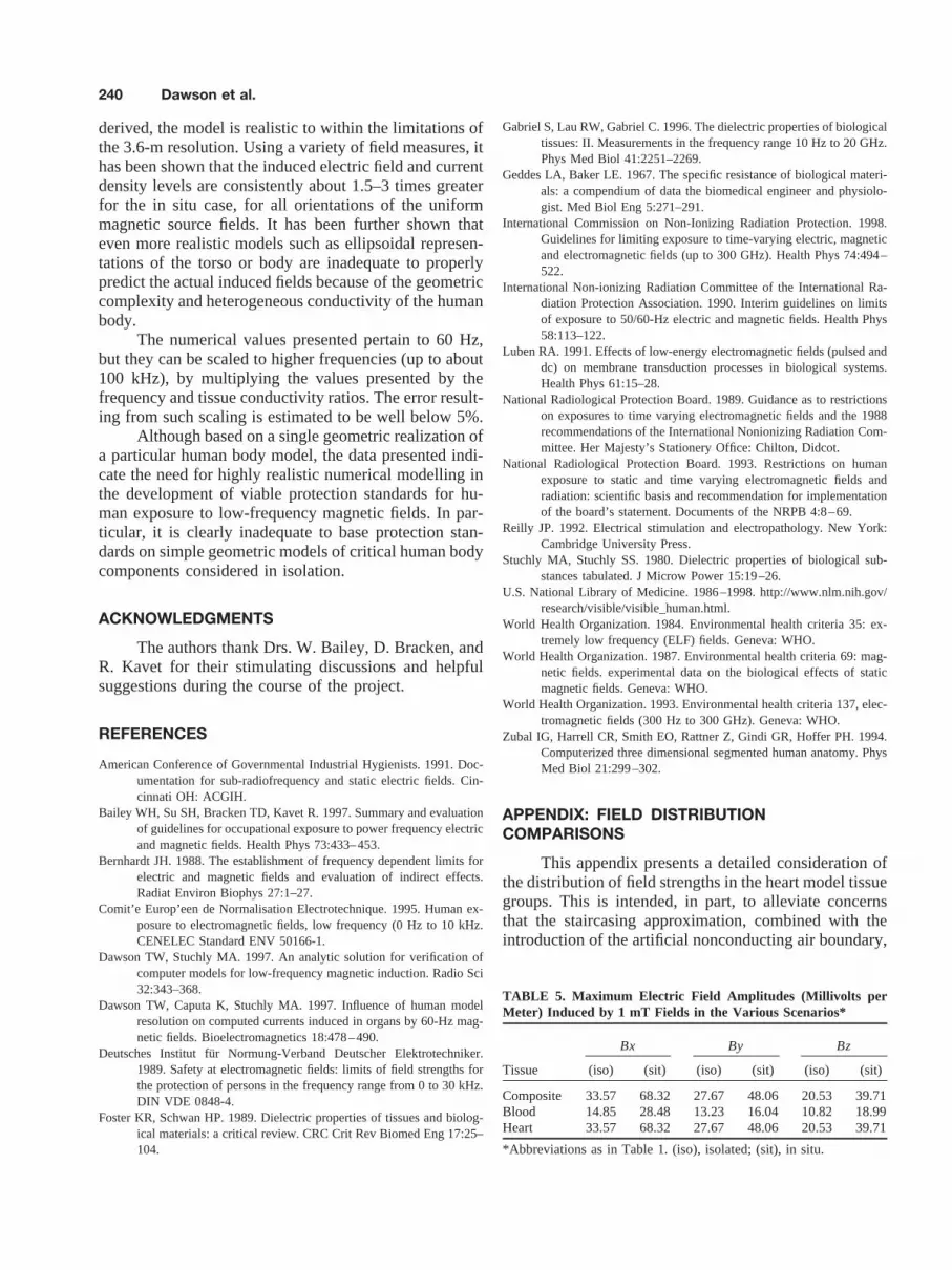
APPENDIX: FIELD DISTRIBUTIONCOMPARISONS

This appendix presents a detailed consideration ofthe distribution of field strengths in the heart model tissuegroups. This is intended, in part, to alleviate concernsthat the staircasing approximation, combined with theintroduction of the artificial nonconducting air boundary,

TABLE 5. Maximum Electric Field Amplitudes (Millivolts perMeter) Induced by 1 mT Fields in the Various Scenarios*

Tissue

Bx By Bz

(iso) (sit) (iso) (sit) (iso) (sit)

Composite 33.57 68.32 27.67 48.06 20.53 39.71Blood 14.85 28.48 13.23 16.04 10.82 18.99Heart 33.57 68.32 27.67 48.06 20.53 39.71

*Abbreviations as in Table 1. (iso), isolated; (sit), in situ.

240 Dawson et al.

Fig. 7. Electric field amplitude histograms for the compositeheart tissue group, under left-to-right (Bx, left column), back-to-front (By, middle column), and foot-to-head (Bz, right column)excitation by 60 Hz, 1 mT source fields. The solid and hollowbars apply to the in situ and isolated cases, respectively. The

height of the various bars indicates the fraction of voxels forwhich the electric field amplitude falls into the associated bin onthe horizontal axis. The width of each bin is 10% of the appro-priate maximum value in each tissue group; numerical values ofthe actual maxima are listed in Table 5.

Fig. 8. Conventions as in Figure 7, except for the heart muscle(lower row) and heart blood pool (upper row). The associatedpeak electric field values are listed in Table 5. Because these

tissue are homogeneous, the histograms also pertain to thecurrent density magnitude, using the maxima listed in Table 6.

Fig. 9. Integrated electric field amplitude histograms for the composite heart model, underleft-to-right (Bx, left column), back-to-front (By, middle column), and foot-to-head (Bz, rightcolumn) excitation by 60 Hz, 1 mT source fields.


might introduce artificially high peak values in the iso-lated heart scenario. This concern is motivated by apreviously published comparison [Dawson and Stuchly,1997] between numerical and analytical solutions forlow-frequency magnetic induction in an equatoriallystratified sphere. There, it was shown that the two solu-tions are in good agreement throughout the sphere inte-rior, even in the presence of strong conductivity gradi-ents. However, they can differ significantly at the con-ductor-air interface.

Values of the maximum electric field magnitudes inthe three tissue groups are listed in Table 5 for thevarious scenarios. It is evident that the in situ maximumvalues are always greater than the corresponding isolatedvalues, typically by a factor of 2.

These numerical values may be used to assist in theinterpretation of the histograms of electric field magni-tude distribution shown in Figure 7 for the composite

TABLE 6. Maximum Current Density Magnitude (Milliamperesper Square Meter) Induced by 1 mT Fields in the VariousScenarios*

Tissue

Bx By Bz

(iso) (sit) (iso) (sit) (iso) (sit)

Composite 10.39 19.93 9.26 11.23 7.57 13.30Blood 10.39 19.93 9.26 11.23 7.57 13.30Heart 3.36 6.83 2.77 4.81 2.05 3.97

*Abbreviations as in Table 1. (iso), isolated; (sit), in situ.

Fig. 10. Conventions as in Figure 9, except for the heart muscle (lower row) and heart blood pool (upper row).

Fig. 11. Conventions as in Figure 7, but for the current density magnitude. Numerical values ofthe actual maximua are listed in Table 6.

242 Dawson et al.

tissue group (heart plus blood) and in Figure 8 for theheart (bottom row) and blood (top row) components. Thewidth of each bin on the horizontal axes in Figures 7 and8 is equal to 10% of the associated maximum value. Thebars on each panel are arranged in pairs, the solid andhollow bars corresponding to the in situ and isolatedscenarios, respectively.

The most notable point is that the histograms are allpredominantly biased to lower field levels (typically lessthan 80% of maximum), and consequently the globalmeasures (which are not dominated by local maxima) inthe Results section provide a reasonable comparison be-tween the two scenarios, for the present model.

Further information can be extracted from the de-tails of the various panels. For example, it is evident fromthe left panel of Figure 7 that the isolated composite heartmodel under left-to-right excitation has a dominant frac-tion of values at the lower end, whereas the in situ caseis weighted toward higher values. This finding is againconsistent with the global measures discussed earlier.The converse behaviour is evident in the blood compo-nent under foot-to-head excitation (upper row, right col-umn of Figure 8).

The bias to lower field values is put on a more solidfoundation in Figures 9 and 10, which show the integralsof the histograms in Figures 7 and 8. Specifically, thesecurves represent the fraction of values less than or equalto the upper limit of the bin indicated on the horizontalaxes. The layout of the panels in the two figures corre-

sponds to those of the associated histograms, and theblack and gray lines pertain to the in situ and isolatedscenarios, respectively. Thus, it is obvious from the firstcolumn that the left-to-right source orientation is associ-ated with a weighting of the isolated heart model to lowervalues for all three heart model tissue groups. The re-maining two source orientations generally show a mixedweighting of values, apart from the rightmost two panelsof the blood tissue group plot. Here the back-to-front andfoot-to-head orientations are associated with an in situweighting toward upper and lower values, respectively.

Figure 11 shows the corresponding histograms forthe current density magnitude in the composite heartmodel. These histograms are to be interpreted in light ofthe maximum values listed in Table 6. Because the bloodand heart tissues are considered as homogeneous in thepresent study, the histograms of Figure 8 also serve forthe associated current density magnitudes, but are now tobe interpreted using the maxima listed in Table 6. It isclear that in all cases the current density values for thecomposite model in the in situ scenario are weightedtoward lower values relative to the isolated scenario. Thisis particularly so under the two horizontal source orien-tations. This observation is supported by the associatedintegrated histograms shown in Figure 12, for which thedominance of lower values in theBx andBy cases forthe in situ scenario is clearly evident. The converse istrue, but to a much lesser degree, for the case ofBzexcitation.

Fig. 12. Conventions as in Figure 9, but for the current density magnitude.
