Embed Size (px)
Citation preview

arX
iv:0
803.
1224
v1 [
astr
o-ph
] 8
Mar
200
8
Magneto-Hydrodynamics of Population III Star Formation
Masahiro N. Machida1, Tomoaki Matsumoto2, and Shu-ichiro Inutsuka1
ABSTRACT
Jet driving and fragmentation process in collapsing primordial cloud are stud-
ied using three-dimensional MHD nested grid simulations. Starting from a ro-
tating magnetized spherical cloud with the number density of nc ≃ 103 cm−3, we
follow the evolution of the cloud up to the stellar density nc ≃ 1022 cm−3. We cal-
culate 36 models parameterizing the initial magnetic and rotational energies (γ0,
β0). In the collapsing primordial clouds, the cloud evolutions are characterized
by the ratio of the initial rotational to magnetic energy, γ0/β0. The Lorentz force
significantly affects the cloud evolution when γ0 > β0, while the centrifugal force
is more dominant than the Lorentz force when β0 > γ0. When the cloud rotates
rapidly with angular velocity of Ω0 > 10−17(nc/103 cm−3)2/3 s−1 and β0 > γ0,
fragmentation occurs before the protostar is formed, but no jet appears after the
protostar formation. On the other hand, a strong jet appears after the proto-
star formation without fragmentation when the initial cloud has the magnetic
field of B0 > 10−9(nc/103 cm−3)2/3 G and γ0 > β0. Our results indicate that
proto-Population III stars frequently show fragmentation and protostellar jet.
Population III stars are therefore born as binary or multiple stellar systems, and
they can drive strong jets, which disturb the interstellar medium significantly, as
well as in the present-day star formation, and thus they may induce the formation
of next generation stars.
Subject headings: binaries: general—cosmology: theory—early universe— ISM:
jets and outflows—MHD—stars: formation
1. INTRODUCTION
Magnetic field plays an important role in present-day star formation. Observations in-
dicate that molecular clouds have the magnetic field strengths of order ∼ µG and magnetic
1Department of Physics, Graduate School of Science, Kyoto University, Sakyo-ku, Kyoto 606-8502, Japan;
[email protected], [email protected]
2Faculty of Humanity and Environment, Hosei University, Fujimi, Chiyoda-ku, Tokyo 102-8160, Japan;

– 2 –
energies comparable to the gravitational energies (Crutcher 1999). These strong fields signif-
icantly affect star formation processes. For example, protostellar jets, which are ubiquitous
phenomena in the star-forming region, is considered to be driven from the protostar by the
Lorentz force (Blandford & Payne 1982; Pudritz & Norman 1986). The jet influences the
gas accretion onto the protostar and disturbs the ambient medium. In addition, the angular
momentum of the cloud is removed by the magnetic braking and protostellar jet. Tomisaka
(2000) showed that, in his two dimensional MHD calculation, 99.9% of the angular momen-
tum is transferred from the center of cloud by the magnetic field. This removal process
of angular momentum makes the protostar formation possible in the parent cloud that has
much larger specific angular momentum than that of the protostar. On the other hand, so
far, magnetic effects in primordial gas clouds have been ignored in many studies because
the magnetic field in the early universe is supposed to be extremely weak. However, recent
studies indicate that moderate strength of magnetic fields exists even in the early universe.
Ichiki et al. (2006) showed that cosmological fluctuations produce magnetic fields before the
epoch of recombination. These fields are large enough to seed the magnetic fields in galaxies.
Langer et al. (2003) proposed the generation mechanism of magnetic fields at the epoch of
the reionization of the universe. They found that magnetic fields in the intergalactic matter
are amplified up to ∼ 10−11 G. These fields can therefore increase up to ≃ 10−7 − 10−8 G
in the first collapsed object having the number density n ∼ 103 cm−3. These fields may
influence the evolution of primordial gas clouds and the formation of Population III stars.
Under the spherical symmetry including the hydrodynamical radiative transfer, the
star formation process are carefully investigated by many authors both in the present-
day (e.g., Larson 1969; Masunaga & Inutsuka 2000) and primordial star formation (e.g.,
Omukai & Nishi 1998). A significant difference between present-day and primordial star for-
mation exists in the thermal evolution of the collapsing gas cloud because of difference in
the abundance of dust grains and metals. In present-day star formation, gas temperature in
molecular clouds is ∼ 10K. These clouds collapse isothermally with polytropic index γ ≃ 1
(P ∝ ργ) in nc . 1011 cm−3, then the gas becomes adiabatic (γ ≃ 7/5) at nc ≃ 1011 cm−3,
and an adiabatic core (or the first core) is formed, where nc denotes the central number
density of the collapsing cloud. When the number density reaches nc ≃ 1016 cm−3, the
molecular hydrogen is dissociated (γ ≃ 1.1), and the cloud begins to collapse rapidly again.
When the number density reaches nc ≃ 1020 cm−3, the equation of state becomes hard again
(γ ≃ 5/3). The protostar is formed at nc ≃ 1021 cm−3. On the other hand, primordial gas
clouds have temperature of ∼ 200 − 300K at nc ≃ 103 cm−3 (Omukai 2000; Omukai et al.
2005; Bromm et al. 2002; Abel et al. 2002; Yoshida et al. 2006). These clouds collapse keep-
ing γ ≃ 1.1 for a long range of 104 . nc . 1016 cm−3. After the central density reaches
nc ≃ 1016 cm−3, the thermal evolution in the primordial collapsing cloud begins to coincide
– 3 –
with that in present-day cloud (for detail, see Fig. 1 of Omukai et al. 2005). The differ-
ence in thermal evolution between present-day and primordial clouds arises in the period of
nc . 1016 cm−3. In present-day star formation, two distinct flows (molecular outflow and op-
tical jet), which are frequently observed in star forming regions, are driven by the respective
core; the outflow is driven by the adiabatic cores (the first core) and the jet is driven by the
protostar (Tomisaka 2002; Machida et al. 2005b, 2007b; Banerjee & Pudritz 2006). In addi-
tion, many numerical simulations have shown that fragmentation of the adiabatic core, and
thus possible formation of binary or multiple stellar systems. In contrast, primordial proto-
stars are formed directly without the prior formation of adiabatic core, because the thermal
pressure smoothly increases keeping γ ≃ 1.1 for nc . 1016 cm−3. Even when the primordial
cloud is strongly magnetized, the wide-angle outflow which corresponds to the present-day
molecular outflow (that is driven from the adiabatic core formed at nc ≃ 1011 cm−3) may
not appear, but the well-collimated jet (that is driven from the protostar) is ejected at
nc & 1021. In addition, it is expected that, in the collapsing primordial cloud, fragmen-
tation rarely occurs for nc . 1016 cm−3, because the cloud continues to collapse and the
perturbation inducing fragmentation cannot grow sufficiently.
Another major difference between present-day and primordial star formation exists in
the magnetic evolution. In present-day star formation, the neutral gas is coupled well with
the ions in nc . 1012 cm−3 and nc & 1015 cm−3, while the magnetic field are dissipated by
the Ohmic dissipation in 1012 cm−3 . nc . 1015 cm−3 (for details, see Nakano et al. 2002).
Machida et al. (2007a) showed that ∼ 99% of the magnetic field in the collapsing cloud is
dissipated in 1012 cm−3 . nc . 1015 cm−3. On the other hand, the magnetic evolution in a
primordial gas cloud is carefully investigated by Maki & Susa (2004, 2007), and they found
that the magnetic field strongly couples with the primordial gas during all the collapse phase,
as long as the initial field strength is weaker than B0 . 10−5(n/103 cm−3)0.55 G. Maki & Susa
(2007) also showed that ionization fraction is high enough for the magnetic field to couple
with the gas even in the accretion phase after the protostar is formed. In summary, the
magnetic field is largely dissipated by the Ohmic dissipation before the protostar formation in
present-day cloud, while the magnetic field can continue to be amplified without dissipation
in primordial cloud.
Recent cosmological simulations inferred that a single massive star is formed without
fragmentation in the first collapsed object that is formed at nc ≃ 103 cm−3 (Abel et al.
2000, 2002; Bromm et al. 2002; Yoshida et al. 2006). However, in their simulations, the
cloud evolution are investigated only for nc . 1017 cm−3. Since the protostar is formed at
nc ≃ 1021 cm−3 (Omukai & Nishi 1998), the protostar is not yet formed in their simulations.
On the other hand, Machida et al. (2007b) showed that fragmentation occurs frequently
after the equation of state becomes hard for nc & 1017 cm−3, indicating that the binary or

– 4 –
multiple stellar system can be formed also in the early universe.
The magnetic field in the collapsing cloud is closely related to fragmentation or formation
of binary or multiple stellar systems. In present-day star formation, the magnetic field
strongly suppresses the rotation driven fragmentation (Machida et al. 2007c; Price & Bate
2007). For the primordial cloud, effects of the magnetic field on fragmentation are still
unknown.
In this paper, we investigate the evolution of weakly magnetized primordial clouds and
formation of Population III stars using three-dimensional MHD simulations, and show the
driving condition of a jet from proto-Population III stars and the fragmentation condition
in the collapsing primordial cloud cores. The structure of the paper is as follows. The
framework of our models and the numerical method are given in §2. The numerical results
are presented in §3. We discuss the fragmentation and jet driving conditions in §4, and
summarize our results in §5.
2. MODEL
Our initial settings are almost the same as those of Machida et al. (2006d, 2007d). To
study the cloud evolution, we use the three-dimensional ideal MHD nested grid code. We
solve the MHD equations including the self-gravity:
∂ρ
∂t+ ∇ · (ρv) = 0, (1)
ρ∂v
∂t+ ρ(v · ∇)v = −∇P − 1
4πB × (∇× B) − ρ∇φ, (2)
∂B
∂t= ∇× (v × B), (3)
∇2φ = 4πGρ, (4)
where ρ, v, P , B, and φ denote the density, velocity, pressure, magnetic flux density, and
gravitational potential, respectively. For gas pressure, we use the barotropic relation that
approximates the result of Omukai et al. (2005). They consider detailed thermal and chem-
ical processes in collapsing primordial gas, adopting the a simple one-zone model where the
core collapses approximately at the free-fall timescale and the size of the core is about the
Jeans length as in the Larson-Penston self-similar solution (Penston 1969; Larson 1969). We
fit to the thermal evolution derived by Omukai et al. (2005) as a function of the density
(see Fig.1 of Machida et al. 2007d), and the pressure is calculated using the fitted function.
Therefore, our equation of state is a barotropic.

– 5 –
As the initial conditions of the clouds, we consider the density profile of the critical
Bonnor-Ebert sphere (Ebert 1955; Bonnor 1956) with perturbations,
ρ(r, ϕ) =
ρBE(r) f [1 + δρ(r, ϕ)] for r < R0,
ρBE(R0) f [1 + δρ(r, ϕ)] for r ≥ R0,(5)
where ρBE(r) denotes the density distribution of the critical Bonnor-Ebert sphere. The
central number density of the Bonnor-Ebert sphere is set at ρBE(0) = 103 cm−3. The factor
f denotes a density enhancement factor, and the density is increased by a factor f = 1.86
to promote the collapse. The initial cloud has therefore the central density of n0 = 1.86 ×103 cm−3. The initial temperature is set at 250K, and the radius of the Bonnor-Ebert
sphere is R0 = 6.5 pc, corresponding to the non-dimensional radius of Bonnor-Ebert sphere,
ξmax = 6.5. Outside this radius, a uniform gas density of nBE(R0) = 130 cm−3 is assumed.
To promote fragmentation, a small m = 2-mode density perturbation is imposed to the
spherical cloud such as,
δρ = Aϕ(r/R0) cos 2ϕ, (6)
where Aϕ is the amplitude of the perturbation and Aϕ = 0.01 is adopted in all models. The
total mass contained inside R0 is Mc = 1.8 × 10⁴ M⊙. The density enhancement factor f
specifies the ratio of the thermal to the gravitational energy α0 (= Eth/|Egrav|), where Eth
and Egrav are the thermal and gravitational energies of the initial cloud). The initial cloud
has α0 = 0.5 when f = 1.86 and Aϕ = 0.
The initial cloud rotates around the z-axis at a uniform angular velocity of Ω0, and it
has a uniform magnetic field B0 parallel to the z-axis (or rotation axis). The initial model
is characterized by two non-dimensional parameters: the ratio of the rotational energy to
the gravitational energy β0 (= Erot/|Egrav|), and the magnetic energy to the gravitational
energy γ0 (= Emag/|Egrav|) , where Erot and Emag are the rotational and magnetic energies.
We made 36 models changing these two parameters. All the models examined here
and their parameters (β0 and γ0) are summarized in Table 1. These tabulated values are
calculated in the cases of spherical clouds, i.e., Aϕ = 0. We examine a large parameter range
of β0 = 10−6−0.1, γ0 = 0−0.2. For convenience, β0 is referred as “initial rotational energy”,
and γ0 as “initial magnetic energy.” The angular velocity Ω0 and magnetic field B0 are also
summarized in Table 1. In addition, we estimate the mass-to-flux ratio,
M
Φ=
M
πR20B0
, (7)
where M and Φ denote the mass contained within the cloud radius R0, and the magnetic
flux threading the cloud, respectively. There exists a critical value of M/Φ below which a

– 6 –
cloud is supported against the gravity by the magnetic field. For a cloud with an uniform
density, Mouschovias & Spitzer (1976) derived a critical mass-to-flux ratio,
(
M
Φ
)
cri
=ζ
3π
(
5
G
)1/2
, (8)
where ζ = 0.53 for uniform spheres (see also, Mac Low & Klessen 2004). For convenience,
we use the mass-to-flux ratio normalized by the critical value,(
M
Φ
)
norm
≡(
M
Φ
)
/
(
M
Φ
)
cri
, (9)
which is summarized in Table 1.
We adopt the nested grid method (for details, see Machida et al. 2005a, 2006a) to
obtain high spatial resolution near the center. Each level of a rectangular grid has the same
number of cells (= 128 × 128 × 64), with the cell width h(l) depending on the grid level
l. The cell width is halved with every increment of the grid level. The highest level of
grids changes dynamically: a new finer grid is generated whenever the minimum local Jeans
length λJ falls below 8 h(lmax), where h is the cell width. The maximum level of grids is
restricted to lmax = 30. Since the density is highest in the finest grid, generation of a new
grid ensures the Jeans condition of Truelove et al. (1997) with a margin of a safety factor
2. We begin our calculations with three grid levels (l = 1 − 3). Box size of the initial finest
grid l = 3 is chosen to be 2R0, where R0 is the radius of the critical Bonnor-Ebert sphere.
The coarsest grid (l = 1) then has box size of 23 R0. The mirror symmetry with respect to
z=0 is imposed. A boundary condition is imposed at r = 23 R0, where the magnetic field
and ambient gas rotate at an angular velocity of Ω0 (for detail, see Matsumoto & Tomisaka
2004). We adopted the hyperbolic ∇ · B cleaning method of Dedner et al. (2002).
3. RESULTS
3.1. Typical Jet Model
Firstly, we show a cloud evolution with a clear jet from a non-fragmentation core.
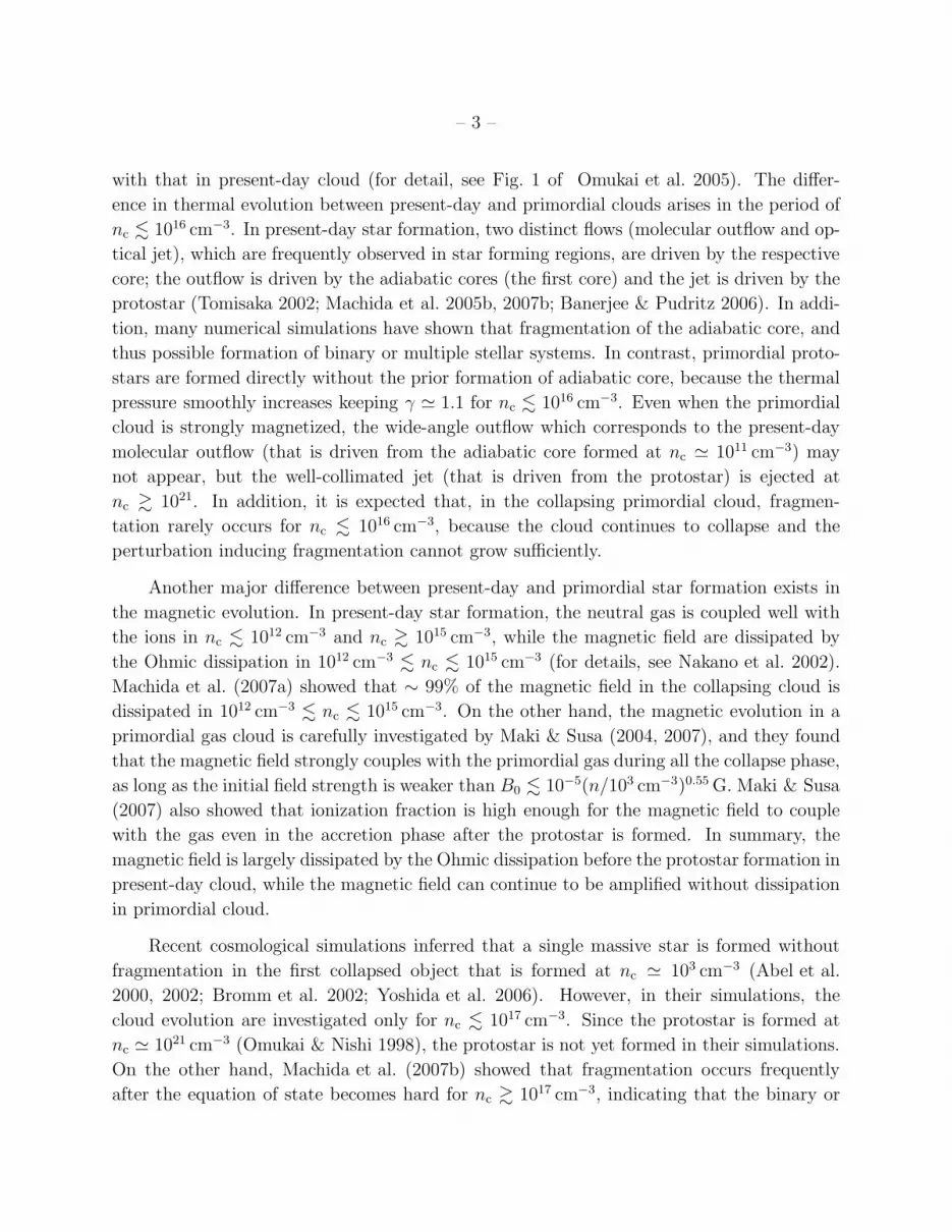
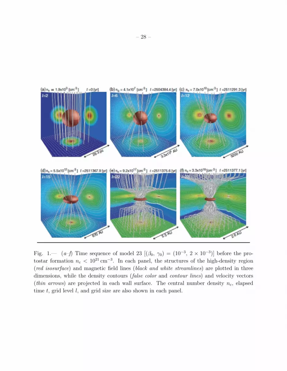
Figure 1 shows the cloud evolution before the protostar formation (nc < 1021 cm−3) from
the initial stage for model 23. Model 23 has parameters of (γ0, β0) = (2 × 10⁻³, 10−4), and
the initial cloud has a magnetic field strength of B0 = 10−6 G, and a angular velocity of
Ω0 = 2.3× 10⁻¹⁶ s−1. Figure 1a shows the initial spherical cloud (i.e., Bonnor-Ebert Sphere)
threaded by the uniform magnetic field. Figures 1b–1d show the cloud structure around the
center of cloud when the central density reaches nc = (b) 4.1×107 cm−3, (c) 7.0×1010 cm−3,

– 7 –
and (d) 5.5 × 1012 cm−3, respectively. The density contours projected on the sidewall in
these figures indicate that the central region becomes oblate as the cloud collapses because
of magnetic field and rotation, both of which are amplified by the cloud collapse. Figures 1a–
1d also show that the magnetic field lines are gradually converged toward the center as the
central density increases.
Figure 1e shows the cloud structure at nc = 9.2 × 1017 cm−3, where a thin disk is
formed at the center of cloud. In this figure, the disk-like structure is threaded by the
magnetic field lines that are strongly converged toward the center of the cloud. The density
contours projected on the sidewall of Figure 1e show the shock waves above and below
the disk (see the crowded contour lines on the right sidewall). Near the shock surface, the
magnetic field lines are bent. Similar structures are seen in the present-day star formation
process (Machida et al. 2005b, 2006a). We discuss the relation between the shock generation
and the evolution of the magnetic field and rotation in §4.1.3. The cloud structure at
nc = 3.3 × 1018 cm−3 are shown in Figure 1f, in which the magnetic field lines are strongly
converged but slightly twisted. Also in this figure, clear shocks are seen above and below
the disk-like structure. Figures 1a–1f show that the magnetic field lines are hardly twisted
before the protostar formation (nc . 1021 cm−3), because the collapse timescale is shorter
than the rotational timescale.
Figure 2 shows the cloud evolution after the protostar formation (nc > 1021 cm−3). The
upper and middle panels show the density and velocity distributions on z = 0 and x = 0
plane, respectively, and the lower panels show the cloud structures and configurations of the
magnetic field lines in three dimensions. Figures 2a–2c show the cloud structure 1.4 days after
the protostar formation. In this model, when the central density reaches nc ≃ 4.7×1021 cm−3,
a protostar surrounded by the strong shock is formed around the center of the cloud. The
protostar has a mass of M = 7.6×10⁻³ M⊙, and a radius of r = 1.1R⊙ at its formation epoch.
The shock front corresponding to protostellar surface is seen in Figure 2a (r ∼ 0.005AU;
contours of n ∼ 1021 cm−3). The density contours projected on the sidewall in Figures 2c also
show the shock surface near the center of the cloud. The magnetic field lines are strongly
converged to the center of the cloud, but slightly twisted at this epoch. The jet starts to
be ejected 1.68 days after the protostar formation. Figures 2e–2g shows the cloud structure
2.82 days after the protostar formation. The jet ejected near the protostar is indicated by the
red contour in Figure 2f and the red transparent surface in Figure 2g, which are a boundary
between the inflow (vr < 0) and jet (vr > 0) regions. The magnetic field lines are twisted
significantly inside the jet region because of the rapid rotation of the protostar. The jet
affects the density distribution; the butterfly-like density distribution is shown in Figures 2f
and 2g (see contour lines near the protostar projected on the right sidewall). The strong
shock waves are generated at the upper and lower ends of the jet, reflecting a strong mass

– 8 –
ejection.
Figures 2h–2j show the cloud structure 3.48 days after the protostar formation, the
last stage of this calculation. Until the last stage, the jet continue to extend as is seen
in Figures 2f and 2i. In Figure 2h, two nested shocks are observed near the center of
the cloud (r ∼ 0.005AU and r ∼ 0.01AU). The outer shock is generated by the mass
ejection (i.e., jet) near the protostar, while the inner one corresponds to the surface of the
protostar. In Figure 2j, the isodensity surface exhibits a shallow cone-shape on the disk,
which corresponds to the outer shock in Figure 2h. The magnetic field lines inside the jet
region are more strongly twisted with times as shown in Figures 2g and 2j. At the end
of the calculation, the jet has a maximum speed of vmax = 66.3 km, and it extends up to
0.05AU. The mass of protostar reaches Mps = 8.5 × 10⁻³ M⊙, while mass of the outflowing
gas is Mout = 1.1 × 10⁻³ M⊙. About 10% of the accreting matter is therefore ejected from
the center of the cloud via the protostellar jet. The mass ejection rate is estimated as
M = 5.9 × 10⁻³ M⊙ yr−1.
3.2. Typical Fragmentation Model
Next, we describe the cloud evolution exhibiting fragmentation. Figure 3 shows the
cloud evolution for model 21 with (γ0, β0) = (2.5× 10⁻⁷, 10−4), which are corresponding to
a magnetic field strength of B0 = 10−8 G and an angular velocity of Ω0 = 2.3 × 10⁻¹⁶ s−1
at the initial stage. Model 21 has the same rotational energy as the model 23, the previous
model, but 10−4 times smaller magnetic energy than model 23. Figures 3a and 3b show the
cloud structure just before the protostar formation (nc = 1.0 × 1017 cm−3). We define the
protostar formation epoch as the stage of nc = 1021 cm−3. Similar to model 23, a thin disk is
formed at the center of the cloud before the protostar formation. The disk keeps an almost
axisymmetric structure in the plane perpendicular to the rotation axis. Although we added
1% of the non-axisymmetric density perturbation to the initial state, the non-axisymmetric
structure hardly evolves before the protostar formation. Figure 3b also shows an hourglass
configuration of the magnetic field lines, similar to model 21.
Figures 3c and 3d show the cloud structure 2.4 days after the protostar formation. The
central region is deformed from a disk structure into a ring at nc ≃ 8 × 1018 cm−3, and the
ring fragments. This is consistent with the fragmentation criterion of Machida et al. (2007d);
a non-magnetized cloud with rotational energy of β0 > 10−5 undergoes fragmentation. The
cloud here has a rotational energy of β0 = 10−4 and the very small magnetic energy of γ0 =
2.5 × 10⁻⁷ at the initial stage. Fragments are located at (x, y) ≃ (±0.035AU, ∓0.055AU)
with long spiral tails that are the remnant of the ring (Fig. 3c). The magnetic field lines are

– 9 –
distributed strongly along the spiral tails (Fig. 3d).
Figures 3e and 3f show the cloud structure 8.8 days after the protostar formation. The
fragments exhibit a round shape in Figure 3e. The central density of the fragments reaches
nc ≃ 1.8 × 1022 cm−3 at this epoch. Fragments are surrounded by their respective disk with
spiral arms, and the disks grow with time, comparing Figures 3c and 3e. At the end of
the calculation, each fragment (i.e., each protostar) has a mass of ∼ 1.3 × 10⁻² M⊙ and a
radius of ∼ 1.4R⊙. The separation between fragments is ∼ 0.89AU. As shown in Figure 3f,
the magnetic field lines are distributed along the spiral tails, indicating that the vertical
component of the magnetic field is weaker than the other component (i.e., Bz ≪ Bx, By).
This is responsible to the weak magnetic field around the protostars, and the magnetic field
lines easily follow the orbital motion of the fragments.
This fragmentation model does not exhibit a jet formation by the end of the calculation
in spite of the same initial rotation speed as in the previous jet model. This is also responsible
to the weak magnetic field. Note that the calculation halts 8.8 10 days after the stellar core
formation, and we does not reject a possibility that a jet appears in later stage.
One may image that this model undergoes the rotation driven fragmentation because of a
weak magnetic braking, and the previous model is kept away from the fragmentation because
of the strong magnetic braking. However, both the models show the same amplification rate
for the magnetic field and the angular velocity during the collapse. The saturation levels of
the amplification for the magnetic field and angular velocity depend on the initial conditions.
The two models track two different evolutional sequences according to their respective γ0/β0.
This point is discussed in §4.2 and §5.
3.3. Fragmentation and Magnetic/Rotational Energy
Figure 4 shows the final stages in the plane of initial magnetic (γ0, x-axis) and rotational
energies (β0, y-axis) for every models. The density distribution in the z = 0 plane is shown
in each panel. Models are classified into four types: fragmentation models (models in the
blue background), non-fragmentation models (models in the red background), merger models
in which the fragments merge after fragmentation (models in the green background), and
no collapsing model (model in the gray background). In fragmentation models, calculations
were stopped when the Jeans condition was violated in a grid except for the finest grid. Such
a case occurs either when fragments escape from the finest grid or when the gas far from
the center becomes denser than that in the finest grid. In non-fragment models, the Jeans
condition was not violated because the densest gas is located at the finest grid, and the

– 10 –
calculations was stopped at some high density. After the protostar formation, the Alfven
velocity becomes extremely large due to the strong magnetic field at the central region,
and the timestep becomes extremely short. We stopped calculation after we checked that
fragmentation was not likely to occur around the protostar. The fragmentation reproduced
here is therefore restricted to the cases where fragmentation occurs near the central region
and fragmentation occurs just after the protostar formation. In merger models [(γ0, β0) =
(2×10⁻³, 10−2), (2×10⁻³, 10−3)], fragments merge to form a single core at the center of the
cloud after fragmentation. The merged core did not undergo fragmentation again although
we calculated merger models for sufficiently long term. In the no collapsing model [(γ0, β0)
= (0.2, 0.1)], the cloud oscillates without collapse because this model has the large magnetic
and rotational energies.
In Figure 4, fragmentation models are distributed in the upper left region, indicating
that a cloud tends to fragment when the initial cloud has a weaker magnetic field and faster
rotation. Namely, the magnetic field suppresses fragmentation, while the rotation promotes
fragmentation. This effect of the magnetic field and rotation on fragmentation is similar to
that in present-day star formation (Hosking & Whitworth 2004; Machida et al. 2004, 2005b,
2007c; Price & Bate 2007; Hennebelle & Teyssier 2007). Firstly, to investigate the effect of
rotation on fragmentation, we focus on models displayed in the fourth column in Figure 4
(models 4, 10, 16, 22, 28, and 34). These models have the same magnetic energies of γ0 =
2×10⁻⁵ and different rotational energies of β0 = 10−6−0.1 at the initial stage. Fragmentation
occurs in models with β0 > 10−4 (models 4, 10, 16, 22), while fragmentation does not occur
in models with β0 < 10−4 (models 28, 34). In addition, models with larger rotational
energies undergo fragmentation in the earlier evolution phases with wider separation. For
example, model 4 (β0 = 0.1) fragments at nc = 9.5 × 1017 cm−3 with the separation of
Rsep ≃ 4.3AU, while model 22 (β0 = 10−4) does at nc = 1.6×1019 cm−3 with the separation of
Rsep ≃ 0.2AU. Machida et al. (2007d) also showed that a cloud with faster rotation exhibits
wider separation. On the other hand, paying attention to the non-fragmentation models,
model 34 exhibits a compact spherical protostar with a disk, while model 28 shows bar and
ring structures. Model 34 did not show any sign of fragmentation, and the central core
continues to grow. Model 28 has marginal parameters for fragmentation since it is located
at the boundary between fragmentation and non-fragmentation models. The protostar fails
to fragment in spite of its bar shape. The spiral arms evolve into a ring, which does not also
fragment.
We now focus on models displayed in the fourth low in Figure 4 (models 19-24), to
investigate the effect of magnetic field on fragmentation. These models have different mag-
netic energies of γ0 = 0 − 0.2 but the same rotational energies of β0 = 10−4 at the initial
stage. In these models, weakly magnetized clouds undergo fragmentation (γ0 < 2 × 10⁻⁵,

– 11 –
models 19-22), while strongly magnetized clouds do not (γ0 > 2 × 10⁻⁵, models 23 and 24).
When clouds have the same rotational energies at the initial stage, model with weaker mag-
netic field undergo fragmentation at the earlier evolutionary phases with wider separation.
For example, the model with weaker magnetic field γ0 = 2 × 10⁻⁹ (model 28) fragments at
nc = 7.8 × 1018 cm−3, while the model with stronger magnetic field γ0 = 2 × 10⁻⁵ (model
22) does at nc = 1.6× 1019 cm−3. Moreover, the models with much larger magnetic energies
(models 23 and 24) produce a single compact core at the center of the cloud.
Fragmentation and non-fragmentation models are clearly separated in Figure 4. In
addition, merger models are located at the boundary between fragmentation and non-
fragmentation models. In fragmentation models, models with weaker magnetic field and
faster rotation tend to have wider separation. In non-fragmentation models, clouds have
more compact cores in models with stronger magnetic fields and slower rotations. These fea-
tures indicate clearly that the rotation promotes fragmentation, and the magnetic field sup-
presses fragmentation in primordial star formation, as well as the present-day star formation.
The models presented here have a small amplitude of the non-axisymmetric density pertur-
bation (Aϕ = 0.01) at the initial stage. If larger amplitude was set at the initial stage, the
boundary between the fragmentation and non-fragmentation models might change slightly.
Machida et al. (2007c) discussed the fragmentation condition for a present-day magnetized
cloud, and indicated that the fragmentation condition does not depend qualitatively on the
initial amplitude of the non-axisymmetric perturbation. Moreover, Machida et al. (2007d)
showed that fragmentation condition for a primordial non-magnetized cloud depend slightly
on the initial amplitude of the non-axisymmetric perturbation. We therefore expect that
the initial amplitude of the non-axisymmetric perturbation hardly affect the fragmentation
condition even in the primordial magnetized collapsing cloud.
3.4. Jet and Magnetic/Rotational Energy
Figure 5 shows final states in the plane of the initial magnetic (γ0, x-axis) and ro-
tational energies (β0, y-axis), contrasting the jets at almost the same evolutionary stage of
nc ≃ 1022−23 cm−3. Each panel shows the density and velocity distribution in the y = 0 plane,
and a thick red contour denotes the boundary between inflow (vr < 0) and outflow (vr > 0)
regions. The gas flows out of the central region inside the red contour. The panels without
thick red contours indicate the models where a jet does not appear. As listed in Table 1, jets
appear in 13 of 36 models. We call these 13 models ‘jet models’, and other models ‘non-jet
models.’ In all the jet models, a jet appears only after a protostar is formed. After the pro-
tostar formation, the rotation timescale becomes shorter than the collapse timescale because

– 12 –
of the accretion of the angular momentum and hardness of the equation of stage at the cloud
center, and the strong centrifugal force drives the jet via disk wind mechanism (Tomisaka
2002; Banerjee & Pudritz 2006; Machida et al. 2007b; Hennebelle & Fromang 2007). The jet
disturbs the density distribution near the protostar. As shown in Figure 5, the jet supplies
gas above and below the disk, and the density becomes higher there for the jet models, while
these region remains less dense for the non-jet models.
The jet models are distributed in the lower right region in Figure 5, indicating that a
jet is driven in strongly magnetized but slowly rotating cloud. It should be also noted that
the non-jet models coincide with the fragmentation models except for models 31 and 32. In
other words, almost all the clouds experience either jet formation or fragmentation. In the
fragmentation models, the angular momentum of the parent cloud is distributed to both the
orbital and spin angular momenta of the fragments, and fragmentation therefore reduces the
spin angular momentum of the protostar. This deficiency of the spin angular momentum of
the fragments suppresses jet formation.
Firstly, to investigate the relation between jet and magnetic field strength, we focus on
models in the fourth row (models 27-30). In model 27, which has a weakest magnetic field
B0 = 10−8 G (or γ0 = 2×10⁻⁷) at the initial stage, no jet appears because of fragmentation.
In model 28, the protostar manages to drive the jet, while the initial cloud has a considerably
small magnetic energy (β0 = 2 × 10⁻⁵). When the cloud has a weak magnetic field, a jet
is considered to be driven by the magnetic pressure gradient force, not by the disk wind
mechanism. The jet structure in model 28 is similar to the magnetic bubble as reproduced by
Tomisaka (2002), Banerjee & Pudritz (2006) and Hennebelle & Fromang (2007). Tomisaka
(2002) shows that when the magnetic field around the central object is extremely weak
(βp ≫ 1, where βp is the plasma beta), the magnetic field is amplified by the spin of the
central object, and the magnetic pressure drives a jet.
A prominent jet is reproduced in model 29, in which the jet is considered to be driven
mainly by the disk wind mechanism. The jet in model 30 is weaker than that in model 29
in spite of the stronger initial field strength; the jet in model 30 has slower average speed
and smaller mass ejection rate than those in model 29. The weakness of the jet in model
30 is attributed to the strong magnetic braking, which slows down the spin of the cloud
before the protostar formation in model 30. In fact, the protostar has an angular velocity
of Ωc = 1.0 × 10⁻⁵ s−1 in model 29 while Ωc = 1.1 × 10⁻⁶ s−1 in model 30 at the protostar
formation epoch. The protostar therefore rotates ∼ 10 times faster in model 29 than that
in model 30. In addition, the growth rate of the angular velocity in the collapsing cloud
is smaller in strongly magnetized cloud (see §4.1.1). In models 27-30, the jet in model 29
has highest speed and largest jet momentum flux at the end of the calculation. As a result,

– 13 –
moderate strength of the magnetic field is necessary to drive strong jet from the protostar.
Next, to investigate dependence on rotation, we focus on the models in the third column
in Figure 5 (models 11, 17, 23, 29, and 35). In these models, the most prominent jet appears
in model 23, while weak jets appear both in slowly (model 35) and rapidly rotating clouds
(model 11). The weakness of the jet in model 35 is due to deficiency of rotation to drive a
strong jet, and that in model 11 is due to a low amplification of the magnetic field during
the collapse; amplification of the magnetic field is related to the rotation, and spin-up is also
related to the magnetic field strength as discussed in §4.1.1. Therefore, a moderate rotation
speed as well as a moderate magnetic field strength is necessary to drive a strong jet. In
summary, a jet appears in models distributed in the lower right region (i.e., models with
stronger magnetic field and slower rotation), and models showing strong jets are limited in
the range of 10−5 . β0 . 10−3 and 10−3 . γ0 . 10−1.
Since we calculated the evolution of the jets only for short duration (∼ a few 10 days) for
numerical limitation, we cannot estimate the momentum of a jet, mass ejection speed and
final speed of jet in long-term evolution. In addition, strength of a jet may largely change
in further long-term evolution. We do not discuss the further evolution of a jet (c.f., final
jet speed, mass ejection rate, etc..) , because our purpose in this paper is to investigate the
condition for driving jet in primordial collapsing clouds.
3.5. Configurations of Jets and Magnetic Field Lines
Figure 6 shows a configuration of magnetic field lines (black-white streamlines) and a
structure of a jet (transparent red iso-velocity surface) for each models.
In the jet models, the magnetic field lines are twisted inside the jet region. Almost
axisymmetric jets are seen in models 18, 23, 24, 28, 29, 34, and 35. These jets have the
hourglass-like configurations of the magnetic field lines, where the poloidal component is
more dominant than the toroidal component as shown in Figure 1f and 2c. These con-
figurations of the magnetic field lines can easily drive a jet by the disk wind mechanism
(e.g., Blandford & Payne 1982). Non-axisymmetric jets are seen in models 17, 30, and 36.
They are caused by the non-axisymmetric density distribution at the protostar formation
epoch. Such a non-axisymmetric density distribution is also reflected by non-axisymmetric
circumstellar disks, represented by a red iso-density surface in Figure 6. For example, model
30 exhibits the non-axisymmetric jet (transparent red iso-velocity surface) driven from the
bar-like density distribution (red iso-density velocity surface) at the root of the jet.
In the fragmentation models, the configurations of the magnetic field lines are disturbed,

– 14 –
and the toroidal field tends to be more dominant than the poloidal filed as shown in models
16 and 22 in Figure 6 and also in Figure 3f. These configurations of the magnetic field
lines indicate weakness of the field strength, which is insufficient to drive a jet. The weak
poloidal field is attributed to the oblique shocks on the surface of the disk envelope, and the
disturbance of the field lines are attributed to the orbital motion of the fragments and the
spin of the fragments. The spin of the fragment winds the magnetic fields around its rotation
axis, and the field strength is amplified. In the further stages, the magnetic pressure may
drive a jet.
4. DISCUSSION
4.1. Magnetic Flux-Spin Relation
4.1.1. Evolution Track for Magnetic Field and Angular Velocity
Figure 7 shows the evolution track of the central magnetic field strength (x-axis) and
central angular velocity (y-axis) from the initial state for some models. The x-axis indicates
Bc/(8πPc)1/2, which corresponds to the pressure ratio of (Pmag/Pc)
1/2 at the center, where
Pmag and Pc denote the central magnetic pressure and the central thermal pressure. This
variable also corresponds to the inverse square root of the plasma beta, β−1/2p . Hereafter this
variable is called the normalized magnetic field. The y-axis indicates Ωc/(4πGρc)1/2, which
corresponds to a ratio of the time scales, tff/trot, at the center, where tff and trot denote
the free-fall and rotation time scales. This variable also coincide with the energy ratio of
(Erot/|Egrav|)1/2 at the center if assuming a uniform sphere. Hereafter this variable is called
the normalized angular velocity. The asterisks at the ends of the loci denote the initial values
of normalized magnetic fields and normalize angular velocities. The diamonds on the loci
denote the stages of nc = 105, 107, · · ·, 1019 cm−3, and these values are labeled for the loci of
models 2, 9, 21, 23, 33, and 35. The arrows on the loci indicate the directions of the cloud
evolutions.
The normalized magnetic fields and angular velocities increase as the central density in-
creases except for stages of very high density in all the models. For comparison, a relationship
ofΩc
(4πGρc)1/2∝ Bc
(8πPc)1/2. (10)
is plotted with the solid line at the lower right corner of Figure 7, and all the model evolves in
the direction almost parallel to this line. This implies that both of the normalized magnetic
fields and the normalized angular velocities are amplified during the early phase of the

– 15 –
collapse at the almost same growth rate. As indicated by Machida et al. (2005a, 2006a,
2007a), the central magnetic field and angular velocity increase as,
Bc, Ωc ∝ ρ2/3c (11)
during the nearly spherical collapse phase that corresponds to Figure 1a–1d. The relationship
of the angular velocity in equation (10) is rewritten as,
Ωc
(4πGρc)1/2∝ ρ1/6
c , (12)
and the relationship of the magnetic field is rewritten as,
Bc
(8πPc)1/2∝ ρ0.12
c . (13)
The power index in the right hand side of (13) is slightly lower than that in equation (12)
although they coincide in the isothermal case. The difference between the power indexes
is attributed to the equation of state in the primordial gas, P = ργ. The polytropic index
γ is assumed as a function of density, and it is approximated to γ ≈ 1.1 for 104 cm−3 .
n . 1017 cm−3 (see Fig.1 of Machida et al. 2007a). Adopting the relation of Pc ∝ ρ1.1c ,
the equation (13) is obtained. The slightly larger power index in the right hand side of
equation (13) is reflected in the slope of loci slightly steeper than that of equation (10). The
relationships of equations (12) and (13) are examined in detail in §4.1.2.
The slope of loci also indicates that the magnetic braking is ineffective during the
spherical collapse phase. If magnetic braking is effective (i.e., it slows down the spin of a
cloud), increase in the angular velocity was less than that indicated by equation (12), and
the slope of the loci would be shallower. We confirmed that the magnetic braking become
prominent only after the protostar formation. In other words, the magnetic field is not
amplified enough to affects the evolution of the cloud during the spherical collapse of the
early phase. In the later phase, the cloud center exhibits transition from nearly spherical
collapse to the disk-like collapse because of rapid rotation and/or strong magnetic field, which
are amplified in the nearly spherical collapse phase, and the evolutionary track stagnated in
the hatched band of Figure 7. The disk-like collapse phase is discussed in §4.1.3.
4.1.2. Magnetic Field and Angular Velocity in the Spherical Collapse Phase
To verify the relation of equations (12) and (13), the evolutions of the central angular
velocities and magnetic fields are plotted against the central density in Figures 8 and 9,
respectively.

– 16 –
Figure 8 shows the evolution of the normalized angular velocity in models 3, 9, 15, 21,
27, and 33, which are located in the third column of Figure 4 and have the common weak
magnetic field B0 = 10−7 G and different angular velocities Ω0 = 2.3×10⁻¹⁷−7.2×10⁻¹⁵ s−1
at the initial stage (see Table 1). In Figure 8, the normalized angular velocities in all
models except for model 3 evolve with ∝ ρ1/6 from the initial stage, indicating the power
law amplification of Ωc ∝ ρ2/3c and spherically collapse of the clouds. On the other hand, the
cloud in model 3 cannot collapse spherically because the cloud has a large rotational energy
at the initial stage.
Figure 9 shows the evolution of the magnetic field strength normalized by the square root
of the density (Fig. 9 upper panel) and the normalized magnetic field (Fig. 9 lower panel) in
models 32-36. Models 32-36 are located in the sixth row in Figure 4, and have the common
small angular velocity Ω0 = 2.3 × 10⁻¹⁷ s−1 and different strengths of the magnetic field
B0 = 10−9 − 10−6 G at the initial stage (see Table 1). The upper panel indicates the power
law amplification of Bc ∝ ρ2/3c (equation [11]) except in the high-density phase and therefore
the spherical collapse of the clouds for all models. Figure 9 lower panel also shows the
evolution of the magnetic field in terms of the β−1/2p (= Bc/
√8πPc). All the curves indicate
the power law amplification of β−1 ∝ ρ0.12, corresponding to equation (13). The curves in
the lower panel undulate more than those in the upper panel because of the undulation in
the pressure included in the normalization. However, the curves in the lower panel converges
well to β−1/2p ≃ 0.2 at the high density phase compared with those in the upper panel. As a
result, when the cloud collapses spherically (i.e., early evolution phase), the evolution of the
angular velocity and magnetic field are well expressed by equation (11), and the normalized
variables are also expressed by equations (12) and (13).
4.1.3. Convergence of the Magnetic Field and Angular Velocity
As the cloud collapses, the normalized angular velocities converge to Ωc/(4πGρc)1/2 ≃
0.25 in Figure 8, and the normalized magnetic fields converge to Bc/(8πPc)1/2 ≃ 0.2 with
initially strong magnetic fields (models 34, 35, and 36) in Figure 9 lower panel. Figures 8
and 9 present only limited models. As shown in Figure 7 where more models are plotted,
the normalized magnetic field and the normalized angular velocity converge to the so-called
flux-spin relation,Ω2
c
(0.25)2 4πGρc+
B2c
(0.2)2 8πPc= 1. (14)
This relation is represented by the gray band in Figure 7. If an initial stage is located in
lower and left-side of the gray band in Figure 7, a points indicated by the two normalized
variables moves in the upper right direction according to equations (12) and (13) in the
– 17 –
nearly spherical collapse phase. When the point reaches the gray band of equation (14), the
cloud changes the geometry of collapse from a sphere to a disk. After the transition, the
point remains around the gray band with small oscillation.
The numerical factors in equation (14) are determined empirically. The horizontal gray
band corresponds to the convergence value in Figure 8 [Ωc/(4πGρc)1/2 ≃ 0.25], and the verti-
cal gray band corresponds to the convergence value in Figure 8 lower panel [Bc/(8πPc)1/2 ≃
0.2]. The convergence value of the angular velocity was found by Matsumoto et al. (1997),
and that of magnetic field was found by Nakamura et al. (1999), for isothermal clouds mod-
eling the present-day star formation. While they considered either rotation or magnetic field,
Machida et al. (2005a, 2006a) considered both the rotation and magnetic field, and obtained
the convergence values for rotation and magnetic field (flux-spin relation) for the present-day
star formation. Equation (14) is an extension of flux-spin relation of Machida et al. (2005a,
2006a) to the primordial star formation. Figure 7 indicates that the magnetic field strengths
and angular velocities converge to the flux-spin relation represented by equation (14) even
in the primordial magnetized clouds.
The length of the locus before the convergence to the spin-flux relation depends on
the initial magnetic field strength and the initial angular velocity. Figures 8 and 9 show
that models having stronger magnetic field and/or more rapid rotation at the initial state
converge to the spin-flux relation in the earlier evolutionary phase (or lower density phase).
In other words, a model initially located near the gray band converges earlier. For example,
in Figure 7, the evolutionary track of model 9 reaches gray band at nc ≃ 109 cm−3, while
that of model 21 reaches the gray band at nc ≃ 1013 cm−3. This is because the initial
normalized angular velocity in model 9 is stronger than that in model 21 (models 9 and 21
have the same strengths of the magnetic field at the initial). In order to confirm the relation
of equations (12) and (13) in Figure 7, we focus on the evolutionary track for model 33,
which has Ωc/(4πGρc)1/2 = 5.5 × 10⁻⁴ and Bc/(8πc2
sρc) = 1.4 × 10⁻⁴ at the initial stage.
The evolutionary track in model 33 reaches gray band at n ≃ 1019 cm−3, that is 1016 times
higher than the initial density. According to equations (12) and (13), the normalized angular
velocity and magnetic field should be amplified by factors of 464 and 83.2 respectively. On
the other hand, the model 33 exhibits Ωc/(4πGρc)1/2 ≃ 0.2 and Bc/(8πc2
sρc) = 1 × 10⁻²
when the evolutionary track reaches gray band, and the amplification factors are therefore
364 and 71.4, which are consistent with that derived from equations (12) and (13).
When an evolutionary track converges to the flux-spin relations, the central cloud de-
forms from a sphere to a disk because the central angular velocity and/or magnetic field
have been amplified during the nearly spherical collapse phase. For example, model 23,
shown in Figure 1, produces a thin disk at nc ≃ 1013 cm−3, at which the evolutionary track

– 18 –
converges to the gray band in Figure 7. After evolutionary track converges to the flux-spin
relation, it oscillates around the flux-spin relation as shown in Figures 7. We also noticed
that the strong accretion shocks are generated on the surfaces of the disk when the model
converges to the flux-spin relation. The shock generation is also related to the oscillation of
the evolutionary track after the convergence. When the evolutionary track oscillates around
the flux-spin relation, a new shock is generated inside the collapsing disk intermittently.
The intermittent shock generation results in a nested structure of the shocks. Such nested
shocks are first reproduced in the simulation of collapse of a rotating isothermal disk by
Norman et al. (1980). The convergence and oscillation is also seen in Figures 8 and 9.
The convergence indicates a power law amplification of angular velocity and magnetic
field during the disk-like collapse phase. In the case of homologous collapse of an isothermal
disk with a thin disk approximation, this power law amplification is expressed as Ωc, Bc ∝ ρ1/2c
(Machida et al. 2005a). For the polytropic gas, the growth rate is modified as Ωc, Bc ∝ ργ/2c .
The normalized variables are also modified as Ωc/(4πGρc)1/2 ∝ ρ
(γ−1)/2c and Bc/(8πPc)
1/2 =
constant (see also Machida et al. 2007d). In our case of γ ≈ 1.1, the normalized angular
velocity would increase slightly in proportion to ρ0.05c , and such a small increase is hardly
seen in Figures 7 and 8 because of the significant amplitude of the oscillation.
4.2. Fragmentation/Jet Condition
All the models examined in this paper exhibit convergence to the flux-spin relation of
equation (14) as shown in Figure 7. A convergence point within the flux-spin relation de-
pends on the initial angular velocity and the initial magnetic field, and the convergence point
characterizes the fate of a cloud. A model with initially fast rotation and weak magnetic
field starts its evolutionary track at a point in the upper left region, and the evolutionary
track converges to the horizontal gray band. Such a model is called “the rotation-dominated
model.” On the other hand, a model with initial slow rotation and strong magnetic field
starts its evolutionary track at a point in the lower right region of Figure 7, and the evo-
lutionary track converges to the vertical gray band. Such a model is called “magnetically-
dominated model.” We classified all the models into the rotation (Ω) and magnetic (B)
dominated models and summarized it in the last column of Table 1.
Only the rotation-dominated models exhibit fragmentation because the rotation is am-
plified enough to promote fragmentation and magnetic braking is insufficient to prevent
fragmentation. Machida et al. (2007d) examined fragmentation of non-magnetized primor-
dial clouds, and showed that fragmentation occurs in the case where the normalized angular

– 19 –
velocity at the center converges to
Ωc√4πGρc
≃ 0.25 (15)
before the protostar formation. A magnetically-dominated model never converges to equa-
tion (15) because the evolutionary track never reaches the horizontal band in Figure 7. A
rotation-dominated model is satisfied with equation (15) when the initial normalized angular
velocity is
Ω0√4πGρ0
& 0.25
(
ρ0
ρcr
)1/6
, (16)
where ρcr ≃ 1017 cm−3 denotes an upper-bound of density where the equation state is ap-
proximated by the polytrope with γ ≈ 1.1, and ρ0 = 1.86 × 103 cm−3 denote the initial
central density. We used the relationship of Ωc ∝ ρ2/3c when equation (16) is derived. Ex-
amining the initial conditions of the rotation-dominated models, all the rotation-dominated
models except for models 31, 32, and 33 satisfies equation (16), and these models exhibit
fragmentation, consistently with the fragmentation condition. The fragmentation condition
of equation (15) is therefore valid even for magnetized primordial clouds.
The fragmentation condition can be rewritten in terms of the rotational energy. As-
suming that the center of the cloud undergoes homologous collapse with rigid rotation, the
parameter β(= Erot/|Egrav|) is expressed as β = Ω2/(4πGρ). Equation (15) therefore indi-
cates that fragmentation occurs when the rotational energy reaches ∼ 6% of the gravitational
energy owing to spinning up of the cloud center.
All the magnetically-dominated models presented here show the jet formation. The
condition for jet formation coincides with the flux-spin relation of the magnetic-dominated
models,Bc√8πPc
≃ 0.2. (17)
When the central magnetic field is amplified up to the level of equation (17) before the
protostar formation, a jet appears just after a protostar is formed. This condition is expressed
as,B0√8πP0
& 0.2
(
ρ0
ρcr
)0.12
, (18)
using the power law amplification of the magnetic field during the spherical collapse (eq.
[13]). Examining the initial conditions of the magnetically-dominated models, they are
satisfied with equation (18) except for model 34, although the evolutionary track of model
34 converges to the point satisfying equation (17). This exceptional feature of model 34 is
attributed to the slightly steeper slope in the lower panel of Figure 8 than that of the reference

– 20 –
line, β−1/2p ∝ n0.12
c . Equation (17) can be rewritten as βp ≃ 25 since Bc/(8πP )1/2 = β−1/2p .
This indicate that a jet is driven by the protostar when the magnetic field is amplified and
the plasma beta reaches β ≃ 25 before the protostar formation. The equation (17) cannot
be realized in rapidly rotating clouds, because the evolutionary track converges to horizontal
gray band in Figure 7 and never reach the vertical band.
Although the magnetically and rotation dominated models are separated clearly, some
models are located on the border between the categories present mixed features. Model 11
and 17 are located near the border between the rotational and magnetic dominated models,
and exhibit both fragmentation and jet. In these models, fragments merge to form a single
core after fragmentation, while other fragmentation model does not show merger until the
end of the calculation. After the merger, the jet begins to be driven from the merged core.
In the fragmentation models, we do not observe a jet driven from either fragment. This
indicates that fragmentation occurs in rotation dominated models where the magnetic field
is too weak to drive the jet. However, it may be possible that the magnetic field amplified by
the spin of the protostars drive the jet in the further stage. We conclude that the condition
of equation (17) is valid for the jet which is formed within a few times 10 days after the
protostar formation.
4.3. Magnetic Fields and Rotation Periods of Proto-Population III Stars
In our calculation, both the normalized angular velocity and normalized magnetic field
are bounded by values expressed by equations (15) and (17) (i.e., gray band in Fig. 7).
Therefore, given a central density, the maximum angular velocity and magnetic field strength
are expressed as,
Ωmax ≤ 0.25√
4πGρc, (19)
and
Bmax ≤ 0.2√
8πPc. (20)
When the protostar is formed at nc = 1021 cm−3, which is 104 times larger than ncr, the
protostar has a maximum angular velocity of
Ωps = 1.1 × 10⁻⁵ s−1, (21)
which corresponds to the rotation period of P > 6.6 days. The maximum magnetic field
strength is given by,
Bps = 2.6 × 10⁴ G. (22)

– 21 –
at the protostar formation epoch (n = 1021 cm−3), where the thermal pressure adopted in
our calculation is used. We measure the magnetic field strengths (Bps) and angular velocities
(Ωps) at the protostar formation epoch for every models, and the measured values are listed in
7th and 8th column of Table 1. For the models with parenthesis, we cannot follow the cloud
evolution by the protostar formation epoch because fragmentation occurs in relatively early
phases. For these models, the magnetic field and angular velocity just before fragmentation
are listed. As listed in Table 1, the protostars at their formation epoch have the angular
velocities in the range of 3.3 × 10⁻⁷ s−1 . Ωps . 1.1 × 10⁻⁵ s−1, which corresponds to the
rotation periods of 6.6 days . P . 220 days. These angular velocities are well bounded by
the value of equation (21). The magnetic fields are ranged in 0.01 G < Bps < 3.1 × 10⁴ G,
which are also bounded by the value of equation (22).
The observations indicate that the present-day protostar have magnetic fields of ∼ 1 kG
at the maximum (Johns-Krull et al. 1999a,b, 2001; Bouvier et al. 2006). According to our
simulations, Population III protostars can possess 10 times stronger magnetic field than
protostars at present day. The smallness of the magnetic field in the present day protostars
is attributed to the magnetic dissipation during the protostellar collapse. Machida et al.
(2007a) studied collapse of magnetized clouds for the present-day star formation, and showed
that the magnetic fields of the protostar is ∼ kG at the maximum because the magnetic field
is largely dissipated by the Ohmic dissipation in the late phase of collapse, 1011 . n .
1015 cm−3 (see also, Nakano et al. 2002). On the other hand, the dissipation of the magnetic
field is not supposed to be effective in primordial collapsing clouds as shown in Maki & Susa
(2004, 2007). Population III stars therefore possess stronger magnetic field than that in
present day if they are formed via the process of the magnetically-dominated models.
The magnetic fields and angular velocities of the protostar listed in Table 1 are the
values at the moment of the protostar formation, in which the mass of protostars is only
∼ 10−3 − 10−2 M⊙. Since stars acquire a large fraction of mass in a subsequent accretion
phase, the magnetic field strength and angular velocity may be changed in further evolution.
The angular momentum is transferred by magnetic interaction between the protostar and
circumstellar disk. The magnetic field can be amplified by convection inside the protostar.
However, since the purpose of this paper is to investigate the magnetic effect in collapsing
primordial clouds, we do not discuss subsequent evolution of the magnetic field and angular
velocity. To determine the magnetic field and angular velocity of Population III stars, further
long-term calculations is necessary including a model of stellar evolution.

– 22 –
5. SUMMARY
In this paper, we calculated cloud evolution from the stage of nc = 103 cm−3 until
the protostar is formed (≃ 1022 cm−3) for 36 models, parameterizing the initial magnetic
field strength and the initial rotation, to investigate effects of magnetic fields in collapsing
primordial clouds. In figure 10, the fates of all the clouds are plotted in the plane of the
parameters γ0 and β0, where the circles, squares, triangles, and crosses mean the models
showing fragmentation, jet, both fragmentation and jet, and neither fragmentation nor jet,
respectively. In model located in the upper right corner (model with diamond), the cloud
oscillates around the initial state without collapse, because strong magnetic field and rapid
rotation suppress the collapse of the cloud. The solid line in Figure 10 represents β0 = γ0,
indicating that the magnetic energy is more dominant than the rotational energy in the
model distributed above the line, and vice versa. All the models showing fragmentation
are distributed above the solid line, while almost all the models showing jet are distributed
below the solid line. The solid line clearly separates the models; fragmentation occurs but
no jet appears when β0 > γ0, and jet appears after without fragmentation when β0 < γ0. In
addition, the solid lines almost coincide with the boundary between the rotation-dominated
model and the magnetically dominated models (see Table 1 for which category each model
falls into). As a result, in the collapsing primordial cloud, the cloud evolution is mainly
controlled by the centrifugal force than the Lorentz force when β0 > γ0, while the Lorenz
force is more dominant than the centrifugal force when γ0 > β0.
The upper and right axes of Figure 10 mean the magnetic field strength and angular
velocity of the initial cloud, respectively. They can be scalable at any initial density as
(nc/103 cm−3)2/3, assuming the spherical collapse, which is approximated well in the early
phase. A jet is driven when the initial cloud has magnetic field of B0 & 10−9(nc/103 cm−3)2/3 G
if the cloud rotates slowly as Ω . 4× 10⁻¹⁷(nc/103 cm−3)2/3 s−1. This condition corresponds
to that in Machida et al. (2006d) and is also consistent with the condition of equation (18).
A strong jet is expected in primordial star formation. The power of a jet, e.g., a mass
ejection rate, is considered to be controlled by the accretion rate as indicated in present-day
star formation; the mass ejection rate of a jet is 1/10 of the mass accretion onto the protostar.
The accretion rate of primordial star formation is expected to be considerably larger than
that at present day, and it produces a stronger jet. The life time of the jet also seems to
be controlled by accretion in the present-day; a jet stops when mass accretion stops. For
Population III stars, the gas accretion does not halt within their lifetimes (Omukai & Palla
2001, 2003). Therefore, a jet also may continue during the all lifetime of the protostar, and
the strong jet propagates to disturb a surrounding medium significantly. The disturbance of
the medium could trigger the subsequent star formation as frequently observed in present-day

– 23 –
star formation.
Assuming the power law growth of B0 ∝ n2/3c , the critical strength of the magnetic
field, B0 = 10−9 G at nc = 103 cm−3 corresponds to B0 = 5 × 10⁻¹³ G at nc = 0.01 cm−3,
which is much stronger than the background magnetic field of 10−18 G derived by Ichiki et al.
(2006). However, when the magnetic field is amplified to B ∼ 10−9(nc/103 cm−3)2/3 G by
some mechanisms, the magnetic field can affect the collapse of the primordial cloud. Even if
a cloud has a magnetic field weaker than the critical strength B0 = 10−9 G, the magnetic field
may play an important role after the protostar formation. Tan & Blackman (2004) studies
analytically the evolution of accretion disks around the first stars, suggesting that magnetic
fields amplified in the circumstellar disk eventually give rise to protostellar jets during the
protostellar accretion phase.
Rotation promotes fragmentation when the first collapsed objects has the angular veloc-
ity of Ω0 & 10−17(nc/103 cm−3)2/3 s−1 as shown in Figure 10. This condition coincides with
that given by equation (16). The fragmentation is expected to produces binary or multiple
stellar system. When a multiple stellar system is formed, some stars can be ejected by close
encounters. At the protostar formation epoch, the protostar has a mass of M ≃ 10−3 M⊙.
The ejected proto-Population III stars may evolve to metal-free brown dwarfs or low-mass
stars. When a binary component in a multiple stellar system is ejected from the parent
cloud by protostellar interaction, a low-mass metal free binary may also be appeared in the
early universe. Suda et al. (2004) indicates that the extremely metal-poor ([Fe/H]<-5) stars
(Christlieb et al. 2001; Frebel et al. 2005) discovered recently are formed as binary members
from metal-free gas, and then have been polluted by the companion stars during the stel-
lar evolution. Komiya et al. (2006) shows that a binary frequency in Population III star is
comparable to or larger than that at present day. In order to confirm the ejection scenario,
the further long-term calculations are required.
We thank K. Omukai for giving us the data of thermal evolution for primordial collapsing
cloud. We also thank T. Hanawa for contribution to the nested grid code. We have greatly
benefited from discussion with T. Tsuribe. SI is grateful for the hospitality of KITP and
interactions with the participants of the program “Star Formation through Cosmic Time”.
Numerical computations were carried out on VPP5000 at Center for Computational Astro-
physics, CfCA, of National Astronomical Observatory of Japan. This work is supported by
the Grants-in-Aid from MEXT (15740118, 16077202,18740113, 18740104).

– 24 –
REFERENCES
Abel, T., Bryan, G. L., & Norman, M. L. 2000, ApJ, 540, 39
Abel, T., Bryan, G. L., & Norman, M. L. 2002, Science, 295, 93
Banerjee, R., & Pudritz, R. E. 2006, ApJ, 641, 949
Bonnor, W. B. 1956, MNRAS, 116, 351
Bouvier, J., Alencar, S. H. P., Harries, T. J., Johns-Krull, C. M., & Romanova, M. M. 2006,
in Protostars and Planets V, ed. B. Reipurth, D. Jewitt, & K. Keil (Tucson: Univ.
Arizona Press), in press (astro-ph/0603498)
Bromm, V., Coppi, P. S., & Larson, R. B., 2002, ApJ, 564, 23
Blandford, R. D., & Payne, D. G. 1982, MNRAS, 199, 883
Christlieb, N., Green, P. J., Wisotzki, L., & Reimers, D. 2001, A&A, 366, 898
Crutcher R. M. 1999, ApJ, 520, 706
Dedner A., Kemm F., Kroner D., Munz C.-D., Schnitzer T., Wesenberg M., 2002, J. Comp.
Phys., 175, 645
Ebert, R. 1955, Z. Astrophys., 37, 222
Frebel, A., et al. 2005, Nature, 434, 871
Hennebelle, P., & Teyssier, R., 2007, A&A, accepted (arXiv:0709.2887)
Hennebelle, P., & Fromang, S., 2007, A&A, accepted (arXiv:0709.2886)
Hosking J. G., & Whitworth A. P., 2004 MNRAS, 347, 3
Ichiki, K., Takahashi, K., Ohno, H., Hanayama, H., & Sugiyama, N., 2006, Science, 311, 787
Johns-Krull, C. M., Valenti, J. A., Hatzes, A. P., & Kanaan, A. 1999a, ApJ, 510, L41
Johns-Krull, C. M., Valenti, J. A., & Koresko, C. 1999b, ApJ, 516, 900
Johns-Krull, C. M., Valenti, J. A., Piskunov, N. E., Saar, S. H., & Hatzes, A. P. 2001, in
ASP Conf. Ser. 248, Magnetic Fields Across the Hertzsprung-Russell Diagram, ed. G.
Mathys, S. K. Solanki, & D. T. Wickramasinghe (San Francisco: ASP), 527

– 25 –
Komiya, Y., Suda, T., Minaguchi, H., Shigeyama, T., Aoki, W., & Fujimoto, M. Y. 2007,
ApJ, 658, 367
Langer, M., Puget, J.-L., & Aghanim, N. 2003, Phys. Rev. D, 67, 043505
Larson, R. B., 1969, MNRAS, 145, 271.
Machida, M. N., Tomisaka, K., & Matsumoto, T. 2004, MNRAS, 348, L1
Machida, M. N., Matsumoto, T., Tomisaka, K., & Hanawa, T. 2005a, MNRAS, 362, 369
Machida, M. N., Matsumoto, T., Hanawa, T., & Tomisaka, K. 2005b, MNRAS, 362, 382
Machida, M. N., Matsumoto, T., Hanawa, T., & Tomisaka, K. 2006a, ApJ, 645, 1227
Machida, M. N., Omukai, K., Matsumoto, T., & Inutsuka, S., 2006d, ApJ, 647, L1
Machida, M. N., Inutsuka, S., & Matsumoto, T., 2007a, ApJ, accepted
Machida, M. N., Inutsuka, S., & Matsumoto, T., 2007b, ApJ, submitted
Machida, M. N., Tomisaka, K., Matsumoto, T., & Inutsuka, S., 2007c, ApJ, submitted
Machida, M. N., Omukai, K., Matsumoto, T., & Inutsuka, S., 2007d, ApJ, submitted
Maki, H., & Susa, H., 2004, ApJ, 609, 473
Maki, H., & Susa, H., 2007, ApJ, accepted (arXiv:0704.1853)
Mac Low, M.-M., & Klessen, R. S. 2004, Rev. Mod. Phys., 76, 125
Masunaga, H., & Inutsuka, S., 2000, ApJ, 531, 350
Matsumoto, T., Hanawa, T., & Nakamura, F. 1997, ApJ, 478, 569
Matsumoto T., & Tomisaka K., 2004, ApJ, 616, 266
Mouschovias, T. Ch., & Spitzer, L. 1976, ApJ, 210, 326
Nakamura F., Matsumoto T., Hanawa T., & Tomisaka K. 1999, ApJ, 510, 274
Nakano, T., Nishi, R., & Umebayashi, T. 2002, ApJ, 573, 199
Norman, M. L., Wilson, J. R., & Barton, R. T. 1980, ApJ, 239, 968
Omukai, K., & Palla, F. 2001, ApJ, 561, L55

– 26 –
Omukai, K., & Palla, F. 2003, ApJ, 589, 677
Omukai, K. & Nishi, R. 1998, ApJ, 508, 141
Omukai, K. 2000, ApJ, 534, 809
Omukai, K., Tsuribe, T., Schneider, R., & Ferrara, A. 2005, ApJ, 626, 627
Penston M. V. 1969, MNRAS, 144, 425
Price, D. J., & Bate M. R., 2007, astro-ph/0702410
Pudritz, R. E., & Norman, C. A. 1986, ApJ, 301, 571
Suda, T., Aikawa, M., Machida, M. N., Fujimoto, M. Y., & Iben, I. J. 2004, ApJ, 611, 476
Tan, J. C., & Blackman, E. G. 2004, ApJ, 603, 401
Truelove J, K., Klein R. I., McKee C. F., Holliman J. H., Howell L. H., & Greenough J. A.,
1997, ApJ, 489, L179
Tomisaka K., 2000, ApJ, 528, L41
—, 2002, ApJ, 575, 306
Yoshida N., Omukai K., Hernquist L., & Abel T., 2006, ApJ, 652, 6
This preprint was prepared with the AAS LATEX macros v5.2.

–27
–
Tab
le1:
Models
Model β0 γ0 Ω0 [s−1] B0 [G] (M/Φ)norm Ωps [s−1] Bps [G] nf ( cm−3) Rs [AU] vm [km s−1] B/Ω
1 0.1 0 7.2 × 10⁻¹⁵ 0 ∞ (6.3 × 10⁻⁸) (0) 9.6 × 10¹⁷ 7.21 — Ω
2 0.1 2 × 10⁻⁹ 7.2 × 10⁻¹⁵ 10−9 3 × 10⁴ (4.0 × 10⁻⁹) (0.01) 3.8 × 10¹⁷ 69.8 — Ω
3 0.1 2 × 10⁻⁷ 7.2 × 10⁻¹⁵ 10−8 3 × 10³ (4.1 × 10⁻⁸) (0.04) 9.1 × 10¹⁷ 0.59 — Ω
4 0.1 2 × 10⁻⁵ 7.2 × 10⁻¹⁵ 10−7 300 (4.4 × 10⁻⁸) (0.3) 9.5 × 10¹⁷ 2.63 — Ω
5 0.1 2 × 10⁻³ 7.2 × 10⁻¹⁵ 10−6 30 (9.2 × 10⁻¹⁰) (0.5) 5.3 × 10¹⁴ 74.2 — Ω
6 0.1 2 × 10⁻¹ 7.2 × 10⁻¹⁵ 10−5 3 (2.7 × 10⁻¹⁰) (0.2) — — — —
7 0.01 0 2.3 × 10⁻¹⁵ 0 ∞ 6.9 × 10⁻⁶ 0 1.0 × 10²¹ 0.05 — Ω
8 0.01 2 × 10⁻⁹ 2.3 × 10⁻¹⁵ 10−9 3 × 10⁴ 7.8 × 10⁻⁶ 1.6 9.9 × 10²⁰ 0.04 — Ω
9 0.01 2 × 10⁻⁷ 2.3 × 10⁻¹⁵ 10−8 3 × 10³ 7.6 × 10⁻⁶ 21 1.0 × 10²¹ 0.04 — Ω
10 0.01 2 × 10⁻⁵ 2.3 × 10⁻¹⁵ 10−7 300 7.9 × 10⁻⁶ 213 1.1 × 10²¹ 0.03 — Ω
11 0.01 2 × 10⁻³ 2.3 × 10⁻¹⁵ 10−6 30 1.1 × 10⁻⁶ 2471 (1.2 × 10²¹) — 37.9 Ω
12 0.01 2 × 10⁻¹ 2.3 × 10⁻¹⁵ 10−5 3 5.6 × 10⁻⁷ 0.01 — — 55.9 B
13 10−3 0 7.2 × 10⁻¹⁶ 0 ∞ (5.9 × 10⁻⁷) (0) 4.0 × 10¹⁸ 0.19 — Ω
14 10−3 2 × 10⁻⁹ 7.2 × 10⁻¹⁶ 10−9 3 × 10⁴ (6.4 × 10⁻⁷) (0.2) 4.8 × 10¹⁸ 0.16 — Ω
15 10−3 2 × 10⁻⁷ 7.2 × 10⁻¹⁶ 10−8 3 × 10³ (6.1 × 10⁻⁷) (1.7) 4.7 × 10¹⁸ 0.17 — Ω
16 10−3 2 × 10⁻⁵ 7.2 × 10⁻¹⁶ 10−7 300 (6.8 × 10⁻⁷) (18.5) 5.4 × 10¹⁸ 0.08 — Ω
17 10−3 2 × 10⁻³ 7.2 × 10⁻¹⁶ 10−6 30 (2.3 × 10⁻⁵) (6659) (2.7 × 10²¹) — 32.5 B
18 10−3 2 × 10⁻¹ 7.2 × 10⁻¹⁶ 10−5 3 (1.5 × 10⁻⁵) (35590) – - — 84.6 B
19 10−4 0 2.3 × 10⁻¹⁶ 0 ∞ (1.6 × 10⁻⁶) (0) 2.4 × 10¹⁹ 0.08 — Ω
20 10−4 2 × 10⁻⁹ 2.3 × 10⁻¹⁶ 10−9 3 × 10⁴ (6.5 × 10⁻⁷) (0.6) 7.9 × 10¹⁸ 0.29 — Ω
21 10−4 2 × 10⁻⁷ 2.3 × 10⁻¹⁶ 10−8 3 × 10³ (6.7 × 10⁻⁷) (5.9) 8.4 × 10¹⁸ 0.11 — Ω
22 10−4 2 × 10⁻⁵ 2.3 × 10⁻¹⁶ 10−7 300 (9.7 × 10⁻⁷) (82) 1.6 × 10¹⁹ 0.08 — Ω
23 10−4 2 × 10⁻³ 2.3 × 10⁻¹⁶ 10−6 30 8.1 × 10⁻⁶ 13631 — — 66.3 B
24 10−4 2 × 10⁻¹ 2.3 × 10⁻¹⁶ 10−5 3 3.5 × 10⁻⁶ 31935 — — 46.8 B
25 10−5 0 7.2 × 10⁻¹⁷ 0 ∞ 1.1 × 10⁻⁵ 0 1.3 × 10²¹ 0.07 — Ω
26 10−5 2 × 10⁻⁹ 7.2 × 10⁻¹⁷ 10−9 3 × 10⁴ 1.0 × 10⁻⁵ 25 1.0 × 10²¹ 0.11 — Ω
27 10−5 2 × 10⁻⁷ 7.2 × 10⁻¹⁷ 10−8 3 × 10³ 1.0 × 10⁻⁵ 238 8.9 × 10²⁰ 0.03 — Ω
28 10−5 2 × 10⁻⁵ 7.2 × 10⁻¹⁷ 10−7 300 1.1 × 10⁻⁵ 4251 (1.8 × 10²¹) — 16.9 B
29 10−5 2 × 10⁻³ 7.2 × 10⁻¹⁷ 10−6 30 1.0 × 10⁻⁵ 20634 — — 79.3 B
30 10−5 2 × 10⁻¹ 7.2 × 10⁻¹⁷ 10−5 3 1.1 × 10⁻⁶ 30545 — — 75.4 B
31 10−6 0 2.3 × 10⁻¹⁷ 0 ∞ 1.0 × 10⁻⁵ 0 — — — Ω
32 10−6 2 × 10⁻⁹ 2.3 × 10⁻¹⁷ 10−9 3 × 10⁴ 1.1 × 10⁻⁵ 161 — — — Ω
33 10−6 2 × 10⁻⁷ 2.3 × 10⁻¹⁷ 10−8 3 × 10³ 1.1 × 10⁻⁵ 16371 — — 34.5 Ω
34 10−6 2 × 10⁻⁵ 2.3 × 10⁻¹⁷ 10−7 300 7.7 × 10⁻⁶ 11616 — — 50.7 B
35 10−6 2 × 10⁻³ 2.3 × 10⁻¹⁷ 10−6 30 3.7 × 10⁻⁶ 25890 — — 35.1 B
36 10−6 2 × 10⁻¹ 2.3 × 10⁻¹⁷ 10−5 3 3.3 × 10⁻⁷ 29874 — — 67.6 B
– 28 –
Fig. 1.— (a–f) Time sequence of model 23 [(β0, γ0) = (10−3, 2 × 10⁻³)] before the pro-
tostar formation nc < 1021 cm−3. In each panel, the structures of the high-density region
(red isosurface) and magnetic field lines (black and white streamlines) are plotted in three
dimensions, while the density contours (false color and contour lines) and velocity vectors
(thin arrows) are projected in each wall surface. The central number density nc, elapsed
time t, grid level l, and grid size are also shown in each panel.

– 29 –
Fig. 2.— Time sequence of model 23 [(β0, γ0) = (10−3, 2× 10⁻³) ] with l = 28 level of grid
after the protostar formation nc > 1021 cm−3. The structure around the center of the cloud
is plotted on z = 0 plane (upper panels), and y = 0 plane (middle panels), and in three
dimension (lower panels). The density distribution (false color and contours) and velocity
vectors (arrows) are plotted in the upper and middle panels. The red curves denote a border
between inflow and outflow regions in the upper panels. The magnetic field lines (black and
white streamlines), high-density region (red isosurface), and outflow region (transparent red
isosurface) are plotted in each lower panel. The density contours (false color and contour
lines) and velocity vectors (thin arrows) are also projected on each wall surface in each lower
panel. The central number density nc, and elapsed time t are denoted at the top of each
upper panel. The elapsed time after the protostar formation tc is shown at the bottom of
each upper panel.

– 30 –
Fig. 3.— Time sequence of model 21 [(β0, γ0) = (10−4, 2×10⁻⁷) ]. The density distribution
(false color and contours) and velocity vectors (arrows) on the z = 0 plane are plotted in
each upper panel. The magnetic field lines (black and white streamlines) and high-density
region (red isosurface) in three dimension are plotted in each lower panel. In each lower
panel, the density contours (false color and contour lines) and velocity vectors (thin arrows)
are also projected on each wall surface. The central number density nc, elapsed time t, and
elapsed time after the protostar formation tc are denoted in each upper panel. The grid level
is shown in the upper left corner of each panel.

– 31 –
Fig. 4.— Final states on the z = 0 plane against parameters γ0 and β0. The model numbers
are described in the upper left corner outside each panel. The density distribution (color-
scale) is plotted in each panel. The grid level, maximum number density (n), and grid scale
are denoted inside each panel. γ0 - β0 plane is divided into four regions indicated by colors:
the fragmentation (blue), non-fragmentation (red), merger (green), and no-collapse (gray)
models.

– 32 –
Fig. 5.— Final states on the y = 0 plane against parameters γ0 and β0. The model
numbers are described in the upper left corner outside each panel. Density (false color and
contours), velocity vectors (arrows) are plotted in each panel. The red line represents the
border between the infall and outflow. The central number density nc, elapsed time t, grid
level, grid scale and velocity unit are shown in each panel.

– 33 –
Fig. 6.— Final states in three dimensions against parameters γ0 and β0. The model numbers
are described in the upper left corner outside each panel. The magnetic field lines (black and
white streamlines), high-density regions (red isosurface), and outflow region (transparent red
isosurface) are plotted in each panel. The density contours (false color and contour lines)
and velocity vectors (thin arrows) are also projected in each wall surface. The grid level,
and grid scale are shown in each panel.

– 34 –
10-5 10-4 10-3 10-2 10-1
Bzc /(8πPc)1/2
10-3
10-2
10-1
Ωc /
(4πG
ρc)1
/2
105
107
109
1011
1013
1015
1017
1019
105
107
1091011
1013
105
107
109
1011
1013
1015
10171019
105
107
initial value [cm-3]
2
14
26
9
21
33
4
16
28
11
23
29
35
6
18
30
105
107
109
1011
1013
1015
1017
105
107
109
1011
1013
1015
∂B zc
P1/
2
Ma
gn
etic
Do
min
ate
d C
lou
d
Rotation Dominated Cloud
ρ1/
2Ωc
Fig. 7.— Magnetic flux–Spin relation. The evolution of magnetic flux density and angular
velocity at the cloud center are plotted. The x-axis indicates the square root of the magnetic
pressure [Bc /(8π)1/2] divided by the square root of the thermal pressure (Pc). The y-axis
represents the angular speed (Ωc) divided by the free-fall rate [(4πGρc)1/2]. The symbols
represent the magnetic field and the angular velocity at the initial state (∗) and at each central
density (⋄: nc = 105, 108, 1011 · · cm−3). Each line denotes the evolution path from the initial
state (nc,0 = 1.86 × 103 cm−3). The arrows mean the direction of evolution. The thick grey
band denotes the magnetic flux–spin relation Ω2c/[(0.25)2 × 4πGρc] + B2
c /[(0.2)2 × 8πPc] = 1
[see eq. (14)].

– 35 –
105 1010 1015 1020
nc [cm-3]
10-3
10-2
10-1
nc1/6
Ωc/(
4πG
ρc)1
/2
model 33
model 27
model 21
model 15model 9
model 3
Fig. 8.— Angular velocity (Ωc) normalized by the freefall timescale (4πGρc) against the
central number density nc for models 3, 9, 15, 21, 27, and 33. The relation Ωc/(4πGρc)1/2 ∝
n1/6c is also plotted.

– 36 –
Fig. 9.— The magnetic field strength normalized by the square root of the density
[Bz/(8πc2s,0Pc)
1/2] (upper panel), where cs,0 is the initial sound speed, and inverse root of
the plasma beta β−1/2p (lower panel) are plotted against the central number density nc for
models 31–35. The relations Bc/(4πc2sρc)
1/2 ∝ n1/6c (upper panel) and β
−1/2p ∝ n0.12
c (lower
panel) are also shown.

– 37 –
10-10 10-8 10-6 10-4 10-2 1γ0
10-6
10-5
10-4
10-3
10-2
10-1
β0
10-9 10-8 10-7 10-6 10-5B0
10-16
10-15
10-14
Ω0
105 104 103 102 10 1
(M/Φ)norm
Rotation-Dominated Cloud
Magnetically-Dominated
Cloud
β 0=
γ 0Fragmentation Outflow
Neither Fragmentation nor Outflow
No Collapse
Both Fragmentation and Outflow
(nc,0 /103 cm-3)2/3 [G]
[s-1]
(nc,0
/10
3 cm
-3)2/3
Fig. 10.— Fragmentation and jet conditions for parameters γ0 and β0. Symbols mean
the models showing fragmentation (), jet (), both fragmentation and jet (), neither
fragmentation nor jet (×), and no collapse (⋄). The upper and right axes indicate the
initial magnetic field strength B0, and angular velocity Ω0 depending on the initial density
(nc,0/103 cm−3)2/3, respectively. The thick line represent β0 = γ0. Bottom axis means the
mass to magnetic flux ratio (M/Φ)norm normalized by its critical value.


