www.elsevier.com/locate/asoc

Applied Soft Computing 7 (2007) 659–667

Manipulator trajectory planning using a MOEA

E.J. Solteiro Pires a,*, P.B. de Moura Oliveira a,b, J.A. Tenreiro Machado c

a Univ. Tras-os-Montes e Alto Douro, Dep. de Engenharia Electrotecnica, 5000-911 Vila Real, Portugalb Centro de Estudos Tecnologicos, do Ambiente e da Vida, 5000-911 Vila Real, Portugal

c Instituto Superior de Engenharia do Porto, Dep. de Engenharia Electrotecnica,

Rua Dr. Antonio Bernadino de Almeida, 4200-072 Porto, Portugal

Received 2 February 2005; received in revised form 21 June 2005; accepted 26 June 2005

Available online 21 February 2006

Abstract

Generating manipulator trajectories considering multiple objectives and obstacle avoidance is a non-trivial optimization problem. In this paper

a multi-objective genetic algorithm based technique is proposed to address this problem. Multiple criteria are optimized considering up to five

simultaneous objectives. Simulation results are presented for robots with two and three degrees of freedom, considering two and five objectives

optimization. A subsequent analysis of the spread and solutions distribution along the converged non-dominated Pareto front is carried out, in terms

of the achieved diversity.

# 2006 Elsevier B.V. All rights reserved.

Keywords: Genetic algorithms; Multi-objective optimization; Robotic manipulators; Trajectory planning

1. Introduction

In the last 20 years genetic algorithms (GAs) have been

applied in a plethora of fields such as: control, system

identification, robotics, planning and scheduling, image proces-

sing, pattern recognition and speech recognition [1]. This paper

addresses the planning of trajectories, meaning the development

of an algorithm to find a continuous motion that takes the robotic

manipulator from a given starting configuration to a desired end

position in the workspace without colliding with any obstacle.

Several single-objective methods for trajectory planning,

collision avoidance and manipulator structure definition have

been proposed. A possible approach for generating the

manipulator trajectories [2,3] consists in adopting the

differential inverse kinematics, using the Jacobian matrix.

However, these techniques must take into account the

kinematic singularities, which may be hard to tackle. To avoid

this problem, other algorithms for the trajectory generation are

based on the direct kinematics [4–8].

Chen and Zalzala [2] proposed a GA method to generate the

position and the configuration of a mobile manipulator. In this

* Corresponding author. Tel.: +351 969 02 96 35; fax: +351 259 35 04 80.

E-mail addresses: epires@utad.pt (E.J. Solteiro Pires), oliveira@utad.pt

(P.B. de Moura Oliveira), jtm@dee.isep.ipp.pt (J.A. Tenreiro Machado).

1568-4946/$ – see front matter # 2006 Elsevier B.V. All rights reserved.

doi:10.1016/j.asoc.2005.06.009

report the inverse kinematics scheme is applied to optimize the

least torque norm, the manipulability, the torque distribution

and the obstacle avoidance. Davidor [3] also applied GAs to

the trajectory generation by searching the inverse kinematics

solutions to pre-defined end effector robot paths. Kubota et al.

[4] studied a hierarchical trajectory planning method for a

redundant manipulator with a virus-evolutionary GA, running

simultaneously two processes. One process calculates some

manipulator collision-free positions and the other generates a

collision free trajectory by combining these intermediate

positions. Rana and Zalzala [5] developed a method to plan a

near time-optimal, collision-free, motion in the case of multi-

arm manipulators. The planning is carried out in the joint

space and the path is represented as a string of via-points

connected through cubic splines. Gacogne [9] presented a

problem involving obstacle avoidance. The proposed techni-

que looks for the emergence of system rules for a mobile robot

to obtain a good road-holding behavior in different play-

grounds. A multi-objective genetic algorithm is used to find

short and readable solutions for every concrete problem.

Indeed, multi-objective techniques using GAs have been

increasing in relevance as a research area. In 1989, Goldberg

[10] suggested the use of a GA to solve multi-objective

problems and since then other investigators have been

developing new methods, such as multi-objective genetic

E.J.Solteiro Pires et al. / Applied Soft Computing 7 (2007) 659–667660

algorithm (MOGA) [11], non-dominated sorted genetic

algorithm (NSGA) [12], niched Pareto genetic algorithm

(NPGA) [13], among many other variants [14].

This paper reports the use of a multi-objective method to

optimize a robotic manipulator trajectory. The proposed

method is based on a GA adopting direct kinematics. The

optimal manipulator front is the one that minimizes the

objectives without any obstacle collision in the workspace.

Following this introduction, the rest of the paper is organized as

follows: Section 2 formulates the problem and the GA-based

method for its resolution. Section 3 presents several simulation

results involving different robots, objectives and workspace

settings. Finally, Section 4 outlines the main conclusions.

2. Problem and algorithm formulation

This study considers robotic manipulators that are required

to move from an initial point up to a given final configuration.

Two and three degrees of freedom (dof) planar manipulators

(i.e. robots with two (2R) and three (3R) rotational joints/links,

see Fig. 1) are used in the experiments with link lengths of 1 m

and rotational joints which are free to rotate 2p rad. However,

this algorithm can be extended to hyper-redundant robots. To

test a possible manipulator/obstacle collision, the arm structure

is analyzed in order to verify if it is inside of any obstacle. The

trajectory consists in a set of strings representing the joint

positions between the initial and final robot configurations.

2.1. Representation

The path for a iR manipulator (i = 2, 3), at generation T, is

directly encoded as vectors in the joint space to be used by the

GA. This is represented by (1), where i is the number of dof and

Dt the sampling time between two consecutive configurations:

½fqðDt;TÞ1 ; . . . ; q

ðDt;TÞi g; fqð2Dt;TÞ

1 ; . . . ; qð2Dt;TÞi g; . . . ;

fqððn�2ÞDt;TÞ1 ; . . . ; q

ððn�2ÞDt;TÞi g� (1)

The joints values qð jDt;0Þl ( j = 1, . . . , n � 2; l = 1, . . . , i) are

randomly initialized in the range [�p, +p] rad. It should be

Fig. 1. Two joint (link) robotic manipulator (2R) (g, gravity constant).

noted that the initial and final configurations are not encoded

into the string because they remain unchanged throughout the

trajectory search. Without losing generality, for simplicity, it is

adopted a normalized time of Dt = 0.1 s, because it is always

possible to perform a time re-scaling.

2.2. Multi-objective genetic algorithm operators

The initial population is randomly generated. The search is

then carried out among this population. Three different

operators are used in the genetic planning: selection, crossover

and mutation, as described in the sequel.

In what concerns the selection operator, the successive

generations of new strings are reproduced in a similar away like

the MOGA algorithm [15]. Initially, each solution of the

population is assigned a fitness value, f , according to its rank

[10]. To promote population diversity the well-known fitness

sharing scheme [12] is used with a sharing radius of

sshare = 0.01 and exponential of a = 2 (2a). In this algorithm

the distance between two solutions is measured in the

parameter space and the sharing is performed considering all

the solutions independently of their rank in spite of performing

the sharing just between population member with same rank, as

proposed by [15]. The metric used, between solutions s and k, is

the Euclidian distance evaluated by Eq. (2b). The final fitness

function are then given by Eq. (2d):

shðdskÞ ¼ 1� dsk

sshare

� �a

if dsk � sshare

0; otherwise

8<: (2a)

dsk ¼

ffiffiffiffiffiffiffiffiffiffiffiffiffiffiffiffiffiffiffiffiffiffiffiffiffiffiffiffiffiffiffiffiffiffiffiffiffiffiffiffiXn

j¼1

�qs

j � qkj

qmaxj � qmin

j

�2vuut (2b)

ncs ¼Xpo psize

k¼1

shðdskÞ (2c)

f 0 ¼ f

ncs(2d)

The simulated binary crossover (SBX) [12] operator is used

with a probability pc = 0.6. The mutation operator replaces one

gene value with probability pm = 0.05 using the Eq. (3), at

generation T, where N(m, s) is the normal distribution function

with average m and standard deviation s.

qð jDt;Tþ1Þi ¼ q

ð jDt;TÞi þ Nð0; 1=

ffiffiffiffiffiffi2ppÞ (3)

2.3. Evolution criteria

Five indices fq; fq; f p; f p; fEa

� �(4) are used to qualify the

evolving trajectory robotic manipulators. These criteria are

E.J.Solteiro Pires et al. / Applied Soft Computing 7 (2007) 659–667 661

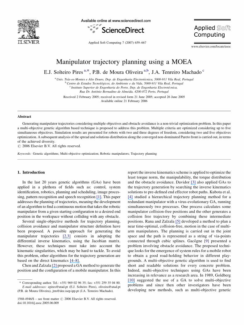
Fig. 2. Optimal fronts for the 2R robot. (a) Pareto optimal front and (b) local optimal front.

minimized by the planner to find the optimal Pareto front.

Before evaluating any solution, in order to remove virtual

jumps, all the values such that jq ð jþ1ÞDt;Tð Þi � q

ð jDt;TÞi j>p are

readjusted, adding or removing a multiple value of 2p, in the

strings:

fq ¼Xn

j¼1

Xi

l¼1

�qð jDt;TÞl

�2

(4a)

fq ¼Xn

j¼1

Xi

l¼1

�qð jDt;TÞl

�2

(4b)

f p ¼Xn

j¼2

dð p j; p j�1Þ2 (4c)

f p ¼Xn

j¼3

�d

�p j; p j�1

�� d

�p j�1; p j�2

��2

(4d)

fEa ¼ ðn� 1ÞDtPa ¼Xn

j¼1

Xi

l¼1

jtl � Dqð jDt;TÞl j (4e)

The joint distance fq (4a) is used to minimize the manipulator

joints traveling distance. In fact, for a function y = g(x) the

curve length is defined by Eq. (5) and, consequently, to mini-

mize the curve length distance the simplified expression (6) is

adopted:

Z 1þ

�dg

dx

�2dx (5)

Z �dg

dx

�2

dx ¼Z

g2 dx (6)

The joint velocity function fq is used to minimize the ripple in

time evolution. The cartesian distance fp (4c) minimizes the

total arm trajectory length, from the initial point up to the final

point, where pj is the robot j intermediate arm cartesian position

and d(�, �) is a function that returns the distance between two

arguments. The cartesian velocity f p (4d) is responsible for

reducing the ripple in arm time evolution. Finally, the energy

fEa in expression (4e), where tl reports the robot joint torques,

is computed assuming that power regeneration is not available

by motors doing negative work, that is, by taking the absolute

value of the power [16].

3. Simulation results

In this section results of various experiments are presented.

In this line of thought, subsections 3.1 and 3.2 present the

trajectory optimization for 2R and 3R robots respectively, using

two objectives (2D). Subsection 3.3 shows the results of a five

dimensional (5D) optimization for a 2R robot. Finally,

subsection 3.4 presents the results of a 5D optimization for a

3R robot in a workspace with an obstacle.

3.1. 2R Robot trajectory with 2D optimization

The first experiment consists on moving a 2R robotic arm

from the starting configuration, defined by the joint coordinates

A � {�1.149, 1.808} rad, up to the final configuration, defined

by B � {1.181, 1.466} rad, in a workspace without obstacles.

The optimization objectives considered in this section are the

joint velocity fq (4b) and the cartesian velocity f p (4d).

The simulations results achieved by the algorithm, with

n = 9 configurations, Tt = 15,000 generations and popsize = 300,

converge to two optimal fronts. One of the fronts (Fig. 2(a))

corresponds to the movement of the manipulator around its base

in the counterclockwise direction. The other front (Fig. 2(b)) is

obtained when the manipulator moves in the clockwise

direction. The solutions a and b, shown in Fig. 2 represents

the best solution found for the fq and f p objectives,

respectively.

In this simulation study, the MOEAwas executed 21 times in

order to study the Pareto optimal convergence. In 66.6% of the

21 total number of runs, the Pareto optimal front was found. In

E.J.Solteiro Pires et al. / Applied Soft Computing 7 (2007) 659–667662

Table 1

Fronts parameters statistics

Pareto front Local front

k a b Length k a b Length

Median 13.46 �8.32 �10.77 38.22 19.23 49.28 �13.02 315.50

Average 13.45 �7.40 �9.95 38.70 19.18 49.48 �13.19 334.32

Standard deviation 0.37 2.71 1.82 7.43 0.30 3.65 0.76 55.79

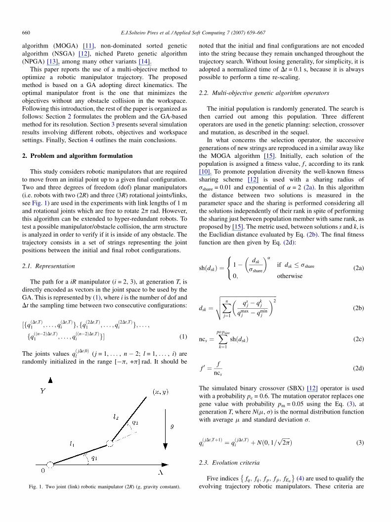
Fig. 3. Normal straight lines to the front obtained with f pð fqÞ function.

all simulations, for both cases, the solutions converged to a

front type, which can be modeled by the following equation (k,

a, b2R):

f pð fqÞ ¼ kfq þ a

fq þ b(7)

The achieved median, average and standard deviation for the

parameters k, a and b of (7) are shown in Table 1, both for the

Pareto optimal and local fronts. From these values it can be

concluded that the algorithm converges always for one of the

fronts. Furthermore, the variation for each type of front is small,

as it can be verified by the achieved standard deviation values.

To study the spread of the fronts the length of the

approximating functions are measured. This length is evaluated

considering the two extreme solutions of the front {a, b}.

Therefore, the length is evaluated between the two points of the

modeled function whose distance is the smaller to front points a

and b, respectively. Table 1 also shows the experiments length

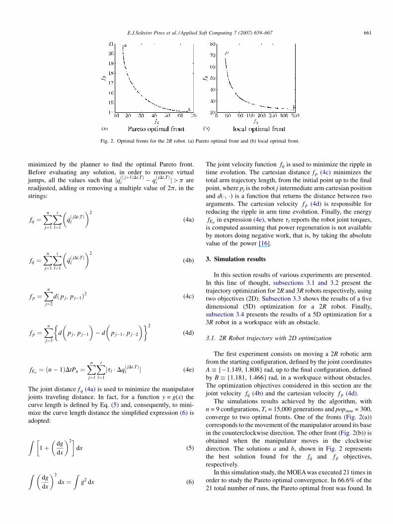
Fig. 4. Solution distribution s

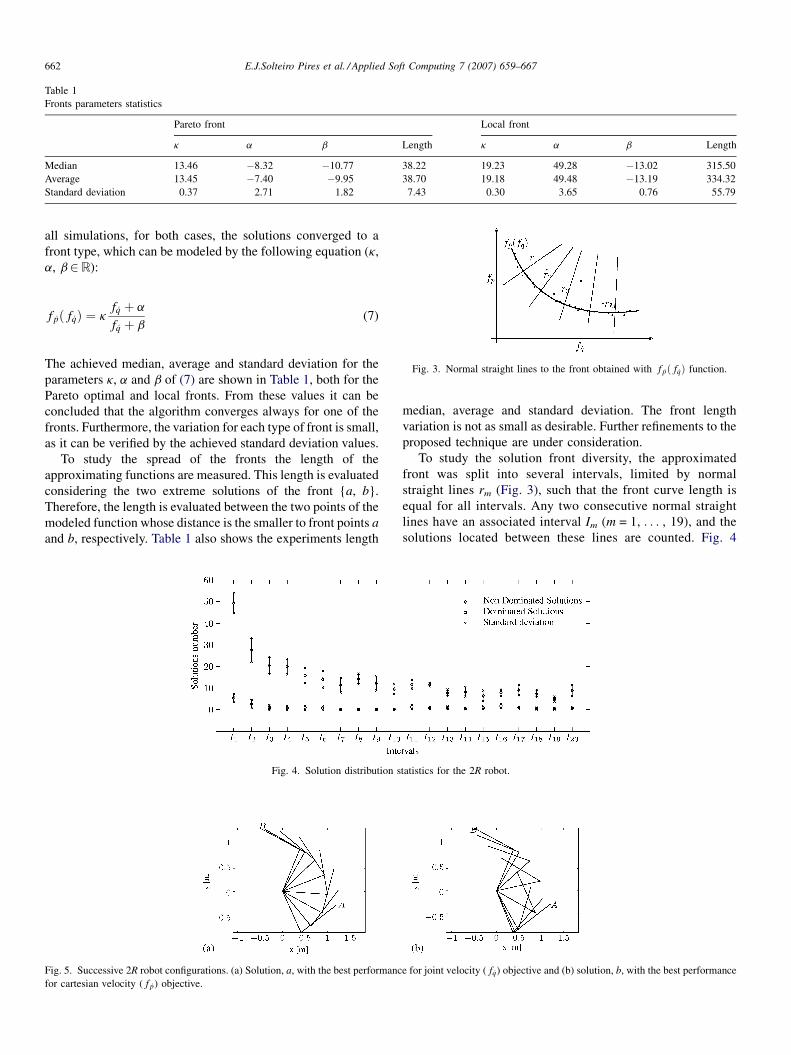
Fig. 5. Successive 2R robot configurations. (a) Solution, a, with the best performanc

for cartesian velocity ( f p) objective.

median, average and standard deviation. The front length

variation is not as small as desirable. Further refinements to the

proposed technique are under consideration.

To study the solution front diversity, the approximated

front was split into several intervals, limited by normal

straight lines rm (Fig. 3), such that the front curve length is

equal for all intervals. Any two consecutive normal straight

lines have an associated interval Im (m = 1, . . . , 19), and the

solutions located between these lines are counted. Fig. 4

tatistics for the 2R robot.

e for joint velocity ( fq) objective and (b) solution, b, with the best performance

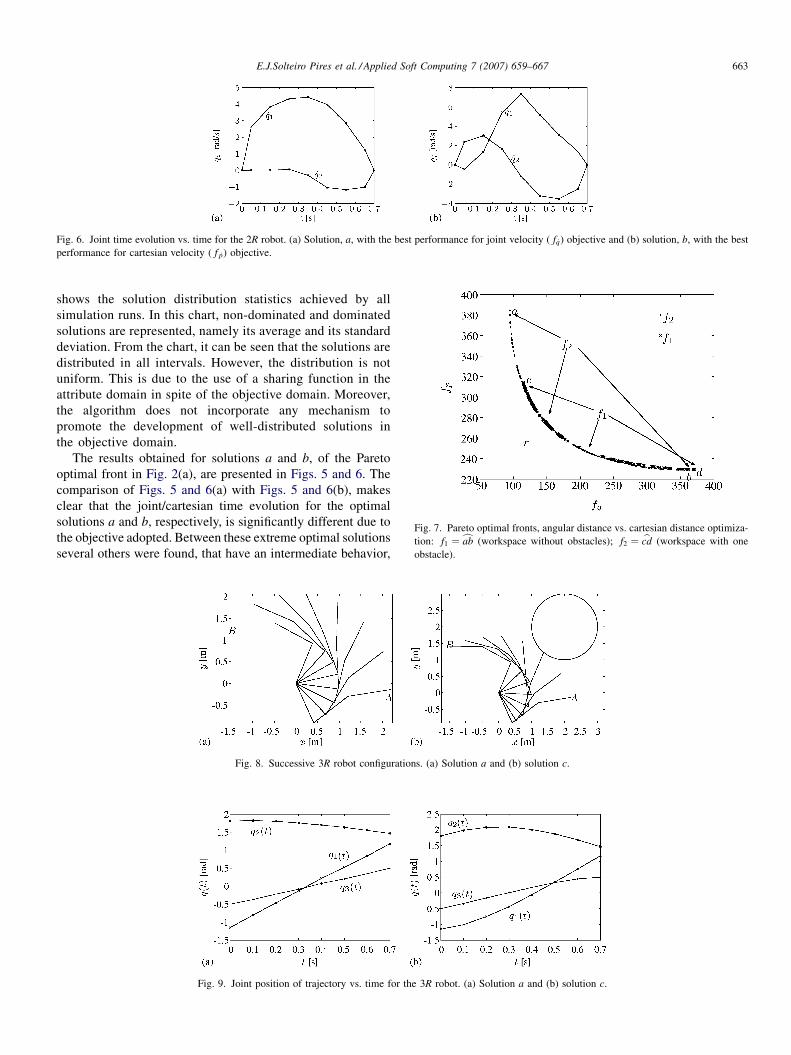
E.J.Solteiro Pires et al. / Applied Soft Computing 7 (2007) 659–667 663

Fig. 6. Joint time evolution vs. time for the 2R robot. (a) Solution, a, with the best performance for joint velocity ( fq) objective and (b) solution, b, with the best

performance for cartesian velocity ( f p) objective.

Fig. 7. Pareto optimal fronts, angular distance vs. cartesian distance optimiza-

tion: f1 ¼cab (workspace without obstacles); f2 ¼ bcd (workspace with one

obstacle).

shows the solution distribution statistics achieved by all

simulation runs. In this chart, non-dominated and dominated

solutions are represented, namely its average and its standard

deviation. From the chart, it can be seen that the solutions are

distributed in all intervals. However, the distribution is not

uniform. This is due to the use of a sharing function in the

attribute domain in spite of the objective domain. Moreover,

the algorithm does not incorporate any mechanism to

promote the development of well-distributed solutions in

the objective domain.

The results obtained for solutions a and b, of the Pareto

optimal front in Fig. 2(a), are presented in Figs. 5 and 6. The

comparison of Figs. 5 and 6(a) with Figs. 5 and 6(b), makes

clear that the joint/cartesian time evolution for the optimal

solutions a and b, respectively, is significantly different due to

the objective adopted. Between these extreme optimal solutions

several others were found, that have an intermediate behavior,

Fig. 8. Successive 3R robot configurations. (a) Solution a and (b) solution c.

Fig. 9. Joint position of trajectory vs. time for the 3R robot. (a) Solution a and (b) solution c.

E.J.Solteiro Pires et al. / Applied Soft Computing 7 (2007) 659–667664

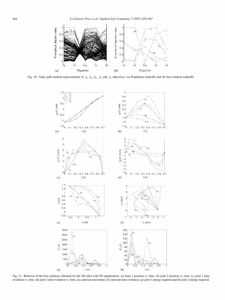
Fig. 10. Value path method representation of fq; fq; fEa ; f p and f p objectives. (a) Population tradeoffs and (b) best solution tradeoffs.

Fig. 11. Behavior of the best solutions obtained for the 2R robot with 5D optimization. (a) Joint 1 position vs. time, (b) joint 2 position vs. time, (c) joint 1 time

evolution vs. time, (d) joint 2 time evolution vs. time, (e) cartesian movement, (f) cartesian time evolution, (g) joint 1 energy required and (h) joint 2 energy required.

E.J.Solteiro Pires et al. / Applied Soft Computing 7 (2007) 659–667 665

Table 2

Range objectives in the 5D optimization for a single run

fq (rad2/s2) fq (rad4/s4) fEa (J) fp (m2/s2) f p (m4/s4)

Minimum 79.8 18.2 1056.7 83.5 15.0

Maximum 182.3 101.7 4602.7 121.8 56.4

Table 3

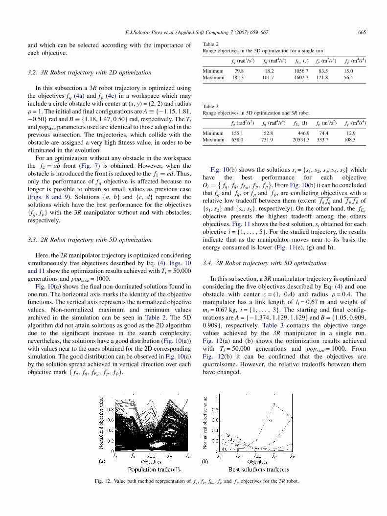
Range objectives in 5D optimization and 3R robot

fq (rad2/s2) fq (rad4/s4) fEa (J) fp (m2/s2) f p (m4/s4)

Minimum 155.1 52.8 446.9 74.4 12.9

Maximum 638.0 731.9 20531.3 333.7 108.3

and which can be selected according with the importance of

each objective.

3.2. 3R Robot trajectory with 2D optimization

In this subsection a 3R robot trajectory is optimized using

the objectives fq (4a) and fp (4c) in a workspace which may

include a circle obstacle with center at (x, y) = (2, 2) and radius

r = 1. The initial and final configurations are A � {�1.15, 1.81,

�0.50} rad and B � {1.18, 1.47, 0.50} rad, respectively. The Tt

and popsize parameters used are identical to those adopted in the

previous subsection. The trajectories, which collide with the

obstacle are assigned a very high fitness value, in order to be

eliminated in the evolution.

For an optimization without any obstacle in the workspace

the f2 ¼cab front (Fig. 7) is obtained. However, when the

obstacle is introduced the front is reduced to the f1 ¼ bcd. Thus,

only the performance of fq objective is affected because no

longer is possible to obtain so small values as previous case

(Figs. 8 and 9). Solutions {a, b} and {c, d} represent the

solutions which have the best performance for the objectives

{fq, fp} with the 3R manipulator without and with obstacles,

respectively.

3.3. 2R Robot trajectory with 5D optimization

Here, the 2R manipulator trajectory is optimized considering

simultaneously five objectives described by Eq. (4). Figs. 10

and 11 show the optimization results achieved with Tt = 50,000

generations and popsize = 1000.

Fig. 10(a) shows the final non-dominated solutions found in

one run. The horizontal axis marks the identity of the objective

functions. The vertical axis represents the normalized objective

values. Non-normalized maximum and minimum values

archived in the simulation can be seen in Table 2. The 5D

algorithm did not attain solutions as good as the 2D algorithm

due to the significant increase in the search complexity;

nevertheless, the solutions have a good distribution (Fig. 10(a))

with values near to the ones obtained for the 2D corresponding

simulation. The good distribution can be observed in Fig. 10(a)

by the solution spread achieved in vertical direction over each

objective mark fq; fq; fEa ; f p; f p

� �.

Fig. 12. Value path method representation of fq;

Fig. 10(b) shows the solutions si = {s1, s2, s3, s4, s5} which

have the best performance for each objective

Oi ¼ fq; fq; fEa ; f p; f p

� �. From Fig. 10(b) it can be concluded

that fq and fq, or fp and f p, are conflicting objectives with a

relative low tradeoff between them (extent fq fq and f p f p of

{s1, s2} and {s4, s5}, respectively). On the other hand, the fEa

objective presents the highest tradeoff among the others

objectives. Fig. 11 shows the best solution, si obtained for each

objective i = {1, . . . , 5}. For the studied trajectory, the results

indicate that as the manipulator moves near to its basis the

energy consumed is lower (Fig. 11(e), (g) and h).

3.4. 3R Robot trajectory with 5D optimization

In this subsection, a 3R manipulator trajectory is optimized

considering the five objectives described by Eq. (4) and one

obstacle with center c = (1, 0.4) and radius r = 0.4. The

manipulator has a link length of li = 0.67 m and weight of

mi = 0.67 kg, i = {1, . . . , 3}. The starting and final config-

urations are A = {�1.374, 1.129, 1.129} and B = {1.05, 0.909,

0.909}, respectively. Table 3 contains the objective range

values achieved by the 3R manipulator in a single run.

Fig. 12(a) and (b) shows the optimization results achieved

with Tt = 50,000 generations and popsize = 1000. From

Fig. 12(b) it can be confirmed that the objectives are

quarrelsome. However, the relative tradeoffs between them

have changed.

fq; fEa ; f p and f p objectives for the 3R robot.

E.J.Solteiro Pires et al. / Applied Soft Computing 7 (2007) 659–667666

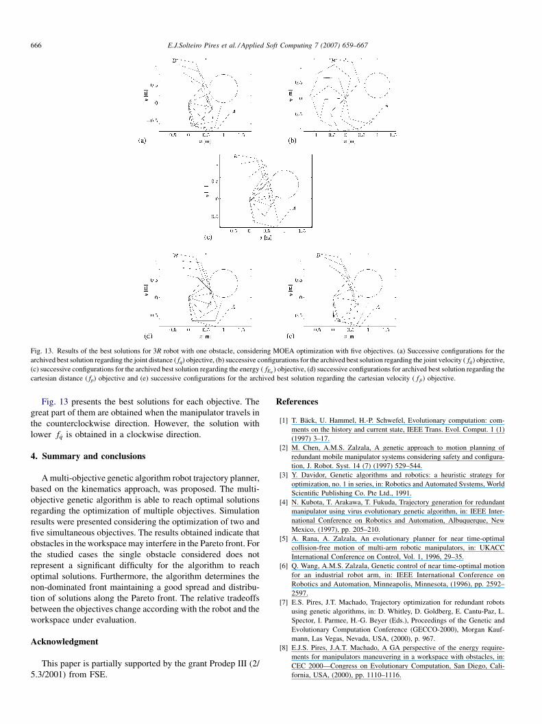
Fig. 13. Results of the best solutions for 3R robot with one obstacle, considering MOEA optimization with five objectives. (a) Successive configurations for the

archived best solution regarding the joint distance ( fq) objective, (b) successive configurations for the archived best solution regarding the joint velocity ( fq) objective,

(c) successive configurations for the archived best solution regarding the energy ( fEa ) objective, (d) successive configurations for archived best solution regarding the

cartesian distance ( fp) objective and (e) successive configurations for the archived best solution regarding the cartesian velocity ( f p) objective.

Fig. 13 presents the best solutions for each objective. The

great part of them are obtained when the manipulator travels in

the counterclockwise direction. However, the solution with

lower fq is obtained in a clockwise direction.

4. Summary and conclusions

A multi-objective genetic algorithm robot trajectory planner,

based on the kinematics approach, was proposed. The multi-

objective genetic algorithm is able to reach optimal solutions

regarding the optimization of multiple objectives. Simulation

results were presented considering the optimization of two and

five simultaneous objectives. The results obtained indicate that

obstacles in the workspace may interfere in the Pareto front. For

the studied cases the single obstacle considered does not

represent a significant difficulty for the algorithm to reach

optimal solutions. Furthermore, the algorithm determines the

non-dominated front maintaining a good spread and distribu-

tion of solutions along the Pareto front. The relative tradeoffs

between the objectives change according with the robot and the

workspace under evaluation.

Acknowledgment

This paper is partially supported by the grant Prodep III (2/

5.3/2001) from FSE.

References

[1] T. Back, U. Hammel, H.-P. Schwefel, Evolutionary computation: com-

ments on the history and current state, IEEE Trans. Evol. Comput. 1 (1)

(1997) 3–17.

[2] M. Chen, A.M.S. Zalzala, A genetic approach to motion planning of

redundant mobile manipulator systems considering safety and configura-

tion, J. Robot. Syst. 14 (7) (1997) 529–544.

[3] Y. Davidor, Genetic algorithms and robotics: a heuristic strategy for

optimization, no. 1 in series, in: Robotics and Automated Systems, World

Scientific Publishing Co. Pte Ltd., 1991.

[4] N. Kubota, T. Arakawa, T. Fukuda, Trajectory generation for redundant

manipulator using virus evolutionary genetic algorithm, in: IEEE Inter-

national Conference on Robotics and Automation, Albuquerque, New

Mexico, (1997), pp. 205–210.

[5] A. Rana, A. Zalzala, An evolutionary planner for near time-optimal

collision-free motion of multi-arm robotic manipulators, in: UKACC

International Conference on Control, Vol. 1, 1996, 29–35.

[6] Q. Wang, A.M.S. Zalzala, Genetic control of near time-optimal motion

for an industrial robot arm, in: IEEE International Conference on

Robotics and Automation, Minneapolis, Minnesota, (1996), pp. 2592–

2597.

[7] E.S. Pires, J.T. Machado, Trajectory optimization for redundant robots

using genetic algorithms, in: D. Whitley, D. Goldberg, E. Cantu-Paz, L.

Spector, I. Parmee, H.-G. Beyer (Eds.), Proceedings of the Genetic and

Evolutionary Computation Conference (GECCO-2000), Morgan Kauf-

mann, Las Vegas, Nevada, USA, (2000), p. 967.

[8] E.J.S. Pires, J.A.T. Machado, A GA perspective of the energy require-

ments for manipulators maneuvering in a workspace with obstacles, in:

CEC 2000—Congress on Evolutionary Computation, San Diego, Cali-

fornia, USA, (2000), pp. 1110–1116.

E.J.Solteiro Pires et al. / Applied Soft Computing 7 (2007) 659–667 667

[9] L. Gacogne, Multiple objective optimization of fuzzy rules for obsta-

cles avoiding by an evolution algorithm with adaptative operators, in:

Proceedings of the Fifth International Mendel Conference on Soft

Computing (Mendel’99), Brno, Czech Republic, (1999), pp. 236–

242.

[10] D.E. Goldberg, Genetic Algorithms in Search, Optimization and Machine

Learning, Addison–Wesley, 1989.

[11] C.M. Fonseca, P.J. Fleming, An overview of evolutionary algorithms

in multi-objective optimization, Evol. Comput. J. 3 (1) (1995) 1–

16.

[12] K. Deb, Multi-objective optimization using evolutionary algorithms, in:

Systems and Optimization, Wiley-Interscience Series, 2001.

[13] J. Horn, N. Nafploitis, D. Goldberg, A niched Pareto genetic algorithm for

multi-objective optimization, in: Proceedings of the First IEEE Confer-

ence on Evolutionary Computation, 1994, pp. 82–87.

[14] C. Coello, A. Carlos, A comprehensive survey of evolutionary-based

multi-objective optimization techniques, Knowl. Inform. Syst. 1 (3)

(1999) 269–308.

[15] C.M. Fonseca, P.J. Fleming, Genetic algorithms for multi-objective

optimization: formulation, discussion and generalization, in: Fifth Inter-

national Conference on Genetic Algorithms, 1993, 416–423.

[16] F. Silva, J.T. Machado, Energy analysis during biped walking, in: Pro-

ceedings of the IEEE International Conference on Robotics and Auto-

mation, Detroit, Michigan, (1999), pp. 59–64.