Mapping and Monitoring of Soil Salinization - Remote Sensing, GIS, Modeling, Electromagnetic Induction and Conventional Methods Case Studies

Proceedings of the International Conference on Soils and Groundwater Salinization in Arid Countries, 59-97 (2010)2010 Sultan Qaboos University

59______________________________

* E-mail: [email protected]

Mapping and Monitoring of Soil Salinization Remote Sensing, GIS, Modeling, Electromagnetic Induction and

Conventional Methods – Case Studies

Shabbir A. Shahid1*, Mahmoud A. Abdelfattah2, Samira A. S. Omar3,Hussein Harahsheh4, Yasser Othman5 and Henda Mahmoudi6

1Salinity Management Scientist and 6Visiting Scientist, International Center for Biosaline Agriculture, P.O. Box 14660 Dubai, United Arab Emirates

2Soil Scientist and 5Remote Sensing Specialist, Environment Agency Abu Dhabi, P.O. Box 54443 Abu Dhabi, United Arab Emirates

3Director Food Resources and Biological Sciences Division, Kuwait Institute for Scientific Research, P.O. Box 24885 Safat 13109, Kuwait

4Marketing and Operation Manager Global Scan Technologies L.L.C. Belhasa Building 204, Al Itthad Road, Deira,

P.O. Box 1286, Dubai, UAE

ABSTRACT: Soil salinity is a major global issue due to its adverse impact on the environment, agro-ecosystems, agricultural productivity and sustainability. Saline soils are significant as formations of ecosystem on the earth affected by high concentrations of soluble salts, and as means of crop production with little economic value. Threats being the water scarcity, drought, degradation of surface and groundwater quality leading to soil salinization. Many plants either fail to grow in saline soils or their growth is retarded significantly. However, few plants grow well on saline soils; therefore, soil salinity often restricts options for cropping in a given area. Therefore, temporal understanding of soil salinity through mapping and monitoring helps understand subtle difference across the landscape and agricultural fields, and allows their precise management. Mapping on regional and national levels is appropriate to be accomplished through interpretation of Remote Sensing Imagery supplemented with limited ground truthing, and through using Geographic Information System salinity maps can be developed, however, at farm level or irrigated fields more intensive salinity assessment and monitoring is required. Under such conditions, salinity is measured using a set of equipment, such as through routine (EC meter, salinity bridge through salinity sensors) and modern equipment (EC Probe, EM38 and automated salinity logging though salinity sensors). The choice of the technique depends upon the purpose, size of the area, soil depth, and frequency of measurement, accuracy required and the available resources. In this keynote paper various techniques of salinity assessment, mapping and monitoring will be presented and experience from Arid regions (case studies) will be shared with conference participants.

Introduction Soil salinity is a major global issue due to its adverse impact on the environment, agro-ecosystems, agricultural productivity and sustainability (Figure 1). Salinity undermines the resource base by decreasing soil quality. Effective soil resource use and management requires scientific based understanding of soil salinization. It is important in the regions where salinity occurs, to generate soil salinity information to determine extent and risk of salinity, of which salinity mapping and regular monitoring has a great role to play. Salinity information at regional, national and local levels, as well as in irrigated fields, therefore, becomes extremely important for decision making and managing these resources. Managing saline soils is highly site specific and depends on factors such as nature of soils, soluble salts and local hydrological conditions. Salinity mapping can be accomplished by various approaches integrating Remote Sensing and GIS at broad scales and small scales, RS imagery is well suited to map the

surface expression of salinity (Spies and Woodgate, 2004), poor vegetation cover could be an indication of salinity in the area. While depth to groundwater and vegetation cover are widely regarded as the most useful indicator for determining salinity trends and risks. The goal of such exercise is to assess and map soil salinity to understand the problem, provide information to take necessary action to prevent its temporal distribution and to manage the improvement and sustainable use of land resources. Salinized and cropped areas can be identified with a salinity index based on greenness and brightness that indicates leaf moisture influenced by salinity, with classical false-color composites of separated bands or with a computer-assisted land-surface classification (Vincent et al., 1996). A brightness index detects brightness appearing at high levels of salinity. A comprehensive review of technologies for salinity mapping and monitoring is give in the respective sections.

60

Shahid and others

61

Mapping and monitoring soil salinization remote sensing, GIS, modeling, electromagnetic induction and conventional methods - case studies

Soil Salinization – A Global Issue Soil salinization is a global issue and affects almost all continents; it is not static but dynamic. Salinization can affects ecosystem to a level where it cannot provide environmental services to its full potential. It is a world-regional-national-site level concern to all of us. Many factors contribute to the development of saline soil conditions. However, most soils become saline through sea water intrusion (costal areas) and through the use

of saline/brackish ground water for irrigation purposes (agricultural farms). Salt concentrations in soil vary widely both vertically and horizontally depending on such conditions, variation in soil texture, plant growth, quality of irrigation water, hydraulic conductivity and irrigation system in place etc.. In general salinity mapping and monitoring plan must be a part of any project dealing with use of irrigation water with salinity/sodicity component. In agricultural farms, an effective salinity-monitoring plan

Salinization in a fallow land Salinization in a fallow agriculture land

Soil salinization in brassica field Soil salinization in wheat field

Water logging and salt kill trees High salinity kill date palm trees

Figure 1. Soil salinity a threat to agriculture and ecosystems.

60

Shahid and others

61


must be prepared to trace salinity changes particularly in the root zone to oversee the impact of management options used to overcome or reduce salinity affects.

One billion of the 13 billion ha land on earth covered with saline and/or sodic soils, between 25 and 30% of irrigated lands are salt-affected and commercially unproductive. In Southwest USA and Mexico about 200 million ha land is affected by salinity. In Spain, Portugal, Greece, and Italy salt water intrusion into aquifers is significant, and in Spain more than 20% land area is desert or seriously degraded and non-productive. In Black Sea desert and salt claiming vast tracts of cultivable land. In the Middle East 20 million ha area is affected by increased groundwater and soil salinity, reasons being irrigation practices, high evaporation rates, growth of sabkhas (salt scalds) increase groundwater salinity. In addition the irrigated lands of Euphrates (Syria, Iraq) seriously constrained by salinity. In Egypt 1 million ha cultivable land along Nile is salt-affected; salt accumulation in Jordan River basin adversely affected agricultural production in Syria, Jordan. In Iran 25 million ha land is unproductive due to salinity. In Africa 80- million hectares are saline, sodic or saline/sodic, of which West Africa Sahel is most affected; in Asia e.g in India 20% cultivable land is affected and distributed mainly in Rajasthan, coastal Gujarat, Indo-Gangetic Plains. In Pakistan 10 million ha are affected; about 5-10 ha per hour lost to salinity and

water logging in inland coastal regions, irrigated Indus basin. In Bangladesh 3 million ha are unproductive due to salinity. In Thailand 3.5 million ha are salt affected (3.0 and 0.58 Mha inland and coastal saline soils respectively. In China 26 million ha total land area is salt-affected (inner Mongolia, Yellow River basin, tidal coastal regions); over 350 million ha in Australia.

Why is Detecting and Monitoring Soil Salinity Important?The knowledge and data gained from Remote Sensing of saline soils is used heavily in agricultural uses all over the world. Predicting sites at risk for possible future salinization is important so that preventative measures such as tree planting can be taken to prevent the soils from becoming saline. Monitoring farming fields and mapping salt affected soils and sodium bearing minerals is important for agricultural production. By knowing soil salinity, crops can be planted or not planted in various regions with a better understanding of how the crops might behave. This is particularly important in impoverished regions where food shortages are a reality. Reclamation projects can benefit from this type of salinity mapping as well. The images taken are then used to monitor the progress of the reclamation project to insure the processes are being carried out accordingly and that the soil is being returned to its original condition. The knowledge gained from the new monitoring techniques, along with that generated by

Salts water irrigation

Salts accumulation

Needs more water

Leaching

Watertable rise

Restriction to leaching

Capillary rise and evaporation

Seepage from the system

Soil impermeability due to high Na

Ionic

imbalance

Ionic

unbalanceSalts water irrigation

Salts accumulation

Needs more water

Leaching

Watertable rise

Restriction to leaching

Capillary rise and evaporation

Seepage from the system

Soil impermeability due to high Na

Ionic

imbalance

Ionic

unbalance

Figure 2. Hypothetical salinization cycle.

imbalance

imbalance

62

Shahid and others

63


decades of painstaking field research, is offering many insights to the causes of salinization. Importantly, this is aiding scientists in the development of methods to predict sites most at risk of salinization so that preventative measures such as tree-planting can be taken.

Salinity Mapping and MonitoringThe aim of soil salinity mapping is to know temporal subtle salinity differences in the landscape and to develop salinity zones to help design management plan for sustainable use of soil resources. Monitoring determines periodic changes in soil salinity. Soil salinity mapping at the regional, national and farm level is becoming increasingly important for resource understanding, use and management reasons. The soil salinity could be caused due to many reasons; natural disasters (Tsunami), sea water intrusion, irrigation with saline and brackish waters etc latter if not properly managed can cause salinization in agricultural farms and decline farm productive capacity. A hypothetical salinity development cycle is shown in Figure 2.

In agricultural fields the water distribution through flood irrigation, and modern irrigation systems (drips and sprinklers) cannot be applied uniformly; therefore, the behavior of salinity development would be heterogeneous. Under such saline conditions many plants either fail to grow or their growth is retarded significantly. However, few plants grow well on saline soils; therefore, salinization often restricts options (biosaline agriculture) for cropping in a given land area. The snapshots (mapping) of salinity at surface and subsoil layers at large (farm level) and small scales (regional & national levels) can help understand the real problem and help develop management and use plan to get more value from each piece of land.

A reliable method for salinity assessment and mapping is needed to delineate areas into soil salinity status zones. At the country level salinity mapping information helps in land use planning, and to address reverse causes of salinization. In agricultural farms salinity maps help farmers to understand subtle difference in soil properties across their fields, allowing them to develop more precise management zones and selection of salt tolerant crops and, ultimately potentially higher yields. It sounds complicated, but salinity mapping at the farm level is one of the simplest and least expensive salinity measurement tools.

Traditionally, soil salinity assessment has been based on geo-referenced field sampling and laboratory analysis where the electrical conductivity of the saturation extract (ECe) is measured and using GIS salinity maps are prepared. This is a tedious, expensive and time consuming procedure that requires intensive field survey, sample collection, preparation of saturated soil pastes to meet the standard criteria, collection of saturation extract and analyses by electrical conductivity meter. Therefore, other quicker methods have been developed that include the use of RS imagery at the regional and national levels and modern equipment at farm level such as salinity probes and electromagnetic (EM) induction (EM38)

characterization. The EM38 is designed to be particularly useful for agricultural surveys and for measuring soil salinity. The use of EM device has gained acceptance due to its simplicity, reliability, rapidity and reproducibility of the results. It covers large areas quickly and provides 1.5 meters and 0.75 meters depth of exploration of the vertical and horizontal dipole modes respectively. It is also a rapid, mobile instrumental technique for measuring bulk soil electrical conductivity as a function of spatial position on the landscape.

There are five basic tools for salinity characterizations; 1) Remote Sensing & GIS; 2) conventional soil sampling and analyses; 3) salinity probes; 4) electromagnetic induction; and 5) salinity modeling. The following sections describe the technologies as well as their application in salinity aspects.

Soil salinity mapping and monitoring using Remote Sensing Imagery and GIS - Scientific Antecedents

Salinity mapping and monitoring through using remote sensing and GIS have been common in many countries; such procedures have recently been used in Kuwait and Abu Dhabi Emirate as part of national soil inventories (KISR, 1999a&b; EAD, 2009; Abdelfattah & Shahid, 2010); at the regional and national levels (Sukchani and Yamamoto, 2005), RS and GIS for water logging and salinity monitoring (Asif and Ahmad, 1999); RS technology for soil salinity (Hussein, 2003), mapping salt-affected soils using RS and GIS (Maher, 1990); mapping salt-affected soils using Landsat satellite data (Joshi and Sahai, 1993); soil salinity mapping using airborne remote sensing and spectroscopy (Bennett, 1998); salinity assessment using RS techniques (Brena et al., 1995); salinity assessment by combined use of RS and GIS (Casas, 1995); multispectral remote sensing of saline seeps (Chaturvedi et al., 1983); detecting saline soils with video imagery (Everitt et al., 1988); selection of best possible Landsat TM band combination for the delineation of salt-affected soils (Dwivedi and Rao, 1992); delineation of salt-affected soils through digital analyses of Landsat MSS data (Singh and Dwivedi, 1989); application of multitemporal Landsat data for salinity identification (Farooq and Din, 1980; Makin, 1986); salinity monitoring using RS and GIS (Goosens et al., 1993); use of remote sensing in salt marsh biomass and stress detection (Hardisk et al., 1983); Remote sensing of salt-affected soils (Mougenot et al., 1993; Verma et al, 1994); Landsat imagery for mapping saline soils (Sharma and Bhargava, 1988); application of Landsat imagery for monitoring soil salinity trends (WAPDA, 1984); integration of RS and conventional information (Zevenbergen, 1990). The TM bands 5 and 7 are frequently used to detect soil salinity or drainage anomalies (Mulders and Epema, 1986; Menenti et al., 1986; Zuluaga, 1990; Vincent et al., 1996); broadscale monitoring of salinity using satellite remote sensing (Dutkiewics and Lewis, 2008).

62

Shahid and others

63


Remote Sensing for Soil Salinity Mapping – Fundamentals - Remote sensing acquires information about the Earth’s surface without actually being in contact with it. This is done by sensing and recording reflected or emitted energy and processing, analyzing, and applying that information”. In much of remote sensing, the process involves an interaction between incident radiation and the targets of interest. This is exemplified by the use of imaging systems where the following seven elements are involved. Note, however that remote sensing also involves the sensing of emitted energy and the use of non-imaging sensors. When the sun’s rays – made up of electromagnetic radiation of many different wavelengths – strike plants, water bodies, soils and other features on the Earth’s surface, some wavelengths are absorbed by molecules in these features and some are reflected. Different features on the Earth’s surface will absorb and reflect different parts of the electromagnetic spectrum depending on their chemical make-up. In this way, different parts of the electromagnetic spectrum provide information about the Earth’s surface that may be useful for the detection of salinization. Electromagnetic reflections are used to sense the differences in the earth’s surface. The majority of the images are supplied from satellites known as Landsat. A Thematic Mapper makes observations in bands ranging from the visible to the thermal on each area of the Earth’s surface, sending information back to Earth.

Electromagnetic RadiationThe first requirement for remote sensing is to have an energy source to illuminate the target (unless the sensed energy is being emitted by the target). This energy is in the form of electromagnetic radiation. All electromagnetic radiation has fundamental properties and behaves in predictable ways according to the basics of wave theory. Electromagnetic radiation consists of an electrical field (E) which varies in magnitude in a direction perpendicular to the direction in which the radiation is traveling, and a magnetic field (M) oriented at right angles to the electrical field. Both these fields travel at the speed of light (c).

The wavelength is the length of one wave cycle, which can be measured as the distance between successive wave crests. Wavelength is usually represented by the Greek letter lambda (Wavelength is measured in meters (m) or some factor of meters such as manometers (nm, 10-9 meters), micrometers (µm, 10-6 meters) or centimeters (cm, 10-2 meters). Frequency refers to the number of cycles of a wave passing a fixed point per unit of time. Frequency is normally measured in hertz (Hz), equivalent to one cycle per second, and various multiples of hertz.

Wavelength and frequency are related by the following formula:

C =

where is the velength (m); v is the frequency (cycle per second, Hz); C is the speed of light (3x 108 m/s).Therefore,

the two are inversely related to each other. The shorter the wavelength, the higher the frequency. The longer the wavelength, the lower the frequency. Understanding the characteristics of electromagnetic radiation in terms of their wavelength and frequency is crucial to understanding the information to be extracted from remote sensing data.

The Electromagnetic SpectrumThe electromagnetic spectrum (Figure 3) ranges from the shorter wavelengths (including gamma and x-rays) to the longer wavelengths (including microwaves and broadcast radio waves). There are several regions of the electromagnetic spectrum which are useful for remote sensing.

Ultraviolet UV - For most purposes, the ultraviolet or UV portion of the spectrum has the shortest wavelengths which are practical for remote sensing. This radiation is just beyond the violet portion of the visible wavelengths, which covers a range from 0.03 to 0.4 µm. Incoming wavelength less than 0.3 µm completely absorbed by ozone in the upper atmosphere. The Photographic UV band ranges from 0.3 to 0.4 µm transmitted through the atmosphere and detectable with film and photodetectors, but atmospheric scattering is severe. Some Earth surface materials, primarily rocks and minerals, fluoresce or emit visible light when illuminated by UV radiation.

Visible Spectrum - The light which our eyes - our “remote sensors” - can detect is part of the visible spectrum. It is important to recognize how small the visible portion is relative to the rest of the spectrum. There is a lot of radiation around us which is “invisible” to our eyes, but can be detected by other remote sensing instruments and used to our advantage. The visible wavelengths cover a range from approximately 0.4 to 0.7 µm. The longest visible wavelength is red and the shortest is violet. Common wavelengths of what we perceive as particular colors from the visible portion of the spectrum are listed below. It is important to note that this is the only portion of the spectrum we can associate with the concept of colors.

Violet: 0.4 - 0.446 µmBlue: 0.446 - 0.500 µmGreen: 0.500 - 0.578 µmYellow: 0.578 - 0.592 µmOrange: 0.592 - 0.620 µmRed 0.620 - 0.7 µm

Blue, green and red are the primary colors or wavelengths of the visible spectrum. They are defined as such because no single primary color can be created from the other two, but all other colors can be formed by combining blue, green, and red in various proportions. Although we see sunlight as a uniform or homogeneous color, it is actually composed of various wavelengths of radiation in primarily the ultraviolet, visible and infrared portions

(�)

��

�

64

Shahid and others

65


of the spectrum. The visible portion of this radiation can be shown in its component colors when sunlight is passed through a prism, which bends the light in differing amounts according to wavelength.

Infrared region - The next portion of the spectrum of interest is the infrared (IR) region which covers the wavelength range from approximately 0.7 µm to 100 µm - more than 100 times as wide as the visible portion. The infrared region can be divided into two categories based on their radiation properties - the reflected IR, and the emitted or thermal IR. Radiation in the reflected IR region is used for remote sensing purposes in ways very similar to radiation in the visible portion. The reflected IR covers wavelengths from approximately 0.7 mm to 3.0 mm. The thermal IR region is quite different than the visible and reflected IR portions, as this energy is essentially the radiation that is emitted from the Earth’s surface in the form of heat. The thermal IR covers wavelengths from approximately 3.0 µm to 100 µm. Images at thermal IR wavelengths are acquired by optical-mechanical scanners and special vidicon system but not by film.

Microwave region - The portion of the spectrum of more recent interest to remote sensing is the microwave region from about 0.1 cm to 100 cm. This covers the longest wavelengths used for remote sensing. The shorter wavelengths have properties similar to the thermal infrared region while the longer wavelengths approach the wavelengths used for radio broadcasts. Longer wavelength can penetrate clouds; fog, and rain, images can acquire in the active or passive system mode.

In the passive remote sensing, the sensors detect natural energy (radiation) that is emitted or reflected by the object or surrounding area being observed. Reflected sunlight is the most common source of radiation measured by passive sensors. Examples of passive remote sensors include film photography, visible and infra-red images from satellite platforms such as Landsat, Ikonos, IRS, Quick Bird, SPOT etc. In the active remote sensing, the sensor collects the return energy from the target terrain

that was emitted from its artificial source. The RADAR and LIDAR images from Radarsat, ERS are examples of active remote sensing where the time delay between emission and return is measured, establishing the location, height, speed and object direction.

A remote sensing process is shown in Figure 4 and different aspects are summarized below.

1) Energy Source or Illumination (A) - the first requirement for remote sensing is to have an energy source which illuminates or provides electromagnetic energy to the target of interest;

2) Radiation and the Atmosphere (B) - as the energy travels from its source to the target, it will come in contact with and interact with the atmosphere it passes through. This interaction may take place a second time as the energy travels from the target to the sensor;

3) Interaction with the Target (C) - once the energy makes its way to the target through the atmosphere, it interacts with the target depending on the properties of both the target and the radiation;

4) Recording of Energy by the Sensor (D) - after the energy has been scattered by, or emitted from the target, we require a sensor (remote - not in contact with the target) to collect and record the electromagnetic radiation;

5) Transmission, Reception, and Processing (E) – the energy recorded by the sensor has to be transmitted, often in electronic form, to a receiving and processing station where the data are processed into an image (hardcopy and/or digital);

6) Interpretation and Analysis (F) - the processed image is interpreted, visually and/or digitally or electronically, to extract information about the target which was illuminated;

7) Application (G) - the final element of the remote sensing process is achieved when we apply the information we have been able to extract from the imagery about the target in order to better understand it, reveal some new

Figure 3. Electromagnetic spectra.

64

Shahid and others

65


information, or assist in solving a particular problem. These seven elements comprise the remote sensing process from beginning to end.

Digital ImageDigital image is a two-dimensional array (or grid) of small areas called pixels (picture elements), and each pixel corresponds spatially to an area on the earth’s surface and represented by a digital number (or DN). These array or grid structure is also called a raster, so image data is often referred to as raster data.

Band: A set of data file values for a specific portion of the electromagnetic spectrum of reflected light or emitted heat, some times called (channel).

Pixel: Abbreviated from “picture element” the smallest part of a picture (image).

Satellite Image ResolutionSpatial resolution is measured as the smallest object that can be resolved by the sensor, or the area on the ground represented by each pixel, the finer the resolution the lower the pixel size (Figure 5).

Spectral Resolution is the specific wavelength intervals in the electromagnetic spectrum that a sensor can record. Band 1 of Landsat Thematic Mapper sensor records energy between 0.45 µm and 0.52 µm in the visible part of the spectrum.

Figure 4. Remote sensing process.

Figure 5. Pixel size resolution.

66

Shahid and others

67


Radiometric Resolution refers to the dynamic range, or number of possible data files values in each band. It is the number of bits required to store all of the data file values in a file some times called pixel depth, e.g., data with pixel depth 8, or 8-bit data, have 256 values for each pixel (2^8 =256), ranging from 0 to 255.

Temporal Resolution refers to how often a sensor obtains imagery of a particular area, e.g., Landsat satellite can view the same area of the globe once every 16 days. SPOT on the other hand, can revisit the same area every 3 days.

Satellite Imagery Sources - wide range of satellite imagery that can be used for evaluating the soil salinity and the selection of the suitable images depends mainly on the objective and the scale of the study. Table 1 displays part of the major characteristics of operational earth resources satellites that are suitable for the global, regional, national and local scale.

Image CorrectionAtmospheric Correction - the effects of the atmosphere upon remotely-sensed data are not considered errors, since they are part of the signal received by the sensing device. However, it is often important to remove atmospheric effects, especially for scene matching and change detection analysis. Three categories are mentioned here: Dark pixel subtraction, Radiance to reflectance conversion, Atmospheric modeling.

Radiometric Correction addresses variations in the pixel intensities (DNs) that are not caused by the object or scene being scanned. Striping, Line Dropout is the most common radiometric errors.

Geometric Correction is the process of correcting the geometric distortion in satellite images due to the motion of the sensor, the curvature of the earth and other by using Ground Control points (GCP).

Image ProcessingImage Enhancement is the process of making an image more interpretable for a particular application.

Radiometric Enhancement is an enhancement technique that deals with the individual values of pixels in an image, e.g., Contrast Stretch/Enhance, Histogram Equalization. Spatial Enhancement is the process of modifying the pixels in an image relative to the pixels that surround them, e.g., Filters.

Spectral Enhancement is the process of modifying the pixels of an image based on the original values of each pixel in the band relative to their values in other bands. These enhancement techniques require more than one band of data, e.g., Band Ratios, Vegetation Index.

Digital Image ClassificationIt is the process of assigning pixels to classes. Usually each pixel is treated as an individual unit composed of values in several bands. There are two broad classification procedure commonly used in the analysis of satellite images. One is referred to as unsupervised classification and the other supervised classification.

Unsupervised Classification is the technique used to identify natural grouping or structures within multi-spectral data. This technique is achieved by using clustering methods defined with a clustering algorithm, which often uses all or many of the pixels in the input data file for its analysis. The cluster algorithm has no regard for the contiguity of the pixels that define each cluster. Isodata cluster method uses spectral distance as in the sequential method, but iteratively classifies the pixel, redefines the criteria for each class, and classifies again.

Supervised Classification is the process of using samples of known identity to classify pixels of unknown identity. Samples of known identity are those pixels located within training areas.

Training Area - the user selects pixels that represent recognized pattern or land cover feature.

Classification Decision Rules - once a set of reliable signatures has been created and evaluated, the next step is to perform a classification of the data. Each pixel is analyzed independently. The measurement vector for each pixel is compared to each signature, according to a decision rule or algorithm.

Salinity Monitoring by aeroplane - Australian scientists have tested a number of techniques to collect and analyze electromagnetic information. For example, color infrared film can be used to take photographs from aeroplanes. Different colors (corresponding to different wavelengths within the infrared band) will show vegetation under varying levels of stress, which can then be related to the degree of salinity. Dark-green vegetation produces a bright red image, light-green foliage a pink image, barren saline soil a white image, salt-stressed vegetation a reddish-brown image. If such photographs are taken of the same area over different years, changes in the pattern of salinization can be monitored. Similarly, video cameras can be used from aeroplanes to collect information in the visible band of the spectrum. The videos show salinity patterns and the way these change over time. Another airborne electromagnetic technique makes use of the fact that electrical conductivity increases with increasing salinity. It involves an aeroplane flying low over the ground. Mounted on board is an electromagnetic transmitter and trailing behind on a cable is a receiver. The transmitter sends out pulses of electromagnetic radiation. When these hit the ground, they

66

Shahid and others

67


Table 1. Characteristics of operation earth resources satellite.

SN SatelliteImage Type

ResolutionSwath width (km)

Stereo- ImageSpatial

(meter)Spectral (band)

Radio-metric (bit)

Temporal (day)

1 Aster VNIR 15 1-3 8 16 60 Yes

SWIR 30 4-9 8

TIR 90 10-14 12

2 GeoEye-1 Pan 0.41 1 11 3 15.3 Yes

VNIR 1.65 1-4

3 IKONOS Pan 1 1 11 3 11.3 Yes

VNIR 4 1-4

4 IRS-P5 Cartosat-1 Pan 2.5 1 ~7 5 30 Yes

5 IRS-P6 LISS-III Resourcesat-1

VNIR 23.5 1-3 7 24 141 No

SWIR 23.5 4

6 IRS-P6 LISS-IV Resourcesat-1

VNIR 5.8 1-3 7 5 23 No

7 Landsat-7 Pan 15 1 8 16 170 No

VNIR 30 1-4

MIR 30 5 , 7

TIR 90 6

8 Quick Bird Pan 0.61 1 11 3.5 16.5 Yes

VNIR 2.44 1-4

9 Spot-5 Pan 2.5 1 8 3 60 Yes

VNIR 10 1-3

SWIR 20 4

10 MODIS Hyper 250 1-2 12 0.5 2330 No

500 3-7

1000 8-36

11 NOAA

AVHRR

VNIR, TIR

1100 1-6 11 Multi time/day

2399 No

68

Shahid and others

69


multispectral system could be build around these bands and acquire essentially the same information as a 70 band hyperspectral system. Hyperspectral remote sensing combines imaging and spectroscopy in single systems which often includes large data sets and require new processing methods. Hyperspectral data sets are generally composed of about 100 to 200 spectral bands of relatively narrow bandwidths (5-10 nm), whereas, multispectral data sets are usually composed of about 5 to 10 bands of relatively large bandwidths (70-400 nm).

Constraints in Remote Sensing of saline soils - satellite images can help in assessing the extent of saline areas and monitoring the changes in real time. Saline fields are often identified by the presence of spotty white patches of precipitated salts. Such precipitates usually occur in elevated or unvegetated areas, where water evaporates and leaves salt behind. Such salt crusts, which can be detected on satellite images, are not reliable evidence of high salinity in the root zone. Inadequate resolution of low cost RS data in optical range limited the identification to surface salt encrustation, therefore, identification of subsurface salinity and waterlogging using optical RS data becomes difficult. Other limitation in salinity mapping with multispectral imagery is where saline soils support productive plant growth (Furby et al., 1995) such as biosaline agriculture, where plant cover obscured direct sensing of the soil, while salt tolerant plants could not be differentiated from other cover.

Geographic Information System – GIS - Combining information on these and other factors could allow the prediction of sites vulnerable to the saline menace. This is where a geographic information system (GIS) can play a role. GIS is a computer application that involves the storage, analysis, retrieval and display of data that are described in terms of their geographic location. The most familiar type of spatial data is a map – GIS is really a way of storing map information electronically. A GIS has a number of advantages over old-style maps, though, one is that because the data are stored electronically they can be analyzed readily by computer. In the case of salinity, scientists can use data on rainfall, topography, soil type – indeed, any spatial information that is available electronically – to first determine the combinations most susceptible to salinization, and then to predict similar regions that may be at risk.

A. CASE STUDY – Abu Dhabi EmirateSoil salinization mapping in Abu Dhabi Emirate has been completed by using both RS imagery interpretation and field soil mapping, the results of which have been presented in this conference as separate paper (Abelfattah and Shahid, 2010). However, here, salinity mapping in one of the four subareas of Abu Dhabi Emirate at the level of suborder and subgroup levels are presented. These four sub-areas have been selected for an intensive soil survey

induce electrical currents to flow in conductive areas. The decay of these currents produces a magnetic field which is recorded by the receiver trailing behind the aircraft. The recording is then analyzed to determine the conductivity of the ground.

Monitoring by satellite - increasingly, scientists are also using satellite images to analyze salinity patterns across large areas. Most images are supplied by a series of scientific satellites known as Landsat. These orbit the Earth, recording information about the electromagnetic radiation reflected by the Earth’s surface. In Landsat satellites, an instrument called a Thematic Mapper makes regular observations in bands ranging from the visible to the thermal on each area of the Earth’s surface, sending the information back to Earth. Many scientists consider that data produced in this way can be used effectively for the detection and monitoring of salinity.

Multispectral remote sensing (MRS) can be defined as an imaging system with 2 or more bands but about 12 to 15 bands is the practical maximum. A “band” is defined as a portion of the spectrum with a given spectral width, such as 10 or 50 nm. Multispectral systems are non-contiguous in their coverage of the spectrum. The bands can be spectrally narrow or wide. Many satellite systems have traditionally had wide (50 - 200 nm) bands while some aircraft systems have discrete narrow bands (around 10 nm). Hyperspectral systems are known for having dozens to hundreds of narrow contiguous bands. Most are able to collect images starting at about 400 nm which is the edge of the blue visible part of the spectrum. Typically these systems can measure energy to 1100 or even 2500 nm. Hyperspectral systems are usually fundamentally different than multispectral systems because they generally build up images line by line as the aircraft moves rather than acquiring a complete image as a camera does.

Hyperspectral Data Analysis and Band Selection - Once hyperspectral images are acquired, corrected, and calibrated, they must be analyzed. There are many analysis techniques, three of which are: 1) Band selection, 2) Vegetation Indices, and 3) Spectral Libraries and Pixel Unmixing (sub-pixel feature extraction). Band selection refers to the use of hyperspectral remote sensing (HRS) to identify a subset of wavelengths most important for identification of feature of interest. Although there may be hundreds of bands available for analysis, many are highly correlated and provide redundant information. Thus, the question becomes, how few bands are needed to identify the materials of interest in a scene? Standard statistical techniques such as multiple regression analysis, clustering, discriminate analysis, etc. can be used to answer this type of question. One recent study by Thenkabail et al., (2000) identified 12 bands important for distinguishing all the major features of interest to research in multiple crops in the range from 400 - 1100 nm. Potentially, a

68

Shahid and others

69


using USDA-NRCS (1999 & 2006) latest norms and standards, modified to fit Abu Dhabi soil conditions. Soil salinity mapping has been completed in the Ghayyathi area (Figure 7, second from right). False color image, seamless mosaic and color composite of UAE are shown in Figure 6 a, b & c).

To achieve the objective of salinity mapping, the remote sensing interpretation was integrated to soil mapping in Ghayyathi area. The aim was to group soils that behave similarly for land use interpretations. It should be remembered that the processed imagery will not be enough in itself to map the soil salinity variation as the images primarily give a spectral reflectance of the ground surface and are not useable to predict soil salinization to lower depths. However, for some localized areas in Abu Dhabi Emirate (eg enriched with salts-salinized) it is expected that remote sensing will be a valuable tool to resolve complex landscape variations such as sand dune and inter-dune sabkha (salt scalds) areas.

Figure 6a. Landsat ETM bands 1,2,3 used to create false color image.

Figure 6b. A Landsat TM 7,4,2 (RGB) seamless mosaic of UAE.

Figure 6c. Color composite image band 123-RGB of Landsat ETM acquired at 2002 covering entire UAE.

70

Shahid and others

71


The objectives of the remotes sensing tasks in Ghayyathi area were to: 1) identify image enhancement and classification techniques applicable to the available Landsat TM and IRS imagery that will help delineate land use, soil and geomorphologic types/units within arid, eolian environments; 2) apply and refine these techniques for the Abu Dhabi environment; 3) create a set of enhanced images and classified datasets. Landsat TM (GeoTIFF) 2000 & 2002 Mosaic from multiple dates and IRS GeoTIFF 2000 Mosaic from multiple dates. Landsat TM/ETM is preferred as a source of imagery over IRS-IC LISS-3 as the IRS multispectral sensor matches Landsat TM only in bands 2 to 5 and IRS has an inferior dynamic range (7 bit) compared to Landsat TM (8 bit). For these reasons it is considered prudent to use Landsat TM for the spectral mapping component of the project.

The image processing techniques carried out within this project are incorporated in standard image processing packages. These techniques include but are not limited to principal component analysis, automatic classifications, supervised classifications, spectral enhancements and data integration. ER Mapper has been chosen as the image processing software workhorse due to its data saving algorithm concept. Intermediate files are not written to disk but are rather stored as a sequence of processing steps in an algorithm. ER Mapper is supported with the ENVI image processing software which is desirable for its spectral processing capability, particularly the Minimum Noise Fraction (MNF) analysis, and the ease

with which spectral profiles of surface materials can be readily displayed. The initial step in any remote sensing project is to visualize the satellite derived digital data. This corresponds to developing a three band (red, green and blue) color composite of a particular satellite scene and then preparing an associated seamless satellite mosaic of the entire study area.

The outstanding feature of the Emirate of Abu Dhabi, from a remote sensing perspective, is that sand dominates the terrain and so the spectrum of the land surface is relatively homogeneous. On the other hand the lack of any substantial vegetative cover will aid the identification of any subtle differences in surface materials. The remote sensing methods used in this project are directed towards: a) statistically de-correlating the data; b) maximizing the amount of spectral information from the limited surface information; c) data integration – landform / surface material associations. Due to the spectral uniformity of the surface materials the bulk of the processing was directed towards de-correlating the data and then classifying the resultant de-correlated datasets. Attempts are made to maximize the spectral differences between materials based on certain physical assumptions. Examples of these assumptions include: a) the oxidation state of the surface materials of the Emirate increases from the coast to the interior; b) coastal sabkha and inland sabkha have salt, carbonate or clay content and associated spectral responses; c) alluvial/colluvial slopes of the interior highlands will have higher organic and clay contents than sandy desert regions.

Figure 7. Ghayyathi sub-area (2nd from right) chosen for salinity mapping through remote sensing.

Ghayyathi

70

Shahid and others

71


Standard image processing packages available have built-in functions/algorithms to streamline the required statistical, spectral and spatial analyses of satellite data. The data is prepared prior to any analysis of the satellite data using a series of steps (Figure 8) as described below. The digital numbers (DN) registered by the sensor were converted to “at satellite radiance” using calibration coefficients (gain and offset) supplied in the meta-data file. The conversion of radiances to reflections is made on the basis of knowledge of the solar irradiance in each band, earth-sun distance and solar elevation angle at the time of the acquisition. The data is now referred as “at satellite reflectance” (or “top of atmosphere reflectance”). In order to calculate “ground reflectance” the data should be corrected for the influence of the atmosphere (remove atmospheric affects). In general, two main processes are dominant: scattering and absorption due to the interaction with the particle constituents in the atmosphere. In case

of multispectral data, such as those acquired by Landsat TM, the phenomenon of absorption is irrelevant while atmospheric scattering is significant, especially in the visible region of the electromagnetic spectrum (the amount of the scattering is band dependent with the shorter wavelength). Thus, in multispectral data subtraction of the atmospheric scattering can provide reflectances very close to true reflectance. It can be easily estimated by using the so-called “dark point” method: if a dark object such a deep inland water body is available, the radiance recorded at that point in each band can be considered due to the atmospheric scattering and then its value can be subtracted in every pixel. It is advisable to leave the data as “top of atmosphere reflectance” if no dark point is available. This would generally be the case in the Abu Dhabi Emirate.

Unsupervised classification techniques group multispectral data into a number of classes based on the same intrinsic similarity within each class. The basic

Collate data and metadata

Load imagery

Radiometric Correction

Geometric transformation

Conversion of radiances to reflectances


Ground control

Digital number to physical units

Remove atmospheric effects

Do dark points exist


Reflectances at Satellite


Reflectance at surface


Subtract dark value

Yes

No

Collate data and metadata

Load imagery

Radiometric Correction


Conversion of radiances to reflectances


Ground control

Digital number to physical units


Do dark points exist


Reflectances at Satellite


Reflectance at surface


Subtract dark value

Yes

No

Figure 8. Flow chart for pre-processing satellite data.

72

Shahid and others

73


premise is that values within a given cover type should be close together in spectral space, as opposed to data in different classes being comparatively well separated. In a supervised classification the identity and location of the land surface material are known beforehand through a combination of field visits and other supplementary datasets such as aerial photography. The analyst attempts to locate specific sites in the satellite data that represent homogeneous examples of these known land cover types.In Single scene - the default standard for a Landsat TM/ETM three band color composite in arid terrain (Abu Dhabi Emirate) is Band 7 (red gun 2.08-2.35 µm SWIR clays/dark soil, red brown), Band 4 (green gun 0.76-0.90 µm NIR vegetation in the area) and Band 2 or 1 (blue gun 0.52-0.60 µm visible green reflective surface as blue).

Multiple Image Mosaic - the production of a seamless, calibrated, three bands Landsat TM mosaic from individual scenes is a complex process. The most robust way to radiometrically correct or adjust the multiple-date images so that they have approximately the same radiometric characteristics is to use an empirical normalization technique. One such method is the ‘like value’ digital count image calibration. It is assumed that the digital counts for any image are related to the digital counts of a chosen reference image via a linear relationship.

The steps to the seamless, calibrated mosaic using this method are: a) select a reference image; b) select target image; c) select invariant targets – invariant targets are

features that have consistent reflectance over time. Targets should cover the range of bright, midrange and dark values and should occur in both the reference and target image; d) calculate the calibration coefficient – extract the intensity values for the target pixels from the images and calculate the regression coefficients (gains and offsets), which relate the overpass image to the reference image for each band. In Abu Dhabi Emirate color response from Landsat 7, 4, 2 (RGB) was Hues of blue to white (coastal sabkha); yellow to brown (iron oxidized staining of interior sand dominated terrain; red brown to dark brown (alluvia/colluvial eastern highland slopes).

Ghayathi Sub Area Monitoring of soil salinity and early warning of salinization cannot be achieved from remote sensing data alone. It requires synergy between remote sensing, field observations, laboratory analysis, and GIS facilities for processing, displaying, modelling. Monitoring soil salinity changes from past to present faces the difficulty that, in general, there is no ground-truth information available for past situations. Consequently, validation of historical remote sensing data involves uncertainties. Fusion of multi-source remote sensing data and their integration with field and laboratory data can overcome part of this problem.

A focused soil salinity assessment using RS imagery and GIS was carried out in a subarea Ghayathi of Abu Dhabi Emirate. The study is completed in two stages.

Figure 9. Location of observation sites in the Ghayyathi sub-area.

72

Shahid and others

73


Stage one was dedicated to data preparation and formatting so that the imagery was ready to be incorporated into a GIS and could be used as a basis for field and final map production. Stage two involved taking the processed data from stage one then applying an unsupervised classification of the satellite imagery for the entire Emirate to generate general soil landscape map. The intention of remote sensing analysis was to undertake a supervised classification of satellite imagery for Ghayyathi subarea based on site soil classifications. It was intended that this classification would clearly delineate areas of known soils, or combinations of soils.

Supervised classification of satellite imagery is the procedure most often used for quantitative analysis of remote sensing image data. It involves labeling the pixels in a satellite image so that they represent particular classes or soil types. This labeling is effected through statistical methods that are usually built into image processing software. It generally requires the identification of “training areas” in which the reflectance of any individual pixel can be attributed to a certain known attribute or attributes of the land at that point (eg soil type). Analysis of patterns can then lead to demarcation of boundaries between areas that are clearly different. During soil mapping project it was recognized that satellite imagery offered limited opportunities for classification of soils and it was considered that the areas selected should offer the greatest opportunity of presenting a meaningful supervised classification of salinized areas. The following datasets were used: Landsat ETM – orthorectified and spectrally calibrated Landsat ETM mosaic for the entire emirate. The soil survey database that provided soil classifications for all sites recorded within the study area. The land use and digital geology. The SRTM digital elevation model – with 90m postings.

Field Validation - Identification of training areas requiredthat the digital processing was supported with an onsitefield inspection in order to relate the satellite imageryspectral properties to the actual ground component. Fieldactivities included: finding spectrally homogeneous areason the satellite imagery; extracting the site coordinates;traveling to that point; and then relating this informationto the soil type and landform observed in the field. Thisinformation was recorded with accompanying GPSco-ordinates and photographs. The results of this fieldinspection suggested that landscape features, such asa surface lag of fine gravels, other than the soil typewhich might be contributing to the image spectral.characteristics

Soil Database is made up of a comprehensive description of soil observations in the study area and is the foundation of the supervised classification as the training site selection (used to generate class statistics) is driven by the soil descriptions identified in the field. Figure 9 provides an illustration of the level of coverage of data in the database in the Ghayyathi sub-area, showing the

location of 606 observations sites. For each observation site, a comprehensive set of data related to the landscape and soil is generated.

The soil database from Ghayyathi area was linked to satellite imagery for the generation of a supervised classification of the satellite imagery. Two distinct methods were evaluated: Method 1: Used the soil database exclusively to generate a classification of Landsat ETM 6 band imagery. This supervised classification of the imagery was undertaken at two different levels of the USDA soil taxonomy hierarchy; A) Soil subgroup classification level (eg. Typic Haplosalids); B) Soil suborder classification level (eg. salids). Method 2: Integrated ancilliary spatial datasets with the satellite imagery and soil database to produce a Suborder soil classification.

The Use of Satellite Imagery - The satellite imagery chosen for the supervised classification is raw, six band Landsat ETM imagery with the thermal band omitted. The imagery has been subjected to ortho-rectification with a pixel size of 28.5 meters. The spatial registration of the satellite imagery needs to be accurate in order to link with the soil database as the soil surveyor’s field site must sit in its true position within the satellite imagery.Extracting the Soil Database Sub-Group statistics from the imagery

The Soil Database has each observation site stored with an easting and northing and the respective soil Subgroup classification. This information was transferred from a vector GIS to a raster Image Processing environment. Each field site could then be spatially located within the satellite image and the spectral signature of a pixel at a survey point attributed to the classification of the soil at that point. Statistics were generated from the 6 bands of Landsat imagery for each pixel location of the chosen soil Subgroup type. The statistics of the chosen Subgroup became the spectral signature of the particular Subgroup. The classification procedure used these statistics to label other pixels within the imagery that were most similar to the statistical signature of the chosen soil Subgroup. This methodology was executed for each Subgroup within the soil database until each pixel of the Landsat imagery was placed into a particular class or soil Subgroup. Advantages of this method are: 1) exact field descriptions are known for the training pixels; 2) no bias or interpretation is introduced by the operator; 3) knowledge of the soil or landform is not required by the operator. Disadvantages of this method are: 1) sufficient training samples for each spectral class (soil Subgroup) must be available to allow reasonable estimates of the mean vector and the covariance matrix to be determined. For Landsat ETM a practical minimum is 10 x (the number of bands) i.e. 60 pixels or field sites for each Subgroup. If this is not available then the operator’s choice of classification method is limited, that the operator might be forced into an inferior method of classification e.g., Minimum Distance classifier as opposed to the superior Maximum Likelihood classifier;

74

Shahid and others

75


2) if there are errors in the soil database descriptions then this will propagate through to the classifications; 3) the method assumes that the sensor spectral sensitivity (bandwidth) is narrow enough to select differences in soil Subgroup type.

Classification based on Soil SubgroupsDue to the limited amount of samples collected for certain soil Subgroups the classification method was limited to the Minimum Distance classifier. The statistics and spectral graphs for the Salids subgroups within the Ghayyathi sub-area show that there are very small to no practical spectral differences either within soil Subgroups or between soil Suborders. All spectral graphs rise and fall in concert and all are contained within a narrow digital count range. Any classifier will be attempting to separate soil Subgroups on very narrow ranges of brightness and not on true opposing spectral reflection minima or maxima. The variation of the within soil Subgroup means (for any soil Subgroup in the Ghayathi region) is, in most cases, less than the standard deviations of that group. This means that the classifier will not be able to separate or label pixels correctly.

Preparation of satellite imagery for spatial correlation with soil SubgroupAll available satellite spectral bands were visually checked for spectral correlation with the soil database. In the case of Landsat ETM two three-band combinations will achieve the desired outcome. In the Ghayyathi study area the two chosen three-band combinations were Landsat ETM 7,5,1 (RGB) and 4,3,2 (RGB). The data were stretched to show

maximum contrast within the image without saturating the image display.

Landform Evaluation - The digital elevation model of the area was viewed prior to training site selection as it can aid in the selection of the training site. Landform, soil and spectral associations were evident in the Ghayyathi sub-area at a mapping scale of around 1:50,000 (Figure 10). Landform and image texture/tone associations were observed in the Ghayyathi sub-area. These were able to be used to guide the selection of training sites.

Classification based on Soil SubordersClassification based on soil suborder was effected by grouping all the soil subgroup pixels into their soil suborder class (e.g. all pixels associated with a Salid soil classification are grouped into a Salid Suborder class). Statistics were then generated for each of these individual Soil Suborder classes and those statistics were used to label all the pixels within the satellite image. The classification was attempted at Suborder level as statistically this classification has a greater chance of giving higher classification accuracies as the class-means of the Suborder groups are more likely to have greater statistical separation compared to the Subgroup class-means. In addition the classes are statistically larger in size and therefore more likely to be normally distributed.

The statistics of the Suborder classes (generated solely from the soil database) also rise and fall in concert and are contained in a narrow digital count range (Figure 15). Bands 5 and 7 of Landsat ETM show small potential for

Figure 10. Landsat 7, 5, 1 RGB, howing landform and spectral associations.

74

Shahid and others

75


separating the soil Suborders present in the Ghayathi region - again on brightness counts. The Suborder classification in the Ghayyathi sub-area (Figure 16) provides much greater accuracy than the soil Subgroup classification with an overall classification accuracy of 40.48%. The Confusion Matrix (which was generated from comparing the correlation of the sample site classification with the image classification) has the soil Suborder Calcids mapped at 73% accuracy while the Gypsids and Orthents were mapped at much lower accuracies at around 30%. Mean spectra of soil suborders from the database is given in Figure 15. Figure 16 shows soil suborders distribution in Ghayyathi area. This clearly distinguish salinity mapping in the form of “Salids” soil suborder level of USDA-NRCS soil taxonomy hierarchy. Salids are soils which presents salic surface diagnostic horizon. Salic horizon is defined as soil layer whose product of ECe (dS/m) with thickness increase 900. Therefore, a 30 cm thick horizon with ECe 30dS/m qualifies for salic horizon.

B) CASE STUDY - Sa l in iz a t io n Ma ppin g in t h e Middle EastAs a part of more comprehensive investigation of Midde East, Hussein (2001) investigated soil salinization in the region. He uses RS imagery and other parameters to develop soil salinization map of the Middle East. The study focuses on the salinization affecting irrigated lands, so it is important to evaluate what is called the intensity of irrigation. For this evaluation it is possible to use two interesting indicators. The rate of use of land equipped for

irrigation, which is that part of the equipped area actually used for production at least once a year. And the cropping intensity, which is the ratio between irrigated crops areas (where double or triple cropping areas are counted twice or three times respectively) and the physical areas equipped for irrigation (FAO, 1997 cf. Hussein, 2001). The FAO (1997) shows that in all countries the rate of use of the equipped area for irrigation was greater than 50%. The statistics show a cropping intensity of 1.66 for Egypt, 1.19 for Syria. In Saudi Arabia, Bahrain and Kuwait the cropping intensity is reported to be 1, probably because no cropping is possible in the hot season, in Qatar it was only 0.66 because of water shortages (all values referring to 1993 or 1991). Groundwater salinity and its use for irrigation are important indicators of salinization. There are indicators frequently used to assess irrigation intensity. The rate of use of land equipped for irrigation and the cropping intensity. The drainage or leaching of irrigated areas plays key role to stop or minimize salinization. So the factor is also used to assess the degree of salinity but in a reverse way, because enhancing the drainage capability decrease the salinity of irrigated lands. Although FAO (1997) survey showed that in general these factors were either not available or not reliable at country level. In this study some estimation were made to overcome the lack of information as the objective is to make a general assessment of salinization problem in the irrigated areas. It is known that salinization is highly linked to the evapotranspiration characteristics, these factors were took in consideration for salinization

Figure 11. The mean spectra of Salids subgroups.

76

Shahid and others

77


Figure 12. The classification distribution of Salids subgroups.

Figure 13. The mean spectra of subgroups of all suborders.

76

Shahid and others

77


Figure 14. Classification distribution of suborders.

Figure 15. Mean spectra of Suborders from.

78

Shahid and others

79


Figure 16. The distribution of the five Suborders in Ghayyathi.

Table 2. Irrigation activity in the Middle East.

Country Land 1000 km2

Cultivable area

1000 km2

Irrigated area

1000 km2

Salinized area km2

Rate of use %

Cropping intensity

Drained area (%)

Saudi Arabia 2149.9 526.8 16 na 100 1 2.75

Yemen 528 36 4 Na 75 0.7 30.00

Kuwait 18 0 0.05 40.80 100 1 0.04

Oman 313 22 1 Na 100 1.15 4.00

Bahrain 1 0 0.03 10.65 100 1 40.63

Qatar 11 0 0.13 Na 66.4 0.66 10.00

UAE 76 1 1 Na 81.7 1 30.00

Iraq 437 115 36 21600.00 54.9 1.2 20.00

Lebanon 10 4 1 Na 80 1.15 10.80

Syria 185 59 10 7000.00 80 1.19 27.30

Jordan 89 4 0.64 22.77 75 1.07 6.25

West Bank 6 Na 0.05 Na 74 1.07 10.00

Turkey 781 281 41 Na 80 1.1 76.66

Iran 1650 510 73 21000.00 100 1 0.55

Israel 21 na 2 Na 100 1.2 50.00

Egypt 1001.45 44.4 33 12100.00 100 1.66 88.82

78

Shahid and others

79


Table 4 presents general salinization classes and area affected by each salinization class. Whereas the salinity map and RS imagery used is shown in Figure 17.

C) CASE STUDY – State of KuwaitPresent salinity mapping is part of the more general understanding of the soils of Kuwait surveyed at the reconnaissance scale (1:100,000). Generally one point per 200 ha was the observation density, making a total of 8,400 points covering an area of 16,191 km2. However, in saline areas more intensive sampling and observations recorded. The soil salinity in particular is mapped only at the surface horizon (0-25 cm), and through a Geographic Information System (GIS) salinity maps showing different levels of ECe are produced.

The data collected was stored and managed in a Soil Information System (SIS. The SIS is developed

mapping, which was processed through the following steps:

Step I: Irrigation factorThe first step consist of integrating the factors of rate of use, cropping intensity and drained area percent (Table 2), we call this integration irrigation intensity factor, which is obtained by the following equation:

Irrigation intensity factor = (Rate of use %) X (Cropping intensity) X (Non-Drained area %).

This factor was scaled to values between 0 and 255 to be used in next step.

Step II: Salinization The salinization layer was obtained by intersection of irrigation intensity factor layer and evapotranspiration factor layer within the irrigated areas, the following equation was used for this integration:

Salinization = (Irrigation intensity factor layer) X (Evapotranspiration layer) X (Mask of irrigated areas).

As for first step this result was scaled to values between 0 and 255.

Salinity classes in the Middle EastTo divide the salinization map into four classes or degrees of importance, it is necessary to establish threshold values, to achieve this task reference is made to the existing information leading to the following threshold values:

Table 3. Level of salinization and threshold values.

Level of salinizaton Threshold value

Slight salinization 0-25

Moderate salinization 25-75

Severe salinization 75-150

Table 4. Salinization classes in the Middle East.

ClassSalinization

Area km2 Area %

Non affected area 3,805,679 57.53

Slight 113,814 1.72

Moderate 109,148 1.65

Severe 380,025 5.74

Very severe 138,204 2.09

Sand 2,068,092 31.26

and commissioned combines the spatial information management of a GIS with the textural information management of relational data base management system (DBMS). The GIS is used for the storage, manipulation, analysis and presentation of spatial data. The two information types are integrated, or the database is connected, through a relational interface system (RIS). This system provides the generic communications interface. The data about soil salinity at the upper soil surface (0-25cm) is then pulled from the DBMS and different ranges of ECe are mapped (Figure 18c).

Overall observations on the soils of Kuwait revealed that the highest soil salinity levels (> 60dS/m) occur mainly in the Bubiyan and Failaka islands as well as in the coastal and sabkha area (Figure 18b), where they are mapped as salids to significant and orthents to a minor extent. Salids occupy 7.08% of the surveyed area, and categorized as gypsic aquisalids (6.03%) and Typic Aquisalids (1.05%). The ECe more than 4 dS/m is also recorded in some of the inland soils such as petrocalcic petrogypsids soils.

The ECe is mapped into five zones. Using the GIS the area covered by each ECe zone is calculated. Area occupied by each zone is 0-2dS/m (53%), 2.1-4dS/m (28.3%), 4.1-10 dS/m (0.685%), 10.5-25 dS/m (4.37%), and more than 60 dS/m (7.06%). This concludes an area of about 12.1% to be affected to varying degrees of soil salinity, in the entire state of Kuwait, of which 4.37% area identifies inland salinity. It is evident that about 81% of the surfaces (0-25 cm) of the soils of Kuwait are non-saline (ECe < 4dS/m). The majority of the soils that present ECe less than 2dS/m are mapped in the south Kuwait and are sandy (typic torripsamments) in nature. Some of the petrogypsids in the north and north-west present surface salinity between 10.5 to 25 dS/m. Surface crust of about 1-2 cm thick was also observed in these soils, the ECe values for crusts have been ignored in salinity mapping, instead the ECe of depths below these crusts mapped and presented.

These soils occupy 4.37% area in Kuwait. The salinity in these soils is related to relatively higher quantities of gypsum. These soils are underlain by hard pan identified as petrogypsids. Soils presenting ECe between 25 and

80

Shahid and others

81


Figure 18a. Landsat TM bands 2,4 and 7 mosaicekd color composite image of Kuwait, January-March 1992 Source Kwarteng and Ajmi (1997).

Figure 17a. RS imagery of Middle East. Figure 17b. Salinization classes in the Middle East.

80

Shahid and others

81


Figure 18b. Soil map of Kuwait – Great Group level of USDA-NRCS Soil taxonomy hierarchy (Omar et al., 2001).

Figure 18c. Salinity map of Kuwait developed through using RS imagery-GIS and field survey (Shahid et al., 2002).

82

Shahid and others

83


Figure 19. Surface coverage before and after tsunami in adjacent area of Banda Aceh (Image of IKONOS) showing salinity affects (Subagyon et al., 2005).

60 dS/m do not occur in Kuwait. Salinity problem may occur in the farming areas of Kuwait where brackish water is used for irrigation; however, these areas were not surveyed at the reconnaissance scale level.

D) CASE STUDY – Indonesia -Tsunami On 26 December 2004 tsunami in the Indian Ocean inundated large areas of low lying agricultural land. This was due to an earthquake occurred about 150 km off the west coast of Aceh province on the northern tip of the island of Sumatra in Indonesia. This caused disaster in 11 countries (Bangladesh, India, Indonesia, Kenya, Malaysia, Maldives, Myanmar, Somalia, Sri Lanka, Tanzania and Thailand). The inundation of sea water in these countries turned normal soils to saline soils. The effects were also occurred of both surface and groundwater quality.

The presentation given by Subagyon et al. (2005) at the Tsunami Workshop clearly revealed the disastrous affect of tsunami. The center of the earthquake was initiated in the Indian ocean near by Meulaboh one of the severely damaged city of the Nangroe Aceh Darussalam province, Indonesia. This earthquake was followed by the giant wave affecting many areas in the Asia and Africa regions, which has impacted the people, livelihood and landscape. In Indonesia, tsunami has affected the major coastal areas of Nangroe Aceh Darussalam (NAD) and the little part of North Sumatra. An example of severely

land damages in the coastal area near by Banda Aceh, the capital city of NAD is shown in Figure 19. Since there have been immediate response to NAD areas concerning the identifying of the damages and the action program for rehabilitation, the paper Subagyon et al. (2005) focused to explore the data of Aceh and the experiences in dealing with rehabilitation strategies. FAO estimated the tsunami affected agricultural areas of NAD to be about 61,816 ha including wetland and dry land. The affected areas of west coast were about 45,755 ha and of east coast were about 16,061 ha. About 50 % of affected areas of east coast belong to low damage and other 50% was medium damage. Out of the total 45,755 ha damaged 10 % with low damage (4,575.5 ha), 20 % with medium damage (9,151 ha), 60% with severely damage (27,453 ha) and 10 % was lost (5,575.5 ha). The damages can be due to salinity, de-surfacing of landscape, and infrastructures.

The images shows (Figure 19) the impact of water salinity on plants growth, which sometimes is a visual guide to the severity of soil salinity. Therefore, RS imagery provides quick facts about salinity damage in agriculture and other affected fields. Different colors (corresponding to different wavelengths within the infrared band) will show vegetation under varying levels of stress, which can then be related to the degree of salinity. Dark-green vegetation produces a bright red image, light-green foliage a pink image, barren saline soil a white image, salt-stressed

82

Shahid and others

83


vegetation a reddish-brown image. If such photographs are taken of the same area over different years, changes in the pattern of salinization can be monitored. In Figure 19, salinity affect on forests, settlements and agricultural area can be generally viewed as reddish brown image, and hence RS imagery proved to be useful for general prediction of salinity affect on the landscape. More detailed salinity information requires integration of RS imagery interpretation, selection of training sites over the affected landscapes and field visit supplemented with soil sampling and salinity analyses to develop different salinity zones for better understanding and management.

E) CASE STUDY – Au s t r a l iaSalinity Prediction – mapping and monitoringIn Western Australia Furby et al. (1998) while collecting ground truth data for salinity mapping and monitoring displayed salinity change map combining with a map of areas predicted to be at risk from salinity in the future. The maps shows different colors assigned to salinization in different years, e.g., green areas were mapped as saline in 1977, light blue areas became saline by 1988, dark blue areas were saline by 1994 and the magenta-colored areas are predicted to be at risk from salinity during the next ten years.

Furby et al. (1998) briefly described the process used to make predictions about which areas will be affected by salinity in the future. Ground data are essential inputs to the process of salinity prediction. The salinity prediction is only as good as the hydrologist and their data and experience. Details about how to prepare and provide ground data for salinity prediction are discussed. The ground data are used to determine local rules which define the relationships between current and historical land condition, landform and salinity. Automated computer processes are used to derive the rules from the ground data. Once these rules are established, they are applied to generate broad-scale maps of areas which are predicted to be at risk of salinity. Data sets used to produce salinity prediction maps include maps showing areas currently affected by salinity and how they have changed through time and landform data derived from digital elevation models. Furby et al. (1998) also developed flowchart showing the steps in the salinity mapping and monitoring and prediction process.

Soil Salinity Modeling Salinity is a dynamic process. To assess the extent of salinity, modeling is often required. One of the main problems of dealing with large areas is lack of information about water-balance components. RS can provide useful information for large-area water and salt balances and identification of parameters such as evapotranspiration, rainfall distribution, interception losses and crop types and intensities that can be used as indirect measures of salinity and waterlogging and as evidence for direct estimates (Ahmad, 1999).

Numerical models can be used as evaluation tools in predicting soil and water salinity related dependent variables that help in decision making. In addition, model results assist in evaluating possible scenario analysis. Models that incorporate all governing elements of nature such as soils, water, crops, agro-meteorology, etc. produces better results as they represents the nature to a large extent. One limitation of such holistic models is extensive data requirements. The potential numerical models, however, need to be locally calibrated and validated for reliable application of model outputs. Modeling soil-water-salt-plant relationships is important for use scaling and extension of technologies and decision support system. How models can be made to predict near to the actual field conditions is essential in modeling development. Since several factors beyond the problems considered in these models play significant deciding role in biological systems like agriculture, issues like climate change and its likely impacts in salt-water dynamics under actual condition should be considered (FAO-ICBA, 2007).

In the First Expert Consultation on Advances in Assessment and Monitoring of Salinization for Managing Salt-affected Habitats (FAO-ICBA, 2007), it was concluded that salinity models could be of limited use if are not well designed, some models can be very vulnerable to particular parameters if not properly developed. Comparison of two models (SMSS2 and SMSS3) with reference to irrigation induced soil and water quality parameters were presented from Morocco. The statistical results from the model outputs supported the reliable use of models. Soil physics character should be studied for reliable prediction models. It was recommended that SWAP model has been efficiently used and needs to be shared with Network member countries. Limitation of using modeling under saline conditions is due to the dynamic nature of salinity problems which should be clearly understood by the model users.

Physically-based models simulating water and solute transport represent an essential tool for predicting soil salinity and/or sodicity. These models enable different options to be compared to develop strategies for sustainable irrigation in the short- and in the long-term. However, calibration and validation of these models against soil and crop field data is needed to check accuracy of the predicted values before these models can be used to develop reliable management scenarios.

Abdelfattah el al. (2009) developed a model that integrates remote sensing data with GIS techniques to assess, characterize and map the state and behavior of soil salinity. The coastal area of Abu Dhabi Emirate, where the issue of salinity is a major concern, has been used as a pilot study area. The development of the salinity model has been structured under four main phases: salinity detection using remote sensing data, site observations (ground truthing), correlation and verification (intersection between salinity map produced from visual interpretation of remotely sensed data and salinity map produced from site observations),

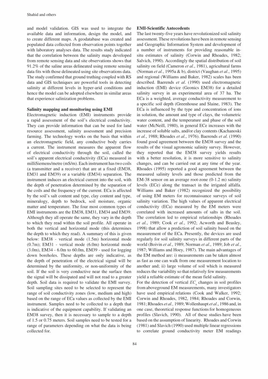
84

Shahid and others

85


and model validation. GIS was used to integrate the available data and information, design the model, and to create different maps. A geodatabase was created and populated data collected from observation points together with laboratory analyses data. The results study indicated that the correlation between the salinity maps developed from remote sensing data and site observations shows that 91.2% of the saline areas delineated using remote sensing data fits with those delineated using site observations data. The study confirmed that ground truthing coupled with RS data and GIS techniques are powerful tools in detecting salinity at different levels in hyper-arid conditions and hence the model can be adopted elsewhere in similar areas that experience salinization problems.

Salinity mapping and monitoring using EMIElectromagnetic induction (EMI) instruments provide a rapid assessment of the soil’s electrical conductivity. They can provide information that can be used for land resource assessment, salinity assessment and precision farming. The technology works on the basis that within an electromagnetic field, any conductive body carries a current. The instrument measures the apparent flow of electrical conductivity through the soil, called the soil’s apparent electrical conductivity (ECa) measured in milliSiemens/metre (mS/m). Each instrument has two coils (a transmitter and a receiver) that are at a fixed (EM38, EM31 and EM39) or a variable (EM34) separation. The instrument induces an electrical current into the soil, with the depth of penetration determined by the separation of the coils and the frequency of the current. ECa is affected by the soil’s salt content and type, clay content and type, mineralogy, depth to bedrock, soil moisture, organic matter and temperature. The four most common types of EMI instruments are the EM38, EM31, EM34 and EM39. Although they all operate the same, they vary in the depth to which they read within the soil profile. All operate in both the vertical and horizontal mode (this determines the depth to which they read). A summary of this is given below: EM38 - vertical mode (1.5m) horizontal mode (0.7m); EM31 - vertical mode (6.0m) horizontal mode (3.0m), EM34 - 6.0m to 60.0m, EM39 - used for logging down boreholes. These depths are only indicative, as the depth of penetration of the electrical signal will be determined by the uniformity, or non-uniformity of the soil. If the soil is very conductive near the surface then the signal will be dissipated and will not read to a greater depth. Soil data is required to validate the EMI survey. Soil sampling sites need to be selected to represent the range of soil conductivity zones (low, medium and high) based on the range of ECa values as collected by the EMI instrument. Samples need to be collected to a depth that is indicative of the equipment capability. If validating an EM38 survey, then it is necessary to sample to a depth of 1.5 or 0.75 meters. Soil samples need to be tested for a range of parameters depending on what the data is being collected for.

EMI-Scientific AntecedentsThe last twenty-five years have revolutionized soil salinity assessment. These revolutions have been in remote sensing and Geographic Information System and development of a number of instruments for providing reasonable in-situ estimates of salinity (Corwin and Rhoades, 1982; Salvich, 1990). Accordingly the spatial distribution of soil salinity on field (Cameron et al., 1981), agricultural farms (Norman et al., 1995a & b), district (Vaughan et al., 1995) and regional (Williams and Baker, 1982) scales has been described. Baerends et al. (1990) used electromagnetic induction (EMI) device (Geonics EM38) for a detailed salinity survey in an experimental area of 37 ha. The ECa is a weighted, average conductivity measurement to a specific soil depth (Greenhouse and Slaine, 1983). The ECa is influenced by the type and concentration of ions in solution, the amount and type of clays, the volumetric water content, and the temperature and phase of the soil water (McNeill, 1980), in general ECe increases with the increase of soluble salts, and/or clay contents (Kachanoski et al., 1988; Rhoades et al., 1976). Baerends et al. (1990) found good agreement between the EM38 survey and the results of the visual agronomic salinity survey. However, they reported that the EM38 survey yields results with a better resolution, it is more sensitive to salinity changes, and can be carried out at any time of the year. Rhoades (1995) reported a good agreement between the measured salinity levels and those predicted from the EM-38 sensor on an average root-zone (0-1.2 m) salinity levels (ECe) along the transact in the irrigated alfalfa. Williams and Baker (1982) recognized the possibility of using EM meters for reconnaissance surveys of soil salinity variation. The high values of apparent electrical conductivity (ECa) measured by the EM meters were correlated with increased amounts of salts in the soil. The correlation led to empirical relationships (Rhoades et al., 1989; Cook et al., 1992; Acworth and Beasley, 1998) that allow a prediction of soil salinity based on the measurement of the ECa. Presently, the devices are used regularly for soil salinity surveys in different parts of the world (Boivin et al., 1989; Norman et al., 1989; Job et al., 1987; Williams and Hoey, 1987). The main advantages of the EM method are: i) measurements can be taken almost as fast as one can walk from one measurement location to another and; ii) large volume of soil which is measured reduces the variability so that relatively few measurements yield a reliable estimate of the mean field salinity.For the detection of vertical ECa changes in soil profiles from aboveground EM measurements, many investigators have used empirical relations (Cook and Walker, 1992; Corwin and Rhoades, 1982, 1984; Rhoades and Corwin, 1981; Rhoades et al., 1989; Wollenhaupt et al., 1986 and, in one case, theoretical response functions for homogeneous profiles (Slavich, 1990). All of these studies have been based on the assumption of linearity. Rhoades and Corwin (1981) and Slavich (1990) used multiple linear regressions

to correlate ground conductivity meter EM readings

84

Shahid and others

85


with measured soil electrical conductivity profiles. The resulting coefficients could be used to predict soil electrical conductivity profiles at points where direct measurements were unavailable. Such regression models proved to be site specific. Hence these relations yield reasonable results at the locations for which they have been developed or at locations with similar characteristics, but they cannot be extrapolated to sites with different characteristics without calibration. For reliable use the instrument needs phasing and instrument zeroing using the manufacturer’s standard calibration method after a warm-up period of 1 h. Calibration of the EM-38 requires that the top instrument in the V–VEM38 mode reads twice the ECa

value of the instrument in the H–HEM38 mode when held 1.5 m above the earth surface.ECa measured by EMI can be rapidly measured on a second-by-second basis, therefore, data population are relatively large and landscape or farming land can be covered more comprehensively in short time than conventional survey tools and methods. As larger volume of data is recorded at relatively larger spatial resolution, EMI surveys are considered as high-intensity surveys. Therefore, salinity maps prepared from ECe provides higher levels resolution than those prepared from conventional surveys (Jaynes, 1995), who further stated that ECa maps can be used as surrogates of soil maps. ECa patterns in existing soil map can provide additional details (Hedley et al., 2004). A major contribution of EMI to soil surveys has been the identification and delineation of small included areas of dissimilar soils within the soil polygons (Fenton and Lauterbach, 1999) and the general distribution of soils within fields (King et al., 2005). EMI has been successfully applied (Doolittle et al., 2009) in high intensity soil mapping in Northern Illinois. They used electromagnetic induction (EMI) to improve the quality of several high-intensity soil surveys in northern Illinois. At each site, apparent conductivity (ECa) data provided an additional

layer of information, which improved knowledge of soils and directed further soil sampling. The information provided by ECa maps and supplementary soil sampling lead soil scientists to recognize additional soils or modify mapping concepts. Within the study sites, ECa maps facilitated the identification and delineation of some soil polygons and improved confidence levels. However, ECa maps lacked sufficient contrast to resolve similar soils and some soil polygons within these sites. While patterns of ECa influenced the judgments of soil scientists, ECa maps were not accepted as substitutes for high-intensity soil maps.

Fundamentals of Electromagnetic induction (EMI)The snapshots of salinity at surface and subsoil layers can help growers improve crop productivity and get more value from each piece of farm land. Traditionally, it has been accomplished through field sampling and laboratory analysis where the electrical conductivity of the saturation extract (ECe) is measured. This is a tedious, laborious and time consuming procedure. Instead, modern electromagnetic induction equipment (EM38) helps collect salinity information and helps selecting crops commensurate with salinity tolerance level. The EM38 measures salinity by transmitting an electric current through the soil, the resulting electromagnetic field is measured by a sensor in the device. This type of EC sensor works on the principle of Electromagnetic Induction (EMI). EMI does not contact the soil surface directly. The instrument is composed of a transmitter and a receiver coil usually installed at opposite ends of a non-conductive bar located at opposite ends of the instrument (Figure 20).

EM-38 works only with a fixed frequency and has an effective measurement depth of 1.5 m in vertical dipole mode or 0.75 m in horizontal dipole mode. EM38 can

Figure 20. Principle of operation for the non-contact type EC sensor (EM38).

86

Shahid and others

87


take two types of measurements: vertical, with equipment lying vertically on soil surface (EMv) or horizontal with equipment lying on its side (EMh). The EMv measurement is more sensitive to soil below 0.45m than the EMh measurement. The EMh measurement is more sensitive to soil above 0.45m than the EMv measurement. The two measurements can be compared to indicate how deeply salt may be penetrated the soil. If soils are moist at depth the EMv reading are higher than EMh. If non saline soil is irrigated with brackish water, this will increase surface salinity and this results salinity EMh being higher than EMv (Figure 21), leaching of salinity to subsoil with rainfall will lower EM reading and eventually result in EMv greater than EMh.

The EM38 is designed to be particularly useful for salinity surveys in agricultural fields. It has gained acceptance due to its simplicity, reliability, rapidity and reproducibility of the results. It is also a rapid, mobile instrumental technique for measuring bulk soil electrical conductivity as a function of spatial position on the landscape. A resulting computer generating salinity maps can add value to farms by helping farmers interpret yield variation. The datalogger attached with EM38 allows rapid record of ECa. Salinity maps help farmers to understand subtle difference in soil properties across their fields, allowing them to develop more precise management zones and, ultimately, potentially higher yields.

Factors affecting EC measurement in soil by EM38 - The conduction of electricity in soil takes place through the moisture-filled pores that occur between individual soils particles. Therefore, the EC of soil is determined by the following soil properties (Tom Doerge, 1999). Greater the soil porosity, the more easily electricity is conducted. Soil with high clay content has higher porosity than sandy soil. Compaction normally increases soil EC. Dry soil has much lower in conductivity than moist soil. Increasing

concentration of electrolytes (salts) in soil water will dramatically increase soil EC. Mineral soil containing high levels of organic matter (humus) and/or 2:1 clay minerals such as montmorillonite, illite, or vermiculite (high cation-exchange-capacity) have a much higher ability to retain positively charged ions (such as Ca, Mg, K, Na, NH4, or H) than soil lacking these constituents. The presence of these ions in the moisture-filled soil pores will enhance soil EC in the same way that salinity does. As soil temperature decreases toward the freezing point of water, soil EC decreases slightly. Below freezing, soil pores become increasingly insulated from each other and overall soil EC declines rapidly. It should be remembered that EMI provides ECa (apparent EC); therefore, calibration of EM38 to generate different depth wise predictive equations to convert ECa to ECe is required. Various regression equations are reported to convert ECa to ECe (Rhoades et al., 1989 & 1999). Im-Erb et al., (2005) in Thailand developed correlation between ECa measured by EM38 reading and ECe (dS/m) of soil samples to quantify EC in the soil profile as follows:

Horizontal reading Y = -0.0003 X2 + 0.1097X + 0.3348

Vertical reading Y = 0.000 X2 + 0.0475X + 0.6609where, Y is the EC of the soil saturation extract of a soil sample (ECe); and X is the apparent electrical conductivity (ECa) from field survey (EM38).

There is no universal relationship between ECe and ECa, in each study area relationship is to be developed.

Pros and cons of EC (salinity) maps. The EC value is a combined result of physical and chemical properties of soil. It has potential applications in agriculture for management decisions and the delineation of management zones. For agriculture applications, EC information works best when yields are primarily affected by factors that are best related to EC, for example, water holding capacity,

Figure 21a. EM38 in grass field – ICBA Station (vertical mode).

Figure 21b. EM 38 in Atriplex field ICBA Station (horizontal mode).

86

Shahid and others

87


salinity level, depth of topsoil, and so on. As a result, it may not work well in areas when other factors (such as disease, pests, etc.) are more predominant. This has to be considered carefully while managing soils from salinity perspectives.

IN-SITU SALINITY ASSESSMENT/MAPPING AND MONITORING BY SALINITY PROBESalinity probes are handy equipment that are easy to use in open field and pot experiments manually and gives instant apparent salinity information (mS/cm & g/l) and avoids conducting soil sampling and preparation. At ICBA we use PNT 3000 COMBI+ model that brings together two important functions of salinity measurement; 1) the salinity measurement directly in soils or substrates (activity), taking into consideration the relevant soil properties, like temperature, soil moisture and soil compaction and; 2) the EC measurement in solutions and suspensions. The PNT COMBI + provides an extended EC-measuring range from 0-20 mS/cm and from 20-200 mS/cm. This universal equipment is commonly used in agriculture, horticulture landscape sites for rapid salinity assessment and monitoring. The instrument included PNT 3000 COMBI-basic unit, stainless steel

measuring electrode 250 mm long for direct soil salinity measurements; EC-plastic probe with platinum-plated ring sensors; EC-control-solution 1,4 mS, 50 ml and high-quality aluminum carrying case. The operation of the equipment is convenient and simple; only one button makes the full operation possible. In this paper results are presented from a grassy plot (paspalum vaginatum) irrigated with 20 dS/m water salinity. The grassy plot (12m x 16m) is showing combined affect of root-zone salinity and leaf burn. A soil salinity investigation was made on a grid basis (2m x 2m) and in-situ salinity (ECa = apparent electrical conductivity) was measured at 6 cm depth on 40 points. Soil samples were also collected at the same depths. These were air-dried and standard saturated soil paste prepared by using distilled water. Soil saturation extract was collected under vacuum and EC measured using calibrated EC meter (ECe). Correlation between ECe & ECa was developed using statistical analyses (linear correlation, polynomial correlation and logarithmic correlation). These correlations provide baseline to convert ECa into ECe, the latter is internationally used to determine salt-tolerance of plants. Salinity map is then prepared using ECe values (Figure 22), this clearly shows relatively higher soil salinity where plants were severely

N 25o 05.748 N 25o 05.750 E 55o23.465 E 55o23.470

N 25o 05.739 N 25o 05.742 E 55o23.469 E 55o23.476

13-14 14-15 15-16 16-17 17-18…………..……….ECe dS/m……………..…………

Figure 22. Soil salinity map in grassy plot.

88

Shahid and others

89


affected by salts (Figure 23), and hence, provide, rapid in-situ salinity testing.

ECe-ECa linear correlation Y = 0.1045x + 9.588 R2 = 0.7225

ECe-ECa logarithmic correlation Y = 5.541 ln(X) – 6.7856 R2 = 0.6997

ECe ECa Polynomial correlation Y = -0.003X2 + 0.448X R2 = 0.5998

Y is the EC of the soil saturation extract of a soil sample (ECe); and X is the apparent electrical conductivity (ECa) from field survey using salinity probe.

Another In-situ salinity assessment was carried out (Figure 24) in a grassy plot irrigated with 10dS/m water salinity (sprinkler irrigation). Below are some salinity values taken from a grass field irrigated with 10 dS/m water salinity (before irrigation, within one minute of irrigation and after 10 minutes from irrigation). Results clearly illustrate high soil salinity measured within 1 minute from irrigation, this is due to the combined affect of the dissolution of preexisting salts in the root zone and irrigation water salinity. Later these salts leached down

due to very high drainage capacity of sandy plot (sand 98%; silt 1%; clay 1%) which reduced the soil salinity, and hence provide rapid salinity assessment in the field. These are the ECa values, to convert to ECe, soil samples are to

Figure 23a. Paspalum vaginatum grassy plot showing salinity affect.

Figure 23b. In-situ salinitfprobe.

Figure 24. In-situ salinity assessment in grassy plot irrigated with 10dS/m water salinity.

Table 5. Root-zone salinity (ECa) by EC probe.

Rootzone depth

(cm)

Soil salinity

(10 minutes prior to

irrigation)

(mS/cm)

Soil salinity within 1

minute after irrigation

(mS/cm)

Soil salinity after 10 minutes

from irrigation

(mS/cm)

5 8.09 14.36 8.64

10 6.12 14.25 9.78

15 8.27 13.76 10.07

20 5.43 13.67 4.57

88

Shahid and others

89


be collected for laboratory assessment of ECe and through developing regression soil salinity can be determined.

CONVENTIONAL SOIL SAMPLING AND MODERN IN-SITU METHODS OF SALINITY MAPPING AND MONITORING

Salinity Monitoring – Choice of TechniqueA number of techniques exist to measure field soil salinity (salinity sensors, electromagnetic devices), however, for many reasons, laboratory analysis of soil saturation extract is still the most common technique for assessing soil salinity and other potential hazards. Merrill et al. (1987) describes saturation extract salinity as standard procedure, because the amount of water that a soil holds at saturation (saturation percentage) is related to a number of soil parameters, such as, texture, surface area, clay content, and cation-exchange-capacity). Merrill et al. (1987) describe lower soil water ratio (1:1; 1:2) to make extraction easier, but cautioned, as less related to field moisture condition than the saturated paste. The choice of equipment/procedure depends upon the purpose of salinity determination, size of the area being evaluated, the depth of soil to be assessed, the number and frequency of measurements needed, the accuracy required and the availability of resources. The standard way is salinity monitoring through collecting soil samples from the root zones over a period of time, and their analyses in the laboratory on a soil saturation extract. Salinity Monitoring – Sampling frequencyA number of sampling techniques exist, and they should be used carefully based on objective of study. Random sampling from a number of representative sites and sample compositing can be made (Figure 25c). The duration of sampling for salinity monitoring is important, and it should be decided on the basis of the project nature and the objectives.

Salinity Monitoring – Sampling zoneThe zone of sampling is also important; particularly in the drip irrigation where the maximum salinity builds up in the periphery of the wetting front. In drip irrigation the salts accumulation occur in two processes: in the first process, the soil becomes saturated and water and solutes spread in various directions saturating the neighboring voids and moving further; in the second process which occurs between consecutive irrigation cycles, evaporation of water and uptake of water and nutrients by plants occur and solutes are redistributed in the soil, the final build up (distribution) of salts in the soil results from the interaction of these two processes throughout the planting period. Sampling the middle soil zone (between two drip lines) will present the maximum salinity and may mislead, however, sampling the root zone can provide a better salinity status. It would be appropriate to assess final salinity buildup in the root zone and around.

Levels of salinity mapping and monitoringSalinity mapping and monitoring is a routine (Shahid, 2005; Shahid et al., 2008) work at ICBA, which accomplishes salinity levels prior to seeding and plantation, and regular monitoring through out the crop season to understand salinity status and to take necessary action for better crop production and to maintain soil health. ICBA performs these tests at three levels; 1) routine salinity assessment and monitoring though soil sampling and analyses in the laboratory; 2) through modern equipment EM38 (see above section on EMI); and 3) Real time dynamic salinity logging system. The three resources at ICBA are described below.

Salinity mapping and monitoring through soil sampling and analysesThe effect of soluble salts on plant growth depends on their concentration in the soil solution; this can be estimated approximately by the measurement of the electrical conductivity. The standard procedure to assess soil salinity and solution chemistry is the analysis of soil saturation extract collected from a saturated soil paste under vacuum (Figure 25c).

At this level ICBA staff collects soil samples from experimental plots irrigated with different water salinity (Figure 25a). The sampling is accomplished through standard soil sampling equipment (sampling tubes & augers) at the root zone and other soil depths. These samples are processed (air drying & sieving through 2 mm sieve) and standard saturated paste prepared for the collection of soil saturation extract for salinity measurement. The EC of the soil saturation extract (ECe) is measured as (milli mhos/cm (mmhos/cm); milli Siemens per cm (mS/cm); desi Siemens per meter (dS/m). The EC readings are recorded in milli-mhos per centimeter (mmhos/cm) or deci-Siemens per meter (dS/m). The use of the unit deci-Siemens is preferred over the unit milli-mhos. Both units are equal, that is, 1 dS/m = 1mmho/cm. Reading are usually taken and reported at a standard temperature of 25°C. Check accuracy of the EC meter using a 0.01 NKCI, solution, which should give a reading of 1.413 dS/m at 25°C.

Saturated Soil Paste-JustificationThe EC of solution extracted from a saturated soil paste (which has water content about double than at field capacity) has been correlated with the response of various crops. This measure, known as electrical conductivity of the soil saturation extract (ECe), is now the generally accepted measure of soil salinity even though the procedure is time-consuming and requires vacuum filtration. It should be noted that EC measurements on extracts or suspensions of fixed soil: water ratio (commonly 1:1, 1:2.5 or 1:5) do not give a reliable correlation. Such extracts or wider ratio are more convenient where the soil sample is limited. This is because the amount of water held at a given tension varies from soil to soil, depending on texture, the type of

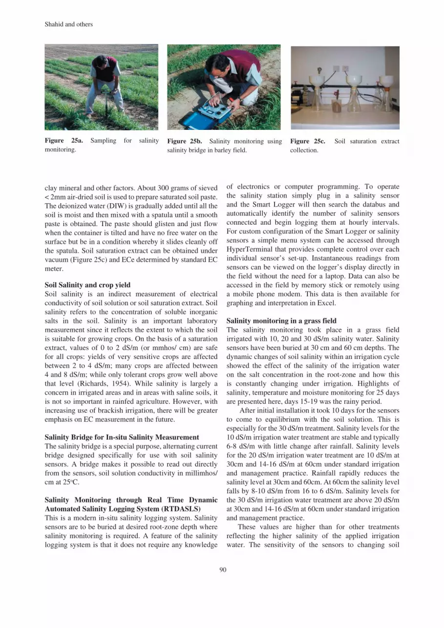
90

Shahid and others

91


clay mineral and other factors. About 300 grams of sieved < 2mm air-dried soil is used to prepare saturated soil paste. The deionized water (DIW) is gradually added until all the soil is moist and then mixed with a spatula until a smooth paste is obtained. The paste should glisten and just flow when the container is tilted and have no free water on the surface but be in a condition whereby it slides cleanly off the spatula. Soil saturation extract can be obtained under vacuum (Figure 25c) and ECe determined by standard EC meter.

Soil Salinity and crop yield Soil salinity is an indirect measurement of electrical conductivity of soil solution or soil saturation extract. Soil salinity refers to the concentration of soluble inorganic salts in the soil. Salinity is an important laboratory measurement since it reflects the extent to which the soil is suitable for growing crops. On the basis of a saturation extract, values of 0 to 2 dS/m (or mmhos/ cm) are safe for all crops: yields of very sensitive crops are affected between 2 to 4 dS/m; many crops are affected between 4 and 8 dS/m; while only tolerant crops grow well above that level (Richards, 1954). While salinity is largely a concern in irrigated areas and in areas with saline soils, it is not so important in rainfed agriculture. However, with increasing use of brackish irrigation, there will be greater emphasis on EC measurement in the future.

Salinity Bridge for In-situ Salinity Measurement The salinity bridge is a special purpose, alternating current bridge designed specifically for use with soil salinity sensors. A bridge makes it possible to read out directly from the sensors, soil solution conductivity in millimhos/cm at 25oC.

Salinity Monitoring through Real Time Dynamic Automated Salinity Logging System (RTDASLS) This is a modern in-situ salinity logging system. Salinity sensors are to be buried at desired root-zone depth where salinity monitoring is required. A feature of the salinity logging system is that it does not require any knowledge

Figure 25a. Sampling for salinity monitoring.

Figure 25b. Salinity monitoring using salinity bridge in barley field.

Figure 25c. Soil saturation extract collection.

of electronics or computer programming. To operate the salinity station simply plug in a salinity sensor and the Smart Logger will then search the databus and automatically identify the number of salinity sensors connected and begin logging them at hourly intervals. For custom configuration of the Smart Logger or salinity sensors a simple menu system can be accessed through HyperTerminal that provides complete control over each individual sensor’s set-up. Instantaneous readings from sensors can be viewed on the logger’s display directly in the field without the need for a laptop. Data can also be accessed in the field by memory stick or remotely using a mobile phone modem. This data is then available for graphing and interpretation in Excel.

Salinity monitoring in a grass fieldThe salinity monitoring took place in a grass field irrigated with 10, 20 and 30 dS/m salinity water. Salinity sensors have been buried at 30 cm and 60 cm depths. The dynamic changes of soil salinity within an irrigation cycle showed the effect of the salinity of the irrigation water on the salt concentration in the root-zone and how this is constantly changing under irrigation. Highlights of salinity, temperature and moisture monitoring for 25 days are presented here, days 15-19 was the rainy period.

After initial installation it took 10 days for the sensors to come to equilibrium with the soil solution. This is especially for the 30 dS/m treatment. Salinity levels for the 10 dS/m irrigation water treatment are stable and typically 6-8 dS/m with little change after rainfall. Salinity levels for the 20 dS/m irrigation water treatment are 10 dS/m at 30cm and 14-16 dS/m at 60cm under standard irrigation and management practice. Rainfall rapidly reduces the salinity level at 30cm and 60cm. At 60cm the salinity level falls by 8-10 dS/m from 16 to 6 dS/m. Salinity levels for the 30 dS/m irrigation water treatment are above 20 dS/m at 30cm and 14-16 dS/m at 60cm under standard irrigation and management practice.

These values are higher than for other treatments reflecting the higher salinity of the applied irrigation water. The sensitivity of the sensors to changing soil

90

Shahid and others

91


salinity levels is illustrated by both the diurnal fluctuation of salinity levels and rapid changes that were measured after rainfall. Diurnally the data is indicating a slight decline in soil salinity as the soil dries between 9:00 am

and 4:00 pm, when irrigation water is again applied to the treatments (Figure 27). AC, EG & IK indicates that the plot was irrigated with 10, 20 & 30 dS/m salinity water. Y-axis shows soil salinity fluctuation in different days.

Sensor placement in the grass rootzone Buried sensorsconnected to smart interface.

Smart interface connected with DataBus Instantaneous salinity data collection on datalogger which is connected with datalogger.

Sensor placement in the grass rootzone Buried sensorsconnected to smart interface.

Smart interface connected with DataBus Instantaneous salinity data collection on datalogger which is connected with datalogger.

Figure 26. Real time automated salinity logging system in grass field. Sensor placement in the grass rootzone Buried sensors connected to smart interface. Smart interface connected with DataBus Instantaneous salinity data collection on datalogger which is connected with datalogger.

Figure 27. Soil salinity monitoring in Distichlis spicata grass field.

Sensor Salinity (Distichlis spicata Experiment)

0

4

8

12

16

20

24

28

Tue

sday

Wed

nesd

ay

Thu

rsda

y

Frid

ay

Sat

urda

y

Sun

day

Mon

day

Tue

sday

Wed

nesd

ay

Thu

rsda

y

Frid

ay

Sat

urda

y

Sun

day

Mon

day

Tue

sday

Wed

nesd

ay

Thu

rsda

y

Frid

ay

Sat

urda

y

Sun

day

Mon

day

Tue

sday

Wed

nesd

ay

Thu

rsda

y

Frid

ay

Time (hourly by 24 hour period)

Sal

init

y (d

S/m

)

A 10 dS/m (30 cm)

C 10 dS/m (60 cm)

E 20 dS/m (30 cm)

G 20 dS/m (60 cm)

I 30 dS/m (30 cm)

K 30 dS/m (60 cm)

Days of Rain

Sensors coming into equilibrium Experimen

92

Shahid and others

93


Large scale in-situ elemental mapping in salinized featureIn-situ elemental mapping in saline lands The electron microscope supplemented with Energy Dispersive X-Rays Analyses or Wavelength Dispersive X-Ray Analyses provides elemental composition in a feature of interest at larger scale. A feature from saline soil (highly polished thin section) is investigated by EMPA using Jeol JXA 3A equipment operated at 20 and 10 kv accelerating voltage and about 0.15 µA specimen current and producing x-ray distribution pattern on a cathode ray oscilloscope (C.R.O) screen and photographed on a polaride film. The x-ray elemental mapping is potentially useful means of qualitatively assessing the gross distribution of an element in the specimen (the white dots). The Figure 28a shows thenardite (Na2SO4) growth over quartz (SiO2) sand grain. Same feature was investigated for elemental mapping the elemental x-ray distribution of Na, S, Cl, Si, Al, Fe, Ca and K are shown in Figure 28b, suggesting dominance of Na and S in the feature and their co-occurrence confirm NaSO4 mineral. A small amount of halite (NaCl) is also implied by x-ray image, on the upper corner a large grain revealing the presence Si, Al and Ca suggest the presence of Ca-feldspar. The peripheral distribution of Fe and K around the Ca-feldspar and some quartz grains is suggested to be due to the presence of a coating of iron oxides and/or phyllosilicate, probably illite, which is also embedded in the thenardan (thenardite coating). In addition calcite (CaCO3) in traces is suggested by Ca-distribution with no other element (lower right). The distribution of Si suggests the presence of quartz grains, these exist either isolated or embedded in the thenardan.

Application of salinity mapping and monitiring in crop yield prediction in irrigated agricultureSalinity mapping and monitoring in irrigated agriculture fields provides general guidance about yields from salinized area relative to that without salinity. Crops can tolerate salinity up to certain levels without a measurable loss in yield (this is called threshold level). At salinity levels greater than the threshold, crop yield reduces linearly as salinity increases. Using the salinity values in a salinity/yield model developed by Maas and Hoffman in 1977, predictions of expected yield loss can be made (Maas, 1986). Typically, plant growth is suppressed when a threshold value of salinity is exceeded. Maas and Hoffman expressed salt tolerance of many crops by this relationship: Yr = 100-s(ECe-t), where Yr = percentage of the yield of crop grown in saline conditions relative to that obtained on non-saline conditions; t = threshold salinity level where yield decrease begin; s = percent yield loss per increase of ECe (dS/m) in excess of t. In this model it is assumed that crops respond primarily to the osmotic potential of soil solution, and specific ion effects is of secondary importance. Salinity monitoring helps understand the root zone salinity levels, whether below or above threshold level of crop in the field. The latter will require extra water to be applied based on the leaching fraction to maintain Figure 28b. Elemental mapping in the above feature.

Figure 28a. Thenardite (Na2SO4) crystallization over quartz grain.

92

Shahid and others

93


the root zone salinity below crop threshold salinity. The Table 6 (Shahid, 2004) provides general information about threshold levels of different crops and relative yield decline above threshold salinity.

Conclusions and Recommendations RS imagery and GIS are great tools to map surface soil salinity at country and regional level. However, it constrains the salinity assessment in the root-zone. The combination of both RS imagery interpretation and field data are the best way for correct salinity prediction. This is great technique for salinity mapping at small scales. In areas where saline/brackish water is used for irrigation purpose, farm based salinity mapping and monitoring tools such as electromagnetic induction (EMI) equipment EM38, EC probes are recommended to understand day to day salinity status in irrigated fields and to manage soils for better agricultural production. Salinity modeling can provide important information, however, they require data which in many developing countries are not east to produce. Elemental mapping through submicroscopic investigation can provide in-situ salinity status and behavior in actual soil environment.

AcknowledgementsAuthors like to thank GRM Int team especially Andrew Buchanan to join ICBA & EAD technical support team to finalize the remote sensing component of the Soil Survey of Abu Dhabi Emirate. Special thanks are due to His Excellency Majid Al Mansouri Secretary General Environment Agency Abu Dhabi for his interest in initiating Soil Survey of Abu Dhabi Emirate and Abu Dhabi Executive Council for providing funds to implement Emirate wide Soil Inventory. The encouragement and support provided by Prof. Dr. Faisal Taha and Dr. Bill Porter in the project activities are highly appreciated.

ReferencesAbdelfattah, M. A., S. A. Shahid and Y. R. Othman. 2008.

Soil Salinity Mapping Model Developed Using RS and GIS – A Case Study from Abu Dhabi, United Arab Emirates. European Journal of Scientific Research, ISSN 1450-216X 26(3)(2009):342-351. available online at: http://www.eurojournals.com/ejsr_26_3_02.pdf (date last accessed: 21st October 2009).

Abdelfattah, M.A., S. A. Shahid, Y. Othman and A. Kumar. 2010. Soil salinity mapping through extensive

Table 6. Relative productivity (%) of some important crops with respect to soil salinity (ECe in dS/m).

Plant Scientific nameRelative productivity (yr) at selected ECe (dS/m)

1 2 4 6 8 10 14 S1 t2

Bean Phaseolus vulgaris 100 81 43 6 0 18.9 1.0Carrot Daucus carota 100 86 58 30 1 0 14.1 1.0

Onion Allium cepa 100 87 55 23 0 16.1 1.2

Cabbage Brassica oleracea 100 98 79 59 40 20 0 9.7 1.8

Cucumber Cucumis sativus 100 100 81 55 29 3 0 13.0 2.5

Pepper Capsicum annum 100 91 65 39 13 0 13.0 1.3

Lettuce Lutuca sativa 100 93 65 37 8 0 14.1 3.2

Potato Solanum tuberasom 100 96 72 48 24 0 12.0 1.7

Radish Raphanus sativus 100 90 64 38 12 0 13.0 1.2

Spinach Spinacia oleracea 100 100 85 70 55 39 9 7.6 2.0

Tomato Lycopersicum esculentum 100 100 85 65 46 26 0 9.9 2.5

Brocoli Brassica oleracea 100 100 89 71 52 34 0 9.1 2.8

Alfalfa Medicago sativa 100 100 85 71 56 42 12 7.3 2.0

Corn (F) Zea mays 100 99 84 69 54 39 10 7.4 1.8

Berseem Trifolium alexandrinium 100 97 86 74 63 51 29 5.8 1.5

Barley (F) Hordeum vulgare 100 100 100 100 86 72 44 7.0 6.0

Barley (G) Hordeum vulgare 100 100 100 100 100 90 70 5.0 8.0

Sorghum Sorghum bicolor 100 100 100 98 78 63 43 7.6 4.8

Wheat Triticum aestivum 100 100 100 100 86 71 43 7.1 6.0Date Phoenix dactylifera 100 100 100 93 86 78 64 3.6 4.0

S1 = % yield decrease per 1 dS/m increase in ECe above threshold ECe

t2 = salinity threshold ECe (dS/m), where yield is optimum

94

Shahid and others

95


measurements. Soil Science Society of America Journal, 46:517-520.

Corwin, D.L., and J.D. Rhoades. 1984. Measurement of inverted electrical conductivity profiles using electromagnetic induction. Soil Sci. Soc. Am. J., 48:288–291.

Doolittle, J. A., R. D. Windhorm, D. L. Withers and R. L. McLeese. 2009. High-intensity soil mapping with the aid of EMI in Northern Illinoise. Soil Survey Horizons, 2(50): 68-74.

Dutkiewics, A. and M. Lewis. 2008. Broadscale monitoring of salinity using satellite remote sensing: where to from here? 2nd International Salinity Forum, Adelaide Australia. Pp. 6.

Dwivedi, R.S. and B.R.M. Rao. 1992. The selection of the best possible Landsat TM band combination for delineating salt-affected soils. Int. J. R.S., 13(11):2 051-2 058.

EAD. 2009. Soil Survey of Abu Dhabi Emirate. Environment Agency Abu Dhabi. 5 Volumes.

Everitt, J. H., D.E. Escobar, A.H. Gerbermann and M.A. Alaniz. 1988. Detecting saline soils with video imagery. Photogrammetric Eng. and R.S., 54(1):283-287.

FAO. 1997. Action in the Near East Region (http://www.fao.org) cf. Hussein, 2001.

FAO-ICBA. 2007. First exoert consultation on Advances in Assessment and Minitiring of Salinization for Managing Salt-Affected Habitats and Meeting on the ’Stayus and Progress of Biosaline Agriculture ofthe Inter-Islamic Network on Biosaline Agriculture 26-29 November, 2007, held at ICBA Dubai.

Farooq, M. and Nur Ud Din. 1980. Application of multitemporal Landsat data in the identification of salinity in the Khairpur pilot project, Pakistan. In: Proceedings of the National Seminar on Application of Remote Sensing Techniques in Water Resources Development and Management, pp. 74-31. Lahore, Pakistan.

Fenton, T.E. and M.A. Lauterbach. 1999. Soil map unit composition and scales of mapping related to interpretations for precision soil and crop management in Iowa. In: Proceeding of the 4th International Conference on Site Specific Management. St Paul, MN. 19-22 July 1998. ASA, Madison, WI.

Furby, S., F. Evans, J. Wallace, R. Ferdowsia and J. Simon. 1998. Collection of ground truth data for salinity mapping and monitoring. Manual published by CSIRO Mathematical and Information Section Agriculture Western Australia.

Furby, S.L., J.F. Vallace, P.A. Caccetta and G.A. Wheaton. 1995. Detecting and monitoring salt-affected land: A report from the LWRRDC project detecting and monitoring changes in land condition through time using remotely sensed data, Remote Sensing and Image Integration Group, CSIRO Division of Mathematics & Statistics, Western Australia.

soil survey and using Geographical information system. Case study from Abu Dhabi. Paper presented at the International Conference on Management of Soil and Groundwater Salinization in Arid Regions, Sultan Qaboos University, Sultanate of Oman 11-14 January 2010.

Acworth, R.I., and R. Beasley. 1998. Investigation of EM31 anomalies at Yarramanbah /Pump Station Creek on the Liverpool Plains of New South Wales. WRL Research Report No. 195.

Ahmad, M.D. 1999. Estimating the interaction between soil moisture and groundwater using geo-information techniques. Enschede, Netherlands, International Institute for Aerospace Survey and Earth Sciences.

Asif, S., and M. D. Ahmed. 1999. Using state-of-the-art RS and GIS for monitoring waterlogging and salinity. Paper publishrd by International Water Management Institute, Lahore, Pakistan pp. 16.

Baerends, B., Z.I. Raza, M. Sadiq, M.A. Chaudhry and J.M.H. Hendrickx. 1990. Soil salinity survey with an electromagnetic induction method. Proc. Indo-Pak Workshop on Soil Salinity and water Management, Feb. 10-14, 1990, Islamabad, Pakistan, Vol.1:201-219.

Bennet, B. A. 1998. Airborne remote sensing and field spectroscopy for soil salinity mapping at Pyramid Hill, Victoria. Unpublished Masters Thesis, School of Geology, UNSW. 65p.

Brena, J., Sanvicente, H. and L. Pulido. 1995. Salinity assessment in Mexico. In A. Vidal and J.A. Sagardoy, eds. Water Report No. 4: use of remote sensing techniques in irrigation and drainage, p. 173-178. Rome, FAO.

Cameron, D. R., E. De Jong, D.W.L. Read and M. Oosterveld. 1981. Mapping salinity using resistivity and electromagnetic inductive techniques. Canadian Journal of Soil Science, 61:67-78.

Casas, S. 1995. Salinity assessment based on combined use of remote sensing and GIS. In A. Vidal and J.A. Sagardoy, eds. Water Report No. 4: use of remote sensing techniques in irrigation and drainage, p. 185-197. Rome, FAO.

Chaturvedi, L., K.R. Carver, J.C. Harlan, G.D. Hancock, F. V. Small and K. J. Dalstead. 1983. Multispectral remote sensing of saline seeps. IEEE Transactions on Geoscience and Remote Sensing, 21(3):239-250.

Cook, P.G., G.R. Walker, G. Buselli, I. Potts and A.R. Dodds. 1992. The application of electromagnetic techniques to groundwater recharge investigations. Journal Hydrology, 130:201-229.

Cook, P.G. and G.R. Walker. 1992. Depth profiles of electrical conductivity from linear combinations of electromagnetic induction measurements. Soil Sci. Soc. Am. J., 56:1015–1022.

Corwin, D.L. and J.D. Rhoades. 1982. An improved technique for determining soil electrical conductivity - depth relations from above ground electromagnetic

94

Shahid and others

95


Greenhouse, J. P., and D. D. Slaine. 1983. The use of reconnaissance electromagnetic methods to map contaminant migration. Ground Water Monitoring Review, 3(2):47-59.

Hardisk, M. A., V. Klemas, V. and F. C. Daiber. 1983. Remote sensing saltmarsh biomass and stress detection. Advances in Space Research, 2:219-229.

Hedley, C.B., I.J. Yule, C.R. Eastwoof, T.G. Shephard, and G. Arnold. 2004. Rapid identification of soil textural and management zones using electromagnetic induction sensing in soils. Australian Journal of Soil Research, 42:389-400.

Hussein, H. 2003. Remote sensing technology for salinity mapping. Presentation given at the training workshop on salinization of Irrigated Land and Reclamation, Held at ICBA Headquarter, Dubai 5-9 April 2003.

Hussein, H. 2001. Development of environmental GIS database and its application to desertification study in middle east. A Remote Sensing and GIS application. Ph.D Thesis, Graduate School of Science and Technology, Chiba University, Japan.

Im-Erb, R., P. Yamclee, and S. Sukchan. Salt-affected soils in Thailand: Assessment and monitoring on salinization. Land Development Department, Bangkok, 10900, Thailand.

Jaynes, D.B. 1995. Electromagnetic induction as a mapping aid for precision farming. p. 153-156. In Clean Water, Clean Environment, 21st Century: Team Agriculture. Working To Protect Water Resources. Kansas City, MO. 5-8 March. 1995.

Job, J. O., J. Y. Loyer and M. Ailoul. 1987. Utilisation de la conductivite electromagnetique pour la mesure directe de la salinite des sols. Cah. ORSTOM, ser.Pedol., 23(2):123-131.

Joshi, M. D., and B. Sahai. 1993. Mapping of salt-affected land in Saurashtra coast using Landsat satellite data. Int. J. R.S., 14(10):1919-1929.

Kachanoski, R. G., E.G. Gregorich and I.J. Van Wasenbeeck. 1988. Estimating spatial variations of soil water content using non contacting electromagnetic inductive methods. Canadian Journal of Soil Science, 68:715-722.

King, J.A., P.M. Dampney, R.M. Lark, H.S. Wheeler, R.I. Bradley and T.R. Mayr. 2005. Mapping potential crop management zones within fields: Use of yield map series and patterns of soil physical properties identified by electromagnetic induction sensing. Precision Agriculture, 6:167-181.

Kwarteng, A.Y. and D. Ajmi. 1997. Satellite remote sensing application in the State of Kuwait. Published by Kuwait Institute for Scientific Reseaech, Kuwait.

KISR. 1999a. Soil Survey for the State of Kuwait – Volume II:Reconnaissance Survey, AACM In, Adelaide, Australia.

KISR. 1999b. Soil Survey for the State of Kuwait – Volume IV: Semi-detailed Survey, AACM International, Adelaide, Australia.

Maher, M.A. A. 1990. The use of remote sensing techniques in combination with a geographic information system for soil studies with emphasis on quantification of salinity and alkalinity in the northern part of the Nile delta. MSc thesis. Enschede, Netherlands, ITC.

Makin, I.W. 1986. Applications of remotely sensed, multi-spectral data in monitoring saline soils. Technical Note No. 19. Amritsar, India, IPRI.

McNeill, J. D. 1980. Electromagnetic terrain conductivity measurements at low induction numbers. Geonics Limited Technical Notes TN-6, Geonics Ltd, Mississauga, Ontario, Canada.

Maas, E.V. 1986. Salt tolerance of plants. Appl. Agric. Res., 1:12-25.

Menenti, M., A. Lorkeers and M. Vissers. 1986. An application of thematic mapper data in Tunisia. ITC Journal, 1:35-42.

Mougenot, B., M. Pouget and G.F. Epema. 1993. Remote sensing of salt affected soils. R.S. Reviews, 7:241-259.

Mulders, M.A. 1987. Remote sensing in soil science. Developments in Soil Science 15. Amsterdam, Elsevier.

Mulders, M. A., and G.F. Epema. 1986. The thematic mapper: a new tool for soil mapping in arid areas. ITC Journals, 1:24-29.

Norman, C. P., C. W. Lyle, A. F. Heuperman, and D. Poulton. 1989. Pyramid hill irrigation area - soil salinity survey, May-June 1988, Res. Rep. Series No. 80 Victoria Dept. of Agriculture and Rural Affairs, Australia.

Norman, C., J. Heath, R. Turnour and P. MacDonald. 1995a. On-farm salinity monitoring and investigations. Institute of Sustainable Irrigated Agriculture (ISIA) Tatura, Victoria, Australia Report 1993-1995, p. 164.

Norman, C., P. Challis, H. Oliver, J. Robinson, K. Gillespie, C. Rankin, S. Tonkins and J. Heath. 1995b. Whole farm soil salinity surveys in the Kerang region. Institute of Sustainable Irrigated Agriculture (ISIA) Tatura, Victoria, Australia Report 1993-1995, p. 162.

Omar, S.A.S., R. Misak, P. King, S.A. Shahid, H. Abo-Rizq, H. Grealish and W. Roy. Mapping the vegetation of Kuwait through reconnaissance soil survey. Journal of Arid Environments, 48:341-355.

Rhoades, J.D., and D.L. Corwin. 1981. Determining soil electrical conductivity—Depth relations using an inductive electromagnetic soil conductivity meter. Soil Sci. Soc. Am. J., 45:255–260.

Rhoades, J. D. 1995. Field investigations and methods of measurements, monitoring and mapping of salinity in salt-affected soils. Paper Presented at Regional Workshop on Management of Salt-Affected Soils in the Arab Gulf States, 29 October - 2 November, Abu Dhabi, UAE.

Rhoades, J.D., P.A. Raats and R.J. Prather. 1976. Effects of liquid-phase electrical conductivity, water content, and surface conductivity on bulk soil electrical

96

Shahid and others

97


Sukchani, S. and Y. Yamamoto. 2005. Classification of salt-affected areas using remote sensing. Paper published by Soil Survey and Classification Division, Department of Land Development (LDD) Ministry of Agriculture and Cooperative, Phaholyothin Road, Chatichak, Bangkok 10900 Thailand and Japan International Research Center for Agricultural Sciences (JIRCAS), Ohwashi 1-1, Tsukuba, Ibaraki 305-8686, Japan, pp. 7.

Thenkabail, P., R. Smith, E. Pauw. 2000. Hyperspectral Vegetation Indices and their Relationships with Agricultural Crop Characteristics. Rem. Sens. Env., 71:158-182.

Tom Doerge. 1999. Soil Electrical Conductivity Mapping, Crop Insights, 9(19).

USDA-NRCS. 1995. Soil Survey Laboratory Information Manual. Soil Survey Investigation Report No. 45, Version 1.0, USDA-SCS. U. S. Govt. Print. Office, Washignton , DC.

USDA-NRCS. 1999. Soil Taxonomy. A Basic System of Soil Classification for Making and Interpretation of Soil Surveys. USDA Agriculture Handbook No. 436, U. S. Govt. Print. Office, Washington, D.C., P. 869.

USDA-NRCS, 2004. Soil Survey Laboratory Methods Manual. Soil survey Investigation Report No. 43. Version 3.0 USDA-NRCS. U.S. Govt. Print. Office, Washington, DC.

USDA-NRCS. 2006. Keys to Soil Taxonomy. 10th Edition. U.S. Govt. Print. Office, Washington, D.C., p. 331.

Vaughan, P. J., S. M. Lesch, D. L. Crown, and D. G. Cone. 1995. Water content effect on soil salinity prediction. A geostatistical study using cokriging. Soil Science Society of America Journal, 59:1146-1156.

Verma, K.S., Saxena, R.K., Barthwal, A.K. and S. N. Deshmukh. 1994. Remote-sensing technique for mapping salt affected soils. Int. J. R.S., 15(9):1901-1914.

Promotion of Education and Information Activities for the Advancement of Space Technology and its Application in Europe.

Vincent, B., A. Vidal, D. Tabbet, A. Baqri and M. Kapur. 1996. Use of satellite remote sensing for the assessment of waterlogging or salinity as an indication of the performance of drained systems. In B. Vincent, ed. Evaluation of performance of subsurface drainage systems: 16th Congress on Irrigation and Drainage, Cairo, p. 203-216, New Delhi, ICID.

WAPDA. 1984. Applicability of Landsat imagery for monitoring soil salinity trends. Publ. 529. Lahore, Pakistan, Directorate of Reclamation and Investigation Organization.

Williams, B. G. and G. C. Baker. 1982. An electromagnetic induction technique for reconnaissance survey of salinity hazards. Australian Journal of Soil Research, 20:107-118.

Williams, B.G. and D. Hoey. 1987. The use of electromagnetic induction to detect the spatial

conductivity. Soil Science Society of America Journal, 40:651-655.

Rhoades, J.D., N.A. Manteghi, P.J. Shouse and W. J. Alves. 1989. Soil electrical conductivity and soil salinity: New formulations and calibrations. Soil Science Society of America Journal, 53:433-439.

Rhoades, J.D., S.M. Lesch, P.J. Shouse and W.J. Alves. 1989. New calibrations for determining soil electrical conductivity—Depth relations from electromagnetic measurements. Soil Sci. Soc. Am. J., 53:74–79.

Richards, L.A. (Ed). 1954. Diagnosis and improvement of saline and alkali soils. USDA Handbook No. 60 (Washington, DC), pp. 79-81.

Salvich, P.G. 1990. Determining ECa-depth profiles from electromagnetic induction measurements. Australian Journal of Soil Research, 28:443-452.

Shahid, S. A., H. Abo-Rezq and S. A. S. Omar. 2002. Mapping soil salinity through a reconnaissance soil survey of Kuwait and Geographic Information System. Annual Research Report, Kuwait Institute for Scientific Research, Kuwait, KSR 6682, p. 56-59.

Shahid, S.A. 2004. Irrigation Water Quality Manual. ERWDA Soils Bulletin No. 2, pp. vii+33.

Shahid, S. A., A. H. Dakheel, K. A. Mufti and G. Shabbir. 2008. Automated in-situ salinity logging in irrigated agriculture. European Journal of Scientific Research, 26(2):288-297.

Sharma, R.C. and G.P. Bhargava. I988. Landsat imagery for mapping saline soils and wet lands in north-west India. Int. J. R.S., 9:39-44.

Singh, A.N. and R.S. Dwivedi. 1989. Delineation of salt-affected soils through digital analysis of Landsat MSS data. Int. J.R.S., 10:83-92.

Soil Survey Division Staff (1993). Soil Survey Manual. USDA-NRCS Agric. Handbbok No. 18, U.S.Govt. Print. Office, Washington, DC.

Spies, B. and P. Woodgate. 2004. Technical Report: Salinity Mapping Methods in the Australian Context, Prepared fir the Programs Committee of the Natural Resources Management, Ministerial Council through Land and Water Australia and the National Dryland Salinity Program.

Subagyono, K., B. Sugiharto and B. Jaya. 2005. Rehabilitation Strategies of the Tsunami Affected Agricultural Areas in Aceh, Indonesia. Center for Soil and Agroclimate Research and Development, Bogor, Indonesia. Special Program for Food Security (SPFS), FAOR, Jakarta, Indonesia. Directorate General of Food Crops, Ministry of Agriculture, Indonesia. Paper Presented at the Regional Workshop on Strategies for Rehabilitation and Management of Salt-affected Soil from Sea Water Intrusion, 31 March to 1 April 2005Bangkok, Thailand.

Sukchan, S. and Y. Yamamoto. 2001. Classification of salt-affected areas using Remote Sensing and GIS. JIRCAS Working Report No. 30, pp. 19.

96

Shahid and others

97


variability of the salt and clay contents of soils. Australian Journal of Soil Research, 25:21-27.

Wollenhaupt, N.C., J. L. Richardson, J. E. Foss, and E. C. Doll. 1986. A rapid method for estimating weighted soil salinity from apparent soil electrical conductivity measured with an above ground electromagnetic induction meter. Can. J. Soil Sci., 66:315–321.

Zevenbergen, A.W. 1990. Integrating remote sensing and conventional information. Land and Water International, 56:7-9.

Zuluaga, J.M. 1990. Remote sensing applications in irrigation management in Mendoza, Argentina. In M. Menenti, ed. Remote sensing in evaluation and management of irrigation, p. 37-58. Mendoza, Argentina, Instituto Nacional de Ciencia y Tecnic.

98

Shahid and others

Documents

Mapping and Monitoring of Soil Salinization - Remote Sensing, GIS, Modeling, Electromagnetic Induction and Conventional Methods Case Studies