Market reactions to CEO turnovers Empirical study on the market reaction to a CEO turnover

Jens Christ ian Aune & Peter Riise Supervisor: Karin Thorburn

Master Thesis, Business & Administration, Finance

NORWEGIAN SCHOOL OF ECONOMICS

This thesis was written as a part of the Master of Science in Economics and Business Administration at NHH. Please note that neither the institution nor the examiners are responsible − through the approval of this thesis − for the theories and methods used, or results and conclusions drawn in this work.

Norwegian School of Economics Bergen, Spring 2015

2"

i . Abstract This thesis examines the effect of CEO attributes and company fundamentals on company performance in CEO turnovers. The analyses were performed on a sample of 899 CEO turnovers between 2003 and 2009 in companies listed on the S&P 1500 composite index in the US. A six-step model exploring various perspectives of the CEO turnover in the period [Event day -1/+2 years] finds that the market, on average, yields negative announcement return and then positive cumulative abnormal return in the subsequent two years. Our main finding is that the market reacts to changes made to the company fundamentals, and that it generally rewards changes in company fundamentals contributing to enhance the robustness of the companies’ balance sheets. We find that MBAs tend to run the operations with lesser margins, in terms of balance sheet robustness. Nonetheless, the different behavior between MBAs and engineers does not explain the market reaction. Even though MBAs and engineers have different fiscal strategies in the way they operate companies, the abnormal return is not sensitive to hiring a CEO with these educational profiles alone. It is rather the experience, and the fact that CEOs, on average, are able to introduce changes that fit the companies’ needs that appear to generate abnormal reactions in stock value. We also find that positive abnormal stock return in the transition year materializes in increased ROA and EBITDA margin in the two subsequent years. This confirms that the market is able to identify CEO turnovers that prove successful. This thesis confirms several previous findings within the research field of CEO turnover, and adds to the understanding of the underlying reasons for market reactions to CEO turnovers. Key words: CEO turnover, abnormal stock return, company performance, CEO attributes, company fundamentals

3"

i i . Content

i . ABSTRACT 2

i i . CONTENT 3

i i i . PREFACE 4

1. INTRODUCTION 5

2. LITERATURE REVIEW 7

3. EXPERIMENT DESIGN 9

4. DATA 11

4.1 DATA SOURCES AND LIMITATIONS 11 4.2 VARIABLES 14

5. METHODOLOGY AND RESULTS 22

5.1 CAR SURROUNDING CEO TURNOVER 22 5.2 CHANGE IN FUNDAMENTALS SURROUNDING CEO TURNOVERS 26 5.3 DRIVERS OF CAR 29 5.4 DRIVERS OF FUNDAMENTALS 34 5.5 PREDICTIVE MODEL FOR SUITED CEO ATTRIBUTES 43 5.6 CAR AS PREDICTOR FOR OPERATIONAL PERFORMANCE METRICS 49

6. CONCLUSION AND INTERPRETATION 52

7. REFERENCES 55

8. APPENDIX 59

8.1 DATA TABLES 59 8.2 STATISTICAL ROBUSTNESS TESTS 65 8.3 ECONOMETRIC TESTS 71 8.4 ELABORATIONS ON STATISTICAL METHODS 75 8.5 CLARIFYING EXAMPLES 77

4"

Jens Christian Aune Peter Riise

i i i . Preface With this thesis we complete our Masters of Science in Economics & Business Administration at the Norwegian School of Economics (NHH). Our major is Financial Economics, and the thesis compiles theory from a variety of classes and fields of studies we have undertaken. Through the curriculum we have completed the past few years, we have accumulated knowledge about corporate finance and investment management, but especially during the case-based course Mergers & Acquisitions, we realized that firm value is just as much influenced by corporate governance than any technical financial theory. In the financial press, we get daily exposure to stories of charismatic and talented executives exercising major influence on their companies and sometimes even being the crucial factor for the companies’ success. With this thesis, we wanted to explore and quantify the impact from such individuals, and more specifically, uncover how much a change of the CEO matters for a company. The work on this thesis has been challenging, yet highly rewarding. It has been exiting to research the field of CEO turnovers, and for every new set of data we have collected, we have discovered new dimensions, nurturing hours of interesting discussions. The new era CEO has become much more than an executive; they are superstars, gurus and trendsetters. We have all been fascinated by the late Steve Job’s characteristic “…there is one more thing…” and Elon Musk’s inspiring dreams and ambitions. It is going to be exiting to follow how key personalities will shape corporations in the future. We wish to state our gratitude towards our supervising professor Karin S. Thorburn, who has been an invaluable partner for discussion and idea generation. Her feedback and contributions has been critical for how this thesis appears. Beyond the classroom and the advisor meetings, she has always been welcoming and willing to share of her knowledge. Bergen, June 19, 2015

5"

1. Introduction The change of CEO is a major event for a company, and could set the pace for change and a new strategic direction for the firm. In the period between 2003 and 2009 an average of ~14% of the largest US corporations replaced their CEO each year for various reasons1.

“Great companies with the way they work, first start with great leaders.” Steve Ballmer, Former CEO of Microsoft

Over the past two decades, empirical researchers have produced a large body of evidence on various aspects of the relation between CEO turnover and firm performance. The first important studies on CEO turnover and performance were conducted in the 1980s, and since then, different scholars have been focusing on a multitude of various aspects of the turnover/performance relation. In section 2 we will present the most recent and notable studies on the field. The announcement of a CEO turnover has been showed to make major impacts on the firm’s stock price, both upward and downward. When Gary Rodkin took over as chief executive in Conagra Foods Inc. the company experienced a 14,9% abnormal stock return in the first year. Dow Chemicals Inc., on the other side, suffered a 9,5% negative abnormal stock return in the one-year period after Andrew Liveris came in as CEO. These two men have different backgrounds; Rodkin is a Harvard MBA while Liveris holds an undergraduate degree in chemical engineering from a reputable university in Australia. Further, the companies they manage operate in different sectors, are of different sizes and found themselves facing deviant business challenges that require different strategies. The backdrop for the deviation in return is fragmented and a sum of numerous events and circumstances. We do not believe we can trace the market reaction to the turnover back to one single attribute or action, as the market will always reflect the whole story. Instead we are aiming to attach separate pieces of the puzzle to better depict how the interaction between the CEO attributes, firm characteristics and strategic actions in sequence impacts the company performance, both measured in abnormal stock return and changes in operational performance metrics. Therefore, this thesis will aim to shed new light on the overall research question:

“What impacts the market reaction to a CEO turnover?”

1 According to Booz & Company’s Annual Global CEO Succession Study of 2011

6"

Subordinately, we will test the following six hypotheses:

1. The market will react positively to a CEO turnover 2. The turnover entails changes in company fundamentals 3. Changes in company fundamentals will impact the abnormal stock return 4. Certain CEO attributes and firm characteristics will dictate the choice of

financing, investment and growth strategy decisions 5. Large deviations between the expected and actual backgrounds and

attributes of the appointed CEO’s will evoke stronger positive reactions in abnormal returns.

6. Abnormal return will materialize in subsequent changes in operational performance metrics

These six hypotheses will provide the basis for the thesis’ layout and structure. They will form the separate pieces of the larger puzzle, and will draw a line from CEO attributes through the changes in company fundamentals to the abnormal stock return. The remainder of the thesis is structured as follows. Section 2 reviews previous literature on the topics discussed. Section 3 describes our empirical strategy. Section 4 will present the data utilized in the thesis, and gives a more thoroughly description of the variables. Section 5 presents the statistical tests we have conducted and discusses the empirical results. Section 6 summarizes the thesis and offers our conclusions.

7"

2. Literature review There have been several researches and papers exploring the field of CEO turnover and company performance in various ways prior to our thesis, as a new CEO talent has proven to signal a new commitment to growth and focus on innovation that could translate into enhanced revenue. Nonetheless, empirical evidence show mixed results from the study of isolated factors that each affects the market reaction to CEO turnovers, without tying them together. The previous literature does not attempt to show the interaction between CEO attributes, firm characteristics and company fundamentals, and abnormal stock performance. Being among the first studies on the topic, Warner, Watts and Wruck (1988) finds association between a firm's stock returns and subsequent top management changes. Consistent with internal monitoring of management, they find an inverse relation between the probability of a management change and a firm's share performance. However, they consider only retrospective performance as an explanation for the turnover, and do not regard the post-turnover stock performance. Later, Jenter and Lewellen (2014) found a close link between firm performance and CEO turnover, and estimate that more than 40% of turnovers in the first eight tenure years are performance-induced, but they do still not address the market reaction after the turnover. Several studies have been conducted on the relation between changes in company fundamentals and company performance in the time surrounding CEO turnovers. On the one hand, Murphy and Zimmerman (1992) examined whether changes in potentially discretionary variables are explained by poor economic performance, rather than direct managerial discretion. They find that turnover-related changes in R&D, advertising, capital expenditures and accounting accruals are due mostly to poor performance, but they do not link these changes to post-turnover performance. Nor do they link the changes in the potential discretionary variables to the new CEO’s attributes or the firm characteristics. On the other side, Barker and Mueller (2002) explore the relation between a discretionary variable and the new CEO’s attributes. They found that a CEO’s undergraduate education does not impact the R&D spending. However, a CEO with an advanced science or engineering degree has a significant increase in R&D spending. However, they do not attempt to tie any of these changes in R&D, nor any other company fundamental, to stock performance.

8"

There have also been conducted studies on the relation between CEO attributes and company performance. Gottesman and Morey (2006) examine the relation between the CEO’s education quality and the company’s performance. They find no evidence of superior performance from CEOs from better schools. Conversely, Jalbert, Rao and Jalbert (2011) find association between both possession of a degree and where the degree was earned, and company performance. Nonetheless, none of these papers link their findings to the CEO’s strategic actions and how these actions would affect the company performance. Further studies examine the relation between CEO attributes and discretionary company fundamentals. Hu and Liu (2014) investigate the impact of CEOs' career experiences on corporate investment decisions and find that firms with CEOs who have more diverse career experiences exhibit lower investment-cash flow sensitivity and exploit more outside funds. However, they do not show how these findings relate to CEO turnovers, nor stock return. The papers we have reviewed each explores one single dimension of a CEO turnover, but none of them attempts to consolidate their findings into a comprehensive system. Our paper is most closely related to the literature examining the market reaction post-turnover, and builds on the previous findings discussed in this section. We utilize parts of the methodology used in each of the papers, and attempts to tie the results together to depict a holistic picture of how CEO attributes and company fundamentals interact, and, in turn, affects the abnormal stock return and company performance.

9"

3. Experiment design The experiment design will be presented in this section, describing the empirical strategy and how we have approached our overall research question and the subordinated hypotheses. This thesis aims to depict the relation between the CEO’s attributes, the level and changes of certain financial variables (we will refer to this as “the company fundamentals”) that are believed to be subject to considerable managerial discretion and the company’s performance. The data will be more thoroughly presented in the next section. In order to support our hypotheses, we have developed a six-step experiment design to explore the relations and interactions between each of these three categories. By approaching the main hypothesis from several different angles, we aim to illuminate the main research question: What impacts the market reaction to a CEO turnover.

Figure 1 - Six-step Experiment Design

1. First, we use Eventus to calculate cumulative abnormal return (CAR) for all

899 CEO turnovers, using the “Date became CEO” as t0. Thereafter, we calculate the average abnormal return in the sample for each day in the time range between 500 days before to 500 days after the turnover. We index the abnormal return (AR) at the turnover date to 100. The results from this test can be found in section 5.1.2.

2. Second, we examine how certain company fundamentals and company performance metrics change in the period surrounding a CEO turnover. We measure the difference between the mean values for each of the variables in

CAR around CEO turnovers!

Change in firm fundamentals surrounding CEO turnover!

Drivers of CAR: ∆ in fundamentals and firm characteristics !

CAR as predicative for operational performance metrics!

Predictive model: CEO attributes for different firms !

Drivers of fundamentals: CEO attributes!

Market reaction to CEO

turnovers!

LT debt! Etc.! ROE! ROA!

Sector! Etc.!

EBITDA margin!

R&D!

CapEx!

MBA! Grad School! Etc.!

LT debt! Etc.!CapEx!

Pre-change: Downward!

Post-change: Upward!

1

2

3

4

5

6

10"

year -1, i.e. the period between day -250 to 0 to the mean values of the same variables in the period between day 0 and 500. By doing this we seek to demonstrate significant differences in the variables before and after the CEO turnover. Section 5.2.2 will further elaborate on the results from this analysis.

3. Third, we examine whether the changes of certain company fundamentals and company characteristics will drive CAR. We now use the year-to-year percentage change in the variable levels to better capture the new CEO’s actions. We run regressions between the fundamentals and characteristics against the CAR in year 0, 1 and 2, i.e. in the periods between day 0–250, 251–500 and 501–750 respectively. We have shown the findings of this step in section 5.3.2.

4. Fourth, we run regressions between the different CEO attributes and the

different company fundamentals to examine whether there are any connections between a CEO’s background and characteristics, and the managerial discretion he exercises. Again, we use the year-to-year change in the fundamental values to capture the CEO’s action. We run regressions on each fundamental on an isolated basis, to avoid cross-elimination in the cases of null- or missing data on some of the fundamentals. The results can be found in section 5.4.2

5. Fifth, we make a predicative model suggesting the probability for hiring a

CEO with specific attributes2 based on several company fundamentals and industry specifics. Thereafter, we measured the fit between the CEO’s actual attributes and the probability for possessing the attributes for a given type of company. Concluding step 5, we run a regression between the absolute value of the difference between the CEO’s attribute and the probability for possessing said attribute against the CAR, thus examining whether an untypical hiring for a given company would yield an abnormal return in the stock price. The results are displayed in section 5.5.2, with further elaborations of the methodology in section 5.5.1.

6. Finally, we test how the CAR in year 0, i.e. day 0 to 250 after the turnover,

can act as a predictor for future operational performance metrics. This is conducted by running regressions between the CAR in year 0 and the change from year 0 to year 1 and 2, respectively. We show the results from this test in section 5.6.2.

2 All CEO attributes in this step are discrete dummy variables, thus categorizing the CEO to belong either belong in the group or are an outsider. The variables are: engineering/non-engineering, MBA/non-MBA, grad school/non-grad school, undergrad school/non-undergrad school, over/under average number of board memberships, top 1/non-top 1 university attendance etc.

11"

4. Data This section presents the data underlying the empirical research in this thesis. First, we will, in section 4.1, account for the sources of the raw data that has been used, and which limitations we have made to the data. Subsection 4.2 will further describe the variables used.

4.1 Data sources and l imitations We obtain data for a sample of 899 CEO turnovers in 729 companies in the period from the beginning of 2003 to the end of 2009 among the S&P 1500 companies from the ExecuComp database. The turnover date is determined by the variable “Date became CEO”. This is the year defined as the turnover year and acts as t throughout the thesis. During this year, both the former and the newly appointed CEO serve part of the year. In the transition year both CEOs will have some influence on the company. Even if the turnover occurs in the beginning of the year, the former CEO might already have set the budget, operating plans and decided on other premises for the transition year. On the other hand, if the turnover happens late in the year the new CEO might have been involved in the planning even before his formal instatement. In this thesis we assume the latter to be applicable to the sample companies, and that the new CEO has exercised influence on the transition year. The variable “Date left as CEO” indicates the day the CEO ended his employment in the company. We choose to omit CEOs with tenure of less than a year, thus eliminating interim CEOs and other CEOs with no opportunity to make an actual impact on the company. As some companies have had several CEO turnovers in the period, we provide each CEO/company combination with a CEO/Ticker ID, and treat each combination as unique events. As shown in figure 2, the number of turnovers in each year is fairly equal, both within the various sectors and in total – thus reducing the cluster effect to a minimum.

12"

Figure 2 - The sample size and distr ibution of the data between sectors3

The CEOs’ education information is obtained through the Capital IQ executive profile database and includes field of study, major and university for all higher education. In the cases of no available education information, we assume the data to be complete and that the CEO has not completed higher education. The exception is where the CEO has completed a graduate or MBA degree even if no undergraduate degree has been recorded – obviously these CEOs had also completed an undergraduate degree of some kind. The education data is supplemented with a modified version of The Times Higher Education World University ranking of 2014 that will be further outlined in section 4.2.1. The degrees come with numerous different names and types so we find it appropriate to compile them into fewer categories of overall fields of study4.

Figure 3 – Number of data points in the period t-1 and t+2 of the transit ion year 3 The remaining unmarked sectors are Utilities, Retail Trade, Wholesale trade, Mining, Construction and Agriculture in that ascending order. 4 The compiled fields of study are business, administration & service, engineering, law, science, social studies and other/unknown.

45" 43"62" 59" 50" 51" 42"

21" 20"

25" 26"25" 27"

25"

14" 17"

18" 13"20" 19"

21"

118" 116"

144"134" 130"

140"

117"

0"

20"

40"

60"

80"

100"

120"

140"

160"

2003" 2004 " 2005" 2006" 2007" 2008" 2009"

MANUFACTURING" FINANCE" SERVICES" UTILITIES"

899" 899" 899"

835"

800"

820"

840"

860"

880"

900"

920"

-1" 0" 1" 2"

13"

We obtain the companies’ fundamental data from the CompuStat database. The fiscal year that the CEO was instated corresponds with the fiscal year of the fundamental data, disregarding the exact month of the instatement. Most of the fundamentals are only reported annually, and will be end-of-year values. For that reason it proves impossible to match the annually reported fundamental data with the exact one-year period from the turnover date. The median turnover month in the sample is May, and we will face a potential error source when matching the first year of the CEO with the year of the fundamental data. We argue that the forthcoming CEO can exercise his influence even before his recorded start date, and thus, we found it the most appropriate procedure to match the year of the turnover to the same fiscal year for the fundamental data. As outlined earlier in this section, we refer to this year as the transition year. Year 1 (the second fiscal year in which the CEO is employed) is thus the first full year the CEO has managed, certain of no overlap with the previous CEO. We obtain data for a period of t-1 years to a maximum of t+2 year from the transition year. If the CEO’s tenure was less than 2 years, we only obtain data until the year he5 left office, explaining the drop in number of data points we see in figure 3 above. We omit CEO turnovers with missing fundamental data for the period t-1, as we cannot measure the impact of the turnover. Some of these companies was first listed or even founded in the period between 2003 and 2009, and the “Date became CEO” variable could very well indicate the IPO date of the company and not indicate a turnover at all.

Figure 4 - Timeline for data

Performance data is collected from two sources; Tobin Q, ROE, ROA and the EBITDA margin are calculated on the basis of the company fundamentals from CompuStat and CAR is calculated using Eventus.

5 Using ‘he’ to describe CEOs reflects more than convention: only 28 of the 899 CEOs depicted in our sample are female.

CEO start date!

Company fundamentals!

2002! 2011!

2003! 2009!

14"

4.2 Variables In this section we will present the variables we use as input data in our statistical analyses, and discuss the limitations and assumptions for each variable. We categorize the variables in accordance to the empirical strategy, and will through this thesis refer to these categories as the CEO’s attributes, the company fundamentals, firm characteristics and the company’s performance metrics. For sources and definition for each variable, see appendix 8.1.1.

4.2.1 CEO attr ibutes The CEO attributes category consists of two subcategories. First, we provide “CEO information” variables. These variables include, but are not limited to, Age, Gender, Recruiting, Former CEO Retention, Forced Exit and Number of Board Memberships. Further, we have included data on CEO compensation for each year; both total compensation and compensation divided into its different components6. We also record the percentage of total shares owned7 in the company by the CEO. The classification of CEO recruiting approach follows Weisbach (1988); A CEO is classified as externally recruited if he has been with the firm for less than one year before he became CEO, and all other successions are classified as internally. In the cases of missing information, we consult previous literature on CEO turnover, and assess the likelihood of the data being true or false. For recruiting, the missing values are due to no listed data for when the CEO first joined the company. We then assume a previous career path within the company and classify them as internally recruited. This is in line with the proportion of external recruiting of 21% that Clayton, Hartzell and Rosenberg (2003) find in their paper. From the variable “Number of Board memberships” we create a dummy variable called “Board Experience” indicating whether the CEO holds more or less positions in boards than the average in the sample. One CEO in particular serves as a good example of why it is important to clean the data for outliers before determining the threshold for the appropriate average: The CEO held 147 board memberships, with the great majority proving to be in various straw/holding companies originating from the same investment vehicle. After cleaning the dataset for such obvious outliers, we find the average to be slightly more than four board memberships per CEO, on par with the median. Thus, a CEO with more than average experience, measured from the number of board memberships, is indicated with the value 1. We find this measurement to be a fair proxy for the scope of the CEO’s post-education experience, his network and capabilities. 6 Total compensation includes Salary, Bonus, Other Annual, Restricted Stock Grants, LTIP Payouts, All Other and Value of Options Exercised. 7 Fully diluted basis, accounting for stock options

15"

The variable “Former CEO retention” indicates whether the former CEO remained in the company as Chairman. To determine this, we use the variable “Last position held” from ExecuComp, and classify all CEOs where last position held include CEO, chief executive officer etc. as not retained. If the last position the CEO held in the company before leaving office was the CEO position, then the person has obviously left the company completely. CEOs with titles like chairman, chrm, etc., but with no mentions of a CEO position, are classified as retained, indicating that the former CEO remained in the company as chairman after the turnover (Maharjan, 2014). The CEOs where last position held does not include any references to neither CEO nor chairman are classified as “Other”. These are assumed to not have a company afterlife where they could impact the operations and strategy. The most widely used procedure to classify turnovers as “forced” follows Parrino (1997) and uses press reports along with an age criterion and further refinements. Peters and Wagner (2014) have assembled a dataset based on these criteria and have kindly shared the turnover data used in their paper “The executive turnover risk premium”. It contains the dates of forced CEO turnovers of all firms recorded in the ExecuComp database between 1993 and 2010, thus covering the entire timespan and all companies mentioned in this thesis. Forced turnovers are, according to Clayton, Hartzell and Rosenberg (2003) not very common, and in their data forced turnovers account for only 17% of all turnovers. Hence, in the cases of missing information on the former CEO, we classify the turnovers as voluntary.

Figure 5 - Sample statist ics of the CEO information

673"

788"

28"

767"

226"

111 "

871"

132"

0"

100"

200"

300"

400"

500"

600"

700"

800"

900"

1000"

Former CEO retention (as chairman)"

External recruiting (within 1 year of turnover) "

Gender (Male = TRUE, Female = FALSE)"

Forced turnover (Forced=TRUE,

voluntary=FALSE)"

FALSE" TRUE"

16"

False % True % Former CEO retention (as chairman) 673 75 % 226 25 % External recruiting (within 1 year of turnover) 788 88 % 111 12 % Gender (Male = TRUE, Female = FALSE) 28 3 % 871 97 % Forced turnover (Forced=TRUE, voluntary=FALSE) 767 85 % 132 15 % Table 1 - Sample statist ics of the CEO information

Further, we describe the “CEO’s educational background”. This data includes field of study, major, university and ranking for both undergraduate-, graduate-, MBA- and PhD level. In total, 716 CEOs completed degrees at different education levels at a total of 417 different universities. The remaining 183 CEOs in the sample do not hold formal education. In the few cases where a CEO has completed more than one degree at the same level at different universities, he is only credited for the highest ranked university. The effect of multiple degrees is accounted for in the variable Number of Degrees. The university ranking is an adjustment to The Times Higher Education World University ranking of 2014. Arguing that universities offer not only education, but also an arena for networking, we accredit the universities for attendance among our sample of CEOs. The university with the highest overall attendance is assigned with a 100% attendance score, and the remaining universities’ attendance ranking is scaled according to their respective overall attendance. The attendance score is then equally weighted to the score from the Times ranking. Hence, we try to capture the effect of the networking opportunities. Let’s use Harvard University as an example. The university is ranked third in the original ranking, but when we include attendance it becomes an undisputed number one. The fact that ~9% of all CEOs in the sample with a degree attended Harvard facilitates for unique network building compared to other top universities, which arguably has comparable educational quality. Further, we observe that near half of the CEOs in the sample attended one or more of the top 50 ranked universities during their education.

“You don’t need to be a genius or a visionary, or even a college graduate for that matter, to be successful. You just need framework and a dream.”

Michael Dell, CEO of Dell Based on the adjusted score, we classify the universities into the following accumulating categories: Top 1, Top 5, Top 10, Top 25 and Top 508. We argue that as long as the CEO has been affiliated with the university at some level, he will benefit from its reputation and the network building opportunities it creates. We acknowledge that candidates attending several of the top ranked universities during 8 A list of the top 50 universities by our modified ranking can be found in appendix 8.1.4

17"

their education could have gained a wider network than those who completed all levels of their education in one university. Nevertheless, we choose to only accredit the CEO for the best of the universities he attended, assuming this would capture the main effect of reputation and networking. In figure 6 below are a summary of the attendance for each education level. A summary of the attendance for the CEOs’ top university can be found in table 2 below.

Figure 6 – Distr ibution between the f ields of study in the sample

The Capital IQ data operates with a multitude of different majors. We find it appropriate to compile these into fewer overall categories: business, engineering, science, law, social studies, administration & service and other/unknown. A total of 1213 degrees have been earned among the CEOs in the sample, with business degrees heavily dominating. Some CEOs have completed a major within more than one field of study. We capture this in two variables; the dummy variable “Dual degree” measures whether the CEO has completed more than one major at the same level of education. The majority of these occurrences are CEOs completing both a BA and a BS. The other variable is the “Number of different fields” measuring how many different fields the CEO has studied throughout his entire education, from undergraduate level up to PhD level. The most usual combinations resulting in multiple majors are a BS in business combined with a JD in law (14 occurrences) and a BS in engineering combined with a MBA (11 occurrences). We also introduce various dummy variables indicating whether the CEO possesses certain qualifications; holding a PhD degree, holding a MBA degree, completed juridical degree, i.e. LLB or JD, completed some kind of engineering degree, completed an undergraduate degree and completed a graduate degree. Throughout the thesis we highlight dummy variables in statistical output by showing them in italics.

228"150"

54" 49"179"

49"

43"

61"

297"

579"

204"

78" 73" 54" 30"

195"

0"

100"

200"

300"

400"

500"

600"

700"

Business" Engineering" Science" Law" Social" A&S" Other"

Undergraduate " Graduate" MBA" PhD"

18"

Panel A

Undergraduate Graduate Count All CEOs With degree Count All CEOs With degree Top 1 12 1,33 % 1,68 % 11 1,22 % 5,47 % Top 5 37 4,12 % 5,17 % 30 3,34 % 14,93 % Top 10 75 8,34 % 10,47 % 45 5,01 % 22,39 % Top 25 116 12,90 % 16,20 % 69 7,68 % 34,33 % Top 50 179 19,91 % 25,00 % 86 9,57 % 42,79 % All Others 521 57,95 % 115 12,79 % No Degree 183 20,36 % 698 77,64 % Missing data 169 Total 899 899 Panel B

MBA PhD Count All CEOs With degree Count All CEOs With degree Top 1 45 5,01 % 15,20 % 0 0,00 % 0,00 % Top 5 93 10,34 % 31,42 % 5 0,56 % 16,67 % Top 10 108 12,01 % 36,49 % 12 1,33 % 40,00 % Top 25 136 15,13 % 45,95 % 14 1,56 % 46,67 % Top 50 159 17,69 % 53,72 % 19 2,11 % 63,33 % All Others 137 15,24 % 11 1,22 % No Degree 603 67,07 % 869 96,66 % Missing data Total 899 899 Panel C

Top degree Count All CEOs With degree Top 1 64 7,12 % 8,94 % Top 5 123 13,68 % 17,18 % Top 10 173 19,24 % 24,16 % Top 25 233 25,92 % 32,54 % Top 50 309 34,37 % 43,16 % All Others 407 45,27 % No Degree 183 20,36 % Total 899 Table 2 - Summary of university attendance at different education levels

9 Some CEOs were listed without an undergraduate degree even if they had completed a graduate or MBA degree. We did managed to retrieve most of the missing data through web searches, but 16 CEOs’ undergraduate education data remain unknown.

19"

4.2.2 Company fundamentals In the second category, we find the “Company characteristics” that are descriptive variables about the company, such as S&P Index, Exchange, Industry Categorization, Credit Rating, Share Structure and Entrenchment Index. The companies in our data sample are all from the S&P 1500 composite index, consisting of the S&P 500 index, the S&P 400 Midcap index and the S&P 600 Smallcap index. The companies in the sample are either traded on NYSE, Nasdaq or AMEX. We have included the AMEX companies in NYSE, as they only amounted for a very small fraction of the total amount of companies and share many characteristics. The industry categorization we use is the Standard Industrial Classification (SIC) system, which classifies the companies into 10 divisions (United States Department of Labor, 2015). The divisions are separated by the first digit in the SIC code and are presented in appendix 8.1.2. The credit rating is obtained from CompuStat and is only available for certain years. We assume the credit rating to remain the same as the adjacent year(s) when data is not listed. Further, the Investor Responsibility Research Center (IRRC) tracks 24 provisions of corporate governance. The entrenchment index (E-index) is an index based on 6 of these provisions10 and was constructed by Bebchuck, Cohen and Ferrell (2009). The index gives each company a score between 0 and 6 that describes to which extent the provisions provide incumbents at least nominally with protection from removal or the consequences of removal in each year. We have also here assumed that years of missing values are equal to the previous year’s index value, as the data is only available for every second year. The Share Structure indicates whether a company operates with a dual or single share structure. This information is also collected from the paper by Bebchuck, Cohen and Ferrell (2009). The second category also comprise of the “Company Fundamentals”, which are selected items from the companies’ financial statements from CompuStat. In this thesis, one of our focus points are the CEO’s actions, which we translate to choices regarding financial variables assumed to be subject to considerable managerial discretion. We will examine the variables Long-term debt, Working Capital, Capital Expenditures, Acquisitions, Dividends and Research & Development. To scale the variables, we use Total Assets to ensure that the variables are comparable across firms of different sizes. This also enables us to disregard the effect of inflation, as all sizes are ratios between two measures from the same year. We primarily use the scaled values for the years leading up to the CEO turnover. In section 6, we will

10 The six provisions are staggered board, limitations to amending bylaws, limitation on amending the charter, supermajority to approve a merger, golden parachute and poison pills

20"

more thoroughly describe how this scaling helps us overcome econometric problems in the data. We also measure the change in the “Company Fundamentals” between the years. This is a more sufficient way to capture the effect of the CEO’s decisions and actions, as it will describe the year-to-year change rather than the level of the relative values. A CEO could be hired by a company with an already high level of debt, and thus his attributes would falsely be recorded as attributes contributing to a high debt level, even if the CEO, on the contrary, induced reductions of leverage when he entered office. The percentage changes in debt from year to year would, however, capture the impact on the debt level by the CEO. We primarily use the change-variables for the period after the turnover.

Figure 7 - Average and median year-to-year change in company fundamentals over the transit ion year and fol lowing two years after CEO turnover

4.2.3 Company performance Finally, in the third category we measure “Company Performance” using five different metrics. We separate between the operational performance metrics including Return on Equity (ROE), Return on Asset (ROA) and EBITDA margin and the market-based performance margins including Tobin’s Q and Cumulative Abnormal Return (CAR). ROE and ROA measures the earnings before interest, taxes, depreciation and amortization (EBITDA) over end-of-year values for Market Value of Equity and Total Assets, respectively. We use EBITDA instead of Net Income to minimize the effect of earnings management that may be done using depreciation, impairments and

26.6

%"

12.5

%"

15.6

%"

2.2

%"

9.3

%"

27.9

%"

23.0

%"

15.4

%"

7.8

%"

5.6

%"

5.0

%"

0%"

5%"

10%"

15%"

20%"

25%"

30%"

Capex" Cash" LT debt" EBITDA" Working Capital " R&D"

Mean" Median"

21"

change in capital structure11. Using EBITDA, we argue that we find a better measure of the firms’ operational returns. We further acknowledge that using start-of-year values is more traditional, but one can just as well argue that end-of-year values are the most appropriate – as we do not know the exact timing during the year that the values were accumulated (Nissim, 2014). The EBITDA margin is the EBITDA divided by the firms’ total revenue. This indicates efficiency in production and will be a measure on profitability in the firms’ operations.

Figure 8 - Operational performance metrics in sample f irst 3 years after CEO turnover

Further, Tobin’s Q measures the ratio between the market value of a firm's existing shares and debt to the replacement cost of the firm's physical assets. We have assumed a 1:1 relation between market value and book value of the debt, and use book value of the total assets as replacement value. The theory further states that if Q is greater than one, additional investment in the firm would make sense because the profits generated would exceed the cost of the firm's assets. If Q is less than one, the firm would be better off selling its assets instead of trying to put them to use (Tobin, 1969). Finally, the CAR measures the sum of the differences between the actual return of a stock and the expected return. A detailed explanation of how we calculated the CAR will follow in section 5.1.112.

11 The EBITDA could be influenced by improvements in the EBITDA margin, suggesting a combination of higher revenues and lower COGS and SG&A. Thus, we measure the impact of cost saving measures indirectly using EBITDA. 12 Announcement returns, i.e. 3-days CAR, for the seperate companies could not be calculated with the input data available to us.

26.6 %"

12.5 %"

15.6 %"

27.9 %"

11.8 %"

15.4 %"

0.0 %"

5.0 %"

10.0 %"

15.0 %"

20.0 %"

25.0 %"

30.0 %"

ROE" ROA" EBITDA margin "

Mean" Median"

22"

5. Methodology and results We have now presented the experiment design and the data. This section will present the methodology and the results from the statistical analyses. For each of the six steps outlined in section 3, we will first go through the methodology and then conclude each step by presenting the statistical output, the results and its implications before moving on to the next step13.

5.1 CAR surrounding CEO turnover The first topic we will address is whether a CEO turnover actually has an impact on stock returns. There are two parallel approaches to explain the expected outcome of the stock return after a CEO turnover: (i) Dezso (2007) argues that corporate boards will only replace a CEO if the potential gain exceeds the cost of firing the former CEO. Thus, we anticipate long-term improvements of the operations after the replacement of a CEO. (ii) McAnally, Srivastava and Weaver (2008) argue that the new CEO will have incentives to actively use earnings management to lower the expectations of future value to lower the strike price for his stock based compensation. This will result in a short-term contraction in CAR before the stock return will pick up in the long-term. We hypothesize that the market will react positively to a CEO turnover in the long-term.

5.1.1 Methodology To determine the market reaction to a CEO turnover we generate the CAR for each individual CEO appointment based on the specific date of the turnover. Using CAR as a metric for stock value assumes that the efficient market theory holds. In 1970, Fama published the article Efficient Capital Markets (Fama, 1970) where the term “efficient market” was first used. However, the idea of efficient markets goes as long back as to the 16th century, and have since then been reviewed and tested by a multitude of scholars (Sewell, 2011). The efficient market hypothesis (EMH) states that it is impossible to "beat the market" because stock market efficiency causes existing share prices to always incorporate and reflect all relevant information. Hence, the only way to increase returns would be accompanied by taking on a larger risk. The assumptions for the hypothesis to hold are exacting requirements, and we will not find a market in the real world where all information is truly fully available. Strictly speaking the EMH has been proven by several studies to be false, but in spirit is profoundly true. We will, in the following, assume that the

13 In the following, ***, ** and * will annotate statistical significance at a 1%, 5% and 10% level respectively. Statistical significance is measured using p-value: *** p<0.01, ** p<0.05, * p<0.1. Standard errors are shown in parentheses.

23"

market will absorb new information and incorporate it in the share price. Thus, when a CEO is replaced and the information about the new CEO’s abilities, attributes and strategy reaches the market, the share price will immediately reflect the market’s assessment of the impact on future performance. Therefore, we are suggesting that, according to EMH, the abnormal return that occurs at the time of the CEO turnover (0 to 250 days) is the markets way of factoring in signal effects for the future potential for value creation within a given firm. Conversely, in year 1 (250 to 500 days) and 2 (500 to 750 days), the abnormal return is expected to respond to fundamental changes implemented by the new CEO. A potential drawback is that the longer the abnormal return is measured post the CEO appointment date, the CAR can be subject to other market shocks than we are able to control for throughout our analysis. Because of this potential issue, we have been reluctant to extend the analysis farther than a maximum of 750 days, or 3 years, post the turnover date, from where we assume that the value effect of the CEO turnover is continuously diluted by other events. To calculate CAR, we have utilized Eventus to run a Fama-French Basic Event Study with daily factors, using the trading day that falls on (or closest to) the recorded date the CEO turnover was completed. As an extension to the calculation of the expected return of a stock or portfolio defined in the capital asset pricing model (CAPM), Fama, French and Carhart (1997) adds three variables to account for company size, value or growth characteristics and the tendency of persistent returns.

! !!! = !! + !!! !!"# ! + !!!!"#! + !!!!"! + !!!"#! + !!! Here, ! !!"# ! measures the daily return of the stock in relation to the return of the CRSP value-weighted market benchmark above the risk free rate14; !"#! controls for value versus growth stocks by including ‘high minus low’ in terms of book-to-market-ratio; !"#! includes firm size by calculating ‘small minus big’ in market capitalization, this controls for the fact that that smaller firms have a higher value potential than larger firms; and, !"#! that includes the market momentum through calculating the premium of positive performance over negative performance on a monthly basis. This factor controls for the fact that future performance is increasingly probable if the stock has been performing at a positive average over the last 12 months. With this four-factor model, Fama, French and Carhart have enabled predictions of expected stock returns far superior to the traditional CAPM model15. Consequently, it adds a high quality CAR variable to our dataset that better illustrates movements in firm value surrounding CEO turnovers.

14 The risk free rate used in Eventus is the yield on the one-month maturity on the US treasury bill 15 R2 of the Fama-French four-factor model is close to 90% compared to CAPM’s 60% in predicting stock returns

24"

In directing Eventus to extract CAR, we have assumed that a year consist of an average of 250 trading days, and we measure CAR in the period t-500 to t+750 days from the turnover date in one year intervals. The period from day 0 to 250 after the turnover date is referred to as year 0, or the transition year. Hence, the CEO will have been in office for all dates included in this data. For CEOs that started later in the year the data will be skewed to some extent, as the CAR follows the one-year period after the turnover date, rather than fiscal years.

Figure 9 - Estimation window and event window used in CAR calculation

The above figure illustrates which ranges we use for estimating the CAR, and how Eventus calculates the abnormal return (Eventus, 2015). In appendix 8.1.6 we elaborate on how CAR is calculated and which settings that have been used in the Eventus software.

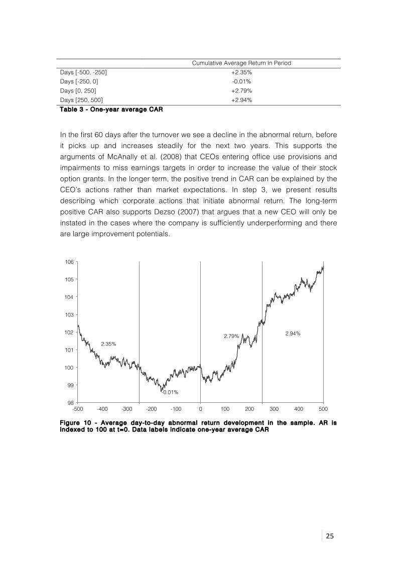
5.1.2 Results In this section we explore changes in CAR surrounding a CEO turnover. We assume CAR to be normally distributed around 0 over time and across companies. In figure 10 below, we show the average AR for each day in the period of 2 years before and after the turnover date. We see that the average AR in the sample is declining towards the turnover date, then to increase steadily for the next 2 years subsequent to the CEO turnover. As displayed in table 3, the CAR in the one-year period before the turnover is -0.01%. The CAR in the first year [Days 0, 250] is 2.79%, and 2.94% in the second year [Days 250, 500] after the turnover. This indicates that, on average, the stocks are underperforming compared to the expected return, suggested by the Fama-French four-factor model, in the time leading up to the turnover. It further suggests that the market responds positively to a change of CEO, yielding a positive CAR over the first year. As we will see in the next subsection, these findings are statistically significant at a 10% level.

-296! 0! +250! +500! +750!-46!

Compute Abnormal Return:!Estimate parameters:!

Estimation Window: !(-46, -296) !

Event day = 0 ! Event Window:!(0,250), (250,500), (500,750)!

25"

Cumulative Average Return in Period Days [-500, -250] +2.35% Days [-250, 0] -0.01% Days [0, 250] +2.79% Days [250, 500] +2.94% Table 3 - One-year average CAR

In the first 60 days after the turnover we see a decline in the abnormal return, before it picks up and increases steadily for the next two years. This supports the arguments of McAnally et al. (2008) that CEOs entering office use provisions and impairments to miss earnings targets in order to increase the value of their stock option grants. In the longer term, the positive trend in CAR can be explained by the CEO’s actions rather than market expectations. In step 3, we present results describing which corporate actions that initiate abnormal return. The long-term positive CAR also supports Dezso (2007) that argues that a new CEO will only be instated in the cases where the company is sufficiently underperforming and there are large improvement potentials.

Figure 10 - Average day-to-day abnormal return development in the sample. AR is indexed to 100 at t=0. Data labels indicate one-year average CAR

2.35%"

-0.01%"

2.79%" 2.94%"

98"

99"

100"

101"

102"

103"

104"

105"

106"

-500" -400" -300" -200" -100" 0" 100" 200" 300" 400" 500"

26"

5.2 Change in fundamentals surrounding CEO turnovers We have now shown that the market tends to react positively to a CEO turnover. Now, we want to explore whether the market reaction is followed by any changes within the firm, in terms of company fundamentals, or if the reaction comes solely from stock return expectations. We hypothesize that the turnover entails changes in company fundamentals. According to Jenter and Lewellen (2014) more than 40% of CEO turnovers are performance-induced. This makes us believe that there is room for improvements in the company, and that new CEOs generally will try to make changes, including the fiscal fundamentals.

5.2.1 Methodology In this step, we summarize changes in firm performance and firm fundamentals from the year before [-250 to 0 days] the CEO turnover and three years into the future ([0 to 250 days], [250 to 500 days], and [500 to 750 days]). This is completed to add to the understanding of how firms are re-structured on average, given changes in several metrics’ on an isolated basis. To perform this analysis, we have conducted t-tests on the equality of the means, which let us conclude whether the changes in means are statistically significant. In theoretical terms, we test if

!!!"#!!"!! = !!!!!"!!"#!:!!!"#!!"!!"":!!!""!!"!!"#!, !"#!!"#"$%"!!

through,

! = (! − !!)√!!

When applying the test to our dataset, the results increase the understanding of which holistic changes that actually yield differences. By including the time aspect, we are able to uncover which re-structuring initiatives that are implemented in the near and long-term.

27"

5.2.2 Results In this subsection we will present the results from the analysis of step 2 and offer our discussion of the meanings and implications of the findings. Days -250 to 0 Days 0 to 500 (1) (2) (3) (4) N Mean Mean Diff. from t-1 CAR 899 0,003 0,027 0,0237* Tobin’s Q 899 1,422 1,383 -0,039 ROE 899 0,335 0,266 -0,0687 ROA 899 0,125 0,125 0,0000 EBITDA margin 899 0,158 0,156 -0,0020 EV / Sales 899 2,339 2,342 0,0037 Revenues / Total Assets 899 0,951 0,939 -0,0119 Acquisitions / Total Assets 899 0,018 0,020 0,0017 Capital Expenditures / Total Assets 899 0,046 0,042 -0,0034** Cash / Total Assets 898 0,041 0,047 0,0053* LT debt / Total Assets 899 0,182 0,178 -0,0040 Working Capital / Total Assets 899 0,156 0,166 0,0101* Dividends / Total Assets 896 0,013 0,015 0,0018* R&D / Total Assets 896 0,022 0,022 0,0004 SG&A / Total Assets 896 0,182 0,181 -0,0019 Sale of Property / Total Assets 896 0,002 0,002 0,0003 Sale of Investments / Total Assets 896 0,070 0,082 0,0115 E-index 706 2,530 2,551 0,0213 CEO ownership 553 0,002 0,004 0,002*** Share Structure 706 0,101 0,097 -0,0033 Table 4 - Change in ( i i) fundamentals and (i i i ) performance around CEO turnover

Column 2 in table 4 above presets the mean value of the variables in the year before the turnover, and column 3 presents the mean over the first two years, or 500 days, after the turnover. We calculate the difference between the two periods in column 4. We see that the only change proving significance on a 1% level, is the CEO ownership variable, suggesting that new CEOs tend to have a greater stakes in the company than their predecessors. We argue that when the board replaces the CEO, they want to better align the incentives of the CEO and the other stakeholders, ultimately the shareholders. We see this as a measure to reduce the agent-principal problems that may arise if the CEO is driven mainly by short-term gains from his bonus rather than the long-term vesting value created from his equity position and the stock options he has been granted16. Recalling the argument on stock option grant and firm value from the previous section, increased CEO ownership may also give incentives to conduct earnings management to lower the value of the firm at the turnover to increase the value of the stock-based compensation package. 16 On average, annual bonuses account for ~50% of a CEO’s Total Current Compensation (Salary + Bonus).

28"

Next, we note that the mean CAR of the sample increases on average by 2,37% on a 10% significance level in the years surrounding the turnover. This confirms that our findings from step 1, displayed in table 3, are valid. Further, we find an increase in Cash, Dividends and Working Capital on a 10% significance level and a decline of Capital Expenditures on a 5% level. The increases in cash and working capital, along with the decline in capital expenditures, are measures that will strengthen the firm’s balance sheet, thus enhancing the robustness of the firm. It has been showed that if a company desires to take a greater risk for bigger profits and losses, it reduces the size of its working capital in relation to its sales. If it is interested in improving its liquidity, it increases the level of its working capital (Sushma & Shah, 2007). For a firm facing earnings cash flow constraints, it is natural that increases in cash and working capital is followed by a decrease in capital expenditure. As mentioned above, Jenter and Lewellen (2014) find that more than 40% of all turnovers are performance-induced, i.e. the change of CEO follows poor firm performance. We argue that a new CEO will aim to secure his position by improving the firm’s ability to withstand forthcoming financial distress by enhancing the robustness. However, the increase in dividend contradicts this explanation, but the difference is the smallest among the significant variables. We will show in section 5.3.2 that an increase of the dividends shortly after the turnover is penalized by the market.

“In business, what’s dangerous is not to evolve.” Jeff Bezos, CEO of Amazon

We do not find evidence for significant changes in the level of any of the other company fundamentals nor in any of the operational performance metrics. Hence, the change in CAR that is not explained by the changes of the significant company fundamentals discussed above, must origin in other factors. We aim to address these factors in section 5.3 and 5.4.

29"

5.3 Drivers of CAR So far we have shown that the market reacts positively to a CEO turnover, and that the CEO turnover actually entails changes in certain company fundamentals and characteristics, mainly associated with increasing the fiscal robustness of the company. The next step will be to determine whether any of these fundamentals have a significant impact on CAR. We hypothesize that CEO initiated changes in company fundamentals will impact the abnormal stock return. Thus, we suggest that the right actions can positively impact how the market views the future value potential of the company.

5.3.1 Methodology In this step, we are trying to use statistical inference to uncover if the isolated fundamental changes stated in step 5.2 have a direct effect on the CAR. In other words, we test if the market, on average, reacts to certain corporate re-structuring initiatives above others. To perform the analysis, we have utilized regression analysis, by ordinary least squares method. This method was found appropriate after testing the firm fixed- versus random effects, and generating the Lagrangian multiplier effect. In essence, the tests suggested insufficient evidence to reject the hypothesis that the between firm error term !! is correlated to the coefficients of the independent variables. Thus, a random effect model does not add explanatory power in excess of the ordinary least squares model17. Consistent with previous discussion, signal effects are the main contributors to announcement CAR, while implementing fundamental changes in subsequent years will be stronger contributors to CAR. Therefore, we construct the analysis separately for the turnover year, the first, and second full year the new CEO has been appointed. We isolate the effect of each independent variable on CAR for both years, capturing how the market reacts to the expectation of value in the turnover year, while the companies have to deliver tangible change for the market to re-price firm value after a period of time. CAR calculations Transition year !"#!!!"#!!"#$ = !! + !∆!!!!! + !∆!!!!! +⋯+ ∆!!!!" + !! First full year !"#!"#!!""!!"#$ = !! + !∆!!!!! + !∆!!!!! +⋯+ ∆!!!!" + !! Second full year !"#!""!!"#!!"#$ = !! + !∆!!!!! + !∆!!!!! +⋯+ ∆!!!!" + !! Table 5 - CAR model for transit ion year, year 1 and year 2

17 For test output see appendix 8.2.1. For further explanation of the theory behind fixed and random effect models, see section 8.3.1.5.

30"

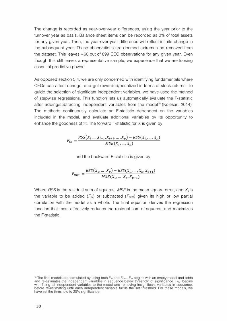
The change is recorded as year-over-year differences, using the year prior to the turnover year as basis. Balance sheet items can be recorded as 0% of total assets for any given year. Then, the year-over-year difference will reflect infinite change in the subsequent year. These observations are deemed extreme and removed from the dataset. This leaves ~60 out of 899 CEO observations for any given year. Even though this still leaves a representative sample, we experience that we are loosing essential predictive power. As opposed section 5.4, we are only concerned with identifying fundamentals where CEOs can affect change, and get rewarded/penalized in terms of stock returns. To guide the selection of significant independent variables, we have used the method of stepwise regressions. This function lets us automatically evaluate the F-statistic after adding/subtracting independent variables from the model18 (Kolesar, 2014). The methods continuously calculate an F-statistic dependent on the variables included in the model, and evaluate additional variables by its opportunity to enhance the goodness of fit. The forward F-statistic for Xi is given by

!!" =!"" !!,…!!!!,!!!!,… ,!! − !""(!!,,… ,!!)

!"#(!!,… ,!!)

and the backward F-statistic is given by,

!!"# =!"" !!,… ,!! − !""(!!,,… ,!!,!!!!)

!"#(!!,… ,!!,!!!!)

Where RSS is the residual sum of squares, MSE is the mean square error, and Xp is the variable to be added (FIN) or subtracted (FOUT) given its high or low partial correlation with the model as a whole. The final equation derives the regression function that most effectively reduces the residual sum of squares, and maximizes the F-statistic.

18 The final models are formulated by using both FIN and FOUT. FIN begins with an empty model and adds and re-estimates the independent variables in sequence below threshold of significance. FOUT begins with fitting all independent variables to the model and removing insignificant variables in sequence, before re-estimating until each independent variable fulfills the set threshold. For these models, we have set the threshold to 20% significance.

31"

5.3.2 Results In this section, we will explore whether changes in company fundamentals will act as drivers of CAR in the transition year and the first two full years the CEO has been in office. In table 6, column 1 shows the regression of firm fundamentals and characteristics on CAR in the transition year. Column 2 presents the same regression for the first full year the CEO held the office, and column 3 presents the regressions for year 2. (1) (2) (3) VARIABLES Year 0 Year 1 Year 2 ∆ Dividends / Total Assets -0.388** -0.841*** (0.193) (0.209) Share structure -0.319** (0.142) ∆ Working Capital / Total Assets 0.0703 0.0891* (0.0431) (0.0485) E-Index 0.0533 0.0875** (0.0398) (0.0371) ∆ CapEx / Total Assets -0.167** 0.156 (0.0770) (0.108) ∆ R&D 0.350* (0.206) ∆ Cash -0.0656** (0.0295) Forced turnover 0.346* (0.193) Constant 0.0838 0.164*** -0.160 (0.121) (0.0479) (0.106) Observations 59 62 60 R-squared 0.249 0.311 0.224 Adjusted R-squared 0.193 0.275 0.152 Type OLS OLS OLS VIF 1.10 1.08 1.25 Table 6: Sensit ivity of CAR to changes in corporate fundamentals from 0 to 750 days post-CEO turnover

We have argued that the market’s view on the new CEO will partly materialize in abnormal return once the information is publicly available, as the efficient market theory suggests. We find that the only two variables returning significant results in the transition year are the ∆ Dividend / Total Assets and the Share Structure, both with a negative impact. This is consistent with table 4 from section 5.2.2. Thus, we find that if the dividend rate is increased during the transition year the market will respond negatively. It also shows that a company introducing or maintaining a dual share structure will have negative impact on the return.

32"

A company with dual share structure will give increased voting power to a certain group of shareholders. The executive group will often be owners of “class A” shares, and if the CEO and his team control enough votes, they have substantial power in the company. This could cause investors to avoid involving themselves in companies where their shareholder power is diluted. If enough investors do not have sufficient confidence in the best judgment of the executive team to create value for shareholders, they may choose not to place their investments in companies that retains or introduces a dual share structure. Therefore, the return on the stock could diminish due to demand deficit. CAR would reflect this, and could explain why we see a negative relation between the dual share structure and CAR. Conversely, a single share structure would have a positive impact on CAR. This is supported by Gompers, Ishii and Metrick (2010) that find strong evidence that firm value is increasing in insiders’ cash-flow rights and decreasing in insider voting rights. Increase in the dividend payments in the transition year also negatively impacts CAR. A company would normally increase their dividend payments when the expected return on new projects is less than the cost of capital (Miller & Modigliani, 1961). Such an action would further signalize poor growth prospects. A CEO increasing the dividend already in the year he is entering office, could be signalizing that he have assessed the growth opportunities to be less attractive than previously believed. By increasing the dividend he is suggesting that the cash would be better deployed outside of the company, and we believe that the negative impact on CAR mirrors the market’s new outlook on the growth opportunities in the company. This is even more statistical significant in year 1 with higher impact on CAR. We suggest that this is due to the fact that after a year, the CEO has gained full information of the state of the company, and an increase in dividend will have stronger signaling power of weak growth prospects. An increase in capital expenditures has a significant negative impact on CAR in the first full year after the CEO turnover. Lowering ∆ Capital Expenditure / Total Assets increases the robustness of the company and we have previously discussed that the market seems to react positively on these measures. Allegedly, the market deems it in the best interest of shareholders to increase the robustness of the firm. In year 2, the CEO has entered office and is arguable in a position where he can make strategic choices. At this point the variables ∆ Working Capital / Total Asset, ∆ Cash / Total Assets E-index and Forced Turnover yield significant results. None of these variables proved significant in the transition year.

33"

We show, in section 5.2.2, that firms tend to take measures to become more fiscally solid after a CEO turnover. We find that changes in working capital are positively correlated to increase in CAR in year 2. However, increases in the cash holdings have negative impacts on CAR, which shows us that the build-up of working capital must consist of non-cash items in order to be welcomed by the market. Noteworthy, the market seems to deprive stock value from companies that holds excessive cash balances, as these are funds that could have been used for internal projects or could have been deployed to the shareholders in increased dividends. This is the very argument the infamous activist investor Carl Icahn is posing to have Apple Inc. reduce its enormous cash holdings by conducting stock repurchases (Icahn, 2013). Further, we find positive relation between the entrenchment of the CEO and the CAR. The market seems to reward if the CEO is more protected from replacement. We argue that to turn around a company takes time and persistency. Keep in mind that more than 40% of the turnovers are performance-induced (Jenter & Lewellen, 2014), and that the majority of companies are in need of large changes in their operations and strategy. A CEO with a higher degree of job security would be enabled to focus on the long-term improvements, rather than short-term gains to keep his job. The shareholders would arguably be better served with someone having the long-term performance in mind, and the entrenchment ensures him the necessary time to fully exercise his strategic plans. To support this, we find a positive relation between entrenchment and the CEO’s tenure19. Finally, the regression yields a positive impact on CAR if the former CEO left office involuntarily. Dezso argues that a CEO will only be fired if the potential gain from employing a new executive exceeds the cost of firing the current CEO (Dezso, 2007). Thus, a board that has actually fired their CEO necessarily believes in a large potential gain from instating a new CEO. The market will, according to the EMH, react to this implied information and we argue that this could cause the CAR to soar. Summing up, certain CEO initiated changes of company fundamentals do have an impact on the abnormal return and enforces our belief that the market reacts to a CEO turnover because the new CEO reveals the true state of the company by performing certain strategic actions.

19 The slope between the E-index and Tenure is 0.46% indicating higher tenure for higher entrenchment of the CEO

34"

5.4 Drivers of fundamentals To this point we have shown that the market reacts positively to a CEO turnover and is followed by changes in certain company fundamentals that appears to strengthen the robustness of the balance sheet. Further, we have shown that the changes in some of these fundamentals have significant impact on the abnormal return. Hence, we have established that the CAR to some extent is influenced by the actions the new CEO induces. Now, we will explore whether the new CEO will be more inclined to perform certain strategic choices, in terms of changing the company fundamentals, depending on his background and other attributes. By testing for this, we are trying to establish a connection between the drivers of abnormal return and the new CEO’s attributes. We hypothesize that certain CEO attributes will shape the new CEO’s attempt to restructure the company through different value creating initiatives.

5.4.1 Methodology The dependent variables in the models are selected based on the CEOs ability to affect the composition. As such, we evaluate the six corporate actions: changes in capital structure, rationalization of working capital, investments in research and development, ability to fund growth through capital expenditures or acquisitions, and, finally, dividend payout policy. As independent variables, the model uses the company fundamentals, E-index, share structure, former CEO retention, and forced turnover; and the CEO appointments’ attributes in internal versus external recruiting, board experience, age, educational background separated in engineering, MBA, and graduate school, and, finally, the percentage ownership in the company. To control for industry fixed effects, we have included industry factor variables by SIC category20. Since the dataset consists of panel data, it is best analyzed through controlling for unobservable effects. The models are formulated given evaluation on whether to transform the estimation through either random or firm fixed effects. In turn, we have selected the final models on the basis of Hausman tests and Lagrangian multiplier tests, which indicate whether it is appropriate to select fixed or random, and unobserved or ordinary least squares models, respectively.

20 Nine industries are included in table 8. However, only eight appears as factor variables in the output as the industry ”Mining” is captured in the constant term.

35"

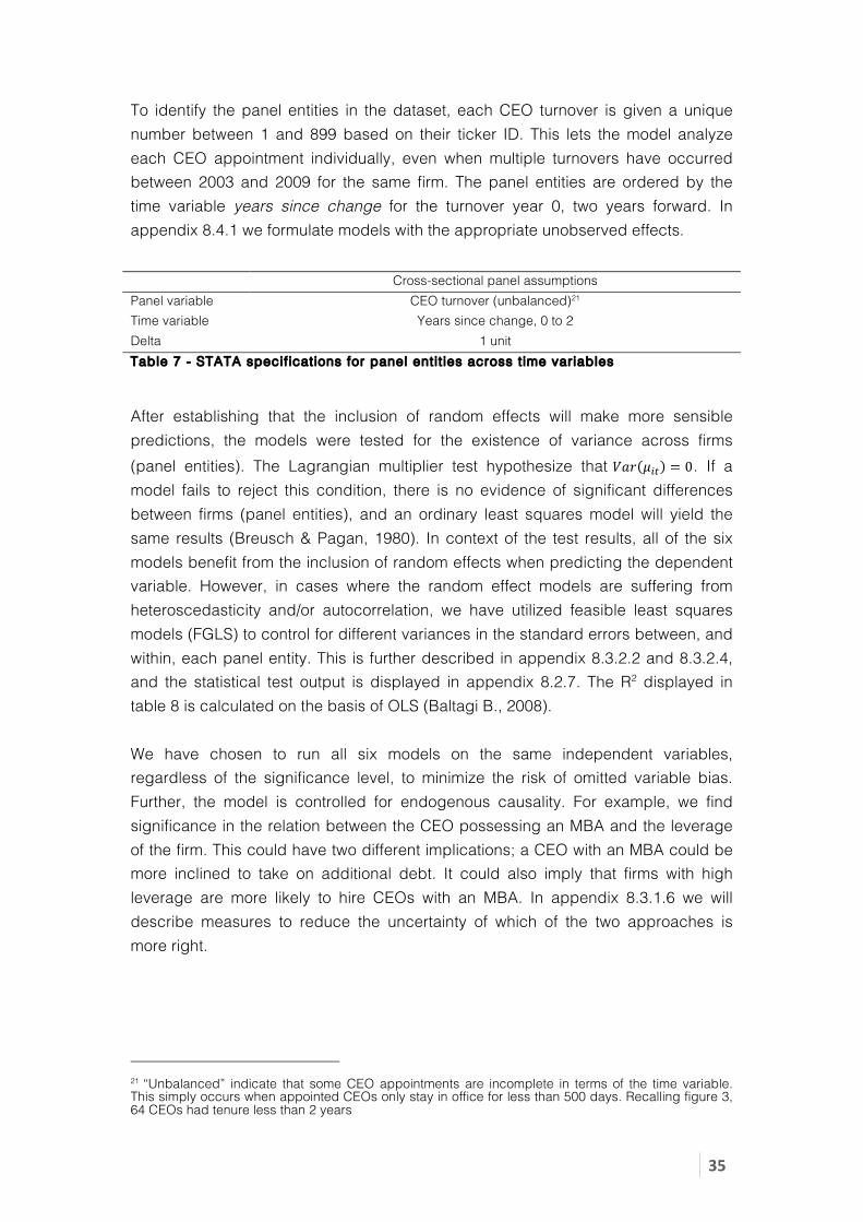
To identify the panel entities in the dataset, each CEO turnover is given a unique number between 1 and 899 based on their ticker ID. This lets the model analyze each CEO appointment individually, even when multiple turnovers have occurred between 2003 and 2009 for the same firm. The panel entities are ordered by the time variable years since change for the turnover year 0, two years forward. In appendix 8.4.1 we formulate models with the appropriate unobserved effects. Cross-sectional panel assumptions Panel variable CEO turnover (unbalanced)21 Time variable Years since change, 0 to 2 Delta 1 unit Table 7 - STATA specif ications for panel entit ies across t ime variables

After establishing that the inclusion of random effects will make more sensible predictions, the models were tested for the existence of variance across firms (panel entities). The Lagrangian multiplier test hypothesize that !"# !!" = 0. If a model fails to reject this condition, there is no evidence of significant differences between firms (panel entities), and an ordinary least squares model will yield the same results (Breusch & Pagan, 1980). In context of the test results, all of the six models benefit from the inclusion of random effects when predicting the dependent variable. However, in cases where the random effect models are suffering from heteroscedasticity and/or autocorrelation, we have utilized feasible least squares models (FGLS) to control for different variances in the standard errors between, and within, each panel entity. This is further described in appendix 8.3.2.2 and 8.3.2.4, and the statistical test output is displayed in appendix 8.2.7. The R2 displayed in table 8 is calculated on the basis of OLS (Baltagi B., 2008). We have chosen to run all six models on the same independent variables, regardless of the significance level, to minimize the risk of omitted variable bias. Further, the model is controlled for endogenous causality. For example, we find significance in the relation between the CEO possessing an MBA and the leverage of the firm. This could have two different implications; a CEO with an MBA could be more inclined to take on additional debt. It could also imply that firms with high leverage are more likely to hire CEOs with an MBA. In appendix 8.3.1.6 we will describe measures to reduce the uncertainty of which of the two approaches is more right.

21 “Unbalanced” indicate that some CEO appointments are incomplete in terms of the time variable. This simply occurs when appointed CEOs only stay in office for less than 500 days. Recalling figure 3, 64 CEOs had tenure less than 2 years

36"

5.4.2 Results In this step, we have tested the company fundamentals against the CEO attributes and the firm characteristics after controlling for industry fixed effects. The regression is found in table 8 below. Controlling for industry fixed effects removes parts of discretionary effects from firm characteristics and CEO attributes on company fundamentals. However, we see different independent variables dictating the change for the various company fundamentals, beyond the industry categorization22.

Leverage First, we have run a set of firm characteristics and CEO attributes against Leverage. Starting at the top of column 1, we find that entrenchment has positive, but small, impact on leverage. However, this finding is not consistent with the majority of previous literature on the topic that concludes that higher entrenchment should imply lower debt levels (Berger, Ofek, & Yermack, 1997). On the other side, John and Litov (2008) contradict this and suggest higher leverage for entrenched managers, arguing that they have better access to the debt market, perhaps as an outcome of conservative investment policy around CEO turnovers. Thereafter, externally recruited CEOs tend to have lower leverage than their internally recruited peers. Cao and Mauer (2010) find that CEO turnovers, in particular external CEO turnovers are a significant determinant of debt policy changes. The CEO has first-order influence on debt policy and we argue that a externally recruited CEO with less internal knowledge about the company’s debt capacity would prefer a lighter debt service during the restructuring period, in line with our argument that the new CEO tends to increase the robustness of the balance sheet.

22 We attempted to create a consolidated model reflecting a ”robustness scale” combining the company fundamentals. However, the model did not yield any unambiguous or significant results.

37"

(1) (2) (3) (4) (5) (6) VARIABLES Leverage WC CapEx Acquisition Dividends R&D E-Index 0.00887*** -0.0240*** -4.46e-05 -0.000980 -0.00143 -0.00282 (0.00326) (0.00194) (0.000309) (0.00175) (0.00100) (0.00176) Share structure -0.0267 0.00729 -0.000187 0.0138* 0.00215 -0.0249*** (0.0170) (0.0236) (0.00232) (0.00734) (0.00438) (0.00954) External recruiting -0.0489*** 0.00476 -0.00194** -0.00510 -0.00377 0.00462 (0.00884) (0.00914) (0.000892) (0.00454) (0.00274) (0.00600) Board experience 0.00511*** -0.00965*** -0.00102*** 0.000386 0.000333 -4.95e-05 (0.00109) (0.00140) (0.000140) (0.000582) (0.000353) (0.000772) Age 0.00391*** 0.000309 -7.25e-05 -0.000156 0.000101 -0.000602 (0.000690) (0.000594) (6.52e-05) (0.000341) (0.000199) (0.000379) CEO retention -0.0188** 0.0351*** 0.00131 0.00189 0.000851 0.0141** (0.00814) (0.00890) (0.000912) (0.00450) (0.00272) (0.00594) Forced turnover 0.0546*** -0.0728*** -0.000397 -0.00891 -0.00408 0.00764 (0.0126) (0.0128) (0.00107) (0.00641) (0.00380) (0.00822) Engineering -0.0354*** 0.0435*** 0.00209 -0.00513 -0.00637** 0.0173*** (0.0100) (0.0114) (0.00151) (0.00492) (0.00298) (0.00653) MBA 0.0497*** -0.0217** -0.00229*** 0.00875** 3.64e-05 -0.00547 (0.0101) (0.00875) (0.000705) (0.00444) (0.00268) (0.00584) Grad school -0.0323*** 0.0674*** -0.00737*** 0.0120** 0.00152 0.0117 (0.0104) (0.0179) (0.00152) (0.00539) (0.00330) (0.00726) Shares owned -0.548 0.116 -0.0619 -0.258 0.0826 0.299** (0.346) (0.102) (0.0430) (0.212) (0.109) (0.150) Construction -0.123*** 0.248*** -0.0931*** -0.00285 0.000982 -0.00316 (0.0298) (0.0358) (0.0142) (0.0243) (0.0148) (0.0325) Manufacturing 0.0280* 0.126*** -0.0968*** -0.00561 0.0118* 0.0441*** (0.0152) (0.0177) (0.00963) (0.0104) (0.00629) (0.0138) Utilities 0.111*** -0.0562*** -0.0500*** -0.0229* 0.0123* -0.000151 (0.0174) (0.0212) (0.0104) (0.0118) (0.00717) (0.0157) Wholesale trade -0.00316 0.176*** -0.113*** 0.00452 0.0137 0.00649 (0.0186) (0.0249) (0.0100) (0.0138) (0.00837) (0.0184) Retail trade 0.00343 0.0715*** -0.0697*** -0.0141 0.00304 -0.00166 (0.0155) (0.0219) (0.0102) (0.0116) (0.00697) (0.0152) Finance -0.0589*** -0.00267 -0.133*** -0.0116 0.00475 0.00361 (0.0216) (0.0199) (0.00962) (0.0125) (0.00755) (0.0166) Services -0.00904 0.111*** -0.107*** 0.00677 -0.00275 0.0362** (0.0181) (0.0254) (0.00972) (0.0113) (0.00681) (0.0149) Constant -0.0906** 0.150*** 0.145*** 0.0328 0.00504 0.0314 (0.0411) (0.0332) (0.0106) (0.0216) (0.0127) (0.0251) Observations 764 764 764 772 769 769 CEO entities 261 261 261 269 268 268 R – squared 0.1494 0.3298 0.4138 0.0681 0.0949 0.2919 Type FGLS FGLS FGLS Random Random Random VIF 2.09 2.09 2.09 2.09 2.08 2.08 Panels Heterosc. Heterosc. Heterosc. Homosc. Homosc. Homosc. Correlation First order First order First order Indep. Indep. Indep. Table 8 - Regression matrix between (i i) company fundamentals and certain ( i) f irm characterist ics and CEO attr ibutes

38"

CEOs with an MBA degree also tend to be employed by companies with higher leverage. We assess two reasons for that; (i) the business school background provides him with the necessary expertise regarding debt capacity and sources, which enables him to seek financing where non-MBAs wound not. More likely, (ii) the CEO has built a network through his studies and as alumni that facilitates for beneficial terms in the debt market. Further, both age and board experience correlates with higher leverage. Both variables are proxies for overall experience, and we argue, similarly to the argument regarding MBA, that with higher experience comes a wider network. Hu and Liu (2015) find in their study on Chinese corporations that CEOs with a larger network exploit more outside funds, such as bank loans and other parts of the debt market. This is in line with the second argument we offer. However, both Engineering and Grad School yield a negative relation to leverage. It seems that only relevant business experience will have the CEO to seek outside funds, also in line with the findings of Hu and Liu. Forced turnovers have a positive correlation with higher debt levels. We argue that the chance of being fired is higher in a company in financial distress where the equity value has seen subpar performance. As more than 40% of all turnovers are performance induced (Jenter & Lewellen, 2014), and highly leveraged firms lose substantial market share to their more conservatively financed competitors in industry downturns (Opler & Titman, 1994), a positive correlation between forced turnovers and leverage is plausible.

Working Capital Second, we assess the drivers of working capital in column 2. Starting at the top, we see that the negative relation between entrenchment and working capital is significant at a 1% level. We have previously argued that the CEO seeks to make the companies more robust once he enters office. If the CEO is more entrenched, i.e. his position is more secure, the need for robustness is smaller and the CEO can run the company with lesser safety margins with regard to working capital. Further, there is a positive relation for external recruiting. Following the same line of arguments, a CEO coming from the outside will have less knowledge about the in-house situation and what safety margins that might be required. We argue that he will seek to increase working capital in order to raise the robustness of the company. Higher experience, measured by the number of board memberships the CEO held, is negatively correlated with working capital. We argue that experience will improve the abilities to determine the minimum required level of working capital and thus achieve a more lean operation. Hence, a more experienced CEO will be more likely to have experience with the mechanics of different business models, which would increase the confidence in lowering the working capital.

39"

Moreover, an engineering degree is positively related to a higher level of working capital. This could imply that engineers tend to hold higher inventory than their non-engineer peers. As the majority of non-engineers fall within the business educated category, we propound that working capital management is a larger focus area within the business studies, something that is supported by the negative relation between working capital and an MBA degree. The last CEO attribute that returns significant results for working capital is the graduate degree variable. It shows a positive relation between having earned a graduate degree and the level of working capital. We allege that this is due to ~50% of the graduates majored in a non-business field. As MBAs are registered separately from other graduate degrees, the increase in working capital will follow the same line of arguments as for engineers earlier in this paragraph; the large degree of non-business graduates will drive the increase in working capital compared to their business educated peers. Lower working capital is associated with higher risk (Sushma & Shah, 2007). This explains the negative relation between forced turnovers and working capital where we argue that in companies where forced turnovers has occurred, the working capital management has been too lean and jeopardized the CEO’s position. Lastly, there is a positive relation between the retention of the former CEO as chairman and working capital. We use the same line of arguments as for forced turnovers. We find that companies that fired their CEO had significantly lower retention of the former CEOs than those who did not23. These two variables have the same underlying reason; low working capital implies higher risk and increased chances of firing of the CEO.

Capital Expenditures Third, column 3 addresses the Capital Expenditure as dependent variable. Holding an MBA degree, being externally recruited, high board experience and holding a graduate degree will be negatively correlated to capital expenditure. Starting with external recruiting, we have previously argued that a CEO from outside of the company will seek higher robustness than an internally recruited CEO due to his inferior knowledge of the financial situation of the company. Hence, the externally recruited CEO will have lower capital expenditures to increase the robustness of the fiscal balance sheet. The next three independent variables all reflects the CEO’s experience, both educational and in business. An MBA would be more inclined to grow through acquisitions, as we show in column 4 in table 8. Following our argument regarding 23 35% of the CEO’s who departed voluntarily was retained as chairman against only 6% of those who were fired.

40"

network, an MBA candidate would arguably be more acquainted with people biased towards M&A transactions, as many MBAs come from investment banking, consulting and similar business areas. This argument is supported by the empirical results presented in table 8 below. Hu and Liu (2014) find similar results in their study on Chinese corporations and their CEOs’ backgrounds. To a certain extent, the same line of arguments are valid for Grad School and Board Experience, as these will also have gained a large network through their education and career, respectively.

Acquisit ions Forth, we show in column 4 the drivers of Acquisitions. We have already discussed the variables MBA in the previous paragraph. In addition, Share Structure and Grad School also proves significant at a 5% level. We have argued that dual share structure gives the executive team increased control of the company, as they usually hold “Class A”- shares. This control would further enable them to pursue growth of the company through acquisitions. In the literature, this is often referred to as Empire Building, and will usually not be in the best interests of the other shareholders (Chevalier, 1998). This could explain the positive relation between Share Structure and Acquisitions, and could also elaborate why dual share structure tends have a negative effect on CAR, as discussed in section 5.3.2. Last, Grad School is positively correlated with Acquisition. Graham, Harvey and Puri (2009) imply an explanation for an inverse relation between overconfidence and a college degree, noting that it might indicate conservatism, as those impatient with their ambition might decide that higher education, especially a graduate degree, is not necessary. Extending to this idea, we argue that more conservative CEOs are less confident on the companies’ own projects, and rather rely on acquisitive growth where targets often have a proven track record. This is supported by a significant negative relation between Grad School and Capital Expenditure.

Dividends Fifth, dividends are displayed in column 5. The regression does only yield significant results within a 5% level for one of the independent variables. Engineers tend to lower the dividend payout, but the evidence is weak and the effect is small. Even though section 5.3.2 argue that increases in the dividend policy is penalized by the market, we find little evidence that variations in firm characteristics and CEO attributes are causing changes in the dividend payouts.

41"

Research & Development Finally, we show the results from the regression between R&D, and the firm characteristics and CEO attributes. The two variables showing the highest level of significance are Engineering and Share Structure, both significant at a 1% level. Starting with Engineering, we find a positive relation with R&D spending. Barker and Mueller (2002) also discover that significant R&D spending increases are found at firms where CEOs have advanced science-related degrees, engineering degrees among them (Barker & Mueller, 2002). We argue that their technical expertise will bias them into prioritizing research and development, as they can easily relate to the output. Further, Shares Owned yields a positive correlation with R&D spending. There is a U-shaped relationship between R&D spending and CEO ownership (Mezghanni, 2010); R&D spending is negatively (positively) associated with CEO ownership at low (high) levels of CEO stockholding. Mezghanni argues that this result implies that at low levels of CEO ownership, an increase in CEO ownership exacerbates CEO myopia and the underinvestment problem with regard to R&D activities. However, at high levels of CEO ownership, CEO becomes more willing to invest in risky R&D projects, which may reflect a closer alignment of managers’ and shareholders’ interests. For our findings to be consistent with Mezghanni’s results, the CEOs in our sample must have relatively high ownership shares in the companies they manage. The average among the 899 CEOs in the sample is 0,45% of total shares. As we examine the 1500 largest companies in the US, we assert that 0,45% is a sufficiently large share of the total market capitalization, and that our findings are in line with those of Mezghanni. “The path to the CEO's office should not be through the CFO's office, and it should not be through the marketing dept. It needs to be through engineering and design”

Elon Musk, CEO of Tesla Motors Thereafter, column 6 shows that Former CEO Retention is positively correlated to R&D spending. We offer two parallel suggestions for this; (i) when the former CEO is retained in the company as CEO, it is natural to believe that he maintains whole or parts of his ownership share in the company. When both the former and current CEO is involved in the decision-making regarding R&D, we argue that the effects discovered by Mezghanni will increase in strength, as incentives will magnify with the combined ownership share between the CEO and chairman. Another factor could be that (ii) certain sectors that tend to retain the former CEO as chairman are also R&D intensive sectors. We have run statistics implying correlation between

42"

CEO retention and R&D spending24. We believe R&D intensive firms has more incentives to retain the former CEO, as he carries valuable knowledge in product development that he could potentially bring to a competitor. Finally, we find a negative relation between dual share structure and R&D investments. Gompers et al. (2008) argue that the separation between control and cash flow rights distorts corporate governance and may lead to a deprivation of value at the expense of minority shareholders. Majority shareholders have a tendency to support short-term compensation schemes over long-term gains from R&D investments. The short-term gain would most likely harm long-term prospects, due to underinvestment in R&D. Showing preferences for short-term gain over long-term is consistent with the theory of hyperbolic discounting, suggesting that humans show a preference for a benefit that arrives sooner rather than later. Humans are said to discount the value of the later reward, by a factor that increases with the length of the delay (Frederick, Loewenstein, & O'Donoghue, 2002). A dual share structure seems to strengthen this relationship in terms of R&D.

Concluding remarks regarding drivers of fundamentals First, we find that MBAs and Engineers tend to have opposite preferences regarding financing, investment and growth strategies. An MBA will seek outside financing and will aim to grow through M&A rather than organically through capital expenditures and R&D. Second, entrenched executives make decisions focusing on short-term gains and self-serving outcomes, where less entrenched CEOs will make decisions more in line with the shareholders’ best interests. Third, more experienced CEOs tend to be less cash constrained and can utilize more financing options through external funding sources. They also tend to run a more lean operation. Finally, we find that more risk in the operations induces forced turnovers and that CEOs that are retained choose a more conservative and safe way in terms of leverage and working capital management.

24 Especially two sectors remarks themselves in both R&D spending and CEO retention; Manufacturing and Services, which contains many of the tech companies known to invest heavily in R&D.

43"

5.5 Predictive model for suited CEO attr ibutes At this stage we have shown positive market reactions to a CEO turnover, and that the turnover is followed by changes in company fundamentals aiming to increase robustness. Further, we have shown that some of these changes in fundamentals have significant impact on the abnormal return. In the previous subsection we showed that CEOs with certain attributes are more inclined to change these fundamentals than others. Here, we described corporate governance issues in relation to financing, investment and growth strategies in CEO turnovers. Now that we know how CEOs act differently based on their attributes, we are transitioning back to measuring market reactions to possessing these various attributes. We aim to separate the impact of certain CEO attributes to see whether they have different impact on CAR depending on what kind of company the CEO is employed in. This separation is important, as different companies will have different operational characteristics that demand certain CEO attributes. Thus, we hypothesize that large deviations between the expected and actual backgrounds and attributes of the appointed CEO’s will evoke stronger positive reactions in abnormal returns. This section aims to translate the findings from section 5.4, and examine how the market reacts when a firm hires an untypical CEO, who will make changes to the predecessor’s fiscal policies.

5.5.1 Methodology This step utilizes a set of logistic models to determine probabilities that all the CEO hires in our dataset was completed with the purpose of finding the best possible fit in terms of industry and firm specific fundamentals. Throughout the thesis, we have assumed that a corporate board hires a CEO in the search for particular ability that can contribute to either maintain or increase firm performance. Further, we assume that S&P 1500 firms are accurate, on average, in finding individuals with the appropriate attributes and background to create shareholder value. In that way, we are able to evaluate the correctness of every CEO turnover based on educational background, quality of educational institutions and diversity from prior industry experience. To model across these qualities, the possession of MBA, engineering and undergraduate degrees are used as dependent variables for the academic field. Having attended a top-50 institution, regardless of education level, is a dependent variable for the quality of education, and the number of board memberships acts as a proxy variable for experience and diversity. As independent variables, the model uses different industries (determined by SIC codes), E-index, whether the firm is listed on New York Stock Exchange or Nasdaq,

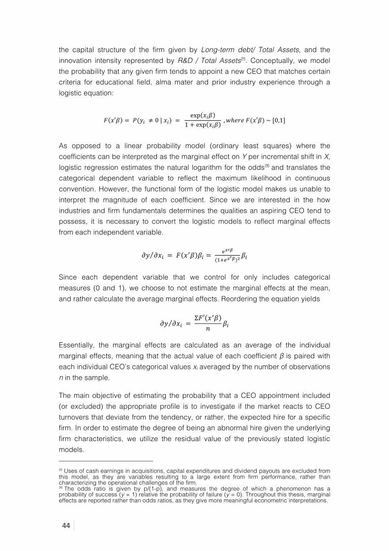
44"

the capital structure of the firm given by Long-term debt/ Total Assets, and the innovation intensity represented by R&D / Total Assets25. Conceptually, we model the probability that any given firm tends to appoint a new CEO that matches certain criteria for educational field, alma mater and prior industry experience through a logistic equation:

! !′! = !!(!! !≠ 0!|!!!) != !!exp !!!

1 + exp !!!! ,!ℎ!"!!!(!′!)!~![0,1]!

As opposed to a linear probability model (ordinary least squares) where the coefficients can be interpreted as the marginal effect on Y per incremental shift in X, logistic regression estimates the natural logarithm for the odds26 and translates the categorical dependent variable to reflect the maximum likelihood in continuous convention. However, the functional form of the logistic model makes us unable to interpret the magnitude of each coefficient. Since we are interested in the how industries and firm fundamentals determines the qualities an aspiring CEO tend to possess, it is necessary to convert the logistic models to reflect marginal effects from each independent variable.

!" !!!! = !! !!! !! = ! !!!!(!!!!!!)! !!

Since each dependent variable that we control for only includes categorical measures (0 and 1), we choose to not estimate the marginal effects at the mean, and rather calculate the average marginal effects. Reordering the equation yields

!" !!!! = !Σ!′ !!!

! !! Essentially, the marginal effects are calculated as an average of the individual marginal effects, meaning that the actual value of each coefficient β is paired with each individual CEO’s categorical values xi averaged by the number of observations n in the sample. The main objective of estimating the probability that a CEO appointment included (or excluded) the appropriate profile is to investigate if the market reacts to CEO turnovers that deviate from the tendency, or rather, the expected hire for a specific firm. In order to estimate the degree of being an abnormal hire given the underlying firm characteristics, we utilize the residual value of the previously stated logistic models. 25 Uses of cash earnings in acquisitions, capital expenditures and dividend payouts are excluded from this model, as they are variables resulting to a large extent from firm performance, rather than characterizing the operational challenges of the firm. 26 The odds ratio is given by p/(1-p), and measures the degree of which a phenomenon has a probability of success (y = 1) relative the probability of failure (y = 0). Throughout this thesis, marginal effects are reported rather than odds ratios, as they give more meaningful econometric interpretations.

45"

! !′! = !!(!! !≠ 1!|!!!) != 1 − ! exp !!!

1 + exp !!!= ! 11 + exp !!!

! ,!ℎ!"!!!(!′!)!~![0,1]!

This approach is equivalent to flipping the notations in the average marginal effects model. As such, we derive the probability of how far a CEO was (dependent on the inherent categorical variable, 0 or 1) from matching the tendency of market hires, and therefore, the higher the residual probability, the more we expect the market to be surprised given our assumption that all firms, on average, tends to select CEO profiles matching their fundamentals. The last ingredient of this computation is to establish a model that evaluates the market shocks, in terms of CAR, to the surprise effect of CEO appointments. This is done through an ordinary least squares model with CAR as the dependent variable and the residual value e of the predicted fit P of CEO educational background and experience as the independent variables.

!"#! = !! ∙ !! ! !"# + !! ∙ !! ! !"#$"%%&$"# + !!! ∙ !! ! !"#$%&%'# + !!!∙ !! ! !"#!50 + !!! ∙ !! !(!"#$%!!"#!$%!&'!) + !!!

With this model, we are able to identify the impact a CEO’s educational background and board experience has on CAR within the year of the turnover.

5.5.2 Results In the following subsection we present the results from the predicative model where we measure the impact on CAR from hiring a CEO with specific attributes in a firm defined by certain firm characteristics and company fundamentals.

“No one is born a CEO, but no one tells you that.” Drew Houston, CEO of Dropbox

Table 9 shows the marginal effects, in probabilities, which the independent variables has on the dependent binary variables. The output is derived by translating probabilities from the underlying logistic models. Furthermore, the model predicts a generalized probability for which CEO profiles firms had a tendency to hire, given their industry and underlying fundamentals.

46"

(1) (2) (3) (4) (5) VARIABLES MBA Engineering Undergrad

school Top 50 Board Experience

Construction -0.325** -0.228 -0.267 -0.0731 -0.210 (0.130) (0.162) (0.170) (0.161) (0.142) Manufacturing -0.0375 -0.123 -0.131* 0.0603 -0.0500 (0.109) (0.108) (0.0671) (0.101) (0.0982) Utilities -0.208* -0.110 -0.115 0.0415 0.154 (0.112) (0.117) (0.0777) (0.110) (0.109) Wholesale trade -0.170 -0.175 -0.238** -0.0821 0.0822 (0.134) (0.129) (0.108) (0.124) (0.138) Retail trade -0.176 -0.276** -0.218*** 0.0229 -0.0836 (0.116) (0.110) (0.0824) (0.112) (0.108) Finance -0.0558 -0.325*** -0.148** 0.0385 -0.0196 (0.112) (0.105) (0.0721) (0.105) (0.101) Services -0.0308 -0.255** -0.0357 0.309*** -0.00979 (0.117) (0.109) (0.0701) (0.110) (0.107) E-index 0.0448*** 0.0117 0.00148 0.00146 -0.0473*** (0.0135) (0.0115) (0.0120) (0.0139) (0.0128) Exchange27 0.0201 -0.00887 0.0540 0.109** 0.112** (0.0449) (0.0372) (0.0372) (0.0472) (0.0453) LT-debt / Total Assets 0.193* -0.0316 0.165 0.237** -0.0854 (0.114) (0.101) (0.111) (0.117) (0.113) Working Capital / Total Assets -0.0170 0.147 -0.189* 0.147 -0.460*** (0.122) (0.0929) (0.109) (0.124) (0.123) R&D / Total Assets -0.107 0.756** 1.929*** 1.160** 1.157*** (0.460) (0.302) (0.617) (0.478) (0.435) Observations 703 703 703 694 703 VIF 2.72 2.72 2.72 2.72 2.72 Table 9 – Marginal effects on probabil i ty for hir ing a CEO possessing various attr ibutes

Starting the interpretation from column 1, a firm in the construction industry decrease the probability of appointing a CEO with an MBA by ~32.5% relative to the mining industry, which is absorbed by the intercept. Likewise, utility firms are ~20.8% less likely to appoint an MBA. Conversely, each incremental increase in the entrenchment index increases the probability of appointing an MBA by ~4.5%, and each percentage increase in Leverage (LT-debt / Total Assets) makes a firm ~0.2% more likely to hire an MBA28. This is consistent with the findings from section 5.4.2.

27 TRUE indicates New York Stock Exchange (NYSE) while FALSE indicated NASDAQ. 28 Even though we comment only on the variables significant at a 10% level, it’s important to note that the insignificant variables are important to each prediction. With the low multicorrelation, chances of introducing biases in the independent variables are considered low.

47"

In column 2, the model shows the marginal effects on the probability of appointing a CEO with an engineering degree. Similarly to what can be generally expected, appointing a CEO with an engineering background have quite contradictory drivers than that for appointing MBAs. In context of the model, retail trade and finance remain as the industries that reduce the probability of hiring an engineer the most, decreasing by ~27.6% and ~32.5%, respectively. Moreover, each percentage increase in a firms research and development intensity (R&D / Total Assets) result in an ~0.76% increase in the probability of appointing an engineer. In column 3, the model evaluates the probability of appointing CEOs with higher educational experience. The criterion is the achievement of an undergraduate degree. When examining the findings, wholesale trade (~23.8%) and retail trade (~21.8%) appear as the industries that reduce the probability of appointing an educated CEO the most. In addition, financial (~14.8%) and manufacturing (~13.1%) firms are less probable to appoint non-educated CEOs. After evaluating the likelihood of appointing educated CEOs, column 4 in table 9 shows the likelihood of appointing CEOs with an alma mater from one of the top 50 universities. The only industry proven to be significant in increasing the probability of appointing CEOs from prestigious schools is Services; if a CEO is appointed in the services industry, he is 30.9% more likely to have graduated from one of the top 50 institutions. Firms in this industry deliver (among other things) technology and consulting services, with firms like Adobe Systems, Ebay, Accenture and Yahoo!.

“Certainly Yahoo! wouldn't exist without the sort of environment that Stanford gave us to allow us to create it.”

Jerry Yang, former CEO of Yahoo! Secondly, a noteworthy finding is that NYSE listed firms are ~10.9% likelier to hire CEOs from top 50 institutions than Nasdaq listed firms. For the fundamentals, both capital structure (LT-debt / Total Assets) and research and development (R&D / Total Assets) have a positive effect on the probability of recruiting from top 50 institutions, with ~0.2% and ~1.2% respectively. Finally, column 5 evaluates the probability of appointing CEOs on the basis of their experience, measured in board memberships. In summary, each increase in the entrenchment index reduces the probability of hiring an experienced CEO by ~4.7%. Firms listed on NYSE are ~11.2% likelier to recruit experienced CEOs. For fundamentals, firms with high working capital needs are less probable to seek out experienced CEOs. Hiring an experienced individual decrease by ~0.5% in probability per percentage increase in working capital (Working Capital / Total Assets). Finally, each percentage increase in research and development (R&D /

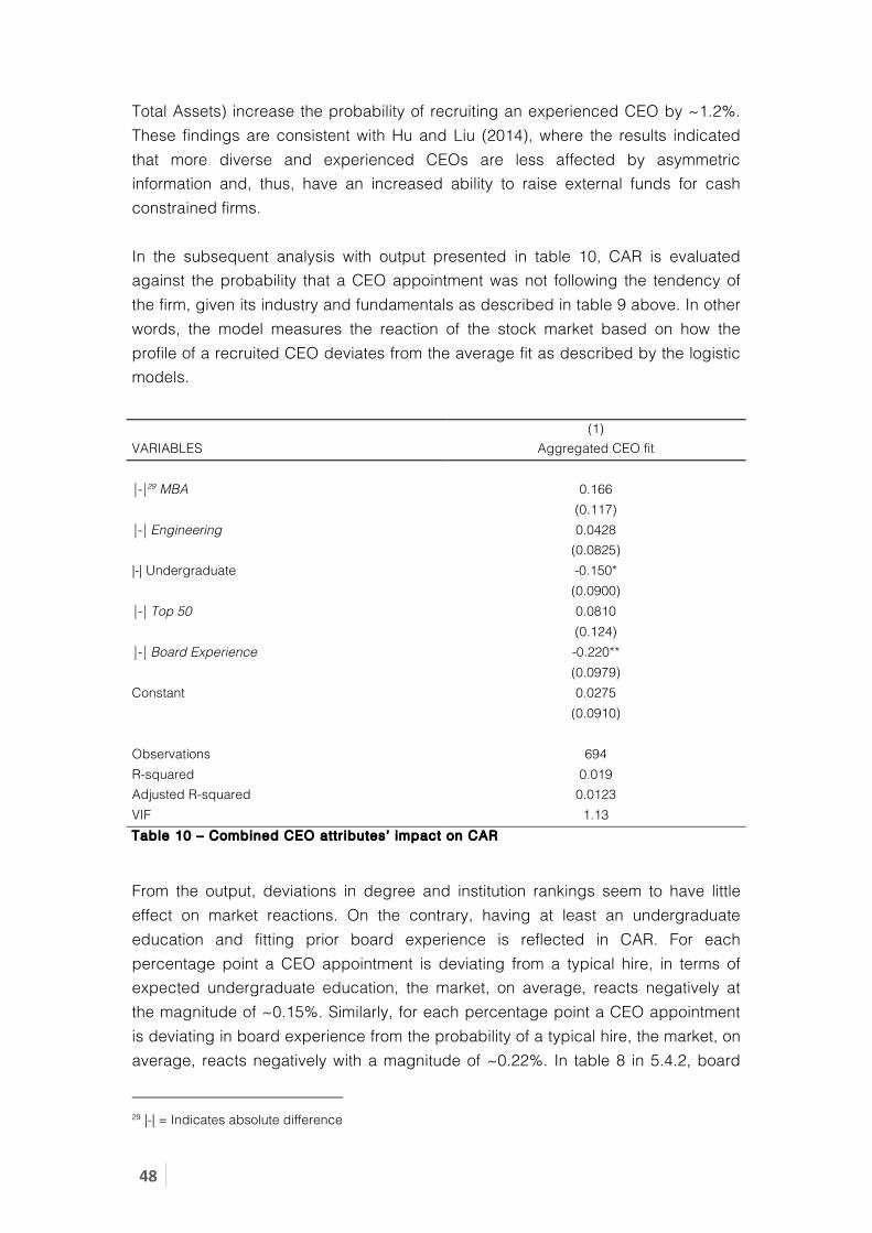
48"

Total Assets) increase the probability of recruiting an experienced CEO by ~1.2%. These findings are consistent with Hu and Liu (2014), where the results indicated that more diverse and experienced CEOs are less affected by asymmetric information and, thus, have an increased ability to raise external funds for cash constrained firms. In the subsequent analysis with output presented in table 10, CAR is evaluated against the probability that a CEO appointment was not following the tendency of the firm, given its industry and fundamentals as described in table 9 above. In other words, the model measures the reaction of the stock market based on how the profile of a recruited CEO deviates from the average fit as described by the logistic models. (1) VARIABLES Aggregated CEO fit |-|29 MBA 0.166 (0.117) |-| Engineering 0.0428 (0.0825) |-| Undergraduate -0.150* (0.0900) |-| Top 50 0.0810 (0.124) |-| Board Experience -0.220** (0.0979) Constant 0.0275 (0.0910) Observations 694 R-squared 0.019 Adjusted R-squared 0.0123 VIF 1.13 Table 10 – Combined CEO attr ibutes’ impact on CAR

From the output, deviations in degree and institution rankings seem to have little effect on market reactions. On the contrary, having at least an undergraduate education and fitting prior board experience is reflected in CAR. For each percentage point a CEO appointment is deviating from a typical hire, in terms of expected undergraduate education, the market, on average, reacts negatively at the magnitude of ~0.15%. Similarly, for each percentage point a CEO appointment is deviating in board experience from the probability of a typical hire, the market, on average, reacts negatively with a magnitude of ~0.22%. In table 8 in 5.4.2, board

29 |-| = Indicates absolute difference

49"

experience proved significant in making changes to company fundamentals. We argue that less cash flow constrains will provide more freedom in restructuring company balance sheets. Moreover, the fact that the market reacts to deviations in board experience, and not educational background, supports the argument that the market finds experience as a stronger determinant of ability to increase firm value30. Concluding the section, we find that the CAR is sensitive to the deviations from the typical CEO appointment, in terms of undergraduate education and board experience. An attribute that is valued in some firms might be penalized by the market in another type of firm31. We found in section 5.4.2 that MBAs and Engineers differ in fiscal strategies. However, when the CEO holds any of these two degrees, and this deviates from what is expected, the market does not react even though it may expect a re-structuring of company fundamentals due to the CEO’s untypical education. To add clarity to how the model works in practice, we have included the example of Jerry Yang from Yahoo! in appendix 8.5.1.

5.6 CAR as predictor for operational performance metrics So far, we have seen that the market reacts positively to CEO turnovers and that the turnover is followed by changes in company fundamentals. Thereafter, we show that the abnormal return is significantly impacted by the changes of the fundamentals. Further, we find that CEOs with certain attributes are more inclined to change these fundamentals than others. However, the different CEO attributes have different impacts depending on which type of company the CEO is employed by. The major trend is that any deviations from the peer norm are penalized by the market. Hence, we disprove an unambiguous relation between CEO attributes and abnormal return through the CEOs’ actions regarding company fundamentals. To conclude this thesis, we will see whether the market in the transition year is efficient in identifying CEO turnovers that yield positive and negative changes in operational performance in the long-term. We hypothesize that abnormal return will materialize in subsequent changes in operational performance metrics.

30 Elaborating on board experience, appointing a CEO with above average board experience to a firm that requires a focused experience profile will impact CAR differently than appointing a CEO with low experience to a firm that require an experienced profile. In appendix 8.1.3, the causality of each independent variable is separated. 31 We have attempted to include the deviation of fit for MBAs and Engineers in the regressions in table 8 in section 5.4.2. However, these did not yield any significant results, suggesting that the deviation of fit does not dictate any changes in the company fundamentals and that the market reaction comes solely from expectations of the new CEO’s ability to improve the business strategy.

50"

5.6.1 Methodology In the final step of the thesis, we construct ordinary least squares models to predict if the stock market as a whole is correct in their reactions to CEO turnovers. To assess this question, we have picked return on assets (ROA) and EBITDA margin as measurements for performance and profitability, respectively. Subsequently, we have calculated the differences in ROA and EBITDA margin for each individual firm from the year prior to the CEO turnover, three years into the future. To test the performance metric against the time of the CEO turnover, we lag the transition year CAR to match the performance and profitability in the two years following each turnover. Lagging Period ROA EBITDA margin Transition year ∆!"#!!!!"# = !!"#!!!!"# ∆!"#$%&!!"#$%&!!!!"# = !!"#!!!!"# First full year ∆!"#!!"#!!"" = !!"#!!!!"# ∆!"#$%&!!"#$%&!!"#!!"" = !!"#!!!!"# Second full year ∆!"#!!""!!"# = !!"#!!!!"# ∆!"#$%&!!"#$%&!!""!!"# = !!"#!!!!"# Table 11 - Measuring the CAR in transit ion year against ROA and EBITDA margin

5.6.2 Results We argue that if the market correctly anticipates improved performance in the future, the effect of improvement would materialize in positive CAR immediately after the information is available to the market32. Hence, we should be able to use the CAR as a predictor for the operational performance metrics. Column 1 in table 13 and 14 below presents the regression between CAR and the operational performance metrics, for the transition year. Column 2 and 3 displays the regression for the first and second full year of the CEO, respectively. We find statistical significance for using the CAR in the transition year as a predictor for both ROA and EBITDA margin in subsequent years33.

32 We have made a point out of drawing a clear line between what we refer to as operational performance metrics, such as ROE, ROA and EBITDA margin, and the market-based performance metrics, such as CAR. The latter metric is based on the stock performance, and hence the markets underlying view on how the company is performing, whereas the operational metrics are measured by items from the financial statement. 33 However, we find no evidence of the same effect for ROE. As ROE only reflects the results of a company's equity investments, a company could be highly leveraged with a risky amount of debt and it will show an improving ROE if that debt is generating income. There are large variations of leverage between the firms in the sample, and this will impact the consistency of ROE. Therefore, we are not baffled by the lack of significance and persistency for this particular performance metric.

51"

(1) (2) (3) VARIABLES Year 0 Year 1 Year 2 CAR 0.000156 0.0166*** 0.00986** (0.00288) (0.00390) (0.00478) Constant -0.00233 -0.000474 0.00301 (0.00162) (0.00219) (0.00266) Observations 899 899 835 R-squared 0.000 0.020 0.005 Adjusted R-squared -0.00111 0.0188 0.00388 Table 12 - CAR as predictor for ROA

We find a positive relation between an increase in CAR in the transition year, and ROA in year 1 and 2. We argue that the market to a certain extent has been able to interpret legitimacy behind the strategy and visions communicated by the new CEO at the time he entered office. We further argue that the CEO actually has been able to deliver the results implicitly expected from him and his company by the market. (1) (2) (3) VARIABLES Year 0 Year 1 Year 2 CAR 0.0972** 0.0796*** 0.0591* (0.0437) (0.0229) (0.0333) Constant -0.0311 0.00915 0.0109 (0.0246) (0.0129) (0.0185) Observations 899 899 835 R-squared 0.005 0.013 0.004 Adjusted R-squared 0.00438 0.0122 0.00257 Table 13 - CAR as predictor for EBITDA margin

We find the same positive relation between the CAR and EBITDA margin. Here, we also find significance in the transition year. A positive CAR in the transition year correlates with increase in the EBITDA margin. We argue that the market has interpreted the skills and strategy of the new CEO correctly, and find the prospects of operational improvements plausible with the new CEO entering office. Our analyses indicate that the market is rational and manages to predict whether the CEOs can make prosperous changes in the firms’ operations that will materialize in improved operational performance metrics.

52"

6. Conclusion and interpretation In this thesis, we have studied the impact on market performance from a CEO turnover. We have explored different aspects of the new CEO’s attributes, firm characteristics and certain company fundamentals that we believe to be subject to considerable managerial discretion, and how they impact the cumulative abnormal return in the time after the turnover date.

“An organization, no matter how well designed, is only as good as the people who live and work in it.”

Dee Hock, Former CEO of VISA We have aimed to shed light on the overall research question “What impacts the market reaction to a CEO turnover?” using a sample of 899 CEO turnovers in S&P 1500 firms from 2003 through 2009. Through a six-step experiment, we have tested various aspects of the turnover, and tested the different aspects against each other. First, we find that the market in general welcomes a CEO turnover, as the CAR is negative in the year leading up to the turnover, and turns positive over the next 2 years. Second, we find that, in addition to a market reaction, there are actually significant changes in certain firm fundamentals before and after the turnover. There is tendency that the new CEO aims to make the company more robust once he enters office. Increases in Working Capital, along with decreases in Capital Expenditure contribute to a more solid balance sheet. Third, we find that these measures to increase the robustness of the firm’s balance sheet tend to be welcomed by the market. Changes in the company fundamentals that are changing after the CEO turnover show significant impact on CAR in the first year the new CEO holds his position. Fourth, we move on to exploring which firm characteristics and CEO attributes that correlates with the company fundamentals that are subject to considerable managerial discretion. We find that CEOs that hold an MBA degree tend to be more biased towards acquisitions over capital expenditures, taking on higher leverage and operate with leaner working capital management. Conversely, the CEOs with an engineering degree act the complete opposite when it comes to financing, investment and growth strategies. They focus on capital expenditure and R&D, in contrast to the MBAs who focus on acquisitions and leverage. Further, we find that entrenched executives make decisions focusing on short-term gains and are self-serving biased, where less entrenched CEOs will make decisions more in line with the shareholders’ best interests. We also find that more experienced CEOs tend to be less cash constrained and can utilize more financing options through external

53"

funding sources. They also tend to run a more lean operation in terms of maintaining a low working capital level. Thereafter, we find that more risk in the operations, given by low working capital levels and high leverage, induces forced turnovers. CEOs that are retained choose a more conservative and safe way in terms of leverage and working capital management. Fifth, we model that various CEO attributes are more common for certain companies than others. To add to the results in step four, the model yields higher probability for hiring MBAs and engineers in companies with high leverage and high R&D, respectively. By aggregating the results, we find that hiring a CEO deviating from the norm will only significantly impact CAR for the variables Undergraduate School and Board Experience. Undereducated CEOs yields reductions in CAR, while both CEOs with higher and lower board experience than the average will reduce CAR. However, other circumstances will play the majority role of driving CAR, as the explanation power is less than 2%. Finally, we show that the improvements anticipated by the market, measured by CAR, actually will materialize by improvements in operational performance metrics. Both ROA and the EBITDA margin, describing operational profitability and efficiency respectively, show positive development in the two years following the transition year where CAR has been positive. To summarize, the market seems to welcome a change of CEO. After the turnover, the new CEO tends to increase the robustness of the company; a strategy that also appears to be rewarded by the market. MBAs and Engineers show opposite behavior on several fundamentals subject to managerial discretion, and MBAs tend to run the operations with lesser margins, in terms of balance sheet robustness. Nonetheless, the different behavior between MBAs and engineers does not explain the market reaction. However, we show that only deviation in (i) experience and (ii) holding at least an undergraduate degree compared to the average hire for the firm is decisive for the market reaction, where only experience also show ability to affect company fundamentals. Lastly, abnormal market returns have been showed to materialize in operational performance in the succeeding years of the turnover, and confirm that the market is able to identify successful CEO turnovers. In whole, the CEO’s background and attributes does not appear to have a large impact on company performance, thus confirming numerous other studies on CEO turnover. There are also several soft factors that are hard to control for, such as the network popularity effect and takeover rumors. To incorporate such effects into the model would be a natural next step of analysis. Then, the model would be able to control for differences due to other items than CEO attributes and changes in company fundamentals. Another interesting factor to incorporate would be to

54"

account for the former CEO’s attributes, and measure its compatibility to the new CEOs background and experience.

55"

7. References

Baltagi, B. H. (2008). Econometric Analysis of Panel Data (4th ed.). Wiley. Baltagi, B. H., & Wu, P. X. (1999). Unequally spaced panel data regressions with AR(1) disturbances. Economic Theory , 15, 814-823. Barker, V. L., & Mueller, G. C. (2002). CEO Characteristics and Firm R&D Spending. Management Science , 48 (6), 782-801. Bebchuk, L., Cohen, A., & Ferrell, A. (2009). What matters in corporate governance? The Review of Financial Studies , 22 (2), 783-827. Berger, P. G., Ofek, E., & Yermack, D. L. (1997). Managerial Entrenchment and Capital Structure Decisions. The Journal of Finance , 52 (4), 1411-1438. Breusch, T. S., & Pagan, A. R. (1980). The Lagrange multiplier test and its applications to model specification in econometrics. Review of Economic Studies , 47, 239–253. Cao, C. X., & Mauer, D. C. (2010). CEO Turnover and Debt Policy Change. Chevalier, J. (1998). Building an Empire: Why Do Managers Undertake Acquisitions? Capital Ideas , 1 (4). Chevalier, J., & Ellison, G. (1998). Career concerns for mutual fund managers. No. w6394 . National Bureau of Economic Research. Clayton, M. J., Hartzell, J. C., & Rosenberg, J. V. (2003, May). The Impact of CEO Turnover on Equity Volatility. Staff Report no. 166 . CompuStat. (2015, February). Fundamentals. Wharton Research Data Service. Dezso, C. L. (2007). Entrenchment and Changes in Performance Following CEO Turnover. Atlanta Competitive Advantage Conference Paper , RHS, 06-103. Drukker, D. M. (2003). Testing for serial correlation in linear panel-data models. Stata Journal , 3, 168–177.

56"

Eventus. (2015, March). Basic Event Study. Wharton Research Data Services. ExecuComp. (2015, Februar). Annual Compensation. Wharton Research Data Service. Fama, E. (1970). Efficient Capital Markets: A review of theory and empirical work. The Journal of Finance , 25 (2), 383-417. Forbes. (2008, February 11). Jerry Yang Indirectly Rejects Microsoft. Retrieved May 12, 2015, from http://www.forbes.com/2008/02/11/yang-yahoo-microsoft-tech-ebiz-cx_wt_0211yang.html Forbes. (2009, August 31). Marvel: How Good A Deal For Disney? Retrieved May 12, 2015, from http://www.forbes.com/2009/08/31/disney-marvel-deal-business-entertainment-marvel2.html Frederick, S., Loewenstein, G., & O'Donoghue, T. (2002). Time Discounting and Time Preference: A Critical Review. Journal of Economic Literature , 40 (2), 351-401. Gompers, P. A., Ishii, J., & Metricks, A. (2010). Extreme Governance: An Analysis of Dual-Class Firms in the United States. The Review of Financial Studies , 23 (3), 1051-1088. Graham, J., Harvey, C., & Puri, M. (2009). Managerial Attitudes and Corporate Actions. (D. University, Ed.) Working Paper . Hamilton, L. (2006). Statistics with Stata (9th ed.). Thomson Books/Cole. Hausman, J. A. (1978). Specification tests in econometrics. Econometrica , 46, 1251–1271. Hoechle, D. (2007). Robust standard errors for panel regressions with cross-sectional dependence. Stata Journal , 7, 281-312. Hosmer, D. W., Lemeshow, S. A., & Sturdivant, R. X. (2013). Applied Logistic Regression. (3. edition, Ed.) Hoboken, NJ: Wiley. Hu, C., & Liu, Y.-J. (2015). Valuing diversity: CEOs' career experiences and corporate investment. Journal of Corporate Finance , 30, 11-31. Icahn, C. (2013). Letter to Apple Inc. CEO Tim Cook.

57"

Jalbert, T., Furumo, K., & Jalbert, M. (2011). Does educational background affect CEO compensation and firm performance? The Journal of Applied Business Research , 27 (1), 15-40. Jalbert, T., Rao, R. P., & Jalbert, M. (2002). Does School Matter? An Empirical Analysis of CEO Education, Compensation, and Firm Performance. International Business and Economics Research Journal , 1 (1), 83-98. Jenter, D., & Lewellen, K. (2014). Performance-induced CEO turnovers. Working Paper . Stanford University. John, K., & Litov, L. P. (2008). Corporate Governance and Financing Policy: New Evidence. Unpublished Working Paper . Kolesar, P. (2014). Special Topics in Multiple Linear Regression. New York: Columbia University. Maharjan, J. (2014). CEO-Chair Duality Split: An Alternative to Firing. McAnally, M. L., Srivastava, A., & Weaver, C. D. (2008). Executive Stock Options, Missed Earnings Targets and Earnings Management. The Accounting Review , 83 (1), 185-216. Mezghanni, B. S. (2010). How CEO attributes affect firm R&D spending? New evidence from a panel of French firms. Crises et nouvelles problématiques de la Valeur . Miller, M. H., & Modigliani, F. (1961). Dividend Policy, Growth, and the Valuation of Shares. The Journal of Business , 34 (4), 411-433. Murphy, K. J., & Zimmerman, J. L. (1992). Financial Performance Surrounding CEO Turnover. Journal of Accounting and Economics , 16, 273-315. Nissim, D. (2014, October). Earnings Quality and Fundamental Analysis. New York, United States: Columbia Business School. Opler, T. C., & Titman, S. (1994). Financial Distress and Corporate Performance. The Journal of Finance , 49 (3), 1015-1040. Peters, F. S., & Wagner, A. F. (2014). The executive turnover risk premium. The Journal of Finance , 69 (4), 1529-1563.

58"

S&P Capital IQ. (2015, March). Executive Profiles. McGraw Hill Financial. Sewell, M. (2011). History of the Efficient Market Hypothesis. Research Note 11/04 . Stock, J. H., & Watson, M. W. (2007). Introduction to econometrics (2nd ed.). Boston: Pearson Addison Wesley. Sushma, V., & Shah, B. K. (2007). Impact of Working Capital Management Policies on Corporate Performance - An Empirical Study. Global Business Review , 8 (2), 267-281. Times Higher Education. (2014, April). The Times Higher Education World University ranking. Retrieved March 17, 2015, from http://www.timeshighereducation.co.uk/world-university-rankings/2014-15/world-ranking Tobin, J. (1969). A General Equilibrium Approach To Monetary Theory. Journal of Money, Credit and Banking , 1 (1), 15-29. United States Department of Labor. (2015, February). OSHA - Occupational Safety and Health Administration. Retrieved February 18, 2015, from SIC manual: https://www.osha.gov/pls/imis/sic_manual.html Williams, R. (2009). Using heterogenous choice models to compare logit and probit coefficients across groups. Sociological Methods & Research , 37, 531-559. Wooldridge, J. M. (2010). Econometric Analysis of Cross Section and Panel Data. Cambridge, MA: MIT Press.

59"

8. Appendix

8.1 Data tables

8.1.1 Variable Descript ions Variable name Descriptions Data source

(i) CEO attributes Age Age in year he became CEO CompuStat

Gender Male or female CompuStat

Corporate afterlife Retained in the company as chairman CompuStat

External Recruiting Joined company within before he became CEO CompuStat

Former CEO retention The former CEO stayed as chairman after he left office CompuStat

Forced turnover Exits that was involuntary – assumed firings The executive turnover risk premium

Number of board memberships Total number of boards the CEO is sitting in Capital IQ

Salary Fixed portion of compensation ExecuComp

Bonus Performance-related portion of compensation ExecuComp

CEO ownership The CEO’s ownership share in the company including stock options ExecuComp

Field of study Business, law, engineering, social studies, service & administrative, science, other Capital IQ

Top school ranking Ranking of the best university attended by the CEO Times Higher Education

Dual Degree Completing more than one degree at the same education level Capital IQ

Number of different fields of study

Number of fields the CEO has completed a degree in throughout his complete education Capital IQ

Qualification dummies

Dummy variables indicating CEO’s qualifications, i.e. completed degrees within misc. fields Capital IQ

(ii) Company fundamentals

S&P index S&P Largecap, Midcap and Smallcap CompuStat

SIC division 10 divisions based on first digit in SIC number CompuStat

Exchange Stock traded on NYSE or Nasdaq CompuStat

Share Structure Dual or single share structure What matters in corporate governance?

Credit rating S&P credit rating for each year CompuStat

E-index Entrenchment index based on IRRC’s provisions What matters in corporate governance?

CapEx Capital Expenditures CompuStat

ACQ Acquisitions CompuStat

SG&A Sales, general and administrative costs CompuStat

R&D Research and development cost CompuStat

Dividend Cash dividends CompuStat

LT debt Long-term debt CompuStat

60"

Variable name Descriptions Data source

(iii) Company Performance

Tobin’s Q Market value / book value of debt and equity CompuStat

ROE Return on Equity: EBITDA / Market Capitalization CompuStat

ROA Return on Equity: EBITDA / Total Assets CompuStat

EBITDA margin EBITDA / Revenues CompuStat

CAR Cumulative Abnormal Return for 1 year intervals over Fama-French four-factor model Eventus

Table 14 – Definit ion and sources of input variables

8.1.2 Sector classif ication Sector SIC number Description Number of companies

A 0000 Agriculture, Forestry and Fishing 1 B 1000 Mining 30 C 1000 Construction 14 D 2000, 3000 Manufacturing 352 E 4000 Transp., com., electric, gas, and sanitary service 97 F 5000 Wholesale trade 34 G 5000 Retail trade 80 H 6000 Finance, insurance and real estate 169 I 7000, 8000 Services 122 J 9000 Public administration - Table 15 – SIC codes included in each overal l sector

8.1.3 Separated coeff icients for CAR impact from CEO fi t model

Figure 11 - The impact on CAR in transit ion year by possessing non-typical attr ibutes

-10.

9 %"

26.9

%"

10.5

%"

6.2

%"

-30.

3 %"

-7.6

%"

9.3

%"

0.0

%"

27.1

%"

-36.

3 %"

-60%"

-40%"

-20%"

0%"

20%"

40%"

60%"

MBA" Engineering" Undergrad" Top 50" High Experience"

FALSE" TRUE"

61"

8.1.4 Modif ied university ranking

# University Country Attrib. Attend. Overall Score

1 Harvard University US 99 % 100 % 100,0 % 2 Stanford University US 99 % 59 % 79,1 % 3 Massachusetts Institute of Technology US 98 % 25 % 61,6 % 4 University of Pennsylvania US 86 % 34 % 60,2 % 5 University of Chicago US 92 % 25 % 59,0 % 6 University of Michigan US 86 % 31 % 58,6 % 7 University of California, Berkeley US 95 % 19 % 57,3 % 8 Columbia University US 88 % 25 % 56,6 % 9 Cornell University US 84 % 25 % 54,9 %

10 Princeton University US 96 % 10 % 53,7 % 11 Northwestern University US 84 % 22 % 53,4 % 12 Yale University US 93 % 12 % 52,6 % 13 California Institute of Technology US 100 % 1 % 51,0 % 14 City University of New York US 74 % 26 % 50,6 % 15 University of California, Los Angeles US 89 % 10 % 50,0 % 16 University of Oxford UK 99 % 0 % 49,7 % 17 University of Cambridge UK 98 % 0 % 49,1 % 18 Johns Hopkins University US 88 % 6 % 47,2 % 19 Imperial College London UK 93 % 0 % 46,6 % 20 University of Wisconsin - Madison US 76 % 16 % 46,5 % 21 University of Washington US 78 % 15 % 46,5 % 22 University of Illinois at Urbana-Champaign US 76 % 15 % 45,8 % 23 Duke University US 85 % 6 % 45,6 % 24 ETH Zürich-Swiss Federal Institute of

Technology Zurich CH 90 % 0 % 45,1 % 25 Carnegie Mellon University US 79 % 10 % 44,8 % 26 Georgia Institute of Technology US 77 % 10 % 44,0 % 27 Pennsylvania State University US 67 % 18 % 42,5 % 28 University of Toronto CA 84 % 0 % 42,3 % 29 University College London UK 84 % 0 % 42,0 % 30 Indiana University US 52 % 31 % 41,8 % 31 University of Southern California US 62 % 19 % 40,8 % 32 University of Tokyo JP 81 % 0 % 40,6 % 33 Boston University US 68 % 12 % 39,8 % 34 University of Texas at Austin US 77 % 1 % 39,3 % 35 Ludwig-Maximilians-Universität München DE 76 % 1 % 39,1 % 36 National University of Singapore SG 78 % 0 % 39,1 % 37 University of British Columbia CA 76 % 1 % 39,0 % 38 University of Virginia US 55 % 22 % 38,9 % 39 University of California, Santa Barbara US 74 % 1 % 38,1 % 40 University of Melbourne AU 76 % 0 % 38,0 % 41 École Polytechnique Fédérale de Lausanne CH 75 % 0 % 37,9 % 42 London School of Economics and Political

Science UK 75 % 0 % 37,8 % 43 University of Edinburgh UK 75 % 0 % 37,5 % 44 University of North Carolina at Chapel Hill US 70 % 4 % 37,4 % 45 Brown University US 68 % 6 % 37,2 % 46 McGill University CA 74 % 0 % 37,1 % 47 Purdue University US 56 % 18 % 37,1 % 48 King’s College London UK 74 % 0 % 37,0 % 49 University of California, San Diego US 73 % 0 % 36,7 % 50 University of Pittsburgh US 60 % 13 % 36,6 %

Table 16 – Top 50 universit ies by the modif ied ranking

62"

8.1.5 Change in fundamentals surrounding CEO turnover

N Mean Mean Diff. Mean Diff. Panel A Days -250 to 0 Days 0 to 250 Days 0 to 500 CAR 899 0,003 0,027 0,0237* 0,028 0,025 Tobin's Q 899 1,422 1,358 -0,0642* 1,383 -0,039 ROE 899 0,335 0,266 -0,0687 0,090 -0,2445** ROA 899 0,125 0,125 0,0000 0,122 -0,002 EBITDA margin 899 0,158 0,156 -0,0020 0,130 -0,028 EV / Sales 899 2,339 2,342 0,0037 2,570 0,232 Revenues / TA 899 0,951 0,939 -0,0119 0,947 -0,003 Acquisitions / TA 899 0,018 0,020 0,0017 0,018 -0,001 Capital Expenditures / TA 899 0,046 0,042 -0,0034** 0,043 -0,003 Cash / TA 898 0,041 0,047 0,0053* 0,049 0,0076** LT debt / TA 899 0,182 0,178 -0,0040 0,181 -0,002 Working Capital / TA 899 0,156 0,166 0,0101* 0,166 0,010 Dividends / TA 896 0,013 0,015 0,0018* 0,015 0,002 R&D / TA 896 0,022 0,022 0,0004 0,022 0,000 SG&A / TA 896 0,182 0,181 -0,0019 0,183 0,000 Sale of Property / TA 896 0,002 0,002 0,0003 0,002 0,000 Sale of Investments / TA 896 0,070 0,082 0,0115 0,065 -0,005 E-index 706 2,530 2,551 0,0213 2,537 0,007 CEO ownership 553 0,002 0,004 0,002*** 0,003 0,0014** Share Structure 706 0,101 0,097 -0,0033 0,101 0,000

N Mean Mean Diff. Mean Diff Panel B Days -250 to 0 Days 250 to 500 Days 500 to 750 CAR 899 0,003 0,032 0,0284* 0,021 0,017 Tobin's Q 899 1,422 1,353 -0,069 1,336 -0,0862* ROE 899 0,335 0,282 -0,053 0,438 0,104 ROA 899 0,125 0,125 0,000 0,127 0,003 EBITDA margin 899 0,158 0,169 0,011 0,170 0,012 EV / Sales 899 2,339 2,234 -0,104 2,213 -0,125 Revenues / TA 899 0,951 0,940 -0,011 0,928 -0,023 Acquisitions / TA 899 0,018 0,021 0,002 0,022 0,0034* Capital Expenditures / TA 899 0,046 0,042 -0,0038** 0,042 -0,0037* Cash / TA 898 0,041 0,046 0,005 0,045 0,004 LT debt / TA 899 0,182 0,176 -0,006 0,179 -0,004 Working Capital / TA 899 0,156 0,168 0,0123* 0,164 0,008 Dividends / TA 896 0,013 0,014 0,001 0,015 0,0023** R&D / TA 896 0,022 0,022 0,000 0,022 0,001 SG&A / TA 896 0,182 0,181 -0,002 0,178 -0,004 Sale of Property / TA 896 0,002 0,002 0,000 0,002 0,000 Sale of Investments / TA 896 0,070 0,090 0,020 0,090 0,020 E-index 706 2,530 2,558 0,028 2,559 0,029 CEO ownership 553 0,002 0,004 0,0022*** 0,006 0,0039*** Share Structure 706 0,101 0,099 -0,001 0,092 -0,009 Table 17 – Change in company fundamentals surrounding CEO turnover in an extended period

63"

8.1.6 Cumulative Abnormal Return calculat ion sett ings Search settings for Eventus calculations Basic event study Daily – with Fama-French Search by PERMNO and CUSIP Grouping No Weighting CRSP Value Weighting Method Fama-French Four-Step Estimation period End Before Event Date (EST): -46 Minimum Estimation Length (MINESTN): 15

Maximum Estimation Length (ESTLEN): 250

Autodate Back Estimate method OLS Event Period Pre: -500 Post: +750 Alternative window -500 to +750 in 250 days intervals Statistical tests Patell and DCA Output parameters P-value and Detail Table 18 - Sett ings that have been used in the Eventus software for our sample To further elaborate on the theoretical steps, the following paragraphs describe how the four-factor Fama-French model is used to calculate CAR in our sample of CEO turnovers. The event’s impact is measured by the “Abnormal return”

!"!" = !!" − ! !!" !! !!!!!!!!!!!!!!!!!!"#!!"#$!!, !"!#$!!"#$!! The market model for expected return – assumes a stable linear relation between the market return and the firm’s return

! !!" !! = !! + !!!"! + !!" Define the estimation window to estimate the parameters:

!! ,!! , !"# !! Then compute the abnormal return

!"!" = !!" − !! − !!!"! Test Null hypothesis: The event has no impact on the behavior of returns (mean or variance).

!"!"~! 0, !"# !"!"

64"

For further inference, abnormal returns must be aggregated over time and across securities.

i) Over time: Cumulative abnormal return from t1 to t2:

!"#! !1, !2 = !"!"!!

!!!

!!"#! !1, !2 = !2 − !1 + 1 !"# !" !!!"#! !1, !2 ~! 0, !"#! !1, !2 !!!

ii) Across securities: Average Abnormal return:

!!"! = !"!"!

!!!!

!

!"# !!"! = 1!! var !"

!

!!!!

iii) Then all securities across time:

!""#! !1, !2 !"!!!!

!!!

!

!"# !""#! !1, !2 var !!"!!!

!!!

!!""#! !1, !2 ~N 0, !"# !""# !1, !2 !

65"

8.2 Statist ical robustness tests

8.2.1 Hausman test for f ixed or random effect Coefficients Variable Fixed Random Difference S.E. ∆ LT-Debt ~t 0.0022258 0.0006564 0.0015694 0.0012228 ∆ CapEx -0.1248847 -0.1319374 0.0070527 0.0404415 ∆ Cash -0.0346438 -0.0241026 -0.0105412 0.0155622 ∆ WC 0.0238834 0.0480894 -0.024206 0.0165983 ∆ R&D 0.031404 0.0016595 0.0297445 0.1447869 ∆Dividends ~l -0.0080135 -0.0117212 0.0037078 0.0405342 Percentage ~d 19.17123 8.640385 10.53084 7.031375 E-Index ~d 0.0350883 0.0567807 -0.0216924 0.1272451 H0: Difference in coefficients not systematic Chi2(8) = (b-B)'[(V_b-V_B)^(-1)](b-B) = 8.87 Prob > chi2 = 0.3534 Table 19 - Hausman test to determine f ixed or random effects. u i correlated with regressors, random effect model appropriate.

8.2.2 Breusch and Pagan Lagrangian mult ipl ier test

Variance St.dev = √Variance CAR 0.1462703 0.382453 e 0.1135495 0.3369711 u 0.0239365 0.1547143

H0: Var(u) = 0 across panel entities Chibar2(01) = 1.57 Prob > chibar2 = 0.1052 Table 20 - Breusch and Pagan Lagrangian mult ipl ier test for random effects test to determine the use of random effect model versus ordinary least squares. No variance across f irms detected. OLS is the appropriate model.

8.2.3 Breuch / Pagan Cook-Weisberg test for heteroscedasticity Variables: fitted values of CAR Year 0 Year 1 Year 2 Chi2(1) = 0.29 1.08 0.81 Prob > chi2 = 0.59 0.30 0.36 H0: Constant variance Table 21 - Breuch / Pagan Cook-Weisberg test for heteroscedasticity to ensure models with constant variance. Model has homoscedastic distr ibution of errors.

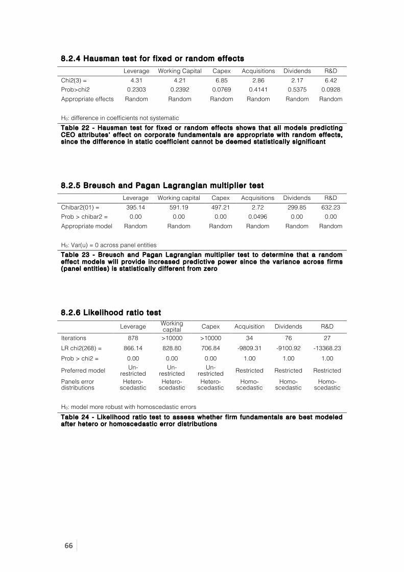
66"

8.2.4 Hausman test for f ixed or random effects

Leverage Working Capital Capex Acquisitions Dividends R&D Chi2(3) = 4.31 4.21 6.85 2.86 2.17 6.42 Prob>chi2 0.2303 0.2392 0.0769 0.4141 0.5375 0.0928 Appropriate effects Random Random Random Random Random Random H0: difference in coefficients not systematic Table 22 - Hausman test for f ixed or random effects shows that al l models predicting CEO attr ibutes’ effect on corporate fundamentals are appropriate with random effects, since the difference in static coeff icient cannot be deemed statist ical ly signif icant

8.2.5 Breusch and Pagan Lagrangian mult ipl ier test

Leverage Working capital Capex Acquisitions Dividends R&D Chibar2(01) = 395.14 591.19 497.21 2.72 299.85 632.23 Prob > chibar2 = 0.00 0.00 0.00 0.0496 0.00 0.00 Appropriate model Random Random Random Random Random Random H0: Var(u) = 0 across panel entities Table 23 - Breusch and Pagan Lagrangian mult ipl ier test to determine that a random effect models wil l provide increased predictive power since the variance across f irms (panel entit ies) is statist ical ly different from zero

8.2.6 Likel ihood rat io test

Leverage Working capital Capex Acquisition Dividends R&D

Iterations 878 >10000 >10000 34 76 27 LR chi2(268) = 866.14 828.80 706.84 -9809.31 -9100.92 -13368.23 Prob > chi2 = 0.00 0.00 0.00 1.00 1.00 1.00

Preferred model Un-restricted

Un-restricted

Un-restricted Restricted Restricted Restricted

Panels error distributions

Hetero-scedastic

Hetero-scedastic

Hetero-scedastic

Homo-scedastic

Homo-scedastic

Homo-scedastic

H0: model more robust with homoscedastic errors Table 24 - Likel ihood ratio test to assess whether f irm fundamentals are best modeled after hetero or homoscedastic error distr ibutions

67"

8.2.7 Wooldridge test for autocorrelat ion in panel data

Leverage Working capital Capex Acquisition Dividends R&D

F(1, 241) 59.55 30.757 7.653 0.868 1.174 1.011 Prob > F 0.00 0.00 0.01 0.35 0.28 0.32 Correlation distributed errors

First order AR(1)

First order AR(1)

First order AR(1) Indep. Indep. Indep.

H0: no first-order autocorrelation Table 25 - Autocorrelat ion tests to determine whether to model f irm fundamentals with independent or f irst order serial correlation in standard errors

8.2.8 Hosmer-Lemeshow tests for goodness of f i t in logist ic models Criteria: MBA

Group Prob Obs_1 Exp_1 Obs_0 Exp_0 Total 1 0.1963 11 11.8 60 59.2 71 2 0.2349 18 15.3 52 54.7 70 3 0.272 17 17.7 53 52.3 70 4 0.299 19 20.3 52 50.7 71 5 0.3292 18 22 52 48 70 6 0.3588 27 24.1 43 45.9 70 7 0.3856 26 26.3 45 44.7 71 8 0.4089 29 27.8 41 42.2 70 9 0.4475 29 30.1 41 39.9 70

10 0.6319 35 33.6 35 36.4 70 Observations 703 Groups 10 Hosmer-Lemeshow chi2(8) 2.67 Prob > chi2 0.9531 H0: probability model is well fitted Table 26 - Hosmer-Lemeshow tests to describe goodness of f i t in logist ic models, measuring the typicali ty of CEO appointments with the criteria MBA

68"

Criteria: Engineering

Group Prob Obs_1 Exp_1 Obs_0 Exp_0 Total 1 0.0312 2 1.9 69 69.1 71 2 0.067 3 2.9 67 67.1 70 3 0.0947 7 5.7 63 64.3 70 4 0.1605 6 8.6 65 62.4 71 5 0.1903 11 12.5 59 57.5 70 6 0.2108 15 14.1 55 55.9 70 7 0.2395 20 15.9 51 55.1 71 8 0.2779 18 18.1 52 51.9 70 9 0.329 16 21.3 54 48.7 70

10 0.6652 33 30.2 37 39.8 70 Observations 703 Groups 10 Hosmer-Lemeshow chi2(8) 5.22 Prob > chi2 0.7338 H0: probability model is well fitted Table 27 - Hosmer-Lemeshow tests to describe goodness of f i t in logist ic models, measuring the typicali ty of CEO appointments with the criteria Engineering

Criteria: Undergraduate degree

Group Prob Obs_1 Exp_1 Obs_0 Exp_0 Total 1 0.6426 43 40.7 28 30.3 71 2 0.7124 44 47.7 26 22.3 70 3 0.7478 54 51.7 16 18.3 70 4 0.7647 47 53.7 24 17.3 71 5 0.7905 55 54.5 15 15.5 70 6 0.8126 55 56.1 15 13.9 70 7 0.8277 67 58.3 4 12.7 71 8 0.8507 61 59.4 10 11.6 71 9 0.8903 58 60.2 11 8.8 69

10 0.9962 63 64.8 7 5.2 70 Observations 703 Groups 10 Hosmer-Lemeshow chi2(8) 13.99 Prob > chi2 0.082 H0: probability model is well fitted Table 28 - Hosmer-Lemeshow tests to describe goodness of f i t in logist ic models, measuring the typicali ty of CEO appointments with the criteria Undergraduate degree

69"

Criteria: Top 50 university

Group Prob Obs_1 Exp_1 Obs_0 Exp_0 Total 1 0.2156 16 12.8 54 57.2 70 2 0.2669 14 17.4 55 51.6 69 3 0.2917 15 19.5 55 50.5 70 4 0.3199 15 21.1 54 47.9 69 5 0.3406 29 22.8 40 46.2 69 6 0.3615 24 24.6 46 45.4 70 7 0.3806 29 25.6 40 43.4 69 8 0.4137 29 27.7 41 42.3 70 9 0.5271 36 31.5 33 37.5 69

10 0.8567 38 41.9 31 27.1 69 Observations 694 Groups 10 Hosmer-Lemeshow chi2(8) 11.22 Prob > chi2 0.1897 H0: probability model is well fitted Table 29 - Hosmer-Lemeshow tests to describe goodness of f i t in logist ic models, measuring the typicali ty of CEO appointments with the criteria Top 50 University

Criteria: Board Experience Group Prob Obs_1 Exp_1 Obs_0 Exp_0 Total

1 0.1526 13 8.4 58 62.6 71 2 0.1934 12 12.3 58 57.7 70 3 0.2212 12 14.5 58 55.5 70 4 0.2537 15 17.1 57 54.9 72 5 0.297 17 18.9 52 50.1 69 6 0.324 18 21.8 52 48.2 70 7 0.3715 27 24.7 44 46.3 71 8 0.4315 26 27.8 44 42.2 70 9 0.5067 39 32.8 31 37.2 70

10 0.6982 40 40.6 30 29.4 70 Observations 703 Groups 10 Hosmer-Lemeshow chi2(8) 7.64 Prob > chi2 0.4695 H0: probability model is well fitted Table 30 - Hosmer-Lemeshow tests to describe goodness of f i t in logist ic models, measuring the typicali ty of CEO appointments with the criteria Board Experience

70"

8.2.9 Breuch / Pagan Cook-Weisberg test for heteroscedasticity Variables Fitted values of CAR given absolute deviation from typical CEO fit chi2(1) = 0.61 Prob > chi2 = 0.4365 H0: Constant variance

Table 31 - Breuch / Pagan Cook-Weisberg test for heteroscedasticity when modeling the effect on CEO background on cumulative abnormal returns in CEO turnovers

8.2.10 Breuch / Pagan Cook-Weisberg test for heteroscedasticity Variables Fitted values of ∆ in ROA from year -1 (-250 to 0 days)

Year 0 Year 1 Year 2 Chi2(1) 0.06 1.25 1.53 Prob > chi2 0.8079 0.263 0.2156

Variables Fitted values of ∆ in EBITDA margin from year -1 (-250 to 0 days) Year 0 Year 1 Year 2 Chi2(1) 0.91 1.34 0.29 Prob > chi2 0.3408 0.2466 0.5908 H0: constant variance Table 32 - Breuch / Pagan Cook-Weisberg test for heteroscedasticity assessing if the market reaction at the t ime of CEO appointments identif ies CEOs with potential to make fundamental changes in companies, across three years post CEO turnover

71"

8.3 Econometric tests

8.3.1 Stat ist ical robustness To further analyze the reliability of our findings, we have tested each individual model for the inclusion of econometric issues. In this section, we will explain the assumptions behind each test and why it is important for the robustness of our results. Each test metric is reported in its respective model, and visual post regression diagnostics are included in appendix 8.2.

8.3.1.1 Level of signif icance Throughout the thesis, we have exclusively evaluated independent variables given a 95% confidence interval. However, since our dataset is capturing all the CEO turnovers for S&P 1500 corporations between 2003 and 2009, we interpret independent variables of up to 10% in p-value, because data collection has reduced the risk of sample selection bias.

8.3.1.2 Heteroscedasticity An important assumption for the use of the functional forms of ordinary least squares, is a constant linear relationship between the dependent variable and independent variables. Heteroscedasticity refers to the circumstance in which the variability of a variable is unequal across the range of values of a second variable that predicts it. To evaluate if a model is appropriate in making statistical inference on the dependent variables’ CAR and corporate re-structuring initiatives, we utilize post regression diagnostics to investigate if the residuals are evenly distributed around the mean, which essentially indicate whether a model is suffering from heteroscedasticity34. Essentially, we utilize the Breusch-Pagan / Cook-Weisberg test to assess if constant variance across independent variables, !"# ! !! = !! , exist. In addition, White’s criterion is added to test the presence of skewness and kurtosis to quantify to what extent a model may be in breach of normality. As the Breusch-Pagan / Cook-Weisberg test alone assumes linear forms of heteroscedasticity, the White component assumes a non-linear relationship between the fitted values ! and the variance !! . When in doubt, the thesis has utilized visual assessments of the residual patterns to select the appropriate test. Thereafter, the functional form of ordinary least squares as the tool for analysis is evaluated for each statistical model. If heteroscedasticity cannot be disproven, other functional forms have been derived.

34 Breusch-Pagan / Cook-Weisberg test for heteroscedasticity is included for each model in appendix 8.2.

72"

For random effect models, we test for heteroscedasticity by comparing two versions of the model: an unrestricted version with heteroscedastic error structure, and a restricted version with homoscedastic error structure (Hoechle, 2007). By fitting both models using generalized least squares method, we utilize the likelihood test statistic to determine if a heteroscedastic error structure (unrestricted model) offers a better fit than homoscedastic (restricted). The steps and test output are presented in appendix 8.2.6.

8.3.1.3 Mult icol l inearity Multicollinearity arises when two or more independent variables show linear correlations. In cases where the correlation between sets of independent variables is high, the statistical inference becomes biased as the standard errors become inflated 35 . Throughout the thesis we have tested for multicollinearity through monitoring the variance inflation factor (VIF), and formulated the statistical models to reflect acceptable VIFs. VIF shows how much an ordinary least squares models’ variance !! increases because of correlation between the independent variables. VIF is derived by

!! = !!!! + !!!!,… ,!!!!" + !!!

Subsequently, the VIF for variable ! is defined as,

VIF! = !1

(1 − R!!)

Where Xi is regressed against all the other independent variables in the model. The VIF is subsequently determined by the magnitude of the goodness of fit !!!. When !!! = 0 the model is perfectly orthogonal with an ideal !"# = 1. A !"# > 5 Indicate strong multicollinearity, and, thus, the statistical models throughout the thesis are constructed to generate mean VIF below this threshold36.

8.3.1.4 Autocorrelat ion To formulate unbiased statistical models, the residuals need to be independent, normally distributed random variables, not only across fitted values !, but also across time. As such, we test for the presence of constant variance (heteroscedasticity), but in time series models it’s particularly important that the variance is uncorrelated between time variables, which in this thesis is years since 35 In this scenario, the likelihood of committing a type 1 error increases. This is rejecting a true null hypothesis due to inflated confidence intervals that inaccurately reduces p-value(s) of independent variables in the model. 36 Mean VIF is reported in every regression model where applicable.

73"

CEO turnover. In consistency with the efficient market hypothesis that abnormal return reacts to different events at different times, we have derived models focusing on particular years since CEO turnover, except in step 4, where we utilized a random effect model across 3 years (0 to 750 days) to assess the relationship between 70 groups of CEO attributes and their potential to change corporate fundamentals. The rationale for constructing this model over several years is the assumption that it takes years until corporate restructurings are reflected on the financial statement. When present in a model, autocorrelation reflects the similarity between observations as a function of time lag between them (Kolesar, 2014) following the equation:

!! =(!! − !)(!!!! − !)!

!!!(!! − !!

!!! )

Where ! is represents autocorrelation given the time lag !, and ! represents the observations at a given point in time. In adherence with Drukker and Wooldridge, we reformulate the random effect functions to test time variant panel data

!!" − !!"!! = !!" − !!"!! !!,… , !!" − !!"!! !! + (!!" − !!"!!) or,

∆!!" = ∆!!"!!,… ,∆!!"!! + ∆!!" This equation derives the effect of the first differences in the CEO attributes in predicting the first differences in corporate initiatives. Now, the autocorrelation test hypothesize that there is insignificant correlation between residuals !!" across time lags for the firms (panel entities) in our sample (Baltagi & Wu, 1999). The random effect models presented in section 5 are all derived to not include autocorrelation37.

8.3.1.5 Fixed and random effects Based on variable inflation factor test for multicollinearity, likelihood ratio tests for heteroscedasticity, and Wooldridge test for autocorrelation in cross-sectional data, the random effect models presented in section 5 includes generalized least squares transformation in the error structures to control for presence of econometric problems where appropriate. The different assumptions are reported in each model, with the tests listed in appendix 8.2.1 to 8.2.6.

37 Wooldridge test for autocorrelation included in appendix 8.2.7

74"

8.3.1.6 Endogeneity When a model is affected by endogeneity, it becomes difficult to conclude on the direction of causality. In every instance where the cumulative abnormal return (CAR) is used as the dependent variable, there is low risk of endogeneity. The reason being that most of the independent variables are either recorded or accumulated at a time prior to deriving CAR, making CAR a complete response to variations in variables surrounding a CEO appointment. Conversely in step 4, level values of corporate re-structuring initiatives can introduce endogeneity. For example, we model under the assumption that education, E-index and share structure all affect the capital structure of a firm, scaled by its total assets. But, in reality, the causality can also run the other way. For instance, an MBA might have a positive effect on leverage, while an engineer has a negative. Here, we cannot rule out that the effect stem from the fact that a highly debt dependent firm needs, and also seeks to hire, CEO candidates with business backgrounds, while the opposite is true for engineers. At the same time, CEOs with more insider equity ownership might be reluctant to issue debt, because it imposes a risk on the value of their stock based compensation. By using a random effect model, we are able to control for the causality between firms (panel entities), which mitigates the issue of endogeneity.

8.3.1.7 Goodness of f i t in logist ic regressions Under the assumptions of ordinary least squares, there will be inefficiencies in the model if heteroscedasticity and/or autocorrelation are present. Since the logistic models formulated in this thesis are strictly focused on the turnover year (0 to 250 days), there is no time variable and autocorrelation will not become an issue. Conversely, the concept of heteroscedasticity changes in logistic models. Recalling section 5.6.1, the dependent variable is a probability rather than a numeric value. Fluctuations around the fitted value may, therefore, be due to uncertainty relating from all the variables not included in the prediction (Williams, 2009). As such, this thesis defines that the probability of a firm’s tendency to hire CEOs with specific backgrounds and experiences is based exclusively on the independent variables that we were able to include. Even though the models are presented with some degree of uncertainty in the residuals, they are tested for joint significance and goodness of fit. As defined in section 8.3.1.3, the logistic models are tested for multicollinearity through assessing the mean variance inflation factor. To estimate the goodness of fit of the logistic models, we order the predicted probabilities in ten equal sized groups, deciles, and evaluate the fitted versus actual values within each group. The reason for this breakdown is that in its non-limited form, the covariate patterns falls close to the number of observations, which makes Pearson !! inappropriate (Hosmer, Lemeshow, & Sturdivant, 2013). The Hosmer-Lemeshow coefficient

75"

hypothesize that the logistic model is well fitted. All the logistic models ensured fulfilling the Hosmer-Lemeshow goodness of fit, and the test output is reported in appendix 8.2.8.

8.3.2 Variable robustness In section 4, we give a thoroughly description of all the variables we have collected in the dataset. In the methodology and result sections not all of these variables are accounted for. The reason is that when we conducted the statistical analyses the omitted variables proved not to be significant in any of the tests, or returned N-values too small for the tests to be valid when these variables were included in the models. We find the same trends and results when including these variables, but chose to omit them as the findings presented in section 5 proved more solid without them. In the same manner, we have also conducted the tests for several different time ranges, concluding that the ranges presented in the section above were the most appropriate. Using the period from -250 to 0 days as the pre-turnover period, and limit the focus on the post-turnover period to 0 to 750 days, we found the models yielding the highest explanation power and significance. The six tests described in section 3 were also tested for the period -500 to 0 days against a variety of ranges between 0 to 250 and 0 to 1000 days after the turnover. Again, we found the time ranges presented in section 5 to be the most appropriate. In appendix 8.1.5 we have included the findings from step 2 for a selection of additional time ranges.

8.4 Elaborations on statist ical methods

8.4.1 Formulation of random versus f ixed models Through the definitions of time variables, we are able to fit a fixed effect model that controls for time in-variant predictors within each firm or CEO characteristic that can bias the estimation of corporate actions (Stock & Watson, 2007). For example, dummy variables related to the appointed CEO’s background, such as whether an individual have an MBA or engineering degree, or if the former CEO left the firm under forced or voluntary terms, will remain constant for the entire estimation period. These characteristics may bias the predictor variables. To elaborate on the previous examples, an MBA might have belonged to a network that gives him a better precondition to affect leverage post-appointment, while an engineer may have perspectives on product development that directly affect the capital allocation to research and development. In addition, if the former CEO was forced out due to lacking performance, the newly appointed CEO may be given a more liberal mandate to restructure the firm. The fixed effect equation is given by

76"

!!" = !!! + !!!!" ,… ,!!!!" + !!!"

In statistical terms, the fixed effect model controls for correlation between the error term (!!") and the unobserved effects (!!). Furthermore, time static variables are considered unique to each individual CEO appointment, and should not have statistical inference with time-variant (such as share ownership, age and board experience) characteristics surrounding the turnover. Following this method, the fixed effect model strips the unobserved intercept (!!) for effects that are constant over time, and allows for correlation with the independent variables. Then, the omission of static variables in tandem with minimizing the variance in the unobserved effects across the time variable, will ensure a model that predicts the dependent variable solely based on factors that a newly appointed CEO is able to change over time. Even though a fixed effect transformation is sensible to isolate CEO specific changes, the difference in static independent variables across firms (panel entities) is important for the ability to affect corporate actions. For instance, if a given firm has a high entrenchment index that remains static over the two-year period, a CEO appointment may have more headroom to make controversial changes to the balance sheet than a CEO appointment that has a low static entrenchment index over the same period. If this assumption holds over the set of static variables that were omitted in the fixed effect model, differences across firms (panel entities) will affect CEOs’ abilities to influence dependent variables. To control for the significance of the time static variables, a random effect model is constructed

!!" = !!! + !!!!" ,… ,!!!!" + !!!" + !!!" Where the error term !!" is added to control for the unobserved effects across firms (panel entities). This relies on the assumption that !!" is not correlated with !! given the independent variables. A premise for choosing random over fixed effect models is that the error term !!" between panel entities is uncorrelated with the independent variables (Hausman, 1978). To test for this, we have utilized the Hausman specification test, which hypothesize that !"# !!" ,!!" = !0. The test results suggest that all of the six models have systematic differences in the coefficients, that !!" is not correlated with the !! given the independent variables specified by the fixed effect models, and indicate that time static variables has an effect on the dependent variables when evaluated across entities.

77"

8.5 Clarifying examples

8.5.1 Predict ive model for market reactions to deviat ing CEO attr ibutes To add further clarity to section 5.5.2, the results are interpreted through the practical example of Jerry Yang, who was appointed as the new CEO of Yahoo! the 18th of June 2007. He holds a masters of science in electrical engineering from Stanford University, and served in 15 boards at the time. Given Yahoo’s characteristics and fundamentals, the model in table 9 calculated a ~24.6% probability that the new appointment should have an MBA, a ~13.0% probability of recruiting an engineer, a ~92.1% tendency to hire an individual with at least an undergraduate degree, a ~52.3% likelihood that this individual should be from a top 50 institution, and a ~45.0% probability that a typical candidate should have above average industry experience. To predict the effect on CAR, the model takes the absolute probability of reciprocal CEO fit. Larger deviations mean increasingly untypical CEO appointment. By aggregating the magnitude the actual values has on each coefficient from table 9, table 10 calculates the predicted CAR.

VARIABLES Degree of

typicality for Yahoo!

Jerry Yang’s attributes

Absolute deviation from typical CEO Effect on CAR

MBA38 24.6% 0 24.6% 4.1% Engineering26 13.0% 1 87.0% 3.7% Undergraduate 92.1% 1 7.9% -1.2% Top 5026 52.3% 1 47.7% 3.9% Board Experience 45.0% 15 55.0% -12.1% Constant 2.8% - - 2.8% Predicted CAR - - - 1.2%

Actual CAR - - - 24.1%

Table 33 – Practical example: the typical f i t of Jerry Yang and the market’s reaction to the CEO turnover at Yahoo in 2007 If the market were only responding to a CEO’s background and board experience and his average fit to the fundamentals of the company, the Yahoo! stock would generate an abnormal return of 1.2% during the first 250 days Jerry Yang was in office. However, the Yahoo! stock actually generated an abnormal return of 24.1%. As such, our model only explains 1.9% of the variations in one-year announcement CAR at CEO turnovers. In the context of stock returns, this is not necessarily a low number. Under the efficient market hypothesis, stock prices follow the predictability 38 Not statistically different from zero, but used in the model for illustrative purposes

78"

of a random walk. This means that if all past data on CEO education, experience and firm fundamentals could predict the price; the abnormal return would be priced in at announcement. But in reality, there are immeasurable factors at play in almost every CEO turnover in our dataset that affect CAR. Consider Bob Iger, who became CEO of Disney in 2005, implemented the acquisition of Pixar Animation Studios in 2006, resulting (at least partly) in a CAR of ~13.2% during the first 250 days. The market simply believed that Disney would be able to create more valuable animation films, and that Bob Iger had the skills needed to continue to find additions to Disney’s intellectual property portfolio. The market was right; in 2008 Disney purchased Marvel Studios, which led to the production of high grossing blockbusters like Spiderman, Ironman, and The Avengers (Forbes, 2009). After understanding how the market reacted to the CEO change in Disney, consider the unexplained effect on the CAR of Yahoo! (Shown in table 11) after the appointment of Jerry Yang. Having founded Yahoo! in the late 1990’s, Yang was seen as a returning visionary at a time Yahoo! was struggling to find value. The contributions to CAR was neither his visionary nor strategic plans – it was rather that the market anticipated he would entertain a hostile takeover bid from Microsoft that valued Yahoo! at a 62% premium. Surprisingly, Yang declined the offer on the grounds that his strategies for Yahoo! would make the future free cash flows more valuable (Forbes, 2008). Thus, Yahoo!’s CAR in 2007 was driven by perceived value from hostile takeover rumors made by Microsoft rather than Jerry Yang’s background and his ability to create strategies to enhance the value of the firm. This is one of several examples in our dataset where it’s hard to quantify factors that affect CAR in CEO turnovers.