Mass balance methods for retail gasoline outlets

1

Mass Balance Calculations for Retail Petroleum Tanks

Brian L. Murphy 2033 Wood Street, Suite 210

Sarasota, FL 34236 [email protected]

Phone: 941.953.6300 Fax: 941.953.6311

Farrukh M. Mohsen 14 Kinglet Drive North Cranbury, NJ 08512

[email protected] Phone: 609.799.7731

Fax: 609.799.1477

Key Words: LUST, tanks, gasoline, mass-balance

Running Head:

2

Abstract

Loss of product at retail gasoline outlets can be determined using mass balance methods. In order

to apply these methods, however, information on vapor capture at the pump, subsequent to

gasoline being metered as sold, and temperature related volume changes must be included. This

paper illustrates these concepts using a model applied to retail gasoline outlets in Florida. Vapor

capture is about 0.6–0.9% of the product sold. The temperature-volume effect is consistent with

a temperature difference between above-ground storage tanks at a depot and buried tanks at the

outlet, with the latter being at the average annual temperature.

Introduction

Detailed records of sales, deliveries, and daily inventory are kept at retail petroleum outlets. A

superficial review of these records can sometimes be sufficient to identify a major leak.

However, to determine if there is a chronic small leak or minor pilferage requires that we know

what the inventory record for a tank without losses should look like, so that we can indentify

discrepencies. This paper describes a model to determine what the cumulative variance in

volume should be for a tank without losses. The cumulative variance is the sum of the daily

variance, which in turn are the difference each day between the record of inventory, deliveries

and sales. There are at least three reasons why a cumulative variance different than zero can

occur, even in an intact tank:

Product already metered as “sold” is recaptured by the vapor recovery system and

returned to the tank,

There is a volume change because product is delivered from an above ground depot and

then stored in below ground tanks at a different temperature,

3

Gasoline may be blended from several tanks at a ratio that is slightly different than what

is intended showing up as a “loss” in one tank and a “gain” in another..

We apply this model to records from 13 Florida retail gasoline outlets with a total of 37

petroleum storage tanks having records12 months long or longer. The outlets were located from

Jacksonville to slightly south of Orlando in the central or eastern part of the State. Table 1

summarizes this information, as well as the average monthly sales over either a 12- or 24-month

period. Sales vary considerably between stations, by a factor of 25 for regular grade. In all cases,

sales of regular are considerable larger than midgrade or premium grades. Where a grade of

gasoline or a diesel tank is not shown, that product was not sold at that outlet. Tanks that were

eliminated during a 12-month period are indicated by an “*”. No tanks were added during the

time period analyzed.

Basic Equations

Data for each tank in Table 1 included inventory at the beginning of the day (Ii) as well as

deliveries (Di), and sales (Si) during the day. Obvious errors in the inventory record were

corrected by M.D. Shaw and Associates of Huntersville, NC, prior to our receiving the data. For

each tank the variance (Vi ) on day i between the inventory record obtained at the beginning of

the day and the volume based on sales and deliveries was computed, as well as the cumulative

variance (CV) according to the following equations:

(1)

∑ ∑ (2)

4

Because of the way that CV is defined, the value on the first day, while generally small, can be

different than zero, namely:

1 (3)

The cumulative variance can also be written as:

∑ ∑ (4)

In the first term f is the fraction of the gasoline metered as “sold” that is subsequently returned to

the tank by the vapor recovery system. (If a meter is inaccurate this will also result in a non-zero

f, either positive or negative.) In the second term ε is the coefficient of thermal expansion (1/ºF)

so that volume shrinkage occurs if the delivered fuel is at a higher temperature than when the

fuel is sold. Ti (ºF) is the temperature of the fuel when the volume is recorded on delivery and T0

is the temperature of the fuel when the volume is recorded at sale.

We assume that fuel at the depot origin is stored above ground and is at a daily average ambient

temperature, Ti and that fuel at the retail outlet is stored below ground and is at the annual

average temperature, which we identify with T0. These assumptions will be validated a

posteriori. Over an annual cycle:

∆ (5)

so that I = n′ and I ≈ n′+182 are the days when the annual average temperature occurs. The

maximum and minimum temperatures (T0 ±∆T) occur at I ≈ n′+91 and I ≈ n′+274 respectively.

5

Substituting Equations (2) and (5) in Equation (4):

1∑

∆ ∑ sin (6)

To perform the second summation we replace Di by the average value over the time period Davg.

The rationale for doing this is that the time between deliveries is generally short compared to the

time scale over which seasonal temperatures change. We expand the sine using the formula for

the difference between angles, and make use of the identities.

∑ sin , and (7a)

∑ cos 1 (7b)

,

where a= . (Weisstein, 2011a & 2011b) Note that in the formulas given in these references the

summation begins at i=0 rather than i=1.

The result is:

1∆ ′

(8)

6

Where DT is the cumulative deliveries between and including days 1 and n.

Parameter Values

In this data set it sometimes happens that there is a period of some days without sales. If this

occurs without a negative value for deliveries no change is made to the above equations.

However, sometimes a period without sales is accompanied by a negative value for deliveries

followed by a period where Ii = 0 and with an unchanging value of CV until deliveries and sales

begin again. These appear to be periods when a tank was removed and replaced.

For the first term in Equation (9), which is proportional to f, it is appropriate to include negative

deliveries in computing total deliveries since this is product that will not be sold, and hence for

which there will be no vapor recovery. Thus DT(n) is defined to include negative deliveries. For

the last term in Equation (8) involving trigonometric functions it is appropriate to ignore negative

values in computing Davg, because the expansion or contraction of product when placed in the

retail tank has already been accounted for. Let the negative delivery amount be D- then Davg(n) is

defined as:

/ , (9)

D- occurs in Equation (9) only after a negative delivery has occurred. Furthermore, because we

treat each year separately, if D- first occurs in year one it does not reoccur in the analysis for year

two.

7

Define:

(n) (10)

and:

∆ (11)

So that Equation (8) becomes:

365

1

2′2

365

1 2

2 1 2 ′ (12)This last result follows from an

algorithm known as prosthaphaeresis (Weisstein 2011c).

Sin sin cos cos (13)

If Davg(n) were constant, the last term on the right would have maximum and minimum values at

n = n′ −0.5, and n = n′ + 182. From n′ −0.5 to n′ + 182 the temperature is below the annual

average and from n′ + 182 to n′ + 364.5 the temperature is above the annual average. As long as

the temperature is below the annual average, the cumulative variance will grow because of the

effect of this term.

Table 2 shows values of fQ-CV for different values of n:

8

From the results in Table 2 we find:

(14)

∆ (15)

n’ tan

(16)

If one solution to this last equation is n′, a second is n′′ ± 365/2. The solution chosen is one that

corresponds closest to the end of October, which as discussed below is one of the two times each

year when the average daily temperature equals the average annual temperature at Orlando.

Equations (14–16) are used to estimate f, n′ and for the various grades of gasoline as well as

diesel. In determining CV, DT, Davg and Q we use the integer values of n shown in Table 2;

otherwise we use the exact value.

The equation used for computing CV(n), written in detail is:

9

1 ∆

cos 1 2 cos 2 1 2

(17)

When the record contains a second year with the cumulative variance carried over from the first

year, we treat the second year independently from the first to compensate for year-to-year trends

in sales and deliveries. To do this, I1 is replaced by I366, the left side of Equation (9) becomes

CV(n) − CV(365), DT(n) is replaced by DT(n)−DT(365), and Davg is computed during the second

year.

Equation (17) can be approximated as:

≅∆

cos

′ (18)

In Equation (18) we have taken f<<1 and have neglected one time removals compared to

cumulative deliveries so thatDT(n) ≈ nDavg (n). The approximation made in the cosine argument

in Equation (18) holds when n >> 1. For a large enough n we also have DT≈ nDavg (n) >> I1 −

In+1.

Examples

Figure 1 compares Equations 17 and 18 with data for the regular tank at Outlet M. Although in

this graph the two equations appear indistinguishable, in fact the fit is slightly better for Equation

10

17. We compute the fit as the average absolute difference between the Equation and the data

over this 2-year period. For Equation 17, the result is 164 gallons, while for Equation (18) it is

191 gallons. Figure 2 is a plot of these absolute differences using the two equations. In general,

there does not appear to be any systematic difference over time. The difference appears to be in

the magnitude of the daily fluctuations. Equation 17 performs slightly better because it

incorporates the daily inventory.

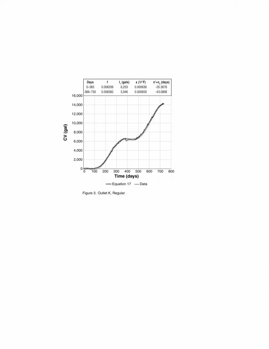
For most purposes Equation (18) should be satisfactory. However, Equation (17) permits one to

distinguish small changes in inventory from apparent losses. An example of this is given in

Figure 3 for the regular tank at Outlet K. On day 387 at Station K there is a drop in CV of 302

gallons causing a discrepancy between Equation 17 and the daily record of CV. This is well

before the regular tank was replaced on day 434. On day 387 there was a delivery of 2,477

gallons of regular grade to a tank with a beginning inventory value of 2,984 gallons, giving a

total before sales of 5,460 gallons. The highest inventory amount for this tank prior to its

replacement beginning on day 434 was 5,230 gallons. It seems likely that the tank was overfilled

by several hundred gallons.

In general the fit between data and model is better for regular tanks than for diesel, presumably

because the higher regular sales volume smoothes out statistical fluctuations. This is the case for

diesel at Outlet K, as shown in Figure 4. Interestingly, the same phenomenon occurs for this

diesel tank as for the regular grade tank. There is a drop in CV of 302 gallons on day 387, which

in this case persists relative to Equation (17). On this day 2,477 gallons were delivered to a tank

with a beginning inventory of 2,984 gallons for a total before sales of 5,461 gallons. The

maximum inventory value prior to the tank being replaced, also on day 434, was 5,230 gallons.

11

The premium and midgrade tanks at this location do not show a large drop in CV on the day of a

delivery, although they also were replaced on day 434. Thus there is some evidence that

replacement of four tanks at this location was in fact triggered by tank overfilling rather than by

tank leakage.

Midgrade and premium tanks also have more scatter in the comparison with Equation 17 than

regular tanks. There is an additional complicating factor for these tanks because their contents

may be blended with regular grade gasoline to produce intermediate octane grades. Negative

values of f, indicating an apparent loss, may occur when in fact the cause is a faulty blend valve.

Negative values of f do not occur for diesel or regular grade tanks where blending is either not an

issue, or is less of an issue because of much higher sales of regular grade than midgrade or

premium. In this case the sum over all gasoline grades can be instructive. In computing the sum

we do not use any 12-month period when a tank was permanently removed from service. This is

illustrated for Outlet M in year 2 when only premium and regular tanks were present. The data

and model results have already been presented for the regular tank in Figure 1. The result for the

premium tank with an apparent loss (negative f) is shown in Figure 5, while Figure 6 shows the

result for regular and premium tanks combined. In spite of an apparent loss of more than 2,000

gallons from the premium tank over the course of a year, the combined tanks are well fit by the

model with values of f, n′, and ε that are consistent with values for other outlets, as described in

the next section.

Premium tanks at Outlets E and F also had negative values of f during the first year. The

midgrade tank for Outlet F also had a negative f value during the one year record. Figures 7–10

show the results for regular, midgrade, and premium gasoline at Outlet E as well as the sum. The

12

poor comparison for the regular tank in this case is a result of our method of curve fitting, i.e., by

using data at 91 and 182 days, we overlook the minimum in the data that occurs between these

two times.

An alternative method of curve fitting involves fitting the extremum. This is done as follows. To

find n′, plot X = f Q(n)−CV(n) versus n, and determine the extreme value that occurs at n = n*.

The derivative of X with respect to n is proportional to 2 1 2 ′ ; when the

argument of the sine is 0 or π, the derivative is zero. Therefore, the extremum occurs at ∗

∗ . Choose the former solution if the extremum of X is a minimum and

the latter if it is a maximum.

At this extreme value the argument of the second cosine in Equation (17) is 0 (X minimum) or π

(X maximum). Therefore:

∗

∆ ∗ for a minimum of X (19a)

∗

∆ ∗ for a maximum of X (19b)

Using this alternative method we find f = −3.4 10−5 (the same as before), n′ = −36 days,

ε=0.001450F−1 for the sum over all tanks. Figure 11 shows the resulting plot for the sum over

gasoline grades at Outlet E based on the alternative method. The fact that f for the sum over all

grades is about 300 times smaller than the average at other stations, as described in the next

section, raises the question of whether there was any vapor recovery at this outlet. Figure 12

13

shows the result for the sum over all tanks for f = 0, ε = 0.0012, and n′ = 15, a fit determined by

trial and error. Because it is possible to obtain a fit with the model for results that are within the

norm, assuming no vapor recovery, this analysis does not support a finding of a true loss.

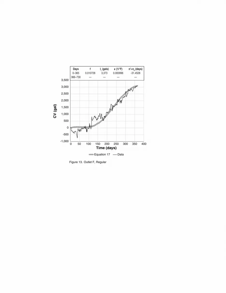
Figures 13–16 show results for the three gasoline tanks at Station F, as well as for the sum. In

this case the drop in CV for premium and midgrade dominates the steady rise in CV for regular

grade with the result that CV for the sum has a drop of more than 2,500 gallons between days

220 and 260. As a result f is negative (−0.00249) for the sum, even though f is positive for the

regular grade tank and consistent with other stations with vapor recovery, as described below. It

seems likely that this is a true loss. Tanks at this location were removed on day 602.

Statistical Results

Premium and midgrade tanks at outlets E, F, and M were removed from the analysis for premium

and midgrade in this section based on the analysis presented above that record keeping for

blending different grades was faulty at these locations. The sum over all tanks at Outlet F was

also removed from the analysis based on the evidence of true loss from premium and midgrade

tanks. In addition the sum over all tanks was not used for any year when a tank was withdrawn

from service, if the tank was not replaced. Outlet E was not used in estimating f for any of the

gasoline tanks based on evidence that this outlet did not have a vapor recovery system during the

period analyzed.

14

Table 3 shows results for the average values and standard deviations of f, ε, and n′ + n0, where n0

is the actual day of the year on which the record starts. Tanks with negative f values have been

excluded. In addition we have excluded the sum of the contents of all gasoline tanks for any 12-

month period when a tank was withdrawn from service. According to data from 1971 to 2000 the

lowest and highest average daily temperatures at Orlando International Airport occur on January

17 and 18 (60˚F) and July 20–August 16 (83˚F). Accordingly, we take ∆T = 11.5˚F (NCDC

2011.). The average annual temperature in this record 72.8˚F occurs on April 22–23 and October

28–29, which are the 112−113th and 301–302nd days of the year. The latter days correspond to

day −64 to −65 of the the previous year..

Discussion

The parameter f does show a systematic increase with the gasoline grade. However, differences

between average values are less than the sum of standard deviations. Thus the larger value of f

for diesel than for any gasoline grades may be an artifact. In general because of recording errors

in blending results for, regular grade, diesel, and the sum of gasoline tank contents should be

more reliable than midgrade or premium grade results.

The day n′ + n0 when ambient and annual average temperatures coincide is predicted to

be from early October to mid-November consistent with central/ northern Florida climate.

As noted above in Orlando, the day with temperature equal to the annual average

temperature is October 28 or 29.consistent with the derived value of n’+ n0.

15

The fraction of gasoline and diesel “sold” and then recaptured by vapor recovery is

slightly less than 1%, probably in the range of 0.6–0.9%.

The coefficient of thermal expansion in the range of temperatures analyzed is consistent

with literature values when uncertainties are taken into account. The coefficient of

expansion for gasoline is given as 0.00069/0F and for diesel is given as 0.0005 at:

http://ts.nist.gov/WeightsAndMeasures/upload/B-015.pdf. This is as compared to our values of

0.00070 and 0.00057 for regular gasoline and diesel.

This last observation indicates that the assumptions regarding the temperature of product as

delivered and as sold are basically correct.

Lastly note that Equation (18) can be differentiated with respect to n to find the local extrema of

CV. The first such value is:

∆, , (19)

where we have used the fact that 2 ≅ . The second derivative is proportional to

, which is positive at the values of n given by equation (18) if f < εΔT. Thus

local minima exist if f < εΔT, because the rate of reduction in fuel volume during the warmer

months of the year will be greater than the apparent rate of increase in volume resulting from

vapor capture.

REFERENCES

16

NCDC. 2011. Climatography of the United States No. 84, 1971–2000. Daily normals of

temperature, precipitation, and heating and cooling degree days. Accessed April 8, 2011.

Available at: http://www.ncdc.noaa.gov/DLYNRMS/dnrm?coopid=086628.

Weisstein, Eric W. (2011a) "Sine." From MathWorld--A Wolfram Web Resource.

http://mathworld.wolfram.com/Sine.html

Weisstein, Eric W. (2011b) "Cosine." From MathWorld--A Wolfram Web Resource.

http://mathworld.wolfram.com/Cosine.html

Weisstein, Eric W. (2011c) "Prosthaphaeresis Formulas." From MathWorld--A Wolfram Web

Resource. http://mathworld.wolfram.com/ProsthaphaeresisFormulas.html

17

Table 1: Average Monthly Sales

Outlet Regular Midgrade Premium Diesel

A 36,178 * 3,281 10,667

44,169 4,4169 *

B 44,621 6,696 7,756

51,161 6,053 6,807

C 71,053 1,1528 3752

76163 1,2100 *

D 19,245 1,9245

19527 1,9527

E 18,452 3,492 2,172 *

17,834 * 2,029

F 25,583 3,201 1,332

G 56,177 6,588

53,581 5,943

H 4,578 830

I 39,215 3,822 2,361

41,382 2,868 2,377

J 12,150 1,564 705

K 87,387 14,602 14,836 14,837

97,348 * 14,203 14,202

L 96,319 * 7,722 21,628

114,569 8,778 17,047

M 70,633 * 18,709 18,709

90,243 21,938 21,938

18

Table 2. Values of the Quantity fQ-CV for Specific Days, n, of the Annual Record

Integer n fQ(n)-CV(n)

365 365 0

n1 =365/4=91.25 91

22 1

3652 1

365

n2 =365/2=182.5 182 2 1365

n3 =365x (3/4)=273.75 274

22 1

3652 1

365

Table 3: Average and Standard Deviations of Computed Parameters

Number of

Outlet-Years

f %a

ε (1/F0) 10−4 Average n′ + n0

(day of the year)

Regular 23 0.63 ± 0.25 6.97 ± 2.51 −54 ± 14

November 8

Midgrade 6 0.69 ± 0.34 14.09 ± 6.18 −78 ± 33

October 15

Premium 17 0.89 ± 0.84 13.77 ± 10.06 −85 ± 30

October 8

19

Sum Over Tanks 17 0.87 ± 0.30 6.87 ± 3.23 −60 ± 14

November 2

Diesel 8 0.95 ± 0.22 5.68 ± 1.90 −49 ± 23

November 13

a Because the one year record at Outlet F was not used, f for gasoline grades is based on one fewer outlet years than other paramete

0 100 200 300 400 500 600 700 800

CV

(g

al)

Time (days)

Figure 1. Outlet M, Regular

Equation 17 Equation 18 Data

Days f I1 (gals) ε (1/°F) n1+n0 (days) 0–365 0.007073 2,247 0.00082 -18.1643 366–730 0.010253 10,237 0.000741 -62.14482

-2,000

0

4,000

2,000

8,000

6,000

10,000

12,000

14,000

16,000

18,000

20,000

0

200

400

600

800

1,000

1,200

0 100 200 300 400 500 600 700 800

CV

(g

al)

Time (days)

Figure 2. Absolute value of the differences between Data and Equations 17 and 18, Outlet M, Regular

Absolute value (Data—Equation 17)

Absolute value(Data— Equation 18)

0 100 200 300 400 500 600 700 800

CV

(g

al)

Time (days)

Figure 3. Outlet K, Regular

Equation 17 Data


0

2,000

4,000

6,000

8,000

10,000

12,000

14,000

16,000

0

500

1,000

1,500

2,000

2,500

3,000

0 100 200 300 400 500 600 700 800

CV

(g

al)

Time (days)

Figure 4. Outlet K, Diesel

Equation 17 Data


0 100 200 300 400 500 600 700 800

CV

(g

al)

Time (days)

Figure 5. Outlet M, Premium Tank

Equation 17 Data


-3,500

-3,000

-2,500

-2,000

-1,500

-1,000

-500

0

500

0 100 200 300 400 500 600 700 800

CV

(g

al)

Time (days)

Figure 6. Outlet M, Combined Regular and Premium Tanks (Year2)

Equation 17 Data

Days f I1 (gals) ε (1/°F) n1+n0 (days) 0–365 — — — — 366–730 0.007061 15,519 0.000692 -54.16894

0

2,000

4,000

6,000

8,000

10,000

12,000

14,000

16,000

0 100 200 300 400 500 600 700 800

CV

(g

al)

Time (days)

Figure 7. Outlet E, Regular

Equation 17 Data


-1,000

-500

0

500

1,000

1,500

2,000

2,500

3,000

0 50 100 150 200 250 300 350 400

CV

(g

al)

Time (days)

Figure 8. Outlet E, Midgrade

Equation 17 Data

Days f I1 (gals) ε (1/°F) n1+n0 (days) 0–365 0.011364 1,685 0.001469 64.084578 366–730 — — — —

0

100

200

300

400

500

600

0 100 200 300 400 500 600 700 800

CV

(g

al)

Time (days)

Figure 9. Outlet E, Premium Grade

Equation 17 Data

Days f I1 (gals) ε (1/°F) n1+n0 (days) 0–365 -0.04104 1,685 0.000852 54.67517 366–730 0.012093 3,227 0.003232 66.9177

-1,400

-1,200

-1,000

-800

-600

-400

-200

0

200

400

-2,000

-1,500

-1,000

-500

0

500

1,000

0 50 100 150 200 250 300 350 400

CV

(g

al)

Time (days)

Figure 10. Outlet E, Combined Tanks

Equation 17 Data

Days f I1 (gals) ε (1/°F) n1+n0 (days) 0–365 0.00034 7,621 0.000594 -42.2998 366–730 — — — —

-2,000

-1,500

-1,000

-500

0

500

1,000

0 50 100 150 200 250 300 350 400

CV

(g

al)

Time (days)

Figure 11. Outlet E, Combined Tanks (using alternative curve-fitting method)

Equation 17 Data

Days f I1 (gals) ε (1/°F) n1+n0 (days) 0–365 0.000034 7,621 0.00145 -36 366–730 — — — —

-2,000

-1,500

-1,000

-500

0

500

1,000

0 50 100 150 200 250 300 350 400

CV

(g

al)

Time (days)

Figure 12. Outlet E, Combined Tanks (based on trial and error curve fitting method)

Equation 17 Data

Days f I1 (gals) ε (1/°F) n1+n0 (days) 0–365 0 7,621 0.0012 -15 366–730 — — — —

0 50 100 150 200 250 300 350 400

CV

(g

al)

Time (days)

Figure 13. Outlet F, Regular

Equation 17 Data


-1,000

-500

0

500

1,000

1,500

2,000

2,500

3,000

3,500

0 50 100 150 200 250 300 350 400

CV

(g

al)

Time (days)

Figure 14. Outlet F, Midgrade

Equation 17 Data

Days f I1 (gals) ε (1/°F) n1+n0 (days) 0–365 -0.07549 2,157 0.010442 163.8509 366–730 — — — —

-3,000

-2,500

-2,000

-1,500

-1,000

-500

0

500

1,000

-1,500

-1,000

-500

0

500

1,000

0 50 100 150 200 250 300 350 400

CV

(g

al)

Time (days)

Figure 15. Outlet F, Premium

Equation 17 Data

Days f I1 (gals) ε (1/°F) n1+n0 (days) 0–365 -0.0778 1,192 0.009879 -217.1746 366–730 — — — —

-1,500

-1,000

-500

0

500

1,000

1,500

0 50 100 150 200 250 300 350 400

CV

(g

al)

Time (days)

Figure 16. Outlet F, Combined Tanks

Equation 17 Data


Documents

Mass balance methods for retail gasoline outlets