Master--slave synchronization of affine cellular automaton pairs

DISCRETE AND CONTINUOUS Website: http://aimSciences.orgDYNAMICAL SYSTEMSVolume 13, Number 2, July 2005 pp. 491–502

MASTER–SLAVE SYNCHRONIZATION OF AFFINE CELLULARAUTOMATON PAIRS

Gelasio Salazar, Edgardo Ugalde and Jesus Urıas

Instituto de Fısica, UASLPAlvaro Obregon 64, San Luis Potosı, SLP, 78000 Mexico

Abstract. Necessary and sufficient conditions are given for master–slave syn-chronization of any pair of unidirectionally coupled one–dimensional affine cel-lular automata of rank one. In each case the synchronization condition is ex-pressed in terms of the coupling and the arithmetic properties of the automatonlocal rule. The asymptotic behavior of finite length affine automata of rankone, subjected to Dirichlet boundary conditions, is shown to be equivalent tothe synchronization problem.

1. Introduction. The synchronization phenomenon observed in coupled subsys-tems has been studied extensively for iterated maps and ordinary differential equa-tions. Some rigorous results have been established for those systems already. Thesynchronization phenomenon has also been observed in several types of interactingextended models.

1. Systems of globally coupled oscillators show a global behavior where all in-dividual oscillators get entrained in periodic orbits [5] when the couplingstrength is big enough.

2. Synchronization of spatiotemporally chaotic extended systems has been stud-ied in the context of coupled one–dimensional complex Ginzburg–Landauequations. The coupled pair shows a regime of spatiotemporal intermittencythat was described in [1] in terms of the space–time synchronized chaoticmotion of localized structures.

However, much less is known about the theoretical basis for the synchronizationphenomenon in interacting extended systems. Here we address the problem ofmaster–slave synchronization in coupled one–dimensional cellular automata. Twoforms of coupling have been considered in the literature. One is to take a stochasticcoupling [11, 2] between automata. The strength of coupling is handled by meansof a probability, and numerical evidence in several examples supports the existenceof a critical value of the probability above which the pair synchronizes identically.The other form is a deterministic coupling as was done in [10]. Therein, necessaryand sufficient conditions for synchronization of coupled affine elementary cellularautomata were given. The proof in [10] is based on the existence of a connectionbetween synchronization and nilpotency of matrices. The natural generalization ofthat approach led us to the study of the nilpotency of a broader class of matri-ces. The answer to the nilpotency problem allows us to give a definitive answer

2000 Mathematics Subject Classification. 15A33, 37B15, 15A90.Key words and phrases. Cellular automata, Synchronization, Dirichlet boundary conditions,

Nilpotency.

491

492 SALAZAR, UGALDE AND URIAS

to the master–slave synchronization problem in coupled pairs of one–dimensionalaffine cellular automata of rank one. It also tells us about the asymptotics of timeevolution of affine cellular automata subjected to Dirichlet boundary conditions.

In Section 2 the interacting scheme between cellular automata is described andthe connection between master–slave synchronization and nilpotency of matrices isestablished as Lemma 2.1. The main theorem about the nilpotency of matrices overZk is stated in Section 3. Its direct consequence on master–slave synchronization isTheorem 4.1 in Section 4. The implications on the asymptotics of cellular automataunder Dirichlet boundary conditions are discussed in Section 5.

All proofs are collected in the Appendices.

2. Master–slave synchronization. Consider the finite cyclic ring Zk of resid-ual classes modulo k. As usual, we identify the elements of Zk with the integers0, 1, . . . , k − 1, and denote a + b and ab the operations a + b (mod k) and ab (modk) respectively. We supply the product space ZZk with the natural coordinate–wiseoperations.

A local map f : Z3k → Zk such that f(x−1x0x1) = ax−1 + bx0 + cx1 + d specifies

the affine cellular automaton F : ZZk → ZZk with n–th coordinate given by

F (x)n = f(xn−1xnxn+1) = axn−1 + bxn + cxn+1 + d, n ∈ Z . (1)

The transformation F is represented in matrix form as

F (x) =

. . . . . . . . .a b c

a b ca b c

. . . . . . . . .

...xn−1

xn

xn+1

...

+

...ddd...

. (2)

In the previous equation let the infinite tridiagonal matrix be denoted by Mabc, andlet d := (. . . , d, d, d, . . .), d ∈ Zk denote the infinite constant vector.

The forward orbit of the configuration x ∈ ZZk under the action of the transfor-mation F is the sequence x, x1, . . . , xt, . . . , with

xt = M tabcx +

t−1∑

j=0

M jabcd , t ≥ 1 . (3)

Two cellular automata, x 7→ Mabcx + d and x 7→ Mabcx + d′ in ZZk (having thesame linear part but may have different constant terms, d and d′ ∈ Zk) are coupledunidirectionally as follows. For C ∈ {0, 1}Z, a constant coupling sequence, considerthe projection ΠC : ZZk → ZZk defined as

(ΠCx)i ={

xi if Ci = 10 otherwise . (4)

The extended automaton(xy

)7→

(Mabcx + d

Mabcy + d′ + ΠC

(Mabc(x− y) + d− d′

))

, (5)

defines an unidirectionally coupled pair, with coupling sequence C. Notice thatfor a coupling sequence C = 0 := (. . ., 0, 0, 0, . . .) the two subsystems in (5)evolve independently, while for the coupling C = 1 := (. . . , 1, 1, 1, . . .) the secondsubsystem is just a copy of the first one.

SYNCHRONIZATION OF CELLULAR AUTOMATA 493

The coupled pair (5) synchronizes if the difference between the xt and yt con-figurations, ∆t := xt − yt, goes in time to a constant configuration δ ∈ ZZk , i. e.,if ∆t → δ as t → ∞, regardless of the initial configurations x0 and y0. In thissituation we say that the extended automaton (5) is a master–slave pair. The sub-system in (5) that is evolving autonomously is called the master subsystem. Thesecond subsystem is called the slave one since it evolves asymptotically, up to aspatially–homogeneous configuration δ, in the same way as the master subsystemdoes. The synchronization regime known as identical synchronization correspondsto ∆t → δ = 0, the null configuration with all its coordinates equal to zero.

For affine automata the difference ∆t evolves according to the rule

∆t+1 =(Π1−CMabc

)∆t + Π1−C(d− d′). (6)

Thus, the coupled pair (5) synchronizes if for any pair x0,y0 ∈ ZZk of initial config-urations the difference

∆t =(MC

abc

)t−1Mabc∆0 +

t−1∑

j=0

(MC

abc

)j(d− d′) → δ, (7)

as t tends to infinity, where MCabc := Π1−CMabcΠ1−C .

The limit ∆t → δ in (7) is supposed to take place with respect to some “natural”metric in ZZk . In order to avoid complications regarding the definition of the metric,from now on we will suppose that the length of a block of consecutive zeros in thecoupling sequence C is bounded. For such a coupling sequence C the operator MC

abc

has the block–diagonal form

MCabc =

. . .Mabc,ì−1

0Mabc,ì

0Mabc,ì+1

. . .

. (8)

Each block Ma,b,c;ì is a ì × ì submatrix of the form

Ma,b,c;ì =

b c 0 · · · 0

a b c...

. . . . . . . . .... a b c0 · · · 0 a b

. (9)

The 1 × 1 zero sub–blocks correspond to the coordinates where C is equal to one,while the positive integer numbers ì, i ∈ Z, are the lengths of the blocks of consec-utive zeros in the coupling sequence C. The evolution of the differences in (7) splitsinto independent finite blocks. For the i–th block we have that for all ∆0 ∈ ZZk ,

M tabc,ì

(MCabc∆

0)Ii +t∑

j=0

M jabc,ì

(d− d′)Ii → δIi, (10)

as t →∞. Here Ii ⊂ Z is the interval of length ì containing all the coordinates ofthe sub–matrix Mabc,ì , and xIi ∈ ZIi

k denotes the restriction of the configuration


x to that interval. Since ZIi

k is a finite set, the convergence in (10) is in fact theeventual equality

M tabc,ì

(MCabc∆

0)Ii +t∑

j=0

M jabc,ì

(d− d′)Ii = δIi, (11)

for all ∆0 ∈ ZZk (for all sufficiently large t) and each i. Thus, we need no metric inZZk .

Assume there exists T such that for every t ≥ T condition (11) is satisfied. Then,putting ∆0 = 0 in (11) shows that

∑tj=0 M j

abc,ì(d − d′)Ii

= δIifor all sufficiently

large t and thus,M t

abc,ì(MC

abc∆0)Ii

= 0,

for all ∆0 and all t ≥ T . Given the block–diagonal form (8) of the operator MCabc,

for each block we haveM t

abc,ìMabc,ì∆

0Ii

= 0 (12)

for all sufficiently large t. Since the initial difference ∆0Ii

is arbitrary, the sub–blockmatrix Mabc,ì has to be nilpotent for condition (12) to hold. The converse followsimmediately: if each one of the sub–matrices Mabc,ì in (8) is nilpotent, then theextended automaton (5) synchronizes in the sense of (7).

The results of the present section are summarized in the following.

Lemma 2.1. The extended automaton (5) is a master–slave pair if and only if theoperator MC

abc := Π1−CMabcΠ1−C , having form (8), is nilpotent. When this is thecase there exists a least positive T < ∞ such that for every t ≥ T : yt = xt − δ withδ = (d− d′)

∑T−1j=0 (a + b + c)j.

3. Result on the nilpotency of matrices. Lemma 2.1 makes the synchroniza-tion problem equivalent to the problem of determining sufficient and necessary con-ditions for the nilpotency of finite–dimensional tridiagonal matrices Ma,b,c;` of theform (9) over the finite ring Zk. The nilpotency problem is solved by the theoremin this section. We are not aware that such a result exists in the literature. Thus,in Appendix 6 we present a detailed proof of Theorem 3.1.

Throughout all that follows, Ma,b,c;` denotes a `× ` matrix of the form (9) withentries a, b and c in Zk.

Theorem 3.1. Let k = ps11 ps2

2 · · · psii · · · psm

m with si > 0 and pi prime numbers inthe order p1 < p2 < · · · pi · · · < pm. Then Ma,b,c;` is nilpotent over Zk if and only if

I) For each pi > 2, ac = b = 0 (mod pi).and

II) For p1 = 2 one of the following conditions holds1. ac = b = 0 (mod 2), or2. abc = 1 (mod 2) and ` = 2, or3. ac = 1 (mod 2), b = 0 (mod 2) and ` ∈ {2n − 1 : n ≥ 1}.

4. Result on synchronization. Theorem 3.1 is translated directly to the follow-ing result on master–slave synchronization of coupled pairs of the type (5).

Theorem 4.1. Let Zk be the ring of definition of the extended automaton (5).Let ps1

1 ps22 · · · psi

i · · · psmm , si > 0, be the factorization of k into primes p1 < p2 <

· · · pi · · · < pm. Then (5) is a master–slave pair if and only if


I) For each pi > 2, ac = b = 0 (mod pi).and

II) For p1 = 2 one of the following conditions holds1. ac = b = 0 (mod 2), or2. abc = 1 (mod 2) and each ` in the coupling sequence C is ` = 2, or3. ac = 1 (mod 2), b = 0 (mod 2) and all the blocks of consecutive zeros in

the coupling sequence C have lengths in the set {2n − 1 : n ≥ 1}.

5. Concluding Remarks.

5.1. Affine cellular automata of higher rank. In this case the synchronizationproblem cannot be reduced in general to a problem of nilpotency of (2r+1)–diagonalmatrices over the ring Zk. Only for very particular coupling sequences is it possibleto decompose the dynamics of the difference between the automaton configurationsinto finite dimensional blocks.

5.2. Strength of coupling and synchronization. It is reasonable to expectthat coupled subsystems synchronize in a master–slave regime when the couplingsequence C is close to the homogeneous configuration 1.

Let {ì : i ∈ Z} be the sequence of lengths of the blocks of zeros in C. If C issuch that

ε(C) := 1− limN→∞

2N + 1∑Ni=−N (ì + 1)

exists, then closeness of C to 1 is measured by ε(C) and we may call it the strengthof coupling configuration C. By analogy to the continuous mapping case, we wouldexpect a transition from non–synchronization to full synchronization as ε(C) ap-proaches 1. However, Theorem 4.1 implies this criterion is not relevant for cou-pled CA.

As an example, consider the automata x 7→ Mabcx + d and x 7→ Mabcx + d′

in ZZ2ps such that (a, b, c)2 = (1, 0, 1), and (a, b, c)p = (a, 0, c), with ac zero or adivisor of zero modulo ps. Let us remind that (a, b, c)q denotes the triple (a(mod q),b(mod q), c(mod q)). If the automata are coupled by means of a coupling sequenceC, each of its zero blocks having length ì = 2ni − 1 for some ni, then the coupledpair synchronizes. Notice that the coupling strengths ε(C) may have any valuein [0, 1] by using coupling configurations C of this kind. For this note that if{ì = 2ni − 1 : i ∈ Z} are the lengths of the zero blocks in C, then ε(C) =limN→∞(2N + 1)/(

∑Ni=−N 2ni).

So, in the example there is no transition from non–synchronization to full syn-chronization as we move the coupling strength ε(C) along the full range (0, 1). Asfar as we use a coupling configuration with zero blocks of lengths ì = 2ni − 1 thepair will always synchronize.

Thus a strong coupling strength is not a necessary condition for synchronization.On the other hand, for automata x 7→ Mabcx+d and x 7→ Mabcx+d′ in ZZp with

p > 2 a prime number and ac 6= 0, the only coupling constant for which the coupledpair synchronizes is C = 1. For any other coupling, the finite matrices associatedto the blocks of consecutive zeros are not nilpotent.

Hence, for the class of cellular automata here considered, the synchronizationphenomenon is not controlled by the strength of the coupling but by the arithmeticproperties of the local rule specifying the cellular automata in the coupled pair.


5.3. Dynamics under Dirichlet boundary conditions. In computer simula-tions we can only consider finite versions of a given cellular automaton, and try toextrapolate to the behavior of the infinite automaton by taking large finite versions.This approach presumes that finite versions converge in some sense to the infinitecellular automaton.

The finite versions of a cellular automaton are obtained by imposing boundaryconditions. The Dirichlet boundary conditions force the configurations to be zeroeverywhere outside a window of finite length `. Denote y[0,N−1] the restrictions tothe interval [0, N − 1], of the configuration y ∈ ZZk . The dynamics of the affineautomaton F (x) = Mabcx + d, when subjected to Dirichlet boundary conditionsinside the finite window [0, N − 1], is determined by

xt[0,N−1] = M t

abc,NxN +t−1∑

j=0

M jabc,Nd[0,N−1] . (13)

A trivial asymptotic behavior of the automaton subjected to Dirichlet bound-ary conditions is equivalent to the nilpotency of the finite matrix determining thedynamics. The following is proved in Appendix 7.

Lemma 5.1. The forward orbit of every initial configuration goes, under Dirichletboundary conditions, to a fixed point in finite time if and only if matrix Mabc,N isnilpotent.

5.4. Thermodynamic limit. One would like to relate the behavior of finite ver-sions of a cellular automaton, that we obtain by imposing Dirichlet boundary con-ditions, to the behavior of the infinite automaton. One way to do this is to comparedifferent finite versions. A limit behavior would exist if large finite versions behavemore similar one to the other as their sizes become larger. Suppose that to eachfinite version of the automaton we associate a natural invariant measure. Then wewould say that two finite versions behave similarly if their corresponding naturalinvariant measures are close in some metric. Then a thermodynamic limit couldbe attained if larger finite versions have more similar invariant measures. On theother hand, if the asymptotic invariant sets of the finite versions do not have a limitbehavior, such thermodynamic limit cannot exist. Next we give an example.

Let p be an odd prime and s ≥ 0. Consider an affine cellular automata x 7→Mabcx+d in ZZ2ps such that (a, b, c)2 = (1, 0, 1), and (a, b, c)p = (a, 0, b) with ac = 0or a divisor of zero modulo ps. Theorem 3.1 ensures that Ma,b,c;` is nilpotentfor all sizes ` = 2n − 1, and only for these sizes. This means that for infinitelymany sizes, the asymptotic behavior of the automaton x 7→ Ma,b,c;`x + d subjectedto Dirichlet boundary conditions is trivial, in the sense that all initial conditionsevolve to a unique fixed point. In this situation, the natural invariant measure is aDirac measure concentrated in this unique fixed point. On the other hand infinitesize behavior cannot be trivial, because for infinitely many lengths the invariantlimit set has more than one point. It is in fact a finite collection of long periodicorbits. Thus, there cannot be a thermodynamic limit for the class of affine cellularautomata described above.

5.5. Invariant measures. There are few works concerning the statistical behav-ior of cellular automata. It was proven in [4, 9] that for a certain class of one–dimensional cellular automata, which includes some of the affine examples, theuniform measure is invariant. Whether this measure can be obtained as a thermo-dynamic limit of uniform invariant measures of finite automata is unknown. There


are some studies on the limit behavior of measures under the action of the automa-ton dynamics [3, 6, 8], and probably the technique therein developed can be usefula tool to deal with the thermodynamic limit problem. As we have shown in thispaper, the limit does not exist in general, but it could exist for particular familiesof cellular automata, such as affine cellular automata on a prime alphabet.

5.6. Applications. Synchronization of cellular automata has been applied to de-vice a pseudorandom number generator that is asymptotically perfect [7]. It is wiredas a digital system that is fast and small, with potential applications to cryptogra-phy.

6. Appendix: Proof of Theorem 3.1. The proof follows three main steps. Thefirst one is to prove that an integer matrix on Zpq, with p and q relatively prime, isnilpotent if and only if it is nilpotent over Zp and over Zq. This is Proposition 6.1below, that reduces the nilpotency problem to prove it for integer matrices Ma,b,c;`

over Zps , with p a prime number and positive s. In the second step, Lemma 6.1, itis proved that an integer matrix is nilpotent over Zps if and only if it is nilpotentover Zp. This reduces the problem to give necessary and sufficient conditions fornilpotency of an integer matrix Ma,b,c;` over Zp, p a prime number. This is done inProposition 6.2 below. This concludes step three and the proof of Theorem 3.1.

Proposition 6.1. Let the integers p > 0 and q > 0 be relatively prime. Let M bea `× ` matrix with entries in Zpq. Then Mn = 0 (mod pq) for some n > 0 if andonly if

(Mn = 0 (mod p)

)and

(Mn = 0 (mod q)

)for the same value of n.

Proof. For k = pq with (p, q) = 1, the transformation

r (mod k) ↔ (r mod p, r mod q)

is a ring isomorphism between Zk and Zp × Zq. This isomorphism induces in anatural way another one between the ring M`(Zk) of ` × ` matrices over Zk andthe ring M`(Zp)×M`(Zq). The proposition then follows. ¤

Thus, the nilpotency of Ma,b,c;` over Zk ((a, b, c) ∈ Z3k) with a composite integer

number k = pq and (p, q) = 1 is determined by the nilpotency of its projectionsM(a,b,c)p;` over Zp and M(a,b,c)q ;` over Zq. Here (a, b, c)p denotes the triple obtainedreducing modulo p each of a, b and c (similarly for (a, b, c)q): M(a,b,c)pq;` is nilpotentif and only if both M(a,b,c)p;` and M(a,b,c)q ;` are.

This first result tells us that in order to decide about the nilpotency of anytridiagonal matrix over cyclic rings it suffices to prove nilpotency of matrices onrings with order the power of a prime number.

Lemma 6.1. Let M be a `× ` integer matrix. Let p be a prime number. Then, fors > 1, Mn = 0 (mod ps) for some n if and only if Mk = 0 (mod p) for some k.Proof. It is evident that Mn = 0 (mod ps) implies Mn = 0 (mod p). Assumenext that Mk = 0 (mod p) for some k. Then there is an integer matrix Q such thatMk = pQ. Thus Mn = 0 (mod ps) with n = ks. ¤

The proof of the following Proposition requires several technical lemmas that arecollected and proved in Appendix 8.

Proposition 6.2. Let matrix Ma,b,c;` have entries in Zp, with p a prime number.Then the following hold.

I) For p > 2 the matrix Ma,b,c;` is nilpotent if and only if ac = b = 0 (mod p).II) For p = 2 the matrix Ma,b,c;` is nilpotent if and only if one of the following

conditions holds.


1. ac = b = 0 (mod 2).2. abc = 1 (mod 2) and ` = 2.3. (a, b, c) = (1, 0, 1) (mod 2) and ` ∈ {2n − 1 : n ≥ 1}.

Proof of Proposition 6.2 I). Proceeds by discrimination of cases.Case ac = b = 0 (mod p). If c 6= 0, then, by Lemma 8.1–(6), Mn

a,b,c;` = 0 for n ≥ `.Otherwise, if a 6= 0, by Lemma 8.1–(1) and 8.1–(6), the same conclusion holds.

Let P`(λ) = λ` + q``−1λ

`−1 + · · · q`1λ + q`

0 be the characteristic polynomial ofmatrix Ma,b,c;`. Because of Lemma 8.3, for the rest of cases it is enough to provethat P`(λ) 6= λ`.Consider first the case of triples (a, b, c) with ac 6= 0 and b = 0. Lemma 8.4 tells usthat

P2m =m∑

j=0

(2m− j

j

)λ2(m−j)(−ac)j ,

P2m+1 =m∑

j=0

(2m + 1− j

j

)λ2(m−j)+1(−ac)j ,

for all m ∈ N. Thus, in the case of an even ` = 2m the constant term q2m0 = (−ac)m

is not null, and this solves the problem for all even `. In the case of odd `, thecoefficients q2m+1

1 = (m + 1)(−ac)m and q2m+12m−1 = 2m(−ac) in P2m+1 are not a

multiple of the prime number p > 2, simultaneously. Here concludes the caseac 6= 0 and b = 0.

Next case consists of triples (a, b, c) with both ac 6= 0 and b 6= 0. A directcomputation of coefficient q`

`−1 of the characteristic polynomial in Lemma 8.4 yieldsq``−1 = −`b that is not zero whenever ` is not a multiple of p. Similarly, in the case

that ` is divisible by p, Lemma 8.4 yields q``−2 = −(`− 1)ac 6= 0. Thus, P`(λ) 6= λ`

for every `.The last case to consider is that of triples (a, b, c) ∈ Z3

p with ac = 0 and b 6= 0.By Lemma 8.4 we have that P`(λ) = (λ− b)`. ¤Proof of Proposition 6.2 II).For (a, b, c) = (1, 0, 1) the characteristic polynomial (18) is

P`(λ) =b`/2c∑

j=0

(`− j

j

)λ`−2j , (14)

with coefficients modulo–2 integer numbers. It is clear that for an even ` thecoefficient q`

0 = 1. Thus P`(λ) 6= λ`, and by Lemma 8.3 Ma,b,c;` is not nilpotent.For ` an odd number we consider separately the cases ` = 2n − 1 and ` = 2n − rwith 1 < r < 2n−1 an odd number.

Consider first ` = 2n − 1. All binomial coefficients in (14) are even for j > 0and then P`(λ) = λ`. This we prove as follows. For j = 1 the binomial coefficientin (14) is an even number. For the rest of values j = 2, 3, . . . , 2n−1 − 1 we have(

`− j

j

)=

2j×

(`− j

j − 1

)× (

2n−1 − j). (15)

Consider first the case j is an odd integer. Since the binomial (15) is an integernumber then j divides the product(

`− j

j − 1

)× (

2n−1 − j)


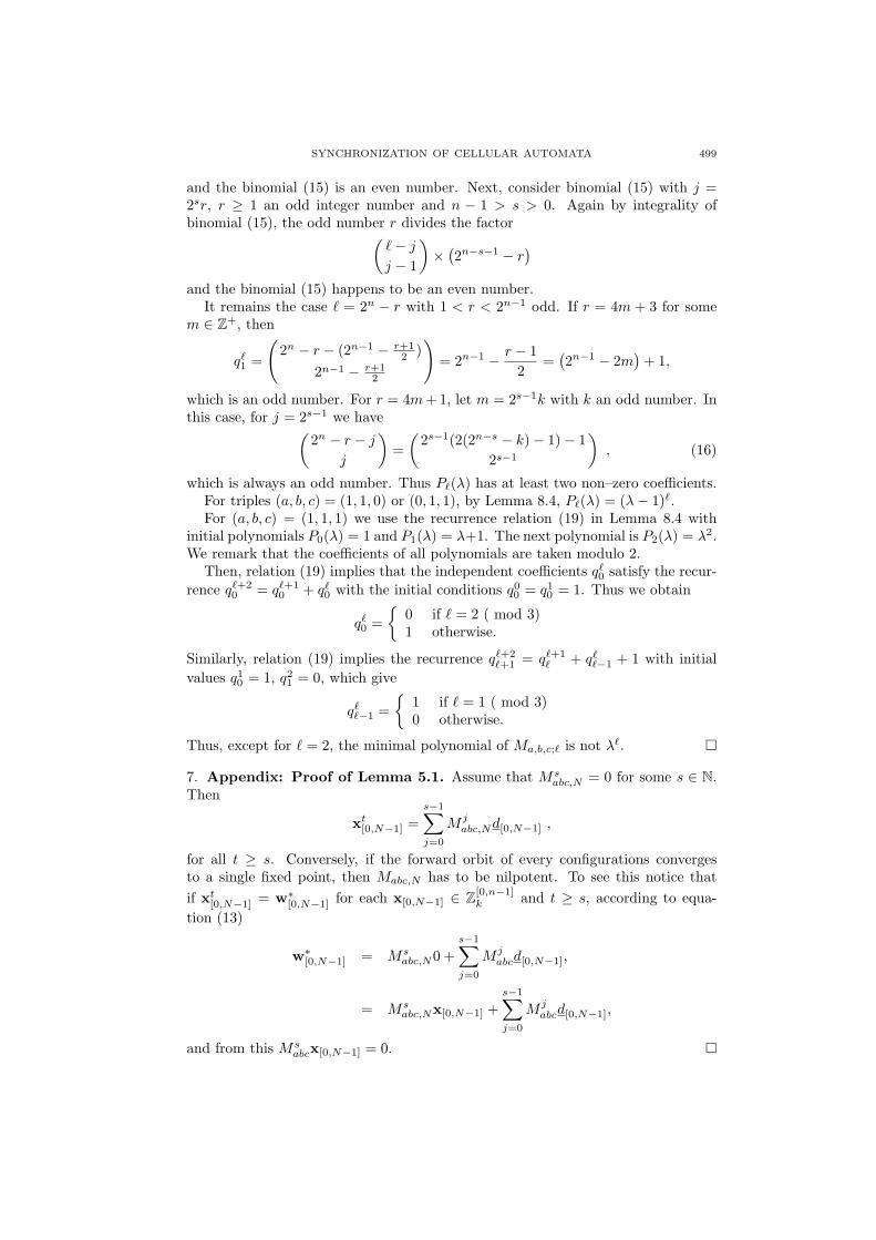
and the binomial (15) is an even number. Next, consider binomial (15) with j =2sr, r ≥ 1 an odd integer number and n − 1 > s > 0. Again by integrality ofbinomial (15), the odd number r divides the factor(

`− j

j − 1

)× (

2n−s−1 − r)

and the binomial (15) happens to be an even number.It remains the case ` = 2n − r with 1 < r < 2n−1 odd. If r = 4m + 3 for some

m ∈ Z+, then

q`1 =

(2n − r − (2n−1 − r+1

2 )2n−1 − r+1

2

)= 2n−1 − r − 1

2=

(2n−1 − 2m

)+ 1,

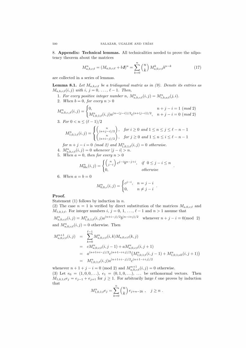
which is an odd number. For r = 4m + 1, let m = 2s−1k with k an odd number. Inthis case, for j = 2s−1 we have(

2n − r − j

j

)=

(2s−1(2(2n−s − k)− 1)− 1

2s−1

), (16)

which is always an odd number. Thus P`(λ) has at least two non–zero coefficients.For triples (a, b, c) = (1, 1, 0) or (0, 1, 1), by Lemma 8.4, P`(λ) = (λ− 1)`.For (a, b, c) = (1, 1, 1) we use the recurrence relation (19) in Lemma 8.4 with

initial polynomials P0(λ) = 1 and P1(λ) = λ+1. The next polynomial is P2(λ) = λ2.We remark that the coefficients of all polynomials are taken modulo 2.

Then, relation (19) implies that the independent coefficients q`0 satisfy the recur-

rence q`+20 = q`+1

0 + q`0 with the initial conditions q0

0 = q10 = 1. Thus we obtain

q`0 =

{0 if ` = 2 ( mod 3)1 otherwise.

Similarly, relation (19) implies the recurrence q`+2`+1 = q`+1

` + q``−1 + 1 with initial

values q10 = 1, q2

1 = 0, which give

q``−1 =

{1 if ` = 1 ( mod 3)0 otherwise.

Thus, except for ` = 2, the minimal polynomial of Ma,b,c;` is not λ`. ¤

7. Appendix: Proof of Lemma 5.1. Assume that Msabc,N = 0 for some s ∈ N.

Then

xt[0,N−1] =

s−1∑

j=0

M jabc,Nd[0,N−1] ,

for all t ≥ s. Conversely, if the forward orbit of every configurations convergesto a single fixed point, then Mabc,N has to be nilpotent. To see this notice thatif xt

[0,N−1] = w∗[0,N−1] for each x[0,N−1] ∈ Z[0,n−1]

k and t ≥ s, according to equa-tion (13)

w∗[0,N−1] = Ms

abc,N0 +s−1∑

j=0

M jabcd[0,N−1],

= Msabc,Nx[0,N−1] +

s−1∑

j=0

M jabcd[0,N−1],

and from this Msabcx[0,N−1] = 0. ¤


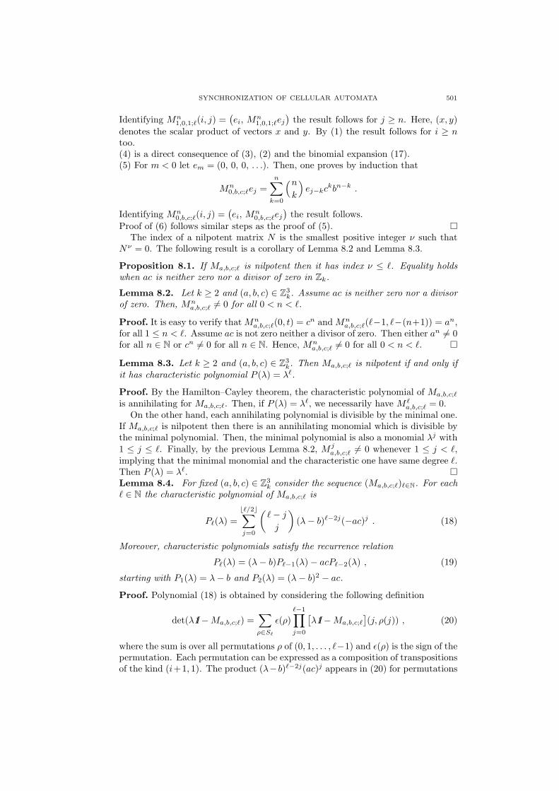
8. Appendix: Technical lemmas. All technicalities needed to prove the nilpo-tency theorem about the matrices

Mna,b,c;` = (Ma,0,c;` + b1I)n =

n∑

k=0

(n

k

)Mk

a,0,c;`bn−k (17)

are collected in a series of lemmas.

Lemma 8.1. Let Ma,b,c;` be a tridiagonal matrix as in (9). Denote its entries asMa,b,c;`(i, j) with i, j = 0, . . . , `− 1. Then,

1. For every positive integer number n, Mna,b,c;`(i, j) = Mn

c,b,a;`(j, i).2. When b = 0, for every n > 0

Mna,0,c,;`(i, j) =

{0, n + j − i = 1 (mod 2)Mn

1,0,1;`(i, j)a(n−(j−i))/2c(n+(j−i))/2, n + j − i = 0 (mod 2)

3. For 0 < n ≤ (`− 1)/2

Mn1,0,1;`(i, j) =

(n

(n+j−i)/2

), for i ≥ 0 and 1 ≤ n ≤ j ≤ `− n− 1(

n(n+i−j)/2

), for j ≥ 0 and 1 ≤ n ≤ i ≤ `− n− 1

for n + j − i = 0 (mod 2) and Mn1,0,1;`(i, j) = 0 otherwise.

4. Mna,b,c;`(i, j) = 0 whenever |j − i| > n.

5. When a = 0, then for every n > 0

Mn0bc(i, j) =

{(n

j−i

)cj−ibn−j+i, if 0 ≤ j − i ≤ n

0, otherwise.

6. When a = b = 0

Mn0,0,c(i, j) =

{cj−i, n = j − i

0, n 6= j − i.

Proof.Statement (1) follows by induction in n.(2) The case n = 1 is verified by direct substitution of the matrices Ma,0,c;` andM1,0,1;`. For integer numbers i, j = 0, 1, . . . , `− 1 and n > 1 assume that

Mna,0,c;`(i, j) = Mn

1,0,1;`(i, j)a(n+i−j)/2b(n−i+j)/2 whenever n + j − i = 0(mod 2)

and Mna,0,c;`(i, j) = 0 otherwise. Then

Mn+1a,0,c;`(i, j) =

`−1∑

k=0

Mna,0,c;`(i, k)Ma,0,c;`(k, j)

= cMna,0,c;`(i, j − 1) + aMn

a,0,c;`(i, j + 1)

= a(n+1+i−j)/2c(n+1−i+j)/2(Mn

1,0,1;`(i, j − 1) + Mn1,0,1;ell(i, j + 1)

)

= Mn1,0,1;`(i, j)a

(n+1+i−j)/2c(n+1−i+j)/2

whenever n + 1 + j − i = 0 (mod 2) and Mn+1a,0,c;`(i, j) = 0 otherwise.

(3) Let e0 = (1, 0, 0, . . .), e1 = (0, 1, 0, . . .), . . . be orthonormal vectors. ThenM1,0,1;èj = ej−1 + ej+1 for j ≥ 1. For arbitrarily large ` one proves by inductionthat

Mn1,0,1;èj =

n∑

k=0

(n

k

)ej+n−2k , j ≥ n .


Identifying Mn1,0,1;`(i, j) =

(ei, Mn

1,0,1;èj

)the result follows for j ≥ n. Here, (x, y)

denotes the scalar product of vectors x and y. By (1) the result follows for i ≥ ntoo.(4) is a direct consequence of (3), (2) and the binomial expansion (17).(5) For m < 0 let em = (0, 0, 0, . . .). Then, one proves by induction that

Mn0,b,c;èj =

n∑

k=0

(n

k

)ej−kckbn−k .

Identifying Mn0,b,c;`(i, j) =

(ei, Mn

0,b,c;èj

)the result follows.

Proof of (6) follows similar steps as the proof of (5). ¤The index of a nilpotent matrix N is the smallest positive integer ν such that

Nν = 0. The following result is a corollary of Lemma 8.2 and Lemma 8.3.

Proposition 8.1. If Ma,b,c;` is nilpotent then it has index ν ≤ `. Equality holdswhen ac is neither zero nor a divisor of zero in Zk.

Lemma 8.2. Let k ≥ 2 and (a, b, c) ∈ Z3k. Assume ac is neither zero nor a divisor

of zero. Then, Mna,b,c;` 6= 0 for all 0 < n < `.

Proof. It is easy to verify that Mna,b,c;`(0, t) = cn and Mn

a,b,c;`(`−1, `−(n+1)) = an,for all 1 ≤ n < `. Assume ac is not zero neither a divisor of zero. Then either an 6= 0for all n ∈ N or cn 6= 0 for all n ∈ N. Hence, Mn

a,b,c;` 6= 0 for all 0 < n < `. ¤

Lemma 8.3. Let k ≥ 2 and (a, b, c) ∈ Z3k. Then Ma,b,c;` is nilpotent if and only if

it has characteristic polynomial P (λ) = λ`.

Proof. By the Hamilton–Cayley theorem, the characteristic polynomial of Ma,b,c;`

is annihilating for Ma,b,c;`. Then, if P (λ) = λ`, we necessarily have M à,b,c;` = 0.

On the other hand, each annihilating polynomial is divisible by the minimal one.If Ma,b,c;` is nilpotent then there is an annihilating monomial which is divisible bythe minimal polynomial. Then, the minimal polynomial is also a monomial λj with1 ≤ j ≤ `. Finally, by the previous Lemma 8.2, M j

a,b,c;` 6= 0 whenever 1 ≤ j < `,implying that the minimal monomial and the characteristic one have same degree `.Then P (λ) = λ`. ¤Lemma 8.4. For fixed (a, b, c) ∈ Z3

k consider the sequence (Ma,b,c;`)`∈N. For each` ∈ N the characteristic polynomial of Ma,b,c;` is

P`(λ) =b`/2c∑

j=0

(`− j

j

)(λ− b)`−2j(−ac)j . (18)

Moreover, characteristic polynomials satisfy the recurrence relation

P`(λ) = (λ− b)P`−1(λ)− acP`−2(λ) , (19)

starting with P1(λ) = λ− b and P2(λ) = (λ− b)2 − ac.

Proof. Polynomial (18) is obtained by considering the following definition

det(λ1I−Ma,b,c;`) =∑

ρ∈S`

ε(ρ)`−1∏

j=0

[λ1I−Ma,b,c;`

](j, ρ(j)) , (20)

where the sum is over all permutations ρ of (0, 1, . . . , `−1) and ε(ρ) is the sign of thepermutation. Each permutation can be expressed as a composition of transpositionsof the kind (i+1, 1). The product (λ−b)`−2j(ac)j appears in (20) for permutations


ρ consisting of j transpositions each, having sign ε(ρ) = (−1)j . Each one of suchpermutations corresponds to a choice of j elements from a set of cardinality `− j.In this way polynomial (18) follows.

The recurrence relation (19) results if we consider the recursive definition of thedeterminant instead. ¤

REFERENCES

[1] A. Amengual, E. Hernandez–Garcıa, R. Montagne and M. San Miguel, Synchronization ofspatiotemporal chaos: The regime of coupled spatiotemporal intermittency. Phys. Rev. Letters78 (1997) 4379–4382.

[2] F. Bagnoli and R. Rechtman, Synchronization and maximum Lyapunov exponents of cellularautomata. Phys. Rev. E 59 (1999) R1307–R1310.

[3] F. Blanchard and P. Tisseur, Some properties of cellular automata with equicontinuity points.Ann. Inst. Henri Poincare, Probabilite et Statistique 35 (2000) 569–582.

[4] F. Blanchard and A. Maass, Dynamical properties of expansive one–sided cellular automata.Israel J. Math. 99 (1997) 149–174.

[5] Y. Kuramoto, Chemical oscillations, waves and turbulence. Springer, Berlin (1984).[6] A. Maass and S. Martınez, On Cesaro limit distribution of a class of permutative cellular

automata. J. Stat. Phys. 90 (1998) 435–458.[7] M. Mejıa and J. Urıas, An asymptotically perfect pseudorandom generator. Discrete and

Continuous Dynamical Sys. 7 (2001) 115–126.[8] M. Pivato and R. Yassawi, Limit measures for affine cellular automata. Ergod. Th. & Dynam.

Sys. (2002), 22, 1269–1287.[9] M. A. Shereshevsky, Ergodic properties of certain surjective cellular automata. Monatshefte

fur Mathematik 114 (2000) 305–316.[10] J. Urıas, G. Salazar and E. Ugalde, Synchronization of cellular automaton pairs. Chaos 8

(1998) 814–818.[11] D.H. Zanette and L.G. Morelli, Synchronization of coupled extended dynamical systems: a

short review. Intl. J. Bifurcation and Chaos 13 (2003) 781–796.

Received October 2004; revised April 2005E-mail address: [gsalazar, ugalde, jurias]@ifisica.uaslp.mx

Documents

Master--slave synchronization of affine cellular automaton pairs