Embed Size (px)
Citation preview

Scalable analytics faster than ever
Second Edition
MasteringApache Spark 2.x
Romeo Kienzler

Mastering Apache Spark 2.xSecond Edition
Romeo Kienzler
BIRMINGHAM - MUMBAI

Mastering Apache Spark 2.x
Second EditionCopyright © 2017 Packt Publishing
All rights reserved. No part of this book may be reproduced, stored in a retrieval system, ortransmitted in any form or by any means, without the prior written permission of thepublisher, except in the case of brief quotations embedded in critical articles or reviews.Every effort has been made in the preparation of this book to ensure the accuracy of theinformation presented. However, the information contained in this book is sold withoutwarranty, either express or implied. Neither the author, nor Packt Publishing, and itsdealers and distributors will be held liable for any damages caused or alleged to be causeddirectly or indirectly by this book. Packt Publishing has endeavored to provide trademarkinformation about all of the companies and products mentioned in this book by theappropriate use of capitals. However, Packt Publishing cannot guarantee the accuracy ofthis information.
First published: September 2015
Second Edition: July 2017
Production reference: 1190717
ISBN 978-1-78646-274-9

Credits
AuthorRomeo Kienzler
Copy EditorTasneem Fatehi
ReviewerMd. Rezaul Karim
Project CoordinatorManthan Patel
Commissioning EditorAmey Varangaonkar
ProofreaderSafis Editing
Acquisition EditorMalaika Monteiro
IndexerTejal Daruwale Soni
Content Development EditorTejas Limkar
GraphicsTania Dutta
Technical EditorDinesh Chaudhary
Production CoordinatorDeepika Naik

About the AuthorRomeo Kienzler works as the chief data scientist in the IBM Watson IoT worldwide team,helping clients to apply advanced machine learning at scale on their IoT sensor data. Heholds a Master's degree in computer science from the Swiss Federal Institute of Technology,Zurich, with a specialization in information systems, bioinformatics, and applied statistics.His current research focus is on scalable machine learning on Apache Spark. He is acontributor to various open source projects and works as an associate professor for artificialintelligence at Swiss University of Applied Sciences, Berne. He is a member of the IBMTechnical Expert Council and the IBM Academy of Technology, IBM's leading brains trust.
Writing a book is quite time-consuming. I want to thank my family for theirunderstanding and my employer, IBM, for giving me the time and flexibility to finish thiswork. Finally, I want to thank the entire team at Packt Publishing, and especially, TejasLimkar, my editor, for all their support, patience, and constructive feedback.

About the ReviewerMd. Rezaul Karim is a research scientist at Fraunhofer Institute for Applied InformationTechnology FIT, Germany. He is also a PhD candidate at the RWTH Aachen University,Aachen, Germany. He holds a BSc and an MSc degree in computer science. Before joiningthe Fraunhofer-FIT, he worked as a researcher at Insight Centre for Data Analytics, Ireland.Prior to that, he worked as a lead engineer with Samsung Electronics' distributed R&DInstitutes in Korea, India, Vietnam, Turkey, and Bangladesh. Previously, he worked as aresearch assistant in the Database Lab at Kyung Hee University, Korea. He also worked asan R&D engineer with BMTech21 Worldwide, Korea. Prior to that, he worked as a softwareengineer with i2SoftTechnology, Dhaka, Bangladesh.
He has more than 8 years' experience in the area of Research and Development with a solidknowledge of algorithms and data structures in C/C++, Java, Scala, R, and Python focusingon big data technologies (such as Spark, Kafka, DC/OS, Docker, Mesos, Zeppelin, Hadoop,and MapReduce) and Deep Learning technologies such as TensorFlow, DeepLearning4j,and H2O-Sparking Water. His research interests include machine learning, deep learning,semantic web/linked data, big data, and bioinformatics. He is the author of the followingbooks with Packt Publishing:
Large-Scale Machine Learning with SparkDeep Learning with TensorFlowScala and Spark for Big Data Analytics
I am very grateful to my parents, who have always encouraged me to pursue knowledge. Ialso want to thank my wife, Saroar, son, Shadman, elder brother, Mamtaz, elder sister,Josna, and friends, who have always been encouraging and have listened to me.

www.PacktPub.comFor support files and downloads related to your book, please visit .
Did you know that Packt offers eBook versions of every book published, with PDF andePub files available? You can upgrade to the eBook version at; and as aprint book customer, you are entitled to a discount on the eBook copy. Get in touch with usat for more details.
At , you can also read a collection of free technical articles, sign up for arange of free newsletters and receive exclusive discounts and offers on Packt books andeBooks.
Get the most in-demand software skills with Mapt. Mapt gives you full access to all Packtbooks and video courses, as well as industry-leading tools to help you plan your personaldevelopment and advance your career.
Why subscribe?Fully searchable across every book published by PacktCopy and paste, print, and bookmark contentOn demand and accessible via a web browser

Customer FeedbackThanks for purchasing this Packt book. At Packt, quality is at the heart of our editorialprocess. To help us improve, please leave us an honest review on this book's Amazon pageat .
If you'd like to join our team of regular reviewers, you can e-mail us at. We award our regular reviewers with free eBooks and
videos in exchange for their valuable feedback. Help us be relentless in improving ourproducts!

Table of ContentsPreface 1
Chapter 1: A First Taste and What’s New in Apache Spark V2 7
Spark machine learning 8Spark Streaming 10Spark SQL 10Spark graph processing 11Extended ecosystem 11What's new in Apache Spark V2? 12Cluster design 12Cluster management 15
Local 15Standalone 15Apache YARN 16Apache Mesos 16
Cloud-based deployments 17Performance 17
The cluster structure 18Hadoop Distributed File System 18Data locality 19Memory 19Coding 20
Cloud 21Summary 21
Chapter 2: Apache Spark SQL 23
The SparkSession--your gateway to structured data processing 24Importing and saving data 25
Processing the text files 25Processing JSON files 26Processing the Parquet files 27
Understanding the DataSource API 28Implicit schema discovery 28Predicate push-down on smart data sources 29
DataFrames 30Using SQL 33

[ ii ]
Defining schemas manually 34Using SQL subqueries 37Applying SQL table joins 38
Using Datasets 41The Dataset API in action 43
User-defined functions 45RDDs versus DataFrames versus Datasets 46Summary 47
Chapter 3: The Catalyst Optimizer 48
Understanding the workings of the Catalyst Optimizer 49Managing temporary views with the catalog API 50The SQL abstract syntax tree 50How to go from Unresolved Logical Execution Plan to Resolved LogicalExecution Plan 51
Internal class and object representations of LEPs 51How to optimize the Resolved Logical Execution Plan 54
Physical Execution Plan generation and selection 54Code generation 55
Practical examples 55Using the explain method to obtain the PEP 56How smart data sources work internally 58
Summary 61
Chapter 4: Project Tungsten 62
Memory management beyond the Java Virtual Machine GarbageCollector 62
Understanding the UnsafeRow object 63The null bit set region 64The fixed length values region 64The variable length values region 65
Understanding the BytesToBytesMap 66A practical example on memory usage and performance 66
Cache-friendly layout of data in memory 69Cache eviction strategies and pre-fetching 69
Code generation 72Understanding columnar storage 73Understanding whole stage code generation 74
A practical example on whole stage code generation performance 74Operator fusing versus the volcano iterator model 77
Summary 77

[ iii ]
Chapter 5: Apache Spark Streaming 78
Overview 79Errors and recovery 81
Checkpointing 81Streaming sources 84
TCP stream 84File streams 86Flume 87Kafka 96
Summary 105
Chapter 6: Structured Streaming 106
The concept of continuous applications 107True unification - same code, same engine 107
Windowing 107How streaming engines use windowing 108How Apache Spark improves windowing 110
Increased performance with good old friends 111How transparent fault tolerance and exactly-once delivery guarantee isachieved 112
Replayable sources can replay streams from a given offset 112Idempotent sinks prevent data duplication 113State versioning guarantees consistent results after reruns 113
Example - connection to a MQTT message broker 113Controlling continuous applications 119More on stream life cycle management 119
Summary 120
Chapter 7: Apache Spark MLlib 121
Architecture 121The development environment 122
Classification with Naive Bayes 124Theory on Classification 124Naive Bayes in practice 126
Clustering with K-Means 134Theory on Clustering 134K-Means in practice 134
Artificial neural networks 139ANN in practice 143
Summary 152

[ iv ]
Chapter 8: Apache SparkML 154
What does the new API look like? 155The concept of pipelines 155
Transformers 156String indexer 156OneHotEncoder 156VectorAssembler 157
Pipelines 157Estimators 158
RandomForestClassifier 158Model evaluation 159CrossValidation and hyperparameter tuning 160
CrossValidation 160Hyperparameter tuning 161
Winning a Kaggle competition with Apache SparkML 164Data preparation 164Feature engineering 167Testing the feature engineering pipeline 171Training the machine learning model 172Model evaluation 173CrossValidation and hyperparameter tuning 174Using the evaluator to assess the quality of the cross-validated andtuned model 175
Summary 176
Chapter 9: Apache SystemML 177
Why do we need just another library? 177Why on Apache Spark? 178The history of Apache SystemML 178
A cost-based optimizer for machine learning algorithms 180An example - alternating least squares 181ApacheSystemML architecture 184
Language parsing 185High-level operators are generated 185How low-level operators are optimized on 187
Performance measurements 188Apache SystemML in action 188Summary 190
Chapter 10: Deep Learning on Apache Spark with DeepLearning4j andH2O 191

[ v ]
H2O 191Overview 192
The build environment 194Architecture 196Sourcing the data 199Data quality 200Performance tuning 201Deep Learning 201
Example code – income 203The example code – MNIST 208H2O Flow 209
Deeplearning4j 223ND4J - high performance linear algebra for the JVM 223Deeplearning4j 224Example: an IoT real-time anomaly detector 231
Mastering chaos: the Lorenz attractor model 231Deploying the test data generator 239
Deploy the Node-RED IoT Starter Boilerplate to the IBM Cloud 240Deploying the test data generator flow 242Testing the test data generator 244
Install the Deeplearning4j example within Eclipse 246Running the examples in Eclipse 246Run the examples in Apache Spark 254
Summary 255
Chapter 11: Apache Spark GraphX 256
Overview 256Graph analytics/processing with GraphX 259
The raw data 259Creating a graph 260Example 1 – counting 262Example 2 – filtering 262Example 3 – PageRank 263Example 4 – triangle counting 264Example 5 – connected components 264
Summary 266
Chapter 12: Apache Spark GraphFrames 267
Architecture 268Graph-relational translation 268Materialized views 270Join elimination 270Join reordering 271

[ vi ]
Examples 274Example 1 – counting 275Example 2 – filtering 275Example 3 – page rank 276Example 4 – triangle counting 277Example 5 – connected components 279
Summary 283
Chapter 13: Apache Spark with Jupyter Notebooks on IBM DataScienceExperience 284
Why notebooks are the new standard 285Learning by example 286
The IEEE PHM 2012 data challenge bearing dataset 289ETL with Scala 291Interactive, exploratory analysis using Python and Pixiedust 296Real data science work with SparkR 301
Summary 303
Chapter 14: Apache Spark on Kubernetes 304
Bare metal, virtual machines, and containers 304Containerization 307
Namespaces 308Control groups 309Linux containers 310
Understanding the core concepts of Docker 310Understanding Kubernetes 313Using Kubernetes for provisioning containerized Spark applications 315Example--Apache Spark on Kubernetes 316
Prerequisites 316Deploying the Apache Spark master 317Deploying the Apache Spark workers 320Deploying the Zeppelin notebooks 322
Summary 324
Index 325

PrefaceApache Spark is an in-memory, cluster-based, parallel processing system that provides awide range of functionality such as graph processing, machine learning, stream processing,and SQL. This book aims to take your limited knowledge of Spark to the next level byteaching you how to expand your Spark functionality.
The book opens with an overview of the Spark ecosystem. The book will introduce you toProject Catalyst and Tungsten. You will understand how Memory Management and BinaryProcessing, Cache-aware Computation, and Code Generation are used to speed things updramatically. The book goes on to show how to incorporate H20 and Deeplearning4j formachine learning and Juypter Notebooks, Zeppelin, Docker and Kubernetes for cloud-based Spark. During the course of the book, you will also learn about the latestenhancements in Apache Spark 2.2, such as using the DataFrame and Dataset APIsexclusively, building advanced, fully automated Machine Learning pipelines with SparkMLand perform graph analysis using the new GraphFrames API.
What this book covers, A First Taste and What's New in Apache Spark V2, provides an overview of Apache
Spark, the functionality that is available within its modules, and how it can be extended. Itcovers the tools available in the Apache Spark ecosystem outside the standard ApacheSpark modules for processing and storage. It also provides tips on performance tuning.
, Apache Spark SQL, creates a schema in Spark SQL, shows how data can bequeried efficiently using the relational API on DataFrames and Datasets, and explores SQL.
, The Catalyst Optimizer, explains what a cost-based optimizer in database systemsis and why it is necessary. You will master the features and limitations of the CatalystOptimizer in Apache Spark.
, Project Tungsten, explains why Project Tungsten is essential for Apache Sparkand also goes on to explain how Memory Management, Cache-aware Computation, andCode Generation are used to speed things up dramatically.
, Apache Spark Streaming, talks about continuous applications using Apache Sparkstreaming. You will learn how to incrementally process data and create actionable insights.

Preface
[ 2 ]
, Structured Streaming, talks about Structured Streaming – a new way of definingcontinuous applications using the DataFrame and Dataset APIs.
, Classical MLlib, introduces you to MLlib, the de facto standard for machinelearning when using Apache Spark.
, Apache SparkML, introduces you to the DataFrame-based machine learninglibrary of Apache Spark: the new first-class citizen when it comes to high performance andmassively parallel machine learning.
, Apache SystemML, introduces you to Apache SystemML, another machinelearning library capable of running on top of Apache Spark and incorporating advancedfeatures such as a cost-based optimizer, hybrid execution plans, and low-level operator re-writes.
, Deep Learning on Apache Spark using H20 and DeepLearning4j, explains that deeplearning is currently outperforming one traditional machine learning discipline after theother. We have three open source first-class deep learning libraries running on top ofApache Spark, which are H2O, DeepLearning4j, and Apache SystemML. Let's understandwhat Deep Learning is and how to use it on top of Apache Spark using these libraries.
, Apache Spark GraphX, talks about Graph processing with Scala using GraphX.You will learn some basic and also advanced graph algorithms and how to use GraphX toexecute them.
, Apache Spark GraphFrames, discusses graph processing with Scala usingGraphFrames. You will learn some basic and also advanced graph algorithms and also howGraphFrames differ from GraphX in execution.
, Apache Spark with Jupyter Notebooks on IBM DataScience Experience, introduces aPlatform as a Service offering from IBM, which is completely based on an Open Sourcestack and on open standards. The main advantage is that you have no vendor lock-in.Everything you learn here can be installed and used in other clouds, in a local datacenter, oron your local laptop or PC.
, Apache Spark on Kubernetes, explains that Platform as a Service cloud providerscompletely manage the operations part of an Apache Spark cluster for you. This is anadvantage but sometimes you have to access individual cluster nodes for debugging andtweaking and you don't want to deal with the complexity that maintaining a real cluster onbare-metal or virtual systems entails. Here, Kubernetes might be the best solution.Therefore, in this chapter, we explain what Kubernetes is and how it can be used to set upan Apache Spark cluster.

Preface
[ 3 ]
What you need for this bookYou will need the following to work with the examples in this book:
A laptop or PC with at least 6 GB main memory running Windows, macOS, orLinuxVirtualBox 5.1.22 or aboveHortonworks HDP Sandbox V2.6 or aboveEclipse Neon or aboveMavenEclipse Maven PluginEclipse Scala PluginEclipse Git Plugin
Who this book is forThis book is an extensive guide to Apache Spark from the programmer's and data scientist'sperspective. It covers Apache Spark in depth, but also supplies practical working examplesfor different domains. Operational aspects are explained in sections on performance tuningand cloud deployments. All the chapters have working examples, which can be replicatedeasily.
ConventionsIn this book, you will find a number of text styles that distinguish between different kindsof information. Here are some examples of these styles and an explanation of their meaning.
Code words in text, database table names, folder names, filenames, file extensions,pathnames, dummy URLs, user input, and Twitter handles are shown as follows: "The nextlines of code read the link and assign it to the to the function."
A block of code is set as follows:
Any command-line input or output is written as follows:
[hadoop@hc2nn ~]# sudo su -[root@hc2nn ~]# cd /tmp

Preface
[ 4 ]
New terms and important words are shown in bold. Words that you see on the screen, forexample, in menus or dialog boxes, appear in the text like this: "In order to download newmodules, we will go to Files | Settings | Project Name | Project Interpreter."
Warnings or important notes appear in a box like this.
Tips and tricks appear like this.
Reader feedbackFeedback from our readers is always welcome. Let us know what you think about thisbook-what you liked or disliked. Reader feedback is important for us as it helps us developtitles that you will really get the most out of.
To send us general feedback, simply e-mail , and mention thebook's title in the subject of your message.
If there is a topic that you have expertise in and you are interested in either writing orcontributing to a book, see our author guide at .
Customer supportNow that you are the proud owner of a Packt book, we have a number of things to help youto get the most from your purchase.
Downloading the example codeYou can download the example code files for this book from your account at
. If you purchased this book elsewhere, you can visit and register to have the files e-mailed directly to you.
You can download the code files by following these steps:
Log in or register to our website using your e-mail address and password.1.Hover the mouse pointer on the SUPPORT tab at the top.2.
Preface
[ 5 ]
Click on Code Downloads & Errata.3.Enter the name of the book in the Search box.4.Select the book for which you're looking to download the code files.5.Choose from the drop-down menu where you purchased this book from.6.Click on Code Download.7.
Once the file is downloaded, please make sure that you unzip or extract the folder using thelatest version of:
WinRAR / 7-Zip for WindowsZipeg / iZip / UnRarX for Mac7-Zip / PeaZip for Linux
The code bundle for the book is also hosted on GitHub at . We also have other code bundles from our rich
catalog of books and videos available at . Checkthem out!
Downloading the color images of this bookWe also provide you with a PDF file that has color images of the screenshots/diagrams usedin this book. The color images will help you better understand the changes in the output.You can download this file from
.
ErrataAlthough we have taken every care to ensure the accuracy of our content, mistakes dohappen. If you find a mistake in one of our books-maybe a mistake in the text or the code-we would be grateful if you could report this to us. By doing so, you can save other readersfrom frustration and help us improve subsequent versions of this book. If you find anyerrata, please report them by visiting , selectingyour book, clicking on the Errata Submission Form link, and entering the details of yourerrata. Once your errata are verified, your submission will be accepted and the errata willbe uploaded to our website or added to any list of existing errata under the Errata section ofthat title.

Preface
[ 6 ]
To view the previously submitted errata, go to and enter the name of the book in the search field. The required information will
appear under the Errata section.
PiracyPiracy of copyrighted material on the Internet is an ongoing problem across all media. AtPackt, we take the protection of our copyright and licenses very seriously. If you comeacross any illegal copies of our works in any form on the Internet, please provide us withthe location address or website name immediately so that we can pursue a remedy.
Please contact us at with a link to the suspected piratedmaterial.
We appreciate your help in protecting our authors and our ability to bring you valuablecontent.
QuestionsIf you have a problem with any aspect of this book, you can contact us at
, and we will do our best to address the problem.

11A First Taste and What’s New
in Apache Spark V2Apache Spark is a distributed and highly scalable in-memory data analytics system,providing you with the ability to develop applications in Java, Scala, and Python, as well aslanguages such as R. It has one of the highest contribution/involvement rates among theApache top-level projects at this time. Apache systems, such as Mahout, now use it as aprocessing engine instead of MapReduce. It is also possible to use a Hive context to havethe Spark applications process data directly to and from Apache Hive.
Initially, Apache Spark provided four main submodules--SQL, MLlib, GraphX, andStreaming. They will all be explained in their own chapters, but a simple overview wouldbe useful here. The modules are interoperable, so data can be passed between them. Forinstance, streamed data can be passed to SQL and a temporary table can be created. Sinceversion 1.6.0, MLlib has a sibling called SparkML with a different API, which we will coverin later chapters.
The following figure explains how this book will address Apache Spark and its modules:
The top two rows show Apache Spark and its submodules. Wherever possible, we will tryto illustrate by giving an example of how the functionality may be extended using extratools.

A First Taste and What’s New in Apache Spark V2
[ 8 ]
We infer that Spark is an in-memory processing system. When used atscale (it cannot exist alone), the data must reside somewhere. It willprobably be used along with the Hadoop tool set and the associatedecosystem.
Luckily, Hadoop stack providers, such as IBM and Hortonworks, provide you with an opendata platform, a Hadoop stack, and cluster manager, which integrates with Apache Spark,Hadoop, and most of the current stable toolset fully based on open source. During thisbook, we will use Hortonworks Data Platform (HDP®) Sandbox 2.6. You can use analternative configuration, but we find that the open data platform provides most of the toolsthat we need and automates the configuration, leaving us more time for development.
In the following sections, we will cover each of the components mentioned earlier in moredetail before we dive into the material starting in the next chapter:
Spark Machine LearningSpark StreamingSpark SQLSpark Graph ProcessingExtended EcosystemUpdates in Apache SparkCluster designCloud-based deploymentsPerformance parameters
Spark machine learningMachine learning is the real reason for Apache Spark because, at the end of the day, youdon't want to just ship and transform data from A to B (a process called ETL (ExtractTransform Load)). You want to run advanced data analysis algorithms on top of your data,and you want to run these algorithms at scale. This is where Apache Spark kicks in.
Apache Spark, in its core, provides the runtime for massive parallel data processing, anddifferent parallel machine learning libraries are running on top of it. This is because there isan abundance on machine learning algorithms for popular programming languages like Rand Python but they are not scalable. As soon as you load more data to the available mainmemory of the system, they crash.

A First Taste and What’s New in Apache Spark V2
[ 9 ]
Apache Spark in contrast can make use of multiple computer nodes to form a cluster andeven on a single node can spill data transparently to disk therefore avoiding the mainmemory bottleneck. Two interesting machine learning libraries are shipped with ApacheSpark, but in this work we'll also cover third-party machine learning libraries.
The Spark MLlib module, Classical MLlib, offers a growing but incomplete list of machinelearning algorithms. Since the introduction of the DataFrame-based machine learning APIcalled SparkML, the destiny of MLlib is clear. It is only kept for backward compatibilityreasons.
This is indeed a very wise decision, as we will discover in the next two chapters thatstructured data processing and the related optimization frameworks are currentlydisrupting the whole Apache Spark ecosystem. In SparkML, we have a machine learninglibrary in place that can take advantage of these improvements out of the box, using it as anunderlying layer.
SparkML will eventually replace MLlib. Apache SystemML introduces thefirst library running on top of Apache Spark that is not shipped with theApache Spark distribution. SystemML provides you with an executionenvironment of R-style syntax with a built-in cost-based optimizer.Massive parallel machine learning is an area of constant change at a highfrequency. It is hard to say where that the journey goes, but it is the firsttime where advanced machine learning at scale is available to everyoneusing open source and cloud computing.
Deep learning on Apache Spark uses H20, Deeplearning4j and Apache SystemML, whichare other examples of very interesting third-party machine learning libraries that are notshipped with the Apache Spark distribution.
While H20 is somehow complementary to MLlib, Deeplearning4j only focuses on deeplearning algorithms. Both use Apache Spark as a means for parallelization of dataprocessing. You might wonder why we want to tackle different machine learning libraries.
The reality is that every library has advantages and disadvantages withthe implementation of different algorithms. Therefore, it often depends onyour data and Dataset size which implementation you choose for bestperformance.

A First Taste and What’s New in Apache Spark V2
[ 10 ]
However, it is nice that there is so much choice and you are not locked in a single librarywhen using Apache Spark. Open source means openness, and this is just one example ofhow we are all benefiting from this approach in contrast to a single vendor, single productlock-in. Although recently Apache Spark integrated GraphX, another Apache Spark libraryinto its distribution, we don't expect this will happen too soon. Therefore, it is most likelythat Apache Spark as a central data processing platform and additional third-party librarieswill co-exist, like Apache Spark being the big data operating system and the third-partylibraries are the software you install and run on top of it.
Spark StreamingStream processing is another big and popular topic for Apache Spark. It involves theprocessing of data in Spark as streams and covers topics such as input and outputoperations, transformations, persistence, and checkpointing, among others.
Apache Spark Streaming will cover the area of processing, and we will also see practicalexamples of different types of stream processing. This discusses batch and window streamconfiguration and provides a practical example of checkpointing. It also covers differentexamples of stream processing, including Kafka and Flume.
There are many ways in which stream data can be used. Other Spark module functionality(for example, SQL, MLlib, and GraphX) can be used to process the stream. You can useSpark Streaming with systems such as MQTT or ZeroMQ. You can even create customreceivers for your own user-defined data sources.
Spark SQLFrom Spark version 1.3, data frames have been introduced in Apache Spark so that Sparkdata can be processed in a tabular form and tabular functions (such as , , and
) can be used to process data. The Spark SQL module integrates with Parquet andJSON formats to allow data to be stored in formats that better represent the data. This alsooffers more options to integrate with external systems.
The idea of integrating Apache Spark into the Hadoop Hive big data database can also beintroduced. Hive context-based Spark applications can be used to manipulate Hive-basedtable data. This brings Spark's fast in-memory distributed processing to Hive's big datastorage capabilities. It effectively lets Hive use Spark as a processing engine.

A First Taste and What’s New in Apache Spark V2
[ 11 ]
Additionally, there is an abundance of additional connectors to access NoSQL databasesoutside the Hadoop ecosystem directly from Apache Spark. In , Apache SparkSQL, we will see how the Cloudant connector can be used to access a remoteApacheCouchDB NoSQL database and issue SQL statements against JSON-based NoSQLdocument collections.
Spark graph processingGraph processing is another very important topic when it comes to data analysis. In fact, amajority of problems can be expressed as a graph.
A graph is basically a network of items and their relationships to each other. Items arecalled nodes and relationships are called edges. Relationships can be directed orundirected. Relationships, as well as items, can have properties. So a map, for example, canbe represented as a graph as well. Each city is a node and the streets between the cities areedges. The distance between the cities can be assigned as properties on the edge.
The Apache Spark GraphX module allows Apache Spark to offer fast big data in-memorygraph processing. This allows you to run graph algorithms at scale.
One of the most famous algorithms, for example, is the traveling salesman problem.Consider the graph representation of the map mentioned earlier. A salesman has to visit allcities of a region but wants to minimize the distance that he has to travel. As the distancesbetween all the nodes are stored on the edges, a graph algorithm can actually tell you theoptimal route. GraphX is able to create, manipulate, and analyze graphs using a variety ofbuilt-in algorithms.
It introduces two new data types to support graph processing in Spark--VertexRDD andEdgeRDD--to represent graph nodes and edges. It also introduces graph processingalgorithms, such as PageRank and triangle processing. Many of these functions will beexamined in , Apache Spark GraphX and , Apache Spark GraphFrames.
Extended ecosystemWhen examining big data processing systems, we think it is important to look at not just thesystem itself, but also how it can be extended and how it integrates with external systems sothat greater levels of functionality can be offered. In a book of this size, we cannot coverevery option, but by introducing a topic, we can hopefully stimulate the reader's interest sothat they can investigate further.

A First Taste and What’s New in Apache Spark V2
[ 12 ]
We have used the H2O machine learning library, SystemML and Deeplearning4j, to extendApache Spark's MLlib machine learning module. We have shown that Deeplearning andhighly performant cost-based optimized machine learning can be introduced to ApacheSpark. However, we have just scratched the surface of all the frameworks' functionality.
What's new in Apache Spark V2?Since Apache Spark V2, many things have changed. This doesn't mean that the API hasbeen broken. In contrast, most of the V1.6 Apache Spark applications will run on ApacheSpark V2 with or without very little changes, but under the hood, there have been a lot ofchanges.
The first and most interesting thing to mention is the newest functionalities of the CatalystOptimizer, which we will cover in detail in , The Catalyst Optimizer. Catalystcreates a Logical Execution Plan (LEP) from a SQL query and optimizes this LEP to createmultiple Physical Execution Plans (PEPs). Based on statistics, Catalyst chooses the best PEPto execute. This is very similar to cost-based optimizers in Relational Data BaseManagement Systems (RDBMs). Catalyst makes heavy use of Project Tungsten, acomponent that we will cover in , Apache Spark Streaming.
Although the Java Virtual Machine (JVM) is a masterpiece on its own, it is a general-purpose byte code execution engine. Therefore, there is a lot of JVM object management andgarbage collection (GC) overhead. So, for example, to store a 4-byte string, 48 bytes on theJVM are needed. The GC optimizes on object lifetime estimation, but Apache Spark oftenknows this better than JVM. Therefore, Tungsten disables the JVM GC for a subset ofprivately managed data structures to make them L1/L2/L3 Cache-friendly.
In addition, code generation removed the boxing of primitive types polymorphic functiondispatching. Finally, a new first-class citizen called Dataset unified the RDD and DataFrameAPIs. Datasets are statically typed and avoid runtime type errors. Therefore, Datasets canbe used only with Java and Scala. This means that Python and R users still have to stick toDataFrames, which are kept in Apache Spark V2 for backward compatibility reasons.
Cluster designAs we have already mentioned, Apache Spark is a distributed, in-memory, parallelprocessing system, which needs an associated storage system. So, when you build a bigdata cluster, you will probably use a distributed storage system such as Hadoop, as well astools to move data such as Sqoop, Flume, and Kafka.
A First Taste and What’s New in Apache Spark V2
[ 13 ]
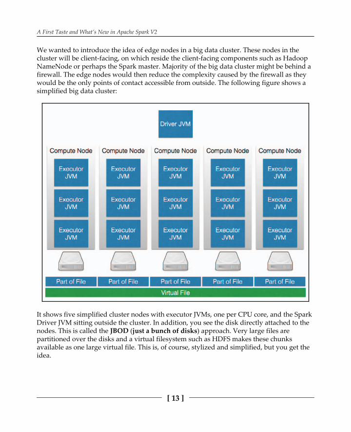
We wanted to introduce the idea of edge nodes in a big data cluster. These nodes in thecluster will be client-facing, on which reside the client-facing components such as HadoopNameNode or perhaps the Spark master. Majority of the big data cluster might be behind afirewall. The edge nodes would then reduce the complexity caused by the firewall as theywould be the only points of contact accessible from outside. The following figure shows asimplified big data cluster:
It shows five simplified cluster nodes with executor JVMs, one per CPU core, and the SparkDriver JVM sitting outside the cluster. In addition, you see the disk directly attached to thenodes. This is called the JBOD (just a bunch of disks) approach. Very large files arepartitioned over the disks and a virtual filesystem such as HDFS makes these chunksavailable as one large virtual file. This is, of course, stylized and simplified, but you get theidea.

A First Taste and What’s New in Apache Spark V2
[ 14 ]
The following simplified component model shows the driver JVM sitting outside thecluster. It talks to the Cluster Manager in order to obtain permission to schedule tasks onthe worker nodes because the Cluster Manager keeps track of resource allocation of allprocesses running on the cluster.
As we will see later, there is a variety of different cluster managers, some of them alsocapable of managing other Hadoop workloads or even non-Hadoop applications in parallelto the Spark Executors. Note that the Executor and Driver have bidirectionalcommunication all the time, so network-wise, they should also be sitting close together:
Generally, firewalls, while adding security to the cluster, also increase the complexity. Portsbetween system components need to be opened up so that they can talk to each other. Forinstance, Zookeeper is used by many components for configuration. Apache Kafka, thepublish/subscribe messaging system, uses Zookeeper to configure its topics, groups,consumers, and producers. So, client ports to Zookeeper, potentially across the firewall,need to be open.
Finally, the allocation of systems to cluster nodes needs to be considered. For instance, ifApache Spark uses Flume or Kafka, then in-memory channels will be used. The size of thesechannels, and the memory used, caused by the data flow, need to be considered. ApacheSpark should not be competing with other Apache components for memory usage.Depending upon your data flows and memory usage, it might be necessary to have Spark,Hadoop, Zookeeper, Flume, and other tools on distinct cluster nodes. Alternatively,resource managers such as YARN, Mesos, or Docker can be used to tackle this problem. Instandard Hadoop environments, YARN is most likely.

A First Taste and What’s New in Apache Spark V2
[ 15 ]
Generally, the edge nodes that act as cluster NameNode servers or Spark master serverswill need greater resources than the cluster processing nodes within the firewall. Whenmany Hadoop ecosystem components are deployed on the cluster, all of them will needextra memory on the master server. You should monitor edge nodes for resource usage andadjust in terms of resources and/or application location as necessary. YARN, for instance, istaking care of this.
This section has briefly set the scene for the big data cluster in terms of Apache Spark,Hadoop, and other tools. However, how might the Apache Spark cluster itself, within thebig data cluster, be configured? For instance, it is possible to have many types of the Sparkcluster manager. The next section will examine this and describe each type of the ApacheSpark cluster manager.
Cluster managementThe Spark context, as you will see in many of the examples in this book, can be defined viaa Spark configuration object and Spark URL. The Spark context connects to the Sparkcluster manager, which then allocates resources across the worker nodes for the application.The cluster manager allocates executors across the cluster worker nodes. It copies theapplication JAR file to the workers and finally allocates tasks.
The following subsections describe the possible Apache Spark cluster manager optionsavailable at this time.
LocalBy specifying a Spark configuration local URL, it is possible to have the application runlocally. By specifying , it is possible to have Spark use n threads to run theapplication locally. This is a useful development and test option because you can also testsome sort of parallelization scenarios but keep all log files on a single machine.
StandaloneStandalone mode uses a basic cluster manager that is supplied with Apache Spark. Thespark master URL will be as follows:

A First Taste and What’s New in Apache Spark V2
[ 16 ]
Here, is the name of the host on which the Spark master is running. We havespecified as the port, which is the default value, but this is configurable. This simplecluster manager currently supports only FIFO (first-in first-out) scheduling. You cancontrive to allow concurrent application scheduling by setting the resource configurationoptions for each application; for instance, using to share cores betweenapplications.
Apache YARNAt a larger scale, when integrating with Hadoop YARN, the Apache Spark cluster managercan be YARN and the application can run in one of two modes. If the Spark master value isset as , then the application can be submitted to the cluster and thenterminated. The cluster will take care of allocating resources and running tasks. However, ifthe application master is submitted as , then the application stays alive duringthe life cycle of processing, and requests resources from YARN.
Apache MesosApache Mesos is an open source system for resource sharing across a cluster. It allowsmultiple frameworks to share a cluster by managing and scheduling resources. It is a clustermanager that provides isolation using Linux containers and allowing multiple systems suchas Hadoop, Spark, Kafka, Storm, and more to share a cluster safely. It is highly scalable tothousands of nodes. It is a master/slave-based system and is fault tolerant, using Zookeeperfor configuration management.
For a single master node Mesos cluster, the Spark master URL will be in this form:
.
Here, is the hostname of the Mesos master server; the port is defined as which is the default Mesos master port (this is configurable). If there are multiple Mesosmaster servers in a large-scale high availability Mesos cluster, then the Spark master URLwould look as follows:
.
So, the election of the Mesos master server will be controlled by Zookeeper. The will be the name of a host in the Zookeeper quorum. Also, the port number,
, is the default master port for Zookeeper.

A First Taste and What’s New in Apache Spark V2
[ 17 ]
Cloud-based deploymentsThere are three different abstraction levels of cloud systems--Infrastructure as a Service(IaaS), Platform as a Service (PaaS), and Software as a Service (SaaS). We will see how touse and install Apache Spark on all of these.
The new way to do IaaS is Docker and Kubernetes as opposed to virtual machines, basicallyproviding a way to automatically set up an Apache Spark cluster within minutes. This willbe covered in , Apache Spark on Kubernetes. The advantage of Kubernetes is that itcan be used among multiple different cloud providers as it is an open standard and alsobased on open source.
You even can use Kubernetes in a local data center and transparently and dynamicallymove workloads between local, dedicated, and public cloud data centers. PaaS, in contrast,takes away from you the burden of installing and operating an Apache Spark clusterbecause this is provided as a service.
There is an ongoing discussion whether Docker is IaaS or PaaS but, in our opinion, this isjust a form of a lightweight preinstalled virtual machine. We will cover more on PaaS in
, Apache Spark with Jupyter Notebooks on IBM DataScience Experience. This isparticularly interesting because the offering is completely based on open sourcetechnologies, which enables you to replicate the system on any other data center.
One of the open source components we'll introduce is Jupyter notebooks, a modern way todo data science in a cloud based collaborative environment. But in addition to Jupyter, thereis also Apache Zeppelin, which we'll cover briefly in , Apache Spark onKubernetes.
PerformanceBefore moving on to the rest of the chapters covering functional areas of Apache Spark andextensions, we will examine the area of performance. What issues and areas need to beconsidered? What might impact the Spark application performance starting at the clusterlevel and finishing with actual Scala code? We don't want to just repeat what the Sparkwebsite says, so take a look at this URL:
.
Here, relates to the version of Spark that you are using; that is, either the latestor something like for a specific version. So, having looked at this page, we willbriefly mention some of the topic areas. We will list some general points in this sectionwithout implying an order of importance.

A First Taste and What’s New in Apache Spark V2
[ 18 ]
The cluster structureThe size and structure of your big data cluster is going to affect performance. If you have acloud-based cluster, your IO and latency will suffer in comparison to an unshared hardwarecluster. You will be sharing the underlying hardware with multiple customers and thecluster hardware may be remote. There are some exceptions to this. The IBM cloud, forinstance, offers dedicated bare metal high performance cluster nodes with an InfiniBandnetwork connection, which can be rented on an hourly basis.
Additionally, the positioning of cluster components on servers may cause resourcecontention. For instance, think carefully about locating Hadoop NameNodes, Spark servers,Zookeeper, Flume, and Kafka servers in large clusters. With high workloads, you mightconsider segregating servers to individual systems. You might also consider using anApache system such as Mesos that provides better distributions and assignment ofresources to the individual processes.
Consider potential parallelism as well. The greater the number of workers in your Sparkcluster for large Datasets, the greater the opportunity for parallelism. One rule of thumb isone worker per hyper-thread or virtual core respectively.
Hadoop Distributed File SystemYou might consider using an alternative to HDFS, depending upon your clusterrequirements. For instance, IBM has the GPFS (General Purpose File System) for improvedperformance.
The reason why GPFS might be a better choice is that, coming from the high performancecomputing background, this filesystem has a full read write capability, whereas HDFS isdesigned as a write once, read many filesystem. It offers an improvement in performanceover HDFS because it runs at the kernel level as opposed to HDFS, which runs in a JavaVirtual Machine (JVM) that in turn runs as an operating system process. It also integrateswith Hadoop and the Spark cluster tools. IBM runs setups with several hundred petabytesusing GPFS.
Another commercial alternative is the MapR file system that, besides performanceimprovements, supports mirroring, snapshots, and high availability.
Ceph is an open source alternative to a distributed, fault-tolerant, and self-healing filesystem for commodity hard drives like HDFS. It runs in the Linux kernel as well andaddresses many of the performance issues that HDFS has. Other promising candidates inthis space are Alluxio (formerly Tachyon), Quantcast, GlusterFS, and Lustre.

A First Taste and What’s New in Apache Spark V2
[ 19 ]
Finally, Cassandra is not a filesystem but a NoSQL key value store and is tightly integratedwith Apache Spark and is therefore traded as a valid and powerful alternative to HDFS--oreven to any other distributed filesystem--especially as it supports predicate push-downusing and the Catalyst optimizer, which we will cover in the followingchapters.
Data localityThe key for good data processing performance is avoidance of network transfers. This wasvery true a couple of years ago but is less relevant for tasks with high demands on CPU andlow I/O, but for low demand on CPU and high I/O demand data processing algorithms, thisstill holds.
We can conclude from this that HDFS is one of the best ways to achievedata locality as chunks of files are distributed on the cluster nodes, in mostof the cases, using hard drives directly attached to the server systems. Thismeans that those chunks can be processed in parallel using the CPUs onthe machines where individual data chunks are located in order to avoidnetwork transfer.
Another way to achieve data locality is using . Depending on theconnector implementation, SparkSQL can make use of data processing capabilities of thesource engine. So for example when using MongoDB in conjunction with SparkSQL parts ofthe SQL statement are preprocessed by MongoDB before data is sent upstream to ApacheSpark.
MemoryIn order to avoid OOM (Out of Memory) messages for the tasks on your Apache Sparkcluster, please consider a number of questions for the tuning:
Consider the level of physical memory available on your Spark worker nodes.Can it be increased? Check on the memory consumption of operating systemprocesses during high workloads in order to get an idea of free memory. Makesure that the workers have enough memory.Consider data partitioning. Can you increase the number of partitions? As a ruleof thumb, you should have at least as many partitions as you have available CPUcores on the cluster. Use the function on the RDD API.

A First Taste and What’s New in Apache Spark V2
[ 20 ]
Can you modify the storage fraction and the memory used by the JVM for storageand caching of RDDs? Workers are competing for memory against data storage.Use the Storage page on the Apache Spark user interface to see if this fraction isset to an optimal value. Then update the following properties:
In addition, the following two things can be done in order to improve performance:
Consider using Parquet as a storage format, which is much more storage effectivethan CSV or JSONConsider using the DataFrame/Dataset API instead of the RDD API as it mightresolve in more effective executions (more about this in the next three chapters)
CodingTry to tune your code to improve the Spark application performance. For instance, filteryour application-based data early in your ETL cycle. One example is when using rawHTML files, detag them and crop away unneeded parts at an early stage. Tune your degreeof parallelism, try to find the resource-expensive parts of your code, and find alternatives.
ETL is one of the first things you are doing in an analytics project. So youare grabbing data from third-party systems, either by directly accessingrelational or NoSQL databases or by reading exports in various fileformats such as, CSV, TSV, JSON or even more exotic ones from local orremote filesystems or from a staging area in HDFS: after some inspectionsand sanity checks on the files an ETL process in Apache Spark basicallyreads in the files and creates RDDs or DataFrames/Datasets out of them.
They are transformed so they fit to the downstream analytics application running on top ofApache Spark or other applications and then stored back into filesystems as either JSON,CSV or PARQUET files, or even back to relational or NoSQL databases.
A First Taste and What’s New in Apache Spark V2
[ 21 ]
Finally, I can recommend the following resource for any performance-related problems with Apache Spark:
.
CloudAlthough parts of this book will concentrate on examples of Apache Spark installed onphysically server-based clusters, we want to make a point that there are multiple cloud-based options out there that imply many benefits. There are cloud-based systems that useApache Spark as an integrated component and cloud-based systems that offer Spark as aservice. Even though this book cannot cover all of them in depth, it would be useful tomention some of them:
, Apache Spark with Jupyter Notebooks on IBM DataScience Experience, isan example of a completely open source based offering from IBM
, Apache Spark on Kubernetes, covers the Kubernetes CloudOrchestrator, which is available as offering of on many cloud services (includingIBM) and also rapidly becoming state-of-the-art in enterprise data centers
SummaryIn closing this chapter, we invite you to work your way through each of the Scala code-based examples in the following chapters. The rate at which Apache Spark has evolved isimpressive, and important to note is the frequency of the releases. So even though, at thetime of writing, Spark has reached 2.2, we are sure that you will be using a later version.
If you encounter problems, report them at and tag themaccordingly; you'll receive feedback within minutes--the user community is very active.Another way of getting information and help is subscribing to the Apache Spark mailinglist: .
By the end of this chapter, you should have a good idea what's waiting for you in this book.We've dedicated our effort to showing you practical examples that are, on the one hand,practical recipes to solve day-to-day problems, but on the other hand, also support you inunderstanding the details of things taking place behind the scenes. This is very importantfor writing good data products and a key differentiation from others.

A First Taste and What’s New in Apache Spark V2
[ 22 ]
The next chapter focuses on . We believe that this is one of the hottesttopics that has been introduced to Apache Spark for two reasons.
First, SQL is a very old and established language for data processing. It was invented byIBM in the 1970s and soon will be nearly half a century old. However, what makes SQLdifferent from other programming languages is that, in SQL, you don't declare howsomething is done but what should be achieved. This gives a lot of room for downstreamoptimizations.
This leads us to the second reason. As structured data processing continuously becomes thestandard way of data analysis in Apache Spark, optimizers such as Tungsten and Catalystplay an important role; so important that we've dedicated two entire chapters to the topic.So stay tuned and enjoy!

22Apache Spark SQL
In this chapter, we will examine ApacheSparkSQL, SQL, DataFrames, and Datasets on topof Resilient Distributed Datasets (RDDs). DataFrames were introduced in Spark 1.3,basically replacing SchemaRDDs, and are columnar data storage structures roughlyequivalent to relational database tables, whereas Datasets were introduced as experimentalin Spark 1.6 and have become an additional component in Spark 2.0.
We have tried to reduce the dependency between individual chapters as much as possiblein order to give you the opportunity to work through them as you like. However, we dorecommend that you read this chapter because the other chapters are dependent on theknowledge of DataFrames and Datasets.
This chapter will cover the following topics:
SparkSessionImporting and saving dataProcessing the text filesProcessing the JSON filesProcessing the Parquet filesDataSource APIDataFramesDatasetsUsing SQLUser-defined functionsRDDs versus DataFrames versus Datasets

Apache Spark SQL
[ 24 ]
Before moving on to SQL, DataFrames, and Datasets, we will cover an overview of theSparkSession.
The SparkSession--your gateway tostructured data processingThe SparkSession is the starting point for working with columnar data in Apache Spark. Itreplaces used in previous versions of Apache Spark. It was created from theSpark context and provides the means to load and save data files of different types usingDataFrames and Datasets and manipulate columnar data with SQL, among other things. Itcan be used for the following functions:
Executing SQL via the methodRegistering user-defined functions via the methodCachingCreating DataFramesCreating Datasets
The examples in this chapter are written in Scala as we prefer thelanguage, but you can develop in Python, R, and Java as well. As statedpreviously, the SparkSession is created from the Spark context.
Using the SparkSession allows you to implicitly convert RDDs into DataFrames or Datasets.For instance, you can convert into a DataFrame or Dataset by calling the or methods:
As you can see, this is very simple as the corresponding methods are on the objectitself.

Apache Spark SQL
[ 25 ]
We are making use of Scala function here because the RDDAPI wasn't designed with DataFrames or Datasets in mind and is thereforelacking the or methods. However, by importing the respective
, this behavior is added on the fly. If you want to learn moreabout Scala , the following links are recommended:
Next, we will examine some of the supported file formats available to import and save data.
Importing and saving dataWe wanted to add this section about importing and saving data here, even though it is notpurely about Spark SQL, so that concepts such as Parquet and JSON file formats could beintroduced. This section also allows us to cover how to access saved data in loose text aswell as the CSV, Parquet, and JSON formats conveniently in one place.
Processing the text filesUsing , it is possible to load a text file in using the method.Additionally, the method can read the contents of a directory to Thefollowing examples show you how a file, based on the local filesystem ( ) or HDFS( ), can be read to a Spark RDD. These examples show you that the data will bedivided into six partitions for increased performance. The first two examples are the sameas they both load a file from the Linux filesystem, whereas the last one resides in HDFS:

Apache Spark SQL
[ 26 ]
Processing JSON filesJavaScript Object Notation (JSON) is a data interchange format developed by theJavaScript ecosystem. It is a text-based format and has the same expressiveness such as, forinstance, XML. The following example uses the method called to load the HDFS-based JSON data file named . . This uses the so-called ApacheSpark DataSource API to read and parse JSON files, but we will come back to that later.
The result is a DataFrame.
Data can be saved in the format using the DataSource API as well, as shown by thefollowing example:
So, the resulting data can be seen on HDFS; the Hadoop filesystem command shows youthat the data resides in the target directory as a success file and eight part files. This isbecause even though small, the underlying RDD was set to have eight partitions, thereforethose eight partitions have been written. This is shown in the following image:
What if we want to obtain a single file? This can be accomplished by repartition to a singlepartition:
If we now have a look at the folder, it is a single file:

Apache Spark SQL
[ 27 ]
There are two important things to know. First, we still get the file wrapped in a subfolder,but this is not a problem as HDFS treats folders equal to files and as long as the containingfiles stick to the same format, there is no problem. So, if you refer to
, which is a folder, you can also use it similarly to asingle file.
In addition, all files starting with are ignored. This brings us to the second point, the file. This is a framework-independent way to tell users of that file that the job
writing this file (or folder respectively) has been successfully completed. Using the Hadoopfilesystem's command, it is possible to display the contents of the JSON data:
If you want to dive more into partitioning and what it means when usingit in conjunction with HDFS, it is recommended that you start with thefollowing discussion thread on StackOverflow:
.
Processing Parquet data is very similar, as we will see next.
Processing the Parquet filesApache Parquet is another columnar-based data format used by many tools in the Hadoopecosystem, such as Hive, Pig, and Impala. It increases performance using efficientcompression, columnar layout, and encoding routines. The Parquet processing example isvery similar to the JSON Scala code. The DataFrame is created and then saved in Parquetformat using the method with a type:
This results in an HDFS directory, which contains eight parquet files:

Apache Spark SQL
[ 28 ]
For more information about possible and methods, check the API documentation of the classes called
and, using the Apache Spark API
reference at .
In the next section, we will examine Apache Spark DataFrames. They were introduced inSpark 1.3 and have become one of the first-class citizens in Apache Spark 1.5 and 1.6.
Understanding the DataSource APIThe DataSource API was introduced in Apache Spark 1.1, but is constantly being extended.You have already used the DataSource API without knowing when reading and writingdata using SparkSession or DataFrames.
The DataSource API provides an extensible framework to read and write data to and froman abundance of different data sources in various formats. There is built-in support forHive, Avro, JSON, JDBC, Parquet, and CSV and a nearly infinite number of third-partyplugins to support, for example, MongoDB, Cassandra, ApacheCouchDB, Cloudant, orRedis.
Usually, you never directly use classes from the DataSource API as they are wrappedbehind the method of or the method of the DataFrame orDataset. Another thing that is hidden from the user is schema discovery.
Implicit schema discoveryOne important aspect of the DataSource API is implicit schema discovery. For a subset ofdata sources, implicit schema discovery is possible. This means that while loading the data,not only are the individual columns discovered and made available in a DataFrame orDataset, but also the column names and types.
Take a file, for example. Column names are already explicitly present in the file. Dueto the dynamic schema of objects per default, the complete file is read todiscover all the possible column names. In addition, the column types are inferred anddiscovered during this parsing process.

Apache Spark SQL
[ 29 ]
If the file gets very large and you want to make use of the lazyloading nature that every Apache Spark data object usually supports, youcan specify a fraction of the data to be sampled in order to infer columnnames and types from a file.
Another example is the the Java Database Connectivity (JDBC) data source where the schema doesn't even need to be inferred but is directly read from the source database.
Predicate push-down on smart data sourcesSmart data sources are those that support data processing directly in their own engine--where the data resides--by preventing unnecessary data to be sent to Apache Spark.
On example is a relational SQL database with a smart data source. Consider a table withthree columns: , , and , where the third column contains atimestamp. In addition, consider an ApacheSparkSQL query using this JDBC data sourcebut only accessing a subset of columns and rows based using projection and selection. Thefollowing SQL query is an example of such a task:
Running on a smart data source, data locality is made use of by letting the SQL database dothe filtering of rows based on timestamp and removal of .
Let's have a look at a practical example on how this is implemented in the Apache SparkMongoDB connector. First, we'll take a look at the class definition:
As you can see, the class extends . This is all that is neededto create a new plugin to the DataSource API in order to support an additional data source.However, this class also implemented the trait adding the
method in order to support filtering on the data source itself. So let's take a lookat the implementation of this method:

Apache Spark SQL
[ 30 ]
It is not necessary to understand the complete code snippet, but you can see that twoparameters are passed to the method: and . Thismeans that the code can use this information to remove columns and rows directly usingthe MongoDB API.
DataFramesWe have already used DataFrames in previous examples; it is based on a columnar format.Temporary tables can be created from it but we will expand on this in the next section.There are many methods available to the data frame that allow data manipulation andprocessing.
Let's start with a simple example and load some JSON data coming from an IoT sensor on awashing machine. We are again using the Apache Spark DataSource API under the hood toread and parse JSON data. The result of the parser is a data frame. It is possible to display adata frame schema as shown here:

Apache Spark SQL
[ 31 ]
As you can see, this is a nested data structure. So, the field contains all the informationthat we are interested in, and we want to get rid of the meta information thatCloudant/ApacheCouchDB added to the original file. This can be accomplished by acall to the method on the DataFrame:

Apache Spark SQL
[ 32 ]
This is the first time that we are using the DataFrame API for data processing. Similar toRDDs, a set of methods is composing a relational API that is in line with, or even exceeding,the expressiveness that SQL has. It is also possible to use the select method to filter columnsfrom the data. In SQL or relational algebra, this is called projection. Let's now look at anexample to better understand the concept:
If we want to see the contents of a DataFrame, we can call the method on it. By default, the first 20 rows are returned. In this case, we'vepassed as an optional parameter limiting the output to the first threerows.
Of course, the method is only useful to debug because it is plain text and cannot beused for further downstream processing. However, we can chain calls together very easily.
Note that the result of a method on a DataFrame returns a DataFrameagain--similar to the concept of methods returning RDDs. This meansthat method calls can be chained as we can see in the next example.
It is possible to filter the data returned from the DataFrame using the method. Here,we filter on and select and :

Apache Spark SQL
[ 33 ]
Semantically, the preceding statement is the same independently if wefirst filter and then select or vice versa. However, it might make adifference on performance due to which approach we choose. Fortunately,we don't have to take care of this as DataFrames - as RDDs - are lazy. Thismeans that until we call a materialization method such as , no dataprocessing can take place. In fact, ApacheSparkSQL optimizes the order ofthe execution under the hood. How this works is covered in the
, The Catalyst Optimizer.
There is also a method to determine volume counts within a Dataset. So let's checkthe number of rows where we had an acceptable :
So, SQL-like actions can be carried out against DataFrames, including , ,, , and . The next section shows you how tables can be created from
DataFrames and how SQL-based actions are carried out against them.
Using SQLAfter using the previous Scala example to create a data frame from a JSON input file onHDFS, we can now define a temporary table based on the data frame and run SQL againstit.

Apache Spark SQL
[ 34 ]
The following example shows you the temporary table called being definedand a row count being created using :
The schema for this data was created on the fly (inferred). This is a very nice function of theApache Spark DataSource API that has been used when reading the file from HDFSusing the object. However, if you want to specify the schema on your own,you can do so.
Defining schemas manuallySo first, we have to some classes. Follow the code to do this:
So let's define a schema for some CSV file. In order to create one, we can simply write theDataFrame from the previous section to HDFS (again using the Apache Spark DatasoureAPI):
Let's double-check the contents of the directory in HDFS:

Apache Spark SQL
[ 35 ]
Finally, double-check the content of one file:
So, we are fine; we've lost the schema information but the rest of the information ispreserved. We can see the following if we use the DataSource API to load this CSV again:
This shows you that we've lost the schema information because all columns are identified asstrings now and the column names are also lost. Now let's create the schema manually:

Apache Spark SQL
[ 36 ]
If we now load , we basically get a list of strings, one string per row:
Now we have to transform this into a slightly more usable RDD containing the object by splitting the row strings and creating the respective objects. In addition, weconvert to the appropriate data types where necessary:
Finally, we recreate our data frame object using the following code:
If we now print the schema, we notice that it is the same again:

Apache Spark SQL
[ 37 ]
Using SQL subqueriesIt is also possible to use subqueries in ApacheSparkSQL. In the following example, a SQLquery uses an anonymous inner query in order to run aggregations on Windows. Theencapsulating query is making use of the virtual/temporal result of the inner query,basically removing empty columns:

Apache Spark SQL
[ 38 ]
The result of the subqueries is as follows:
Applying SQL table joinsIn order to examine the table joins, we have created some additional test data. Let's considerbanking data. We have an account table called and a customer datatable called . So let's take a look at the two JSON files.
First, let's look at :

Apache Spark SQL
[ 39 ]
Next, let's look at :
As you can see, of refers to of . Therefore, weare able to join the two files but before we can do this, we have to load them:
Then we register these two DataFrames as temporary tables:
Let's query these individually, first:
Apache Spark SQL
[ 40 ]
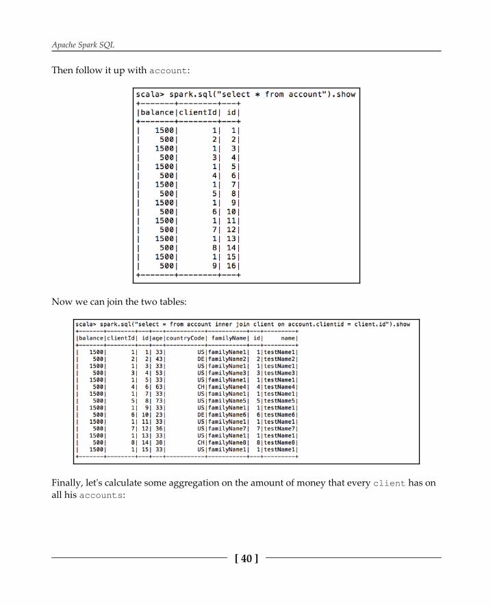
Then follow it up with :
Now we can join the two tables:
Finally, let's calculate some aggregation on the amount of money that every has onall his :

Apache Spark SQL
[ 41 ]
Using DatasetsThis API as been introduced since Apache Spark 1.6 as experimental and finally became afirst-class citizen in Apache Spark 2.0. It is basically a strongly typed version of DataFrames.
DataFrames are kept for backward compatibility and are not going to be deprecated for tworeasons. First, a DataFrame since Apache Spark 2.0 is nothing else but a Dataset where thetype is set to This means that you actually lose the strongly static typing and fall backto a dynamic typing. This is also the second reason why DataFrames are going to stay.Dynamically typed languages such as Python or R are not capable of using Datasetsbecause there isn't a concept of strong, static types in the language.
So what are Datasets exactly? Let's create one:
As you can see, we are defining a case class in order to determine the types of objects storedin the Dataset. This means that we have a strong, static type here that is clear at compiletime already. So no dynamic type inference is taking place there. This allows for a lot offurther performance optimization and also adds compile type safety to your applications.We'll cover the performance optimization aspect in more detail in the , TheCatalyst Optimizer, and , Project Tungsten. As you have seen before, DataFramescan be created from an RDD containing objects. These also have a schema. Note that thedifference between Datasets and DataFrame is that the objects are not static types as theschema can be created during runtime by passing it to the constructor using objects (refer to the last section on DataFrames). As mentioned before, a DataFrame-equivalent Dataset would contain only elements of the type. However, we can dobetter. We can define a static case class matching the schema of our client data stored in
:

Apache Spark SQL
[ 42 ]
Now we can reread our file but this time, we convert it to a Dataset:
Now we can use it similarly to DataFrames, but under the hood, typed objects are used torepresent the data:
If we print the schema, we get the same as the formerly used DataFrame:

Apache Spark SQL
[ 43 ]
The Dataset API in actionWe conclude on Datasets with a final aggregation example using the relational Dataset API.Note that we now have an additional choice of methods inspired by RDDs. So we can mixin the map function known from RDDs as follows:
Let's understand how this works step by step:
This basically takes the Dataset and filters it to rows containing clients with ages1.over 18.Then, from the object c, we only take the and 2.columns. This process is again a projection and could have been done using the
method. The method is only used here to show the capabilities ofusing lambda functions in conjunction with Datasets without directly touchingthe underlying RDD.Now, we group by . We are using the so-called Catalyst (DSL3.Domain Specific Language) in the method to actually refer to thesecond element of the tuple that we created in the previous step.Finally, we average on the groups that we previously created--basically4.averaging the age per country.
The result is a new strongly typed Dataset containing the average age for adults by country:
Apache Spark SQL
[ 44 ]
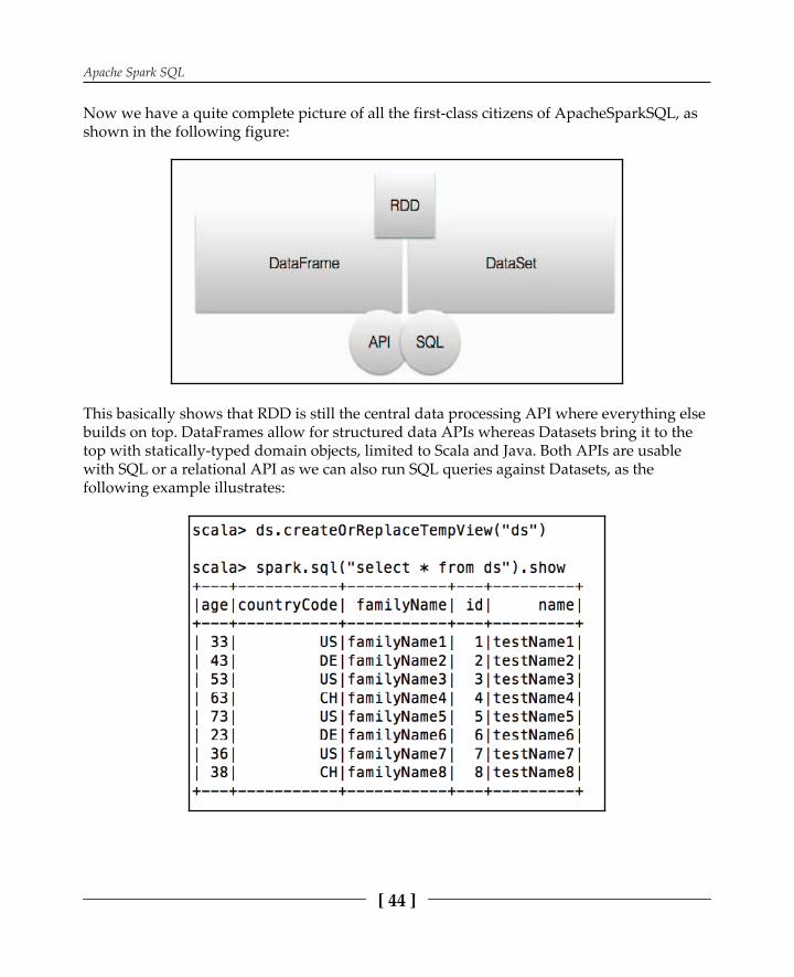
Now we have a quite complete picture of all the first-class citizens of ApacheSparkSQL, asshown in the following figure:
This basically shows that RDD is still the central data processing API where everything elsebuilds on top. DataFrames allow for structured data APIs whereas Datasets bring it to thetop with statically-typed domain objects, limited to Scala and Java. Both APIs are usablewith SQL or a relational API as we can also run SQL queries against Datasets, as thefollowing example illustrates:

Apache Spark SQL
[ 45 ]
This gives us some idea of the SQL-based functionality within Apache Spark, but what if wefind that the method that needed is not available? Perhaps we need a new function. This iswhere user-defined functions (UDFs) are useful. We will cover them in the next section.
User-defined functionsIn order to create user-defined functions in Scala, we need to examine our data in theprevious Dataset. We will use the age property on the client entries in the previouslyintroduced . We plan to create an UDF that will enumerate the age column.This will be useful if we need to use the data for machine learning as a lesser number ofdifferent values is sometimes useful. This process is also called binning or categorization.This is the file with the property added:
Now let's define a Scala enumeration that converts ages into age range codes. If we use thisenumeration among all our relations, we can ensure consistent and proper coding of theseranges:

Apache Spark SQL
[ 46 ]
We can now register this function using in Scala so that it can be used in aSQL statement:
The newly registered function called can now be used in the statement. It takes as a parameter and returns a string for the range:
RDDs versus DataFrames versus DatasetsTo make it clear, we are discouraging you from using RDDs unless there is a strong reasonto do so for the following reasons:
RDDs, on an abstraction level, are equivalent to assembler or machine code whenit comes to system programmingRDDs express how to do something and not what is to be achieved, leaving noroom for optimizersRDDs have proprietary syntax; SQL is more widely known
Whenever possible, use Datasets because their static typing makes them faster. As long asyou are using statically typed languages such as Java or Scala, you are fine. Otherwise, youhave to stick with DataFrames.

Apache Spark SQL
[ 47 ]
SummaryThis chapter started by explaining the object and file I/O methods. It thenshowed that Spark- and HDFS-based data could be manipulated as both, DataFrames withSQL-like methods and Datasets as strongly typed version of Dataframes, and with SparkSQL by registering temporary tables. It has been shown that schema can be inferred usingthe DataSource API or explicitly defined using on DataFrames or
on Datasets.
Next, user-defined functions were introduced to show that the functionality of Spark SQLcould be extended by creating new functions to suit your needs, registering them as UDFs,and then calling them in SQL to process data. This lays the foundation for most of thesubsequent chapters as the new DataFrame and Dataset API of Apache Spark is the way togo and RDDs are only used as fallback.
In the coming chapters, we'll discover why these new APIs are much faster than RDDs bytaking a look at some internals of Apache SparkSQL in order to understand why ApacheSparkSQL provides such dramatic performance improvements over the RDD API. Thisknowledge is important in order to write efficient SQL queries or data transformations ontop of the DataFrame or Dataset relational API. So, it is of utmost importance that we take alook at the Apache Spark optimizer called Catalyst, which actually takes your high-levelprogram and transforms it into efficient calls on top of the RDD API and, in later chapters,Tungsten, which is integral to the study of Apache Spark.

33The Catalyst Optimizer
The Catalyst Optimizer is one of the most exciting developments in Apache Spark. This isbecause it basically frees your mind from writing effective data processing pipelines, andlets the optimizer do it for you.
In this chapter, we will like to introduce the Catalyst Optimizer of Apache Spark SQLrunning on top of SQL, DataFrames, and Datasets.
This chapter will cover the following topics:
The catalogAbstract syntax treesThe optimization process on logical and physical execution plansCode generationOne practical code walk-through

The Catalyst Optimizer
[ 49 ]
Understanding the workings of the CatalystOptimizerSo how does the optimizer work? The following figure shows the core components andhow they are involved in a sequential optimization process:
First of all, it has to be understood that it doesn't matter if a DataFrame, the Dataset API, orSQL is used. They all result in the same Unresolved Logical Execution Plan (ULEP). A
is unresolved if the column names haven't been verified and the column typeshaven't been looked up in the catalog. A Resolved Logical Execution Plan (RLEP) is thentransformed multiple times, until it results in an Optimized Logical Execution Plan. LEPsdon't contain a description of how something is computed, but only what has to becomputed. The optimized LEP is transformed into multiple Physical Execution Plans (PEP)using so-called strategies. Finally, an optimal PEP is selected to be executed using a costmodel by taking statistics about the Dataset to be queried into account. Note that the finalexecution takes place on RDD objects.

The Catalyst Optimizer
[ 50 ]
Managing temporary views with the catalogAPISince Apache Spark 2.0, the catalog API is used to create and remove temporary views froman internal meta store. This is necessary if you want to use SQL, because it basicallyprovides the mapping between a virtual table name and a DataFrame or Dataset.
Internally, Apache Spark uses the class to manage
temporary views as well as persistent tables.
Temporary views are stored in the object, as persistent tables are stored inan external metastore. The abstract base class
is extended for variousmeta store providers. One already exists for using Apache Derby and another one for theApache Hive metastore, but anyone could extend this class and make Apache Spark useanother metastore as well.
The SQL abstract syntax treeAs explained earlier, it doesn't matter if you are using SQL, DataFrame, or Dataset, theApache Spark SQL parser returns an abstract syntax tree. However, DataFrames or Datasetscan be used as starting points. The result of all these methods is again a tree-based structurecalled ULEP. The following figure is an example of such an AST (abstract syntax tree)adding an attribute coming from a row in a table and two literals together:

The Catalyst Optimizer
[ 51 ]
So as you can see, at the bottom of the tree (those nodes are also called leaves since theydon't have any further nodes connecting to them) we have two integer literals: one and two.On top we have an operation taking those two literals and adding them together. Youshould note that those literals could also be loaded from a persistent data store. The Addoperation virtually turns into another literal (three in this case), which then again is used byanother Add operation as one of its inputs. The other input labeled as Attribute(x) nowtakes the value of x of that particular relation and exposes it as materialized value to theAdd operator. So in other words, this AST does nothing else than add the number three toeach of the values in column x.
How to go from Unresolved LogicalExecution Plan to Resolved LogicalExecution PlanThe ULEP basically reflects the structure of an AST. So again, the AST is generated from theuser's code implemented either on top of the relational API of DataFrames and Datasets orusing SQL, or all three. This AST can be easily transformed into a ULEP. But, of course, aULEP can't be executed. The first thing that is checked is if the referred relations exist in thecatalog. This means all table names and fields expressed in the SQL statement or relationalAPI have to exist. If the table (or relation) exists, the column names are verified. In addition,the column names that are referred to multiple times are given an alias in order to readthem only once. This is already a first stage optimization taking place here. Finally, the datatypes of the columns are determined in order to check if the operations expressed on top ofthe columns are valid. So for example taking the sum of a string doesn't work and this erroris already caught at this stage. The result of this operation is a Resolved Logical ExecutionPlan (LEP).
Internal class and object representations of LEPsAs an unresolved plan is basically the first tree created from either SQL statements or therelational API of DataFrames and Datasets, it is mainly composed of sub-types of the
objects, which are bound together by the objects, thereforeforming a tree of the objects since all these objects are sub-types of .Overall, this data structure is a , which is therefore reflected as a
object. Note that extends , and itself is again. In other words, is nothing else than a set of
objects.

The Catalyst Optimizer
[ 52 ]
The following two figures illustrate the inheritance tree of the different objects discussed:
As can be seen clearly in the previous figure, is the parent of most of thefunctional operators. Let's take for example. , a child class of ,is parent to and .

The Catalyst Optimizer
[ 53 ]
An easy way to explore Java and Scala inheritance trees in Eclipse is byopening any particular class or interface using the function(Navigate | Open Type...) and then just type in the desired name, forexample LeafExpression. Once the type is opened, the Open TypeHierarchy (Navigate | Open Type Hierarchy...) function can be used togenerate those diagrams, as can be seen in previous figures.
Since in an SQL expression denotes all columns of a particular relation, Catalyst has toquery the catalog in order to determine the names and types of columns referred to. So oncethe tree gets transformed from to , also those classes are replaced.All these classes are inherited from and are used to form abstract syntax trees.The same holds true not only for abstract syntax trees, but also for execution plans, as
also inherits from :

The Catalyst Optimizer
[ 54 ]
How to optimize the Resolved Logical ExecutionPlanThe resolved LEP can now be optimized. This is done using a set of transformation rules.
Since a LEP is just a tree, the rules transform from one tree to another. This is doneiteratively until no rule fires anymore and keeps the LEP stable and the process is finished.The result of this step is an Optimized Logical Execution Plan.
Physical Execution Plan generation and selectionThe Resolved and Optimized LEP is used to generate a large set of PEP candidates. PEPsare execution plans that have been completely resolved. This means that a PEP containsdetailed instructions to generate the desired result. They are generated by so-calledstrategies. Strategies are used to optimize selection of join algorithms based on statistics. Inaddition, rules are executed for example to pipeline multiple operations on an RDD into asingle, more complex operation. After a set of PEPs has been generated - they all will returnthe exact same result - the best one is chosen based on heuristics in order to minimizeexecution time.
In case the data source supports it, operations are pushed down to the source, namely forfiltering (predicate) or selection of attributes (projection). This concept is explained in verydetail on , Apache Spark SQL, in the section called Predicate push-down on smart datasources.
The main idea of predicate push-down is that parts of the AST are not executed by ApacheSpark but by the data source itself. So for example filtering rows on column names can bedone much more efficient by a relational or NoSQL database since it sits closer to the dataand therefore can avoid data transfers between the database and Apache Spark. Also, theremoval of unnecessary columns is a job done more effectively by the database.

The Catalyst Optimizer
[ 55 ]
Code generationFinally, things can be improved even more, since Apache Spark runs on the Java VirtualMachine (JVM), which allows byte code to be created and modified during runtime. Let'sconsider an addition of values and , resulting in the expression . Normally, thisexpression had to be interpreted by the JVM for each row of the Dataset. It would be nice ifwe could generate the JVM ByteCode for this expression on the fly. This is possible, andCatalyst makes use of a very cool Scala feature called Quasiquotes, which basically allowsan arbitrary string containing Scala code to be compiled into ByteCode on the fly, if it startswith . So for example, will tell the Scala compiler to usethis String to generate further JVM byte code. This way, less code has to be interpreted,which speeds things up.
Practical examplesIn order to facilitate understanding of these components, we'll introduce some practicalexamples using Scala code. Consider data about clients and accounts according to thefollowing schemas:
As you might now, a class is somehow the Scala equivalent toJavaBeans and is meant for implementing data transfer objects (DTOs)without further logic built into the class. A class is compared byvalue and not by reference, which is the default for all other classes.Finally, the copy method allows for easy duplications of DTOs.
This case class specifies the schema for rows of the relation. Let's have a look at theschema for the relation:

The Catalyst Optimizer
[ 56 ]
Now we can create Datasets from different files and file types in order to see how theoptimizer reacts:
Then we register all as temporary tables, so that we can write ordinary SQL statementsagainst them. First, we'll do this for the backed DataFrames:
Then we also do the same for the backed DataFrames:
Using the explain method to obtain the PEPIn order to get an idea of what is happening behind the scenes, we can call the method on the Dataset. This returns (as text) an output what the Catalyst Optimizer didbehind the scenes by printing a text representation of the PEP.
So let's have a look at what happens if we join two Datasets backed by the files:

The Catalyst Optimizer
[ 57 ]
The resulting execution plan (PEP) looks like this:
Since this might be a bit hard to read for beginners, find the same plan in the followingfigure:
So what is done here is basically--when read from bottom to top--two read operations to files followed by a filter operations to ensure that the columns of the join predicate
are not null. This is important since otherwise the join operation fails.
In relational databases, the filter would be a redundant step,since RDBMS recognizes the notion of not nullable columns; therefore, thenull check is done during insert and not during read.

The Catalyst Optimizer
[ 58 ]
Then, a projection operation is performed, which basically means that unnecessary columnsare removed. We are only selecting , but for the operation, and
are also necessary. Therefore, these fields are included in the set of column names to beobtained as well.
Finally, all data is available to execute the join.
Note that in the preceding diagram, is illustrated assingle stage, but in reality, a join spans partitions over - potentially -multiple physical nodes. Therefore, the two tree branches are executed inparallel and the results are shuffled over the cluster using hash bucketingbased on the join predicate.
As previously stated, the files are smart data sources, since projection and filteringcan be performed at the storage level, eliminating disk reads of unnecessary data. This canbe seen in the and sections in the explained plan, where the
operation and the projection on , , and is directly performed at the read level of the files.
How smart data sources work internallyJDBC stands for Java Database Connectivity. When talking about Apache Spark and JDBCthere is sometimes a bit of confusion because JDBC can be used in the context of a datasource as well as referred to Apache Spark's capability to serve as JDBC-compliant datasource to other systems. The latter is not further covered in this book, whereas the former isonly used as one particular example where the data source (in this case a relationaldatabase) can be transparently used for data pre-processing without the user of ApacheSparkSQL further noticing it.
If you want to use Apache SparkSQL as a data source for otherJAVA/JVM-based applications you have to start the JDBC Thrift server, asexplained here:
. Thefollowing website explains how to connect to a MySQL database fromApache SparkSQL using JDBC:
. And more on JDBC in generalcan be found here:
.

The Catalyst Optimizer
[ 59 ]
Now we want to show how Apache Spark internally implements smart data sourcesexemplified on a filter pushed down to a JDBC data source. This means that if in a PEP datahas to be filtered, then this filter will be executed in the SQL statement on the RDBMS whenthe underlying data is read. This way, reading unnecessary data is avoided. Depending onthe seductiveness of the filter predicate, the performance gain can be multiple orders ofmagnitude.
):
This trait defines a method called , which takes two parameters. First, a list ofcolumn names which have to be included in the result, and second, an array of filter objectsbasically expressing the query predicate pushed down to the underlying smart data source.The return type is of . One example is implemented in the class(again, here is the link to the source code
):
implemented the method in the following way:

The Catalyst Optimizer
[ 60 ]
As we can see, this method is just a . Therefore, we have to have a look at the method of the class. It is interesting to note that, in case of ,
support for predicate push-down is implemented directly in the class. But we'll skip the method for now, since it just parameterizes and creates a new object.
So the most interesting method in is , which it inherits from the abstract class. Through the method, Apache Spark tells this RDD to get out of lazy
mode and materialize itself whenever it is appropriate during computation of a dataprocessing job. We'll show you two important fractions of this method after we have had alook at the method signature:
Here you can see that the return type is of , which allows a lazy underlying datasource to be read lazily as well. As we can see, this is the case for this particularimplementation as well:
Note that the SQL statement created and stored in the constant isreferencing two interesting variables: and .Both are derived from the and argumentspassed to the class.
Therefore, this data source can be called a smart source, because the underlying storagetechnology (an SQL database in this case) can be told to only return columns and rowswhich are actually requested. And as already mentioned, the data source supports passinglazy data access patterns to be pushed to the underlying database as well. Here you can seethat the JDBC result set is wrapped into a typed iterator,
. Since this matches the return type of the method, weare done upon execution of the following code:

The Catalyst Optimizer
[ 61 ]
Note that obtained from the JDBC database query is passed to (wrappedinto) a object. Therefore, the JDBC connection stays open, and the RDBMScourser doesn't get destroyed and can be used to return subsequent data once requestedfrom Apache Spark.
SummaryThis chapter basically was a sales pitch for using DataFrames, Datasets, and SQL overRDDs, because in the majority of cases, the optimizer does such a great job that theperformance is nearly equal to hand-optimized code on RDDs. You now know the internalsof the optimizer, which will give you a solid foundation in using all components that arebased on it and that are introduced in the subsequent chapters.
The next chapter is dedicated to Tungsten Phase I and Phase II, which is a mind-blowingtechnology that accelerates computations by a factor of 100, so stay tuned!

44Project Tungsten
This chapter introduces Project Tungsten. CPU and main memory performance became thenew bottlenecks in big data processing after the massive increase in I/O performance due tothe usage of solid state disks (SSDs) and 10 Gbps Ethernet. Therefore, Project Tungsten,the core of the Apache Spark execution engine, aims at improving performance at the CPUand main memory level. This chapter will cover the following topics:
Memory management beyond the Java Virtual Machine (JVM) GarbageCollector (GC)Cache-friendly layout of data in memoryCode generation
We will have an in-depth look at all these three topics now.
Memory management beyond the JavaVirtual Machine Garbage Collector
The JVM Garbage Collector is in support of the whole object's life cyclemanagement the JVM provides. Whenever you see the word in Javacode, memory is allocated in a JVM memory segment called .

Project Tungsten
[ 63 ]
Java completely takes care of memory management and it is impossible to overwritememory segments that do not belong to you (or your object). So if you write something toan object's memory segment on the heap (for example by updating a class property value oftype , you are changing 32 bit on the heap) you don't use the actual heap memoryaddress for doing so but you use the reference to the object and either access the object'sproperty or use a setter method.
So we've learned about allocated memory on the heap, but how does it ever get freed?This is where the Java Garbage collector kicks in. It continuously monitors how many activereferences to a certain object on the heap exist and once no more references exist thoseobjects are destroyed and the allocated memory is freed.
References to an object can either exist within objects on the heap itself or in the stack. Thestack is a memory segment where variables in method calls and variables defined withinmethods reside. They are usually short lived whereas data on the heap might live forlonger.
This topic would be worth a book on it's own, because there are a lot of catches, for examplecircular references of objects which are not used anymore but kind of dead-lock themselvesand many more. Therefore we stop there on explaining how exactly this works but let'sconclude with the following statement: The Garbage Collector is a highly complex component and has been optimized to support Online Transaction Processing (OLTP)workloads whereas Apache Spark concentrates on Online Analytical Processing (OLAP).There is a clash between optimizing a garbage collector for both disciplines at the same timesince the object life cycle is very different between those two disciplines.
The main idea behind Tungsten is to get rid of the JVM Garbage Collector. Although for thegeneral purpose bytecode, the GC does a pretty awesome job of predicting object life cycles,and the resulting frequency and bearing of GC cycles. But Apache Spark knows betterwhich data has to be kept and which data can be removed from the memory. Therefore,Tungsten bypasses the managed (and safe) memory management system which the JVMprovides and uses the classes from the package, which allows Tungstento manage memory layout on its behalf.
Understanding the UnsafeRow objectAt its core, since Apache Spark V1.4 Tungsten uses
, which is a binaryrepresentation of a row object. An object consists of three regions, as illustratedin the following figure:
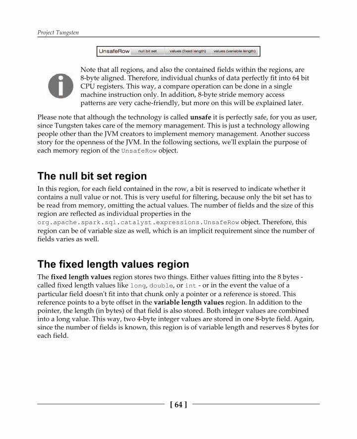
Project Tungsten
[ 64 ]
Note that all regions, and also the contained fields within the regions, are8-byte aligned. Therefore, individual chunks of data perfectly fit into 64 bitCPU registers. This way, a compare operation can be done in a singlemachine instruction only. In addition, 8-byte stride memory accesspatterns are very cache-friendly, but more on this will be explained later.
Please note that although the technology is called unsafe it is perfectly safe, for you as user,since Tungsten takes care of the memory management. This is just a technology allowingpeople other than the JVM creators to implement memory management. Another successstory for the openness of the JVM. In the following sections, we'll explain the purpose ofeach memory region of the object.
The null bit set regionIn this region, for each field contained in the row, a bit is reserved to indicate whether itcontains a null value or not. This is very useful for filtering, because only the bit set has tobe read from memory, omitting the actual values. The number of fields and the size of thisregion are reflected as individual properties in the
object. Therefore, thisregion can be of variable size as well, which is an implicit requirement since the number offields varies as well.
The fixed length values regionThe fixed length values region stores two things. Either values fitting into the 8 bytes -called fixed length values like , , or - or in the event the value of aparticular field doesn't fit into that chunk only a pointer or a reference is stored. Thisreference points to a byte offset in the variable length values region. In addition to thepointer, the length (in bytes) of that field is also stored. Both integer values are combinedinto a long value. This way, two 4-byte integer values are stored in one 8-byte field. Again,since the number of fields is known, this region is of variable length and reserves 8 bytes foreach field.

Project Tungsten
[ 65 ]
The variable length values regionFinally, the variable length values region, the last region of an object, containsvariable-sized fields like strings. As mentioned earlier, a pointer containing the offset to theposition in the variable length values region is stored in the fixed length values region.Since offset and length are known to be stored in the fixed length values region, a variablesized value can be easily addressed.
For those of you interested in getting a better idea about how these offsets are calculated,let's have a look at some code. Note that this code is Java code, since has beenimplemented in Java instead of Scala:
The method returns the byte offset of a fixed size field by using of the object itself, adding the size of the first region to it
( ) and finally jumping right to the start of the correct slot by usingordinal, which stores the number/id of the field multiplied by eight. We multiply by eightbecause all slots are 8-byte aligned.
Slightly more complicated is addressing variable sized fields. Let's have a look at thecorresponding Java code:
First, we check in the fixed size region if the value is , because then we can alreadystop here and return . Then, is obtained by reading an ordinary from the fixed size region, which stores the offset and length of variable size objects in thevariable sized objects area. Next, this value has to be split into two values,containing offset and size separately, therefore , right-shifted 32 bits andcast to to resemble the offset value, whereas only casting to resembles the size value. Finally, using all these address values, a object is createdfrom the raw bytes within the object.

Project Tungsten
[ 66 ]
Understanding the BytesToBytesMapA very common data structure in Java is . The advantage of such adata structure is fast, but more importantly, convenient data access since only a key, whichcan be any sort of Java object, has to be provided to obtain the value; again, any type of Javaobject is supported as the key. While convenient for the programmer, has some drawbacks. The most important are:
Memory overhead due to usage of objects as keys and valuesVery cache-unfriendly memory layoutImpossible to directly address fields by calculating offsets
This means that simple but important things, such as sequential scans, result in veryrandom and cache-unfriendly memory access patterns. Therefore, Tungsten has introduceda new data structure called , which has improved the memory localityand has led to less space overhead by avoiding the usage of heavyweight Java objects,which has improved performance. Sequential scans are very cache friendly, since theyaccess the memory in sequence.
A practical example on memory usage andperformanceSo let's have a look at how Tungsten actually saves a lot of memory when usingDataFrames or Datasets in contrast to RDDs. Let's have a look at the following code:
Here we create a Scala list containing 1,000,000 integers, create a RDD out of it, cache it, andfinally count the number of entries. We can do the same using a DataFrame:

Project Tungsten
[ 67 ]
Again, we take the list of integers, but this time we create a DataFrame out of it. And again,we cache and count.
Luckily Apache Spark provides very detailed insights into its internals. We can access themanagement UI of Apache Spark on port . Besides job-and task-related information,the Storage tab provides information on each RDD currently existing on the cluster. Let'shave a look at memory usage:
We can see that the RDD takes nearly 4 megabytes of memory, whereas DataFrame (whichis backed by a object) takes only 1 megabyte. Unfortunately, while the wrappingof values into the objects has advantages for memory consumption, it hasdisadvantages for execution performance. Therefore, we give it another try using a Dataset:
First, we create a class for the Dataset's content, since Datasets are strongly (andstatically) typed. Then we use the existing DataFrame object in order to create a Dataset
out of it. And then, again, we count. Now we ran three Apache Spark jobs on the threedifferent data types and we can take a look at their execution times:

Project Tungsten
[ 68 ]
As we can see, the first job on the RDD took only 500 ms, whereas the second job on theDataFrame took two seconds. This means that saving memory actually caused an increasein execution time.
Fortunately, when using Datasets, this performance loss is mitigated and we can takeadvantage of both the fast execution time and the efficient usage of memory.
Why are we using DataFrames and Datasets at all if RDDs are faster? Wecould also just put additional memory to the cluster. Note that althoughthis particular execution on an RDD runs faster, Apache Spark jobs arevery rarely composed only out of a single operation on an RDD. In theoryyou could write very efficient Apache Spark jobs on RDDs only, butactually re-writing your Apache Spark application for performance tuningwill take a lot of time. So the best way is to use DataFrames and Datasets,to make use of the Catalyst optimizer, in order to get efficient calls to theRDD operations generated.

Project Tungsten
[ 69 ]
Cache-friendly layout of data in memoryIn order to understand how data structures can be laid out in a cache-friendly manner, let'shave a brief look at how caches work in general. Memory on a modern computer system isaddressed using 64 bit addresses pointing to 64 bit memory blocks. Remember, Tungstentries to always use 8-byte Datasets which perfectly fit into these 64-bit memory blocks.
So between your CPU cores and main memory, there is a hierarchical list of L1, L2, and L3caches-with increasing size. Usually, L3 is shared among all the cores. If your CPU corerequests a certain main memory address to be loaded into the CPU core's register (a registeris a memory area in your CPU core) - this happens by an explicit machine code (assembler)instruction - then first the L1-3 cache hierarchy is checked to see if it contains the requestedmemory address.
We call data associated with such an address a memory page. If this is the case, then mainmemory access is omitted and the page is directly loaded from the L1, L2, or L3 cache.Otherwise, the page is loaded from main memory, resulting in higher latency. The latency isso high that the CPU core is waiting (or executing other work) for multiple CPU clockcycles, until the main memory page is transferred into the CPU core's register. In addition,the page is also put into all caches, and in case they are full, less frequently accessedmemory pages are deleted from the caches.
This brings us to the following two conclusions:
Caching only makes sense if memory pages are accessed multiple times during acomputation.Since caches are far smaller than main memory, they only contain subsets of themain memory pages. Therefore, a temporally close access pattern is required inorder to benefit from the caches, because if the same page is accessed at a verylate stage of the computation, it might have already gotten evicted from thecache.
Cache eviction strategies and pre-fetchingOf course, modern computer systems not only use least recently used (LRU) memory pageeviction strategies to delete cached memory pages from the caches, they also try to predictthe access pattern in order to keep the memory pages that are old but have a highprobability of being requested again. In addition, modern CPUs also try to predict futurememory page requests and try to pre-fetch them. Nevertheless, random memory accesspatterns should always be avoided and the more sequential memory access patterns are,usually the faster they are executed.
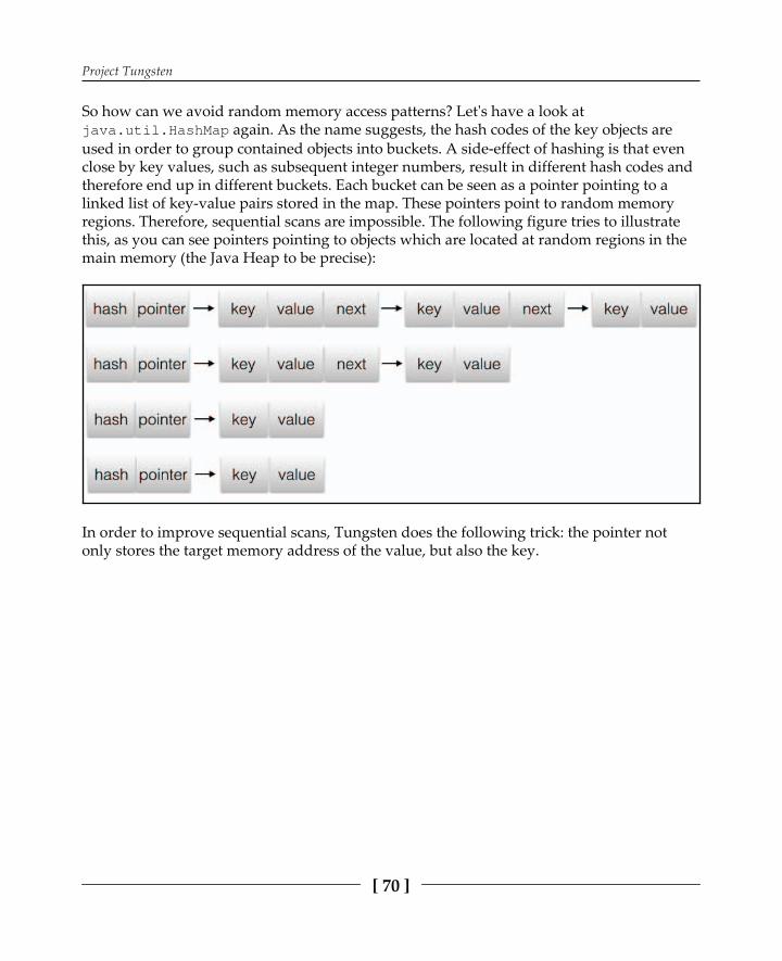
Project Tungsten
[ 70 ]
So how can we avoid random memory access patterns? Let's have a look at again. As the name suggests, the hash codes of the key objects are
used in order to group contained objects into buckets. A side-effect of hashing is that evenclose by key values, such as subsequent integer numbers, result in different hash codes andtherefore end up in different buckets. Each bucket can be seen as a pointer pointing to alinked list of key-value pairs stored in the map. These pointers point to random memoryregions. Therefore, sequential scans are impossible. The following figure tries to illustratethis, as you can see pointers pointing to objects which are located at random regions in themain memory (the Java Heap to be precise):
In order to improve sequential scans, Tungsten does the following trick: the pointer notonly stores the target memory address of the value, but also the key.

Project Tungsten
[ 71 ]
We have learned about this concept already, where an 8-byte memory region is used tostore two integer values, for example, in this case the key and the pointer to the value. Thisway, one can run a sorting algorithm with sequential memory access patterns (for example,quick-sort). The following figure illustrates this layout:
This way, when sorting, the key and pointer combination memory region must be movedaround but the memory region where the values are stored can be kept constant. While thevalues can still be randomly spread around the memory, the key and pointer combinationare sequentially laid out, as the following figure tries to illustrate:

Project Tungsten
[ 72 ]
This optimization was introduced in Apache Spark V1.5 and requested in the SPARK-7082feature request ( ).
Code generationApache Spark V1.5 introduced code generation for expression evaluation. In order tounderstand this, let's start with an example. Let's have a look at the following expression:
Imagine and are data coming from a row in a table. Now, consider that this expressionis applied for every row in a table of, let's say, one billion rows. Now the Java VirtualMachine has to execute (interpret) this expression one billion times, which is a hugeoverhead. So what Tungsten actually does is transform this expression into byte-code andhave it shipped to the executor thread.
As you might know, every class executed on the JVM is byte-code. This is an intermediateabstraction layer to the actual machine code specific for each different micro-processorarchitecture. This was one of the major selling points of Java decades ago. So the basicworkflow is:
Java source code gets compiled into Java byte-code.1.Java byte-code gets interpreted by the JVM.2.The JVM translates this byte-code and issues platform specific-machine code3.instructions to the target CPU.
These days nobody ever thinks of creating byte-code on the fly, but this is what's happeningin code generation. Apache Spark Tungsten analyzes the task to be executed and instead ofrelying on chaining pre-compiled components it generates specific, high-performing bytecode as written by a human to be executed by the JVM.
Another thing Tungsten does is to accelerate the serialization and deserialization of objects,because the native framework that the JVM provides tends to be very slow. Since the mainbottleneck on every distributed data processing system is the shuffle phase (used for sortingand grouping similar data together), where data gets sent over the network in ApacheSpark, object serialization and deserialization are the main contributor to the bottleneck(and not I/O bandwidth), also adding to the CPU bottleneck. Therefore increasingperformance here reduces the bottleneck.

Project Tungsten
[ 73 ]
All things introduced until now are known as Tungsten Phase 1 improvements. WithApache Spark V2.0, Tungsten Phase 2 improvements went live, which are the following:
Columnar storageWhole stage code generation
Understanding columnar storageWith Apache Spark V2.0, columnar storage was introduced. Many on-disk technologies,such as parquet, or relational databases, such as IBM DB2 BLU or dashDB, support it. So itwas an obvious choice to add this to Apache Spark as well. So what is it all about? Considerthe following figure:
If we now transpose, we get the following column-based layout:
In contrast to row-based layouts, where fields of individual records are memory-alignedclose together, in columnar storage values from similar columns of different records areresiding close together in memory. This changes performance significantly. Not only cancolumnar data such as parquet be read faster by an order of magnitude, columnar storagealso benefits when it comes to indexing individual columns or projection operations.

Project Tungsten
[ 74 ]
Understanding whole stage code generationTo understand whole stage code generation, we have to understand the Catalyst Optimizeras well, because whole stage code generation is nothing but a set of rules during theoptimization of a Logical Execution Plan (LEP). The object called
, extending , is the object used by ApacheSpark for transforming a LEP, by fusing supported operators together. This is done bycreating byte code of a new custom operator with the same functionality of the originaloperators which has been fused together.
A practical example on whole stage code generationperformanceSo let's actually run a little test. We join one billion integers. Once with whole stage codegeneration turned off and once with it turned on. So let's first have a look at thecorresponding explained outputs:
An asterisk symbol, in the explained output, indicates that these operations are executed asa single thread with whole stage generated code. Note that the operation, which belongs to , is not part of this, since it might run onanother machine.
Operator fusing: Other data processing systems call this techniqueoperator fusing. In Apache Spark whole stage code generation is actuallythe only means for doing so.
Now, let's actually turn off this feature:
scala> spark.conf.set("spark.sql.codegen.wholeStage",false)

Project Tungsten
[ 75 ]
If we now explain the preceding statement again, we get the following output:
The only difference is the missing asterisk symbol in front of some operators, and thisactually means that each operator is executed as a single thread or at least as different codefragments, passing data from one to another.
So let's actually materialize this query by calling the method, once with and oncewithout whole stage code generation, and have a look at the performance differences:
As we can see, without whole stage code generation, the operations (composed of job 0 andjob 1) take nearly 32 seconds, whereas with whole stage code generation enabled, it takesonly slightly more than half a second (job id 2 and 3).

Project Tungsten
[ 76 ]
If we now click on the job's description, we can obtain a DAG visualization, where DAGstands for directed acyclic graph - another way of expressing a data processing workflow:
DAG visualization is a very important tool when it comes to manualperformance optimization. This is a very convenient way to find out howApache Spark translates your queries into a physical execution plan. Andtherefore a convenient way of discovering performance bottlenecks.
By the way, RDBMS administrators use a similar visualization mechanism in relationaldatabase tooling which is called visual explain. As we can see in Apache Spark V2.0, withthe whole stage code generation enabled, multiple operators get fused together.
Project Tungsten
[ 77 ]
Operator fusing versus the volcano iterator modelThe volcano iterator model is an internal data processing model. Nearly every relationaldatabase system makes use of it. It basically says that each atomic operation is only capableto processing one row at a time. By expressing a database query as a directed acyclic graph(DAG), which connects individual operators together, data flows in the opposite directionof the edge direction of the graph. Again, one row at a time, which means that multipleoperators run in parallel, but every operator processes a different, and only one, row at atime. When fusing operators together (this is what whole stage code generation does), thevolcano iterator model is violated. It is interesting to see that such a violation was done afterdecades of database research and actually leads to better performance.
SummaryThis chapter and the preceding chapter on Catalyst Optimizer have been quite challenging.However, it makes sense to cover so many Apache Spark internals, as in the subsequentchapters we will always refer back to the functionalities provided by Catalyst andTungsten.
We've learned that many features the JVM provides are far from optimal for massiveparallel data processing. This starts with the Garbage Collectors, includes inefficient datastructures and ends with the introduction of columnar storage and the removal of thevolcano iterator model by fusing individual operators together using whole stage codegeneration.
In the next chapter we'll have a look at a more practical function of Apache Spark. We'lltake a look at how to process data in real-time using Apache Spark Streaming.

55Apache Spark Streaming
The Apache Streaming module is a stream processing-based module within Apache Spark.It uses the Spark cluster to offer the ability to scale to a high degree. Being based on Spark, itis also highly fault tolerant, having the ability to rerun failed tasks by checkpointing thedata stream that is being processed. The following topics will be covered in this chapterafter an introductory section, which will provide a practical overview of how Apache Sparkprocesses stream-based data:
Error recovery and checkpointingTCP-based stream processingFile streamsKafka stream source
For each topic, we will provide a worked example in Scala and show how the stream-basedarchitecture can be set up and tested.

Apache Spark Streaming
[ 79 ]
OverviewThe following diagram shows potential data sources for Apache Streaming, such as Kafka,Flume, and HDFS:
These feed into the Spark Streaming module and are processed as Discrete Streams. Thediagram also shows that other Spark module functionality, such as machine learning, can beused to process stream-based data.
The fully processed data can then be an output for HDFS, databases, or dashboards. Thisdiagram is based on the one at the Spark streaming website, but we wanted to extend it toexpress the Spark module functionality:

Apache Spark Streaming
[ 80 ]
When discussing Spark Discrete Streams, the previous figure, taken from the Spark websiteat , is the diagram that we would like to use.
The green boxes in the previous figure show the continuous data stream sent to Spark beingbroken down into a Discrete Stream (DStream).
A DStream is nothing other than an ordered set of RDDs. Therefore, ApacheSpark Streaming is not real streaming, but micro-batching. The size of theRDDs backing the DStream determines the batch size. This way DStreams canmake use of all the functionality provided by RDDs including fault toleranceand the capability of being spillable to disk. The size of each element in thestream is then based on a batch time, which might be two seconds.
It is also possible to create a window, expressed as the previous red box, over the DStream.For instance, when carrying out trend analysis in real time, it might be necessary todetermine the top ten Twitter-based hashtags over a ten-minute window.
So, given that Spark can be used for stream processing, how is a stream created? Thefollowing Scala-based code shows how a Twitter stream can be created. This example issimplified because Twitter authorization has not been included, but you get the idea. (Thefull example code is in the Checkpointing section.)
The Spark Stream Context (SSC) is created using the Spark Context, . A batch time is specified when it is created; in this case, seconds. A Twitter-based DStream, called stream,is then created from using a window of seconds:
Stream processing can be started with the stream context method (shown next), andthe method indicates that it should process until stopped. So, if thiscode is embedded in a library-based application, it will run until the session is terminated,perhaps with Crtl + C:
This explains what Spark Streaming is and what it does, but it does not explain errorhandling or what to do if your stream-based application fails. The next section will examineSpark Streaming error management and recovery.

Apache Spark Streaming
[ 81 ]
Errors and recoveryGenerally, the question that needs to be asked for your application is: is it critical that you receive and process all the data? If not, then on failure, you might just be able to restart theapplication and discard the missing or lost data. If this is not the case, then you will need touse checkpointing, which will be described in the next section.
It is also worth noting that your application's error management should be robust and self-sufficient. What we mean by this is that if an exception is non-critical, then manage theexception, perhaps log it, and continue processing. For instance, when a task reaches themaximum number of failures (specified by ), it will terminateprocessing.
This property, among others can be set during creation of the object or as additional command line parameters when
invoking or .
CheckpointingOn batch processing we are used to having fault tolerance. This means, in case a nodecrashed, the job doesn't loose its state and the lost tasks are rescheduled on other workers.Intermediate results are written to persistent storage (which of course has to be faulttolerant as well which is the case for HDFS, GPFS or Cloud Object Storage). Now we wantto achieve the same guarantees in streaming as well, since it might be crucial that the datastream we are processing is not lost.
It is possible to set up an HDFS-based checkpoint directory to store Apache Spark-basedstreaming information. In this Scala example, data will be stored in HDFS under
. The following HDFS filesystem command shows thatbefore starting, the directory does not exist:
[hadoop@hc2nn stream]$ hdfs dfs -ls /data/spark/checkpoint ls: `/data/spark/checkpoint': No such file or directory
For replicating the following example, Twitter API credentials are used in order to connectto the Twitter API and obtain a stream of tweets. The following link explains how suchcredentials are created within the Twitter UI:
.

Apache Spark Streaming
[ 82 ]
The following Scala code sample starts by importing Spark Streaming Context and Twitter-based functionality. It then defines an application object named :
Next, a method is defined called , which will be used to create both theSpark and Streaming contexts. It will also checkpoint the stream to the HDFS-baseddirectory using the streaming context checkpoint method, which takes a directory path as aparameter. The directory path the value that was passed to the method:
Now, the main method is defined as is the HDFS directory, as well as Twitter accessauthority and parameters. The Spark Streaming context is either retrieved or createdusing the HDFS checkpoint directory via the method-- . Ifthe directory doesn't exist, then the previous method called is called,which will create the context and . Obviously, we have truncated our ownTwitter in this example for security reasons:
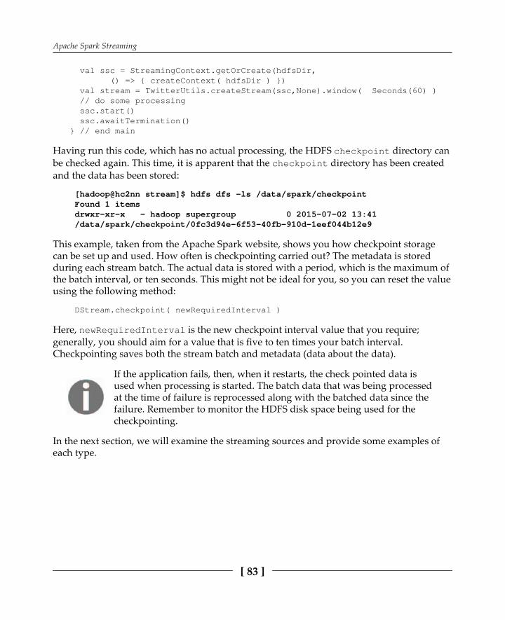
Apache Spark Streaming
[ 83 ]
Having run this code, which has no actual processing, the HDFS directory canbe checked again. This time, it is apparent that the directory has been createdand the data has been stored:
[hadoop@hc2nn stream]$ hdfs dfs -ls /data/spark/checkpoint Found 1 items drwxr-xr-x - hadoop supergroup 0 2015-07-02 13:41/data/spark/checkpoint/0fc3d94e-6f53-40fb-910d-1eef044b12e9
This example, taken from the Apache Spark website, shows you how checkpoint storagecan be set up and used. How often is checkpointing carried out? The metadata is storedduring each stream batch. The actual data is stored with a period, which is the maximum ofthe batch interval, or ten seconds. This might not be ideal for you, so you can reset the valueusing the following method:
Here, is the new checkpoint interval value that you require;generally, you should aim for a value that is five to ten times your batch interval.Checkpointing saves both the stream batch and metadata (data about the data).
If the application fails, then, when it restarts, the check pointed data isused when processing is started. The batch data that was being processedat the time of failure is reprocessed along with the batched data since thefailure. Remember to monitor the HDFS disk space being used for thecheckpointing.
In the next section, we will examine the streaming sources and provide some examples ofeach type.

Apache Spark Streaming
[ 84 ]
Streaming sourcesWe will not be able to cover all the stream types with practical examples in this section, butwhere this chapter is too small to include code, we will at least provide a description. In thischapter, we will cover the TCP and file streams and the Flume, Kafka, and Twitter streams.Apache Spark tends only to support this limited set out of the box, but this is not a problemsince 3rd party developers provide connectors to other sources as well. We will start with apractical TCP-based example. This chapter examines stream processing architecture.
For instance, what happens in cases where the stream data delivery rateexceeds the potential data processing rate? Systems such as Kafka providethe possibility of solving this issue by caching data until it is requestedwith the additional ability to use multiple data topics and consumers(publish-subscribe model).
TCP streamThere is a possibility of using the Spark Streaming Context method called
to stream data via TCP/IP, by specifying a hostname and port number.The Scala-based code example in this section will receive data on port that was supplied using the Linux command.
The command is a Linux/Unix command which allows you tosend and receive data to or from local or remote IP destinations using TCPor UDP. This way every shell script can play the role of a full networkclient or server. The following is a good tutorial on how to use :
.
The code sample starts by importing Spark, the context, and the streaming classes. Theobject class named is defined as it is the main method with arguments:

Apache Spark Streaming
[ 85 ]
The number of arguments passed to the class is checked to ensure that it is the hostnameand port number. A Spark configuration object is created with an application name defined.The Spark and streaming contexts are then created. Then, a streaming batch time of seconds is set:
A DStream called is created by calling the method of thestreaming context using the and port name parameters:
A top-ten word count is created from the raw stream data by splitting words with spacing.Then, a (key,value) pair is created as (word,1), which is reduced by the key value, this beingthe word. So now, there is a list of words and their associated counts. The key and value areswapped so the list becomes (count and word). Then, a sort is done on the key, which isnow the count. Finally, the top 10 items in the RDD within the DStream are taken andprinted out:
The code closes with the Spark Streaming and methods beingcalled to start the stream processing and await process termination:

Apache Spark Streaming
[ 86 ]
The data for this application is provided, as we stated previously, by the Linux Netcat ( )command. The Linux command dumps the contents of a log file, which is piped to .The options force Netcat to listen for connections and keep on listening if the connectionis lost. This example shows that the port being used is :
[root@hc2nn log]# pwd /var/log [root@hc2nn log]# cat ./anaconda.storage.log | nc -lk 10777
The output from this TCP-based stream processing is shown here. The actual output is notas important as the method demonstrated. However, the data shows, as expected, a list of10 log file words in descending count order. Note that the top word is empty because thestream was not filtered for empty words:
List : (17104,) List : (2333,=) List : (1656,:) List : (1603,;) List : (1557,DEBUG) List : (564,True) List : (495,False) List : (411,None) List : (356,at) List : (335,object)
This is interesting if you want to stream data using Apache Spark Streaming based onTCP/IP from a host and port. However, what about more exotic methods? What if you wishto stream data from a messaging system or via memory-based channels? What if you wantto use some of the big data tools available today such as Flume and Kafka? The nextsections will examine these options, but, first, we will demonstrate how streams can bebased on files.
File streamsWe have modified the Scala-based code example in the last section to monitor an HDFS-based directory by calling the Spark Streaming Context method called .We will not display all of the code, given this small change. The application class is nowcalled , which takes a single parameter--the HDFS directory. The directory pathcould be on another storage system as well (all the code samples will be available with thisbook):

Apache Spark Streaming
[ 87 ]
The stream processing is the same as before. The stream is split into words and the top-tenword list is printed. The only difference this time is that the data must be put in the HDFSdirectory while the application is running. This is achieved with the HDFS filesystem command here:
[root@hc2nn log]# hdfs dfs -put ./anaconda.storage.log /data/spark/stream
As you can see, the HDFS directory used is , and the text-basedsource log file is (under ). As expected, the same wordlist and count is printed:
List : (17104,)List : (2333,=)...List : (564,True)List : (495,False)List : (411,None)List : (356,at)List : (335,object)
These are simple streaming methods based on TCP and filesystem data. What if we want touse some of the built-in streaming functionality in Spark Streaming? This will be examinednext. The Spark Streaming Flume library will be used as an example.
FlumeFlume is an Apache open source project and product, which is designed to move largeamounts of data at a big data scale. It is highly scalable, distributed, and reliable, workingon the basis of data source, data sink, and data channels, as shown in the following diagramtaken from :

Apache Spark Streaming
[ 88 ]
Flume uses agents to process data streams. As can be seen in the previous figure, an agenthas a data source, data processing channel, and data sink. A clearer way to describe thisflow is via the figure we just saw. The channel acts as a queue for the sourced data and thesink passes the data to the next link in the chain.
Flume agents can form Flume architectures; the output of one agent's sink can be the inputto a second agent. Apache Spark allows two approaches to using Apache Flume. The first isan Avro push-based in-memory approach, whereas the second one, still based on Avro, is apull-based system using a custom Spark sink library. We are using Flume version 1.5 forthis example:
[root@hc2nn ~]# flume-ng versionFlume 1.5.0-cdh5.3.3Source code repository: https://git-wip-us.apache.org/repos/asf/flume.gitRevision: b88ce1fd016bc873d817343779dfff6aeea07706Compiled by jenkins on Wed Apr 8 14:57:43 PDT 2015From source with checksum 389d91c718e03341a2367bf4ef12428e
The Flume-based Spark example that we will initially implement here is the Flume-basedpush approach, where Spark acts as a receiver and Flume pushes the data to Spark. Thefollowing figure represents the structure that we will implement on a single node:
The message data will be sent to port on a host called using the Linux ( ) command. This will act as a source ( ) for the Flume agent ( ),
which will have an in-memory channel called . The sink used by will beApache Avro-based, again on a host called , but this time, the port number will be
The Apache Spark Flume application (which we will describe shortly)will listen for Flume stream data on this port.

Apache Spark Streaming
[ 89 ]
We start the streaming process by executing the command against the port. Now,when we type text in this window, it will be used as a Flume source and the data will besent to the Spark application:
[hadoop@hc2nn ~]$ nc hc2r1m1.semtech-solutions.co.nz 10777
In order to run the Flume agent, , we have created a Flume configuration file called, which describes the agent's source, channel, and sink. The contents of
the file are as follows. The first section defines the source, channel, and sink names.
agent1.sources = source1agent1.channels = channel1agent1.sinks = sink1
The next section defines to be netcat-based, running on the host called and the port:
agent1.sources.source1.channels=channel1agent1.sources.source1.type=netcatagent1.sources.source1.bind=hc2r1m1.semtech-solutions.co.nzagent1.sources.source1.port=10777
The channel, , is defined as a memory-based channel with a maximumevent capacity of events:
agent1.channels.channel1.type=memoryagent1.channels.channel1.capacity=1000
Finally, the sink, , is defined as an Apache Avro sink on the host called and the port:
agent1.sinks.sink1.type=avroagent1.sinks.sink1.hostname=hc2r1m1.semtech-solutions.co.nzagent1.sinks.sink1.port=11777agent1.sinks.sink1.channel=channel1
We have created a Bash script called to run the Flume agent, . It looksas follows:
[hadoop@hc2r1m1 stream]$ more flume.bash#!/bin/bash# run the bash agentflume-ng agent \ --conf /etc/flume-ng/conf \ --conf-file ./agent1.flume.cfg \ -Dflume.root.logger=DEBUG,INFO,console \ -name agent1

Apache Spark Streaming
[ 90 ]
The script calls the Flume executable , passing the configuration file. Thecall specifies the agent named . It also specifies the Flume configuration directory tobe , the default value. Initially, we will use a Flume sourcewith a Scala-based example to show how data can be sent to an Apache Spark application.Then, we will show how an RSS-based data feed can be processed in a similar way. Soinitially, the Scala code that will receive the data looks like this. The applicationclass name is defined. The necessary classes for Spark and Flume are imported. Finally, themain method is defined:
The Spark and Streaming contexts are created. Then, the Flume-based data stream is createdusing the stream context host and port number. The Flume-based class, , hasbeen used to do this by calling its method:
Finally, a stream event count is printed and (for debug purposes while we test the stream)the stream content is dumped. After this, the stream context is started and configured to rununtil terminated via the application:

Apache Spark Streaming
[ 91 ]
Having compiled it, we will run this application using . In some of the otherchapters of this book, we will use a Bash-based script called to executethe job. The script looks as follows:
[hadoop@hc2r1m1 stream]$ more run_stream.bash#!/bin/bashSPARK_HOME=/usr/local/sparkSPARK_BIN=$SPARK_HOME/binSPARK_SBIN=$SPARK_HOME/sbinJAR_PATH=/home/hadoop/spark/stream/target/scala-2.10/streaming_2.10-1.0.jarCLASS_VAL=$1CLASS_PARAMS="${*:2}"STREAM_JAR=/usr/local/spark/lib/spark-examples-1.3.1-hadoop2.3.0.jarcd $SPARK_BIN./spark-submit \ --class $CLASS_VAL \ --master spark://hc2nn.semtech-solutions.co.nz:7077 \ --executor-memory 100M \ --total-executor-cores 50 \ --jars $STREAM_JAR \ $JAR_PATH \ $CLASS_PARAMS
So, this script sets some Spark-based variables and a JAR library path for this job. It takesthe Spark class to run as its first parameter. It passes all the other variables as parameters tothe Spark application class job. So, the execution of the application looks as follows:
[hadoop@hc2r1m1 stream]$ ./run_stream.bash stream4 hc2r1m1 11777
This means that the Spark application is ready and is running as a Flume sink on port. The Flume input is ready, running as a task on port . Now, the Flume
agent, , can be started using the Flume script called to send the source-based data to the Apache Spark Flume-based sink:
[hadoop@hc2r1m1 stream]$ ./flume.bash
Now, when the text is passed to the session, it should flow through Flume and beprocessed as a stream by Spark. Let's try it:
[hadoop@hc2nn ~]$ nc hc2r1m1.semtech-solutions.co.nz 10777

Apache Spark Streaming
[ 92 ]
I hope that Apache Spark will print this OK I hope that Apache Spark will print this OK I hope that Apache Spark will print this OK
Three simple pieces of text have been added to the session and acknowledged withan so that they can be passed to Flume. The debug output in the Flume session showsthat the events (one per line ) have been received and processed:
Finally, in the Spark application session, three events have been received andprocessed; in this case, they have been dumped to the session to prove the point that thedata arrived. Of course, this is not what you would normally do, but we wanted to provedata transit through this configuration:
------------------------------------------- Time: 1436163210000 ms ------------------------------------------- >>> Received events : 3 ------------------------------------------- Time: 1436163210000 ms ------------------------------------------- I hope that Apache Spark will print this I hope that Apache Spark will print this I hope that Apache Spark will print this

Apache Spark Streaming
[ 93 ]
This is interesting, but it is not really a production-worthy example of Spark Flume dataprocessing. So, in order to demonstrate a potentially real data processing approach, we willchange the Flume configuration file source details so that it uses a Perl script, which isexecutable as follows:
agent1.sources.source1.type=execagent1.sources.source.command=./rss.perl
The Perl script, which has been referenced previously, , just acts as a source ofReuters science news. It receives the news as XML and converts it into JSON format. It alsocleans the data of unwanted noise. First, it imports packages such as LWP and to enable XML processing. Then, it specifies a science-based Reuters news data source andcreates a new LWP agent to process the data, similar to the following:
If the request is successful, then the XML data returned is defined as the decoded content ofthe request. Title information is extracted from the XML via an XPath call using the pathcalled :
For each node in the extracted title data string, data is extracted. It is cleaned ofunwanted tags and added to a Perl-based array called titles:

Apache Spark Streaming
[ 94 ]
The same process is carried out for description-based data in the request response XML.The XPath value used this time is . There are manymore tags to be cleaned from the description data, so there are many more Perl searches andline replacements that act on this data ( ):
Finally, the XML-based title and description data is output in the RSS JSON format using a command. The script then sleeps for 30 seconds and requests more RSS news
information to process:

Apache Spark Streaming
[ 95 ]
We have created a second Scala-based stream processing code example called . It issimilar to the example, but it now processes the item data from the stream.Next, is defined to process the category, title, and summary from the XML RSSinformation. An HTML location is defined to store the resulting data that comes from theFlume channel:
The RSS stream data from the Flume-based event is converted to a string. It is thenformatted using the case class called . If there is event data, it is then written to anHDFS directory using the previous path:
Running this code sample, it is possible to see that the Perl RSS script is producing data,because the Flume script output indicates that 80 events have been accepted and received:

Apache Spark Streaming
[ 96 ]
The events have been stored on HDFS under the expected directory, as the Hadoopfilesystem command shows here:
[hadoop@hc2r1m1 stream]$ hdfs dfs -ls /data/spark/flume/rss/ Found 2 items drwxr-xr-x - hadoop supergroup 0 2015-07-07 14:09/data/spark/flume/rss/file_1436234439794 drwxr-xr-x - hadoop supergroup 0 2015-07-07 14:14/data/spark/flume/rss/file_1436235208370
Also, using the Hadoop filesystem command, it is possible to prove that the files onHDFS contain feed news-based data, as shown here:
[hadoop@hc2r1m1 stream]$ hdfs dfs -cat/data/spark/flume/rss/file_1436235208370/part-00000 | head -1{"category":"healthcare","title":"BRIEF-Aetna CEO says has not had specificconversations with DOJ on Humana - CNBC","summary":"* Aetna CEO Says HasNot Had Specific Conversations With Doj About Humana Acquisition - CNBC"}
This Spark stream-based example has used Apache Flume to transmit data from an source, through Flume, to HDFS via a Spark consumer. This is a good example, but what ifyou want to publish data to a group of consumers? In the next section, we will examineApache Kafka--a publish/subscribe messaging system--and determine how it can be usedwith Spark.
KafkaApache Kafka ( ) is a top-level open source project in Apache. Itis a big data publish/subscribe messaging system that is fast and highly scalable. It usesmessage brokers for data management and ZooKeeper for configuration so that data can beorganized into consumer groups and topics.
Data in Kafka is split into partitions. In this example, we will demonstrate a receiverlessSpark-based Kafka consumer so that we don't need to worry about configuring Spark datapartitions when compared to our Kafka data. In order to demonstrate Kafka-based messageproduction and consumption, we will use the Perl RSS script from the last section as a datasource. The data passing into Kafka and to Spark will be Reuters RSS news data in the JSONformat. As topic messages are created by message producers, they are placed in partitionsin message order sequence. The messages in the partitions are retained for a configurabletime period. Kafka then stores the offset value for each consumer, which is that consumer'sposition (in terms of message consumption) in that partition.

Apache Spark Streaming
[ 97 ]
We are currently using Kafka 0.10.1.0. We have used Kafka message brokers on theHortonworks HDP 2.6 Sandbox virtual machine. We then set the Kafka broker ID values foreach Kafka broker server, giving them a number of 1 through 4. As Kafka usesZooKeeper for cluster data configuration, we wanted to keep all the Kafka data in a top-level node called kafka in ZooKeeper. In order to do this, we set the Kafka ZooKeeper rootvalue, called , to . After making these changes, we restarted theKafka servers for the changes to take effect.
With Kafka installed, we can check the scripts available to test. The following list showsKafka-based scripts for message producers and consumers as well as scripts to managetopics and check consumer offsets. These scripts will be used in this section in order todemonstrate Kafka functionality:
[hadoop@hc2nn ~]$ ls /usr/bin/kafka*/usr/bin/kafka-console-consumer /usr/bin/kafka-run-class/usr/bin/kafka-console-producer /usr/bin/kafka-topics/usr/bin/kafka-consumer-offset-checker
In order to run the installed Kafka servers, we need to have the broker server ID's( ) values set; otherwise, an error will occur. Once Kafka is running, we will needto prepare a message producer script. The simple Bash script given next, called
, defines a comma-separated broker list of hosts and ports. It also defines atopic called . It then calls the Perl script to generate the RSS-based data. Thisdata is then piped into the Kafka producer script called kafka-console-producer to be sent toKafka.
[hadoop@hc2r1m1 stream]$ more kafka.bash#!/bin/bash#BROKER_LIST="hc2r1m1:9092,hc2r1m2:9092,hc2r1m3:9092,hc2r1m4:9092"BROKER_LIST="hc2r1m1:9092"TOPIC="rss"./rss.perl | /usr/bin/kafka-console-producer --broker-list $BROKER_LIST --topic $TOPIC
Notice that we are only running against a single broker, but a link how to use multiplebrokers has been provided as well. Also notice that we have not mentioned Kafka topics atthis point. When a topic is created in Kafka, the number of partitions can be specified. In thefollowing example, the kafka-topics script has been called with the create option. Thenumber of partitions have been set to , and the data replication factor has been set to .The ZooKeeper server string has been defined as with a port number of .Also note that the top level ZooKeeper Kafka node has been defined as in theZooKeeper string:
/usr/bin/kafka-topics \

Apache Spark Streaming
[ 98 ]
--create \ --zookeeper hc2r1m1:2181:2181/kafka \ --replication-factor 3 \ --partitions 5 \ --topic rss
We have also created a Bash script called for use during testing, whichchecks all the Kafka topics that have been created, and also the Kafka consumer offsets. Itcalls the Kafka-topics commands with a list option, and a ZooKeeper string to get a list ofcreated topics. It then calls the Kafka script called Kafka-consumer-offset-checker with aZooKeeper string--the topic name and a group name to get a list of consumer offset values.Using this script, we can check that our topics are created, and the topic data is beingconsumed correctly:
[hadoop@hc2r1m1 stream]$ cat kafka_list.bash#!/bin/bashZOOKEEPER="hc2r1m1:2181:2181/kafka"TOPIC="rss"GROUP="group1"echo ""echo "================================"echo " Kafka Topics "echo "================================"/usr/bin/kafka-topics --list --zookeeper $ZOOKEEPERecho ""echo "================================"echo " Kafka Offsets "echo "================================"/usr/bin/kafka-consumer-offset-checker \ --group $GROUP \ --topic $TOPIC \ --zookeeper $ZOOKEEPER
Next, we need to create the Apache Spark Scala-based Kafka consumer code. As we said,we will create a receiver-less example, so that the Kafka data partitions match in both,Kafka and Spark. The example is called . First, the classes are imported for Kafka,spark, context, and streaming. Then, the object class called , and the main methodare defined. The code looks like this:
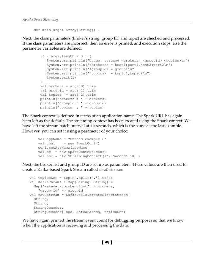
Apache Spark Streaming
[ 99 ]
Next, the class parameters (broker's string, group ID, and topic) are checked and processed.If the class parameters are incorrect, then an error is printed, and execution stops, else theparameter variables are defined:
The Spark context is defined in terms of an application name. The Spark URL has againbeen left as the default. The streaming context has been created using the Spark context. Wehave left the stream batch interval at seconds, which is the same as the last example.However, you can set it using a parameter of your choice:
Next, the broker list and group ID are set up as parameters. These values are then used tocreate a Kafka-based Spark Stream called :
We have again printed the stream event count for debugging purposes so that we knowwhen the application is receiving and processing the data:

Apache Spark Streaming
[ 100 ]
The HDFS location for the Kafka data has been defined as . Ithas been mapped from the into the variable lines. Using the method,a check on the data count is carried out on the variable before saving the data inHDFS using the method:
Finally, the Scala script closes by starting the stream processing and setting the applicationclass to run until terminated with :
With all of the scripts explained and the Kafka brokers running, it is time to examine theKafka configuration, which, if you remember, is maintained by Apache ZooKeeper. (All ofthe code samples that have been described so far will be released with the book.) We willuse the tool and connect to the ZooKeeper server on the host called
on the port. As you can see here, we have received a connected messagefrom the client session:
[hadoop@hc2r1m1 stream]$ /usr/bin/zookeeper-client -server hc2r1m2:2181[zk: hc2r1m2:2181(CONNECTED) 0]
If you remember, we specified the top-level ZooKeeper directory for Kafka to be .If we examine this now via a client session, we can see the Kafka ZooKeeper structure. Wewill be interested in brokers (the Kafka broker servers) and consumers (the previous SparkScala code). The ZooKeeper command shows that the four Kafka servers are registeredwith ZooKeeper and are listed by their configuration values, one to four:
[zk: hc2r1m2:2181(CONNECTED) 2] ls /kafka [consumers, config, controller, admin, brokers, controller_epoch][zk: hc2r1m2:2181(CONNECTED) 3] ls /kafka/brokers [topics, ids][zk: hc2r1m2:2181(CONNECTED) 4] ls /kafka/brokers/ids

Apache Spark Streaming
[ 101 ]
[3, 2, 1, 4]
We will create the topic that we want to use for this test using the Kafka script, , with a flag. We do this manually because we want to demonstrate the
definition of the data partitions while we do it. Note that we have set the partitions in theKafka topic to , as shown in the following piece of code. Note also that the ZooKeeperconnection string for the command has a comma-separated list of ZooKeeper servers,terminated by the top-level ZooKeeper Kafka directory called . This means that thecommand puts the new topic in the proper place:
[hadoop@hc2nn ~]$ /usr/bin/kafka-topics \ > --create \ > --zookeeper hc2r1m2:2181,hc2r1m3:2181,hc2r1m4:2181/kafka \ > --replication-factor 3 \ > --partitions 5 \ > --topic rssCreated topic "rss".
Now, when we use the ZooKeeper client to check the Kafka topic configuration, we can seethe correct topic name and the expected number of the partitions:
[zk: hc2r1m2:2181(CONNECTED) 5] ls /kafka/brokers/topics [rss][zk: hc2r1m2:2181(CONNECTED) 6] ls /kafka/brokers/topics/rss [partitions][zk: hc2r1m2:2181(CONNECTED) 7] ls /kafka/brokers/topics/rss/partitions [3, 2, 1, 0, 4]
This describes the configuration for the Kafka broker servers in ZooKeeper, but what aboutthe data consumers? Well, the following list shows where the data will be held. Rememberthat, at this time, there is no consumer running, so it is not represented in ZooKeeper:
[zk: hc2r1m2:2181(CONNECTED) 9] ls /kafka/consumers [] [zk: hc2r1m2:2181(CONNECTED) 10] quit
In order to start this test, we will run our Kafka data producer and consumer scripts. Wewill also check the output of the Spark application class and check the Kafka partitionoffsets and HDFS to make sure that the data has arrived. This is quite complicated, so wewill add a diagram here to explain the test architecture:

Apache Spark Streaming
[ 102 ]
The Perl script called will be used to provide a data source for a Kafka dataproducer, which will feed data to the Hortonworks Kafka broker servers. The data will bestored in ZooKeeper, in the structure that has just been examined, under the top-level nodecalled . The Apache Spark Scala-based application will then act as a Kafka consumerand read the data that it will store under HDFS.
In order to try and explain the complexity here, we will examine our method of running theApache Spark class. It will be started via the command. Remember that allof these scripts will be released with this book, so you can examine them in your own time.We always use scripts for server test management so that we encapsulate complexity, andcommand execution is quickly repeatable. The script, , is like manyexample scripts that have already been used in this chapter and in this book. It accepts aclass name and class parameters, and runs the class via :
[hadoop@hc2r1m1 stream]$ more run_stream.bash#!/bin/bashSPARK_HOME=/usr/local/sparkSPARK_BIN=$SPARK_HOME/binSPARK_SBIN=$SPARK_HOME/sbinJAR_PATH=/home/hadoop/spark/stream/target/scala-2.10/streaming_2.10-1.0.jarCLASS_VAL=$1CLASS_PARAMS="${*:2}"STREAM_JAR=/usr/local/spark/lib/spark-examples-1.3.1-hadoop2.3.0.jarcd $SPARK_BIN

Apache Spark Streaming
[ 103 ]
./spark-submit \ --class $CLASS_VAL \ --master spark://hc2nn.semtech-solutions.co.nz:7077 \ --executor-memory 100M \ --total-executor-cores 50 \ --jars $STREAM_JAR \ $JAR_PATH \ $CLASS_PARAMS
We then used a second script, which calls the script to executethe Kafka consumer code in the previous application class. Note that this scriptsets up the full application class name--the broker server list. It also sets up the topic name,called RSS, to use for data consumption. Finally, it defines a consumer group called .Remember that Kafka is a publish/subscribe message brokering system. There may be manyproducers and consumers organized by topic, group, and partition:
[hadoop@hc2r1m1 stream]$ more run_kafka_example.bash#!/bin/bashRUN_CLASS=nz.co.semtechsolutions.stream6BROKERS="hc2r1m1:9092,hc2r1m2:9092,hc2r1m3:9092,hc2r1m4:9092"GROUPID=group1TOPICS=rss# run the Apache Spark Kafka example./run_stream.bash $RUN_CLASS \ $BROKERS \ $GROUPID \ $TOPICS
So, we will start the Kafka consumer by running the script,which, in turn, will run the previous Scala code using . Whilemonitoring Kafka data consumption using the script called , we wereable to get the kafka-consumer-offset-checker script to list the Kafka-based topics, but forsome reason, it will not check the correct path (under in ZooKeeper) when checkingthe offsets, as shown here:
[hadoop@hc2r1m1 stream]$ ./kafka_list.bash================================ Kafka Topics================================ __consumer_offsets rss================================ Kafka Offsets================================Exiting due to: org.apache.zookeeper.KeeperException$NoNodeException:KeeperErrorCode = NoNode for /consumers/group1/offsets/rss/4.

Apache Spark Streaming
[ 104 ]
By starting the Kafka producer feed using the script, we can now startfeeding the RSS-based data through Kafka into Spark, and then into HDFS. Periodicallychecking the session output, it can be seen that events are passing throughthe Spark-based Kafka DStream. The following output comes from the stream count in theScala code and shows that, at that point, events were processed:
------------------------------------------- Time: 1436834440000 ms ------------------------------------------- >>>>>>>>>>>>>>> Received events : 28
By checking HDFS under the directory via the Hadoopfilesystem command, it can be seen that there is now data stored on HDFS:
[hadoop@hc2r1m1 stream]$ hdfs dfs -ls /data/spark/kafka/rss Found 1 items drwxr-xr-x - hadoop supergroup 0 2015-07-14 12:40/data/spark/kafka/rss/file_1436833769907
By checking the contents of this directory, it can be seen that an HDFS part data file exists,which should contain the RSS-based data from Reuters:
[hadoop@hc2r1m1 stream]$ hdfs dfs -ls/data/spark/kafka/rss/file_1436833769907 Found 2 items -rw-r--r-- 3 hadoop supergroup 0 2015-07-14 12:40/data/spark/kafka/rss/file_1436833769907/_SUCCESS -rw-r--r-- 3 hadoop supergroup 8205 2015-07-14 12:40/data/spark/kafka/rss/file_1436833769907/part-00001
Using the Hadoop filesystem Command, we can dump the contents of this HDFS-based file to check its contents. We have used the Linux head command to limit the data tosave space. Clearly, this is RSS Reuters science-based information that the Perl script
has converted from XML to RSS JSON format.
[hadoop@hc2r1m1 stream]$ hdfs dfs -cat/data/spark/kafka/rss/file_1436833769907/part-00001 | head -2{"category": "science", "title": "Bear necessities: low metabolism letspandas survive on bamboo", "summary": "WASHINGTON (Reuters) - Giant pandaseat vegetables even though their bodies are better equipped to eat meat. Sohow do these black-and-white bears from the remote misty mountains ofcentral China survive on a diet almost exclusively of a low-nutrient foodlike bamboo?"}{"category": "science", "title": "PlanetiQ tests sensor for commercialweather satellites", "summary": "CAPE CANAVERAL (Reuters) - PlanetiQ aprivately owned company is beginning a key test intended to pave the wayfor the first commercial weather satellites."}

Apache Spark Streaming
[ 105 ]
This ends this Kafka example. It can be seen that Kafka brokers have been configured. Itshows that an RSS data-based Kafka producer has fed data to the brokers. It has beenproved, using the ZooKeeper client, that the Kafka architecture matching the brokers,topics, and partitions has been set up in ZooKeeper. Finally, it has been shown using theApache Spark-based Scala code in the application, that the Kafka data has beenconsumed and saved to HDFS.
SummaryWe could have provided streaming examples for other systems as well, but there was noroom in this chapter. Twitter streaming has been examined by example in the Checkpointingsection. This chapter has provided practical examples of data recovery via checkpointing inSpark Streaming. It has also touched on the performance limitations of checkpointing andshown that the checkpointing interval should be set at five to ten times the Spark streambatch interval.
Checkpointing provides a stream-based recovery mechanism in the case of Sparkapplication failure. This chapter has provided some stream-based worked examples forTCP, File, Flume, and Kafka-based Spark stream coding. All the examples here are based onScala and compiled with . In case you are more familiar with Maven the followingtutorial explains how to set up a Maven based Scala project:
.
All of the code will be released with this book. Where the example architecture has becomeovercomplicated, we have provided an architecture diagram (the Kafka example). It is clearto us that the Apache Spark streaming module contains a rich source of functionality thatshould meet most of your needs and will grow as future releases of Spark are delivered.Apache Spark Streaming was introduced before Catalyst and Tungsten. So let's have a lookhow Apache Spark Structured Streaming can make use of those in the next chapter.

66Structured Streaming
As you might already have understood from the previous chapters, Apache Spark iscurrently in transition from RDD-based data processing to a more structured one, backedby DataFrames and Datasets in order to let Catalyst and Tungsten kick in for performanceoptimizations. This means that the community currently uses a double-tracked approach.While the unstructured APIs are still supported--they haven't even been marked asdeprecated yet ,and it is questionable if they ever will--a new set of structured APIs hasbeen introduced for various components with Apache Spark V 2.0, and this is also true forSpark Streaming. Structured Steaming was marked stable in Apache Spark V 2.2. Note that,as of Apache Spark V 2.1 when we started writing this chapter, Structured Streaming is wasmarked as alpha. This is another example of the extreme pace at which Apache Spark isdeveloping.
The following topics will be covered in this chapter:
The concept of continuous applicationsUnification of batch and stream processingWindowingEvent versus processing time and how to handle late arriving dataHow Catalyst and Tungsten support streamingHow fault tolerance and end-to-end exactly-once delivery guarantee is achievedAn example of subscribing to a stream on a message hubStream life cycle management

Structured Streaming
[ 107 ]
The concept of continuous applicationsStreaming apps tend to grow in complexity. Streaming computations don't run in isolation;they interact with storage systems, batch applications, and machine learning libraries.Therefore, the notion of continuous applications--in contrast to batch processing--emerged,and basically means the composite of batch processing and real-time stream processingwith a clear focus of the streaming part being the main driver of the application, and justaccessing the data created or processed by batch processes for further augmentation.Continuous applications never stop and continuously produce data as new data arrives.
True unification - same code, same engineSo a continuous application could also be implemented on top of RDDs and DStreams butwould require the use of use two different APIs. In Apache Spark Structured Streaming theAPIs are unified. This unification is achieved by seeing a structured stream as a relationaltable without boundaries where new data is continuously appended to the bottom of it. Inbatch processing on DataFrames using the relational API or SQL, intermediate DataFramesare created. As stream and batch computing are unified on top of the Apache SparkSQLengine, when working with structured streams, intermediate relational tables withoutboundaries are created.
It is important to note that one can mix (join) static and incremental datawithin the same query called a continuous application, which is anapplication taking static and dynamic data into account and never stops,producing output all the time or, at least when new data arrives. Acontinuous application doesn't necessarily need access to static data, it canalso process streaming data only. But an example for using static data onstreams is when getting GPS locations in as a stream and matching thoseGPS locations to addresses stored in persistent storage. The output of suchan operation is a stream of addresses.
WindowingOpen source and commercial streaming engines such as IBM Streams, Apache Storm, orApache Flink are using the concept of windows.
Structured Streaming
[ 108 ]
Windows specify the granularity or number of subsequent records, whichare taken into account when executing aggregation functions on streams.
How streaming engines use windowingThere exist five different properties in two dimensions, which is how windows can bedefined, where each window definition needs to use one property of each dimension.
The first property is the mode in which subsequent windows of a continuous stream oftuples can be created: sliding and tumbling.
The second is that the number of tuples that fall into a window has to be specified: eithercount-based, time-based or session-based.
Let's take a look at what they mean:
Sliding windows: A sliding window removes a tuple from it whenever a newtuple is eligible to be included.Tumbling windows: A tumbling window removes all tuples from it wheneverthere are enough tuples arriving to create a new window.Count-based windows: Such windows always have the n newest elements in it.Note that this can be achieved either by a sliding or tumbling tuple update policy.Time-based windows: This window takes the timestamp of a tuple into accountin order to determine whether it belongs to a certain window or not. Such awindow can contain the latest n seconds worth of data, for example. Such awindow can be sliding and tumbling as well.Time-based windows especially are eligible for late arriving data, which is a veryinteresting concept that Apache Spark Structured Streaming makes possible.Session-based windows: This window takes a session ID of a tuple into accountin order to determine whether it belongs to a certain window or not. Such awindow eventually contains all data from a user interaction with an online shop,for example. Such a window can be sliding and tumbling as well, although thisnotion doesn't make really sense here because you want eventually act on/react toall data belonging to a specific session.
Time-based and Session-based windows especially are eligible for late arriving data, whichis a very interesting concept that Apache Spark Structured Streaming makes possible.

Structured Streaming
[ 109 ]
Let's take a look at the following figure, which illustrates tumbling windows:
As can be observed, every tuple (or message respectively) ends up in one single window.Now let's have a look at sliding windows:
Sliding windows are meant to share tuples among their neighbors. This means that forevery tuple arriving, a new window is issued. One example of such a paradigm is thecalculation of a moving average once a tuple arrives for the last 100 data points. Now let'sconsider time based windows:
Finally, this last illustration shows time-based windows. It's important to notice that thenumber of tuples per window can be different as it only depends on how many messages ina certain time frame have arrived; only those will be included in the respective window. Sofor example consider an HTTP server log file to be streamed into Apache Spark StructuredStreaming (using Flume as a possible solution). We are grouping tuples (which are theindividual lines of the log file) together on a minute basis. Since the number of concurrentusers are different at each point in time during the day the size of the minute windows willalso vary depending on it.
Structured Streaming
[ 110 ]
How Apache Spark improves windowingApache Spark structured streaming is significantly more flexible in the window-processingmodel. As streams are virtually treated as continuously appended tables, and every row insuch a table has a timestamp, operations on windows can be specified in the query itselfand each query can define different windows. In addition, if there is a timestamp present instatic data, window operations can also be defined, leading to a very flexible stream-processing model.
In other words, Apache Spark windowing is just a sort of special type of grouping on thetimestamp column. This makes it really easy to handle late arriving data as well becauseApache Spark can include it in the appropriate window and rerun the computation on thatwindow when a certain data item arrives late. This feature is highly configurable.
Event time versus processing time: In time series analysis and especiallyin stream computing, each record is assigned to a particular timestamp.One way of creating such a timestamp is the arrival time at the stream-processing engine. Often, this is not what you want. Usually, you want toassign an event time for each record at that particular point in time whenit was created, for example, when a measurement on an IoT device tookplace. This allows coping with latency between creating and processing ofan event, for example, when an IoT sensor was offline for a certain amountof time, or network congestion caused a delay of data delivery.
The concept of late data is interesting when using event time instead of processing time toassign a unique timestamp to each tuple. Event time is the timestamp when a particularmeasurement took place, for example. Apache Spark structured streaming can automatically cope with subsets of data arriving at a later point in time transparently.
Late data: If a record arrives at any streaming engine, it is processedimmediately. Here, Apache Spark streaming doesn't differ from otherengines. However, Apache Spark has the capability of determining thecorresponding windows a certain tuple belongs to at any time. If, forwhatever reason, a tuple arrives late, all affected windows will be updatedand all affected aggregate operations based on these updated windows arererun. This means that results are allowed to change over time in case latedata arrives. This is supported out of the box without the programmerworrying about it. Finally, since Apache Spark V2.1, it is possible tospecify the amount of time that the system accepts late data using the
method.

Structured Streaming
[ 111 ]
The watermark is basically the threshold used to define how old a late arriving data point isallowed to be in order to still be included in the respective window. Again, consider theHTTP server log file working over a minute length window. If, for whatever reason, a datatuple arrives which is more than 4 hours old it might not make sense to include it in thewindows if, for example, this application is used to create a time-series forecast model on anhourly basis to provision or de-provision additional HTTP servers to a cluster. A four-hour-old data point just wouldn't make sense to process, even if it could change the decision, asthe decision has already been made.
Increased performance with good old friendsAs in Apache SparkSQL for batch processing and, as Apache Spark structured streaming ispart of Apache SparkSQL, the Planner (Catalyst) creates incremental execution plans as wellfor mini batches. This means that the whole streaming model is based on batches. This is thereason why a unified API for streams and batch processing could be achieved. The price wepay is that Apache Spark streaming sometimes has drawbacks when it comes to very lowlatency requirements (sub-second, in the range of tens of ms). As the name StructuredStreaming and the usage of DataFrames and Datasets implies, we are also benefiting fromperformance improvements due to project Tungsten, which has been introduced in aprevious chapter. To the Tungsten engine itself, a mini batch doesn't look considerablydifferent from an ordinary batch. Only Catalyst is aware of the incremental nature ofstreams. Therefore, as of Apache Spark V2.2, the following operations are not (yet)supported, but they are on the roadmap to be supported eventually:
Chain of aggregationsTaking first n rowsDistinctSorting before aggregationsOuter joins between streaming and static data (only limited support)
As this is constantly changing; it is best to refer to the latest documentation: .
Structured Streaming
[ 112 ]
How transparent fault tolerance and exactly-once delivery guarantee is achievedApache Spark structured streaming supports full crash fault tolerance and exactly-oncedelivery guarantee without the user taking care of any specific error handling routines. Isn'tthis amazing? So how is this achieved?
Full crash fault tolerance and exactly-once delivery guarantee are terms ofsystems theory. Full crash fault tolerance means that you can basically pullthe power plug of the whole data center at any point in time, and no datais lost or left in an inconsistent state. Exactly-once delivery guaranteemeans, even if the same power plug is pulled, it is guaranteed that eachtuple- end-to-end from the data source to the data sink - is delivered -only, and exactly, once. Not zero times and also not more than one time.Of course those concepts must also hold in case a single node fails ormisbehaves (for example- starts throttling).
First of all, states between individual batches and offset ranges (position in a source stream)are kept in-memory but are backed by a Write Ahead Log (WAL) in a fault-tolerant filesystem such as HDFS. A WAL is basically a log file reflecting the overall streamprocessing state in a pro-active fashion. This means, before data is transformed though anoperator, it is first persistently stored in the WAL in a way it can be recovered after a crash.So, in other words, during the processing of an individual mini batch, the regions of theworker memory, as well as the position offset of the streaming source, are persisted to disk.In case the system fails and has to recover, it can re-request chunks of data from the source.Of course, this is only possible if the source supports these semantics.
Replayable sources can replay streams from agiven offsetEnd-to-end exactly-once delivery guarantee requires the streaming source to support somesort of stream replay at a requested position. This is true for file sources and Apache Kafka,for example, as well as the IBM Watson Internet of Things platform, where the followingexample in this chapter will be based on.

Structured Streaming
[ 113 ]
Idempotent sinks prevent data duplicationAnother key to end-to-end exactly-once delivery guarantee is idempotent sinks. Thisbasically means that sinks are aware of which particular write operation has succeeded inthe past. This means that such a smart sink can re-request data in case of a failure and alsodrop data in case the same data has been sent multiple times.
State versioning guarantees consistent resultsafter rerunsWhat about state? Imagine that a machine learning algorithm maintains a count variable onall the workers. If you replay the exact same data twice, you will end up counting the datamultiple times. Therefore, the query planner also maintains a versioned key-value mapwithin the workers, which are persisting their state in turn to HDFS--which is by designfault tolerant.
So, in case of a failure, if data has to be replayed, the planner makes sure that the correctversion of the key-value map is used by the workers.
Example - connection to a MQTT messagebrokerSo, let's start with a sample use case. Let's connect to an Internet of Things (IoT) sensordata stream. As we haven't covered machine learning so far, we don't analyze the data, wejust showcase the concept.
We are using the IBM Watson IoT platform as a streaming source. At its core, the WatsonIoT platform is backed by an MQTT (Message Queue Telemetry Transport) messagebroker. MQTT is a lightweight telemetry protocol invented by IBM in 1999 and became-- anOASIS (Organization for the Advancement of Structured Information Standards, a globalnonprofit consortium that works on the development, convergence, and adoption ofstandards for security, Internet of Things, energy, content technologies, emergencymanagement, and other areas) standard in 2013--the de facto standard for IoT dataintegration.

Structured Streaming
[ 114 ]
Messaging between applications can be backed by a message queue whichis a middleware system supporting asynchronous point to point channelsin various delivery modes like first-in first-out (FIFO), last-in first-out(LIFO) or Priority Queue (where each message can be re-ordered bycertain criteria).
This is already a very nice feature but still couples applications in a certain way because,once a message is read, it is made unavailable to others.
This way N to N communication is hard (but not impossible) to achieve. Ina publish/subscribe model applications are completely de-coupled. Theredoesn't exists any queues anymore but the notion of topics is introduced.Data providers publish messages on specific topics and data consumerssubscribe to those topics. This way N to N communication is verystraightforward to achieve since it is reflected by the underlying messagedelivery model. Such a middleware is called a Message Broker in contrastto a Message Queue.
As cloud services tend to change constantly, and cloud in general is introduced later in thisbook, the following tutorial explains how to set up the test data generator in the cloud andconnect to the remote MQTT message broker. In this example, we will use the IBM WatsonIoT Platform, which is an MQTT message broker available in the cloud. Alternatively onecan install an open source message broker like MOSQUITTO which also provides a publiclyavailable test installation on the following URL: .
In order to replicate the example, the following steps (1) and (2) are necessary as describedin the following tutorial:
. Please make sure to note down , , , and during execution of the tutorial. Those are needed later in
order to subscribe to data using Apache Spark Structured Streaming.

Structured Streaming
[ 115 ]
As the IBM Watson IoT platform uses the open MQTT standard, no special IBM componentis necessary to connect to the platform. Instead, we are using MQTT and Apache Bahir as aconnector between MQTT and Apache Spark structured streaming.
The goal of the Apache Bahir project is to provide a set of source and sinkconnectors for various data processing engines including Apache Sparkand Apache Flink since they are lacking those connectors. In this case wewill use the Apache Bahir MQTT data source for MQTT.
In order to use Apache Bahir, we need to add two dependencies to our local mavenrepository. A complete file is provided in the download section of this chapter.Let's have a look at the dependency section of :
We are basically getting the MQTT Apache structured streaming adapter of Apache Bahirand a dependent package for low-level MQTT processing. A simple
command in the directory of the file pulls the requireddependencies into our local maven repository, where they can be accessed by the ApacheSpark driver and transferred to the Apache Spark workers automatically.
Another way of resolving the dependencies is when using the following command in orderto start a spark-shell (spark-submit works the same way); the necessary dependencies areautomatically distributed to the workers:

Structured Streaming
[ 116 ]
Now we need the MQTT credentials that we've obtained earlier. Let's set the values here:
Now we can start creating a stream connecting to an MQTT message broker. We are tellingApache Spark to use the Apache Bahir MQTT streaming source:
We need to specify credentials such as , , and inorder to pull data from the MQTT message broker; the link to the tutorial mentioned earlierexplains how to obtain these:

Structured Streaming
[ 117 ]
As we are using a publish/subscribe messaging model, we have to provide the topic that weare subscribing to--this topic is used by the test data generator that you've deployed to thecloud before:
Once everything is set on the configuration side, we have to provide the endpoint host andport in order to create the stream:
Interestingly, as can be seen in the following screenshot, this leads to the creation of aDataFrame:
Note that the schema is fixed to and cannot be changed duringstream creation--this is a limitation of the Apache Bahir library. However, using the richDataFrame API, you can parse the value, a JSON string for example, and create newcolumns.
As discussed before, this is one of the powerful features of Apache Spark structuredstreaming, as the very same DataFrame (and Dataset) API now can be used to processhistoric and real-time data. So let's take a look at the contents of this stream by writing it tothe console:

Structured Streaming
[ 118 ]
As output mode, we choose to enforce incremental display and avoid having thecomplete contents of the historic stream being written to the console again and again. As
, we specify as we just want to debug what's happening on the stream:
Finally, the method initiates query processing, as can be seen here:

Structured Streaming
[ 119 ]
Controlling continuous applicationsOnce a continuous application (even a simple one, not taking historic data into account) isstarted and running, it has to be controlled somehow as the call to the methodimmediately starts processing, but also returns without blocking. In case you want yourprogram to block at this stage until the application has finished, one can use the
method as follows:
This is particularly important when precompiling code and using the command. When using , the application is not terminated anyway.
More on stream life cycle managementStreaming tends to be used in the creation of continuous applications. This means that theprocess is running in the background and, in contrast to batch processing, doesn't have aclear stop time; therefore, DataFrames and Datasets backed by a streaming source, supportvarious methods for stream life cycle management, which are explained as follows:
: This starts the continuous application. This method doesn't block. If this isnot what you want, use .
: This terminates the continuous application. : As mentioned earlier, starting a stream using the
method immediately returns, which means that the call is not blocking.Sometimes you want to wait until the stream is terminated, either by someoneelse calling on it or by an error.
: In case a stream stopped because of an error, the cause can be readusing this method.
: This is to obtain real-time meta information on the streamingsource.
: This is to obtain real-time meta information on the streaming sink.
Sinks in Apache Spark streaming are smart in the sense that they support fault toleranceand end-to-end exactly-once delivery guarantee as mentioned before. In addition, ApacheSpark needs them to support different output methods. Currently, the following threeoutput methods, , , and , significantly change the underlyingsemantics. The following paragraph contains more details about the different outputmethods.

Structured Streaming
[ 120 ]
Different output modes on sinks: Sinks can be specified to handle output in different ways.This is known as . The naive choice would use an incremental approach as weare processing incremental data with streaming anyway. This mode is referred to as
. However, there exist requirements where data already processed by the sink has tobe changed. One example is the late arrival problem of missing data in a certain timewindow, which can lead to changing results once the computation for that particular timewindow is recomputed. This mode is called .
Since Version 2.1 of Apache Spark, the mode was introduced thatbehaves similarly to the mode but only changes rows that havebeen altered, therefore saving processing resources and improving speed.Some types of modes do not support all query types. As this is constantlychanging, it is best to refer to the latest documentation at
SummarySo why do we have two different streaming engines within the same data processingframework? We hope that after reading this chapter, you'll agree that the main pain pointsof the classical DStream based engine have been addressed. Formerly, event time-basedprocessing was not possible and only the arrival time of data was considered. Then, latedata has simply been processed with the wrong timestamp as only processing time could beused. Also, batch and stream processing required using two different APIs: RDDs andDStreams. Although the API is similar, it is not exactly the same; therefore, the rewriting ofcode when going back and forth between the two paradigms was necessary. Finally, end-to-end delivery guarantee was hard to achieve and required lots of user intervention andthinking.
This fault-tolerant end-to-end exactly-once delivery guarantee is achieved through offsettracking and state management in a fault-tolerant Write Ahead Log in conjunction withfault-tolerant sources and sinks. Finally, the unification of batch and streaming APIs on topof Catalyst and Tungsten is one of the most important innovations in Apache Spark sinceversion 2.0.
Now let's examine the very interesting topic of machine learning in the next chapter.

77Apache Spark MLlib
MLlib is the original machine learning library that is provided with Apache Spark, the in-memory cluster-based open source data processing system. This library is still based on theRDD API. In a later chapter, we'll also learn how machine learning on the newer DataFrameand Dataset API works. In this chapter, we will examine the functionality provided with theMLlib library in terms of areas such as regression, classification, and neural networkprocessing. We will examine the theory behind each algorithm before providing workingexamples that tackle real problems. The example code and documentation on the web canbe sparse and confusing.
We will take a step-by-step approach in describing how the following algorithms can beused and what they are capable of doing:
ArchitectureClassification with Naive BayesClustering with K-MeansImage classification with artificial neural networks
ArchitectureRemember that, although Spark is used for the speed of its in-memory distributedprocessing, it doesn't provide storage. You can use the Host (local) filesystem to read andwrite your data, but if your data volumes are big enough to be described as big data, then itmakes sense to use a cloud-based distributed storage system such as OpenStack SwiftObject Storage, which can be found in many cloud environments and can also be installedin private data centers.

Apache Spark MLlib
[ 122 ]
In case very high I/O is needed, HDFS would also be an option. Moreinformation on HDFS can be found here:
.
The development environmentThe Scala language will be used for the coding samples in this book. This is because, as ascripting language, it produces less code than Java. It can also be used from the Spark shellas well as compiled with Apache Spark applications. We will be using the sbt tool tocompile the Scala code, which we have installed into Hortonworks HDP 2.6 Sandbox asfollows:
[hadoop@hc2nn ~]# sudo su -[root@hc2nn ~]# cd /tmp[root@hc2nn ~]#wgethttp://repo.scala-sbt.org/scalasbt/sbt-native-packages/org/scala-sbt/sbt/0.13.1/sbt.rpm[root@hc2nn ~]# rpm -ivh sbt.rpm
The following URL provides instructions to install sbt on other operating systems includingWindows, Linux and macOS: .
We used a generic Linux account called Hadoop. As the previous commands show, weneed to install as the root account, which we have accessed via (switchuser). We then downloaded the file to the directory from the web-basedserver called using . Finally, we installed the file using the
command with the options for install, for verify, and to print the hash markswhile the package is being installed.
We developed all of the Scala code for Apache Spark in this chapter on the Linux server,using the Linux Hadoop account. We placed each set of code within a subdirectory under
. For instance, the following structure diagram shows that theMLlib Naive Bayes code is stored in a subdirectory called under the Sparkdirectory. What the diagram also shows is that the Scala code is developed within asubdirectory structure named under the directory. The filescalled and contain the Naive Bayes code that will be usedin the next section:

Apache Spark MLlib
[ 123 ]
The file is a configuration file used by the tool, which describes how tocompile the Scala files within the Scala directory. (Note that if you were developing in Java,you would use a path of the form .) The contents of the
file are shown next. The and Linux commands remind you of the filelocation and also remind you to dump the file contents.
The , , and options set the details of the project and theversion of Scala to be used. The options define where the Hadoopand Spark libraries can be located.
[hadoop@hc2nn nbayes]$ pwd/home/hadoop/spark/nbayes[hadoop@hc2nn nbayes]$ cat bayes.sbtname := "Naive Bayes"version := "1.0"scalaVersion := "2.11.2"libraryDependencies += "org.apache.hadoop" % "hadoop-client" % "2.8.1"libraryDependencies += "org.apache.spark" %% "spark-core" % "2.6.0"libraryDependencies += "org.apache.spark" %% "spark-mllib" % "2.1.1"
The Scala project code can be compiled from the subdirectory using thiscommand:
[hadoop@hc2nn nbayes]$ sbt compile

Apache Spark MLlib
[ 124 ]
The command is used to compile the code into classes. The classes are thenplaced in the directory. The compiled classes canbe packaged in a JAR file with this command:
[hadoop@hc2nn nbayes]$ sbt package
The command will create a JAR file under the directory. As we can see in the example in the sbt structure diagram, the JAR file named
has been created after a successful compile and package.This JAR file, and the classes that it contains, can then be used in a command. This will be described later as the functionality in the Apache Spark MLlibmodule is explored.
Classification with Naive BayesThis section will provide a working example of the Apache Spark MLlib Naive Bayesalgorithm. It will describe the theory behind the algorithm and will provide a step-by-stepexample in Scala to show how the algorithm may be used.
Theory on ClassificationIn order to use the Naive Bayes algorithm to classify a dataset, the data must be linearlydivisible; that is, the classes within the data must be linearly divisible by class boundaries.The following figure visually explains this with three datasets and two class boundariesshown via the dotted lines:
Naive Bayes assumes that the features (or dimensions) within a dataset are independent ofone another; that is, they have no effect on each other. The following example considers theclassification of e-mails as spam. If you have 100 e-mails, then perform the following:

Apache Spark MLlib
[ 125 ]
60% of emails are spam80% of spam emails contain the word buy20% of spam emails don't contain the word buy40% of emails are not spam10% of non spam emails contain the word buy90% of non spam emails don't contain the word buy
Let's convert this example into conditional probabilities so that a Naive Bayes classifier canpick it up:
P(Spam) = the probability that an email is spam = 0.6P(Not Spam) = the probability that an email is not spam = 0.4P(Buy|Spam) = the probability that an email that is spam has the word buy =0.8P(Buy|Not Spam) = the probability that an email that is not spam has theword buy = 0.1
What is the probability that an e-mail that contains the word buy is spam? Well, this wouldbe written as P (Spam|Buy). Naive Bayes says that it is described by the equation in thefollowing figure:
So, using the previous percentage figures, we get the following:
P(Spam|Buy) = ( 0.8 * 0.6 ) / (( 0.8 * 0.6 ) + ( 0.1 * 0.4 ) ) = ( .48 ) / ( .48 + .04 )
= .48 / .52 = .923
This means that it is 92 percent more likely that an e-mail that contains the word buy isspam. That was a look at the theory; now it's time to try a real-world example using theApache Spark MLlib Naive Bayes algorithm.
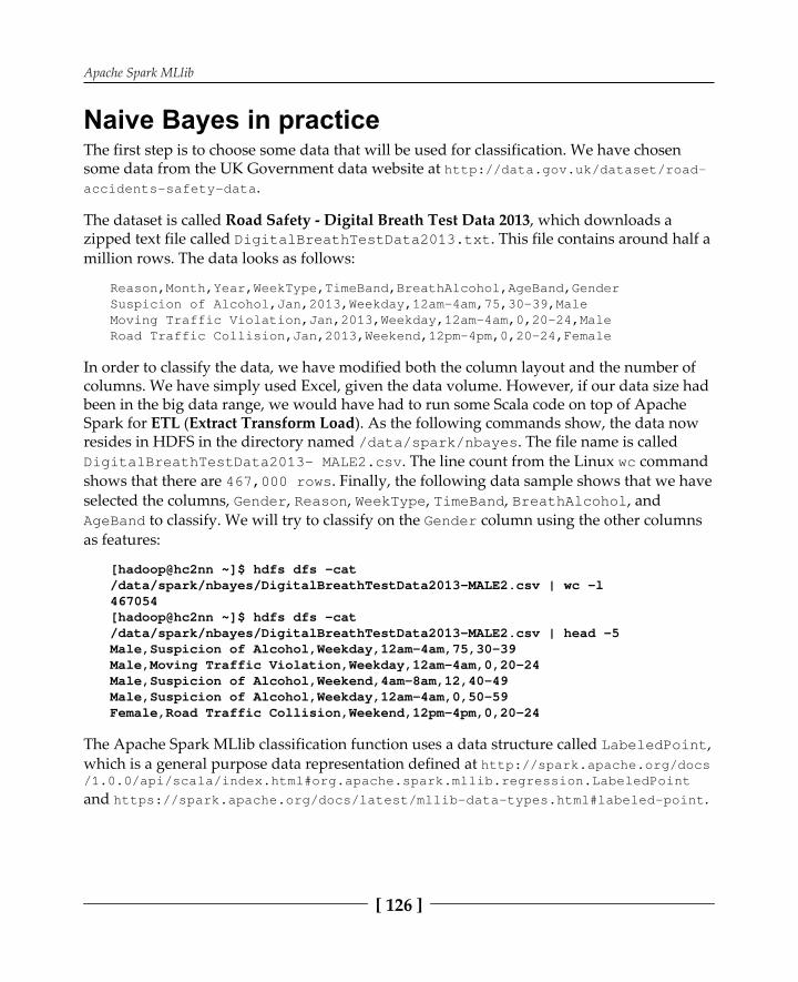
Apache Spark MLlib
[ 126 ]
Naive Bayes in practiceThe first step is to choose some data that will be used for classification. We have chosensome data from the UK Government data website at
.
The dataset is called Road Safety - Digital Breath Test Data 2013, which downloads azipped text file called . This file contains around half amillion rows. The data looks as follows:
In order to classify the data, we have modified both the column layout and the number ofcolumns. We have simply used Excel, given the data volume. However, if our data size hadbeen in the big data range, we would have had to run some Scala code on top of ApacheSpark for ETL (Extract Transform Load). As the following commands show, the data nowresides in HDFS in the directory named . The file name is called
. The line count from the Linux commandshows that there are . Finally, the following data sample shows that we haveselected the columns, , , , , , and
to classify. We will try to classify on the column using the other columnsas features:
[hadoop@hc2nn ~]$ hdfs dfs -cat/data/spark/nbayes/DigitalBreathTestData2013-MALE2.csv | wc -l467054[hadoop@hc2nn ~]$ hdfs dfs -cat/data/spark/nbayes/DigitalBreathTestData2013-MALE2.csv | head -5Male,Suspicion of Alcohol,Weekday,12am-4am,75,30-39Male,Moving Traffic Violation,Weekday,12am-4am,0,20-24Male,Suspicion of Alcohol,Weekend,4am-8am,12,40-49Male,Suspicion of Alcohol,Weekday,12am-4am,0,50-59Female,Road Traffic Collision,Weekend,12pm-4pm,0,20-24
The Apache Spark MLlib classification function uses a data structure called ,which is a general purpose data representation defined at
and .

Apache Spark MLlib
[ 127 ]
This structure only accepts double values, which means that the text values in the previousdata need to be classified numerically. Luckily, all of the columns in the data will convert tonumeric categories, and we have provided a program in the software package with thisbook under the directory to do just that. It is called
. It takes the contents of the file and converts each record into a double vector.
The directory structure and files for an Scala-based development environment havealready been described earlier. We are developing our Scala code on the Linux server usingthe Linux account, Hadoop. Next, the Linux and commands show our top-level
development directory with the configuration file, whose contents havealready been examined:
[hadoop@hc2nn nbayes]$ pwd/home/hadoop/spark/nbayes[hadoop@hc2nn nbayes]$ lsbayes.sbt target project src
The Scala code to run the Naive Bayes example is in the subdirectoryunder the directory:
[hadoop@hc2nn scala]$ pwd/home/hadoop/spark/nbayes/src/main/scala[hadoop@hc2nn scala]$ lsbayes1.scala convert.scala
We will examine the file later, but first, the text-based data on HDFS mustbe converted into numeric double values. This is where the file is used.The code is as follows:
These lines import classes for the Spark context, the connection to the Apache Spark cluster,and the Spark configuration. The object that is being created is called . It is anapplication as it extends the class:

Apache Spark MLlib
[ 128 ]
The next line creates a function called . It has a parameter called, which is an array of and returns :
The function then enumerates the text values in each column, so, for instance, Malebecomes . These numeric values are stored in values such as :

Apache Spark MLlib
[ 129 ]
A comma-separated string called is created from the numericcolumn values and is then returned. The function closes with the finalbrace character. Note that the data line created next starts with a labelvalue at column one and is followed by a vector, which represents thedata.
The vector is space-separated while the label is separated from the vector by a comma.Using these two separator types allows us to process both--the label and vector--in twosimple steps:
The main script defines the HDFS server name and path. It defines the input file and theoutput path in terms of these values. It uses the Spark URL and application name to create anew configuration. It then creates a new context or connection to Spark using these details:
val hdfsServer = "hdfs://localhost:8020"val hdfsPath = "/data/spark/nbayes/"val inDataFile = hdfsServer + hdfsPath + "DigitalBreathTestData2013-MALE2.csv"val outDataFile = hdfsServer + hdfsPath + "result"val sparkMaster = "spark://localhost:7077"val appName = "Convert 1"val sparkConf = new SparkConf()sparkConf.setMaster(sparkMaster)sparkConf.setAppName(appName)val sparkCxt = new SparkContext(sparkConf)

Apache Spark MLlib
[ 130 ]
The CSV-based raw data file is loaded from HDFS using the Spark context method. Then, a data row count is printed:
val csvData = sparkCxt.textFile(inDataFile)println("Records in : "+ csvData.count() )
The CSV raw data is passed line by line to the function. Thereturned string-based numeric data is stored in the variable:
val enumRddData = csvData.map { csvLine => val colData = csvLine.split(',') enumerateCsvRecord(colData) }
Finally, the number of records in the variable is printed, and the enumerateddata is saved to HDFS:
println("Records out : "+ enumRddData.count() ) enumRddData.saveAsTextFile(outDataFile)} // end object
In order to run this script as an application against Spark, it must be compiled. This iscarried out with the command, which also compiles the code. The followingcommand is run from the directory:
[hadoop@hc2nn nbayes]$ sbt packageLoading /usr/share/sbt/bin/sbt-launch-lib.bash....[info] Done packaging.[success] Total time: 37 s, completed Feb 19, 2015 1:23:55 PM
This causes the compiled classes that are created to be packaged into a JAR library, asshown here:
[hadoop@hc2nn nbayes]$ pwd/home/hadoop/spark/nbayes[hadoop@hc2nn nbayes]$ ls -l target/scala-2.10total 24drwxrwxr-x 2 hadoop hadoop 4096 Feb 19 13:23 classes-rw-rw-r-- 1 hadoop hadoop 17609 Feb 19 13:23 naive-bayes_2.10-1.0.jar
The application can now be run against Spark using the application name, SparkURL, and full path to the JAR file that was created. Some extra parameters specify memoryand the maximum cores that are supposed to be used:
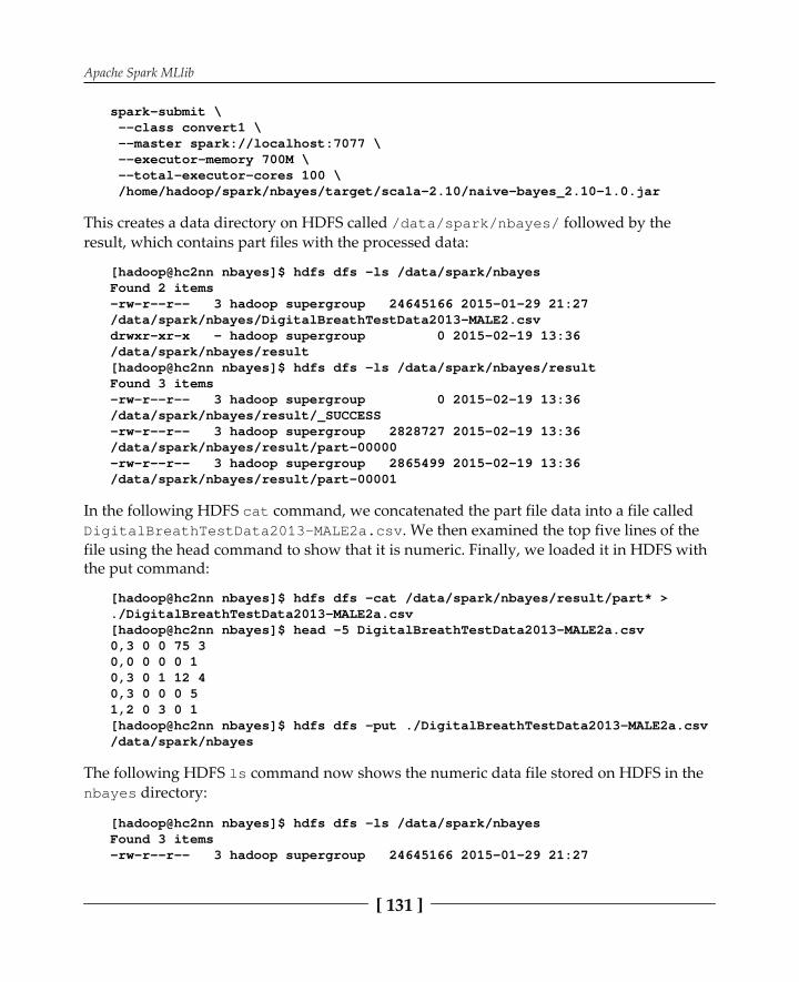
Apache Spark MLlib
[ 131 ]
spark-submit \ --class convert1 \ --master spark://localhost:7077 \ --executor-memory 700M \ --total-executor-cores 100 \ /home/hadoop/spark/nbayes/target/scala-2.10/naive-bayes_2.10-1.0.jar
This creates a data directory on HDFS called followed by theresult, which contains part files with the processed data:
[hadoop@hc2nn nbayes]$ hdfs dfs -ls /data/spark/nbayesFound 2 items-rw-r--r-- 3 hadoop supergroup 24645166 2015-01-29 21:27/data/spark/nbayes/DigitalBreathTestData2013-MALE2.csvdrwxr-xr-x - hadoop supergroup 0 2015-02-19 13:36/data/spark/nbayes/result[hadoop@hc2nn nbayes]$ hdfs dfs -ls /data/spark/nbayes/resultFound 3 items-rw-r--r-- 3 hadoop supergroup 0 2015-02-19 13:36/data/spark/nbayes/result/_SUCCESS-rw-r--r-- 3 hadoop supergroup 2828727 2015-02-19 13:36/data/spark/nbayes/result/part-00000-rw-r--r-- 3 hadoop supergroup 2865499 2015-02-19 13:36/data/spark/nbayes/result/part-00001
In the following HDFS command, we concatenated the part file data into a file called. We then examined the top five lines of the
file using the head command to show that it is numeric. Finally, we loaded it in HDFS withthe put command:
[hadoop@hc2nn nbayes]$ hdfs dfs -cat /data/spark/nbayes/result/part* >./DigitalBreathTestData2013-MALE2a.csv[hadoop@hc2nn nbayes]$ head -5 DigitalBreathTestData2013-MALE2a.csv0,3 0 0 75 30,0 0 0 0 10,3 0 1 12 40,3 0 0 0 51,2 0 3 0 1[hadoop@hc2nn nbayes]$ hdfs dfs -put ./DigitalBreathTestData2013-MALE2a.csv/data/spark/nbayes
The following HDFS command now shows the numeric data file stored on HDFS in the directory:
[hadoop@hc2nn nbayes]$ hdfs dfs -ls /data/spark/nbayesFound 3 items-rw-r--r-- 3 hadoop supergroup 24645166 2015-01-29 21:27

Apache Spark MLlib
[ 132 ]
/data/spark/nbayes/DigitalBreathTestData2013-MALE2.csv-rw-r--r-- 3 hadoop supergroup 5694226 2015-02-19 13:39/data/spark/nbayes/DigitalBreathTestData2013-MALE2a.csvdrwxr-xr-x - hadoop supergroup 0 2015-02-19 13:36/data/spark/nbayes/result
Now that the data has been converted into a numeric form, it can be processed with theMLlib Naive Bayes algorithm; this is what the Scala file, , does. This fileimports the same configuration and context classes as before. It also imports MLlib classesfor Naive Bayes, vectors, and the structure. The application class that iscreated this time is called :
The HDFS data file is again defined, and a Spark context is created as before:
The raw CSV data is loaded and split by the separator characters. The first column becomesthe label (Male/Female) that the data will be classified on. The final columns separated byspaces become the classification features:
val csvData = sparkCxt.textFile(dataFile) val ArrayData = csvData.map { csvLine => val colData = csvLine.split(',') LabeledPoint(colData(0).toDouble, Vectors.dense(colData(1) .split('') .map(_.toDouble) ) )

Apache Spark MLlib
[ 133 ]
}
The data is then randomly divided into training (70%) and testing (30%) datasets:
val divData = ArrayData.randomSplit(Array(0.7, 0.3), seed = 13L) val trainDataSet = divData(0) val testDataSet = divData(1)
The Naive Bayes MLlib function can now be trained using the previous training set. Thetrained Naive Bayes model, held in the variable, can then be used to predict theMale/Female result labels against the testing data:
val nbTrained = NaiveBayes.train(trainDataSet) val nbPredict = nbTrained.predict(testDataSet.map(_.features))
Given that all of the data already contained labels, the original and predicted labels for thetest data can be compared. An accuracy figure can then be computed to determine howaccurate the predictions were, by comparing the original labels with the prediction values:
val predictionAndLabel = nbPredict.zip(testDataSet.map(_.label)) val accuracy = 100.0 * predictionAndLabel.filter(x => x._1 ==x._2).count() / testDataSet.count() println( "Accuracy : " + accuracy );}
So, this explains the Scala Naive Bayes code example. It's now time to run the compiled application using and determine the classification accuracy. The
parameters are the same. It's just the class name that has changed:
spark-submit \ --class bayes1 \ --master spark://hc2nn.semtech-solutions.co.nz:7077 \ --executor-memory 700M \ --total-executor-cores 100 \ /home/hadoop/spark/nbayes/target/scala-2.10/naive-bayes_2.10-1.0.jar
The resulting accuracy given by the Spark cluster is just percent, which seems to implythat this data is not suitable for Naive Bayes:
Accuracy: 43.30
Luckily we'll introduce artificial neural networks later in the chapter, a more powerfulclassifier. In the next example, we will use K-Means to try to determine what clusters existwithin the data. Remember, Naive Bayes needs the data classes to be linearly separablealong the class boundaries. With K-Means, it will be possible to determine both: themembership and centroid location of the clusters within the data.

Apache Spark MLlib
[ 134 ]
Clustering with K-MeansThis example will use the same test data from the previous example, but we will attempt tofind clusters in the data using the MLlib K-Means algorithm.
Theory on ClusteringThe K-Means algorithm iteratively attempts to determine clusters within the test data byminimizing the distance between the mean value of cluster center vectors, and the newcandidate cluster member vectors. The following equation assumes dataset members thatrange from X1 to Xn; it also assumes K cluster sets that range from S1 to Sk, where K <= n.
K-Means in practiceThe K-Means MLlib functionality uses the structure to process its data andso it needs numeric input data. As the same data from the last section is being reused, wewill not explain the data conversion again. The only change that has been made in dataterms in this section, is that processing in HDFS will now take place under the
directory. Additionally, the conversion Scala script for the K-Means example produces a record that is all comma-separated.

Apache Spark MLlib
[ 135 ]
The development and processing for the K-Means example has taken place under the directory to separate the work from other development.
The configuration file is now called and is identical to the last example,except for the project name:
name := "K-Means"
The code for this section can be found in the software package under .So, looking at the code for , which is stored under
, some similar actions occur. The import statements refer to theSpark context and configuration. This time, however, the K-Means functionality is beingimported from MLlib. Additionally, the application class name has been changed for thisexample to :
The same actions are being taken as in the last example to define the data file--to define theSpark configuration and create a Spark context:
Next, the CSV data is loaded from the data file and split by comma characters into the variable:

Apache Spark MLlib
[ 136 ]
A object is initialized, and the parameters are set to define the number of clustersand the maximum number of iterations to determine them:
val kMeans = new KMeans val numClusters = 3 val maxIterations = 50
Some default values are defined for the initialization mode, number of runs, and Epsilon,which we needed for the K-Means call but did not vary for the processing. Finally, theseparameters were set against the object:
We cached the training vector data to improve the performance and trained the object using the vector data to create a trained K-Means model:
VectorData.cache val kMeansModel = kMeans.run( VectorData )
We have computed the K-Means cost and number of input data rows, and have output theresults via statements. The cost value indicates how tightly the clusters are packedand how separate the clusters are:
val kMeansCost = kMeansModel.computeCost( VectorData ) println( "Input data rows : " + VectorData.count() ) println( "K-Means Cost : " + kMeansCost )
Next, we have used the K-Means Model to print the cluster centers as vectors for each of thethree clusters that were computed:
kMeansModel.clusterCenters.foreach{ println }
Finally, we use the K-Means model predict function to create a list of cluster membershippredictions. We then count these predictions by value to give a count of the data points ineach cluster. This shows which clusters are bigger and whether there really are threeclusters:
val clusterRddInt = kMeansModel.predict( VectorData ) val clusterCount = clusterRddInt.countByValue clusterCount.toList.foreach{ println }

Apache Spark MLlib
[ 137 ]
} // end object kmeans1
So, in order to run this application, it must be compiled and packaged from the subdirectory as the Linux command shows here:
[hadoop@hc2nn kmeans]$ pwd/home/hadoop/spark/kmeans[hadoop@hc2nn kmeans]$ sbt packageLoading /usr/share/sbt/bin/sbt-launch-lib.bash[info] Set current project to K-Means (in buildfile:/home/hadoop/spark/kmeans/)[info] Compiling 2 Scala sources to/home/hadoop/spark/kmeans/target/scala-2.10/classes...[info] Packaging /home/hadoop/spark/kmeans/target/scala-2.10/k-means_2.10-1.0.jar ...[info] Done packaging.[success] Total time: 20 s, completed Feb 19, 2015 5:02:07 PM
Once this packaging is successful, we check HDFS to ensure that the test data is ready. As inthe last example, we convert our data to numeric form using the file,provided in the software package. We will process the
data file in the HDFS directory, , as follows:
[hadoop@hc2nn nbayes]$ hdfs dfs -ls /data/spark/kmeansFound 3 items-rw-r--r-- 3 hadoop supergroup 24645166 2015-02-05 21:11/data/spark/kmeans/DigitalBreathTestData2013-MALE2.csv-rw-r--r-- 3 hadoop supergroup 5694226 2015-02-05 21:48/data/spark/kmeans/DigitalBreathTestData2013-MALE2a.csvdrwxr-xr-x - hadoop supergroup 0 2015-02-05 21:46/data/spark/kmeans/result
The tool is used to run the K-Means application. The only change in thiscommand is that the class is now :
spark-submit \ --class kmeans1 \ --master spark://localhost:7077 \ --executor-memory 700M \ --total-executor-cores 100 \ /home/hadoop/spark/kmeans/target/scala-2.10/k-means_2.10-1.0.jar
The output from the Spark cluster run is shown to be as follows:
Input data rows : 467054K-Means Cost : 5.40312223450789E7

Apache Spark MLlib
[ 138 ]
The previous output shows the input data volume, which looks correct; it also shows the value. The cost is based on the Within Set Sum of Squared Errors (WSSSE)
which basically gives a measure how well the found cluster centroids are matching thedistribution of the data points. The better they are matching, the lower the cost. Thefollowing link
explains WSSSE and how to find a good value for k in more detail.
Next come the three vectors, which describe the data cluster centers with the correctnumber of dimensions. Remember that these cluster centroid vectors will have the samenumber of columns as the original vector data:
[0.24698249738061878,1.3015883142472253,0.005830116872250263,2.9173747788555207,1.156645130895448,3.4400290524342454][0.3321793984152627,1.784137241326256,0.007615970459266097,2.5831987075928917,119.58366028156011,3.8379106085083468][0.25247226760684494,1.702510963969387,0.006384899819416975,2.231404248000688,52.202897927594805,3.551509158139135]
Finally, cluster membership is given for clusters 1 to 3 with cluster 1 (index 0) having thelargest membership at member vectors:
(0,407539)(1,12999)(2,46516)
So, these two examples show how data can be classified and clustered using Naive Bayesand K-Means. What if I want to classify images or more complex patterns, and use a blackbox approach to classification? The next section examines Spark-based classification usingANNs, or artificial neural networks.

Apache Spark MLlib
[ 139 ]
Artificial neural networksThe following figure shows a simple biological neuron to the left. The neuron has dendritesthat receive signals from other neurons. A cell body controls activation, and an axon carriesan electrical impulse to the dendrites of other neurons. The artificial neuron to the right hasa series of weighted inputs: a summing function that groups the inputs and a firingmechanism (F(Net)), which decides whether the inputs have reached a threshold, and, if so,the neuron will fire:

Apache Spark MLlib
[ 140 ]
Neural networks are tolerant of noisy images and distortion, and so are useful when a blackbox classification method is needed for potentially degraded images. The next area toconsider is the summation function for the neuron inputs. The following diagram shows thesummation function called Net for neuron i. The connections between the neurons thathave the weighting values, contain the stored knowledge of the network. Generally, anetwork will have an input layer, output layer, and a number of hidden layers. A neuronwill fire if the sum of its inputs exceeds a threshold:
In the previous equation, the diagram and key show that the input values from a pattern Pare passed to neurons in the input layer of a network. These values become the input layerneuron activation values; they are a special case. The inputs to neuron i are the sum of theweighting value for neuron connection i-j, multiplied by the activation from neuron j. Theactivation at neuron j (if it is not an input layer neuron) is given by F(Net), the squashingfunction, which will be described next.

Apache Spark MLlib
[ 141 ]
A simulated neuron needs a firing mechanism, which decides whether the inputs to theneuron have reached a threshold. Then, it fires to create the activation value for that neuron.This or function can be described by the generalized functionshown in the following figure:
This function has two constants: A and B; B affects the shape of the activation curve asshown in the previous graph. The bigger the value, the more similar a function becomes toan on/off step. The value of A sets a minimum for the returned activation. In the previousgraph, it is zero.

Apache Spark MLlib
[ 142 ]
So, this provides a mechanism to simulate a neuron, create weighting matrices as theneuron connections, and manage the neuron activation. How are the networks organized?The next diagram shows a suggested architecture--the neural network has an input layer ofneurons, an output layer, and one or more hidden layers. All neurons in each layer areconnected to each neuron in the adjacent layers:
During the training, activation passes from the input layer through the network to theoutput layer. Then, the error or difference between the expected or actual output causeserror deltas to be passed back through the network, altering the weighting matrix values.Once the desired output layer vector is achieved, then the knowledge is stored in theweighting matrices and the network can be further trained or used for classification.
So, the theory behind neural networks has been described in terms of back propagation.Now is the time to obtain some practical knowledge.
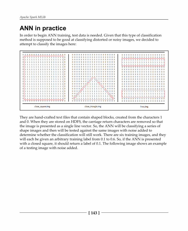
Apache Spark MLlib
[ 143 ]
ANN in practiceIn order to begin ANN training, test data is needed. Given that this type of classificationmethod is supposed to be good at classifying distorted or noisy images, we decided toattempt to classify the images here:
They are hand-crafted text files that contain shaped blocks, created from the characters 1and 0. When they are stored on HDFS, the carriage return characters are removed so thatthe image is presented as a single line vector. So, the ANN will be classifying a series ofshape images and then will be tested against the same images with noise added todetermine whether the classification will still work. There are six training images, and theywill each be given an arbitrary training label from 0.1 to 0.6. So, if the ANN is presentedwith a closed square, it should return a label of 0.1. The following image shows an exampleof a testing image with noise added.

Apache Spark MLlib
[ 144 ]
The noise, created by adding extra zero (0) characters within the image, has beenhighlighted:
As before, the ANN code is developed using the Linux Hadoop account in a subdirectorycalled . The file exists in the directory:
[hadoop@hc2nn ann]$ pwd/home/hadoop/spark/ann
[hadoop@hc2nn ann]$ lsann.sbt project src target
The contents of the file have been changed to use full paths of JAR library files forthe Spark dependencies:
name := "A N N"version := "1.0"scalaVersion := "2.11.2"libraryDependencies += "org.apache.hadoop" % "hadoop-client" % "2.8.1"
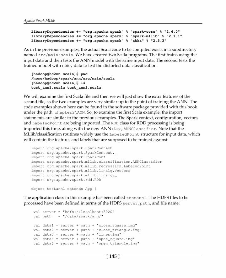
Apache Spark MLlib
[ 145 ]
libraryDependencies += "org.apache.spark" % "spark-core" % "2.6.0"libraryDependencies += "org.apache.spark" % "spark-mllib" % "2.1.1"libraryDependencies += "org.apache.spark" % "akka" % "2.5.3"
As in the previous examples, the actual Scala code to be compiled exists in a subdirectorynamed . We have created two Scala programs. The first trains using theinput data and then tests the ANN model with the same input data. The second tests thetrained model with noisy data to test the distorted data classification:
[hadoop@hc2nn scala]$ pwd/home/hadoop/spark/ann/src/main/scala[hadoop@hc2nn scala]$ lstest_ann1.scala test_ann2.scala
We will examine the first Scala file and then we will just show the extra features of thesecond file, as the two examples are very similar up to the point of training the ANN. Thecode examples shown here can be found in the software package provided with this bookunder the path, . So, to examine the first Scala example, the importstatements are similar to the previous examples. The Spark context, configuration, vectors,and are being imported. The class for RDD processing is beingimported this time, along with the new ANN class, . Note that theMLlib/classification routines widely use the structure for input data, whichwill contain the features and labels that are supposed to be trained against:
The application class in this example has been called . The HDFS files to beprocessed have been defined in terms of the HDFS , , and file name:

Apache Spark MLlib
[ 146 ]
The Spark context has been created with the URL for the Spark instance, which now has adifferent port number-- . The application name is . This will appear on the Sparkweb UI when the application is run:
val sparkMaster = "spark://localhost:8077" val appName = "ANN 1" val conf = new SparkConf()
conf.setMaster(sparkMaster) conf.setAppName(appName)
val sparkCxt = new SparkContext(conf)
The HDFS-based input training and test data files are loaded. The values on each line aresplit by space characters, and the numeric values have been converted into doubles. Thevariables that contain this data are then stored in an array called inputs. At the same time,an array called outputs is created, containing the labels from to . These values willbe used to classify the input patterns:
val rData1 = sparkCxt.textFile(data1).map(_.split("").map(_.toDouble)).collect val rData2 = sparkCxt.textFile(data2).map(_.split("").map(_.toDouble)).collect val rData3 = sparkCxt.textFile(data3).map(_.split("").map(_.toDouble)).collect val rData4 = sparkCxt.textFile(data4).map(_.split("").map(_.toDouble)).collect val rData5 = sparkCxt.textFile(data5).map(_.split("").map(_.toDouble)).collect val rData6 = sparkCxt.textFile(data6).map(_.split("").map(_.toDouble)).collect val inputs = Array[Array[Double]] ( rData1(0), rData2(0), rData3(0), rData4(0), rData5(0), rData6(0) ) val outputs = Array[Double]( 0.1, 0.2, 0.3, 0.4, 0.5, 0.6 )
The input and output data, representing the input data features and labels, are thencombined and converted into a structure. Finally, the data is parallelised inorder to partition it for optimal parallel processing:
val ioData = inputs.zip( outputs ) val lpData = ioData.map{ case(features,label) =>
LabeledPoint( label, Vectors.dense(features) ) } val rddData = sparkCxt.parallelize( lpData )

Apache Spark MLlib
[ 147 ]
Variables are created to define the hidden layer topology of the ANN. In this case, we havechosen to have two hidden layers, each with 100 neurons. The maximum number ofiterations is defined as well as a batch size (six patterns) and convergence tolerance. Thetolerance refers to how big the training error can get before we can consider training to haveworked. Then, an ANN model is created using these configuration parameters and theinput data:
val hiddenTopology : Array[Int] = Array( 100, 100 ) val maxNumIterations = 1000 val convTolerance = 1e-4 val batchSize = 6 val annModel = ANNClassifier.train(rddData, batchSize, hiddenTopology, maxNumIterations, convTolerance)
In order to test the trained ANN model, the same input training data is used as testing datato obtain prediction labels. First, an input data variable is created called .Then, the data is partitioned and, finally, the predictions are obtained using the trainedANN model. For this model to work, it must output the labels, to :
val rPredictData = inputs.map{ case(features) => ( Vectors.dense(features) ) } val rddPredictData = sparkCxt.parallelize( rPredictData ) val predictions = annModel.predict( rddPredictData )
The label predictions are printed and the script closes with a closing bracket:
predictions.toArray().foreach( value => println( "prediction > " + value ))} // end ann1
So, in order to run this code sample, it must first be compiled and packaged. By now, youmust be familiar with the command, executed from the subdirectory:
[hadoop@hc2nn ann]$ pwd/home/hadoop/spark/ann[hadoop@hc2nn ann]$ sbt package
The command is then used from within the new path usingthe new Spark-based URL at port to run the application, :
/home/hadoop/spark/spark/bin/spark-submit \ --class testann1 \ --master spark://localhost:8077 \

Apache Spark MLlib
[ 148 ]
--executor-memory 700M \ --total-executor-cores 100 \ /home/hadoop/spark/ann/target/scala-2.10/a-n-n_2.10-1.0.jar
By checking the Apache Spark web URL at , it is now possibleto see the application running. The following figure shows the application runningas well as the previously completed executions:

Apache Spark MLlib
[ 149 ]
By selecting one of the cluster host worker instances, it is possible to see a list of executorsthat actually carry out cluster processing for that worker:

Apache Spark MLlib
[ 150 ]
Finally, by selecting one of the executors, it is possible to see its history and configuration aswell as links to the log file and error information. At this level, with the log informationprovided, debugging is possible. These log files can be checked to process error messages:
The application provides the following output to show that it has reclassified thesame input data correctly. The reclassification has been successful as each of the inputpatterns has been given the same label that it was trained with:
prediction > 0.1prediction > 0.2prediction > 0.3prediction > 0.4prediction > 0.5prediction > 0.6

Apache Spark MLlib
[ 151 ]
So, this shows that ANN training and test prediction will work with the same data. Now,we will train with the same data, but test with distorted or noisy data, an example of whichwe already demonstrated. This example can be found in the file called in your software package. It is very similar to the first example, so we will just demonstratethe changed code. The application is now called :
object testann2 extends App
An extra set of testing data is created, after the ANN model has been created using thetraining data. This testing data contains noise:
val tData1 = server + path + "close_square_test.img" val tData2 = server + path + "close_triangle_test.img" val tData3 = server + path + "lines_test.img" val tData4 = server + path + "open_square_test.img" val tData5 = server + path + "open_triangle_test.img" val tData6 = server + path + "plus_test.img"
This data is processed into input arrays and partitioned for cluster processing:
val rtData1 = sparkCxt.textFile(tData1).map(_.split("").map(_.toDouble)).collect val rtData2 = sparkCxt.textFile(tData2).map(_.split("").map(_.toDouble)).collect val rtData3 = sparkCxt.textFile(tData3).map(_.split("").map(_.toDouble)).collect val rtData4 = sparkCxt.textFile(tData4).map(_.split("").map(_.toDouble)).collect val rtData5 = sparkCxt.textFile(tData5).map(_.split("").map(_.toDouble)).collect val rtData6 = sparkCxt.textFile(tData6).map(_.split("").map(_.toDouble)).collect val tInputs = Array[Array[Double]] ( rtData1(0), rtData2(0), rtData3(0), rtData4(0), rtData5(0), rtData6(0))
val rTestPredictData = tInputs.map{ case(features) => (Vectors.dense(features) ) } val rddTestPredictData = sparkCxt.parallelize( rTestPredictData )
It is then used to generate label predictions in the same way as the first example. If themodel classifies the data correctly, then the same label values should be printed from to
:
val testPredictions = annModel.predict( rddTestPredictData ) testPredictions.toArray().foreach( value => println( "test prediction > "+ value ) )
Apache Spark MLlib
[ 152 ]
The code has already been compiled, so it can be run using the command:
/home/hadoop/spark/spark/bin/spark-submit \ --class testann2 \ --master spark://localhost:8077 \ --executor-memory 700M \ --total-executor-cores 100 \ /home/hadoop/spark/ann/target/scala-2.10/a-n-n_2.10-1.0.jar
Here is the cluster output from this script, which shows a successful classification using atrained ANN model and some noisy test data. The noisy data has been classified correctly.For instance, if the trained model had become confused, it might have given a value of 0.15for the noisy test image in position one, instead of returning as it did:
test prediction > 0.1test prediction > 0.2test prediction > 0.3test prediction > 0.4test prediction > 0.5test prediction > 0.6
SummaryThis chapter has attempted to provide you with an overview of some of the functionalityavailable within the Apache Spark MLlib module. It has also shown the functionality thatwill soon be available in terms of ANNs or artificial neural networks. You might have beenimpressed how well ANNs work, so there is a lot more on ANNs in a later Chaptercovering DeepLearning. It is not possible to cover all the areas of MLlib due to the time andspace allowed for this chapter. In addition, we now want to concentrate more on theSparkML library in the next chapter, which speeds up machine learning by supportingDataFrames and the underlying Catalyst and Tungsten optimizations.
We saw how to develop Scala-based examples for Naive Bayes classification, K-Meansclustering, and ANNs. You learned how to prepare test data for these Spark MLlib routines.You also saw that they all accept the structure, which contains features andlabels.
Apache Spark MLlib
[ 153 ]
Additionally, each approach takes a training and prediction step to training and testing amodel using different datasets. Using the approach shown in this chapter, you can nowinvestigate the remaining functionality in the MLlib library. You can refer to
and ensure that you refer to the correct version when checkingdocumentation.
Having examined the Apache Spark MLlib machine learning library in this chapter, it isnow time to consider Apache Spark's SparkML. The next chapter will examine machinelearning on top of DataFrames.

88Apache SparkML
So now that you've learned a lot about MLlib, why another ML API? First of all, it is acommon task in data science to work with multiple frameworks and ML libraries as thereare always advantages and disadvantages; mostly, it is a trade-off between performanceand functionality. R, for instance, is the king when it comes to functionality--there existmore than 6000 R add-on packages. However, R is also one of the slowest executionenvironments for data science. SparkML, on the other hand, currently has relatively limitedfunctionality but is one of the fastest libraries. Why is this so? This brings us to the secondreason why SparkML exists.
The duality between RDD on the one hand and DataFrames and Datasets on the other islike a red thread in this book and doesn't stop influencing the machine learning chapters.As MLlib is designed to work on top of RDDs, SparkML works on top of DataFrames andDatasets, therefore making use of all the new performance benefits that Catalyst andTungsten bring.
We will cover the following topics in this chapter:
Introduction to the SparkML APIThe concept of pipelinesTransformers and estimatorsA working example

Apache SparkML
[ 155 ]
What does the new API look like?When it comes to machine learning on Apache Spark, we are used to transforming data intoan appropriate format and data types before we actually feed them to our algorithms.Machine learning practitioners around the globe discovered that the preprocessing tasks ona machine learning project usually follow the same pattern:
Data preparationTrainingEvaluatingHyperparameter tuning
Therefore, the new ApacheSparkML API supports this process out of the box. It is calledpipelines and is inspired by scikit-learn , a very popularmachine learning library for the Python programming language. The central data structureis a DataFrame and all operations run on top of it.
The concept of pipelinesApacheSparkML pipelines have the following components:
DataFrame: This is the central data store where all the original data andintermediate results are stored in.Transformer: As the name suggests, a transformer transforms one DataFrameinto another by adding additional (feature) columns in most of the cases.Transformers are stateless, which means that they don't have any internalmemory and behave exactly the same each time they are used; this is a conceptyou might be familiar with when using the map function of RDDs.Estimator: In most of the cases, an estimator is some sort of machine learningmodel. In contrast to a transformer, an estimator contains an internal staterepresentation and is highly dependent on the history of the data that it hasalready seen.Pipeline: This is the glue which is joining the preceding components, DataFrame,Transformer and Estimator, together.Parameter: Machine learning algorithms have many knobs to tweak. These arecalled hyperparameters and the values learned by a machine learning algorithmto fit data are called parameters. By standardizing how hyperparameters areexpressed, ApacheSparkML opens doors to task automation, as we will see later.

Apache SparkML
[ 156 ]
TransformersLet's start with something simple. One of the most common tasks in machine learning datapreparation is string indexing and one-hot encoding of categorical values. Let's see how thiscan be done.
String indexerLet's assume that we have a DataFrame containing a column called color of categoricallabels--red, green, and blue. We want to encode them as integer or float values. This iswhere kicks in. It automaticallydetermines the cardinality of the category set and assigns each one a distinct value. So inour example, a list of categories such as red, red, green, red, blue, green should betransformed into 1, 1, 2, 1, 3, 2:
The result of this transformation is a DataFrame called indexed that, in addition to thecolors column of the String type, now contains a column called of typedouble.
OneHotEncoderWe are only halfway through. Although machine learning algorithms are capable of makinguse of the column, they perform better if we one-hot encode it. Thisactually means that, instead of having a column containing label indexesbetween one and three, it is better if we have three columns--one for each color--with theconstraint that every row is allowed to set only one of these columns to one, otherwise zero.Let's do it:

Apache SparkML
[ 157 ]
Intuitively, we would expect that we get three additional columns in the encodedDataFrame, for example, , , and
. However, this is not the case. In contrast, we just get one additionalcolumn in the DataFrame and its type is . It usesits internal representation and we basically don't have to care about it, as allApacheSparkML transformers and estimators are compatible to that format.
VectorAssemblerBefore we start with the actual machine learning algorithm, we need to apply one finaltransformation. We have to create one additional column containing all theinformation of the columns that we want the machine learning algorithm to consider. Thisis done by as follows:
This transformer adds only one single column to the resulting DataFrame called features,which is of the type. In other words, this newcolumn called features, created by the , contains all the defined columns(in this case, , , , and ) encoded in a single vector object foreach row. This is the format the Apache SparkML algorithms are happy with.
PipelinesBefore we dive into estimators--we've already used one in --let's firstunderstand the concept of pipelines. As you might have noticed, the transformers add onlyone single column to a DataFrame and basically omit all other columns not explicitlyspecified as input columns; they can only be used in conjunction with
, which glues individual transformers (and estimators)together to form a complete data analysis process. So let's do this for our two stages:

Apache SparkML
[ 158 ]
The now obtained DataFrame called transformed contains all the original columns plus thecolumns added by the and stages. This is the way in whichApacheSparkML data processing jobs are defined.
EstimatorsWe've used estimators before in . We've already stated that estimatorssomehow contain state that changes while looking at data, whereas this is not the case fortransformers. So why is an estimator? This is because it needs toremember all the previously seen strings and maintain a mapping table between strings andlabel indexes.
In machine learning, it is common to use at least a training and testingsubset of your available training data. It can happen that an estimator inthe pipeline, such as , has not seen all the string labelswhile looking at the training dataset. Therefore, you'll get an exceptionwhen evaluating the model using the test dataset as the now encounters labels that it has not seen before. This is, in fact, a veryrare case and basically could mean that the sample function you use toseparate the training and testing datasets is not working; however, there isan option called and your problem issolved.
Another easy way to distinguish between an estimator and a transformer is the additionalmethod called on the estimators. Fit actually populates the internal data managementstructure of the estimators based on a given dataset, which, in the case of ,is the mapping table between label strings and label indexes. So now let's take a look atanother estimator, an actual machine learning algorithm.
RandomForestClassifierLet's assume that we are in a binary classification problem setting and want to use
. All SparkML algorithms have a compatible API, so they canbe used interchangeably. So it really doesn't matter which one we use, but
has more (hyper)parameters than more simple models likelogistic regression. At a later stage we'll use (hyper)parameter tuning which is also inbuiltin Apache SparkML. Therefore it makes sense to use an algorithm where more knobs can betweaked. Adding such a binary classifier to our is very simple:

Apache SparkML
[ 159 ]
As you can see, takes two parameters: the column name of theactual labels (remember that we are in a supervised learning setting) and the features thatwe've created before. All other parameters are default values and we'll take care of themlater. We can just add this machine learning model as a final stage to the :
. Then, we call fit and transform--always passing our DataFrame as aparameter--and we obtain a final DataFrame called result, which basically containseverything from the DataFrame plus an additional column called predictions. Done!We've created our first machine learning with Apache SparkML. Now, we wantto check how well we are doing against our test dataset. This is also built-in to ApacheSparkML.
Model evaluationAs mentioned before, model evaluation is built-in to ApacheSparkML and you'll find allthat you need in the package. Let's continue withour binary classification. This means that we'll have to use
:
To code previous initialized a function and tells it tocalculate the , one of the many possible metrics to assess the predictionperformance of a machine learning algorithm.
As we have the actual label and the prediction present in a DataFrame called , it issimple to calculate this score and is done using the following line of code:

Apache SparkML
[ 160 ]
CrossValidation and hyperparameter tuningWe will be looking at one example each of and hyperparameter tuning.Let's take a look at .
CrossValidationAs stated before, we've used the default parameters of the machine learning algorithm andwe don't know if they are a good choice. In addition, instead of simply splitting your datainto training and testing, or training, testing, and validation sets, mightbe a better choice because it makes sure that eventually all the data is seen by the machinelearning algorithm.
basically splits your complete available training datainto a number of k folds. This parameter k can be specified. Then, thewhole is run once for every fold and one machine learningmodel is trained for each fold. Finally, the different machine learningmodels obtained are joined. This is done by a voting scheme for classifiersor by averaging for regression.
The following figure illustrates ten-fold :

Apache SparkML
[ 161 ]
Hyperparameter tuning is often used in conjunction with so-called (hyper)parameter tuning.
What are hyperparameters? These are the various knobs that you can tweak on yourmachine learning algorithm. For example, these are some parameters of the Random Forestclassifier:
Number of treesFeature subset strategyImpurityMaximal number of binsMaximal tree depth
Setting these parameters can have a significant influence on the performance of the trainedclassifier. Often, there is no way of choosing them based on a clear recipe--of course,experience helps--but hyperparameter tuning is considered as black magic. Can't we justchoose many different parameters and test the prediction performance? Of course we can.This feature is also inbuilt in Apache SparkML. The only thing to consider is that such asearch can be quite exhaustive. So luckily, Apache Spark is a linearly scalable infrastructureand we can test multiple models very fast.
Note that the hyperparameters form an n-dimensional space where n isthe number of hyperparameters. Every point in this space is one particularhyperparameter configuration, which is a hyperparameter vector. Ofcourse, we can't explore every point in this space, so what we basically dois a grid search over a (hopefully evenly distributed) subset in that space.
All of this is completely integrated and standardized in Apache SparkML; isn't that great?Let's take a look at the following code:
In order to perform such a grid search over the hyperparameter space, we need to define itfirst. Here, the functional programming properties of Scala are quite handy because we justadd function pointers and the respective parameters to be evaluated to the parameter grid:

Apache SparkML
[ 162 ]
Then we create a . Note that in the method of the object, we set our existing . We are able to do so since the
Pipeline by itself turns out to be an estimator as it extends from it. In the method we set our parameter grid. Finally, we define the
number of folds used for , pass an instance of our, and we are done:
Although there is so much stuff going on behind the scenes, the interface to our object stays slim and well-known as also extends from
and supports the method. This means that, after calling fit, the completepredefined , including all feature preprocessing and the RandomForest classifier,is executed multiple times--each time with a different hyperparameter vector.
So let's do some math. How many RandomForest models are executed once this code hasrun? Basically, this is a number exponentially dependent on the number of parameters to beevaluated and the different parameter values for each parameter. In this case, we have fiveparameters with parameter values ranging between 2 and 3. So the math is as simple as this:3 * 2 * 2 * 2 = 24. 24 models have completed, and by just adding additional parameters orparameter values, this number always doubles. So here we are really happy to run on alinearly scalable infrastructure!
So let's evaluate the result:
As is an returning a model of the type, we can use it as an ordinary Apache SparkML model by just calling transform on it inorder to obtain predictions. The automatically chooses the learnedhyperparameters of the underlying model (in this case, ) to dothe prediction. In order to check how well we are doing, we can run our again:

Apache SparkML
[ 163 ]
In case we are curious and want to know the optimal parameters, we can pull the stagesfrom the and check on the parameters used:
Then we pull from the best stage and check on theparameters:
This is enough of theory and it is impossible to cover all transformers, estimators, andhelper functions of Apache SparkML but we think this is a very good start. So let's concludethis chapter with a practical example.
The illustrated image is a good example of the pipeline we want to implement:

Apache SparkML
[ 164 ]
Winning a Kaggle competition with ApacheSparkMLWinning a Kaggle competition is an art by itself, but we just want to show you how theApache SparkML tooling can be used efficiently to do so.
We'll use an archived competition for this offered by BOSCH, a German multinationalengineering and electronics company, on production line performance data. Details for thecompetition data can be found at
.
Data preparationThe challenge data comes in three ZIP packages but we only use two of them. One containscategorical data, one contains continuous data, and the last one contains timestamps ofmeasurements, which we will ignore for now.
If you extract the data, you'll get three large CSV files. So the first thing that we want to dois re-encode them into parquet in order to be more space-efficient:
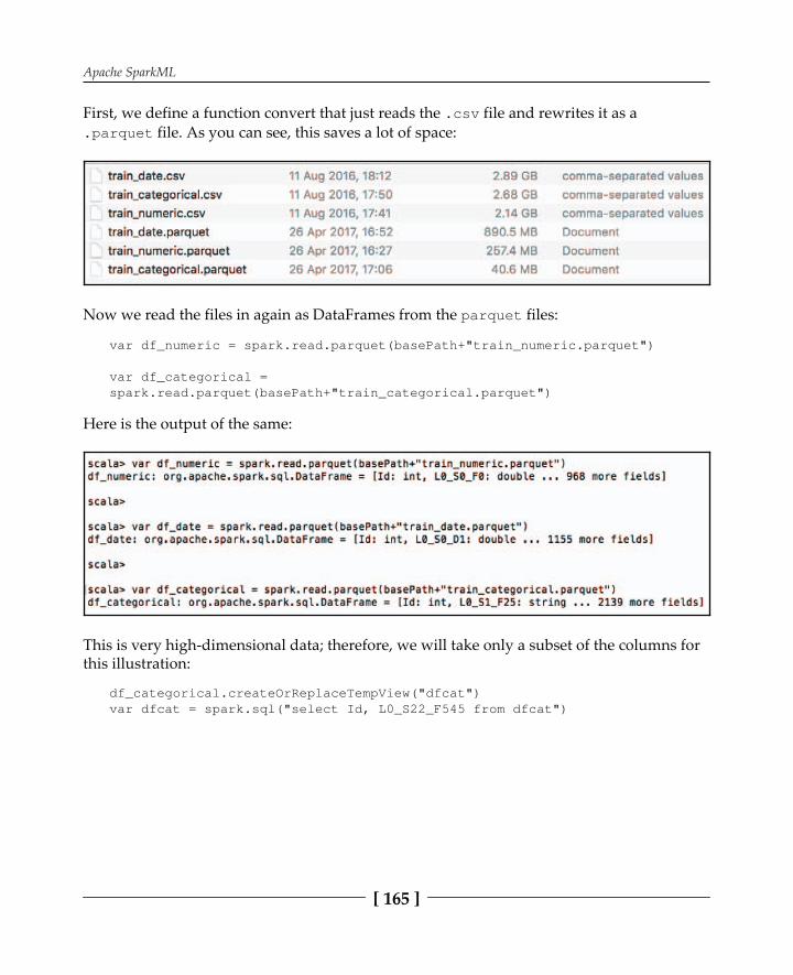
Apache SparkML
[ 165 ]
First, we define a function convert that just reads the file and rewrites it as a file. As you can see, this saves a lot of space:
Now we read the files in again as DataFrames from the files:
Here is the output of the same:
This is very high-dimensional data; therefore, we will take only a subset of the columns forthis illustration:

Apache SparkML
[ 166 ]
In the following picture, you can see the unique categorical values of that column:
Now let's do the same with the numerical dataset:
Here is the output of the same:
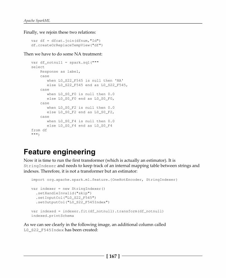
Apache SparkML
[ 167 ]
Finally, we rejoin these two relations:
Then we have to do some NA treatment:
Feature engineeringNow it is time to run the first transformer (which is actually an estimator). It is
and needs to keep track of an internal mapping table between strings andindexes. Therefore, it is not a transformer but an estimator:
As we can see clearly in the following image, an additional column called has been created:

Apache SparkML
[ 168 ]
Finally, let's examine some content of the newly created column and compare it with thesource column.
We can clearly see how the category string gets transformed into a float index:
Now we want to apply , which is a transformer, in order to generate betterfeatures for our machine learning model:

Apache SparkML
[ 169 ]
As you can see in the following figure, the newly created column contains objects, which is a compressedrepresentation of a sparse vector:
Sparse vector representations: The , as many otheralgorithms, returns a sparse vector of the
type as, according tothe definition, only one element of the vector can be one, the rest has toremain zero. This gives a lot of opportunity for compression as only theposition of the elements that are non-zero has to be known. Apache Sparkuses a sparse vector representation in the following format: (l,[p],[v]),where l stands for length of the vector, p for position (this can also be anarray of positions), and v for the actual values (this can be an array ofvalues). So if we get (13,[10],[1.0]), as in our earlier example, the actualsparse vector looks like this: (0.0,0.0,0.0,0.0,0.0,0.0,0.0,0.0,0.0,1.0,0.0,0.0,0.0).
So now that we are done with our feature engineering, we want to create one overall sparsevector containing all the necessary columns for our machine learner. This is done using
:

Apache SparkML
[ 170 ]
We basically just define a list of column names and a target column, and the rest is done forus:
As the view of the column got a bit squashed, let's inspect one instance of thefeature field in more detail:
We can clearly see that we are dealing with a sparse vector of length 16 where positions 0,13, 14, and 15 are non-zero and contain the following values: , , , and
. Done! Let's create a out of these components.

Apache SparkML
[ 171 ]
Testing the feature engineering pipelineLet's create a out of our transformers and estimators:
Note that the method of just expects an array of and, which we had created earlier. As parts of the contain estimators,
we have to run on our first. The obtained object takes a in the method and returns the results of the transformations:
As expected, we obtain the very same DataFrame as we had while running the stagesindividually in a sequence.
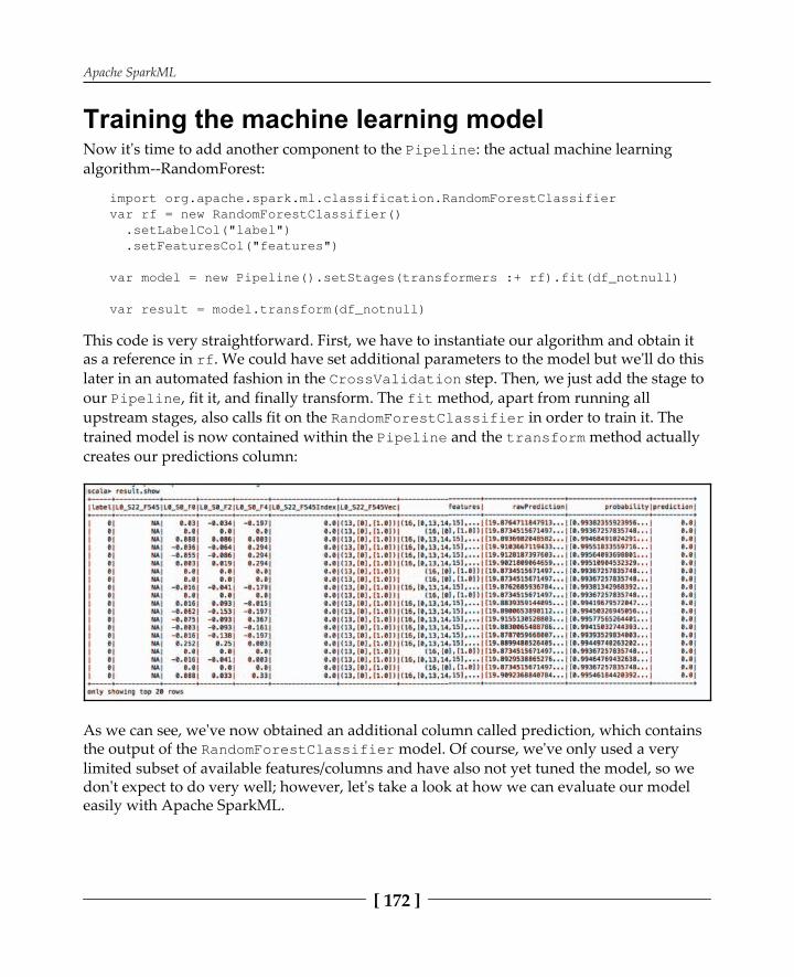
Apache SparkML
[ 172 ]
Training the machine learning modelNow it's time to add another component to the : the actual machine learningalgorithm--RandomForest:
This code is very straightforward. First, we have to instantiate our algorithm and obtain itas a reference in . We could have set additional parameters to the model but we'll do thislater in an automated fashion in the step. Then, we just add the stage toour , fit it, and finally transform. The method, apart from running allupstream stages, also calls fit on the in order to train it. Thetrained model is now contained within the and the method actuallycreates our predictions column:
As we can see, we've now obtained an additional column called prediction, which containsthe output of the model. Of course, we've only used a verylimited subset of available features/columns and have also not yet tuned the model, so wedon't expect to do very well; however, let's take a look at how we can evaluate our modeleasily with Apache SparkML.

Apache SparkML
[ 173 ]
Model evaluationWithout evaluation, a model is worth nothing as we don't know how accurately it performs.Therefore, we will now use the built-in in order toassess prediction performance and a widely used measure called (goinginto detail here is beyond the scope of this book):
As we can see, there is a built-in class called and there are
some other classes for other prediction use cases such as or. The takes a parameter map--in this
case, we are telling it to use the metric--and finally, the evaluate methodevaluates the result:
As we can see, is . An ideal classifier would return ascore of one. So we are only doing a bit better than random guesses but, as already stated,the number of features that we are looking at is fairly limited.
In the previous example we are using the metric which isused for evaluation of binary classifiers. There exist an abundance of othermetrics used for different disciplines of machine learning such asaccuracy, precision, recall and F1 score. The following provides a goodoverview
This is in fact a very bad value. Let's see if choosing better parameters forour model increases this a bit in the next section.

Apache SparkML
[ 174 ]
CrossValidation and hyperparameter tuningAs explained before, a common step in machine learning is cross-validating your modelusing testing data against training data and also tweaking the knobs of your machinelearning algorithms. Let's use Apache SparkML in order to do this for us, fully automated!
First, we have to configure the parameter map and :
The is used in order to define thehyperparameter space where the has to search and finally, the
takes our , thehyperparameter space of our RandomForest classifier, and the number of folds for the
as parameters. Now, as usual, we just need to call fit and transform onthe and it will basically run our multiple times and return amodel that performs the best. Do you know how many different models are trained? Well,we have five folds on and five-dimensional hyperparameter spacecardinalities between two and eight, so let's do the math: 5 * 8 * 5 * 2 * 7 * 7 = 19600 times!

Apache SparkML
[ 175 ]
Using the evaluator to assess the quality of thecross-validated and tuned modelNow that we've optimized our in a fully automatic fashion, let's see how our bestmodel can be obtained:
The code basically returns the best . Nowwe use to obtain the individual stages and obtain the tuned
using.
Note that addresses the last stage in the , which is our.
So now, we can basically run using the best model and see how it performs:
You might have noticed that is less than , aswe've obtained before. So why is this the case? Actually, this time we used cross-validation,which means that the model is less likely to over fit and therefore the score is a bit lower.
So let's take a look at the parameters of the best model:

Apache SparkML
[ 176 ]
Note that we've limited the hyperparameter space, so , , and have been limited to five, and bigger trees will most likely perform better. So feel free toplay around with this code and add features, and also use a bigger hyperparameter space,say, bigger trees.
SummaryYou've learned that, as in many other places, the introduction of leads to thedevelopment of complementary frameworks that are not using RDDs directly anymore.This is also the case for machine learning but there is much more to it. actuallytakes machine learning in Apache Spark to the next level as it improves the productivity ofthe data scientist dramatically.
The compatibility between all intermediate objects and well-thought-out concepts is justawesome. This framework makes it very easy to build your own stacked and bagged modelwith the full support of the underlying performance optimizations with Tungsten andCatalyst.
Great! Finally, we've applied the concepts that we discussed on a real dataset from a Kagglecompetition, which is a very nice starting point for your own machine learning project withApache SparkML. The next Chapter covers Apache SystemML, which is a 3rd partymachine learning library for Apache Spark. Let's see why it is useful and what thedifferences are to SparkML.

99Apache SystemML
So far, we have only covered components that came along with the standard distribution ofApache Spark (except HDFS, Kafka and Flume, of course). However, Apache Spark can alsoserve as runtime for third-party components, making it as some sort of operating system forbig data applications. In this chapter, we want to introduce Apache SystemML, an amazingpiece of technology initially developed by the IBM Almaden Research Lab in California.Apache SystemML went through many transformation stages and has now become anApache top level project.
In this chapter, we will cover the following topics to get a greater insight into the subject:
Using SystemML for your own machine learning applications on top of ApacheSparkLearning the fundamental differences between SystemML and other machinelearning libraries for Apache SparkDiscovering the reason why another machine library exists for Apache Spark
Why do we need just another library?In order to answer this question, we have to know something about SystemML's history,which began ten years ago in 2007 as a research project in the IBM Almaden Research Lab inCalifornia. The project was driven by the intention to improve the workflow of datascientists, especially those who want to improve and add functionality to existing machinelearning algorithms.

Apache SystemML
[ 178 ]
So, SystemML is a declarative markup language that can transparentlydistribute work on Apache Spark. It supports Scale-up usingmultithreading and SIMD instructions on CPUs as well as GPUs and alsoScale-out using a cluster, and of course, both together.
Finally, there is a cost-based optimizer in place to generate low-level execution plans takingstatistics about the Dataset sizes into account. In other words, Apache SystemML is formachine learning, what Catalyst and Tungsten are for DataFrames.
Why on Apache Spark?Apache Spark solves a lot of common issues in data processing and machine learning, soApache SystemML can make use of these features. For example, Apache Spark supports theunification of SQL, Graph, Stream, and machine learning data processing on top of acommon RDD structure.
In other words, it is a general DAG (directed acyclic graph) execution engine supportinglazy evaluation and distributed in-memory caching.
The history of Apache SystemMLApache SystemML is already ten years old. Of course, it went through multiple refactoringsand is now a state-of-the-art, and one of the fastest, machine learning libraries in the world.Recently, DeepLearning has also been added, which we will cover briefly in the followingchapter on DeepLearning:

Apache SystemML
[ 179 ]
As you can see in the preceding figure, a lot of research has been done for ApacheSystemML. It is two years older than Apache Spark and in 2017 it has been turned into a toplevel Apache project, leaving incubator status. Even during the time SystemML was started,the researchers at IBM Research Almaden realized that, very often, out-of-the box machinelearning algorithms perform very poorly on large Datasets.

Apache SystemML
[ 180 ]
So, the data analysis pipeline had to be tuned after a small-scale version of it had beenprototyped. The following figure illustrates this:
This means that the data scientist will prototype his application in a programming languageof his choice, most likely Matlab, R or python and, finally, a systems programmer will pickthis up and re-implement this in a JVM language like Java or Scala, which usually turns outto provide better performance and also linearly scales on data parallel framework likeApache Spark.
The scaled version of the prototype will return results on the whole Dataset and the datascientist again is in charge of modifying the prototype and the whole cycle begins again.Not only the IBM Almaden Research staff members have experienced this, but even ourteam has seen it. So let's make the systems programmer redundant (or at least require himonly to take care of our Apache Spark jobs) using Apache SystemML.
A cost-based optimizer for machine learningalgorithmsLet's start with an example to exemplify how Apache SystemML works internally. Considera recommender system.

Apache SystemML
[ 181 ]
An example - alternating least squaresA recommender system tries to predict the potential items that a user might be interestedin, based on a history from other users.
So let's consider a so-called item-user or product-customer matrix, as illustrated here:
This is a so-called sparse matrix because only a couple of cells are populated with non-zerovalues indicating a match between a customer i and a product j. Either by just putting a onein the cell or any other numerical value, for example, indicating the number of productsbought or a rating for that particular product j from customer i. Let's call this matrix rui,where u stands for user and i for item.
Those of you familiar with linear algebra might know that any matrix can be factorized bytwo smaller matrices. This means that you have to find two matrices pu and qi that, whenmultiplied with each other, reconstruct the original matrix rui; let's call the reconstructionrui'. The goal is to find pu and qi to reconstruct rui' such that it doesn't differ too much from rui.This is done using a sum of squared errors objective.

Apache SystemML
[ 182 ]
The following figure illustrates this and the sparsity property of the matrix:
Once we've found good factors pu and qi, we can construct rui' and, finally, new non-zerocells will be present, which become the new predicted product suggestions. In case youhaven't understood all the details, don't worry, as we don't need too much of this exampleto understand the rest of this chapter.
A common algorithm to find pu and qi is called alternating least squares (ALS)--alternatingbecause in each iteration the optimization objective switches from pu to qi and vice versa.Don't get bothered with it too much, but this is how it actually works, and, in Apache SparkMLlib, this is just a single line of Scala code:

Apache SystemML
[ 183 ]
So what's wrong with this? Before we explain this, let's take a look at how ALS isimplemented in a statistical programming language such as R:

Apache SystemML
[ 184 ]
Again, don't worry if you don't understand each line, but the purpose of this figure is toshow you that in R, this algorithm needs only 27 lines of code to be expressed. If we nowtake a look at the ALS implementation in MLlib, we'll see that it has more than 800 lines.You can find this implementation at
.
So why do we need more than 800 lines in Scala on Spark and only 27 in R? This is becauseof performance optimizations. The ALS implementation in MLlib consists of more than 50%of performance optimization code. So what if we could perform the following?
Get rid of all performance optimizations in our algorithm implementationPort our R code 1:1 to some parallel frameworkIn case of changes, just change our R implementation
This is where Apache SystemML kicks in, it supports all this. Apache SystemML's DSL(domain specific language) is a subset of R syntax, so you can just take the previousexample and run it 1:1 without any modification on top of Apache SystemML. In addition, acost-based performance optimizer generates a physical execution plan on top of ApacheSpark in order to minimize execution time based on size properties of your data. So let'sfind out how this works.
ApacheSystemML architectureSo the key thing on Apache SystemML is the optimizer. This component turns a high-leveldescription of an algorithm in a domain-specific language into a highly optimized physicalexecution on Apache Spark, as shown in the following figure:

Apache SystemML
[ 185 ]
Language parsingLet's open this black box a bit in order to understand what exactly is going on in the ApacheSystemML optimizer. The first thing that the engine does is a compile step on the DSL. Sofirst, syntax checking, then live variable analysis in order to determine which intermediateresults are still needed, and finally a semantic check.
High-level operators are generatedOnce the previous step is passed, the execution plan using so-called high-level operators(HOPs) is generated. These are constructed from the abstract syntax tree (AST) of the DSL.The following important optimization steps are taking place during this phase:
Static rewrites: The DSL offers a rich set of syntactical and semantic features thatmakes an implementation easy to understand but may result in a non-optimalexecution. Apache SystemML detects these branches of the AST and staticallyrewrites them to a better version, maintaining the semantic equivalency.Dynamic rewrites: Dynamic rewrites are very similar to static rewrites but aredriven by cost-based statistics considering the size of the Datasets to beprocessed.

Apache SystemML
[ 186 ]
The following figure illustrates a static rewrite where a branch of the AST performing amatrix multiplication, is actually rewritten to use a HOP called wdivmm (weighted dividematrix multiplication), which is a way of computing results of matrix multiplication of thatparticular form, without materializing a very large intermediate dense matrix in order tosave memory:

Apache SystemML
[ 187 ]
How low-level operators are optimized onLet's have a look on how low-level operators are selected and optimized on. We'll stick tothe weighted divide matrix multiplication example--a HOP that has been selected before theHOP optimizations process over an ordinary sequence of matrix multiplications. So nowthe question arises, for example, if it makes sense to use a parallel version of a LOP runningparallel on the Apache Spark workers, or whether a local execution is preferable. In thisexample, Apache SystemML determines that all intermediate results fit into the mainmemory of the driver node and chooses the local operator, WDivMM, over the paralleloperator, MapWDivMM. The following figure illustrates this process:

Apache SystemML
[ 188 ]
Performance measurementsSo is all this effort worth it? Let's take a look at some performance comparisons between alocal R script, MLlib, and Apache SystemML:
The ALS algorithm has been run on different Datasets with 1.2, 12, and 120 GB size using R,MLlib, and ApacheSystemML. We can clearly see that, even on the smallest Dataset, R is nota feasible solution as it took more than 24 hours, and we are not sure if it would have evercompleted. On the 12 GB Dataset, we've noticed that ApacheSystemML runs significantlyfaster than MLlib, and finally, on the 120 GB Dataset, the ALS implementation of MLlibdidn't finish in one day and we gave up.
Apache SystemML in actionSo let's take a look at a very simple example. Let's create a script in Apache SystemML DSL--an R-like syntax--in order to multiply two matrices:

Apache SystemML
[ 189 ]
Then, we generate some test data:
In order to use Apache SystemML, we have to create an object:
Now we have to convert our data to a format that Apache SystemML understands:

Apache SystemML
[ 190 ]
Now, we pass the data and to the Apache SystemML runtime and also preregister avariable called in order to obtain the result from the runtime:
Finally, we actually execute the script stored in with the method and obtain the result from the runtime:
Now contains with the result of the matrix multiplication. Done!
SummaryYou've learned that there is room for additional machine learning frameworks and librarieson top of Apache Spark and that a cost-based optimizer similar to what we are alreadyusing in Catalyst can speed things up tremendously. In addition, separation fromperformance optimizations code and code for the algorithm facilitates furtherimprovements on the algorithm side without having to care about performance at all.
Additionally, these execution plans are highly adaptable to the size of the data and also tothe available hardware configuration based on main memory size and potential acceleratorssuch as GPUs. Apache SystemML dramatically improves on the life cycle of machinelearning applications, especially if machine learning algorithms are not used out of the box,but an experienced data scientists works on low level details on it in a mathematical orstatistical programming language.
In Apache SystemML, this low level, mathematical code can be used out of the box, withoutany manual transformation or translation to other programming languages . It can beexecuted on top of Apache Spark.
In the next chapter we'll cover DeepLearning and how it can be used on top of ApacheSpark. This is one of the hottest topics in 2017, so stay tuned!

110Deep Learning on Apache
Spark with DeepLearning4j andH2O
This chapter will give you an introduction to Deep Learning and how you can use third-party machine learning libraries on top of Apache Spark in order to do so. Deep Learning isoutperforming a variety of state-of-the-art machine learning algorithms, and it is a veryactive area of research, so there is more to come soon. Therefore, it is important to knowhow Deep Learning works and how it can be applied in a parallel data processingenvironment such as Apache Spark.
This chapter will cover the following topics in detail:
Introduction to the installation and usage of the H2O frameworkIntroduction to Deeplearning4j with an IoT anomaly detection example
H2OH2O is an open source system developed in Java by for machine learning.It offers a rich set of machine learning algorithms and a web-based data processing userinterface. It offers the ability to develop in a range of languages: Java, Scala, Python, and R.
It also has the ability to interface with Spark, HDFS, SQL, and NoSQL databases. Thischapter will concentrate on H2O's integration with Apache Spark using the Sparkling Watercomponent of H2O. A simple example developed in Scala will be used based on real data tocreate a deep-learning model.

Deep Learning on Apache Spark with DeepLearning4j and H2O
[ 192 ]
The next step will be to provide an overview of the H2O functionality and the SparklingWater architecture that will be used in this chapter.
OverviewSince it is only possible to examine and use a small amount of H2O's functionality in thischapter, we thought that it would be useful to provide a list of all of the functional areasthat it covers. This list is taken from the website at
and is based upon wrangling data, modeling using the data, and scoringthe resulting models:
ProcessModelThe score toolData profilingGeneralized linear models (GLM)PredictSummary statisticsDecision treesConfusion matrixAggregate, filter, bin, and derive columnsGradient boosting machine (GBM)AUCSlice, log transform, and anonymizeK-meansHit ratioVariable creationAnomaly detectionPCA/PCA scoreDeep learningMultimodel scoringTraining and validation sampling planNaive BayesGrid search
The following section will explain the environment used for the Spark and H2O examplesin this chapter and some of the problems encountered.
Deep Learning on Apache Spark with DeepLearning4j and H2O
[ 193 ]
For completeness, we will show you how we downloaded, installed, and used H2O.Although we finally settled on version 0.2.12-95, we first downloaded and used 0.2.12-92.This section is based on the earlier install, but the approach used to source the software isthe same. The download link changes over time, so follow the Sparkling Water downloadoption at .
This will source the zipped Sparkling Water release, as shown in the file listing here:
[hadoop@hc2r1m2 h2o]$ pwd ; ls -l /home/hadoop/h2o total 15892 -rw-r--r-- 1 hadoop hadoop 16272364 Apr 11 12:37 sparkling-water-0.2.12-92.zip
This zipped release file is unpacked using the Linux command, and it results in aSparkling Water release file tree:
[hadoop@hc2r1m2 h2o]$ unzip sparkling-water-0.2.12-92.zip
[hadoop@hc2r1m2 h2o]$ ls -d sparkling-water* sparkling-water-0.2.12-92 sparkling-water-0.2.12-92.zip
We have moved the release tree to the area using the root account andcreated a simple symbolic link to the release called H2O. This means that our H2O-basedbuild can refer to this link, and it doesn't need to change as new versions of Sparkling Waterare sourced. We have also made sure, using the Linux command, that ourdevelopment account, Hadoop, has access to the release:
[hadoop@hc2r1m2 h2o]$ su -[root@hc2r1m2 ~]# cd /home/hadoop/h2o[root@hc2r1m2 h2o]# mv sparkling-water-0.2.12-92 /usr/local[root@hc2r1m2 h2o]# cd /usr/local
[root@hc2r1m2 local]# chown -R hadoop:hadoop sparkling-water-0.2.12-92[root@hc2r1m2 local]# ln –s sparkling-water-0.2.12-92 h2o
[root@hc2r1m2 local]# ls –lrt | grep sparklingtotal 52drwxr-xr-x 6 hadoop hadoop 4096 Mar 28 02:27 sparkling-water-0.2.12-92lrwxrwxrwx 1 root root 25 Apr 11 12:43 h2o -> sparkling-water-0.2.12-92
The release has been installed on all the nodes of our Hadoop clusters.

Deep Learning on Apache Spark with DeepLearning4j and H2O
[ 194 ]
The build environmentFrom past examples, you know that we favor sbt as a build tool for developing Scala sourceexamples.
We have created a development environment on the Linux server called using theHadoop development account. The development directory is called :
[hadoop@hc2r1m2 h2o_spark_1_2]$ pwd /home/hadoop/spark/h2o_spark_1_2
Our SBT build configuration file named is located here; it contains the following:
[hadoop@hc2r1m2 h2o_spark_1_2]$ more h2o.sbt
name := "H 2 O"
version := "1.0"
scalaVersion := "2.10.4"
libraryDependencies += "org.apache.hadoop" % "hadoop-client" % "2.3.0"
libraryDependencies += "org.apache.spark" % "spark-core" % "1.2.0" from"file:///usr/hdp/2.6.0.3-8/spark/lib/spark-assembly-1.6.3.2.6.0.3-8-hadoop2.7.3.2.6.0.3-8.jar"
libraryDependencies += "org.apache.spark" % "mllib" % "1.2.0" from"file:///usr/hdp/2.6.0.3-8/spark/lib/spark-assembly-1.6.3.2.6.0.3-8-hadoop2.7.3.2.6.0.3-8.jar"
libraryDependencies += "org.apache.spark" % "sql" % "1.2.0" from"file:///usr/hdp/2.6.0.3-8/spark/lib/spark-assembly-1.6.3.2.6.0.3-8-hadoop2.7.3.2.6.0.3-8.jar"
libraryDependencies += "org.apache.spark" % "h2o" % "0.2.12-95" from"file:///usr/local/h2o/assembly/build/libs/sparkling-water-assembly-0.2.12-95-all.jar"
libraryDependencies += "hex.deeplearning" % "DeepLearningModel" %"0.2.12-95" from "file:///usr/local/h2o/assembly/build/libs/sparkling-water-assembly-0.2.12-95-all.jar"
libraryDependencies += "hex" % "ModelMetricsBinomial" % "0.2.12-95" from"file:///usr/local/h2o/assembly/build/libs/sparkling-water-assembly-0.2.12-95-all.jar"
libraryDependencies += "water" % "Key" % "0.2.12-95" from

Deep Learning on Apache Spark with DeepLearning4j and H2O
[ 195 ]
"file:///usr/local/h2o/assembly/build/libs/sparkling-water-assembly-0.2.12-95-all.jar"
libraryDependencies += "water" % "fvec" % "0.2.12-95" from"file:///usr/local/h2o/assembly/build/libs/sparkling-water-assembly-0.2.12-95-all.jar"
We provided configuration examples in the previous chapters, so we won't go into line-by line-detail here. We have used the file-based URLs to define the library dependenciesand sourced the Hadoop JAR files from Hadoop home.
The Sparkling Water JAR path is defined as that was just created.We use a Bash script called within this development directory to executeour H2O-based example code. It takes the application class name as a parameter and isshown as follows:
[hadoop@hc2r1m2 h2o_spark_1_2]$ more run_h2o.bash
#!/bin/bash
SPARK_HOME=/usr/hdp/current/spark-client SPARK_LIB=$SPARK_HOME/lib SPARK_BIN=$SPARK_HOME/bin SPARK_SBIN=$SPARK_HOME/sbin SPARK_JAR=$SPARK_LIB/spark-assembly-1.6.3.2.6.0.3-8-hadoop2.7.3.2.6.0.3-8.jar
H2O_PATH=/usr/local/h2o/assembly/build/libs H2O_JAR=$H2O_PATH/sparkling-water-assembly-0.2.12-95-all.jar
PATH=$SPARK_BIN:$PATH PATH=$SPARK_SBIN:$PATH export PATH
cd $SPARK_BIN
./spark-submit \ --class $1 \ --master spark://hc2nn.semtech-solutions.co.nz:7077 \ --executor-memory 512m \ --total-executor-cores 50 \ --jars $H2O_JAR \ /home/hadoop/spark/h2o_spark_1_2/target/scala-2.10/h-2-o_2.10-1.0.jar

Deep Learning on Apache Spark with DeepLearning4j and H2O
[ 196 ]
This example of Spark application submission has already been covered, so again, we won'tgo into detail. Setting the executor memory at a correct value was critical to avoiding out-of-memory issues and performance problems. This is examined in the Performance tuningsection.As in the previous examples, the application Scala code is located in the subdirectory under the development directory level. The next section will examine theApache Spark and the H2O architectures.
ArchitectureThe diagrams in this section have been sourced from the website at
to provide aclear method of describing the way in which H2O Sparkling Water can be used to extendthe functionality of Apache Spark. Both H2O and Spark are open source systems. SparkMLlib contains a great deal of functionality, while H2O extends this with a wide range ofextra functionality, including Deep Learning. It offers tools to munge (transform), model,and score the data, as we can find in Apache SparkML. It also offers a web-based userinterface to interact with.
The next diagram, borrowed from , shows how H2O integrates with Spark.As we already know, Spark has master and worker servers; the workers create executors todo the actual work.
The following steps occur to run a Sparkling Water-based application:
Spark's submit command sends the Sparkling Water JAR to the Spark masterThe Spark master starts the workers and distributes the JAR fileThe Spark workers start the executor JVMs to carry out the workThe Spark executor starts an H2O instance

Deep Learning on Apache Spark with DeepLearning4j and H2O
[ 197 ]
The H2O instance is embedded with the Executor JVM, and so it shares the JVM heap spacewith Spark. When all of the H2O instances have started, H2O forms a cluster, and then theH2O flow web interface is made available.

Deep Learning on Apache Spark with DeepLearning4j and H2O
[ 198 ]
The preceding diagram explains how H2O fits into the Apache Spark architecture and howit starts, but what about data sharing? How does data pass between Spark and H2O? Thefollowing diagram explains this:
A new H2O RDD data structure has been created for H2O and Sparkling Water. It is a layerbased at the top of an H2O frame, each column of which represents a data item and isindependently compressed to provide the best compression ratio.
In the Deep Learning example Scala code presented later in this chapter, you will see that adata frame has been created implicitly from a Spark schema RDD, and a columnar data itemincome has been enumerated.

Deep Learning on Apache Spark with DeepLearning4j and H2O
[ 199 ]
We won't dwell on this now, as it will be explained later, but this is a practical example ofthe architecture explained earlier:
val testFrame:DataFrame = schemaRddTest testFrame.replace( testFrame.find("income"), testFrame.vec("income").toEnum)
In the Scala-based example that will be tackled in this chapter, the following actions willtake place:
Data will be sourced from HDFS and stored in a Spark RDDSpark SQL will be used to filter dataThe Spark schema RDD will be converted into an H2O RDDThe H2O-based processing and modeling will occurThe results will be passed back to Spark for accuracy checking
At this point, the general architecture of H2O has been examined, and the product has beensourced for use. The development environment has been explained, and the process bywhich H2O and Spark integrate has been considered. Now it is time to delve into a practicalexample of the use of H2O. First though, some real-world data must be sourced formodeling purposes.
Sourcing the dataSince we have already used the Artificial Neural Net (ANN) functionality, in the chapteron Apache Spark MLlib to classify images, it seems only fitting that we use H2O deeplearning to classify data in this chapter. In order to do this, we need to source Datasets thatare suitable for classification. We need either image data with associated image labels ordata containing vectors and a label that we can enumerate so that we can force H2O to useits classification algorithm.
The MNIST test and training image data was sourced from. It contains 50,000 training rows and 10,000 rows for
testing. It contains digital images of the numbers 0 to 9 and associated labels.We were not able to use this data, as, at the time of writing, there was a bug in H2OSparkling Water which limited the record size to 128 elements. The MNIST data has arecord size of 28 x 28 + 1 elements for the image plus the label, since one image is 28 pixelswide, 28 pixels high and has one label assigned to it:
15/05/14 14:05:27 WARN TaskSetManager: Lost task 0.0 in stage 9.0 (TID 256,hc2r1m4.semtech-solutions.co.nz): java.lang.ArrayIndexOutOfBoundsException:-128

Deep Learning on Apache Spark with DeepLearning4j and H2O
[ 200 ]
This issue should have been fixed and released by the time you read this, but in the shortterm, we sourced another Dataset called income from
, which contains Canadian employee income data. The followinginformation shows the attributes and the data volume. It also shows the list of columns inthe data and a sample row of the data:
We will enumerate the last column in the data, the income bracket, so will enumerateto . This will allow us to force the H2O deep learning algorithm to carry out classificationrather than regression. We will also use Spark SQL to limit the data columns and filter thedata.
As in all machine learning applications, data quality is absolutely critical when creating anH2O-based example as described in this chapter. The next section examines the steps thatcan be taken to improve the data quality and, hence, save time.
Data qualityWhen importing CSV data files from HDFS to the Spark Scala H2O example code, we canfilter the incoming data. The following example code contains two filter lines--the firstchecks that a data line is not empty, while the second checks that the final column in eachdata row (income), which will be enumerated, is not empty:
val testRDD = rawTestData .filter(!_.isEmpty) .map(_.split(",")) .filter( rawRow => ! rawRow(14).trim.isEmpty )
We also needed to clean our raw data. There are two Datasets, one for training and anotherfor testing. It is important that the training and testing data have the following:
The same number of columnsThe same data typesThe enumerated type values must match, especially for the labels

Deep Learning on Apache Spark with DeepLearning4j and H2O
[ 201 ]
So, we think that time and effort should be spent safeguarding the data quality as a pre-stepto training and testing machine learning functionality, so that time is not lost and no extralabor cost incurres.
Performance tuningIt is important to monitor the Spark application errors and the standard output logs in theSpark web user interface if you see errors such as the following:
05-15 13:55:38.176 192.168.1.105:54321 6375 Thread-10 ERRR: Out ofMemory and no swap space left from hc2r1m1.semtech-solutions.co.nz/192.168.1.105:54321
If you encounter instances where application executors seem to hang without response, youmay need to tune your executor memory. You need to do so if you see an error such as thefollowing in your executor log:
05-19 13:46:57.300 192.168.1.105:54321 10044 Thread-11 WARN: Unblockallocations; cache emptied but memory is low: OOM but cache is emptied:MEM_MAX = 89.5 MB, DESIRED_CACHE = 96.4 MB, CACHE = N/A, POJO = N/A, thisrequest bytes = 36.4 MB
This can cause a loop, as the application requests more memory than is available and,hence, waits until the next iteration retries.
The application can seem to hang until the executors are killed, and the tasks are re-executed on alternate nodes. A short task's runtime can extend considerably due to suchproblems.
Monitor the Spark logs for these types of errors. In the previous example, changing theexecutor memory setting in the spark-submit command removes the error and reduces theruntime substantially.
The memory value requested has been reduced to a number below that which is available.
Deep LearningNeural networks were introduced in the chapter on Apache Spark MLlib. This chapterbuilds upon this understanding by introducing Deep Learning, which uses deep neuralnetworks. These are neural networks that are feature-rich and contain extra hidden layersso that their ability to extract data features is increased.
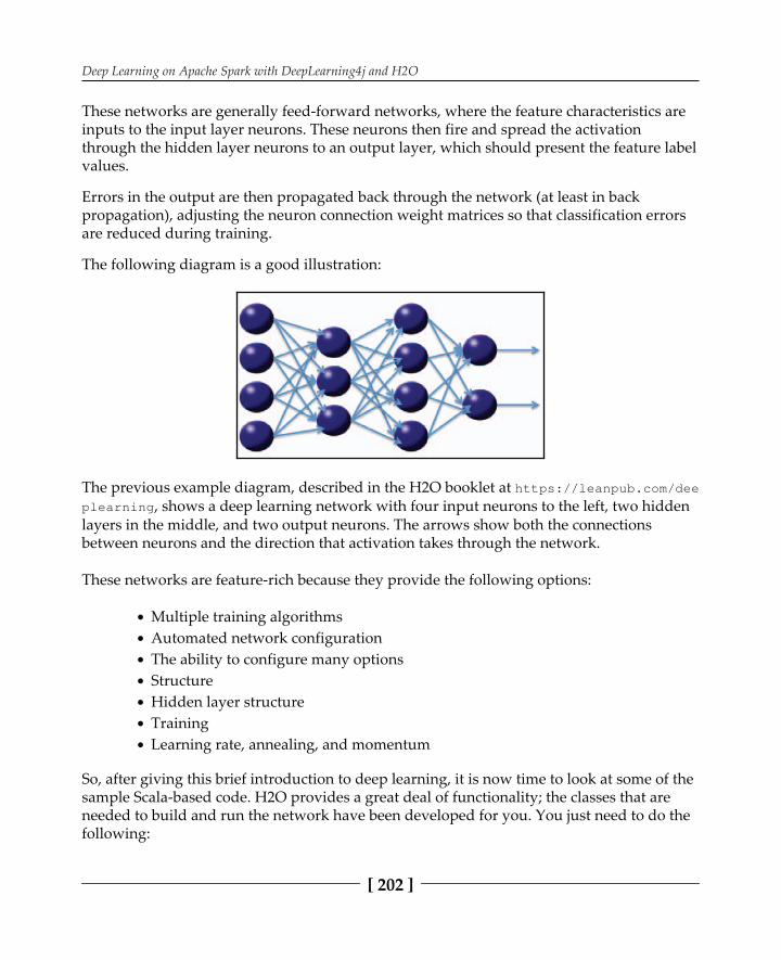
Deep Learning on Apache Spark with DeepLearning4j and H2O
[ 202 ]
These networks are generally feed-forward networks, where the feature characteristics areinputs to the input layer neurons. These neurons then fire and spread the activationthrough the hidden layer neurons to an output layer, which should present the feature labelvalues.
Errors in the output are then propagated back through the network (at least in backpropagation), adjusting the neuron connection weight matrices so that classification errorsare reduced during training.
The following diagram is a good illustration:
The previous example diagram, described in the H2O booklet at , shows a deep learning network with four input neurons to the left, two hidden
layers in the middle, and two output neurons. The arrows show both the connectionsbetween neurons and the direction that activation takes through the network.
These networks are feature-rich because they provide the following options:
Multiple training algorithmsAutomated network configurationThe ability to configure many optionsStructureHidden layer structureTrainingLearning rate, annealing, and momentum
So, after giving this brief introduction to deep learning, it is now time to look at some of thesample Scala-based code. H2O provides a great deal of functionality; the classes that areneeded to build and run the network have been developed for you. You just need to do thefollowing:

Deep Learning on Apache Spark with DeepLearning4j and H2O
[ 203 ]
Prepare the data and parametersCreate and train the modelValidate the model with a second DatasetScore the validation Dataset output
When scoring your model, you must hope for a high value in percentage terms. Your modelmust be able to accurately predict and classify your data.
This section examines the Scala-based H2O Sparkling Water Deep Learning example usingthe previous Canadian income data source. First, the Spark (Context, Conf, MLlib, andRDD) and H2O (h2o, deeplearning, and water) classes are imported:
Next, an application class called is defined, the master URL is created, andthen a configuration object is created based on this URL and the application name.
The Spark context is then created using the configuration object:
An H2O context is created from the Spark context, and also an SQL context:

Deep Learning on Apache Spark with DeepLearning4j and H2O
[ 204 ]
The H2O Flow user interface is started with the command:
The training and testing of the data files are now defined (on HDFS) using the server URL,path, and the filenames:
The CSV-based training and testing data is loaded using the Spark SQL context's method:
Now the schema is defined in terms of a string of attributes. Then, a schema variable iscreated by splitting the string using a series of , based on each column. Thedata types are left as String, and the true value allows for the null values in the data:
The raw CSV line training and testing data is now split by commas into columns. The datais filtered on empty lines to ensure that the last column (income) is not empty. The actualdata rows are created from the fifteen (0-14) trimmed elements in the raw CSV data. Boththe training and the test Datasets are processed:

Deep Learning on Apache Spark with DeepLearning4j and H2O
[ 205 ]
Spark Schema RDD variables are now created for the training and test Datasets by applyingthe schema variable created previously for the data using the Spark context's method:
Temporary tables are created for the training and testing data:
Now, SQL is run against these temporary tables, both to filter the number of columns and topotentially limit the data. We could have added a or clause. This is a usefulapproach that enables us to manipulate both the column and row-based data:

Deep Learning on Apache Spark with DeepLearning4j and H2O
[ 206 ]
The H2O data frames are now created from the data. The final column in each Dataset(income) is enumerated because this is the column that will form the Deep Learning labelfor the data. Also, enumerating this column forces the Deep Learning model to carry outclassification rather than regression:
The enumerated results data income column is now saved so that the values in this columncan be used to score the tested model prediction values:
The Deep Learning model parameters are now set up in terms of the number of epochs oriterations--the Datasets for training and validation and the label column income, which willbe used to classify the data.
Also, we chose to use variable importance to determine which data columns are the mostimportant in the data. This parameter tells the model to calculate the effect of each featureto the target variable. This way, after the training, a table with that data can be plotted. TheDeep Learning model is then created:

Deep Learning on Apache Spark with DeepLearning4j and H2O
[ 207 ]
The model is then scored against the test Dataset for predictions, and these incomepredictions are compared to the previously stored enumerated test data income values.Finally, an accuracy percentage is output from the test data:
In the last step, the application is stopped, the H2O functionality is terminated via a call, and then the Spark context is stopped:
Based upon a training Dataset of 32,000 and a test Dataset of 16,000 income records, thisDeep Learning model is quite accurate. It reaches an accuracy level of percent, which isimpressive for a few lines of code, small Datasets, and just 100 epochs, as the run outputshows:

Deep Learning on Apache Spark with DeepLearning4j and H2O
[ 208 ]
This is of course not a very impressive number. The next steps to improve this numberwould include hyper-parameter tuning in order to find a better parametrization of theneural network, but in order to really outperform this number, a different neural network type has to be used, which is called a convolutional neural network (CNN). Unfortunately,H2O lacks direct support for CNNs and needs to make use of third-party integration toframeworks such as TensorFlow, Caffe, and MXNet. But Deeplearning4j, which is alsocovered in this chapter, supports CNNs out-of-the-box.
In the next section, we will examine some of the coding needed to process the MNIST data,even though that example could not be completed due to an H2O limitation at the time ofcoding.
The example code – MNISTSince the MNIST image data record is so big, it presents problems while creating a SparkSQL schema and processing a data record. The records in this data are in CSV format andare formed from a 28 x 28 digit image.
Each line is then terminated by a label value for the image. We have created our schema bydefining a function to create the schema string to represent the record and then calling it:
The same general approach to Deep Learning can be taken to data processing as theprevious example, apart from the actual processing of the raw CSV data. There are toomany columns to process individually, and they all need to be converted into integers torepresent their data type. This can be done in two ways.

Deep Learning on Apache Spark with DeepLearning4j and H2O
[ 209 ]
In the first example, var args can be used to process all the elements in the row:
The second example uses the method to process the row elements:
In the next section, the H2O Flow user interface will be examined to see how it can be usedto both monitor H2O and process the data.
H2O FlowH2O Flow is a web-based open source user interface for H2O and, given that it is beingused with Spark, Sparkling Water. It is a fully functional H2O web interface for monitoringthe H2O Sparkling Water cluster jobs, and also for manipulating data and training models.
We have created some simple example code to start the H2O interface. As in the previousScala-based code samples, all we need to do is create a Spark, an H2O context, and then callthe command, which will start the Flow interface.The following Scala code example just imports classes for Spark context, configuration, andH2O. It then defines the configuration in terms of the application name and the Sparkcluster URL.
A Spark context is then created using the configuration object:

Deep Learning on Apache Spark with DeepLearning4j and H2O
[ 210 ]
An H2O context is then created and started using the Spark context. The H2O contextclasses are imported, and the Flow user interface is started with the command:
Note that, for the purposes of this example and to enable us to use the Flow application, wehave commented out the H2O shutdown and the Spark context stop options. We would notnormally do this, but we wanted to make this application long-running so that it gives usplenty of time to use the interface:
We use our Bash script with the application class name called as a parameter. This script contains a call to the command,
which will execute the compiled application:
[hadoop@hc2r1m2 h2o_spark_1_2]$ ./run_h2o.bash h2o_spark_ex2
When the application runs, it lists the state of the H2O cluster and provides a URL by whichthe H2O Flow browser can be accessed:
15/05/20 13:00:21 INFO H2OContext: Sparkling Water started, status ofcontext: Sparkling Water Context: * number of executors: 4 * list of used executors: (executorId, host, port) ------------------------ (1,hc2r1m4,54321) (3,hc2r1m2,54321) (0,hc2r1m3,54321) (2,hc2r1m1,54321) ------------------------

Deep Learning on Apache Spark with DeepLearning4j and H2O
[ 211 ]
Open H2O Flow in browser: (CMD + click in macOS).The previous example shows that we can access the H2O interface using the port number
on the host IP address .
So, we can access the interface using the URL. The following screenshotshows the Flow interface with no data loaded.
There are data processing and administration menu options, and buttons at the top of thepage. To the right, there are help options to enable you to learn more about H2O:

Deep Learning on Apache Spark with DeepLearning4j and H2O
[ 212 ]
The following screenshot shows the menu options and buttons in greater detail. In thefollowing sections, we will use a practical example to explain some of these options, butthere will not be enough space in this chapter to cover all the functionality. Check the
website to learn about the Flow application in detail, available at :
In greater definition, you can see that the previous menu options and buttons allow you toboth administer your H2O Spark cluster and also manipulate the data that you wish toprocess.
The following screenshot shows a reformatted list of the help options available, so that ifyou get stuck, you can investigate solving your problem from the same interface:
If we go to Menu | Admin | Cluster Status, we will obtain the following screenshot, whichshows us the status of each cluster server in terms of memory, disk, load, and cores.
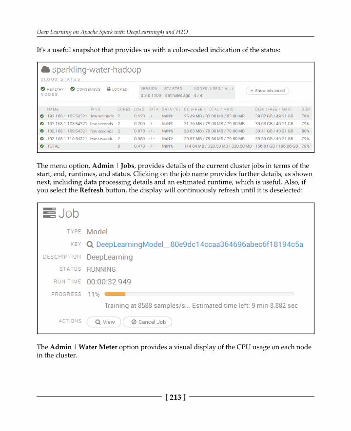
Deep Learning on Apache Spark with DeepLearning4j and H2O
[ 213 ]
It's a useful snapshot that provides us with a color-coded indication of the status:
The menu option, Admin | Jobs, provides details of the current cluster jobs in terms of thestart, end, runtimes, and status. Clicking on the job name provides further details, as shownnext, including data processing details and an estimated runtime, which is useful. Also, ifyou select the Refresh button, the display will continuously refresh until it is deselected:
The Admin | Water Meter option provides a visual display of the CPU usage on each nodein the cluster.

Deep Learning on Apache Spark with DeepLearning4j and H2O
[ 214 ]
As you can see in the following screenshot, our meter shows that my cluster was idle:
Using the menu option, Flow | Upload File, we have uploaded some of the training dataused in the previous Deep Learning Scala-based example.
The data has been loaded into a data preview pane; we can see a sample of the data that hasbeen organized into cells. Also, an accurate guess has been made of the data types so thatwe can see which columns can be enumerated. This is useful if we want to considerclassification:

Deep Learning on Apache Spark with DeepLearning4j and H2O
[ 215 ]
Having loaded the data, we are now presented with a Frame display, which offers us theability to view, inspect, build a model, create a prediction, or download the data. The datadisplay shows information such as min, max, and mean.
It shows data types, labels, and a zero data count, as shown in the following screenshot:

Deep Learning on Apache Spark with DeepLearning4j and H2O
[ 216 ]
We thought that it would be useful to create a Deep Learning classification model based onthis data to compare the Scala-based approach to this H2O user interface. Using the viewand inspect options, it is possible to visually and interactively check the data, as well ascreate plots relating to the data. For instance, using the previous inspect option followed bythe plot columns option, we were able to create a plot of data labels versus zero counts inthe column data. The following screenshot shows the result:
By selecting the Build Model option, a menu option is offered that lets us choose a modeltype. We will select deeplearning, as we already know that this data is suited to thisclassification approach.

Deep Learning on Apache Spark with DeepLearning4j and H2O
[ 217 ]
The previous Scala-based model resulted in an accuracy level of 83 percent:
We have selected the deeplearning option. Having chosen this option, we are able to setmodel parameters such as training and validation Datasets, as well as choose the datacolumns that our model should use (obviously, the two Datasets should contain the samecolumns).
The following screenshot displays the Datasets and the model columns being selected:

Deep Learning on Apache Spark with DeepLearning4j and H2O
[ 218 ]
There is a large range of basic and advanced model options available. A selection of them isshown in the following screenshot.
We have set the response column to as the income column. We have also set theVARIABLE_IMPORTANCES option. Note that we don't need to enumerate the responsecolumn, as it has been done automatically:
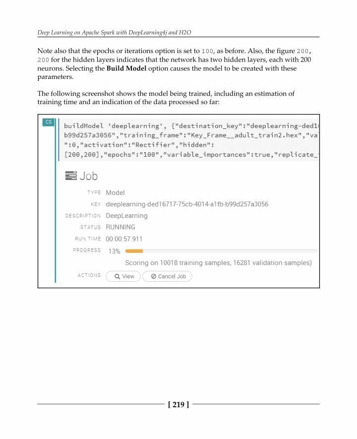
Deep Learning on Apache Spark with DeepLearning4j and H2O
[ 219 ]
Note also that the epochs or iterations option is set to , as before. Also, the figure for the hidden layers indicates that the network has two hidden layers, each with 200
neurons. Selecting the Build Model option causes the model to be created with theseparameters.
The following screenshot shows the model being trained, including an estimation oftraining time and an indication of the data processed so far:

Deep Learning on Apache Spark with DeepLearning4j and H2O
[ 220 ]
Viewing the model, once trained, shows training and validation metrics, as well as a list ofthe important training parameters:
Selecting the Predict option allows an alternative validation Dataset to be specified.Choosing the Predict option using the new Dataset causes the already trained model to bevalidated against a new test Dataset:

Deep Learning on Apache Spark with DeepLearning4j and H2O
[ 221 ]
Selecting the Predict option causes the prediction details for the DeepLearning model andthe Dataset to be displayed, as shown in the following screenshot:
The preceding screenshot shows the test data frame and the model category, as well as thevalidation statistics in terms of AUC, GINI, and MSE.The AUC value, or area under the curve, relates to the ROC, or the receiver operatorcharacteristics curve, which is also shown in the following screenshot.
TPR means True Positive Rate, and FPR means False Positive Rate.

Deep Learning on Apache Spark with DeepLearning4j and H2O
[ 222 ]
AUC is a measure of accuracy, with a value of one being perfect. So, the blue line showsgreater accuracy than that of the red line, which is basically random guessing:
There is a great deal of functionality available within this interface that we have notexplained, but we hope that we have given you a feel for its power and potential. You canuse this interface to inspect your data and create reports before attempting to develop code,or as an application in its own right to delve into your data.

Deep Learning on Apache Spark with DeepLearning4j and H2O
[ 223 ]
Deeplearning4jDeeplearning4j is developed by a Silicon Valley startup called Skymind and can be foundat . It is open source and runs in many different environments,including Apache Spark.
The most important components of the framework are as follows:
Deeplearning4j runtime: This is the core module that allows you to define andexecute all sorts of neural networks on top of Apache Spark, but it does not useApache Spark directly; it uses a a tensor library similar to NumPy for Python.ND4J/ND4S: This tensor library is really the heart of Deeplearning4j. It can alsobe used standalone and provides accelerated linear algebra on top of CPUs andGPUs. For porting code to a GPU, no code changes are required, since a JVMproperty configures the underlying execution engine, which can also be a CUDAbackend for nVidia GPU cards.
In contrast to H2O, Deeplearning4j doesn't necessarily need any additional components tobe installed, since it is a native Apache Spark application using the interfaces that ApacheSpark provides.
ND4J - high performance linear algebra for theJVMLet's have a look at ND4J first. As already mentioned, ND4J is a tensor and linear algebralibrary. This means multidimensional arrays (also called tensors) and operations on themare the main purpose. Operations are simple but fast, for example, like in NumPy forPython, if you are familiar with it.
So what's the advantage of using ND4J over NumPy?
First of all, when using Apache Spark, we stay in the same JVM process and don'thave to pay the overhead of IPC (inter process communication) at all.Then, ND4J is capable of using SIMD instruction sets on modern CPUs, whichdoubles the performance of ND4J over NumPy. This is achieved by usingOpenBLAS.Finally, ND4J can take advantage of the GPUs present on your machine by justsetting a system property on the JVM, provided a recent version of the CUDAdrivers and framework is installed on your system.

Deep Learning on Apache Spark with DeepLearning4j and H2O
[ 224 ]
So, let's have a taste of what this looks like, syntax wise, in Scala:
As you can see, we are creating two matrices and of type using the method. In order to do so, we have to provide a nested Scala array of type
, which we can create inline like this:
Finally, the code actually triggers the matrix multiplication, again, either on aCPU or GPU, but this is totally transparent to us.
Deeplearning4jSo, now that we've covered ND4J, we want to actually create our neural network. So let'sstart with the famous XOR example, which actually trains a neural network for learningXOR.
Let's first generate some training data inline:

Deep Learning on Apache Spark with DeepLearning4j and H2O
[ 225 ]
Now we have created two ND4J arrays, one called containing the features, and onecalled containing the expected outcome.

Deep Learning on Apache Spark with DeepLearning4j and H2O
[ 226 ]
Just as a reminder, the function table looks like this:
Please note that the output is one if only, and exactly, one of the two inputs is one. This isthe function table of the function.
Now let's use the data we created in the preceding section in order to prepare it for neuralnetwork training:
A Dataset, not to be confused with the one from Apache SparkSQL, is a Deeplearning4j datastructure containing ND4J arrays for training.
Here, you can see what this looks like internally:
This reflects the structure of the function table with two differences:
ND4J uses as internal data type representationThe output is in binary form, for example, a two-dimensional array, a fact veryhandy for training binary classifiers with neural networks where we have twooutput neurons

Deep Learning on Apache Spark with DeepLearning4j and H2O
[ 227 ]
Now it's time to create a --this is the way to defineand create neural networks in Deeplearning4j:

Deep Learning on Apache Spark with DeepLearning4j and H2O
[ 228 ]
The preceding code basically just sets parameters global to the neural network. Digging intoeach of those is beyond the scope of this book. Now let's add individual neural networklayers in order to form a deep neural network:

Deep Learning on Apache Spark with DeepLearning4j and H2O
[ 229 ]
This code basically adds two layers to the neural network: an input layer with two neurons(each one for one column of the function table) and an output layer with two neurons,one for each class (as we have outcomes zero and one in the function table). Again, yousee that we can specify an abundance of layer-specific parameters (also beyond the scope ofthis book). Now let's actually create the neural network:

Deep Learning on Apache Spark with DeepLearning4j and H2O
[ 230 ]
Now the variable contains our ready-made neural network, and the only thing we haveto do in order to train it with our function table is run the following code:
If we now look at the output , we see a debug message on how the learningprogresses:
As you can see, there are iterations where the neural network is trained (so basically,the very same Dataset is shown to the neural network multiple times), and for every 100iterations, a measure called score is printed.
This is the so-called Root Mean Square Error (RMSE)--a measure of how well the neuralnetwork fits to the data; the lower the better. As you can observe, after 10,000 iterations, theRMSE went down to , which is a very good value in this case. So,let's check on how well we are actually doing. As in Apache SparkML, Deeplearning4j has abuilt-in component for the evaluation:

Deep Learning on Apache Spark with DeepLearning4j and H2O
[ 231 ]
The code produces an output of the following measures on the prediction (classification)performance:
This actually means that we have 100 percent on all the measures, so we've built a perfectclassifier to compute . Well done!
In reality, things such as perfect classifiers don't exist. It is trivial to train aneural network in order to do zero errors on the set of only four possibleinputs on . But in reality, as soon as you at least have one continuousfeature as opposed to categorical ones, you'll end up with infinite inputpossibilities. So you can only approximate a perfect classifier. This isknown as the bias-variance trade-off. Let's consider spam classification asan example. This means either you build a classifier that is capable ofrecognizing all spam, but then will also mark real emails as spam (falsepositives), or it won't mark real emails as spam but will miss marking allspam emails as spam (false negatives).
Example: an IoT real-time anomaly detectorNow let's get started with building something useful on Apache Spark with Deeplearning4j.We're using an IoT use case again as we did in , Structured Streaming.
Again, we need an IBM Cloud account for the test data generator. The test data generator isNode-RED based, but this time, it generates a different type of data.
Mastering chaos: the Lorenz attractor modelIn order to get good simulated test data, we are using the so-called Lorenz attractor model.

Deep Learning on Apache Spark with DeepLearning4j and H2O
[ 232 ]
Let's start with a little sample use case. Consider the task of detecting anomalies in vibration(accelerometer) sensor data measuring a bearing. In order to obtain such a data stream, wesimply attach such a sensor to or near the bearing:
The Lorenz attractor model is a physical model capable of generating a three-dimensionaldata stream, which we will use in place of a real accelerometer sensor stream. By the way,Lorenz was one of the founders of the chaos theory.
Now our task is to detect anomalies using a neural network, basically predicting when abearing is about to break.

Deep Learning on Apache Spark with DeepLearning4j and H2O
[ 233 ]
Therefore, we can switch the test data generator between two states, healthy and broken.This is a phase plot showing the three vibration dimensions on a time series:

Deep Learning on Apache Spark with DeepLearning4j and H2O
[ 234 ]
We can observe the same when changing the parameters of the physical model slightly inorder to get a faulty state:

Deep Learning on Apache Spark with DeepLearning4j and H2O
[ 235 ]
For those not familiar with phase plots, let's use a run chart for the three time series, againin the healthy state:

Deep Learning on Apache Spark with DeepLearning4j and H2O
[ 236 ]
This is in the faulty state:
One common technique is to transform these data from the time to the frequency domainusing discrete Fourier transformation (DFT ) or wavelets.

Deep Learning on Apache Spark with DeepLearning4j and H2O
[ 237 ]
Again, the FFT for the healthy state is shown here:

Deep Learning on Apache Spark with DeepLearning4j and H2O
[ 238 ]
And this is for the faulty state:
We can clearly observe that the faulty state has more energy and additional frequenciespresent. So, this would be sufficient to train a classifier, as we learned before, but we can dobetter. Let's construct a system capable of learning normal behavior from data, and once itsees data (or sequential patterns) it hasn't seen before, have it raise an alert.

Deep Learning on Apache Spark with DeepLearning4j and H2O
[ 239 ]
Such a system is an LSTM-based auto-encoder as shown in the following figure:
This basically compresses the vast amount of data through a neural bottleneck in order totry to reconstruct the very same data it has seen but, of course, via a bottleneck losing vastamounts of irrelevant information.
Therefore, such a neural network will learn how a system normally behaves, and as soon asnew patterns are seen, it will have a hard time reconstructing the data, and therefore, wecan raise an alert.
The LSTM layers keep track of the inherent state, basically making the neural networkaware of the time domain by adding memory to the neurons. We will now implement thissystem end-to-end from the sensor to the insight, so stay tuned!
Deploying the test data generatorIn order to have a simple framework for creating data, we started writing a test data creator,which will be part of a bigger time series and machine learning toolkit. This tool is runningon the open source data flow platform called Node-RED--a graphical flow editor on top ofNode.js. This is quite handy since Node.js is very lightweight and can, therefore, run onnearly any device, even IoT gateways such as the Raspberry Pi or BeagleBone.

Deep Learning on Apache Spark with DeepLearning4j and H2O
[ 240 ]
We covered Node-RED and how to use it for generating test data in , StructuredStreaming. So, in this case, we'll use it in order to implement the Lorenz attractor model, asexplained previously.
The final idea is that this becomes part of the time series toolkit as well, with the capabilityof generating data by sampling various physical models, and you can decide on the degreeof noise and also switch between different states of the physical model for anomalydetection and classification tasks.
But, for now, we've implemented the Lorenz attractor model only. This is a very simple butinteresting physical model. Lorenz was one of the pioneers of the chaos theory, and he wasable to show that a very simple model consisting only of three equations and four modelparameters can create chaotic behaviour, a system highly sensitive to initial conditions andalso oscillating between multiple semi-stable states, where state transitions are very hard topredict.
As the simulator is completely implemented as a Node-RED flow, we can just create aNode-RED IoT Starter Boilerplate on the IBM Cloud (of course, it runs on any Node-REDinstance, even on a Raspberry Pi, where it can be used to simulate sensor data on the edge)or on your local machine.
The steps to get the simulator up and running are as follows:
Deploy the Node-RED IoT Starter Boilerplate to the IBM Cloud.1.Deploy the test data generator flow.2.Test the test data generator.3.Get the IBM Watson IoT platform credentials in order to consume the data via4.MQTT from any place in the world.
Deploy the Node-RED IoT Starter Boilerplate to the IBMCloudYou'll need an IBM Bluemix Cloud account. Most likely, you already have one, sinceexamples of other chapters are dependent on it as well. If not, you can get one for free here:
. Once done, here are the steps to get Node-REDdeployed to your cloud account:

Deep Learning on Apache Spark with DeepLearning4j and H2O
[ 241 ]
Open the following link: 1.
.Name your application (note that the hostname gets updated as well), and click2.on Create.Once done, click on Connections.3.On the Internet of Things Platform tile, click onView credentials.4.Write down the values of the following properties, as you will need them later:5.
Close this view.6.Wait until your application starts, and then click onVisit App URL.7.When asked, set a and for your application, and note it8.down.Click on Go to our Node-RED flow editor.9.
Congratulations, you should see something like this:
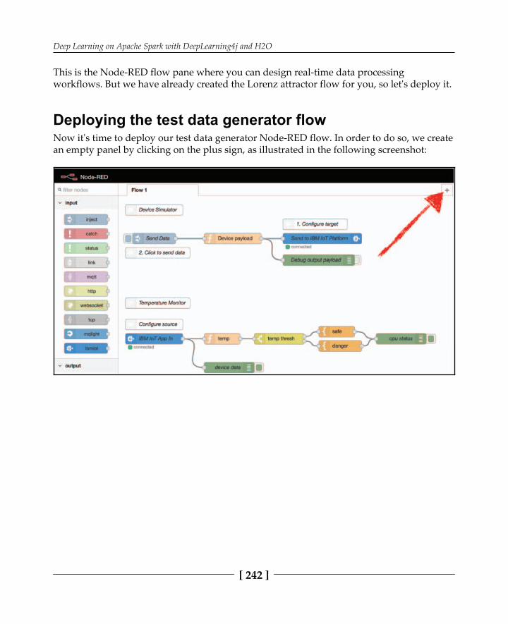
Deep Learning on Apache Spark with DeepLearning4j and H2O
[ 242 ]
This is the Node-RED flow pane where you can design real-time data processingworkflows. But we have already created the Lorenz attractor flow for you, so let's deploy it.
Deploying the test data generator flowNow it's time to deploy our test data generator Node-RED flow. In order to do so, we createan empty panel by clicking on the plus sign, as illustrated in the following screenshot:

Deep Learning on Apache Spark with DeepLearning4j and H2O
[ 243 ]
Now it's time to click on the upper-right menu, as illustrated in the following screenshot:

Deep Learning on Apache Spark with DeepLearning4j and H2O
[ 244 ]
We now paste the contents of the URL , into the text area
by opening the URL and copy-pasting the JSON contents into the text area, as illustratedhere:
We click on Import, drag the flow to the panel, and click on it in order to fix it. Now we hitdeploy at the top right, and we are done!
Testing the test data generatorThis is an easy step. Just click on the reset button once, and the generator will generate 3,000data points in order for us to analyze them.

Deep Learning on Apache Spark with DeepLearning4j and H2O
[ 245 ]
If you click on the debug tab on the right-hand side, you'll see the data points beinggenerated:
In the debug pane, you'll see some error messages:
These are due to the flow running in tab one, and these can be ignored.

Deep Learning on Apache Spark with DeepLearning4j and H2O
[ 246 ]
Install the Deeplearning4j example within EclipseThe first thing we need to do is start Eclipse with an empty workspace. Then we have tograb the whole Deeplearning4j examples tree from Git and install it through Maven.Fortunately, the Git and Maven plugins will do this for you. Please follow the steps on thistutorial in order to install the examples:
.
Once we've run the example successfully, we can finalize the installation:
First, we switch to the Scala perspective. We right-click on the dl4j-examples-1.spark project, and then go to Configure | Add Scala Nature.Then, we right-click on the dl4j-examples-spark project again, and then click on2.Maven | Update Project… and wait until the rebuild takes place.
Please ignore the Maven errors so far. As long as compileswithout error, you are fine!
Then we update with3.the credentials of the IBM Watson IoT platform by setting the , , and
we discovered previously during the installation of the test datagenerator.
Running the examples in EclipseNow, as everything is set up, let's run the examples. We can simply run the class as the Scala application, as illustrated in the following screenshot:

Deep Learning on Apache Spark with DeepLearning4j and H2O
[ 247 ]
This application will connect to the MQTT message broker, which is part of the IBM WatsonIoT Platform running in the cloud. That's the message hub where the test data generatorpublished data to, and we'll just subscribe to this data:

Deep Learning on Apache Spark with DeepLearning4j and H2O
[ 248 ]
Please ignore warnings that the is not found. Those are onlywarnings and don't affect the behavior of the application.
Now it's time to start the test data generator in the cloud running on Node-RED, therefore,we will open up the browser again, and click on the reset button in order to send another 30seconds worth of data to the message broker, where we can pick it up:
Now the application will receive the subscribed data from the message hub and fill atumbling, count-based window. We covered sliding, tumbling, count and time-basedwindows in , Structured Streaming.

Deep Learning on Apache Spark with DeepLearning4j and H2O
[ 249 ]
Once this window is full, the data is sent to the neural network, where it gets analyzed:

Deep Learning on Apache Spark with DeepLearning4j and H2O
[ 250 ]
We see that we have started at iteration 0 with an initial reconstruction error of. This is due to random initialization of the neural network weight
parameters and will, therefore, change on each subsequent run.
An autoencoder provides two things. First, through a neural bottleneck, itprovides a non-linear lower dimensional representation of your data.Second, it tries to reconstruct the input signal at the output, runningthough the bottleneck. Therefore it doesn't learn noise and irrelevant data.Since an autoencoder measures the reconstruction error on the signaltrained on, we can use it as anomaly detector. Data which has been seenbefore will yield to a lower reconstruction error. More on the topic can befound here: and
.
This is demonstrated as follows:

Deep Learning on Apache Spark with DeepLearning4j and H2O
[ 251 ]
So, we end up with as the reconstruction error, since the neuralnetwork got used to the inherit hidden patterns in this signal. Let's run it again by againclicking on the reset button of the test data generator:
Now we end up with a value of . This value will further decrease aslong as we show the normal signal to the neural network over and over again, but will alsoconverge to a minimal value.

Deep Learning on Apache Spark with DeepLearning4j and H2O
[ 252 ]
So, now, let's change the nature of the signal by clicking on broken in the test datagenerator:
Then, again, we click on reset in order to send the next 30 seconds worth of data to theneural network:

Deep Learning on Apache Spark with DeepLearning4j and H2O
[ 253 ]
If we now check on the reconstruction error, we'll see something interesting:
Now we end up with a reconstruction error of , which issignificantly higher than and clearly shows us how anomalies can bedetected on any time series signal without further knowledge of the underlying domain.
So, the only remaining thing is pushing this application to Apache Spark, because youmight have noticed that this example only runs locally on your machine. But, at least itsupports OpenBLAS, so it makes use of the SIMD instructions on your CPU, which speedsthings up a bit. So let's push to Apache Spark!

Deep Learning on Apache Spark with DeepLearning4j and H2O
[ 254 ]
Run the examples in Apache SparkIn order to run on Apache Spark, we'll use the Hortonworks HDP Sandbox. In contrast toother chapters, where we just used the and pasted some lines of Scala code,in this case, this is not possible anymore. So we need to create a self-contained JAR file thatcontains the Deeplearning4j application plus all dependencies in a single JAR file.
Sound tedious? Luckily, Maven is our best friend. So, first, using the command line we justinto the root folder within the workspace of the folder, and run
:
It takes quite some time, but after a while, the command ends with the following output:
Now we need to copy this JAR to the Apache Spark cluster using (SSH Secure Copy).On a Mac, we are using the following command line for doing so:
Then we SSH to the cluster, and run the following command:
We see that the system is waiting for data. Therefore, we just click on the reset button of thetest data generator again, and the tumbling window waits to be filled:
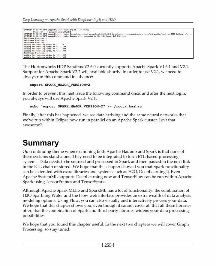
Deep Learning on Apache Spark with DeepLearning4j and H2O
[ 255 ]
The Hortonworks HDP Sandbox V2.6.0 currently supports Apache Spark V1.6.1 and V2.1.Support for Apache Spark V2.2 will available shortly. In order to use V2.1, we need toalways run this command in advance:
export SPARK_MAJOR_VERSION=2
In order to prevent this, just issue the following command once, and after the next login,you always will use Apache Spark V2.1:
echo "export SPARK_MAJOR_VERSION=2" >> /root/.bashrc
Finally, after this has happened, we see data arriving and the same neural networks thatwe've run within Eclipse now run in parallel on an Apache Spark cluster. Isn't thatawesome?
SummaryOur continuing theme when examining both Apache Hadoop and Spark is that none ofthese systems stand alone. They need to be integrated to form ETL-based processingsystems. Data needs to be sourced and processed in Spark and then passed to the next linkin the ETL chain or stored. We hope that this chapter showed you that Spark functionalitycan be extended with extra libraries and systems such as H2O, DeepLearning4j. EvenApache SystemML supports DeepLearning now and TensorFlow can be run within ApacheSpark using TensorFrames and TensorSpark.
Although Apache Spark MLlib and SparkML has a lot of functionality, the combination ofH2O Sparkling Water and the Flow web interface provides an extra wealth of data analysismodeling options. Using Flow, you can also visually and interactively process your data.We hope that this chapter shows you, even though it cannot cover all that all these librariesoffer, that the combination of Spark and third-party libraries widens your data processingpossibilities.
We hope that you found this chapter useful. In the next two chapters we will cover GraphProcessing, so stay tuned.

111Apache Spark GraphX
In this chapter, we want to examine the Apache Spark GraphX module and graphprocessing, in general. So, this chapter will cover the topic of implementing graph analysisworkflows on top of GraphX.
The GraphX coding section, written in Scala, will provide a series of graph coding examples.
Before writing code in Scala to use the Spark GraphX module, we think it will be useful toprovide an overview of what a graph actually is in terms of graph processing. Thefollowing section provides a brief introduction using a couple of simple graphs asexamples.
In this chapter we will cover:
Creating a graph from raw dataCountingFilteringPageRankTriangle countConnected components
OverviewA graph can be considered to be a data structure that consists of a group of vertices andedges connecting them. The vertices or nodes in the graph can be anything as long it is anobject (so people for example), and the edges are the relationships between them. The edgescan be un-directional or directional, meaning that the relationship operates from one nodeto another. For instance, node A is the parent of node B.
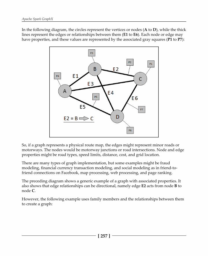
Apache Spark GraphX
[ 257 ]
In the following diagram, the circles represent the vertices or nodes (A to D), while the thicklines represent the edges or relationships between them (E1 to E6). Each node or edge mayhave properties, and these values are represented by the associated gray squares (P1 to P7):
So, if a graph represents a physical route map, the edges might represent minor roads ormotorways. The nodes would be motorway junctions or road intersections. Node and edgeproperties might be road types, speed limits, distance, cost, and grid location.
There are many types of graph implementation, but some examples might be fraudmodeling, financial currency transaction modeling, and social modeling as in friend-to-friend connections on Facebook, map processing, web processing, and page ranking.
The preceding diagram shows a generic example of a graph with associated properties. Italso shows that edge relationships can be directional, namely edge E2 acts from node B tonode C.
However, the following example uses family members and the relationships between themto create a graph:

Apache Spark GraphX
[ 258 ]
Note that there can be multiple edges between two nodes or vertices, forinstance, the husband and wife relationships between and .Also, it is possible that there could be multiple properties on a node oredge.
So, in the preceding example, the property acts from node 6 to node 1 .These are simple graphs to explain the structure of the graph and the element's nature. Realgraph applications can reach extreme sizes and require both distributed processing andstorage to enable them to be manipulated.
Facebook is able to process graphs containing over 1 trillion edges using Apache Giraph(source Avery Ching Facebook). Giraph ( ) is an ApacheHadoop ecosystem tool for graph processing, which historically based its processing onMapReduce but now uses TinkerPop ( ).
Although this book concentrates on Apache Spark, that number of theFacebook graph provides a very impressive indicator of the size that agraph can reach.

Apache Spark GraphX
[ 259 ]
In the next section, we will examine the use of the Apache Spark GraphX module usingScala.
Graph analytics/processing with GraphXThis section will examine Apache Spark GraphX programming in Scala using the familyrelationship graph data sample shown in the last section. This data will be accessed as a listof vertices and edges. Although this data set is small, the graphs that you build in this waycould be very large. For example we've been able to analyze 30 TB of financial transactiondata of a large bank using only four Apache Spark workers.
The raw dataWe are working with two data files. They contain the data that will be used for this sectionin terms of the vertices and edges that make up a graph:
The file contains just six lines representing the graph used in the last section. Each represents a person and has a vertex ID number, a name, and an age value:
The file contains a set of directed values in the form source vertex ID,destination vertex ID, and relationship. So, record 1 forms a relationship between
and :
Apache Spark GraphX
[ 260 ]
Lets, examine some GraphX code samples.
Creating a graphThis section will explain generic Scala code up to the point of creating a GraphX graph fromdata. This will save time as the same code is reused in each example. Once this is explained,we will concentrate on the actual graph-based manipulation in each code example.
The generic code starts by importing Spark context, GraphX, and RDD1.functionality for use in the Scala code:
Then an application is defined, which the class. The application2.name changes for each example from to . This application namewill be used when running the application using :
As already mentioned, there are two data files that contain and 3.information:
The Spark Master URL is defined as the application name, which will appear in4.the Spark user interface when the application runs. A new Spark configurationobject is created, and the URL and name are assigned to it:

Apache Spark GraphX
[ 261 ]
A new Spark context is created using the configuration that was just defined:5.
The information from the file is then loaded into an RDD-based structure6.called vertices using the method. The data is stored as aLong and strings to represent the person's name and age. The datalines are split by commas as this is CSV-based data:
Similarly, the data is loaded into an RDD-based data structure called edges.7.The CSV-based data is again split by comma values. The first two data values areconverted to long values as they represent the source and destination vertex IDs.The final value representing the relationship of the edge is left as . Notethat each record in the RDD structure edges is actually now an record:
A default value is defined in case a connection or is missing; the graph is8.then constructed from the RDD-based structures vertices and edges and the
record:
This creates a GraphX-based structure called , which can now be used for9.each of the examples. Remember that, although these data samples might besmall, you could create extremely large graphs using this approach.
Many of these algorithms are iterative applications, for instance, PageRank and trianglecount. As a result, the programs will generate many iterative Spark jobs.

Apache Spark GraphX
[ 262 ]
Example 1 – countingThe graph has been loaded, and we know the data volumes in the data files. But what aboutthe data content in terms of vertices and edges in the actual graph itself? It is very simple toextract this information using the vertices and edges function shown as follows:
Running the example using the example name and the file created earlier willprovide the information. The master URL is supplied to connect to the Spark cluster,and some default parameters are supplied for the executor memory and total executorcores:
The Spark cluster job provides the following output, which is what would beexpected and matches the data files:
Example 2 – filteringWhat happens if we need to create a sub graph from the main graph and filter on personage or relationships? The example code from the second example Scala file showshow this can be done:
Two example counts have been created from the main graph: the first filters person-basedvertices on age only, taking those people who are greater than forty years old. Notice thatthe value, which was stored as a string, has been converted to a long for thecomparison.

Apache Spark GraphX
[ 263 ]
The second example filters the edges on the relationship property of or .Two count values and are created and printed as the Spark run output, shown asfollows:
Example 3 – PageRankThe PageRank algorithm provides a ranking value for each of the vertices in a graph. Itmakes the assumption that the vertices that are connected to the most edges are the mostimportant.
Search engines use PageRank to provide ordering for page display during a web search ascan be seen from the following code:
The example code creates a tolerance value and calls the graph method using it.The vertices are then ranked into a new value ranking. In order to make the ranking moremeaningful, the ranking values are joined with the original vertices RDD. The
value then contains the , , and name.
The PageRank result held in is then printed record by record using a statement to identify the record contents and a format statement to print the contents. Wedid this because we wanted to define the format of the rank value, which can vary:
The output from the application is then shown as follows; as expected, and have the highest rank as they have the most relationships:

Apache Spark GraphX
[ 264 ]
Example 4 – triangle countingThe triangle count algorithm provides a vertex-based count of the number of trianglesassociated with that vertex. For instance, vertex (1) is connected to (5), who isconnected to (2), is connected to (1), and so a triangle is formed. This canbe useful for route finding where triangle free minimum spanning tree graphs need to begenerated for route planning.
The code to execute a triangle count and print it is simple as shown next. The graph method is executed for the graph vertices. The result is saved in the value
and printed:
The results of the application job show that vertices (4) and (6) have no triangles,while (1) and (2) have the most as expected, as they have the mostrelationships:
Example 5 – connected componentsWhen a large graph is created from data, it might contain unconnected sub graphs or subgraphs that are isolated from each other and might contain no bridging or connecting edgesbetween them. These algorithms provide a measure of that connectivity. It might beimportant depending on your processing to know that all vertices are connected.
The Scala code for this example calls two graph methods, and. The method required a maximum iteration
count, which has been set to . These counts are acting on the graph vertices:

Apache Spark GraphX
[ 265 ]
The counts are then joined with the original records so that connectioncounts can be associated with the information such as person name:
The results are then output using a statement and formatted for printing:
As expected, for the algorithm, the results show that, for each, there is only one component. That means that all the vertices are members of a
single graph as the graph diagram earlier in the chapter showed:
The method gives a measure of the connectivity in agraph, taking into account the direction of the relationships between them. The results forthe algorithm are output as follows:
You might notice from the graph that the relationships and act fromvertices (6) and (4) to (1) as the and data shows:

Apache Spark GraphX
[ 266 ]
So the method output shows that, for most vertices, there is only one graphcomponent signified by in the second column. However, vertices and are notreachable due to the direction of their relationship, and so they have a vertex ID instead of acomponent ID:
SummaryThis chapter showed by example how Scala-based code can be used to call GraphXalgorithms in Apache Spark. Scala has been used because it requires less code to developthe examples than Java, which saves time. Note that GraphX is not available for Python orR. A Scala-based shell can be used, and the code can be compiled into Spark applications.
The most common graph algorithms have been covered and you should have an idea nowon how to solve any graph problem with GraphX. Especially since you've understood that aGraph in GraphX is still represented and backed by RDDs, so you are already familiar withusing them. The configuration and code examples from this chapter will also be availablefor download with the book.
We hope that you found this chapter useful. The next chapter will delve into graph frames,which make use of DataFrames, Tungsten, and Catalyst for graph processing.

112Apache Spark GraphFrames
GraphFrames is the new graph library of Apache Spark. It supports loss-lesstransformations of graph representations between GraphFrames and GraphX. Whileintroducing another Apache Spark library equivalent to an existing one, we have to explainthe motivation behind this decision. The motivation is the same as it was when introducingSparkML over MLlib. The idea was to have an equivalent to GraphX, which supportsDataFrames, in order to make use of the optimizations that Catalyst and Tungsten bring.
Another goal was to progress further with unification by integrating graph algorithms andgraph queries and optimizing their execution.
Although GraphX supports relational queries on graph structures, it doesn't support graphqueries.
Therefore, GraphFrames was implemented with the goal of unifying graph algorithms,graph queries, and DataFrames (and therefore relational queries).
This chapter will cover the following topics:
Architecture of GraphFramesPerformance optimizationsPractical examples in Scala
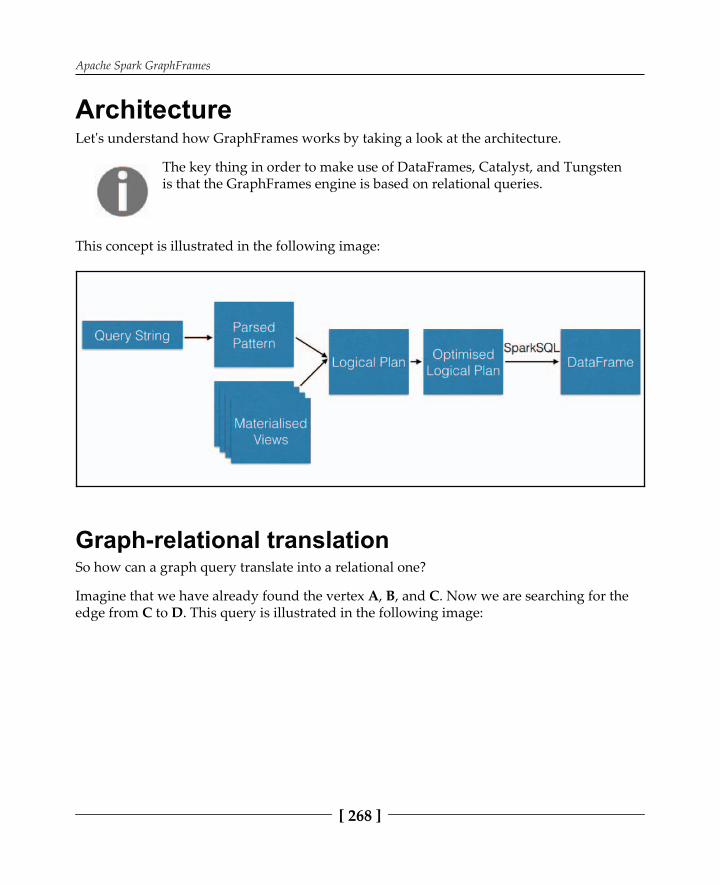
Apache Spark GraphFrames
[ 268 ]
ArchitectureLet's understand how GraphFrames works by taking a look at the architecture.
The key thing in order to make use of DataFrames, Catalyst, and Tungstenis that the GraphFrames engine is based on relational queries.
This concept is illustrated in the following image:
Graph-relational translationSo how can a graph query translate into a relational one?
Imagine that we have already found the vertex A, B, and C. Now we are searching for theedge from C to D. This query is illustrated in the following image:

Apache Spark GraphFrames
[ 269 ]
This is pretty straightforward as we can scan the vertex table and search for entries wherethe Src (source) field is C. Once we have found out that the Dst (destination) field points toD (let's assume that we are also interested in the properties of the node D), we finally jointhe vertex table in order to obtain these properties of D.
The following image illustrates such a practically complete query and the resulting joinoperations:

Apache Spark GraphFrames
[ 270 ]
You might wonder at the fact that we are using a lot of joins in order toconstruct the query. This is true. However, there is a subsequent stage thatis responsible for join elimination. So don't worry too much about this yet.
Materialized viewsA common practice for query performance optimization in relational databases systems ismaterialized views.
A view is a subset of your data that (usually) cannot be updated directlybut reflects the superset of the data it is based on. A materialized view isan extension to this concept by not only generating a view on a subset ofdata, but also storing the representation of that view to persistent storage.This especially makes sense if the construction of such a materialized viewis computationally expensive. This is because, in subsequent queriesmaking use of such a view, the amount of time that the creation of such amaterialized view would have taken can be saved in each of those queries.
The same concept also applies for graph databases. Common subgraphs, which are usedamong multiple queries, can be defined as materialized views. Therefore, graph queriesmaking use of these subgraphs can benefit using them.
In GraphX, only subgraphs with a triplet structure can be used butGraphFrames supports arbitrary subgraph structures. Materialized viewsin GraphFrames can be defined manually and all queries automaticallymake use of them.
Join eliminationAs the vertex and edge table in GraphFrames satisfies the referential integrity constraint,the join of the vertex table can be eliminated if no field of that table is specified in the selectstatement.

Apache Spark GraphFrames
[ 271 ]
So let's take a look at the following SQL statement:
As the field of the vertices table is never read, this statements gets automaticallyrewritten:
GraphFrames added unique and foreign key hints to the optimizer of Catalyst. Therefore,Catalyst itself is now responsible for join elimination. Refer to , The CatalystOptimizer, to read more about the Catalyst Optimizer.
Join reorderingAnother way to improve query performance is join reordering.
Let's consider the following query structure with a binary relationship between edges Aand B and incoming and outgoing relations (vertices) between B, C, D, and E:

Apache Spark GraphFrames
[ 272 ]
In a naive way, a query planner will create a query plan similar to this during the graph-relational translation where the resolution of each vertex between two edges basically leadsto the creation of one join operation in the execution plan:
This is known as a left deep plan, which of course is not optimal as it can only be executedsequentially and also incorporates a lot of join operations that are computationallyexpensive. Finally, there is no common pattern or structure in such a left deep plan thatwould allow us to create materialized views to speed up things.
Now let's consider the following execution plan, which is semantically equivalent to theprevious one but the joins have been reordered and the overall structure changed:

Apache Spark GraphFrames
[ 273 ]
This is also known as a bushy plan, which builds up two intermediate results and joinsthem together. This leads to exactly the same results as the left deep plan, but it has a coupleof advantages. They are listed as follows:
First, you might have noticed that there is one fewer join operation. Already1.good.Second, as not all subsequent joins are waiting for the results of the previous join,2.this query can be run in parallel.Then, often the intermediate results are smaller than in the left deep plan.3.Finally, the complete right-hand side sub query can be defined as a materialized4.view.
Currently, there is research work in progress to create such materialized views based onquery history automatically.
Apache Spark GraphFrames
[ 274 ]
Graph structure query languages allow defining topological patterns,which are used to search for similar structures in the database. One veryfamous graph database is Neo4J. Its query language is called cypher.GraphFrames uses a subset of this query language, called motifes for now.More on Neo4J can be found here andmore on cypher can be found here
.
Although GraphFrames is in its pretty early stages, comparisons to Neo4J showperformance improvements by a factor of four, as stated by a Databricks software engineerduring Spark Summit 2016.
Comparisons to GraphX show about the same performance. However,note that GraphX is pretty mature and a lot of work has been done forperformance optimizations, and GraphFrames mostly takes onlyadvantage of Catalyst and Tungsten through the DataFrames API.
ExamplesNow let's look at a couple of examples in order to understand how to use the new GraphFrames API.
First of all, we need to create a GraphFrames object from data files. Before we do this, weneed to install GraphFrames. Fortunately, this is very easy as the package is available on aMaven repository and we can just pass the dependency to the and
commands:
spark-shell --packages graphframes:graphframes:0.5.0-spark2.1-s_2.11
Then, we need to import the required package:
import org.graphframes._
As our graph is based on two CSV files--one for the and one for the --weneed to create two DataFrames out of them:
val vertex = spark.read.option("header","true").csvgraph1_vertex.csv")val edges = spark.read.option("header","true").csvgraph1_edges.csv")
Finally, we create a GraphFrames object out of these:
val graph = GraphFrame(vertex, edges)

Apache Spark GraphFrames
[ 275 ]
Example 1 – countingThe graph has been loaded and we know the data volumes in the data files but what aboutthe data content in terms of vertices and edges in the actual graph itself? It is very simple toextract this information using the vertices and edges count functions, as shown in thefollowing code:
As expected, we get 6 and 12 .
Example 2 – filteringWhat happens if we need to create a subgraph from the main graph and filter on theperson's age or relationships? The following example code shows how this can be done.
First, we'll select only the vertices where age is greater than :
This returns a DataFrame, and using the method, we obtain a print of the table:
Apache Spark GraphFrames
[ 276 ]
Now let's structure a query in order to find out the taking part in a father ormother relationship.
As already mentioned, GraphFrames supports a subset of the cypher query language thatNeo4J supports. Unfortunately, as of Apache Spark 2.2 and GraphFrames 0.5, this is notfully implemented to support this query in a nice way. Otherwise, the query would look asfollows:
Therefore, let's implement the query in a slightly more verbose way:
Example 3 – page rankThe page rank algorithm provides a ranking value for each of the vertices in a graph; itmakes the assumption that those vertices that are connected to the most edges, directly orindirectly, are the most important. Search engines use page rank to provide ordering forpage display during a web search. So let's see how to implement this in GraphFrames.
First, we run the actual algorithm. It is important to notice that the algorithm1.returns no DataFrame. The algorithm returns a GraphFrames object again bymerging the results into the :
So now take a look at this result:2.
We are accessing the vertices of the graph. Note that the algorithm of3.GraphFrames created an additional attribute, , which we are nowaccessing through the DataFrame API.In addition, we order the result by :4.

Apache Spark GraphFrames
[ 277 ]
Example 4 – triangle countingThe triangle count algorithm provides a vertex-based count of the number of trianglesassociated with that vertex. For instance, vertex (1) is connected to (5) who isconnected to (2), is connected to (1), and so a triangle is formed:

Apache Spark GraphFrames
[ 278 ]
This can be useful for route finding where triangle-free minimum spanning tree graphsneed to be generated for route planning.
The code to execute a triangle count and print it is simple, as shown in the following code.The GraphFrames method is executed for the graph vertices. The result issaved in the value results, which is a DataFrame:
Now let's plot the results:
The following image shows the result:
So let's have a look at this result. It basically lists the vertex IDs on the left-hand side and thenumber of triangles that this particular vertex is taking part in.

Apache Spark GraphFrames
[ 279 ]
So let's again look at the structure of our sample graph:
We can clearly see that the result is correct. and are participating in twotriangles, and only in one, and and on none. Done!
Example 5 – connected componentsWhen a large graph is created from data, it might contain unconnected subgraphs--subgraphs that are isolated from each other and contain no bridging or connecting edgesbetween them. These algorithms provide a measure of that connectivity; it might beimportant depending on your processing to know that all vertices are connected.

Apache Spark GraphFrames
[ 280 ]
The code for this example calls two graph methods, and. The strong method required a maximum iteration
count, which has been set to 10. These counts are acting on the graph vertices.
So let's run the first code snippet:
As expected for the algorithm, the results show that for eachvertex, there is only one component. This can be verified as the algorithm result assignseach vertex to the same component ID.
This means that all the vertices are members of a single graph, as the graph diagramintroduced in the Section on Triangle Count earlier in the chapter showed:
The method gives a measure of the connectivity in agraph, taking into account the direction of the relationships between them. So let's run thecorresponding code:

Apache Spark GraphFrames
[ 281 ]
You might notice from the graph that the relationships, and , act fromvertices ( ) and ( ) to ( ) as the edge and vertex data, as shown in thefollowing code:
So, the strong method output shows that for most vertices, there is only one graph.However, vertices 4 and 6 are not reachable due to the direction of their relationship and sothey are assigned to another component, indicated by a different component ID:
In order to make this example a bit clearer, let's add a disconnected vertex to the graph. Thiscan be done by simply adding the following line to the file:
Now, the vertex with ID is not connected with the rest of the graph because we didn't adda connecting edge to the file. Let's rerun the algorithm. Before we dothis, we have to reread the files and recreate the GraphFrames object.

Apache Spark GraphFrames
[ 282 ]
As expected, the algorithm assigns vertex to adifferent component ID:
During the last call, the algorithm assigned each vertex to the samecomponent ID, but now we can see that vertex 7 gets its own component ID:

Apache Spark GraphFrames
[ 283 ]
SummaryThis chapter started with an architectural overview on GraphFrames. We saw howGraphFrames can make use of the Catalyst and Tungsten optimizers by running on top ofDataFrames.
Additional optimizations on top of these were explained. Finally, we showed, by example,how Scala-based code can be used to call GraphFrames algorithms in Apache Spark. Scalahas been used because it requires less code to develop the examples, which saves time; aScala-based shell can be used and the code can be compiled into Spark applications.
The configuration and code examples from this chapter are also available for downloadwith the book. If you want to learn more on GraphFrames please refer to this link
.
Now let's have a look how Apache Spark can be used in the Cloud in conjunction withJupyter in the next chapter. This is a very convenient user interface from which to do datascience.

113Apache Spark with Jupyter
Notebooks on IBM DataScienceExperience
When talking about the cloud, nearly everybody has a different view. Some think of virtualmachines, which you can start and stop instantaneously, while some others think of filestorage. But the cloud is more than that. In this chapter, we will talk about using ApacheSpark in the cloud. But this is, of course, more than provisioning some virtual machines andinstalling an Apache Spark cluster on it.
We are talking about the so-called Platform as a service clouds (PaaS), where everything isa service, ready to be consumed, and the operation of components is done by the cloudprovider. Therefore, on PaaS clouds, Apache Spark is pre-installed. This is done in a waythat workers can be added to and removed from the cluster on-the-fly. But not only isApache Spark pre-installed, the required tooling around it is also available.
In this chapter, we'll introduce the following:
Why notebooks are the new standard for data scienceA practical example in how to analyze bearing vibration dataThe trinity of data science programming languages (Scala, Python, R) in actionInteractive, exploratory data analysis and visualization

Apache Spark with Jupyter Notebooks on IBM DataScience Experience
[ 285 ]
In data science it is common practice now to use notebooks such as Juypter (covered in thischapter) and Zeppelin (covered in the next chapter on running Apache Spark onKubernetes).
Another practice we are seeing more and more is that people tend to prefer Python and Rover Scala and Java, especially for one-time scripts and visualization as opposed to long-term Extract Transform Load (ETL) processes where Scala and Java still are leaders.
Why notebooks are the new standardJupyter notebooks are rapidly becoming the default way to apply data science. They can beseen as Google Docs for analytics. Documentation, lines of code, and output from that code(text, data tables, charts, and plots) are all united.
In addition, such notebooks are easily shareable, even without a backend. Just export themas JSON documents.
Jupyter notebooks preserve all output cells even if the cell duringexecution has been connected on a large scale Apache Spark clusterprocessing hundreds of gigabytes of data.
In my experience, notebooks are used mostly in the following scenarios:
Notebooks are an ideal tool for creating and sharing a knowledge base on bestpractices a core data science team executes. This way, their knowledge isdocumented in an executable way.Notebooks are used to document the variety of available data sources in anenterprise and to provide executable quick-start code.Creating master-templates - casting best practices and company codingconventions into derived notebooks in order to preserve quality of those.

Apache Spark with Jupyter Notebooks on IBM DataScience Experience
[ 286 ]
Dividing data science work between business analysts, data preparation, andsenior data scientist within a single notebook, including knowledge transferamong those roles.
Learning by exampleLet's have a look at an example in order to learn how to use this tool:
If you don't have a Bluemix account, register for one here:1..
Once you have an account in place, go to , and2.click on Sign In.Click on Sign-In with your IBM ID, and follow the instructions.3.
Once you are ready to go, let's start with a small hello world project by creating a Jupyternotebook on Scala with Apache Spark 2.x.
As illustrated in the following screenshot, click on the Create notebook button:

Apache Spark with Jupyter Notebooks on IBM DataScience Experience
[ 287 ]
This opens the Create notebook dialog as illustrated here:
Apache Spark with Jupyter Notebooks on IBM DataScience Experience
[ 288 ]
So let's have a look at what information we need to provide:
First of all, each notebook needs a name. We choose as the1.name.Then we select Scala as the programming language.2.We want to run our code on an Apache Spark 2.x instance.3.We choose Default Project. Putting notebooks into projects facilitates4.collaboration, resource assignments, and version management of third-partylibraries.Finally, we choose an Apache Spark instance running on the IBM Bluemix cloud,5.where our code has to be executed. This service is completely containerized;therefore, it can handle each of the supported Apache Spark versions andprogramming languages, which, at the time of writing this book, are Scala,Python 2.7, Python 3.5, and R on Apache Spark versions 1.6, 2.0, and 2.1.
So let's start with a motivating example and see how easy it is to interact with the object. This is the first time we will run Scala code within Apache Spark without usingeither the command or the command.
We'll also use Python, R and Scala interchangeably in different notebooks since eachprogramming language has its own strengths-–Jupyter notebooks make it easy to use such ahybrid approach because no further programming language-dependent skills, other thansyntax such as IDEs or build tools, are required.
Let's consider the real-life scenario of a small industrial enterprise doing analytics in thecloud. As you've might have experienced, good data scientists are a rare species, and mostof them don't come with a Scala background. Mostly, they work with MATLAB, R, andPython. The same holds for this enterprise. They have plenty of Java developers but onlyone data scientist. Therefore, it is a good idea to create different roles.
Finally, this data product development process based on Jupyter and Apache Spark as aservice catalyzes communication and exchange between skill groups involved in datascience projects. The software engineer becomes a better mathematician, and themathematician becomes a better software engineer because everyone can have a look at(and modify) the assets created by the other since all are in one central place and not buriedbehind server logins and shell scripts. In addition, they are very readable since they containnot only code but also documentation and output from that code.

Apache Spark with Jupyter Notebooks on IBM DataScience Experience
[ 289 ]
Let's start with the first example, where we perform the following steps:
The Java software engineer is responsible for implementing the ETL process. He1.pulls data from machines (in this example, we'll pull a dataset from the web),transforms it, and then loads data into a cloud object store. This is entirely doneusing a Scala notebook. Although the software engineer is not an expert in Scala,he has acquired enough knowledge for this task. The fact that he can use ANSISQL for querying data really helps since most software engineers have basic SQLskills. Those notebooks can also be triggered and run automatically on a periodicbasis in order to update data.Once the data is prepared and available in the object store, the data scientist can2.create an interactive analytics notebook based on Python and the Pixiedustinteractive data visualization library in order to get an idea of what the data lookslike.Python is a very easy-to-learn programming language, so it can be seen as theintersection between software engineers and statisticians since you can pick it upreally fast if you are coming from a Java and R/MATLAB background.Use an R notebook and the famous library for creating awesome,3.publishable plots.
ETL: Why is ETL always needed? Usually, the persons involved in thedata sources responsible for export don't have the usability of their exportin mind. They just want to make sure they have put enough informationinto the export and they want to keep the process slim on their side. That'sthe reason why data scientists always struggle with ETL. Either we have tocope with some lousy exported data or we have to directly access aSystem of Records (SOR ) via, for example, a read-only materializedview.
The IEEE PHM 2012 data challenge bearingdatasetWe are taking vibration sensor data from an accelerometer attached to a bearing in anexperiment setup. This bearing is put on heavy load in order to make it fail fast.

Apache Spark with Jupyter Notebooks on IBM DataScience Experience
[ 290 ]
The whole process has been extensively discussed in the followingpublication: Nectoux, R. Gouriveau, K. Medjaher, E. Ramasso, B. Morello,N. Zerhouni, C. Varnier. PRONOSTIA: An Experimental Platform forBearings Accelerated Life Test. IEEE International Conference on Prognosticsand Health Management, Denver, CO, USA, 2012
The basic experiment setup is as follows:
You don't have to understand each component on this setup, but the most important onesinclude the Cylinder Pressure, which generates force against the Bearing tested in order tomake it fail fast, and the two Accelerometers, which record vibration data.

Apache Spark with Jupyter Notebooks on IBM DataScience Experience
[ 291 ]
It is important to notice that those data points are recorded at a sampling frequency of 25.6kHz for a period of 100 ms (2,560 data points per second), followed by a pause of 9,900 msas illustrated in the following figure:
ETL with ScalaLet's have a look at the first Scala-based notebook where our ETL process is expressed.Fortunately, the IEEE website allows us to download a ZIP file containing all the data. We'lluse a Scala-based notebook to perform the following steps:
Download the ZIP file to a local staging area within the Apache Spark driver. The1.download location is already included in the notebook file that you candownload from the book's download page. But for more information on the dataset please refer to
.Unzip the file.2.Create an Apache Spark DataFrame out of the nested folder structure to get a3.unique and queryable view of all data.Use an SQL statement for data transformation.4.Save the result into a single JSON file on the IBM Cloud OpenStack Swift-based5.ObjectStore.

Apache Spark with Jupyter Notebooks on IBM DataScience Experience
[ 292 ]
So let's have a look at each individual step:
Downloading the ZIP file to the staging area:1.In the IBM Data Science Experience platform, the Apache Spark cluster lives in aDocker/Kubernetes-based environment (more on this in the next chapter). Thisalso holds for the Apache Spark driver container. This means we can callordinary shell commands within the driver container and also use this as thestaging area:

Apache Spark with Jupyter Notebooks on IBM DataScience Experience
[ 293 ]
As you can see in the following screenshot, IBM provides plenty of free space in2.this staging area by mounting a GPFS cluster file system onto the drivercontainer. In this case, we have more than 70 TB of space in this staging area. Incase we need to load more than 70 TB, we need to split the data andincrementally load it. IBM Cloud OpenStack Swift-based ObjectStore providesunlimited storage capacity, and there is no need be concerned about scalability.The client is charged per GB on a monthly basis. More details on pricing can befound here
:
Next let's unzip the data:3.

Apache Spark with Jupyter Notebooks on IBM DataScience Experience
[ 294 ]
Now we have a huge number of individual CSV files, which we want to use to4.create a DataFrame. Note that we can filter individual files using a wildcard. Soin this case, we are only interested in the accelerometer data, ignoring thetemperature data for now:

Apache Spark with Jupyter Notebooks on IBM DataScience Experience
[ 295 ]
As we can see, we are double-checking whether the schema was inferredcorrectly, and we also have a look at the first rows of the dataset to get anidea of what's inside.
The column names represent the following:
: hour: minute: second: millisecond: horizontal acceleration: vertical acceleration
It is obvious that some data transformation is necessary. The 5.especially is in a very unusable format. The data scientist also told us to create anadditional column containing an aggregation key called cluster composed ofhours, minutes, and seconds.The following script does the job:
The final step is to store the resulting DataFrame as JSON into the IBM Cloud6.OpenStack Swift-based ObjectStore:
This concludes our ETL process. Once we are convinced that everything runsfine by manually running the notebook, we can automatically schedule it torun once every hour if we like:

Apache Spark with Jupyter Notebooks on IBM DataScience Experience
[ 296 ]
Interactive, exploratory analysis using Pythonand PixiedustNow since our ETL process is in place, let's use a more lightweight programmingenvironment based on Python for some exploratory data analysis in order to get an idea of what the data looks like. We'll use a visualizations/charting library called Pixiedust here.

Apache Spark with Jupyter Notebooks on IBM DataScience Experience
[ 297 ]
The main advantage is that you can directly pass DataFrame objects to it, independent oftheir size, and Pixiedust will take care of the correct down sampling where necessary. It cancreate charts with only a single line of code whereas other libraries such as matplotlib needfar more complex code to obtain similar charts. And the good news is: It is open source onthe Apache V2 license but powered by IBM Watson Data Lab developers. More on Pixiedust can be found here: .
We'll now implement this as a Python notebook executing the following steps:
Load the DataFrame from the ObjectStore.1.Create an interactive chart using Pixiedust.2.
Let's go over every step in detail:
First, we load the DataFrame. Loading data as a DataFrame from the ObjectStore1.is straightforward. Here is how you go about it:

Apache Spark with Jupyter Notebooks on IBM DataScience Experience
[ 298 ]
And so is using Pixiedust, which is just another two lines of Python code:2.
By default, you are presented with a table view containing the first rows of the3.dataset. It is important to notice that, independent of the size of the DataFrame,we can just visualize it, and Pixiedust takes care of using the Apache SparkDataFrame API to just pull the necessary data in order to prevent unnecessaryoperations:

Apache Spark with Jupyter Notebooks on IBM DataScience Experience
[ 299 ]
Now let's create a graph by clicking on the respective symbol:4.
We have specified that the field containing the , which resides on5.the x-axis, and the and fields containing the vibration data are plottedagainst the on the y-axis.
The result looks like his:

Apache Spark with Jupyter Notebooks on IBM DataScience Experience
[ 300 ]
Again, it is important to notice that we didn't do any sampling in order tovisualize that data. And it doesn't matter whether the DataFrame containsone MB, one TB, or even one PB since Pixiedust uses the DataFrame API inorder to obtain the required samples.
We can clearly see that the vibrations increase as time progresses and finally, at the end ofthe recordings, which is when the bearing breaks, they reach their maximum.

Apache Spark with Jupyter Notebooks on IBM DataScience Experience
[ 301 ]
Real data science work with SparkROur Chief Data Scientist in the project is very skilled; unfortunately, he has no Apache Spark expertise since he is a mathematician mainly working with MATLAB and R. So inthese cases, SparkR is a good choice to facilitate the transition to using Apache Spark. Thefollowing notebook is based on the R programming language. An Apache Spark expertcreated the initial DataFrame loading code, whereas the rest of the notebook was directlyworking on a local R DataFrame in contrast to an Apache Spark DataFrame -– somethingthe Data Scientist was familiar with.
So, let's have a look at the steps executed in this notebook:
Load the DataFrame from the ObjectStore.1.Generate some additional columns in the dataset based on mean and standard2.deviation.Plot the additional columns.3.
So again, loading data from ObjectStore using Apache SparkR is straightforward:
Now it's time for the Data Scientist to create some additional columns based on the meanand standard deviation. He is using SQL since this is within his skill set:

Apache Spark with Jupyter Notebooks on IBM DataScience Experience
[ 302 ]
By calling , an R DataFrame called is created, which can beused out-of-the-box by any R programmer without Apache Spark skills. This R DataFrameis used in order to plot those additional columns. Let's have a look at one:

Apache Spark with Jupyter Notebooks on IBM DataScience Experience
[ 303 ]
As can be seen from the preceding figure, the standard deviation of the horizontalvibrations dramatically increases as the life of the bearing approaches it's end. This isenough for our Data Scientist to do some magic in R, which we than can port back toApache SparkML in order to scale. Of course in the long term we hope that our DataScientist will be able to write Apache Spark code himself.
SummaryApache Spark in the cloud is the perfect solution for data scientists and data engineers whowant to concentrate on getting the actual work done without being concerned about theoperation of an Apache Spark cluster.
We saw that Apache Spark in the cloud is much more than just installing Apache Spark ona couple of virtual machines. It comes as a whole package for the data scientist, completelybased on open-source components, which makes it easy to migrate to other cloud providersor to local datacenters if necessary.
We also learned that, in a typical data science project, the variety of skills is huge, which istaken care of by supporting all common programming languages and open-source dataanalytics frameworks on top of Apache Spark and Jupyter notebooks, and by completelyeliminating the necessity for operational skills required to maintain the Apache Sparkcluster.
Sometimes just one level of increased access to the underlying infrastructure is necessary.Maybe some specific versions of patch levels of software are needed or very specificconfiguration settings need to be used. So normally this would be the cast for going back toIaaS and installing everything on our own. But this is not really necessary; fortunately thereis a better solution that still provides a fair amount of automatizations and still pushing thehard parts of operations to the cloud provider.
This and more is explained in the next Chapter, Apache Spark on Kubernetes.

114Apache Spark on Kubernetes
In this chapter, we'll talk about one of the most exciting movements in Apache Sparkdeployments: the deployments on the open source based Kubernetes cloud platform. Inorder to understand these concepts, this chapter explains the following:
The difference between container and virtual machine based system abstractionCore concepts of the Docker platformCore concepts of KubernetesDeployment of containerized Apache Spark on Kubernetes and DockerA practical example on Apache Spark deployment on Kubernetes
Bare metal, virtual machines, and containersIt turns out that until the late 1990s, most of IT applications were deployed to bare metalmachines. This means that you used some sort of server hardware and installed anoperating system on it, and on top of that, your applications were installed.
But virtual machines are quite old. In fact, by the early 1960s, IBM was capable of runningvirtual machines on their mainframes, but it took decades until virtual machinesexperienced huge market adoption. Most likely, the reason for this was that consumergrade hardware was not powerful enough to run virtual systems efficiently. However, aswe all know, this has changed dramatically.

Apache Spark on Kubernetes
[ 305 ]
Nowadays, a modern server can run hundreds of virtual machines and thousands ofcontainers, but let's have a look at one after the other. So how do virtual machines work? Inthe following section, we'll first contrast a bare metal deployment with a virtual machineone.
The following figure illustrates such a bare metal deployment:
So as we can see on the bare metal hardware layer, an operating system is installed whichaccesses different hardware components through drivers and makes them available to theuser application through a common API.
Let's contrast this to a virtual machine deployment:

Apache Spark on Kubernetes
[ 306 ]
As we can see, there is an additional component present here, called hypervisor. Thiscomponent basically runs as a user application on the bare metal operating system andemulates a complete hardware stack, so that it can host another operating system runninguser applications.
The operating system running on top (or within) of the hypervisor is called guest while theoperating system running on top of the real bare metal hardware is called host. The idea is that the guest operating system is not aware that it is running inside a virtualized hardware,which has two main advantages:
Security: The guest operating system and guest user application can't accessresources on the host operating system without being controlled by thehypervisor.Scalability and elasticity: As the following figure illustrates, multiple guestsystems can be run on a (powerful) host system allowing for scaling (imaginethere are many host systems in the data center). Also, starting and stopping guestsystems is relatively fast (in minutes), so a system can react to different loadsituations (especially in cloud deployments where virtually infinite resources arepresent across multiple host systems).
As you can see, there is a huge overhead. In the previous figure, there are six operatingsystems running to serve five user applications. Five are labeled as VIRTUAL MACHINEOS inside the virtual machine and one is still necessary running on top of the realhardware, labeled as OPERATING SYSTEM.

Apache Spark on Kubernetes
[ 307 ]
There is a special case where no host operating system is required, andtherefore the so-called hypervisor runs directly on the bare metalhardware.
Not all virtual machine environments support running a hypervisor directly on bare metal,but the deployment would look like the following, where the guest operating systemfunctionality basically is provided by the hypervisor itself:
ContainerizationOperating system processes are the central units of work that anoperating system runs. So each user application, which basically is nothingother than a set of machine code on permanent storage, is transformedinto a running process by reading it from disk, mapping it to the mainmemory, and starting to execute the contained set of instructions on theprocessor.An application can contain one or more processes, and on Linux, eachapplication thread is executed as a separate process sharing the samememory area. Otherwise, a process can't access memory that the otherprocesses are using; this is an important concept for security and stability.But still, all processes can see and use the same set of resources that theoperating system provides.

Apache Spark on Kubernetes
[ 308 ]
With hypervisors directly running on the bare metal hardware, at least we got rid of thehost operating system and saved some resources. But is there a better way? Can't we get ridof the guest operating systems as well? Let's have a look at containerization:
As you might have noticed, we got rid of the guest operating systems and replaced themwith containers. So what's the advantage here?
A container does not run on top of a virtualized hardware stack. In fact, all userapplications are run directly on the host operating system. The only difference is that theindividual operating system processes (the runtime components making up a userapplication) are fenced against each other and also against the host operating system. Infact, a user application has the feeling that it is alone on the host operating system since itdoesn't see what's going on, on the host operating system, and therefore also doesn't see thecontents of other containers.
So how is this achieved? This concept was born on the Linux kernel and is the de factostandard for container-based virtualization. There are two major Linux kernel extensions,which make this possible: cgroups and namespaces.
NamespacesWith isolation as the goal, Linux needed some way to separate resource views of differentoperating system processes from each other. The answer was namespaces. There arecurrently six namespaces implemented:
: controls access to the filesystems: controls access to different processes

Apache Spark on Kubernetes
[ 309 ]
: controls access to networking resources: controls inter-process communication: returns a different hostname per namespace
: enables separate user management per process
In order to use namespaces, only one single system call has been implemented: .
The following figure shows the namespace mapping of a random process with ID :
It can be seen that the root name spaces are mapped to encapsulated and controllednamespaces with a specific ID. Since every process (or group of processes) is assigned to asub-namespace of all the six groups mentioned earlier, access to filesystems, otherprocesses, network resources, and user IDs can be restricted. This is an important featurefor security.
So the only thing missing is a mechanism to prevent a single process from eating up all theCPU power of the host machine. This is done using control groups.
Control groupsControl groups are the last piece of the puzzle to create containers in a Linux environment.The cgroups subsystem provides means of processing resource management to the Linuxkernel.
This subsystem is used to control resources such as:
Main memory quotaCPU slicesFilesystem quotaNetwork priority

Apache Spark on Kubernetes
[ 310 ]
In addition to that, cgroups provide an additional transient filesystem type. This meansthat, all data written to that filesystem is destroyed after reboot of the host system. Thisfilesystem is ideal for being assigned to a container. This is because, as we'll learn later,access to real (persistent) filesystems is not possible within a container. Access to persistentfilesystems must be specified through mounts during the start of the containers.
Linux containersSo now let's fuse together namespaces, cgroups, and some common version baseline in theLinux kernel, and you'll get LXC, which stands for Linux containers.
LXC has been part of the vanilla Linux kernel since February 20, 2014, andtherefore can be used out-of-the-box on every Linux server.
Understanding the core concepts of DockerSo now it's time to further unfold the topic by introducing Docker. Docker basically makesuse of LXC but adds support for building, shipping, and running operation system images.So there exists a layered image format, which makes it possible to pack the filesystemcomponents necessary for running a specific application into a Docker images file.
Although not necessary for this chapter because it is already provided bythe following package we are using, Docker can be easilyinstalled on different operating systems. Since Docker uses functionalityonly present in the Linux kernel, it can be run natively only on Linux (andonly there you will see the performance benefits over using virtualmachines). But you still can use it on macOS and Windows, where aseparate hypervisor is running Docker on Linux in the background. So onUbuntu Linux, we'll just provide the command here since it is so simple:
.Please have a look at the following link in order to install Docker on allother flavors of Linux and on other operating systems:

Apache Spark on Kubernetes
[ 311 ]
The advantage is that this format is layered, so downstream changes to the image result inthe addition of a layer. Therefore, a Docker image can be easily synchronized and kept upto date over a network and the internet, since only the changed layers have to betransferred. In order to create Docker images, Docker is shipped with a little build toolwhich supports building Docker images from so-called Dockerfiles.
The following listing shows such a Dockerfile for creating a single container Apache Sparkcluster using the standalone cluster manager:

Apache Spark on Kubernetes
[ 312 ]
So let's have a look at the most important commands in order to understand the contents ofthe Dockerfile. Before we do that, it is important to notice that everyone with an activeinternet connection is able to create a Docker image from a Dockerfile. Therefore, besidessavings on transfer times, it brings along an important security aspect. You know exactlywhat's inside the images and don't have to trust the provider of the image blindly anymore.So here are the most important directives used in this Dockerfile:
: This is the start of each Dockerfile and tells Docker, based on which(official or unofficial) root image, this image should be based on. We are based onUbuntu 16.04 here, which is the latest Long Time Support (LTS) version ofUbuntu. It contains a minimal subset of components and basically provides uswith an empty Ubuntu Linux installation. Of course, you can base your imagealso on other images you have created before.
: Everything after the directive is directly executed as a shell commandduring the image creation, so the important steps done here are:
Installing components using the command.1.Downloading, extracting, and installing a JVM and Apache Spark.2.Creating users and groups.3.Configuring .4.
: During the image creation, we are running as user root. In case we want torun as an underprivileged user, we can change it using the directive.
: This directive allows us to set operating system wide environment variablesduring runtime of the image.
: This directive tells Docker during runtime of the image which IP portsshould be made available from outside. It acts as some sort of firewall where perdefault all ports from outside are closed. These values can be reconfigured duringthe start of the image and are not fixed to the image itself.
If you now run the following command, a Docker image is created from the Docker file:
specifies that the Docker daemon should pick the Dockerfile from thecurrent location and build the image.

Apache Spark on Kubernetes
[ 313 ]
You can now start this Docker container with the following command:
But as we know, an Apache Spark cluster is built using multiple machines and not just one.In addition, it makes no sense to divide a single node into multiple containers using ApacheSpark since we want to achieve exactly the opposite--Apache Spark makes multiple nodesbehave like a single, big one. This is the one and only reason for using a data parallelframework, such as Apache Spark, to create virtual bigger compute resources out of smallones. So why does this all make sense? Let's have a look at Kubernetes first.
Understanding KubernetesKubernetes (K8s) is an orchestrator of containers. It supports various containertechnologies, but here we'll concentrate on Docker.
More on Kubernetes can be found here: .
So let's have a look at the Kubernetes architecture:

Apache Spark on Kubernetes
[ 314 ]
As in nearly every cluster infrastructure, there exists a master node managing the whole ofthe cluster. So let's have a brief look at the responsibilities of each of its components:
API server: The API server provides a means of communication between theKubernetes cluster and external system administrators. It provides a REST APIused by the command line tool. This API can also be used by otherconsumers, making it possible to plug-in Kubernetes in existing infrastructuresand automated processes.Controller manager: The controller manager is responsible for managing the corecontroller processes within a Kubernetes cluster.Scheduler: The scheduler is responsible for matching the supply of resourcesprovided by the aggregated set of Kubernetes nodes to the demand of resourcesof the currently undeployed pods (pods are the basic scheduling units ofKubernetes; more on this later).In addition, the scheduler also needs to keep track of the user-defined policiesand constraints, such as node affinity or data locality, in order to take the correctdecisions as to where to place the container.
Data locality is only considered by Kubernetes during deployment andshouldn't be confused with data locality provided by the HadoopDistributed File System (HDFS). More on data locality in HDFS can befound here:
.
Etcd: Etcd is a reliable key-value store, storing the overall state of the cluster andall deployed applications at any given point in time.
But without any workers, a cluster manager is useless, so let's have a look at thecomponents running on the Kubernetes nodes:
POD: PODs are the basic scheduling units of Kubernetes. A POD consists of atleast one or more containers, which are co-located on the same node, so that theycan share resources. Such resources include IP addresses (in fact, one physical IPis assigned to each POD so no port conflicts arise between them) and local diskresources which are assigned to all containers of the POD.

Apache Spark on Kubernetes
[ 315 ]
Kublet: The kublet is the Kubernetes manager for each Kubernetes node. It isresponsible for starting and stopping containers as directed by the controller. It isalso responsible for maintaining a PODs state (for example, the number of activecontainers) and monitoring. Through regular heartbeats, the master is informedabout the states of all PODs managed by the kublet.Kube-proxy: The kube-proxy serves as a load balancer among the incomingrequests and PODs.
There exists an abundance of additional components supporting very complex deploymentscenarios, but for the sake of simplicity, we'll skip those here.
Using Kubernetes for provisioningcontainerized Spark applicationsSo what's in it for Apache Spark here? Let's assume we have a set of powerful nodes in ourlocal data center. What is the advantage of using Kubernetes for deployment over justinstalling Apache Spark on bare metal? Let's take the question the other way round. Let'shave a look at the disadvantages of using Kubernetes in this scenario. Actually, there is no disadvantage at all.
The link is a 2014
paper of IBM Research, stating that performance within a Dockercontainer is nearly identical to bare metal.
So this means that the only disadvantage is the effort you invest in installing andmaintaining Kubernetes. But what you gain are the following:
Easy installation and updates of Apache Spark and other additional softwarepackages (such as Apache Flink, Jupyter, or Zeppelin)Easy switching between different versionsParallel deployment of multiple clusters for different users or user groupsFair resource assignment to users and user groupsStraightforward hybrid cloud integration, since the very same setup can be runon any cloud provider supporting Kubernetes as a service

Apache Spark on Kubernetes
[ 316 ]
So how do we get started? The following section provides a step-by-step example of how toset up a single node installation of Kubernetes on your machine and how to deploy anApache Spark cluster, including Zeppelin, on it; so stay tuned!
Example--Apache Spark on KubernetesThis example is taken directly from the Kubernetes GitHub page, which can be found at
. We've donesome modification to that example, since we are using a very specific Kubernetesdeployment called Minikube. But we still want it to be based on the original example, sincewhen you are using this link, you are guaranteed to always obtain an updated versioncompatible with the latest Kubernetes version in place. So these are the required steps,which are explained in detail in the next sections:
Install Minikube local Kubernetes to your machine.1.Deploy the Apache Spark master node.2.Deploy the Apache Spark worker nodes.3.Deploy the Apache Kubernetes notebook application and test the whole cluster4.(optional).
The following section describes the prerequisites to run the example on your own.
PrerequisitesIn order to get started quickly, it is highly recommended to either use one of the existingcloud services for Kubernetes (for example, from IBM you get a free 30 days trial at
) or use Minikube,which creates a single node Kubernetes cluster on your machine.
The package needs a hypervisor. Although many aresupported, the most straightforward way is to use VirtualBox. Instructionsfor installation can be found at
. VirtualBox is free of charge.Then, and the command line tool have to be installed,as explained at
.

Apache Spark on Kubernetes
[ 317 ]
Finally, the following command will start your Kubernetes cluster, and we are ready to go:
minikube start
Deploying the Apache Spark masterNow let's start with deploying the Apache Spark master service. This is straightforward. Wejust need to run the following command:
kubectl create -fhttps://raw.githubusercontent.com/Kubernetes/Kubernetes/master/examples/spark/spark-master-controller.yaml
This command results in the following:
So this command basically deployed a POD containing the Apache Spark master Dockerimage. The exact image location is specified in the configuration file.
So let's have a look at the actual status of this POD:
As we can see, the POD is still under construction, since the actual status is. Let's wait a bit and re-issue the command:
Now we are lucky. The POD's status is . It took quite a while, but don't forget thatthis is a test environment running inside a virtual machine.

Apache Spark on Kubernetes
[ 318 ]
In order to be 100 percent sure that the deployment succeeded, let's have a look at the logs:
So this looks very nice. But as of now, there is no way that our application running insidethe POD is reached via an IP connection from outside Kubernetes since no ports aremapped on the Docker container where the application runs in. Therefore, we have tocreate a so-called service:
By creating a service, we basically allow ports from outside the containers to be mapped toports inside the containers. Let's examine the file:
The key specified the outside port (we'll explain later what outside exactly means inKubernetes) and the key is the port inside the Docker containers of the PODwhere we want to map to from outside.
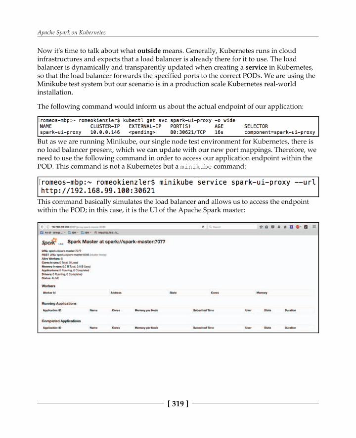
Apache Spark on Kubernetes
[ 319 ]
Now it's time to talk about what outside means. Generally, Kubernetes runs in cloudinfrastructures and expects that a load balancer is already there for it to use. The loadbalancer is dynamically and transparently updated when creating a service in Kubernetes,so that the load balancer forwards the specified ports to the correct PODs. We are using theMinikube test system but our scenario is in a production scale Kubernetes real-worldinstallation.
The following command would inform us about the actual endpoint of our application:
But as we are running Minikube, our single node test environment for Kubernetes, there isno load balancer present, which we can update with our new port mappings. Therefore, weneed to use the following command in order to access our application endpoint within thePOD. This command is not a Kubernetes but a command:
This command basically simulates the load balancer and allows us to access the endpointwithin the POD; in this case, it is the UI of the Apache Spark master:

Apache Spark on Kubernetes
[ 320 ]
Deploying the Apache Spark workersThis looks very nice, but note that there are no workers present. An Apache Spark masterwithout workers is useless. Therefore, let's create the PODs for two workers:
Again, let's check the status of the additional POD:
As we can see, the two additional workers are already running successfully. Since thishappened very fast, let's examine the log file of the master once again in order to see ifthey've been registered correctly:
This was a complete success. We've added two Apache Spark workers in a matter ofseconds! Isn't that great?

Apache Spark on Kubernetes
[ 321 ]
As you've just seen, adding (and also removing) Apache Spark workers toa master is very fast on Kubernetes. There exist cloud services whichprovide Kubernetes as a service. This means you can use Kubernetes andthe required resources backed by Docker containers running on realhardware as an offering in clouds and you are charged on individuallydeployed Docker containers (and maybe their main memory and CPUconsumption) on an hourly basis. We would suggest that you start offwith a minimal Apache Spark configuration just like the one we arecurrently creating here, and in case you run into heavy analytics andresource demands, you can dynamically grow and shrink your ApacheSpark cluster on demand. This is called elasticity and is one of the mainreasons many companies have recently started to run Apache Spark onKubernetes as a service in the cloud. One cloud provider is IBM and thereis a free 30-day trial on the Kubernetes cloud service. An excellent tutorialon this can be found here:
.
To complete the picture, let's check the UI of the master again:
And here we are. We have installed an Apache Spark cluster with one master and twoworkers on Kubernetes with just a couple of commands.

Apache Spark on Kubernetes
[ 322 ]
We can already use this cluster, but let's follow along this example a bit more, since a veryinteresting component will be installed, that is Zeppelin.
Deploying the Zeppelin notebooksApache Zeppelin is the answer of the Apache Foundation to Jupyter notebooks. Jupyternotebooks have been introduced in the earlier chapter on Apache Spark in the cloud wherewe've introduced the IBM Data Science Experience offering which is based on Jupyternotebooks.
So why do we need another notebook implementation? The first thing you might notice ifyou use Jupyter is that the UI seems to be quite outdated. And this is sad, but true.
Zeppelin is based on modern technologies such as AngularJS andBootstrap. One very nice feature is that you can create customized formswithin Zeppelin and the variables are directly passed to the embedded R,Scala, or Python code running in the notebook. In addition, Zeppelin has abuilt-in charting function, whereas in Jupyter you have to use externallibraries. Finally, Zeppelin allows you to mix multiple programminglanguages, whereas in Jupyter you are bound to a single programminglanguage per notebook. Jupyter has a much larger community butZeppelin seems to be slowly catching up. So it is at least worth having alook at it.
Zeppelin could run completely outside Kubernetes and access Apache Spark remotely, butsince installing things in Kubernetes is so straightforward, let's use Kubernetes to deploy aZeppelin POD:
Again, we want to make sure that the POD is up and running, so we regularly check:
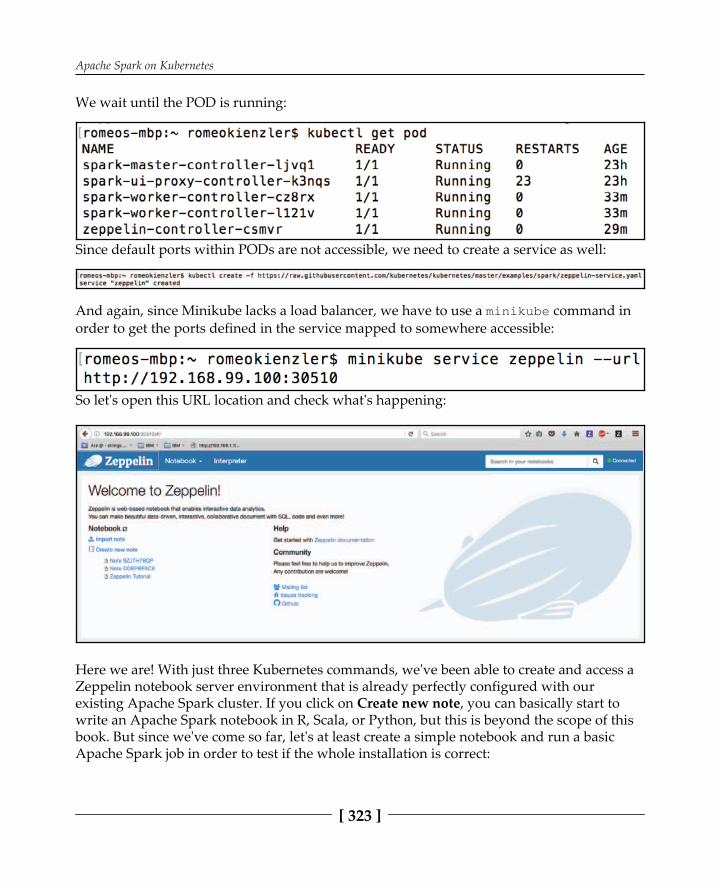
Apache Spark on Kubernetes
[ 323 ]
We wait until the POD is running:
Since default ports within PODs are not accessible, we need to create a service as well:
And again, since Minikube lacks a load balancer, we have to use a command inorder to get the ports defined in the service mapped to somewhere accessible:
So let's open this URL location and check what's happening:
Here we are! With just three Kubernetes commands, we've been able to create and access aZeppelin notebook server environment that is already perfectly configured with ourexisting Apache Spark cluster. If you click on Create new note, you can basically start towrite an Apache Spark notebook in R, Scala, or Python, but this is beyond the scope of thisbook. But since we've come so far, let's at least create a simple notebook and run a basicApache Spark job in order to test if the whole installation is correct:
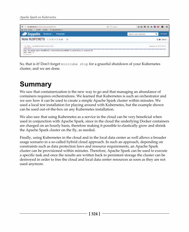
Apache Spark on Kubernetes
[ 324 ]
So, that is it! Don't forget for a graceful shutdown of your Kubernetescluster, and we are done.
SummaryWe saw that containerization is the new way to go and that managing an abundance ofcontainers requires orchestrations. We learned that Kubernetes is such an orchestrator andwe saw how it can be used to create a simple Apache Spark cluster within minutes. Weused a local test installation for playing around with Kubernetes, but the example showncan be used out-of-the-box on any Kubernetes installation.
We also saw that using Kubernetes as a service in the cloud can be very beneficial whenused in conjunction with Apache Spark, since in the cloud the underlying Docker containersare charged on an hourly basis, therefore making it possible to elastically grow and shrinkthe Apache Spark cluster on the fly, as needed.
Finally, using Kubernetes in the cloud and in the local data center as well allows a broaderusage scenario in a so-called hybrid cloud approach. In such an approach, depending onconstraints such as data protection laws and resource requirements, an Apache Sparkcluster can be provisioned within minutes. Therefore, Apache Spark can be used to executea specific task and once the results are written back to persistent storage the cluster can bedestroyed in order to free the cloud and local data center resources as soon as they are notused anymore.

Index
Aabstract syntax tree (AST) , Alluxio alternating least squares (ALS) Apache Giraph reference Apache Mesos Apache Parquet Apache Spark GraphX module Apache Spark GraphX overview , , Apache Spark on Kubernetes example Apache Spark V2.2 unsupported operations Apache Spark V2 changes Apache Spark about cluster design , , , Deeplearning4j example, running in windowing, improving , Apache Streaming data sources Apache SystemML about , , history , , performance measurements working , Apache YARN ApacheSparkML pipelines components ApacheSystemML architecture about high-level operators, generating , language parsing
low-level operators, optimizing Artificial Neural Net (ANN) functionality artificial neural networks (ANNs) about , , , working , , , attributes
Bbare metal deployment batch time binding Bluemix account registration link bushy plan BytesToBytesMap
Ccache eviction strategies , , cache-friendly layout of data, in memory Cassandra catalog API temporary views, managing with Catalyst Optimizer about working categorization Ceph checkpointing , classification with Naive Bayes Cloud cloud-based deployments cluster management cluster manager options, Apache Spark local standalone ,

[ 326 ]
cluster structure clustering with K-means code generation, for expression evaluation code generation about practical examples , coding columnar storage components, ApacheSparkML pipelines DataFrame estimator , parameter pipeline , , transformer components, Kubernetes architecture API server controller manager etcd scheduler components, Kubernetes nodes kube-proxy kublet PODs container versus virtual machine based system abstraction
, containerization about control groups , Linux containers namespaces , containerized Spark applications provisioning, Kubernetes used continuous applications about controlling unification control groups convolutional neural network (CNN) cost-based optimizer, for machine learning
algorithms about alternating least squares, example , ,
,
count-based windows CrossValidation cypher reference
Ddata locality data transfer objects (DTOs) data importing saving DataFrame DataFrame-based machine learning API DataFrames , , , Dataset API working , Datasets using DataSource API about implicit schema discovery , predicate push-down, on smart data sources Deeplearning4j example installing, within Eclipse running, in Apache Spark running, in Eclipse , , , Deeplearning4j runtime Deeplearning4j about , , , , reference directed acyclic graph (DAG) , directives, Dockerfiles ENV EXPOSE FROM RUN USER discrete Fourier transformation (DFT) Docker container starting Docker about reference Dockerfiles about

[ 327 ]
directives Domain Specific Language (DSL) DSL (domain specific language) dynamic rewrites
EEclipse Deeplearning4j example, installing within Deeplearning4j example, running in , ,
, edges elasticity errors estimators about RandomForestClassifier ETL (Extract Transform Load) ETL with Scala , event time versus processing time exactly-once delivery guarantee achieving , example, Apache Spark on Kubernetes about Apache Spark master, deploying , Apache Spark workers, deploying , prerequisites Zeppelin notebooks, deploying examples, GraphFrames API about connected components example , , ,
counting example filtering example , page rank algorithm triangle count algorithm , , explain method used, for obtaining Physical Execution Plan ,
, exploratory analysis with Pixiedust , , , with Python , , , extended ecosystem , Extract Transform Load (ETL) , ,
FFacebook features FIFO (first-in first-out) scheduling file streams , filtering firing mechanism (F(Net) first-in first-out (FIFO) Flume about reference working , , , ,
Ggarbage collection (GC) GlusterFS GPFS (General Purpose File System) graph , graph analytics/processing, with GraphX about connected components example , , counting example filtering example graph, creating , PageRank example raw data triangle counting example graph processing graph-relational translation , GraphFrames architecture examples , , , , , , ,
guest
HH2O Flow about , , , , , , , reference H2O about architecture , build environment data quality

[ 328 ]
data, sourcing deep learning income example code , , MNIST example code overview performance tuning reference Hadoop Hadoop Distributed File System Hadoop Distributed File System (HDFS) reference , hashing high-level operators (HOPs) Hortonworks Data Platform (HDP) Sandbox 2.6 host hyperparameter tuning , , hyperparameters hypervisor
IIBM Cloud Node-RED IoT Starter Boilerplate, deploying to
IEEE PHM 2012 data challenge bearing dataset ,
in-memory processing system Infrastructure as a Service (IaaS) inputs interactive analysis with Pixiedust , , , with Python , , , Internet of Things (IoT) IoT real-time anomaly detector example IPC (inter process communication)
JJava Database Connectivity (JDBC) , Java Virtual Machine (JVM) , , JavaScript Object Notation (JSON) JBOD (just a bunch of disks) approach JSON files processing , Jupyter notebooks about example , , ,
using, scenarios ,
KK-Means working , , , Kafka about reference using , , , , Kaggle competition, winning with Apache SparkML about CrossValidation data preparation , , , evaluator, used for assessing quality of cross-
validated model , feature engineering , , feature engineering pipeline, testing hyperparameter tuning machine learning model, training model evaluation kube-proxy Kubernetes architecture Kubernetes nodes components , Kubernetes about reference using, for provisioning containerized Spark
applications kublet
Llast-in first-out (LIFO) late data LeafExpression least recently used (LRU) Linux containers Logical Execution Plan (LEP) about internal class , object representations , Long Time Support (LTS) Lorenz attractor model , , , LSTM-based auto-encoder Lustre

[ 329 ]
MMapR file system memory management beyond Java Virtual Machine Garbage Collector
Minikube model evaluation MQTT MQTT (Message Queue Telemetry Transport) MQTT message broker connection example , , , ,
NNaive Bayes using , working , , , , ND4J about advantage ND4S Neo4J reference Net function netcat reference Node-RED Node-RED IoT Starter Boilerplate deploying, to IBM Cloud nodes
OOneHotEncoder , Online Analytical Processing (OLAP) Online Transaction Processing (OLTP) OOM (Out of Memory) messages avoiding operator fusing versus volcano iterator model Optimized Logical Execution Plan
Pparameters Parquet files processing
performance performance-related problems, Spark reference Physical Execution Plan (PEP) about , explain method, used for obtaining , , generating selecting pipelines , Pixiedust reference used, for interactive/exploratory analysis ,
, , Platform as a Service (PaaS) Platform as a service clouds (PaaS) POD pre-fetching , Priority Queue processing time versus event time Python about used, for interactive/exploratory analysis ,
, ,
QQuantcast Quasiquotes query performance optimization join elimination , join reordering , , , materialized views
RRandomForestClassifier RDDs versus DataFrames versus Datasets real data science with SparkR , recovery Relational Data Base Management Systems
(RDBMs) relationships Resolved Logical Execution Plan (RLEP)

[ 330 ]
about optimizing Root Mean Square Error (RMSE)
Ssbt tool Scala Scala implicits references schemas defining, manually , , session-based windows Skymind sliding windows smart data sources working , , , Software as a Service (SaaS) Spark graph processing Spark machine learning , Spark MLlib architecture development environment , Spark SQL Spark Stream Context (SSC) Spark Streaming SparkContext methods reference Sparkling Water download option reference Sparkling Water-based application running, steps SparkML SparkML API SparkR real data science, working , SparkSession methods reference SparkSession about using sparse matrix sparse vector representations SQL subqueries using SQL table joins
applying , , SQL using , static rewrites strategies stream life cycle management , stream processing streaming engines windowing, using , Streaming sources about file streams , Flume Kafka TCP stream , , string indexer System of Records (SOR )
TTachyon TCP stream , , temporary views managing, with catalog API test data generator flow deploying test data generator testing test generator deploying text files processing time-based windows TinkerPop reference transformers about , OneHotEncoder , string indexer VectorAssembler transparent fault tolerance achieving , tumbling windows Tungsten memory usage, example , performance, example ,

UUnresolved Logical Execution Plan (ULEP) about to Resolved Logical Execution Plan UnsafeRow object about fixed length values region null bit set region variable length values region user-defined functions
VVectorAssembler virtual machine based system abstraction versus container , virtual machine deployment
VirtualBox reference visual explain volcano iterator model versus operator fusing
Wwdivmm (weighted divide matrix multiplication) whole stage code generation about performance, example , , windowing Within Set Sum of Squared Errors (WSSSE) Write Ahead Log (WAL)
ZZeroMQ


