Embed Size (px)
Citation preview

“Comninos” — 2005/8/31 — 20:17 — page i — #1
Mathematical and Computer ProgrammingTechniques for Computer Graphics
“Comninos” — 2005/8/31 — 20:17 — page iii — #3
Peter Comninos
Mathematical andComputerProgrammingTechniques forComputer Graphics
With 311 Figures

“Comninos” — 2005/8/31 — 20:17 — page iv — #4
Peter Comninos, Dip (Comp. Prog.), BSc (Hons) (Comp. Sc.), PhD (Comp. Sc.)The National Centre for Computer AnimationWeymouth HouseBournemouth UniversityPoole BH12 5BBUnited [email protected]
British Library Cataloguing in Publication DataA catalogue record for this book is available from the British Library
Library of Congress Control Number: 2005925503
ISBN-10: 1-85233-902-0 Printed on acid-free paperISBN-13: 978-1-8233-902-9
© Springer-Verlag London Limited 2006
Apart from any fair dealing for the purposes of research or private study, or criticism or review, aspermitted under the Copyright, Designs and Patents Act 1988, this publication may only be repro-duced, stored or transmitted, in any form or by any means, with the prior permission in writing ofthe publishers, or in the case of reprographic reproduction in accordance with the terms of licencesissued by the Copyright Licensing Agency. Enquiries concerning reproduction outside those termsshould be sent to the publishers.
The use of registered names, trademarks, etc. in this publication does not imply, even in the ab-sence of a specific statement, that such names are exempt from the relevant laws and regulationsand therefore free for general use.
The publisher makes no representation, express or implied, with regard to the accuracy of the infor-mation contained in this book and cannot accept any legal responsibility or liability for any errorsor omissions that may be made.
Printed in the United States of America (SPI/MVY)
9 8 7 6 5 4 3 2 1
Springer Science+Business Mediaspringeronline.com

“Comninos” — 2005/8/31 — 20:17 — page v — #5
“The knowledge of which geometry aims is the knowledge of the eternal.”
Plato Republic, VII, 52.
“There is geometry in the humming of the strings.”
Pythagoras
“Mathematics is the most beautiful and most powerful creation of the humanspirit. Mathematics is as old as Man.”
Stefan Banach
“The mathematician’s best work is art, a high perfect art, as daring as the mostsecret dreams of imagination, clear and limpid. Mathematical genius and artisticgenius touch one another.”
Gosta Mittag-Leffler
“It is not only important, it is essential!”
Dr. Strangelove
“Comninos” — 2005/8/31 — 20:17 — page vii — #7
Preface
This book introduces undergraduate and postgraduate students to mathematicsand related computer programming techniques used in Computer Graphics. In agradual approach, the book exposes students to the underlying mathematical ideasand leads them towards a level of sufficient understanding of detail to be able toimplement libraries and programs for 2D and 3D graphics. Through the use ofnumerous code examples, the students are encouraged to explore and experimentwith data structures and computer programs (in the C programming language) andto master the related mathematical techniques.
This book is meant for students with a minimum prerequisite knowledge ofmathematics. It assumes very little and any high school graduate should be able tofollow this book. The intended reader is expected to have had some basic exposureto topics such as functions, trigonometric functions, elementary geometry andnumber theory, and elements of set theory. The reader is also expected to havesome familiarity with some computer programming language such as C, althoughany algorithmic language will serve the purpose.
The book includes a simple but effective set of routines, organised as a library,that covers both 2D and 3D graphics. This parallel approach of exposing thestudents to the mathematical theory and showing them how to incorporate it intoexample programs is the major strength of this book. It both demystifies themathematics and it demonstrates its relevance to 2D and 3D computer graphics,thus motivating and rewarding the reader.
This book is organised into ten chapters and four appendices. Chapters 1–4 arecharacterised as survival kits, as they introduce the basic mathematical conceptsand techniques that are applied and are essential for a thorough understanding ofthe remaining six chapters. The material presented in this book has been used toteach mathematical and programming techniques to both Computer Scientists andArtists. For a Bachelor degree that covers the mathematics for computer graphicsover three years, Chapter 1 would normally be taught at the end of year one,Chapters 2–9 would normally be taught in year two of the course and Chapter 10may be taught at the end of year two or the beginning of year three.
Chapter 1 introduces readers to concepts of set theory and function theory. Itassumes no prior knowledge of these topics and it is self-contained.
vii
“Comninos” — 2005/8/31 — 20:17 — page viii — #8
viii Preface
Chapter 2 deals with vectors and vector algebra. It introduces readers to thesetopics assuming no prior knowledge save a rudimentary understanding of 2D and3D geometry and some elements of trigonometry. Once readers have masteredthe material presented in this chapter, they will be able to solve complex vectoralgebra problems and to implement their solutions in computer programs. Appen-dix 1, which is associated with this chapter, presents an example implementationof a 3D vector-algebra library.
Chapter 3 deals with matrices and matrix algebra. It introduces readers to thesetopics assuming no prior knowledge of matrices but requiring a good understand-ing of vector algebra. Once readers have mastered the material presented in thischapter, they will be able to solve complex matrix algebra problems and to imple-ment their solutions in computer programs. Appendix 2, which is associated withthis chapter, presents an example implementation of a 4D matrix-algebra library.
Chapter 4 deals with vector spaces, which is one of the most abstract subjectsdealt with in this book and thus one of the topics that some students find moredifficult. This chapter requires a good understanding of both vector and matrixalgebra. It is self-contained and, although it introduces the very important conceptof the change of basis matrix, it may be omitted by the uninterested reader.
Chapters 5 and 6 deal with the concepts of 2D transformations and 2D clippingalgorithms respectively, and their implementation. Appendix 3, which is associ-ated with these two chapters, presents an example implementation of a compre-hensive 2D graphics library.
Chapter 7 deals with the concepts of viewing and projection transformations,3D clipping, and their implementation. Appendix 4, which is associated with thischapter, presents an example implementation of a comprehensive 3D graphicslibrary.
Chapter 9 examines the data structures required to represent 3D models andsome of the hidden-surface removal and rendering techniques used in the creationof computer generated images. This chapter also introduces readers to some ofthe simple empirical lighting and shading models used in real-time graphics.
Finally, Chapter 10 presents a much more detailed exposition of the nature oflight and examines, in some detail, physically-based lighting and shading models,and rendering techniques and algorithms. The material presented in this chapteris more mathematically challenging.
Most of the material presented in this book has been designed to be accessibleto B.A., B.Sc., M.A. and M.Sc. students of a computer animation, digital spe-cial effects or technical direction degree course. This book however will also beuseful to computer science students studying a graphics or animation unit and totechnical directors in CGI production.
The vector and matrix notation of this book is designed to appeal to both NorthAmerican and International readers.

“Comninos” — 2005/8/31 — 20:17 — page ix — #9
Acknowledgements
I express my unreserved gratitude to countless students at the National Centre forComputer Animation who have helped me “debug” this text and improve its read-ability. My sincere thanks also go to my wife Daniele and my daughter Celina.Without their support and understanding writing this book would have been im-possible.
Last but not least I would like to express my gratitude to my colleagueand friend Peter Hardie for allowing me to use his computer art on the coverof this book. More information on Peter’s work can be found online athttp://ncca.bournemouth.ac.uk/newhome/announce phsab.html.
ix
“Comninos” — 2005/8/31 — 20:17 — page xi — #11
Contents
Preface vii
Acknowledgements ix
Some Definitions of Terms 1
1 Set Theory Survival Kit 31.1 Some Basic Notations and Definitions . . . . . . . . . . . . . . . 4
1.1.1 Sets and Elements . . . . . . . . . . . . . . . . . . . . . 41.1.2 Notation and Set Specification . . . . . . . . . . . . . . 41.1.3 Set Membership . . . . . . . . . . . . . . . . . . . . . . 51.1.4 Finite and Infinite Sets . . . . . . . . . . . . . . . . . . 6
1.2 Equality of Sets . . . . . . . . . . . . . . . . . . . . . . . . . . 61.3 The Null Set or Empty Set . . . . . . . . . . . . . . . . . . . . . 61.4 Subsets . . . . . . . . . . . . . . . . . . . . . . . . . . . . . . . 61.5 Supersets . . . . . . . . . . . . . . . . . . . . . . . . . . . . . . 71.6 Proper Subsets and Supersets . . . . . . . . . . . . . . . . . . . 71.7 Comparable Sets . . . . . . . . . . . . . . . . . . . . . . . . . . 81.8 The Universal Set . . . . . . . . . . . . . . . . . . . . . . . . . 81.9 Disjoint Sets . . . . . . . . . . . . . . . . . . . . . . . . . . . . 81.10 Venn-Euler Diagrams . . . . . . . . . . . . . . . . . . . . . . . 81.11 Line Diagrams . . . . . . . . . . . . . . . . . . . . . . . . . . . 111.12 Basic Set Operations . . . . . . . . . . . . . . . . . . . . . . . . 11
1.12.1 Set Union . . . . . . . . . . . . . . . . . . . . . . . . . 111.12.2 Set Intersection . . . . . . . . . . . . . . . . . . . . . . 121.12.3 Set Difference . . . . . . . . . . . . . . . . . . . . . . . 131.12.4 The Symmetric Difference of Two Sets . . . . . . . . . . 141.12.5 The Complement of a Set . . . . . . . . . . . . . . . . . 18
Theorem 1.1 . . . . . . . . . . . . . . . . . . . . . . . . 191.12.6 Theorems on Comparable Sets . . . . . . . . . . . . . . 20
Theorem 1.2 . . . . . . . . . . . . . . . . . . . . . . . . 20Theorem 1.3 . . . . . . . . . . . . . . . . . . . . . . . . 20
xi
“Comninos” — 2005/8/31 — 20:17 — page xii — #12
xii Contents
Theorem 1.4 . . . . . . . . . . . . . . . . . . . . . . . 20Theorem 1.5 . . . . . . . . . . . . . . . . . . . . . . . 21Theorem 1.6 . . . . . . . . . . . . . . . . . . . . . . . 22
1.13 The Algebra of Sets . . . . . . . . . . . . . . . . . . . . . . . . 221.13.1 The Rules of the Algebra of Sets . . . . . . . . . . . . 22
Theorem 1.7 . . . . . . . . . . . . . . . . . . . . . . . 23Theorem 1.8 . . . . . . . . . . . . . . . . . . . . . . . 23
1.13.2 The Duality Principle . . . . . . . . . . . . . . . . . . 24Theorem 1.9 . . . . . . . . . . . . . . . . . . . . . . . 24
1.14 Numbers and Sets . . . . . . . . . . . . . . . . . . . . . . . . . 251.14.1 Classes of Numbers . . . . . . . . . . . . . . . . . . . 251.14.2 Closure . . . . . . . . . . . . . . . . . . . . . . . . . . 251.14.3 The Set of Real Numbers R . . . . . . . . . . . . . . . 261.14.4 The Set of Rational Numbers Q . . . . . . . . . . . . . 261.14.5 The Set of Irrational Numbers Q
′ . . . . . . . . . . . . 271.14.6 The Set of Natural Numbers N . . . . . . . . . . . . . 271.14.7 The Set of Integer Numbers Z . . . . . . . . . . . . . . 281.14.8 Other useful Sets of Numbers . . . . . . . . . . . . . . 28
1.14.8.1 The Set of Complex Numbers C . . . . . . . 281.14.8.2 The Set of Algebraic Numbers A . . . . . . . 281.14.8.3 The Set of Transcendental Numbers T . . . . 28
1.14.9 Ordering Relations or Inequalities . . . . . . . . . . . . 29The Reflexivity Property . . . . . . . . . . . 29The Trichotomy Property . . . . . . . . . . . 29The Antisymmetry Property . . . . . . . . . 29The Transitivity Property . . . . . . . . . . . 29The Additional and Subtraction Property . . 29The Multiplication and Division Property . . 30Examples . . . . . . . . . . . . . . . . . . . 30
1.14.10 The Absolute Value or Modulus of a Number . . . . . . 301.14.11 Real Number Intervals . . . . . . . . . . . . . . . . . . 321.14.12 Properties of Real Number Intervals . . . . . . . . . . 341.14.13 Real Number Interval Arithmetic . . . . . . . . . . . . 341.14.14 Bounded and Unbounded Real Number Sets . . . . . . 35
1.15 Ordered Pairs and Ordered n-tuples . . . . . . . . . . . . . . . . 361.16 The Cartesian Product of Sets . . . . . . . . . . . . . . . . . . . 371.17 Functions . . . . . . . . . . . . . . . . . . . . . . . . . . . . . . 38
1.17.1 The Formal Definition of a Function . . . . . . . . . . 391.17.2 Mappings, Operators and Transformations . . . . . . . 411.17.3 Equality of Functions . . . . . . . . . . . . . . . . . . 411.17.4 The Range of a Function . . . . . . . . . . . . . . . . . 431.17.5 Different Types of Functions . . . . . . . . . . . . . . 43
1.17.5.1 Many-to-One Functions . . . . . . . . . . . 431.17.5.2 Injective Functions or One-to-One Functions 431.17.5.3 Surjective Functions or Onto Functions . . . 44
“Comninos” — 2005/8/31 — 20:17 — page xiii — #13
Contents xiii
1.17.5.4 Bijective Functions or One-to-OneCorrespondences . . . . . . . . . . . . . . . 45
1.17.6 Constant Functions . . . . . . . . . . . . . . . . . . . 471.17.7 The Identity Function or Identity Transformation . . . . 481.17.8 The Composition or Product of Functions . . . . . . . . 481.17.9 The Inverse of a Function . . . . . . . . . . . . . . . . 49
1.17.9.1 Applying the Inverse of a Function to anElement of its Co-domain . . . . . . . . . . 50
1.17.9.2 Applying the Inverse of a Function to aSubset of its Co-domain . . . . . . . . . . . 50
1.17.10 The Inverse Function . . . . . . . . . . . . . . . . . . 521.17.11 Theorems on the Inverse Function . . . . . . . . . . . . 53
Theorem 1.10 . . . . . . . . . . . . . . . . . . . . . . 53Theorem 1.11 . . . . . . . . . . . . . . . . . . . . . . 54
1.17.12 The Graph of a Function . . . . . . . . . . . . . . . . . 541.17.13 The Redefinition of a Function as a Set of
Ordered Pairs . . . . . . . . . . . . . . . . . . . . . . 571.18 Families of Indexed Sets . . . . . . . . . . . . . . . . . . . . . . 581.19 The Generalised Set Union and Intersection Operations . . . . . 60
1.19.1 The Negation of the Generalised Set Operations . . . . 611.19.2 Some Algebraic Rules for the Generalised Set
Operations . . . . . . . . . . . . . . . . . . . . . . . . 611.20 The Cardinality or Size of a Set . . . . . . . . . . . . . . . . . . 62
1.20.1 Equivalent Sets . . . . . . . . . . . . . . . . . . . . . 621.20.2 The Cardinal Number or Cardinality of a Set . . . . . . 63
1.21 The Power Set of a Set . . . . . . . . . . . . . . . . . . . . . . . 63
2 Vector Algebra Survival Kit 652.1 Some Basic Definitions and Notation . . . . . . . . . . . . . . . 652.2 Multiplication of a Vector by a Scalar . . . . . . . . . . . . . . . 682.3 Vector Addition . . . . . . . . . . . . . . . . . . . . . . . . . . 692.4 Position Vectors and Free Vectors . . . . . . . . . . . . . . . . . 712.5 The Vector Equation of a Line . . . . . . . . . . . . . . . . . . . 712.6 Linear Dependence/Independence of Vectors . . . . . . . . . . . 722.7 Vector Bases . . . . . . . . . . . . . . . . . . . . . . . . . . . . 742.8 The Components of a Vector . . . . . . . . . . . . . . . . . . . . 74
2.8.1 Multiplication of a Vector by a Scalar . . . . . . . . . . 742.8.2 Vector Addition . . . . . . . . . . . . . . . . . . . . . 742.8.3 Vector Equality . . . . . . . . . . . . . . . . . . . . . 75
2.9 Orthogonal, Orthonormal and Right-Handed Vector Bases . . . . 752.10 Cartesian Bases and Cartesian Coordinates . . . . . . . . . . . . 772.11 The Length of a Vector . . . . . . . . . . . . . . . . . . . . . . . 782.12 The Scalar Product of Vectors . . . . . . . . . . . . . . . . . . . 782.13 The Scalar Product Expressed in Terms of its Components . . . . 802.14 Properties and Applications of the Scalar Product . . . . . . . . . 80
“Comninos” — 2005/8/31 — 20:17 — page xiv — #14
xiv Contents
2.14.1 The Magnitude of a Vector Using its Components . . . . 802.14.2 Normalising a Vector . . . . . . . . . . . . . . . . . . . 802.14.3 The Projection of a Vector onto Another . . . . . . . . . 812.14.4 The Cosine of the Angle Between two Vectors . . . . . . 822.14.5 The Scalar Product of Collinear Vectors . . . . . . . . . 822.14.6 The Scalar Product of Orthogonal Vectors . . . . . . . . 82
2.15 The Direction Ratios and Direction Cosines of a Vector . . . . . 822.16 The Vector Product of two Vectors . . . . . . . . . . . . . . . . 842.17 The Vector Product Expressed in Terms of its Components . . . . 852.18 Properties of the Vector Product . . . . . . . . . . . . . . . . . . 86
2.18.1 The Geometric Interpretation of the Vector Product . . . 862.18.2 The Magnitude of the Vector Product in Terms of its
Components . . . . . . . . . . . . . . . . . . . . . . . . 872.18.3 The Square of the Magnitude of the Vector Product . . . 872.18.4 The Magnitude of the Sine of the Angle between Two
Vectors . . . . . . . . . . . . . . . . . . . . . . . . . . 872.19 Triple Products of Vectors . . . . . . . . . . . . . . . . . . . . . 88
2.19.1 The Triple Scalar Product . . . . . . . . . . . . . . . . . 882.19.2 The Triple Vector Product . . . . . . . . . . . . . . . . 902.19.3 The Scalar Product of Two Vector Products . . . . . . . 912.19.4 The Vector Product of two Vector Products . . . . . . . 92
2.20 The Components of a Vector Relative to a Non-orthogonalBasis . . . . . . . . . . . . . . . . . . . . . . . . . . . . . . . . 92
2.21 The Decomposition of a Vector According to a Basis . . . . . . . 952.22 The Vector Equation of the Line Revisited . . . . . . . . . . . . 96
2.22.1 The Line Defined by Two Position Vectors . . . . . . . . 962.22.2 The Line Defined by a Position Vector and Direction
Vector . . . . . . . . . . . . . . . . . . . . . . . . . . . 972.23 The Vector Equation of the Plane . . . . . . . . . . . . . . . . . 98
2.23.1 The Plane Defined by a Position Vector and a NormalVector . . . . . . . . . . . . . . . . . . . . . . . . . . . 98
2.23.2 The Plane Defined by three Position Vectors . . . . . . . 992.24 Some Applications of Vector Algebra in Analytical Geometry . . 101
2.24.1 The Distance Between Two Points in Space . . . . . . . 1012.24.2 The Perpendicular Distance from a Point to a Line . . . . 1022.24.3 The Distance of a Point from a Line . . . . . . . . . . . 1032.24.4 The Distance Between Two Parallel Lines . . . . . . . . 1042.24.5 The Distance Between Two Non-Parallel Lines . . . . . 1052.24.6 The Cosine of the Angle Between Two Lines . . . . . . 1062.24.7 The Cosine of the Angle Between Two Planes . . . . . . 1062.24.8 The Distance of a Point from a Plane . . . . . . . . . . . 1072.24.9 The Point of Intersection of a Line and a Plane . . . . . 109
2.25 Summary of Vector Algebra Axioms and Rules . . . . . . . . . . 1102.26 A Simple Vector Algebra C Library . . . . . . . . . . . . . . . . 113
“Comninos” — 2005/8/31 — 20:17 — page xv — #15
Contents xv
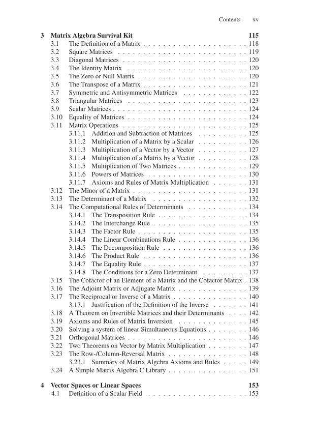
3 Matrix Algebra Survival Kit 1153.1 The Definition of a Matrix . . . . . . . . . . . . . . . . . . . . . 1183.2 Square Matrices . . . . . . . . . . . . . . . . . . . . . . . . . . 1193.3 Diagonal Matrices . . . . . . . . . . . . . . . . . . . . . . . . . 1203.4 The Identity Matrix . . . . . . . . . . . . . . . . . . . . . . . . 1203.5 The Zero or Null Matrix . . . . . . . . . . . . . . . . . . . . . . 1203.6 The Transpose of a Matrix . . . . . . . . . . . . . . . . . . . . . 1213.7 Symmetric and Antisymmetric Matrices . . . . . . . . . . . . . 1223.8 Triangular Matrices . . . . . . . . . . . . . . . . . . . . . . . . 1233.9 Scalar Matrices . . . . . . . . . . . . . . . . . . . . . . . . . . . 1243.10 Equality of Matrices . . . . . . . . . . . . . . . . . . . . . . . . 1243.11 Matrix Operations . . . . . . . . . . . . . . . . . . . . . . . . . 125
3.11.1 Addition and Subtraction of Matrices . . . . . . . . . . 1253.11.2 Multiplication of a Matrix by a Scalar . . . . . . . . . . 1263.11.3 Multiplication of a Vector by a Vector . . . . . . . . . . 1273.11.4 Multiplication of a Matrix by a Vector . . . . . . . . . . 1283.11.5 Multiplication of Two Matrices . . . . . . . . . . . . . . 1293.11.6 Powers of Matrices . . . . . . . . . . . . . . . . . . . . 1303.11.7 Axioms and Rules of Matrix Multiplication . . . . . . . 131
3.12 The Minor of a Matrix . . . . . . . . . . . . . . . . . . . . . . . 1313.13 The Determinant of a Matrix . . . . . . . . . . . . . . . . . . . 1323.14 The Computational Rules of Determinants . . . . . . . . . . . . 134
3.14.1 The Transposition Rule . . . . . . . . . . . . . . . . . . 1343.14.2 The Interchange Rule . . . . . . . . . . . . . . . . . . . 1353.14.3 The Factor Rule . . . . . . . . . . . . . . . . . . . . . . 1353.14.4 The Linear Combinations Rule . . . . . . . . . . . . . . 1363.14.5 The Decomposition Rule . . . . . . . . . . . . . . . . . 1363.14.6 The Product Rule . . . . . . . . . . . . . . . . . . . . . 1363.14.7 The Equality Rule . . . . . . . . . . . . . . . . . . . . . 1373.14.8 The Conditions for a Zero Determinant . . . . . . . . . 137
3.15 The Cofactor of an Element of a Matrix and the Cofactor Matrix . 1383.16 The Adjoint Matrix or Adjugate Matrix . . . . . . . . . . . . . . 1393.17 The Reciprocal or Inverse of a Matrix . . . . . . . . . . . . . . . 140
3.17.1 Justification of the Definition of the Inverse . . . . . . . 1413.18 A Theorem on Invertible Matrices and their Determinants . . . . 1423.19 Axioms and Rules of Matrix Inversion . . . . . . . . . . . . . . 1453.20 Solving a system of linear Simultaneous Equations . . . . . . . . 1463.21 Orthogonal Matrices . . . . . . . . . . . . . . . . . . . . . . . . 1463.22 Two Theorems on Vector by Matrix Multiplication . . . . . . . . 1473.23 The Row-/Column-Reversal Matrix . . . . . . . . . . . . . . . . 148
3.23.1 Summary of Matrix Algebra Axioms and Rules . . . . . 1493.24 A Simple Matrix Algebra C Library . . . . . . . . . . . . . . . . 151
4 Vector Spaces or Linear Spaces 1534.1 Definition of a Scalar Field . . . . . . . . . . . . . . . . . . . . 153
“Comninos” — 2005/8/31 — 20:17 — page xvi — #16
xvi Contents
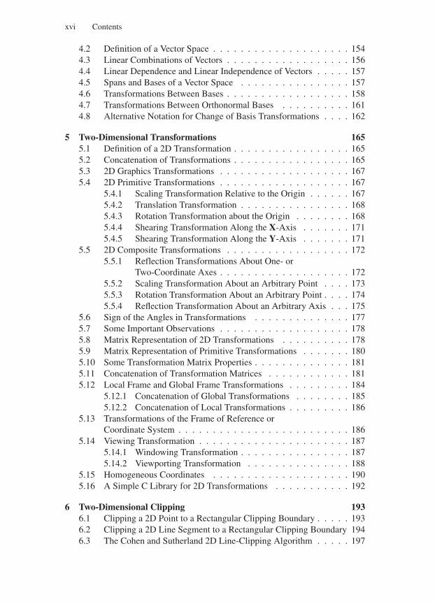
4.2 Definition of a Vector Space . . . . . . . . . . . . . . . . . . . . 1544.3 Linear Combinations of Vectors . . . . . . . . . . . . . . . . . . 1564.4 Linear Dependence and Linear Independence of Vectors . . . . . 1574.5 Spans and Bases of a Vector Space . . . . . . . . . . . . . . . . 1574.6 Transformations Between Bases . . . . . . . . . . . . . . . . . . 1584.7 Transformations Between Orthonormal Bases . . . . . . . . . . 1614.8 Alternative Notation for Change of Basis Transformations . . . . 162
5 Two-Dimensional Transformations 1655.1 Definition of a 2D Transformation . . . . . . . . . . . . . . . . . 1655.2 Concatenation of Transformations . . . . . . . . . . . . . . . . . 1655.3 2D Graphics Transformations . . . . . . . . . . . . . . . . . . . 1675.4 2D Primitive Transformations . . . . . . . . . . . . . . . . . . . 167
5.4.1 Scaling Transformation Relative to the Origin . . . . . . 1675.4.2 Translation Transformation . . . . . . . . . . . . . . . . 1685.4.3 Rotation Transformation about the Origin . . . . . . . . 1685.4.4 Shearing Transformation Along the X-Axis . . . . . . . 1715.4.5 Shearing Transformation Along the Y-Axis . . . . . . . 171
5.5 2D Composite Transformations . . . . . . . . . . . . . . . . . . 1725.5.1 Reflection Transformations About One- or
Two-Coordinate Axes . . . . . . . . . . . . . . . . . . . 1725.5.2 Scaling Transformation About an Arbitrary Point . . . . 1735.5.3 Rotation Transformation About an Arbitrary Point . . . . 1745.5.4 Reflection Transformation About an Arbitrary Axis . . . 175
5.6 Sign of the Angles in Transformations . . . . . . . . . . . . . . 1775.7 Some Important Observations . . . . . . . . . . . . . . . . . . . 1785.8 Matrix Representation of 2D Transformations . . . . . . . . . . 1785.9 Matrix Representation of Primitive Transformations . . . . . . . 1805.10 Some Transformation Matrix Properties . . . . . . . . . . . . . . 1815.11 Concatenation of Transformation Matrices . . . . . . . . . . . . 1815.12 Local Frame and Global Frame Transformations . . . . . . . . . 184
5.12.1 Concatenation of Global Transformations . . . . . . . . 1855.12.2 Concatenation of Local Transformations . . . . . . . . . 186
5.13 Transformations of the Frame of Reference orCoordinate System . . . . . . . . . . . . . . . . . . . . . . . . . 186
5.14 Viewing Transformation . . . . . . . . . . . . . . . . . . . . . . 1875.14.1 Windowing Transformation . . . . . . . . . . . . . . . . 1875.14.2 Viewporting Transformation . . . . . . . . . . . . . . . 188
5.15 Homogeneous Coordinates . . . . . . . . . . . . . . . . . . . . 1905.16 A Simple C Library for 2D Transformations . . . . . . . . . . . 192
6 Two-Dimensional Clipping 1936.1 Clipping a 2D Point to a Rectangular Clipping Boundary . . . . . 1936.2 Clipping a 2D Line Segment to a Rectangular Clipping Boundary 1946.3 The Cohen and Sutherland 2D Line-Clipping Algorithm . . . . . 197
“Comninos” — 2005/8/31 — 20:17 — page xvii — #17
Contents xvii
6.4 2D Polygon Clipping . . . . . . . . . . . . . . . . . . . . . . . . 2026.4.1 The Sutherland and Hodgman Polygon-Clipping Algorithm 2036.4.2 The Weiler and Atherton Polygon-Clipping Algorithm . . . 219
References . . . . . . . . . . . . . . . . . . . . . . . . . . . . . . . . . 223
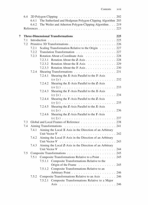
7 Three-Dimensional Transformations 2257.1 Introduction . . . . . . . . . . . . . . . . . . . . . . . . . . . . . 2257.2 Primitive 3D Transformations . . . . . . . . . . . . . . . . . . . . 226
7.2.1 Scaling Transformation Relative to the Origin . . . . . . . 2277.2.2 Translation Transformation . . . . . . . . . . . . . . . . . 2277.2.3 Rotation About a Coordinate Axis . . . . . . . . . . . . . 228
7.2.3.1 Rotation About the Z-Axis . . . . . . . . . . . . . 2287.2.3.2 Rotation About the X-Axis . . . . . . . . . . . . 2297.2.3.3 Rotation About the Y-Axis . . . . . . . . . . . . . 230
7.2.4 Shearing Transformations . . . . . . . . . . . . . . . . . . 2317.2.4.1 Shearing the X-Axis Parallel to the Y-Axis
(sx ‖y ) . . . . . . . . . . . . . . . . . . . . . . . 2327.2.4.2 Shearing the X-Axis Parallel to the Z-Axis
(sx ‖z ) . . . . . . . . . . . . . . . . . . . . . . . 2337.2.4.3 Shearing the Y-Axis Parallel to the X-Axis
(sy ‖x ) . . . . . . . . . . . . . . . . . . . . . . . 2347.2.4.4 Shearing the Y-Axis Parallel to the Z-Axis
(sy ‖z ) . . . . . . . . . . . . . . . . . . . . . . . 2357.2.4.5 Shearing the Z-Axis Parallel to the X-Axis
(sz ‖x ) . . . . . . . . . . . . . . . . . . . . . . . 2367.2.4.6 Shearing the Z-Axis Parallel to the Y-Axis
(sz ‖y ) . . . . . . . . . . . . . . . . . . . . . . . 2377.3 Global and Local Frames of Reference . . . . . . . . . . . . . . . 2387.4 Aiming Transformations . . . . . . . . . . . . . . . . . . . . . . 241
7.4.1 Aiming the Local X-Axis in the Direction of an ArbitraryUnit Vector V . . . . . . . . . . . . . . . . . . . . . . . . 242
7.4.2 Aiming the Local Y-Axis in the Direction of an ArbitraryUnit Vector V . . . . . . . . . . . . . . . . . . . . . . . . 243
7.4.3 Aiming the Local Z-Axis in the Direction of an ArbitraryUnit Vector V . . . . . . . . . . . . . . . . . . . . . . . . 244
7.5 Composite Transformations . . . . . . . . . . . . . . . . . . . . . 2457.5.1 Composite Transformations Relative to a Point . . . . . . . 245
7.5.1.1 Composite Transformations Relative to theOrigin of the Frame . . . . . . . . . . . . . . . . 245
7.5.1.2 Composite Transformations Relative to anArbitrary Point . . . . . . . . . . . . . . . . . . . 246
7.5.2 Composite Transformations Relative to an Axis . . . . . . 2467.5.2.1 Composite Transformations Relative to a Major
Axis . . . . . . . . . . . . . . . . . . . . . . . . 246
“Comninos” — 2005/8/31 — 20:17 — page xviii — #18
xviii Contents
7.5.2.2 Composite Transformations Relative to an AxisParallel to a Major Axis . . . . . . . . . . . . . 247
7.5.2.3 Composite Transformations Relative to anArbitrary Axis . . . . . . . . . . . . . . . . . . 248
7.5.3 Composite Transformations Relative to a Plane . . . . . . 2497.5.3.1 Composite Transformations Relative to a Major
Plane . . . . . . . . . . . . . . . . . . . . . . . 2497.5.3.2 Composite Transformations Relative to an
Arbitrary Plane . . . . . . . . . . . . . . . . . . 2507.6 Local Frame and Global Frame Transformations . . . . . . . . . 2517.7 Transformations of the Frame of Reference or Coordinate System 252References . . . . . . . . . . . . . . . . . . . . . . . . . . . . . . . . . 252
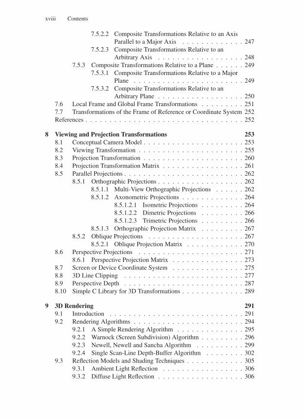
8 Viewing and Projection Transformations 2538.1 Conceptual Camera Model . . . . . . . . . . . . . . . . . . . . . 2538.2 Viewing Transformation . . . . . . . . . . . . . . . . . . . . . . 2558.3 Projection Transformation . . . . . . . . . . . . . . . . . . . . . 2608.4 Projection Transformation Matrix . . . . . . . . . . . . . . . . . 2618.5 Parallel Projections . . . . . . . . . . . . . . . . . . . . . . . . . 262
8.5.1 Orthographic Projections . . . . . . . . . . . . . . . . . . 2628.5.1.1 Multi-View Orthographic Projections . . . . . . 2628.5.1.2 Axonometric Projections . . . . . . . . . . . . . 264
8.5.1.2.1 Isometric Projections . . . . . . . . . 2648.5.1.2.2 Dimetric Projections . . . . . . . . . 2668.5.1.2.3 Trimetric Projections . . . . . . . . . 266
8.5.1.3 Orthographic Projection Matrix . . . . . . . . . 2678.5.2 Oblique Projections . . . . . . . . . . . . . . . . . . . . 267
8.5.2.1 Oblique Projection Matrix . . . . . . . . . . . . 2708.6 Perspective Projections . . . . . . . . . . . . . . . . . . . . . . 271
8.6.1 Perspective Projection Matrix . . . . . . . . . . . . . . . 2738.7 Screen or Device Coordinate System . . . . . . . . . . . . . . . 2758.8 3D Line Clipping . . . . . . . . . . . . . . . . . . . . . . . . . 2778.9 Perspective Depth . . . . . . . . . . . . . . . . . . . . . . . . . 2878.10 Simple C Library for 3D Transformations . . . . . . . . . . . . . 289
9 3D Rendering 2919.1 Introduction . . . . . . . . . . . . . . . . . . . . . . . . . . . . 2919.2 Rendering Algorithms . . . . . . . . . . . . . . . . . . . . . . . 294
9.2.1 A Simple Rendering Algorithm . . . . . . . . . . . . . . 2959.2.2 Warnock (Screen Subdivision) Algorithm . . . . . . . . . 2969.2.3 Newell, Newell and Sancha Algorithm . . . . . . . . . . 2999.2.4 Single Scan-Line Depth-Buffer Algorithm . . . . . . . . 302
9.3 Reflection Models and Shading Techniques . . . . . . . . . . . . 3059.3.1 Ambient Light Reflection . . . . . . . . . . . . . . . . . 3069.3.2 Diffuse Light Reflection . . . . . . . . . . . . . . . . . . 306
“Comninos” — 2005/8/31 — 20:17 — page xix — #19
Contents xix
9.3.3 Specular Light Reflection . . . . . . . . . . . . . . . . 3089.3.3.1 Horn’s Method for Computing the Specular
Reflection Function . . . . . . . . . . . . . 3099.3.3.2 Blinn’s Method for Computing the
Specular Reflection Function . . . . . . . . 3109.3.4 Phong’s Lighting Model . . . . . . . . . . . . . . . . . 311
9.3.4.1 Simulating Multiple Light Sources . . . . . 3119.3.4.2 Simulating Distant Light Sources . . . . . . 3119.3.4.3 Coloured Light Sources . . . . . . . . . . . 312
9.4 Shading Techniques . . . . . . . . . . . . . . . . . . . . . . . 3139.4.1 Flat Polygon Shading Technique . . . . . . . . . . . . 3139.4.2 Gouraud Smooth Shading Technique . . . . . . . . . . 3139.4.3 Phong Smooth Shading Technique . . . . . . . . . . . 315
References . . . . . . . . . . . . . . . . . . . . . . . . . . . . . . . . 316
10 Physically Based Lighting and Shading Models and RenderingAlgorithms 31710.1 Evolution of the Theory of Light . . . . . . . . . . . . . . . . . 31710.2 Nature of Light . . . . . . . . . . . . . . . . . . . . . . . . . . 32010.3 Interaction of Light with Various Materials . . . . . . . . . . . 324
10.3.1 Light Reflection . . . . . . . . . . . . . . . . . . . . . 32510.3.2 Light Refraction and Transmission . . . . . . . . . . . 32610.3.3 Total Internal Reflection . . . . . . . . . . . . . . . . . 32810.3.4 Light Scattering and Absorption . . . . . . . . . . . . 32910.3.5 Subsurface Scattering . . . . . . . . . . . . . . . . . . 330
10.4 Some Useful Concepts, Definitions and Conventions . . . . . . 33110.4.1 Spherical Coordinates of a Vector . . . . . . . . . . . . 33310.4.2 Determining the Reflection Vector . . . . . . . . . . . 33510.4.3 Determining the Transmission Vector . . . . . . . . . . 33510.4.4 Illuminating Hemisphere and Solid Angles . . . . . . . 337
10.5 Some Basic Terminology of Lighting . . . . . . . . . . . . . . 34110.6 Light Emission . . . . . . . . . . . . . . . . . . . . . . . . . . 34710.7 The Scattering and Reflection Functions . . . . . . . . . . . . . 349
10.7.1 Bi-directional Scattering Surface ReflectanceDistribution Function (BSSRDF) . . . . . . . . . . . . 350
10.7.2 Bi-directional Reflectance Distribution Function(BRDF) . . . . . . . . . . . . . . . . . . . . . . . . . 351
10.7.3 Reflectance, Transmittance and Scattering Equations . . 35410.7.4 Properties of the BRDFs . . . . . . . . . . . . . . . . . 355
10.7.4.1 Non-Negativity Property . . . . . . . . . . 35510.7.4.2 Symmetry Property or the Helmholtz
Reciprocity Property . . . . . . . . . . . . . 35510.7.4.3 Energy Conservation Property . . . . . . . . 356
10.8 Reflectance Function of a Surface . . . . . . . . . . . . . . . . 35610.9 Transmittance Function of a Surface . . . . . . . . . . . . . . . 358
“Comninos” — 2005/8/31 — 20:17 — page xx — #20
xx Contents
10.10 Reflection and Transmission Models . . . . . . . . . . . . . . 35910.10.1 Diffuse Reflection Model . . . . . . . . . . . . . . . 36010.10.2 Specular Reflection Model . . . . . . . . . . . . . . 36110.10.3 Fresnel Effect . . . . . . . . . . . . . . . . . . . . . 36310.10.4 Glossy or Semi-coherent Reflections . . . . . . . . . 372
10.11 Some Classical and Physically Plausible Shading Models . . . 37410.11.1 The Phong Shader . . . . . . . . . . . . . . . . . . . 37510.11.2 The Modified Phong Shader . . . . . . . . . . . . . 37710.11.3 The Cook-Torrance Shaders . . . . . . . . . . . . . 37810.11.4 The Ashikmin-Shirley Shader . . . . . . . . . . . . . 382
10.12 Illumination Models and Rendering Equation . . . . . . . . . 38510.12.1 Local or Direct Illumination Model . . . . . . . . . . 38610.12.2 Global or Indirect Illumination Model . . . . . . . . 387
10.13 Monte Carlo Method and Monte Carlo Integration . . . . . . . 39110.14 Physically-Based Rendering Algorithms . . . . . . . . . . . . 393
10.14.1 Object-Space Rendering Algorithms . . . . . . . . . 39410.14.1.1 The Radiosity Algorithm . . . . . . . . . 394
10.14.2 Image-Space Rendering Algorithms . . . . . . . . . 39510.14.2.1 The Recursive Ray-Tracing Algorithm . . 39610.14.2.2 The Distributed Ray-Tracing Algorithm . 39810.14.2.3 The Path-Tracing Algorithm . . . . . . . 40010.14.2.4 The Bi-directional Path-Tracing
Algorithm . . . . . . . . . . . . . . . . . 40310.14.2.5 The Metropolis Light Transport
Algorithm . . . . . . . . . . . . . . . . . 40910.14.2.6 The Photon-Mapping Technique . . . . . 410
10.14.2.6.1 Photon-Mapping Pass . . . 41110.14.2.6.2 Emission of Photons . . . . 41110.14.2.6.3 Scattering and Tracing of
Photons . . . . . . . . . . . 41210.14.2.6.4 Storage of Photons . . . . . 41210.14.2.6.5 Photon Density Estimation . 41310.14.2.6.6 Rendering Pass . . . . . . . 41410.14.2.6.7 Observations . . . . . . . . 417
10.14.3 Hybrid Multi-Pass Rendering Algorithms . . . . . . 418References . . . . . . . . . . . . . . . . . . . . . . . . . . . . . . . . 418
Appendix 1 A Simple Vector Algebra C Library 423
Appendix 2 A Simple Matrix Algebra C Library 437
Appendix 3 A Simple C Library for 2D Transformations 449
Appendix 4 A Simple C Library for 3D Transformations 467
Index 531
“Comninos” — 2005/8/31 — 20:17 — page 1 — #21
Some Definitions of Terms
Before we proceed with the main business of this book, let us start by presentingsome definitions of terms frequently used in mathematics.
Definitions of Mathematical Terms
Proposition A statement that is to be proved.
True A statement that is rigorously known to be correct. In preposi-tional logic any statement can be true or false.
False A statement that is rigorously known not to be true.
Axiom A statement considered to be self-evidently true without the needfor any proof. The term axiom is an archaic synonym for the termpostulate. In contrast the terms conjecture or hypothesis denotea statement that is apparently true (i.e. it is consistent with theavailable data) but is not self-evidently true. The word axiom isderived from the Greek noun “axioma” which is derived from theGreek verb “axio” meaning to claim or to demand [that a statementis true].
Postulate A statement that is self-evidently true without the need for anyproof. Postulates are the basic building blocks from which lemmasand theorems are derived. The entire topic of Euclidean geometryis based on five postulates that are known as Euclid’s postulates(see below).
Conjecture A proposition that is consistent with the available data (knownfacts), but has neither been shown (proven) to be true or false.A conjecture is sometimes known as a hypothesis.
Hypothesis A proposition that is consistent with the available data (knownfacts), but has neither been shown (proven) to be true or false.A hypothesis is sometimes known as a conjecture.
1
“Comninos” — 2005/8/31 — 20:17 — page 2 — #22
2 Mathematical and Computer Programming Techniques for Computer Graphics
Lemma A short theorem used as a stepping stone in proving a larger (morecomplex) theorem.
Theorem A statement that can be demonstrated to be true by a series of mathe-matical operations and logical arguments. A theorem is the embodi-ment of some general principle and forms part of a larger theory. Theprocess of proving the correctness of a theorem is called a proof. It isestimated that 250,000 theorems are published each year. The wordtheorem is derived from the Greek noun “theorima” which is derivedfrom the Greek verb “theoro” meaning to consider or to regard [thata statement is true].
Proof A rigorous mathematical argument that unambiguously demon-strates the truth of a given proposition.
What normally determines the elegance of a mathematical theory is its relianceon as few ideas as possible that we take for granted and that we do not have toor we cannot prove, i.e. its reliance on as few axioms or postulates as possible toensure its logical consistency. In order to illustrate the use of axioms or postulatesin a definition of a mathematical theory, let us examine how the famous Greekmathematician Euclid based the entire formulation of his geometry on just fiveself-evidently true but unprovable statements.
Euclid’s Postulates
The whole logical structure of Euclidean geometry is based on the following fivepostulates or axioms:
1. Any two points in space define a straight-line or a straight-line segment can bedrawn by joining two points in space.
2. Any straight-line segment can be extended indefinitely into a straight-line.3. Given any straight-line segment, a circle can be drawn having this segment as
its radius and one of its endpoints as its centre.4. All right angles are congruent (i.e. equal to one another).5. If two lines are drawn which intersect a third in such a way that the sum of
the two interior angles on the same side of the third line is less than two rightangles, then these two lines, if extended infinitely, must intersect each otheron that side of the third line. This postulate is known as the parallel postulate.
“Comninos” — 2005/8/31 — 14:52 — page 3 — #1
1
Set Theory Survival Kit
Unlike many other branches of mathematics, where the formulation of ideas andconcepts occurs gradually over time and is developed by many mathematiciansbefore it is formalised into a single theory, the formulation of set theory is almostthe single-handed creation of one mathematician, namely Georg Cantor.
Georg Ferdinand Ludwig Philipp Cantor (1845–1918) was born in Russia to aDanish father and a Russian mother and spent most of his life in Germany. Be-tween the years 1879 and 1884 Cantor published a six-part treatise on set theory(where he introduced some of the fundamental notions of this theory) followedby the publication of a two-part treatise between the years 1895 and 1897 (wherehe clarified and systematised what he had introduced in his first cycle of publi-cations).
Between the years 1897 and 1902 a number of paradoxes in Cantor’s set the-ory began to emerge. These paradoxes were discovered by Cantor himself and,among others, by the Italian mathematician Cesare Burali-Forti (1861–1931), theGerman mathematician Ernst Friedrich Ferdinand Zermelo (1871–1953) and theBritish mathematician Bertrand Arthur William Russell (1872–1970).
In 1908, Zermelo was the first to attempt to introduce an axiomatic approach tothe study of set theory. Since then, many mathematicians proved influential in thefurther development of set theory. Among these are the German mathematicianAdolf Abraham Halevi Fraenkel (1891–1965), the Hungarian mathematician andcomputer scientist John von Neumann (1903–1957), the Swiss mathematicianPaul Isaac Bernays (1888–1977) and the Czech mathematician Kurt Godel (1906–1978).
Since its introduction, set theory has proved to be of great importance to themodern formulation of many topics of pure mathematics. In current mathemati-cal practice, such topics as numbers, relations, intervals, functions and transfor-mations are defined in terms of sets. In our study of computer graphics we willfrequently use sets to explain a number of other mathematical concepts. Thus, itis important to gain a good understanding of sets and set theory.
3
“Comninos” — 2005/8/31 — 14:52 — page 4 — #2
4 Mathematical and Computer Programming Techniques for Computer Graphics
1.1 Some Basic Notations and Definitions
1.1.1 Sets and Elements
The concept of the set is one of the basic concepts of mathematics and is funda-mental to most branches of modern mathematics. Thus, we start our discussion bydefining the terms set and element or member. A set is any well-defined list, col-lection or class of objects, in which the order and multiplicity of these objects hasno significance and is ignored. These objects are called the elements or membersof the set. The phrase well-defined means that there is a clear and unambiguousway of defining the elements of a set, i.e. of determining if a given element is amember of a given set.
Sets may be finite or infinite depending on the number of their elements.Set theory is the branch of mathematics that concerns the study of sets and their
properties.
1.1.2 Notation and Set Specification
Usually sets are denoted by upper-case bold italic characters such as A, B, S1 orS2, while their elements are denoted by non-bold italic characters such as a, b, e1or e2.
We may define a particular set in two distinct ways. We may define a set bylisting its elements. For instance:
A = 2, 3, 6, 8We call such a definition the tabular form of the set.
Alternatively, we may define a set by stating one or more properties that itselements must satisfy in order to belong to this set. For instance:
B = x | x is an odd integer or B = x : x is an odd integerWe call such a definition the set-builder form or the set-comprehension form of
the set. Here the symbols “|” and “:” are read as “where”.Consider the following examples of set definitions:
S1 = John, Paul, George, RingoS2 = x | x is a person living in EuropeS3 = 1, 3, 5, 7, . . .S4 = cyan, magenta, yellowS5 = magenta, yellow, cyanS6 = cyan, cyan, magenta, yellow, yellowS7 = x | x is a primary colour of the subtractive colour system
Here, set S1 represents the members of the sixties popular group “The Beatles”,set S2 is a very large set containing every person living in Europe at this instance
“Comninos” — 2005/8/31 — 14:52 — page 5 — #3
Set Theory Survival Kit 5
in time, and S3 is the set of all odd integers which is identical to the set B definedabove.
Also, the alternative definitions S4 to S7 specify the same set (i.e. the primarycolours of the subtractive colour system). Observe that the order of the elementsand the repetition of elements in a set definition are irrelevant and are ignored.
A more general form of the set-builder form of a set can be written as:
S = x | ℘(x)which denotes the set of all the entities (objects) for which the condition (propo-sition) ℘ (x) holds true. For instance, the definition:
S = x | x is a dog wi th blue eyes or S = x | ℘ (x)denotes the set of all dogs with blue eyes when the proposition ℘(x) = x is a dogwi th blue eyes.
Let us consider some variations on the theme of the set-builder form of setdefinitions. In the following examples, Z denotes the set of all integers.
• S1 = x ∈ S | ℘ (x) denotes the set of all elements that belong to set S and sat-isfy the proposition ℘ (x). For instance, S1 = x ∈ Z | ℘ (x) (where ℘ (x) =x is odd) denotes the set of odd integers.
• S2 = f (x) | x ∈ S denotes the set of elements obtained by applying the func-tion f to the elements of set S. For instance, the set definition S2 = f (x) | x ∈Z (where f (x) = 2x) denotes the set of all even integers.
• S3 = f (x) | ℘ (x) denotes the set of all elements obtained by applying thefunction f to all the objects that satisfy the proposition ℘. For instance, thedefinition S3 = x2 | x is a member of the set −3,−2,−1, 1, 2, 3 denotesthe set 1, 4, 9. Here f (x) = x2 and ℘(x) = x is a member of the set −3,−2,−1, 1, 2, 3.
1.1.3 Set Membership
If an object x is a member of a set A, i.e. if A contains x as one of its elements,then we denote this relationship as:
x ∈ A
which reads x belongs to A, x is a member of A or x is in A.If an object x is not a member of a set A, then we denote this relationship as:
x /∈ A
which reads x does not belong to A, x is not a member of A or x is not in A.The symbol “∈” was introduced by the Italian mathematician Giuseppe Peano
in 1888 and is derived from the first letter of the Greek word “ειναι”meaning “is”.
“Comninos” — 2005/8/31 — 14:52 — page 6 — #4
6 Mathematical and Computer Programming Techniques for Computer Graphics
1.1.4 Finite and Infinite Sets
We say that a set is finite if it consists of a specific number of different elements,i.e. if the process of counting its elements can terminate. Otherwise, we say thatthe set is infinite. For instance:
• If D is the set of the days of the week, then D is a finite set.• If O = 1, 3, 5, 7, . . ., then O is an infinite set.• If M = x | x is a mountain of this planet, then M is a finite set, even though
it may be very difficult to count all the mountains of this planet.
If a set S has n elements (where n is a non-negative integer), then we say thatS has cardinality n.
1.2 Equality of Sets
A set A is said to be equal to a set B, if both sets have the same members, i.e. ifevery element of A also belongs to B and if every element of B also belongs toA. We denote this equality as A = B. If the two sets are not equal, then we writeA = B. For instance:
• If A = 1, 2, 3, 4 and B = 3, 1, 4, 2, then A = B (as a set does not change ifits elements are rearranged).
• If C = 5, 6, 5, 7 and D = 7, 5, 7, 6, then C = D (as a set does not change ifits elements are repeated).
1.3 The Null Set or Empty Set
A set that contains no elements is called a null set or an empty set and is denotedby the symbol “Ø”or by two empty braces “”. For instance:
• If A is the set of all people in the world who are older than 500 years, then A isthe empty set, i.e. A = Ø.
• If B = x | x2 = 4 ∧ x is an odd integer
, then B = Ø. In this definition the
symbol “∧” is read as “and”.• Empty sets have zero cardinality.
1.4 Subsets
If every element of a set A is also an element of a set B, then set A is called asubset of set B. This relationship is denoted as A ⊆ B which reads “A is a subsetof B” or “A is contained in B”. Thus, given two sets A and B:
A ⊆ B, if x ∈ A ⇒ x ∈ B
“Comninos” — 2005/8/31 — 14:52 — page 7 — #5
Set Theory Survival Kit 7
For instance:
• If C = 1, 3, 5 and D = 5, 4, 3, 2, 1, then C ⊆ D.
• If E = 2, 4, 6 and F = 6, 4, 2, then E ⊆ F.
Two sets A and B are said to be equal if and only if A ⊆ B and B ⊆ A(i.e. A = B ⇔ A ⊆ B ∧ B ⊆ A).
1.5 Supersets
If set A is a subset of set B (i.e. A ⊆ B), then we can also denote this as B ⊇ A,which reads B is a superset of A or B contains A.
If set A is not a subset of set B, then we can denote this as A ⊆ B or B ⊇ A.Observe that:
• The null set Ø is the subset of every set.
• If A ⊆ B, then this means that there is at least one element of set A that is not amember of set B.
1.6 Proper Subsets and Supersets
A set A is called a proper subset of a set B if A is a subset of B and A is not equalto B, i.e.
A ⊂ B, if A ⊆ B and A = B
If set A is a proper subset of set B (i.e. A ⊂ B), then we can also denote this asB ⊃ A, which reads “B is a proper superset of A”, i.e.
B ⊃ A, if A ⊂ B
If set A is not a proper subset of set B, then we can denote this as A ⊂ B(which reads A is not a proper subset of B) or B ⊃ A (which reads B is not aproper superset of A).
The use of the symbols “⊆” and “⊂” to represent the ordinary and proper subsetoperators is symmetrical to the use of the symbols “≤” and “<” to representthe less than or equal and less than scalar operators. Similarly, the use of thesymbols “⊇” and “⊃” to represent the ordinary and proper superset operatorsis symmetrical to the use of the symbols “≥” and “>” to represent the greaterthan or equal and greater than scalar operators. In some literature there is nodistinction made between the ordinary and proper subset/superset operators whichare represented by the symbols “⊂” and “⊃”, respectively.
“Comninos” — 2005/8/31 — 14:52 — page 8 — #6
8 Mathematical and Computer Programming Techniques for Computer Graphics
1.7 Comparable Sets
Two sets A and B are said to be comparable if A ⊂ B or B ⊂ A, that is if one ofthe two sets is a subset of the other set. Conversely, two sets A and B are said tobe non-comparable (incomparable) if A ⊂ B and B ⊂ A.
If a set A is not comparable to a set B, then there is an element of A which isnot in B and an element in B which is not in A. For instance:
• If A = a, b and B = a, b, c, then A is comparable to B (since A ⊂ B).• If R = a, b and S = b, c, then these sets are non-comparable (since a ∈ R
and a /∈ S, and c ∈ S and c /∈ R).
1.8 The Universal Set
In any application of set theory, all the sets under investigation are likely to besubsets of a fixed set. We call this set the universal set or the universe of discourseand we denote it by the capital letter U. Any set can act as the universal set,provided that we are investigating this particular set and its subsets. For instance,if we are investigating the set of real numbers and their subsets, then the realnumber set R can be taken to be the universal set for our investigation (i.e. in thiscase, U = R).
The universal set is only defined in the context of our investigation and it isnot an absolute concept. Thus, we can not speak of an absolute universal set thatcontains everything.
1.9 Disjoint Sets
If two sets A and B have no elements in common (i.e. if no element of A is inB and no element of B is in A), then we say that A and B are disjoint sets. Forinstance:
• If A = 1, 3, 7, 8 and B = 2, 4, 7, 9, then A and B are not disjoint (as 7 ∈ Aand 7 ∈ B).
• If A = 1, 2, 3 and B = 4, 5, 6, then A and B are disjoint.• If A = x | x > 0 and B = x | x < 0, then A and B are disjoint.
1.10 Venn-Euler Diagrams
A Venn-Euler diagram is a pictorial representation of specific sets and their rela-tionships, using sets of points on the plane to represent them.
These diagrams were invented by Leonhard Euler (1707–1783) and about onehundred years later by John Venn (1834–1923). Euler and Venn diagrams areidentical in their appearance and are only differentiated by their domain of appli-cation. Euler used his diagrams in an attempt to illustrate specific sets and their
“Comninos” — 2005/8/31 — 14:52 — page 9 — #7
Set Theory Survival Kit 9
subsets, while Venn used his diagrams to illustrate all possible relationships be-tween specific sets. These diagrams are commonly known as Venn diagrams sincethey represent the only major contribution of Venn to mathematics, whereas Euleris remembered for his many contributions to the field.
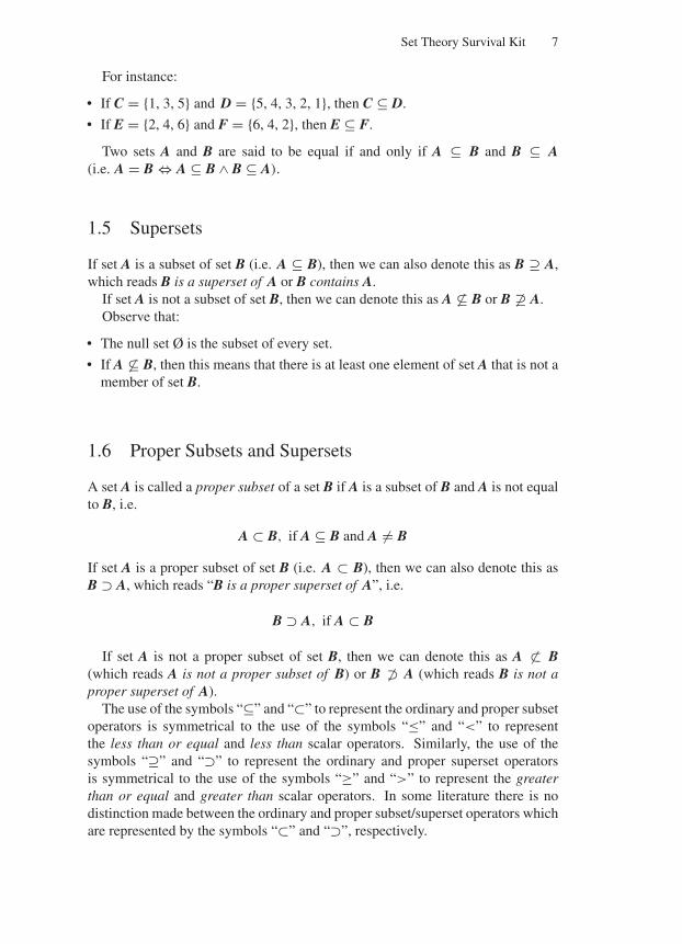
In a Venn diagram, the universal set is represented by a region of the planedescribed by a rectangle and the other sets under investigation are representedby regions of the plane described by ellipses or closed curves. For instance, ifthe universal set U represents all animals, the region labelled C represents the setof all camels, the region labelled B represents the set of all birds and the regionlabelled A represents the set of all albatrosses, then the Venn diagram shown inFig. 1.1 represents the relationship of these sets.
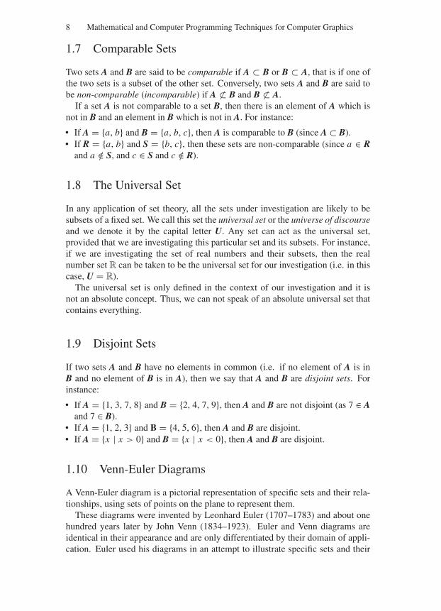
Figures 1.2–1.5 illustrate the use of Venn diagrams to represent various rela-tionships between two sets A and B. Figure 1.2 represents the relationship “set A isa proper subset of set B”, i.e. A ⊂ B. Figure 1.3 represents the relationship “set A
U
C
B
A
FIGURE 1.1. The relationship of camels, birds and albatrosses.
U
B
A
FIGURE 1.2. The Venn diagram of the set relationship A ⊂ B.
“Comninos” — 2005/8/31 — 14:52 — page 10 — #8
10 Mathematical and Computer Programming Techniques for Computer Graphics
U
BA
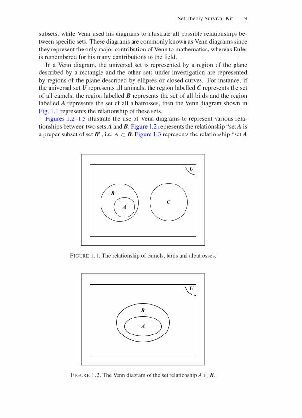
FIGURE 1.3. The Venn diagram of two disjoint sets.
U
BA
FIGURE 1.4. The Venn diagram of two incomparable sets.
U
BAe1•
•
•
•
•
•e2
e3
e4
e5
e6
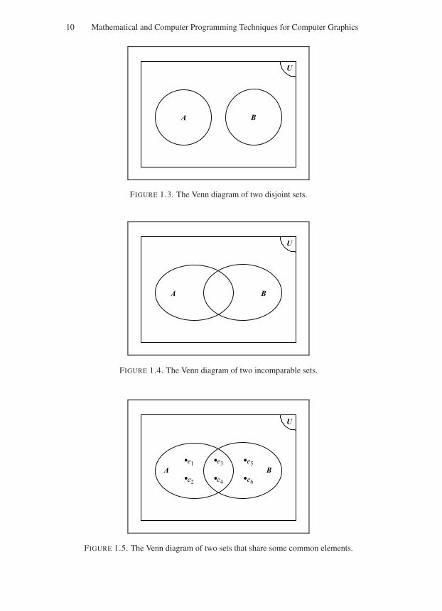
FIGURE 1.5. The Venn diagram of two sets that share some common elements.
“Comninos” — 2005/8/31 — 14:52 — page 11 — #9
Set Theory Survival Kit 11
B
A
C
B
A
C
BAB
DC
A
(a) (b) (c) (d)
FIGURE 1.6. (a), (b), (c), (d)
is disjoint from set B”. Figure 1.4 represents the relationship “sets A and B areincomparable”. Figure 1.5 represents the relationship between set A = e1, e2,e3, e4 and set B = e3, e4, e5, e6.
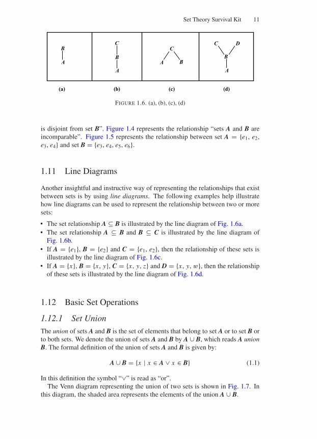
1.11 Line Diagrams
Another insightful and instructive way of representing the relationships that existbetween sets is by using line diagrams. The following examples help illustratehow line diagrams can be used to represent the relationship between two or moresets:
• The set relationship A ⊆ B is illustrated by the line diagram of Fig. 1.6a.• The set relationship A ⊆ B and B ⊆ C is illustrated by the line diagram of
Fig. 1.6b.• If A = e1, B = e2 and C = e1, e2, then the relationship of these sets is
illustrated by the line diagram of Fig. 1.6c.• If A = x, B = x , y, C = x , y, z and D = x , y, w, then the relationship
of these sets is illustrated by the line diagram of Fig. 1.6d.
1.12 Basic Set Operations
1.12.1 Set Union
The union of sets A and B is the set of elements that belong to set A or to set B orto both sets. We denote the union of sets A and B by A ∪ B, which reads A unionB. The formal definition of the union of sets A and B is given by:
A ∪ B = x | x ∈ A ∨ x ∈ B (1.1)
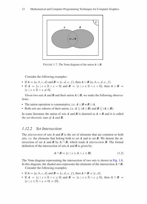
In this definition the symbol “∨” is read as “or”.The Venn diagram representing the union of two sets is shown in Fig. 1.7. In
this diagram, the shaded area represents the elements of the union A ∪ B.
“Comninos” — 2005/8/31 — 14:52 — page 12 — #10
12 Mathematical and Computer Programming Techniques for Computer Graphics
U
BA
BA
FIGURE 1.7. The Venn diagram of the union A ∪ B.
Consider the following examples:
• If A = a, b, c, d and B = c, d, e, f , then A ∪ B a, b, c, d, e, f .• If A = x | x ∈ R ∧ x > 0 and B = x | x ∈ R ∧ x < 0, then A ∪ B =
x | x ∈ R ∧ x = 0.Given two sets A and B and their union A ∪ B, we make the following observa-
tions:
• The union operation is commutative, i.e. A ∪ B = B ∪ A.• Both sets are subsets of their union, i.e. A ⊆ (A ∪ B) and B ⊆ (A ∪ B).
In some literature the union of sets A and B is denoted as A + B and it is calledthe set-theoretic sum of A and B.
1.12.2 Set Intersection
The intersection of sets A and B is the set of elements that are common to bothsets, i.e. the elements that belong both to set A and to set B. We denote the in-tersection of set A and B by A ∩ B, which reads A intersection B. The formaldefinition of the intersection of sets A and B is given by:
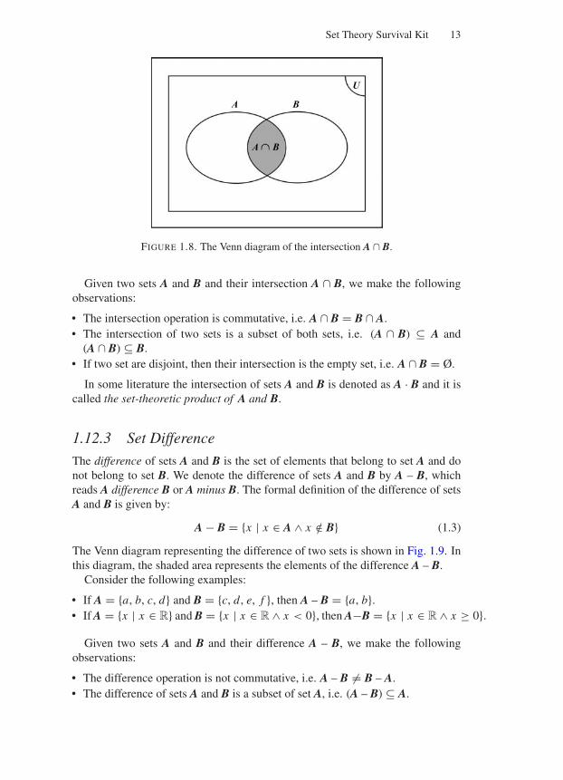
A ∩ B = x | x ∈ A ∧ x ∈ B (1.2)
The Venn diagram representing the intersection of two sets is shown in Fig. 1.8.In this diagram, the shaded area represents the elements of the intersection A ∩ B.
Consider the following examples:
• If A = a, b, c, d and B = c, d, e, f , then A ∩ B = c, d.• If A = x | x ∈ R ∧ x ≥ 0 and B = x | x ∈ R ∧ x ≤ 0, then A ∩ B =
x | x ∈ R ∧ x = 0 = 0.
“Comninos” — 2005/8/31 — 14:52 — page 13 — #11
Set Theory Survival Kit 13
U
BA
BA
FIGURE 1.8. The Venn diagram of the intersection A ∩ B.
Given two sets A and B and their intersection A ∩ B, we make the followingobservations:
• The intersection operation is commutative, i.e. A ∩ B = B ∩ A.• The intersection of two sets is a subset of both sets, i.e. (A ∩ B) ⊆ A and
(A ∩ B) ⊆ B.• If two set are disjoint, then their intersection is the empty set, i.e. A ∩ B = Ø.
In some literature the intersection of sets A and B is denoted as A · B and it iscalled the set-theoretic product of A and B.
1.12.3 Set Difference
The difference of sets A and B is the set of elements that belong to set A and donot belong to set B. We denote the difference of sets A and B by A – B, whichreads A difference B or A minus B. The formal definition of the difference of setsA and B is given by:
A − B = x | x ∈ A ∧ x /∈ B (1.3)
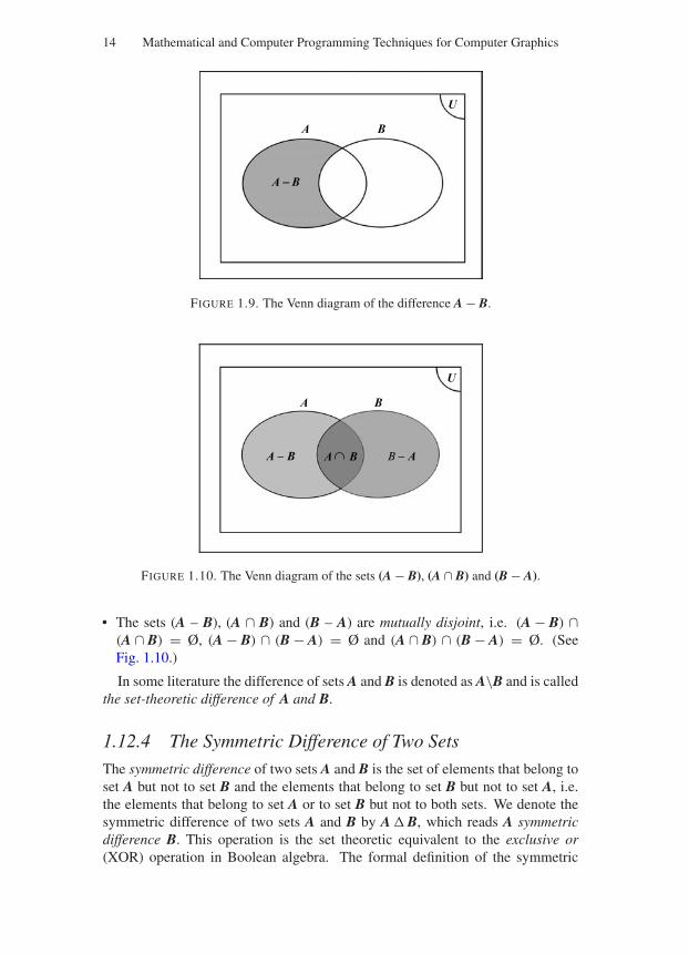
The Venn diagram representing the difference of two sets is shown in Fig. 1.9. Inthis diagram, the shaded area represents the elements of the difference A – B.
Consider the following examples:
• If A = a, b, c, d and B = c, d, e, f , then A – B = a, b.• If A = x | x ∈ R and B = x | x ∈ R ∧ x < 0, then A−B = x | x ∈ R ∧ x ≥ 0.
Given two sets A and B and their difference A – B, we make the followingobservations:
• The difference operation is not commutative, i.e. A – B = B – A.• The difference of sets A and B is a subset of set A, i.e. (A – B) ⊆ A.
“Comninos” — 2005/8/31 — 14:52 — page 14 — #12
14 Mathematical and Computer Programming Techniques for Computer Graphics
U
BA
A - B
FIGURE 1.9. The Venn diagram of the difference A − B.
U
B − AA − B BA
BA
FIGURE 1.10. The Venn diagram of the sets (A − B), (A ∩ B) and (B − A).
• The sets (A – B), (A ∩ B) and (B – A) are mutually disjoint, i.e. (A − B) ∩(A ∩ B) = Ø, (A − B) ∩ (B − A) = Ø and (A ∩ B) ∩ (B − A) = Ø. (SeeFig. 1.10.)
In some literature the difference of sets A and B is denoted as A\B and is calledthe set-theoretic difference of A and B.
1.12.4 The Symmetric Difference of Two Sets
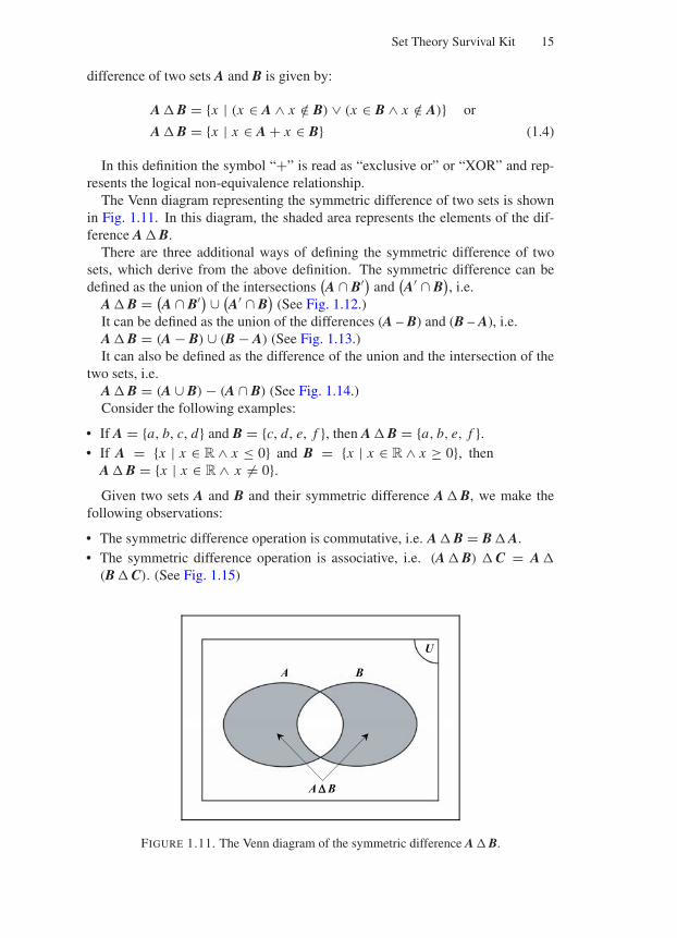
The symmetric difference of two sets A and B is the set of elements that belong toset A but not to set B and the elements that belong to set B but not to set A, i.e.the elements that belong to set A or to set B but not to both sets. We denote thesymmetric difference of two sets A and B by A B, which reads A symmetricdifference B. This operation is the set theoretic equivalent to the exclusive or(XOR) operation in Boolean algebra. The formal definition of the symmetric
“Comninos” — 2005/8/31 — 14:52 — page 15 — #13
Set Theory Survival Kit 15
difference of two sets A and B is given by:
A B = x | (x ∈ A ∧ x /∈ B) ∨ (x ∈ B ∧ x /∈ A) or
A B = x | x ∈ A + x ∈ B (1.4)
In this definition the symbol “+” is read as “exclusive or” or “XOR” and rep-resents the logical non-equivalence relationship.
The Venn diagram representing the symmetric difference of two sets is shownin Fig. 1.11. In this diagram, the shaded area represents the elements of the dif-ference A B.
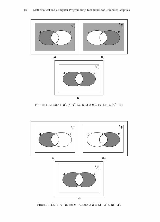
There are three additional ways of defining the symmetric difference of twosets, which derive from the above definition. The symmetric difference can bedefined as the union of the intersections
(A ∩ B′) and
(A′ ∩ B
), i.e.
A B = (A ∩ B′) ∪ (
A′ ∩ B)
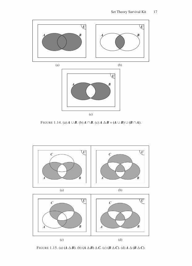
(See Fig. 1.12.)It can be defined as the union of the differences (A – B) and (B – A), i.e.A B = (A − B) ∪ (B − A) (See Fig. 1.13.)It can also be defined as the difference of the union and the intersection of the
two sets, i.e.A B = (A ∪ B) − (A ∩ B) (See Fig. 1.14.)Consider the following examples:
• If A = a, b, c, d and B = c, d, e, f , then A B = a, b, e, f .• If A = x | x ∈ R ∧ x ≤ 0 and B = x | x ∈ R ∧ x ≥ 0, then
A B = x | x ∈ R ∧ x = 0.Given two sets A and B and their symmetric difference A B, we make the
following observations:
• The symmetric difference operation is commutative, i.e. A B = B A.• The symmetric difference operation is associative, i.e. (A B) C = A
(B C). (See Fig. 1.15)
U
BA
A D B
FIGURE 1.11. The Venn diagram of the symmetric difference A B.
“Comninos” — 2005/8/31 — 14:52 — page 16 — #14
16 Mathematical and Computer Programming Techniques for Computer Graphics
(a) (b)
(c)
U
BA
U
BA
U
BA
FIGURE 1.12. (a) A ∩ B′. (b) A′ ∩ B. (c) A B = (A ∩ B′) ∪ (A′ − B).
U
BA
(c)
U
BA
U
BA
(a) (b)
FIGURE 1.13. (a) A – B. (b) B – A. (c) A B = (A – B) ∪ (B – A).
“Comninos” — 2005/8/31 — 14:52 — page 17 — #15
Set Theory Survival Kit 17
U
BA
U
BA
(a) (b)
U
BA
(c)
FIGURE 1.14. (a) A ∪ B. (b) A ∩ B. (c) A B = (A ∪ B) ∪ (B ∩ A).
U
BA
CU
BA
C
(a) (b)
(c) (d)
U
BA
CU
BA
C
FIGURE 1.15. (a) (A B). (b) (A B) C. (c) (B C). (d) A (B C).
“Comninos” — 2005/8/31 — 14:52 — page 18 — #16
18 Mathematical and Computer Programming Techniques for Computer Graphics
U
BA
CU
BA
C
(a) (b)
U
BA
CU
BA
C
(c) (d)
U
BA
C
(e)
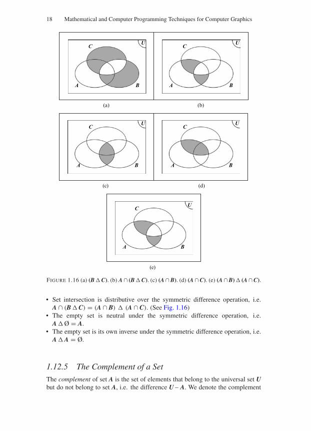
FIGURE 1.16 (a) (B C). (b) A ∩ (B C). (c) (A ∩ B). (d) (A ∩ C). (e) (A ∩ B) (A ∩ C).
• Set intersection is distributive over the symmetric difference operation, i.e.A ∩ (B C) = (A ∩ B) (A ∩ C). (See Fig. 1.16)
• The empty set is neutral under the symmetric difference operation, i.e.A Ø = A.
• The empty set is its own inverse under the symmetric difference operation, i.e.A A = Ø.
1.12.5 The Complement of a Set
The complement of set A is the set of elements that belong to the universal set Ubut do not belong to set A, i.e. the difference U – A. We denote the complement
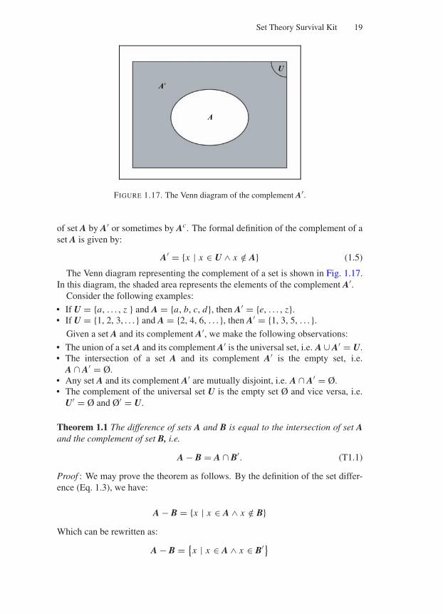
“Comninos” — 2005/8/31 — 14:52 — page 19 — #17
Set Theory Survival Kit 19
U
A
A
FIGURE 1.17. The Venn diagram of the complement A′.
of set A by A′ or sometimes by Ac. The formal definition of the complement of aset A is given by:
A′ = x | x ∈ U ∧ x /∈ A (1.5)
The Venn diagram representing the complement of a set is shown in Fig. 1.17.In this diagram, the shaded area represents the elements of the complement A′.
Consider the following examples:
• If U = a, . . . , z and A = a, b, c, d, then A′ = e, . . . , z.• If U = 1, 2, 3, . . . and A = 2, 4, 6, . . . , then A′ = 1, 3, 5, . . . .
Given a set A and its complement A′, we make the following observations:
• The union of a set A and its complement A′ is the universal set, i.e. A ∪ A′ = U.• The intersection of a set A and its complement A′ is the empty set, i.e.
A ∩ A′ = Ø.• Any set A and its complement A′ are mutually disjoint, i.e. A ∩ A′ = Ø.• The complement of the universal set U is the empty set Ø and vice versa, i.e.
U′ = Ø and Ø′ = U.
Theorem 1.1 The difference of sets A and B is equal to the intersection of set Aand the complement of set B, i.e.
A − B = A ∩ B′. (T1.1)
Proof : We may prove the theorem as follows. By the definition of the set differ-ence (Eq. 1.3), we have:
A − B = x | x ∈ A ∧ x /∈ BWhich can be rewritten as:
A − B = x | x ∈ A ∧ x ∈ B′
“Comninos” — 2005/8/31 — 14:52 — page 20 — #18
20 Mathematical and Computer Programming Techniques for Computer Graphics
Which in turn is the definition of the intersection of sets A and B′. (See Eq. 1.2.)Thus,
A − B = A ∩ B′.
1.12.6 Theorems on Comparable Sets
Given that two sets A and B are comparable (i.e. A ⊆ B or B ⊆ A), we can provethe following theorems.
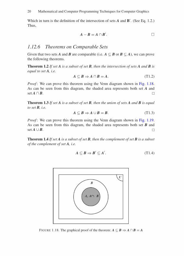
Theorem 1.2 If set A is a subset of set B, then the intersection of sets A and B isequal to set A, i.e.
A ⊆ B ⇒ A ∩ B = A. (T1.2)
Proof : We can prove this theorem using the Venn diagram shown in Fig. 1.18.As can be seen from this diagram, the shaded area represents both set A andset A ∩ B.
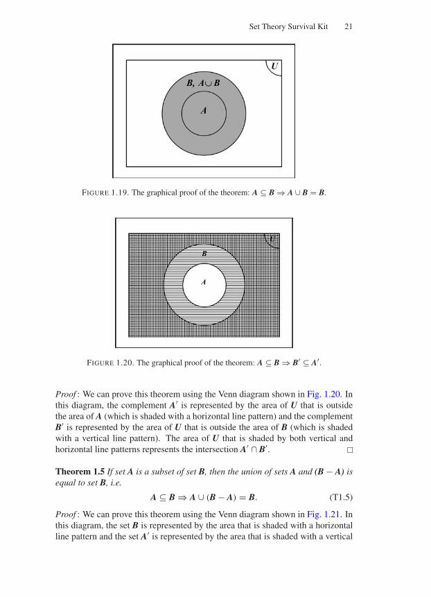
Theorem 1.3 If set A is a subset of set B, then the union of sets A and B is equalto set B, i.e.
A ⊆ B ⇒ A ∪ B = B. (T1.3)
Proof : We can prove this theorem using the Venn diagram shown in Fig. 1.19.As can be seen from this diagram, the shaded area represents both set B andset A ∪ B.
Theorem 1.4 If set A is a subset of set B, then the complement of set B is a subsetof the complement of set A, i.e.
A ⊆ B ⇒ B′ ⊆ A′. (T1.4)
U
B
A, A B
FIGURE 1.18. The graphical proof of the theorem: A ⊆ B ⇒ A ∩ B = A
“Comninos” — 2005/8/31 — 14:52 — page 21 — #19
Set Theory Survival Kit 21
U
A
B, A B
FIGURE 1.19. The graphical proof of the theorem: A ⊆ B ⇒ A ∪ B = B.
U
A
B
FIGURE 1.20. The graphical proof of the theorem: A ⊆ B ⇒ B′ ⊆ A′.
Proof : We can prove this theorem using the Venn diagram shown in Fig. 1.20. Inthis diagram, the complement A′ is represented by the area of U that is outsidethe area of A (which is shaded with a horizontal line pattern) and the complementB′ is represented by the area of U that is outside the area of B (which is shadedwith a vertical line pattern). The area of U that is shaded by both vertical andhorizontal line patterns represents the intersection A′ ∩ B′.
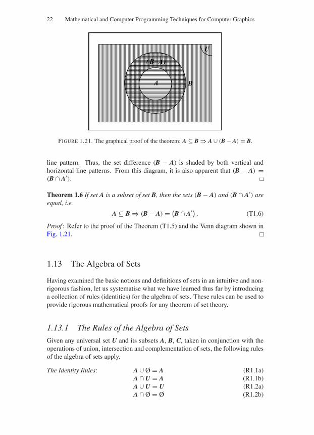
Theorem 1.5 If set A is a subset of set B, then the union of sets A and (B − A) isequal to set B, i.e.
A ⊆ B ⇒ A ∪ (B − A) = B. (T1.5)
Proof : We can prove this theorem using the Venn diagram shown in Fig. 1.21. Inthis diagram, the set B is represented by the area that is shaded with a horizontalline pattern and the set A′ is represented by the area that is shaded with a vertical
“Comninos” — 2005/8/31 — 14:52 — page 22 — #20
22 Mathematical and Computer Programming Techniques for Computer Graphics
U
A B
(B−A)
FIGURE 1.21. The graphical proof of the theorem: A ⊆ B ⇒ A ∪ (B − A) = B.
line pattern. Thus, the set difference (B − A) is shaded by both vertical andhorizontal line patterns. From this diagram, it is also apparent that (B − A) =(B ∩ A′).
Theorem 1.6 If set A is a subset of set B, then the sets (B − A) and (B ∩ A′) areequal, i.e.
A ⊆ B ⇒ (B − A) = (B ∩ A′) . (T1.6)
Proof : Refer to the proof of the Theorem (T1.5) and the Venn diagram shown inFig. 1.21.
1.13 The Algebra of Sets
Having examined the basic notions and definitions of sets in an intuitive and non-rigorous fashion, let us systematise what we have learned thus far by introducinga collection of rules (identities) for the algebra of sets. These rules can be used toprovide rigorous mathematical proofs for any theorem of set theory.
1.13.1 The Rules of the Algebra of Sets
Given any universal set U and its subsets A, B, C, taken in conjunction with theoperations of union, intersection and complementation of sets, the following rulesof the algebra of sets apply.
The Identity Rules: A ∪ Ø = A (R1.1a)A ∩ U = A (R1.1b)A ∪ U = U (R1.2a)A ∩ Ø = Ø (R1.2b)
“Comninos” — 2005/8/31 — 14:52 — page 23 — #21
Set Theory Survival Kit 23
The Complement Rules: A ∪ A′ = U (R1.3a)A ∩ A′ = Ø (R1.3b)U′ = Ø (R1.4a)Ø′ = U (R1.4b)(A′)′ = A (R1.5)
The Idempotent Rules: A ∪ A = A (R1.6a)A ∩ A = A (R1.6b)
The Commutative Rules: A ∪ B = B ∪ A (R1.7a)A ∩ B = B ∩ A (R1.7b)
The Associative Rules: (A ∪ B) ∪ C = A ∪ (B ∪ C) (R1.8a)(A ∩ B) ∩ C = A ∩ (B ∩ C) (R1.8b)
The Distributive Rules: A ∪ (B ∩ C) = (A ∪ B) ∩ (A ∪ C) (R1.9a)A ∩ (B ∪ C) = (A ∩ B) ∪ (A ∩ C) (R1.9b)
The De Morgan Rules: (A ∪ B)′ = A′ ∩ B′ (R1.10a)(A ∩ B)′ = A′ ∪ B′ (R1.10b)
In the above list of rules an idempotent element (or idempotent for short) is anentity that when operated upon by itself, yields (results in) itself.
Observe that these rules do not cover the concept of an element belonging to aset (i.e. a ∈ A). Also, that the concepts of the subset and proper subset are notcovered by these rules.
In this algebra of sets, these concepts are defined as follows:
Subset/Superset: A ⊆ B∨B ⊇ A ⇒ A∩B = A (1.6)
Proper Subset/Superset: A ⊂ B ∨ B ⊃ A ⇒ A ∩ B = A ∧ B − A = Ø (1.7)
Let us now use the rules of the algebra of sets to prove some theorems.
Theorem 1.7 Given any two sets A and B, we say that:
A, B ⊆ U ⇒ (A ∩ B) ∪ (A ∩ B′) = A. (T1.7)
Proof : Starting with the left-hand side of this equality and using the distributiverule (R1.9b) we get:
(A ∩ B) ∪ (A ∩ B′) = A ∩ (
B ∪ B′)
Using the complement rule (R1.3a) we get:
(A ∩ B) ∪ (A ∩ B′) = A ∩ U
Finally, using the identity rule (R1.1b) we get:
(A ∩ B) ∪ (A ∩ B′) = A.
Theorem 1.8 Given that A ⊆ B and B ⊆ C, then A ⊆ C, i.e.
A ⊆ B ∧ B ⊆ C ⇒ A ⊆ C. (T1.8)
“Comninos” — 2005/8/31 — 14:52 — page 24 — #22
24 Mathematical and Computer Programming Techniques for Computer Graphics
Proof : From the definition of a subset (1.6) we have:
A = A ∩ B (1.8)
andB = B ∩ C (1.9)
By substituting (1.9) into the right-hand side of equality (1.8) we get:
A = A ∩ (B ∩ C)
Using the associative rule (R1.8b) we get:
A = (A ∩ B) ∩ C
Using Eq. (1.8) we get:A = A ∩ C
Which is the definition of A ⊆ C.
1.13.2 The Duality Principle
In mathematics, a dual is a pair of identities or a grouping of two identities. Asit applies to set theory, the duality principle can be expressed as follows. Givena set identity (i.e. an expression of set relationships) I, we can construct its dualidentity I∗ by interchanging each occurrence of the symbols ∪ and ∩, and thesymbols Ø and U in the original identity. For instance:
• The dual of the identity A ∪ (B ∩ C) = (A ∪ B) ∩ (A ∪ C) is the identity A ∩(B ∪ C) = (A ∩ B) ∪ (A ∩ C).
• The dual of the identity A ∪ A′ = U is the identity A ∩ A′ = Ø.• The dual of the identity (A ∩ B) ∪ (
A ∩ B′) = A is the identity (A ∪ B) ∩(A ∪ B′) = A.
This is precisely why, in the above table of set algebraic rules, we have arrangedthese rules in pairs (duals). The principle of duality implies that if we use asequence of axioms or rules to prove the validity of an identity, then we can usethe duals of these axioms and rules to prove the validity of the dual of the originalidentity. For instance in Theorem (T1.7) we proved that A, B ⊆ U ⇒ (A ∩ B) ∪(A ∩ B′) = A. We can now employ the principle of duality to prove the dual of
this identity.
Theorem 1.9 Given any two sets A and B, we say that:
A, B ⊆ U ⇒ (A ∪ B) ∩ (A ∪ B′) = A. (T1.9)
Proof : Starting with the left-hand side of this equality and using the distributiverule (R1.9a), which is the dual of rule (R1.9b) that we have used in the first stepof the proof of Theorem (T1.7), we get:
(A ∪ B) ∩ (A ∪ B′) = A ∪ (
B ∩ B′)
“Comninos” — 2005/8/31 — 14:52 — page 25 — #23
Set Theory Survival Kit 25
Using the complement rule (R1.3b), which is the dual of rule (R1.3a) that we haveused in the second step of the proof of Theorem (T1.7), we get:
(A ∪ B) ∩ (A ∪ B′) = A ∪ Ø
Finally, using the identity rule (R1.1a), which is the dual of rule (R1.1b) that wehave used in the third step of the proof of Theorem (T1.7), we get:
(A ∪ B)∩ (A ∪ B′) = A.
1.14 Numbers and Sets
1.14.1 Classes of Numbers
A number is an abstract entity that can be used to represent a quantity (i.e. a mea-surement, a count or an amount). There are many different classes of numbersand all numbers belonging to each class can be considered as elements belongingto a particular set. One of the earliest examples of these number classes is thatof the natural numbers, which are represented by the set N = 0, 1, 2, 3, . . ..Since the dawn of civilisation this class of numbers has been used for count-ing. The natural numbers 1, 2, 3, . . . are sometimes referred to as positivewhole numbers. If we augment the set of natural numbers by the set of nega-tive whole numbers, we get the set of integer numbers which is represented asZ = . . . ,−3,−2,−1, 0, 1, 2, 3, . . ..
The ratio of integers, where the divisor is non-zero, is called a rational numberor a fraction. The set of all rational numbers is represented as Q = x | x = a/b∧a, b ∈ Z ∧ b = 0. A characteristic of rational numbers is that their decimal ex-pansion is periodic in nature.
If we augment the set of rational numbers with the set of all other numbers thathave a non-periodic decimal expansion, we get the set of real numbers that arerepresented by the symbol R. The set of all the real numbers that are non-rational(i.e. these numbers that can not be represented as the ratio of two integers, wherethe divisor is non-zero) are called irrational numbers and are represented by thesymbol Q
′.From the above we can observe that N ⊂ Z ⊂ Q ⊂ R. Thus, for the purposes
of our discussion we will assume that the set of real numbers is our universal set,i.e. U = R.
In the discussion that follows we will make use of the concept of the closure ofsets. So, let us begin by defining this concept.
1.14.2 Closure
Given a set S, we say that this set is closed under a binary operation “×”, if andonly if the result of this operation on two elements of the set is also an element ofthis set (i.e. iff ∀ s1, s2 ∈ S ⇒ s1 × s2 ∈ S). Thus, for instance, the set of natural
“Comninos” — 2005/8/31 — 14:52 — page 26 — #24
26 Mathematical and Computer Programming Techniques for Computer Graphics
numbers is closed under the binary operation of addition “+”, since by addingtwo natural numbers together results in a natural number (i.e. ∀s1, s2 ∈ N ⇒s1 + s2 ∈ N). Similarly, natural numbers are closed under the binary operationof multiplication “∗”, as the product of two natural numbers results in a naturalnumber (i.e. ∀s1, s2 ∈ N ⇒ s1 ∗ s2 ∈ N). Alternatively, natural numbers arenot closed under the binary operation of subtraction “−”, as the difference oftwo natural numbers may be a negative integer rather than a natural number (i.e.∀s1, s2 ∈ N ⇒ /s1 − s2 ∈ N). Set N is also not closed under division, as thequotient of two naturals may be a real.
In general the closure of a set S is the set C (S) which is the smallest supersetof set S.
1.14.3 The Set of Real Numbers R
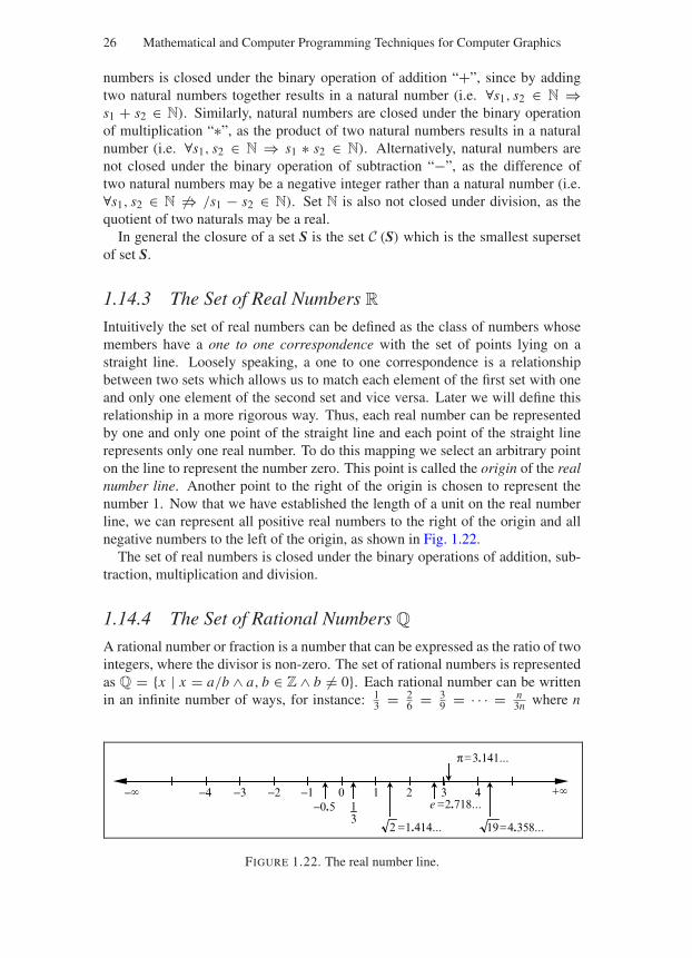
Intuitively the set of real numbers can be defined as the class of numbers whosemembers have a one to one correspondence with the set of points lying on astraight line. Loosely speaking, a one to one correspondence is a relationshipbetween two sets which allows us to match each element of the first set with oneand only one element of the second set and vice versa. Later we will define thisrelationship in a more rigorous way. Thus, each real number can be representedby one and only one point of the straight line and each point of the straight linerepresents only one real number. To do this mapping we select an arbitrary pointon the line to represent the number zero. This point is called the origin of the realnumber line. Another point to the right of the origin is chosen to represent thenumber 1. Now that we have established the length of a unit on the real numberline, we can represent all positive real numbers to the right of the origin and allnegative numbers to the left of the origin, as shown in Fig. 1.22.
The set of real numbers is closed under the binary operations of addition, sub-traction, multiplication and division.
1.14.4 The Set of Rational Numbers Q
A rational number or fraction is a number that can be expressed as the ratio of twointegers, where the divisor is non-zero. The set of rational numbers is representedas Q = x | x = a/b ∧ a, b ∈ Z ∧ b = 0. Each rational number can be writtenin an infinite number of ways, for instance: 1
3 = 26 = 3
9 = · · · = n3n where n
31
0 1 2 3 4 +−1−2−3−4−
2 =1.414...
π=3.141...
e =2.718...
19=4.358...
−0.5
FIGURE 1.22. The real number line.
“Comninos” — 2005/8/31 — 14:52 — page 27 — #25
Set Theory Survival Kit 27
can be any integer not equal to zero. One important characteristic of any rationalnumber is that its decimal expansion is periodic or recurring in nature. This meansthat its representation, following the decimal point, may start with a non-repeatingsequence of digits but eventually continues with a sequence of digits that recur(repeat) ad infinitum. For instance:
• 12 = 0.50, where the final decimal digit recurs (i.e. 1
2 = 0.5000 · · · );• 1
3 = 0.3, where the final decimal digit recurs (i.e. 13 = 0.333 · · · );
• 16 = 0.16, where the final decimal digit recurs (i.e. 1
6 = 0.1666 · · · );• 1
7 = 0.142857, where the sequence of decimal digits 142857 recurs (i.e. 17 =
0.142857142857142857 . . .).
It is worth observing that, immaterial of the number base (decimal, binary,octal, etc.) that we choose to represent a rational number in, its expansion isalways periodic in nature.
The set of rational numbers is closed under the binary operations of addition,subtraction, multiplication and division (except division by zero). The set of ra-tional numbers is a proper subset of the set of real numbers, i.e. Q ⊂ R.
1.14.5 The Set of Irrational Numbers Q′
An irrational number is any real number that is not a rational number. In otherwords any real number that cannot be expressed as the ratio of two integers, wherethe devisor is not zero. The decimal expansion of an irrational number is notperiodic or recurring. The set of irrational numbers is defined as the complementof the set of rational numbers, when the universal set is taken to be the set of realnumbers, i.e. Q
′ = (R − Q).We observe that U = R ⇔ R = Q ∪ Q
′ and that Q′ ⊂ R.
Examples of irrational numbers are√
2,√
3, 3√
5, π = 3.14159 · · · , e =2.71828 · · · .
1.14.6 The Set of Natural Numbers N
As we have seen above, the set of natural numbers is defined as N =0, 1, 2, 3, . . .. This is the definition given by the DIN 5473 standard “Logic andSet Theory, Symbols and Concepts” published in 1992 by DIN (the DeutschesInstitute fur Normung-the German Institute for Standardisation). In some otherliterature the number zero is not included in the set of natural numbers. The nat-ural numbers 1, 2, 3, . . . are sometimes referred to as positive whole numbersor cardinal numbers and are defined as N
∗ = N − 0 = 1, 2, 3, . . ..The set of natural numbers is closed under the binary operations of addition and
multiplication but not subtraction and division, as the difference of two naturalnumbers may be a negative integer and the quotient of two natural numbers maybe a real number.
We observe that N ⊂ R.
“Comninos” — 2005/8/31 — 14:52 — page 28 — #26
28 Mathematical and Computer Programming Techniques for Computer Graphics
1.14.7 The Set of Integer Numbers Z
The set of integers is the union of the set of natural numbers N = 0, 1, 2, 3, . . .and the set of negative whole numbers −1,−2,−3, . . .. Thus, the set of integersis defined as Z = . . . ,−3,−2,−1, 0, 1, 2, 3, . . . or Z = 0,±1,±2,±3, . . ..The name of this set originates from the German word Zahlen (meaning numbers).
The set of integers is closed under the binary operations of addition, subtractionand multiplication but not division, as the quotient of two integers may be a realnumber.
We observe that N ⊂ Z ⊂ R.
1.14.8 Other useful Sets of Numbers
1.14.8.1 The Set of Complex Numbers C
A superset of the set of real numbers R is the set of complex numbers C in whichall non-constant polynomials have real roots. Complex numbers have wide ap-plication in many field of mathematics, such as: differential equations, controltheory, quantum mechanics, relativity, fluid dynamics, fractals, etc. Complexnumbers are defined as C =
x | x = a + bi ∧ a, b ∈ R ∧ i = √−1. Thus, a
complex number x consists of a real part a and an imaginary part bi and requiresthe imaginary unit i = √−1 (i.e. i2 = −1) for its definition.
We observe that R ⊂ C.
1.14.8.2 The Set of Algebraic Numbers A
An algebraic number is any real number that is the solution of a polynomialequation with integer coefficients of the form:
cn xn + cn−1xn−1 + cn−2xn−2 + · · · + c2x2 + c1x1 + c0x0 = 0 for n > 0
where ci are integer coefficients and cn = 0.From the definition of rational numbers we know that any rational number is
of the form x = a/b. Thus, any rational number can be expressed in the formbx −a = 0 (with the root x = a/b), which in turn means that every rational num-ber is an algebraic number. Some irrational numbers are also algebraic numbers.For instance, the irrational number
√2 can also be expressed as a polynomial
with integer coefficients, 1x2 − 2 = 0, with the root x = √2. Thus,
√2 is both
irrational and algebraic.
1.14.8.3 The Set of Transcendental Numbers T
A transcendental number is any irrational number that is not the solution of anypolynomial equation with integer coefficients. The French mathematician JosephLiouville (1809-1882) first established the existence of transcendental numbersin an 1851 paper. Examples of transcendental numbers are π = 3.14159 · · · ,
e = 2.71828 · · · , sin (π), cos (2π), and tan(π
4
).
“Comninos” — 2005/8/31 — 14:52 — page 29 — #27
Set Theory Survival Kit 29
We observe that the set of real numbers is the union of the algebraic and tran-scendental numbers, i.e. R = A ∪ T.
1.14.9 Ordering Relations or Inequalities
An inequality is an assertion about the relative size or order of two quantities, i.e.a statement of their relation. Given two real numbers a and b, they may have thefollowing ordering relations:
• a = b which signifies that a is equal to b (i.e. that the numbers a and bcorrespond to the same point on the real number line);
• a < b which signifies that a is less than b (i.e. that number a corresponds toa point, on the real line, that lies to the left of the point corresponding to thenumber b);
• a ≤ b which signifies that a is less than or equal to b (i.e. that number acorresponds to a point, on the real line, that lies on or to the left of the pointcorresponding to the number b);
• a > b which signifies that a is greater than b (i.e. that number a corresponds toa point, on the real line, that lies to the right of the point corresponding to thenumber b);
• a ≥ b which signifies that a is greater than or equal to b (i.e. that number acorresponds to a point, on the real line, that lies on or to the right of the pointcorresponding to the number b).
The inequalities of real numbers exhibit the following properties:
The Reflexivity PropertyGiven any real number a, a ≤ a.
The Trichotomy PropertyGiven any two real numbers a and b, only one of the following relations is true:a < b, a = b or a > b.
The Antisymmetry PropertyGiven any two real numbers a and b, then a ≤ b ∧ b ≤ a ⇒ a = b.
The Transitivity PropertyGiven any three real numbers a, b and c, then a ≤ b ∧ b ≤ c ⇒ a ≤ c.
The Addition and Subtraction PropertyGiven the inequalities a ≤ b and a ≥ b (between two real numbers a and b),we may add or subtract to or from both sides of these inequalities the same realnumber c without changing the sense of the inequalities, i.e.
• a ≤ b ⇒ a + c ≤ b + c• a ≤ b ⇒ a − c ≤ b − c• a ≥ b ⇒ a + c ≥ b + c• a ≥ b ⇒ a − c ≥ b − c
“Comninos” — 2005/8/31 — 14:52 — page 30 — #28
30 Mathematical and Computer Programming Techniques for Computer Graphics
The Multiplication and Division PropertyGiven the inequalities a ≤ b and a ≥ b (between two real numbers a and b), wemay multiply or divide both sides of these inequalities by the same non-negativereal number c without changing the sense of the inequalities. If, however, wemultiply or divide by a negative real number, the sense of the inequalities will bereversed. Thus:
• a ≤ b ∧ c ≥ 0 ⇒ a · c ≤ b · c• a ≤ b ∧ c ≥ 0 ⇒ a/c ≤ b/c• a ≤ b ∧ c < 0 ⇒ a · c ≥ b · c• a ≤ b ∧ c < 0 ⇒ a/c ≥ b/c• a ≥ b ∧ c ≥ 0 ⇒ a · c ≥ b · c• a ≥ b ∧ c ≥ 0 ⇒ a/c ≥ b/c• a ≥ b ∧ c < 0 ⇒ a · c ≤ b · c• a ≥ b ∧ c < 0 ⇒ a/c ≤ b/c
ExamplesConsider the following examples of inequalities:
• x < 6 which signifies that the value of x is less than 6 (i.e. that number x corre-sponds to a point, on the real line, that lies to the left of the point correspondingto the number 6);
• 1 < x < 6 which signifies that the value of x is greater than 1 and less than6 (i.e. that number x corresponds to a point, on the real line, that lies to theright of the point corresponding to the number 1 and to the left of the pointcorresponding to the number 6);
• 1 ≤ x ≤ 6 which signifies that the value of x is greater than or equal to 1 andless than or equal to 6 (i.e. that number x corresponds to a point, on the realline, that lies on or to the right of the point corresponding to the number 1 andon or to the left of the point corresponding to the number 6).
1.14.10 The Absolute Value or Modulus of a Number
The absolute value or modulus of a real number x represents its size or magnitudeand is defined as:
|x | =
x, x ≥ 0−x, otherwise
We observe that |x | ≥ 0 for all x ∈ R. In geometric terms, |xi | represents thedistance between the point corresponding to the value of xi on the real numberline and the origin (i.e. the point corresponding to the number 0). See Fig. 1.23.
Given two real numbers x1 and x2 the distance between the two points, on thereal number line, corresponding to these numbers is given by |x2−x1| = |x1−x2|.See Fig. 1.24.
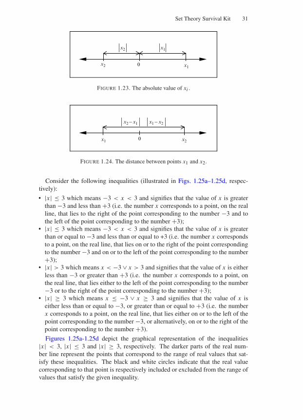
“Comninos” — 2005/8/31 — 14:52 — page 31 — #29
Set Theory Survival Kit 31
0 x1
x1x2
x2
FIGURE 1.23. The absolute value of xi .
0x1
x1 − x2x2 − x1
x2
FIGURE 1.24. The distance between points x1 and x2.
Consider the following inequalities (illustrated in Figs. 1.25a–1.25d, respec-tively):
• |x | ≤ 3 which means −3 < x < 3 and signifies that the value of x is greaterthan −3 and less than +3 (i.e. the number x corresponds to a point, on the realline, that lies to the right of the point corresponding to the number −3 and tothe left of the point corresponding to the number +3);
• |x | ≤ 3 which means −3 < x < 3 and signifies that the value of x is greaterthan or equal to −3 and less than or equal to +3 (i.e. the number x correspondsto a point, on the real line, that lies on or to the right of the point correspondingto the number −3 and on or to the left of the point corresponding to the number+3);
• |x | > 3 which means x < −3 ∨ x > 3 and signifies that the value of x is eitherless than −3 or greater than +3 (i.e. the number x corresponds to a point, onthe real line, that lies either to the left of the point corresponding to the number−3 or to the right of the point corresponding to the number +3);
• |x | ≥ 3 which means x ≤ −3 ∨ x ≥ 3 and signifies that the value of x iseither less than or equal to −3, or greater than or equal to +3 (i.e. the numberx corresponds to a point, on the real line, that lies either on or to the left of thepoint corresponding to the number −3, or alternatively, on or to the right of thepoint corresponding to the number +3).
Figures 1.25a-1.25d depict the graphical representation of the inequalities|x | < 3, |x | ≤ 3 and |x | ≥ 3, respectively. The darker parts of the real num-ber line represent the points that correspond to the range of real values that sat-isfy these inequalities. The black and white circles indicate that the real valuecorresponding to that point is respectively included or excluded from the range ofvalues that satisfy the given inequality.
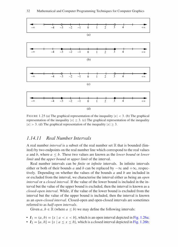
“Comninos” — 2005/8/31 — 14:52 — page 32 — #30
32 Mathematical and Computer Programming Techniques for Computer Graphics
0 1 2 3 4−1−2−3−4−
+
+
+
+
−1−2−3−4−
−1−2−3−4−
−1−2−3−4−
0 1 2 3 4
0 1 2 3 4
0 1 2 3 4
(a)
(b)
(c)
(d)
FIGURE 1.25 (a) The graphical representation of the inequality |x | < 3. (b) The graphicalrepresentation of the inequality |x | ≤ 3. (c) The graphical representation of the inequality|x | > 3. (d) The graphical representation of the inequality |x | ≥ 3.
1.14.11 Real Number Intervals
A real number interval is a subset of the real number set R that is bounded (lim-ited) by two endpoints on the real number line which correspond to the real valuesa and b, where a ≤ b. These two values are known as the lower bound or lowerlimit and the upper bound or upper limit of the interval.
Real number intervals can be finite or infinite intervals. In infinite intervalseither or both of their bounds a and b can be replaced by −∞ and +∞, respec-tively. Depending on whether the values of the bounds a and b are included inor excluded from the interval, we characterise the interval either as being an openinterval or a closed interval. If the value of the lower bound is included in the in-terval but the value of the upper bound is excluded, then the interval is known as aclosed-open interval. While, if the value of the lower bound is excluded from theinterval but the value of the upper bound is included, then the interval is knownas an open-closed interval. Closed-open and open-closed intervals are sometimesreferred to as half-open intervals.
Given a, b ∈ R (where a ≤ b) we may define the following intervals:
• I1 = (a, b) = x | a < x < b, which is an open interval depicted in Fig. 1.26a;• I2 = [a, b] = x | a ≤ x ≤ b, which is a closed interval depicted in Fig. 1.26b;
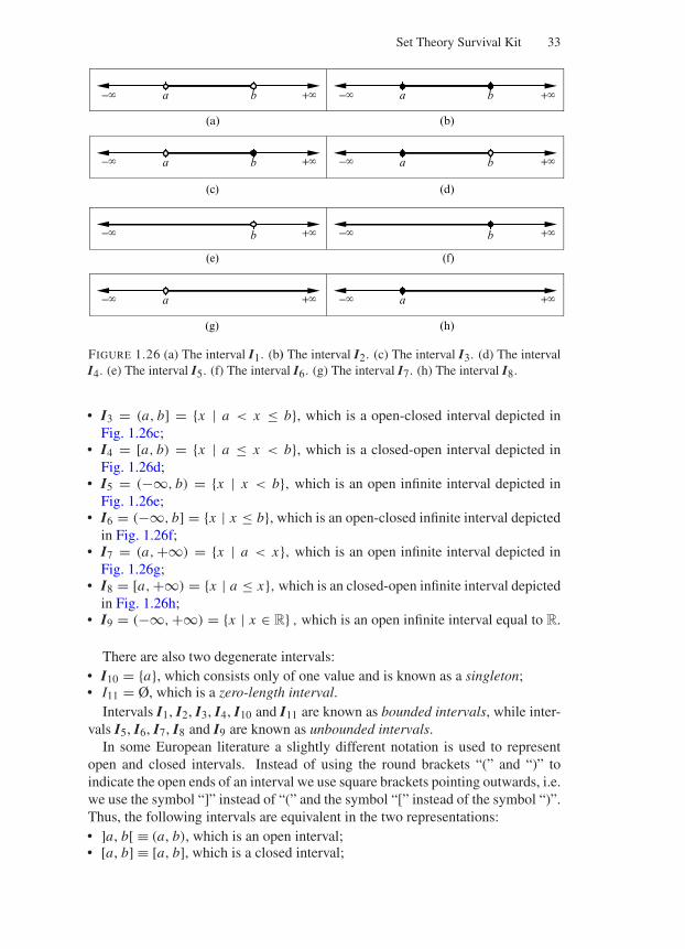
“Comninos” — 2005/8/31 — 14:52 — page 33 — #31
Set Theory Survival Kit 33
ba−
−
−
−
+
+
+
+
ba
ba ba
(a) (b)
(c) (d)
b b
a a
(e) (f)
(g) (h)
−
−
−
−
+
+
+
+
FIGURE 1.26 (a) The interval I1. (b) The interval I2. (c) The interval I3. (d) The intervalI4. (e) The interval I5. (f) The interval I6. (g) The interval I7. (h) The interval I8.
• I3 = (a, b] = x | a < x ≤ b, which is a open-closed interval depicted inFig. 1.26c;
• I4 = [a, b) = x | a ≤ x < b, which is a closed-open interval depicted inFig. 1.26d;
• I5 = (−∞, b) = x | x < b, which is an open infinite interval depicted inFig. 1.26e;
• I6 = (−∞, b] = x | x ≤ b, which is an open-closed infinite interval depictedin Fig. 1.26f;
• I7 = (a,+∞) = x | a < x, which is an open infinite interval depicted inFig. 1.26g;
• I8 = [a,+∞) = x | a ≤ x, which is an closed-open infinite interval depictedin Fig. 1.26h;
• I9 = (−∞,+∞) = x | x ∈ R , which is an open infinite interval equal to R.
There are also two degenerate intervals:• I10 = a, which consists only of one value and is known as a singleton;• I11 = Ø, which is a zero-length interval.
Intervals I1, I2, I3, I4, I10 and I11 are known as bounded intervals, while inter-vals I5, I6, I7, I8 and I9 are known as unbounded intervals.
In some European literature a slightly different notation is used to representopen and closed intervals. Instead of using the round brackets “(” and “)” toindicate the open ends of an interval we use square brackets pointing outwards, i.e.we use the symbol “]” instead of “(” and the symbol “[” instead of the symbol “)”.Thus, the following intervals are equivalent in the two representations:• ]a, b[ ≡ (a, b), which is an open interval;• [a, b] ≡ [a, b], which is a closed interval;
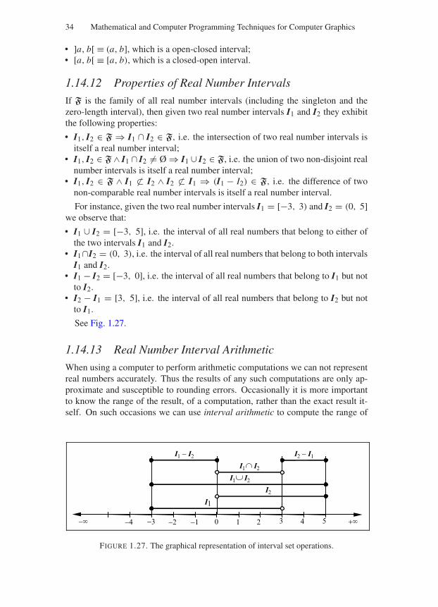
“Comninos” — 2005/8/31 — 14:52 — page 34 — #32
34 Mathematical and Computer Programming Techniques for Computer Graphics
• ]a, b[ ≡ (a, b], which is a open-closed interval;• [a, b[ ≡ [a, b), which is a closed-open interval.
1.14.12 Properties of Real Number Intervals
If F is the family of all real number intervals (including the singleton and thezero-length interval), then given two real number intervals I1 and I2 they exhibitthe following properties:
• I1, I2 ∈ F ⇒ I1 ∩ I2 ∈ F, i.e. the intersection of two real number intervals isitself a real number interval;
• I1, I2 ∈ F ∧ I1 ∩ I2 = Ø ⇒ I1 ∪ I2 ∈ F, i.e. the union of two non-disjoint realnumber intervals is itself a real number interval;
• I1, I2 ∈ F ∧ I1 ⊂ I2 ∧ I2 ⊂ I1 ⇒ (I1 − I2) ∈ F, i.e. the difference of twonon-comparable real number intervals is itself a real number interval.
For instance, given the two real number intervals I1 = [−3, 3) and I2 = (0, 5]we observe that:
• I1 ∪ I2 = [−3, 5], i.e. the interval of all real numbers that belong to either ofthe two intervals I1 and I2.
• I1∩I2 = (0, 3), i.e. the interval of all real numbers that belong to both intervalsI1 and I2.
• I1 − I2 = [−3, 0], i.e. the interval of all real numbers that belong to I1 but notto I2.
• I2 − I1 = [3, 5], i.e. the interval of all real numbers that belong to I2 but notto I1.
See Fig. 1.27.
1.14.13 Real Number Interval Arithmetic
When using a computer to perform arithmetic computations we can not representreal numbers accurately. Thus the results of any such computations are only ap-proximate and susceptible to rounding errors. Occasionally it is more importantto know the range of the result, of a computation, rather than the exact result it-self. On such occasions we can use interval arithmetic to compute the range of
0 1 2 3 4−1−2−3−4 5
I1
I2
I2I1
I2I1
I1 − I2 I2 − I1
− +
FIGURE 1.27. The graphical representation of interval set operations.
“Comninos” — 2005/8/31 — 14:52 — page 35 — #33
Set Theory Survival Kit 35
the result. Given two closed real number intervals A = [aL , aU ] and B = [bL ,bU ], the operations of addition, subtraction, multiplication and division of realnumber intervals are defined as follows:
C = [aL , aU ] + [bL , bU ] = [aL + bL , aU + bU ] (1.10a)
C = [aL , aU ] − [bL , bU ] = [aL − bU , aU − bL ] (1.10b)
C = [aL , aU ] · [bL , bU ] = [min (aL · bL , aL · bU , aU · bL , aU · bU ) ,
max (aL · bL , aL · bU , aU · bL , aU · bU )] (1.10c)
C = [aL , aU ] / [bL , bU ] = [min
(aL/bL , aL/bU , aU /bL , aU /bU
),
max (aL/bL , aL/bU , aU /bL , aU /bU )] (1.10d)
For example, if we know that a real number a lies in the interval A = [−2, 2]and that the real number b lies in the interval B = [2, 3], then we can say withcertainty that the result of their addition, subtraction, multiplication and divisionlie in the following intervals, respectively:
• (a + b) ∈ [−2 + 2, 2 + 3] = [0, 5]• (a − b) ∈ [−2 + 2, 2 − 3] = [−4,−2]• (a · b) ∈ [min (−2 · 2,−2 · 3, 2 · 2, 2 · 3), max (−2 · 2,−2 · 3, 2 · 2, 2 · 3)] =
[min (−4,−6, 4, 6), max (−4,−6, 4, 6)] = [−6, 6]
• (a/b) ∈[min
(−22 , −2
3 , 22 , 2
3
), max
(−22 , −2
3 , 22 , 2
3
)]=
[min
(−1,− 2
3 , 1, 23
), max
(−1,− 2
3 , 1, 23
)]= [−1, 1]
1.14.14 Bounded and Unbounded Real Number Sets
Roughly speaking, a bounded set is a set that has a finite size and it is thus a subsetof a finite set. A set that is not bounded is called an unbounded set.
More precisely given a set of real numbers S, if there exists a real number sU
such that s ≤ sU for every s ∈ S, then we call S an upper bounded set and wesay that sU is the upper bound of S. Also if there exists a real number sL suchthat sL ≤ s for every s ∈ S, then we call S a lower bounded set and we say thatsL is the lower bound of S. If the set S is both upper and lower bounded (i.e. iffsL ≤ s ≤ sU ∀s ∈ S), then we call S a bounded set. Thus, in general a set isbounded if it is a subset of a finite interval, i.e. S is bounded iff S ⊆ [sL , sU ].
Alternatively, we may say that a real number set S is bounded iff |s| ≤b ∀ b ≥ 0 ∧ b, s ∈ S, which means that S ⊆ [−b, b].
Consider the following examples:
• If S1 =
1, 12 , 1
4 , 18 , . . .
, then S1 is bounded as S1 ⊆ [0, 1].
• If S2 = 1, 3, 5, 7, . . ., then S2 is unbounded as we can not find a positivenumber b such that |s| ≤ b ∀ s ∈ S2.
• If S3 = 33,−2, 56, 77,−22, then S3 is bounded as S3 ⊆ [−22, 77].
We observe that if a real number set is finite, then its is bounded (as is the case ofset S3 above) and if it is infinite, then it may be bounded (as is the case of set S1above) or it may be unbounded (as is the case of set S2 above).
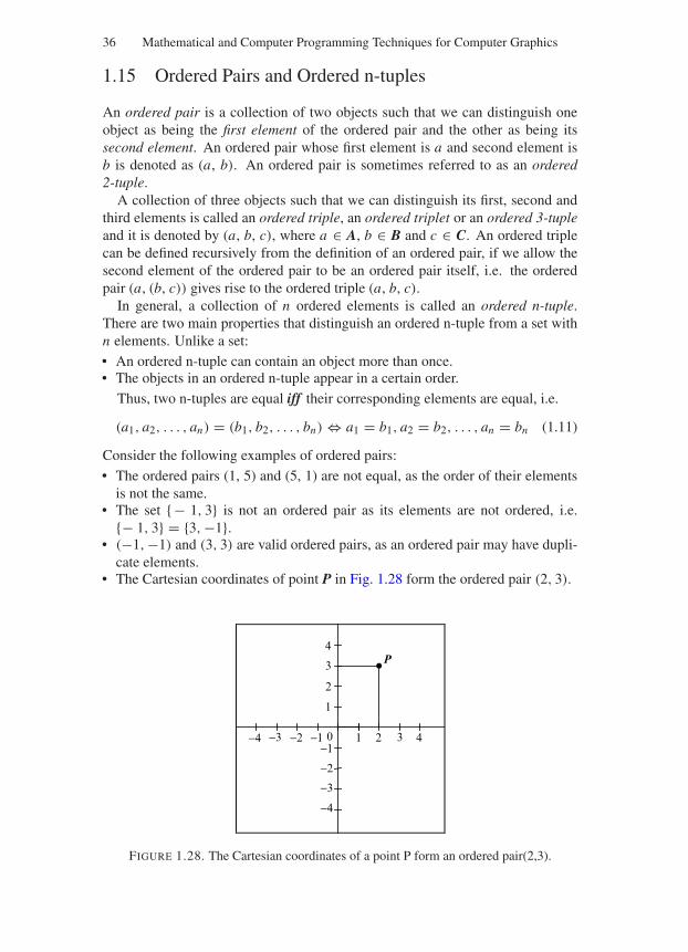
“Comninos” — 2005/8/31 — 14:52 — page 36 — #34
36 Mathematical and Computer Programming Techniques for Computer Graphics
1.15 Ordered Pairs and Ordered n-tuples
An ordered pair is a collection of two objects such that we can distinguish oneobject as being the first element of the ordered pair and the other as being itssecond element. An ordered pair whose first element is a and second element isb is denoted as (a, b). An ordered pair is sometimes referred to as an ordered2-tuple.
A collection of three objects such that we can distinguish its first, second andthird elements is called an ordered triple, an ordered triplet or an ordered 3-tupleand it is denoted by (a, b, c), where a ∈ A, b ∈ B and c ∈ C. An ordered triplecan be defined recursively from the definition of an ordered pair, if we allow thesecond element of the ordered pair to be an ordered pair itself, i.e. the orderedpair (a, (b, c)) gives rise to the ordered triple (a, b, c).
In general, a collection of n ordered elements is called an ordered n-tuple.There are two main properties that distinguish an ordered n-tuple from a set withn elements. Unlike a set:• An ordered n-tuple can contain an object more than once.• The objects in an ordered n-tuple appear in a certain order.
Thus, two n-tuples are equal iff their corresponding elements are equal, i.e.
(a1, a2, . . . , an) = (b1, b2, . . . , bn) ⇔ a1 = b1, a2 = b2, . . . , an = bn (1.11)
Consider the following examples of ordered pairs:• The ordered pairs (1, 5) and (5, 1) are not equal, as the order of their elements
is not the same.• The set − 1, 3 is not an ordered pair as its elements are not ordered, i.e.
− 1, 3 = 3,−1.• (−1,−1) and (3, 3) are valid ordered pairs, as an ordered pair may have dupli-
cate elements.• The Cartesian coordinates of point P in Fig. 1.28 form the ordered pair (2, 3).
0 1 2 3 4−1−2−3−4
P
−1
−2
−3
−4
1
2
3
4
FIGURE 1.28. The Cartesian coordinates of a point P form an ordered pair(2,3).
“Comninos” — 2005/8/31 — 14:52 — page 37 — #35
Set Theory Survival Kit 37
1.16 The Cartesian Product of Sets
The set of all ordered pairs (a, b), where a ∈ A and b ∈ B, is called the Cartesianproduct of sets A and B and is denoted as A × B, which is read as A cross B. Theformal definition of the Cartesian product of two sets A and B is given by:
A × B = (a, b) | a ∈ A ∧ b ∈ B (1.12)
Consider the following examples:
• If X = x1, x2, x3 and Y = y1, y2, then their Cartesian product is given by:X × Y = (x1, y1), (x1, y2), (x2, y1), (x2, y2), (x3, y1), (x3, y2).
• The Cartesian plane, shown in Fig. 1.28, is the set of all ordered pairs that areelements of the Cartesian product R
2 = R × R.
We observe that:
• If set A has n elements and set B has m elements, then their Cartesian productA × B has n × m elements.
• If set A or set B are empty, then their Cartesian product is the empty set, i.e.A = Ø ∨ B = Ø ⇒ A × B = Ø.
• If one of two sets is infinite and the other is not empty, then their Cartesianproduct is an infinite set.
• In general, the product of two sets A and B is not commutative, i.e. A × B =B × A.
The binary Cartesian product, defined in Eq. (1.12), can be extended to then-ary Cartesian product as follows:
n∏
i=1
Si =S1×S2×· · ·×Sn =(s1, s2, · · · , sn) | s1 ∈ S1 ∧ s2 ∈ S2 ∧ · · · ∧ sn ∈ Sn(1.13)
An example of this type of product is the three-dimensional Cartesian space,which is defined as the Cartesian product R
3 = R × R × R.The Cartesian product is named after the French mathematician and philoso-
pher Rene Descartes (1596–1650) who formulated the principles of analyticalgeometry and first used the product R × R.
The Cartesian product A×B of two sets A and B can be represented graphicallyby a coordinate diagram. In such a diagram the horizontal and vertical axes rep-resent the first and second sets of the Cartesian product. Subdivisions along theseaxes represent the respective elements of these sets and the points of intersectionof vertical and horizontal lines, corresponding to these set elements, represent theordered pairs that define the Cartesian product.
For instance, given a set A = a1, a2, a3, a4 and a set B = b1, b2, b3 the co-ordinate diagram representing the Cartesian product A × B is shown in Fig. 1.29.In this diagram, the intersection point P represents the ordered pair (a2, b3). Alto-gether there are twelve intersection points representing the ordered pairs that de-fine the Cartesian product A × B = (a1, b1), (a1, b2), (a1, b3), (a2, b1), (a2, b2),(a2, b3), (a3, b1), (a3, b2), (a3, b3), (a4, b1), (a4, b2), (a4, b3).
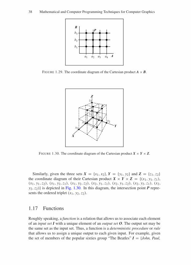
“Comninos” — 2005/8/31 — 14:52 — page 38 — #36
38 Mathematical and Computer Programming Techniques for Computer Graphics
a1 a2 a3 a4
b3
b2
b1
A
BP
FIGURE 1.29. The coordinate diagram of the Cartesian product A × B.
x1
x2
y1y2
z1
z2
X
Y
Z
P
FIGURE 1.30. The coordinate diagram of the Cartesian product X × Y × Z.
Similarly, given the three sets X = x1, x2, Y = y1, y2 and Z = z1, z2the coordinate diagram of their Cartesian product X × Y × Z = (x1, y1, z1),(x1, y1, z2), (x1, y2, z1), (x1, y2, z2), (x2, y1, z1), (x2, y1, z2), (x2, y2, z1), (x2,
y2, z2) is depicted in Fig. 1.30. In this diagram, the intersection point P repre-sents the ordered triplet (x1, y2, z2).
1.17 Functions
Roughly speaking, a function is a relation that allows us to associate each elementof an input set I with a unique element of an output set O. The output set may bethe same set as the input set. Thus, a function is a deterministic procedure or rulethat allows us to assign a unique output to each given input. For example, giventhe set of members of the popular sixties group “The Beatles” I = John, Paul,
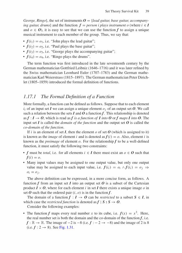
“Comninos” — 2005/8/31 — 14:52 — page 39 — #37
Set Theory Survival Kit 39
George, Ringo, the set of instruments O = lead guitar, base guitar, accompany-ing guitar, drums and the function f = person i plays instrument o (where i ∈ Iand o ∈ O), it is easy to see that we can use the function f to assign a uniquemusical instrument to each member of the group. Thus, we say that:
• f (i1) = o1, i.e. “John plays the lead guitar”;• f (i2) = o2, i.e. “Paul plays the base guitar”;• f (i3) = o3, i.e. “George plays the accompanying guitar”;• f (i4) = o4, i.e. “Ringo plays the drums”.
The term function was first introduced in the late seventeenth century by theGerman mathematician Gottfried Leibniz (1646–1716) and it was later refined bythe Swiss mathematician Leonhard Euler (1707–1783) and the German mathe-matician Karl Weierstrass (1815–1897). The German mathematician Peter Dirich-let (1805–1859) introduced the formal definition of functions.
1.17.1 The Formal Definition of a Function
More formally, a function can be defined as follows. Suppose that to each elementii of an input set I we can assign a unique element o j of an output set O. We callsuch a relation between the sets I and O a function f . This relationship is denotedas f : I → O, which is read as f is a function of I into O or f maps I into O. Theinput set I is called the domain of the function and the output set O is called theco-domain of the function.
If i is an element of set I, then the element o of set O (which is assigned to it)is known as the image of element i and is denoted as f (i) = o. Also, element i isknown as the preimage of element o. For the relationship f to be a well-definedfunction, it must satisfy the following two constraints:
• f must be total, i.e. for all elements i ∈ I there must exist an o ∈ O such thatf (i) = o.
• Many input values may be assigned to one output value, but only one outputvalue may be assigned to each input value, i.e. f (ii ) = oi ∧ f (ii ) = o j ⇒oi = o j .
The above definition can be expressed, in a more concise form, as follows. Afunction f from an input set I into an output set O is a subset of the Cartesianproduct I × O, where for each element i in set I there exists a unique image o inset O such that the ordered pair (i , o) is in the function f .
The domain of a function f : I → O can be restricted to a subset S ∈ I, inwhich case the restricted function is denoted as f | S : S → O.
Consider the following examples:
• The function f maps every real number x to its cube, i.e. f (x) = x3. Here,the real number set is both the domain and the co-domain of the function f , i.e.f : R → R. The image of −2 is −8 (i.e. f : − 2 → −8) and the image of 2 is 8(i.e. f : 2 → 8). See Fig. 1.31.
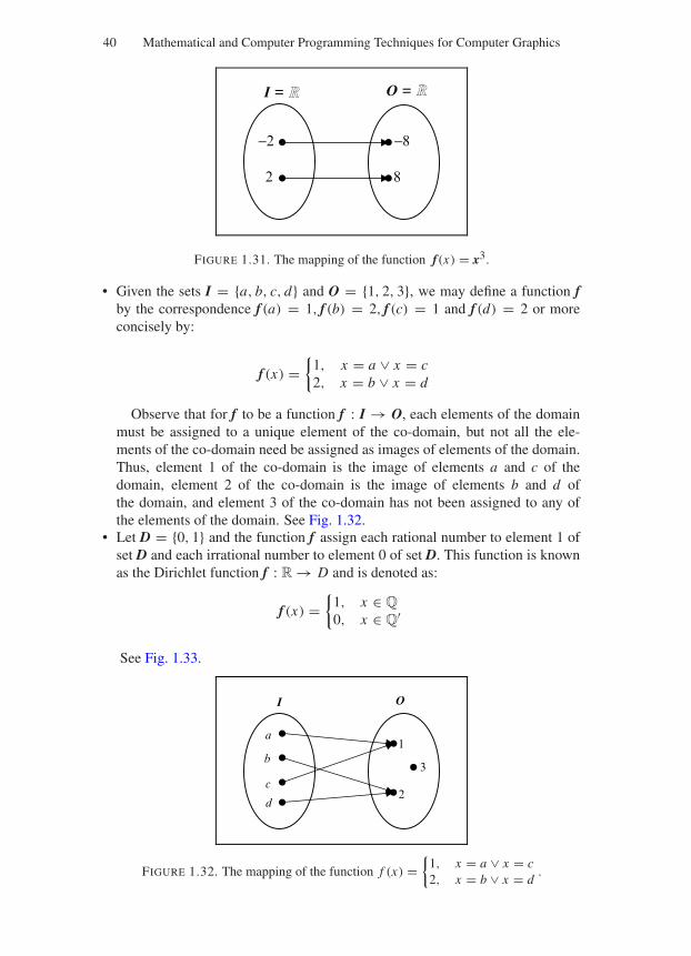
“Comninos” — 2005/8/31 — 14:52 — page 40 — #38
40 Mathematical and Computer Programming Techniques for Computer Graphics
I = R R
−2
O =
−8
2 8
FIGURE 1.31. The mapping of the function f (x) = x3.
• Given the sets I = a, b, c, d and O = 1, 2, 3, we may define a function fby the correspondence f (a) = 1, f (b) = 2, f (c) = 1 and f (d) = 2 or moreconcisely by:
f (x) =
1, x = a ∨ x = c2, x = b ∨ x = d
Observe that for f to be a function f : I → O, each elements of the domainmust be assigned to a unique element of the co-domain, but not all the ele-ments of the co-domain need be assigned as images of elements of the domain.Thus, element 1 of the co-domain is the image of elements a and c of thedomain, element 2 of the co-domain is the image of elements b and d ofthe domain, and element 3 of the co-domain has not been assigned to any ofthe elements of the domain. See Fig. 1.32.
• Let D = 0, 1 and the function f assign each rational number to element 1 ofset D and each irrational number to element 0 of set D. This function is knownas the Dirichlet function f : R → D and is denoted as:
f (x) =
1, x ∈ Q
0, x ∈ Q′
See Fig. 1.33.
I
a
O
1
2
b
c
d
3
FIGURE 1.32. The mapping of the function f (x) =
1, x = a ∨ x = c2, x = b ∨ x = d
.
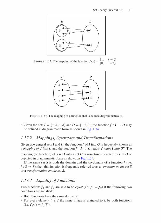
“Comninos” — 2005/8/31 — 14:52 — page 41 — #39
Set Theory Survival Kit 41
DR
Q
Q9
1
0
FIGURE 1.33. The mapping of the function f (x) =
1, x = Q
0, x = Q′ .
I
a
O
1
2
b
c
d
3
FIGURE 1.34. The mapping of a function that is defined diagrammatically.
• Given the sets I = a, b, c, d and O = 1, 2, 3, the function f : I → O maybe defined in diagrammatic form as shown in Fig. 1.34.
1.17.2 Mappings, Operators and Transformations
Given two general sets I and O, the function f of I into O is frequently known asa mapping of I into O and the notation f : I → O reads “f maps I into O”. The
mapping (or function) of a set I into a set O is sometimes denoted by If→ O or
depicted in diagrammatic form as shown in Fig. 1.35.If the same set S is both the domain and the co-domain of a function f (i.e.
f : S → S), then this function is frequently referred to as an operator on the set Sor a transformation on the set S.
1.17.3 Equality of Functions
Two functions f 1 and f 2 are said to be equal (i.e. f 1 = f 2) if the following twoconditions are satisfied:
• Both functions have the same domain I.• For every element i ∈ I the same image is assigned to it by both functions
(i.e. f 1(i) = f 2(i)).
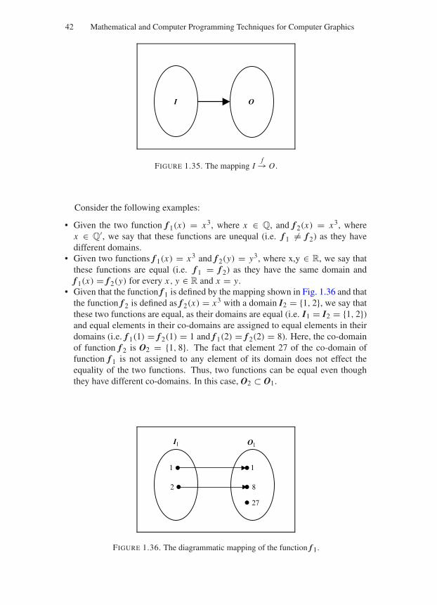
“Comninos” — 2005/8/31 — 14:52 — page 42 — #40
42 Mathematical and Computer Programming Techniques for Computer Graphics
I O
FIGURE 1.35. The mapping If→ O .
Consider the following examples:
• Given the two function f 1(x) = x3, where x ∈ Q, and f 2(x) = x3, wherex ∈ Q
′, we say that these functions are unequal (i.e. f 1 = f 2) as they havedifferent domains.
• Given two functions f 1(x) = x3 and f 2(y) = y3, where x,y ∈ R, we say thatthese functions are equal (i.e. f 1 = f 2) as they have the same domain andf 1(x) = f 2(y) for every x, y ∈ R and x = y.
• Given that the function f 1 is defined by the mapping shown in Fig. 1.36 and thatthe function f 2 is defined as f 2(x) = x3 with a domain I2 = 1, 2, we say thatthese two functions are equal, as their domains are equal (i.e. I1 = I2 = 1, 2)and equal elements in their co-domains are assigned to equal elements in theirdomains (i.e. f 1(1) = f 2(1) = 1 and f 1(2) = f 2(2) = 8). Here, the co-domainof function f 2 is O2 = 1, 8. The fact that element 27 of the co-domain offunction f 1 is not assigned to any element of its domain does not effect theequality of the two functions. Thus, two functions can be equal even thoughthey have different co-domains. In this case, O2 ⊂ O1.
I1 O1
1
8
27
1
2
FIGURE 1.36. The diagrammatic mapping of the function f1.
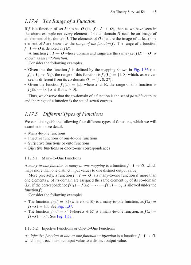
“Comninos” — 2005/8/31 — 14:52 — page 43 — #41
Set Theory Survival Kit 43
1.17.4 The Range of a Function
If f is a function of set I into set O (i.e. f : I → O), then as we have seen inthe above example not every element of its co-domain O need be an image ofan element of its domain I. The elements of O that are the image of at least oneelement of I are known as the range of the function f . The range of a functionf : I → O is denoted as f (I).
A function f : I → O whose domain and range are the same (i.e. f (I) = O) isknown as an endofunction.
Consider the following examples:
• Given that the function f is defined by the mapping shown in Fig. 1.36 (i.e.f 1 : I1 → O1), the range of this function is f 1(I1) = 1, 8 which, as we cansee, is different from its co-domain O1 = 1, 8, 27.
• Given the function f 2(x) = |x |, where x ∈ R, the range of this function isf 2(R) = x | x ∈ R ∧ x ≥ 0.Thus, we observe that the co-domain of a function is the set of possible outputs
and the range of a function is the set of actual outputs.
1.17.5 Different Types of Functions
We can distinguish the following four different types of functions, which we willexamine in more detail.
• Many-to-one functions• Injective functions or one-to-one functions• Surjective functions or onto functions• Bijective functions or one-to-one correspondences
1.17.5.1 Many-to-One Functions
A many-to-one function or many-to-one mapping is a function f : I → O, whichmaps more than one distinct input values to one distinct output value.
More precisely, a function f : I → O is a many-to-one function if more thanone elements ii of its domain are assigned the same element o j of its co-domain(i.e. if the correspondence f (i1) = f (i2) = · · · = f (in) = o j is allowed under thefunction f ).
Consider the following examples:
• The function f (x) = |x | (where x ∈ R) is a many-to-one function, as f (x) =f (−x) = |x |. See Fig. 1.37.
• The function f (x) = x2 (where x ∈ R) is a many-to-one function, as f (x) =f (−x) = x2. See Fig. 1.38.
1.17.5.2 Injective Functions or One-to-One Functions
An injective function or one-to-one function or injection is a function f : I → O,which maps each distinct input value to a distinct output value.
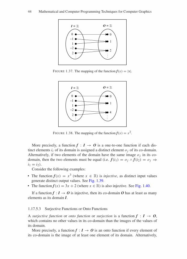
“Comninos” — 2005/8/31 — 14:52 — page 44 — #42
44 Mathematical and Computer Programming Techniques for Computer Graphics
I = R R
−1
O =
1
−22
0 0
1
2 ......
FIGURE 1.37. The mapping of the function f (x) = |x|.
I =
−1
O =
1
−24
......
0 0
1
2
R R
FIGURE 1.38. The mapping of the function f (x) = x2.
More precisely, a function f : I → O is a one-to-one function if each dis-tinct elements ii of its domain is assigned a distinct element o j of its co-domain.Alternatively, if two elements of the domain have the same image o j in its co-domain, then the two elements must be equal (i.e. f (i1) = o j ∧ f (i2) = o j ⇒i1 = i2).
Consider the following examples:
• The function f (x) = x3 (where x ∈ R) is injective, as distinct input valuesgenerate distinct output values. See Fig. 1.39.
• The function f (x) = 3x + 2 (where x ∈ R) is also injective. See Fig. 1.40.
If a function f : I → O is injective, then its co-domain O has at least as manyelements as its domain I.
1.17.5.3 Surjective Functions or Onto Functions
A surjective function or onto function or surjection is a function f : I → O,which contains no other values in its co-domain than the images of the values ofits domain.
More precisely, a function f : I → O is an onto function if every element ofits co-domain is the image of at least one element of its domain. Alternatively,
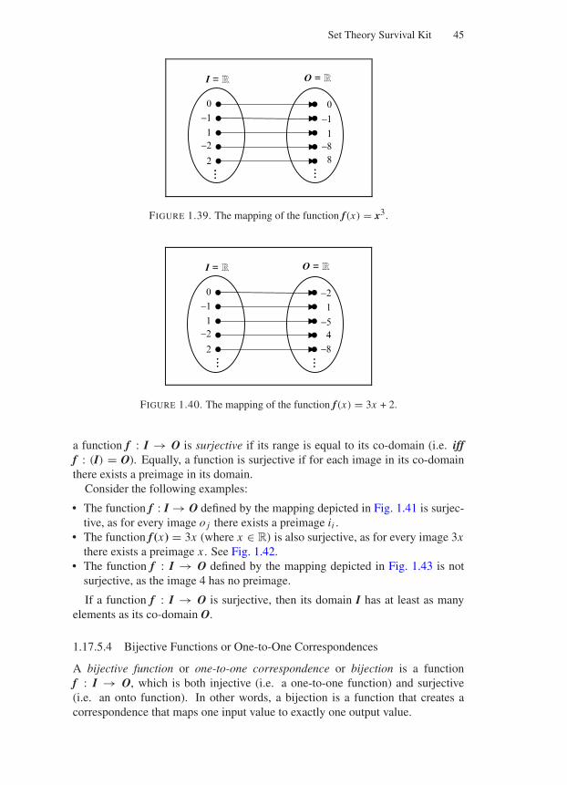
“Comninos” — 2005/8/31 — 14:52 — page 45 — #43
Set Theory Survival Kit 45
I =
−1
O =
−2
8
0 0
1
2
−1
1−8
R R
FIGURE 1.39. The mapping of the function f (x) = x3.
I =
−1
O =
−2
−8
0 −2
1
2
1
−54
R R
FIGURE 1.40. The mapping of the function f (x) = 3x + 2.
a function f : I → O is surjective if its range is equal to its co-domain (i.e. ifff : (I) = O). Equally, a function is surjective if for each image in its co-domainthere exists a preimage in its domain.
Consider the following examples:
• The function f : I → O defined by the mapping depicted in Fig. 1.41 is surjec-tive, as for every image o j there exists a preimage ii .
• The function f (x) = 3x (where x ∈ R) is also surjective, as for every image 3xthere exists a preimage x . See Fig. 1.42.
• The function f : I → O defined by the mapping depicted in Fig. 1.43 is notsurjective, as the image 4 has no preimage.
If a function f : I → O is surjective, then its domain I has at least as manyelements as its co-domain O.
1.17.5.4 Bijective Functions or One-to-One Correspondences
A bijective function or one-to-one correspondence or bijection is a functionf : I → O, which is both injective (i.e. a one-to-one function) and surjective(i.e. an onto function). In other words, a bijection is a function that creates acorrespondence that maps one input value to exactly one output value.
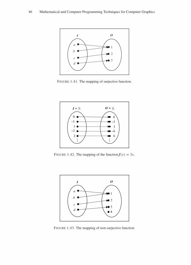
“Comninos” — 2005/8/31 — 14:52 — page 46 — #44
46 Mathematical and Computer Programming Techniques for Computer Graphics
I
a
O
1
3
b
c
d
2
FIGURE 1.41. The mapping of surjective function.
I =
−1
O =
−2
6
0 0
1
2
−3
3−6
R R
FIGURE 1.42. The mapping of the function f (x) = 3x .
I
a
O
1
3
b
c
d
2
4
FIGURE 1.43. The mapping of non-surjective function.
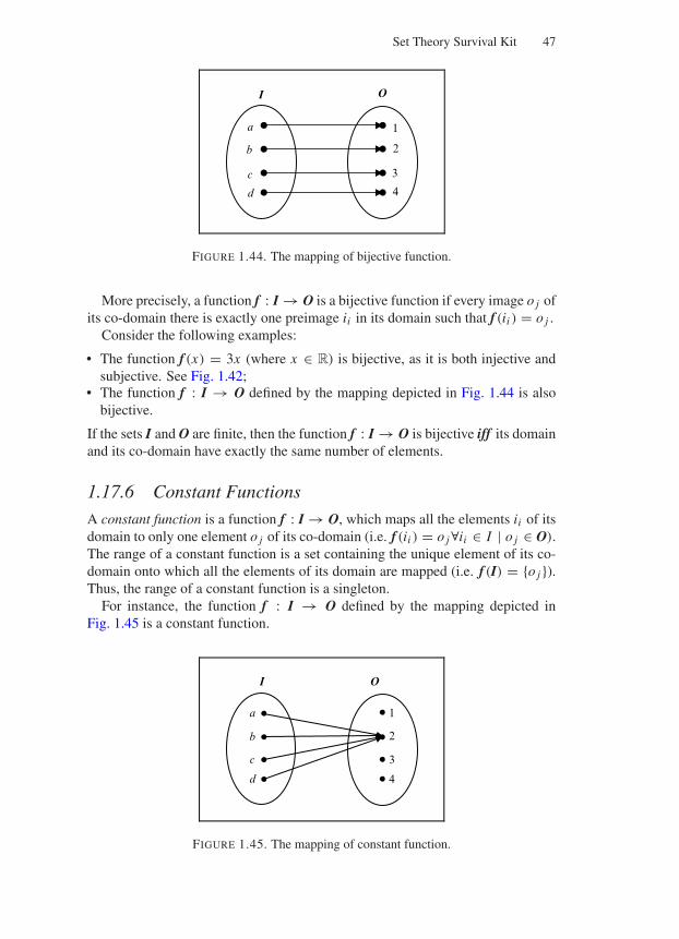
“Comninos” — 2005/8/31 — 14:52 — page 47 — #45
Set Theory Survival Kit 47
I
a
O
1
3
b
c
d
2
4
FIGURE 1.44. The mapping of bijective function.
More precisely, a function f : I → O is a bijective function if every image o j ofits co-domain there is exactly one preimage ii in its domain such that f (ii ) = o j .
Consider the following examples:
• The function f (x) = 3x (where x ∈ R) is bijective, as it is both injective andsubjective. See Fig. 1.42;
• The function f : I → O defined by the mapping depicted in Fig. 1.44 is alsobijective.
If the sets I and O are finite, then the function f : I → O is bijective iff its domainand its co-domain have exactly the same number of elements.
1.17.6 Constant Functions
A constant function is a function f : I → O, which maps all the elements ii of itsdomain to only one element o j of its co-domain (i.e. f (ii ) = o j∀ii ∈ I | o j ∈ O).The range of a constant function is a set containing the unique element of its co-domain onto which all the elements of its domain are mapped (i.e. f (I) = o j ).Thus, the range of a constant function is a singleton.
For instance, the function f : I → O defined by the mapping depicted inFig. 1.45 is a constant function.
I
a
O
1
3
b
c
d
2
4
FIGURE 1.45. The mapping of constant function.
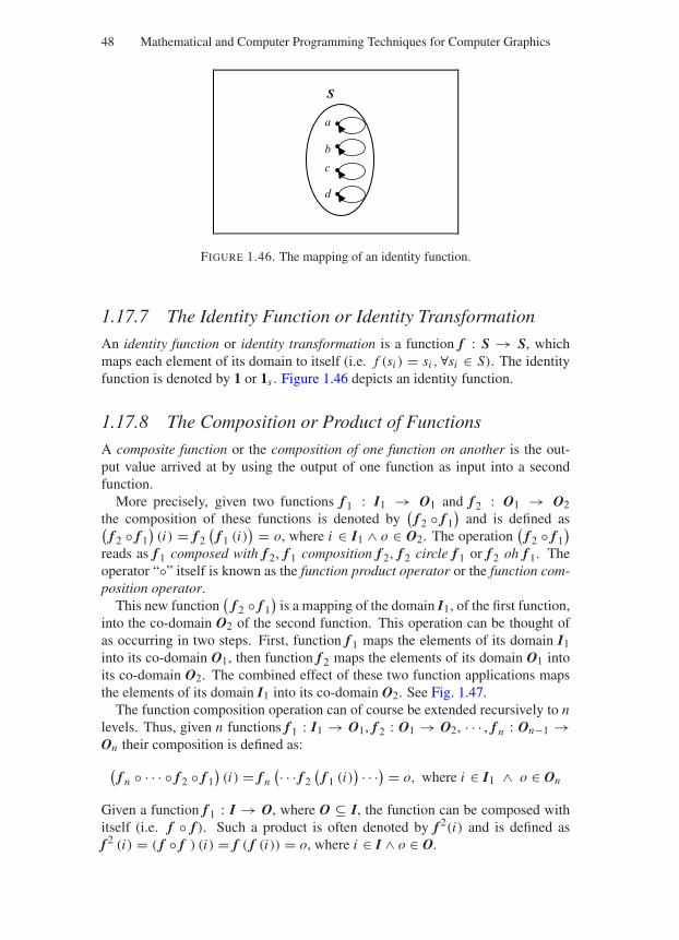
“Comninos” — 2005/8/31 — 14:52 — page 48 — #46
48 Mathematical and Computer Programming Techniques for Computer Graphics
S
a
b
c
d
FIGURE 1.46. The mapping of an identity function.
1.17.7 The Identity Function or Identity Transformation
An identity function or identity transformation is a function f : S → S, whichmaps each element of its domain to itself (i.e. f (si ) = si ,∀si ∈ S). The identityfunction is denoted by 1 or 1s . Figure 1.46 depicts an identity function.
1.17.8 The Composition or Product of Functions
A composite function or the composition of one function on another is the out-put value arrived at by using the output of one function as input into a secondfunction.
More precisely, given two functions f 1 : I1 → O1 and f 2 : O1 → O2the composition of these functions is denoted by
(f 2 f 1
)and is defined as(
f 2 f 1)(i) = f 2
(f 1 (i)
) = o, where i ∈ I1 ∧ o ∈ O2. The operation(
f 2 f 1)
reads as f 1 composed with f 2, f 1 composition f 2, f 2 circle f 1 or f 2 oh f 1. Theoperator “” itself is known as the function product operator or the function com-position operator.
This new function(
f 2 f 1)
is a mapping of the domain I1, of the first function,into the co-domain O2 of the second function. This operation can be thought ofas occurring in two steps. First, function f 1 maps the elements of its domain I1into its co-domain O1, then function f 2 maps the elements of its domain O1 intoits co-domain O2. The combined effect of these two function applications mapsthe elements of its domain I1 into its co-domain O2. See Fig. 1.47.
The function composition operation can of course be extended recursively to nlevels. Thus, given n functions f 1 : I1 → O1, f 2 : O1 → O2, · · · , f n : On−1 →On their composition is defined as:
(f n · · · f 2 f 1
)(i) = f n
(· · · f 2(
f 1 (i)) · · ·) = o, where i ∈ I1 ∧ o ∈ On
Given a function f 1 : I → O, where O ⊆ I, the function can be composed withitself (i.e. f f ). Such a product is often denoted by f 2(i) and is defined asf 2 (i) = ( f f ) (i) = f ( f (i)) = o, where i ∈ I ∧ o ∈ O.
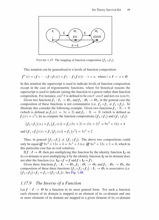
“Comninos” — 2005/8/31 — 14:52 — page 49 — #47
Set Theory Survival Kit 49
f1(i)i f2( f1(i))
I1 O1 O2f1 f2
f1f2 o
FIGURE 1.47. The mapping of function composition(
f2 f1).
This notation can be generalised to n levels of function composition:
f n (i) = ( f · · · f f ) (i) = f (· · · f ( f (i)) · · ·) = o, where i ∈ I ∧ o ∈ O.
In this notation the superscript is used to indicate levels of function compositionexcept in the case of trigonometric functions, where for historical reasons thesuperscript is used to indicate raising the function to a power rather than functioncomposition. For instance, cos2 θ is defined to be cos θ ·cos θ and not cos (cos θ).
Given two functions f 1 : I1 → O1, and f 2 : O1 → O2, in the general case thecomposition of these functions is not commutative (i.e. f 2 f 1 = f 1 f 2). Toillustrate this consider the following example. Given two functions f 1 : R → R
(which is defined as f 1(x) = 3x + 2) and f 2 : R → R (which is defined asf 2(x) = x2), let us compute the function compositions
(f 2 f 1
)and
(f 1 f 2
):
(f 2 f 1
)(x) = f 2
(f 1 (x)
) = f 2 (3x + 2) = (3x + 2)2 = 9x2 + 12x + 4
and(
f 1 f 2)(x) = f 1
(f 2 (x)
) = f 1(x2
) = 3x2 + 2
Thus, in general(
f 2 f 1) = (
f 1 f 2). The above two compositions could
only be equal iff 9x2 + 12x + 4 = 3x2 + 2 (i.e. iff 6x2 + 12x + 2 = 0, which inthis particular case has no real solution).
If f : I → O, then pre-multiplying this function by the identity function 1o onits co-domain or post-multiplying it by the identity function 1I on its domain doesnot alter the function (i.e. 1O f = f and f 1I = f ).
Given three functions f 1 : I1 → O1, f 2 : O1 → O2 and f 3 : O2 → O3, thecomposition of these three functions
(f 3 f 2 f 1
): I1 → O3 is associative (i.e.(
f 3 f 2) f 1 = f 3 (
f 2 f 1)). See Fig. 1.48.
1.17.9 The Inverse of a Function
Let f : I → O be a function in its most general form. For such a functioneach element of its domain is mapped to an element of its co-domain and oneor more elements of its domain are mapped to a given element of its co-domain
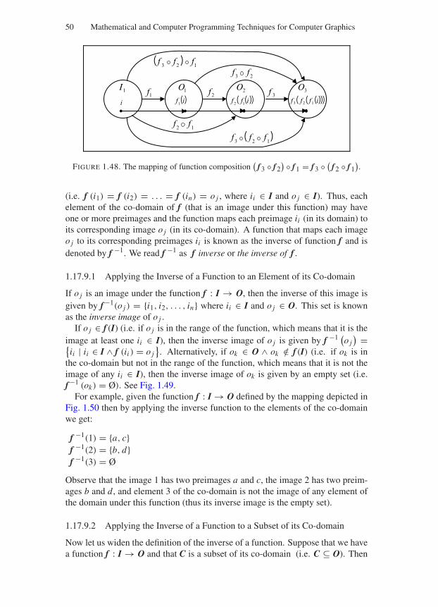
“Comninos” — 2005/8/31 — 14:52 — page 50 — #48
50 Mathematical and Computer Programming Techniques for Computer Graphics
( )i1fi ( )( )i12 ff
1I 1O 2O1f 2f
12 ff
( )( )( )i123 fff
3O3f
( )123 fff
23 ff( ) 123 fff
FIGURE 1.48. The mapping of function composition(
f3 f2) f1 = f3 (
f2 f1).
(i.e. f (i1) = f (i2) = . . . = f (in) = o j , where ii ∈ I and o j ∈ I). Thus, eachelement of the co-domain of f (that is an image under this function) may haveone or more preimages and the function maps each preimage ii (in its domain) toits corresponding image o j (in its co-domain). A function that maps each imageo j to its corresponding preimages ii is known as the inverse of function f and isdenoted by f −1. We read f −1 as f inverse or the inverse of f .
1.17.9.1 Applying the Inverse of a Function to an Element of its Co-domain
If o j is an image under the function f : I → O, then the inverse of this image isgiven by f−1(o j ) = i1, i2, . . . , in where ii ∈ I and o j ∈ O. This set is knownas the inverse image of o j .
If o j ∈ f (I) (i.e. if o j is in the range of the function, which means that it is theimage at least one ii ∈ I), then the inverse image of o j is given by f −1 (
o j) =
ii | ii ∈ I ∧ f (ii ) = o j. Alternatively, if ok ∈ O ∧ ok /∈ f (I) (i.e. if ok is in
the co-domain but not in the range of the function, which means that it is not theimage of any ii ∈ I), then the inverse image of ok is given by an empty set (i.e.f−1 (ok) = Ø). See Fig. 1.49.
For example, given the function f : I → O defined by the mapping depicted inFig. 1.50 then by applying the inverse function to the elements of the co-domainwe get:
f −1(1) = a, cf −1(2) = b, df −1(3) = Ø
Observe that the image 1 has two preimages a and c, the image 2 has two preim-ages b and d, and element 3 of the co-domain is not the image of any element ofthe domain under this function (thus its inverse image is the empty set).
1.17.9.2 Applying the Inverse of a Function to a Subset of its Co-domain
Now let us widen the definition of the inverse of a function. Suppose that we havea function f : I → O and that C is a subset of its co-domain (i.e. C ⊆ O). Then
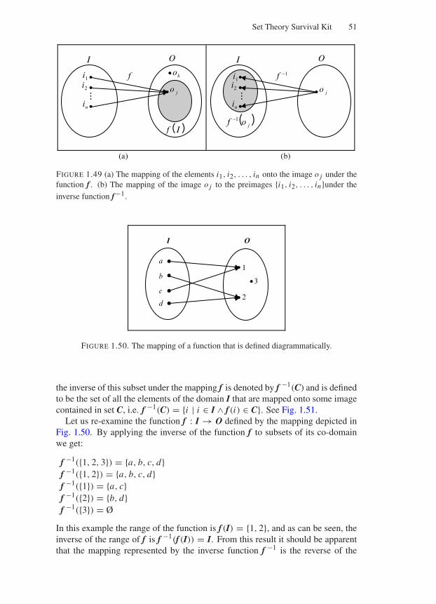
“Comninos” — 2005/8/31 — 14:52 — page 51 — #49
Set Theory Survival Kit 51
I
1i
O
2i
ni
jo
f ko
( )If
I
1i
O
2i
ni
jo
f
( )jf o−1
(a) (b)
−1
FIGURE 1.49 (a) The mapping of the elements i1, i2, . . . , in onto the image o j under thefunction f . (b) The mapping of the image o j to the preimages i1, i2, . . . , inunder the
inverse function f−1.
I
a
O
1
2
b
c
d
3
FIGURE 1.50. The mapping of a function that is defined diagrammatically.
the inverse of this subset under the mapping f is denoted by f −1(C) and is definedto be the set of all the elements of the domain I that are mapped onto some imagecontained in set C, i.e. f −1(C) = i | i ∈ I ∧ f (i) ∈ C. See Fig. 1.51.
Let us re-examine the function f : I → O defined by the mapping depicted inFig. 1.50. By applying the inverse of the function f to subsets of its co-domainwe get:
f −1(1, 2, 3) = a, b, c, df −1(1, 2) = a, b, c, df −1(1) = a, cf −1(2) = b, df −1(3) = Ø
In this example the range of the function is f (I) = 1, 2, and as can be seen, theinverse of the range of f is f −1(f (I)) = I. From this result it should be apparentthat the mapping represented by the inverse function f −1 is the reverse of the
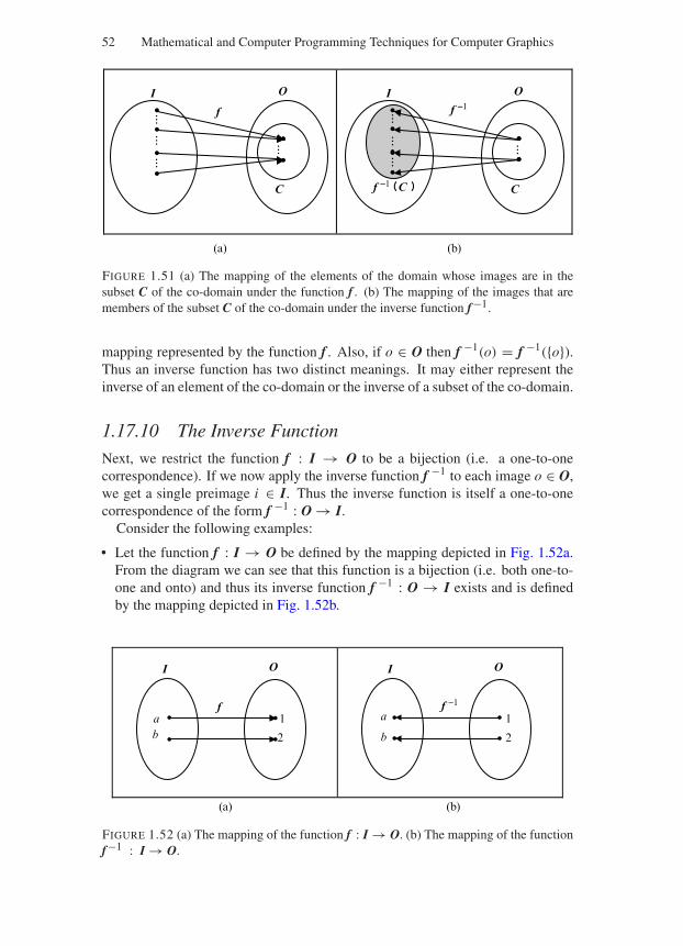
“Comninos” — 2005/8/31 — 14:52 — page 52 — #50
52 Mathematical and Computer Programming Techniques for Computer Graphics
I O
f
C
I O
f -1
( )Cf -1 C
(a) (b)
FIGURE 1.51 (a) The mapping of the elements of the domain whose images are in thesubset C of the co-domain under the function f . (b) The mapping of the images that aremembers of the subset C of the co-domain under the inverse function f−1.
mapping represented by the function f . Also, if o ∈ O then f −1(o) = f −1(o).Thus an inverse function has two distinct meanings. It may either represent theinverse of an element of the co-domain or the inverse of a subset of the co-domain.
1.17.10 The Inverse Function
Next, we restrict the function f : I → O to be a bijection (i.e. a one-to-onecorrespondence). If we now apply the inverse function f −1 to each image o ∈ O,we get a single preimage i ∈ I. Thus the inverse function is itself a one-to-onecorrespondence of the form f −1 : O → I.
Consider the following examples:
• Let the function f : I → O be defined by the mapping depicted in Fig. 1.52a.From the diagram we can see that this function is a bijection (i.e. both one-to-one and onto) and thus its inverse function f −1 : O → I exists and is definedby the mapping depicted in Fig. 1.52b.
I
a
O
1b 2
f
I
a
O
1
b 2
f −1
(a) (b)
FIGURE 1.52 (a) The mapping of the function f : I → O. (b) The mapping of the functionf−1 : I → O.
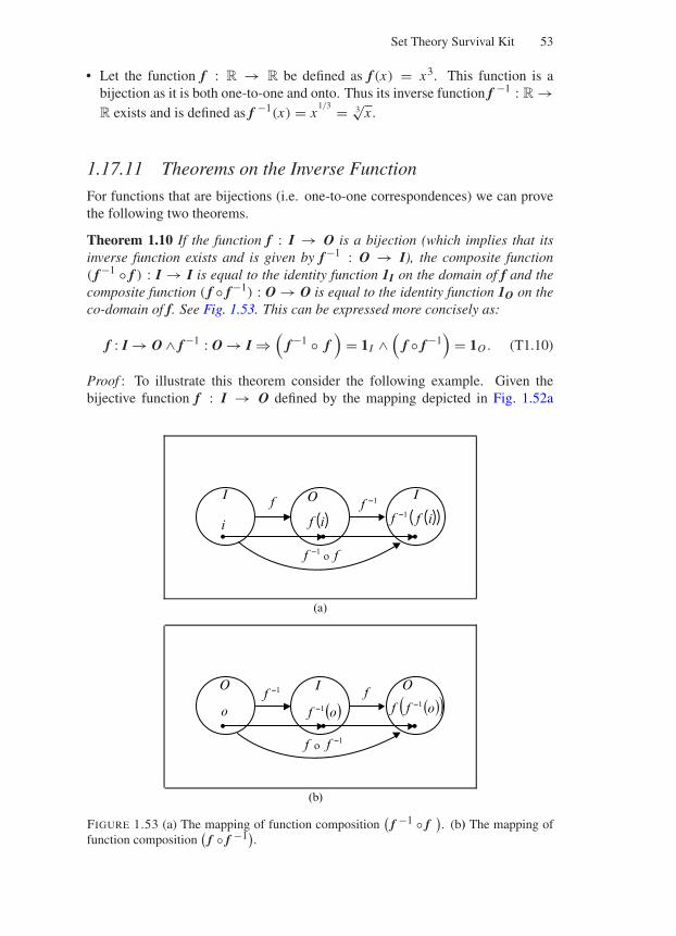
“Comninos” — 2005/8/31 — 14:52 — page 53 — #51
Set Theory Survival Kit 53
• Let the function f : R → R be defined as f (x) = x3. This function is abijection as it is both one-to-one and onto. Thus its inverse function f −1 : R →R exists and is defined as f −1(x) = x
1/3 = 3√
x .
1.17.11 Theorems on the Inverse Function
For functions that are bijections (i.e. one-to-one correspondences) we can provethe following two theorems.
Theorem 1.10 If the function f : I → O is a bijection (which implies that itsinverse function exists and is given by f −1 : O → I), the composite function( f −1 f ) : I → I is equal to the identity function 1I on the domain of f and thecomposite function ( f f−1) : O → O is equal to the identity function 1O on theco-domain of f. See Fig. 1.53. This can be expressed more concisely as:
f : I → O ∧ f −1 : O → I ⇒(
f−1 f)
= 1I ∧(
f f −1)
= 1O . (T1.10)
Proof : To illustrate this theorem consider the following example. Given thebijective function f : I → O defined by the mapping depicted in Fig. 1.52a
( )ifi ( )( )if
I Of
ff -1
f -1
f -1
o
I
(a)
( )oo ( )( )of -1
f -1
f -1
f -1
f
O I f
f o
O
(b)
FIGURE 1.53 (a) The mapping of function composition(
f −1 f). (b) The mapping of
function composition(
f f −1).
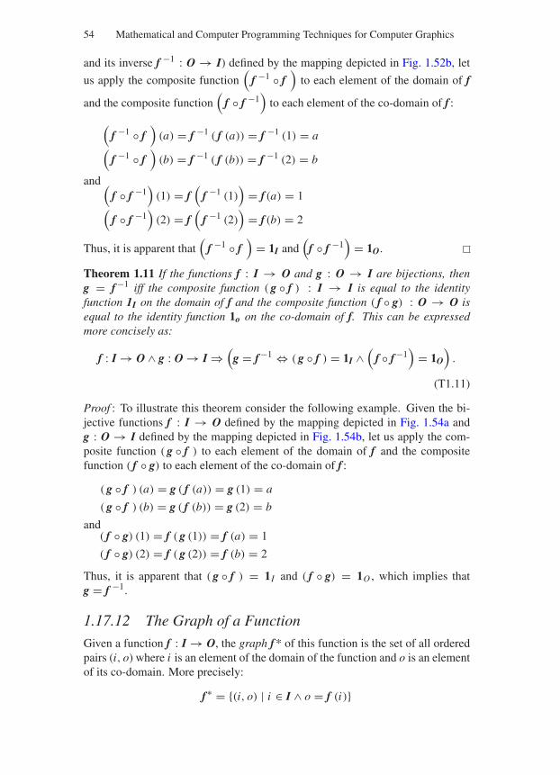
“Comninos” — 2005/8/31 — 14:52 — page 54 — #52
54 Mathematical and Computer Programming Techniques for Computer Graphics
and its inverse f −1 : O → I) defined by the mapping depicted in Fig. 1.52b, let
us apply the composite function(
f −1 f)
to each element of the domain of f
and the composite function(
f f −1)
to each element of the co-domain of f :
(f −1 f
)(a) = f −1 ( f (a)) = f −1 (1) = a
(f −1 f
)(b) = f −1 ( f (b)) = f −1 (2) = b
and (f f −1
)(1) = f
(f −1 (1)
)= f (a) = 1
(f f −1
)(2) = f
(f −1 (2)
)= f (b) = 2
Thus, it is apparent that(
f −1 f)
= 1I and(
f f −1)
= 1O.
Theorem 1.11 If the functions f : I → O and g : O → I are bijections, theng = f −1 iff the composite function ( g f ) : I → I is equal to the identityfunction 1I on the domain of f and the composite function ( f g) : O → O isequal to the identity function 1o on the co-domain of f. This can be expressedmore concisely as:
f : I → O ∧ g : O → I ⇒(
g = f−1 ⇔ ( g f ) = 1I ∧(
f f−1)
= 1O
).
(T1.11)
Proof : To illustrate this theorem consider the following example. Given the bi-jective functions f : I → O defined by the mapping depicted in Fig. 1.54a andg : O → I defined by the mapping depicted in Fig. 1.54b, let us apply the com-posite function ( g f ) to each element of the domain of f and the compositefunction ( f g) to each element of the co-domain of f :
( g f ) (a) = g ( f (a)) = g (1) = a
( g f ) (b) = g ( f (b)) = g (2) = b
and( f g) (1) = f ( g (1)) = f (a) = 1
( f g) (2) = f ( g (2)) = f (b) = 2
Thus, it is apparent that ( g f ) = 1I and ( f g) = 1O , which implies thatg = f −1.
1.17.12 The Graph of a Function
Given a function f : I → O, the graph f* of this function is the set of all orderedpairs (i, o) where i is an element of the domain of the function and o is an elementof its co-domain. More precisely:
f∗ = (i, o) | i ∈ I ∧ o = f (i)
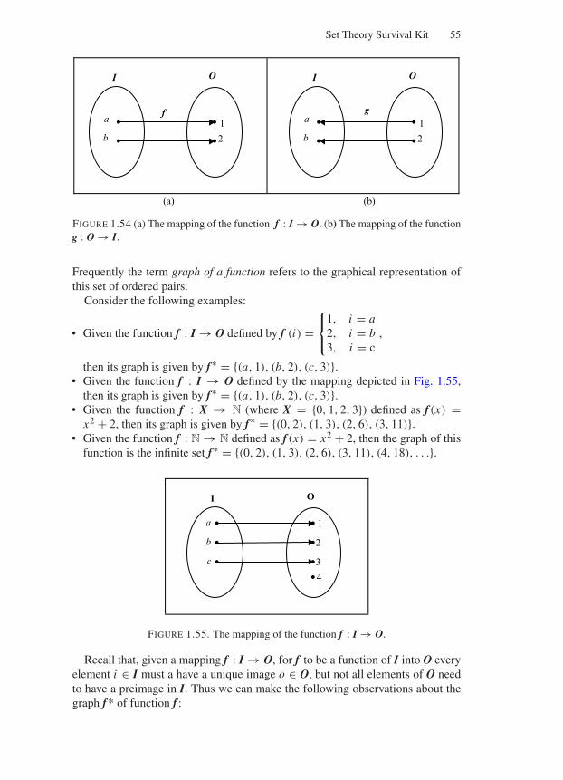
“Comninos” — 2005/8/31 — 14:52 — page 55 — #53
Set Theory Survival Kit 55
I
a
O
1
b 2
f
I
a
O
1
b 2
g
(a) (b)
FIGURE 1.54 (a) The mapping of the function f : I → O. (b) The mapping of the functiong : O → I.
Frequently the term graph of a function refers to the graphical representation ofthis set of ordered pairs.
Consider the following examples:
• Given the function f : I → O defined by f (i) =⎧⎨
⎩
1, i = a2, i = b3, i = c
,
then its graph is given by f∗ = (a, 1), (b, 2), (c, 3).• Given the function f : I → O defined by the mapping depicted in Fig. 1.55,
then its graph is given by f∗ = (a, 1), (b, 2), (c, 3).• Given the function f : X → N (where X = 0, 1, 2, 3) defined as f (x) =
x2 + 2, then its graph is given by f∗ = (0, 2), (1, 3), (2, 6), (3, 11).• Given the function f : N → N defined as f (x) = x2 + 2, then the graph of this
function is the infinite set f∗ = (0, 2), (1, 3), (2, 6), (3, 11), (4, 18), . . ..
I
a
O
1
3
b
c
2
4
FIGURE 1.55. The mapping of the function f : I → O.
Recall that, given a mapping f : I → O, for f to be a function of I into O everyelement i ∈ I must a have a unique image o ∈ O, but not all elements of O needto have a preimage in I. Thus we can make the following observations about thegraph f* of function f :
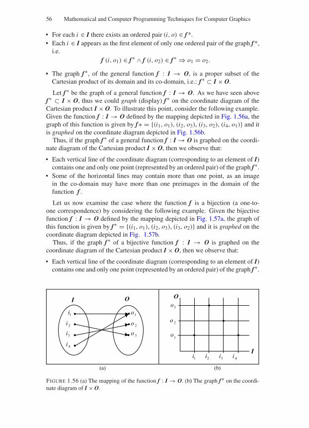
“Comninos” — 2005/8/31 — 14:52 — page 56 — #54
56 Mathematical and Computer Programming Techniques for Computer Graphics
• For each i ∈ I there exists an ordered pair (i, o) ∈ f*.• Each i ∈ I appears as the first element of only one ordered pair of the graph f*,
i.e.f (i, o1) ∈ f∗ ∧ f (i, o2) ∈ f∗ ⇒ o1 = o2.
• The graph f∗, of the general function f : I → O, is a proper subset of theCartesian product of its domain and its co-domain, i.e.: f∗ ⊂ I × O.
Let f∗ be the graph of a general function f : I → O. As we have seen abovef∗ ⊂ I × O, thus we could graph (display) f∗ on the coordinate diagram of theCartesian product I × O. To illustrate this point, consider the following example.Given the function f : I → O defined by the mapping depicted in Fig. 1.56a, thegraph of this function is given by f∗ = (i1, o1), (i2, o3), (i3, o2), (i4, o1) and itis graphed on the coordinate diagram depicted in Fig. 1.56b.
Thus, if the graph f∗ of a general function f : I → O is graphed on the coordi-nate diagram of the Cartesian product I × O, then we observe that:
• Each vertical line of the coordinate diagram (corresponding to an element of I)contains one and only one point (represented by an ordered pair) of the graph f∗.
• Some of the horizontal lines may contain more than one point, as an imagein the co-domain may have more than one preimages in the domain of thefunction f .
Let us now examine the case where the function f is a bijection (a one-to-one correspondence) by considering the following example. Given the bijectivefunction f : I → O defined by the mapping depicted in Fig. 1.57a, the graph ofthis function is given by f∗ = (i1, o1), (i2, o3), (i3, o2) and it is graphed on thecoordinate diagram depicted in Fig. 1.57b.
Thus, if the graph f∗ of a bijective function f : I → O is graphed on thecoordinate diagram of the Cartesian product I × O, then we observe that:
• Each vertical line of the coordinate diagram (corresponding to an element of I)contains one and only one point (represented by an ordered pair) of the graph f∗.
I
1i
O
2i
3i
4i
1o
2o
3o
I1i
O
2i 3i 4i
1o
2o
3o
(a) (b)
FIGURE 1.56 (a) The mapping of the function f : I → O. (b) The graph f∗ on the coordi-nate diagram of I × O.
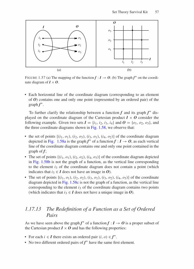
“Comninos” — 2005/8/31 — 14:52 — page 57 — #55
Set Theory Survival Kit 57
I
i1
O
i2
i3
o1
o2
o3
Ii1
O
i2 i3
o1
o2
o3
(a) (b)
FIGURE 1.57 (a) The mapping of the function f : I → O. (b) The graph f∗ on the coordi-nate diagram of I × O.
• Each horizontal line of the coordinate diagram (corresponding to an elementof O) contains one and only one point (represented by an ordered pair) of thegraph f∗.
To further clarify the relationship between a function f and its graph f∗ dis-played on the coordinate diagram of the Cartesian product I × O consider thefollowing example. Given two sets I = i1, i2, i3, i4 and O = o1, o2, o3, andthe three coordinate diagrams shown in Fig. 1.58, we observe that:
• the set of points (i1, o1), (i2, o3), (i3, o1), (i4, o2) of the coordinate diagramdepicted in Fig. 1.58a is the graph f∗ of a function f : I → O, as each verticalline of the coordinate diagram contains one and only one point contained in thegraph of f ;
• The set of points (i1, o1), (i2, o2), (i4, o3) of the coordinate diagram depictedin Fig. 1.58b is not the graph of a function, as the vertical line correspondingto the element i3 of the coordinate diagram does not contain a point (whichindicates that i3 ∈ I does not have an image in O).
• The set of points (i1, o1), (i2, o2), (i3, o1), (i3, o2), (i4, o3) of the coordinatediagram depicted in Fig. 1.58c is not the graph of a function, as the vertical linecorresponding to the element i3 of the coordinate diagram contains two points(which indicates that i3 ∈ I does not have a unique image in O).
1.17.13 The Redefinition of a Function as a Set of OrderedPairs
As we have seen above the graph f∗ of a function f : I → O is a proper subset ofthe Cartesian product I × O and has the following properties:
• For each i ∈ I there exists an ordered pair (i, o) ∈ f∗.• No two different ordered pairs of f∗ have the same first element.
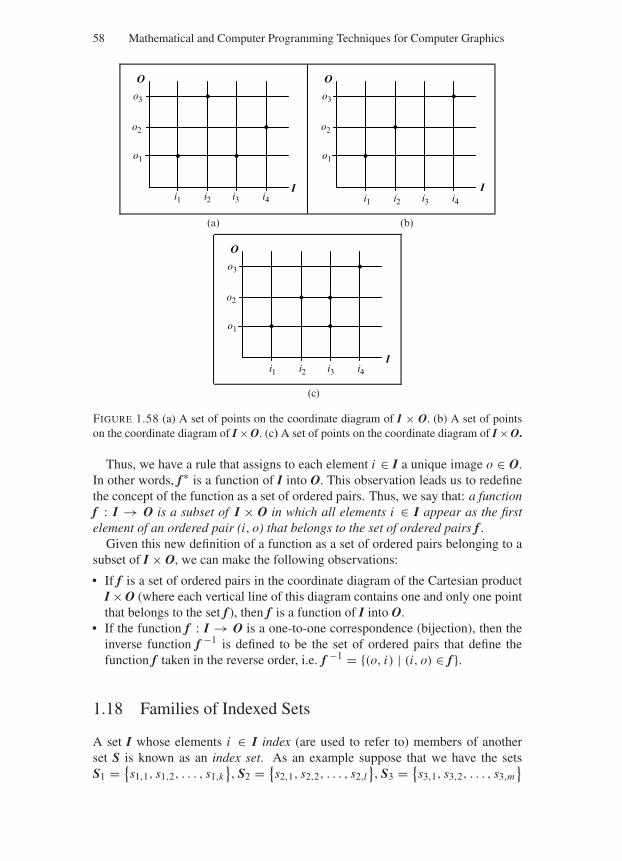
“Comninos” — 2005/8/31 — 14:52 — page 58 — #56
58 Mathematical and Computer Programming Techniques for Computer Graphics
Ii1
O
i2 i3 i4 i1 i2 i3 i4
o1
o2
o3
o1
o2
o3
I
O
(a) (b)
i1 i2 i3 i4
o1
o2
o3
I
O
(c)
FIGURE 1.58 (a) A set of points on the coordinate diagram of I × O. (b) A set of pointson the coordinate diagram of I × O. (c) A set of points on the coordinate diagram of I × O.
Thus, we have a rule that assigns to each element i ∈ I a unique image o ∈ O.In other words, f∗ is a function of I into O. This observation leads us to redefinethe concept of the function as a set of ordered pairs. Thus, we say that: a functionf : I → O is a subset of I × O in which all elements i ∈ I appear as the firstelement of an ordered pair (i, o) that belongs to the set of ordered pairs f .
Given this new definition of a function as a set of ordered pairs belonging to asubset of I × O, we can make the following observations:
• If f is a set of ordered pairs in the coordinate diagram of the Cartesian productI × O (where each vertical line of this diagram contains one and only one pointthat belongs to the set f ), then f is a function of I into O.
• If the function f : I → O is a one-to-one correspondence (bijection), then theinverse function f −1 is defined to be the set of ordered pairs that define thefunction f taken in the reverse order, i.e. f −1 = (o, i) | (i, o) ∈ f .
1.18 Families of Indexed Sets
A set I whose elements i ∈ I index (are used to refer to) members of anotherset S is known as an index set. As an example suppose that we have the setsS1 =
s1,1, s1,2, . . . , s1,k, S2 =
s2,1, s2,2, . . . , s2,l, S3 =
s3,1, s3,2, . . . , s3,m
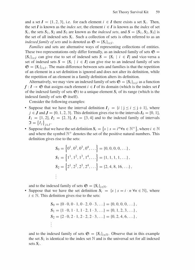
“Comninos” — 2005/8/31 — 14:52 — page 59 — #57
Set Theory Survival Kit 59
and a set I = 1, 2, 3, i.e. for each element i ∈ I there exists a set Si . Then,the set I is known as the index set, the element i ∈ I is known as the index of setSi , the sets S1, S2 and S3 are known as the indexed sets, and S = S1, S2, S3 isthe set of all indexed sets Si . Such a collection of sets is often referred to as anindexed family of sets and is denoted as S = Si i∈I .
Families and sets are alternative ways of representing collections of entities.These two representations only differ formally, as an indexed family of sets S =Si i∈I can give rise to set of indexed sets S = Si | i ∈ I and vice-versa aset of indexed sets S = Si | i ∈ I can give rise to an indexed family of setsS = Si i∈I . The main difference between sets and families is that the repetitionof an element in a set definition is ignored and does not alter its definition, whilethe repetition of an element in a family definition alters its definition.
Alternatively, we may view an indexed family of sets S = Si i∈I as a functionf : I → S that assigns each element i ∈ I of its domain (which is the index set Iof the indexed family of sets S) to a unique element Si of its range (which is theindexed family of sets S itself).
Consider the following examples:
• Suppose that we have the interval definition I j = i | j ≤ i ≤ j + 1, wherej ∈ J and J = 0, 1, 2, 3. This definition gives rise to the intervals I0 = [0, 1],I1 = [1, 2], I2 = [2, 3], I3 = [3, 4] and to the indexed family of intervalsI =
I j
j∈J .
• Suppose that we have the set definition Si = s | s = in∀n ∈ N
+, where i ∈ N
and where the symbol N+ denotes the set of the positive natural numbers. This
definition gives rise to the sets:
S0 =
01, 02, 03, 04, . . .
= 0, 0, 0, 0, . . . ,
S1 =
11, 12, 13, 14, . . .
= 1, 1, 1, 1, . . . ,
S2 =
21, 22, 23, 24, . . .
= 2, 4, 8, 16, . . . ,
...
and to the indexed family of sets S = Si i∈N.• Suppose that we have the set definition Si = s | s = i · n ∀n ∈ N, where
i ∈ N. This definition gives rise to the sets:
S0 = 0 · 0, 0 · 1, 0 · 2, 0 · 3, . . . = 0, 0, 0, 0, . . . ,
S1 = 1 · 0, 1 · 1, 1 · 2, 1 · 3, . . . = 0, 1, 2, 3, . . . ,
S2 = 2 · 0, 2 · 1, 2 · 2, 2 · 3, . . . = 0, 2, 4, 6, . . . ,
...
and to the indexed family of sets S = Si i∈N. Observe that in this examplethe set S1 is identical to the index set N and is the universal set for all indexedsets Si .
“Comninos” — 2005/8/31 — 14:52 — page 60 — #58
60 Mathematical and Computer Programming Techniques for Computer Graphics
Above we have observed that any indexed family of sets S = Si i∈I can bethought of as a function f : I → S. Replacing the function f by the identityfunction on S we get 1S : S → S, which is another way of saying thatS = Si i∈S, where Si ∈ S and i = Si (i.e. the index of any set in the family ofindexed sets S is the set itself). Now, we can rewrite S as S = ii∈S and saythat any indexed family of sets S can be indexed by itself.
1.19 The Generalised Set Union and Intersection Operations
Earlier in this chapter we have defined the operations of union and intersectionbetween two sets. Now, we will extend these operations to deal with a finitenumber of sets. Thus, given n sets S1, S2, . . . , Sn we refine the definition of theseset operations as follows. The union of n sets is defined as:
n⋃
i=1
Si = S1 ∪ S2 ∪ · · · ∪ Sn (1.14)
orn⋃
i=1
Si = s | (∃i ∈ 1, 2, . . . , n) : (s ∈ Si ) (1.15)
Which reads “the union of the sets Si for i from 1 to n is equal to the set ofelements s such that there exists a value of i that belongs to the set 1, 2, . . . , nfor which element s belongs to the set Si ”, i.e. the elements of the union of thesets belong to at least one of the sets Si .
Similarly, the intersection of n sets is defined as:
n⋂
i=1
Si = S1 ∩ S2 ∩ · · · ∩ Sn (1.16)
orn⋂
i=1
Si = s | (∀i ∈ 1, 2, . . . , n) : (s ∈ Si ) (1.17)
Which reads “the intersection of the sets Si for i from 1 to n is equal to the set ofelements s such that for all values of i that belong to the set 1, 2, . . ., n elements belongs to the set Si ”, i.e. the elements of the intersection of the sets belong toall the sets Si .
As we have seen before in some literature the union and intersection of two setsA and B are denoted as A + B and A · B, respectively. If this notation is used, thegeneralised union and intersection of n sets S1, S2, · · · , Sn are denoted as:
n⋃
i=1
Si ≡n∑
i=1
Si = S1 + S2 + · · · + Sn (1.18)
“Comninos” — 2005/8/31 — 14:52 — page 61 — #59
Set Theory Survival Kit 61
n⋂
i=1
Si ≡n∏
i=1
Si = S1 · S2 . . . Sn (1.19)
Next, we further generalise the union and intersection operations to deal with fam-ilies of indexed sets. Thus, given a family of indexed sets S = Sii∈I (where I isthe index set of the family) we refine the definition of the union and intersectionoperations as follows. The union operation of a family of indexed sets is definedas:
⋃
i∈I
Si = s | (∃i ∈ I) : (s ∈ Si ) (1.20)
If the index set is not ambiguous, the notation⋃
i∈I Si can be shortened to⋃
Si.Similarly, the intersection of a family of indexed sets is defined as:
⋂
i∈I
S = s | (∀i ∈ I) : (s ∈ Si) (1.21)
Again, If the index set is not ambiguous, the notation⋂
i∈I Si can be shortened to⋂Si.
1.19.1 The Negation of the Generalised Set Operations
We must be particularly careful when negating a generalised union or intersectionoperation on a family of indexed sets. For instance, the expression s ∈ ⋃
i∈I Si
means that there is at least one value of the index i for which s ∈ Si and converselythe expression s /∈ ⋃
i∈I Si means that s /∈ Si for all values of the index i ∈ I.Similarly, the expression s ∈ ⋂
i∈I Si means that s ∈ Si for all values of the indexi ∈ I and conversely the expression s /∈ ⋂
i∈I Si means that s /∈ Si for at least onevalue of the index i .
1.19.2 Some Algebraic Rules for the Generalised SetOperations
The distributive rules of the union over intersection (R1.9a) and of the intersectionover union (R1.9b) can be extended to deal with a set A and a family of indexedsets S = Sii∈I (where I is the index set of the family). Starting from thedistributive rule of the union over intersection A ∪ (B ∩ C) = (A ∪ B) ∩ (A ∪ C)
we get:
A ∪(
⋂
i∈I
Si
)
=⋂
i∈I
(A ∪ Si) (1.22)
Similarly, starting from the distributive rule of the intersection over union A ∩(B ∪ C) = (A ∩ B) ∪ (A ∩ C) we get:
A ∩(
⋃
i∈I
Si
)
=⋃
i∈I
(A ∩ Si) (1.23)
“Comninos” — 2005/8/31 — 14:52 — page 62 — #60
62 Mathematical and Computer Programming Techniques for Computer Graphics
Also, the De Morgan rules for the negation of the union of two sets (R1.10a)and the negation of the intersection of two sets (R1.10b) can be extended to dealwith a family of indexed sets S = Sii∈I (where I is the index set of the fam-ily). Starting from the De Morgan rule for the negation of the union of two sets(A ∪ B)′ = A′ ∩ B′ we get:
(⋃
i∈I
Si
)′=
⋂
i∈I
S′i (1.24)
Similarly, starting from the De Morgan rule for the negation of the intersection oftwo sets (A ∩ B)′ = A′ ∪ B′ we get:
(⋂
i∈I
Si
)′=
⋃
i∈I
S′i (1.25)
1.20 The Cardinality or Size of a Set
When dealing with sets we frequently wish to know what is the size of a set orindeed if two sets have the same size. With finite sets this is easy, all we have todo is to count the number of their elements. With infinite sets, however, this ismore difficult (as we can not count the elements of infinite sets) and it depends onhow we define the sets to have the same number of elements.
1.20.1 Equivalent Sets
Two sets A and B are said to be equivalent, equipotent or equipollent if there existsa bijective function (i.e. a one-to-one correspondence) f such that f : A → B.The equivalence of sets A and B is denoted by A ∼ B.
If the sets A and B are finite, then it is easy to see that these sets can only beequivalent if and only if they have the same number of elements. For instance,given the sets A = 0, 1, 2, 3, B = 0, 3, 6, 9 and the bijective function f : A →B defined by f (x) = 3x it is easy to see that each element of the domain of fhas a unique image in its co-domain and that each element in its co-domain hasa unique preimage in its domain. This is inherent in the definition of a bijectivefunction. It should also be apparent that the function f can only be defined if itsdomain and its co-domain have exactly the same number of elements.
On the other hand, if the two sets are infinite, one of the sets can be equivalentto a proper subset of itself. For instance, consider the sets N = 0, 1, 2, 3, . . .,M = 0, 3, 6, 9, . . . and the bijective function f : N → M defined by f (x) = 3x .Here both sets N and M are infinite, the function f is bijective and its is obviousthat M ⊂ N. Thus, we arrive at the following definitions:
• A set is infinite if it is equivalent to a proper subset of itself.• A set is finite if it is not equivalent to a proper subset of itself.
“Comninos” — 2005/8/31 — 14:52 — page 63 — #61
Set Theory Survival Kit 63
Given three sets A, B and C we observe that:
• For any set A, A ∼ A (i.e. (∀A) : (A ∼ A)).• If A ∼ B, then B ∼ A (i.e. (A ∼ B) ⇔ (B ∼ A)).• If A ∼ B and B ∼ C, then A ∼ C (i.e. (A ∼ B) ∧ (B ∼ C) ⇒ (A ∼ C)).
1.20.2 The Cardinal Number or Cardinality of a Set
The cardinal number, cardinal, cardinality or power of a set S describes the sizeof the set, is denoted as #(S) or |S| and is defined as “if a set S contains a finitenumber of unique elements, then its cardinality |S| is the number of elements inS”. Thus:
the set has cardinality 0,the set 0 has cardinality 1,the set 0, 1 has cardinality 2,the set 0, 1, 2 has cardinality 3,and so on. . .
According to this definition the sets S1 = 1, 2, 3 and S2 = a, b, c have thesame cardinality and are said to be equivalent, equipotent, equipollent or equinu-merous (equal in their number of elements).
1.21 The Power Set of a Set
Given a set S, the power set of S is the set of all subsets of S. The power set of aset S is denoted as P (S) or 2S . For instance, given the set S = 1, 2, 3, its powerset P (S) = , 1 , 2 , 3 , 1, 2 , 1, 3 2, 3 , 1, 2, 3.
If the set S has cardinality |S| = n, then its power set has cardinality |P (S)| =2n . In the above example |S| = 3 and |P (S)| = 23 = 8.
To represent a set with cardinality n in computer memory we would requirean n-bit field, with each bit of the field corresponding to a given element of theset. The presence of a given element in the set would be indicated by setting thecorresponding bit of the n-bit field to 1, while the absence of an element wouldbe indicated by setting the corresponding bit to 0.
“Comninos” — 2005/8/31 — 18:32 — page 65 — #1
2
Vector Algebra Survival Kit
Vector algebra is one of the most important topics in modern mathematics. TheCzech mathematician Bernard Bolzano first developed the concept of a vectorin 1804. This concept was further developed by the French mathematician JeanArgand, the German mathematician August Mobius, the Irish mathematician SirWilliam Hamilton (who is believed to have coined the term vector) and culmi-nated in the development of the theory of vectors by the Polish mathematicianHermann Grassmann in 1844. The concept of the vector continued to developthrough the late nineteenth century and early twentieth century until the Ameri-can mathematician Josiah Gibbs introduced the theory of vector analysis in 1890and the theory of vector spaces in 1930.
In our study of computer graphics we will frequently use vectors to solve a va-riety of problems in such diverse areas as geometric modelling, transformations,projections, visibility determination, lighting, shading and texturing, and the de-velopment of curves, surfaces and deformations. Thus it is important to gain athorough understanding of vector algebra.
2.1 Some Basic Definitions and Notation
Let us start by defining the terms scalar and vector. A scalar is a quantity that iscompletely determined by a single numerical value, which consists of a possiblysigned magnitude (i.e. a real number). For instance, quantities such as tempera-ture, time, length, mass, and speed are all represented by scalars. A vector, on theother hand, is a quantity that is determined by a direction and a magnitude. It isa directed quantity represented by an arrow. The direction and the length of thisarrow determine the vector’s direction and magnitude, respectively.
In everyday language it is common to use quantities such as speed and velocityinterchangeably. This use however is inaccurate as the speed of a vehicle repre-sents the magnitude of its movement alone and gives no indication of its directionof movement, while the velocity of a vehicle represents both its magnitude and itsdirection of movement. A scalar is a single dimensional quantity, while a vectoris a multidimensional quantity.
65
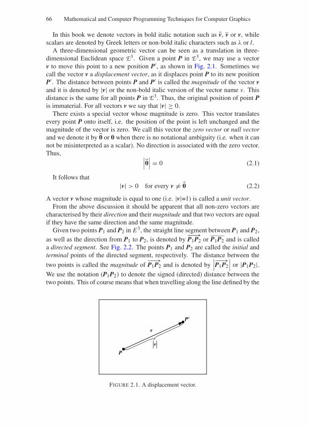
“Comninos” — 2005/8/31 — 18:32 — page 66 — #2
66 Mathematical and Computer Programming Techniques for Computer Graphics
In this book we denote vectors in bold italic notation such as v, v or v, whilescalars are denoted by Greek letters or non-bold italic characters such as λ or l.
A three-dimensional geometric vector can be seen as a translation in three-dimensional Euclidean space E3. Given a point P in E3, we may use a vectorv to move this point to a new position P′, as shown in Fig. 2.1. Sometimes wecall the vector v a displacement vector, as it displaces point P to its new positionP′. The distance between points P and P′ is called the magnitude of the vector vand it is denoted by |v| or the non-bold italic version of the vector name v. Thisdistance is the same for all points P in E3. Thus, the original position of point Pis immaterial. For all vectors v we say that |v| ≥ 0.
There exists a special vector whose magnitude is zero. This vector translatesevery point P onto itself, i.e. the position of the point is left unchanged and themagnitude of the vector is zero. We call this vector the zero vector or null vectorand we denote it by 0 or 0 when there is no notational ambiguity (i.e. when it cannot be misinterpreted as a scalar). No direction is associated with the zero vector.Thus, ∣∣∣0
∣∣∣ = 0 (2.1)
It follows that|v| > 0 for every v = 0 (2.2)
A vector v whose magnitude is equal to one (i.e. |v|=1) is called a unit vector.From the above discussion it should be apparent that all non-zero vectors are
characterised by their direction and their magnitude and that two vectors are equalif they have the same direction and the same magnitude.
Given two points P1 and P2 in E3, the straight line segment between P1 and P2,as well as the direction from P1 to P2, is denoted by
−−→P1P2 or P1P2 and is called
a directed segment. See Fig. 2.2. The points P1 and P2 are called the initial andterminal points of the directed segment, respectively. The distance between the
two points is called the magnitude of−−→P1P2 and is denoted by
∣∣∣−−→P1P2
∣∣∣ or |P1P2|.We use the notation (P1P2) to denote the signed (directed) distance between thetwo points. This of course means that when travelling along the line defined by the
P
P
v
v
FIGURE 2.1. A displacement vector.
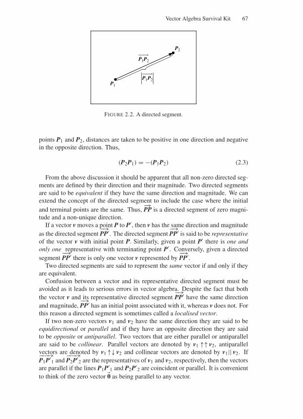
“Comninos” — 2005/8/31 — 18:32 — page 67 — #3
Vector Algebra Survival Kit 67
P1
P2P1
P2
P2P1
FIGURE 2.2. A directed segment.
points P1 and P2, distances are taken to be positive in one direction and negativein the opposite direction. Thus,
(P2P1) = −(P1P2) (2.3)
From the above discussion it should be apparent that all non-zero directed seg-ments are defined by their direction and their magnitude. Two directed segmentsare said to be equivalent if they have the same direction and magnitude. We canextend the concept of the directed segment to include the case where the initialand terminal points are the same. Thus,
−→PP is a directed segment of zero magni-
tude and a non-unique direction.If a vector v moves a point P to P′, then v has the same direction and magnitude
as the directed segment−→PP′. The directed segment
−→PP′ is said to be representative
of the vector v with initial point P. Similarly, given a point P′ there is one andonly one representative with terminating point P′. Conversely, given a directedsegment
−→PP′ there is only one vector v represented by
−→PP′.
Two directed segments are said to represent the same vector if and only if theyare equivalent.
Confusion between a vector and its representative directed segment must beavoided as it leads to serious errors in vector algebra. Despite the fact that boththe vector v and its representative directed segment
−→PP′ have the same direction
and magnitude,−→PP′ has an initial point associated with it, whereas v does not. For
this reason a directed segment is sometimes called a localised vector.If two non-zero vectors v1 and v2 have the same direction they are said to be
equidirectional or parallel and if they have an opposite direction they are saidto be opposite or antiparallel. Two vectors that are either parallel or antiparallelare said to be collinear. Parallel vectors are denoted by v1 ↑↑ v2, antiparallelvectors are denoted by v1 ↑↓ v2 and collinear vectors are denoted by v1|| v2. If−−−→P1P′
1 and−−−→P2P′
2 are the representatives of v1 and v2, respectively, then the vectorsare parallel if the lines P1P′
1 and P2P′2 are coincident or parallel. It is convenient
to think of the zero vector 0 as being parallel to any vector.
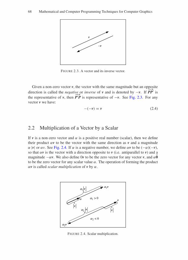
“Comninos” — 2005/8/31 — 18:32 — page 68 — #4
68 Mathematical and Computer Programming Techniques for Computer Graphics
v
−v
FIGURE 2.3. A vector and its inverse vector.
Given a non-zero vector v, the vector with the same magnitude but an oppositedirection is called the negative or inverse of v and is denoted by −v. If
−→PP′ is
the representative of v, then−→P′P is representative of −v. See Fig. 2.3. For any
vector v we have:
−(−v) = v (2.4)
2.2 Multiplication of a Vector by a Scalar
If v is a non-zero vector and α is a positive real number (scalar), then we definetheir product αv to be the vector with the same direction as v and a magnitudeα |v| or αv. See Fig. 2.4. If α is a negative number, we define αv to be (−α)(−v),so that αv is the vector with a direction opposite to v (i.e. antiparallel to v) and amagnitude −αv. We also define 0v to be the zero vector for any vector v, and α0to be the zero vector for any scalar value α. The operation of forming the productαv is called scalar multiplication of v by α.
v
v
v
vva2
a1v
a2v
va1
a1 > 0
a2 < 0
FIGURE 2.4. Scalar multiplication.
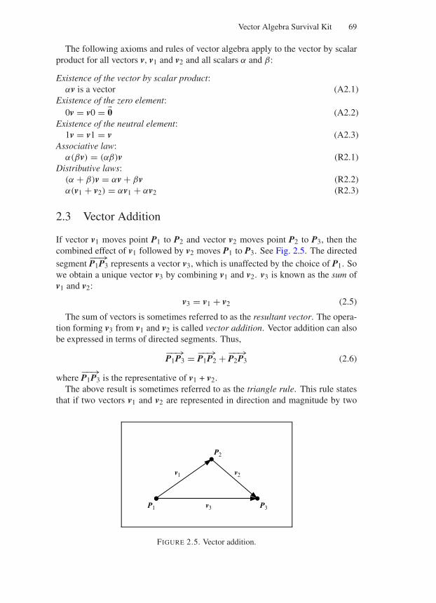
“Comninos” — 2005/8/31 — 18:32 — page 69 — #5
Vector Algebra Survival Kit 69
The following axioms and rules of vector algebra apply to the vector by scalarproduct for all vectors v, v1 and v2 and all scalars α and β:
Existence of the vector by scalar product:αv is a vector (A2.1)
Existence of the zero element:0v = v0 = 0 (A2.2)
Existence of the neutral element:1v = v1 = v (A2.3)
Associative law:α(βv) = (αβ)v (R2.1)
Distributive laws:(α + β)v = αv + βv (R2.2)α(v1 + v2) = αv1 + αv2 (R2.3)
2.3 Vector Addition
If vector v1 moves point P1 to P2 and vector v2 moves point P2 to P3, then thecombined effect of v1 followed by v2 moves P1 to P3. See Fig. 2.5. The directedsegment
−−→P1P3 represents a vector v3, which is unaffected by the choice of P1. So
we obtain a unique vector v3 by combining v1 and v2. v3 is known as the sum ofv1 and v2:
v3 = v1 + v2 (2.5)
The sum of vectors is sometimes referred to as the resultant vector. The opera-tion forming v3 from v1 and v2 is called vector addition. Vector addition can alsobe expressed in terms of directed segments. Thus,
−−→P1P3 = −−→
P1P2 + −−→P2P3 (2.6)
where−−→P1P3 is the representative of v1 + v2.
The above result is sometimes referred to as the triangle rule. This rule statesthat if two vectors v1 and v2 are represented in direction and magnitude by two
v1 v2
v3P1
P2
P3
FIGURE 2.5. Vector addition.
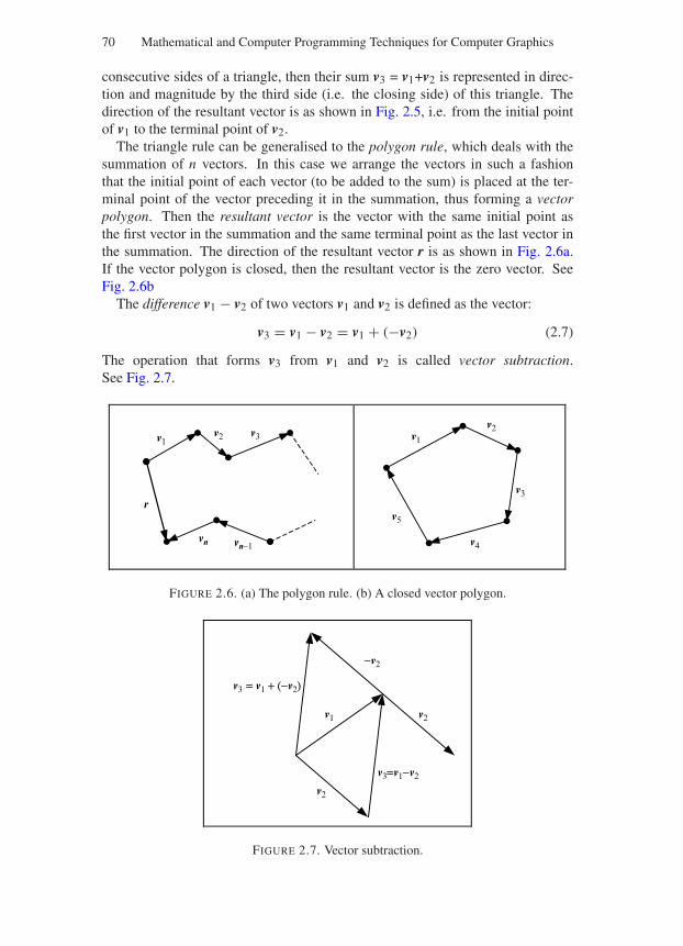
“Comninos” — 2005/8/31 — 18:32 — page 70 — #6
70 Mathematical and Computer Programming Techniques for Computer Graphics
consecutive sides of a triangle, then their sum v3 = v1+v2 is represented in direc-tion and magnitude by the third side (i.e. the closing side) of this triangle. Thedirection of the resultant vector is as shown in Fig. 2.5, i.e. from the initial pointof v1 to the terminal point of v2.
The triangle rule can be generalised to the polygon rule, which deals with thesummation of n vectors. In this case we arrange the vectors in such a fashionthat the initial point of each vector (to be added to the sum) is placed at the ter-minal point of the vector preceding it in the summation, thus forming a vectorpolygon. Then the resultant vector is the vector with the same initial point asthe first vector in the summation and the same terminal point as the last vector inthe summation. The direction of the resultant vector r is as shown in Fig. 2.6a.If the vector polygon is closed, then the resultant vector is the zero vector. SeeFig. 2.6b
The difference v1 − v2 of two vectors v1 and v2 is defined as the vector:
v3 = v1 − v2 = v1 + (−v2) (2.7)
The operation that forms v3 from v1 and v2 is called vector subtraction.See Fig. 2.7.
v1v2 v3
r
vn vn-1
v1
v2
v3
v4
v5
FIGURE 2.6. (a) The polygon rule. (b) A closed vector polygon.
v1 v2
v3=v1−v2
−v2
v2
v3 = v1 + (−v2)
FIGURE 2.7. Vector subtraction.
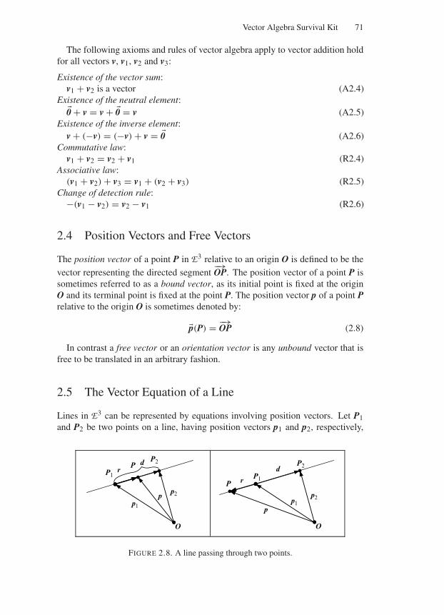
“Comninos” — 2005/8/31 — 18:32 — page 71 — #7
Vector Algebra Survival Kit 71
The following axioms and rules of vector algebra apply to vector addition holdfor all vectors v, v1, v2 and v3:
Existence of the vector sum:v1 + v2 is a vector (A2.4)
Existence of the neutral element:0 + v = v + 0 = v (A2.5)
Existence of the inverse element:v + (−v) = (−v) + v = 0 (A2.6)
Commutative law:v1 + v2 = v2 + v1 (R2.4)
Associative law:(v1 + v2) + v3 = v1 + (v2 + v3) (R2.5)
Change of detection rule:−(v1 − v2) = v2 − v1 (R2.6)
2.4 Position Vectors and Free Vectors
The position vector of a point P in E3 relative to an origin O is defined to be the
vector representing the directed segment−→OP. The position vector of a point P is
sometimes referred to as a bound vector, as its initial point is fixed at the originO and its terminal point is fixed at the point P. The position vector p of a point Prelative to the origin O is sometimes denoted by:
p(P) = −→OP (2.8)
In contrast a free vector or an orientation vector is any unbound vector that isfree to be translated in an arbitrary fashion.
2.5 The Vector Equation of a Line
Lines in E3 can be represented by equations involving position vectors. Let P1and P2 be two points on a line, having position vectors p1 and p2, respectively,
p1
p2p
O
P1r
P2P d
p1p2
p
O
P1r
P2
P
d
FIGURE 2.8. A line passing through two points.
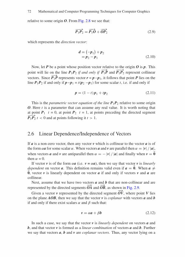
“Comninos” — 2005/8/31 — 18:32 — page 72 — #8
72 Mathematical and Computer Programming Techniques for Computer Graphics
relative to some origin O. From Fig. 2.8 we see that:
−−→P1P2 = −−→
P1O + −−→OP2 (2.9)
which represents the direction vector:
d = (−p1) + p2
= p2 − p1 (2.10)
Now, let P be a point whose position vector relative to the origin O is p. Thispoint will lie on the line P1P2 if and only if
−→P1P and
−−→P1P2 represent collinear
vectors. Since−→P1P represents vector r = p−p1, it follows that point P lies on the
line P1P2 if and only if p−p1 = t(p2 −p1) for some scalar t , i.e. if and only if
p = (1 − t) p1 + tp2 (2.11)
This is the parametric vector equation of the line P1P2 relative to some originO. Here t is a parameter that can assume any real value. It is worth noting thatat point P1 t = 0, at point P2 t = 1, at points preceding the directed segment−−→P1P2 t < 0 and at points following it t > 1.
2.6 Linear Dependence/Independence of Vectors
If a is a non-zero vector, then any vector v which is collinear to the vector a is ofthe form αa for some scalar α. When vectors a and v are parallel then α = |v| / |a|,when vectors a and v are antiparallel then α = − |v| / |a| and finally when v = 0then α = 0.
If vector v is of the form αa (i.e. v = αa), then we say that vector v is linearlydependent on vector a. This definition remains valid even if a = 0. When a =0, vector v is linearly dependent on vector a if and only if vectors v and a arecollinear.
Next, assume that we have two vectors a and b that are non-collinear and arerepresented by the directed segments
−→OA and
−→OB, as shown in Fig. 2.9.
Given a vector v represented by the directed segment−→OV, where point V lies
on the plane AOB, then we say that the vector v is coplanar with vectors a and bif and only if there exist scalars α and β such that:
v = αa + βb (2.12)
In such a case, we say that the vector v is linearly dependent on vectors a andb, and that vector v is formed as a linear combination of vectors a and b. Furtherwe say that vectors a, b and v are coplanar vectors. Thus, any vector lying on a
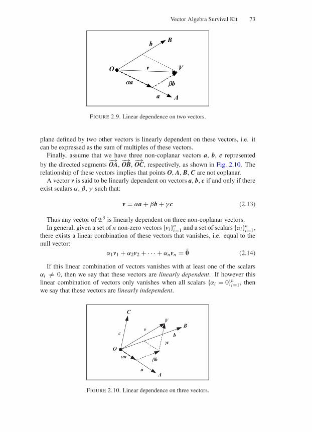
“Comninos” — 2005/8/31 — 18:32 — page 73 — #9
Vector Algebra Survival Kit 73
v
b
a
B
A
O V
aa bb
FIGURE 2.9. Linear dependence on two vectors.
plane defined by two other vectors is linearly dependent on these vectors, i.e. itcan be expressed as the sum of multiples of these vectors.
Finally, assume that we have three non-coplanar vectors a, b, c represented
by the directed segments−→OA,
−→OB,
−→OC, respectively, as shown in Fig. 2.10. The
relationship of these vectors implies that points O, A, B, C are not coplanar.A vector v is said to be linearly dependent on vectors a, b, c if and only if there
exist scalars α, β, γ such that:
v = αa + βb + γ c (2.13)
Thus any vector of E3 is linearly dependent on three non-coplanar vectors.In general, given a set of n non-zero vectors vi n
i=1 and a set of scalars αi ni=1,
there exists a linear combination of these vectors that vanishes, i.e. equal to thenull vector:
α1v1 + α2v2 + · · · + αnvn = 0 (2.14)
If this linear combination of vectors vanishes with at least one of the scalarsαi = 0, then we say that these vectors are linearly dependent. If however thislinear combination of vectors only vanishes when all scalars αi = 0n
i=1, thenwe say that these vectors are linearly independent.
vb
a
B
A
O
V
C
c
aa bb
gc
FIGURE 2.10. Linear dependence on three vectors.
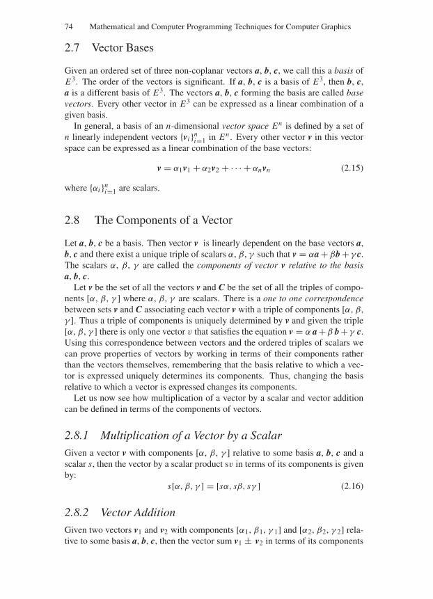
“Comninos” — 2005/8/31 — 18:32 — page 74 — #10
74 Mathematical and Computer Programming Techniques for Computer Graphics
2.7 Vector Bases
Given an ordered set of three non-coplanar vectors a, b, c, we call this a basis ofE3. The order of the vectors is significant. If a, b, c is a basis of E3, then b, c,a is a different basis of E3. The vectors a, b, c forming the basis are called basevectors. Every other vector in E3 can be expressed as a linear combination of agiven basis.
In general, a basis of an n-dimensional vector space En is defined by a set ofn linearly independent vectors vi n
i=1 in En . Every other vector v in this vectorspace can be expressed as a linear combination of the base vectors:
v = α1v1 + α2v2 + · · · + αnvn (2.15)
where αi ni=1 are scalars.
2.8 The Components of a Vector
Let a, b, c be a basis. Then vector v is linearly dependent on the base vectors a,b, c and there exist a unique triple of scalars α, β, γ such that v = αa + βb + γ c.The scalars α, β, γ are called the components of vector v relative to the basisa, b, c.
Let v be the set of all the vectors v and C be the set of all the triples of compo-nents [α, β, γ ] where α, β, γ are scalars. There is a one to one correspondencebetween sets v and C associating each vector v with a triple of components [α, β,γ ]. Thus a triple of components is uniquely determined by v and given the triple[α, β, γ ] there is only one vector v that satisfies the equation v = α a +β b + γ c.Using this correspondence between vectors and the ordered triples of scalars wecan prove properties of vectors by working in terms of their components ratherthan the vectors themselves, remembering that the basis relative to which a vec-tor is expressed uniquely determines its components. Thus, changing the basisrelative to which a vector is expressed changes its components.
Let us now see how multiplication of a vector by a scalar and vector additioncan be defined in terms of the components of vectors.
2.8.1 Multiplication of a Vector by a Scalar
Given a vector v with components [α, β, γ ] relative to some basis a, b, c and ascalar s, then the vector by a scalar product sv in terms of its components is givenby:
s[α, β, γ ] = [sα, sβ, sγ ] (2.16)
2.8.2 Vector Addition
Given two vectors v1 and v2 with components [α1, β1, γ 1] and [α2, β2, γ 2] rela-tive to some basis a, b, c, then the vector sum v1 ± v2 in terms of its components
“Comninos” — 2005/8/31 — 18:32 — page 75 — #11
Vector Algebra Survival Kit 75
is given by:
[α1, β1, γ1] ± [α2, β2, γ2] = [α1 ± α2, β1 ± β2, γ1 ± γ2] (2.17)
2.8.3 Vector Equality
Given two vectors v1 and v2 with components [α1, β1, γ 1] and [α2, β2, γ 2]relative to some basis a, b, c, then the vectors are said to be equal if their corre-sponding components are equal, i.e.
[α1, β1, γ1] = [α2, β2, γ2] ⇔ α1 = α2 ∧ β1 = β2 ∧ γ1 = γ2 (2.18)
The components [α, β, γ ] of a vector v can either be written in row or in columnform, i.e.
[α, β, γ ] or
⎡
⎣α
β
γ
⎤
⎦
The row form is said to be the transpose of the column form and vice versa, i.e.
[α, β, γ ]T =⎡
⎣α
β
γ
⎤
⎦ and
⎡
⎣α
β
γ
⎤
⎦
T
= [α, β, γ ]
These two representations are equivalent and the choice of one over the otheris a matter of taste.
2.9 Orthogonal, Orthonormal and Right-Handed VectorBases
A basis is said to be orthogonal if its base vectors are mutually perpendicular andit is said to be orthonormal if its base vectors are mutually perpendicular unitvectors.
Given an orthogonal basis a, b, c and any vector v, the directed segments−→OA,
−→OB,
−→OC,
−→OV represent the a, b, c, v vectors, respectively, as shown in
Fig. 2.11.Let P be the foot of the perpendicular from point V to the plane AOB (i.e. the
projection of point V on the plane AOB) and let Q be the foot of the perpendicularfrom point P to the line OA. From this figure we see that:
−→OV = −→
OQ + −→QP + −→
PV (2.19)
If vector v has components [α, β, γ ] relative to the orthogonal basis a, b, c,
then−→OV represents the vector sum α a + β b + γ c. But the directed segments−→
OQ,−→QP,
−→PV have the same directions as a, b, c, respectively. Thus
−→OQ,
−→QP,
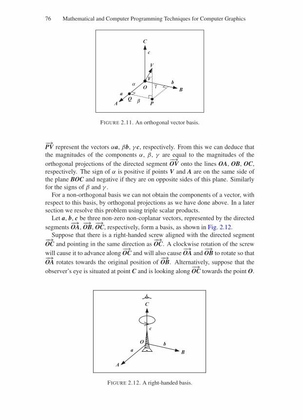
“Comninos” — 2005/8/31 — 18:32 — page 76 — #12
76 Mathematical and Computer Programming Techniques for Computer Graphics
b
aB
A
O
V
C
c
PQ b
a γV
FIGURE 2.11. An orthogonal vector basis.
−→PV represent the vectors αa, βb, γ c, respectively. From this we can deduce thatthe magnitudes of the components α, β, γ are equal to the magnitudes of the
orthogonal projections of the directed segment−→OV onto the lines OA, OB, OC,
respectively. The sign of α is positive if points V and A are on the same side ofthe plane BOC and negative if they are on opposite sides of this plane. Similarlyfor the signs of β and γ .
For a non-orthogonal basis we can not obtain the components of a vector, withrespect to this basis, by orthogonal projections as we have done above. In a latersection we resolve this problem using triple scalar products.
Let a, b, c be three non-zero non-coplanar vectors, represented by the directed
segments−→OA,
−→OB,
−→OC, respectively, form a basis, as shown in Fig. 2.12.
Suppose that there is a right-handed screw aligned with the directed segment−→OC and pointing in the same direction as
−→OC. A clockwise rotation of the screw
will cause it to advance along−→OC and will also cause
−→OA and
−→OB to rotate so that−→
OA rotates towards the original position of−→OB. Alternatively, suppose that the
observer’s eye is situated at point C and is looking along−→OC towards the point O.
ba B
A
O
C
c
FIGURE 2.12. A right-handed basis.
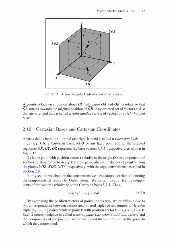
“Comninos” — 2005/8/31 — 18:32 — page 77 — #13
Vector Algebra Survival Kit 77
vj
iY
X
O
V
Z
k
Vxy
YOZ
vxXOZ
XOY
vy
vz
FIGURE 2.13. A rectangular Cartesian coordinate system.
A counter-clockwise rotation about−→OC will cause
−→OA and
−→OB to rotate so that−→
OA rotates towards the original position of−→OB. Any ordered set of vectors a, b, c
that are arranged thus is called a right-handed system of vectors or a right-handedbasis.
2.10 Cartesian Bases and Cartesian Coordinates
A basis that is both orthonormal and right-handed is called a Cartesian basis.Let i, j, k be a Cartesian basis, let O be any fixed point and let the directed
segments−→OX,
−→OY,
−→OZ represent the base vectors i, j, k, respectively, as shown in
Fig. 2.13.If v is the point with position vector v relative to the origin O, the components of
vector v relative to the basis i, j, k are the perpendicular distances of point V fromthe planes YOZ, XOZ, XOY, respectively, with the sign conventions described inSection 2.9.
In this section we abandon the conventions we have adopted earlier of denotingthe components of vectors by Greek letters. We write vx , vy , vz for the compo-nents of the vector v relative to some Cartesian basis i, j, k. Thus,
v = vx i + vy j + vzk (2.20)
By expressing the position vectors of points in this way, we establish a one toone correspondence between vectors and ordered triples of real numbers. Here thetriple
[vx , vy, vz
]corresponds to point V with position vector v = vx i+ vy j+ vzk.
Such a correspondence is called a rectangular Cartesian coordinate system andthe components of the position vector are called the coordinates of the point towhich they correspond.
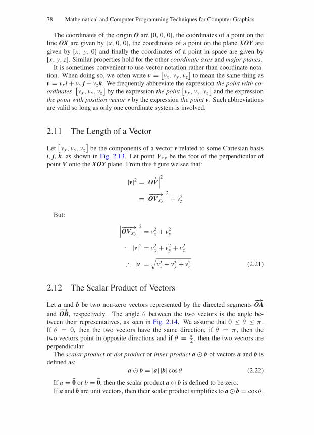
“Comninos” — 2005/8/31 — 18:32 — page 78 — #14
78 Mathematical and Computer Programming Techniques for Computer Graphics
The coordinates of the origin O are [0, 0, 0], the coordinates of a point on theline OX are given by [x , 0, 0], the coordinates of a point on the plane XOY aregiven by [x , y, 0] and finally the coordinates of a point in space are given by[x , y, z]. Similar properties hold for the other coordinate axes and major planes.
It is sometimes convenient to use vector notation rather than coordinate nota-tion. When doing so, we often write v = [
vx , vy, vz]
to mean the same thing asv = vx i + vy j + vzk. We frequently abbreviate the expression the point with co-ordinates
[vx , vy, vz
]by the expression the point
[vx , vy, vz
]and the expression
the point with position vector v by the expression the point v. Such abbreviationsare valid so long as only one coordinate system is involved.
2.11 The Length of a Vector
Let[vx , vy, vz
]be the components of a vector v related to some Cartesian basis
i, j, k, as shown in Fig. 2.13. Let point Vxy be the foot of the perpendicular ofpoint V onto the XOY plane. From this figure we see that:
|v|2 =∣∣∣−→OV
∣∣∣2
=∣∣∣−−−→OVxy
∣∣∣2 + v2
z
But:∣∣∣−−−→OVxy
∣∣∣2 = v2
x + v2y
∴ |v|2 = v2x + v2
y + v2z
∴ |v| =√
v2x + v2
y + v2z (2.21)
2.12 The Scalar Product of Vectors
Let a and b be two non-zero vectors represented by the directed segments−→OA
and−→OB, respectively. The angle θ between the two vectors is the angle be-
tween their representatives, as seen in Fig. 2.14. We assume that 0 ≤ θ ≤ π .If θ = 0, then the two vectors have the same direction, if θ = π , then thetwo vectors point in opposite directions and if θ = π
2 , then the two vectors areperpendicular.
The scalar product or dot product or inner product a b of vectors a and b isdefined as:
a b = |a| |b| cos θ (2.22)
If a = 0 or b = 0, then the scalar product a b is defined to be zero.If a and b are unit vectors, then their scalar product simplifies to a b = cos θ .
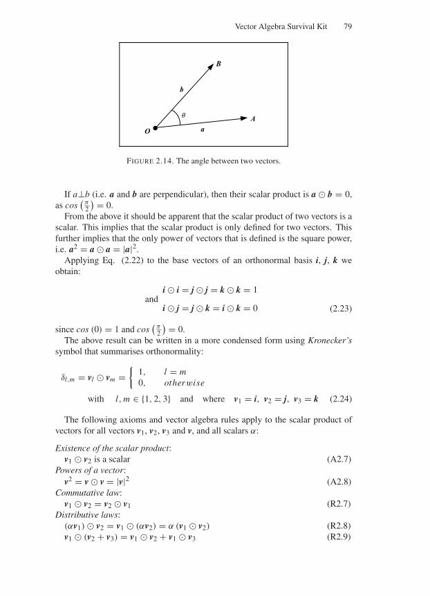
“Comninos” — 2005/8/31 — 18:32 — page 79 — #15
Vector Algebra Survival Kit 79
a
b
O
A
B
q
FIGURE 2.14. The angle between two vectors.
If a⊥b (i.e. a and b are perpendicular), then their scalar product is a b = 0,as cos
(π2
) = 0.From the above it should be apparent that the scalar product of two vectors is a
scalar. This implies that the scalar product is only defined for two vectors. Thisfurther implies that the only power of vectors that is defined is the square power,i.e. a2 = a a = |a|2.
Applying Eq. (2.22) to the base vectors of an orthonormal basis i, j, k weobtain:
andi i = j j = k k = 1
i j = j k = i k = 0 (2.23)
since cos (0) = 1 and cos(
π2
) = 0.The above result can be written in a more condensed form using Kronecker’s
symbol that summarises orthonormality:
δl,m = vl vm =
1,
0,
l = motherwise
with l, m ∈ 1, 2, 3 and where v1 = i, v2 = j, v3 = k (2.24)
The following axioms and vector algebra rules apply to the scalar product ofvectors for all vectors v1, v2, v3 and v, and all scalars α:
Existence of the scalar product:v1 v2 is a scalar (A2.7)
Powers of a vector:v2 = v v = |v|2 (A2.8)
Commutative law:v1 v2 = v2 v1 (R2.7)
Distributive laws:(αv1) v2 = v1 (αv2) = α (v1 v2) (R2.8)v1 (v2 + v3) = v1 v2 + v1 v3 (R2.9)
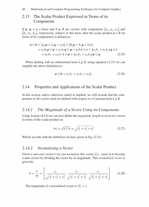
“Comninos” — 2005/8/31 — 18:32 — page 80 — #16
80 Mathematical and Computer Programming Techniques for Computer Graphics
2.13 The Scalar Product Expressed in Terms of itsComponents
If p, q, r is a basis and if a, b are vectors with components[ax , ay, az
]and[
bx , by, bz], respectively, relative to this basis, then the scalar product a b (in
terms of its components) is defined as:
a b = (ax p + ayq + azr
) (bx p + byq + bzr
)
= ax bx p p + aybyq q + azbzr r + (aybz + azby
)q r
+ (azbx + ax bz) r p + (ax by + aybx
)p q (2.25)
When dealing with an orthonormal basis i, j, k, using equation (2.23) we cansimplify the above definition to:
a b = ax bx + ayby + azbz (2.26)
2.14 Properties and Applications of the Scalar Product
In this section, unless otherwise stated or implied, we will assume that the com-ponents of all vectors used are defined with respect to a Cartesian basis i, j, k.
2.14.1 The Magnitude of a Vector Using its Components
Using Axiom (A2.8) we can now define the magnitude, length or norm of a vectorin terms of the scalar product as:
|v| = √v v =
√v2
x + v2y + v2
z (2.27)
Which accords with the definition we have given in Eq. (2.21).
2.14.2 Normalising a Vector
Given a non-zero vector v we can normalise this vector (i.e. cause it to becomea unit-vector) by dividing the vector by its magnitude. This normalised vector isgiven by:
v = v|v| =
⎡
⎣ vx√v2
x + v2y + v2
z
,vy√
v2x + v2
y + v2z
,vz√
v2x + v2
y + v2z
⎤
⎦ (2.28)
The magnitude of a normalised vector is∣∣v
∣∣ = 1.
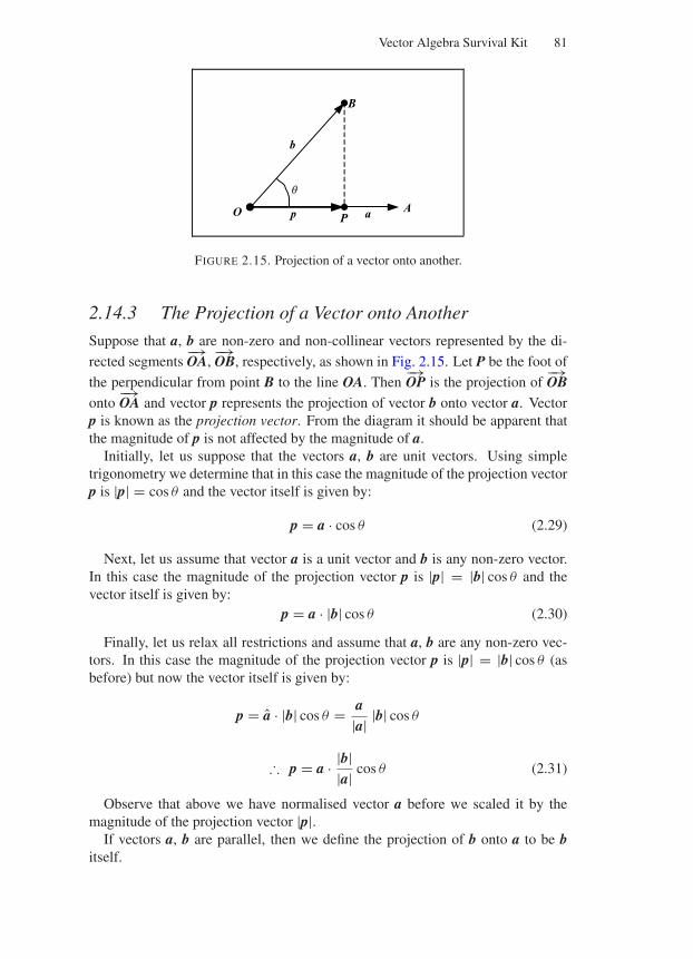
“Comninos” — 2005/8/31 — 18:32 — page 81 — #17
Vector Algebra Survival Kit 81
a
b
O A
B
p P
q
FIGURE 2.15. Projection of a vector onto another.
2.14.3 The Projection of a Vector onto Another
Suppose that a, b are non-zero and non-collinear vectors represented by the di-
rected segments−→OA,
−→OB, respectively, as shown in Fig. 2.15. Let P be the foot of
the perpendicular from point B to the line OA. Then−→OP is the projection of
−→OB
onto−→OA and vector p represents the projection of vector b onto vector a. Vector
p is known as the projection vector. From the diagram it should be apparent thatthe magnitude of p is not affected by the magnitude of a.
Initially, let us suppose that the vectors a, b are unit vectors. Using simpletrigonometry we determine that in this case the magnitude of the projection vectorp is |p| = cos θ and the vector itself is given by:
p = a · cos θ (2.29)
Next, let us assume that vector a is a unit vector and b is any non-zero vector.In this case the magnitude of the projection vector p is |p| = |b| cos θ and thevector itself is given by:
p = a · |b| cos θ (2.30)
Finally, let us relax all restrictions and assume that a, b are any non-zero vec-tors. In this case the magnitude of the projection vector p is |p| = |b| cos θ (asbefore) but now the vector itself is given by:
p = a · |b| cos θ = a|a| |b| cos θ
∴ p = a · |b||a| cos θ (2.31)
Observe that above we have normalised vector a before we scaled it by themagnitude of the projection vector |p|.
If vectors a, b are parallel, then we define the projection of b onto a to be bitself.
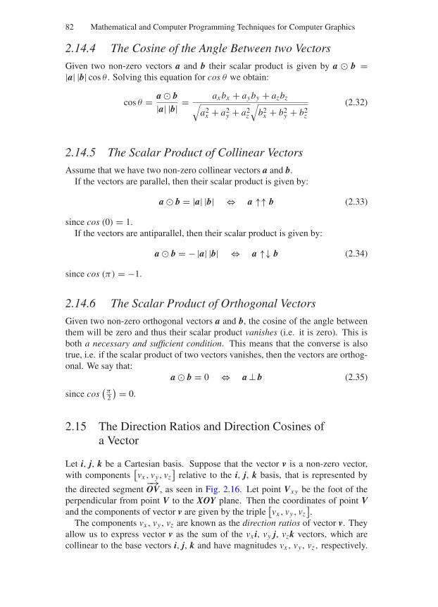
“Comninos” — 2005/8/31 — 18:32 — page 82 — #18
82 Mathematical and Computer Programming Techniques for Computer Graphics
2.14.4 The Cosine of the Angle Between two Vectors
Given two non-zero vectors a and b their scalar product is given by a b =|a| |b| cos θ . Solving this equation for cos θ we obtain:
cos θ = a b|a| |b| = ax bx + ayby + azbz√
a2x + a2
y + a2z
√b2
x + b2y + b2
z
(2.32)
2.14.5 The Scalar Product of Collinear Vectors
Assume that we have two non-zero collinear vectors a and b.If the vectors are parallel, then their scalar product is given by:
a b = |a| |b| ⇔ a ↑↑ b (2.33)
since cos (0) = 1.If the vectors are antiparallel, then their scalar product is given by:
a b = − |a| |b| ⇔ a ↑↓ b (2.34)
since cos (π) = −1.
2.14.6 The Scalar Product of Orthogonal Vectors
Given two non-zero orthogonal vectors a and b, the cosine of the angle betweenthem will be zero and thus their scalar product vanishes (i.e. it is zero). This isboth a necessary and sufficient condition. This means that the converse is alsotrue, i.e. if the scalar product of two vectors vanishes, then the vectors are orthog-onal. We say that:
a b = 0 ⇔ a ⊥ b (2.35)
since cos(
π2
) = 0.
2.15 The Direction Ratios and Direction Cosines ofa Vector
Let i, j, k be a Cartesian basis. Suppose that the vector v is a non-zero vector,with components
[vx , vy, vz
]relative to the i, j, k basis, that is represented by
the directed segment−→OV, as seen in Fig. 2.16. Let point Vxy be the foot of the
perpendicular from point V to the XOY plane. Then the coordinates of point Vand the components of vector v are given by the triple
[vx , vy, vz
].
The components vx , vy , vz are known as the direction ratios of vector v. Theyallow us to express vector v as the sum of the vx i, vy j, vzk vectors, which arecollinear to the base vectors i, j, k and have magnitudes vx , vy , vz, respectively.
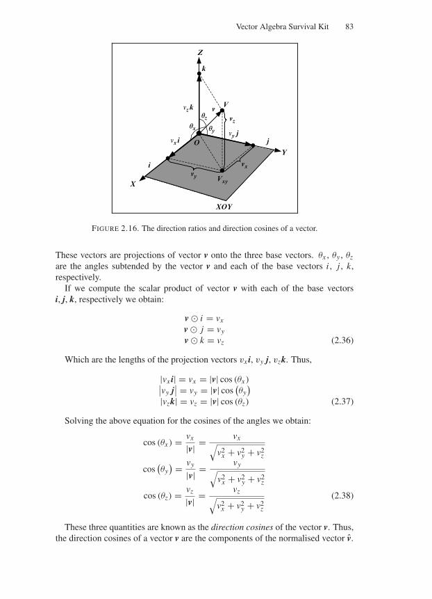
“Comninos” — 2005/8/31 — 18:32 — page 83 — #19
Vector Algebra Survival Kit 83
v
j
i
Y
X
O
V
Z
k
Vxy
vx
XOY
vy
vz
vx i
vy j
vz k
qx qy
qz
FIGURE 2.16. The direction ratios and direction cosines of a vector.
These vectors are projections of vector v onto the three base vectors. θx , θy , θz
are the angles subtended by the vector v and each of the base vectors i , j , k,respectively.
If we compute the scalar product of vector v with each of the base vectorsi, j, k, respectively we obtain:
v i = vx
v j = vy
v k = vz (2.36)
Which are the lengths of the projection vectors vx i, vy j, vzk. Thus,
|vx i| = vx = |v| cos (θx )∣∣vy j∣∣ = vy = |v| cos
(θy
)
|vzk| = vz = |v| cos (θz) (2.37)
Solving the above equation for the cosines of the angles we obtain:
cos (θx ) = vx
|v| = vx√v2
x + v2y + v2
z
cos(θy
) = vy
|v| = vy√v2
x + v2y + v2
z
cos (θz) = vz
|v| = vz√v2
x + v2y + v2
z
(2.38)
These three quantities are known as the direction cosines of the vector v. Thus,the direction cosines of a vector v are the components of the normalised vector v.
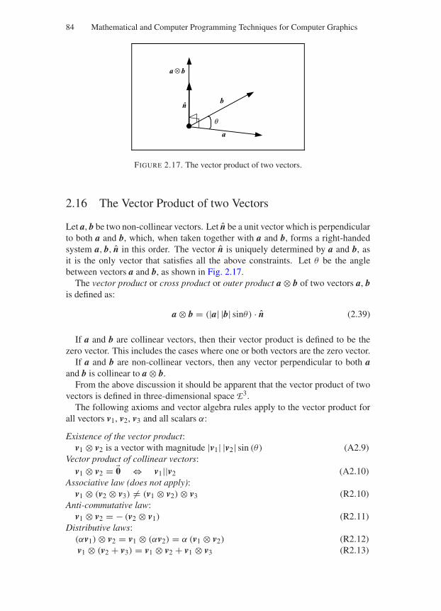
“Comninos” — 2005/8/31 — 18:32 — page 84 — #20
84 Mathematical and Computer Programming Techniques for Computer Graphics
a
bn
a ⊗ b
q
FIGURE 2.17. The vector product of two vectors.
2.16 The Vector Product of two Vectors
Let a, b be two non-collinear vectors. Let n be a unit vector which is perpendicularto both a and b, which, when taken together with a and b, forms a right-handedsystem a, b, n in this order. The vector n is uniquely determined by a and b, asit is the only vector that satisfies all the above constraints. Let θ be the anglebetween vectors a and b, as shown in Fig. 2.17.
The vector product or cross product or outer product a ⊗ b of two vectors a, bis defined as:
a ⊗ b = (|a| |b| sinθ) · n (2.39)
If a and b are collinear vectors, then their vector product is defined to be thezero vector. This includes the cases where one or both vectors are the zero vector.
If a and b are non-collinear vectors, then any vector perpendicular to both aand b is collinear to a ⊗ b.
From the above discussion it should be apparent that the vector product of twovectors is defined in three-dimensional space E3.
The following axioms and vector algebra rules apply to the vector product forall vectors v1, v2, v3 and all scalars α:
Existence of the vector product:v1 ⊗ v2 is a vector with magnitude |v1| |v2| sin (θ) (A2.9)
Vector product of collinear vectors:v1 ⊗ v2 = 0 ⇔ v1||v2 (A2.10)
Associative law (does not apply):v1 ⊗ (v2 ⊗ v3) = (v1 ⊗ v2) ⊗ v3 (R2.10)
Anti-commutative law:v1 ⊗ v2 = − (v2 ⊗ v1) (R2.11)
Distributive laws:(αv1) ⊗ v2 = v1 ⊗ (αv2) = α (v1 ⊗ v2) (R2.12)v1 ⊗ (v2 + v3) = v1 ⊗ v2 + v1 ⊗ v3 (R2.13)
“Comninos” — 2005/8/31 — 18:32 — page 85 — #21
Vector Algebra Survival Kit 85
Given a Cartesian basis i, j, k, then the vector products of combinations of itsbase vectors are given by:
i ⊗ i = j ⊗ j = k ⊗ k = 0 (N.B. This result is also true for any basis) (2.40)
i ⊗ j = k, j ⊗ k = i, k ⊗ i = j (2.41)
j ⊗ i = −k, k ⊗ j = −i, i ⊗ k = −j (2.42)
2.17 The Vector Product Expressed in Terms of itsComponents
If p, q, r is a right-handed basis and if a, b are vectors with components[ax , ay, az
]
and[bx , by, bz
], respectively, relative to this basis, then the vector product a ⊗ b
(in terms of its components) is defined as:
a ⊗ b = (ax p + ayq + azr
) ⊗ (bx p + byq + bzr
)
= ax p ⊗ bx p + ax p ⊗ byq + ax p ⊗ bzr
+ ayq ⊗ bx p + ayq ⊗ byq + ayq ⊗ bzr
+ azr ⊗ bx p + azr ⊗ byq + azr ⊗ bzr
= ax bx p ⊗ p + aybyq ⊗ q + azbzr ⊗ r
+ (aybzq ⊗ r + azbyr ⊗ q
) + (azbx r ⊗ p + ax bzp ⊗ r)
+ (ax byp ⊗ q + aybx q ⊗ p
)
Using the anti-commutative law (R2.11) and since p ⊗ p = 0, q ⊗ q = 0 andr ⊗ r = 0 we can simplify the above expression to:
a⊗b = (aybz − azby
)q⊗r+(azbx − ax bz) r⊗p+(
ax by − aybx)
p⊗q (2.43)
The above definition of the vector product applies to any right-handed basisp, q, r. When dealing with a Cartesian basis i, j, k using Eq. (2.41) we can furthersimplify the above definition to:
a ⊗ b = (aybz − azby
)i + (azbx − ax bz) j + (
ax by − aybx)
k (2.44)
Thus, the vector product a ⊗ b is a vector with components:
a ⊗ b = [(aybz − azby
), (azbx − ax bz) ,
(ax by − aybx
)](2.45)
Alternatively:
a ⊗ b =⎡
⎣ax
ay
az
⎤
⎦ ⊗⎡
⎣bx
by
bz
⎤
⎦ =⎡
⎣aybz − azby
azbx − ax bz
ax by − aybx
⎤
⎦ (2.46)
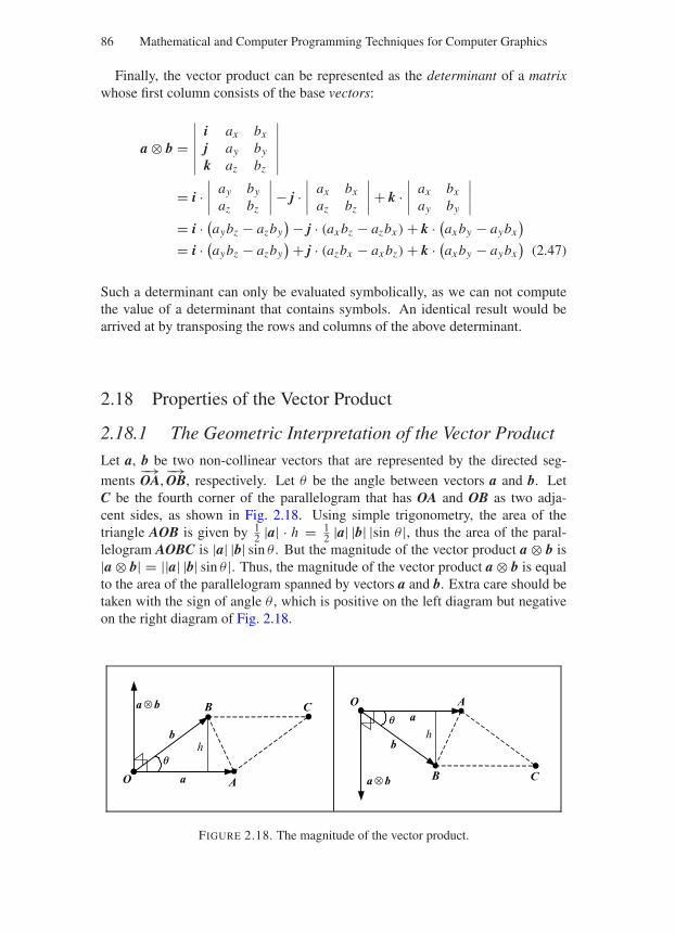
“Comninos” — 2005/8/31 — 18:32 — page 86 — #22
86 Mathematical and Computer Programming Techniques for Computer Graphics
Finally, the vector product can be represented as the determinant of a matrixwhose first column consists of the base vectors:
a ⊗ b =∣∣∣∣∣∣
i ax bx
j ay by
k az bz
∣∣∣∣∣∣
= i ·∣∣∣∣
ay by
az bz
∣∣∣∣ − j ·∣∣∣∣
ax bx
az bz
∣∣∣∣ + k ·∣∣∣∣
ax bx
ay by
∣∣∣∣
= i · (aybz − azby
) − j · (ax bz − azbx ) + k · (ax by − aybx
)
= i · (aybz − azby
) + j · (azbx − ax bz) + k · (ax by − aybx
)(2.47)
Such a determinant can only be evaluated symbolically, as we can not computethe value of a determinant that contains symbols. An identical result would bearrived at by transposing the rows and columns of the above determinant.
2.18 Properties of the Vector Product
2.18.1 The Geometric Interpretation of the Vector Product
Let a, b be two non-collinear vectors that are represented by the directed seg-
ments−→OA,
−→OB, respectively. Let θ be the angle between vectors a and b. Let
C be the fourth corner of the parallelogram that has OA and OB as two adja-cent sides, as shown in Fig. 2.18. Using simple trigonometry, the area of thetriangle AOB is given by 1
2 |a| · h = 12 |a| |b| |sin θ |, thus the area of the paral-
lelogram AOBC is |a| |b| sin θ . But the magnitude of the vector product a ⊗ b is|a ⊗ b| = ||a| |b| sin θ |. Thus, the magnitude of the vector product a ⊗ b is equalto the area of the parallelogram spanned by vectors a and b. Extra care should betaken with the sign of angle θ , which is positive on the left diagram but negativeon the right diagram of Fig. 2.18.
a
b
a ⊗ b
a ⊗ bO A
B C
h
a
b
O A
B C
h
q
q
FIGURE 2.18. The magnitude of the vector product.
“Comninos” — 2005/8/31 — 18:32 — page 87 — #23
Vector Algebra Survival Kit 87
2.18.2 The Magnitude of the Vector Product in Terms ofits Components
As we have seen in Eq. (2.45), given two non-collinear vectors a and b withcomponents
[ax , ay, az
]and
[bx , by, bz
]relative to a Cartesian basis i, j, k, the
components of their vector product are:
a ⊗ b = [(aybz − azby
), (azbx − ax bz) ,
(ax by − aybx
)]
Thus the magnitude of the vector product a ⊗ b, in terms of the components ofa and b, is given by:
|a ⊗ b| =√(
aybz − azby)2 + (azbx − ax bz)
2 + (ax by − aybx
)2 (2.48)
2.18.3 The Square of the Magnitude of the Vector Product
Given two non-collinear vectors a and b, the square of the magnitude of theirvector product a ⊗ b is given by:
|a ⊗ b|2 = |a|2 |b|2 sin2 θ
= |a|2 |b|2(
1 − cos2 θ)
= |a|2 |b|2 − (|a| |b| cos θ)2
= |a|2 |b|2 − (a b)2
∴ |a ⊗ b|2 = |a|2 |b|2 − (a b)2 (2.49)
2.18.4 The Magnitude of the Sine of the Angle betweenTwo Vectors
Given two non-zero and non-collinear vectors a and b, the magnitude of theirvector product a ⊗ b is given by:
|a ⊗ b| = ||a| |b | sin θ |Solving this equation for |sin θ | we obtain:
|sin θ | = |a ⊗ b||a| |b| (2.50)
If the components of the vectors a and b are defined relative to a Cartesian basisi, j, k, then |sin (θ)| is given by:
|sin θ | = |a ⊗ b||a | |b| =
√(aybz − azby
)2 + (azbx − ax bz)2 + (
ax by − aybx)2
√a2
x + a2y + a2
z
√b2
x + b2y + b2
z
(2.51)
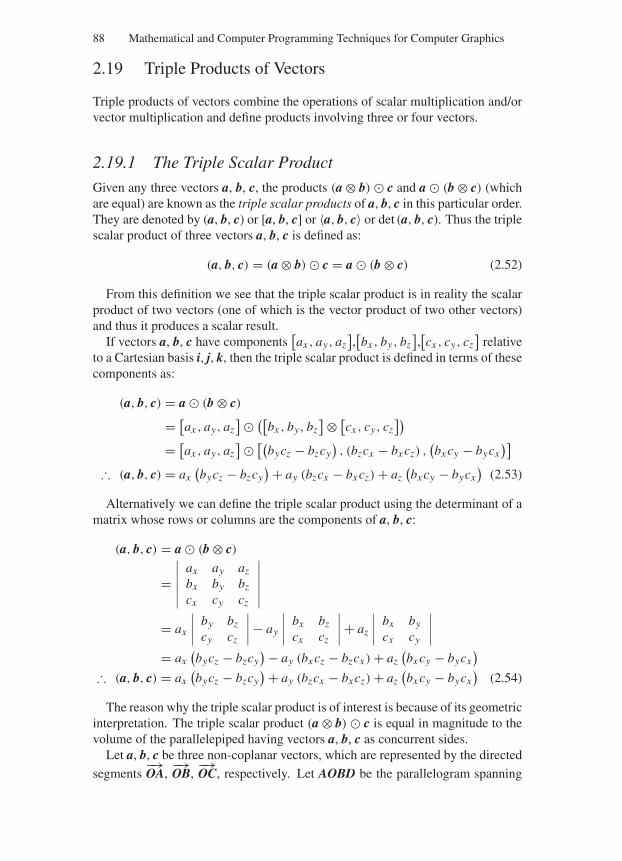
“Comninos” — 2005/8/31 — 18:32 — page 88 — #24
88 Mathematical and Computer Programming Techniques for Computer Graphics
2.19 Triple Products of Vectors
Triple products of vectors combine the operations of scalar multiplication and/orvector multiplication and define products involving three or four vectors.
2.19.1 The Triple Scalar Product
Given any three vectors a, b, c, the products (a ⊗ b) c and a (b ⊗ c) (whichare equal) are known as the triple scalar products of a, b, c in this particular order.They are denoted by (a, b, c) or [a, b, c] or 〈a, b, c〉 or det (a, b, c). Thus the triplescalar product of three vectors a, b, c is defined as:
(a, b, c) = (a ⊗ b) c = a (b ⊗ c) (2.52)
From this definition we see that the triple scalar product is in reality the scalarproduct of two vectors (one of which is the vector product of two other vectors)and thus it produces a scalar result.
If vectors a, b, c have components[ax , ay, az
],[bx , by, bz
],[cx , cy, cz
]relative
to a Cartesian basis i, j, k, then the triple scalar product is defined in terms of thesecomponents as:
(a, b, c) = a (b ⊗ c)
= [ax , ay, az
] ([bx , by, bz
] ⊗ [cx , cy, cz
])
= [ax , ay, az
] [(bycz − bzcy
), (bzcx − bx cz) ,
(bx cy − bycx
)]
∴ (a, b, c) = ax(bycz − bzcy
) + ay (bzcx − bx cz) + az(bx cy − bycx
)(2.53)
Alternatively we can define the triple scalar product using the determinant of amatrix whose rows or columns are the components of a, b, c:
(a, b, c) = a (b ⊗ c)
=∣∣∣∣∣∣
ax ay az
bx by bz
cx cy cz
∣∣∣∣∣∣
= ax
∣∣∣∣by bz
cy cz
∣∣∣∣ − ay
∣∣∣∣bx bz
cx cz
∣∣∣∣ + az
∣∣∣∣bx by
cx cy
∣∣∣∣
= ax(bycz − bzcy
) − ay (bx cz − bzcx ) + az(bx cy − bycx
)
∴ (a, b, c) = ax(bycz − bzcy
) + ay (bzcx − bx cz) + az(bx cy − bycx
)(2.54)
The reason why the triple scalar product is of interest is because of its geometricinterpretation. The triple scalar product (a ⊗ b) c is equal in magnitude to thevolume of the parallelepiped having vectors a, b, c as concurrent sides.
Let a, b, c be three non-coplanar vectors, which are represented by the directed
segments−→OA,
−→OB,
−→OC, respectively. Let AOBD be the parallelogram spanning
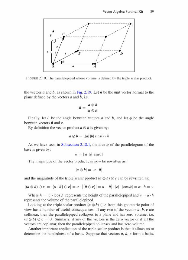
“Comninos” — 2005/8/31 — 18:32 — page 89 — #25
Vector Algebra Survival Kit 89
a
b
n
O A
B
C
D
c
h
q
f
FIGURE 2.19. The parallelepiped whose volume is defined by the triple scalar product.
the vectors a and b, as shown in Fig. 2.19. Let n be the unit vector normal to theplane defined by the vectors a and b, i.e.
n = a ⊗ b|a ⊗ b|
Finally, let θ be the angle between vectors a and b, and let φ be the anglebetween vectors n and c.
By definition the vector product a ⊗ b is given by:
a ⊗ b = (|a| |b| sin θ) · n
As we have seen in Subsection 2.18.1, the area α of the parallelogram of thebase is given by:
α = ||a| |b| sin θ |The magnitude of the vector product can now be rewritten as:
|a ⊗ b| = ∣∣α · n∣∣
and the magnitude of the triple scalar product (a ⊗ b) c can be rewritten as:
|(a ⊗ b) c| = ∣∣(α · n) c
∣∣ = α · ∣∣(n c)∣∣ = α · ∣
∣n∣∣ · |c| · |cos φ| = α · h = ν
Where h = |c| · |cos φ| represents the height of the parallelepiped and ν = α ·hrepresents the volume of the parallelepiped.
Looking at the triple scalar product (a ⊗ b) c from this geometric point ofview has a number of useful consequences. If any two of the vectors a, b, c arecollinear, then the parallelepiped collapses to a plane and has zero volume, i.e.(a ⊗ b) c = 0. Similarly, if any of the vectors is the zero vector or if all thevectors are coplanar, then the parallelepiped collapses and has zero volume.
Another important application of the triple scalar product is that it allows us todetermine the handedness of a basis. Suppose that vectors a, b, c form a basis.
“Comninos” — 2005/8/31 — 18:32 — page 90 — #26
90 Mathematical and Computer Programming Techniques for Computer Graphics
This implies that (a, b, c) = 0. If (a, b, c) > 0, then this basis is right-handed.Alternatively, if (a, b, c) < 0, then it is left-handed. Thus, the basis i, j, k isright-handed, while the basis i, j, k is left-handed.
The following axioms and vector algebra rules apply to the triple scalar productfor all vectors v1, v2, v3:
Existence of the triple scalar product:(v1, v2, v3) is a scalar (A2.11)
Triple scalar product of coplanar vectors:i f all v1, v2, v3 are coplanar ⇒ (v1, v2, v3) = 0 (A2.12)
Triple scalar product of zero vectors:v1 = 0 ∨ v2 = 0 ∨ v3 = 0 ⇒ (v1, v2, v3) = 0 (A2.13)
Triple scalar product of collinear vectors:v1||v2 ∨ v2||v3 ∨ v3||v1 ⇒ (v1, v2, v3) = 0 (A2.14)
Cyclic permutation rule:(v1, v2, v3) = (v2, v3, v1) = (v3, v1, v2) (R2.14)i.e., v1 (v2 ⊗ v3) = v2 (v3 ⊗ v1) = v3 (v1 ⊗ v2)
and (v1 ⊗ v2) v3 = (v2 ⊗ v3) v1 = (v3 ⊗ v1) v2Non-cyclic permutation rule:
(v2, v1, v3) = (v3, v2, v1) = (v1, v3, v2) = − (v1, v2, v3) (R2.15)
2.19.2 The Triple Vector Product
Given any three vectors a, b, c, the products (a ⊗ b) ⊗ c and a ⊗ (b ⊗ c) (whichare not equal in general) are known as the triple vector products of a, b, c inthis particular order. If vectors a, b, c have components
[ax , ay, az
],[bx , by, bz
],[
cx , cy, cz]
relative to a Cartesian basis i, j, k, then the triple vector product isdefined in terms of these components as:
(a ⊗ b) ⊗ c = ([ax , ay, az
] ⊗ [bx , by, bz
]) ⊗ [cx , cy, cz
]
= [(aybz − azby
), (azbx − ax bz) ,
(ax by − aybx
)] ⊗ [cx , cy, cz
]
∴ (a ⊗ b) ⊗ c =⎡
⎢⎣
(azbx − ax bz) cz − (ax by − aybx
)cy(
ax by − aybx)
cx − (aybz − azby
)cz(
aybz − azby)
cy − (azbx − ax bz) cx
⎤
⎥⎦
T
(2.55)
Expanding the first component of this vector we get:
(azbx − ax bz) cz − (ax by − aybx
)cy = azczbx − bzczax − bycyax + aycybx
= azczbx − bzczax − bycyax + aycybx
+ ax cx bx − bx cx ax
= (ax cx + aycy + azcz
)bx
− (bx cx + bycy + bzcz
)ax
= (a c) bx − (b c) ax
“Comninos” — 2005/8/31 — 18:32 — page 91 — #27
Vector Algebra Survival Kit 91
Expanding its second component we get:(ax by − aybx
)cx − (
aybz − azby)
cz = ax cx by − bx cx ay − bzczay + azczby
= ax cx by − bx cx ay − bzczay + azczby
+aycyby − bycyay
= (ax cx + aycy + azcz
)by
− (bx cx + bycy + bzcz
)ay
= (a c) by − (b c) ay
Expanding its third component we get:(aybz − azby
)cy − (azbx − ax bz) cx = aycybz − bycyaz − bx cx az + ax cx bz
= aycybz − bycyaz − bx cx az + ax cx bz
+azczbz − bzczaz
= (ax cx + aycy + azcz
)bz
− (bx cx + bycy + bzcz
)az
= (a c) bz − (b c) az
Thus:
(a ⊗ b) ⊗ c = [((a c)bx − (b c)ax ) ,((a c) by − (b c)ay
), ((a c)bz − (b c)az)
]
∴ (a ⊗ b) ⊗ c = (a c)b − (b c)a (2.56)
Similarly we can prove that:
a ⊗ (b ⊗ c) = (a c)b − (a b)c
The following axioms and vector algebra rules apply to the triple vector productfor all vectors v1, v2, v3:
Existence of the triple vector product:(v1 ⊗ v2) ⊗ v3 is a vector (A2.15)
Associative law (does not apply):(v1 ⊗ v2) ⊗ v3 = v1 ⊗ (v2 ⊗ v3) (R2.16)
Permutation rule:(v1 ⊗ v2) ⊗ v3 = v3 ⊗ (v2 ⊗ v1) (R2.17)
Expansion rules:(v1 ⊗ v2) ⊗ v3 = (v1 v3) v2 − (v2 v3) v1 (R2.18)v1 ⊗ (v2 ⊗ v3) = (v1 v3) v2 − (v1 v2) v3 (R2.19)
2.19.3 The Scalar Product of Two Vector Products
Given any four vectors a, b, c, d, the product (a ⊗ b) (c ⊗ d) is known as thescalar product of two vector products or the scalar product of four vectors. Sucha product results in a scalar.
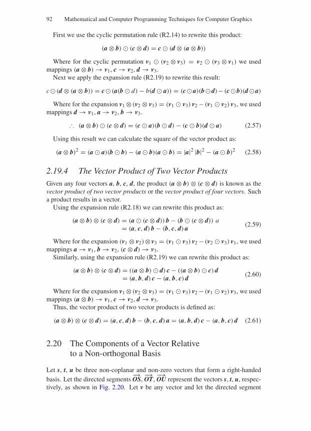
“Comninos” — 2005/8/31 — 18:32 — page 92 — #28
92 Mathematical and Computer Programming Techniques for Computer Graphics
First we use the cyclic permutation rule (R2.14) to rewrite this product:
(a ⊗ b) (c ⊗ d) = c (d ⊗ (a ⊗ b))
Where for the cyclic permutation v1 (v2 ⊗ v3) = v2 (v3 ⊗ v1) we usedmappings (a ⊗ b) → v1, c → v2, d → v3.
Next we apply the expansion rule (R2.19) to rewrite this result:
c (d ⊗ (a ⊗ b)) = c (a(b d) − b(d a)) = (ca)(bd)− (cb)(da)
Where for the expansion v1 ⊗ (v2 ⊗ v3) = (v1 v3) v2 − (v1 v2) v3, we usedmappings d → v1, a → v2, b → v3.
∴ (a ⊗ b) (c ⊗ d) = (c a)(b d) − (c b)(d a) (2.57)
Using this result we can calculate the square of the vector product as:
(a ⊗ b)2 = (a a)(b b) − (a b)(a b) = |a|2 |b|2 − (a b)2 (2.58)
2.19.4 The Vector Product of Two Vector Products
Given any four vectors a, b, c, d, the product (a ⊗ b) ⊗ (c ⊗ d) is known as thevector product of two vector products or the vector product of four vectors. Sucha product results in a vector.
Using the expansion rule (R2.18) we can rewrite this product as:
(a ⊗ b) ⊗ (c ⊗ d) = (a (c ⊗ d)) b − (b (c ⊗ d)) a= (a, c, d) b − (b, c, d) a
(2.59)
Where for the expansion (v1 ⊗ v2)⊗ v3 = (v1 v3) v2 − (v2 v3) v1, we usedmappings a → v1, b → v2, (c ⊗ d) → v3.
Similarly, using the expansion rule (R2.19) we can rewrite this product as:
(a ⊗ b) ⊗ (c ⊗ d) = ((a ⊗ b) d) c − ((a ⊗ b) c) d= (a, b, d) c − (a, b, c) d
(2.60)
Where for the expansion v1 ⊗ (v2 ⊗ v3) = (v1 v3) v2 − (v1 v2) v3, we usedmappings (a ⊗ b) → v1, c → v2, d → v3.
Thus, the vector product of two vector products is defined as:
(a ⊗ b) ⊗ (c ⊗ d) = (a, c, d) b − (b, c, d) a = (a, b, d) c − (a, b, c) d (2.61)
2.20 The Components of a Vector Relativeto a Non-orthogonal Basis
Let s, t, u be three non-coplanar and non-zero vectors that form a right-handed
basis. Let the directed segments−→OS,
−→OT,
−→OU represent the vectors s, t, u, respec-
tively, as shown in Fig. 2.20. Let v be any vector and let the directed segment
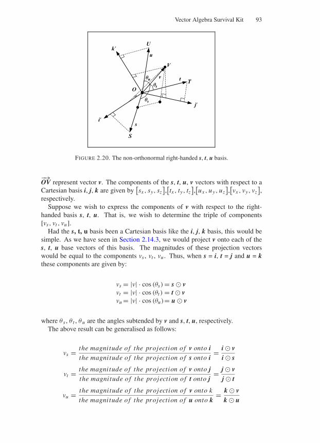
“Comninos” — 2005/8/31 — 18:32 — page 93 — #29
Vector Algebra Survival Kit 93
v
s
O
k
i
j
t
u
S
T
U
V
qt
qu
qs
FIGURE 2.20. The non-orthonormal right-handed s, t, u basis.
−→OV represent vector v. The components of the s, t, u, v vectors with respect to aCartesian basis i, j, k are given by
[sx , sy, sz
],[tx , ty, tz
],[ux , uy, uz
],[vx , vy, vz
],
respectively.Suppose we wish to express the components of v with respect to the right-
handed basis s, t, u. That is, we wish to determine the triple of components[vs, vt , vu].
Had the s, t, u basis been a Cartesian basis like the i, j, k basis, this would besimple. As we have seen in Section 2.14.3, we would project v onto each of thes, t, u base vectors of this basis. The magnitudes of these projection vectorswould be equal to the components vs , vt , vu . Thus, when s = i, t = j and u = kthese components are given by:
vs = |v| · cos (θs) = s vvt = |v| · cos (θt ) = t vvu = |v| · cos (θu)= u v
where θ s , θ t , θu are the angles subtended by v and s, t, u, respectively.The above result can be generalised as follows:
vs = the magnitude of the projection of v onto ithe magnitude of the projection of s onto i
= i vi s
vt = the magnitude of the projection of v onto jthe magnitude of the projection of t onto j
= j vj t
vu = the magnitude of the projection of v onto k
the magnitude of the projection of u onto k= k v
k u
“Comninos” — 2005/8/31 — 18:32 — page 94 — #30
94 Mathematical and Computer Programming Techniques for Computer Graphics
Which when s = i, t = j and u = k reduces to:
vs = i vi i
= s v1
= s v
vt = j vj j
= t v1
= t v
vu = k vk k
= u v1
= u v
In the general case however s = i, t = j and u = k, we must compute a new setof vectors i′, j′, k′ that correspond to base vectors i, j, k. As vector i is normal tothe plane defined by the other two vectors j, k (of the i, j, k basis), so i′ must benormal to the plane defined by vectors t, u (of the s, t, u basis). Similarly j′ mustbe normal to the plane defined by u, s, and k′ must be normal to the plane definedby s, t.
Thus:i′ = t ⊗ uj′ = u ⊗ sk′ = s ⊗ t
Using this new set of vectors i′, j′, k′ we can compute the components of vectorv with respect to the right-handed basis s, t, u:
vs = (t ⊗ u) v(t ⊗ u) s
= (t, u, v)(t, u, s)
vt = (u ⊗ s) v(u ⊗ s) t
= (u, s, v)(u, s, t)
(2.62)
vu = (s ⊗ t) v(s ⊗ t) u
= (s, t, v)(s, t, u)
Expanding the triple scalar products we obtain:
vs = (t, u, v)(t, u, s)
=(tyuz − tzuy
)vx + (tzux − tx uz) vy + (
tx uy − tyux)
vz(tyuz − tzuy
)sx + (tzux − tx uz) sy + (
tx uy − tyux)
sz
vt = (u, s, v)(u, s, t)
=(uysz − uzsy
)vx + (uzsx − ux sz) vy + (
ux sy − uysx)
vz(uysz − uzsy
)tx + (uzsx − ux sz) ty + (
ux sy − uysx)
tz
vu = (s, t, v)(s, t, u)
=(sytz − szty
)vx + (sztx − sx tz) vy + (
sx ty − sytx)
vz(sytz − szty
)ux + (sztx − sx tz) uy + (
sx ty − sytx)
uz
(2.63)
The above discussion was useful in illuminating the geometric aspects of ourproblem. It illustrated how geometric arguments are helpful in reasoning andsolving problems in vector algebra, but it did not provide a conclusive mathemat-ical proof of the correctness of our arguments. At some stage of our discussionwe claimed that a result could be generalised without offering any evidence toback our claim. We will do so in the next section.
“Comninos” — 2005/8/31 — 18:32 — page 95 — #31
Vector Algebra Survival Kit 95
2.21 The Decomposition of a Vector According to a Basis
In this section we revisit the problem dealt with in the previous section, but we doso in a more mathematically rigorous way and provide a vector algebraic proof ofour argument.
We start by restating the problem. Given four non-coplanar and non-zero vec-tors a, b, c, d decompose vector d according to a basis a, b, c, i.e. express thecomponents of d with respect to a right-handed basis a, b, c (which is not re-quired to be orthonormal or even orthogonal). From Section 2.7 we know thatthis is possible. Indeed, given any four non-coplanar and non-zero vectors in E3
we can express one of the vectors as a linear combination of the remaining threevectors.
By combining Eqs. (2.59) and (2.60) we obtain:
(a, b, d) c − (a, b, c) d = (a, c, d) b − (b, c, d) a
∴ (b, c, d) a − (a, c, d) b + (a, b, d) c − (a, b, c) d = −→0
Using the non-cyclic permutation rule (R2.15) we obtain:
(b, c, d) a + (a, d, c) b + (a, b, d) c − (a, b, c) d = −→0
But given that any four vectors in E3 are always linearly dependent (i.e. we candecompose one in terms of the remaining three), we can solve the above equationfor d:
(b, c, d) a + (a, d, c) b + (a, b, d) c = (a, b, c) d
∴ d = (b, c, d) a + (a, d, c) b + (a, b, d) c(a, b, c)
= (b, c, d)
(a, b, c)a+ (a, d, c)
(a, b, c)b+ (a, b, d)
(a, b, c)c
Expressing d in component form we obtain:
d =[(b, c, d)
(a, b, c),(a, d, c)(a, b, c)
,(a, b, d)
(a, b, c)
]
Using the cyclic permutation rule (R2.14) we obtain:
d =[(b, c, d)
(b, c, a),(c, a, d)
(c, a, b),(a, b, d)
(a, b, c)
]
Finally, expanding the triple scalar products we obtain:
d =[(b ⊗ c) d(b ⊗ c) a
,(c ⊗ a) d(c ⊗ a) b
,(a ⊗ b) d(a ⊗ b) c
]
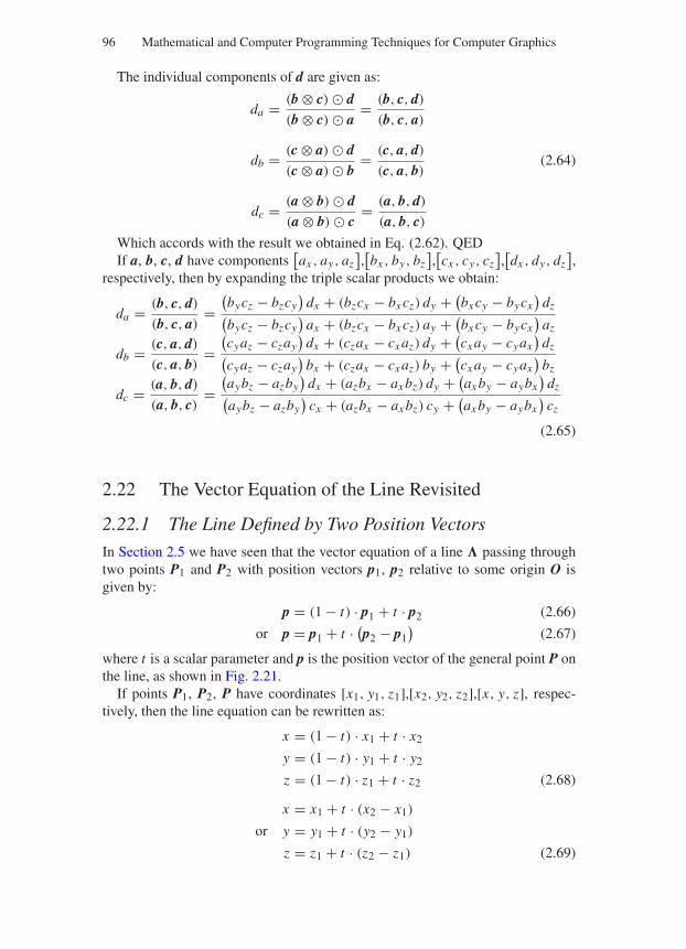
“Comninos” — 2005/8/31 — 18:32 — page 96 — #32
96 Mathematical and Computer Programming Techniques for Computer Graphics
The individual components of d are given as:
da = (b ⊗ c) d(b ⊗ c) a
= (b, c, d)
(b, c, a)
db = (c ⊗ a) d(c ⊗ a) b
= (c, a, d)
(c, a, b)(2.64)
dc = (a ⊗ b) d(a ⊗ b) c
= (a, b, d)
(a, b, c)
Which accords with the result we obtained in Eq. (2.62). QEDIf a, b, c, d have components
[ax , ay, az
],[bx , by, bz
],[cx , cy, cz
],[dx , dy, dz
],
respectively, then by expanding the triple scalar products we obtain:
da = (b, c, d)
(b, c, a)=
(bycz − bzcy
)dx + (bzcx − bx cz) dy + (
bx cy − bycx)
dz(bycz − bzcy
)ax + (bzcx − bx cz) ay + (
bx cy − bycx)
az
db = (c, a, d)
(c, a, b)=
(cyaz − czay
)dx + (czax − cx az) dy + (
cx ay − cyax)
dz(cyaz − czay
)bx + (czax − cx az) by + (
cx ay − cyax)
bz
dc = (a, b, d)
(a, b, c)=
(aybz − azby
)dx + (azbx − ax bz) dy + (
ax by − aybx)
dz(aybz − azby
)cx + (azbx − ax bz) cy + (
ax by − aybx)
cz
(2.65)
2.22 The Vector Equation of the Line Revisited
2.22.1 The Line Defined by Two Position Vectors
In Section 2.5 we have seen that the vector equation of a line passing throughtwo points P1 and P2 with position vectors p1, p2 relative to some origin O isgiven by:
p = (1 − t) · p1 + t · p2 (2.66)
or p = p1 + t · (p2 − p1
)(2.67)
where t is a scalar parameter and p is the position vector of the general point P onthe line, as shown in Fig. 2.21.
If points P1, P2, P have coordinates [x1, y1, z1],[x2, y2, z2],[x, y, z], respec-tively, then the line equation can be rewritten as:
x = (1 − t) · x1 + t · x2
y = (1 − t) · y1 + t · y2
z = (1 − t) · z1 + t · z2 (2.68)
x = x1 + t · (x2 − x1)
or y = y1 + t · (y2 − y1)
z = z1 + t · (z2 − z1) (2.69)
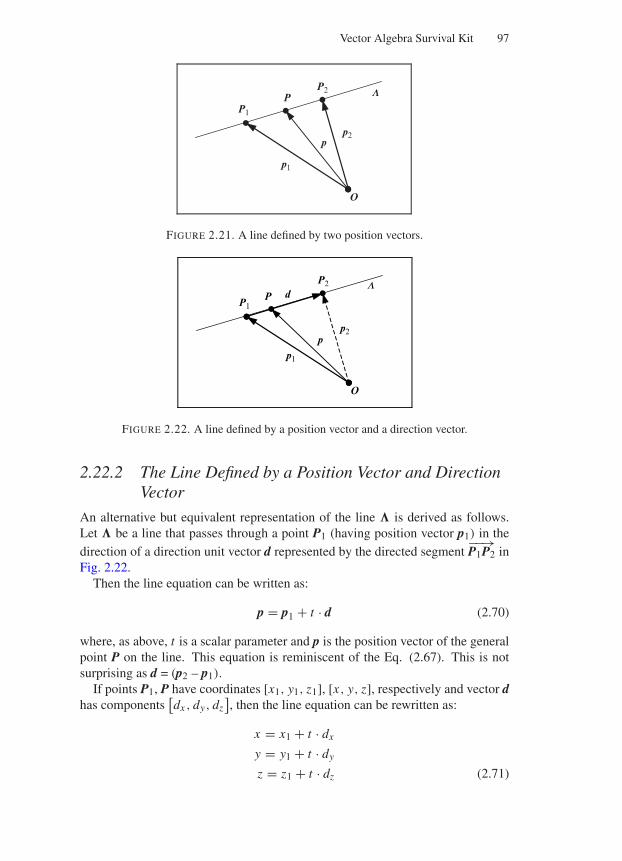
“Comninos” — 2005/8/31 — 18:32 — page 97 — #33
Vector Algebra Survival Kit 97
p1
p2p
O
P1
P2P L
FIGURE 2.21. A line defined by two position vectors.
p1
d
p
O
P1
P2
P
p2
L
FIGURE 2.22. A line defined by a position vector and a direction vector.
2.22.2 The Line Defined by a Position Vector and DirectionVector
An alternative but equivalent representation of the line is derived as follows.Let be a line that passes through a point P1 (having position vector p1) in thedirection of a direction unit vector d represented by the directed segment
−−→P1P2 in
Fig. 2.22.Then the line equation can be written as:
p = p1 + t · d (2.70)
where, as above, t is a scalar parameter and p is the position vector of the generalpoint P on the line. This equation is reminiscent of the Eq. (2.67). This is notsurprising as d = (p2 – p1).
If points P1, P have coordinates [x1, y1, z1], [x, y, z], respectively and vector dhas components
[dx , dy, dz
], then the line equation can be rewritten as:
x = x1 + t · dx
y = y1 + t · dy
z = z1 + t · dz (2.71)
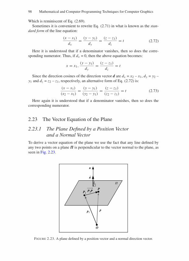
“Comninos” — 2005/8/31 — 18:32 — page 98 — #34
98 Mathematical and Computer Programming Techniques for Computer Graphics
Which is reminiscent of Eq. (2.69).Sometimes it is convenient to rewrite Eq. (2.71) in what is known as the stan-
dard form of the line equation:
(x − x1)
dx= (y − y1)
dy= (z − z1)
dz= t (2.72)
Here it is understood that if a denominator vanishes, then so does the corre-sponding numerator. Thus, if dx = 0, then the above equation becomes:
x = x1,(y − y1)
dy= (z − z1)
dz= t
Since the direction cosines of the direction vector d are dx = x2 – x1, dy = y2 –y1 and dz = z2 – z1, respectively, an alternative form of Eq. (2.72) is:
(x − x1)
(x2 − x1)= (y − y1)
(y2 − y1)= (z − z1)
(z2 − z1)= t (2.73)
Here again it is understood that if a denominator vanishes, then so does thecorresponding numerator.
2.23 The Vector Equation of the Plane
2.23.1 The Plane Defined by a Position Vectorand a Normal Vector
To derive a vector equation of the plane we use the fact that any line defined byany two points on a plane Π is perpendicular to the vector normal to the plane, asseen in Fig. 2.23.
n
p
O
P1PP1
P
p1
n
P
FIGURE 2.23. A plane defined by a position vector and a normal direction vector.
“Comninos” — 2005/8/31 — 18:32 — page 99 — #35
Vector Algebra Survival Kit 99
Let P1 be a point on the plane with position vector p1 and let P be the generalpoint on the plane with position vector p. Let n be a vector that is normal tothe plane and let n be the unit normal of the plane. Let vectors p1, p, n havecomponents [x1, y1, z1],[x, y, z],[a, b, c], respectively. The directed segment
−→P1P
represents vector (p – p1), which is perpendicular to n. Thus:
(p − p1) n = 0 (2.74)
∴ p n − p1 n = 0
∴ p n = p1 n (2.75)
or p n = do (2.76)
Equations (2.74), (2.75) and (2.76) are all alternative forms of the vector equa-tion of the plane. In the special case where n = n, then do represents the distanceof the plane from the origin O.
Expressing Eq. (2.74) in component form we obtain:
a · (x − x1) + b · (y − y1) + c · (z − z1) = 0 (2.77)
This equation provides both the necessary and sufficient condition for a point[x , y, z] to lie on the plane containing the point [x1, y1, z1] and being perpendic-ular to the direction [a, b, c].
Similarly Eq. (2.76) in component form gives:
a · x + b · y + c · z + d = 0 (2.78)
where d = −do is the negative distance of the plane from the origin. Thus theplane is represented by a linear equation of x , y, z.
2.23.2 The Plane Defined by Three Position Vectors
Let P1, P2, P3 be three non-collinear points lying on a plane Π with positionvectors p1, p2, p3 and components [x1, y1, z1], [x2, y2, z2], [x3, y3, z3], respec-tively. Directed segments
−−→P1P2,
−−→P1P3 represent the vectors (p2 − p1), (p3 − p1),
respectively, as shown in Fig. 2.24.Both directed segments lie on the plane and are therefore perpendicular to
the normal of the plane. Thus:
n = (p2 − p1
) ⊗ (p3 − p1
)(2.79)
Using the distributive rule (R2.13):
n = p2 ⊗ p3 − p2 ⊗ p1 − p1 ⊗ p3 + p1 ⊗ p1
Using axiom (A2.10) and the anti-commutative rule (R2.11):
n = p2 ⊗ p3 + p1 ⊗ p2 + p3 ⊗ p1
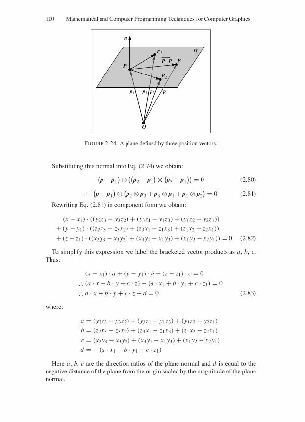
“Comninos” — 2005/8/31 — 18:32 — page 100 — #36
100 Mathematical and Computer Programming Techniques for Computer Graphics
n
p
O
P1
P1 P P
p1
P2
P3
p3 p2
P
FIGURE 2.24. A plane defined by three position vectors.
Substituting this normal into Eq. (2.74) we obtain:(p − p1
) ((p2 − p1
) ⊗ (p3 − p1
)) = 0 (2.80)
∴(p − p1
) (p2 ⊗ p3 + p3 ⊗ p1 + p1 ⊗ p2
) = 0 (2.81)
Rewriting Eq. (2.81) in component form we obtain:
(x − x1) · ((y2z3 − y3z2) + (y3z1 − y1z3) + (y1z2 − y2z1))
+ (y − y1) · ((z2x3 − z3x2) + (z3x1 − z1x3) + (z1x2 − z2x1))
+ (z − z1) · ((x2 y3 − x3 y2) + (x3 y1 − x1 y3) + (x1 y2 − x2 y1)) = 0 (2.82)
To simplify this expression we label the bracketed vector products as a, b, c.Thus:
(x − x1) · a + (y − y1) · b + (z − z1) · c = 0
∴ (a · x + b · y + c · z) − (a · x1 + b · y1 + c · z1) = 0
∴ a · x + b · y + c · z + d = 0 (2.83)
where:
a = (y2z3 − y3z2) + (y3z1 − y1z3) + (y1z2 − y2z1)
b = (z2x3 − z3x2) + (z3x1 − z1x3) + (z1x2 − z2x1)
c = (x2 y3 − x3 y2) + (x3 y1 − x1 y3) + (x1 y2 − x2 y1)
d = − (a · x1 + b · y1 + c · z1)
Here a, b, c are the direction ratios of the plane normal and d is equal to thenegative distance of the plane from the origin scaled by the magnitude of the planenormal.
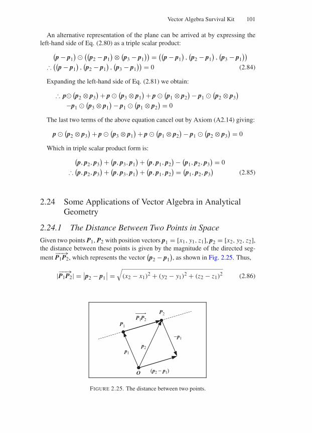
“Comninos” — 2005/8/31 — 18:32 — page 101 — #37
Vector Algebra Survival Kit 101
An alternative representation of the plane can be arrived at by expressing theleft-hand side of Eq. (2.80) as a triple scalar product:
(p − p1
) ((p2 − p1
) ⊗ (p3 − p1
)) = ((p − p1
),(p2 − p1
),(p3 − p1
))
∴((
p − p1),(p2 − p1
),(p3 − p1
)) = 0 (2.84)
Expanding the left-hand side of Eq. (2.81) we obtain:
∴ p (p2 ⊗ p3
) + p (p3 ⊗ p1
) + p (p1 ⊗ p2
) − p1 (p2 ⊗ p3
)
−p1 (p3 ⊗ p1
) − p1 (p1 ⊗ p2
) = 0
The last two terms of the above equation cancel out by Axiom (A2.14) giving:
p (p2 ⊗ p3
) + p (p3 ⊗ p1
) + p (p1 ⊗ p2
) − p1 (p2 ⊗ p3
) = 0
Which in triple scalar product form is:(p, p2, p3
) + (p, p3, p1
) + (p, p1, p2
) − (p1, p2, p3
) = 0
∴(p, p2, p3
) + (p, p3, p1
) + (p, p1, p2
) = (p1, p2, p3
)(2.85)
2.24 Some Applications of Vector Algebra in AnalyticalGeometry
2.24.1 The Distance Between Two Points in Space
Given two points P1, P2 with position vectors p1 = [x1, y1, z1], p2 = [x2, y2, z2],the distance between these points is given by the magnitude of the directed seg-ment
−−→P1P2, which represents the vector
(p2 − p1
), as shown in Fig. 2.25. Thus,
|−−→P1P2| = ∣∣p2 − p1
∣∣ =√
(x2 − x1)2 + (y2 − y1)
2 + (z2 − z1)2 (2.86)
p1
p2
(p2 − p1)O
P1
P2P2P1
−p1
FIGURE 2.25. The distance between two points.
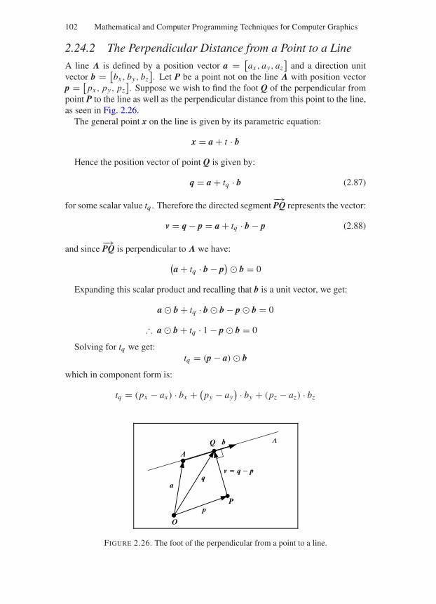
“Comninos” — 2005/8/31 — 18:32 — page 102 — #38
102 Mathematical and Computer Programming Techniques for Computer Graphics
2.24.2 The Perpendicular Distance from a Point to a Line
A line Λ is defined by a position vector a = [ax , ay, az
]and a direction unit
vector b = [bx , by, bz
]. Let P be a point not on the line Λ with position vector
p = [px , py, pz
]. Suppose we wish to find the foot Q of the perpendicular from
point P to the line as well as the perpendicular distance from this point to the line,as seen in Fig. 2.26.
The general point x on the line is given by its parametric equation:
x = a + t · b
Hence the position vector of point Q is given by:
q = a + tq · b (2.87)
for some scalar value tq . Therefore the directed segment−→PQ represents the vector:
v = q − p = a + tq · b − p (2.88)
and since−→PQ is perpendicular to Λ we have:
(a + tq · b − p
) b = 0
Expanding this scalar product and recalling that b is a unit vector, we get:
a b + tq · b b − p b = 0
∴ a b + tq · 1 − p b = 0
Solving for tq we get:tq = (p − a) b
which in component form is:
tq = (px − ax ) · bx + (py − ay
) · by + (pz − az) · bz
q
b
p
O
A
Q
P
a
q − pv =
L
FIGURE 2.26. The foot of the perpendicular from a point to a line.
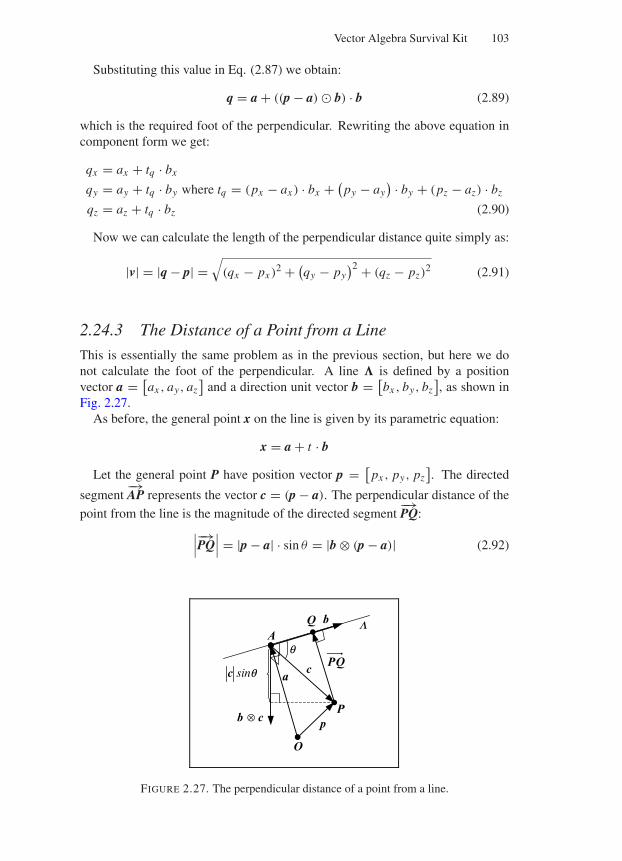
“Comninos” — 2005/8/31 — 18:32 — page 103 — #39
Vector Algebra Survival Kit 103
Substituting this value in Eq. (2.87) we obtain:
q = a + ((p − a) b) · b (2.89)
which is the required foot of the perpendicular. Rewriting the above equation incomponent form we get:
qx = ax + tq · bx
qy = ay + tq · by where tq = (px − ax ) · bx + (py − ay
) · by + (pz − az) · bz
qz = az + tq · bz (2.90)
Now we can calculate the length of the perpendicular distance quite simply as:
|v| = |q − p| =√
(qx − px )2 + (
qy − py)2 + (qz − pz)
2 (2.91)
2.24.3 The Distance of a Point from a Line
This is essentially the same problem as in the previous section, but here we donot calculate the foot of the perpendicular. A line is defined by a positionvector a = [
ax , ay, az]
and a direction unit vector b = [bx , by, bz
], as shown in
Fig. 2.27.As before, the general point x on the line is given by its parametric equation:
x = a + t · b
Let the general point P have position vector p = [px , py, pz
]. The directed
segment−→AP represents the vector c = (p − a). The perpendicular distance of the
point from the line is the magnitude of the directed segment−→PQ:
∣∣∣−→PQ
∣∣∣ = |p − a| · sin θ = |b ⊗ (p − a)| (2.92)
c
b
p
O
AQ
P
a
b ⊗ c
sinqcPQ
L
q
FIGURE 2.27. The perpendicular distance of a point from a line.
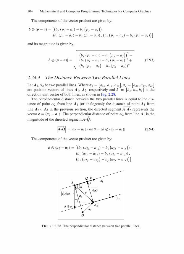
“Comninos” — 2005/8/31 — 18:32 — page 104 — #40
104 Mathematical and Computer Programming Techniques for Computer Graphics
The components of the vector product are given by:
b ⊗ (p − a) = [(by (pz − az) − bz
(py − ay
)),
(bz (px − ax ) − bx (pz − az)) ,(bx
(py − ay
) − by (px − ax ))]
and its magnitude is given by:
|b ⊗ (p − a)| =
√√√√√√
(by (pz − az) − bz
(py − ay
))2 +(bz (px − ax ) − bx (pz − az))
2 +(bx
(py − ay
) − by (px − ax ))2
(2.93)
2.24.4 The Distance Between Two Parallel Lines
Let Λ1,Λ2 be two parallel lines. Where a1 = [a1x , a1y, a1z
], a2 = [
a2x , a2y, a2z]
are position vectors of lines Λ1, Λ2, respectively and b = [bx , by, bz
]is the
direction unit vector of both lines, as shown in Fig. 2.28.The perpendicular distance between the two parallel lines is equal to the dis-
tance of point A2 from line Λ1 (or analogously the distance of point A1 from
line Λ2). As in the previous section, the directed segment−−→A1A2 represents the
vector c = (a2 − a1). The perpendicular distance of point A2 from line Λ1 is the
magnitude of the directed segment−−→A2Q:
∣∣∣−−→A2Q
∣∣∣ = |a2 − a1| · sin θ = |b ⊗ (a2 − a1)| (2.94)
The components of the vector product are given by:
b ⊗ (a2 − a1) = [(by (a2z − a1z) − bz
(a2y − a1y
)),
(bz (a2x − a1x ) − bx (a2z − a1z)) ,(bx
(a2y − a1y
) − by (a2x − a1x ))]
c
b
a2
O
A1
Q
A2
a1
b ⊗ c
sinqcA2Q
b
L1
L2
q
FIGURE 2.28. The perpendicular distance between two parallel lines.
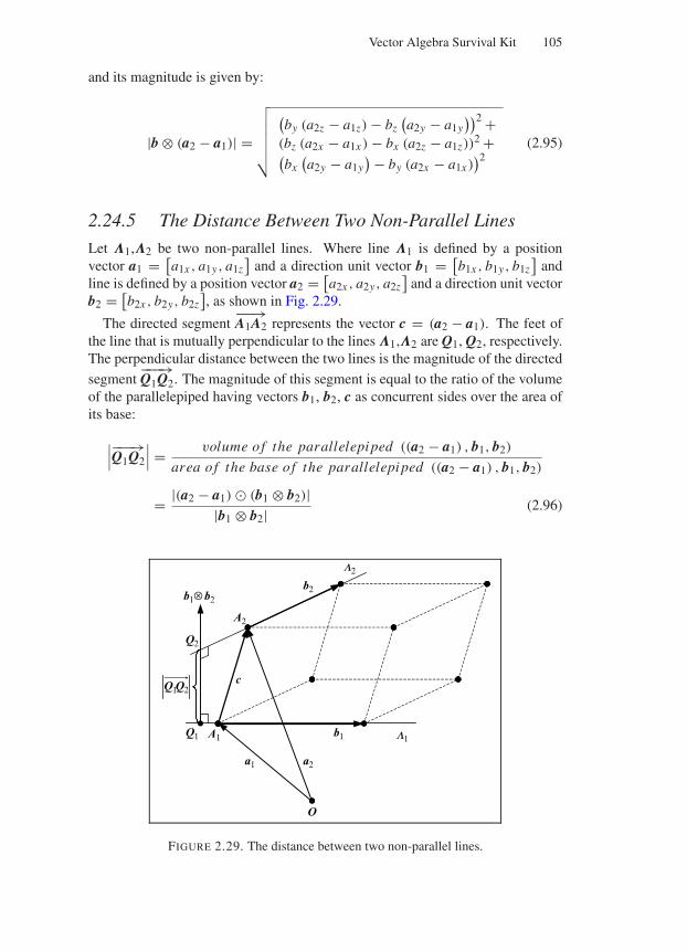
“Comninos” — 2005/8/31 — 18:32 — page 105 — #41
Vector Algebra Survival Kit 105
and its magnitude is given by:
|b ⊗ (a2 − a1)| =
√√√√√√
(by (a2z − a1z) − bz
(a2y − a1y
))2 +(bz (a2x − a1x ) − bx (a2z − a1z))
2 +(bx
(a2y − a1y
) − by (a2x − a1x ))2
(2.95)
2.24.5 The Distance Between Two Non-Parallel Lines
Let Λ1,Λ2 be two non-parallel lines. Where line Λ1 is defined by a positionvector a1 = [
a1x , a1y, a1z]
and a direction unit vector b1 = [b1x , b1y, b1z
]and
line is defined by a position vector a2 = [a2x , a2y, a2z
]and a direction unit vector
b2 = [b2x , b2y, b2z
], as shown in Fig. 2.29.
The directed segment−−→A1A2 represents the vector c = (a2 − a1). The feet of
the line that is mutually perpendicular to the lines Λ1,Λ2 are Q1, Q2, respectively.The perpendicular distance between the two lines is the magnitude of the directed
segment−−−→Q1Q2. The magnitude of this segment is equal to the ratio of the volume
of the parallelepiped having vectors b1, b2, c as concurrent sides over the area ofits base:
∣∣∣−−−→Q1Q2
∣∣∣ = volume of the parallelepiped ((a2 − a1) , b1, b2)
area of the base of the parallelepiped ((a2 − a1) , b1, b2)
= |(a2 − a1) (b1 ⊗ b2)||b1 ⊗ b2| (2.96)
a1
b2b1⊗ b2
O
A1Q1
c
b1
A2
a2
Q2
Q2Q1
L1
L2
FIGURE 2.29. The distance between two non-parallel lines.
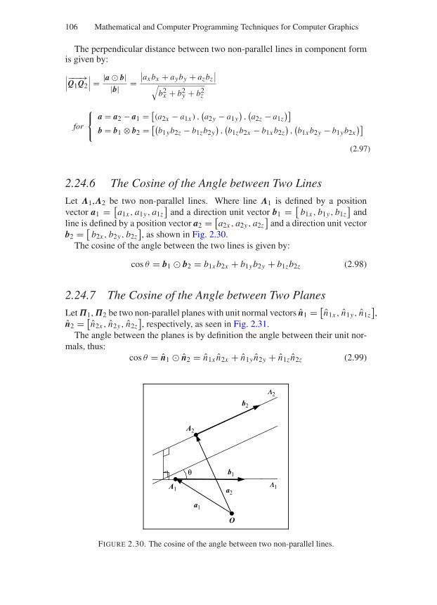
“Comninos” — 2005/8/31 — 18:32 — page 106 — #42
106 Mathematical and Computer Programming Techniques for Computer Graphics
The perpendicular distance between two non-parallel lines in component formis given by:
∣∣∣−−−→Q1Q2
∣∣∣ = |a b||b| =
∣∣ax bx + ayby + azbz∣∣
√b2
x + b2y + b2
z
for
⎧⎨
⎩
a = a2 − a1 = [(a2x − a1x ) ,
(a2y − a1y
),(a2z − a1z
)]
b = b1 ⊗ b2 = [(b1yb2z − b1zb2y
),(b1zb2x − b1x b2z
),(b1x b2y − b1yb2x
)]
(2.97)
2.24.6 The Cosine of the Angle between Two Lines
Let Λ1,Λ2 be two non-parallel lines. Where line Λ1 is defined by a positionvector a1 = [
a1x , a1y, a1z]
and a direction unit vector b1 = [b1x , b1y, b1z
]and
line is defined by a position vector a2 = [a2x , a2y, a2z
]and a direction unit vector
b2 = [b2x , b2y, b2z
], as shown in Fig. 2.30.
The cosine of the angle between the two lines is given by:
cos θ = b1 b2 = b1x b2x + b1yb2y + b1zb2z (2.98)
2.24.7 The Cosine of the Angle between Two Planes
Let Π1, Π2 be two non-parallel planes with unit normal vectors n1 = [n1x , n1y, n1z
],
n2 = [n2x , n2y, n2z
], respectively, as seen in Fig. 2.31.
The angle between the planes is by definition the angle between their unit nor-mals, thus:
cos θ = n1 n2 = n1x n2x + n1y n2y + n1z n2z (2.99)
a1
b2
O
A1L1
b1
A2
a2
L2
θ
FIGURE 2.30. The cosine of the angle between two non-parallel lines.
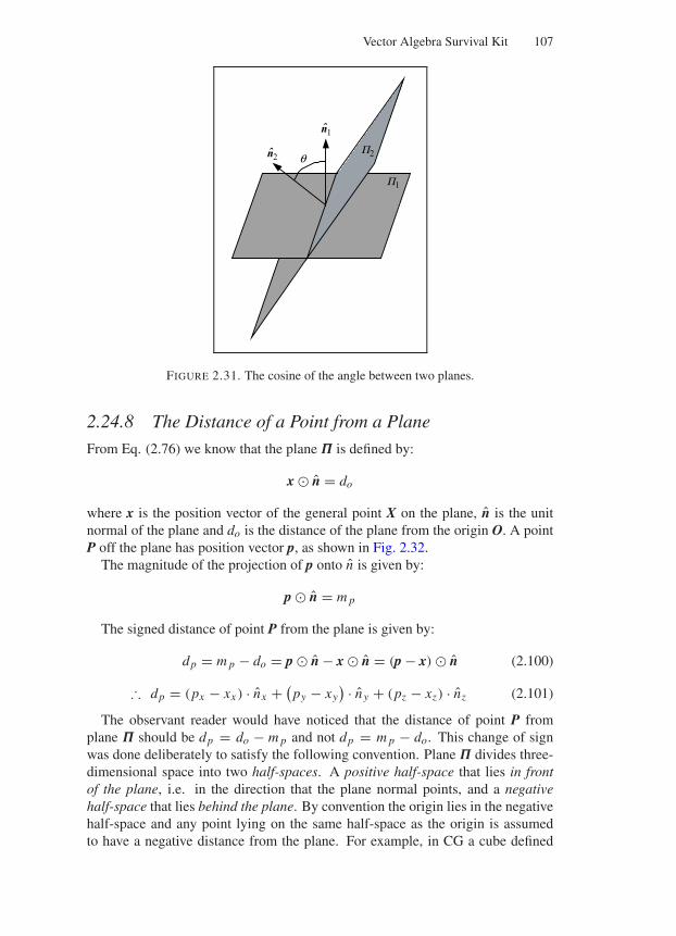
“Comninos” — 2005/8/31 — 18:32 — page 107 — #43
Vector Algebra Survival Kit 107
n1ˆ
n2ˆ θ
P1
P2
FIGURE 2.31. The cosine of the angle between two planes.
2.24.8 The Distance of a Point from a Plane
From Eq. (2.76) we know that the plane Π is defined by:
x n = do
where x is the position vector of the general point X on the plane, n is the unitnormal of the plane and do is the distance of the plane from the origin O. A pointP off the plane has position vector p, as shown in Fig. 2.32.
The magnitude of the projection of p onto n is given by:
p n = m p
The signed distance of point P from the plane is given by:
dp = m p − do = p n − x n = (p − x) n (2.100)
∴ dp = (px − xx ) · nx + (py − xy
) · n y + (pz − xz) · nz (2.101)
The observant reader would have noticed that the distance of point P fromplane Π should be dp = do − m p and not dp = m p − do. This change of signwas done deliberately to satisfy the following convention. Plane Π divides three-dimensional space into two half-spaces. A positive half-space that lies in frontof the plane, i.e. in the direction that the plane normal points, and a negativehalf-space that lies behind the plane. By convention the origin lies in the negativehalf-space and any point lying on the same half-space as the origin is assumedto have a negative distance from the plane. For example, in CG a cube defined
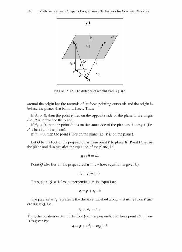
“Comninos” — 2005/8/31 — 18:32 — page 108 — #44
108 Mathematical and Computer Programming Techniques for Computer Graphics
X
n
Q
P
do x
Pp
dp
mp
q
O
FIGURE 2.32. The distance of a point from a plane.
around the origin has the normals of its faces pointing outwards and the origin isbehind the planes that form its faces. Thus:
If dp > 0, then the point P lies on the opposite side of the plane to the origin(i.e. P is in front of the plane).
If dp < 0, then the point P lies on the same side of the plane as the origin (i.e.P is behind of the plane).
If dp = 0, then the point P lies on the plane (i.e. P is on the plane).
Let Q be the foot of the perpendicular from point P to plane Π. Point Q lies onthe plane and thus satisfies the equation of the plane, i.e.
q n = do
Point Q also lies on the perpendicular line whose equation is given by:
xl = p + t · n
Thus, point Q satisfies the perpendicular line equation:
q = p + tq · n
The parameter tq represents the distance travelled along n, starting from P andending at Q, i.e.
tq = do − m p
Thus, the position vector of the foot Q of the perpendicular from point P to planeΠ is given by:
q = p + (do − m p
) · n
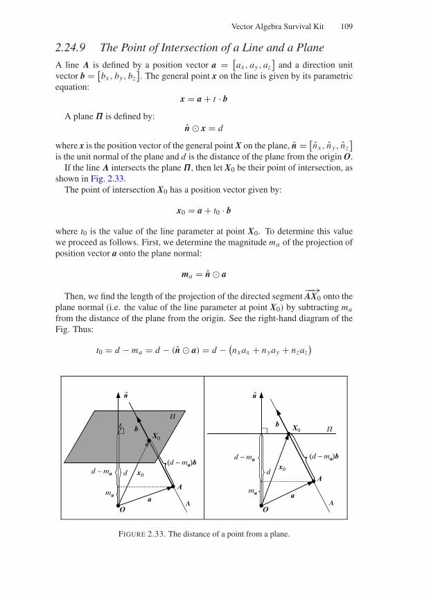
“Comninos” — 2005/8/31 — 18:32 — page 109 — #45
Vector Algebra Survival Kit 109
2.24.9 The Point of Intersection of a Line and a Plane
A line Λ is defined by a position vector a = [ax , ay, az
]and a direction unit
vector b = [bx , by, bz
]. The general point x on the line is given by its parametric
equation:x = a + t · b
A plane Π is defined by:n x = d
where x is the position vector of the general point X on the plane, n = [nx , n y, nz
]
is the unit normal of the plane and d is the distance of the plane from the origin O.If the line Λ intersects the plane Π, then let X0 be their point of intersection, as
shown in Fig. 2.33.The point of intersection X0 has a position vector given by:
x0 = a + t0 · b
where t0 is the value of the line parameter at point X0. To determine this valuewe proceed as follows. First, we determine the magnitude ma of the projection ofposition vector a onto the plane normal:
ma = n a
Then, we find the length of the projection of the directed segment−−→AX0 onto the
plane normal (i.e. the value of the line parameter at point X0) by subtracting ma
from the distance of the plane from the origin. See the right-hand diagram of theFig. Thus:
t0 = d − ma = d − (n a) = d − (nx ax + nyay + nzaz
)
d x0x0
O
A
X0
X0
a
n
mama
b
d − ma
d − ma(d − ma)b(d − ma)b
d
O
A
a
n
b
L L
P
P
FIGURE 2.33. The distance of a point from a plane.
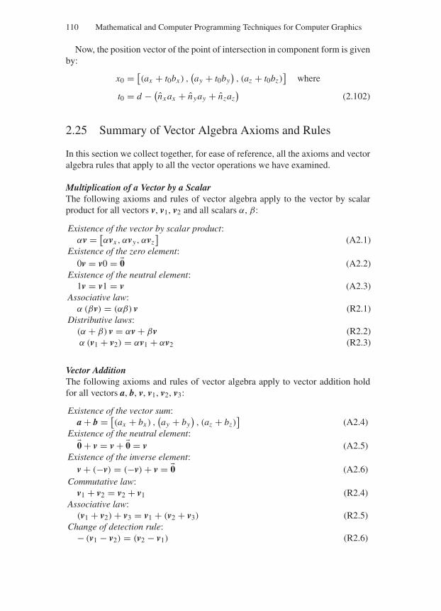
“Comninos” — 2005/8/31 — 18:32 — page 110 — #46
110 Mathematical and Computer Programming Techniques for Computer Graphics
Now, the position vector of the point of intersection in component form is givenby:
x0 = [(ax + t0bx ) ,
(ay + t0by
), (az + t0bz)
]where
t0 = d − (nx ax + n yay + nzaz
)(2.102)
2.25 Summary of Vector Algebra Axioms and Rules
In this section we collect together, for ease of reference, all the axioms and vectoralgebra rules that apply to all the vector operations we have examined.
Multiplication of a Vector by a ScalarThe following axioms and rules of vector algebra apply to the vector by scalarproduct for all vectors v, v1, v2 and all scalars α, β:
Existence of the vector by scalar product:αv = [
αvx , αvy, αvz]
(A2.1)Existence of the zero element:
0v = v0 = 0 (A2.2)Existence of the neutral element:
1v = v1 = v (A2.3)Associative law:
α (βv) = (αβ) v (R2.1)Distributive laws:
(α + β) v = αv + βv (R2.2)α (v1 + v2) = αv1 + αv2 (R2.3)
Vector AdditionThe following axioms and rules of vector algebra apply to vector addition holdfor all vectors a, b, v, v1, v2, v3:
Existence of the vector sum:a + b = [
(ax + bx ) ,(ay + by
), (az + bz)
](A2.4)
Existence of the neutral element:0 + v = v + 0 = v (A2.5)
Existence of the inverse element:v + (−v) = (−v) + v = 0 (A2.6)
Commutative law:v1 + v2 = v2 + v1 (R2.4)
Associative law:(v1 + v2) + v3 = v1 + (v2 + v3) (R2.5)
Change of detection rule:− (v1 − v2) = (v2 − v1) (R2.6)
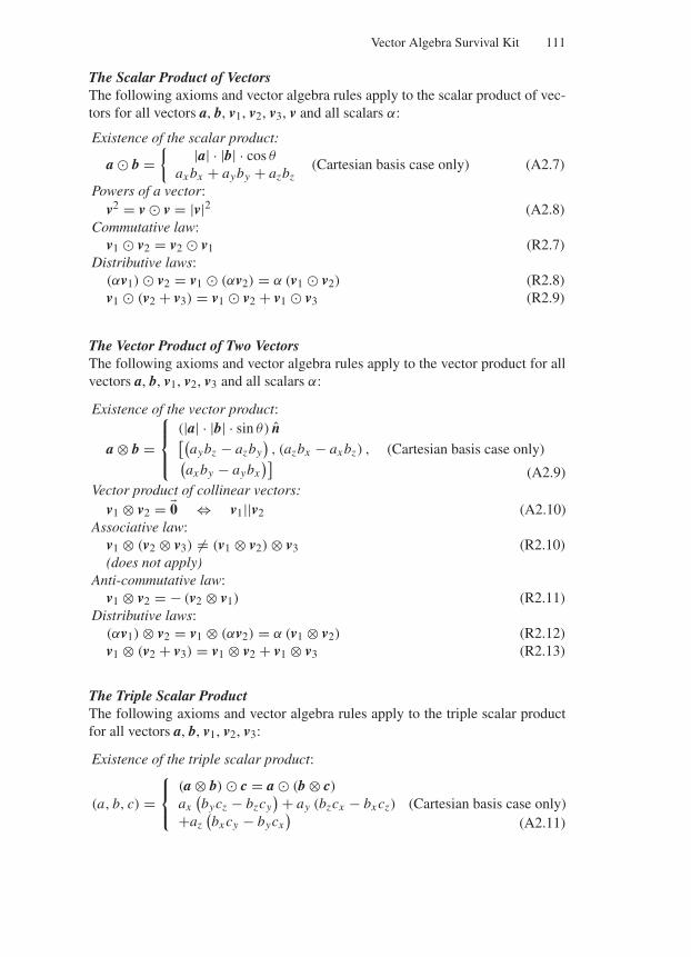
“Comninos” — 2005/8/31 — 18:32 — page 111 — #47
Vector Algebra Survival Kit 111
The Scalar Product of VectorsThe following axioms and vector algebra rules apply to the scalar product of vec-tors for all vectors a, b, v1, v2, v3, v and all scalars α:
Existence of the scalar product:
a b = |a| · |b| · cos θ
ax bx + ayby + azbz(Cartesian basis case only) (A2.7)
Powers of a vector:v2 = v v = |v|2 (A2.8)
Commutative law:v1 v2 = v2 v1 (R2.7)
Distributive laws:(αv1) v2 = v1 (αv2) = α (v1 v2) (R2.8)v1 (v2 + v3) = v1 v2 + v1 v3 (R2.9)
The Vector Product of Two VectorsThe following axioms and vector algebra rules apply to the vector product for allvectors a, b, v1, v2, v3 and all scalars α:
Existence of the vector product:
a ⊗ b =
⎧⎪⎨
⎪⎩
(|a| · |b| · sin θ) n[(
aybz − azby), (azbx − ax bz) ,
(ax by − aybx
)] (Cartesian basis case only)
(A2.9)Vector product of collinear vectors:
v1 ⊗ v2 = 0 ⇔ v1||v2 (A2.10)Associative law:
v1 ⊗ (v2 ⊗ v3) = (v1 ⊗ v2) ⊗ v3 (R2.10)(does not apply)
Anti-commutative law:v1 ⊗ v2 = − (v2 ⊗ v1) (R2.11)
Distributive laws:(αv1) ⊗ v2 = v1 ⊗ (αv2) = α (v1 ⊗ v2) (R2.12)v1 ⊗ (v2 + v3) = v1 ⊗ v2 + v1 ⊗ v3 (R2.13)
The Triple Scalar ProductThe following axioms and vector algebra rules apply to the triple scalar productfor all vectors a, b, v1, v2, v3:
Existence of the triple scalar product:
(a, b, c) =⎧⎨
⎩
(a ⊗ b) c = a (b ⊗ c)ax
(bycz − bzcy
) + ay (bzcx − bx cz)
+az(bx cy − bycx
) (Cartesian basis case only)(A2.11)
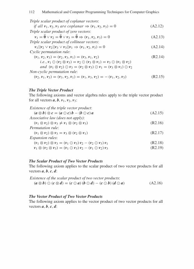
“Comninos” — 2005/8/31 — 18:32 — page 112 — #48
112 Mathematical and Computer Programming Techniques for Computer Graphics
Triple scalar product of coplanar vectors:if all v1, v2, v3 are coplanar ⇒ (v1, v2, v3) = 0 (A2.12)
Triple scalar product of zero vectors:v1 = 0 ∨ v2 = 0 ∨ v3 = 0 ⇒ (v1, v2, v3) = 0 (A2.13)
Triple scalar product of collinear vectors:v1||v2 ∨ v2||v3 ∨ v3||v1 ⇒ (v1, v2, v3) = 0 (A2.14)
Cyclic permutation rule:(v1, v2, v3) = (v2, v3, v1) = (v3, v1, v2) (R2.14)
i.e., v1 (v2 ⊗ v3) = v2 (v3 ⊗ v1) = v3 (v1 ⊗ v2)
and (v1 ⊗ v2) v3 = (v2 ⊗ v3) v1 = (v3 ⊗ v1) v2Non-cyclic permutation rule:
(v2, v1, v3) = (v3, v2, v1) = (v1, v3, v2) = − (v1, v2, v3) (R2.15)
The Triple Vector ProductThe following axioms and vector algebra rules apply to the triple vector productfor all vectors a, b, v1, v2, v3:
Existence of the triple vector product:(a ⊗ b) ⊗ c = (a c) b − (b c) a (A2.15)
Associative law (does not apply):(v1 ⊗ v2) ⊗ v3 = v1 ⊗ (v2 ⊗ v3) (R2.16)
Permutation rule:(v1 ⊗ v2) ⊗ v3 = v3 ⊗ (v2 ⊗ v1) (R2.17)
Expansion rules:(v1 ⊗ v2) ⊗ v3 = (v1 v3) v2 − (v2 v3) v1 (R2.18)v1 ⊗ (v2 ⊗ v3) = (v1 v3) v2 − (v1 v2) v3 (R2.19)
The Scalar Product of Two Vector ProductsThe following axiom applies to the scalar product of two vector products for allvectors a, b, c, d:
Existence of the scalar product of two vector products:(a ⊗ b) (c ⊗ d) = (c a) (b d) − (c b) (d a) (A2.16)
The Vector Product of Two Vector ProductsThe following axiom applies to the vector product of two vector products for allvectors a, b, c, d:

“Comninos” — 2005/8/31 — 18:32 — page 113 — #49
Vector Algebra Survival Kit 113
Existence of the vector product of two vector products:
(a ⊗ b) ⊗ (c ⊗ d) =
(a, c, d) b − (b, c, d) a(a, b, d) c − (a, b, c) d
(A2.17)
2.26 A Simple Vector Algebra C Library
See Appendix 1.
“Comninos” — 2005/8/31 — 15:34 — page 115 — #1
3
Matrix Algebra Survival Kit
The theory of matrices and their determinants is closely related to the problem ofsolving a system of linear simultaneous equations.
The Babylonians appear to be among the first people to have investigated thisproblem. In a clay tablet, which has been dated to approximately 400–300 BC,the following problem was formulated.
Two fields have a total area of 1800 square yards. One field produces grain at therate of 2/3 of a bushel per square yard, while the other produces grain at the rateof 1/2 a bushel per square yard. If the total yield is 1100 bushels, what is the sizeof each field?
In today’s terminology, this problem can be represented by the following sys-tem of linear simultaneous equations:
1 · x1 + 1 · x2 = 1800
23 · x1 + 1
2 · x2 = 1100
which, when solved, yields x1 = 1200 yd2 and x2 = 600 yd2 where x1, x2 representthe areas of the first and second fields, respectively.
The earliest example of the use of a determinant appears in the Chinese textentitled Nine Chapters of the Mathematical Art, which was written in 200 BCduring the Hun Dynasty. In this text the following problem, which is similar tothe Babylonian problem, was formulated.
There are three types of corn, of which three bundles of the first, two of the second,and one of the third make 39 measures. Two of the first, three of the second andone of the third make 34 measures. And one of the first, two of the second andthree of the third make 26 measures. How many measures of corn are containedin one bundle of each type?
Today we would represent this problem by the following system of linear si-multaneous equations:
3 · x1 + 2 · x2 + 1 · x3 = 392 · x1 + 3 · x2 + 1 · x3 = 341 · x1 + 2 · x2 + 3 · x3 = 26
115
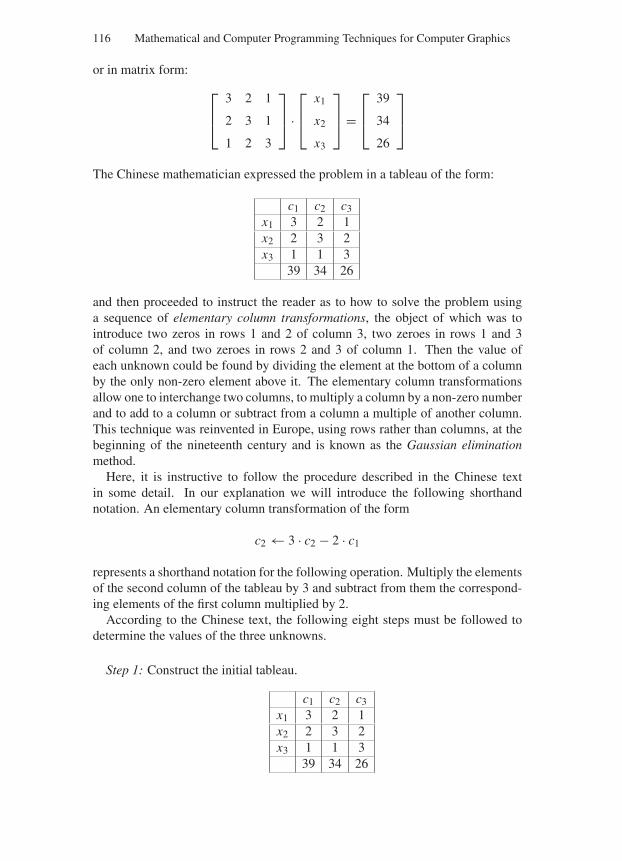
“Comninos” — 2005/8/31 — 15:34 — page 116 — #2
116 Mathematical and Computer Programming Techniques for Computer Graphics
or in matrix form:
⎡
⎢⎣
3 2 1
2 3 1
1 2 3
⎤
⎥⎦ ·
⎡
⎢⎣
x1
x2
x3
⎤
⎥⎦ =
⎡
⎢⎣
39
34
26
⎤
⎥⎦
The Chinese mathematician expressed the problem in a tableau of the form:
c1 c2 c3
x1 3 2 1x2 2 3 2x3 1 1 3
39 34 26
and then proceeded to instruct the reader as to how to solve the problem usinga sequence of elementary column transformations, the object of which was tointroduce two zeros in rows 1 and 2 of column 3, two zeroes in rows 1 and 3of column 2, and two zeroes in rows 2 and 3 of column 1. Then the value ofeach unknown could be found by dividing the element at the bottom of a columnby the only non-zero element above it. The elementary column transformationsallow one to interchange two columns, to multiply a column by a non-zero numberand to add to a column or subtract from a column a multiple of another column.This technique was reinvented in Europe, using rows rather than columns, at thebeginning of the nineteenth century and is known as the Gaussian eliminationmethod.
Here, it is instructive to follow the procedure described in the Chinese textin some detail. In our explanation we will introduce the following shorthandnotation. An elementary column transformation of the form
c2 ← 3 · c2 − 2 · c1
represents a shorthand notation for the following operation. Multiply the elementsof the second column of the tableau by 3 and subtract from them the correspond-ing elements of the first column multiplied by 2.
According to the Chinese text, the following eight steps must be followed todetermine the values of the three unknowns.
Step 1: Construct the initial tableau.
c1 c2 c3
x1 3 2 1x2 2 3 2x3 1 1 3
39 34 26

“Comninos” — 2005/8/31 — 15:34 — page 117 — #3
Matrix Algebra Survival Kit 117
Step 2: By setting c2 ← 3 · c2 − 2 · c1 we obtain
c1 c2 c3
x1 3 0 1x2 2 5 2x3 1 1 3
39 24 26
Step 3: By setting c3 ← 3 · c3 − 1 · c1 we obtain
c1 c2 c3
x1 3 0 0x2 2 5 4x3 1 1 8
39 24 39
Step 4: By setting c3 ← 5 · c3 − 4 · c2 we obtain
c1 c2 c3
x1 3 0 0x2 2 5 0x3 1 1 36
39 24 99
Step 5: By setting c2 ← 36 · c2 − 1 · c3 we obtain
c1 c2 c3
x1 3 0 0x2 2 180 0x3 1 0 36
39 765 99
Step 6: By setting c1 ← 36 · c1 − 1 · c3 we obtain
c1 c2 c3
x1 108 0 0x2 72 180 0x3 0 0 36
1305 765 99
Step 7: By setting c1 ← 5 · c1 − 2 · c2 we obtain
c1 c2 c3
x1 540 0 0x2 0 180 0x3 0 0 36
4995 765 99
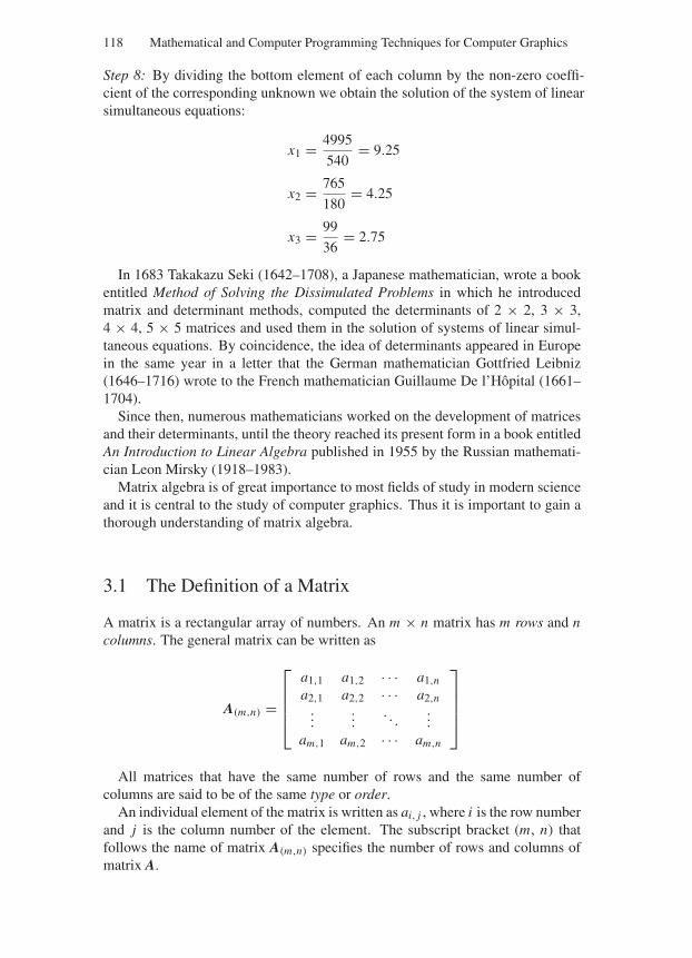
“Comninos” — 2005/8/31 — 15:34 — page 118 — #4
118 Mathematical and Computer Programming Techniques for Computer Graphics
Step 8: By dividing the bottom element of each column by the non-zero coeffi-cient of the corresponding unknown we obtain the solution of the system of linearsimultaneous equations:
x1 = 4995
540= 9.25
x2 = 765
180= 4.25
x3 = 99
36= 2.75
In 1683 Takakazu Seki (1642–1708), a Japanese mathematician, wrote a bookentitled Method of Solving the Dissimulated Problems in which he introducedmatrix and determinant methods, computed the determinants of 2 × 2, 3 × 3,4 × 4, 5 × 5 matrices and used them in the solution of systems of linear simul-taneous equations. By coincidence, the idea of determinants appeared in Europein the same year in a letter that the German mathematician Gottfried Leibniz(1646–1716) wrote to the French mathematician Guillaume De l’Hopital (1661–1704).
Since then, numerous mathematicians worked on the development of matricesand their determinants, until the theory reached its present form in a book entitledAn Introduction to Linear Algebra published in 1955 by the Russian mathemati-cian Leon Mirsky (1918–1983).
Matrix algebra is of great importance to most fields of study in modern scienceand it is central to the study of computer graphics. Thus it is important to gain athorough understanding of matrix algebra.
3.1 The Definition of a Matrix
A matrix is a rectangular array of numbers. An m × n matrix has m rows and ncolumns. The general matrix can be written as
A(m,n) =
⎡
⎢⎢⎢⎣
a1,1 a1,2 · · · a1,n
a2,1 a2,2 · · · a2,n...
.... . .
...
am,1 am,2 · · · am,n
⎤
⎥⎥⎥⎦
All matrices that have the same number of rows and the same number ofcolumns are said to be of the same type or order.
An individual element of the matrix is written as ai, j , where i is the row numberand j is the column number of the element. The subscript bracket (m, n) thatfollows the name of matrix A(m,n) specifies the number of rows and columns ofmatrix A.
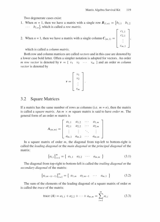
“Comninos” — 2005/8/31 — 15:34 — page 119 — #5
Matrix Algebra Survival Kit 119
Two degenerate cases exist:1. When m = 1, then we have a matrix with a single row B(1,n) = [
b1,1 b1,2· · · b1,n
], which is called a row matrix.
2. When n = 1, then we have a matrix with a single column C(m,1) =
⎡
⎢⎢⎢⎣
c1,1c2,1...
cm,1
⎤
⎥⎥⎥⎦
,
which is called a column matrix.Both row and column matrices are called vectors and in this case are denoted by
a lower case bold letter. Often a simpler notation is adopted for vectors. An orderm row vector is denoted by v = [ v1 v2 · · · vm ] and an order m columnvector is denoted by
v =
⎡
⎢⎢⎢⎣
v1v2...
vm
⎤
⎥⎥⎥⎦
.
3.2 Square Matrices
If a matrix has the same number of rows as columns (i.e. m = n), then the matrixis called a square matrix. An m × m square matrix is said to have order m. Thegeneral form of an order m matrix is
A(m,m) =
⎡
⎢⎢⎢⎣
a1,1 a1,2 · · · a1,m
a2,1 a2,2 · · · a2,m...
.... . .
...
am,1 am,2 · · · am,m
⎤
⎥⎥⎥⎦
In a square matrix of order m, the diagonal from top-left to bottom-right iscalled the leading diagonal or the main diagonal or the principal diagonal of thematrix:
ai,i
mi=1 =
a1,1 a2,2 · · · am,m
(3.1)
The diagonal from top-right to bottom-left is called the trailing diagonal or thesecondary diagonal of the matrix:
ai,m−(i−1)
mi=1 =
a1,m a2,m−1 · · · am,1
(3.2)
The sum of the elements of the leading diagonal of a square matrix of order mis called the trace of the matrix:
trace (A) = a1,1 + a2,2 + · · · + am,m =m∑
i=1
ai,i (3.3)
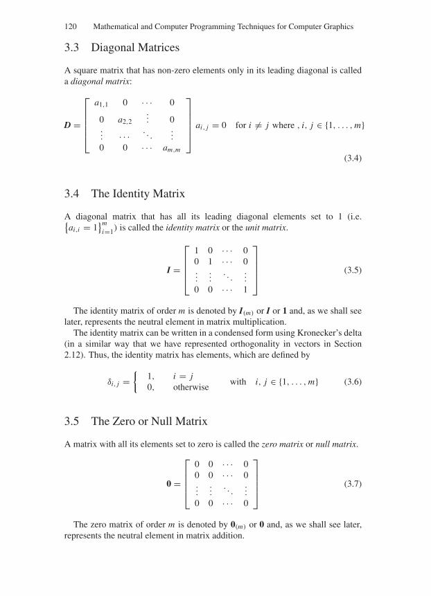
“Comninos” — 2005/8/31 — 15:34 — page 120 — #6
120 Mathematical and Computer Programming Techniques for Computer Graphics
3.3 Diagonal Matrices
A square matrix that has non-zero elements only in its leading diagonal is calleda diagonal matrix:
D =
⎡
⎢⎢⎢⎢⎣
a1,1 0 · · · 0
0 a2,2... 0
... · · · . . ....
0 0 · · · am,m
⎤
⎥⎥⎥⎥⎦
ai, j = 0 for i = j where , i, j ∈ 1, . . . , m
(3.4)
3.4 The Identity Matrix
A diagonal matrix that has all its leading diagonal elements set to 1 (i.e.ai,i = 1
mi=1) is called the identity matrix or the unit matrix.
I =
⎡
⎢⎢⎢⎣
1 0 · · · 00 1 · · · 0...
.... . .
...
0 0 · · · 1
⎤
⎥⎥⎥⎦
(3.5)
The identity matrix of order m is denoted by I(m) or I or 1 and, as we shall seelater, represents the neutral element in matrix multiplication.
The identity matrix can be written in a condensed form using Kronecker’s delta(in a similar way that we have represented orthogonality in vectors in Section2.12). Thus, the identity matrix has elements, which are defined by
δi, j =
1,
0,
i = jotherwise
with i, j ∈ 1, . . . , m (3.6)
3.5 The Zero or Null Matrix
A matrix with all its elements set to zero is called the zero matrix or null matrix.
0 =
⎡
⎢⎢⎢⎣
0 0 · · · 00 0 · · · 0...
.... . .
...
0 0 · · · 0
⎤
⎥⎥⎥⎦
(3.7)
The zero matrix of order m is denoted by 0(m) or 0 and, as we shall see later,represents the neutral element in matrix addition.
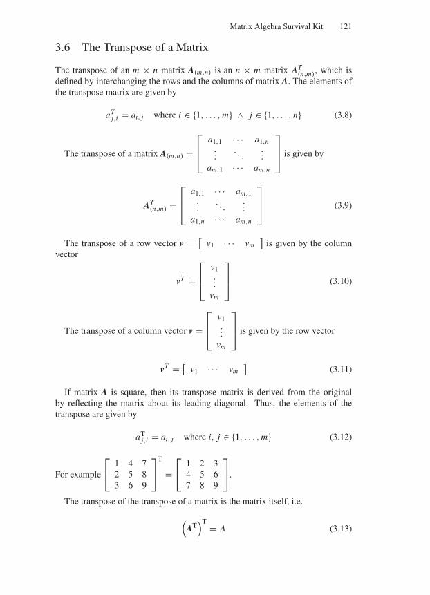
“Comninos” — 2005/8/31 — 15:34 — page 121 — #7
Matrix Algebra Survival Kit 121
3.6 The Transpose of a Matrix
The transpose of an m × n matrix A(m,n) is an n × m matrix AT(n,m), which is
defined by interchanging the rows and the columns of matrix A. The elements ofthe transpose matrix are given by
aTj,i = ai, j where i ∈ 1, . . . , m ∧ j ∈ 1, . . . , n (3.8)
The transpose of a matrix A(m,n) =⎡
⎢⎣
a1,1 · · · a1,n...
. . ....
am,1 · · · am,n
⎤
⎥⎦ is given by
AT(n,m) =
⎡
⎢⎣
a1,1 · · · am,1...
. . ....
a1,n · · · am,n
⎤
⎥⎦ (3.9)
The transpose of a row vector v = [v1 · · · vm
]is given by the column
vector
vT =⎡
⎢⎣
v1...
vm
⎤
⎥⎦ (3.10)
The transpose of a column vector v =⎡
⎢⎣
v1...
vm
⎤
⎥⎦ is given by the row vector
vT = [v1 · · · vm
](3.11)
If matrix A is square, then its transpose matrix is derived from the originalby reflecting the matrix about its leading diagonal. Thus, the elements of thetranspose are given by
aTj,i = ai, j where i, j ∈ 1, . . . , m (3.12)
For example
⎡
⎣1 4 72 5 83 6 9
⎤
⎦
T
=⎡
⎣1 2 34 5 67 8 9
⎤
⎦.
The transpose of the transpose of a matrix is the matrix itself, i.e.
(AT
)T = A (3.13)
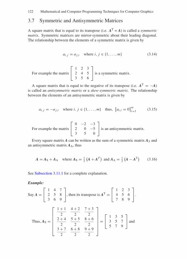
“Comninos” — 2005/8/31 — 15:34 — page 122 — #8
122 Mathematical and Computer Programming Techniques for Computer Graphics
3.7 Symmetric and Antisymmetric Matrices
A square matrix that is equal to its transpose (i.e. AT = A) is called a symmetricmatrix. Symmetric matrices are mirror-symmetric about their leading diagonal.The relationship between the elements of a symmetric matrix is given by
ai, j = a j,i where i, j ∈ 1, . . . , m (3.14)
For example the matrix
⎡
⎣1 2 32 4 53 5 6
⎤
⎦ is a symmetric matrix.
A square matrix that is equal to the negative of its transpose (i.e. AT = −A)is called an antisymmetric matrix or a skew-symmetric matrix. The relationshipbetween the elements of an antisymmetric matrix is given by
ai, j = −a j,i where i, j ∈ 1, . . . , m thus,ai,i = 0
mi=1 (3.15)
For example the matrix
⎡
⎣0 −2 −32 0 −53 5 0
⎤
⎦ is an antisymmetric matrix.
Every square matrix A can be written as the sum of a symmetric matrix AS andan antisymmetric matrix AA, thus
A = AS + AA where AS = 12
(A + AT
)and AA = 1
2
(A − AT)
(3.16)
See Subsection 3.11.1 for a complete explanation.
Example:
Say A =⎡
⎣1 4 72 5 83 6 9
⎤
⎦, then its transpose is AT =⎡
⎣1 2 34 5 67 8 9
⎤
⎦.
Thus, AS =
⎡
⎢⎢⎢⎢⎢⎢⎣
1 + 1
2
4 + 2
2
7 + 3
22 + 4
2
5 + 5
2
8 + 6
23 + 7
2
6 + 8
2
9 + 9
2
⎤
⎥⎥⎥⎥⎥⎥⎦
=⎡
⎣1 3 53 5 75 7 9
⎤
⎦ and
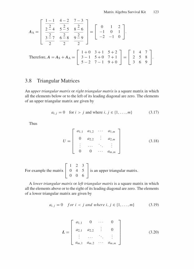
“Comninos” — 2005/8/31 — 15:34 — page 123 — #9
Matrix Algebra Survival Kit 123
AA =
⎡
⎢⎢⎢⎢⎣
1 − 1
2
4 − 2
2
7 − 3
22 − 4
2
5 − 5
2
8 − 6
23 − 7
2
6 − 8
2
9 − 9
2
⎤
⎥⎥⎥⎥⎦
=⎡
⎣0 1 2
−1 0 1−2 −1 0
⎤
⎦.
Therefore, A = AS + AA =⎡
⎣1 + 0 3 + 1 5 + 23 − 1 5 + 0 7 + 15 − 2 7 − 1 9 + 0
⎤
⎦ =⎡
⎣1 4 72 5 83 6 9
⎤
⎦.
3.8 Triangular Matrices
An upper triangular matrix or right triangular matrix is a square matrix in whichall the elements below or to the left of its leading diagonal are zero. The elementsof an upper triangular matrix are given by
ai, j = 0 for i > j and where i, j ∈ 1, . . . , m (3.17)
Thus
U =
⎡
⎢⎢⎢⎢⎣
a1,1 a1,2 · · · a1,m
0 a2,2... a2,m
... · · · . . ....
0 0 · · · am,m
⎤
⎥⎥⎥⎥⎦
(3.18)
For example the matrix
⎡
⎣1 2 30 4 50 0 6
⎤
⎦ is an upper triangular matrix.
A lower triangular matrix or left triangular matrix is a square matrix in whichall the elements above or to the right of its leading diagonal are zero. The elementsof a lower triangular matrix are given by
ai, j = 0 f or i < j and where i, j ∈ 1, . . . , m (3.19)
L =
⎡
⎢⎢⎢⎢⎣
a1,1 0 · · · 0
a2,1 a2,2... 0
... · · · . . ....
am,1 am,2 · · · am,m
⎤
⎥⎥⎥⎥⎦
(3.20)
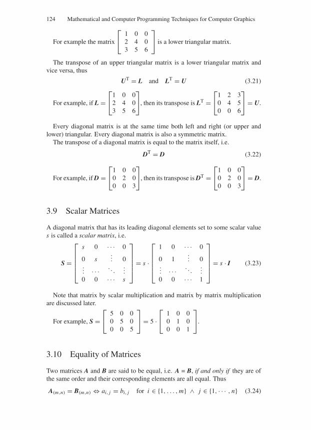
“Comninos” — 2005/8/31 — 15:34 — page 124 — #10
124 Mathematical and Computer Programming Techniques for Computer Graphics
For example the matrix
⎡
⎣1 0 02 4 03 5 6
⎤
⎦ is a lower triangular matrix.
The transpose of an upper triangular matrix is a lower triangular matrix andvice versa, thus
UT = L and LT = U (3.21)
For example, if L =⎡
⎣1 0 02 4 03 5 6
⎤
⎦, then its transpose is LT =⎡
⎣1 2 30 4 50 0 6
⎤
⎦ = U.
Every diagonal matrix is at the same time both left and right (or upper andlower) triangular. Every diagonal matrix is also a symmetric matrix.
The transpose of a diagonal matrix is equal to the matrix itself, i.e.
DT = D (3.22)
For example, if D =⎡
⎣1 0 00 2 00 0 3
⎤
⎦, then its transpose is DT =⎡
⎣1 0 00 2 00 0 3
⎤
⎦ = D.
3.9 Scalar Matrices
A diagonal matrix that has its leading diagonal elements set to some scalar values is called a scalar matrix, i.e.
S =
⎡
⎢⎢⎢⎢⎣
s 0 · · · 0
0 s... 0
... · · · . . ....
0 0 · · · s
⎤
⎥⎥⎥⎥⎦
= s ·
⎡
⎢⎢⎢⎢⎣
1 0 · · · 0
0 1... 0
... · · · . . ....
0 0 · · · 1
⎤
⎥⎥⎥⎥⎦
= s · I (3.23)
Note that matrix by scalar multiplication and matrix by matrix multiplicationare discussed later.
For example, S =⎡
⎣5 0 00 5 00 0 5
⎤
⎦ = 5 ·⎡
⎣1 0 00 1 00 0 1
⎤
⎦.
3.10 Equality of Matrices
Two matrices A and B are said to be equal, i.e. A = B, if and only if they are ofthe same order and their corresponding elements are all equal. Thus
A(m,n) = B(m,n) ⇔ ai, j = bi, j for i ∈ 1, . . . , m ∧ j ∈ 1, · · · , n (3.24)
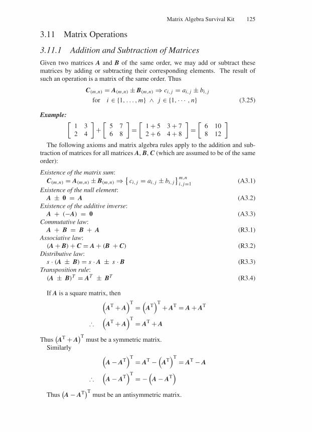
“Comninos” — 2005/8/31 — 15:34 — page 125 — #11
Matrix Algebra Survival Kit 125
3.11 Matrix Operations
3.11.1 Addition and Subtraction of Matrices
Given two matrices A and B of the same order, we may add or subtract thesematrices by adding or subtracting their corresponding elements. The result ofsuch an operation is a matrix of the same order. Thus
C(m,n) = A(m,n) ± B(m,n) ⇒ ci, j = ai, j ± bi, j
for i ∈ 1, . . . , m ∧ j ∈ 1, · · · , n (3.25)
Example:[
1 32 4
]+
[5 76 8
]=
[1 + 5 3 + 72 + 6 4 + 8
]=
[6 108 12
]
The following axioms and matrix algebra rules apply to the addition and sub-traction of matrices for all matrices A, B, C (which are assumed to be of the sameorder):
Existence of the matrix sum:C(m,n) = A(m,n) ± B(m,n) ⇒
ci, j = ai, j ± bi, jm,n
i, j=1 (A3.1)Existence of the null element:
A ± 0 = A (A3.2)Existence of the additive inverse:
A + (−A) = 0 (A3.3)Commutative law:
A + B = B + A (R3.1)Associative law:
(A + B) + C = A + (B + C) (R3.2)Distributive law:
s · (A ± B) = s · A ± s · B (R3.3)Transposition rule:
(A ± B)T = AT ± BT (R3.4)
If A is a square matrix, then(
AT + A)T =
(AT
)T + AT = A + AT
∴(
AT + A)T = AT + A
Thus(AT + A
)Tmust be a symmetric matrix.
Similarly(
A − AT)T = AT −
(AT
)T = AT − A
∴(
A − AT)T = −
(A − AT
)
Thus(A − AT)T
must be an antisymmetric matrix.
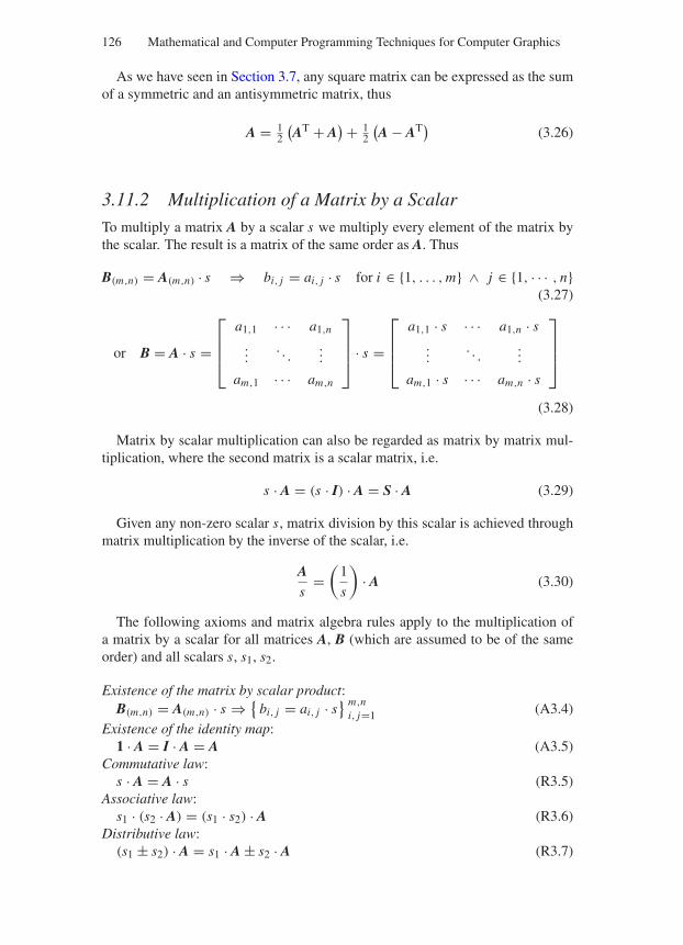
“Comninos” — 2005/8/31 — 15:34 — page 126 — #12
126 Mathematical and Computer Programming Techniques for Computer Graphics
As we have seen in Section 3.7, any square matrix can be expressed as the sumof a symmetric and an antisymmetric matrix, thus
A = 12
(AT + A
) + 12
(A − AT)
(3.26)
3.11.2 Multiplication of a Matrix by a Scalar
To multiply a matrix A by a scalar s we multiply every element of the matrix bythe scalar. The result is a matrix of the same order as A. Thus
B(m,n) = A(m,n) · s ⇒ bi, j = ai, j · s for i ∈ 1, . . . , m ∧ j ∈ 1, · · · , n(3.27)
or B = A · s =
⎡
⎢⎢⎣
a1,1 · · · a1,n
.... . .
...
am,1 · · · am,n
⎤
⎥⎥⎦ · s =
⎡
⎢⎢⎣
a1,1 · s · · · a1,n · s...
. . ....
am,1 · s · · · am,n · s
⎤
⎥⎥⎦
(3.28)
Matrix by scalar multiplication can also be regarded as matrix by matrix mul-tiplication, where the second matrix is a scalar matrix, i.e.
s · A = (s · I) · A = S · A (3.29)
Given any non-zero scalar s, matrix division by this scalar is achieved throughmatrix multiplication by the inverse of the scalar, i.e.
As
=(
1
s
)· A (3.30)
The following axioms and matrix algebra rules apply to the multiplication ofa matrix by a scalar for all matrices A, B (which are assumed to be of the sameorder) and all scalars s, s1, s2.
Existence of the matrix by scalar product:B(m,n) = A(m,n) · s ⇒
bi, j = ai, j · s m,n
i, j=1 (A3.4)Existence of the identity map:
1 · A = I · A = A (A3.5)Commutative law:
s · A = A · s (R3.5)Associative law:
s1 · (s2 · A) = (s1 · s2) · A (R3.6)Distributive law:
(s1 ± s2) · A = s1 · A ± s2 · A (R3.7)
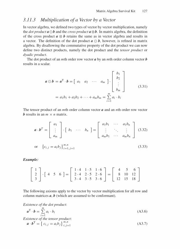
“Comninos” — 2005/8/31 — 15:34 — page 127 — #13
Matrix Algebra Survival Kit 127
3.11.3 Multiplication of a Vector by a Vector
In vector algebra, we defined two types of vector by vector multiplication, namelythe dot product ab and the cross product a⊗b. In matrix algebra, the definitionof the cross product a ⊗ b retains the same as in vector algebra and results ina vector. The definition of the dot product a b, however, is refined in matrixalgebra. By disallowing the commutative property of the dot product we can nowdefine two distinct products, namely the dot product and the tensor product ordyadic product.
The dot product of an mth order row vector a by an mth order column vector bresults in a scalar.
a b = aT · b = [a1 a2 · · · am
] ·
⎡
⎢⎢⎢⎣
b1b2...
bm
⎤
⎥⎥⎥⎦
= a1b1 + a2b2 + · · · + ambm =m∑
i=1ai · bi
(3.31)
The tensor product of an mth order column vector a and an nth order row vectorb results in an m × n matrix.
a · bT =⎡
⎢⎣
a1...
am
⎤
⎥⎦ · [
b1 · · · bn] =
⎡
⎢⎣
a1b1 · · · a1bn...
. . ....
amb1 · · · ambn
⎤
⎥⎦ (3.32)
orci, j = ai b j
m,ni=1, j=1 (3.33)
Example:
⎡
⎣123
⎤
⎦ · [4 5 6
] =⎡
⎣1 · 4 1 · 5 1 · 62 · 4 2 · 5 2 · 63 · 4 3 · 5 3 · 6
⎤
⎦ =⎡
⎣4 5 68 10 12
12 15 18
⎤
⎦
The following axioms apply to the vector by vector multiplication for all row andcolumn matrices a, b (which are assumed to be conformant).
Existence of the dot product:
aT · b =m∑
i=1ai · bi (A3.6)
Existence of the tensor product:a · bT =
ci, j = ai b j m,n
i, j=1 (A3.7)
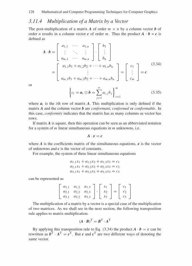
“Comninos” — 2005/8/31 — 15:34 — page 128 — #14
128 Mathematical and Computer Programming Techniques for Computer Graphics
3.11.4 Multiplication of a Matrix by a Vector
The post-multiplication of a matrix A of order m × n by a column vector b oforder n results in a column vector c of order m. Thus the product A · b = c isdefined as
A · b =⎡
⎢⎣
a1,1 · · · a1,n...
. . ....
am,1 · · · am,n
⎤
⎥⎦ ·
⎡
⎢⎣
b1...
bn
⎤
⎥⎦
(3.34)
=⎡
⎢⎣
a1,1b1 + a1,2b2 + · · · + a1,nbn...
am,1b1 + am,2b2 + · · · + am,nbn
⎤
⎥⎦ =
⎡
⎢⎣
c1...
cm
⎤
⎥⎦ = c
or ci = ai b =
n∑
j=1
ai, j b j
m
i=1(3.35)
where ai is the i th row of matrix A. This multiplication is only defined if thematrix A and the column vector b are conformant, conformal or conformable. Inthis case, conformity indicates that the matrix has as many columns as vector hasrows.
If matrix A is square, then this operation can be seen as an abbreviated notationfor a system of m linear simultaneous equations in m unknowns, i.e.
A · x = c
where A is the coefficients matrix of the simultaneous equations, x is the vectorof unknowns and c is the vector of constants.
For example, the system of three linear simultaneous equations
a1,1x1 + a1,2x2 + a1,3x3 = c1a2,1x1 + a2,2x2 + a2,3x3 = c2a3,1x1 + a3,2x2 + a3,3x3 = c3
can be represented as⎡
⎣a1,1 a1,2 a1,3a2,1 a2,2 a2,3a3,1 a3,2 a3,3
⎤
⎦ ·⎡
⎣x1x2x3
⎤
⎦ =⎡
⎣c1c2c3
⎤
⎦
The multiplication of a matrix by a vector is a special case of the multiplicationof two matrices. As we shall see in the next section, the following transpositionrule applies to matrix multiplication.
(A · B)T = BT · AT
By applying this transposition rule to Eq. (3.34) the product A · b = c can berewritten as bT · AT = cT. But c and cT are two different ways of denoting thesame vector.
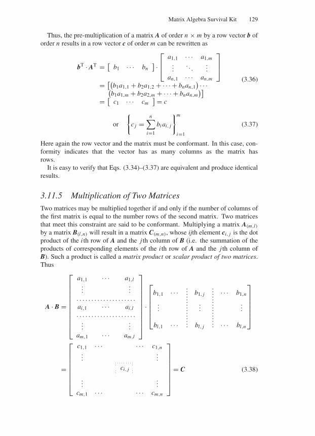
“Comninos” — 2005/8/31 — 15:34 — page 129 — #15
Matrix Algebra Survival Kit 129
Thus, the pre-multiplication of a matrix A of order n × m by a row vector b oforder n results in a row vector c of order m can be rewritten as
bT · AT = [b1 · · · bn
] ·⎡
⎢⎣
a1,1 · · · a1,m...
. . ....
an,1 · · · an,m
⎤
⎥⎦
= [(b1a1,1 + b2a1,2 + · · · + bnan,1
) · · ·(b1a1,m + b2a2,m + · · · + bnan,m
)]
= [c1 · · · cm
] = c
(3.36)
or
c j =n∑
i=1
bi ai, j
m
i=1
(3.37)
Here again the row vector and the matrix must be conformant. In this case, con-formity indicates that the vector has as many columns as the matrix hasrows.
It is easy to verify that Eqs. (3.34)–(3.37) are equivalent and produce identicalresults.
3.11.5 Multiplication of Two Matrices
Two matrices may be multiplied together if and only if the number of columns ofthe first matrix is equal to the number rows of the second matrix. Two matricesthat meet this constraint are said to be conformant. Multiplying a matrix A(m,l)
by a matrix B(l,n) will result in a matrix C(m,n), whose ijth element ci, j is the dotproduct of the i th row of A and the j th column of B (i.e. the summation of theproducts of corresponding elements of the i th row of A and the j th column ofB). Such a product is called a matrix product or scalar product of two matrices.Thus
A · B =
⎡
⎢⎢⎢⎢⎢⎢⎢⎢⎢⎢⎣
a1,1 · · · a1,l...
...
. . . . . . . . . . . . . . . . . . . .
ai,1 · · · ai,l
. . . . . . . . . . . . . . . . . . . ....
...
am,1 · · · am,l
⎤
⎥⎥⎥⎥⎥⎥⎥⎥⎥⎥⎦
·
⎡
⎢⎢⎢⎢⎢⎣
b1,1 · · · ... b1, j... · · · b1,n.........
......
.........
...
bl,1 · · · ... bl, j... · · · bl,n
⎤
⎥⎥⎥⎥⎥⎦
=
⎡
⎢⎢⎢⎢⎢⎢⎢⎣
c1,1 · · · · · · c1,n...
...
ci, j
......
cm,1 · · · · · · cm,n
⎤
⎥⎥⎥⎥⎥⎥⎥⎦
= C (3.38)

“Comninos” — 2005/8/31 — 15:34 — page 130 — #16
130 Mathematical and Computer Programming Techniques for Computer Graphics
If ai denotes the i th row of A and b j denotes the j th column of B, then elementci, j of the product is defined as
ci, j = ai b j = ai,1b1, j + ai,2b2, j + · · · + ai,lbl, j =l∑
k=1
ai,kbk, j
m,n
i=1, j=1
(3.39)
Matrix by matrix multiplication can be implemented by the following pseudo-code:
for i = 1..m dofor j = 1..n dobeginci, j ← 0for k = 1..l doci, j ← ci, j + ai,k · bk, j
end
Division of a matrix A by a matrix B is carried out through the multiplication of Aby the reciprocal or inverse matrix B−1. Inversion of matrices will be examinedin Section 3.17.
Example:
C(3,3) = A(3,2) · B(2,3)
=⎡
⎢⎣
a1,1 a1,2
a2,1 a2,2
a3,1 a3,2
⎤
⎥⎦ ·
[b1,1 b1,2 b1,3
b2,1 b2,2 b2,3
]
=⎡
⎢⎣
a1,1b1,1 + a1,2b2,1 a1,1b1,2 + a1,2b2,2 a1,1b1,3 + a1,2b2,3
a2,1b1,1 + a2,2b2,1 a2,1b1,2 + a2,2b2,2 a2,1b1,3 + a2,2b2,3
a3,1b1,1 + a3,2b2,1 a3,1b1,2 + a3,2b2,2 a3,1b1,3 + a3,2b2,3
⎤
⎥⎦
3.11.6 Powers of Matrices
Given a square matrix A, we can define the powers of this matrix through repeatedmatrix multiplication. The zero power of the matrix is defined to be the identitymatrix. And the first power of a matrix is the matrix itself. Thus
A0 = I, A1 = A, A2 = A · A, A3 = A2 · A, · · · , Am = A(m−1) · A(3.40)
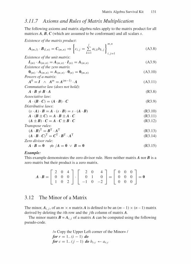
“Comninos” — 2005/8/31 — 15:34 — page 131 — #17
Matrix Algebra Survival Kit 131
3.11.7 Axioms and Rules of Matrix Multiplication
The following axioms and matrix algebra rules apply to the matrix product for allmatrices A, B, C (which are assumed to be conformant) and all scalars s.
Existence of the matrix product:
A(m,l) · B(l,n) = C(m,n) ⇒
ci, j =l∑
k=1ai,kbk, j
m,n
i, j=1
(A3.8)
Existence of the unit matrix:I(m) · A(m,n) = A(m,n) · I(n) = A(m,n) (A3.9)
Existence of the zero matrix0(m) · A(m,n) = A(m,n) · 0(n) = 0(m,n) (A3.10)
Powers of a matrix:A0 = I ∧ Am = A(m−1) · A (A3.11)
Commutative law (does not hold):A · B = B · A (R3.8)
Associative law:A · (B · C) = (A · B) · C (R3.9)
Distributive laws:(s · A) · B = A · (s · B) = s · (A · B) (R3.10)A · (B ± C) = A · B ± A · C (R3.11)(A ± B) · C = A · C ± B · C (R3.12)
Transpose rules:(A · B)T = BT · AT (R3.13)(A · B · C)T = CT · BT · AT (R3.14)
Zero divisor rule:A · B = 0 ⇒ /A = 0 ∨ B = 0 (R3.15)
Example:This example demonstrates the zero divisor rule. Here neither matrix A nor B is azero matrix but their product is a zero matrix.
A · B =⎡
⎣2 0 40 0 01 0 2
⎤
⎦ ·⎡
⎣2 0 40 1 0
−1 0 −2
⎤
⎦ =⎡
⎣0 0 00 0 00 0 0
⎤
⎦ = 0
3.12 The Minor of a Matrix
The minor, Ai, j , of an m × n matrix A is defined to be an (m – 1) × (n – 1) matrixderived by deleting the i th row and the j th column of matrix A.
The minor matrix B = Ai, j of a matrix A can be computed using the followingpseudo-code.
/∗ Copy the Upper Left corner of the Minor∗ /for r = 1.. (i − 1) dofor c = 1.. ( j − 1) do br,c ← ar,c
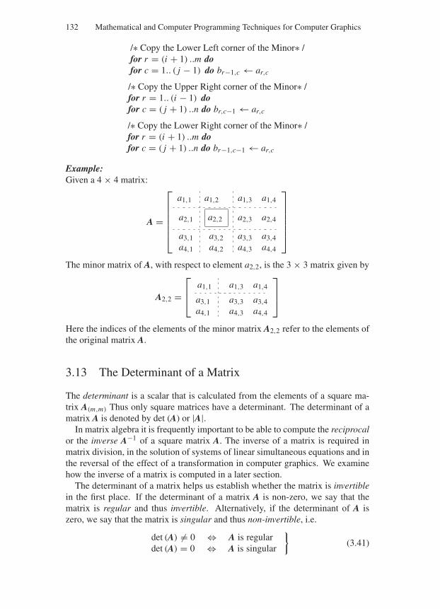
“Comninos” — 2005/8/31 — 15:34 — page 132 — #18
132 Mathematical and Computer Programming Techniques for Computer Graphics
/∗ Copy the Lower Left corner of the Minor∗ /for r = (i + 1) ..m dofor c = 1.. ( j − 1) do br−1,c ← ar,c
/∗ Copy the Upper Right corner of the Minor∗ /for r = 1.. (i − 1) dofor c = ( j + 1) ..n do br,c−1 ← ar,c
/∗ Copy the Lower Right corner of the Minor∗ /for r = (i + 1) ..m dofor c = ( j + 1) ..n do br−1,c−1 ← ar,c
Example:Given a 4 × 4 matrix:
A =
⎡
⎢⎢⎢⎢⎢⎣
a1,1 a1,2 a1,3 a1,4
a2,1 a2,2 a2,3 a2,4
a3,1 a3,2 a3,3 a3,4a4,1 a4,2 a4,3 a4,4
⎤
⎥⎥⎥⎥⎥⎦
The minor matrix of A, with respect to element a2,2, is the 3 × 3 matrix given by
A2,2 =⎡
⎢⎣
a1,1 a1,3 a1,4
a3,1 a3,3 a3,4a4,1 a4,3 a4,4
⎤
⎥⎦
Here the indices of the elements of the minor matrix A2,2 refer to the elements ofthe original matrix A.
3.13 The Determinant of a Matrix
The determinant is a scalar that is calculated from the elements of a square ma-trix A(m,m) Thus only square matrices have a determinant. The determinant of amatrix A is denoted by det (A) or |A|.
In matrix algebra it is frequently important to be able to compute the reciprocalor the inverse A−1 of a square matrix A. The inverse of a matrix is required inmatrix division, in the solution of systems of linear simultaneous equations and inthe reversal of the effect of a transformation in computer graphics. We examinehow the inverse of a matrix is computed in a later section.
The determinant of a matrix helps us establish whether the matrix is invertiblein the first place. If the determinant of a matrix A is non-zero, we say that thematrix is regular and thus invertible. Alternatively, if the determinant of A iszero, we say that the matrix is singular and thus non-invertible, i.e.
det (A) = 0 ⇔ A is regulardet (A) = 0 ⇔ A is singular
(3.41)
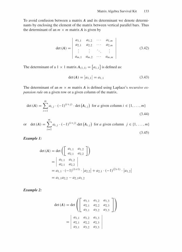
“Comninos” — 2005/8/31 — 15:34 — page 133 — #19
Matrix Algebra Survival Kit 133
To avoid confusion between a matrix A and its determinant we denote determi-nants by enclosing the element of the matrix between vertical parallel bars. Thusthe determinant of an m × m matrix A is given by
det (A) =
∣∣∣∣∣∣∣∣∣
a1,1 a1,2 · · · a1,m
a2,1 a2,2 · · · a2,m...
.... . .
...
am,1 am,2 · · · am,m
∣∣∣∣∣∣∣∣∣
(3.42)
The determinant of a 1 × 1 matrix A(1,1) = [a1,1
]is defined as:
det(A) = ∣∣a1,1∣∣ = a1,1 (3.43)
The determinant of an m × m matrix A is defined using Laplace’s recursive ex-pansion rule on a given row or a given column of the matrix.
det (A) =m∑
i=1
ai, j · (−1)(i+ j) · det(Ai, j
)for a given column i ∈ 1, . . . , m
(3.44)
or det (A) =m∑
i=1
ai, j · (−1)(i+ j)·det(Ai, j
)for a given column j ∈ 1, . . . , m
(3.45)
Example 1:
det (A) = det
([a1,1 a1,2a2,1 a2,2
])
=∣∣∣∣
a1,1 a1,2a2,1 a2,2
∣∣∣∣
= a1,1 · (−1)(1+1) · ∣∣a2,2∣∣ + a2,1 · (−1)(2+1) · ∣∣a1,2
∣∣
= a1,1a2,2 − a2,1a1,2
Example 2:
det (A) = det
⎛
⎝
⎡
⎣a1,1 a1,2 a1,3a2,1 a2,2 a2,3a3,1 a3,2 a3,3
⎤
⎦
⎞
⎠
=∣∣∣∣∣∣
a1,1 a1,2 a1,3a2,1 a2,2 a2,3a3,1 a3,2 a3,3
∣∣∣∣∣∣
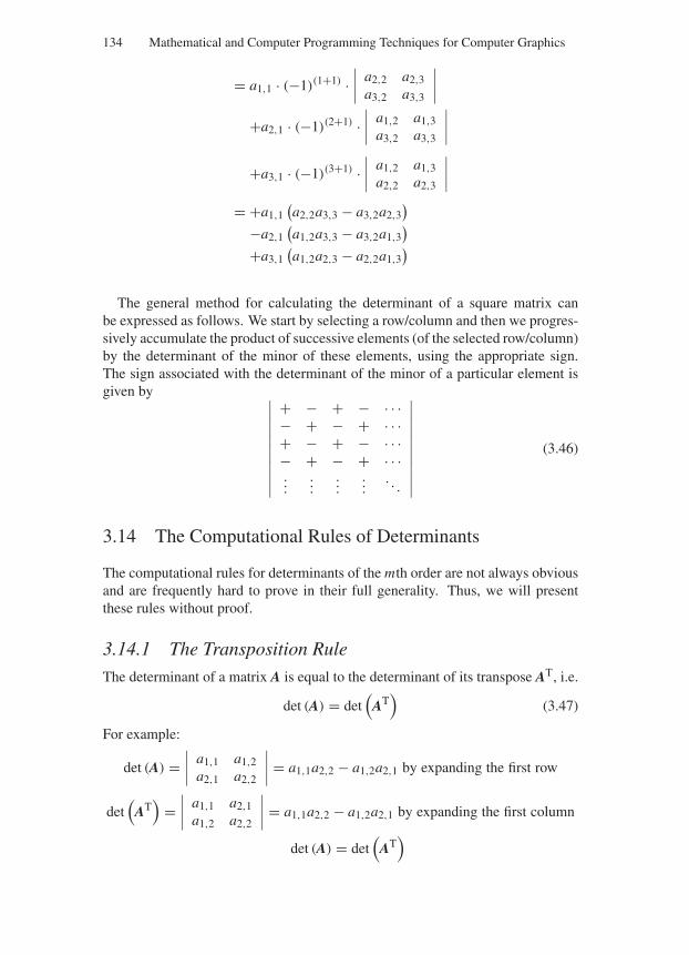
“Comninos” — 2005/8/31 — 15:34 — page 134 — #20
134 Mathematical and Computer Programming Techniques for Computer Graphics
= a1,1 · (−1)(1+1) ·∣∣∣∣
a2,2 a2,3a3,2 a3,3
∣∣∣∣
+a2,1 · (−1)(2+1) ·∣∣∣∣
a1,2 a1,3a3,2 a3,3
∣∣∣∣
+a3,1 · (−1)(3+1) ·∣∣∣∣
a1,2 a1,3a2,2 a2,3
∣∣∣∣
= +a1,1(a2,2a3,3 − a3,2a2,3
)
−a2,1(a1,2a3,3 − a3,2a1,3
)
+a3,1(a1,2a2,3 − a2,2a1,3
)
The general method for calculating the determinant of a square matrix canbe expressed as follows. We start by selecting a row/column and then we progres-sively accumulate the product of successive elements (of the selected row/column)by the determinant of the minor of these elements, using the appropriate sign.The sign associated with the determinant of the minor of a particular element isgiven by ∣∣∣∣∣∣∣∣∣∣∣
+ − + − · · ·− + − + · · ·+ − + − · · ·− + − + · · ·...
......
.... . .
∣∣∣∣∣∣∣∣∣∣∣
(3.46)
3.14 The Computational Rules of Determinants
The computational rules for determinants of the mth order are not always obviousand are frequently hard to prove in their full generality. Thus, we will presentthese rules without proof.
3.14.1 The Transposition Rule
The determinant of a matrix A is equal to the determinant of its transpose AT, i.e.
det (A) = det(
AT)
(3.47)
For example:
det (A) =∣∣∣∣
a1,1 a1,2a2,1 a2,2
∣∣∣∣ = a1,1a2,2 − a1,2a2,1 by expanding the first row
det(
AT)
=∣∣∣∣
a1,1 a2,1a1,2 a2,2
∣∣∣∣ = a1,1a2,2 − a1,2a2,1 by expanding the first column
det (A) = det(
AT)
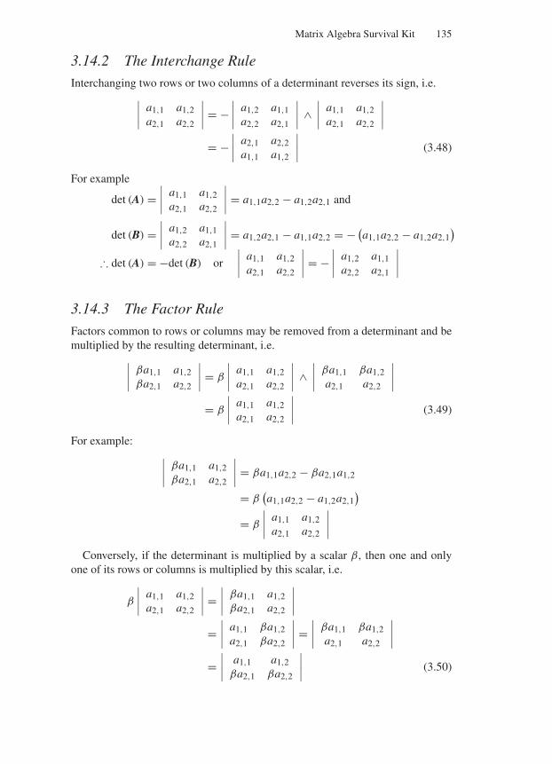
“Comninos” — 2005/8/31 — 15:34 — page 135 — #21
Matrix Algebra Survival Kit 135
3.14.2 The Interchange Rule
Interchanging two rows or two columns of a determinant reverses its sign, i.e.∣∣∣∣
a1,1 a1,2a2,1 a2,2
∣∣∣∣ = −∣∣∣∣
a1,2 a1,1a2,2 a2,1
∣∣∣∣ ∧∣∣∣∣
a1,1 a1,2a2,1 a2,2
∣∣∣∣
= −∣∣∣∣
a2,1 a2,2a1,1 a1,2
∣∣∣∣ (3.48)
For example
det (A) =∣∣∣∣
a1,1 a1,2a2,1 a2,2
∣∣∣∣ = a1,1a2,2 − a1,2a2,1 and
det (B) =∣∣∣∣
a1,2 a1,1a2,2 a2,1
∣∣∣∣ = a1,2a2,1 − a1,1a2,2 = − (a1,1a2,2 − a1,2a2,1
)
∴ det (A) = −det (B) or
∣∣∣∣a1,1 a1,2a2,1 a2,2
∣∣∣∣ = −∣∣∣∣
a1,2 a1,1a2,2 a2,1
∣∣∣∣
3.14.3 The Factor Rule
Factors common to rows or columns may be removed from a determinant and bemultiplied by the resulting determinant, i.e.
∣∣∣∣βa1,1 a1,2βa2,1 a2,2
∣∣∣∣ = β
∣∣∣∣a1,1 a1,2a2,1 a2,2
∣∣∣∣ ∧∣∣∣∣
βa1,1 βa1,2a2,1 a2,2
∣∣∣∣
= β
∣∣∣∣a1,1 a1,2a2,1 a2,2
∣∣∣∣ (3.49)
For example:∣∣∣∣
βa1,1 a1,2βa2,1 a2,2
∣∣∣∣ = βa1,1a2,2 − βa2,1a1,2
= β(a1,1a2,2 − a1,2a2,1
)
= β
∣∣∣∣a1,1 a1,2a2,1 a2,2
∣∣∣∣
Conversely, if the determinant is multiplied by a scalar β, then one and onlyone of its rows or columns is multiplied by this scalar, i.e.
β
∣∣∣∣a1,1 a1,2a2,1 a2,2
∣∣∣∣ =∣∣∣∣
βa1,1 a1,2βa2,1 a2,2
∣∣∣∣
=∣∣∣∣
a1,1 βa1,2a2,1 βa2,2
∣∣∣∣ =∣∣∣∣
βa1,1 βa1,2a2,1 a2,2
∣∣∣∣
=∣∣∣∣
a1,1 a1,2βa2,1 βa2,2
∣∣∣∣ (3.50)
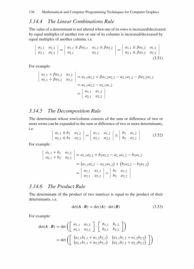
“Comninos” — 2005/8/31 — 15:34 — page 136 — #22
136 Mathematical and Computer Programming Techniques for Computer Graphics
3.14.4 The Linear Combinations Rule
The value of a determinant is not altered when one of its rows is increased/decreasedby equal multiples of another row or one of its columns is increased/decreased byequal multiples of another column, i.e.
∣∣∣∣a1,1 a1,2a2,1 a2,2
∣∣∣∣ =∣∣∣∣
a1,1 ± βa2,1 a1,2 ± βa2,2a2,1 a2,2
∣∣∣∣ =∣∣∣∣
a1,1 ± βa1,2 a1,2a2,1 ± βa2,2 a2,2
∣∣∣∣
(3.51)
For example:∣∣∣∣
a1,1 + βa1,2 a1,2a2,1 + βa2,2 a2,2
∣∣∣∣ = a1,1a2,2 + βa1,2a2,2 − a2,1a1,2 − βa2,2a1,2
= a1,1a2,2 − a2,1a1,2
=∣∣∣∣
a1,1 a1,2a2,1 a2,2
∣∣∣∣
3.14.5 The Decomposition Rule
The determinant whose row/column consists of the sum or difference of two ormore terms can be expanded to the sum or difference of two or more determinants,i.e. ∣∣∣∣
a1,1 ± b1 a1,2a2,1 ± b2 a2,2
∣∣∣∣ =∣∣∣∣
a1,1 a1,2a2,1 a2,2
∣∣∣∣ ±∣∣∣∣
b1 a1,2b2 a2,2
∣∣∣∣ (3.52)
For example:∣∣∣∣
a1,1 + b1 a1,2a2,1 + b2 a2,2
∣∣∣∣ = a1,1a2,2 + b1a2,2 − a2,1a1,2 − b2a1,2
= (a1,1a2,2 − a2,1a1,2
) + (b1a2,2 − b2a1,2
)
=∣∣∣∣
a1,1 a1,2a2,1 a2,2
∣∣∣∣ +∣∣∣∣
b1 a1,2b2 a2,2
∣∣∣∣
3.14.6 The Product Rule
The determinant of the product of two matrices is equal to the product of theirdeterminants, i.e.
det(A · B) = det (A) · det (B) (3.53)
For example:
det(A · B) = det
([a1,1 a1,2a2,1 a2,2
]·[
b1,1 b1,2b2,1 b2,2
])
= det
([ (a1,1b1,1 + a1,2b2,1
) (a1,1b1,2 + a1,2b2,2
)(a2,1b1,1 + a2,2b2,1
) (a2,1b1,2 + a2,2b2,2
)])
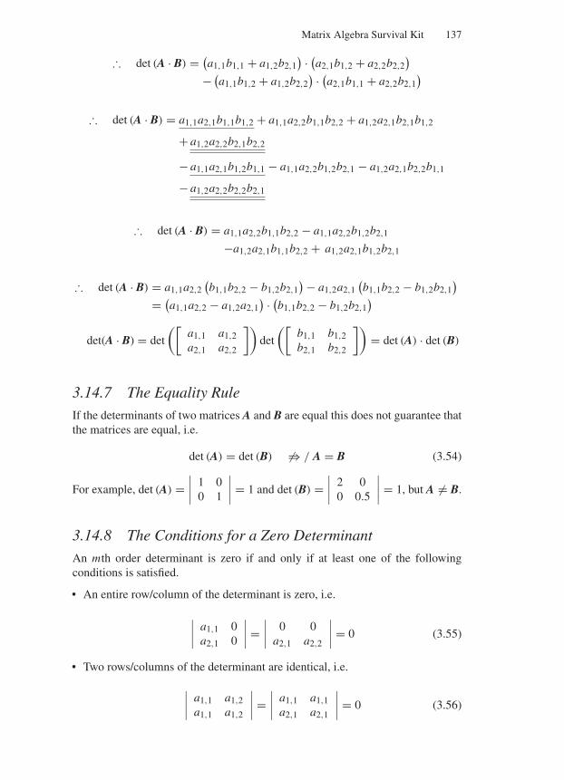
“Comninos” — 2005/8/31 — 15:34 — page 137 — #23
Matrix Algebra Survival Kit 137
∴ det (A · B) = (a1,1b1,1 + a1,2b2,1
) · (a2,1b1,2 + a2,2b2,2
)
− (a1,1b1,2 + a1,2b2,2
) · (a2,1b1,1 + a2,2b2,1
)
∴ det (A · B) = a1,1a2,1b1,1b1,2 + a1,1a2,2b1,1b2,2 + a1,2a2,1b2,1b1,2
+ a1,2a2,2b2,1b2,2
− a1,1a2,1b1,2b1,1 − a1,1a2,2b1,2b2,1 − a1,2a2,1b2,2b1,1
− a1,2a2,2b2,2b2,1
∴ det (A · B) = a1,1a2,2b1,1b2,2 − a1,1a2,2b1,2b2,1
−a1,2a2,1b1,1b2,2 + a1,2a2,1b1,2b2,1
∴ det (A · B) = a1,1a2,2(b1,1b2,2 − b1,2b2,1
) − a1,2a2,1(b1,1b2,2 − b1,2b2,1
)
= (a1,1a2,2 − a1,2a2,1
) · (b1,1b2,2 − b1,2b2,1
)
det(A · B) = det
([a1,1 a1,2a2,1 a2,2
])det
([b1,1 b1,2b2,1 b2,2
])= det (A) · det (B)
3.14.7 The Equality Rule
If the determinants of two matrices A and B are equal this does not guarantee thatthe matrices are equal, i.e.
det (A) = det (B) ⇒ / A = B (3.54)
For example, det (A) =∣∣∣∣
1 00 1
∣∣∣∣ = 1 and det (B) =∣∣∣∣
2 00 0.5
∣∣∣∣ = 1, but A = B.
3.14.8 The Conditions for a Zero Determinant
An mth order determinant is zero if and only if at least one of the followingconditions is satisfied.
• An entire row/column of the determinant is zero, i.e.
∣∣∣∣a1,1 0a2,1 0
∣∣∣∣ =∣∣∣∣
0 0a2,1 a2,2
∣∣∣∣ = 0 (3.55)
• Two rows/columns of the determinant are identical, i.e.
∣∣∣∣a1,1 a1,2a1,1 a1,2
∣∣∣∣ =∣∣∣∣
a1,1 a1,1a2,1 a2,1
∣∣∣∣ = 0 (3.56)
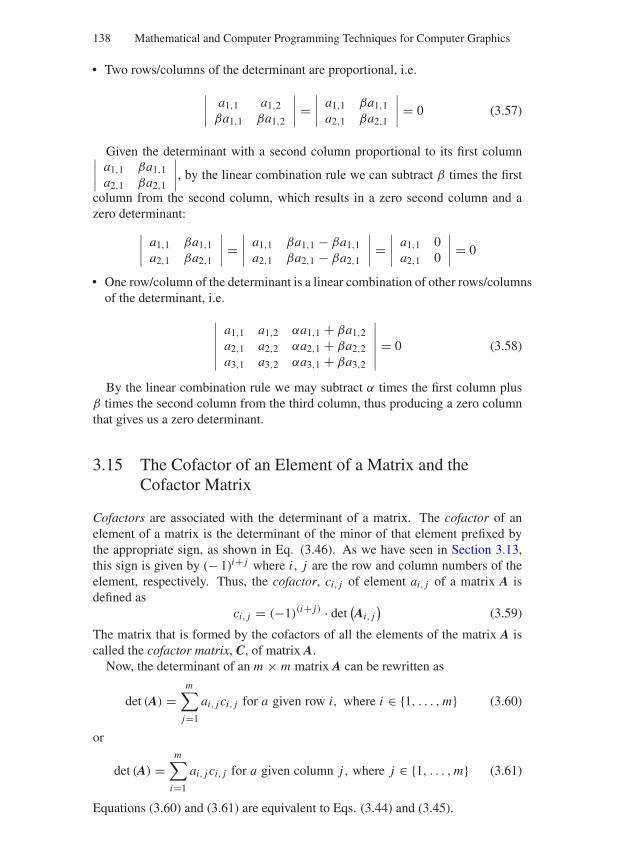
“Comninos” — 2005/8/31 — 15:34 — page 138 — #24
138 Mathematical and Computer Programming Techniques for Computer Graphics
• Two rows/columns of the determinant are proportional, i.e.
∣∣∣∣a1,1 a1,2βa1,1 βa1,2
∣∣∣∣ =∣∣∣∣
a1,1 βa1,1a2,1 βa2,1
∣∣∣∣ = 0 (3.57)
Given the determinant with a second column proportional to its first column∣∣∣∣a1,1 βa1,1a2,1 βa2,1
∣∣∣∣, by the linear combination rule we can subtract β times the first
column from the second column, which results in a zero second column and azero determinant:
∣∣∣∣
a1,1 βa1,1a2,1 βa2,1
∣∣∣∣ =
∣∣∣∣
a1,1 βa1,1 − βa1,1a2,1 βa2,1 − βa2,1
∣∣∣∣ =
∣∣∣∣
a1,1 0a2,1 0
∣∣∣∣ = 0
• One row/column of the determinant is a linear combination of other rows/columnsof the determinant, i.e.
∣∣∣∣∣∣
a1,1 a1,2 αa1,1 + βa1,2a2,1 a2,2 αa2,1 + βa2,2a3,1 a3,2 αa3,1 + βa3,2
∣∣∣∣∣∣= 0 (3.58)
By the linear combination rule we may subtract α times the first column plusβ times the second column from the third column, thus producing a zero columnthat gives us a zero determinant.
3.15 The Cofactor of an Element of a Matrix and theCofactor Matrix
Cofactors are associated with the determinant of a matrix. The cofactor of anelement of a matrix is the determinant of the minor of that element prefixed bythe appropriate sign, as shown in Eq. (3.46). As we have seen in Section 3.13,this sign is given by (− 1)i+ j where i , j are the row and column numbers of theelement, respectively. Thus, the cofactor, ci, j of element ai, j of a matrix A isdefined as
ci, j = (−1)(i+ j) · det(Ai, j
)(3.59)
The matrix that is formed by the cofactors of all the elements of the matrix A iscalled the cofactor matrix, C, of matrix A.
Now, the determinant of an m × m matrix A can be rewritten as
det (A) =m∑
j=1
ai, j ci, j for a given row i, where i ∈ 1, . . . , m (3.60)
or
det (A) =m∑
i=1
ai, j ci, j for a given column j, where j ∈ 1, . . . , m (3.61)
Equations (3.60) and (3.61) are equivalent to Eqs. (3.44) and (3.45).
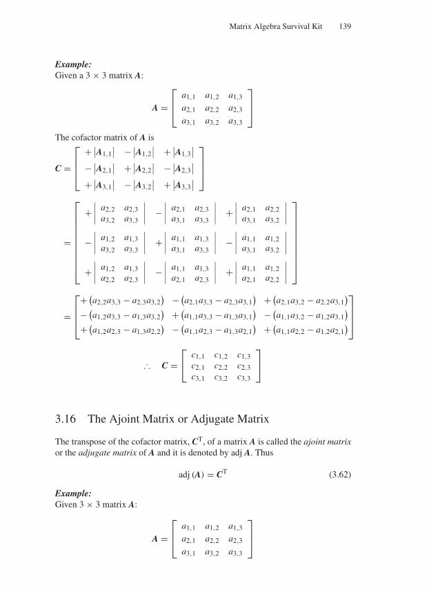
“Comninos” — 2005/8/31 — 15:34 — page 139 — #25
Matrix Algebra Survival Kit 139
Example:Given a 3 × 3 matrix A:
A =⎡
⎢⎣
a1,1 a1,2 a1,3
a2,1 a2,2 a2,3
a3,1 a3,2 a3,3
⎤
⎥⎦
The cofactor matrix of A is
C =
⎡
⎢⎢⎣
+ ∣∣A1,1∣∣ − ∣∣A1,2
∣∣ + ∣∣A1,3∣∣
− ∣∣A2,1∣∣ + ∣∣A2,2
∣∣ − ∣∣A2,3∣∣
+ ∣∣A3,1∣∣ − ∣∣A3,2
∣∣ + ∣∣A3,3∣∣
⎤
⎥⎥⎦
=
⎡
⎢⎢⎢⎢⎢⎢⎢⎢⎢⎣
+∣∣∣∣
a2,2 a2,3a3,2 a3,3
∣∣∣∣ −∣∣∣∣
a2,1 a2,3a3,1 a3,3
∣∣∣∣ +∣∣∣∣
a2,1 a2,2a3,1 a3,2
∣∣∣∣
−∣∣∣∣
a1,2 a1,3a3,2 a3,3
∣∣∣∣ +∣∣∣∣
a1,1 a1,3a3,1 a3,3
∣∣∣∣ −∣∣∣∣
a1,1 a1,2a3,1 a3,2
∣∣∣∣
+∣∣∣∣
a1,2 a1,3a2,2 a2,3
∣∣∣∣ −∣∣∣∣
a1,1 a1,3a2,1 a2,3
∣∣∣∣ +∣∣∣∣
a1,1 a1,2a2,1 a2,2
∣∣∣∣
⎤
⎥⎥⎥⎥⎥⎥⎥⎥⎥⎦
=
⎡
⎢⎢⎣
+ (a2,2a3,3 − a2,3a3,2
) − (a2,1a3,3 − a2,3a3,1
) + (a2,1a3,2 − a2,2a3,1
)
− (a1,2a3,3 − a1,3a3,2
) + (a1,1a3,3 − a1,3a3,1
) − (a1,1a3,2 − a1,2a3,1
)
+ (a1,2a2,3 − a1,3a2,2
) − (a1,1a2,3 − a1,3a2,1
) + (a1,1a2,2 − a1,2a2,1
)
⎤
⎥⎥⎦
∴ C =⎡
⎣c1,1 c1,2 c1,3c2,1 c2,2 c2,3c3,1 c3,2 c3,3
⎤
⎦
3.16 The Ajoint Matrix or Adjugate Matrix
The transpose of the cofactor matrix, CT, of a matrix A is called the ajoint matrixor the adjugate matrix of A and it is denoted by adj A. Thus
adj (A) = CT (3.62)
Example:Given 3 × 3 matrix A:
A =⎡
⎢⎣
a1,1 a1,2 a1,3
a2,1 a2,2 a2,3
a3,1 a3,2 a3,3
⎤
⎥⎦
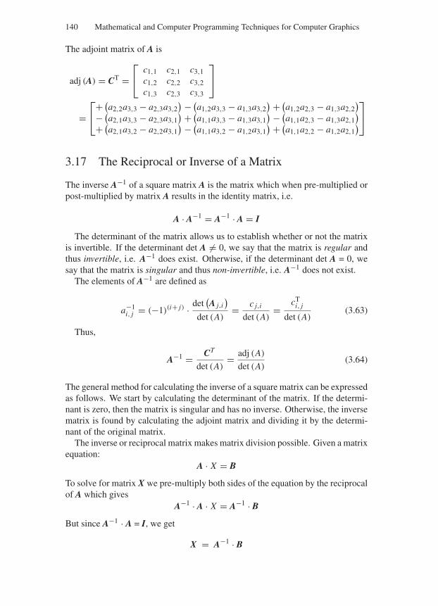
“Comninos” — 2005/8/31 — 15:34 — page 140 — #26
140 Mathematical and Computer Programming Techniques for Computer Graphics
The adjoint matrix of A is
adj (A) = CT =⎡
⎣c1,1 c2,1 c3,1c1,2 c2,2 c3,2c1,3 c2,3 c3,3
⎤
⎦
=⎡
⎣+ (
a2,2a3,3 − a2,3a3,2) − (
a1,2a3,3 − a1,3a3,2) + (
a1,2a2,3 − a1,3a2,2)
− (a2,1a3,3 − a2,3a3,1
) + (a1,1a3,3 − a1,3a3,1
) − (a1,1a2,3 − a1,3a2,1
)
+ (a2,1a3,2 − a2,2a3,1
) − (a1,1a3,2 − a1,2a3,1
) + (a1,1a2,2 − a1,2a2,1
)
⎤
⎦
3.17 The Reciprocal or Inverse of a Matrix
The inverse A−1 of a square matrix A is the matrix which when pre-multiplied orpost-multiplied by matrix A results in the identity matrix, i.e.
A · A−1 = A−1 · A = I
The determinant of the matrix allows us to establish whether or not the matrixis invertible. If the determinant det A = 0, we say that the matrix is regular andthus invertible, i.e. A−1 does exist. Otherwise, if the determinant det A = 0, wesay that the matrix is singular and thus non-invertible, i.e. A−1 does not exist.
The elements of A−1 are defined as
a−1i, j = (−1)(i+ j) · det
(A j,i
)
det (A)= c j,i
det (A)= cT
i, j
det (A)(3.63)
Thus,
A−1 = CT
det (A)= adj (A)
det (A)(3.64)
The general method for calculating the inverse of a square matrix can be expressedas follows. We start by calculating the determinant of the matrix. If the determi-nant is zero, then the matrix is singular and has no inverse. Otherwise, the inversematrix is found by calculating the adjoint matrix and dividing it by the determi-nant of the original matrix.
The inverse or reciprocal matrix makes matrix division possible. Given a matrixequation:
A · X = B
To solve for matrix X we pre-multiply both sides of the equation by the reciprocalof A which gives
A−1 · A · X = A−1 · B
But since A−1 · A = I, we get
X = A−1 · B
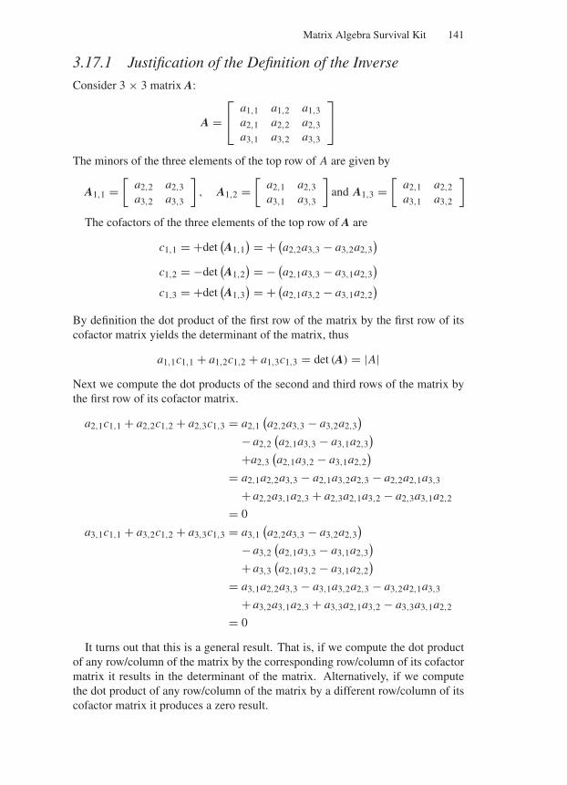
“Comninos” — 2005/8/31 — 15:34 — page 141 — #27
Matrix Algebra Survival Kit 141
3.17.1 Justification of the Definition of the Inverse
Consider 3 × 3 matrix A:
A =⎡
⎣a1,1 a1,2 a1,3a2,1 a2,2 a2,3a3,1 a3,2 a3,3
⎤
⎦
The minors of the three elements of the top row of A are given by
A1,1 =[
a2,2 a2,3a3,2 a3,3
], A1,2 =
[a2,1 a2,3a3,1 a3,3
]and A1,3 =
[a2,1 a2,2a3,1 a3,2
]
The cofactors of the three elements of the top row of A are
c1,1 = +det(A1,1
) = + (a2,2a3,3 − a3,2a2,3
)
c1,2 = −det(A1,2
) = − (a2,1a3,3 − a3,1a2,3
)
c1,3 = +det(A1,3
) = + (a2,1a3,2 − a3,1a2,2
)
By definition the dot product of the first row of the matrix by the first row of itscofactor matrix yields the determinant of the matrix, thus
a1,1c1,1 + a1,2c1,2 + a1,3c1,3 = det (A) = |A|Next we compute the dot products of the second and third rows of the matrix bythe first row of its cofactor matrix.
a2,1c1,1 + a2,2c1,2 + a2,3c1,3 = a2,1(a2,2a3,3 − a3,2a2,3
)
− a2,2(a2,1a3,3 − a3,1a2,3
)
+a2,3(a2,1a3,2 − a3,1a2,2
)
= a2,1a2,2a3,3 − a2,1a3,2a2,3 − a2,2a2,1a3,3
+ a2,2a3,1a2,3 + a2,3a2,1a3,2 − a2,3a3,1a2,2
= 0
a3,1c1,1 + a3,2c1,2 + a3,3c1,3 = a3,1(a2,2a3,3 − a3,2a2,3
)
− a3,2(a2,1a3,3 − a3,1a2,3
)
+ a3,3(a2,1a3,2 − a3,1a2,2
)
= a3,1a2,2a3,3 − a3,1a3,2a2,3 − a3,2a2,1a3,3
+ a3,2a3,1a2,3 + a3,3a2,1a3,2 − a3,3a3,1a2,2
= 0
It turns out that this is a general result. That is, if we compute the dot productof any row/column of the matrix by the corresponding row/column of its cofactormatrix it results in the determinant of the matrix. Alternatively, if we computethe dot product of any row/column of the matrix by a different row/column of itscofactor matrix it produces a zero result.
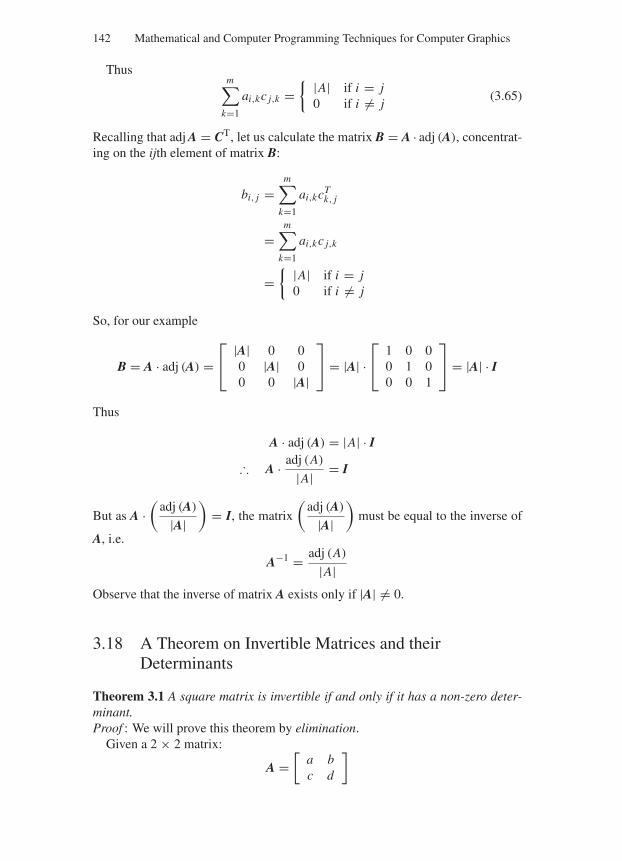
“Comninos” — 2005/8/31 — 15:34 — page 142 — #28
142 Mathematical and Computer Programming Techniques for Computer Graphics
Thusm∑
k=1
ai,kc j,k = |A| if i = j
0 if i = j(3.65)
Recalling that adj A = CT, let us calculate the matrix B = A · adj (A), concentrat-ing on the ijth element of matrix B:
bi, j =m∑
k=1
ai,kcTk, j
=m∑
k=1
ai,kc j,k
= |A| if i = j
0 if i = j
So, for our example
B = A · adj (A) =⎡
⎣|A| 0 00 |A| 00 0 |A|
⎤
⎦ = |A| ·⎡
⎣1 0 00 1 00 0 1
⎤
⎦ = |A| · I
Thus
A · adj (A) = |A| · I
∴ A · adj (A)
|A| = I
But as A ·(
adj (A)
|A|)
= I, the matrix
(adj (A)
|A|)
must be equal to the inverse of
A, i.e.
A−1 = adj (A)
|A|Observe that the inverse of matrix A exists only if |A| = 0.
3.18 A Theorem on Invertible Matrices and theirDeterminants
Theorem 3.1 A square matrix is invertible if and only if it has a non-zero deter-minant.Proof : We will prove this theorem by elimination.
Given a 2 × 2 matrix:
A =[
a bc d
]
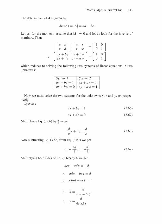
“Comninos” — 2005/8/31 — 15:34 — page 143 — #29
Matrix Algebra Survival Kit 143
The determinant of A is given by
det (A) = |A| = ad − bc
Let us, for the moment, assume that |A| = 0 and let us look for the inverse ofmatrix A. Then
[a bc d
]·[
x yz w
]=
[1 00 1
]
∴[
ax + bz ay + bw
cx + dz cy + dw
]=
[1 00 1
]
which reduces to solving the following two systems of linear equations in twounknowns:
System 1 System 2ax + bz = 1 cx + dz = 0ay + bw = 0 cy + dw = 1
Now we must solve the two systems for the unknowns x , z and y, w, respec-tively.
System 1ax + bz = 1 (3.66)
cx + dz = 0 (3.67)
Multiplying Eq. (3.66) by db we get
ad
bx + dz = d
b(3.68)
Now subtracting Eq. (3.68) from Eq. (3.67) we get
cx − ad
bx = −d
b(3.69)
Multiplying both sides of Eq. (3.69) by b we get
bcx − adx = −d
∴ adx − bcx = d
∴ x (ad − bc) = d
∴ x = d
(ad − bc)
∴ x = d
det (A)
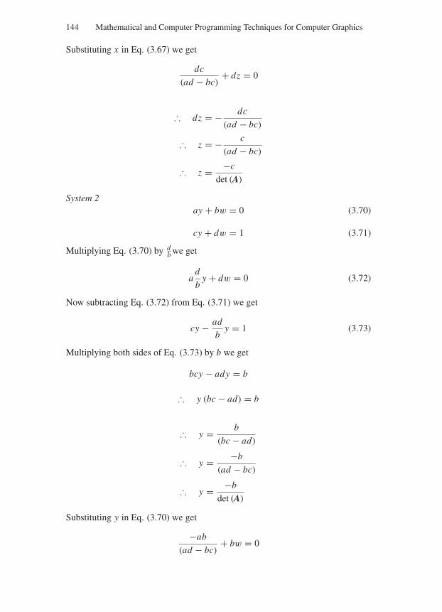
“Comninos” — 2005/8/31 — 15:34 — page 144 — #30
144 Mathematical and Computer Programming Techniques for Computer Graphics
Substituting x in Eq. (3.67) we get
dc
(ad − bc)+ dz = 0
∴ dz = − dc
(ad − bc)
∴ z = − c
(ad − bc)
∴ z = −c
det (A)
System 2ay + bw = 0 (3.70)
cy + dw = 1 (3.71)
Multiplying Eq. (3.70) by db we get
ad
by + dw = 0 (3.72)
Now subtracting Eq. (3.72) from Eq. (3.71) we get
cy − ad
by = 1 (3.73)
Multiplying both sides of Eq. (3.73) by b we get
bcy − ady = b
∴ y (bc − ad) = b
∴ y = b
(bc − ad)
∴ y = −b
(ad − bc)
∴ y = −b
det (A)
Substituting y in Eq. (3.70) we get
−ab
(ad − bc)+ bw = 0
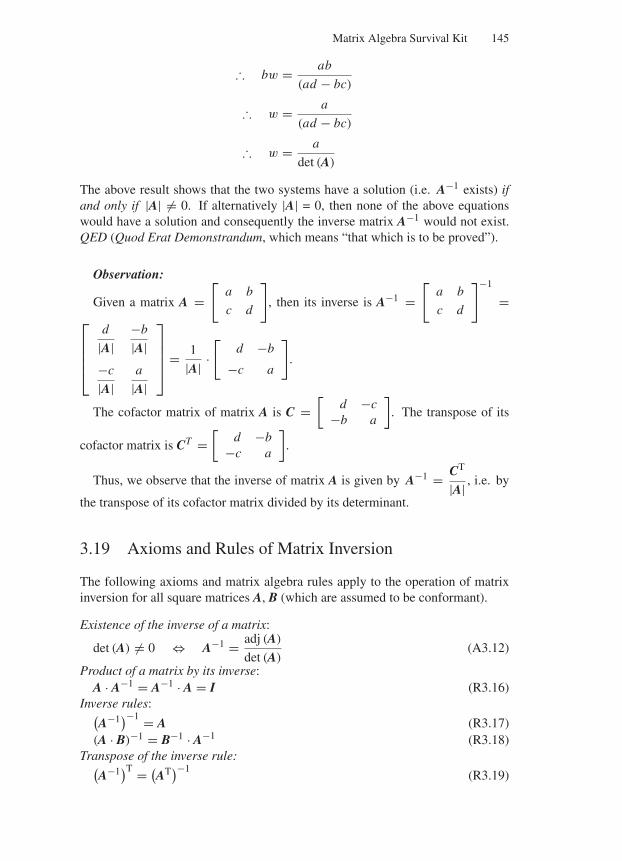
“Comninos” — 2005/8/31 — 15:34 — page 145 — #31
Matrix Algebra Survival Kit 145
∴ bw = ab
(ad − bc)
∴ w = a
(ad − bc)
∴ w = a
det (A)
The above result shows that the two systems have a solution (i.e. A−1 exists) ifand only if |A| = 0. If alternatively |A| = 0, then none of the above equationswould have a solution and consequently the inverse matrix A−1 would not exist.QED (Quod Erat Demonstrandum, which means “that which is to be proved”).
Observation:
Given a matrix A =[
a b
c d
]
, then its inverse is A−1 =[
a b
c d
]−1
=⎡
⎢⎢⎢⎣
d
|A|−b
|A|−c
|A|a
|A|
⎤
⎥⎥⎥⎦
= 1
|A| ·[
d −b
−c a
]
.
The cofactor matrix of matrix A is C =[
d −c−b a
]. The transpose of its
cofactor matrix is CT =[
d −b−c a
].
Thus, we observe that the inverse of matrix A is given by A−1 = CT
|A| , i.e. by
the transpose of its cofactor matrix divided by its determinant.
3.19 Axioms and Rules of Matrix Inversion
The following axioms and matrix algebra rules apply to the operation of matrixinversion for all square matrices A, B (which are assumed to be conformant).
Existence of the inverse of a matrix:
det (A) = 0 ⇔ A−1 = adj (A)
det (A)(A3.12)
Product of a matrix by its inverse:A · A−1 = A−1 · A = I (R3.16)
Inverse rules:(A−1)−1 = A (R3.17)
(A · B)−1 = B−1 · A−1 (R3.18)Transpose of the inverse rule:
(A−1)T = (
AT)−1(R3.19)
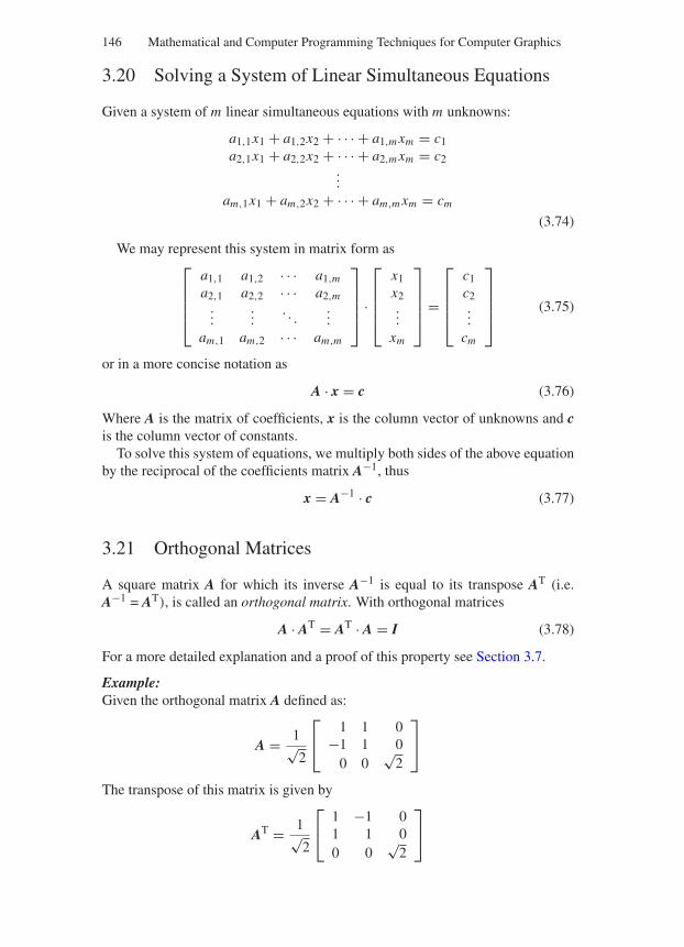
“Comninos” — 2005/8/31 — 15:34 — page 146 — #32
146 Mathematical and Computer Programming Techniques for Computer Graphics
3.20 Solving a System of Linear Simultaneous Equations
Given a system of m linear simultaneous equations with m unknowns:
a1,1x1 + a1,2x2 + · · · + a1,m xm = c1a2,1x1 + a2,2x2 + · · · + a2,m xm = c2
...
am,1x1 + am,2x2 + · · · + am,m xm = cm
(3.74)
We may represent this system in matrix form as⎡
⎢⎢⎢⎣
a1,1 a1,2 · · · a1,m
a2,1 a2,2 · · · a2,m...
.... . .
...
am,1 am,2 · · · am,m
⎤
⎥⎥⎥⎦
·
⎡
⎢⎢⎢⎣
x1x2...
xm
⎤
⎥⎥⎥⎦
=
⎡
⎢⎢⎢⎣
c1c2...
cm
⎤
⎥⎥⎥⎦
(3.75)
or in a more concise notation as
A · x = c (3.76)
Where A is the matrix of coefficients, x is the column vector of unknowns and cis the column vector of constants.
To solve this system of equations, we multiply both sides of the above equationby the reciprocal of the coefficients matrix A−1, thus
x = A−1 · c (3.77)
3.21 Orthogonal Matrices
A square matrix A for which its inverse A−1 is equal to its transpose AT (i.e.A−1 = AT), is called an orthogonal matrix. With orthogonal matrices
A · AT = AT · A = I (3.78)
For a more detailed explanation and a proof of this property see Section 3.7.
Example:Given the orthogonal matrix A defined as:
A = 1√2
⎡
⎣1 1 0
−1 1 00 0
√2
⎤
⎦
The transpose of this matrix is given by
AT = 1√2
⎡
⎣1 −1 01 1 00 0
√2
⎤
⎦
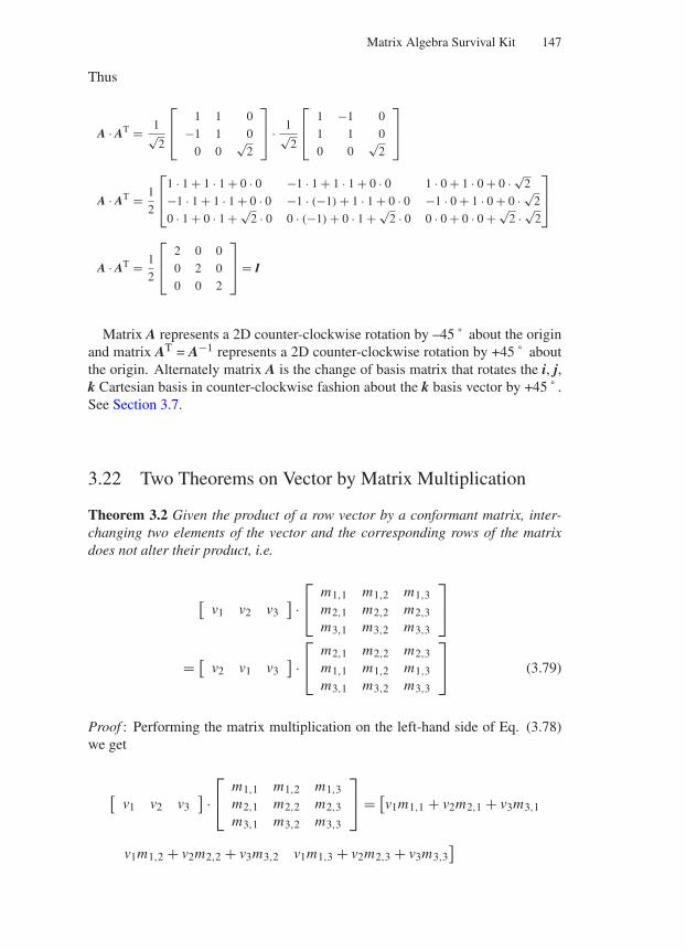
“Comninos” — 2005/8/31 — 15:34 — page 147 — #33
Matrix Algebra Survival Kit 147
Thus
A · AT = 1√2
⎡
⎢⎣
1 1 0
−1 1 0
0 0√
2
⎤
⎥⎦ · 1√
2
⎡
⎢⎣
1 −1 0
1 1 0
0 0√
2
⎤
⎥⎦
A · AT = 1
2
⎡
⎢⎣
1 · 1 + 1 · 1 + 0 · 0 −1 · 1 + 1 · 1 + 0 · 0 1 · 0 + 1 · 0 + 0 · √2
−1 · 1 + 1 · 1 + 0 · 0 −1 · (−1) + 1 · 1 + 0 · 0 −1 · 0 + 1 · 0 + 0 · √2
0 · 1 + 0 · 1 + √2 · 0 0 · (−1) + 0 · 1 + √
2 · 0 0 · 0 + 0 · 0 + √2 · √
2
⎤
⎥⎦
A · AT = 1
2
⎡
⎢⎣
2 0 0
0 2 0
0 0 2
⎤
⎥⎦ = I
Matrix A represents a 2D counter-clockwise rotation by –45 ˚ about the originand matrix AT = A−1 represents a 2D counter-clockwise rotation by +45 ˚ aboutthe origin. Alternately matrix A is the change of basis matrix that rotates the i, j,k Cartesian basis in counter-clockwise fashion about the k basis vector by +45 ˚ .See Section 3.7.
3.22 Two Theorems on Vector by Matrix Multiplication
Theorem 3.2 Given the product of a row vector by a conformant matrix, inter-changing two elements of the vector and the corresponding rows of the matrixdoes not alter their product, i.e.
[v1 v2 v3
] ·⎡
⎣m1,1 m1,2 m1,3m2,1 m2,2 m2,3m3,1 m3,2 m3,3
⎤
⎦
= [v2 v1 v3
] ·⎡
⎣m2,1 m2,2 m2,3m1,1 m1,2 m1,3m3,1 m3,2 m3,3
⎤
⎦ (3.79)
Proof : Performing the matrix multiplication on the left-hand side of Eq. (3.78)we get
[v1 v2 v3
] ·⎡
⎣m1,1 m1,2 m1,3m2,1 m2,2 m2,3m3,1 m3,2 m3,3
⎤
⎦ = [v1m1,1 + v2m2,1 + v3m3,1
v1m1,2 + v2m2,2 + v3m3,2 v1m1,3 + v2m2,3 + v3m3,3]
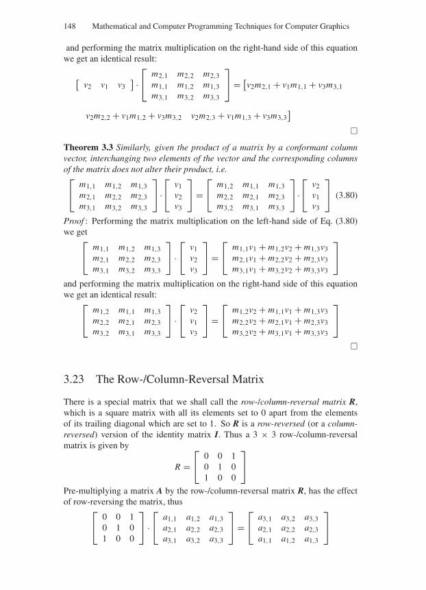
“Comninos” — 2005/8/31 — 15:34 — page 148 — #34
148 Mathematical and Computer Programming Techniques for Computer Graphics
and performing the matrix multiplication on the right-hand side of this equationwe get an identical result:
[v2 v1 v3
] ·⎡
⎣m2,1 m2,2 m2,3m1,1 m1,2 m1,3m3,1 m3,2 m3,3
⎤
⎦ = [v2m2,1 + v1m1,1 + v3m3,1
v2m2,2 + v1m1,2 + v3m3,2 v2m2,3 + v1m1,3 + v3m3,3]
Theorem 3.3 Similarly, given the product of a matrix by a conformant columnvector, interchanging two elements of the vector and the corresponding columnsof the matrix does not alter their product, i.e.⎡
⎣m1,1 m1,2 m1,3m2,1 m2,2 m2,3m3,1 m3,2 m3,3
⎤
⎦ ·⎡
⎣v1v2v3
⎤
⎦ =⎡
⎣m1,2 m1,1 m1,3m2,2 m2,1 m2,3m3,2 m3,1 m3,3
⎤
⎦ ·⎡
⎣v2v1v3
⎤
⎦ (3.80)
Proof : Performing the matrix multiplication on the left-hand side of Eq. (3.80)we get
⎡
⎣m1,1 m1,2 m1,3m2,1 m2,2 m2,3m3,1 m3,2 m3,3
⎤
⎦ ·⎡
⎣v1v2v3
⎤
⎦ =⎡
⎣m1,1v1 + m1,2v2 + m1,3v3m2,1v1 + m2,2v2 + m2,3v3m3,1v1 + m3,2v2 + m3,3v3
⎤
⎦
and performing the matrix multiplication on the right-hand side of this equationwe get an identical result:
⎡
⎣m1,2 m1,1 m1,3m2,2 m2,1 m2,3m3,2 m3,1 m3,3
⎤
⎦ ·⎡
⎣v2v1v3
⎤
⎦ =⎡
⎣m1,2v2 + m1,1v1 + m1,3v3m2,2v2 + m2,1v1 + m2,3v3m3,2v2 + m3,1v1 + m3,3v3
⎤
⎦
3.23 The Row-/Column-Reversal Matrix
There is a special matrix that we shall call the row-/column-reversal matrix R,which is a square matrix with all its elements set to 0 apart from the elementsof its trailing diagonal which are set to 1. So R is a row-reversed (or a column-reversed) version of the identity matrix I. Thus a 3 × 3 row-/column-reversalmatrix is given by
R =⎡
⎣0 0 10 1 01 0 0
⎤
⎦
Pre-multiplying a matrix A by the row-/column-reversal matrix R, has the effectof row-reversing the matrix, thus
⎡
⎣0 0 10 1 01 0 0
⎤
⎦ ·⎡
⎣a1,1 a1,2 a1,3a2,1 a2,2 a2,3a3,1 a3,2 a3,3
⎤
⎦ =⎡
⎣a3,1 a3,2 a3,3a2,1 a2,2 a2,3a1,1 a1,2 a1,3
⎤
⎦
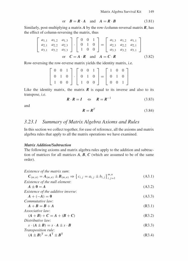
“Comninos” — 2005/8/31 — 15:34 — page 149 — #35
Matrix Algebra Survival Kit 149
or B = R · A and A = R · B (3.81)
Similarly, post-multiplying a matrix A by the row-/column-reversal matrix R, hasthe effect of column-reversing the matrix, thus
⎡
⎣a1,1 a1,2 a1,3a2,1 a2,2 a2,3a3,1 a3,2 a3,3
⎤
⎦ ·⎡
⎣0 0 10 1 01 0 0
⎤
⎦ =⎡
⎣a1,3 a1,2 a1,1a2,3 a2,2 a2,1a3,3 a3,2 a3,1
⎤
⎦
or C = A · R and A = C · R (3.82)
Row-reversing the row-reverse matrix yields the identity matrix, i.e.⎡
⎢⎣
0 0 1
0 1 0
1 0 0
⎤
⎥⎦ ·
⎡
⎢⎣
0 0 1
0 1 0
1 0 0
⎤
⎥⎦ =
⎡
⎢⎣
1 0 0
0 1 0
0 0 1
⎤
⎥⎦
Like the identity matrix, the matrix R is equal to its inverse and also to itstranspose, i.e.
R · R = I ⇔ R = R−1 (3.83)
andR = RT (3.84)
3.23.1 Summary of Matrix Algebra Axioms and Rules
In this section we collect together, for ease of reference, all the axioms and matrixalgebra rules that apply to all the matrix operations we have examined.
Matrix Addition/SubtractionThe following axioms and matrix algebra rules apply to the addition and subtrac-tion of matrices for all matrices A, B, C (which are assumed to be of the sameorder).
Existence of the matrix sum:C(m,n) = A(m,n) ± B(m,n) ⇒
ci, j = ai, j ± bi, jm,n
i, j=1 (A3.1)Existence of the null element:
A ± 0 = A (A3.2)Existence of the additive inverse:
A + (−A) = 0 (A3.3)Commutative law:
A + B = B + A (R3.1)Associative law:
(A + B) + C = A + (B + C) (R3.2)Distributive law:
s · (A ± B) = s · A ± s · B (R3.3)Transposition rule:
(A ± B)T = AT ± BT (R3.4)
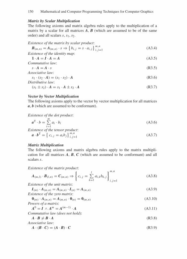
“Comninos” — 2005/8/31 — 15:34 — page 150 — #36
150 Mathematical and Computer Programming Techniques for Computer Graphics
Matrix by Scalar MultiplicationThe following axioms and matrix algebra rules apply to the multiplication of amatrix by a scalar for all matrices A, B (which are assumed to be of the sameorder) and all scalars s, s1, s2.
Existence of the matrix by scalar product:B(m,n) = A(m,n) · s ⇒
bi, j = s · ai, j m,n
i, j=1 (A3.4)Existence of the identity map:
1 · A = I · A = A (A3.5)Commutative law:
s · A = A · s (R3.5)Associative law:
s1 · (s2 · A) = (s1 · s2) · A (R3.6)Distributive law:
(s1 ± s2) · A = s1 · A ± s2 · A (R3.7)
Vector by Vector MultiplicationThe following axioms apply to the vector by vector multiplication for all matricesa, b (which are assumed to be conformant).
Existence of the dot product:
aT · b =m∑
i=1ai · bi (A3.6)
Existence of the tensor product:a · bT =
ci, j = ai b j m,n
i, j=1 (A3.7)
Matrix MultiplicationThe following axioms and matrix algebra rules apply to the matrix multipli-cation for all matrices A, B, C (which are assumed to be conformant) and allscalars s.
Existence of the matrix product:
A(m,l) · B(l,n) = C(m,n) ⇒
ci, j =l∑
k=1ai,kbk, j
m,n
i, j=1
(A3.8)
Existence of the unit matrix:I(m) · A(m,n) = A(m,n) · I(n) = A(m,n) (A3.9)
Existence of the zero matrix:0(m) · A(m,n) = A(m,n) · 0(n) = 0(m,n) (A3.10)
Powers of a matrix:A0 = I ∧ Am = A(m−1) · A (A3.11)
Commutative law (does not hold):A · B = B · A (R3.8)
Associative law:A · (B · C) = (A · B) · C (R3.9)
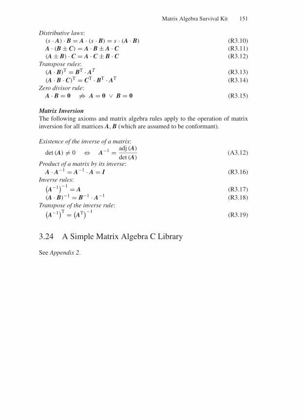
“Comninos” — 2005/8/31 — 15:34 — page 151 — #37
Matrix Algebra Survival Kit 151
Distributive laws:(s · A) · B = A · (s · B) = s · (A · B) (R3.10)A · (B ± C) = A · B ± A · C (R3.11)(A ± B) · C = A · C ± B · C (R3.12)
Transpose rules:(A · B)T = BT · AT (R3.13)(A · B · C)T = CT · BT · AT (R3.14)
Zero divisor rule:A · B = 0 ⇒ A = 0 ∨ B = 0 (R3.15)
Matrix InversionThe following axioms and matrix algebra rules apply to the operation of matrixinversion for all matrices A, B (which are assumed to be conformant).
Existence of the inverse of a matrix:
det (A) = 0 ⇔ A−1 = adj (A)
det (A)(A3.12)
Product of a matrix by its inverse:A · A−1 = A−1 · A = I (R3.16)
Inverse rules:(A−1)−1 = A (R3.17)
(A · B)−1 = B−1 · A−1 (R3.18)Transpose of the inverse rule:
(A−1)T = (
AT)−1(R3.19)
3.24 A Simple Matrix Algebra C Library
See Appendix 2.
“Comninos” — 2005/8/31 — 15:41 — page 153 — #1
4
Vector Spaces or Linear Spaces
The introduction of Cartesian coordinates in the 1630s by the French mathe-maticians Pierre de Fermat (1601–1665) and Rene Descartes (1596–1650) hada profound influence on the development of mathematics. Cartesian coordinatesallowed mathematicians to introduce algebraic methods into the study of geome-try. By the middle of the 1800s, however, there was a general dissatisfaction withthese coordinate methods and mathematicians began to look for more general andabstract ways by which they could study geometry without referring to coordi-nate systems. This search leads to the development of vectors and matrices, andeventually to the development of vector spaces or linear spaces.
Among the first to introduce a geometry without coordinates was the Prussianmathematician Hermann Gunter Grassman (1809–1877). In his 1844 book DieAusdehnungslehre (Extension Theory) he introduced the notion of abstract quan-tities and he defined the operations of addition and scalar multiplication on theseabstract quantities. It was, however, the Italian mathematician Giuseppe Piano(1858–1932) who introduced the first axiomatic definition of a vector space inhis 1888 book Calcolo Geometrico (Geometric Calculus). This book was wellin advance of its time and introduced most of the concepts of vector spaces. Thecomplete axiomatic definition of vector spaces appeared in the 1920 doctoral dis-sertation of the Polish mathematician Stefan Banach (1892–1945).
As the theory of vector spaces underpins much of the work in computer graph-ics and curve and surface theory, we will briefly introduce some of the basic ideasof vector spaces in this chapter.
Underlying the concept of a vector space is the concept of a scalar field. Let usstart by defining what a scalar field is.
4.1 Definition of a Scalar Field
A scalar field is defined as a non-empty set of scalars for which the operationsof addition and multiplication are defined, such that for any scalars s1, s2, s3 thatbelong to the scalar field S the following axioms are satisfied:
153
“Comninos” — 2005/8/31 — 15:41 — page 154 — #2
154 Mathematical and Computer Programming Techniques for Computer Graphics
Closure of a Scalar FieldClosure under addition:
s1, s2 ∈ S ⇒ s1 + s2 ∈ SClosure under multiplication:
s1, s2 ∈ S ⇒ s1 · s2 ∈ S
Addition of ScalarsComutativity of addition:
s1 + s2 = s2 + s1Associativity of addition:
s1 + (s2 + s3) = (s1 + s2) + s3Existence of the additive identity element:
s1 + 0 = 0 + s1 = s1Existence of the additive inverse:
s1 + (−s1) = 0,
i.e. ∀ s1 ∈ S ∃ (−s1) ∈ S
Multiplication of ScalarsComutativity of multiplication:
s1 · s2 = s2 · s1Associativity of multiplication:
s1 · (s2 · s3) = (s1 · s2) · s3Distributivity of multiplication over addition:
s1 · (s2 + s3) = s1 · s2 + s1 · s3Distributivity of addition over multiplication:
(s1 + s2) · s3 = s1 · s3 + s2 · s3Existence of the multiplicative identity element:
1 · s1 = s1 · 1 = s1Existence of the multiplicative inverse:
s1 · 1
s1= 1 ⇔ s1 = 0
Examples of scalar fields are the set of real numbers R, the set of rationalnumbers Q and the set of complex numbers C.
Having defined scalar fields, we are now ready to define a vector space in termsof a scalar field.
4.2 Definition of a Vector Space
A vector space V is a non-empty set of abstract entities called vectors takentogether with the algebraic rules for vector addition and scalar by vector mul-tiplication.
Given a scalar field S, we can construct a vector as the ordered n-tuple v =[v1, v2, . . . , vn], where the components of the vector v1, v2, . . . , vn ∈ S and thevector v ∈ Sn .
“Comninos” — 2005/8/31 — 15:41 — page 155 — #3
Vector Spaces or Linear Spaces 155
Given two vectors v1, v2 ∈ Sn , vector addition is defined as
v1 + v2 = [v11, v12, . . . , v1n] + [v21, v22, . . . , v2n]
= [v11 + v21, v12 + v22, . . . , v1n + v2n]
where [ v11 + v21, v12 + v22, . . . , v1n + v2n] ∈ Sn and (v11 + v21) , (v12 + v22) ,
. . . , (v1n + v2n) ∈ S.Given a scalar s ∈ S and a vector v ∈ Sn , scalar by vector multiplication is
defined as
s · v = s · [v1, v2, . . . , vn] = [s · v1, s · v2, . . . , s · vn]
where [s · v1, s · v2, . . . , s · vn] ∈ Sn and s · v1, s · v2, . . . , s · vn ∈ S.Given two vectors v1, v2 ∈ Sn , the equality of two vectors is defined as
[v11, v12, . . . , v1n] = [v21, v22, . . . , v2n] ⇔ v1i = v2i ni=1
We say that a non-empty set of vectors V is a vector space over a scalar field S,if and only if for any vectors v1, v2, v3 ∈ V and any scalars s1, s2 ∈ S the followingaxioms are satisfied.
Closure of a Vector SpaceClosure under addition:
v1, v2 ∈ V ⇒ v1 + v2 ∈ V (A4.1)Closure under multiplication:
s1 ∈ S ∧ v1 ∈ V ⇒ s1 · v1 ∈ V (A4.2)
Addition of VectorsComutativity of addition:
v1 + v2 = v2 + v1 (A4.3)Associativity of addition:
v1 + (v2 + v3) = (v1 + v2) + v3 (A4.4)Existence of the additive identity element:
v1 + 0 = 0 + v1 = v1 where 0 ∈ V (A4.5)Existence of the additive inverse:
v1 + (−v1) = 0 where (−v1) , 0 ∈ V (A4.6)
Multiplication of a Vector by a ScalarDistributivity of scalar multiplication over addition:
s1 · (v1 + v2) = s1 · v1 + s1 · v2 (A4.7)Distributivity of scalar addition over multiplication:
(s1 + s2) · v1 = s1 · v1 + s2 · v1 (A4.8)Associativity of scalar multiplication:
s1 · (s2 · v1) = (s1 · s2) · v1 (A4.9)Existence of the multiplicative identity element:
1 · v1 = v1 · 1 = v1 where 1 ∈ S (A4.10)
In the above axioms the zero vector is given by 0 = [0, 0, . . . , 0], where 0 ∈ V.
“Comninos” — 2005/8/31 — 15:41 — page 156 — #4
156 Mathematical and Computer Programming Techniques for Computer Graphics
A real vector space is a vector space V that obeys Axioms (A4.1)–(A4.10) andis defined over the scalar field of real numbers (i.e. S = R). There are manyexamples of such vector spaces.
Vector Space of Real NumbersReal numbers are members of the scalar field S = R and as they satisfy Axioms(A4.1)–(A4.10) they form a vector space. Here S = R, V = R
1, the operation ofvector addition reduces to the addition of two real numbers and the operation ofscalar by vector multiplication reduces to the multiplication of two real numbers.
Vector Space of 2D VectorsThe vectors of the two-dimensional (2D) Euclidean space E2 are 2-tuples that aremembers of the set S2 = R
2. In this example S = R, V = v : v = [v1, v2] ∧vi ∈ R, vector addition and scalar by vector multiplication are performed in acomponent-wise fashion. Thus, it is clear that 2D vectors satisfy Axioms (A4.1)–(A4.10) and form a vector space.
Vector Space of 3D VectorsThe vectors of the three-dimensional Euclidean space E3 are 3-tuples that aremembers of the set S3 = R
3. In this example S = R, V = v : v = [v1, v2, v3] ∧vi ∈ R, vector addition and scalar by vector multiplication are performed in acomponent-wise fashion. Thus, it is clear that 3D vectors satisfy Axioms (A4.1)–(A4.10) and form a vector space.
Vector Space of m × n Matrices
In this example S = R, V =
⎧⎪⎨
⎪⎩A : A =
⎡
⎢⎣
a1,1 · · · a1,n...
. . ....
am,1 · · · am,n
⎤
⎥⎦ ∧ ai, j ∈ R
⎫⎪⎬
⎪⎭,
matrix addition and scalar by matrix multiplication are performed in a component-wise fashion. Thus, it is clear that set of matrices of order m × n satisfies Axioms(A4.1)–(A4.10) and forms a vector space.
In the discussion that follows we will concentrate on real vector spaces.
4.3 Linear Combinations of Vectors
Let Vm = v1, v2, . . . , vm be any set of vectors in vector space V and lets1, s2, . . . , sm be any set of scalars (i.e. si m
i=1 ∈ R). Then any vectorv of the form
v = s1 · v1 + s2 · v2 + · · · + sm · vm (4.1)
is said to be a linear combination of the vectors in Vm and vector v is said tobe linearly dependant on the vectors in Vm . Vector v is also a member of the
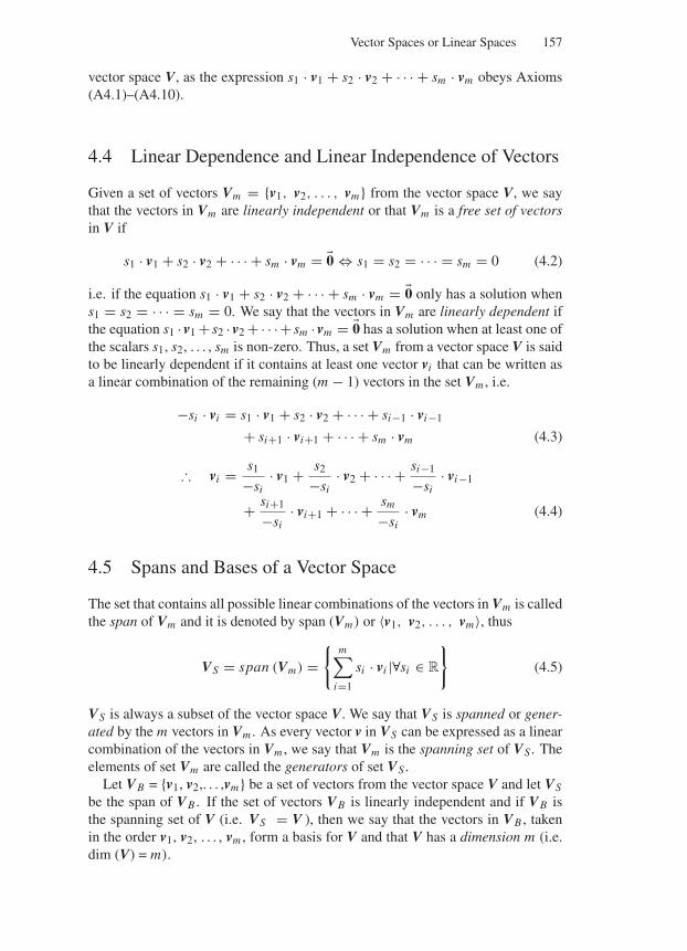
“Comninos” — 2005/8/31 — 15:41 — page 157 — #5
Vector Spaces or Linear Spaces 157
vector space V, as the expression s1 · v1 + s2 · v2 + · · · + sm · vm obeys Axioms(A4.1)–(A4.10).
4.4 Linear Dependence and Linear Independence of Vectors
Given a set of vectors Vm = v1, v2, . . . , vm from the vector space V, we saythat the vectors in Vm are linearly independent or that Vm is a free set of vectorsin V if
s1 · v1 + s2 · v2 + · · · + sm · vm = 0 ⇔ s1 = s2 = · · · = sm = 0 (4.2)
i.e. if the equation s1 · v1 + s2 · v2 + · · · + sm · vm = 0 only has a solution whens1 = s2 = · · · = sm = 0. We say that the vectors in Vm are linearly dependent ifthe equation s1 · v1 + s2 · v2 +· · ·+ sm · vm = 0 has a solution when at least one ofthe scalars s1, s2, . . . , sm is non-zero. Thus, a set Vm from a vector space V is saidto be linearly dependent if it contains at least one vector vi that can be written asa linear combination of the remaining (m − 1) vectors in the set Vm , i.e.
−si · vi = s1 · v1 + s2 · v2 + · · · + si−1 · vi−1
+ si+1 · vi+1 + · · · + sm · vm (4.3)
∴ vi = s1
−si· v1 + s2
−si· v2 + · · · + si−1
−si· vi−1
+ si+1
−si· vi+1 + · · · + sm
−si· vm (4.4)
4.5 Spans and Bases of a Vector Space
The set that contains all possible linear combinations of the vectors in Vm is calledthe span of Vm and it is denoted by span (Vm) or 〈v1, v2, . . . , vm〉, thus
VS = span (Vm) =
m∑
i=1
si · vi |∀si ∈ R
(4.5)
VS is always a subset of the vector space V. We say that VS is spanned or gener-ated by the m vectors in Vm . As every vector v in VS can be expressed as a linearcombination of the vectors in Vm , we say that Vm is the spanning set of VS . Theelements of set Vm are called the generators of set VS .
Let VB = v1, v2,. . . ,vm be a set of vectors from the vector space V and let VS
be the span of VB . If the set of vectors VB is linearly independent and if VB isthe spanning set of V (i.e. VS = V ), then we say that the vectors in VB , takenin the order v1, v2, . . . , vm , form a basis for V and that V has a dimension m (i.e.dim (V) = m).
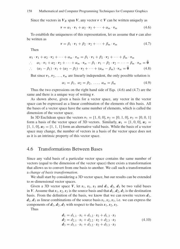
“Comninos” — 2005/8/31 — 15:41 — page 158 — #6
158 Mathematical and Computer Programming Techniques for Computer Graphics
Since the vectors in VB span V, any vector v ∈ V can be written uniquely as
v = α1 · v1 + α2 · v2 + · · · + αm · vm (4.6)
To establish the uniqueness of this representation, let us assume that v can alsobe written as
v = β1 · v1 + β2 · v2 + · · · + βm · vm (4.7)
Then
α1 · v1 + α2 · v2 + · · · + αm · vm = β1 · v1 + β2 · v2 + · · · + βm · vm
∴ α1 · v1 + α2 · v2 + · · · + αm · vm − β1 · v1 − β2 · v2 − · · · − βm · vm = 0∴ (α1 − β1) · v1 + (α2 − β2) · v2 + · · · + (αm − βm) · vm = 0 (4.8)
But since v1, v2, . . . , vm are linearly independent, the only possible solution is
α1 = β1, α2 = β2, . . . , αm = βm (4.9)
Thus the two expressions on the right hand side of Eqs. (4.6) and (4.7) are thesame and there is a unique way of writing v.
As shown above, given a basis for a vector space, any vector in the vectorspace can be expressed as a linear combination of the elements of this basis. Allthe bases of a vector space have the same number of elements, which is called thedimension of the vector space.
In 3D Euclidean space the vectors v1 = [1, 0, 0], v2 = [0, 1, 0], v3 = [0, 0, 1]form a basis of the vector space of 3D vectors. Similarly, u1 = [1, 0, 0], u2 =[1, 1, 0], u3 = [1, 1, 1] form an alternative valid basis. While the basis of a vectorspace may change, the number of vectors in a basis of the vector space does notas it is an intrinsic property of this vector space.
4.6 Transformations Between Bases
Since any valid basis of a particular vector space contains the same number ofvectors (equal to the dimension of the vector space) there exists a transformationthat allows us to convert from one basis to another. We call such a transformationa change of basis transformation.
We shall start by considering a 3D vector space, but our results can be extendedto m-dimensional vector spaces.
Given a 3D vector space V, let s1, s2, s3 and d1, d2, d3 be two valid basesin V. Assume that s1, s2, s3 is the source basis and that d1, d2, d3 is the destinationbasis. From the definition of the basis, we know that we can rewrite vectors d1,d2, d3 as linear combinations of the source basis s1, s2, s3, i.e. we can express thecomponents of d1, d2, d3 with respect to the basis s1, s2, s3.
Thus
d1 = d1,1 · s1 + d1,2 · s2 + d1,3 · s3d2 = d2,1 · s1 + d2,2 · s2 + d2,3 · s3d3 = d3,1 · s1 + d3,2 · s2 + d3,3 · s3
(4.10)
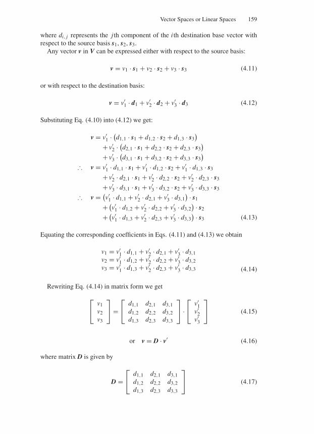
“Comninos” — 2005/8/31 — 15:41 — page 159 — #7
Vector Spaces or Linear Spaces 159
where di, j represents the j th component of the i th destination base vector withrespect to the source basis s1, s2, s3.
Any vector v in V can be expressed either with respect to the source basis:
v = v1 · s1 + v2 · s2 + v3 · s3 (4.11)
or with respect to the destination basis:
v = v′1 · d1 + v′
2 · d2 + v′3 · d3 (4.12)
Substituting Eq. (4.10) into (4.12) we get:
v = v′1 · (
d1,1 · s1 + d1,2 · s2 + d1,3 · s3)
+ v′2 · (
d2,1 · s1 + d2,2 · s2 + d2,3 · s3)
+ v′3 · (
d3,1 · s1 + d3,2 · s2 + d3,3 · s3)
∴ v = v′1 · d1,1 · s1 + v′
1 · d1,2 · s2 + v′1 · d1,3 · s3
+ v′2 · d2,1 · s1 + v′
2 · d2,2 · s2 + v′2 · d2,3 · s3
+ v′3 · d3,1 · s1 + v′
3 · d3,2 · s2 + v′3 · d3,3 · s3
∴ v = (v′
1 · d1,1 + v′2 · d2,1 + v′
3 · d3,1) · s1
+ (v′
1 · d1,2 + v′2 · d2,2 + v′
3 · d3,2) · s2
+ (v′
1 · d1,3 + v′2 · d2,3 + v′
3 · d3,3) · s3 (4.13)
Equating the corresponding coefficients in Eqs. (4.11) and (4.13) we obtain
v1 = v′1 · d1,1 + v′
2 · d2,1 + v′3 · d3,1
v2 = v′1 · d1,2 + v′
2 · d2,2 + v′3 · d3,2
v3 = v′1 · d1,3 + v′
2 · d2,3 + v′3 · d3,3 (4.14)
Rewriting Eq. (4.14) in matrix form we get
⎡
⎣v1v2v3
⎤
⎦ =⎡
⎣d1,1 d2,1 d3,1d1,2 d2,2 d3,2d1,3 d2,3 d3,3
⎤
⎦ ·⎡
⎣v′
1v′
2v′
3
⎤
⎦ (4.15)
or v = D · v′ (4.16)
where matrix D is given by
D =⎡
⎣d1,1 d2,1 d3,1d1,2 d2,2 d3,2d1,3 d2,3 d3,3
⎤
⎦ (4.17)
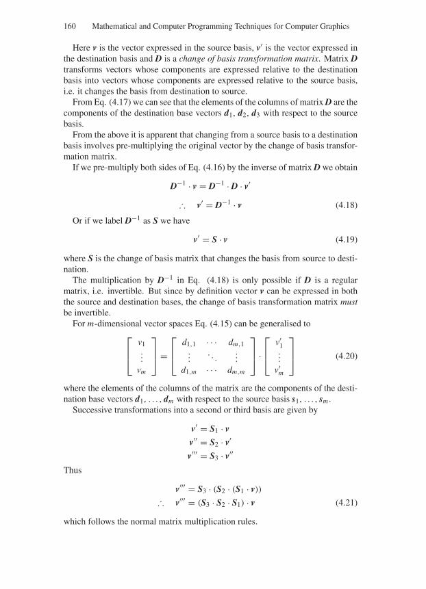
“Comninos” — 2005/8/31 — 15:41 — page 160 — #8
160 Mathematical and Computer Programming Techniques for Computer Graphics
Here v is the vector expressed in the source basis, v′ is the vector expressed inthe destination basis and D is a change of basis transformation matrix. Matrix Dtransforms vectors whose components are expressed relative to the destinationbasis into vectors whose components are expressed relative to the source basis,i.e. it changes the basis from destination to source.
From Eq. (4.17) we can see that the elements of the columns of matrix D are thecomponents of the destination base vectors d1, d2, d3 with respect to the sourcebasis.
From the above it is apparent that changing from a source basis to a destinationbasis involves pre-multiplying the original vector by the change of basis transfor-mation matrix.
If we pre-multiply both sides of Eq. (4.16) by the inverse of matrix D we obtain
D−1 · v = D−1 · D · v′
∴ v′ = D−1 · v (4.18)
Or if we label D−1 as S we have
v′ = S · v (4.19)
where S is the change of basis matrix that changes the basis from source to desti-nation.
The multiplication by D−1 in Eq. (4.18) is only possible if D is a regularmatrix, i.e. invertible. But since by definition vector v can be expressed in boththe source and destination bases, the change of basis transformation matrix mustbe invertible.
For m-dimensional vector spaces Eq. (4.15) can be generalised to⎡
⎢⎣
v1...
vm
⎤
⎥⎦ =
⎡
⎢⎣
d1,1 · · · dm,1...
. . ....
d1,m · · · dm,m
⎤
⎥⎦ ·
⎡
⎢⎣
v′1...
v′m
⎤
⎥⎦ (4.20)
where the elements of the columns of the matrix are the components of the desti-nation base vectors d1, . . . , dm with respect to the source basis s1, . . . , sm .
Successive transformations into a second or third basis are given by
v′ = S1 · v
v′′ = S2 · v′
v′′′ = S3 · v′′
Thus
v′′′ = S3 · (S2 · (S1 · v))
∴ v′′′ = (S3 · S2 · S1) · v (4.21)
which follows the normal matrix multiplication rules.
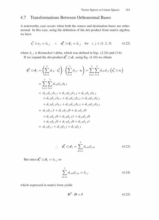
“Comninos” — 2005/8/31 — 15:41 — page 161 — #9
Vector Spaces or Linear Spaces 161
4.7 Transformations Between Orthonormal Bases
A noteworthy case occurs when both the source and destination bases are ortho-normal. In this case, using the definition of the dot product from matrix algebra,we have
sTi s j = δi, j ∧ dT
i d j = δi, j for i, j ∈ 1, 2, 3 (4.22)
where δi, j is Kronecker’s delta, which was defined in Eqs. (2.24) and (3.6).If we expand the dot product dT
i d j using Eq. (4.10) we obtain
dTi d j =
(3∑
k=1
di,k · sTk
)
·(
3∑
l=1
d j,l · sl
)
=3∑
k=1
3∑
l=1
di,kd j,l
(sT
k sl
)
=3∑
k=1
3∑
l=1
di,kd j,lδk,l
= di,1d j,1δ1,1 + di,1d j,2δ1,2 + di,1d j,3δ1,3
+ di,2d j,1δ2,1 + di,2d j,2δ2,2 + di,2d j,3δ2,3
+ di,3d j,1δ3,1 + di,3d j,2δ3,2 + di,3d j,3δ3,3
= di,1d j,11 + di,1d j,20 + di,1d j,30
+ di,2d j,10 + di,2d j,21 + di,2d j,30
+ di,3d j,10 + di,3d j,20 + di,3d j,31
= di,1d j,1 + di,2d j,2 + di,3d j,3
∴ dTi d j =
3∑
m=1
di,md j,m (4.23)
But since dTi d j = δi, j so
3∑
m=1
di,md j,m = δi, j (4.24)
which expressed in matrix form yields
DT · D = I (4.25)
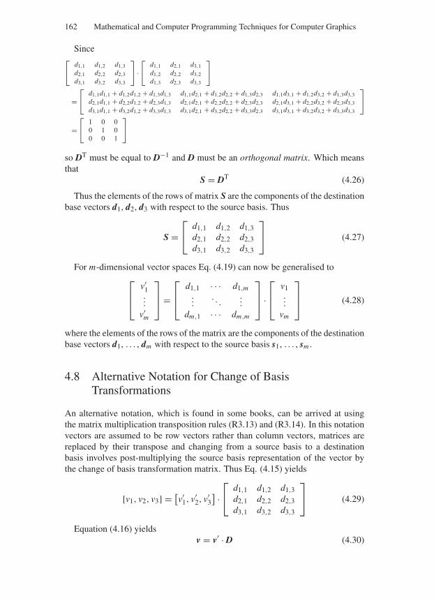
“Comninos” — 2005/8/31 — 15:41 — page 162 — #10
162 Mathematical and Computer Programming Techniques for Computer Graphics
Since⎡
⎣d1,1 d1,2 d1,3d2,1 d2,2 d2,3d3,1 d3,2 d3,3
⎤
⎦ ·⎡
⎣d1,1 d2,1 d3,1d1,2 d2,2 d3,2d1,3 d2,3 d3,3
⎤
⎦
=⎡
⎣d1,1d1,1 + d1,2d1,2 + d1,3d1,3 d1,1d2,1 + d1,2d2,2 + d1,3d2,3 d1,1d3,1 + d1,2d3,2 + d1,3d3,3d2,1d1,1 + d2,2d1,2 + d2,3d1,3 d2,1d2,1 + d2,2d2,2 + d2,3d2,3 d2,1d3,1 + d2,2d3,2 + d2,3d3,3d3,1d1,1 + d3,2d1,2 + d3,3d1,3 d3,1d2,1 + d3,2d2,2 + d3,3d2,3 d3,1d3,1 + d3,2d3,2 + d3,3d3,3
⎤
⎦
=⎡
⎣1 0 00 1 00 0 1
⎤
⎦
so DT must be equal to D−1 and D must be an orthogonal matrix. Which meansthat
S = DT (4.26)
Thus the elements of the rows of matrix S are the components of the destinationbase vectors d1, d2, d3 with respect to the source basis. Thus
S =⎡
⎣d1,1 d1,2 d1,3d2,1 d2,2 d2,3d3,1 d3,2 d3,3
⎤
⎦ (4.27)
For m-dimensional vector spaces Eq. (4.19) can now be generalised to⎡
⎢⎣
v′1...
v′m
⎤
⎥⎦ =
⎡
⎢⎣
d1,1 · · · d1,m...
. . ....
dm,1 · · · dm,m
⎤
⎥⎦ ·
⎡
⎢⎣
v1...
vm
⎤
⎥⎦ (4.28)
where the elements of the rows of the matrix are the components of the destinationbase vectors d1, . . . , dm with respect to the source basis s1, . . . , sm .
4.8 Alternative Notation for Change of BasisTransformations
An alternative notation, which is found in some books, can be arrived at usingthe matrix multiplication transposition rules (R3.13) and (R3.14). In this notationvectors are assumed to be row vectors rather than column vectors, matrices arereplaced by their transpose and changing from a source basis to a destinationbasis involves post-multiplying the source basis representation of the vector bythe change of basis transformation matrix. Thus Eq. (4.15) yields
[v1, v2, v3] = [v′
1, v′2, v′
3
] ·⎡
⎣d1,1 d1,2 d1,3d2,1 d2,2 d2,3d3,1 d3,2 d3,3
⎤
⎦ (4.29)
Equation (4.16) yieldsv = v′ · D (4.30)
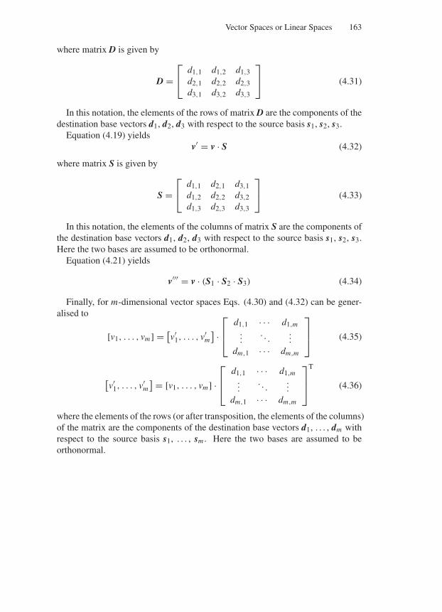
“Comninos” — 2005/8/31 — 15:41 — page 163 — #11
Vector Spaces or Linear Spaces 163
where matrix D is given by
D =⎡
⎣d1,1 d1,2 d1,3d2,1 d2,2 d2,3d3,1 d3,2 d3,3
⎤
⎦ (4.31)
In this notation, the elements of the rows of matrix D are the components of thedestination base vectors d1, d2, d3 with respect to the source basis s1, s2, s3.
Equation (4.19) yieldsv′ = v · S (4.32)
where matrix S is given by
S =⎡
⎣d1,1 d2,1 d3,1d1,2 d2,2 d3,2d1,3 d2,3 d3,3
⎤
⎦ (4.33)
In this notation, the elements of the columns of matrix S are the components ofthe destination base vectors d1, d2, d3 with respect to the source basis s1, s2, s3.Here the two bases are assumed to be orthonormal.
Equation (4.21) yields
v′′′ = v · (S1 · S2 · S3) (4.34)
Finally, for m-dimensional vector spaces Eqs. (4.30) and (4.32) can be gener-alised to
[v1, . . . , vm] = [v′
1, . . . , v′m
] ·⎡
⎢⎣
d1,1 · · · d1,m...
. . ....
dm,1 · · · dm,m
⎤
⎥⎦ (4.35)
[v′
1, . . . , v′m
] = [v1, . . . , vm] ·⎡
⎢⎣
d1,1 · · · d1,m...
. . ....
dm,1 · · · dm,m
⎤
⎥⎦
T
(4.36)
where the elements of the rows (or after transposition, the elements of the columns)of the matrix are the components of the destination base vectors d1, . . . , dm withrespect to the source basis s1, . . . , sm . Here the two bases are assumed to beorthonormal.
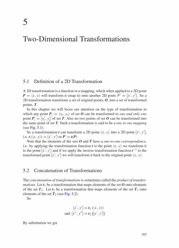
“Comninos” — 2005/8/31 — 15:47 — page 165 — #1
5
Two-Dimensional Transformations
5.1 Definition of a 2D Transformation
A 2D transformation is a function or a mapping, which when applied to a 2D pointP = 〈x, y〉 will transform it (map it) onto another 2D point P ′ = ⟨
x ′, y′⟩. So a2D transformation transforms a set of original points, O, into a set of transformedpoints, T.
In this chapter we will focus our attention on the type of transformation inwhich any point Pi = 〈xi , yi 〉 of set O can be transformed to one and only onepoint P′
i = ⟨x ′
i , y′i
⟩of set T. Also no two points of set O can be transformed into
the same point of set T. Such a transformation is said to be a one to one mapping(see Fig. 5.1).
So a transformation t can transform a 2D point 〈x, y〉 into a 2D point⟨x ′, y′⟩,
i.e. t (〈x, y〉) = ⟨x ′, y′⟩ or P′ = t(P)
Note that the elements of the sets O and T have a one-to-one correspondence,i.e. by applying the transformation function t to the point 〈x, y〉 we transform itto the point
⟨x ′, y′⟩ and if we apply the inverse transformation function t−1 to the
transformed point⟨x ′, y′⟩ we will transform it back to the original point 〈x, y〉.
5.2 Concatenation of Transformations
The concatenation of transformations is sometimes called the product of transfor-mations. Let t1 be a transformation that maps elements of the set O onto elementsof the set T1. Let t2 be a transformation that maps elements of the set T1 ontoelements of the set T2 (see Fig. 5.2).
So
⟨x ′, y′⟩ = t1 (〈x, y〉)
and⟨x ′′, y′′⟩ = t2
(⟨x ′, y′⟩)
By substitution we get
165
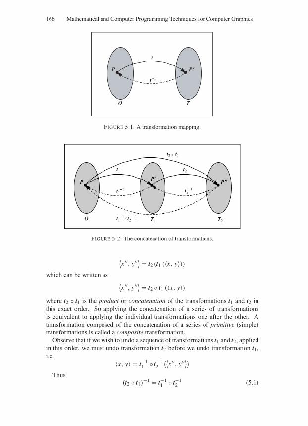
“Comninos” — 2005/8/31 — 15:47 — page 166 — #2
166 Mathematical and Computer Programming Techniques for Computer Graphics
P P ¢
t
O
t -1
T
FIGURE 5.1. A transformation mapping.
P P ¢
t1
O
t1-1
t1-1
t2 -1
t2-1
T1
P ¢¢
t2
T2
t2 t1
FIGURE 5.2. The concatenation of transformations.
⟨x ′′, y′′⟩ = t2 (t1 (〈x, y〉))
which can be written as⟨x ′′, y′′⟩ = t2 t1 (〈x, y〉)
where t2 t1 is the product or concatenation of the transformations t1 and t2 inthis exact order. So applying the concatenation of a series of transformationsis equivalent to applying the individual transformations one after the other. Atransformation composed of the concatenation of a series of primitive (simple)transformations is called a composite transformation.
Observe that if we wish to undo a sequence of transformations t1 and t2, appliedin this order, we must undo transformation t2 before we undo transformation t1,i.e.
〈x, y〉 = t−11 t−1
2
(⟨x ′′, y′′⟩)
Thus(t2 t1)−1 = t−1
1 t−12 (5.1)
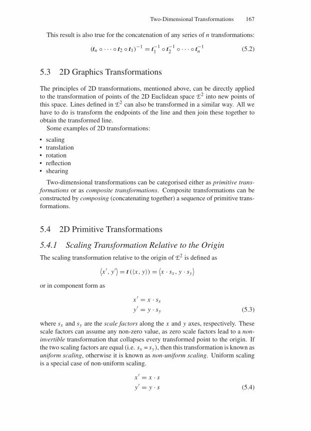
“Comninos” — 2005/8/31 — 15:47 — page 167 — #3
Two-Dimensional Transformations 167
This result is also true for the concatenation of any series of n transformations:
(tn · · · t2 t1)−1 = t−11 t−1
2 · · · t−1n (5.2)
5.3 2D Graphics Transformations
The principles of 2D transformations, mentioned above, can be directly appliedto the transformation of points of the 2D Euclidean space E2 into new points ofthis space. Lines defined in E2 can also be transformed in a similar way. All wehave to do is transform the endpoints of the line and then join these together toobtain the transformed line.
Some examples of 2D transformations:
• scaling• translation• rotation• reflection• shearing
Two-dimensional transformations can be categorised either as primitive trans-formations or as composite transformations. Composite transformations can beconstructed by composing (concatenating together) a sequence of primitive trans-formations.
5.4 2D Primitive Transformations
5.4.1 Scaling Transformation Relative to the Origin
The scaling transformation relative to the origin of E2 is defined as⟨x ′, y′⟩ = t (〈x, y〉) = ⟨
x · sx , y · sy⟩
or in component form as
x ′ = x · sx
y′ = y · sy (5.3)
where sx and sy are the scale factors along the x and y axes, respectively. Thesescale factors can assume any non-zero value, as zero scale factors lead to a non-invertible transformation that collapses every transformed point to the origin. Ifthe two scaling factors are equal (i.e. sx = sy), then this transformation is known asuniform scaling, otherwise it is known as non-uniform scaling. Uniform scalingis a special case of non-uniform scaling.
x ′ = x · s
y′ = y · s (5.4)
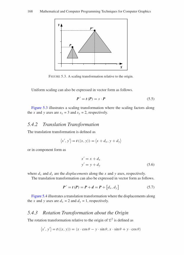
“Comninos” — 2005/8/31 — 15:47 — page 168 — #4
168 Mathematical and Computer Programming Techniques for Computer Graphics
P
X
YP ¢
FIGURE 5.3. A scaling transformation relative to the origin.
Uniform scaling can also be expressed in vector form as follows.
P ′ = t (P) = s · P (5.5)
Figure 5.3 illustrates a scaling transformation where the scaling factors alongthe x and y axes are sx = 3 and sy = 2, respectively.
5.4.2 Translation Transformation
The translation transformation is defined as
⟨x ′, y′⟩ = t (〈x, y〉) = ⟨
x + dx , y + dy⟩
or in component form as
x ′ = x + dx
y′ = y + dy (5.6)
where dx and dy are the displacements along the x and y axes, respectively.The translation transformation can also be expressed in vector form as follows.
P ′ = t (P) = P + d = P + [dx , dy
](5.7)
Figure 5.4 illustrates a translation transformation where the displacements alongthe x and y axes are dx = 2 and dy = 1, respectively.
5.4.3 Rotation Transformation about the Origin
The rotation transformation relative to the origin of E2 is defined as
⟨x ′, y′⟩ = t (〈x, y〉) = 〈x · cos θ − y · sin θ, x · sin θ + y · cos θ〉
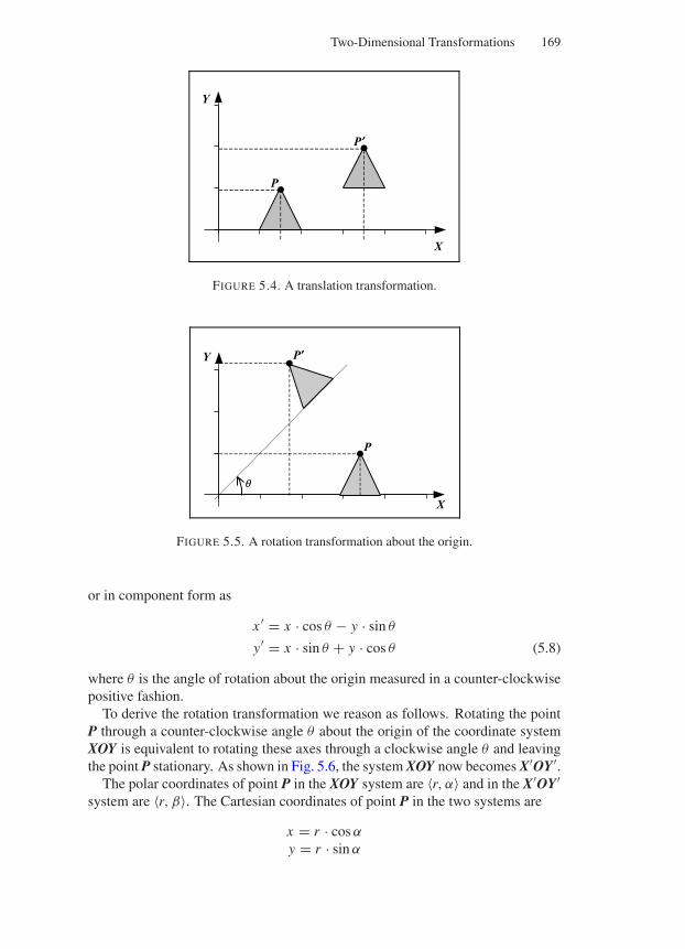
“Comninos” — 2005/8/31 — 15:47 — page 169 — #5
Two-Dimensional Transformations 169
P
P ¢
X
Y
FIGURE 5.4. A translation transformation.
P
P¢
X
Y
q
FIGURE 5.5. A rotation transformation about the origin.
or in component form as
x ′ = x · cos θ − y · sin θ
y′ = x · sin θ + y · cos θ (5.8)
where θ is the angle of rotation about the origin measured in a counter-clockwisepositive fashion.
To derive the rotation transformation we reason as follows. Rotating the pointP through a counter-clockwise angle θ about the origin of the coordinate systemXOY is equivalent to rotating these axes through a clockwise angle θ and leavingthe point P stationary. As shown in Fig. 5.6, the system XOY now becomes X′OY′.
The polar coordinates of point P in the XOY system are 〈r, α〉 and in the X′OY′system are 〈r, β〉. The Cartesian coordinates of point P in the two systems are
x = r · cos α
y = r · sin α
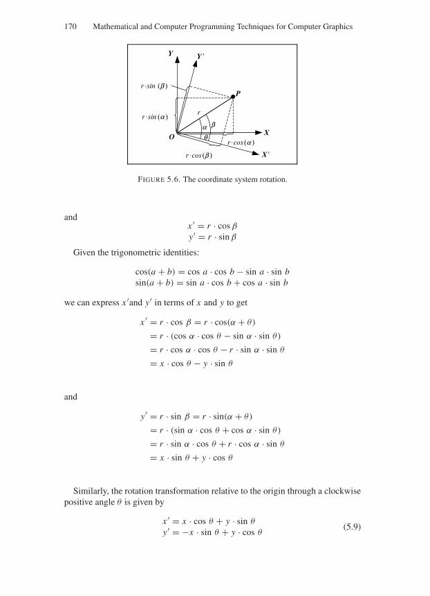
“Comninos” — 2005/8/31 — 15:47 — page 170 — #6
170 Mathematical and Computer Programming Techniques for Computer Graphics
a
P
X
Y
q
Y
X
b
r .sin (b )
r .sin (a )
r .cos (b )
r .cos (a )O
r
FIGURE 5.6. The coordinate system rotation.
andx ′ = r · cos β
y′ = r · sin β
Given the trigonometric identities:
cos(a + b) = cos a · cos b − sin a · sin bsin(a + b) = sin a · cos b + cos a · sin b
we can express x ′and y′ in terms of x and y to get
x ′ = r · cos β = r · cos(α + θ)
= r · (cos α · cos θ − sin α · sin θ)
= r · cos α · cos θ − r · sin α · sin θ
= x · cos θ − y · sin θ
and
y′ = r · sin β = r · sin(α + θ)
= r · (sin α · cos θ + cos α · sin θ)
= r · sin α · cos θ + r · cos α · sin θ
= x · sin θ + y · cos θ
Similarly, the rotation transformation relative to the origin through a clockwisepositive angle θ is given by
x ′ = x · cos θ + y · sin θ
y′ = −x · sin θ + y · cos θ(5.9)
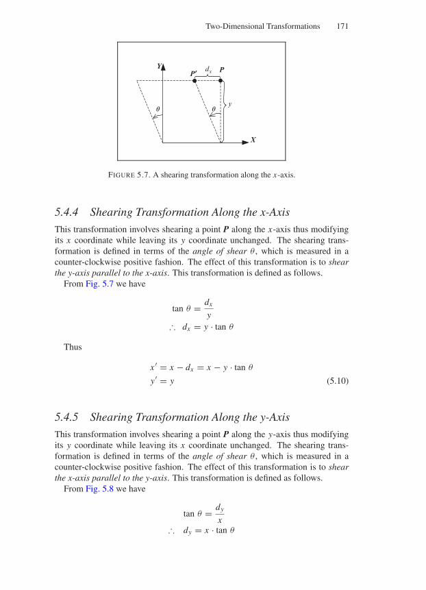
“Comninos” — 2005/8/31 — 15:47 — page 171 — #7
Two-Dimensional Transformations 171
P
X
Y
qy
P¢
q
dx
FIGURE 5.7. A shearing transformation along the x-axis.
5.4.4 Shearing Transformation Along the x-Axis
This transformation involves shearing a point P along the x-axis thus modifyingits x coordinate while leaving its y coordinate unchanged. The shearing trans-formation is defined in terms of the angle of shear θ , which is measured in acounter-clockwise positive fashion. The effect of this transformation is to shearthe y-axis parallel to the x-axis. This transformation is defined as follows.
From Fig. 5.7 we have
tan θ = dx
y∴ dx = y · tan θ
Thus
x ′ = x − dx = x − y · tan θ
y′ = y (5.10)
5.4.5 Shearing Transformation Along the y-Axis
This transformation involves shearing a point P along the y-axis thus modifyingits y coordinate while leaving its x coordinate unchanged. The shearing trans-formation is defined in terms of the angle of shear θ , which is measured in acounter-clockwise positive fashion. The effect of this transformation is to shearthe x-axis parallel to the y-axis. This transformation is defined as follows.
From Fig. 5.8 we have
tan θ = dy
x∴ dy = x · tan θ
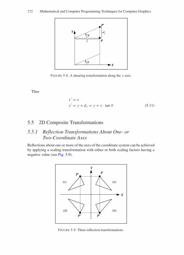
“Comninos” — 2005/8/31 — 15:47 — page 172 — #8
172 Mathematical and Computer Programming Techniques for Computer Graphics
P
X
Yq
x
dy
P¢
q
FIGURE 5.8. A shearing transformation along the y-axis.
Thus
x ′ = x
y′ = y + dy = y + x · tan θ (5.11)
5.5 2D Composite Transformations
5.5.1 Reflection Transformations About One- orTwo-Coordinate Axes
Reflections about one or more of the axes of the coordinate system can be achievedby applying a scaling transformation with either or both scaling factors having anegative value (see Fig. 5.9).
P
X
Y
(a)
P¢
P¢ P¢
(c)
(d) (b)
FIGURE 5.9. Three reflection transformations.
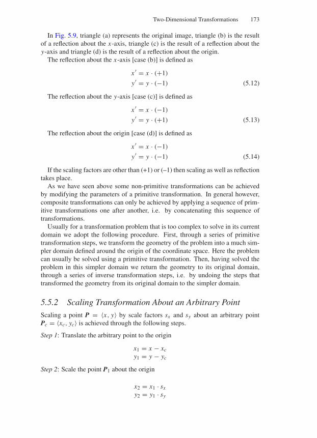
“Comninos” — 2005/8/31 — 15:47 — page 173 — #9
Two-Dimensional Transformations 173
In Fig. 5.9, triangle (a) represents the original image, triangle (b) is the resultof a reflection about the x-axis, triangle (c) is the result of a reflection about they-axis and triangle (d) is the result of a reflection about the origin.
The reflection about the x-axis [case (b)] is defined as
x ′ = x · (+1)
y′ = y · (−1) (5.12)
The reflection about the y-axis [case (c)] is defined as
x ′ = x · (−1)
y′ = y · (+1) (5.13)
The reflection about the origin [case (d)] is defined as
x ′ = x · (−1)
y′ = y · (−1) (5.14)
If the scaling factors are other than (+1) or (–1) then scaling as well as reflectiontakes place.
As we have seen above some non-primitive transformations can be achievedby modifying the parameters of a primitive transformation. In general however,composite transformations can only be achieved by applying a sequence of prim-itive transformations one after another, i.e. by concatenating this sequence oftransformations.
Usually for a transformation problem that is too complex to solve in its currentdomain we adopt the following procedure. First, through a series of primitivetransformation steps, we transform the geometry of the problem into a much sim-pler domain defined around the origin of the coordinate space. Here the problemcan usually be solved using a primitive transformation. Then, having solved theproblem in this simpler domain we return the geometry to its original domain,through a series of inverse transformation steps, i.e. by undoing the steps thattransformed the geometry from its original domain to the simpler domain.
5.5.2 Scaling Transformation About an Arbitrary Point
Scaling a point P = 〈x, y〉 by scale factors sx and sy about an arbitrary pointPc = 〈xc, yc〉 is achieved through the following steps.
Step 1: Translate the arbitrary point to the origin
x1 = x − xc
y1 = y − yc
Step 2: Scale the point P1 about the origin
x2 = x1 · sx
y2 = y1 · sy
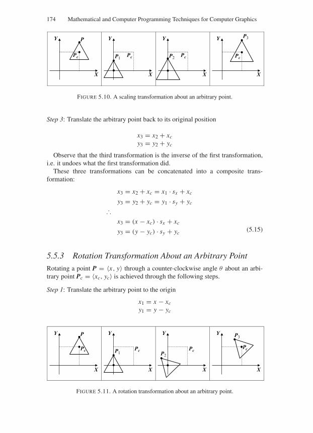
“Comninos” — 2005/8/31 — 15:47 — page 174 — #10
174 Mathematical and Computer Programming Techniques for Computer Graphics
P
X
Y
Pc P1
X
Y
Pc P2
X
Y
Pc
P3
X
Y
Pc
FIGURE 5.10. A scaling transformation about an arbitrary point.
Step 3: Translate the arbitrary point back to its original position
x3 = x2 + xc
y3 = y2 + yc
Observe that the third transformation is the inverse of the first transformation,i.e. it undoes what the first transformation did.
These three transformations can be concatenated into a composite trans-formation:
x3 = x2 + xc = x1 · sx + xc
y3 = y2 + yc = y1 · sy + yc
∴x3 = (x − xc) · sx + xc
y3 = (y − yc) · sy + yc(5.15)
5.5.3 Rotation Transformation About an Arbitrary Point
Rotating a point P = 〈x, y〉 through a counter-clockwise angle θ about an arbi-trary point Pc = 〈xc, yc〉 is achieved through the following steps.
Step 1: Translate the arbitrary point to the origin
x1 = x − xc
y1 = y − yc
P
X
Y
Pc P1
X
Y
PcP2
X
Y
Pc
P3
X
Y
Pc
FIGURE 5.11. A rotation transformation about an arbitrary point.
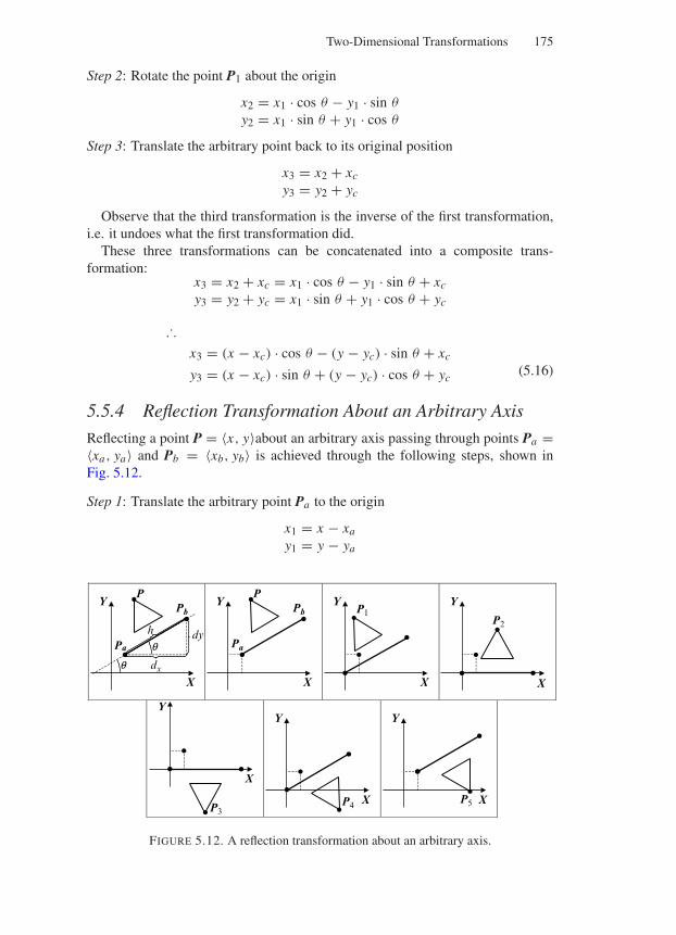
“Comninos” — 2005/8/31 — 15:47 — page 175 — #11
Two-Dimensional Transformations 175
Step 2: Rotate the point P1 about the origin
x2 = x1 · cos θ − y1 · sin θ
y2 = x1 · sin θ + y1 · cos θ
Step 3: Translate the arbitrary point back to its original position
x3 = x2 + xc
y3 = y2 + yc
Observe that the third transformation is the inverse of the first transformation,i.e. it undoes what the first transformation did.
These three transformations can be concatenated into a composite trans-formation:
x3 = x2 + xc = x1 · cos θ − y1 · sin θ + xc
y3 = y2 + yc = x1 · sin θ + y1 · cos θ + yc
∴x3 = (x − xc) · cos θ − (y − yc) · sin θ + xc
y3 = (x − xc) · sin θ + (y − yc) · cos θ + yc(5.16)
5.5.4 Reflection Transformation About an Arbitrary Axis
Reflecting a point P = 〈x, y〉about an arbitrary axis passing through points Pa =〈xa, ya〉 and Pb = 〈xb, yb〉 is achieved through the following steps, shown inFig. 5.12.
Step 1: Translate the arbitrary point Pa to the origin
x1 = x − xa
y1 = y − ya
P
X
Y
Pa
Pb
h
dx
dy
q
q
P
X
Y
Pa
Pb P1
X
Y
P2
X
Y
P3
X
Y
P4 X
Y
P5 X
Y
FIGURE 5.12. A reflection transformation about an arbitrary axis.
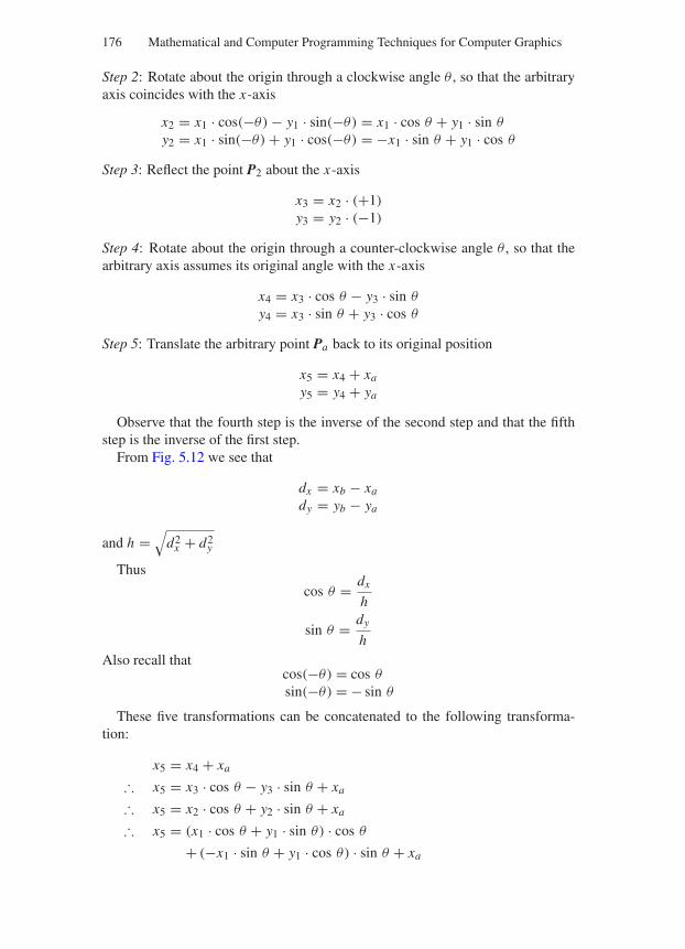
“Comninos” — 2005/8/31 — 15:47 — page 176 — #12
176 Mathematical and Computer Programming Techniques for Computer Graphics
Step 2: Rotate about the origin through a clockwise angle θ , so that the arbitraryaxis coincides with the x-axis
x2 = x1 · cos(−θ) − y1 · sin(−θ) = x1 · cos θ + y1 · sin θ
y2 = x1 · sin(−θ) + y1 · cos(−θ) = −x1 · sin θ + y1 · cos θ
Step 3: Reflect the point P2 about the x-axis
x3 = x2 · (+1)
y3 = y2 · (−1)
Step 4: Rotate about the origin through a counter-clockwise angle θ , so that thearbitrary axis assumes its original angle with the x-axis
x4 = x3 · cos θ − y3 · sin θ
y4 = x3 · sin θ + y3 · cos θ
Step 5: Translate the arbitrary point Pa back to its original position
x5 = x4 + xa
y5 = y4 + ya
Observe that the fourth step is the inverse of the second step and that the fifthstep is the inverse of the first step.
From Fig. 5.12 we see that
dx = xb − xa
dy = yb − ya
and h =√
d2x + d2
y
Thus
cos θ = dx
h
sin θ = dy
hAlso recall that
cos(−θ) = cos θ
sin(−θ) = − sin θ
These five transformations can be concatenated to the following transforma-tion:
x5 = x4 + xa
∴ x5 = x3 · cos θ − y3 · sin θ + xa
∴ x5 = x2 · cos θ + y2 · sin θ + xa
∴ x5 = (x1 · cos θ + y1 · sin θ) · cos θ
+ (−x1 · sin θ + y1 · cos θ) · sin θ + xa
“Comninos” — 2005/8/31 — 15:47 — page 177 — #13
Two-Dimensional Transformations 177
∴ x5 = [(x − xa) · cos θ + (y − ya) · sin θ] · cos θ
+ [− (x − xa) · sin θ + (y − ya) · cos θ] · sin θ + xa
∴ x5 = (x − xa) · cos2 θ + (y − ya) · sin θ · cos θ − (x − xa) · sin2 θ
+ (y − ya) · cos θ · sin θ + xa
∴ x5 =[(x − xa) · cos2 θ − (x − xa) · sin2 θ
]
+ [(y − ya) · sin θ · cos θ + (y − ya) · cos θ · sin θ ] + xa
∴ x5 = (x − xa) · cos(2θ) + (y − ya) · sin(2θ) + xa
and
y5 = y4 + ya
∴ y5 = x3 · sin θ + y3 · cos θ + ya
∴ y5 = x2 · sin θ − y2 · cos θ + ya
∴ y5 = (x1 · cos θ + y1 · sin θ) · sin θ
− (−x1 · sin θ + y1 · cos θ) · cos θ + ya
∴ y5 = [(x − xa) · cos θ + (y − ya) · sin θ ] · sin θ
− [− (x − xa) · sin θ + (y − ya) · cos θ] · cos θ + ya
∴ y5 = (x − xa) · cos θ · sin θ + (y − ya) · sin2 θ
+ (x − xa) · sin θ · cos θ − (y − ya) · cos2 θ + ya
∴ y5 = [(x − xa) · cos θ · sin θ + (x − xa) · sin θ · cos θ ]
+[(y − ya) · sin2 θ − (y − ya) · cos2 θ
]+ ya
∴ y5 = (x − xa) · sin(2θ) − (y − ya) · cos(2θ) + ya
Thus the concatenated transformation is given by
x5 = (x − xa) · cos(2θ) + (y − ya) · sin(2θ) + xa
y5 = (x − xa) · sin(2θ) − (y − ya) · cos(2θ) + ya (5.17)
5.6 Sign of the Angles in Transformations
In our discussion so far all the angles used in transformations were assumed tobe measured in a counter-clockwise positive fashion. This was a purely arbitrarychoice. Some writers choose to define their angles as being counter-clockwisepositive and others as being clockwise positive. This is a matter of taste anddifferent graphics libraries and systems do it differently. The important thing toremember is that, in order to convert from one system to the other we just need tonegate the angles in our transformations recalling that
sin(−θ) = − sin θ
cos(−θ) = cos θ
tan(−θ) = − tan θ
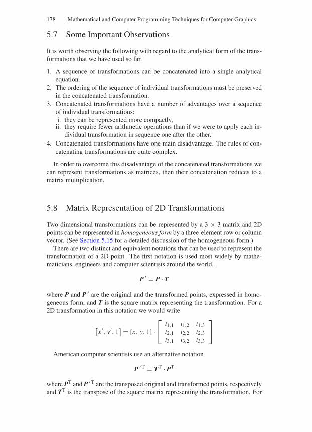
“Comninos” — 2005/8/31 — 15:47 — page 178 — #14
178 Mathematical and Computer Programming Techniques for Computer Graphics
5.7 Some Important Observations
It is worth observing the following with regard to the analytical form of the trans-formations that we have used so far.
1. A sequence of transformations can be concatenated into a single analyticalequation.
2. The ordering of the sequence of individual transformations must be preservedin the concatenated transformation.
3. Concatenated transformations have a number of advantages over a sequenceof individual transformations:i. they can be represented more compactly,
ii. they require fewer arithmetic operations than if we were to apply each in-dividual transformation in sequence one after the other.
4. Concatenated transformations have one main disadvantage. The rules of con-catenating transformations are quite complex.
In order to overcome this disadvantage of the concatenated transformations wecan represent transformations as matrices, then their concatenation reduces to amatrix multiplication.
5.8 Matrix Representation of 2D Transformations
Two-dimensional transformations can be represented by a 3 × 3 matrix and 2Dpoints can be represented in homogeneous form by a three-element row or columnvector. (See Section 5.15 for a detailed discussion of the homogeneous form.)
There are two distinct and equivalent notations that can be used to represent thetransformation of a 2D point. The first notation is used most widely by mathe-maticians, engineers and computer scientists around the world.
P ′ = P · T
where P and P ′ are the original and the transformed points, expressed in homo-geneous form, and T is the square matrix representing the transformation. For a2D transformation in this notation we would write
[x ′, y′, 1
] = [x, y, 1] ·⎡
⎣t1,1 t1,2 t1,3t2,1 t2,2 t2,3t3,1 t3,2 t3,3
⎤
⎦
American computer scientists use an alternative notation
P ′ T = TT · PT
where PT and P ′ T are the transposed original and transformed points, respectivelyand TT is the transpose of the square matrix representing the transformation. For
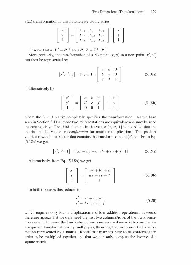
“Comninos” — 2005/8/31 — 15:47 — page 179 — #15
Two-Dimensional Transformations 179
a 2D transformation in this notation we would write⎡
⎣x ′y′1
⎤
⎦ =⎡
⎣t1,1 t2,1 t3,1t1,2 t2,2 t3,2t1,3 t2,3 t3,3
⎤
⎦ ·⎡
⎣xy1
⎤
⎦
Observe that as P ′ = P ′ T so is P · T = TT · PT.More precisely, the transformation of a 2D point 〈x, y〉 to a new point
⟨x ′, y′⟩
can then be represented by
[x ′, y′, 1
] = [x, y, 1] ·⎡
⎣a d 0b e 0c f 1
⎤
⎦ (5.18a)
or alternatively by
⎡
⎣x ′y′1
⎤
⎦ =⎡
⎣a b cd e f0 0 1
⎤
⎦ ·⎡
⎣xy1
⎤
⎦ (5.18b)
where the 3 × 3 matrix completely specifies the transformation. As we haveseen in Section 3.11.4, those two representations are equivalent and may be usedinterchangeably. The third element in the vector [x , y, 1] is added so that thematrix and the vector are conformant for matrix multiplication. This productyields a row/column vector that contains the transformed point
⟨x ′, y′⟩. From Eq.
(5.18a) we get
[x ′, y′, 1
] = [ax + by + c, dx + ey + f, 1] (5.19a)
Alternatively, from Eq. (5.18b) we get
⎡
⎣x ′y′1
⎤
⎦ =⎡
⎣ax + by + cdx + ey + f
1
⎤
⎦ (5.19b)
In both the cases this reduces to
x ′ = ax + by + cy′ = dx + ey + f
(5.20)
which requires only four multiplication and four addition operations. It wouldtherefore appear that we only need the first two columns/rows of the transforma-tion matrix. However, the third column/row is necessary if we wish to concatenatea sequence transformations by multiplying them together or to invert a transfor-mation represented by a matrix. Recall that matrices have to be conformant inorder to be multiplied together and that we can only compute the inverse of asquare matrix.
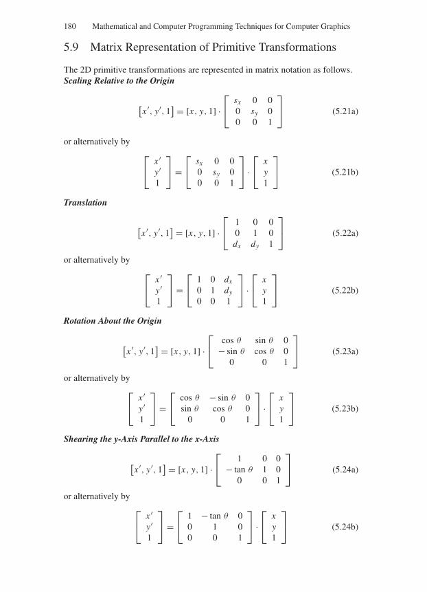
“Comninos” — 2005/8/31 — 15:47 — page 180 — #16
180 Mathematical and Computer Programming Techniques for Computer Graphics
5.9 Matrix Representation of Primitive Transformations
The 2D primitive transformations are represented in matrix notation as follows.Scaling Relative to the Origin
[x ′, y′, 1
] = [x, y, 1] ·⎡
⎣sx 0 00 sy 00 0 1
⎤
⎦ (5.21a)
or alternatively by⎡
⎣x ′y′1
⎤
⎦ =⎡
⎣sx 0 00 sy 00 0 1
⎤
⎦ ·⎡
⎣xy1
⎤
⎦ (5.21b)
Translation
[x ′, y′, 1
] = [x, y, 1] ·⎡
⎣1 0 00 1 0dx dy 1
⎤
⎦ (5.22a)
or alternatively by⎡
⎣x ′y′1
⎤
⎦ =⎡
⎣1 0 dx
0 1 dy
0 0 1
⎤
⎦ ·⎡
⎣xy1
⎤
⎦ (5.22b)
Rotation About the Origin
[x ′, y′, 1
] = [x, y, 1] ·⎡
⎣cos θ sin θ 0
− sin θ cos θ 00 0 1
⎤
⎦ (5.23a)
or alternatively by⎡
⎣x ′y′1
⎤
⎦ =⎡
⎣cos θ − sin θ 0sin θ cos θ 0
0 0 1
⎤
⎦ ·⎡
⎣xy1
⎤
⎦ (5.23b)
Shearing the y-Axis Parallel to the x-Axis
[x ′, y′, 1
] = [x, y, 1] ·⎡
⎣1 0 0
− tan θ 1 00 0 1
⎤
⎦ (5.24a)
or alternatively by⎡
⎣x ′y′1
⎤
⎦ =⎡
⎣1 − tan θ 00 1 00 0 1
⎤
⎦ ·⎡
⎣xy1
⎤
⎦ (5.24b)
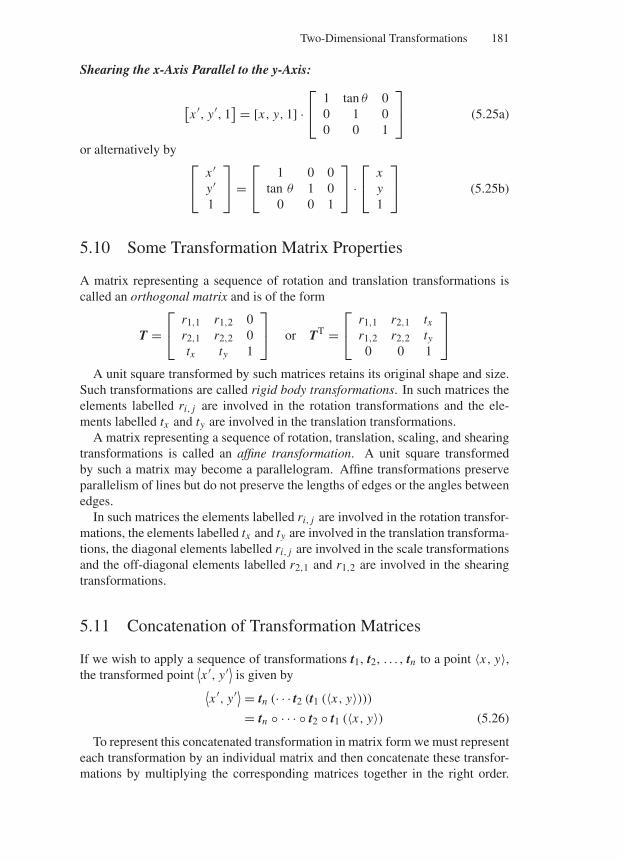
“Comninos” — 2005/8/31 — 15:47 — page 181 — #17
Two-Dimensional Transformations 181
Shearing the x-Axis Parallel to the y-Axis:
[x ′, y′, 1
] = [x, y, 1] ·⎡
⎣1 tan θ 00 1 00 0 1
⎤
⎦ (5.25a)
or alternatively by⎡
⎣x ′y′1
⎤
⎦ =⎡
⎣1 0 0
tan θ 1 00 0 1
⎤
⎦ ·⎡
⎣xy1
⎤
⎦ (5.25b)
5.10 Some Transformation Matrix Properties
A matrix representing a sequence of rotation and translation transformations iscalled an orthogonal matrix and is of the form
T =⎡
⎣r1,1 r1,2 0r2,1 r2,2 0tx ty 1
⎤
⎦ or TT =⎡
⎣r1,1 r2,1 txr1,2 r2,2 ty
0 0 1
⎤
⎦
A unit square transformed by such matrices retains its original shape and size.Such transformations are called rigid body transformations. In such matrices theelements labelled ri, j are involved in the rotation transformations and the ele-ments labelled tx and ty are involved in the translation transformations.
A matrix representing a sequence of rotation, translation, scaling, and shearingtransformations is called an affine transformation. A unit square transformedby such a matrix may become a parallelogram. Affine transformations preserveparallelism of lines but do not preserve the lengths of edges or the angles betweenedges.
In such matrices the elements labelled ri, j are involved in the rotation transfor-mations, the elements labelled tx and ty are involved in the translation transforma-tions, the diagonal elements labelled ri, j are involved in the scale transformationsand the off-diagonal elements labelled r2,1 and r1,2 are involved in the shearingtransformations.
5.11 Concatenation of Transformation Matrices
If we wish to apply a sequence of transformations t1, t2, . . . , tn to a point 〈x, y〉,the transformed point
⟨x ′, y′⟩ is given by⟨x ′, y′⟩ = tn (· · · t2 (t1 (〈x, y〉)))
= tn · · · t2 t1 (〈x, y〉) (5.26)
To represent this concatenated transformation in matrix form we must representeach transformation by an individual matrix and then concatenate these transfor-mations by multiplying the corresponding matrices together in the right order.
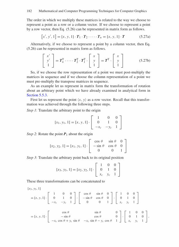
“Comninos” — 2005/8/31 — 15:47 — page 182 — #18
182 Mathematical and Computer Programming Techniques for Computer Graphics
The order in which we multiply these matrices is related to the way we choose torepresent a point as a row or a column vector. If we choose to represent a pointby a row vector, then Eq. (5.26) can be represented in matrix form as follows.
[x ′, y′, 1
] = [x, y, 1] · T1 · T2 · · · · · Tn = [x, y, 1] · T (5.27a)
Alternatively, if we choose to represent a point by a column vector, then Eq.(5.26) can be represented in matrix form as follows.
⎡
⎣x ′y′1
⎤
⎦ = TTn · · · · · TT
2 · TT1 ·
⎡
⎣xy1
⎤
⎦ = TT ·⎡
⎣xy1
⎤
⎦ (5.27b)
So, if we choose the row representation of a point we must post-multiply thematrices in sequence and if we choose the column representation of a point wemust pre-multiply the transpose matrices in sequence.
As an example let us represent in matrix form the transformation of rotationabout an arbitrary point which we have already examined in analytical form inSection 5.5.3.
First let us represent the point 〈x, y〉 as a row vector. Recall that this transfor-mation was achieved through the following three steps.
Step 1: Translate the arbitrary point to the origin
[x1, y1, 1] = [x, y, 1] ·⎡
⎣1 0 00 1 0
−xc −yc 1
⎤
⎦
Step 2: Rotate the point P1 about the origin
[x2, y2, 1] = [x1, y1, 1] ·⎡
⎣cos θ sin θ 0
− sin θ cos θ 00 0 1
⎤
⎦
Step 3: Translate the arbitrary point back to its original position
[x3, y3, 1] = [x2, y2, 1] ·⎡
⎣1 0 00 1 0xc yc 1
⎤
⎦
These three transformations can be concatenated to
[x3, y3, 1]
= [x, y, 1] ·⎡
⎣1 0 00 1 0
−xc −yc 1
⎤
⎦ ·⎡
⎣cos θ sin θ 0
− sin θ cos θ 00 0 1
⎤
⎦ ·⎡
⎣1 0 00 1 0xc yc 1
⎤
⎦
= [x, y, 1] ·⎡
⎣cos θ sin θ 0
− sin θ cos θ 0−xc cos θ + yc sin θ −xc sin θ − yc cos θ 1
⎤
⎦ ·⎡
⎣1 0 00 1 0xc yc 1
⎤
⎦ ,
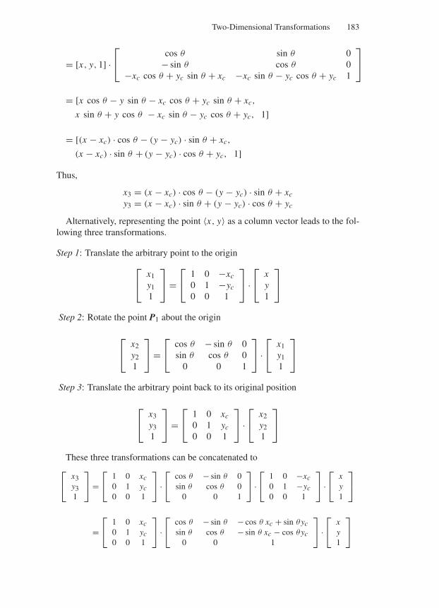
“Comninos” — 2005/8/31 — 15:47 — page 183 — #19
Two-Dimensional Transformations 183
= [x, y, 1] ·⎡
⎣cos θ sin θ 0
− sin θ cos θ 0−xc cos θ + yc sin θ + xc −xc sin θ − yc cos θ + yc 1
⎤
⎦
= [x cos θ − y sin θ − xc cos θ + yc sin θ + xc,
x sin θ + y cos θ − xc sin θ − yc cos θ + yc, 1]
= [(x − xc) · cos θ − (y − yc) · sin θ + xc,
(x − xc) · sin θ + (y − yc) · cos θ + yc, 1]
Thus,
x3 = (x − xc) · cos θ − (y − yc) · sin θ + xc
y3 = (x − xc) · sin θ + (y − yc) · cos θ + yc
Alternatively, representing the point 〈x, y〉 as a column vector leads to the fol-lowing three transformations.
Step 1: Translate the arbitrary point to the origin
⎡
⎣x1y11
⎤
⎦ =⎡
⎣1 0 −xc
0 1 −yc
0 0 1
⎤
⎦ ·⎡
⎣xy1
⎤
⎦
Step 2: Rotate the point P1 about the origin
⎡
⎣x2y21
⎤
⎦ =⎡
⎣cos θ − sin θ 0sin θ cos θ 0
0 0 1
⎤
⎦ ·⎡
⎣x1y11
⎤
⎦
Step 3: Translate the arbitrary point back to its original position
⎡
⎣x3y31
⎤
⎦ =⎡
⎣1 0 xc
0 1 yc
0 0 1
⎤
⎦ ·⎡
⎣x2y21
⎤
⎦
These three transformations can be concatenated to⎡
⎣x3y31
⎤
⎦ =⎡
⎣1 0 xc0 1 yc0 0 1
⎤
⎦ ·⎡
⎣cos θ − sin θ 0sin θ cos θ 0
0 0 1
⎤
⎦ ·⎡
⎣1 0 −xc0 1 −yc0 0 1
⎤
⎦ ·⎡
⎣xy1
⎤
⎦
=⎡
⎣1 0 xc0 1 yc0 0 1
⎤
⎦ ·⎡
⎣cos θ − sin θ − cos θ xc + sin θycsin θ cos θ − sin θ xc − cos θyc
0 0 1
⎤
⎦ ·⎡
⎣xy1
⎤
⎦
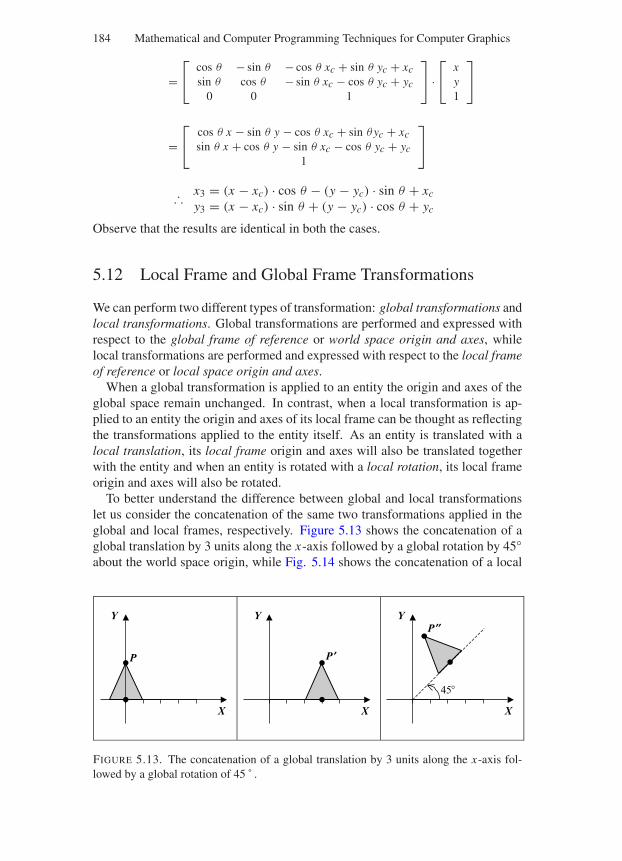
“Comninos” — 2005/8/31 — 15:47 — page 184 — #20
184 Mathematical and Computer Programming Techniques for Computer Graphics
=⎡
⎣cos θ − sin θ − cos θ xc + sin θ yc + xcsin θ cos θ − sin θ xc − cos θ yc + yc
0 0 1
⎤
⎦ ·⎡
⎣xy1
⎤
⎦
=⎡
⎣cos θ x − sin θ y − cos θ xc + sin θyc + xcsin θ x + cos θ y − sin θ xc − cos θ yc + yc
1
⎤
⎦
∴ x3 = (x − xc) · cos θ − (y − yc) · sin θ + xc
y3 = (x − xc) · sin θ + (y − yc) · cos θ + yc
Observe that the results are identical in both the cases.
5.12 Local Frame and Global Frame Transformations
We can perform two different types of transformation: global transformations andlocal transformations. Global transformations are performed and expressed withrespect to the global frame of reference or world space origin and axes, whilelocal transformations are performed and expressed with respect to the local frameof reference or local space origin and axes.
When a global transformation is applied to an entity the origin and axes of theglobal space remain unchanged. In contrast, when a local transformation is ap-plied to an entity the origin and axes of its local frame can be thought as reflectingthe transformations applied to the entity itself. As an entity is translated with alocal translation, its local frame origin and axes will also be translated togetherwith the entity and when an entity is rotated with a local rotation, its local frameorigin and axes will also be rotated.
To better understand the difference between global and local transformationslet us consider the concatenation of the same two transformations applied in theglobal and local frames, respectively. Figure 5.13 shows the concatenation of aglobal translation by 3 units along the x-axis followed by a global rotation by 45about the world space origin, while Fig. 5.14 shows the concatenation of a local
P
X
Y
P ¢
X
YP ¢¢
X
Y
45
FIGURE 5.13. The concatenation of a global translation by 3 units along the x-axis fol-lowed by a global rotation of 45 ˚ .
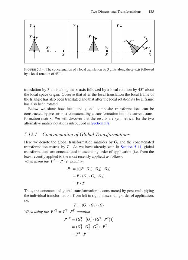
“Comninos” — 2005/8/31 — 15:47 — page 185 — #21
Two-Dimensional Transformations 185
P
X
Y
XL
YL P ′
X
Y
XL
YL
P ′′
X
Y
XLYL
45
FIGURE 5.14. The concatenation of a local translation by 3 units along the x-axis followedby a local rotation of 45 ˚ .
translation by 3 units along the x-axis followed by a local rotation by 45 aboutthe local space origin. Observe that after the local translation the local frame ofthe triangle has also been translated and that after the local rotation its local framehas also been rotated.
Below we show how local and global composite transformations can beconstructed by pre- or post-concatenating a transformation into the current trans-formation matrix. We will discover that the results are symmetrical for the twoalternative matrix notations introduced in Section 5.8.
5.12.1 Concatenation of Global Transformations
Here we denote the global transformation matrices by Gi and the concatenatedtransformation matrix by T. As we have already seen in Section 5.11, globaltransformations are concatenated in ascending order of application (i.e. from theleast recently applied to the most recently applied) as follows.When using the P ′ = P · T notation
P ′ = (((P · G1) · G2) · G3)
= P · (G1 · G2 · G3)
= P · T
Thus, the concatenated global transformation is constructed by post-multiplyingthe individual transformations from left to right in ascending order of application,i.e.
T = (G1 · G2) · G3
When using the P ′ T = TT · PT notation
P ′ T = (GT
3 · (GT
2 · (GT
1 · PT)))
= (GT
3 · GT2 · GT
1
) · PT
= TT · PT
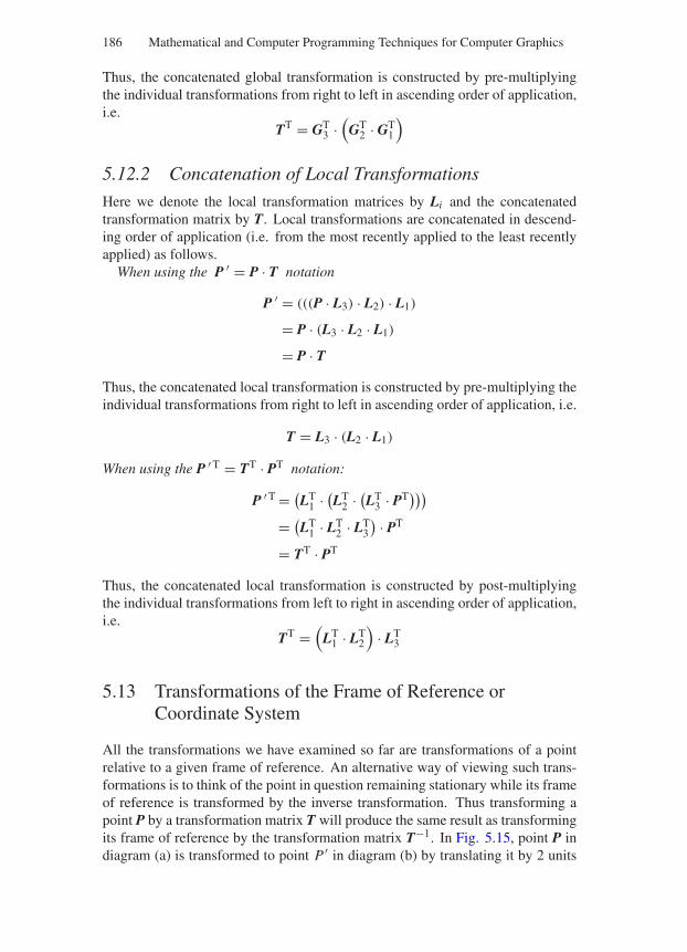
“Comninos” — 2005/8/31 — 15:47 — page 186 — #22
186 Mathematical and Computer Programming Techniques for Computer Graphics
Thus, the concatenated global transformation is constructed by pre-multiplyingthe individual transformations from right to left in ascending order of application,i.e.
TT = GT3 ·
(GT
2 · GT1
)
5.12.2 Concatenation of Local Transformations
Here we denote the local transformation matrices by Li and the concatenatedtransformation matrix by T. Local transformations are concatenated in descend-ing order of application (i.e. from the most recently applied to the least recentlyapplied) as follows.
When using the P ′ = P · T notation
P ′ = (((P · L3) · L2) · L1)
= P · (L3 · L2 · L1)
= P · T
Thus, the concatenated local transformation is constructed by pre-multiplying theindividual transformations from right to left in ascending order of application, i.e.
T = L3 · (L2 · L1)
When using the P ′ T = TT · PT notation:
P ′ T = (LT
1 · (LT
2 · (LT
3 · PT)))
= (LT
1 · LT2 · LT
3
) · PT
= TT · PT
Thus, the concatenated local transformation is constructed by post-multiplyingthe individual transformations from left to right in ascending order of application,i.e.
TT =(
LT1 · LT
2
)· LT
3
5.13 Transformations of the Frame of Reference orCoordinate System
All the transformations we have examined so far are transformations of a pointrelative to a given frame of reference. An alternative way of viewing such trans-formations is to think of the point in question remaining stationary while its frameof reference is transformed by the inverse transformation. Thus transforming apoint P by a transformation matrix T will produce the same result as transformingits frame of reference by the transformation matrix T−1. In Fig. 5.15, point P indiagram (a) is transformed to point P ′ in diagram (b) by translating it by 2 units
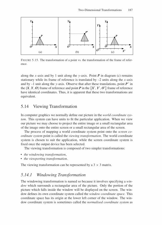
“Comninos” — 2005/8/31 — 15:47 — page 187 — #23
Two-Dimensional Transformations 187
P
X
Y
(a) (b) (c)
O
P¢
X
Y
O
P
X¢
Y¢
O¢O X
Y
FIGURE 5.15. The transformation of a point vs. the transformation of the frame of refer-ence.
along the x-axis and by 1 unit along the y-axis. Point P in diagram (c) remainsstationary while its frame of reference is translated by –2 units along the x-axisand by –1 unit along the y-axis. Observe that after these translations, point P ′ inthe X, Y, O frame of reference and point P in the
X′, Y′, O′ frame of reference
have identical coordinates. Thus, it is apparent that these two transformations areequivalent.
5.14 Viewing Transformation
In computer graphics we normally define our picture in the world coordinate sys-tem. This system can have units to fit the particular application. When we viewour picture we may choose to project the entire image or a small rectangular areaof the image onto the entire screen or a small rectangular area of the screen.
The process of mapping a world coordinate system point onto the screen co-ordinate system point is called the viewing transformation. The world coordinatesystem is chosen to suit the application, while the screen coordinate system isfixed once the output device has been selected.
The viewing transformation is composed of two simpler transformations:
• the windowing transformation,• the viewporting transformation.
The viewing transformation can be represented by a 3 × 3 matrix.
5.14.1 Windowing Transformation
The windowing transformation is named so because it involves specifying a win-dow which surrounds a rectangular area of the picture. Only the portion of thepicture which falls inside the window will be displayed on the screen. The win-dow defines its own coordinate system called the window coordinate space. Thiscoordinate space has its origin at the lower left corner of the window. The win-dow coordinate system is sometimes called the normalised coordinate system as
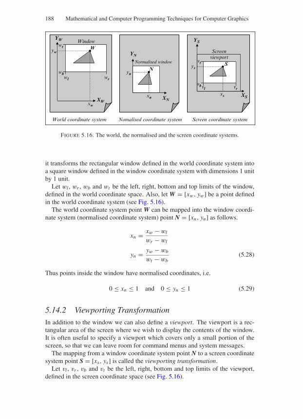
“Comninos” — 2005/8/31 — 15:47 — page 188 — #24
188 Mathematical and Computer Programming Techniques for Computer Graphics
XW
World coordinate system Nomalised coordinate system Screen coordinate system
Window
Normalised windowviewportScreen
YW
XN
YN
XS
YS
W
NS
wl wr
wb
wt
vl vrvb
vt
xw
yw
yn
xn
ys
xs
FIGURE 5.16. The world, the normalised and the screen coordinate systems.
it transforms the rectangular window defined in the world coordinate system intoa square window defined in the window coordinate system with dimensions 1 unitby 1 unit.
Let wl , wr , wb and wt be the left, right, bottom and top limits of the window,defined in the world coordinate space. Also, let W = [xw, yw] be a point definedin the world coordinate system (see Fig. 5.16).
The world coordinate system point W can be mapped into the window coordi-nate system (normalised coordinate system) point N = [xn, yn] as follows.
xn = xw − wl
wr − wl
yn = yw − wb
wt − wb(5.28)
Thus points inside the window have normalised coordinates, i.e.
0 ≤ xn ≤ 1 and 0 ≤ yn ≤ 1 (5.29)
5.14.2 Viewporting Transformation
In addition to the window we can also define a viewport. The viewport is a rec-tangular area of the screen where we wish to display the contents of the window.It is often useful to specify a viewport which covers only a small portion of thescreen, so that we can leave room for command menus and system messages.
The mapping from a window coordinate system point N to a screen coordinatesystem point S = [xs, ys] is called the viewporting transformation.
Let vl , vr , vb and vt be the left, right, bottom and top limits of the viewport,defined in the screen coordinate space (see Fig. 5.16).
“Comninos” — 2005/8/31 — 15:47 — page 189 — #25
Two-Dimensional Transformations 189
The viewporting transformation is defined as follows.
xs = xn · (vr − vl) + vl
ys = yn · (vt − vb) + vb (5.30)
So the points inside the viewport have coordinates in the range
vl ≤ xs ≤ vr and vb ≤ ys ≤ vt (5.31)
The windowing and the viewporting transformations can be concatenated intoa composite viewing transformation as follows.
xs = xw − wl
wr − wl· (vr − vl) + vl
ys = yw − wb
wt − wb· (vt − vb) + vb
which can be rewritten as
xs = (xw − wl) · vr − vl
wr − wl+ vl
ys = (yw − wb) · vt − vb
wt − wb+ vb (5.32)
which expands to
xs = xw · vr − vl
wr − wl− wl · vr − vl
wr − wl+ vl
ys = yw · vt − vb
wt − wb− wb · vt − vb
wt − wb+ vb
which can be rewritten as
xs = xw · sx + dx
ys = yw · sy + dy (5.33)
where
sx = vr − vl
wr − wl
dx = −wl · vr − vl
wr − wl+ vl
(5.34)sy = vt − vb
wt − wb
dy = −wb · vt − vb
wt − wb+ vb
“Comninos” — 2005/8/31 — 15:47 — page 190 — #26
190 Mathematical and Computer Programming Techniques for Computer Graphics
We only need to compute the values of sx , dx , sy and dy once, when the win-dow and the viewport are defined. And so we can transform every point inour picture by a computation involving only two multiplication and two additionoperations.
Clipping can be applied either to the screen space points using the viewportperimeter as the clipping boundary or to the world space points using the windowperimeter as the clipping boundary.
The analytical equations, developed above, can be rewritten in matrix form asfollows.
[xs, ys, 1] = [xw, yw, 1] ·⎡
⎣sx 0 00 sy 0dx dy 1
⎤
⎦ (5.34a)
or alternatively as⎡
⎣xs
ys
1
⎤
⎦ =⎡
⎣sx 0 dx
0 sy dy
0 0 1
⎤
⎦ ·⎡
⎣xw
yw
1
⎤
⎦ (5.34b)
The viewing transformation matrix can be concatenated with the matrix con-taining all other transformations, thus allowing us to apply all transformationswith one matrix multiplication operation. In this case, clipping must be applied tothe screen space points using the viewport perimeter as the clipping boundary.
5.15 Homogeneous Coordinates
The homogeneous representation of an entity defined in n-dimensional space isanother entity defined in (n+1)-dimensional space. The mapping from n-space to(n + 1)-space is a one-to-many mapping. Thus, the n-space entity has an infinityof images (representations) in (n + 1)-space. The inverse mapping, which is amany-to-one mapping, is a central projection that uses the origin as its centre ofprojection.
A point/vector in n-dimensional Euclidean space can be represented as an(n + 1)-dimensional homogeneous space point/vector by the introduction of anadditional coordinate or component that also acts as a scale factor.
The homogeneous representation of a 2D point P = [x y
]is the homoge-
neous point P h = [w · x w · y w
], where w is the homogeneous coordinate
which is a non-zero scalar frequently known as the weight of the point. By se-lecting different values for w we produce different homogeneous mappings of theoriginal point. Thus, the homogeneous points
P h1 = [
w1 · x w1 · y w1], P h
2 = [w2 · x w2 · y w2
],
P h3 = [
w3 · x w3 · y w3], . . .
are all valid homogeneous mappings of the point P = [x y
]and there is an
infinity of such mappings.
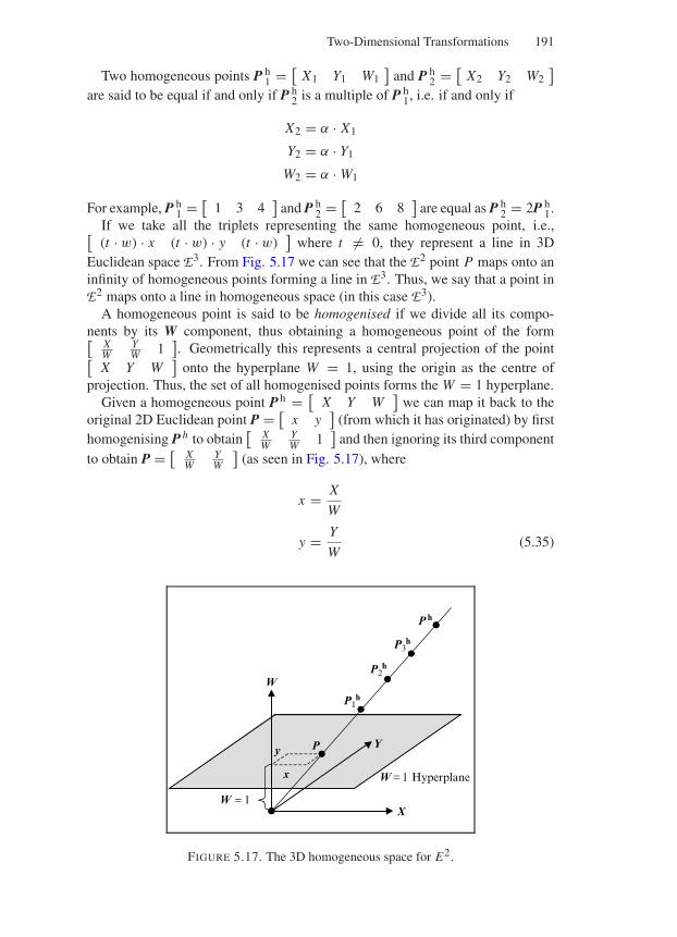
“Comninos” — 2005/8/31 — 15:47 — page 191 — #27
Two-Dimensional Transformations 191
Two homogeneous points P h1 = [
X1 Y1 W1]
and P h2 = [
X2 Y2 W2]
are said to be equal if and only if P h2 is a multiple of P h
1, i.e. if and only if
X2 = α · X1
Y2 = α · Y1
W2 = α · W1
For example, P h1 = [
1 3 4]
and P h2 = [
2 6 8]
are equal as P h2 = 2P h
1.If we take all the triplets representing the same homogeneous point, i.e.,[(t · w) · x (t · w) · y (t · w)
]where t = 0, they represent a line in 3D
Euclidean space E3. From Fig. 5.17 we can see that the E2 point P maps onto aninfinity of homogeneous points forming a line in E3. Thus, we say that a point inE2 maps onto a line in homogeneous space (in this case E3).
A homogeneous point is said to be homogenised if we divide all its compo-nents by its W component, thus obtaining a homogeneous point of the form[
XW
YW 1
]. Geometrically this represents a central projection of the point[
X Y W]
onto the hyperplane W = 1, using the origin as the centre ofprojection. Thus, the set of all homogenised points forms the W = 1 hyperplane.
Given a homogeneous point P h = [X Y W
]we can map it back to the
original 2D Euclidean point P = [x y
](from which it has originated) by first
homogenising P h to obtain[
XW
YW 1
]and then ignoring its third component
to obtain P = [XW
YW
](as seen in Fig. 5.17), where
x = X
W
y = Y
W(5.35)
P1h
X
YP
W=1 Hyperplane
WP2
h
P3h
W = 1
x
y
P h
FIGURE 5.17. The 3D homogeneous space for E2.
“Comninos” — 2005/8/31 — 15:47 — page 192 — #28
192 Mathematical and Computer Programming Techniques for Computer Graphics
This process is called a projective map H and is the inverse of the mapping thatoriginally mapped point P onto the homogeneous point P h .
In 2D Euclidean space both points and vectors are represented by two com-ponents and can only be distinguished by their context. They are however quitedifferent. A vector has a magnitude and a direction, but no fixed position, while apoint has a position but no magnitude or direction.
By examining Eq. (5.35) we can see that as W approaches 0 both x and yapproach infinity from a particular direction. Thus, we may think of the homo-geneous point
[w · x w · y w
]as representing the point
[x y
]and the
homogeneous point[
x y 0]
as representing the vector[
x y]. So, in ho-
mogeneous space we have a way of distinguishing between points and vectors.Three-dimensional Euclidean points/vectors are represented analogously al-
though their homogeneous representation is more difficult to visualise. Moreformally, a point/vector P = [
x y z]
in 3D Euclidean space may be rep-resented by the 4D homogeneous point
P h = [
w · x w · y w · z w],
[x y z 0
],
w = 0w = 0
(5.36)
The original point/vector P may be retrieved from its homogeneous represen-tation P h by using the projective map H, which is defined as
H([
X Y Z W]) =
[XW
YW
ZW
], W = 0
direction([
X Y Z])
, W = 0(5.37)
Thus, the projective map H uses the origin as the centre of projection to projectthe homogeneous point/vector P h onto the hyperplane W = 1 in order to retrievethe 3D point/vector P.
P = H(
P h)
(5.38)
5.16 A Simple C Library for 2D Transformations
See Appendix 3.
6
Two-Dimensional Clipping
Clipping is a process that subdivides each element of a picture to be displayedinto its visible and invisible parts, thus allowing us to discard the invisible partsof the picture. In 2D, the clipping process can be applied to a variety of graphicsprimitives such as points, lines, polygons and curves. Clipping is performed withrespect to a clipping boundary, which may be a convex or concave polygonalboundary. Clipping to a convex polygonal boundary is much simpler, thus we willstart our discussion by looking at various algorithms that clip graphics primitivesagainst a convex polygonal boundary. In its simplest form, a convex polygonalboundary consists of the four edges of the world window or the screen viewport.In this case, xl (x-left), xr (x-right), yb (y-bottom) and yt (y-top) represent thefour extremities of this rectangular clipping boundary.
6.1 Clipping a 2D Point to a Rectangular Clipping Boundary
Clipping 2D points to a rectangular clipping boundary is very simple. All wehave to do is to determine whether the point 〈x, y〉 satisfies the following fourinequalities.
xl ≤ x ≤ xr and yb ≤ y ≤ yt (6.1)
If the point satisfies all four inequalities, then it is visible otherwise it is invisible(see Fig. 6.1).
The following C Boolean function clips a point to a rectangular clippingboundary.
/* Define the Boolean type and constants */
typedef unsigned char boolean_t;
boolean_t clip_point(double x, double y,double xl, double xr, double yb, double yt)
193
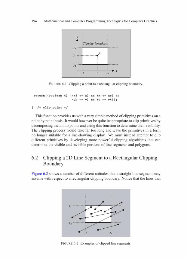
194 Mathematical and Computer Programming Techniques for Computer Graphics
Clipping boundary
X
Y
P
xl xr
yb
yt
y
x
FIGURE 6.1. Clipping a point to a rectangular clipping boundary.
return((boolean_t) ((xl <= x) && (x <= xr) &&(yb <= y) && (y <= yt));
/* clip_point */
This function provides us with a very simple method of clipping primitives on apoint by point basis. It would however be quite inappropriate to clip primitives bydecomposing them into points and using this function to determine their visibility.The clipping process would take far too long and leave the primitives in a formno longer suitable for a line-drawing display. We must instead attempt to clipdifferent primitives by developing more powerful clipping algorithms that candetermine the visible and invisible portions of line segments and polygons.
6.2 Clipping a 2D Line Segment to a Rectangular ClippingBoundary
Figure 6.2 shows a number of different attitudes that a straight line segment mayassume with respect to a rectangular clipping boundary. Notice that the lines that
xl xr
yb
yt
FIGURE 6.2. Examples of clipped line segments.
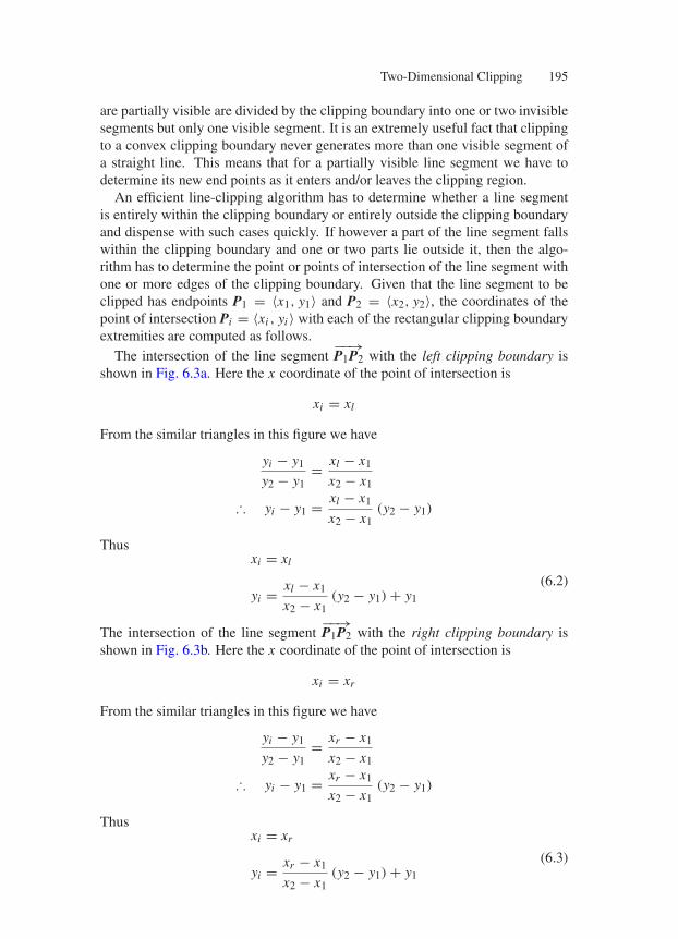
Two-Dimensional Clipping 195
are partially visible are divided by the clipping boundary into one or two invisiblesegments but only one visible segment. It is an extremely useful fact that clippingto a convex clipping boundary never generates more than one visible segment ofa straight line. This means that for a partially visible line segment we have todetermine its new end points as it enters and/or leaves the clipping region.
An efficient line-clipping algorithm has to determine whether a line segmentis entirely within the clipping boundary or entirely outside the clipping boundaryand dispense with such cases quickly. If however a part of the line segment fallswithin the clipping boundary and one or two parts lie outside it, then the algo-rithm has to determine the point or points of intersection of the line segment withone or more edges of the clipping boundary. Given that the line segment to beclipped has endpoints P1 = 〈x1, y1〉 and P2 = 〈x2, y2〉, the coordinates of thepoint of intersection Pi = 〈xi , yi 〉 with each of the rectangular clipping boundaryextremities are computed as follows.
The intersection of the line segment−−→P1P2 with the left clipping boundary is
shown in Fig. 6.3a. Here the x coordinate of the point of intersection is
xi = xl
From the similar triangles in this figure we have
yi − y1
y2 − y1= xl − x1
x2 − x1
∴ yi − y1 = xl − x1
x2 − x1(y2 − y1)
Thusxi = xl
yi = xl − x1
x2 − x1(y2 − y1) + y1
(6.2)
The intersection of the line segment−−→P1P2 with the right clipping boundary is
shown in Fig. 6.3b. Here the x coordinate of the point of intersection is
xi = xr
From the similar triangles in this figure we have
yi − y1
y2 − y1= xr − x1
x2 − x1
∴ yi − y1 = xr − x1
x2 − x1(y2 − y1)
Thusxi = xr
yi = xr − x1
x2 − x1(y2 − y1) + y1
(6.3)
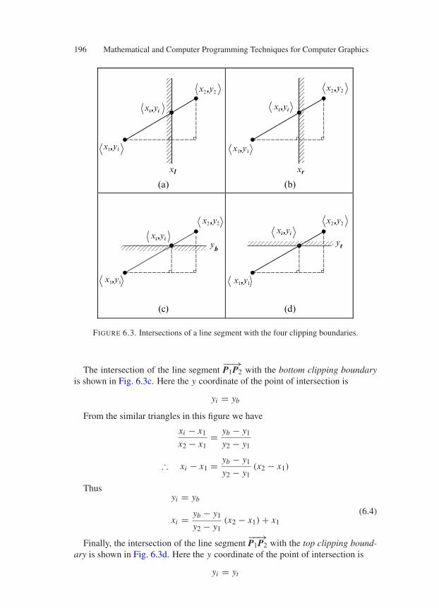
196 Mathematical and Computer Programming Techniques for Computer Graphics
x1,y1
xl
(a) (b)
(d)(c)
x2 ,y2x2 ,y2
x2 ,y2x2 ,y2
xi ,yixi ,yi
xi ,yixi ,yi
x1,y1
x1,y1x1,y1
xr
ybyt
FIGURE 6.3. Intersections of a line segment with the four clipping boundaries.
The intersection of the line segment−−→P1P2 with the bottom clipping boundary
is shown in Fig. 6.3c. Here the y coordinate of the point of intersection is
yi = yb
From the similar triangles in this figure we have
xi − x1
x2 − x1= yb − y1
y2 − y1
∴ xi − x1 = yb − y1
y2 − y1(x2 − x1)
Thusyi = yb
xi = yb − y1
y2 − y1(x2 − x1) + x1
(6.4)
Finally, the intersection of the line segment−−→P1P2 with the top clipping bound-
ary is shown in Fig. 6.3d. Here the y coordinate of the point of intersection is
yi = yt
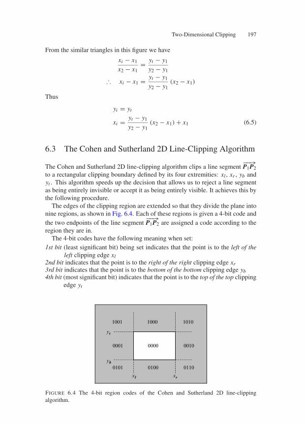
Two-Dimensional Clipping 197
From the similar triangles in this figure we have
xi − x1
x2 − x1= yt − y1
y2 − y1
∴ xi − x1 = yt − y1
y2 − y1(x2 − x1)
Thus
yi = yt
xi = yt − y1
y2 − y1(x2 − x1) + x1 (6.5)
6.3 The Cohen and Sutherland 2D Line-Clipping Algorithm
The Cohen and Sutherland 2D line-clipping algorithm clips a line segment−−→P1P2
to a rectangular clipping boundary defined by its four extremities: xl , xr , yb andyt . This algorithm speeds up the decision that allows us to reject a line segmentas being entirely invisible or accept it as being entirely visible. It achieves this bythe following procedure.
The edges of the clipping region are extended so that they divide the plane intonine regions, as shown in Fig. 6.4. Each of these regions is given a 4-bit code andthe two endpoints of the line segment
−−→P1P2 are assigned a code according to the
region they are in.The 4-bit codes have the following meaning when set:
1st bit (least significant bit) being set indicates that the point is to the left of theleft clipping edge xl
2nd bit indicates that the point is to the right of the right clipping edge xr3rd bit indicates that the point is to the bottom of the bottom clipping edge yb4th bit (most significant bit) indicates that the point is to the top of the top clipping
edge yt
xl xr
yb
yt
10001001 1010
00000001 0010
0101 0100 0110
FIGURE 6.4 The 4-bit region codes of the Cohen and Sutherland 2D line-clippingalgorithm.
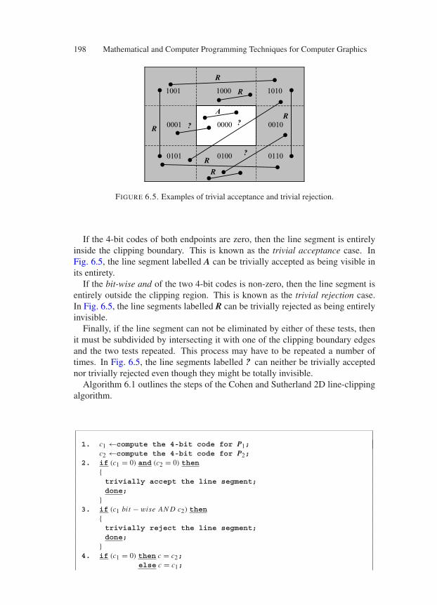
198 Mathematical and Computer Programming Techniques for Computer Graphics
R10001001 1010
00000001 0010
0101 0100 0110
R
RA
R
R
R
??
?
FIGURE 6.5. Examples of trivial acceptance and trivial rejection.
If the 4-bit codes of both endpoints are zero, then the line segment is entirelyinside the clipping boundary. This is known as the trivial acceptance case. InFig. 6.5, the line segment labelled A can be trivially accepted as being visible inits entirety.
If the bit-wise and of the two 4-bit codes is non-zero, then the line segment isentirely outside the clipping region. This is known as the trivial rejection case.In Fig. 6.5, the line segments labelled R can be trivially rejected as being entirelyinvisible.
Finally, if the line segment can not be eliminated by either of these tests, thenit must be subdivided by intersecting it with one of the clipping boundary edgesand the two tests repeated. This process may have to be repeated a number oftimes. In Fig. 6.5, the line segments labelled ? can neither be trivially acceptednor trivially rejected even though they might be totally invisible.
Algorithm 6.1 outlines the steps of the Cohen and Sutherland 2D line-clippingalgorithm.
1. c1 ←compute the 4-bit code for P1;c2 ←compute the 4-bit code for P2;
2. if (c1 = 0) and (c2 = 0) thentrivially accept the line segment;done;
3. if (c1 bit − wise AN D c2) then
trivially reject the line segment;done;
4. if (c1 = 0) then c = c2;
else c = c1;
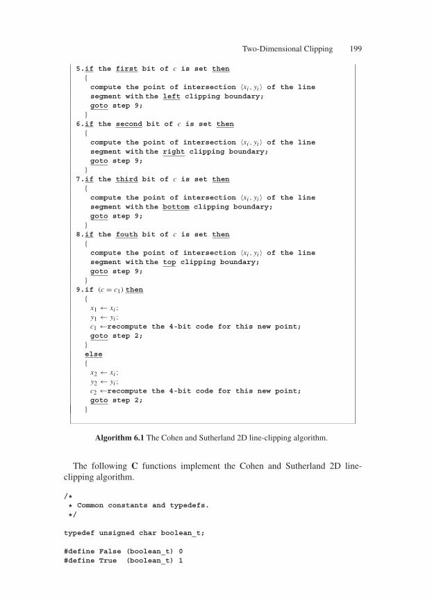
Two-Dimensional Clipping 199
5.if the first bit of c is set thencompute the point of intersection 〈xi , yi 〉 of the linesegment with the left clipping boundary;goto step 9;
6.if the second bit of c is set then
compute the point of intersection 〈xi , yi 〉 of the linesegment with the right clipping boundary;goto step 9;
7.if the third bit of c is set then
compute the point of intersection 〈xi , yi 〉 of the linesegment with the bottom clipping boundary;goto step 9;
8.if the fouth bit of c is set then
compute the point of intersection 〈xi , yi 〉 of the linesegment with the top clipping boundary;goto step 9;
9.if (c = c1) then
x1 ← xi ;y1 ← yi ;c1 ←recompute the 4-bit code for this new point;goto step 2;
else
x2 ← xi ;y2 ← yi ;c2 ←recompute the 4-bit code for this new point;goto step 2;
Algorithm 6.1 The Cohen and Sutherland 2D line-clipping algorithm.
The following C functions implement the Cohen and Sutherland 2D line-clipping algorithm.
/** Common constants and typedefs.
*/
typedef unsigned char boolean_t;
#define False (boolean_t) 0#define True (boolean_t) 1
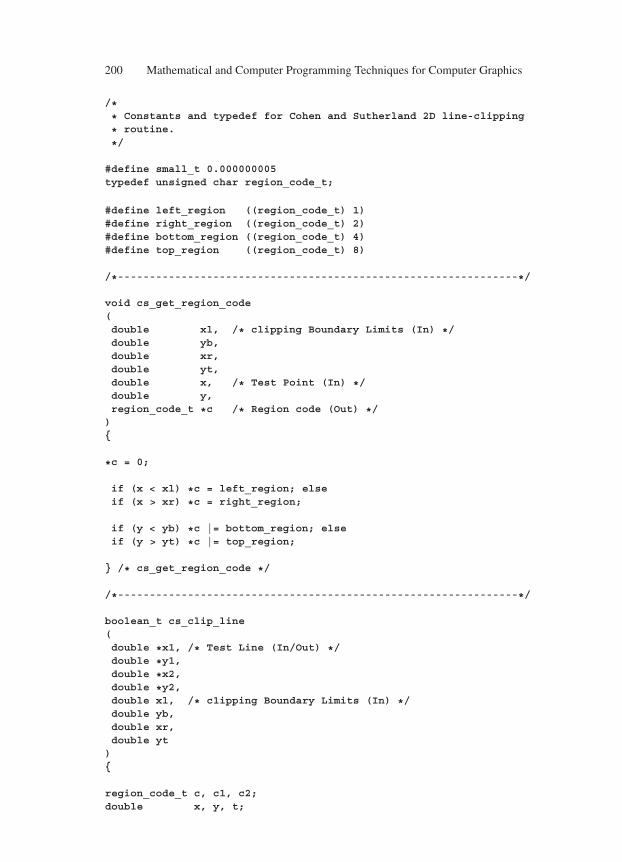
200 Mathematical and Computer Programming Techniques for Computer Graphics
/** Constants and typedef for Cohen and Sutherland 2D line-clipping
* routine.
*/
#define small_t 0.000000005typedef unsigned char region_code_t;
#define left_region ((region_code_t) 1)#define right_region ((region_code_t) 2)#define bottom_region ((region_code_t) 4)#define top_region ((region_code_t) 8)
/*---------------------------------------------------------------*/
void cs_get_region_code(double xl, /* clipping Boundary Limits (In) */double yb,double xr,double yt,double x, /* Test Point (In) */double y,region_code_t *c /* Region code (Out) */)
*c = 0;
if (x < xl) *c = left_region; elseif (x > xr) *c = right_region;
if (y < yb) *c |= bottom_region; elseif (y > yt) *c |= top_region;
/* cs_get_region_code */
/*---------------------------------------------------------------*/
boolean_t cs_clip_line(double *x1, /* Test Line (In/Out) */double *y1,double *x2,double *y2,double xl, /* c1ipping Boundary Limits (In) */double yb,double xr,double yt)
region_code_t c, c1, c2;double x, y, t;
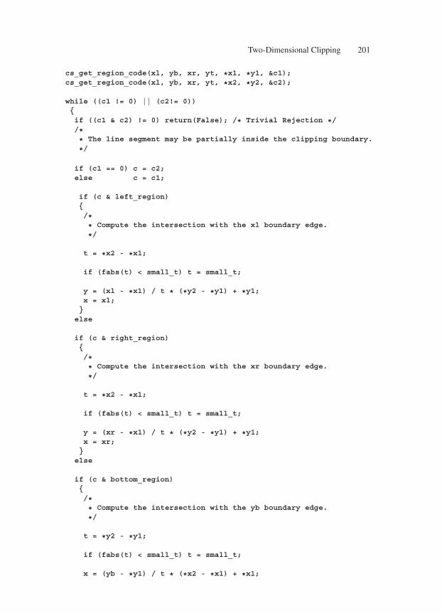
Two-Dimensional Clipping 201
cs_get_region_code(xl, yb, xr, yt, *x1, *y1, &c1);cs_get_region_code(xl, yb, xr, yt, *x2, *y2, &c2);
while ((c1 != 0) || (c2!= 0))if ((c1 & c2) != 0) return(False); /* Trivial Rejection *//** The line segment may be partially inside the c1ipping boundary.
*/
if (c1 == 0) c = c2;else c = c1;
if (c & left_region)/** Compute the intersection with the xl boundary edge.
*/
t = *x2 - *x1;
if (fabs(t) < small_t) t = small_t;
y = (xl - *x1) / t * (*y2 - *y1) + *y1;x = xl;
else
if (c & right_region)/** Compute the intersection with the xr boundary edge.
*/
t = *x2 - *x1;
if (fabs(t) < small_t) t = small_t;
y = (xr - *x1) / t * (*y2 - *y1) + *y1;x = xr;
else
if (c & bottom_region)/** Compute the intersection with the yb boundary edge.
*/
t = *y2 - *y1;
if (fabs(t) < small_t) t = small_t;
x = (yb - *y1) / t * (*x2 - *x1) + *x1;
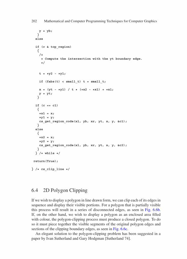
202 Mathematical and Computer Programming Techniques for Computer Graphics
y = yb;else
if (c & top_region)/** Compute the intersection with the yt boundary edge.
*/
t = *y2 - *y1;
if (fabs(t) < small_t) t = small_t;
x = (yt - *y1) / t * (*x2 - *x1) + *x1;y = yt;
if (c == c1)
*x1 = x;
*y1 = y;cs_get_region_code(xl, yb, xr, yt, x, y, &c1);
else
*x2 = x;
*y2 = y;cs_get_region_code(xl, yb, xr, yt, x, y, &c2);
/* while */
return(True);
/* cs_clip_line */
6.4 2D Polygon Clipping
If we wish to display a polygon in line drawn form, we can clip each of its edges insequence and display their visible portions. For a polygon that is partially visiblethis process will result in a series of disconnected edges, as seen in Fig. 6.6b.If, on the other hand, we wish to display a polygon as an enclosed area filledwith colour, the polygon-clipping process must produce a closed polygon. To doso it must piece together the visible segments of the original polygon edges andsections of the clipping boundary edges, as seen in Fig. 6.6c.
An elegant solution to the polygon-clipping problem has been suggested in apaper by Ivan Sutherland and Gary Hodgman [Sutherland 74].
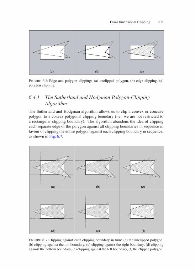
Two-Dimensional Clipping 203
(a) (b) (c)
FIGURE 6.6 Edge and polygon clipping: (a) unclipped polygon, (b) edge clipping, (c)polygon clipping.
6.4.1 The Sutherland and Hodgman Polygon-ClippingAlgorithm
The Sutherland and Hodgman algorithm allows us to clip a convex or concavepolygon to a convex polygonal clipping boundary (i.e. we are not restricted toa rectangular clipping boundary). The algorithm abandons the idea of clippingeach separate edge of the polygon against all clipping boundaries in sequence infavour of clipping the entire polygon against each clipping boundary in sequence,as shown in Fig. 6.7.
(a) (b) (c)
(d) (e) (f)
FIGURE 6.7 Clipping against each clipping boundary in turn: (a) the unclipped polygon,(b) clipping against the top boundary, (c) clipping against the right boundary, (d) clippingagainst the bottom boundary, (e) clipping against the left boundary, (f) the clipped polygon.
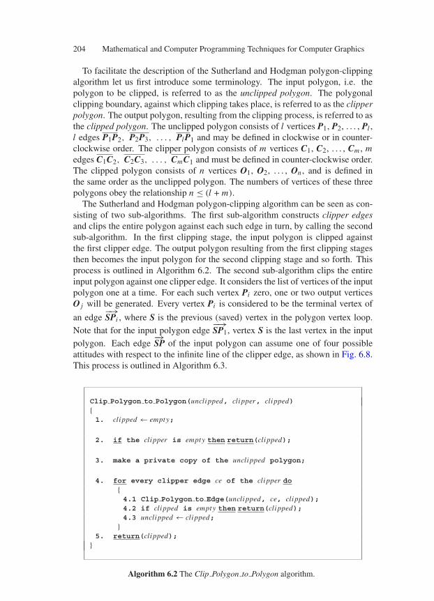
204 Mathematical and Computer Programming Techniques for Computer Graphics
To facilitate the description of the Sutherland and Hodgman polygon-clippingalgorithm let us first introduce some terminology. The input polygon, i.e. thepolygon to be clipped, is referred to as the unclipped polygon. The polygonalclipping boundary, against which clipping takes place, is referred to as the clipperpolygon. The output polygon, resulting from the clipping process, is referred to asthe clipped polygon. The unclipped polygon consists of l vertices P1, P2, . . . , Pl ,l edges P1P2, P2P3, . . . , PlP1 and may be defined in clockwise or in counter-clockwise order. The clipper polygon consists of m vertices C1, C2, . . . , Cm , medges C1C2, C2C3, . . . , CmC1 and must be defined in counter-clockwise order.The clipped polygon consists of n vertices O1, O2, . . . , On , and is defined inthe same order as the unclipped polygon. The numbers of vertices of these threepolygons obey the relationship n ≤ (l + m).
The Sutherland and Hodgman polygon-clipping algorithm can be seen as con-sisting of two sub-algorithms. The first sub-algorithm constructs clipper edgesand clips the entire polygon against each such edge in turn, by calling the secondsub-algorithm. In the first clipping stage, the input polygon is clipped againstthe first clipper edge. The output polygon resulting from the first clipping stagesthen becomes the input polygon for the second clipping stage and so forth. Thisprocess is outlined in Algorithm 6.2. The second sub-algorithm clips the entireinput polygon against one clipper edge. It considers the list of vertices of the inputpolygon one at a time. For each such vertex Pi zero, one or two output verticesO j will be generated. Every vertex Pi is considered to be the terminal vertex of
an edge−→SPi , where S is the previous (saved) vertex in the polygon vertex loop.
Note that for the input polygon edge−→SP1, vertex S is the last vertex in the input
polygon. Each edge−→SP of the input polygon can assume one of four possible
attitudes with respect to the infinite line of the clipper edge, as shown in Fig. 6.8.This process is outlined in Algorithm 6.3.
Clip Polygon to Polygon(unclipped, clipper, clipped)1. clipped ← empty;
2. if the clipper is empty then return(clipped);
3. make a private copy of the unclipped polygon;
4. for every clipper edge ce of the clipper do4.1 Clip Polygon to Edge(unclipped, ce, clipped);4.2 if clipped is empty then return(clipped);4.3 unclipped ← clipped;
5. return(clipped);
Algorithm 6.2 The Clip Polygon to Polygon algorithm.
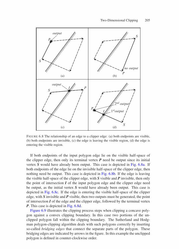
Two-Dimensional Clipping 205
(a) (b)
(c) (d)
output
no output
P
S
S
P
S
outputI P
PI
S
2nd output
1stoutput
FIGURE 6.8 The relationship of an edge to a clipper edge: (a) both endpoints are visible,(b) both endpoints are invisible, (c) the edge is leaving the visible region, (d) the edge isentering the visible region.
If both endpoints of the input polygon edge lie on the visible half-space ofthe clipper edge, then only its terminal vertex P need be output since its initialvertex S would have already been output. This case is depicted in Fig. 6.8a. Ifboth endpoints of the edge lie on the invisible half-space of the clipper edge, thennothing need be output. This case is depicted in Fig. 6.8b. If the edge is leavingthe visible half-space of the clipper edge, with S visible and P invisible, then onlythe point of intersection I of the input polygon edge and the clipper edge needbe output, as the initial vertex S would have already been output. This case isdepicted in Fig. 6.8c. If the edge is entering the visible half-space of the clipperedge, with S invisible and P visible, then two outputs must be generated, the pointof intersection I of the edge and the clipper edge, followed by the terminal vertexP. This case is depicted in Fig. 6.8d.
Figure 6.9 illustrates the clipping process steps when clipping a concave poly-gon against a convex clipping boundary. In this case two portions of the un-clipped polygon fall within the clipping boundary. The Sutherland and Hodg-man polygon-clipping algorithm deals with such polygons correctly by insertingso-called bridging edges that connect the separate parts of the polygon. Thesebridging edges are indicated by arrows in the figure. In this example the unclippedpolygon is defined in counter-clockwise order.
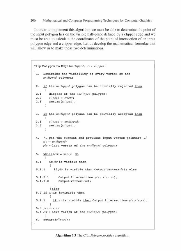
206 Mathematical and Computer Programming Techniques for Computer Graphics
In order to implement this algorithm we must be able to determine if a point ofthe input polygon lies on the visible half-plane defined by a clipper edge and wemust be able to calculate the coordinates of the point of intersection of an inputpolygon edge and a clipper edge. Let us develop the mathematical formulae thatwill allow us to make those two determinations.
Clip Polygon to Edge(unclipped, ce, clipped)1. Determine the visibility of every vertex of the
unclipped polygon;
2. if the unclipped polygon can be trivially rejected then
2.1 dispose of the unclipped polygon;2.2 clipped ← empty;2.3 return(clipped);
3. if the unclipped polygon can be trivially accepted then
3.1 clipped ← unclipped;3.2 return(clipped);
4. /* get the current and previous input vertex pointers */civ ← unclipped;piv ←last vertex of the unclipped polygon;
5. while(civ = empty) do
5.1 if civ is visible then
5.1.1 if piv is visible then Output Vertex(civ); else
5.1.2.1 Output Intersection(piv, civ, ce);5.1.2.2 Output Vertex(civ);
else
5.2 if civis invisible then
5.2.1 if piv is visible then Output Intersection(piv,civ,ce);
5.3 piv ← civ;5.4 civ ←next vertex of the unclipped polygon;
6. return(clipped);
Algorithm 6.3 The Clip Polygon to Edge algorithm.
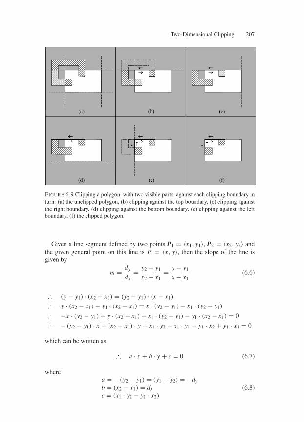
Two-Dimensional Clipping 207
(a) (b) (c)
(d) (e) (f)
FIGURE 6.9 Clipping a polygon, with two visible parts, against each clipping boundary inturn: (a) the unclipped polygon, (b) clipping against the top boundary, (c) clipping againstthe right boundary, (d) clipping against the bottom boundary, (e) clipping against the leftboundary, (f) the clipped polygon.
Given a line segment defined by two points P1 = 〈x1, y1〉, P2 = 〈x2, y2〉 andthe given general point on this line is P = 〈x, y〉, then the slope of the line isgiven by
m = dy
dx= y2 − y1
x2 − x1= y − y1
x − x1(6.6)
∴ (y − y1) · (x2 − x1) = (y2 − y1) · (x − x1)
∴ y · (x2 − x1) − y1 · (x2 − x1) = x · (y2 − y1) − x1 · (y2 − y1)
∴ −x · (y2 − y1) + y · (x2 − x1) + x1 · (y2 − y1) − y1 · (x2 − x1) = 0
∴ − (y2 − y1) · x + (x2 − x1) · y + x1 · y2 − x1 · y1 − y1 · x2 + y1 · x1 = 0
which can be written as
∴ a · x + b · y + c = 0 (6.7)
wherea = − (y2 − y1) = (y1 − y2) = −dy
b = (x2 − x1) = dx
c = (x1 · y2 − y1 · x2)
(6.8)
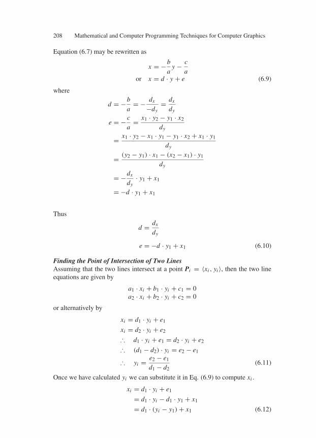
208 Mathematical and Computer Programming Techniques for Computer Graphics
Equation (6.7) may be rewritten as
x = −b
ay − c
aor x = d · y + e (6.9)
where
d = −b
a= − dx
−dy= dx
dy
e = − c
a= x1 · y2 − y1 · x2
dy
= x1 · y2 − x1 · y1 − y1 · x2 + x1 · y1
dy
= (y2 − y1) · x1 − (x2 − x1) · y1
dy
= −dx
dy· y1 + x1
= −d · y1 + x1
Thus
d = dx
dy
e = −d · y1 + x1 (6.10)
Finding the Point of Intersection of Two LinesAssuming that the two lines intersect at a point Pi = 〈xi , yi 〉, then the two lineequations are given by
a1 · xi + b1 · yi + c1 = 0a2 · xi + b2 · yi + c2 = 0
or alternatively by
xi = d1 · yi + e1
xi = d2 · yi + e2
∴ d1 · yi + e1 = d2 · yi + e2
∴ (d1 − d2) · yi = e2 − e1
∴ yi = e2 − e1
d1 − d2(6.11)
Once we have calculated yi we can substitute it in Eq. (6.9) to compute xi .
xi = d1 · yi + e1
= d1 · yi − d1 · y1 + x1
= d1 · (yi − y1) + x1 (6.12)
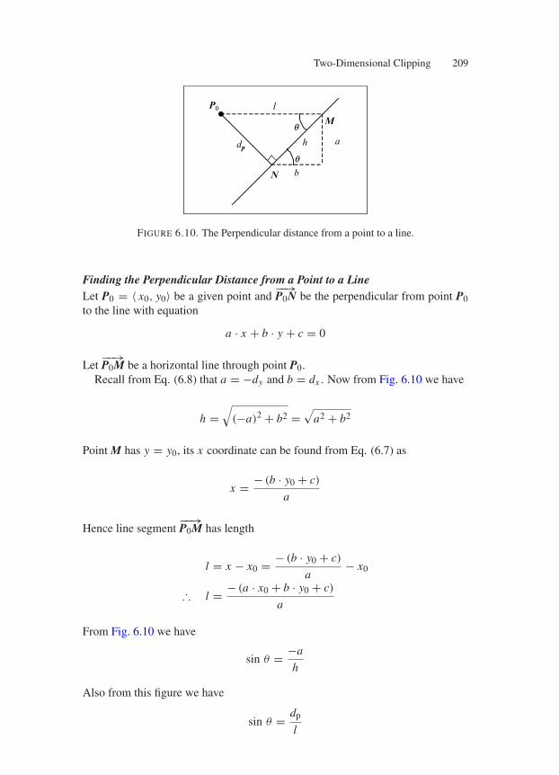
Two-Dimensional Clipping 209
P0
M
N
a
q
qb
h
l
dp
FIGURE 6.10. The Perpendicular distance from a point to a line.
Finding the Perpendicular Distance from a Point to a LineLet P0 = 〈 x0, y0〉 be a given point and
−−→P0N be the perpendicular from point P0
to the line with equation
a · x + b · y + c = 0
Let−−→P0M be a horizontal line through point P0.
Recall from Eq. (6.8) that a = −dy and b = dx . Now from Fig. 6.10 we have
h =√
(−a)2 + b2 =√
a2 + b2
Point M has y = y0, its x coordinate can be found from Eq. (6.7) as
x = − (b · y0 + c)
a
Hence line segment−−→P0M has length
l = x − x0 = − (b · y0 + c)
a− x0
∴ l = − (a · x0 + b · y0 + c)
a
From Fig. 6.10 we have
sin θ = −a
h
Also from this figure we have
sin θ = dp
l
210 Mathematical and Computer Programming Techniques for Computer Graphics
Thus the perpendicular distance dp of the point P0 from the line is given by
dp = l · sin θ
= − (a · x0 + b · y0 + c)
a· −a
h
= a · x0 + b · y0 + c
h
∴ dp = a · x0 + b · y0 + c√a2 + b2
(6.13)
The sign of this expression is sometimes positive and sometimes negative, asthe line divides the plane in two half-planes.
If the line segment−−→NM is directed and forms part of a counter-clockwise polyg-
onal outline, then dp is positive when the point P0 lies inside the polygon andnegative when P0 lies outside the polygon. Observe that the denominator of thefraction in Eq. (6.13) will always be positive. Thus, if we are only interested inthe sign of dp we can simplify this expression to
sign(dp
) = sign (a · x0 + b · y0 + c) (6.14)
The following C functions implement the Sutherland and Hodgman polygon-clipping algorithm.
/** Common constants and typedefs.
*/
#include <stdio.h>#include <math.h>
#define small_t 0.000000005
typedef unsigned char boolean_t;
#define False (boolean_t) 0#define True (boolean_t) 1
/** Constants and typedefs for the Sutherland and Hodgman
* polygon-clipping routine.
*/
typedef struct poly_vtx_t *poly_vtx_ptr_t;
typedef struct poly_vtx_tdouble x, y; /* Point coordinates */poly_vtx_ptr_t next_vtx; /* Next vertex pointer */boolean_t inside; /* Inside clipper indicator */ poly_vtx_t;
Two-Dimensional Clipping 211
typedef struct clipper_edge_tdouble x1, y1; /* Clipper Edge 1st Endpoint Coordinates */double x2, y2; /* Clipper Edge 2nd Endpoint Coordinates */double a, b, c; /* Clipper Edge Line Equation Coefficients */ clipper_edge_t;
/*---------------------------------------------------------------*/
void sh_output_vertex(poly_vtx_ptr_t civp, /* Current Input Clip Vertex Pointer */poly_vtx_ptr_t *fovp, /* First Output Clip Vertex Pointer */poly_vtx_ptr_t *covp /* Current Output Clip Vertex Pointer */)/** Output the current input vertex.
*/
poly_vtx_ptr_t nvp;
nvp = (poly_vtx_ptr_t) malloc(sizeof(poly_vtx_t));
/** Copy the structure.
*/
*nvp = *civp;
nvp->next_vtx = NULL;
if (*fovp == NULL) *fovp = nvp;else (*covp)->next_vtx = nvp;
*covp = nvp;
/* sh_output_vertex */
/*---------------------------------------------------------------*/
void sh_output_intersection(poly_vtx_ptr_t civp, /* Current Input Clip Vtx ptr */poly_vtx_ptr_t pivp, /* Previous Input Clip Vtx ptr */poly_vtx_ptr_t *fovp, /* First Output Clip Vtx ptr */poly_vtx_ptr_t *covp, /* Current Output Clip Vtx ptr */clipper_edge_t ce /* Clipper Edge Data */
)poly_vtx_ptr_t nvp;double t,
ux1, uy1,ux2, uy2,
212 Mathematical and Computer Programming Techniques for Computer Graphics
ua, ub,d1, d2,xi, yi;
/** Compute and output the point of intersection of the current
* unclipped polygon edge with the current clipper edge.
*/
/** Create a new vertex.
*/
nvp = (poly_vtx_ptr_t) malloc(sizeof(poly_vtx_t));
if (*fovp == NULL) *fovp = nvp;else (*covp)->next_vtx = nvp;
*covp = nvp;
/** Compute the intersection of the unclipped edge with the
* clipper edge.
*/
ux1 = pivp->x;uy1 = pivp->y;
ux2 = civp->x;uy2 = civp->y;
ua = uy1 - uy2;ub = ux2 - ux1;
if (fabs(ua) < small_t)/** Unclipped edge is vertical.
*/
t = ce.y2 - ce.y1;
if (fabs(t) < small_t) t = small_t;
xi = (uy1 - ce.y1) / t * ce.b + ce.x1;yi = uy1;
else
if (fabs (ce.a) < small_t)/** Clipper edge is horizontal.
*/
Two-Dimensional Clipping 213
t = uy2 - uy1;
if (fabs(t) < small_t) t = small_t;
xi = (ce.y1 - uy1) / t * ub + ux1;yi = ce.y1;else/** General case.
*/
d1 = ub / -ua;d2 = ce.b / -ce.a;
/** From: d1 * yi + e1 = d2 * yi + e2
** we get: yi = (e2 - e1) / (d1 - d2)
** where: e1 = (ux1 - uy1 * d1) and e2 = (ce.x1 - ce.y1 * d2).
*/
yi = (ce.x1 - ce.y1 * d2 - ux1 + uy1 * d1) / (d1 - d2);
/** From: (xi - ux1) / (yi - uy1) = d1
** we get: xi = (yi - uy1) * d1 + ux1.
*/
xi = (yi - uy1) * d1 + ux1;
(*covp)->x = xi;(*covp)->y = yi;(*covp)->next_vtx = NULL;
/* sh_output_intersection */
/*---------------------------------------------------------------*/
void sh_clip_polygon_to_edge(poly_vtx_ptr_t ivp, /* Input Polygon (In) */poly_vtx_ptr_t *ovp, /* Output Polygon (Out) */clipper_edge_t ce /* Clipper Edge Data (In) */)poly_vtx_ptr_t civp; /* Current Input Clip Vertex Pointer */poly_vtx_ptr_t pivp; /* Previous Input Clip Vertex Pointer */poly_vtx_ptr_t livp; /* Last Input Clip Vertex Pointer */
214 Mathematical and Computer Programming Techniques for Computer Graphics
poly_vtx_ptr_t fovp; /* First Output Clip Vertex Pointer */poly_vtx_ptr_t covp; /* Current Output Clip Vertex Pointer */boolean_t all_inside,
all_outside;double d;
/** Determine the visibility of each vertex of the input polygon
* relative to the current clipping boundary.
** Determine if the input polygon can be trivially accepted or
* rejected.
** Also find the last vertex of the input polygon and use it as the
* start vertex.
*/
all_inside = True;all_outside = True;
pivp = NULL;civp = ivp;
while (civp != NULL)pivp = civp;
/** Compute the signed distance of the point from the clipper edge.
** The signed distance of a point <x, y> from the line with
* equation:
** a*x+b*y+c=O
** is given by:
** d = (a * x + b * y + c) / sqrt(aˆ2 + bˆ2).
** In this case we only need the sign of d, so we only need to
* compute numerator of the above fraction.
*/
d = ce.a * civp->x + ce.b * civp->y + ce.c;
/** Do the inside test.
*/
civp->inside = (d >= 0);all_inside = (all_inside & civp->inside);
/** Do the outside test.

Two-Dimensional Clipping 215
*/
all_outside = (all_outside & (d <= 0));civp = civp->next_vtx;
/** Save the pointer to the last vertex in the input polygon.
*/
livp = pivp;
if (all_inside)/** Trivially accepted.
*/
*ovp = ivp;return;
if (all_outside)/** Trivially rejected.
*/
*ovp = NULL;
/** Dispose of the input polygon.
*/
while (ivp != NULL)civp = ivp;ivp = ivp->next_vtx;free(civp);
return;
/** Must process further.
*/
fovp = NULL;covp = NULL;civp = ivp;
while (civp != NULL)
216 Mathematical and Computer Programming Techniques for Computer Graphics
/** For every vertex in the input polygon.
*/
if (civp->inside)/** Current input vertex is inside.
*/
if (pivp->inside)/** Previous input vertex is inside.
*/
sh_output_vertex(civp, &fovp, &covp);else/** Previous Input Vertex is Outside.
*/
sh_output_intersection(civp, pivp, &fovp, &covp, ce);sh_output_vertex(civp, &fovp, &covp);
else/** Current input vertex is outside.
*/
if (pivp->inside)/** Previous input vertex is inside.
*/
sh_output_intersection(civp, pivp, &fovp, &covp, ce);
pivp = civp;civp = civp->next_vtx;
*ovp = fovp;
/** Dispose of the input polygon.
Two-Dimensional Clipping 217
*/
while (ivp != NULL)civp = ivp;ivp = ivp->next_vtx;free(civp);
/* sh_clip_polygon_to_edge */
/*---------------------------------------------------------------*/
poly_vtx_ptr_t sh_copy_polygon(poly_vtx_ptr_t ivp)poly_vtx_ptr_t fvp, nvp, lvp;
fvp = NULL;nvp = NULL;
while (ivp != NULL)lvp = nvp;
nvp = (poly_vtx_ptr_t) malloc(sizeof(poly_vtx_t));
if (fvp == NULL) fvp = nvp;
nvp->x = ivp->x;nvp->y = ivp->y;nvp->next_vtx = NULL;
if (lvp != NULL) lvp->next_vtx = nvp;
ivp = ivp->next_vtx;
return(fvp);
/* sh_copy_polygon */
/*---------------------------------------------------------------*/
void sh_clip_polygon_to_polygon(poly_vtx_ptr_t unclipped, /* Input Poly (In) */poly_vtx_ptr_t clipper, /* Clipper Poly (In) */poly_vtx_ptr_t *clipped /* Output Poly (Out) */)/** This is an implementation of the Sutherland and Hodgman
* polygon-clipping algorithm. This version clips the unclipped
* polygon to the clipping boundary specified by the

218 Mathematical and Computer Programming Techniques for Computer Graphics
* clipper polygon.
** The unclipped polygon pointer points to a linked list of polygon
* vertices provided by the caller.
** The clipped polygon pointer points to a linked list of polygon
* vertices returned by this function. If the clipped polygon is
* empty a NULL pointer is returned.
** The clipper polygon pointer points to a linked list of polygon
* vertices provided by the caller. The clipper must be specified
* in counter-clockwise order and must be a convex polygon.
** This function works with empty input polygons as well!
*/
poly_vtx_ptr_t fcvp; /* First Clipper Vertex Pointer */poly_vtx_ptr_t ccvp; /* Current Clipper Vertex Pointer */poly_vtx_ptr_t ncvp; /* Next Clipper Vertex Pointer */clipper_edge_t ce; /* Clipper Edge Data */double dx, dy;
/** First check if the clipper is empty.
*/
*clipped = NULL;
if (!clipper) return;
/** Make a private copy of the unclipped polygon. This is required
* as this function disposes of the unclipped polygon and the
* caller might not like this!
*/
unclipped = sh_copy_polygon(unclipped);
/** Clip the unclipped polygon against all the clipper edges.
*/
fcvp = NULL;ccvp = clipper;
while (ccvp != fcvp)if (!fcvp) fcvp = ccvp;
ncvp = ccvp->next_vtx;
if (!ncvp) ncvp = fcvp;
/** Compute the line equation of the clipper edge.
Two-Dimensional Clipping 219
*/
ce.x1 = ccvp->x;ce.y1 = ccvp->y;ce.x2 = ncvp->x;ce.y2 = ncvp->y;
dx = ce.x2 - ce.x1;dy = ce.y2 - ce.y1;
ce.a = -dy;ce.b = dx;ce.c = ce.x1 * dy - ce.y1 * dx;
sh_clip_polygon_to_edge(unclipped, clipped, ce);
if (!(*clipped)) return;
unclipped = *clipped;
ccvp = ncvp;
/* sh_clip_polygon_to_polygon */
6.4.2 The Weiler and Atherton Polygon-Clipping Algorithm
The Sutherland–Hodgman algorithm allows us to clip a convex or concave poly-gon to a convex clipping boundary. If we wish to clip a to a convex or concaveclipping boundary we have to use the Weiler–Atherton algorithm [Weiler 77].This is a generalised-polygon clipper that is capable of clipping a concave poly-gon with holes to the borders of a concave polygon with holes.
The polygon to be clipped is called the subject polygon and clipping is per-formed to the borders of the clip polygon.
The algorithm represents a polygon as a set of contours. These contours can beoutline contours or hole contours. Each contour is represented as a circular listof vertices. Unlike the Sutherland–Hodgman algorithm, the vertices of an outlinecontour are linked in a clockwise order and those of a hole contour are linkedin counter-clockwise order. Using this order, as one follows along the chain ofvertices of the polygon, the interior of the polygon is always to the right of theborder (see Fig. 6.11).
The clipping process may fragment the subject polygon in more than one visi-ble polygons (see Fig. 6.12).
The clipping process has the following steps:1. The borders of the two polygons are compared for intersections. At each in-
tersection a new false vertex is added into the contour chain of each of thetwo intersecting polygons and it is marked as an intersection vertex. A linkis established between each pair of intersection vertices, thus allowing us toswitch ( jump) between the two polygons whenever they intersect.
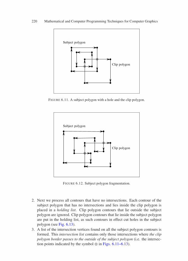
220 Mathematical and Computer Programming Techniques for Computer Graphics
Subject polygon
Clip polygon
⊗
⊗
FIGURE 6.11. A subject polygon with a hole and the clip polygon.
Subject polygon
Clip polygon
⊗
⊗
FIGURE 6.12. Subject polygon fragmentation.
2. Next we process all contours that have no intersections. Each contour of thesubject polygon that has no intersections and lies inside the clip polygon isplaced in a holding list. Clip polygon contours that lie outside the subjectpolygon are ignored. Clip polygon contours that lie inside the subject polygonare put in the holding list, as such contours in effect cut holes in the subjectpolygon (see Fig. 6.13).
3. A list of the intersection vertices found on all the subject polygon contours isformed. This intersection list contains only those intersections where the clippolygon border passes to the outside of the subject polygon (i.e. the intersec-tion points indicated by the symbol ⊗ in Figs. 6.11–6.13).
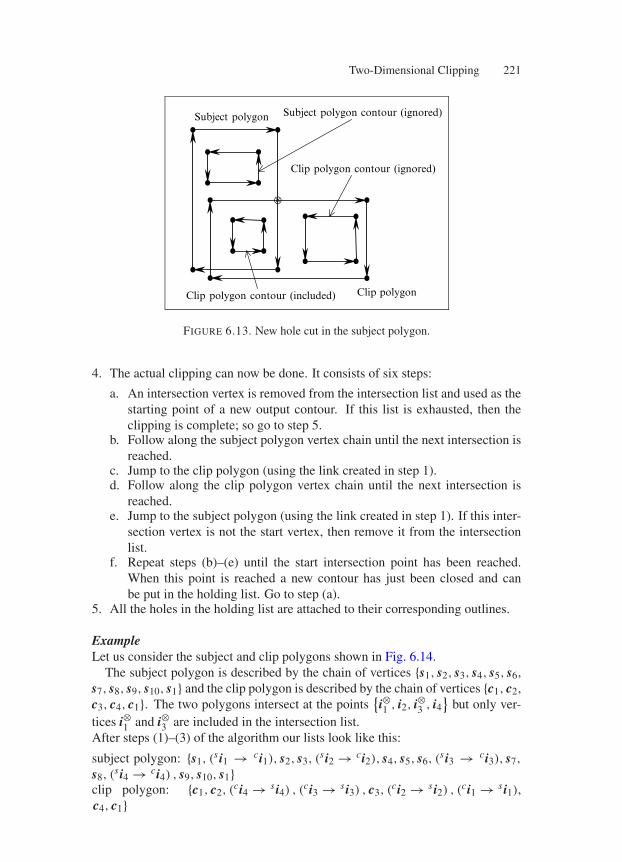
Two-Dimensional Clipping 221
Subject polygon
Clip polygon
Subject polygon contour (ignored)
Clip polygon contour (ignored)
Clip polygon contour (included)
⊗
FIGURE 6.13. New hole cut in the subject polygon.
4. The actual clipping can now be done. It consists of six steps:
a. An intersection vertex is removed from the intersection list and used as thestarting point of a new output contour. If this list is exhausted, then theclipping is complete; so go to step 5.
b. Follow along the subject polygon vertex chain until the next intersection isreached.
c. Jump to the clip polygon (using the link created in step 1).d. Follow along the clip polygon vertex chain until the next intersection is
reached.e. Jump to the subject polygon (using the link created in step 1). If this inter-
section vertex is not the start vertex, then remove it from the intersectionlist.
f. Repeat steps (b)–(e) until the start intersection point has been reached.When this point is reached a new contour has just been closed and canbe put in the holding list. Go to step (a).
5. All the holes in the holding list are attached to their corresponding outlines.
ExampleLet us consider the subject and clip polygons shown in Fig. 6.14.
The subject polygon is described by the chain of vertices s1, s2, s3, s4, s5, s6,s7, s8, s9, s10, s1 and the clip polygon is described by the chain of vertices c1, c2,c3, c4, c1. The two polygons intersect at the points
i⊗1 , i2, i⊗3 , i4
but only ver-
tices i⊗1 and i⊗3 are included in the intersection list.After steps (1)–(3) of the algorithm our lists look like this:
subject polygon: s1, (s i1 → ci1), s2, s3, (
s i2 → ci2), s4, s5, s6, (s i3 → ci3), s7,
s8, (s i4 → ci4) , s9, s10, s1
clip polygon: c1, c2, (ci4 → s i4) , (ci3 → s i3) , c3, (
ci2 → s i2) , (ci1 → s i1),c4, c1
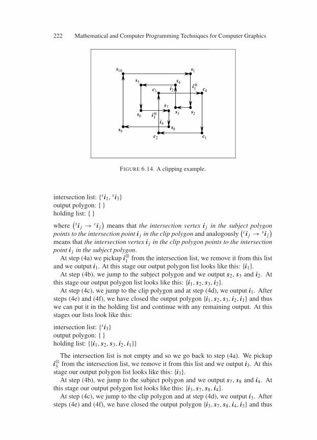
222 Mathematical and Computer Programming Techniques for Computer Graphics
s1
s2s3
s4s5
s6
s7
s8s9
s10
c1c2
c3 c4i2
i⊗3
i⊗1
i4
FIGURE 6.14. A clipping example.
intersection list: s i1, s i3output polygon: holding list: where
(s i j → ci j
)means that the intersection vertex i j in the subject polygon
points to the intersection point i j in the clip polygon and analogously(
ci j → s i j)
means that the intersection vertex i j in the clip polygon points to the intersectionpoint i j in the subject polygon.
At step (4a) we pickup i⊗1 from the intersection list, we remove it from this listand we output i1. At this stage our output polygon list looks like this: i1.
At step (4b), we jump to the subject polygon and we output s2, s3 and i2. Atthis stage our output polygon list looks like this: i1, s2, s3, i2.
At step (4c), we jump to the clip polygon and at step (4d), we output i1. Aftersteps (4e) and (4f), we have closed the output polygon i1, s2, s3, i2, i1 and thuswe can put it in the holding list and continue with any remaining output. At thisstages our lists look like this:
intersection list: s i3output polygon: holding list: i1, s2, s3, i2, i1
The intersection list is not empty and so we go back to step (4a). We pickupi⊗3 from the intersection list, we remove it from this list and we output i3. At thisstage our output polygon list looks like this: i3.
At step (4b), we jump to the subject polygon and we output s7, s8 and i4. Atthis stage our output polygon list looks like this: i3, s7, s8, i4.
At step (4c), we jump to the clip polygon and at step (4d), we output i3. Aftersteps (4e) and (4f), we have closed the output polygon i3, s7, s8, i4, i3 and thus
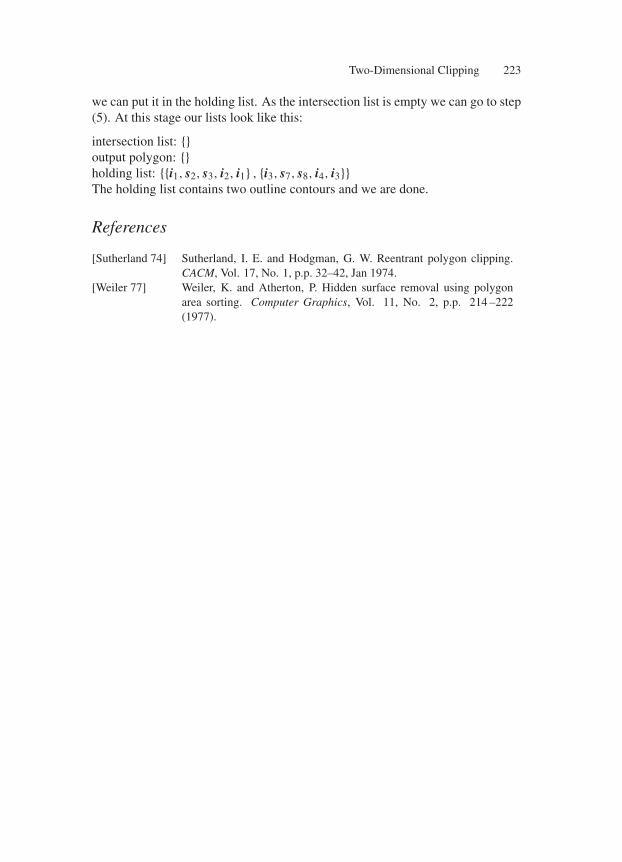
Two-Dimensional Clipping 223
we can put it in the holding list. As the intersection list is empty we can go to step(5). At this stage our lists look like this:
intersection list: output polygon: holding list: i1, s2, s3, i2, i1 , i3, s7, s8, i4, i3The holding list contains two outline contours and we are done.
References
[Sutherland 74] Sutherland, I. E. and Hodgman, G. W. Reentrant polygon clipping.CACM, Vol. 17, No. 1, p.p. 32–42, Jan 1974.
[Weiler 77] Weiler, K. and Atherton, P. Hidden surface removal using polygonarea sorting. Computer Graphics, Vol. 11, No. 2, p.p. 214 –222(1977).
“Comninos” — 2005/8/31 — 15:57 — page 225 — #1
7
Three-Dimensional Transformations
7.1 Introduction
Geometric transformations play an important part in the visualisation of three-dimensional scenes. The ability to rotate, translate and scale an object is fun-damental to the understanding of its shape. This can easily be demonstrated bypicking up a relatively complex and unfamiliar object. In an effort to understandits shape one rotates the object and looks at it from close or at arms length. In thegeneration of different views of a given scene with the computer, transformationsare used to achieve the effect of different viewing positions and directions.
The techniques we shall develop in this chapter for expressing 3D transforma-tions will be an extension of the 2D techniques that we have developed in thechapter concerning 2D transformations.
Two important points to remember are
1. A transformation can be represented by a transformation matrix.2. Complex transformations can be expressed as a sequence of primitive trans-
formations and can be concatenated to yield a single transformation matrix,which has the same effect as the sequence of the primitive transformations.
Three-dimensional transformations can be represented by a 4 × 4 matrix and3D points can be represented in homogeneous form by a four-element row orcolumn vector. As with 2D transformations there are two distinct and equivalentnotations that can be used to represent the transformation of a 3D point. The firstnotation is
P ′ = P · T
where P and P′ are the original and the transformed points, expressed in homoge-neous form, and T is the square matrix representing the transformation. For a 3Dtransformation in this notation we would write
[x ′, y′, z′, 1
] = [x, y, z, 1] ·
⎡
⎢⎢⎣
r1,1 r1,2 r1,3 0r2,1 r2,2 r2,3 0r3,1 r3,2 r3,3 0tx ty tz 1
⎤
⎥⎥⎦
225
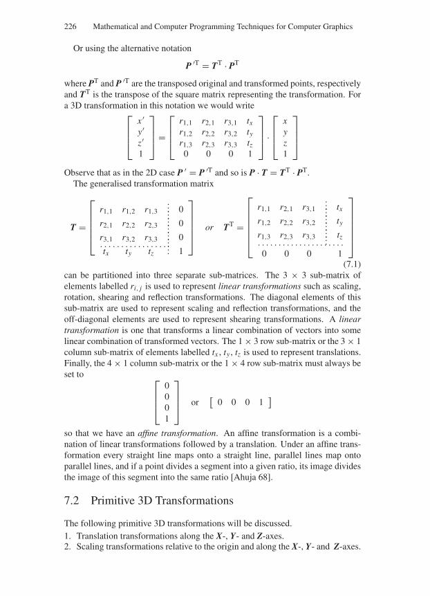
“Comninos” — 2005/8/31 — 15:57 — page 226 — #2
226 Mathematical and Computer Programming Techniques for Computer Graphics
Or using the alternative notation
P ′T = TT · PT
where PT and P ′T are the transposed original and transformed points, respectivelyand TT is the transpose of the square matrix representing the transformation. Fora 3D transformation in this notation we would write
⎡
⎢⎢⎣
x ′y′z′1
⎤
⎥⎥⎦ =
⎡
⎢⎢⎣
r1,1 r2,1 r3,1 txr1,2 r2,2 r3,2 ty
r1,3 r2,3 r3,3 tz0 0 0 1
⎤
⎥⎥⎦ ·
⎡
⎢⎢⎣
xyz1
⎤
⎥⎥⎦
Observe that as in the 2D case P ′ = P ′T and so is P · T = TT · PT.The generalised transformation matrix
T =
⎡
⎢⎢⎢⎢⎣
r1,1 r1,2 r1,3... 0...
r2,1 r2,2 r2,3... 0...
r3,1 r3,2 r3,3... 0
. . . . . . . . . . . . . . . ....
tx ty tz... 1
⎤
⎥⎥⎥⎥⎦
or TT =
⎡
⎢⎢⎢⎢⎢⎣
r1,1 r2,1 r3,1... tx...
r1,2 r2,2 r3,2... ty...
r1,3 r2,3 r3,3... tz.... . . . . . . . . . . . . . . . . . . . .
0 0 0 1
⎤
⎥⎥⎥⎥⎥⎦
(7.1)can be partitioned into three separate sub-matrices. The 3 × 3 sub-matrix ofelements labelled ri, j is used to represent linear transformations such as scaling,rotation, shearing and reflection transformations. The diagonal elements of thissub-matrix are used to represent scaling and reflection transformations, and theoff-diagonal elements are used to represent shearing transformations. A lineartransformation is one that transforms a linear combination of vectors into somelinear combination of transformed vectors. The 1 × 3 row sub-matrix or the 3 × 1column sub-matrix of elements labelled tx , ty , tz is used to represent translations.Finally, the 4 × 1 column sub-matrix or the 1 × 4 row sub-matrix must always beset to ⎡
⎢⎢⎣
0001
⎤
⎥⎥⎦ or
[0 0 0 1
]
so that we have an affine transformation. An affine transformation is a combi-nation of linear transformations followed by a translation. Under an affine trans-formation every straight line maps onto a straight line, parallel lines map ontoparallel lines, and if a point divides a segment into a given ratio, its image dividesthe image of this segment into the same ratio [Ahuja 68].
7.2 Primitive 3D Transformations
The following primitive 3D transformations will be discussed.1. Translation transformations along the X-, Y- and Z-axes.2. Scaling transformations relative to the origin and along the X-, Y- and Z-axes.
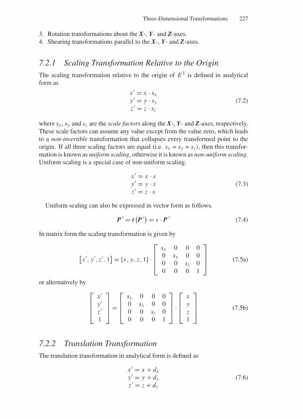
“Comninos” — 2005/8/31 — 15:57 — page 227 — #3
Three-Dimensional Transformations 227
3. Rotation transformations about the X-, Y- and Z-axes.4. Shearing transformations parallel to the X-, Y- and Z-axes.
7.2.1 Scaling Transformation Relative to the Origin
The scaling transformation relative to the origin of E3 is defined in analyticalform as
x ′ = x · sx
y′ = y · sy
z′ = z · sz
(7.2)
where sx , sy and sz are the scale factors along the X-, Y- and Z-axes, respectively.These scale factors can assume any value except from the value zero, which leadsto a non-invertible transformation that collapses every transformed point to theorigin. If all three scaling factors are equal (i.e. sx = sy = sz), then this transfor-mation is known as uniform scaling, otherwise it is known as non-uniform scaling.Uniform scaling is a special case of non-uniform scaling.
x ′ = x · sy′ = y · sz′ = z · s
(7.3)
Uniform scaling can also be expressed in vector form as follows.
P ′ = t(P ′) = s · P ′ (7.4)
In matrix form the scaling transformation is given by
[x ′, y′, z′, 1
] = [x, y, z, 1] ·
⎡
⎢⎢⎣
sx 0 0 00 sy 0 00 0 sz 00 0 0 1
⎤
⎥⎥⎦ (7.5a)
or alternatively by⎡
⎢⎢⎣
x ′y′z′1
⎤
⎥⎥⎦ =
⎡
⎢⎢⎣
sx 0 0 00 sy 0 00 0 sz 00 0 0 1
⎤
⎥⎥⎦ ·
⎡
⎢⎢⎣
xyz1
⎤
⎥⎥⎦ (7.5b)
7.2.2 Translation Transformation
The translation transformation in analytical form is defined as
x ′ = x + dx
y′ = y + dy
z′ = z + dz
(7.6)
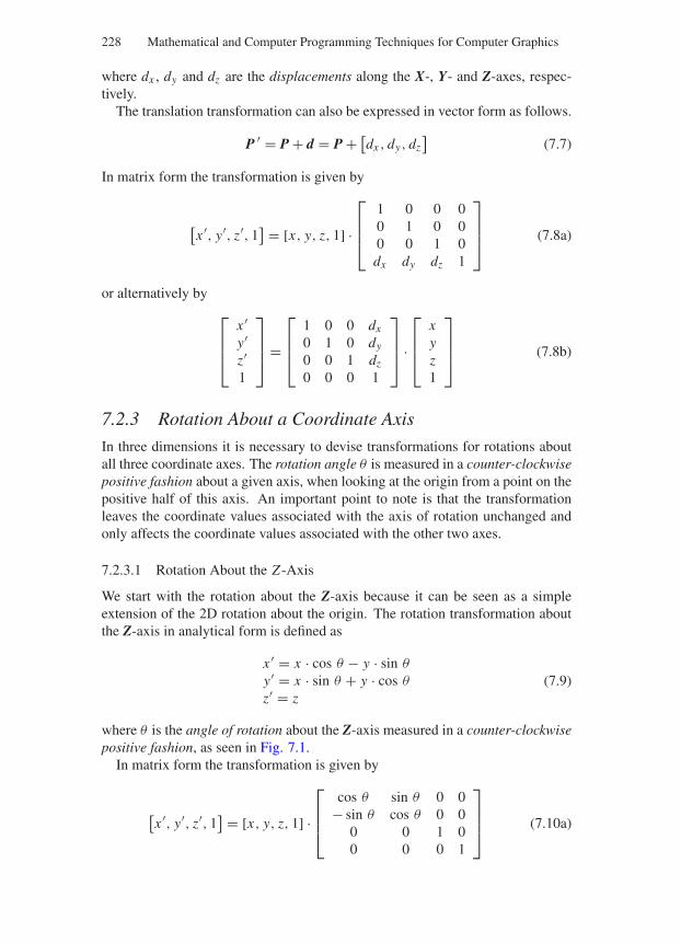
“Comninos” — 2005/8/31 — 15:57 — page 228 — #4
228 Mathematical and Computer Programming Techniques for Computer Graphics
where dx , dy and dz are the displacements along the X-, Y- and Z-axes, respec-tively.
The translation transformation can also be expressed in vector form as follows.
P ′ = P + d = P + [dx , dy, dz
](7.7)
In matrix form the transformation is given by
[x ′, y′, z′, 1
] = [x, y, z, 1] ·
⎡
⎢⎢⎣
1 0 0 00 1 0 00 0 1 0dx dy dz 1
⎤
⎥⎥⎦ (7.8a)
or alternatively by
⎡
⎢⎢⎣
x ′y′z′1
⎤
⎥⎥⎦ =
⎡
⎢⎢⎣
1 0 0 dx
0 1 0 dy
0 0 1 dz
0 0 0 1
⎤
⎥⎥⎦ ·
⎡
⎢⎢⎣
xyz1
⎤
⎥⎥⎦ (7.8b)
7.2.3 Rotation About a Coordinate Axis
In three dimensions it is necessary to devise transformations for rotations aboutall three coordinate axes. The rotation angle θ is measured in a counter-clockwisepositive fashion about a given axis, when looking at the origin from a point on thepositive half of this axis. An important point to note is that the transformationleaves the coordinate values associated with the axis of rotation unchanged andonly affects the coordinate values associated with the other two axes.
7.2.3.1 Rotation About the Z -Axis
We start with the rotation about the Z-axis because it can be seen as a simpleextension of the 2D rotation about the origin. The rotation transformation aboutthe Z-axis in analytical form is defined as
x ′ = x · cos θ − y · sin θ
y′ = x · sin θ + y · cos θ
z′ = z(7.9)
where θ is the angle of rotation about the Z-axis measured in a counter-clockwisepositive fashion, as seen in Fig. 7.1.
In matrix form the transformation is given by
[x ′, y′, z′, 1
] = [x, y, z, 1] ·
⎡
⎢⎢⎣
cos θ sin θ 0 0− sin θ cos θ 0 0
0 0 1 00 0 0 1
⎤
⎥⎥⎦ (7.10a)
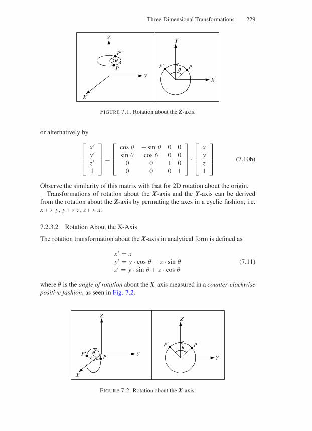
“Comninos” — 2005/8/31 — 15:57 — page 229 — #5
Three-Dimensional Transformations 229
P
q
q
P9
X
Y
Z
PP9
X
Y
FIGURE 7.1. Rotation about the Z-axis.
or alternatively by
⎡
⎢⎢⎣
x ′y′z′1
⎤
⎥⎥⎦ =
⎡
⎢⎢⎣
cos θ − sin θ 0 0sin θ cos θ 0 0
0 0 1 00 0 0 1
⎤
⎥⎥⎦ ·
⎡
⎢⎢⎣
xyz1
⎤
⎥⎥⎦ (7.10b)
Observe the similarity of this matrix with that for 2D rotation about the origin.Transformations of rotation about the X-axis and the Y-axis can be derived
from the rotation about the Z-axis by permuting the axes in a cyclic fashion, i.e.x → y, y → z, z → x .
7.2.3.2 Rotation About the X-Axis
The rotation transformation about the X-axis in analytical form is defined as
x ′ = xy′ = y · cos θ − z · sin θ
z′ = y · sin θ + z · cos θ
(7.11)
where θ is the angle of rotation about the X-axis measured in a counter-clockwisepositive fashion, as seen in Fig. 7.2.
PP9
X
Y
Z
PP9
Y
Z
FIGURE 7.2. Rotation about the X-axis.
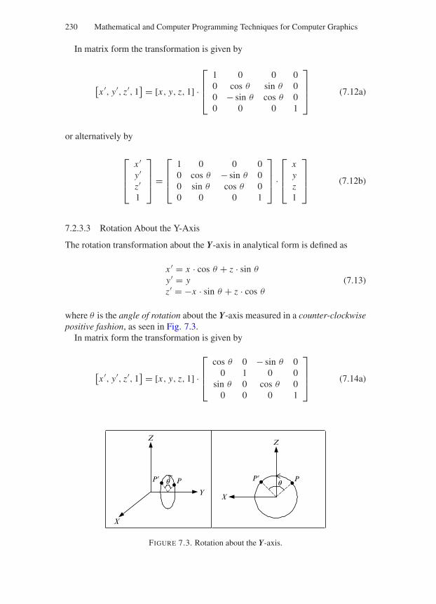
“Comninos” — 2005/8/31 — 15:57 — page 230 — #6
230 Mathematical and Computer Programming Techniques for Computer Graphics
In matrix form the transformation is given by
[x ′, y′, z′, 1
] = [x, y, z, 1] ·
⎡
⎢⎢⎣
1 0 0 00 cos θ sin θ 00 − sin θ cos θ 00 0 0 1
⎤
⎥⎥⎦ (7.12a)
or alternatively by
⎡
⎢⎢⎣
x ′y′z′1
⎤
⎥⎥⎦ =
⎡
⎢⎢⎣
1 0 0 00 cos θ − sin θ 00 sin θ cos θ 00 0 0 1
⎤
⎥⎥⎦ ·
⎡
⎢⎢⎣
xyz1
⎤
⎥⎥⎦ (7.12b)
7.2.3.3 Rotation About the Y-Axis
The rotation transformation about the Y-axis in analytical form is defined as
x ′ = x · cos θ + z · sin θ
y′ = yz′ = −x · sin θ + z · cos θ
(7.13)
where θ is the angle of rotation about the Y-axis measured in a counter-clockwisepositive fashion, as seen in Fig. 7.3.
In matrix form the transformation is given by
[x ′, y′, z′, 1
] = [x, y, z, 1] ·
⎡
⎢⎢⎣
cos θ 0 − sin θ 00 1 0 0
sin θ 0 cos θ 00 0 0 1
⎤
⎥⎥⎦ (7.14a)
PP
X
Y
Z
PP
X
Z
q q
FIGURE 7.3. Rotation about the Y-axis.
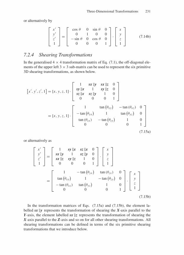
“Comninos” — 2005/8/31 — 15:57 — page 231 — #7
Three-Dimensional Transformations 231
or alternatively by
⎡
⎢⎢⎣
x ′y′z′1
⎤
⎥⎥⎦ =
⎡
⎢⎢⎣
cos θ 0 sin θ 00 1 0 0
− sin θ 0 cos θ 00 0 0 1
⎤
⎥⎥⎦ ·
⎡
⎢⎢⎣
xyz1
⎤
⎥⎥⎦ (7.14b)
7.2.4 Shearing Transformations
In the generalised 4 × 4 transformation matrix of Eq. (7.1), the off-diagonal ele-ments of the upper left 3 × 3 sub-matrix can be used to represent the six primitive3D shearing transformations, as shown below.
[x ′, y′, z′, 1
] = [x, y, z, 1] ·
⎡
⎢⎢⎣
1 sx ‖y sx ‖z 0sy ‖x 1 sy ‖z 0sz ‖x sz ‖y 1 0
0 0 0 1
⎤
⎥⎥⎦
= [x, y, z, 1] ·
⎡
⎢⎢⎢⎣
1 tan(θxy
) − tan (θxz) 0
− tan(θyx
)1 tan
(θyz
)0
tan (θzx ) − tan(θzy
)1 0
0 0 0 1
⎤
⎥⎥⎥⎦
(7.15a)
or alternatively as
⎡
⎢⎢⎣
x ′y′z′1
⎤
⎥⎥⎦ =
⎡
⎢⎢⎣
1 sy ‖x sz ‖x 0sx ‖y 1 sz ‖y 0sx ‖z sy ‖z 1 0
0 0 0 1
⎤
⎥⎥⎦ ·
⎡
⎢⎢⎣
xyz1
⎤
⎥⎥⎦
=
⎡
⎢⎢⎢⎣
1 − tan(θyx
)tan (θzx ) 0
tan(θxy
)1 − tan
(θzy
)0
− tan (θxz) tan(θyz
)1 0
0 0 0 1
⎤
⎥⎥⎥⎦
·
⎡
⎢⎢⎣
xyz1
⎤
⎥⎥⎦
(7.15b)
In the transformation matrices of Eqs. (7.15a) and (7.15b), the element la-belled sx ‖y represents the transformation of shearing the X-axis parallel to theY-axis, the element labelled sx ‖z represents the transformation of shearing theX-axis parallel to the Z-axis and so on for all other shearing transformations. Allshearing transformations can be defined in terms of the six primitive shearingtransformations that we introduce below.
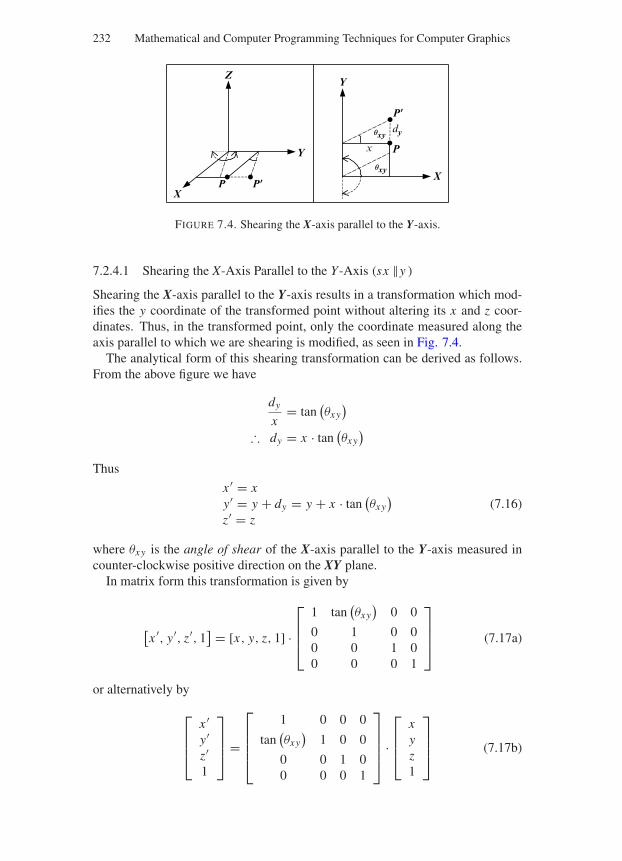
“Comninos” — 2005/8/31 — 15:57 — page 232 — #8
232 Mathematical and Computer Programming Techniques for Computer Graphics
P P9X
Y
Z
P
P9
Xqxy
Y
qxydy
x
FIGURE 7.4. Shearing the X-axis parallel to the Y-axis.
7.2.4.1 Shearing the X-Axis Parallel to the Y-Axis (sx ‖y )
Shearing the X-axis parallel to the Y-axis results in a transformation which mod-ifies the y coordinate of the transformed point without altering its x and z coor-dinates. Thus, in the transformed point, only the coordinate measured along theaxis parallel to which we are shearing is modified, as seen in Fig. 7.4.
The analytical form of this shearing transformation can be derived as follows.From the above figure we have
dy
x= tan
(θxy
)
∴ dy = x · tan(θxy
)
Thus
x ′ = xy′ = y + dy = y + x · tan
(θxy
)
z′ = z(7.16)
where θxy is the angle of shear of the X-axis parallel to the Y-axis measured incounter-clockwise positive direction on the XY plane.
In matrix form this transformation is given by
[x ′, y′, z′, 1
] = [x, y, z, 1] ·
⎡
⎢⎢⎣
1 tan(θxy
)0 0
0 1 0 00 0 1 00 0 0 1
⎤
⎥⎥⎦ (7.17a)
or alternatively by
⎡
⎢⎢⎣
x ′y′z′1
⎤
⎥⎥⎦ =
⎡
⎢⎢⎢⎣
1 0 0 0
tan(θxy
)1 0 0
0 0 1 00 0 0 1
⎤
⎥⎥⎥⎦
·
⎡
⎢⎢⎣
xyz1
⎤
⎥⎥⎦ (7.17b)
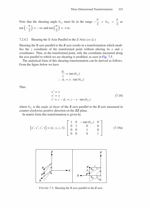
“Comninos” — 2005/8/31 — 15:57 — page 233 — #9
Three-Dimensional Transformations 233
Note that the shearing angle θxy must lie in the range −π
2< θxy <
π
2as
tan(−π
2
)= −∞ and tan
(π
2
)= +∞.
7.2.4.2 Shearing the X-Axis Parallel to the Z-Axis (sx ‖z )
Shearing the X-axis parallel to the Z-axis results in a transformation which modi-fies the z coordinate of the transformed point without altering its x and ycoordinates. Thus, in the transformed point, only the coordinate measured alongthe axis parallel to which we are shearing is modified, as seen in Fig. 7.5.
The analytical form of this shearing transformation can be derived as follows.From the figure below we have
dz
x= tan (θxz)
∴ dz = x · tan (θxz)
Thus
x ′ = xy′ = yz′ = z − dz = z − x · tan (θxz)
(7.18)
where θxz is the angle of shear of the X-axis parallel to the Z-axis measured incounter-clockwise positive direction on the XZ plane.
In matrix form this transformation is given by
[x ′, y′, z′, 1
] = [x, y, z, 1] ·
⎡
⎢⎢⎣
1 0 − tan (θxz) 00 1 0 00 0 1 00 0 0 1
⎤
⎥⎥⎦ (7.19a)
P
P9
X
Y
Z
P
P9X qxz
Z
qxzdz
x
FIGURE 7.5. Shearing the X-axis parallel to the Z-axis.
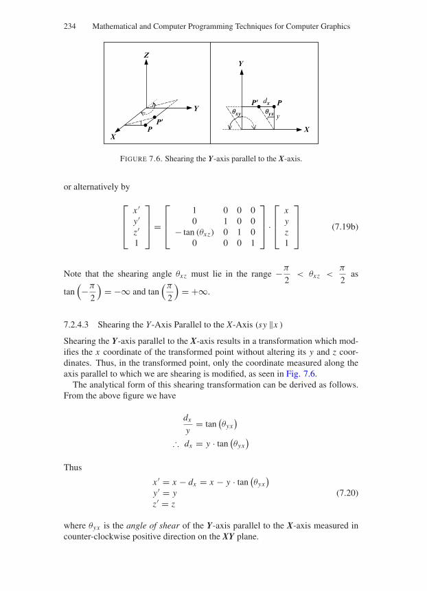
“Comninos” — 2005/8/31 — 15:57 — page 234 — #10
234 Mathematical and Computer Programming Techniques for Computer Graphics
PP9
X
Y
Z
PP9
X
Y
qyxqxy
dx
y
FIGURE 7.6. Shearing the Y-axis parallel to the X-axis.
or alternatively by
⎡
⎢⎢⎣
x ′y′z′1
⎤
⎥⎥⎦ =
⎡
⎢⎢⎣
1 0 0 00 1 0 0
− tan (θxz) 0 1 00 0 0 1
⎤
⎥⎥⎦ ·
⎡
⎢⎢⎣
xyz1
⎤
⎥⎥⎦ (7.19b)
Note that the shearing angle θxz must lie in the range −π
2< θxz <
π
2as
tan(−π
2
)= −∞ and tan
(π
2
)= +∞.
7.2.4.3 Shearing the Y-Axis Parallel to the X-Axis (sy ‖x )
Shearing the Y-axis parallel to the X-axis results in a transformation which mod-ifies the x coordinate of the transformed point without altering its y and z coor-dinates. Thus, in the transformed point, only the coordinate measured along theaxis parallel to which we are shearing is modified, as seen in Fig. 7.6.
The analytical form of this shearing transformation can be derived as follows.From the above figure we have
dx
y= tan
(θyx
)
∴ dx = y · tan(θyx
)
Thus
x ′ = x − dx = x − y · tan(θyx
)
y′ = yz′ = z
(7.20)
where θyx is the angle of shear of the Y-axis parallel to the X-axis measured incounter-clockwise positive direction on the XY plane.
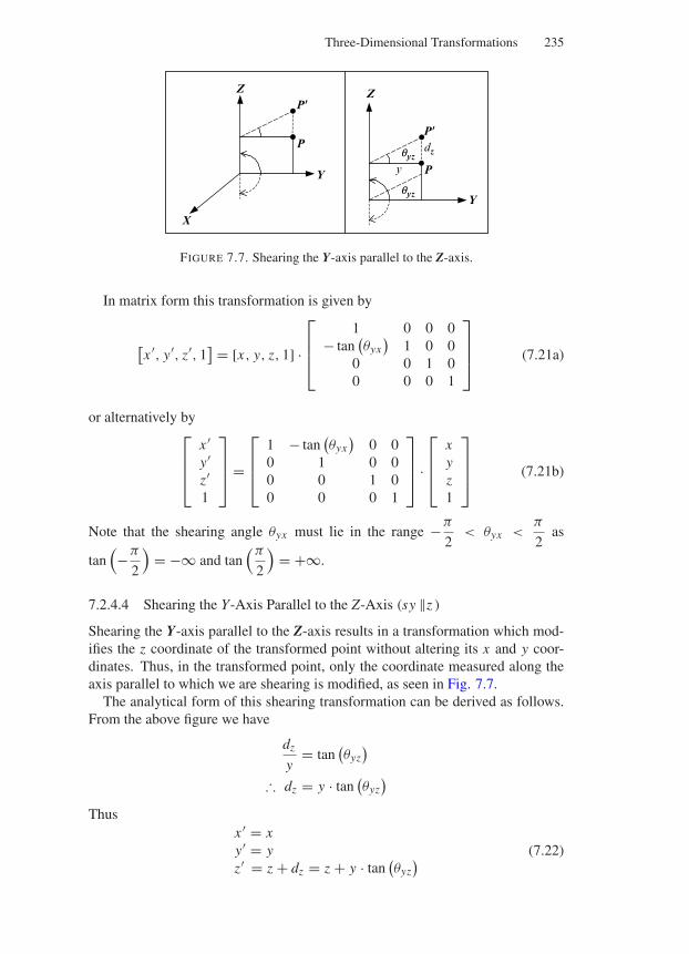
“Comninos” — 2005/8/31 — 15:57 — page 235 — #11
Three-Dimensional Transformations 235
P
P9
X
Y
Z
P
P9
Y
Z
dz
yqyz
qyz
FIGURE 7.7. Shearing the Y-axis parallel to the Z-axis.
In matrix form this transformation is given by
[x ′, y′, z′, 1
] = [x, y, z, 1] ·
⎡
⎢⎢⎣
1 0 0 0− tan
(θyx
)1 0 0
0 0 1 00 0 0 1
⎤
⎥⎥⎦ (7.21a)
or alternatively by⎡
⎢⎢⎣
x ′y′z′1
⎤
⎥⎥⎦ =
⎡
⎢⎢⎣
1 − tan(θyx
)0 0
0 1 0 00 0 1 00 0 0 1
⎤
⎥⎥⎦ ·
⎡
⎢⎢⎣
xyz1
⎤
⎥⎥⎦ (7.21b)
Note that the shearing angle θyx must lie in the range −π
2< θyx <
π
2as
tan(−π
2
)= −∞ and tan
(π
2
)= +∞.
7.2.4.4 Shearing the Y-Axis Parallel to the Z-Axis (sy ‖z )
Shearing the Y-axis parallel to the Z-axis results in a transformation which mod-ifies the z coordinate of the transformed point without altering its x and y coor-dinates. Thus, in the transformed point, only the coordinate measured along theaxis parallel to which we are shearing is modified, as seen in Fig. 7.7.
The analytical form of this shearing transformation can be derived as follows.From the above figure we have
dz
y= tan
(θyz
)
∴ dz = y · tan(θyz
)
Thusx ′ = xy′ = yz′ = z + dz = z + y · tan
(θyz
) (7.22)
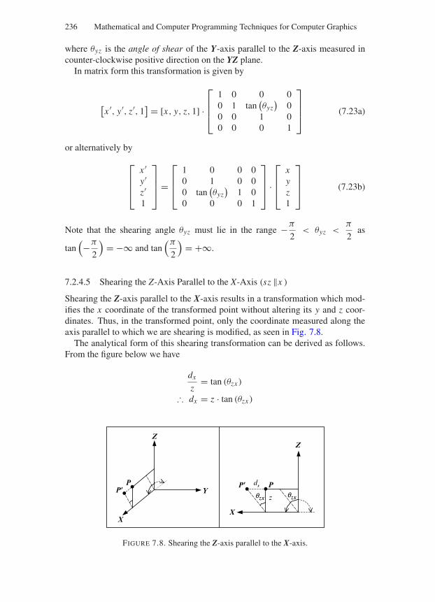
“Comninos” — 2005/8/31 — 15:57 — page 236 — #12
236 Mathematical and Computer Programming Techniques for Computer Graphics
where θyz is the angle of shear of the Y-axis parallel to the Z-axis measured incounter-clockwise positive direction on the YZ plane.
In matrix form this transformation is given by
[x ′, y′, z′, 1
] = [x, y, z, 1] ·
⎡
⎢⎢⎣
1 0 0 00 1 tan
(θyz
)0
0 0 1 00 0 0 1
⎤
⎥⎥⎦ (7.23a)
or alternatively by
⎡
⎢⎢⎣
x ′y′z′1
⎤
⎥⎥⎦ =
⎡
⎢⎢⎣
1 0 0 00 1 0 00 tan
(θyz
)1 0
0 0 0 1
⎤
⎥⎥⎦ ·
⎡
⎢⎢⎣
xyz1
⎤
⎥⎥⎦ (7.23b)
Note that the shearing angle θyz must lie in the range −π
2< θyz <
π
2as
tan(−π
2
)= −∞ and tan
(π
2
)= +∞.
7.2.4.5 Shearing the Z-Axis Parallel to the X-Axis (sz ‖x )
Shearing the Z-axis parallel to the X-axis results in a transformation which mod-ifies the x coordinate of the transformed point without altering its y and z coor-dinates. Thus, in the transformed point, only the coordinate measured along theaxis parallel to which we are shearing is modified, as seen in Fig. 7.8.
The analytical form of this shearing transformation can be derived as follows.From the figure below we have
dx
z= tan (θzx )
∴ dx = z · tan (θzx )
PP9
X
Y
Z
PP9
X
Z
dx
zqzx qzx
FIGURE 7.8. Shearing the Z-axis parallel to the X-axis.
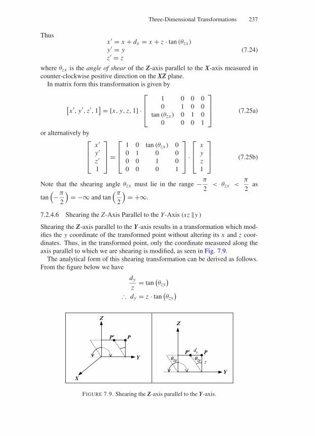
“Comninos” — 2005/8/31 — 15:57 — page 237 — #13
Three-Dimensional Transformations 237
Thusx ′ = x + dx = x + z · tan (θzx )
y′ = yz′ = z
(7.24)
where θzx is the angle of shear of the Z-axis parallel to the X-axis measured incounter-clockwise positive direction on the XZ plane.
In matrix form this transformation is given by
[x ′, y′, z′, 1
] = [x, y, z, 1] ·
⎡
⎢⎢⎣
1 0 0 00 1 0 0
tan (θzx ) 0 1 00 0 0 1
⎤
⎥⎥⎦ (7.25a)
or alternatively by⎡
⎢⎢⎣
x ′y′z′1
⎤
⎥⎥⎦ =
⎡
⎢⎢⎣
1 0 tan (θzx ) 00 1 0 00 0 1 00 0 0 1
⎤
⎥⎥⎦ ·
⎡
⎢⎢⎣
xyz1
⎤
⎥⎥⎦ (7.25b)
Note that the shearing angle θzx must lie in the range −π
2< θzx <
π
2as
tan(−π
2
)= −∞ and tan
(π
2
)= +∞.
7.2.4.6 Shearing the Z-Axis Parallel to the Y-Axis (sz ‖y )
Shearing the Z-axis parallel to the Y-axis results in a transformation which mod-ifies the y coordinate of the transformed point without altering its x and z coor-dinates. Thus, in the transformed point, only the coordinate measured along theaxis parallel to which we are shearing is modified, as seen in Fig. 7.9.
The analytical form of this shearing transformation can be derived as follows.From the figure below we have
dy
z= tan
(θzy
)
∴ dy = z · tan(θzy
)
PP9
X
Y
Z
PP9
Y
qzy qzy
Z
dy
z
FIGURE 7.9. Shearing the Z-axis parallel to the Y-axis.
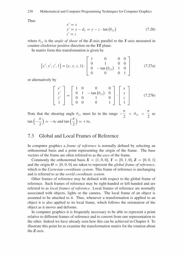
“Comninos” — 2005/8/31 — 15:57 — page 238 — #14
238 Mathematical and Computer Programming Techniques for Computer Graphics
Thusx ′ = xy′ = y − dy = y − z · tan
(θzy
)
z′ = z(7.26)
where θzy is the angle of shear of the Z-axis parallel to the Y-axis measured incounter-clockwise positive direction on the YZ plane.
In matrix form this transformation is given by
[x ′, y′, z′, 1
] = [x, y, z, 1] ·
⎡
⎢⎢⎣
1 0 0 00 1 0 00 − tan
(θzy
)1 0
0 0 0 1
⎤
⎥⎥⎦ (7.27a)
or alternatively by⎡
⎢⎢⎣
x ′y′z′1
⎤
⎥⎥⎦ =
⎡
⎢⎢⎣
1 0 0 00 1 − tan
(θzy
)0
0 0 1 00 0 0 1
⎤
⎥⎥⎦ ·
⎡
⎢⎢⎣
xyz1
⎤
⎥⎥⎦ (7.27b)
Note that the shearing angle θzy must lie in the range −π
2< θzy <
π
2as
tan(−π
2
)= −∞ and tan
(π
2
)= +∞.
7.3 Global and Local Frames of Reference
In computer graphics a frame of reference is normally defined by selecting anorthonormal basis and a point representing the origin of the frame. The basevectors of the frame are often referred to as the axes of the frame.
Commonly the orthonormal basis X = [1, 0, 0], Y = [0, 1, 0], Z = [0, 0, 1]and the origin O = [0, 0, 0] are taken to represent the global frame of reference,which is the Cartesian coordinate system. This frame of reference is unchangingand is referred to as the world coordinate system.
Other frames of reference may be defined with respect to the global frame ofreference. Such frames of reference may be right-handed or left-handed and arereferred to as local frames of reference. Local frames of reference are normallyassociated with objects, lights or the camera. The local frame of an object isassumed to be attached to it. Thus, whenever a transformation is applied to anobject it is also applied to its local frame, which follows the orientation of theobject as it moves and deforms.
In computer graphics it is frequently necessary to be able to represent a pointrelative to different frames of reference and to convert from one representation tothe other. Indeed we have already seen how this can be achieved in Chapter 4. Toillustrate this point let us examine the transformation matrix for the rotation aboutthe Z-axis.
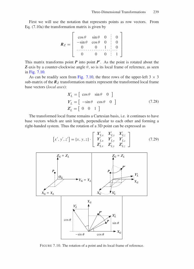
“Comninos” — 2005/8/31 — 15:57 — page 239 — #15
Three-Dimensional Transformations 239
First we will use the notation that represents points as row vectors. FromEq. (7.10a) the transformation matrix is given by
RZ =
⎡
⎢⎢⎢⎢⎣
cos θ sin θ 0... 0
−sin θ cos θ 0... 0
0 0 1... 0
. . . . . . . . . . . . . . . . . . . . . .
0 0 0... 1
⎤
⎥⎥⎥⎥⎦
This matrix transforms point P into point P′. As the point is rotated about theZ-axis by a counter-clockwise angle θ , so is its local frame of reference, as seenin Fig. 7.10.
As can be readily seen from Fig. 7.10, the three rows of the upper-left 3 × 3sub-matrix of the RZ transformation matrix represent the transformed local framebase vectors (local axes):
X′L = [
cos θ sin θ 0]
Y′L = [ −sin θ cos θ 0
]
Z′L = [
0 0 1]
(7.28)
The transformed local frame remains a Cartesian basis, i.e. it continues to havebase vectors which are unit length, perpendicular to each other and forming aright-handed system. Thus the rotation of a 3D point can be expressed as
[x ′, y′, z′] = [x, y, z] ·
⎡
⎣X′
Lx X′Ly X′
LzY′
Lx Y′Ly Y′
LzZ′
Lx Z′Ly Z′
Lz
⎤
⎦ (7.29)
P
ZG = ZL
YG = YL
XG = XL
ZG = ZL
OG
PP9
XG
YG
X9L
Y9L
P
P9
XG
YG
cos q
X9L
Y9L
sin q
−sin q
cos q
FIGURE 7.10. The rotation of a point and its local frame of reference.
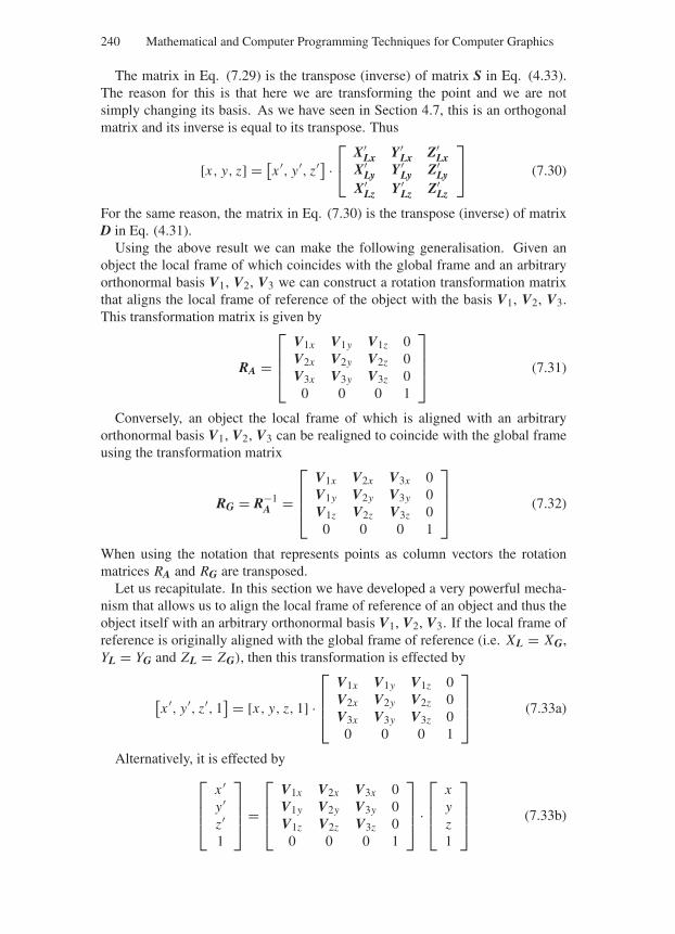
“Comninos” — 2005/8/31 — 15:57 — page 240 — #16
240 Mathematical and Computer Programming Techniques for Computer Graphics
The matrix in Eq. (7.29) is the transpose (inverse) of matrix S in Eq. (4.33).The reason for this is that here we are transforming the point and we are notsimply changing its basis. As we have seen in Section 4.7, this is an orthogonalmatrix and its inverse is equal to its transpose. Thus
[x, y, z] = [x ′, y′, z′] ·
⎡
⎣X′
Lx Y′Lx Z′
LxX′
Ly Y′Ly Z′
LyX′
Lz Y′Lz Z′
Lz
⎤
⎦ (7.30)
For the same reason, the matrix in Eq. (7.30) is the transpose (inverse) of matrixD in Eq. (4.31).
Using the above result we can make the following generalisation. Given anobject the local frame of which coincides with the global frame and an arbitraryorthonormal basis V1, V2, V3 we can construct a rotation transformation matrixthat aligns the local frame of reference of the object with the basis V1, V2, V3.This transformation matrix is given by
RA =
⎡
⎢⎢⎣
V1x V1y V1z 0V2x V2y V2z 0V3x V3y V3z 0
0 0 0 1
⎤
⎥⎥⎦ (7.31)
Conversely, an object the local frame of which is aligned with an arbitraryorthonormal basis V1, V2, V3 can be realigned to coincide with the global frameusing the transformation matrix
RG = R−1A =
⎡
⎢⎢⎣
V1x V2x V3x 0V1y V2y V3y 0V1z V2z V3z 00 0 0 1
⎤
⎥⎥⎦ (7.32)
When using the notation that represents points as column vectors the rotationmatrices RA and RG are transposed.
Let us recapitulate. In this section we have developed a very powerful mecha-nism that allows us to align the local frame of reference of an object and thus theobject itself with an arbitrary orthonormal basis V1, V2, V3. If the local frame ofreference is originally aligned with the global frame of reference (i.e. XL = XG,YL = YG and ZL = ZG), then this transformation is effected by
[x ′, y′, z′, 1
] = [x, y, z, 1] ·
⎡
⎢⎢⎣
V1x V1y V1z 0V2x V2y V2z 0V3x V3y V3z 0
0 0 0 1
⎤
⎥⎥⎦ (7.33a)
Alternatively, it is effected by⎡
⎢⎢⎣
x ′y′z′1
⎤
⎥⎥⎦ =
⎡
⎢⎢⎣
V1x V2x V3x 0V1y V2y V3y 0V1z V2z V3z 00 0 0 1
⎤
⎥⎥⎦ ·
⎡
⎢⎢⎣
xyz1
⎤
⎥⎥⎦ (7.33b)
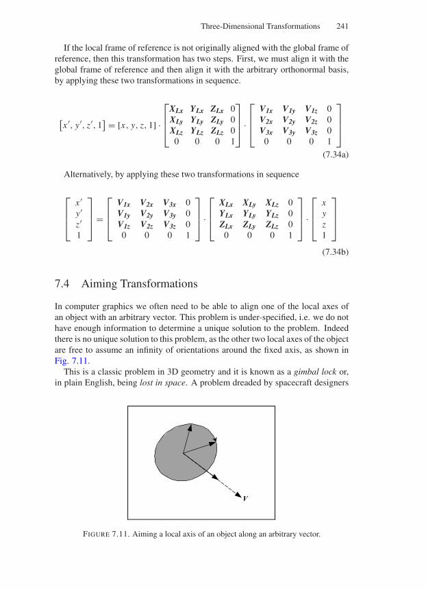
“Comninos” — 2005/8/31 — 15:57 — page 241 — #17
Three-Dimensional Transformations 241
If the local frame of reference is not originally aligned with the global frame ofreference, then this transformation has two steps. First, we must align it with theglobal frame of reference and then align it with the arbitrary orthonormal basis,by applying these two transformations in sequence.
[x ′, y′, z′, 1
] = [x, y, z, 1] ·
⎡
⎢⎢⎣
XLx YLx ZLx 0XLy YLy ZLy 0XLz YLz ZLz 0
0 0 0 1
⎤
⎥⎥⎦ ·
⎡
⎢⎢⎣
V1x V1y V1z 0V2x V2y V2z 0V3x V3y V3z 0
0 0 0 1
⎤
⎥⎥⎦
(7.34a)
Alternatively, by applying these two transformations in sequence
⎡
⎢⎢⎣
x ′y′z′1
⎤
⎥⎥⎦ =
⎡
⎢⎢⎣
V1x V2x V3x 0V1y V2y V3y 0V1z V2z V3z 00 0 0 1
⎤
⎥⎥⎦ ·
⎡
⎢⎢⎣
XLx XLy XLz 0YLx YLy YLz 0ZLx ZLy ZLz 0
0 0 0 1
⎤
⎥⎥⎦ ·
⎡
⎢⎢⎣
xyz1
⎤
⎥⎥⎦
(7.34b)
7.4 Aiming Transformations
In computer graphics we often need to be able to align one of the local axes ofan object with an arbitrary vector. This problem is under-specified, i.e. we do nothave enough information to determine a unique solution to the problem. Indeedthere is no unique solution to this problem, as the other two local axes of the objectare free to assume an infinity of orientations around the fixed axis, as shown inFig. 7.11.
This is a classic problem in 3D geometry and it is known as a gimbal lock or,in plain English, being lost in space. A problem dreaded by spacecraft designers
V
FIGURE 7.11. Aiming a local axis of an object along an arbitrary vector.
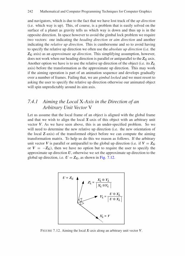
“Comninos” — 2005/8/31 — 15:57 — page 242 — #18
242 Mathematical and Computer Programming Techniques for Computer Graphics
and navigators, which is due to the fact that we have lost track of the up direction(i.e. which way is up). This, of course, is a problem that is easily solved on thesurface of a planet as gravity tells us which way is down and thus up is in theopposite direction. In space however to avoid the gimbal lock problem we requiretwo vectors: one indicating the heading direction or aim direction and anotherindicating the relative up direction. This is cumbersome and so to avoid havingto specify the relative up direction we often use the absolute up direction (i.e. theZG axis) as an approximate up direction. This simplifying assumption, however,does not work when our heading direction is parallel or antiparallel to the ZG axis.Another option we have is to use the relative up direction of the object (i.e. its ZLaxis) before the transformation as the approximate up direction. This may workif the aiming operation is part of an animation sequence and develops graduallyover a number of frames. Failing that, we are gimbal locked and we must resort toasking the user to specify the relative up direction otherwise our animated objectwill spin unpredictably around its aim axis.
7.4.1 Aiming the Local X-Axis in the Direction of anArbitrary Unit Vector V
Let us assume that the local frame of an object is aligned with the global frameand that we wish to align the local X-axis of this object with an arbitrary unitvector V. As we have seen above, this is an under-specified problem. So wewill need to determine the new relative up direction (i.e. the new orientation ofthe local Z-axis) of the transformed object before we can compute the aimingtransformation matrix. To help us do this we reason as follows. If the arbitraryunit vector V is parallel or antiparallel to the global up direction (i.e. if V = ZGor V = −ZG), then we have no option but to require the user to specify theapproximate up direction U, otherwise we set the approximate up direction to theglobal up direction, i.e. U = ZG, as shown in Fig. 7.12.
XL = V
U ⊗ XL
U ⊗ XLYL =
XL ⊗YL
XL ⊗ YLZL =
U = ZG
FIGURE 7.12. Aiming the local X-axis along an arbitrary unit vector V.
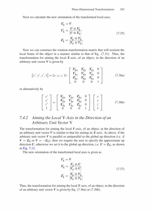
“Comninos” — 2005/8/31 — 15:57 — page 243 — #19
Three-Dimensional Transformations 243
Next we calculate the new orientation of the transformed local axes.
X′L = V
Y′L = U ⊗ X′
L∣∣∣U ⊗ X′L
∣∣∣
Z′L = X′
L ⊗ Y′L∣∣∣X′
L ⊗ Y′L
∣∣∣
(7.35)
Now we can construct the rotation transformation matrix that will reorient thelocal frame of the object in a manner similar to that of Eq. (7.31). Thus, thetransformation for aiming the local X-axis, of an object, in the direction of anarbitrary unit vector V is given by
[x ′, y′, z′, 1
] = [x, y, z, 1] ·
⎡
⎢⎢⎣
X′Lx X′
Ly X′Lz 0
Y′Lx Y′
Ly Y′Lz 0
Z′Lx Z′
Ly Z′Lz 0
0 0 0 1
⎤
⎥⎥⎦ (7.36a)
or alternatively by
⎡
⎢⎢⎣
x ′y′z′1
⎤
⎥⎥⎦ =
⎡
⎢⎢⎣
X′Lx Y′
Lx Z′Lx 0
X′Ly Y′
Ly Z′Ly 0
X′Lz Y′
Lz Z′Lz 0
0 0 0 1
⎤
⎥⎥⎦ ·
⎡
⎢⎢⎣
xyz1
⎤
⎥⎥⎦ (7.36b)
7.4.2 Aiming the Local Y-Axis in the Direction of anArbitrary Unit Vector V
The transformation for aiming the local Y-axis, of an object, in the direction ofan arbitrary unit vector V is similar to that for aiming its X-axis. As above, if thearbitrary unit vector V is parallel or antiparallel to the global up direction (i.e. ifV = ZG or V = −ZG), then we require the user to specify the approximate updirection U, otherwise we set it to the global up direction, i.e. U = ZG, as shownin Fig. 7.13.
The new orientation of the transformed local axes is given as
Y′L = V
X′L = Y′
L ⊗ U∣∣∣Y′L ⊗ U
∣∣∣
Z′L = X′
L ⊗ Y′L∣∣∣X′
L ⊗ Y′L
∣∣∣
(7.37)
Thus, the transformation for aiming the local Y-axis, of an object, in the directionof an arbitrary unit vector V is given by Eq. (7.36a) or (7.36b).
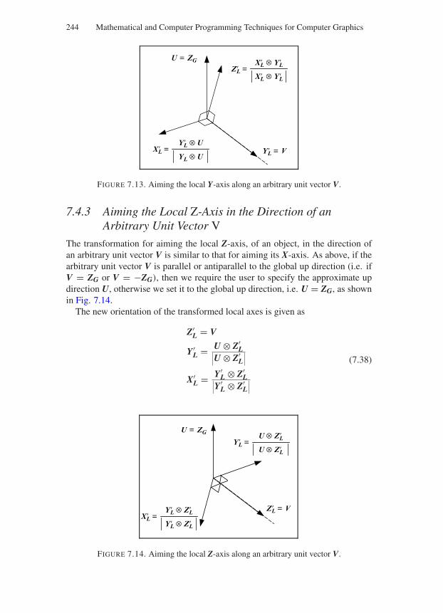
“Comninos” — 2005/8/31 — 15:57 — page 244 — #20
244 Mathematical and Computer Programming Techniques for Computer Graphics
YL = V
ZL =
U = ZG
XL ⊗ YL
XL ⊗ YL
XL =YL ⊗ U
YL ⊗ U
FIGURE 7.13. Aiming the local Y-axis along an arbitrary unit vector V.
7.4.3 Aiming the Local Z-Axis in the Direction of anArbitrary Unit Vector V
The transformation for aiming the local Z-axis, of an object, in the direction ofan arbitrary unit vector V is similar to that for aiming its X-axis. As above, if thearbitrary unit vector V is parallel or antiparallel to the global up direction (i.e. ifV = ZG or V = −ZG), then we require the user to specify the approximate updirection U, otherwise we set it to the global up direction, i.e. U = ZG, as shownin Fig. 7.14.
The new orientation of the transformed local axes is given as
Z′L = V
Y′L = U ⊗ Z′
L∣∣∣U ⊗ Z′L
∣∣∣
X′L = Y′
L ⊗ Z′L∣∣∣Y′
L ⊗ Z′L
∣∣∣
(7.38)
ZL = V
YL =
U = ZG
U ⊗ ZL
U ⊗ ZL
XL =YL ⊗ ZL
YL ⊗ ZL
FIGURE 7.14. Aiming the local Z-axis along an arbitrary unit vector V.
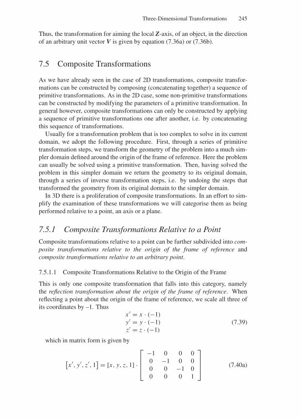
“Comninos” — 2005/8/31 — 15:57 — page 245 — #21
Three-Dimensional Transformations 245
Thus, the transformation for aiming the local Z-axis, of an object, in the directionof an arbitrary unit vector V is given by equation (7.36a) or (7.36b).
7.5 Composite Transformations
As we have already seen in the case of 2D transformations, composite transfor-mations can be constructed by composing (concatenating together) a sequence ofprimitive transformations. As in the 2D case, some non-primitive transformationscan be constructed by modifying the parameters of a primitive transformation. Ingeneral however, composite transformations can only be constructed by applyinga sequence of primitive transformations one after another, i.e. by concatenatingthis sequence of transformations.
Usually for a transformation problem that is too complex to solve in its currentdomain, we adopt the following procedure. First, through a series of primitivetransformation steps, we transform the geometry of the problem into a much sim-pler domain defined around the origin of the frame of reference. Here the problemcan usually be solved using a primitive transformation. Then, having solved theproblem in this simpler domain we return the geometry to its original domain,through a series of inverse transformation steps, i.e. by undoing the steps thattransformed the geometry from its original domain to the simpler domain.
In 3D there is a proliferation of composite transformations. In an effort to sim-plify the examination of these transformations we will categorise them as beingperformed relative to a point, an axis or a plane.
7.5.1 Composite Transformations Relative to a Point
Composite transformations relative to a point can be further subdivided into com-posite transformations relative to the origin of the frame of reference andcomposite transformations relative to an arbitrary point.
7.5.1.1 Composite Transformations Relative to the Origin of the Frame
This is only one composite transformation that falls into this category, namelythe reflection transformation about the origin of the frame of reference. Whenreflecting a point about the origin of the frame of reference, we scale all three ofits coordinates by –1. Thus
x ′ = x · (−1)
y′ = y · (−1)
z′ = z · (−1)
(7.39)
which in matrix form is given by
[x ′, y′, z′, 1
] = [x, y, z, 1] ·
⎡
⎢⎢⎣
−1 0 0 00 −1 0 00 0 −1 00 0 0 1
⎤
⎥⎥⎦ (7.40a)
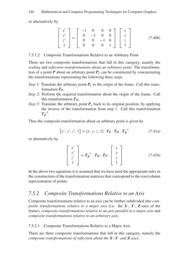
“Comninos” — 2005/8/31 — 15:57 — page 246 — #22
246 Mathematical and Computer Programming Techniques for Computer Graphics
or alternatively by
⎡
⎢⎢⎣
x ′y′z′1
⎤
⎥⎥⎦ =
⎡
⎢⎢⎣
−1 0 0 00 −1 0 00 0 −1 00 0 0 1
⎤
⎥⎥⎦ ·
⎡
⎢⎢⎣
xyz1
⎤
⎥⎥⎦ (7.40b)
7.5.1.2 Composite Transformations Relative to an Arbitrary Point
There are two composite transformations that fall in this category, namely thescaling and reflection transformations about an arbitrary point. The transforma-tion of a point P about an arbitrary point Pc can be constructed by concatenatingthe transformations representing the following three steps.
Step 1: Translate the arbitrary point Pc to the origin of the frame. Call this trans-formation TP.
Step 2: Perform the required transformation about the origin of the frame. Callthis transformation TO.
Step 3: Translate the arbitrary point Pc back to its original position, by applyingthe inverse of the transformation from step 1. Call this transformationT−1
P .
Thus the composite transformation about an arbitrary point is given by
[x ′, y′, z′, 1
] = [x, y, z, 1] · TP · TO · T−1P (7.41a)
or alternatively by
⎡
⎢⎢⎣
x ′y′z′1
⎤
⎥⎥⎦ = T−1
P · TO · TP ·
⎡
⎢⎢⎣
xyz1
⎤
⎥⎥⎦ (7.41b)
In the above two equations it is assumed that we have used the appropriate rules inthe construction of the transformation matrices that correspond to the row/columnrepresentation of points.
7.5.2 Composite Transformations Relative to an Axis
Composite transformations relative to an axis can be further subdivided into com-posite transformations relative to a major axis (i.e. the X-, Y-, Z-axes of theframe), composite transformations relative to an axis parallel to a major axis andcomposite transformations relative to an arbitrary axis.
7.5.2.1 Composite Transformations Relative to a Major Axis
There are three composite transformations that fall in this category, namely thecomposite transformations of reflection about the X-,Y- and Z-axes.
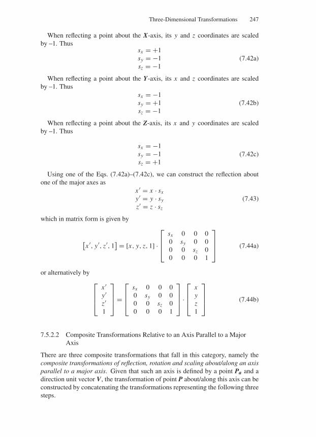
“Comninos” — 2005/8/31 — 15:57 — page 247 — #23
Three-Dimensional Transformations 247
When reflecting a point about the X-axis, its y and z coordinates are scaledby –1. Thus
sx = +1sy = −1sz = −1
(7.42a)
When reflecting a point about the Y-axis, its x and z coordinates are scaledby –1. Thus
sx = −1sy = +1sz = −1
(7.42b)
When reflecting a point about the Z-axis, its x and y coordinates are scaledby –1. Thus
sx = −1sy = −1sz = +1
(7.42c)
Using one of the Eqs. (7.42a)–(7.42c), we can construct the reflection aboutone of the major axes as
x ′ = x · sx
y′ = y · sy
z′ = z · sz
(7.43)
which in matrix form is given by
[x ′, y′, z′, 1
] = [x, y, z, 1] ·
⎡
⎢⎢⎣
sx 0 0 00 sy 0 00 0 sz 00 0 0 1
⎤
⎥⎥⎦ (7.44a)
or alternatively by
⎡
⎢⎢⎣
x ′y′z′1
⎤
⎥⎥⎦ =
⎡
⎢⎢⎣
sx 0 0 00 sy 0 00 0 sz 00 0 0 1
⎤
⎥⎥⎦ ·
⎡
⎢⎢⎣
xyz1
⎤
⎥⎥⎦ (7.44b)
7.5.2.2 Composite Transformations Relative to an Axis Parallel to a MajorAxis
There are three composite transformations that fall in this category, namely thecomposite transformations of reflection, rotation and scaling about/along an axisparallel to a major axis. Given that such an axis is defined by a point Pa and adirection unit vector V, the transformation of point P about/along this axis can beconstructed by concatenating the transformations representing the following threesteps.
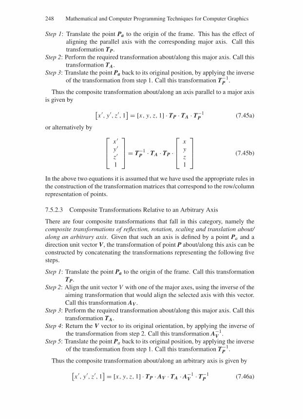
“Comninos” — 2005/8/31 — 15:57 — page 248 — #24
248 Mathematical and Computer Programming Techniques for Computer Graphics
Step 1: Translate the point Pa to the origin of the frame. This has the effect ofaligning the parallel axis with the corresponding major axis. Call thistransformation TP.
Step 2: Perform the required transformation about/along this major axis. Call thistransformation TA.
Step 3: Translate the point Pa back to its original position, by applying the inverseof the transformation from step 1. Call this transformation T−1
P .
Thus the composite transformation about/along an axis parallel to a major axisis given by
[x ′, y′, z′, 1
] = [x, y, z, 1] · TP · TA · T−1P (7.45a)
or alternatively by⎡
⎢⎢⎣
x ′y′z′1
⎤
⎥⎥⎦ = T−1
P · TA · TP ·
⎡
⎢⎢⎣
xyz1
⎤
⎥⎥⎦ (7.45b)
In the above two equations it is assumed that we have used the appropriate rules inthe construction of the transformation matrices that correspond to the row/columnrepresentation of points.
7.5.2.3 Composite Transformations Relative to an Arbitrary Axis
There are four composite transformations that fall in this category, namely thecomposite transformations of reflection, rotation, scaling and translation about/along an arbitrary axis. Given that such an axis is defined by a point Pa and adirection unit vector V, the transformation of point P about/along this axis can beconstructed by concatenating the transformations representing the following fivesteps.
Step 1: Translate the point Pa to the origin of the frame. Call this transformationTP.
Step 2: Align the unit vector V with one of the major axes, using the inverse of theaiming transformation that would align the selected axis with this vector.Call this transformation AV .
Step 3: Perform the required transformation about/along this major axis. Call thistransformation TA.
Step 4: Return the V vector to its original orientation, by applying the inverse ofthe transformation from step 2. Call this transformation A−1
V .Step 5: Translate the point Pa back to its original position, by applying the inverse
of the transformation from step 1. Call this transformation T−1P .
Thus the composite transformation about/along an arbitrary axis is given by
[x ′, y′, z′, 1
] = [x, y, z, 1] · TP · AV · TA · A−1V · T−1
P (7.46a)
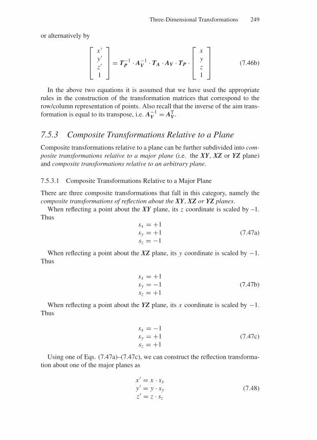
“Comninos” — 2005/8/31 — 15:57 — page 249 — #25
Three-Dimensional Transformations 249
or alternatively by
⎡
⎢⎢⎣
x ′y′z′1
⎤
⎥⎥⎦ = T−1
P · A−1V · TA · AV · TP ·
⎡
⎢⎢⎣
xyz1
⎤
⎥⎥⎦ (7.46b)
In the above two equations it is assumed that we have used the appropriaterules in the construction of the transformation matrices that correspond to therow/column representation of points. Also recall that the inverse of the aim trans-formation is equal to its transpose, i.e. A−1
V = ATV .
7.5.3 Composite Transformations Relative to a Plane
Composite transformations relative to a plane can be further subdivided into com-posite transformations relative to a major plane (i.e. the XY, XZ or YZ plane)and composite transformations relative to an arbitrary plane.
7.5.3.1 Composite Transformations Relative to a Major Plane
There are three composite transformations that fall in this category, namely thecomposite transformations of reflection about the XY, XZ or YZ planes.
When reflecting a point about the XY plane, its z coordinate is scaled by –1.Thus
sx = +1sy = +1sz = −1
(7.47a)
When reflecting a point about the XZ plane, its y coordinate is scaled by −1.Thus
sx = +1sy = −1sz = +1
(7.47b)
When reflecting a point about the YZ plane, its x coordinate is scaled by −1.Thus
sx = −1sy = +1sz = +1
(7.47c)
Using one of Eqs. (7.47a)–(7.47c), we can construct the reflection transforma-tion about one of the major planes as
x ′ = x · sx
y′ = y · sy
z′ = z · sz
(7.48)
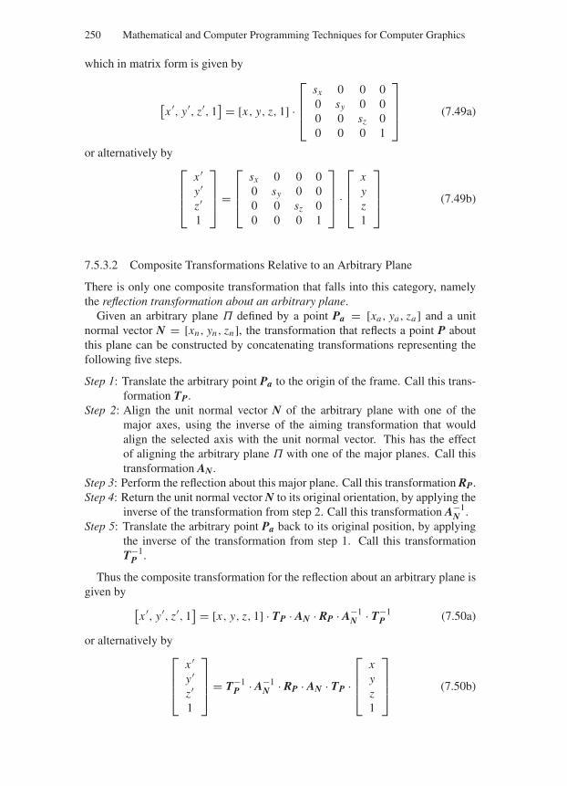
“Comninos” — 2005/8/31 — 15:57 — page 250 — #26
250 Mathematical and Computer Programming Techniques for Computer Graphics
which in matrix form is given by
[x ′, y′, z′, 1
] = [x, y, z, 1] ·
⎡
⎢⎢⎣
sx 0 0 00 sy 0 00 0 sz 00 0 0 1
⎤
⎥⎥⎦ (7.49a)
or alternatively by⎡
⎢⎢⎣
x ′y′z′1
⎤
⎥⎥⎦ =
⎡
⎢⎢⎣
sx 0 0 00 sy 0 00 0 sz 00 0 0 1
⎤
⎥⎥⎦ ·
⎡
⎢⎢⎣
xyz1
⎤
⎥⎥⎦ (7.49b)
7.5.3.2 Composite Transformations Relative to an Arbitrary Plane
There is only one composite transformation that falls into this category, namelythe reflection transformation about an arbitrary plane.
Given an arbitrary plane Π defined by a point Pa = [xa, ya, za] and a unitnormal vector N = [xn, yn, zn], the transformation that reflects a point P aboutthis plane can be constructed by concatenating transformations representing thefollowing five steps.
Step 1: Translate the arbitrary point Pa to the origin of the frame. Call this trans-formation TP.
Step 2: Align the unit normal vector N of the arbitrary plane with one of themajor axes, using the inverse of the aiming transformation that wouldalign the selected axis with the unit normal vector. This has the effectof aligning the arbitrary plane Π with one of the major planes. Call thistransformation AN.
Step 3: Perform the reflection about this major plane. Call this transformation RP.Step 4: Return the unit normal vector N to its original orientation, by applying the
inverse of the transformation from step 2. Call this transformation A−1N .
Step 5: Translate the arbitrary point Pa back to its original position, by applyingthe inverse of the transformation from step 1. Call this transformationT−1
P .
Thus the composite transformation for the reflection about an arbitrary plane isgiven by
[x ′, y′, z′, 1
] = [x, y, z, 1] · TP · AN · RP · A−1N · T−1
P (7.50a)
or alternatively by⎡
⎢⎢⎣
x ′y′z′1
⎤
⎥⎥⎦ = T−1
P · A−1N · RP · AN · TP ·
⎡
⎢⎢⎣
xyz1
⎤
⎥⎥⎦ (7.50b)
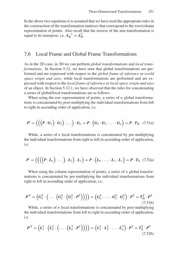
“Comninos” — 2005/8/31 — 15:57 — page 251 — #27
Three-Dimensional Transformations 251
In the above two equations it is assumed that we have used the appropriate rules inthe construction of the transformation matrices that correspond to the row/columnrepresentation of points. Also recall that the inverse of the aim transformation isequal to its transpose, i.e. A−1
N = ATN.
7.6 Local Frame and Global Frame Transformations
As in the 2D case, in 3D we can perform global transformations and local trans-formations. In Section 5.12, we have seen that global transformations are per-formed and are expressed with respect to the global frame of reference or worldspace origin and axes, while local transformations are performed and are ex-pressed with respect to the local frame of reference or local space origin and axesof an object. In Section 5.12.1, we have observed that the rules for concatenatinga series of global/local transformations are as follows.
When using the row representation of points, a series of n global transforma-tions is concatenated by post-multiplying the individual transformations from leftto right in ascending order of application, i.e.
P′ =(((
P · G1
)· G2
)· . . .
)· Gn = P ·
(G1 · G2 · . . . · Gn
)= P · TG (7.51a)
While, a series of n local transformations is concatenated by pre-multiplyingthe individual transformations from right to left in ascending order of application,i.e.
P′ =((((
P · Ln
)· . . .
)· L2
)· L1
)= P ·
(Ln · . . . · L2 · L1
)= P · TL (7.52a)
When using the column representation of points, a series of n global transfor-mations is concatenated by pre-multiplying the individual transformations fromright to left in ascending order of application, i.e.
P′T =(
GTn ·
(. . . ·
(GT
2 ·(
GT1 · PT
))))=
(GT
n · . . . · GT2 · GT
1
)· PT = TT
G · PT
(7.51b)While, a series of n local transformations is concatenated by post-multiplying
the individual transformations from left to right in ascending order of application,i.e.
P′T =(
LT1 ·
(LT
2 ·(. . . ·
(LT
n · PT))))
=(
LT1 · LT
2 · . . . · LTn
)· PT = TT
L · PT
(7.52b)

“Comninos” — 2005/8/31 — 15:57 — page 252 — #28
252 Mathematical and Computer Programming Techniques for Computer Graphics
7.7 Transformations of the Frame of Reference orCoordinate System
Analogously to the 2D case, which we have examined in Section 5.13, trans-forming a point P by a transformation matrix T relative to a frame of referenceF is equivalent to leaving the point P stationary while transforming the frame ofreference F by the inverse transformation matrix T−1.
References
[Ahuja 68] Ahuja, D. V. and Coons, S. A. Geometry for construction and display.IBM System Journal, vol. 3 & 4, p.p. 188–205 1968.
8
Viewing and Projection Transformations
In computer graphics we are often concerned with representing three-dimensionalscenes on a two-dimensional surface. In order to generate an image of a 3D objecton a 2D display, we must first project this object onto a projection plane and thendisplay this projected image.
A point of a 3D object is expressed in terms of the object-space coordinate sys-tem (sometimes referred to as the world-space coordinate system), the projectionof such a point onto the projection plane is expressed in terms of the projection-space coordinate system and the final image of this point on the display device isexpressed in terms of the screen-space coordinate system (sometimes referred toas the image-space coordinate system). The complete transformation of a pointfrom the object-space coordinate system to the screen-space system is achievedthrough the concatenation of three distinct transformations.
• The viewing transformation (or the object-space to eye-space coordinatetransformation) expresses the location of object-space points relative to theobserver’s eye, accounting for the observer’s position and direction of view.
• The projection transformation (or the eye-space to projection-space coordinatetransformation) expresses the location of eye-space points relative to the pro-jection plane, accounting for the effects of the type of projection used.
• The viewporting transformation (or the projection-space to screen-space coor-dinate transformation) expresses the location of projection-space points relativeto a viewport of the screen, accounting for the viewport size and displacement.
In order to best understand the viewing transformation we will attempt to ex-plain it in terms of a conceptual camera model.
8.1 Conceptual Camera Model
When we shoot a picture with a camera, we are looking at a 3D scene, namely theworld, every point of which may be expressed in terms of three coordinates mea-sured from a given origin. In our conceptual camera model, this coordinate systemis called the object-space or world-space coordinate system. By convention, this
253
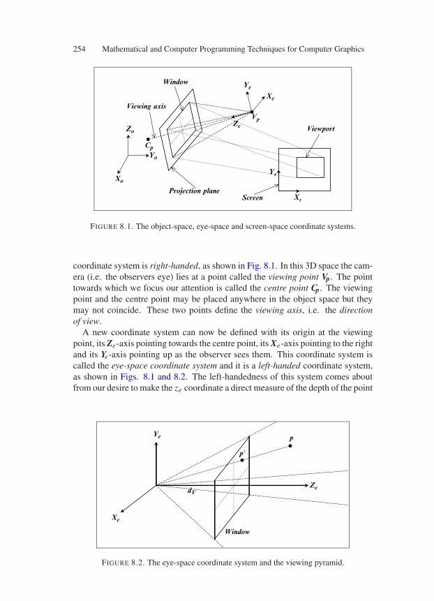
254 Mathematical and Computer Programming Techniques for Computer Graphics
Projection plane
Xo
Zo
Yo
Xe
Ze
Ye
Vp
Cp
Xs
Ys
Screen
Viewport
Window
Viewing axis
FIGURE 8.1. The object-space, eye-space and screen-space coordinate systems.
coordinate system is right-handed, as shown in Fig. 8.1. In this 3D space the cam-era (i.e. the observers eye) lies at a point called the viewing point Vp. The pointtowards which we focus our attention is called the centre point Cp. The viewingpoint and the centre point may be placed anywhere in the object space but theymay not coincide. These two points define the viewing axis, i.e. the directionof view.
A new coordinate system can now be defined with its origin at the viewingpoint, its Ze-axis pointing towards the centre point, its Xe-axis pointing to the rightand its Ye-axis pointing up as the observer sees them. This coordinate system iscalled the eye-space coordinate system and it is a left-handed coordinate system,as shown in Figs. 8.1 and 8.2. The left-handedness of this system comes aboutfrom our desire to make the ze coordinate a direct measure of the depth of the point
dV
Xe
Ye
Ze
Window
p
p
FIGURE 8.2. The eye-space coordinate system and the viewing pyramid.
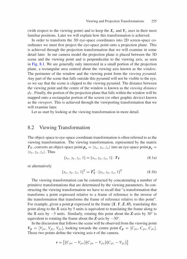
Viewing and Projection Transformations 255
(with respect to the viewing point) and to keep the Xe and Ye axes in their mostfamiliar positions. Later we will explain how this transformation is achieved.
In order to transform the 3D eye-space coordinates into 2D screen-space co-ordinates we must first project the eye-space point onto a projection plane. Thisis achieved through the projection transformation that we will examine in somedetail later. In our camera model the projection plane is placed between the 3Dscene and the viewing point and is perpendicular to the viewing axis, as seenin Fig. 8.1. We are generally only interested in a small portion of the projectionplane, a rectangular area centred about the viewing axis known as the window.The perimeter of the window and the viewing point form the viewing pyramid.Any part of the scene that falls outside this pyramid will not be visible to the eye,so we say that the scene is clipped to the viewing pyramid. The distance betweenthe viewing point and the centre of the window is known as the viewing distancedV . Finally, the portion of the projection plane that falls within the window will bemapped onto a rectangular portion of the screen (or other graphic device) knownas the viewport. This is achieved through the viewporting transformation that wewill examine later.
Let us start by looking at the viewing transformation in more detail.
8.2 Viewing Transformation
The object-space to eye-space coordinate transformation is often referred to as theviewing transformation. The viewing transformation, represented by the matrixTV , converts an object-space point po = 〈xo, yo, zo〉 into an eye-space point pe =〈xe, ye, ze〉. Thus
[xe, ye, ze, 1] = [xo, yo, zo, 1] · TV (8.1a)
or alternatively
[xe, ye, ze, 1]T = TTV · [xo, yo, zo, 1]T (8.1b)
The viewing transformation can be constructed by concatenating a number ofprimitive transformations that are determined by the viewing parameters. In con-structing the viewing transformation we have to recall that “a transformation thattransforms a point expressed relative to a frame of reference is the inverse ofthe transformation that transforms the frame of reference relative to this point”.For example, given a point p expressed in the frame X, Y, Z, O, translating thispoint along to the X-axis by 5 units is equivalent to translating the frame along tothe X-axis by −5 units. Similarly, rotating this point about the Z-axis by 30 isequivalent to rotating the frame about the Z-axis by −30.
In the discussion that follows the scene will be observed from the viewing pointVp = ⟨
Vpx , Vpy, Vpz⟩, looking towards the centre point Cp = ⟨
C px , C py, C pz⟩.
Those two points define the viewing axis v of the camera.
v = [(C px − Vpx
)(C py − Vpy
)(C pz − Vpz
)]
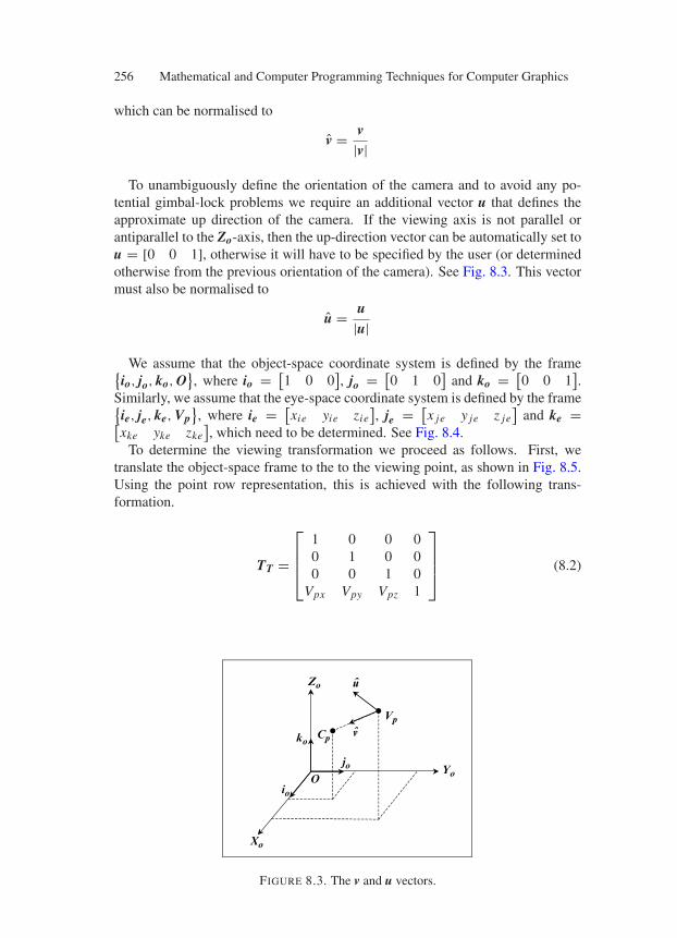
256 Mathematical and Computer Programming Techniques for Computer Graphics
which can be normalised to
v = v|v|
To unambiguously define the orientation of the camera and to avoid any po-tential gimbal-lock problems we require an additional vector u that defines theapproximate up direction of the camera. If the viewing axis is not parallel orantiparallel to the Zo-axis, then the up-direction vector can be automatically set tou = [0 0 1], otherwise it will have to be specified by the user (or determinedotherwise from the previous orientation of the camera). See Fig. 8.3. This vectormust also be normalised to
u = u|u|
We assume that the object-space coordinate system is defined by the frameio, jo, ko, O
, where io = [
1 0 0], jo = [
0 1 0]
and ko = [0 0 1
].
Similarly, we assume that the eye-space coordinate system is defined by the frameie, je, ke, Vp
, where ie = [
xie yie zie], je = [
x je y je z je]
and ke =[xke yke zke
], which need to be determined. See Fig. 8.4.
To determine the viewing transformation we proceed as follows. First, wetranslate the object-space frame to the to the viewing point, as shown in Fig. 8.5.Using the point row representation, this is achieved with the following trans-formation.
TT =
⎡
⎢⎢⎣
1 0 0 00 1 0 00 0 1 0
Vpx Vpy Vpz 1
⎤
⎥⎥⎦ (8.2)
Oio
jo
ko
Xo
Yo
Zo
Cp
Vp
v
u
FIGURE 8.3. The v and u vectors.
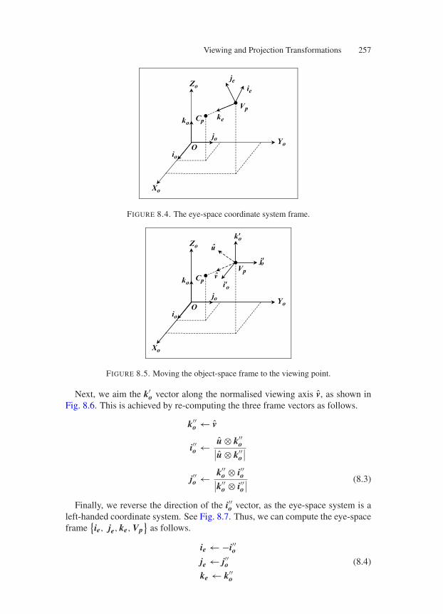
Viewing and Projection Transformations 257
Oio
jo
ko
Xo
Yo
Zo
Cp
Vp
ke
ie
je
FIGURE 8.4. The eye-space coordinate system frame.
Oio
jo
ko
Xo
Yo
Zo
Cp
Vp
k9o
j9o
i9v
u
o
FIGURE 8.5. Moving the object-space frame to the viewing point.
Next, we aim the k′o vector along the normalised viewing axis v, as shown in
Fig. 8.6. This is achieved by re-computing the three frame vectors as follows.
k′′o ← v
i′′o ← u ⊗ k′′o∣∣u ⊗ k′′o
∣∣
j′′o ← k′′o ⊗ i′′o∣∣k′′o ⊗ i′′o
∣∣ (8.3)
Finally, we reverse the direction of the i′′o vector, as the eye-space system is aleft-handed coordinate system. See Fig. 8.7. Thus, we can compute the eye-spaceframe
ie, je, ke, Vp
as follows.
ie ← −i′′oje ← j′′oke ← k′′
o
(8.4)
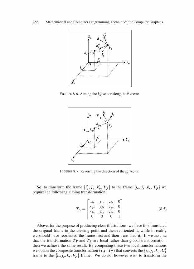
258 Mathematical and Computer Programming Techniques for Computer Graphics
Oio
jo
ko
Xo
Yo
Zo
Cp
Vp
j99o
k99o
i99oj99o
v
u
FIGURE 8.6. Aiming the k′o vector along the v vector.
Oio
jo
ko
Xo
Yo
Zo
Cp
Vpek
ieje
v
u
FIGURE 8.7. Reversing the direction of the i′′o vector.
So, to transform the framei′o, j′o, k′
o, Vp
to the frameie, je, ke, Vp
we
require the following aiming transformation.
TA =
⎡
⎢⎢⎣
xie yie zie 0x je y je z je 0xke yke zke 00 0 0 1
⎤
⎥⎥⎦ (8.5)
Above, for the purpose of producing clear illustrations, we have first translatedthe original frame to the viewing point and then reoriented it, while in realitywe should have reoriented the frame first and then translated it. If we assumethat the transformation TT and TA are local rather than global transformation,then we achieve the same result. By composing these two local transformationswe obtain the composite transformation (TA · TT) that converts the
io, jo, ko, O
frame to theie, je, ke, Vp
frame. We do not however wish to transform the

Viewing and Projection Transformations 259
frames of the coordinate systems, but to transform points from the object-spaceto the eye-space coordinate systems. Thus, we must use the inverse of the matrixproduct that would transform the frames. The inverse matrices for TT and TA aregiven by
T −1T =
⎡
⎢⎢⎣
1 0 0 00 1 0 00 0 1 0
−Vpx −Vpy −Vpz 1
⎤
⎥⎥⎦ (8.6)
and
T −1A =
⎡
⎢⎢⎣
xie x je xke 0yie y je yke 0zie z je zke 00 0 0 1
⎤
⎥⎥⎦ (8.7)
as TA is an orthogonal matrix and its inverse is the same as its transpose, i.e.T −1
A = T TA.
The viewing transformation can now be written as
TV = (TA · TT)−1 = T −1T · T −1
A
∴ TV =
⎡
⎢⎢⎣
1 0 0 00 1 0 00 0 1 0
−Vpx −Vpy −Vpz 1
⎤
⎥⎥⎦ ·
⎡
⎢⎢⎣
xie x je xke 0yie y je yke 0zie z je zke 00 0 0 1
⎤
⎥⎥⎦
∴ TV =
⎡
⎢⎢⎢⎢⎣
xie x je xke 0yie y je yke 0zie z je zke 0
−xie · Vpx − yie· −x je · Vpx − y je· −xke · Vpx − yke·Vpy − zie · Vpz Vpy − z je · Vpz Vpy − zke·Vpz 1
⎤
⎥⎥⎥⎥⎦
TV =
⎡
⎢⎢⎣
⎡
⎣ie
⎤
⎦
⎡
⎣je
⎤
⎦
⎡
⎣ke
⎤
⎦000
−ie Vp −je Vp −ke Vp 1
⎤
⎥⎥⎦ (8.8)
Hence
[xe, ye, ze, 1] = [xo, yo, zo, 1] · TV (8.9a)
or alternatively
[xe, ye, ze, 1]T = TTV · [xo, yo, zo, 1]T (8.9b)
where 〈xe, ye, ze〉 is the point expressed in the eye-space coordinate system.
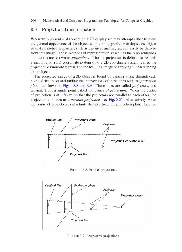
260 Mathematical and Computer Programming Techniques for Computer Graphics
8.3 Projection Transformation
When we represent a 3D object on a 2D display we may attempt either to showthe general appearance of the object, as in a photograph, or to depict the objectso that its metric properties, such as distances and angles, can easily be derivedfrom this image. Those methods of representation as well as the representationsthemselves are known as projections. Thus, a projection is defined to be botha mapping of a 3D coordinate system onto a 2D coordinate system, called theprojection coordinate system, and the resulting image of applying such a mappingto an object.
The projected image of a 3D object is found by passing a line through eachpoint of the object and finding the intersections of these lines with the projectionplane, as shown in Figs. 8.8 and 8.9. These lines are called projectors, andemanate from a single point called the centre of projection. When the centreof projection is at infinity, so that the projectors are parallel to each other, theprojection is known as a parallel projection (see Fig. 8.8). Alternatively, whenthe centre of projection is at a finite distance from the projection plane, then the
Projection planeProjectors
Projected line
Original line
Projection at centre at α
FIGURE 8.8. Parallel projections.
Projection planeProjectors
Projected line
Original line
Projection centre
FIGURE 8.9. Perspective projections.
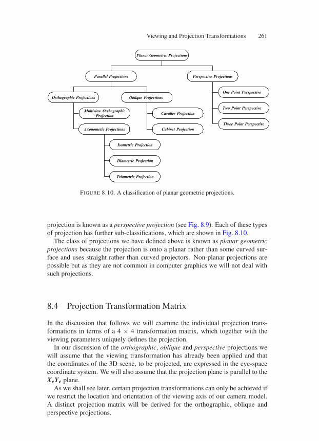
Viewing and Projection Transformations 261
One Point Perspective
Perspective Projections
Planar Geometric Projections
Parallel Projections
Orthographic Projections
Axonometic Projections
Multiview OrthographicProjection
Isometric Projection
Diametric Projection
Triametric Projection
Oblique Projections
Cabinet Projection
Cavalier ProjectionTwo Point Perspective
Three Point Perspective
FIGURE 8.10. A classification of planar geometric projections.
projection is known as a perspective projection (see Fig. 8.9). Each of these typesof projection has further sub-classifications, which are shown in Fig. 8.10.
The class of projections we have defined above is known as planar geometricprojections because the projection is onto a planar rather than some curved sur-face and uses straight rather than curved projectors. Non-planar projections arepossible but as they are not common in computer graphics we will not deal withsuch projections.
8.4 Projection Transformation Matrix
In the discussion that follows we will examine the individual projection trans-formations in terms of a 4 × 4 transformation matrix, which together with theviewing parameters uniquely defines the projection.
In our discussion of the orthographic, oblique and perspective projections wewill assume that the viewing transformation has already been applied and thatthe coordinates of the 3D scene, to be projected, are expressed in the eye-spacecoordinate system. We will also assume that the projection plane is parallel to theXeYe plane.
As we shall see later, certain projection transformations can only be achieved ifwe restrict the location and orientation of the viewing axis of our camera model.A distinct projection matrix will be derived for the orthographic, oblique andperspective projections.
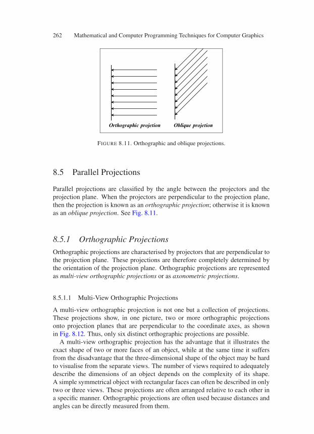
262 Mathematical and Computer Programming Techniques for Computer Graphics
Orthographic projetion Oblique projetion
FIGURE 8.11. Orthographic and oblique projections.
8.5 Parallel Projections
Parallel projections are classified by the angle between the projectors and theprojection plane. When the projectors are perpendicular to the projection plane,then the projection is known as an orthographic projection; otherwise it is knownas an oblique projection. See Fig. 8.11.
8.5.1 Orthographic Projections
Orthographic projections are characterised by projectors that are perpendicular tothe projection plane. These projections are therefore completely determined bythe orientation of the projection plane. Orthographic projections are representedas multi-view orthographic projections or as axonometric projections.
8.5.1.1 Multi-View Orthographic Projections
A multi-view orthographic projection is not one but a collection of projections.These projections show, in one picture, two or more orthographic projectionsonto projection planes that are perpendicular to the coordinate axes, as shownin Fig. 8.12. Thus, only six distinct orthographic projections are possible.
A multi-view orthographic projection has the advantage that it illustrates theexact shape of two or more faces of an object, while at the same time it suffersfrom the disadvantage that the three-dimensional shape of the object may be hardto visualise from the separate views. The number of views required to adequatelydescribe the dimensions of an object depends on the complexity of its shape.A simple symmetrical object with rectangular faces can often be described in onlytwo or three views. These projections are often arranged relative to each other ina specific manner. Orthographic projections are often used because distances andangles can be directly measured from them.
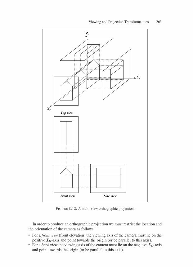
Viewing and Projection Transformations 263
Xo
Yo
Zo
Top view
Front view Side view
FIGURE 8.12. A multi-view orthographic projection.
In order to produce an orthographic projection we must restrict the location andthe orientation of the camera as follows.
• For a front view (front elevation) the viewing axis of the camera must lie on thepositive XO-axis and point towards the origin (or be parallel to this axis).
• For a back view the viewing axis of the camera must lie on the negative XO-axisand point towards the origin (or be parallel to this axis).
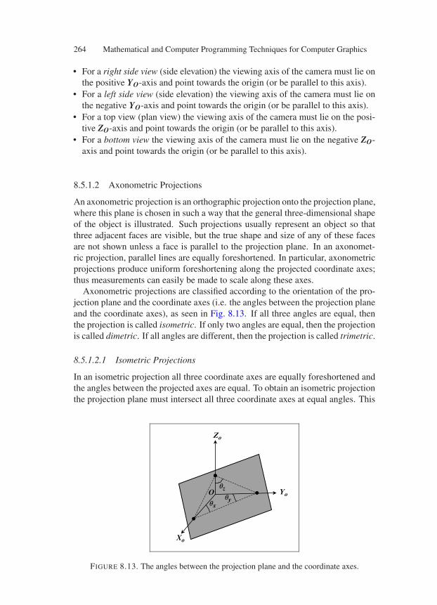
264 Mathematical and Computer Programming Techniques for Computer Graphics
• For a right side view (side elevation) the viewing axis of the camera must lie onthe positive YO-axis and point towards the origin (or be parallel to this axis).
• For a left side view (side elevation) the viewing axis of the camera must lie onthe negative YO-axis and point towards the origin (or be parallel to this axis).
• For a top view (plan view) the viewing axis of the camera must lie on the posi-tive ZO-axis and point towards the origin (or be parallel to this axis).
• For a bottom view the viewing axis of the camera must lie on the negative ZO-axis and point towards the origin (or be parallel to this axis).
8.5.1.2 Axonometric Projections
An axonometric projection is an orthographic projection onto the projection plane,where this plane is chosen in such a way that the general three-dimensional shapeof the object is illustrated. Such projections usually represent an object so thatthree adjacent faces are visible, but the true shape and size of any of these facesare not shown unless a face is parallel to the projection plane. In an axonomet-ric projection, parallel lines are equally foreshortened. In particular, axonometricprojections produce uniform foreshortening along the projected coordinate axes;thus measurements can easily be made to scale along these axes.
Axonometric projections are classified according to the orientation of the pro-jection plane and the coordinate axes (i.e. the angles between the projection planeand the coordinate axes), as seen in Fig. 8.13. If all three angles are equal, thenthe projection is called isometric. If only two angles are equal, then the projectionis called dimetric. If all angles are different, then the projection is called trimetric.
8.5.1.2.1 Isometric Projections
In an isometric projection all three coordinate axes are equally foreshortened andthe angles between the projected axes are equal. To obtain an isometric projectionthe projection plane must intersect all three coordinate axes at equal angles. This
O
qxqy
qz
Xo
Yo
Zo
FIGURE 8.13. The angles between the projection plane and the coordinate axes.
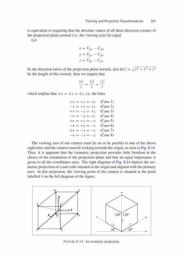
Viewing and Projection Transformations 265
is equivalent to requiring that the absolute values of all three direction cosines ofthe projection plane normal (i.e. the viewing axis) be equal.
Let
x = Vpx − C px
y = Vpy − C py
z = Vpz − C pz
be the direction ratios of the projection plane normal, also let l = √x2 + y2 + z2
be the length of this normal, then we require that
|x |l
= |y|l
= |z|l
which implies that ±x = ±y = ±z, i.e. the lines
+x = +y = +z (Case 1)
−x = +y = +z (Case 2)
+x = −y = +z (Case 3)
−x = −y = +z (Case 4)
+x = +y = −z (Case 5)
−x = +y = −z (Case 6)
+x = −y = −z (Case 7)
−x = −y = −z (Case 8)
The viewing axis of our camera must lie on or be parallel to one of the aboveeight lines and the camera must be looking towards the origin, as seen in Fig. 8.14.Thus, it is apparent that the isometric projection provides little freedom in thechoice of the orientation of the projection plane and that an equal importance isgiven to all the coordinates axes. The right diagram of Fig. 8.14 depicts the iso-metric projection of a unit cube situated at the origin and aligned with the primaryaxes. In this projection, the viewing point of the camera is situated at the pointlabelled 4 on the left diagram of the figure.
X
Y
Z
1
2
3
4
5
6
7
8
308
12081208
308
111
FIGURE 8.14. An isometric projection.
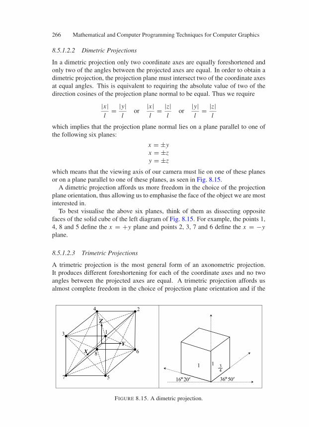
266 Mathematical and Computer Programming Techniques for Computer Graphics
8.5.1.2.2 Dimetric Projections
In a dimetric projection only two coordinate axes are equally foreshortened andonly two of the angles between the projected axes are equal. In order to obtain adimetric projection, the projection plane must intersect two of the coordinate axesat equal angles. This is equivalent to requiring the absolute value of two of thedirection cosines of the projection plane normal to be equal. Thus we require
|x |l
= |y|l
or|x |l
= |z|l
or|y|l
= |z|l
which implies that the projection plane normal lies on a plane parallel to one ofthe following six planes:
x = ±yx = ±zy = ±z
which means that the viewing axis of our camera must lie on one of these planesor on a plane parallel to one of these planes, as seen in Fig. 8.15.
A dimetric projection affords us more freedom in the choice of the projectionplane orientation, thus allowing us to emphasise the face of the object we are mostinterested in.
To best visualise the above six planes, think of them as dissecting oppositefaces of the solid cube of the left diagram of Fig. 8.15. For example, the points 1,4, 8 and 5 define the x = +y plane and points 2, 3, 7 and 6 define the x = −yplane.
8.5.1.2.3 Trimetric Projections
A trimetric projection is the most general form of an axonometric projection.It produces different foreshortening for each of the coordinate axes and no twoangles between the projected axes are equal. A trimetric projection affords usalmost complete freedom in the choice of projection plane orientation and if the
X
Y
Z
1
2
3
4
5
6
7
8
368509168209
1 143
FIGURE 8.15. A dimetric projection.
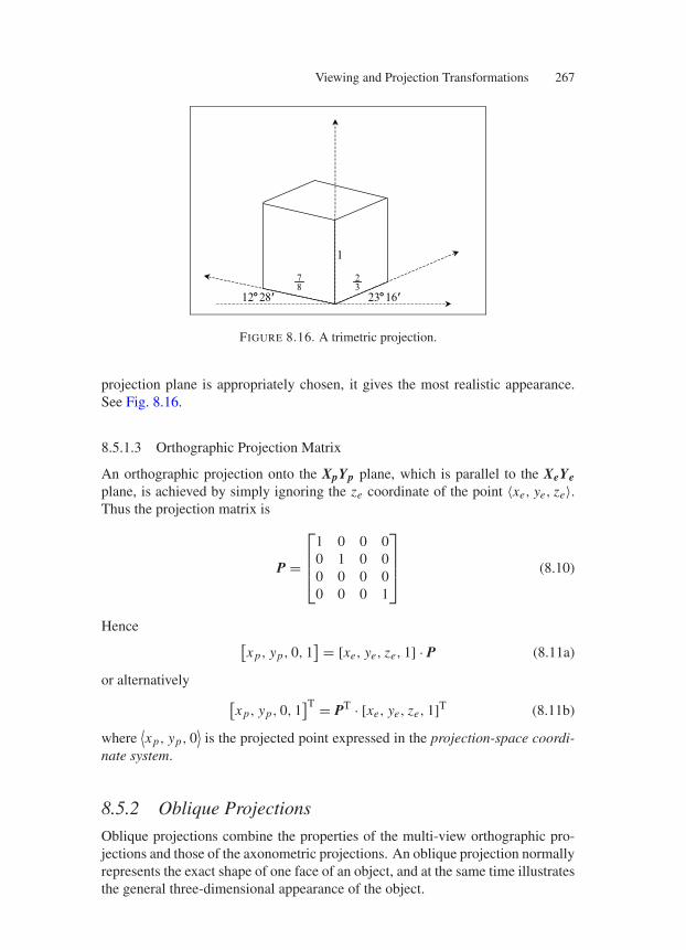
Viewing and Projection Transformations 267
87
32
1
238169128289
FIGURE 8.16. A trimetric projection.
projection plane is appropriately chosen, it gives the most realistic appearance.See Fig. 8.16.
8.5.1.3 Orthographic Projection Matrix
An orthographic projection onto the XpYp plane, which is parallel to the XeYeplane, is achieved by simply ignoring the ze coordinate of the point 〈xe, ye, ze〉.Thus the projection matrix is
P =
⎡
⎢⎢⎣
1 0 0 00 1 0 00 0 0 00 0 0 1
⎤
⎥⎥⎦ (8.10)
Hence[x p, yp, 0, 1
] = [xe, ye, ze, 1] · P (8.11a)
or alternatively[x p, yp, 0, 1
]T = PT · [xe, ye, ze, 1]T (8.11b)
where⟨x p, yp, 0
⟩is the projected point expressed in the projection-space coordi-
nate system.
8.5.2 Oblique Projections
Oblique projections combine the properties of the multi-view orthographic pro-jections and those of the axonometric projections. An oblique projection normallyrepresents the exact shape of one face of an object, and at the same time illustratesthe general three-dimensional appearance of the object.
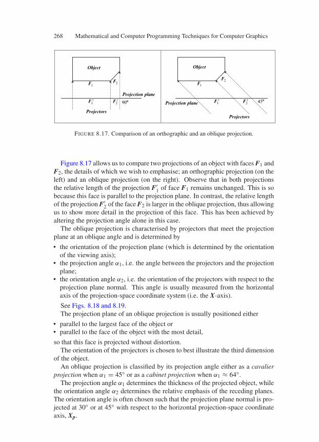
268 Mathematical and Computer Programming Techniques for Computer Graphics
908
Projection plane
Projectors
Object
F1 F1
F1 F1F2 F2
F2F2
458Projection plane
Projectors
Object
FIGURE 8.17. Comparison of an orthographic and an oblique projection.
Figure 8.17 allows us to compare two projections of an object with faces F1 andF2, the details of which we wish to emphasise; an orthographic projection (on theleft) and an oblique projection (on the right). Observe that in both projectionsthe relative length of the projection F′
1 of face F1 remains unchanged. This is sobecause this face is parallel to the projection plane. In contrast, the relative lengthof the projection F′
2 of the face F2 is larger in the oblique projection, thus allowingus to show more detail in the projection of this face. This has been achieved byaltering the projection angle alone in this case.
The oblique projection is characterised by projectors that meet the projectionplane at an oblique angle and is determined by
• the orientation of the projection plane (which is determined by the orientationof the viewing axis);
• the projection angle α1, i.e. the angle between the projectors and the projectionplane;
• the orientation angle α2, i.e. the orientation of the projectors with respect to theprojection plane normal. This angle is usually measured from the horizontalaxis of the projection-space coordinate system (i.e. the X-axis).
See Figs. 8.18 and 8.19.The projection plane of an oblique projection is usually positioned either
• parallel to the largest face of the object or• parallel to the face of the object with the most detail,
so that this face is projected without distortion.The orientation of the projectors is chosen to best illustrate the third dimension
of the object.An oblique projection is classified by its projection angle either as a cavalier
projection when α1 = 45 or as a cabinet projection when α1 ≈ 64.The projection angle α1 determines the thickness of the projected object, while
the orientation angle α2 determines the relative emphasis of the receding planes.The orientation angle is often chosen such that the projection plane normal is pro-jected at 30 or at 45 with respect to the horizontal projection-space coordinateaxis, Xp.
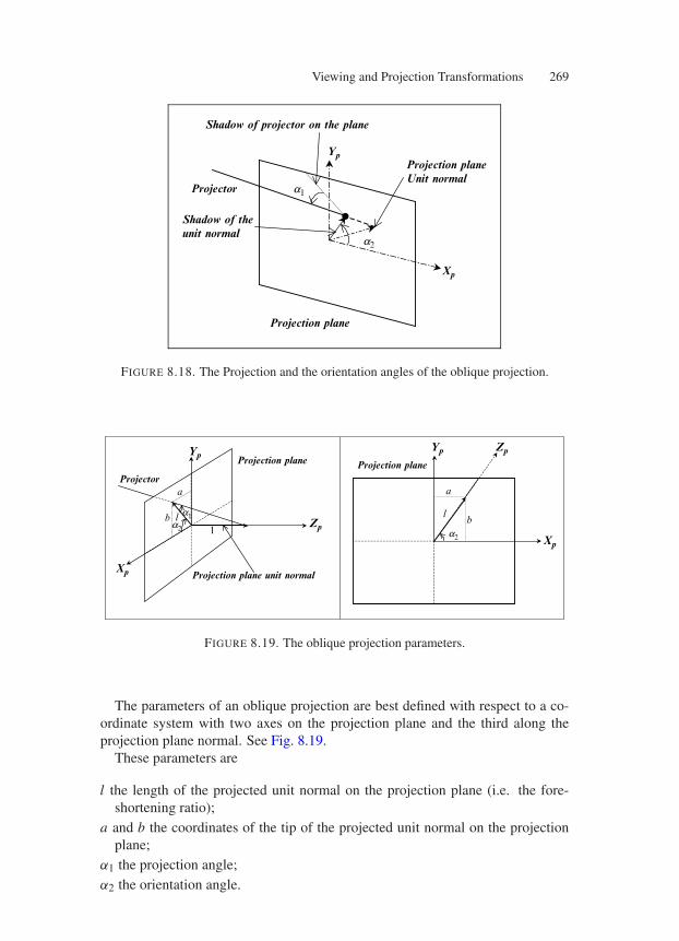
Viewing and Projection Transformations 269
a2
Projector
Projection plane
Projection planeUnit normal
Shadow of projector on the plane
Xp
Yp
Shadow of theunit normal
a1
FIGURE 8.18. The Projection and the orientation angles of the oblique projection.
a2
a1
Projector
Projection plane
Projection plane unit normal
a
b1
l
a
a2
Projection plane
Xp
bl
ZpYp
Zp
Yp
Xp
FIGURE 8.19. The oblique projection parameters.
The parameters of an oblique projection are best defined with respect to a co-ordinate system with two axes on the projection plane and the third along theprojection plane normal. See Fig. 8.19.
These parameters are
l the length of the projected unit normal on the projection plane (i.e. the fore-shortening ratio);
a and b the coordinates of the tip of the projected unit normal on the projectionplane;
α1 the projection angle;α2 the orientation angle.
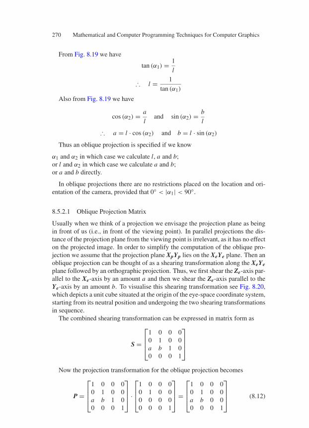
270 Mathematical and Computer Programming Techniques for Computer Graphics
From Fig. 8.19 we have
tan (α1) = 1
l
∴ l = 1
tan (α1)
Also from Fig. 8.19 we have
cos (α2) = a
land sin (α2) = b
l
∴ a = l · cos (α2) and b = l · sin (α2)
Thus an oblique projection is specified if we know
α1 and α2 in which case we calculate l, a and b;or l and α2 in which case we calculate a and b;or a and b directly.
In oblique projections there are no restrictions placed on the location and ori-entation of the camera, provided that 0 < |α1| < 90.
8.5.2.1 Oblique Projection Matrix
Usually when we think of a projection we envisage the projection plane as beingin front of us (i.e., in front of the viewing point). In parallel projections the dis-tance of the projection plane from the viewing point is irrelevant, as it has no effecton the projected image. In order to simplify the computation of the oblique pro-jection we assume that the projection plane XpYp lies on the XeYe plane. Then anoblique projection can be thought of as a shearing transformation along the XeYeplane followed by an orthographic projection. Thus, we first shear the Ze-axis par-allel to the Xe-axis by an amount a and then we shear the Ze-axis parallel to theYe-axis by an amount b. To visualise this shearing transformation see Fig. 8.20,which depicts a unit cube situated at the origin of the eye-space coordinate system,starting from its neutral position and undergoing the two shearing transformationsin sequence.
The combined shearing transformation can be expressed in matrix form as
S =
⎡
⎢⎢⎣
1 0 0 00 1 0 0a b 1 00 0 0 1
⎤
⎥⎥⎦
Now the projection transformation for the oblique projection becomes
P =
⎡
⎢⎢⎣
1 0 0 00 1 0 0a b 1 00 0 0 1
⎤
⎥⎥⎦ ·
⎡
⎢⎢⎣
1 0 0 00 1 0 00 0 0 00 0 0 1
⎤
⎥⎥⎦ =
⎡
⎢⎢⎣
1 0 0 00 1 0 0a b 0 00 0 0 1
⎤
⎥⎥⎦ (8.12)
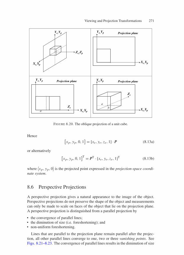
Viewing and Projection Transformations 271
Projection plane
Xe,Xp
Xe,Xp
Ze,Zp
Xe,Xp
Ye,Yp
Ye,Xp
Ye,Yp
Ye,Yp
Xe,Xpa
Projection plane
a
Projection plane
bZe
Ze
FIGURE 8.20. The oblique projection of a unit cube.
Hence[x p, yp, 0, 1
] = [xe, ye, ze, 1] · P (8.13a)
or alternatively[x p, yp, 0, 1
]T = PT · [xe, ye, ze, 1]T (8.13b)
where⟨x p, yp, 0
⟩is the projected point expressed in the projection-space coordi-
nate system.
8.6 Perspective Projections
A perspective projection gives a natural appearance to the image of the object.Perspective projections do not preserve the shape of the object and measurementscan only be made to scale on faces of the object that lie on the projection plane.A perspective projection is distinguished from a parallel projection by
• the convergence of parallel lines;• the diminution of size (i.e. foreshortening); and• non-uniform foreshortening.
Lines that are parallel to the projection plane remain parallel after the projec-tion, all other parallel lines converge to one, two or three vanishing points. SeeFigs. 8.21–8.23. The convergence of parallel lines results in the diminution of size
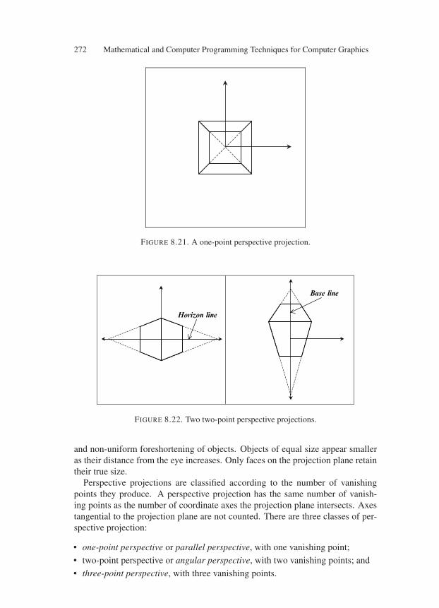
272 Mathematical and Computer Programming Techniques for Computer Graphics
FIGURE 8.21. A one-point perspective projection.
Horizon line
Base line
FIGURE 8.22. Two two-point perspective projections.
and non-uniform foreshortening of objects. Objects of equal size appear smalleras their distance from the eye increases. Only faces on the projection plane retaintheir true size.
Perspective projections are classified according to the number of vanishingpoints they produce. A perspective projection has the same number of vanish-ing points as the number of coordinate axes the projection plane intersects. Axestangential to the projection plane are not counted. There are three classes of per-spective projection:
• one-point perspective or parallel perspective, with one vanishing point;• two-point perspective or angular perspective, with two vanishing points; and
• three-point perspective, with three vanishing points.
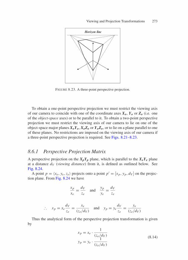
Viewing and Projection Transformations 273
Horizon line
FIGURE 8.23. A three-point perspective projection.
To obtain a one-point perspective projection we must restrict the viewing axisof our camera to coincide with one of the coordinate axes Xo, Yo or Zo (i.e. oneof the object-space axes) or to be parallel to it. To obtain a two-point perspectiveprojection we must restrict the viewing axis of our camera to lie on one of theobject-space major planes XoYo, XoZo or YoZo, or to lie on a plane parallel to oneof these planes. No restrictions are imposed on the viewing axis of our camera ifa three-point perspective projection is required. See Figs. 8.21–8.23.
8.6.1 Perspective Projection Matrix
A perspective projection on the XpYp plane, which is parallel to the XeYe planeat a distance dV (viewing distance) from it, is defined as outlined below. SeeFig. 8.24.
A point p = 〈xe, ye, ze〉 projects onto a point p′ = ⟨x p, yp, dV
⟩on the projec-
tion plane. From Fig. 8.24 we have
x p
xe= dV
zeand
yp
ye= dV
ze
∴ x p = xedV
ze= xe
(ze/dV )and yp = ye
dV
ze= ye
(ze/dV )
Thus the analytical form of the perspective projection transformation is givenby
x p = xe · 1
(ze/dV )
yp = ye · 1
(ze/dV )
(8.14)
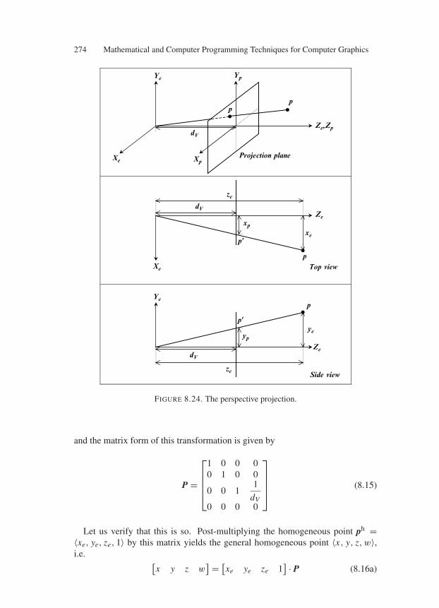
274 Mathematical and Computer Programming Techniques for Computer Graphics
dV
dV
dV
pp
Projection plane
p
p9
Top view
p
p9
Side view
Ze,Zp
Ze
Ze
xe
yeyp
ze
xp
ze
YpYe
XpXe
Xe
Ye
FIGURE 8.24. The perspective projection.
and the matrix form of this transformation is given by
P =
⎡
⎢⎢⎢⎣
1 0 0 00 1 0 0
0 0 11
dV0 0 0 0
⎤
⎥⎥⎥⎦
(8.15)
Let us verify that this is so. Post-multiplying the homogeneous point ph =〈xe, ye, ze, 1〉 by this matrix yields the general homogeneous point 〈x, y, z, w〉,i.e.
[x y z w
] = [xe ye ze 1
] · P (8.16a)
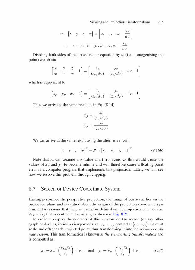
Viewing and Projection Transformations 275
or[x y z w
] =[
xe ye zeze
dV
]
∴ x = xe, y = ye, z = ze, w = ze
dV
Dividing both sides of the above vector equation by w (i.e. homogenising thepoint) we obtain
[ x
w
y
w
z
w1]
=[
xe
(ze/dV )
ye
(ze/dV )dV 1
]
which is equivalent to
[x p yp dV 1
] =[
xe
(ze/dV )
ye
(ze/dV )dV 1
]
Thus we arrive at the same result as in Eq. (8.14).
x p = xe
(ze/dV )
yp = ye
(ze/dV )
We can arrive at the same result using the alternative form
[x y z w
]T = PT · [xe ye ze 1
]T (8.16b)
Note that ze can assume any value apart from zero as this would cause thevalues of x p and yp to become infinite and will therefore cause a floating pointerror in a computer program that implements this projection. Later, we will seehow we resolve this problem through clipping.
8.7 Screen or Device Coordinate System
Having performed the perspective projection, the image of our scene lies on theprojection plane and is centred about the origin of the projection coordinate sys-tem. Let us assume that there is a window defined on the projection plane of size2sx × 2sy that is centred at the origin, as shown in Fig. 8.25.
In order to display the contents of this window on the screen (or any othergraphics device), inside a viewport of size vsx × vsy centred at
⟨vcx , vcy
⟩, we must
scale and offset each projected point, thus transforming it into the screen coordi-nate system. This transformation is known as the viewporting transformation andis computed as
xs = x p ·(
vsx/2
sx
)+ vcx and ys = yp ·
(vsy/2
sy
)+ vcy (8.17)
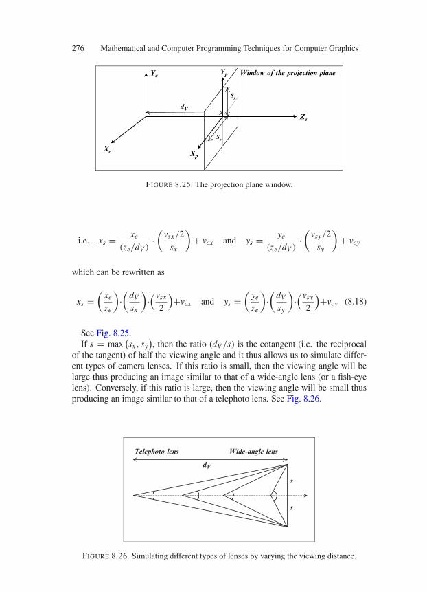
276 Mathematical and Computer Programming Techniques for Computer Graphics
dV
Window of the projection plane
Ze
XpXe
Ye Yp
Sy
Sx
FIGURE 8.25. The projection plane window.
i.e. xs = xe
(ze/dV )·(
vsx/2
sx
)+ vcx and ys = ye
(ze/dV )·(
vsy/2
sy
)+ vcy
which can be rewritten as
xs =(
xe
ze
)·(
dV
sx
)·(vsx
2
)+vcx and ys =
(ye
ze
)·(
dV
sy
)·(vsy
2
)+vcy (8.18)
See Fig. 8.25.If s = max
(sx , sy
), then the ratio (dV /s) is the cotangent (i.e. the reciprocal
of the tangent) of half the viewing angle and it thus allows us to simulate differ-ent types of camera lenses. If this ratio is small, then the viewing angle will belarge thus producing an image similar to that of a wide-angle lens (or a fish-eyelens). Conversely, if this ratio is large, then the viewing angle will be small thusproducing an image similar to that of a telephoto lens. See Fig. 8.26.
Telephoto lens Wide-angle lens
s
s
dV
FIGURE 8.26. Simulating different types of lenses by varying the viewing distance.
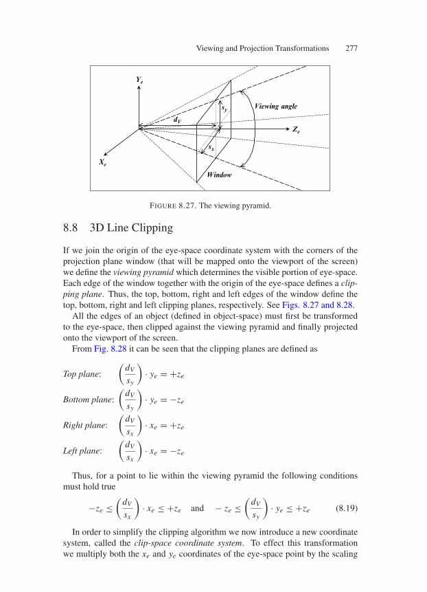
Viewing and Projection Transformations 277
sy
sx
Window
Viewing angle
Ze
Xe
Ye
dV
FIGURE 8.27. The viewing pyramid.
8.8 3D Line Clipping
If we join the origin of the eye-space coordinate system with the corners of theprojection plane window (that will be mapped onto the viewport of the screen)we define the viewing pyramid which determines the visible portion of eye-space.Each edge of the window together with the origin of the eye-space defines a clip-ping plane. Thus, the top, bottom, right and left edges of the window define thetop, bottom, right and left clipping planes, respectively. See Figs. 8.27 and 8.28.
All the edges of an object (defined in object-space) must first be transformedto the eye-space, then clipped against the viewing pyramid and finally projectedonto the viewport of the screen.
From Fig. 8.28 it can be seen that the clipping planes are defined as
Top plane:
(dV
sy
)· ye = +ze
Bottom plane:
(dV
sy
)· ye = −ze
Right plane:
(dV
sx
)· xe = +ze
Left plane:
(dV
sx
)· xe = −ze
Thus, for a point to lie within the viewing pyramid the following conditionsmust hold true
−ze ≤(
dV
sx
)· xe ≤ +ze and − ze ≤
(dV
sy
)· ye ≤ +ze (8.19)
In order to simplify the clipping algorithm we now introduce a new coordinatesystem, called the clip-space coordinate system. To effect this transformationwe multiply both the xe and ye coordinates of the eye-space point by the scaling
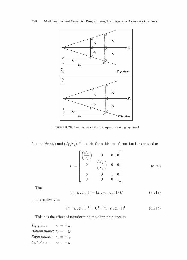
278 Mathematical and Computer Programming Techniques for Computer Graphics
Top view
Side view
Ze
Ze
−xe
+xe
sx
sx
+ye
−ye
sy
sy
ze
dV
ze
dV
Xe
Ye
FIGURE 8.28. Two views of the eye-space viewing pyramid.
factors (dV /sx ) and(dV /sy
). In matrix form this transformation is expressed as
C =
⎡
⎢⎢⎢⎢⎢⎢⎢⎣
(dV
sx
)0 0 0
0
(dV
sy
)0 0
0 0 1 00 0 0 1
⎤
⎥⎥⎥⎥⎥⎥⎥⎦
(8.20)
Thus[xc, yc, zc, 1] = [xe, ye, ze, 1] · C (8.21a)
or alternatively as
[xc, yc, zc, 1]T = CT · [xe, ye, ze, 1]T (8.21b)
This has the effect of transforming the clipping planes to
Top plane: yc = +zc
Bottom plane: yc = −zc
Right plane: xc = +zc
Left plane: xc = −zc
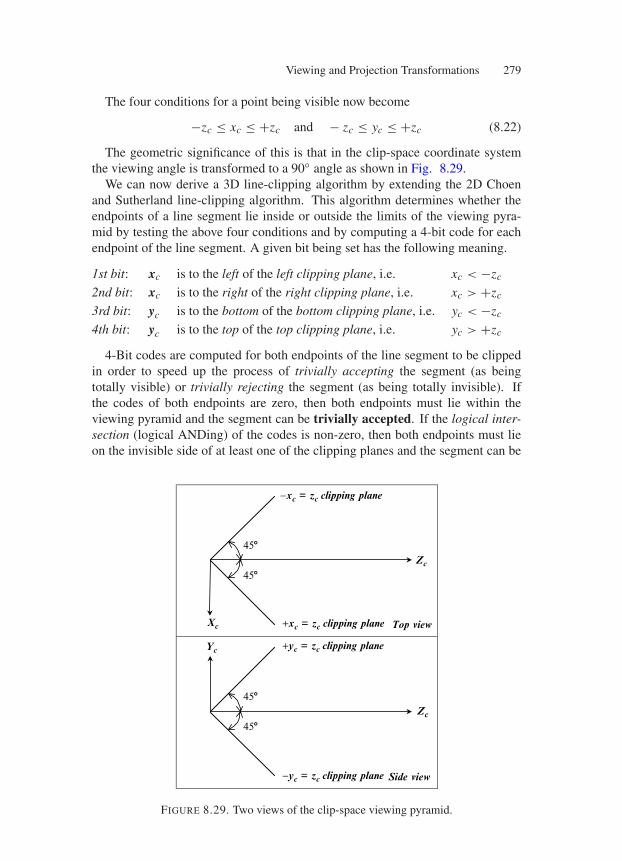
Viewing and Projection Transformations 279
The four conditions for a point being visible now become
−zc ≤ xc ≤ +zc and − zc ≤ yc ≤ +zc (8.22)
The geometric significance of this is that in the clip-space coordinate systemthe viewing angle is transformed to a 90 angle as shown in Fig. 8.29.
We can now derive a 3D line-clipping algorithm by extending the 2D Choenand Sutherland line-clipping algorithm. This algorithm determines whether theendpoints of a line segment lie inside or outside the limits of the viewing pyra-mid by testing the above four conditions and by computing a 4-bit code for eachendpoint of the line segment. A given bit being set has the following meaning.
1st bit: xc is to the left of the left clipping plane, i.e. xc < −zc
2nd bit: xc is to the right of the right clipping plane, i.e. xc > +zc
3rd bit: yc is to the bottom of the bottom clipping plane, i.e. yc < −zc
4th bit: yc is to the top of the top clipping plane, i.e. yc > +zc
4-Bit codes are computed for both endpoints of the line segment to be clippedin order to speed up the process of trivially accepting the segment (as beingtotally visible) or trivially rejecting the segment (as being totally invisible). Ifthe codes of both endpoints are zero, then both endpoints must lie within theviewing pyramid and the segment can be trivially accepted. If the logical inter-section (logical ANDing) of the codes is non-zero, then both endpoints must lieon the invisible side of at least one of the clipping planes and the segment can be
Top view
458
458
458
458
Zc
Side view
Zc
Xc
Yc
−xc = zc clipping plane
+xc = zc clipping plane
+yc = zc clipping plane
−yc = zc clipping plane
FIGURE 8.29. Two views of the clip-space viewing pyramid.
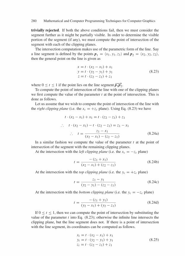
280 Mathematical and Computer Programming Techniques for Computer Graphics
trivially rejected. If both the above conditions fail, then we must consider thesegment further as it might be partially visible. In order to determine the visibleportion of the segment (if any), we must compute the point of intersection of thesegment with each of the clipping planes.
The intersection computation makes use of the parametric form of the line. Saya line segment is defined by the points p1 = 〈x1, y1, z1〉 and p2 = 〈x2, y2, z2〉,then the general point on the line is given as
x = t · (x2 − x1) + x1y = t · (y2 − y1) + y1z = t · (z2 − z1) + z1
(8.23)
where 0 ≤ t ≤ 1 if the point lies on the line segment −−→p1p2.To compute the point of intersection of the line with one of the clipping planes
we first compute the value of the parameter t at the point of intersection. This isdone as follows.
Let us assume that we wish to compute the point of intersection of the line withthe right clipping plane (i.e. the xc = +zc plane). Using Eq. (8.23) we have
t · (x2 − x1) + x1 = t · (z2 − z1) + z1
∴ t · (x2 − x1) − t · (z2 − z1) = z1 − x1
∴ t = z1 − x1
(x2 − x1) − (z2 − z1)(8.24a)
In a similar fashion we compute the value of the parameter t at the point ofintersection of the segment with the remaining clipping planes.
At the intersection with the left clipping plane (i.e. the xc = −zc plane)
t = − (z1 + x1)
(x2 − x1) + (z2 − z1)(8.24b)
At the intersection with the top clipping plane (i.e. the yc = +zc plane)
t = z1 − y1
(y2 − y1) − (z2 − z1)(8.24c)
At the intersection with the bottom clipping plane (i.e. the yc = −zc plane)
t = − (z1 + y1)
(y2 − x1) + (y2 − z1)(8.24d)
If 0 ≤ t ≤ 1, then we can compute the point of intersection by substituting thevalue of the parameter t into Eq. (8.23); otherwise the infinite line intersects theclipping plane, but the line segment does not. If there is a point of intersectionwith the line segment, its coordinates can be computed as follows.
xi = t · (x2 − x1) + x1yi = t · (y2 − y1) + y1zi = t · (z2 − z1) + z1
(8.25)
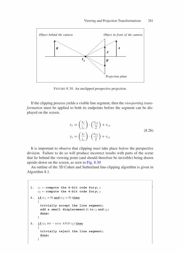
Viewing and Projection Transformations 281
AA
B
BVp
Projection plane
Object in front of the cameraObject behind the camera
FIGURE 8.30. An unclipped perspective projection.
If the clipping process yields a visible line segment, then the viewporting trans-formation must be applied to both its endpoints before the segment can be dis-played on the screen.
xs =(
xc
zc
)·(vsx
2
)+ vcx
ys =(
yc
zc
)·(vsy
2
)+ vcy
(8.26)
It is important to observe that clipping must take place before the perspectivedivision. Failure to do so will produce incorrect results with parts of the scenethat lie behind the viewing point (and should therefore be invisible) being drawnupside-down on the screen, as seen in Fig. 8.30
An outline of the 3D Cohen and Sutherland line-clipping algorithm is given inAlgorithm 8.1.
1. c1 ← compute the 4-bit code for p1 ;c2 ← compute the 4-bit code for p2 ;
2. if (c1 = 0) and (c2 = 0) thentrivially accept the line segment;add a small displacement dz to z1 and z2;done;
3. if (c1 bit − wise AN D c2) then
trivially reject the line segment;done;

282 Mathematical and Computer Programming Techniques for Computer Graphics
4. if (c1 = 0) then c = c2;else c = c1 ;
5. if the first bit of c is set thencompute the point of intersection 〈xi , yi , zi 〉 of the linesegment with the left clipping plane;goto step 9;
6. if the second bit of c is set then
compute the point of intersection
⟨xi, yi, zi
⟩of the line
segment with the right clipping plane;goto step 9;
7. if the third bit of c is set thencompute the point of intersection
⟨xi, yi, zi
⟩of the line
segment with the bottom clipping plane;goto step 9;
8. if the fourth bit of c is set then
compute the point of intersection
⟨xi, yi, zi
⟩of the line
segment with the top clipping plane;goto step 9;
9. if (c = c1) then
x1 ← xi;y1 ← yi;z1 ← zi;c1 ← recompute the 4-bit code for this point;goto step 2;
else
x2 ← xi;y2 ← yi;z2 ← zi;c2 ← recompute the 4-bit code for this point;goto step 2;
Algorithm 8.1 The 3D Choen and Sutherland line-clipping algorithm.
The following C functions implement a 3D point-clipping routine and theCohen and Sutherland 3D line-clipping algorithm.
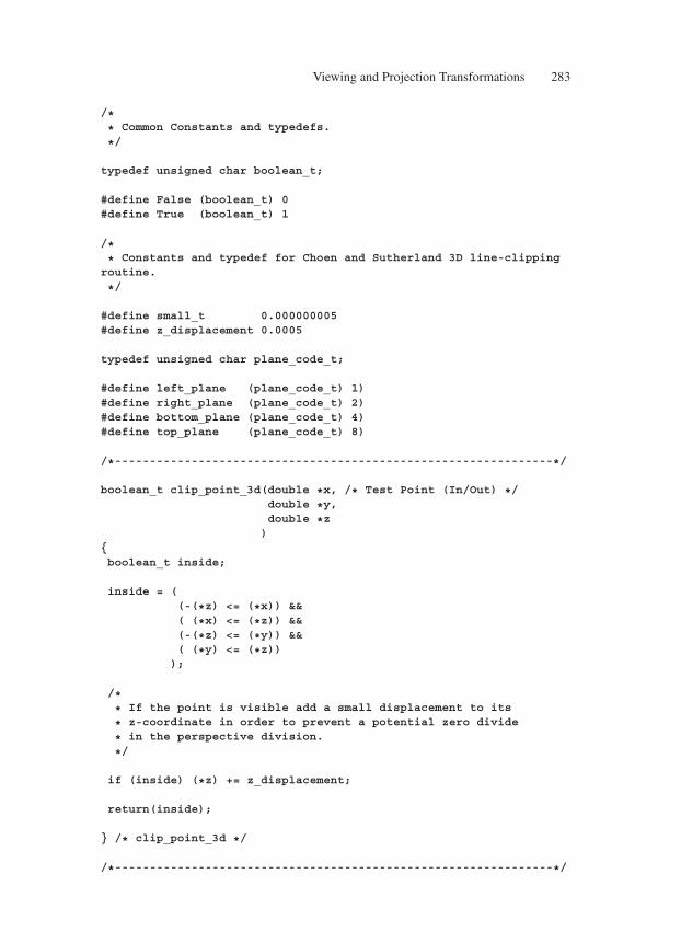
Viewing and Projection Transformations 283
/** Common Constants and typedefs.
*/
typedef unsigned char boolean_t;
#define False (boolean_t) 0#define True (boolean_t) 1
/** Constants and typedef for Choen and Sutherland 3D line-clippingroutine.
*/
#define small_t 0.000000005#define z_displacement 0.0005
typedef unsigned char plane_code_t;
#define left_plane (plane_code_t) 1)#define right_plane (plane_code_t) 2)#define bottom_plane (plane_code_t) 4)#define top_plane (plane_code_t) 8)
/*---------------------------------------------------------------*/
boolean_t clip_point_3d(double *x, /* Test Point (In/Out) */double *y,double *z)
boolean_t inside;
inside = ((-(*z) <= (*x)) &&( (*x) <= (*z)) &&(-(*z) <= (*y)) &&( (*y) <= (*z)));
/** If the point is visible add a small displacement to its
* z-coordinate in order to prevent a potential zero divide
* in the perspective division.
*/
if (inside) (*z) += z_displacement;
return(inside);
/* clip_point_3d */
/*---------------------------------------------------------------*/
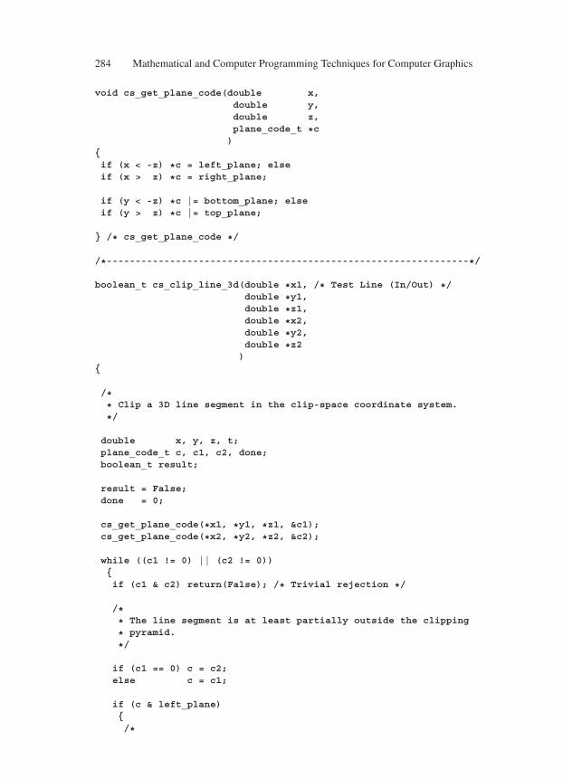
284 Mathematical and Computer Programming Techniques for Computer Graphics
void cs_get_plane_code(double x,double y,double z,plane_code_t *c)
if (x < -z) *c = left_plane; elseif (x > z) *c = right_plane;
if (y < -z) *c |= bottom_plane; elseif (y > z) *c |= top_plane;
/* cs_get_plane_code */
/*---------------------------------------------------------------*/
boolean_t cs_clip_line_3d(double *x1, /* Test Line (In/Out) */double *y1,double *z1,double *x2,double *y2,double *z2)
/** Clip a 3D line segment in the clip-space coordinate system.
*/
double x, y, z, t;plane_code_t c, c1, c2, done;boolean_t result;
result = False;done = 0;
cs_get_plane_code(*x1, *y1, *z1, &c1);cs_get_plane_code(*x2, *y2, *z2, &c2);
while ((c1 != 0) || (c2 != 0))if (c1 & c2) return(False); /* Trivial rejection */
/** The line segment is at least partially outside the clipping
* pyramid.
*/
if (c1 == 0) c = c2;else c = c1;
if (c & left_plane)/*
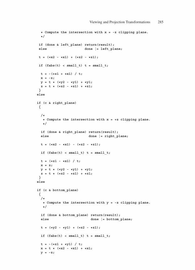
Viewing and Projection Transformations 285
* Compute the intersection with x = -z clipping plane.
*/
if (done & left_plane) return(result);else done |= left_plane;
t = (*x2 - *x1) + (*z2 - *z1);
if (fabs(t) < small_t) t = small_t;
t = -(*z1 + *x1) / t;x = -z;y = t * (*y2 - *y1) + *y1;z = t * (*z2 - *z1) + *z1;else
if (c & right_plane)
/** Compute the intersection with x = +z clipping plane.
*/
if (done & right_plane) return(result);else done |= right_plane;
t = (*x2 - *x1) - (*z2 - *z1);
if (fabs(t) < small_t) t = small_t;
t = (*z1 - *x1) / t;x = z;y = t * (*y2 - *y1) + *y1;z = t * (*z2 - *z1) + *z1;else
if (c & bottom_plane)/** Compute the intersection with y = -z clipping plane.
*/
if (done & bottom_plane) return(result);else done |= bottom_plane;
t = (*y2 - *y1) + (*z2 - *z1);
if (fabs(t) < small_t) t = small_t;
t = -(*z1 + *y1) / t;x = t * (*x2 - *x1) + *x1;y = -z;
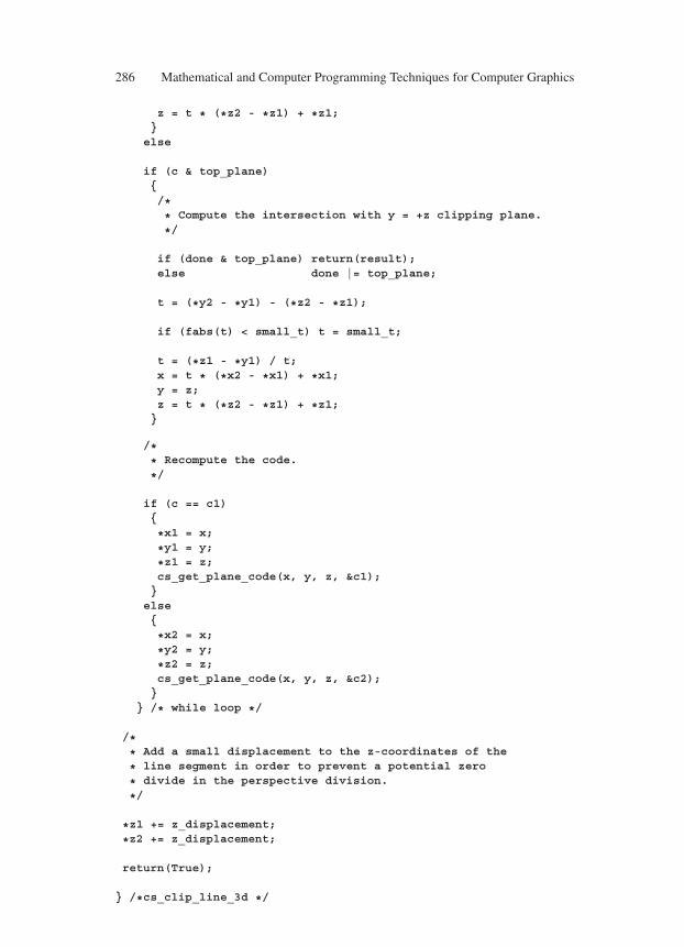
286 Mathematical and Computer Programming Techniques for Computer Graphics
z = t * (*z2 - *z1) + *z1;
else
if (c & top_plane)/** Compute the intersection with y = +z clipping plane.
*/
if (done & top_plane) return(result);else done |= top_plane;
t = (*y2 - *y1) - (*z2 - *z1);
if (fabs(t) < small_t) t = small_t;
t = (*z1 - *y1) / t;x = t * (*x2 - *x1) + *x1;y = z;z = t * (*z2 - *z1) + *z1;
/** Recompute the code.
*/
if (c == c1)
*x1 = x;
*y1 = y;
*z1 = z;cs_get_plane_code(x, y, z, &c1);
else
*x2 = x;
*y2 = y;
*z2 = z;cs_get_plane_code(x, y, z, &c2);
/* while loop */
/** Add a small displacement to the z-coordinates of the
* line segment in order to prevent a potential zero
* divide in the perspective division.
*/
*z1 += z_displacement;
*z2 += z_displacement;
return(True);
/*cs_clip_line_3d */
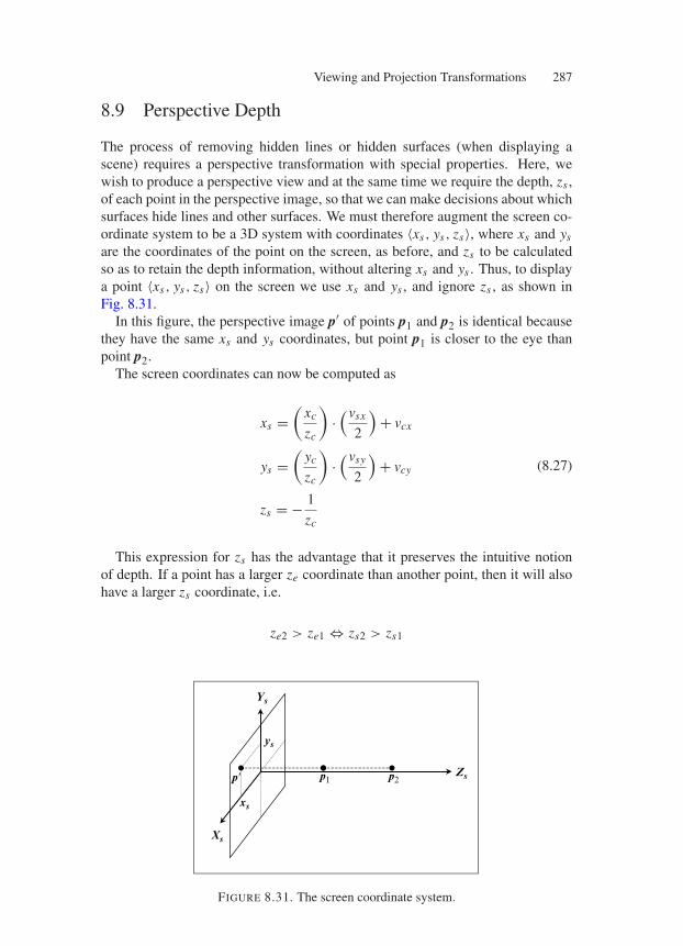
Viewing and Projection Transformations 287
8.9 Perspective Depth
The process of removing hidden lines or hidden surfaces (when displaying ascene) requires a perspective transformation with special properties. Here, wewish to produce a perspective view and at the same time we require the depth, zs ,of each point in the perspective image, so that we can make decisions about whichsurfaces hide lines and other surfaces. We must therefore augment the screen co-ordinate system to be a 3D system with coordinates 〈xs, ys, zs〉, where xs and ys
are the coordinates of the point on the screen, as before, and zs to be calculatedso as to retain the depth information, without altering xs and ys . Thus, to displaya point 〈xs, ys, zs〉 on the screen we use xs and ys , and ignore zs , as shown inFig. 8.31.
In this figure, the perspective image p′ of points p1 and p2 is identical becausethey have the same xs and ys coordinates, but point p1 is closer to the eye thanpoint p2.
The screen coordinates can now be computed as
xs =(
xc
zc
)·(vsx
2
)+ vcx
ys =(
yc
zc
)·(vsy
2
)+ vcy
zs = − 1
zc
(8.27)
This expression for zs has the advantage that it preserves the intuitive notionof depth. If a point has a larger ze coordinate than another point, then it will alsohave a larger zs coordinate, i.e.
ze2 > ze1 ⇔ zs2 > zs1
p Zs
Ys
ys
xs
Xs
p2p1
FIGURE 8.31. The screen coordinate system.
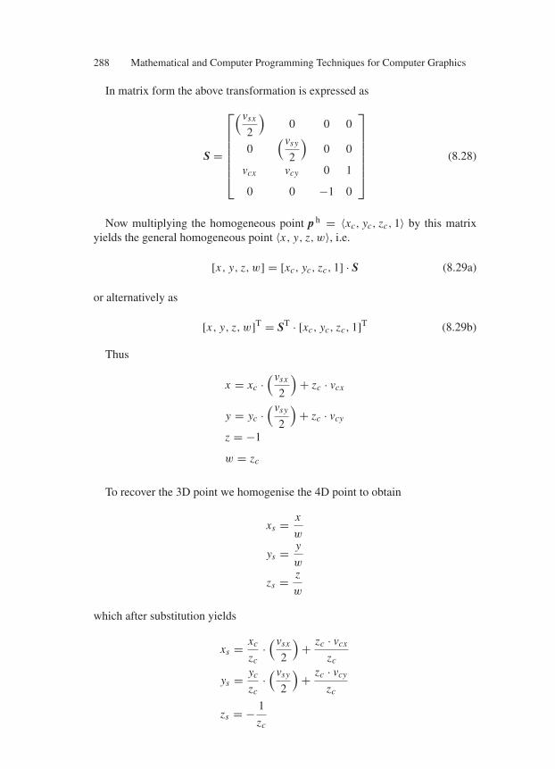
288 Mathematical and Computer Programming Techniques for Computer Graphics
In matrix form the above transformation is expressed as
S =
⎡
⎢⎢⎢⎢⎢⎢⎣
(vsx
2
)0 0 0
0(vsy
2
)0 0
vcx vcy 0 1
0 0 −1 0
⎤
⎥⎥⎥⎥⎥⎥⎦
(8.28)
Now multiplying the homogeneous point p h = 〈xc, yc, zc, 1〉 by this matrixyields the general homogeneous point 〈x, y, z, w〉, i.e.
[x, y, z, w] = [xc, yc, zc, 1] · S (8.29a)
or alternatively as
[x, y, z, w]T = ST · [xc, yc, zc, 1]T (8.29b)
Thus
x = xc ·(vsx
2
)+ zc · vcx
y = yc ·(vsy
2
)+ zc · vcy
z = −1
w = zc
To recover the 3D point we homogenise the 4D point to obtain
xs = x
w
ys = y
w
zs = z
w
which after substitution yields
xs = xc
zc·(vsx
2
)+ zc · vcx
zc
ys = yc
zc·(vsy
2
)+ zc · vcy
zc
zs = − 1
zc
Viewing and Projection Transformations 289
and after simplification we obtain the same result as in Eq. (8.27):
xs =(
xc
zc
)·(vsx
2
)+ vcx
ys =(
yc
zc
)·(vsy
2
)+ vcy
zs = − 1
zc
8.10 Simple C Library for 3D Transformations
See Appendix 4.
“Comninos” — 2005/8/31 — 18:28 — page 291 — #1
9
3D Rendering
9.1 Introduction
Computer image synthesis is the process of generating a two-dimensional pictor-ial representation of a mathematically defined three-dimensional object or scene.Sometimes this process is referred to as rendering the scene and the computerprogram that caries out this process is called a renderer.
Given the mathematical description of a collection of objects or curved surfacesin a scene, there are three main ways in which we may render this scene. We mayrender it as
• a wire-frame drawing, depicting all the edges or curves, as shown in Fig. 9.1a;• a hidden-line drawing, depicting only the visible edges or curves (i.e. all the
edges or curves not obscured by any faces or surfaces closer to the observer),as shown in Fig. 9.1b;
• a shaded image, which attempts to capture the photographic appearance of thescene by simulating how light is reflected off the surface of its objects or curvedsurfaces, as shown in Fig. 9.1c.
There are clear distinctions between these three techniques of rendering, whichwe shall examine shortly.
To simplify our discussion, we will only deal with scenes that are describedas a collection of polygons. In this scheme, curved surfaces are assumed to havebeen decomposed into polygonal meshes which approximate their shape. This iscommon practice in most rendering schemes.
In our scheme, a scene is defined as a set (collection) of objects, i.e. S =O1, O2, . . . , Ok. Each object is defined as a set of polygons, faces or facetsF, a set of edges E and a set of vertices V. Thus an object O is defined asO = F, E, V, where F =
f 1, f 2, . . . , f l, E = e1, e2, . . . , em and V =
v1, v2, . . . , vn. Each vertex vi is defined by its three coordinates vi = xi , yi , zi ,each edge e j is defined by its two endpoints ej = vs, ve and each face fp maybe defined by the set of edges fp = e or by the set of vertices fp = v thatdescribe it.
291
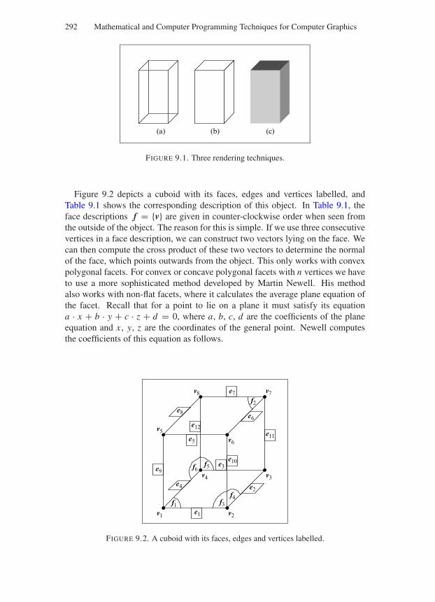
“Comninos” — 2005/8/31 — 18:28 — page 292 — #2
292 Mathematical and Computer Programming Techniques for Computer Graphics
(a) (b) (c)
FIGURE 9.1. Three rendering techniques.
Figure 9.2 depicts a cuboid with its faces, edges and vertices labelled, andTable 9.1 shows the corresponding description of this object. In Table 9.1, theface descriptions f = v are given in counter-clockwise order when seen fromthe outside of the object. The reason for this is simple. If we use three consecutivevertices in a face description, we can construct two vectors lying on the face. Wecan then compute the cross product of these two vectors to determine the normalof the face, which points outwards from the object. This only works with convexpolygonal facets. For convex or concave polygonal facets with n vertices we haveto use a more sophisticated method developed by Martin Newell. His methodalso works with non-flat facets, where it calculates the average plane equation ofthe facet. Recall that for a point to lie on a plane it must satisfy its equationa · x + b · y + c · z + d = 0, where a, b, c, d are the coefficients of the planeequation and x , y, z are the coordinates of the general point. Newell computesthe coefficients of this equation as follows.
v8
v1 v2
v3v4
v5
v6
v7
e8
e1
e2
e3
e4
e5
e6
e7
e9
e10
e11
e12
f2
f3f4
f5f6
f1
FIGURE 9.2. A cuboid with its faces, edges and vertices labelled.
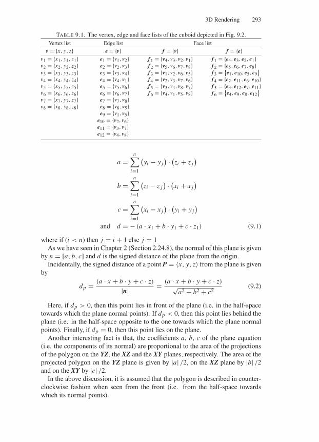
“Comninos” — 2005/8/31 — 18:28 — page 293 — #3
3D Rendering 293
TABLE 9.1. The vertex, edge and face lists of the cuboid depicted in Fig. 9.2.Vertex list Edge list Face list
v = x, y, z e = v f = v f = ev1 = x1, y1, z1 e1 = v1, v2 f1 = v4, v3, v2, v1 f1 = e4, e3, e2, e1v2 = x2, y2, z2 e2 = v2, v3 f2 = v5, v6, v7, v8 f2 = e5, e6, e7, e8v3 = x3, y3, z3 e3 = v3, v4 f3 = v1, v2, v6, v5 f3 =
e1, e10, e5, e9
v4 = x4, y4, z4 e4 = v4, v1 f4 = v2, v3, v7, v6 f4 = e2, e11, e6, e10v5 = x5, y5, z5 e5 = v5, v6 f5 = v3, v4, v8, v7 f5 = e3, e12, e7, e11v6 = x6, y6, z6 e6 = v6, v7 f6 = v4, v1, v5, v8 f6 =
e4, e9, e8, e12
v7 = x7, y7, z7 e7 = v7, v8v8 = x8, y8, z8 e8 = v8, v5
e9 = v1, v5e10 = v2, v6e11 = v3, v7e12 = v4, v8
a =n∑
i=1
(yi − y j
) · (zi + z j
)
b =n∑
i=1
(zi − z j
) · (xi + x j
)
c =n∑
i=1
(xi − x j
) · (yi + y j
)
and d = − (a · x1 + b · y1 + c · z1) (9.1)
where if (i < n) then j = i + 1 else j = 1As we have seen in Chapter 2 (Section 2.24.8), the normal of this plane is given
by n = [a, b, c] and d is the signed distance of the plane from the origin.Incidentally, the signed distance of a point P = 〈x, y, z〉 from the plane is given
by
dp = (a · x + b · y + c · z)
|n| = (a · x + b · y + c · z)√a2 + b2 + c2
(9.2)
Here, if dp > 0, then this point lies in front of the plane (i.e. in the half-spacetowards which the plane normal points). If dp < 0, then this point lies behind theplane (i.e. in the half-space opposite to the one towards which the plane normalpoints). Finally, if dp = 0, then this point lies on the plane.
Another interesting fact is that, the coefficients a, b, c of the plane equation(i.e. the components of its normal) are proportional to the area of the projectionsof the polygon on the YZ, the XZ and the XY planes, respectively. The area of theprojected polygon on the YZ plane is given by |a| /2, on the XZ plane by |b| /2and on the XY by |c| /2.
In the above discussion, it is assumed that the polygon is described in counter-clockwise fashion when seen from the front (i.e. from the half-space towardswhich its normal points).
“Comninos” — 2005/8/31 — 18:28 — page 294 — #4
294 Mathematical and Computer Programming Techniques for Computer Graphics
9.2 Rendering Algorithms
Producing a wire-frame drawing of the objects in a scene is fairly simple. Firstwe must transform all the vertices of the scene into the eye-space coordinate sys-tem. Then, we clip each edge of the scene against the viewing pyramid and ifthe clipped edge is at least partially visible, we transform its endpoints into theimage-space coordinate system and we draw a 2D line segment using the availablegraphics package.
Producing a hidden-line drawing or a shaded image of the objects in a sceneis slightly more complex. In both cases, we first transform all the vertices of thescene into the eye-space coordinate system and we clip all the polygons of thescene against the viewing pyramid using a 3D polygon-clipping algorithm.
To produce a hidden-line drawing of the scene we need to use a hidden-lineelimination algorithm. This algorithm examines each edge in the scene and com-pares it against each face in the scene in order to determine if it is obscured byany face that is closer to the observer. If the algorithm determines that an edgeis totally obscured by a face, then it eliminates this edge and proceeds with thenext one. If an edge is partially obscured by a face, then the algorithm removesthe invisible part and continues checking the visible part of the edge against theremaining faces. If an entire edge or a part of an edge is found to be obscured bynone of the faces, then its endpoints are transformed into the image-space coordi-nate system and it is displayed as before.
To produce a shaded image of the scene we need to use a hidden-surface elim-ination algorithm and a shading algorithm. In this case our image can only bedisplayed on a raster scan display device. Such devices are capable of display-ing a number of scan-lines on the screen. A scan-line is a horizontal line on thescreen which is composed of a number of pixels (picture elements) that appearas dots on the screen. A typical display may consist of 1024 scan-lines each ofwhich has 1280 pixels, which gives us a total of 1,310,720 pixels. These pixelsare commonly stored in a rectangular array in memory called the frame-buffer.
At each pixel of the frame-buffer, the hidden-surface elimination algorithm hasto examine each polygon in the scene in order to determine the polygon that isclosest to the observer thus obscuring all other polygons at that pixel. While per-forming this determination, the algorithm needs to store the depth of the polygonfound to be the closest to the observer so far. These depths are stored in a rectan-gular array, called the depth-buffer or z-buffer, which has the same dimensions asthe frame-buffer.
After the hidden-surface elimination algorithm has determined the closestpolygon at a given pixel, the shading algorithm must determine the intensity andcolour of the light reflected by the polygon covering the pixel. This intensity andcolour will depend on the surface finish and colour texture of the polygon, on thelighting characteristics of the light source, on whether the polygon is lit directlyor is in shadow and on whether the polygon is opaque or transparent. The morerealistic the rendering is required to be the more complex and computationallyexpensive the rendering algorithm becomes.
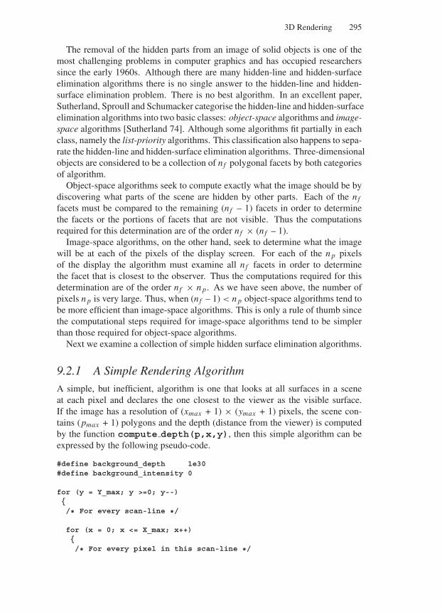
“Comninos” — 2005/8/31 — 18:28 — page 295 — #5
3D Rendering 295
The removal of the hidden parts from an image of solid objects is one of themost challenging problems in computer graphics and has occupied researcherssince the early 1960s. Although there are many hidden-line and hidden-surfaceelimination algorithms there is no single answer to the hidden-line and hidden-surface elimination problem. There is no best algorithm. In an excellent paper,Sutherland, Sproull and Schumacker categorise the hidden-line and hidden-surfaceelimination algorithms into two basic classes: object-space algorithms and image-space algorithms [Sutherland 74]. Although some algorithms fit partially in eachclass, namely the list-priority algorithms. This classification also happens to sepa-rate the hidden-line and hidden-surface elimination algorithms. Three-dimensionalobjects are considered to be a collection of nf polygonal facets by both categoriesof algorithm.
Object-space algorithms seek to compute exactly what the image should be bydiscovering what parts of the scene are hidden by other parts. Each of the nf
facets must be compared to the remaining (nf – 1) facets in order to determinethe facets or the portions of facets that are not visible. Thus the computationsrequired for this determination are of the order nf × (nf – 1).
Image-space algorithms, on the other hand, seek to determine what the imagewill be at each of the pixels of the display screen. For each of the n p pixelsof the display the algorithm must examine all nf facets in order to determinethe facet that is closest to the observer. Thus the computations required for thisdetermination are of the order nf × n p. As we have seen above, the number ofpixels n p is very large. Thus, when (nf – 1) < n p object-space algorithms tend tobe more efficient than image-space algorithms. This is only a rule of thumb sincethe computational steps required for image-space algorithms tend to be simplerthan those required for object-space algorithms.
Next we examine a collection of simple hidden surface elimination algorithms.
9.2.1 A Simple Rendering Algorithm
A simple, but inefficient, algorithm is one that looks at all surfaces in a sceneat each pixel and declares the one closest to the viewer as the visible surface.If the image has a resolution of (xmax + 1) × (ymax + 1) pixels, the scene con-tains (pmax + 1) polygons and the depth (distance from the viewer) is computedby the function compute depth(p,x,y), then this simple algorithm can beexpressed by the following pseudo-code.
#define background_depth 1e30#define background_intensity 0
for (y = Y_max; y >=0; y--)/* For every scan-line */
for (x = 0; x <= X_max; x++)/* For every pixel in this scan-line */
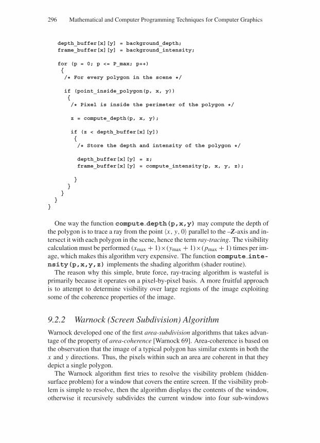
“Comninos” — 2005/8/31 — 18:28 — page 296 — #6
296 Mathematical and Computer Programming Techniques for Computer Graphics
depth_buffer[x][y] = background_depth;frame_buffer[x][y] = background_intensity;
for (p = 0; p <= P_max; p++)/* For every polygon in the scene */
if (point_inside_polygon(p, x, y))/* Pixel is inside the perimeter of the polygon */
z = compute_depth(p, x, y);
if (z < depth_buffer[x][y])/* Store the depth and intensity of the polygon */
depth_buffer[x][y] = z;frame_buffer[x][y] = compute_intensity(p, x, y, z);
One way the function compute depth(p,x,y) may compute the depth ofthe polygon is to trace a ray from the point 〈x, y, 0〉 parallel to the –Z-axis and in-tersect it with each polygon in the scene, hence the term ray-tracing. The visibilitycalculation must be performed (xmax + 1)×(ymax + 1)×(pmax + 1) times per im-age, which makes this algorithm very expensive. The function compute inte-nsity(p,x,y,z) implements the shading algorithm (shader routine).
The reason why this simple, brute force, ray-tracing algorithm is wasteful isprimarily because it operates on a pixel-by-pixel basis. A more fruitful approachis to attempt to determine visibility over large regions of the image exploitingsome of the coherence properties of the image.
9.2.2 Warnock (Screen Subdivision) Algorithm
Warnock developed one of the first area-subdivision algorithms that takes advan-tage of the property of area-coherence [Warnock 69]. Area-coherence is based onthe observation that the image of a typical polygon has similar extents in both thex and y directions. Thus, the pixels within such an area are coherent in that theydepict a single polygon.
The Warnock algorithm first tries to resolve the visibility problem (hidden-surface problem) for a window that covers the entire screen. If the visibility prob-lem is simple to resolve, then the algorithm displays the contents of the window,otherwise it recursively subdivides the current window into four sub-windows
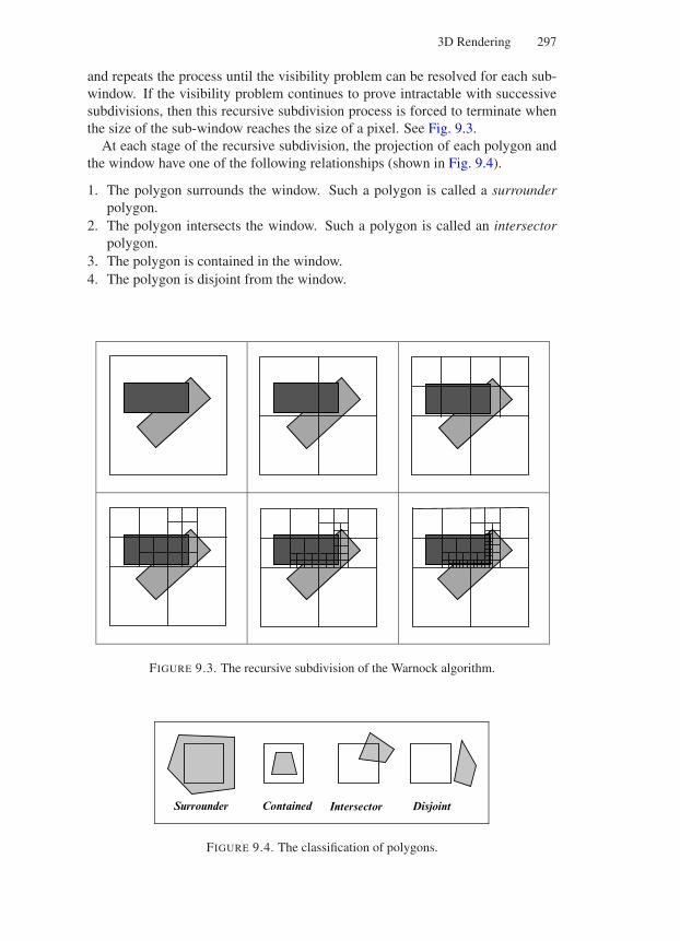
“Comninos” — 2005/8/31 — 18:28 — page 297 — #7
3D Rendering 297
and repeats the process until the visibility problem can be resolved for each sub-window. If the visibility problem continues to prove intractable with successivesubdivisions, then this recursive subdivision process is forced to terminate whenthe size of the sub-window reaches the size of a pixel. See Fig. 9.3.
At each stage of the recursive subdivision, the projection of each polygon andthe window have one of the following relationships (shown in Fig. 9.4).
1. The polygon surrounds the window. Such a polygon is called a surrounderpolygon.
2. The polygon intersects the window. Such a polygon is called an intersectorpolygon.
3. The polygon is contained in the window.4. The polygon is disjoint from the window.
FIGURE 9.3. The recursive subdivision of the Warnock algorithm.
Surrounder Contained Intersector Disjoint
FIGURE 9.4. The classification of polygons.

“Comninos” — 2005/8/31 — 18:28 — page 298 — #8
298 Mathematical and Computer Programming Techniques for Computer Graphics
Decisions about the visibility problem at a given window are made as follows.
1 If all the polygons are disjoint from the window, then
1.1 fill the window with the background colour;1.2 done (return to the caller).
2 If there is only one polygon contained in the window, then
2.1 fill the window with the background colour;2.2 fill the polygon (by scan-converting it);2.3 done (return to the caller).
3 If there is only one polygon intersecting the window then
3.1 fill the window with the background colour;3.2 clip the polygon to the window;3.3 fill the polygon (by scan-converting it);3.4 done (return to the caller).
4 If there is only one polygon surrounding the window then
4.1 clip the polygon to the window;4.2 fill the polygon (by scan-converting it);4.3 done (return to the caller).
otherwise there must be more than one polygons intersecting, contained or sur-rounding the window.
5 If there is only one polygon surrounding the window and it is in front of allother polygons then
5.1 clip the surrounder polygon to the window;5.2 fill this polygon (by scan-converting it);5.3 done (return to the caller).
6 If the size of the window is greater than one pixel then
6.1 recursively subdivide this window into four sub-windows and repeat thealgorithm for each sub-window;
6.2 done (return to the caller). otherwise6.3 compute the depth of all polygons at the centre of the window and use the
closest polygon to colour the pixel;6.4 done (return to the caller).
Determining that the surrounder polygon is in front of all other polygons isdone as follows.for each polygon compute the depth of its plane at the four corners of the window.If there is a surrounder that has z coordinates closer to the viewing point than anyother polygon
then the test succeeds (see Fig. 9.5a);else the test fails (see Fig. 9.5b).
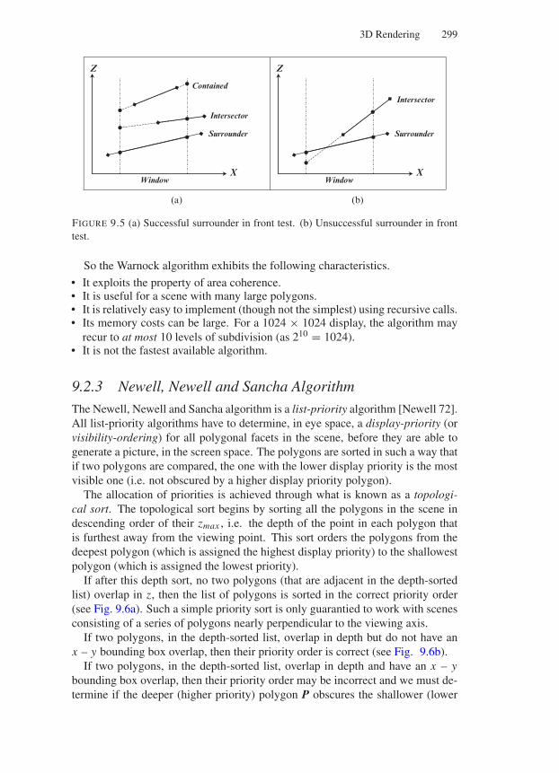
“Comninos” — 2005/8/31 — 18:28 — page 299 — #9
3D Rendering 299
X
Z
Window
(a) (b)
Surrounder
Intersector
Contained
X
Z
Window
Surrounder
Intersector
FIGURE 9.5 (a) Successful surrounder in front test. (b) Unsuccessful surrounder in fronttest.
So the Warnock algorithm exhibits the following characteristics.
• It exploits the property of area coherence.• It is useful for a scene with many large polygons.• It is relatively easy to implement (though not the simplest) using recursive calls.• Its memory costs can be large. For a 1024 × 1024 display, the algorithm may
recur to at most 10 levels of subdivision (as 210 = 1024).• It is not the fastest available algorithm.
9.2.3 Newell, Newell and Sancha Algorithm
The Newell, Newell and Sancha algorithm is a list-priority algorithm [Newell 72].All list-priority algorithms have to determine, in eye space, a display-priority (orvisibility-ordering) for all polygonal facets in the scene, before they are able togenerate a picture, in the screen space. The polygons are sorted in such a way thatif two polygons are compared, the one with the lower display priority is the mostvisible one (i.e. not obscured by a higher display priority polygon).
The allocation of priorities is achieved through what is known as a topologi-cal sort. The topological sort begins by sorting all the polygons in the scene indescending order of their zmax , i.e. the depth of the point in each polygon thatis furthest away from the viewing point. This sort orders the polygons from thedeepest polygon (which is assigned the highest display priority) to the shallowestpolygon (which is assigned the lowest priority).
If after this depth sort, no two polygons (that are adjacent in the depth-sortedlist) overlap in z, then the list of polygons is sorted in the correct priority order(see Fig. 9.6a). Such a simple priority sort is only guarantied to work with scenesconsisting of a series of polygons nearly perpendicular to the viewing axis.
If two polygons, in the depth-sorted list, overlap in depth but do not have anx – y bounding box overlap, then their priority order is correct (see Fig. 9.6b).
If two polygons, in the depth-sorted list, overlap in depth and have an x – ybounding box overlap, then their priority order may be incorrect and we must de-termine if the deeper (higher priority) polygon P obscures the shallower (lower
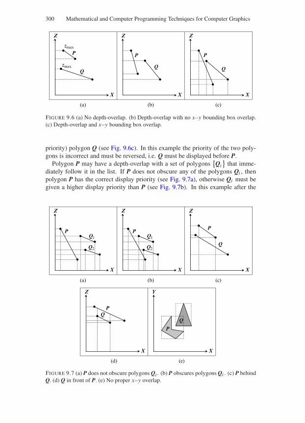
“Comninos” — 2005/8/31 — 18:28 — page 300 — #10
300 Mathematical and Computer Programming Techniques for Computer Graphics
X
Z
P
Q
zmax
zmax
X
Z
P
Q
X
Z
P
Q
(a) (b) (c)
FIGURE 9.6 (a) No depth-overlap. (b) Depth-overlap with no x–y bounding box overlap.(c) Depth-overlap and x–y bounding box overlap.
priority) polygon Q (see Fig. 9.6c). In this example the priority of the two poly-gons is incorrect and must be reversed, i.e. Q must be displayed before P.
Polygon P may have a depth-overlap with a set of polygonsQi
that imme-
diately follow it in the list. If P does not obscure any of the polygons Qi , thenpolygon P has the correct display priority (see Fig. 9.7a), otherwise Qi must begiven a higher display priority than P (see Fig. 9.7b). In this example after the
X
Z
PQ1
Q2
X
Z
PQ1
Q2
X
Z
P
Q
X
Z
PQ
X
Y
P
Q
(a) (b)
(d) (e)
(c)
FIGURE 9.7 (a) P does not obscure polygons Qi . (b) P obscures polygons Qi . (c) P behindQ. (d) Q in front of P. (e) No proper x–y overlap.
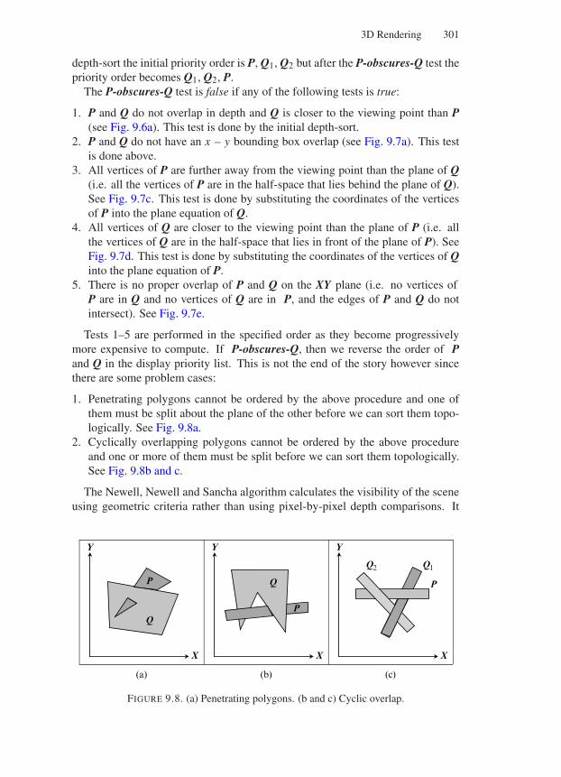
“Comninos” — 2005/8/31 — 18:28 — page 301 — #11
3D Rendering 301
depth-sort the initial priority order is P, Q1, Q2 but after the P-obscures-Q test thepriority order becomes Q1, Q2, P.
The P-obscures-Q test is false if any of the following tests is true:
1. P and Q do not overlap in depth and Q is closer to the viewing point than P(see Fig. 9.6a). This test is done by the initial depth-sort.
2. P and Q do not have an x – y bounding box overlap (see Fig. 9.7a). This testis done above.
3. All vertices of P are further away from the viewing point than the plane of Q(i.e. all the vertices of P are in the half-space that lies behind the plane of Q).See Fig. 9.7c. This test is done by substituting the coordinates of the verticesof P into the plane equation of Q.
4. All vertices of Q are closer to the viewing point than the plane of P (i.e. allthe vertices of Q are in the half-space that lies in front of the plane of P). SeeFig. 9.7d. This test is done by substituting the coordinates of the vertices of Qinto the plane equation of P.
5. There is no proper overlap of P and Q on the XY plane (i.e. no vertices ofP are in Q and no vertices of Q are in P, and the edges of P and Q do notintersect). See Fig. 9.7e.
Tests 1–5 are performed in the specified order as they become progressivelymore expensive to compute. If P-obscures-Q, then we reverse the order of Pand Q in the display priority list. This is not the end of the story however sincethere are some problem cases:
1. Penetrating polygons cannot be ordered by the above procedure and one ofthem must be split about the plane of the other before we can sort them topo-logically. See Fig. 9.8a.
2. Cyclically overlapping polygons cannot be ordered by the above procedureand one or more of them must be split before we can sort them topologically.See Fig. 9.8b and c.
The Newell, Newell and Sancha algorithm calculates the visibility of the sceneusing geometric criteria rather than using pixel-by-pixel depth comparisons. It
X
Y
P
Q
X
Y
P
Q
X
Y
Q1Q2
P
(a) (b) (c)
FIGURE 9.8. (a) Penetrating polygons. (b and c) Cyclic overlap.
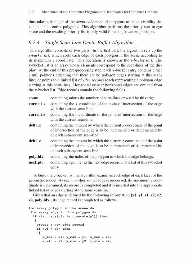
“Comninos” — 2005/8/31 — 18:28 — page 302 — #12
302 Mathematical and Computer Programming Techniques for Computer Graphics
thus takes advantage of the depth coherence of polygons to make visibility de-cisions about entire polygons. This algorithm performs the priority sort in eyespace and the resulting priority list is only valid for a single camera position.
9.2.4 Single Scan-Line Depth-Buffer Algorithm
This algorithm consists of two parts. In the first part, the algorithm sets up they-bucket list, which sorts each edge of each polygon in the scene according toits maximum y coordinate. This operation is known as the y-bucket sort. They-bucket list is an array whose elements correspond to the scan-lines of the dis-play. At the end of this pre-processing step, each y-bucket entry contains eithera null pointer (indicating that there are no polygon edges starting at this scan-line) or points to a linked list of edge records (each representing a polygon edgestarting at this scan-line). Horizontal or near horizontal edges are omitted fromthe y-bucket list. Edge records contain the following fields.
count containing minus the number of scan-lines crossed by this edge.
current x containing the x coordinate of the point of intersection of the edgewith the current scan-line.
current z containing the z coordinate of the point of intersection of the edgewith the current scan-line.
delta x containing the amount by which the current x coordinate of the pointof intersection of the edge is to be incremented or decremented byon each subsequent scan-line.
delta z containing the amount by which the current z coordinate of the pointof intersection of the edge is to be incremented or decremented byon each subsequent scan-line.
poly idx containing the index of the polygon to which the edge belongs.
next ptr containing a pointer to the next edge record in the list of this y-bucketentry.
To build the y-bucket list the algorithm examines each edge of each facet of thegeometric model. As each non-horizontal edge is processed, its maximum y coor-dinate is determined, its record is completed and it is inserted into the appropriatelinked list of edges starting at the same scan-line.
Given that an edge is defined by the following information x1, y1, z1, x2, y2,z2, poly idx, its edge record is completed as follows.
for every polygon in the scene dofor every edge in this polygon doif (truncate(y1) != truncate(y2)) thencreate a new edge record;if (y1 > y2) thenx_max = x1; y_max = y1; z_max = z1;x_min = x2; y_min = y2; z_min = z2;
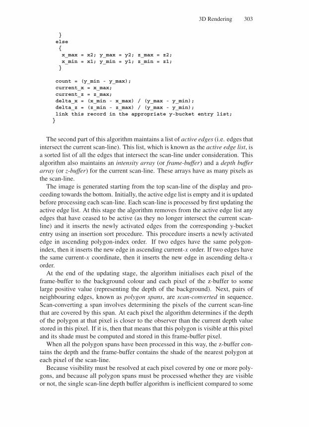
“Comninos” — 2005/8/31 — 18:28 — page 303 — #13
3D Rendering 303
elsex_max = x2; y_max = y2; z_max = z2;x_min = x1; y_min = y1; z_min = z1;
count = (y_min - y_max);current_x = x_max;current_z = z_max;delta_x = (x_min - x_max) / (y_max - y_min);delta_z = (z_min - z_max) / (y_max - y_min);link this record in the appropriate y-bucket entry list;
The second part of this algorithm maintains a list of active edges (i.e. edges thatintersect the current scan-line). This list, which is known as the active edge list, isa sorted list of all the edges that intersect the scan-line under consideration. Thisalgorithm also maintains an intensity array (or frame-buffer) and a depth bufferarray (or z-buffer) for the current scan-line. These arrays have as many pixels asthe scan-line.
The image is generated starting from the top scan-line of the display and pro-ceeding towards the bottom. Initially, the active edge list is empty and it is updatedbefore processing each scan-line. Each scan-line is processed by first updating theactive edge list. At this stage the algorithm removes from the active edge list anyedges that have ceased to be active (as they no longer intersect the current scan-line) and it inserts the newly activated edges from the corresponding y-bucketentry using an insertion sort procedure. This procedure inserts a newly activatededge in ascending polygon-index order. If two edges have the same polygon-index, then it inserts the new edge in ascending current-x order. If two edges havethe same current-x coordinate, then it inserts the new edge in ascending delta-xorder.
At the end of the updating stage, the algorithm initialises each pixel of theframe-buffer to the background colour and each pixel of the z-buffer to somelarge positive value (representing the depth of the background). Next, pairs ofneighbouring edges, known as polygon spans, are scan-converted in sequence.Scan-converting a span involves determining the pixels of the current scan-linethat are covered by this span. At each pixel the algorithm determines if the depthof the polygon at that pixel is closer to the observer than the current depth valuestored in this pixel. If it is, then that means that this polygon is visible at this pixeland its shade must be computed and stored in this frame-buffer pixel.
When all the polygon spans have been processed in this way, the z-buffer con-tains the depth and the frame-buffer contains the shade of the nearest polygon ateach pixel of the scan-line.
Because visibility must be resolved at each pixel covered by one or more poly-gons, and because all polygon spans must be processed whether they are visibleor not, the single scan-line depth buffer algorithm is inefficient compared to some
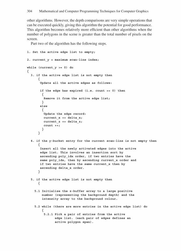
“Comninos” — 2005/8/31 — 18:28 — page 304 — #14
304 Mathematical and Computer Programming Techniques for Computer Graphics
other algorithms. However, the depth comparisons are very simple operations thatcan be executed quickly, giving this algorithm the potential for good performance.This algorithm becomes relatively more efficient than other algorithms when thenumber of polygons in the scene is greater than the total number of pixels on thescreen.
Part two of the algorithm has the following steps.
1. Set the active edge list to empty;
2. current_y = maximum scan-line index;
while (current_y >= 0) do
3. if the active edge list is not empty thenUpdate all the active edges as follows:
if the edge has expired (i.e. count == 0) thenRemove it from the active edge list;
elseUpdate the edge record:current_x += delta_x;current_z += delta_z;count ++;
4. if the y-bucket entry for the current scan-line is not empty thenInsert all the newly activated edges into the activeedge list. This involves an insertion sort byascending poly_idx order, if two entries have thesame poly_idx, then by ascending current_x order andif two entries have the same current_x then byascending delta_x order.
5. if the active edge list is not empty then
5.1 Initialise the z-buffer array to a large positivenumber (representing the background depth) and theintensity array to the background colour.
5.2 while (there are more entries in the active edge list) do5.2.1 Pick a pair of entries from the active
edge list. (each pair of edges defines anactive polygon span).
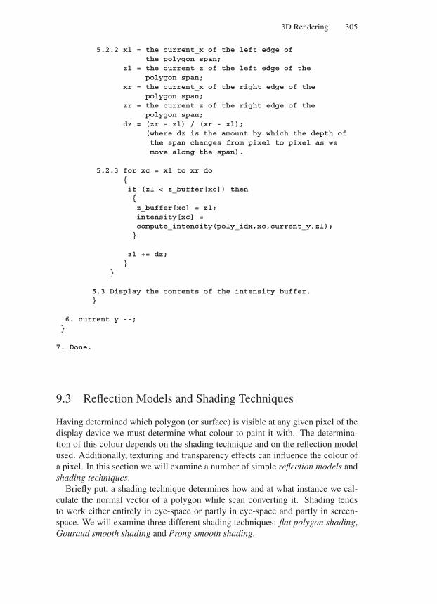
“Comninos” — 2005/8/31 — 18:28 — page 305 — #15
3D Rendering 305
5.2.2 xl = the current_x of the left edge ofthe polygon span;
zl = the current_z of the left edge of thepolygon span;
xr = the current_x of the right edge of thepolygon span;
zr = the current_z of the right edge of thepolygon span;
dz = (zr - zl) / (xr - xl);(where dz is the amount by which the depth ofthe span changes from pixel to pixel as wemove along the span).
5.2.3 for xc = xl to xr doif (zl < z_buffer[xc]) thenz_buffer[xc] = zl;intensity[xc] =compute_intencity(poly_idx,xc,current_y,zl);
zl += dz;
5.3 Display the contents of the intensity buffer.
6. current_y --;
7. Done.
9.3 Reflection Models and Shading Techniques
Having determined which polygon (or surface) is visible at any given pixel of thedisplay device we must determine what colour to paint it with. The determina-tion of this colour depends on the shading technique and on the reflection modelused. Additionally, texturing and transparency effects can influence the colour ofa pixel. In this section we will examine a number of simple reflection models andshading techniques.
Briefly put, a shading technique determines how and at what instance we cal-culate the normal vector of a polygon while scan converting it. Shading tendsto work either entirely in eye-space or partly in eye-space and partly in screen-space. We will examine three different shading techniques: flat polygon shading,Gouraud smooth shading and Prong smooth shading.
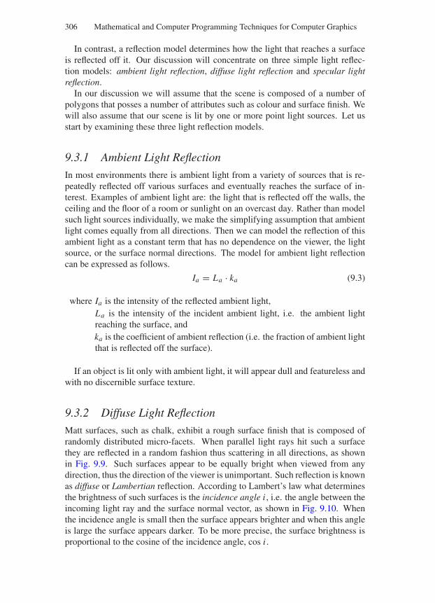
“Comninos” — 2005/8/31 — 18:28 — page 306 — #16
306 Mathematical and Computer Programming Techniques for Computer Graphics
In contrast, a reflection model determines how the light that reaches a surfaceis reflected off it. Our discussion will concentrate on three simple light reflec-tion models: ambient light reflection, diffuse light reflection and specular lightreflection.
In our discussion we will assume that the scene is composed of a number ofpolygons that posses a number of attributes such as colour and surface finish. Wewill also assume that our scene is lit by one or more point light sources. Let usstart by examining these three light reflection models.
9.3.1 Ambient Light Reflection
In most environments there is ambient light from a variety of sources that is re-peatedly reflected off various surfaces and eventually reaches the surface of in-terest. Examples of ambient light are: the light that is reflected off the walls, theceiling and the floor of a room or sunlight on an overcast day. Rather than modelsuch light sources individually, we make the simplifying assumption that ambientlight comes equally from all directions. Then we can model the reflection of thisambient light as a constant term that has no dependence on the viewer, the lightsource, or the surface normal directions. The model for ambient light reflectioncan be expressed as follows.
Ia = La · ka (9.3)
where Ia is the intensity of the reflected ambient light,La is the intensity of the incident ambient light, i.e. the ambient lightreaching the surface, andka is the coefficient of ambient reflection (i.e. the fraction of ambient lightthat is reflected off the surface).
If an object is lit only with ambient light, it will appear dull and featureless andwith no discernible surface texture.
9.3.2 Diffuse Light Reflection
Matt surfaces, such as chalk, exhibit a rough surface finish that is composed ofrandomly distributed micro-facets. When parallel light rays hit such a surfacethey are reflected in a random fashion thus scattering in all directions, as shownin Fig. 9.9. Such surfaces appear to be equally bright when viewed from anydirection, thus the direction of the viewer is unimportant. Such reflection is knownas diffuse or Lambertian reflection. According to Lambert’s law what determinesthe brightness of such surfaces is the incidence angle i , i.e. the angle between theincoming light ray and the surface normal vector, as shown in Fig. 9.10. Whenthe incidence angle is small then the surface appears brighter and when this angleis large the surface appears darker. To be more precise, the surface brightness isproportional to the cosine of the incidence angle, cos i .
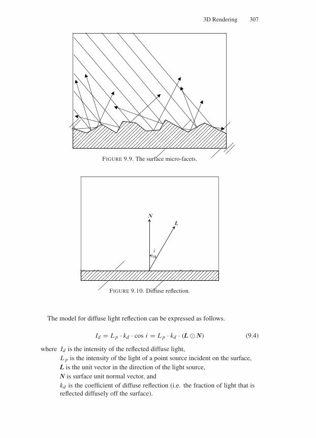
“Comninos” — 2005/8/31 — 18:28 — page 307 — #17
3D Rendering 307
FIGURE 9.9. The surface micro-facets.
NL
i
FIGURE 9.10. Diffuse reflection.
The model for diffuse light reflection can be expressed as follows.
Id = L p · kd · cos i = L p · kd · (L N) (9.4)
where Id is the intensity of the reflected diffuse light,L p is the intensity of the light of a point source incident on the surface,L is the unit vector in the direction of the light source,N is surface unit normal vector, andkd is the coefficient of diffuse reflection (i.e. the fraction of light that isreflected diffusely off the surface).
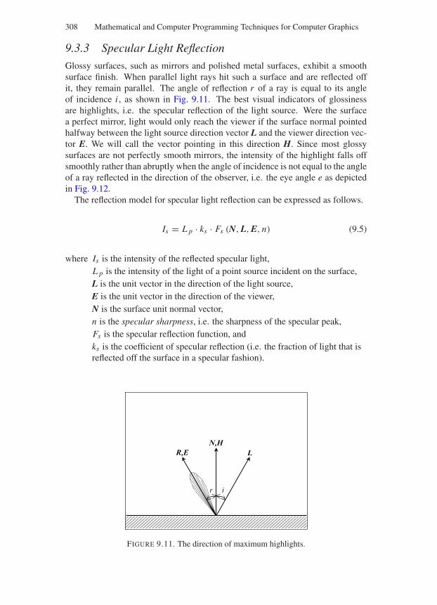
“Comninos” — 2005/8/31 — 18:28 — page 308 — #18
308 Mathematical and Computer Programming Techniques for Computer Graphics
9.3.3 Specular Light Reflection
Glossy surfaces, such as mirrors and polished metal surfaces, exhibit a smoothsurface finish. When parallel light rays hit such a surface and are reflected offit, they remain parallel. The angle of reflection r of a ray is equal to its angleof incidence i , as shown in Fig. 9.11. The best visual indicators of glossinessare highlights, i.e. the specular reflection of the light source. Were the surfacea perfect mirror, light would only reach the viewer if the surface normal pointedhalfway between the light source direction vector L and the viewer direction vec-tor E. We will call the vector pointing in this direction H. Since most glossysurfaces are not perfectly smooth mirrors, the intensity of the highlight falls offsmoothly rather than abruptly when the angle of incidence is not equal to the angleof a ray reflected in the direction of the observer, i.e. the eye angle e as depictedin Fig. 9.12.
The reflection model for specular light reflection can be expressed as follows.
Is = L p · ks · Fs (N, L, E, n) (9.5)
where Is is the intensity of the reflected specular light,L p is the intensity of the light of a point source incident on the surface,L is the unit vector in the direction of the light source,E is the unit vector in the direction of the viewer,N is the surface unit normal vector,n is the specular sharpness, i.e. the sharpness of the specular peak,Fs is the specular reflection function, andks is the coefficient of specular reflection (i.e. the fraction of light that isreflected off the surface in a specular fashion).
N,HL
i
R,E
r
FIGURE 9.11. The direction of maximum highlights.
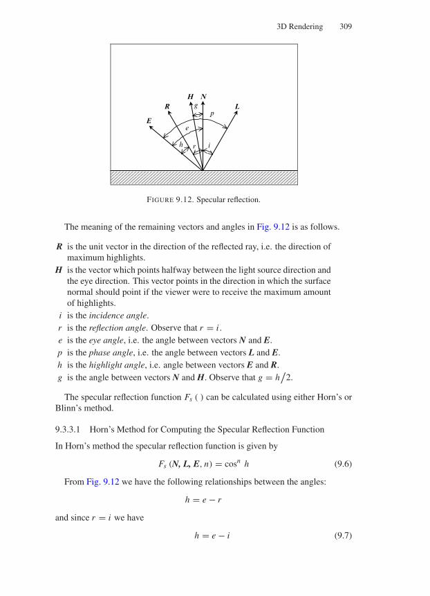
“Comninos” — 2005/8/31 — 18:28 — page 309 — #19
3D Rendering 309
NL
i
E
r
HR
h
gp
e
FIGURE 9.12. Specular reflection.
The meaning of the remaining vectors and angles in Fig. 9.12 is as follows.
R is the unit vector in the direction of the reflected ray, i.e. the direction ofmaximum highlights.
H is the vector which points halfway between the light source direction andthe eye direction. This vector points in the direction in which the surfacenormal should point if the viewer were to receive the maximum amountof highlights.
i is the incidence angle.r is the reflection angle. Observe that r = i .e is the eye angle, i.e. the angle between vectors N and E.p is the phase angle, i.e. the angle between vectors L and E.h is the highlight angle, i.e. angle between vectors E and R.g is the angle between vectors N and H. Observe that g = h
/2.
The specular reflection function Fs ( ) can be calculated using either Horn’s orBlinn’s method.
9.3.3.1 Horn’s Method for Computing the Specular Reflection Function
In Horn’s method the specular reflection function is given by
Fs (N, L, E, n) = cosn h (9.6)
From Fig. 9.12 we have the following relationships between the angles:
h = e − r
and since r = i we have
h = e − i (9.7)
“Comninos” — 2005/8/31 — 18:28 — page 310 — #20
310 Mathematical and Computer Programming Techniques for Computer Graphics
also p = e + i (9.8)
Given the trigonometric identities:
cos (α − β) = cos α · cos β + sin α · sin β (9.9)
and cos (α + β) = cos α · cos β − sin α · sin β (9.10)
Combining Eqs. (9.7) and (9.9), and Eqs. (9.8) and (9.10) we get
cos h = cos (e − i) = cos e · cos i + sin e · sin i (9.11)
and cos p = cos (e + i) = cos e · cos i − sin e · sin i (9.12)
Adding Eqs. (9.11) and (9.12) we can eliminate all the sines:
cos h + cos p = 2 · cos e · cos i
∴ cos h = 2 · cos e · cos i − cos p
∴ cos h = 2 · (N E) · (N L) − (E L) (9.13)
Therefore the specular reflection function can be computed as
Fs (N, L, E, n) = [2 · (N E) · (N L) − (E L)]n (9.14)
where n > 4 for glossy surfaces and n < 2 for less shinny surfaces.
9.3.3.2 Blinn’s Method for Computing the Specular Reflection Function
In Blinn’s method the specular reflection function is given by
Fs (N, L, E, n) = cosn g (9.15)
This is a simplification of Horn’s function based on the observation that g =h/2.
Now, from Fig. 9.12 we have
cos g = N H
where N is known and H is easy to compute as it is the vector halfway betweenthe vectors E and L. Thus
H = E + L|E + L|
Thus the specular reflection function can be computed as
Fs (N, L, E, n) = (N H)n (9.16)
where n > 20 for glossy surfaces and n < 8 for less shinny surfaces.Both Horn’s and Blinn’s methods are essentially the same as g = h/2, but
Horn’s highlights decay faster and are therefore sharper and look more realistic.
“Comninos” — 2005/8/31 — 18:28 — page 311 — #21
3D Rendering 311
9.3.4 Phong’s Lighting Model
Phong’s lighting model is based on the observation that “real life” surfaces aresometimes glossy or chalky or something in-between, and incorporates all threereflection models that we have examined so far. Thus
I = Ia + Id + Is
i.e. I = La · ka + L p · [kd · (L N) + ks · Fs (N, L, E, n)] (9.17)
9.3.4.1 Simulating Multiple Light Sources
Phong’s lighting model can farther be improved by allowing for multiple lightsources.
I = La · ka +m∑
j=1
I j (9.18)
where I is the total intensity of the reflected light,La is the incident ambient light intensity,ka is the ambient reflection coefficient of the surface, 0 ≤ ka ≤ 1,I j is the intensity of reflected light contributed by the j th light source,andm is the number of light sources.
The intensity of reflected light contributed by the j th light source is given by
I j = L pj · [kd · (
L j N) + ks · Fs
(N, L j , E, n
)](9.19)
where L pj is the incident intensity of the j th light source,kd is the coefficient of diffuse reflection of the surface, 0 ≤ kd ≤ 1,ks is the coefficient of specular reflection of the surface, 0 ≤ ks ≤ 1,N is the surface unit normal vector,L j is the unit vector in the direction of the j th light source,E is the unit vector in the direction of the viewer,n is the specular sharpness, andFs is the specular reflection function.
9.3.4.2 Simulating Distant Light Sources
This model can further be improved by attenuating the intensity of reflected lightcontributed by the j th light source, I j , by the distance of this light source fromthe surface. Thus
I j = A(d j
) · L pj · [kd · (
L j N) + ks · Fs
(N, L j , E, n
)](9.20)
where d j is the distance of the j th light source from the surface, andA is the intensity attenuation function.
“Comninos” — 2005/8/31 — 18:28 — page 312 — #22
312 Mathematical and Computer Programming Techniques for Computer Graphics
A number of intensity attenuation functions may be constructed. One suchfunction is
A (d) = 1
d2 + 1(9.21)
Although this function is based on Lambert’s law and it is physically correct,it causes the intensity to decay too dramatically and does not produce good CGresults. Observe that we have augmented Lambert’s law by adding 1 to the de-nominator of the fraction to avoid a division by zero when the light source is verynear the surface.
An alternative attenuation function is
A (d) = 1
d + k(9.22)
where k is an arbitrary constant. This function is based on empirical observation.Another alternative attenuation function is
A (d) = kd (9.23)
where k is an arbitrary constant, 0 ≤ k ≤ 1. This is an empirical function,which is easy to control, and produces good visual results. If, say, we require theintensity contributed by a given light source to fall to half the original intensity ata distance of 20 units from the light source, then we set the value of the constantto k = 0.51/20. In general, if we require the intensity contributed by the lightsource to fall to a fraction f of the original intensity at a distance of d f units fromthe light source, then we set the value of the constant to k = f (1/d f ).
9.3.4.3 Coloured Light Sources
Phong’s lighting model, as presented above, only deals with white ambient lightand white light sources. We can easily modify this lighting model to deal withcoloured lights. To do this we have to rewrite Eq. (9.18) as a set of three equations,one for each of the primary colour components of light.
IR = La R · ka +m∑
j=1I j R
IG = LaG · ka +m∑
j=1I jG
IB = La B · ka +m∑
j=1I j B
(9.24)
where IR, IG , IB are the RGB components of the total intensity of thereflected light,
La R, LaG, La B are the RGB components of the incident ambient lightintensity,
I j R, I jG , I j B are the RGB components of the intensity of reflectedlight contributed by the j th light source,
and all other terms retain their original meaning.
“Comninos” — 2005/8/31 — 18:28 — page 313 — #23
3D Rendering 313
Equation (9.20) will also have to be rewritten as a set of three equations:
I j R = A(d j
) · L pj R · [kd · (
L j N) + ks · Fs
(N, L j , E, n
)]
I jG = A(d j
) · L pjG · [kd · (
L j N) + ks · Fs
(N, L j , E, n
)](9.25)
I j B = A(d j
) · L pj B · [kd · (
L j N) + ks · Fs
(N, L j , E, n
)]
where L pj R, L pjG , L pj B are the RGB components of the incident intensity of thej th light source, and all other terms retain their original meaning.
9.4 Shading Techniques
Having developed a number of reflection models, let us now examine how shadingof a given polygon is achieved. We will examine three simple shading techniques:flat polygon shading, Gouraud smooth shading and Prong smooth shading.
Let us start with the simplest of these techniques.
9.4.1 Flat Polygon Shading Technique
In the simplest case, each polygon is assigned a fixed shade value (i.e. reflectedcolour value). Then whenever the polygon is visible, this fixed shade value iswritten into the appropriate pixel of the frame buffer. To calculate the polygon’sshade value we use the polygon’s normal to calculate the RGB colour compo-nents of the intensity of the reflected light and then we use the components of thepolygon colour to modulate the colour components of this intensity. Thus
SR = PR · IR
SG = PG · IG
SB = PB · IB
(9.26)
where SR, SG , SB are the RGB components of the shade value,PR, PG , PB are the RGB components of the polygon colour, andIR, IG , IB are the RGB components of the total intensity of light
reflected off the polygon.
If a polyhedral object is flat polygon shaded, its individual facets will be dis-cernible and it will appear faceted.
9.4.2 Gouraud Smooth Shading Technique
If the polygons to be displayed are meant to approximate a curved surface, theflat polygon shading technique will produce an object with a faceted appearance,thus betraying the construction method of the geometric model. A possible solu-tion to this problem is to approximate the curved surface with a large number ofpolygons. Then the differences in shade between adjacent polygons will be too
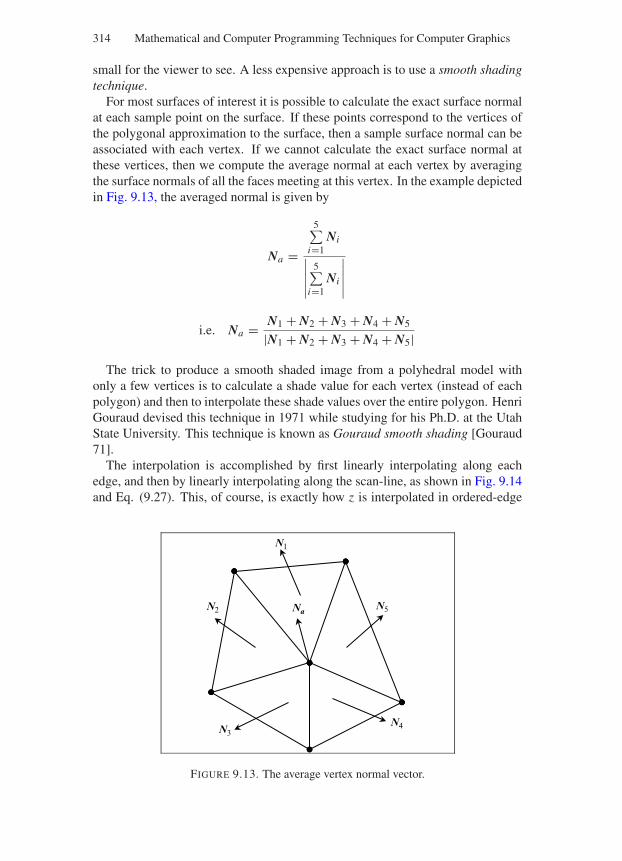
“Comninos” — 2005/8/31 — 18:28 — page 314 — #24
314 Mathematical and Computer Programming Techniques for Computer Graphics
small for the viewer to see. A less expensive approach is to use a smooth shadingtechnique.
For most surfaces of interest it is possible to calculate the exact surface normalat each sample point on the surface. If these points correspond to the vertices ofthe polygonal approximation to the surface, then a sample surface normal can beassociated with each vertex. If we cannot calculate the exact surface normal atthese vertices, then we compute the average normal at each vertex by averagingthe surface normals of all the faces meeting at this vertex. In the example depictedin Fig. 9.13, the averaged normal is given by
Na =
5∑
i=1Ni
∣∣∣∣∣
5∑
i=1Ni
∣∣∣∣∣
i.e. Na = N1 + N2 + N3 + N4 + N5
|N1 + N2 + N3 + N4 + N5|The trick to produce a smooth shaded image from a polyhedral model with
only a few vertices is to calculate a shade value for each vertex (instead of eachpolygon) and then to interpolate these shade values over the entire polygon. HenriGouraud devised this technique in 1971 while studying for his Ph.D. at the UtahState University. This technique is known as Gouraud smooth shading [Gouraud71].
The interpolation is accomplished by first linearly interpolating along eachedge, and then by linearly interpolating along the scan-line, as shown in Fig. 9.14and Eq. (9.27). This, of course, is exactly how z is interpolated in ordered-edge
N1
N2
N3N4
N5Na
FIGURE 9.13. The average vertex normal vector.
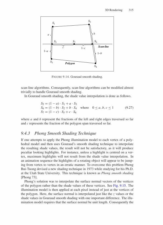
“Comninos” — 2005/8/31 — 18:28 — page 315 — #25
3D Rendering 315
S1
S5
S3
S7 S6
S2
S4
Polygon
Scan-line
a
1−a1−c
1−b
b
c
FIGURE 9.14. Gouraud smooth shading.
scan-line algorithms. Consequently, scan-line algorithms can be modified almosttrivially to handle Gouraud smooth shading.
In Gouraud smooth shading, the shade value interpolation is done as follows.
S5 = (1 − a) · S1 + a · S3S6 = (1 − b) · S2 + b · S4 where 0 ≤ a, b, c ≤ 1S7 = (1 − c) · S5 + c · S6
(9.27)
where a and b represent the fractions of the left and right edges traversed so farand c represents the fraction of the polygon span traversed so far.
9.4.3 Phong Smooth Shading Technique
If one attempts to apply the Phong illumination model to each vertex of a poly-hedral model and then uses Gouraud’s smooth shading technique to interpolatethe resulting shade values, the result will not be satisfactory, as it will producepeculiar looking highlights. For instance, unless a highlight is centred on a ver-tex, maximum highlights will not result from the shade value interpolation. Inan animation sequence the highlights of a rotating object will appear to be jump-ing from vertex to vertex in an erratic manner. To overcome this problem PhongBui-Tuong devised a new shading technique in 1973 while studying for his Ph.D.at the Utah State University. This technique is known as Phong smooth shading[Phong 73].
Phong’s solution was to interpolate the surface normal vectors of the verticesof the polygon rather than the shade values of these vertices. See Fig. 9.15. Theillumination model is then applied at each pixel instead of just at the vertices ofthe polygon. Here, the surface normal is interpolated just like the z values or theshade values in Gouraud smooth shading with one important difference. The illu-mination model requires that the surface normal be unit length. Consequently the
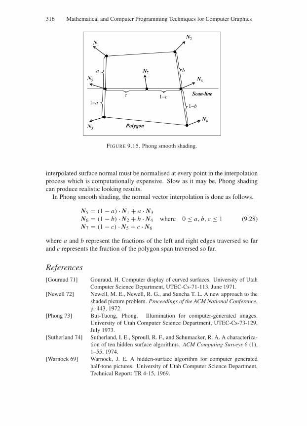
“Comninos” — 2005/8/31 — 18:28 — page 316 — #26
316 Mathematical and Computer Programming Techniques for Computer Graphics
N1
N5
N3
N4
N6
N2
N7a
1−a1−c
1−b
b
c
Polygon
Scan-line
FIGURE 9.15. Phong smooth shading.
interpolated surface normal must be normalised at every point in the interpolationprocess which is computationally expensive. Slow as it may be, Phong shadingcan produce realistic looking results.
In Phong smooth shading, the normal vector interpolation is done as follows.
N5 = (1 − a) · N1 + a · N3N6 = (1 − b) · N2 + b · N4 where 0 ≤ a, b, c ≤ 1N7 = (1 − c) · N5 + c · N6
(9.28)
where a and b represent the fractions of the left and right edges traversed so farand c represents the fraction of the polygon span traversed so far.
References[Gouraud 71] Gouraud, H. Computer display of curved surfaces. University of Utah
Computer Science Department, UTEC-Cs-71-113, June 1971.[Newell 72] Newell, M. E., Newell, R. G., and Sancha T. L. A new approach to the
shaded picture problem. Proceedings of the ACM National Conference,p. 443, 1972.
[Phong 73] Bui-Tuong, Phong. Illumination for computer-generated images.University of Utah Computer Science Department, UTEC-Cs-73-129,July 1973.
[Sutherland 74] Sutherland, I. E., Sproull, R. F., and Schumacker, R. A. A characteriza-tion of ten hidden surface algorithms. ACM Computing Surveys 6 (1),1–55, 1974.
[Warnock 69] Warnock, J. E. A hidden-surface algorithm for computer generatedhalf-tone pictures. University of Utah Computer Science Department,Technical Report: TR 4-15, 1969.
“Comninos” — 2005/8/31 — 19:01 — page 317 — #1
10
Physically Based Lighting and ShadingModels and Rendering Algorithms
In the last chapter we have examined a simple model of how light, emanatingfrom light sources, interacts with the surfaces of objects in a scene. This modelis purely empirical and bears very little relation to what actually takes place inreality. In this chapter we will introduce a much more sophisticated physicallybased model of light and examine how it interacts with the surfaces, volume andsubstance of objects in a computer-generated scene. To do that we must firstexamine the nature of light and of the materials lit by it. We start by examininghow our understanding of light and its perception has evolved over the ages.
10.1 Evolution of the Theory of Light
Much of our interaction with the physical universe is mediated by light or throughimages generated by the mediation of light. So understanding what light is andhow we perceive it has preoccupied human beings since the dawn of history.
The early Greeks believed that Aphrodite, the goddess of love, made the humaneye using the four elements (of water, earth, wind and fire) and lit the fire thatshines out of the eye as light rays, thus making sight possible. This simple beliefdoes not explain why we cannot see at night and why we see shadows during theday. In computer graphics terms this is equivalent to ray tracing a scene which islit by a single point light source situated at the eye.
The Greek philosopher Empedocles of Acrages in Sicily (492–432 BC) ques-tioned this belief and postulated an interaction between the rays from the eyes andthe rays from an external light source such as the sun. In computer graphics termsthis is equivalent to ray tracing a scene which is lit by external light sources.
The Greek mathematician Euclid of Alexandria (325–265 BC) wrote his book“Optica” around 300 BC, in which he presented a mathematical study of lightand optics. Euclid postulated that light travels in straight lines and developed themathematics for the law of reflection.
317
“Comninos” — 2005/8/31 — 19:01 — page 318 — #2
318 Mathematical and Computer Programming Techniques for Computer Graphics
In 50 BC, the Roman poet Titus Lucratius Charus (99–55 BC) wrote a poementitled “On the Nature of the Universe” in which he wrote “the light and the heatof the sun are composed of minute atoms which, when they are shoved off, loseno time in shooting right across the inter-space of air in the direction imparted bythe shove”. He was thus the first person to express the idea that light is composedof particles.
Following the Greeks, the next big breakthrough in our understanding of lightcame from the Arab mathematician Abu Ali al-Hasan ibn al-Haytham who wasborn in Basra (Iraq) in AD 965 and died in Cairo (Egypt) in AD 1040. He wrotethat light emanates from light sources, is reflected off surfaces and enters the eye,thus making sight possible. He used a pinhole camera to prove his point. Inthis type of camera, light enters the camera chamber through a pinhole situatedon the front wall of the chamber and the image is formed upside-down on theback wall of the chamber. His experiment showed that rays emanating from theeye were not required in order to generate an image. Al-Haytham believed thatlight is composed of tiny particles that travel in straight lines. He further believedthat these particles must travel at a very high but finite speed and that their speedvaried depending on the medium through which they travelled, and he thoughtthat this was the reason why refraction took place. Unfortunately, his writingswere not available to European readers until the end of the sixteenth century, hiswork went unnoticed and European thinkers continued to subscribe to the Greekexplanation of sight.
At the beginning of the seventeenth century the German astronomer JohannesKepler (1571–1630) worked on optics and was the first to develop a correct mathe-matical explanation of the camera obscura and to correctly explain how the humaneye works.
In the last third of the seventeenth century two opposing major theories of lightwere put forward. The first theory was put forward by the English mathematicianIsaac Newton (1643–1727). The second theory was developed independently bythe Dutch astronomer Christian Huygens (1629–1695) and by the English scholarRobert Hook (1635–1703). Newton’s theory was corpuscular in nature (i.e. itwas a particle theory), while the Huygens–Hook theories were wave theories. ForNewton’s theory to be correct it was necessary for light to travel faster in densermaterials (which we now know is false) and for the Huygens–Hook theories to becorrect it was necessary for light to travel slower in denser materials (which wenow know is true).
During the eighteenth century most mathematicians and scientists sided withNewton, but in 1799 the English philosopher Thomas Young (1773–1829) pro-duced some experimental results in favour of the wave theory of light.
In 1817, the work of the French mathematician Augustin Jean Fresnel (1788–1827) on light diffraction provided further proof of the validity of the wave theoryof light.
In 1849, the French physicist Armand Hyppolyte Louis Fizeau (1819–1896)determined experimentally the speed of light to be 300,000 km/s.
“Comninos” — 2005/8/31 — 19:01 — page 319 — #3
Physically Based Lighting and Shading Models and Rendering Algorithms 319
In 1862, the English natural philosopher (physicist) James Clark Maxwell(1831–1879) realised that electromagnetic phenomena are related to light whenhe discovered that electromagnetic waves travelled at the same speed as light.Maxwell is considered to be both the person that completed the classical descrip-tion of light and that instigated some of the modern developments in the theory oflight.
In 1887, the German physicist Heinrich Hertz (1857–1894) discovered the pho-toelectric effect. By experimenting he noticed that when he shone ultraviolet lighton two metallic electrodes this lowered the voltage at which a spark would beproduced between the two electrodes. This effect could only be explained usingthe particle theory of light and we now know that it is caused by electrons beingejected from the surface of the electrodes when they are struck by light rays.
In 1905, the German physicist Albert Einstein (1879–1955) published his spe-cial relativity theory in which he suggests that the speed of light remains constantfor all observers independent of their relative velocities. Despite the fact that thisnotion is difficult to accept, it is less paradoxical than the alternative proposedby the classical theory – according to which an observer travelling faster than thespeed of light could arrive at his destination in time to be able to observe himselfsetting off for the journey. In his paper Einstein showed how the photoelectriceffect could be explained if we accept that light is composed of discrete particleswhich are energy quanta. These particles are called photons and derive their namefrom the Greek word ϕωτos (meaning of the light).
In 1915, Einstein published his general relativity theory in which he predictedthat light rays can be bent when passing through a gravitational field.
In 1924, the Indian physicist Satyendranath Bose (1894–1974) put forward thehypothesis that light consists of particles that obeyed certain statistical laws.
In the same year, the French physicist Pierre Raymond duc de Broglie (1892–1887) put forward his wave-particle duality theory that states that matter has boththe properties of waves and particles. Thus, not only photons act as waves butelectrons could as well. Such particles are often referred to as wavicles (short forwave-particles).
In 1926, the American physicist Albert Abraham Michelson (1852–1931) ac-curately established the speed of light to be 299,796 km/s.
By 1930 the stage was set for the Danish physicist Neils Henrik David Bohr(1885–1962) and his group of collaborators to complete the Copenhagen inter-pretation of quantum theory. This interpretation of quantum theory attempts toexplain the dual wave-particle nature of light by stating that light “travels as awave but departs and arrives as a particle”. The main idea behind the Copenhageninterpretation is that observing light waves causes them to change into particles.This interpretation, which seems to indicate that the observer affects the way lightbehaves, although difficult to accept seems to be supported by experimental ev-idence. In 1928, Bohr put forward the complementarity principle which statesthat photons could behave either as waves or as particles but that it is impossibleto observe both these aspects of their behaviour at the same time. Some recent
“Comninos” — 2005/8/31 — 19:01 — page 320 — #4
320 Mathematical and Computer Programming Techniques for Computer Graphics
experiments, however, have created situations where light behaves both as wavesand particles at the same time, which contradicts the complementarity principle.
10.2 Nature of Light
Let us now put together what we know about the nature of light from physics.Light is electromagnetic radiation in a range of wavelengths that can be detectedby the human visual system.
According to the wave-particle duality principle of quantum theory, light ex-hibits properties of both waves and particles. Alternatively, light consists ofquanta (small packets) of excitation of a quantised electromagnetic field, calledphotons. Thus a photon is both a fundamental particle and a small packet of elec-tromagnetic radiation (i.e. an electromagnetic wave). In this sense a photon isthe smallest building block of electromagnetic radiation and all electromagneticradiation (from radio waves to gamma rays) is quantised as photons.
Photons have an infinite lifetime, although they can be created and destroyed.Photons can be created in a variety of ways. For instance, a photon can be createdwhen an electron changes its energy state, during a nuclear transition in a particle–antiparticle collision or due to the fluctuation of an electromagnetic field.
Table 10.1 represents the entire spectrum of electromagnetic radiation. In thistable the various types of electromagnetic waves are tabulated in ascending orderof wavelength. The frequency of each type of wave and the associated energyof the corresponding photon is also shown. A more detailed explanation of theseterms will follow shortly. The wavelength of an electromagnetic wave is measuredin meters (m), its frequency is measured in Hertz (Hz) and the energy of thecorresponding photon is measured in electron-volts (eV). A Hertz is the numberof events per second; thus a wave that completes 10 complete undulations in asecond is said to have a frequency of 10 Hz. An electron-volt is the very smallamount of energy that a free electron gains when it falls through an electrostaticpotential difference of 1 V. Note that 1 eV = 1.602176462 × 10⁻¹⁹ J (joules).
At the top of this table we find γ (gamma) rays. These correspond to the mostenergetic photons with energies in the range of mega-electron-volts, wavelengthsin the range of pico-meters and frequencies in the range of a few hexa-Hertz.While, at the bottom of this table we find extremely low frequency waves thatcan be detected as very base sounds reproduced by subwoofer speakers or in thetransmission of electrical currents. The photons corresponding to such waveshave energies in the range of pico-electron-volts, wavelengths in the range ofmega-meters and frequencies in the range of a few Hertz. Visible light representsa very narrow electromagnetic spectrum band that lies in the wavelength rangebetween 380 and 740 nm and the frequency range of 789 and 480 tera-Hz. Mostof the Sun’s radiation is emitted at this wavelength range and thus the humanvisual system has evolved to detect radiation at this range. Similarly skin sensorshave evolved to detect infrared radiation as heat.
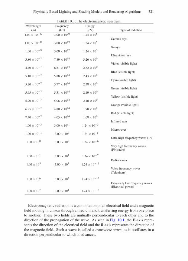
“Comninos” — 2005/8/31 — 19:01 — page 321 — #5
Physically Based Lighting and Shading Models and Rendering Algorithms 321
TABLE 10.1. The electromagnetic spectrum.Wavelength Frequency Energy
(m) (Hz) (eV) Type of radiation
1.00 × 10⁻¹² 3.00 × 10²⁰ 1.24 × 10⁶
Gamma rays1.00 × 10−11 3.00 × 10¹⁹ 1.24 × 10⁵
X-rays1.00 × 10−9 3.00 × 10¹⁷ 1.24 × 10³
Ultraviolet rays3.80 × 10−7 7.89 × 10¹⁴ 3.26 × 100
Violet (visible light)4.40 × 10⁻⁷ 6.81 × 10¹⁴ 2.82 × 100
Blue (visible light)5.10 × 10⁻⁷ 5.88 × 10¹⁴ 2.43 × 100
Cyan (visible light)5.20 × 10⁻⁷ 5.77 × 10¹⁴ 2.38 × 100
Green (visible light)5.65 × 10⁻⁷ 5.31 × 10¹⁴ 2.19 × 100
Yellow (visible light)5.90 × 10⁻⁷ 5.08 × 10¹⁴ 2.10 × 100
Orange (visible light)6.25 × 10⁻⁷ 4.80 × 10¹⁴ 1.98 × 100
Red (visible light)7.40 × 10⁻⁷ 4.05 × 10¹⁴ 1.68 × 100
Infrared rays1.00 × 10−3 3.00 × 10¹¹ 1.24 × 10⁻³
Microwaves1.00 × 10−1 3.00 × 10⁹ 1.24 × 10⁻⁵
Ultra high frequency waves (TV)1.00 × 100 3.00 × 10⁸ 1.24 × 10⁻⁶
Very high frequency waves(FM radio)
1.00 × 101 3.00 × 10⁷ 1.24 × 10⁻⁷
Radio waves1.00 × 105 3.00 × 10³ 1.24 × 10⁻¹¹
Voice frequency waves(Telephony)
1.00 × 10⁶ 3.00 × 10² 1.24 × 10⁻¹²
Extremely low frequency waves(Electrical power)
1.00 × 10⁷ 3.00 × 101 1.24 × 10⁻¹³
Electromagnetic radiation is a combination of an electrical field and a magneticfield moving in unison through a medium and transferring energy from one placeto another. These two fields are mutually perpendicular to each other and to thedirection of the propagation of the wave. As seen in Fig. 10.1, the E-axis repre-sents the direction of the electrical field and the B-axis represents the direction ofthe magnetic field. Such a wave is called a transverse wave, as it oscillates in adirection perpendicular to which it advances.
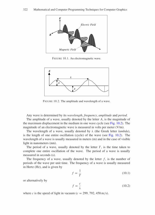
“Comninos” — 2005/8/31 — 19:01 — page 322 — #6
322 Mathematical and Computer Programming Techniques for Computer Graphics
E
B
Electric Field
Magnetic Field
FIGURE 10.1. An electromagnetic wave.
A
E
A
l
FIGURE 10.2. The amplitude and wavelength of a wave.
Any wave is determined by its wavelength, frequency, amplitude and period.The amplitude of a wave, usually denoted by the letter A, is the magnitude of
the maximum displacement in the medium in one wave cycle (see Fig. 10.2). Themagnitude of an electromagnetic wave is measured in volts per meter (V/m).
The wavelength of a wave, usually denoted by λ (the Greek letter lambda),is the length of one entire oscillation (cycle) of the wave (see Fig. 10.2). Thewavelength of a wave is usually measured in meters (m) and in the case of visiblelight in nanometers (nm).
The period of a wave, usually denoted by the letter T , is the time taken tocomplete one entire oscillation of the wave. The period of a wave is usuallymeasured in seconds (s).
The frequency of a wave, usually denoted by the letter f , is the number ofperiods of the wave per unit time. The frequency of a wave is usually measuredin Hertz (Hz), and is given by
f = 1
T(10.1)
or alternatively by
f = c
λ(10.2)
where c is the speed of light in vacuum (c = 299, 792, 458 m/s).
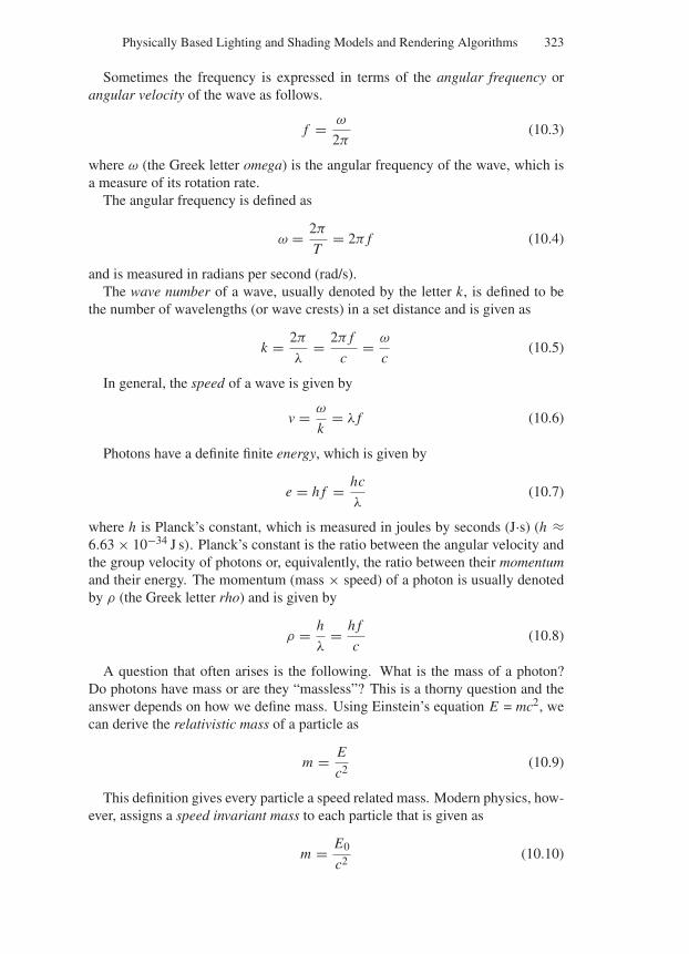
“Comninos” — 2005/8/31 — 19:01 — page 323 — #7
Physically Based Lighting and Shading Models and Rendering Algorithms 323
Sometimes the frequency is expressed in terms of the angular frequency orangular velocity of the wave as follows.
f = ω
2π(10.3)
where ω (the Greek letter omega) is the angular frequency of the wave, which isa measure of its rotation rate.
The angular frequency is defined as
ω = 2π
T= 2π f (10.4)
and is measured in radians per second (rad/s).The wave number of a wave, usually denoted by the letter k, is defined to be
the number of wavelengths (or wave crests) in a set distance and is given as
k = 2π
λ= 2π f
c= ω
c(10.5)
In general, the speed of a wave is given by
v = ω
k= λ f (10.6)
Photons have a definite finite energy, which is given by
e = h f = hc
λ(10.7)
where h is Planck’s constant, which is measured in joules by seconds (J·s) (h ≈6.63 × 10⁻³⁴ J s). Planck’s constant is the ratio between the angular velocity andthe group velocity of photons or, equivalently, the ratio between their momentumand their energy. The momentum (mass × speed) of a photon is usually denotedby ρ (the Greek letter rho) and is given by
ρ = h
λ= h f
c(10.8)
A question that often arises is the following. What is the mass of a photon?Do photons have mass or are they “massless”? This is a thorny question and theanswer depends on how we define mass. Using Einstein’s equation E = mc2, wecan derive the relativistic mass of a particle as
m = E
c2(10.9)
This definition gives every particle a speed related mass. Modern physics, how-ever, assigns a speed invariant mass to each particle that is given as
m = E0
c2(10.10)
“Comninos” — 2005/8/31 — 19:01 — page 324 — #8
324 Mathematical and Computer Programming Techniques for Computer Graphics
where E0 is the energy of a particle at rest (called the rest energy). This mass iscalled the rest mass or invariant mass of the particle. Photons have zero invariantmass.
In vacuum, photons of all wavelengths travel with the speed of light and in theabsence of a gravitational field they travel in a straight line.
In a material, photons behave in a more complex manner. When a photon,which as we have seen is an electromagnetic wave, enters a material, its elec-trical field causes a disturbance to the charges of the electrons of the atoms ofthe material (causing them to oscillate). This disturbance is proportional to thepermittivity of the material. The permittivity, ε, of a material (medium) is a mea-sure of how much the medium changes to absorb energy when subjected to anelectrical field. This oscillation of the charges of the electrons in turn causes theradiation of an electromagnetic wave that is slightly out of phase with the electro-magnetic wave that the photon represents. The sum of these two electromagneticwaves is now a wave with the same frequency but a shorter wavelength than theoriginal electromagnetic wave of the photon. This explains why photons travelslower in materials than they do in the vacuum.
In quantum physics this electromagnetic disturbance caused by the photon en-tering the material is called an excitation and is represented by quasi-particlescalled excitons. Thus when a photon enters a medium it couples with it. Thismeans that the photon gets absorbed and the medium gets excited, which in turnmeans that the photon gets transformed into an exciton. When in this state, iteither gets absorbed by the medium and its energy is stored as heat in the medium(which is likely to occur in opaque materials) or it gets transformed back into aphoton that re-emerges from the surface of the medium into space (which is likelyto occur in transparent materials). This transformation from an exciton back intoa photon is due to the medium relaxing and re-emitting the stored energy in theform of a photon.
This is a simplified explanation of what is believed to occur, but will suffice forthe purposes of our discussion.
10.3 Interaction of Light with Various Materials
There are two distinct illumination phenomena that we will examine in more de-tail below. The interaction of light with the boundaries between different typesof materials and the scattering and absorption of light as it is reflected from thesurface of and transmitted through the volume of different types of materials.
We can categorise the materials found in nature as being homogenous and non-homogenous. Homogenous materials have a constant composition and the sameoptical properties/qualities throughout their volume, while non-homogenous ma-terials are composed of two or more different types of homogenous materials(where one type is embedded within another) and their optical properties mayvary widely throughout their volume (depending on the concentration of the vari-ous homogenous materials that make up their volume).
“Comninos” — 2005/8/31 — 19:01 — page 325 — #9
Physically Based Lighting and Shading Models and Rendering Algorithms 325
Homogenous materials can be further subdivided into opaque and transparentmaterials.
Opaque materials are frequently called conductors or conducting materials, asthey tend to be good conductors of electrical currents. Examples of conductingmaterials are iron and copper. Some opaque materials, however, are bad con-ductors, such as plastics and wood. Opaque materials prevent light from passingthrough their volume.
Transparent materials are frequently called dielectric materials, as they tend tobe insulators (i.e. they do not conduct electrical currents). Examples of dielectricmaterials are gases and glass. Some transparent materials, however, are goodconductors, such as water and other liquids. Transparent materials allow light topass through their volume.
Some materials are called translucent, because they are semitransparent. Theyallow light to pass through them only diffusely. Thus, we can see light passingthough such materials but we cannot see a clear image. Examples of translucentmaterials are smoke, steam, paper, frosted glass and some plastics.
In computer graphics we are usually interested in the behaviour of light at thesurface between two different types of material. We shall call such a surfacethe interface and the two materials either side of it the participating materials orparticipating media. Of most interest are the interface between two transparentmaterials and between a transparent and an opaque material.
When a beam of light, consisting of many photons, collides with the interfacebetween two participating materials, we observe the phenomena of reflection, re-fraction and transmission, scattering, absorption and subsurface scattering.
10.3.1 Light Reflection
Light reflection is a phenomenon observed when a light beam travels throughthe first participating medium, collides with the interface surface, its direction oftravel changes abruptly and continues to travel in the first participating medium.We can distinguish two types of reflections, namely specular reflections and dif-fuse reflections. Specular or mirror-like reflections are most pronounced when theinterface surface between the two participating media is smooth (shiny). In thiscase an incoming ray of light is reflected in one direction as shown in Fig. 10.3. Inthis figure, N represents the unit normal vector of the surface, the angle θi (knownas the angle of incidence) is the angle between the incoming ray and the surfacenormal, and the angle θr (known as the angle of reflection) is the angle betweenthe reflected (outgoing) ray and the surface normal. The law of reflection statesthat θi = θr . If the light beam collides with the interface surface at right angles,then the light beam bounces in the direction from which it came. This kind ifreflection is called retro-reflection.
Diffuse reflections are most pronounced when the interface surface betweenthe two participating media is rough (matt) and can be seen to be composed ofmany micro-facets, as shown in Fig. 10.4a. In this case an incoming ray of lightis reflected in many different directions, as shown in Fig. 10.4. In Fig. 10.4b, N
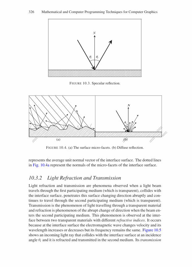
“Comninos” — 2005/8/31 — 19:01 — page 326 — #10
326 Mathematical and Computer Programming Techniques for Computer Graphics
N
θi θr
FIGURE 10.3. Specular reflection.
N
iq
(a) (b)
FIGURE 10.4. (a) The surface micro-facets. (b) Diffuse reflection.
represents the average unit normal vector of the interface surface. The dotted linesin Fig. 10.4a represent the normals of the micro-facets of the interface surface.
10.3.2 Light Refraction and Transmission
Light refraction and transmission are phenomena observed when a light beamtravels through the first participating medium (which is transparent), collides withthe interface surface, penetrates this surface changing direction abruptly and con-tinues to travel through the second participating medium (which is transparent).Transmission is the phenomenon of light travelling through a transparent materialand refraction is phenomenon of the abrupt change of direction when the beam en-ters the second participating medium. This phenomenon is observed at the inter-face between two transparent materials with different refractive indices. It occursbecause at the interface surface the electromagnetic wave changes velocity and itswavelength increases or decreases but its frequency remains the same. Figure 10.5shows an incoming light ray that collides with the interface surface at an incidenceangle θi and it is refracted and transmitted in the second medium. Its transmission
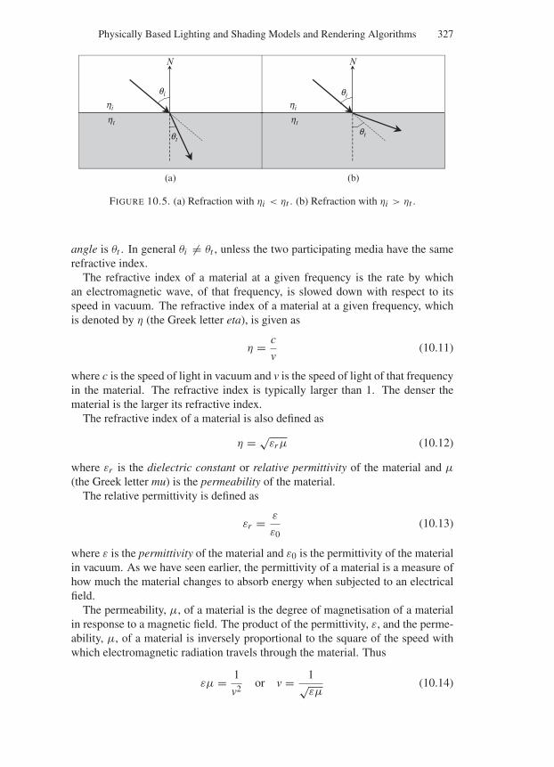
“Comninos” — 2005/8/31 — 19:01 — page 327 — #11
Physically Based Lighting and Shading Models and Rendering Algorithms 327
N
qi
qt
hi
ht
N
qi
qt
hi
ht
(a) (b)
FIGURE 10.5. (a) Refraction with ηi < ηt . (b) Refraction with ηi > ηt .
angle is θt . In general θi = θt , unless the two participating media have the samerefractive index.
The refractive index of a material at a given frequency is the rate by whichan electromagnetic wave, of that frequency, is slowed down with respect to itsspeed in vacuum. The refractive index of a material at a given frequency, whichis denoted by η (the Greek letter eta), is given as
η = c
v(10.11)
where c is the speed of light in vacuum and v is the speed of light of that frequencyin the material. The refractive index is typically larger than 1. The denser thematerial is the larger its refractive index.
The refractive index of a material is also defined as
η = √εrµ (10.12)
where εr is the dielectric constant or relative permittivity of the material and µ
(the Greek letter mu) is the permeability of the material.The relative permittivity is defined as
εr = ε
ε0(10.13)
where ε is the permittivity of the material and ε0 is the permittivity of the materialin vacuum. As we have seen earlier, the permittivity of a material is a measure ofhow much the material changes to absorb energy when subjected to an electricalfield.
The permeability, µ, of a material is the degree of magnetisation of a materialin response to a magnetic field. The product of the permittivity, ε, and the perme-ability, µ, of a material is inversely proportional to the square of the speed withwhich electromagnetic radiation travels through the material. Thus
εµ = 1
v2or v = 1√
εµ(10.14)
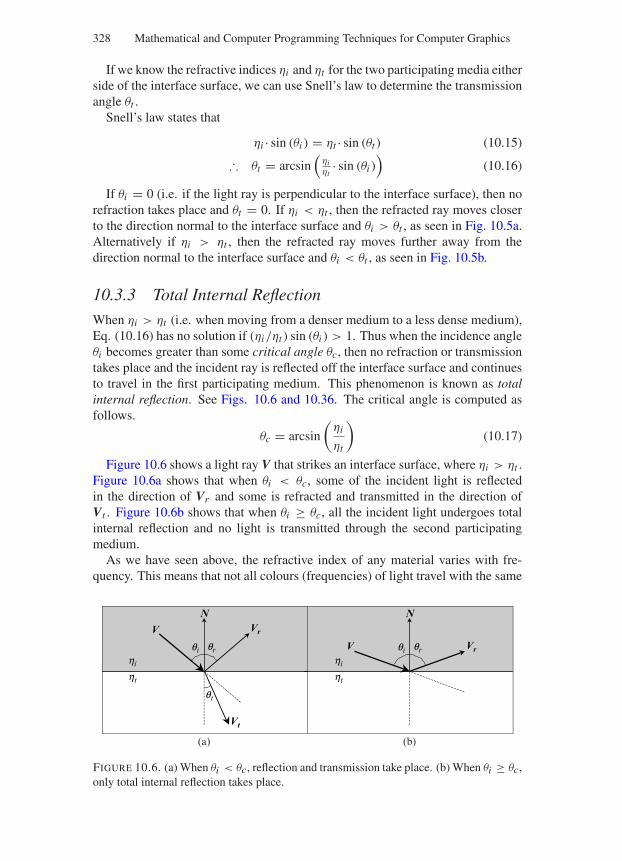
“Comninos” — 2005/8/31 — 19:01 — page 328 — #12
328 Mathematical and Computer Programming Techniques for Computer Graphics
If we know the refractive indices ηi and ηt for the two participating media eitherside of the interface surface, we can use Snell’s law to determine the transmissionangle θt .
Snell’s law states that
ηi · sin (θi ) = ηt · sin (θt ) (10.15)
∴ θt = arcsin(
ηiηt
· sin (θi ))
(10.16)
If θi = 0 (i.e. if the light ray is perpendicular to the interface surface), then norefraction takes place and θt = 0. If ηi < ηt , then the refracted ray moves closerto the direction normal to the interface surface and θi > θt , as seen in Fig. 10.5a.Alternatively if ηi > ηt , then the refracted ray moves further away from thedirection normal to the interface surface and θi < θt , as seen in Fig. 10.5b.
10.3.3 Total Internal Reflection
When ηi > ηt (i.e. when moving from a denser medium to a less dense medium),Eq. (10.16) has no solution if (ηi/ηt ) sin (θi ) > 1. Thus when the incidence angleθi becomes greater than some critical angle θc, then no refraction or transmissiontakes place and the incident ray is reflected off the interface surface and continuesto travel in the first participating medium. This phenomenon is known as totalinternal reflection. See Figs. 10.6 and 10.36. The critical angle is computed asfollows.
θc = arcsin
(ηi
ηt
)(10.17)
Figure 10.6 shows a light ray V that strikes an interface surface, where ηi > ηt .Figure 10.6a shows that when θi < θc, some of the incident light is reflectedin the direction of Vr and some is refracted and transmitted in the direction ofVt . Figure 10.6b shows that when θi ≥ θc, all the incident light undergoes totalinternal reflection and no light is transmitted through the second participatingmedium.
As we have seen above, the refractive index of any material varies with fre-quency. This means that not all colours (frequencies) of light travel with the same
N
V
Vt
Vr
N
V Vr
qt
qi qrhi
ht
qi qrhi
ht
(a) (b)
FIGURE 10.6. (a) When θi < θc, reflection and transmission take place. (b) When θi ≥ θc,only total internal reflection takes place.
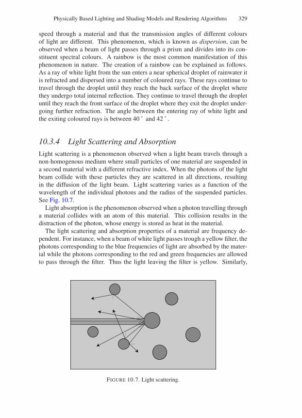
“Comninos” — 2005/8/31 — 19:01 — page 329 — #13
Physically Based Lighting and Shading Models and Rendering Algorithms 329
speed through a material and that the transmission angles of different coloursof light are different. This phenomenon, which is known as dispersion, can beobserved when a beam of light passes through a prism and divides into its con-stituent spectral colours. A rainbow is the most common manifestation of thisphenomenon in nature. The creation of a rainbow can be explained as follows.As a ray of white light from the sun enters a near spherical droplet of rainwater itis refracted and dispersed into a number of coloured rays. These rays continue totravel through the droplet until they reach the back surface of the droplet wherethey undergo total internal reflection. They continue to travel through the dropletuntil they reach the front surface of the droplet where they exit the droplet under-going further refraction. The angle between the entering ray of white light andthe exiting coloured rays is between 40 ˚ and 42 ˚ .
10.3.4 Light Scattering and Absorption
Light scattering is a phenomenon observed when a light beam travels through anon-homogenous medium where small particles of one material are suspended ina second material with a different refractive index. When the photons of the lightbeam collide with these particles they are scattered in all directions, resultingin the diffusion of the light beam. Light scattering varies as a function of thewavelength of the individual photons and the radius of the suspended particles.See Fig. 10.7.
Light absorption is the phenomenon observed when a photon travelling througha material collides with an atom of this material. This collision results in thedistraction of the photon, whose energy is stored as heat in the material.
The light scattering and absorption properties of a material are frequency de-pendent. For instance, when a beam of white light passes trough a yellow filter, thephotons corresponding to the blue frequencies of light are absorbed by the mater-ial while the photons corresponding to the red and green frequencies are allowedto pass through the filter. Thus the light leaving the filter is yellow. Similarly,
FIGURE 10.7. Light scattering.
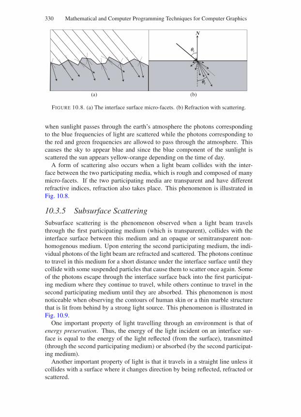
“Comninos” — 2005/8/31 — 19:01 — page 330 — #14
330 Mathematical and Computer Programming Techniques for Computer Graphics
N
qt
qi
(a) (b)
FIGURE 10.8. (a) The interface surface micro-facets. (b) Refraction with scattering.
when sunlight passes through the earth’s atmosphere the photons correspondingto the blue frequencies of light are scattered while the photons corresponding tothe red and green frequencies are allowed to pass through the atmosphere. Thiscauses the sky to appear blue and since the blue component of the sunlight isscattered the sun appears yellow-orange depending on the time of day.
A form of scattering also occurs when a light beam collides with the inter-face between the two participating media, which is rough and composed of manymicro-facets. If the two participating media are transparent and have differentrefractive indices, refraction also takes place. This phenomenon is illustrated inFig. 10.8.
10.3.5 Subsurface Scattering
Subsurface scattering is the phenomenon observed when a light beam travelsthrough the first participating medium (which is transparent), collides with theinterface surface between this medium and an opaque or semitransparent non-homogenous medium. Upon entering the second participating medium, the indi-vidual photons of the light beam are refracted and scattered. The photons continueto travel in this medium for a short distance under the interface surface until theycollide with some suspended particles that cause them to scatter once again. Someof the photons escape through the interface surface back into the first participat-ing medium where they continue to travel, while others continue to travel in thesecond participating medium until they are absorbed. This phenomenon is mostnoticeable when observing the contours of human skin or a thin marble structurethat is lit from behind by a strong light source. This phenomenon is illustrated inFig. 10.9.
One important property of light travelling through an environment is that ofenergy preservation. Thus, the energy of the light incident on an interface sur-face is equal to the energy of the light reflected (from the surface), transmitted(through the second participating medium) or absorbed (by the second participat-ing medium).
Another important property of light is that it travels in a straight line unless itcollides with a surface where it changes direction by being reflected, refracted orscattered.
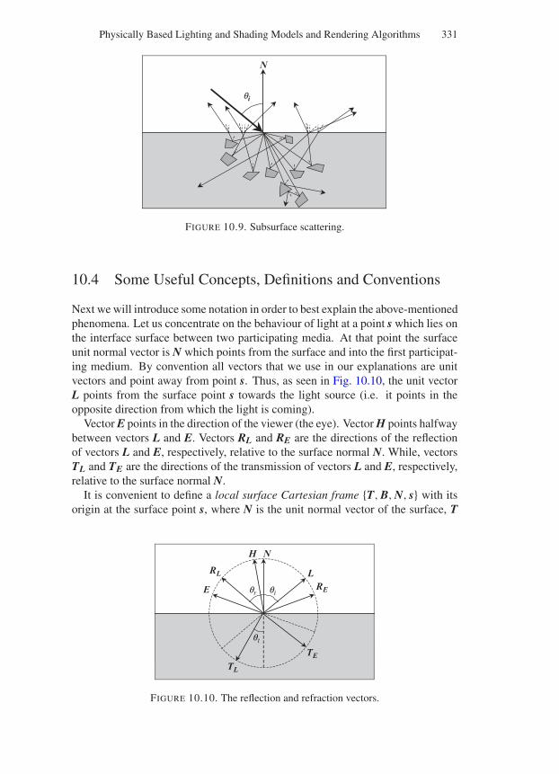
“Comninos” — 2005/8/31 — 19:01 — page 331 — #15
Physically Based Lighting and Shading Models and Rendering Algorithms 331
N
qi
FIGURE 10.9. Subsurface scattering.
10.4 Some Useful Concepts, Definitions and Conventions
Next we will introduce some notation in order to best explain the above-mentionedphenomena. Let us concentrate on the behaviour of light at a point s which lies onthe interface surface between two participating media. At that point the surfaceunit normal vector is N which points from the surface and into the first participat-ing medium. By convention all vectors that we use in our explanations are unitvectors and point away from point s. Thus, as seen in Fig. 10.10, the unit vectorL points from the surface point s towards the light source (i.e. it points in theopposite direction from which the light is coming).
Vector E points in the direction of the viewer (the eye). Vector H points halfwaybetween vectors L and E. Vectors RL and RE are the directions of the reflectionof vectors L and E, respectively, relative to the surface normal N. While, vectorsTL and TE are the directions of the transmission of vectors L and E, respectively,relative to the surface normal N.
It is convenient to define a local surface Cartesian frame T, B, N, s with itsorigin at the surface point s, where N is the unit normal vector of the surface, T
N
LRL
TL
E RE
H
TE
qiqr
qt
FIGURE 10.10. The reflection and refraction vectors.
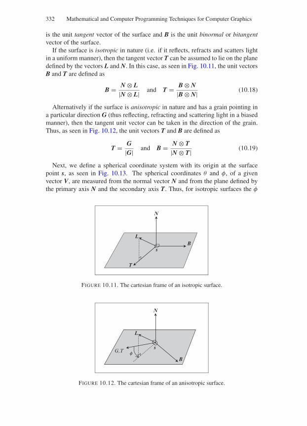
“Comninos” — 2005/8/31 — 19:01 — page 332 — #16
332 Mathematical and Computer Programming Techniques for Computer Graphics
is the unit tangent vector of the surface and B is the unit binormal or bitangentvector of the surface.
If the surface is isotropic in nature (i.e. if it reflects, refracts and scatters lightin a uniform manner), then the tangent vector T can be assumed to lie on the planedefined by the vectors L and N. In this case, as seen in Fig. 10.11, the unit vectorsB and T are defined as
B = N ⊗ L|N ⊗ L| and T = B ⊗ N
|B ⊗ N| (10.18)
Alternatively if the surface is anisotropic in nature and has a grain pointing ina particular direction G (thus reflecting, refracting and scattering light in a biasedmanner), then the tangent unit vector can be taken in the direction of the grain.Thus, as seen in Fig. 10.12, the unit vectors T and B are defined as
T = G|G| and B = N ⊗ T
|N ⊗ T| (10.19)
Next, we define a spherical coordinate system with its origin at the surfacepoint s, as seen in Fig. 10.13. The spherical coordinates θ and φ, of a givenvector V, are measured from the normal vector N and from the plane defined bythe primary axis N and the secondary axis T. Thus, for isotropic surfaces the φ
N
LB
T
s
FIGURE 10.11. The cartesian frame of an isotropic surface.
N
L
B
G,Ts
f
FIGURE 10.12. The cartesian frame of an anisotropic surface.
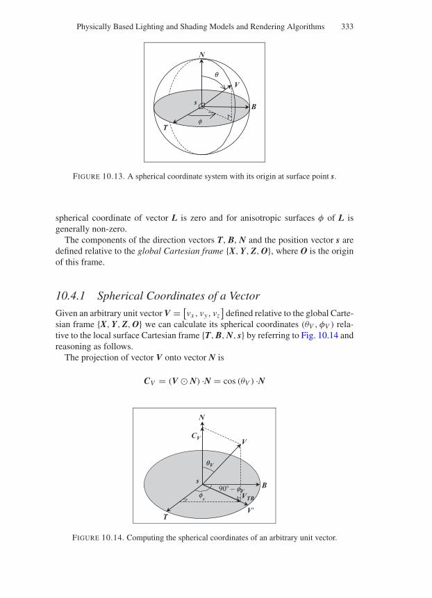
“Comninos” — 2005/8/31 — 19:01 — page 333 — #17
Physically Based Lighting and Shading Models and Rendering Algorithms 333
N
V
B
T
s
f
q
FIGURE 10.13. A spherical coordinate system with its origin at surface point s.
spherical coordinate of vector L is zero and for anisotropic surfaces φ of L isgenerally non-zero.
The components of the direction vectors T, B, N and the position vector s aredefined relative to the global Cartesian frame X, Y, Z, O, where O is the originof this frame.
10.4.1 Spherical Coordinates of a Vector
Given an arbitrary unit vector V = [vx , vy, vz]
defined relative to the global Carte-sian frame X, Y, Z, O we can calculate its spherical coordinates (θV , φV ) rela-tive to the local surface Cartesian frame T, B, N, s by referring to Fig. 10.14 andreasoning as follows.
The projection of vector V onto vector N is
CV = (V N) ·N = cos (θV ) ·N
N
V
B
T
qV
fV
s
VTB
V
CV
90 − fV
FIGURE 10.14. Computing the spherical coordinates of an arbitrary unit vector.
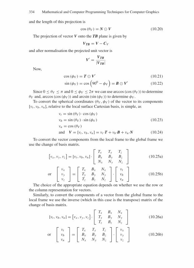
“Comninos” — 2005/8/31 — 19:01 — page 334 — #18
334 Mathematical and Computer Programming Techniques for Computer Graphics
and the length of this projection is
cos (θV ) = N V (10.20)
The projection of vector V onto the TB plane is given by
VTB = V − CV
and after normalisation the projected unit vector is
V′ = VTB
|VTB|Now,
cos (φV ) = T V′ (10.21)
sin (φV ) = cos(
900 − φV
)= B V′ (10.22)
Since 0 ≤ θV ≤ π and 0 ≤ φV ≤ 2π we can use arccos (cos (θV )) to determineθV and, arccos (cos (φV )) and arcsin (sin (φV )) to determine φV .
To convert the spherical coordinates (θV , φV ) of the vector to its components[vt , vb, vn], relative to the local surface Cartesian basis, is simple, as
vt = sin (θV ) · cos (φV )
vb = sin (θV ) · sin (φV ) (10.23)
vn = cos (θV )
and V = [vt , vb, vn] = vt ·T + vb·B + vn ·N (10.24)
To convert the vector components from the local frame to the global frame weuse the change of basis matrix.
[vx , vy, vz
] = [vt , vb, vn] ·⎡
⎣Tx Ty Tz
Bx By Bz
Nx Ny Nz
⎤
⎦ (10.25a)
or
⎡
⎣vx
vy
vz
⎤
⎦ =⎡
⎣Tx Bx Nx
Ty By Ny
Tz Bz Nz
⎤
⎦ ·⎡
⎣vt
vb
vn
⎤
⎦ (10.25b)
The choice of the appropriate equation depends on whether we use the row orthe column representation for vectors.
Similarly, to convert the components of a vector from the global frame to thelocal frame we use the inverse (which in this case is the transpose) matrix of thechange of basis matrix.
[vt , vb, vn] = [vx , vy, vz] ·⎡
⎣Tx Bx Nx
Ty By Ny
Tz Bz Nz
⎤
⎦ (10.26a)
or
⎡
⎣vt
vb
vn
⎤
⎦ =⎡
⎣Tx Ty Tz
Bx By Bz
Nx Ny Nz
⎤
⎦ ·⎡
⎣vx
vy
vz
⎤
⎦ (10.26b)
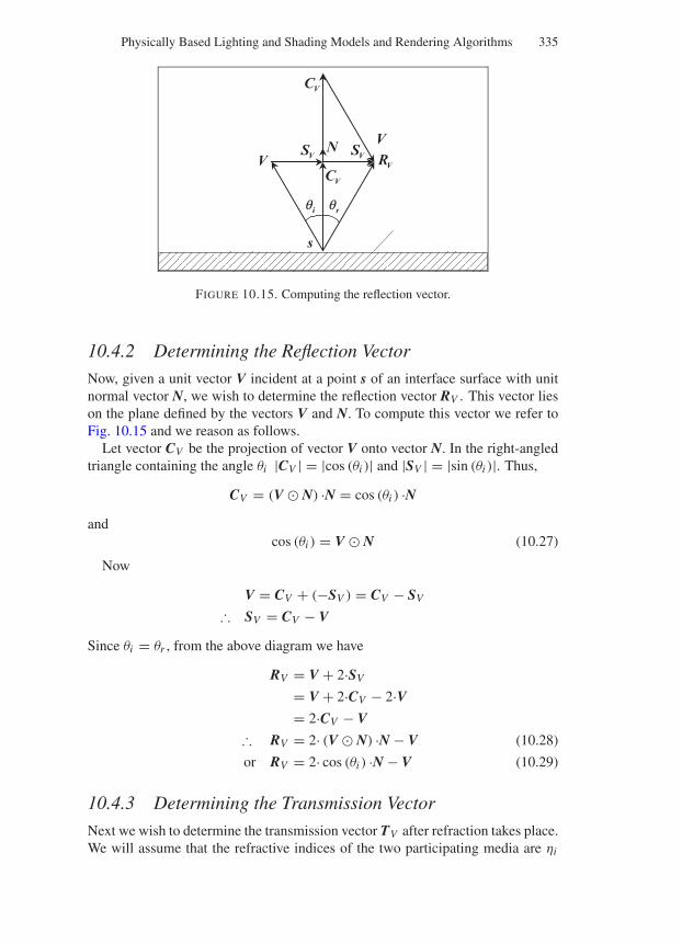
“Comninos” — 2005/8/31 — 19:01 — page 335 — #19
Physically Based Lighting and Shading Models and Rendering Algorithms 335
NV VR
VC
VS
iq rq
VSV
VC
s
FIGURE 10.15. Computing the reflection vector.
10.4.2 Determining the Reflection Vector
Now, given a unit vector V incident at a point s of an interface surface with unitnormal vector N, we wish to determine the reflection vector RV . This vector lieson the plane defined by the vectors V and N. To compute this vector we refer toFig. 10.15 and we reason as follows.
Let vector CV be the projection of vector V onto vector N. In the right-angledtriangle containing the angle θi |CV | = |cos (θi )| and |SV | = |sin (θi )|. Thus,
CV = (V N) ·N = cos (θi ) ·Nand
cos (θi ) = V N (10.27)
Now
V = CV + (−SV ) = CV − SV
∴ SV = CV − V
Since θi = θr , from the above diagram we have
RV = V + 2·SV
= V + 2·CV − 2·V= 2·CV − V
∴ RV = 2· (V N) ·N − V (10.28)
or RV = 2· cos (θi ) ·N − V (10.29)
10.4.3 Determining the Transmission Vector
Next we wish to determine the transmission vector TV after refraction takes place.We will assume that the refractive indices of the two participating media are ηi
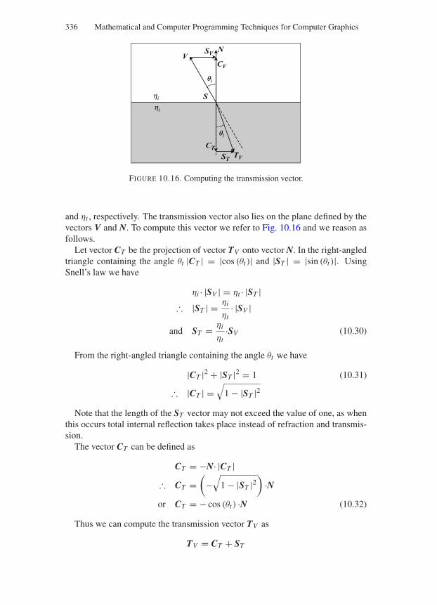
“Comninos” — 2005/8/31 — 19:01 — page 336 — #20
336 Mathematical and Computer Programming Techniques for Computer Graphics
NV
S
TV
SV
CV
CT
ST
qi
qt
hi
ht
FIGURE 10.16. Computing the transmission vector.
and ηt , respectively. The transmission vector also lies on the plane defined by thevectors V and N. To compute this vector we refer to Fig. 10.16 and we reason asfollows.
Let vector CT be the projection of vector TV onto vector N. In the right-angledtriangle containing the angle θt |CT | = |cos (θt )| and |ST | = |sin (θt )|. UsingSnell’s law we have
ηi · |SV | = ηt · |ST |∴ |ST | = ηi
ηt· |SV |
and ST = ηi
ηt·SV (10.30)
From the right-angled triangle containing the angle θt we have
|CT |2 + |ST |2 = 1 (10.31)
∴ |CT | =√
1 − |ST |2
Note that the length of the ST vector may not exceed the value of one, as whenthis occurs total internal reflection takes place instead of refraction and transmis-sion.
The vector CT can be defined as
CT = −N· |CT |∴ CT =
(−√
1 − |ST |2)
·Nor CT = − cos (θt ) ·N (10.32)
Thus we can compute the transmission vector TV as
TV = CT + ST
“Comninos” — 2005/8/31 — 19:01 — page 337 — #21
Physically Based Lighting and Shading Models and Rendering Algorithms 337
Using Eqs. (10.32) and (10.30) we can expand this to
TV = ηi
ηt·SV − cos (θt ) ·N
∴ TV = ηi
ηt· (CV − V) − cos (θt ) ·N
∴ TV = ηi
ηt· [cos (θi ) ·N − V] − cos (θt ) ·N
∴ TV =[ηi
ηt· cos (θi ) − cos (θt )
]·N − ηi
ηt·V (10.33)
To compute the cosine of the transmission angle we start from Eq. (10.31) andproceed as follows.
|CT |2 = 1 − |ST |2∴ cos2 (θt ) = 1 − sin2 (θt ) and
cos (θt ) =√
1 − sin2 (θt )
=√
1 − (sin (θt ))2
=√
1 −[ηi
ηtsin (θi )
]2
=√
1 −(
ηi
ηt
)2
· sin2 (θi )
∴ cos (θt ) =√
1 −(
ηi
ηt
)2
· [1 − cos2 (θi )]
(10.34)
Thus collecting all the above results we have
cos (θi ) = V N
cos (θt ) =√
1 −(
ηi
ηt
)2
· [1 − cos2 (θi )]
RV = 2· cos (θi ) ·N − V
TV =[ηi
ηt· cos (θi ) − cos (θt )
]·N − ηi
ηt·V
10.4.4 Illuminating Hemisphere and Solid Angles
Given a synthetic scene that we wish to render, we will assume that its geometryconsists of a finite set of surfaces that exist in E3. Each surface is assumed to bea two-dimensional differentiable manifold Mi with boundary ∂Mi . A 2D man-ifold is an entity that is topologically equivalent to a 2D Euclidean space. Thusa polygon and its outline or a curved surface patch and its boundary curves, al-though they may exist in a 3D Euclidean space, they are topologically equivalent
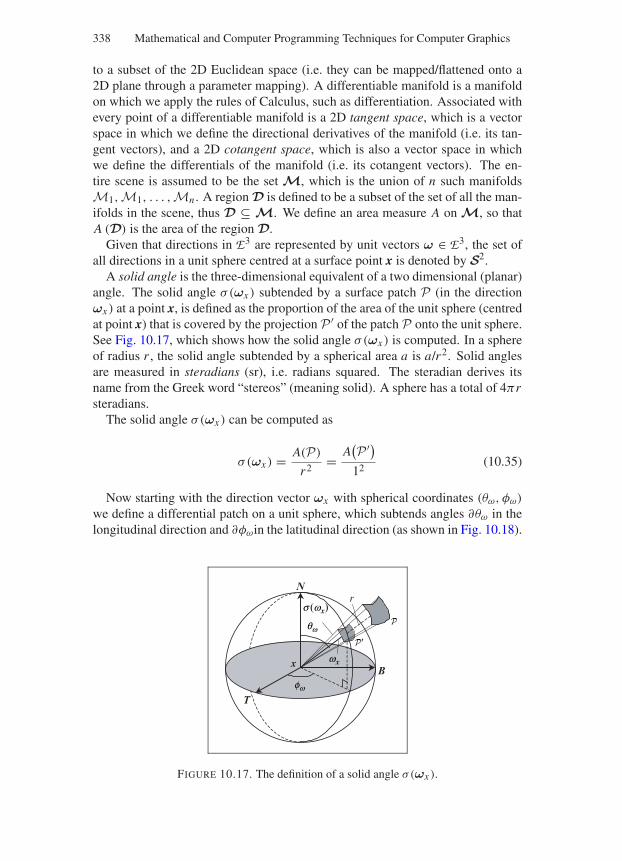
“Comninos” — 2005/8/31 — 19:01 — page 338 — #22
338 Mathematical and Computer Programming Techniques for Computer Graphics
to a subset of the 2D Euclidean space (i.e. they can be mapped/flattened onto a2D plane through a parameter mapping). A differentiable manifold is a manifoldon which we apply the rules of Calculus, such as differentiation. Associated withevery point of a differentiable manifold is a 2D tangent space, which is a vectorspace in which we define the directional derivatives of the manifold (i.e. its tan-gent vectors), and a 2D cotangent space, which is also a vector space in whichwe define the differentials of the manifold (i.e. its cotangent vectors). The en-tire scene is assumed to be the set M, which is the union of n such manifoldsM1,M1, . . . ,Mn . A region D is defined to be a subset of the set of all the man-ifolds in the scene, thus D ⊆ M. We define an area measure A on M, so thatA (D) is the area of the region D.
Given that directions in E3 are represented by unit vectors ω ∈ E3, the set ofall directions in a unit sphere centred at a surface point x is denoted by S2.
A solid angle is the three-dimensional equivalent of a two dimensional (planar)angle. The solid angle σ(ωx ) subtended by a surface patch P (in the directionωx ) at a point x, is defined as the proportion of the area of the unit sphere (centredat point x) that is covered by the projection P ′ of the patch P onto the unit sphere.See Fig. 10.17, which shows how the solid angle σ(ωx ) is computed. In a sphereof radius r , the solid angle subtended by a spherical area a is a/r2. Solid anglesare measured in steradians (sr), i.e. radians squared. The steradian derives itsname from the Greek word “stereos” (meaning solid). A sphere has a total of 4πrsteradians.
The solid angle σ(ωx ) can be computed as
σ(ωx ) = A(P)
r2= A(P ′)
12(10.35)
Now starting with the direction vector ωx with spherical coordinates (θω, φω)
we define a differential patch on a unit sphere, which subtends angles ∂θω in thelongitudinal direction and ∂φωin the latitudinal direction (as shown in Fig. 10.18).
N
wx
s (wx)
qw
fw
B
T
x
9
r
FIGURE 10.17. The definition of a solid angle σ(ωx ).
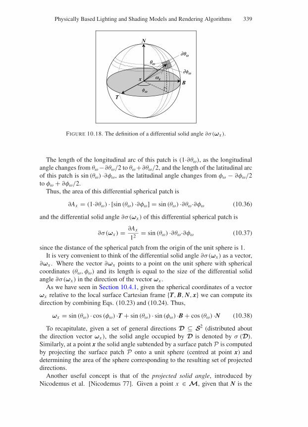
“Comninos” — 2005/8/31 — 19:01 — page 339 — #23
Physically Based Lighting and Shading Models and Rendering Algorithms 339
N
B
T
x wx
qw
∂qw
fw
∂fw
FIGURE 10.18. The definition of a differential solid angle ∂σ(ωx ).
The length of the longitudinal arc of this patch is (1·∂θω), as the longitudinalangle changes from θω −∂θω/2 to θω +∂θω/2, and the length of the latitudinal arcof this patch is sin (θω) ·∂φω, as the latitudinal angle changes from φω − ∂φω/2to φω + ∂φω/2.
Thus, the area of this differential spherical patch is
∂Ax = (1·∂θω) · [sin (θω) ·∂φω] = sin (θω) ·∂θω·∂φω (10.36)
and the differential solid angle ∂σ (ωx ) of this differential spherical patch is
∂σ (ωx ) = ∂Ax
12= sin (θω) ·∂θω·∂φω (10.37)
since the distance of the spherical patch from the origin of the unit sphere is 1.It is very convenient to think of the differential solid angle ∂σ (ωx ) as a vector,
∂ωx . Where the vector ∂ωx points to a point on the unit sphere with sphericalcoordinates (θω, φω) and its length is equal to the size of the differential solidangle ∂σ (ωx ) in the direction of the vector ωx .
As we have seen in Section 10.4.1, given the spherical coordinates of a vectorωx relative to the local surface Cartesian frame T, B, N, x we can compute itsdirection by combining Eqs. (10.23) and (10.24). Thus,
ωx = sin (θω) · cos (φω) ·T + sin (θω) · sin (φω) ·B + cos (θω) ·N (10.38)
To recapitulate, given a set of general directions D ⊆ S2 (distributed aboutthe direction vector ωx ), the solid angle occupied by D is denoted by σ (D).Similarly, at a point x the solid angle subtended by a surface patch P is computedby projecting the surface patch P onto a unit sphere (centred at point x) anddetermining the area of the sphere corresponding to the resulting set of projecteddirections.
Another useful concept is that of the projected solid angle, introduced byNicodemus et al. [Nicodemus 77]. Given a point x ∈ M, given that N is the
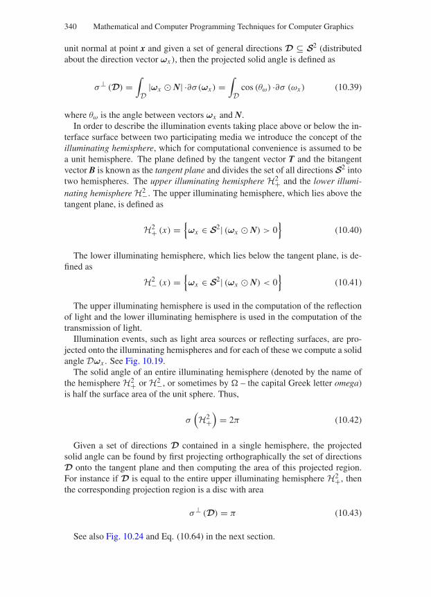
“Comninos” — 2005/8/31 — 19:01 — page 340 — #24
340 Mathematical and Computer Programming Techniques for Computer Graphics
unit normal at point x and given a set of general directions D ⊆ S2 (distributedabout the direction vector ωx ), then the projected solid angle is defined as
σ⊥ (D) =∫
D|ωx N| ·∂σ (ωx ) =
∫
Dcos (θω) ·∂σ (ωx ) (10.39)
where θω is the angle between vectors ωx and N.In order to describe the illumination events taking place above or below the in-
terface surface between two participating media we introduce the concept of theilluminating hemisphere, which for computational convenience is assumed to bea unit hemisphere. The plane defined by the tangent vector T and the bitangentvector B is known as the tangent plane and divides the set of all directions S2 intotwo hemispheres. The upper illuminating hemisphere H2+ and the lower illumi-nating hemisphere H2−. The upper illuminating hemisphere, which lies above thetangent plane, is defined as
H2+ (x) =ωx ∈ S2| (ωx N) > 0
(10.40)
The lower illuminating hemisphere, which lies below the tangent plane, is de-fined as
H2− (x) =ωx ∈ S2| (ωx N) < 0
(10.41)
The upper illuminating hemisphere is used in the computation of the reflectionof light and the lower illuminating hemisphere is used in the computation of thetransmission of light.
Illumination events, such as light area sources or reflecting surfaces, are pro-jected onto the illuminating hemispheres and for each of these we compute a solidangle Dωx . See Fig. 10.19.
The solid angle of an entire illuminating hemisphere (denoted by the name ofthe hemisphere H2+ or H2−, or sometimes by – the capital Greek letter omega)is half the surface area of the unit sphere. Thus,
σ(H2+)
= 2π (10.42)
Given a set of directions D contained in a single hemisphere, the projectedsolid angle can be found by first projecting orthographically the set of directionsD onto the tangent plane and then computing the area of this projected region.For instance if D is equal to the entire upper illuminating hemisphere H2+, thenthe corresponding projection region is a disc with area
σ⊥ (D) = π (10.43)
See also Fig. 10.24 and Eq. (10.64) in the next section.
“Comninos” — 2005/8/31 — 19:01 — page 341 — #25
Physically Based Lighting and Shading Models and Rendering Algorithms 341
N
B
T
xwx1Dwx2
12
9192
FIGURE 10.19. The definition of a number of solid angles.
10.5 Some Basic Terminology of Lighting
As we have seen before, light sources radiate energy in the form of photons. Theenergy of a photon, whose wavelength is λ, is denoted by eλ and is given as
eλ = h·cλ
(10.44)
where h is Planck’s constant and c is the speed of light.The energy of a beam of n photons of wavelength λ is known as the spectral
radiant energy Qλ and is defined as
Qλ = n·eλ = n·h·cλ
(10.45)
The energy of a collection of photons over the entire visible spectrum is knownas the radiant energy Q and is defined as the sum or integral of spectral radiantenergy over the entire wavelength spectrum. Thus,
Q =∫ ∞
0Qλ∂λ (10.46)
The radiant energies Qλ and Q are measured in Joules per nano-meter (J·nm−1)
and Joules (J), respectively.The rate of flow of the radiant energy Q over time t is known as the radiant
power, radiant flux or simply flux and is given by
Φ = ∂ Q
∂t(10.47)
Flux is the radiant energy flowing through a surface per unit time and is mea-sured in Watts (W), where watts are joules per second.
Similarly, the rate of flow of spectral radiant energy Qλ over time t is calledthe spectral radiant flux or simply spectral flux and is given by
Φλ = ∂ Qλ
∂t(10.48)
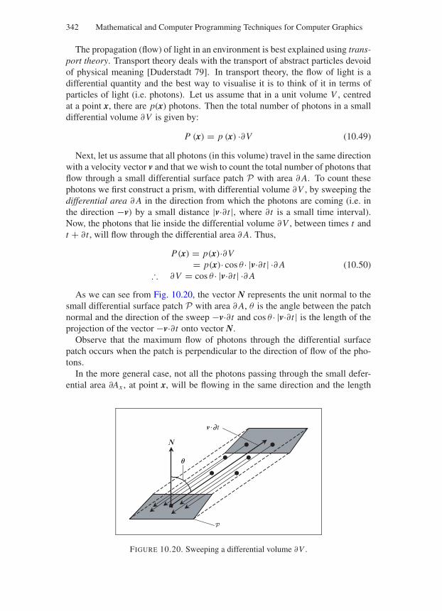
“Comninos” — 2005/8/31 — 19:01 — page 342 — #26
342 Mathematical and Computer Programming Techniques for Computer Graphics
The propagation (flow) of light in an environment is best explained using trans-port theory. Transport theory deals with the transport of abstract particles devoidof physical meaning [Duderstadt 79]. In transport theory, the flow of light is adifferential quantity and the best way to visualise it is to think of it in terms ofparticles of light (i.e. photons). Let us assume that in a unit volume V , centredat a point x, there are p(x) photons. Then the total number of photons in a smalldifferential volume ∂V is given by:
P (x) = p (x) ·∂V (10.49)
Next, let us assume that all photons (in this volume) travel in the same directionwith a velocity vector v and that we wish to count the total number of photons thatflow through a small differential surface patch P with area ∂ A. To count thesephotons we first construct a prism, with differential volume ∂V , by sweeping thedifferential area ∂ A in the direction from which the photons are coming (i.e. inthe direction −v) by a small distance |v·∂t |, where ∂t is a small time interval).Now, the photons that lie inside the differential volume ∂V , between times t andt + ∂t , will flow through the differential area ∂ A. Thus,
P(x) = p(x)·∂V= p(x)· cos θ · |v·∂t | ·∂ A
∴ ∂V = cos θ · |v·∂t | ·∂ A(10.50)
As we can see from Fig. 10.20, the vector N represents the unit normal to thesmall differential surface patch P with area ∂ A, θ is the angle between the patchnormal and the direction of the sweep −v·∂t and cos θ · |v·∂t | is the length of theprojection of the vector −v·∂t onto vector N.
Observe that the maximum flow of photons through the differential surfacepatch occurs when the patch is perpendicular to the direction of flow of the pho-tons.
In the more general case, not all the photons passing through the small defer-ential area ∂Ax , at point x, will be flowing in the same direction and the length
N
v.∂t
q
FIGURE 10.20. Sweeping a differential volume ∂V .
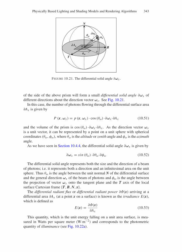
“Comninos” — 2005/8/31 — 19:01 — page 343 — #27
Physically Based Lighting and Shading Models and Rendering Algorithms 343
N
B
T
x
wx
∂wx
∂Ax
fw
qw
FIGURE 10.21. The differential solid angle ∂ωx .
of the side of the above prism will form a small differential solid angle ∂ωx ofdifferent directions about the direction vector ωx . See Fig. 10.21.
In this case, the number of photons flowing through the differential surface area∂Ax is given by
P (x,ωx ) = p (x,ωx ) · cos (θω) ·∂ωx ·∂Ax (10.51)
and the volume of the prism is cos (θω) ·∂ωx ·∂Ax . As the direction vector ωx
is a unit vector, it can be represented by a point on a unit sphere with sphericalcoordinates (θω, φω), where θω is the altitude or zenith angle and φω is the azimuthangle.
As we have seen in Section 10.4.4, the differential solid angle ∂ωx is given by
∂ωx = sin (θω) ·∂θω·∂φω (10.52)
The differential solid angle represents both the size and the direction of a beamof photons; i.e. it represents both a direction and an infinitesimal area on the unitsphere. Thus θω is the angle between the unit normal N of the differential surfaceand the general direction ωx of the beam of photons and φω is the angle betweenthe projection of vector ωx onto the tangent plane and the T axis of the localsurface Cartesian frame T, B, N, x.
The differential radiant flux or differential radiant power ∂Φ(x) arriving at adifferential area ∂Ax (at a point x on a surface) is known as the irradiance E(x),which is defined as
E(x) = ∂Φ(x)
∂Ax(10.53)
This quantity, which is the unit energy falling on a unit area surface, is mea-sured in Watts per square meter (W·m−2) and corresponds to the photometricquantity of illuminance (see Fig. 10.22a).
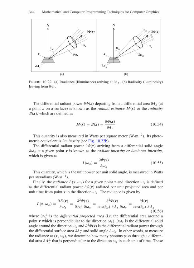
“Comninos” — 2005/8/31 — 19:01 — page 344 — #28
344 Mathematical and Computer Programming Techniques for Computer Graphics
ωx ωx
∂Ax ∂Ax
x
∂Φ(x) ∂Φ(x)
∂ωx ∂ωx
N
x
N
θω θω
(a) (b)
FIGURE 10.22. (a) Irradiance (Illuminance) arriving at ∂Ax . (b) Radiosity (Luminosity)leaving from ∂Ax .
The differential radiant power ∂Φ(x) departing from a differential area ∂Ax (ata point x on a surface) is known as the radiant exitance M(x) or the radiosityB(x), which are defined as
M(x) = B(x) = ∂Φ(x)
∂Ax(10.54)
This quantity is also measured in Watts per square meter (W·m−2). Its photo-metric equivalent is luminosity (see Fig. 10.22b).
The differential radiant power ∂Φ(x) arriving from a differential solid angle∂ωx at a given point x is known as the radiant intensity or luminous intensity,which is given as
I (ωx ) = ∂Φ(x)
∂ωx(10.55)
This quantity, which is the unit power per unit solid angle, is measured in Wattsper steradians (W·sr−1).
Finally, the radiance L(x,ωx ) for a given point x and direction ωx is definedas the differential radiant power ∂Φ(x) radiated per unit projected area and perunit time from point x in the direction ωx . The radiance is given by
L(x,ωx ) = ∂ E(x)
∂ωx= ∂2Φ(x)
∂ A⊥x ·∂ωx
= ∂2Φ(x)
cos(θω)·∂ Ax ·∂ωx= ∂I(x)
cos(θω)·∂ Ax(10.56)
where ∂A⊥x is the differential projected area (i.e. the differential area around a
point x which is perpendicular to the direction ωx ), ∂ωx is the differential solidangle around the direction ωx and ∂2Φ(x) is the differential radiant power throughthe differential surface area ∂A⊥
x and solid angle ∂ωx . In other words, to measurethe radiance at (x, ωx ), we determine how many photons pass through a differen-tial area ∂ A⊥
x that is perpendicular to the direction ωx in each unit of time. These
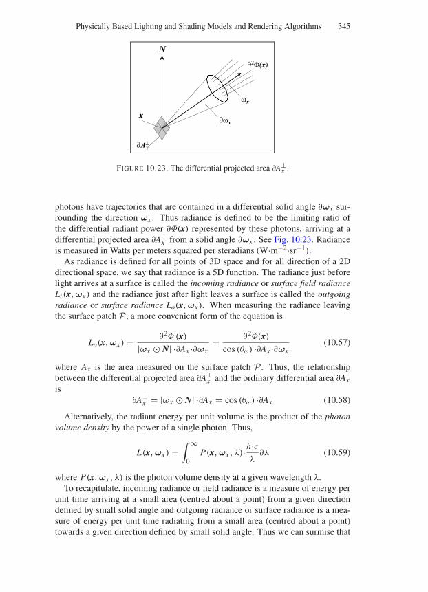
“Comninos” — 2005/8/31 — 19:01 — page 345 — #29
Physically Based Lighting and Shading Models and Rendering Algorithms 345
x
N
∂Ax^
∂ωx
ωx
∂2Φ(x)
FIGURE 10.23. The differential projected area ∂A⊥x .
photons have trajectories that are contained in a differential solid angle ∂ωx sur-rounding the direction ωx . Thus radiance is defined to be the limiting ratio ofthe differential radiant power ∂Φ(x) represented by these photons, arriving at adifferential projected area ∂A⊥
x from a solid angle ∂ωx . See Fig. 10.23. Radianceis measured in Watts per meters squared per steradians (W·m−2·sr−1).
As radiance is defined for all points of 3D space and for all direction of a 2Ddirectional space, we say that radiance is a 5D function. The radiance just beforelight arrives at a surface is called the incoming radiance or surface field radianceLi (x,ωx ) and the radiance just after light leaves a surface is called the outgoingradiance or surface radiance Lo(x,ωx ). When measuring the radiance leavingthe surface patch P , a more convenient form of the equation is
Lo(x,ωx ) = ∂2Φ (x)
|ωx N| ·∂Ax ·∂ωx= ∂2Φ(x)
cos (θω) ·∂Ax ·∂ωx(10.57)
where Ax is the area measured on the surface patch P . Thus, the relationshipbetween the differential projected area ∂A⊥
x and the ordinary differential area ∂Ax
is∂A⊥
x = |ωx N| ·∂Ax = cos (θω) ·∂Ax (10.58)
Alternatively, the radiant energy per unit volume is the product of the photonvolume density by the power of a single photon. Thus,
L(x,ωx ) =∫ ∞
0P(x,ωx , λ)·h·c
λ∂λ (10.59)
where P(x,ωx , λ) is the photon volume density at a given wavelength λ.To recapitulate, incoming radiance or field radiance is a measure of energy per
unit time arriving at a small area (centred about a point) from a given directiondefined by small solid angle and outgoing radiance or surface radiance is a mea-sure of energy per unit time radiating from a small area (centred about a point)towards a given direction defined by small solid angle. Thus we can surmise that
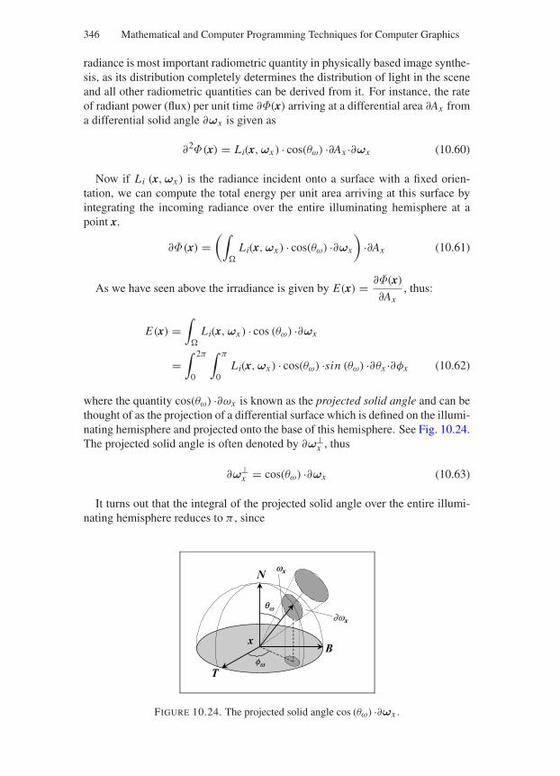
“Comninos” — 2005/8/31 — 19:01 — page 346 — #30
346 Mathematical and Computer Programming Techniques for Computer Graphics
radiance is most important radiometric quantity in physically based image synthe-sis, as its distribution completely determines the distribution of light in the sceneand all other radiometric quantities can be derived from it. For instance, the rateof radiant power (flux) per unit time ∂Φ(x) arriving at a differential area ∂Ax froma differential solid angle ∂ωx is given as
∂2Φ(x) = Li(x,ωx ) · cos(θω) ·∂Ax ·∂ωx (10.60)
Now if Li (x,ωx ) is the radiance incident onto a surface with a fixed orien-tation, we can compute the total energy per unit area arriving at this surface byintegrating the incoming radiance over the entire illuminating hemisphere at apoint x.
∂Φ(x) =(∫
Li(x,ωx ) · cos(θω) ·∂ωx
)·∂Ax (10.61)
As we have seen above the irradiance is given by E(x) = ∂Φ(x)
∂Ax, thus:
E(x) =∫
Li(x,ωx ) · cos (θω) ·∂ωx
=∫ 2π
0
∫ π
0Li(x,ωx ) · cos(θω) ·sin (θω) ·∂θx ·∂φx (10.62)
where the quantity cos(θω) ·∂ωx is known as the projected solid angle and can bethought of as the projection of a differential surface which is defined on the illumi-nating hemisphere and projected onto the base of this hemisphere. See Fig. 10.24.The projected solid angle is often denoted by ∂ω⊥
x , thus
∂ω⊥x = cos(θω) ·∂ωx (10.63)
It turns out that the integral of the projected solid angle over the entire illumi-nating hemisphere reduces to π , since
N
B
T
x
∂wx
wx
qw
fw
FIGURE 10.24. The projected solid angle cos (θω) ·∂ωx .
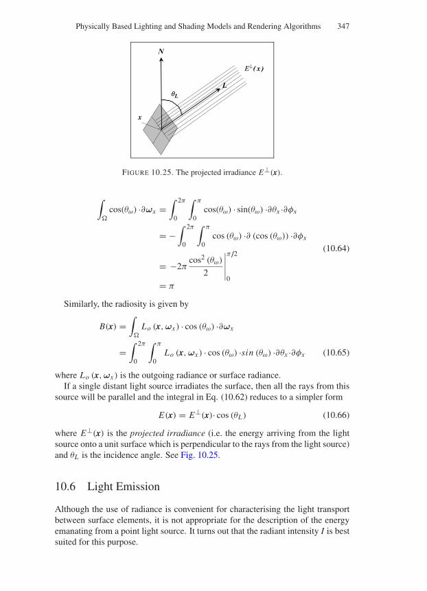
“Comninos” — 2005/8/31 — 19:01 — page 347 — #31
Physically Based Lighting and Shading Models and Rendering Algorithms 347
x
E⊥(x)
qL
N
L
FIGURE 10.25. The projected irradiance E⊥(x).
∫
cos(θω) ·∂ωx =∫ 2π
0
∫ π
0cos(θω) · sin(θω) ·∂θx ·∂φx
= −∫ 2π
0
∫ π
0cos (θω) ·∂ (cos (θω)) ·∂φx
(10.64)
= −2πcos2 (θω)
2
∣∣∣∣∣
π/2
0= π
Similarly, the radiosity is given by
B(x) =∫
Lo (x,ωx ) · cos (θω) ·∂ωx
=∫ 2π
0
∫ π
0Lo (x,ωx ) · cos (θω) ·sin (θω) ·∂θx ·∂φx (10.65)
where Lo (x,ωx ) is the outgoing radiance or surface radiance.If a single distant light source irradiates the surface, then all the rays from this
source will be parallel and the integral in Eq. (10.62) reduces to a simpler form
E(x) = E⊥(x)· cos (θL) (10.66)
where E⊥(x) is the projected irradiance (i.e. the energy arriving from the lightsource onto a unit surface which is perpendicular to the rays from the light source)and θL is the incidence angle. See Fig. 10.25.
10.6 Light Emission
Although the use of radiance is convenient for characterising the light transportbetween surface elements, it is not appropriate for the description of the energyemanating from a point light source. It turns out that the radiant intensity I is bestsuited for this purpose.
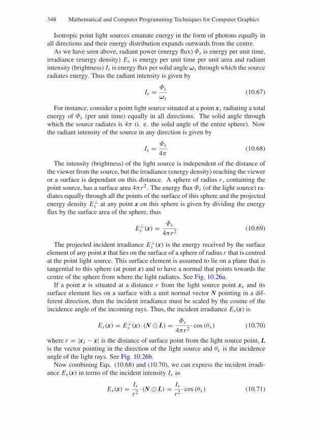
“Comninos” — 2005/8/31 — 19:01 — page 348 — #32
348 Mathematical and Computer Programming Techniques for Computer Graphics
Isotropic point light sources emanate energy in the form of photons equally inall directions and their energy distribution expands outwards from the centre.
As we have seen above, radiant power (energy flux) Φs is energy per unit time,irradiance (energy density) Es is energy per unit time per unit area and radiantintensity (brightness) Is is energy flux per solid angle ωs through which the sourceradiates energy. Thus the radiant intensity is given by
Is = Φs
ωs(10.67)
For instance, consider a point light source situated at a point xs radiating a totalenergy of Φs (per unit time) equally in all directions. The solid angle throughwhich the source radiates is 4π (i. e. the solid angle of the entire sphere). Nowthe radiant intensity of the source in any direction is given by
Is = Φs
4π(10.68)
The intensity (brightness) of the light source is independent of the distance ofthe viewer from the source, but the irradiance (energy density) reaching the vieweror a surface is dependant on this distance. A sphere of radius r , containing thepoint source, has a surface area 4πr2. The energy flux Φs (of the light source) ra-diates equally through all the points of the surface of this sphere and the projectedenergy density E⊥
s at any point x on this sphere is given by dividing the energyflux by the surface area of the sphere, thus
E⊥s (x) = Φs
4πr2(10.69)
The projected incident irradiance E⊥s (x) is the energy received by the surface
element of any point x that lies on the surface of a sphere of radius r that is centredat the point light source. This surface element is assumed to lie on a plane that istangential to this sphere (at point x) and to have a normal that points towards thecentre of the sphere from where the light radiates. See Fig. 10.26a.
If a point x is situated at a distance r from the light source point xs and itssurface element lies on a surface with a unit normal vector N pointing in a dif-ferent direction, then the incident irradiance must be scaled by the cosine of theincidence angle of the incoming rays. Thus, the incident irradiance Es(x) is
Es(x) = E⊥s (x)· (N L) = Φs
4πr2· cos (θx ) (10.70)
where r = |xs − x| is the distance of surface point from the light source point, Lis the vector pointing in the direction of the light source and θx is the incidenceangle of the light rays. See Fig. 10.26b.
Now combining Eqs. (10.68) and (10.70), we can express the incident irradi-ance Es(x) in terms of the incident intensity Is as
Es(x) = Is
r2· (N L) = Is
r2· cos (θx ) (10.71)
“Comninos” — 2005/8/31 — 19:01 — page 349 — #33
Physically Based Lighting and Shading Models and Rendering Algorithms 349
(a) (b)
E⊥s
N
xs
x x
Es
qx
NL
xs
FIGURE 10.26. (a) The projected incident irradianceE⊥s (x). (b) The incident irradiance
Es(x).
10.7 The Scattering and Reflection Functions
As we have seen previously, when a light beam strikes an interface surface be-tween two participating media it can undergo reflection, refraction followed bytransmission, or subsurface scattering followed by reflection. In this section wewill examine the scattering and reflection functions that model these phenomena.
Let us start by examining what happens to a single photon when it strikes aninterface surface. Figure 10.27a depicts a photon striking the interface surface andundergoing reflection, while Fig. 10.27b depicts a photon striking the interfacesurface and undergoing subsurface scattering followed by reflection.
As we can see from the latter diagram, a light beam may strike the surface atone point, undergo subsurface scattering and leave the surface from another point.For this reason, we momentarily drop any reference to points from our notation.Thus, the incoming (field) radiance will be denoted by Li (ωi ) and the outgoing(surface) radiance will be denoted by Lr (ωr ). In general the outgoing radiance Lr
depends on the radiance arriving at a given point from all directions. To simplifythings, we will fix a particular direction ωi and consider only the incident lightarriving at a point from a solid angle ∂ωi . Let us assume that this light strikes thesurface at a point and generates an irradiance Ei (ωi ) which given by
∂ Ei (ωi ) = Li (ωi )·∂ω⊥i (10.72)
where ∂ω⊥i is the projected solid angle in the direction ωi . This light is subse-
quently scattered by the surface in all directions.Let ∂Lr (ωr ) represent the contribution made to the outgoing radiance in the di-
rection ωr with a solid angle ∂ωr . Experiments have shown that the incident lightenergy ∂ Ei (ωi ) arriving onto the surface is proportional to the reflected radianceLr (ωr ) [Clarke 85]. Thus,
∂Lr (ωr ) ∝ ∂ Ei (ωi ) (10.73)
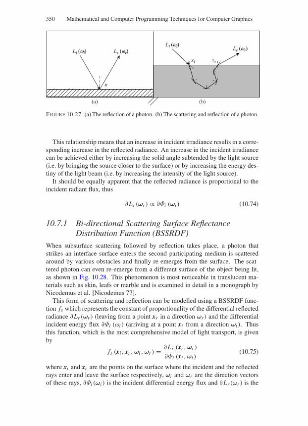
“Comninos” — 2005/8/31 — 19:01 — page 350 — #34
350 Mathematical and Computer Programming Techniques for Computer Graphics
xi xr
Li (wi) Lr (wr)Li (wi) Lr (wr)
x
(a) (b)
FIGURE 10.27. (a) The reflection of a photon. (b) The scattering and reflection of a photon.
This relationship means that an increase in incident irradiance results in a corre-sponding increase in the reflected radiance. An increase in the incident irradiancecan be achieved either by increasing the solid angle subtended by the light source(i.e. by bringing the source closer to the surface) or by increasing the energy des-tiny of the light beam (i.e. by increasing the intensity of the light source).
It should be equally apparent that the reflected radiance is proportional to theincident radiant flux, thus
∂Lr (ωr ) ∝ ∂Φi (ωi ) (10.74)
10.7.1 Bi-directional Scattering Surface ReflectanceDistribution Function (BSSRDF)
When subsurface scattering followed by reflection takes place, a photon thatstrikes an interface surface enters the second participating medium is scatteredaround by various obstacles and finally re-emerges from the surface. The scat-tered photon can even re-emerge from a different surface of the object being lit,as shown in Fig. 10.28. This phenomenon is most noticeable in translucent ma-terials such as skin, leafs or marble and is examined in detail in a monograph byNicodemus et al. [Nicodemus 77].
This form of scattering and reflection can be modelled using a BSSRDF func-tion fs which represents the constant of proportionality of the differential reflectedradiance ∂Lr (ωr ) (leaving from a point xr in a direction ωr ) and the differentialincident energy flux ∂Φi (ωi ) (arriving at a point xi from a direction ωi ). Thusthis function, which is the most comprehensive model of light transport, is givenby
fs (xi , xr ,ωi ,ωr ) = ∂Lr (xr ,ωr )
∂Φi (xi ,ωi )(10.75)
where xi and xr are the points on the surface where the incident and the reflectedrays enter and leave the surface respectively, ωi and ωr are the direction vectorsof these rays, ∂Φi (ωi ) is the incident differential energy flux and ∂Lr (ωr ) is the
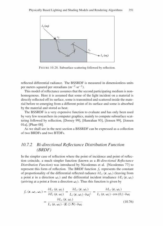
“Comninos” — 2005/8/31 — 19:01 — page 351 — #35
Physically Based Lighting and Shading Models and Rendering Algorithms 351
Li (wi)
Lr (wr)
xi
xr
FIGURE 10.28. Subsurface scattering followed by reflection.
reflected differential radiance. The BSSRDF is measured in dimensionless unitsper meters squared per steradians (m−2·sr−1).
This model of reflectance assumes that the second participating medium is non-homogenous. Here it is assumed that some of the light incident on a material isdirectly reflected off its surface, some is transmitted and scattered inside the mate-rial before re-emerging from a different point of its surface and some is absorbedby the material and stored as heat.
The BSSRDF is a very expensive function to evaluate and has only been usedby very few researchers in computer graphics, mainly to compute subsurface scat-tering followed by reflection, [Dorsey 99], [Hanrahan 93], [Jensen 99], [Jensen01a], [Pharr 00].
As we shall see in the next section a BSSRDF can be expressed as a collectionof two BRDFs and two BTDFs.
10.7.2 Bi-directional Reflectance Distribution Function(BRDF)
In the simpler case of reflection where the point of incidence and point of reflec-tion coincide, a much simpler function (known as a Bi-directional ReflectanceDistribution Function) was introduced by Nicodemus et al. [Nicodemus 77] torepresent this form of reflection. The BRDF function fr represents the constantof proportionality of the differential reflected radiance ∂Lr (x,ωr ) (leaving froma point x in a direction ωr ) and the differential incident irradiance ∂ Ei (x,ωi )
(arriving at a point x from a direction ωi ). Thus this function is given by
fr (x,ωi ,ωr ) = ∂Lr (x,ωr )
∂ Ei (x,ωi )= ∂Lr (x,ωr )
Li (x,ωi ) ·∂ω⊥i
= ∂Lr (x,ωr )
Li (x,ωi ) · cos (θi ) ·∂ωi
= ∂Lr (x,ωr )
Li (x,ωi ) · (L N) ·∂ωi(10.76)
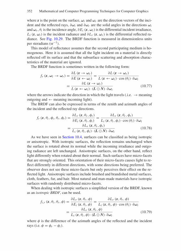
“Comninos” — 2005/8/31 — 19:01 — page 352 — #36
352 Mathematical and Computer Programming Techniques for Computer Graphics
where x is the point on the surface, ωi and ωr are the direction vectors of the inci-dent and the reflected rays, ∂ωi and ∂ωr are the solid angles in the directions ωi
and ωr , θi is the incidence angle, ∂ Ei (x,ωi ) is the differential incident irradiance,Li (x,ωi ) is the incident radiance and ∂Lr (x,ωr ) is the differential reflected ra-diance. See Fig. 10.29. The BRDF function is measured in dimensionless unitsper steradians (sr−1).
This model of reflectance assumes that the second participating medium is ho-mogenous. Here it is assumed that all the light incident on a material is directlyreflected off its surface and that the subsurface scattering and absorption charac-teristics of the material are ignored.
The BRDF function is sometimes written in the following form:
fr (x,ωi → ωr ) = ∂L (x → ωr )
∂ E (x ← ωi )= ∂L (x → ωr )
L (x ← ωi ) · cos (θi ) ·∂ωi
= ∂L (x → ωr )
L (x ← ωi ) · (L N) ·∂ωi(10.77)
where the arrows indicate the direction in which the light travels (.i.e. → meaningoutgoing and ← meaning incoming light).
The BRDF can also be expressed in terms of the zenith and azimuth angles ofthe incident and the reflected ray directions.
fr (x, θi , φi , θr , φr ) = ∂Lr (x, θr , φr )
∂ Ei (x, θi , φi )= ∂Lr (x, θr , φr )
Li (x, θi , φi ) · cos (θi ) ·∂ωi
= ∂Lr (x, θr , φr )
Li (x, θi , φi ) · (L N) ·∂ωi(10.78)
As we have seen in Section 10.4, surfaces can be classified as being isotropicor anisotropic. With isotropic surfaces, the reflection remains unchanged whenthe surface is rotated about its normal while the incoming irradiance and outgo-ing radiance are left unchanged. Anisotropic surfaces, on the other hand, reflectlight differently when rotated about their normal. Such surfaces have micro-facetsthat are strongly oriented. This orientation of their micro-facets causes light to re-flect differently in different directions, with some directions being preferred. Theobserver does not see these micro-facets but only perceives their effect on the re-flected light. Anisotropic surfaces include brushed and brandished metal surfaces,cloth, feathers, fur, and hair. Most natural and man-made materials have isotropicsurfaces with randomly distributed micro-facets.
When dealing with isotropic surfaces a simplified version of the BRDF, knownas an isotropic BRDF, can be used.
fi,r (x, θi , θr , φ) = ∂Lr (x, θr , φ)
∂ Ei (x, θi , φ)= ∂Lr (x, θr , φ)
Li (x, θi , φ) · cos (θi ) ·∂ωi
= ∂Lr (x, θr , φ)
Li (x, θi , φ) · (L N) ·∂ωi(10.79)
where φ is the difference of the azimuth angles of the reflected and the incidentrays (i.e. φ = φr − φi ).
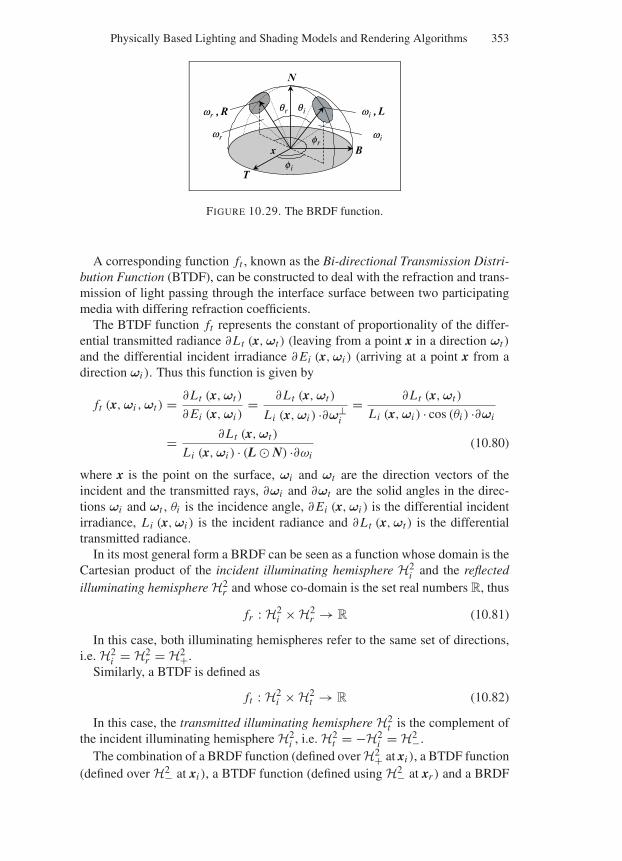
“Comninos” — 2005/8/31 — 19:01 — page 353 — #37
Physically Based Lighting and Shading Models and Rendering Algorithms 353
N
B
T
x
qi
fi
qr
fr
wr , R
wr
wi , L
wi
FIGURE 10.29. The BRDF function.
A corresponding function ft , known as the Bi-directional Transmission Distri-bution Function (BTDF), can be constructed to deal with the refraction and trans-mission of light passing through the interface surface between two participatingmedia with differing refraction coefficients.
The BTDF function ft represents the constant of proportionality of the differ-ential transmitted radiance ∂Lt (x,ωt ) (leaving from a point x in a direction ωt )
and the differential incident irradiance ∂ Ei (x,ωi ) (arriving at a point x from adirection ωi ). Thus this function is given by
ft (x,ωi ,ωt ) = ∂Lt (x,ωt )
∂ Ei (x,ωi )= ∂Lt (x,ωt )
Li (x,ωi ) ·∂ω⊥i
= ∂Lt (x,ωt )
Li (x,ωi ) · cos (θi ) ·∂ωi
= ∂Lt (x,ωt )
Li (x,ωi ) · (L N) ·∂ωi(10.80)
where x is the point on the surface, ωi and ωt are the direction vectors of theincident and the transmitted rays, ∂ωi and ∂ωt are the solid angles in the direc-tions ωi and ωt , θi is the incidence angle, ∂ Ei (x,ωi ) is the differential incidentirradiance, Li (x,ωi ) is the incident radiance and ∂Lt (x,ωt ) is the differentialtransmitted radiance.
In its most general form a BRDF can be seen as a function whose domain is theCartesian product of the incident illuminating hemisphere H2
i and the reflectedilluminating hemisphere H2
r and whose co-domain is the set real numbers R, thus
fr : H2i × H2
r → R (10.81)
In this case, both illuminating hemispheres refer to the same set of directions,i.e. H2
i = H2r = H2+.
Similarly, a BTDF is defined as
ft : H2i × H2
t → R (10.82)
In this case, the transmitted illuminating hemisphere H2t is the complement of
the incident illuminating hemisphere H2i , i.e. H2
t = −H2i = H2−.
The combination of a BRDF function (defined over H2+ at xi ), a BTDF function(defined over H2− at xi ), a BTDF function (defined using H2− at xr ) and a BRDF
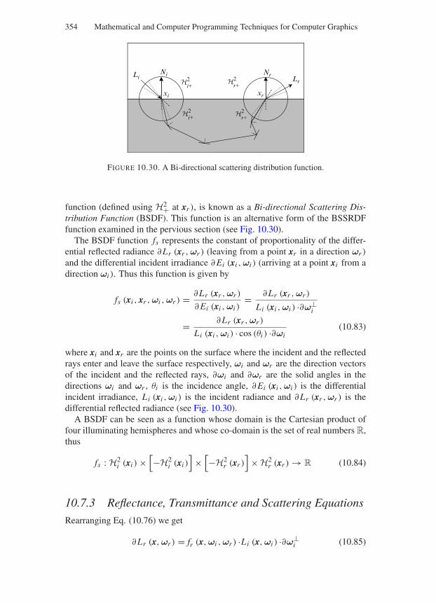
“Comninos” — 2005/8/31 — 19:01 — page 354 — #38
354 Mathematical and Computer Programming Techniques for Computer Graphics
Li Lr
xi xr
NrNi2r+
2r+
2i+
2i+
FIGURE 10.30. A Bi-directional scattering distribution function.
function (defined using H2+ at xr ), is known as a Bi-directional Scattering Dis-tribution Function (BSDF). This function is an alternative form of the BSSRDFfunction examined in the pervious section (see Fig. 10.30).
The BSDF function fs represents the constant of proportionality of the differ-ential reflected radiance ∂Lr (xr ,ωr ) (leaving from a point xr in a direction ωr )
and the differential incident irradiance ∂ Ei (xi ,ωi ) (arriving at a point xi from adirection ωi ). Thus this function is given by
fs (xi , xr ,ωi ,ωr ) = ∂Lr (xr ,ωr )
∂ Ei (xi ,ωi )= ∂Lr (xr ,ωr )
Li (xi ,ωi ) ·∂ω⊥i
= ∂Lr (xr ,ωr )
Li (xi ,ωi ) · cos (θi ) ·∂ωi(10.83)
where xi and xr are the points on the surface where the incident and the reflectedrays enter and leave the surface respectively, ωi and ωr are the direction vectorsof the incident and the reflected rays, ∂ωi and ∂ωr are the solid angles in thedirections ωi and ωr , θi is the incidence angle, ∂ Ei (xi ,ωi ) is the differentialincident irradiance, Li (xi ,ωi ) is the incident radiance and ∂Lr (xr ,ωr ) is thedifferential reflected radiance (see Fig. 10.30).
A BSDF can be seen as a function whose domain is the Cartesian product offour illuminating hemispheres and whose co-domain is the set of real numbers R,thus
fs : H2i (xi ) ×
[−H2
i (xi )]
×[−H2
r (xr )]
× H2r (xr ) → R (10.84)
10.7.3 Reflectance, Transmittance and Scattering Equations
Rearranging Eq. (10.76) we get
∂Lr (x,ωr ) = fr (x,ωi ,ωr ) ·Li (x,ωi ) ·∂ω⊥i (10.85)
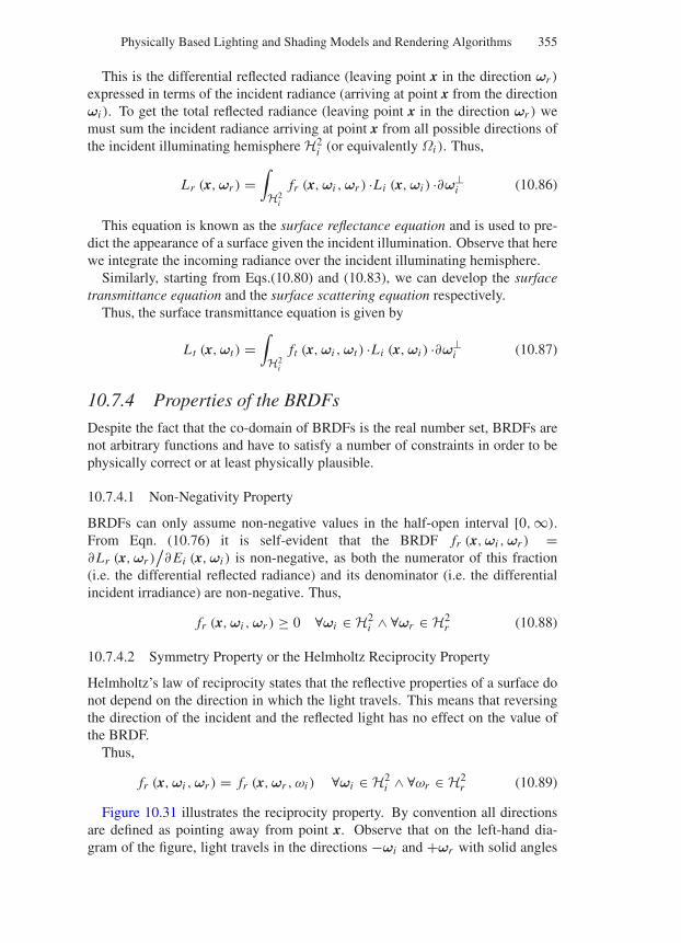
“Comninos” — 2005/8/31 — 19:01 — page 355 — #39
Physically Based Lighting and Shading Models and Rendering Algorithms 355
This is the differential reflected radiance (leaving point x in the direction ωr )
expressed in terms of the incident radiance (arriving at point x from the directionωi ). To get the total reflected radiance (leaving point x in the direction ωr ) wemust sum the incident radiance arriving at point x from all possible directions ofthe incident illuminating hemisphere H2
i (or equivalently Ωi ). Thus,
Lr (x,ωr ) =∫
H2i
fr (x,ωi ,ωr ) ·Li (x,ωi ) ·∂ω⊥i (10.86)
This equation is known as the surface reflectance equation and is used to pre-dict the appearance of a surface given the incident illumination. Observe that herewe integrate the incoming radiance over the incident illuminating hemisphere.
Similarly, starting from Eqs.(10.80) and (10.83), we can develop the surfacetransmittance equation and the surface scattering equation respectively.
Thus, the surface transmittance equation is given by
Lt (x,ωt ) =∫
H2i
ft (x,ωi ,ωt ) ·Li (x,ωi ) ·∂ω⊥i (10.87)
10.7.4 Properties of the BRDFs
Despite the fact that the co-domain of BRDFs is the real number set, BRDFs arenot arbitrary functions and have to satisfy a number of constraints in order to bephysically correct or at least physically plausible.
10.7.4.1 Non-Negativity Property
BRDFs can only assume non-negative values in the half-open interval [0,∞).From Eqn. (10.76) it is self-evident that the BRDF fr (x,ωi ,ωr ) =∂Lr (x,ωr )
/∂ Ei (x,ωi ) is non-negative, as both the numerator of this fraction
(i.e. the differential reflected radiance) and its denominator (i.e. the differentialincident irradiance) are non-negative. Thus,
fr (x,ωi ,ωr ) ≥ 0 ∀ωi ∈ H2i ∧ ∀ωr ∈ H2
r (10.88)
10.7.4.2 Symmetry Property or the Helmholtz Reciprocity Property
Helmholtz’s law of reciprocity states that the reflective properties of a surface donot depend on the direction in which the light travels. This means that reversingthe direction of the incident and the reflected light has no effect on the value ofthe BRDF.
Thus,
fr (x,ωi ,ωr ) = fr (x,ωr , ωi ) ∀ωi ∈ H2i ∧ ∀ωr ∈ H2
r (10.89)
Figure 10.31 illustrates the reciprocity property. By convention all directionsare defined as pointing away from point x. Observe that on the left-hand dia-gram of the figure, light travels in the directions −ωi and +ωr with solid angles
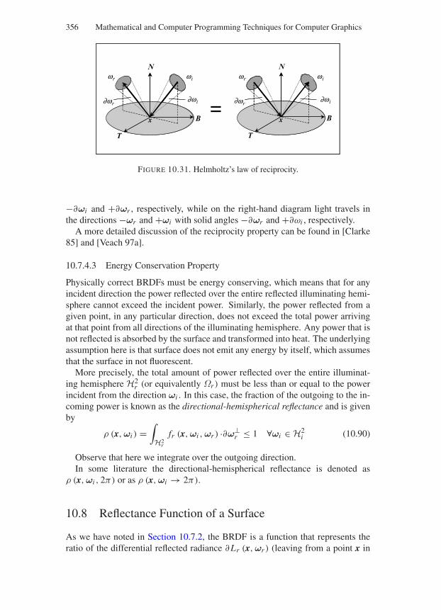
“Comninos” — 2005/8/31 — 19:01 — page 356 — #40
356 Mathematical and Computer Programming Techniques for Computer Graphics
N
B=
T
x
N
B
T
xx x
wrwi
wr wi
wrwi
wr wi
∂∂∂∂
FIGURE 10.31. Helmholtz’s law of reciprocity.
−∂ωi and +∂ωr , respectively, while on the right-hand diagram light travels inthe directions −ωr and +ωi with solid angles −∂ωr and +∂ωi , respectively.
A more detailed discussion of the reciprocity property can be found in [Clarke85] and [Veach 97a].
10.7.4.3 Energy Conservation Property
Physically correct BRDFs must be energy conserving, which means that for anyincident direction the power reflected over the entire reflected illuminating hemi-sphere cannot exceed the incident power. Similarly, the power reflected from agiven point, in any particular direction, does not exceed the total power arrivingat that point from all directions of the illuminating hemisphere. Any power that isnot reflected is absorbed by the surface and transformed into heat. The underlyingassumption here is that surface does not emit any energy by itself, which assumesthat the surface in not fluorescent.
More precisely, the total amount of power reflected over the entire illuminat-ing hemisphere H2
r (or equivalently Ωr ) must be less than or equal to the powerincident from the direction ωi . In this case, the fraction of the outgoing to the in-coming power is known as the directional-hemispherical reflectance and is givenby
ρ (x,ωi ) =∫
H2r
fr (x,ωi ,ωr ) ·∂ω⊥r ≤ 1 ∀ωi ∈ H2
i (10.90)
Observe that here we integrate over the outgoing direction.In some literature the directional-hemispherical reflectance is denoted as
ρ (x,ωi , 2π) or as ρ (x,ωi → 2π).
10.8 Reflectance Function of a Surface
As we have noted in Section 10.7.2, the BRDF is a function that represents theratio of the differential reflected radiance ∂Lr (x,ωr ) (leaving from a point x in
“Comninos” — 2005/8/31 — 19:01 — page 357 — #41
Physically Based Lighting and Shading Models and Rendering Algorithms 357
a direction ωr ) and the differential incident irradiance ∂ Ei (x,ωi ) (arriving at apoint x from a direction ωi ). Although this function gives us the ratio of thereflected to the incident light energy for a surface, it is not very intuitive, as itsrange is the infinite interval [0,∞). To overcome this difficulty we define anotherfunction, which represents the fraction of the incident light reflected off a surface.This function is known as the reflectance of the surface and has a range [0, 1]. Todetermine this function we proceed as follows. We start by considering the ratioof the reflected differential flux to the incident differential flux at a point x. UsingEqs. (10.61) and (10.63) we get
∂Φr (x)
∂Φi (x)=(∫
H2r
Lr (x,ωr ) ·∂ω⊥r
)·∂ Ax
(∫H2
iLi (x,ωi ) ·∂ω⊥
i
)·∂ Ax
=∫H2
rLr (x,ωr ) ·∂ω⊥
r∫H2
iLi (x,ωi ) ·∂ω⊥
i
Using Eq. (10.86) we can expand this result to get
∂Φr (x)
∂Φi (x)=∫H2
r
∫H2
ifr (x,ωi ,ωr ) ·Li (x,ωi ) ·∂ω⊥
i ·∂ω⊥r
∫H2
iLi (x,ωi ) ·∂ω⊥
i
If we assume that the incident radiance Li (x,ωi ) is both uniform and isotropic,then we can remove it from both integrals of the numerator and the denominatorof this fraction. The simplified fraction defines the reflectance function of thesurface.
ρ (x,ωi ,ωr ) =∫H2
r
∫H2
ifr (x,ωi ,ωr ) ·∂ω⊥
i ·∂ω⊥r
∫H2
i∂ω⊥
i
(10.91a)
or equivalently
ρ (x,ωi ,ωr ) =∫H2
r
∫H2
ifr (x,ωi ,ωr ) · cos (θi ) ·∂ωi · cos (θr ) ·∂ωr
∫H2
icos (θi ) ·∂ωi
(10.91b)
Observe that the reflectance of the surface changes as the incidence angle θi
changes.In the arrow notation this function is denoted by ρ (x,ωi → ωr ).The reflectance function involves the evaluation of a double integral over the
incident and reflected directions. The limits of these integrals can be set to a dif-ferential solid angle range [∂ωa, ∂ωb], a finite solid angle range [Dωa,Dωb] orthe entire illuminating hemisphere H2
i or H2r .
Depending on the chosen integration limits for the incident and reflected di-rections we can use a qualifier that characterises the reflectance function. Thisqualifier is constructed by juxtaposing the type of the integration limits usedin the incident and the reflected directions. The integration limit types are re-ferred to by the terms directional (for a differential solid angle range), coni-cal (for a finite solid angle range) and hemispherical (for an entire illuminatinghemisphere). By permutating these three integration limit types we can generatenine such reflectance qualifiers. Thus, the qualifiers for the following reflectancefunctions are:
“Comninos” — 2005/8/31 — 19:01 — page 358 — #42
358 Mathematical and Computer Programming Techniques for Computer Graphics
ρ (x,ωi → ωr ) is a bi-directional reflectance function,ρ (x,ωi → Dωr ) is a directional-conical reflectance function,ρ(x,ωi → H2
r
)is a directional-hemispherical reflectance function,
ρ (x,Dωi → ωr ) is a conical-directional reflectance function,ρ (x,Dωi → Dωr ) is a bi-conical reflectance function,ρ(x,Dωi → H2
r
)is a conical-hemispherical reflectance function,
ρ(x,H2
i → ωr)
is a hemispherical-directional reflectance function,ρ(x,H2
i → Dωr)
is a hemispherical-conical reflectance function,ρ(x,H2
i → H2r
)is a bi-hemispherical reflectance function.
10.9 Transmittance Function of a Surface
Following an analogous argument for the transmission of light, to that we usedin the previous section for the reflection of light, we can derive the transmittancefunction of a surface. As before, we start by considering the ratio of the transmit-ted differential flux to the incident differential flux at a point x:
∂Φt (x)
∂Φi (x)=(∫
H2t
Lt (x,ωt ) ·∂ω⊥t
)·∂ Ax
(∫H2
iLi (x,ωi ) ·∂ω⊥
i
)·∂ Ax
=∫H2
tLt (x,ωt ) ·∂ω⊥
t∫H2
iLi (x,ωi ) ·∂ω⊥
i
Expanding this result we get
∂Φt (x)
∂Φi (x)=∫H2
t
∫H2
ift (x,ωi ,ωt ) ·Li (x,ωi ) ·∂ω⊥
i ·∂ω⊥t
∫H2
iLi (x,ωi ) ·∂ω⊥
i
Once again, assuming that the incident radiance Li (x, ωi ) is both uniform andisotropic, we can remove it from both integrals of the numerator and the denom-inator of this fraction. The simplified fraction defines the transmittance functionof the surface.
τ (x,ωi ,ωt ) =∫H2
t
∫H2
ift (x,ωi ,ωt ) ·∂ω⊥
i ·∂ω⊥t
∫H2
i∂ω⊥
i
(10.92a)
or equivalently
τ (x,ωi ,ωt ) =∫H2
t
∫H2
ift (x,ωi ,ωt ) · cos (θi ) ·∂ωi · cos (θt ) ·∂ωt
∫H2
icos (θi ) ·∂ωi
(10.92b)
Again, observe that the transmittance of the surface changes as the incidenceangle θi changes and that in the arrow notation this function is denoted byτ (x,ωi → ωt ).
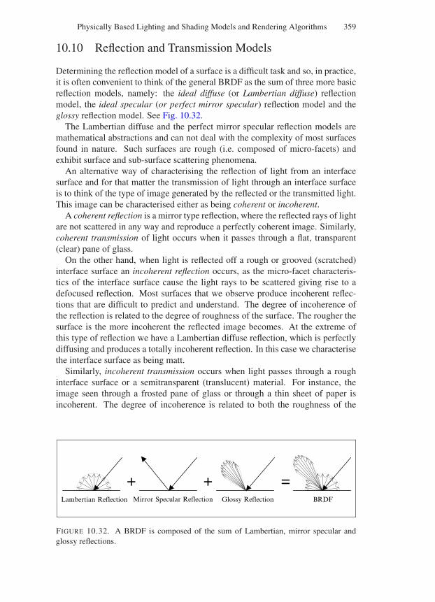
“Comninos” — 2005/8/31 — 19:01 — page 359 — #43
Physically Based Lighting and Shading Models and Rendering Algorithms 359
10.10 Reflection and Transmission Models
Determining the reflection model of a surface is a difficult task and so, in practice,it is often convenient to think of the general BRDF as the sum of three more basicreflection models, namely: the ideal diffuse (or Lambertian diffuse) reflectionmodel, the ideal specular (or perfect mirror specular) reflection model and theglossy reflection model. See Fig. 10.32.
The Lambertian diffuse and the perfect mirror specular reflection models aremathematical abstractions and can not deal with the complexity of most surfacesfound in nature. Such surfaces are rough (i.e. composed of micro-facets) andexhibit surface and sub-surface scattering phenomena.
An alternative way of characterising the reflection of light from an interfacesurface and for that matter the transmission of light through an interface surfaceis to think of the type of image generated by the reflected or the transmitted light.This image can be characterised either as being coherent or incoherent.
A coherent reflection is a mirror type reflection, where the reflected rays of lightare not scattered in any way and reproduce a perfectly coherent image. Similarly,coherent transmission of light occurs when it passes through a flat, transparent(clear) pane of glass.
On the other hand, when light is reflected off a rough or grooved (scratched)interface surface an incoherent reflection occurs, as the micro-facet characteris-tics of the interface surface cause the light rays to be scattered giving rise to adefocused reflection. Most surfaces that we observe produce incoherent reflec-tions that are difficult to predict and understand. The degree of incoherence ofthe reflection is related to the degree of roughness of the surface. The rougher thesurface is the more incoherent the reflected image becomes. At the extreme ofthis type of reflection we have a Lambertian diffuse reflection, which is perfectlydiffusing and produces a totally incoherent reflection. In this case we characterisethe interface surface as being matt.
Similarly, incoherent transmission occurs when light passes through a roughinterface surface or a semitransparent (translucent) material. For instance, theimage seen through a frosted pane of glass or through a thin sheet of paper isincoherent. The degree of incoherence is related to both the roughness of the
Lambertian Reflection Mirror Specular Reflection Glossy Reflection BRDF
=++
FIGURE 10.32. A BRDF is composed of the sum of Lambertian, mirror specular andglossy reflections.
“Comninos” — 2005/8/31 — 19:01 — page 360 — #44
360 Mathematical and Computer Programming Techniques for Computer Graphics
interface surface and transparency/translucency of the material through which thelight has to travel before it reaches us.
Thus one can see that light reflection and transmission can be characterisedas being perfectly diffuse (i.e. totally incoherent), perfectly specular (i.e. totallycoherent) and something in-between these two extremes (i.e. semi-coherent). Inorder to simulate these three types of reflection and transmission, we can usecorrespondingly the diffuse reflection model, the specular reflection model and amixture of these two idealised models.
10.10.1 Diffuse Reflection Model
A surface that exhibits diffuse reflection characteristics scatters all incoming en-ergy in all possible directions of the reflected illuminating hemisphere H2
r . In theideal case of Lambertian diffuse reflection, it is assumed that the micro-facets ofthe surface are perfectly evenly distributed in all directions and thus they scatterlight evenly in all directions of H2
r . In this case, the reflected radiance is con-stant in all directions regardless of the direction of the incoming radiance. Whichmeans that the BRDF is constant and does not depend on the incident and thereflected directions ωi and ωr . Thus, Eq. (10.86) becomes
Lr,d (x,ωr ) =∫
H2i
fr,d(x)·Li (x,ωi ) ·∂ω⊥i
= fr,d(x)·∫
H2i
Li (x,ωi ) ·∂ω⊥i
= fr,d(x)·Ei (x) (10.93)
From the above equation we can see that the reflected radiance is proportionalto the incident irradiance and that it is constant and has the same value in alldirections, since neither the BRDF fr,d (x) nor the irradiance Ei (x) depend onthe incident or reflected directions.
By forcing the bi-hemispherical reflectance ρd(x,H2
i → H2r
)to be less than
or equal to 1, we make sure that the energy conservation property is adhered to.Thus,
ρd
(x,H2
i ,H2r
)= Φr,d(x)
Φi (x)
=∫H2
rLr,d (x,ωr ) ·∂ω⊥
r∫H2
iLi (x,ωi ) ·∂ω⊥
i
=Lr,d (x,ωr ) · ∫H2
r∂ω⊥
r
Ei (x)
= Lr,d (x,ωr ) ·πEi (x)
∴ ρd
(x,H2
i ,H2r
)= fr,d(x)·π (10.94)
“Comninos” — 2005/8/31 — 19:01 — page 361 — #45
Physically Based Lighting and Shading Models and Rendering Algorithms 361
since Lr,d (x,ωr ) is constant and has the same value in all directions, and∫H2
r∂ω⊥
r = π .But if the Lambertian BRDF is constant, since it does not depend on the inci-
dent direction ωi , then the Lambertian reflectance ρd must also be constant. Nowwe can express the Lambertian BRDF in terms of the Lambertian reflectance as
fr,d(x) = ρd(x)
π(10.95)
A physically plausible Lambertian reflectance is usually denoted by a constantkd ≤ 1, known as the diffuse coefficient of reflectance.
10.10.2 Specular Reflection Model
In a perfect mirror reflection the light reaching a perfectly smooth (polished) sur-face is reflected in only one direction and no surface scattering occurs. In thiscase, the angle of incidence θi is equal to the angle of reflection θr and, since aperfect mirror surface is isotropic, the reflected ray vector RL lies on the planedefined by the light ray vector L and the surface normal vector N. Recall that inSection 10.4.1 we have shown how the reflected ray vector could be computed.
Thus, for perfect mirror reflections we have
θr = θi
φr = φi ± π(10.96)
As we have also seen in Section 10.4.1, the reflection occurs in the direction
ωr = 2· (N ωi ) ·N − ωi (10.97)
In some literature the direction of the reflection vector is given as
ωr = R(N)·ωi (10.98)
where R(N ) is a matrix known as the Householder transformation matrix. Thismatrix is defined as follows:
R(N) = 2·N·NT − I (10.99)
i.e. as twice the Cartesian product of the unit surface normal by its transposedminus the identity matrix.
Expanding this product we get
R(N) = 2·⎡
⎣Nx
Ny
Nz
⎤
⎦ · [ Nx Ny Nz]−⎡
⎣1 0 00 1 00 0 1
⎤
⎦
∴ R(N) =⎡
⎣2N 2
x − 1 2Nx Ny 2Nx Nz
2Ny Nx 2N 2y − 1 2Ny Nz
2Nz Nx 2Nz Ny 2N 2z − 1
⎤
⎦ (10.100)
“Comninos” — 2005/8/31 — 19:01 — page 362 — #46
362 Mathematical and Computer Programming Techniques for Computer Graphics
As this matrix is symmetric, it is equal to its transpose (i.e. R(N) = RT(N)).
With a perfect mirror surface, the incoming light is only reflected in the mir-ror direction and we have a perfect specular reflection. For such reflections, thereflected radiance is related to the incident radiance by
Lr (x,ωr ) = ρs (x,ωi , ωr ) ·Li (x,ωi ) (10.101)
For perfect mirror specular reflections, the value of the specular reflectanceρs (x,ωi ,ωr ) must be equal to 1 in the direction ωr and equal to 0 in all otherdirections. The corresponding BRDF is usually defined in terms of two Diracdelta functions.
Dirac’s delta function δ (x) can informally be thought of as a function that hasthe value
δ(x) = ∞, x = 0
0, x = 0(10.102a)
and has a total integral equal to 1, i.e.
∫ +∞
−∞δ(x)·∂x = 1 (10.102b)
The delta function obeys the sifting property, i.e.
∫ +∞
−∞f (x) ·δ (x − x0) ·∂x = f (x0) (10.102c)
Cohen and Wallace [Cohen 93] have developed a perfect mirror surface BRDFthat uses two Dirac delta functions to achieve a non-zero result in only one partic-ular direction. In their definition of the BRDF they use the spherical coordinatesof the incident and the reflected directions. Thus, they define their BRDF as fol-lows :
fr,s (x,ωi ,ωr ) = δ (cos (θi ) − cos (θr ))
cos (θi )δ (φi − (φr ± π)) (10.103)
In this function the first delta function has the value zero unless θr = ±θi andthe second delta function has the value zero unless φr = φi ±π , which guaranteesthe BRDF only has a non-zero value in the direction ωr .
Cohen and Wallace, using the above BRDF for a perfect mirror reflection,showed that the radiance incident (at a surface point x) is equal to the reflected ra-diance (from that point). They did so by expressing the incident radiance Li (θi , φi )
and the reflected radiance Lr (θr , φr ) in terms of spherical coordinates.Thus, they showed that
Lr (θr , φr ) = Li (θi , φi ) = Li (θr , (φr ± π)) (10.104)
They proved this by evaluating the integral over the entire incident illuminatinghemisphere
“Comninos” — 2005/8/31 — 19:01 — page 363 — #47
Physically Based Lighting and Shading Models and Rendering Algorithms 363
Lr (θr , φr ) =∫
H2i
δ (cos (θi ) − cos (θr ))
cos (θi )
·δ (φi − (φr ± π)) ·Li (θi , φi ) · cos (θi ) ·∂θi ·∂φi
= Li (θr , (φr ± π))
10.10.3 Fresnel Effect
As we have observed in Section 10.3.2, when light strikes a smooth interfacesurface between two participating media with different refractive indices ηi = ηt
that are transparent, some of the incident light is reflected and some is refractedand transmitted into the second participating medium. The portion of the lightenergy that is reflected, is reflected in a specular fashion. Both the reflection andtransmission of light is known as the Fresnel effect. This effect is responsible forthe stronger specular reflections at larger incidence angles and for the strongertransmission at lower incidence angles.
The Fresnel effect is a direct consequence of the electromagnetic nature oflight. As we have explained in Section 10.2, light is a combination of an electricalfield E and magnetic field B, which are perpendicular to each other and to thedirection k of the propagation of the wave. The Fresnel effect both depends on andinfluences the polarisation of light during specular reflection and transmission.The directional nature of both the electrical and magnetic fields of light explainsthe phenomenon of polarisation.
Polarisation represents the orientation of the electrical field of the light withrespect to the plane of incidence, which contains the surface normal, the incident,the reflected and the transmitted rays. If the electric field is parallel to the planeof incidence, then we say that the light is P-polarised and if the electric field isperpendicular to the plane of incidence, then we say that the light is S-polarised.The letters “S” and “P” in the terms S-polarised and P-polarised are derived fromthe German words “Senkrecht” and “Parallele” meaning perpendicular and par-allel respectively (see Figs. 10.33 and 10.34). These figures show two differentdepictions of the incident, reflected and transmitted rays of light at the interfacesurface between two participating media with refractive indices ηi and ηt , respec-tively. In these figures, the vectors e(i)
P and e(i)S represent the orientation of the
electrical fields of the P-polarised and S-polarised incident light, respectively andvector k(i) represents the direction of the propagation of the light wave. Similarly,the e(r)
P , e(r)S , k(r) and e(t)
P , e(t)S , k(t) represent these directions for the reflected and
transmitted light respectively.Recall that the energy (power) of an electromagnetic wave is proportional to its
amplitude. To determine the ratios of the reflected to the incident and the trans-mitted to incident electrical field magnitudes we use the Fresnel equations. Thereare four such equations that define the four Fresnel factors: one pair of amplitudereflection and amplitude transmission coefficients for S-polarised light (rs and ts)and one pair of amplitude reflection and amplitude transmission coefficients forP-polarised light (rP and tP ).
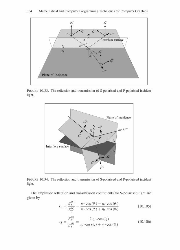
“Comninos” — 2005/8/31 — 19:01 — page 364 — #48
364 Mathematical and Computer Programming Techniques for Computer Graphics
e(r)S
e(t)P
e(t)S
e(i)S
e(i)P e(r)
Pek(r)
k(t)
k(i)
N
qt
qi
ht
hi
Plane of Incidence
Interface surface
FIGURE 10.33. The reflection and transmission of S-polarised and P-polarised incidentlight.
Plane of incidence
Interface surface
Nk
(r)
hi
ht
qi
e(i)S
k(i)
k(t)
e(r)S
e(i)P
e(t)P
e(t)S
e(i)P
FIGURE 10.34. The reflection and transmission of S-polarised and P-polarised incidentlight.
The amplitude reflection and transmission coefficients for S-polarised light aregiven by
rS = E (r)S
E (i)S
= ηi · cos (θi ) − ηt · cos (θt )
ηi · cos (θi ) + ηt · cos (θt )(10.105)
tS = E (t)S
E (i)S
= 2·ηi · cos (θi )
ηi · cos (θi ) + ηt · cos (θt )(10.106)
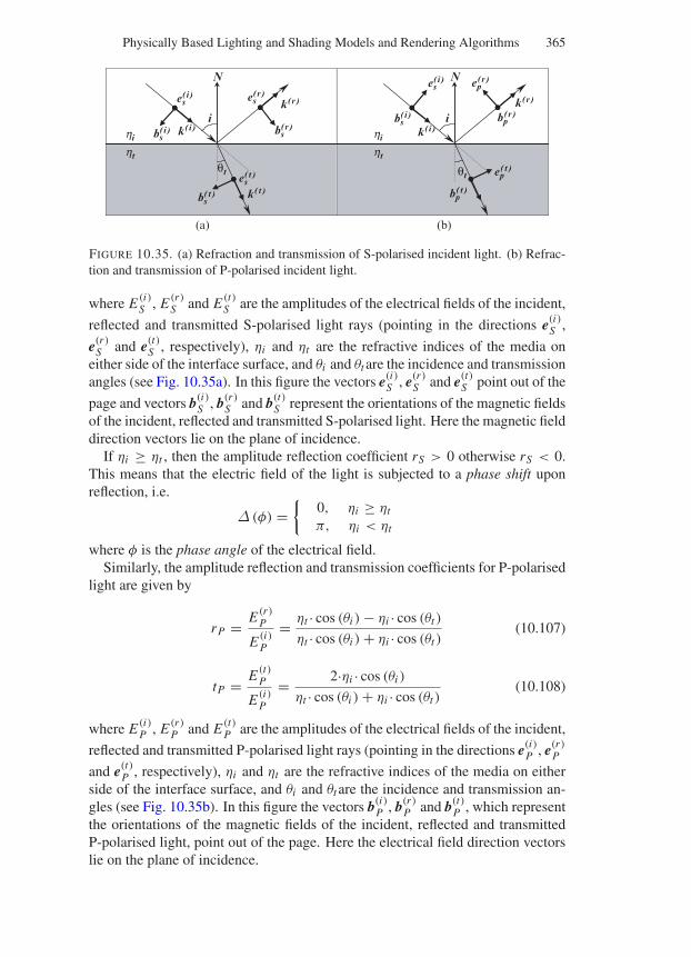
“Comninos” — 2005/8/31 — 19:01 — page 365 — #49
Physically Based Lighting and Shading Models and Rendering Algorithms 365
N
i
θt θt
hi
ht
bs(r)
bp(r)
bs(t)
bs(i)
bs(i)
k(r) k(r)
k(i) k(i)
k(t) k(t)
es(r)
ep(r)
es(i)
es(i)
es(t)
N
ihi
ht
bp(t)
ep(t)θt
(a) (b)
FIGURE 10.35. (a) Refraction and transmission of S-polarised incident light. (b) Refrac-tion and transmission of P-polarised incident light.
where E (i)S , E (r)
S and E (t)S are the amplitudes of the electrical fields of the incident,
reflected and transmitted S-polarised light rays (pointing in the directions e(i)S ,
e(r)S and e(t)
S , respectively), ηi and ηt are the refractive indices of the media oneither side of the interface surface, and θi and θt are the incidence and transmissionangles (see Fig. 10.35a). In this figure the vectors e(i)
S , e(r)S and e(t)
S point out of the
page and vectors b(i)S , b(r)
S and b(t)S represent the orientations of the magnetic fields
of the incident, reflected and transmitted S-polarised light. Here the magnetic fielddirection vectors lie on the plane of incidence.
If ηi ≥ ηt , then the amplitude reflection coefficient rS > 0 otherwise rS < 0.This means that the electric field of the light is subjected to a phase shift uponreflection, i.e.
∆ (φ) =
0, ηi ≥ ηt
π, ηi < ηt
where φ is the phase angle of the electrical field.Similarly, the amplitude reflection and transmission coefficients for P-polarised
light are given by
rP = E (r)P
E (i)P
= ηt · cos (θi ) − ηi · cos (θt )
ηt · cos (θi ) + ηi · cos (θt )(10.107)
tP = E (t)P
E (i)P
= 2·ηi · cos (θi )
ηt · cos (θi ) + ηi · cos (θt )(10.108)
where E (i)P , E (r)
P and E (t)P are the amplitudes of the electrical fields of the incident,
reflected and transmitted P-polarised light rays (pointing in the directions e(i)P , e(r)
P
and e(t)P , respectively), ηi and ηt are the refractive indices of the media on either
side of the interface surface, and θi and θt are the incidence and transmission an-gles (see Fig. 10.35b). In this figure the vectors b(i)
P , b(r)P and b(t)
P , which representthe orientations of the magnetic fields of the incident, reflected and transmittedP-polarised light, point out of the page. Here the electrical field direction vectorslie on the plane of incidence.
“Comninos” — 2005/8/31 — 19:01 — page 366 — #50
366 Mathematical and Computer Programming Techniques for Computer Graphics
The squares of these four amplitude coefficients are known as the reflectancecoefficients and the transmittance coefficients, which can be thought of as poweror intensity coefficients.
RS = (rS)2 =[ηi · cos (θi ) − ηt · cos (θt )
ηi · cos (θi ) + ηt · cos (θt )
]2(10.109)
TS = (tS)2 =[
2·ηi · cos (θi )
ηi · cos (θi ) + ηt · cos (θt )
]2(10.110)
RP = (rP )2 =[ηt · cos (θi ) − ηi · cos (θt )
ηt · cos (θi ) + ηi · cos (θt )
]2(10.111)
TP = (tP )2 =[
2·ηi · cos (θi )
ηt · cos (θi ) + ηi · cos (θt )
]2(10.112)
The reflectance coefficients RS and RP represent the directional-hemisphericalspectral reflectivities of the interface surface.
The power reflectance and transmittance coefficients are sometimes given as
RS =[− sin (θi − θt )
sin (θi + θt )
]2(10.113)
TS =[−2· cos (θi ) · sin (θt )
sin (θi + θt )
]2(10.114)
RP =[
tan (θi − θt )
tan (θi + θt )
]2
=[
sin (θt ) · cos (θt ) − sin (θi ) · cos (θi )
sin (θt ) · cos (θt ) + sin (θi ) · cos (θi )
]2(10.115)
TP =[
2· cos (θi ) · sin (θt )
sin (θi + θt ) · cos (θi − θt )
]2(10.116)
Equations (10.109) – (10.112), however, are more frequently used in computergraphics, as they only involve the cosines of the incidence and the transmissionangles which are easy to compute from the surface normal and, the incidence andtransmission directions (i.e. cos (θi ) = N L and cos (θt ) = −N TL).
Because the amplitude reflection and transmission coefficients are different forS-polarised and P-polarised light both the reflected and transmitted light are po-larised. In computer graphics we usually assume that the incident light is unpo-larised, thus the unpolarised reflectance and transmittance coefficients are givenas
R = (rS)2 + (rP )2
2(10.117)
T = (tS)2 + (tP )2
2(10.118)
“Comninos” — 2005/8/31 — 19:01 — page 367 — #51
Physically Based Lighting and Shading Models and Rendering Algorithms 367
Despite the assumption that the incoming light is unpolarised, the outgoingreflected and transmitted light will be polarised.
The Fresnel effect does not take into account light absorption, thus
R + T = 1
When the incident light direction is near-normal to the interface surface (i.e. whenθi ≈ θr ≈ θt ≈ 00), then the amplitude reflection and transmission coefficientsof the S-polarised and the P-polarised light coincide, giving
rS = rP = ηi − ηt
ηi + ηt(10.119)
tS = tP = 2ηi
ηi + ηt(10.120)
Thus,
R =[
ηi − ηt
ηi + ηt
]2(10.121)
T =[
2ηi
ηi + ηt
]2(10.122)
In all the equations presented above, the transmission angle θt is computedusing Snell’s law (that we have examined in detail in Section 10.3.2). Recall that
θi = arccos (L N)
where N and L are the unit surface normal and the unit vector pointing in thedirection of the of the light source. Using Snell’s law, we have
θt = arcsin
(ηi
ηt· sin (θi )
)
The formulae for the computation of the reflectance and transmittance coefficientsgiven above are valid whenever the transmission angle θt has a real value. This isalways the case for external reflections where ηi < ηt and for internal reflectionswith ηi > ηt but where the incidence angle is smaller than the critical angle(i.e. when θi < θc). See Fig. 10.36.
The latter case was examined in Section 10.3.3. Figure 10.37 depicts externalreflections. It shows a graph of the reflectivity (reflectance coefficient) for S-polarised, P-polarised and unpolarised light at the interface surface between air(with ηi = 1.0) and glass (with ηt = 1.5). From this figure we can see that asθi increases above zero the P-polarised reflectivity RP first decreases, reaching azero value at approximately 560, and then increases reaching a value of one at 900.The angle at which the reflectivity reaches the value zero is known as Brewster’sangle.
As we have seen in Section 10.3.3, internal reflections occur at the interfaceof a dense and a less dense material (i.e. when ηi > ηt ). When θi < θc, then
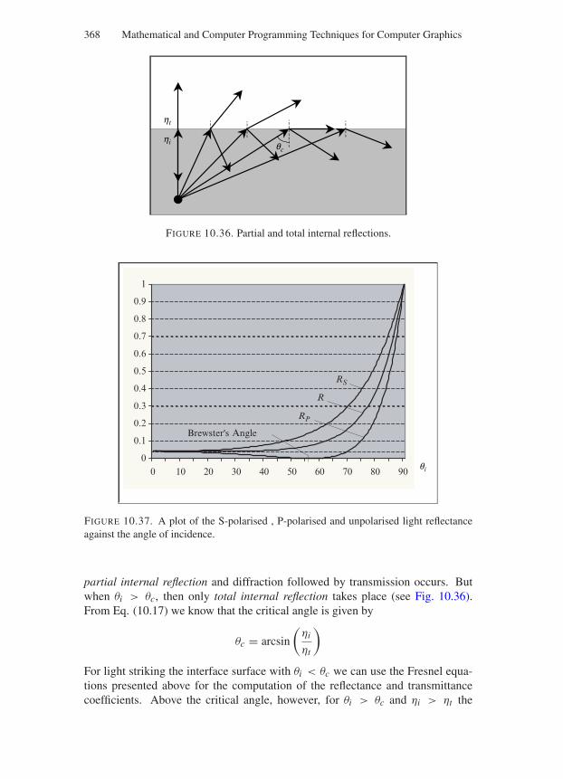
“Comninos” — 2005/8/31 — 19:01 — page 368 — #52
368 Mathematical and Computer Programming Techniques for Computer Graphics
qc
ht
hi
FIGURE 10.36. Partial and total internal reflections.
0
0.1
0.2
0.3
0.4
0.5
0.6
0.7
0.8
0.9
1
0 10 20 30 40 50 60 70 80 90qi
Brewster's Angle
RS
RP
R
FIGURE 10.37. A plot of the S-polarised , P-polarised and unpolarised light reflectanceagainst the angle of incidence.
partial internal reflection and diffraction followed by transmission occurs. Butwhen θi > θc, then only total internal reflection takes place (see Fig. 10.36).From Eq. (10.17) we know that the critical angle is given by
θc = arcsin
(ηi
ηt
)
For light striking the interface surface with θi < θc we can use the Fresnel equa-tions presented above for the computation of the reflectance and transmittancecoefficients. Above the critical angle, however, for θi > θc and ηi > ηt the
“Comninos” — 2005/8/31 — 19:01 — page 369 — #53
Physically Based Lighting and Shading Models and Rendering Algorithms 369
following equations must be used to compute the amplitude reflection and trans-mission coefficients.
rS =cos (θi ) − i ·
√
sin2 (θi ) −(
ηtηi
)2
cos (θi ) + i ·√
sin2 (θi ) −(
ηtηi
)2(10.123)
tS = 0 (10.124)
rP =(
ηtηi
)2 · cos (θi ) − i ·√
sin2 (θi ) −(
ηtηi
)2
(ηtηi
)2 · cos (θi ) − i ·√
sin2 (θi ) −(
ηtηi
)2(10.125)
tP = 0 (10.126)
where i = √−1 is the imaginary unit.In practice however, above the critical angle, we only need to compute the
power reflectance and transmittance coefficients, which can be taken to be:
RS = (rS)2 = 1 (10.127)
TS = 0 (10.128)
RP = (rP )2 = 1 (10.129)
TP = 0 (10.130)
Above the critical angle, both rS and rP have an absolute value of one and arepure phase shifts. In this case, the phase shift of the electrical field is given by
(φ) = 2· arctan
⎛
⎝cos (θi ) ·√
sin2 (θi ) −(
ηt
ηi
)2/
sin2 (θi )
⎞
⎠
where φ is the phase angle of the electrical field.Figure 10.38 depicts this case. It shows a graph of the reflectivity for S-
polarised, P-polarised and unpolarised light at the interface surface between glass(with ηi = 1.5) and air (with ηt = 1.0). In this figure Brewster’s angle is approx-imately 340and the critical angle is approximately 41.80.
The electrical properties of a material have the greatest influence on how lighttravels through it. As we have seen in Section 10.2, the magnetic field of a waveeffects the electrons of the material and the freedom of these electrons to respondto this field determines the optical characteristics of the material.
Dielectric materials are largely unaffected by the passage of light through them,as their electrons have very stable orbits that are not disturbed by the passingelectromagnetic wave.
Conductors, on the other hand, have free electrons (i.e. electrons that are freeto move inside the material) which are made to oscillate under the influence ofthe magnetic field of the wave. The oscillations of the free electrons match the
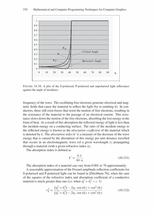
“Comninos” — 2005/8/31 — 19:01 — page 370 — #54
370 Mathematical and Computer Programming Techniques for Computer Graphics
0
0.1
0.2
0.3
0.4
0.5
0.6
0.7
0.8
0.9
1
0 10 20 30 40 50 60 70 80 90 qi
Brewster's Angle
Critical Angle
R S
R P
R
FIGURE 10.38. A plot of the S-polarised, P-polarised and unpolarised light reflectanceagainst the angle of incidence.
frequency of the wave. The oscillating free electrons generate electrical and mag-netic fields that cause the material to reflect the light (by re-emitting it). In con-ductors, there still exist forces that resist the motion of free electrons, resulting inthe resistance of the material to the passage of an electrical current. This resis-tance slows down the motion of the free electrons, absorbing the lost energy in theform of heat. As a result of this absorption the reflected energy of light is less thanthe incident energy on a conducting surface. The ratio of the incident energy tothe reflected energy is known as the absorption coefficient of the material whichis denoted by k. The absorption index k′ is a measure of the decrease of the waveenergy that is caused by the absorption of this energy per unit distance travelledthat occurs in an electromagnetic wave (of a given wavelength λ) propagatingthrough a material (with a given refractive index η).
The absorption index is defined as
k′ = k·λ4π ·η (10.131)
The absorption index of a material can vary from 0.001 to 70 approximately.A reasonable approximation of the Fresnel amplitude reflection coefficients for
S-polarised and P-polarised light can be found in [Ditchburn 76], when the sumof the squares of the refractive index and absorption coefficient of a conductivematerial is much greater than one (i.e. when η2
t + k2t >> 1)
r2S =(η2
t + k2t
)− 2ηt · cos (θi ) + cos2 (θi )(η2
t + k2t)− 2ηt · cos (θi ) + cos2 (θi )
(10.132)
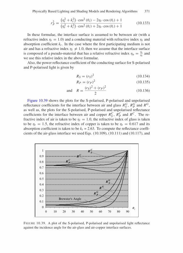
“Comninos” — 2005/8/31 — 19:01 — page 371 — #55
Physically Based Lighting and Shading Models and Rendering Algorithms 371
r2P =(η2
t + k2t
) · cos2 (θi ) − 2ηt · cos (θi ) + 1(η2
t + k2t) · cos2 (θi ) + 2ηt · cos (θi ) + 1
(10.133)
In these formulae, the interface surface is assumed to be between air (with arefractive index ηi = 1.0) and a conducting material with refractive index ηt andabsorption coefficient kt . In the case where the first participating medium is notair and has a refractive index ηi = 1.0, then we assume that the interface surfaceis composed of a pseudo-material that has a relative refractive index ηa = ηt
ηiand
we use this relative index in the above formulae.Also, the power reflectance coefficient of the conducting surface for S-polarised
and P-polarised light is given by
RS = (rS)2 (10.134)
RP = (rP )2 (10.135)
and R = (rS)2 + (rP )2
2(10.136)
Figure 10.39 shows the plots for the S-polarised, P-polarised and unpolarisedreflectance coefficients for the interface between air and glass RG
S , RGP and RG ,
as well as, the plots for the S-polarised, P-polarised and unpolarised reflectancecoefficients for the interface between air and copper RC
S , RCP and RC . The re-
fractive index of air is taken to be ηi = 1.0, the refractive index of glass is takento be ηt = 1.5, the refractive index of copper is taken to be ηt = 0.617 and itsabsorption coefficient is taken to be kt = 2.63. To compute the reflectance coeffi-cients of the air-glass interface we used Eqs. (10.109), (10.111) and (10.117), and
0
0.1
0.2
0.3
0.4
0.5
0.6
0.7
0.8
0.9
1
0 10 20 30 40 50 60 70 80 90q i
Brewster's Angle
R CS
R CP
R GS
R GP
R G
R C
FIGURE 10.39. A plot of the S-polarised, P-polarised and unpolarised light reflectanceagainst the incidence angle for the air-glass and air-copper interface surfaces.
“Comninos” — 2005/8/31 — 19:01 — page 372 — #56
372 Mathematical and Computer Programming Techniques for Computer Graphics
for the reflectance coefficients of the air-copper interface we used Eqs. (10.132),(10.133) and (10.136).
The low reflectance of glass is characteristic of all dielectric materials and thehigh reflectance of copper is characteristic of all conductors. As can also beseen from this diagram, all materials become 100% reflective at grazing angles(i.e. when θi ≈ 900). This is why when we observe a surface at an acute angle wesee glare from the surface.
Although the Fresnel relationship provides a valuable insight as to how lightbehaves at an interface surface, its usefulness is often limited in practice as thereis very little reliable data on the refractive indices and absorption coefficients ofmaterials. This is exacerbated by the fact that the refractive index and absorptioncoefficient of a given material is wavelength dependent. Frequently, these val-ues only exist for a single wavelength value of light and this information is notsufficient for our purposes in computer graphics. Useful source of such data are[Jenkins 76] and [Palik 85]. Also the website [WWW 1] is a source of very usefullighting data, listing indices of refraction and providing a photonics calculator.
Where there is missing or insufficient data for the refractive indices of partic-ipating materials and the absorption coefficients of conducting materials, we canuse a set of techniques, developed by Cook and Torrance, to approximate this data[Cook 82].
For unpolarised light, a good approximation of the average reflectance coeffi-cient of a given material is given in [Schlick 93]
R (θi ) ≈ R0 + (1 − R0) · (1 − cos (θi ))5 (10.137)
where R (θi ) is the average reflectance at incidence angle θi and R0 is the mea-sured value of the reflectance at normal incidence (i.e. measured in the directionof the normal of the surface.
In some literature the quantities that relate to S-polarised and P-polarised lightare either subscripted or superscripted by the symbols “⊥” and “‖”, respectively.Thus the terms rS , tS , RS , TS , rP , tP , RP and TP may also be written as r⊥, t⊥,R⊥, T⊥, r‖, t‖, R‖ and T‖, respectively.
10.10.4 Glossy or Semi-coherent Reflections
Most surfaces that we observe and we are likely to wish to simulate in computergraphics produce neither ideal mirror reflections (totally coherent reflections) norideal Lambertian reflections (totally incoherent reflections). They produce semi-coherent reflections that we have chosen to refer to as glossy reflections. Thename chosen is descriptive of their properties, but is by no means the only es-tablished name in the literature. Other authors call such surfaces rough specular,semi-coherent, directional diffuse or wide and narrow diffuse.
As we have observed before, perfectly smooth surfaces produce totally coher-ent reflections, rough surfaces produce semi-coherent reflections and perfectly
“Comninos” — 2005/8/31 — 19:01 — page 373 — #57
Physically Based Lighting and Shading Models and Rendering Algorithms 373
rough surfaces produce totally incoherent reflections. The degree of smoothnessor roughness of a surface is explained in terms of the micro-facets that make upthe surface.
Perfectly smooth surfaces are composed of micro-facets that are perfectlyaligned and have normals that point in the same direction. Thus, they reflect andtransmit light in the directions and proportions predicted by the Fresnel equationsand Snell’s law.
Perfectly rough surfaces (matt surfaces) have micro-facets that are totally ran-domly oriented and have normals that are evenly distributed over the entire illu-minating hemisphere. Thus, they reflect and transmit light evenly in all directionsand obey Lambert’s law.
Rough surfaces are composed of micro-facets that are unevenly distributed andhave normals that are statistically distributed around the main (average) normal ofthe surface. This micro-facet normal distribution can be biased in certain direc-tions to account for grooves, scratches, cracks or some other surface finish. Thus,such surfaces reflect and transmit light in a more complex and unpredictable wayand give rise to semi-coherent (defocused) reflections. In this case, the amount oflight from a given light source being reflected in the direction of the viewer is pro-portional to the number of micro-facets that have their normals aligned halfwaybetween the vectors pointing, out of the surface, towards the light source and theviewer. This direction is represented by the H vector in Fig. 10.10. This unitvector is computed as
H = L + E|L + E| (10.138)
where L is the unit vector pointing in the direction of the light source and E is theunit vector pointing in the direction of the viewer (eye).
Various models with varying degrees of sophistication have been developed bycomputer graphics researchers over the years. Some of these models are purelyempirical in nature, while others are physically plausible or even more physicallybased. A good survey of the early models can be found in [Hall 89] and a moreup to date treatment in [Lewis 93].
For most surfaces that occur in nature, getting the precise physical model ofthe interaction of light with the surface is very difficult if not impossible. Mostresearchers in the field have concentrated on developing models that are goodapproximations of physical phenomena while being both visually accurate andeasy to compute.
For simple renderers, visual believability and ease of computation are the pri-mary criteria for selecting a particular model. With more sophisticated renderers,using radiosity computations which are energy conserving, the selected modelmust also be physically plausible. This of course does not necessarily mean thatthe model is physically accurate, but only that it does not violate the laws ofphysics and it is thus a believable model of a physical process.
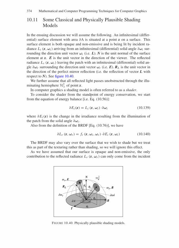
“Comninos” — 2005/8/31 — 19:01 — page 374 — #58
374 Mathematical and Computer Programming Techniques for Computer Graphics
10.11 Some Classical and Physically Plausible ShadingModels
In the ensuing discussion we will assume the following. An infinitesimal (differ-ential) surface element with area ∂A is situated at a point x on a surface. Thissurface element is both opaque and non-emissive and is being lit by incident ra-diance Li (x,ωi ) arriving from an infinitesimal (differential) solid angle ∂ωi sur-rounding the direction unit vector ωi (i.e. L). N is the unit normal of the surfaceelement at x. E is the unit vector in the direction of the viewer. The reflectedradiance Lr (x,ωr ) leaving the patch with an infinitesimal (differential) solid an-gle ∂ωr surrounding the direction unit vector ωr (i.e. E). RL is the unit vector inthe direction of the perfect mirror reflection (i.e. the reflection of vector L withrespect to N). See figure 10.40.
We further assume that all reflected light passes unobstructed through the illu-minating hemisphere H2+ of point x.
In computer graphics a shading model is often referred to as a shader.To consider the shader from the standpoint of energy conservation, we start
from the equation of energy balance [i.e. Eq. (10.56)]:
∂ Ei (x) = Li (x,ωi ) ·∂ωi (10.139)
where ∂ Ei (x) is the change in the irradiance resulting from the illumination ofthe patch from the solid angle ∂ωi .
Also from the definition of the BRDF [Eq. (10.76)], we have
∂Lr (x,ωr ) = fr (x,ωi ,ωr ) ·∂ Ei (x,ωi ) (10.140)
The BRDF may also vary over the surface that we wish to shade but we treatthis as part of the texturing rather than shading, so we will ignore this effect.
As we have assumed that our surface is opaque and non-emissive, the onlycontribution to the reflected radiance Lr (x,ωr ) can only come from the incident
N
B
T
x
qi
fi
fr
RL
2i
∂w r
w r , E
∂w i
w i , B
∂A
qr
FIGURE 10.40. Physically plausible shading models.
“Comninos” — 2005/8/31 — 19:01 — page 375 — #59
Physically Based Lighting and Shading Models and Rendering Algorithms 375
illuminating hemisphere H2i , thus
Lr (x,ωt ) =∫
H2i
fr (x,ωi ,ωr ) ·Li (x,ωi ) ·∂ω⊥i
=∫
H2i
fr (x,ωi ,ωr ) ·Li (x,ωi ) · (N ωi ) ·∂ωi
=∫
H2i
fr (x,ωi ,ωr ) ·Li (x,ωi ) · cos (θi ) ·∂ωi (10.141)
Next we will consider some of the most common shaders used in computergraphics expressed as BRDFs.
10.11.1 Phong Shader
As we have seen in Chapter 9, the Phong shader is given by the equation
Lr = ka ·La + (kd · (N L) + ks ·Fs (N, L, E, ns)) ·Ld (10.142)
where ka is the ambient reflection coefficient, La is the ambient radiance evenlydistributed over the incident illuminating hemisphere H2
i , kd is the diffuse reflec-tion coefficient, ks is the specular reflection coefficient, Fs is the specular reflec-tion function, ns is the specular sharpness and Ld is the radiance coming from thedirection L of the light source.
As we have seen in Section 9.3.3, the specular function can be defined usingHorn’s method:
Fs (N, L, E, ns) = (2· (N E) · (N L) − (E L))ns (10.143)
or Blinn’s method:
Fs (N, L, E, ns) =(
N L + E|L + E|
) ns
(10.144)
Let us examine how the Phong shader of Eq. (10.142) corresponds to Eq.(10.141). Our surface patch is illuminated by the directed radiance Ld comingfrom the direction of the light source and by the ambient radiance La which isconstant over H2
i . From the directional illumination we have θi = θl and φi = φl .We can now express the resulting incident radiance as
Li = La + Ld ·δ (cos (θi ) − cos (θl)) ·δ (φi − φl) (10.145)
Equation (10.141) can be rewritten as
Lr =∫
H2i
fr (θi , φi , E) ·Li · cos (θi ) ·∂θi ·∂φi (10.146)
Substituting equation (10.145) into equation (10.146) we get
Lr = La ·∫
H2i
fr (θl , φl , E) · cos (θl) ·∂θl ·∂φl + Ld · fr (θi , φi , E) · cos (θi )
“Comninos” — 2005/8/31 — 19:01 — page 376 — #60
376 Mathematical and Computer Programming Techniques for Computer Graphics
which can be rewritten as
Lr = La ·∫
H2i
fr (L, E) · (N L) ·∂ωi + Ld · fr (L, E) · (N L) (10.147)
By combining Eqs. (10.142) and (10.147) we get
ka ·La + (kd · (N L) + ks ·Fs (N, L, E, ns)) ·Ld
= La ·∫
H2i
fr (L, E) · (N L) ·∂ωi + Ld · fr (L, E) · (N L)
This equality must be valid for all values of La and Ld . Equating the compo-nents of this equation that deal with the directed radiance Ld , we get
Ld · fr (L, E) · (N L) = (kd · (N L) + ks ·Fs (N, L, E, ns)) ·Ld
∴ fr (L, E) · (N L) = kd · (N L) + ks ·Fs (N, L, E, ns)
∴ fr (L, E) = kd · (N L) + ks ·Fs (N, L, E, ns)
(N L)
Thus, the Phong shader BRDF is given by
fr (x, L, E) = kd + ks · Fs (N, L, E, ns)
(N L)(10.148)
Note that the specular function in Eq. (10.143) can also be written as
Fs (N, L, E, ns) = (E RL)ns (10.149a)
where RL is the unit vector representing the reflection of L with respect to N,which as we have seen in Section 10.4.2 can be computed as
RL = 2· (N L) ·N − L
or alternatively using the Householder matrix as
RL = R(N)·LEqually, the specular function can be rewritten as
Fs (N, L, E, ns) = (L RE )ns (10.149b)
where
RE = 2· (N E) ·N − E
or RE = R(N)·EThe original Phong model is not physically plausible, since it obeys neither the
energy conservation property nor the reciprocity property.
“Comninos” — 2005/8/31 — 19:01 — page 377 — #61
Physically Based Lighting and Shading Models and Rendering Algorithms 377
10.11.2 Modified Phong Shader
Lafortune and Willems proposed a modified version of the Phong model, whichdeals with the lack of reciprocity and energy conservation of the original model[Lafortune 94]. Their BRDF is given as the sum of a diffuse BRDF and a specularBRDF.
fr (x,ωi ,ωr ) = fr,d (x,ωi ,ωr ) + fr,s (x,ωi ,ωr )
i.e. fr (x, L, E) = kd · 1
π+ ks ·ns + 2
2π· cosns α (10.150)
where kd is the diffuse reflectivity (i.e. the fraction of incoming energy that isreflected diffusely), ks is the specular reflectivity (i.e. the fraction of incomingenergy that is reflected in a specular manner), ns is the specular sharpness (i.e. thehigher this exponent is the sharper the specular reflections) and α is the highlightangle (i.e. the angle between vectors E and RL or between L and ER). This anglemust be clamped to π
/2, to avoid negative cosine values. The cosine of this angle
is given as
cos α = (E RL) = (L RE ) (10.151)
Lafortune and Willems show that the modified Phong model obeys the Helmholtzreciprocity property and that the total hemispherical reflectivity of this model be-comes
ρ (x,ωi ,ωr ) =∫
H2r
fr (x,ωi ,ωr ) · cos (θr ) ·∂ωr
=∫
H2r
(kd · 1
π+ ks ·ns + 2
2π· cosns α
)· cos (θr ) ·∂ωr
= kd + ks ·ns + 2
2π
∫
H2r
cosns α· cos (θr ) ·∂ωr
= ρd + ρs (x,ωi ,ωr )
As the integral∫H2
rcosns α· cos (θr ) ·∂ωr reaches its maximum value of
2π/(ns + 2) at a normal incident direction (i.e. when α = θr ), we have
ρmax = kd + ks
In order for the BRDF to obey the energy conservation property we must have
kd + ks ≤ 1 (10.152)
Thus, the Lafortune and Willems modifications of the Phong model make itphysically plausible.
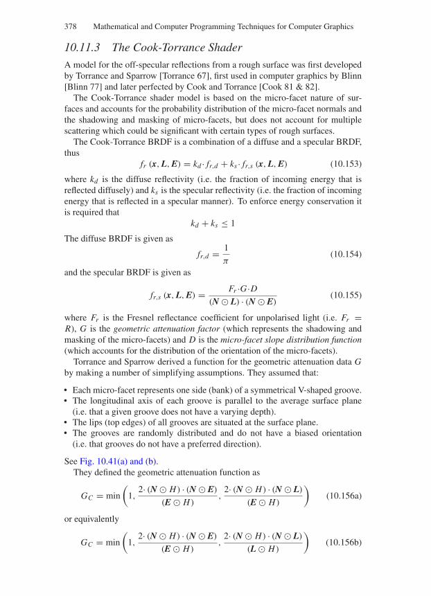
“Comninos” — 2005/8/31 — 19:01 — page 378 — #62
378 Mathematical and Computer Programming Techniques for Computer Graphics
10.11.3 The Cook-Torrance Shader
A model for the off-specular reflections from a rough surface was first developedby Torrance and Sparrow [Torrance 67], first used in computer graphics by Blinn[Blinn 77] and later perfected by Cook and Torrance [Cook 81 & 82].
The Cook-Torrance shader model is based on the micro-facet nature of sur-faces and accounts for the probability distribution of the micro-facet normals andthe shadowing and masking of micro-facets, but does not account for multiplescattering which could be significant with certain types of rough surfaces.
The Cook-Torrance BRDF is a combination of a diffuse and a specular BRDF,thus
fr (x, L, E) = kd · fr,d + ks · fr,s (x, L, E) (10.153)
where kd is the diffuse reflectivity (i.e. the fraction of incoming energy that isreflected diffusely) and ks is the specular reflectivity (i.e. the fraction of incomingenergy that is reflected in a specular manner). To enforce energy conservation itis required that
kd + ks ≤ 1
The diffuse BRDF is given as
fr,d = 1
π(10.154)
and the specular BRDF is given as
fr,s (x, L, E) = Fr ·G·D(N L) · (N E)
(10.155)
where Fr is the Fresnel reflectance coefficient for unpolarised light (i.e. Fr =R), G is the geometric attenuation factor (which represents the shadowing andmasking of the micro-facets) and D is the micro-facet slope distribution function(which accounts for the distribution of the orientation of the micro-facets).
Torrance and Sparrow derived a function for the geometric attenuation data Gby making a number of simplifying assumptions. They assumed that:
• Each micro-facet represents one side (bank) of a symmetrical V-shaped groove.• The longitudinal axis of each groove is parallel to the average surface plane
(i.e. that a given groove does not have a varying depth).• The lips (top edges) of all grooves are situated at the surface plane.• The grooves are randomly distributed and do not have a biased orientation
(i.e. that grooves do not have a preferred direction).
See Fig. 10.41(a) and (b).They defined the geometric attenuation function as
GC = min
(1,
2· (N H) · (N E)
(E H),
2· (N H) · (N L)
(E H)
)(10.156a)
or equivalently
GC = min
(1,
2· (N H) · (N E)
(E H),
2· (N H) · (N L)
(L H)
)(10.156b)
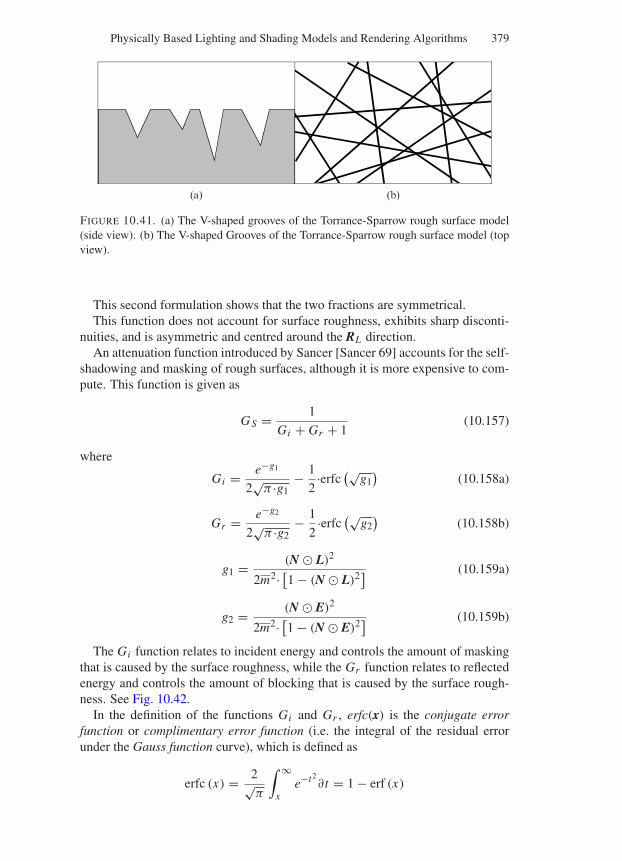
“Comninos” — 2005/8/31 — 19:01 — page 379 — #63
Physically Based Lighting and Shading Models and Rendering Algorithms 379
(a) (b)
FIGURE 10.41. (a) The V-shaped grooves of the Torrance-Sparrow rough surface model(side view). (b) The V-shaped Grooves of the Torrance-Sparrow rough surface model (topview).
This second formulation shows that the two fractions are symmetrical.This function does not account for surface roughness, exhibits sharp disconti-
nuities, and is asymmetric and centred around the RL direction.An attenuation function introduced by Sancer [Sancer 69] accounts for the self-
shadowing and masking of rough surfaces, although it is more expensive to com-pute. This function is given as
GS = 1
Gi + Gr + 1(10.157)
where
Gi = e−g1
2√
π ·g1− 1
2·erfc(√
g1)
(10.158a)
Gr = e−g2
2√
π ·g2− 1
2·erfc(√
g2)
(10.158b)
g1 = (N L)2
2m2· [1 − (N L)2] (10.159a)
g2 = (N E)2
2m2· [1 − (N E)2] (10.159b)
The Gi function relates to incident energy and controls the amount of maskingthat is caused by the surface roughness, while the Gr function relates to reflectedenergy and controls the amount of blocking that is caused by the surface rough-ness. See Fig. 10.42.
In the definition of the functions Gi and Gr , erfc(x) is the conjugate errorfunction or complimentary error function (i.e. the integral of the residual errorunder the Gauss function curve), which is defined as
erfc (x) = 2√π
∫ ∞
xe−t2
∂t = 1 − erf (x)
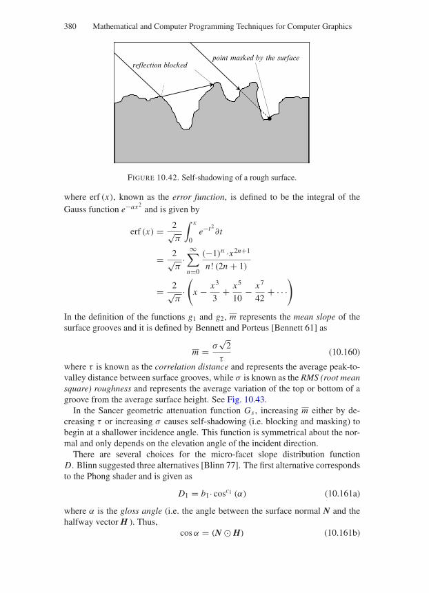
“Comninos” — 2005/8/31 — 19:01 — page 380 — #64
380 Mathematical and Computer Programming Techniques for Computer Graphics
reflection blockedpoint masked by the surface
FIGURE 10.42. Self-shadowing of a rough surface.
where erf (x), known as the error function, is defined to be the integral of theGauss function e−ax2
and is given by
erf (x) = 2√π
∫ x
0e−t2
∂t
= 2√π
·∞∑
n=0
(−1)n ·x2n+1
n! (2n + 1)
= 2√π
·(
x − x3
3+ x5
10− x7
42+ · · ·)
In the definition of the functions g1 and g2, m represents the mean slope of thesurface grooves and it is defined by Bennett and Porteus [Bennett 61] as
m = σ√
2
τ(10.160)
where τ is known as the correlation distance and represents the average peak-to-valley distance between surface grooves, while σ is known as the RMS (root meansquare) roughness and represents the average variation of the top or bottom of agroove from the average surface height. See Fig. 10.43.
In the Sancer geometric attenuation function Gs , increasing m either by de-creasing τ or increasing σ causes self-shadowing (i.e. blocking and masking) tobegin at a shallower incidence angle. This function is symmetrical about the nor-mal and only depends on the elevation angle of the incident direction.
There are several choices for the micro-facet slope distribution functionD. Blinn suggested three alternatives [Blinn 77]. The first alternative correspondsto the Phong shader and is given as
D1 = b1· cosc1 (α) (10.161a)
where α is the gloss angle (i.e. the angle between the surface normal N and thehalfway vector H ). Thus,
cos α = (N H) (10.161b)
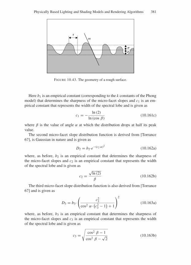
“Comninos” — 2005/8/31 — 19:01 — page 381 — #65
Physically Based Lighting and Shading Models and Rendering Algorithms 381
m
ss
t
FIGURE 10.43. The geometry of a rough surface.
Here b1 is an empirical constant (corresponding to the k constants of the Phongmodel) that determines the sharpness of the micro-facet slopes and c1 is an em-pirical constant that represents the width of the spectral lobe and is given as
c1 = − ln (2)
ln (cos β)(10.161c)
where β is the value of angle α at which the distribution drops at half its peakvalue.
The second micro-facet slope distribution function is derived from [Torrance67], is Gaussian in nature and is given as
D2 = b2·e−(c2·α)2(10.162a)
where, as before, b2 is an empirical constant that determines the sharpness ofthe micro-facet slopes and c2 is an empirical constant that represents the widthof the spectral lobe and is given as
c2 =√
ln (2)
β(10.162b)
The third micro-facet slope distribution function is also derived from [Torrance67] and is given as
D3 = b3·(
c23
cos2 α· (c23 − 1)+ 1
)2
(10.163a)
where, as before, b3 is an empirical constant that determines the sharpness ofthe micro-facet slopes and c3 is an empirical constant that represents the widthof the spectral lobe and is given as
c3 =√
cos2 β − 1
cos2 β − √2
(10.163b)
“Comninos” — 2005/8/31 — 19:01 — page 382 — #66
382 Mathematical and Computer Programming Techniques for Computer Graphics
Cook and Torrance introduced an alternative micro-facet slope distribution func-tion [Cook 82], which is derived from [Beckmann 63]. This function is given as
D4 = 1
4m2· cos4 α·e−(
1−cos2 α
m2 · cos2 α
)
(10.164a)
where m is the RMS micro-facet slope distribution of the rough surface, which isgive as
m = tan β√ln (2) − 4· ln (cos β)
(10.164b)
The Cook-Torrance shader is reciprocal and appears to conserve energy, but itfails to account for the blocked and masked energy. The shader does not treat sec-ondary reflections and instead it treats blocked or masked light as being absorbedby the surface.
10.11.4 The Ashikmin-Shirley Shader
Ashikmin and Shirley developed a shading model based on the Blinn variation ofthe Phong shading model [Ashikmin 00a, 00b & 00c]. Their version of the Phongmodel incorporates and refines some of the improvements first introduced to thismodel by Schlick [Schlick 93], Newmann et al. [Neumann 99a & 99b] and Lafor-tune et al. [Lafortune 97]. The Ashikmin and Shirley model is a modern versionof the Phong model which is energy preserving, reciprocal, has a sophisticatednon-Lambertian non-constant diffuse term (which decreases as the incidence an-gle increases), takes into account the Fresnel effect, is capable of describing bothisotropic and anisotropic surface finishes and uses an intuitive set of parameters.In their publications, they state that their BRDF is the sum of a diffuse and aspecular component, i.e.
fr (x, L, E) = fr,d (x, L, E) + fr,s (x, L, E) (10.165)
If we examine their model more carefully however, we realise that it is not justthe sum of a diffuse and a specular component but a linear combination of thesetwo components. This relationship can be expressed as follows:
fr (x, L, E) = [1 − ks (α)] ·kd · f ′r,d (x, L, E) + ks (α) · f ′
r,s (x, L, E) (10.166)
where f ′r,d and f ′
r,s are the diffuse and specular BRDF components before scaling,kd is the diffuse reflection coefficient (a constant), ks (α) is the specular reflectioncoefficient function and α is the angle whose cosine is used to shape the specularlobe.
This type of shading model was designed to simulate the reflection of lightfrom polished surfaces and an earlier version of it is described in Shirley’s Ph.Dthesis [Shirley 91]. A polished surface reflector can be thought of as a diffusereflector covered by a transparent specular coating. A simplified depiction ofsuch a polished surface is shown in Fig. 10.44.
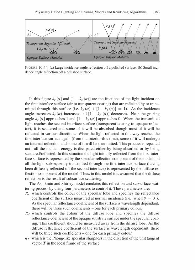
“Comninos” — 2005/8/31 — 19:01 — page 383 — #67
Physically Based Lighting and Shading Models and Rendering Algorithms 383
ks(a)
Air
1-ks(a)
Transparent Specular Material
Opaque Diffuse Material
ks(a)
Air
Transparent SpecularMaterial
Opaque Diffuse Material
1-ks(a)
FIGURE 10.44. (a) Large incidence angle reflection off a polished surface. (b) Small inci-dence angle reflection off a polished surface.
In this figure ks [α] and [1 − ks (α)] are the fractions of the light incident onthe first interface surface (air to transparent coating) that are reflected by or trans-mitted through this surface (i.e. ks (α) + [1 − ks (α)] = 1). As the incidenceangle increases ks (α) increases and [1 − ks (α)] decreases. Near the grazingangle ks [α] approaches 1 and [1 − ks (α)] approaches 0. When the transmittedlight reaches the second interface surface (transparent coating to opaque reflec-tor), it is scattered and some of it will be absorbed though most of it will bereflected in various directions. When the light reflected in this way reaches thefirst interface surface again (from the interior this time), some of it will undergoan internal reflection and some of it will be transmitted. This process is repeateduntil all the incident energy is dissipated either by being absorbed or by beingscattered/reflected. In this situation the light initially reflected from the first inter-face surface is represented by the specular reflection component of the model andall the light subsequently transmitted through the first interface surface (havingbeen diffusely reflected off the second interface) is represented by the diffuse re-flection component of the model. Thus, in this model it is assumed that the diffusereflection is the result of subsurface scattering.
The Ashikmin and Shirley model emulates this reflection and subsurface scat-tering process by using four parameters to control it. These parameters are:Rs which controls the colour of the specular lobe and specifies the reflectance
coefficient of the surface measured at normal incidence (i.e. when θi = 00).As the specular reflectance coefficient of the surface is wavelength dependant,there will be three such coefficients – one for each primary colour.
Rd which controls the colour of the diffuse lobe and specifies the diffusereflectance coefficient of the opaque substrate surface under the specular coat-ing. This coefficient should be measured away from the diffuse lobe. As thediffuse reflectance coefficient of the surface is wavelength dependant, therewill be three such coefficients – one for each primary colour.
nT which is the Phong-like specular sharpness in the direction of the unit tangentvector T in the local frame of the surface.
“Comninos” — 2005/8/31 — 19:01 — page 384 — #68
384 Mathematical and Computer Programming Techniques for Computer Graphics
nB which is the Phong-like specular sharpness in the direction of the unit bitan-gent vector B in the local frame of the surface.
As we have seen above, the specular part f r,s of the BRDF does not representa pure specular reflection and cannot be modelled with a combination of Dirac’sdelta functions. It represents the glossy part of the BRDF and has a lobe that isnot symmetric about the surface normal (as we use two specular sharpness valuesnT and nB).
The diffuse part f r,d of the BRDF is not constant, as it is view dependent andhas a lobe that exhibits rotational symmetry about the surface normal. This partof the BRDF models the phenomenon by which the diffuse colour of a surfacedisappears near the grazing angle, as most of the light is reflected in a specularfashion at that angle. Thus the fraction of energy that is scattered diffusely isdependent on the fraction of energy that is reflected in a specular fashion, whichin turn depends on the incidence angle.
With this model, to represent metal surfaces f r,d is forced to zero by setting theRd parameter to zero. To represent brushed metal surfaces we can vary the valuesof the specular sharpens in the T and B directions in a non-uniform fashion. Torepresent polished surfaces, such as smooth plastics, we must set Rd and Rs tonon-zero values. For plastics typically Rs = 0.05. Finally, to represent diffusesurfaces we must set the Rs coefficient to a very small value.
The Ashikmin and Shirley specular BRDF is given as
fr,s (x, E, L) =√
(nT + 1) · (nB + 1)
8π
· (N H)[nT (T H)2+nB (BH)2]/
[1−(NH)2]
cos α· max ((N L) , (N E))
·Fr (cos α) (10.167)
where H is the halfway vector H = (L + E)/|L + E|, T and B are the tangent
and bitangent vectors, respectively. Fr () is the Fresnel reflectance coefficientcomputed using Schlick’s approximation [Schlick 93], i.e.
Fr (cos α) = Rs + (1 − Rs) · (1 − cos α)5 (10.168)
and where α is the angle that is used to shape the lobe of the specular BRDF.Normally cos α = (L H) or cos α = (E H).
The Ashikmin and Shirley diffuse BRDF is given as
fr,d (x, L, E) = Rd · (1 − Rs) ·(
28
23π
)·(
1 −(
1 − (N L)
2
)5)
·(
1 −(
1 − (N E)
2
)5)
(10.169)
The constant 28/
23π was selected to enforce energy conservation. Observethat the diffuse component of the BRDF is isotropic, as it does not depend on nT
and nB .
“Comninos” — 2005/8/31 — 19:01 — page 385 — #69
Physically Based Lighting and Shading Models and Rendering Algorithms 385
To represent isotropic surfaces we can set nT = nB = nS , in which case thespecular component BRDF can be simplified to
fr,s (x, E, L) = (nS + 1)
8π· (N H)nS
cos α· max ((N L) , (N E))·Fr (cos α)
(10.170)The Ashikmin and Shirley BRDF although based on an empirical model, sim-
ulates a number of physical effects and it is physically plausible, thus it is consid-ered to be a physically based BRDF.
10.12 Illumination Models and the Rendering Equation
The application of our knowledge of optics and physics to computer generatedrendering is an evolutionary process which at any given time is dependant onthe following three factors: the sophistication of the currently available hidden-surface removal algorithms, the degree of realism that is currently deemed ac-ceptable and the computational cost per computer generated frame currently con-sidered affordable. The illumination models used in the computer graphics andanimation production process differ significantly from the theoretical physicallybased models. Computer generated rendering has always been and is likely tocontinue to be a feasibility versus quality versus cost compromise.
In Section 10.7.3, we have seen how the surface reflectance, transmittance andscattering equations can be used to compute the reflected, transmitted and scat-tered light distribution from the incident light distribution and the BRDF, BTDFand BSDF of the interface surface. All these equations are of the form
Lo (x,ωo) =∫
H2i
fT (x, ωi ,ωo) ·Li (x,ωi ) · cos (θi ) ·∂ωi (10.171)
where the subscripts i and o indicate the incoming and outgoing radiance andangles, respectively, and the subscript T can be one of r , t or s indicating thebi-directional distribution function of the surface for reflection, transmission orscattering, respectively.
In Section 10.11, we have seen how some empirical (classical) and some phys-ically plausible shading models can be defined.
The one remaining task left to do is to determine how we compute the incomingradiance Li (x,ωi ). The simulation of the incoming light distribution is oftenreferred to as the illumination model. We can distinguish two different typesof illumination model, namely: the local illumination model, also known as thedirect illumination model, and the global illumination model, also known as theindirect illumination model.
The local or direct illumination model is the simplest to explain and understand,as it only deals with the light, from simple light sources, arriving on the surfaceunobstructed by other surfaces and objects in the scene. This model can only dealwith a small number of point or parallel light sources, which can be shaped, in
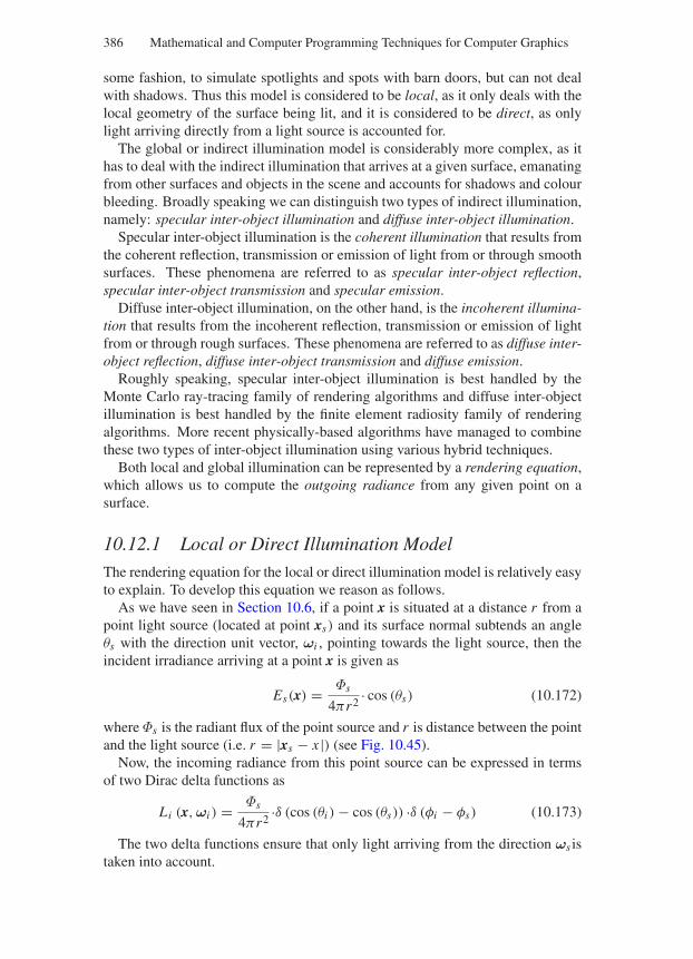
“Comninos” — 2005/8/31 — 19:01 — page 386 — #70
386 Mathematical and Computer Programming Techniques for Computer Graphics
some fashion, to simulate spotlights and spots with barn doors, but can not dealwith shadows. Thus this model is considered to be local, as it only deals with thelocal geometry of the surface being lit, and it is considered to be direct, as onlylight arriving directly from a light source is accounted for.
The global or indirect illumination model is considerably more complex, as ithas to deal with the indirect illumination that arrives at a given surface, emanatingfrom other surfaces and objects in the scene and accounts for shadows and colourbleeding. Broadly speaking we can distinguish two types of indirect illumination,namely: specular inter-object illumination and diffuse inter-object illumination.
Specular inter-object illumination is the coherent illumination that results fromthe coherent reflection, transmission or emission of light from or through smoothsurfaces. These phenomena are referred to as specular inter-object reflection,specular inter-object transmission and specular emission.
Diffuse inter-object illumination, on the other hand, is the incoherent illumina-tion that results from the incoherent reflection, transmission or emission of lightfrom or through rough surfaces. These phenomena are referred to as diffuse inter-object reflection, diffuse inter-object transmission and diffuse emission.
Roughly speaking, specular inter-object illumination is best handled by theMonte Carlo ray-tracing family of rendering algorithms and diffuse inter-objectillumination is best handled by the finite element radiosity family of renderingalgorithms. More recent physically-based algorithms have managed to combinethese two types of inter-object illumination using various hybrid techniques.
Both local and global illumination can be represented by a rendering equation,which allows us to compute the outgoing radiance from any given point on asurface.
10.12.1 Local or Direct Illumination Model
The rendering equation for the local or direct illumination model is relatively easyto explain. To develop this equation we reason as follows.
As we have seen in Section 10.6, if a point x is situated at a distance r from apoint light source (located at point xs) and its surface normal subtends an angleθs with the direction unit vector, ωi , pointing towards the light source, then theincident irradiance arriving at a point x is given as
Es(x) = Φs
4πr2· cos (θs) (10.172)
where Φs is the radiant flux of the point source and r is distance between the pointand the light source (i.e. r = |xs − x |) (see Fig. 10.45).
Now, the incoming radiance from this point source can be expressed in termsof two Dirac delta functions as
Li (x,ωi ) = Φs
4πr2·δ (cos (θi ) − cos (θs)) ·δ (φi − φs) (10.173)
The two delta functions ensure that only light arriving from the direction ωs istaken into account.
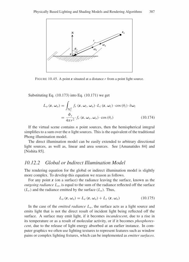
“Comninos” — 2005/8/31 — 19:01 — page 387 — #71
Physically Based Lighting and Shading Models and Rendering Algorithms 387
N
x
w i
xs
rw s
q s
FIGURE 10.45. A point x situated at a distance r from a point light source.
Substituting Eq. (10.173) into Eq. (10.171) we get
Lo (x,ωo) =∫
H2i
fr (x,ωi ,ωo) ·Li (x,ωi ) · cos (θi ) ·∂ωi
= Φs
4πr2· fr (x,ωs,ωo) · cos (θs) (10.174)
If the virtual scene contains n point sources, then the hemispherical integralsimplifies to a sum over the n light sources. This is the equivalent of the traditionalPhong illumination model.
The direct illumination model can be easily extended to arbitrary directionallight sources, as well as, linear and area sources. See [Amanatides 84] and[Nishita 85].
10.12.2 Global or Indirect Illumination Model
The rendering equation for the global or indirect illumination model is slightlymore complex. To develop this equation we reason as follows.
For any point x (on a surface) the radiance leaving the surface, known as theoutgoing radiance Lo, is equal to the sum of the radiance reflected off the surface(Lr ) and the radiance emitted by the surface (Le). Thus,
Lo (x,ωo) = Le (x,ωo) + Lr (x,ωo) (10.175)
In the case of the emitted radiance Le, the surface acts as a light source andemits light that is not the direct result of incident light being reflected off thesurface. A surface may emit light, if it becomes incandescent, due to a rise inits temperature or as a result of molecular activity, or if it becomes phosphores-cent, due to the release of light energy absorbed at an earlier instance. In com-puter graphics we often use lighting textures to represent features such as windowpains or complex lighting fixtures, which can be implemented as emitter surfaces.
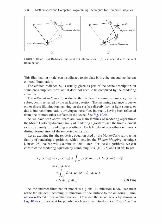
“Comninos” — 2005/8/31 — 19:01 — page 388 — #72
388 Mathematical and Computer Programming Techniques for Computer Graphics
Direct Illumination
Transparent Surface
Indirect Illumination
Transparent Surface
(a) (b)
FIGURE 10.46. (a) Radiance due to direct illumination. (b) Radiance due to indirectillumination.
This illumination model can be adjusted to simulate both coherent and incoherentemitted illumination.
The emitted radiance Le is usually given as part of the scene description, insome pre-computed form, and it does not need to be computed by the renderingequation.
The reflected radiance Lr is due to the incident incoming radiance Li that issubsequently reflected by the surface in question. The incoming radiance is due toeither direct illumination, arriving on the surface directly from a light source, ordue to indirect illumination, arriving at the surface indirectly having been reflectedfrom one or more other surfaces in the scene. See Fig. 10.46.
As we have seen above, there are two main families of rendering algorithms:the Monte Carlo ray-tracing family of rendering algorithms and the finite elementradiosity family of rendering algorithms. Each family of algorithms requires adistinct formulation of the rendering equation.
Let us examine first the rendering equation used by the Monte Carlo ray-tracingfamily of rendering algorithms, which includes the Photon Mapping technique[Jensen 96] that we will examine in detail later. For these algorithms, we canconstruct the rendering equation by combining Eqs. (10.175) and (10.86) to get
Lo (x,ωo) = Le (x,ωo) +∫
H2i
fr (x,ωi ,ωo) ·Li (x,ωi ) ·∂ω⊥i
= Le (x,ωo)
+∫
H2i
fr (x,ωi ,ωo) ·Li (x,ωi )
· (N ωi ) ·∂ωi (10.176)
As the indirect illumination model is a global illumination model, we mustrelate the incident incoming illumination of one surface to the outgoing illumi-nation reflected from another surface. Consider the scene geometry shown inFig. 10.47a. To account for possible occlusions we introduce a visibility function
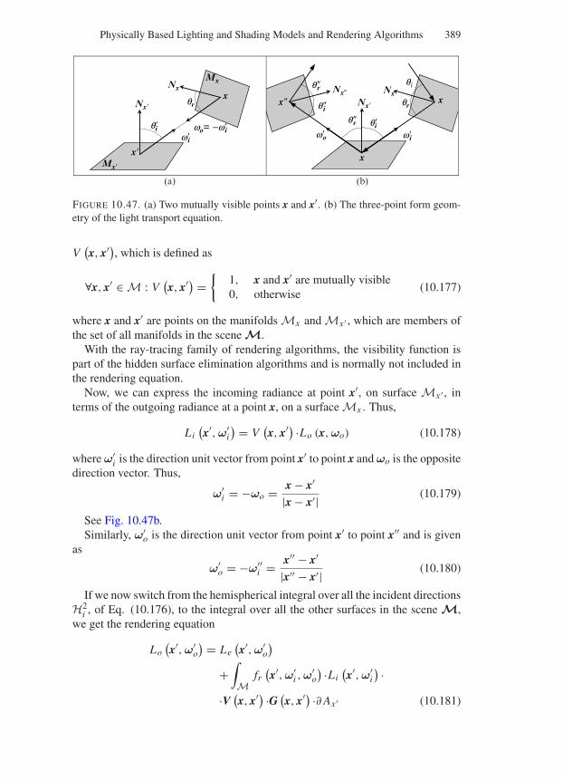
“Comninos” — 2005/8/31 — 19:01 — page 389 — #73
Physically Based Lighting and Shading Models and Rendering Algorithms 389
Nx
Nx
Mx
Mx
qiqi
qi
qi
qr
qr
wi wiwo
qr qr
wo= −wi
x
x NxNx
x
xNx
x
(a) (b)
FIGURE 10.47. (a) Two mutually visible points x and x′. (b) The three-point form geom-etry of the light transport equation.
V(x, x′), which is defined as
∀x, x′ ∈ M : V(x, x′) =
1, x and x′ are mutually visible0, otherwise
(10.177)
where x and x′ are points on the manifolds Mx and Mx ′ , which are members ofthe set of all manifolds in the scene M.
With the ray-tracing family of rendering algorithms, the visibility function ispart of the hidden surface elimination algorithms and is normally not included inthe rendering equation.
Now, we can express the incoming radiance at point x′, on surface Mx ′ , interms of the outgoing radiance at a point x, on a surface Mx . Thus,
Li(x′,ω′
i
) = V(x, x′) ·Lo (x,ωo) (10.178)
where ω′i is the direction unit vector from point x′ to point x and ωo is the opposite
direction vector. Thus,
ω′i = −ωo = x − x′
|x − x′| (10.179)
See Fig. 10.47b.Similarly, ω′
o is the direction unit vector from point x′ to point x′′ and is givenas
ω′o = −ω′′
i = x′′ − x′
|x′′ − x′| (10.180)
If we now switch from the hemispherical integral over all the incident directionsH2
i , of Eq. (10.176), to the integral over all the other surfaces in the scene M,we get the rendering equation
Lo(x′,ω′
o
) = Le(x′,ω′
o
)
+∫
Mfr(x′,ω′
i ,ω′o
) ·Li(x′,ω′
i
) ··V (x, x′) ·G (x, x′) ·∂ Ax ′ (10.181)
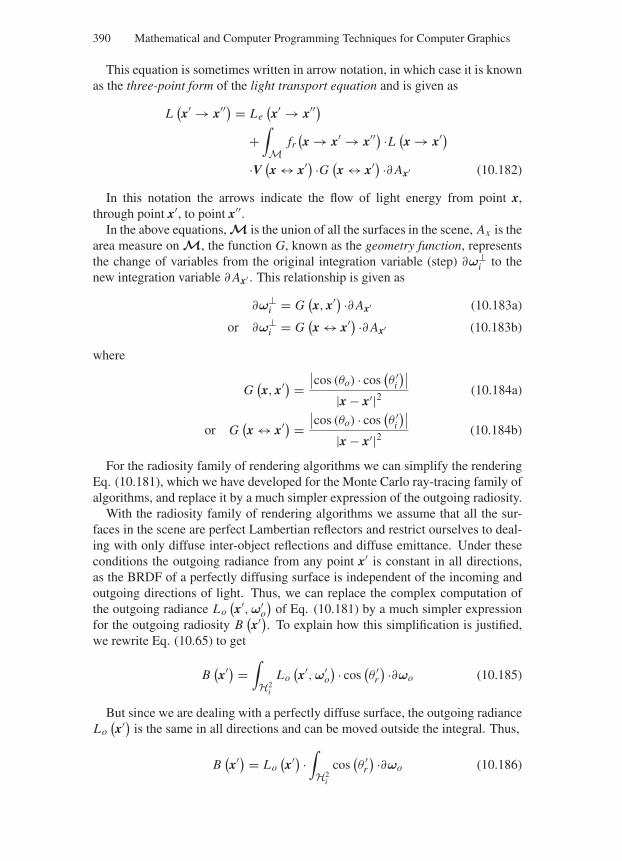
“Comninos” — 2005/8/31 — 19:01 — page 390 — #74
390 Mathematical and Computer Programming Techniques for Computer Graphics
This equation is sometimes written in arrow notation, in which case it is knownas the three-point form of the light transport equation and is given as
L(x′ → x′′) = Le
(x′ → x′′)
+∫
Mfr(x → x′ → x′′) ·L (x → x′)
·V (x ↔ x′) ·G (x ↔ x′) ·∂ Ax′ (10.182)
In this notation the arrows indicate the flow of light energy from point x,through point x′, to point x′′.
In the above equations, M is the union of all the surfaces in the scene, Ax is thearea measure on M, the function G, known as the geometry function, representsthe change of variables from the original integration variable (step) ∂ω⊥
i to thenew integration variable ∂ Ax′ . This relationship is given as
∂ω⊥i = G
(x, x′) ·∂ Ax′ (10.183a)
or ∂ω⊥i = G
(x ↔ x′) ·∂ Ax′ (10.183b)
where
G(x, x′) =
∣∣cos (θo) · cos(θ ′
i
)∣∣
|x − x′|2 (10.184a)
or G(x ↔ x′) =
∣∣cos (θo) · cos(θ ′
i
)∣∣
|x − x′|2 (10.184b)
For the radiosity family of rendering algorithms we can simplify the renderingEq. (10.181), which we have developed for the Monte Carlo ray-tracing family ofalgorithms, and replace it by a much simpler expression of the outgoing radiosity.
With the radiosity family of rendering algorithms we assume that all the sur-faces in the scene are perfect Lambertian reflectors and restrict ourselves to deal-ing with only diffuse inter-object reflections and diffuse emittance. Under theseconditions the outgoing radiance from any point x′ is constant in all directions,as the BRDF of a perfectly diffusing surface is independent of the incoming andoutgoing directions of light. Thus, we can replace the complex computation ofthe outgoing radiance Lo
(x′,ω′
o
)of Eq. (10.181) by a much simpler expression
for the outgoing radiosity B(x′). To explain how this simplification is justified,
we rewrite Eq. (10.65) to get
B(x′) =∫
H2i
Lo(x′,ω′
o
) · cos(θ ′
r
) ·∂ωo (10.185)
But since we are dealing with a perfectly diffuse surface, the outgoing radianceLo(x′) is the same in all directions and can be moved outside the integral. Thus,
B(x′) = Lo
(x′) ·∫
H2i
cos(θ ′
r
) ·∂ωo (10.186)
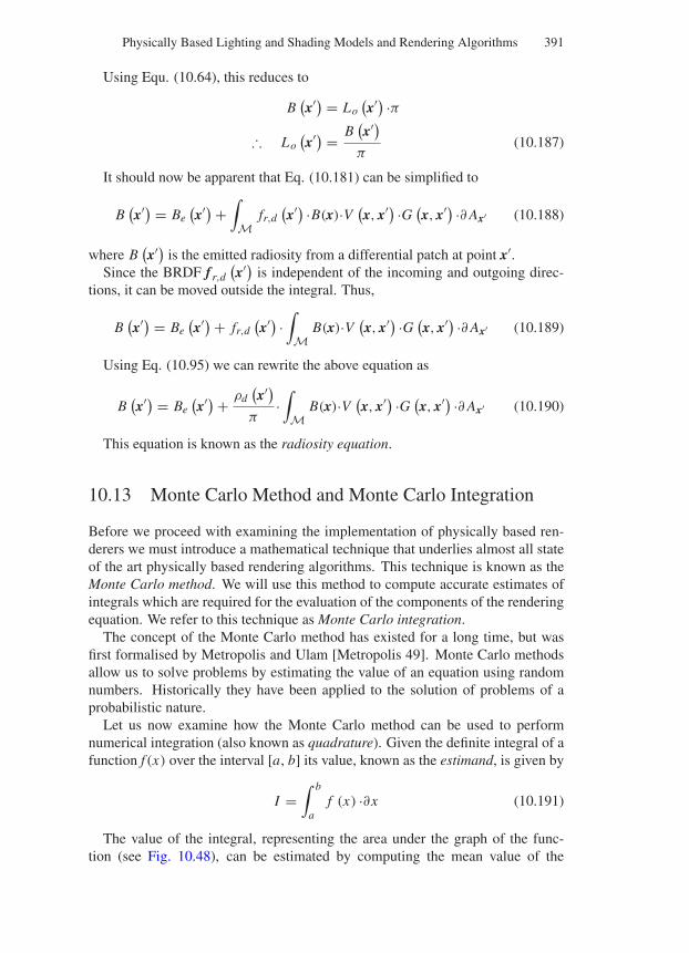
“Comninos” — 2005/8/31 — 19:01 — page 391 — #75
Physically Based Lighting and Shading Models and Rendering Algorithms 391
Using Equ. (10.64), this reduces to
B(x′) = Lo
(x′) ·π
∴ Lo(x′) = B
(x′)
π(10.187)
It should now be apparent that Eq. (10.181) can be simplified to
B(x′) = Be
(x′)+∫
Mfr,d(x′) ·B(x)·V (x, x′) ·G (x, x′) ·∂ Ax′ (10.188)
where B(x′) is the emitted radiosity from a differential patch at point x′.
Since the BRDF f r,d(x′) is independent of the incoming and outgoing direc-
tions, it can be moved outside the integral. Thus,
B(x′) = Be
(x′)+ fr,d
(x′) ·∫
MB(x)·V (x, x′) ·G (x, x′) ·∂ Ax′ (10.189)
Using Eq. (10.95) we can rewrite the above equation as
B(x′) = Be
(x′)+ ρd
(x′)
π·∫
MB(x)·V (x, x′) ·G (x, x′) ·∂ Ax′ (10.190)
This equation is known as the radiosity equation.
10.13 Monte Carlo Method and Monte Carlo Integration
Before we proceed with examining the implementation of physically based ren-derers we must introduce a mathematical technique that underlies almost all stateof the art physically based rendering algorithms. This technique is known as theMonte Carlo method. We will use this method to compute accurate estimates ofintegrals which are required for the evaluation of the components of the renderingequation. We refer to this technique as Monte Carlo integration.
The concept of the Monte Carlo method has existed for a long time, but wasfirst formalised by Metropolis and Ulam [Metropolis 49]. Monte Carlo methodsallow us to solve problems by estimating the value of an equation using randomnumbers. Historically they have been applied to the solution of problems of aprobabilistic nature.
Let us now examine how the Monte Carlo method can be used to performnumerical integration (also known as quadrature). Given the definite integral of afunction f (x) over the interval [a, b] its value, known as the estimand, is given by
I =∫ b
af (x) ·∂x (10.191)
The value of the integral, representing the area under the graph of the func-tion (see Fig. 10.48), can be estimated by computing the mean value of the
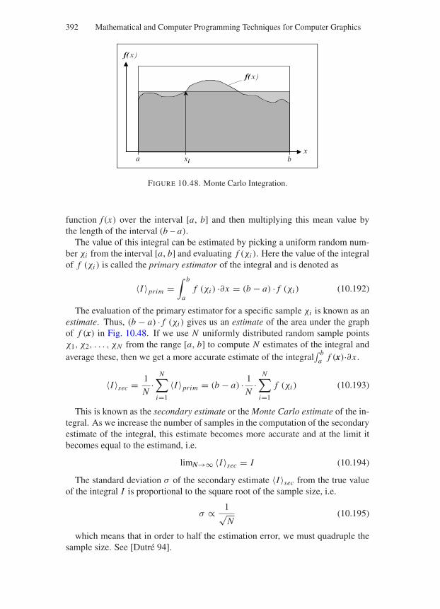
“Comninos” — 2005/8/31 — 19:01 — page 392 — #76
392 Mathematical and Computer Programming Techniques for Computer Graphics
f(x)
x
f(x)
a bxi
FIGURE 10.48. Monte Carlo Integration.
function f (x) over the interval [a, b] and then multiplying this mean value bythe length of the interval (b – a).
The value of this integral can be estimated by picking a uniform random num-ber χi from the interval [a, b] and evaluating f (χi ). Here the value of the integralof f (χi ) is called the primary estimator of the integral and is denoted as
〈I 〉prim =∫ b
af (χi ) ·∂x = (b − a) · f (χi ) (10.192)
The evaluation of the primary estimator for a specific sample χi is known as anestimate. Thus, (b − a) · f (χi ) gives us an estimate of the area under the graphof f (x) in Fig. 10.48. If we use N uniformly distributed random sample pointsχ1, χ2, . . . , χN from the range [a, b] to compute N estimates of the integral andaverage these, then we get a more accurate estimate of the integral
∫ ba f (x)·∂x .
〈I 〉sec = 1
N·
N∑
i=1
〈I 〉prim = (b − a) · 1
N·
N∑
i=1
f (χi ) (10.193)
This is known as the secondary estimate or the Monte Carlo estimate of the in-tegral. As we increase the number of samples in the computation of the secondaryestimate of the integral, this estimate becomes more accurate and at the limit itbecomes equal to the estimand, i.e.
limN→∞ 〈I 〉sec = I (10.194)
The standard deviation σ of the secondary estimate 〈I 〉sec from the true valueof the integral I is proportional to the square root of the sample size, i.e.
σ ∝ 1√N
(10.195)
which means that in order to half the estimation error, we must quadruple thesample size. See [Dutre 94].
“Comninos” — 2005/8/31 — 19:01 — page 393 — #77
Physically Based Lighting and Shading Models and Rendering Algorithms 393
10.14 Physically-Based Rendering Algorithms
The eventual output of any computer visualisation process is the production ofa rendered image of the input scene. The geometry of a virtual scene can bedescribed by a combination of geometric primitives which can either take theform of a solid representation or a boundary representation.
A solid representation is usually based on an implicit functional representationthat describes the shape (i.e. the volume and boundary) of the object in question.A representation of this type is often referred to as an F-rep.
Complex object representations of this form are composed by blending andcombining the functional representations of primitive solid objects, such as cubes,cylinders, cones, spheres and super-ellipsoids. Each of these primitives can berepresented by a unique implicit function that allows us to test if a given point inspace lies inside of, on the surface of or outside the solid object. These simplesolid primitives can be combined through blending operations or Boolean alge-bra operations (such as union, intersection and difference) to form more complexsolid objects. Most manufactured objects can easily be composed in this fashion.The F-rep is also ideally suited for the representation of soft objects and ethe-real phenomena, such as steam, smoke and fire. It is common to use ray-tracingrendering techniques to render such arbitrary geometries.
A boundary representation, on the other hand, is composed of a set of bound-ary surfaces that represent the skin of the solid object. Such boundary surfacesare represented in the form of parametric equations that describe curved surfacesdelimited by their boundary curves or polygons delimited by their outlines. Arepresentation of this type is often referred to as a B-rep.
Boolean algebra operations can also be applied to B-reps to generate more com-plex forms. With a boundary representation it is much more difficult to deter-mine if a given point in space lies inside, on the surface or outside a solid object.This makes the implementation of Boolean algebra operations on B-reps moredifficult. B-reps are ideally suited, however, for the representation of free-formsurfaces, which are best suited for the description of bodies of cars, ships andaeroplanes.
Other information that is required by the renderer, in order to be able to rendera virtual scene, includes a description of the light scattering properties of the sur-faces in the scene, a description of the light sources in the scene and a descriptionof the virtual camera.
The description of the light scattering properties of the various surfaces is pro-vided through the specification of their respective BRDFs, BTDFs and BSDFs, aswe have seen earlier in this chapter.
The description of each light source in the scene should include its type (i.e.point, parallel, linear, area or solid shape light source), its position and directionof emission, and its emittance characteristics (i.e. its power or intensity and itscolour).
Additionally, for each surface in the scene that is a light emitter we must de-scribe its emittance distribution function.
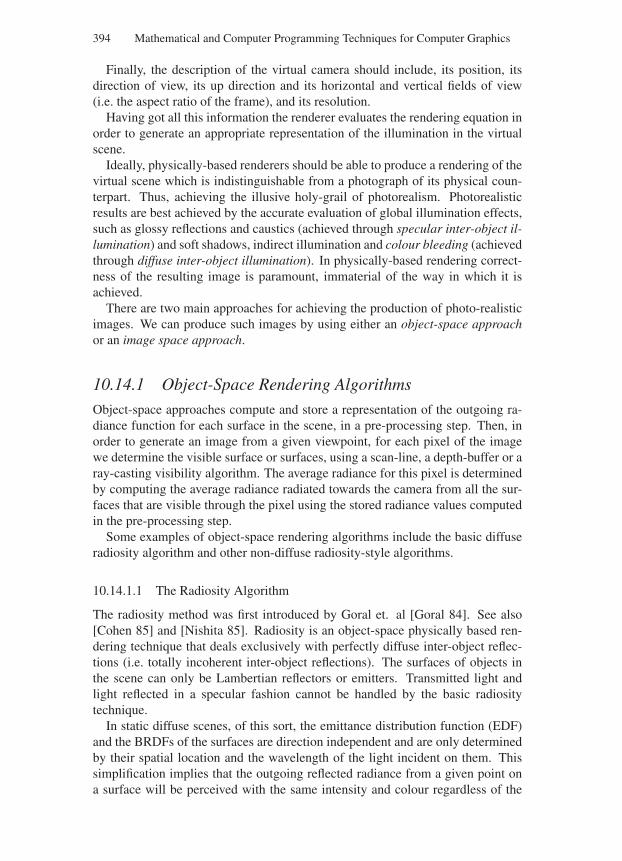
“Comninos” — 2005/8/31 — 19:01 — page 394 — #78
394 Mathematical and Computer Programming Techniques for Computer Graphics
Finally, the description of the virtual camera should include, its position, itsdirection of view, its up direction and its horizontal and vertical fields of view(i.e. the aspect ratio of the frame), and its resolution.
Having got all this information the renderer evaluates the rendering equation inorder to generate an appropriate representation of the illumination in the virtualscene.
Ideally, physically-based renderers should be able to produce a rendering of thevirtual scene which is indistinguishable from a photograph of its physical coun-terpart. Thus, achieving the illusive holy-grail of photorealism. Photorealisticresults are best achieved by the accurate evaluation of global illumination effects,such as glossy reflections and caustics (achieved through specular inter-object il-lumination) and soft shadows, indirect illumination and colour bleeding (achievedthrough diffuse inter-object illumination). In physically-based rendering correct-ness of the resulting image is paramount, immaterial of the way in which it isachieved.
There are two main approaches for achieving the production of photo-realisticimages. We can produce such images by using either an object-space approachor an image space approach.
10.14.1 Object-Space Rendering Algorithms
Object-space approaches compute and store a representation of the outgoing ra-diance function for each surface in the scene, in a pre-processing step. Then, inorder to generate an image from a given viewpoint, for each pixel of the imagewe determine the visible surface or surfaces, using a scan-line, a depth-buffer or aray-casting visibility algorithm. The average radiance for this pixel is determinedby computing the average radiance radiated towards the camera from all the sur-faces that are visible through the pixel using the stored radiance values computedin the pre-processing step.
Some examples of object-space rendering algorithms include the basic diffuseradiosity algorithm and other non-diffuse radiosity-style algorithms.
10.14.1.1 The Radiosity Algorithm
The radiosity method was first introduced by Goral et. al [Goral 84]. See also[Cohen 85] and [Nishita 85]. Radiosity is an object-space physically based ren-dering technique that deals exclusively with perfectly diffuse inter-object reflec-tions (i.e. totally incoherent inter-object reflections). The surfaces of objects inthe scene can only be Lambertian reflectors or emitters. Transmitted light andlight reflected in a specular fashion cannot be handled by the basic radiositytechnique.
In static diffuse scenes, of this sort, the emittance distribution function (EDF)and the BRDFs of the surfaces are direction independent and are only determinedby their spatial location and the wavelength of the light incident on them. Thissimplification implies that the outgoing reflected radiance from a given point ona surface will be perceived with the same intensity and colour regardless of the
“Comninos” — 2005/8/31 — 19:01 — page 395 — #79
Physically Based Lighting and Shading Models and Rendering Algorithms 395
viewing position. By reducing the dimension of the radiance, employing thesesimplifications, it becomes feasible to store accurate object-space representationsof the radiance of complex scenes. This of course means that the output producedby the pre-processing step can be used to render images from different viewpointsin the scene.
With such diffuse environments it is more appropriate to use the radiosity(i.e. radiant exitance) rather than the radiance to quantify the illumination at agiven location and wavelength.
Some non-diffuse radiosity-style algorithms compute the average radiance emit-ted by each surface in the scene towards all other surfaces in the scene. See[Aupperle 93] and [Stamminger 98]. Some other implementations use an angularrather than a spatial parameterisation to represent the directional dependence ofthe radiance. See [Immel 86] and [Sillion 91].
The major advantage of representing the scene illumination in object space isthat we can reuse the results of the radiance computation, output from the pre-processing step of the these algorithms, to render images of the scene from dif-ferent viewpoints. Thus these algorithms exhibit frame-to-frame coherence. 3Dgraphics hardware can be used to accelerate the rendering stage of these algo-rithms.
With these algorithms, a significant proportion of the pre-computed radiancecan often be reused even if the geometry of the light emission or the surfacescattering properties of the virtual scene are altered. See [George 90], [Chen 90]and [Drettakis 97].
The main disadvantage of the object-space rendering algorithms is the exces-sive amount of storage required to accurately represent the highly direction depen-dant radiance functions required to represent specular inter-object illumination.Even for the diffuse inter-object illumination of large virtual scenes, the storagerequirements of these algorithms become prohibitive.
10.14.2 Image-Space Rendering Algorithms
Image-space rendering algorithms compute the average incoming radiance at eachpixel on the fly, without relying on a pre-processing step to compute an object-space representation of the radiance reflected from each surface of the virtualscene. This family of algorithms solves the rendering equation for each pixel orgroup of pixels in the rendered image. Although the underlying global illumi-nation method used by all the image-space algorithms is basically the same, thealgorithms themselves are quite different. Examples of such algorithms are theray-tracing algorithm [Whitted 80], the distributed ray-tracing algorithm [Cook84], the path-tracing algorithm [Kajiya 86][Dutre 94], the bi-directional path-tracing algorithm [Lafortune 93][Veach 94], the Metropolis light transport algo-rithm [Veach 97b] and the photon-mapping algorithm [Jensen 95a].
The major advantage of the image-space algorithms is that they require verylittle storage, as they compute the visible surface solution on a per-pixel basis. Ingeneral these algorithms are more suitable than the object-space algorithms formore complex virtual scenes and can handle more complex illumination models.
“Comninos” — 2005/8/31 — 19:01 — page 396 — #80
396 Mathematical and Computer Programming Techniques for Computer Graphics
The more sophisticated algorithms of this type can handle both specular inter-object and diffuse inter-object illumination, as well as, deal with volume renderingfor participating media.
Let us now examine the family of image-space rendering algorithms in moredetail.
10.14.2.1 The Recursive Ray-Tracing Algorithm
The concept of ray tracing first appeared in a 1971 paper by Goldstein and Nagel[Goldstein 71]. In the early eighties, Whitted introduced the concept of recursiveray tracing [Whitted 80].
Ray tracing is a simple and elegant algorithm that is able to handle specularinter-object illumination. Thus, it deals with specular reflection and transmissionand generates sharp shadows.
For each pixel of the image, we spawn one primary ray that starts from theviewing point and passes through the centre of the pixel. If this ray intersectsnone of the surfaces in the scene, then the pixel is painted with the backgroundcolour and we proceed to the next pixel. If the ray, however, intersects some ofthe surfaces in the scene, we pick the surface whose intersection point is clos-est to the observer. Once we have identified the closest surface, we compute itsunit normal at the point of intersection. This vector is then used in the shadingcalculations.
How the light is reflected from a surface depends on the type of surface thatwe are dealing with. If the surface is diffuse (rough), the reflected light willdepend only on the illumination arriving directly from the light sources in thescene. Alternatively, if the surface is specular (smooth), the reflected light willdepend on the illumination arriving directly from the light sources and on the in-direct illumination arriving on this surface after having been reflected off othersurfaces in the scene or been transmitted through the surface (if it is transpar-ent). To discover if the point is directly illuminated, we have to trace a shadowray to each of the light sources. If the surface point is visible from a lightsource, then it will receive direct illumination from this source, otherwise itwill not.
If the surface in question is smooth, then we recursively spawn a ray in thereflection direction and if the surface is transparent, a second ray in the trans-mission direction. We follow these rays repeating the process recursively untilwe satisfy one of the recursion termination conditions. The recursion will ter-minate when one of the three following conditions is met. When the ray hitsa rough surface, in which case the light reflected from this surface is returnedby the ray since this will be the incoming light at the point of origin of the ray.When the ray misses all surfaces in the scene, in which case the ray returns thebackground colour. Finally, when a user defined maximum level of recursion hasbeen reached, no new rays are generated. Upon returning from a recursive call weaccumulate all the calculated radiance contributions.
An outline of the recursive ray-tracing algorithm is presented in Algorithm10.1. In this algorithm, the function emitter shader() computes the light emit-ted by an emitter surface and the function direct shader() computes the directillumination component of the light reflected from the surface.
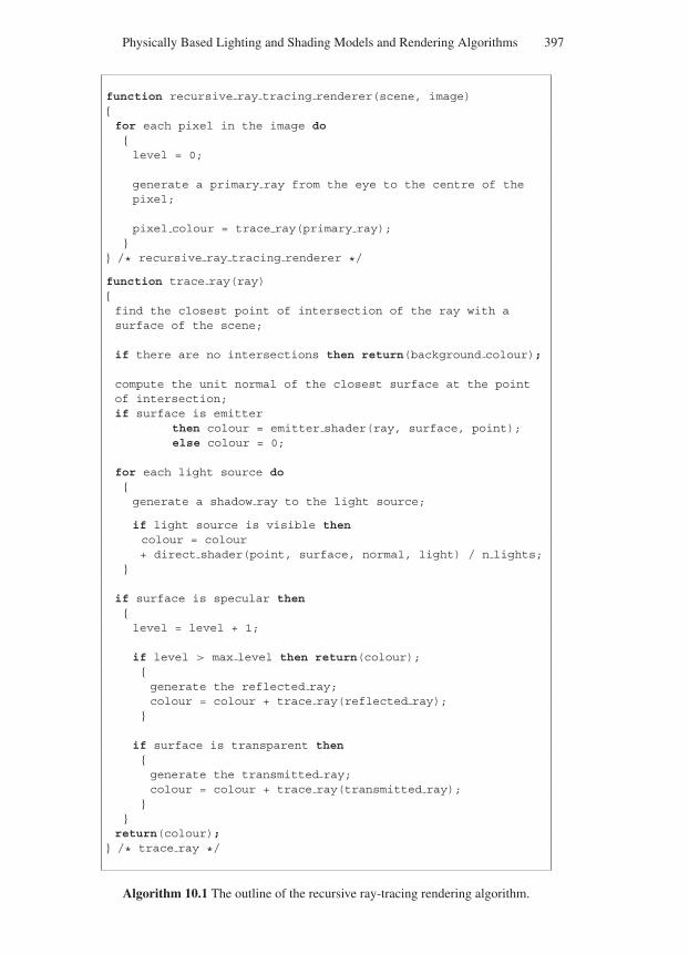
“Comninos” — 2005/8/31 — 19:01 — page 397 — #81
Physically Based Lighting and Shading Models and Rendering Algorithms 397
function recursive ray tracing renderer(scene, image)for each pixel in the image do
level = 0;
generate a primary ray from the eye to the centre of thepixel;
pixel colour = trace ray(primary ray);
/* recursive ray tracing renderer */
function trace ray(ray)find the closest point of intersection of the ray with asurface of the scene;
if there are no intersections then return(background colour);
compute the unit normal of the closest surface at the pointof intersection;if surface is emitter
then colour = emitter shader(ray, surface, point);else colour = 0;
for each light source dogenerate a shadow ray to the light source;
if light source is visible thencolour = colour+ direct shader(point, surface, normal, light) / n lights;
if surface is specular thenlevel = level + 1;
if level > max level then return(colour);generate the reflected ray;colour = colour + trace ray(reflected ray);
if surface is transparent thengenerate the transmitted ray;colour = colour + trace ray(transmitted ray);
return(colour); /* trace ray */
Algorithm 10.1 The outline of the recursive ray-tracing rendering algorithm.
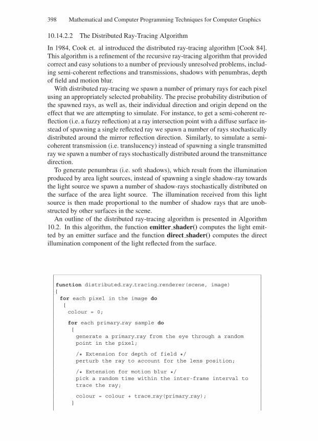
“Comninos” — 2005/8/31 — 19:01 — page 398 — #82
398 Mathematical and Computer Programming Techniques for Computer Graphics
10.14.2.2 The Distributed Ray-Tracing Algorithm
In 1984, Cook et. al introduced the distributed ray-tracing algorithm [Cook 84].This algorithm is a refinement of the recursive ray-tracing algorithm that providedcorrect and easy solutions to a number of previously unresolved problems, includ-ing semi-coherent reflections and transmissions, shadows with penumbras, depthof field and motion blur.
With distributed ray-tracing we spawn a number of primary rays for each pixelusing an appropriately selected probability. The precise probability distribution ofthe spawned rays, as well as, their individual direction and origin depend on theeffect that we are attempting to simulate. For instance, to get a semi-coherent re-flection (i.e. a fuzzy reflection) at a ray intersection point with a diffuse surface in-stead of spawning a single reflected ray we spawn a number of rays stochasticallydistributed around the mirror reflection direction. Similarly, to simulate a semi-coherent transmission (i.e. translucency) instead of spawning a single transmittedray we spawn a number of rays stochastically distributed around the transmittancedirection.
To generate penumbras (i.e. soft shadows), which result from the illuminationproduced by area light sources, instead of spawning a single shadow-ray towardsthe light source we spawn a number of shadow-rays stochastically distributed onthe surface of the area light source. The illumination received from this lightsource is then made proportional to the number of shadow rays that are unob-structed by other surfaces in the scene.
An outline of the distributed ray-tracing algorithm is presented in Algorithm10.2. In this algorithm, the function emitter shader() computes the light emit-ted by an emitter surface and the function direct shader() computes the directillumination component of the light reflected from the surface.
function distributed ray tracing renderer(scene, image)for each pixel in the image do
colour = 0;
for each primary ray sample dogenerate a primary ray from the eye through a randompoint in the pixel;
/* Extension for depth of field */perturb the ray to account for the lens position;
/* Extension for motion blur */pick a random time within the inter-frame interval totrace the ray;
colour = colour + trace ray(primary ray);
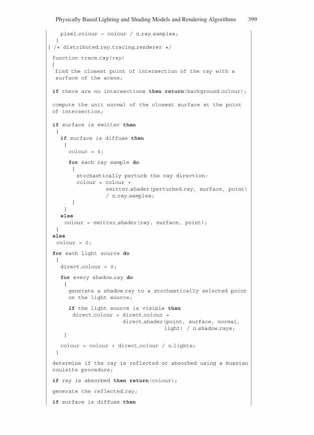
“Comninos” — 2005/8/31 — 19:01 — page 399 — #83
Physically Based Lighting and Shading Models and Rendering Algorithms 399
pixel colour = colour / n ray samples;
/* distributed ray tracing renderer */
function trace ray(ray)find the closest point of intersection of the ray with asurface of the scene;
if there are no intersections then return(background colour);
compute the unit normal of the closest surface at the pointof intersection;
if surface is emitter thenif surface is diffuse then
colour = 0;
for each ray sample dostochastically perturb the ray direction;colour = colour +
emitter shader(perturbed ray, surface, point)/ n ray samples;
elsecolour = emitter shader(ray, surface, point);
elsecolour = 0;
for each light source dodirect colour = 0;
for every shadow ray dogenerate a shadow ray to a stochastically selected pointon the light source;
if the light source is visible thendirect colour = direct colour +
direct shader(point, surface, normal,light) / n shadow rays;
colour = colour + direct colour / n lights;
determine if the ray is reflected or absorbed using a Russianroulette procedure;
if ray is absorbed then return(colour);
generate the reflected ray;
if surface is diffuse then
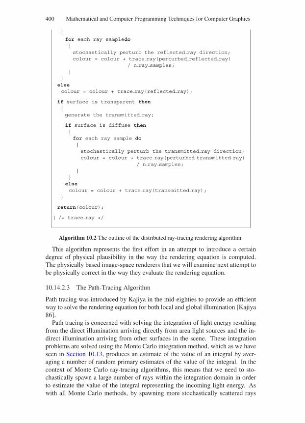
“Comninos” — 2005/8/31 — 19:01 — page 400 — #84
400 Mathematical and Computer Programming Techniques for Computer Graphics
for each ray sampledo
stochastically perturb the reflected ray direction;colour = colour + trace ray(perturbed reflected ray)
/ n ray samples;
elsecolour = colour + trace ray(reflected ray);
if surface is transparent thengenerate the transmitted ray;
if surface is diffuse thenfor each ray sample do
stochastically perturb the transmitted ray direction;colour = colour + trace ray(perturbed transmitted ray)
/ n ray samples;
elsecolour = colour + trace ray(transmitted ray);
return(colour);
/* trace ray */
Algorithm 10.2 The outline of the distributed ray-tracing rendering algorithm.
This algorithm represents the first effort in an attempt to introduce a certaindegree of physical plausibility in the way the rendering equation is computed.The physically based image-space renderers that we will examine next attempt tobe physically correct in the way they evaluate the rendering equation.
10.14.2.3 The Path-Tracing Algorithm
Path tracing was introduced by Kajiya in the mid-eighties to provide an efficientway to solve the rendering equation for both local and global illumination [Kajiya86].
Path tracing is concerned with solving the integration of light energy resultingfrom the direct illumination arriving directly from area light sources and the in-direct illumination arriving from other surfaces in the scene. These integrationproblems are solved using the Monte Carlo integration method, which as we haveseen in Section 10.13, produces an estimate of the value of an integral by aver-aging a number of random primary estimates of the value of the integral. In thecontext of Monte Carlo ray-tracing algorithms, this means that we need to sto-chastically spawn a large number of rays within the integration domain in orderto estimate the value of the integral representing the incoming light energy. Aswith all Monte Carlo methods, by spawning more stochastically scattered rays
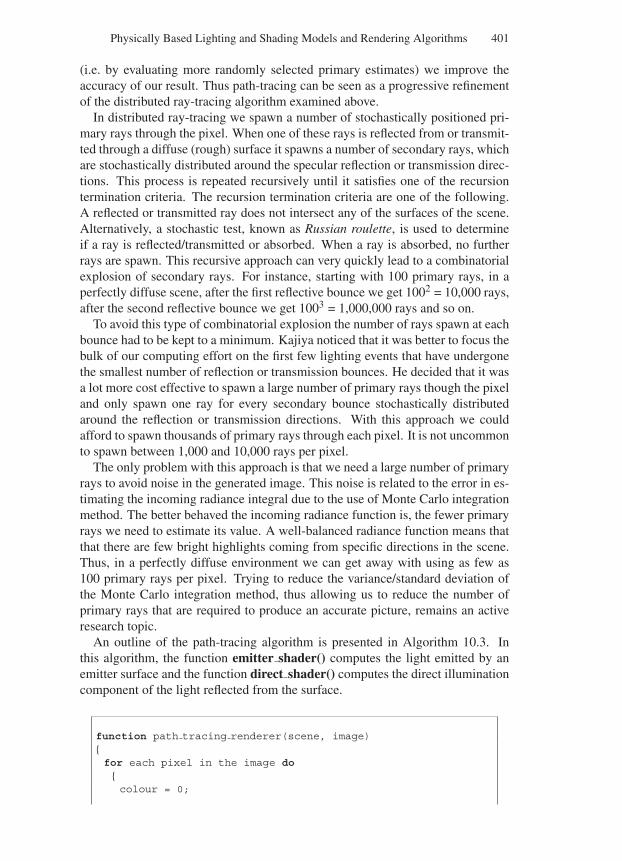
“Comninos” — 2005/8/31 — 19:01 — page 401 — #85
Physically Based Lighting and Shading Models and Rendering Algorithms 401
(i.e. by evaluating more randomly selected primary estimates) we improve theaccuracy of our result. Thus path-tracing can be seen as a progressive refinementof the distributed ray-tracing algorithm examined above.
In distributed ray-tracing we spawn a number of stochastically positioned pri-mary rays through the pixel. When one of these rays is reflected from or transmit-ted through a diffuse (rough) surface it spawns a number of secondary rays, whichare stochastically distributed around the specular reflection or transmission direc-tions. This process is repeated recursively until it satisfies one of the recursiontermination criteria. The recursion termination criteria are one of the following.A reflected or transmitted ray does not intersect any of the surfaces of the scene.Alternatively, a stochastic test, known as Russian roulette, is used to determineif a ray is reflected/transmitted or absorbed. When a ray is absorbed, no furtherrays are spawn. This recursive approach can very quickly lead to a combinatorialexplosion of secondary rays. For instance, starting with 100 primary rays, in aperfectly diffuse scene, after the first reflective bounce we get 1002 = 10,000 rays,after the second reflective bounce we get 1003 = 1,000,000 rays and so on.
To avoid this type of combinatorial explosion the number of rays spawn at eachbounce had to be kept to a minimum. Kajiya noticed that it was better to focus thebulk of our computing effort on the first few lighting events that have undergonethe smallest number of reflection or transmission bounces. He decided that it wasa lot more cost effective to spawn a large number of primary rays though the pixeland only spawn one ray for every secondary bounce stochastically distributedaround the reflection or transmission directions. With this approach we couldafford to spawn thousands of primary rays through each pixel. It is not uncommonto spawn between 1,000 and 10,000 rays per pixel.
The only problem with this approach is that we need a large number of primaryrays to avoid noise in the generated image. This noise is related to the error in es-timating the incoming radiance integral due to the use of Monte Carlo integrationmethod. The better behaved the incoming radiance function is, the fewer primaryrays we need to estimate its value. A well-balanced radiance function means thatthat there are few bright highlights coming from specific directions in the scene.Thus, in a perfectly diffuse environment we can get away with using as few as100 primary rays per pixel. Trying to reduce the variance/standard deviation ofthe Monte Carlo integration method, thus allowing us to reduce the number ofprimary rays that are required to produce an accurate picture, remains an activeresearch topic.
An outline of the path-tracing algorithm is presented in Algorithm 10.3. Inthis algorithm, the function emitter shader() computes the light emitted by anemitter surface and the function direct shader() computes the direct illuminationcomponent of the light reflected from the surface.
function path tracing renderer(scene, image)for each pixel in the image do
colour = 0;
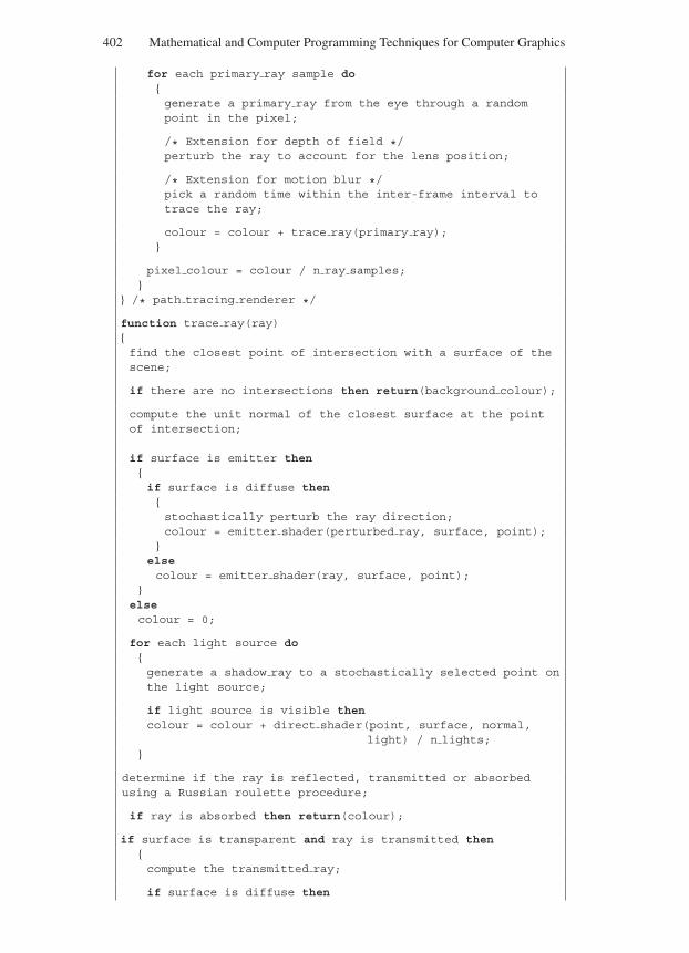
“Comninos” — 2005/8/31 — 19:01 — page 402 — #86
402 Mathematical and Computer Programming Techniques for Computer Graphics
for each primary ray sample dogenerate a primary ray from the eye through a randompoint in the pixel;
/* Extension for depth of field */perturb the ray to account for the lens position;
/* Extension for motion blur */pick a random time within the inter-frame interval totrace the ray;
colour = colour + trace ray(primary ray);
pixel colour = colour / n ray samples;
/* path tracing renderer */
function trace ray(ray)find the closest point of intersection with a surface of thescene;
if there are no intersections then return(background colour);
compute the unit normal of the closest surface at the pointof intersection;
if surface is emitter thenif surface is diffuse then
stochastically perturb the ray direction;colour = emitter shader(perturbed ray, surface, point);
elsecolour = emitter shader(ray, surface, point);
elsecolour = 0;
for each light source dogenerate a shadow ray to a stochastically selected point onthe light source;
if light source is visible thencolour = colour + direct shader(point, surface, normal,
light) / n lights;
determine if the ray is reflected, transmitted or absorbedusing a Russian roulette procedure;
if ray is absorbed then return(colour);
if surface is transparent and ray is transmitted thencompute the transmitted ray;
if surface is diffuse then
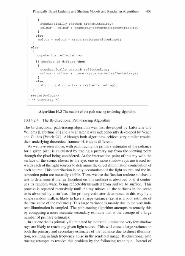
“Comninos” — 2005/8/31 — 19:01 — page 403 — #87
Physically Based Lighting and Shading Models and Rendering Algorithms 403
stochastically perturb transmitted ray;colour = colour + trace ray(perturbed transmitted ray);
elsecolour = colour + trace ray(transmitted ray);
else
compute the reflected ray;
if surface is diffuse thenstochastically perturb reflected ray;colour = colour + trace ray(perturbed reflected ray);
elsecolour = colour + trace ray(reflected ray);
return(colour);
/* trace ray */
Algorithm 10.3 The outline of the path-tracing rendering algorithm.
10.14.2.4 The Bi-directional Path-Tracing Algorithm
The bi-directional path-tracing algorithm was first developed by Lafortune andWillems [Lafortune 93] and a year later it was independently developed by Veachand Guibas [Veach 94]. Although both algorithms achieve very similar results,their underlying theoretical framework is quite different.
As we have seen above, with path tracing the primary estimator of the radiancefor a given pixel is calculated by tracing a primary ray from the viewing pointthrough the pixel being considered. At the intersection point of this ray with thesurface of the scene, closest to the eye, one or more shadow rays are traced to-wards each of the light sources to determine the direct illumination contribution ofeach source. This contribution is only accumulated if the light source and the in-tersection point are mutually visible. Then, we use the Russian roulette stochastictest to determine if the ray (incident on this surface) is absorbed or if it contin-ues its random walk, being reflected/transmitted from surface to surface. Thisprocess is repeated recursively until the ray misses all the surfaces in the sceneor is absorbed by a surface. The primary estimator determined in this way by asingle random walk is likely to have a large variance (i.e. it is a poor estimate ofthe true value of the radiance). This large variance is mainly due to the way indi-rect illumination is sampled. The path-tracing algorithm attempts to remedy thisby computing a more accurate secondary estimate that is the average of a largenumber of primary estimates.
In a scene that is primarily illuminated by indirect illumination very few shadowrays are likely to reach any given light source. This will cause a large variance inboth the primary and secondary estimates of the radiance due to direct illumina-tion, resulting in high frequency noise in the rendered image. Bi-directional pathtracing attempts to resolve this problem by the following technique. Instead of
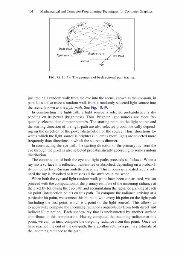
“Comninos” — 2005/8/31 — 19:01 — page 404 — #88
404 Mathematical and Computer Programming Techniques for Computer Graphics
screen
eye pathlight source
light path
shadow rays
FIGURE 10.49. The geometry of bi-directional path tracing.
just tracing a random walk from the eye into the scene, known as the eye-path, inparallel we also trace a random walk from a randomly selected light source intothe scene, known as the light-path. See Fig. 10.49.
In constructing the light-path, a light source is selected probabilistically de-pending on its power (brightness). Thus, brighter light sources are more fre-quently selected than dimmer sources. The starting point on the light source andthe starting direction of the light-path are also selected probabilistically depend-ing on the direction of the power distribution of the source. Thus, directions to-wards which the light source is brighter (i.e. emits more light) are selected morefrequently than directions in which the source is dimmer.
In constructing the eye-path, the starting direction of the primary ray from theeye through the pixel is also selected probabilistically according to some randomdistribution.
The construction of both the eye and light-paths proceeds as follows. When aray hits a surface it is reflected, transmitted or absorbed, depending on a probabil-ity computed by a Russian roulette procedure. This process is repeated recursivelyuntil the ray is absorbed or it misses all the surfaces in the scene.
When both the eye and light random walk paths have been constructed, we canproceed with the computation of the primary estimate of the incoming radiance atthe pixel by following the eye-path and accumulating the radiance arriving at eachhit point (intersection point) on this path. To compute the radiance arriving at aparticular hit point, we connect this hit point with every hit point on the light-path(including the first point, which is a point on the light source). This allows usto accurately compute the incoming radiance contributions from both direct andindirect illumination. Each shadow ray that is unobstructed by another surfacecontributes to this computation. Having computed the incoming radiance at thispoint, we can, in turn, compute the outgoing radiance from this point. Once wehave reached the end of the eye-path, the algorithm returns a primary estimate ofthe incoming radiance at the pixel.
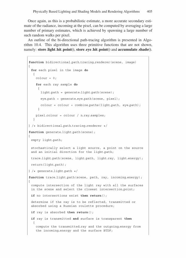
“Comninos” — 2005/8/31 — 19:01 — page 405 — #89
Physically Based Lighting and Shading Models and Rendering Algorithms 405
Once again, as this is a probabilistic estimate, a more accurate secondary esti-mate of the radiance, incoming at the pixel, can be computed by averaging a largenumber of primary estimates, which is achieved by spawning a large number ofsuch random walks per pixel.
An outline of the bi-directional path-tracing algorithm is presented in Algo-rithm 10.4. This algorithm uses three primitive functions that are not shown,namely: store light hit point(), store eye hit point() and accumulate shade().
function bidirectional path tracing renderer(scene, image)for each pixel in the image do
colour = 0;
for each ray sample dolight path = generate light path(scene);
eye path = generate eye path(scene, pixel);
colour = colour + combine paths(light path, eye path);
pixel colour = colour / n ray samples;
/* bidirectional path tracing renderer */
function generate light path(scene);empty light path;
stochastically select a light source, a point on the sourceand an initial direction for the light path;
trace light path(scene, light path, light ray, light energy);
return(light path);
/* generate light path */
function trace light path(scene, path, ray, incoming energy);compute intersection of the light ray with all the surfacesin the scene and select the closest intersection point;
if no intersections exist then return();
determine if the ray is to be reflected, transmitted orabsorbed using a Russian roulette procedure;
if ray is absorbed then return();
if ray is transmitted and surface is transparent thencompute the transmitted ray and the outgoing energy fromthe incoming energy and the surface BTDF;
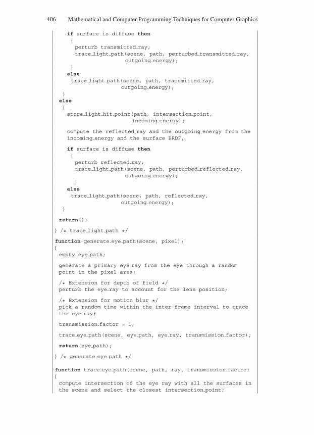
“Comninos” — 2005/8/31 — 19:01 — page 406 — #90
406 Mathematical and Computer Programming Techniques for Computer Graphics
if surface is diffuse thenperturb transmitted ray;trace light path(scene, path, perturbed transmitted ray,
outgoing energy);
elsetrace light path(scene, path, transmitted ray,
outgoing energy);
elsestore light hit point(path, intersection point,
incoming energy);
compute the reflected ray and the outgoing energy from theincoming energy and the surface BRDF;
if surface is diffuse thenperturb reflected ray;trace light path(scene, path, perturbed reflected ray,
outgoing energy);
elsetrace light path(scene, path, reflected ray,
outgoing energy);
return();
/* trace light path */
function generate eye path(scene, pixel);empty eye path;
generate a primary eye ray from the eye through a randompoint in the pixel area;
/* Extension for depth of field */perturb the eye ray to account for the lens position;
/* Extension for motion blur */pick a random time within the inter-frame interval to tracethe eye ray;
transmission factor = 1;
trace eye path(scene, eye path, eye ray, transmission factor);
return(eye path);
/* generate eye path */
function trace eye path(scene, path, ray, transmission factor)compute intersection of the eye ray with all the surfaces inthe scene and select the closest intersection point;
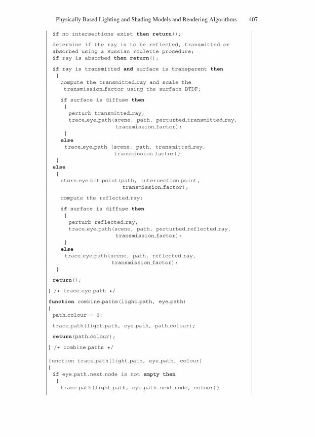
“Comninos” — 2005/8/31 — 19:01 — page 407 — #91
Physically Based Lighting and Shading Models and Rendering Algorithms 407
if no intersections exist then return();
determine if the ray is to be reflected, transmitted orabsorbed using a Russian roulette procedure;if ray is absorbed then return();
if ray is transmitted and surface is transparent thencompute the transmitted ray and scale thetransmission factor using the surface BTDF;
if surface is diffuse thenperturb transmitted ray;trace eye path(scene, path, perturbed transmitted ray,
transmission factor);
elsetrace eye path (scene, path, transmitted ray,
transmission factor);
elsestore eye hit point(path, intersection point,
transmission factor);
compute the reflected ray;
if surface is diffuse thenperturb reflected ray;trace eye path(scene, path, perturbed reflected ray,
transmission factor);
elsetrace eye path(scene, path, reflected ray,
transmission factor);
return();
/* trace eye path */
function combine paths(light path, eye path)path colour = 0;
trace path(light path, eye path, path colour);
return(path colour);
/* combine paths */
function trace path(light path, eye path, colour)if eye path.next node is not empty then
trace path(light path, eye path.next node, colour);
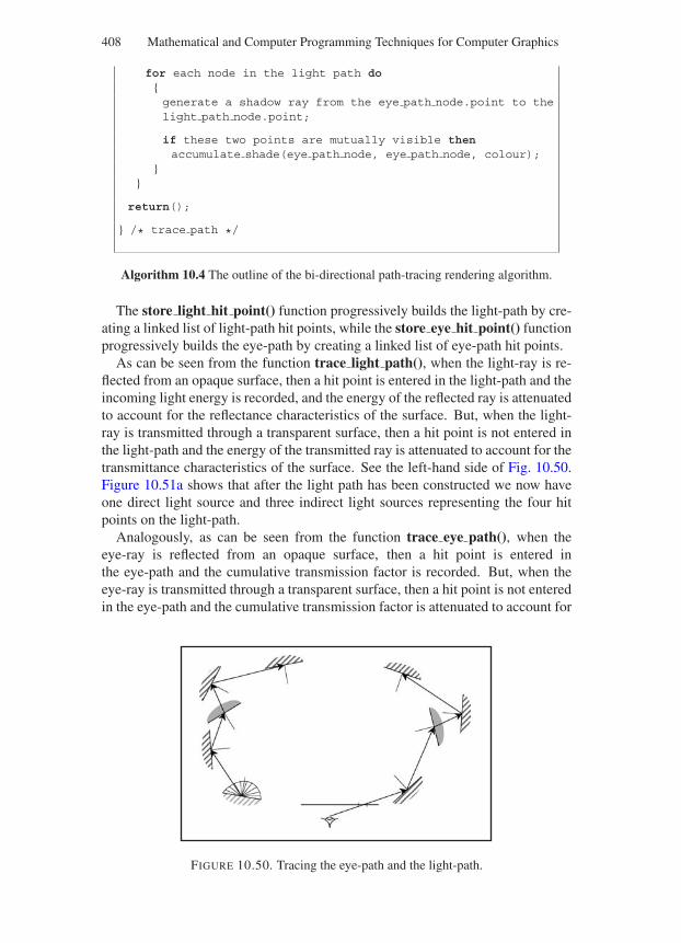
“Comninos” — 2005/8/31 — 19:01 — page 408 — #92
408 Mathematical and Computer Programming Techniques for Computer Graphics
for each node in the light path dogenerate a shadow ray from the eye path node.point to thelight path node.point;
if these two points are mutually visible thenaccumulate shade(eye path node, eye path node, colour);
return();
/* trace path */
Algorithm 10.4 The outline of the bi-directional path-tracing rendering algorithm.
The store light hit point() function progressively builds the light-path by cre-ating a linked list of light-path hit points, while the store eye hit point() functionprogressively builds the eye-path by creating a linked list of eye-path hit points.
As can be seen from the function trace light path(), when the light-ray is re-flected from an opaque surface, then a hit point is entered in the light-path and theincoming light energy is recorded, and the energy of the reflected ray is attenuatedto account for the reflectance characteristics of the surface. But, when the light-ray is transmitted through a transparent surface, then a hit point is not entered inthe light-path and the energy of the transmitted ray is attenuated to account for thetransmittance characteristics of the surface. See the left-hand side of Fig. 10.50.Figure 10.51a shows that after the light path has been constructed we now haveone direct light source and three indirect light sources representing the four hitpoints on the light-path.
Analogously, as can be seen from the function trace eye path(), when theeye-ray is reflected from an opaque surface, then a hit point is entered inthe eye-path and the cumulative transmission factor is recorded. But, when theeye-ray is transmitted through a transparent surface, then a hit point is not enteredin the eye-path and the cumulative transmission factor is attenuated to account for
FIGURE 10.50. Tracing the eye-path and the light-path.
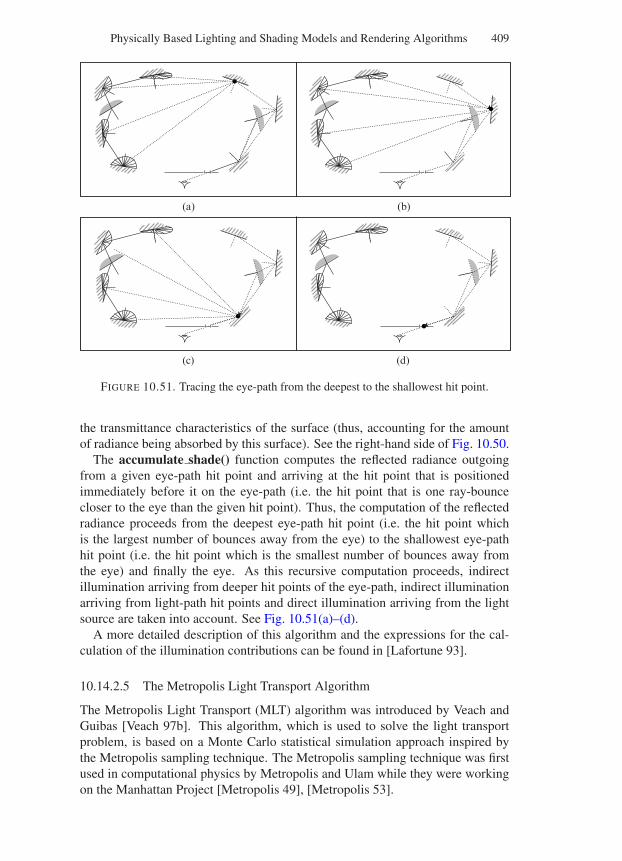
“Comninos” — 2005/8/31 — 19:01 — page 409 — #93
Physically Based Lighting and Shading Models and Rendering Algorithms 409
(a) (b)
(d)(c)
FIGURE 10.51. Tracing the eye-path from the deepest to the shallowest hit point.
the transmittance characteristics of the surface (thus, accounting for the amountof radiance being absorbed by this surface). See the right-hand side of Fig. 10.50.
The accumulate shade() function computes the reflected radiance outgoingfrom a given eye-path hit point and arriving at the hit point that is positionedimmediately before it on the eye-path (i.e. the hit point that is one ray-bouncecloser to the eye than the given hit point). Thus, the computation of the reflectedradiance proceeds from the deepest eye-path hit point (i.e. the hit point whichis the largest number of bounces away from the eye) to the shallowest eye-pathhit point (i.e. the hit point which is the smallest number of bounces away fromthe eye) and finally the eye. As this recursive computation proceeds, indirectillumination arriving from deeper hit points of the eye-path, indirect illuminationarriving from light-path hit points and direct illumination arriving from the lightsource are taken into account. See Fig. 10.51(a)–(d).
A more detailed description of this algorithm and the expressions for the cal-culation of the illumination contributions can be found in [Lafortune 93].
10.14.2.5 The Metropolis Light Transport Algorithm
The Metropolis Light Transport (MLT) algorithm was introduced by Veach andGuibas [Veach 97b]. This algorithm, which is used to solve the light transportproblem, is based on a Monte Carlo statistical simulation approach inspired bythe Metropolis sampling technique. The Metropolis sampling technique was firstused in computational physics by Metropolis and Ulam while they were workingon the Manhattan Project [Metropolis 49], [Metropolis 53].
“Comninos” — 2005/8/31 — 19:01 — page 410 — #94
410 Mathematical and Computer Programming Techniques for Computer Graphics
The general approach used in the MLT algorithm can be outlined as follows.To render an image of a 3D scene, we start with a single light transport path,known as the current path, and we progressively generate a set of alternative pathsby stochastically mutating the current path. We use an appropriately selectedprobability, to accept or reject a mutated path, ensuring that the retained paths aresampled with an order that reflects their statistical contribution to the ideal image.Then, we estimate this ideal image by sampling a large number of the mutatedpaths and by recording their positions on the image plane that is represented by a2D array in memory.
The MLT algorithm is unbiased, it is capable of handling the most general geo-metric and BSDF models, it is economical in storage and it can be significantlyfaster than other unbiased algorithms. The MLT algorithm is very different fromboth the path-tracing and the bi-directional path-tracing algorithms. Unlike otherMonte Carlo methods, instead of randomly sampling the value of a function inorder to estimate the value of its integral, the Metropolis method generates a dis-tribution of samples to the unknown function value. To achieve this samplingdistribution the MLT algorithm starts with a random sampling of the space of alllight paths in the scene. These initial paths are generated using the bi-directionalpath-tracing algorithm and are subsequently cloned and mutated in order to com-pute the radiance of the final image.
The most important advantage of the MLP algorithm is that it explores the pathspace locally, selecting more frequently mutations arrived at by applying minorincremental modifications to the current path. Using this progressive refinementapproach has the following beneficial consequences. The average cost for eachsample path is relatively small, as very few rays are used. Once an important pathis identified, nearby paths are employed as well, thus spreading the cost of deter-mining such a “good” path over many neighbouring paths. The set of mutationoperations applied, by the MLT algorithm, to a “good” path is easy to extend. Byselecting mutations that retain certain of the properties of a given “good” pathwhile changing other properties, we can take advantage of any type of coherencethat is present in the scene. In this way, it is often possible to deal with differenttypes of lighting problems more effectively by designing specialised mutations tohandle these particular situations.
The propensity of the MLT algorithm to concentrate on incremental changesto a path, once it has found a “good” path, also leads to one of the main weak-nesses of this algorithm. With scenes that do not exhibit space coherence, thealgorithm may be caught by one particular feature and be prevented from con-verging quickly. Consider, for instance, a scene containing a surface with a gridof holes lit from behind. The MLT algorithm can be “trapped” by one of the holesand will fail to investigate properly the illumination from neighbouring holes.
A more detailed explanation of the algorithm can be found in [Veach 97a] and[Veach 97b].
10.14.2.6 The Photon-Mapping Technique
The photon-mapping technique was developed by Jensen and Christensen as anefficient alternative to pure Monte Carlo ray-tracing techniques [Jensen 95a]. This
“Comninos” — 2005/8/31 — 19:01 — page 411 — #95
Physically Based Lighting and Shading Models and Rendering Algorithms 411
technique de-couples the representation of the illumination from the representa-tion of the geometry of the scene. Thus, allowing us to handle arbitrarily complexgeometric models and BRDFs.
To best visualise the photon map we may think of it as the cache of all thelight paths in the bi-directional path-tracing algorithm. The photon map couldindeed be used for this purpose. It is however used to estimate the illuminationin the scene based on an estimation of the light energy density. The estimationerror resulting from the use of the photon map, to estimate the illumination ofthe scene, results in low frequency noise, as opposed to the high frequency noiseresulting from using the traditional Monte Carlo techniques. The density estima-tion method that uses a photon map is much faster than the pure Monte Carlotechniques. The main disadvantage, however, of this estimation method is that itis biased.
The algorithm that generates, stores and uses illumination as points on the sur-faces of objects in the scene is known as photon mapping and the data structurethat is used to store these illumination points is known as the photon map. Thetechnique that is used to generate the illumination points is known as the photon-tracing algorithm. Thus, a renderer that uses the photon-mapping technique hastwo distinct passes. The photon-mapping pass, which builds the photon mapdata structure by spawning photon rays from the light sources and tracing themthrough the objects in the scene and the rendering pass, which renders the sceneusing the illumination information stored in the photon map (thus speeding up therendering process).
As this has proved to be a very influential algorithm, we will examine it in somedetail.
10.14.2.6.1 The Photon-Mapping Pass
The photon-mapping pass is an essential pre-processing step of any renderingalgorithm that uses the photon-mapping technique. During this pass photons areemitted from the light sources, their paths are traced through the scene and whenthey hit a diffuse surface their location and power are recorded in the photon map.
10.14.2.6.2 Emission of Photons
A large number of photons are emitted by each light source in the scene. Thepower (i.e. the wattage) of a light source is divided equally among all the photonsthat it emits. Thus, each emitted photon transports a fraction of the power of thelight source. The Jensen-Christensen model supports many different types of lightsource.
Diffuse point light sources emit photons uniformly in all directions using oneof two Monte Carlo sampling techniques. Explicit sampling, which randomlyselects two spherical coordinate angles, and rejection sampling, which randomlygenerates points inside a unit cube and selects the first such point that lies insidethe unit sphere.
Spherical light sources emit photons in all directions. First a random point isselected on the surface of the light source sphere and then a random direction is
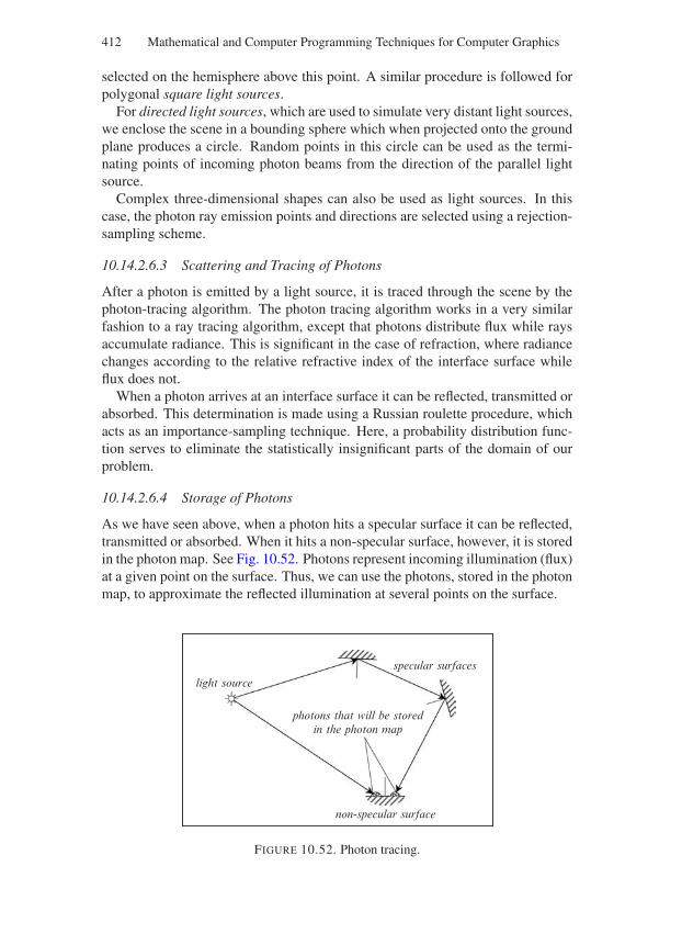
“Comninos” — 2005/8/31 — 19:01 — page 412 — #96
412 Mathematical and Computer Programming Techniques for Computer Graphics
selected on the hemisphere above this point. A similar procedure is followed forpolygonal square light sources.
For directed light sources, which are used to simulate very distant light sources,we enclose the scene in a bounding sphere which when projected onto the groundplane produces a circle. Random points in this circle can be used as the termi-nating points of incoming photon beams from the direction of the parallel lightsource.
Complex three-dimensional shapes can also be used as light sources. In thiscase, the photon ray emission points and directions are selected using a rejection-sampling scheme.
10.14.2.6.3 Scattering and Tracing of Photons
After a photon is emitted by a light source, it is traced through the scene by thephoton-tracing algorithm. The photon tracing algorithm works in a very similarfashion to a ray tracing algorithm, except that photons distribute flux while raysaccumulate radiance. This is significant in the case of refraction, where radiancechanges according to the relative refractive index of the interface surface whileflux does not.
When a photon arrives at an interface surface it can be reflected, transmitted orabsorbed. This determination is made using a Russian roulette procedure, whichacts as an importance-sampling technique. Here, a probability distribution func-tion serves to eliminate the statistically insignificant parts of the domain of ourproblem.
10.14.2.6.4 Storage of Photons
As we have seen above, when a photon hits a specular surface it can be reflected,transmitted or absorbed. When it hits a non-specular surface, however, it is storedin the photon map. See Fig. 10.52. Photons represent incoming illumination (flux)at a given point on the surface. Thus, we can use the photons, stored in the photonmap, to approximate the reflected illumination at several points on the surface.
non-specular surface
specular surfaces
photons that will be storedin the photon map
light source
FIGURE 10.52. Photon tracing.
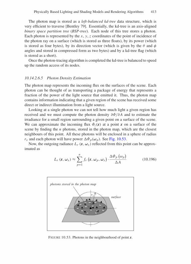
“Comninos” — 2005/8/31 — 19:01 — page 413 — #97
Physically Based Lighting and Shading Models and Rendering Algorithms 413
The photon map is stored as a left-balanced kd-tree data structure, which isvery efficient to traverse [Bentley 79]. Essentially, the kd-tree is an axis-alignedbinary space partition tree (BSP-tree). Each node of this tree stores a photon.Each photon is represented by the x , y, z coordinates of the point of incidence ofthe photon ray on a surface (which is stored as three floats), by its power (whichis stored as four bytes), by its direction vector (which is given by the θ and φ
angles and stored in compressed form as two bytes) and by a kd-tree flag (whichis stored as a short).
Once the photon-tracing algorithm is completed the kd-tree is balanced to speedup the random access of its nodes.
10.14.2.6.5 Photon Density Estimation
The photon map represents the incoming flux on the surfaces of the scene. Eachphoton can be thought of as transporting a package of energy that represents afraction of the power of the light source that emitted it. Thus, the photon mapcontains information indicating that a given region of the scene has received somedirect or indirect illumination from a light source.
Looking at a single photon we can not tell how much light a given region hasreceived and we must compute the photon density ∂Φ/∂ A and to estimate theirradiance for a small region surrounding a given point on a surface of the scene.We can approximate the incoming flux Φi (x) at a point x on a surface of thescene by finding the n photons, stored in the photon map, which are the closestneighbours of this point. All these photons will be enclosed in a sphere of radiusrx and each photon will have power Φp(ωp). See Fig. 10.53.
Now, the outgoing radiance Lr (x,ωx ) reflected from this point can be approx-imated as
Lr (x,ωx ) ≈n∑
p=1
fr(x,ωp,ωx
) ·Φp(ωp)
A(10.196)
photons stored in the photon map
surface
x
rx
FIGURE 10.53. Photons in the neighbourhood of point x.
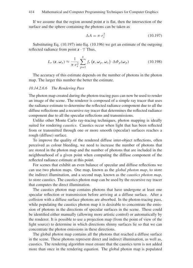
“Comninos” — 2005/8/31 — 19:01 — page 414 — #98
414 Mathematical and Computer Programming Techniques for Computer Graphics
If we assume that the region around point x is flat, then the intersection of thesurface and the sphere containing the photons can be taken as
A = π ·r2x (10.197)
Substituting Eq. (10.197) into Eq. (10.196) we get an estimate of the outgoingreflected radiance from point x · Thus,
Lr (x,ωx ) ≈ 1
π ·r2x
n∑
p=1
fr(x,ωp,ωx
) ·Φp(ωp) (10.198)
The accuracy of this estimate depends on the number of photons in the photonmap. The larger this number the better the estimate.
10.14.2.6.6 The Rendering Pass
The photon map created during the photon-tracing pass can now be used to renderan image of the scene. The renderer is composed of a simple ray tracer that usesthe radiance estimate to determine the reflected radiance component due to all thediffuse reflections and a recursive ray tracer that determines the reflected radiancecomponent due to all the specular reflections and transmissions.
Unlike other Monte Carlo ray-tracing techniques, photon mapping is ideallysuited for rendering caustics. Caustics occur when light that has been reflectedfrom or transmitted through one or more smooth (specular) surfaces reaches arough (diffuse) surface.
To improve the quality of the rendered diffuse inter-object reflections, oftenperceived as colour bleeding, we need to increase the number of photons thatare stored in the photon map and the number of photons that are included in theneighbourhood of a given point when computing the diffuse component of thereflected radiance estimate at this point.
For scenes that exhibit an even balance of specular and diffuse reflections wecan use two photon maps. One map, known as the global photon map, to storethe indirect illumination, and a second map, known as the caustics photon map,to store caustics. The caustics photon map can be used by the recursive ray tracerthat computes the direct illumination.
The caustics photon map contains photons that have undergone at least onespecular reflection or transmission before arriving at a diffuse surface. After acollision with a diffuse surface photons are absorbed. In the photon-tracing pass,while populating the caustics photon map it is desirable to concentrate the emis-sion of photons in the directions of specular surfaces in the scene. These couldbe identified either manually (allowing more artistic control) or automatically bythe renderer. It is possible to use a projection map (from the point of view of thelight source) to determine in which directions shinny surfaces lie so that we canconcentrate the photon emissions in these directions.
The global photon map contains all the photons that reached a diffuse surfacein the scene. These photons represent direct and indirect illumination, as well as,caustics. The rendering algorithm must ensure that the caustics term is not addedmore than once in the rendering equation. The global photon map is populated
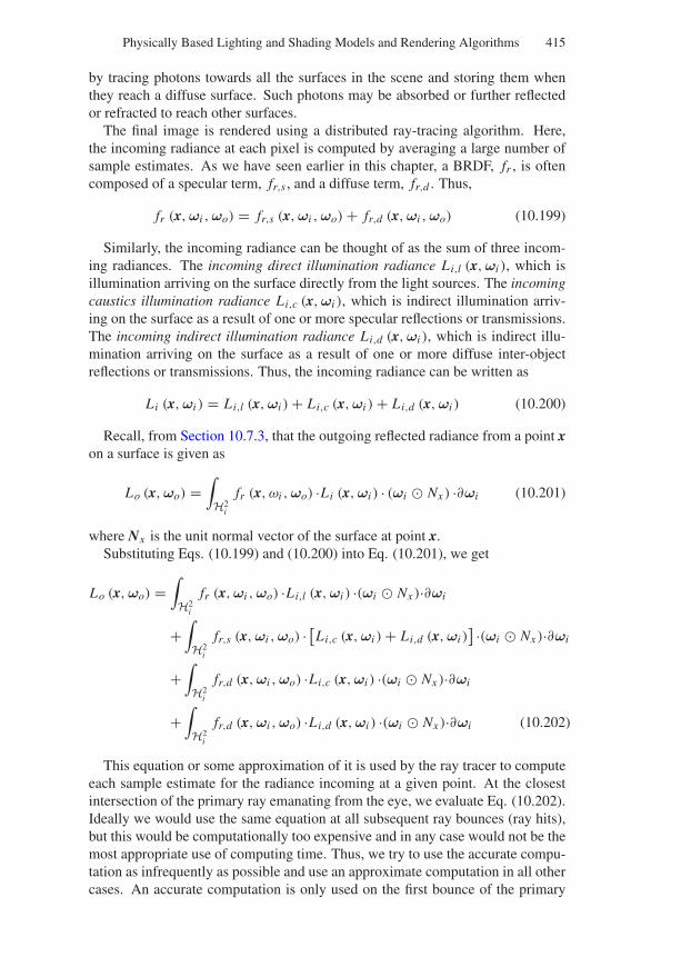
“Comninos” — 2005/8/31 — 19:01 — page 415 — #99
Physically Based Lighting and Shading Models and Rendering Algorithms 415
by tracing photons towards all the surfaces in the scene and storing them whenthey reach a diffuse surface. Such photons may be absorbed or further reflectedor refracted to reach other surfaces.
The final image is rendered using a distributed ray-tracing algorithm. Here,the incoming radiance at each pixel is computed by averaging a large number ofsample estimates. As we have seen earlier in this chapter, a BRDF, fr , is oftencomposed of a specular term, fr,s , and a diffuse term, fr,d . Thus,
fr (x,ωi ,ωo) = fr,s (x,ωi ,ωo) + fr,d (x,ωi ,ωo) (10.199)
Similarly, the incoming radiance can be thought of as the sum of three incom-ing radiances. The incoming direct illumination radiance Li,l (x,ωi ), which isillumination arriving on the surface directly from the light sources. The incomingcaustics illumination radiance Li,c (x,ωi ), which is indirect illumination arriv-ing on the surface as a result of one or more specular reflections or transmissions.The incoming indirect illumination radiance Li,d (x,ωi ), which is indirect illu-mination arriving on the surface as a result of one or more diffuse inter-objectreflections or transmissions. Thus, the incoming radiance can be written as
Li (x,ωi ) = Li,l (x,ωi ) + Li,c (x,ωi ) + Li,d (x,ωi ) (10.200)
Recall, from Section 10.7.3, that the outgoing reflected radiance from a point xon a surface is given as
Lo (x,ωo) =∫
H2i
fr (x, ωi ,ωo) ·Li (x,ωi ) · (ωi Nx ) ·∂ωi (10.201)
where Nx is the unit normal vector of the surface at point x.Substituting Eqs. (10.199) and (10.200) into Eq. (10.201), we get
Lo (x,ωo) =∫
H2i
fr (x,ωi ,ωo) ·Li,l (x,ωi ) ·(ωi Nx )·∂ωi
+∫
H2i
fr,s (x,ωi ,ωo) · [Li,c (x,ωi ) + Li,d (x,ωi )] ·(ωi Nx )·∂ωi
+∫
H2i
fr,d (x,ωi ,ωo) ·Li,c (x,ωi ) ·(ωi Nx )·∂ωi
+∫
H2i
fr,d (x,ωi ,ωo) ·Li,d (x,ωi ) ·(ωi Nx )·∂ωi (10.202)
This equation or some approximation of it is used by the ray tracer to computeeach sample estimate for the radiance incoming at a given point. At the closestintersection of the primary ray emanating from the eye, we evaluate Eq. (10.202).Ideally we would use the same equation at all subsequent ray bounces (ray hits),but this would be computationally too expensive and in any case would not be themost appropriate use of computing time. Thus, we try to use the accurate compu-tation as infrequently as possible and use an approximate computation in all othercases. An accurate computation is only used on the first bounce of the primary
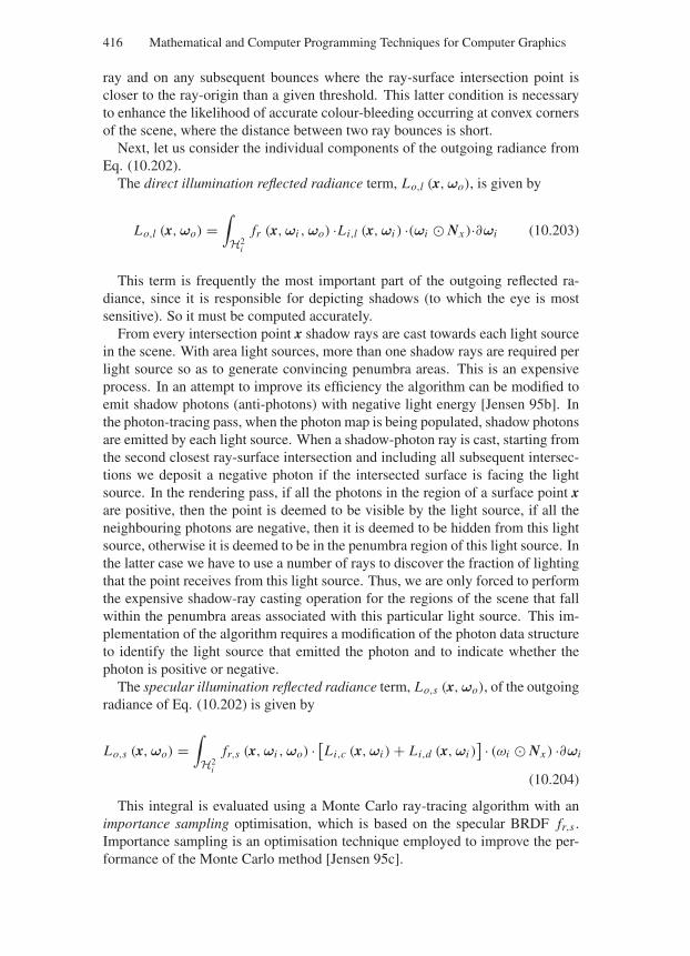
“Comninos” — 2005/8/31 — 19:01 — page 416 — #100
416 Mathematical and Computer Programming Techniques for Computer Graphics
ray and on any subsequent bounces where the ray-surface intersection point iscloser to the ray-origin than a given threshold. This latter condition is necessaryto enhance the likelihood of accurate colour-bleeding occurring at convex cornersof the scene, where the distance between two ray bounces is short.
Next, let us consider the individual components of the outgoing radiance fromEq. (10.202).
The direct illumination reflected radiance term, Lo,l (x,ωo), is given by
Lo,l (x,ωo) =∫
H2i
fr (x,ωi ,ωo) ·Li,l (x,ωi ) ·(ωi Nx )·∂ωi (10.203)
This term is frequently the most important part of the outgoing reflected ra-diance, since it is responsible for depicting shadows (to which the eye is mostsensitive). So it must be computed accurately.
From every intersection point x shadow rays are cast towards each light sourcein the scene. With area light sources, more than one shadow rays are required perlight source so as to generate convincing penumbra areas. This is an expensiveprocess. In an attempt to improve its efficiency the algorithm can be modified toemit shadow photons (anti-photons) with negative light energy [Jensen 95b]. Inthe photon-tracing pass, when the photon map is being populated, shadow photonsare emitted by each light source. When a shadow-photon ray is cast, starting fromthe second closest ray-surface intersection and including all subsequent intersec-tions we deposit a negative photon if the intersected surface is facing the lightsource. In the rendering pass, if all the photons in the region of a surface point xare positive, then the point is deemed to be visible by the light source, if all theneighbouring photons are negative, then it is deemed to be hidden from this lightsource, otherwise it is deemed to be in the penumbra region of this light source. Inthe latter case we have to use a number of rays to discover the fraction of lightingthat the point receives from this light source. Thus, we are only forced to performthe expensive shadow-ray casting operation for the regions of the scene that fallwithin the penumbra areas associated with this particular light source. This im-plementation of the algorithm requires a modification of the photon data structureto identify the light source that emitted the photon and to indicate whether thephoton is positive or negative.
The specular illumination reflected radiance term, Lo,s (x,ωo), of the outgoingradiance of Eq. (10.202) is given by
Lo,s (x,ωo) =∫
H2i
fr,s (x,ωi ,ωo) · [Li,c (x,ωi ) + Li,d (x,ωi )] · (ωi Nx ) ·∂ωi
(10.204)
This integral is evaluated using a Monte Carlo ray-tracing algorithm with animportance sampling optimisation, which is based on the specular BRDF fr,s .Importance sampling is an optimisation technique employed to improve the per-formance of the Monte Carlo method [Jensen 95c].
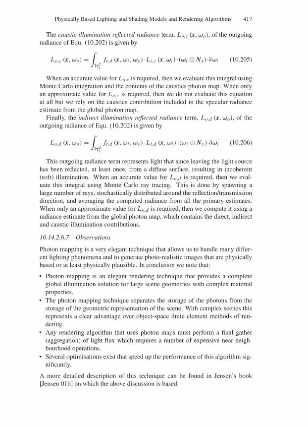
“Comninos” — 2005/8/31 — 19:01 — page 417 — #101
Physically Based Lighting and Shading Models and Rendering Algorithms 417
The caustic illumination reflected radiance term, Lo,c (x,ωo), of the outgoingradiance of Equ. (10.202) is given by
Lo,c (x,ωo) =∫
H2i
fr,d (x,ωi ,ωo) ·Li,c (x,ωi ) ·(ωi Nx )·∂ωi (10.205)
When an accurate value for Lo,c is required, then we evaluate this integral usingMonte Carlo integration and the contents of the caustics photon map. When onlyan approximate value for Lo,c is required, then we do not evaluate this equationat all but we rely on the caustics contribution included in the specular radianceestimate from the global photon map.
Finally, the indirect illumination reflected radiance term, Lo,d (x,ωo), of theoutgoing radiance of Equ. (10.202) is given by
Lo,d (x,ωo) =∫
H2i
fr,d (x,ωi ,ωo) ·Li,d (x,ωi ) ·(ωi Nx )·∂ωi (10.206)
This outgoing radiance term represents light that since leaving the light sourcehas been reflected, at least once, from a diffuse surface, resulting in incoherent(soft) illumination. When an accurate value for Lo,d is required, then we eval-uate this integral using Monte Carlo ray tracing. This is done by spawning alarge number of rays, stochastically distributed around the reflection/transmissiondirection, and averaging the computed radiance from all the primary estimates.When only an approximate value for Lo,d is required, then we compute it using aradiance estimate from the global photon map, which contains the direct, indirectand caustic illumination contributions.
10.14.2.6.7 Observations
Photon mapping is a very elegant technique that allows us to handle many differ-ent lighting phenomena and to generate photo-realistic images that are physicallybased or at least physically plausible. In conclusion we note that:
• Photon mapping is an elegant rendering technique that provides a completeglobal illumination solution for large scene geometries with complex materialproperties.
• The photon mapping technique separates the storage of the photons from thestorage of the geometric representation of the scene. With complex scenes thisrepresents a clear advantage over object-space finite element methods of ren-dering.
• Any rendering algorithm that uses photon maps must perform a final gather(aggregation) of light flux which requires a number of expensive near neigh-bourhood operations.
• Several optimisations exist that speed up the performance of this algorithm sig-nificantly.
A more detailed description of this technique can be found in Jensen’s book[Jensen 01b] on which the above discussion is based.
“Comninos” — 2005/8/31 — 19:01 — page 418 — #102
418 Mathematical and Computer Programming Techniques for Computer Graphics
10.14.3 Hybrid Multi-Pass Rendering Algorithms
A promising approach is to use a hybrid algorithm for rendering, which involvesmultiple passes. The first pass of such an algorithm adopts an object-space ap-proach and deals with the diffuse inter-object illumination problem, by comput-ing and storing the outgoing radiance diffusely reflected from the surfaces of thescene. The second pass of such an algorithm adopts an image-space approach anddeals with specular inter-object illumination, by accessing the pre-stored object-space solution and by computing (on the fly) for each pixel the radiance con-tributed by the specular inter-object illumination, which would be impossible tocompute and store in the first pass.
Such algorithms can be designed to take advantage of the strengths of bothobject-space and image-space techniques.
Examples of such multi-pass algorithms are found in [Wallace 87], [Sillion 89],[Chen 91], [Jensen 96] and [Suykens 99].
References
[Amanatides 84] Amanatides, J. Ray tracing with cones. Proceedings of SIGGRAPH 84.Computer Graphics, Vol. 18, No. 3, p.p. 129–135, 1984.
[Ashikmin 00a] Ashikmin, M. and Shirley, P. An anisotropic Phong light reflectionmodel. Technical Report UUCS-00-014, Computer Science Depart-ment, University of Utah, p.p. 1–11, June 2000.
[Ashikmin 00b] Ashikmin, M. and Shirley, P. An anisotropic phong BRDF model.Journal of Graphics Tools, Vol. 5, No. 2, p.p. 25–32, 2000.
[Ashikmin 00c] Ashikmin, M., Premoze, S., and Shirley, P. A microfacet-based BRDFgenerator, Proceedings of SIGGRAPH 2000, Computer Graphics, ACMPress/ACM SIGGRAPH/Addison Wesley Longman, p.p. 65–74, 2000.
[Aupperle 93] Aupperle, L. and Hanrahan, P. A hierarchical illumination algorithmfor surfaces with glossy reflection”. Proceedings of SIGGRAPH 93,Computer Graphics, Vol. 27, No. 4, p.p. 155–162 1993.
[Beckmann 63] Beckmann, P. and Spizzichino, A. The Scattering of ElectromagneticWaves from Rough Surfaces. Pergamin Press, Oxford, England (1963).
[Bennett 61] Bennett, R. A. and Porteus, J. O. Relation between surface roughnessand specular reflectance at normal incidence, Journal of the OpticalSociety of America, Vol. 51, p.p. 123–129, 1961.
[Bentley 79] Bentley, J. L. and Friedman, J. H. Data structures for range searching,Computing Surveys, Vol. 11, No. 4, p.p. 397–409, 1979.
[Blinn 77] Blinn, J. F. Models of light reflection for computer synthesized pictures.Proceedings of SIGGRAPH 77, Computer Graphics, Vol. 11, No. 2,p.p. 192–198, 1977.
[Chen 90] Chen, S. E. Incremental radiosity: An extension of progressive radiosityto an interactive image synthesis system. Proceedings of SIGGRAPH90, Computer Graphics, Vol. 24, No. 4, p.p. 135–144, (1990).
[Chen 91] Chen, S. E., Rushmeier, H. E., Miller, G., and Turner, D. A progressivemulti-path method for global illumination, Proceedings of SIGGRAPH91, Computer Graphics, Vol. 25, No. 4, p.p. 165–174, 1991.
[Clarke 85] Clarke, F. J. J. and Parry, D. J. Helmholz reciprocity: Its Vlvidity andapplication to reflectometry, Lighting Research and Technology, Vol.17, No. 1, p.p. 1–11, 1985.
“Comninos” — 2005/8/31 — 19:01 — page 419 — #103
Physically Based Lighting and Shading Models and Rendering Algorithms 419
[Cohen 93] Cohen, M. F. and Wallace, J. R. Radiosity and Realistic ImageSynthesis, Academic Press, San Diego, CA (1993).
[Cohen 85] Cohen, M. F. and Greenberg, D. P. The hemi-cube: A Rdriositysolution for complex environments. Proceedings of SIGGRAPH 85,Computer Graphics, Vol. 19, No. 3, p.p. 31–40, 1985.
[Cook 81] Cook, R. L. and Torrance, K. E. A reflection model for computergraphics. Proceedings SIGGRAPH 81, Computer Graphics, Vol. 15,No. 4, p.p. 307–316, 1981.
[Cook 82] Cook, R. L. and Torrance, K. E. A reflection model for computergraphics. ACM Transactions on Graphics, Vol. 1, No. 1, p.p. 7–24,1982.
[Cook 84] Cook, R., L., Porter, T. and Carpenter, L. Distributed ray tracing. Pro-ceedings of SIGGRAPH 84, Computer Graphics, Vol. 18, No. 3, p.p.137–145, 1984.
[Ditchburn 76] Ditchburn, R. W. Light, Vols. 1 and 2. Academic Press, London(1976).
[Dorsey 99] Dorsey, J., Edelman, A., Jensen, H. W., Legakis, J., and Pedersen,H. K. Modelling and rendering of weathered stone. Proceedings ofSIGGRAPH 99, pp. 225–234. Addison-Wesley, Reading, MA (1999).
[Drettakis 97] Drettakis, G. and Sillion, F., X. Interactive update of global illumi-nation using a line-space hierarchy. Proceedings of SIGGRAPH 97.Computer Graphics, Vol. 31, No. 4, p.p. 57–64, 1997.
[Duderstadt 79] Duderstadt, J. J. and Martin, W. R. Transport Theory. John Wiley &Sons, New York (1979).
[Dutre 94] Dutre, Ph. and Willems, Y. D., Importance-Driven Monte Carlo lighttracing. Proceedings of the Fifth Eurographics Workshop on Render-ing, Darmstadt, Germany, Eurographics Association, p.p. 185–194(1994).
[Dutre 98] Dutre, Ph. Mathematical Framework and Monte Carlo Algorithms forGlobal Illumination in Computer Graphics. Ph.D Thesis, Universityof Leuven (1998).
[George 90] George, D. W., Sillion, F. X., and Greenberg, D., P. RadiosityRedistribution for Dynamic Environments, IEEE, Computer Graphicsand Applications, Vol. 10, No. 4, p.p. 26–34, July 1990.
[Goldstein 71] Goldstein, R. A. and Nagel, R. 3-D Visual Simulation. Simulation,p.p. 25–31 Jan 1971.
[Goral 84] Goral, C. M., Torrance, K. E., Greenberg, D. P., and Battaile, B. Mod-eling the interaction of light between diffuse surfaces. Proceedings ofSIGGRAPH 84, Computer Graphics, Vol. 18, No. 3, p.p. 213–222,1984.
[Hall 89] Hall, R. Illumination and Color in Computer Generated Imagery.Springer-Verlag, New York (1989).
[Hanrahan 93] Hanrahan, P. and Krueger, W. Reflection from layered surfaces due tosubsurface scattering. Proceedings of SIGGRAPH 93, 165–174, ACMPress, New York (1993).
[Immel 86] Immel, D. S., Cohen, M. F. and Greenberg, D. P. A radiositymethod for non-diffuse environments. Proceedings of SIGGRAPH 86,Computer Graphics, Vol. 20, No. 4, p.p. 133–142, 1986.
[Jenkins 76] Jenkins, F. A. and White, H. E. Fundamentals of Optics. McGraw-Hill, New York (1976).
[Jensen 95a] Jensen, H. W. and Christensen, N. J. Photon maps in bi-directionalMonte Carlo ray tracing of complex objects. Computers & Graphics,Vol. 19, No. 2, p.p. 215–224, 1995.
“Comninos” — 2005/8/31 — 19:01 — page 420 — #104
420 Mathematical and Computer Programming Techniques for Computer Graphics
[Jensen 95b] Jensen, H. W. and Christensen, N. J. Efficiently rendering shadowsusing the photon map. Proceedings of CompuGraphics 95, p.p.285–291 Dec 1995.
[Jensen 95c] Jensen, H. W. Importance driven path tracing using the photon map.Proceedings of the Eurographics Rendering Workshop 95, Euro-graphics Association, p.p. 326– 335, June 1995.
[Jensen 96] Jensen, H. W. Global illumination using photon maps. Proceedingsof the Eurographics Rendering Workshop 1996. Springer-Verlag,Vienna, p.p. 21–30, 1996.
[Jensen 99] Jensen, H. W., Legakis, J., and Dorsey, J. Rendering of wet mate-rials, In: C. Lischinski and G. W. Larson (Eds.), Rendering Tech-niques’99. Springer-Verlag, Vienna (1999).
[Jensen 01a] Jensen, H. W., Marschner, S., Levoy, M., and Hanrahan, P. Apractical model for subsurface light transport. Proceedings ofSIGGRAPH 2001, p.p. 399–408. Addison-Wesley, Reading MA(2001).
[Jensen 01b] Jensen, H. W. Realistic Image Synthesis using Photon Mapping. A.K. Peters Ltd., Natick, Massachusetts (2001).
[Kajiya 86] Kajiya, J. T. The rendering equation. Proceedings of SIGGRAPH86, Computer Graphics, Vol. 20, No. 4, p.p. 143–150, 1986.
[Lafortune 93] Lafortune, E. P. and Willems, Y. D. Bi-directional path tracing.Proceedings of the International Computer Graphics and Visual-isation Techniques, CompuGraphics 93. Avlor, Portugal, p.p. 145–153 1993.
[Lafortune 94] Lafortune, E. and Willems, Y. Using the modified Phongreflectance model for physically based rendering, Technical ReportCW 194, Department of Computer Science, K.U., Leuven, p.p. 1–18, Nov 1994.
[Lafortune 97] Lafortune, E. P. F., Foo, S. C., Torrance, K. E., and Greenberg D. P.Non-linear approximation of reflectance functions. Proceedings ofSIGGRAPH 97, Computer Graphics, No. 31, p.p. 117–126, 1997.
[Lewis 93] Lewis, R. R. Making shaders more physically plausible.Proceedings of the Fourth Eurographics Workshop on Rendering,Paris, France. Eurographics Series EG 93 RW, pp. 47–62 June1993.
[Metropolis 49] Metropolis, N. and Ulam, S. The Monte Carlo method, Journal ofthe American Statistical Association, Vol. 44, No. 247, p.p. 335–341, 1949.
[Metropolis 53] Metropolis, N., Rosenbluth, A. W., Rosenbluth, M. N., Teller, A.H., and Teller, E. Equations of state calculations by fast computingmachines, Journal of Chemical Physics 21, p.p. 1087–1091, 1953.
[Neumann 99a] Neumann, L., Neumann, A., and Szirmay-Kalos L. Compactmetallic reflectance models, Computer Graphics Forum (Euro-graphics ’99). The Eurographics Association and Blackwell Pub-lishers, Vol. 18, No. 3, p.p. 161–172, 1999.
[Neumann 99b] Neumann, L., Neumann, A., and Szirmay-Kalos L. Reflectancemodels with fast importance sampling, Computer Graphics Forum,Vol. 18, No. 4, p.p. 249–265, 1999.
[Nicodemus 77] Nicodemus, F. E., Richmond, J. C., Hsia, J. J., Ginburg, I. W.,and Limperis, T. Geometric considerations and nomenclature forreflectance, Monograph 161, National Bureau of Standards (US)Oct 1977.
“Comninos” — 2005/8/31 — 19:01 — page 421 — #105
Physically Based Lighting and Shading Models and Rendering Algorithms 421
[Nishita 85] Nishita, T. and Nakamae, E. Continuous tone representation of three-dimensional objects taking account of shadows and inter-reflection.Proceedings of SIGGRAPH 85, Computer Graphics, Vol. 19, No. 3,p.p. 23–30, 1985.
[Palik 85] Palik, E. D. Handbook of Optical Constants of Solids. AcademicPress, New York, NY (1985).
[Pharr 00] Pharr, M. and Hanrahan, P. Monte Carlo evaluation of non-linearscattering equations for subsurface reflection. Proceedings of SIG-GRAPH 2000, pp. 75–84. Addison-Wesley, Reading, MA (2000).
[Sancer 69] Sancer, M. I. Shadow-corrected electromagnetic scattering from arandomly rough surface, IEEE Transactions on Antennas and Prop-agation, Vol. 17, No. 5, p.p. 577–585, 1969.
[Schlick 93] Schlick, C. A customizable reflectance model for everydayrendering. Proceedings of the Fourth Eurographics Workshop onRendering. Series EG 93 RW. Paris, France, p.p. 73–84 June 1993.
[Shirley 91] Shirley, P. Physically Based Lighting Calculations for ComputerGraphics, Ph.D Thesis, University of Illinois at Urbana ChampaignJan 1991.
[Sillion 89] Sillion, F. and Puech, C. A general two-pass method integrating spec-ular and diffuse reflection. Proceedings of SIGGRAPH 89, ComputerGraphics, Vol. 23, No. 4, p.p. 335–344, 1989.
[Sillion 91] Sillion, F., Avro, J., Westin, S., and Greenberg, D. P. A global illumi-nation solution for general reflectance distributions. Proceedings ofSIGGRAPH 91, Computer Graphics, Vol. 25, No. 4, p.p. 187–1961991.
[Stamminger 98] Stamminger, M., Slusallek, Ph., and Seidel, P. H. Three point cluster-ing for radiance computations. Proceedings of the EurographicsRendering Workshop 98. Eurographics Association, p.p. 211–222,1998.
[Suykens 99] Suykens, F. and Willems, Y. D. Weighted multi-pass method forglobal illumination. Proceedings of Eurographics 99, ComputerGraphics Forum, Vol. 18, No. 3, p.p. 209–220, 1999.
[Torrance 67] Torrance, K. E. and Sparrow, E. M. Theory of off-specular reflectionfrom roughened surfaces, Journal of the Optical Society of America,Vol. 57, No. 9, p.p. 1105–1114, 1967.
[Veach 94] Veach, E. and Guibas, L. J. Bi-directional estimates for light trans-port. Proceedings of the Fifth Eurographics Workshop on Rendering,Darmstadt, Germany. Eurographics Association, p.p. 147–162 1994.
[Veach 97a] Veach, E. Robust Monte Carlo Methods for Light Transport. Ph.DThesis, Department of Computer Science, Stanford University(1997).
[Veach 97b] Veach, E. and Guibas, L. J. Metropolis light transport. Proceedingsof SIGGRAPH 97, Computer Graphics, Vol. 31, No. 4, p.p. 65–76,1997.
[Wallace 87] Wallace, J. R., Cohen, M. F., and Greenberg, D. P. A two-passsolution to the rendering equation: A synthesis of ray tracingand radiosity methods. Proceedings of SIGGRAPH 97, ComputerGraphics, Vol. 21, No. 4, p.p. 311–320, 1987.
[Whitted 80] Whitted, T. An improved illumination model for shaded display.Communications of the ACM, Vol. 23, No. 6, p.p. 343–349, 1980.
[WWW 1] http://www.luxpop.com
“Comninos” — 2005/8/31 — 18:23 — page 423 — #1
Appendix 1
A Simple Vector Algebra C Library
In this Appendix we examine a simple C library that implements all the vectoralgebra operations we have defined in Chapter 2.
#include <stdio.h>#include <math.h>
/*----------------------------------------------------------------*/
/** Three-dimensional vectors are stored as three doubles and a
* single byte header which is a vector type indicator.
** Temporary vectors have their type indicator set to 1 and
* Permanent vectors have their type indicator set to 2.
** All vector operations return temporary vectors so they can be
* nested without memory leakage. Each vector function checks its
* vector parameters and destroys them if they are found to be
* temporary.
** In its current implementation this library deals with 3D vectors
* and all vector components are stored as doubles.
*/
#define temporary_vector 1#define permanent_vector 2
typedef double *vector_t;typedef unsigned char *header_t;
/** Key to global constants:
** vector_length_bytes - Length of the vector components in
* bytes.
** vt_length_bytes - Length of the header excluding the
* filler bytes.
423
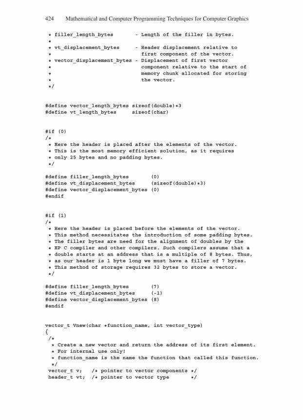
“Comninos” — 2005/8/31 — 18:23 — page 424 — #2
424 Mathematical and Computer Programming Techniques for Computer Graphics
* filler_length_bytes - Length of the filler in bytes.
** vt_displacement_bytes - Header displacement relative to
* first component of the vector.
* vector_displacement_bytes - Displacement of first vector
* component relative to the start of
* memory chunk allocated for storing
* the vector.
*/
#define vector_length_bytes sizeof(double)*3#define vt_length_bytes sizeof(char)
#if (0)/** Here the header is placed after the elements of the vector.
* This is the most memory efficient solution, as it requires
* only 25 bytes and no padding bytes.
*/
#define filler_length_bytes (0)#define vt_displacement_bytes (sizeof(double)*3)#define vector_displacement_bytes (0)#endif
#if (1)/** Here the header is placed before the elements of the vector.
* This method necessitates the introduction of some padding bytes.
* The filler bytes are need for the alignment of doubles by the
* HP C compiler and other compilers. Such compilers assume that a
* double starts at an address that is a multiple of 8 bytes. Thus,
* as our header is 1 byte long we must have a filler of 7 bytes.
* This method of storage requires 32 bytes to store a vector.
*/
#define filler_length_bytes (7)#define vt_displacement_bytes (-1)#define vector_displacement_bytes (8)#endif
vector_t Vnew(char *function_name, int vector_type)/** Create a new vector and return the address of its first element.
* For internal use only!
* function_name is the name the function that called this function.
*/vector_t v; /* pointer to vector components */header_t vt; /* pointer to vector type */
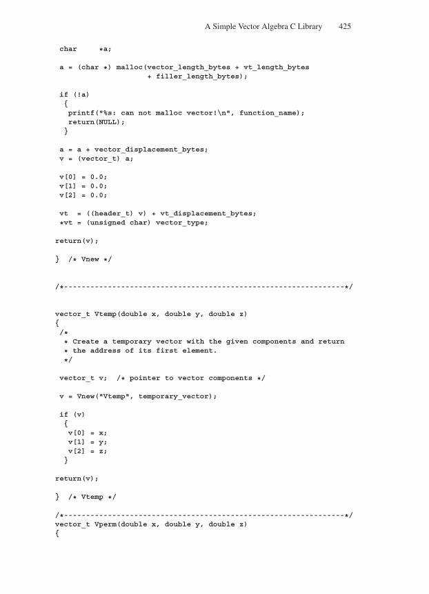
“Comninos” — 2005/8/31 — 18:23 — page 425 — #3
A Simple Vector Algebra C Library 425
char *a;
a = (char *) malloc(vector_length_bytes + vt_length_bytes+ filler_length_bytes);
if (!a)printf("%s: can not malloc vector!\n", function_name);return(NULL);
a = a + vector_displacement_bytes;v = (vector_t) a;
v[0] = 0.0;v[1] = 0.0;v[2] = 0.0;
vt = ((header_t) v) + vt_displacement_bytes;
*vt = (unsigned char) vector_type;
return(v);
/* Vnew */
/*----------------------------------------------------------------*/
vector_t Vtemp(double x, double y, double z)/** Create a temporary vector with the given components and return
* the address of its first element.
*/
vector_t v; /* pointer to vector components */
v = Vnew("Vtemp", temporary_vector);
if (v)v[0] = x;v[1] = y;v[2] = z;
return(v);
/* Vtemp */
/*----------------------------------------------------------------*/vector_t Vperm(double x, double y, double z)
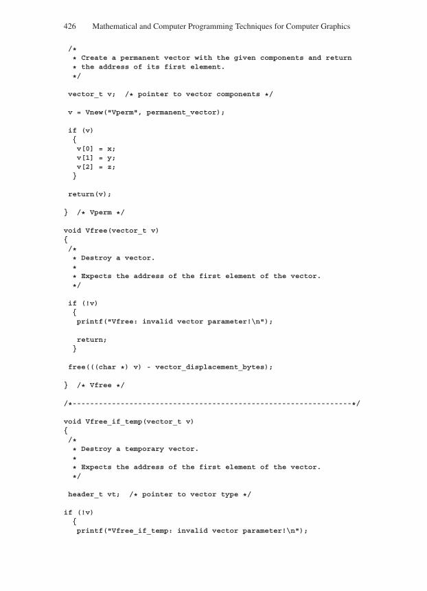
“Comninos” — 2005/8/31 — 18:23 — page 426 — #4
426 Mathematical and Computer Programming Techniques for Computer Graphics
/** Create a permanent vector with the given components and return
* the address of its first element.
*/
vector_t v; /* pointer to vector components */
v = Vnew("Vperm", permanent_vector);
if (v)v[0] = x;v[1] = y;v[2] = z;
return(v);
/* Vperm */
void Vfree(vector_t v)/** Destroy a vector.
** Expects the address of the first element of the vector.
*/
if (!v)printf("Vfree: invalid vector parameter!\n");
return;
free(((char *) v) - vector_displacement_bytes);
/* Vfree */
/*----------------------------------------------------------------*/
void Vfree_if_temp(vector_t v)/** Destroy a temporary vector.
** Expects the address of the first element of the vector.
*/
header_t vt; /* pointer to vector type */
if (!v)printf("Vfree_if_temp: invalid vector parameter!\n");
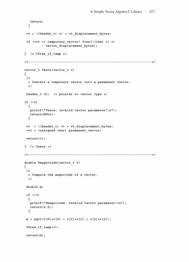
“Comninos” — 2005/8/31 — 18:23 — page 427 — #5
A Simple Vector Algebra C Library 427
return;
vt = ((header_t) v) + vt_displacement_bytes;
if (*vt == temporary_vector) free(((char *) v)- vector_displacement_bytes);
/* Vfree_if_temp */
/*----------------------------------------------------------------*/
vector_t Vsave(vector_t v)/** Convert a temporary vector into a permanent vector.
*/
header_t vt; /* pointer to vector type */
if (!v)printf("Vsave: invalid vector parameter!\n");return(NULL);
vt = ((header_t) v) + vt_displacement_bytes;
*vt = (unsigned char) permanent_vector;
return(v);
/* Vsave */
/*----------------------------------------------------------------*/
double Vmagnitude(vector_t v)/** Compute the magnitude of a vector.
*/
double m;
if (!v)printf("Vmagnitude: Invalid vector parameter!\n");return(0.0);
m = sqrt(v[0]*v[0] + v[1]*v[1] + v[2]*v[2]);
Vfree_if_temp(v);
return(m);
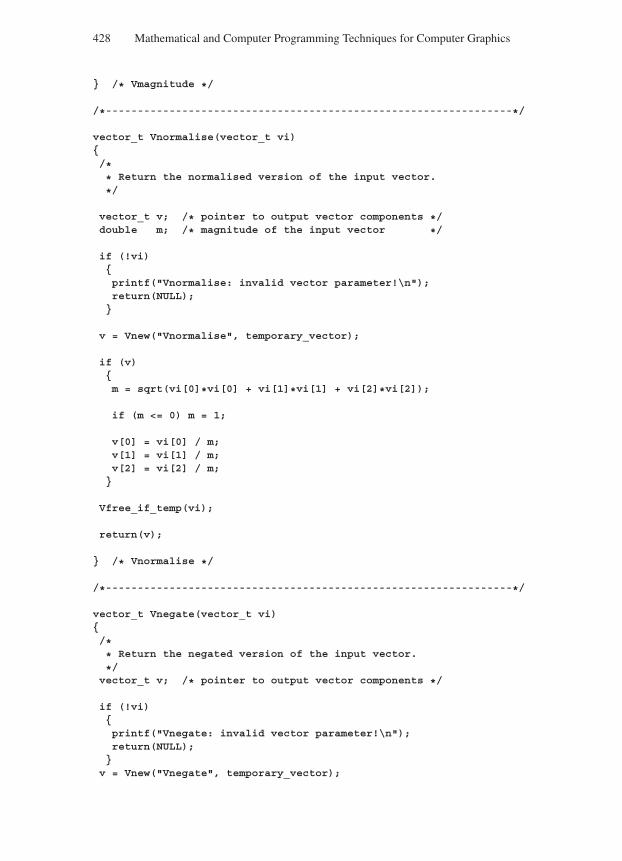
“Comninos” — 2005/8/31 — 18:23 — page 428 — #6
428 Mathematical and Computer Programming Techniques for Computer Graphics
/* Vmagnitude */
/*----------------------------------------------------------------*/
vector_t Vnormalise(vector_t vi)/** Return the normalised version of the input vector.
*/
vector_t v; /* pointer to output vector components */double m; /* magnitude of the input vector */
if (!vi)printf("Vnormalise: invalid vector parameter!\n");return(NULL);
v = Vnew("Vnormalise", temporary_vector);
if (v)m = sqrt(vi[0]*vi[0] + vi[1]*vi[1] + vi[2]*vi[2]);
if (m <= 0) m = 1;
v[0] = vi[0] / m;v[1] = vi[1] / m;v[2] = vi[2] / m;
Vfree_if_temp(vi);
return(v);
/* Vnormalise */
/*----------------------------------------------------------------*/
vector_t Vnegate(vector_t vi)/** Return the negated version of the input vector.
*/vector_t v; /* pointer to output vector components */
if (!vi)printf("Vnegate: invalid vector parameter!\n");return(NULL);
v = Vnew("Vnegate", temporary_vector);
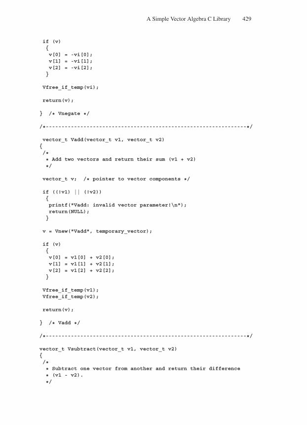
“Comninos” — 2005/8/31 — 18:23 — page 429 — #7
A Simple Vector Algebra C Library 429
if (v)v[0] = -vi[0];v[1] = -vi[1];v[2] = -vi[2];
Vfree_if_temp(vi);
return(v);
/* Vnegate */
/*----------------------------------------------------------------*/
vector_t Vadd(vector_t v1, vector_t v2)/** Add two vectors and return their sum (v1 + v2)
*/
vector_t v; /* pointer to vector components */
if ((!v1) || (!v2))printf("Vadd: invalid vector parameter!\n");return(NULL);
v = Vnew("Vadd", temporary_vector);
if (v)v[0] = v1[0] + v2[0];v[1] = v1[1] + v2[1];v[2] = v1[2] + v2[2];
Vfree_if_temp(v1);Vfree_if_temp(v2);
return(v);
/* Vadd */
/*----------------------------------------------------------------*/
vector_t Vsubtract(vector_t v1, vector_t v2)/** Subtract one vector from another and return their difference
* (v1 - v2).
*/
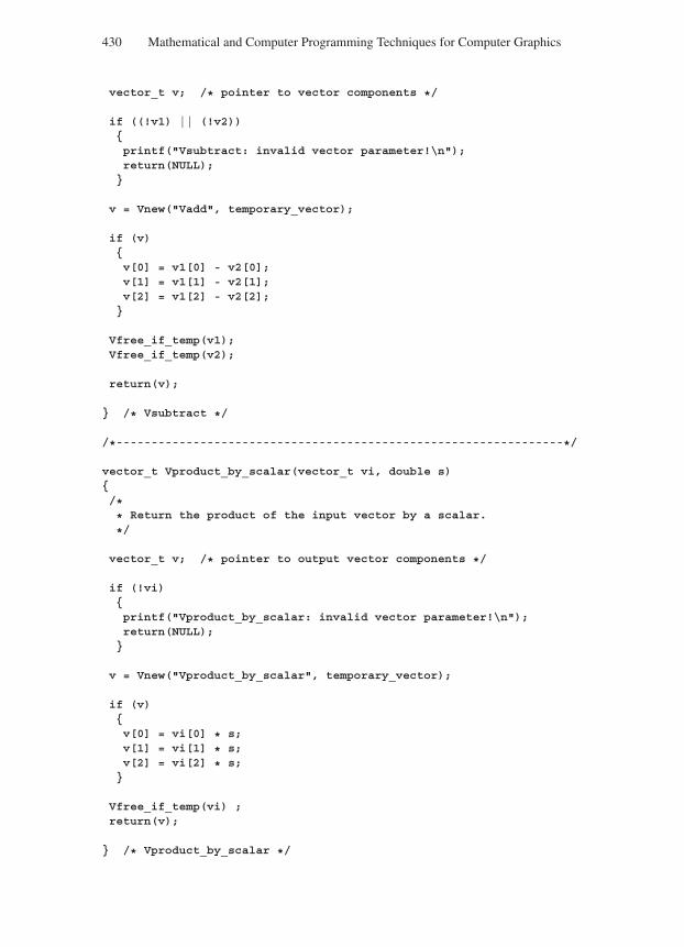
“Comninos” — 2005/8/31 — 18:23 — page 430 — #8
430 Mathematical and Computer Programming Techniques for Computer Graphics
vector_t v; /* pointer to vector components */
if ((!v1) || (!v2))printf("Vsubtract: invalid vector parameter!\n");return(NULL);
v = Vnew("Vadd", temporary_vector);
if (v)v[0] = v1[0] - v2[0];v[1] = v1[1] - v2[1];v[2] = v1[2] - v2[2];
Vfree_if_temp(v1);Vfree_if_temp(v2);
return(v);
/* Vsubtract */
/*----------------------------------------------------------------*/
vector_t Vproduct_by_scalar(vector_t vi, double s)/** Return the product of the input vector by a scalar.
*/
vector_t v; /* pointer to output vector components */
if (!vi)printf("Vproduct_by_scalar: invalid vector parameter!\n");return(NULL);
v = Vnew("Vproduct_by_scalar", temporary_vector);
if (v)v[0] = vi[0] * s;v[1] = vi[1] * s;v[2] = vi[2] * s;
Vfree_if_temp(vi) ;return(v);
/* Vproduct_by_scalar */
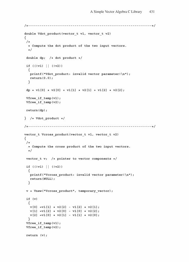
“Comninos” — 2005/8/31 — 18:23 — page 431 — #9
A Simple Vector Algebra C Library 431
/*----------------------------------------------------------------*/
double Vdot_product(vector_t v1, vector_t v2)/** Compute the dot product of the two input vectors.
*/
double dp; /* dot product */
if ((!v1) || (!v2))printf("Vdot_product: invalid vector parameter!\n");return(0.0);
dp = v1[0] * v2[0] + v1[1] * v2[1] + v1[2] * v2[2];
Vfree_if_temp(v1);Vfree_if_temp(v2);
return(dp);
/* Vdot_product */
/*----------------------------------------------------------------*/
vector_t Vcross_product(vector_t v1, vector_t v2)/** Compute the cross product of the two input vectors.
*/
vector_t v; /* pointer to vector components */
if ((!v1) || (!v2))printf("Vcross_product: invalid vector parameter!\n");return(NULL);
v = Vnew("Vcross_product", temporary_vector);
if (v)v[0] =v1[1] * v2[2] - v1[2] * v2[1];v[1] =v1[2] * v2[0] - v1[0] * v2[2];v[2] =v1[0] * v2[1] - v1[1] * v2[0];
Vfree_if_temp(v1);Vfree_if_temp(v2);
return (v);
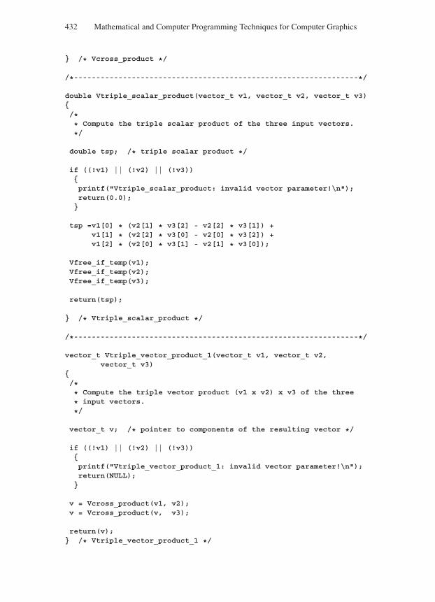
“Comninos” — 2005/8/31 — 18:23 — page 432 — #10
432 Mathematical and Computer Programming Techniques for Computer Graphics
/* Vcross_product */
/*----------------------------------------------------------------*/
double Vtriple_scalar_product(vector_t v1, vector_t v2, vector_t v3)/** Compute the triple scalar product of the three input vectors.
*/
double tsp; /* triple scalar product */
if ((!v1) || (!v2) || (!v3))printf("Vtriple_scalar_product: invalid vector parameter!\n");return(0.0);
tsp =v1[0] * (v2[1] * v3[2] - v2[2] * v3[1]) +v1[1] * (v2[2] * v3[0] - v2[0] * v3[2]) +v1[2] * (v2[0] * v3[1] - v2[1] * v3[0]);
Vfree_if_temp(v1);Vfree_if_temp(v2);Vfree_if_temp(v3);
return(tsp);
/* Vtriple_scalar_product */
/*----------------------------------------------------------------*/
vector_t Vtriple_vector_product_1(vector_t v1, vector_t v2,vector_t v3)
/** Compute the triple vector product (v1 x v2) x v3 of the three
* input vectors.
*/
vector_t v; /* pointer to components of the resulting vector */
if ((!v1) || (!v2) || (!v3))printf("Vtriple_vector_product_1: invalid vector parameter!\n");return(NULL);
v = Vcross_product(v1, v2);v = Vcross_product(v, v3);
return(v); /* Vtriple_vector_product_1 */
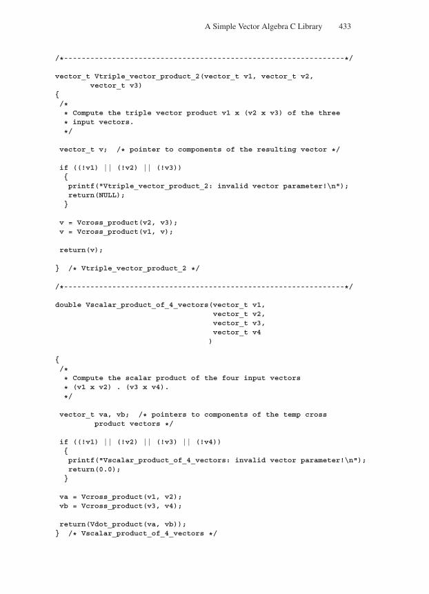
“Comninos” — 2005/8/31 — 18:23 — page 433 — #11
A Simple Vector Algebra C Library 433
/*----------------------------------------------------------------*/
vector_t Vtriple_vector_product_2(vector_t v1, vector_t v2,vector_t v3)
/** Compute the triple vector product v1 x (v2 x v3) of the three
* input vectors.
*/
vector_t v; /* pointer to components of the resulting vector */
if ((!v1) || (!v2) || (!v3))printf("Vtriple_vector_product_2: invalid vector parameter!\n");return(NULL);
v = Vcross_product(v2, v3);v = Vcross_product(v1, v);
return(v);
/* Vtriple_vector_product_2 */
/*----------------------------------------------------------------*/
double Vscalar_product_of_4_vectors(vector_t v1,vector_t v2,vector_t v3,vector_t v4)
/** Compute the scalar product of the four input vectors
* (v1 x v2) . (v3 x v4).
*/
vector_t va, vb; /* pointers to components of the temp crossproduct vectors */
if ((!v1) || (!v2) || (!v3) || (!v4))printf("Vscalar_product_of_4_vectors: invalid vector parameter!\n");return(0.0);
va = Vcross_product(v1, v2);vb = Vcross_product(v3, v4);
return(Vdot_product(va, vb)); /* Vscalar_product_of_4_vectors */
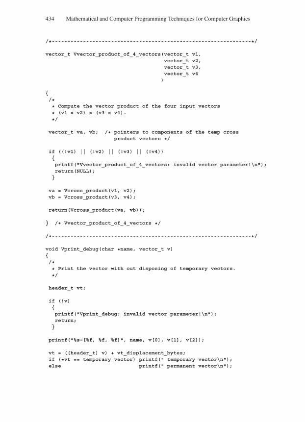
“Comninos” — 2005/8/31 — 18:23 — page 434 — #12
434 Mathematical and Computer Programming Techniques for Computer Graphics
/*----------------------------------------------------------------*/
vector_t Vvector_product_of_4_vectors(vector_t v1,vector_t v2,vector_t v3,vector_t v4)
/** Compute the vector product of the four input vectors
* (v1 x v2) x (v3 x v4).
*/
vector_t va, vb; /* pointers to components of the temp crossproduct vectors */
if ((!v1) || (!v2) || (!v3) || (!v4))printf("Vvector_product_of_4_vectors: invalid vector parameter!\n");return(NULL);
va = Vcross_product(v1, v2);vb = Vcross_product(v3, v4);
return(Vcross_product(va, vb));
/* Vvector_product_of_4_vectors */
/*----------------------------------------------------------------*/
void Vprint_debug(char *name, vector_t v)/** Print the vector with out disposing of temporary vectors.
*/
header_t vt;
if (!v)printf("Vprint_debug: invalid vector parameter!\n");return;
printf("%s=[%f, %f, %f]", name, v[0], v[1], v[2]);
vt = ((header_t) v) + vt_displacement_bytes;if (*vt == temporary_vector) printf(" temporary vector\n");else printf(" permanent vector\n");
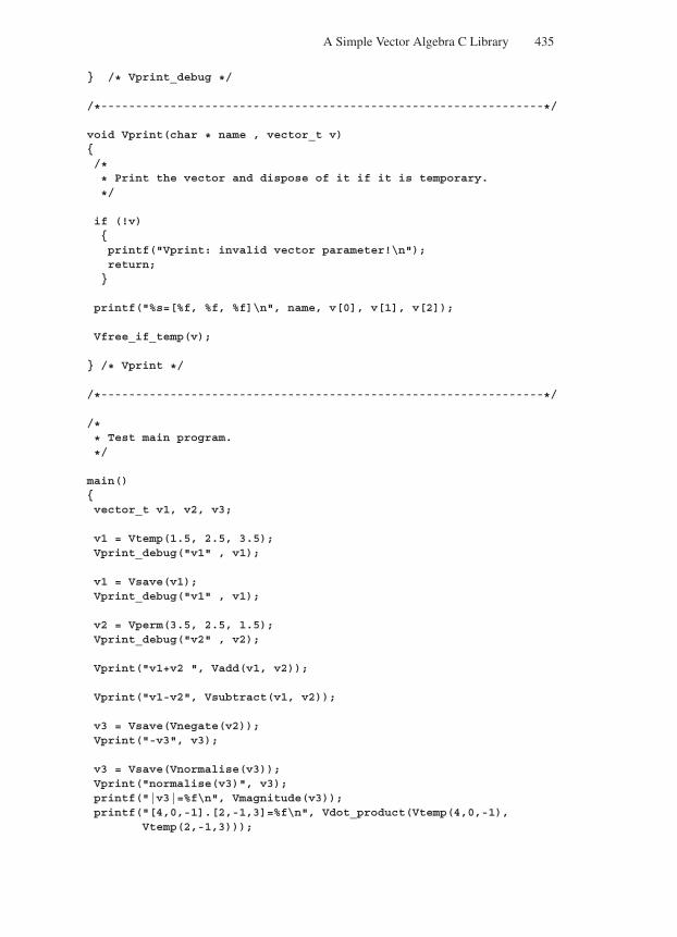
“Comninos” — 2005/8/31 — 18:23 — page 435 — #13
A Simple Vector Algebra C Library 435
/* Vprint_debug */
/*----------------------------------------------------------------*/
void Vprint(char * name , vector_t v)/** Print the vector and dispose of it if it is temporary.
*/
if (!v)printf("Vprint: invalid vector parameter!\n");return;
printf("%s=[%f, %f, %f]\n", name, v[0], v[1], v[2]);
Vfree_if_temp(v);
/* Vprint */
/*----------------------------------------------------------------*/
/** Test main program.
*/
main()vector_t v1, v2, v3;
v1 = Vtemp(1.5, 2.5, 3.5);Vprint_debug("v1" , v1);
v1 = Vsave(v1);Vprint_debug("v1" , v1);
v2 = Vperm(3.5, 2.5, 1.5);Vprint_debug("v2" , v2);
Vprint("v1+v2 ", Vadd(v1, v2));
Vprint("v1-v2", Vsubtract(v1, v2));
v3 = Vsave(Vnegate(v2));Vprint("-v3", v3);
v3 = Vsave(Vnormalise(v3));Vprint("normalise(v3)", v3);printf("|v3|=%f\n", Vmagnitude(v3));printf("[4,0,-1].[2,-1,3]=%f\n", Vdot_product(Vtemp(4,0,-1),
Vtemp(2,-1,3)));
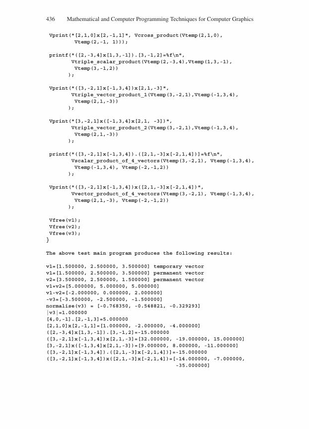
“Comninos” — 2005/8/31 — 18:23 — page 436 — #14
436 Mathematical and Computer Programming Techniques for Computer Graphics
Vprint("[2,1,0]x[2,-1,1]", Vcross_product(Vtemp(2,1,0),Vtemp(2,-1, 1)));
printf("([2,-3,4]x[1,3,-1]).[3,-1,2]=%f\n",Vtriple_scalar_product(Vtemp(2,-3,4),Vtemp(1,3,-1),Vtemp(3,-1,2))
);
Vprint("([3,-2,1]x[-1,3,4])x[2,1,-3]",Vtriple_vector_product_1(Vtemp(3,-2,1),Vtemp(-1,3,4),Vtemp(2,1,-3))
);
Vprint("[3,-2,1]x([-1,3,4]x[2,1, -3])",Vtriple_vector_product_2(Vtemp(3,-2,1),Vtemp(-1,3,4),Vtemp(2,1,-3))
);
printf("([3,-2,1]x[-1,3,4]).([2,1,-3]x[-2,1,4])]=%f\n",Vscalar_product_of_4_vectors(Vtemp(3,-2,1), Vtemp(-1,3,4),Vtemp(-1,3,4), Vtemp(-2,-1,2))
);
Vprint("([3,-2,1]x[-1,3,4])x([2,1,-3]x[-2,1,4])",Vvector_product_of_4_vectors(Vtemp(3,-2,1), Vtemp(-1,3,4),Vtemp(2,1,-3), Vtemp(-2,-1,2))
);
Vfree(v1);Vfree(v2);Vfree(v3);
The above test main program produces the following results:
v1=[1.500000, 2.500000, 3.500000] temporary vectorv1=[1.500000, 2.500000, 3.500000] permanent vectorv2=[3.500000, 2.500000, 1.500000] permanent vectorv1+v2=[5.000000, 5.000000, 5.000000]v1-v2=[-2.000000, 0.000000, 2.000000]-v3=[-3.500000, -2.500000, -1.500000]normalise(v3) = [-0.768350, -0.548821, -0.329293]|v3|=1.000000[4,0,-1].[2,-1,3]=5.000000[2,1,0]x[2,-1,1]=[1.000000, -2.000000, -4.000000]([2,-3,4]x[1,3,-1]).[3,-1,2]=-15.000000([3,-2,1]x[-1,3,4])x[2,1,-3]=[32.000000, -19.000000, 15.000000][3,-2,1]x([-1,3,4]x[2,1,-3])=[9.000000, 8.000000, -11.000000]([3,-2,1]x[-1,3,4]).([2,1,-3]x[-2,1,4])]=-15.000000([3,-2,1]x[-1,3,4])x([2,1,-3]x[-2,1,4])=[-14.000000, -7.000000,
-35.000000]
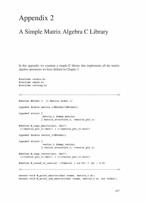
“Comninos” — 2005/8/31 — 18:23 — page 437 — #15
Appendix 2
A Simple Matrix Algebra C Library
In this appendix we examine a simple C library that implements all the matrixalgebra operations we have defined in Chapter 3.
#include <stdio.h>#include <math.h>#include <string.h>
/*----------------------------------------------------------------*/
#define MOrder 3 /* Matrix Order */
typedef double matrix_t[MOrder][MOrder];
typedef struct matrix_t dummy_matrix; matrix_structure_t, *matrix_ptr_t;
#define M_copy_matrix(src, dst)\
*((matrix_ptr_t)(dst)) = *((matrix_ptr_t)(src))
typedef double vector_t[MOrder];
typedef struct vector_t dummy_vector; vector_structure_t, *vector_ptr_t;
#define M_copy_vector(src, dst)\
*((vector_ptr_t)(dst)) = *((vector_ptr_t)(src))
#define M_round_to_zero(x) ((fabs(x) > le-33) ? (x) : 0.0)
/*----------------------------------------------------------------*/
extern void M_print_matrix(char *name, matrix_t m);extern void M_print_sub_matrix(char *name, matrix_t m, int order);
437
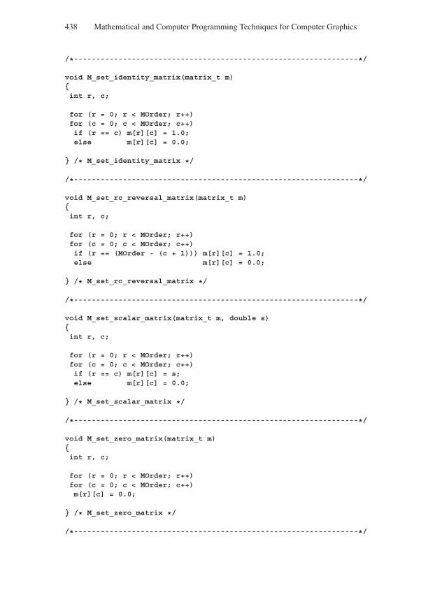
“Comninos” — 2005/8/31 — 18:23 — page 438 — #16
438 Mathematical and Computer Programming Techniques for Computer Graphics
/*----------------------------------------------------------------*/
void M_set_identity_matrix(matrix_t m)int r, c;
for (r = 0; r < MOrder; r++)for (c = 0; c < MOrder; c++)if (r == c) m[r][c] = 1.0;else m[r][c] = 0.0;
/* M_set_identity_matrix */
/*----------------------------------------------------------------*/
void M_set_rc_reversal_matrix(matrix_t m)int r, c;
for (r = 0; r < MOrder; r++)for (c = 0; c < MOrder; c++)if (r == (MOrder - (c + 1))) m[r][c] = 1.0;else m[r][c] = 0.0;
/* M_set_rc_reversal_matrix */
/*----------------------------------------------------------------*/
void M_set_scalar_matrix(matrix_t m, double s)int r, c;
for (r = 0; r < MOrder; r++)for (c = 0; c < MOrder; c++)if (r == c) m[r][c] = s;else m[r][c] = 0.0;
/* M_set_scalar_matrix */
/*----------------------------------------------------------------*/
void M_set_zero_matrix(matrix_t m)int r, c;
for (r = 0; r < MOrder; r++)for (c = 0; c < MOrder; c++)m[r][c] = 0.0;
/* M_set_zero_matrix */
/*----------------------------------------------------------------*/
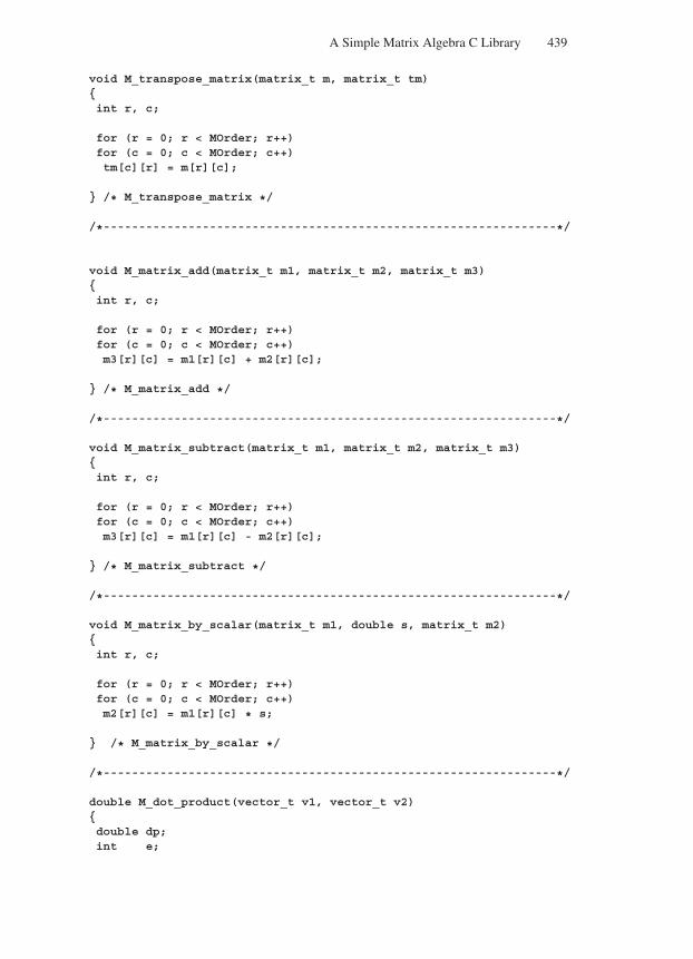
“Comninos” — 2005/8/31 — 18:23 — page 439 — #17
A Simple Matrix Algebra C Library 439
void M_transpose_matrix(matrix_t m, matrix_t tm)int r, c;
for (r = 0; r < MOrder; r++)for (c = 0; c < MOrder; c++)tm[c][r] = m[r][c];
/* M_transpose_matrix */
/*----------------------------------------------------------------*/
void M_matrix_add(matrix_t m1, matrix_t m2, matrix_t m3)int r, c;
for (r = 0; r < MOrder; r++)for (c = 0; c < MOrder; c++)m3[r][c] = m1[r][c] + m2[r][c];
/* M_matrix_add */
/*----------------------------------------------------------------*/
void M_matrix_subtract(matrix_t m1, matrix_t m2, matrix_t m3)int r, c;
for (r = 0; r < MOrder; r++)for (c = 0; c < MOrder; c++)m3[r][c] = m1[r][c] - m2[r][c];
/* M_matrix_subtract */
/*----------------------------------------------------------------*/
void M_matrix_by_scalar(matrix_t m1, double s, matrix_t m2)int r, c;
for (r = 0; r < MOrder; r++)for (c = 0; c < MOrder; c++)m2[r][c] = m1[r][c] * s;
/* M_matrix_by_scalar */
/*----------------------------------------------------------------*/
double M_dot_product(vector_t v1, vector_t v2)double dp;int e;
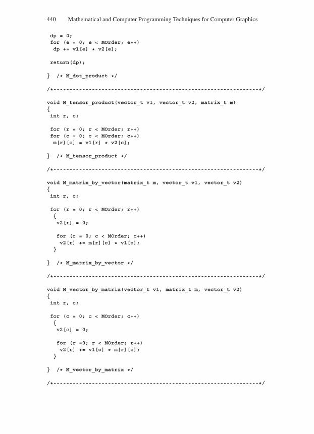
“Comninos” — 2005/8/31 — 18:23 — page 440 — #18
440 Mathematical and Computer Programming Techniques for Computer Graphics
dp = 0;for (e = 0; e < MOrder; e++)dp += v1[e] * v2[e];
return(dp);
/* M_dot_product */
/*----------------------------------------------------------------*/
void M_tensor_product(vector_t v1, vector_t v2, matrix_t m)int r, c;
for (r = 0; r < MOrder; r++)for (c = 0; c < MOrder; c++)m[r][c] = v1[r] * v2[c];
/* M_tensor_product */
/*----------------------------------------------------------------*/
void M_matrix_by_vector(matrix_t m, vector_t v1, vector_t v2)int r, c;
for (r = 0; r < MOrder; r++)v2[r] = 0;
for (c = 0; c < MOrder; c++)v2[r] += m[r][c] * v1[c];
/* M_matrix_by_vector */
/*----------------------------------------------------------------*/
void M_vector_by_matrix(vector_t v1, matrix_t m, vector_t v2)int r, c;
for (c = 0; c < MOrder; c++)v2[c] = 0;
for (r =0; r < MOrder; r++)v2[r] += v1[c] * m[r][c];
/* M_vector_by_matrix */
/*----------------------------------------------------------------*/
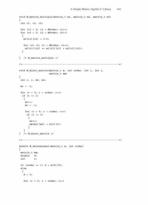
“Comninos” — 2005/8/31 — 18:23 — page 441 — #19
A Simple Matrix Algebra C Library 441
void M_matrix_multiply(matrix_t m1, matrix_t m2, matrix_t m3)int r1, c1, c2;
for (r1 = 0; r1 < MOrder; r1++)for (c2 = 0; c2 < MOrder; c2++)m3[r1][c2] = 0.0;
for (c1 =0; c1 < MOrder; c1++)m3[r1][c2] += m1[r1][c1] * m2[c1][c2];
/* M_matrix_multiply */
/*----------------------------------------------------------------*/
void M_minor_matrix(matrix_t m, int order, int i, int j,matrix_t mm)
int r, c, mr, mc;
mr = -1;
for (r = 0; r < order; r++)if (r != i)mr++;mc = -1;
for (c = 0; c < order; c++)if (c != j)mc++;mm[mr][mc] = m[r][c];
/* M_minor_matrix */
/*----------------------------------------------------------------*/
double M_determinant(matrix_t m, int order)matrix_t mm;double d;int r;
if (order == 1) d = m[0][0];elsed = 0;
for (r = 0; r < order; r++)
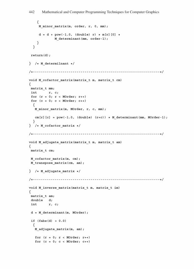
“Comninos” — 2005/8/31 — 18:23 — page 442 — #20
442 Mathematical and Computer Programming Techniques for Computer Graphics
M_minor_matrix(m, order, r, 0, mm);
d = d + pow(-1.0, (double) r) * m[r][0] *M_determinant(mm, order-1);
return(d);
/* M_determilnant */
/*----------------------------------------------------------------*/
void M_cofactor_matrix(matrix_t m, matrix_t cm)matrix_t mm;int r, c;for (r = 0; r < MOrder; r++)for (c = 0; c < MOrder; c++)M_minor_matrix(m, MOrder, r, c, mm);
cm[r][c] = pow(-1.0, (double) (r+c)) * M_determinant(mm, MOrder-1);
/* M_cofactor_matrix */
/*----------------------------------------------------------------*/
void M_adjugate_matrix(matrix_t m, matrix_t am)matrix_t cm;
M_cofactor_matrix(m, cm);M_transpose_matrix(cm, am);
/* M_adjugate_matrix */
/*----------------------------------------------------------------*/
void M_inverse_matrix(matrix_t m, matrix_t im)matrix_t am;double d;int r, c;
d = M_determinant(m, MOrder);
if (fabs(d) > 0.0)M_adjugate_matrix(m, am);
for (r = 0; r < MOrder; r++)for (c = 0; c < MOrder; c++)
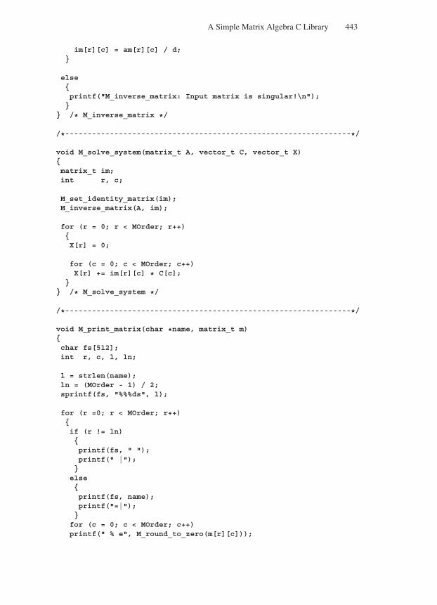
“Comninos” — 2005/8/31 — 18:23 — page 443 — #21
A Simple Matrix Algebra C Library 443
im[r][c] = am[r][c] / d;
elseprintf("M_inverse_matrix: Input matrix is singular!\n");
/* M_inverse_matrix */
/*----------------------------------------------------------------*/
void M_solve_system(matrix_t A, vector_t C, vector_t X)matrix_t im;int r, c;
M_set_identity_matrix(im);M_inverse_matrix(A, im);
for (r = 0; r < MOrder; r++)X[r] = 0;
for (c = 0; c < MOrder; c++)X[r] += im[r][c] * C[c];
/* M_solve_system */
/*----------------------------------------------------------------*/
void M_print_matrix(char *name, matrix_t m)char fs[512];int r, c, l, ln;
l = strlen(name);ln = (MOrder - 1) / 2;sprintf(fs, "%%%ds", l);
for (r =0; r < MOrder; r++)if (r != ln)printf(fs, " ");printf(" |");elseprintf(fs, name);printf("=|");for (c = 0; c < MOrder; c++)printf(" % e", M_round_to_zero(m[r][c]));
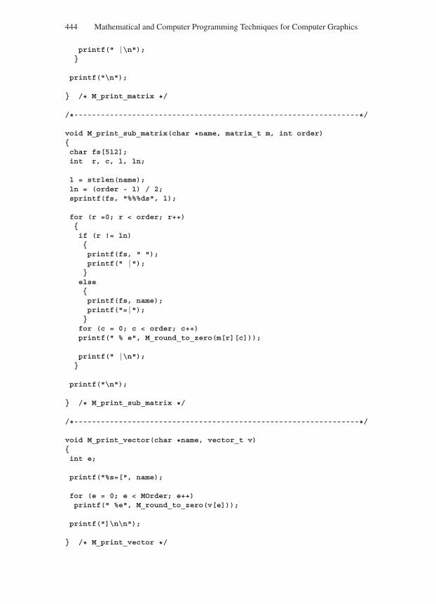
“Comninos” — 2005/8/31 — 18:23 — page 444 — #22
444 Mathematical and Computer Programming Techniques for Computer Graphics
printf(" |\n");
printf("\n");
/* M_print_matrix */
/*----------------------------------------------------------------*/
void M_print_sub_matrix(char *name, matrix_t m, int order)char fs[512];int r, c, l, ln;
l = strlen(name);ln = (order - 1) / 2;sprintf(fs, "%%%ds", l);
for (r =0; r < order; r++)if (r != ln)printf(fs, " ");printf(" |");
elseprintf(fs, name);printf("=|");
for (c = 0; c < order; c++)printf(" % e", M_round_to_zero(m[r][c]));
printf(" |\n");
printf("\n");
/* M_print_sub_matrix */
/*----------------------------------------------------------------*/
void M_print_vector(char *name, vector_t v)int e;
printf("%s=[", name);
for (e = 0; e < MOrder; e++)printf(" %e", M_round_to_zero(v[e]));
printf("]\n\n");
/* M_print_vector */
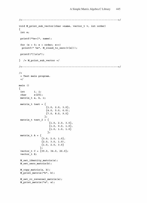
“Comninos” — 2005/8/31 — 18:23 — page 445 — #23
A Simple Matrix Algebra C Library 445
/*----------------------------------------------------------------*/
void M_print_sub_vector(char *name, vector_t v, int order)int e;
printf("%s=[", name);
for (e = 0; e < order; e++)printf(" %e", M_round_to_zero(v[e]));
printf("]\n\n");
/* M_print_sub_vector */
/*----------------------------------------------------------------*/
/** Test main program.
*/
main ()int i, j;char s[25];matrix_t a, b, c;
matrix_t test = 1.0, 2.0, 3.0,4.0, 5.0, 6.0),7.0, 8.0, 9.0;
matrix_t test_2 = 1.0, 2.0, 3.0,1.0, 0.0, 1.0,1.0, 1.0, 1.0
;matrix_t A =
3.0, 2.0, 1.0,2.0, 3.0, 1.0),1.0, 2.0, 3.0
;vector_t C = 39.0, 34.0, 26.0;vector_t X;
M_set_identity_matrix(a);M_set_zero_matrix(b);
M_copy_matrix(a, b);M_print_matrix("b", b);
M_set_rc_reversal_matrix(a);M_print_matrix("a", a);
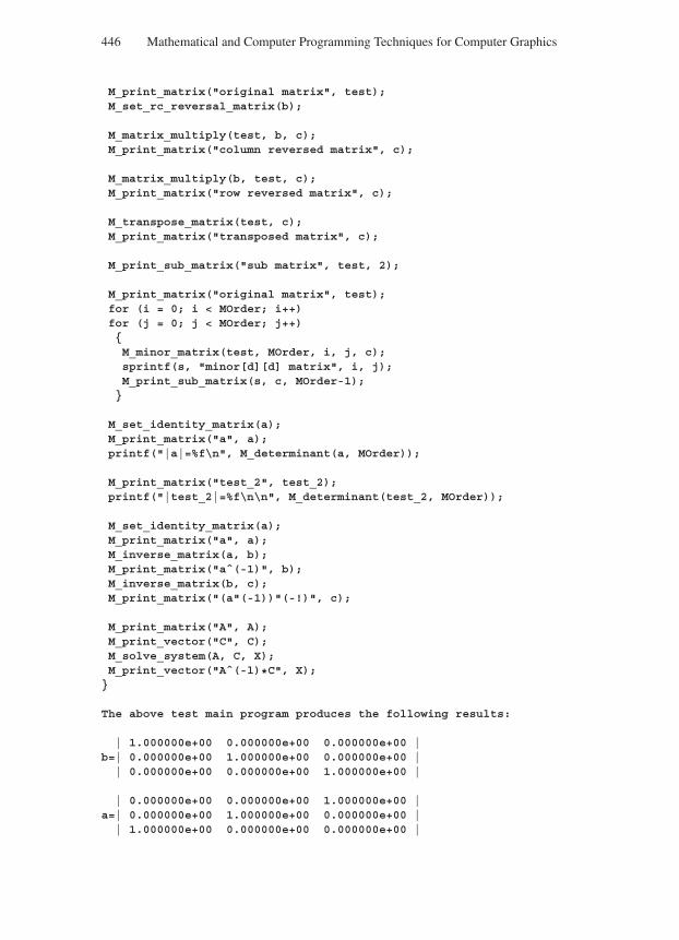
“Comninos” — 2005/8/31 — 18:23 — page 446 — #24
446 Mathematical and Computer Programming Techniques for Computer Graphics
M_print_matrix("original matrix", test);M_set_rc_reversal_matrix(b);
M_matrix_multiply(test, b, c);M_print_matrix("column reversed matrix", c);
M_matrix_multiply(b, test, c);M_print_matrix("row reversed matrix", c);
M_transpose_matrix(test, c);M_print_matrix("transposed matrix", c);
M_print_sub_matrix("sub matrix", test, 2);
M_print_matrix("original matrix", test);for (i = 0; i < MOrder; i++)for (j = 0; j < MOrder; j++)M_minor_matrix(test, MOrder, i, j, c);sprintf(s, "minor[d][d] matrix", i, j);M_print_sub_matrix(s, c, MOrder-1);
M_set_identity_matrix(a);M_print_matrix("a", a);printf("|a|=%f\n", M_determinant(a, MOrder));
M_print_matrix("test_2", test_2);printf("|test_2|=%f\n\n", M_determinant(test_2, MOrder));
M_set_identity_matrix(a);M_print_matrix("a", a);M_inverse_matrix(a, b);M_print_matrix("aˆ(-1)", b);M_inverse_matrix(b, c);M_print_matrix("(a"(-1))"(-!)", c);
M_print_matrix("A", A);M_print_vector("C", C);M_solve_system(A, C, X);M_print_vector("Aˆ(-l)*C", X);
The above test main program produces the following results:
| 1.000000e+00 0.000000e+00 0.000000e+00 |b=| 0.000000e+00 1.000000e+00 0.000000e+00 |
| 0.000000e+00 0.000000e+00 1.000000e+00 |
| 0.000000e+00 0.000000e+00 1.000000e+00 |a=| 0.000000e+00 1.000000e+00 0.000000e+00 |
| 1.000000e+00 0.000000e+00 0.000000e+00 |
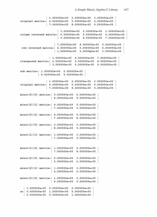
“Comninos” — 2005/8/31 — 18:23 — page 447 — #25
A Simple Matrix Algebra C Library 447
| 1.000000e+00 2.000000e+00 3.000000e+00 |original matrix=| 4.000000e+00 5.000000e+00 6.000000e+00 |
| 7.000000e+00 8.000000e+00 9.000000e+00 |
| 3.000000e+00 2.000000e+00 1.000000e+00 |column reversed matrix=| 6.000000e+00 5.000000e+00 4.000000e+00 |
| 9.000000e+00 8.000000e+00 7.000000e+00 |
| 7.000000e+00 8.000000e+00 9.000000e+00 |row reversed matrix=| 4.000000e+00 5.000000e+00 6.000000e+00 |
| 1.000000e+00 2.0000Q0e+00 3.000000e+00 |
| 1.000000e+00 4.000000e+00 7.000000e+00 |transposed matrix=| 2.000000e+00 5.000000e+00 8.000000e+00 |
| 3.000000e+00 6.000000e+00 9.000000e+00 |
sub matrix=| 1.000000e+00 2.000000e+00 || 4.000000e+00 5.000000e+00 |
| 1.000000e+00 2.000000e+00 3.000000e+00 |original matrix=| 4.000000e+00 5.000000e+00 6.000000e+00 |
| 7.000000e+00 8.000000e+00 9.000000e+00 |
minor[0][0] matrix=| 5.000000e+00 6.000000e+00 || 8.000000e+00 9.000000e+00 |
minor[0][1] matrix=| 4.000000e+00 6.000000e+00 || 7.000000e+00 9.000000e+00 |
minor[0][2] matrix=| 4.000000e+00 5.000000e+00 || 7.000000e+00 8.000000e+00 |
minor[1][0] matrix=| 2.000000e+00 3.000000e+00 || 8.000000e+00 9.000000e+00 |
minor[1][1] matrix=| 1.000000e+00 3.000000e+00 || 7.000000e+00 9.000000e+00 |
minor[1][2] matrix=| 1.000000e+00 2.000000e+00 || 7.000000e+00 8.000000e+00 |
minor[2][0] matrix=| 2.000000e+00 3.000000e+00 || 5.000000e+00 6.000000e+00 |
minor[2][1] matrix=| 1.000000e+00 3.000000e+00 || 4.000000e+00 6.000000e+00 |
minor[2][2] matrix=| 1.000000e+00 2.000000e+00 || 4.000000e+00 5.000000e+00 |
| 1.000000e+00 0.000000e+00 0.000000e+00 |a=| 0.000000e+00 1.000000e+00 0.000000e+00 || 0.000000e+00 0.000000e+00 1.000000e+00 |
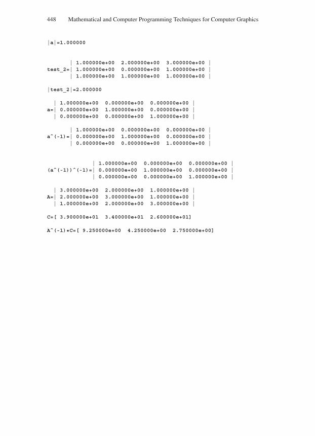
“Comninos” — 2005/8/31 — 18:23 — page 448 — #26
448 Mathematical and Computer Programming Techniques for Computer Graphics
|a|=1.000000
| 1.000000e+00 2.000000e+00 3.000000e+00 |test_2=| 1.000000e+00 0.000000e+00 1.000000e+00 |
| 1.000000e+00 1.000000e+00 1.000000e+00 |
|test_2|=2.000000
| 1.000000e+00 0.000000e+00 0.000000e+00 |a=| 0.000000e+00 1.000000e+00 0.000000e+00 |
| 0.000000e+00 0.000000e+00 1.000000e+00 |
| 1.000000e+00 0.000000e+00 0.000000e+00 |aˆ(-1)=| 0.000000e+00 1.000000e+00 0.000000e+00 |
| 0.000000e+00 0.000000e+00 1.000000e+00 |
| 1.000000e+00 0.000000e+00 0.000000e+00 |(aˆ(-1))ˆ(-1)=| 0.000000e+00 1.000000e+00 0.000000e+00 |
| 0.000000e+00 0.000000e+00 1.000000e+00 |
| 3.000000e+00 2.000000e+00 1.000000e+00 |A=| 2.000000e+00 3.000000e+00 1.000000e+00 |
| 1.000000e+00 2.000000e+00 3.000000e+00 |
C=[ 3.900000e+01 3.400000e+01 2.600000e+01]
Aˆ(-1)*C=[ 9.250000e+00 4.250000e+00 2.750000e+00]
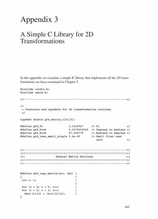
“Comninos” — 2005/8/31 — 18:23 — page 449 — #27
Appendix 3
A Simple C Library for 2DTransformations
In this appendix we examine a simple C library that implements all the 2D trans-formations we have examined in Chapter 5.
#include <stdio.h>#include <math.h>
/*----------------------------------------------------------------*/
/** Constants and typedefs for 2D transformation routines.
*/
typedef double g2d_matrix_t[3][3];
#define g2d_Pi 3.1415927 /* Pi */#define g2d_DtoR 0.0174532925 /* Degrees to Radians */#define g2d_RtoD 57.295778 /* Radians to Degrees */#define g2d_ieee_small_single 3.4e-45 /* Small float near
zero */
/*----------------------------------------------------------------*//*!!!!!!!!!!!!!!!!!!!!!!!!!!!!!!!!!!!!!!!!!!!!!!!!!!!!!!!!!!!!!!!!*//*! General Matrix Routines !*//*!!!!!!!!!!!!!!!!!!!!!!!!!!!!!!!!!!!!!!!!!!!!!!!!!!!!!!!!!!!!!!!!*//*----------------------------------------------------------------*/
#define g2d_copy_matrix(src, dst) \ \int r, c; \
\for (r = 0; r < 3; r++) \for (c = 0; c < 3; c++) \(dst)[r][c] = (src)[r][c]; \
449
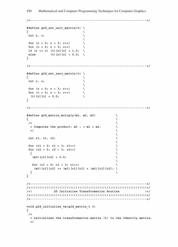
“Comninos” — 2005/8/31 — 18:23 — page 450 — #28
450 Mathematical and Computer Programming Techniques for Computer Graphics
/*----------------------------------------------------------------*/
#define g2d_set_unit_matrix(t) \ \int r, c; \
\for (r = 0; r < 3; r++) \for (c = 0; c < 3; c++) \if (r == c) (t)[r][c] = 1.0; \else (t)[r][c] = 0.0; \
/*----------------------------------------------------------------*/
#define g2d_set_zero_matrix(t) \ \int r, c; \
\for (r = 0; r < 3; r++) \for (c = 0; c < 3; c++) \(t)[r][c] = 0.0; \
/*----------------------------------------------------------------*/
#define g2d_matrix_mutiply(ml, m2, m3) \ \/* \
* Computes the product: m3 : = ml * m2. \
*/ \\
int r1, c1, c2; \\
for (r1 = 0; r1 < 3; r1++) \for (c2 = 0; c2 < 3; c2++) \ \(m3)[r1][c2] = 0.0; \
\for (c1 = 0; c1 < 3; c1++) \(m3)[r1][c2] += (ml)[r1][c1] * (m2)[c1][c2]; \
\
/*----------------------------------------------------------------*//*!!!!!!!!!!!!!!!!!!!!!!!!!!!!!!!!!!!!!!!!!!!!!!!!!!!!!!!!!!!!!!!!*//*! 2D Initialise Transformation Routine !*//*!!!!!!!!!!!!!!!!!!!!!!!!!!!!!!!!!!!!!!!!!!!!!!!!!!!!!!!!!!!!!!!!*//*----------------------------------------------------------------*/
void g2d_initialise_tm(g2d_matrix_t t)/** Initialises the transformation matrix (t) to the Identity matrix.
*/
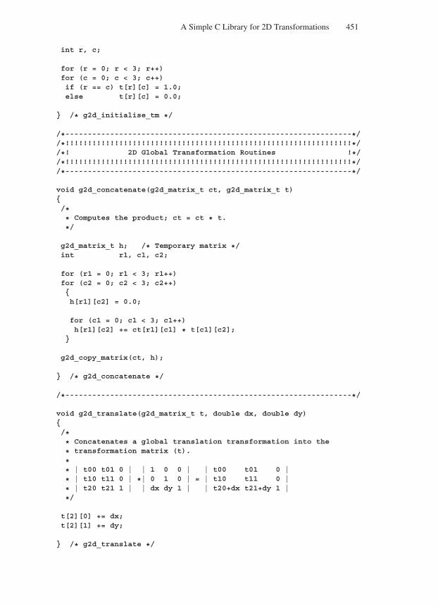
“Comninos” — 2005/8/31 — 18:23 — page 451 — #29
A Simple C Library for 2D Transformations 451
int r, c;
for (r = 0; r < 3; r++)for (c = 0; c < 3; c++)if (r == c) t[r][c] = 1.0;else t[r][c] = 0.0;
/* g2d_initialise_tm */
/*----------------------------------------------------------------*//*!!!!!!!!!!!!!!!!!!!!!!!!!!!!!!!!!!!!!!!!!!!!!!!!!!!!!!!!!!!!!!!!*//*! 2D Global Transformation Routines !*//*!!!!!!!!!!!!!!!!!!!!!!!!!!!!!!!!!!!!!!!!!!!!!!!!!!!!!!!!!!!!!!!!*//*----------------------------------------------------------------*/
void g2d_concatenate(g2d_matrix_t ct, g2d_matrix_t t)/** Computes the product; ct = ct * t.
*/
g2d_matrix_t h; /* Temporary matrix */int r1, c1, c2;
for (r1 = 0; r1 < 3; r1++)for (c2 = 0; c2 < 3; c2++)h[r1][c2] = 0.0;
for (c1 = 0; c1 < 3; c1++)h[r1][c2] += ct[r1][c1] * t[c1][c2];
g2d_copy_matrix(ct, h);
/* g2d_concatenate */
/*----------------------------------------------------------------*/
void g2d_translate(g2d_matrix_t t, double dx, double dy)/** Concatenates a global translation transformation into the
* transformation matrix (t).
** | t00 t01 0 | | 1 0 0 | | t00 t01 0 |
* | t10 t11 0 | *| 0 1 0 | = | t10 t11 0 |
* | t20 t21 1 | | dx dy 1 | | t20+dx t21+dy 1 |
*/
t[2][0] += dx;t[2][1] += dy;
/* g2d_translate */
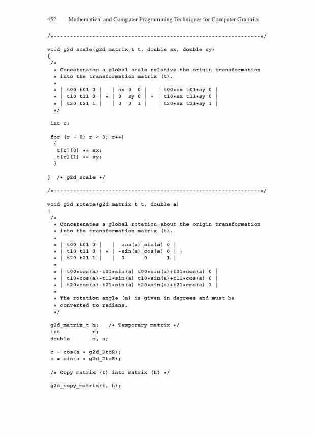
“Comninos” — 2005/8/31 — 18:23 — page 452 — #30
452 Mathematical and Computer Programming Techniques for Computer Graphics
/*----------------------------------------------------------------*/
void g2d_scale(g2d_matrix_t t, double sx, double sy)/** Concatenates a global scale relative the origin transformation
* into the transformation matrix (t).
** | t00 t01 0 | | sx 0 0 | | t00*sx t01*sy 0 |
* | t10 t11 0 | * | 0 sy 0 | = | t10*sx t11*sy 0 |
* | t20 t21 1 | | 0 0 1 | | t20*sx t21*sy 1 |
*/
int r;
for (r = 0; r < 3; r++)t[r][0] *= sx;t[r][1] *= sy;
/* g2d_scale */
/*----------------------------------------------------------------*/
void g2d_rotate(g2d_matrix_t t, double a)(/** Concatenates a global rotation about the origin transformation
* into the transformation matrix (t).
** | t00 t01 0 | | cos(a) sin(a) 0 |
* | t10 t11 0 | * | -sin(a) cos(a) 0 | =
* | t20 t21 1 | | 0 0 1 |
** | t00*cos(a)-t01*sin(a) t00*sin(a)+t01*cos(a) 0 |
* | t10*cos(a)-t11*sin(a) t10*sin(a)+t11*cos(a) 0 |
* | t20*cos(a)-t21*sin(a) t20*sin(a)+t21*cos(a) 1 |
** The rotation angle (a) is given in degrees and must be
* converted to radians.
*/
g2d_matrix_t h; /* Temporary matrix */int r;double c, s;
c = cos(a * g2d_DtoR);s = sin(a * g2d_DtoR);
/* Copy matrix (t) into matrix (h) */
g2d_copy_matrix(t, h);
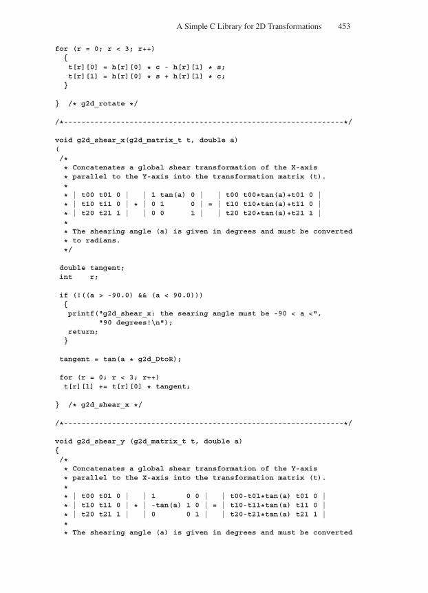
“Comninos” — 2005/8/31 — 18:23 — page 453 — #31
A Simple C Library for 2D Transformations 453
for (r = 0; r < 3; r++)t[r][0] = h[r][0] * c - h[r][1] * s;t[r][1] = h[r][0] * s + h[r][1] * c;
/* g2d_rotate */
/*----------------------------------------------------------------*/
void g2d_shear_x(g2d_matrix_t t, double a)(/** Concatenates a global shear transformation of the X-axis
* parallel to the Y-axis into the transformation matrix (t).
** | t00 t01 0 | | 1 tan(a) 0 | | t00 t00*tan(a)+t01 0 |
* | t10 t11 0 | * | 0 1 0 | = | t10 t10*tan(a)+t11 0 |
* | t20 t21 1 | | 0 0 1 | | t20 t20*tan(a)+t21 1 |
** The shearing angle (a) is given in degrees and must be converted
* to radians.
*/
double tangent;int r;
if (!((a > -90.0) && (a < 90.0)))printf("g2d_shear_x: the searing angle must be -90 < a <",
"90 degrees!\n");return;
tangent = tan(a * g2d_DtoR);
for (r = 0; r < 3; r++)t[r][1] += t[r][0] * tangent;
/* g2d_shear_x */
/*----------------------------------------------------------------*/
void g2d_shear_y (g2d_matrix_t t, double a)/** Concatenates a global shear transformation of the Y-axis
* parallel to the X-axis into the transformation matrix (t).
** | t00 t01 0 | | 1 0 0 | | t00-t01*tan(a) t01 0 |
* | t10 t11 0 | * | -tan(a) 1 0 | = | t10-t11*tan(a) t11 0 |
* | t20 t21 1 | | 0 0 1 | | t20-t21*tan(a) t21 1 |
** The shearing angle (a) is given in degrees and must be converted
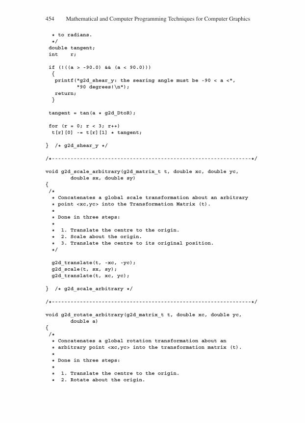
“Comninos” — 2005/8/31 — 18:23 — page 454 — #32
454 Mathematical and Computer Programming Techniques for Computer Graphics
* to radians.
*/double tangent;int r;
if (!((a > -90.0) && (a < 90.0)))printf("g2d_shear_y: the searing angle must be -90 < a <",
"90 degrees!\n");return;
tangent = tan(a * g2d_DtoR);
for (r = 0; r < 3; r++)t[r][0] -= t[r][1] * tangent;
/* g2d_shear_y */
/*----------------------------------------------------------------*/
void g2d_scale_arbitrary(g2d_matrix_t t, double xc, double yc,double sx, double sy)
/** Concatenates a global scale transformation about an arbitrary
* point <xc,yc> into the Transformation Matrix (t).
** Done in three steps:
** 1. Translate the centre to the origin.
* 2. Scale about the origin.
* 3. Translate the centre to its original position.
*/
g2d_translate(t, -xc, -yc);g2d_scale(t, sx, sy);g2d_translate(t, xc, yc);
/* g2d_scale_arbitrary */
/*----------------------------------------------------------------*/
void g2d_rotate_arbitrary(g2d_matrix_t t, double xc, double yc,double a)
/** Concatenates a global rotation transformation about an
* arbitrary point <xc,yc> into the transformation matrix (t).
** Done in three steps:
** 1. Translate the centre to the origin.
* 2. Rotate about the origin.
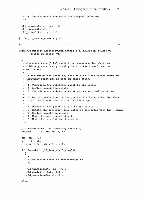
“Comninos” — 2005/8/31 — 18:23 — page 455 — #33
A Simple C Library for 2D Transformations 455
* 3. Translate the centre to its original position.
*/
g2d_translate(t, -xc, -yc);g2d_rotate(t, a);g2d_translate(t, xc, yc);
/* g2d_rotate_arbitrary */
/*----------------------------------------------------------------*/
void g2d_reflect_arbitrary(g2d_matrix_t t, double x1,double y1,double x2,double y2)
/** Concatenates a global reflection transformation about an
* arbitrary axis <<x1,y1>,<x2,y2>> into the transformation
* matrix (t).
** If the two points coincide, then this is a reflection about an
* arbitrary point and is done in three steps:
** 1. Translate the arbitrary point to the origin.
* 2. Reflect about the origin.
* 3. Translate the arbitrary point to its original position.
** If the two points are distinct, then this is a reflection about
* an arbitrary axis and is done in five steps:
** 1. Translate the point <x1,y1> to the origin.
* 2. Rotate the arbitrary axis until it coincides with the x-axis.
* 3. Reflect about the x-axis.
* 4. Undo the rotation of step 2.
* 5. Undo the translation of step 1.
*/
g2d_matrix_t m; /* Temporary matrix */double h, dx, dy, s, c;
dx = x2 - x1;dy = y2 - y1;h = sqrt(dx * dx + dy * dy);
if (fabs(h) < g2d_ieee_small_single)/** Reflection about an arbitrary point.
*/
g2d_translate(t, -x1, -y1);g2d_scale(t, -1.0, -1.0);g2d_translate(t, x1, y1);
else
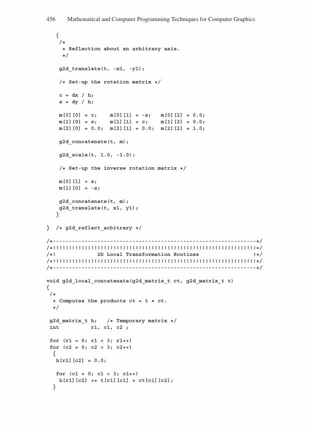
“Comninos” — 2005/8/31 — 18:23 — page 456 — #34
456 Mathematical and Computer Programming Techniques for Computer Graphics
/** Reflection about an arbitrary axis.
*/
g2d_translate(t, -x1, -y1);
/* Set-up the rotation matrix */
c = dx / h;s = dy / h;
m[0][0] = c; m[0][1] = -s; m[0][2] = 0.0;m[1][0] = s; m[1][1] = c; m[1][2] = 0.0;m[2][0] = 0.0; m[2][1] = 0.0; m[2][2] = 1.0;
g2d_concatenate(t, m);
g2d_scale(t, 1.0, -1.0);
/* Set-up the inverse rotation matrix */
m[0][1] = s;m[1][0] = -s;
g2d_concatenate(t, m);g2d_translate(t, x1, y1);
/* g2d_reflect_arbitrary */
/*----------------------------------------------------------------*//*!!!!!!!!!!!!!!!!!!!!!!!!!!!!!!!!!!!!!!!!!!!!!!!!!!!!!!!!!!!!!!!!*//*! 2D Local Transformation Routines !*//*!!!!!!!!!!!!!!!!!!!!!!!!!!!!!!!!!!!!!!!!!!!!!!!!!!!!!!!!!!!!!!!!*//*----------------------------------------------------------------*/
void g2d_local_concatenate(g2d_matrix_t ct, g2d_matrix_t t)/** Computes the products ct = t * ct.
*/
g2d_matrix_t h; /* Temporary matrix */int r1, c1, c2 ;
for (r1 = 0; r1 < 3; r1++)for (c2 = 0; c2 < 3; c2++)h[r1][c2] = 0.0;
for (c1 = 0; c1 < 3; c1++)h[r1][c2] += t[r1][c1] * ct[c1][c2];
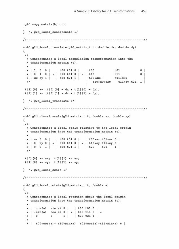
“Comninos” — 2005/8/31 — 18:23 — page 457 — #35
A Simple C Library for 2D Transformations 457
g2d_copy_matrix(h, ct);
/* g2d_local_concatenate */
/*----------------------------------------------------------------*/
void g2d_local_translate(g2d_matrix_t t, double dx, double dy)/** Concatenates a local translation transformation into the
* transformation matrix (t).
** | 1 0 0 | | t00 t01 0 | | t00 t01 0 |
* | 0 1 0 | * | t10 t11 0 | = | t10 t11 0 |
* | dx dy 1 | | t20 t21 1 | | t00*dx+ t01*dx+ |
*/ | t10*dy+t20 t11*dy+t21 1 |
t[2][0] += (t[0][0] * dx + t[1][0] * dy);t[2][1] += (t[0][1] * dx + t[1][1] * dy);
/* g2d_local_translate */
/*----------------------------------------------------------------*/
void g2d_.local_scale(g2d_matrix_t t, double sx, double sy)/** Concatenates a local scale relative to the local origin
* transformation into the transformation matrix (t).
** | sx 0 0 | | t00 t01 0 | | t00*sx t01*sx 0 |
* | 0 sy 0 | * | t10 t11 0 | = | t10*sy t11*sy 0 |
* | 0 0 1 | | t20 t21 1 | | t20 t21 1 |
*/
t[0][0] *= sx; t[0][1] *= sx;t[1][0] *= sy; t[1][1] *= sy;
/* g2d_local_scale */
/*----------------------------------------------------------------*/
void g2d_local_rotate(g2d_matrix_t t, double a)/** Concatenates a local rotation about the local origin
* transformation into the transformation matrix (t).
** | cos(a) sin(a) 0 | | t00 t01 0 |
* | -sin(a) cos(a) 0 | * | t10 t11 0 | =
* | 0 0 1 | | t20 t21 1 |
** | t00*cos(a)+ t10*sin(a) t01*cos(a)+t11*sin(a) 0 |
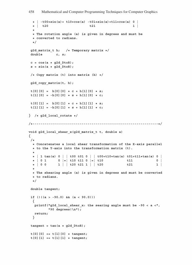
“Comninos” — 2005/8/31 — 18:23 — page 458 — #36
458 Mathematical and Computer Programming Techniques for Computer Graphics
* | -t00*sin(a)+ t10*cos(a) -t01*sin(a)+t11*cos(a) 0 |
* | t20 t21 1 |
** The rotation angle (a) is given in degrees and must be
* converted to radians.
*/
g2d_matrix_t h; /* Temporary matrix */double c, s;
c = cos(a * g2d_DtoR);s = sin(a * g2d_DtoR);
/* Copy matrix (t) into matrix (h) */
g2d_copy_matrix(t, h);
t[0][0] = h[0][0] * c + h[1][0] * s;t[1][0] = -h[0][0] * s + h[1][0] * c;
t[0][1] = h[0][1] * c + h[1][1] * s;t[1][1] = -h[0][1] * s + h[1][1] * c;
/* g2d_local_rotate */
/*----------------------------------------------------------------*/
void g2d_local_shear_x(g2d_matrix_t t, double a)/** Concatenates a local shear transformation of the X-axis parallel
* to the Y-axis into the transformation matrix (t).
** | 1 tan(a) 0 | | t00 t01 0 | | t00+t10*tan(a) t01+t11*tan(a) 0 |
* | 0 1 0 |*| t10 t11 0 |=| t10 t11 0 |
* | 0 0 1 | | t20 t21 1 | | t20 t21 1 |
** The shearing angle (a) is given in degrees and must be converted
* to radians.
*/
double tangent;
if (!((a > -90.0) && (a < 90.0)))printf("g2d_local_shear_x: the searing angle must be -90 < a <",
"90 degrees!\n");return;
tangent = tan(a * g2d_DtoR);
t[0][0] += t[1][0] * tangent;t[0][1] += t[1][1] * tangent;
“Comninos” — 2005/8/31 — 18:23 — page 459 — #37
A Simple C Library for 2D Transformations 459
/* g2d_local_shear_x */
/*----------------------------------------------------------------*/
void g2d_local_shear_y(g2d_matrix_t t, double a)/** Concatenates a local shear transformation of the Y-axis parallel
* to the X-axis into the transformation matrix (t).
** | 1 0 0 | | t00 t01 0 | | t00 t01 0 |
* | -tan(a) 1 0 |*| t10 t11 0 |=| -t00*tan(a)+ -t01*tan (a)+ |
* | 0 0 1 | | t20 t21 1 | | t10 t11 0 |
* | t20 t21 1 |
** The shearing angle (a) is given in degrees and must be converted
* to radians.
*/
double tangent;
if (!((a > -90.0) && (a < 90.0)))printf("g2d_shear_ys the searing angle must be -90 < a <",
"90 degrees!\n");return;
tangent = tan(a * g2d_DtoR);
t[1][0] -= t[0][0] * tangent;t[1][1] -= t[0][1] * tangent;
/* g2d_local_shear_y */
/*----------------------------------------------------------------*/
void g2d_local_scale_arbitrary(g2d_matrix_t t,double xc,double yc,double sx,double sy)
/** Concatenates a local scale transformation about an arbitrary
* point <xc,yc> into the Transformation Matrix (t).
** Done in three steps:
** 1. Translate the centre to the local origin.
* 2. Scale about the local origin.
“Comninos” — 2005/8/31 — 18:23 — page 460 — #38
460 Mathematical and Computer Programming Techniques for Computer Graphics
* 3. Translate the centre to its original position.
*/
g2d_local_translate(t, -xc, -yc);g2d_local_scale(t, sx, sy);g2d_local_translate(t, xc, yc);
/* g2d_local_scale_arbitrary */
/*----------------------------------------------------------------*/void g2d_local_rotate_arbitrary(g2d_matrix_t t,
double xc,double yc,double a)
/** Concatenates a local rotation transformation about an arbitrary
* point <xc,yc> into the transformation matrix (t).
** Done in three steps:
** 1. Translate the centre to the local origin.
* 2. Rotate about the local origin.
* 3. Translate the centre to its original position.
*/
g2d_local_translate(t, -xc, -yc);g2d_local_rotate(t, a);g2d_local_translate(t, xc, yc);
/* g2d_local_rotate_arbitrary */
/*----------------------------------------------------------------*/
void g2d_local_reflect_arbitrary(g2d_matrix_t t,double x1,double y1,double x2,double y2)
/** Concatenates a local reflection transformation about a local
* arbitrary axis <<x1,y1>,<x2 ,y2>> into the transformation
* matrix (t).
** If the two points coincide, then this is a reflection about an
* arbitrary point and is done in three steps:
** 1. Translate the arbitrary point to the local origin,
* 2. Reflect about the local origin.
* 3. Translate the arbitrary point to its original position.
*
“Comninos” — 2005/8/31 — 18:23 — page 461 — #39
A Simple C Library for 2D Transformations 461
* If the two points are distinct, then this is a Reflection about
* an arbitrary axis and is done in five steps:
** 1. Translate the point <x1,y1> to the local origin.
* 2. Rotate the arbitrary axis until it coincides with the local
* x-axis.
* 3. Reflect about local the x-axis.
* 4. Undo the rotation of step 2.
* 5. Undo the translation of step 1.
*/
g2d_matrix_t m; /* Temporary matrix */double h, dx, dy, s, c;
dx = x2 - x1;dy = y2 - y1;h = sqrt(dx * dx + dy * dy);
if (fabs(h) < g2d_ieee_small_single)/** Reflection about an arbitrary point.
*/
g2d_local_translate(t, -x1, -y1);g2d_local_scale(t, -1.0, -1.0);g2d_local_translate(t, x1, y1);
else/** Reflection about an arbitrary axis.
*/
g2d_local_translate(t, -x1, -y1);
/* Set-up the rotation matrix */
c = dx / h;s = dy / h;
m[0][0] = c; m[0][1] = -s; m[0][2] = 0.0;m[1][0] = s; m[1][1] = c; m[1][2] = 0.0;m[2][0] = 0.0; m[2][1] = 0.0; m[2][2] = 1.0;
g2d_local_concatenate(t, m);
g2d_local_scale(t, 1.0, -1.0);
/* Set-up the inverse rotation matrix */
m[0][1] = s;m[1][0] = -s;
“Comninos” — 2005/8/31 — 18:23 — page 462 — #40
462 Mathematical and Computer Programming Techniques for Computer Graphics
g2d_local_concatenate(t, m);
g2d_local_translate(t, x1, y1);
/* g2d_local_reflect_arbitrary */
/*----------------------------------------------------------------*//*!!!!!!!!!!!!!!!!!!!!!!!!!!!!!!!!!!!!!!!!!!!!!!!!!!!!!!!!!!!!!!!!*//*! 2D Viewing Transformation Routines !*//*!!!!!!!!!!!!!!!!!!!!!!!!!!!!!!!!!!!!!!!!!!!!!!!!!!!!!!!!!!!!!!!!*//*----------------------------------------------------------------*/
void g2d_viewing_transformation(g2d_matrix_t t, /* Transformation Matrix (In/Out) */double wl, /* Window Limits (In) */double wb,double wr,double wt,int vl, /* Viewport Limits (In) */int vb,int vr,int vt)/** Concatenates a viewing transformation into the transformation
* matrix (t).
** This version of the viewing transformation is defined by
* specifying the coordinates of the bottom-left and top-right
* corners of the window and the viewport.
*/
double sx, sy, dx, dy;
/** Compute the coefficients of the viewing transformation.
** Xs = sx * Xw + dx
* Ys = sy * Yw + dy
*/
sx = (vr - vl) / (wr - wl);sy = (vt - vb) / (wt - wb);dx = vl - sx * wl;dy = vb - sy * wb;
/** Perform the matrix multiplication:
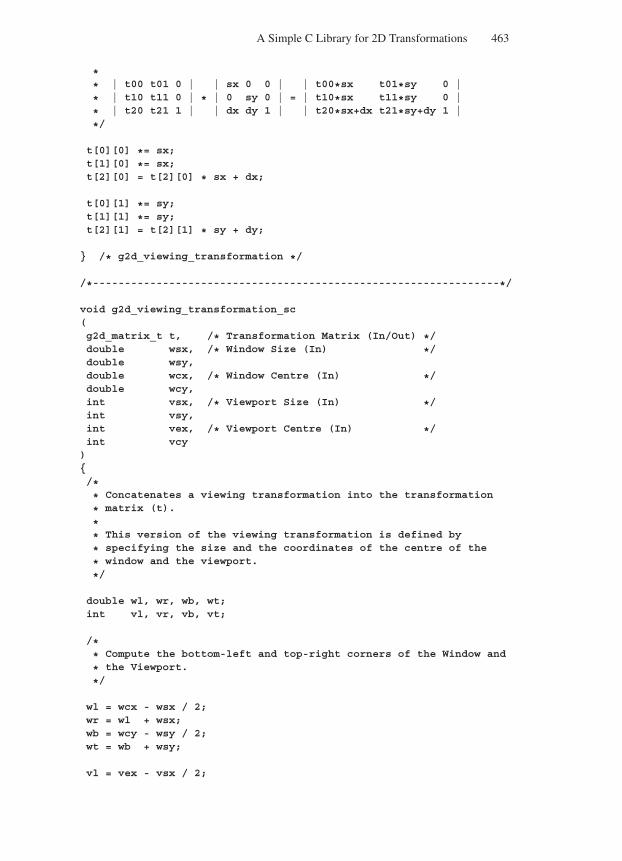
“Comninos” — 2005/8/31 — 18:23 — page 463 — #41
A Simple C Library for 2D Transformations 463
** | t00 t01 0 | | sx 0 0 | | t00*sx t01*sy 0 |
* | t10 t11 0 | * | 0 sy 0 | = | t10*sx t11*sy 0 |
* | t20 t21 1 | | dx dy 1 | | t20*sx+dx t21*sy+dy 1 |
*/
t[0][0] *= sx;t[1][0] *= sx;t[2][0] = t[2][0] * sx + dx;
t[0][1] *= sy;t[1][1] *= sy;t[2][1] = t[2][1] * sy + dy;
/* g2d_viewing_transformation */
/*----------------------------------------------------------------*/
void g2d_viewing_transformation_sc(g2d_matrix_t t, /* Transformation Matrix (In/Out) */double wsx, /* Window Size (In) */double wsy,double wcx, /* Window Centre (In) */double wcy,int vsx, /* Viewport Size (In) */int vsy,int vex, /* Viewport Centre (In) */int vcy)/** Concatenates a viewing transformation into the transformation
* matrix (t).
** This version of the viewing transformation is defined by
* specifying the size and the coordinates of the centre of the
* window and the viewport.
*/
double wl, wr, wb, wt;int vl, vr, vb, vt;
/** Compute the bottom-left and top-right corners of the Window and
* the Viewport.
*/
wl = wcx - wsx / 2;wr = wl + wsx;wb = wcy - wsy / 2;wt = wb + wsy;
vl = vex - vsx / 2;
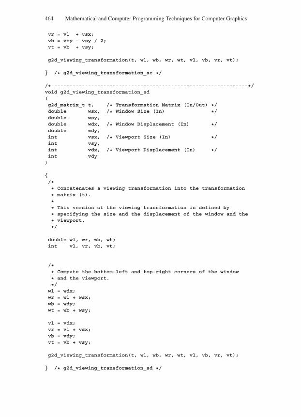
“Comninos” — 2005/8/31 — 18:23 — page 464 — #42
464 Mathematical and Computer Programming Techniques for Computer Graphics
vr = vl + vsx;vb = vcy - vsy / 2;vt = vb + vsy;
g2d_viewing_transformation(t, wl, wb, wr, wt, vl, vb, vr, vt);
/* g2d_viewing_transformation_sc */
/*----------------------------------------------------------------*/void g2d_viewing_transformation_sd(g2d_matrix_t t, /* Transformation Matrix (In/Out) */double wsx, /* Window Size (In) */double wsy,double wdx, /* Window Displacement (In) */double wdy,int vsx, /* Viewport Size (In) */int vsy,int vdx, /* Viewport Displacement (In) */int vdy)
/** Concatenates a viewing transformation into the transformation
* matrix (t).
** This version of the viewing transformation is defined by
* specifying the size and the displacement of the window and the
* viewport.
*/
double wl, wr, wb, wt;int vl, vr, vb, vt;
/** Compute the bottom-left and top-right corners of the window
* and the viewport.
*/wl = wdx;wr = wl + wsx;wb = wdy;wt = wb + wsy;
vl = vdx;vr = vl + vsx;vb = vdy;vt = vb + vsy;
g2d_viewing_transformation(t, wl, wb, wr, wt, vl, vb, vr, vt);
/* g2d_viewing_transformation_sd */
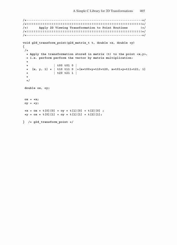
“Comninos” — 2005/8/31 — 18:23 — page 465 — #43
A Simple C Library for 2D Transformations 465
/*----------------------------------------------------------------*//*!!!!!!!!!!!!!!!!!!!!!!!!!!!!!!!!!!!!!!!!!!!!!!!!!!!!!!!!!!!!!!!!*//*! Apply 2D Viewing Transformation to Point Routines !*//*!!!!!!!!!!!!!!!!!!!!!!!!!!!!!!!!!!!!!!!!!!!!!!!!!!!!!!!!!!!!!!!!*//*----------------------------------------------------------------*/
void g2d_transform_point(g2d_matrix_t t, double *x, double *y)/** Apply the transformation stored in matrix (t) to the point <x,y>,
* i.e. perform perform the vector by matrix multiplication:
** | t00 t01 0 |
* [x, y, 1] * | t10 t11 0 |=[x*t00+y*t10+t20, x*t01+y*t11+t21, 1]
* | t20 t21 1 |
**/
double ox, oy;
ox = *x;oy = *y;
*x = ox * t[0][0] + oy * t[1][0] + t[2][0] ;
*y = ox * t[0][1] + oy * t[1][1] + t[2][1];
/* g2d_transform_point */
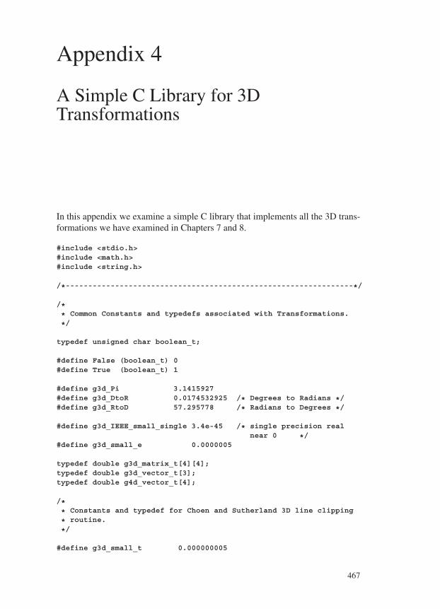
“Comninos” — 2005/8/31 — 18:23 — page 467 — #45
Appendix 4
A Simple C Library for 3DTransformations
In this appendix we examine a simple C library that implements all the 3D trans-formations we have examined in Chapters 7 and 8.
#include <stdio.h>#include <math.h>#include <string.h>
/*----------------------------------------------------------------*/
/** Common Constants and typedefs associated with Transformations.
*/
typedef unsigned char boolean_t;
#define False (boolean_t) 0#define True (boolean_t) 1
#define g3d_Pi 3.1415927#define g3d_DtoR 0.0174532925 /* Degrees to Radians */#define g3d_RtoD 57.295778 /* Radians to Degrees */
#define g3d_IEEE_small_single 3.4e-45 /* single precision realnear 0 */
#define g3d_small_e 0.0000005
typedef double g3d_matrix_t[4][4];typedef double g3d_vector_t[3];typedef double g4d_vector_t[4];
/** Constants and typedef for Choen and Sutherland 3D line clipping
* routine.
*/
#define g3d_small_t 0.000000005
467
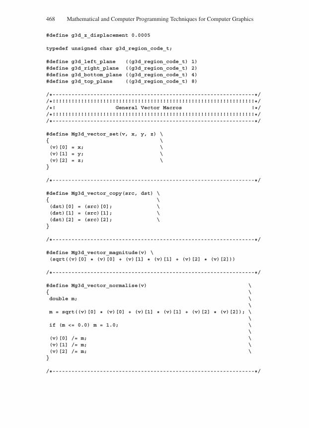
“Comninos” — 2005/8/31 — 18:23 — page 468 — #46
468 Mathematical and Computer Programming Techniques for Computer Graphics
#define g3d_z_displacement 0.0005
typedef unsigned char g3d_region_code_t;
#define g3d_left_plane ((g3d_region_code_t) 1)#define g3d_right_plane ((g3d_region_code_t) 2)#define g3d_bottom_plane ((g3d_region_code_t) 4)#define g3d_top_plane ((g3d_region_code_t) 8)
/*----------------------------------------------------------------*//*!!!!!!!!!!!!!!!!!!!!!!!!!!!!!!!!!!!!!!!!!!!!!!!!!!!!!!!!!!!!!!!!*//*! General Vector Macros !*//*!!!!!!!!!!!!!!!!!!!!!!!!!!!!!!!!!!!!!!!!!!!!!!!!!!!!!!!!!!!!!!!!*//*----------------------------------------------------------------*/
#define Mg3d_vector_set(v, x, y, z) \ \(v)[0] = x; \(v)[1] = y; \(v)[2] = z; \
/*----------------------------------------------------------------*/
#define Mg3d_vector_copy(src, dst) \ \(dst)[0] = (src)[0]; \(dst)[1] = (src)[1]; \(dst)[2] = (src)[2]; \
/*----------------------------------------------------------------*/
#define Mg3d_vector_magnitude(v) \(sqrt((v)[0] * (v)[0] + (v)[1] * (v)[1] + (v)[2] * (v)[2]))
/*----------------------------------------------------------------*/
#define Mg3d_vector_normalise(v) \ \double m; \
\m = sqrt((v)[0] * (v)[0] + (v)[1] * (v)[1] + (v)[2] * (v)[2]); \
\if (m <= 0.0) m = 1.0; \
\(v)[0] /= m; \(v)[1] /= m; \(v)[2] /= m; \
/*----------------------------------------------------------------*/

“Comninos” — 2005/8/31 — 18:23 — page 469 — #47
A Simple C Library for 3D Transformations 469
#define Mg3d_vector_dot(v1, v2) \((v1)[0] * (v2)[0] + (v1)[1] * (v2)[1] + (v1)[2] * (v2)[2])
/*----------------------------------------------------------------*/
#define Mg3d_vector_cross(v1, v2, v3) \ \(v3)[0] = (v1)[1] * (v2)[2] - (v1)[2] * (v2)[1]; \(v3)[1] = (v1)[2] * (v2)[0] - (v1)[0] * (v2)[2]; \(v3)[2] = (v1)[0] * (v2)[1] - (v1)[1] * (v2)[0]; \
/*----------------------------------------------------------------*//*!!!!!!!!!!!!!!!!!!!!!!!!!!!!!!!!!!!!!!!!!!!!!!!!!!!!!!!!!!!!!!!!*//*! General Matrix Routines !*//*!!!!!!!!!!!!!!!!!!!!!!!!!!!!!!!!!!!!!!!!!!!!!!!!!!!!!!!!!!!!!!!!*//*----------------------------------------------------------------*/
void g3d_initialize_matrix(g3d_matrix_t tm) /* TransformationMatrix (Out) */
/** Initialises the Matrix (tm) to the Identity Matrix.
*/
int r, c;
for (r = 0; r <= 3; r++)for (c = 0; c <= 3; c++)if (r == c) tm[r][c] = 1.0;else tm[r][c] = 0.0;
/* g3d_initialize_matrix */
/*----------------------------------------------------------------*/
void g3d_matrix_multiply(g3d_matrix_t m1, /* (In) */g3d_matrix_t m2, /* (In) */g3d_matrix_t m3 /* (Out) */)
/** Computes the product: m3 := m1 * m2.
*/
int r1, c1, c2;
for (r1 = 0; r1 <= 3; r1++)for (c2 = 0; c2 <= 3; c2++)m3[r1][c2] = 0.0;for (c1 = 0; c1 <= 3; c1++)m3[r1][c2] += m1[r1][c1] * m2[c1][c2];
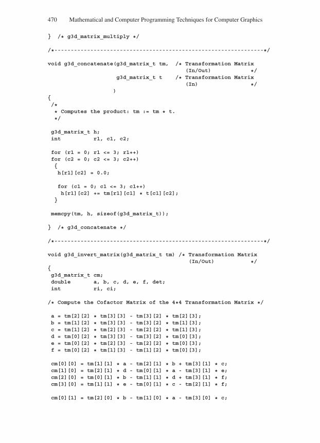
“Comninos” — 2005/8/31 — 18:23 — page 470 — #48
470 Mathematical and Computer Programming Techniques for Computer Graphics
/* g3d_matrix_multiply */
/*----------------------------------------------------------------*/
void g3d_concatenate(g3d_matrix_t tm, /* Transformation Matrix(In/Out) */
g3d_matrix_t t /* Transformation Matrix(In) */
)/** Computes the product: tm := tm * t.
*/
g3d_matrix_t h;int r1, c1, c2;
for (r1 = 0; r1 <= 3; r1++)for (c2 = 0; c2 <= 3; c2++)h[r1][c2] = 0.0;
for (c1 = 0; c1 <= 3; c1++)h[r1][c2] += tm[r1][c1] * t[c1][c2];
memcpy(tm, h, sizeof(g3d_matrix_t));
/* g3d_concatenate */
/*----------------------------------------------------------------*/
void g3d_invert_matrix(g3d_matrix_t tm) /* Transformation Matrix(In/Out) */
g3d_matrix_t cm;double a, b, c, d, e, f, det;int ri, ci;
/* Compute the Cofactor Matrix of the 4*4 Transformation Matrix */
a = tm[2][2] * tm[3][3] - tm[3][2] * tm[2][3];b = tm[1][2] * tm[3][3] - tm[3][2] * tm[1][3];c = tm[1][2] * tm[2][3] - tm[2][2] * tm[1][3];d = tm[0][2] * tm[3][3] - tm[3][2] * tm[0][3];e = tm[0][2] * tm[2][3] - tm[2][2] * tm[0][3];f = tm[0][2] * tm[1][3] - tm[1][2] * tm[0][3];
cm[0][0] = tm[1][1] * a - tm[2][1] * b + tm[3][1] * c;cm[1][0] = tm[2][1] * d - tm[0][1] * a - tm[3][1] * e;cm[2][0] = tm[0][1] * b - tm[1][1] * d + tm[3][1] * f;cm[3][0] = tm[1][1] * e - tm[0][1] * c - tm[2][1] * f;
cm[0][1] = tm[2][0] * b - tm[1][0] * a - tm[3][0] * c;
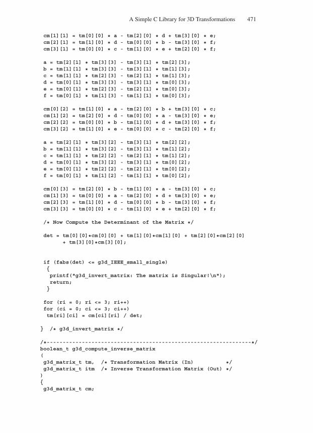
“Comninos” — 2005/8/31 — 18:23 — page 471 — #49
A Simple C Library for 3D Transformations 471
cm[1][1] = tm[0][0] * a - tm[2][0] * d + tm[3][0] * e;cm[2][1] = tm[1][0] * d - tm[0][0] * b - tm[3][0] * f;cm[3][1] = tm[0][0] * c - tm[1][0] * e + tm[2][0] * f;
a = tm[2][1] * tm[3][3] - tm[3][1] * tm[2][3];b = tm[1][1] * tm[3][3] - tm[3][1] * tm[1][3];c = tm[1][1] * tm[2][3] - tm[2][1] * tm[1][3];d = tm[0][1] * tm[3][3] - tm[3][1] * tm[0][3];e = tm[0][1] * tm[2][3] - tm[2][1] * tm[0][3];f = tm[0][1] * tm[1][3] - tm[1][1] * tm[0][3];
cm[0][2] = tm[1][0] * a - tm[2][0] * b + tm[3][0] * c;cm[1][2] = tm[2][0] * d - tm[0][0] * a - tm[3][0] * e;cm[2][2] = tm[0][0] * b - tm[1][0] * d + tm[3][0] * f;cm[3][2] = tm[1][0] * e - tm[0][0] * c - tm[2][0] * f;
a = tm[2][1] * tm[3][2] - tm[3][1] * tm[2][2];b = tm[1][1] * tm[3][2] - tm[3][1] * tm[1][2];c = tm[1][1] * tm[2][2] - tm[2][1] * tm[1][2];d = tm[0][1] * tm[3][2] - tm[3][1] * tm[0][2];e = tm[0][1] * tm[2][2] - tm[2][1] * tm[0][2];f = tm[0][1] * tm[1][2] - tm[1][1] * tm[0][2];
cm[0][3] = tm[2][0] * b - tm[1][0] * a - tm[3][0] * c;cm[1][3] = tm[0][0] * a - tm[2][0] * d + tm[3][0] * e;cm[2][3] = tm[1][0] * d - tm[0][0] * b - tm[3][0] * f;cm[3][3] = tm[0][0] * c - tm[1][0] * e + tm[2][0] * f;
/* Now Compute the Determinant of the Matrix */
det = tm[0][0]*cm[0][0] + tm[1][0]*cm[1][0] + tm[2][0]*cm[2][0]+ tm[3][0]*cm[3][0];
if (fabs(det) <= g3d_IEEE_small_single)printf("g3d_invert_matrix: The matrix is Singular!\n");return;
for (ri = 0; ri <= 3; ri++)for (ci = 0; ci <= 3; ci++)tm[ri][ci] = cm[ci][ri] / det;
/* g3d_invert_matrix */
/*----------------------------------------------------------------*/boolean_t g3d_compute_inverse_matrix(g3d_matrix_t tm, /* Transformation Matrix (In) */g3d_matrix_t itm /* Inverse Transformation Matrix (Out) */)g3d_matrix_t cm;
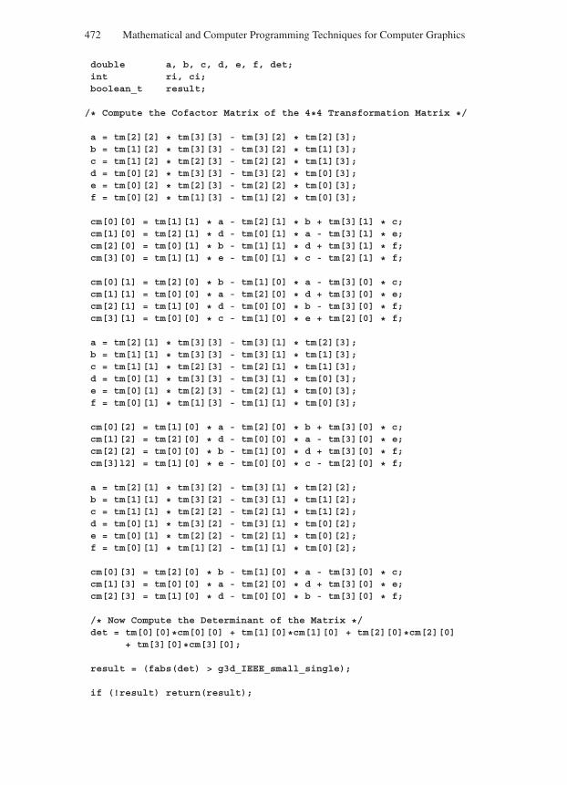
“Comninos” — 2005/8/31 — 18:23 — page 472 — #50
472 Mathematical and Computer Programming Techniques for Computer Graphics
double a, b, c, d, e, f, det;int ri, ci;boolean_t result;
/* Compute the Cofactor Matrix of the 4*4 Transformation Matrix */
a = tm[2][2] * tm[3][3] - tm[3][2] * tm[2][3];b = tm[1][2] * tm[3][3] - tm[3][2] * tm[1][3];c = tm[1][2] * tm[2][3] - tm[2][2] * tm[1][3];d = tm[0][2] * tm[3][3] - tm[3][2] * tm[0][3];e = tm[0][2] * tm[2][3] - tm[2][2] * tm[0][3];f = tm[0][2] * tm[1][3] - tm[1][2] * tm[0][3];
cm[0][0] = tm[1][1] * a - tm[2][1] * b + tm[3][1] * c;cm[1][0] = tm[2][1] * d - tm[0][1] * a - tm[3][1] * e;cm[2][0] = tm[0][1] * b - tm[1][1] * d + tm[3][1] * f;cm[3][0] = tm[1][1] * e - tm[0][1] * c - tm[2][1] * f;
cm[0][1] = tm[2][0] * b - tm[1][0] * a - tm[3][0] * c;cm[1][1] = tm[0][0] * a - tm[2][0] * d + tm[3][0] * e;cm[2][1] = tm[1][0] * d - tm[0][0] * b - tm[3][0] * f;cm[3][1] = tm[0][0] * c - tm[1][0] * e + tm[2][0] * f;
a = tm[2][1] * tm[3][3] - tm[3][1] * tm[2][3];b = tm[1][1] * tm[3][3] - tm[3][1] * tm[1][3];c = tm[1][1] * tm[2][3] - tm[2][1] * tm[1][3];d = tm[0][1] * tm[3][3] - tm[3][1] * tm[0][3];e = tm[0][1] * tm[2][3] - tm[2][1] * tm[0][3];f = tm[0][1] * tm[1][3] - tm[1][1] * tm[0][3];
cm[0][2] = tm[1][0] * a - tm[2][0] * b + tm[3][0] * c;cm[1][2] = tm[2][0] * d - tm[0][0] * a - tm[3][0] * e;cm[2][2] = tm[0][0] * b - tm[1][0] * d + tm[3][0] * f;cm[3]l2] = tm[1][0] * e - tm[0][0] * c - tm[2][0] * f;
a = tm[2][1] * tm[3][2] - tm[3][1] * tm[2][2];b = tm[1][1] * tm[3][2] - tm[3][1] * tm[1][2];c = tm[1][1] * tm[2][2] - tm[2][1] * tm[1][2];d = tm[0][1] * tm[3][2] - tm[3][1] * tm[0][2];e = tm[0][1] * tm[2][2] - tm[2][1] * tm[0][2];f = tm[0][1] * tm[1][2] - tm[1][1] * tm[0][2];
cm[0][3] = tm[2][0] * b - tm[1][0] * a - tm[3][0] * c;cm[1][3] = tm[0][0] * a - tm[2][0] * d + tm[3][0] * e;cm[2][3] = tm[1][0] * d - tm[0][0] * b - tm[3][0] * f;
/* Now Compute the Determinant of the Matrix */det = tm[0][0]*cm[0][0] + tm[1][0]*cm[1][0] + tm[2][0]*cm[2][0]
+ tm[3][0]*cm[3][0];
result = (fabs(det) > g3d_IEEE_small_single);
if (!result) return(result);
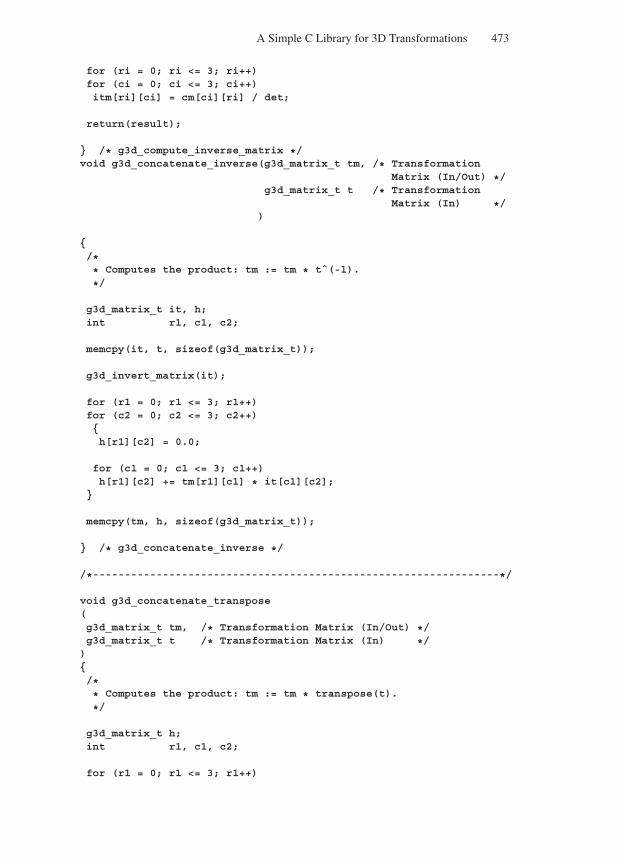
“Comninos” — 2005/8/31 — 18:23 — page 473 — #51
A Simple C Library for 3D Transformations 473
for (ri = 0; ri <= 3; ri++)for (ci = 0; ci <= 3; ci++)itm[ri][ci] = cm[ci][ri] / det;
return(result);
/* g3d_compute_inverse_matrix */void g3d_concatenate_inverse(g3d_matrix_t tm, /* Transformation
Matrix (In/Out) */g3d_matrix_t t /* Transformation
Matrix (In) */)
/** Computes the product: tm := tm * tˆ(-l).
*/
g3d_matrix_t it, h;int r1, c1, c2;
memcpy(it, t, sizeof(g3d_matrix_t));
g3d_invert_matrix(it);
for (r1 = 0; r1 <= 3; r1++)for (c2 = 0; c2 <= 3; c2++)h[r1][c2] = 0.0;
for (c1 = 0; c1 <= 3; c1++)h[r1][c2] += tm[r1][c1] * it[c1][c2];
memcpy(tm, h, sizeof(g3d_matrix_t));
/* g3d_concatenate_inverse */
/*----------------------------------------------------------------*/
void g3d_concatenate_transpose(g3d_matrix_t tm, /* Transformation Matrix (In/Out) */g3d_matrix_t t /* Transformation Matrix (In) */)/** Computes the product: tm := tm * transpose(t).
*/
g3d_matrix_t h;int r1, c1, c2;
for (r1 = 0; r1 <= 3; r1++)
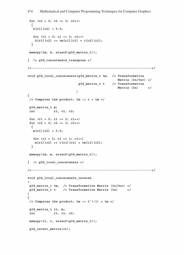
“Comninos” — 2005/8/31 — 18:23 — page 474 — #52
474 Mathematical and Computer Programming Techniques for Computer Graphics
for (c2 = 0; c2 <= 3; c2++)h[r1][c2] = 0.0;
for (c1 = 0; c1 <= 3; c1++)h[r1][c2] += tm[r1][c1] * t[c2][c1];
memcpy(tm, h, sizeof(g3d_matrix_t));
/* g3d_concatenate_transpose */
/*----------------------------------------------------------------*/
void g3d_local_concatenate(g3d_matrix_t tm, /* TransformationMatrix (In/Out) */
g3d_matrix_t t /* TransformationMatrix (In) */
)/* Computes the product: tm := t * tm */
g3d_matrix_t m;int r1, c1, c2;
for (r1 = 0; r1 <= 3; r1++)for (c2 = 0; c2 <= 3; c2++)m[r1][c2] = 0.0;
for (c1 = 0; c1 <= 3; c1++)m[r1][c2] += t[r1][c1] * tm[c1][c2];
memcpy(tm, m, sizeof(g3d_matrix_t));
/* g3d_local_concatenate */
/*----------------------------------------------------------------*/
void g3d_local_concatenate_inverse(g3d_matrix_t tm, /* Transformation Matrix (In/Out) */g3d_matrix_t t /* Transformation Matrix (In) */)/* Computes the product: tm := tˆ(-l) * tm */
g3d_matrix_t it, m;int r1, c1, c2;
memcpy(it, t, sizeof(g3d_matrix_t));
g3d_invert_matrix(it);
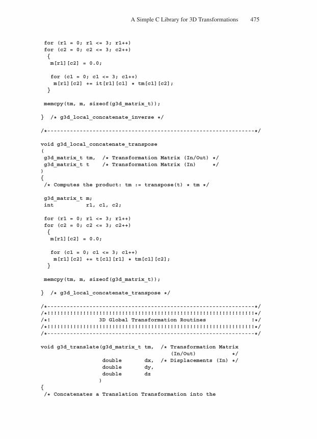
“Comninos” — 2005/8/31 — 18:23 — page 475 — #53
A Simple C Library for 3D Transformations 475
for (r1 = 0; r1 <= 3; r1++)for (c2 = 0; c2 <= 3; c2++)m[r1][c2] = 0.0;
for (c1 = 0; c1 <= 3; c1++)m[r1][c2] += it[r1][c1] * tm[c1][c2];
memcpy(tm, m, sizeof(g3d_matrix_t));
/* g3d_local_concatenate_inverse */
/*----------------------------------------------------------------*/
void g3d_local_concatenate_transpose(g3d_matrix_t tm, /* Transformation Matrix (In/Out) */g3d_matrix_t t /* Transformation Matrix (In) */)/* Computes the product: tm := transpose(t) * tm */
g3d_matrix_t m;int r1, c1, c2;
for (r1 = 0; r1 <= 3; r1++)for (c2 = 0; c2 <= 3; c2++)m[r1][c2] = 0.0;
for (c1 = 0; c1 <= 3; c1++)m[r1][c2] += t[c1][r1] * tm[c1][c2];
memcpy(tm, m, sizeof(g3d_matrix_t));
/* g3d_local_concatenate_transpose */
/*----------------------------------------------------------------*//*!!!!!!!!!!!!!!!!!!!!!!!!!!!!!!!!!!!!!!!!!!!!!!!!!!!!!!!!!!!!!!!!*//*! 3D Global Transformation Routines !*//*!!!!!!!!!!!!!!!!!!!!!!!!!!!!!!!!!!!!!!!!!!!!!!!!!!!!!!!!!!!!!!!!*//*----------------------------------------------------------------*/
void g3d_translate(g3d_matrix_t tm, /* Transformation Matrix(In/Out) */
double dx, /* Displacements (In) */double dy,double dz)
/* Concatenates a Translation Transformation into the
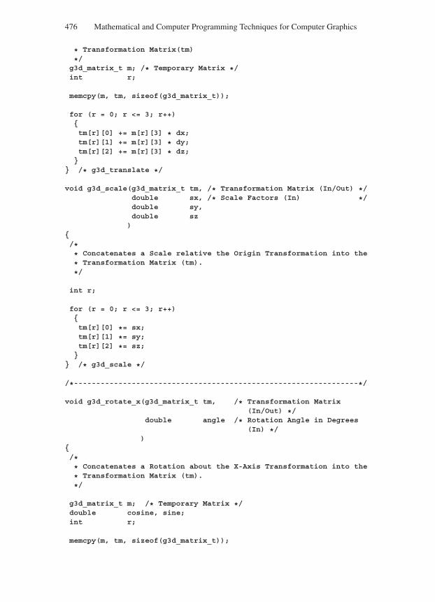
“Comninos” — 2005/8/31 — 18:23 — page 476 — #54
476 Mathematical and Computer Programming Techniques for Computer Graphics
* Transformation Matrix(tm)
*/g3d_matrix_t m; /* Temporary Matrix */int r;
memcpy(m, tm, sizeof(g3d_matrix_t));
for (r = 0; r <= 3; r++)tm[r][0] += m[r][3] * dx;tm[r][1] += m[r][3] * dy;tm[r][2] += m[r][3] * dz;
/* g3d_translate */
void g3d_scale(g3d_matrix_t tm, /* Transformation Matrix (In/Out) */double sx, /* Scale Factors (In) */double sy,double sz)
/** Concatenates a Scale relative the Origin Transformation into the
* Transformation Matrix (tm).
*/
int r;
for (r = 0; r <= 3; r++)tm[r][0] *= sx;tm[r][1] *= sy;tm[r][2] *= sz;
/* g3d_scale */
/*----------------------------------------------------------------*/
void g3d_rotate_x(g3d_matrix_t tm, /* Transformation Matrix(In/Out) */
double angle /* Rotation Angle in Degrees(In) */
)/** Concatenates a Rotation about the X-Axis Transformation into the
* Transformation Matrix (tm).
*/
g3d_matrix_t m; /* Temporary Matrix */double cosine, sine;int r;
memcpy(m, tm, sizeof(g3d_matrix_t));
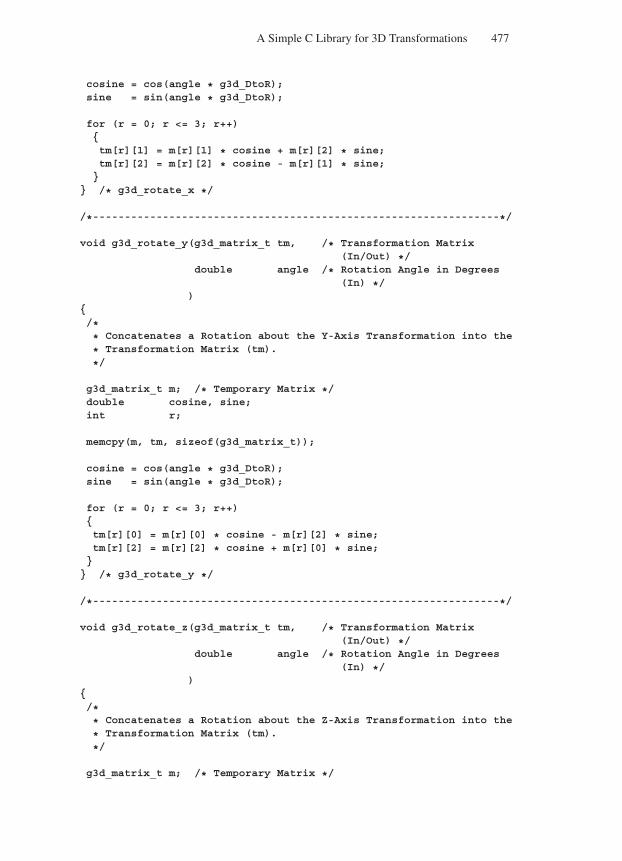
“Comninos” — 2005/8/31 — 18:23 — page 477 — #55
A Simple C Library for 3D Transformations 477
cosine = cos(angle * g3d_DtoR);sine = sin(angle * g3d_DtoR);
for (r = 0; r <= 3; r++)tm[r][1] = m[r][1] * cosine + m[r][2] * sine;tm[r][2] = m[r][2] * cosine - m[r][1] * sine;
/* g3d_rotate_x */
/*----------------------------------------------------------------*/
void g3d_rotate_y(g3d_matrix_t tm, /* Transformation Matrix(In/Out) */
double angle /* Rotation Angle in Degrees(In) */
)/** Concatenates a Rotation about the Y-Axis Transformation into the
* Transformation Matrix (tm).
*/
g3d_matrix_t m; /* Temporary Matrix */double cosine, sine;int r;
memcpy(m, tm, sizeof(g3d_matrix_t));
cosine = cos(angle * g3d_DtoR);sine = sin(angle * g3d_DtoR);
for (r = 0; r <= 3; r++)tm[r][0] = m[r][0] * cosine - m[r][2] * sine;tm[r][2] = m[r][2] * cosine + m[r][0] * sine; /* g3d_rotate_y */
/*----------------------------------------------------------------*/
void g3d_rotate_z(g3d_matrix_t tm, /* Transformation Matrix(In/Out) */
double angle /* Rotation Angle in Degrees(In) */
)/** Concatenates a Rotation about the Z-Axis Transformation into the
* Transformation Matrix (tm).
*/
g3d_matrix_t m; /* Temporary Matrix */
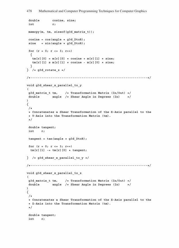
“Comninos” — 2005/8/31 — 18:23 — page 478 — #56
478 Mathematical and Computer Programming Techniques for Computer Graphics
double cosine, sine;int r;
memcpy(m, tm, sizeof(g3d_matrix_t));
cosine = cos(angle * g3d_DtoR);sine = sin(angle * g3d_DtoR);
for (r = 0; r <= 3; r++)tm[r][0] = m[r][0] * cosine + m[r][1] * sine;tm[r][1] s m[r][1] * cosine - m[r][0] * sine;
/* g3d_rotate_z */
/*----------------------------------------------------------------*/
void g3d_shear_x_parallel_to_y(g3d_matrix_t tm, /* Transformation Matrix (In/Out) */double angle /* Shear Angle in Degrees (In) */)/** Concatenates a Shear Transformation of the X-Axis parallel to the
* Y-Axis into the Transformation Matrix (tm).
*/
double tangent;int r;
tangent = tan(angle * g3d_DtoR);
for (r = 0; r <= 3; r++)tm[r][1] -= tm[r][0] * tangent;
/* g3d_shear_x_parallel_to_y */
/*----------------------------------------------------------------*/
void g3d_shear_x_parallel_to_z(g3d_matrix_t tm, /* Transformation Matrix (In/Out) */double angle /* Shear Angle in Degrees (In) */)/** Concatenates a Shear Transformation of the X-Axis parallel to the
* Z-Axis into the Transformation Matrix (tm).
*/
double tangent;int r;
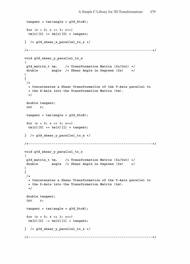
“Comninos” — 2005/8/31 — 18:23 — page 479 — #57
A Simple C Library for 3D Transformations 479
tangent = tan(angle * g3d_DtoR);
for (r = 0; r <= 3; r++)tm[r][2] += tm[r][0] * tangent;
/* g3d_shear_x_parallel_to_z */
/*----------------------------------------------------------------*/
void g3d_shear_y_parallel_to_x(g3d_matrix_t tm, /* Transformation Matrix (In/Out) */double angle /* Shear Angle in Degrees (In) */)/** Concatenates a Shear Transformation of the Y-Axis parallel to
* the X-Axis into the Transformation Matrix (tm).
*/
double tangent;int r;
tangent = tan(angle * g3d_DtoR);
for (r = 0; r <= 3; r++)tm[r][0] += tm[r][1] * tangent;
/* g3d_shear_y_parallel_to_x */
/*----------------------------------------------------------------*/
void g3d_shear_y_parallel_to_z(g3d_matrix_t tm, /* Transformation Matrix (In/Out) */double angle /* Shear Angle in Degrees (In) */)/** Concatenates a Shear Transformation of the Y-Axis parallel to
* the Z-Axis into the Transformation Matrix (tm).
*/
double tangent;int r;
tangent = tan(angle * g3d_DtoR);
for (r = 0; r <= 3; r++)tm[r][2] -= tm[r][1] * tangent;
/* g3d_shear_y_parallel_to_z */
/*----------------------------------------------------------------*/
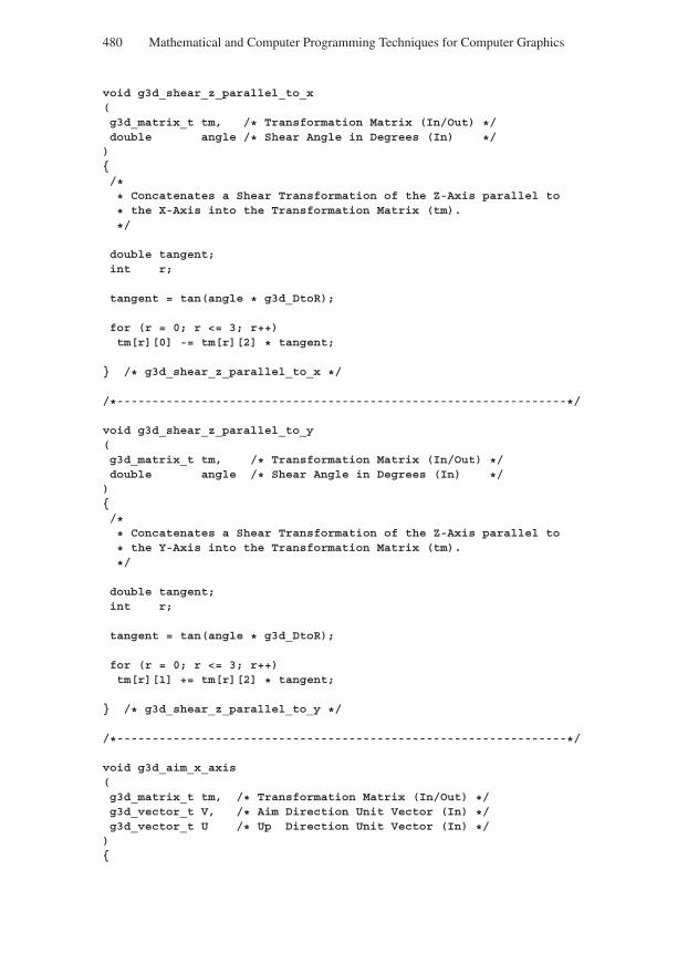
“Comninos” — 2005/8/31 — 18:23 — page 480 — #58
480 Mathematical and Computer Programming Techniques for Computer Graphics
void g3d_shear_z_parallel_to_x(g3d_matrix_t tm, /* Transformation Matrix (In/Out) */double angle /* Shear Angle in Degrees (In) */)/** Concatenates a Shear Transformation of the Z-Axis parallel to
* the X-Axis into the Transformation Matrix (tm).
*/
double tangent;int r;
tangent = tan(angle * g3d_DtoR);
for (r = 0; r <= 3; r++)tm[r][0] -= tm[r][2] * tangent;
/* g3d_shear_z_parallel_to_x */
/*----------------------------------------------------------------*/
void g3d_shear_z_parallel_to_y(g3d_matrix_t tm, /* Transformation Matrix (In/Out) */double angle /* Shear Angle in Degrees (In) */)/** Concatenates a Shear Transformation of the Z-Axis parallel to
* the Y-Axis into the Transformation Matrix (tm).
*/
double tangent;int r;
tangent = tan(angle * g3d_DtoR);
for (r = 0; r <= 3; r++)tm[r][1] += tm[r][2] * tangent;
/* g3d_shear_z_parallel_to_y */
/*----------------------------------------------------------------*/
void g3d_aim_x_axis(g3d_matrix_t tm, /* Transformation Matrix (In/Out) */g3d_vector_t V, /* Aim Direction Unit Vector (In) */g3d_vector_t U /* Up Direction Unit Vector (In) */)
“Comninos” — 2005/8/31 — 18:23 — page 481 — #59
A Simple C Library for 3D Transformations 481
/** Concatenates into the Transformation Matrix (tm) a Global Aim
* transformation which causes the Global X-axis to be aligned to
* the aim in the direction of the unit vector (V). The (U) vector
* represents the relative up direction unit vector with respect to
* the (V) vector.
*/
g3d_matrix_t A; /* Aim transformation matrix */g3d_vector_t X, /* Local Axes */
Y,Z;
/* Compute the new orientation of the transformed local axes */
Mg3d_vector_copy(V, X);Mg3d_vector_normalise(X);
Mg3d_vector_cross(U, X, Y);Mg3d_vector_normalise(Y);
Mg3d_vector_cross(X, Y, Z);Mg3d_vector_normalise(Z);
/* Construct the aim transformation matrix */
A[0][0] = X[0]; A[0][1] = X[1]; A[0][2] = X[2]; A[0][3] = 0;A[1][0] = Y[0]; A[1][1] = Y[1]; A[1][2] = Y[2]; A[1][3] = 0;A[2][0] = Z[0]; A[2][1] = Z[1]; A[2][2] = Z[2]; A[2][3] = 0;A[3][0] = 0; A[3][1] = 0; A[3][2] = 0; A[3][3] = 1;
/* Concatenate the aim transformation with the (tm) transformationmatrix */
g3d_concatenate(tm, A);
/* g3d_aim_x_axis */
/*----------------------------------------------------------------*/
void g3d_aim_y_axis(g3d_matrix_t tm, /* Transformation Matrix (In/Out) */g3d_vector_t V, /* Aim Direction Unit Vector (In) */g3d_vector_t U /* Up Direction Unit Vector (In) */)/** Concatenates into the Transformation Matrix (tm) a Global Aim
* transformation which causes the Global Y-axis to be aligned to
* the aim in the direction of the unit vector (V). The (U) vector
* represents the relative up direction unit vector with respect to
* the (V) vector.
*/
“Comninos” — 2005/8/31 — 18:23 — page 482 — #60
482 Mathematical and Computer Programming Techniques for Computer Graphics
g3d_matrix_t A; /* Aim transformation matrix */g3d_vector_t X, /* Local Axes */
Y,Z;
/* Compute the new orientation of the transformed local axes */
Mg3d_vector_copy(V, Y);Mg3d_vector_normalise(Y);
Mg3d_vector_cross(Y, U, X);Mg3d_vector_normalise(X);
Mg3d_vector_cross(X, Y, Z);Mg3d_vector_normalise(Z);
/* Construct the aim transformation matrix */
A[0][0] = X[0]; A[0][1] = X[1]; A[0][2] = X[2]; A[0][3] = 0;A[1][0] = Y[0]; A[1][1] = Y[1]; A[1][2] = Y[2]; A[1][3] = 0;A[2][0] = Z[0]; A[2][1] = Z[1]; A[2][2] = Z[2]; A[2][3] = 0;A[3][0] = 0; A[3][1] = 0; A[3][2] = 0; A[3][3] = 1;
/* Concatenate the aim transformation with the (tm) transformationmatrix */
g3d_concatenate(tm, A);
/* g3d_aim_y_axis */
/*----------------------------------------------------------------*/void g3d_aim_z_axis(g3d_matrix_t tm, /* Transformation Matrix (In/Out) */g3d_vector_t V, /* Aim Direction Unit Vector (In) */g3d_vector_t U /* Up Direction Unit Vector (In) */)/** Concatenates into the Transformation Matrix (tm) a Global Aim
* transformation which causes the Global Z-axis to be aligned to
* the aim in the direction of the unit vector (V). The (U) vector
* represents the relative up direction unit vector with respect to
* the (V) vector.
*/
g3d_matrix_t A; /* Aim transformation matrix */g3d_vector_t X, /* Local Axes */
Y,Z;
/* Compute the new orientation of the transformed local axes */
“Comninos” — 2005/8/31 — 18:23 — page 483 — #61
A Simple C Library for 3D Transformations 483
Mg3d_vector_copy(V, Z);Mg3d_vector_normalise(Z);
Mg3d_vector_cross(u, Z, Y);Mg3d_vector_normalise(Y);
Mg3d_vector_cross(Y, Z, X);Mg3d_vector_normalise(X);
/* Construct the aim transformation matrix */
A[0][0] = X[0]; A[0][1] = X[1]; A[0][2] = X[2]; A[0][3] = 0;A[1][0] = Y[0]; A[1][1] = Y[1]; A[1][2] = Y[2]; A[1][3] = 0;A[2][0] = Z[0]; A[2][1] = Z[1]; A[2][2] = Z[2]; A[2][3] = 0;A[3][0] = 0; A[3][1] = 0; A[3][2] = 0; A[3][3] = 1;
/* Concatenate the aim transformation with the (tm) transformationmatrix */
g3d_concatenate(tm, A); /* g3d_aim_z_axis */
/*----------------------------------------------------------------*/
void g3d_reflect_about_arbitrary_point(g3d_matrix_t tm, /* Transformation Matrix (In/Out) */g3d_vector_t C /* Centre of Reflection (In) */)/** Concatenates a Global Reflection Transformation about an
* arbitrary point (C) into the Transformation Matrix (tm).
** Done in three steps:
** 1. Translate the centre to the origin.
** 2. Reflect about the origin.
** 3. Translate the centre to its original position.
*/
g3d_translate(tm, -C[0], -C[1], -C[2]);g3d_scale(tm, -1.0, -1.0, -1.0);g3d_translate(tm, C[0], C[1], C[2]);
/* g3d_reflect_about_arbitrary_point */
/*----------------------------------------------------------------*/
void g3d_scale_about_arbitrary_point(g3d_matrix_t tm, /* Transformation Matrix (In/Out) */
“Comninos” — 2005/8/31 — 18:23 — page 484 — #62
484 Mathematical and Computer Programming Techniques for Computer Graphics
g3d_vector_t C, /* Centre of Scale (In) */double sx, /* Scale Factors (In) */double sy,double sz)/** Concatenates a Global Scale Transformation about an arbitrary
* point (C) into the Transformation Matrix (tm).
** Done in three steps:
** 1. Translate the centre to the origin.
** 2. Scale about the origin.
** 3. Translate the centre to its original position.
*/
g3d_translate(tm, -C[0], -C[1], -C[2]);g3d_scale(tm, sx, sy, sz);g3d_translate(tm, C[0], C[1], C[2]);
/* g3d_scale_about_arbitrary_point */
/*----------------------------------------------------------------*/
void g3d_reflect_about_arbitrary_axis(g3d_matrix_t tm, /* Transformation Matrix (In/Out) */g3d_vector_t P, /* Point on the Arbitrary Axis (In) */g3d_vector_t D /* Direction Unit Vector of the Arbitrary
Axis (In) */)g3d_matrix_t A; /* Aim transformation matrix */g3d_vector_t V, /* Aim Direction Unit Vector */
U, /* Relative Up Direction Unit Vector */X, /* Local Axes */Y,Z;
/** Concatenates a Global Reflection Transformation about an
* arbitrary Axis into the Transformation Matrix (tm).
** The Arbitrary Axis is defined by a point (P) and a direction
* unit vector (D).
** This transformation is constructed by the following five steps:
** Step 1. Translate the point (P) to the origin.
*/
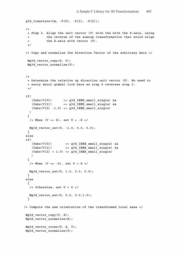
“Comninos” — 2005/8/31 — 18:23 — page 485 — #63
A Simple C Library for 3D Transformations 485
g3d_translate(tm, -P[0], -P[1], -P[2]);
/** Step 2. Align the unit vector (V) with the with the X-axis, using
* the inverse of the aiming transformation that would align
* the X-axis with vector (V).
*/
/* Copy and normalise the Direction Vector of the arbitrary Axis */
Mg3d_vector_copy(D, V);Mg3d_vector_normalise(V);
/** Determine the relative up direction unit vector (U). No need to
* worry about gimbal lock here as step 4 reverses step 2.
*/
if((fabs(V[0]) <= g3d_IEEE_small_single) &&(fabs(V[1]) <= g3d_IEEE_small_single) &&(fabs(V[2] -1.0) <= g3d_IEEE_small_single))
/* When (V == Z), set U = -X */
Mg3d_vector_set(U, -1.0, 0.0, 0.0);elseif(
(fabs(V[0]) <= g3d_IEEE_small_single) &&(fabs(V[1]) <= g3d_IEEE_small_single) &&(fabs(V[2] + 1.0) <= g3d_IEEE_small_single))
/* When (V == -Z), set U = X */
Mg3d_vector_set(U, 1.0, 0.0, 0.0);else/* Otherwise, set U = Z */
Mg3d_vector_set(U, 0.0, 0.0,1.0);
/* Compute the new orientation of the transformed local axes */
Mg3d_vector_copy(V, X);Mg3d_vector_normalise(X);
Mg3d_vector_cross(U, X, Y);Mg3d_vector_normalise(Y);
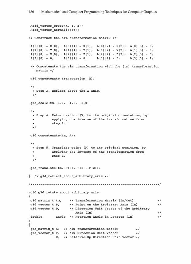
“Comninos” — 2005/8/31 — 18:23 — page 486 — #64
486 Mathematical and Computer Programming Techniques for Computer Graphics
Mg3d_vector_cross(X, Y, Z);Mg3d_vector_normalise(Z);
/* Construct the aim transformation matrix */
A[0][0] = X[0]; A[0][1] = X[1]; A[0][2] = X[2]; A[0][3] = 0;A[1][0] = Y[0]; A[1][1] = Y[1]; A[1][2] = Y[2]; A[1][3] = 0;A[2][0] = Z[0]; A[2][1] = Z[1]; A[2][2] = Z[2]; A[2][3] = 0;A[3][0] = 0; A[3][1] = 0; A[3][2] = 0; A[3][3] = 1;
/* Concatenate the aim transformation with the (tm) transformationmatrix */
g3d_concatenate_transpose(tm, A);
/** Step 3. Reflect about the X-axis.
*/
g3d_scale(tm, 1.0, -1.0, -1.0);
/** Step 4. Return vector (V) to its original orientation, by
* applying the inverse of the transformation from
* step 2.
*/
g3d_concatenate(tm, A);
/** Step 5. Translate point (P) to its original position, by
* applying the inverse of the transformation from
* step 1.
*/
g3d_translate(tm, P[0], P[1], P[2]);
/* g3d_reflect_about_arbitrary_axis */
/*----------------------------------------------------------------*/
void g3d_rotate_about_arbitrary_axis(g3d_matrix_t tm, /* Transformation Matrix (In/Out) */g3d_vector_t P, /* Point on the Arbitrary Axis (In) */g3d_vector_t D, /* Direction Unit Vector of the Arbitrary
Axis (In) */double angle /* Rotation Angle in Degrees (In) */)g3d_matrix_t A; /* Aim transformation matrix */g3d_vector_t V, /* Aim Direction Unit Vector */
U, /* Relative Up Direction Unit Vector */
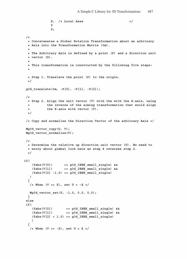
“Comninos” — 2005/8/31 — 18:23 — page 487 — #65
A Simple C Library for 3D Transformations 487
X, /* Local Axes */YZ;
/** Concatenates a Global Rotation Transformation about an arbitrary
* Axis into the Transformation Matrix (tm).
** The Arbitrary Axis is defined by a point (P) and a direction unit
* vector (D).
** This transformation is constructed by the following five steps:
*
* Step 1. Translate the point (P) to the origin.
*/
g3d_translate(tm, -P[0], -P[1], -P[2]);
/** Step 2. Align the unit vector (V) with the with the X-axis, using
* the inverse of the aiming transformation that would align
* the X-axis with vector (V).
*/
/* Copy and normalise the Direction Vector of the arbitrary Axis */
Mg3d_vector_copy(D, V);Mg3d_vector_normalise(V);
/** Determine the relative up direction unit vector (U). No need to
* worry about gimbal lock here as step 4 reverses step 2.
*/
if((fabs(V[0]) <= g3d_IEEE_small_single) &&(fabs(V[1]) <= g3d_IEEE_small_single) &&(fabs(V[2] -1.0) <= g3d_IEEE_small_single))
/* When (V == Z), set U = -X */
Mg3d_vector_set(U, -1.0, 0.0, 0.0);elseif(
(fabs(V[0]) <= g3d_IEEE_small_single) &&(fabs(V[1]) <= g3d_IEEE_small_single) &&(fabs(V[2] + 1.0) <= g3d_IEEE_small_single))
/* When (V == -Z), set U = X */
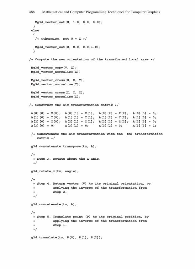
“Comninos” — 2005/8/31 — 18:23 — page 488 — #66
488 Mathematical and Computer Programming Techniques for Computer Graphics
Mg3d_vector_set(U, 1.0, 0.0, 0.0);
else/* Otherwise, set U = Z */
Mg3d_vector_set(U, 0.0, 0.0,1.0);
/* Compute the new orientation of the transformed local axes */
Mg3d_vector_copy(V, X);Mg3d_vector_normalise(X);
Mg3d_vector_cross(U, X, Y);Mg3d_vector_normalise(Y);
Mg3d_vector_cross(X, Y, Z);Mg3d_vector_normalise(Z);
/* Construct the aim transformation matrix */
A[0][0] = X[0]; A[0][1] = X[1]; A[0][2] = X[2]; A[0][3] = 0;A[1][0] = Y[0]; A[1][1] = Y[1]; A[1][2] = Y[2]; A[1][3] = 0;A[2][0] = Z[0]; A[2][1] = Z[1]; A[2][2] = Z[2]; A[2][3] = 0;A[3][0] = 0; A[3][1] = 0; A[3][2] = 0; A[3][3] = 1;
/* Concatenate the aim transformation with the (tm) transformationmatrix */
g3d_concatenate_transpose(tm, A);
/** Step 3. Rotate about the X-axis.
*/
g3d_rotate_x(tm, angle);
/** Step 4. Return vector (V) to its original orientation, by
* applying the inverse of the transformation from
* step 2.
*/
g3d_concatenate(tm, A);
/** Step 5. Translate point (P) to its original position, by
* applying the inverse of the transformation from
* step 1.
*/
g3d_translate(tm, P[0], P[1], P[2]);
“Comninos” — 2005/8/31 — 18:23 — page 489 — #67
A Simple C Library for 3D Transformations 489
/* g3d_rotate_about_arbitrary_axis */
/*----------------------------------------------------------------*/
void g3d_scale_along_arbitrary_axis(g3d_matrix_t tm, /* Transformation Matrix (In/Out) */g3d_vector_t P, /* Point on the Arbitrary Axis (In) */g3d_vector_t D, /* Direction Unit Vector of the Arbitrary */
Axis (In) */double sf /* Scale Factor (In) */)g3d_matrix_t A; /* Aim transformation matrix */g3d_vector_t V, /* Aim Direction Unit Vector */
U, /* Relative Up Direction Unit Vector */X, /* Local Axes */Y,Z;
/** Concatenates a Global Scaling Transformation along an arbitrary
* Axis into the Transformation Matrix (tm).
** The Arbitrary Axis is defined by a point (P) and a direction
* unit vector (D).
** This transformation is constructed by the following five steps:
** Step 1. Translate the point (P) to the origin.
*/
g3d_translate(tm, -P[0], -P[1], -P[2]);
/** Step 2. Align the unit vector (V) with the X-axis, using
* the inverse of the aiming transformation that would
* align the X-axis with vector (V).
*/
/* Copy and normalise the Direction Vector of the arbitrary Axis */
Mg3d_vector_copy(D, V);Mg3d_vector_normalise(V);
/** Determine the relative up direction unit vector (U). No need to
* worry about gimbal lock here as step 4 reverses step 2.
*/
if((fabs(V[0]) <= g3d_IEEE_small_single) &&(fabs(V[1]) <= g3d_IEEE_small_single) &&
“Comninos” — 2005/8/31 — 18:23 — page 490 — #68
490 Mathematical and Computer Programming Techniques for Computer Graphics
(fabs(V[2] -1.0) <= g3d_IEEE_small_single))/* When (V == Z), set U = -X */
Mg3d_vector_set(U, -1.0, 0.0, 0.0);
elseif(
(fabs(V[0]) <= g3d_IEEE_small_single) &&(fabs(V[1]) <= g3d_IEEE_small_single) &&(fabs(V[2] + 1.0) <= g3d_IEEE_small_single))
/* When (V == -Z), set U = X */
Mg3d_vector_set(U, 1.0, 0.0, 0.0);
else/* Otherwise, set U = Z */
Mg3d_vector_set(U, 0.0, 0.0,1.0);
/* Compute the new orientation of the transformed local axes */
Mg3d_vector_copy(V, X);Mg3d_vector_normalise(X);
Mg3d_vector_cross(U, X, Y);Mg3d_vector_normalise(Y);
Mg3d_vector_cross(X, Y, Z);Mg3d_vector_normalise(Z);
/* Construct the aim transformation matrix */
A[0][0] = X[0]; A[0][1] = X[1]; A[0][2] = X[2]; A[0][3] = 0;A[1][0] = Y[0]; A[1][1] = Y[1]; A[1][2] = Y[2]; A[1][3] = 0;A[2][0] = Z[0]; A[2][1] = Z[1]; A[2][2] = Z[2]; A[2][3] = 0;A[3][0] = 0; A[3][1] = 0; A[3][2] = 0; A[3][3] = 1;
/* Concatenate the aim transformation with the (tm) transformationmatrix */
g3d_concatenate_transpose(tm, A);
/** Step 3. Scale along the X-axis.
*/
g3d_scale(tm, sf, 1.0,1.0);
“Comninos” — 2005/8/31 — 18:23 — page 491 — #69
A Simple C Library for 3D Transformations 491
/** Step 4. Return vector (V) to its original orientation, by
* applying the inverse of the transformation from
* step 2.
*/
g3d_concatenate(tm, A);
/** Step 5. Translate point (P) to its original position, by
* applying the inverse of the transformation from
* step 1.
*/
g3d_translate(tm, P[0], P[1], P[2]);
/* g3d_scale_along_arbitrary_axis */
void g3d_translate_along_arbitrary_axis(g3d_matrix_t tm, /* Transformation Matrix (In/Out) */g3d_vector_t P, /* Point on the Arbitrary Axis (In) */g3d_vector_t D, /* Direction Unit Vector of the Arbitrary
Axis (In) */double dd /* Displacement (In) */)g3d_matrix_t A; /* Aim transformation matrix */g3d_vector_t V, /* Aim Direction Unit Vector */
U, /* Relative Up Direction Unit Vector */X, /* Local Axes */Y,Z;
/** Concatenates a Global Translation Transformation along an
* arbitrary Axis into the Transformation Matrix (tm).
** The Arbitrary Axis is defined by a point (P) and a direction
* unit vector (D).
* This transformation is constructed by the following five steps:
** Step 1. Translate the point (P) to the origin.
*/
g3d_translate(tm, -P[0], -P[1], -P[2]);
/** Step 2. Align the unit vector (V) with the with the X-axis, using
* the inverse of the aiming transformation that would align
* the X-axis with vector (V).
*/
/* Copy and normalise the Direction Vector of the arbitrary Axis */
“Comninos” — 2005/8/31 — 18:23 — page 492 — #70
492 Mathematical and Computer Programming Techniques for Computer Graphics
Mg3d_vector_copy(D, V);Mg3d_vector_normalise(V);
/** Determine the relative up direction unit vector (U). No need to
* worry about gimbal lock here as step 4 reverses step 2.
*/
if((fabs(V[0]) <= g3d_IEEE_small_single) &&(fabs(V[1]) <= g3d_IEEE_small_single) &&(fabs(V[2] -1.0) <= g3d_IEEE_small_single))/* When (V == Z), set U = -X */
Mg3d_vector_set(U, -1.0, 0.0, 0.0);
elseif(
(fabs(V[0]) <= g3d_IEEE_small_single) &&(fabs(V[1]) <= g3d_IEEE_small_single) &&(fabs(V[2] + 1.0) <= g3d_IEEE_small_single))
/* When (V == -Z), set U = X */
Mg3d_vector_set(U, 1.0, 0.0, 0.0);
else/* Otherwise, set U = Z */
Mg3d_vector_set(U, 0.0, 0.0,1.0);
/* Compute the new orientation of the transformed local axes */
Mg3d_vector_copy(V, X);Mg3d_vector_normalise(X);
Mg3d_vector_cross(U, X, Y);Mg3d_vector_normalise(Y);
Mg3d_vector_cross(X, Y, Z);Mg3d_vector_normalise(Z);
/* Construct the aim transformation matrix */
A[0][0] = X[0]; A[0][1] = X[1]; A[0][2] = X[2]; A[0][3] = 0;A[1][0] = Y[0]; A[1][1] = Y[1]; A[1][2] = Y[2]; A[1][3] = 0;A[2][0] = Z[0]; A[2][1] = Z[1]; A[2][2] = Z[2]; A[2][3] = 0;
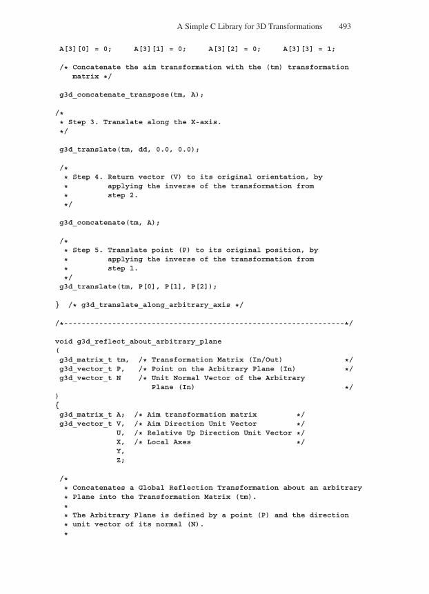
“Comninos” — 2005/8/31 — 18:23 — page 493 — #71
A Simple C Library for 3D Transformations 493
A[3][0] = 0; A[3][1] = 0; A[3][2] = 0; A[3][3] = 1;
/* Concatenate the aim transformation with the (tm) transformationmatrix */
g3d_concatenate_transpose(tm, A);
/** Step 3. Translate along the X-axis.
*/
g3d_translate(tm, dd, 0.0, 0.0);
/** Step 4. Return vector (V) to its original orientation, by
* applying the inverse of the transformation from
* step 2.
*/
g3d_concatenate(tm, A);
/** Step 5. Translate point (P) to its original position, by
* applying the inverse of the transformation from
* step 1.
*/g3d_translate(tm, P[0], P[1], P[2]);
/* g3d_translate_along_arbitrary_axis */
/*----------------------------------------------------------------*/
void g3d_reflect_about_arbitrary_plane(g3d_matrix_t tm, /* Transformation Matrix (In/Out) */g3d_vector_t P, /* Point on the Arbitrary Plane (In) */g3d_vector_t N /* Unit Normal Vector of the Arbitrary
Plane (In) */)g3d_matrix_t A; /* Aim transformation matrix */g3d_vector_t V, /* Aim Direction Unit Vector */
U, /* Relative Up Direction Unit Vector */X, /* Local Axes */Y,Z;
/** Concatenates a Global Reflection Transformation about an arbitrary
* Plane into the Transformation Matrix (tm).
** The Arbitrary Plane is defined by a point (P) and the direction
* unit vector of its normal (N).
*
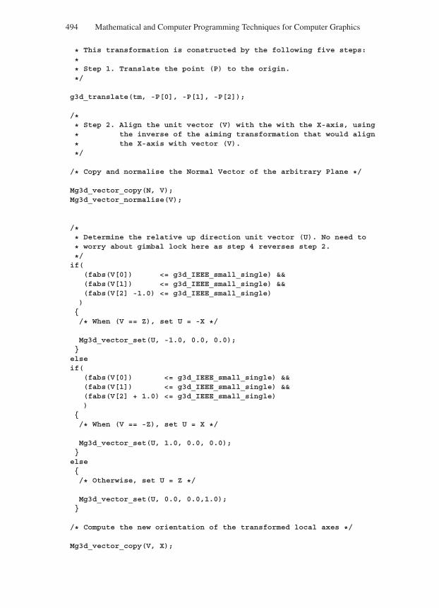
“Comninos” — 2005/8/31 — 18:23 — page 494 — #72
494 Mathematical and Computer Programming Techniques for Computer Graphics
* This transformation is constructed by the following five steps:
** Step 1. Translate the point (P) to the origin.
*/
g3d_translate(tm, -P[0], -P[1], -P[2]);
/** Step 2. Align the unit vector (V) with the with the X-axis, using
* the inverse of the aiming transformation that would align
* the X-axis with vector (V).
*/
/* Copy and normalise the Normal Vector of the arbitrary Plane */
Mg3d_vector_copy(N, V);Mg3d_vector_normalise(V);
/** Determine the relative up direction unit vector (U). No need to
* worry about gimbal lock here as step 4 reverses step 2.
*/if(
(fabs(V[0]) <= g3d_IEEE_small_single) &&(fabs(V[1]) <= g3d_IEEE_small_single) &&(fabs(V[2] -1.0) <= g3d_IEEE_small_single))/* When (V == Z), set U = -X */
Mg3d_vector_set(U, -1.0, 0.0, 0.0);
elseif(
(fabs(V[0]) <= g3d_IEEE_small_single) &&(fabs(V[1]) <= g3d_IEEE_small_single) &&(fabs(V[2] + 1.0) <= g3d_IEEE_small_single))
/* When (V == -Z), set U = X */
Mg3d_vector_set(U, 1.0, 0.0, 0.0);
else/* Otherwise, set U = Z */
Mg3d_vector_set(U, 0.0, 0.0,1.0);
/* Compute the new orientation of the transformed local axes */
Mg3d_vector_copy(V, X);
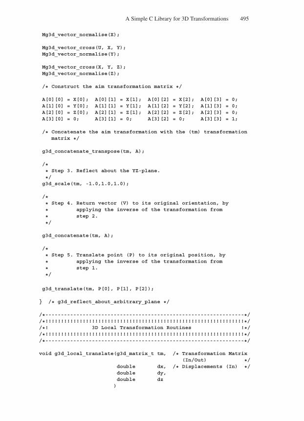
“Comninos” — 2005/8/31 — 18:23 — page 495 — #73
A Simple C Library for 3D Transformations 495
Mg3d_vector_normalise(X);
Mg3d_vector_cross(U, X, Y);Mg3d_vector_normalise(Y);
Mg3d_vector_cross(X, Y, Z);Mg3d_vector_normalise(Z);
/* Construct the aim transformation matrix */
A[0][0] = X[0]; A[0][1] = X[1]; A[0][2] = X[2]; A[0][3] = 0;A[1][0] = Y[0]; A[1][1] = Y[1]; A[1][2] = Y[2]; A[1][3] = 0;A[2][0] = Z[0]; A[2][1] = Z[1]; A[2][2] = Z[2]; A[2][3] = 0;A[3][0] = 0; A[3][1] = 0; A[3][2] = 0; A[3][3] = 1;
/* Concatenate the aim transformation with the (tm) transformationmatrix */
g3d_concatenate_transpose(tm, A);
/** Step 3. Reflect about the YZ-plane.
*/g3d_scale(tm, -1.0,1.0,1.0);
/** Step 4. Return vector (V) to its original orientation, by
* applying the inverse of the transformation from
* step 2.
*/
g3d_concatenate(tm, A);
/** Step 5. Translate point (P) to its original position, by
* applying the inverse of the transformation from
* step 1.
*/
g3d_translate(tm, P[0], P[1], P[2]);
/* g3d_reflect_about_arbitrary_plane */
/*----------------------------------------------------------------*//*!!!!!!!!!!!!!!!!!!!!!!!!!!!!!!!!!!!!!!!!!!!!!!!!!!!!!!!!!!!!!!!!*//*! 3D Local Transformation Routines !*//*!!!!!!!!!!!!!!!!!!!!!!!!!!!!!!!!!!!!!!!!!!!!!!!!!!!!!!!!!!!!!!!!*//*----------------------------------------------------------------*/
void g3d_local_translate(g3d_matrix_t tm, /* Transformation Matrix(In/Out) */
double dx, /* Displacements (In) */double dy,double dz)
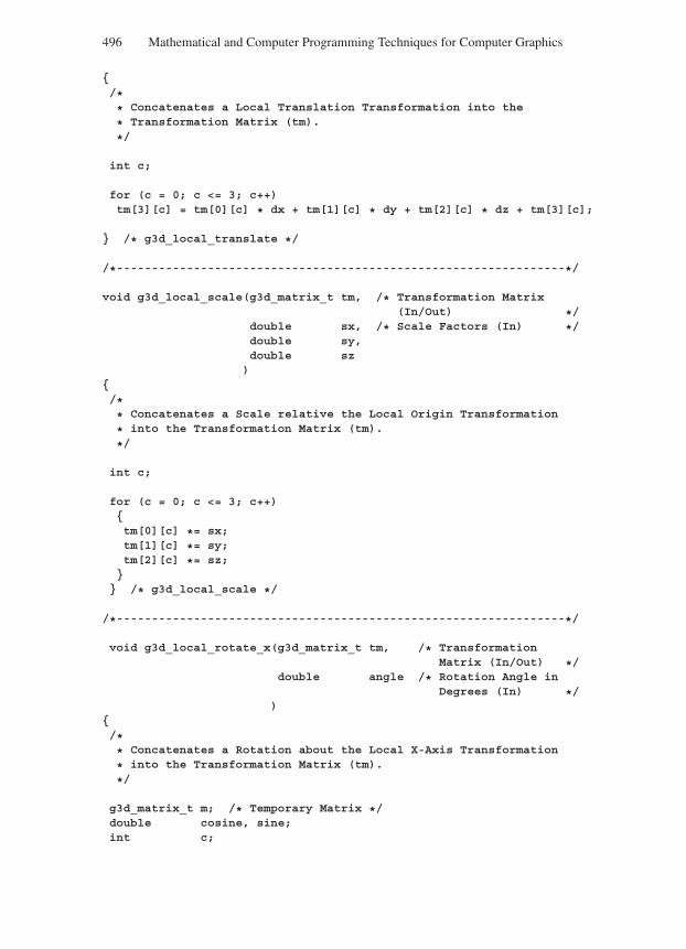
“Comninos” — 2005/8/31 — 18:23 — page 496 — #74
496 Mathematical and Computer Programming Techniques for Computer Graphics
/** Concatenates a Local Translation Transformation into the
* Transformation Matrix (tm).
*/
int c;
for (c = 0; c <= 3; c++)tm[3][c] = tm[0][c] * dx + tm[1][c] * dy + tm[2][c] * dz + tm[3][c];
/* g3d_local_translate */
/*----------------------------------------------------------------*/
void g3d_local_scale(g3d_matrix_t tm, /* Transformation Matrix(In/Out) */
double sx, /* Scale Factors (In) */double sy,double sz)
/** Concatenates a Scale relative the Local Origin Transformation
* into the Transformation Matrix (tm).
*/
int c;
for (c = 0; c <= 3; c++)tm[0][c] *= sx;tm[1][c] *= sy;tm[2][c] *= sz;
/* g3d_local_scale */
/*----------------------------------------------------------------*/
void g3d_local_rotate_x(g3d_matrix_t tm, /* TransformationMatrix (In/Out) */
double angle /* Rotation Angle inDegrees (In) */
)/** Concatenates a Rotation about the Local X-Axis Transformation
* into the Transformation Matrix (tm).
*/
g3d_matrix_t m; /* Temporary Matrix */double cosine, sine;int c;
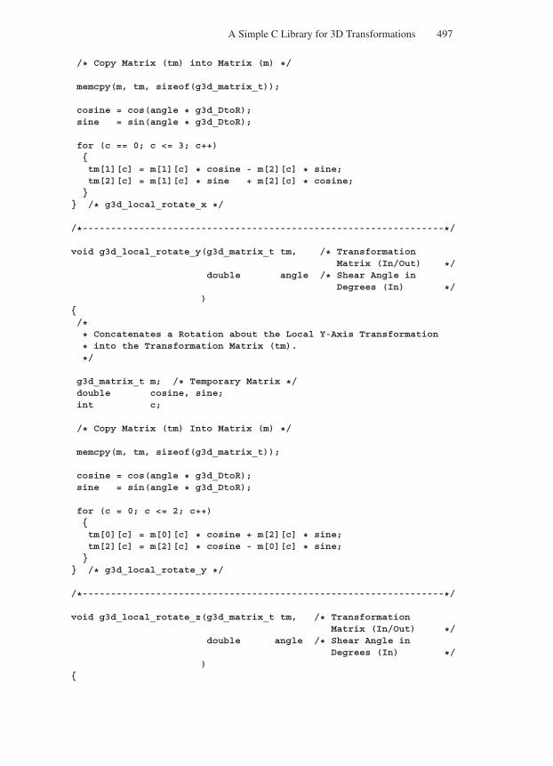
“Comninos” — 2005/8/31 — 18:23 — page 497 — #75
A Simple C Library for 3D Transformations 497
/* Copy Matrix (tm) into Matrix (m) */
memcpy(m, tm, sizeof(g3d_matrix_t));
cosine = cos(angle * g3d_DtoR);sine = sin(angle * g3d_DtoR);
for (c == 0; c <= 3; c++)tm[1][c] = m[1][c] * cosine - m[2][c] * sine;tm[2][c] = m[1][c] * sine + m[2][c] * cosine;
/* g3d_local_rotate_x */
/*----------------------------------------------------------------*/
void g3d_local_rotate_y(g3d_matrix_t tm, /* TransformationMatrix (In/Out) */
double angle /* Shear Angle inDegrees (In) */
)/** Concatenates a Rotation about the Local Y-Axis Transformation
* into the Transformation Matrix (tm).
*/
g3d_matrix_t m; /* Temporary Matrix */double cosine, sine;int c;
/* Copy Matrix (tm) Into Matrix (m) */
memcpy(m, tm, sizeof(g3d_matrix_t));
cosine = cos(angle * g3d_DtoR);sine = sin(angle * g3d_DtoR);
for (c = 0; c <= 2; c++)tm[0][c] = m[0][c] * cosine + m[2][c] * sine;tm[2][c] = m[2][c] * cosine - m[0][c] * sine;
/* g3d_local_rotate_y */
/*----------------------------------------------------------------*/
void g3d_local_rotate_z(g3d_matrix_t tm, /* TransformationMatrix (In/Out) */
double angle /* Shear Angle inDegrees (In) */
)
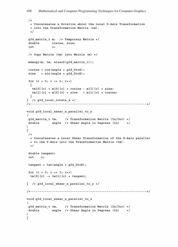
“Comninos” — 2005/8/31 — 18:23 — page 498 — #76
498 Mathematical and Computer Programming Techniques for Computer Graphics
/** Concatenates a Rotation about the Local Z-Axis Transformation
* into the Transformation Matrix (tm).
*/
g3d_matrix_t m; /* Temporary Matrix */double cosine, sine;int c;
/* Copy Matrix (tm) into Matrix (m) */
memcpy(m, tm, sizeof(g3d_matrix_t));
cosine = cos(angle * g3d_DtoR);sine = sin(angle * g3d_DtoR);
for (c = 0; c <= 2; c++)tm[0][c] = m[0][c] * cosine - m[1][c] * sine;tm[1][c] = m[0][c] * sine + m[1][c] * cosine;
/* g3d_local_rotate_z *//*----------------------------------------------------------------*/
void g3d_local_shear_x_parallel_to_y(g3d_matrix_t tm, /* Transformation Matrix (In/Out) */double angle /* Shear Angle in Degrees (In) */)/** Concatenates a Local Shear Transformation of the X-Axis parallel
* to the Y-Axis into the Transformation Matrix (tm).
*/
double tangent;int c;
tangent = tan(angle * g3d_DtoR);
for (c = 0; c <= 3; c++)tm[0][c] -= tm[1][c] * tangent;
/* g3d_local_shear_x_parallel_to_y */
/*----------------------------------------------------------------*/
void g3d_local_shear_x_parallel_to_z(g3d_matrix_t tm, /* Transformation Matrix (In/Out) */double angle /* Shear Angle in Degrees (In) */)
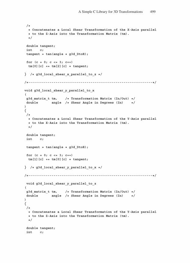
“Comninos” — 2005/8/31 — 18:23 — page 499 — #77
A Simple C Library for 3D Transformations 499
/** Concatenates a Local Shear Transformation of the X-Axis parallel
* to the Z-Axis into the Transformation Matrix (tm).
*/
double tangent;int c;tangent = tan(angle * g3d_DtoR);
for (c = 0; c <= 3; c++)tm[0][c] += tm[2][c] * tangent;
/* g3d_local_shear_x_parallel_to_z */
/*----------------------------------------------------------------*/
void g3d_local_shear_y_parallel_to_x(g3d_matrix_t tm, /* Transformation Matrix (In/Out) */double angle /* Shear Angle in Degrees (In) */)/** Concatenates a Local Shear Transformation of the Y-Axis parallel
* to the X-Axis into the Transformation Matrix (tm).
*/
double tangent;int c;
tangent = tan(angle * g3d_DtoR);
for (c = 0; c <= 3; c++)tm[1][c] += tm[0][c] * tangent;
/* g3d_local_shear_y_parallel_to_x */
/*----------------------------------------------------------------*/
void g3d_local_shear_y_parallel_to_z(g3d_matrix_t tm, /* Transformation Matrix (In/Out) */double angle /* Shear Angle in Degrees (In) */)/** Concatenates a Local Shear Transformation of the Y-Axis parallel
* to the Z-Axis into the Transformation Matrix (tm).
*/
double tangent;int c;
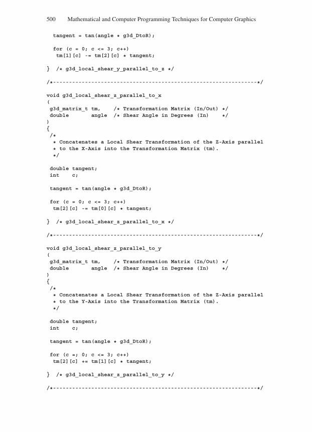
“Comninos” — 2005/8/31 — 18:23 — page 500 — #78
500 Mathematical and Computer Programming Techniques for Computer Graphics
tangent = tan(angle * g3d_DtoR);
for (c = 0; c <= 3; c++)tm[1][c] -= tm[2][c] * tangent;
/* g3d_local_shear_y_parallel_to_z */
/*----------------------------------------------------------------*/
void g3d_local_shear_z_parallel_to_x(g3d_matrix_t tm, /* Transformation Matrix (In/Out) */double angle /* Shear Angle in Degrees (In) */)/** Concatenates a Local Shear Transformation of the Z-Axis parallel
* to the X-Axis into the Transformation Matrix (tm).
*/
double tangent;int c;
tangent = tan(angle * g3d_DtoR);
for (c = 0; c <= 3; c++)tm[2][c] -= tm[0][c] * tangent;
/* g3d_local_shear_z_parallel_to_x */
/*----------------------------------------------------------------*/
void g3d_local_shear_z_parallel_to_y(g3d_matrix_t tm, /* Transformation Matrix (In/Out) */double angle /* Shear Angle in Degrees (In) */)/** Concatenates a Local Shear Transformation of the Z-Axis parallel
* to the Y-Axis into the Transformation Matrix (tm).
*/
double tangent;int c;
tangent = tan(angle * g3d_DtoR);
for (c =; 0; c <= 3; c++)tm[2][c] += tm[1][c] * tangent;
/* g3d_local_shear_z_parallel_to_y */
/*----------------------------------------------------------------*/
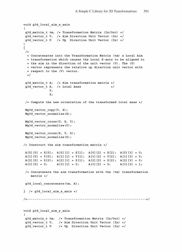
“Comninos” — 2005/8/31 — 18:23 — page 501 — #79
A Simple C Library for 3D Transformations 501
void g3d_local_aim_x_axis(g3d_matrix_t tm, /* Transformation Matrix (In/Out) */g3d_vector_t V, /* Aim Direction Unit Vector (In) */g3d_vector_t U /* Up Direction Unit Vector (In) */)/** Concatenates into the Transformation Matrix (tm) a Local Aim
* transformation which causes the Local X-axis to be aligned to
* the aim in the direction of the unit vector (V). The (U)
* vector represents the relative up direction unit vector with
* respect to the (V) vector.
*/
g3d_matrix_t A; /* Aim transformation matrix */g3d_vector_t X, /* Local Axes */
Y,Z;
/* Compute the new orientation of the transformed local axes */
Mg3d_vector_copy(V, X);Mg3d_vector_normalise(X);
Mg3d_vector_cross(U, X, Y);Mg3d_vector_normalise(Y);
Mg3d_vector_cross(X, Y, Z);Mg3d_vector_normalise(Z);
/* Construct the aim transformation matrix */
A[0][0] = X[0]; A[0][1] = X[1]; A[0][2] = X[2]; A[0][3] = 0;A[1][0] = Y[0]; A[1][1] = Y[1]; A[1][2] = Y[2]; A[1][3] = 0;A[2][0] = Z[0]; A[2][1] = Z[1]; A[2][2] = Z[2]; A[2][3] = 0;A[3][0] = 0; A[3][1] = 0; A[3][2] = 0; A[3][3] = 1;
/* Concatenate the aim transformation with the (tm) transformationmatrix */
g3d_local_concatenate(tm, A);
/* g3d_local_aim_x_axis */
/*----------------------------------------------------------------*/
void g3d_local_aim_y_axis(g3d_matrix_t tm, /* Transformation Matrix (In/Out) */g3d_vector_t V, /* Aim Direction Unit Vector (In) */g3d_vector_t U /* Up Direction Unit Vector (In) */
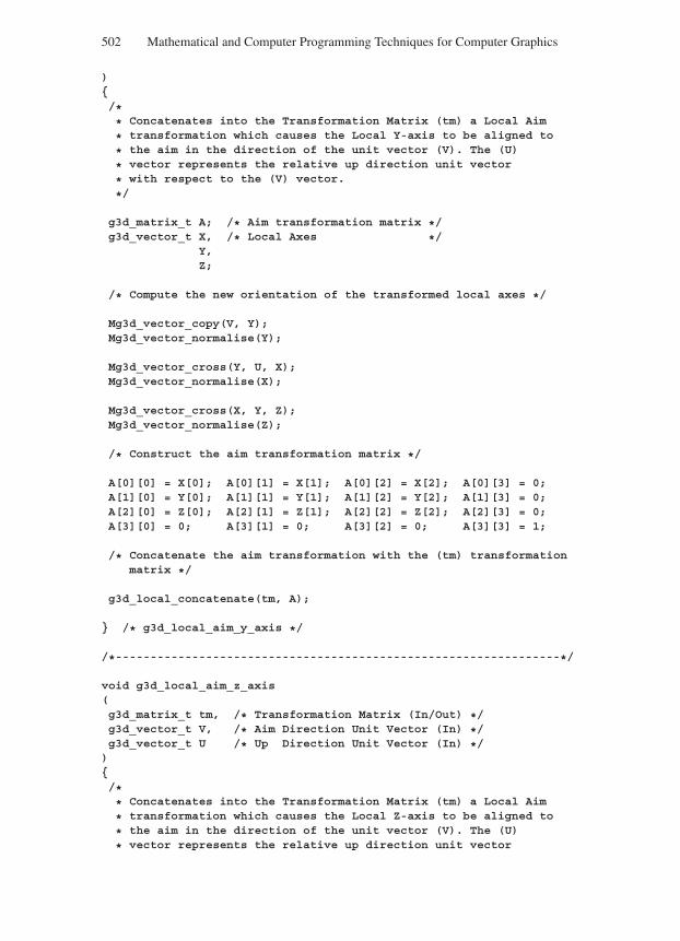
“Comninos” — 2005/8/31 — 18:23 — page 502 — #80
502 Mathematical and Computer Programming Techniques for Computer Graphics
)/** Concatenates into the Transformation Matrix (tm) a Local Aim
* transformation which causes the Local Y-axis to be aligned to
* the aim in the direction of the unit vector (V). The (U)
* vector represents the relative up direction unit vector
* with respect to the (V) vector.
*/
g3d_matrix_t A; /* Aim transformation matrix */g3d_vector_t X, /* Local Axes */
Y,Z;
/* Compute the new orientation of the transformed local axes */
Mg3d_vector_copy(V, Y);Mg3d_vector_normalise(Y);
Mg3d_vector_cross(Y, U, X);Mg3d_vector_normalise(X);
Mg3d_vector_cross(X, Y, Z);Mg3d_vector_normalise(Z);
/* Construct the aim transformation matrix */
A[0][0] = X[0]; A[0][1] = X[1]; A[0][2] = X[2]; A[0][3] = 0;A[1][0] = Y[0]; A[1][1] = Y[1]; A[1][2] = Y[2]; A[1][3] = 0;A[2][0] = Z[0]; A[2][1] = Z[1]; A[2][2] = Z[2]; A[2][3] = 0;A[3][0] = 0; A[3][1] = 0; A[3][2] = 0; A[3][3] = 1;
/* Concatenate the aim transformation with the (tm) transformationmatrix */
g3d_local_concatenate(tm, A);
/* g3d_local_aim_y_axis */
/*----------------------------------------------------------------*/
void g3d_local_aim_z_axis(g3d_matrix_t tm, /* Transformation Matrix (In/Out) */g3d_vector_t V, /* Aim Direction Unit Vector (In) */g3d_vector_t U /* Up Direction Unit Vector (In) */)/** Concatenates into the Transformation Matrix (tm) a Local Aim
* transformation which causes the Local Z-axis to be aligned to
* the aim in the direction of the unit vector (V). The (U)
* vector represents the relative up direction unit vector
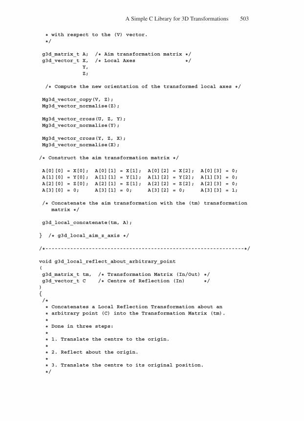
“Comninos” — 2005/8/31 — 18:23 — page 503 — #81
A Simple C Library for 3D Transformations 503
* with respect to the (V) vector.
*/
g3d_matrix_t A; /* Aim transformation matrix */g3d_vector_t X, /* Local Axes */
Y,Z;
/* Compute the new orientation of the transformed local axes */
Mg3d_vector_copy(V, Z);Mg3d_vector_normalise(Z);
Mg3d_vector_cross(U, Z, Y);Mg3d_vector_normalise(Y);
Mg3d_vector_cross(Y, Z, X);Mg3d_vector_normalise(X);
/* Construct the aim transformation matrix */
A[0][0] = X[0]; A[0][1] = X[1]; A[0][2] = X[2]; A[0][3] = 0;A[1][0] = Y[0]; A[1][1] = Y[1]; A[1][2] = Y[2]; A[1][3] = 0;A[2][0] = Z[0]; A[2][1] = Z[1]; A[2][2] = Z[2]; A[2][3] = 0;A[3][0] = 0; A[3][1] = 0; A[3][2] = 0; A[3][3] = 1;
/* Concatenate the aim transformation with the (tm) transformationmatrix */
g3d_local_concatenate(tm, A);
/* g3d_local_aim_z_axis */
/*----------------------------------------------------------------*/
void g3d_local_reflect_about_arbitrary_point(g3d_matrix_t tm, /* Transformation Matrix (In/Out) */g3d_vector_t C /* Centre of Reflection (In) */)/** Concatenates a Local Reflection Transformation about an
* arbitrary point (C) into the Transformation Matrix (tm).
** Done in three steps:
** 1. Translate the centre to the origin.
** 2. Reflect about the origin.
** 3. Translate the centre to its original position.
*/
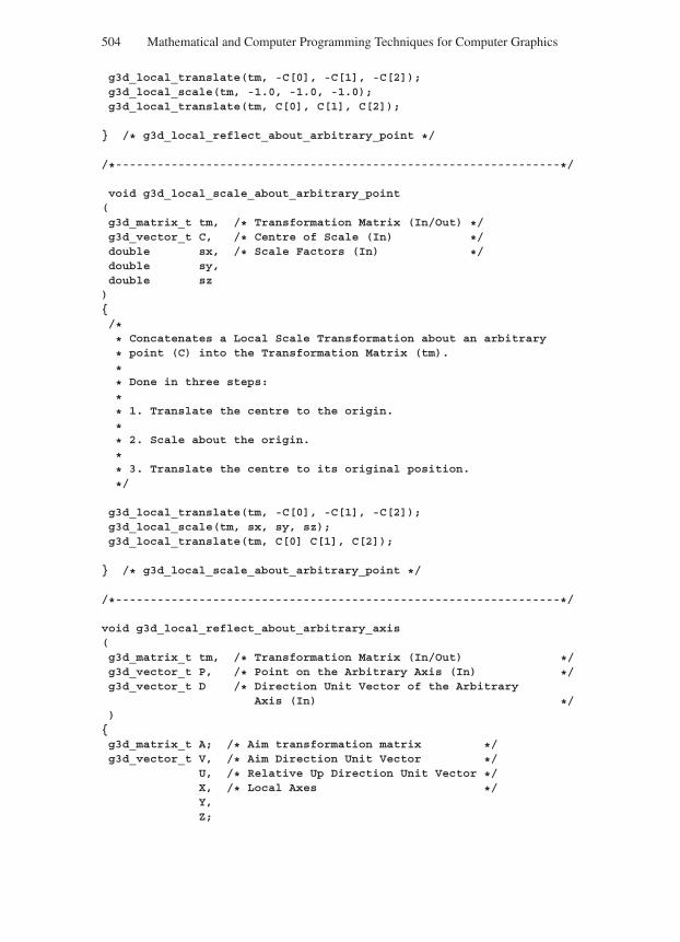
“Comninos” — 2005/8/31 — 18:23 — page 504 — #82
504 Mathematical and Computer Programming Techniques for Computer Graphics
g3d_local_translate(tm, -C[0], -C[1], -C[2]);g3d_local_scale(tm, -1.0, -1.0, -1.0);g3d_local_translate(tm, C[0], C[1], C[2]);
/* g3d_local_reflect_about_arbitrary_point */
/*----------------------------------------------------------------*/
void g3d_local_scale_about_arbitrary_point(g3d_matrix_t tm, /* Transformation Matrix (In/Out) */g3d_vector_t C, /* Centre of Scale (In) */double sx, /* Scale Factors (In) */double sy,double sz)/** Concatenates a Local Scale Transformation about an arbitrary
* point (C) into the Transformation Matrix (tm).
** Done in three steps:
** 1. Translate the centre to the origin.
** 2. Scale about the origin.
** 3. Translate the centre to its original position.
*/
g3d_local_translate(tm, -C[0], -C[1], -C[2]);g3d_local_scale(tm, sx, sy, sz);g3d_local_translate(tm, C[0] C[1], C[2]);
/* g3d_local_scale_about_arbitrary_point */
/*----------------------------------------------------------------*/
void g3d_local_reflect_about_arbitrary_axis(g3d_matrix_t tm, /* Transformation Matrix (In/Out) */g3d_vector_t P, /* Point on the Arbitrary Axis (In) */g3d_vector_t D /* Direction Unit Vector of the Arbitrary
Axis (In) */)g3d_matrix_t A; /* Aim transformation matrix */g3d_vector_t V, /* Aim Direction Unit Vector */
U, /* Relative Up Direction Unit Vector */X, /* Local Axes */Y,Z;
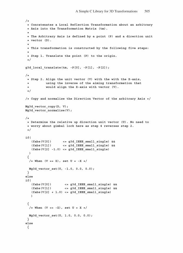
“Comninos” — 2005/8/31 — 18:23 — page 505 — #83
A Simple C Library for 3D Transformations 505
/** Concatenates a Local Reflection Transformation about an arbitrary
* Axis into the Transformation Matrix (tm).
** The Arbitrary Axis is defined by a point (P) and a direction unit
* vector (D).
** This transformation is constructed by the following five steps:
** Step 1. Translate the point (P) to the origin.
*/
g3d_local_translate(tm, -P[0], -P[1], -P[2]);
/** Step 2. Align the unit vector (V) with the with the X-axis,
* using the inverse of the aiming transformation that
* would align the X-axis with vector (V).
*/
/* Copy and normalise the Direction Vector of the arbitrary Axis */
Mg3d_vector_copy(D, V);Mg3d_vector_normalise(V);
/** Determine the relative up direction unit vector (U). No need to
* worry about gimbal lock here as step 4 reverses step 2.
*/
if((fabs(V[0]) <= g3d_IEEE_small_single) &&(fabs(V[1]) <= g3d_IEEE_small_single) &&(fabs(V[2] -1.0) <= g3d_IEEE_small_single))
/* When (V == Z), set U = -X */
Mg3d_vector_set(U, -1.0, 0.0, 0.0);elseif(
(fabs(V[0]) <= g3d_IEEE_small_single) &&(fabs(V[1]) <= g3d_IEEE_small_single) &&(fabs(V[2] + 1.0) <= g3d_IEEE_small_single))
/* When (V == -Z), set U = X */
Mg3d_vector_set(U, 1.0, 0.0, 0.0);else
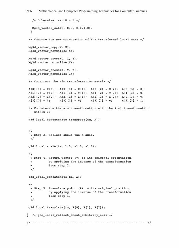
“Comninos” — 2005/8/31 — 18:23 — page 506 — #84
506 Mathematical and Computer Programming Techniques for Computer Graphics
/* Otherwise, set U = Z */
Mg3d_vector_set(U, 0.0, 0.0,1.0);
/* Compute the new orientation of the transformed local axes */
Mg3d_vector_copy(V, X);Mg3d_vector_normalise(X);
Mg3d_vector_cross(U, X, Y);Mg3d_vector_normalise(Y);
Mg3d_vector_cross(X, Y, Z);Mg3d_vector_normalise(Z);
/* Construct the aim transformation matrix */
A[0][0] = X[0]; A[0][1] = X[1]; A[0][2] = X[2]; A[0][3] = 0;A[1][0] = Y[0]; A[1][1] = Y[1]; A[1][2] = Y[2]; A[1][3] = 0;A[2][0] = Z[0]; A[2][1] = Z[1]; A[2][2] = Z[2]; A[2][3] = 0;A[3][0] = 0; A[3][1] = 0; A[3][2] = 0; A[3][3] = 1;
/* Concatenate the aim transformation with the (tm) transformationmatrix */
g3d_local_concatenate_transpose(tm, A);
/** Step 3. Reflect about the X-axis.
*/
g3d_local_scale(tm, 1.0, -1.0, -1.0);
/** Step 4. Return vector (V) to its original orientation,
* by applying the inverse of the transformation
* from step 2.
*/
g3d_local_concatenate(tm, A);
/** Step 5. Translate point (P) to its original position,
* by applying the inverse of the transformation
* from step 1.
*/
g3d_local_translate(tm, P[0], P[1], P[2]);
/* g3d_local_reflect_about_arbitrary_axis */
/*----------------------------------------------------------------*/
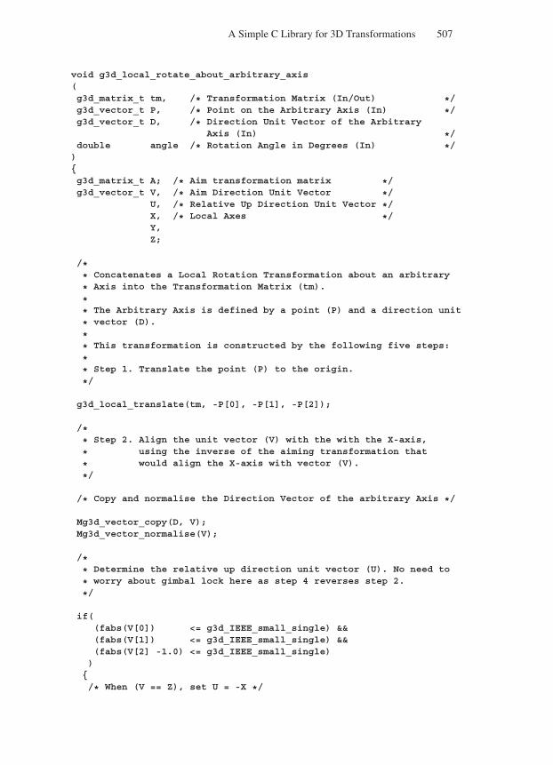
“Comninos” — 2005/8/31 — 18:23 — page 507 — #85
A Simple C Library for 3D Transformations 507
void g3d_local_rotate_about_arbitrary_axis(g3d_matrix_t tm, /* Transformation Matrix (In/Out) */g3d_vector_t P, /* Point on the Arbitrary Axis (In) */g3d_vector_t D, /* Direction Unit Vector of the Arbitrary
Axis (In) */double angle /* Rotation Angle in Degrees (In) */)g3d_matrix_t A; /* Aim transformation matrix */g3d_vector_t V, /* Aim Direction Unit Vector */
U, /* Relative Up Direction Unit Vector */X, /* Local Axes */Y,Z;
/** Concatenates a Local Rotation Transformation about an arbitrary
* Axis into the Transformation Matrix (tm).
** The Arbitrary Axis is defined by a point (P) and a direction unit
* vector (D).
** This transformation is constructed by the following five steps:
** Step 1. Translate the point (P) to the origin.
*/
g3d_local_translate(tm, -P[0], -P[1], -P[2]);
/** Step 2. Align the unit vector (V) with the with the X-axis,
* using the inverse of the aiming transformation that
* would align the X-axis with vector (V).
*/
/* Copy and normalise the Direction Vector of the arbitrary Axis */
Mg3d_vector_copy(D, V);Mg3d_vector_normalise(V);
/** Determine the relative up direction unit vector (U). No need to
* worry about gimbal lock here as step 4 reverses step 2.
*/
if((fabs(V[0]) <= g3d_IEEE_small_single) &&(fabs(V[1]) <= g3d_IEEE_small_single) &&(fabs(V[2] -1.0) <= g3d_IEEE_small_single))
/* When (V == Z), set U = -X */
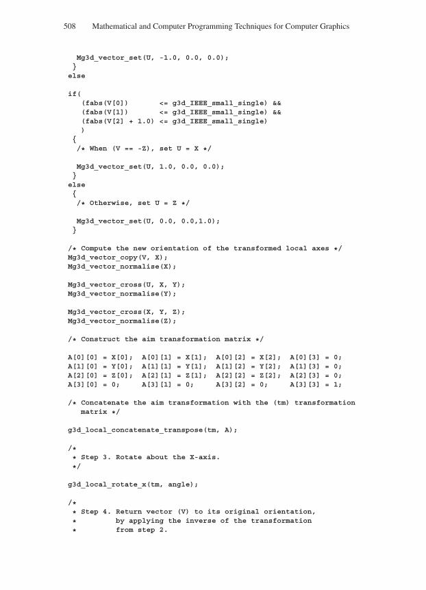
“Comninos” — 2005/8/31 — 18:23 — page 508 — #86
508 Mathematical and Computer Programming Techniques for Computer Graphics
Mg3d_vector_set(U, -1.0, 0.0, 0.0);
else
if((fabs(V[0]) <= g3d_IEEE_small_single) &&(fabs(V[1]) <= g3d_IEEE_small_single) &&(fabs(V[2] + 1.0) <= g3d_IEEE_small_single))
/* When (V == -Z), set U = X */
Mg3d_vector_set(U, 1.0, 0.0, 0.0);
else/* Otherwise, set U = Z */
Mg3d_vector_set(U, 0.0, 0.0,1.0);
/* Compute the new orientation of the transformed local axes */Mg3d_vector_copy(V, X);Mg3d_vector_normalise(X);
Mg3d_vector_cross(U, X, Y);Mg3d_vector_normalise(Y);
Mg3d_vector_cross(X, Y, Z);Mg3d_vector_normalise(Z);
/* Construct the aim transformation matrix */
A[0][0] = X[0]; A[0][1] = X[1]; A[0][2] = X[2]; A[0][3] = 0;A[1][0] = Y[0]; A[1][1] = Y[1]; A[1][2] = Y[2]; A[1][3] = 0;A[2][0] = Z[0]; A[2][1] = Z[1]; A[2][2] = Z[2]; A[2][3] = 0;A[3][0] = 0; A[3][1] = 0; A[3][2] = 0; A[3][3] = 1;
/* Concatenate the aim transformation with the (tm) transformationmatrix */
g3d_local_concatenate_transpose(tm, A);
/** Step 3. Rotate about the X-axis.
*/
g3d_local_rotate_x(tm, angle);
/** Step 4. Return vector (V) to its original orientation,
* by applying the inverse of the transformation
* from step 2.
“Comninos” — 2005/8/31 — 18:23 — page 509 — #87
A Simple C Library for 3D Transformations 509
*/
g3d_local_concatenate(tm, A);
/** Step 5. Translate point (P) to its original position,
* by applying the inverse of the transformation
* from step 1.
*/
g3d_local_translate(tm, P[0], P[1], P[2]);
/* g3d_local_rotate_about_arbitrary_axis */
/*----------------------------------------------------------------*/
void g3d_local_scale_along_arbitrary_axis(g3d_matrix_t tm, /* Transformation Matrix (In/Out) */g3d_vector_t P, /* Point on the Arbitrary Axis (In) */g3d_vector_t D, /* Direction Unit Vector of the Arbitrary
Axis (In) */double sf /* Scale Factor (In) */)g3d_matrix_t A; /* Aim transformation matrix */g3d_vector_t V, /* Aim Direction Unit Vector */
U, /* Relative Up Direction Unit Vector */X, /* Local Axes */Y,Z;
/** Concatenates a Local Scaling Transformation along an arbitrary
* Axis into the Transformation Matrix (tm).
** The Arbitrary Axis is defined by a point (P) and a direction
* unit vector (D).
** This transformation is constructed by the following five steps:
** Step 1. Translate the point (P) to the origin.
*/
g3d_local_translate(tm, -P[0], -P[1], -P[2]);
/** Step 2. Align the unit vector (V) with the with the X-axis,
* using the inverse of the aiming transformation that
* would align the X-axis with vector (V).
*/
/* Copy and normalise the Direction Vector of the arbitrary Axis */
“Comninos” — 2005/8/31 — 18:23 — page 510 — #88
510 Mathematical and Computer Programming Techniques for Computer Graphics
Mg3d_vector_copy(D, V);Mg3d_vector_normalise(V);
/** Determine the relative up direction unit vector (U). No need to
* worry about gimbal lock here as step 4 reverses step 2.
*/
if((fabs(V[0]) <= g3d_IEEE_small_single) &&(fabs(V[1]) <= g3d_IEEE_small_single) &&(fabs(V[2] -1.0) <= g3d_IEEE_small_single))/* When (V == Z), set U = -X */
Mg3d_vector_set(U, -1.0, 0.0, 0.0);
elseif(
(fabs(V[0]) <= g3d_IEEE_small_single) &&(fabs(V[1]) <= g3d_IEEE_small_single) &&(fabs(V[2] + 1.0) <= g3d_IEEE_small_single))
/* When (V == -Z), set U = X */
Mg3d_vector_set(U, 1.0, 0.0, 0.0);
else/* Otherwise, set U = Z */
Mg3d_vector_set(U, 0.0, 0.0,1.0);
/* Compute the new orientation of the transformed local axes */
Mg3d_vector_copy(V, X);Mg3d_vector_normalise(X);
Mg3d_vector_cross(U, X, Y);Mg3d_vector_normalise(Y);
Mg3d_vector_cross(X, Y, Z);Mg3d_vector_normalise(Z);
/* Construct the aim transformation matrix */
A[0][0] = X[0]; A[0][1] = X[1]; A[0][2] = X[2]; A[0][3] = 0;A[1][0] = Y[0]; A[1][1] = Y[1]; A[1][2] = Y[2]; A[1][3] = 0;A[2][0] = Z[0]; A[2][1] = Z[1]; A[2][2] = Z[2]; A[2][3] = 0;A[3][0] = 0; A[3][1] = 0; A[3][2] = 0; A[3][3] = 1;
“Comninos” — 2005/8/31 — 18:23 — page 511 — #89
A Simple C Library for 3D Transformations 511
/* Concatenate the aim transformation with the (tm) transformationmatrix */
g3d_local_concatenate_transpose(tm, A);
/** Step 3. Scale along the X-axis.
*/
g3d_local_scale(tm, sf, 1.0,1.0);
/** Step 4. Return vector (V) to its original orientation,
* by applying the inverse of the transformation
* from step 2.
*/
g3d_local_concatenate(tm, A);
/** Step 5. Translate point (P) to its original position,
* by applying the inverse of the transformation
* from step 1.
*/
g3d_local_translate(tm, P[0], P[1], P[2]);
/* g3d_local_scale_along_arbitrary_axis */
/*----------------------------------------------------------------*/
void g3d_local_translate_along_arbitrary_axis(g3d_matrix_t tm, /* Transformation Matrix (In/Out) */g3d_vector_t P, /* Point on the Arbitrary Axis (In) */g3d_vector_t D, /* Direction Unit Vector of the Arbitrary
Axis (In) */double dd /* Displacement (In) */)g3d_matrix_t A; /* Aim transformation matrix */g3d_vector_t V, /* Aim Direction Unit Vector */
U, /* Relative Up Direction Unit Vector */X, /* Local Axes */Y,Z;
/** Concatenates a Local Translation Transformation along an
* arbitrary Axis into the Transformation Matrix (tm).
** The Arbitrary Axis is defined by a point (P) and a direction unit
* vector (D).
*
“Comninos” — 2005/8/31 — 18:23 — page 512 — #90
512 Mathematical and Computer Programming Techniques for Computer Graphics
* This transformation is constructed by the following five steps:
** Step 1. Translate the point (P) to the origin.
*/
g3d_local_translate(tm, -P[0], -P[1], -P[2]);
/** Step 2. Align the unit vector (V) with the with the X-axis,
* using the inverseof the aiming transformation that
* would align the X-axis with vector (V).
*/
/* Copy and normalise the Direction Vector of the arbitrary Axis */
Mg3d_vector_copy(D, V);Mg3d_vector_normalise(V);
/** Determine the relative up direction unit vector (U). No need to
* worry about gimbal lock here as step 4 reverses step 2.
*/
if((fabs(V[0]) <= g3d_IEEE_small_single) &&(fabs(V[1]) <= g3d_IEEE_small_single) &&(fabs(V[2] -1.0) <= g3d_IEEE_small_single))/* When (V == Z), set U = -X */
Mg3d_vector_set(U, -1.0, 0.0, 0.0);
elseif(
(fabs(V[0]) <= g3d_IEEE_small_single) &&(fabs(V[1]) <= g3d_IEEE_small_single) &&(fabs(V[2] + 1.0) <= g3d_IEEE_small_single))
/* When (V == -Z), set U = X */
Mg3d_vector_set(U, 1.0, 0.0, 0.0);
else/* Otherwise, set U = Z */
Mg3d_vector_set(U, 0.0, 0.0,1.0);
/* Compute the new orientation of the transformed local axes */
Mg3d_vector_copy(V, X);
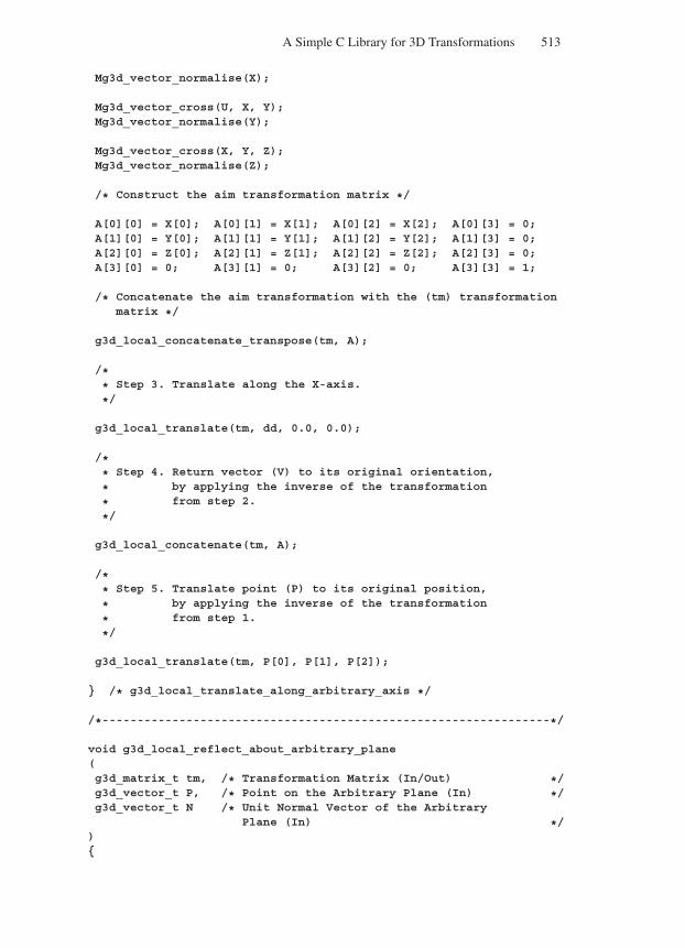
“Comninos” — 2005/8/31 — 18:23 — page 513 — #91
A Simple C Library for 3D Transformations 513
Mg3d_vector_normalise(X);
Mg3d_vector_cross(U, X, Y);Mg3d_vector_normalise(Y);
Mg3d_vector_cross(X, Y, Z);Mg3d_vector_normalise(Z);
/* Construct the aim transformation matrix */
A[0][0] = X[0]; A[0][1] = X[1]; A[0][2] = X[2]; A[0][3] = 0;A[1][0] = Y[0]; A[1][1] = Y[1]; A[1][2] = Y[2]; A[1][3] = 0;A[2][0] = Z[0]; A[2][1] = Z[1]; A[2][2] = Z[2]; A[2][3] = 0;A[3][0] = 0; A[3][1] = 0; A[3][2] = 0; A[3][3] = 1;
/* Concatenate the aim transformation with the (tm) transformationmatrix */
g3d_local_concatenate_transpose(tm, A);
/** Step 3. Translate along the X-axis.
*/
g3d_local_translate(tm, dd, 0.0, 0.0);
/** Step 4. Return vector (V) to its original orientation,
* by applying the inverse of the transformation
* from step 2.
*/
g3d_local_concatenate(tm, A);
/** Step 5. Translate point (P) to its original position,
* by applying the inverse of the transformation
* from step 1.
*/
g3d_local_translate(tm, P[0], P[1], P[2]);
/* g3d_local_translate_along_arbitrary_axis */
/*----------------------------------------------------------------*/
void g3d_local_reflect_about_arbitrary_plane(g3d_matrix_t tm, /* Transformation Matrix (In/Out) */g3d_vector_t P, /* Point on the Arbitrary Plane (In) */g3d_vector_t N /* Unit Normal Vector of the Arbitrary
Plane (In) */)
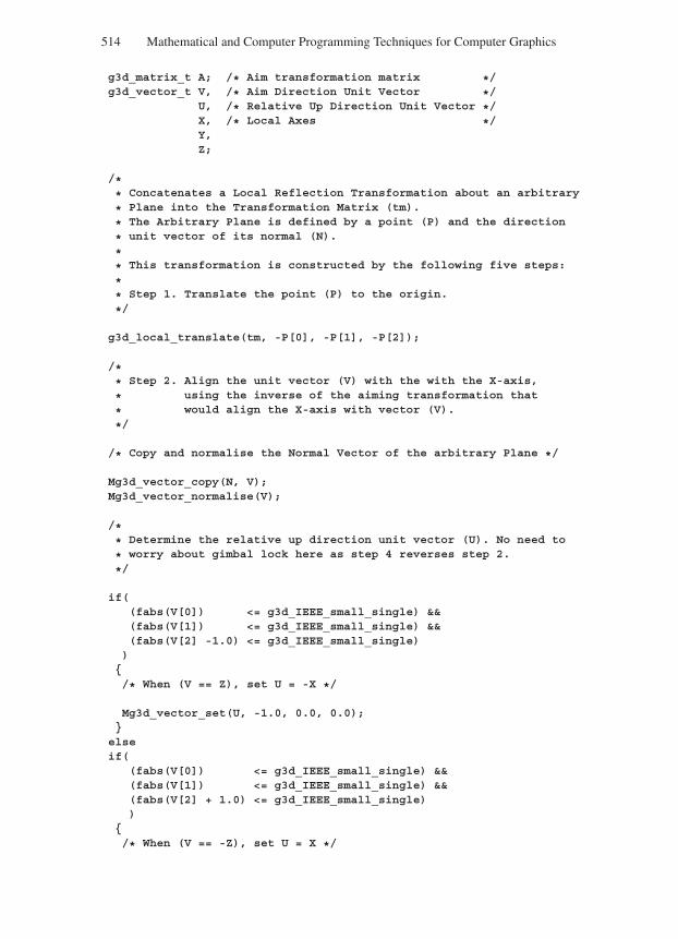
“Comninos” — 2005/8/31 — 18:23 — page 514 — #92
514 Mathematical and Computer Programming Techniques for Computer Graphics
g3d_matrix_t A; /* Aim transformation matrix */g3d_vector_t V, /* Aim Direction Unit Vector */
U, /* Relative Up Direction Unit Vector */X, /* Local Axes */Y,Z;
/** Concatenates a Local Reflection Transformation about an arbitrary
* Plane into the Transformation Matrix (tm).
* The Arbitrary Plane is defined by a point (P) and the direction
* unit vector of its normal (N).
** This transformation is constructed by the following five steps:
** Step 1. Translate the point (P) to the origin.
*/
g3d_local_translate(tm, -P[0], -P[1], -P[2]);
/** Step 2. Align the unit vector (V) with the with the X-axis,
* using the inverse of the aiming transformation that
* would align the X-axis with vector (V).
*/
/* Copy and normalise the Normal Vector of the arbitrary Plane */
Mg3d_vector_copy(N, V);Mg3d_vector_normalise(V);
/** Determine the relative up direction unit vector (U). No need to
* worry about gimbal lock here as step 4 reverses step 2.
*/
if((fabs(V[0]) <= g3d_IEEE_small_single) &&(fabs(V[1]) <= g3d_IEEE_small_single) &&(fabs(V[2] -1.0) <= g3d_IEEE_small_single))/* When (V == Z), set U = -X */
Mg3d_vector_set(U, -1.0, 0.0, 0.0);
elseif(
(fabs(V[0]) <= g3d_IEEE_small_single) &&(fabs(V[1]) <= g3d_IEEE_small_single) &&(fabs(V[2] + 1.0) <= g3d_IEEE_small_single))
/* When (V == -Z), set U = X */
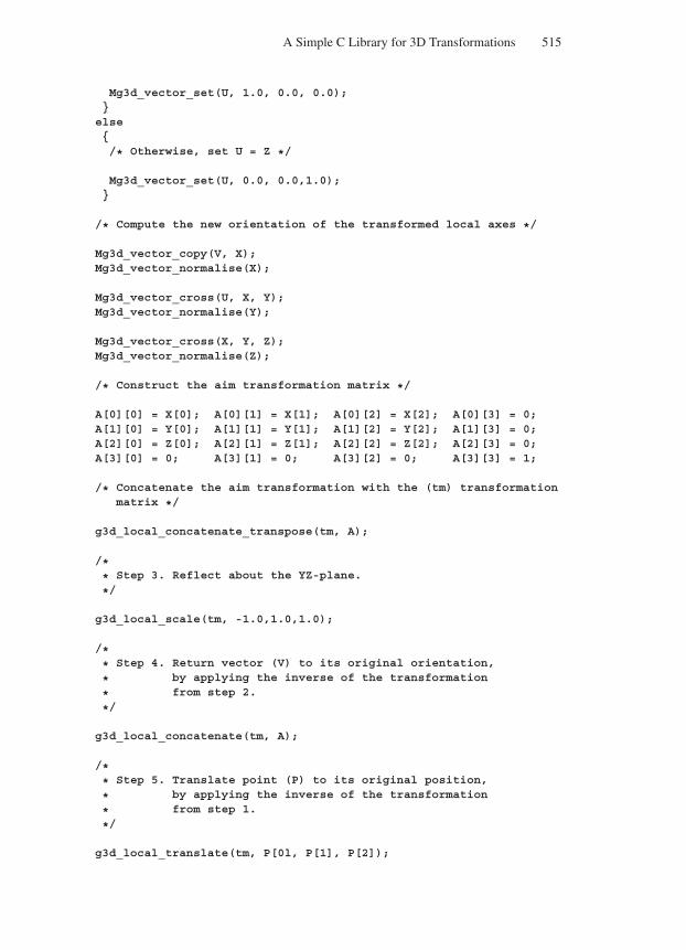
“Comninos” — 2005/8/31 — 18:23 — page 515 — #93
A Simple C Library for 3D Transformations 515
Mg3d_vector_set(U, 1.0, 0.0, 0.0);else/* Otherwise, set U = Z */
Mg3d_vector_set(U, 0.0, 0.0,1.0);
/* Compute the new orientation of the transformed local axes */
Mg3d_vector_copy(V, X);Mg3d_vector_normalise(X);
Mg3d_vector_cross(U, X, Y);Mg3d_vector_normalise(Y);
Mg3d_vector_cross(X, Y, Z);Mg3d_vector_normalise(Z);
/* Construct the aim transformation matrix */
A[0][0] = X[0]; A[0][1] = X[1]; A[0][2] = X[2]; A[0][3] = 0;A[1][0] = Y[0]; A[1][1] = Y[1]; A[1][2] = Y[2]; A[1][3] = 0;A[2][0] = Z[0]; A[2][1] = Z[1]; A[2][2] = Z[2]; A[2][3] = 0;A[3][0] = 0; A[3][1] = 0; A[3][2] = 0; A[3][3] = 1;
/* Concatenate the aim transformation with the (tm) transformationmatrix */
g3d_local_concatenate_transpose(tm, A);
/** Step 3. Reflect about the YZ-plane.
*/
g3d_local_scale(tm, -1.0,1.0,1.0);
/** Step 4. Return vector (V) to its original orientation,
* by applying the inverse of the transformation
* from step 2.
*/
g3d_local_concatenate(tm, A);
/** Step 5. Translate point (P) to its original position,
* by applying the inverse of the transformation
* from step 1.
*/
g3d_local_translate(tm, P[0l, P[1], P[2]);
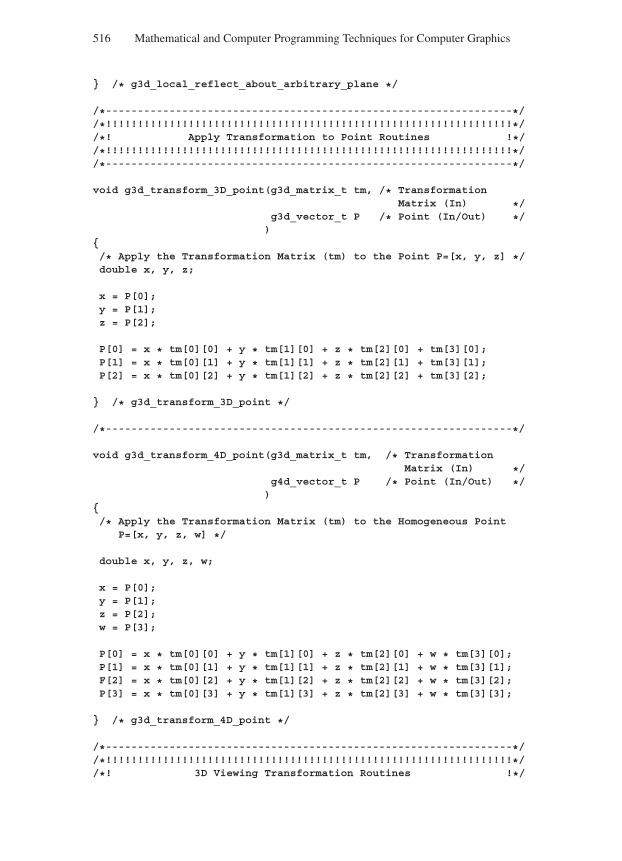
“Comninos” — 2005/8/31 — 18:23 — page 516 — #94
516 Mathematical and Computer Programming Techniques for Computer Graphics
/* g3d_local_reflect_about_arbitrary_plane */
/*----------------------------------------------------------------*//*!!!!!!!!!!!!!!!!!!!!!!!!!!!!!!!!!!!!!!!!!!!!!!!!!!!!!!!!!!!!!!!!*//*! Apply Transformation to Point Routines !*//*!!!!!!!!!!!!!!!!!!!!!!!!!!!!!!!!!!!!!!!!!!!!!!!!!!!!!!!!!!!!!!!!*//*----------------------------------------------------------------*/
void g3d_transform_3D_point(g3d_matrix_t tm, /* TransformationMatrix (In) */
g3d_vector_t P /* Point (In/Out) */)
/* Apply the Transformation Matrix (tm) to the Point P=[x, y, z] */double x, y, z;
x = P[0];y = P[1];z = P[2];
P[0] = x * tm[0][0] + y * tm[1][0] + z * tm[2][0] + tm[3][0];P[1] = x * tm[0][1] + y * tm[1][1] + z * tm[2][1] + tm[3][1];P[2] = x * tm[0][2] + y * tm[1][2] + z * tm[2][2] + tm[3][2];
/* g3d_transform_3D_point */
/*----------------------------------------------------------------*/
void g3d_transform_4D_point(g3d_matrix_t tm, /* TransformationMatrix (In) */
g4d_vector_t P /* Point (In/Out) */)
/* Apply the Transformation Matrix (tm) to the Homogeneous Point
P=[x, y, z, w] */
double x, y, z, w;
x = P[0];y = P[1];z = P[2];w = P[3];
P[0] = x * tm[0][0] + y * tm[1][0] + z * tm[2][0] + w * tm[3][0];P[1] = x * tm[0][1] + y * tm[1][1] + z * tm[2][1] + w * tm[3][1];F[2] = x * tm[0][2] + y * tm[1][2] + z * tm[2][2] + w * tm[3][2];P[3] = x * tm[0][3] + y * tm[1][3] + z * tm[2][3] + w * tm[3][3];
/* g3d_transform_4D_point */
/*----------------------------------------------------------------*//*!!!!!!!!!!!!!!!!!!!!!!!!!!!!!!!!!!!!!!!!!!!!!!!!!!!!!!!!!!!!!!!!*//*! 3D Viewing Transformation Routines !*/
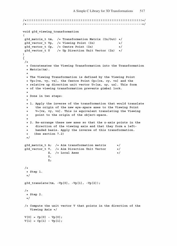
“Comninos” — 2005/8/31 — 18:23 — page 517 — #95
A Simple C Library for 3D Transformations 517
/*!!!!!!!!!!!!!!!!!!!!!!!!!!!!!!!!!!!!!!!!!!!!!!!!!!!!!!!!!!!!!!!!*//*----------------------------------------------------------------*/
void g3d_viewing_transformation(g3d_matrix_t tm, /* Transformation Matrix (In/Out) */g3d_vector_t Vp, /* Viewing Point (In) */g3d_vector_t Cp, /* Centre Point (In) */g3d_vector_t U /* Up Direction Unit Vector (In) */)/** Concatenates the Viewing Transformation into the Transformation
* Matrix(tm).
** The Viewing Transformation is defined by the Viewing Point
* Vp=[vx, vy, vz], the Centre Point Cp=[cx, cy, vz] and the
* relative up direction unit vector U=[ux, uy, uz]. This form
* of the viewing transformation prevents gimbal lock.
** Done in two steps:
** 1. Apply the inverse of the transformation that would translate
* the origin of the new eye-space axes to the Viewing Point
* V=[vx, vy, vz]. This is equivalent translating the Viewing
* point to the origin of the object-space.
** 2. Re-arrange these new axes so that the z-axis points in the
* direction of the viewing axis and that they form a left-
* handed basis. Apply the inverse of this transformation.
* (See section 7.2)
*/
g3d_matrix_t A; /* Aim transformation matrix */g3d_vector_t V, /* Aim Direction Unit Vector */
X, /* Local Axes */Y,Z;
/** Step 1.
*/
g3d_translate(tm, -Vp[0], -Vp[1], -Vp[2]);
/** Step 2.
*/
/* Compute the unit vector V that points in the direction of theViewing Axis */
V[0] = Cp[0] - Vp[0];V[1] = Cp[1] - Vp[1];
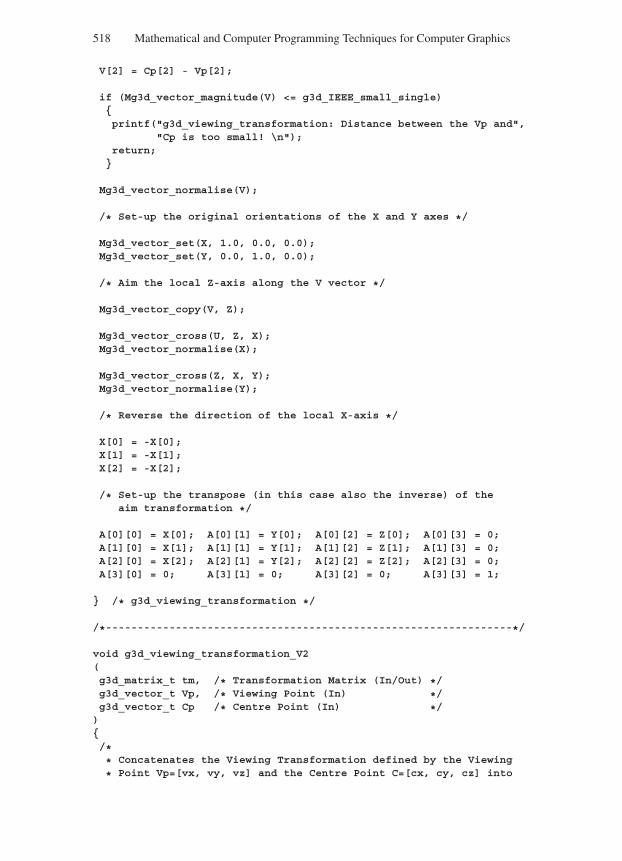
“Comninos” — 2005/8/31 — 18:23 — page 518 — #96
518 Mathematical and Computer Programming Techniques for Computer Graphics
V[2] = Cp[2] - Vp[2];
if (Mg3d_vector_magnitude(V) <= g3d_IEEE_small_single)printf("g3d_viewing_transformation: Distance between the Vp and",
"Cp is too small! \n");return;
Mg3d_vector_normalise(V);
/* Set-up the original orientations of the X and Y axes */
Mg3d_vector_set(X, 1.0, 0.0, 0.0);Mg3d_vector_set(Y, 0.0, 1.0, 0.0);
/* Aim the local Z-axis along the V vector */
Mg3d_vector_copy(V, Z);
Mg3d_vector_cross(U, Z, X);Mg3d_vector_normalise(X);
Mg3d_vector_cross(Z, X, Y);Mg3d_vector_normalise(Y);
/* Reverse the direction of the local X-axis */
X[0] = -X[0];X[1] = -X[1];X[2] = -X[2];
/* Set-up the transpose (in this case also the inverse) of theaim transformation */
A[0][0] = X[0]; A[0][1] = Y[0]; A[0][2] = Z[0]; A[0][3] = 0;A[1][0] = X[1]; A[1][1] = Y[1]; A[1][2] = Z[1]; A[1][3] = 0;A[2][0] = X[2]; A[2][1] = Y[2]; A[2][2] = Z[2]; A[2][3] = 0;A[3][0] = 0; A[3][1] = 0; A[3][2] = 0; A[3][3] = 1;
/* g3d_viewing_transformation */
/*----------------------------------------------------------------*/
void g3d_viewing_transformation_V2(g3d_matrix_t tm, /* Transformation Matrix (In/Out) */g3d_vector_t Vp, /* Viewing Point (In) */g3d_vector_t Cp /* Centre Point (In) */)/** Concatenates the Viewing Transformation defined by the Viewing
* Point Vp=[vx, vy, vz] and the Centre Point C=[cx, cy, cz] into
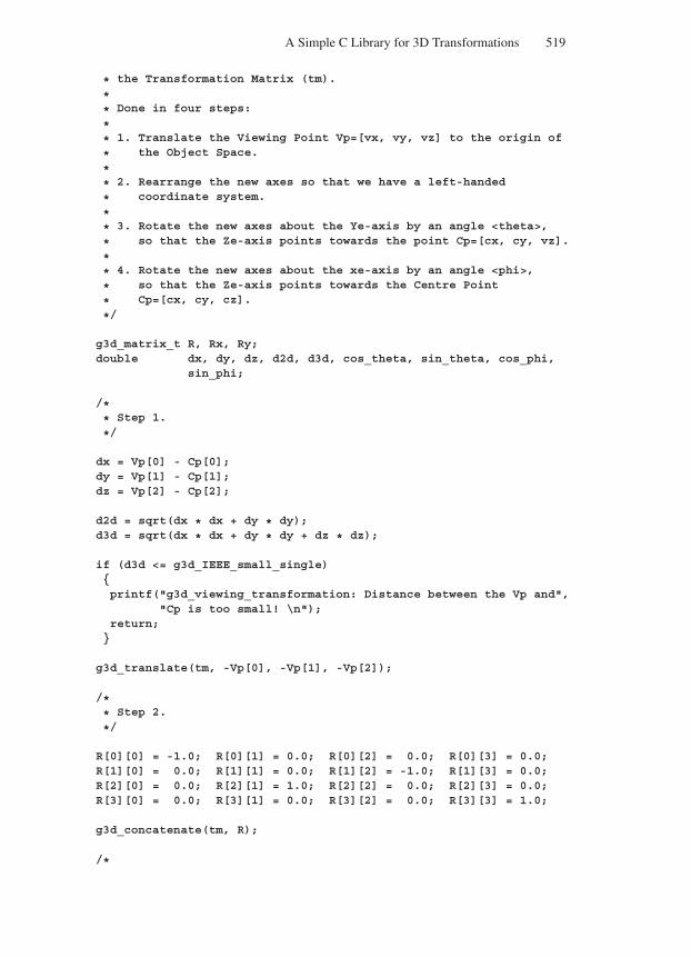
“Comninos” — 2005/8/31 — 18:23 — page 519 — #97
A Simple C Library for 3D Transformations 519
* the Transformation Matrix (tm).
** Done in four steps:
** 1. Translate the Viewing Point Vp=[vx, vy, vz] to the origin of
* the Object Space.
** 2. Rearrange the new axes so that we have a left-handed
* coordinate system.
** 3. Rotate the new axes about the Ye-axis by an angle <theta>,
* so that the Ze-axis points towards the point Cp=[cx, cy, vz].
** 4. Rotate the new axes about the xe-axis by an angle <phi>,
* so that the Ze-axis points towards the Centre Point
* Cp=[cx, cy, cz].
*/
g3d_matrix_t R, Rx, Ry;double dx, dy, dz, d2d, d3d, cos_theta, sin_theta, cos_phi,
sin_phi;
/** Step 1.
*/
dx = Vp[0] - Cp[0];dy = Vp[1] - Cp[1];dz = Vp[2] - Cp[2];
d2d = sqrt(dx * dx + dy * dy);d3d = sqrt(dx * dx + dy * dy + dz * dz);
if (d3d <= g3d_IEEE_small_single)printf("g3d_viewing_transformation: Distance between the Vp and",
"Cp is too small! \n");return;
g3d_translate(tm, -Vp[0], -Vp[1], -Vp[2]);
/** Step 2.
*/
R[0][0] = -1.0; R[0][1] = 0.0; R[0][2] = 0.0; R[0][3] = 0.0;R[1][0] = 0.0; R[1][1] = 0.0; R[1][2] = -1.0; R[1][3] = 0.0;R[2][0] = 0.0; R[2][1] = 1.0; R[2][2] = 0.0; R[2][3] = 0.0;R[3][0] = 0.0; R[3][1] = 0.0; R[3][2] = 0.0; R[3][3] = 1.0;
g3d_concatenate(tm, R);
/*
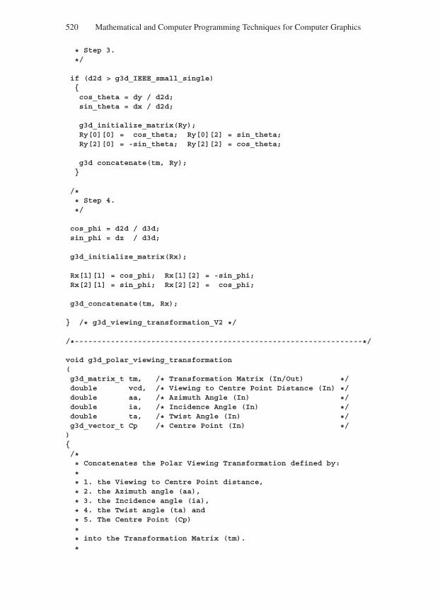
“Comninos” — 2005/8/31 — 18:23 — page 520 — #98
520 Mathematical and Computer Programming Techniques for Computer Graphics
* Step 3.
*/
if (d2d > g3d_IEEE_small_single)cos_theta = dy / d2d;sin_theta = dx / d2d;
g3d_initialize_matrix(Ry);Ry[0][0] = cos_theta; Ry[0][2] = sin_theta;Ry[2][0] = -sin_theta; Ry[2][2] = cos_theta;
g3d concatenate(tm, Ry);
/** Step 4.
*/
cos_phi = d2d / d3d;sin_phi = dz / d3d;
g3d_initialize_matrix(Rx);
Rx[1][1] = cos_phi; Rx[1][2] = -sin_phi;Rx[2][1] = sin_phi; Rx[2][2] = cos_phi;
g3d_concatenate(tm, Rx);
/* g3d_viewing_transformation_V2 */
/*----------------------------------------------------------------*/
void g3d_polar_viewing_transformation(g3d_matrix_t tm, /* Transformation Matrix (In/Out) */double vcd, /* Viewing to Centre Point Distance (In) */double aa, /* Azimuth Angle (In) */double ia, /* Incidence Angle (In) */double ta, /* Twist Angle (In) */g3d_vector_t Cp /* Centre Point (In) */)/** Concatenates the Polar Viewing Transformation defined by:
** 1. the Viewing to Centre Point distance,
* 2. the Azimuth angle (aa),
* 3. the Incidence angle (ia),
* 4. the Twist angle (ta) and
* 5. The Centre Point (Cp)
** into the Transformation Matrix (tm).
*
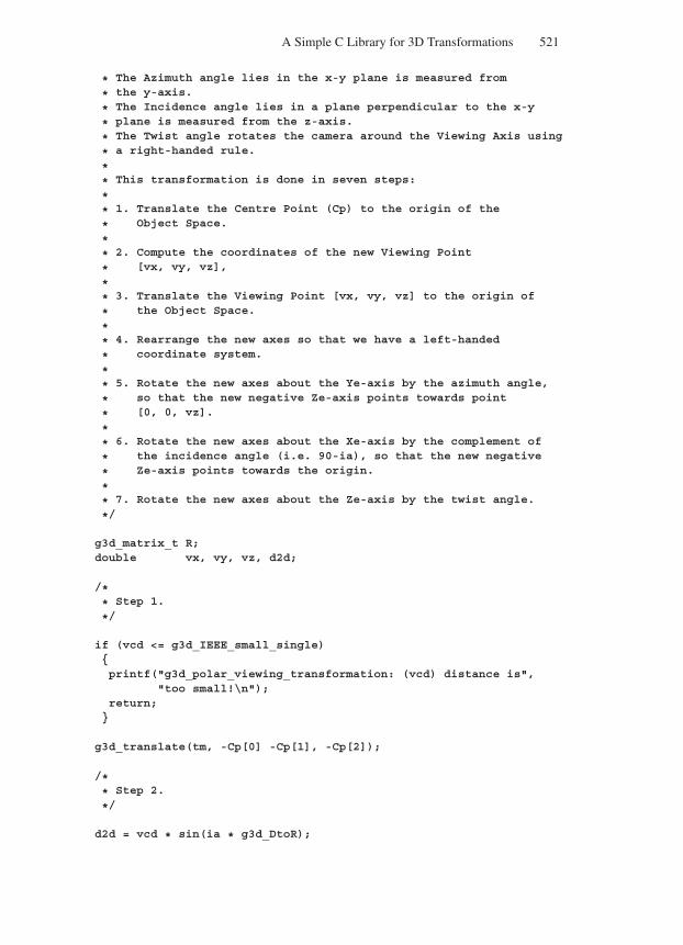
“Comninos” — 2005/8/31 — 18:23 — page 521 — #99
A Simple C Library for 3D Transformations 521
* The Azimuth angle lies in the x-y plane is measured from
* the y-axis.
* The Incidence angle lies in a plane perpendicular to the x-y
* plane is measured from the z-axis.
* The Twist angle rotates the camera around the Viewing Axis using
* a right-handed rule.
** This transformation is done in seven steps:
** 1. Translate the Centre Point (Cp) to the origin of the
* Object Space.
** 2. Compute the coordinates of the new Viewing Point
* [vx, vy, vz],
** 3. Translate the Viewing Point [vx, vy, vz] to the origin of
* the Object Space.
** 4. Rearrange the new axes so that we have a left-handed
* coordinate system.
** 5. Rotate the new axes about the Ye-axis by the azimuth angle,
* so that the new negative Ze-axis points towards point
* [0, 0, vz].
** 6. Rotate the new axes about the Xe-axis by the complement of
* the incidence angle (i.e. 90-ia), so that the new negative
* Ze-axis points towards the origin.
** 7. Rotate the new axes about the Ze-axis by the twist angle.
*/
g3d_matrix_t R;double vx, vy, vz, d2d;
/** Step 1.
*/
if (vcd <= g3d_IEEE_small_single)printf("g3d_polar_viewing_transformation: (vcd) distance is",
"too small!\n");return;
g3d_translate(tm, -Cp[0] -Cp[1], -Cp[2]);
/** Step 2.
*/
d2d = vcd * sin(ia * g3d_DtoR);
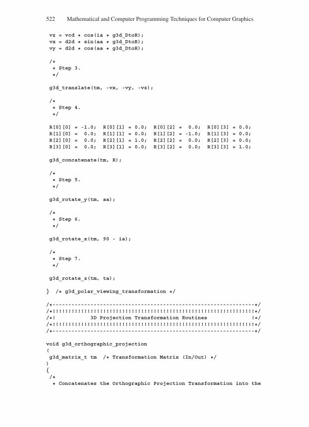
“Comninos” — 2005/8/31 — 18:23 — page 522 — #100
522 Mathematical and Computer Programming Techniques for Computer Graphics
vz = vcd * cos(ia * g3d_DtoR);vx = d2d * sin(aa * g3d_DtoR);vy = d2d * cos(aa * g3d_DtoR);
/** Step 3.
*/
g3d_translate(tm, -vx, -vy, -vz);
/** Step 4.
*/
R[0][0] = -1.0; R[0][1] = 0.0; R[0][2] = 0.0; R[0][3] = 0.0;R[1][0] = 0.0; R[1][1] = 0.0; R[1][2] = -1.0; R[1][3] = 0.0;R[2][0] = 0.0; R[2][1] = 1.0; R[2][2] = 0.0; R[2][3] = 0.0;R[3][0] = 0.0; R[3][1] = 0.0; R[3][2] = 0.0; R[3][3] = 1.0;
g3d_concatenate(tm, R);
/** Step 5.
*/
g3d_rotate_y(tm, aa);
/** Step 6.
*/
g3d_rotate_x(tm, 90 - ia);
/** Step 7.
*/
g3d_rotate_z(tm, ta);
/* g3d_polar_viewing_transformation */
/*----------------------------------------------------------------*//*!!!!!!!!!!!!!!!!!!!!!!!!!!!!!!!!!!!!!!!!!!!!!!!!!!!!!!!!!!!!!!!!*//*! 3D Projection Transformation Routines !*//*!!!!!!!!!!!!!!!!!!!!!!!!!!!!!!!!!!!!!!!!!!!!!!!!!!!!!!!!!!!!!!!!*//*----------------------------------------------------------------*/
void g3d_orthographic_projection(g3d_matrix_t tm /* Transformation Matrix (In/Out) */)/** Concatenates the Orthographic Projection Transformation into the
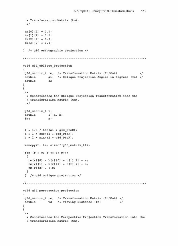
“Comninos” — 2005/8/31 — 18:23 — page 523 — #101
A Simple C Library for 3D Transformations 523
* Transformation Matrix (tm).
*/
tm[0][2] = 0.0;tm[1][2] = 0.0;tm[2][2] = 0.0;tm[3][2] = 0.0;
/* g3d_orthographic_projection */
/*----------------------------------------------------------------*/
void g3d_oblique_projection(g3d_matrix_t tm, /* Transformation Matrix (In/Out) */double a1, /* Oblique Projection Angles in Degrees (In) */double a2)/** Concatenates the Oblique Projection Transformation into the
* Transformation Matrix (tm).
*/
g3d_matrix_t h;double l, a, b;int r;
l = 1.0 / tan(a1 * g3d_DtoR);a = l * cos(a2 * g3d_DtoR);b = l * sin(a2 * g3d_DtoR);
memcpy(h, tm, sizeof(g3d_matrix_t));
for (r = 0; r <= 3; r++)tm[r][0] = h[r][0] + h[r][2] * a;tm[r][1] = h[r][1] + h[r][2] * b;tm[r][2] = 0.0;
/* g3d_oblique_projection */
/*----------------------------------------------------------------*/
void g3d_perspective_projection(g3d_matrix_t tm, /* Transformation Matrix (In/Out) */double vd /* Viewing Distance (In) */)/** Concatenates the Perspective Projection Transformation into the
* Transformation Matrix (tm).
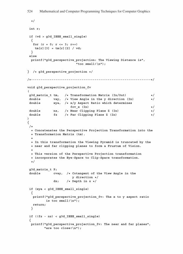
“Comninos” — 2005/8/31 — 18:23 — page 524 — #102
524 Mathematical and Computer Programming Techniques for Computer Graphics
*/
int r;
if (vd > g3d_IEEE_small_single)for (r = 0; r <= 3; r++)tm[r][3] = tm[r][2] / vd;
elseprintf("g3d_perspective_projection: The Viewing Distance is",
"too small!\n");
/* g3d_perspective_projection */
/*----------------------------------------------------------------*/
void g3d_perspective_projection_fv(g3d_matrix_t tm, /* Transformation Matrix (In/Out) */double vay, /* View Angle in the y direction (In) */double xya, /* x/y Aspect Ratio which determines
fov_x (In) */double nz, /* Near Clipping Plane Z (In) */double fz /* Far Clipping Plane Z (In) */)/** Concatenates the Perspective Projection Transformation into the
* Transformation Matrix (tm).
** In this transformation the Viewing Pyramid is truncated by the
* near and far clipping planes to form a Frustum of Vision.
** This version of the Perspective Projection transformation
* incorporates the Eye-Space to Clip-Space transformation.
*/
g3d_matrix_t P;double cvay, /* Cotangent of the View Angle in the
y direction */dz; /* Depth in z */
if (xya < g3d_IEEE_small_single)printf("g3d_perspective_projection_fv: The x to y aspect ratio
is too small!\n");return;
if ((fz - nz) < g3d_IEEE_small_single)printf("g3d_perspective_projection_fv: The near and far planes",
"are too close!\n");
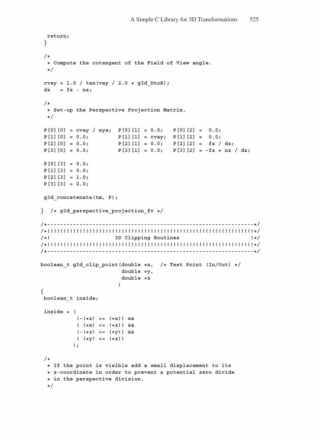
“Comninos” — 2005/8/31 — 18:23 — page 525 — #103
A Simple C Library for 3D Transformations 525
return;
/** Compute the cotangent of the Field of View angle.
*/
cvay = 1.0 / tan(vay / 2.0 * g3d_DtoR);dz = fz - nz;
/** Set-up the Perspective Projection Matrix.
*/
P[0][0] = cvay / xya; P[0][1] = 0.0; P[0][2] = 0.0;P[1][0] = 0.0; P[1][1] = cvay; P[1][2] = 0.0;P[2][0] = 0.0; P[2][1] = 0.0; P[2][2] = fz / dz;P[3][0] = 0.0; P[3][1] = 0.0; P[3][2] = -fz * nz / dz;
P[0][3] = 0.0;P[1][3] = 0.0;P[2][3] = 1.0;P[3][3] = 0.0;
g3d_concatenate(tm, P);
/* g3d_perspective_projection_fv */
/*----------------------------------------------------------------*//*!!!!!!!!!!!!!!!!!!!!!!!!!!!!!!!!!!!!!!!!!!!!!!!!!!!!!!!!!!!!!!!!*//*! 3D Clipping Routines !*//*!!!!!!!!!!!!!!!!!!!!!!!!!!!!!!!!!!!!!!!!!!!!!!!!!!!!!!!!!!!!!!!!*//*----------------------------------------------------------------*/
boolean_t g3d_clip_point(double *x, /* Test Point (In/Out) */double *y,double *z)
boolean_t inside;
inside = ((-(*z) <= (*x)) &&( (*x) <= (*z)) &&(-(*z) <= (*y)) &&( (*y) <= (*z)));
/** If the point is visible add a small displacement to its
* z-coordinate in order to prevent a potential zero divide
* in the perspective division.
*/
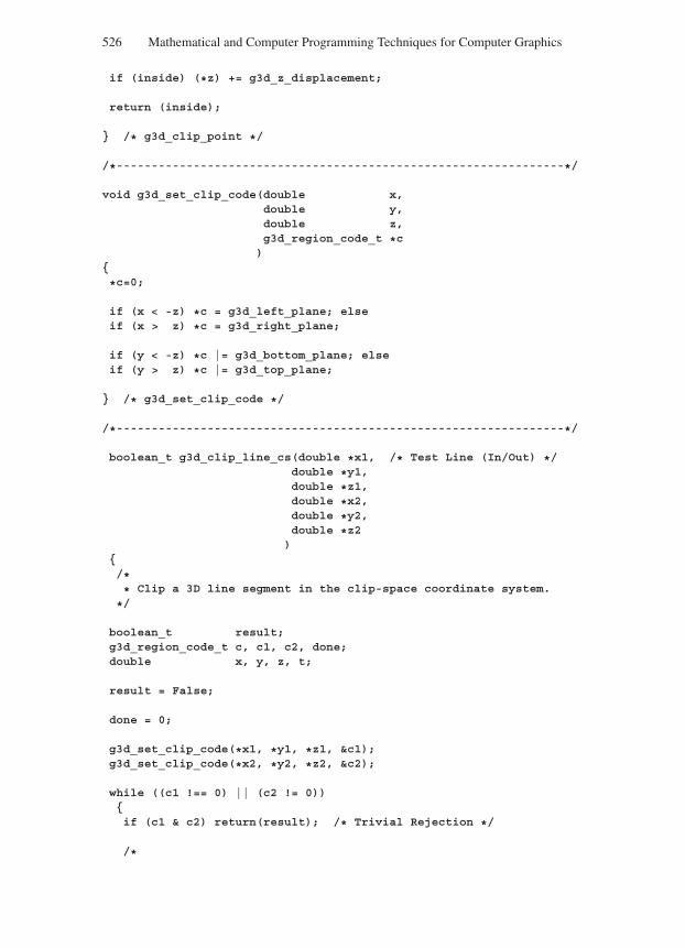
“Comninos” — 2005/8/31 — 18:23 — page 526 — #104
526 Mathematical and Computer Programming Techniques for Computer Graphics
if (inside) (*z) += g3d_z_displacement;
return (inside);
/* g3d_clip_point */
/*----------------------------------------------------------------*/
void g3d_set_clip_code(double x,double y,double z,g3d_region_code_t *c)
*c=0;
if (x < -z) *c = g3d_left_plane; elseif (x > z) *c = g3d_right_plane;
if (y < -z) *c |= g3d_bottom_plane; elseif (y > z) *c |= g3d_top_plane;
/* g3d_set_clip_code */
/*----------------------------------------------------------------*/
boolean_t g3d_clip_line_cs(double *x1, /* Test Line (In/Out) */double *y1,double *z1,double *x2,double *y2,double *z2)
/** Clip a 3D line segment in the clip-space coordinate system.
*/
boolean_t result;g3d_region_code_t c, c1, c2, done;double x, y, z, t;
result = False;
done = 0;
g3d_set_clip_code(*x1, *y1, *z1, &c1);g3d_set_clip_code(*x2, *y2, *z2, &c2);
while ((c1 !== 0) || (c2 != 0))if (c1 & c2) return(result); /* Trivial Rejection */
/*
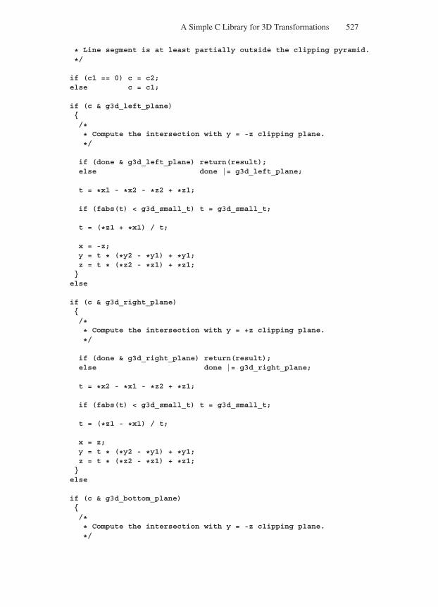
“Comninos” — 2005/8/31 — 18:23 — page 527 — #105
A Simple C Library for 3D Transformations 527
* Line segment is at least partially outside the clipping pyramid.
*/
if (c1 == 0) c = c2;else c = c1;
if (c & g3d_left_plane)/** Compute the intersection with y = -z clipping plane.
*/
if (done & g3d_left_plane) return(result);else done |= g3d_left_plane;
t = *x1 - *x2 - *z2 + *z1;
if (fabs(t) < g3d_small_t) t = g3d_small_t;
t = (*z1 + *x1) / t;
x = -z;y = t * (*y2 - *y1) + *y1;z = t * (*z2 - *z1) + *z1;else
if (c & g3d_right_plane)/** Compute the intersection with y = +z clipping plane.
*/
if (done & g3d_right_plane) return(result);else done |= g3d_right_plane;
t = *x2 - *x1 - *z2 + *z1;
if (fabs(t) < g3d_small_t) t = g3d_small_t;
t = (*z1 - *x1) / t;
x = z;y = t * (*y2 - *y1) + *y1;z = t * (*z2 - *z1) + *z1;else
if (c & g3d_bottom_plane)/** Compute the intersection with y = -z clipping plane.
*/
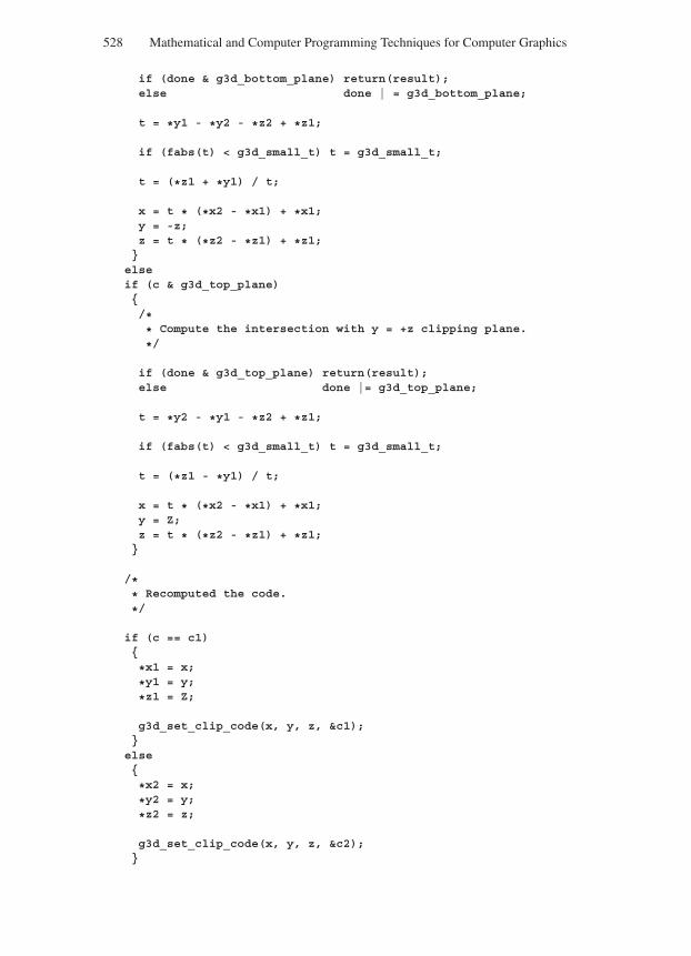
“Comninos” — 2005/8/31 — 18:23 — page 528 — #106
528 Mathematical and Computer Programming Techniques for Computer Graphics
if (done & g3d_bottom_plane) return(result);else done | = g3d_bottom_plane;
t = *y1 - *y2 - *z2 + *z1;
if (fabs(t) < g3d_small_t) t = g3d_small_t;
t = (*z1 + *y1) / t;
x = t * (*x2 - *x1) + *x1;y = -z;z = t * (*z2 - *z1) + *z1;
elseif (c & g3d_top_plane)/** Compute the intersection with y = +z clipping plane.
*/
if (done & g3d_top_plane) return(result);else done |= g3d_top_plane;
t = *y2 - *y1 - *z2 + *z1;
if (fabs(t) < g3d_small_t) t = g3d_small_t;
t = (*z1 - *y1) / t;
x = t * (*x2 - *x1) + *x1;y = Z;z = t * (*z2 - *z1) + *z1;
/** Recomputed the code.
*/
if (c == c1)
*x1 = x;
*y1 = y;
*z1 = Z;
g3d_set_clip_code(x, y, z, &c1);else
*x2 = x;
*y2 = y;
*z2 = z;
g3d_set_clip_code(x, y, z, &c2);

“Comninos” — 2005/8/31 — 18:23 — page 529 — #107
A Simple C Library for 3D Transformations 529
/* while loop */
/** Add a small displacement to the z-coordinates of the line
* segment in order to prevent a potential zero divide in the
* perspective division.
*/
*z1 += g3d_z_displacement;
*z2 += g3d_z_displacement;
return(True);
/ * g3d_clip_line_cs */
“Comninos” — 2005/8/31 — 20:02 — page 531 — #1
Index
A
absolute value of a number, 30absorption, 324
coefficient, 370index, 370
active edge, 303active edge list, 303adjugate matrix, 139affine transformation, 181, 226ajoint matrix, 139algebra of sets, 22algebraic number, 28ambient light, 306ambient light reflection, 306amplitude, 322
reflection coefficient, 365transmission coefficient, 363
angleeye, 308highlight, 309incidence, 309of incidence, 308, 325of reflection, 308, 325of shear, 171, 232-238orientation, 268phase, 309, 365projection, 268reflection, 309
angularfrequency, 323perspective, 272velocity, 323
anisotropic surface, 328
antiparallel vectors, 67antisymmetric matrix, 122area
of a differential spherical patch, 339of the projected polygon, 293
area-coherence property, 296arrow notation, 357Ashikmin-Shirley
diffuse BRDF, 382reflection model, 384shader, 382specular BRDF, 382
axiom, 1axonometric projections, 264-267
B
base vectors, 74basis, 74
Cartesian, 77of a vector space, 158orthogonal, 75orthonormal, 75right-handed, 75
bi-conical reflectance function, 358bi-directional
path-tracing algorithm, 403reflectance distribution function, 351reflectance function, 358scattering distribution function, 358scattering surface reflectance
distribution function, 354transmission distribution function,
353
531
“Comninos” — 2005/8/31 — 20:02 — page 532 — #2
532 Index
bi-hemispherical reflectance function,358
bijection, 45bijective
function, 45mapping, 45
binary space partition tree, 413binormal vector, 332bitangent vector, 332Blinn’s specular reflection function, 310bound vector, 71boundary representation, 393bounded set, 35BRDF, 351BRDF properties
energy conservation property, 356Helmholtz reciprocity property, 355non-negativity property, 355symmetry property, 355
Brewster’s angle, 367bridging edges, 205brightness, 348BSDF, 354BSP-tree, 413BSSRDF, 350BTDF, 353
C
cabinet projection, 268camera, 253cardinal number of a set, 63cardinality of a set, 62, 63Cartesian
basis, 77coordinates, 77product of sets, 37
caustic illumination reflected radianceterm, 417
caustics, 414photon map, 411
cavalier projection, 268central projection, 190centre
of projection, 260point, 254
change of basistransformation, 158, 162transformation matrix, 160
clip polygon, 219clipped polygon, 204clipper polygon, 204clipping,
2D polygon clipping, 202-2233D line clipping, 277-286a 2D line segment to a rectangular
boundary, 194a 2D point to a rectangular boundary,
194bridging edge, 205clip polygon, 219clipped polygon, 204clipper polygon, 204Cohen-Sutherland 2D line-clipping
algorithm, 197false vertex, 219holding list, 219hole contours, 220intersection vertex, 219outline contours, 219perpendicular distance from a point
to a line, 209point of intersection of two lines, 208subject polygon, 219Sutherland-Hodgman 2D
polygon-clipping algorithm, 203trivial acceptance, 198,279trivial rejection, 198,279unclipped polygon, 204Weiler-Atherton 2D
polygon-clipping algorithm, 219clip-space coordinate system, 279closed interval, 32closed-open interval, 32closure, 25co-domain of a function, 39coefficient
of ambient reflection, 306, 375of diffuse reflection, 307, 375, 382of specular reflection, 308, 375, 382
cofactormatrix, 138of an element of a matrix, 138
Cohen-Sutherland2D line-clipping algorithm, 1973D line-clipping algorithm, 279
coherentillumination, 386
“Comninos” — 2005/8/31 — 20:02 — page 533 — #3
Index 533
coherent (continued)image, 359reflection, 359transmission, 359
collinear vectors, 67column matrix, 119column-reversal matrix, 148column-reversed matrix, 148comparable sets, 8complex number, 28colour bleeding, 386, 394, 414, 416complementarity principle, 319complimentary error function, 379components of a vector, 74
relative to an orthogonal basis, 75relative to an non-orthogonal basis,
92composite
function, 48transformation, 166, 167, 172
composition of functions, 48computer image synthesis, 291concatenation
of 2D global transformations, 185of 2D local transformations, 186of 2D transformations, 165of transformation matrices, 181
conceptual camera model, 253condition, 5conducting materials, 325conductors, 325conformable, 128conformal, 128conformant, 128conformity, 128conical-directional reflectance function,
358conical-hemispherical reflectance
function, 358conjecture, 1conjugate error function, 379constant function, 47Cook-Torrance shader, 378coordinate diagram, 37coordinate system
2D transformations of the, 1863D transformations of the, 252clip-space, 279device, 275
coordinate system (continued)image-space, 253left-handed, 254normalised, 187object-space, 253projection-space, 253right-handed, 254screen, 187screen-space, 253, 275world, 187world-space, 253
coordinatesCartesian, 77polar, 169spherical, 332
Copenhagen interpretation of quantumtheory, 319
correlation distance, 380cosine of the angle between two
lines, 106planes, 106vectors, 82
cotangent space, 338critical angle, 328, 367cross product of vectors, 84current path, 410
D
decomposition of a vector according toa basis, 95
degenerate interval, 33delta-x-order, 303depth-buffer, 294, 303depth-coherence property, 302determinant of a matrix, 132determinant rules, 134
conditions for a zero determinant,137
decomposition rule, 136equality rule, 137factor rule, 135interchange rule, 135linear combinations rule, 136product rule, 136transposition rule, 134
device coordinate system, 275diagonal matrix, 120
“Comninos” — 2005/8/31 — 20:02 — page 534 — #4
534 Index
dielectricconstant, 327materials, 325
differentiable manifold, 337differential
area, 342projected area, 344radiant flux, 343radiant power, 343solid angle, 339, 343
diffuseemission, 386inter-object illumination, 386, 394inter-object reflection, 386inter-object transmission, 386light reflection, 306, 375point light sources, 411reflection model, 360reflection, 306, 325
dimension of a vector space, 157dimetric projection, 266Dirac’s delta function, 362direct
illumination model, 385, 386illumination reflected radiance term,
416directed light sources, 412directed segment, 66
initial point of, 66terminal point of, 66
directioncosines of a vector, 82of vector, 65of view, 254ratios of a vector, 82
directional diffuse surface, 372directional-conical reflectance function,
358directional-hemispherical reflectance
function, 358directional-hemispherical reflectance,
356dispersion, 325displacement vector, 66distance
between two non-parallel lines, 105between two parallel lines, 104between two points in space, 101of a point from a line, 103
distance (continued)of a point from a plane, 106
distributed ray-tracing algorithm, 398disturbance of a material, 324domain of a function, 39dot product of vectors, 78dual identity, 24duality principle, 24
E
edge record, 302electromagnetic
radiation, 320spectrum, 320
elementary column transformations,116
empty set, 6equality
of matrices, 124of sets, 6
emission of photons, 411emittance distribution function, 393emitted
radiance, 387radiosity, 391
emitter surface, 387energy
density, 348of a photon, 341preservation, 330
equidirectional vectors, 67equinumerous sets, 63equipollent sets, 62equipotent sets, 62equivalent sets, 62error function, 380estimand, 391estimate, 391Euclid’s postulates, 2Euler diagram, 8excitation, 324excitons, 324exclusive or, 15explicit sampling technique, 411external reflection, 363eye angle, 309eye-path, 404
“Comninos” — 2005/8/31 — 20:02 — page 535 — #5
Index 535
F
face, 291facet, 291false, 1false vertex, 219family of indexed sets, 58finite element radiosity rendering
algorithms, 386fish-eye lens, 276flat polygon shading, 305, 309flux, 341frame-buffer, 294, 303free vector, 71frequency, 322Fresnel effect, 363function, 38
bijective, 45co-domain of a, 39composite, 48constant, 47domain of a, 39formal definition of a, 39graph of a, 54identity, 48injective, 43inverse, 52inverse of a, 49many-to-one, 43one-to-one, 43onto, 44range of a, 43restricted, 39surjective, 44
functionscomposition of, 48equality of, 41types of, 43
fuzzy reflection, 398
G
Gauss function, 379Gaussian elimination, 116general relativity theory, 319generalised set
intersection, 60union, 60
generator of a set, 157geometric attenuation factor, 378
geometry function, 390global
Cartesian frame, 333frame of reference, 184frame transformations, 184illumination model, 385, 387photon map, 414transformations, 184
gloss angle, 380glossiness, 308glossy
reflection model, 359reflections, 372surface, 308, 372
Gouraud smooth shading, 305, 309graph of a function, 54
H
hemispherical-conical reflectancefunction, 358
hemispherical-directional reflectancefunction, 358
hidden-linedrawing, 291elimination algorithm, 294
hidden-surface elimination algorithm,294
highlight angle, 309holding list, 220hole contours, 219homogeneous
coordinates, 190point, 190
homogenised point, 187homogenous materials, 324Horn’s specular reflection function, 309Householder transformation matrix, 361hybrid multi-pass rendering algorithms,
418hypothesis, 1
I
idealdiffuse reflection model, 359specular reflection model, 359
identityfunction, 48
“Comninos” — 2005/8/31 — 20:02 — page 536 — #6
536 Index
identity (continued)matrix, 120transformation, 48
illuminance, 343illuminating hemisphere, 337, 340illumination models, 385image-space
algorithms, 295approach, 394coordinate system, 253rendering algorithms, 395-417
implicit functional representation, 393importance sampling, 416incandescent surface, 387incidence angle, 309incident illuminating hemisphere, 353incoherent
illumination, 386image, 359reflection, 359transmission, 359
incomingcaustics illumination radiance, 415direct illumination radiance, 415indirect illumination radiance, 415radiance, 345, 389
index set, 58indexed
family of sets, 59set, 58
indirect illuminationmodel, 385, 387reflected radiance term, 417
inequalities, 29inequality property
of addition, 29of antisymmetry, 29of division, 30of multiplication, 30of trichotomy, 29of reflexivity, 29of subtraction, 29
injection, 43injective function, 43inner product of vectors, 78insulators, 325integer number, 25, 28interface surface, 325internal reflection, 363
intervalclosed, 32degenerate, 33lower bound of, 32lower limit of, 32of real numbers, 32open, 32upper bound of, 32upper limit of, 32zero-length, 33
intensityarray, 303attenuation function, 311
intersection vertex, 219intersector polygon, 297inverse
function, 52matrix, 132, 140of a function, 49of a vector, 68
invertible matrix, 132, 140irrational number, 25, 27isometric projection, 264isotropic
BRDF, 351surface, 332
K
kd-tree, 413Kronecker δ (delta), 79, 120Kronecker’s symbol, 79, 120
L
Lambert’s law, 306Lambertian diffuse reflection model,
359Lambertian reflection, 306Laplace’s recursive expansion rule, 133leading diagonal of a matrix, 119left triangular matrix, 123left-balanced kd-tree, 408left-handed coordinate system, 254lemma, 2length of a vector, 78, 80light
absorption, 325emission, 347

“Comninos” — 2005/8/31 — 20:02 — page 537 — #7
Index 537
light (continued)reflection, 325refraction, 322scattering, 325, 329transmission, 322transport equation, 389, 390
light-path, 404line diagram, 11line equation defined by
a position vector and a directionvector, 97
two position vectors, 96linear
combination of vectors, 72, 156dependence of vectors, 72, 156independence of vectors, 72, 156linear transformation, 226simultaneous equations, 128, 146space, 153
list-priority algorithms, 295, 299list-priority, 299local
frame of reference, 184frame transformations, 184illumination model, 385, 386surface Cartesian frame, 331transformations, 184
logical proposition, 5lower
bound of interval, 32bounded set, 35illuminating hemisphere, 340limit of interval, 32triangular matrix, 123
luminosity, 348luminous intensity, 348
M
magnitudeof a vector product, 87of a vector, 65, 66, 78, 80
main diagonal of a matrix, 119many-to-one function, 43mapping, 41
bijective, 45many-to-one, 43one-to-one, 43onto, 44
matrixaddition, 125adjugate, 140ajoint, 140algebra theorems, 142, 147-148antisymmetric, 122cofactor of an element of a, 138cofactor, 138column, 119column-reversal, 148column-reversed, 148conformable, 128conformal, 128conformant, 128definition of a, 118determinant of a, 132diagonal, 120equality, 124identity, 120inverse of a, 132, 140invertible, 132, 140leading diagonal of a, 119left triangular, 123lower triangular, 123main diagonal of a, 119minor of a, 131multiplication with a matrix, 129multiplication with a scalar, 126multiplication with a vector, 128non-invertible, 132, 140null, 120operations, 125order, 118orthogonal, 146power of a, 128principal diagonal of a, 119reciprocal of a, 132, 140regular, 132, 140right triangular, 123row, 119row-reversal, 148row-reversed, 148scalar, 124secondary diagonal of a, 119singular, 132, 140skew-symmetric, 122square, 119subtraction, 125symmetric, 122
“Comninos” — 2005/8/31 — 20:02 — page 538 — #8
538 Index
matrix (continued)trace of a, 119trailing diagonal of a, 119transpose of a, 121triangular, 123type, 118unit, 120upper triangular, 123zero, 120representation of 2D transformations,
178matrix algebra axioms and rules,
149-151Metropolis light transport algorithm,
409micro-facet slope distribution function,
378, 380minor of a matrix, 131mirror-like reflection, 325MLT, 409modified Phong shader, 378modulus of a number, 30Monte Carlo
estimate, 391integration, 391method, 391ray-tracing rendering algorithms, 388
multiplicationof a matrix by a matrix, 129of a matrix by a scalar, 126of a matrix by a vector, 128of a scalar by a vector, 74of a vector by a vector, 127
multi-view orthographic projection, 262mutated path, 410
N
natural number, 25, 27negative vector, 68Newell, Newell and Sancha algorithm,
299Newell’s plane equation, 292non-homogenous materials, 324non-invertible matrix, 132, 140normalised vector, 80normalising a vector, 80null
matrix, 120
null (continued)set, 6vector, 66
numberabsolute value of a, 30algebraic, 28complex, 28integer, 25irrational, 25, 27modulus of a, 30natural, 25, 27rational, 25real, 26sets, 25transcendental, 28whole, 25
O
object-spacealgorithms, 295approach, 394coordinate system, 253rendering algorithms, 394-395
obliqueprojection matrix, 270projection, 267
one-point perspective projection, 272one-to-one
correspondence, 45function, 43mapping, 43
ontofunction, 44mapping, 44
opaque materials, 325open interval, 32open-closed interval, 32operator, 41opposite vectors, 67ordered
2-tuple, 363-tuple, 36n-tuple, 36pair, 36triple, 36triplet, 36
orientationangle, 268
“Comninos” — 2005/8/31 — 20:02 — page 539 — #9
Index 539
orientation (continued)vector, 71
orthogonalbasis, 75matrix, 146
orthographicprojection matrix, 267projection, 262-267
orthonormal basis, 75outer product of vectors, 84outgoing radiance, 345, 387outline contours, 219
P
parallelperspective projection, 272projection, 260, 262-271vectors, 67
participatingmaterials, 325media, 325
path-tracing algorithm, 400perfect mirror specular reflection
model, 359period, 322permeability, 327permittivity, 324, 327perpendicular distance from a point to a
line, 102, 209perspective
depth, 287projection, 260, 271projection matrix, 270
phaseangle, 309, 365, 369shift, 365, 369
Phongshader, 375smooth shading, 305, 315
Phong’s lighting model, 311-313for coloured light sources, 312for distant light sources, 311for multiple light sources, 311
phosphorescent surface, 387photoelectric effect, 319photon, 319
density estimation, 413energy, 319
photon (continued)map, 411mapping technique, 411mapping, 411rays, 411volume density, 345
photon-mappingpass, 411technique, 411
photon-tracing algorithm, 412physically-based rendering algorithms,
393pixel, 294planar geometric projection, 261Planck’s constant, 323plane of incidence, 363polarisation of light, 363plane equation defined by
a position vector and a normal vector,98
three position vectors, 99p-obscures-q test, 301P-polarised light, 363point of intersection of two lines, 208polygon
clipping, 202-203rule, 70span, 303
polygon-index order, 303position vector, 71postulate, 1power
of a matrix, 128set of a set, 63
primaryestimator, 391ray, 396
primitive transformation, 167principal diagonal of a matrix, 119product
Cartesian, 37cross, 84, 127dot, 78, 127dyadic, 127inner, 78of 2D transformations, 165of a matrix by a matrix, 129of a matrix by a scalar, 126of a matrix by a vector, 128
“Comninos” — 2005/8/31 — 20:02 — page 540 — #10
540 Index
product (continued)outer, 84scalar, 78tensor, 127triple scalar, 88triple vector, 90
projectedincident irradiance, 348irradiance, 347solid angle, 340, 346, 349
projectionangle, 268axonometric, 264-267cabinet, 268cavalier, 268central, 190centre of, 260dimetric, 266isometric, 268multi-view orthographic, 262oblique, 267oblique projection matrix, 270of a vector, 81one-point perspective, 272orthographic, 262-267orthographic projection matrix, 267parallel, 260, 262-271parallel perspective, 272perspective, 260, 271perspective projection matrix, 273planar geometric, 261plane, 260transformation, 253, 260-277
projective map, 192projectors, 260proof, 2proper
subset, 7superset, 7
properties ofreal number intervals, 34vector products, 86
proposition, 1
Q
quadrature, 391quanta, 320
R
radiance, 344radiant
energy, 341exitance, 344flux, 341intensity, 344, 347-348power, 341
radiosity, 344algorithm, 394equation, 391
range of a function, 43raster scan display, 294rational number, 25real number, 26
interval, 32interval arithmetic, 34line, 26
reciprocal matrix, 132, 140recursive ray-tracing algorithm, 396reflectance
coefficient, 366equation, 355
reflectance functionbi-conical, 358bi-directional, 358bi-hemispherical, 358conical-directional, 358conical-hemispherical, 358directional-conical, 358directional-hemispherical, 358hemispherical-conical, 358hemispherical-directional, 358
reflectedilluminating hemisphere, 353radiance, 388
reflection modelglossy, 359ideal specular, 359Lambertian diffuse, 359perfect mirror specular, 359
reflection, 325angle, 309function, 349models, 305-313, 359vector, 335
reflectivity, 367; see also reflectancecoefficient
“Comninos” — 2005/8/31 — 20:02 — page 541 — #11
Index 541
refraction, 325refractive index, 327regular matrix, 132, 140rejection sampling technique, 411relative permittivity, 327relativistic mass, 323renderer, 295rendering, 295
algorithms, 294-305equation, 385pass, 411, 414
rest energy, 324restricted function, 39resultant vector, 69retro-reflection, 325right triangular matrix, 123right-handed coordinate system, 254RMS roughness, 380root mean square roughness, 380rough specular surface, 372row matrix, 119row-reversal matrix, 148row-reversed matrix, 148Russian roulette procedure, 401, 403,
412
S
Sancer’s geometric attenuationfunction, 380
scalar, 65field, 153matrix, 124multiplication, 68
scalar productof four vectors, 91of two collinear vectors, 82of two orthogonal vectors, 82of two vector products, 91of two vectors, 78
scan-convert, 303scattering, 325, 349
and tracing of photons, 412equation, 354function, 349
screen subdivision algorithm, 296screen-space coordinate system, 253,
275
secondarydiagonal of a matrix, 119estimate, 391
semi-coherentreflections, 372surface, 372
setbounded, 35cardinal number of a, 63cardinality of a, 62, 63complement of a, 18difference, 13element, 4empty, 6equality, 6finite, 4, 6generator of a, 157index, 58infinite, 4, 6intersection, 12lower bounded, 35mapping of a, 41member, 4membership, 5notation, 4null, 6operator on a, 41power set of a, 63size of a, 62span of a, 157spanning set of a, 157specification, 4tabular form, 4theory theorems, 19-23, 53-54transformation on a, 41unbounded, 35union, 11universal, 8upper bounded, 35
set-comprehension form, 4sets
algebra of, 22Cartesian product of, 37comparable, 8disjoint, 8equinumerous, 63equipollent, 62equipotent, 62equivalent, 62
“Comninos” — 2005/8/31 — 20:02 — page 542 — #12
542 Index
sets (continued)family of indexed, 58generalised intersection of, 60generalised union of, 60indexed family of, 59indexed, 58symmetric difference of two, 14
shade value, 313shaded image, 291shading
algorithm, 294techniques, 305, 313-316
shadow ray, 396, 398, 403, 416simple rendering algorithm, 295single scan-line depth-buffer algorithm,
302singleton, 33singular matrix, 132, 140size of a set, 62skew-symmetric matrix, 122Snell’s law, 328solid
angle, 338representation, 393
span of a vector space, 157spanning set of a vector space, 157special relativity theory, 319spectral
flux, 341radiant energy, 341radiant flux, 341
specularemission, 386illumination reflected radiance term,
416inter-object illumination, 386, 394inter-object reflection, 386inter-object transmission, 386light reflection, 306, 308reflection function, 308reflection model, 361reflection, 308, 325sharpness, 308
speedinvariant mass, 323of light, 322
sphericalcoordinates of a vector, 333light sources, 411
S-polarised light, 363square
light sources, 412matrix, 119
steradian, 338steradians, 338storage of photons, 412subject polygon, 219subset, 6subsurface scattering, 325, 330, 349,
351, 383superset, 7surface
field radiance, 345radiance, 345reflectance function, 356transmittance function, 358
surface typedirectional diffuse, 372glossy, 372rough specular, 372semi-coherent, 372wide and narrow diffuse, 372
surjection, 44surjective function, 44surrounder polygon, 297Sutherland-Hodgman 2D polygon-
clipping algorithm, 203symmetric matrix, 122
T
tangent space, 334telephoto lens, 276theorem, 2theory of light, 317three-point
form, 389, 390perspective projection, 271
topological sort, 299total internal reflection, 328, 367totally
coherent reflection, 360coherent transmission, 360incoherent reflection, 360incoherent transmission, 360
trace of a matrix, 119trailing diagonal of a matrix, 119transcendental number, 28
“Comninos” — 2005/8/31 — 20:02 — page 543 — #13
Index 543
transformation, 41between general bases, 158between orthonormal bases, 161
transformations,2D, 165-1902D global frame of reference, 1842D global frame transformations, 1842D global transformations, 1842D local frame of reference, 1842D local frame transformations, 1842D local transformations, 1842D primitive, 1672D reflection about an arbitrary axis,
1752D reflection about the origin, 1722D reflection about the x-axis, 1722D reflection about the y-axis, 1722D rotation about an arbitrary point,
174, 1822D rotation about the origin, 168, 1802D scaling about an arbitrary point,
1732D scaling about the origin, 167, 1802D shearing along the x-axis, 171,
1802D shearing along the y-axis, 171,
1802D transformation matrix properties,
1812D transformations of the coordinate
system, 1862D transformations of the frame of
reference, 1862D translation, 168, 1802D viewing, 1872D viewporting, 1882D windowing, 1873D, 225-2903D aiming the local x-axis, 2423D aiming the local y-axis, 2433D aiming the local z-axis, 2443D aiming, 244-2443D change of frame of reference,
238-2413D composite transformations
relative to a major axis, 2463D composite transformations
relative to a major plane, 249
transformations (continued)3D composite transformations
relative to a plane, 249-2513D composite transformations
relative to a point, 245-2463D composite transformations
relative to an arbitrary axis, 2483D composite transformations
relative to an arbitrary plane,250
3D composite transformationsrelative to an arbitrary point,246
3D composite transformationsrelative to an axis parallel to amajor axis, 247
3D composite transformationsrelative to an axis, 246-249
3D composite transformationsrelative to the origin of theframe, 245
3D composite, 245-2513D local frame, 2513D primitive, 226-2383D reflection about an arbitrary axis,
2483D reflection about an arbitrary
plane, 2503D reflection about an arbitrary
point, 2463D reflection about an axis parallel to
a major axis, 2473D reflection about the origin of the
frame, 2453D reflection about the x-axis, 2463D reflection about the y-axis, 2463D reflection about the z-axis, 2463D reflection about xy-plane, 2493D reflection about xz-plane, 2493D reflection about yz-plane, 2493D rotation about a coordinate axis,
228-2313D rotation about an arbitrary axis,
2483D rotation about an axis parallel to a
major axis, 2473D rotation about the x-axis, 229

“Comninos” — 2005/8/31 — 20:02 — page 544 — #14
544 Index
transformations (continued)3D rotation about the y-axis, 2303D rotation about the z-axis, 2283D scaling about the origin, 2273D scaling along an arbitrary axis,
2483D scaling along an axis parallel to a
major axis, 2473D shearing the x-axis parallel to the
y-axis, 2323D shearing the x-axis parallel to the
z-axis, 2333D shearing the y-axis parallel to the
x-axis, 2343D shearing the y-axis parallel to the
z-axis, 2353D shearing the z-axis parallel to the
x-axis, 2363D shearing the z-axis parallel to the
y-axis, 2373D shearing, 231-2383D transformations of the coordinate
system, 2523D transformations of the frame of
reference, 2523D translation along an arbitrary
axis, 2483D translation, 227affine, 226composite 2D, 166, 167, 172concatenation of 2D global, 185concatenation of 2D local, 186concatenation of 2D, 165concatenation of the matrices of 2D,
181linear, 226matrix representation of 2D, 178product of 2D, 165projection, 253, 260-277viewing, 253, 255-259viewporting, 253
translucent materials, 325transmission, 320
angle, 327models, 359vector, 335
transmittancecoefficient, 366equation, 354
transmitted illuminating hemisphere,353
transparent materials, 325transport theory, 342transpose matrix, 121transverse wave, 321triangle rule, 69triangular matrix, 123trimetric projection, 266triple
products of vectors, 88scalar product, 88vector product, 90
trivial acceptance, 198, 279trivial rejection, 198, 279true, 1two-point perspective projection, 272
U
unbound vector, 71unbounded set, 35unclipped polygon, 204unit matrix, 120universal set, 8upper
bound of interval, 32bounded set, 35illuminating hemisphere, 340limit of interval, 32triangular matrix, 123
V
vanishing point, 271-272vector, 65
addition, 69, 74bases, 74bound, 71components of a, 74difference, 70direction cosines of a, 82direction of a, 65direction ratios of a, 82displacement, 66equation of a line, 71free, 71inverse of a, 68length of a, 78, 80magnitude of a, 65, 66, 80multiplication of a scalar by a, 74
“Comninos” — 2005/8/31 — 20:02 — page 545 — #15
Index 545
vector (continued)negative, 68, 77normalised, 80normalising a, 80null, 66orientation, 71position, 71product of vectors, 84projection of a, 81resultant, 69subtraction, 70, 74unbound, 71zero, 66
vectorsantiparallel, 67base, 74collinear, 67cosine of the angle between two, 82cross product of, 84dot product of, 78equality of, 74equidirectional, 67inner product of, 78linear combination of, 72linear dependence of, 72linear independence of, 72opposite, 67outer product of, 84parallel, 67scalar product of collinear, 82scalar product of orthogonal, 82scalar product of, 78triple products of, 88triple scalar product of, 88triple vector product of, 90vector product of two, 84
vector algebra axioms and rules,110-113
vector equationof the line, 96, 97of the plane, 98, 99
vector product, 84magnitude of a, 87of four vectors, 91of two vector products, 91properties of a, 86
vector spacebasis of a, 157definition, 154-156dimension of a, 157
span of a, 157spanning set of a, 157transformation between bases of a,
158transformation between orthonormal
bases of a, 161Venn diagram, 8viewing
axis, 254distance, 255point, 254pyramid 255, 277transformation, 253, 255-259
viewport, 255viewporting transformation, 253visibility function, 389visibility-ordering, 299
W
Warnock algorithm, 296wave number, 323wavelength, 322wave-particle duality theory, 319wavicle, 319Weiler-Atherton 2D polygon-clipping
algorithm, 219wide and narrow diffuse surface, 372wide-angle lens, 276window, 255wire-frame drawing, 295world-space coordinate system, 253
X
XOR, 15x-order, 303
Y
y-bucketlist, 302sort, 302
Z
z-buffer, 294, 303zero
matrix, 120vector, 66
zero-length interval, 33
“Comninos” — 2005/8/31 — 20:02 — page 546 — #16
546 Index
Symbols
A, 28C, 28N, 27R, 26Q, 26T, 28Z, 28↑↑, 67↑↓, 67||, 67|, 4:, 4∈, 5∈, 5Ø, 6∪, 11∩, 12⊂, 7⊆, 6⊃, 7⊇, 7, 14⊕, 15⊗, 84×, 25, 37, 48∼, 62-, 13
2D
clippinga line segment to a rectangular
boundary, 194a point to a rectangular boundary,
194Cohen-Sutherland 2D line-clipping
algorithm, 197composite transformation, 166, 167,
172concatenation
of global transformations, 185of local transformations, 186of transformation matrices, 181of transformations, 165
globalframe of reference, 184frame transformations, 184
global (continued)transformations, 184
homogeneouscoordinates, 190point, 190
homogenised point, 191local
frame of reference, 184frame transformations, 184transformations, 184
matrix representation oftransformations, 178
normalised coordinate system, 187perpendicular distance from a point to a
line, 209point of intersection of two lines, 208polygon clipping, 202-223primitive transformation, 167product of transformations, 165screen coordinate system, 187transformation, 165
matrix properties, 181of reflection about an arbitrary axis,
175of reflection about the origin, 172of reflection about the x-axis, 172of reflection about the y-axis, 172of rotation about an arbitrary point,
174, 182of rotation about the origin, 168, 180of scaling about an arbitrary point,
173of scaling about the origin, 167, 180of shearing along the x-axis, 171, 180of shearing along the y-axis, 171, 181of the coordinate system, 186of the frame of reference, 186of translation, 168, 180viewing, 187viewporting, 188windowing, 187
Weiler-Atherton 2D polygon-clippingalgorithm, 219
world coordinate system, 187
3D
affine transformation, 226aiming transformations, 244-244
“Comninos” — 2005/8/31 — 20:02 — page 547 — #17
Index 547
change of frame of referencetransformation, 238-241
Cohen-Sutherland 3D line-clippingalgorithm, 279
composite transformations, 245-251relative to a major axis, 246relative to a major plane, 249relative to a plane, 249-251relative to a point, 245-246relative to an arbitrary axis, 248relative to an arbitrary plane, 250relative to an arbitrary point, 246relative to an axis parallel to a major
axis, 247relative to an axis, 246-249relative to the origin of the frame,
245global frame of reference, 238, 251line clipping, 277-286linear transformation, 226local frame
of reference, 238, 251transformations, 251
primitive transformations, 226-238shearing transformations, 231-238transformation, 225
of aiming the local x-axis, 242of aiming the local y-axis, 243of aiming the local z-axis, 244of reflection about an arbitrary axis,
248of reflection about an arbitrary plane,
250of reflection about an arbitrary point,
246of reflection about an axis parallel to
a major axis, 247of reflection about the origin of the
frame, 245
of reflection about the x-axis, 246of reflection about the y-axis, 246of reflection about the z-axis, 246of reflection about xy-plane, 249of reflection about xz-plane, 249of reflection about yz-plane, 249of rotation about a coordinate axis,
228-231of rotation about an arbitrary axis,
248of rotation about an axis parallel to a
major axis, 247of rotation about the x-axis, 229of rotation about the y-axis, 230of rotation about the z-axis, 228of scaling about the origin, 227of scaling along an arbitrary axis, 248of scaling along an axis parallel to a
major axis, 247of shearing the x-axis parallel to the
y-axis, 232of shearing the x-axis parallel to the
z-axis, 233of shearing the y-axis parallel to the
x-axis, 234of shearing the y-axis parallel to the
z-axis, 235of shearing the z-axis parallel to the
x-axis, 236of shearing the z-axis parallel to the
y-axis, 237of translation along an arbitrary axis,
248of translation, 227of the coordinate system, 252of the frame of reference, 252


