Mathematical multi-scale model of the cardiovascular system including mitral valve dynamics. Application to ischemic mitral insufficiency

RESEARCH Open Access

Mathematical multi-scale model of thecardiovascular system including mitral valvedynamics. Application to ischemic mitralinsufficiencySabine Paeme1*, Katherine T Moorhead1, J Geoffrey Chase2, Bernard Lambermont1, Philippe Kolh1, Vincent D’orio1,Luc Pierard1, Marie Moonen1, Patrizio Lancellotti1, Pierre C Dauby1 and Thomas Desaive1

* Correspondence: [email protected] Research Center,University of Liege, Liege, BelgiumFull list of author information isavailable at the end of the article

Abstract

Background: Valve dysfunction is a common cardiovascular pathology. Despitesignificant clinical research, there is little formal study of how valve dysfunctionaffects overall circulatory dynamics. Validated models would offer the ability to betterunderstand these dynamics and thus optimize diagnosis, as well as surgical andother interventions.

Methods: A cardiovascular and circulatory system (CVS) model has already beenvalidated in silico, and in several animal model studies. It accounts for valve dynamicsusing Heaviside functions to simulate a physiologically accurate “open on pressure,close on flow” law. However, it does not consider real-time valve opening dynamicsand therefore does not fully capture valve dysfunction, particularly where thedysfunction involves partial closure. This research describes an updated version ofthis previous closed-loop CVS model that includes the progressive opening of themitral valve, and is defined over the full cardiac cycle.

Results: Simulations of the cardiovascular system with healthy mitral valve areperformed, and, the global hemodynamic behaviour is studied compared withpreviously validated results. The error between resulting pressure-volume (PV) loopsof already validated CVS model and the new CVS model that includes theprogressive opening of the mitral valve is assessed and remains within typicalmeasurement error and variability. Simulations of ischemic mitral insufficiency arealso performed. Pressure-Volume loops, transmitral flow evolution and mitral valveaperture area evolution follow reported measurements in shape, amplitude andtrends.

Conclusions: The resulting cardiovascular system model including mitral valvedynamics provides a foundation for clinical validation and the study of valvulardysfunction in vivo. The overall models and results could readily be generalised toother cardiac valves.

Paeme et al. BioMedical Engineering OnLine 2011, 10:86http://www.biomedical-engineering-online.com/content/10/1/86

© 2011 Paeme et al; licensee BioMed Central Ltd. This is an Open Access article distributed under the terms of the Creative CommonsAttribution License (http://creativecommons.org/licenses/by/2.0), which permits unrestricted use, distribution, and reproduction inany medium, provided the original work is properly cited.

mailto:[email protected]

mailto:[email protected]

http://creativecommons.org/licenses/by/2.0

BackgroundMitral insufficiency (MI) is a frequent valvular pathology that develops as a result of

dysfunction or modification in one of the elements of the mitral valvular complex

(leaflets, tendinous chords, papillary muscles, left atrial wall or ventricular myocardium

located next to papillary muscles). During MI, blood in the left ventricle flows back

through the mitral valve towards the left atrium due to the loss of integrity of the

valve, and a loss of the atrio-ventricular pressure gradient during systole [1-3]. The

presence of a MI leads to a chronic overload in volume which is responsible for left

ventricular dilatation, which, in its turn, increases the mitral insufficiency [3].

Ischemic mitral insufficiency (IMI) results from a ventricular remodeling usually fol-

lowing myocardial infarction. It is observed in 15 to 30% of the patients after acute

myocardial infarction [4] and in 56% of the patients having a chronic left ventricular

systolic dysfunction (ejection fraction < 40%) [5]. IMI is a dynamic condition whereby

the severity of the regurgitation changes with time. This dynamic behavior can be

responsible for the non-detection of the insufficiency for certain patients at high risk

of morbidity and mortality [6,7]. Recent clinical studies have detected and quantified

this dynamic behavior using Doppler echography [3].

As it is well-known mathematical models of the cardiovascular system (CVS) offer a

promising method of assisting in understanding cardiovascular dysfunction, this

research propose such a model to study IMI.

Mathematical models of the CVS vary significantly in their complexity and their

objectives. They range from the simple Windkessel model [8], a zero-dimensional

model, to very complex network representations of the vascular tree [9] or even finite

element models of several million degrees of freedom [10,11]. All of them have differ-

ent uses or goals, but they all share the common goal of understanding non invasively

the cardiovascular function [12].

One example of low to intermediate complexity model, known as a “minimal cardiac

model”, has been developed and optimized [13-15] to assist health professionals in

selecting reliable and appropriate therapies for Intensive Care Unit (ICU) patients. It is

based on a “pressure-volume” (PV) lumped element modeling approach, the principle

of which is that the continuous variation of the system’s state variables in space is

represented by a finite number of variables, defined at special points called nodes [12].

The cardiovascular system is thus divided into several chambers described by their

own PV relationship [13,16]. The main advantage of this technique is that it only

requires a small number of parameters, allowing for easy and rapid simulations and for

patient-specific identification of disease state at the bedside with readily available clini-

cal data [17-19].

This model has been proven to provide reliable description of the global cardiac

function in several disease states such as pulmonary embolism and septic shock

[20,21]. However, it does not allow for the description of lower anatomical scales, such

as the valvular level.

The simplest description of the heart valve used in 0D CVS models represents the

valve as a diode plus a resistance [9,16,22-24]. This description assumes the ideal charac-

teristic of one-way flow in a heart valve, while more complex dynamics, such as regurgi-

tant flow, can’t be simulated. Žáček and Krause [25] used time dependent drag

coefficients in a way that valve closing is achieved by letting the drag coefficient


Page 2 of 20

approach infinity. This model improves heart valve modelling, but the leaflet motion was

prescribed instead of computed. An attempt to describe the progressive opening of the

mitral valve based on physical properties of the valve was made by Szabó et al.

[12,26-28]. However, their model is only valid during the early ventricular filling phase

also referred to as E-wave filling. As we want to keep the minimal model’s simplicity and

therapeutic use, we can’t use other valve models that are either too complex or/and do

not account for dynamics over a full cardiac cycle [29-31].

This paper presents a minimal closed-loop model of the CVS including a description

of the progressive opening and closing of the mitral valve at more refined scale. This

new multi-scale model is validated for a healthy mitral valve. The impact of the pro-

gressive opening and closing of the mitral valve on circulatory dynamics is analyzed,

with emphasis on IMI. Clinically, understanding this impact and the ability to identify

it from clinical data would lead directly to new model-based diagnostic capabilities.

MethodsThis section first describes the existing and previously validated minimal model of the

cardiovascular system, on which our model is based. Then, it describes a model of the

mitral valve and its integration into the CSV model. Finally, methods used to analyse

and criticize the results are presented.

CVS model

The CVS model used to describe the cardiovascular system was first described by

Smith et al [13] and has already been validated in silico and in several animal model

studies [15,17,20,21,32,33]. It is a lumped parameter model consisting of six elastic

chambers, the left ventricle (lv), the right (rv) ventricle, the vena cava (vc), the aorta

(ao), the pulmonary artery (pa) and the pulmonary veins (pu), linked by vessels

presenting a resistance to the blood flow. The diagram of this model is presented in

Figure 1.

The systemic and pulmonary circulation networks are modelled by the resistances

Rsys and Rpul, respectively, while the cardiac valves are modeled by a resistance and a

diode that opens when the pressure upstream exceeds the pressure downstream and

Figure 1 Cardiovascular system model consisting of 6 cardiac chambers, vascular flow resistances,on/off heart valves and including ventricular interaction. The 6 cardiac chambers are the left ventricle(lv), the right (rv) ventricle, the vena cava (vc), the aorta (ao), the pulmonary artery (pa) and the pulmonaryveins (pu). Systemic and pulmonary circulation flow resistances are Rsys and Rpul. The cardiac valves aremodeled by a resistance (Rmt, Rao, Rtc and Rpv) and a diode. Inertia of the blood in the aorta andpulmonary artery are described by hydraulic inductances (Lav and Lpv, respectively).


Page 3 of 20

closes when the flow of blood is reversed. Inertia of the blood in the aorta and

pulmonary artery are described by hydraulic inductances (Lav and Lpv, respectively) at

the exit of the ventricles. The model takes into account ventricular interaction by

means of the displacement of the septum, as it was found to have a significant impact

on the cardiovascular system dynamics [13,34-36].

Each cardiac chamber is described by its pressure (P) -volume (V) relationship and

provides volume and flow conditions around the physiological elements modelled by

the resistances. Both cardiac chambers describing the ventricles are active. The relation

linking the pressure to the volume is therefore not fixed and can be expressed by

means of a time varying elastance (E(t)), an intrinsic property of each active cardiac

chamber defined as:

E(t) =P(t)V(t)

(1)

This PV relationship varies between the PV relationships at the end of systole

(ESPVR) and at the end of diastole (EDPVR), as shown on Figure 2.

ESPVR : PES(V) = EES(V − Vd) (2)

EDPVR : PED(V) = P0(eλ(V−V0) − 1) (3)

Where PES is the end-systolic pressure, EES the end-systolic elastance, V the volume,

Vd the volume at zero pressure, PED the end-diastolic pressure and P0, l, V0 are three

parameters of the nonlinear relationship.

The transition between these two extremities is realised by several quasi-linear PV

relationships, the slope of which is given by the activation function, also named the

driver function, e(t) :

e(t) =N∑

i=1

Aie−Bi((t mod Di)−Ci)2

(4)

Figure 2 Overview of a pressure-volume loop stuck between the pressure-volume relationships atthe end of systole (ESPVR) and at the end of diastole (EDPVR).


Page 4 of 20

With the number of Gaussians N = 1, the magnitude A1 = 1, the width B1 = 80s-2 ,

the delay C1 = 0.27 s and the duration of a cardiac cycle D1 = 1s, as defined in Smith

et al. [15]. Heart rate (HR beats/min) does not appear explicitly, but it is used to deter-

mine the value of one diver function parameter, D1 = 60/HR. This model doesn’t use

ECG data, but information relative to timing, delay and duration of the ventricular

contraction is contained in the driver function parameters. This activation function

accounts for myocardial activation and drives the changes in elastance. It varies

between 0 and 1.

Then, the pressure in the ventricle at any time t of a cardiac cycle is linked to the

volume by:

P(t) = e(t)×EES(V(t) − Vd)

+ (1 − e(t))

× P0(eλ(V(t)−V0) − 1)

(5)

The 4 elastic cardiac chambers representing the major blood vessels are passive and

the pressure is assumed to be proportional to the volume of the chamber. The con-

stant ratio of P/V is denoted E and represents the so-called elastance of the chamber.

The behaviour of each chamber is characterised by the flow in and out of the cham-

ber (Qin, Qout), the pressure upstream and downstream (Pup, Pdown), the resistances of

the valves (Rin, Rout), and inertia of the blood (Lin, Lout) [13], yielding:

dVdt

= Qin − Qout (6)

dQin

dt=

Pup − P − QinRin

Lin(7)

dQout

dt=

Pdown − P − QoutRout

Lout(8)

Equations 6 and 7 are solved when Qin > 0, during the filling stage, and Equations 6

and 8 are solved when Qout > 0, during the ejection stage. During the iso-metric

expansion and contraction phases, the model becomes much simpler, with volume and

pressure linked by Equation 5.

Four cardiac valves are located in the heart, at the entrance and the exit of each ven-

tricle. On Figure 1, these are represented by the electric symbol of a diode. Relations 7

and 8 describe the flows, but do not take into account the presence of valves regulating

the flow. Indeed, they allow backflow (i.e. a negative blood flow) in the system. The

physiological role of valves is exactly to prevent backflow by closing. To correctly

model the effect of the valves, a negative flow must be replaced by no flow. It can be

very simply modeled by replacing every appearance of a flow (Q) controlled by a valve

by (H(Q) Q), where the notation H denotes the function of Heaviside [14], defined by:

H(x) =

{0 if x ≤ 0

1 if x > 0(9)

The introduction of this H function allows to describe the “close on flow” property

[13,15] of the valve. To describe the “open on pressure” property [13,15], another H


Page 5 of 20

function must be introduced in Equations 7 and 8, to allow blood flow (Q) from the

time when upstream pressure is higher than downstream pressure, until the time when

blood flow becomes negative. It is written. H((Pup - Pdown) + Q - 0.5).

Finally, the overall hemodynamic model reads the system of differential equations

(Equations 10 to 19):

dVpu

dt= H(Qpul)Qpul − H(Qmt)Qmt (10)

dQmt

dt= H(H(Ppu − Plv) + H(Qmt)

−0.5)

× [(1

/Lmt)

((Ppu − Plv )

−Qmt Rmt)]

(11)

dVlv

dt= H(Qmt)Qmt − H(Qav)Qav (12)

dQav

dt= H(H(Plv − Pao) + H(Qav)

−0.5)

× [(1

/Lav)

((Plv − Pao)

−Qav Rav)]

(13)

dVao

dt= H(Qav)Qav − H(Qsys)Qsys (14)

dVvc

dt= H(Qsys)Qsys − H(Qtc)Qtc (15)

dQtc

dt= H(H(Pvc − Prv) + H(Qtc)

−0.5)

× [(1

/Ltc)

((Pvc − Prv)

−Qtc Rtc)]

(16)

dVrv

dt= H(Qtc)Qtc − H(Qpv)Qpv (17)

dQpv

dt= H(H(Prv − Ppa) + H(Qpv)

−0.5)

× [(1

/Lpv)

((Prv − Ppa)

−Qpv Rpv)]

(18)

dVpa

dt= H(Qpv)Qpv − H(Qpul)Qpul (19)

Mitral valve model

The main drawback of using the Heaviside functions to model the behaviour of the

valves, is that this cannot take into account the physiological time scale of valve


Page 6 of 20

opening [37]. Therefore, the initial model introduced above is not able to fully capture

valve dysfunctions.

As mentioned previously, an attempt to describe the progressive opening of the

mitral valve was made by Szabó et al. [12,26-28] to assess diastolic left ventricular

function based on Doppler velocity waveforms and cardiac geometry. The Szabó et al.

model of early ventricular filling [12,28] begins at the time of mitral valve opening,

when the pressures in the atrium and ventricle are equal and it describes the flow and

pressure during ventricular filling until the atrial systole. The input pressure difference

profile, ΔP(t), shown in Figure 3 was taken from measured animal data [37]. This pres-

sure difference was inferred from left atrial pressure (Pla) and left ventricular pressure

(Plv) profiles, measured invasively with catheters. The two peaks in valve opening

angle θ(t) evolution in Figure 3 refer to the E-wave and A-wave, which correspond to

the passive filling of the ventricle and the active filling resulting from atrial contraction,

respectively.

The main limitation of the mitral valve model by Szabó et al. is that it is only valid

during a small part of the cardiac cycle (the E-wave). To couple the mitral valve model

with the existing closed-loop CVS model, the model must be valid over a complete

cardiac cycle. However, the existing CVS model does not include a chamber for the

left atrium so it does not strictly capture atrial systole, also referred to as the A-wave

[13]. In this research, the mitral valve dynamics during the active filling phase is

assumed to be the same as during the passive filling phase so that all valvular para-

meters fixed by Szabo [12,28] are now used over the entire cardiac cycle. The A-wave

is therefore not modelled.

Figure 3 Animal data [37]showing measured Pla, Plv and theta, and the calculated ΔP. Pla and Plvprofiles were measured invasively with catheters. This animal data also consisted of distancemeasurements of the amount the chords moved during a heartbeat, as measured by camera in a catheteror endoscope. It was assumed the movement of the chords would reasonably correlate to the change inopening angle, θ(t).


Page 7 of 20

As proposed by Szabo [12,28], a system of three ordinary differential equations can

be used to describe the dynamics of the mitral valve. The first equation describes the

flow rate through the mitral valve (Qmt). Thus, the corresponding equation from the

original CSV model has been modified to add a term that accounts for the variation in

the cross-sectional area of the mitral aperture. The differential equation then becomes:

Q·mt =

Ppu − Plv

Lmt− Qmt

Rmt

Lmt+ Qmt

A(t)A(t)

(20)

Where:

Ppu = pulmonary veins pressure

Plv = left ventricular pressure

Qmt = instantaneous flow rate through the mitral valve

Rmt = mitral viscous resistance

Lmt = mitral inertance term

A = area of mitral valve aperture

The resistance and the inertance of the mitral valve, Rmt and Lmt, are defined to take

into account the existence of two states of the mitral valve (open and close). Therefore,

the “open on pressure, close on flow” law is no longer required in the equation defin-

ing the dynamics of transmitral blood flow. Thus, the H (H(Ppu - Plv) + H (Qmt) - 0.5)

and H (Qmt) factors can be removed from Equation 10, 11 and 12.

When the valve is open, Rmt, is low and when the valve is closed, the resistance is

infinitely high. Applying the definition of hydraulic resistance in a cylindrical flow to

this case [12] yields:

Rmt =8πμl

A(t)2 (21)

Similarly, the inertance is defined:

Lmt =ρl

A(t)(22)

Where r represents blood density in kg/m3, l represents the blood column length

through the mitral valve in m and μ the viscosity in Ns/m2.

The case A(t) ® 0 is numerically prevented working with (A(t) + ε) instead of A(t) in

the numerical simulations, when it is needed to divide by A(t).

Dynamics of the mitral valve

The intrinsic dynamics of the valve must be able to describe all the modifications

applied that are not due to an outside force. Therefore, it depends on the mechanical

and geometrical properties of the valve, as well as on its composition. It is assumed

that intrinsic dynamics is governed by inertia, due to the mass and the size of leaflets,

by the elasticity of valvular tissues, and by the damping due to the blood surrounding

the leaflets. Szabo et al. proposed that variation of the effective area of the mitral valve

aperture can be defined by a second order differential equation [12,28] similar to that

defining the evolution of a linear damped oscillator.

In the presence of external forces, the dynamics becomes that of a forced oscillator.

These forces are mainly due to the pressure difference between both faces of the valve.


Page 8 of 20

This pressure force is applied on the valve surface across the flow. When the mitral

valve closes, it places the surface (Amax - A) across the fluid flow, where Amax is the

maximal surface that the mitral aperture can reach.

The second order differential equation defining area of mitral valve aperture is written:

1ω2

A +2D

ωA+A

= (Amax − A)

× [Ks(Ppu − Plv)

] (23)

where D is the damping coefficient describing the amount of damping experienced

by the valve cusps, ω is the natural frequency of the valve, Amax is the maximal surface

that the mitral aperture can reach and KS is a coefficient introduced to adapt has the

dimension of right term.

This approach introduces two new state variables, A and A, and consequently two

new ordinary differential Equations 24 and 25.

dAdt

= A (24)

dAdt

= ω2(Amax − A)[Ks(Ppu − Plv)

]− 2DAω − Aω2

(25)

To ensure that A(t) remains positive, the two differential Equations 24 and 25 are

pre- multiplied by a Heaviside function: H{H(Ppu - Plv) + H(A) - 0.5}. The differential

equation is thus multiplied by zero when Ppu <Plv and A becomes zero, and variations

of A and A will be allowed when Ppu = Plv.

The resulting overall hemodynamic model reads now the system of differential equa-

tions (Equations 26 to 37):

dVpu

dt= H(Qpul)Qpul − Qmt (26)

dQmt

dt=

[(1

/Lmt)

((Ppu − Plv )

−Qmt Rmt)]

+(QmtA)/

A

(27)

dVlv

dt= Qmt − H(Qav)Qav (28)

dQav

dt= H(H(Plv − Pao) + H(Qav)

−0.5)

× [(1

/Lav) ((Plv − Pao)

−Qav Rav)]

(29)

dVao

dt= H(Qav)Qav − H(Qsys)Qsys (30)


Page 9 of 20

dVvc

dt= H(Qsys)Qsys − H(Qtc)Qtc (31)

dQtc

dt= H(H(Pvc − Prv) + H(Qtc)

−0.5)

× [(1

/Ltc) ((Pvc − Prv)

−Qtc Rtc)]

(32)

dVrv

dt= H(Qtc)Qtc − H(Qpv)Qpv (33)

dQpv

dt= H(H(Prv − Ppa) + H(Qpv)

−0.5)

× [(1

/Lpv) ((Prv − Ppa

)−Qpv Rpv)

](34)

dVpa

dt= H(Qpv)Qpv − H(Qpul)Qpul (35)

dAdt

= H(H(Ppu − Plv) + H(A) − 0.5)A (36)

dAdt

= H(H(Ppu − Plv) + H(A) − 0.5)

× [(Amax− A)ω2Ks(Ppu

−Plv) − 2DAω − A ω2](37)

These differential equations are valid over the entire cardiac cycle. All other equa-

tions in the CVS model are unchanged.

Simulations of this resulting extended and physiologically multi-scale CVS model are

performed using a standard ODE solver in Matlab (The MathWorks, USA). Note that

this approach to describe the mitral valve can be generalized to other cardiac valves.

The previously validated CVS model with Heaviside formulation and the new CVS

model with variable mitral valve effective area are simulated for a healthy human using

parameters from Tables 1, 2, 3 and 4.

Table 1 Base value of the pressure-volume relationship parameters used in the CSVmodel (healthy heart)

Parameter (unit) Ees (mmHg/ml) Vd (ml) V0 (ml) l (1/ml) P0 (mmHg)

Left ventricle free wall (lvf) 2.8798 0 0 0.033 0.1203

Right ventricle free wall (rvf) 0.5850 0 0 0.023 0.2157

Septum free wall (spt) 48.7540 2.00 2.00 0.435 1.1101

Pericardium (pcd) - - 200.00 0.030 0.5003

Vena cava (vc) 0.0059 0 - - -

Pulmonary artery (pa) 0.3690 0 - - -

Pulmonary vein (pu) 0.0073 0 - - -

Aorta (ao) 0.0 0 - - -


Page 10 of 20

Mitral valve insufficiency

The closure and position of mitral leaflets are determined by the balance between two

forces acting on them: the closing forces generated by the LV systolic contraction

which effectively closes the valve, and the tethering forces that restrain the leaflets

avoiding leaflet prolapse. When tethering forces are increased by displacement of the

papillary muscles and the closure forces are reduced by LV dysfunction, the equili-

brium between these two forces is broken in favor of tethering forces with displace-

ment of the coaptation point of the leaflets in the ventricle, with a typical pattern of

incomplete mitral leaflet closure.

A valve presenting a closure defect due to a restricted motion of the papillary mus-

cles and whose leaflet structure is not affected, is considered to approach, at most, a

case of ischemic mitral insufficiency (IMI). Thus, the size and the shape of the mitral

leaflets do not change, and the parameters ω and D remain the same as in healthy

simulations. In contrast, Amax is increased to take into account the mitral annular

dilation [38] (Table 5). The closure defect (dc) observed consecutively to the displace-

ment of the papillary muscles attached to the leaflets of the valve is taken into account

in the Heaviside function that controls variations of A and A. The differential equa-

tions related to A and A (Equations 36 and 37) thus become:

dAdt

= H{H(Ppu − Plv) + H(A − dc) − 0.5}× A

(38)

dAdt

= H{H(Ppu − Plv) + H(A − dc) − 0.5}× [

ω2(Amax− A)Ks(Ppu

− Plv) − 2DAω − A ω2](39)

Results and discussionBefore discussing simulations of IMI, we find need to validate our model. Given the

model assumptions, the main goal is to obtain a macroscopic behaviour similar to the

existing, previously validated CVS model. PV loops will be compared to evaluate over-

all accuracy in pressure and volume at the end of systole and the end of diastole.

A minimal error shows that the modified model matches the fundamental dynamics of

the clinically validated original CVS model.

Table 2 Base value of the resistance and inertance parameters used in the CSV model

Parameter (unit) R (mmHg s/ml) L (mmHg s2/ml)

Mitral valve (mt) 0.0158 7.6968 × 10-5

Tricuspid valve (tc) 0.0237 8.0093 × 10-5

Aortic valve (av) 0.0180 1.2189 × 10-4

Pulmonary valve (pv) 0.0055 1.4868 × 10-4

Table 3 Base value of other parameters used in the CSV model

Parameter (unit) Value (unit)

Heart rate (HR) 60 (bpm)

Total blood volume (Vtot) 5.5 (l)

Thoracic cavity pressure (Pth) -4 (mmHg)


Page 11 of 20

Validation on normal human heart

The previously validated CVS model with Heaviside formulation and the new CVS

model with variable mitral valve effective area are simulated for a healthy human using

parameters from Tables 1, 2, 3 and 4.

Figure 4 shows left ventricular PV loops and Figure 5, right ventricular PV loops of

both models. Both models give effectively identical results. The mean relative error in

PV loops at the four corners of the PV loops is (0 mmHg, 0.000 ml), (-0.01 mmHg,

1.176 ml), (0 mmHg, 0.130 ml) and (0 mmHg, 0 ml), which is within typical measure-

ment error and variability. These errors may also be due to computational differences.

While showing no global cardiac function difference, the new model provides a more

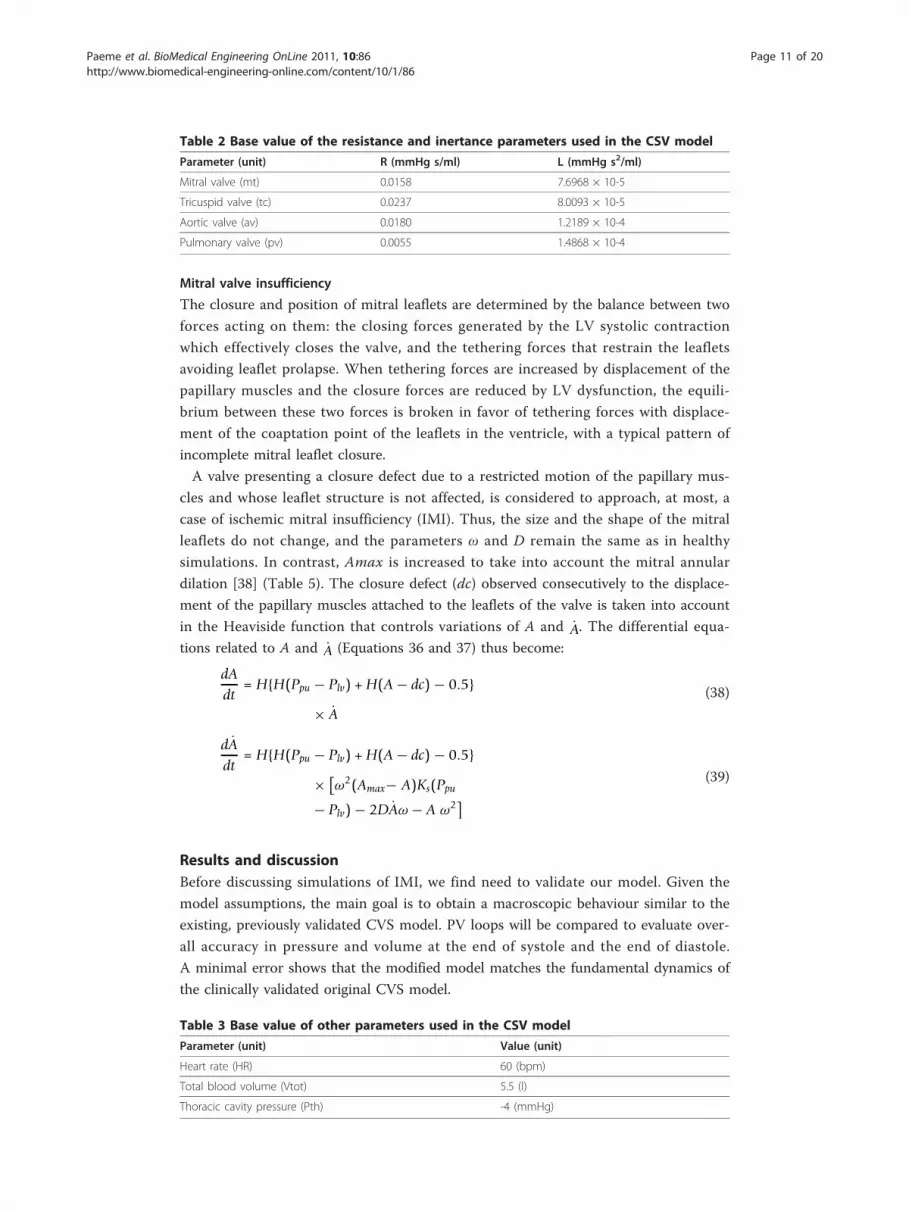
realistic description of the mitral valve. First, timing parameters are respected. In fact,

physiologically, the passive filling of the left ventricle is characterised by 3 crossovers

of pressures acting on both parts of the mitral valve. These 3 crossovers are critical for

the timing of mitral valve opening. The first is related to the opening time of the

mitral valve, the second to the maximum of the E-wave measured with Doppler and

the last one to the end of the E-wave [39]. Time between the first and the third cross-

over is the duration of the early ventricular filling, typically between 0.14s and 0.20s

depending of the heart state [12,37]. This period of early filling ends with the third

crossover and is followed by a diastasis phase during which pressures on both parts of

the valve remain very close, followed by atrial systole which leads to the active filling

of the left ventricle, measured as the A-wave. The ventricle then starts to contract,

driving ventricular pressure higher than atrial pressure, closing the mitral valve. Thus,

the mitral valve remains open during about 0.27s to 0.32s [37].

Parameters of the mitral valve model have been chosen to fit opening and closing

times. So even if all of pressure crossovers can’t be found in the pressure evolution dia-

gram (Figure 6), opening time, maximum opening of the early ventricular filling time

and closing time are respected. In fact, mitral valve opens at time t = 0.589s, reaches its

maximum at t = 0.666s and closes at time t = 0.921s as shown in Figure 7 which shows

the evolution of mitral valve aperture area for the previous model with “open on pres-

sure, close on flow” law for the mitral valve dynamics and for the new model. It means

that mitral valve remains open during 0.3320s which is close to physiological values [37].

Table 4 Base value of parameters used in the mitral valve model (healthy mitral valve)

Parameter (unit) Value (unit)

Static gain factor (Ks) 0.05 (1/mmHg)

Maximal mitral valve area (Amax) 1.1 (cm2)

Eigen frequency (ω) 30(rad/s)

Damping factor (D) 10 (1/rad)

Table 5 Base value of parameters used in the mitral valve model (mitral insufficiency)

Parameter (unit) value

Static gain factor (Ks) 0.05 (1/mmHg)

Maximal mitral valve area (Amax) 1.3 (cm2)

Eigen frequency (ω) 30 (rad/s)

Damping factor (D) 10 (1/rad)

Defect of closure (dc) 0.2 (cm2)


Page 12 of 20

Figure 4 Simulated left ventricular pressure-volume loops for a healthy valve. Blue dotted: previouslyvalidated model, red linear: new model. Emphasis on the resemblance of the results in term of globalbehavior of the heart.

Figure 5 Simulated right ventricular pressure-volume loops for a healthy valve. Blue dotted:previously validated model, red linear: new model. Emphasis on the resemblance of the results in term ofglobal behavior of the heart.


Page 13 of 20

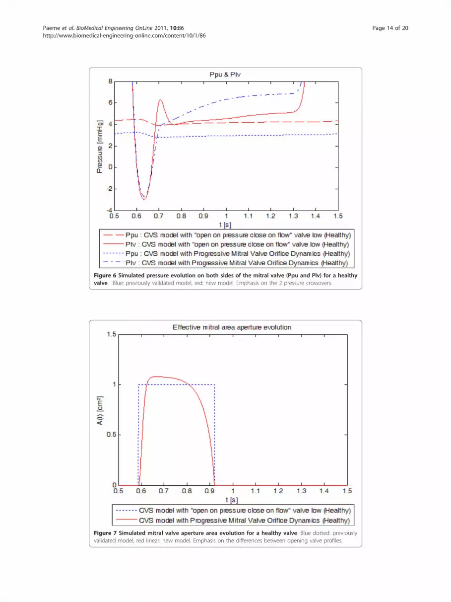
Figure 6 Simulated pressure evolution on both sides of the mitral valve (Ppu and Plv) for a healthyvalve. Blue: previously validated model, red: new model. Emphasis on the 2 pressure crossovers.

Figure 7 Simulated mitral valve aperture area evolution for a healthy valve. Blue dotted: previouslyvalidated model, red linear: new model. Emphasis on the differences between opening valve profiles.


Page 14 of 20

The time of maximum opening of the early ventricular filling is reached 0.077s after the

mitral valve opens while this time is about 71 to 96 ms in literature [39], depending on

the location of the measurement.

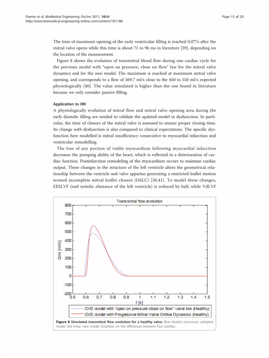
Figure 8 shows the evolution of transmitral blood flow during one cardiac cycle for

the previous model with “open on pressure, close on flow” law for the mitral valve

dynamics and for the new model. The maximum is reached at maximum mitral valve

opening, and corresponds to a flow of 569.7 ml/s close to the 450 to 550 ml/s expected

physiologically [40]. The value simulated is higher than the one found in literature

because we only consider passive filling.

Application to IMI

A physiologically evolution of mitral flow and mitral valve opening area during the

early diastolic filling are needed to validate the updated model in dysfunction. In parti-

cular, the time of closure of the mitral valve is assessed to ensure proper closing time.

Its change with dysfunction is also compared to clinical expectations. The specific dys-

function here modelled is mitral insufficiency consecutive to myocardial infarction and

ventricular remodelling.

The loss of any portion of viable myocardium following myocardial infarction

decreases the pumping ability of the heart, which is reflected in a deterioration of car-

diac function. Postinfarction remodeling of the myocardium occurs to maintain cardiac

output. These changes in the structure of the left ventricle alters the geometrical rela-

tionship between the ventricle and valve appartus generating a restricted leaflet motion

termed incomplete mitral leaflet closure (IMLC) [38,41]. To model these changes,

EESLVF (end systolic elastance of the left ventricle) is reduced by half, while VdLVF

Figure 8 Simulated transmitral flow evolution for a healthy valve. Blue dotted: previously validatedmodel, red linear: new model. Emphasis on the differences between flow profiles.


Page 15 of 20

(dead volume of the left ventricle) and V0LVF (initial volume of the left ventricle) are

first doubled and then gradually reduced to their initial values mimicking the experi-

mental work of Shioura et al. [42].

Realistic acute mitral valve regurgitation due to a permanent defect of closure

(Tables 2, 3, 5 and 6) was simulated. Figure 9 shows the evolution of mitral valve aper-

ture area over a cardiac cycle evidencing the permanent opening of the mitral valve.

Figure 10 shows the left PV loops for a healthy heart versus a remodelled heart with

IMI. Left PV loops for the diseased heart are qualitatively similar to those observed

experimentally [42] and clinically [1]. In fact, Raff and colleagues [1] have shown that

pressure-volume loops are modified in the presence of valvular dysfunction and more

specifically, that a global increase in ventricular volume is observed (PV loops move

towards the right), as well as an increase in stroke volume. In Figure 10, minimal

ventricular volume passes from 47.47 ml for the simulation of the healthy valve to

83.20 ml for the simulation of the incompetent valve while stroke volume passes from

79.43 ml to 92.80 ml. Raff et al. [1] also evidenced the disappearance of isovolumetric

phases, isovolumetric contraction and isovolumetric relaxation. Figure 10 shows that

these 2 phases have also disappeared because the mitral valve remains at least partly

open during the entire cardiac cycle. In fact, when the ventricle contracts, some blood

goes backward from the ventricle to the pulmonary veins chamber in the model result-

ing in negative transmitral flow, as shown in Figure 11, reducing the amount of blood

at the end of the contraction just before the aortic valve opens.

Our results thus prove that our simple model can capture both the healthy state and

valvular incompetence due to a defect in closure with appropriate variable changes.

Limitations

While these results show strong physiological correlation to independently measured

data, the second order model used to model the mitral valve aperture dynamics is not

completely physiologically relevant. Specifically, the terms in the Equation 39 do not

relate directly to the observed anatomical structure and function of the valve. Hence,

the model itself, while capturing the effective dynamics, can provide no insight into

specific disease impact or damage that results in valve dysfunction, even though it can

model that dysfunction.

While we could compare pressure and flow curves, the measurement of the variable

mitral valve area was not possible. To our best knowledge, no such data have been

published for humans or pigs until recently. Using the newest developments in

Table 6 Base value of the pressure-volume relationship parameters used in the CSVmodel (heart remodeled after ischemic event)

Parameter (unit) Ees (mmHg/ml) Vd (ml) V0 (ml) l (1/ml) P0 (mmHg)

Left ventricle free wall (lvf) 1.4399 30 20 0.023 0.1203

Right ventricle free wall (rvf) 0.5850 0 0 0.023 0.2157

Septum free wall (spt) 48.7540 2.00 2.00 0.435 1.1101

Pericardium (pcd) - - 200.00 0.030 0.5003

Vena cava (vc) 0.0059 0 - - -

Pulmonary artery (pa) 0.3690 0 - - -

Pulmonary vein (pu) 0.0073 0 - - -

Aorta (ao) 0.0 0 - - -


Page 16 of 20

Figure 9 Simulated mitral valve aperture area evolution for a healthy heart versus a remodelledheart with an ischemic mitral regurgitation. Blue dotted: new model simulated for a healthy heart, redlinear: new model simulated for a remodelled heart with an ischemic mitral regurgitation. Emphasis on thedifferences between healthy and diseased profiles, and the remaining opening of the diseased valve.

Figure 10 Simulated left ventricular pressure-volume loops for a healthy heart versus a remodelledheart with an ischemic mitral regurgitation. Blue dotted: new model simulated for a healthy heart, redlinear: new model simulated for a remodelled heart with an ischemic mitral regurgitation. Emphasis on thedifferences of the results in term of global behaviour of the heart.


Page 17 of 20

magnetic resonance technology and 4-dimensional echocardiography the authors are

currently involved in a study to determine the time course of mitral valve opening.

Even if we were not able to measure variable mitral valve area, the very good agree-

ment between measured and calculated pressure and flow curves indicates that the

simulated curves of mitral valve opening should be close to the natural time course.

In this model atrial contraction is not included. Further work will be needed to

extend this model to include atrial systole and, to be able to model physiologically late

diastolic filling. However, this limitation is not central to determine the efficiency of a

refined mitral valve model, although some results in timing may be affected. This

improvement would also widen the number of types of mitral insufficiencies that could

be simulated. As noted before it would also enable a better assessment of timing pro-

blems due to a bad delay between atrial and ventricular contraction.

ConclusionsThis work describes a new multi-scale closed-loop physiological model of the cardio-

vascular system that accounts for progressive mitral valve motion. Simulations show

that expected trends are respected for healthy and diseased valve states. These results

suggest a further use of this model to track, diagnose and control valvular pathologies.

The large number of valve model parameters indicates a need for new minimal and

more physiologically relevant mitral valve models that are readily identifiable to achieve

maximum benefit in real-time use of such models. However, the overall approach and

modelling framework are readily generalisable to both other valves and more relevant

valve models, proving the overall concept and approach.

Figure 11 Simulated transmitral flow evolution for a healthy heart versus a remodelled heart withan ischemic mitral regurgitation. Red dotted: new model simulated for a healthy heart, blue linear: newmodel simulated for a remodelled heart with an ischemic mitral regurgitation. Emphasis on the backflow(negative flow) for the diseased profile.


Page 18 of 20

AcknowledgementsThis work was supported by the F.R.I.A. (Belgium), the FNRS (Belgium) and the French Community of Belgium (Actionsde Recherches Concertées Académie Wallonie-Europe)

Author details1Cardiovascular Research Center, University of Liege, Liege, Belgium. 2Department of Mechanical Engineering,University of Canterbury, Christchurch, New Zealand.

Authors’ contributionsSP, TD, KTM, JGC and PCD conceived and developed the models and this analysis. SP did most of the computationalanalysis with input from TD, PCD, JGC and KTM. BL, MM, PL, VD, PK and LP supplied the clinical information andsuggested how to model mitral valve dysfunctions. SP, TD, KTM, JGC drafted the manuscript primarily although allauthors made contributions. All authors approved the final manuscript.

Competing interestsThe authors declare that they have no competing interests.

Received: 11 May 2011 Accepted: 24 September 2011 Published: 24 September 2011

References1. Raff U, Culclasure TF, Clark C, Overturf L, Groves BM: Computerized left ventricular pressure-volume relationships (pv-

loops) using disposable angiographic tip transducer pigtail catheters. Int J Card Imaging 2000, 16:13-21.2. Etiology, clinical features, and evaluation of chronic mitral regurgitation. [http://www.uptodate.com/patients/

content/topic.do?topicKey=~JTi881I452juyjT].3. Lancellotti P: L’insuffisance mutrale dynamique. Rôle de l’échocardiographie d’effort. PhD thesis University of Liège,

Faculté de Médecine, Service de Cardiologie;2004-2005.4. Tcheng JE, Jackman JD, Nelson CL, Gardner LH, Smith LR, Rankin JS, Califf RM, Stack RS: Outcome of Patients

Sustaining Acute Ischemic Mitral Regurgitation during Myocardial-Infarction. Ann Intern Med 1992, 117:18-24.5. Trichon BH, Felker GM, Shaw LK, Cabell CH, O’Connor CM: Relation of frequency and severity of mitral regurgitation

to survival among patients with left ventricular systolic dysfunction and heart failure. Am J Cardiol 2003, 91:538-543.6. Lancellotti P, Lebrun F, Pierard LA: Determinants of exercise-induced changes in mitral regurgitation in patients

with coronary artery disease and left ventricular dysfunction. J Am Coll Cardiol 2003, 42:1921-1928.7. Lancellotti P, Troisfontaines P, Toussaint AC, Pierard LA: Prognostic importance of exercise-induced changes in mitral

regurgitation in patients with chronic ischemic left ventricular dysfunction. Circulation 2003, 108:1713-1717.8. Burkhoff D, Alexander J, Schipke J: Assessment of Windkessel as a Model of Aortic Input Impedance. Am J Physiol

1988, 255:H742-H753.9. Shim EB, Jun HM, Leem CH, Matusuoka S, Noma A: A new integrated method for analyzing heart mechanics using a

cell-hemodynamics-autonomic nerve control coupled model of the cardiovascular system. Prog Biophys Mol Biol2008, 96:44-59.

10. Kerckhoffs RCP, Neal ML, Gu Q, Bassingthwaighte JB, Omens JH, McCulloch AD: Coupling of a 3D finite elementmodel of cardiac ventricular mechanics to lumped systems models of the systemic and pulmonic circulation. AnnBiomed Eng 2007, 35:1-18.

11. Hunter PJ, Nielsen PMF, Smaill BH, Legrice IJ, Hunter IW: An Anatomical Heart Model with Applications to MyocardialActivation and Ventricular Mechanics. Crit Rev Biomed Eng 1992, 20:403-426.

12. Waite L, Fine J: Applied Biofluid Mechanics The McGraw-Hill Companies, Inc; 2007.13. Smith BW, Chase JG, Nokes RI, Shaw GM, Wake G: Minimal haemodynamic system model including ventricular

interaction and valve dynamics. Med Eng Phys 2004, 26:131-139.14. Hann CE, Chase JG, Shaw GM: Efficient implementation of non-linear valve law and ventricular interaction dynamics

in the minimal cardiac model. Comput Methods Programs Biomed 2005, 80:65-74.15. Smith BW, Chase JG, Shaw GM, Nokes RI: Experimentally verified minimal cardiovascular system model for rapid

diagnostic assistance. Control Engineering Practice 2005, 13:1183-1193.16. Olansen JB, Clark JW, Khoury D, Ghorbel F, Bidani A: A closed-loop model of the canine cardiovascular system that

includes ventricular interaction. Comput Biomed Res 2000, 33:260-295.17. Desaive T, Lambermont B, Ghuysen A, Kolh P, Dauby PC, Starfinger C, Hann CE, Chase JG, Shaw GM: Cardiovascular

Modelling and Identification in Septic Shock - Experimental validation. Proceedings of the 17th IFAC World CongressJuly 6-11, 2008, Seoul, Korea 2008, 2976-2979.

18. Desaive T, Ghuysen A, Lambermont B, Kolh P, Dauby PC, Starfinger C, Hann CE, Chase J, Shaw GM: Study of ventricularinteraction during pulmonary embolism using clinical identification in a minimum cardiovascular system model.Conf Proc IEEE Eng Med Biol Soc 2007, 2007:2976-2979.

19. Starfinger C: Patient-Specific Modelling of the Cardiovascular System for Diagnosis and Therapy Assistance inCritical Care. PhD thesis University of Canterbury; 2008.

20. Starfinger C, Chase JG, Hann CE, Shaw GM, Lambermont B, Ghuysen A, Kolh P, Dauby PC, Desaive T: Model-basedidentification and diagnosis of a porcine model of induced endotoxic shock with hemofiltration. Math Biosci 2008,216:132-139.

21. Starfinger C, Hann CE, Chase JG, Desaive T, Ghuysen A, Shaw GM: Model-based cardiac diagnosis of pulmonaryembolism. Comput Methods Programs Biomed 2007, 87:46-60.

22. Segers P, Stergiopulos N, Westerhof N, Wouters P, Kolh P, Verdonck P: Systemic and pulmonary hemodynamicsassessed with a lumped-parameter heart-arterial interaction model. Journal of Engineering Mathematics 2003,47:185-199.

23. Conlon MJ, Russell DL, Mussivand T: Development of a mathematical model of the human circulatory system. AnnBiomed Eng 2006, 34:1400-1413.


Page 19 of 20

http://www.ncbi.nlm.nih.gov/pubmed/10832620?dopt=Abstract


http://www.uptodate.com/patients/content/topic.do?topicKey=~JTi881I452juyjT

http://www.uptodate.com/patients/content/topic.do?topicKey=~JTi881I452juyjT





























24. Kozarski M, Ferrari G, Zielinski K, Gorczynska K, Palko KJ, Tokarz A, Darowski M: A new hybrid electro-numerical modelof the left ventricle. Comput Biol Med 2008, 38:979-989.

25. Zacek M, Krause E: Numerical simulation of the blood flow in the human cardiovascular system. J Biomech 1996,29:13-20.

26. Waite L, Schulz S, Szabo G, Vahl CF: A lumped parameter model of left ventricular filling-pressure waveforms.Biomed Sci Instrum 2000, 36:75-80.

27. Franck CF, Waite L: Mathematical model of a variable aperture mitral valve. Biomed Sci Instrum 2002, 38:327-331.28. Szabó G, Soans D, Graf A, J Beller C, Waite L, Hagl S: A new computer model of mitral valve hemodynamics during

ventricular filling. Eur J Cardiothorac Surg 2004, 26:239-247.29. De Hart J, Peters GW, Schreurs PJ, Baaijens FP: A two-dimensional fluid-structure interaction model of the aortic

valve [correction of value]. J Biomech 2000, 33:1079-1088.30. De Hart J, Peters GW, Schreurs PJ, Baaijens FP: A three-dimensional computational analysis of fluid-structure

interaction in the aortic valve. J Biomech 2003, 36:103-112.31. van Loon R, Anderson PD, van de Vosse FN: A fluid-structure interaction method with solid-rigid contact for heart

valve dynamics. Journal of Computational Physics 2006, 217:806-823.32. Starfinger C, Chase JG, Hann CE, Shaw GM, Lambert P, Smith BW, Sloth E, Larsson A, Andreassen S, Rees S: Model-

based identification of PEEP titrations during different volemic levels. Comput Methods Programs Biomed 2008,91:135-144.

33. Starfinger C, Chase JG, Hann CE, Shaw GM, Lambert P, Smith BW, Sloth E, Larsson A, Andreassen S, Rees S: Predictionof hemodynamic changes towards PEEP titrations at different volemic levels using a minimal cardiovascularmodel. Comput Methods Programs Biomed 2008, 91:128-134.

34. Santamore WP, Burkhoff D: Hemodynamic consequences of ventricular interaction as assessed by model analysis.Am J Physiol 1991, 260:H146-157.

35. Smith BW, Chase JG, Shaw GM, Nokes RI: Simulating transient ventricular interaction using a minimal cardiovascularsystem model. Physiol Meas 2006, 27:165-179.

36. Dutron S: Modélisation de l’interaction ventriculaire. Master thesis University of Liège; 2005.37. Saito S, Araki Y, Usui A, Akita T, Oshima H, Yokote J, Ueda Y: Mitral valve motion assessed by high-speed video

camera in isolated swine heart. Eur J Cardiothorac Surg 2006, 30:584-591.38. Agricola E, Oppizzi M, Pisani M, Meris A, Maisano F, Margonato A: Ischemic mitral regurgitation: mechanisms and

echocardiographic classification. Eur J Echocardiogr 2008, 9:207-221.39. Courtois M, Kovacs SJ Jr, Ludbrook PA: Transmitral pressure-flow velocity relation. Importance of regional pressure

gradients in the left ventricle during diastole. Circulation 1988, 78:661-671.40. Flewitt JA, Hobson TN, Wang J, Johnston CR, Shrive NG, Belenkie I, Parker KH, Tyberg JV: Wave intensity analysis of left

ventricular filling: application of windkessel theory. Am J Physiol Heart Circ Physiol 2007, 292:H2817-2823.41. Hashim SW, Rousou AJ, Geirsson A, Ragnarsson S: Solving the puzzle of chronic ischemic mitral regurgitation. Yale J

Biol Med 2008, 81:167-173.42. Shioura KM, Geenen DL, Goldspink PH: Assessment of cardiac function with the pressure-volume conductance

system following myocardial infarction in mice. Am J Physiol Heart Circ Physiol 2007, 293:H2870-2877.

doi:10.1186/1475-925X-10-86Cite this article as: Paeme et al.: Mathematical multi-scale model of the cardiovascular system including mitralvalve dynamics. Application to ischemic mitral insufficiency. BioMedical Engineering OnLine 2011 10:86.

Submit your next manuscript to BioMed Centraland take full advantage of:

• Convenient online submission

• Thorough peer review

• No space constraints or color figure charges

• Immediate publication on acceptance

• Inclusion in PubMed, CAS, Scopus and Google Scholar

• Research which is freely available for redistribution

Submit your manuscript at www.biomedcentral.com/submit


Page 20 of 20































Documents

Mathematical multi-scale model of the cardiovascular system including mitral valve dynamics. Application to ischemic mitral insufficiency