Measurement of the B ! �Dð�ÞDð�ÞK branching fractions

P. del Amo Sanchez,1 J. P. Lees,1 V. Poireau,1 E. Prencipe,1 V. Tisserand,1 J. Garra Tico,2 E. Grauges,2

M. Martinelli,3a,3b A. Palano,3a,3b M. Pappagallo,3a,3b G. Eigen,4 B. Stugu,4 L. Sun,4 M. Battaglia,5 D.N. Brown,5

B. Hooberman,5 L. T. Kerth,5 Yu. G. Kolomensky,5 G. Lynch,5 I. L. Osipenkov,5 T. Tanabe,5 C.M. Hawkes,6

A. T. Watson,6 H. Koch,7 T. Schroeder,7 D. J. Asgeirsson,8 C. Hearty,8 T. S. Mattison,8 J. A. McKenna,8 A. Khan,9

A. Randle-Conde,9 V. E. Blinov,10 A. R. Buzykaev,10 V. P. Druzhinin,10 V. B. Golubev,10 A. P. Onuchin,10

S. I. Serednyakov,10 Yu. I. Skovpen,10 E. P. Solodov,10 K.Yu. Todyshev,10 A.N. Yushkov,10 M. Bondioli,11 S. Curry,11

D. Kirkby,11 A. J. Lankford,11 M. Mandelkern,11 E. C. Martin,11 D. P. Stoker,11 H. Atmacan,12 J.W. Gary,12 F. Liu,12

O. Long,12 G.M. Vitug,12 C. Campagnari,13 T.M. Hong,13 D. Kovalskyi,13 J. D. Richman,13 C. West,13 A.M. Eisner,14

C. A. Heusch,14 J. Kroseberg,14 W. S. Lockman,14 A. J. Martinez,14 T. Schalk,14 B. A. Schumm,14 A. Seiden,14

L. O. Winstrom,14 C.H. Cheng,15 D.A. Doll,15 B. Echenard,15 D.G. Hitlin,15 P. Ongmongkolkul,15 F. C. Porter,15

A. Y. Rakitin,15 R. Andreassen,16 M. S. Dubrovin,16 G. Mancinelli,16 B. T. Meadows,16 M.D. Sokoloff,16

P. C. Bloom,17 W. T. Ford,17 A. Gaz,17 M. Nagel,17 U. Nauenberg,17 J. G. Smith,17 S. R. Wagner,17 R. Ayad,18,*

W.H. Toki,18 H. Jasper,19 T.M. Karbach,19 J. Merkel,19 A. Petzold,19 B. Spaan,19 K. Wacker,19 M. J. Kobel,20

K. R. Schubert,20 R. Schwierz,20 D. Bernard,21 M. Verderi,21 P. J. Clark,22 S. Playfer,22 J. E. Watson,22

M. Andreotti,23a,23b D. Bettoni,23a C. Bozzi,23a R. Calabrese,23a,23b A. Cecchi,23a,23b G. Cibinetto,23a,23b

E. Fioravanti,23a,23b P. Franchini,23a,23b E. Luppi,23a,23b M. Munerato,23a,23b M. Negrini,23a,23b A. Petrella,23a,23b

L. Piemontese,23a R. Baldini-Ferroli,24 A. Calcaterra,24 R. de Sangro,24 G. Finocchiaro,24 M. Nicolaci,24 S. Pacetti,24

P. Patteri,24 I.M. Peruzzi,24,† M. Piccolo,24 M. Rama,24 A. Zallo,24 R. Contri,25a,25b E. Guido,25a,25b

M. Lo Vetere,25a,25b M. R. Monge,25a,25b S. Passaggio,25a C. Patrignani,25a,25b E. Robutti,25a S. Tosi,25a,25b

B. Bhuyan,26 V. Prasad,26 C. L. Lee,27 M. Morii,27 A. Adametz,28 J. Marks,28 U. Uwer,28 F. U. Bernlochner,29

M. Ebert,29 H.M. Lacker,29 T. Lueck,29 A. Volk,29 P. D. Dauncey,30 M. Tibbetts,30 P. K. Behera,31 U. Mallik,31

C. Chen,32 J. Cochran,32 H. B. Crawley,32 L. Dong,32 W. T. Meyer,32 S. Prell,32 E. I. Rosenberg,32 A. E. Rubin,32

A.V. Gritsan,33 Z. J. Guo,33 N. Arnaud,34 M. Davier,34 D. Derkach,34 J. Firmino da Costa,34 G. Grosdidier,34

F. Le Diberder,34 A.M. Lutz,34 B. Malaescu,34 A. Perez,34 P. Roudeau,34 M.H. Schune,34 J. Serrano,34 V. Sordini,34,‡

A. Stocchi,34 L. Wang,34 G. Wormser,34 D. J. Lange,35 D.M. Wright,35 I. Bingham,36 C. A. Chavez,36 J. P. Coleman,36

J. R. Fry,36 E. Gabathuler,36 R. Gamet,36 D. E. Hutchcroft,36 D. J. Payne,36 C. Touramanis,36 A. J. Bevan,37

F. Di Lodovico,37 R. Sacco,37 M. Sigamani,37 G. Cowan,38 S. Paramesvaran,38 A. C. Wren,38 D.N. Brown,39

C. L. Davis,39 A. G. Denig,40 M. Fritsch,40 W. Gradl,40 A. Hafner,40 K. E. Alwyn,41 D. Bailey,41 R. J. Barlow,41

G. Jackson,41 G.D. Lafferty,41 J. Anderson,42 R. Cenci,42 A. Jawahery,42 D.A. Roberts,42 G. Simi,42 J.M. Tuggle,42

C. Dallapiccola,43 E. Salvati,43 R. Cowan,44 D. Dujmic,44 G. Sciolla,44 M. Zhao,44 D. Lindemann,45 P.M. Patel,45

S. H. Robertson,45 M. Schram,45 P. Biassoni,46a,46b A. Lazzaro,46a,46b V. Lombardo,46a F. Palombo,46a,46b

S. Stracka,46a,46b L. Cremaldi,47 R. Godang,47,x R. Kroeger,47 P. Sonnek,47 D. J. Summers,47 X. Nguyen,48

M. Simard,48 P. Taras,48 G. De Nardo,49a,49b D. Monorchio,49a,49b G. Onorato,49a,49b C. Sciacca,49a,49b G. Raven,50

H. L. Snoek,50 C. P. Jessop,51 K. J. Knoepfel,51 J.M. LoSecco,51 W. F. Wang,51 L. A. Corwin,52 K. Honscheid,52

R. Kass,52 J. P. Morris,52 N. L. Blount,53 J. Brau,53 R. Frey,53 O. Igonkina,53 J. A. Kolb,53 R. Rahmat,53 N. B. Sinev,53

D. Strom,53 J. Strube,53 E. Torrence,53 G. Castelli,54a,54b E. Feltresi,54a,54b N. Gagliardi,54a,54b M. Margoni,54a,54b

M. Morandin,54a M. Posocco,54a M. Rotondo,54a F. Simonetto,54a,54b R. Stroili,54a,54b E. Ben-Haim,55

G. R. Bonneaud,55 H. Briand,55 G. Calderini,55 J. Chauveau,55 O. Hamon,55 Ph. Leruste,55 G. Marchiori,55 J. Ocariz,55

J. Prendki,55 S. Sitt,55 M. Biasini,56a,56b E. Manoni,56a,56b A. Rossi,56a,56b C. Angelini,57a,57b G. Batignani,57a,57b

S. Bettarini,57a,57b M. Carpinelli,57a,57b,k G. Casarosa,57a,57b A. Cervelli,57a,57b F. Forti,57a,57b M.A. Giorgi,57a,57b

A. Lusiani,57a,57c N. Neri,57a,57b E. Paoloni,57a,57b G. Rizzo,57a,57b J. J. Walsh,57a D. Lopes Pegna,58 C. Lu,58 J. Olsen,58

A. J. S. Smith,58 A.V. Telnov,58 F. Anulli,59a E. Baracchini,59a,59b G. Cavoto,59a R. Faccini,59a,59b F. Ferrarotto,59a

F. Ferroni,59a,59b M. Gaspero,59a,59b L. Li Gioi,59a M.A. Mazzoni,59a G. Piredda,59a F. Renga,59a,59b T. Hartmann,60

T. Leddig,60 H. Schroder,60 R. Waldi,61 T. Adye,61 B. Franek,61 E. O. Olaiya,61 F. F. Wilson,61 S. Emery,62

G. Hamel de Monchenault,62 G. Vasseur,62 Ch. Yeche,62 M. Zito,62 M. T. Allen,63 D. Aston,63 D. J. Bard,63

R. Bartoldus,63 J. F. Benitez,63 C. Cartaro,63 M. R. Convery,63 J. Dorfan,63 G. P. Dubois-Felsmann,63 W. Dunwoodie,63

R. C. Field,63 M. Franco Sevilla,63 B. G. Fulsom,63 A.M. Gabareen,63 M. T. Graham,63 P. Grenier,63 C. Hast,63

W.R. Innes,63 M.H. Kelsey,63 H. Kim,63 P. Kim,63 M. L. Kocian,63 D.W.G. S. Leith,63 S. Li,63 B. Lindquist,63

S. Luitz,63 V. Luth,63 H. L. Lynch,63 D. B. MacFarlane,63 H. Marsiske,63 D. R. Muller,63 H. Neal,63 S. Nelson,63

PHYSICAL REVIEW D 83, 032004 (2011)

1550-7998=2011=83(3)=032004(16) 032004-1 � 2011 American Physical Society

C. P. O’Grady,63 I. Ofte,63 M. Perl,63 T. Pulliam,63 B. N. Ratcliff,63 A. Roodman,63 A.A. Salnikov,63 V. Santoro,63

R. H. Schindler,63 J. Schwiening,63 A. Snyder,63 D. Su,63 M.K. Sullivan,63 S. Sun,63 K. Suzuki,63 J.M. Thompson,63

J. Va’vra,63 A. P. Wagner,63 M. Weaver,63 C.A. West,63 W. J. Wisniewski,63 M. Wittgen,63 D. H. Wright,63

H.W. Wulsin,63 A.K. Yarritu,63 C. C. Young,63 V. Ziegler,63 X. R. Chen,64 W. Park,64 M.V. Purohit,64 R.M. White,64

J. R. Wilson,64 S. J. Sekula,65 M. Bellis,66 P. R. Burchat,66 A. J. Edwards,66 T. S. Miyashita,66 S. Ahmed,67

M. S. Alam,67 J. A. Ernst,67 B. Pan,67 M.A. Saeed,67 S. B. Zain,67 N. Guttman,68 A. Soffer,68 P. Lund,69

S.M. Spanier,69 R. Eckmann,70 J. L. Ritchie,70 A.M. Ruland,70 C. J. Schilling,70 R. F. Schwitters,70 B. C. Wray,70

J.M. Izen,71 X. C. Lou,71 F. Bianchi,72a,72b D. Gamba,72a,72b M. Pelliccioni,72a,72b M. Bomben,73a,73b L. Lanceri,73a,73b

L. Vitale,73a,73b N. Lopez-March,74 F. Martinez-Vidal,74 D.A. Milanes,74 A. Oyanguren,74 J. Albert,75 Sw. Banerjee,75

H.H. F. Choi,75 K. Hamano,75 G. J. King,75 R. Kowalewski,75 M. J. Lewczuk,75 I.M. Nugent,75 J.M. Roney,75

R. J. Sobie,75 T. J. Gershon,76 P. F. Harrison,76 T. E. Latham,76 E.M. T. Puccio,76 H. R. Band,77 S. Dasu,77

K. T. Flood,77 Y. Pan,77 R. Prepost,77 C.O. Vuosalo,77 and S. L. Wu77

(BABAR Collaboration)

1Laboratoire d’Annecy-le-Vieux de Physique des Particules (LAPP), Universite de Savoie,CNRS/IN2P3, F-74941 Annecy-Le-Vieux, France

2Universitat de Barcelona, Facultat de Fisica, Departament ECM, E-08028 Barcelona, Spain3aINFN Sezione di Bari, I-70126 Bari, Italy

3bDipartimento di Fisica, Universita di Bari, I-70126 Bari, Italy4University of Bergen, Institute of Physics, N-5007 Bergen, Norway

5Lawrence Berkeley National Laboratory and University of California, Berkeley, California 94720, USA6University of Birmingham, Birmingham, B15 2TT, United Kingdom

7Ruhr Universitat Bochum, Institut fur Experimentalphysik 1, D-44780 Bochum, Germany8University of British Columbia, Vancouver, British Columbia, Canada V6T 1Z1

9Brunel University, Uxbridge, Middlesex UB8 3PH, United Kingdom10Budker Institute of Nuclear Physics, Novosibirsk 630090, Russia11University of California at Irvine, Irvine, California 92697, USA

12University of California at Riverside, Riverside, California 92521, USA13University of California at Santa Barbara, Santa Barbara, California 93106, USA

14University of California at Santa Cruz, Institute for Particle Physics, Santa Cruz, California 95064, USA15California Institute of Technology, Pasadena, California 91125, USA

16University of Cincinnati, Cincinnati, Ohio 45221, USA17University of Colorado, Boulder, Colorado 80309, USA

18Colorado State University, Fort Collins, Colorado 80523, USA19Technische Universitat Dortmund, Fakultat Physik, D-44221 Dortmund, Germany

20Technische Universitat Dresden, Institut fur Kern- und Teilchenphysik, D-01062 Dresden, Germany21Laboratoire Leprince-Ringuet, CNRS/IN2P3, Ecole Polytechnique, F-91128 Palaiseau, France

22University of Edinburgh, Edinburgh EH9 3JZ, United Kingdom23aINFN Sezione di Ferrara, I-44100 Ferrara, Italy

23bDipartimento di Fisica, Universita di Ferrara, I-44100 Ferrara, Italy24INFN Laboratori Nazionali di Frascati, I-00044 Frascati, Italy

25aINFN Sezione di Genova, I-16146 Genova, Italy25bDipartimento di Fisica, Universita di Genova, I-16146 Genova, Italy

26Indian Institute of Technology Guwahati, Guwahati, Assam, 781 039, India27Harvard University, Cambridge, Massachusetts 02138, USA

28Universitat Heidelberg, Physikalisches Institut, Philosophenweg 12, D-69120 Heidelberg, Germany29Humboldt-Universitat zu Berlin, Institut fur Physik, Newtonstr. 15, D-12489 Berlin, Germany

30Imperial College London, London, SW7 2AZ, United Kingdom31University of Iowa, Iowa City, Iowa 52242, USA

32Iowa State University, Ames, Iowa 50011-3160, USA33Johns Hopkins University, Baltimore, Maryland 21218, USA

34Laboratoire de l’Accelerateur Lineaire, IN2P3/CNRS et Universite Paris-Sud 11,Centre Scientifique d’Orsay, B. P. 34, F-91898 Orsay Cedex, France

35Lawrence Livermore National Laboratory, Livermore, California 94550, USA36University of Liverpool, Liverpool L69 7ZE, United Kingdom

37Queen Mary, University of London, London, E1 4NS, United Kingdom38University of London, Royal Holloway and Bedford New College, Egham, Surrey TW20 0EX, United Kingdom

P. DEL AMO SANCHEZ et al. PHYSICAL REVIEW D 83, 032004 (2011)

032004-2

39University of Louisville, Louisville, Kentucky 40292, USA40Johannes Gutenberg-Universitat Mainz, Institut fur Kernphysik, D-55099 Mainz, Germany

41University of Manchester, Manchester M13 9PL, United Kingdom42University of Maryland, College Park, Maryland 20742, USA

43University of Massachusetts, Amherst, Massachusetts 01003, USA44Massachusetts Institute of Technology, Laboratory for Nuclear Science, Cambridge, Massachusetts 02139, USA

45McGill University, Montreal, Quebec, Canada H3A 2T846aINFN Sezione di Milano, I-20133 Milano, Italy

46bDipartimento di Fisica, Universita di Milano, I-20133 Milano, Italy47University of Mississippi, University, Mississippi 38677, USA

48Universite de Montreal, Physique des Particules, Montreal, Quebec, Canada H3C 3J749aINFN Sezione di Napoli, I-80126 Napoli, Italy

49bDipartimento di Scienze Fisiche, Universita di Napoli Federico II, I-80126 Napoli, Italy50NIKHEF, National Institute for Nuclear Physics and High Energy Physics, NL-1009 DB Amsterdam, The Netherlands

51University of Notre Dame, Notre Dame, Indiana 46556, USA52Ohio State University, Columbus, Ohio 43210, USA53University of Oregon, Eugene, Oregon 97403, USA54aINFN Sezione di Padova, I-35131 Padova, Italy

54bDipartimento di Fisica, Universita di Padova, I-35131 Padova, Italy55Laboratoire de Physique Nucleaire et de Hautes Energies, IN2P3/CNRS, Universite Pierre et Marie Curie-Paris6,

Universite Denis Diderot-Paris7, F-75252 Paris, France56aINFN Sezione di Perugia, I-06100 Perugia, Italy

56bDipartimento di Fisica, Universita di Perugia, I-06100 Perugia, Italy57aINFN Sezione di Pisa, I-56127 Pisa, Italy

57bDipartimento di Fisica, Universita di Pisa, I-56127 Pisa, Italy57cScuola Normale Superiore di Pisa, I-56127 Pisa, Italy

58Princeton University, Princeton, New Jersey 08544, USA59aINFN Sezione di Roma, I-00185 Roma, Italy

59bDipartimento di Fisica, Universita di Roma La Sapienza, I-00185 Roma, Italy60Universitat Rostock, D-18051 Rostock, Germany

61Rutherford Appleton Laboratory, Chilton, Didcot, Oxon, OX11 0QX, United Kingdom62CEA, Irfu, SPP, Centre de Saclay, F-91191 Gif-sur-Yvette, France

63SLAC National Accelerator Laboratory, Stanford, California 94309 USA64University of South Carolina, Columbia, South Carolina 29208, USA

65Southern Methodist University, Dallas, Texas 75275, USA66Stanford University, Stanford, California 94305-4060, USA67State University of New York, Albany, New York 12222, USA

68Tel Aviv University, School of Physics and Astronomy, Tel Aviv, 69978, Israel69University of Tennessee, Knoxville, Tennessee 37996, USA70University of Texas at Austin, Austin, Texas 78712, USA

71University of Texas at Dallas, Richardson, Texas 75083, USA72aINFN Sezione di Torino, I-10125 Torino, Italy

72bDipartimento di Fisica Sperimentale, Universita di Torino, I-10125 Torino, Italy73aINFN Sezione di Trieste, I-34127 Trieste, Italy

73bDipartimento di Fisica, Universita di Trieste, I-34127 Trieste, Italy74IFIC, Universitat de Valencia-CSIC, E-46071 Valencia, Spain

75University of Victoria, Victoria, British Columbia, Canada V8W 3P676Department of Physics, University of Warwick, Coventry CV4 7AL, United Kingdom, USA

77University of Wisconsin, Madison, Wisconsin 53706, USA(Received 17 November 2010; published 3 February 2011)

We present a measurement of the branching fractions of the 22 decay channels of the B0 and Bþ mesons

to �Dð�ÞDð�ÞK, where the Dð�Þ and �Dð�Þ mesons are fully reconstructed. Summing the 10 neutral modes and

the 12 charged modes, the branching fractions are found to be BðB0! �Dð�ÞDð�ÞKÞ¼ ð3:68�0:10�0:24Þ% and BðBþ ! �Dð�ÞDð�ÞKÞ ¼ ð4:05� 0:11� 0:28Þ%, where the first uncertainties are statistical

*Now at Temple University, Philadelphia, PA 19122, USA†Also with Universita di Perugia, Dipartimento di Fisica, Perugia, Italy‡Also with Universita di Roma La Sapienza, I-00185 Roma, ItalyxNow at University of South Alabama, Mobile, AL 36688, USAkAlso with Universita di Sassari, Sassari, Italy

MEASUREMENT OF THE . . . PHYSICAL REVIEW D 83, 032004 (2011)

032004-3

and the second systematic. The results are based on 429 fb�1 of data containing 471� 106B �B

pairs collected at the �ð4SÞ resonance with the BABAR detector at the SLAC National Accelerator

Laboratory.

DOI: 10.1103/PhysRevD.83.032004 PACS numbers: 13.25.Hw, 14.40.Nd

I. INTRODUCTION

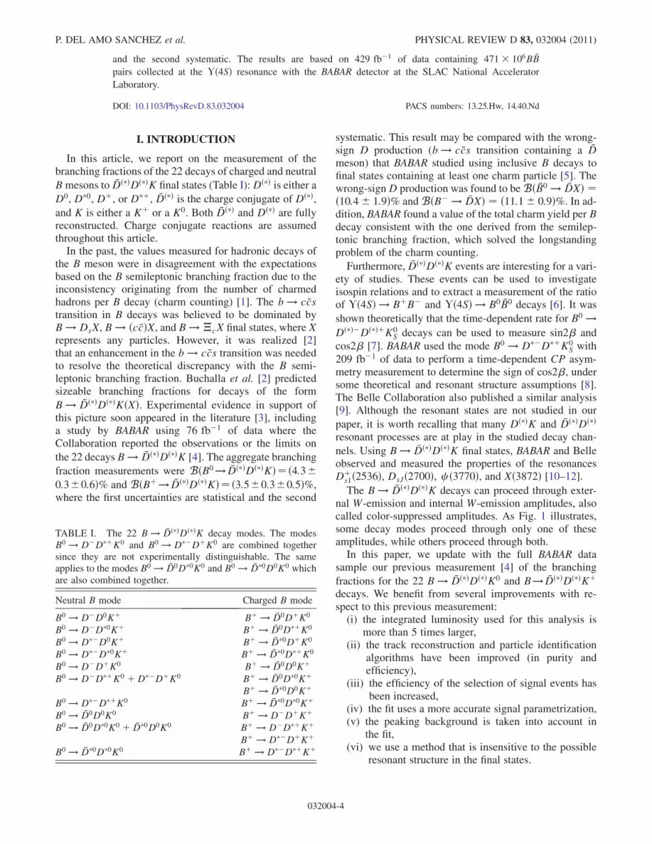
In this article, we report on the measurement of thebranching fractions of the 22 decays of charged and neutral

Bmesons to �Dð�ÞDð�ÞK final states (Table I):Dð�Þ is either aD0, D�0, Dþ, or D�þ, �Dð�Þ is the charge conjugate of Dð�Þ,and K is either a Kþ or a K0. Both �Dð�Þ and Dð�Þ are fullyreconstructed. Charge conjugate reactions are assumedthroughout this article.

In the past, the values measured for hadronic decays ofthe B meson were in disagreement with the expectationsbased on the B semileptonic branching fraction due to theinconsistency originating from the number of charmedhadrons per B decay (charm counting) [1]. The b ! c �cstransition in B decays was believed to be dominated byB ! DsX, B ! ðc �cÞX, and B ! �cX final states, where Xrepresents any particles. However, it was realized [2]that an enhancement in the b ! c �cs transition was neededto resolve the theoretical discrepancy with the B semi-leptonic branching fraction. Buchalla et al. [2] predictedsizeable branching fractions for decays of the form

B ! �Dð�ÞDð�ÞKðXÞ. Experimental evidence in support ofthis picture soon appeared in the literature [3], includinga study by BABAR using 76 fb�1 of data where theCollaboration reported the observations or the limits on

the 22 decays B ! �Dð�ÞDð�ÞK [4]. The aggregate branching

fraction measurements were BðB0! �Dð�ÞDð�ÞKÞ¼ ð4:3�0:3�0:6Þ% and BðBþ! �Dð�ÞDð�ÞKÞ¼ ð3:5�0:3�0:5Þ%,where the first uncertainties are statistical and the second

systematic. This result may be compared with the wrong-sign D production (b ! c �cs transition containing a �Dmeson) that BABAR studied using inclusive B decays tofinal states containing at least one charm particle [5]. Thewrong-signD production was found to beBð �B0 ! �DXÞ ¼ð10:4� 1:9Þ% and BðB� ! �DXÞ ¼ ð11:1� 0:9Þ%. In ad-dition, BABAR found a value of the total charm yield per Bdecay consistent with the one derived from the semilep-tonic branching fraction, which solved the longstandingproblem of the charm counting.

Furthermore, �Dð�ÞDð�ÞK events are interesting for a vari-ety of studies. These events can be used to investigateisospin relations and to extract a measurement of the ratioof �ð4SÞ ! BþB� and �ð4SÞ ! B0 �B0 decays [6]. It was

shown theoretically that the time-dependent rate for B0 !Dð�Þ�Dð�ÞþK0

S decays can be used to measure sin2� and

cos2� [7]. BABAR used the mode B0 ! D��D�þK0S with

209 fb�1 of data to perform a time-dependent CP asym-metry measurement to determine the sign of cos2�, undersome theoretical and resonant structure assumptions [8].The Belle Collaboration also published a similar analysis[9]. Although the resonant states are not studied in our

paper, it is worth recalling that many Dð�ÞK and �Dð�ÞDð�Þresonant processes are at play in the studied decay chan-

nels. Using B ! �Dð�ÞDð�ÞK final states, BABAR and Belleobserved and measured the properties of the resonancesDþ

s1ð2536Þ, DsJð2700Þ, c ð3770Þ, and Xð3872Þ [10–12].The B ! �Dð�ÞDð�ÞK decays can proceed through exter-

nal W-emission and internal W-emission amplitudes, alsocalled color-suppressed amplitudes. As Fig. 1 illustrates,some decay modes proceed through only one of theseamplitudes, while others proceed through both.In this paper, we update with the full BABAR data

sample our previous measurement [4] of the branching

fractions for the 22 B ! �Dð�ÞDð�ÞK0 and B! �Dð�ÞDð�ÞKþdecays. We benefit from several improvements with re-spect to this previous measurement:(i) the integrated luminosity used for this analysis is

more than 5 times larger,(ii) the track reconstruction and particle identification

algorithms have been improved (in purity andefficiency),

(iii) the efficiency of the selection of signal events hasbeen increased,

(iv) the fit uses a more accurate signal parametrization,(v) the peaking background is taken into account in

the fit,(vi) we use a method that is insensitive to the possible

resonant structure in the final states.

TABLE I. The 22 B ! �Dð�ÞDð�ÞK decay modes. The modesB0 ! D�D�þK0 and B0 ! D��DþK0 are combined togethersince they are not experimentally distinguishable. The sameapplies to the modes B0 ! �D0D�0K0 and B0 ! �D�0D0K0 whichare also combined together.

Neutral B mode Charged B mode

B0 ! D�D0Kþ Bþ ! �D0DþK0

B0 ! D�D�0Kþ Bþ ! �D0D�þK0

B0 ! D��D0Kþ Bþ ! �D�0DþK0

B0 ! D��D�0Kþ Bþ ! �D�0D�þK0

B0 ! D�DþK0 Bþ ! �D0D0KþB0 ! D�D�þK0 þD��DþK0 Bþ ! �D0D�0Kþ

Bþ ! �D�0D0KþB0 ! D��D�þK0 Bþ ! �D�0D�0KþB0 ! �D0D0K0 Bþ ! D�DþKþB0 ! �D0D�0K0 þ �D�0D0K0 Bþ ! D�D�þKþ

Bþ ! D��DþKþB0 ! �D�0D�0K0 Bþ ! D��D�þKþ

P. DEL AMO SANCHEZ et al. PHYSICAL REVIEW D 83, 032004 (2011)

032004-4

Measuring the 22 modes altogether allows to avoid biasesin the branching fraction measurement by correctly takinginto account the cross-feed events, which are events fromone mode being reconstructed as a candidate for anothermode.

II. THE BABAR DETECTOR ANDDATA SAMPLE

The data were recorded by the BABAR detector at thePEP-II asymmetric-energy eþe� storage ring operating atthe SLAC National Accelerator Laboratory. We analyzethe complete BABAR data sample collected at the �ð4SÞresonance corresponding to an integrated luminosity of429 fb�1, giving NB �B ¼ ð470:9� 0:1� 2:8Þ � 106 B �Bpairs produced, where the first uncertainty is statisticaland the second systematic.

The BABAR detector is described in detail elsewhere[13]. Charged particles are detected and their momentameasured with a five-layer silicon vertex tracker and a40-layer drift chamber in a 1.5 T axial magnetic field.Charged particle identification is based on the measure-ments of the energy loss in the tracking devices and of theCherenkov radiation in the ring-imaging detector. The

energies and locations of showers associated with photonsare measured in the electromagnetic calorimeter. Muonsare identified by the instrumented magnetic-flux return,which is located outside the magnet.We employ a Monte Carlo (MC) simulation to study the

relevant backgrounds and estimate the selection efficien-cies. We use EVTGEN [14] to model the kinematics of Bmesons and JETSET [15] to model continuum processes,eþe� ! q �q (q ¼ u, d, s, c). The BABAR detector and itsresponse to particle interactions are modeled using theGEANT4 [16] simulation package.

III. B CANDIDATE SELECTION

We reconstruct the B0 and Bþ mesons in the 22�Dð�ÞDð�ÞK modes. The level of background widely variesamong the signal channels, even within a specific B modedepending on the D meson decay type. A different opti-mization of the selection criteria is implemented for eachof the final states. The optimization determines the selec-

tion which maximizes S=ffiffiffiffiffiffiffiffiffiffiffiffiffiSþ B

p, where S and B are the

expected number of events for the signal and for thebackground in the signal region, based, respectively,on signal and background MC simulated events. The

u

b_

u

c_cd_ds_

B+ D(*)0

D(*)+

K0

W+

u

b_

u

s_c

d_d

c_

B+

K+

D(*)+

D(*)-

W+

u

b_

us_cu_uc_

B+

K+

D(*)0

D(*)0

+

W+

ub_

uc_cuu_s_

B+ D(*)0

D(*)0

K+

W+

d

b_

d

c_cu_us_

B0 D(*)-

D(*)0

K+

W+

d

b_

d

s_c

u

u_

c_

B0

K0

D(*)0

D(*)0

W+

d

b_

ds_cd_dc_

B0

K0

D(*)+

D(*)-

+

W+

db_

dc_cd_ds_

B0 D(*)-

D(*)+

K0

W+

FIG. 1. Top left: external W-emission amplitude for the decays Bþ ! �Dð�Þ0Dð�ÞþK0. Top center: internal W-emission amplitude forthe decays Bþ ! Dð�Þ�Dð�ÞþKþ. Top right: externalþ internal W-emission amplitudes for the decays Bþ ! �Dð�Þ0Dð�Þ0Kþ. Bottomrow: same as top row, respectively, for B0 ! Dð�Þ�Dð�Þ0Kþ, B0 ! �Dð�Þ0Dð�Þ0K0, and B0 ! Dð�Þ�Dð�ÞþK0.

MEASUREMENT OF THE . . . PHYSICAL REVIEW D 83, 032004 (2011)

032004-5

branching fractions for the computation of S are taken fromour previous measurements of these channels [4].

We identify charged kaons using either loose or tightcriteria depending on the decay mode. The loose criterionis typically 98% efficient with pion misidentification ratesat the 15% level, while the tight criterion is 85% efficientwith a misidentification around 2%. We use only the K0

S

meson when a neutral K meson is present in the final state.The K0

S candidates are reconstructed from two oppositely

charged tracks assumed to be pions consistent with comingfrom a common vertex and having an invariant mass within�9:5 MeV=c2 of the nominal K0

S mass [17]. The displace-

ment of the K0S vertex in the plane transverse to the beam

axis is required to be at least 0.2 cm.The �0 candidates are reconstructed from pairs of pho-

tons with energies E� > 30 MeV in the laboratory frame

that have an invariant mass of 115<m�� < 150 MeV=c2.

We reconstruct D mesons in the modes D0 ! K��þ,K��þ�0,K��þ���þ, andDþ ! K��þ�þ. TheK and� tracks are required to originate from a common vertex.The invariant masses of theD candidates are required to liewithin �2:5�D of the measured D mass, where �D is theD invariant mass resolution. This resolution is measuredto be 5:8 MeV=c2 for D0 ! K��þ, 9:5 MeV=c2 forD0 ! K��þ�0, 4:7 MeV=c2 for D0 ! K��þ���þ,and 4:2 MeV=c2 for Dþ ! K��þ�þ. To reduce thecombinatorial background, for some of the B decays in-volving D0 ! K��þ�0, we use the distribution of eventsin the Dalitz plot of the squared invariant massesm2ðK��þÞ �m2ðK��0Þ, where we select events that arelocated in the enhanced regions dominated by theK�ð892Þþ, K�ð892Þ0, and �ð770Þþ resonances [18].

The D� candidates are reconstructed in the decay modesD�þ ! D0�þ, D�þ ! Dþ�0, D�0 ! D0�0, and D�0 !D0�. The �0 and the �þ candidates must have a momen-tum smaller than 450 MeV=c in the �ð4SÞ rest frame,while the � energy in the laboratory frame must be largerthan 100 MeV. The mass difference between the D�þ andD candidates is required to be within �3 MeV=c2 of thenominal value [17]. For D�0 meson decays, the massdifference between the D�0 and D0 candidates is requiredto lie between 138 and 146 MeV=c2 for D�0 ! D0�0 andbetween 130 and 150 MeV=c2 for D�0 ! D0�.

The B candidates are reconstructed by combining a �Dð�Þ,aDð�Þ and aK candidate in one of the 22 modes. For modesinvolving two D0 mesons, at least one of them is requiredto decay to K��þ, except for the decay modesD��D�þK0, D��D�þKþ, and D��D0Kþ, which havelower background and for which all combinations areaccepted. For modes containing a D�þ meson, we lookonly to the decay D�þ ! D0�þ, except for the modescontaining D��D�þ, where we also reconstruct D�þ !Dþ�0. A mass-constrained kinematic fit is applied to theintermediate particles (D�0, D�þ, D0, Dþ, K0

S, �0) to

improve their momentum resolution.

To suppress the continuum background, we removeevents with R2 > 0:3 (where R2 is the ratio of the secondto zeroth Fox-Wolfram moments of the event [19]) andevents with j cosð�BÞj> 0:9 (where �B is the angle be-tween the thrust axis of the candidate decay and the thrustaxis of the rest of the event).Two kinematic variables are used to isolate the B-meson

signal. The first variable is the beam-energy-substitutedmass defined as

mES ¼ffiffiffiffiffiffiffiffiffiffiffiffiffiffiffiffiffiffiffiffiffiffiffiffiffiffiffiffiffiffiffiffiffiffiffiffiffiffiffiffiffiffiffiffiffiffiffiffiffiffiffi�s=2þ ~p0: ~pB

E0

�2 � j ~pBj2

s; (1)

whereffiffiffis

pis the eþe� center-of-mass energy. For the

momenta ~p0, ~pB and the energy E0, the subscripts 0 andB refer to the eþe� system and the reconstructed Bmeson,respectively. The other variable is �E, the difference be-tween the reconstructed energy of the B candidate andthe beam energy in the eþe� center-of-mass frame.Signal events have mES compatible with the knownB-meson mass [17] and�E compatible with 0 MeV, withintheir respective resolutions. At this stage, we keep onlyevents which satisfy mES > 5:20 GeV=c2.We obtain a few signal B candidates per event on aver-

age. When the final state contains noD� meson, we get 1.0to 1.3 candidates per event depending on the specific mode,1.3 to 1.9 candidates per event for final states containingoneD� meson, and 1.7 to 2.1 candidates per event when thefinal state contains two D� mesons (except for Bþ !�D�0D�0Kþ with 2.9 candidates per event). If more thanone candidate is selected in an event, we retain the one withthe smallest value of j�Ej (‘‘best candidate selection’’).According to MC studies, this criterion finds the correctcandidate when this one is present in the candidate list inmore than 95% of the cases for final states with no D�0meson and more than 80% of the cases for modes with oneor two neutral D� mesons. We keep only events withj�Ej< Ec, with Ec varying from 7 MeV to 56 MeVdepending on the decay mode of the B and D mesons.The resolution on �E varies between 5.6 and 14.3 MeV formodes with zero or one D�0 meson in the final state andbetween 11.6 and 19.5 MeV for modes containing twoneutral D� mesons.The efficiency for signal events varies from 0.5% to

22.2% depending on the final state (being typically in the5%–10% range). The modes with the lowest efficiency arethe ones containing one or two charged D� mesons.Figure 2 presents the �E and mES distributions after the

complete selection is applied. The �E distributions arepresented for events in the signal region defined by mES >5:27 GeV=c2 and are shown without applying the bestcandidate selection. Signal events appear in the peak near�E� 0 MeVwhen reconstructed correctly, while the peakaround �160 MeV is due to �D�DK and �DD�K decaysreconstructed as �DDK and to �D�D�K decays reconstructed

P. DEL AMO SANCHEZ et al. PHYSICAL REVIEW D 83, 032004 (2011)

032004-6

as �D�DK or �DD�K. Both�E andmES distributions show aclear excess of events in the signal region.

IV. FITS OF THE DATA DISTRIBUTIONS

Wepresent the fits used to extract the branching fractions.For eachmode, we fit themES distribution between 5.22 and5:30 GeV=c2 to get the signal yield. The data samplescorresponding to each B decay mode are disjoint and thefits are performed independently for each mode. Accordingto their physical origin, four categories of eventswith differ-ently shaped mES distributions are separately considered:�Dð�ÞDð�ÞK signal events, cross-feed events, combinatorialbackground events, and peaking background events. Thetotal probability density function (PDF) is a sum of thesecontributions. Event yields are obtained from extendedmaximum likelihood unbinned fits.

A. Signal contribution

The shape of the signal is determined from fits to themES

distributions of signal MC samples. ACrystal Ball function

[20] (Gaussian modified to include a power-law tail on thelow side of the peak), P SðmES;mS; �S; �S; nSÞ, is used todescribe the signal (see Eq. (A1) in the Appendix A). Theparameters of this PDF are mS and �S, the mean and thewidth of the Gaussian part, and �S and nS, the parametersof the tail part. The signal yield,NS, is determined from thefit to the data.

B. Cross-feed contribution

We call ‘‘cross feed’’ the events from all of the�Dð�ÞDð�ÞK modes, except the one we reconstruct, thatpass the complete selection and that are reconstructedin the given mode. The cross-feed events are a non-negligible part of the mES peak in some of the modes,and the signal event yield must be corrected for thesecross-feed events.We observe from the analysis of simulated samples that

most of the cross feed originates from the combination ofan unrelated soft �0 or � with the D0 decayed from theD�þ to form a wrong D�0 candidate. The cross-feed pro-portion is often in the 10% range relative to the signal yield

E (GeV)∆

Eve

nts/

5 M

eV

1000

1500

2000

2500

3000

3500

4000

4500 modes0B

E (GeV)∆

Eve

nts/

5 M

eV

2000

3000

4000

5000

6000

7000 modes+B

)2 (GeV/cESm

2E

vent

s/1

MeV

/c

0

200

400

600

800

1000

1200

1400 modes0B

)2 (GeV/cESm

-0.2 -0.15 -0.1 -0.05 0 0.05 0.1 0.15 0.2 -0.2 -0.15 -0.1 -0.05 0 0.05 0.1 0.15 0.2

5.22 5.23 5.24 5.25 5.26 5.27 5.28 5.29 5.3 5.22 5.23 5.24 5.25 5.26 5.27 5.28 5.29 5.3

2E

vent

s/1

MeV

/c

0

200

400

600

800

1000

1200

1400

1600

1800 modes+B

FIG. 2. Distributions of the �E variable (top plots) and of the mES variable (bottom plots) for the sum of all the B0 ! �Dð�ÞDð�ÞKmodes (left-hand plots) and for the sum of all the Bþ ! �Dð�ÞDð�ÞK modes (right-hand plots). The �E distributions are shown after thecomplete selection but before the choice of the best candidate and for 5:27<mES < 5:29 GeV=c2, and themES distributions are shownafter the complete selection, including the selection on the �E variable.

MEASUREMENT OF THE . . . PHYSICAL REVIEW D 83, 032004 (2011)

032004-7

but can be comparable or larger than the signal contribu-

tion, especially for modes containing �Dð�Þ0D�0 in the finalstate. To account for the cross-feed events, an iterativeprocedure, described in Sec. IV F, is used to extract thesignal yields and the branching fractions.

Cross-feed distributions for modes containing noD�0 meson can be described by a Gaussian function

P peakingCF ðmES;mCF; �CFÞ for the peaking part, where mCF

and �CF are the mean and the width of the peaking com-ponent [Eq. (A2)]. For modes containing at least oneneutral D� meson, the peaking component is described

by a function P 0peakingCF ðmES;mCF; �CF; tCFÞ which is able

to model the tail at low mass [Eq. (A3)]. The parametersmCF and �CF represent the position of the maximum valueand the width of the peak, and tCF represents the tailof the function. The nonpeaking part of the cross-feedcontribution is described by an Argus function [21]

P nonpeakingCF ðmES;m0; �CFÞ, where m0 represents the kine-

matic upper limit for the constrained mass and �CF is theArgus shape parameter [Eq. (A4)].

The total PDF for cross-feed events is

P CFðmES;mCF; �CF; tCF; m0; �CFÞ¼ Npeaking

CF � P ð0ÞpeakingCF þ Nnonpeaking

CF � P nonpeakingCF ; (2)

where P ð0ÞpeakingCF represents either P peaking

CF or P 0peakingCF de-

pending on the number of neutral D� meson in the final

state. The quantities NpeakingCF and Nnonpeaking

CF are the num-

bers of events in the peaking PDF and in the nonpeakingPDF, respectively. The values of the parameters ofthe cross-feed PDF are determined by fitting signal MCmES distributions, except for the value of m0 which is

fixed to 5:2892 GeV=c2. The cross-feed yield, NCF ¼N

nonpeakingCF þ N

peakingCF , is also extracted from the fit.

C. Combinatorial background contribution

The combinatorial background events are composed ofgeneric B decays and of continuum events, which account,respectively, for about 88% and 12% of the total number ofbackground events. The combinatorial background eventsare described by an Argus function P CBðmES;m0; �CBÞ,where �CB is the shape parameter [Eq. (A5)]. The parame-ter �CB is free to float in the fit to the data whilem0 is fixedto 5:2892 GeV=c2. The yield for the combinatorial back-ground, NCB, is also obtained from the data fit.

D. Peaking background contribution

We call ‘‘peaking background’’ the part of the back-ground that is peaking in the signal region and that is notdue to cross feed. To extract the peaking background, we fitthe mES distributions from generic MC samples eþe� !q �q (q ¼ u, d, s, c, b) satisfying the �Dð�ÞDð�ÞK selection andscale the results to the data luminosity.

The simulated distribution is fitted with an Argus func-tion describing the nonpeaking part and a Gaussian func-tion P PBðmES;mPB; �PBÞ describing the peaking part,where mPB and �PB are the mean and width of theGaussian [Eq. (A6)]. The parameters mPB and �PB arefree to float in the fits to the simulated events, except formodes with nonconverging fits, wheremPB is fixed to the Bmass. These modes are B0 ! D�DþK0, Bþ ! �D0DþK0,B0 ! D��D0Kþ, Bþ ! �D�0DþK0, Bþ! �D0D�þK0,B0!D��D�0Kþ, B0! �D�0D�0K0, and Bþ! �D�0D�0Kþ.The fit also returns the value of the peaking backgroundyield, NPB, which is shown in Table II. Only the peakingpart P PB is used in the fit to the data, the nonpeaking partbeing included in the combinatorial background.

E. Fits

We fit themES distribution using the PDFs for the signal,for the cross feed, for the combinatorial background, andfor the peaking background as detailed in the previoussections. The total PDF P tot can be written as

P tot ¼ NS � P SðmES;mS; �S; �S; nSÞþ NCF � P CFðmES;mCF; �CF; tCF; m0; �CFÞþ NCB � P CBðmES;m0; �CBÞþ NPB � P PBðmES;mPB; �PBÞ: (3)

The free parameters of the fit are NS, mS, NCB, and �CB.All other parameters, except m0, are fixed to thevalues obtained from the simulation. For modes with lowsignal statistics in the data, namely, B0 ! �D0D0K0,B0 ! �D0D�0K0 þ �D�0D0K0, and B0 ! �D�0D�0K0, wefix mS to the value obtained from the simulation.The free parameters are extracted by maximizing the

unbinned extended likelihood

L ¼ e�NNn

n!

Yni¼1

P tot; (4)

where n is the number of events in the sample and N is theexpectation value for the total number of events.

F. Iterative procedure

Because of the presence of cross-feed events, the fit forthe branching fraction for one channel uses as inputs thebranching fractions from other channels. Since thesebranching fractions are in principle not known, we employan iterative procedure. In practice, we perform the com-plete analysis for each Bmode, using as a starting point thebranching fractions measured by BABAR in Ref. [4]. Weobtain new measurements of the branching fractions thatwe use in the next step to fix the cross-feed proportion. Werepeat this procedure until the differences between theactual branching fractions and the previous ones are

P. DEL AMO SANCHEZ et al. PHYSICAL REVIEW D 83, 032004 (2011)

032004-8

smaller than 2% of the statistical uncertainty. Using thiscriterion, four iterations are needed. We keep the lastiteration as the final result.

G. Fit results

The results of the fits are shown in Figs. 3 and 4, and aredisplayed in Table II. All the fits show a good descriptionof the data. Although we perform an unbinned fit, we cancompute a 2 value using bins of 2:5 MeV=c2 width.We observe values of 2=Ndof typically close to 1, with

Ndof ¼ Nbin � Nfloat, where Nbin is the number of bins andNfloat is the number of floating parameters in the fit.

V. BRANCHING FRACTION MEASUREMENTS

A. Method

In this paper, we measure the branching fractions of the

22 �Dð�ÞDð�ÞK modes, including nonresonant and resonant

modes. It has been shown that �Dð�ÞDð�ÞK events contain

)2 (GeV/cESm5.22 5.23 5.24 5.25 5.26 5.27 5.28 5.29 5.3

2E

vent

s/2.

5 M

eV/c

0

100

200

300

400

500+K0D- D→0B

)2 (GeV/cESm5.22 5.23 5.24 5.25 5.26 5.27 5.28 5.29 5.3

2E

vent

s/2.

5 M

eV/c

0

100

200

300

400

500

600

700 +K*0D- D→0B

)2 (GeV/cESm5.22 5.23 5.24 5.25 5.26 5.27 5.28 5.29 5.3

)2 (GeV/cESm5.22 5.23 5.24 5.25 5.26 5.27 5.28 5.29 5.3

)2 (GeV/cESm5.22 5.23 5.24 5.25 5.26 5.27 5.28 5.29 5.3

)2 (GeV/cESm5.22 5.23 5.24 5.25 5.26 5.27 5.28 5.29 5.3

)2 (GeV/cESm5.22 5.23 5.24 5.25 5.26 5.27 5.28 5.29 5.3

)2 (GeV/cESm5.22 5.23 5.24 5.25 5.26 5.27 5.28 5.29 5.3

)2 (GeV/cESm5.22 5.23 5.24 5.25 5.26 5.27 5.28 5.29 5.3

)2 (GeV/cESm5.22 5.23 5.24 5.25 5.26 5.27 5.28 5.29 5.3

2E

vent

s/2.

5 M

eV/c

0

100

200

300

400

500

600

700+K0D*- D→0B

2E

vent

s/2.

5 M

eV/c

0

100

200

300

400

500

600

700 +K*0D*- D→0B

2E

vent

s/2.

5 M

eV/c

0

510

152025

3035

4045

0K+D- D→0B

2E

vent

s/2.

5 M

eV/c

020406080

100120140160180 0K+D*- + D0K*+D- D→0B

2E

vent

s/2.

5 M

eV/c

020406080

100120140160180200 0K*+D*- D→0B

2E

vent

s/2.

5 M

eV/c

0

20

40

60

80

100

120

0K0D0

D→0B

2E

vent

s/2.

5 M

eV/c

020406080

100120140160180200220

0K0D*0

D + 0K*0D0

D→0B

2E

vent

s/2.

5 M

eV/c

020406080

100120140160180200

0K*0D*0

D→0B

FIG. 3 (color online). Fits of the mES data distributions for the neutral modes, B0 ! �Dð�ÞDð�ÞK. The decay mode is indicated in theplots. Points with statistical errors are data events, the red dashed line represents the signal PDF, the blue long-dashed line representsthe cross-feed event PDF, the blue dashed-dotted line represents the combinatorial background PDF, and the blue dotted line representsthe peaking background PDF. The black solid line shows the total PDF.

MEASUREMENT OF THE . . . PHYSICAL REVIEW D 83, 032004 (2011)

032004-9

resonant contributions. This was first reported by theBABAR Collaboration in Ref. [4], where it was observedthat the three-body phase-space decay model does not givea satisfactory description of these decays. In a subsequentstudy [11], we showed the presence of Dþ

s1ð2536Þ,c ð3770Þ, and Xð3872Þ mesons in these final states. FromBelle [10], we know that the DsJð2700Þ meson has a largecontribution in the mode Bþ ! �D0D0Kþ. This meson is

expected to be present in �Dð�ÞDð�ÞK final states containingD0Kþ and DþK0, as well as in the final states containing

D�0Kþ and D�þK0, since it was recently seen decaying toD�K [22]. There is in addition the possibility of having

unknown resonances in the �Dð�ÞDð�ÞK final states.Simulations of the known resonances indicate that theefficiencies for nonresonant modes and resonant modesare significantly different. This is due to the fact that theefficiency is not uniform across the phase space and thatresonant events, depending on the mass, the width, and thespin of the resonance, populate differently the Dalitz plane.Ignoring this effect would introduce a bias of up to 9% in

)2 (GeV/cESm5.22 5.23 5.24 5.25 5.26 5.27 5.28 5.29 5.3

)2 (GeV/cESm5.22 5.23 5.24 5.25 5.26 5.27 5.28 5.29 5.3

2E

vent

s/2.

5 M

eV/c

020406080

100120140160180200220

0K+D0

D→+B

)2 (GeV/cESm5.22 5.23 5.24 5.25 5.26 5.27 5.28 5.29 5.3

)2 (GeV/cESm5.22 5.23 5.24 5.25 5.26 5.27 5.28 5.29 5.3

2E

vent

s/2.

5 M

eV/c

0

20

40

60

80

100

1200K*+D

0D→+B

)2 (GeV/cESm5.22 5.23 5.24 5.25 5.26 5.27 5.28 5.29 5.3

)2 (GeV/cESm5.22 5.23 5.24 5.25 5.26 5.27 5.28 5.29 5.3

)2 (GeV/cESm5.22 5.23 5.24 5.25 5.26 5.27 5.28 5.29 5.3

)2 (GeV/cESm5.22 5.23 5.24 5.25 5.26 5.27 5.28 5.29 5.3

)2 (GeV/cESm5.22 5.23 5.24 5.25 5.26 5.27 5.28 5.29 5.3

)2 (GeV/cESm5.22 5.23 5.24 5.25 5.26 5.27 5.28 5.29 5.3

)2 (GeV/cESm5.22 5.23 5.24 5.25 5.26 5.27 5.28 5.29 5.3

)2 (GeV/cESm5.22 5.23 5.24 5.25 5.26 5.27 5.28 5.29 5.3

2E

vent

s/2.

5 M

eV/c

020406080

100120140160180200220

0K+D*0

D→+B

2E

vent

s/2.

5 M

eV/c

0

20

40

60

80

100

120

1400K*+D

*0D→+B

2E

vent

s/2.

5 M

eV/c

0

100

200

300

400

500

600

700+K0D

0D→+B

2E

vent

s/2.

5 M

eV/c

0

200

400

600

800

1000 +K*0D0

D→+B

2E

vent

s/2.

5 M

eV/c

0

100

200

300

400

500

600 +K0D*0

D→+B

2E

vent

s/2.

5 M

eV/c

0

200

400

600

800

1000

1200

1400 +K*0D*0

D→+B

2E

vent

s/2.

5 M

eV/c

0

10

20

30

40

50

60 +K+D- D→+B

2E

vent

s/2.

5 M

eV/c

0

10

20

30

40

50

60+K*+D- D→+B

2E

vent

s/2.

5 M

eV/c

0

10

20

30

40

50+K+D*- D→+B

2E

vent

s/2.

5 M

eV/c

0

20

40

60

80

100

120

140+K*+D*- D→+B

FIG. 4 (color online). Fits of the mES data distributions for the charged modes, Bþ ! �Dð�ÞDð�ÞK. The decay mode is indicated in theplots. Points with statistical errors are data events, the red dashed line represents the signal PDF, the blue long-dashed line representsthe cross-feed event PDF, the blue dashed-dotted line represents the combinatorial background PDF, and the blue dotted line representsthe peaking background PDF. The black solid line shows the total PDF.

P. DEL AMO SANCHEZ et al. PHYSICAL REVIEW D 83, 032004 (2011)

032004-10

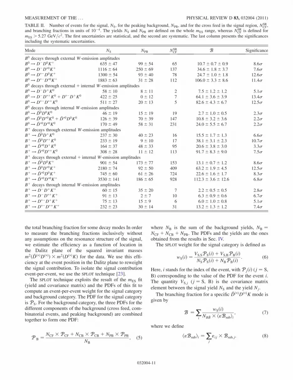
the total branching fraction for some decay modes In orderto measure the branching fractions inclusively withoutany assumptions on the resonance structure of the signal,we estimate the efficiency as a function of location inthe Dalitz plane of the squared invariant masses

m2ð �Dð�ÞDð�ÞÞ �m2ðDð�ÞKÞ for the data. We use this effi-ciency at the event position in the Dalitz plane to reweightthe signal contribution. To isolate the signal contributionevent-per-event, we use the SPLOT technique [23].

The SPLOT technique exploits the result of the mES fit(yield and covariance matrix) and the PDFs of this fit tocompute an event-per-event weight for the signal categoryand background category. The PDF for the signal categoryis P S. For the background category, the three PDFs for thedifferent components of the background (cross feed, com-binatorial events, and peaking background) are combinedtogether to form one PDF:

P B ¼ NCF � P CF þ NCB � P CB þ NPB � P PB

NB

; (5)

where NB is the sum of the background yields, NB ¼NCF þ NCB þ NPB. The PDFs and the yields are the onesobtained from the results in Sec. IV.The SPLOT weight for the signal category is defined as

wSðiÞ ¼ VS;SP SðiÞ þ VS;BP BðiÞNSP SðiÞ þ NBP BðiÞ : (6)

Here, i stands for the index of the event, with P jðiÞ (j ¼ S,

B) corresponding to the value of the PDF for the event i.The quantity VS;j (j ¼ S, B) is the covariance matrix

element between the signal yield NS and the yield Nj.

The branching fraction for a specific �Dð�ÞDð�ÞK mode isgiven by

B ¼ Xi

wSðiÞNB �B � h"Bsubii ; (7)

where we define

h"Bsubii ¼Xj

"ij �Bsub;j: (8)

TABLE II. Number of events for the signal, NS, for the peaking background, NPB, and for the cross feed in the signal region, NSRCF ,

and branching fractions in units of 10�4. The yields NS and NPB are defined on the whole mES range, whereas NSRCF is defined for

mES > 5:27 GeV=c2. The first uncertainties are statistical, and the second are systematic. The last column presents the significancesincluding the systematic uncertainties.

Mode NS NPB NSRCF B Significance

B0 decays through external W-emission amplitudes

B0 ! D�D0Kþ 635� 47 99� 54 65 10:7� 0:7� 0:9 8:6�B0 ! D�D�0Kþ 1116� 64 250� 69 137 34:6� 1:8� 3:7 7:6�B0 ! D��D0Kþ 1300� 54 93� 40 78 24:7� 1:0� 1:8 12:6�B0 ! D��D�0Kþ 1883� 63 31� 28 112 106:0� 3:3� 8:6 11:4�B0 decays through externalþ internal W-emission amplitudes

B0 ! D�DþK0 58� 10 8� 11 2 7:5� 1:2� 1:2 5:1�B0 ! D�D�þK0 þD��DþK0 422� 25 0� 12 7 64:1� 3:6� 3:9 13:4�B0 ! D��D�þK0 511� 27 20� 13 5 82:6� 4:3� 6:7 12:5�B0 decays through internal W-emission amplitudes

B0 ! �D0D0K0 46� 19 15� 19 19 2:7� 1:0� 0:5 2:3�B0 ! �D0D�0K0 þ �D�0D0K0 126� 39 70� 39 147 10:8� 3:2� 3:6 2:2�B0 ! �D�0D�0K0 170� 49 58� 31 231 24:0� 5:5� 6:7 2:2�Bþ decays through external W-emission amplitudes

Bþ ! �D0DþK0 237� 30 40� 23 16 15:5� 1:7� 1:3 6:6�Bþ ! �D0D�þK0 233� 19 9� 10 17 38:1� 3:1� 2:3 10:7�Bþ ! �D�0DþK0 164� 37 48� 33 95 20:6� 3:8� 3:0 3:3�Bþ ! �D�0D�þK0 308� 28 11� 12 113 91:7� 8:3� 9:0 7:5�Bþ decays through externalþ internal W-emission amplitudes

Bþ ! �D0D0Kþ 901� 54 173� 77 153 13:1� 0:7� 1:2 8:6�Bþ ! �D0D�0Kþ 2180� 74 92� 50 409 63:2� 1:9� 4:5 12:5�Bþ ! �D�0D0Kþ 745� 60 61� 26 724 22:6� 1:6� 1:7 8:3�Bþ ! �D�0D�0Kþ 3530� 141 186� 65 928 112:3� 3:6� 12:6 6:8�Bþ decays through internal W-emission amplitudes

Bþ ! D�DþKþ 60� 15 35� 20 7 2:2� 0:5� 0:5 2:8�Bþ ! D�D�þKþ 91� 13 2� 7 10 6:3� 0:9� 0:6 6:7�Bþ ! D��DþKþ 75� 13 15� 9 6 6:0� 1:0� 0:8 5:1�Bþ ! D��D�þKþ 232� 23 30� 14 31 13:2� 1:3� 1:2 7:4�

MEASUREMENT OF THE . . . PHYSICAL REVIEW D 83, 032004 (2011)

032004-11

The sum on j is over all the D subdecays of a particular�Dð�ÞDð�ÞK mode. The term Bsub;j is the product of the

secondary branching fractions of the subdecay j:

B sub;j ¼ B �Dð�Þ �BDð�Þ �BK; (9)

where B �Dð�Þ , BDð�Þ , and BK are the secondary branching

fractions of the �Dð�Þ,Dð�Þ andK mesons [17] (withBK ¼ 1for Kþ mesons). The quantity "ij is the efficiency for the

subdecay j at the Dalitz position of event i. In practice, for

a specific �Dð�ÞDð�ÞK mode with given D subdecays (e.g.�D0 ! Kþ�� �D0 ! K��þ�0), the efficiency is ob-tained by using the specific simulated signal and dividingthe reconstructed signal by the generated signal in the

Dalitz plane m2ð �Dð�ÞDð�ÞÞ �m2ðDð�ÞKÞ, which is dividedin 15� 15 bins for the operation. The size of the bins isroughly 0:52� 0:77 GeV2=c4, 0:46� 0:68 GeV2=c4, and0:38� 0:58 GeV2=c4 for decay modes with no D�, oneD�, and two D� mesons, respectively, depending on theavailable phase space. Neighboring bins are added togetherif one bin contains fewer than 10 events in the recon-structed Dalitz plane. The signal is simulated assuming aflat (phase space) distribution in this Dalitz plane.

The statistical uncertainty on the branching fraction isgiven by [23]

�B ¼ffiffiffiffiffiffiffiffiffiffiffiffiffiffiffiffiffiffiffiffiffiffiffiffiffiffiffiffiffiffiffiffiffiffiffiffiffiffiffiffiffiffiffiffiffiXi

�wSðiÞ

NB �B � h"Bsubii�2

vuut : (10)

B. Validation

The analysis is validated at all stages by use of MCsamples. These samples consist of a mixture of continuum

events and generic B decays containing the �Dð�ÞDð�ÞKsignals with branching fractions close to the ones measuredin our previous result [4]. As a preliminary remark, it has tobe noted that the analysis technique, including the selec-tion optimization and the procedure for the fit and for thebranching fraction measurement, is first determined solelyon MC simulations (‘‘blind’’ analysis).

First, we show that the fit is able to find the true numberof simulated signal events within a 1� interval for the22 modes, where � is the statistical uncertainty reportedby the fit.

Furthermore, the SPLOT method is tested on simulatedsamples. It is shown that this technique is able to tag trueMC signal events with very good performance. A featureof the SPLOT method is that the sum of SPLOTweights for agiven category is equal to the yield of this category [23].We determine that the sum of SPLOT signal weights for theMC signal events is equal to the number of simulated MCsignal events with a relative difference smaller than 1.5%for the majority of the modes. We also check that the sumof SPLOT signal weights for the MC background events iscompatible with zero as expected.

Finally, we perform the measurement on MC simula-tions and find that the analysis is able to find the branchingfractions set in the simulation within a 1� interval for mostof the 22 modes, where � is the total uncertainty on thebranching fraction (combining in quadrature statistical andsystematic uncertainties). We also test the iterative proce-dure by randomizing the initial branching fractions andcheck that the branching fractions are converging to theexpected values after a few iterations.

C. Measurement

For each event, we obtain the SPLOTweight as well as theefficiency at its Dalitz position. Using Eq. (7), we computethe branching fraction for each of the Bmodes. We presentthese results in Table II. We assume equal B0 �B0 and BþB�production [17].

VI. SYSTEMATIC UNCERTAINTIES

We consider several sources of systematic uncertaintieson the branching fraction measurements. Their contribu-tions are summarized in Table III.(a) We fix the width of the signal PDF from the value

obtained in the fit to the signal MC sample. To estimate thesystematic uncertainties originating from this choice, werepeat the fit with the width free to float for modes withhigh significance, namely, B0 ! D�D�þK0 þD��DþK0,B0 ! D��D�þK0, B0 ! D��D�0Kþ, and Bþ !�D0D�þK0. The difference observed between the widthfrom the data and from the MC events is roughly equalto 0:1 MeV=c2. Using this number, we repeat the fits for allmodes adding�0:1 MeV=c2 to the value of the width. Thedifference with the nominal branching fraction gives thesystematic contribution associated to the signal shape. In

addition, as mentioned in Sec. IVE, three �Dð�ÞDð�ÞK modeswith low signal statistics have their PDF mean fixed to thevalue obtained for the simulation. We repeat the fit usingthe PDF mean obtained from a mode with a large statistics(namely B0 ! D��D�þK0) and take the difference inbranching fraction as the systematic uncertainty. Thesetwo contributions of the systematic uncertainties are addedin quadrature.(b) The cross-feed determination introduces systematic

uncertainties of which two sources are identified. First, weuse an alternate function for the cross-feed PDF [using anonparametric function rather than Eq. (2)], which givesrelative systematic uncertainties below 1%. Second, thecross-feed branching fractions and their uncertainties areknown from the results of this analysis. To estimatethe systematic uncertainties coming from this effect, werepeat the measurement applying �1� of the statisticaluncertainty on each cross-feed contribution to a givenmode. These different contributions for each cross-feedmode are then combined quadratically.(c) The peaking background contributions are fixed from

fits to the background MC simulation, using a Gaussian

P. DEL AMO SANCHEZ et al. PHYSICAL REVIEW D 83, 032004 (2011)

032004-12

PDF. In these fits, the three parameters, namely, the num-ber of events, the mean, and the width, are correlated. Wegenerate several sets of these parameters based on thecovariance matrix of the fits and recompute the branchingfractions for each of these sets. From the distribution of thebranching fractions, we extract the systematic uncertaintiesoriginating from the peaking background. Another system-atic effect arises from the fact that we use the MC afterhaving scaled it to the data luminosity (using the totalnumber of MC events passing the selection, the numberof B �B pairs, and the cross-section of eþe� ! q �q, whereq ¼ u, d, s, c). We estimate the data-MC agreement bycomputing the ratio of number of events for data andsimulation for mES between 5.22 and 5:25 GeV=c2. Werescale the peaking background events using the ratiofound in the specific mode (0.9 in average) and repeat thebranching fraction measurement. The difference with the

nominal branching fraction gives the systematic uncer-tainty related to this effect. We combine these two sourcesof uncertainties in quadrature. Given the difficulty of esti-mating the peaking background, this is the dominant sys-

tematic uncertainty for most of the �Dð�ÞDð�ÞK modes.(d) The systematic uncertainty associated with the as-

sumption of a fixed value of the end point in the Argusfunction is estimated by repeating the fit and letting the endpoint free to vary in the physical region between 5.288 and5:292 GeV=c2 to account for possible variations in thebeam energy measurement. The difference in the branch-ing fraction between this fit and the nominal fit gives thesystematic contribution related to the combinatorialbackground.(e) We investigate the fit procedure performing a large

number of test fits to MC samples obtained from the PDFsfitted to the data and look for the presence of possible bias

TABLE III. Summary of the absolute systematic uncertainties on the branching fractions for each �Dð�ÞDð�ÞK mode (in units of 10�4).The values listed in this table correspond to the systematic uncertainties associated with the signal shape (a), the cross-feedcontribution (b), the peaking background (c), the combinatorial background (d), the fit bias (e), the iterative procedure (f), thelimited MC statistics (g), the number of bins of the Dalitz plane (h), the particle detection efficiency (i), and finally the secondarybranching fractions and the number of B �B pairs (j). The letters in parenthesis refer to the specific paragraph in Sec. VI. The last columnpresents the total systematic uncertainties.

Mode

Signal

shape

Cross

feed

Peaking

back.

Comb.

back.

Fit

bias

Iter.

proc.

MC

stat.

Bins Particle

detection

BFþNB �B

Total

syst.

(a) (b) (c) (d) (e) (f) (g) (h) (i) ( j)

B0 decays through external W-emission amplitudes

B0 ! D�D0Kþ 0.2 0.1 0.5 0.0 0.0 0.0 0.2 0.2 0.5 0.3 0.9

B0 ! D�D�0Kþ 0.7 0.1 2.4 0.0 0.0 0.1 1.3 1.1 1.9 1.1 3.7

B0 ! D��D0Kþ 0.5 0.0 0.7 0.0 0.0 0.0 0.5 0.5 1.3 0.8 1.8

B0 ! D��D�0Kþ 2.0 0.2 1.6 0.1 0.0 0.2 1.8 3.8 6.4 2.9 8.6

B0 decays through externalþ internal W-emission amplitudes

B0 ! D�DþK0 0.1 0.0 1.0 0.0 0.2 0.0 0.1 0.1 0.2 0.4 1.2

B0 ! D�D�þK0 þD��DþK0 0.9 0.0 1.3 0.1 0.1 0.0 1.3 0.9 2.4 2.2 3.9

B0 ! D��D�þK0 1.2 0.0 2.0 0.0 0.0 0.0 3.2 2.1 4.2 2.9 6.7

B0 decays through internal W-emission amplitudes

B0 ! �D0D0K0 0.2 0.0 0.4 0.1 0.1 0.0 0.1 0.2 0.1 0.1 0.5

B0 ! �D0D�0K0 þ �D�0D0K0 0.3 0.4 3.4 0.1 0.5 0.1 0.5 0.3 0.5 0.3 3.6

B0 ! �D�0D�0K0 0.9 1.6 5.2 0.2 0.8 1.8 1.1 2.6 1.7 0.6 6.7

Bþ decays through external W-emission amplitudes

Bþ ! �D0DþK0 0.4 0.0 0.9 0.1 0.0 0.0 0.3 0.2 0.5 0.5 1.3

Bþ ! �D0D�þK0 0.5 0.3 1.0 0.1 0.1 0.0 0.8 0.3 1.4 1.0 2.3

Bþ ! �D�0DþK0 0.5 0.3 2.5 0.3 0.3 0.3 0.8 0.5 1.0 0.7 3.0

Bþ ! �D�0D�þK0 1.6 1.3 2.5 0.1 0.1 0.4 3.1 5.5 4.9 2.4 9.0

Bþ decays through externalþ internal W-emission amplitudes

Bþ ! �D0D0Kþ 0.3 0.0 1.0 0.0 0.0 0.0 0.2 0.2 0.6 0.3 1.2

Bþ ! �D0D�0Kþ 1.2 0.2 1.0 0.0 0.1 0.3 0.9 1.4 3.6 1.6 4.5

Bþ ! �D�0D0Kþ 0.4 0.2 0.5 0.0 0.1 0.3 0.6 0.5 1.3 0.6 1.7

Bþ ! �D�0D�0Kþ 2.0 0.6 2.8 0.7 0.2 1.3 4.2 6.2 9.0 3.0 12.6

Bþ decays through internal W-emission amplitudes

Bþ ! D�DþKþ 0.1 0.0 0.5 0.0 0.1 0.0 0.0 0.0 0.1 0.1 0.5

Bþ ! D�D�þKþ 0.1 0.0 0.4 0.0 0.0 0.0 0.2 0.3 0.3 0.2 0.6

Bþ ! D��DþKþ 0.1 0.0 0.6 0.1 0.0 0.0 0.3 0.1 0.3 0.2 0.8

Bþ ! D��D�þKþ 0.2 0.0 0.5 0.0 0.1 0.0 0.6 0.2 0.7 0.4 1.2

MEASUREMENT OF THE . . . PHYSICAL REVIEW D 83, 032004 (2011)

032004-13

in the number of signal events. We observe that the biasesare in most cases smaller than 10% of the statistical un-certainty. We do not correct these small biases but takethem into account in the total systematic uncertainties.

(f) An iterative procedure is performed to compute thebranching fractions. We check this procedure on the MCsimulation, where the results should not depend on theprocedure used. The difference between the iterative andnoniterative methods is small but non-negligible in somecases. We take the relative difference as the systematiccontribution on the data due to the iterative procedure.

(g) The limited Monte Carlo statistics induce an uncer-tainty on the computation of the signal efficiency.We use anefficiency mapping in the Dalitz plane with 15� 15 bins.To take into account this uncertainty, we generate severalefficiencymappings, where in each binwe vary the nominalefficiency according to the efficiency uncertainty distribu-tion.We obtain a distribution of branching fractions that weemploy to determine the systematic contribution.

(h) We extract the efficiency in the Dalitz plane from a15� 15 bin mapping. We vary the numbers of bins from1� 1 bin to 20� 20 bins and recompute the branchingfractions. This test is performed on MC simulation con-

taining signal and background events, where the �Dð�ÞDð�ÞKsignal is purely nonresonant. In this case, the results shouldnot depend on the number of bins since no resonant statesare present. The maximal difference with the nominalbranching fraction is taken as the systematic uncertainty.

(i) From the differences in the reconstruction and particleidentification efficiencies for the data and MC controlsamples, we derive systematic uncertainties of 0.2% percharged track, 1.7% per soft pion fromD� decays, 1.2% perK0

S, 3% per �0, and 1.8% per single photon. Additionally,

the systematic uncertainties for the Kþ identification areranging from 2% to 4% (in total) depending on the mode.

( j) Finally, the uncertainties on theDð�Þ andK0S branching

fractions are [17] accounted for. The total systematic un-

certainty also takes into account the number of Bmesons inthe data sample, which is known with a 0.6% uncertainty.Table III shows a summary of the systematic uncertain-

ties. The uncertainties from the different contributions areadded together in quadrature to give the total systematicuncertainty for a specific mode.

VII. RESULTS

The final results on the data using the full BABAR datasample can be found in Table II. In this Table, the quantityNSR

CF is the number of cross-feed events in the signal

region (i.e. integrating the cross-feed PDF for mES >5:27 GeV=c2) determined from the MC simulation scaledto the data luminosity using the branching fractions mea-sured in this analysis (this includes peaking and nonpeak-ing cross-feed contributions). We indicate the significances(including systematic uncertainties) of the observations. Tocompute these significances, we repeat the fits using nocontribution from the signal. We compute the statisticalsignificance Sstat calculating PROB[2 lnðLsignal=L0Þ,Ndof],

where Lsignal (L0) is the maximum of the likelihood with

(without) the signal contribution,Ndof is the number of freeparameters in the signal PDF (two here), and PROB is theupper tail probability of a chi-squared distribution,converting this probability into a number of standard de-viations. We then take the systematic uncertainty intoaccount by smearing Sstat by use of a Gaussian with a

width equal to the systematic uncertainty: Sstatþsyst ¼Sstat=

ffiffiffiffiffiffiffiffiffiffiffiffiffiffiffiffiffiffiffiffiffiffiffiffiffiffiffiffiffiffiffiffiffið1þ �2

syst=�2statÞ

q, where �stat and �syst are, respec-

tively, the statistical and systematic uncertainties on thebranching fraction measurement.

We check isospin invariance using the �Dð�ÞDð�ÞK decays.Assuming isospin invariance in the B decay, interchangingthe u and d quarks in the Feynman diagrams of Fig. 1should not modify the amplitude values. Table IV presents

TABLE IV. Ratios of neutral to charged branching fractions. The second column shows the ratio r, where the first uncertainty isstatistical and the second is systematic. The third column shows this value multiplied by the ratio of the charged to neutral B mesonlifetimes, where the error includes all uncertainties.

Mode r r� Bþ=B0

BðB0 ! D�D0KþÞ=BðBþ ! �D0DþK0Þ 0:69� 0:09� 0:08 0:74� 0:13BðB0 ! D�D�0KþÞ=BðBþ ! �D0D�þK0Þ 0:91� 0:09� 0:11 0:97� 0:15BðB0 ! D��D0KþÞ=BðBþ ! �D�0DþK0Þ 1:20� 0:23� 0:20 1:28� 0:32BðB0 ! D��D�0KþÞ=BðBþ ! �D�0D�þK0Þ 1:16� 0:11� 0:15 1:24� 0:20BðB0 ! D�DþK0Þ=BðBþ ! �D0D0KþÞ 0:57� 0:10� 0:10 0:61� 0:15

BðB0!D�D�þK0þD��DþK0ÞBðBþ! �D0D�0KþÞþBðBþ! �D�0D0KþÞ 0:75� 0:05� 0:07 0:80� 0:09

BðB0 ! D��D�þK0Þ=BðBþ ! �D�0D�0KþÞ 0:74� 0:05� 0:10 0:79� 0:12

BðB0 ! �D0D0K0Þ=BðBþ ! D�DþKþÞ 1:20� 0:53� 0:36 1:28� 0:69

BðB0! �D0D�0K0þ �D�0D0K0ÞBðBþ!D�D�þKþÞþBðBþ!D��DþKþÞ 0:88� 0:27� 0:31 0:94� 0:44

BðB0 ! �D�0D�0K0Þ=BðBþ ! D��D�þKþÞ 1:81� 0:45� 0:53 1:94� 0:75

P. DEL AMO SANCHEZ et al. PHYSICAL REVIEW D 83, 032004 (2011)

032004-14

the ratios of the modes which are related by isospin sym-metry. In the ratio of the branching fractions, all factorscancel except the amplitudes and the B0=Bþ lifetimes(neglecting the small mass differences between neutraland charged states for the B, D�, D, and K mesons). Wemultiply the ratios of the neutral to charged branchingfractions, r, by the ratio of the charged to neutral B mesonlifetimes, Bþ=B0 ¼ 1:071� 0:009 [17]. The uncertaintyon these values reported in Table IV combines the statis-tical and systematic uncertainties of our measurement, aswell as the uncertainty on the lifetime ratio. The values ofr� Bþ=B0 should be equal to unity if isospin invarianceis verified. Although some values are compatible with thisequality, for some others we observe discrepancies up to2:6� (where � is the 68% standard deviation). This resultis obtained assuming equal production of B0 and Bþmesons.

VIII. CONCLUSION

We have analyzed 471� 106 pairs of B mesons pro-duced in the BABAR experiment and studied the exclusive

decays of B0= �B0, B� to �Dð�ÞDð�ÞK� and B0= �B0, B� to�Dð�ÞDð�ÞK0. We measure the branching fractions for the 22modes (see Table II). Some of the modes have been ob-served for the first time here: Bþ ! �D�0D0Kþ (8:3�),Bþ ! D��D�þKþ (7:4�), Bþ ! D�D�þKþ (6:7�),Bþ ! �D0DþK0 (6:6�), and B0 ! D�DþK0 (5:1�). Inaddition, we show evidence for the mode Bþ !�D�0DþK0 (3:3�) for the first time. We also report theobservation of some of the color-suppressed modes,namely Bþ ! D��D�þKþ (7:4�), Bþ ! D�D�þKþ(6:7�), and Bþ ! D��DþKþ (5:1�). The other color-suppressed modes are seen with a lower significance:Bþ ! D�DþKþ (2:8�), B0 ! �D0D0K0 (2:3�), B0 !�D�0D�0K0 (2:2�), and B0 ! �D0D�0K0 þ �D�0D0K0

(2:2�).Summing the 10 neutral modes and the 12 charged

modes, wemeasure that �Dð�ÞDð�ÞK events represent ð3:68�0:10� 0:24Þ% of the B0 decays and ð4:05� 0:11�0:28Þ% of the Bþ decays, where the first uncertaintiesare statistical and the second systematic, taking into accountthe correlations amongst the systematic uncertainties.These decays do not saturate the wrong-sign D productionand account roughly for one third of this production.

This result implies that probably decays of the type B !�Dð�ÞDð�ÞKðn�Þ (with n � 1) have a non-negligible contri-bution to the b ! c �cs transition (for example through the

decays B ! �Dð�ÞDð�ÞK� or B ! �Dð�ÞD��K, whereD�� is anexcited D meson other than D�þ and D�0).

The results obtained here are found to be in satisfactoryagreement with those of the previous study by BABARusing 76 fb�1 [4] and supersede these previous measure-ments. Our branching fraction measurement of the modeB0 ! D��D�þK0 is found in good agreement with the

values reported in Refs. [8,9] and supersedes our previousresult [8]. However, our branching fraction measurementof the mode Bþ ! �D0D0Kþ is in disagreement at a 2:1�level with the Belle result [10].We believe that the discrepancy with Ref. [10] and

the fact that the branching fractions measured here arealmost systematically lower than the ones in Ref. [4](although most of the time compatible) are due to thefact that in the present work we employ a more accurateparametrization of the signal mES distribution in the fit andthat we take into account both the cross feed and thepeaking background contributions. In Ref. [4], only crossfeed was accounted for but the peaking background wasnot considered due to the lower statistics. In addition, theefficiency correction used in obtaining the branching frac-tions accounts for the presence of resonant intermediatestates in the data.Finally, from neutral to charged B meson ratios of the

branching fractions, assuming equal B0 �B0 and BþB� pro-duction and taking into account the B meson lifetimes, wenote that some mode ratios respect the isospin invariance,while some others show discrepancies up to 2:6�.

ACKNOWLEDGMENTS

We are grateful for the extraordinary contributionsof our PEP-II colleagues in achieving the excellent lumi-nosity and machine conditions that have made this workpossible. The success of this project also relies critically onthe expertise and dedication of the computing organiza-tions that support BABAR. The collaborating institutionswish to thank SLAC for its support and the kind hospitalityextended to them. This work is supported by the USDepartment of Energy and National Science Foundation,the Natural Sciences and Engineering Research Council(Canada), the Commissariat a l’Energie Atomique andInstitut National de Physique Nucleaire et de Physiquedes Particules (France), the Bundesministerium furBildung und Forschung and Deutsche Forschungs-gemeinschaft (Germany), the Istituto Nazionale di FisicaNucleare (Italy), the Foundation for Fundamental Researchon Matter (The Netherlands), the Research Council ofNorway, the Ministry of Education and Science of theRussian Federation, Ministerio de Ciencia e Innovacion(Spain), and the Science and Technology Facilities Council(United Kingdom). Individuals have received support fromthe Marie-Curie IEF program (European Union), the A. P.Sloan Foundation (U.S.) and the Binational ScienceFoundation (U.S.-Israel).

APPENDIX A: FIT PDF EXPRESSIONS

We give the expressions of the PDFs introduced inSec. IV (along with their parameters) and used to fit themES distribution in the data.

MEASUREMENT OF THE . . . PHYSICAL REVIEW D 83, 032004 (2011)

032004-15

1. Signal PDF

The signal PDF is given by

P SðmES;mS; �S; �S; nSÞ

¼8><>:exp½�ðmES �mSÞ2=ð2�2

S� mES >mS � �S�S

ðnS�SÞnS expð��2

S=2Þ

ððmS�mESÞ=�SþnS�S��SÞnS mES � mS � �S�S:

(A1)

In this equation and in the following, we omit the factorthat normalizes the PDF to unity.

2. Cross-feed PDF

The cross-feed PDF for modes containing noD�0 mesonis described for the peaking part by

P peakingCF ðmES;mCF; �CFÞ ¼ exp½�ðmES �mCFÞ2=ð2�2

CF�:(A2)

For modes containing at least one neutral D� meson, thepeaking component is represented by an empirical functiondescribing an asymmetric peak:

P 0peakingCF ðmES;mCF; �CF; tCFÞ

¼ exp

24�ln2

�1þ tCF�

mES�mCF

�CF

�2t2CF

� t2CF2

35; (A3)

where � ¼ sinhðtCFffiffiffiffiffiffiffiln4

p Þ=ðtCFffiffiffiffiffiffiffiln4

p Þ. This function ap-proaches a Gaussian function when the parameter tCFvanishes.The nonpeaking part PDF is

P nonpeakingCF ðmES;m0; �CFÞ¼ mES

ffiffiffiffiffiffiffiffiffiffiffiffiffiffiffiffiffiffiffiffiffiffiffiffiffiffiffiffiffiffiffiffi1� ðmES=m0Þ2

q� exp½��CFð1� ðmES=m0Þ2Þ�:

(A4)

3. Combinatorial background PDF

The combinatorial background PDF can be expressed as

P CBðmES;m0; �CBÞ ¼ mES

ffiffiffiffiffiffiffiffiffiffiffiffiffiffiffiffiffiffiffiffiffiffiffiffiffiffiffiffiffiffiffiffi1� ðmES=m0Þ2

q� exp½��CBð1� ðmES=m0Þ2Þ�:

(A5)

4. Peaking background PDF

The peaking background PDF is given by

P PBðmES;mPB; �PBÞ ¼ exp½�ðmES �mPBÞ2=ð2�2PBÞ�:(A6)

[1] I. I. Bigi, B. Blok, M. Shifman, and A. Vainshtein, Phys.Lett. B 323, 408 (1994); T. Browder, Proceedings of the1996 Warsaw ICHEP Conference, edited by Z. Ajduk andA.K. Wroblewski (World Scientific, Singapore, 1997),p. 1139.

[2] G. Buchalla, I. Dunietz, and H. Yamamoto, Phys. Lett. B364, 188 (1995).

[3] CLEO Collaboration, CLEO CONF 97-26, EPS97 337,1997); T. E. Coan (CLEO Collaboration), Phys. Rev. Lett.80, 1150 (1998); R. Barate (ALEPH Collaboration), Eur.Phys. J. C 4, 387 (1998).

[4] B. Aubert (BABAR Collaboration), Phys. Rev. D 68,092001 (2003).

[5] B. Aubert (BABAR Collaboration), Phys. Rev. D 75,072002 (2007).

[6] M. Zito, Phys. Lett. B 586, 314 (2004).[7] J. Charles et al., Phys. Lett. B 425, 375 (1998); T. E.

Browder, A. Datta, P. J. O’Donnell, and S. Pakvasa,Phys. Rev. D 61, 054009 (2000).

[8] B. Aubert (BABAR Collaboration), Phys. Rev. D 74,091101 (2006).

[9] J. Dalseno (Belle Collaboration), Phys. Rev. D 76, 072004(2007).

[10] J. Brodzicka (Belle Collaboration), Phys. Rev. Lett. 100,092001 (2008).

[11] B. Aubert (BABAR Collaboration), Phys. Rev. D 77,011102 (2008).

[12] T. Aushev, N. Zwahlen (Belle Collaboration), Phys. Rev.D 81, 031103 (2010).

[13] B. Aubert (BABAR Collaboration), Nucl. Instrum.Methods Phys. Res., Sect. A 479, 1 (2002).

[14] D. J. Lange, Nucl. Instrum. Methods Phys. Res., Sect. A462, 152 (2001).

[15] T. Sjostrand, S. Mrenna, and P. Skands, J. High EnergyPhys. 05(2006) 026.

[16] S. Agostinelli (GEANT4 Collaboration), Nucl. Instrum.Methods Phys. Res., Sect. A 506, 250 (2003).

[17] C. Amsler (Particle Data Group), Phys. Lett. B 667, 1(2008) and 2009 partial update for the 2010 edition.

[18] J. C. Anjos (E691 Collaboration), Phys. Rev. D 48, 56(1993).

[19] G. C. Fox and S. Wolfram, Nucl. Phys. B149, 413 (1979).[20] E. D. Bloom and C. Peck, Annu. Rev. Nucl. Part. Sci. 33,

143 (1983).[21] H. Albrecht (Argus Collaboration), Phys. Lett. B 241, 278

(1990).[22] B. Aubert (BABAR Collaboration), Phys. Rev. D 80,

092003 (2009).[23] M. Pivk and F. R. Le Diberder, Nucl. Instrum. Methods

555, 356 (2005).

P. DEL AMO SANCHEZ et al. PHYSICAL REVIEW D 83, 032004 (2011)

032004-16