arX

iv:1

109.

6831

v1 [

hep-

ex]

30

Sep

2011

EUROPEAN ORGANIZATION FOR NUCLEAR RESEARCH (CERN)

LHCb-PAPER-2011-016CERN-PH-EP-2011-151

September 17, 2014

Measurements of the Branchingfractions for B(s) → D(s)πππ and

Λ0b→ Λ+

cπππ

The LHCb Collaboration 1

Abstract

Branching fractions of the decays Hb → Hcπ−π+π− relative to Hb → Hcπ

− arepresented, where Hb (Hc) represents B0 (D+), B− (D0), B0

s (D+s ) and Λ0

b (Λ+c ).

The measurements are performed with the LHCb detector using 35 pb−1 of datacollected at

√s = 7 TeV. The ratios of branching fractions are measured to be

B(B0 → D+π−π+π−)

B(B0 → D+π−)= 2.38 ± 0.11 ± 0.21

B(B− → D0π−π+π−)

B(B− → D0π−)= 1.27 ± 0.06 ± 0.11

B(B0s → D+

s π−π+π−)

B(B0s → D+

s π−)= 2.01 ± 0.37 ± 0.20

B(Λ0b → Λ+

c π−π+π−)

B(Λ0b→ Λ+

c π−)= 1.43 ± 0.16 ± 0.13.

We also report measurements of partial decay rates of these decays to excited charmhadrons. These results are of comparable or higher precision than existing measure-ments.

1Authors are listed on the following pages.

R. Aaij23, B. Adeva36, M. Adinolfi42, C. Adrover6, A. Affolder48, Z. Ajaltouni5, J. Albrecht37,F. Alessio37, M. Alexander47, G. Alkhazov29, P. Alvarez Cartelle36, A.A. Alves Jr22, S. Amato2,Y. Amhis38, J. Anderson39, R.B. Appleby50, O. Aquines Gutierrez10, F. Archilli18,37, L. Arrabito53,A. Artamonov 34, M. Artuso52,37, E. Aslanides6, G. Auriemma22,m, S. Bachmann11, J.J. Back44,D.S. Bailey50, V. Balagura30,37, W. Baldini16, R.J. Barlow50, C. Barschel37, S. Barsuk7, W. Barter43,A. Bates47, C. Bauer10, Th. Bauer23, A. Bay38, I. Bediaga1, K. Belous34, I. Belyaev30,37,E. Ben-Haim8, M. Benayoun8, G. Bencivenni18, S. Benson46, J. Benton42, R. Bernet39, M.-O. Bettler17, M. van Beuzekom23, A. Bien11, S. Bifani12, A. Bizzeti17,h, P.M. Bjørnstad50,T. Blake49, F. Blanc38, C. Blanks49, J. Blouw11, S. Blusk52, A. Bobrov33, V. Bocci22, A. Bondar33,N. Bondar29, W. Bonivento15, S. Borghi47, A. Borgia52, T.J.V. Bowcock48, C. Bozzi16, T. Brambach9,J. van den Brand24, J. Bressieux38, D. Brett50, S. Brisbane51, M. Britsch10, T. Britton52, N.H. Brook42,H. Brown48, A. Buchler-Germann39, I. Burducea28, A. Bursche39, J. Buytaert37, S. Cadeddu15,J.M. Caicedo Carvajal37, O. Callot7, M. Calvi20,j, M. Calvo Gomez35,n, A. Camboni35, P. Campana18,37,A. Carbone14, G. Carboni21,k, R. Cardinale19,i,37, A. Cardini15, L. Carson36, K. Carvalho Akiba23,G. Casse48, M. Cattaneo37, M. Charles51, Ph. Charpentier37, N. Chiapolini39, K. Ciba37, X. Cid Vidal36,G. Ciezarek49, P.E.L. Clarke46,37, M. Clemencic37, H.V. Cliff43, J. Closier37, C. Coca28, V. Coco23,J. Cogan6, P. Collins37, F. Constantin28, G. Conti38, A. Contu51, A. Cook42, M. Coombes42, G. Corti37,G.A. Cowan38, R. Currie46, B. D’Almagne7, C. D’Ambrosio37, P. David8, I. De Bonis4, S. De Capua21,k,M. De Cian39, F. De Lorenzi12, J.M. De Miranda1, L. De Paula2, P. De Simone18, D. Decamp4,M. Deckenhoff9, H. Degaudenzi38,37, M. Deissenroth11, L. Del Buono8, C. Deplano15, O. Deschamps5,F. Dettori15,d, J. Dickens43, H. Dijkstra37, P. Diniz Batista1, S. Donleavy48, A. Dosil Suarez36,D. Dossett44, A. Dovbnya40, F. Dupertuis38, R. Dzhelyadin34, C. Eames49, S. Easo45, U. Egede49,V. Egorychev30, S. Eidelman33, D. van Eijk23, F. Eisele11, S. Eisenhardt46, R. Ekelhof9, L. Eklund47,Ch. Elsasser39, D.G. d’Enterria35,o, D. Esperante Pereira36, L. Esteve43, A. Falabella16,e, E. Fanchini20,j ,C. Farber11, G. Fardell46, C. Farinelli23, S. Farry12, V. Fave38, V. Fernandez Albor36, M. Ferro-Luzzi37, S. Filippov32, C. Fitzpatrick46, M. Fontana10, F. Fontanelli19,i, R. Forty37, M. Frank37,C. Frei37, M. Frosini17,f,37, S. Furcas20, A. Gallas Torreira36, D. Galli14,c, M. Gandelman2, P. Gandini51,Y. Gao3, J-C. Garnier37, J. Garofoli52, J. Garra Tico43, L. Garrido35, C. Gaspar37, N. Gauvin38,M. Gersabeck37, T. Gershon44,37, Ph. Ghez4, V. Gibson43, V.V. Gligorov37, C. Gobel54, D. Golubkov30,A. Golutvin49,30,37, A. Gomes2, H. Gordon51, M. Grabalosa Gandara35, R. Graciani Diaz35,L.A. Granado Cardoso37, E. Grauges35, G. Graziani17, A. Grecu28, S. Gregson43, B. Gui52, E. Gushchin32,Yu. Guz34, T. Gys37, G. Haefeli38, C. Haen37, S.C. Haines43, T. Hampson42, S. Hansmann-Menzemer11,R. Harji49, N. Harnew51, J. Harrison50, P.F. Harrison44, J. He7, V. Heijne23, K. Hennessy48, P. Henrard5,J.A. Hernando Morata36, E. van Herwijnen37, E. Hicks48, W. Hofmann10, K. Holubyev11, P. Hopchev4,W. Hulsbergen23, P. Hunt51, T. Huse48, R.S. Huston12, D. Hutchcroft48, D. Hynds47, V. Iakovenko41,P. Ilten12, J. Imong42, R. Jacobsson37, A. Jaeger11, M. Jahjah Hussein5, E. Jans23, F. Jansen23,P. Jaton38, B. Jean-Marie7, F. Jing3, M. John51, D. Johnson51, C.R. Jones43, B. Jost37, S. Kandybei40,M. Karacson37, T.M. Karbach9, J. Keaveney12, U. Kerzel37, T. Ketel24, A. Keune38, B. Khanji6,Y.M. Kim46, M. Knecht38, S. Koblitz37, P. Koppenburg23, A. Kozlinskiy23, L. Kravchuk32, K. Kreplin11,M. Kreps44, G. Krocker11, P. Krokovny11, F. Kruse9, K. Kruzelecki37, M. Kucharczyk20,25,37,S. Kukulak25, R. Kumar14,37, T. Kvaratskheliya30,37, V.N. La Thi38, D. Lacarrere37, G. Lafferty50,A. Lai15, D. Lambert46, R.W. Lambert37, E. Lanciotti37, G. Lanfranchi18, C. Langenbruch11,T. Latham44, R. Le Gac6, J. van Leerdam23, J.-P. Lees4, R. Lefevre5, A. Leflat31,37, J. Lefrancois7,O. Leroy6, T. Lesiak25, L. Li3, L. Li Gioi5, M. Lieng9, M. Liles48, R. Lindner37, C. Linn11,B. Liu3, G. Liu37, J.H. Lopes2, E. Lopez Asamar35, N. Lopez-March38, J. Luisier38, F. Machefert7,I.V. Machikhiliyan4,30, F. Maciuc10, O. Maev29,37, J. Magnin1, S. Malde51, R.M.D. Mamunur37,G. Manca15,d, G. Mancinelli6, N. Mangiafave43, U. Marconi14, R. Marki38, J. Marks11, G. Martellotti22,A. Martens7, L. Martin51, A. Martın Sanchez7, D. Martinez Santos37, A. Massafferri1, Z. Mathe12,C. Matteuzzi20, M. Matveev29, E. Maurice6, B. Maynard52, A. Mazurov32,16,37, G. McGregor50,R. McNulty12, C. Mclean14, M. Meissner11, M. Merk23, J. Merkel9, R. Messi21,k, S. Miglioranzi37,D.A. Milanes13,37, M.-N. Minard4, S. Monteil5, D. Moran12, P. Morawski25, R. Mountain52, I. Mous23,F. Muheim46, K. Muller39, R. Muresan28,38, B. Muryn26, M. Musy35, J. Mylroie-Smith48, P. Naik42,

i

T. Nakada38, R. Nandakumar45, J. Nardulli45, I. Nasteva1, M. Nedos9, M. Needham46, N. Neufeld37,C. Nguyen-Mau38,p, M. Nicol7, S. Nies9, V. Niess5, N. Nikitin31, A. Oblakowska-Mucha26, V. Obraztsov34,S. Oggero23, S. Ogilvy47, O. Okhrimenko41, R. Oldeman15,d, M. Orlandea28, J.M. Otalora Goicochea2,P. Owen49, B. Pal52, J. Palacios39, M. Palutan18, J. Panman37, A. Papanestis45, M. Pappagallo13,b,C. Parkes47,37, C.J. Parkinson49, G. Passaleva17, G.D. Patel48, M. Patel49, S.K. Paterson49,G.N. Patrick45, C. Patrignani19,i, C. Pavel-Nicorescu28, A. Pazos Alvarez36, A. Pellegrino23, G. Penso22,l,M. Pepe Altarelli37, S. Perazzini14,c, D.L. Perego20,j, E. Perez Trigo36, A. Perez-Calero Yzquierdo35,P. Perret5, M. Perrin-Terrin6, G. Pessina20, A. Petrella16,37, A. Petrolini19,i, B. Pie Valls35, B. Pietrzyk4,T. Pilar44, D. Pinci22, R. Plackett47, S. Playfer46, M. Plo Casasus36, G. Polok25, A. Poluektov44,33,E. Polycarpo2, D. Popov10, B. Popovici28, C. Potterat35, A. Powell51, T. du Pree23, J. Prisciandaro38,V. Pugatch41, A. Puig Navarro35, W. Qian52, J.H. Rademacker42, B. Rakotomiaramanana38,M.S. Rangel2, I. Raniuk40, G. Raven24, S. Redford51, M.M. Reid44, A.C. dos Reis1, S. Ricciardi45,K. Rinnert48, D.A. Roa Romero5, P. Robbe7, E. Rodrigues47, F. Rodrigues2, P. Rodriguez Perez36,G.J. Rogers43, S. Roiser37, V. Romanovsky34, J. Rouvinet38, T. Ruf37, H. Ruiz35, G. Sabatino21,k,J.J. Saborido Silva36, N. Sagidova29, P. Sail47, B. Saitta15,d, C. Salzmann39, M. Sannino19,i,R. Santacesaria22, R. Santinelli37, E. Santovetti21,k, M. Sapunov6, A. Sarti18,l, C. Satriano22,m,A. Satta21, M. Savrie16,e, D. Savrina30, P. Schaack49, M. Schiller11, S. Schleich9, M. Schmelling10,B. Schmidt37, O. Schneider38, A. Schopper37, M.-H. Schune7, R. Schwemmer37, A. Sciubba18,l,M. Seco36, A. Semennikov30, K. Senderowska26, I. Sepp49, N. Serra39, J. Serrano6, P. Seyfert11,B. Shao3, M. Shapkin34, I. Shapoval40,37, P. Shatalov30, Y. Shcheglov29, T. Shears48, L. Shekhtman33,O. Shevchenko40, V. Shevchenko30, A. Shires49, R. Silva Coutinho54, H.P. Skottowe43, T. Skwarnicki52,A.C. Smith37, N.A. Smith48, K. Sobczak5, F.J.P. Soler47, A. Solomin42, F. Soomro49, B. Souza De Paula2,B. Spaan9, A. Sparkes46, P. Spradlin47, F. Stagni37, S. Stahl11, O. Steinkamp39, S. Stoica28,S. Stone52,37, B. Storaci23, M. Straticiuc28, U. Straumann39, N. Styles46, V.K. Subbiah37, S. Swientek9,M. Szczekowski27, P. Szczypka38, T. Szumlak26, S. T’Jampens4, E. Teodorescu28, F. Teubert37,C. Thomas51,45, E. Thomas37, J. van Tilburg11, V. Tisserand4, M. Tobin39, S. Topp-Joergensen51,M.T. Tran38, A. Tsaregorodtsev6, N. Tuning23, A. Ukleja27, P. Urquijo52, U. Uwer11, V. Vagnoni14,G. Valenti14, R. Vazquez Gomez35, P. Vazquez Regueiro36, S. Vecchi16, J.J. Velthuis42, M. Veltri17,g,K. Vervink37, B. Viaud7, I. Videau7, X. Vilasis-Cardona35,n, J. Visniakov36, A. Vollhardt39, D. Voong42,A. Vorobyev29, H. Voss10, K. Wacker9, S. Wandernoth11, J. Wang52, D.R. Ward43, A.D. Webber50,D. Websdale49, M. Whitehead44, D. Wiedner11, L. Wiggers23, G. Wilkinson51, M.P. Williams44,45,M. Williams49, F.F. Wilson45, J. Wishahi9, M. Witek25,37, W. Witzeling37, S.A. Wotton43, K. Wyllie37,Y. Xie46, F. Xing51, Z. Yang3, R. Young46, O. Yushchenko34, M. Zavertyaev10,a, L. Zhang52,W.C. Zhang12, Y. Zhang3, A. Zhelezov11, L. Zhong3, E. Zverev31, A. Zvyagin 37.

1Centro Brasileiro de Pesquisas Fısicas (CBPF), Rio de Janeiro, Brazil2Universidade Federal do Rio de Janeiro (UFRJ), Rio de Janeiro, Brazil3Center for High Energy Physics, Tsinghua University, Beijing, China4LAPP, Universite de Savoie, CNRS/IN2P3, Annecy-Le-Vieux, France5Clermont Universite, Universite Blaise Pascal, CNRS/IN2P3, LPC, Clermont-Ferrand, France6CPPM, Aix-Marseille Universite, CNRS/IN2P3, Marseille, France7LAL, Universite Paris-Sud, CNRS/IN2P3, Orsay, France8LPNHE, Universite Pierre et Marie Curie, Universite Paris Diderot, CNRS/IN2P3, Paris, France9Fakultat Physik, Technische Universitat Dortmund, Dortmund, Germany10Max-Planck-Institut fur Kernphysik (MPIK), Heidelberg, Germany11Physikalisches Institut, Ruprecht-Karls-Universitat Heidelberg, Heidelberg, Germany12School of Physics, University College Dublin, Dublin, Ireland13Sezione INFN di Bari, Bari, Italy14Sezione INFN di Bologna, Bologna, Italy

ii

15Sezione INFN di Cagliari, Cagliari, Italy16Sezione INFN di Ferrara, Ferrara, Italy17Sezione INFN di Firenze, Firenze, Italy18Laboratori Nazionali dell’INFN di Frascati, Frascati, Italy19Sezione INFN di Genova, Genova, Italy20Sezione INFN di Milano Bicocca, Milano, Italy21Sezione INFN di Roma Tor Vergata, Roma, Italy22Sezione INFN di Roma La Sapienza, Roma, Italy23Nikhef National Institute for Subatomic Physics, Amsterdam, Netherlands24Nikhef National Institute for Subatomic Physics and Vrije Universiteit, Amsterdam, Netherlands25Henryk Niewodniczanski Institute of Nuclear Physics Polish Academy of Sciences, Cracow, Poland26Faculty of Physics & Applied Computer Science, Cracow, Poland27Soltan Institute for Nuclear Studies, Warsaw, Poland28Horia Hulubei National Institute of Physics and Nuclear Engineering, Bucharest-Magurele, Romania29Petersburg Nuclear Physics Institute (PNPI), Gatchina, Russia30Institute of Theoretical and Experimental Physics (ITEP), Moscow, Russia31Institute of Nuclear Physics, Moscow State University (SINP MSU), Moscow, Russia32Institute for Nuclear Research of the Russian Academy of Sciences (INR RAN), Moscow, Russia33Budker Institute of Nuclear Physics (SB RAS) and Novosibirsk State University, Novosibirsk, Russia34Institute for High Energy Physics (IHEP), Protvino, Russia35Universitat de Barcelona, Barcelona, Spain36Universidad de Santiago de Compostela, Santiago de Compostela, Spain37European Organization for Nuclear Research (CERN), Geneva, Switzerland38Ecole Polytechnique Federale de Lausanne (EPFL), Lausanne, Switzerland39Physik-Institut, Universitat Zurich, Zurich, Switzerland40NSC Kharkiv Institute of Physics and Technology (NSC KIPT), Kharkiv, Ukraine41Institute for Nuclear Research of the National Academy of Sciences (KINR), Kyiv, Ukraine42H.H. Wills Physics Laboratory, University of Bristol, Bristol, United Kingdom43Cavendish Laboratory, University of Cambridge, Cambridge, United Kingdom44Department of Physics, University of Warwick, Coventry, United Kingdom45STFC Rutherford Appleton Laboratory, Didcot, United Kingdom46School of Physics and Astronomy, University of Edinburgh, Edinburgh, United Kingdom47School of Physics and Astronomy, University of Glasgow, Glasgow, United Kingdom48Oliver Lodge Laboratory, University of Liverpool, Liverpool, United Kingdom49Imperial College London, London, United Kingdom50School of Physics and Astronomy, University of Manchester, Manchester, United Kingdom51Department of Physics, University of Oxford, Oxford, United Kingdom52Syracuse University, Syracuse, NY, United States53CC-IN2P3, CNRS/IN2P3, Lyon-Villeurbanne, France, associated member54Pontifıcia Universidade Catolica do Rio de Janeiro (PUC-Rio), Rio de Janeiro, Brazil, associated to 2

aP.N. Lebedev Physical Institute, Russian Academy of Science (LPI RAS), Moscow, RussiabUniversita di Bari, Bari, Italy

iii

cUniversita di Bologna, Bologna, ItalydUniversita di Cagliari, Cagliari, ItalyeUniversita di Ferrara, Ferrara, ItalyfUniversita di Firenze, Firenze, ItalygUniversita di Urbino, Urbino, ItalyhUniversita di Modena e Reggio Emilia, Modena, ItalyiUniversita di Genova, Genova, ItalyjUniversita di Milano Bicocca, Milano, ItalykUniversita di Roma Tor Vergata, Roma, ItalylUniversita di Roma La Sapienza, Roma, ItalymUniversita della Basilicata, Potenza, ItalynLIFAELS, La Salle, Universitat Ramon Llull, Barcelona, SpainoInstitucio Catalana de Recerca i Estudis Avancats (ICREA), Barcelona, SpainpHanoi University of Science, Hanoi, Viet Nam

iv

1 Introduction

Over the last two decades, a wealth of information has been accumulated on the decaysof b-hadrons. Measurements of their decays have been used to test the CKM mecha-nism [1] for describing weak decay phenomena in the Standard Model, as well as providemeasurements against which various theoretical approaches, such as HQET [2] and thefactorization hypothesis, can be compared. While many decays have been measured, alarge number remain either unobserved or poorly measured, most notably in the decaysof B0

s mesons and Λ0b baryons. Among the largest hadronic branching fractions are the

decays Hb → Hcπ−π+π−, where Hb (Hc) represents B

0 (D+), B− (D0), B0s (D+

s ) and Λ0b

(Λ+c ). The first three branching fractions were determined with only 30-40% accuracy,

and the Λ0b → Λ+

c π−π+π− branching fraction was unmeasured.

Beyond improving our overall understanding of hadronic b decays, these decays areof interest because of their potential use in CP violation studies. It is well known thatthe Cabibbo-suppressed decays B− → DK− [3, 4, 5] and B0

s → D±s K

∓ [6, 7] provideclean measurements of the weak phase γ through time-independent and time-dependentrate measurements, respectively. Additional sensitivity can be obtained by using B0 →D+π− [8] decays. As well as these modes, one can exploit higher multiplicity decays,such as B0 → DK∗0, B− → DK−π+π− [9] and B0

s → D±s K

∓π±π∓. Moreover, thedecay B0

s → D+s π

−π+π− has been used to measure ∆ms [10], and with a sufficiently largesample, provides a calibration for the flavor-mistag rate for the time-dependent analysisof B0

s → D±s K

∓π±π∓.The first step towards exploiting these multi-body decays is to observe them and

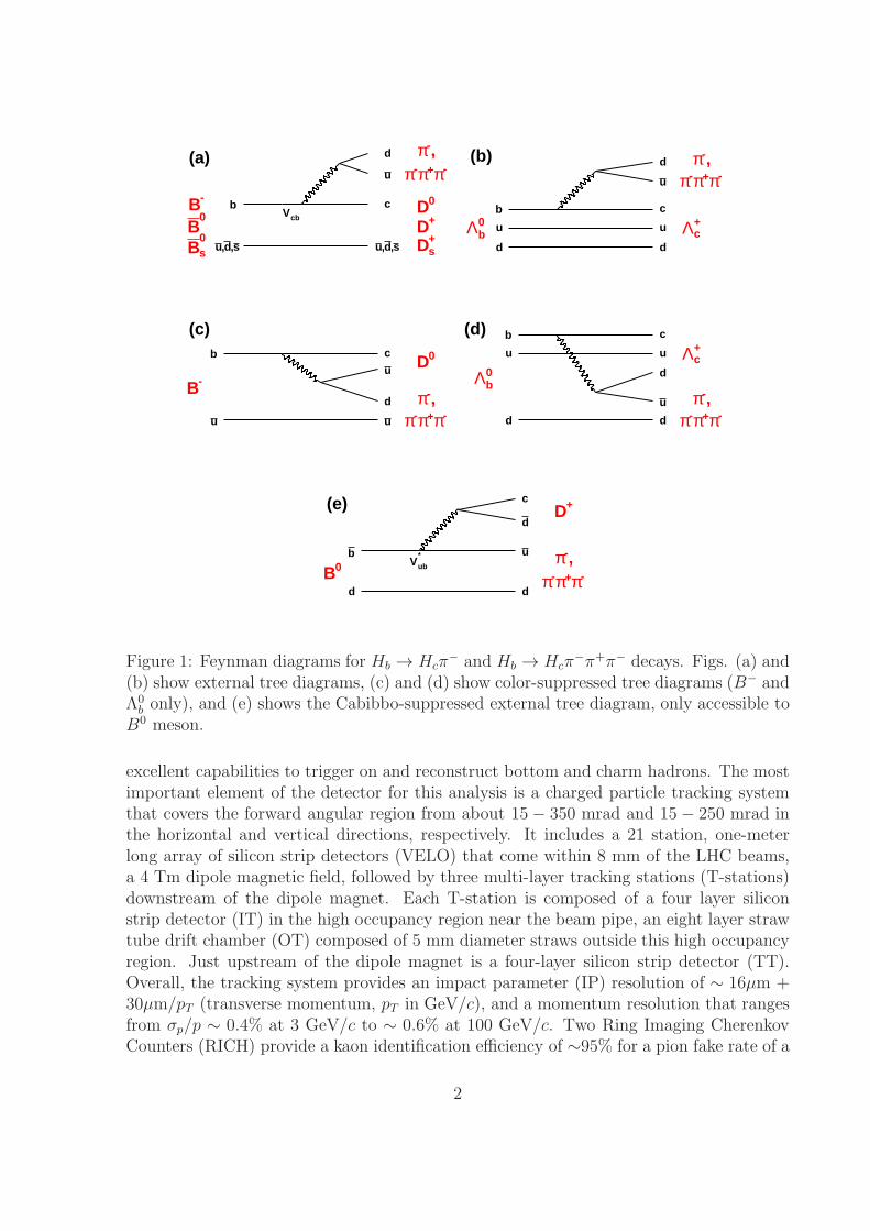
quantify their branching fractions. The more interesting Cabibbo-suppressed decays areO(λ3) in the Wolfenstein parameterization [11], and therefore require larger data samples.Here, we present measurements of the Cabibbo-favored Hb → Hcπ

−π+π− decays. Theleading amplitudes contributing to these final states are shown in Fig. 1. Additionalcontributions from annihilation and W -exchange diagrams are suppressed and are notshown here. Note that for the B− and Λ0

b decays, unlike the B0 and B0

s, there is potentialfor interference between diagrams with similar magnitudes. In Ref. [12], it is argued thatthis interference can explain the larger rate for B− → D0π− compared to B0 → D+π−.Thus, it is interesting to see whether this is also true when the final state contains threepions.

In this paper, we report measurements of the Hb → Hcπ−π+π− branching frac-

tions, relative to Hb → Hcπ−. We also report on the partial branching fractions,

Hb → H∗cπ

−, H∗c → Hcπ

+π−, where Hb is either B0, B−, or Λ0b , and H∗

c refers toD1(2420)

+,0, D∗2(2460)

0, Λc(2595)+, or Λc(2625)

+. We also present results on the partialrates for Λ0

b → Σc(2544)0,++π±π−. Charge conjugate final states are implied throughout.

2 Detector and Trigger

The data used for this analysis were collected by the LHCb experiment during the 2010data taking period and comprise about 35 pb−1 of integrated luminosity. LHCb has

1

(a)

b

s,d,u

c

s,d,u

cbV

d

u

-B0

B0sB

0D+D+sD

,-π-π+π-π

(b)

b

u

d

c

u

d

d

u

0bΛ +

cΛ

,-π-π+π-π

(c)b

u

c

u

u

d

-B

0D

,-π-π+π-π

(d) b

u

d

c

u

d

d

u

0bΛ

+cΛ

,-π-π+π-π

(e)

b

d

u

d

*ubV

c

d

0B

+D

,-π-π+π-π

Figure 1: Feynman diagrams for Hb → Hcπ− and Hb → Hcπ

−π+π− decays. Figs. (a) and(b) show external tree diagrams, (c) and (d) show color-suppressed tree diagrams (B− andΛ0

b only), and (e) shows the Cabibbo-suppressed external tree diagram, only accessible toB0 meson.

excellent capabilities to trigger on and reconstruct bottom and charm hadrons. The mostimportant element of the detector for this analysis is a charged particle tracking systemthat covers the forward angular region from about 15− 350 mrad and 15 − 250 mrad inthe horizontal and vertical directions, respectively. It includes a 21 station, one-meterlong array of silicon strip detectors (VELO) that come within 8 mm of the LHC beams,a 4 Tm dipole magnetic field, followed by three multi-layer tracking stations (T-stations)downstream of the dipole magnet. Each T-station is composed of a four layer siliconstrip detector (IT) in the high occupancy region near the beam pipe, an eight layer strawtube drift chamber (OT) composed of 5 mm diameter straws outside this high occupancyregion. Just upstream of the dipole magnet is a four-layer silicon strip detector (TT).Overall, the tracking system provides an impact parameter (IP) resolution of ∼ 16µm +30µm/pT (transverse momentum, pT in GeV/c), and a momentum resolution that rangesfrom σp/p ∼ 0.4% at 3 GeV/c to ∼ 0.6% at 100 GeV/c. Two Ring Imaging CherenkovCounters (RICH) provide a kaon identification efficiency of ∼95% for a pion fake rate of a

2

few percent, integrated over the momentum range from 3−100 GeV/c. Downstream of thesecond RICH is a Preshower/Scintillating Pad Detector (PS/SPD), and electromagnetic(ECAL) and hadronic (HCAL) calorimeters. Information from the ECAL/HCAL is usedto form the hadronic triggers. Finally, a muon system consisting of five stations is usedfor triggering on and identifying muons.

To reduce the 40 MHz crossing rate to about 2 kHz for permanent storage, LHCbuses a two-level trigger system. The first level of the trigger, L0, is hardware based andsearches for either a large transverse energy cluster (ET > 3.6 GeV) in the calorimeters, ora single high pT or di-muon pair in the muon stations. Events passing L0 are read out andsent to a large computing farm, where they are analyzed using a software-based trigger.The first level of the software trigger, called HLT1, uses a simplified version of the offlinesoftware to apply tighter selections on charged particles based on their pT and minimal IPto any primary vertex (PV), defined as the location of the reconstructed pp collision(s).The HLT1 trigger relevant for this analysis searches for a single track with IP larger than125 µm, pT > 1.8 GeV/c, p > 12.5 GeV/c, along with other track quality requirements.Events that pass HLT1 are analyzed by a second software level, HLT2, where the event issearched for 2, 3, or 4-particle vertices that are consistent with b-hadron decays. Tracksare required to have p > 5 GeV/c, pT > 0.5 GeV/c and IP χ2 larger than 16 to any PV,where the χ2 value is obtained assuming the IP is equal to zero. We also demand thatat least one track has pT > 1.5 GeV/c, a scalar pT sum of the track in the vertex exceed4 GeV/c, and that the corrected mass2 is between 4 and 7 GeV/c2. These HLT triggerselections each have an efficiency in the range of 80−90% for events that pass typicaloffline selections for a large range of B decays. A more detailed description of the LHCbdetector can be found in Ref. [13].

Events with large occupancy are known to have intrinsically high backgrounds and tobe slow to reconstruct. Therefore such events were suppressed by applying global eventcuts (GECs) to hadronically triggered decays. These GECs included a maximum of 3000VELO clusters, 3000 IT hits, and 10,000 OT hits. In addition, hadron triggers wererequired to have less than 900 or 450 hits in the SPD, depending on the specific triggersetting.

3 Candidate Reconstruction and Selection

Charged particles likely to come from a b-hadron decay are first identified by requiringthat they have a minimum IP χ2 with respect to any PV of more than 9. We alsorequire a minimum transverse momentum, pT > 300 MeV/c, except for Hb → Hcπ

−π+π−

decays, where we allow (at most) one track to have 200 < pT < 300 MeV/c. Hadrons areidentified using RICH information by requiring the difference in log-likelihoods (∆LL)of the different mass hypotheses to satisfy ∆LL(K − π) > −5, ∆LL(p − π) > −5 and

2The corrected mass is defined as Mcor =√

M2 + p2trans

, where M is the invariant mass of the 2, 3or 4-track candidate (assuming the kaon mass for each particle), and ptrans is the momentum imbalancetransverse to the direction of flight, defined by the vector that joins the primary and secondary vertices.

3

∆LL(K − π) < 12, for kaons, protons and pions, respectively. These particle hypothesesare not mutually exclusive, however the same track cannot enter more than once in thesame decay chain.

Charm particle candidates are reconstructed in the decay modes D0 → K−π+, D+ →K−π+π+, D+

s → K+K−π+ and Λ+c → pK−π+. The candidate is associated to one of the

PVs in the event based on the smallest IP χ2 between the charm particle’s reconstructedtrajectory and all PVs in the event. A number of selection criteria are imposed to reducebackgrounds from both prompt charm with random tracks as well as purely combinatorialbackground. To reduce the latter, we demand that each candidate is well separated fromthe associated PV by requiring that its flight distance (FD) projected onto the z-axis islarger than 2 mm, the FD χ2 > 493, and that the distance in the transverse direction (∆R)is larger than 100 µm. Background from random track combinations is also suppressedby requiring the vertex fit χ2/ndf< 8, and pT > 1.25 GeV/c (1.5 GeV/c for D+

(s) in

B0s → D+

s π−.) To reduce the contribution from prompt charm, we require that the

charm particle has a minimal IP larger than 80 µm and IP χ2 > 12.25 with respectto its associated PV. For D+

s → K+K−π+, we employ tighter particle identificationrequirements on the kaons, namely ∆LL(K − π) > 0, if the K+K− invariant mass isoutside a window of ±20 MeV/c2 of the φ mass [15]. Lastly, we require the reconstructedcharm particles masses to be within 25 MeV/c2 of their known values.

The bachelor pion for Hb → Hcπ− is required to have pT > 0.5 GeV/c, p > 5.0 GeV/c

and IP χ2 > 16. For the 3π vertex associated with the Hb → Hcπ−π+π− decays, we apply

a selection identical to that for the charm particle candidates, except we only require thepT of the 3π system to be larger than 1 GeV/c and that the invariant mass is in the rangefrom 0.8 GeV/c2 < M(πππ) < 3.0 GeV/c2.

Beauty hadrons are formed by combining a charm particle with either a single pioncandidate (for Hb → Hcπ

−) or a 3π candidate (for Hb → Hcπ−π+π−.) The b-hadron is

required to have a transverse momentum of at least 1 GeV/c. As with the charm hadron,we require it is well-separated from its associated PV, with FD larger than 2 mm, FDχ2 > 49 and ∆R > 100 µm. We also make a series of requirements that ensure that theb-hadron candidate is consistent with a particle produced in a proton-proton interaction.We require the candidate to have IP<90 µm, IP χ2 < 16, and that the angle θ betweenthe b-hadron momentum and the vector formed by joining the associated PV and thedecay vertex satisfies cos θ > 0.99996. To ensure a good quality vertex fit, we require avertex fit χ2/ndf< 6 (8 for Hb → Hcπ

−.)To limit the timing to process high occupancy events, we place requirements on the

number of tracks4 in an event. For B0 → D+π− and B0s → D+

s π−, the maximum number

of tracks is 180, and for Λ0b → Λ+

c π− and B− → D0π− it is 120. These selections are 99%

and 95% efficient, respectively, after the GECs. The Hb → Hcπ−π+π− selection requires

fewer than 300 tracks, and thus is essentially 100% efficient after the GECs.Events are required to pass the triggers described above. This alone does not imply

3This is the χ2 with respect to the FD=0 hypothesis.4Here, tracks refer to charged particles that have segments in both the VELO and the T-stations.

4

that the signal b-hadron decay was directly responsible for the trigger. We therefore alsorequire that one or more of the signal b-hadron daughters is responsible for triggering theevent. We thus explicitly select events that Triggered On the Signal decay (TOS) at L0,HLT1 and HLT2. For the measurements of excited charm states, where our yields arestatistically limited, we also make use of L0-triggers that Triggered Independently of theSignal decay (TIS). In this case, the L0 trigger is traced to one or more particles otherthan those in the signal decay.

Lastly, we note that in Hb → Hcπ−π+π− candidate events, between 4% and 10% have

multiple candidates (mostly two) in the same event. In such cases we choose the candidatewith the largest transverse momentum. This criterion is estimated to be (75 ± 20)%efficient for choosing the correct candidate. For Hb → Hcπ

− multiple candidates occur inless than 1% of events, from which we again choose the one with the largest pT .

3.1 Selection Efficiencies

Selection and trigger efficiencies are estimated using Monte Carlo (MC) simulations. TheMC samples are generated with an average number of interactions per crossing equalto 2.5, which is similar to the running conditions for the majority of the 2010 data.The b-hadrons are produced using pythia [16] and decayed using evtgen [17]. TheHb → Hcπ

−π+π− decays are produced using a cocktail for the πππ system that is∼2/3 a1(1260)

− → ρ0π− and about 1/3 non-resonant ρ0π−. Smaller contributions fromD0

1(2420)π and D∗02 (2460)π are each included at the 5% level to B− → D0π−π+π− and

2% each for B0 → D+π−π+π−. For Λ0b → Λ+

c π−π+π−, we include contributions from

Λc(2595)+ and Λc(2625)

+, which contribute 9% and 7% to the MC sample. The detectoris simulated with geant4 [18], and the event samples are subsequently analyzed in thesame way as data.

We compute the total kinematic efficiency, ǫkin from the MC simulation as the fractionof all events that pass all reconstruction and selection requirements. These selected eventsare then passed through a software emulation of the L0 trigger, and the HLT software usedto select the data, from which we compute the trigger efficiency (ǫtrig). The efficienciesfor the decay modes under study are shown in Table 1. Only the relative efficiencies areused to obtain the results in this paper.

4 Reconstructed Signals in Data

The reconstructed invariant mass distributions are shown in Figs. 2 and 3 for the signaland normalization modes, respectively. Unbinned likelihood fits are performed to extractthe signal yields, where the likelihood functions are given by the sums of signal and severalbackground components. The signal and background components are shown in the figures.The signal contributions are each described by the sum of two Gaussian shapes with equalmeans. The relative width and fraction of the wider Gaussian shape with respect to thenarrower one are constrained to the values found from MC simulation based on agreement

5

Table 1: Summary of efficiencies for decay channels under study. Here, ǫkin is the totalkinematic selection efficiency, ǫtrig is the trigger efficiency, and ǫtot is their product. Theuncertainties shown are statistical only.

Decay ǫkin ǫtrig ǫtot(%) (%) (%)

B0 → D+π−π+π− 0.153± 0.003 22.6± 0.5 0.0347± 0.0011B− → D0π−π+π− 0.275± 0.007 27.4± 0.6 0.0753± 0.0019B0

s → D+s π

−π+π− 0.137± 0.003 24.9± 0.7 0.0342± 0.0012Λ0

b → Λ+c π

−π+π− 0.110± 0.005 24.0± 0.7 0.0264± 0.0008

B0 → D+π− 0.882± 0.014 20.8± 0.3 0.184± 0.004B− → D0π− 1.54± 0.02 27.4± 0.3 0.421± 0.007B0

s → D+s π

− 0.868± 0.010 23.1± 0.2 0.201± 0.003Λ0

b → Λ+c π

− 0.732± 0.015 24.7± 0.4 0.181± 0.004

with data in the large yield signal modes. This constraint is included with a 10-12%uncertainty (mode-dependent), which is the level of agreement found between data andMC simulation. The absolute width of the narrower Gaussian is a free parameter in thefit, since the data shows a slightly worse (∼10%) resolution that MC simulation.

For B0s → D+

s π− and B0

s → D+s π

−π+π− decays, there are peaking backgrounds fromB0 → D+π− and B0 → D+π−π+π− just below the B0

s mass. We therefore fix their coreGaussian widths as well, based on the resolutions found in data for the kinematicallysimilar B0 → D+π− and B0 → D+π−π+π− decays, scaled by 0.93, which is the ratio ofexpected widths obtained from MC simulation.

A number of backgrounds contribute to these decays. Below the b-hadron masses thereare generally peaking background structures due to partially reconstructed B decays.These decays include B(s) → D∗

(s)π(ππ), with a missed photon, π0 or π+, as well as

B(s) → D(s)ρ−, where the π0 is not included in the decay hypothesis. For the B0 → D+π−

and B− → D0π− decays, the shapes of these backgrounds are taken from dedicated signalMC samples. The double-peaked background shape from partially-reconstructed D∗πdecays is obtained by fitting the background MC sample to the sum of two Gaussianshapes with different means. The difference in their means is then fixed, while theiraverage is a free parameter in subsequent fits to the data. For B0 → D+π−π+π− andB− → D0π−π+π−, the shape of the partially-reconstructed D∗πππ background is not aseasily derived since the helicity amplitudes are not known. This low mass background isalso parametrized using a two-Gaussian model, but we let the parameters float in the fit tothe data. ForB0

s → D+s π

− and B0s → D+

s π−π+π−, we obtain the background shape from a

large B0s → D+

s X inclusive MC sample. Less is known about the Λ0b hadronic decays that

would contribute background to the Λ0b → Λ+

c π− and Λ0

b → Λ+c π

−π+π− invariant massspectra. For Λ0

b → Λ+c π

−π+π−, we see no clear structure due to partially-reconstructedbackgrounds. For Λ0

b → Λ+c π

−, there does appear to be structure at about 5430 MeV/c2,

6

)2Mass (MeV/c5000 5200 5400

)2C

andi

date

s / (

10 M

eV/c

0

100

200

DataTotal PDF

Signal0B Back.πππD* Refl.ππDK

Comb. Back.

LHCb

)2Mass (MeV/c5000 5200 5400

) 2C

andi

date

s / (

10 M

eV/c

0

50

100

150

200

DataTotal PDF

Signal-B Back.πππD* Refl.ππDK

Comb. Back.

LHCb

)2Mass (MeV/c5000 5200 5400 5600

)2C

andi

date

s / (

10 M

eV/c

0

20

40

60

DataTotal PDF

Signal0sB Incl. Back.sD

Refl.-π+π-π+D Refl.-π+π-π+

cΛComb. Back.

LHCb

)2Mass (MeV/c5400 5600 5800

)2C

andi

date

s / (

10 M

eV/c

0

20

40

Data

Total PDF

Signal0bΛ

Refl.-π+π-π+sD

Comb. Back.

LHCb

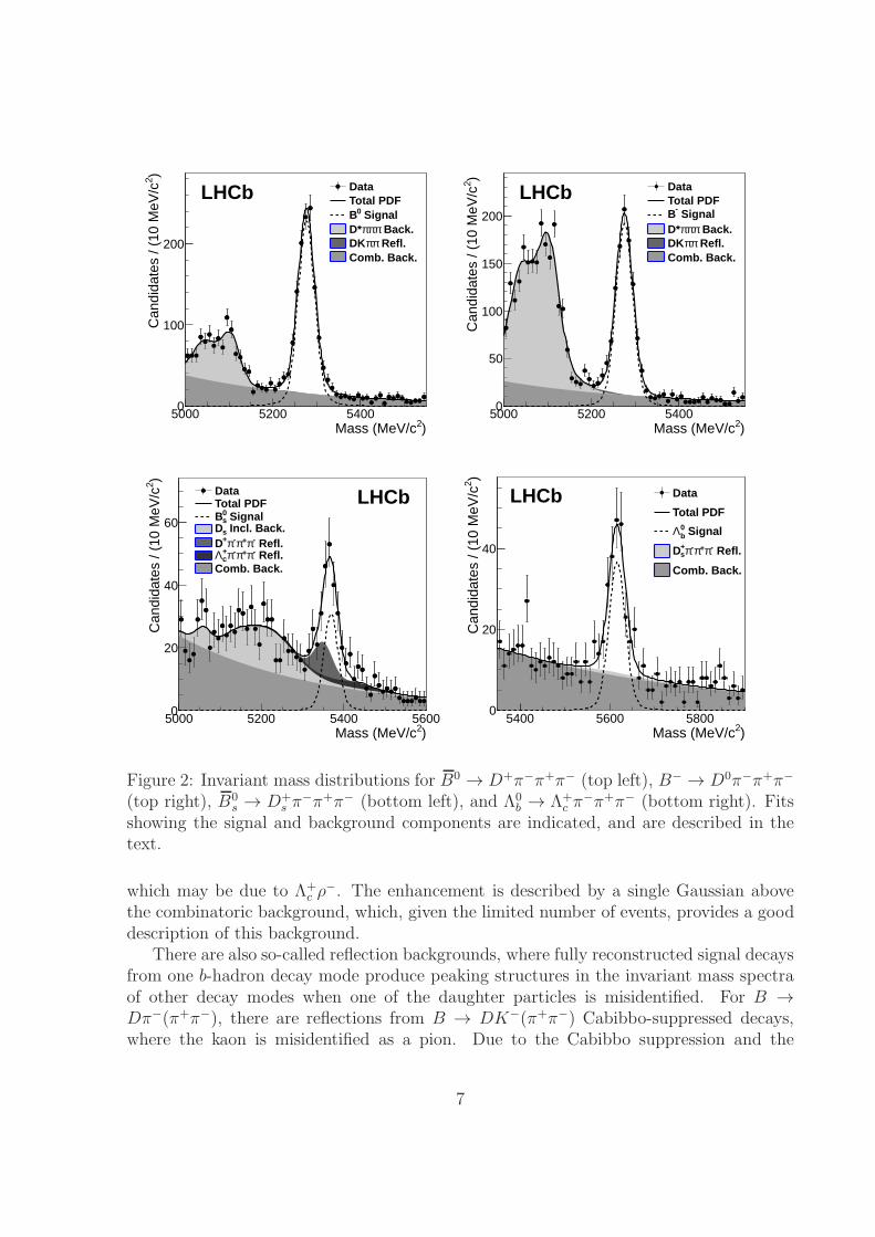
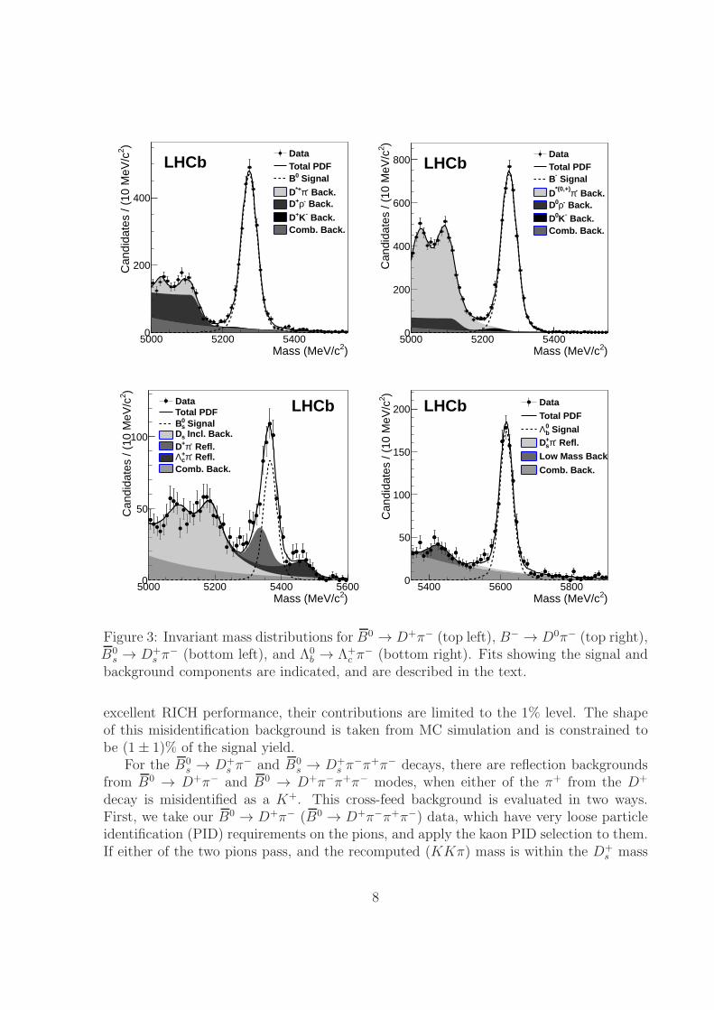
Figure 2: Invariant mass distributions for B0 → D+π−π+π− (top left), B− → D0π−π+π−

(top right), B0s → D+

s π−π+π− (bottom left), and Λ0

b → Λ+c π

−π+π− (bottom right). Fitsshowing the signal and background components are indicated, and are described in thetext.

which may be due to Λ+c ρ

−. The enhancement is described by a single Gaussian abovethe combinatoric background, which, given the limited number of events, provides a gooddescription of this background.

There are also so-called reflection backgrounds, where fully reconstructed signal decaysfrom one b-hadron decay mode produce peaking structures in the invariant mass spectraof other decay modes when one of the daughter particles is misidentified. For B →Dπ−(π+π−), there are reflections from B → DK−(π+π−) Cabibbo-suppressed decays,where the kaon is misidentified as a pion. Due to the Cabibbo suppression and the

7

)2Mass (MeV/c5000 5200 5400

) 2C

andi

date

s / (

10 M

eV/c

0

200

400

DataTotal PDF

Signal0B Back.-π*+D Back.-ρ+D Back.-K+D

Comb. Back.

LHCb

)2Mass (MeV/c5000 5200 5400

)2C

andi

date

s / (

10 M

eV/c

0

200

400

600

800DataTotal PDF

Signal-B

Back.-π*(0,+)D

Back.-ρ0D Back.-K0D

Comb. Back.

LHCb

)2Mass (MeV/c5000 5200 5400 5600

)2C

andi

date

s / (

10 M

eV/c

0

50

100

DataTotal PDF

Signal0sB Incl. Back.sD

Refl.-π+D Refl.-π+

cΛComb. Back.

LHCb

)2Mass (MeV/c5400 5600 5800

) 2C

andi

date

s / (

10 M

eV/c

0

50

100

150

200DataTotal PDF

Signal0bΛ

Refl.-π+sD

Low Mass Back

Comb. Back.

LHCb

Figure 3: Invariant mass distributions for B0 → D+π− (top left), B− → D0π− (top right),B0

s → D+s π

− (bottom left), and Λ0b → Λ+

c π− (bottom right). Fits showing the signal and

background components are indicated, and are described in the text.

excellent RICH performance, their contributions are limited to the 1% level. The shapeof this misidentification background is taken from MC simulation and is constrained tobe (1± 1)% of the signal yield.

For the B0s → D+

s π− and B0

s → D+s π

−π+π− decays, there are reflection backgroundsfrom B0 → D+π− and B0 → D+π−π+π− modes, when either of the π+ from the D+

decay is misidentified as a K+. This cross-feed background is evaluated in two ways.First, we take our B0 → D+π− (B0 → D+π−π+π−) data, which have very loose particleidentification (PID) requirements on the pions, and apply the kaon PID selection to them.If either of the two pions pass, and the recomputed (KKπ) mass is within the D+

s mass

8

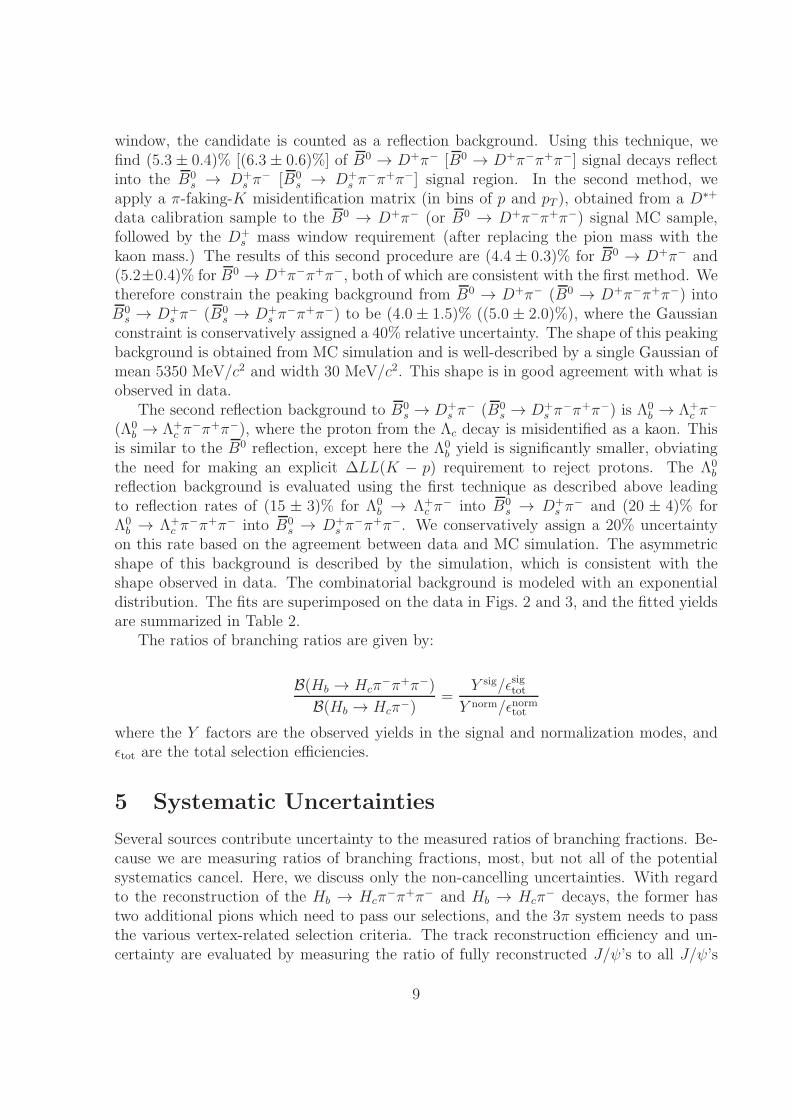
window, the candidate is counted as a reflection background. Using this technique, wefind (5.3 ± 0.4)% [(6.3 ± 0.6)%] of B0 → D+π− [B0 → D+π−π+π−] signal decays reflectinto the B0

s → D+s π

− [B0s → D+

s π−π+π−] signal region. In the second method, we

apply a π-faking-K misidentification matrix (in bins of p and pT ), obtained from a D∗+

data calibration sample to the B0 → D+π− (or B0 → D+π−π+π−) signal MC sample,followed by the D+

s mass window requirement (after replacing the pion mass with thekaon mass.) The results of this second procedure are (4.4 ± 0.3)% for B0 → D+π− and(5.2±0.4)% for B0 → D+π−π+π−, both of which are consistent with the first method. Wetherefore constrain the peaking background from B0 → D+π− (B0 → D+π−π+π−) intoB0

s → D+s π

− (B0s → D+

s π−π+π−) to be (4.0 ± 1.5)% ((5.0 ± 2.0)%), where the Gaussian

constraint is conservatively assigned a 40% relative uncertainty. The shape of this peakingbackground is obtained from MC simulation and is well-described by a single Gaussian ofmean 5350 MeV/c2 and width 30 MeV/c2. This shape is in good agreement with what isobserved in data.

The second reflection background to B0s → D+

s π− (B0

s → D+s π

−π+π−) is Λ0b → Λ+

c π−

(Λ0b → Λ+

c π−π+π−), where the proton from the Λc decay is misidentified as a kaon. This

is similar to the B0 reflection, except here the Λ0b yield is significantly smaller, obviating

the need for making an explicit ∆LL(K − p) requirement to reject protons. The Λ0b

reflection background is evaluated using the first technique as described above leadingto reflection rates of (15 ± 3)% for Λ0

b → Λ+c π

− into B0s → D+

s π− and (20 ± 4)% for

Λ0b → Λ+

c π−π+π− into B0

s → D+s π

−π+π−. We conservatively assign a 20% uncertaintyon this rate based on the agreement between data and MC simulation. The asymmetricshape of this background is described by the simulation, which is consistent with theshape observed in data. The combinatorial background is modeled with an exponentialdistribution. The fits are superimposed on the data in Figs. 2 and 3, and the fitted yieldsare summarized in Table 2.

The ratios of branching ratios are given by:

B(Hb → Hcπ−π+π−)

B(Hb → Hcπ−)=

Y sig/ǫsigtotY norm/ǫnormtot

where the Y factors are the observed yields in the signal and normalization modes, andǫtot are the total selection efficiencies.

5 Systematic Uncertainties

Several sources contribute uncertainty to the measured ratios of branching fractions. Be-cause we are measuring ratios of branching fractions, most, but not all of the potentialsystematics cancel. Here, we discuss only the non-cancelling uncertainties. With regardto the reconstruction of the Hb → Hcπ

−π+π− and Hb → Hcπ− decays, the former has

two additional pions which need to pass our selections, and the 3π system needs to passthe various vertex-related selection criteria. The track reconstruction efficiency and un-certainty are evaluated by measuring the ratio of fully reconstructed J/ψ’s to all J/ψ’s

9

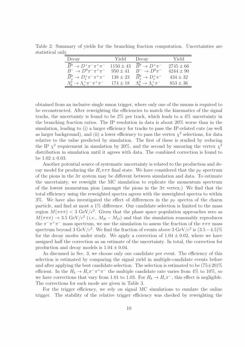
Table 2: Summary of yields for the branching fraction computation. Uncertainties arestatistical only.

Decay Yield Decay Yield

B0 → D+π−π+π− 1150± 43 B0 → D+π− 2745± 66B− → D0π−π+π− 950± 41 B− → D0π− 4244± 90B0

s → D+s π

−π+π− 138± 23 B0s → D+

s π− 434± 32

Λ0b → Λ+

c π−π+π− 174± 18 Λ0

b → Λ+c π

− 853± 36

obtained from an inclusive single muon trigger, where only one of the muons is required tobe reconstructed. After reweighting the efficiencies to match the kinematics of the signaltracks, the uncertainty is found to be 2% per track, which leads to a 4% uncertainty inthe branching fraction ratios. The IP resolution in data is about 20% worse than in thesimulation, leading to (i) a larger efficiency for tracks to pass the IP-related cuts (as wellas larger background), and (ii) a lower efficiency to pass the vertex χ2 selections, for datarelative to the value predicted by simulation. The first of these is studied by reducingthe IP χ2 requirement in simulation by 20%, and the second by smearing the vertex χ2

distribution in simulation until it agrees with data. The combined correction is found tobe 1.02± 0.03.

Another potential source of systematic uncertainty is related to the production and de-cay model for producing the Hcπππ final state. We have considered that the pT spectrumof the pions in the 3π system may be different between simulation and data. To estimatethe uncertainty, we reweight the MC simulation to replicate the momentum spectrumof the lowest momentum pion (amongst the pions in the 3π vertex.) We find that thetotal efficiency using the reweighted spectra agrees with the unweighted spectra to within3%. We have also investigated the effect of differences in the pT spectra of the charmparticle, and find at most a 1% difference. Our candidate selection is limited to the massregion M(πππ) < 3 GeV/c2. Given that the phase space population approaches zero asM(πππ) → 3.5 GeV/c2 (i.e., MB −MD) and that the simulation reasonably reproducesthe π−π+π− mass spectrum, we use the simulation to assess the fraction of the πππ massspectrum beyond 3 GeV/c2. We find the fraction of events above 3 GeV/c2 is (3.5−4.5)%for the decay modes under study. We apply a correction of 1.04 ± 0.02, where we haveassigned half the correction as an estimate of the uncertainty. In total, the correction forproduction and decay models is 1.04± 0.04.

As discussed in Sec. 3, we choose only one candidate per event. The efficiency of thisselection is estimated by comparing the signal yield in multiple-candidate events beforeand after applying the best candidate selection. The selection is estimated to be (75±20)%efficient. In the Hb → Hcπ

−π+π− the multiple candidate rate varies from 4% to 10%, sowe have corrections that vary from 1.01 to 1.03. For Hb → Hcπ

−, this effect is negligible.The corrections for each mode are given in Table 3.

For the trigger efficiency, we rely on signal MC simulations to emulate the onlinetrigger. The stability of the relative trigger efficiency was checked by reweighting the

10

b-hadron pT spectra for both the signal and normalization modes, and re-evaluating thetrigger efficiency ratios. We find maximum differences of 2% for L0, 1% for HLT1 and 1%for HLT2, (2.4% total) which we assign as a systematic uncertainty.

Fitting systematics are evaluated by varying the background shapes and assumptionsabout the signal parameterization for both the Hb → Hcπ

−π+π− and Hb → Hcπ− modes

and re-measuring the yield ratios. For the combinatorial background, using first andsecond order polynomials leads to a 3% uncertainty on the relative yield. Reflectionbackground uncertainties are negligible, except for B0

s → D+s π

−π+π− and B0s → D+

s π−,

where we find deviations as large as 5% when varying the central value of the constraintson the B0 → D+π−π+π− and B0 → D+π− reflections by ±1 standard deviation. Wehave checked our sensitivity to the signal model by varying the constraints on the widthratio and core Gaussian area fraction by one standard deviation (2%). We also includea systematic uncertainty of 1% for neglecting the small radiative tail in the fit, which isestimated by comparing the yields between our double Gaussian signal model and thesum of a Gaussian and Crystal Ball [20] line shape. Taken together, we assign a 4%uncertainty to the relative yields. For the B0

s branching fraction ratio, the total fittinguncertainty is 6.4%.

Another difference between the Hb → Hcπ− and Hb → Hcπ

−π+π− selection is theupper limit on the number of tracks. The efficiencies of the lower track multiplicityrequirements can be evaluated using the samples with higher track multiplicity require-ments. Using this technique, we find corrections of 0.95±0.01 for the B− and Λ0

b branchingfraction ratios, and 0.99± 0.01 for the B0 and B0

s branching fraction ratios.We have also studied the PID efficiency uncertainty using a D∗+ calibration sample

in data. Since the PID requirements are either common to the signal and normalizationmodes, or in the case of the bachelor pion(s), the selection is very loose, the uncertaintyis small and we estimate a correction of 1.01 ± 0.01. We have also considered possiblebackground from Hb → HcD

−s which results in a correction of 0.99± 0.01.

All of our MC samples have a comparable number of events, from which we incur 3-4%uncertainty in the efficiency ratio determinations. The full set of systematic uncertaintiesand corrections are shown in Table 3. In total, the systematic uncertainty is ∼9%, withcorrection factors that range from 1.01 to 1.07.

11

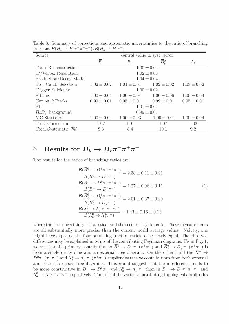
Table 3: Summary of corrections and systematic uncertainties to the ratio of branchingfractions B(Hb → Hcπ

−π+π−)/B(Hb → Hcπ−).

Source central value ± syst. error

B0 B− B0s Λb

Track Reconstruction 1.00± 0.04IP/Vertex Resolution 1.02± 0.03Production/Decay Model 1.04± 0.04Best Cand. Selection 1.02± 0.02 1.01± 0.01 1.02± 0.02 1.03± 0.02Trigger Efficiency 1.00± 0.02Fitting 1.00± 0.04 1.00± 0.04 1.00± 0.06 1.00± 0.04Cut on #Tracks 0.99± 0.01 0.95± 0.01 0.99± 0.01 0.95± 0.01PID 1.01± 0.01HcD

+s background 0.99± 0.01

MC Statistics 1.00± 0.04 1.00± 0.03 1.00± 0.04 1.00± 0.04Total Correction 1.07 1.01 1.07 1.03Total Systematic (%) 8.8 8.4 10.1 9.2

6 Results for Hb → Hcπ−π

+π

−

The results for the ratios of branching ratios are

B(B0 → D+π−π+π−)

B(B0 → D+π−)= 2.38± 0.11± 0.21

B(B− → D0π−π+π−)

B(B− → D0π−)= 1.27± 0.06± 0.11 (1)

B(B0s → D+

s π−π+π−)

B(B0s → D+

s π−)

= 2.01± 0.37± 0.20

B(Λ0b → Λ+

c π−π+π−)

B(Λ0b → Λ+

c π−)

= 1.43± 0.16± 0.13,

where the first uncertainty is statistical and the second is systematic. These measurementsare all substantially more precise than the current world average values. Naively, onemight have expected the four branching fraction ratios to be nearly equal. The observeddifferences may be explained in terms of the contributing Feynman diagrams. From Fig. 1,we see that the primary contribution to B0 → D+π−(π+π−) and B0

s → D+s π

−(π+π−) isfrom a single decay diagram, an external tree diagram. On the other hand the B− →D0π−(π+π−) and Λ0

b → Λ+c π

−(π+π−) amplitudes receive contributions from both externaland color-suppressed tree diagrams. This would suggest that the interference tends tobe more constructive in B− → D0π− and Λ0

b → Λ+c π

− than in B− → D0π−π+π− andΛ0

b → Λ+c π

−π+π− respectively. The role of the various contributing topological amplitudes

12

and the strong phases in B → Dπ is discussed in the literature [12]. In general we see thebranching fractions for the Hcπππ final states are at least as large or even twice as largeas the single-π bachelor states.

7 Kinematic Distributions and Mass Spectra in the

π−π

+π

− System

Since we rely on MC simulation to estimate signal efficiencies, we now compare a fewdistributions between signal MC simulation and data. The higher signal yield B0 →D+π− and B0 → D+π−π+π− decay modes are used, and for each we perform a sidebandsubtraction, where the signal region includes candidates within 50 MeV/c2 of the B0

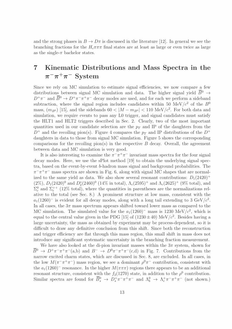
mass, (mB0) [15], and the sidebands 60 < |M −mB0 | < 110 MeV/c2. For both data andsimulation, we require events to pass any L0 trigger, and signal candidates must satisfythe HLT1 and HLT2 triggers described in Sec. 2. Clearly, two of the most importantquantities used in our candidate selection are the pT and IP of the daughters from theD+ and the recoiling pion(s). Figure 4 compares the pT and IP distributions of the D+

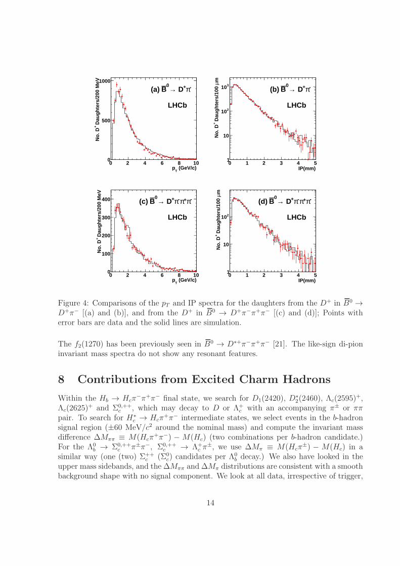
daughters in data to those from signal MC simulation. Figure 5 shows the correspondingcomparisons for the recoiling pion(s) in the respective B decay. Overall, the agreementbetween data and MC simulation is very good.

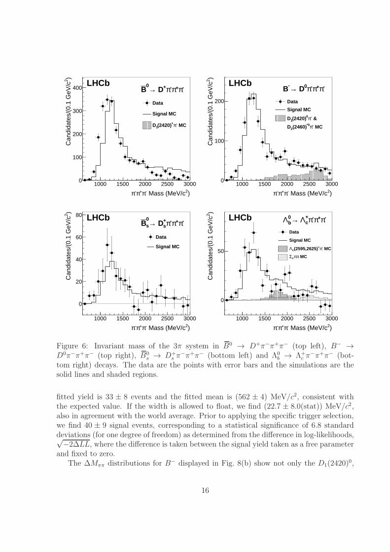
It is also interesting to examine the π−π+π− invariant mass spectra for the four signaldecay modes. Here, we use the sPlot method [19] to obtain the underlying signal spec-tra, based on the event-by-event b-hadron mass signal and background probabilities. Theπ−π+π− mass spectra are shown in Fig. 6, along with signal MC shapes that are normal-ized to the same yield as data. We also show several resonant contributions: D1(2420)

+

(2%), D1(2420)0 and D∗

2(2460)0 (14% in total), Λc(2595)

+ and Λc(2625)+ (9% total), and

Σ0c and Σ++

c (12% total), where the quantities in parentheses are the normalizations rel-ative to the total (see Sec. 8.) A prominent structure at low mass, consistent with thea1(1260)

− is evident for all decay modes, along with a long tail extending to 3 GeV/c2.In all cases, the 3π mass spectrum appears shifted toward lower mass as compared to theMC simulation. The simulated value for the a1(1260)

− mass is 1230 MeV/c2, which isequal to the central value given in the PDG [15] of (1230±40) MeV/c2. Besides having alarge uncertainty, the mass as obtained by experiment may be process-dependent, so it isdifficult to draw any definitive conclusion from this shift. Since both the reconstructionand trigger efficiency are flat through this mass region, this small shift in mass does notintroduce any significant systematic uncertainty in the branching fraction measurement.

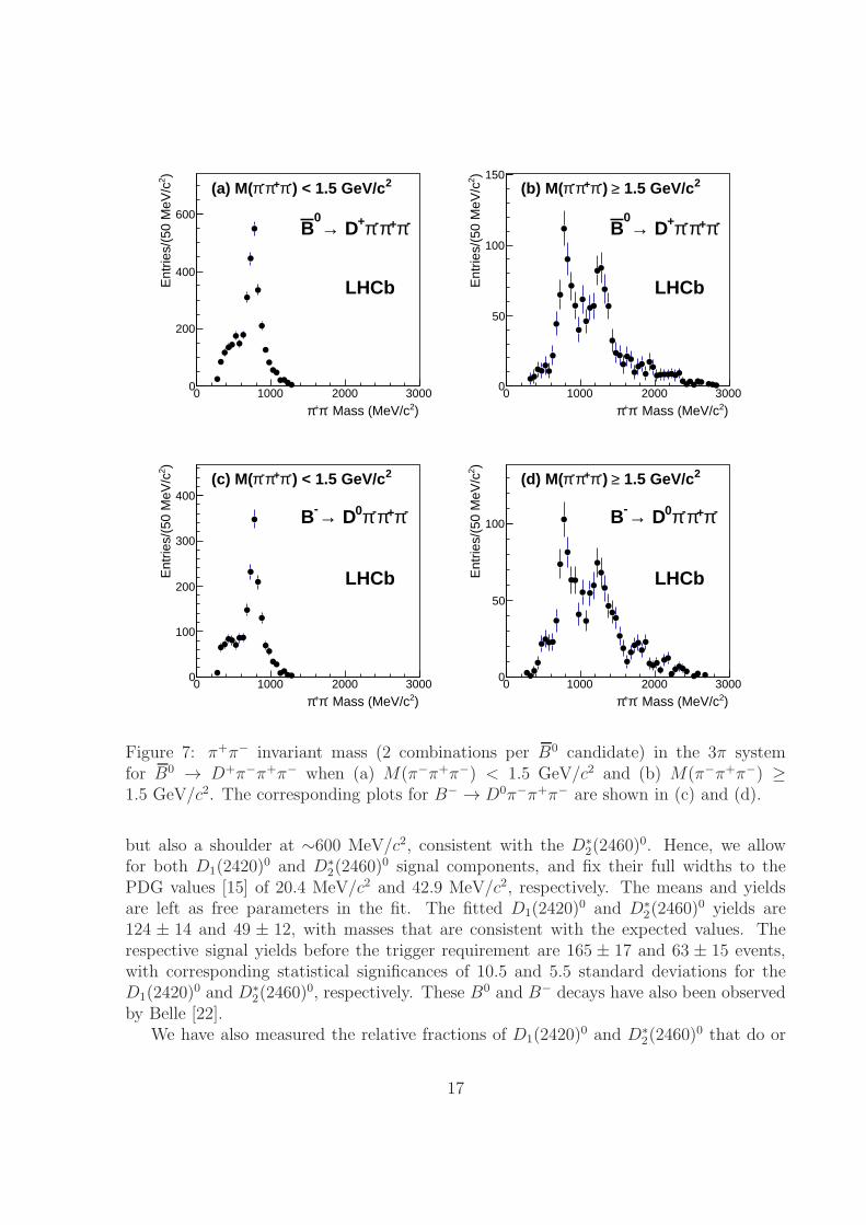
We have also looked at the di-pion invariant masses within the 3π system, shown forB0 → D+π−π+π−(a,b) and B− → D0π−π+π−(c,d) in Fig. 7. Contributions from thenarrow excited charm states, which are discussed in Sec. 8, are excluded. In all cases, inthe low M(π−π+π−) mass region, we see a dominant ρ0π− contribution, consistent withthe a1(1260)

− resonance. In the higherM(πππ) regions there appears to be an additionalresonant structure, consistent with the f2(1270) state, in addition to the ρ0 contribution.Similar spectra are found for B0

s → D+s π

−π+π− and Λ0b → Λ+

c π−π+π− (not shown.)

13

(GeV/c)T

p0 2 4 6 8 10

Dau

ghte

rs/2

00 M

eV+

No.

D

0

500

1000-π+ D→

0B(a)

LHCb

IP(mm)0 1 2 3 4 5

mµ D

augh

ters

/100

+

No.

D

1

10

210

310 -π+ D→0

B(b)

LHCb

(GeV/c)T

p0 2 4 6 8 10

Dau

ghte

rs/2

00 M

eV+

No.

D

0

100

200

300

400 -π+π-π+ D→0

B(c)

LHCb

IP(mm)0 1 2 3 4 5

mµ D

augh

ters

/100

+

No.

D

1

10

210

-π+π-π+ D→0

B(d)

LHCb

Figure 4: Comparisons of the pT and IP spectra for the daughters from the D+ in B0 →D+π− [(a) and (b)], and from the D+ in B0 → D+π−π+π− [(c) and (d)]; Points witherror bars are data and the solid lines are simulation.

The f2(1270) has been previously seen in B0 → D∗+π−π+π− [21]. The like-sign di-pioninvariant mass spectra do not show any resonant features.

8 Contributions from Excited Charm Hadrons

Within the Hb → Hcπ−π+π− final state, we search for D1(2420), D

∗2(2460), Λc(2595)

+,Λc(2625)

+ and Σ0,++c , which may decay to D or Λ+

c with an accompanying π± or ππpair. To search for H∗

c → Hcπ+π− intermediate states, we select events in the b-hadron

signal region (±60 MeV/c2 around the nominal mass) and compute the invariant massdifference ∆Mππ ≡ M(Hcπ

+π−) − M(Hc) (two combinations per b-hadron candidate.)For the Λ0

b → Σ0,++c π±π−, Σ0,++

c → Λ+c π

±, we use ∆Mπ ≡ M(Hcπ±) − M(Hc) in a

similar way (one (two) Σ++c (Σ0

c) candidates per Λ0b decay.) We also have looked in the

upper mass sidebands, and the ∆Mππ and ∆Mπ distributions are consistent with a smoothbackground shape with no signal component. We look at all data, irrespective of trigger,

14

(GeV/c)T

p0 5 10

No.

Dau

ghte

rs/2

00 M

eV

0

50

100

150-π+ D→

0B(a)

LHCb

IP (mm)0 1 2 3 4 5

mµN

o. D

augh

ters

/100

1

10

210

-π+ D→0

B(b)

LHCb

(GeV/c)T

p0 2 4 6 8 10

No.

Dau

ghte

rs/2

00 M

eV

0

100

200

300

400-π+π-π+ D→

0B(c)

LHCb

IP (mm)0 1 2 3 4 5

mµN

o. D

augh

ters

/100

1

10

210

310-π+π-π+ D→

0B(d)

LHCb

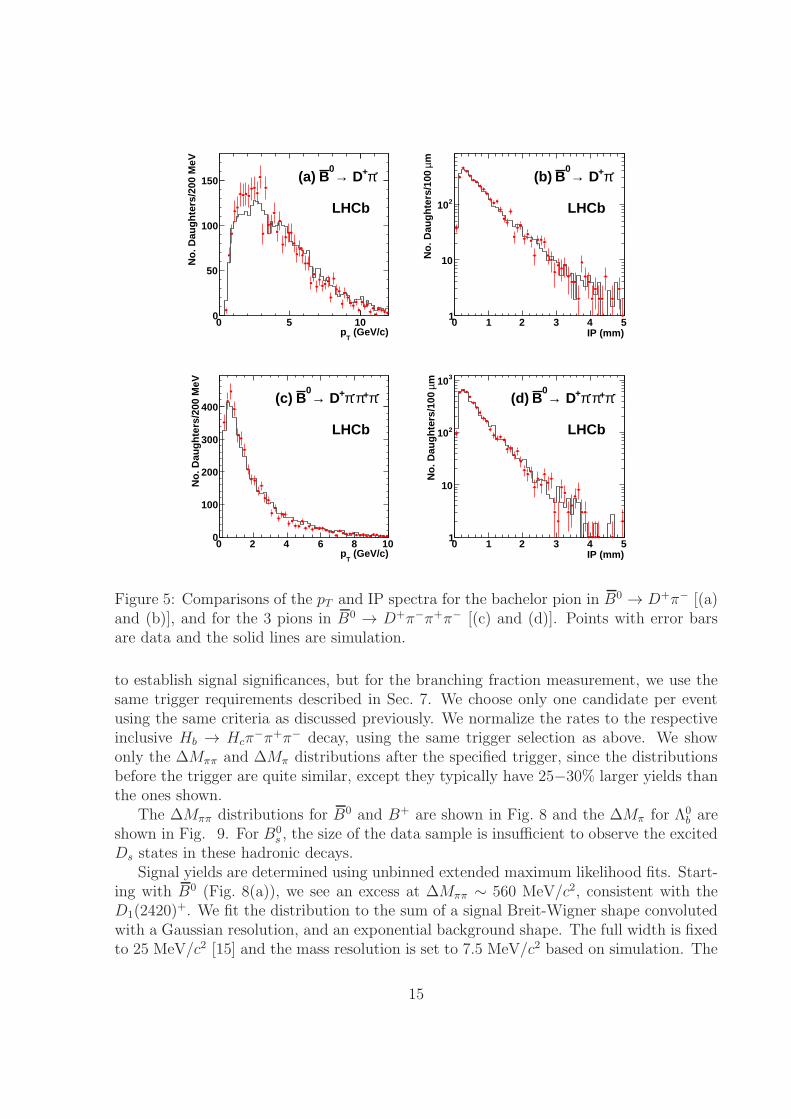
Figure 5: Comparisons of the pT and IP spectra for the bachelor pion in B0 → D+π− [(a)and (b)], and for the 3 pions in B0 → D+π−π+π− [(c) and (d)]. Points with error barsare data and the solid lines are simulation.

to establish signal significances, but for the branching fraction measurement, we use thesame trigger requirements described in Sec. 7. We choose only one candidate per eventusing the same criteria as discussed previously. We normalize the rates to the respectiveinclusive Hb → Hcπ

−π+π− decay, using the same trigger selection as above. We showonly the ∆Mππ and ∆Mπ distributions after the specified trigger, since the distributionsbefore the trigger are quite similar, except they typically have 25−30% larger yields thanthe ones shown.

The ∆Mππ distributions for B0 and B+ are shown in Fig. 8 and the ∆Mπ for Λ0b are

shown in Fig. 9. For B0s , the size of the data sample is insufficient to observe the excited

Ds states in these hadronic decays.Signal yields are determined using unbinned extended maximum likelihood fits. Start-

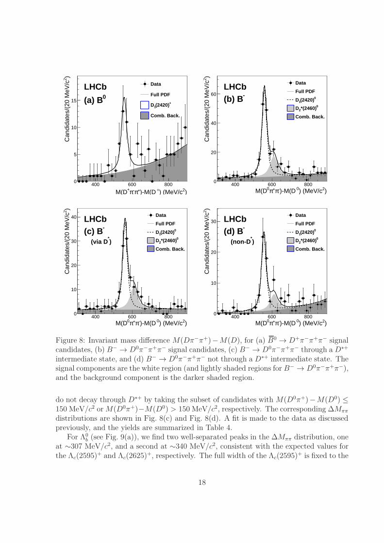
ing with B0 (Fig. 8(a)), we see an excess at ∆Mππ ∼ 560 MeV/c2, consistent with theD1(2420)

+. We fit the distribution to the sum of a signal Breit-Wigner shape convolutedwith a Gaussian resolution, and an exponential background shape. The full width is fixedto 25 MeV/c2 [15] and the mass resolution is set to 7.5 MeV/c2 based on simulation. The

15

)2 Mass (MeV/c-π+π-π1000 1500 2000 2500 3000

)2C

andi

date

s/(0

.1 G

eV/c

0

100

200

300

400

Data

Signal MC

MC-π+(2420)1D

-π+π-π+ D→0

BLHCb

)2 Mass (MeV/c-π+π-π1000 1500 2000 2500 3000

)2C

andi

date

s/(0

.1 G

eV/c

0

100

200 Data

Signal MC

&-π0(2420)1D

MC-π*0(2460)2D

-π+π-π0 D→-BLHCb

)2 Mass (MeV/c-π+π-π1000 1500 2000 2500 3000

)2C

andi

date

s/(0

.1 G

eV/c

0

20

40

60

80-π+π-πs

+ D→s0

B

Data

Signal MC

LHCb

)2 Mass (MeV/c-π+π-π1000 1500 2000 2500 3000

)2C

andi

date

s/(0

.1 G

eV/c

0

50

Data

Signal MC

MC-π+(2595,2625)cΛ

MCππcΣ

-π+π-πc+Λ →0

bΛLHCb

Figure 6: Invariant mass of the 3π system in B0 → D+π−π+π− (top left), B− →D0π−π+π− (top right), B0

s → D+s π

−π+π− (bottom left) and Λ0b → Λ+

c π−π+π− (bot-

tom right) decays. The data are the points with error bars and the simulations are thesolid lines and shaded regions.

fitted yield is 33 ± 8 events and the fitted mean is (562 ± 4) MeV/c2, consistent withthe expected value. If the width is allowed to float, we find (22.7 ± 8.0(stat)) MeV/c2,also in agreement with the world average. Prior to applying the specific trigger selection,we find 40 ± 9 signal events, corresponding to a statistical significance of 6.8 standarddeviations (for one degree of freedom) as determined from the difference in log-likelihoods,√−2∆LL, where the difference is taken between the signal yield taken as a free parameter

and fixed to zero.The ∆Mππ distributions for B− displayed in Fig. 8(b) show not only the D1(2420)

0,

16

)2 Mass (MeV/c-π+π 0 1000 2000 3000

)2E

ntrie

s/(5

0 M

eV/c

0

200

400

600

2) < 1.5 GeV/c-π+π-π(a) M(

-π+π-π+ D→0

B

LHCb

)2 Mass (MeV/c-π+π 0 1000 2000 3000

)2E

ntrie

s/(5

0 M

eV/c

0

50

100

1502 1.5 GeV/c≥) -π+π-π(b) M(

-π+π-π+ D→0

B

LHCb

)2 Mass (MeV/c-π+π 0 1000 2000 3000

)2E

ntrie

s/(5

0 M

eV/c

0

100

200

300

400

2) < 1.5 GeV/c-π+π-π(c) M(

-π+π-π0 D→-B

LHCb

)2 Mass (MeV/c-π+π 0 1000 2000 3000

)2E

ntrie

s/(5

0 M

eV/c

0

50

100

2 1.5 GeV/c≥) -π+π-π(d) M(

-π+π-π0 D→-B

LHCb

Figure 7: π+π− invariant mass (2 combinations per B0 candidate) in the 3π systemfor B0 → D+π−π+π− when (a) M(π−π+π−) < 1.5 GeV/c2 and (b) M(π−π+π−) ≥1.5 GeV/c2. The corresponding plots for B− → D0π−π+π− are shown in (c) and (d).

but also a shoulder at ∼600 MeV/c2, consistent with the D∗2(2460)

0. Hence, we allowfor both D1(2420)

0 and D∗2(2460)

0 signal components, and fix their full widths to thePDG values [15] of 20.4 MeV/c2 and 42.9 MeV/c2, respectively. The means and yieldsare left as free parameters in the fit. The fitted D1(2420)

0 and D∗2(2460)

0 yields are124 ± 14 and 49 ± 12, with masses that are consistent with the expected values. Therespective signal yields before the trigger requirement are 165 ± 17 and 63 ± 15 events,with corresponding statistical significances of 10.5 and 5.5 standard deviations for theD1(2420)

0 and D∗2(2460)

0, respectively. These B0 and B− decays have also been observedby Belle [22].

We have also measured the relative fractions of D1(2420)0 and D∗

2(2460)0 that do or

17

)2) (MeV/c +)-M(D+π-π+M(D400 600 800

)2C

andi

date

s/(2

0 M

eV/c

0

5

10

15

Data

Full PDF

+(2420)1D

Comb. Back.

LHCb0(a) B

)2) (MeV/c 0)-M(D-π+π0M(D400 600 800

)2C

andi

date

s/(2

0 M

eV/c

0

20

40

60

Data

Full PDF0(2420)1D

0*(2460)2D

Comb. Back.

LHCb-(b) B

)2) (MeV/c 0)-M(D-π+π0M(D400 600 800

)2C

andi

date

s/(2

0 M

eV/c

0

10

20

30

40 Data

Full PDF0(2420)1D

0*(2460)2D

Comb. Back.

LHCb-(c) B

)*

(via D

)2) (MeV/c 0)-M(D-π+π0M(D400 600 800

)2C

andi

date

s/(2

0 M

eV/c

0

10

20

30Data

Full PDF0(2420)1D

0*(2460)2D

Comb. Back.

LHCb-(d) B

)*

(non-D

Figure 8: Invariant mass difference M(Dπ−π+)−M(D), for (a) B0 → D+π−π+π− signalcandidates, (b) B− → D0π−π+π− signal candidates, (c) B− → D0π−π+π− through a D∗+

intermediate state, and (d) B− → D0π−π+π− not through a D∗+ intermediate state. Thesignal components are the white region (and lightly shaded regions for B− → D0π−π+π−),and the background component is the darker shaded region.

do not decay through D∗+ by taking the subset of candidates with M(D0π+)−M(D0) ≤150 MeV/c2 orM(D0π+)−M(D0) > 150 MeV/c2, respectively. The corresponding ∆Mππ

distributions are shown in Fig. 8(c) and Fig. 8(d). A fit is made to the data as discussedpreviously, and the yields are summarized in Table 4.

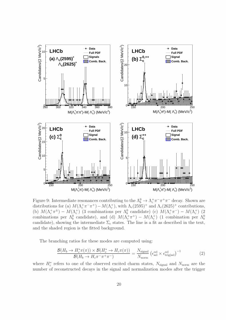
For Λ0b (see Fig. 9(a)), we find two well-separated peaks in the ∆Mππ distribution, one

at ∼307 MeV/c2, and a second at ∼340 MeV/c2, consistent with the expected values forthe Λc(2595)

+ and Λc(2625)+, respectively. The full width of the Λc(2595)

+ is fixed to the

18

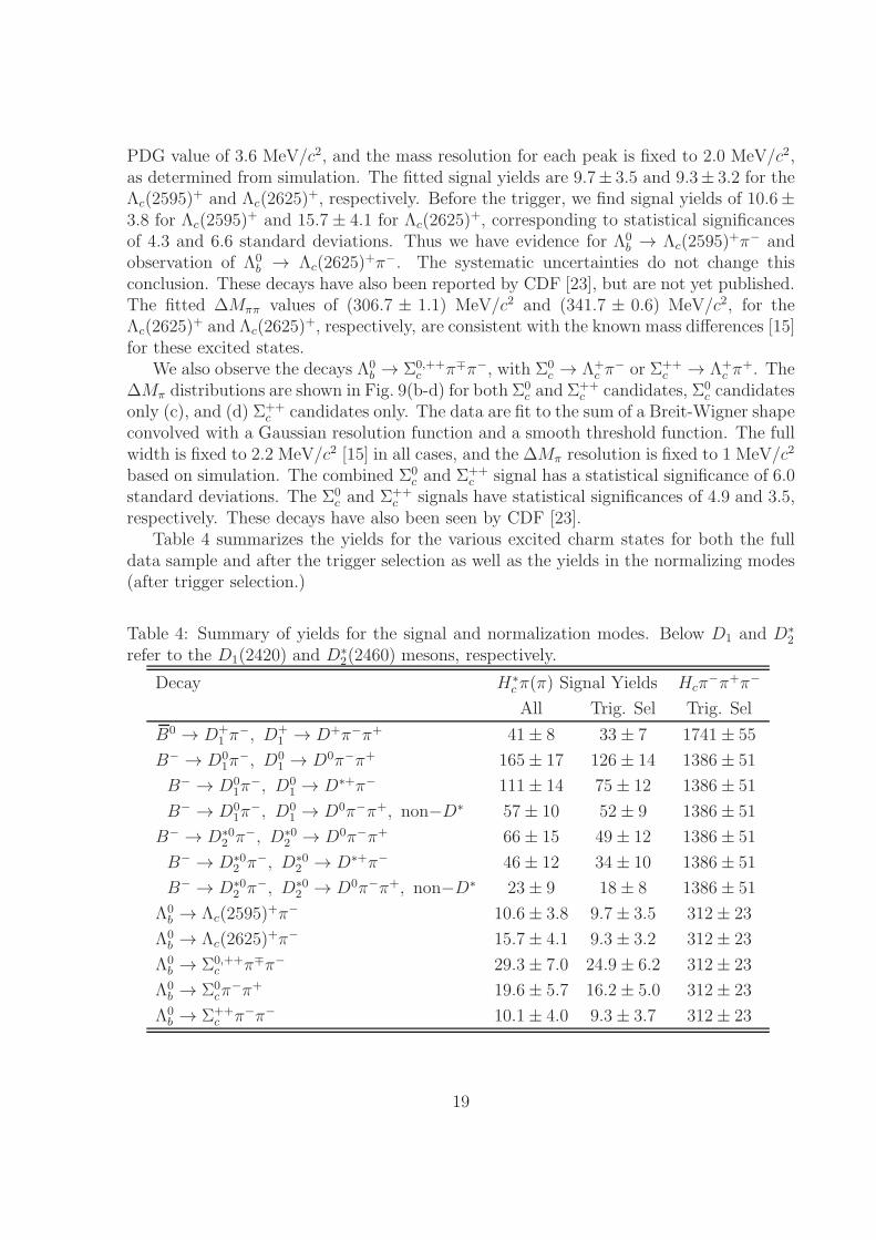
PDG value of 3.6 MeV/c2, and the mass resolution for each peak is fixed to 2.0 MeV/c2,as determined from simulation. The fitted signal yields are 9.7± 3.5 and 9.3± 3.2 for theΛc(2595)

+ and Λc(2625)+, respectively. Before the trigger, we find signal yields of 10.6±

3.8 for Λc(2595)+ and 15.7 ± 4.1 for Λc(2625)

+, corresponding to statistical significancesof 4.3 and 6.6 standard deviations. Thus we have evidence for Λ0

b → Λc(2595)+π− and

observation of Λ0b → Λc(2625)

+π−. The systematic uncertainties do not change thisconclusion. These decays have also been reported by CDF [23], but are not yet published.The fitted ∆Mππ values of (306.7 ± 1.1) MeV/c2 and (341.7 ± 0.6) MeV/c2, for theΛc(2625)

+ and Λc(2625)+, respectively, are consistent with the known mass differences [15]

for these excited states.We also observe the decays Λ0

b → Σ0,++c π∓π−, with Σ0

c → Λ+c π

− or Σ++c → Λ+

c π+. The

∆Mπ distributions are shown in Fig. 9(b-d) for both Σ0c and Σ++

c candidates, Σ0c candidates

only (c), and (d) Σ++c candidates only. The data are fit to the sum of a Breit-Wigner shape

convolved with a Gaussian resolution function and a smooth threshold function. The fullwidth is fixed to 2.2 MeV/c2 [15] in all cases, and the ∆Mπ resolution is fixed to 1 MeV/c2

based on simulation. The combined Σ0c and Σ++

c signal has a statistical significance of 6.0standard deviations. The Σ0

c and Σ++c signals have statistical significances of 4.9 and 3.5,

respectively. These decays have also been seen by CDF [23].Table 4 summarizes the yields for the various excited charm states for both the full

data sample and after the trigger selection as well as the yields in the normalizing modes(after trigger selection.)

Table 4: Summary of yields for the signal and normalization modes. Below D1 and D∗2

refer to the D1(2420) and D∗2(2460) mesons, respectively.

Decay H∗cπ(π) Signal Yields Hcπ

−π+π−

All Trig. Sel Trig. Sel

B0 → D+1 π

−, D+1 → D+π−π+ 41± 8 33± 7 1741± 55

B− → D01π

−, D01 → D0π−π+ 165± 17 126± 14 1386± 51

B− → D01π

−, D01 → D∗+π− 111± 14 75± 12 1386± 51

B− → D01π

−, D01 → D0π−π+, non−D∗ 57± 10 52± 9 1386± 51

B− → D∗02 π

−, D∗02 → D0π−π+ 66± 15 49± 12 1386± 51

B− → D∗02 π

−, D∗02 → D∗+π− 46± 12 34± 10 1386± 51

B− → D∗02 π

−, D∗02 → D0π−π+, non−D∗ 23± 9 18± 8 1386± 51

Λ0b → Λc(2595)

+π− 10.6± 3.8 9.7± 3.5 312± 23

Λ0b → Λc(2625)

+π− 15.7± 4.1 9.3± 3.2 312± 23

Λ0b → Σ0,++

c π∓π− 29.3± 7.0 24.9± 6.2 312± 23

Λ0b → Σ0

cπ−π+ 19.6± 5.7 16.2± 5.0 312± 23

Λ0b → Σ++

c π−π− 10.1± 4.0 9.3± 3.7 312± 23

19

)2) (MeV/c+cΛ)-M( +π-π+

cΛM(280 300 320 340 360 380

)2C

andi

date

s/(2

MeV

/c

0

5

10DataFull PDFSignals

Comb. Back.

LHCb+(2595)cΛ(a)

+(2625)cΛ

)2) (MeV/c+cΛ)-M( ±π+

cΛM(150 200 250

)2C

andi

date

s/(2

MeV

/c

0

10

20

DataFull PDFSignal

Comb. Back.

LHCb0,++cΣ(b)

)2) (MeV/c+cΛ)-M( -π+

cΛM(150 200 250

)2C

andi

date

s/(2

MeV

/c

0

5

10

15

20 DataFull PDFSignal

Comb. Back.

LHCb0cΣ(c)

)2) (MeV/c+cΛ)-M( +π+

cΛM(150 200 250

)2C

andi

date

s/(2

MeV

/c

0

5

10

DataFull PDFSignal

Comb. Back.

LHCb

++cΣ(d)

Figure 9: Intermediate resonances contributing to the Λ0b → Λ+

c π−π+π− decay. Shown are

distributions for (a)M(Λ+c π

−π+)−M(Λ+c ), with Λc(2595)

+ and Λc(2625)+ contributions,

(b) M(Λ+c π

±) − M(Λ+c ) (3 combinations per Λ0

b candidate) (c) M(Λ+c π

−) − M(Λ+c ) (2

combinations per Λ0b candidate), and (d) M(Λ+

c π+) − M(Λ+

c ) (1 combination per Λ0b

candidate), showing the intermediate Σc states. The line is a fit as described in the text,and the shaded region is the fitted background.

The branching ratios for these modes are computed using:

B(Hb → H∗cπ(π))× B(H∗

c → Hcπ(π))

B(Hb → Hcπ−π+π−)=Nsignal

Nnorm

(

ǫrelsel × ǫreltrig|sel

)−1(2)

where H∗c refers to one of the observed excited charm states, Nsignal and Nnorm are the

number of reconstructed decays in the signal and normalization modes after the trigger

20

requirement, ǫrelsel is the reconstruction and selection efficiency relative to the normalizationmode, and ǫreltrig|sel is the relative trigger efficiency. All efficiencies are given for the mass

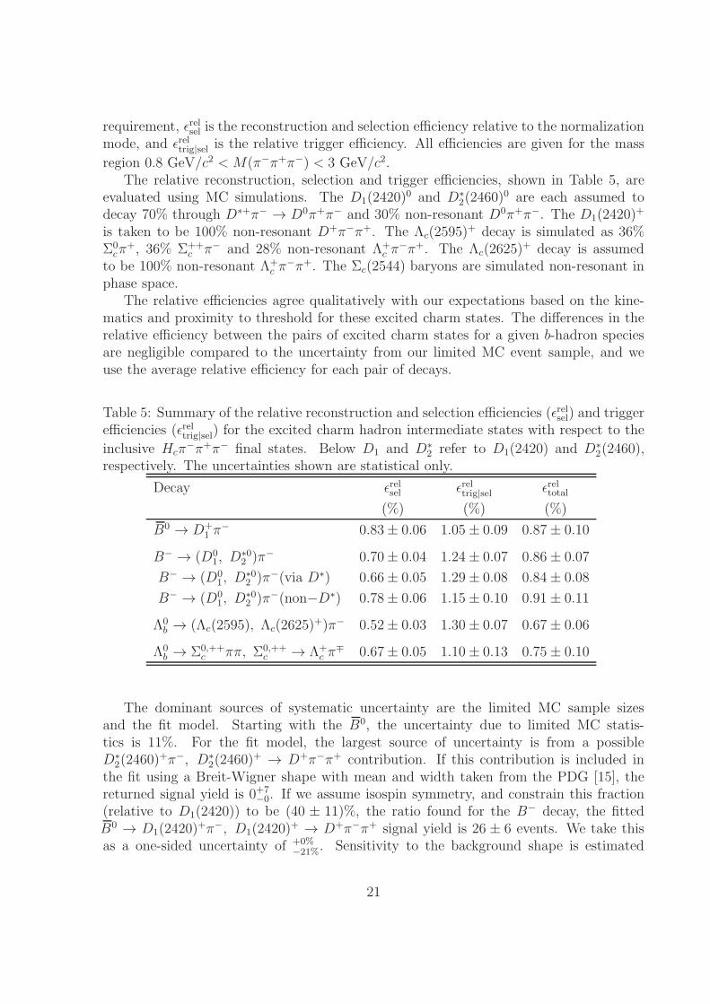
region 0.8 GeV/c2 < M(π−π+π−) < 3 GeV/c2.The relative reconstruction, selection and trigger efficiencies, shown in Table 5, are

evaluated using MC simulations. The D1(2420)0 and D∗

2(2460)0 are each assumed to

decay 70% through D∗+π− → D0π+π− and 30% non-resonant D0π+π−. The D1(2420)+

is taken to be 100% non-resonant D+π−π+. The Λc(2595)+ decay is simulated as 36%

Σ0cπ

+, 36% Σ++c π− and 28% non-resonant Λ+

c π−π+. The Λc(2625)

+ decay is assumedto be 100% non-resonant Λ+

c π−π+. The Σc(2544) baryons are simulated non-resonant in

phase space.The relative efficiencies agree qualitatively with our expectations based on the kine-

matics and proximity to threshold for these excited charm states. The differences in therelative efficiency between the pairs of excited charm states for a given b-hadron speciesare negligible compared to the uncertainty from our limited MC event sample, and weuse the average relative efficiency for each pair of decays.

Table 5: Summary of the relative reconstruction and selection efficiencies (ǫrelsel) and triggerefficiencies (ǫreltrig|sel) for the excited charm hadron intermediate states with respect to the

inclusive Hcπ−π+π− final states. Below D1 and D∗

2 refer to D1(2420) and D∗2(2460),

respectively. The uncertainties shown are statistical only.

Decay ǫrelsel ǫreltrig|sel ǫreltotal

(%) (%) (%)

B0 → D+1 π

− 0.83± 0.06 1.05± 0.09 0.87± 0.10

B− → (D01, D

∗02 )π− 0.70± 0.04 1.24± 0.07 0.86± 0.07

B− → (D01, D

∗02 )π−(via D∗) 0.66± 0.05 1.29± 0.08 0.84± 0.08

B− → (D01, D

∗02 )π−(non−D∗) 0.78± 0.06 1.15± 0.10 0.91± 0.11

Λ0b → (Λc(2595), Λc(2625)

+)π− 0.52± 0.03 1.30± 0.07 0.67± 0.06

Λ0b → Σ0,++

c ππ, Σ0,++c → Λ+

c π∓ 0.67± 0.05 1.10± 0.13 0.75± 0.10

The dominant sources of systematic uncertainty are the limited MC sample sizesand the fit model. Starting with the B0, the uncertainty due to limited MC statis-tics is 11%. For the fit model, the largest source of uncertainty is from a possibleD∗

2(2460)+π−, D∗

2(2460)+ → D+π−π+ contribution. If this contribution is included in

the fit using a Breit-Wigner shape with mean and width taken from the PDG [15], thereturned signal yield is 0+7

−0. If we assume isospin symmetry, and constrain this fraction(relative to D1(2420)) to be (40 ± 11)%, the ratio found for the B− decay, the fittedB0 → D1(2420)

+π−, D1(2420)+ → D+π−π+ signal yield is 26 ± 6 events. We take this

as a one-sided uncertainty of +0%−21%. Sensitivity to the background shape is estimated

21

by using a second order polynomial for the background (3%). The B0 mass sidebands,which have a D1(2420)

+ fitted yield of 2+3−2 events from which we conservatively assign

as a one-sided systematic uncertainty of +0%−6%. For the signal decays, 4% of events have

M(π−π+π−) > 3 GeV/c2, whereas for the D1(2420)+, we find a negligible fraction fail

this requirement. We therefore apply a correction of 0.96 ± 0.02, where we have taken50% uncertainty on the correction as the systematic error. The systematic uncertaintyon the yield in the B0 → D+π−π+π− normalizing mode is 3%. We thus arrive at a totalsystematic error on the B0 branching fraction ratio of +12

−25%.For the B−, we have a similar set of uncertainties. They are as follows: MC sample

size (8%), background model (1%, 2%), D1(2420)0 width (2%, 4%), D∗

2(2460)0 width

(1%, 3%), where the two uncertainties are for the (D1(2420)0, D∗

2(2460)0) intermediate

states. We have not accounted for interference, and have assumed it is negligible comparedto other uncertainties. A factor of 0.98 ± 0.01 is applied to correct for the fractionof events with M(π−π+π−) > 3 GeV/c2. Including a 3% uncertainty on the B− →D0π−π+π− yield, we find total systematic errors of 9% and 10% for the D1(2420)

0 andD∗

2(2460)0 intermediate states, respectively. For the D∗ sub-decays, the total systematic

uncertainties are 10% and 11% for B− → D1(2420)0π−, D1(2420)

0 → D∗+π− and B− →D∗

2(2460)0π−, D∗

2(2460)0 → D∗+π−, respectively. For final states not through D∗, we

find a total systematic uncertainty of 13% for both intermediate states. In all cases, thedominant systematic uncertainty is the limited number of MC events.

For the Λ0b branching fraction ratios, we attribute uncertainty to limited MC sample

sizes (8%), the Λ+c (2595) width (+9%

−5%), Λ0b → Λ+

c π−π+π− signal yield (3%), and apply a

correction of 0.96 ± 0.02 for the ratio of yields with M(π−π+π−) > 3 GeV/c2. In total,the systematic uncertainties on the Λ+

c (2595)+ and Λc(2625)

+ partial branching fractionsare +13%

−10% and ±10%, respectively.For the Σ0,++

c intermediate states, the systematic uncertainties include 14% from finiteMC statistics, and 4% from the Σ0,++

c width. For the Σ0,++c simulation, 10% of decays

have M(π−π+π−) > 3 GeV/c2, compared to 4% for the normalizing mode. We thereforeapply a correction of 1.06±0.03 to the ratio of branching fractions. All other uncertaintiesare negligible in comparison. We thus arrive at a total systematic uncertainty of 16%.

22

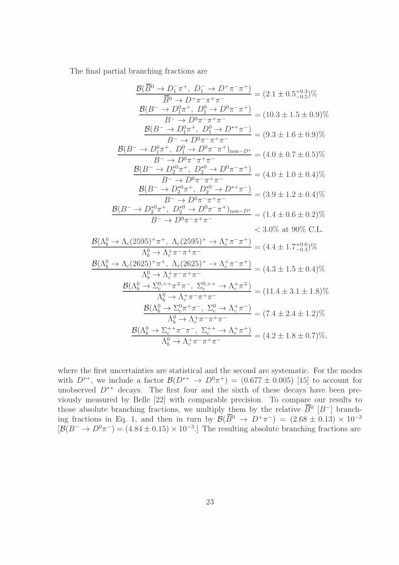
The final partial branching fractions are

B(B0 → D−1 π

+, D−1 → D+π−π+)

B0 → D+π−π+π−= (2.1± 0.5+0.3

−0.5)%

B(B− → D01π

+, D01 → D0π−π+)

B− → D0π−π+π−= (10.3± 1.5± 0.9)%

B(B− → D01π

+, D01 → D∗+π−)

B− → D0π−π+π−= (9.3± 1.6± 0.9)%

B(B− → D01π

+, D01 → D0π−π+)non−D∗

B− → D0π−π+π−= (4.0± 0.7± 0.5)%

B(B− → D∗02 π

+, D∗02 → D0π−π+)

B− → D0π−π+π−= (4.0± 1.0± 0.4)%

B(B− → D∗02 π

+, D∗02 → D∗+π−)

B− → D0π−π+π−= (3.9± 1.2± 0.4)%

B(B− → D∗02 π

+, D∗02 → D0π−π+)non−D∗

B− → D0π−π+π−= (1.4± 0.6± 0.2)%

< 3.0% at 90% C.L.

B(Λ0b → Λc(2595)

+π+, Λc(2595)+ → Λ+

c π−π+)

Λ0b → Λ+

c π−π+π−

= (4.4± 1.7+0.6−0.4)%

B(Λ0b → Λc(2625)

+π+, Λc(2625)+ → Λ+

c π−π+)

Λ0b → Λ+

c π−π+π−

= (4.3± 1.5± 0.4)%

B(Λ0b → Σ0,++

c π∓π−, Σ0,++c → Λ+

c π∓)

Λ0b → Λ+

c π−π+π−

= (11.4± 3.1± 1.8)%

B(Λ0b → Σ0

cπ+π−, Σ0

c → Λ+c π

−)

Λ0b → Λ+

c π−π+π−

= (7.4± 2.4± 1.2)%

B(Λ0b → Σ++

c π−π−, Σ++c → Λ+

c π+)

Λ0b → Λ+

c π−π+π−

= (4.2± 1.8± 0.7)%,

where the first uncertainties are statistical and the second are systematic. For the modeswith D∗+, we include a factor B(D∗+ → D0π+) = (0.677 ± 0.005) [15] to account forunobserved D∗+ decays. The first four and the sixth of these decays have been pre-viously measured by Belle [22] with comparable precision. To compare our results tothose absolute branching fractions, we multiply them by the relative B0 [B−] branch-ing fractions in Eq. 1, and then in turn by B(B0 → D+π−) = (2.68 ± 0.13) × 10−3

[B(B− → D0π−) = (4.84± 0.15)× 10−3.] The resulting absolute branching fractions are

23

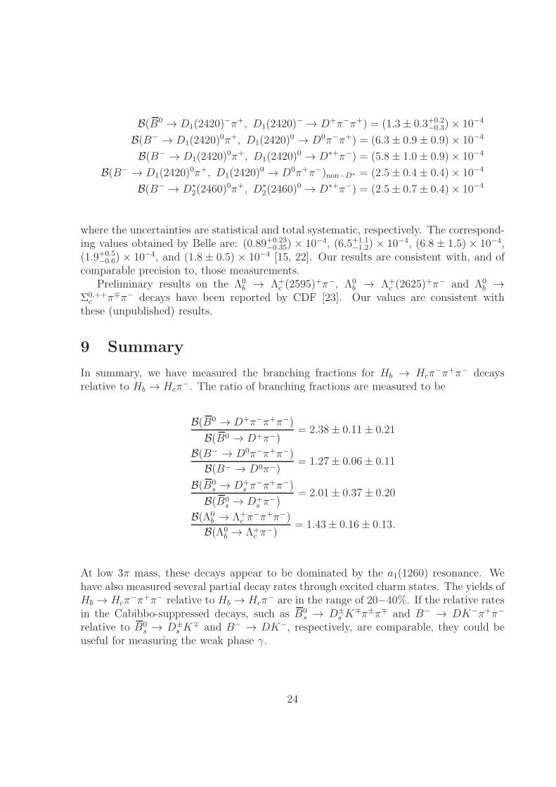
B(B0 → D1(2420)−π+, D1(2420)

− → D+π−π+) = (1.3± 0.3+0.2−0.3)× 10−4

B(B− → D1(2420)0π+, D1(2420)

0 → D0π−π+) = (6.3± 0.9± 0.9)× 10−4

B(B− → D1(2420)0π+, D1(2420)

0 → D∗+π−) = (5.8± 1.0± 0.9)× 10−4

B(B− → D1(2420)0π+, D1(2420)

0 → D0π+π−)non−D∗ = (2.5± 0.4± 0.4)× 10−4

B(B− → D∗2(2460)

0π+, D∗2(2460)

0 → D∗+π−) = (2.5± 0.7± 0.4)× 10−4

where the uncertainties are statistical and total systematic, respectively. The correspond-ing values obtained by Belle are: (0.89+0.23

−0.35) × 10−4, (6.5+1.1−1.2) × 10−4, (6.8 ± 1.5)× 10−4,

(1.9+0.5−0.6) × 10−4, and (1.8 ± 0.5) × 10−4 [15, 22]. Our results are consistent with, and of

comparable precision to, those measurements.Preliminary results on the Λ0

b → Λ+c (2595)

+π−, Λ0b → Λ+

c (2625)+π− and Λ0

b →Σ0,++

c π∓π− decays have been reported by CDF [23]. Our values are consistent withthese (unpublished) results.

9 Summary

In summary, we have measured the branching fractions for Hb → Hcπ−π+π− decays

relative to Hb → Hcπ−. The ratio of branching fractions are measured to be

B(B0 → D+π−π+π−)

B(B0 → D+π−)= 2.38± 0.11± 0.21

B(B− → D0π−π+π−)

B(B− → D0π−)= 1.27± 0.06± 0.11

B(B0s → D+

s π−π+π−)

B(B0s → D+

s π−)

= 2.01± 0.37± 0.20

B(Λ0b → Λ+

c π−π+π−)

B(Λ0b → Λ+

c π−)

= 1.43± 0.16± 0.13.

At low 3π mass, these decays appear to be dominated by the a1(1260) resonance. Wehave also measured several partial decay rates through excited charm states. The yields ofHb → Hcπ

−π+π− relative to Hb → Hcπ− are in the range of 20−40%. If the relative rates

in the Cabibbo-suppressed decays, such as B0s → D±

s K∓π±π∓ and B− → DK−π+π−

relative to B0s → D±

s K∓ and B− → DK−, respectively, are comparable, they could be

useful for measuring the weak phase γ.

24

Acknowledgments

We express our gratitude to our colleagues in the CERN accelerator departments forthe excellent performance of the LHC. We thank the technical and administrative staff atCERN and at the LHCb institutes, and acknowledge support from the National Agencies:CAPES, CNPq, FAPERJ and FINEP (Brazil); CERN; NSFC (China); CNRS/IN2P3(France); BMBF, DFG, HGF and MPG (Germany); SFI (Ireland); INFN (Italy); FOMand NWO (Netherlands); SCSR (Poland); ANCS (Romania); MinES of Russia andRosatom (Russia); MICINN, XuntaGal and GENCAT (Spain); SNSF and SER (Switzer-land); NAS Ukraine (Ukraine); STFC (United Kingdom); NSF (USA). We also acknowl-edge the support received from the ERC under FP7 and the Region Auvergne.

References

[1] N. Cabibbo, Phys. Rev. Lett. 10, 531 (1963); M. Kobayashi and T. Maskawa, Prog.Theor. Phys. 49, 652 (1973).

[2] E. Eichten and B. R. Hill, Phys. Lett. B234, 511 (1990); N. Isgur and M. B. Wise,Phys.Lett. B232, 113 (1989); H. Georgi, Phys. Lett. B240, 447 (1990); E. Eichtenand B. R. Hill, Phys. Lett. B243, 427 (1990); B. Grinstein, Nucl. Phys. B339, 253(1990).

[3] I. Dunietz, Phys. Lett. B270, 75 (1991); I. Dunietz, Z. Phys. C56, 129 (1992);D. Atwood, G. Eilam, M. Gronau, and A. Soni, Phys. Lett. B341, 372 (1995); D.Atwood, I. Dunietz and A. Soni, Phys. Rev. Lett. 78, 3257 (1997).

[4] M. Gronau and D. London, Phys. Lett. B253, 483 (1991); M. Gronau and D. Tyler,Phys. Lett. B265, 172 (1991).

[5] A. Giri, Y. Grossman, A. Soffer and J. Zupan, Phys. Rev. D68 054018 (2003).

[6] R. Aleksan, I. Dunietz, and B. Kayser, Z. Phys. C54, 653 (1992).

[7] I. Dunietz, Phys. Rev. D52, 3048 (1995).

[8] C. S. Kim and S. Oh, Eur. Phys. J. C21, 495 (2001).

[9] M. Gronau, Phys. Lett. B557, 198-206 (2003).

[10] Measurement of ∆ms in the Decay B0s → D−

s ((K−K+π−)(3)π, [LHCb Collabora-

tion], LHCb-CONF-2011-005 (2011).

[11] L. Wolfenstein, Phys. Rev. Lett. 51, 1945 (1983).

[12] C.-W. Chiang and J. Rosner, Phys. Rev. F67, 074013 (2003); C. S. Kim et al , Phys.Lett B621, 259-268 (2004).

25

[13] A. A. Alves Jr. et al. [LHCb Collaboration], JINST 3, S08005 (2008).

[14] M. Williams et. al., LHCb Public Document, LHCb-PUB-2011-002.

[15] K. Nakamura et al., J. Phys. G37, 075021 (2010).

[16] T. Sjostrand, S. Mrenna and P. Skands, JHEP 0605, 026 (2006).

[17] D. J. Lange, Nucl. Instrum. Meth. A462, 152 (2001).

[18] S. Agostinelli et al. [GEANT4 Collaboration], Nucl. Instrum. Meth. A506, 250(2003).

[19] M. Pivk and F. Le Diberder, Nucl Instrum. Meth A555, 356 (2005).

[20] T. Skwarnicki, A study of the radiative cascade transitions between the Upsilon-prime

and Upsilon resonances. PhD thesis, Institute of Nuclear Physics, Krakow, 1986.DESY-F31-86-02.

[21] D. Monorchio, Study of the properties of the a1 meson produced in the B → D∗−a+1at the BABAR Experiment, PhD thesis, Universita Degli Studi Di Napoli, 2005.

[22] K. Abe et al. [Belle Collaboration] Phys. Rev. Lett. 94, 221805 (2005); Phys. Rev.D69, 112002 (2004).

[23] P. Azzurri et al. [CDF Collaboration], in Proceedings of Lepton Photon 2009 Con-

ference, Hamburg, Germany, 17-22 Aug. 2009, p 434, edited by T. Behnke and J.Mnich [arXiv:0912.4380].

26