Measuring Data Dependencies in Large Databases

Gregory Piatetsky-Shapiro, Christopher J. Matheus

GTE Laboratories, MS 4540 Sylvan Road, Waltham MA 02154

{gps0,matheus}@gte.com

Abstract

Data dependencies play an important role in analyzing and explaining the data. In this paper, welook at dependencies between discrete values and a~aalyze several dependency measures. We examine aspecial case of binary fields and show how to efficiently use SQL interface for analyzing dependencies inlarge databases.

1 Introduction

|Analysis of data dependencms is an important and active area of research. A number of methods have beendeveloped in database theory for determining functional dependencies (Mannila and Raiha 1987), (Siegel1988), where the value of one field certainly and precisely determines the value of second field.

There are many more approximate dependencies, where the value of one field determines the value ofanother field with some uncertainty or imprecision. Knowing such dependencies is helpful for understandingdomain structure, relating discovered patterns, data summarization (PiatetskyoShapiro and Matheus 1991),and improving learning of decision trees (Almoaullim and Dietterich 1991).

Several methods have recently been developed for discovery of dependency networks. A method fordetermining dependencies in numerical data using the Tetrad differences is given in (Glymour et al 1987,Spirtes et al 1993). Methods for analyzing the dependency networks and determining the directionalityof links and equivalence of different networks are presented in (Geiger et al 1990). Pearl (1992) presentsa comprehensive approach to inferring causal models. For discrete-valued data, there is a Cooper andHerskovitz (1991) Bayesian algorithm for deriving a dependency network. A problem with these approachesis that they rely on assumptions on data distribution, such as normality and acyclieity of the dependencygraph. Not all of these methods provide a readily available quantitative measure of dependency strength.

In this paper we deal with discrete-valued fields. We propose a direct and quantitative measure of howmuch the knowledge of field X helps to predict the value of field Y. This measure does not depend ondata distribution assumptions, and measures dependency in each direction separately. The measure, called aprobabilistic dependency, or pdep(X, It), is a natural 1 generalization of functional dependency. A normalizedversion of pdep(X, Y) is equivalent to Goodman and Kruskal (1954) measure of association v (tan). pdep measure can be efficiently computed, since it takes no more time than sorting value pairs of X and Y.

We analyze the behaviour of pdep(X, Y) and r under randomization and prove surprisingly simple formulasfor their expected values. In particular, if N is the number of records and dx is the number of distinct values

1 So natural, that it was rediscovered several times. A measure similar to pdep was proposed by Russell (1986) under the nameof partial de~ermlna~ion. We proposed pdep measure in (Piatetsky-Shapiro and Matheus, 1991). Independently, desJardins(1992, p. 70) proposed a measure called uniformity (as a variation of Russell’s measure), which turns out to be identical topdep measure.

Page 162 Knowledge Discovery in Databases Workshop 1993 AAAL93

From: AAAI Technical Report WS-93-02. Compilation copyright © 1993, AAAI (www.aaai.org). All rights reserved.

of X, then E[v(X, Y)] = (dx - 1)/(N - 1). This formula has significant implications for work on automaticderivation of dependency networks in data, since it measures the bias in favor of fields with more distinctvalues. It also has potential applications for the analysis of decision tree accuracy and pruning measures.

Note that the dependence of Y on X does not necessarily indicate causality. For example, we found adata dependency discharge diagnosis ---* admission diagnosia, even though the causal dependency isin the other direction. However, the dependency information in combination with domain knowledge of time(or other) order between variables helps in understanding domain structure (e.g. the discharge diagnosis a refinement of the admission diagnosis).

Measures like X2 can test for independence between the discrete field values and provide a significancelevel for the independence hypothesis. The pdep measure does two things that X2 does not: 1) it indicatesthe direction of the dependence, and 2) it directly measures how much the knowledge of one field helps inpredicting the other field. Our experiments indicate that X2 significance levels are similar to pdep significancelevels obtained using the randomization approach. Thus, it is possible to use X2 to determine the presenceof dependence and use pdep to determine the direction and strength of dependence.

This paper is limited to measures of dependency between nominal (discrete and unordered) values,such as maritM status or insurance type. Various regression techniques exist for deMing with dependencybetween continuous field vMues, such as height or weight. An intermediate case is that of ordinal fields,which are discrete yet ordered (e.g. number of children or level of education). Statistical measures association between ordinal vMues include 7, proposed by Goodman and Kruskal (1954, 1979) and Kendall’stau (Agresti 1984). Those measures, however, are symmetric and cannot be used for determining the directionof dependency.

2 A Probabilistic Dependency Measure

In the rest of this paper we will assume that data is represented as a table with N rows and two fields, Xand Y (there may be many other fields, but we examine two fields at a time).

We want to define a dependency measure dep(X, Y) with several desirable features. We want dep(X, Y)to be in the interval [0, 1]. If there is a functional dependency between X and Y, dep(X, Y) should be 1.If the dependency is less than functional, e.g. some amount of random noise is added to X or Y, we wantdep(X, Y) to decrease as the amount of noise increases. When X, Y are two independent random variables,we want dep(X, Y) to be close to zero. Finally, to measure the direction of dependency dep(X, Y) shouldbe asymmetric and not always equal to dep(Y, X). With these criteria in mind, we define the dependencymeasure as follows.

Definition 1. Given two rows R1, R2, randomly selected from data table, theprobabilistic dependency from X to Y, denoted pdep(X, Y) is the conditionalprobability that R1.Y = R2.Y, given that R1.X = R2.X. Formally,

pdep(X, Y) = p(R1.Y = R~.Y I R1.X = R2.X)

We note that pdep(X, Y) approaches (and becomes equal to) 1 when the dependency approaches (andbecomes) a functional one.

To derive the formula for pdep(X, Y), we first examine the self-dependency measures pdep(Y), which isthe probability that Y values will be equal in two randomly selected rows. Without loss of generality, letY take values 1,..., M, with frequencies yl,..., YM. The probability that both randomly selected rows will

~denoted pdep!(Y) in Piatetsky-Shaplro (1992)

AAAI-93 Knowledge Discovery in Databases Workshop 1993 Page 163

have Y = j is p(Y = j) x p(Y = j) = 2, and pdep(Y) is t he sum of t hese probabilities over all j , i. e.

m 2

pdep(Y) = Ep(r = j)’ = E NY~ (1)j=l

Let X take values 1, .... K with frequencies zl,..., ZK, and let nq be the number of records with X -- i,Y = j. Assume that the first row R1 had X - i. Selection of the second row R2 is limited to the subset ofsize zl where X = i. The probability that two rows randomly chosen from that subset will have the same Yvalue is equal to pdep(Y[X = i) for that subset, which is

M M 2nij

pdep(YIX = i) y]~p(Y = jl X = 02= z_,z?~=1 j=l *

(2)

Since the probability of choosing row Rx with value X = i is zi/N, we can compute pdep(X, Y) as theweighted sum of pdep(YIX = i), i.e.

K K M_2 K M

pdep(X,y)=Ep(X=i)pdep(Y.X=,) ~"~ziX"’’li~1~n~’= Z--~NZ---a z? = z--7

i=1 i=1 j=l t = =

I

The following table 1 shows a sample data set and a corresponding frequency table.

(3)

DataFile

Table 1: An example dataset

X Y Y=i 2[x_iFrequency --+ ....... +--

i I Table X= 11 2 0 [ 2i i 2li 1122 1 31 0 11 12 2 +3 2 y_jl3 215

Here we have pdep(Y) = 9/25+4/25 = 0.52, and pdep(X, Y) = 0.8, while pdep(X) = 4/25+4/25+ 1/25 =0.36, and pdep(Y, X) = 0.533.

By itself, however, the measure pdep(X, Y) is insufficient. If, for example, almost all values of Y arethe same, then any field will be a good predictor of Y. Thus we need to compare pdep(X, Y) with pdep(Y)to determine the relative significance of pdep(X, Y). The relationship between these measures is given intheorem 1.

Theorem 1.K--1 K M

1 (zhnq -- Zinhj)2pdep(X,r) pdep(V): x,,x,h=l i=h+l j=l

Proof: By rearranging sums (details omitted for lack of space).

(4)

This theorem implies

Page 164 Knowledge Discovery in Databases Workshop 1993 AAAL93

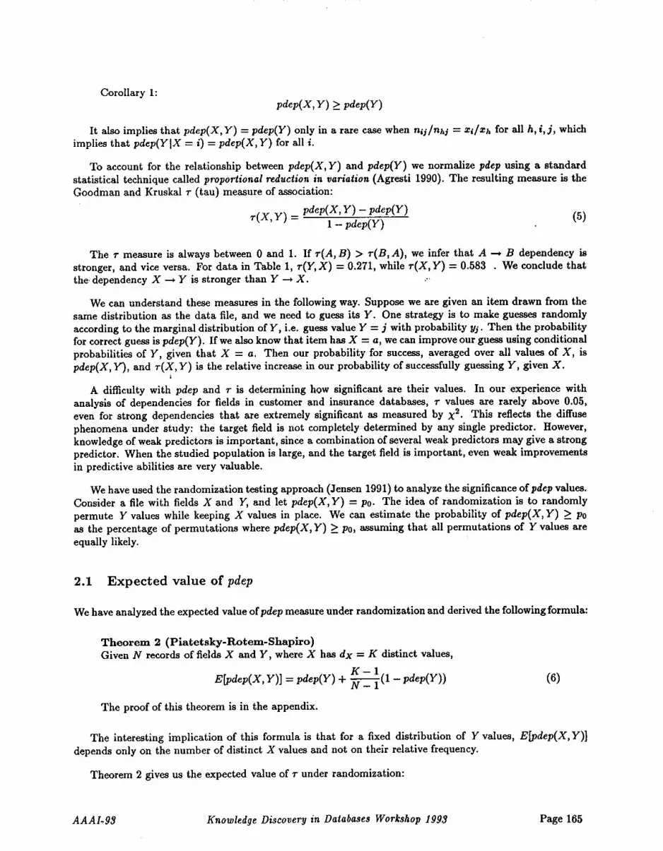
Corollary 1:pdep(X, Y) >_ pdep(Y)

It also implies that pdep(X, Y) = pdep(Y) only in a rare ease when no/nhj - zi/za for all h, i,j, whichimplies that pdep(YlX = i) = pdep(X, for all i.

To account for the relationship between pdep(X, Y) and pdep(Y) we normalize pdep using a standardstatistical technique called proportional reduction in variation (Agresti 1990). The resulting measure is theGoodman and Kruskal r (tau) measure of association:

r(X, Y) pdep(X, Y) - pdep(Y) (5)1 - pdep(Y)

The r measure is always between 0 and 1. If r(A, B) > v(B, A), we infer that A ---, B dependency stronger, and vice versa. For data in Table 1, r(Y,X) = 0.271, while r(X,Y) = 0.583 . We conclude thatthe dependency X --* Y is stronger than Y -* X. ~-

We can understand these measures in the following way. Suppose we are given an item drawn from thesame distribution as the data file, and we need to guess its Y. One strategy is to make guesses randomlyaccording to the marginal distribution of Y, i.e. guess value Y = j with probability yj. Then the probabilityfor correct guess is pdep(Y). If we also know that item has X = a, we can improve our guess using conditionalprobabilities of Y, given that X = a. Then our probability for success, averaged over all values of X, ispdep(X, Y’), and r(X, Y) is the relative increase in our probability of successfully guessing Y, given

l

A difficulty with pdep and r is determining how significant are their values. In our experience withanalysis of dependencies for fields in customer and insurance databases, r values are rarely above 0.05,even for strong dependencies that are extremely significant as measured by X2. This reflects the diffusephenomena under study: the target field is not completely determined by any single predictor. However,knowledge of weak predictors is important, since a combination of several weak predictors may give a strongpredictor. When the studied population is large, and the target field is important, even weak improvementsin predictive abilities are very valuable.

We have used the randomization testing approach (Jensen 1991) to analyze the significance of pdep values.Consider a file with fields X and Y, and let pdep(X, Y) = po. The idea of randomization is to randomlypermute Y values while keeping X values in place. We can estimate the probability of pdep(X, Y) > as the percentage of permutations where pdep(X, Y) > Po, assuming that all permutations of Y values areequally likely.

2.1 Expected value of pdep

We have analyzed the expected value ofpdep measure under randomization and derived the following formula:

Theorem 2 (Piatetsky-Rotem-Shapiro)Given N records of fields X and Y, where X has dx = K distinct values,

K-1E[pdep(X, Y)] = pdep(Y) ~-~--T(1 -p dep(Y)) (6)

The proof of this theorem is in the appendix.

The interesting implication of this formula is that for a fixed distribution of Y values, E[pdep(X, Y)]depends only on the number of distinct X values and not on their relative frequency.

Theorem 2 gives us the expected value of 1- under randomization:

AAAI.93 Knowledge Discovery in Databases Workshop 1993 Page 165

Corollary 2.1

Elf(X, Y)] - E~dep(X, Y)] - pdep(Y) _ K - 1 (7)1 - pdep(Y) N - 1

So, if dx > dz, then for any field Y, X is expected to be a better predictor of Y than Z. Tan valuesthat are higher than the expected value indicate additional relationship between the fields. This formula isespecially important when the number of distinct field values is close to the number of records.

We can further refine our analysis of dependency by observing that pdep(X, Y) (and r) will indicate significant dependency for large values of dx, even for a random permutation of all Y values (which destroysany intrinsic relationship between X and Y). We can compensate for this effect by introducing a new measurep, which normalizes pdep(X, Y) with respect to E~dep(X, Y)] instead of pdep(Y):

p(X, Y) pdep(X, Y) - S~dep(X, Y)] 1 - pdep(X, Y) N - 11 - E~dep(X, Y)] - 1 - 1 - pdep(Y) g - (8)

Since E~dep(X, Y)I >_ pdep(Y), we have p(X, Y) < r(X, Y). When N/K increases, E[pdep(X, Y)]asymptotically decreases to pdep(Y), and p(X,Y) asymptotically increases to r(X,Y). The additionaladvantage of p is that it increases, like X2, if the data set size is doubled, whereas pdep and tan do notchange.

We used the randomization approach to compute the exact significance values for pdep(X, Y) (see pendix). However, for large datasets the exact computation is too computationally expensive. Instead, weuse X2 statistic for measuring the significance of dependency. Our experiments indicate that randomizationand X2 significance levels are quite close.

Finally, we note that the two-field dependency analysis of Y on X can be straightforwardly generalizedinto a multi-field dependency analysis of Y on several fields, X1, X2,.. ¯ by replacing conditional probabilitiesp(Y = blX = a) with p(Y = blX1 = 1, X2 - 2,...) (see also Goodman and Kruskal, 1979).

3 Binary Fields

An important and frequent special case is that of binary fields. Assuming that there is a significant depen-dency between X and Y, as measured by standard tests for 2x2 tables, we want to know the direction of thedependency. When both X and Y have only two values, then we cannot use r or p measures to determinethe direction of dependency, since r(X, Y) = r(Y,

For binary fields, the value (w.l.g. denoted as "t" for true) which indicates the presence of a desirablefeature is generally more useful than the other value (denoted as "f" for false). So we need to compare therules (X = t) --* (Y = t) versus (g = t) --* (X = t). If, It, if, it, denote the counts of X =f, Y=f; X=f,Y=t; X=t, Y-f; and X=t, Y=t, respectively.

Ix=t & Y=t] tt of cases, while (Y -- t) ---* (X = t) is true Then (X = t) ~ (Y = t) is true IX=, l =u of cases. Hence the rule (X = t) --* (Y = t) is stronger tf < f t, and the inverse rule is st ronger if

~t+lttf > ft.

The following table shows the statistics for a sample of customer data for fields CHILD-O-5, CHILD-O-17,and FEMALE-35-44, which have a value "Y" if the household has such a person, and "N" otherwise.

In the first case, the rule Child 0-17 --* Child 0-5 is correct 2~--+~s24 - 31% of the time, while the ruleChild 0-5 ---* Child 0-17 is correct 100%, so the second rule is obviousTy better. In the second case, rule Child

327 = 37%.327 = 43%, while the inverse rule has correctness0-17 --~ Female 35-44 has correctnessThus, the first rule is preferred.

Page 166 Knowledge Discovery in Databases Workshop 1993 AAAI-93

Child 0-17

Child 0-5 Female 35-44N Y N Y

+ .......... + ~ +

N I 5363 OI NI 4803 860 IY J 524 238J YI 435 327 I

+ .......... + 4 +

4 Using SQL interface to compute Dependencies

Some databases are so large that they cannot be analyzed in memory. Such databases can be analyzed by

using a DBMS query interface to retrieve data and to perform at least some of the computation. We limitour discussion to SQL interfaces, since SQL, with all its limitations, is the de-facto standard query language.Using SQL for data access makes analysis tools more portable to other DBMS.

Here we examine the use of SQL queries on a file File1 to perform the dependency analysis. In thesimplest case of both X and Y being discrete, we can extract the necessary statistics for computing pdepwith the query

select X, Y0 count(*) from Filel group by X,

A more interesting case arises when we need to discretize numeric data fields. Consider a field Y whichcontains toll-call revenue. While Y has many distinct values, we are interested in whether Y = 0 (no usage);0 < Y < 3 (low usage); 3 < < 10(medium usage); or Y >10(h igh usage). Such d iscre tization may neto be done frequently, and for different sets of ranges.

To get the necessary statistics for computing dependency of discretized Y upon some X we have to issuefour standard SQL queries:3

select X, count(*) from Filei where Y = 0 group by

select X, count(*) from Filel where Y > 0 and Y <= 3 group by select X, count(*) from Filel where Y > 3 and Y <= I0 group by

select X, count(*) from Filel where Y > I0 group by

If X is discretized into 5 buckets and Y is discretized into 3, then 5 x 3 = 15 queries would be neededto compute the dependency. Fortunately, several popular DBMS, such as Oracle" or Raima"n, have SQLextensions that allow us to compute the necessary statistics with just one query.

4.1 Dynamic Discretization using Raima

Dynamic discretization is relatively straightforward using Raima, which has a conditional column functionif(condition1, exprl, expr2), meaning if condltionl is true, then exprl else expr2. Expressions exprl,expr2 may in turn contain conditional columns. The necessary code for the above example is:

select X, if(Y=O, O, if(Y<=3, 2, if(Y<=lO,5,10))), count(*) from

group by 1, 2;

In general, the code for discretization is specified as one long conditional column in a straightforwardmanner.

3The last query can be avoided if we have previously computed select X, count(*) from Filet group by

AAAI-93 Knowledge Discovery in Databases Workshop 1993 Page 167

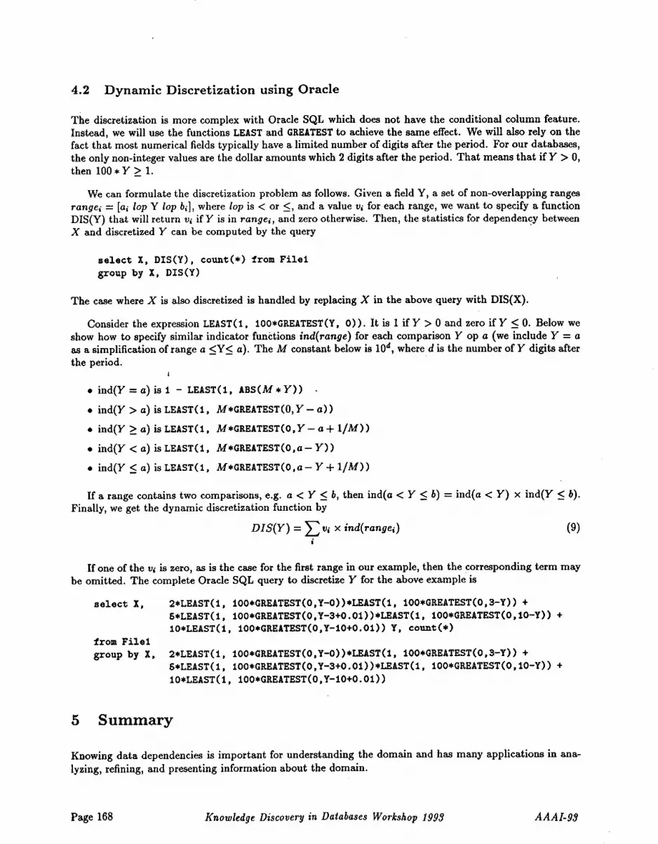
4.2 Dynamic Discretization using Oracle

The discretization is more complex with Oracle SQL which does not have the conditional column feature.Instead, we will use the functions LEAST and GREATEST to achieve the same effect. We will also rely on thefact that most numerical fields typically have a limited number of digits after the period. For our databases,the only non-integer values are the dollar amounts which 2 digits after the period. That means that if Y > 0,then 100 * Y ~ 1.

We can formulate the discretization problem as follows. Given a field Y, a set of non-overlapping rangesrangei = [al lop Y lop bi], where lop is < or <, and a value vi for each range, we want to specify a functionDIS(Y) that will return vl if Y is in rangel, and zero otherwise. Then, the statistics for dependency betweenX and discretized Y can be computed by the query

select X, DIS(Y), count(*) from Filelgroup by X, DIS(Y)

The case where X is also discretized is handled by replacing X in the above query with DIS(X).

Consider the expression LEAST(I, IO0*GREATEST(Y, 0)). It is 1 if Y > 0 and zero if Y ~ O. Below show how to specify similar indicator functions ind(range) for each comparison Y op a (we include Y = as a simplification of range a <Y< a). The M constant below is 10d, where d is the number of Y digits afterthe period.

¯ ind(Y = a)

¯ ind(Y > a)

¯ ind(Y > a)

¯ ind(Y < a)

¯ ind(Y < a)

I

1 - LEAST(l, ABS(M,Y))

LEAST(i, M*GREATEST(0,Y-- a))

LEAST(i, M*GREATEST(0,Y-- a+I/M))

LEAST(l, M*GREATEST(O,a-- Y))

LEAST(i, M*GREATEST(O,a--Y+I/M))

If a range contains two comparisons, e.g. a < Y < b, then ind(a < Y _~ b) = ind(a < Y) x ind(Y _~ Finally, we get the dynamic discretization function by

DIS(Y) = Z vi × ind(rangei) (9)i

If one of the vi is zero, as is the case for the first range in our example, then the corresponding term maybe omitted. The complete Oracle SQL query to discretize Y for the above example is

select X,

from Filelgroup by X,

2*LEAST(I, IO0*GREATEST(O,Y-O))*LEAST(I, IO0*GREATEST(O,3-Y)) 5*LEAST(I, IO0*GREATEST(O,Y-3+O.OI))*LEAST(I, IO0*GREATEST(O,IO-Y)) IO*LEAST(I, IO0*GREATEST(O,Y-IO+O.OI)) Y, count(*)

2*LEAST(I, IO0,GREATEST(O,Y-O))*LEAST(I, IO0*GREATEST(O,3-Y)) +S,LEAST(I, IOO*GREATEST(O,Y-3+O.OI))*LEAST(I, IO0*GREATEST(O,IO-Y)) IO*LEAST(I, IO0*GREATEST(O,Y-IO+O.OI))

5 Summary

Knowing data dependencies is important for understanding the domain and has many applications in ana-lyzing, refining, and presenting information about the domain.

Page 168 Knowledge Discovery in Databases Workshop 1993 AAAI-93

In this paper, we have discussed ways to measure the strength of approximate, or probabilistic, depen-dencies between nominal values and showed how to determine the significance of a dependency value usingthe randomization approach. We proved formulas for the expected values of pdep and Goodman-Kruskal runder data randomization.

We also described how to efficiently use SQL interface for analyzing dependencies in large databases.

Acknowledgments. We thank Philip Chan, Greg Cooper, Marie desJardins, Greg Duncan, and GailGill for their insightful comments and useful suggestions. We are grateful to Shri Goyal for his encouragementand support.

6 References

Agresti, A. (1984). Analysis of Ordinal Categorical Data. New York: John Wiley.

Agresti, A. (1990). Categorical Data Analysis, New York: John Wiley.

Almoaullim, H., and Dietterich, T. (1991). Learning with Many Irrelevant Features, In Proceedings AAAI-91,547-552.

Cooper, G., and Herskovits, E. (1991). A Bayesian Method for the Induction of Probabilistic Networks fromData. Stanford KnOwledge Systems Laboratory Report KSL-91-02.

desJardins, M. E. (1992). PAGODA: A Model for Autonomous Learning in Probabilistic Domains, Ph.D.Thesis, Dept. of Computer Science, ’University of Berkeley.

Geiger, D., Pat, A., and Pearl, J. (1990). Learning Causal Trees from Dependence Information. Proceedingsof AAAI-90, 770-776, AAAI Press.

Glymour, C., Scheines, R., Spirtes, P., and Kelly, K. (1987). Discovering Causal Structure. Orlando, Fla.:Academic Press.

Goodman, L. A., and Kruskal, W. H. (1954). Measures of Association for Cross Classification, J. of AmericanStatistical Association, 49,732-764.

Goodman, L. A., and Kruskal, W. H. (1979). Measures of Association for Cross Classifications. Springer-Verlag, New York.

Jensen, D. (1991). Knowledge Discovery Through Induction with Randomization Testing, in G. Piatetsky-Shapiro, ed., Proceedings of AAAI-91 Knowledge Discovery in Databases Workshop, 148-159, Anaheim,CA.

Mannila, H. and Raiha, K.-J. (1987). Dependency inference. Proceedings of the Thirteenth InternationalConference on Very Large Data Bases (VLDB’87), 155-158.

Pearl, J. (1992). Probabilistic Reasoning in Intelligent Systems: Networks of plausible inference, 2nd edition.San Mateo, Calif.: Morgan Kaufmann.

Piatetsky-Shapiro, G. and Matheus, C. (1991). Knowledge Discovery Workbench: An Exploratory Envi-ronment for Discovery in Business Databases, Proceedings of AAAI-91 Knowledge Discovery in DatabasesWorkshop, 11-24, Anaheim, CA.

Piatetsky-Shapiro, G. (1992). Probabilistic Data Dependencies, in J. Zytkow, ed., Proceedings of MachineDiscovery Workshop, Aberdeen, Scotland.

AAAI-93 Knowledge Discovery in Databases Workshop 1993 Page 169

Piatetsky-Shapiro, G. and Matheus, C. (1992). Knowledge Discovery Workbench for Discovery in BusinessDatabases, In special issue of Int. J. of Intelligent Systems on Knowledge Discovery in Databases andKnowledgeBases, 7(7) 675-686.

Russell, S. J. (1986). AnalogicM and Inductive Reasoning, Ph. D. Thesis, Dept. of Computer Science,Stanford University, chapter 4.

Siegel, M. (1988). Automatic rule derivation for semantic query optimization, Proceedings Expert DatabaseSystems Conference, 371-385.

Spirtes, P., Glymour, C., and Scheines, R. (1993). Causality, Prediction, and Search. New York: Springer-Verlag.

A Analysis of the PDEP measure under Randomization

We use the randomization testing approach (Jensen 1991) for analyzing the pdep measure. First, we provea formula for the expected value of pdep under randomization, and then we discuss ways of measuring thesignificance of pdep value.

Consider a file with only two fields X and Y, and let pdep(X, Y) = Po. The idea of randomization is torandomly permute Yvalues while keeping X vMues in place. We can estimate the probability ofpdep(X, Y) P0 as the percentagd of permutations where pdep(X, Y) > Po, assuming that all permutations of Y valuesare equally likely.

A.1 Expected Value of PDEP under Randomization

Without loss of generality we can assume that X takes values from 1 to K, and Y takes values from 1 toM. Let N be the number of records. Then we have the following theorem, proposed by Gregory Piatetsky-Shapiro and proved by Doron l~tem.

Theorem 2 (Piatetsky-t~tem-Shapiro): The expected value of pdep(X, Y) under random-ization is

N-K K-1E~dep(X, Y)] = pdep(Y)--ff-~ + N ------1

K-1-- pdep(Y) ~- --~(1 - pdep(Y)) (10)

Proof: For convenience, we reformulate this problem in terms of balls and cells. We will call a set oftuples with equal y-values a y-set. We have M y-sets, each consisting of yj bMls. Partitioning of the recordaccording to K distinct X values is equivalent to partitioning the N cells into K compartments, each of zicells. From the definition of pdep it is clear that

K My

E~dep(X,Y)] -" Z Z E~dep(X -- i,Y = j)]i=1 j=l

(11)

First, we will compute E~dep(X = i, Y = j)] by looking at the problem of placing yj balls among N cells,so that r balls fall into a compartment of size zi, contributing r~/(Nz~) to pdep.

Let( n) n~.i -- ~ denote the number of ways to select i items from n.

Page 170 Knowledge Discovery in Databases Workshop 1993 AAAI-93

For a given y-set with yj balls, the probability that r balls fall into a compartment of size zl is

r xi--r r yj --r(12)

Then E~dep(X = i, Y = j)] is the sum of the above equation from r = 1 to r = zl (r = 0 contributes zeroto pdep), which is

N =Y~

(13)

We reduce this sum to a closed form using the following combinatorial lemmas.

Lemma 2.1:

i=0

Proof: Consider the task of placing b balls into n cells. Assume that the first a cells are marked as special.The number of placements of b balls into n cells, so that exactly / of them will fall into special cells is

(a)(n-a)i . Summing this for i fromO to a givesthe sum on the l eft . This sumis al so equal to the

()total number of placements of b balls into n cells (regardless of the partition), which n Q.E.D.b "

Corollary 2.2

"()( )( Ei a n--a n--1i b i

-a b 1i=0

Proof: By reducing to Lemma 2.1.

(15)

Corollary 2.3

()( )()( ~-’~(i + 1)a n - a n n - 1i b-i = b +a b-1

i=0

Proof: By summing the previous two equations.

We can now reexamine the sum in earlier equation 13 after replacing r with r’ = r - 1,

r -- ~-~(r’+l) zi-1(N 1)

r- 1 yj -r dr=l rl=0

(16)

(17)

We see that Corollary 2.3 applies, with a = z~ - 1, b = yj - 1, and n = N - 1. Hence E~dep(X = i, Y = j)](from equation 13) is equal

1 [(N-l)

(N-2)1

(x,- 1)(yj

N()yi yjl +(zi- 1)YJ -2 = --~-- (1 -I-N2 N- 1 -1))(18)

Finally, to compute E~pdep(X, Y = j)] we sum the above over all zi, obtaining (since E xi = N)

E[pdep(X,Y=j)] = ~ yj (1+ -1))=~ 1).)i----1

AAAI-93 Knowledge Discovery in Databases Workshop 1993 Page 171

V] N-K K-1N2 N - 1 -b yj N(N - 1) (19)

As we can see there is no dependence of this expression on zi, but only on N, yj, and K. Finally, the valueof E~dep(X, Y)] is obtained by summing the above equation over all y-sets:

M 2 N-KK-1E[pdep(X’Y)] ~’ ~(~2 N--1 +Y I N( N--1))

j=l(20)

Since ~’~’~M1 yj ---- N and ~--~M y~/N2 = pdep(Y), the above simplifies to

N-K K-1 K-1E[pdep(X, Y)] = pdep(Y)~ + N ----~1 -- pdep(Y) ~-~-T(1 - pdep(Y)) (21)

End of Proof.

A.2 Determining significance of PDEP

Table 2: Sample Data partitioned by different X values.X Y

l

Data I I pdep(X,Y) = 0.800File I I

.... pdep(Y) = O.S22 1 !I=5, K=32 2

3 2

For our sample data, we have dependency X ---* Y with pdep(X, Y) = 0.800. How significant is this? Letus consider permutations of record numbers and their Y values, while keeping X values in the same place.Each permutation is partitioned into three parts: records with X = 1, X = 2, and X = 3. Let us denote aparticular permutation by listing its Y values, with a vertical bar to denote the partition. The above tablewould be denoted as [1,1 I 1,2 [ 2], where the first section 1,1 represents Y values for X = 1, the secondpart 1,2 is Y values for X = 2, and the last part 2 is Y value for X = 3.

For the purpose of measuring pdep, the order of Y values within a partition is irrelevant. Consider apermutation that leads to a partition [vl,v2 I v3,v4 I vS]. Any permutation of values in the first (orsecond) part will lead to a partition with the same pdep. Partitions are differentiated by the count of valueswith Y - 1 and Y - 2 in each part, called the partition signature. Since the number of values in each partis 2, 2, and 1, respectively, each signature will appear at least 2!2!1! = 4 times among the 5!--120 possiblepermutations.

(3)Consider partition [1,1 [ 1,2 [ 2]. There are 2 =3 ways to choose 2 records with Y = 1 in the first

part’ (2) 1)1 1 -2waystochooserecordswithY--landY-2inthesecondpart, andoneway

to choose the remaining record in the third part. Thus, there are 3x2-6 choices that lead to signature [1,1[ 1,2 [ 2]. For comparison, signature [2,2 [ 1,1 [ 2] can be chosen in 3 ways.

Regardless of the signature, each choice can be permuted in 2!2!1! = 4 ways to get a pdep-equivalentpartition. These results are summarized in tables 3A and 3B.

Page 172 Knowledge Discovery in Databases Workshop 1993 AAAI-93

Table 3A. Pdep and prob. of all signatures

-y-signature--- choices probability pdep[1,1 ] 2,2 1 I] 3 3x4/120 = 0.1 1.0[2,2 ] I,I [ 1] 3 3x4/120 = 0.1 1.0[I,I [ 1,2 [ 2] 6 6x4/120 = 0.2 0.8[1,2 I 1,1 I 2] 6 6x4/120 = 0.2 0.8[I,2 ] 1,2 1 i] 12 12x4/120 = 0.4 0.6

Table 3B. Pdep probability s~mmary

pdep probability1 0.20.8 0.40.6 0.4

Here the probability ofpdep(X, Y) >_ 0.8 for a random permutation of Y values is p(pdep -- 1) + p(pdep = 0.8)= 0.2+0.4 = 0.6.

We can also use table 3B to check Theorem 2. From table we get E[pdep(X, Y)] = 1 x 0.2 + 0.8 x 0.4 0.6 x 0.4 = 0.76. For this data pdep(Y) 0.52, K = 3,andN = 5, and Theorem 2 givesE[pdep(X, Y)] =

3--I0.52 + ~:T(1 - 0.52) = 0.76, same answer[

Let us consider a general case where X has values 1, 2,... K, and Y has values 1, 2,... M. Let zi be the countofX = i, yj be the count ofY = j, nq be the count ofX = i, Y = j, and N be the total number of records.Let C(N, nl, n2,..., nk) = N!/(nl!n2!...nk!) be the number of ways to distribute (without remainder) items into K bins, so that bin i will have.nl items.

The probability of a~ particular combination is obtained by the following reasoning. Let us group togetherrecords with the same value of X. This will produce K bins, one bin for each value. First bin has nilrecords with Y = 1, second has n12, etc. There are C(y1,n11,n21,...,nK1) ways to put Yt records withY = 1 into those bins. Similarly, there are C(y2, n12, n22,...,nK2) ways to place Y2 records with Y = 2.After all records have been placed, records in each bin can be independently permuted. This will producezl!z2!.., zg[ permutations. The product of all those factors should be divided by N!, the total number ofpermutations. Hence the total probability of a particular configuration [nq ...] is

prob([n,i." .]) = 1-IM1C(yj,nlj,...,ngj) I-I,K=I xi! = I’IM1C(yj,nlj,...,nKj) (22)N! C( N, Xl, . . . , xlf )

It is possible to enumerate all the partition signatures and construct a complete distribution of pdep valuesand their probabilities. However, the number of different signatures grows very fast and it is impractical toenumerate them for a large number of partitions. Instead, we can use X2 statistic to measure the significanceof the dependency.

To compare X~ and pdep significance levels, we computed them for datasets obtained by repeating N timesthe data in Table 1. The following table summarizes the results, which indicate that pdep and X~ are quiteclose.

Table 5. Sig(p obtained by randomization vs significance of X2

Significance N=2 3 4 6 8 16sig(pdep) 0.934 0.984 0.9973 0.99995 1 - 1.5 x 10-6 1 - 7.8 x 10-l asig(x 0.946 0.987 0.9971 0.99985 1 - 8.6 x 10-6 1-7.4x 10-11

Note that since pdep and 1" values do not change, when the data set is doubled (which increases significance),pdep or r values cannot be used by themselves to measure the significance of dependency and should be usedonly together with N.

AAAI-93 Knowledge Discovery in Databases Workshop 1993 Page 173