Embed Size (px)
Citation preview
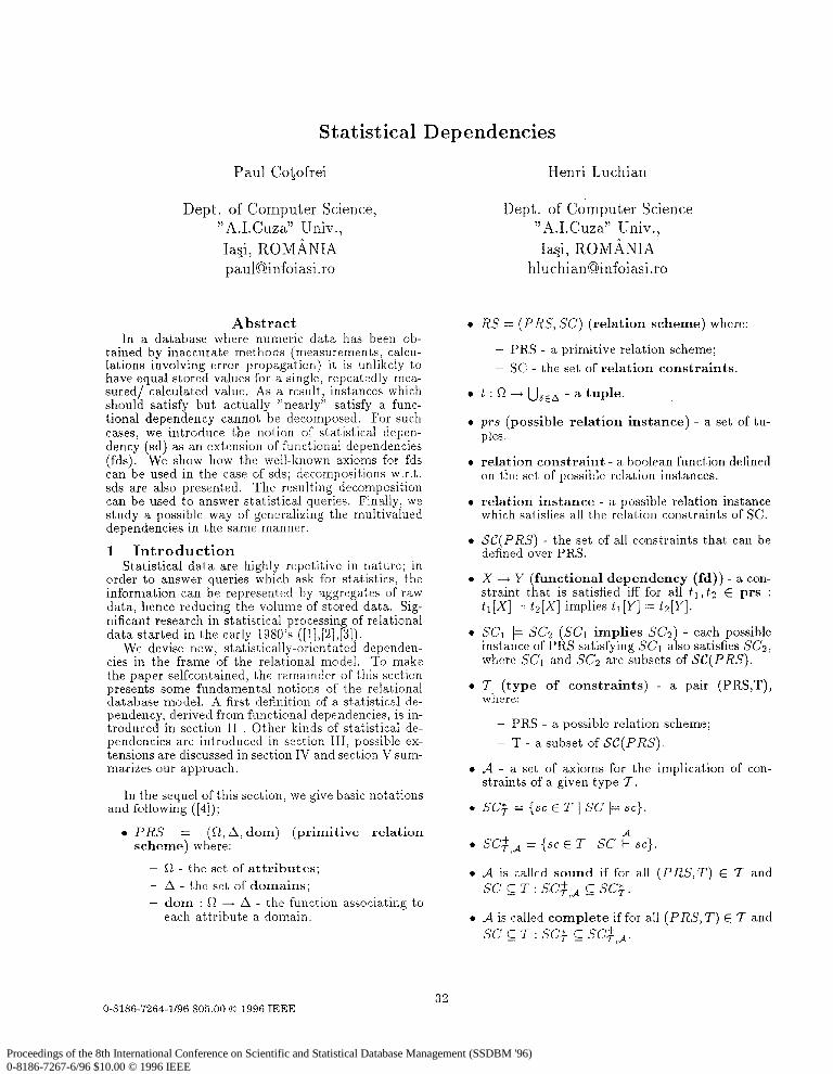
Statistical Dependencies
Paul Cofofrei
Dept. of Computer Science, “A.I.Cuza” Univ., Iasj, ROMANIA [email protected]
Abstract In a database where numeric data has been ob-
tained by inaccurate methods (measurements, calcu- lations involving error propagation) it is unlikely to have equal stored values for a single, repeatedly mea- sured/ calculated value. As a result, instances which should satisfy but actually “nearly” satisfy a func- tional dependency cannot be decomposed. For such cases, we introduce the notion of statistical depen- dency (sd) as an extension of functional dependencies (fds). We show how the well-known axioms for fds can be used in the case of sds; decompositions w.r.t. sds are also presented. The resulting decomposition can be used to answer statistical queries. Finally, we study a possible way of generalizing the multivalued dependencies in the same manner.
1 Introduction Statistical data are highly repetitive in nature; in
order to answer queries which ask for statistics, the information can be represented by aggregates of raw data, hence reducing the volume of stored data. Sig- nificant research in statistical processin of relational data started in the early 1980’s ([1],[211/!l]).
We devise new, statistically-orientated dependen- cies in the frame of the relational model. To make the paper selfcontained, the remainder of this section presents some fundamental notions of the relational database model. A first definition of a statistical de- pendency, derived from functional dependencies, is in- troduced in section II . Other kinds of statistical de- pendencies are introduced in section III, possible ex- tensions are discussed in section IV and section V sum- marizes our approach.
In the sequel of this section, we give basic notations and following ([4]);
. PRS = (R, A, dom) (primitive relation scheme) where:
- R - the set of attributes; - A - the set of domains; - dom : R -+ A - the function associating to
each attribute a dornain.
Henri Luchian
Dept. of Computer Science “A.I.Cuza” Univ., Ia$, ROMANIA
l RS = (PRS, SC) (relation scheme) where:
- PRS - a primitive relation scheme; - SC - the set of relation constraints.
l t : R + UaEa - a tuple.
l prs (possibl e relation instance) - a set of tu- ples.
l relation constraint - a boolean function defined on the set of possible relation instances.
l relation instance - a possible relation instance which satisfies all the relation constraints of SC.
l SC(PRS) - the set of all constraints that can be defined over PRS.
l X - Y functional dependency (fd)) - a con- h straint t at is satisfied iff for all tl, t2 E prs :
tl[X] = tz[X] implies ti[Y] = tz[Y].
l SC1 + SC2 (SC1 implies SC2) - each possible instance of PRS satisfying SC1 also satisfies SC2, where SC1 and SC2 are subsets of SC(PRS).
l 7 (type of constraints) - a pair (PRS,T), where:
- PRS - a possible relation scheme; - T - a subset of SC(PRS).
l A - a set of axioms for the implication of con- straints of a given type Q+.
l SC? = {SC E T / SC t= SC}.
l SC,+,, = {SC E T 1 SC i-” SC}.
l A is called sound if for all (PRS,T) E 7 and SC c T : SC,+,, _ c SC?.
l A is called complete if for all (PRS, T) E 7 and SC C T : SC? C SC,+>,.
O-8186-7264-1/96 $05.00 0 1996 IEEE 32
Proceedings of the 8th International Conference on Scientific and Statistical Database Management (SSDBM '96) 0-8186-7267-6/96 $10.00 © 1996 IEEE
l A is called non-redu,ndant if for all B g A: SC,+,, = SC’S,, implies B = A.
The well-known set of axi’oms for the implication of fds given by Armstrong is non-redundant , sound and complete ([5]).
Theorem 1.1 Let F be Ihe following system of a- xioms:
0 k X ---) Y if Y C X (kavial fds) X ---) Y t- X -+ XY (aug*men2at ion rule) gj {x-+Y,Y+z}tx -+ Z (transitivity rule) (F3) F is non-redundant) sov,nd and complete for the
implicalion of fds
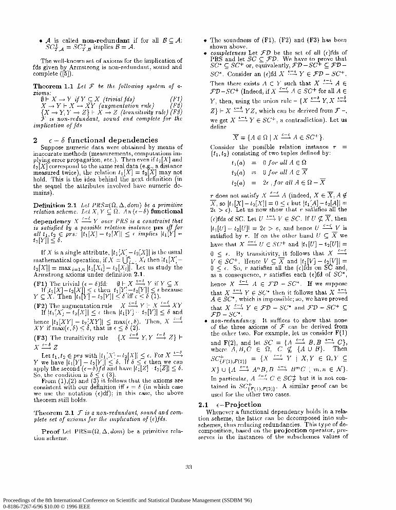
2 E - S functional diependencies Suppose numeric data were obtained by means of
inaccurate methods (measursements, computat ions im- plying error propagat ion, etc.). Then even if tl[X] and tz[X] correspond to the same real data (e. ., a distance measured twice), the relation tl[X] = t2 X] f may not hold. This is the idea behind the next definition in the sequel the attributes in.volved have numeric d o- mains).
Definition 2.1 Let PRS=(R, A, dom) be a primitive relation scheme. Le2 X, Y C R. An (c-6) functional dependency X * Y over PRS is a cons2rainl that is sakfied by a possible relation instance prs iff for all tl,tz E prs: Itl[X] - ta[X]l 5 E implies ltl[Y] - tz[Yll 26.
If X is a single attribute, Itl[X] -tz[X]I is the usual mathematical operation, if X = Unzl Xi then Itl[X]- tz[X]I = maxi=l,, jtl[Xi] - tz[Xi]l. Let us study the Armstrong axioms under definition 2.1. (Fl) The trivial (E - 6)fd: 0kXf-4YifYCX
If Itl[X]-tz X 1 < 6 then Itl[Y]-ta[Y]I 5 E because Y C X. Then tl Y] - tz[Y]I < 6 iff E 5 6 (1). i 1 (F2) The augmentat ion rule x’-4YtxxxY
If Itl[X] - tz[X]l 5 E then ltl[Y] - tz[Y]l 5 6 and hence Itl[XY] - tz[XY]I 5 max ~,b). Then, X s XY if max(c, 6) 2 6, that is t 5 b (2).
(F3) The transitivity rule {X 2 Y,Y 3 Z} t x”-4z
Let tl, t2 E prs with Itl[X] - tz[X]I 2 E. For X 2 Y we have jtl[Y] - t2 Y]l 5: 6. If S 2 c then we can apply the second (c-6 fd and have Itl[Z]-tz[Z]I 5 6. i So, the condit ion is 5 5 E (3).
From (l),(2) and (3) it follows that the axioms are consistent with our definition iff c = b (in which case we use the notation (c)df); in this case, the above theorem still holds.
Theorem 2.1 3 is a non-redundant , sound and com- plete set of axioms for the implica2ion of (c)fds.
Proof Let PRS=(R, A, tiom) be a primitive rela- tion scheme.
l
l
The soundness of (Fl), (F2) and (F3) has been shown above. compleleness Let 3’D be the set of all (ofds of PRS and let SC C 3D. W e have to prove that SC* C SC+ or, equivalently, 3D -SC+ & 3V - SC*. Consider an (c)fd X z Y E 3V - SC+. Then there exists A E Y such that X z A E 3D--SC+ (Indeed, if X z A E SC+ for all A E Y, then, using the union rule - {X * Y, X 5
Z}t-x5 YZ, which can be derived from 3 -, we get X z Y E SC+, a contradiction). Let us define
Consider the possible relation instance T = {tl, t2) consisting of two tuples def ined by:
tl(a) = 0 for all A E R
tz(a) = 0 for all A E x
tz(a) = 2~ , for all A E R - 57
r does not satisfy X z A ( indeed, X E x, A @ x, so tIIX] - t2[X]l = 0 < E but Itl[A] -tz[A]I = 2~ > E i . Let us now show that r satisfies all the (c)fds of SC. Let U 2 V E SC. If U cf x, then
Itl[u] - tz[lY]l = 26 > e, and hence U z V is satisfied by r. If on the other hand U C 57 we have that X z U E SC+ and Itl[U] - te[U]l = 0 5 6. By transitivity, it follows that X G V E SC+. Hence V s ‘;i?; and Itl[V] - tz V]l = 0 5 E. So, r satisfies all the (c)fds on S L and, as a consequence, r satisfies each (c)fd of SC*, hence X z A E 3lJ - SC*. If we suppose that X G Y E SC* then it follows that X z A E SC*, which is impossible; so, we have proved that X G Y E 3D - SC* and 3D - SC+ c 3v-sc*. non-redundancy. It suffices to show that none of the three axioms of 3 can be derived from the other two. For example, let us consider F(1) and F(2 , and let SC = {A z B, B z C}, where A ,B,C E R, C g {A U B}. Then
= {X =G Y 1 X,Y E O,Y 2
X} u {A = A”B,B z B”C I m,n E N}. In particular, A z C E SC$ but it is not con- tained in SC~~~1~,F~2~~. A similar proof can be used for the other two cases.
E-Projection Whenever a functional dependency holds in a rela-
tion scheme, the latter can be decomposed into sub- scheme!, thus reducing redundancies. This type of de- composlt lon, based on the projection operator, pre- serves in the instances of the subschemes values of
33
Proceedings of the 8th International Conference on Scientific and Statistical Database Management (SSDBM '96) 0-8186-7267-6/96 $10.00 © 1996 IEEE
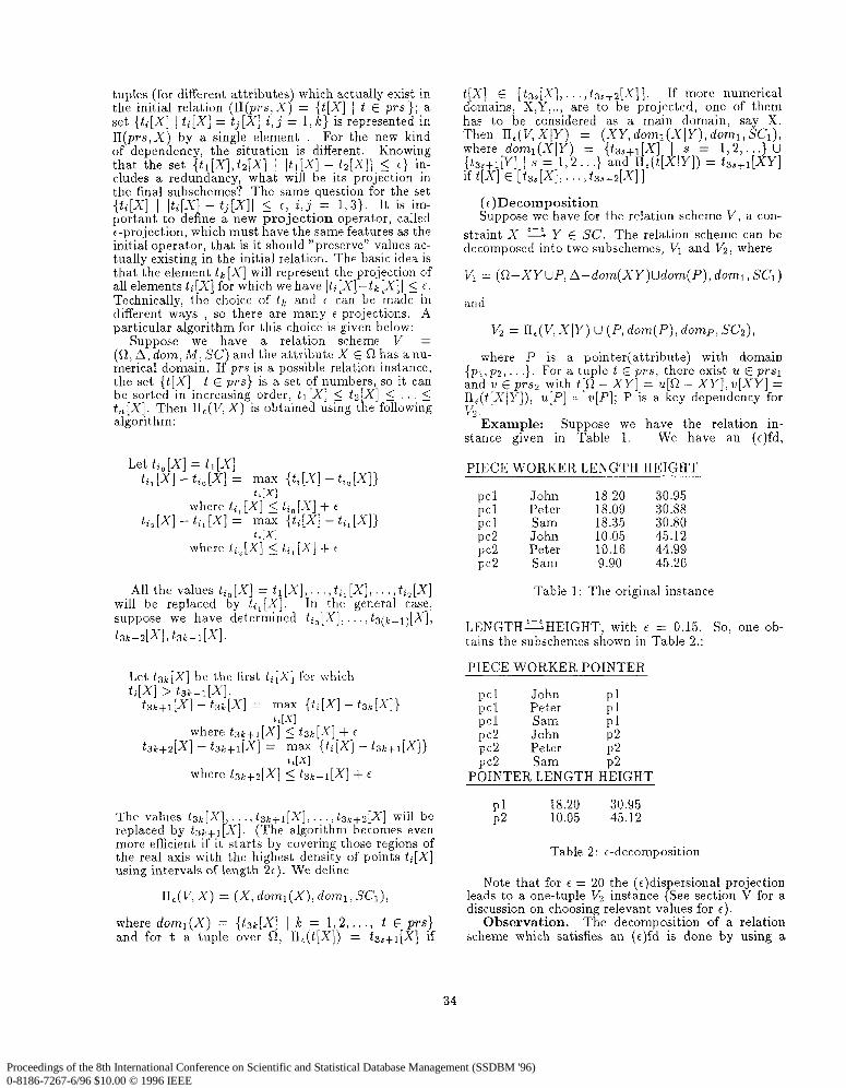
tuples (for different attributes) which actually exist in the initial relation (II@ rs,X) = {t[X] 1 t E p-s}; a set {ti [X] 1 ti[X] = tj [X] i, j = 1, Ic} is represented in II(prs,X) by a single element . For the new kind of dependency, the situation is different. Knowing that the set {tr[X],22[X] ) ]tl[X] - ta[X]l 5 E} in- cludes a redundancy, what will be its projection in the final subschemes? The same question for the set {ti[X] 1 Iti[X] - tj[X]I 5 E, i,j = 1,3}. It is im- portant to define a new projection operator, called c-projection, which must have the same features as the initial operator! that is it should “preserve” values ac- tually existing m the initial relation. The basic idea is that the element tk[X] will represent the projection of all elements ti[X] f or which we have Iti[X]-tk[X]( <_ E. Technically, the choice of tk and E can be made in different ways , so there are many E-projections. A particular algorithm for this choice is given below:
Suppose we have a relation scheme V = (0, A, dom, M, SC) and the attribute X E 51 has a nu- merical domain. If prs is a possible relation instance, the set {t[X] I t E prs} is a set of numbers, so it can be sorted in increasing order, tl[X] 5 tx[X] < 2 tn[X]. Then n,(V, X) is obtained using the following algorithm:
Let ti, [X] = tr [X] ti, [Xl - ti, [Xl = max {h[Xl - ti,[Xl}
tz1x1 where ti, [X] 5 ti, [X] + E
ti, [Xl - ti, [Xl = mm {ti[X] - ti, [Xl> tz1x1
where ti,[X] 1. t;,[X] + 6
All the values tiOIX] = tl[X], . , ti, [Xl, . . , &[X] will be replaced by ti,[X]. In the general case, suppose we have determined ti, [Xl, ) t3(km1)[X], t3k-Z[X], t3k-l[X].
Let tsk(X] be the first ti[X] for which t&q > t3k-l[X].
tsk+l[xl - t3kp-l = mm {t;[X] - t3k[X])
tt[Xl where h+l[X] 5 h[X] + E
t3k+2[X] - t3k+l[X] = max {b[X] - t3k+l[X]} t*lXl
where t3k+2[X] F t3k+l[X] + 6
The values tsk[X , . . , tsk+r[X], , tsk+z[X] will be replaced by tsk+l X]. 1 (The algorithm becomes even more efficient if it starts by covering those regions of the real axis with the highest density of points ti[X] using intervals of length 2~). We define
WV, X) = (X, d oml(X), d-1, SG),
where doml(X) = {t3k[X] 1 k = 1,2,. . ., t E prs} and for t a tuple over R, II,(t[X]) = tss+i[X] if
t[X] E [tz>[X], . , tas+a[X]]. If more numerical domains, X,Y,.., are to be projected, one of them has to be considered as a main domain, say X. Then II,(V,XlY) = (XY, doml(XIY), doml, SCI), where doml(XIY) = {tzs+l[X] I s = 1,2,. . .} U {t~~+l[Y] ) s = 1,2.. .} and &(t[XlY]) = h+l[XY] ift[Xl E [t3J[Xl,...,t3,+2[X11
Suppose we have for the relation scheme V, a con- straint X s Y E SC. The relation scheme can be decomposed into two subschemes, VI and V2, where
VI = (R-XY UP, A-dom(XY)Udom(P), doml, SCI)
and
V2 = II,(V, XIY) U (P, dam(P), damp, SCz),
where P is a pointer(attribute) with domain {p1,p2,. . .}. For a tuple t E prs, there exist u E prsi and 21 E prss with t[R - XY] = u[Q - XY], v[XY] = TJ,(t[XjY]), u[P] = u[P]; P is a key dependency for v2.
Example: Suppose we have the relation in- stance given in Table 1. We have an (e)fd,
PIECE WORKER LENGTH HEIGHT
PC1 PC1 PC1 PC2 PC2 PC2
John 18.20 30.95 Peter 18.09 30.88 Sam 18.35 30.80 John 10.05 45.12 Peter 10.16 44.99 Sam 9.90 45.26
Table 1: The original instance
LENGTHGHEIGHT, with E = 0.15. So, one ob- tains the subschemes shown in Table 2.:
PIECE WORKER POINTER
PC1 John Pl PC1 Peter PI PC1 Sam PI PC2 John P2 PC2 Peter P2 PC2 Sam P2
POINTER LENGTH HEIGHT
Pl 18.20 30.95 P2 10.05 45.12
Table 2: c-decomposition
Note that for t = 20 the (t)dispersional projection leads to a one-tuple V2 instance (See section V for a discussion on choosing relevant values for E).
Observation. The decomposition of a relation scheme which satisfies an (e)fd is done by using a
34
Proceedings of the 8th International Conference on Scientific and Statistical Database Management (SSDBM '96) 0-8186-7267-6/96 $10.00 © 1996 IEEE
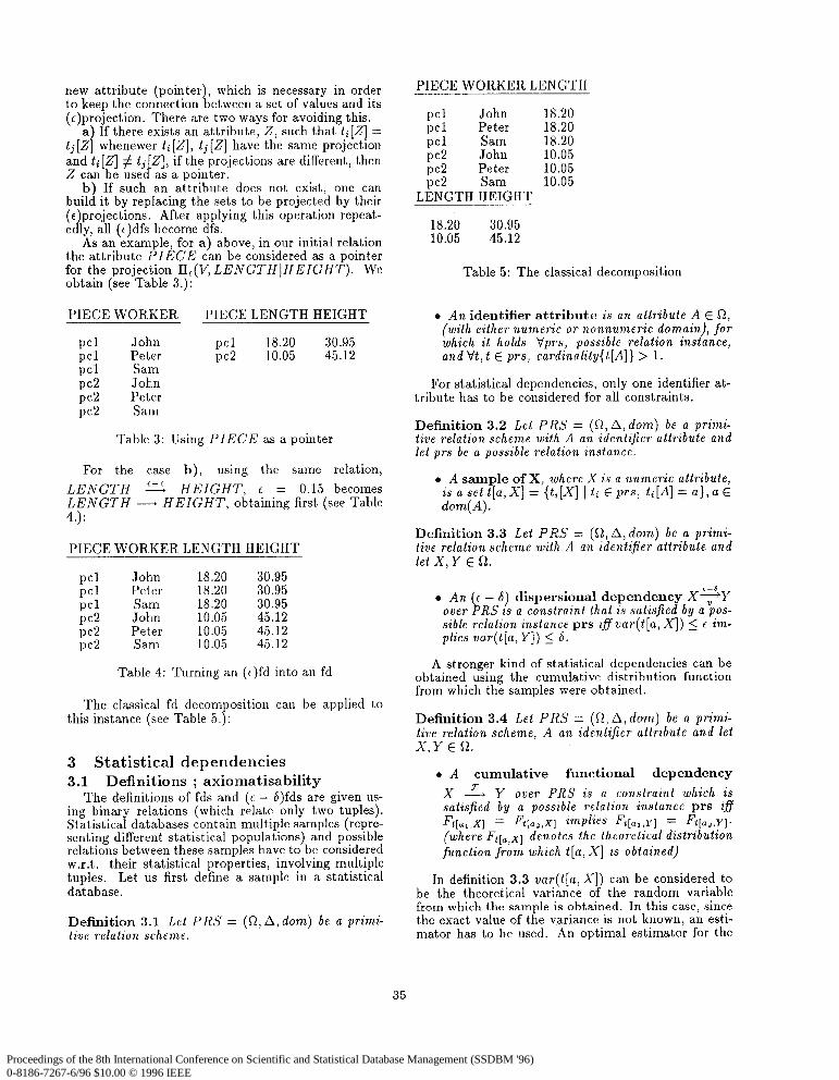
new attribute (pointer), which is necessary in order to keep the connection between a set of values and its (c)projection. There are two ways for avoiding this.
a If there exists an attribute, 2, such that ti[Z] = tj[Z whenewer ti[Z], tj[Z] have the same projection and ti[Z] # tj[Z], if the projections are different, then Z can be used as a pointer.
b) If such an attribute (does not exist, one can build it by replacing the sets to be projected by their
After applying this operation repeat- ~~~?l?[i,’ become dfs
is an lxa:ple, for a) above, in our initial relation the attribute PIECE can be considered as a pointer for the projection II,(V, LENGTHIHEIGHT). We obtain (see Table 3.):
PIECE WORKER
PC1 John PC1 Peter PcI Sam PC2 John PC2 Peter PC2 Sam
PIECE LENGTH HEIGHT
PC1 18.20 30.95 PC2 10.05 45.12
Table 3: Using PIECE as a pointer
For the case b), using the same relation, LENGTH = HEIGHT, E = 0.15 becomes LENGTH ---+ HEIGHT, obtaining first (see Table 4.):
PIECE WORKER LENGTH HEIGHT
PCI John 18.20 30.95 PCI Peter 18.20 30.95 PC1 Sam 18.20 30.95 PC2 John 10.05 45.12 PC2 Peter 10.05 45.12 PC2 Sam 10.05 45.12
Table 4: Turning an (e)fd into an fd
The classical fd decomposition can be applied to this instance (see Table 5.):
3 Statistical depend.encies 3.1 Definitions ; axiomatisability
The definitions of fds and1 (6 - S)fds are given us- ing binary relations (which relate only two tuples). Statistical databases contain multiple samples (repre- senting different statistical populations) and possible relations between these samples have to be considered w.r.t. their statistical properties, involving multiple tuples. Let us first define ,a sample in a statistical database.
Definition 3.1 Let PRS = (Cl, A, dom) be a primi- tive relation scheme.
PIECE WORKER LENGTH
PcI John 18.20 PCI Peter 18.20 PC1 Sam 18.20 PC2 John 10.05 PC2 Peter 10.05 PC2 Sam 10.05
LENGTH HEIGHT
18.20 30.95 10.05 45.12
Table 5: The classical decomposition
l An identifier attribute is an attribute A E 0, (with either numeric or nonnumeric domain), for which it holds vprs, possible relation instance, and Vt, t E prs, cardinality{t[A]} > 1.
For statistical dependencies, only one identifier at- tribute has to be considered for all constraints.
Definition 3.2 Let PRS = (R, A, dom) be a primi- tive relation scheme with A an identifier attribute and let prs be a possible relation instance.
l A sample of X, where X is a numeric attribute, is a set t[a, X] = {ti[X] 1 ti E prs, &[A] = a}, a E dam(A).
Definition 3.3 Let PRS = (Q,A,dom) be a primi- tive relation scheme with A an identifier attribute and letX,Y ER.
r--6 l An (6 - 6) dispersional dependency XTY
over PRS is a constraint that is satisfied by a pos- sible relation instance prs i#var(t[a, X]) 5 6 im- plies vur(t[u, Y]) 5 6.
A stronger kind of statistical dependencies can be obtained using the cumulative distribution function from which the samples were obtained.
Definition 3.4 Let PRS = (R, A, dom) be a primi- tive relation scheme, A an identifier attribute and let X,YER.
*A cumulative functional dependency X -% Y over PRS is a constraint which is satisfied by a possible relation instance prs iff Ft[al,x] = Ft[a,,x] implies Ft[al,~l = Fqaz,~l.
(where F,[,,xI denotes the theoretical distribution function from which t[u, X] is obtained)
In definition 3.3 var(t[u,X] can be considered to be the theoretical variance o ) the random variable from which the sample is obtained. In this case, since the exact value of the variance is not known, an esti- mator has to be used. An optimal estimator for the
35
Proceedings of the 8th International Conference on Scientific and Statistical Database Management (SSDBM '96) 0-8186-7267-6/96 $10.00 © 1996 IEEE
variance is S2 = zf
~=i(~i-Z)~/(n-1)([6]). S2 belongs to a large class o estimators - the scale estimators - among which : the standard deviation, the range, the median absolute deviation, etc. If we consider 5’ to be such an estimator, we get a general form of definition 99 3.5.
Definition 3.5 Let PRS = (Q,A, dom) be a primi- tive relation scheme with A an identifier attribute and letX,Y EC?.
c-6
o An (C - 6) S dependency XTY over PRS is a constraint that is satisfied by a possible re- lation instance prs iff S(t[a, X]) 5 e implies wm) L 6.
The definition 3.4 gives rise to the same kind of problems. Neither F’l,,,~l nor F,l,,,~l are known (the same goes for Ftla,,~l and &l,,,yl). One can use the Kolmogorov-Smirnov test for deciding whether or not the two empirical cumulative distribution functions are equal. Because the test may reject the hypothesis (HO:Fl = F2) even when it is true, with a probabi- lity a, (chosen at the beginning), the notation for this type of dependencies will be X 2 Y.
We have defined war(t[a, X]) where X is a single attribute. For X a set of attributes we will con- sider: var(t[a, X]) = max;=l,,{var(t[a, Xi])} ’ where X = lJ=l,m Xi. Under definition 3.3 the axioms (Fl),(F2),(F3) remain true, provided that S = E.
Theorem 3.1 F is a non-redundant sound and com- plete system of axioms for the implication of (e - e)dd.
Proof Let PRS = (0, A, dom) be a primitive rela- tion scheme and B an identifier attribute.
l soundness and l non-redundancy. The proof is similar to that of
theorem 2.1. e completeness The proof proceeds along the
same lines as the completeness part for theo- rem 2.1. Consider the possible relation instance T = {tl, t2} consisting of two tuples defined by:
tl[B] = 0 t2[B] = 0 tl[A] = 0,forallAEti
t2[A] = 0, for all A E 5?
tz[A] = 44, for all A E R - x
There exists a sample {O,O} for each A E 7 and also a sample {0,4&} for each A E s2 - x.
This instance does not satisfy XYA (indeed, X E ??,A @ x, so vnr(t[O, X]) = 0 _< E but
= 4~ > E). But T satisfies all the SC (see the proof of theorem 2.1).
‘we do not consider here multidimensional variables
Intuitively, var(t[u! X]) < E means that all the va- lues are closed to then mean (for small E) and so the sample can be meaningfully represented’by a single value.
In the case of cumulative functional dependencies, the same steps have to be undertaken. First, for X = Ui=l,n Xi, F[al,~l = FI~*,xI iffy&, we have F[,l,~,l = Flaz,x;l. The axioms (Fl),(F2),(F3) remain true and we have the theorem:
Theorem 3.2 F is a non-redundant, sound and com- plete system of axioms for the implication of cumula- tive functional dependencies.
Proof: Let PRS = (R, A, dom) be a primitive re- lation scheme with B an identifier attribute.
l soundness and l non-redundancy See the proof of theorem 2.1 l completeness. Consider the possible relation in-
stance
r=(tl..., tn,tn+l,. t .., n+m )
consisting of n + m tuples defined by:
ti[B] = 0, Vi=l...n ti[B] = 1, Vi=n+l...n+m t;[A] = 0, VAER, V’i=l...n+m &[A] = 0, VA~??V’i=n...r~+rn
&[A] = 1, VAESZ-5?, V’i=n...n+m
We have Ft[O,A](z) = y ff z 2 i for all -
&[I,A](~) = 0 if z<l 1 if z>l # F+,A](~) for
A @ I?. This instance does not satisfy X 2 A (X E 17, A $5?); nevertheless, it satisfies all the cumulative functional dependencies of SC (see the proof of theorem 2.1).
3.2 Projections for statistical dependen- cies
3.2.1 (6)Dispersional Projection
In the case of statistical dependencies defined above, statistical methods have to be used in order to elimi- nate redundancies by means of decomposition. The projection operator for this case will be defined us- ing specific statistical tools methods. The decompo- sition defined using this projection operator will pro- duce sub-relations which will only preserve some spe- cific statistical parameters of the initial populations. This is the inherent price one has to pay for “compac- ting” statistical data: some statistical parameters are lost after decomposition. The loss of information in the case of (e)-projection is not important if the user considers that “nearly equal” values represent only one
36
Proceedings of the 8th International Conference on Scientific and Statistical Database Management (SSDBM '96) 0-8186-7267-6/96 $10.00 © 1996 IEEE
actual value. For a discussion on how “nearly equal values”can be defined, see section V.
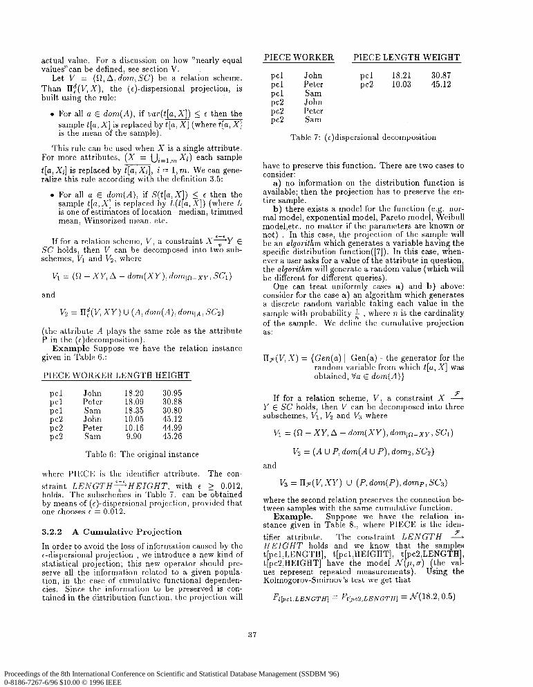
Let V = (R,a,d om, SC) be a relation scheme. Than IIf(V, X), the (e)-dispersional projection, is built using the rule:
l For all a E dam(A), if vur(t[u,X]) 5 6 then the sample t[a, X] is replaced by t[a, X] (where t[a, X] is the mean of the sample).
This rule can be used when X is a single attribute. For more attributes, (X = Ui=l,n Xi) each sample t[a, Xi] is replaced by t[a, Xi], i = 1, m. We can gene- ralize this rule according with the definition 3.5:
l For all a E dam(A), if S(t[a, X ) 5 E then the sample t[a, X] is replaceId by L(t 1 a, X]) (where L is one of estimators of location - median, tr immed mean, Winsorized mean, etc.
e-e If for a relation scheme, v, a constraint XTY E
SC holds, then V can be decomposed into two sub- schemes, VI and Vz, where
VI = (0 - XY, A - dom(XY), dornl~-x~, SC1)
and
V2 = nf(V, XY) U (A, dam(A), damp, SC?)
(the attribute A plays the satme role as the attribute P in the (c)decomposition).
Example Suppose we ha.ve the relation instance given in Table 6.:
PIECE WORKER LENGTH HEIGHT
PCI PCI PC1 PC2 PC2 PC2
John 18.20 30.95 Peter 18.09 30.88 Sam 18.35 30.80 John 10.05 45.12 Peter 10.16 44.99 Sam 9.90 45.26
Table 6: The original instance
where PIECE is the identifier attribute. The con- straint LENGTH=HEIGHT, with E > 0.012, holds. The subschemes in Table 7. can be-obtained by means of (e)-dispersional projection, provided that one chooses e = 0.012.
3.2.2 A Cumulative Projection
In order to avoid the loss of information caused by the e-dispersional projection ! we introduce a new kind of statistical projection; this new operator should pre- serve all the information related to a given popula- tion, in the case of cumulat,ive functional dependen- cies. Since the information to be preserved is con- tained in the distribution function, the projection will
PIECE WORKER PIECE LENGTH WEIGHT
PCI John PCI 18.21 30.87 PC1 Peter PC2 10.03 45.12 pcl Sam PC2 John PC2 Peter PC2 Sam
Table 7: (c)dispersional decomposition
have to preserve this function. There are two cases to consider:
a) no information on the distribution function is available; then the projection has to preserve the en- tire sample.
b) there exists a model for the function (e.g. nor- mal model, exponential model, Pareto model, Weibull model,etc. no matter if the parameters are known or not) . In this case, the projection of the sample will be an algorithm which generates a variable having the specific distribution function([7]). In this case, when- ever a user asks for a value of the attribute in question, the algorithm will generate a random value (which will be different for different queries).
One can treat uniformly cases a) and b) above: consider for the case a) an algorithm which generates a discrete random variable taking each value in the sample with probability $ , where n is the cardinality of the sample. We define the cumulative projection as:
ll~(V, X) = {Gen(u) ] Gen(a) - the generator for the random variable from which t[u, X] was obtained, Vu E dam(A)}
If for a relation scheme, V, a constraint X --% Y E SC holds, then V can be decomposed into three subschemes, VI, Vz and V! where
VI = (!J - XV, A - dom(XY), dornln-xy , SC1)
Vz = (A U P, dom(A U P), doma, SCz)
and
V3 = n,(V,XY) U (P, dam(P), domp, SC’s)
where the second relation preserves the connection be- tween samples with the same cumulative function.
Example. Suppose we have the relation in- stance given in Table 8., where PIECE is the iden- tifier attribute. The constraint LENGTH z HEIGHT holds and we know that the samples t pcl,LENGTH], t pc2,HEIGHT] 1
t[pcl,HEIGHT], t pc2,LENGTH], have the model N ~,a) i (the val-
ues represent repeated measurements). Using the Kolmogorov-Smirnov’s test we get that
Ft[pcl,LENGTH] = FtlpcZ,LENGTH] = N(18.‘4 0.5)
37
Proceedings of the 8th International Conference on Scientific and Statistical Database Management (SSDBM '96) 0-8186-7267-6/96 $10.00 © 1996 IEEE
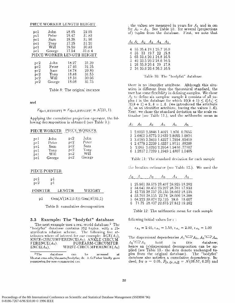
PIECE WORKER LENGTH HEIGHT
PC1 John 18.65 29.95 PC1 Peter 18.47 31.83 PC1 Sam 18.38 31.96 PC1 Tony 17.35 31.20 PC1 Will 18.59 30.83 PC1 George 17.54 31.6 4
PIECE WORKER LENGTH HEIGHT
PC2 PC2 PC2 PC2 PC2 PC2
John 18.27 31.39 Peter 17.46 31.25 Sam 18.78 29.80
Tony 18.88 31.55 Will 18.34 30.06
George 18.08 31.75
Table 8: The original instance
and
~t’t[pcl,HEIGHT] = Ft[pcZ,HEIGHT] = N(31, 1).
Applying the cumulative projection operator, the fol- lowing decomposition is obtained (see Table 9.):
PIECE WORKER PIECE WORKER
PC1 John PC2 John PC1 Peter PC2 Peter PC1 Sam PC2 Sam PC1 Tony PC2 Tony PC1 Will PC2 Will pcl George pc2 George
PIECE POINTER
PC1 Pl PC2 Pl
POINTER LENGTH WEIGHT
Pl Gen(N(l8.2,0.5)) Gen(N(31,l)
Table 9: cumulative decomposition
3.3 Example: The “bodyfat” database The next example uses a real-world database.2 The
“bodyfat” database contains 252 tuples, with a 15- attributes relation scheme. The following five at- tributes where of interest for our example: AGE(Ar), KNEE-CIRCUMFERENCE(A2), ANKLE-CIRCUM- ;gyE7yy43L FOREARM-CIRCUMFER-
4 > WRIST-CIRCUMFERENCE(As)
ZThe database can be accessed at lib.stat.cmu.edu/datasets/bodyfat; dr. A.G.Fisher kindly gave permission for non-commercial use.
; the values are measured in years for Al and in cm for A2 - As. See Table 10. for several (projections of) tuples from the database. First, we note that
Ao Al A2 A3 A4 As
4 55 35.4 19.1 25.7 16.9 4 55 33 19.7 22 15.8 5 65 33.4 20.1 24.8 16.5 3 40 33.5 20.2 24.6 16.5 1 26 35.9 20.4 29 17.8 2 34 35.6 20.4 26.2 16.5
Table 10: The “bodyfat” database
there is no identifier attribute. Although this situ- ation is different from the theoretical standard, the user has some flexibility in defining samples. We chose A1 to define six samples: sample k consists of all tu- ples t in the database for which lO(k + 1) < t[Al] 5 lO(k + 1) + 9, k = 1..6. ( we introduced the attribute A0 as an identifier attribute, having the values 1..6). Next, we chose the standard deviation as the scale es- timator (see Table ll.), and the arithmetic mean as
Ao AI A2 A3 A4 A5
1 2.0021 2.3846 1.4021 1.876 0.7655 2 2.6802 2.6775 2.2432 2.8055 1.0824 3 3.0185 2.3403 1.4327 1.7904 .92419 4 2.4778 2.2239 1.4337 1.9711 .88288 5 2.665 2.6293 2.3954 1.9416 .77107 6 1.2817 2.7239 1.1949 1.4807 1.0405
Table 11: The standard deviation for each sample
the location estimator (see Table 12.). We used the
Ao AI A2 -43 A4 A5
1 25.861 38.575 23.497 28.925 18.202 2 34.641 38.451 23.207 28.761 17.933 3 43.755 38.757 23.135 28.662 18.135 4 53.766 38.155 22.74 28.606 18.308 5 64.222 39.074 23.125 28.6 18.607 6 71.75 38.437 22.675 27.812 19.162
Table 12: The arithmetic mean for each sample
following initial values for c :
EA2 = 2.40, CA3 = 1.50, CA4 = 2.00, <As = 1.00
The dispersional dependencies Azfz3A~, A3’DA4, &=?A4 hold this database. hence an (t)dispersional gcomposition can be apl plied (see Table 13.- the dots denote unchanged tu- ples from the original database). The ” bodyfat” database also satisfies a cumulative dependency. In- deed, for (Y = 0.05, Flk,llk,~,~l = N(38.57, 6.26) and
38
Proceedings of the 8th International Conference on Scientific and Statistical Database Management (SSDBM '96) 0-8186-7267-6/96 $10.00 © 1996 IEEE
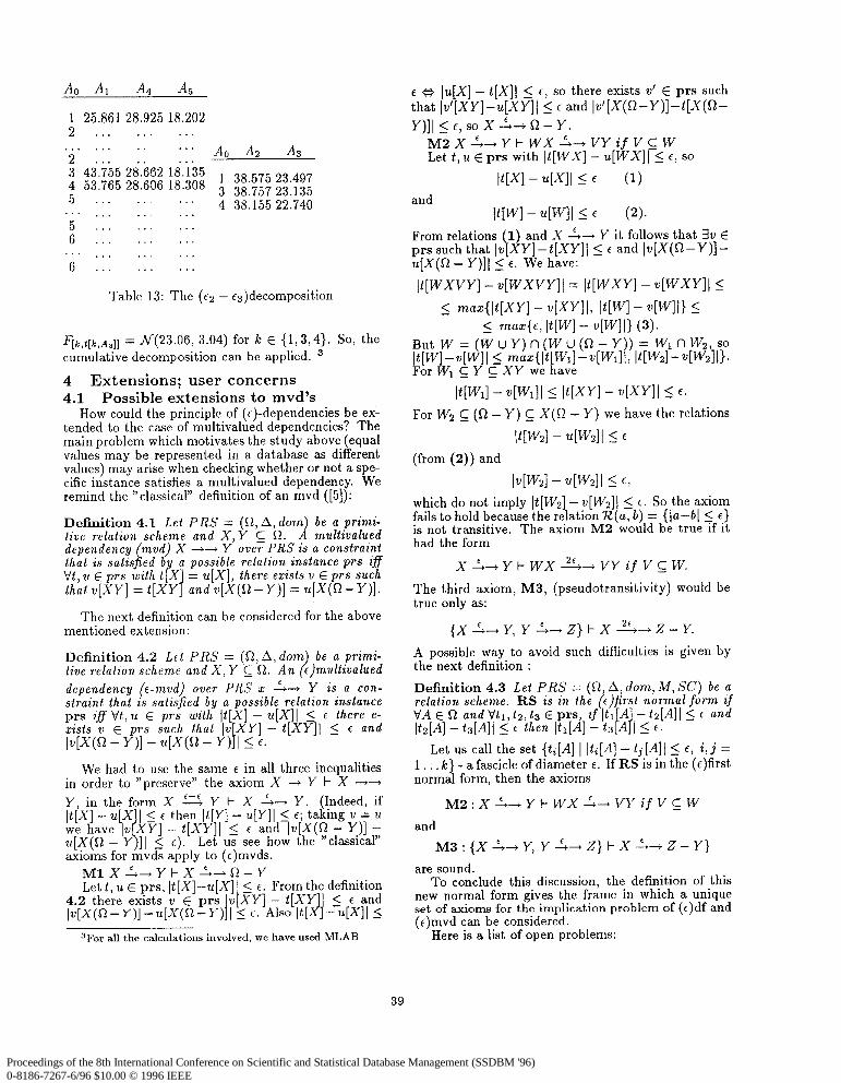
Ao AI A4 -45
1 25.861 28.925 18.202 2 . , . . . . . . .
.,, *** ..* . . . 2 Ao AZ A3
. . . ..~ . . .
3 . . . ..~ . . . 4 38.155 22.740 ... . . . . . . . . . 5 . . . . I . . . 6 . . . ..~ . . .
“. .,. *** . . . 6 . . . ..I . . .
Table 13: The ( ~2 - cs)decomposit ion
F[k,l[k,Asll = n/(23.06, 3.04) for lc E {1,3,4}. So, the cumulative decomposit ion can be applied. 3
4 Extensions; user concerns 4.1 Possible extensions to mvd’s
How could the principle of (c)-dependencies be ex- tended to the case of multivalued dependencies? The main problem which motivates the study above (equal values may be represented in. a database as different values) may arise when checking whether or not a spe- cific instance satisfies a mult-ivalued dependency. W e remind the “classical” definition of an mvd ([5]):
Definition 4.1 Let PRS = (Sl,A,dom) be a primi- tive relation scheme and X,Y g R. A multivalued dependency (mud) X --+- Y over PRS is a constraint that is satisfied by a possible relation instance prs iff Vt, u E prs with t[X = u[X], there exists v E prs such that v[XY] = t[XY 3 and v[X(R-Y)] = u[X(R-Y)].
The next definition can be considered for the above ment ioned extension:
Definition 4.2 Let PRS = tive relation scheme and X, Y dependency (c-mvd) over PRS x A-+ Y is a con- straint that is satisfied by a possible relation instance prs ifl Vt, u E prs with It[X] - u[X]I 5 6 there e- xists v E prs such that Iw[X(cl - Y)] - u[X(s2 - Y)
.XY] - t[XY]l 2 E and 1 5 E.
W e had to use the same t in all three inequalit ies in order to “preserve” the axiom X -+ Y k X ---f+ Y, in the form X ‘-’ : :~X~,~~~~~~~h~~~-~~~~l~~~~~~~ ‘u’
u[X(Q - Y ]I 2 c). Let us see how the “classical” axioms for mvds apply to (c)mvds.
MlX1-+Yl-X:-G!-Y Let t, u E prs, It[X]-u[X] < E. From the definition
4.2 there exists v E prs v’XY] - t[XY] 5 E and Iv[X(fl-Y)] -u[X(Q--Y) I’ 1 1 e. Also jt[X -u[X]I 5
3For all the calculations involved, we have used MLAB
6 * I4Xl - t[Xll 5 6, so there exists o’ E prs such that jv’[XY]-u[XY]I < 6 and Iv’[X(R-Y)]-t[X(R- Y)]l~E,SOX~4-Y.
M2X~-+Yl-+VX~--+VYifVCW Let t, u E prs with It[WX] - u[WX]I 2 6, so
W I - W I 5 E (1) and
ItW l - 4 W I 5 6 (2). From relations 1) and X
\ L+ Y it follows that 3w E
prs such that IZI XY] -t[XY]l 2 c and Iw[X(Q-Y)] - u[X(G! - Y)]l < e. W e have:
It[WXVY] - v[WXVY]( = It[WxY] - v[WXY]I 5
L max{It[XYl - G W I, IOU - 4 W II I I made, IOU - 4 W II (3).
But W = (W u Y) n (W u (0 - Y ) = W 1 n Wz, so ~~~~~~]I~xmya~~~~~~-w[WiI 1 , IW21--4W2lI~~
l- - IWlI - ~[Wlll L: Iwq - 4XYII 56.
For W z C (a - Y) 2 X(fl - Y) we have the relations
It[Wzl - dW2II 5 6
(from (2)) and
b[W21 - 4472lI I 6, which do not imply It[Wz] - v[Wz]I 5 E. So the axiom fails to hold because the relation %!(a, b) = {la-b1 < E} is not transitive. The axiom M2 would be true if it had the form
X:+YtWX%+VYifVCW.
The third axiom, M3, (pseudotransitivity) would be true only as:
{x~~Y,Y~~Z}tX~-Z-Y.
A possible way to avoid such difficulties is given by the next definition :
Definition 4.3 Let PRS = (Q,A,dom,M,SC) be a relation scheme. RS is in the (c)first normal form if VA E R and Vtl, t2, t3 E prs, if ItI A - ts[A]l 5 e and
H ltz[A] - ts[A]l 5 E then ltl[A] - t3 A I 5 E.
Let us call the set {ti[A] I [&[A] - tj[A]l 5 E, i,j = 1 . . . Ic} - a fascicle of diameter E. If RS is in the (c)first normal form, then the axioms
M2:X:-Yl-WX:+VYifVCW
and
M3:{X:+Y,YA-Z}tX:+Z-Y}
are sound. To conclude this discussion, the definition of this
new normal form gives the frame in which a unique set of axioms for the implication problem of (E)df and (omvd can be considered.
Here is a list of open problems:
39
Proceedings of the 8th International Conference on Scientific and Statistical Database Management (SSDBM '96) 0-8186-7267-6/96 $10.00 © 1996 IEEE
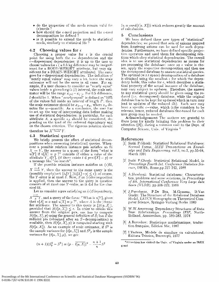
4.2
do the properties of the mvds remain valid for (e)mvds ? how should the c-mvd projection and the e-mvd decomposition be defined ? is it possible to extend the mvds to statistical mvds, similarly to statistical fds ?
Choosing values for 6 Choosing a proper value for E is the crucial
point for using both the E- dependencies and the e-dispersional dependencies; it is up to the user to choose values for c ( a 0.5 kg difference may be insignif- icant for a BODY-WEIGHT attribute, but very sig- nificant for a BRAIN-WEIGHT attribute). The same goes for e-dispersional dependencies. The definition of “nearly equal values” may vary a lot, hence the scale estimator will not be the same in all cases. For ex- ample, if a user chooses to consider as “nearly equal” values inside a given-length (I) interval, the scale esti- mator will be the range z(“) - ~(1). For 0.5 difference, 1 should be 1. When “nearly-equal” is defined as “90% of the values fall inside an interval of length 1”) then the scale estimator should be ~i-~ -z,, where 2, de- notes the a-quantile. As a conclusion, the user has to set up the way of interpreting data before making use of statistical dependencies; in particular, for each attribute A, a specific eA should be considered, de- pending on the kind of the enforced dependency and on the chosen criterion. The rigorous notation should therefore be XEXzYY. 4.3 Statistical queries
We briefly present the effect of statistical decom- positions when answering (statistical) queries. When- ever a possible relation instance prs satisfies an fd X + Y, the answer to a query of the form “what is ulY1 if ulX1 = n ?” consists of either a value of the aitributeLYi t[Yj, (if there exists t E prst[X] = p) or a message hke “no match”.
If the possible relation instance satisfies an (e)fd,
X % Y, then the answer to the same query is the (possibly empty) set {ti[Y] 1 ]ti[X] -pj 5 e}; of course, the Y-error is at most 6. Now, if an (E)decomposition is applied, then the answer to the query in question consists of at most one Y-value, as it did for the clas- sical fd.
Let us consider a prs satisfying an (e)Sdependency, c-6
X TY, and a query of the form: “What is .[Y], given that u[A] = a and u[X] = p ?“, where A is the identi- fier attribute. The answer to this query is L(t[a,X]), provided that S(t[a,X]) 5 <. In order to obtain this answer from the original pm, one has to compute S(t[a, X], p) using the general definition of S; but if the reduced prs (obtained after an S-decomposition) is available, then S(t[a, X],p) is computed starting with S(t[a, Xl). As an example of scale estimator, if S2 is the sample variance for {t[a, X]} and S2, is the sample variance for {t[a, X],p}, we get:
~,,c,~~~~~~;,xl>) h’ h d w ic re uces greatly the amount
5 Conclusions We have defined three new types of “statistical”
dependencies; we proved that sets of axioms inspired from Amstrong axioms can be used for such depen- dencies. Furthermore, we have defined specific projec- tion operators and used them for decomposing rela- tions which obey statistical dependencies. The overall idea is to use statistical dependencies as means for pre-processing the database: once an E value is cho- sen, apply the respective decomposition and then use the decomposed database to answer statistical queries. The optimal (w.r.t space) decomposition of a database is obtained using the smallest E for which the depen- dency holds; this value for E, which describes a statis- tical property of the actual instance of the database, may vary subject to updates. Therefore, the answer to any statistical query should be given using the re- duced (i.e. decomposed) database, while the original database has to be kept for updates which
\ in turn may
lead to updates of the reduced db Each user may have a specific c-value, which (s)he considers to be relevant; hence, reduced databases fine-tuned for each user group may be needed.
Acknowledgement The authors are grateful to Hans Lenz for kindly bringing this problem to their attention ([S]), d uring a common visit to the Dept. of Computer Science, Univ. of Virginia 4
References P I
PI
131
P I
[51
F31
P-1
Satki P.Ghosh: Statistical Relational Databases: Normal Forms, IEEE Transactions on Knowl- edge and Data Engineering, ~013, no.1, pp.55-64, March 1991
Satki P.Ghosh: Statistical Relational Model, in Proceedings Fourth Int. Conference Statistics Sci- ence, DBMS, Rome,pp.227-242, 1988
AShoshani: Statistical databases: Characteris- tics, problems and some solutions, in Proceedings of 8th. International Conference Very Large data bases (VLDB), pp.208-222, 1983
J.Paredaens, P.De Bra, M.Gyssens, D.Van Gueht: The Structure of the Relational Database Model, EATCS Monographs on Theoretical Com- puter Science, Springer-Verlang Berlin 1989
W.W.Amstrong: Dependency Structures of Data Base Relationships. Proceedings IFIP, North- Holland, Amsterdam, pp. 580-583, 1974
A.Borovkov: Statistique mathematique, traduc- tion fransaise, Edition Mir, 1987
I.Vaduva, Modele de simulare cu calculatorul, Editura Tehnica, Bucuregti, 1977
(n + l)($ - S2) = (p - t[a, X1)2 - +.sQ 4H.Luchian has visited the Univ. of Virginia under an IREX
grant
40
Proceedings of the 8th International Conference on Scientific and Statistical Database Management (SSDBM '96) 0-8186-7267-6/96 $10.00 © 1996 IEEE

[S] 1H,tJti;;e igy’ersonal communication, Char- ,
41
Proceedings of the 8th International Conference on Scientific and Statistical Database Management (SSDBM '96) 0-8186-7267-6/96 $10.00 © 1996 IEEE