Mechanics of universal horizons

Per Berglund,∗ Jishnu Bhattacharyya,† and David Mattingly‡

Department of Physics, University of New Hampshire, Durham, NH 03824, USA

Modified gravity models such as Horava-Lifshitz gravity or Einstein-æther theory violate localLorentz invariance and therefore destroy the notion of a universal light cone. Despite this, in theinfrared limit both models above possess static, spherically symmetric solutions with “universalhorizons” - hypersurfaces that are causal boundaries between an interior region and asymptoticspatial infinity. In other words, there still exist black hole solutions. We construct a Smarr formula(the relationship between the total energy of the spacetime and the area of the horizon) for such ahorizon in Einstein-æther theory. We further show that a slightly modified first law of black holemechanics still holds with the relevant area now a cross-section of the universal horizon. We constructnew analytic solutions for certain Einstein-æther Lagrangians and illustrate how our results work inthese exact cases. Our results suggest that holography may be extended to these theories despite thevery different causal structure as long as the universal horizon remains the unique causal boundarywhen matter fields are added.

I. INTRODUCTION

In the four decades since the seminal work of Bardeen,Carter, and Hawking [1] on the laws of black hole me-chanics, a tremendous amount of effort has gone in tounderstanding horizon behavior. From the discoveryof Hawking radiation [2], and the recognition that thefour laws have a thermodynamic interpretation [3], toholography [4, 5] and its concrete realization through theAdS/CFT correspondence [6–8], the physics of horizonshas provided useful information about quantum gravity.Using horizon thermodynamics and some mild assump-tions about the behavior of matter, one can reverse thelogic and reconstruct general relativity as the thermody-namic limit of a more fundamental theory of gravity [9–11]. Integral to horizon dynamics is the first law of blackhole mechanics, which for the simplest Schwarzschildcase, and the most similar to what we are interested in,is just

δMadm =κkh δAkh

8πGn. (1)

Here Madm is the ADM mass of the spacetime and κkhand Akh are the surface gravity and cross-sectional areaevaluated on the Killing horizon, respectively. Identify-ing (8πGn)−1κkh as the temperature of the horizon andthe area with the entropy allows one to make the analogywith the first law of thermodynamics, δE = TδS.

In order to have an appropriate formulation of thermo-dynamics for the black hole itself, as well as the combinedsystem of the black hole and the exterior environment, itis necessary for the horizon to have an inherent entropy.If there was no entropy associated with the horizon, onecould simply toss objects into the black hole and reducethe total entropy of the black hole and exterior system,

∗ per.berglund@unh.edu† jishnu.b@unh.edu‡ dyo7@unh.edu

thereby violating the second law of thermodynamics. If,however, the horizon has an associated entropy, then onecan reformulate the usual second law into the generalizedsecond law

δ (Soutside + Shorizon) = 0. (2)

The generalized second law and the thought experimentsbehind it imply that any causal boundary in a gravi-tational theory should have an entropy associated withit. In general relativity, the entropy can be shown to beproportional to the area of a slice of the Killing horizon.However, if one includes higher curvature terms the en-tropy is still a function of the metric and matter fieldsevaluated on a slice of the Killing horizon, though nolonger proportional to the surface area alone [12].

A much stronger departure from general relativitycomes when one considers models that allow vacuum so-lutions with non-zero tensor fields besides the metric. Inthese models Lorentz symmetry and the equivalence prin-ciple are in general broken. A simple example of such amodel is that of Einstein-æther theory [13], which intro-duces an æther vector field ua and a dynamical constraintwhich forces ua to be a timelike unit vector everywhere.The introduction of the æther vector preserves generalcovariance, but allows for novel effects such as matterfields travelling faster than the speed of light [14] andnew gravitational wave polarizations that travel at dif-ferent speeds [15]. Given certain choices of the actionfor the æther, the theory can be made phenomenolog-ically viable [16, 17], have positive energy [18], and beghost free [19]. In addition, the æther vector establishesa preferred frame and causality can be imposed in thatframe [20] by requiring that all matter excitations prop-agate towards the future, even if the momentum vectorof an excitation is spacelike. Since there is a preferredframe, Lorentz invariance does not hold, nor do the usualLorentz invariance based arguments that a spacelike mo-mentum vector in one frame immediately imply the ex-istence of past directed momentum vectors. Thus, thepropagation faster than the speed of light does not vio-late causality.

arX

iv:1

202.

4497

v2 [

hep-

th]

17

Oct

201

2

2

Even though there is a notion of causality, it seemsat first glance as if there would be no causal boundariesequivalent to an event horizon in the Einstein-æther the-ory – by coupling the æther vector ua to matter kineticterms, the matter Lagrangian can be chosen to makematter perturbations about flat space propagate arbi-trarily fast. This is incorrect – causally separated re-gions of spacetime can exist even in this case. In thestatic, spherically symmetric and asymptotically flat so-lutions of Einstein-æther theory found by Eling and Ja-cobson [21] there exists such a region, and the boundaryof this region has been dubbed the “universal horizon”1.Since the notion of a causal boundary and infinite speedmodes is counterintuitive, we give a brief explanation ofwhy they can occur here, postponing an in-depth discus-sion of universal horizons until later.

Consider a static, spherically symmetric spacetime,and cover it with Eddington-Finkelstein type coordinatessuch that the metric takes the form

ds2 = −e(r)dv2 + 2f(r)dvdr + r2dΩ22 , (3)

and the time translation Killing vector is χa = 1, 0, 0, 0.Now let ΣU denote a surface orthogonal to the æther vec-tor ua, so that U is the “æther time” generated by ua thatspecifies each hypersurface in a foliation. At asymptoticspatial infinity χa and ua coincide, but as one moves intowards r = 0 each ΣU hypersurface bends down to theinfinite past in v, eventually asymptoting to a 3 dimen-sional spacelike hypersurface on which (u ·χ) = 0, whichimplies that the Killing vector χa becomes tangent toΣU . This hypersurface is the universal horizon. It isa causal boundary, as any signal must propagate to thefuture in U , which is necessarily towards decreasing rat the universal horizon. The surface is regular, and infact Barausse, Jacobson and Sotiriou [22] have numeri-cally continued the solution for metric and æther fieldsbeyond the universal horizon.

Since such a causal boundary exists, it is natural tospeculate that there must be an entropy associated withthe universal horizon as well. In spherical symmetry, onedoes not need to worry about the zeroth law of black holemechanics, as the symmetry enforces that all geometricquantities are constant over the universal horizon auto-matically. Hence one can immediately proceed to derivea Smarr formula and a corresponding first law. There aresubtleties, however, as the boundary data of the theoryat infinity naively contains two parameters. However, asnoted in [21, 22], the boundary data can be reduced toone parameter, which is the total mass of the solution, byrequiring that the solution is regular outside the univer-sal horizon (see section IV for details). If one considersonly regular solutions, we show that there is a Smarr re-lation between the total mass and geometric quantities

1 This point was first noted by Sergey Sibiryakov at Peyresq, 2010.

evaluated on the universal horizon. In particular, the re-sulting Smarr relation contains a contribution from theextrinsic curvature of the ΣU hypersurface in addition tothe standard surface gravity term. We further show usinga scaling argument that if one considers a transition be-tween two regular solutions then there is also a first lawthat may admit a thermodynamic interpretation. Withcertain choices of the Lagrangian for Einstein-æther the-ory, we construct new, exact solutions and use those asexamples to gain insight into the thermodynamics of thefirst law.

It is important to note that in previous works, blackhole thermodynamics has failed when the limiting speedof matter fields is finite, but not necessarily the speed oflight. In these cases one can construct perpetuum mo-biles that violate the second law [23–25]. We will notconsider any specific matter action in this paper, as ourpurpose is simply to determine whether a first law ofmechanics holds for the universal horizon so that a ther-modynamic interpretation might exist. However it is cer-tainly possible that a true thermodynamic interpretationcould only hold if the universal horizon is the only causalboundary for all fields. This could, for instance, be doneif the Lagrangian for any matter fields contained higherderivatives that made the local speed of excitations in-finite as the energy increased. From the point of viewof effective field theory this is natural as one expects allterms consistent with the symmetries of the problem toappear in any operator expansion.

The paper is organized as follows. We first providethe background for Einstein-æther theory in Sec. II. InSec. III we construct a Smarr formula and first law forspherically symmetric solutions. We then use two newexact, analytic solutions as examples in Sec. IV to ver-ify the Smarr formula and the first law, as well as dis-cuss the regularity of these solutions. We conclude withsome more speculative comments on how to proceed toestablish the thermodynamic connection and the obsta-cles that still remain.

II. THE EINSTEIN-ÆTHER THEORY

Einstein-æther theory was originally constructed [13]as a mechanism for breaking local Lorentz symmetry yetretaining as many of the other positive characteristics ofgeneral relativity as possible. In particular it is the mostgeneral action involving the metric and a unit timelikevector ua that is two-derivative in fields and generallycovariant. General covariance is maintained by enforc-ing the unit constraint on ua via a Lagrange multiplier.Following the presentation in [18] the action of Einstein-æther theory is a sum of the usual Einstein-Hilbert actionSeh and the æther action Sæ [13]

S = Seh + Sæ =1

16πGæ

∫d4x√−g (R + Læ) . (4)

3

In terms of the tensor Zabcd defined as2

Zabcd = c1gabgcd + c2δ

acδbd + c3δ

adδbc − c4uaubgcd , (5)

where ci, i = 1, . . . , 4 are “coupling constants” (or cou-plings, for short) of the theory, the æther Lagrangian Læ

is given by

−Læ = Zabcd (∇auc)(∇bud)− λ(u2 + 1). (6)

The æther Lagrangian is therefore the sum of all possibleterms for the æther field ua up to mass dimension two,and a the constraint term λ(u2 + 1) with the Lagrangemultiplier λ implementing the normalization condition3

u2 = −1. (7)

An additional term, R abuaub is a combination of the

above terms when integrated by parts, and is not in-cluded here.

There exists a number of theoretical as well as observa-tional bounds on the couplings ci, i = 1, . . . , 4 – see e.g.[16, 17] for a comprehensive review. In this work, we as-sume the following constraints to hold on these couplings

0 5 c14 < 2, 2 + c13 + 3c2 > 0, c13 < 1 , (8)

where we have defined c13 = (c1 +c3) and c14 = (c1 +c4).As we will see, these combinations of couplings, as wellas c123 = (c1 + c2 + c3), play a more direct role in ouranalysis than the individual couplings ci.

The constraints (8) come from the following conditions.If c14 = 2 gravity becomes repulsive and one loses theproper Newtonian limit. Furthermore, in addition to theusual spin-2 gravitons, Einstein-æther theory also pos-sesses two vector and one scalar modes (correspondingto the three degrees of freedom of ua). If c14 < 0 or2+c13 +3c2 < 0 then the scalar mode squared speed (see(50) below) about flat space becomes negative, signalingan instability of flat space to the production of scalaræther-metric excitations. Also, 2 + c13 + 3c2 cannot bestrictly zero, as the Gcosmo appearing in the Friedmannequations derived from the Einstein-æther theory needsto be positive and finite [26]. Similarly, if c13 = 1 thenthe squared speed of the usual spin-2 graviton in flatspace becomes infinite or negative, which generates thesame problem but with the usual spin-2 graviton modes.As we will also see, the Smarr formula and the first lawof black hole mechanics that we derive below becomesunphysical if c13 = 1. There are other observational lim-its on the couplings, e.g., coming from the requirementthat propagating high energy cosmic rays do not lose en-ergy due to vacuum Cerenkov radiation of gravitons [27].We will explicitly not impose this constraint here as we

2 Note the indicial symmetry Zbadc = Zab

cd .3 We use a convention where the metric has signature (−,+,+,+).

are interested in the behavior of the scalar mode, the in-terplay of any scalar mode horizon with the Killing anduniversal horizons, and the possible role of Cerenkov ra-diation from the universal horizon. Allowing the scalarmode to have any speed from almost zero to infinity istherefore theoretically useful.

The constant Gæ in the action (4) is related to Gn,Newton’s gravitational constant, via

Gæ =(

1− c14

2

)Gn , (9)

as can be established using the weak field/slow-motionlimit of the Einstein-æther theory [26].

The equations of motion, obtained by varying the ac-tion (4) with respect to the metric, ua, and λ, are

Gab = T æab, Æa = 0, u2 = −1, (10)

respectively, where the æther stress tensor T æab is given

by

T æab =λuaub + c4aaab −

1

2gabY

cd ∇cud +∇cXc

ab

+ c1 [(∇auc)(∇buc)− (∇cua)(∇cub)] ,(11)

and to make the notation more compact we have intro-duced the following

Æa = ∇bY ba + λua + c4(∇aub)ab ,Y ab = Zacbd∇cud ,Xc

ab = Y c(a ub) − u(aYc

b) + ucY(ab) .

(12)

The acceleration vector aa appearing in the expression forthe æther stress tensor is defined as the parallel transportof the æther field along the æther field4

aa = ∇uua . (13)

A. Static, spherically symmetric expansions

We now turn to the static, spherically symmetric caseand provide some useful expansions which we will lateruse to analyze the equations of motion. Eling and Ja-cobson observed that for any spherically symmetric so-lution of Einstein-æther theory, ua is hypersurface or-thogonal5 [21], which in turn implies that the twist of ua

vanishes, i.e.

u[a∇buc] = 0. (14)

4 We use the conventional notation ∇X for the directional deriva-tive (Xa∇a) along any vector field Xa. Once the normalizationcondition (7) is imposed, the acceleration is always orthogonal tothe æther field (i.e. u · a = 0), and therefore, is always spacelike.

5 In fact they are also solutions of Horava gravity [28, 29].

4

An immmediate consequence of the hypersurface orthog-onality condition is that there exists a one-parameter re-dundancy among the couplings ci. Using the unit normconstraint (7), the squared twist can be expressed as

ω2 = (∇aub)(∇aub)− (∇aub)(∇bua) + a2 , (15)

which also vanishes for hypersurface orthogonal solu-tions. We can, therefore, add any multiple of ω2 to theaction without affecting the solutions. In particular, byadding

∆S = − c016πGæ

∫d4x√−g ω2 (16)

to the action (4), where c0 is an arbitrary real constant,the sole effect would be to obtain a new æther LagrangianL ′æ, otherwise identical to (6), except with a new setof coupling constants c′i, i = 1, ..., 4, related to the un-primed ci through

c′1 = c1+c0, c′2 = c2, c′3 = c3−c0, c′4 = c4−c0. (17)

Thus, by appropriately choosing c0, one can set any oneof the couplings c1, c3 and c4, or any appropriate combi-nations of them, to any preassigned value. On the otherhand, the coupling c2, as well as combinations like c13,c14 and c123 (8) stay invariant under the above redefini-tion of the couplings (17).

Our analysis will be further facilitated by defining aset of basis vectors at every point in spacetime so thatwe can project out various components of the equationsof motion. Staticity and spherical symmetry implies theexistence of a time translation Killing vector χa as wellas three rotational Killing vectors ζa(i), i = 1, 2, 3 (only

two of the three are linearly independent). It is oftenconvenient to choose χa as one of the basis vectors, butin this case it is actually more helpful to use a differentbasis. We first take ua to be the (timelike) basis vector.We next pick any two spacelike unit vectors, call themma and na, both of which are normalized to unity, aremutually orthogonal and lie on the tangent plane of thetwo-spheres B that foliate the hypersurface ΣU . Finally,we use sa, the spacelike unit vector orthogonal to ua, ma

and na that points “outwards” along a ΣU hypersurface.Note that the acceleration aa only has a component alongsa by spherical symmetry, i.e.

aa = (a · s)sa . (18)

Thus, our tetrad consists of ua, sa,ma, na. By spheri-cal symmetry, any physical vector may have componentsalong ua and sa, while any rank-two tensor may havecomponents along the bi-vectors uaub, u(asb), u[asb], sasband gab, where gab is the projection tensor onto the two-sphere B, bounding a section of a ΣU hypersurface. Forexample, the basis-expansion of the extrinsic curvatureof a ΣU hypersurface is

Kab = K0sasb +K

2gab , (19)

where K0 and K6 are scalar parameters related to eachother through

K = K0 + K , (20)

with K the trace of the extrinsic curvature of the ΣUhypersurface. We ask the reader to refer to appendix Afor further details on these points.

Finally, we work out some geometric quantities relatedto the Killing vector χa. We first use the spherical sym-metry to write the timelike Killing vector χa as

χa = −(u · χ)ua + (s · χ)sa . (21)

The basis-expansion of ∇aχb takes the following form

∇aχb = −κ(uasb − saub) . (22)

Here κ is defined as the surface gravity on any two-sphereB since, as we will now show, (at least outside the Killinghorizon) κ is the acceleration of a static observer on Bas measured by an observer at asymptotic infinity. Firstconsider the region outside the Killing horizon wherethere exists an outward pointing spacelike unit vectorra, the radial unit vector, orthogonal to χa. The tan-gent vector χa to the world line of a static observer onany two-sphere B is simply the unit timelike vector alongχa. In terms of the redshift factor ρ, we can then writeχa = ρχa (i.e. ρ2 = −χ · χ). Using (22), the directionalderivative of χa along itself is given by ∇χχa = aχr

a,where aχ = (κ/ρ) is the local acceleration of the staticobserver. In other words, κ = ρaχ is the redshifted ac-celeration with respect to an observer at infinity, whichprompts us to call κ the surface gravity on the two-sphereB. The mathematical analysis also follows through in-side the Killing horizon7 and the local acceleration is stillgiven by (κ/ρ), but the interpretation of ρ as the redshiftfactor no longer holds. Nevertheless, we will continue tocall κ the surface gravity. Using the results from ap-pendix A, the surface gravity is explicitly given by8

κ =

√−1

2(∇aχb)(∇aχb) = −(a·s)(u·χ)+K0(s·χ) . (23)

6 As a consequence of spherical symmetry and ua being orthogonalon the hypersurface ΣU , we have s∧ ds = 0 – compare with (14).Thus the vectors sa are orthogonal to the hypersurfaces Σs,foliating the spacetime. It can then be shown that K is thetrace of the extrinsic curvature of the two-spheres B due to theirembedding in Σs. See appendix A for further details.

7 Note however that inside the Killing horizon χa is spacelike andra is timelike. Associating a spacelike unit vector with an ob-server is allowed here since there is no local limiting speed.

8 We thank Ted Jacobson for pointing out reference [30] in thiscontext, where the surface gravity at the Killing horizon isgenerally shown to be proportional to the expansion of a con-gruence of timelike geodesics. However, we emphasize that inthe present paper, equation (23) holds everywhere in spacetimerather than just at the Killing horizon. We also note thatusing (u · χ)kh = −(s · χ)kh at the Killing horizon, we haveκkh = −(u ·χ)kh(a ·s)+K0kh from (23). However, this relationand the the central result of [30], although similar in appearance,actually differ since the æther does not define a geodesic flow.

5

As mentioned in the introduction, the universal hori-zon occurs when the Killing vector becomes tangent to aΣU hypersurface. Therefore as one travels inwards fromspatial infinity along a ΣU hypersurface, the universalhorizon is actually reached only as a limit. Hence ourquantities defined as “on the universal horizon” refer tothis limit, rather than some actual intersection of ΣU andthe universal horizon which is a hypersurface of constantr (again in Eddington-Finkelstein coordinates). On theuniversal horizon, (u · χ)uh = 0 and (s · χ)uh = |χ|uhwhere |χ|uh is the magnitude of the Killing vector χa onthe universal horizon. Therefore the surface gravity onthe universal horizon is

κuh = K0,uh|χ|uh . (24)

By spherical symmetry, the surface gravity is constantover any two-sphere, and thus on the universal horizonas well.

B. Equations of motion for the static, sphericallysymmetric case

We next study Einstein’s equations and the ætherequations of motion (10) by explicitly using the timetranslational and spherical symmetries of the problem,in addition to hypersurface orthogonality. To set upthe Einstein’s equations, we need to know the basis-expansion of the æther stress tensor and the Ricci tensor.By spherical symmetry, they take the following form

T æab = T æ

uuuaub − 2T æusu(asb) + T æ

sssasb +ˆT æ

2gab , (25)

and

R ab = R uuuaub−2R usu(asb) +R sssasb+R2gab , (26)

respectively. The coefficients of T æab in (25) are computed

from the general expression (11) for the stress tensor, us-ing the results in appendix A. The corresponding coeffi-cients for R ab, on the other hand, are computed from thedefining equation

[∇a,∇b

]Xc = −R c

abd Xd by choosing

Xa = ua or sa, and then contracting the expression againwith ua and/or sa appropriately9. For our present pur-pose, it is sufficient to show the components T æ

us and R us,which are given as follows

T æus = c14(K(a · s) +∇u(a · s)) ,

R us = (K0 − K/2)k −∇sK ,(27)

9 We note that the coefficient R cannot be constructed in thismethod. This is not an obstruction for most part since we donot need the explicit expression for R . In section IV we use theexplicit coordinates to construct R .

where k is the extrinsic curvature of the two-spheres Bdue to their embedding in ΣU (see appendix A)10. Com-paring (25) and (26), we see that there are altogetherfour11 non-trivial components of the Einstein’s equations.

The æther’s equations of motion (10), on the otherhand, reduce to the scalar equation12

0 = (s ·Æ) = c13∇sK0 + c13(K0 − K/2)k

+ c2∇sK − T æus ,

(28)

as a consequence of hypersurface orthogonality andspherical symmetry. Quite naturally, the coupling con-stants that appear in (28) above are precisely those whichare invariant under (17).

A well-known fact in general relativity is that theBianchi identities (a consequence of general covariance)can be used to show that a subset of the Einstein equa-tions are actually constraint equations. In Einstein-æthertheory, which is also generally covariant, there are gener-alized Bianchi identities, and projections of these give riseto constraint equations as well. As explained in [31] (seealso [22]), the generalized Bianchi identities for Einstein-æther theory are

∇a [Gab − T æab + uaÆb] + Æa∇bua = 0 , (29)

and the corresponding constraint equations for the ΣUhypersurfaces are [22, 31]

(Gab − T æab)u

a −Æb = 0 . (30)

Projecting (30) along sb and using (27) and (28) the ex-plicit form of the constraint equation, adapted to thefoliation ΣU , is

0 = c123∇sK0 − (1− c13)(K0 − K/2)k

+ (1 + c2)∇sK .(31)

On the other hand, subtracting the equation c13(R us−T æus) = 013 from the æther’s equation of motion (28), we

get

c123∇sK = (1− c13)T æus . (32)

Equations (31) and (32) are two independent linear com-binations of the æther’s equation of motion (28) and theEinstein equation R us = T æ

us. Therefore the two sets ofequations are equivalent. In section IV, we study these

10 Intimately related to this is the fact that k/2 is the coefficient ofgab in the basis-expansion of ∇asb.

11 We have one extra Einstein’s equation, because we do not assumestaticity here. Thus these equations can also be used to studytime dependent but spherically symmetric perturbations aroundstatic solutions.

12 After solving for the Lagrange multiplier there is no non-trivialprojection of Æa (12) along ua.

13 This equation, obviously, follows from the Einstein equation(R us − T æ

us) = 0.

6

equations along with the uu, ss and the spherical com-ponents of the Einstein’s equations.

Finally, considering the projection of the æther equa-tions of motion along the Killing vector χa, we arrive atthe following equation of central importance in this paper(as it will be used to derive a Smarr formula)

∇bFab = 0, Fab = q(uasb − saub) , (33)

where the quantity q is given by

q = −(

1− c14

2

)(a · s)(u · χ) + (1− c13)K0(s · χ)

+c123

2K(s · χ) .

(34)

The derivation of (33) closely follows the manipulationsleading to the Smarr formula in [1]. We also found thealgebraic relations of appendix A, especially those dis-cussed in the last part of the appendix, useful in arrivingat (33).

The similarity between (33) and the source freeMaxwell’s equations allows us to solve (33) exactly oncewe adopt a particular coordinate system. A useful choiceis Eddington-Finklestein like coordinates (see equation(44) in section IV), as these coordinates are good every-where in the spacetime. Because of staticity and spher-ical symmetry, in this particular coordinate system Fabhas only one non-trivial component, namely Fvr. There-fore, solving (33) amounts to solving for the electrostaticfield of a point charge at r = 0 in this particular geom-etry. By Gauss’s law, we conclude q ∼ r−2. Using theasymptotic series solutions (49) we then fix the constantof proportionality and obtain

q =(

1− c14

2

) r0

2r2, (35)

where r0 is the single free parameter which defines theregular Einstein-æther black hole solutions. We ask thereader to refer to section IV for a more detailed discus-sion of how the parameter counting works and relatedissues. The parameter r0, as we show in the follow-ing section, defines the mass of the Einstein-æther blackholes. With the aid of equations (33), (34) and (35) andthe fact that the Einstein-æther black holes constitute aone-parameter family of solutions, one can provide verysimple derivations of the Smarr relation and the first lawfor Einstein-æther black hole mechanics, which we nowturn to.

III. THE SMARR FORMULA AND FIRST LAW

In this section we give very simple derivations of theSmarr formula and the first law of (universal) horizonmechanics for a general static and spherically symmetricEinstein-æther black hole.

To begin with, we need a suitable definition of the massof the Einstein-æther black holes. In this case, the ADM

mass of a solution is identical to its Komar mass. Fromthe general definition of the Komar mass of a stationarysolution

Madm = − 1

4πGæ

∫B∞

dΣab∇aχb , (36)

where dΣab is the integration measure on any two-sphereB, explicitly given by

dΣab = −u[asb]dA ,

with dA the differential area element on the two-sphereB, and B∞ is the sphere at infinity. Note the apperanceof Gæ (as opposed to Gn) in (36) – this ensures the cor-rect weak field/slow-motion limit of the Einstein-æthertheory, as we will see below.

We can further express the right hand side of (36) interms of the surface gravity on the sphere at infinity fol-lowing (22). Using the asymptotic expressions of (49)– in which a particular choice of coordinates have beenmade – in (23), we find

Madm = − 1

4πGæ

∫B∞

dA (a · s)(u · χ)

=1

4πGæ

∫B∞

dA (a · s) =r0

2Gæ.

(37)

Our starting point of the derivation of the Smarr re-lation is equation (33). As already noted, structurally(33) resembles the source free Maxwell’s equations withFab akin to a purely electrostatic field. In particular, byGauss’ law the flux of Fab through the sphere at asymp-totic infinity equals the flux through sphere at the uni-versal horizon14. Performing the flux integrals and usingthe expression for the ADM mass (37), we arrive at thepromised Smarr relation(

1− c14

2

)Madm =

quhAuh

4πGæ, (38)

where Auh is the area of the universal horizon, quh is thevalue of q (34) on the universal horizon,

quh = (1− c13)κuh +c123

2Kuh|χ|uh , (39)

and we have used the expression (24) for the surface grav-ity at the universal horizon, κuh, to write quh as above.Following [32, 33] and [18] we can furthermore introduceMæ, given by

Mæ =(

1− c14

2

)Madm , (40)

14 According to (A10), the flux of Fab through any two-sphere, Br,at radius r, is the surface integral of q over Br. By sphericalsymmetry, this flux is the value of q at r, i.e., q(r), times thearea of the sphere Br itself.

7

which is the total mass of an asymptotically flat solu-tion defined in the asymptotic æther rest frame. Using(37) and the relation (9) between Gn and Gæ, we thenhave [18, 32, 33]

Mæ =r0

2Gn⇔ MæGn = MadmGæ . (41)

The above relation between Mæ and r0 ensures that onegets the correct Newtonian limit of the Einstein-æthertheory far away from the sources [26, 32, 33]. In terms ofthe total mass, one also obtains a more natural presen-tation of the Smarr formula (38), namely

Mæ =quhAuh

4πGæ. (42)

To obtain the first law for the Einstein-æther blackholes, we need to consider a variation which takes usfrom a given regular solution to a distinct nearby regularsolution. The key observation leading to the first law isthat the regular Einstein-æther black hole solutions de-pend on the single dimensionful parameter r0 introducedin (35). As a result, the location of the universal hori-zon, ruh, is related to r0 through a relation of the formruh = µr0, where µ is a dimensionless quantity whichcan depend only on the coefficients c2, c13 and c14. Fromthe proportionality between ruh and r0, we now havequh ∼ r−1

0 from (35), while Auh = 4πr2uh ∼ r2

0, and henceδquhAuh = − 1

2quhδAuh. Considering then a variation ofthe Smarr relation (42), the first law for Einstein-ætherblack holes follows in a straightforward manner [34]

δMæ =quhδAuh

8πGæ. (43)

Note that our derivation of the Smarr formula and thefirst law makes it manifest that at least when sphericalsymmetry is present, we can always have a “first law”applied to any sphere15, where a variation of the totalmass is proportional to q evaluated on the sphere, timesthe variation of the area of the sphere. Furthermore,since on dimensional grounds q ∼ r−1

0 as well as κ ∼ r−10 ,

where q and κ are the values of the respective quantitiesevaluated on the sphere in question, we can always writesuch a first law in terms of the surface gravity on thesphere. However, the importance of the universal horizonrests on the fact that it is the causal boundary in thespacetime and therefore, only (43) should possibly havea thermodynamic interpretation.

IV. THE SOLUTIONS

In this section, our main goal is to present two exact,asymptotically flat, static, spherically symmetric, single

15 This point has also been stressed in [21], where a first law for theæther black holes applied to the spin-0 horizon was obtained.For earlier work on the first law for an æther black hole at theKilling horizon using the Noether approach [35], see [33].

parameter families of æther black hole solutions. Thesesolutions provide additional evidence for the general re-sult [21, 22] that all asymptotically flat, static and spher-ically symmetric æther black holes depend on a singleparameter after imposing a regularity condition (to bediscussed below). This single-parameter dependence, asalready emphasized earlier, is crucial in our derivation ofthe first law. With our exact solutions, we furthermoreverify the Smarr formula (42) and the first law (43). Aswe will also see, the interesting piece in quh (39), that de-pends on the trace of the extrinsic curvature at the uni-versal horizon, is absent (for separate reasons) for boththese special solutions.

In the following, we first adopt a convenient coordinatesystem to express the equations of motion (see the para-graph following (32)). Next, we present an asymptoticseries solution of these equations, valid for large r and forarbitrary nonzero values of the couplings c2, c13, c123 andc14. The asymptotic solution has already been obtainedin previus work [21, 22], and our purpose of presentingit here is three-fold: First of all, the asymptotic analy-sis determines the asymptotic (and sometimes the exact)nature of various relevant functions in the problem (e.g.the functional form q in (35)) and allows us to obtainthe ADM mass (37). Secondly, the asymptotic analysisreveals that the general æther black hole solution candepend on at most two parameters, thereby providing anatural route to the topic of regularity of the solutions.Finally, the asymptotic analysis for two special choices ofcoupling constants lead to the exact solutions mentionedabove. We discuss these special solutions in subsectionsIV A and IV B, respectively.

To perform an asymptotic analysis of the equations, weset up an Eddington-Finklestein-like coordinate systemwhich naturally respects the symmetries of the problem.With this choice of coordinates, the metric takes the form

ds2 = −e(r)dv2 + 2f(r)dvdr + r2dΩ22 , (44)

and the timelike Killing vector is

χa = 1, 0, 0, 0 . (45)

The æther field can be parametrized as

ua = α(r), β(r), 0, 0 , β(r) =e(r)α(r)2 − 1

2f(r)α(r), (46)

where the relation between α(r) and β(r) takes care ofthe unit norm constraint (7). Therefore, to perform theasymptotic analysis, we only need the asymptotic be-haviour of the three functions e(r), f(r) and α(r), whichare given as follows

e(r) = 1+O(r−1), f(r) = 1 + O(r−1) ,

α(r) = 1 + O(r−1) .(47)

The boundary conditions on the metric coefficients aresuch that the solution is asymptotically flat, while those

8

for the æther components are such that (the boundarycondition on α(r) implies β(r) = O(r−1) asymptotically)

limr→∞

ua = 1, 0, 0, 0 . (48)

It is worthwhile to make the following comments atthis stage: we set up the asymptotic analysis for arbi-trary non-zero values of the coefficients c2, c13 and c14

such that c123 6= 0. Although the results we present donot show this explicitly, if one takes the limit c123 → 0 ofthis solution, most of the coefficients in the 1/r expan-sions of e(r), f(r) and α(r) diverge. Therefore, we needto set up a separate asymptotic analysis when c123 = 0(but c14 6= 0), and we then discover the exact solutionpresented in section IV B. On the other hand, if one takesthe c14 → 0 of the general asymptotic solution by keep-ing c123 non-zero, the exact solution presented in sectionIV A is obtained16.

We can now solve the Einstein’s equations and theæther’s equation of motion order by order in 1/r. Wehave solved the relevant equations to O(r−10) which de-termines the functions e(r), f(r) and α(r) to O(r−8)17.Not surprisingly, the asymptotic forms of these functions,as well as those which depend on them are quite cumber-some and do not convey too much information beyondthat they can be found. We thus quote the relevantresults only up to O(r−2). To begin with, the metriccomponents are

e(r) = 1− r0

r+ O(r−3) ,

f(r) = 1 +c14r

20

16r2+ O(r−3) ,

(49a)

while the components of the æther are

α(r) = 1 +r0

2r+

3r20 − 8r2

æ

8r2+ O(r−3) ,

β(r) = −r2æ

r2+ O(r−3) .

(49b)

Our results agree perfectly with those in [22] (see equa-tions 24−26), under the identification F1 ↔ −r0 andA2 ↔ ( 3

8r20 − r2

æ).Given the results in (49a) and (49b), we can compute

the series expansion for everything else; for example theasymptotic forms of (a · s), (u · χ) and (s · χ) are

(a · s) =r0

2r2+ O(r−3) ,

(u · χ) = −1 +r0

2r+

r20

8r2+ O(r−3) ,

(s · χ) =r2æ

r2+ O(r−3) ,

(49c)

16 The scalar equation of motion (32) becomes trivially satisfiedif both c123 and c14 vanish simultaneously, and consequentlythe structure and solution space of the field equations changessignificantly.

17 All the equations are second order ODEs in r and hence atO(r−(n+2)) the functions only up to O(r−n) contribute.

respectively. The various components of the extrinsiccurvature Kab, as well as its trace, are likewise

K0 =2r2

æ

r3+ O(r−5) ,

K = −2r2æ

r3+ O(r−5),

K = O(r−5) .

(49d)

These results are useful to compute the ADM mass (37).The solution, at this stage, depends on two parameters

namely r0 and ræ. Among these, the length scale r0 isakin to the “Schwarzschild radius” and is related to thetotal mass of the black hole according to (41). The pa-rameter ræ is essentially the O(r−2) coefficient of α(r),and is defined in this way for convenience. From theasymptotic analysis, it appears that ræ is a second freeparameter on which the solutions depend. This, as wenow explain following [21, 22], is not the case after all;rather ræ is related to r0 upon requiring that the solu-tions are regular everywhere outside the universal hori-zon.

We begin our discussion with the observation that theEinstein-æther theory admits a “ground state” solutionwhere the spacetime is four dimensional Minkowski andthe æther is 1, 0, 0, 0 with respect to an observer in thepreferred frame (called the æther rest frame). In [15], theauthors consider perturbations around this backgroundand show, in particular, that there is a spin-018 modewhich propogates with a speed s0 given by

s20 =

c123(2− c14)

c14(1− c13)(2 + c13 + 3c2), (50)

with respect to the æther rest frame. Because of gen-eral covariance of the Einstein-æther theory, perturba-tions around an æther black hole background will alsogive rise to a spin-0 mode with a local speed givenby (50). The spin-0 horizon is a hypersurface beyondwhich any outward moving excitation travelling with s0

(or less) gets trapped. More precisely, the spin-0 hori-zon is hypersurface where the timelike Killing vector be-comes null with respect to the “effective spin-0 metric”

g(0)ab = gab − (s2

0 − 1)uaub [21, 22]. Equivalently, we canalso define the spin-0 horizon as the hypersurface where(s · χ)2 = s2

0(u · χ)2.For generic values of the couplings c2, c13 and c14,

which respect (8), the spin-0 speed s0 is a non-zero finitequantity. Consequently, the spin-0 horizon can be located

18 The results of [15] show that when the æther is not hypersurfaceorthogonal and if no symmetry is assumed, there are additionalspin-1 and spin-2 modes. In our case, the condition of hyper-surface orthogonality of the æther will prevent any spin-1 modefrom propagating in the black hole backgrounds we consider.Likewise, any spin-2 mode will be excluded because of sphericalsymmetry.

9

anywhere outside the universal horizon. However, for fi-nite non-zero s0 one can always apply the field redefini-tions introduced in [36] to set s0 = 1, thereby making thespin-0 horizon coincide with the Killing horizon [21, 22].This extra condition therefore reduces the number of in-dependent couplings from three to two. However, weshould emphasize that this does not mean we are explor-ing a restricted coupling space. Rather, we are using anextra freedom in the theory (the field redefinitions) toconveniently choose (by imposing s0 = 1) typical setsof couplings c2, c13, c14 which label larger equivalentclasses. In [21, 22], the authors use the above logic to ef-fectively scan a smaller coupling space in their numericalconstructions of asymptotically flat, static and spheri-cally symmetric æther black holes. Those studies clearlyprove that a solution for generic values of r0 and ræ issingular, precisely at the location of the spin-0 horizon.However, once the solution is required to be regular ev-erywhere outside the universal horizon, the extra con-straint automatically makes ræ dependent on r0, i.e., theformer cannot be an extra parameter. Since the gen-eral asymptotically flat solution can at most depend ontwo parameters, the regularity condition reduce the pa-rameter space so that we have a one-parameter familyof solutions. In this manner, [21, 22] obtain a uniqueasymptotically flat æther black hole solution for a givenvalue of the parameter r0 (and a given set of couplings) bymaking the solution regular at the corresponding spin-0horizon.

The field redefinitions of [36] (see also [21]) mentionedabove also scale c123 and (1− c13) in the same way whilekeep c14 invariant. It is then clear that such a transfor-mation does not exist when either of c123 or c14 vanishor when c13 = 1 (we can rule out this last possibilityowing to (8)). At the same time, according to (50), thespin-0 speed diverges as c14 → 0, while it vanishes asc123 → 019. In the context of a black hole solution, whenc14 = 0, the spin-0 horizon coincides with the universalhorizon, since as noted in the introduction, the latter isthe causal boundary for arbitrarily fast excitations. Onthe other hand, when c123 = 0, the spin-0 horizon in ablack hole solution is pushed all the way to spatial infinityand so overlaps with the asymptotic boundary. Owing tothe absence of the field redefinitions for these cases how-ever, the spin-0 horizons cannot be mapped on to themetric horizon. Remarkably, there exists exact solutionsfor these special cases, where the spin-0 regularity condi-tion can be illustrated in an explicit manner. We presentthese solutions in the following two subsections.

19 We note that there are other limits of (50) when s0 can vanishor diverge: c14 → 2 (s0 vanishes), c13 → 1 (s0 diverges) and(2 + c13 + 3c2)→ 0 (s0 diverges). However, they all violate theconstraints (8), and therefore are excluded on physical grounds.

A. Exact solution for c14 = 0

When the coupling c14 is set to zero, the system admitsan exact solution given by

e(r) = 1− r0

r− c13r

4æ

r4, f(r) = 1 , (51a)

and

α(r) =1

e(r)

(−r

2æ

r2+

√e(r) +

r4æ

r4

),

β(r) = −r2æ

r2.

(51b)

From the explicit solution, we further work out

(s · χ) = −β(r) =r2æ

r2,

(u · χ) = −√e(r) + β(r)2 = −

√1− r0

r+

(1− c13)r4æ

r4.

(51c)

As mentioned in the beginning (8), we always assumec13 < 1.

We now investigate the locations of the Killing anduniversal horizons in this solution. By definition, theKilling horizon is located where (χ · χ) = 0, or equiva-lently, at the largest root of e(r) = 0, and the universalhorizon is located at the largest root of (u ·χ) = 0. From(51a) and (51c) this amounts to solving two quartic equa-tions. Rather than doing this directly, we extract mostof the important properties of these roots from simplearguments.

We begin by noting that e′(r) > 0 everywhere owingto c13 > 0. Therefore, e(r) is a monotonically increasingfunction and we have a single real root20 at r = rkh,which is the location of the Killing horizon. Secondly,from (51c) (u · χ)2 = e(r) + (s · χ)2 – therefore fromthe monotonicity of e(r), even the largest root of (u ·χ)2 is necessarily located at some r = ruh < rkh. Wealso conclude that (u · χ)2 = 0 has at most two realroots by noting that the function has a single minimumat r = 3

√4(1− c13)r4

æ/r0. Furthermore, the two rootsare distinct when ræ < r∗æ, they coincide when ræ = r∗æ,and there are no real roots when ræ > r∗æ, where

r∗æ =r0

4

[27

1− c13

]1/4

.

The situation should be contrasted with the existenceof an event horizon for the usual charged (Reissner-Nordstrom) black hole. However, there is an important

20 Of course, e(r) = 0 must have at least two real roots, but thesecond real root must be negative by the above argument, andhence unphysical.

10

0.2 0.4 0.6 0.8 1.0c 13

0

1

2

3

4

5

6

rKH

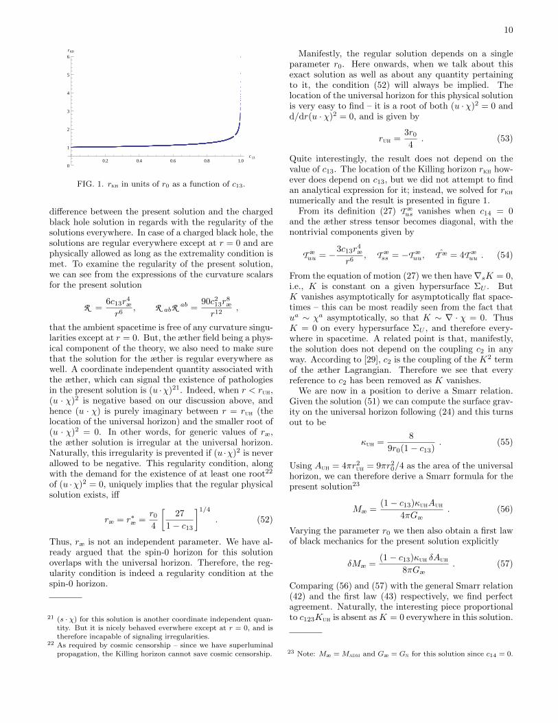
FIG. 1. rkh in units of r0 as a function of c13.

difference between the present solution and the chargedblack hole solution in regards with the regularity of thesolutions everywhere. In case of a charged black hole, thesolutions are regular everywhere except at r = 0 and arephysically allowed as long as the extremality condition ismet. To examine the regularity of the present solution,we can see from the expressions of the curvature scalarsfor the present solution

R =6c13r

4æ

r6, R abR ab =

90c213r8æ

r12,

that the ambient spacetime is free of any curvature singu-larities except at r = 0. But, the æther field being a phys-ical component of the theory, we also need to make surethat the solution for the æther is regular everywhere aswell. A coordinate independent quantity associated withthe æther, which can signal the existence of pathologiesin the present solution is (u ·χ)21. Indeed, when r < ruh,(u · χ)2 is negative based on our discussion above, andhence (u · χ) is purely imaginary between r = ruh (thelocation of the universal horizon) and the smaller root of(u · χ)2 = 0. In other words, for generic values of ræ,the æther solution is irregular at the universal horizon.Naturally, this irregularity is prevented if (u ·χ)2 is neverallowed to be negative. This regularity condition, alongwith the demand for the existence of at least one root22

of (u ·χ)2 = 0, uniquely implies that the regular physicalsolution exists, iff

ræ = r∗æ =r0

4

[27

1− c13

]1/4

. (52)

Thus, ræ is not an independent parameter. We have al-ready argued that the spin-0 horizon for this solutionoverlaps with the universal horizon. Therefore, the reg-ularity condition is indeed a regularity condition at thespin-0 horizon.

21 (s · χ) for this solution is another coordinate independent quan-tity. But it is nicely behaved everwhere except at r = 0, and istherefore incapable of signaling irregularities.

22 As required by cosmic censorship – since we have superluminalpropagation, the Killing horizon cannot save cosmic censorship.

Manifestly, the regular solution depends on a singleparameter r0. Here onwards, when we talk about thisexact solution as well as about any quantity pertainingto it, the condition (52) will always be implied. Thelocation of the universal horizon for this physical solutionis very easy to find – it is a root of both (u · χ)2 = 0 andd/dr(u · χ)2 = 0, and is given by

ruh =3r0

4. (53)

Quite interestingly, the result does not depend on thevalue of c13. The location of the Killing horizon rkh how-ever does depend on c13, but we did not attempt to findan analytical expression for it; instead, we solved for rkhnumerically and the result is presented in figure 1.

From its definition (27) T æus vanishes when c14 = 0

and the æther stress tensor becomes diagonal, with thenontrivial components given by

T æuu = −3c13r

4æ

r6, T æ

ss = −T æuu, ˆT æ = 4T æ

uu . (54)

From the equation of motion (27) we then have∇sK = 0,i.e., K is constant on a given hypersurface ΣU . ButK vanishes asymptotically for asymptotically flat space-times – this can be most readily seen from the fact thatua ∼ χa asymptotically, so that K ∼ ∇ · χ = 0. ThusK = 0 on every hypersurface ΣU , and therefore every-where in spacetime. A related point is that, manifestly,the solution does not depend on the coupling c2 in anyway. According to [29], c2 is the coupling of the K2 termof the æther Lagrangian. Therefore we see that everyreference to c2 has been removed as K vanishes.

We are now in a position to derive a Smarr relation.Given the solution (51) we can compute the surface grav-ity on the universal horizon following (24) and this turnsout to be

κuh =8

9r0(1− c13). (55)

Using Auh = 4πr2uh = 9πr2

0/4 as the area of the universalhorizon, we can therefore derive a Smarr formula for thepresent solution23

Mæ =(1− c13)κuhAuh

4πGæ. (56)

Varying the parameter r0 we then also obtain a first lawof black mechanics for the present solution explicitly

δMæ =(1− c13)κuh δAuh

8πGæ. (57)

Comparing (56) and (57) with the general Smarr relation(42) and the first law (43) respectively, we find perfectagreement. Naturally, the interesting piece proportionalto c123Kuh is absent as K = 0 everywhere in this solution.

23 Note: Mæ = Madm and Gæ = Gn for this solution since c14 = 0.

11

B. Exact solution for c123 = 0

When the coupling c123 is set to zero, we also have anexact solution given by

e(r) = 1− r0

r− ru(r0 + ru)

r2, f(r) = 1 ,

α(r) =(

1 +rur

)−1

, β(r) = −r0 + 2ru2r

,

(58)

where ru is a positive constant, given by

ru =

[√2− c14

2(1− c13)− 1

]r0

2. (59)

The requirement of positivity of ru follows from demand-ing the function α(r) be regular everywhere. Conse-quently, this imposes the following bound on the cou-plings c13 and c14

c14 5 2c13 . (60)

Therefore, for this special case we also need to ensure thatc13 is non-negative in addition to c13 < 1 and 0 5 c14 < 2as we assume in general (8). The positivity of ru criterionalso rules out another possible solution for ru

ru = −

[√2− c14

2(1− c13)+ 1

]r0

2,

which solves all the equations of motion, but is manifestlynegative for all values of c13 and c14. The curvature in-variants for this solution are

R = 0, R abR ab =4r2u(r0 + ru)2

r8,

demonstrating that the geometry is free from any curva-ture singularity everywhere except at r = 0. Thus thesolution is regular everywhere.

The reader might have spotted that the parameter ræ

does not appear in this solution. Instead we have theparameter ru, which is however not a free parameter.Rather, there are two possible choices for ru as functionsr0 and this ambiguity is resolved (in the form of choosingru positive) by demanding that the solution be regulareverwhere except at r = 0. One way to appreciate thedifference between the present solution and all the so-lutions with c123 6= 0, is to note that we need separateasymptotic analysis for the cases c123 6= 0 and c123 = 024.As it turns out, when c123 6= 0, the equations of motionforce the O(r−1) coefficient of α(r) to be r0/2 (49b).When c123 = 0, this requirement no longer holds and weare left with a free parameter ru. Furthermore, when

24 There is no such need when the coupling in question is c14 as thegeneral asymptotic solution (49) admits a smooth c14 → 0 limit.

c123 6= 0, the parameter ræ appears as the O(r−2) coef-ficient of α(r) and stays as the second free parameter inthe general asymptotic analysis. For the c123 = 0 casehowever, the O(r−2) coefficient is a function of ru, andas the subsequent analysis reveals, the equations of mo-tion eventually restrict ru to take one of the two choicesmentioned above. The requirement for regularity thenremoves one of the choices. We have already argued ear-lier that the spin-0 horizon for this solution “coincides”with the asymptotic boundary at infinity. We thus seethat even with the correct boundary conditions imposed,there can be two different solutions corresponding to twodifferent values of the paremeter ru

25. The actual regu-larity condition here comes in the form of choosing thecorrect value of ru as given in (59). Manifestly, the reg-ular solution depends on a single parameter r0.

We next adress the issue of the locations of the Killingand universal horizons. From the explicit solution, wefurther work out

(s ·χ) = −β(r) =r0 + 2ru

2r, (u ·χ) = −1+

r0

2r. (61)

The roots of e(r) = 0 can be explicitly found in this caseand they are r = (r0 +ru) and r = −ru respectively. Thesecond root is negative, i.e. unphysical, and the uniqueKilling horizon is at

rkh = r0 + ru . (62)

On the other hand, (u · χ) has a unique root at r = r0/2which is therefore the location of the universal horizon inthis solution

ruh =r0

2. (63)

As in the case of the exact solution with c14 = 0, thelocation of the universal horizon does not depend on thecoupling constants for the present case either, while thelocation of the Killing horizon does.

With T æus vanishing according to (32) the stress ten-

sor is also diagonal in this solution, with the non-trivialcomponents given by

T æuu = −2c13(r0 + 2ru)2 − c14r

20

8r4,

T æss = −T æ

uu, ˆT æ = 2T æuu .

(64)

To derive a Smarr relation, we proceed as before andcompute the surface gravity on the universal horizon from(24) using the present solution (58)

κuh =2− c14

(1− c13)r0. (65)

25 The choice of the correct asymptotic boundary conditions withappropriate fall off conditions for the various fields should betreated as partly making the spin-0 horizon regular in this case.In particular, this seems to be the reason for no additional con-tinuous parameter in the solution.

12

This time, using Auh = 4πr2uh = πr2

0 as the area of theuniversal horizon, we arrive at the Smarr formula for thepresent solution

Mæ =(1− c13)κuhAuh

4πGæ. (66)

Therefore, the first law of black mechanics for the presentsolution is

δMæ =(1− c13)κuh δAuh

8πGæ. (67)

We find perfect agreement, once again, upon comparing(66) and (67) with the general Smarr formula (42) andthe first law (43) respectively. This time, the interestingpiece proportional to c123Kuh is absent for the obviousreason.

V. SUMMARY AND CONCLUSIONS

In this paper we have studied static, spherically sym-metric, asymptotically flat black hole solutions of theEinstein-æther theory, a generally covariant modificationof general relativity where a vector field, the æther, isforced to satisfy a unit normalization constraint. Sincethere is a preferred frame of reference defined by theæther, the solutions of the theory violate local Lorentzinvariance and so matter fields do not necessarily have afinite local limiting speed. Even though at first sight thenotion of a black hole seems impossible in such a situa-tion, earlier work [21, 22] provided concrete evidence insupport of the existence of a single parameter family ofstatic, spherically symmetric, asymptotically flat blackhole solutions. The causal boundary in question, calledthe universal horizon, is a hypersurface which traps ex-citations travelling even at infinite local speed.

In this work, we extend these earlier studies by demon-strating that a Smarr relation and a first law of black holemechanics associated with the universal horizon can befound. We also provide analytical evidence for the exis-tence of a universal horizon by constructing two exact so-lutions for special choices of the couplings of the Einstein-æther theory, and verify the Smarr formula and the firstlaw with these special cases. Critical to our proof of thefirst law is the fact that the solutions depend on a singleparameter, namely the mass of the solution [21, 22].

The Smarr formula (42) and the first law (43) suggestthat in the present context, the quantity quh (39) playsthe same role as surface gravity at the Killing horizonof a black hole in general relativity. Indeed, from (39)quh does include a contribution from the surface gravityat the universal horizon, but there is also an additionalpiece that depends on the extrinsic curvature of the pre-ferred foliation as it asymptotes to the universal horizon.Based on the causal nature of the universal horizon, athermodynamic interpretation of the first law (43) seemsnecessary, along the lines of [2].

Implementing such a thermodynamic interpretation ina concrete manner may, however, prove problematic. Inderiving a Smarr formula and first law we have just dealtwith classical, low energy physics. There is no need toworry about quantum effects in either the matter or grav-itational sectors or the ultimately necessary ultravioletcompletion of Einstein-æther theory. However, if onewants to provide an explicit and consistent thermody-namic interpretation of a horizon entropy one must intro-duce radiation from the causal horizon and now one runsinto problematic issues. In the usual picture of Hawkingradiation from a black hole, finite wavelength modes atinfinity originates as infinitely short wavelengths near thehorizon. If exact local Lorentz invariance holds then theultraviolet near horizon modes are not an issue - the nec-essary microscopic physics is determined by the symme-try. This however, requires assumptions about Lorentzsymmetry at untested energies and it is not conclusivelyproven that the microscopic structure of spacetime re-spects exact Lorentz invariance (although we have neverseen a violation of Lorentz invariance [20, 37]). Thisis the so-called “transplanckian problem” of black holephysics [38]. Similarly, in the Einstein-æther case, modesthat escape to infinity have infinitely high speeds/shortwavelengths with respect to the æther frame near theuniversal horizon. Yet here we have neither local Lorentzsymmetry nor a unique ultraviolet completion to the the-ory that would provide the necessary microscopic frame-work to unambiguously specify the near horizon modebehavior.

While there are only very few studies of the thermo-dynamics of universal horizons (c.f. the discussion onuniversal horizons in Einstein-æther theory in [39]), anumber of authors have studied radiation from a Killinghorizon when Lorentz symmetry is broken in the ultravi-olet for the quantum field. The thermal nature of Hawk-ing radiation from a Killing horizon has been shown to befairly robust against ultraviolet modifications to Lorentzsymmetry that yield subluminal propagation for quan-tum fields [40] but the behavior for superluminal fields ismuch less straightforward [41]. Hence the radiation spec-trum from a universal horizon, which is not a Killing hori-zon and where modes are necessarily “superluminal”, iscompletely unknown. Finally, if Einstein-æther is the lowenergy limit of a renormalizable theory such as Horava-Lifshitz gravity, then there are difficulties with assign-ing a holographic entropy to black holes, as this mayinterfere with the necessary ultraviolet behavior (c.f. thediscussion in [42]). On the other hand, simple generalthermodynamic arguments imply that there should be anentropy and our first law hints that the entropy is still afunction of variables on a horizon area. These are puz-zles that requires further investigation, which we leavefor future work.

There is one more practical complication that ariseswhen deriving thermodynamics as in Einstein-æther the-ory Cerenkov radiation generically occurs since æther-metric modes and matter fields all have different speeds.

13

In particular, a matter field mode propagating out-wards from the universal horizon would emit spin-0Cerenkov radiation, thereby modifying any thermal spec-trum. Since no detailed examination of the radiationspectrum from a universal horizon has been made yet, itis unclear whether or not there is a Cerenkov-type com-ponent in addition to any presumed thermal flux. Note,however, that when c14 → 0 the speed of the spin-0 modegoes to infinity, and so there is no possibility of emissionof spin-0 Cerenkov radiation. On the other hand, whenc123 → 0, the speed of the spin-0 mode goes to zero, andso any spin-0 Cerenkov radiation would carry no energyaway from the universal horizon. Thus, in both cases thereduction to a situation where the presumed temperatureis proportional to the surface gravity is consistent witha limit where any Cerenkov radiation would naturallybecome unimportant.

ACKNOWLEDGMENTS

We are grateful to Ted Jacobson for critically review-ing an earlier draft of this paper and for providing nu-merous invaluable suggestions. P.B. acknowledges thehospitality of the KITPC, Beijing, the Berkeley Centerfor Theoretical Physics and the theory group at CERN.The work of P.B. and J.B. is supported by the NSF CA-REER grant PHY-0645686. D.M. thanks the Universityof New Hampshire for research support.

Appendix A: Some algebraic details

In this appendix, we provide some of the technical alge-braic details behind our analysis. Of central importanceto our analysis is the hypersurface orthogonality relation(14), as well as the assumptions of spherical symmetryand staticity. We already noted in section II (see thefootnote around (20)) that as a consequence of the hy-persurface orthogonality of ua, spherical symmetry andstaticity, the vector sa is hypersurface orthogonal withrespect to the foliations Σs of the spacetime, and satisfys∧ ds = 0. Contracting these hypersurface orthogonalityconditions with ua and sa respectively, we obtain

∇[aub] = −(a · s)u[asb], ∇[asb] = −K0u[asb] (A1)

Further contractions of these relations with any Killingvector ηa and with ua and/or sa lead to extremely usefulscalar identities which play a major role in our analysis,and in particular, in the derivation of (33). One of ourgoals in this appendix is to briefly outline how these iden-tities are obtained in a generalized and coherent fashion.To that end, we recall (as already noted in the para-gragh following (18)) that by the spherical symmetry ofthe problem, any rank-two tensor can have componentsonly along the bi-vectors uaub, u(asb), u[asb], sasb andgab. The most basic among these basis-expansions are

those for ∇aub

∇aub = −(a · s)uasb +Kab,

Kab = K0sasb +K

2gab

(A2)

and for ∇asb

∇asb = K0saub +K(s)ab ,

K(s)ab = −(a · s)uaub +

k

2gab

(A3)

where K(s)ab is the extrinsic curvature of the hypersur-

faces Σs due to their embedding in the spacetime, and

k and K are the traces of the extrinsic curvatures of thetwo-spheres B due to their embeddings in ΣU and Σsrespectively

k = (1/2)gab£sgab, K = (1/2)gab£ugab (A4)

Our results in this paper make heavy uses of (A2) and(A3).

Now, consider an arbitrary vector of the following form

Aa = −fua + hsa (A5)

where f and h are arbitrary functions respecting the sym-metries of the problem. A natural construct is the two-form

Fab = ∇[aAb] = Qu[asb] (A6)

where the second equality follows by the spherical sym-metry of the problem, and the scalar Q is given by

Q = f(a · s) +∇sf − hK0 −∇uh (A7)

Using the torsion-free condition of the covariant deriva-tive, it can be shown that Q, like Fab, is invariant underthe “gauge transformations” Aa 7→ A′a = Aa +∇aΛ.

Comparing (A1) with (A6), we see that the formerrelations are special cases of the latter. Contracting (A6)with a Killing vector ηa yields

∇a(A · η) = Q(s · η)ua −Q(u · η)sa (A8)

Contracting (A8) further with ua and sa gives

∇u(A · η) = −Q(s · η), ∇s(A · η) = −Q(u · η) (A9)

We make ample use of the special cases of (A8) and (A9)for Aa = ua and Aa = sa throughout the analysis.

The flux of Fab over any two-sphere B is∫B

dΣabFab =

∫B

dAQ (A10)

Since Fab is antisymmetric, we have a kinematically con-served current Ja through

∇bF ab = Ja (A11)

14

We call Ja a kinematically conserved current since it sat-isfies the continuity equation ∇·J = 0 irrespective of anyequations of motion.

By spherical symmetry, the current can only have com-ponents along ua and sa. These projections are given by

(u · J) = −(kQ+∇sQ) = −~∇ · [Q~s] ,(s · J) = −(KQ+∇uQ) = −∇ · [Qu]

(A12)

where ~va = Pabvb and va = Pabvb are projections of anyfour vector va on the hypersurfaces ΣU and Σs respec-tively, Pab = uaub + δab and Pab = −sasb + δab are the

corresponding projection tensors, and ~∇a = P ba ∇b and

∇a = P ba ∇b are the corresponding projections of the co-

variant derivatives.The most important example of a kinematically con-

served current, which is central in the derivation of (33),is that due to the timelike Killing vector χa. Choos-ing the vector Aa = (1/2)χa in (A5), so that from (A6)Fab = ∇aχb, we obtain Q = −κ. From the identity∇b∇aχb = R a

bχb, which forms the basis of the Smarr

relation, we find that the kinematically conserved cur-rent is Jaχ = R a

bχb such that

(u · Jχ) = ~∇ · [κ~s], (s · Jχ) = ∇ · [κu] (A13)

We conclude this appendix by noting the following twoidentities

(u · η)(∇ · v) = ~∇ ·[− (u · v)(s · η) + (s · v)(u · η)

~s]

(A14)and

(s · η)(∇ · v) = ∇ ·[− (u · v)(s · η) + (s · v)(u · η)

u]

(A15)valid for any four-vector va. The identities (A14) and(A15) are indispensible for dealing with the contributionsfrom the æther in the derivation of (33).

Appendix B: More on spin-0 horizon (ir)regularity

In this appendix, we present some further studies ofthe equations of motion, where the irregularity of a gen-eral æther black hole solution near its spin-0 horizon forgeneric values of r0 and ræ [21, 22] manifests itself ininteresting ways.

We have performed a near-universal-horizon analysisof the equations of motion to lowest order in the near-universal-horizon radial coordinate. The most strikingfeature of the analysis is that two separate treatmentsare required for the cases c14 6= 0 and c14 = 0, since,the series coefficients are divergent in c14 in the c14 6=0 case26. Indeed, in this case the near-univeral-horizon

26 The situation should be compared with the asymptotic analysis

region is also the near-spin-0-horizon region when c14 issufficiently small. Since we did not impose any a prioriregularity condition on the solution in our analysis, thisdivergent behaviour is clearly due to the irregularity ofthe solution at the spin-0 horizon.

The near-universal-horizon analysis for c14 = 0, on theother hand, successfully reproduces27 the near-universal-horizon behaviour of the exact solution for c14 = 0.Likewise, upon taking the limit c123 → 0 of the near-universal-horizon solution for c14 6= 0, we successfullyreproduce the near-universal-horizon behaviour of thec123 = 0 exact solution.

We have also studied perturbative corrections to theexact solutions for c14 = 0 (51) and c123 = 0 (58) – forsmall c14 in the former case, and for small c123 in thelatter. The former analysis (i.e around the c14 = 0 ex-act solution) did not yield a complete solution becauseof the very complicated nature of the relevant equations– we could only find the O(c14) correction to the func-tion f(r). In the context of the c123 = 0 exact solutionhowever, with an additional mild assumption, namelyc14 = 2c13 − ε where c123 = ε 1, we found the O(c123)correction to all the three basic functions e(r), f(r) andα(r)28. The most important property of the perturbativecorrections, relevant for the present discussion, is that thecorrections have logarithmic singularities at the locationof the unperturbed spin-0 horizon29. More specifically,the O(c123) correction functions to the c123 = 0 exactsolution depend on log(r/r0)30, while for the c14 = 0 ex-act solution, the O(c14) correction to f(r) depends on

when c123 6= 0 and the corresponding divergence of the asymp-totic solution in c123 – see the comments following equation (48).As discussed earlier, for small c123 the spin-0 horizon is pushedtowards asymptotic infinity. Therefore the asymptotic solution isa good approximation to the near-spin-0-horizon region of the so-lution for sufficiently small values of c123. The divergence here istherefore a manifestation of the irregularity of the general asymp-totic solution (where no regularity is imposed) at its spin-0 hori-zon.

27 Of course, the exact values of the functions at the universal hori-zon, as well as the radial location of the universal horizon inthe Eddington-Finklestein radial coordinate (44), depend on thenormalization of the asymptotic data and the actual definitionof the radial coordinate itself, and cannot be “derived” in thiskind of an analysis.

28 In our analysis, the spin-0 speed s0 can be kept arbitrarily smallas long as c123 c13 < 1; therefore, the spin-0 horizon can be“arbitrarily far away”, i.e., “arbitrarily close” to the asymptoticboundary. Looking at the expression for ru (59) we further no-tice that the assumption on c14 implies that the perturbativecorrection we are studying can also be thought of as a pertur-bation around a Schwarzschild background. We also refer thereader to a useful study of non-spherical perturbations aboutblack hole solutions in extended Horava gravity and Einstein-æther theory [39].

29 Even though our analysis of the small c14 perturbation aroundthe c14 = 0 exact solution is incomplete, the statement is true forthe O(c14) correction for the function f(r) – see below. The rele-vant equations in this context also indicate that such logarithmicsingularities will be present for e(r) and α(r).

30 One might be worried that the O(c123) correction functions to

15

log(1 − 3r0/4r). Now, although the exact solutions areregular everywhere, their first order corrected counter-

parts are a priori not so. The logarithmic divergence atthe unperturbed spin-0 horizon therefore clearly signalsan irregular behaviour31.

[1] J. M. Bardeen, B. Carter, S. W. Hawking, “The Fourlaws of black hole mechanics,” Commun. Math. Phys.31, 161-170 (1973).

[2] S. W. Hawking, “Particle Creation by Black Holes,”Commun. Math. Phys. 43, 199 (1975) [Erratum-ibid. 46,206 (1976)].

[3] J. D. Bekenstein, “Black holes and entropy,” Phys. Rev.D 7, 2333 (1973).

[4] G. ’t Hooft, “Dimensional reduction in quantum gravity,”gr-qc/9310026.

[5] L. Susskind, “The World as a hologram,” J. Math. Phys.36, 6377 (1995) [hep-th/9409089].

[6] J. M. Maldacena, “The Large N limit of superconformalfield theories and supergravity,” Adv. Theor. Math. Phys.2, 231 (1998) [Int. J. Theor. Phys. 38, 1113 (1999)] [hep-th/9711200].

[7] S. S. Gubser, I. R. Klebanov and A. M. Polyakov, “Gaugetheory correlators from noncritical string theory,” Phys.Lett. B 428, 105 (1998) [hep-th/9802109].

[8] E. Witten, “Anti-de Sitter space and holography,” Adv.Theor. Math. Phys. 2, 253 (1998) [hep-th/9802150].

[9] T. Jacobson, “Thermodynamics of space-time: The Ein-stein equation of state,” Phys. Rev. Lett. 75, 1260 (1995)[gr-qc/9504004].

[10] E. P. Verlinde, “On the Origin of Gravity and the Lawsof Newton,” JHEP 1104, 029 (2011) [arXiv:1001.0785[hep-th]].

[11] T. Padmanabhan, “Gravity and the thermodynamics ofhorizons,” Phys. Rept. 406, 49 (2005) [gr-qc/0311036].

[12] T. Jacobson, G. Kang and R. C. Myers, “On black holeentropy,” Phys. Rev. D 49, 6587 (1994) [gr-qc/9312023].

[13] T. Jacobson and D. Mattingly, “Gravity with a dynam-ical preferred frame,” Phys. Rev. D 64 (2001) 024028[gr-qc/0007031].

[14] T. Jacobson and D. Mattingly, “Generally covariantmodel of a scalar field with high frequency dispersion

the c123 = 0 solution destroy the asymptotic flatness condition,due to the presence of the log(r/r0) in their expressions. Wehowever do not claim that the O(c123) correction approximatesthe actual solution everywhere in spacetime. Indeed, the O(c123)correction can be a good approximation near the universal andthe Killing horizons, but we need to consider higher order correc-tions in c123 to approximate the actual solution as we move outin r, and presumably we need to go to all orders in c123 in orderto “approximate” the actual solution at asymptotic infinity. Onthe other hand, by the results of [21, 22] we are guaranteed toreach an asymptotically flat regular solution (provided we choosethe appropriate boundary conditions for the perturbation at theuniversal horizon).

31 The irregularity occurs at the unperturbed spin-0 horizon insteadof at the true spin-0 horizon of the actual solution, because,the first order corrections that we have considered here do notapproximate the solution near the spin-0 horizon for the actualsolution (see the previous footnote), and one needs to considersuccessively higher order corrections to the exact solutions to seethe irregularity at the correct location properly.

and the cosmological horizon problem,” Phys. Rev. D63, 041502 (2001) [hep-th/0009052].

[15] T. Jacobson and D. Mattingly, “Einstein-æther waves,”Phys. Rev. D 70, 024003 (2004) [gr-qc/0402005].

[16] T. Jacobson, “Einstein-æther gravity: Theory and obser-vational constraints,” arXiv:0711.3822 [gr-qc].

[17] T. Jacobson, “Einstein-æther gravity: A Status report,”PoS QG -PH (2007) 020 [arXiv:0801.1547 [gr-qc]].

[18] D. Garfinkle, T. Jacobson, “A positive energy theoremfor Einstein-æther and Horava gravity,” arXiv:1108.1835[gr-qc]].

[19] C. Eling, T. Jacobson and D. Mattingly, “Einstein-æthertheory,” gr-qc/0410001.

[20] D. Mattingly, “Modern tests of Lorentz invariance,” Liv-ing Rev. Rel. 8, 5 (2005) [gr-qc/0502097].

[21] C. Eling, T. Jacobson, “Black Holes in Einstein-ætherTheory,” Class. Quant. Grav. 23, 5643-5660 (2006), [gr-qc/0604088].

[22] E. Barausse, T. Jacobson, T. P. Sotiriou, “Black holes inEinstein-æther and Horava-Lifshitz gravity,” Phys. Rev.D83, 124043 (2011), [arXiv:1104.2889 [gr-qc]].

[23] S. L. Dubovsky and S. M. Sibiryakov, “Spontaneousbreaking of Lorentz invariance, black holes and per-petuum mobile of the 2nd kind,” Phys. Lett. B 638, 509(2006) [hep-th/0603158].

[24] C. Eling, B. Z. Foster, T. Jacobson and A. C. Wall,“Lorentz violation and perpetual motion,” Phys. Rev.D 75, 101502 (2007) [hep-th/0702124 [HEP-TH]].

[25] T. Jacobson and A. C. Wall, “Black Hole Thermody-namics and Lorentz Symmetry,” Found. Phys. 40, 1076(2010) [arXiv:0804.2720 [hep-th]].

[26] S. M. Carroll and E. A. Lim, “Lorentz-violating vectorfields slow the universe down,” Phys. Rev. D 70, 123525(2004) [hep-th/0407149].

[27] J. W. Elliott, G. D. Moore and H. Stoica, “Constrain-ing the new Aether: Gravitational Cerenkov radiation,”JHEP 0508, 066 (2005) [hep-ph/0505211].

[28] P. Horava, “Quantum Gravity at a Lifshitz Point,” Phys.Rev. D 79 (2009) 084008 [arXiv:0901.3775 [hep-th]].

[29] T. Jacobson, “Extended Horava gravity and Einstein-æther theory,” Phys. Rev. D 81, 101502 (2010) [Erratum-ibid. D 82, 129901 (2010)] [arXiv:1001.4823 [hep-th]].

[30] T. Jacobson and R. Parentani, “Horizon surface grav-ity as 2d geodesic expansion,” Class. Quant. Grav. 25,195009 (2008) [arXiv:0806.1677 [gr-qc]].

[31] T. Jacobson, “Initial value constraints with tensor mat-ter,” [arXiv:1108.1496 [gr-qc]].

[32] C. Eling, “Energy in the Einstein-æther theory,” Phys.Rev. D 73, 084026 (2006) [Erratum-ibid. D 80, 129905(2009)] [gr-qc/0507059].

[33] B. Z. Foster, “Noether charges and black hole mechan-ics in Einstein-æther theory,” Phys. Rev. D 73, 024005(2006) [gr-qc/0509121].

[34] See any standard discussion on the derivation of thelaws of black hole mechanics via the scaling argument,e.g., P. K. Townsend, “Black holes: Lecture notes,” gr-

16

qc/9707012, page 113.[35] R. M. Wald, “Black hole entropy is the Noether charge,”

Phys. Rev. D 48, 3427 (1993) [gr-qc/9307038].[36] B. Z. Foster, “Metric redefinitions in Einstein-æther the-

ory,” Phys. Rev. D 72, 044017 (2005) [gr-qc/0502066].[37] V. A. Kostelecky and N. Russell, “Data Tables for

Lorentz and CPT Violation,” Rev. Mod. Phys. 83, 11(2011) [arXiv:0801.0287 [hep-ph]].

[38] T. Jacobson, “Black hole evaporation and ultrashort dis-tances,” Phys. Rev. D 44, 1731 (1991).

[39] D. Blas and S. Sibiryakov, “Horava gravity versus ther-

modynamics: The Black hole case,” Phys. Rev. D 84,124043 (2011) [arXiv:1110.2195 [hep-th]].

[40] W. G. Unruh and R. Schutzhold, “On the universalityof the Hawking effect,” Phys. Rev. D 71, 024028 (2005)[gr-qc/0408009].

[41] C. Barcelo, L. J. Garay and G. Jannes, “Sensitivity ofHawking radiation to superluminal dispersion relations,”Phys. Rev. D 79, 024016 (2009) [arXiv:0807.4147 [gr-qc]].

[42] A. Shomer, “A Pedagogical explanation for the non-renormalizability of gravity,” arXiv:0709.3555 [hep-th].