Median Matrix Completion: from Embarrassment to Optimality

Median Matrix Completion: from Embarrassment to Optimality

Weidong Liu 1 Xiaojun Mao 2 Raymond K. W. Wong 3

AbstractIn this paper, we consider matrix completion withabsolute deviation loss and obtain an estimatorof the median matrix. Despite several appealingproperties of median, the non-smooth absolutedeviation loss leads to computational challengefor large-scale data sets which are increasinglycommon among matrix completion problems. Asimple solution to large-scale problems is paral-lel computing. However, embarrassingly paral-lel fashion often leads to inefficient estimators.Based on the idea of pseudo data, we proposea novel refinement step, which turns such ineffi-cient estimators into a rate (near-)optimal matrixcompletion procedure. The refined estimator isan approximation of a regularized least medianestimator, and therefore not an ordinary regular-ized empirical risk estimator. This leads to a non-standard analysis of asymptotic behaviors. Em-pirical results are also provided to confirm theeffectiveness of the proposed method.

1. IntroductionMatrix completion (MC) has recently gained a substantialamount of popularity among researchers and practitionersdue to its wide applications; as well as various related the-oretical advances Candes & Recht (2009); Candes & Plan(2010); Koltchinskii et al. (2011); Klopp (2014). Perhapsthe most well-known example of a MC problem is the Net-flix prize problem (Bennett & Lanning, 2007), of whichthe goal is to predict missing entries of a partially observedmatrix of movie ratings. Two commonly shared challengesamong MC problems are high dimensionality of the matrixand a huge proportion of missing entries. For instance, Net-

*Equal contribution 1School of Mathematical Sciences andMoE Key Lab of Artificial Intelligence Shanghai Jiao Tong Uni-versity, Shanghai, 200240, China 2School of Data Science, FudanUniversity, Shanghai, 200433, China 3Department of Statistics,Texas A&M University, College Station, TX 77843, U.S.A.. Cor-respondence to: Xiaojun Mao <[email protected]>.

Proceedings of the 37 th International Conference on MachineLearning, Online, PMLR 119, 2020. Copyright 2020 by the au-thor(s).

flix data has less than 1% of observed entries of a matrixwith around 5×105 rows and 2×104 customers. With tech-nological advances in data collection, we are confrontingincreasingly large matrices nowadays.

Without any structural assumption on the target matrix, itis well-known that MC is an ill-posed problem. A pop-ular and often well-justified assumption is low rankness,which however leads to a challenging and non-convex rankminimization problem (Srebro et al., 2005). The seminalworks of Candes & Recht (2009); Candes & Tao (2010);Gross (2011) showed that, when the entries are observedwithout noise, a perfect recovery of a low-rank matrix canbe achieved by a convex optimization via near minimal or-der of sample size, with high probability. As for the noisysetting, some earlier work (Candes & Plan, 2010; Keshavanet al., 2010; Chen et al., 2019b) focused on arbitrary, notnecessarily random, noise. In general, the arbitrariness mayprevent asymptotic recovery even in a probability sense.

Recently, a significant number of works (e.g. Bach, 2008;Koltchinskii et al., 2011; Negahban & Wainwright, 2011;Rohde & Tsybakov, 2011; Negahban & Wainwright, 2012;Klopp, 2014; Cai & Zhou, 2016; Fan et al., 2019; Xia &Yuan, 2019) targeted at more amenable random error mod-els, under which (near-)optimal estimators had been pro-posed. Among these work, trace regression model is one ofthe most popular models due to its regression formulation.Assume N independent pairs (Xk, Yk), for k = 1, . . . , N ,are observed, where Xk’s are random design matrices ofdimension n1 × n2 and Yk’s are response variables in R.The trace regression model assumes

Yk = tr(XTkA?

)+ εk, k = 1, . . . , N, (1.1)

where tr(A) denotes the trace of a matrix A, and A? ∈Rn1×n2 is an unknown target matrix. Moreover, the ele-ments of ε = (ε1, . . . , εN ) are N i.i.d. random noise vari-ables independent of the design matrices. In MC setup,the design matrices Xk’s are assumed to lie in the set ofcanonical bases

X = ej(n1)ek(n2)T : j = 1, . . . , n1; k = 1, . . . , n2,(1.2)

where ej(n1) is the j-th unit vector in Rn1 , and ek(n2) isthe k-th unit vector in Rn2 . Most methods then apply aregularized empirical risk minimization (ERM) framework

Distributed Median Matrix Completion

with a quadratic loss. It is well-known that the quadraticloss is most suitable for light-tailed (sub-Gaussian) error,and leads to non-robust estimations. In the era of big data,a thorough and accurate data cleaning step, as part of datapreprocessing, becomes virtually impossible. In this regard,one could argue that robust estimations are more desirable,due to their reliable performances even in the presence ofoutliers and violations of model assumptions. While robuststatistics is a well-studied area with a rich history (Davies,1993; Huber, 2011), many robust methods were developedfor small data by today’s standards, and are deemed toocomputationally intensive for big data or complex models.This work can be treated as part of the general effort tobroaden the applicability of robust methods to modern dataproblems.

1.1. Related Work

Many existing robust MC methods adopt regularized ERMand assume observations are obtained from a low-rank-plus-sparse structureA?+S+E, where the low-rank matrixA?

is the target uncontaminated component; the sparse matrixS models the gross corruptions (outliers) locating at a smallproportion of entries; and E is an optional (dense) noisecomponent. As gross corruptions are already taken intoaccount, many methods with low-rank-plus-sparse structureare based on quadratic loss. Chandrasekaran et al. (2011);Candes et al. (2011); Chen et al. (2013); Li (2013) con-sidered the noiseless setting (i.e., no E) with an element-wisely sparse S. Chen et al. (2011) studied the noiselessmodel with column-wisely sparse S. Under the model withelement-wisely sparse S, Wong & Lee (2017) looked intothe setting of arbitrary (not necessarily random) noise E,while Klopp et al. (2017) and Chen et al. (2020) studiedrandom (sub-Gaussian) noise model for E. In particular,it was shown in Proposition 3 of Wong & Lee (2017) thatin the regularized ERM framework, a quadratic loss withelement-wise `1 penalty on the sparse component is equiv-alent to a direct application of a Huber loss without thesparse component. Roughly speaking, this class of robustmethods, based on the low-rank-plus-sparse structure, canbe understood as regularized ERMs with Huber loss.

Another class of robust MC methods is based on the absolutedeviation loss, formally defined in (2.1). The minimizer ofthe corresponding risk has an interpretation of median (seeSection 2.1), and so the regularized ERM framework thatapplies absolute deviation loss is coined as median matrixcompletion (Elsener & van de Geer, 2018; Alquier et al.,2019). In the trace regression model, if the medians of thenoise variables are zero, the median MC estimator can betreated as a robust estimation of A?. Although median isone of the most commonly used robust statistics, the medianMC methods have not been studied until recently. Elsener &van de Geer (2018) derived the asymptotic behavior of the

trace-norm regularized estimators under both the absolutedeviation loss and the Huber loss. Their convergence ratesmatch with the rate obtained in Koltchinskii et al. (2011)under certain conditions. More complete asymptotic resultshave been developed in Alquier et al. (2019), which derivesthe minimax rates of convergence with any Lipschitz lossfunctions including absolute deviation loss.

To the best of our knowledge, the only existing computa-tional algorithm of median MC in the literature is proposedby Alquier et al. (2019), which is an alternating directionmethod of multiplier (ADMM) algorithm developed for thequantile MC with median MC being a special case. How-ever, this algorithm is slow and not scalable to large matricesdue to the non-smooth nature of both the absolute deviationloss and the regularization term.

Despite the computational challenges, the absolute devi-ation loss has a few appealing properties as compared tothe Huber loss. First, absolute deviation loss is tuning-freewhile Huber loss has a tuning parameter, which is equivalentto the tuning parameter in the entry-wise `1 penalty in thelow-rank-plus-sparse model. Second, absolute deviationloss is generally more robust than Huber loss. Third, theminimizer of expected absolute deviation loss is naturallytied to median, and is generally more interpretable than theminimizer of expected Huber loss (which may vary with itstuning parameter).

1.2. Our Goal and Contributions

Our goal is to develop a robust and scalable estimator formedian MC, in large-scale problems. The proposed esti-mator approximately solves the regularized ERM with thenon-differentiable absolute deviation loss. It is obtainedthrough two major stages — (1) a fast and simple initialestimation via embarrassingly parallel computing and (2)a refinement stage based on pseudo data. As pointed outearlier (with more details in Section 2.2), existing compu-tational strategy (Alquier et al., 2019) does not scale wellwith the dimensions of the matrix. Inspired by Mackeyet al. (2015), a simple strategy is to divide the target matrixinto small sub-matrices and perform median MC on everysub-matrices in an embarrassingly parallel fashion, and thennaively concatenate all estimates of these sub-matrices toform an initial estimate of the target matrix. Therefore, mostcomputations are done on much smaller sub-matrices, andhence this computational strategy is much more scalable.However, since low-rankness is generally a global (whole-matrix) structure, the lack of communications between thecomputations of different sub-matrices lead to sub-optimalestimation (Mackey et al., 2015). The key innovation ofthis paper is a fast refinement stage, which transforms theregularized ERM with absolute deviation loss into a reg-ularized ERM with quadratic loss, for which many fast


algorithms exist, via the idea of pseudo data. Motivated byChen et al. (2019a), we develop the pseudo data based on aNewton-Raphson iteration in expectation. The constructionof the pseudo data requires only a rough initial estimate(see Condition (C6) in Section 3), which is obtained inthe first stage. As compared to Huber-loss-based methods(sparse-plus-low-rank model), the underlying absolute de-viation loss is non-differentiable, leading to computationaldifficulty for large-scale problems. The proposed strategyinvolves a novel refinement stage to efficiently combine andimprove the embarrassingly parallel sub-matrix estimations.

We are able to theoretically show that this refinement stagecan improve the convergence rate of the sub-optimal initialestimator to near-optimal order, as good as the computation-ally expensive median MC estimator of Alquier et al. (2019).To the best of our knowledge, this theoretical guarantee fordistributed computing is the first of its kind in the literatureof matrix completion.

2. Model and Algorithms2.1. Regularized Least Absolute Deviation Estimator

Let A? = (A?,ij)n1,n2

i,j=1 ∈ Rn1×n2 be an unknown high-dimensional matrix. Assume the N pairs of observations(Xk, Yk)Nk=1 satisfy the trace regression model (1.1) withnoise εkNk=1. The design matrices are assumed to bei.i.d. random matrices that take values in X (1.2). Letπst = Pr(Xk = es(n1)eT

t (n2)) be the probability of ob-serving (a noisy realization of) the (s, t)-th entry of A? anddenote Π = (π1,1, . . . , πn1,n2

)T. Instead of the uniformsampling where πst ≡ π (Koltchinskii et al., 2011; Rohde& Tsybakov, 2011; Elsener & van de Geer, 2018), out setupallows sampling probabilities to be different across entries,such as in Klopp (2014); Lafond (2015); Cai & Zhou (2016);Alquier et al. (2019). See Condition (C1) for more details.Overall, (Y1,X1, ε1), . . . , (YN ,XN , εN ) are i.i.d. tuples ofrandom variables. For notation’s simplicity, we let (Y,X, ε)be a generic independent tuple of random variables thathave the same distribution as (Y1,X1, ε1). Without addi-tional specification, the noise variable ε is not identifiable.For example, one can subtract a constant from all entriesof A? and add this constant to the noise. To identify thenoise, we assume P(ε ≤ 0) = 0.5, which naturally leadsto an interpretation of A? as median, i.e., A?,ij is the me-dian of Y | X = ei(n1)ej(n2)T. If the noise distributionis symmetric and light-tailed (so that the expectation ex-ists), then E(εk) = 0, and A? is the also the mean matrix(A?,ij = E(Y | X = ei(n1)ej(n2)T)), which aligns withthe target of common MC techniques (Elsener & van deGeer, 2018). Let f be the probability density function ofthe noise. For the proposed method, the required conditionof f is specified in Condition (C3) of Section 3, which isfairly mild and is satisfied by many heavy-tailed distribu-

tions whose expectation may not exist.

Define a hypothesis class B(a, n,m) = A ∈ Rn×m :‖A‖∞ ≤ a where a > 0 such that A? ∈ B(a, n,m).In this paper, we use the absolute deviation loss insteadof the common quadratic loss (e.g., Candes & Plan, 2010;Koltchinskii et al., 2011; Klopp, 2014). According to Sec-tion 4 of the Supplementary Material (Elsener & van deGeer, 2018), A? is also characterized as the minimizer ofthe population risk:

A? = arg minA∈B(a,n1,n2)

E∣∣Y − tr(XTA)

∣∣ . (2.1)

To encourage a low-rank solution, one natural candidate isthe following regularized empirical risk estimator (Elsener& van de Geer, 2018; Alquier et al., 2019):

ALADMC = arg minA∈B(a,n1,n2)

1

N

N∑k=1

∣∣Yk − tr(XTkA)

∣∣+ λ′N ‖A‖∗ , (2.2)

where ‖A‖∗ denotes the nuclear norm and λ′N ≥ 0 is atuning parameter. The nuclear norm is a convex relaxationof the rank which flavors the optimization and analysis ofthe statistical property (Candes & Recht, 2009).

Due to non-differentiability of the absolute deviationloss, the objective function in (2.1) is the sum of twonon-differentiable terms, rendering common computa-tional strategies based on proximal gradient method (e.g.,Mazumder et al., 2010; Wong & Lee, 2017) inapplicable.To the best of our knowledge, there is only one existingcomputational algorithm for (2.1), which is based on a di-rect application of alternating direction method of multiplier(ADMM) (Alquier et al., 2019). However, this algorithmis slow and not scalable in practice, when the sample sizeand the matrix dimensions are large, possibly due to thenon-differentiable nature of the loss.

We aim to derive a computationally efficient method forestimating the median matrix A? in large-scale MC prob-lems. More specifically, the proposed method consists oftwo stages: (1) an initial estimation via distributed com-puting (Section 2.2) and (2) a refinement stage to achievenear-optimal estimation (Section 2.3).

2.2. Distributed Initial Estimator

Similar to many large-scale problems, it is common to har-ness distributed computing to overcome computational bar-riers. Motivated by Mackey et al. (2015), we divide theunderlying matrix into several sub-matrices, estimate eachsub-matrix separately in an embarrassingly parallel fashionand then combine them to form a computationally efficient(initial) estimator of A?.


? 2 ? ? 3 ?

5 ? ? · · · · · · · · · ? ? 4

? 3 ? ? 1 ?...

. . ....

.... . .

......

. . ....

? 4 ? ? 2 ?

2 5 ? · · · · · · · · · ? 1 5

? 1 ? ? 3 ?

m1

m2

n1

n2

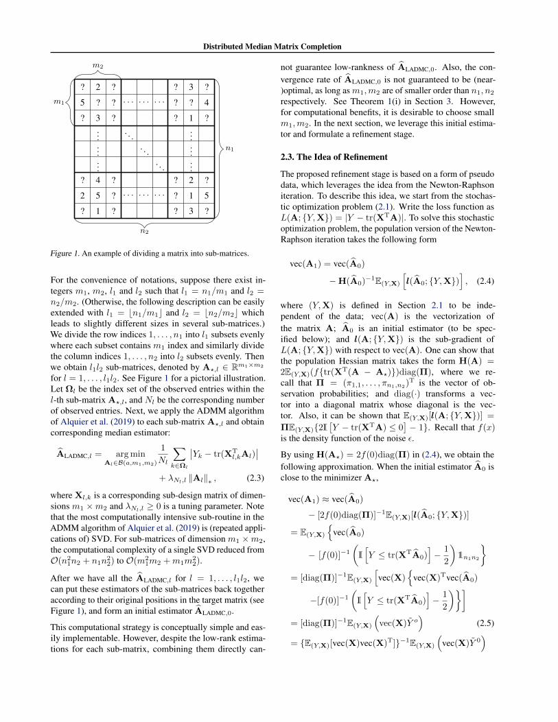
Figure 1. An example of dividing a matrix into sub-matrices.

For the convenience of notations, suppose there exist in-tegers m1, m2, l1 and l2 such that l1 = n1/m1 and l2 =n2/m2. (Otherwise, the following description can be easilyextended with l1 = bn1/m1c and l2 = bn2/m2c whichleads to slightly different sizes in several sub-matrices.)We divide the row indices 1, . . . , n1 into l1 subsets evenlywhere each subset contains m1 index and similarly dividethe column indices 1, . . . , n2 into l2 subsets evenly. Thenwe obtain l1l2 sub-matrices, denoted by A?,l ∈ Rm1×m2

for l = 1, . . . , l1l2. See Figure 1 for a pictorial illustration.Let Ωl be the index set of the observed entries within thel-th sub-matrix A?,l, and Nl be the corresponding numberof observed entries. Next, we apply the ADMM algorithmof Alquier et al. (2019) to each sub-matrix A?,l and obtaincorresponding median estimator:

ALADMC,l = arg minAl∈B(a,m1,m2)

1

Nl

∑k∈Ωl

∣∣Yk − tr(XTl,kAl)

∣∣+ λNl,l ‖Al‖∗ , (2.3)

where Xl,k is a corresponding sub-design matrix of dimen-sions m1 ×m2 and λNl,l ≥ 0 is a tuning parameter. Notethat the most computationally intensive sub-routine in theADMM algorithm of Alquier et al. (2019) is (repeated appli-cations of) SVD. For sub-matrices of dimension m1 ×m2,the computational complexity of a single SVD reduced fromO(n21n2 + n1n

22) to O(m2

1m2 +m1m22).

After we have all the ALADMC,l for l = 1, . . . , l1l2, wecan put these estimators of the sub-matrices back togetheraccording to their original positions in the target matrix (seeFigure 1), and form an initial estimator ALADMC,0.

This computational strategy is conceptually simple and eas-ily implementable. However, despite the low-rank estima-tions for each sub-matrix, combining them directly can-

not guarantee low-rankness of ALADMC,0. Also, the con-vergence rate of ALADMC,0 is not guaranteed to be (near-)optimal, as long as m1,m2 are of smaller order than n1, n2respectively. See Theorem 1(i) in Section 3. However,for computational benefits, it is desirable to choose smallm1,m2. In the next section, we leverage this initial estima-tor and formulate a refinement stage.

2.3. The Idea of Refinement

The proposed refinement stage is based on a form of pseudodata, which leverages the idea from the Newton-Raphsoniteration. To describe this idea, we start from the stochas-tic optimization problem (2.1). Write the loss function asL(A; Y,X) = |Y − tr(XTA)|. To solve this stochasticoptimization problem, the population version of the Newton-Raphson iteration takes the following form

vec(A1) = vec(A0)

−H(A0)−1E(Y,X)

[l(A0; Y,X)

], (2.4)

where (Y,X) is defined in Section 2.1 to be inde-pendent of the data; vec(A) is the vectorization ofthe matrix A; A0 is an initial estimator (to be spec-ified below); and l(A; Y,X) is the sub-gradient ofL(A; Y,X) with respect to vec(A). One can show thatthe population Hessian matrix takes the form H(A) =2E(Y,X)(ftr(XT(A − A?))diag(Π), where we re-call that Π = (π1,1, . . . , πn1,n2

)T is the vector of ob-servation probabilities; and diag(·) transforms a vec-tor into a diagonal matrix whose diagonal is the vec-tor. Also, it can be shown that E(Y,X)[l(A; Y,X)] =

ΠE(Y,X)2I[Y − tr(XTA) ≤ 0

]− 1. Recall that f(x)

is the density function of the noise ε.

By using H(A?) = 2f(0)diag(Π) in (2.4), we obtain thefollowing approximation. When the initial estimator A0 isclose to the minimizer A?,

vec(A1) ≈ vec(A0)

− [2f(0)diag(Π)]−1E(Y,X)[l(A0; Y,X)]

= E(Y,X)

vec(A0)

− [f(0)]−1(I[Y ≤ tr(XTA0)

]− 1

2

)1n1n2

= [diag(Π)]−1E(Y,X)

[vec(X)

vec(X)Tvec(A0)

−[f(0)]−1(I[Y ≤ tr(XTA0)

]− 1

2

)]= [diag(Π)]−1E(Y,X)

(vec(X)Y o

)(2.5)

= E(Y,X)[vec(X)vec(X)T]−1E(Y,X)

(vec(X)Y 0

)


where we define the theoretical pseudo data

Y o = tr(XTA0)−[f(0)]−1(I[Y ≤ tr(XTA0)

]− 1

2

).

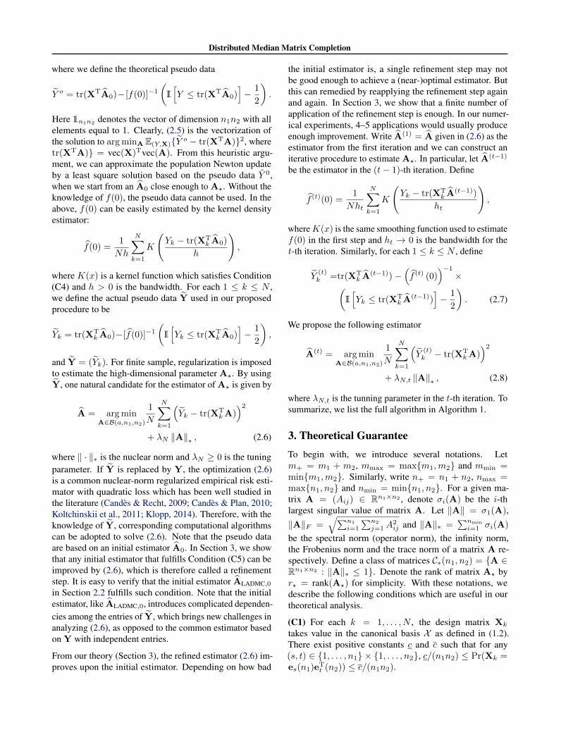
Here 1n1n2 denotes the vector of dimension n1n2 with allelements equal to 1. Clearly, (2.5) is the vectorization ofthe solution to arg minA E(Y,X)Y o − tr(XTA)2, wheretr(XTA) = vec(X)Tvec(A). From this heuristic argu-ment, we can approximate the population Newton updateby a least square solution based on the pseudo data Y 0,when we start from an A0 close enough to A?. Without theknowledge of f(0), the pseudo data cannot be used. In theabove, f(0) can be easily estimated by the kernel densityestimator:

f(0) =1

Nh

N∑k=1

K

(Yk − tr(XT

k A0)

h

),

where K(x) is a kernel function which satisfies Condition(C4) and h > 0 is the bandwidth. For each 1 ≤ k ≤ N ,we define the actual pseudo data Y used in our proposedprocedure to be

Yk = tr(XTk A0)−[f(0)]−1

(I[Yk ≤ tr(XT

k A0)]− 1

2

),

and Y = (Yk). For finite sample, regularization is imposedto estimate the high-dimensional parameter A?. By usingY, one natural candidate for the estimator of A? is given by

A = arg minA∈B(a,n1,n2)

1

N

N∑k=1

(Yk − tr(XT

kA))2

+ λN ‖A‖∗ , (2.6)

where ‖ · ‖∗ is the nuclear norm and λN ≥ 0 is the tuningparameter. If Y is replaced by Y, the optimization (2.6)is a common nuclear-norm regularized empirical risk esti-mator with quadratic loss which has been well studied inthe literature (Candes & Recht, 2009; Candes & Plan, 2010;Koltchinskii et al., 2011; Klopp, 2014). Therefore, with theknowledge of Y, corresponding computational algorithmscan be adopted to solve (2.6). Note that the pseudo dataare based on an initial estimator A0. In Section 3, we showthat any initial estimator that fulfills Condition (C5) can beimproved by (2.6), which is therefore called a refinementstep. It is easy to verify that the initial estimator ALADMC,0in Section 2.2 fulfills such condition. Note that the initialestimator, like ALADMC,0, introduces complicated dependen-cies among the entries of Y, which brings new challenges inanalyzing (2.6), as opposed to the common estimator basedon Y with independent entries.

From our theory (Section 3), the refined estimator (2.6) im-proves upon the initial estimator. Depending on how bad

the initial estimator is, a single refinement step may notbe good enough to achieve a (near-)optimal estimator. Butthis can remedied by reapplying the refinement step againand again. In Section 3, we show that a finite number ofapplication of the refinement step is enough. In our numer-ical experiments, 4–5 applications would usually produceenough improvement. Write A(1) = A given in (2.6) as theestimator from the first iteration and we can construct aniterative procedure to estimate A?. In particular, let A(t−1)

be the estimator in the (t− 1)-th iteration. Define

f (t)(0) =1

Nht

N∑k=1

K

(Yk − tr(XT

k A(t−1))

ht

),

whereK(x) is the same smoothing function used to estimatef(0) in the first step and ht → 0 is the bandwidth for thet-th iteration. Similarly, for each 1 ≤ k ≤ N , define

Y(t)k =tr(XT

k A(t−1))−(f (t) (0)

)−1×(

I[Yk ≤ tr(XT

k A(t−1))]− 1

2

). (2.7)

We propose the following estimator

A(t) = arg minA∈B(a,n1,n2)

1

N

N∑k=1

(Y

(t)k − tr(XT

kA))2

+ λN,t ‖A‖∗ , (2.8)

where λN,t is the tunning parameter in the t-th iteration. Tosummarize, we list the full algorithm in Algorithm 1.

3. Theoretical GuaranteeTo begin with, we introduce several notations. Letm+ = m1 + m2, mmax = maxm1,m2 and mmin =minm1,m2. Similarly, write n+ = n1 + n2, nmax =maxn1, n2 and nmin = minn1, n2. For a given ma-trix A = (Aij) ∈ Rn1×n2 , denote σi(A) be the i-thlargest singular value of matrix A. Let ‖A‖ = σ1(A),

‖A‖F =√∑n1

i=1

∑n2

j=1A2ij and ‖A‖∗ =

∑nmin

i=1 σi(A)

be the spectral norm (operator norm), the infinity norm,the Frobenius norm and the trace norm of a matrix A re-spectively. Define a class of matrices C∗(n1, n2) = A ∈Rn1×n2 : ‖A‖∗ ≤ 1. Denote the rank of matrix A? byr? = rank(A?) for simplicity. With these notations, wedescribe the following conditions which are useful in ourtheoretical analysis.

(C1) For each k = 1, . . . , N , the design matrix Xk

takes value in the canonical basis X as defined in (1.2).There exist positive constants c and c such that for any(s, t) ∈ 1, . . . , n1 × 1, . . . , n2, c/(n1n2) ≤ Pr(Xk =es(n1)eT

t (n2)) ≤ c/(n1n2).


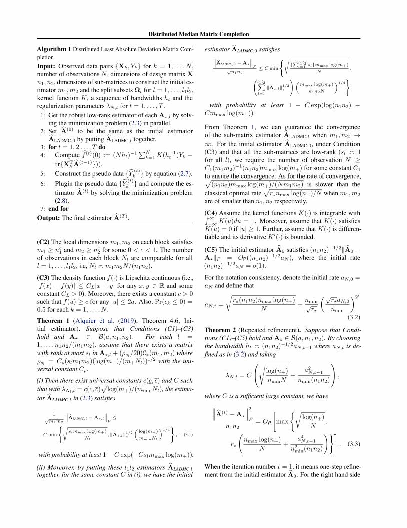
Algorithm 1 Distributed Least Absolute Deviation Matrix Com-pletion

Input: Observed data pairs Xk, Yk for k = 1, . . . , N ,number of observations N , dimensions of design matrix Xn1, n2, dimensions of sub-matrices to construct the initial es-timator m1,m2 and the split subsets Ωl for l = 1, . . . , l1l2,kernel function K, a sequence of bandwidths ht and theregularization parameters λN,t for t = 1, . . . , T .

1: Get the robust low-rank estimator of each A?,l by solv-ing the minimization problem (2.3) in parallel.

2: Set A(0) to be the same as the initial estimatorALADMC,0 by putting ALADMC,l together.

3: for t = 1, 2 . . . , T do4: Compute f (t)(0) := (Nht)

−1∑Nk=1K(h−1t (Yk −

trXTk A(t−1))).

5: Construct the pseudo data Y (t)k by equation (2.7).

6: Plugin the pseudo data Y (t)k and compute the es-

timator A(t) by solving the minimization problem(2.8).

7: end forOutput: The final estimator A(T ).

(C2) The local dimensions m1,m2 on each block satisfiesm1 ≥ nc1 and m2 ≥ nc2 for some 0 < c < 1. The numberof observations in each block Nl are comparable for alll = 1, . . . , l1l2, i.e, Nl m1m2N/(n1n2).

(C3) The density function f(·) is Lipschitz continuous (i.e.,|f(x) − f(y)| ≤ CL|x − y| for any x, y ∈ R and someconstant CL > 0). Moreover, there exists a constant c > 0such that f(u) ≥ c for any |u| ≤ 2a. Also, Pr(εk ≤ 0) =0.5 for each k = 1, . . . , N .

Theorem 1 (Alquier et al. (2019), Theorem 4.6, Ini-tial estimator). Suppose that Conditions (C1)–(C3)hold and A? ∈ B(a, n1, n2). For each l =1, . . . , n1n2/(m1m2), assume that there exists a matrixwith rank at most sl in A?,l + (ρsl/20)C∗(m1,m2) whereρsl = Cρ(slm1m2)(log(m+)/(m+Nl))

1/2 with the uni-versal constant Cρ.

(i) Then there exist universal constants c(c, c) and C suchthat with λNl,l = c(c, c)

√log(m+)/(mminNl), the estima-

tor ALADMC,l in (2.3) satisfies

1√m1m2

∥∥∥ALADMC,l −A?,l

∥∥∥F≤

Cmin

√slmmax log(m+)

Nl

, ‖A?,l‖1/2∗

(log(m+)

mminNl

)1/4

, (3.1)

with probability at least 1− C exp(−Cslmmax log(m+)).

(ii) Moreover, by putting these l1l2 estimators ALADMC,ltogether, for the same constant C in (i), we have the initial

estimator ALADMC,0 satisfies∥∥∥ALADMC,0 −A?

∥∥∥F√

n1n2

≤ Cmin

√∑l1l2

l=1 slmmax log(m+)

N,

l1l2∑l=1

‖A?,l‖1/2∗

(mmax log(m+)

n1n2N

)1/4

,

with probability at least 1 − C exp(log(n1n2) −Cmmax log(m+)).

From Theorem 1, we can guarantee the convergenceof the sub-matrix estimator ALADMC,l when m1,m2 →∞. For the initial estimator ALADMC,0, under Condition(C3) and that all the sub-matrices are low-rank (sl 1for all l), we require the number of observation N ≥C1(m1m2)−1(n1n2)mmax log(m+) for some constant C1

to ensure the convergence. As for the rate of convergence,√(n1n2)mmax log(m+)/(Nm1m2) is slower than the

classical optimal rate√r?nmax log(n+)/N when m1,m2

are of smaller than n1, n2 respectively.

(C4) Assume the kernel functions K(·) is integrable with∫∞−∞K(u)du = 1. Moreover, assume that K(·) satisfiesK(u) = 0 if |u| ≥ 1. Further, assume that K(·) is differen-tiable and its derivative K ′(·) is bounded.

(C5) The initial estimator A0 satisfies (n1n2)−1/2‖A0 −A?‖F = OP((n1n2)−1/2aN ), where the initial rate(n1n2)−1/2aN = o(1).

For the notation consistency, denote the initial rate aN,0 =aN and define that

aN,t =

√r?(n1n2)nmax log(n+)

N+nmin√r?

(√r?aN,0nmin

)2t

(3.2)

Theorem 2 (Repeated refinement). Suppose that Condi-tions (C1)–(C5) hold and A? ∈ B(a, n1, n2). By choosingthe bandwidth ht (n1n2)−1/2aN,t−1 where aN,t is de-fined as in (3.2) and taking

λN,t = C

√ log(n+)

nminN+

a2N,t−1nmin(n1n2)

,

where C is a sufficient large constant, we have∥∥∥A(t) −A?

∥∥∥2F

n1n2= OP

[max

√log(n+)

N,

r?

(nmax log(n+)

N+

a4N,t−1n2min(n1n2)

)]. (3.3)

When the iteration number t = 1, it means one-step refine-ment from the initial estimator A0. For the right hand side


of (3.3), it is noted that both the first term√

log(n+)/Nand the second term r?nmax log(n+)/N are seen in the er-ror bound of existing works (Elsener & van de Geer, 2018;Alquier et al., 2019). The bound has an extra third termr?a

4N,0/(n

2min(n1n2)) due to the initial estimator. After

one round of refinement, one can see that the third termr?a

4N,0/(n

2min(n1n2)) in (3.3) is faster than a2N,0/(n1n2),

the convergence rate of the initial estimator (see Condition(C5)), because r?n−2mina

2N,0 = o(1).

With the increasing of the iteration number t, Theorem 2shows that the estimator can be refined again and again,until near-optimal rate of convergence is achieved. It canbe shown that when the iteration number t exceeds certainnumber, i.e,

t ≥ log

log(r2?n

2max log(n+))− log(nminN)

c0 log(r?a2N,0)− 2c0 log(nmin)

/ log(2),

for some c0 > 0, the second term in the term associatedwith r? is dominated by the first term and the convergencerate of A(t) becomes r?nmaxN

−1 log(n+) which is thenear-optimal rate r?nmaxN

−1 (optimal up to a logarithmicfactor). Note that the number of iteration t is usually smalldue to the logarithmic transformation.

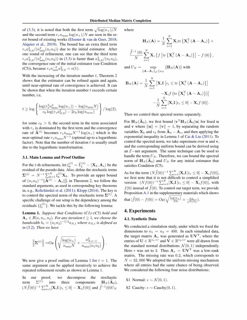
3.1. Main Lemma and Proof Outline

For the t-th refinements, let ξ(t)k = Y(t)k − 〈Xk,A?〉 be the

residual of the pseudo data. Also, define the stochastic termsΣ(t) = N−1

∑Nk=1 ξ

(t)k Xk. To provide an upper bound

of (n1n2)−1‖A(t) − A?‖2F in Theorem 2, we follow thestandard arguments, as used in corresponding key theoremsin, e.g., Koltchinskii et al. (2011); Klopp (2014). The key isto control the spectral norm of the stochastic term Σ(t). Aspecific challenge of our setup is the dependency among theresiduals ξ(t)i . We tackle this by the following lemma:

Lemma 1. Suppose that Conditions (C1)–(C5) hold andA? ∈ B(a, n1, n2). For any iteration t ≥ 1, we choose thebandwidth ht (n1n2)−1/2aN,t where aN,t is defined asin (3.2). Then we have

∥∥∥Σ(t)∥∥∥ =OP

√ log(n+)

nminN+

a2N,t−1nmin(n1n2)

.

We now give a proof outline of Lemma 1 for t = 1. Thesame argument can be applied iteratively to achieve therepeated refinement results as shown in Lemma 1.

In our proof, we decompose the stochasticterm Σ(1) into three components HN (A0),(Nf(0))−1

∑Ni=1[XiI [εi ≤ 0] − Xif(0)] and f−1(0)UN

where

HN (A) =1

N

N∑i=1

XitrXTi (A−A?)

+

f−1 (0)

N

N∑i=1

Xi

f[trXTi (A−A?)

]− f (0)

,

and UN = sup‖A−A?‖F≤aN

‖BN (A)‖ with

BN (A) =1

N

N∑i=1

[XiI

[εi ≤ tr

XTi (A−A?)

]−Xif

(trXTi (A−A?)

)]− 1

N

N∑i=1

[XiI [εi ≤ 0]−Xif (0)] .

Then we control their spectral norms separately.

For HN (A0), we first bound |vTHN (A0)u| for fixed uand v where ‖u‖ = ‖v‖ = 1, by separating the randomvariables Xk and εk from A0 −A?, and then applying theexponential inequality in Lemma 1 of Cai & Liu (2011). Tocontrol the spectral norm, we take supremum over u and v,and the corresponding uniform bound can be derived usingan E−net argument. The same technique can be used tohandle the term UN . Therefore, we can bound the spectralnorm of HN (A0) and UN for any initial estimator thatsatisfies Condition (C5).

As for the term (Nf(0))−1∑Ni=1[XiI [εi ≤ 0]−Xif(0)],

we first note that it is not difficult to control a simplifiedversion: (Nf(0))−1

∑Ni=1[XiI [εi ≤ 0] − Xif(0)], with

f(0) instead of f(0). To control our target term, we provideProposition A.1 in the supplementary materials which shows

that |f(0)− f(0)| = OP(√

log(n+)Nh + aN√

n1n2).

4. Experiments4.1. Synthetic Data

We conducted a simulation study, under which we fixed thedimensions to n1 = n2 = 400. In each simulated data,the target matrix A? was generated as UVT, where theentries of U ∈ Rn1×r and V ∈ Rn2×r were all drawn fromthe standard normal distributions N (0, 1) independently.Here r was set to 3. Thus A? = UVT was a low-rankmatrix. The missing rate was 0.2, which corresponds toN = 32, 000 We adopted the uniform missing mechanismwhere all entries had the same chance of being observed.We considered the following four noise distributions:

S1 Normal: ε ∼ N (0, 1).

S2 Cauchy: ε ∼ Cauchy(0, 1).


S3 Exponential: ε ∼ exp(1).

S4 t-distribution with degree of freedom 1: ε ∼ t1.

We note that Cauchy distribution is a very heavy-taileddistribution and its first moment (expectation) does not exist.For each of these four settings, we repeated the simulationfor 500 times.

Denote the proposed median MC proceduregiven in Algorithm 1 by DLADMC (DistributedLeast Absolute Deviations Matrix Completion).Due to Theorem 1(ii), ‖ALADMC,0 − A?‖F =

Op(√

(n1n2)2mmax log(m+)/(m1m2N)), we fixed

aN = aN,0 = c1

√(n1n2)2mmax log(m+)

m1m2N,

where the constant c1 = 0.1. From our experiences, smallerc1 leads to similar results. As h (n1n2)−1/2aN , thebandwidth h was simply set to h = c2(n1n2)−1/2aN , andsimilarly, ht = c2(n1n2)−1/2aN,t where aN,t was definedby (3.2) with c2 = 0.1. In addition, all the tuning parame-ters λN,t in Algorithm 1 were chosen by validation. Namely,we minimized the absolute deviation loss evaluated on anindependently generated validation sets with the same di-mensions n1, n2. For the choice of the kernel functionsK(·), we adopt the commonly used bi-weight kernel func-tion,

K(x) =

0, x ≤ −1

− 31564

x6 + 73564

x4 − 52564

x2 + 10564

, −1 ≤ x ≤ 1

0, x ≥ 1

.

It is easy to verify that K(·) satisfies Condition (C1) in Sec-tion 3. If we compute e = ‖A(t) − A(t−1)‖2F /‖A(t−1)‖2Fand stop the algorithm once e ≤ 10−5, it typically onlyrequires 4− 5 iterations. We simply report the results of theestimators with T = 4 or T = 5 iterations in Algorithm 1(depending on the noise distribution).

We compared the performance of the proposed method(DLADMC) with three other approaches:

(a) BLADMC: Blocked Least Absolute Deviation MatrixCompletion ALADMC,0, the initial estimator proposedin section 2.2. Number of row subsets l1 = 2, numberof column subsets l2 = 2.

(b) ACL: Least Absolute Deviation Matrix Completionwith nuclear norm penalty based on the computation-ally expensive ADMM algorithm proposed by Alquieret al. (2019).

c) MHT: The squared loss estimator with nuclear normpenalty proposed by Mazumder et al. (2010).

The tuning parameters in these four methods were chosenbased on the same validation set. We followed the selec-tion procedure in Section 9.4 of Mazumder et al. (2010) tochoose λ. Instead of fixing K to 1.5 or 2 as in Mazumderet al. (2010), we choose K by an additional pair of trainingand validation sets (aside from the 500 simulated datasets).We did this for every method to ensure a fair comparison.The performance of all the methods were evaluated via rootmean square error (RMSE) and mean absolute error (MAE).The estimated ranks are also reported.

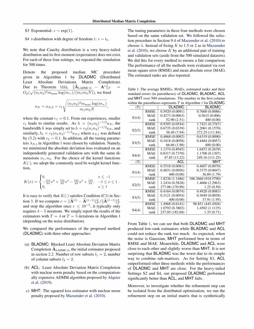
Table 1. The average RMSEs, MAEs, estimated ranks and theirstandard errors (in parentheses) of DLADMC, BLADMC, ACLand MHT over 500 simulations. The number in the first columnwithin the parentheses represents T in Algorithm 1 for DLADMC.

(T) DLADMC BLADMC

S1(4)

RMSE 0.5920 (0.0091) 0.7660 (0.0086)MAE 0.4273 (0.0063) 0.5615 (0.006)rank 52.90 (2.51) 400 (0.00)

S2(5)

RMSE 0.9395 (0.0544) 1.7421 (0.3767)MAE 0.6735 (0.0339) 1.2061 (0.1570)rank 36.49 (7.94) 272.25 (111.84)

S3(5)

RMSE 0.4868 (0.0092) 0.6319 (0.0090)MAE 0.3418 (0.0058) 0.4484 (0.0057)rank 66.66 (1.98) 400 (0.00)

S4(4)

RMSE 1.1374 (0.8945) 1.6453 (0.2639)MAE 0.8317 (0.7370) 1.1708 (0.1307)rank 47.85 (13.22) 249.16 (111.25)

(T) ACL MHT

S1(4)

RMSE 0.5518 (0.0081) 0.4607 (0.0070)MAE 0.4031 (0.0056) 0.3375 (0.0047)rank 400 (0.00) 36.89 (1.79)

S2(5)

RMSE 1.8236 (1.1486) 106.3660 (918.5790)MAE 1.2434 (0.5828) 1.4666 (2.2963)rank 277.08 (170.99) 1.25 (0.50)

S3(5)

RMSE 0.4164 (0.0074) 0.4928 (0.0083)MAE 0.3121 (0.0054) 0.3649 (0.0058)rank 400 (0.00) 37.91 (1.95)

S4(4)

RMSE 1.4968 (0.6141) 98.851 (445.4504)MAE 1.0792 (0.3803) 1.4502 (1.1135)rank 237.05 (182.68) 1.35 (0.71)

From Table 1, we can see that both DLADMC and MHTproduced low-rank estimators while BLADMC and ACLcould not reduce the rank too much. As expected, whenthe noise is Gaussian, MHT performed best in terms ofRMSE and MAE. Meanwhile, DLADMC and ACL wereclose to each other and slightly worse than MHT. It is notsurprising that BLADMC was the worst due to its simpleway to combine sub-matrices. As for Setting S3, ACLoutperformed other three methods while the performancesof DLADMC and MHT are close. For the heavy-tailedSettings S2 and S4, our proposed DLADMC performedsignificantly better than ACL, and MHT fails.

Moreover, to investigate whether the refinement step canbe isolated from the distributed optimization, we run therefinement step on an initial matrix that is synthetically


generated by making small noises to the ground-truth matrixA?, as suggested by a reviewer. We provide these results inSection B.1 of the supplementary material.

4.2. Real-World Data

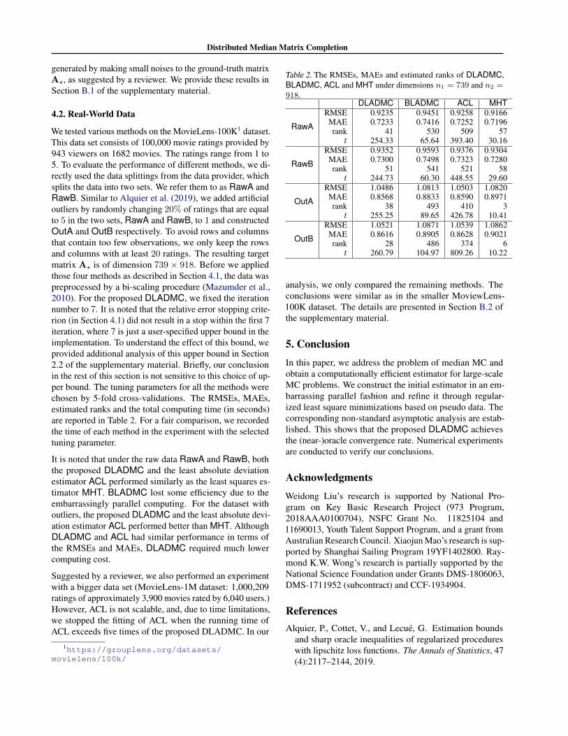
We tested various methods on the MovieLens-100K1 dataset.This data set consists of 100,000 movie ratings provided by943 viewers on 1682 movies. The ratings range from 1 to5. To evaluate the performance of different methods, we di-rectly used the data splittings from the data provider, whichsplits the data into two sets. We refer them to as RawA andRawB. Similar to Alquier et al. (2019), we added artificialoutliers by randomly changing 20% of ratings that are equalto 5 in the two sets, RawA and RawB, to 1 and constructedOutA and OutB respectively. To avoid rows and columnsthat contain too few observations, we only keep the rowsand columns with at least 20 ratings. The resulting targetmatrix A? is of dimension 739 × 918. Before we appliedthose four methods as described in Section 4.1, the data waspreprocessed by a bi-scaling procedure (Mazumder et al.,2010). For the proposed DLADMC, we fixed the iterationnumber to 7. It is noted that the relative error stopping crite-rion (in Section 4.1) did not result in a stop within the first 7iteration, where 7 is just a user-specified upper bound in theimplementation. To understand the effect of this bound, weprovided additional analysis of this upper bound in Section2.2 of the supplementary material. Briefly, our conclusionin the rest of this section is not sensitive to this choice of up-per bound. The tuning parameters for all the methods werechosen by 5-fold cross-validations. The RMSEs, MAEs,estimated ranks and the total computing time (in seconds)are reported in Table 2. For a fair comparison, we recordedthe time of each method in the experiment with the selectedtuning parameter.

It is noted that under the raw data RawA and RawB, boththe proposed DLADMC and the least absolute deviationestimator ACL performed similarly as the least squares es-timator MHT. BLADMC lost some efficiency due to theembarrassingly parallel computing. For the dataset withoutliers, the proposed DLADMC and the least absolute devi-ation estimator ACL performed better than MHT. AlthoughDLADMC and ACL had similar performance in terms ofthe RMSEs and MAEs, DLADMC required much lowercomputing cost.

Suggested by a reviewer, we also performed an experimentwith a bigger data set (MovieLens-1M dataset: 1,000,209ratings of approximately 3,900 movies rated by 6,040 users.)However, ACL is not scalable, and, due to time limitations,we stopped the fitting of ACL when the running time ofACL exceeds five times of the proposed DLADMC. In our

1https://grouplens.org/datasets/movielens/100k/

Table 2. The RMSEs, MAEs and estimated ranks of DLADMC,BLADMC, ACL and MHT under dimensions n1 = 739 and n2 =918.

DLADMC BLADMC ACL MHT

RawA

RMSE 0.9235 0.9451 0.9258 0.9166MAE 0.7233 0.7416 0.7252 0.7196rank 41 530 509 57

t 254.33 65.64 393.40 30.16

RawB

RMSE 0.9352 0.9593 0.9376 0.9304MAE 0.7300 0.7498 0.7323 0.7280rank 51 541 521 58

t 244.73 60.30 448.55 29.60

OutA

RMSE 1.0486 1.0813 1.0503 1.0820MAE 0.8568 0.8833 0.8590 0.8971rank 38 493 410 3

t 255.25 89.65 426.78 10.41

OutB

RMSE 1.0521 1.0871 1.0539 1.0862MAE 0.8616 0.8905 0.8628 0.9021rank 28 486 374 6

t 260.79 104.97 809.26 10.22

analysis, we only compared the remaining methods. Theconclusions were similar as in the smaller MoviewLens-100K dataset. The details are presented in Section B.2 ofthe supplementary material.

5. ConclusionIn this paper, we address the problem of median MC andobtain a computationally efficient estimator for large-scaleMC problems. We construct the initial estimator in an em-barrassing parallel fashion and refine it through regular-ized least square minimizations based on pseudo data. Thecorresponding non-standard asymptotic analysis are estab-lished. This shows that the proposed DLADMC achievesthe (near-)oracle convergence rate. Numerical experimentsare conducted to verify our conclusions.

AcknowledgmentsWeidong Liu’s research is supported by National Pro-gram on Key Basic Research Project (973 Program,2018AAA0100704), NSFC Grant No. 11825104 and11690013, Youth Talent Support Program, and a grant fromAustralian Research Council. Xiaojun Mao’s research is sup-ported by Shanghai Sailing Program 19YF1402800. Ray-mond K.W. Wong’s research is partially supported by theNational Science Foundation under Grants DMS-1806063,DMS-1711952 (subcontract) and CCF-1934904.

ReferencesAlquier, P., Cottet, V., and Lecue, G. Estimation bounds

and sharp oracle inequalities of regularized procedureswith lipschitz loss functions. The Annals of Statistics, 47(4):2117–2144, 2019.

https://grouplens.org/datasets/movielens/100k/

https://grouplens.org/datasets/movielens/100k/


Bach, F. R. Consistency of trace norm minimization. Jour-nal of Machine Learning Research, 9(Jun):1019–1048,2008.

Bennett, J. and Lanning, S. The netflix prize. In Proceedingsof KDD cup and workshop, volume 2007, pp. 35, 2007.

Cai, T. T. and Liu, W. Adaptive thresholding for sparsecovariance matrix estimation. Journal of the AmericanStatistical Association, 106(494):672–684, 2011.

Cai, T. T. and Zhou, W.-X. Matrix completion via max-normconstrained optimization. Electronic Journal of Statistics,10(1):1493–1525, 2016.

Candes, E. J. and Plan, Y. Matrix completion with noise.Proceedings of the IEEE, 98(6):925–936, 2010.

Candes, E. J. and Recht, B. Exact matrix completion via con-vex optimization. Foundations of Computational Mathe-matics, 9(6):717–772, 2009.

Candes, E. J. and Tao, T. The power of convex relaxation:Near-optimal matrix completion. Information Theory,IEEE Transactions on, 56(5):2053–2080, 2010.

Candes, E. J., Li, X., Ma, Y., and Wright, J. Robust principalcomponent analysis? Journal of the ACM (JACM), 58(3):11, 2011.

Chandrasekaran, V., Sanghavi, S., Parrilo, P. A., and Willsky,A. S. Rank-sparsity incoherence for matrix decomposi-tion. SIAM Journal on Optimization, 21(2):572–596,2011.

Chen, X., Liu, W., Mao, X., and Yang, Z. Distributed high-dimensional regression under a quantile loss function.arXiv preprint arXiv:1906.05741, 2019a.

Chen, Y., Xu, H., Caramanis, C., and Sanghavi, S. Robustmatrix completion and corrupted columns. In Proceed-ings of the 28th International Conference on MachineLearning (ICML-11), pp. 873–880, 2011.

Chen, Y., Jalali, A., Sanghavi, S., and Caramanis, C. Low-rank matrix recovery from errors and erasures. IEEETransactions on Information Theory, 59(7):4324–4337,2013.

Chen, Y., Chi, Y., Fan, J., Ma, C., and Yan, Y. Noisymatrix completion: Understanding statistical guaranteesfor convex relaxation via nonconvex optimization. arXivpreprint arXiv:1902.07698, 2019b.

Chen, Y., Fan, J., Ma, C., and Yan, Y. Bridging convexand nonconvex optimization in robust pca: Noise, out-liers, and missing data. arXiv preprint arXiv:2001.05484,2020.

Davies, P. L. Aspects of robust linear regression. The Annalsof statistics, 21(4):1843–1899, 1993.

Elsener, A. and van de Geer, S. Robust low-rank matrixestimation. The Annals of Statistics, 46(6B):3481–3509,2018.

Fan, J., Gong, W., and Zhu, Z. Generalized high-dimensional trace regression via nuclear norm regulariza-tion. Journal of Econometrics, 212(1):177–202, 2019.

Gross, D. Recovering low-rank matrices from few coeffi-cients in any basis. Information Theory, IEEE Transac-tions on, 57(3):1548–1566, 2011.

Huber, P. J. Robust statistics. Springer, 2011.

Keshavan, R. H., Montanari, A., and Oh, S. Matrix com-pletion from noisy entries. Journal of Machine LearningResearch, 11(69):2057–2078, 2010.

Klopp, O. Noisy low-rank matrix completion with generalsampling distribution. Bernoulli, 20(1):282–303, 2014.

Klopp, O., Lounici, K., and Tsybakov, A. B. Robust matrixcompletion. Probability Theory and Related Fields, 169(1-2):523–564, 2017.

Koltchinskii, V., Lounici, K., and Tsybakov, A. B. Nuclear-norm penalization and optimal rates for noisy low-rankmatrix completion. The Annals of Statistics, 39(5):2302–2329, 2011.

Lafond, J. Low rank matrix completion with exponentialfamily noise. In Conference on Learning Theory, pp.1224–1243, 2015.

Li, X. Compressed sensing and matrix completion withconstant proportion of corruptions. Constructive Approx-imation, 37(1):73–99, 2013.

Mackey, L., Talwalkar, A., and Jordan, M. I. Distributedmatrix completion and robust factorization. Journal ofMachine Learning Research, 16(28):913–960, 2015.

Mazumder, R., Hastie, T., and Tibshirani, R. Spectral reg-ularization algorithms for learning large incomplete ma-trices. Journal of Machine Learning Research, 11(80):2287–2322, 2010.

Negahban, S. and Wainwright, M. J. Estimation of (near)low-rank matrices with noise and high-dimensional scal-ing. The Annals of Statistics, 39(2):1069–1097, 2011.

Negahban, S. and Wainwright, M. J. Restricted strong con-vexity and weighted matrix completion: Optimal boundswith noise. Journal of Machine Learning Research, 13(53):1665–1697, 2012.


Rohde, A. and Tsybakov, A. B. Estimation of high-dimensional low-rank matrices. The Annals of Statistics,39(2):887–930, 2011.

Srebro, N., Rennie, J., and Jaakkola, T. S. Maximum-marginmatrix factorization. In Advances in neural informationprocessing systems, pp. 1329–1336, 2005.

Wong, R. K. W. and Lee, T. C. M. Matrix completion withnoisy entries and outliers. Journal of Machine LearningResearch, 18(147):1–25, 2017.

Xia, D. and Yuan, M. Statistical inferences of linearforms for noisy matrix completion. arXiv preprintarXiv:1909.00116, 2019.

Documents

Median Matrix Completion: from Embarrassment to Optimality