Embed Size (px)
Citation preview
Journal of Mathematical Economics 20 (1991) 155-180. North-Holland
Optimal growth and Pareto optimality
Rose-Anne Dana
VniversitP Paris-VI, 75252 Paris, France
Cuong Le Van
CNRS-CEPREMAP, 75013, Paris, France
Submitted January 1989, accepted August 1989
The purpose of this paper is to show that in a stationary intertemporal economy where agents have recursive utilities every Pareto optimum is a solution of a generalized McKenzie problem. An ‘abstract’ state space is introduced as the space of couples of capital stock and utilities that can be reached by n- 1 agents from that capital stock. ‘Generalized technological’ conditions are then defined on that abstract space as well as a recursive criterion on sequences of its elements. The criterion generalizes the additively separable one. As Bellman’s and Euler’s equations still hold, many dynamical results known for the additively separable one-agent case can be generalized.
1. Introduction
The purpose of this paper is to provide a framework to discuss the dynamic properties, stability and unstability of the equilibria of a stationary intertemporal economy. As equilibria are Pareto optima, we shall first study their dynamic properties, avoiding multiplicity problems. We use here the same approach as McKenzie-Montrucchio for optimal growth. We show that the study of the dynamic properties of Pareto optima can be reduced to that of a well-defined map defined on the space of capital stock and utilities that can be reached by n- 1 agents.
We consider an economy where a finite number of infinitely lived agents live for an infinite number of discrete periods. The set of goods producible at each date is invariant in time and depends only on capital stocks available in the previous period. Agents have stationary utilities rather than additively separable utilities. These utilities are usually called ‘recursive utilities’ in the literature.
In the last few years a great deal of attention has been focused on ‘recursive utilities’. Roughly speaking papers can be classified in two catego- ries. The first, which follows Koopmans’ early work [Koopmans (1960),
0304-4068/91/%03.50 0 1991-Elsevier Science Publishers B.V. (North-Holland)
156 R.-A. Dana and C. Le Van, Optimal growth and Pareto optimality
Koopmans et al. (1964)] is concerned with the axiomatics of preferences leading to a ‘recursive’ representation of utilities [for example, Streufert (1986a)]. The second tries to describe the dynamic properties of models where one or several agents have recursive preferences [Koopmans et al. (1964), Iwai (1972), Lucas and Stokey (1984), Benhabib, Majumdar and Nishimura (1985) Benhabib, Jafarey and Nishimura (1985), Epstein (1987a, b), Boyd (1986)]. We carry on this work one step further in a more genera1 setting (e.g. we use many consumption goods). In particular, it has been shown by Lucas and Stokey (1984), Dana and Le Van (1987), Epstein (1987a) that a Pareto-optima1 allocation could be viewed as a function of the trajectory of a dynamic system on the product of the capita1 space by the simplex. This approach uses the characterization of a Pareto optimum as the maximizer of a weighted sum of the utilities of the different agents. Unless agents have separable utilities, this approach does not seem to be very tractable because the dynamic system involved is not characterized simply. The methods that have been used in the one-agent separable case do not trivially carry over. Concurrently, Benhabib, Jafarey and Nishimura (1985) and Epstein (1987b) defined a dynamic system on the set of couples of capita1 stock and utilities that can be reached by n- 1 agents from that capita1 stock. They used the fact that a Pareto optimum maximizes the utility of one agent given that his (her) utility and the others’ utilities are attainable. This paper builds on this second approach.
In order to construct and characterize the dynamic system we eliminate consumption variables. We show that the search for Pareto optima of a stationary intertemporal economy where agents have recursive utilities can be transformed into a generalized McKenzie problem with recursive criter- ion. This result is well known in the case of additively separable utilities and same discount factor and is obtained using weights. It is far from being obvious in the genera1 case.
As it is well known, McKenzie’s mode1 has played a key role in the study of the dynamic properties of optima1 paths in the neoclassical theory of growth. It has been used to obtain turnpike results [McKenzie (1985), Scheinkman (1976)], cycle results [Benhabib and Nishimura (1985)]. More recently Boldrin and Montrucchio (1986), Deneckere and Pelikan (1986) have used it to show that the dynamics of optima1 growth paths could be arbitrarily complex. Two tools have been used, Bellman’s and Euler’s equations.
As in our generalized McKenzie problem Bellman’s and Euler’s equations still hold, we provide a framework to generalize the dynamic results that have been obtained for the one-agent, additively separable case. In particular we give turnpike theorems leaving to further work the study of unstability results (e.g. cycles, chaos).
The paper is organized as follows:
R.-A. Dana and C. Le Van, Optimal growth and Pareto optimality 157
In section 2 we recall the axiomatics of recursive utilities. This section generalizes the findings of Koopmans et al. (1964) and Lucas and Stokey (1984).
In section 3 we introduce a generalized version of McKenzie’s model and extend a few dynamical results of optimal paths [e.g. Mangasarian’s result (1966), stability results].
In section 4 we show that every Pareto optimum is a solution of a generalized McKenzie’s model. An ‘abstract’ state space is introduced as the space of couples of capital stock and utilities that can be reached by n- 1 agents from that capital stock. ‘Generalized technological’ conditions are then defined on that abstract space as well as a recursive criterion on sequences of its elements. We then use the dynamic results of section 3 to give properties of examples studied in the literature [Benhabib, Jafarey and Nishimura (1985), Lucas and Stokey (1984)].
2. Recursive representation
Following Beals and Koopmans (1969) and Lucas and Stokey (1984), we introduce an uggregator function defined as follows.
Definition I. Let 4 be an integer. Let C be a closed convex set of R?+. A function W from C x R, into R + is an aggregator function if it satisfies the following properties:
W.I. Continuous; 3M > 0 such that W(x, 0) 5 M, Vx E C;
W.2. Concave;
W.3. 3/?~[0, l[ such that IW(x,z)- W(x,z’)lsfi[z-z’l, VXEC, Vz, VZ’ER.;
w.4. z < z’* W(x, z) 5 W(x, z’), vx E c.
Let X be the space (R”,)” endowed with the product topology. An element in X is denoted by x=(x0,x1...). Let L denote the shift operator on X, i.e. Lx=(xl,x2,...).
Let Q be a closed convex, L-invariant subset of X; S will denote the space of bounded continuous functions from Q into R, endowed with the sup-norm, llull =~up,~cu(x). Let f,: X+(Ry)‘+l be the map x+(x0,x1,. . . ,x,) and let C=f,(Q).
We have the following theorem:
Theorem 2.1. With every aggregator W defined on C x R, one can associate an operator on S as follows:
TwW = WM u(W). (2.1)
158 R.-A. Dana and C. Lx Van, Optimal growth and Pareto optimality
Tw is a contraction. Hence there exists a unique u, which is concave, such that:
vx~ Q, W=Wfi(~),&W). (2.2)
Proof. Let T, be defined by (2.1). Then T,u belongs to S since it is continuous and bounded on Q; indeed by W.l and W.3:
By W.3, Tw is a /I-contraction on S. The unique fixed point since, under W.2 and W.4, T, maps concave functions selves. Q.E.D.
Let us introduce the following axioms:
(2.3)
24 is concave into them-
W.2. bis. W is concave and for every z, W( ., z) is strictly concave.
W.4. bis. (x, z) #(x’, z’) and (x, z) 5(x’, z’) implies W(x, z) < W(x’, z’).
W.5. OEC and W(O,O)=O.
The following proposition is proved in Dana and Le Van (1990).
Proposition 2.1. (a) If W satisfies W.l, W.2bis. W.3, W.4bis, then u is strictly concave. (b) If W satisfies W.1, W.2, W.3, W.4 bis, then u is increasing. (c) If W satisfies W.I-W.5, then u(O) =O.
Example 2.1: The discounted case. Let Q=X: then C=(Rm+)*+l. Let v= C-CO, l] be any continuous concave function. Let W: C x R, +R+ be defined by
W(XO,Xl,..., x,;z)=v(xo,xl )...) x,)+Pz, PEP, 1c. (2.4)
Then W is an aggregator and the unique fixed point of T, is
u(x)= f /jfv(x,,x,+1,..., x,+A. (2.5) t=o
For r = 0, we obtain the utility of a sequence of consumptions. For r= 1, we find again the utility of a sequence of capital stocks as in
McKenzie reduced form.
R.-A. Dana and C. Lx Van, Optimal growth and Pareto optimality 159
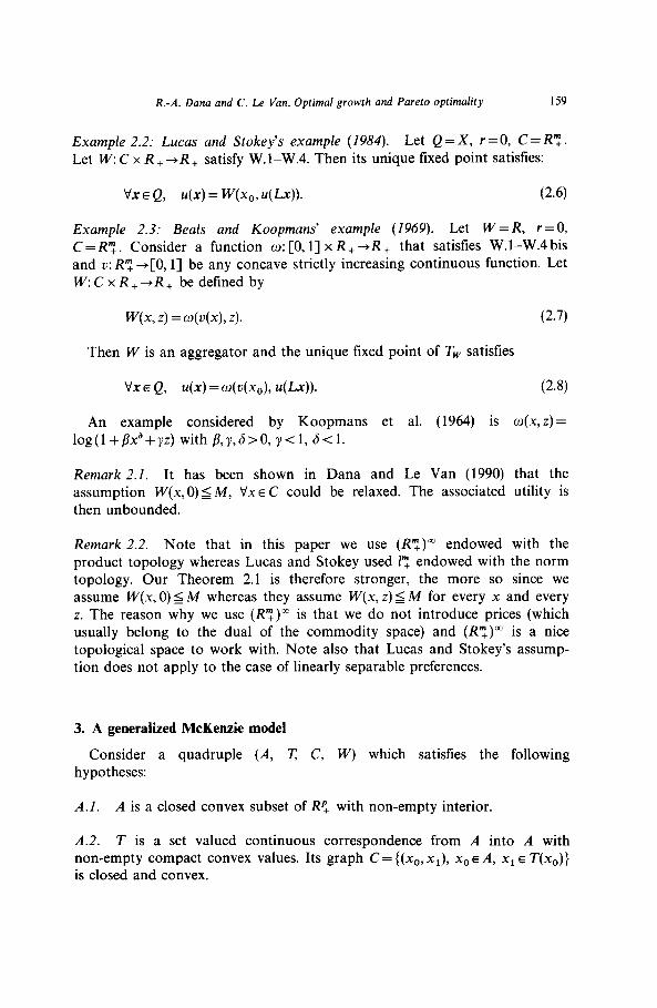
Example 2.2: Lucas and Stokey’s example (1984). Let Q =X, r = 0, C = R”, . Let W: C x R, +R + satisfy W.l-W.4. Then its unique fixed point satisfies:
Vx E Q, u(x) = W(x,, u(Lx)). (2.6)
Example 2.3: Beals and Koopmans’ example (1969). Let W = R, r = 0, C = R”, . Consider a function w: [0, l] x R + +R + that satisfies W.l-W.4 bis and u: R”, --+[O, l] be any concave strictly increasing continuous function. Let W:Cx R++R, be defined by
W(x, z) = o(u(x), z).
Then W is an aggregator and the unique fixed point of T, satisfies
VXEQ, u(x)=o(u(x,,), u(Lx)).
(2.7)
(2.8)
An example considered by Koopmans et al. (1964) is o(x, z) =
log(l+/?x’+yz) with p,y,6>0, y<l, 6~1.
Remark 2.1. It has been shown in Dana and Le Van (1990) that the assumption W(x,O)s M, Vx E C could be relaxed. The associated utility is then unbounded.
Remark 2.2. Note that in this paper we use (R”,)” endowed with the product topology whereas Lucas and Stokey used I”, endowed with the norm topology. Our Theorem 2.1 is therefore stronger, the more so since we assume W(x, 0) s M whereas they assume W(x, z) 5 M for every x and every z. The reason why we use (Ry)” is that we do not introduce prices (which usually belong to the dual of the commodity space) and (R”,)” is a nice topological space to work with. Note also that Lucas and Stokey’s assump- tion does not apply to the case of linearly separable preferences.
3. A generalized McKenzie model
Consider a quadruple (A, 7; C, W) which satisfies the following hypotheses:
A.1. A is a closed convex subset of RP, with non-empty interior.
A.2. T is a set valued continuous correspondence from A into A with non-empty compact convex values. Its graph C = {(x,, xi), x0 E A, x1 E T(x,)} is closed and convex.
160 R.-A. Dana and C. Le Van, Optimal growth and Pareto optimality
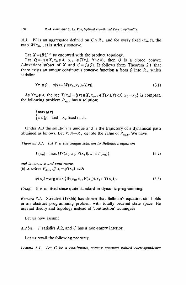
A.3. W is an aggregator defined on C x R, and for every fixed (x,,z), the map II+,, . , z) is strictly concave.
Let X=(Rp+)a, be endowed with the product topology. Let Q={~EX,X~EA, x~+~ E T(x,), Vt ZO}, then Q is a closed convex
L-invariant subset of X and C=fr(Q). It follows from Theorem 2.1 that there exists an unique continuous concave function u from Q into R, which satisfies:
t/x E Q, u(x) = W(x,, x1, u(Lx)). (3.1)
As VX,, E A, the set X(X,) = {(x) E X, x,, 1 E T(x,), Vt 2 0, x0 =X0> is compact, the following problem P,,,. has a solution:
max u(x)
XEQ, and x0 fixed in A.
Under A.3 the solution is unique and is the trajectory of a dynamical path obtained as follows. Let 1/: A+R+ denote the value of P,,,,. We have
Theorem 3.1. (a) V is the unique solution to Bellman’s equation
(3.2)
and is concave and continuous. (b) x solves P,,,, iff x, = t,Y(x,) with
Il/(xo) =aw max {W(xo,xl. V(xd), x1 E W,)). (3.3)
Proof: It is omitted since quite standard in dynamic programming.
Remark 3.1. Streufert (1986b) has shown that Bellman’s equation still holds in an abstract programming problem with totally ordered state space. He uses set theory and topology instead of ‘contraction’ techniques
Let us now assume
A.2bis. T satisfies A.2, and C has a non-empty interior.
Let us recall the following property.
Lemma 3.1. Let G be a continuous, convex compact valued correspondence
R.-A. Dana and C. Le Van, Optimal growth and Pareto optimality 161
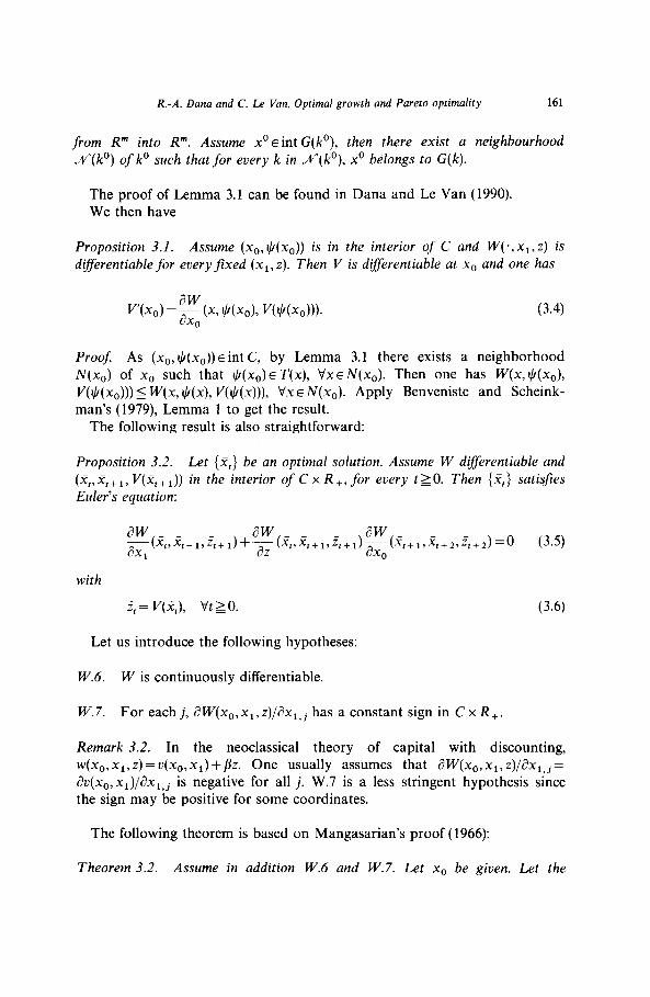
from R” into R”. Assume x0 dint G(k’), then there exist a neighbourhood N(kO) of k” such that for every k in N(k’), x0 belongs to G(k).
The proof of Lemma 3.1 can be found in Dana and Le Van (1990). We then have
Proposition 3.1. Assume (x0,$(x0)) . 1s in the interior of C and W( ., x1, z) is differentiable for everyfixed (x,,z). Then V is differentiable at x0 and one has
V(x0) =g (x9 $(x0), V($(xo))). (3.4) 0
Proof: As (xo,~(xo)) lint C, by Lemma 3.1 there exists a neighborhood N(x,) of x0 such that $(x~)E T(x), VXEN(X~). Then one has W(x, $(x0), V($(x,))) 5 W(x, t,+(x), V($(x))), Vx E N(x,). Apply Benveniste and Scheink- man’s (1979) Lemma 1 to get the result.
The following result is also straightforward:
Proposition 3.2. Let {X,} be an optimal solution. Assume W differentiable and
(%-%+I, V(%+,)) in the interior of C x R +, for every t 2 0. Then {&} satisfies Euler’s equation:
with
i;= V(X,), vtzo.
Let us introduce the following hypotheses:
W.6. W is continuously differentiable.
W.7. For each j, ~W(X~,X,,Z)/I~X,,~ has a constant sign in C x R,.
(3.5)
(3.6)
Remark 3.2. In the neoclassical theory of capital with discounting, w(x,, x,,z) =v(xo,xl) +flz. One usually assumes that 13W(x,, x1, z)/~x,,~= &I(x,,x,)/~x,,~ is negative for all j. W.7 is a less stringent hypothesis since the sign may be positive for some coordinates.
The following theorem is based on Mangasarian’s proof (1966):
Theorem 3.2. Assume in addition W.6 and W.7. Let x0 be given. Let the
162 R.-A. Dana and C. L_e Van, Optimal growth and Pareto optimality
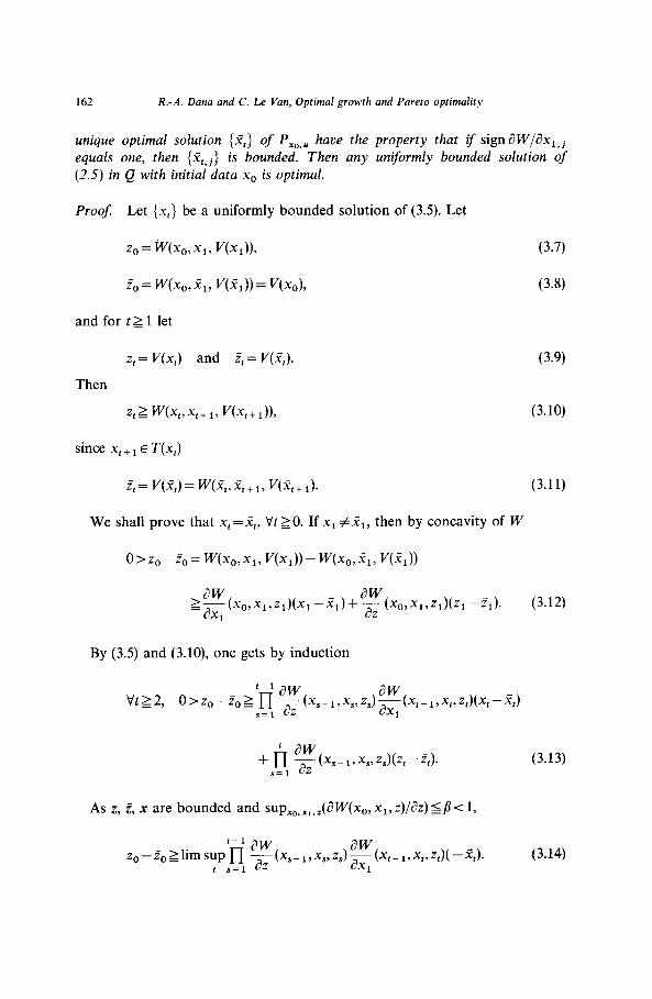
unique optimal solution {&} of P,,,. have the property that ij- sign awl&z,, j equals one, then {z?~,~} is bounded. Then any un$ormly bounded solution of (2.5) in Q with initial data x0 is optimal.
Proof Let {xt} be a uniformly bounded solution of (3.5). Let
zo = wxo, Xl, Vx,)), (3.7)
50 = wxo, 21, KG)) = Vxo), (3.8)
and for t 2 1 let
z, = V(x,) and i; = V(X,).
Then
z,L wb,,x,+l~ wG.l)),
since x,, 1 E T(x,)
(3.9)
(3.10)
z*= V(X,)= W(X,,X,+,, V(X,,l). (3.11)
We shall prove that x,=X,, Vt 2 0. If x1 #X1, then by concavity of W
L~(xO,xl,zl)lxl-X1)+~(xO,X1,Z1)(Z1-Z1). (3.12) 1
By (3.5) and (3.10), one gets by induction
As z, Z, x are bounded and sup,,,,,,.(aW(xo,x,,z)/az)~p< 1,
zo-~o~limsup*~ ~~(x,_I.x,.z,)~(x,_I,xIIzI)(-XI). f s=l 1
(3.14)
R.-A. Dana and C. Lx Van, Optimal growth and Pareto optimality 163
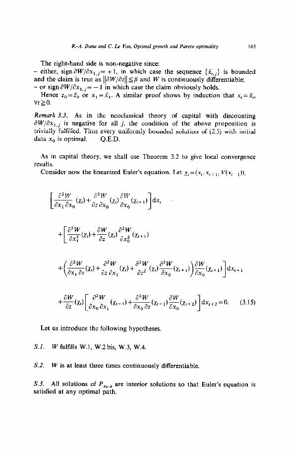
The right-hand side is non-negative since: - either, signaW/ax,,j= + 1, in which case the sequence {Zl,j} is bounded and the claim is true as /aW/dzll sfi and W is continuously differentiable; - or sign dW/ax,, j= - 1 in which case the claim obviously holds.
Hence zO = ZO or x1 =X1. A similar proof shows by induction that x, = Xt, vtzo.
Remark 3.3. As in the neoclassical theory of capital with discounting aW/ax,,j is negative for all j, the condition of the above proposition is trivially fulfilled. Thus every uniformly bounded solution of (2.5) with initial data x,, is optimal. Q.E.D..
As in capital theory, we shall use Theorem 3.2 to give local convergence results.
Consider now the linearized Euler’s equation. Let xr = (x,, xt+ 1, I/(x,+ 1)),
Let us introduce the following hypotheses.
S.I. W fulfills W.l, W.2bis, W.3, W.4.
S.2. W is at least three times continuously differentiable.
S.3. All solutions of P,,,. are interior solutions so that Euler’s equation is satisfied at any optimal path.
164 R.-A. Dana and C. Le Van, Optimal growth and Pareto optimality
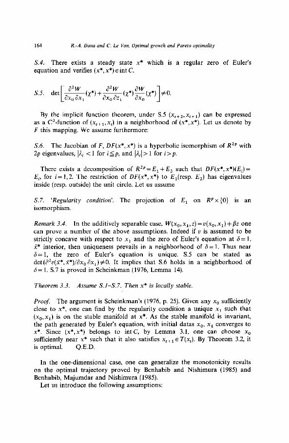
S.4. There exists a steady state x* which is a regular zero of Euler’s equation and verifies (x*,x*) E int C.
S.5. det ~(“*)+~(~*)~(X*)]#o~
By the implicit function theorem, under S.5 (x,+~,x,+~) can be expressed as a C2-function of (x, + i, x,) in a neighborhood of (x*,x*). Let us denote by F this mapping. We assume furthermore:
S.6. The Jacobian of F, DF(x*,x*) is a hyperbolic isomorphism of R2P with 2p eigenvalues, llzil < 1 for isp, and /Ail > 1 for i>p.
There exists a decomposition of R 2p = E, + E, such that DF(x*, x*)(Ei) = Ei, for i= 1,2. The restriction of DF(x*,x*) to E,(resp. E2) has eigenvalues inside (resp. outside) the unit circle. Let us assume
S.7. ‘Regularity condition’. The projection of E, on RP x {0} is an isomorphism.
Remark 3.4. In the additively separable case, W(x,, xi, z) = u(x,,, xi) +/?z one can prove a number of the above assumptions. Indeed if v is assumed to be strictly concave with respect to xi and the zero of Euler’s equation at 6= 1, X* interior, then uniqueness prevails in a neighborhood of 6= 1. Thus near 6= 1, the zero of Euler’s equation is unique. S.5 can be stated as det(#v(X*,X*)/ax, ax,)#O. It implies that S.6 holds in a neighborhood of 6= 1. S.7 is proved in Scheinkman (1976, Lemma 14).
Theorem 3.3. Assume S.I-S.7. Then x* is locally stable.
Proof. The argument is Scheinkman’s (1976, p. 25). Given any x0 sufficiently close to x*, one can find by the regularity condition a unique xi such that (x0,x,) is on the stable manifold at x *. As the stable manifold is invariant, the path generated by Euler’s equation, with initial datas x0, xi converges to x*. Since (x*,x*) belongs to int C, by Lemma 3.1, one can choose x0 sufficiently near x* such that it also satisfies x,, 1 E T(x,). By Theorem 3.2, it is optimal. Q.E.D.
In the one-dimensional case, one can generalize the monotonicity results on the optimal trajectory proved by Benhabib and Nishimura (1985) and Benhabib, Majumdar and Nishimura (1985).
Let us introduce the following assumptions:
R.-A. Dana and C. Lx Van, Optimal growth and Pareto optimality 165
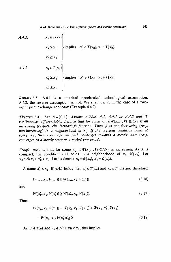
A.4.1. x1 E T(x,)l
x;sx, I implies xi E T(x,), x1 E T(xb).
xb>,x()
A.4.2. Xl E Wo) 1 x; 2x1 I implies xi E T(x,), x1 E T(xb).
x;rx, J Remark 3.5. A.4.1 is a standard neoclassical technological assumption. A.4.2, the reverse assumption, is not. We shall use it in the case of a two- agent pure exchange economy (Example 4.4.2).
Theorem 3.4. Let A=[O,l]. Assume A.2bis, A.3, A.4.1 or A.4.2 and W continuously diflerentiable. Assume that for some x,,, aW(xO;, V(*))/ax, is an increasing (respectively decreasing) function. Then $ is non-decreasing (resp. non-increasing) in a neighborhood of x,,. Zf the previous condition holds at every X,, then every optimal path converges towards a steady state (resp. converges to a steady state or a period-two cycle).
Proof. Assume that for some x0, aW(x,;, V(+))/ax, is increasing. As A is compact, the condition still holds in a neighborhood of x0, N(x,). Let xb E N(x,), xb > x0. Let us denote x1 = t&x0), xi = +(xb).
Assume x’, <x1. If A.4.1 holds then x; E T(x,) and x1 E T(xb) and therefore:
w&3,x1, vx,))~wxo,x;, wl)) (3.16)
and
lVx;,x;, V(x>))Z W(xb,x1r Vx,)). (3.17)
Thus,
W(x,,x,, V(x,))- W(xb,x,, V(x,))+ w(xb?x;, V(x>)
- W(x,, x;, V(xi)) 20. (3.18)
As xi E T(u) and x1 E T(u), Vuzx,, this implies
166 R.-A. Dana and C. Le Van, Optimal growth and Pareto optimality
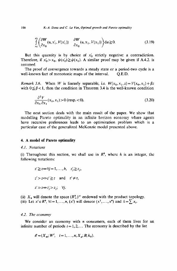
u,x;, l’(x;)) - $f&,x,. l’(x,)) duZ0. 0
(3.19)
But this quantity is by choice of xb strictly negative: a contradiction. Therefore, if xb>x,, tj(xb) 21,15(x~). A similar proof may be given if A.4.2. is assumed.
The proof of convergence towards a steady state or a period-two cycle is a well-known fact of monotonic maps of the interval. Q.E.D.
Remark 3.6. When W is linearly separable, i.e. W(x,, x1, z) = V(x,, x1) + /?z
with Osfi < 1, then the condition in Theorem 3.4 is the well-known condition
&(x0, x1) > 0 (resp. < 0). 0 1
(3.20)
The next section deals with the main result of the paper. We show that modelling Pareto optimality in an infinite horizon economy where agents have recursive preferences leads to an optimization problem which is a particular case of the generalized McKenzie model presented above.
4. A model of Pareto optimality
4.1. Notations
(i) Throughout this section, we following notations:
shall use in Rh, where h is an integer, the
z'zzoVj= l,..., h, z>zzj,
z’>zoz’~z and z’#z,
z’>>zozJ>zj; Vj.
(ii) X, will denote the space (R’!+)” endowed with the product topology. (iii) Let xi E Rh, Vi = 1,. . . , n, (xi) will denote (xl,. . . , x”) and ~ = C Xi.
4.2. The economy
We consider an economy with n consumers, each of them lives for an infinite number of periods t = 1,2,. . . The economy is described by the list
8=(X,; W’, i=l,..., n;X,;B;k,).
R.-A. Dana and C. LQ Van, Optimal growth and Pareto optimality 167
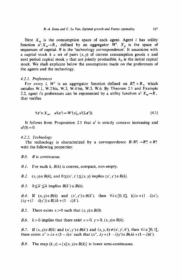
Here X, is the consumption space of each agent. Agent i has utility function ui: X,+R+ defined by an aggregator W’. X, is the space of sequences of capital. B is the ‘technology correspondence’. It associates with a capital stock k a set of pairs (x, y) of current consumption goods x and next period capital stock y that are jointly producible. k, is the initial capital stock. We shall explicate below the assumptions made on the preferences of the agents and the technology.
4.2.1. Preferences For every i, W’ is an aggregator function defined on R”, x R, which
satisfies W.l, W.2 bis, W.3, W.4 bis, W.5, W.6. By Theorem 2.1 and Example 2.2, agent i’s preferences can be represented by a utility function ui: X,+R+ that verifies
VX’E x,, d(2) = W’(x& u’(Lx’)). (4.1)
It follows from Proposition 2.1 that ui is strictly concave increasing and u’( 0) = 0.
4.2.2. Technology The technology is characterized by a correspondence B: Rp+ +R”, x R$
with the following properties:
B.O. B is continuous.
B.1. For each k, B(k) is convex, compact, non-empty.
B.2. (x,y)~B(k), and 05(x’,y’)S(x,y) implies (x’,y’)~B(k).
B.3. 0 5 k’ 5 k implies B(k’) G B(k).
8.4. If (x, y) E B(k) and (x’, y’) E B(k’), then Vll E [0, 11, ((Ax +( 1 -L)x’), (Ay+(l-I)y’))EB(lk+(l-I)k’).
B.5. There exists x >O such that (x, y) E B(0).
B.6. k>O implies that there exist x>O, y>O, (x, y) E B(k).
B.7. If (x,y)~B(k) and (x’,y’)~B(k’) and (x,y,k)#(x’,y’,k’), then VIE]O, l[, there exists x”>Ix+(l-2)x’ such that (x”, Ay+(l -L)~‘)E B(;Lk+(l -A)k’).
B.8. The map (k, y)+{xl(x, y) E B(k)} is lower semi-continuous.
168 R.-A. Dana and C. 12 Van, Optimal growth and Pareto optimality
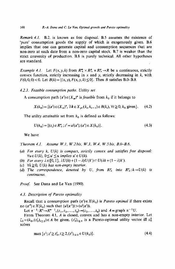
Remark 4.1. B.2. is known as free disposal. B.5 assumes the existence of ‘pure’ consumption goods the supply of which is exogenously given. B.6 implies that one can generate capital and consumption sequences that are non-zero at each date from a non-zero capital stock. B.7 is weaker than the strict convexity of production. B.8 is purely technical. All other hypotheses are standard.
Example 4.1. Let F(x, y, k) from R”, x Rp+ x Rp+ +R be a continuous, strictly convex function, strictly increasing in x and y, strictly decreasing in k, with F(O,O, 0) < 0. Let B(k) = ((x, y), F(x, y, k) 5 O}. Then B satisfies B.O-B.8.
4.2.3. Feasible consumption paths. Utility set
A consumption path (xi) E (X,)” is feasible from k, if it belongs to
X(k,) = {(xi) E(XJ, 3 k~Xr,(& k,, 1) EB(~,), Vt 20; k0 given}. (4.2)
The utility attainable set from k, is defined as follows:
U(h) = {(ZJ E R”, ; zi = u’(x’);(x’) EX(~~)}. (4.3)
We have
Theorem 4.1. Assume W.1, W.2bis, W.3, W.4, W.5 bis, B.O-B.6.
(4
V-4
ii
For every k, U(k) is compact, strictly convex and satisfies free disposal: Vu E U(k), O~u’~u implies U’E U(k). For every ,I~[0,1], AU(k)+(l-1)U(k’)cU(Ak+(l_A)k’). Vk 2 0, U(k) has non-empty interior. The correspondence, denoted by U, from RP, into R”+: k+U(k) is continuous.
Proof See Dana and Le Van (1990).
4.3. Description of Pareto optimality
Recall that a consumption path (xi) E X(k,) is Pareto optimal if there exists no (x”) E X(k,) such that (ui(Yi)) > (ui(xi)).
Let z-~:R”+R”-~,(z~,z~ ,..., z,)+(z2 ,..., z,) and A=graph 7c-lU. From Theorem 4.1, A is closed, convex and has a non-empty interior. Let
& =(k,,(~b)~~z) E A be given. (z&, r is a Pareto-optimal utility vector iff z: solves
max (z’;zi~~b,i~2,(zi)t~1 E U(k,)). (4.4)
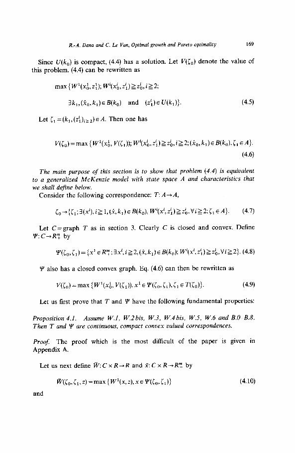
R.-A. Dana and C. 12 Van, Optimal growth and Pareto optima/icy 169
Since U(k,) is compact, (4.4) has a solution. Let V([,,) denote the value of this problem. (4.4) can be rewritten as
(4.5)
Let iI =(k,,(z’,)i,,)EA. Then one has
V&J =max { W’(& Vid); W XL, z;) 2 zb, i 2 2; (&,, k,) E B(k,), iI E A}.
(4.6)
The main purpose of this section is to show that problem (4.4) is equivalent to a generalized McKenzie model with state space A and characteristics that we shall define below.
Consider the following correspondence: T: A-+ A,
io-{il;3(xi),i~1,(~,k,)EB(k,),Wi(x’,zl)~zb,Vi~2;5,EA}. (4.7)
Let C=graph T as in section 3. Clearly C is closed and convex. Define Y:C+R”, by
‘f”(io, iJ = {x1 E R7; 3xi,iz2,(x, k,)EB(k,); W’(x’,z~)~z&Vi~2). (4.8)
YJ also has a closed convex graph. Eq. (4.6) can then be rewritten as
Viol =max I W’(& ViJ),x’ E ‘CL, id, Cl E T(L)). (4.9)
Let us first prove that T and Y have the following fundamental properties:
Proposition 4.1. Assume W.1, W.2bis, W.3. W.4 his, W.5, W.6 and B.O-B.8. Then T and Y are continuous, compact convex valued correspondences.
Proof: The proof which is the most difficult of the paper is given in Appendix A.
Let us next define w: C x R+R and X: C x R-+ R”, by
~(50,il,z)=max{W’(x,z),x~~I(i0,il))
and
(4.10)
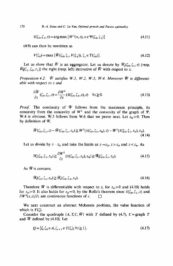
170 R.-A. Dana and C. Le Van, Optimal growth and Pareto optimality
X(6& Cl, 4 = arg max { Wx, 4, x E Y(L, Cd> (4.11)
(4.9) can then be rewritten as
Let us show that IV is an aggregator. Let us denote by ~~(&,,~i,z) (resp. q(cl, &,,z,)) the right (resp. left) derivative of FV with respect to z.
Proposition 4.2. w satisfies W.1, W.2, W.3, W.4. Moreover m is differenti- able with respect to z and
(4.13)
Proof: The continuity of iV follows from the maximum principle, its concavity from the concavity of W’ and the convexity of the graph of Y. W.4 is obvious. W.3 follows from W.6 that we prove next. Let z0 > 0. Then by definition of q
Let us divide by z - z0 and take the limits as z+z,,, z > z0 and z < ze. As
As iVis concave,
Therefore FV is differentiable with respect to z, for z,>O and (4.10) holds for z0 > 0. It also holds for z,, = 0, by the Rolle’s theorem since X([e, cl, z) and fYW’(x,z)/C?z are continuous functions of z. 0
We next construct an abstract Mckenzie problem, the value function of which is V(c).
Consider the quadruple (A, IT; C, w) with T defined by (4.7), C= graph T and w defined by (4.10). Let
Q=(5,roEA,51+1ET(r,),Vthl}. (4.17)
R.-A. Dana and C. LX Van, Optimal growth and Pareto optimality 171
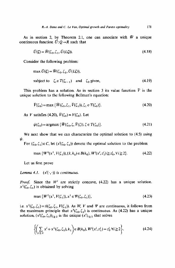
As in section 2, by Theorem 2.1, one can associate with w a unique continuous function 0: Q+R such that
Consider the following problem:
subject to cto T(c,_,) and &, given, (4.19)
This problem has a solution. As in section 3 its value function P is the unique solution to the following Bellman’s equation:
As V satisfies (4.20), V(<r,,) = V(l,). Let
We next show that we can characterize the optimal solution to (4.5) using
** For (co, cl) E C, let (x’(c,, iI)) denote the optimal solution to the problem
max {W’(x’, V(c,)),(& kl)~B(ko), W’(x’,z’;)Zz&ViZ2). (4.22)
Let us first prove
Lemma 4.2. (x’( ., .)) is continuous.
ProoJ: Since the W’ are strictly concave, (4.22) has a unique solution. x’([,,iJ is obtained by solving
(4.23)
i.e. x’(~,,,[~)=X(&,, cl, V(cl)). As w V and Y are continuous, it follows from the maximum principle that x’([,,,~~) is continuous. As (4.22) has a unique solution, (x’(&,, cl))iZZ is the unique (Xi)i~2 that solves
&x’+xlK 5 1 k ,,, 1 , 1 _ >
EB(k,),W’(x’,z’;)=zbVi~2 . (4.24)
172 R.-A. Dana and C. Le Van, Optimal growth and Pareto optimality
Let ([&[y)+([O,[l). Let (X’)ihz be a limit point of (x’(&C’;))~~~. Then (Xi)i22 satisfies (4.24). As (4.24) has a unique solution (z?‘)~~~ =(x’([,,,~~))~~~. This-implies the continuity of (x’( ., .))iz 2.
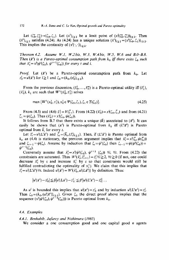
Theorem 4.2. Assume W.1, W.2bis, W.3, W.4 his, W.5, W.6 and B.O-B.8.
Then (Xi) is a Pareto-optimal consumption path from k, iff there exits &, such that Zf=x’($‘(&,), $“‘(i,,)) for every t and i.
Proof. Let (Xi) be a Pareto-optimal consumption path from k,. Let zb=a’(X’) for ill and [o=(ko,(zb)ig2).
From the previous discussion, (,?A,. . . , Zt) is a Pareto-optimal utility iff (Z\), ($,), k, are such that W’(X&Z:) solves
max {~‘(&z&x~~ ViO,il),~i E Vi,)}. (4.25)
From (4.5) and (4.6) 2: = V(ri). From (4.22) (Z~)=X’([~,[~) and from (4.21)
ci = $(io). Thus (2;) = x’(io, NM). It follows from B.7 that there exists a unique (E) associated to (Xi). It can
easily be shown that (Xi) is Pareto-optimal from k, iff (L’X’) is Pareto optimal from E, for every t.
Let ,%: = u’(L’X’) and & =(Et,(zf),,,). Then, if (L’X’) is Pareto optimal from k,, as (4.4) is stationary, the previous argument implies that Zf=~‘(r~,$(rJ) and rt+r= *'+l(~o)_ NJ. A
ssume by induction that rt=~t([o) then r,+r =$($‘(i,,))=
Conversely assume that ,$=x’($‘(&), I,V” (co)) Vi, Vt. From (4.22) the constraints are saturated. Thus W’(Zf, Zf+ 1) = Zf Vi 2 2, Vt 2 0 (if not, one could decrease .Yf by E and increase X: by E so that constraints would still be fulfilled contradicting the optimality of 2:). We claim that this implies that Zf = u’(L’X’) Vt. Indeed u’(X’) = W’(& u’(LX’)) by definition. Thus:
As ui is bounded this implies that u’(X’) = .$, and by induction u’(L’X’) = Zf. Thus [,, =(k,,(~‘(%‘))~~~). Given c,, the direct proof above implies that the sequence (x’(+‘(&), I++“‘(&,))) is Pareto optimal from k,.
4.4. Examples
4.4.1. Benhabib, Jafarey and Nishimura (1985) We consider a one consumption good and one capital good n agents
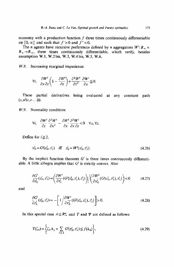
R.-A. Dana and C. Lx Van, Optimal growth and Pareto optimality 173
economy with a production function f three times continuously differentiable on [0, UJ~ and such that f’ > 0 and f” ~0.
The n agents have recursive preferences defined by n aggregators W’: R, x
R++R+, three times continuously differentiable, which verify, besides assumption W.l, W.2 bis, W.3, W.4 bis, W.5, W.6,
W.8. Increasing marginal impatience:
Vi, awi -( > ax aZ 1 awi I a2wi.awic0
aZ a22 ax = .
These partial derivatives being evaluated at any constant path (c, ui(c, c . . .))).
W.9. Normality condition:
vi awialwi awia2wic0 vx vz ~__ ___~ ’ aZ ax2 axaxaz ‘.
Define for i 2 2,
xi = G’(z& zi) iff zb = W’(xb, ~1). (4.26)
By the implicit function theorem G’ is three times continuously differenti- able. A little albegra implies that G’ is strictly convex. Also
$(G'( (4.27) 0
and
1 >O.
In this special case AE R”, and T and Y are defined as follows:
(4.28)
T(io)= ii;kl+ 1 G’(zb,z’;)Sf(ko) 3 (4.29) ir2
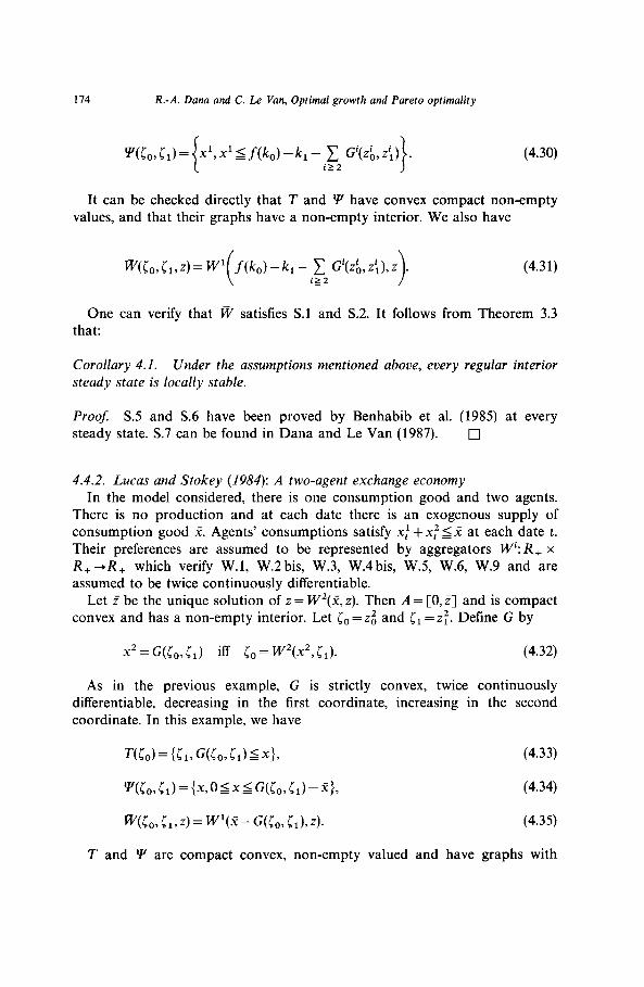
174 R.-A. Dana and C. L.e Van, Optimal growth and Pareto optimality
Y’(&,, cl) = x1, x1 5 f(k,) -k, - c G’(z;, zi,) . i22
(4.30)
It can be checked directly that T and !P have convex compact non-empty values, and that their graphs have a non-empty interior. We also have
W(&,,il,z)=W1 f(k,)-k,- 1 G’(z&z;),z .
iz2 >
(4.3 1)
One can verify that FI’ satisfies S.l and S.2. It follows from Theorem 3.3 that:
Corollary 4.1. Under the assumptions mentioned above, every regular interior steady state is locally stable.
Proof. S.5 and S.6 have been proved by Benhabib et al. (1985) at every
steady state. S.7 can be found in Dana and Le Van (1987). 0
4.4.2. Lucas and Stokey (1984): A two-agent exchange economy In the model considered, there is one consumption good and two agents.
There is no production and at each date there is an exogenous supply of consumption good X. Agents’ consumptions satisfy xi +xF 5 X at each date t. Their preferences are assumed to be represented by aggregators W’: R, x
R++R+ which verify W.l, W.2 bis, W.3, W.4 bis, W.5, W.6, W.9 and are
assumed to be twice continuously differentiable. Let Z be the unique solution of z = W2(X, z). Then A = [0, Z] and is compact
convex and has a non-empty interior. Let co =zg and cl =z:. Define G by
x2 = G(i,,,iJ iff lo = Wz(x2, id. (4.32)
As in the previous example, G is strictly convex, twice continuously differentiable, decreasing in the first coordinate, increasing in the second coordinate. In this example, we have
T(i,) = {ii, G(io, Cl) 5x1,
y(50,il)={~,Oj~~G(io,il)-x),
w(C,,ii,z)= II%-G(i,, 1&z).
T and Y are compact convex, non-empty
(4.33)
(4.34)
(4.35)
valued and have graphs with
R.-A. Dana and C. Le Van, Optimal growth and Pareto optimality 175
non-empty interior. m satisfies W.l, W.2 bis, W.3, W.4 and is twice conti- nuously differentiable. A.2 bis, A.3, A.4.2 are thus fulfilled.
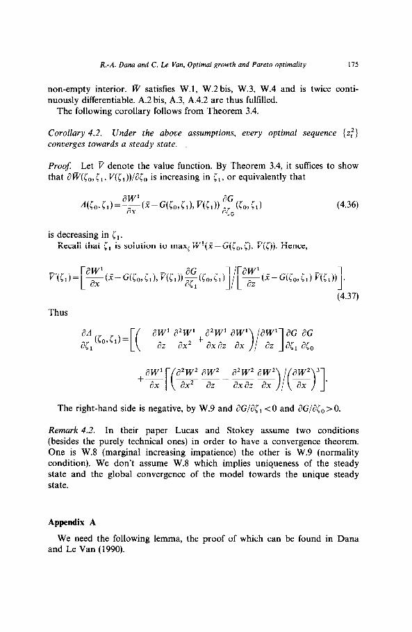
The following corollary follows from Theorem 3.4.
Corollary 4.2. Under the above assumptions, every optimal sequence {zf} converges towards a steady state.
Proof. Let P denote the value function. By Theorem 3.4, it s&ices to show that aF([,,i,, v([,))/&, is increasing in cl, or equivalently that
(4.36)
is decreasing in ii. Recall that ii is solution to maxr W’(,--G(i,,i), V(i)). Hence,
Thus
g4co,i1,= 1 K awl a2w1+a2wl awl awl ac ac -~~ ~~
aZ ax2 axaZ ax 1:’ 1 az x1 x0
+awl -K a2w2 aw2 a2w2 aw2 ax FaZ - dx x)/(Z)‘3.
The right-hand side is negative, by W.9 and aG/at;, < 0 and aG/aio > 0.
Remark 4.2. In their paper Lucas and Stokey assume two conditions (besides the purely technical ones) in order to have a convergence theorem. One is W.8 (marginal increasing impatience) the other is W.9 (normality condition). We don’t assume W.8 which implies uniqueness of the steady state and the global convergence of the model towards the unique steady state.
Appendix A
We need the following lemma, the proof of which can be found in Dana and Le Van (1990).
176 R.-A. Dana and C. Le Van, Optimal growth and Pareto optimality
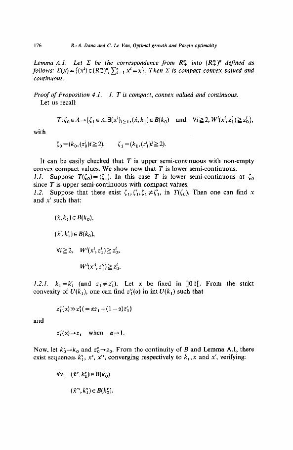
Lemma A.1. Let C be the correspondence from R”, into (R”,)” defined as follows: C(x) = {(xi) E(R’;)“, c;=I xi = x}. Then C is compact convex valued and continuous.
Proof of Proposition 4.1. 1. T is compact, convex valued and continuous. Let us recall:
T:[~EA+{[~ •A;3(X’)i~1,(~,k,)~B(ko) and Vi~2,W’(x’,z~)~z~},
with
Co = (k,, (zb)i 2 2), ii =(k,,(z’,)iz2).
It can be easily checked that T is upper semi-continuous with non-empty convex compact values. We show now that T is lower semi-continuous. 1.1. Suppose T(i,)= (cl). In this case T is lower semi-continuous at i,, since T is upper semi-continuous with compact values. 1.2. Suppose that there exist il,[‘i,[l#[‘i, in T([,). Then one can find x and x’ such that:
Vi 2 2, W’(x’, zi) 1 zb,
wi(x’i, z;i) 2 z;.
Z.2.I. k,=k; (and zi #z;). Let 01 be fixed in 10 l[. From the strict convexity of U(k,), one can find z;‘(a) in int U(k,) such that
and
zI;(a)>>z;( =az1 +(l -a)zi)
z;(a)-+zi when a+l.
Now, let k’,-+k, and zYg+z,,. From the continuity of B and Lemma A.l, there exist sequences k;, xv, x”, converging respectively to k,, x and x’, verifying:
Vv, (iv, k;) E B(k;;)
(Y, k;) E B(k;;).
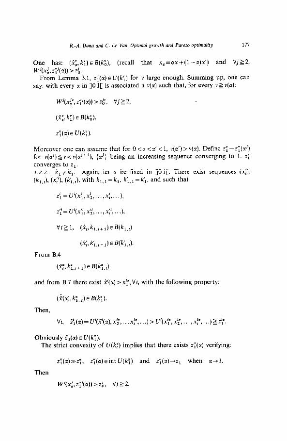
R.-A. Dana and C. Le Van, Optimal growth and Pareto optimality 111
One has: (ai, k;) E B(k’,), (recall that x, = c(x + (1 - a)~‘) and Vj 2 2, W’(x’,, z;‘(cr)) > z’o.
From Lemma 3.1, Z;(CI)E U(k;) for v large enough. Summing up, one can say: with every u in 10 l[ is associated a v(a) such that, for every V~V(CL):
Wj(xc, z;‘(a)) > zg, Vj 2 2,
z;(a) E U(kT).
Moreover one can assume that for 0 < c( < ~1’ < 1, V(CX’) > v(a). Define z; = z;(olj) for v(clj)jv<v(~~j+~), {&} b . g em an increasing sequence converging to 1. z; converges to zr. 1.2.2. k, #k;. Again, let CI be fixed in 10 l[. There exist sequences (xi), (k,,,), (xi’), (k;,,), with k,,,=k,, k;,,=k;, and such that
z’;=U’(x’;,x’; )...) xf )... ),
z;i= U’(x’;‘,x;‘, . . . ,xy,. . .),
K,k;,,+,)~W;,,). From B.4
(~;~k”l.,+,)~WW
and from B.7 there exist j?(c() >x’;“,Vi, with the following property:
(hU;,d WC).
Then,
Vi, F:(m) = U’(9(cr), x:, . . . xfor,. . .) > U’(x’;“, xt,. . . , xfa, . . .) 2 z’;“.
Obviously z”r(a) E U(kT). The strict convexity of U(kT) implies that there exists zI;(c1) verifying:
z;(a)>>z;, z’;(cr)~int U(k;) and z;(cc)+z, when a+l.
Then
Wj(x$ z;lj(tl)) > 26. Vj 2 2.
178 R.-A. Dana and C. Le Van, Optimal growth and Pareto optimality
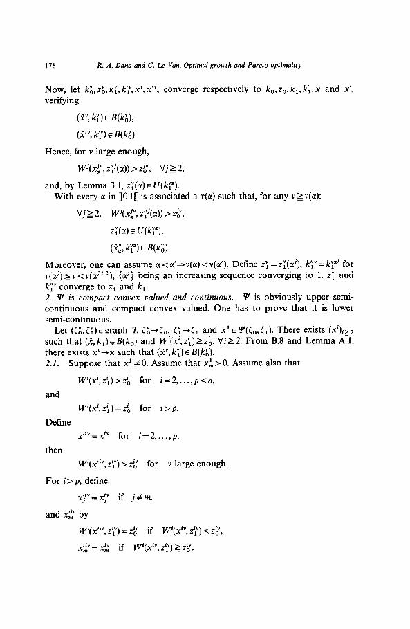
Now, let k&z;;, k;, k;‘, xv, x’“, converge respectively to ko,zo, kl, k;,x and x’, verifying:
(kv, k;) E YG,),
(P’, k;‘) E B(k;).
Hence, for v large enough,
Wj(xc, z;j(c~)) > zjo’, Vj 2 2,
and, by Lemma 3.1, Z;(U) E U(k;“). With every CI in 10 l[ is associated a V(U) such that, for any V~V(CL):
Vj 2 2, Wj(xj,, zl;j(cl)) > z’,‘,
z;(a) E U(k;a),
(a;, k;“) E B(k;;).
Moreover, one can assume IX < CI’*V(CI) < ~(a’). Define z; = z;(aj), k’;” = ky’ for v(orj)5v<v(aj+‘), {c&} b ein an increasing sequence converging to 1. z; and g k;” converge to zr and k,. 2. Y is compact convex valued and continuous. Y is obviously upper semi- continuous and compact convex valued. One has to prove that it is lower semi-continuous.
Let (G, 5’1) E graph 17; G-G, G +ir and x1 E Y([,, cr). There exists (x’)itz such that (a, k,) eB(ko) and W’(x’,z~) kzb, Viz2. From B.8 and Lemma A.l, there exists xv-+x such that (a”, k;) E B(ki). 2.1. Suppose that x1 #O. Assume that xA>O. Assume also that
W’(x’,z’,)>zb for i=2 ,..., p<n,
and
W’(x’,z\)=zb for i>p.
Define
X riv
=x iv for i=2,...,p,
then
wi(x’ivY zy) > zg for v large enough.
For i>p, define:
xy’ = xy if j#m,
and x2 by
wi(xliv, zy) = zp if Wi(xiv, zy) < zg,
x:=x: if Wi(xiV, zy, 2 z;.
R.-A. Dana and C. Le Van, Optimal growth and Pareto optima/icy 179
Clearly
xfiv+xi m l?l*
Define
X ~lv=gv_ C Xliv,
is2
then one easily checks that:
(a”‘, k;) =(a”, k;) E B(k;;),
Wi(x’iV,zI;y)~z;) viz2,
X ‘I” 2 0 for v sufficiently large,
X /IV
-+X1.
2.2. x1 =O. Since (&,[;)Egraph 7; there exists x”” such that:
(i”v, k;) E B(k;;),
wi(x”iv ) z;‘) 2 z$, Vi22.
Define
X +=x’liv for iz2,
X /IV
=o.
One has:
2” 2 ill,,
which implies
(a’“, k;) E B(k;;).
In other words.
0 E Y(& ii) for every v. Q.E.D.
References
Beak, R. and T. Koopmans, 1969, Maximising stationary utility in a constant technology, S.I.A.M. Journal of Applied Mathematics 17, 100-1015.
180 R.-A. Dana and C. Le Van, Optimal growth and Pareto optimality
Benhabib, J. and K. Nishimura, 1985, Competitive equilibrium cycles, Journal of Economic Theory 35, 284306.
Benhabib, J., M. Majumdar and K. Nishimura, 1985, Global equilibrium dynamics with stationary recursive preferences, Working paper.
Benhabib, J., S. Jafarey and K. Nishimura, 1985, The dynamics of efftcient intertemporal allocations with many agents, recursive preferences and production, Working paper.
Benveniste, L.M. and J.A. Scheinkman, 1979, On the differentiability of the value function in dynamic model of economics, Econometrica 47, no. 3.
Boldrin, M. and L. Montrucchio, 1986, On the indeterminacy of capital accumulation paths, Journal of Economic Theory 40.
Boyd, J.H., 1986, Recursive utility and the Ramsey problem, Working paper no. 60 (Rochester Center for Economic Research, Rochester).
Dana, R.A. and C. Le Van, 1987, On the structure of Pareto-optima in an infinite horizon economy where agents have recursive preferences, Working paper no. 8711 (CEPREMAP, Paris).
Dana, R.A. and C. Le Van, 1990, Structure of Pareto-optima in an infinite horizon economy where agents have recursive preferences, Journal of Optimisation Theory and Applications 64, 269-292.
Deneckere, R. and S. Pelikan, 1986, Competitive chaos, Journal of Economic Theory 40. Epstein, L.C., 1987a, The global stability of efficient intertemporal allocations, Econometrica 55,
329-355. Epstein, L.C., 1987b, A simple dynamic general equilibrium model, Journal of Economic Theory
41, 68-95. Iwai, K., 1972, Optimal economic growth and stationary ordinal utility, a Fisherian approach,
Journal of Economic Theory 4, 88-93. Koopmans, T., 1960, Stationary ordinal utility and impatience, Econometrica 28, 287-309. Koopmans, T., P. Diamond and R. Williamson, 1964, Stationary utility and time perspective,
Econometrica 32, 82-100. Lucas, R. and N. Stokey, 1984, Optimal growth with many consumers, Journal of Economic
Theory 32, 139-171. McKenzie, L.W., 1985, Optimal economic growth and turnpike theorems, in: K.J. Arrow and
M.D. Intriligator, eds., Handbook of mathematical economics, Vol. III (North-Holland, Amsterdam).
Mangasarian, O.L., 1966, Sutlicient conditions for the optimal control of non linear systems, S.I.A.M. Journal on Control 4, no. 1.
Scheinkman, J.A., 1976, On optimal steady states of n-sector growth models when utility is discounted, Journal of Economic Theory 12, 1 l-20.
Streufert, P.A., 1986a, The recursive expression of consistent intergenerational utility functions, Working paper no. 8609 (University of Wisconsin-Madison, Madison, WI).
Streufert, P.A., 1986b, Abstract dynamic programming, Working paper no. 8619 (University of Wisconsin-Madison, Madison, WI).


