Embed Size (px)
Citation preview
Mendelian randomization with invalid instruments:
effect estimation and bias detection through Egger
regression
Jack Bowden1,2, George Davey Smith2 & Stephen Burgess3
1 MRC Biostatistics Unit, Cambridge.2 MRC Integrative Epidemiology Unit, University of Bristol.
3 Department of Public Health and Primary Care, University of Cambridge
Abstract
Background: The number of Mendelian randomization analyses including largenumbers of genetic variants is rapidly increasing. This is due to the proliferationof genome-wide association studies, and the desire to obtain more precise estimatesof causal effects. However, some genetic variants may not be valid instrumental vari-ables, in particular due to them having more than one proximal phenotypic correlate(pleiotropy).
Methods: We view Mendelian randomization with multiple instruments as a meta-analysis, and show that bias caused by pleiotropy can be regarded as analogous tosmall study bias. Causal estimates using each instrument can be displayed visually bya funnel plot to assess potential asymmetry. Egger regression, a tool to detect smallstudy bias, can be adapted to test for bias from pleiotropy, and the slope coefficientfrom Egger regression provides an estimate of the causal effect. Under the assumptionthat the association of each genetic variant with the exposure is independent of thepleiotropic effect of the variant (not via the exposure), Egger’s test gives a valid testof the null causal hypothesis and a consistent causal effect estimate even when all thegenetic variants are invalid instrumental variables.
Results: We illustrate the use of Egger’s test by re-analysing two published Mendelianrandomization studies of the causal effect of height on lung function, and the causaleffect of blood pressure on coronary artery disease risk. The conservative nature ofthis approach is illustrated with these examples.
Conclusions: Egger regression can detect some violations of the standard instru-mental variable assumptions, and provide an effect estimate which is not subject to
1
these violations. The approach provides a sensitivity analysis for the robustness ofthe findings from a Mendelian randomization investigation. (272 words)
Keywords: Mendelian randomization, Invalid instruments, Meta-analysis, Pleiotropy,Small study bias , MR-Egger test.
Introduction
Mendelian randomization [1] is becoming an established method for testing whether amodifiable exposure has a causal role in the aetiology of a disease [2, 3]. As the subjectmoves forward, ever more ambitious analyses are being attempted. In particular, dueto the proliferation of genome-wide association studies, the number of Mendelianrandomization analyses using a large number of genetic variants is rapidly increasing[4, 5]. If the variants in total explain a larger proportion of the variance in theexposure, this will lead to more precise estimates of causal effects, thus increasing thepower for testing causal hypotheses [6, 7]. However, an enlarged set of genetic variantsis more likely to contain invalid instrument variables (IVs), due to violations of theassumptions necessary for valid causal inferences. The issue of horizontal pleiotropy– where a genetic variant affects the outcome via a different biological pathway thanthe exposure under investigation – is a particular concern [1, 3, 8]. The inclusion ofpleiotropic variants in a Mendelian randomization analysis can lead to biased causaleffect estimates and increased type I error rates for testing the causal null hypothesis[9]. If the instrumental variable assumptions are violated, the findings of a Mendelianrandomization analysis are open to the same criticisms as those levelled at traditionalobservational epidemiological analyses [10].
In this paper, we view Mendelian randomization of a single study with multipleIVs as analogous to a meta-analysis. The overall causal estimate based on all theIVs can be interpreted as a weighted average of the individual IV estimates, justlike a meta-analysis of separate study results. We show that bias resulting frompleiotropy is analogous to small study bias in meta-analysis, where small studies(with less precise estimates) tend to report larger estimates than big studies (withmore precise estimates). One reason for this is that estimates from small studies withnull findings tend not to be published. This induces a negative correlation acrossstudies between the magnitude and precision of estimates. In the context of Mendelianrandomization with multiple instruments, we equate the precision of a single study’sestimate with the strength of a single instrument. Publication bias is one aspect ofthe wider issue of dissemination bias [11]. Moreover, there may be a host of complex,context-specific reasons that lead to differences between results from small and largestudies in a specific meta-analysis. The general phenomenon is therefore prudentlyreferred to under the umbrella term of “small study” bias [12, 13, 14]. Under certainassumptions, applying the regression method underlying Egger’s test – a method forassessing small study bias in meta-analysis [12, 15] – is shown to give a consistentcausal effect estimate even when all the genetic variants violate the standard IV
2
assumptions.In this paper, we describe a general statistical model for Mendelian randomization
data with multiple potentially invalid instruments. Using the graphical representa-tions of a scatter plot and a funnel plot, we discuss why the standard method ofestimation, two-stage least squares (TSLS), may be biased when pleiotropy is presentand when Egger regression can provide a consistent estimate of the causal effect.We apply both methods to data available from two published Mendelian randomiza-tion studies, and explore their performance further using simulated data. Finally, weemphasize that the method advanced here can strengthen or weaken evidence for acausal effect but, as for any single Mendelian Randomization method, is itself subjectto assumptions and limitations.
Methods
We consider data from a Mendelian randomization study on N participants. Foreach participant, indexed by i, we measure J genetic variants (Gi1, Gi2, . . . , GiJ),a modifiable exposure, (Xi), and an outcome (Yi). We assume that confounders(represented by a single variable Ui) are unknown. The genetic variants are assumedto take the values 0, 1, or 2 (representing the number of exposure-increasing alleles ofa biallelic single nucleotide polymorphism). The exposure is taken as a linear functionof the genetic variants, the confounders, and an independent error term (ǫXi ). Thecoefficients γj for each variant j represent the effects of the genetic variants on theexposure. The outcome is taken as a linear function of the genetic variants, theexposure, the confounders, and an independent error term (ǫYi ). The causal effect ofthe exposure on the outcome is β. The coefficients αj for each variant j representthe direct effects of the genetic variants on the outcome that are not mediated by theexposure. The total effect of each variant on the outcome comprises the direct effect(αj) and the indirect effect via the exposure (βγj).
Xi =J∑
j=1
γjGij + Ui + ǫXi (1)
Yi =J∑
j=1
αjGij + βXi + Ui + ǫYi (2)
. Although the effects of the confounders on the exposure and on the outcome aretaken as equal in equations (1) and (2), this assumption is not necessary and furtherparameters for these effects could be introduced into the model without affecting themethodological developments in this paper.
A genetic variant is a valid instrumental variable if the following assumptions hold:
• IV1: The genetic variant is independent of confounders U ;
• IV2: The genetic variant is associated with the exposure X;
3
• IV3: The genetic variant is independent of the outcome Y conditional on theexposure X and confounders U .
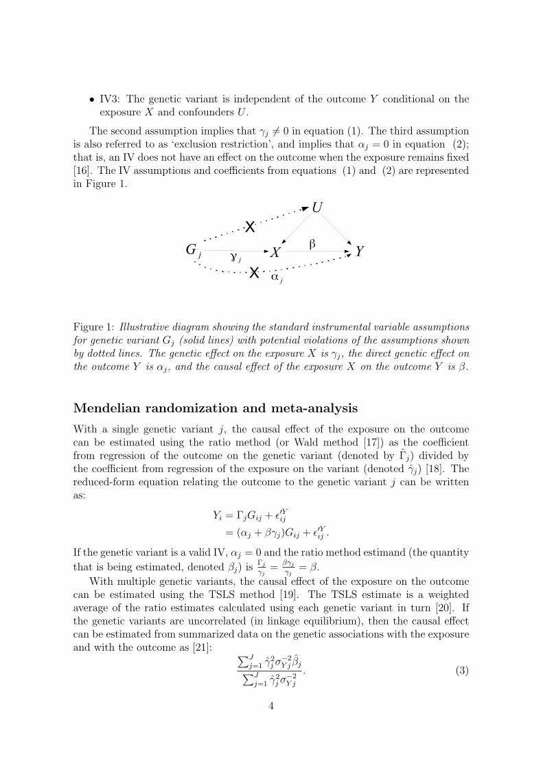
The second assumption implies that γj 6= 0 in equation (1). The third assumptionis also referred to as ‘exclusion restriction’, and implies that αj = 0 in equation (2);that is, an IV does not have an effect on the outcome when the exposure remains fixed[16]. The IV assumptions and coefficients from equations (1) and (2) are representedin Figure 1.
� �
�
� �
�� �
�
�
� �
Figure 1: Illustrative diagram showing the standard instrumental variable assumptionsfor genetic variant Gj (solid lines) with potential violations of the assumptions shownby dotted lines. The genetic effect on the exposure X is γj, the direct genetic effect onthe outcome Y is αj, and the causal effect of the exposure X on the outcome Y is β.
Mendelian randomization and meta-analysis
With a single genetic variant j, the causal effect of the exposure on the outcomecan be estimated using the ratio method (or Wald method [17]) as the coefficientfrom regression of the outcome on the genetic variant (denoted by Γj) divided bythe coefficient from regression of the exposure on the variant (denoted γj) [18]. Thereduced-form equation relating the outcome to the genetic variant j can be writtenas:
Yi = ΓjGij + ǫ′Yij
= (αj + βγj)Gij + ǫ′Yij .
If the genetic variant is a valid IV, αj = 0 and the ratio method estimand (the quantity
that is being estimated, denoted βj) isΓj
γj=
βγjγj
= β.
With multiple genetic variants, the causal effect of the exposure on the outcomecan be estimated using the TSLS method [19]. The TSLS estimate is a weightedaverage of the ratio estimates calculated using each genetic variant in turn [20]. Ifthe genetic variants are uncorrelated (in linkage equilibrium), then the causal effectcan be estimated from summarized data on the genetic associations with the exposureand with the outcome as [21]:
∑J
j=1γ2
jσ−2
Y j βj∑J
j=1γ2
jσ−2
Y j
. (3)
4
where βj =Γj
γjis the ratio method estimate for variant j, and σY j is the standard error
in the regression of the outcome on the jth genetic variant, assumed to be known.This same weighted average formula is used in a fixed-effect meta-analysis, where theIV-specific causal estimates βj are the study-specific estimates, and the weights arethe inverse-variance weights [22]. This summarized estimate, which we refer to as aninverse-variance weighted (IVW) estimate, will differ slightly from the TSLS estimatein finite samples, as the correlation between independent genetic variants will notexactly equal zero [23], but the two estimates will be equal asymptotically (that is,they both tend towards the same quantity as their sample sizes increase towardsinfinity). However, an advantage of the IVW estimate is that it can be calculatedfrom summarized data, whereas the TSLS estimate requires individual-level data. Weassume for the remainder of the manuscript that the genetic variants are uncorrelatedin their distributions (that is, knowledge of one does not help to predict the valueof any other), as typically in Mendelian randomization one variant is taken fromeach gene region. Distantly located variants are usually uncorrelated; correlationsbetween variants that are physically close can be found using an online tool such ashttp://www.broadinstitute.org/mpg/snap/ldsearchpw.php.
If genetic variant j is not a valid IV, in particular because it has a direct effect onthe outcome (αj 6= 0), then we have βj = β+
αj
γj. The ratio estimate based on genetic
variant j in an infinite sample will equal the true causal effect β plus an error termαj
γj. In the same way, the TSLS and IVW estimates will tend towards:
β +
∑J
j=1γjσ
−2
Y jαj∑J
j=1γ2
jσ−2
Y j
= β + Bias(α, γ).
This implies that the TSLS estimate is consistent when the assumption IV3 is trueand all the αj parameters are zero. It is also consistent if the pleiotropic effectshappen to cancel out, such that the bias term is equal to zero [24]. Although this willnot be universally plausible, we explore the condition that the correlation between thegenetic associations with the exposure (the γj parameters) and the direct effects of thegenetic variants on the outcome (the αj parameters) is zero. We refer to the conditionthat the distributions of these parameters are independent as InSIDE (InstrumentStrength Independent of Direct Effect). It can be viewed as a weaker version of theexclusion restriction assumption. This relaxation of the IV assumptions was recentlyinvestigated by Kolesar et al. [25], although their work differs from ours and is notpresented within the context of Mendelian randomization.
Illustrative example
Illustrative data on the associations of multiple genetic variants with an exposurevariable and with an outcome variable for 15 variants are displayed as a scatter plotin Figure 2. This is similar to a radial plot occasionally used in meta-analysis todisplay multiple estimates of the same quantity having different precisions [26]. Inthis example, all of the IVs are invalid, but the InSIDE condition holds. The true
5

causal effect is shown by the dotted line. The ratio estimates based on each geneticvariant are the gradients of the slopes from the origin to the datapoint for that variant.The IVW estimate (shown by the solid red line) is the slope of the best fitting linethrough the data points that also passes through the origin. This is equal to thecoefficient from a weighted regression of the gene–outcome association estimates (Γj)on the gene–exposure association estimates (γj) with the intercept constrained to zero,and weighted by the inverse of the precision of the IV–outcome coefficients (σ−2
Y j ) [27].Here, all of the instruments are invalid, and so the slope of this line differs substantiallyfrom the true causal effect.
Under the InSIDE assumption, the numerator of the bias term of the ratio estimatefor the jth genetic variant αj is independent of its denominator, γj. This means that
the bias of the ratio estimate βj =Γj
γjis inversely proportional to γj. Consequently,
ratio estimates for stronger genetic variants (ones with greater values of γj), such asthe variant marked (i) in Figure 2, will be on average closer to the true causal effectthan those from weaker genetic variants, such as the variant marked (ii).
��
��
��
��������
�� ���� ������
���
��� ��
�����
��������
�������������������������������
Figure 2: Plot of the gene–outcome (Γ) versus gene–exposure (γ) regression coeffi-cients for a fictional Mendelian randomization analysis with 15 genetic variants. Thetrue slope is shown by a dotted line, the inverse-variance weighted (IVW) estimate bya red line, and the MR-Egger regression estimate by a blue line.
The data can also be displayed visually by a funnel plot [28]. In the context ofmeta-analysis, this is a plot of a measure of the precision of study estimates versusthe estimates themselves (see Figure’s 3 and 4). Asymmetry in the funnel plot willoccur if there is directional small study bias, as extreme results from smaller studiesare more likely to be published. In the context of Mendelian randomization, we plot
6
the genetic associations with the exposure γj against the individual IV estimates βj,as the genetic associations with the exposure are related to the precision of the IVestimates. We refer to asymmetry in this plot as ‘directional’ pleiotropy, meaningthat the pleiotropic effects of genetic variants are not balanced about the null.
We consider regression of the Γj coefficients on the γj coefficients where the inter-cept is not constrained to be zero. We fit the linear model:
Γj = β0E + βE γj. (4)
(We draw attention to the slight oddity in notation: the Γj and γj association esti-mates are the data in this model, and β0E and βE are the coefficients in the regressionmodel; estimates of these coefficients are also denoted by hats – β0E and βE.)
This model performs Egger regression, a special case of the general method of meta-regression [15]. Egger’s test for small study bias in meta-analysis assesses whether theintercept term β0E is significantly different from zero. This will occur if the estimatesfrom small studies (in the case of Mendelian randomization, estimates from weakergenetic variants) are more skewed towards either high or low values compared withestimates from large studies (stronger variants). The estimated value of the interceptin Egger regression β0E can be interpreted as an estimate of the average pleiotropiceffect across the genetic variants. An intercept term that differs from zero is indicativeof overall directional pleiotropy.
It has been also asserted that βE is a bias-reduced estimate for the true causaleffect [14]. Under model (1), we have the following equation for the slope coefficientfrom Egger regression:
βE =cov(Γ, γ)
var(γ)= β +
cov(α, γ)
var(γ).
In the limit as both the sample size and the number of genetic variants increase to
infinity, the InSIDE condition ensures that cov(α, γ)N→∞
−−−→ cov(α, γ)J→∞
−−−→ 0 andtherefore βE is a consistent estimate of the causal effect β. This is illustrated by thesolid blue line in Figure 2.
If genetic variants have different minor allele frequencies (MAFs), then a bettermeasure of instrument strength can be constructed, as causal estimates from variantswith low minor allele frequencies will have low precision. If the MAF of variant j
is πj, then a more efficient version of Egger’s test for directional pleiotropy can be
obtained by regressing the Γj coefficients on γCj = γj
√
πj(1− πj). Provided that thegenetic associations with the outcome are all estimated on the same individuals, theMAF-correction factors
√
πj(1− πj) will be proportional to the standard errors ofthe gene–outcome associations σY j present in equation (3) under the assumption thatthe variant is in Hardy–Weinberg equilibrium, and so this correction is equivalent toperforming Egger regression as a weighted linear regression using the σ−2
Y j as weights.The MAF-corrected weights are the same as those used by the IVW method in for-mula (3). If one uses the MAF-corrected weights within Egger regreesion, the InSIDEassumption must be that they are independent of the direct effects on the outcome.
7
In order to distinguish our novel adaptation of Egger regression to Mendelian random-ization from its original context, we will henceforth refer to its general application inthis setting as ‘MR-Egger regression’ and Egger’s test as the ‘MR-Egger’ test.
Examples
To demonstrate this approach for the assessment of directional pleiotropy, we considertwo illustrative examples of Mendelian randomization using many genetic variantsthat have been recently published. We use the available data on genetic associationswith the exposure and with the outcome to construct a funnel plot and perform avisual inspection for asymmetry, as well as a formal statistical test using MR-Eggerregression. We comment on the differences between the IVW causal effect estimatefrom equation (3), which assumes that all the genetic variants are valid IVs, and theMR-Egger estimate from equation (4), which makes assumptions IV1, IV2, and theInSIDE assumption.
Causal effect of height on lung function
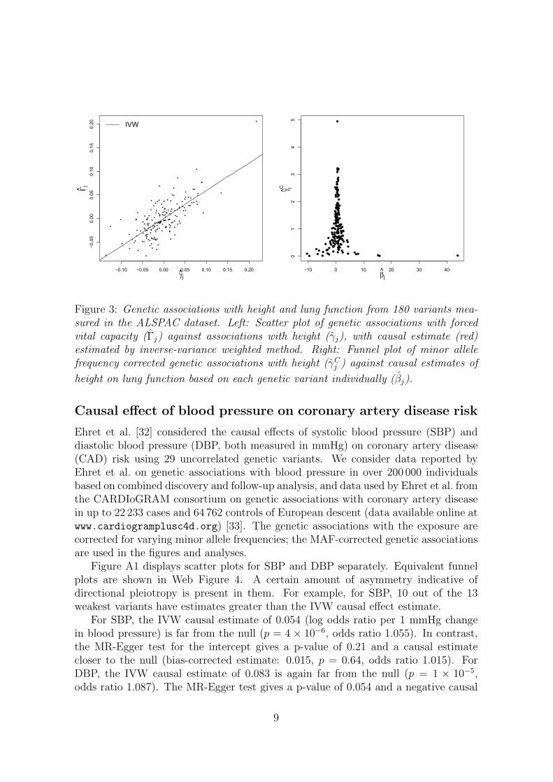
In a primarily methodological investigation of weak instrument bias, Davies et al. [29]considered the causal effect of height (standardized) on lung function (measured asforced vital capacity, FVC, measured in mL) using 180 genetic variants as IVs withdata on 3631 participants from the Avon Longitudinal Study of Parents and Children(ALSPAC) cohort [30]. These variants were originally identified in a genome-wideassociation study [31]. The associations of the variants with height and with FVCare displayed in a scatter plot in Figure 3 (left). The slope of the line through thescatter plot is the IVW causal effect estimate using all the variants as IVs of 0.59 (95%confidence interval, CI: 0.50, 0.67). This is similar to the TSLS estimate of 0.60 (95%CI: 0.52, 0.68) reported by Davies et al. The causal estimates represent the increasein FVC for a 1 standard deviation increase in height.
Figure 3 (right) shows a funnel plot of the MAF-corrected genetic associations withthe exposure against the individual causal effect estimates for each variant. A visualinspection of the funnel plot suggests that there is little asymmetry present. ApplyingMR-Egger regression with MAF-corrected weights to the summarized data yields anintercept estimate -0.0009 with an associated p-value of 0.75. The bias-adjusted causaleffect estimate from MR-Egger regression is 0.60 (95% CI: 0.46, 0.75), a slight increasein magnitude and uncertainty compared with the IVW and TSLS estimates. Therewas also no apparent heterogeneity in the IV estimates from each genetic variantindividually, as evidenced by Cochran’s Q test (p = 0.99). In the Web Appendix weshow how the IVW and MR-Egger regression methods were implemented on thesedata with just a single line of computer code (using R and Stata). In summary, thereis no evidence that directional pleiotropy is an important factor for these data.
8
�0.10 �0.05 0.00 0.05 0.10 0.15 0.20
�0.0
50.0
00.0
50.1
00.1
50.2
0
●
●
●
●
●
●
●
●
●
●
●
●
●
●
●
●
●
●
●
●
●
●
●
●
●
●
●
●
●
●
●
●
●
●●
●
●
●
●
●
●
● ●
●
●
●
●
●
●
●
●
●
●
●
●
●
●
●
●
●
●
●
●
●
●
●
●
●
●
●●
●
●
●
●
●
●
●
●
●
●
●
●
●
●
●
●
●
●
●
●
●
●
●
●
●
●
●
●
●
●
●
●
●
●
●
●
●
●
●
●
●
●
●
●
●
●
●
●
●
●
●
●
●
●
●
●
●
●
●
●
●
●
●
●
●
●●
●
●●
●
●
●
●
●
●
●
●
●
●
●
●
●
●
●
●
●
●
●●
● ●
●●
●
●
●
●
●
●
●
●
●
●
● ●
●
●
●
γj
Γ^j
IVW
●
●
●
● ●
●
●
●
●
●
●
●
●
●
●
●
●
●
●
●●
●
●
●●
●
●
●
●
●
●
●
●
●
●
●
●
●
●
●
●●
●
●
●
●
●
●
●
●
●
●
●
●
●
●
●
●
●
●
●
●●●
●
●
●●
●
●
●
●
●
●
●
●
●
●
●
●
●
●
●
●
●
●
●
●
●
●
●
●
●
●
●
●
●
●
●
●
●
●
●
●
●
●
●
●
●
●
●
●
●
●●
●●
●
●
●
●
●
●
●
●●
●●
●
●
●
●●
●
●
●
●
●
●
●
●
●
●●
●
●
●
●
●
●
●
●
●
●
●
●
●
●
●
●
●
●
●
●
●
●
●
●
●
●
●
●
●
●
●●
●
●
●
●
�10 0 10 20 30 40
01
23
45
β^
j
γ jC
Figure 3: Genetic associations with height and lung function from 180 variants mea-sured in the ALSPAC dataset. Left: Scatter plot of genetic associations with forcedvital capacity (Γj) against associations with height (γj), with causal estimate (red)estimated by inverse-variance weighted method. Right: Funnel plot of minor allelefrequency corrected genetic associations with height (γC
j ) against causal estimates of
height on lung function based on each genetic variant individually (βj).
Causal effect of blood pressure on coronary artery disease risk
Ehret et al. [32] considered the causal effects of systolic blood pressure (SBP) anddiastolic blood pressure (DBP, both measured in mmHg) on coronary artery disease(CAD) risk using 29 uncorrelated genetic variants. We consider data reported byEhret et al. on genetic associations with blood pressure in over 200 000 individualsbased on combined discovery and follow-up analysis, and data used by Ehret et al. fromthe CARDIoGRAM consortium on genetic associations with coronary artery diseasein up to 22 233 cases and 64 762 controls of European descent (data available online atwww.cardiogramplusc4d.org) [33]. The genetic associations with the exposure arecorrected for varying minor allele frequencies; the MAF-corrected genetic associationsare used in the figures and analyses.
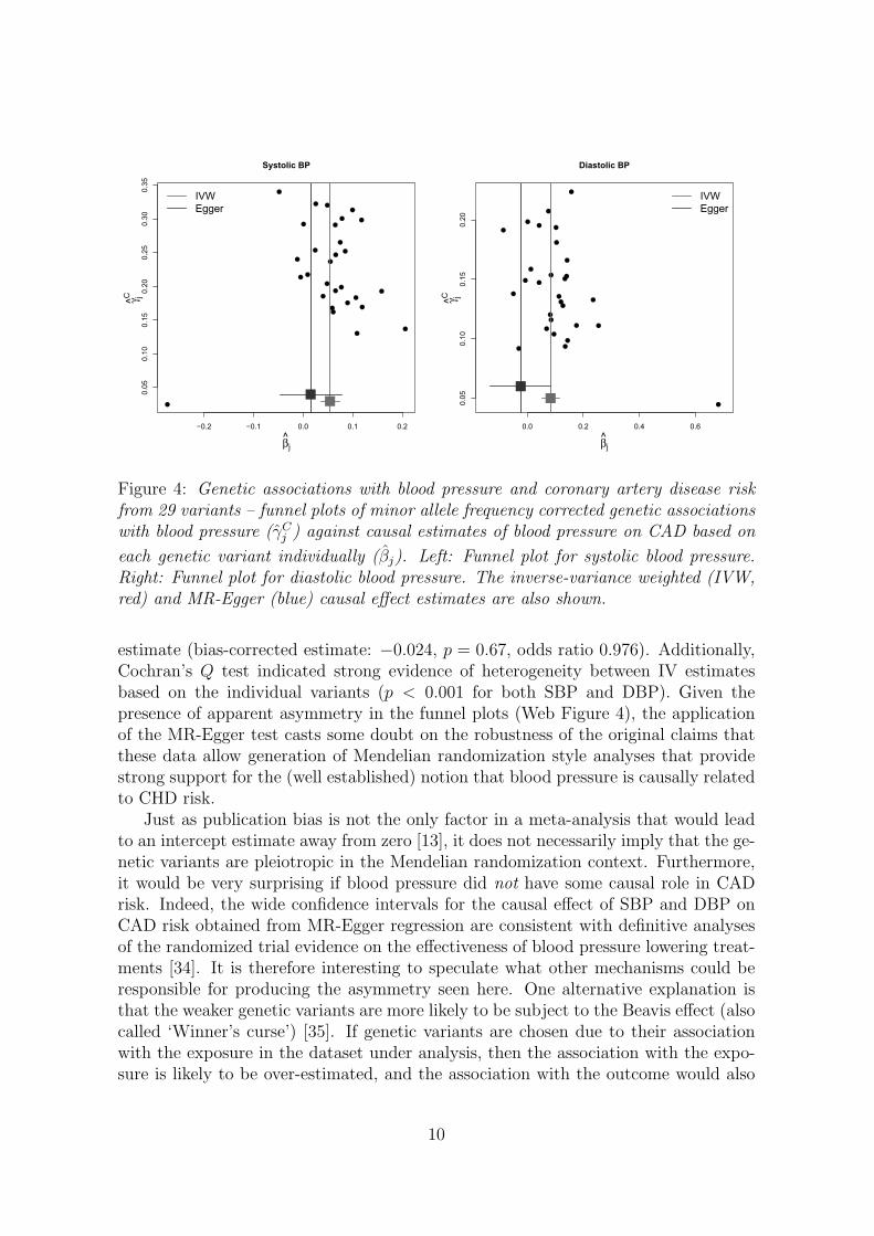
Figure A1 displays scatter plots for SBP and DBP separately. Equivalent funnelplots are shown in Web Figure 4. A certain amount of asymmetry indicative ofdirectional pleiotropy is present in them. For example, for SBP, 10 out of the 13weakest variants have estimates greater than the IVW causal effect estimate.
For SBP, the IVW causal estimate of 0.054 (log odds ratio per 1 mmHg changein blood pressure) is far from the null (p = 4 × 10⁻⁶, odds ratio 1.055). In contrast,the MR-Egger test for the intercept gives a p-value of 0.21 and a causal estimatecloser to the null (bias-corrected estimate: 0.015, p = 0.64, odds ratio 1.015). ForDBP, the IVW causal estimate of 0.083 is again far from the null (p = 1 × 10⁻⁵,odds ratio 1.087). The MR-Egger test gives a p-value of 0.054 and a negative causal
9
●
●
●
●
●
●
●
●
●●
●
●
●
●
●
●
●
●
●
●
●
●
●
●
●
●
●
●
●
�0.2 �0.1 0.0 0.1 0.2
0.0
50.1
00.1
50.2
00.2
50.3
00.3
5
Systolic BP
IVW
Egger
β^
j
γ jC
●
●
●
●
●
●
●
●
●●
● ●
●
●
●
●
●
●
●
●
●
●
●
●
●
●
●
●
●
0.0 0.2 0.4 0.6
0.0
50.1
00.1
50.2
0
Diastolic BP
IVW
Egger
β^
jγ jC
Figure 4: Genetic associations with blood pressure and coronary artery disease riskfrom 29 variants – funnel plots of minor allele frequency corrected genetic associationswith blood pressure (γC
j ) against causal estimates of blood pressure on CAD based on
each genetic variant individually (βj). Left: Funnel plot for systolic blood pressure.Right: Funnel plot for diastolic blood pressure. The inverse-variance weighted (IVW,red) and MR-Egger (blue) causal effect estimates are also shown.
estimate (bias-corrected estimate: −0.024, p = 0.67, odds ratio 0.976). Additionally,Cochran’s Q test indicated strong evidence of heterogeneity between IV estimatesbased on the individual variants (p < 0.001 for both SBP and DBP). Given thepresence of apparent asymmetry in the funnel plots (Web Figure 4), the applicationof the MR-Egger test casts some doubt on the robustness of the original claims thatthese data allow generation of Mendelian randomization style analyses that providestrong support for the (well established) notion that blood pressure is causally relatedto CHD risk.
Just as publication bias is not the only factor in a meta-analysis that would leadto an intercept estimate away from zero [13], it does not necessarily imply that the ge-netic variants are pleiotropic in the Mendelian randomization context. Furthermore,it would be very surprising if blood pressure did not have some causal role in CADrisk. Indeed, the wide confidence intervals for the causal effect of SBP and DBP onCAD risk obtained from MR-Egger regression are consistent with definitive analysesof the randomized trial evidence on the effectiveness of blood pressure lowering treat-ments [34]. It is therefore interesting to speculate what other mechanisms could beresponsible for producing the asymmetry seen here. One alternative explanation isthat the weaker genetic variants are more likely to be subject to the Beavis effect (alsocalled ‘Winner’s curse’) [35]. If genetic variants are chosen due to their associationwith the exposure in the dataset under analysis, then the association with the expo-sure is likely to be over-estimated, and the association with the outcome would also
10
be over-estimated due to confounding. This is known to lead to bias in Mendelianrandomization estimates when there is overlap in the datasets used for estimating thegenetic associations with the exposure and with the outcome (as is the case here) [36].However, genetic associations with SBP and DBP from the replication analyses onlywere not reported in the original study, limiting the possibility to distinguish whetherthe asymmetry in the funnel plot is due to directional pleiotropy or the winner’s curse.
Simulations
To further investigate the statistical properties of MR-Egger regression under realisticconditions, we perform a simulation study, generating artificial data with 25 geneticvariants used as instrumental variables. We generate data in a two-sample Mendelianrandomization setting, in which data on the genetic associations with the exposureand with the outcome are estimated in non-overlapping sets of individuals. Further-more, we allow ourselves to make use of the summary data estimates only (e.g. theindividual estimates for γj, Γj and σ2
Y j, j = 1, . . . , 25). The summarized data settingis increasingly common for applied Mendelian randomization investigations, such asthe example of blood pressure and coronary artery disease risk. The IVW estimatorwas therefore felt to be the most natural implementation of the ‘standard’ approach toMendelian randomization that could also be applied in this context, and so we chosethis as our comparator. We expect its performance to closely mirror the two-sampletwo-stage least squares (TS2SLS) method [37], a variant of TSLS that can be appliedto individual participant data in the two-sample setting, given their asymptotic equiv-alence. The simulations are repeated in the Web Appendix in a one-sample setting.In this case, we found that the performance of standard one-sample TSLS and theIVW method were indeed highly similar.
We consider four scenarios for the pattern of pleiotropy, and consider the biasand coverage properties of the estimators with null and positive causal effects. Thescenarios considered are:
(a) No pleiotropy, InSIDE assumption trivially satisfied (all the α parameters, rep-resenting the direct effects of genetic variants on the outcome, are equal to zero);
(b) Balanced pleiotropy, InSIDE assumption satisfied (α parameters take positiveand negative values);
(c) Directional pleiotropy, InSIDE assumption satisfied (α parameters take onlypositive values, but are generated independently from the γ parameters, repre-senting genetic effects on the exposure);
(d) Directional pleiotropy, InSIDE assumption not satisfied (α parameters take pos-itive values, and are correlated with the direct genetic effects on the exposure).
A possible situation corresponding to scenario (d) is that the pleiotropic effectsof the genetic variants on the outcome act via a confounder. Specifically, if a ge-netic variant is associated with a confounder of the relationship between the exposure
11
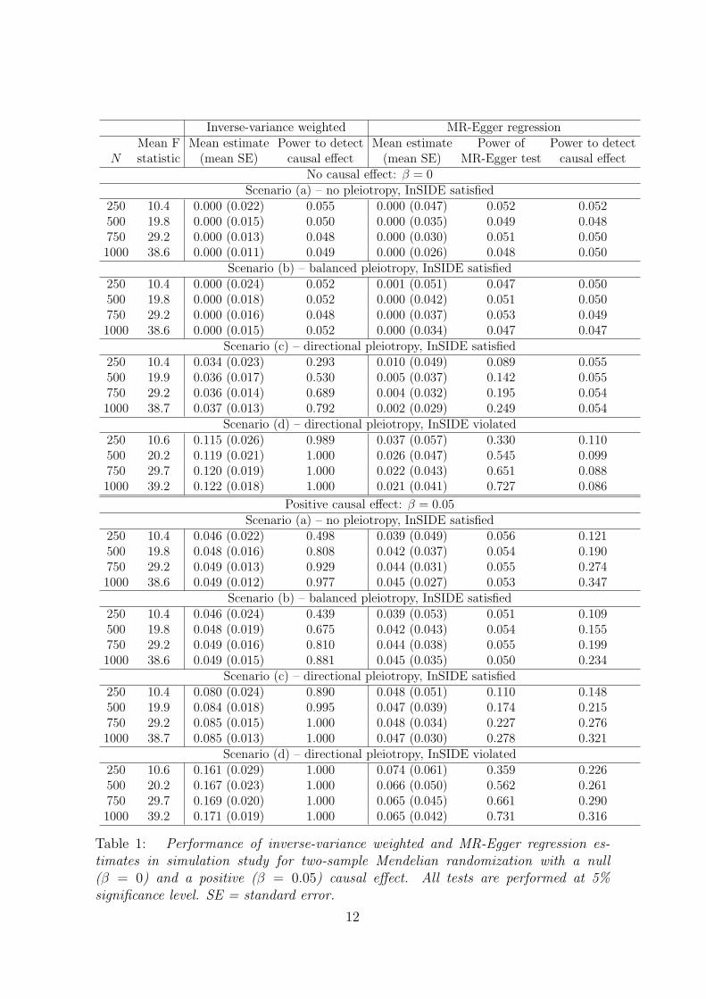
Inverse-variance weighted MR-Egger regressionMean F Mean estimate Power to detect Mean estimate Power of Power to detect
N statistic (mean SE) causal effect (mean SE) MR-Egger test causal effectNo causal effect: β = 0
Scenario (a) – no pleiotropy, InSIDE satisfied250 10.4 0.000 (0.022) 0.055 0.000 (0.047) 0.052 0.052500 19.8 0.000 (0.015) 0.050 0.000 (0.035) 0.049 0.048750 29.2 0.000 (0.013) 0.048 0.000 (0.030) 0.051 0.0501000 38.6 0.000 (0.011) 0.049 0.000 (0.026) 0.048 0.050
Scenario (b) – balanced pleiotropy, InSIDE satisfied250 10.4 0.000 (0.024) 0.052 0.001 (0.051) 0.047 0.050500 19.8 0.000 (0.018) 0.052 0.000 (0.042) 0.051 0.050750 29.2 0.000 (0.016) 0.048 0.000 (0.037) 0.053 0.0491000 38.6 0.000 (0.015) 0.052 0.000 (0.034) 0.047 0.047
Scenario (c) – directional pleiotropy, InSIDE satisfied250 10.4 0.034 (0.023) 0.293 0.010 (0.049) 0.089 0.055500 19.9 0.036 (0.017) 0.530 0.005 (0.037) 0.142 0.055750 29.2 0.036 (0.014) 0.689 0.004 (0.032) 0.195 0.0541000 38.7 0.037 (0.013) 0.792 0.002 (0.029) 0.249 0.054
Scenario (d) – directional pleiotropy, InSIDE violated250 10.6 0.115 (0.026) 0.989 0.037 (0.057) 0.330 0.110500 20.2 0.119 (0.021) 1.000 0.026 (0.047) 0.545 0.099750 29.7 0.120 (0.019) 1.000 0.022 (0.043) 0.651 0.0881000 39.2 0.122 (0.018) 1.000 0.021 (0.041) 0.727 0.086
Positive causal effect: β = 0.05Scenario (a) – no pleiotropy, InSIDE satisfied
250 10.4 0.046 (0.022) 0.498 0.039 (0.049) 0.056 0.121500 19.8 0.048 (0.016) 0.808 0.042 (0.037) 0.054 0.190750 29.2 0.049 (0.013) 0.929 0.044 (0.031) 0.055 0.2741000 38.6 0.049 (0.012) 0.977 0.045 (0.027) 0.053 0.347
Scenario (b) – balanced pleiotropy, InSIDE satisfied250 10.4 0.046 (0.024) 0.439 0.039 (0.053) 0.051 0.109500 19.8 0.048 (0.019) 0.675 0.042 (0.043) 0.054 0.155750 29.2 0.049 (0.016) 0.810 0.044 (0.038) 0.055 0.1991000 38.6 0.049 (0.015) 0.881 0.045 (0.035) 0.050 0.234
Scenario (c) – directional pleiotropy, InSIDE satisfied250 10.4 0.080 (0.024) 0.890 0.048 (0.051) 0.110 0.148500 19.9 0.084 (0.018) 0.995 0.047 (0.039) 0.174 0.215750 29.2 0.085 (0.015) 1.000 0.048 (0.034) 0.227 0.2761000 38.7 0.085 (0.013) 1.000 0.047 (0.030) 0.278 0.321
Scenario (d) – directional pleiotropy, InSIDE violated250 10.6 0.161 (0.029) 1.000 0.074 (0.061) 0.359 0.226500 20.2 0.167 (0.023) 1.000 0.066 (0.050) 0.562 0.261750 29.7 0.169 (0.020) 1.000 0.065 (0.045) 0.661 0.2901000 39.2 0.171 (0.019) 1.000 0.065 (0.042) 0.731 0.316
Table 1: Performance of inverse-variance weighted and MR-Egger regression es-timates in simulation study for two-sample Mendelian randomization with a null(β = 0) and a positive (β = 0.05) causal effect. All tests are performed at 5%significance level. SE = standard error.
12
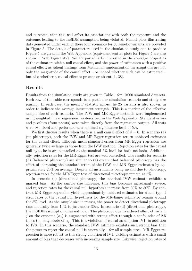
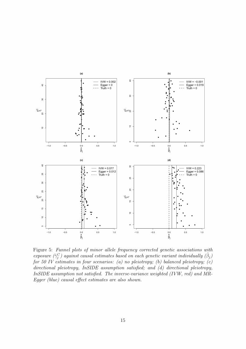
and outcome, then this will affect its associations with both the exposure and theoutcome, leading to the InSIDE assumption being violated. Funnel plots illustratingdata generated under each of these four scenarios for 50 genetic variants are providedin Figure 5. The details of parameters used in the simulation study and to produceFigure 5 are given in the Web Appendix (equivalent scatter plots for Figure 5 are alsoshown in Web Figure A2). We are particularly interested in the coverage propertiesof the estimators with a null causal effect, and the power of estimators with a positivecausal effect, as salient findings from Mendelian randomization investigations are notonly the magnitude of the causal effect – or indeed whether such can be estimated –but also whether a causal effect is present or absent [1, 38].
Results
Results from the simulation study are given in Table 1 for 10 000 simulated datasets.Each row of the table corresponds to a particular simulation scenario and study sizepairing. In each case, the mean F statistic across the 25 variants is also shown, inorder to indicate the average instrument strength. This is a marker of the effectivesample size of each scenario. The IVW and MR-Egger methods were implementedusing weighted linear regression, as described in the Web Appendix. Standard errorsand p-values (from t-tests) were taken directly from the regression output. All testswere two-sided and performed at a nominal significance level of 5%.
We first discuss results when there is a null causal effect of β = 0. In scenario (a)(no pleiotropy), both the IVW and MR-Egger regression return unbiased estimatesfor the causal effect, although mean standard errors from MR-Egger regression aregenerally twice as large as those from the IVW method. Rejection rates for the causalnull hypothesis are controlled at the nominal 5% level for both methods. Addition-ally, rejection rates for the MR-Egger test are well controlled. The results for scenario(b) (balanced pleiotropy) are similar to (a) except that balanced pleiotropy has theeffect of increasing the standard errors of the IVW and MR-Egger estimates by ap-proximately 20% on average. Despite all instruments being invalid due to pleiotropy,rejection rates for the MR-Egger test of directional pleiotropy remain at 5%.
In scenario (c) (directional pleiotropy) the standard IVW estimate exhibits amarked bias. As the sample size increases, this bias becomes increasingly severe,and rejection rates for the causal null hypothesis increase from 30% to 80%. By con-trast MR-Egger regression yields approximately unbiased estimates for β and type Ierror rates of the causal null hypothesis for the MR-Egger estimator remain aroundthe 5% level. As the sample size increases, the power to detect directional pleiotropyrises modestly from 10% to just under 30%. In scenario (d) (directional pleiotropy),the InSIDE assumption does not hold. The pleiotropy due to a direct effect of variantj on the outcome (αj) is augmented with strong effect through a confounder of 2.5times the magnitude of αj. This is a violation of causal assumption IV1, in additionto IV3. In this scenario, the standard IVW estimate exhibits such strong bias thatthe power to reject the causal null is essentially 1 for all sample sizes. MR-Egger re-gression is more robust to this strong violation of IV1, yielding estimates with a smallamount of bias that decreases with increasing sample size. Likewise, rejection rates of
13
the causal null hypothesis using MR-Egger regression are only slightly inflated. Thepower of the MR-Egger test to detect pleiotropy is also dramatically increased underscenario (d), being over 70% when N = 1000.
Inverse-variance weighted MR-Egger regressionMean F Mean estimate Power to detect Mean estimate Power of Power to detect
J statistic (mean SE) causal effect (mean SE) MR-Egger test causal effectNo causal effect: β = 0
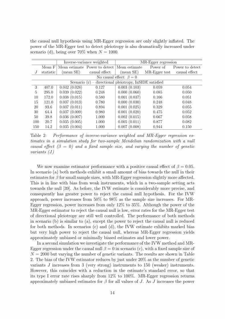
Scenario (c) – directional pleiotropy, InSIDE satisfied3 407.0 0.042 (0.028) 0.127 0.003 (0.103) 0.059 0.0545 295.0 0.039 (0.022) 0.248 0.000 (0.060) 0.085 0.05010 172.0 0.038 (0.015) 0.580 0.001 (0.037) 0.166 0.05115 121.0 0.037 (0.013) 0.780 0.000 (0.030) 0.248 0.04820 93.6 0.037 (0.011) 0.894 0.001 (0.025) 0.329 0.05530 64.4 0.037 (0.009) 0.980 0.001 (0.020) 0.475 0.05250 39.8 0.036 (0.007) 1.000 0.002 (0.015) 0.667 0.058100 20.7 0.035 (0.005) 1.000 0.005 (0.011) 0.877 0.082150 14.2 0.035 (0.004) 1.000 0.007 (0.008) 0.944 0.150
Table 2: Performance of inverse-variance weighted and MR-Egger regression es-timates in a simulation study for two-sample Mendelian randomization with a nullcausal effect (β = 0) and a fixed sample size, and varying the number of geneticvariants (J)
We now examine estimator performance with a positive causal effect of β = 0.05.In scenario (a) both methods exhibit a small amount of bias towards the null in theirestimates for β for small sample sizes, with MR-Egger regression slightly more affected.This is in line with bias from weak instruments, which in a two-sample setting actstowards the null [39]. As before, the IVW estimate is considerably more precise, andconsequently has greater power to reject the causal null hypothesis. For the IVWapproach, power increases from 50% to 98% as the sample size increases. For MR-Egger regression, power increases from only 12% to 35%. Although the power of theMR-Egger estimator to reject the causal null is low, error rates for the MR-Egger testof directional pleiotropy are still well controlled. The performance of both methodsin scenario (b) is similar to (a), except the power to reject the causal null is reducedfor both methods. In scenarios (c) and (d), the IVW estimate exhibits marked biasbut very high power to reject the causal null, whereas MR-Egger regression yieldsapproximately unbiased or minimally biased estimates and lower power.
In a second simulation we investigate the performance of the IVWmethod and MR-Egger regression under the causal null β = 0 in scenario (c), with a fixed sample size ofN = 2000 but varying the number of genetic variants. The results are shown in Table2. The bias of the IVW estimator reduces by just under 20% as the number of geneticvariants J increases from 3 (very strong) instruments to 150 (weaker) instruments.However, this coincides with a reduction in the estimate’s standard error, so thatits type I error rate rises sharply from 12% to 100%. MR-Egger regression returnsapproximately unbiased estimates for β for all values of J . As J increases the power
14
●
●
●
●
●
●
●
●
●
●
●
●
●
●
●
●
●
●
●
●
●
●
●
●
●
●
●
●●
●
●
●
●
●
●
●
●
●
●
●
●
●
●
●
●
●
●
●
●
●
�1.0 �0.5 0.0 0.5 1.0
10
20
30
40
(a)
β^
j
γ jC
IVW = 0.002Egger = 0Truth = 0
●
●
●
●
●
●
●
●
●
●
●
●
●
●
●
● ●
●
●
●
●
●
●
●
●
●
●
●
●
●
●
●
●
●
●
●
●
●
●
●
●
●
●
●
●
●
●
�1.0 �0.5 0.0 0.5 1.0
01
02
03
04
0
(b)
β^
j
γ jC
IVW = �0.001Egger = 0.019Truth = 0
●
●
● ●
●
●
●
●
●
●
●
●
●
●
●
●
●
●
●
●
●
●
●
●
●
●
●
●
●
●
●●
●
●
●
●
●
●
●
●
●
●
●
●
●
●
●
●
●
●
�1.0 �0.5 0.0 0.5 1.0
51
01
52
02
53
03
54
0
(c)
β^
j
γ jC
IVW = 0.077Egger = 0.012Truth = 0
●
●
●
●
●
●
●
●
●
●
●
●
●
●
●
●
●
●
●
●
●
●
●
●
●
●●
●
●
●
●
●
●
●
●
●
●
●
●
●
●
●
●
●
●
●
●●
●
●
�1.0 �0.5 0.0 0.5 1.0
51
01
52
02
53
0
(d)
β^
j
γ jC
IVW = 0.223Egger = 0.086Truth = 0
Figure 5: Funnel plots of minor allele frequency corrected genetic associations withexposure (γC
j ) against causal estimates based on each genetic variant individually (βj)for 50 IV estimates in four scenarios: (a) no pleiotropy; (b) balanced pleiotropy; (c)directional pleiotropy, InSIDE assumption satisfied; and (d) directional pleiotropy,InSIDE assumption not satisfied. The inverse-variance weighted (IVW, red) and MR-Egger (blue) causal effect estimates are also shown.
15
of the MR-Egger test to detect directional pleiotropy increases from around 5% to95%. The type I error rate of MR-Egger regression to detect a causal effect is wellcontrolled for J ≤ 50 variants, but for over 100 variants some type I error inflation isapparent. In summary, MR-Egger regression works well with large numbers of geneticvariants (in the sense that it has an increased power to detect pleiotropy), as long asthe variants are not too weak.
Discussion
In this paper we have proposed a simple sensitivity analysis for Mendelian randomiza-tion investigations using large numbers of genetic variants, that may or may not havepleiotropic effects on the outcome of interest. Egger’s test is widely used as a toolfor detecting small study bias in meta-analysis. Under the InSIDE assumption thatthe direct pleiotropic effects of the genetic variants on the outcome are distributedindependently of the genetic associations with the exposure, MR-Egger regressionprovides a valid test of directional (imbalanced) pleiotropy, and a valid test of thecausal null hypothesis. Under this assumption, the slope estimate from MR-Egger re-gression is a consistent estimate of the true causal effect. When there are pleiotropicinstruments but the InSIDE assumption is not satisfied, MR-Egger regression doesnot give a consistent estimate of causal effect, but remains a more robust method ofinference compared to standard approaches which rely on the stronger assumptionthat there is no pleiotropy. This renders it an important sensitivity analysis tool inthe Mendelian randomization context. In Box 1 we re-state the critical assumptionsrequired for the valid application of MR-Egger regression in the MR context andprovide a step-by-step guide to its application in practice.
16
Box 1: Summary of assumptions for application of MR-Egger regression
We take summarized genetic association estimates with the exposure (γ1, . . . , γJ), withthe outcome (Γ1, . . . , ΓJ), and standard errors of the genetic associations with theoutcome (σY 1, . . . , σY J) for J genetic variants which are: i) robustly associated withthe exposure, ii) uncorrelated with each other, and iii) in Hardy–Weinberg equilibrium.All variants must be orientated such that the genetic associations with the exposurehave the same sign (that is, they must all be positive or all negative).
For the standard inverse-variance weighted method, we perform a weighted linearregression of the genetic associations with the outcome on the genetic associationswith the exposure, weighting by the inverse-variance of the genetic associations withthe outcome (σ−2
Y j ). In this regression model, the intercept is constrained to equalzero. This analysis assumes that all genetic variants are valid instrumental variables.
For the proposed MR-Egger method, we perform the same weighted linear regressionwith the intercept unconstrained. The intercept represents the average pleiotropiceffect across the genetic variants (the average direct effect of a variant with theoutcome). If the intercept differs from zero (the MR-Egger test), then there is evidenceof directional pleiotropy. Under the assumption that the associations of the geneticvariants with the exposure are independent of the direct effects of the genetic variantson the outcome (the InSIDE assumption), the slope coefficient from the MR-Eggerregression is a consistent estimate of the causal effect. This is a weaker assumptionthan the assumption that all genetic variants are valid instrumental variables. TheInSIDE assumption would be violated if the pleiotropic effects act via a confounderof the exposureoutcome association.
R and Stata code to perform the inverse-variance weighted and MR-Egger methodsis provided in the Web Appendix.
Relation to existing literature
Several statistical methods have been proposed for consistent estimation of causaleffects when the IV assumptions are not all satisfied. For example, Kang et al. [40]propose a scenario in which only half of the genetic variants are required to be validIVs. If infinite data were available, the identity of the valid IVs would be clear, as theywould identify the same causal effect. Kang et al. provide an estimation method basedon lasso penalization [41] which not only gives consistent causal estimates in infinitesamples, but also has reasonable finite sample properties. However, in contrast withthe method proposed in this paper, which allows all the genetic variants to be invalidIVs, Kang et al. require at least half of the genetic variants to be valid IVs. Otherwise,if causal estimates from the two sets of valid and invalid genetic variants tendedtowards different values, it would not be possible to distinguish which of those valuesis the causal effect. A similar approach is simply to calculate the causal estimatesusing each genetic variants individually, rank the estimates in order of magnitude, and
17
take the median estimate [42]. Again, this is guaranteed to give a consistent causalestimate if at least half of the genetic variants are valid IVs, although at the costof a considerable reduction in precision of the causal estimate . Kolesar et al. [25]also propose a consistent causal estimator under the same conditions as considered inthis paper. This is based on a modified version of the bias-corrected TSLS estimator,which is part of the wider group of k-class estimators, a group that also includes theTSLS, bias-corrected TSLS, and limited information maximum likelihood estimators[43]. Further theoretical work is needed to compare the statistical properties of thisestimator with the MR-Egger estimator proposed in this paper.
As Mendelian randomization with multiple IVs can be viewed as a meta-analysisof summarized genetic association estimates, methods and diagnostic tools developedfor meta-analysis can also be used for Mendelian randomization. This is particularlyrelevant as summarized genetic association estimates from large consortia are increas-ingly becoming publicly available (such as those from the CARDIoGRAM consortiumused in this paper) [44]. It has been shown that Mendelian randomization analysesbased on summarized data are as efficient as those based on individual-level data[23]. Other tools from the meta-analysis literature include methods for bias adjust-ment, such as the trim-and-fill method [45] and the use of pseudo-data [46]. Anotherdiagnostic tool is a heterogeneity test, which tests whether differences between esti-mates from different studies are compatible with chance variation [47]. This can beperformed using Cochran’s Q statistic [44]. The null hypothesis is that the underly-ing association is the same in each study. In the Mendelian randomization context,we can test whether causal estimates from different genetic variants are compatible.Considerable heterogeneity would be evidence that the genetic variants are estimatingdifferent quantities, and would cast doubt on the IV assumptions being valid for allthe variants. In IV analysis more generally, a heterogeneity test is equivalent to anover-identification test, often performed with individual-level data as part of a TSLSanalysis [48].
Another problem with the use of many genetic variants is that of weak instru-ments. With many IVs in a one-sample setting (genetic variants, exposure and out-come measured in the same participants), IV estimates (particularly those from theTSLS method) are biased in the direction of the observational association between theexposure and the outcome [49]. This bias depends on the strength of the association ofthe IVs with the exposure, and is typically small if there is one IV [50] or if the IVs arestrongly associated with the exposure, but the bias may be substantial for Mendelianrandomization in realistic settings [36]. In a two-sample setting, weak instrument biasis in the direction of the null, and hence is a less serious problem, as it will not leadto false positive findings [37, 39]. One solution proposed for weak instrument biasis the use of allele scores, whereby the number of exposure-increasing alleles acrossmultiple genetic variants is summed up across individuals [9]. The total number ofalleles (possibly weighted according to their association with the exposure) is thenused as a single IV, rather than the genetic variants each being used as separate IVs.Provided that the weights are not taken from the data under analysis, this leads toestimates that are less affected by weak instrument bias. However, if results are solely
18
given in terms of an allele score and not in terms of the individual variants, then in-consistency of causal estimates from different variants (either directional pleiotropy orheterogeneity) may not be evident. Failure of the MR-Egger test does not necessarilyimply that the allele score estimate will be biased; however, it strongly suggests thatbias may be an issue. It is therefore important not simply to report the associationsof exposure and outcome with the allele score, but also associations with the geneticvariants individually, such as in the scatter plot or funnel plot representations shownin this paper.
Limitations of the proposed approach
While the InSIDE assumption is plausible in some cases, it will not be valid in allcircumstances, particularly if the pleiotropic effects of genetic variants act on con-founders of the exposure–outcome association. This is because the confounders willinduce a correlation between the direct effects of the variants on the outcome and thegenetic associations with the exposure. This would occur, for example, in the caseof population stratification. Another important way this could occur is if a geneticvariant in truth affects an exposure causally upstream of the one under investigation(for example, if the exposure of interest is C-reactive protein but an included variantis associated with body mass index). However in simulation scenario (d), where thepleiotropic effects through confounders (violating InSIDE) were 2.5 times larger thanthe direct pleiotropic effects (satisfying InSIDE), estimates from MR-Egger regressionwere much less biased and rejection rates of the causal null hypothesis were muchcloser to the nominal 5% rate than those from conventional IV methods. A relatedlimitation is power – while the MR-Egger regression estimator was more robust, powerto detect a causal effect was much reduced.
At present, we have not validated a universally reliable method for determin-ing standard errors of the MR-Egger estimator when the causal effect is non-zero.Possible approaches include bootstrapping in a one-sample setting, or a hierarchicallikelihood-based model that accounts for uncertainty in the genetic associations usedas datapoints in the regression model. Other methods for giving valid inferences in thecontext of a meta-analysis and small study bias have been discussed in the literature[14, 15]. The methods described in this paper therefore provide a sensitivity analysisto assess robustness of the conclusions of a Mendelian randomization investigationto potential bias from directional pleiotropy, and contribute to the overall evidenceregarding the existence, direction and magnitude of the causal effect. If the MR-Eggerestimate differs substantially from a conventional IV estimate, as in the example ofblood pressure and coronary artery disease risk, the causal finding clearly requiresadditional interrogation. However, confidence intervals for the causal effect should beinterpreted with caution when far from the null, for the reasons discussed.
In this manuscript, we have assumed that genetic variants are uncorrelated. If thevariants are correlated, and the correlations between variants are known, then theycan be taken into account by using generalized weighted linear regression in place ofweighted linear regression in either the IVW or MR-Egger method, incorporating thecorrelations into the weighting matrix. Further work is currently being undertaken to
19
explore this method.One further limitation of this approach is the assumption that the same causal
effect is identified by multiple IVs. This assumption is not unique to our approach,as it is commonly made in IV analyses with multiple IVs. The presence of ‘treatmenteffect heterogeneity’ is a complicating factor in causal analyses more generally, asit is not clear how to interpret a causal effect estimate if its magnitude dependson the nature of the intervention on the exposure. It is particularly problematic inour approach and in those of Kang et al. and Kolesar et al., as differences betweencausal estimates from different genetic variants are interpreted as evidence that thevariants are not valid IVs, whereas the differences may simply reflect treatment effectheterogeneity, in which case all the variants may be valid IVs. It is particularlyimportant in the Mendelian randomization context to distinguish between treatmenteffect heterogeneity among individuals to a common intervention, and heterogeneity ofresponse in relation to different methods of influencing the intermediate phenotype.Ascertaining the likelihood of each type of heterogeneity in the MR context anddeveloping methods that are robust to both is an important avenue for future study.
Conclusion
In conclusion, the approaches of this paper should not be interpreted as a pretext forconducting Mendelian randomization analyses with large numbers of genetic variantswithout prior regard to the validity of the IV assumptions. However, they providesimple graphical and statistical methods that can detect some violations of the IVassumptions, and can therefore can used as a sensitivity analysis for assessing whetherthe effect estimation in a Mendelian randomization analysis is influenced by directionalpleiotropic effects of the genetic variants.
Key messages:
• Mendelian randomization analyses using multiple genetic variants can be viewedas a meta-analysis of the causal estimates from each variant.
• If the genetic variants have pleiotropic effects on the outcome, these causalestimates will be biased.
• Funnel plots offer a simple way to detect directional pleiotropy; that is, whethercausal estimates from weaker variants tend to be skewed in one direction.
• Under a weaker set of assumptions than typically used in Mendelianrandomization, MR-Egger regression can be used to detect and correct for thebias due to directional pleiotropy.
20
Acknowledgements
The authors would like to thank the reviewers for their helpful comments, whichgreatly improved this paper. We would also like to thank Neil M. Davies for pro-viding data for the lung function example. Jack Bowden is supported by an MRCMethodology Research Fellowship (grant MR/L012286/1). Stephen Burgess is sup-ported by the Wellcome Trust (grant number 100114).
References
[1] G. Davey Smith and S. Ebrahim. ‘Mendelian randomization’: can genetic epi-demiology contribute to understanding environmental determinants of disease?International Journal of Epidemiology, 32:1–22, 2003.
[2] S. Burgess, A. Butterworth, A. Malarstig, and S. Thompson. Use of Mendelianrandomisation to assess potential benefit of clinical intervention. British MedicalJournal, 345:e7325, 2012.
[3] G. Davey Smith and G. Hemani. Mendelian randomization: genetic anchors forcausal inference in epidemiological studies. Human Molecular Genetics, 23:89–98,2014.
[4] P. Sleiman and S. Grant. Mendelian randomization in the era of genomewideassociation studies. Clinical Chemistry, 56:723–728, 2010.
[5] A. Boef, O. Dekkers O, and S. Le Cessie. Mendelian randomization studies: areview of the approaches used and the quality of reporting. 2015. InternationalJournal of Epidemiology, 44:In press, 2015.
[6] G. Freeman, B.J Cowling, and C.M Schooling. Power and sample size calculationsfor mendelian randomization studies using one genetic instrument. InternationalJournal of Epidemiology, 42:1157–1163, 2013.
[7] M.J. Brion, K. Shakhbazov, and P.M. Visscher. Calculating statistical powerin mendelian randomization studies. International Journal of Epidemiology,42:1497–1501, 2013.
[8] D. Lawlor, R. Harbord, J. Sterne, N. Timpson, and G. Davey Smith. Mendelianrandomization: using genes as instruments for making causal inferences in epi-demiology. Statistics in Medicine, 27:1133–1163, 2008.
[9] S. Burgess and S. Thompson. Use of allele scores as instrumental variables forMendelian randomization. International Journal of Epidemiology, 42:1134–1144,2013.
[10] G. Davey Smith and S. Ebrahim. Data dredging, bias, or confounding. BritishMedical Journal, 325:1437–1438, 2002.
21
[11] J. Bowden, D. Jackson, and S. Thompson. Modelling multiple sources of dissem-ination bias in meta-analysis. Statistics in Medicine, 29:945–955, 2010.
[12] M. Egger, G. Davey Smith, M. Schneider, and C. Minder. Bias in meta-analysisdetected by a simple, graphical test. British Medical Journal, 315:629–634, 1997.
[13] J. Sterne, A. Sutton, J. Ioannidis, et al. Recommendations for examining andinterpreting funnel plot asymmetry in meta-analyses of randomised controlledtrials. British Medical Journal, 343:d4002, 2011.
[14] G. Rucker, G. Schwarzer, J. Carpenter, H. Binder, and M. Schumacher.Treatment-effect estimates adjusted for small study effects via a limit meta-analysis. Biostatistics, 12:122–142, 2011.
[15] J. Copas and P. Malley. A robust p-value for treatment effect in meta-analysiswith publication bias. Statistics in Medicine, 27:4267–4278, 2008.
[16] J. Angrist, G. Imbens, and D. Rubin. Identification of causal effects using instru-mental variables. Journal of the American Statistical Association, 91:444–455,1996.
[17] A. Wald. The fitting of straight lines if both variables are subject to error. Annalsof Mathematical Statistics, 11:284–300, 1940.
[18] V. Didelez and N. Sheehan. Mendelian randomisation as an instrumental variableapproach to causal inference. Statistical Methods in Medical Research, 16:309–330, 2007.
[19] J. Angrist and G. Imbens. Two-stage least squares estimation of average causaleffects in models with variable treatment intensity. Journal of the AmericanStatistical Association, 90:431–442, 1995.
[20] J. Wooldridge. Introductory econometrics: A modern approach. Chapter 15:Instrumental variables estimation and two stage least squares. South-Western,Nashville, TN, 2009.
[21] T. Johnson. Efficient calculation for multi-SNP genetic risk scores. Tech-nical report, The Comprehensive R Archive Network, 2013. Availableat http://cran.r-project.org/web/packages/gtx/vignettes/ashg2012.pdf [last ac-cessed 2014/11/19].
[22] M. Borenstein, L. Hedges, J. Higgins, and H. Rothstein. Introduction to meta-analysis. Chapter 34: Generality of the basic inverse-variance method. Wiley,2009.
[23] S. Burgess, A. Butterworth, and S. Thompson. Mendelian randomization analysiswith multiple genetic variants using summarized data. Genetic Epidemiology,37:658–665, 2013.
22
[24] G. Davey Smith. Random allocation in observational data: how small but robusteffects could facilitate hypothesis-free causal inference. Epidemiology, 22:460–463,2011.
[25] M. Kolesar, R. Chetty, J. Friedman, E. Glaeser, and G. Imbens. Identification andinference with many invalid instruments. NBER Working Paper 17519, NationalBureau of Economic Research, 2014.
[26] R. Galbraith. Some applications of radial plots. Journal of the American Statis-tical Association, 89:1232–1242, 1994.
[27] S. Thompson and S. Sharp. Explaining heterogeneity in meta-analysis: a com-parison of methods. Statistics in Medicine, 18:2693–2708, 1999.
[28] J. Sterne and M. Egger. Funnel plots for detecting bias in meta-analysis: Guide-lines on choice of axis. Journal of Clinical Epidemiology, 54:1046–1055, 2001.
[29] N. Davies, S.H.K. Scholder, H. Farbmacher., S. Burgess, F. Windmeijer, andG. Davey Smith. The many weak instrument problem and Mendelian random-ization. Statistics in Medicine, 34:454–468, 2015.
[30] A. Boyd, J. Golding, J. Macleod, D. Lawlor, A. Fraser, J. Henderson, L. Molloy,A. Ness, S. Ring, and G. Davey Smith. Cohort profile: the “Children of the 90s”- the index offspring of the Avon Longitudinal Study of Parents and Children.International Journal of Epidemiology, 42:111–127, 2012.
[31] H. Lango Allen, K. Estrada, G. Lettre, et al. Hundreds of variants clustered ingenomic loci and biological pathways affect human height. Nature, 467:832–838,2010.
[32] G. Ehret and P. Munroe and K. Rice and others. Genetic variants in novel path-ways influence blood pressure and cardiovascular disease risk. Nature, 478:103–109, 2011.
[33] H. Schunkert, I. Konig, S. Kathiresan, et al. Large-scale association analysisidentifies 13 new susceptibility loci for coronary artery disease. Nature Genetics,43:333–338, 2011.
[34] M.R. Law, J.K. Morris, and N.J. Wald. Use of blood pressure lowering drugs inthe prevention of cardiovascular disease: meta-analysis of 147 randomised trialsin the context of expectations from prospective epidemiological studies. BritishMedical Journal, (338):b1665, 2009.
[35] A. Taylor, N. Davies, J. Ware, T. VanderWeele, G. Davey Smith, and M. Munafo.Mendelian randomization in health research: Using appropriate genetic variantsand avoiding biased estimates. Economics & Human Biology, 13:99–106, 2014.
23
[36] S. Burgess, S. Thompson, and CRP CHD Genetics Collaboration. Avoidingbias from weak instruments in Mendelian randomization studies. InternationalJournal of Epidemiology, 40:755–764, 2011.
[37] A. Inoue and G. Solon. Two-sample instrumental variables estimators. TheReview of Economics and Statistics, 92:557–561, 2010.
[38] T. VanderWeele, E. Tchetgen Tchetgen, M. Cornelis, and P. Kraft. Methodolog-ical challenges in Mendelian randomization. Epidemiology, 25:427–435, 2014.
[39] B. Pierce and S. Burgess. Efficient design for Mendelian randomization studies:subsample and two-sample instrumental variable estimators. American Journalof Epidemiology, 178:1177–1184, 2013.
[40] H. Kang, A. Zhang, T. Cai, and D. Small. Instrumental variables estimationwith some invalid instruments, and its application to Mendelian randomisation.Technical report, Department of Statistics, University of Pennsylvania, 2014.
[41] R. Tibshirani. Regression shrinkage and selection via the lasso. Journal of theRoyal Statistical Society: Series B (Methodological), 58:267–288, 1996.
[42] C. Han. Detecting invalid instruments using L1-GMM. Economics Letters,101:285–287, 2008.
[43] A. Nagar. The bias and moment matrix of the general k-class estimators of theparameters in simultaneous equations. Econometrica: Journal of the EconometricSociety, 27:575–595, 1959.
[44] S. Burgess, R. Scott, N. Timpson, G. Davey Smith, S. Thompson, and EPIC-InterAct Consortium. Using published data in Mendelian randomization: ablueprint for efficient identification of causal risk factors. European Journal ofEpidemiology, 2015. In press.
[45] S. Duval and R. Tweedie. Trim and fill: A simple funnel-plot-based method oftesting and adjusting for publication bias in meta-analysis. Biometrics, 56:455–463, 2000.
[46] J. Bowden, J. Thompson, and P. Burton. Using pseudo-data to correct for pub-lication bias in meta-analysis. Statistics in Medicine, 25:3798–3813, 2006.
[47] J. Higgins, S. Thompson, J. Deeks, and D. Altman. Measuring inconsistency inmeta-analyses. British Medical Journal, 327:557–560, 2003.
[48] D. Small. Sensitivity analysis for instrumental variables regression with overiden-tifying restrictions. Journal of the American Statistical Association, 102:1049–1058, 2007.
[49] D. Staiger and J. Stock. Instrumental variables regression with weak instruments.Econometrica, 65:557–586, 1997.
24
[50] J. Angrist and J-S. Pischke. Mostly harmless econometrics: an empiricist’s com-panion. Chapter 4: Instrumental variables in action: sometimes you get whatyou need. Princeton University Press, 2009.
25
Web Appendix (updated 31/7/15)
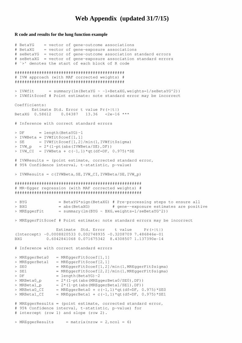
R code and results for the lung function example
# BetaYG = vector of gene-outcome associations # BetaXG = vector of gene-exposure associations # seBetaYG = vector of gene-outcome association st andard errors # seBetaXG = vector of gene-exposure association s tandard errors # `>’ denotes the start of each block of R code ############################################# # IVW approach (with MAF corrected weights) # ############################################# > IVWfit = summary(lm(BetaYG ~ -1+BetaXG,weigh ts=1/seBetaYG^2)) > IVWfit$coef # Point estimate: note standard error may be incorrect Coefficients: Estimate Std. Error t value Pr(>|t|) BetaXG 0.58612 0.04387 13.36 <2e-16 *** # Inference with correct standard errors > DF = length(BetaYG)-1 > IVWBeta = IVWfit$coef[1,1] > SE = IVWfit$coef[1,2]/min(1,IVWfit$sigma) > IVW_p = 2*(1-pt(abs(IVWBeta/SE),DF)) > IVW_CI = IVWBeta + c(-1,1)*qt(df=DF, 0.975)*SE # IVWResults = (point estimate, corrected standard error, # 95% Confidence interval, t-statistic, p-value) > IVWResults = c(IVWBeta,SE,IVW_CI,IVWBeta/SE,IVW_p ) ################################################### # # MR-Egger regression (with MAF corrected weights) # ################################################### # > BYG = BetaYG*sign(BetaXG) # Pre-proce ssing steps to ensure all > BXG = abs(BetaXG) # gene--exp osure estimates are positive > MREggerFit = summary(lm(BYG ~ BXG,weights=1/ seBetaYG^2)) > MREggerFit$coef # Point estimate: note standard e rrors may be incorrect Estimate Std. Error t value Pr(>|t|) (Intercept) -0.0008820533 0.002748935 -0.3208709 7. 486846e-01 BXG 0.6042841068 0.071675342 8.4308507 1. 137390e-14 # Inference with correct standard errors > MREggerBeta0 = MREggerFit$coef[1,1] > MREggerBeta1 = MREggerFit$coef[2,1] > SE0 = MREggerFit$coef[1,2]/min(1,MREgg erFit$sigma) > SE1 = MREggerFit$coef[2,2]/min(1,MREgg erFit$sigma) > DF = length(BetaYG)-2 > MRBeta0_p = 2*(1-pt(abs(MREggerBeta0/SE0),DF )) > MRBeta1_p = 2*(1-pt(abs(MREggerBeta1/SE1),DF )) > MRBeta0_CI = MREggerBeta0 + c(-1,1)*qt(df=DF, 0.975)*SE0 > MRBeta1_CI = MREggerBeta1 + c(-1,1)*qt(df=DF, 0.975)*SE1 # MREggerResults = (point estimate, corrected stand ard error, # 95% Confidence interval, t-statistic, p-value) fo r # intercept (row 1) and slope (row 2). > MREggerResults = matrix(nrow = 2,ncol = 6)
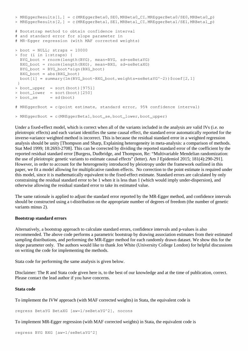
> MREggerResults[1,] = c(MREggerBeta0,SE0,MRBeta0_C I,MREggerBeta0/SE0,MRBeta0_p) > MREggerResults[2,] = c(MREggerBeta1,SE1,MRBeta1_C I,MREggerBeta1/SE1,MRBeta1_p) # Bootstrap method to obtain confidence interval # and standard error for slope parameter in # MR-Egger regression (with MAF corrected weights) > boot = NULL; straps = 10000 > for (i in 1:straps) { BYG_boot = rnorm(length(BYG), mean=BYG, sd=seBeta YG) BXG_boot = rnorm(length(BXG), mean=BXG, sd=seBeta XG) BYG_boot = BYG_boot*sign(BXG_boot) BXG_boot = abs(BXG_boot) boot[i] = summary(lm(BYG_boot~BXG_boot,weights=se BetaYG^-2))$coef[2,1] } > boot_upper = sort(boot)[9751] > boot_lower = sort(boot)[250] > boot_se = sd(boot) # MREggerBoot = c(point estimate, standard error, 9 5% confidence interval) > MREggerBoot = c(MREggerBeta1,boot_se,boot_lower,b oot_upper)
Under a fixed-effect model, which is correct when all of the variants included in the analysis are valid IVs (i.e. no pleiotropic effects) and each variant identifies the same causal effect, the standard error automatically reported for the inverse-variance weighted method is incorrect. This is because the residual standard error in a weighted regression analysis should be unity [Thompson and Sharp, Explaining heterogeneity in meta-analysis: a comparison of methods. Stat Med 1999; 18:2693-2708]. This can be corrected by dividing the reported standard error of the coefficient by the reported residual standard error [Burgess, Dudbridge, and Thompson, Re: “Multivariable Mendelian randomization: the use of pleiotropic genetic variants to estimate causal effects” (letter). Am J Epidemiol 2015; 181(4):290-291]. However, in order to account for the heterogeneity introduced by pleiotropy under the framework outlined in this paper, we fit a model allowing for multiplicative random effects. No correction to the point estimate is required under this model, since it is mathematically equivalent to the fixed-effect estimate. Standard errors are calculated by only constraining the residual standard error to be 1 when it is less than 1 (which would imply under-dispersion), and otherwise allowing the residual standard error to take its estimated value.
The same rationale is applied to adjust the standard error reported by the MR-Egger method, and confidence intervals should be constructed using a t-distribution on the appropriate number of degrees of freedom (the number of genetic variants minus 2).
Bootstrap standard errors
Alternatively, a bootstrap approach to calculate standard errors, confidence intervals and p-values is also recommended. The above code performs a parametric bootstrap by drawing association estimates from their estimated sampling distributions, and performing the MR-Egger method for each randomly drawn dataset. We show this for the slope parameter only. The authors would like to thank Jon White (University College London) for helpful discussions on writing the code for implementing the methods.
Stata code for performing the same analysis is given below.
Disclaimer: The R and Stata code given here is, to the best of our knowledge and at the time of publication, correct. Please contact the lead author if you have concerns.
Stata code
To implement the IVW approach (with MAF corrected weights) in Stata, the equivalent code is
regress BetaYG BetaXG [aw=1/seBetaYG^2], nocons
To implement MR-Egger regression (with MAF corrected weights) in Stata, the equivalent code is
regress BYG BXG [aw=1/seBetaYG^2]
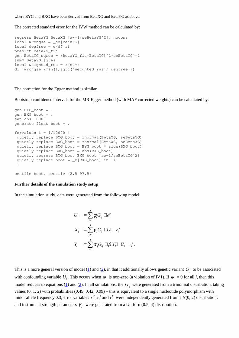
where BYG and BXG have been derived from BetaXG and BetaYG as above.
The corrected standard error for the IVW method can be calculated by:
regress BetaYG BetaXG [aw=1/seBetaYG^2], nocons local wrongse = _se[BetaXG] local degfree = e(df_r) predict BetaYG_fit gen BetaYG_sqres = (BetaYG_fit-BetaYG)^2*seBetaYG^- 2 summ BetaYG_sqres local weighted_rss = r(sum) di `wrongse'/min(1,sqrt(`weighted_rss'/`degfree'))
The correction for the Egger method is similar.
Bootstrap confidence intervals for the MR-Egger method (with MAF corrected weights) can be calculated by:
gen BYG_boot = . gen BXG_boot = . set obs 10000 generate float boot = . forvalues i = 1/10000 { quietly replace BYG_boot = rnormal(BetaYG, seBetaY G) quietly replace BXG_boot = rnormal(BetaXG, seBetaX G) quietly replace BYG_boot = BYG_boot * sign(BXG_boo t) quietly replace BXG_boot = abs(BXG_boot) quietly regress BYG_boot BXG_boot [aw=1/seBetaYG^2 ] quietly replace boot = _b[BXG_boot] in `i' } centile boot, centile (2.5 97.5)
Further details of the simulation study setup
In the simulation study, data were generated from the following model:
1
1
1
.
J
Ui j ij i
j
JX
i j ij i ij
JY
i j ij i i ij
U G
X G U
Y G X U
φ
γ
α β
=
=
=
= +
= + +
= + + +
∑
∑
∑
ε
ε
ε
This is a more general version of model (1) and (2), in that it additionally allows genetic variant jG to be associated
with confounding variable iU . This occurs when jφ is non-zero (a violation of IV1). If jφ = 0 for all j, then this
model reduces to equations (1) and (2). In all simulations: the ijG were generated from a trinomial distribution, taking
values (0, 1, 2) with probabilities (0.49, 0.42, 0.09) – this is equivalent to a single nucleotide polymorphism with minor allele frequency 0.3; error variables , and U X Y
i i iε ε ε were independently generated from a N(0, 2) distribution;
and instrument strength parameters jγ were generated from a Uniform(0.5, 4) distribution.
The performance of the standard IVW method and MR-Egger regression were investigated in a two-sample Mendelian randomization analysis context with J = 25 variants, with a null (β = 0) and a positive (β = 0.05) causal effect. Two independent samples of N subjects were generated from the above model. For variant j out of 25, estimates for the gene-exposure associations (ˆ
jγ ) were obtained from the first sample and estimates for the gene-
outcome associations (ˆjΓ ) were obtained from the second sample, in order to calculate the ratio estimates
ˆ ˆ ˆ/j j jβ γ= Γ . Simulation scenarios (a)–(d) were implemented by additionally specifying values for jα and jφ as
below:
• No pleiotropy, InSIDE satisfied: jα = 0, jφ = 0;
• Balanced pleiotropy, InSIDE satisfied: jα ~ Uniform(-0.2,0.2), jφ = 0;
• Directional pleiotropy, InSIDE satisfied: jα ~ Uniform(0,0.2), jφ = 0;
• Directional pleiotropy, InSIDE not satisfied: jα ~ Uniform(0,0.2), jφ ~ Uniform(0,0.5).
In scenario (a), the ratio estimand based on the jth variant is equal to β. In scenario’s (b) and (c), the ratio estimand
based on the jth variant is equal to j
j
αβ
γ+ but InSIDE holds. In scenario (d) the ratio estimand based on the jth
variant is equal to
.j j
j j
α φβ
γ φ+
++
The InSIDE assumption is not satisfied in this case because the numerator of the bias term (which represents the total ‘direct’ effect not via the exposure) and its denominator (which represents the instrument strength) contain the common term ϕj. Simulation results are shown in Table 1.
Data for the four funnel plots shown in Figure 5 were generated under the causal null hypothesis for scenarios (a)–(d), using the same two-sample approach. In order to accentuate the shapes of the funnel plots for illustrative purposes, we used J = 50 genetic variants and doubled the range of the Uniform sampling densities for jα and jφ . Web
Figure A2 shows the equivalent scatter plots.
Results from the simulation study in a one-sample setting
The previous simulations were repeated in a one-sample Mendelian randomization setting. One sample of N subjects was generated, and estimates for the gene-exposure associations ( jγ ) and estimates for the gene-outcome associations
( ˆjΓ ) were obtained from the same sample.
Results are shown in Table A1 and A2. The pattern of results is generally similar to the two-sample case, but both methods perform slightly worse in terms of small sample bias and Type I error rate inflation, and markedly worse with weak instruments. Weak instrument bias is more problematic in the one sample context because it acts in the direction of the confounded observational association. It appears to be slightly worse for estimates from MR-Egger regression, while Type I error rate is worse for estimates from the IVW method.
These simulations were repeated using standard one-sample TSLS instead of IVW as the comparator method, and the results were very similar (data not shown). We conclude that IV analysis with weak instruments in a one-sample setting is troublesome, and that these difficulties are not resolved by the application of MR-Egger regression.
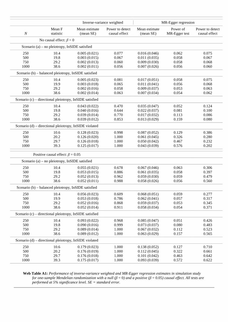
Inverse-variance weighted MR-Egger regression
Mean F Mean estimate Power to detect Mean estimate Power of Power to detect N statistic (mean SE) causal effect (mean SE) MR-Egger test causal effect
No causal effect: β = 0
Scenario (a) – no pleiotropy, InSIDE satisfied
250 10.4 0.005 (0.021) 0.077 0.016 (0.046) 0.062 0.075 500 19.8 0.003 (0.015) 0.067 0.011 (0.035) 0.058 0.067 750 29.2 0.002 (0.013) 0.060 0.009 (0.030) 0.058 0.068 1000 38.6 0.002 (0.011) 0.056 0.007 (0.026) 0.056 0.060
Scenario (b) – balanced pleiotropy, InSIDE satisfied
250 10.4 0.005 (0.023) 0.081 0.017 (0.051) 0.058 0.075 500 19.9 0.003 (0.018) 0.065 0.011 (0.041) 0.056 0.068 750 29.2 0.002 (0.016) 0.058 0.009 (0.037) 0.053 0.063 1000 38.6 0.002 (0.014) 0.063 0.007 (0.034) 0.054 0.062
Scenario (c) – directional pleiotropy, InSIDE satisfied
250 10.4 0.043 (0.022) 0.470 0.035 (0.047) 0.052 0.124 500 19.8 0.040 (0.016) 0.644 0.022 (0.037) 0.081 0.100 750 29.2 0.039 (0.014) 0.770 0.017 (0.032) 0.113 0.086 1000 38.6 0.039 (0.012) 0.853 0.013 (0.029) 0.159 0.080
Scenario (d) – directional pleiotropy, InSIDE violated
250 10.6 0.128 (0.023) 0.998 0.087 (0.052) 0.129 0.386 500 20.2 0.126 (0.020) 1.000 0.061 (0.045) 0.326 0.280 750 29.7 0.126 (0.018) 1.000 0.050 (0.042) 0.467 0.232 1000 39.3 0.125 (0.017) 1.000 0.043 (0.039) 0.576 0.202
Positive causal effect: β = 0.05
Scenario (a) – no pleiotropy, InSIDE satisfied
250 10.4 0.055 (0.021) 0.678 0.067 (0.046) 0.063 0.306 500 19.8 0.053 (0.015) 0.886 0.061 (0.035) 0.058 0.397 750 29.2 0.052 (0.013) 0.962 0.059 (0.030) 0.059 0.479 1000 38.6 0.052 (0.011) 0.988 0.058 (0.026) 0.056 0.560
Scenario (b) – balanced pleiotropy, InSIDE satisfied
250 10.4 0.056 (0.023) 0.609 0.068 (0.051) 0.059 0.277 500 19.9 0.053 (0.018) 0.786 0.062 (0.041) 0.057 0.317 750 29.2 0.052 (0.016) 0.868 0.059 (0.037) 0.053 0.345 1000 38.6 0.052 (0.014) 0.911 0.058 (0.034) 0.054 0.371
Scenario (c) – directional pleiotropy, InSIDE satisfied
250 10.4 0.093 (0.022) 0.968 0.085 (0.047) 0.051 0.426 500 19.8 0.090 (0.016) 0.999 0.073 (0.037) 0.080 0.483 750 29.2 0.089 (0.014) 1.000 0.067 (0.032) 0.112 0.523 1000 38.6 0.089 (0.012) 1.000 0.063 (0.029) 0.157 0.565
Scenario (d) – directional pleiotropy, InSIDE violated
250 10.6 0.179 (0.023) 1.000 0.138 (0.052) 0.127 0.710 500 20.2 0.176 (0.019) 1.000 0.112 (0.045) 0.322 0.661 750 29.7 0.176 (0.018) 1.000 0.101 (0.042) 0.463 0.642 1000 39.3 0.175 (0.017) 1.000 0.093 (0.039) 0.572 0.622
Web Table A1: Performance of inverse-variance weighted and MR-Egger regression estimates in simulation study
for one-sample Mendelian randomization with a null (β = 0) and a positive (β = 0.05) causal effect. All tests are performed at 5% significance level. SE = standard error.
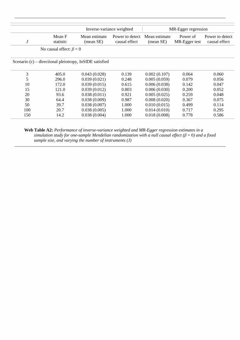
Inverse-variance weighted MR-Egger regression
Mean F Mean estimate Power to detect Mean estimate Power of Power to detect J statistic (mean SE) causal effect (mean SE) MR-Egger test causal effect
No causal effect: β = 0
Scenario (c) – directional pleiotropy, InSIDE satisfied
3 405.0 0.043 (0.028) 0.139 0.002 (0.107) 0.064 0.060 5 296.0 0.039 (0.021) 0.248 0.005 (0.059) 0.079 0.056 10 172.0 0.039 (0.015) 0.615 0.006 (0.038) 0.142 0.047 15 121.0 0.039 (0.012) 0.803 0.006 (0.030) 0.200 0.052 20 93.6 0.038 (0.011) 0.921 0.005 (0.025) 0.259 0.048 30 64.4 0.038 (0.009) 0.987 0.008 (0.020) 0.367 0.075 50 39.7 0.038 (0.007) 1.000 0.010 (0.015) 0.499 0.114 100 20.7 0.038 (0.005) 1.000 0.014 (0.010) 0.717 0.295 150 14.2 0.038 (0.004) 1.000 0.018 (0.008) 0.778 0.586
Web Table A2: Performance of inverse-variance weighted and MR-Egger regression estimates in a
simulation study for one-sample Mendelian randomization with a null causal effect (β = 0) and a fixed sample size, and varying the number of instruments (J)
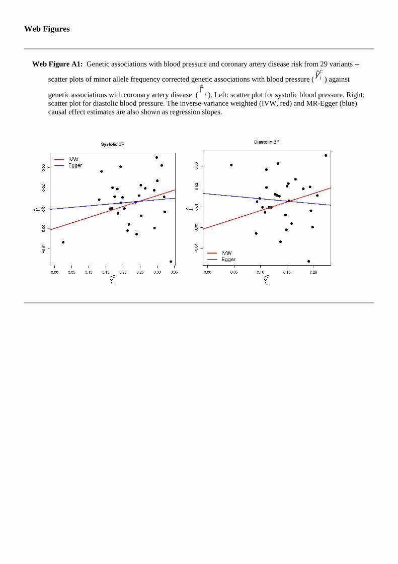
Web Figures
Web Figure A1: Genetic associations with blood pressure and coronary artery disease risk from 29 variants --
scatter plots of minor allele frequency corrected genetic associations with blood pressure (ˆC
jγ) against
genetic associations with coronary artery disease (ˆ
jΓ). Left: scatter plot for systolic blood pressure. Right:
scatter plot for diastolic blood pressure. The inverse-variance weighted (IVW, red) and MR-Egger (blue) causal effect estimates are also shown as regression slopes.
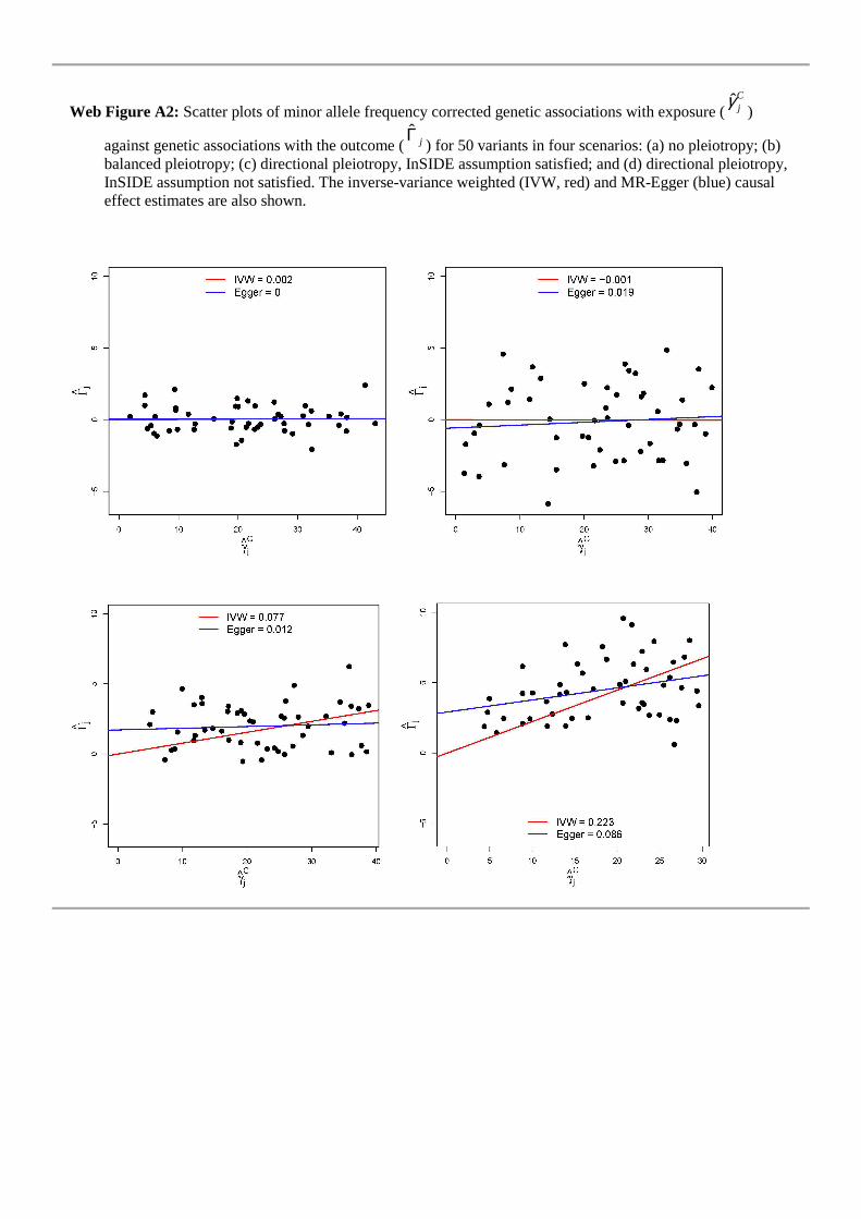
Web Figure A2: Scatter plots of minor allele frequency corrected genetic associations with exposure (ˆC
jγ)
against genetic associations with the outcome (ˆ
jΓ) for 50 variants in four scenarios: (a) no pleiotropy; (b)
balanced pleiotropy; (c) directional pleiotropy, InSIDE assumption satisfied; and (d) directional pleiotropy, InSIDE assumption not satisfied. The inverse-variance weighted (IVW, red) and MR-Egger (blue) causal effect estimates are also shown.


