Microbial community dynamics based on 16S rRNA gene profiles in a Pacific Northwest estuary and its tributaries

www.fems-microbiology.org

FEMS Microbiology Ecology 52 (2005) 115–128

Microbial community dynamics based on 16S rRNA gene profilesin a Pacific Northwest estuary and its tributaries

Anne E. Bernhard a,*,1, Debbie Colbert b, James McManus b, Katharine G. Field a

a Department of Microbiology, Oregon State University, Corvallis, OR 97331, USAb College of Oceanic and Atmospheric Sciences, Oregon State University, Corvallis, OR 97331, USA

Received 8 June 2004; received in revised form 12 October 2004; accepted 28 October 2004

First published online 28 November 2004

Abstract

We analyzed bacterioplankton community structure in Tillamook Bay, Oregon and its tributaries to evaluate phylogenetic var-

iability and its relation to changes in environmental conditions along an estuarine gradient. Using eubacterial primers, we amplified

16S rRNA genes from environmental DNA and analyzed the PCR products by length heterogeneity polymerase chain reaction (LH-

PCR), which discriminates products based on naturally occurring length differences. Analysis of LH-PCR profiles by multivariate

ordination methods revealed differences in community composition along the estuarine gradient that were correlated with changes in

environmental variables. Microbial community differences were also detected among different rivers. Using partial 16S rRNA

sequences, we identified members of dominant or unique gene fragment size classes distributed along the estuarine gradient. Gam-

maproteobacteria and Betaproteobacteria and members of the Bacteroidetes dominated in freshwater samples, while Alphaproteobac-

teria, Cyanobacteria and chloroplast genes dominated in marine samples. Changes in the microbial communities correlated most

strongly with salinity and dissolved silicon, but were also strongly correlated with precipitation. We also identified specific gene frag-

ments that were correlated with inorganic nutrients. Our data suggest that there is a significant and predictable change in microbial

species composition along an estuarine gradient, shifting from a more complex community structure in freshwater habitats to a com-

munity more typical of open ocean samples in the marine-influenced sites. We also demonstrate the resolution and power of LH-

PCR and multivariate analyses to provide a rapid assessment of major community shifts, and show how these shifts correlate with

environmental variables.

� 2004 Federation of European Microbiological Societies. Published by Elsevier B.V. All rights reserved.

Keywords: Estuary; 16S ribosomal RNA; Microbial community; Salinity gradient; LH-PCR; Tillamook bay

1. Introduction

The mixing of marine and fresh waters in estuaries

creates steep physico-chemical gradients, which are

undoubtedly accompanied by shifts in the biological

0168-6496/$22.00 � 2004 Federation of European Microbiological Societies

doi:10.1016/j.femsec.2004.10.016

* Corresponding author. Tel.: +1 860 439 2580; fax: +1 860 439

2519.

E-mail address: [email protected] (A.E. Bernhard).1 Current address: Connecticut College, Department of Biology,

New London, CT, USA.

communities. The ephemeral nature of microbes pre-

dicts that these communities, in particular, will undergo

dynamic changes along the estuarine gradient. Rapid

fluctuations in environmental conditions demand meta-

bolic plasticity of the resident microbes, or, alterna-

tively, genetically diverse microbial assemblages that

exploit niche differentiation. Shifts in estuarine micro-bial community structure may be regulated by the abil-

ity of individual populations to overcome various

environmental stresses. These stresses include changes

in nutrient concentrations, tidal currents, and predation,

. Published by Elsevier B.V. All rights reserved.

mailto:[email protected]

116 A.E. Bernhard et al. / FEMS Microbiology Ecology 52 (2005) 115–128

but the primary factor is thought to be changes in salin-

ity [1]. Most freshwater bacteria cannot survive even in

oligohaline waters [2,3], and salinity effects have been

observed on bacterial abundance and activity [4].

Changes in salinity also affect chemical constituents

[5], which may, in turn, affect the microbialcommunities.

In addition to the effects of salinity, seasonally driven

changes in microbial communities in estuaries [6] and

rivers [7] also occur. Changes may result from variations

in freshwater flow, which would covary with changes in

salinity. In addition, high flow may supply large pulses

of nutrient-rich material, driving bacterial productivity

up within the estuary and ultimately leading to a net het-erotrophic system [8]. Since bacteria are primarily

responsible for degradation and remineralization of dis-

solved organic material, changes in nutrient concentra-

tion and composition may lead to differences in

distributions of major bacterial populations [9,10].

Extensive studies of microbial diversity and commu-

nity structure have been carried out in ocean and lake

ecosystems (e.g. [11,12]), but only recently haveresearchers begun to address this subject in estuaries

[13–17]. Other studies in estuaries have focused on the

structure and function of bacterioplankton as a group

(e.g. [8,18]), disregarding population dynamics within

the communities. Because of the substantial contribu-

tion of bacterial production to ecosystem function in

estuaries, it is important to investigate the structure of

these bacterial communities and what factors contributemost to microbial species composition.

Recent advances in molecular techniques provide

necessary tools for microbial ecologists to assess com-

munity structure using culture-independent methods

[19]. One such technique, length-heterogeneity polymer-

ase chain reaction (LH-PCR) [20], discriminates among

numerically dominant 16S rRNA genes based solely on

length polymorphisms of the PCR products. The resultis a community profile of 16S rRNA gene products rep-

resenting different populations of bacteria. Because the

method is based on length of DNA sequences, presump-

tive identifications can be assigned to each different peak

in the profile by comparisons to sequences in the public

databases or by comparison to sequences obtained from

clone libraries. A major advantage of LH-PCR over

other molecular methods, such as gene cloning andsequencing, is that it provides a quick way to analyze

and compare communities from a large number of sam-

ples. Recently, microbial communities in soil [21] and

coastal [20,22,23] ecosystems have been characterized

by LH-PCR.

We applied LH-PCR to characterize the microbial

community structure along a salinity gradient in Tilla-

mookBay,Oregonand itsmajor tributaries, and to followmicrobial community dynamics over several seasons. Til-

lamook Bay is a drowned-river estuary in the Pacific

Northwest and is prone to high levels of fecal pollution

and sedimentation from five major rivers that drain into

the bay. The watershed is primarily forested, but the

bay is significantly influenced by agricultural, urban,

and rural land uses. TillamookBay experiences large tidal

changes, with low tides exposing more than 50% of thebay. This twice daily flux may have a significant impact

on the microbial communities, shifting from halophilic

and halotolerant organisms dominating at high tide to

halophobic organisms at low tide. Seasonal changes, such

as fluctuations in freshwater inflow, nutrient inputs, sun-

light, and temperature, may also be important factors in

determining microbial community composition.

The objectives of this study were fourfold. First, wecharacterized the major microbial populations in the

estuary based on 16S rRNA gene profiles and identified

major environmental factors correlated with the com-

munity changes. Second, we used 16S rRNA sequences

from clone libraries to identify potential members of

these communities. Third, because LH-PCR is a rela-

tively new technique, we evaluated its efficacy in produc-

ing ecologically meaningful community data that couldbe analyzed using classical community ecology methods.

And finally, we assessed the impact of including rare

species (or gene products) in the community analysis.

2. Methods and materials

2.1. Sampling site

Tillamook Bay is a shallow estuary on the northwest

coast of Oregon (Fig. 1). The Tillamook watershed cov-

ers nearly 1500 km2, and is drained by five major rivers.

A large floodplain created by drainage from the Tilla-

mook, Trask, Wilson, and Kilchis Rivers is mostly

developed, with the majority in dairy farms. The remain-

der of the drainage basin consists mainly of steep for-ested slopes. The bay is also the site of commercial

and recreational fisheries, including shellfish.

The climate in the Tillamook watershed is under a

strong marine influence from the Pacific Ocean, leading

to very wet winters and dry summers. Average annual

rainfall is approximately 250 cm, with most of this fall-

ing during the fall and winter months, especially during

large winter storms.

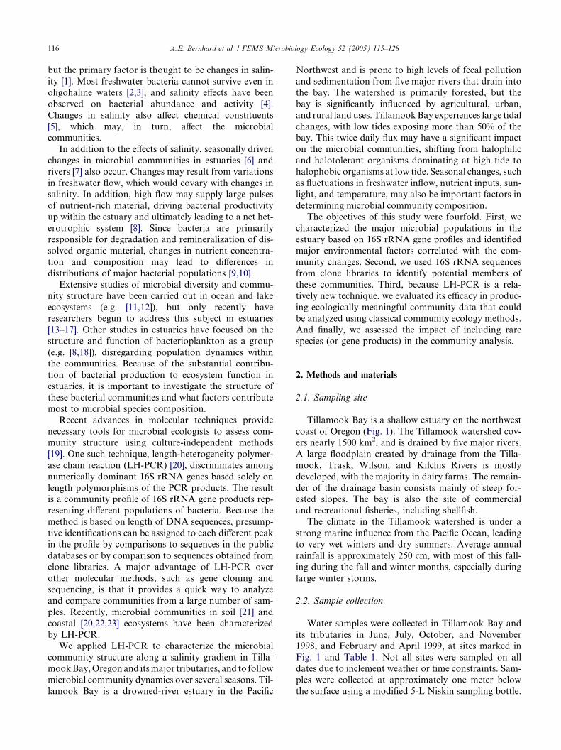
2.2. Sample collection

Water samples were collected in Tillamook Bay and

its tributaries in June, July, October, and November

1998, and February and April 1999, at sites marked in

Fig. 1 and Table 1. Not all sites were sampled on all

dates due to inclement weather or time constraints. Sam-ples were collected at approximately one meter below

the surface using a modified 5-L Niskin sampling bottle.

Fig. 1. Sampling sites in Tillamook Bay, Oregon (45�N, 123�W) and its tributaries.

Table 1

Samples collected on each sampling date

Sampling date Sites sampled

June 1998 B1, B3, B8, R2, R4

July 1998 B1, B4, B8

October 1998 B1–B4, B6, B7, R5, T4, W4

November 1998 B1–B3, R1, R5, T4, W4

February 1999 R1, R3, R4, T2, T3, W1–W3

April 1999 B1–B8, R1, R3–R7, T1–T4, W1, W3, W4

Sample sites are shown in Fig. 1.

A.E. Bernhard et al. / FEMS Microbiology Ecology 52 (2005) 115–128 117

Samples were subdivided for chemical, physical and bio-

logical analyses and stored on ice in the dark during

transport to the laboratory.

2.3. DNA extraction and PCR

One-liter subsamples were filtered through 0.2 lm fil-

ters (Supor-200, Gelman, Ann Arbor, MI). Filters were

placed in 50 ml centrifuge tubes with 5 ml of sucrose ly-

sis buffer (0.75 M sucrose, 40 mM EDTA, 400 mM

NaCl, and 50 mM Tris, pH 9.0), and stored at �80

�C. We extracted DNA from the samples according tothe method of Giovannoni et al. [24], omitting the ce-

sium trifluoroacetate and ultracentrifugation steps.

Briefly, frozen filters were treated with sodium dodecyl

sulfate, proteinase K, and heat, followed by phenol/

chloroform extraction and ethanol precipitation.

A portion of the 5 0 end of the 16S rDNA was ampli-

fied using the eubacterial primers 27F [25] and 338R

[26]. 27F was fluorescently labeled with 6-FAM (Genset,LaJolla, CA). Each 50 ll PCR contained 1X Taq poly-

merase buffer, 0.2 lM each primer, 200 lM each dNTP,

1.25 units of Taq polymerase, 640 ng ll�1 non-acety-

lated bovine serum albumin, and 1.5 mM MgCl2.

Approximately 5 ng of DNA from each water sample

was amplified in a mini-thermal cycler (MJ Research,

Watertown, MA) under the following conditions: 25 cy-


cles of 94 �C for 30 s, 55 �C for 1 min, 72 �C for 1 min,

followed by a final extension at 72 �C for 6 min. PCR

products were analyzed by electrophoresis in a 1% aga-

rose gel stained with 1 lg ml�1 ethidium bromide. Con-

centrations of the PCR products were estimated by

comparison of band intensities to DNA mass standards(Gibco-BRL, Gaithersburg, MD).

2.4. Gene scan analysis

Approximately 10–15 fmol of PCR product were re-

solved on a Long Ranger polyacrylamide gel (FMC,

Rockland, ME) on an ABI 377 automated DNA

sequencer using GeneScan software (Applied Biosys-tems Inc., Fremont, CA). The internal size standard,

GS400HD-ROX (ABI), was loaded in each lane. Sizes

of the PCR products were estimated using the third or-

der cubic spline method in GeneScan software v. 3.1

(ABI). We used the software to convert fluorescence

data from the gel into electropherograms, in which the

bands were represented by peaks and the integrated

fluorescence of each band was the area under the peaks.The relative abundance of each different size PCR prod-

uct was estimated by calculating the ratio of the area un-

der each peak to the total area for each sample. Each

peak in the profile represented one PCR product size

in base pairs (LH-PCR gene fragment) and the area un-

der the peak represented the relative abundance of the

gene fragment. Artifactual peaks were minimized by

using a threshold of 100 fluorescence units. High repro-ducibility of this method using the same primers, PCR

conditions, and the same ABI system at Oregon State

University has been previously determined [21].

2.5. Clone library construction, sequencing and

phylogenetic analyses

Samples collected during February, June, July, andOctober from sites B1, B7, B8, B9, T4, and R3 (Fig.

1) were chosen to represent a range of salinities (0–30

ppt) and environmental conditions. Environmental

DNAs were amplified with eubacterial primers 27F

and 1522R [27]. Pooled PCR products were gel purified

using a gel purification kit (Qiagen, Valencia, CA) and

cloned into the pGEM-T Easy vector (Promega, Madi-

son, WI) according to the manufacturer�s directions.Transformants were randomly selected and inoculated

into 100 ll LB broth with 100 lg ampicillin ml�1 in

96-well microtiter plates. The plates were incubated for

six hours and then one replica plate was made from each

original microtiter plate. All plates were incubated over-

night at 37 �C. LH-PCR peak sizes were determined for

138 clones by the methods described above.

Thirty-three plasmid DNAs from clones correspond-ing to dominant or unique LH-PCR fragments in marine

and freshwater sites were prepared using the Qiaprep

Spin Column Purification Kit (Qiagen) according to

the manufacturer�s directions. DNAs were quantified

spectrophotometrically on a UV/Vis Spectrophotometer

(Shimadzu, Columbia, MD). Bidirectional sequences

were obtained using the primers 27F and 700R [12]. Se-

quences were determined on an ABI 377 DNA Sequencerusing dye-terminator chemistry. We aligned the se-

quences using the sequence editor and Fast Align in

ARB [28] and checked all alignments manually. Regions

of ambiguous alignments were excluded from the analy-

sis. All phylogenetic analyses were done using PAUP* v.

4.0 [29]. Phylogenetic trees were constructed using neigh-

bor-joining and maximum parsimony. The relative con-

fidence in branching order was evaluated byperforming 100 bootstrap replicates. Sequences were

checked for possible chimeric structure by using the

CHECK_CHIMERA program available from the

RDP [30] and by comparison of neighbor-joining trees

based on different regions of the sequence.

2.6. Environmental variables

Nutrient analyses are discussed in detail elsewhere

[31]. Briefly, dissolved inorganic phases of nitrogen

ðNHþ4 and NO�

3 þNO�2 Þ, dissolved silicon, and phos-

phorous were determined within 12 h of filtration using

standard analytical techniques [32] adapted for a seg-

mented-flow autoanalyzer [33]. Dissolved organic car-

bon was determined by high temperature combustion

on a Shimadzu TOC-5000 analyzer. Salinity was calcu-lated from measured chloride concentration using the

expression S = 1.80655 · chlorinity [34]. Chloride con-

centration was determined using conductivity detection

with a DIONEX ED40 Electrochemical Detector. Salin-

ity was measured for all samples except during Novem-

ber, and is reported in Practical Salinity Scale units.

Because salinity and dissolved silicon were linearly re-

lated (r2 = 0.97), salinity values for November sampleswere predicted from dissolved silicon concentrations.

Samples with salinity values less than 1 were classified

as freshwater; samples with salinity values greater than

or equal to 1 were classified as marine. Precipitation

data were obtained from the Oregon Climate Service

Website (www.ocs.orst.edu/) for the Tillamook Station

1W (45�2700W and 123�5200N). We used the sum of pre-

cipitation over the five days prior to and including theday of sampling.

2.7. Statistical analysis

All multivariate analyses were performed using PC-

ORD version 4 [35]. The relative abundance data were

transformed by an arcsine square root function to reduce

skew. Beta-diversity (a measure of compositional hetero-geneity), average half changes (amount of change in spe-

cies composition along a gradient), skewness, and

http://www.ocs.orst.edu/


coefficient of variation (CV) for rows (samples) and col-

umns (gene fragments) were determined before and after

the transformation. The transformation of the raw data

did not affect the beta-diversity and produced a 42% and

35% reduction in row and column skewness, respectively,

and a 25% reduction in the CV for gene fragment totals.Non-metric multidimensional scaling (NMS) [36] was

used to ordinate samples in gene fragment space, using

the SØrenson�s distance measure. Nonmetric scaling is

an ordination method based on ranked distances and

uses an iterative optimization procedure. The effect of

rare fragments on the ordination results was assessed

by progressively deleting fragments that occurred in

fewer than X% of samples (values for X were 0, 5, 10,and 20) and re-running the ordination. In a separate

analysis, we also evaluated the effect of excluding peaks

that were less than 1% of the total area. The autopilot

option was set to the slow and thorough level for all

ordinations. Dimensionality (the optimal number of

dimensions or axes required to explain a sufficient pro-

portion of the variance) was assessed by choosing the

number of axes that minimized final stress and maxi-mized interpretability of the results. The axes have no

real significance and can be rotated or mirrored without

influencing the relative distances between the points.

Stress is a measure of departure from monotonicity in

the relationship between the dissimilarity in the original

p-dimensional space and the dissimilarity in the reduced

k-dimensional ordination space and is a measure of

goodness of fit. Stability of the solutions was assessedby the final instability output and by plotting final stress

versus number of iterations. Monte Carlo tests were run

to confirm that results obtained were significantly better

than would be obtained from randomized data. Addi-

tionally, the proportion of variance explained by each

axis and the cumulative variance explained was deter-

mined for each analysis by calculating the coefficient

of determination between distances in ordination spaceand distances in the original 57-dimensional space. Cor-

relation coefficients in the ordination space were deter-

mined for each environmental variable and gene

fragment by rotating the ordination to maximize the

coefficient on one axis (using the varimax rotation op-

tion in PC-ORD) and were used to improve the inter-

pretability of the solution, not the quality of the

mathematical fit.

2.8. GenBank accession numbers

Nucleotide sequences for 16S rRNA gene clones can

be found under Accession Nos.: AY628650, AY628651,

AY628652, AY628653, AY628654, AY628655,

AY628656, AY628657, AY628658, AY628659,

AY628660, AY628661, AY628662, AY628663,AY628664, AY628665, AY628666, AY628667,

AY628668, AY628669, AY628670, AY628671,

AY628672, AY628673, AY628674, AY628675,

AY628676, AY628677, AY628678, AY628679,

AY628680.

3. Results

We compared 16S rRNA gene profiles of planktonic

microbial communities in Tillamook Bay, Oregon, to

evaluate spatial and temporal differences and correlated

these differences to changes in environmental conditions

by using multivariate statistics. The community profiles

were generated by PCR, which is known to have poten-

tial kinetic biases, partly due to the number of cyclesperformed [20]. To test the effects of different cycle num-

bers of the PCR on the relative abundance of each frag-

ment, we performed 15, 20, 25, and 30 cycles of

amplification and compared the results. The CV of rela-

tive abundance of each peak between PCRs of different

cycle numbers was much lower (12.4%) when we used

the data set that exluded peaks representing less than

1% of the total area than when all peaks were included(42%). This CV is very similar to the PCR variation

found by Ritchie et al. [21]. These data suggest no signif-

icant kinetic bias from 15 to 30 cycles, so we chose 25

cycles because it was the lowest cycle number that con-

sistently produced easily observable PCR product in a

gel.

We also evaluated the effect of deleting rare fragment

lengths to simulate the common, and often recom-mended, practice of deleting rare species in community

composition analyses [37]. We progressively deleted

fragment lengths that occurred in fewer than 5%, 10%,

and 20% of the samples. Our analyses, however, re-

vealed little effect on the ordination, as determined by fi-

nal stress, and instability (Table 2). Based on these

results, the data matrix containing all fragment lengths

representing greater than 1% of the total area was usedfor additional analyses, so that maximal data were re-

tained without increasing noise. It should be noted that

each LH-PCR peak may represent many different bacte-

rial populations. Additionally, the relative abundance of

each gene fragment does not necessarily represent the

abundance of that gene in a natural sample due to po-

tential PCR bias.

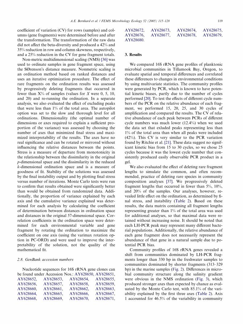
Community profiles of 16S rRNA genes revealed ashift from communities dominated by LH-PCR frag-

ments longer than 330 bp in the freshwater samples to

communities dominated by shorter fragments (313–329

bp) in the marine samples (Fig. 2). Differences in micro-

bial community structure along the salinity gradient

were obvious in the NMS ordination (Fig. 3), which

produced stronger axes than expected by chance as eval-

uated by the Monte Carlo test, with 85.1% of the vari-ability explained by the first three axes (Table 2). Axis

1 accounted for 46.5% of the variability in community

Table 2

Results from NMS ordinations and the effect of deleting rare LH-PCR fragments

Deletion criteria n Stress Instability r2 Iterations Monte Carlo test

Stress p

0% 50 13.2 0.00001 0.851 109 22.7 0.0196

5% 49 13.6 0.00001 0.851 149 22.5 0.0196

10% 45 13.3 0.00001 0.851 85 22.6 0.0196

20% 34 12.9 0.00001 0.856 133 22.7 0.0196

<1% of area 46 13.1 0.00001 0.854 78 23.8 0.0196

Fragments were deleted that occurred in fewer than X% (deletion criteria) of the samples; n is the number of fragments included in each analysis;

stress is the final stress of the ordination; instability is the final instability of the ordination; r2 is the cumulative coefficient of determination for the

correlations between ordination distances and distances in the original 57-dimensional space and represents the variability explained by the first three

axes; iterations is the total number of iterations run in the final analysis; the Monte Carlo test evaluates the chance that the results from the real data

set could be obtained by chance.


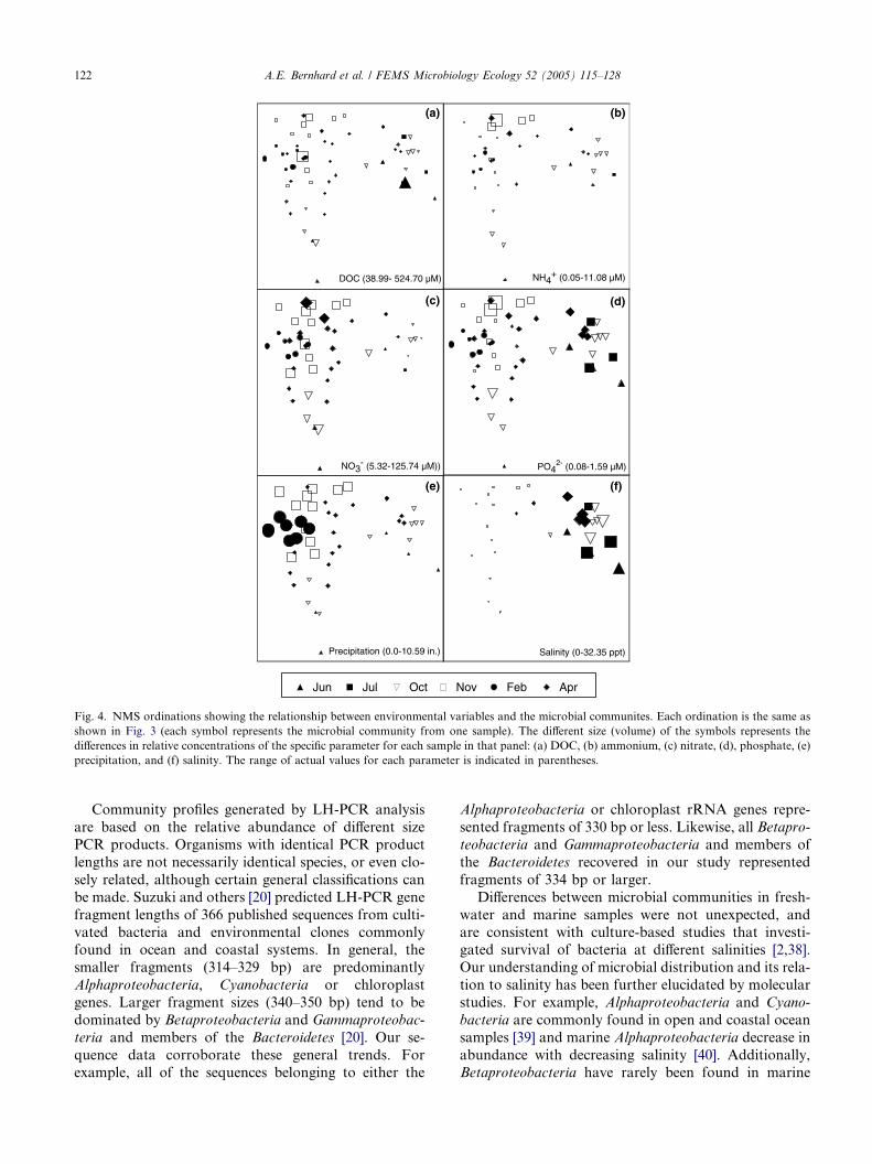
structure and was positively correlated with salinity and

phosphate (Table 3, Fig. 4). Dissolved silicon and ni-

trate were generally higher in the freshwater samples

and negatively correlated with axis 1. Precipitation was

also negatively correlated with axis 1. Axis 2 accounted

for 25.0% of the variability and was negatively corre-

lated with phosphate and positively correlated with pre-

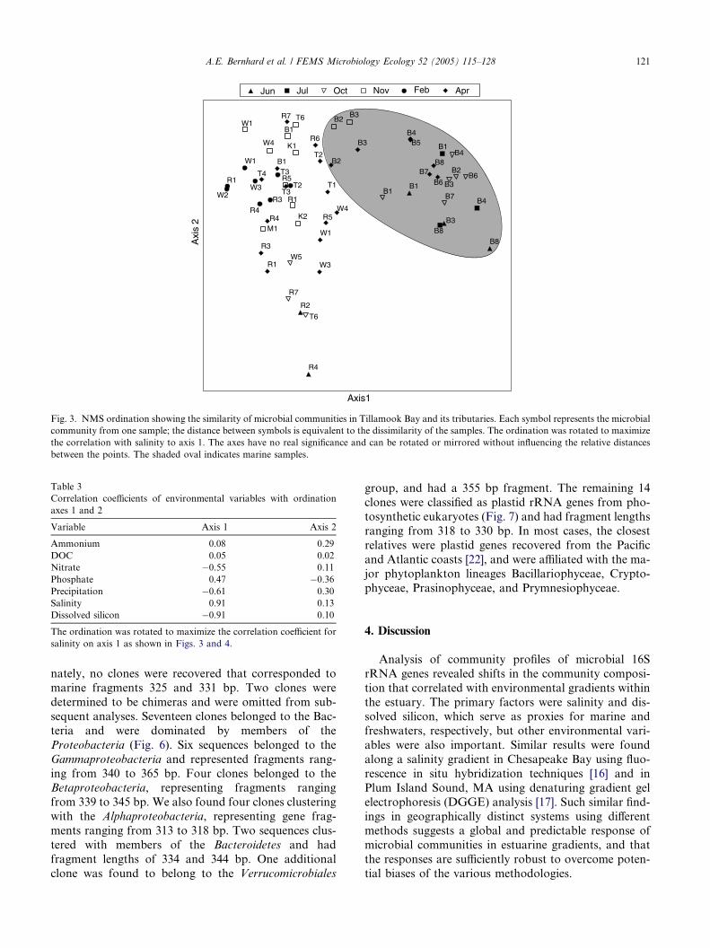
cipitation and ammonium.In addition to the differences detected along a salinity

gradient, community differences were also detected

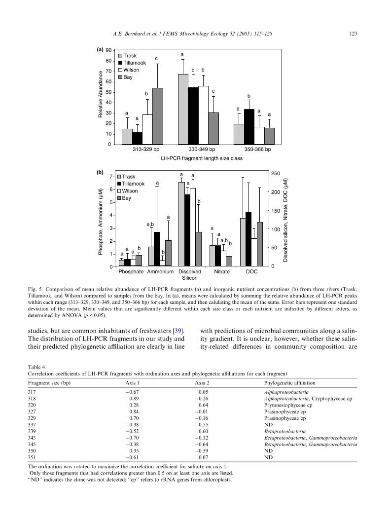
among different rivers (Fig. 5(a)). Relative abundance

0

500

1000

1500

2000

0500

1000150020002500

0

500

1000

1500

Rel

ativ

e Fl

uore

scen

ce U

nits

300 310 320 330 340 350 360 370 380 390

0

800

1600

2400

3200

0500

1000150020002500

T4

B1

B3

B6

B8

Fragment Size (base pairs)

(0.06)

(0.10)

(6.26)

(22.48)

(32.31)

Fig. 2. LH-PCR community profiles of a region of the 16S rRNA gene

amplified from environmental DNA using eubacterial primers 27F and

338R. Samples were collected in April 1999 and represent a salinity

gradient (values in parentheses) from freshwater (T4) to the mouth of

the estuary (B8).

of smaller fragments (<330 bp) was significantly higher

in the Wilson River, compared to the Trask and the Til-

lamook Rivers. Conversely, the Trask River was domi-

nated by LH-PCR fragments of intermediate length

(330–349 bp), while the Tillamook River had signifi-

cantly greater abundance of the large LH-PCR frag-

ments (350–366 bp). There was a general trend of

lower nutrients (ammonium, nitrate, and DOC) in theWilson River compared to the Trask and Tillamook,

but significant differences were detected only for ammo-

nium between the Wilson and the Tillamook (Fig. 5(b)).

Data from the Kilchis and Miami Rivers were excluded

from this analysis because they were sampled on only

one date.

Of the 46 LH-PCR fragments, three (318, 327, and

329) showed strong positive correlations to axis one (Ta-ble 4), suggesting an affinity for marine or brackish envi-

ronments. Four (317, 339, 343, 351) had strong negative

correlations to axis one, suggesting an affinity for fresh-

water environments. Additionally, we found four gene

fragments unique to marine environments (325, 327,

329, and 331 bp fragments) and six fragments unique

to freshwater sites (317, 330, 355, 357, 364, and 365 bp

fragments).We also found significant correlations of relative

abundance of many LH-PCR fragments with environ-

mental variables (Table 5). In general, relative abun-

dances of the smaller LH-PCR fragments were

negatively correlated with ammonium and nitrate, and

positively correlated with salinity. On the contrary, rel-

ative abundances of intermediate LH-PCR fragments

(331–350 bp) were positively correlated with nitrate,negatively correlated with salinity. Additionally, the

intermediate size fragments were often correlated with

DOC. Similarly, relative abundances of the largest

LH-PCR fragments (351–366 bp) were also positively

correlated with nitrate, negatively correlated with salin-

ity, but did not correlate with DOC.

We screened clone libraries by LH-PCR and se-

quenced 33 clones corresponding to dominant or uniquefragment lengths along the estuarine gradient. Unfortu-

B1B2

B3T6

R1

R5

K1

K2

M1

W1

W4

B1 B2

B3B4

B5

B6B7

B8

T1

T2

T3

T4

R1

R3

R4 R5

R6

R7

W1

W3

W4

T2

T3R1

R3R4

W1

W2W3 B1

B3

B8

R2

R4

B1

B4

B8

B1

B2

B3

B4

B7

B6

T6

R7

W5

Jun Jul Oct Nov Feb Apr

Axis1

Axi

s 2

Fig. 3. NMS ordination showing the similarity of microbial communities in Tillamook Bay and its tributaries. Each symbol represents the microbial

community from one sample; the distance between symbols is equivalent to the dissimilarity of the samples. The ordination was rotated to maximize

the correlation with salinity to axis 1. The axes have no real significance and can be rotated or mirrored without influencing the relative distances

between the points. The shaded oval indicates marine samples.

Table 3

Correlation coefficients of environmental variables with ordination

axes 1 and 2

Variable Axis 1 Axis 2

Ammonium 0.08 0.29

DOC 0.05 0.02

Nitrate �0.55 0.11

Phosphate 0.47 �0.36

Precipitation �0.61 0.30

Salinity 0.91 0.13

Dissolved silicon �0.91 0.10

The ordination was rotated to maximize the correlation coefficient for

salinity on axis 1 as shown in Figs. 3 and 4.


nately, no clones were recovered that corresponded to

marine fragments 325 and 331 bp. Two clones were

determined to be chimeras and were omitted from sub-

sequent analyses. Seventeen clones belonged to the Bac-

teria and were dominated by members of the

Proteobacteria (Fig. 6). Six sequences belonged to the

Gammaproteobacteria and represented fragments rang-

ing from 340 to 365 bp. Four clones belonged to theBetaproteobacteria, representing fragments ranging

from 339 to 345 bp. We also found four clones clustering

with the Alphaproteobacteria, representing gene frag-

ments ranging from 313 to 318 bp. Two sequences clus-

tered with members of the Bacteroidetes and had

fragment lengths of 334 and 344 bp. One additional

clone was found to belong to the Verrucomicrobiales

group, and had a 355 bp fragment. The remaining 14

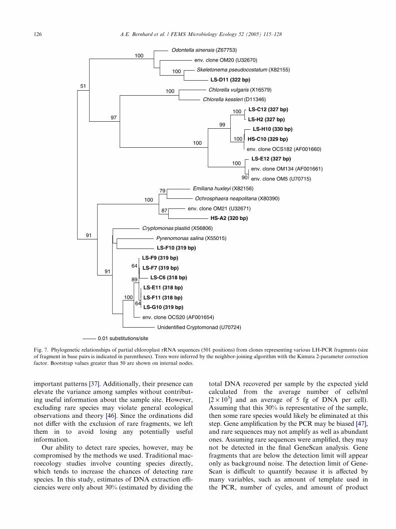
clones were classified as plastid rRNA genes from pho-

tosynthetic eukaryotes (Fig. 7) and had fragment lengths

ranging from 318 to 330 bp. In most cases, the closest

relatives were plastid genes recovered from the Pacific

and Atlantic coasts [22], and were affiliated with the ma-

jor phytoplankton lineages Bacillariophyceae, Crypto-

phyceae, Prasinophyceae, and Prymnesiophyceae.

4. Discussion

Analysis of community profiles of microbial 16S

rRNA genes revealed shifts in the community composi-

tion that correlated with environmental gradients within

the estuary. The primary factors were salinity and dis-solved silicon, which serve as proxies for marine and

freshwaters, respectively, but other environmental vari-

ables were also important. Similar results were found

along a salinity gradient in Chesapeake Bay using fluo-

rescence in situ hybridization techniques [16] and in

Plum Island Sound, MA using denaturing gradient gel

electrophoresis (DGGE) analysis [17]. Such similar find-

ings in geographically distinct systems using differentmethods suggests a global and predictable response of

microbial communities in estuarine gradients, and that

the responses are sufficiently robust to overcome poten-

tial biases of the various methodologies.

DOC (38.99- 524.70 µM) NH4+ (0.05-11.08 µM)

NO3- (5.32-125.74 µM)) PO4

2- (0.08-1.59 µM)

Precipitation (0.0-10.59 in.) Salinity (0-32.35 ppt)

Jun Jul Oct Nov Feb Apr

(a)

(c)

(e) (f)

(d)

(b)

Fig. 4. NMS ordinations showing the relationship between environmental variables and the microbial communites. Each ordination is the same as

shown in Fig. 3 (each symbol represents the microbial community from one sample). The different size (volume) of the symbols represents the

differences in relative concentrations of the specific parameter for each sample in that panel: (a) DOC, (b) ammonium, (c) nitrate, (d), phosphate, (e)

precipitation, and (f) salinity. The range of actual values for each parameter is indicated in parentheses.


Community profiles generated by LH-PCR analysis

are based on the relative abundance of different size

PCR products. Organisms with identical PCR product

lengths are not necessarily identical species, or even clo-

sely related, although certain general classifications can

be made. Suzuki and others [20] predicted LH-PCR gene

fragment lengths of 366 published sequences from culti-

vated bacteria and environmental clones commonlyfound in ocean and coastal systems. In general, the

smaller fragments (314–329 bp) are predominantly

Alphaproteobacteria, Cyanobacteria or chloroplast

genes. Larger fragment sizes (340–350 bp) tend to be

dominated by Betaproteobacteria and Gammaproteobac-

teria and members of the Bacteroidetes [20]. Our se-

quence data corroborate these general trends. For

example, all of the sequences belonging to either the

Alphaproteobacteria or chloroplast rRNA genes repre-

sented fragments of 330 bp or less. Likewise, all Betapro-

teobacteria and Gammaproteobacteria and members of

the Bacteroidetes recovered in our study represented

fragments of 334 bp or larger.

Differences between microbial communities in fresh-

water and marine samples were not unexpected, and

are consistent with culture-based studies that investi-gated survival of bacteria at different salinities [2,38].

Our understanding of microbial distribution and its rela-

tion to salinity has been further elucidated by molecular

studies. For example, Alphaproteobacteria and Cyano-

bacteria are commonly found in open and coastal ocean

samples [39] and marine Alphaproteobacteria decrease in

abundance with decreasing salinity [40]. Additionally,

Betaproteobacteria have rarely been found in marine

0

10

20

30

40

50

60

70

80

90

313-329 bp 330-349 bp 350-366 bp

Trask TillamookWilsonBay

Trask TillamookWilsonBay

a

a aaa

a

a

a

a

aa

a

a

a,b

a,b

a a

a

b

b

b

bb

b

b

b

c

c

0

1

2

3

4

5

6

7

0

50

100

150

200

250

LH-PCR fragment length size class

Pho

spha

te, A

mm

oniu

m (

µM)

Rel

ativ

e A

bund

ance

Dis

solv

ed s

ilico

n, N

itrat

e, D

OC

(µM

)

(a)

(b)

Phosphate Ammonium DissolvedSilicon

Nitrate DOC

Fig. 5. Comparison of mean relative abundance of LH-PCR fragments (a) and inorganic nutrient concentrations (b) from three rivers (Trask,

Tillamook, and Wilson) compared to samples from the bay. In (a), means were calculated by summing the relative abundance of LH-PCR peaks

within each range (313–329, 330–349, and 350–366 bp) for each sample, and then calulating the mean of the sums. Error bars represent one standard

deviation of the mean. Mean values that are significantly different within each size class or each nutrient are indicated by different letters, as

determined by ANOVA (p < 0.05).


studies, but are common inhabitants of freshwaters [39].

The distribution of LH-PCR fragments in our study and

their predicted phylogenetic affiliation are clearly in line

Table 4

Correlation coefficients of LH-PCR fragments with ordination axes and phy

Fragment size (bp) Axis 1 A

317 �0.67

318 0.89 �320 0.28

327 0.84 �329 0.70 �337 �0.38

339 �0.52

343 �0.70 �345 �0.38 �350 0.35 �351 �0.61

The ordination was rotated to maximize the correlation coefficient for salini

Only those fragments that had correlations greater than 0.5 on at least one

‘‘ND’’ indicates the clone was not detected; ‘‘cp’’ refers to rRNA genes from

with predictions of microbial communities along a salin-

ity gradient. It is unclear, however, whether these salin-

ity-related differences in community composition are

logenetic affiliations for each fragment

xis 2 Phylogenetic affiliation

0.05 Alphaproteobacteria

0.26 Alphaproteobacteria, Cryptophyceae cp

0.64 Prymnesiophyceae cp

0.01 Prasinophyceae cp

0.16 Prasinophyceae cp

0.55 ND

0.60 Betaproteobacteria

0.12 Betaproteobacteria, Gammaproteobacteria

0.64 Betaproteobacteria, Gammaproteobacteria

0.59 ND

0.07 ND

ty on axis 1.

axis are listed.

chloroplasts.

Table 5

Correlation coefficients of LH-PCR fragments with environmental

variables

LH-PCR

fragment size

Phosphate Ammonium Nitrate DOC Salinity

313 �0.27

314 �0.31 �0.33

317 �0.44 �0.37 �0.51

318 0.39 �0.48 0.77

319 �0.29 �0.40

320 �0.35 �0.46 �0.32 0.27

322 �0.27 0.42

325 0.51

327 0.43 �0.56 0.84

329 0.36 �0.43 0.75

331 0.47

334 0.59 �0.46

336 0.29 0.49 0.28 �0.41

337 �0.60 �0.37 �0.37 �0.40

338 0.29 0.30

339 �0.53 �0.31 �0.30 �0.61

340 0.38

341 �0.28

342 0.36 0.46 �0.33

343 0.61 �0.71

345 0.39 0.32 �0.39

348 0.40

350 0.34 0.27

351 �0.30 0.32 �0.49

352 0.33

353 0.29 �0.39

355 0.30

356 �0.36

358 �0.31

359 0.37

361 �0.27 0.30 �0.29

362 �0.31

363 �0.35

366 0.71

Only those fragments with significant correlation (a = 0.05) with at

least one variable are shown.


due to the direct effects of salinity (i.e. an inability to

adapt to osmotic stress) or some other factor or group

of factors that co-vary with salinity.

Like salinity, dissolved silicon had a strong correla-

tion with the differences in microbial community struc-

ture, and was inversely related to salinity. Although

changes in bacterial communities may be due to the sim-

ple absence of salt, changes in dissolved silicon may alsoaffect community differences. Dissolved silicon is often

associated with increased suspended material of terres-

trial origin, and tends to be higher in rivers than in

coastal waters [41]. The increase in particulate material

provides additional surfaces for bacterial colonization,

which has been shown to influence community composi-

tion [42].

Differences in microbial community compositionwere detected not only between freshwater and marine

samples, but also among different rivers. The shift in

the Wilson River towards smaller LH-PCR fragments

compared to the Tillamook and the Trask Rivers may

reflect lower inorganic nutrients, particularly ammo-

nium. This is consistent with the negative correlations

between the smaller LH-PCR fragments and inorganic

nutrients. Conversely, the Tillamook River, which had

the highest ammonium and DOC levels, had signifi-cantly more of the larger LH-PCR fragments compared

to the Trask and Wilson Rivers. Although there are not

sufficient data to thoroughly address this issue, our data

suggest the potential to use microbial community com-

position as a proxy for nutrient loading in rivers and

bays. This hypothesis warrants further study.

We also detected a seasonal influence in microbial

community composition. These differences are likelydue to significant differences in precipitation and/or in-

creased runoff, which may bring large amounts of soil

particles and bacteria into the river. During February,

sampling was carried out during a storm, and as a result,

the samples were heavily laden with sediment. Microbial

communities from these samples were all very similar

and clustered together in the ordination, suggesting a

common factor influencing these communities. Similarresults were observed in November, when precipitation

was also quite high (over 7 in.).

Although phylogenetic identification does not neces-

sarily predict physiology, it is tempting to speculate,

based on dominant fragment sizes in particular environ-

ments. For example, samples collected from nutrient-

rich river sites were dominated by longer fragments,

which we found to be represented mostly by Betaprote-

obacteria and Gammaproteobacteria. Many Gammapro-

teobacteria are adapted to high nutrient conditions

[43], such as those found in many of the freshwater sites

in our study. The larger LH-PCR fragments, which in-

clude the Betaproteobacteria and Gammaproteobacteria

and Bacteroidetes, were generally negatively correlated

with salinity, and many were positively correlated with

nitrate. Conversely, fragments representing Alphaprote-

obacteria, Cyanobacteria, and plastid genes dominated

the marine samples, which generally had lower inorganic

nutrient concentrations. Alphaproteobacteria, particu-

larly members of the Roseobacter group and the

SAR11 clade, are often dominant members of marine

bacterioplankton [11,40], and many are adapted to oli-

gotrophic conditions [43]. In our study, populations rep-

resented by smaller LH-PCR fragments such as theAlphaproteobacteria and Cyanobacteria were generally

negatively correlated to inorganic nutrients, and had sig-

nificant positive correlations with salinity. Finding

phototrophic populations to be negatively correlated

with inorganic nutrients initially seemed surprising,

since phototrophs are often nitrogen limited in estuaries

and marine systems [44,45]. However, we cannot distin-

guish phototrophic LH-PCR fragments from heterotro-phic Alphaproteobacterial fragments with certainty

because they often share the same size fragments.

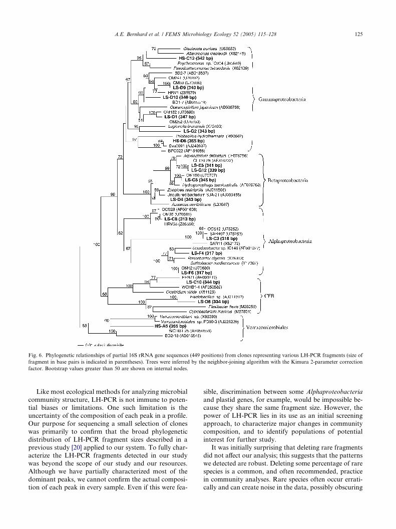
Fig. 6. Phylogenetic relationships of partial 16S rRNA gene sequences (449 positions) from clones representing various LH-PCR fragments (size of

fragment in base pairs is indicated in parentheses). Trees were inferred by the neighbor-joining algorithm with the Kimura 2-parameter correction

factor. Bootstrap values greater than 50 are shown on internal nodes.


Like most ecological methods for analyzing microbial

community structure, LH-PCR is not immune to poten-

tial biases or limitations. One such limitation is the

uncertainty of the composition of each peak in a profile.

Our purpose for sequencing a small selection of clones

was primarily to confirm that the broad phylogenetic

distribution of LH-PCR fragment sizes described in a

previous study [20] applied to our system. To fully char-acterize the LH-PCR fragments detected in our study

was beyond the scope of our study and our resources.

Although we have partially characterized most of the

dominant peaks, we cannot confirm the actual composi-

tion of each peak in every sample. Even if this were fea-

sible, discrimination between some Alphaproteobacteria

and plastid genes, for example, would be impossible be-

cause they share the same fragment size. However, the

power of LH-PCR lies in its use as an initial screening

approach, to characterize major changes in community

composition, and to identify populations of potential

interest for further study.

It was initially surprising that deleting rare fragmentsdid not affect our analysis; this suggests that the patterns

we detected are robust. Deleting some percentage of rare

species is a common, and often recommended, practice

in community analyses. Rare species often occur errati-

cally and can create noise in the data, possibly obscuring

Odontella sinensis (Z67753)

env. clone OM20 (U32670)

Skeletonema pseudocostatum (X82155)

LS-D11 (322 bp)

Chlorella vulgaris (X16579)

Chlorella kessleri (D11346)

LS-C12 (327 bp)

LS-H2 (327 bp)

LS-H10 (330 bp)

HS-C10 (329 bp)

env. clone OCS182 (AF001660)

LS-E12 (327 bp)

env. clone OM134 (AF001661)


Emiliana huxleyi (X82156)

Ochrosphaera neapolitana (X80390)


HS-A2 (320 bp)

Cryptomonas plastid (X56806)

Pyrenomonas salina (X55015)

LS-F10 (319 bp)

LS-F9 (319 bp)

LS-F7 (319 bp)

LS-C6 (318 bp)

LS-E11 (318 bp)

LS-F11 (318 bp)

LS-G10 (319 bp)

env. clone OCS20 (AF001654)

Unidentified Cryptomonad (U70724)

0.01 substitutions/site

100

100

100

100

100

100

100

100

100

9997

79

87

91

91

89

64

64

51

90

Fig. 7. Phylogenetic relationships of partial chloroplast rRNA sequences (501 positions) from clones representing various LH-PCR fragments (size

of fragment in base pairs is indicated in parentheses). Trees were inferred by the neighbor-joining algorithm with the Kimura 2-parameter correction

factor. Bootstrap values greater than 50 are shown on internal nodes.


important patterns [37]. Additionally, their presence can

elevate the variance among samples without contribut-

ing useful information about the sample site. However,

excluding rare species may violate general ecological

observations and theory [46]. Since the ordinations did

not differ with the exclusion of rare fragments, we left

them in to avoid losing any potentially usefulinformation.

Our ability to detect rare species, however, may be

compromised by the methods we used. Traditional mac-

roecology studies involve counting species directly,

which tends to increase the chances of detecting rare

species. In this study, estimates of DNA extraction effi-

ciencies were only about 30% (estimated by dividing the

total DNA recovered per sample by the expected yield

calculated from the average number of cells/ml

[2 · 105] and an average of 5 fg of DNA per cell).

Assuming that this 30% is representative of the sample,

then some rare species would likely be eliminated at this

step. Gene amplification by the PCR may be biased [47],

and rare sequences may not amplify as well as abundantones. Assuming rare sequences were amplified, they may

not be detected in the final GeneScan analysis. Gene

fragments that are below the detection limit will appear

only as background noise. The detection limit of Gene-

Scan is difficult to quantify because it is affected by

many variables, such as amount of template used in

the PCR, number of cycles, and amount of product


loaded in the gel. Since we were interested in major com-

munity shifts, we optimized the amount of DNA ana-

lyzed to maintain a maximum peak height below 6000

relative fluorescent units, to avoid cut-off peaks (with

flat tops). Additionally, each LH-PCR fragment likely

represents more than one species of bacteria, so that rarespecies may, in fact, be included in some of the frag-

ments, but we were unable to detect them individually.

In conclusion, our investigation of the diversity in

estuarine bacterioplankton and its relation to physical

and chemical parameters suggests that the differences

observed reflect the phylogenetic variability of the com-

munities under different conditions, rather than physio-

logical plasticity of the same microbial assemblage.Additionally, we have demonstrated that LH-PCR and

NMS are powerful tools for analyzing microbial com-

munity dynamics over spatial and temporal scales and

identifying factors that most influence these dynamics.

Although these methods alone do not provide informa-

tion on individual species within a sample, they equip

investigators with the ability to process many samples

quickly, thus providing information on heterogeneitywithin a system. Additionally, by identifying unique or

dominant gene fragments in a community, researchers

can streamline DNA sequencing, easily targeting only

those fragments of interest.

Acknowledgments

We thankMichael Rappe for comments on the manu-

script and phylogenetic expertise and Bruce McCune for

statistical expertise and guidance. We also thank the Ore-

gon State University Center for Gene Research and Bio-

technology Central Services Lab for GeneScan analyis

and DNA sequencing. Funding for A.B. and K.F. was

provided by Grant NA76RG0476 (project R/ECO-04)

from the National Oceanic and Atmospheric Adminis-tration to the Oregon State University Sea Grant College

Program, by Grant NCERQAR-827639-01 from the US

Environmental Protection Agency, and by appropria-

tions made by the Oregon state legislature. Funding for

J.M. and D.C. was provided by the EPA�s Water and

Watersheds program: GAD#R825751.

References

[1] Prieur, D., Troussellier, M., Romana, A., Chamroux, S., Mevel,

G. and Baleux, B. (1987) Evolution of bacterial communities in

the Gironde Estuary (France) according to a salinity gradient.

Estuarine Coastal Shelf Sci. 24, 95–108.

[2] Bordalo, A.A. (1993) Effects of salinity on bacterioplankton: field

and microcosm experiments. J. Appl. Bacteriol. 75, 393–398.

[3] Painchaud, J., Therriault, J.-C. and Legendre, L. (1995) Assess-

ment of salinity-related mortality of freshwater bacteria in the St.

Lawrence Estuary. Appl. Environ. Microbiol. 61, 205–208.

[4] Revilla, M., Iriarte, A., Madariaga, I. and Orive, E. (2000)

Bacterial and phytoplankton dynamics along a trophic gradient in

a shallow temperate estuary. Estuarine Coastal Shelf Sci. 50, 297–

313.

[5] Eyre, B. and Balls, P. (1999) A comparative study of nutrient

behavior along the salinity gradient of tropical and temperate

estuaries. Estuaries 22, 313–326.

[6] Soto, Y., Bianchi, M., Martinez, J. and Rego, J.V. (1993)

Seasonal evolution of microplanktonic communities in the estu-

arine front ecosystem of the Rhone River plume (North-western

Mediterranean Sea). Estuarine Coastal Shelf Sci. 37, 1–13.

[7] Lemke, M.J. and Leff, L.G. (1999) Bacterial populations in an

anthropogenically disturbed stream: comparison of different

seasons. Microb. Ecol. 38, 234–243.

[8] Findlay, S., Pace, M.L., Lints, D., Cole, J.J., Caraco, N.F. and

Peierls, B. (1991) Weak coupling of bacterial and algal production

in a heterotrophic ecosystem: the Hudson River estuary. Limnol.

Oceanogr. 36, 268–278.

[9] Murrell, M.C., Hollibaugh, J.T., Silver, M.W. and Wong, P.S.

(1999) Bacterioplankton dynamics in northern San Francisco

Bay: role of particle association and seasonal freshwater flow.

Limnol. Oceanogr. 44, 295–308.

[10] Cottrell, M.T. and Kirchman, D.L. (2000) Natural assemblages of

marine proteobacteria and members of the Cytophaga–Flavob-

acter cluster consuming low- and high-molecular-weight dissolved

organic matter. Appl. Environ. Microbiol. 66, 1692–1697.

[11] Giovannoni, S.J., Britschgi, T.B., Moyer, C.L. and Field, K.G.

(1990) Genetic diversity in Sargasso Sea bacterioplankton. Nature

345, 60–63.

[12] Urbach, E., Vergin, K.L., Young, L., Morse, A., Larson, G.L.

and Giovannoni, S.J. (2001) Unusual bacterioplankton commu-

nity structure in ultra-oligotrophic Crater Lake. Limnol. Oceangr.

46, 557–572.

[13] Benlloch, S., Rodriguez-Valera, F. and Martinez-Murcia, A.J.

(1995) Bacterial diversity in two coastal lagoons deduced from

16S rDNA PCR amplification and partial sequencing. FEMS

Microbiol. Ecol. 18, 267–280.

[14] Crump, B.C., Armbrust, V. and Baross, J.A. (1999) Phylogenetic

analysis of particle-attached and free-living bacterial communities

in the Columbia River, its estuary, and the adjacent coastal ocean.

Appl. Environ. Microbiol. 65, 3192–3204.

[15] Murray, A.E., Hollibaugh, J.T. and Orrego, C. (1996) Phyloge-

netic compositions of bacterioplankton from two California

estuaries compared by denaturing gradient gel electrophoresis of

16S rDNA fragments. Appl. Environ. Microbiol. 62, 2676–2680.

[16] Bouvier, T.C. and del Giorgio, P.A. (2002) Compositional

changes in free-living bacterial communities along a salinity

gradient in two temperate estuaries. Limnol. Oceanogr. 47, 453–

470.

[17] Crump, B.C., Hopkinson, C.S., Sogin, M.L. and Hobbie, J.E.

(2004) Microbial biogeography along an estuarine salinity gradi-

ent: combined influences of bacterial growth and residence time.


[18] Hollibaugh, J.T. and Wong, P.S. (1999) Microbial processes in the

San Francisco Bay estuarine turbidity maximum. Estuaries 22,

848–862.

[19] Giovannoni, S.J., Mullins, T.D. and Field, K.G. (1995) Microbial

diversity in oceanic systems: rRNA approaches to the study of

unculturable microbes In: Molecular Ecology of Aquatic

Microbes (Joint, I., Ed.). Springer, Berlin.

[20] Suzuki, M.T., Rappe, M.S. and Giovannoni, S.J. (1998) Kinetic

bias in estimates of coastal picoplankton community structure

obtained by measurements of small subunit rRNA gene PCR

amplicon length heterogeneity. Appl. Environ. Microbiol. 64,

4522–4529.

[21] Ritchie, N.J., Schutter, M.E., Dick, R.P. and Myrold, D.D.

(2000) Use of length heterogeneity PCR and FAME to charac-


terize microbial communities in soil. Appl. Environ. Microbiol.

66, 1668–1675.

[22] Rappe, M.S., Suzuki, M.T., Vergin, K.L. and Giovannoni, S.J.

(1998) Phylogenetic diversity of ultraplankton plastid small-

subunit rRNA genes recovered in environmental nucleic acid

samples from the Pacific and Atlantic coasts of the United States.


[23] Bernhard, A.E. and Field, K.G. (2000) Identification of nonpoint

sources of fecal pollution in coastal waters by using host-specific

16S ribosomal DNA genetic markers from fecal anaerobes. Appl.

Environ. Microbiol. 66, 1587–1594.

[24] Giovannoni, S.J., DeLong, E.F., Schmidt, T.M. and Pace, N.R.

(1990) Tangential flow filtration and preliminary phylogenetic

analysis of marine picoplankton. Appl. Environ. Microbiol. 56,

2572–2575.

[25] Lane, D.J. (1991) 16S/23S rRNA sequencing In: Nucleic acid

Techniques in Bacterial Systematics (Stackebrandt, E. and

Goodfellow, M., Eds.), pp. 115–175. Wiley, New York.

[26] Amann, R.I., Binder, B.J., Olson, R.J., Chisholm, S.W., Deve-

reux, R. and Stahl, D.A. (1990) Combination of 16S rRNA-

targeted oligonucleotide probes with flow cytometry for analyzing

mixed microbial populations. Appl. Environ. Microbiol. 56,

1919–1925.

[27] Giovannoni, S.J. (1991) The polymerase chain reaction In:

Sequencing and Hybridization Techniques in Bacterial Systemat-

ics (Stackebrandt, E. and Goodfellow, M., Eds.), pp. 177–201.

Wiley, New York.

[28] Ludwig, W. et al. (2004) ARB: a software environment for

sequence data. Nucleic Acids Res. 32, 1363–1371.

[29] Swofford, D.L. (1991) PAUP: Phylogenetic Analysis using Par-

simony. Sinauer Associates Inc., Fitchberg, MA.

[30] Maidak, B.L. et al. (2001) The RDP-II (Ribosomal Database

Project). Nucleic Acids Res. 29, 173–174.

[31] Colbert, D. and McManus, J. (2003) Nutrient biogeochemistry in

an upwelling-influenced estuary of the Pacific Northwest (Tilla-

mook Bay, Oregon, USA). Estuaries 26, 1205–1219.

[32] Stickland, J.D.H. and Parsons, T.R. (1972) A Practical Hand-

book of Seawater Analysis. Fisheries Research Board, Canada.

[33] Gordon, L.I., Jennings, J.C., Ross, A.A. and Krest, J.M. (1995) A

suggested protocol for continuous flow automated analysis of

seawater nutrients (phosphate, nitrate, nitrite, and silicic acid) In:

WOCE Hydrographic Program and the Joint Global Ocean

Fluxes Study, Methods Manual 91-1 WHOI, Woods Hole, MA.

[34] Knauss, J.A. (1978) Introduction to Physical Oceanography.

Prentice-Hall, Englewood Cliffs, NJ.

[35] McCune, B. and Mefford, M.J. (1999) PC-ORD, Multivariate

Analysis of Ecological Data.MjMSoftware, Gleneden Beach, OR.

[36] Kruskal, J.B. (1964) Nonmetric multidimensional scaling: a

numerical method. Psychometrika 29, 115–129.

[37] Gauch Jr., H.G. (1982) Multivariate Analysis in Community

Ecology. Cambridge Press, New York.

[38] Valdes, M. and Albright, L.J. (1981) Survival and heterotrophic

activities of Fraser River and Strait of Georgia bacterioplankton

within the Fraser River plume. Mar. Biol. 64, 231–241.

[39] Glockner, F.O., Fuchs, B.M. and Amann, R. (1999) Bacterio-

plankton compositions of lakes and oceans: a first comparison

based on fluorescence in situ hybridization. Appl. Environ.

Microbiol. 65, 3721–3726.

[40] Gonzalez, J.M., Whitman, W.B., Hodson, R.E. and Moran, M.A.

(1996) Identifying numerically abundant culturable bacteria from

complex communities: an example from a lignin enrichment

culture. Appl. Environ. Microbiol. 62, 4433–4440.

[41] Conley, D.J. and Malone, T.C. (1992) Annual cycle of dissolved

silicate in chesapeake bay – implications for the production and

fate of phytoplankton. Biomass 81, 121–128.

[42] DeLong, E.F., Franks, D.G. and Alldredge, A.L. (1993) Phylo-

genetic diversity of aggregate-attached vs. free-living marine

bacterial assemblages. Limnol. Oceanogr. 38, 924–934.

[43] Zavarzin, G.A., Stackebrandt, E. and Murray, R.G. (1991) A

correlation of phylogenetic diversity in the Proteobacteria with

the influences of ecological forces. Can. J. Microbiol. 37, 1–6.

[44] Bernhard, A.E. and Peele, E.R. (1997) Nitrogen limitation of

phytoplankton in a shallow embayment in northern Puget Sound.

Estuaries 20, 759–769.

[45] Howarth, R.W. (1988) Nutrient limitation of net primary

production in marine ecosystems. Annu. Rev. Ecol. 19, 89–110.

[46] Cao, Y., Williams, D.D. and Williams, N.E. (1998) How

important are rare species in aquatic community ecology and

bioassessment?. Limnol. Oceanogr. 43, 1403–1409.

[47] Suzuki, M.T. and Giovannoni, S.J. (1996) Bias caused by

template annealing in the amplification of mixtures of 16S rRNA

genes by PCR. Appl. Environ. Microbiol. 62, 625–630.

Documents

Microbial community dynamics based on 16S rRNA gene profiles in a Pacific Northwest estuary and its tributaries